coordinate descent algorithms - optimization · pdf filecoordinate descent algorithms stephen...
TRANSCRIPT

Noname manuscript No.(will be inserted by the editor)
Coordinate Descent Algorithms
Stephen J. Wright
Received: date / Accepted: date
Abstract Coordinate descent algorithms solve optimization problems by suc-cessively performing approximate minimization along coordinate directions orcoordinate hyperplanes. They have been used in applications for many years,and their popularity continues to grow because of their usefulness in data anal-ysis, machine learning, and other areas of current interest. This paper describesthe fundamentals of the coordinate descent approach, together with variantsand extensions and their convergence properties, mostly with reference to con-vex objectives. We pay particular attention to a certain problem structure thatarises frequently in machine learning applications, showing that efficient im-plementations of accelerated coordinate descent algorithms are possible forproblems of this type. We also present some parallel variants and discuss theirconvergence properties under several models of parallel execution.
Keywords coordinate descent · randomized algorithms · parallel numericalcomputing
1 Introduction
Coordinate descent (CD) algorithms for optimization have a history that datesto the foundation of the discipline. They are iterative methods in which eachiterate is obtained by fixing most components of the variable vector x at theirvalues from the current iteration, and approximately minimizing the objective
The author was supported by NSF Awards DMS-1216318 and IIS-1447449, ONR AwardN00014-13-1-0129, AFOSR Award FA9550-13-1-0138, and Subcontract 3F-30222 from Ar-gonne National Laboratory.
Stephen J. WrightDepartment of Computer Sciences, University of Wisconsin-Madison, 1210 W. Dayton St.,Madison, WI 53706-1685, USATel.: +1 608 316 4358E-mail: [email protected]
2 Stephen J. Wright
with respect to the remaining components. Each such subproblem is a lower-dimensional (even scalar) minimization problem, and thus can typically besolved more easily than the full problem.
CD methods are the archetype of an almost universal approach to algo-rithmic optimization: solving an optimization problem by solving a sequenceof simpler optimization problems. The obviousness of the CD approach andits acceptable performance in many situations probably account for its long-standing appeal among practitioners. Paradoxically, the apparent lack of so-phistication may also account for its unpopularity as a subject for investigationby optimization researchers, who have usually been quick to suggest alterna-tive approaches in any given situation. There are some very notable exceptions.The 1970 text of Ortega and Rheinboldt [40, Section 14.6] included a compre-hensive discussion of “univariate relaxation,” and such optimization specialistsas Luo and Tseng [30,31], Tseng [55], and Bertsekas and Tsitsiklis [5] madeimportant contributions to understanding the convergence properties of thesemethods in the 1980s and 1990s.
The situation has changed in recent years. Various applications (includ-ing several in computational statistics and machine learning) have yieldedproblems for which CD approaches are competitive in performance with morereputable alternatives. The properties of these problems (for example, the lowcost of calculating one component of the gradient, and the need for solutionsof only modest accuracy) lend themselves well to efficient implementations ofCD, and CD methods can be adapted well to handle such special featuresof these applications as nonsmooth regularization terms and a small numberof equality constraints. At the same time, there have been improvements inthe algorithms themselves and in our understanding of them. Besides theirextension to handle the features just mentioned, new variants that make useof randomization and acceleration have been introduced. Parallel implemen-tations that lend themselves well to modern computer architectures have beenimplemented and analyzed. Perhaps most surprisingly, these developments arerelevant even to the most fundamental problem in numerical computation:solving the linear equations Aw = b.
In the remainder of this section, we state the problem types for whichCD methods have been developed, and sketch the most fundamental versionsof CD. Section 2 surveys applications both historical and modern. Section 3sketches the types of algorithms that have been implemented and analyzed,and presents several representative convergence results. Section 4 focuses onparallel CD methods, describing the behavior of these methods under syn-chronous and asynchronous models of computation.
Our approach throughout is to describe the CD methods in their simplestforms, to illustrate the fundamentals of the applications, implementations, andanalysis. We focus almost exclusively on methods that adjust just one coordi-nate on each iteration. Most applications use block coordinate descent meth-ods, which adjust groups of blocks of indices at each iteration, thus searchingalong a coordinate hyperplane rather than a single coordinate direction. Mostderivation and analysis of single-coordinate descent methods can be extended

Coordinate Descent Algorithms 3
without great difficulty to the block-CD setting; the concepts do not changefundamentally. We mention too that much effort has been devoted to devel-oping more general forms of CD algorithms and analysis, involving weightednorms and other features, that allow more flexible implementation and al-low the proof of stronger and more general (though usually not qualitativelydifferent) convergence results.
1.1 Formulations
The problem considered in most of this paper is the following unconstrainedminimization problem:
minx
f(x), (1)
where f : Rn → R is continuous. Different variants of CD make further as-sumptions about f . Sometimes it is assumed to be smooth and convex, some-times smooth and possibly nonconvex, and sometimes smooth but with a re-stricted domain. (We will make such assumptions clear in each discussion ofalgorithmic variants and convergence results.)
Motivated by recent popular applications, it is common to consider thefollowing structured formulation:
minx
h(x) := f(x) + λΩ(x), (2)
where f is smooth, Ω is a regularization function that may be nonsmooth andextended-valued, and λ > 0 is a regularization parameter. Ω is often convexand usually assumed to be separable or block-separable. When separable, Ωhas the form
Ω(x) =
n∑i=1
Ωi(xi). (3)
where Ωi : R → R for all i. The best known examples of separability are the`1-norm (in which Ω(x) = ‖x‖1 and hence Ωi(xi) = |xi|) and box constraints(in which Ωi(xi) = I[li,ui](xi) is the indicator function for the interval [li, ui]).Block separability means that the n × n identity matrix can be partitionedinto column submatrices Ui, i = 1, 2, . . . , N such that
Ω(x) =
N∑i=1
Ωi(UTi x). (4)
Block-separable examples include group-sparse regularizers in which Ωi(zi) :=‖zi‖2. Formulations of the type (2), with separable or block-separable regu-larizers, arise in such applications as compressed sensing, statistical variableselection, and model selection.
4 Stephen J. Wright
The class of problems known as empirical risk minimization (ERM) givesrise to a formulation that is particularly amenable to coordinate descent; see[52]. These problems have the form
minw∈Rd
1
n
n∑i=1
φi(cTi w) + λg(w), (5)
for vectors ci ∈ Rd, i = 1, 2, . . . , n and convex functions φi, i = 1, 2, . . . , nand g. We can express linear least-squares, logistic regression, support vec-tor machines, and other problems in this framework. Recalling the followingdefinition of the conjugate t∗ of a convex function t:
t∗(y) = supz
(zT y − t(z)), (6)
we can write the Fenchel dual [49, Section 31] of (5) as follows:
minx∈Rn
1
n
n∑i=1
φ∗i (−xi) + λg∗(
1
λnCx
), (7)
where C is the d × n matrix whose columns are ci, i = 1, 2, . . . , n. The dualformulation (7) is has special appeal as a target for coordinate descent, becauseof separability of the summation term.
One interesting case is the system of linear equations
Aw = b, where A ∈ Rm×n, (8)
which we assume to be a feasible system. The least-norm solution is found bysolving
minw∈Rn
1
2‖w‖22 subject to Aw = b, (9)
whose Lagrangian dual is
minx∈Rm
f(x) :=1
2‖ATx‖22 − bTx. (10)
(We recover the primal solution from (10) by setting w = ATx.) We can seethat (10) is a special case of the Fenchel dual (7) obtained from (5) if we set
C ← AT , g(w) =1
2‖w‖22, φi(ti) = Ibi(ti), λ = 1/n,
where Ibi denotes the indicator function for bi, which is zero at bi and infiniteelsewhere. (Its conjugate is I∗bi(si) = bisi.) The primal problem (9) can berestated correspondingly as
minw∈Rn
1
m
m∑i=1
Ibi(Aiw) +1
n‖w‖22,
where Ai denotes the ith row of the matrix A in (8), which has the form (5).

Coordinate Descent Algorithms 5
1.2 Outline of Coordinate Descent Algorithms
The basic coordinate descent framework for continuously differentiable mini-mization is shown in Algorithm 1. Each step consists of evaluation of a singlecomponent ik of the gradient ∇f at the current point, followed by adjustmentof the ik component of x, in the opposite direction to this gradient compo-nent. (Here and throughout, we use [∇f(x)]i to denote the ith component ofthe gradient ∇f(x).) There is much scope for variation within this framework.The components can be selected in a cyclic fashion, in which i0 = 1 and
ik+1 = [ik mod n] + 1, k = 0, 1, 2, . . . . (11)
They can be required to satisfy an “essentially cyclic” condition, in which forsome T ≥ n, each component is modified at least once in every stretch of Titerations, that is,
∪Tj=0ik−j = 1, 2, . . . , n, for all k ≥ T . (12)
Alternatively, they can be selected randomly at each iteration (though notnecessarily with equal probability). Turning to steplength αk: we may per-form exact minimization along the ik component, or choose a value of αkthat satisfies traditional line-search conditions (such as sufficient decrease), ormake a predefined “short-step” choice of αk based on prior knowledge of theproperties of f .
Algorithm 1 Coordinate Descent for (1)
Set k ← 0 and choose x0 ∈ Rn;repeat
Choose index ik ∈ 1, 2, . . . , n;xk+1 ← xk − αk[∇f(xk)]ikeik for some αk > 0;k ← k + 1;
until termination test satisfied;
The CD framework for the separable regularized problem (2), (3) is shownin Algorithm 2. At iteration k, a scalar subproblem is formed by making alinear approximation to f along the ik coordinate direction at the currentiterate xk, adding a quadratic damping term weighted by 1/αk (where αkplays the role of a steplength), and treating the relevant regularization termΩi explicitly. Note that when the regularizer Ωi is not present, the step isidentical to the one taken in Algorithm 1. For some interesting choices of Ωi(for example Ωi(·) = | · |), it is possible to write down a closed-form solutionof the subproblem; no explicit search is needed. The operation of solving suchsubproblems is often referred to as a “shrink operation,” which we denote bySβ and define as follows:
Sβ(τ) := minχ
1
2β‖χ− τ‖22 +Ωi(χ). (13)
6 Stephen J. Wright
By stating the subproblem in Algorithm 2 equivalently as
minχ
1
2λαk
∥∥χ− (xkik − αk[∇f(xk)]ik)∥∥2 +Ωi(χ),
we can express the CD update as zkik ← Sλαk(xkik − αk[∇f(xk)]ik).
Algorithm 2 Coordinate Descent for (2),(3)
Set k ← 0 and choose x0 ∈ Rn;repeat
Choose index ik ∈ 1, 2, . . . , n;zkik ← arg minχ (χ− xkik )T [∇f(xk)]ik + 1
2αk‖χ− xkik‖
22 + λΩi(χ) for some αk > 0;
xk+1 ← xk + (zkik − xkik
)eik ;
k ← k + 1;until termination test satisfied;
Algorithms 1 and 2 can be extended to block-CD algorithms in a straight-forward way, by updating a block of coordinates (denoted by the columnsubmatrix Uik of the identity matrix) rather than a single coordinate. InAlgorithm 2, it is assumed that the choice of block is consistent with theblock-separable structure of the regularization function Ω, that is, Uik is aconcatenation of several of the submatrices Ui in (4).
1.3 Application to Linear Equations
For the formulation (10) that arises from the linear system Aw = b, let usassume that the rows of A are normalized, that is,
‖Ai‖2 = 1 for i = 1, 2, . . . ,m. (14)
Applying Algorithm 1 to (10) with αk ≡ 1, each step has the form
xk+1 ← xk − (AikATxk − bik)eik . (15)
If we maintain and update the estimate wk of the solution to the primalproblem (9) after each update of xk, according to wk = ATxk, we obtain
wk+1 ← wk − (AikATxk − bik)ATik = wk − (Aikw
k − bik)ATik , (16)
which is the update formula for the Kaczmarz algorithm [22]. Following thisupdate, we have using (14) that
Aikwk+1 = Aikw
k − (Aikwk − bik) = bik ,
so that the ik equation in the system Aw = b is now satisfied. This method ifsometimes known as the “method of successive projections” because it projectsonto the feasible hyperplane for a single constraint at every iteration.
Coordinate Descent Algorithms 7
1.4 Relationship to Other Methods
Stochastic gradient (SG) methods, also undergoing a revival of interest becauseof their usefulness in data analysis and machine learning applications, minimizea smooth function f by taking a (negative) step along an estimate gk of thegradient ∇f(xk) at iteration k. It is often assumed that gk is an unbiasedestimate of ∇f(xk), that is, ∇f(xk) = E(gk), where the expectation is takenover whatever random variables were used in obtaining gk from the currentiterate xk. Randomized CD algorithms can be viewed as a special case ofSG methods, in which gk = n[∇f(xk)]ikeik , where ik is chosen uniformly atrandom from 1, 2, . . . , n. Here, ik is the random variable, and we have
E(gk) =1
n
n∑i=1
n[∇f(xk)]iei = ∇f(xk),
certifying unbiasedness. However, CD algorithms have the advantage over gen-eral SG methods that descent in f can be guaranteed at every iteration. More-over, the variance of the gradient estimate gk shrinks to zero as the iteratesconverge to a solution x∗, since every component of ∇f(x∗) is zero. By con-trast, in general SG methods, the gradient estimates gk may be nonzero evenwhen xk is a solution.
The relationship between CD and SG methods can also be discerned fromthe Fenchel dual pair (5) and (7). SG methods are quite popular for solvingformulation (5), where the estimate gk is obtained by taking a single term ikfrom the summation and using ∇φik(cTikw)cik as the estimate of the gradientof the full summation. This approach corresponds to applying CD to the dual(7), where the component ik of x is selected for updating at iteration k. Thisrelationship is typified by the Kaczmarz algorithm for Aw = b, which can bederived either as CD applied to the dual formulation (10) or as SG applied tothe sum-of-squares problem
minw
1
2‖Aw − b‖22 =
1
2
m∑i=1
(Aiw − bi)2. (17)
CD is related in an obvious way to the Gauss-Seidel method for n×n sys-tems of linear equations, which adjusts the ik variable to ensure satisfactionof the ik equation, at iteration k. (Successive over-relaxation (SOR) modifiesthis approach by scaling each Gauss-Seidel step by a factor (1 + ω) for someconstan ω ∈ [0, 1), chosen so as to improve the convergence rate.) StandardGauss-Seidel and SOR use the cyclic choice of coordinates (11), whereas a ran-dom choice of ik would correspond to “randomized” versions of these methods.To make the connections more explicit: The Gauss-Seidel method applied tothe normal equations for (8) — that is, ATAw = AT b — is equivalent to apply-ing Algorithm 1 to the least-squares problem (17), when the steplength αk ischosen to minimize the objective exactly along the given coordinate direction.SOR also corresponds to Algorithm 1, with αk chosen to be a factor (1 + ω)times the exact minimum. These equivalences allow the results of Section 3
8 Stephen J. Wright
to be used to derive convergence rates for Gauss-Seidel applied to the normalequations, including linear convergence when ATA is nonsingular. Note thatthese results do not require feasibility of the original equations (8).
2 Applications
We mention here several applications of CD methods to practical problems,some dating back decades and others relatively new. Our list is necessarily in-complete, but it attests to the popularity of CD in a wide variety of applicationcommunities.
Bouman and Sauer [7] discuss an application to positron emission tomog-raphy (PET) in which the objective has the form (2) where f is smooth andconvex and Ω is a sum of terms of the form |xj − xl|q for some pairs of com-ponents (j, l) of x and some q ∈ [1, 2]. Ye et al. [57] apply a similar method toa different objective arising from optical diffusion tomography.
Liu, Paratucco, and Zhang [26] describe a block CD approach for linearleast squares plus a regularization function consisting of a sum of `∞ normsof subvectors of x. The technique is applied to semantic basis discovery, whichlearns from data how to identify and classify the functional MRI response ofa person’s brain when they hear certain English words.
Canutescu and Dunbrack [11] describe a cyclic coordinate descent methodfor determining protein structure, adjusting the dihedral angles in a proteinchain so that the atom at the end of the chain comes close to a specifiedposition in space.
Florian and Chen [17] recover origin-destination matrices from observedtraffic flows by alternately solving a bilevel optimization problem over twoblocks of variables: the origin-destination demands and the proportion of eachorigin-destination flow assigned to each arc in the network.
Breheny and Huang [10] discuss coordinate descent for linear and logisticregression with nonconvex separable regularization terms, reporting results forgenetic association and gene expression studies. The SparseNet algorithm [33]applied to problems with these same nonconvex separable regularizers useswarm-started cyclic coordinate descent as an inner loop to solve a sequence ofproblems in which the regularization parameter λ in (2) and the parametersdefining concavity of the regularization functions are varied.
Friedman, Hastie, and Tibshirani [18] propose a block CD algorithm forestimating a sparse inverse covariance matrix, given a sample covariance ma-trix S and taking the variable in their formulation to be a modification W ofS, such that W−1 is sparse. The resulting “graphical lasso” algorithm cyclesthrough the rows/columns of W (in the style of block CD), solving a standardlasso problem to calculate each update. The same authors [19] apply CD togeneralized linear models such as linear least squares and logistic regression,with convex regularization terms. Their framework include such formulationsas lasso, graphical lasso, elastic net, and the Dantzig selector, and is imple-mented in the package glmnet.

Coordinate Descent Algorithms 9
Chang, Hsieh, and Lin [12] use cyclic and stochastic CD to solve a squared-loss formulation of the support vector machine (SVM) problem in machinelearning, that is,
minw
m∑i=1
max(1− yixTi w, 0)2 +λ
2wTw. (18)
where (xi, yi) ∈ RN × 0, 1 are feature vector / label pairs and λ is a reg-ularization parameter. This problem is an important instance of the ERMform (5). In the best known early application of coordinate descent to SVM,Platt [42] deals with a hinge-loss formulation of SVM, which is identical to(18) except that the square on each term of the summation is omitted. Thedual of this problem has bounds on its variables along with a single linearconstraint. Platt’s procedure SMO (for “sequential minimal optimization”),applied to the dual, changes two variables at a time, with the variable pairchosen according to a “greedy” criterion and the search direction chosen tomaintain feasibility of the linear constraint.
Sardy, Bruce, and Tseng [50] consider the basis-pursuit formulation ofwavelet denoising:
minx
1
2‖Φx− y‖22 + λ‖x‖1.
This formulation is equivalent to the well known lasso of Tibshirani [54] and hasbecome famous because of its applicability to sparse recovery and compressedsensing. Although this formulation fits the ERM framework (5) and could thusbe dualized before applying CD, the approach of [50] applies block CD directlyto the primal formulation.
Applications of block CD approaches to transceiver design for cellular net-works and to tensor factorization are discussed in Razaviyayn [45, Section 8].
Finally, we mention several popular problem classes and algorithms thatcan be interpreted as CD algorithms, but for which such an interpretation maynot be particularly helpful in understanding the performance of the algorithm.First, we consider low-rank matrix completion problems in which we are pre-sented with limited information about a rectangular matrix M ∈ Rm×n andseek matrices U ∈ Rn×r and V ∈ Rm×r (with r small) such that UV T is con-sistent with the observations of M . When the observations satisfy a restrictedisometry property (an assumption commonly made in compressed sensing; see[46, Definition 3.1] for a definition that applies to matrix completion), the blockCD approach of Jain, Netrapalli, and Sanghavi [21, Algorithm 1] converges toa solution. This approach defines the objective to be the least-squares fit be-tween the observations and their predicted values according to the productUV T — a function that is nonconvex with respect to (U, V ) — and minimizesalternately over U and V , respectively. Standard analysis of CD for nonconvexfunctions would yield at best stationarity of accumulation points, but muchstronger results are attained in [21] because of special assumptions that aremade on the problem in this paper.

10 Stephen J. Wright
Second, we consider the “alternating-direction method of multipliers” (ADMM)[13,8], which has gained great currency in the past few years because of itsusefulness in solving regularized problems in statistics and machine learning,and in designing parallel algorithms. Each major iteration of ADMM consistsof an (approximate) minimization of the augmented Lagrangian function for aconstrained optimization problem over each block of primal variables in turn,followed by an update to the Lagrange multiplier estimates. It might seemappealing to do multiple cycles of updating the primal variable blocks, in themanner of cyclic block CD, thus finding a better approximation to the so-lution of each subproblem over all primal variables and moving the methodcloser to the standard augmented Lagrangian approach. Eckstein and Yao [14]show, however, that this “approximate augmented Lagrangian” approach hasa fundamentally different theoretical interpretation from ADMM, and a com-putational comparison between the two approaches [14, Section 5] appears toshow an advantage for ADMM.
3 Coordinate Descent: Algorithms, Convergence, Implementations
We now describe the most important variants of coordinate descent and presenttheir convergence properties, including the proofs of some fundamental results.We also discuss the implementation of accelerated CD methods for problemsof the form (7) and for the Kaczmarz algorithm for Aw = b. As mentionedin the introduction, we deal with the most elementary framework possible, toexpose the essential properties of the methods.
3.1 Powell’s Example
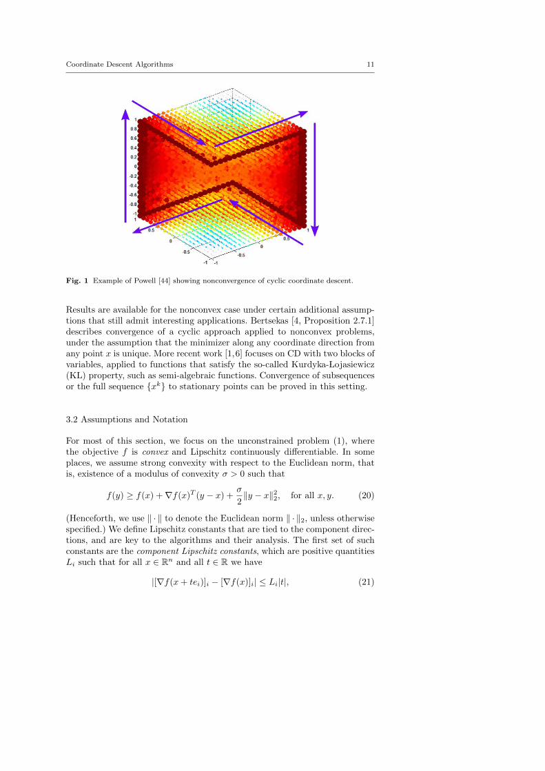
We start with a simple but intriguing example due to Powell [44, formula (2)]of a function in R3 for which cyclic CD fails to converge to a stationary point.The nonconvex, continuously differentiable function f : R3 → R is defined asfollows:
f(x1, x2, x3) = −(x1x2 + x2x3 + x1x3) +
3∑i=1
(|xi| − 1)2+. (19)
It has minimizers at the corners (1, 1, 1)T and (−1,−1,−1)T of the unit cube,but coordinate descent with exact minimization, started near (but just outsideof) one of the other vertices of the cube cycles around the neighborhoods ofsix points that are close to the six non-optimal vertices. Powell shows thatthe cyclic nonconvergence behavior is rather special and is destroyed by smallperturbations on this particular example, and we can note that a randomizedcoordinate descent method applied to this example would be expected to con-verge to the vicinity of a solution within a few steps. Still, this example andothers in [44] make it clear that we cannot expect a general convergence resultfor nonconvex functions, of the type that are available for full-gradient descent.
Coordinate Descent Algorithms 11
Fig. 1 Example of Powell [44] showing nonconvergence of cyclic coordinate descent.
Results are available for the nonconvex case under certain additional assump-tions that still admit interesting applications. Bertsekas [4, Proposition 2.7.1]describes convergence of a cyclic approach applied to nonconvex problems,under the assumption that the minimizer along any coordinate direction fromany point x is unique. More recent work [1,6] focuses on CD with two blocks ofvariables, applied to functions that satisfy the so-called Kurdyka- Lojasiewicz(KL) property, such as semi-algebraic functions. Convergence of subsequencesor the full sequence xk to stationary points can be proved in this setting.
3.2 Assumptions and Notation
For most of this section, we focus on the unconstrained problem (1), wherethe objective f is convex and Lipschitz continuously differentiable. In someplaces, we assume strong convexity with respect to the Euclidean norm, thatis, existence of a modulus of convexity σ > 0 such that
f(y) ≥ f(x) +∇f(x)T (y − x) +σ
2‖y − x‖22, for all x, y. (20)
(Henceforth, we use ‖ · ‖ to denote the Euclidean norm ‖ · ‖2, unless otherwisespecified.) We define Lipschitz constants that are tied to the component direc-tions, and are key to the algorithms and their analysis. The first set of suchconstants are the component Lipschitz constants, which are positive quantitiesLi such that for all x ∈ Rn and all t ∈ R we have
|[∇f(x+ tei)]i − [∇f(x)]i| ≤ Li|t|, (21)

12 Stephen J. Wright
We define the coordinate Lipschitz constant Lmax to be such that
Lmax = maxi=1,2,...,n
Li. (22)
The standard Lipschitz constant L is such that
‖∇f(x+ d)−∇f(x)‖ ≤ L‖d‖, (23)
for all x and d of interest. By referring to relationships between norm andtrace of a symmetric matrix, we can assume that 1 ≤ L/Lmax ≤ n. (Theupper bound is achieved when f(x) = e(eTx), for e = (1, 1, . . . , 1)T .) We alsodefine the restricted Lipschitz constant Lres such that the following propertyis true for all x ∈ Rn, all t ∈ R, and all i = 1, 2, . . . , n:
‖∇f(x+ tei)−∇f(x)‖ ≤ Lres|t|. (24)
Clearly, Lres ≤ L. The ratio
Λ := Lres/Lmax (25)
is important in our analysis of asynchronous parallel algorithms in Section 4. Inthe case of f convex and twice continuously differentiable, we have by positivesemidefiniteness of the ∇2f(x) at all x that
|[∇2f(x)]ij | ≤([∇2f(x)]ii[∇2f(x)]jj
)1/2,
from which we can deduce that
1 ≤ Λ ≤√n.
However, we can derive stronger bounds on Λ for functions f in which thecoupling between components of x is weak. In the extreme case in which fis separable, we have Λ = 1. The coordinate Lipschitz constant correspondsLmax to the maximal absolute value of the diagonal elements of the Hessian∇2f(x), while the restricted Lipschitz constant Lres is related to the maximalcolumn norm of the Hessian. Therefore, if the Hessian is positive semidefiniteand diagonally dominant, the ratio Λ is at most 2.
The following assumption is useful in the remainder of the paper.
Assumption 1 The function f in (1) is convex and uniformly Lipschitz con-tinuously differentiable, and attains its minimum value f∗ on a set S. Thereis a finite R0 such that the level set for f defined by x0 is bounded, that is,
maxx∗∈S
maxx‖x− x∗‖ : f(x) ≤ f(x0) ≤ R0. (26)

Coordinate Descent Algorithms 13
Algorithm 3 Randomized Coordinate Descent for (1)
Choose x0 ∈ Rn;Set k ← 0;repeat
Choose index ik with uniform probability from 1, 2, . . . , n, independently of choicesat prior iterations;
Set xk+1 ← xk − αk[∇f(xk)]ikeik for some αk > 0;k ← k + 1;
until termination test satisfied;
3.3 Randomized Algorithms
In randomized CD algorithms, the update component ik is chosen randomlyat each iteration. In Algorithm 3 we consider the simplest variant in whicheach ik is selected from 1, 2, . . . , n with equal probability, independently ofthe selections made at previous iterations. (We can think of this scheme as“sampling with replacement” from the set 1, 2, . . . , n.)
We denote expectation with respect to a single random index ik by Eik(·),while E(·) denotes expectation with respect to all random variables i0, i1, i2, . . . .
We prove a convergence result for the randomized algorithm, for the sim-ple steplength choice αk ≡ 1/Lmax. (The proof is a simplified version of theanalysis in Nesterov [37, Section 2]. A result similar to (27) is proved byShalev-Schwartz and Tewari [51] for certain types of `1-regularized problems.)
Theorem 1 Suppose that Assumption 1 holds. Suppose that αk ≡ 1/Lmax inAlgorithm 3. Then for all k > 0 we have
E(f(xk))− f∗ ≤ 2nLmaxR20
k. (27)
When σ > 0 in (20), we have in addition that
E(f(xk)
)− f∗ ≤
(1− σ
nLmax
)k(f(x0)− f∗). (28)
Proof By application of Taylor’s theorem, and using (21) and (22), we have
f(xk+1) = f(xk − αk[∇f(xk)]ikeik
)≤ f(xk)− αk[∇f(xk)]2ik +
1
2α2kLik [∇f(xk)]2ik
≤ f(xk)− αk(
1− Lmax
2αk
)[∇f(xk)]2ik
= f(xk)− 1
2Lmax[∇f(xk)]2ik , (29)
14 Stephen J. Wright
where we substituted the choice αk = 1/Lmax in the last equality. Taking theexpectation of both sides of this expression over the random index ik, we have
Eikf(xk+1) ≤ f(xk)− 1
2Lmax
1
n
m∑i=1
[∇f(xk)]2i
= f(xk)− 1
2nLmax‖∇f(xk)‖2. (30)
(We used here the facts that xk does not depend on ik, and that ik was chosenfrom among 1, 2, . . . , n with equal probability.) We now subtract f(x∗) fromboth sides this expression, take expectation of both sides with respect to allrandom variables i0, i1, . . . , and use the notation
φk := E(f(xk))− f∗. (31)
to obtain
φk+1 ≤ φk −1
2nLmaxE(‖∇f(xk)‖2
)≤ φk −
1
2nLmax
[E(‖∇f(xk)‖)
]2. (32)
(We used Jensen’s Inequality in the second inequality.) By convexity of f wehave for any x∗ ∈ S that
f(xk)− f∗ ≤ ∇f(xk)T (xk − x∗) ≤ ‖∇f(xk)‖‖xk − x∗‖ ≤ R0‖∇f(xk)‖,
where the final inequality is because f(xk) ≤ f(x0), so that xk is in the levelset in (26). By taking expectations of both sides, we obtain
E(‖∇f(xk)‖) ≥ 1
R0φk.
When we substitute this bound into (32), and rearrange, we obtain
φk − φk+1 ≥1
2nLmax
1
R20
φ2k.
We thus have
1
φk+1− 1
φk=φk − φk+1
φkφk+1≥ φk − φk+1
φ2k≥ 1
2nLmaxR20
.
By applying this formula recursively, we obtain
1
φk≥ 1
φ0+
k
2nLmaxR20
≥ k
2nLmaxR20
,
so that (27) holds, as claimed.In the case of f strongly convex with modulus σ > 0, we have by taking
the minimum of both sides with respect to y in (20), and setting x = xk, that
f∗ ≥ f(xk)− 1
2σ‖∇f(xk)‖2.
Coordinate Descent Algorithms 15
By using this expression to bound ‖∇f(xk)‖2 in (32), we obtain
φk+1 ≤ φk −σ
nLmaxφk =
(1− σ
nLmax
)φk.
Recursive application of this formula leads to (28).
Note that the same convergence expressions can be obtained for more re-fined choices of steplength αk, by making minor adjustments to the logic in(29). For example, the choice αk = 1/Lik leads to the same bounds (27) and(28). The same bounds hold too when αk is the exact minimizer of f alongthe coordinate search direction; we modify the logic in (29) for this case bytaking the minimum of all expressions with respect to αk, and use the factthat αk = 1/Lmax is in general a suboptimal choice.
We can compare (27) with the corresponding result for full-gradient descentwith constant steplength αk = 1/L (where L is from (23)). The iteration
xk+1 = xk − 1
L∇f(xk)
leads to a convergence expression
f(xk)− f∗ ≤ 2LR20
k(33)
(see, for example, [36]). Since, as we have noted, L can be as large as nLmax,the bound in this expression may be equivalent to (27) in extreme cases. Moretypically, these two Lipschitz constants are comparable in size, and the ap-pearance of the additional factor n in (27) indicates that we pay a price interms of slower convergence for using only one component of ∇f(xk), ratherthan the full vector.
Expected linear convergence rates have been proved under assumptionsweaker than strong convexity; see for example the “essential strong convexity”property of [28], the “optimal strong convexity” property of [27], the “gener-alized error bound” property of [34], and [56, Assumption 2], which concernslinear growth in a measure of the gradient with distance from the solution set.
A variant on Algorithm 3 uses “sampling without replacement.” Here thecomputation proceeds in “epochs” of n consecutive iterations. At the start ofeach epoch, the set 1, 2, . . . , n is shuffled. The iterations then proceed bysetting ik to each entry in turn from the ordered set. This kind of randomiza-tion has been shown in several contexts to be superior to the sampling-with-replacement scheme analyzed above, but a theoretical understanding of thisphenomenon remains elusive.
Randomized Kaczmarz Algorithm. It is worth proving an expected linear con-vergence result for the Kaczmarz iteration (16) for linear equations Aw = bas a separate, more elementary analysis. In one sense, the result is a specialcase of Theorem 1 since, as we showed above, the iteration (16) is obtained by
16 Stephen J. Wright
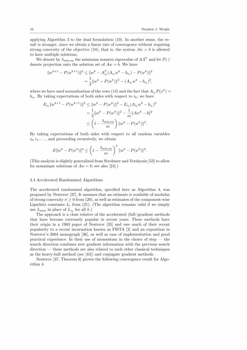
applying Algorithm 3 to the dual formulation (10). In another sense, the re-sult is stronger, since we obtain a linear rate of convergence without requiringstrong convexity of the objective (10), that is, the system Aw = b is allowedto have multiple solutions.
We denote by λmin,nz the minimum nonzero eigenvalue of AAT and let P (·)denote projection onto the solution set of Aw = b. We have
‖wk+1 − P (wk+1)‖2 ≤ ‖wk −ATik(Aikwk − bik)− P (wk)‖2
=1
2‖wk − P (wk)‖2 − (Aikw
k − bik)2,
where we have used normalization of the rows (14) and the fact thatAikP (xk) =bik . By taking expectations of both sides with respect to ik, we have
Eik‖wk+1 − P (wk+1)‖2 ≤ ‖wk − P (wk)‖2 − Eik(Aikwk − bik)2
=1
2‖wk − P (wk)‖2 − 1
m‖Awk − b‖2
≤(
1− λmin,nz
m
)‖wk − P (wk)‖2.
By taking expectations of both sides with respect to all random variablesi0, i1, . . . , and proceeding recursively, we obtain
E‖wk − P (wk)‖2 ≤(
1− λmin,nz
m
)k‖w0 − P (w0)‖2.
(This analysis is slightly generalized from Strohmer and Vershynin [53] to allowfor nonunique solutions of Aw = b; see also [24].)
3.4 Accelerated Randomized Algorithms
The accelerated randomized algorithm, specified here as Algorithm 4, wasproposed by Nesterov [37]. It assumes that an estimate is available of modulusof strong convexity σ ≥ 0 from (20), as well as estimates of the component-wiseLipschitz constants Li from (21). (The algorithm remains valid if we simplyuse Lmax in place of Lik for all k.)
The approach is a close relative of the accelerated (full-)gradient methodsthat have become extremely popular in recent years. These methods havetheir origin in a 1983 paper of Nesterov [35] and owe much of their recentpopularity to a recent incarnation known as FISTA [2] and an exposition inNesterov’s 2004 monograph [36], as well as ease of implementation and goodpractical experience. In their use of momentum in the choice of step — thesearch direction combines new gradient information with the previous searchdirection — these methods are also related to such other classical techniquesas the heavy-ball method (see [43]) and conjugate gradient methods.
Nesterov [37, Theorem 6] proves the following convergence result for Algo-rithm 4.
Coordinate Descent Algorithms 17
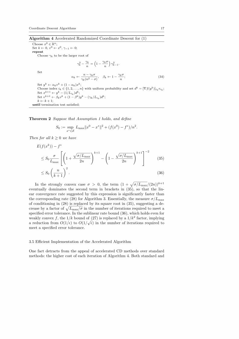
Algorithm 4 Accelerated Randomized Coordinate Descent for (1)
Choose x0 ∈ Rn;Set k ← 0, v0 ← x0, γ−1 ← 0;repeat
Choose γk to be the larger root of
γ2k −γk
n=
(1−
γkσ
n
)γ2k−1.
Set
αk ←n− γkσγk(n2 − σ)
, βk ← 1−γkσ
n; (34)
Set yk ← αkvk + (1− αk)xk;
Choose index ik ∈ 1, 2, . . . , n with uniform probability and set dk = [∇f(yk)]ikeik ;
Set xk+1 ← yk − (1/Lik )dk;
Set vk+1 ← βkvk + (1− βk)yk − (γk/Lik )dk;
k ← k + 1;until termination test satisfied;
Theorem 2 Suppose that Assumption 1 holds, and define
S0 := supx∗∈S
Lmax‖x0 − x∗‖2 + (f(x0)− f∗)/n2.
Then for all k ≥ 0 we have
E(f(xk))− f∗
≤ S0σ
Lmax
(1 +
√σ/Lmax
2n
)k+1
−
(1−
√σ/Lmax
2n
)k+1−2 (35)
≤ S0
(n
k + 1
)2
. (36)
In the strongly convex case σ > 0, the term (1 +√σ/Lmax/(2n))k+1
eventually dominates the second term in brackets in (35), so that the lin-ear convergence rate suggested by this expression is significantly faster thanthe corresponding rate (28) for Algorithm 3. Essentially, the measure σ/Lmax
of conditioning in (28) is replaced by its square root in (35), suggesting a de-crease by a factor of
√Lmax/σ in the number of iterations required to meet a
specified error tolerance. In the sublinear rate bound (36), which holds even forweakly convex f , the 1/k bound of (27) is replaced by a 1/k2 factor, implyinga reduction from O(1/ε) to O(1/
√ε) in the number of iterations required to
meet a specified error tolerance.
3.5 Efficient Implementation of the Accelerated Algorithm
One fact detracts from the appeal of accelerated CD methods over standardmethods: the higher cost of each iteration of Algorithm 4. Both standard and

18 Stephen J. Wright
Algorithm 5 Accelerated Randomized Kaczmarz for (8), (14)
Choose w0 ∈ Rn;Set k ← 0, v0 ← w0, γ−1 ← 0;repeat
Choose γk to be the larger root of
γ2k −γk
n=
(1−
γkσ
n
)γ2k−1.
Set
αk ←n− γkσγk(n2 − σ)
, βk ← 1−γkσ
n; (37)
Set yk ← αk vk + (1− αk)wk;
Choose index ik ∈ 1, 2, . . . ,m with uniform probability and set dk = (Aik yk −
bik )ATik ;
Set wk+1 ← yk − dk;Set vk+1 ← βk v
k + (1− βk)yk − γkdk;k ← k + 1;
until termination test satisfied;
accelerated variants require calculation of one element of the gradient, butAlgorithm 3 requires an update of just a single component of x, whereas Al-gorithm 4 also requires manipulation of the generally dense vectors y and v.Moreover, the gradient is evaluated at xk in Algorithm 3, where the argumentchanges by only one component from the prior iteration, a fact that can beexploited in several contexts. In Algorithm 4, the argument yk for the gradi-ent changes more extensively from one iteration to the next, making it lessobvious whether such economies are available. However, by using a change ofvariables due to Lee and Sidford [23], it is possible to implement the acceler-ated randomized CD approach efficiently for problems with certain structure,including the linear system Aw = b and certain problems of the form (5).
We explain the Lee-Sidford technique in the context of the Kaczmarz algo-rithm for (8), assuming normalization of the rows of A (14). As we explained in(16), the Kaczmarz algorithm is obtained by applying CD to the dual formu-lation (10) with variables x, but operating in the space of “primal” variables wusing the transformation w = ATx. If we apply the transformations vk = AT vk
and yk = AT yk to the other vectors in Algorithm 4, and use the fact of nor-malization (14) (and hence (AAT )ii = 1 for all i = 1, 2, . . . ,m) to note thatLi ≡ 1 in (21), we obtain Algorithm 5.
When the matrix A is dense, there is only a small factor of differencebetween the per-iteration workload of the standard Kaczmarz algorithm andits accelerated variant, Algorithm 5. Both require O(m + n) operations periteration. However, when A is sparse, the computational difference between thetwo algorithms becomes substantial. At iteration k, the standard Kaczmarzalgorithm requires computation proportion to a small multiple of the numberof nonzeros in row Aik (which we denote by |Aik |). Meanwhile, iteration kof Algorithm 5 requires manipulation of the dense vectors vk and yk — bothO(n) processes — and the benefits of sparsity are lost. This apparent defect was
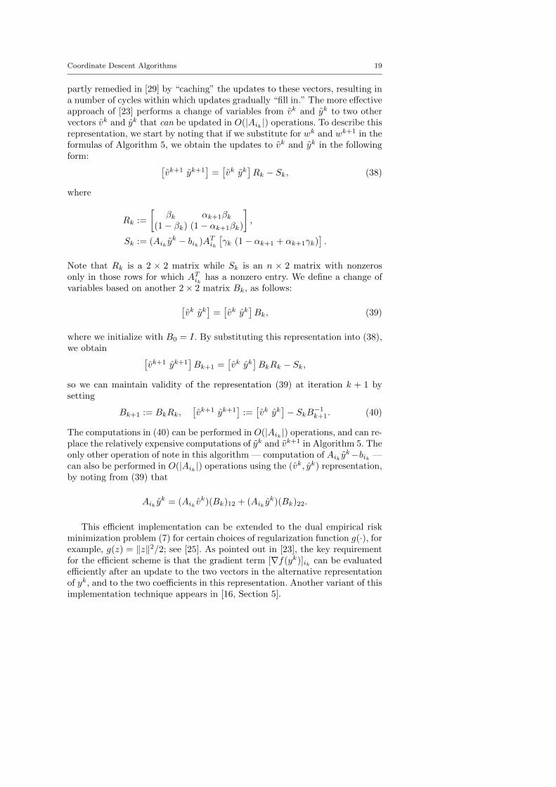
Coordinate Descent Algorithms 19
partly remedied in [29] by “caching” the updates to these vectors, resulting ina number of cycles within which updates gradually “fill in.” The more effectiveapproach of [23] performs a change of variables from vk and yk to two othervectors vk and yk that can be updated in O(|Aik |) operations. To describe thisrepresentation, we start by noting that if we substitute for wk and wk+1 in theformulas of Algorithm 5, we obtain the updates to vk and yk in the followingform: [
vk+1 yk+1]
=[vk yk
]Rk − Sk, (38)
where
Rk :=
[βk αk+1βk
(1− βk) (1− αk+1βk)
],
Sk := (Aik yk − bik)ATik
[γk (1− αk+1 + αk+1γk)
].
Note that Rk is a 2 × 2 matrix while Sk is an n × 2 matrix with nonzerosonly in those rows for which ATik has a nonzero entry. We define a change ofvariables based on another 2× 2 matrix Bk, as follows:[
vk yk]
=[vk yk
]Bk, (39)
where we initialize with B0 = I. By substituting this representation into (38),we obtain [
vk+1 yk+1]Bk+1 =
[vk yk
]BkRk − Sk,
so we can maintain validity of the representation (39) at iteration k + 1 bysetting
Bk+1 := BkRk,[vk+1 yk+1
]:=[vk yk
]− SkB−1k+1. (40)
The computations in (40) can be performed in O(|Aik |) operations, and can re-place the relatively expensive computations of yk and vk+1 in Algorithm 5. Theonly other operation of note in this algorithm — computation of Aik y
k−bik —can also be performed in O(|Aik |) operations using the (vk, yk) representation,by noting from (39) that
Aik yk = (Aik v
k)(Bk)12 + (Aik yk)(Bk)22.
This efficient implementation can be extended to the dual empirical riskminimization problem (7) for certain choices of regularization function g(·), forexample, g(z) = ‖z‖2/2; see [25]. As pointed out in [23], the key requirementfor the efficient scheme is that the gradient term [∇f(yk)]ik can be evaluatedefficiently after an update to the two vectors in the alternative representationof yk, and to the two coefficients in this representation. Another variant of thisimplementation technique appears in [16, Section 5].

20 Stephen J. Wright
3.6 Cyclic Variants
We have the following result from [3] for the cyclic variant of Algorithm 1.
Theorem 3 Suppose that Assumption 1 holds. Suppose that αk ≡ 1/Lmax inAlgorithm 1, with the index ik at iteration k chosen according to the cyclicordering (11) (with i0 = 1). Then for k = n, 2n, 3n, . . . , we have
f(xk)− f∗ ≤ 4nLmax(1 + nL2/L2max)R2
0
k + 8. (41)
When σ > 0 in the strong convexity condition (20), we have in addition fork = n, 2n, 3n, . . . that
f(xk)− f∗ ≤(
1− σ
2Lmax(1 + nL2/L2max)
)k/n(f(x0)− f∗). (42)
Proof The result (41) follows from Theorems 3.6 and 3.9 in [3] when we notethat (i) each iteration of Algorithm BCGD in [3] corresponds to a “cycle” ofn iterations in Algorithm 1; (ii) we update coordinates rather than blocks, sothat the parameter p in [3] is equal to n; (iii) we set Lmax and Lmin in [3] bothto Lmax.
Comparing the complexity bounds for the cyclic variant with the corre-sponding bounds proved in Theorem 1 for the randomized variant, we see thatsince L ≥ Lmax in general, the numerator in (41) is O(n2), in contrast toO(n) term in (27). A similar factor of n in seen in comparing (28) to (42),when we note that (1 − ε)1/n ≈ 1 − ε/n for small values of ε. The bounds inTheorem 3 are deterministic, however, rather than being bounds on expectednonoptimality, as in Theorem 1.
We noted in Subsection 3.2 that the ratio L/Lmax lies in the interval [1, n]when f is a convex quadratic function and both parameters are set to theirbest values. Lower values of this ratio are attained on functions that are “moredecoupled” and larger values attained when there is a greater dependencebetween the coordinates. Larger values lead to weaker bounds in Theorem 3,which accords with our intuition; we expect CD methods to require moreiterations to resolve the coupling of the coordinates.
We are free to make other, larger choices of Lmax; they need only satisfythe conditions (21) and (22). Larger values of Lmax lead to shorter steps αk =1/Lmax and different complexity expressions. For Lmax = L, for example, thebound in (41) becomes
4n(n+ 1)LR20
k + 8,
which is worse by a factor of approximately 2n2 than the bound (33) for thefull-step gradient descent approach. For Lmax =
√nL, we obtain
8n3/2LR20
k + 8,
which still trails (33) by a factor of 4n3/2.
Coordinate Descent Algorithms 21
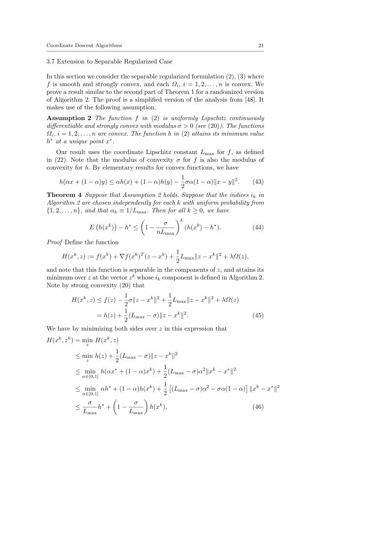
3.7 Extension to Separable Regularized Case
In this section we consider the separable regularized formulation (2), (3) wheref is smooth and strongly convex, and each Ωi, i = 1, 2, . . . , n is convex. Weprove a result similar to the second part of Theorem 1 for a randomized versionof Algorithm 2. The proof is a simplified version of the analysis from [48]. Itmakes use of the following assumption.
Assumption 2 The function f in (2) is uniformly Lipschitz continuouslydifferentiable and strongly convex with modulus σ > 0 (see (20)). The functionsΩi, i = 1, 2, . . . , n are convex. The function h in (2) attains its minimum valueh∗ at a unique point x∗.
Our result uses the coordinate Lipschitz constant Lmax for f , as definedin (22). Note that the modulus of convexity σ for f is also the modulus ofconvexity for h. By elementary results for convex functions, we have
h(αx+ (1− α)y) ≤ αh(x) + (1− α)h(y)− 1
2σα(1− α)‖x− y‖2. (43)
Theorem 4 Suppose that Assumption 2 holds. Suppose that the indices ik inAlgorithm 2 are chosen independently for each k with uniform probability from1, 2, . . . , n, and that αk ≡ 1/Lmax. Then for all k ≥ 0, we have
E(h(xk)
)− h∗ ≤
(1− σ
nLmax
)k(h(x0)− h∗). (44)
Proof Define the function
H(xk, z) := f(xk) +∇f(xk)T (z − xk) +1
2Lmax‖z − xk‖2 + λΩ(z),
and note that this function is separable in the components of z, and attains itsminimum over z at the vector zk whose ik component is defined in Algorithm 2.Note by strong convexity (20) that
H(xk, z) ≤ f(z)− 1
2σ‖z − xk‖2 +
1
2Lmax‖z − xk‖2 + λΩ(z)
= h(z) +1
2(Lmax − σ)‖z − xk‖2. (45)
We have by minimizing both sides over z in this expression that
H(xk, zk) = minz
H(xk, z)
≤ minz
h(z) +1
2(Lmax − σ)‖z − xk‖2
≤ minα∈[0,1]
h(αx∗ + (1− α)xk) +1
2(Lmax − σ)α2‖xk − x∗‖2
≤ minα∈[0,1]
αh∗ + (1− α)h(xk) +1
2
[(Lmax − σ)α2 − σα(1− α)
]‖xk − x∗‖2
≤ σ
Lmaxh∗ +
(1− σ
Lmax
)h(xk), (46)
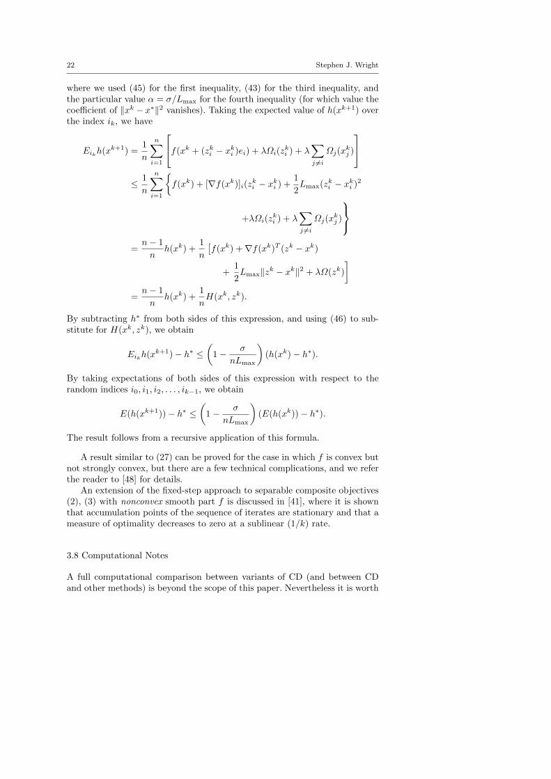
22 Stephen J. Wright
where we used (45) for the first inequality, (43) for the third inequality, andthe particular value α = σ/Lmax for the fourth inequality (for which value thecoefficient of ‖xk − x∗‖2 vanishes). Taking the expected value of h(xk+1) overthe index ik, we have
Eikh(xk+1) =1
n
n∑i=1
f(xk + (zki − xki )ei) + λΩi(zki ) + λ
∑j 6=i
Ωj(xkj )
≤ 1
n
n∑i=1
f(xk) + [∇f(xk)]i(z
ki − xki ) +
1
2Lmax(zki − xki )2
+λΩi(zki ) + λ
∑j 6=i
Ωj(xkj )
=n− 1
nh(xk) +
1
n
[f(xk) +∇f(xk)T (zk − xk)
+1
2Lmax‖zk − xk‖2 + λΩ(zk)
]=n− 1
nh(xk) +
1
nH(xk, zk).
By subtracting h∗ from both sides of this expression, and using (46) to sub-stitute for H(xk, zk), we obtain
Eikh(xk+1)− h∗ ≤(
1− σ
nLmax
)(h(xk)− h∗).
By taking expectations of both sides of this expression with respect to therandom indices i0, i1, i2, . . . , ik−1, we obtain
E(h(xk+1))− h∗ ≤(
1− σ
nLmax
)(E(h(xk))− h∗).
The result follows from a recursive application of this formula.
A result similar to (27) can be proved for the case in which f is convex butnot strongly convex, but there are a few technical complications, and we referthe reader to [48] for details.
An extension of the fixed-step approach to separable composite objectives(2), (3) with nonconvex smooth part f is discussed in [41], where it is shownthat accumulation points of the sequence of iterates are stationary and that ameasure of optimality decreases to zero at a sublinear (1/k) rate.
3.8 Computational Notes
A full computational comparison between variants of CD (and between CDand other methods) is beyond the scope of this paper. Nevertheless it is worth
Coordinate Descent Algorithms 23
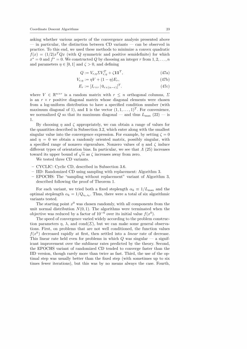
asking whether various aspects of the convergence analysis presented above— in particular, the distinction between CD variants — can be observed inpractice. To this end, we used these methods to minimize a convex quadraticf(x) = (1/2)xTQx (with Q symmetric and positive semidefinite) for whichx∗ = 0 and f∗ = 0. We constructed Q by choosing an integer r from 1, 2, . . . , nand parameters η ∈ [0, 1] and ζ > 0, and defining
Q := Vr,ηΣVTr,η + ζ11T , (47a)
Vr,η := ηV + (1− η)Er, (47b)
Er := [Ir×r | 0r×(n−r)]T . (47c)
where V ∈ Rn×r is a random matrix with r ≤ n orthogonal columns, Σis an r × r positive diagonal matrix whose diagonal elements were chosenfrom a log-uniform distribution to have a specified condition number (withmaximum diagonal of 1), and 1 is the vector (1, 1, . . . , 1)T . For convenience,we normalized Q so that its maximum diagonal — and thus Lmax (22) — is1.
By choosing η and ζ appropriately, we can obtain a range of values forthe quantities described in Subsection 3.2, which enter along with the smallestsingular value into the convergence expression. For example, by setting ζ = 0and η = 0 we obtain a randomly oriented matrix, possibly singular, witha specified range of nonzero eigenvalues. Nonzero values of η and ζ inducedifferent types of orientation bias. In particular, we see that Λ (25) increasestoward its upper bound of
√n as ζ increases away from zero.
We tested three CD variants.
– CYCLIC: Cyclic CD, described in Subsection 3.6.– IID: Randomized CD using sampling with replacement: Algorithm 3.– EPOCHS: The “sampling without replacement” variant of Algorithm 3,
described following the proof of Theorem 1.
For each variant, we tried both a fixed steplength αk ≡ 1/Lmax and theoptimal steplength αk = 1/Qik,ik . Thus, there were a total of six algorithmicvariants tested.
The starting point x0 was chosen randomly, with all components from theunit normal distribution N(0, 1). The algorithms were terminated when theobjective was reduced by a factor of 10−6 over its initial value f(x0).
The speed of convergence varied widely according to the problem construc-tion parameters η, λ, and cond(Σ), but we can make some general observa-tions. First, on problems that are not well conditioned, the function valuesf(xk) decreased rapidly at first, then settled into a linear rate of decrease.This linear rate held even for problems in which Q was singular — a signif-icant improvement over the sublinear rates predicted by the theory. Second,the EPOCHS variant of randomized CD tended to converge faster than theIID version, though rarely more than twice as fast. Third, the use of the op-timal step was usually better than the fixed step (with sometimes up to sixtimes fewer iterations), but this was by no means always the case. Fourth,
24 Stephen J. Wright
while there were extensive regimes of parameter values in which all six vari-ants performed similarly, there were numerous “stressed” settings in which theCYCLIC variants are much slower than the randomized variants, by factorsof 10 or more.
4 Parallel CD Algorithms
CD methods lend themselves to different kinds of parallel implementation.Even basic algorithm frameworks such as Algorithm 1 may be amenable toapplication-specific parallelism, when the computations involved in evaluatinga single element of the gradient vector are substantial enough to be spread outacross cores of a multicore computer. We concern ourselves here with moregeneric forms of parallelism, which involve multiple instances of the basic CDalgorithm, running in parallel on multiple processors.
We can distinguish different types of parallel CD algorithms. Synchronousalgorithms are those that partition the computation into pieces that can beexecuted in parallel on multiple processors (or cores of a multicore machine),but that synchronize frequently across all processors, to ensure consistencyof the information available to all processors at certain points in time. Forexample, each processor could update a subset of components of x in parallel(with the subsets being disjoint), and the synchronization step could ensurethat the results of all updates are shared across all processors before furthercomputation occurs. The synchronization step often detracts from the perfor-mance of algorithms, not only because some processors may be forced to idlewhile others complete their work, but also because the overheads associatedwith (hardware and software) locking of memory accesses can be high. Thus,asynchronous methods, which weaken or eliminate the requirement of consis-tent information across processors, are preferred in practice. Analysis of suchmethods is more difficult, but results have been obtained that accord withpractical experience of such methods. Indeed, it can be verified that in certainregimes, linear speedup can be expected across a modest number of processors.
4.1 Synchronous Parallelism
We mention several synchronous parallel variants of CD that appear in therecent literature. We note that in the some of these papers, the computa-tional results were obtained by implementing the methods in an asynchronousfashion, disregarding the synchronization step required by the analysis.
Bradley at al. [9] consider a bound-constrained problem that is a reformu-lation of the problem (2) with specific choices of f and with Ω(x) = ‖x‖1.Their algorithm performs short-step updates of individual components of xin parallel on P processors, with synchronization after each round of parallelupdating. This scheme essentially updates a randomly-chosen block of P vari-ables at each cycle. By modifying the analysis of [51], they show that the 1/k
Coordinate Descent Algorithms 25
sublinear convergence rate bound is not affected provided that P is no largerthan n/L, where L is the Lipschitz constant from (23).
Jaggi et al. [20] perform a synchronized CD method on the dual ERMmodel (7) for the case of g(w) = g∗(w) = (1/2)‖w‖2, partitioning componentsof the dual variable x between cores and sharing a copy of the vector Ax acrosscores, updating this vector at each synchronization point. The approach canbe thought of as a nonlinear block Gauss-Jacobi method (by contrast with thecoordinate Gauss-Seidel approaches discussed in Section 3).
Richtarik and Takac [47] describe a method for the separably regularizedformulation (2), (3) in which a subset of indices Sk ⊂ 1, 2, . . . , n is updatedaccording to the formula in Algorithm 2. The work of updating the compo-nents in Sk is divided between processors; essentially, a synchronization steptakes place at each iteration. This scheme is enhanced with an accelerationstep in [15]; the extra computations associated with the acceleration step tooare parallelized, using ideas from [23]. In the scheme of Marecek, Richtarik,and Takac [32], the variable vector x is partitioned into subvectors, and eachprocessor is assigned the responsibility for updating one of these subvectors.On each processor, the updating scheme described in [47] is applied, provid-ing a second level of parallelism. Synchronization takes place at each outeriteration. Details of the information-sharing between processors required foraccurate computation of gradients in different applications are described in[32, Section 6].
4.2 Asynchronous Parallelism
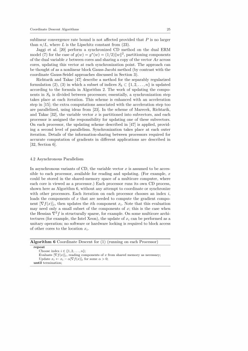
In asynchronous variants of CD, the variable vector x is assumed to be acces-sible to each processor, available for reading and updating. (For example, xcould be stored in the shared-memory space of a multicore computer, whereeach core is viewed as a processor.) Each processor runs its own CD process,shown here as Algorithm 6, without any attempt to coordinate or synchronizewith other processors. Each iteration on each processor chooses an index i,loads the components of x that are needed to compute the gradient compo-nent [∇f(x)]i, then updates the ith component xi. Note that this evaluationmay need only a small subset of the components of x; this is the case whenthe Hessian ∇2f is structurally sparse, for example. On some multicore archi-tectures (for example, the Intel Xeon), the update of xi can be performed as aunitary operation; no software or hardware locking is required to block accessof other cores to the location xi.
Algorithm 6 Coordinate Descent for (1) (running on each Processor)repeat
Choose index i ∈ 1, 2, . . . , n;Evaluate [∇f(x)]i, reading components of x from shared memory as necessary;Update xi ← xi − α[∇f(x)]i for some α > 0;
until termination;
26 Stephen J. Wright
We can take a global view of the entire parallel process, consisting of mul-tiple processors each executing Algorithm 6, by defining a global counter kthat is incremented whenever any processor updates an element of x: see Al-gorithm 7. Note that the only difference with the basic framework of Algo-rithm 1 is in the argument of the gradient component: In Algorithm 1 this isthe latest iterate xk whereas in Algorithm 7 it is a vector xk that is generallymade up of components of vectors from previous iterations xj , j = 0, 1, . . . , k.The reason for this discrepancy is that between the time at which a processorreads the vector x from shared storage in order to calculate [∇f(x)]i, and thetime at which it updates component i, other processors have generally madechanges to x. In consequence, each update step is using slightly stale informa-tion about x. To prove convergence results, we need to make assumptions onhow much “staleness” can be tolerated, and to modify the convergence anal-ysis quite substantially. Indeed, proofs of convergence even for the most basicasynchronous algorithms are quite technical.
Algorithm 7 Asynchronous Coordinate Descent for (1)
Set k ← 0 and choose x0 ∈ Rn;repeat
Choose index ik ∈ 1, 2, . . . , n;xk+1 ← xk − αk[∇f(xk)]ikeik for some αk > 0;k ← k + 1;
until termination test satisfied;
Asynchronous CD algorithms are distinguished from each other mostly bythe assumptions they make on the the choice of update components ik andon the “ages” of the components of xk, that is, the iterations at which eachcomponent of this vector was last updated. In the terminology of Bertsekasand Tsitsiklis [5], the algorithm is totally asynchronous if
(a) each index i ∈ 1, 2, . . . , n of x is updated at infinitely many iterations;and
(b) if νkj denotes the iteration at which component j of the vector xk was last
updated, then νkj →∞ as k →∞ for all j = 1, 2, . . . , n.
In other words, each component of x is updated infinitely often, and all com-ponents used in successive evaluation vectors xk are also updated infinitelyoften.
The following convergence result for totally asynchronous variants of Al-gorithm 7 is due to Bertsekas and Tsitsiklis; see in particular [5, Sections 6.1,6.2, and 6.3.3].
Theorem 5 Suppose that the problem (1) has a unique solution x∗ and thatf is convex and continuously differentiable. Suppose that Algorithm 7 is imple-mented in a totally asynchronous fashion. Suppose that the mapping T definedby T (x) := x−α∇f(x) for some α > 0 (for which x∗ is the unique fixed point)
Coordinate Descent Algorithms 27
is strictly contractive in the `∞ norm, that is,
‖T (x)− x∗‖∞ ≤ η‖x− x∗‖∞, for some η ∈ (0, 1). (48)
Then if we set αk ≡ α in Algorithm 7, the sequence xk converges to x∗.
We cannot expect to obtain a convergence rate in this setting (such as sublinearwith rate 1/k), given that the assumptions on the ages of the components inxk are so weak. Although this result can be generalized impressively and itsproof is not too complex, we should note that the `∞ contraction assumption(48) is quite strong. It is violated even by some strictly convex objectives f .For example, when f(x) = (1/2)xTQx with
Q =
[1 11 2
],
we have f strictly convex with minimizer x∗ = 0. However the mappingT (x) = (I − αQ)x is not contractive for any α > 0; we have for examplethat ‖T (x)‖∞ ≥ ‖x‖∞ when x = (1,−1)T .
We turn now to partly asynchronous variants of Algorithm 7, in whichwe make stronger assumptions on the ages of the components of xk. Liu andWright [27] consider a version of Algorithm 7 that is the parallel analog ofAlgorithm 3, in that each update component ik is chosen independently andrandomly with equal probability from 1, 2, . . . , n. They assume that no com-ponent of xk is older than a nonnegative integer τ — the “maximum delay”— for any k. Specifically, they express the difference between xk and xk interms of “missed updates” to x, as follows:
xk = xk +∑
l∈K(j)
(xl+1 − xl), (49)
where K(j) is a set of iteration numbers drawn from the set j − q : q =1, 2, . . . , τ. The value of τ is related to the number of processors P involvedin the computation. If all processors are performing their updates at approx-imately the same rates, we could expect τ to be a modest multiple of P —perhaps τ = 2P or τ = 3P , to allow a safety margin for occasional delays.Hence the value of τ is an indicator of potential parallelism in the algorithm.
In [27], the steplengths in Algorithm 7 are fixed as follows:
αk ≡γ
Lmax, (50)
where γ is chosen to ensure that Algorithm 7 progresses steadily toward a solu-tion, but not too rapidly. Too-rapid convergence would cause the informationin xk to become too stale too quickly, so the gradient component [∇f(xk)]ikwould lose its relevance as a suitable update for the variable component xikat iteration k. Steady convergence is enforced by choosing some ρ > 1 andrequiring that
E‖xk−1 − xk‖2 ≤ ρE‖xk − xk+1‖2, (51)

28 Stephen J. Wright
where xk is the vector that would hypothetically be obtained if we were toapply the the update to all components, that is,
xk+1 := xk − γ
Lmax∇f(xk),
and the expectations E(·) are taken over all random variables i0, i2, . . . . Con-dition (51) ensures that the “expected squared update norms” decrease by atmost a factor of 1/ρ at each iteration.
The main results in [27] apply to composite functions (2), (3), but for sim-plicity here we state the result in terms of the problem (1), where f is convexand continuously differentiable, with nonempty solution set S and optimalobjective value f∗. We use PS to denote projection onto S, and recall thedefinition (25) of the ratio Λ between different varieties of Lipschitz constants.The results also make use of an optimal strong convexity condition, which isthat the following inequality holds for some σ > 0:
f(x)− f∗ ≥ σ
2‖x− PS(x)‖2, for all x. (52)
The following result is a modification of [27, Corollary 2].
Theorem 6 Suppose that Assumption 1 holds, and that
4eΛ(τ + 1)2 ≤√n. (53)
Then by setting γ = 1/2 in (50) (that is, choosing steplengths αk ≡ 1/(2Lmax)),we have that
E(f(xk)
)− f∗ ≤ n(Lmax‖x0 − PS(x0)‖2 + f(x0)− f∗)
n+ k. (54)
Assuming in addition that (52) is satisfied for some σ > 0, we obtain thefollowing linear rate:
E(f(xk)
)− f∗
≤(
1− σ
n(σ + 2Lmax)
)k(Lmax‖x0 − PS(x0)‖2 + f(x0)− f∗). (55)
A comparison with Theorem 1, which shows convergence rates for serial ran-domized CD (Algorithm 3) shows a striking similarity in convergence bounds.The factor-of-2 difference in steplength between the serial and parallel vari-ants accounts for most of the difference between the linear rates (28) and (55),while there is an extra term n in the denominator of the sublinear rate (54). Weconclude that we do not pay q high overhead (in terms of total workload) forparallel implementation, and hence that near-linear speedup can be expected.(Indeed, computational results in [27] and [28] observe near-linear speedup formulticore asynchronous implementations.)
These encouraging conclusions depend critically on the condition (53),which is an upper bound on the allowable delay τ in terms of n and the ratio

Coordinate Descent Algorithms 29
Λ from (25). For functions f with weak coupling between the components ofx (for example, when off-diagonals in the Hessian ∇2f(x) are small relative tothe diagonals), we have Λ not much greater than 1, so the maximum delay canbe of the order of n1/4 before there is any attenuation of linear speedup. Whenstronger coupling exists, the restriction on τ may be quite tight, possibly notmuch greater than 1. A more general convergence result [27, Theorem 1] showsthat in this case, we can choose smaller values of γ in (50), allowing grace-ful degradation of the convergence bounds while still obtaining fairly efficientparallel implementations.
We note that an earlier analysis in [28] made a stronger assumption on xk
— that it is equal to some earlier iterate xj of Algorithm 7, where k ≥ j ≥ k−τ ,that is, the earlier iterate is no more than τ cycles old. (A similar assumptionwas used to analyze convergence of as asynchronous stochastic gradient algo-rithm in [39].) This stronger assumption yields stronger convergence results,in that the bound on τ in (53) can be loosened. However, the assumption maynot always hold, since some parts of x in memory may be altered by somecores as they are being read by another core, a phenomenon referred to in [27]as “inconsistent reading.”
5 Conclusion
We have surveyed the state of the art in convergence of coordinate descentmethods, with a focus on the most elementary settings and the most funda-mental algorithms. The recent literature contains many extensions, enhance-ments, and elaborations; we refer interested readers to the bibliography of thispaper, and note that new works are appearing at a rapid pace.
Coordinate descent method have become an important tool in the opti-mization toolbox that is used to solve problems that arise in machine learningand data analysis, particularly in “big data” settings. We expect to see fur-ther developments and extensions, further customization of the approach tospecific problem structures, further adaptation to various computer platforms,and novel combinations with other optimization tools to produce effective “so-lutions” for key application areas.
Acknowledgements I thank Ji Liu for the pleasure of collaborating with him on this topicover the past two years. I am grateful to the editors and referees of the paper, whose expertand constructive comments led to numerous improvements.
References
1. Attouch, H., Bolte, J., Redont, P., Soubeyran, A.: Proximal alternating minimizationand projection methods for nonconvex problems: an approach based on the kurdyka-lojasiewicz inequality. Mathematics of Operations Research 35(2), 438–457 (2010)
2. Beck, A., Teboulle, M.: A fast iterative shrinkage-threshold algorithm for linear inverseproblems. SIAM Journal on Imaging Sciences 2(1), 183–202 (2009)
30 Stephen J. Wright
3. Beck, A., Tetruashvili, L.: On the convergence of block coordinate descent methods.SIAM Journal on Optimization 23(4), 2037–2060 (2013)
4. Bertsekas, D.P.: Nonlinear Programming, second edn. Athena Scientific (1999)5. Bertsekas, D.P., Tsitsiklis, J.N.: Parallel and Distributed Computation: Numerical
Methods. Prentice-Hall, Inc., Englewood Cliffs, New Jersey (1989)6. Bolte, J., Sabach, S., Teboulle, M.: Proximal alternating linearized minimization for
nonconvex and nonsmooth problems. Mathematical Programming, Series A 146, 1–36(2014)
7. Bouman, C.A., Sauer, K.: A unified approach to statistical tomography using coordinatedescent optimization. IEEE Transactions on Image Processing 5(3), 480–492 (1996)
8. Boyd, S., Parikh, N., Chu, E., Peleato, B., Eckstein, J.: Distributed optimization andstatistical learning via the alternating direction methods of multipliers. Foundationsand Trends in Machine Learning 3(1), 1–122 (2011)
9. Bradley, J.K., Kyrola, A., Bickson, D., Guestrin, C.: Parallel coordunate descent for`1-regularized loss minimization. In: Proceedings of the 28 International Conference onMachine Learning (ICML 2011) (2011)
10. Breheny, P., Huang, J.: Coordunate descent algroithms for nonconvex penalized regres-sion, with applications to biological feature selection. Annals of Applied Statistics 5(1),232–252 (2011)
11. Canutescu, A.A., Dunbrack, R.L.: Cyclic coordinate descent: A robotics algorithm forprotein loop closure. Protein Science 12(5), 963–972 (2003)
12. Chang, K., Hsieh, C., Lin, C.: Coordinate descent method for large-scale l2-loss linearsupport vector machines. Journal of Machine Learning Research 9, 1369–1398 (2008)
13. Eckstein, J., Bertsekas, D.P.: On the Douglas-Rachford splitting method and the proxi-mal point algorithm for maximal monotone operators. Mathematical Programming 55,293–318 (1992)
14. Eckstein, J., Yao, W.: Understanding the convergence of the alternating directionmethod of multipliers: Theoretical and computational perspectives. Technical report,RUTCOR, Rutgers University (2014)
15. Fercoq, O., Qu, Z., Richtarik, P., Takac, M.: Fast distributed coordinate descent fornon-strongly convex losses. arxiv:1405.5300 (2014)
16. Fercoq, O., Richtarik, P.: Accelerated, parallel, and proximal coordinate descent. Tech-nical Report arXiv:1312.5799, School of Mathematics, University of Edinburgh (2013)
17. Florian, M., Chen, Y.: A coordinate descent method for the bilevel O-D matrix ad-justment problem. International Transactions on Operational Research 2(2), 165–179(1995)
18. Friedman, J., Hastie, T., Tibshirani, R.: Sparse inverse covariance estimation with thegraphical lasso. Biostatistics 9(3), 432–441 (2008)
19. Friedman, J.H., Hastie, T., Tibshirani, R.: Regularization paths for generalized linearmodels via coordinate descent. Journal of Statitsical Software 33(1), 1–22 (2010)
20. Jaggi, M., Smith, V., Takac, M., Terhorst, J., Krishnan, S., Hoffman, T., Jordan, M.I.:Communication-efficient distributed dual coordinate ascent. Advances in Neural Infor-mation Processing Systems 27 (2014)
21. Jain, P., Netrapalli, P., Sanghavi, S.: Low-rank matrix completion using alternatingminimization. Technical Report arXiv:1212.0467 (2012)
22. Kaczmarz, S.: Angenaherte auflosung von systemen linearer gleichungen. Bulletin In-ternational de l’Academie Polonaise des Sciences et des Lettres 35, 355–357 (1937)
23. Lee, Y.T., Sidford, A.: Efficient accelerated coordinate descent methods and faster al-gorihtms for solving linear systems. In: 54th Annual Symposium on Foundations ofComputer Science, pp. 147–156 (2013)
24. Leventhal, D., Lewis, A.S.: Randomized methods for linear constraints: Convergencerates and conditioning. Mathematics of Operations Research (2010)
25. Lin, Q., Lu, Z., Xiao, L.: An accelerated proximal coordinate gradient method and itsapplication to empirical risk minimization. Technical Report arXiv:1407.1296, MicrosoftResearch (2014)
26. Liu, H., Palatucci, M., Zhang, J.: lockwise coordinate descent procedures for the multi-task lasso, with applications to neural semantic basis discovery. In: Proceedings of the26th Annual International Conference on Machine Learning, ICML ’09, pp. 649–656.ACM, New York, NY, USA (2009)
Coordinate Descent Algorithms 31
27. Liu, J., Wright, S.J.: Asynchronous stochastic coordinate descent: Parallelism and con-vergence properties. Technical Report arXiv:1403.3862, University of Wisconsin, Madi-son (2014). To appear in SIAM Journal on Optimization
28. Liu, J., Wright, S.J., Re, C., Bittorf, V., Sridhar, S.: An asynchronous parallel stochasticcoordinate descent algorithm. Technical Report arXiv:1311.1873, Computer SciencesDepartment, University of Wisconsin-Madison (2013). To appear in Journal of MachineLearning Research
29. Liu, J., Wright, S.J., Sridhar, S.: An accelerated randomized Kaczmarz algorithm. Tech-nical Report arXiv 1310.2887, Computer Sciences Department, University of Wisconsin-Madison (2013). To appear in Mathematics of Computation
30. Luo, Z.Q., Tseng, P.: On the convergence of the coordinate descent method for convexdifferentiable minimization. Journal of Optimization Theory and Applications 72(1),7–35 (1992)
31. Luo, Z.Q., Tseng, P.: Error bounds and convergence analysis of feasible descent methods:a general approach. Annals of Operations Research 46, 157–178 (1993)
32. Marecek, J., Richtarik, P., Takac, M.: Distributed block coordinate descent for mini-mizing partially separable functions. Technical Report arXiv:1406.0238 (2014)
33. Mazumder, R., Friedman, J.H., Hastie, T.: SparseNet: Coordinate descent with noncon-vex penalties. Journal of the American Statistical Association 106, 1125–1138 (2011)
34. Necoara, I., Clipici, D.: Distributed random coordinate descent method for compositeminimization. Technical Report 1-41, University Politehnica Bucharest (2013)
35. Nesterov, Y.: A method for unconstrained convex problem with the rate of convergenceO(1/k2). Doklady AN SSSR 269, 543–547 (1983)
36. Nesterov, Y.: Introductory Lectures on Convex Optimization: A Basic Course. KluwerAcademic Publishers (2004)
37. Nesterov, Y.: Efficiency of coordinate descent methods on huge-scale optimization prob-lems. SIAM Journal on Optimization 22, 341–362 (2012)
38. Nesterov, Y.: Subgradient methods for huge-scale optimization problems. MathematicalProgramming, Series A 146, 275–297 (2014)
39. Niu, F., Recht, B., Re, C., Wright, S.J.: Hogwild!: A lock-free approach to parallelizingstochastic gradient descent. In: Advances in Neural Information Processing Systems(2011)
40. Ortega, J.M., Rheinboldt, W.C.: Iterative solution of nonlinear equations in severalvariables. Academic Press, New York and London (1970)
41. Patrascu, A., Necoara, I.: Efficient random coordinate descent algorithms for large-scale structured nonconvex optimization. Journal of Global Optimization (2013). DOI:10.1007/s10898-014-0151-9
42. Platt, J.C.: Fast training of support vector machines using sequential minimal optimiza-tion. In: B. Scholkopf, C.J.C. Burges, A.J. Smola (eds.) Advances in Kernel Methods— Support Vector Learning, pp. 185–208. MIT Press, Cambridge, MA (1999)
43. Polyak, B.T.: Introduction to Optimization. Optimization Software (1987)44. Powell, M.J.D.: On search directions for minimization algorithms. Mathematical Pro-
gramming 4, 193–201 (1973)45. Razaviyayn, M., Hong, M., Luo, Z.Q.: A unified convergence analysis of block successive
minimization methods for nonsmooth optimization. SIAM Journal on Optimization23(2), 1126–1153 (2013)
46. Recht, B., Fazel, M., Parrilo, P.: Guaranteed minimum-rank solutions to linear matrixequations via nuclear norm minimization. SIAM Review 52(3), 471–501 (2010)
47. Richtarik, P., Takac, M.: Parallel coordinate descent methods for big data optimiza-tion. Technical Report arXiv:1212.0873, School of Mathematics, University of Edin-burgh (2013)
48. Richtarik, P., Takac, M.: Iteration complexity of a randomized block-coordinate descentmethods for minimizing a composite function. Mathematical Programming, Series A144(1), 1–38 (2014)
49. Rockafellar, R.T.: Convex Analysis. Princeton University Press, Princeton, N.J. (1970)50. Sardy, S., Bruce, A., Tseng, P.: Block coordinate relaxation methods for nonparametric
wavelet denoising. Journal of Computational and Graphical Statistics 9, 361–379 (2000)51. Shalev-Shwartz, S., Tewari, A.: Stochastic methods for `1-regularized loss minimization.
Journal of Machine Learning Research 12, 1865–1892 (2011)

32 Stephen J. Wright
52. Shalev-Shwartz, S., Zhang, T.: Stochastic dual coordinate ascent mehods for regularizedloss minimization. Journal of Machine Learning Research 14, 437–469 (2013)
53. Strohmer, T., Vershynin, R.: A randomized Kaczmarz algorithm with exponential con-vergence. Journal of Fourier Analysis and Applications 15, 262–278 (2009)
54. Tibshirani, R.: Regression shrinkage and selection via the LASSO. Journal of the RoyalStatistical Society B 58, 267–288 (1996)
55. Tseng, P.: Convergence of a block coordinate descent method for nondifferentiable min-imization. Journal of Optimization Theory and Applications 109(3), 475–494 (2001)
56. Tseng, P., Yun, S.: A coordinate gradient descent method for nonsmooth separableminimization. Mathematical Programming, Series B 117, 387–423 (2009)
57. Ye, J.C., Webb, K.J., Bouman, C.A., Millane, R.P.: Optical diffusion tomography byiterative-coordinate-descent optimization in a bayesian framework. Journal of the Op-tical Society of America A 16(10), 2400–2412 (1999)