on entropy generation and dissipation of kinetic energy in high-resolution shock-capturing schemes

Available online at www.sciencedirect.com

Journal of Computational Physics 227 (2008) 4853–4872

www.elsevier.com/locate/jcp

On entropy generation and dissipation of kinetic energyin high-resolution shock-capturing schemes q

B. Thornber a, D. Drikakis a,*, R.J.R. Williams b, D. Youngs b

a Fluid Mechanics and Computational Science Group, Aerospace Sciences Department, School of Engineering,

Cranfield University, Cranfield MK43 0AL, United Kingdomb AWE, Aldermaston, United Kingdom

Received 25 April 2007; received in revised form 26 December 2007; accepted 14 January 2008Available online 2 February 2008

Abstract

This paper addresses entropy generation and the corresponding dissipation of kinetic energy associated with high-res-olution, shock-capturing (Godunov) methods. Analytical formulae are derived for the rate of increase of entropy givenarbitrary jumps in primitive variables at a cell interface. It is demonstrated that for general continuously varying flowsthe inherent numerical entropy increase of Godunov methods is not proportional to the velocity jump cubed as is com-monly assumed, but it is proportional to the velocity jump squared. Furthermore, the dissipation of kinetic energy isdirectly linked to temperature multiplied by change in entropy at low Mach numbers. The kinetic energy dissipation rateis shown to be proportional to the velocity jump squared and the speed of sound. The leading order dissipation rate asso-ciated with jumps in pressure, density and shear waves is detailed and further shown that at low Mach number it is thedissipation due to the perpendicular velocity jumps which dominates. This explains directly the poor performance ofGodunov methods at low Mach numbers. The analysis is also applied to high-order accurate methods in space and timeand all analytical results are validated with simple numerical experiments.� 2008 Elsevier Inc. All rights reserved.

Keywords: High-resolution methods; Godunov methods; Dissipation; Kinetic energy; Entropy; Large eddy simulation; Low Machnumber

1. Introduction

The finite volume (FV) high-resolution, shock-capturing methods (henceforth labelled as Godunov meth-ods) have proven extremely successful in the simulation of high-speed flows and is an essential tool in manyapplications in the broader field of compressible fluid dynamics. The Euler equations can form steep discon-tinuities in compressible flows and in order to provide a stable and non-oscillatory solution a certain level of

0021-9991/$ - see front matter � 2008 Elsevier Inc. All rights reserved.

doi:10.1016/j.jcp.2008.01.035

q Contains material � British Crown Copyright 2006/MOD.* Corresponding author. Tel.: +44 1234 754796; fax: +44 1234 752149.

E-mail address: [email protected] (D. Drikakis).

mailto:[email protected]

4854 B. Thornber et al. / Journal of Computational Physics 227 (2008) 4853–4872

artificial dissipation is added to the solution. In a Godunov method this dissipation is added through theupwind behaviour of the numerical scheme. Unfortunately, the numerical dissipation required to stabilisethe solution also causes anomalous increase in entropy, and corresponding dissipation of kinetic energy.The aim of this paper is to understand the rate of dissipation of kinetic energy and rate of entropy increase.These are issues especially important in describing the poor performance of Godunov methods in simulationsof low Mach number flows; determining the implicit subgrid model for implicit large eddy simulations (ILES);and in eliminating entropy errors associated with unsteady flow features. Issues such as convergence problemsand difficulties due to round off errors are not dealt with in this paper, for further information see for example[1,2] and references within.

Several previous papers have discussed the influence of artificial viscosity on the simulation of inviscidflows, primarily applied to finite difference methods. Noh [3] detailed the behaviour of finite differenceschemes, highlighting the sometimes undesirable effects of the von Neumann and Richtmyer type viscositywhen simulating strong shock waves due to the overly dissipative nature of certain formulations, especiallyin the absence of heat conduction. Christensen [4] draws parallels between the dissipation inherent in a Godu-nov method and that due to artificial viscosity method. The different forms of artificial viscosity are furtherdiscussed in Benson [5] with respect to their performance in capturing shock waves. Volpe [6] demonstratedusing several numerical examples that FV methods provide inaccurate results at low Mach number flowsdue to excess numerical dissipation. Later, Menikoff [7] noted that artificial viscosity is responsible for theentropy errors associated with a diffused shock and that this error does not disappear with mesh refinement.This type of entropy error is commonly referred to as ‘wall heating’ in the literature. Several papers by Guil-lard [8,9,1] examine the low Mach number problem, demonstrating that at low Mach numbers the artificialviscosity present in Godunov schemes leads to an undesirable scaling of the pressure with respect to the Machnumber (in the absence of acoustic waves) and proposing a form of preconditioning of the governing equa-tions to correct this. However, to the authors knowledge, an analytical form of entropy generation and dis-sipation of kinetic energy in Godunov schemes has not been yet been derived. This paper details the firstvalidated analytical description of the dissipation of kinetic energy in Godunov methods.

Two factors have increased the importance of the dissipation of kinetic energy by Godunov methods.Firstly, as computational power and grid size increases, numerical simulations can resolve relatively low Machnumber perturbations. An example of this is in the simulation of compressible turbulent flows. The large scalesare at a relatively high Mach number, whereas small instabilities can occur at low Mach number. These cangrow in size and affect the development of the larger scales (especially in fundamental instabilities such as Ray-leigh Taylor, Richtmyer–Meshkov and Kelvin–Helmholtz). Critically, Godunov methods were largelydesigned for the simulation of flows with a steady frame of reference – typically those involving relativelysmooth flow fields containing isolated discontinuities. Modern computing power allows simulations of flows,which are without a steady frame of reference in time and space, where velocities, pressure and density varycontinuously throughout the flow field. It is important to understand the mechanism of dissipation of turbu-lent kinetic energy within high-resolution shock-capturing schemes, to better represent the growth of smallinstabilities, and hence reliably model the actual flow physics.

Secondly, a there has been a rapid increase in the use of implicit large eddy simulation in a variety of appli-cations [10,11], where the dissipation inherent within the numerical method is employed ‘in lieu’ of an explicitsubgrid model. To design future implicit models, an analytical description of the leading order dissipativeterms is required so that this can be matched to the expected dissipation rate (such as that due to Kolmogo-rov’s refined similarity hypothesis [12]).

The layout of the paper is as follows: Section 2 derives an equation to link entropy generation with dissi-pation of kinetic energy. By considering both entropy generation and kinetic energy dissipation together, it iseasier to understand the mechanism of numerical dissipation. For example, it is expected that understandingof the kinetic energy dissipation rate should describe the increase in dissipation at low Mach numbers. Section3 shows that the dissipation due to a shock of fixed strength is constant with Mach number at leading order,thus this cannot be the leading source of dissipation of kinetic energy (or generation of entropy). Next, thepossibility that there are more shocks in the discrete Riemann problem at low Mach numbers is investigatedin Section 4. It is shown that although the structure of the problem does change at low Mach number, this isnot the direct source of increase of dissipation as it does not change significantly below a Mach number of

B. Thornber et al. / Journal of Computational Physics 227 (2008) 4853–4872 4855

� 0:2. Section 5 demonstrates via an asymptotic analysis of the discrete problem that the leading order dissi-pation is due primarily to the reaveraging process and that the irreversible dissipation of kinetic energy is pro-portional to the magnitude of the velocity gradient squared multiplied by the speed of sound. This is validatednumerically using several different Riemann solvers, exact and approximate. Finally, the analysis is extendedto include higher order methods in space and time.

2. The relationship between kinetic energy and entropy

Before commencing the analysis, it is important to clarify the governing equations and essential to discussthe relationship between kinetic energy and entropy. This paper is concerned solely with the analysis of theEuler equations of gas flow, where the viscosity is assumed negligible (Re!1). The homogeneity propertyof the Euler equations means that the properties can be analysed using the following governing equations ineach principal direction:

oU

otþ oE

ox¼ 0; ð1Þ

where

U ¼ ½q; qu; qv; qw;E�T; ð2Þ

E ¼ qu; qu2 þ p; quv; quw; ðE þ pÞu� �T

; ð3ÞE ¼ qeþ 0:5qðu2 þ v2 þ w2Þ ð4Þ

and q, e, u, v, w are the density, specific internal energy per unit volume and Cartesian velocity components,respectively. Throughout this paper it is assumed that the fluid satisfies the ideal gas equation of state

p ¼ qeðc� 1Þ; ð5Þ
where c is the ratio of specific heats. In a Godunov method the governing equations are solved in integral formwhere the cell averaged conserved variables at the new time step, Unþ1, are computed according to
Unþ1 ¼ Un � DtDxðEiþ1=2 � Ei�1=2Þ ¼ 0; ð6Þ

where Dt and Dx are the time step and width of the cell. The time averaged numerical fluxes Ei�1=2 are com-puted from the Riemann problem at the cell interface. This is typically seen as the solution of the Riemannproblem along the line x=t ¼ 0, where x is centred at the interface. At any interface where the velocity or pres-sure differs from one side to the next, the solution will normally split into three waves, a contact surface sand-wiched by two waves which are either a shock or rarefaction. Only the shock wave adds irreversibledissipation, as the rarefaction and contact surface are isentropic phenomena. Thus, irreversible dissipation oc-curs only when the solution to the Riemann problem at x=t ¼ 0 (the star quantities) lies between the contactsurface and the shock wave.

Understanding the role of entropy in the context of dissipation of specific kinetic energy is key to under-standing the dissipative properties of Godunov methods. Specific entropy is defined through the Gibbs equa-tion (see for example [13] for a full derivation),

dS ¼ 1

Tde� p

q2Tdq; ð7Þ

where T is the temperature of the system. Integrating this equation gives

S ¼ cv lnT nþ1

T n

� �� R ln

qnþ1

qn

� �þ Sn; ð8Þ

where Sn is the initial entropy at time n, cv is the specific heat at constant volume and R is the specific gas con-stant. Noting that T ¼ p=ðRqÞ and cv ¼ R=ðc� 1Þ, the above equation can be rearranged into the followingform for a change of entropy DS


DS ¼ Rc� 1

lnpqc

� �nþ1 qc

p

� �n" #

: ð9Þ

The numerical solution to the Euler equations is constructed in a such a form that mass, momentum and totalenergy are conserved, but kinetic energy is not conserved due to numerical dissipation. The behaviour of thechange of kinetic energy within a compressible fluid is similar to that of a damped spring. There are changes ofkinetic energy, which are accompanied by an isentropic change in pressure, as is the case for an ideal inviscidflow without shocks. In this case, although the kinetic energy has changed, there has been no actual dissipationof kinetic energy and thus the flow behaves like an undamped spring. However, if the entropy increases thenthere has been an irreversible dissipation of specific kinetic energy, which acts as a dampener to the isentropicmotion.

A direct relationship between kinetic energy and entropy will now be derived, assuming a continuous (infi-nitely differentiable) flow field. The derivation begins with the conservation equation for kinetic energy in vec-tor notation without external forces,

qDDt

1

2V 2

� �¼ �½r � ðpuÞ � pr � u� þDw �Dg; ð10Þ

where q is the density, V ¼ffiffiffiffiffiffiffiffiffiffiffiffiffiffiffiffiffiffiffiffiffiffiffiffiffiu2 þ v2 þ w2p

, p is the pressure, u is the vector of velocities, D=Dt represents thematerial or total derivative. The first group of terms on the right hand side relates to flow work due to thepressure on the control volume minus the work that does not increase the kinetic energy. By analogy tothe Navier–Stokes equations (where Dw ¼ r � ðs � uÞ, and Dg ¼ s : ru) Dw is the total work that the surround-ings do on the fluid through the numerical shear stress and Dg is the portion of the work due to numericalshear stresses, which dissipates kinetic energy. For some numerical methods the analogy with the NavierStokes equations can be considered directly, for example, it was shown by Fureby and Grinstein [14] thatthe numerical viscosity of FV methods can be written as a shear stress s. Note that in this derivation it is as-sumed that positive numerical viscosity exists, however the form of the numerical viscosity does not need to bespecified. Conservation of total energy without external forces for the fluid under consideration gives,

qDDt

eþ 1

2V 2

� �¼ �r � q� ½r � ðpuÞ � pr � u� þDw; ð11Þ

where q is the numerical heat diffusion. By subtracting the kinetic energy equation from the total energy equa-tion, a conservation equation for internal energy e without external sources can be written

qDDtðeÞ ¼ �r � q� pr � uþDg: ð12Þ

Note that the sink term due to numerical dissipation present in the kinetic energy equations appears identicallyin the internal energy equation as a source term. There is an additional source term due to the numerical heatdiffusion flux q and due to pressure work compressing the element.

Entropy is a scalar quantity which is transported with the heat flow rate q. The transport equation forentropy is [13]

qDsDt¼ �r � q

T

� �þ _Ps; ð13Þ

where the first term on the right hand side represents flux of entropy via heat conduction, _Ps is the productionrate of entropy and T is the temperature. Next, using the Gibbs equation

qDsDt¼ q

TDeDt� p

qTDqDt

: ð14Þ

Combining this with the continuity equation and equation for the evolution of internal energy gives [15]

_Ps ¼qrT

T 2þDg

T: ð15Þ


The second term on the right hand side refers to a production of entropy via shear stresses and is identical tothe sink term in the kinetic energy equation divided by temperature. Consider a typical low Mach numberflow, where it is assumed that production of entropy due to numerical thermal conduction is small in compar-ison to production via numerical shear stresses. For this case, temperature multiplied by production of entro-py is equal to the irreversible numerical shear dissipation in Eq. (10), or

T _Ps ¼ Dg ¼ �1

2q

DðV 2ÞDt

� �irreversible

: ð16Þ

The result directly relates the increase of entropy with the dissipation of kinetic energy pointwise within a sys-tem due to the presence of numerical dissipation of kinetic energy Dg. No assumption has been made of theform of the dissipation of kinetic energy, hence this analysis is valid for both physical and numericaldissipation.

A useful property of the directional split Godunov methods is that many of the properties of the schemecan be illustrated through simple one-dimensional test cases, such as the combination of isentropic andnon-isentropic behaviour. Consider the shock tube problem

x < 0:5; pL ¼ pR ¼ p0 1þ c� 1

2M2

� � cc�1ð Þ

; u ¼ Ma=2; ð17Þ

x > 0:5; qL ¼ qR ¼ q0 1þ c� 1

2M2

� � 1c�1ð Þ

; u ¼ �Ma=2; ð18Þ

where a is the speed of sound and M is the Mach number. The computational domain is 200 cells in a region ofdimension 1 and the boundary conditions are periodic. First-order time-stepping and first-order piecewise con-stant in space reconstruction is used. This problem is formulated so that the left and right hand quantities areisentropic realisations of the same flow and that the mean momentum is zero. Fig. 1a shows the variation ofspecific kinetic energy with time compared to the variation of TDS where the values of p0 and q0 are chosensuch that the Mach number of the flow is 0.1. The kinetic energy behaves as a damped spring as describedpreviously, where the isentropic variations in kinetic energy are much more rapid than the non-isentropic vari-ations. However, it is clear that the irreversible decrease in kinetic energy is mirrored exactly by an increase inTDS. Fig. 1b shows the same test case for a Mach number of 0.01. The same relationship can be seen, howeverthe rate of decrease of kinetic energy is much more rapid, illustrating the strong Mach number dependence ofdissipation of kinetic energy.

As a more complex case, consider homogeneous decaying turbulence in a periodic cube at resolution 323

using the fifth-order MUSCL reconstruction in space and the third-order TVD Runge–Kutta in time. Follow-ing [16,11], the initial condition is specified as a summation of Fourier modes of random phase correspondingto the kinetic energy spectra

EðkÞ ¼ u2 k4

k4p

ffiffiffiffiffiffiffi8

k2pp

sexpð�2ðk=kpÞ2Þ; ð19Þ

where k is the wave number and the peak of the energy spectrum was chosen at kp ¼ 4. Additionally, the initialkinetic energy magnitude and Mach number are chosen as

KE ¼ 3

2u2 ¼ 0:5; ð20Þ

M ¼ uc¼ 0:1; ð21Þ

where u is the mean turbulent velocity. Fig. 2 shows the time variation of kinetic energy compared to the initialkinetic energy minus TDS. The agreement is exact. From these two examples it is clear that if the behaviour ofentropy is understood, then an understanding of the dissipation of kinetic energy by Godunov schemes followsnaturally.

Time

Mea

n En

ergy

Per

Cel

l

0 0.2 0.4 0.6 0.8 10

0.0005

0.001

0.0015

0.002

KE M = 0.1KE0-T ΔSM =0.1

M = 0.1

Time

Mea

n En

ergy

Per

Cel

l

0 0.2 0.40

0.0005

0.001

0.0015

0.002

KE M = 0.01KE0-T Δ SM =0.01

M = 0.01

a

b

Fig. 1. Actual change of kinetic energy plotted with the predicted change using the initial kinetic energy minus TDS for a shock tubeproblem.

Time

Mea

n En

ergy

Per

Cel

l

10-2 10-1 100 101 10210-3

10-2

10-1

100

KE M = 0.1KE0-T ΔS

Fig. 2. Actual change of kinetic energy plotted with the predicted change using the initial kinetic energy minus TDS for homogeneousdecaying turbulence in a cube.



3. The dissipation of kinetic energy across a shock wave

The passage of a shock wave causes an increase in entropy, thus leads to irreversible dissipation of kineticenergy. Consider a stationary shock wave with preshock velocity u, specific volume V, Temperature T andpressure p. Bethe [17] (reproduced in [18]) utilised the Hugoniot relations to derive the leading order entropyincrease as

DS ¼ �o2p

oV2

S

DV3

12T: ð22Þ

This relationship is accurate to within 15% where Du=u and Dq=q are less than 10% and M s < 1:05. From ther-modynamic principles the second derivative of the pressure with respect to the specific volume can be ex-pressed as [19]

o2p

oV2

S

¼ 2Gcp

V2; ð23Þ

where G is the curvature of the isentrope. Using Eq. (23) in (22) gives

DS ¼ �Ga2

6TDVV

� �3

: ð24Þ

Considering conservation of mass across a stationary shock

u1

V¼ u2

V2

; ð25Þ

where u1 and u2 are the pre- and post-shock flow velocities, V and V2 the pre- and post-shock specific volumes,the difference in specific volume DV can be related to the difference in velocity

DVV¼ Dus

u1

; ð26Þ

where Dus is the velocity jump at the shock. The change of entropy can now be written as

DS ¼ �Ga2

6TDus

u1

� �3

: ð27Þ

Finally, as noted in [19] the curvature of the isotrope for an ideal gas is

G ¼ 1

2cþ 1ð Þ: ð28Þ

Inserting this into Eq. (27), the irreversible increase of specific internal energy TDS is

TDS ¼ �ðcþ 1Þa2

12

Dus

u1

� �3

: ð29Þ

As this is relative to a stationary shock, then as the Mach number tends to zero, u1 ! a, showing that thedissipation of a shock of fixed Mach number decreases proportionally to 1=a. However, the shock wave travelsat a speed proportional to a thus the dissipation rate due to the passage of a shock of fixed Mach number isconstant in time and independent of flow Mach number. This demonstrates that the increase in dissipation atlow Mach numbers is not physical, but is a property of the discrete system.

4. The form of the solution to the discrete Riemann problem

As the dissipation due to a shock wave is not dependent on the flow Mach number, then the sources ofgeneration of entropy in the discrete system must be identified and examined. The sources are most easilyclassified by considering the ‘reconstruct-solve-average’ picture of Godunov methods as suggested by Leveque[20]. In the discrete system, entropy generation will occur in all three stages. Entropy generation in the


reconstruction stage will be dealt with in Section 5.3, as at present the focus is on first-order piecewise constantreconstruction. This section examines the increase of entropy in the ‘solve’ part of the process, due to changesin the solution to the Riemann problem computed at the cell interface at low Mach number. It is possible thatthe number of interfaces where the solution of the Riemann problem lies between the shock and contact sur-face increases as the Mach number decreases, thus causing an increase in the rate of generation of entropy.

To compute the solution to the Riemann problem exactly an iterative process must be employed to deter-mine the velocity v�, density q� and pressure p� between the waves. However, at low Mach number or wherethe jumps are not extreme, the solution to the Riemann problem can be attained with reasonable accuracyusing the primitive variable linearised solution [21] for p�

p� ¼ 1

2ðpL þ pRÞ þ

1

2ðuL � uRÞ�q�a; ð30Þ

which can be rearranged as

p� ¼ pR þDp2|{z}

OðM2Þ

þDu2

�q�a|fflffl{zfflffl}OðMÞ

: ð31Þ

Scaling arguments can be used to deduce the behaviour of the flow field at low Mach number. It is commonlyaccepted that, in the absence of acoustic waves, pressure differences in an incompressible flow field scale withM2, and velocity differences scale with M (see for example [1,2,22,23]). The second term on the left hand side ofEq. (31) is OðM2Þ whereas the final term scales as OðMÞ. This means that in low Mach number flows it is ex-pected that the majority of Riemann problems will result in a two-shock or two-rarefaction configuration, aspointed out in [9]. These are generated when p� < maxðpL; pRÞ or p� < minðpL; pRÞ, respectively.

Indeed, examining each cell interface for the homogeneous decaying turbulence problem shows that atMach number 0.2 the structure of the field is 46% two-shock, 46% two-rarefaction and 7% single-shock, sin-gle-rarefaction solutions. Reducing the Mach number to 0.02 gives 48% two-rarefaction and 52% two-shock.This does not change as Mach number decreases. As expected, as the Mach number decreases the occurrenceof single-shock, single rarefaction solutions becomes increasingly rare. The typical structure of the solution tothe Riemann problem changes as the Mach number decreases, however, once M < 0:1 the structure does notchange significantly and so is not likely to be the direct cause of increased dissipation.

5. Irreversible dissipation due to solution reaveraging

5.1. Linear advection equation

The linear advection equation is particularly useful to demonstrate the irreversible dissipation of kineticenergy in the FV framework. Consider

ut þ aux ¼ 0; ð32Þ
where u can be taken as a velocity and a is the signal speed, assumed positive. In this case there are no dis-sipative terms thus the exact solution conserves kinetic energy. The problem can be discretised at first-orderaccuracy in time and upwind in space as follows:
unþ1i ¼ un

i � maðuni � un

i�1Þ; ð33Þ
where m ¼ Dt=Dx. Taking the initial conditions as un
i�1 ¼ �Du=2 and uni ¼ un

iþ1 ¼ Du=2, consider the solution incell i at time nþ 1

unþ1i ¼ Du

2ð1� 2maÞ: ð34Þ

The theoretical change in kinetic energy is zero, but computationally it is

ðunþ1i Þ

2exact � ðunþ1

i Þ2numerical ¼

1

2Du2mað1� maÞ; ð35Þ


giving a dissipation rate increasing proportional to Du2 and the speed of sound a. Note that this result can alsobe gained via standard modified equation analysis [21]. It was also shown by Merriam [24] that the productionof entropy (defined by the entropy pair S ¼ �u2 and F ¼ �cu2) for the wave equation in this first-orderscheme is proportional to Du2 and a, mirroring the decrease in kinetic energy shown here. As the flux is exact,

the dissipation is due solely to the reaveraging process where u2 6¼ ðuþ u0Þ2. This implies that a similar dissi-pation due to the reaveraging process should occur in the FV representation of the Euler equations. The fol-lowing section investigates this by examining the variation of the entropy over a single time step.

5.2. The Euler equations

To derive the actual change of entropy in the discrete system, the entropy change in a single computationalcell in a single time step is considered. The derivation of the leading order entropy change for the case of anisolated jump in velocity is detailed in full in Appendix A to allow the reader to repeat the analysis. This solu-tion was first gained by hand and was subsequently used to validate solutions gained using the symbolicmanipulation software Mathematica for the more complex but common case of a jump in all primitivevariables.

5.2.1. Isolated velocity discontinuity

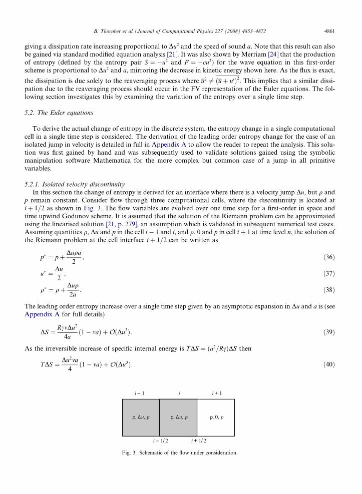
In this section the change of entropy is derived for an interface where there is a velocity jump Du, but q andp remain constant. Consider flow through three computational cells, where the discontinuity is located atiþ 1=2 as shown in Fig. 3. The flow variables are evolved over one time step for a first-order in space andtime upwind Godunov scheme. It is assumed that the solution of the Riemann problem can be approximatedusing the linearised solution [21, p. 279], an assumption which is validated in subsequent numerical test cases.Assuming quantities q, Du and p in the cell i� 1 and i, and q, 0 and p in cell iþ 1 at time level n, the solution ofthe Riemann problem at the cell interface iþ 1=2 can be written as

p� ¼ p þ Duqa2

; ð36Þ

u� ¼ Du2; ð37Þ

q� ¼ qþ Duq2a

: ð38Þ

The leading order entropy increase over a single time step given by an asymptotic expansion in Du and a is (seeAppendix A for full details)

DS ¼ RcmDu2

4að1� maÞ þOðDu3Þ: ð39Þ

As the irreversible increase of specific internal energy is T DS ¼ ða2=RcÞDS then

TDS ¼ Du2ma4ð1� maÞ þOðDu3Þ: ð40Þ

, u, p , u, p , 0, p

i 1 i i + 1

i 1/ 2 i + 1/ 2

Fig. 3. Schematic of the flow under consideration.

Table 1Rate of increase of TDS for an isolated velocity jump per unit time

Du=a Eq. (41) Exact PVRS HLLC

0.5 0.00024 0.00026 0.00025 0.000260.1 0.0011 0.0011 0.0011 0.00110.01 0.01 0.01 0.01 0.010.001 0.104 0.104 0.104 0.104


It can be seen that the increase of entropy is only positive as long as 1� ma > 0, which is the low Mach numberlimit of the familiar CFL condition. Eq. (40) can be converted to time rate of dissipation, given thatm ¼ Dt=Dx � C=a, where C is the Courant–Friedrichs–Lewy number,

�Du ¼ TDS=Dt ¼ Du2a4Dxð1� maÞ þOðDu3Þ; ð41Þ

where � is the irreversible change of kinetic energy per unit time. This is consistent with analysis of the increaseof entropy by Barth [25], which also points to an increase of entropy proportional to the jump size squared.Additionally, the entropy generation over the single time step is proportional to 1=a, as opposed to 1=a2 pre-dicted for the entropy rise over a shock wave (Eq. (29)).

The asymptotic analysis has been validated using a one-dimensional test case for a first-order in time andspace Godunov method solving the Riemann problem with an exact Riemann solver, the HLLC solver and theprimitive variable Riemann solver (for details about these Riemann solvers consult [21]). Table 1 shows therate of entropy increase in the first time step for a shock tube case where the left and right states are definedas

pL ¼ pR ¼ qa2; qL ¼ qR ¼ q; uL ¼ Du; uR ¼ 0: ð42Þ
The results show excellent agreement with all numerical schemes even where the Mach number of the velocityjump is as high as 0.5. This agreement is to be expected as Eq. (41) is a leading order approximation in terms ofMach number of the velocity jump and in terms of order of the velocity jump itself, thus it is applicable be-yond the incompressible regime.
The dependence of the dissipation rate on the speed of sound and Du2 is clearly different from the dissipa-tion inherent in the solution of the Euler equations (Eq. (29)). Eq. (29) was derived assuming the validity of theHugoniot relations [26], which only hold true when all gradients of the flow exiting the control volume arezero, and the rate of change of these gradients is zero in a given frame of reference. Clearly, this is not thegeneral case for an arbitrary interface where there is a difference in all primitive variables. Thus, the Hugoniotrelations hold in a global sense, but the above expansion applies in the case of unsteady flow for an interfacewith a local variation in velocity from the left to right state.

Taking the initialisation of a shock wave on a grid as an example, the validity of the result becomes clear. Inthe first time step a dissipation proportional to Du2

s acts on the initialised velocity jump. This is larger than thedissipation rate for an ideal shock wave derived by Bethe and thus the shock is diffused. After several timesteps a steady state solution is gained where the sum of several smaller Du2 equals the entropy gain of a singleglobal increase proportional to Du3. In this process the excess entropy produced in the first time step at a rateof Du2

s manifests itself as an entropy ‘anomaly’. It has also been termed ‘wall heating’, although this is slightlymisleading as the entropy errors occur throughout the flow field. A similar process occurs when shock wavesinteract and causes excess heating in the Noh test case, which can be viewed as a shock interaction problem [3].

The dependence on Du2 is due to an interaction of both the governing equations and the reaveraging pro-cess. If the increase of entropy was solely due to the reaveraging of the continuous function to a fixed mesh,then the leading order error terms would be of order Du. However, the governing equations are constructed insuch a manner that the leading order fluctuations (i.e. Dp and Dq) are isentropic in nature and so cancel in theasymptotic expansion.

Menikoff [7] examined the variation of entropy when initialising a shock wave, or when shock waves inter-act and demonstrated that an entropy anomaly occurs due to the finite width of a viscous shock profile, whichis a special case of the general asymptotic expansion presented here.


As also observed numerically in [7], under refinement of the mesh the spatial extent of the anomaly reduces,but the magnitude does not. Thus, in employing a Godunov method to simulation a turbulent flow field, thereis no steady frame of reference and these entropy ‘anomalies’ occur throughout the field providing a dissipa-tion rate proportional to Du2 and a. It is then expected that ILES simulations using a Godunov method wouldhave a subgrid model more akin to a physical viscosity than proportional to Du3 as ideally desired. As thenumerical viscosity increases above that required to mimic the behaviour of the subgrid scales then a greaterseparation is required between the highest wave number captured on the grid and the beginning of the sub-inertial range. When simulating low Mach number turbulence with Godunov methods this effect means thata large number of finite volumes must be employed to give the required separation. This explains why thekinetic energy spectra gained using shock-capturing Godunov-type methods are typically overly dissipativein the high wave number range (see for example [27,28]).

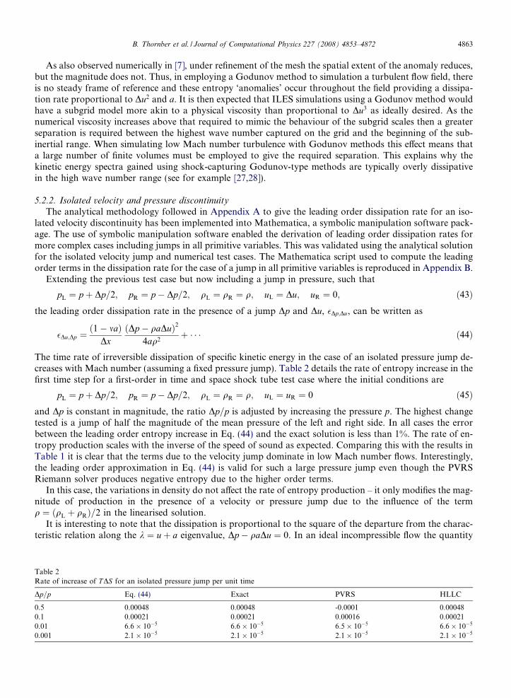
5.2.2. Isolated velocity and pressure discontinuity

The analytical methodology followed in Appendix A to give the leading order dissipation rate for an iso-lated velocity discontinuity has been implemented into Mathematica, a symbolic manipulation software pack-age. The use of symbolic manipulation software enabled the derivation of leading order dissipation rates formore complex cases including jumps in all primitive variables. This was validated using the analytical solutionfor the isolated velocity jump and numerical test cases. The Mathematica script used to compute the leadingorder terms in the dissipation rate for the case of a jump in all primitive variables is reproduced in Appendix B.

Extending the previous test case but now including a jump in pressure, such that

TableRate o

Dp=p

0.50.10.010.001

pL ¼ p þ Dp=2; pR ¼ p � Dp=2; qL ¼ qR ¼ q; uL ¼ Du; uR ¼ 0; ð43Þ
the leading order dissipation rate in the presence of a jump Dp and Du, �Dp;Du, can be written as
�Du;Dp ¼ð1� maÞ

DxðDp � qaDuÞ2

4aq2þ � � � ð44Þ

The time rate of irreversible dissipation of specific kinetic energy in the case of an isolated pressure jump de-creases with Mach number (assuming a fixed pressure jump). Table 2 details the rate of entropy increase in thefirst time step for a first-order in time and space shock tube test case where the initial conditions are

pL ¼ p þ Dp=2; pR ¼ p � Dp=2; qL ¼ qR ¼ q; uL ¼ uR ¼ 0 ð45Þ
and Dp is constant in magnitude, the ratio Dp=p is adjusted by increasing the pressure p. The highest changetested is a jump of half the magnitude of the mean pressure of the left and right side. In all cases the errorbetween the leading order entropy increase in Eq. (44) and the exact solution is less than 1%. The rate of en-tropy production scales with the inverse of the speed of sound as expected. Comparing this with the results inTable 1 it is clear that the terms due to the velocity jump dominate in low Mach number flows. Interestingly,the leading order approximation in Eq. (44) is valid for such a large pressure jump even though the PVRSRiemann solver produces negative entropy due to the higher order terms.
In this case, the variations in density do not affect the rate of entropy production – it only modifies the mag-nitude of production in the presence of a velocity or pressure jump due to the influence of the termq ¼ ðqL þ qRÞ=2 in the linearised solution.

It is interesting to note that the dissipation is proportional to the square of the departure from the charac-teristic relation along the k ¼ uþ a eigenvalue, Dp � qaDu ¼ 0. In an ideal incompressible flow the quantity

2f increase of TDS for an isolated pressure jump per unit time

Eq. (44) Exact PVRS HLLC

0.00048 0.00048 -0.0001 0.000480.00021 0.00021 0.00016 0.000216:6� 10�5 6:6� 10�5 6:5� 10�5 6:6� 10�5

2:1� 10�5 2:1� 10�5 2:1� 10�5 2:1� 10�5


qaDu is of order M, compared to pressure which is of order M2, meaning that this is not likely to become smallat low Mach number.

The analysis within this subsection has assumed that u� is positive, i.e. that the solution at x=t ¼ 0 lies to theleft of the contact surface and thus can be described by Eq. (38), but there is no assumption in the direction ofthe jumps as long as this criterion remains valid. If it is assumed that the velocity jump is sufficiently negative,or that the pressure increases from left to right such that u� < 0 then the solution for q� changes to [21, p. 297]

TableRate o

Du=a

0.50.10.010.001

q� ¼ qR þ ðu� � uRÞq=a: ð46Þ
Utilising the script in Appendix B, the leading order rate of dissipation in this case is
�u�<0 ¼ �Du;Dp þDpðDp � a2DqÞ2Dxq2aðc� 1Þ þ � � � ð47Þ

For a constant pressure and density jump there is an additional component of dissipation which increases asthe Mach number decreases, proportional to DpDq. However, this would scale as M�4 in incompressible flowsor at least M�2 for unpreconditioned compressible FV schemes so would not dominate over the terms in Du2.The characteristic invariant along the k ¼ u eigenvalue also appears in this expression, so it appears that dis-sipation is minimised only when all jumps are zero, or when the jumps correspond exactly to the characteristicequations for the waves passing into the cell.

5.2.3. Shear waves

For a three-dimensional direction split method the shear waves are typically advected passively. This meansthat the accuracy of the projected value of the velocities parallel to the interface, in this case the v velocity, willalso affect dissipation. In the case of a single isolated jump in v velocity it is expected that dissipation will onlyoccur if the contact wave enters the cell under consideration. This is because the components parallel to theinterface only change across the contact surface. For example, if the jump in v velocity takes place at the righthand interface, dissipation occurs only if u� is negative.

Following the methodology detailed in Appendix A, the leading order irreversible dissipation rate has beenderived given the initial conditions in Eq. (43) and additionally vL ¼ Dv=2, vR ¼ �Dv=2. The leading orderterm is constant with respect to the speed of sound,

�Dv ¼Dv2ðDq� 2qÞu

4qDxþ � � � ; ð48Þ

thus it does not influence the asymptotic behaviour of the system. In a simple shock tube case with constant u,p, q and a step discontinuity in the v velocity component Eq. (48) is accurate to within 1% in validation caseswhere Dv=a < 0:5.

5.3. Higher order methods

5.3.1. Temporal discretisation

The analysis within the previous subsections is not valid for higher order time-stepping methods and wouldhave to be repeated for each different time-stepping method. As all higher order methods are multi-step then itis expected that the resulting expressions would be quite complex. However, the asymptotic behaviour can eas-ily be examined numerically. Table 3 shows the velocity jump test case in Section 5.2 repeated using second-

3f increase of TDS for a fixed magnitude velocity jump (varying the speed of sound) for several different time stepping methods

2nd TVD RK 2nd DT 3rd TVD RK 3rd ES RK

0.00028 0.00023 0.00029 0.00030.0012 0.0010 0.0012 0.00140.011 0.010 0.013 0.0130.118 0.103 0.130 0.130


order total variation diminishing (TVD) Runge–Kutta method [29], implicit–explicit dual time-stepping (DT)method [30], third-order TVD Runge–Kutta method [31] and third-order extended stability (ES) Runge–Kutta [32] with first-order spatial reconstruction using the exact Riemann solver. These results demonstratethat the dissipation increases linearly with speed of sound with all time stepping methods as was the casefor the first-order in time computations. Additional tests varying the magnitude of isolated velocity disconti-nuities whilst holding the speed of sound constant are detailed in Table 4. It confirms that the dissipation rateis proportional to Du2 for all higher order time-stepping methods examined. This confirms that the sametrends detailed for the first-order schemes apply to higher order in time computations.

5.3.2. Spatial discretisation

The previous sections discuss only the first-order in space Godunov method. The majority of practical sim-ulations are conducted with second or even higher order methods in space and so it is useful to extend theabove analysis. This subsection analyses the dissipative properties of a Godunov method employing a sec-ond-order accurate MUSCL reconstruction with the van Leer limiter [33]. The left and right interface vari-ables are defined from

TableRate o

Du=a

0.10.20.4

PLiþ1=2 ¼ Pi þ

1

2/limðrlim;LÞðPi � Pi�1Þ; ð49Þ

PRiþ1=2 ¼ Piþ1 �

1

2/limðrlim;RÞðPiþ2 � Piþ1Þ; ð50Þ

where P is the vector of cell averaged primitive variables and the cells are labelled by the integer i. Also,

rlim;Li ¼ Piþ1 � Pi

Pi � Pi�1

; rlim;Ri ¼ Pi � Pi�1

Piþ1 � Pi: ð51Þ

The van Leer limiter can be written as

/limVL ¼

2rlim

1þ rlim: ð52Þ

Additionally, it is constrained to first-order at maxima and minima in the standard manner. There are two keydifferences when employing variable extrapolation methods; firstly they increase the cell averaged kinetic en-ergy within a given cell via the process of interpolation itself (relative to piecewise constant methods) andchange the total entropy within the cell; secondly, in smooth regions, higher order interpolation in spacewould act to reduce the magnitude of the jumps between the left and right quantities.

Following standard modified equation analysis [34,35] it can be shown that a Taylor series expansion ofMUSCL reconstruction using the van Leer interpolation method of the vector of cell averaged primitive vari-ables P gives

~PRðxÞ ¼ Pi þ Dx2

Pix þ Dx3 �ðP

ixxÞ

2

8Pix

þ 1

12Pi

xxx

!þOðDx5Þ; ð53Þ

where Pi indicates functions evaluated at the cell centre. The exact expansion from the cell averaged quantityto the continuous function gives

PðxÞ ¼ Pi þ Dx2

Pix þ

Dx2

12Pi

xx þOðDx4Þ; ð54Þ

4f increase of TDS for a variable velocity jump (fixed speed of sound) for several different time-stepping methods

2nd TVD RK 2nd DT 3rd TVD RK 3rd ES RK

0.0012 0.0010 0.0012 0.00140.0052 0.0043 0.0055 0.00560.023 0.019 0.023 0.023


confirming that the van Leer limiter is second-order accurate in the MUSCL reconstruction. From this pointon the superscripts ð:Þi will be omitted for clarity.

The generation of entropy during the solution of the Riemann problem and the subsequent time evolutionof the cell average quantities can now be computed using the extrapolated variables. The process followed inSection 5.2.1 was repeated to compute the entropy rise, however with the key difference that the velocity isassumed to vary continuously through the group of three cells instead of employing a discontinuous initialcondition. For discontinuous flows (e.g. a square wave initial condition) the traditional MUSCL and WENOschemes will reduce to the first-order solution in the first time step, as the construction of MUSCL schemesensure piecewise constant reconstruction and the class of Essentially Non-Oscillatory methods will give extre-mely small weightings to the stencils which cross the discontinuity. Hence, the entropy increase in discontin-uous flows will be identical to that predicted for the first-order scheme.

The fluxes at the iþ 1=2 and i� 1=2 interfaces are computed from the Taylor series expansion of the vanLeer extrapolation. These are then evolved at first-order in time and the change of entropy over the time stepcomputed. The Mathematica script used to generate these results is included in Appendix C. Next, this processwas repeated using the exact solution at the cell interfaces (i.e. the same process but with the exact Taylor ser-ies expansion). The leading order change in entropy in the discrete solution with van Leer limiting is then sub-tracted from the exact solution, giving the dissipation rate due to the errors in the spatial discretisation as

TableKinetithird-o

M

0.10.010.001

�VLDu ¼

Dx2

12uuxuxx þ

Dx3a24ð3u2

xx þ ð2C � 3ÞuxuxxxÞ: ð55Þ

The second-order term is locally dispersive, however the third-order term is dissipative as long as the CFLconstraint is satisfied. Furthermore, the dissipation rate is proportional to the magnitude of the velocity deriv-atives squared multiplied by the speed of sound. The leading order term is Dx3 as expected, which is the leadingorder difference between the left and right van Leer interpolated quantities. This is consistent with the resultsof the first-order analysis.

The conclusions of this analysis have been tested numerically by examining the increase of entropy in thefirst time step from the following initial condition:

pL ¼ pR ¼ p0=M2; q ¼ q0; u ¼ Ma sinð4pxÞ=2; ð56Þ
where a is the speed of sound and M is the Mach number. The computational domain is 200 cells in a region ofdimension 1, the boundary conditions are periodic and C ¼ 0:5. The object of this initial condition was to cre-ate a smooth flow field, as the dissipation rate for a discontinuous flow field could be heavily influenced by thefirst-order points. The test case uses third-order extended stability Runge–Kutta time-stepping with a second-order van Leer spatial discretisation and uses the exact Riemann solver.
Table 5 details the dissipation rate in the first time step as a function of Mach number. These results con-firm that the dissipation rate increases inversely proportional to the Mach number as expected. Next, the pres-sure and density are fixed and the magnitude of the initial velocity is varied. This is to investigate the u2

dependence of the dissipation rate. The results are detailed in Table 6, where it can be clearly seen that thedissipation rate is proportional to the velocity magnitude squared, again in excellent agreement with the the-oretical result.

Finally, it is predicted that the entropy increase is proportional to Dx3. Table 7 shows TDS for the sameinitial condition fixed at Mach number of 0:1 for three different grid sizes. Clearly, the dissipation rate isapproximately proportional to Dx3, as each doubling in grid points should decrease the dissipation eight-fold.There is a slight deviation at high resolution, which is due to the first-order points at the maxima and minimaof the sine wave.

5c energy decay rate � for a fixed magnitude velocity field (varying the speed of sound) using the second-order van Leer limiter withrder ES RK over a single time step

� Normalised

3:00� 10�5 13:00� 10�4 102:97� 10�3 99

Table 6Kinetic energy decay rate � with increasing velocity magnitude (fixed speed of sound) using the second-order van Leer limiter with third-order ES RK over a single time step

M � Normalised

0.1 3:00� 10�5 10.2 1:19� 10�4 40.4 4:84� 10�4 16

Table 7Variation of entropy rise with grid size at Mach number 0.1 using the second-order van Leer limiter with third-order ES RK over a singletime step

Grid points TDS � Normalised

100 5:0� 10�7 2:4� 10�4 1200 3:1� 10�8 3:0� 10�5 8400 2:0� 10�9 4:0� 10�6 61


This confirms that the key parameter in the design of numerical schemes is to minimise the differencebetween the left and right quantities, not necessarily the formal order of accuracy. As an example of this,the Minmod and van Leer limiters have the same formal order of accuracy when used in a MUSCL formu-lation. Despite this the van Leer limiter will normally resolve interfaces much more sharply. The underlyingreason for this difference is that although both limiters have second-order accurate interpolation, the jumpfrom the left to right side interpolated values is second-order for Minmod, but third-order for van Leer. Thisgives the observed improvement in performance.

6. Conclusions

The analytical results derived within this paper demonstrate that the numerical dissipation rate of Godunovmethods for a typical unsteady flow is not of the same form as the irreversible dissipation in the governingEuler equations. In shock tube cases the global dissipation of the solution for a shock wave can be computedusing the Hugoniot relations and has been shown previously to be proportional to the velocity jump across theshock wave cubed. However, in the case of an unsteady flow feature, the local increase in entropy is dependenton the numerical viscosity which in the FV Godunov method is proportional to the magnitude of the velocitygradients squared over the speed of sound, a. Under the assumption of low production of entropy due to ther-mal gradients, this corresponds to a kinetic energy dissipation rate proportional to the speed of sound andmagnitude of the velocity derivatives squared, explaining directly the poor performance of Godunov methodsat low Mach numbers. The conclusions of the theoretical analysis have been numerically validated for first-order in time and space and second-order van Leer reconstruction in space with third-order Runge–Kutta timeintegration. The analysis has shown that in the same way that each numerical method has its own unique rateof kinetic energy dissipation in unsteady flows, it also has its own rate of entropy generation.

This has important ramifications in the simulation of low Mach number flows, where excess damping offlow structures leads to extremely inaccurate solutions. It is also of importance for implicit large eddy simu-lation. The expressions within this paper can be used to derive new variable extrapolation methods, tailored toimprove the ability of Godunov methods at low Mach number flows.

Acknowledgments

The authors would like to thank Evgeniy Shapiro (Fluid Mechanics and Computational Sciences Group,Cranfield University) and Anthony Weatherhead (AWE, Aldermaston) for their advice and suggestions whilstcompleting the analysis, as well as Bill Rider (Sandia) for productive discussions. Ben Thornber is supportedby an EPSRC-AWE PhD Case award and Dimitris Drikakis would also like to acknowledge the financial sup-port from EPSRC, MoD and AWE through the EPSRC(EP/C515153)-JGS (No. 971) project.


Appendix A. Entropy increase in the case of an isolated velocity discontinuity

Beginning with the one-dimensional Euler equations

oU

otþ oE

ox¼ 0; ðA:1Þ

where

U ¼ ½q; qu;E�T; ðA:2ÞE ¼ ½qu; qu2 þ p; ðE þ pÞu�T; ðA:3Þ

E ¼ qeþ 1

2qu2; ðA:4Þ

p ¼ qeðc� 1Þ; ðA:5Þ

and q, e, u are the density, specific internal energy per unit volume and x-direction velocity component, respec-tively. Throughout this paper it is assumed that the fluid satisfies the ideal gas equation of state. The Eulerequations are discretised using a first-order accurate method in time and space

Unþ1i ¼ Un

i � mðEniþ1=2 � En

i�1=2Þ; ðA:6Þ

m ¼ DtDx: ðA:7Þ

Given initial conditions

pL ¼ pR ¼ p; qL ¼ qR ¼ q; ruL ¼ Du; uR ¼ 0; ðA:8Þ
where the cells i and i� 1 are in the left state, cell iþ 1 is the right state. The interface flux En
i�1=2 is computeddirectly from the left hand quantities. The values of the primitive variables required to compute En

iþ1=2 aredetermined by solving the Riemann problem at the interface with the left and right quantities. This can beestimated with reasonable accuracy using a linearised approximation [21, p. 279]

p� ¼ p þ Duqa2

; ðA:9Þ

u� ¼ Du2; ðA:10Þ

q� ¼ qþ Duq2a

: ðA:11Þ

Thus, the conserved variables at the next time step are

Unþ1i ¼

q

qDup

c�1þ 1

2qDu2

264

375þ m

qDu� qþ Duq2a

� �Du2

qDu2 þ p � qþ Duq2a

� �Du2

4� p � Duqa

2

pcDuc�1þ 1

2qDu3

� �� pþDuqa

2ð ÞcDu

2 c�1ð Þ þ qþ Duq2a

� �Du3

16

� �26664

37775; ðA:12Þ

simplifying,

qnþ1 ¼ q 1þ mDu4

2� Dua

� �� ; ðA:13Þ

unþ1 ¼ Du1þ mDu

86� Du

a � 4aDu

� �1þ mDu

42� Du

a

� �� ; ðA:14Þ

Enþ1 ¼ pc� 1

1þ mcDu2

� �þ 1

2qDu2 1þ mDu

1614� Du

a� 8ca

Du c� 1ð Þ

� � �: ðA:15Þ

Next the pressure can be computed from ðE � 1=2qu2Þnþ1ðc� 1Þ


pnþ1 ¼ pc� 1

1þ mcDu2

� �þ 1

2qDu2 1þ mDu

1614� Du

a� 8ca

Duðc� 1Þ

� � �"

� 1

2qDu2 1þ mDu

86� Du

a � 4aDu

� �� 2

1þ mDu4

2� Dua

� �� #ðc� 1Þ: ðA:16Þ

At this point the pressure at time level nþ 1 is simplified by expanding the last term in the above equation in abinomial series, ð1þ xÞ�1 � 1� xþ x2 � � � �, where terms up to order Du2 are kept. Starting with thedenominator

1

1þ mDu2� mDu2

4a

� 1� mDu2þ mDu2

4aþ m2Du2

4þO

Dua

� �3

� 1; ðA:17Þ

multiplying out the numerator

1þ mDu8

6� Dua� 4a

Du

� � �2

� 1� maþ m2a2

4; ðA:18Þ

the pressure can now be written as

pnþ1 � p 1þ mcDu2þ cmDu2

8að2c� 4� maðc� 1ÞÞ

�: ðA:19Þ

For unþ1 and qnþ1:

qnþ1 ¼ q 1þ mDu2� mDu2

4a

� �; ðA:20Þ

unþ1 � Du 1� ma2

� �: ðA:21Þ

Setting m ¼ C=a and M ¼ 0 clearly gives limM!0DS ¼ 0. In practise this limit is not reached for flows of typicalinterest (i.e. moving flows). The change in entropy is

DS ¼ Rc� 1

lnpqc

� �nþ1

� Rc� 1

lnpqc

� �n

� Rc� 1

lnp 1þ mcDu

2þ cmDu2

8a 2c� 4� ma c� 1ð Þð Þh i

q 1þ mDu2� mDu2

4a

� �� c0@

1A� R

c� 1ln

pqc

� �

� Rc� 1

ln1þ mcDu

2þ cmDu2

8a 2c� 4� ma c� 1ð Þð Þ1þ mDu

2� mDu2

4a

� �c !

: ðA:22Þ

Expanding the denominator in a series where

1

ð1þ zÞm ¼ 1� mzþ mðmþ 1Þ2!

z2 � mðmþ 1Þðmþ 2Þ3!

z3 þ � � � ; ðA:23Þ

1

1þ mDu2� mDu2

4a

� �c ¼ 1� cmDu2þ cmDu2

4aþ c cþ 1ð Þ m

2Du2

8þOðDu3Þ: ðA:24Þ

Multiplying this by the numerator gives

1þ cmDu2þ cmDu2

8a ð2c� 4� maðc� 1ÞÞ1þ mDu

2� mDu2

4a

� �c� 1þ cmDu

2þ cmDu2

8að2c� 4� maðc� 1ÞÞ

� �1� cmDu

2þ cmDu2

4aþ cðcþ 1Þ m

2Du2

8

� �

� 1þ cmDu2

8a½2c� 2þ 2mað1� cÞ�: ðA:25Þ


Additionally, for j cmDu2

8a ½2c� 2þ 2mað1� cÞ�j < 1 the series expansion of the natural logarithm can beemployed:

lnð1þ xÞ ¼ x� x2

2þ x3

3; ðA:26Þ

to give Eq. (39).

Appendix B. Mathematica script for first-order methods

The leading order dissipation rate at an interface where there is a jump in all primitive variables can becomputed using the following script in the symbolic manipulation software Mathematica.

(*Initial Conditions*)pr=p - dp/2;

pl=p+dp/2;

ur=u - du/2;

ul=u+du/2;

rr=r - dr/2;

rl=r+dr/2;

(*Star Quantities*)
ps=(pr+pl)/2+(ul - ur)r a/2;
us=(ur+ul)/2+(pl - pr)/(2 r a);

rs=rl+(ul - us) r/a;

(*Compute conservative variables at the next time step*)
u1=rl+v (rl ul - rs us)
u2=rl ul+v (rl ul^2+pl - rs us

^2 - ps)

u3=pl/(g - 1)+rl ul^2/2+

v ((pl g/(g - 1)+rl ul^2/2) ul - (ps g/(g - 1)+rs us

^2/2)us)

(*Calculate primitive variables at the next times step*)
r1=Simplify[Expand[u1]]
u1=Simplify[Expand[u2/u1]]

e1=Simplify[Expand[u3]]

p1=(g - 1)(e1 - 1/2 r1 u1^2)

(*Calculate the entropy change and multiply by temperature*)
ln=p1/r1
^g ((rl)

^g/(pl));

ds=RGAS/(g - 1)(ln - 1);

Tds=ds a^2/(g RGAS);

(*Expand each variable in terms of the jump size to gain the leading order terms*)
TdsExp=Expand[Normal[Series[Normal[Series[Normal[Series[Tds, dp, 0, 2]],
du, 0, 2]], dr, 0, 2]]]

(*Substitute speed of sound instead of pressure p*)TdsExp2=TdsExp1/. p -> r a

^2/g

All that remains is to simplify the resulting expression to gain several leading order terms.


Appendix C. Mathematica script for higher order methods

This appendix details the Mathematica script used to computed the change in entropy over a single timestep using van Leer extrapolation in a flow field where velocity varies, but pressure and density are locallyconstant.

(*Initial Conditions for interface i+1/2 and soln of RP using the Taylor series

expansion of the van Leer limited velocities*)pr=P[x];

pl=P[x];

ur=U[x]+dx U0[x]/2+dx^3(U00[x]^2/8U0[x]-u000[x]/6);

ul=U[x]+dx U0[x]/2+dx^3(-U00[x]^2/8U0[x]+u000[x]/12);

rr=R[x];

rl=R[x];

psp=(pr+pl)/2+(ul - ur)(rr+rl) a/4;

usp=(ur+ul)/2+(pl - pr)/((rr+rl) a);

rsp=rl+(ul - usp) (rr+rl)/2/a;

(*Initial Conditions for interface i - 1/2 and soln of RP using the Taylor series

expansion of the van Leer limited velocities*)prm=P[x];

plm=P[x];

urm=U[x]-dx U0[x]/2+dx^3(U00[x]^2/8U0[x]-u000[x]/12);

ulm=U[x]-dx U0[x]/2+dx^3(-U00[x]^2/8U0[x]+u000[x]/6);

rrm=R[x];

rlm=R[x];

psm=(prm+plm)/2+(ulm - urm)(rrm+rlm) a/4;

usm=(urm+ulm)/2+(plm - prm)/((rrm+rlm) a);

rsm=rlm+(ulm - usm) (rrm+rlm)/2/a;

(*Compute conservative variables at the next time step*)
u1=R[x]+v (rsm usm - rsp usp);
u2=R[x] U[x]+v (rsm usm^2+psm - rsp usp

^2 - psp);

u3=P[x]/(g - 1)+R[x] U[x]^2/2+v ((psm g/(g - 1)+rsm usm

^2/2)

usm - (psp g/(g - 1)+rsp usp^2/2)usp);

(*Calculate primitive variables at the next times step*)
r1=Simplify[Expand[u1]]
u1=Simplify[Expand[u2/u1]]

e1=Simplify[Expand[u3]]

p1=(g - 1)(e1 - 1/2 r1 u1^2)

(*Calculate the entropy change and multiply by temperature*)
ln=p1/r1
^g ((rl)

^g/(pl));

ds=RGAS/(g - 1)(ln - 1);

Tds=ds a^2/(g RGAS);

(*Substitute speed of sound instead of pressure p and substitute dt for dx, CFL and

a*) Tds2=Tds/. p -> r a^2/g; Tdsodt= Collect[Tds2/dt/. v -> dt/dx/. dt -> dx CFL/a, a];


To compute the entropy increase due to spatial discretisation, then it is necessary to repeat the above anal-ysis for the exact Taylor series expansion of the cell average quantities to the cell interface and then subtractthe entropy rise with the exact from the entropy rise of the van Leer interpolated method.

References

[1] H. Guillard, Recent developments in the computation of compressible low Mach number flows, Flow Turbul. Combust. 76 (2006)363–369.

[2] E. Turkel, A. Fiterman, B. van Leer, Preconditioning and the Limit of the Compressible to the Incompressible Flow Equations forFinite Difference Schemes, John Wiley and Sons, 1994.

[3] W. Noh, Errors for calculations of strong shocks using and artificial viscosity and an artificial heat flux, J. Comput. Phys. 72 (1987)78–120.

[4] R. Christensen, Godunov methods on a staggered mesh – an improved artificial viscosity, Tech. Rep., Lawrence Livermore NationalLaboratory, 1990.

[5] D. Benson, Computational methods in Lagrangian and Eulerian hydrocodes, Comput. Meth. Appl. Mech. Eng. (1992) 235–394.[6] G. Volpe, Performance of compressible flow codes at low Mach number, AIAA J. 31 (1993) 49–56.[7] R. Menikoff, Numerical anomalies mimicking physical effects, Tech. Rep., Los Alamos, 1995.[8] H. Guillard, C. Viozat, On the behaviour of upwind schemes in the low Mach number limit, Comput. Fluids 28 (1999) 63–86.[9] H. Guillard, A. Murrone, On the behaviour of upwind schemes in the low Mach number limit: II. Godunov type schemes, Comput.

Fluid 33 (2004) 655–675.[10] J. Boris, F. Grinstein, E. Oran, R. Kolbe, New insights into large eddy simulation, Fluid Dyn. Res. 10 (1992) 199–228.[11] D. Youngs, Application of MILES to Rayleigh–Taylor and Richtmyer–Meshkov mixing, AIAA-2003-4102.[12] A. Kolmogorov, A refinement of previous hypotheses concerning the local structure of turbulence in a viscous incompressible fluid at

high Reynolds number, J. Fluid Mech. 13 (1962) 82–85.[13] G. Naterer, Heat Transfer in Single and Multiphase Systems, CRC Press, 2003.[14] C. Fureby, F. Grinstein, Monotonically integrated large eddy simulation of free shear flows, AIAA J. 37 (5) (1999) 544–556.[15] A. Bejan, Entropy Generation Minimization: The Method of Thermodynamic Optimization of Finite-Time Systems and Finite-Time

Processes, CRC Press, 1996.[16] D. Youngs, Three-dimensional numerical simulation of turbulent mixing by Rayleigh–Taylor instability, Phys. Fluids A 3 (5) (1991)

1312–1320.[17] H. Bethe, On the theory of shock waves for an arbitrary equation of state, Tech. Rep., Office of Scientific Research and Development,

1942.[18] J. Johnson, R. Cheret (Eds.), Classic Papers in Shock Compression Science, Springer-Verlag, 1998.[19] R. Menikoff, B. Plohr, The Riemann problem for fluid flow of real materials, Rev. Mod. Phys. 61 (1) (1989) 75–130.[20] R. Leveque, Finite Volume Methods for Hyperbolic Problems, Cambridge University Press, 2002.[21] E. Toro, Riemann Solvers and Numerical Methods for Fluid Dynamics, Springer-Verlag, 1997.[22] S. Klainerman, A. Madja, Compressible and incompressible fluids, Commun. Pure Appl. Math. 33 (1982) 399–440.[23] R. Klein, Semi-implicit extension of a Godunov-type scheme based on low Mach number asymptotics I: one-dimensional flow, J.

Comput. Phys. 121 (1995) 213–237.[24] M. Merriam, Smoothing and the second law, Comput. Method Appl. M 64 (1987) 177–193.[25] T. Barth, Numerical methods for gasdynamic systems on unstructured meshes, in: Introduction to Recent Developments in Theory

and Numerics for Conservation Laws, Springer-Verlag, 1999.[26] H. Hugonoit, On the propagation of motion in bodies and in perfect gases in particular – II, J. de l’Ecole Polytech. 58 (1889) 1–125.[27] B. Thornber, A. Mosedale, D. Drikakis, On the implicit large eddy simulation of homogeneous decaying turbulence, J. Comput. Phys.

226 (2007) 1902–1929.[28] E. Garnier, M. Mossi, P. Sagaut, P. Comte, M. Deville, On the use of shock-capturing schemes for large-eddy simulation, J. Comput.

Phys. 153 (1999) 273–311.[29] C.-W. Shu, Total-variation-diminishing time discretizations, SIAM J. Sci. Stat. Comp. 9 (1988) 1073–1084.[30] A. Jameson, Time dependent calculations using multigrid, with applications to unsteady flows past airfoils and wings, AIAA 91-1596.[31] S. Gottlieb, C.-W. Shu, Total variation diminishing Runge–Kutta schemes, Math. Comput. 67 (221) (1998) 73–85.[32] R. Spiteri, S. Ruuth, A class of optimal high-order strong-stability preserving time discretization methods, SIAM J. Sci. Comput. 40

(2) (2002) 469–491.[33] B. van Leer, Towards the ultimate conservative difference scheme: IV. A new approach to numerical convection, J. Comput. Phys. 23

(1977) 276–299.[34] D. Drikakis, W. Rider, High-Resolution Methods for Incompressible and Low-Speed Flows, Springer Verlag, 2004.[35] F. Grinstein, L. Margolin, W. Rider (Eds.), Implicit Large Eddy Simulation: Computing Turbulent Fluid Dynamics, Cambridge

University Press, 2007.

on entropy generation and dissipation of kinetic energy in high-resolution shock-capturing schemes

Documents