old and new concentration inequalitiesfan/complex/ch2.pdf · chapter 2 old and new concentration...

$: Old and New Concentration Inequalitiesfan/complex/ch2.pdf · CHAPTER 2 Old and New Concentration Inequalities In the study of random graphs or any randomly chosen objects, the \tools$
CHAPTER 2

Old and New Concentration Inequalities

In the study of random graphs or any randomly chosen objects, the “toolsof the trade” mainly concern various concentration inequalities and martingaleinequalities.

Suppose we wish to predict the outcome of a problem of interest. One reason-able guess is the expected value of the object. However, how can we tell how goodthe expected value is to the actual outcome of the event? It can be very usefulif such a prediction can be accompanied by a guarantee of its accuracy (within acertain error estimate, for example). This is exactly the role that the concentrationinequalities play. In fact, analysis can easily go astray without the rigorous controlcoming from the concentration inequalities.

In our study of random power law graphs, the usual concentration inequalitiesare simply not enough. The reasons are multi-fold: Due to uneven degree distri-bution, the error bound of those very large degrees offset the delicate analysis inthe sparse part of the graph. Furthermore, our graph is dynamically evolving andtherefore the probability space is changing at each tick of the clock. The problemsarising in the analysis of random power law graphs provide impetus for improvingour technical tools.

Indeed, in the course of our study of general random graphs, we need to useseveral strengthened versions of concentration inequalities and martingale inequali-ties. They are interesting in their own right and are useful for many other problemsas well.

In the next several sections, we state and prove a number of variations andgeneralizations of concentration inequalities and martingale inequalities. Many ofthese will be used in later chapters.

2.1. The binomial distribution and its asymptotic behavior

Bernoulli trials, named after James Bernoulli, can be thought of as a sequenceof coin flips. For some fixed value p, where 0 ≤ p ≤ 1, the outcome of the cointossing process has probability p of getting a “head”. Let Sn denote the number ofheads after n tosses. We can write Sn as a sum of independent random variablesXi as follows:

Sn = X1 +X2 + · · · +Xn

23

24 2. OLD AND NEW CONCENTRATION INEQUALITIES

where, for each i, the random variable Xi satisfies

Pr(Xi = 1) = p,

Pr(Xi = 0) = 1 − p.(2.1)

A classical question is to determine the distribution of Sn. It is not too difficult tosee that Sn has the binomial distribution B(n, p):

Pr(Sn = k) =(n

k

)pk(1 − p)n−k, for k = 0, 1, 2, . . . , n.

The expectation and variance of B(n, p) are

E(Sn) = np, Var(Sn) = np(1 − p).

To better understand the asymptotic behavior of the binomial distribution, wecompare it with the normal distribution N(a, σ), whose density function is givenby

f(x) =1√2πe−

(x−α)2

2σ2 , −∞ < x <∞

where α denotes the expectation and σ2 is the variance.

The case N(0, 1) is called the standard normal distribution whose density func-tion is given by

f(x) =1√2πe−x2/2, −∞ < x <∞.

0

0.001

0.002

0.003

0.004

0.005

0.006

0.007

0.008

4600 4800 5000 5200 5400

Pro

babi

lity

value

0

0.05

0.1

0.15

0.2

0.25

0.3

0.35

0.4

-10 -5 0 5 10

Pro

babi

lity

dens

ity

value

Figure 1. The Bi-nomial distributionB(10000, 0.5).

Figure 2. The Stan-dard normal distribu-tion N(0, 1).

When p is a constant, the limit of the binomial distribution, after scaling, isthe standard normal distribution and can be viewed as a special case of the CentralLimit Theorem, sometimes called the DeMoivre-Laplace Limit Theorem [53].

2.1. THE BINOMIAL DISTRIBUTION AND ITS ASYMPTOTIC BEHAVIOR 25

Theorem 2.1. The binomial distribution B(n, p) for Sn, as defined in (2.1),satisfies, for two constants a and b,

limn→∞ Pr(aσ < Sn − np < bσ) =

∫ b

a

1√2πe−x2/2dx

where σ =√np(1 − p), provided np(1 − p) → ∞ as n→ ∞.

Proof. We use Stirling’s formula for n! (see [70]).

n! = (1 + o(1))√

2πn(n

e)n

or, equivalently, n! ≈√

2πn(n

e)n.

For any constant a and b, we have

Pr(aσ < Sn − np < bσ)

=∑

aσ<k−np<bσ

(n

k

)pk(1 − p)n−k

≈∑

aσ<k−np<bσ

1√2π

√n

k(n− k)nn

kk(n− k)n−kpk(1 − p)n−k

=∑

aσ<k−np<bσ

1√2πnp(1 − p)

(npk

)k+1/2(n(1 − p)n− k

)n−k+1/2

=∑

aσ<k−np<bσ

1√2πσ

(1 +

k − np

np

)−k−1/2(1 − k − np

n(1 − p))−n+k−1/2

.

To approximate the above sum, we consider the following slightly simpler expres-sion. Here, to estimate the lower order term, we use the fact that k = np + O(σ)and 1 + x = eln(1+x) = ex−x2+O(x3), for x = o(1). To proceed, we have

Pr(aσ < Sn − np < bσ)

≈∑

aσ<k−np<bσ

1√2πσ

(1 +

k − np

np

)−k(1 − k − np

n(1 − p))−n+k

≈∑

aσ<k−np<bσ

1√2πσ

e− k(k−np)

np + (n−k)(k−np)n(1−p) + k(k−np)2

n2p2 + (n−k)(k−np)2

n2(1−p)2+O( 1

σ )

=∑

aσ<k−np<bσ

1√2πσ

e−12 ( k−np

σ )2+O( 1σ )

≈∑

aσ<k−np<bσ

1√2πσ

e−12 ( k−np

σ )2 .

Now, we set x = xk = k−npσ , and the increment ‘dx’= xk − xk−1 = 1/σ. Note that

a < x1 < x2 < · · · < b forms a 1/σ-net for the interval (a, b). As n approachesinfinity, the limit exists. We have

limn→∞ Pr(aσ < Sn − np < bσ) =

∫ b

a

1√2πe−x2/2dx.


Thus, the limit distribution of the normalized binomial distribution is the normaldistribution.

When np is upper bounded (by a constant), the above theorem is no longertrue. For example, for p = λ

n , the limit distribution of B(n, p) is the so-calledPoisson distribution P (λ):

Pr(X = k) =λk

k!e−λ, for k = 0, 1, 2, . . . .

The expectation and variance of the Poisson distribution P (λ) is given by

E(X) = λ, and Var(X) = λ.

Theorem 2.2. For p = λn , where λ is a constant, the limit distribution of

binomial distribution B(n, p) is the Poisson distribution P (λ).

Proof. We consider

limn→∞ Pr(Sn = k) = lim

n→∞

(n

k

)pk(1 − p)n−k

= limn→∞

λk∏k−1

i=0 (1 − in )

k!e−p(n−k)

=λk

k!e−λ.

0

0.05

0.1

0.15

0.2

0.25

0 5 10 15 20

Pro

babi

lity

value

0

0.05

0.1

0.15

0.2

0.25

0 5 10 15 20

Pro

babi

lity

value


Figure 4. The Poissondistribution P (3).

As p decreases from Θ(1) to Θ( 1n ), the asymptotic behavior of the binomial

distribution B(n, p) changes from the normal distribution to the Poisson distribu-tion. (Some examples are illustrated in Figures 5 and 6). Theorem 2.1 states thatthe asymptotic behavior of B(n, p) within the interval (np−Cσ, np+Cσ) (for anyconstant C) is close to the normal distribution. In some applications, we mightneed asymptotic estimates beyond this interval.

2.2. GENERAL CHERNOFF INEQUALITIES 27

0

0.01

0.02

0.03

0.04

0.05

70 80 90 100 110 120 130

Pro

babi

lity

value

0

0.02

0.04

0.06

0.08

0.1

0.12

0.14

0 5 10 15 20 25

Pro

babi

lity

value



2.2. General Chernoff inequalities

If the random variable under consideration can be expressed as a sum of in-dependent variables, it is possible to derive good estimates. The binomial distri-bution is one such example where Sn =

∑ni=1Xi and the Xi’s are independent

and identical. In this section, we consider sums of independent variables that arenot necessarily identical. To control the probability of how close a sum of randomvariables is to the expected value, various concentration inequalities are in play. Atypical version of the Chernoff inequalities, attributed to Herman Chernoff, can bestated as follows:

Theorem 2.3. [28] Let X1, . . . , Xn be independent random variables such thatE(Xi) = 0 and |Xi| ≤ 1 for all i. Let X =

∑ni=1Xi and σ2 be the variance of Xi.

ThenPr(|X | ≥ kσ) ≤ 2e−k2/4,

for any 0 ≤ k ≤ 2σ.

If the random variables Xi under consideration assume non-negative values,the following version of Chernoff inequalities is often useful.

Theorem 2.4. [28] Let X1, . . . , Xn be independent random variables with

Pr(Xi = 1) = pi, Pr(Xi = 0) = 1 − pi.

We consider the sum X =∑n

i=1Xi, with expectation E(X) =∑n

i=1 pi. Then wehave

(Lower tail) Pr(X ≤ E(X) − λ) ≤ e−λ2/2E(X),

(Upper tail) Pr(X ≥ E(X) + λ) ≤ e−λ2

2(E(X)+λ/3) .

We remark that the term λ/3 appearing in the exponent of the bound for theupper tail is significant. This covers the case when the limit distribution is Poissonas well as normal.


There are many variations of the Chernoff inequalities. Due to the fundamen-tal nature of these inequalities, we will state several versions and then prove thestrongest version from which all the other inequalities can be deduced. (See Fig-ure 7 for the flowchart of these theorems.) In this section, we will prove Theorem2.8 and deduce Theorems 2.6 and 2.5. Theorems 2.10 and 2.11 will be stated andproved in the next section. Theorems 2.9, 2.7, 2.13, and 2.14 on the lower tail canbe deduced by reflecting X to −X .

Theorem 2.8 Theorem 2.9

Theorem 2.6 Theorem 2.7

Theorem 2.5

Theorem 2.4

Theorem 2.10 Theorem 2.13 Theorem 2.14Theorem 2.11

Upper tails Lower tails

Figure 7. The flowchart for theorems on the sum of independent variables.

The following inequality is a generalization of the Chernoff inequalities for thebinomial distribution:

Theorem 2.5. [34] Let X1, . . . , Xn be independent random variables with

Pr(Xi = 1) = pi, Pr(Xi = 0) = 1 − pi.

For X =∑n

i=1 aiXi with ai > 0, we have E(X) =∑n

i=1 aipi and we define ν =∑ni=1 a

2i pi. Then we have

Pr(X ≤ E(X) − λ) ≤ e−λ2/2ν(2.2)

Pr(X ≥ E(X) + λ) ≤ e−λ2

2(ν+aλ/3)(2.3)

where a = maxa1, a2, . . . , an.

To compare inequalities (2.2) to (2.3), we consider an example in Figure 8.The cumulative distribution is the function Pr(X > x). The dotted curve in Figure8 illustrates the cumulative distribution of the binomial distribution B(1000, 0.1)with the value ranging from 0 to 1 as x goes from −∞ to ∞. The solid curve atthe lower-left corner is the bound e−λ2/2ν for the lower tail. The solid curve at theupper-right corner is the bound 1 − e−

λ22(ν+aλ/3) for the upper tail.


0

0.2

0.4

0.6

0.8

1

70 80 90 100 110 120 130

Cum

ulat

ive

Pro

babi

lity

value

Figure 8. Chernoff inequalities.

The inequality (2.3) in the above theorem is a corollary of the following generalconcentration inequality (also see Theorem 2.7 in the survey paper by McDiarmid[99]).

Theorem 2.6. [99] Let Xi be independent random variables satisfying Xi ≤E(Xi) + M , for 1 ≤ i ≤ n. We consider the sum X =

∑ni=1Xi with expectation

E(X) =∑n

i=1 E(Xi) and variance Var(X) =∑n

i=1 Var(Xi). Then we have

Pr(X ≥ E(X) + λ) ≤ e− λ2

2(Var(X)+Mλ/3) .

In the other direction, we have the following inequality.

Theorem 2.7. If X1, X2, . . . , Xn are non-negative independent random vari-ables, we have the following bounds for the sum X =

∑ni=1Xi:

Pr(X ≤ E(X) − λ) ≤ e− λ2

2Pn

i=1 E(X2i) .

A strengthened version of the above theorem is as follows:

Theorem 2.8. Suppose Xi are independent random variables satisfying Xi ≤M , for 1 ≤ i ≤ n. Let X =

∑ni=1Xi and ‖X‖ =

√∑ni=1 E(X2

i ). Then we have

Pr(X ≥ E(X) + λ) ≤ e− λ2

2(‖X‖2+Mλ/3) .

Replacing X by −X in the proof of Theorem 2.8, we have the following theoremfor the lower tail.

Theorem 2.9. Let Xi be independent random variables satisfying Xi ≥ −M ,for 1 ≤ i ≤ n. Let X =

∑ni=1Xi and ‖X‖ =

√∑ni=1 E(X2

i ). Then we have

Pr(X ≤ E(X) − λ) ≤ e− λ2

2(‖X‖2+Mλ/3) .


Before we give the proof of Theorem 2.8, we will first show the implications ofTheorems 2.8 and 2.9. Namely, we will show that the other concentration inequal-ities can be derived from Theorems 2.8 and 2.9.

Fact: Theorem 2.8 =⇒ Theorem 2.6:

Proof. Let X ′i = Xi − E(Xi) and X ′ =

∑ni=1X

′i = X − E(X). We have

X ′i ≤M for 1 ≤ i ≤ n.

We also have

‖X ′‖2 =n∑

i=1

E(X ′i2)

=n∑

i=1

E((Xi − E(Xi))2)

=n∑

i=1

Var(Xi)

= Var(X).

Applying Theorem 2.8, we get

Pr(X ≥ E(X) + λ) = Pr(X ′ ≥ λ)

≤ e− λ2

2(‖X′‖2+Mλ/3)

≤ e− λ2

2(Var(X)+Mλ/3) .

Fact: Theorem 2.9 =⇒ Theorem 2.7The proof is straightforward by choosing M = 0.

Fact: Theorem 2.6 and 2.7 =⇒ Theorem 2.5

Proof. We define Yi = aiXi. Note that

‖X‖2 =n∑

i=1

E(Y 2i ) =

n∑i=1

a2i pi = ν.

Equation (2.2) now follows from Theorem 2.7 since the Yi’s are non-negative.

For the other direction, we have

Yi ≤ ai ≤ a ≤ E(Yi) + a.

Equation (2.3) now follows from Theorem 2.6.

Fact: Theorem 2.8 and Theorem 2.9 =⇒ Theorem 2.3

The proof is by choosing Y = X − E(X), M = 1 and applying Theorems 2.8 and2.9 to Y .


Fact: Theorem 2.5 =⇒ Theorem 2.4

The proof follows by choosing a1 = a2 = · · · = an = 1.

Finally, we give the complete proof of Theorem 2.8 and thus finish the proofsfor all the above theorems on Chernoff inequalities.

Proof of Theorem 2.8: We consider

E(etX) = E(etP

i Xi) =n∏

i=1

E(etXi)

since the Xi’s are independent.

We define g(y) = 2∑∞

k=2yk−2

k! = 2(ey−1−y)y2 , and use the following facts:

• g(0) = 1.• g(y) ≤ 1, for y < 0.• g(y) is monotone increasing, for y ≥ 0.• For y < 3, we have

g(y) = 2∞∑

k=2

yk−2

k!≤

∞∑k=2

yk−2

3k−2=

11 − y/3

since k! ≥ 2 · 3k−2. Then we have, for k ≥ 2,

E(etX) =n∏

i=1

E(etXi)

=n∏

i=1

E(∞∑

k=0

tkXki

k!)

=n∏

i=1

E(1 + tE(Xi) +12t2X2

i g(tXi))

≤n∏

i=1

(1 + tE(Xi) +12t2E(X2

i )g(tM))

≤n∏

i=1

etE(Xi)+12 t2E(X2

i )g(tM)

= etE(X)+ 12 t2g(tM)

Pni=1 E(X2

i )

= etE(X)+ 12 t2g(tM)‖X‖2

.

Hence, for t satisfying tM < 3, we have

Pr(X ≥ E(X) + λ) = Pr(etX ≥ etE(X)+tλ)

≤ e−tE(X)−tλE(etX)

≤ e−tλ+ 12 t2g(tM)‖X‖2

≤ e−tλ+ 12 t2‖X‖2 1

1−tM/3 .


To minimize the above expression, we choose t = λ‖X‖2+Mλ/3 . Therefore, tM < 3

and we have

Pr(X ≥ E(X) + λ) ≤ e−tλ+ 12 t2‖X‖2 1

1−tM/3

= e− λ2

2(‖X‖2+Mλ/3) .

The proof is complete.

2.3. More concentration inequalities

Here we state several variations and extensions of the concentration inequalitiesin Theorem 2.8. We first consider the upper tail.

Theorem 2.10. Let Xi denote independent random variables satisfying Xi ≤E(Xi) + ai +M , for 1 ≤ i ≤ n. For, X =

∑ni=1Xi, we have

Pr(X ≥ E(X) + λ) ≤ e− λ2

2(Var(X)+Pn

i=1 a2i+Mλ/3) .

Proof. Let X ′i = Xi − E(Xi) − ai and X ′ =

∑ni=1X

′i. We have

X ′i ≤M for 1 ≤ i ≤ n.

X ′ − E(X ′) =n∑

i=1

(X ′i − E(X ′

i))

=n∑

i=1

(X ′i + ai)

=n∑

i=1

(Xi − E(Xi))

= X − E(X).

Thus,

‖X ′‖2 =n∑

i=1

E(X ′i2)

=n∑

i=1

E((Xi − E(Xi) − ai)2)

=n∑

i=1

(E((Xi − E(Xi))2 + a2

i

)

= Var(X) +n∑

i=1

a2i .

By applying Theorem 2.8, the proof is finished.

2.3. MORE CONCENTRATION INEQUALITIES 33

Theorem 2.11. Suppose Xi are independent random variables satisfying Xi ≤E(Xi) + Mi, for 0 ≤ i ≤ n. We order the Xi’s so that the Mi are in increasingorder. Let X =

∑ni=1Xi. Then for any 1 ≤ k ≤ n, we have

Pr(X ≥ E(X) + λ) ≤ e− λ2

2(Var(X)+Pn

i=k(Mi−Mk)2+Mkλ/3) .

Proof. For fixed k, we choose M = Mk and

ai =

0 if 1 ≤ i ≤ k,Mi −Mk if k ≤ i ≤ n.

We haveXi − E(Xi) ≤Mi ≤ ai +Mk for 1 ≤ k ≤ n,

n∑i=1

a2i =

n∑i=k

(Mi −Mk)2.

Using Theorem 2.10, we have

Pr(Xi ≥ E(X) + λ) ≤ e− λ2

2(Var(X)+Pn


Example 2.12. Let X1, X2, . . . , Xn be independent random variables. For1 ≤ i ≤ n− 1, suppose Xi follows the same distribution with

Pr(Xi = 0) = 1 − p and Pr(Xi = 1) = p,

and Xn follows the distribution with

Pr(Xn = 0) = 1 − p and Pr(Xn =√n) = p.

Consider the sum X =∑n

i=1Xi.

We have

E(X) =n∑

i=1

E(Xi)

= (n− 1)p+√np.

Var(X) =n∑

i=1

Var(Xi)

= (n− 1)p(1 − p) + np(1 − p)= (2n− 1)p(1 − p).

Apply Theorem 2.6 with M = (1 − p)√n. We have

Pr(X ≥ E(X) + λ) ≤ e− λ2

2((2n−1)p(1−p)+(1−p)√

nλ/3) .

In particular, for constant p ∈ (0, 1) and λ = Θ(n12+ε), we have

Pr(X ≥ E(X) + λ) ≤ e−Θ(nε).


Now we apply Theorem 2.11 with M1 = · · · = Mn−1 = (1 − p) and Mn =√n(1 − p). Choosing k = n− 1, we have

Var(X) + (Mn −Mn−1)2 = (2n− 1)p(1 − p) + (1 − p)2(√n− 1)2

≤ (2n− 1)p(1 − p) + (1 − p)2n≤ (1 − p2)n.

Thus,

Pr(Xi ≥ E(X) + λ) ≤ e− λ2

2((1−p2)n+(1−p)2λ/3) .

For constant p ∈ (0, 1) and λ = Θ(n12+ε), we have

Pr(X ≥ E(X) + λ) ≤ e−Θ(n2ε).

From the above examples, we note that Theorem 2.11 gives a significantly betterbound than that in Theorem 2.6 if the random variablesXi have very different upperbounds.

For completeness, we also list the corresponding theorems for the lower tails.(These can be derived by replacing X by −X .)

Theorem 2.13. Let Xi denote independent random variables satisfying Xi ≥E(Xi) − ai −M , for 0 ≤ i ≤ n. For X =

∑ni=1Xi, we have

Pr(X ≤ E(X) − λ) ≤ e− λ2

2(Var(X)+Pn

i=1 a2i+Mλ/3) .

Theorem 2.14. Let Xi denote independent random variables satisfying Xi ≥E(Xi) −Mi, for 0 ≤ i ≤ n. We order the Xi’s so that the Mi are in increasingorder. Let X =

∑ni=1Xi. Then for any 1 ≤ k ≤ n, we have

Pr(X ≤ E(X) − λ) ≤ e− λ2

2(Var(X)+Pn


Continuing the above example, we choose M1 = M2 = · · · = Mn−1 = p, andMn =

√np. We choose k = n− 1, so we have

Var(X) + (Mn −Mn−1)2 = (2n− 1)p(1 − p) + p2(√n− 1)2

≤ (2n− 1)p(1 − p) + p2n

≤ p(2 − p)n.

Using Theorem 2.14, we have

Pr(X ≤ E(X) − λ) ≤ e− λ2

2(p(2−p)n+p2λ/3) .

For a constant p ∈ (0, 1) and λ = Θ(n12+ε), we have

Pr(X ≤ E(X) − λ) ≤ e−Θ(n2ε).

2.4. A CONCENTRATION INEQUALITY WITH A LARGE ERROR ESTIMATE 35

2.4. A concentration inequality with a large error estimate

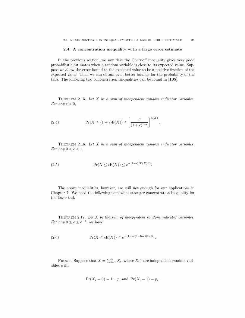
In the previous section, we saw that the Chernoff inequality gives very goodprobabilistic estimates when a random variable is close to its expected value. Sup-pose we allow the error bound to the expected value to be a positive fraction of theexpected value. Then we can obtain even better bounds for the probability of thetails. The following two concentration inequalities can be found in [105].

Theorem 2.15. Let X be a sum of independent random indicator variables.For any ε > 0,

(2.4) Pr(X ≥ (1 + ε)E(X)) ≤[

eε

(1 + ε)1+ε

]E(X)

.

Theorem 2.16. Let X be a sum of independent random indicator variables.For any 0 < ε < 1,

(2.5) Pr(X ≤ εE(X)) ≤ e−(1−ε)2E(X)/2.

The above inequalities, however, are still not enough for our applications inChapter 7. We need the following somewhat stronger concentration inequality forthe lower tail.

Theorem 2.17. Let X be the sum of independent random indicator variables.For any 0 ≤ ε ≤ e−1, we have

(2.6) Pr(X ≤ εE(X)) ≤ e−(1−2ε(1−ln ε))E(X).

Proof. Suppose that X =∑n

i=1Xi, where Xi’s are independent random vari-ables with

Pr(Xi = 0) = 1 − pi and Pr(Xi = 1) = pi.


We have

Pr(X ≤ εE(X)) =bεE(X)c∑

k=0

Pr(X = k)

=bεE(X)c∑

k=0

∑|S|=k

∏i∈S

pi

∏i6∈S

(1 − pi)

≤bεE(X)c∑

k=0

∑|S|=k

∏i∈S

pi

∏i6∈S

e−pi

=bεE(X)c∑

k=0

∑|S|=k

∏i∈S

pie−Pi6∈S pi

=bεE(X)c∑

k=0

∑|S|=k

∏i∈S

pie−Pn

i=1 pi+P

i∈S pi

≤bεE(X)c∑

k=0

∑|S|=k

∏i∈S

pie−E(X)+k

≤bεE(X)c∑

k=0

e−E(X)+k (∑n

i=1 pi)k

k!

= e−E(X)

bεE(X)c∑k=0

(eE(X))k

k!.

When εE(X) < 1, the statement is true since

Pr(X ≤ εE(X)) ≤ e−E(X) ≤ e−(1−2ε(1−ln ε))E(X).

Now we consider the case εE(X) ≥ 1.

Note that g(k) = (eE(X))k

k! increases when k < eE(X). Let k0 = bεE(X)c ≤εE(X).

We have

Pr(X ≤ εE(X)) ≤ e−E(X)k0∑

k=0

(eE(X))k

k!

≤ e−E(X)(k0 + 1)(eE(X))k0

k0!.

By using Stirling’s formula

n! ≈√

2πn(n

e)n ≥ (

n

e)n,

2.5. MARTINGALES AND AZUMA’S INEQUALITY 37

we have

Pr(X ≤ εE(X)) ≤ e−E(X)(k0 + 1)(eE(X))k0

k0!

≤ e−E(X)(k0 + 1)(e2E(X)k0

)k0

≤ e−E(X)(εE(X) + 1)(e2

ε)εE(X)

= (εE(X) + 1)e−(1−2ε+ε ln ε)E(X).

Here we replaced k0 by εE(X) since the function (x+ 1)( e2E(X)x )x is increasing for

x < eE(X).

To simplify the above expression, we have

E(X) ≥ 1ε≥ 1

1 − ε

since εE(X) ≥ 1 and ε ≤ e−1 ≤ 1 − ε. Thus, εE(X) + 1 ≤ E(X).

Also, we have E(X) ≥ 1ε ≥ e. The function ln x

x is decreasing for x ≥ e. Thus,

ln E(X)E(X)

≤ ln 1ε

1ε

= −ε ln ε.

We have

Pr(X ≤ εE(X)) ≤ (εE(X) + 1)e−(1−2ε+ε ln ε)E(X)

≤ E(X)e−(1−2ε)E(X)e−ε ln εE(X)

≤ e−(1−2ε)E(X)e−2ε ln εE(X)

= e−(1−2ε(1−ln ε))E(X).

The proof of Theorem 2.17 is complete.

2.5. Martingales and Azuma’s inequality

A martingale is a sequence of random variables X0, X1, . . . with finite meanssuch that the conditional expectation of Xn+1 given X0, X1, . . . , Xn is equal to Xn.

The above definition is given in the classical book of Feller (see [53], p. 210).However, the conditional expectation depends on the random variables under con-sideration and can be difficult to deal with in various cases. In this book we willuse the following definition which is concise and basically equivalent for the finitecases.

Suppose that Ω is a probability space with a probability distribution p. Let Fdenote a σ-field on Ω. (A σ-field on Ω is a collection of subsets of Ω which contains∅ and Ω, and is closed under unions, intersections, and complementation.) In aσ-field F of Ω, the smallest set in F containing an element x is the intersection ofall sets in F containing x. A function f : Ω → R is said to be F -measurable if


f(x) = f(y) for any y in the smallest set containing x. (For more terminology onmartingales, the reader is referred to [80].)

If f : Ω → R is a function, we define the expectation E(f) = E(f(x) | x ∈ Ω)by

E(f) = E(f(x) | x ∈ Ω) :=∑x∈Ω

f(x)p(x).

If F is a σ-field on Ω, we define the conditional expectation E(f | F) : Ω → R bythe formula

E(f | F)(x) :=1∑

y∈F(x) p(y)

∑y∈F(x)

f(y)p(y)

where F(x) is the smallest element of F which contains x.

A filter F is an increasing chain of σ-subfields

0,Ω = F0 ⊂ F1 ⊂ · · · ⊂ Fn = F .A martingale (obtained from) X is associated with a filter F and a sequence ofrandom variables X0, X1, . . . , Xn satisfying Xi = E(X | Fi) and, in particular,X0 = E(X) and Xn = X .

Example 2.18. For given independent random variables Y1, Y2, . . . , Yn, we candefine a martingale X = Y1+Y2+· · ·+Yn as follows. Let Fi be the σ-field generatedby Y1, . . . , Yi. (In other words, Fi is the minimum σ-field so that Y1, . . . , Yi are Fi-measurable.) We have a natural filter F:

0,Ω = F0 ⊂ F1 ⊂ · · · ⊂ Fn = F .Let Xi =

∑ij=1 Yj +

∑nj=i+1 E(Yj). Then, X0, X1, X2, . . . , Xn form a martingale

corresponding to the filter F.

For c = (c1, c2, . . . , cn) a vector with positive entries, the martingale X is saidto be c-Lipschitz if

|Xi −Xi−1| ≤ ci(2.7)

for i = 1, 2, . . . , n. A powerful tool for controlling martingales is the following:

Theorem 2.19 (Azuma’s inequality). If a martingale X is c-Lipschitz, then

Pr(|X − E(X)| ≥ λ) ≤ 2e− λ2

2Pn

i=1 c2i ,(2.8)

where c = (c1, . . . , cn).

Theorem 2.20. Let X1, X2, . . . , Xn be independent random variables satisfying

|Xi − E(Xi)| ≤ ci, for 1 ≤ i ≤ n.

Then we have the following bound for the sum X =∑n

i=1Xi.

Pr(|X − E(X)| ≥ λ) ≤ 2e− λ2

2Pn

i=1 c2i .

2.5. MARTINGALES AND AZUMA’S INEQUALITY 39

Proof of Azuma’s inequality: For a fixed t, we consider the convex functionf(x) = etx. For any |x| ≤ c, f(x) is below the line segment from (−c, f(−c)) to(c, f(c)). In other words, we have

etx ≤ 12c

(etc − e−tc)x+12

(etc + e−tc).

Therefore, we can write

E(et(Xi−Xi−1)|Fi−1) ≤ E(1

2ci(etci − e−tci)(Xi −Xi−1) +

12

(etci + e−tci)|Fi−1)

=12

(etci + e−tci)

≤ et2c2i /2.

Here we apply the conditions E(Xi −Xi−1|Fi−1) = 0 and |Xi −Xi−1| ≤ ci.

Hence,

E(etXi |Fi−1) ≤ et2c2i /2etXi−1 .

Inductively, we have

E(etX) = E(E(etXn |Fn−1))

≤ et2c2n/2E(etXn−1)

≤ · · ·

≤n∏

i=1

et2c2i /2E(etX0)

= e12 t2Pn

i=1 c2i etE(X).

Therefore,

Pr(X ≥ E(X) + λ) = Pr(et(X−E(X)) ≥ etλ)

≤ e−tλE(et(X−E(X)))

≤ e−tλe12 t2Pn

i=1 c2i

= e−tλ+ 12 t2Pn

i=1 c2i .

We choose t = λPni=1 c2

i(in order to minimize the above expression). We have

Pr(X ≥ E(X) + λ) ≤ e−tλ+ 12 t2Pn

i=1 c2i

= e− λ2

2Pn

i=1 c2i .

To derive a similar lower bound, we consider −Xi instead of Xi in the precedingproof. Then we obtain the following bound for the lower tail.

Pr(X ≤ E(X) − λ) ≤ e− λ2

2Pn

i=1 c2i .


2.6. General martingale inequalities

Many problems which can be set up as a martingale do not satisfy the Lipschitzcondition. It is desirable to be able to use tools similar to Azuma’s inequality insuch cases. In this section, we will first state and then prove several extensions ofAzuma’s inequality (see Figure 9).

Figure 9. The flowchart for theorems on martingales.

Our starting point is the following well known concentration inequality (see[99]):

Theorem 2.21. Let X be the martingale associated with a filter F satisfying

(1) Var(Xi|Fi−1) ≤ σ2i , for 1 ≤ i ≤ n;

(2) Xi −Xi−1 ≤M , for 1 ≤ i ≤ n.

Then, we have

Pr(X − E(X) ≥ λ) ≤ e− λ2

2(Pn

i=1 σ2i+Mλ/3) .

Since the sum of independent random variables can be viewed as a martingale(see Example 2.18), Theorem 2.21 implies Theorem 2.6. In a similar way, thefollowing theorem is associated with Theorem 2.10.


(1) Var(Xi|Fi−1) ≤ σ2i , for 1 ≤ i ≤ n;

(2) Xi −Xi−1 ≤Mi, for 1 ≤ i ≤ n.

Then, we have

Pr(X − E(X) ≥ λ) ≤ e− λ2

2Pn

i=1(σ2i+M2

i) .

The above theorem can be further generalized:

2.6. GENERAL MARTINGALE INEQUALITIES 41


(1) Var(Xi|Fi−1) ≤ σ2i , for 1 ≤ i ≤ n;

(2) Xi −Xi−1 ≤ ai +M , for 1 ≤ i ≤ n.

Then, we have

Pr(X − E(X) ≥ λ) ≤ e− λ2

2(Pn

i=1(σ2i+a2

i)+Mλ/3) .

Theorem 2.23 implies Theorem 2.21 by choosing a1 = a2 = · · · = an = 0.

We also have the following theorem corresponding to Theorem 2.11.


(1) Var(Xi|Fi−1) ≤ σ2i , for 1 ≤ i ≤ n;

(2) Xi −Xi−1 ≤Mi, for 1 ≤ i ≤ n.

Then, for any M , we have

Pr(X − E(X) ≥ λ) ≤ e− λ2

2(Pn

i=1 σ2i+P

Mi>M (Mi−M)2+Mλ/3) .

Theorem 2.23 implies Theorem 2.24 by choosing

ai =

0 if Mi ≤M,Mi −M if Mi ≥M.

It suffices to prove Theorem 2.23 so that all the above stated theorems hold.

Proof of Theorem 2.23:

Recall that g(y) = 2∑∞

k=2yk−2

k! satisfies the following properties:

• g(y) ≤ 1, for y < 0.• limy→0 g(y) = 1.• g(y) is monotone increasing, for y ≥ 0.• When b < 3, we have g(b) ≤ 1

1−b/3 .


Since E(Xi|Fi−1) = Xi−1 and Xi −Xi−1 − ai ≤M , we have

E(et(Xi−Xi−1−ai)|Fi−1) = E(∞∑

k=0

tk

k!(Xi −Xi−1 − ai)k|Fi−1)

= 1 − tai + E(∞∑

k=2

tk

k!(Xi −Xi−1 − ai)k|Fi−1)

≤ 1 − tai + E(t2

2(Xi −Xi−1 − ai)2g(tM)|Fi−1)

= 1 − tai +t2

2g(tM)E((Xi −Xi−1 − ai)2|Fi−1)

= 1 − tai +t2

2g(tM)(E((Xi −Xi−1)2|Fi−1) + a2

i )

≤ 1 − tai +t2

2g(tM)(σ2

i + a2i )

≤ e−tai+t22 g(tM)(σ2

i +a2i ).

Thus,

E(etXi |Fi−1) = E(et(Xi−Xi−1−ai)|Fi−1)etXi−1+tai

≤ e−tai+t22 g(tM)(σ2

i +a2i )etXi−1+tai

= et22 g(tM)(σ2

i +a2i )etXi−1 .

Inductively, we have

E(etX) = E(E(etXn |Fn−1))

≤ et22 g(tM)(σ2

n+a2n)E(etXn−1)

≤ · · ·

≤n∏

i=1

et22 g(tM)(σ2

i +a2i )E(etX0)

= e12 t2g(tM)

Pni=1(σ2

i +a2i )etE(X).

Then for t satisfying tM < 3, we have

Pr(X ≥ E(X) + λ) = Pr(etX ≥ etE(X)+tλ)

≤ e−tE(X)−tλE(etX)

≤ e−tλe12 t2g(tM)

Pni=1(σ

2i +a2

i )

= e−tλ+ 12 t2g(tM)

Pni=1(σ

2i +a2

i )

≤ e−tλ+ 12

t21−tM/3

Pni=1(σ

2i +a2

i ).

We choose t = λPni=1(σ2

i +a2i )+Mλ/3

. Clearly tM < 3 and

Pr(X ≥ E(X) + λ) ≤ e−tλ+ 12

t21−tM/3

Pni=1(σ2

i +c2i )

= e− λ2

2(Pn

i=1(σ2i+c2

i)+Mλ/3) .

The proof of the theorem is complete.

2.7. SUPERMARTINGALES AND SUBMARTINGALES 43

For completeness, we state the following theorems for the lower tails. Theproofs are almost identical and will be omitted.


(1) Var(Xi|Fi−1) ≤ σ2i , for 1 ≤ i ≤ n;

(2) Xi−1 −Xi ≤ ai +M , for 1 ≤ i ≤ n.

Then, we have

Pr(X − E(X) ≤ −λ) ≤ e− λ2

2(Pn

i=1(σ2i+a2

i)+Mλ/3) .


(1) Var(Xi|Fi−1) ≤ σ2i , for 1 ≤ i ≤ n;

(2) Xi−1 −Xi ≤Mi, for 1 ≤ i ≤ n.

Then, we have

Pr(X − E(X) ≤ −λ) ≤ e− λ2

2Pn

i=1(σ2i+M2

i) .


(1) Var(Xi|Fi−1) ≤ σ2i , for 1 ≤ i ≤ n;

(2) Xi−1 −Xi ≤Mi, for 1 ≤ i ≤ n.

Then, for any M , we have

Pr(X − E(X) ≤ −λ) ≤ e− λ2

2(Pn

i=1 σ2i+P

Mi>M (Mi−M)2+Mλ/3) .

2.7. Supermartingales and Submartingales

In this section, we consider further strengthened versions of the martingaleinequalities that were mentioned so far. Instead of a fixed upper bound for thevariance, we will assume that the variance Var(Xi|Fi−1) is upper bounded by alinear function of Xi−1. Here we assume this linear function is non-negative for allvalues that Xi−1 takes. We first need some terminology.

For a filter F:∅,Ω = F0 ⊂ F1 ⊂ · · · ⊂ Fn = F ,

a sequence of random variables X0, X1, . . . , Xn is called a submartingale if Xi isFi-measurable (i.e., Xi(a) = Xi(b) if all elements of Fi containing a also contain band vice versa) then E(Xi | Fi−1) ≥ Xi−1, for 1 ≤ i ≤ n.

A sequence of random variables X0, X1, . . . , Xn is said to be a supermartingaleif Xi is Fi-measurable and E(Xi | Fi−1) ≤ Xi−1, for 1 ≤ i ≤ n.

To avoid repetition, we will first state a number of useful inequalities for sub-martingales and supermartingales. Then we will give the proof for the generalinequalities in Theorem 2.32 for submartingales and in Theorem 2.30 for super-martingales. Furthermore, we will show that all the stated theorems follow from


Theorems 2.32 and 2.30 (See Figure 10). Note that the inequalities for submartin-gales and supermartingales are not quite symmetric.

Figure 10. The flowchart for theorems on submartingales and supermartingales.

Theorem 2.28. Suppose that a supermartingale X, associated with a filter F,satisfies

Var(Xi|Fi−1) ≤ φiXi−1

andXi − E(Xi|Fi−1) ≤M

for 1 ≤ i ≤ n. Then we have

Pr(Xn ≥ X0 + λ) ≤ e− λ2

2((X0+λ)(Pn

i=1 φi)+Mλ/3) .

Theorem 2.29. Suppose that a submartingale X, associated with a filter F,satisfies, for 1 ≤ i ≤ n,


andE(Xi|Fi−1) −Xi ≤M.

Then we have

Pr(Xn ≤ X0 − λ) ≤ e− λ2

2(X0(Pn

i=1 φi)+Mλ/3) ,

for any λ ≤ X0.

Theorem 2.30. Suppose that a supermartingale X, associated with a filter F,satisfies

Var(Xi|Fi−1) ≤ σ2i + φiXi−1

andXi − E(Xi|Fi−1) ≤ ai +M

for 1 ≤ i ≤ n. Here σi, ai, φi and M are non-negative constants. Then we have

Pr(Xn ≥ X0 + λ) ≤ e− λ2

2(Pn

i=1(σ2i+a2

i)+(X0+λ)(

Pni=1 φi)+Mλ/3) .

Remark 2.31. Theorem 2.30 implies Theorem 2.28 by setting all σi’s and ai’sto zero. Theorem 2.30 also implies Theorem 2.23 by choosing φ1 = · · · = φn = 0.

The theorem for a submartingale is slightly different due to the asymmetry ofthe condition on the variance.


Theorem 2.32. Suppose a submartingale X, associated with a filter F, satis-fies, for 1 ≤ i ≤ n,


andE(Xi|Fi−1) −Xi ≤ ai +M,

where M , ai’s, σi’s, and φi’s are non-negative constants. Then we have

Pr(Xn ≤ X0 − λ) ≤ e− λ2

2(Pn

i=1(σ2i+a2

i)+X0(

Pni=1 φi)+Mλ/3) ,

for any λ ≤ 2X0 +Pn

i=1(σ2i +a2

i )Pni=1 φ .

Remark 2.33. Theorem 2.32 implies Theorem 2.29 by setting all σi’s and ai’sto zero. Theorem 2.32 also implies Theorem 2.25 by choosing φ1 = · · · = φn = 0.


For a positive t (to be chosen later), we consider

E(etXi |Fi−1) = etE(Xi|Fi−1)+taiE(et(Xi−E(Xi|Fi−1)−ai)|Fi−1)

= etE(Xi|Fi−1)+tai

∞∑k=0

tk

k!E((Xi − E(Xi|Fi−1) − ai)k|Fi−1)

≤ etE(Xi|Fi−1)+P∞

k=2tk

k! E((Xi−E(Xi|Fi−1)−ai)k|Fi−1).

Recall that g(y) = 2∑∞

k=2yk−2

k! satisfies

g(y) ≤ g(b) <1

1 − b/3

for all y ≤ b and 0 ≤ b ≤ 3.

Since Xi − E(Xi|Fi−1) − ai ≤M , we have∞∑

k=2

tk

k!E((Xi − E(Xi|Fi−1) − ai)k|Fi−1)

≤ g(tM)2

t2E((Xi − E(Xi|Fi−1) − ai)2|Fi−1)

=g(tM)

2t2(Var(Xi|Fi−1) + a2

i )

≤ g(tM)2

t2(σ2i + φiXi−1 + a2

i ).

Since E(Xi|Fi−1) ≤ Xi−1, we have

E(etXi |Fi−1) ≤ etE(Xi|Fi−1)+P∞

k=2tk

k! E((Xi−E(Xi|Fi−1)−ai)k|Fi−1)

≤ etXi−1+ g(tM)2 t2(σ2

i +φiXi−1+a2i )

= e(t+g(tM)

2 φit2)Xi−1e

t22 g(tM)(σ2

i +a2i ).


We define ti ≥ 0 for 0 < i ≤ n, satisfying

ti−1 = ti +g(t0M)

2φit

2i ,

while t0 will be chosen later. Then

tn ≤ tn−1 ≤ · · · ≤ t0,

and

E(etiXi |Fi−1) ≤ e(ti+g(tiM)

2 φit2i )Xi−1e

t2i2 g(tiM)(σ2

i +a2i )

≤ e(ti+g(t0M)

2 t2i φi)Xi−1et2i2 g(tiM)(σ2

i +a2i )

= eti−1Xi−1et2i2 g(tiM)(σ2

i +a2i )

since g(y) is increasing for y > 0.

By Markov’s inequality, we have

Pr(Xn ≥ X0 + λ) ≤ e−tn(X0+λ)E(etnXn)

= e−tn(X0+λ)E(E(etnXn |Fn−1))

≤ e−tn(X0+λ)E(etn−1Xn−1)et2i2 g(tiM)(σ2

i +a2i )

≤ · · ·≤ e−tn(X0+λ)E(et0X0)e

Pni=1

t2i2 g(tiM)(σ2

i +a2i )

≤ e−tn(X0+λ)+t0X0+t202 g(t0M)

Pni=1(σ

2i +a2

i ).

Note that

tn = t0 −n∑

i=1

(ti−1 − ti)

= t0 −n∑

i=1

g(t0M)2

φit2i

≥ t0 − g(t0M)2

t20

n∑i=1

φi.

Hence

Pr(Xn ≥ X0 + λ) ≤ e−tn(X0+λ)+t0X0+t202 g(t0M)

Pni=1(σ

2i +a2

i )

≤ e−(t0− g(t0M)2 t20

Pni=1 φi)(X0+λ)+t0X0+

t202 g(t0M)

Pni=1(σ

2i +a2

i )

= e−t0λ+g(t0M)

2 t20(Pn

i=1(σ2i +a2

i )+(X0+λ)Pn

i=1 φi).

Now we choose t0 = λPni=1(σ

2i +a2

i )+(X0+λ)(Pn

i=1 φi)+Mλ/3. Using the fact that t0M <

3, we have

Pr(Xn ≥ X0 + λ) ≤ e−t0λ+t20(

Pni=1(σ2

i +a2i )+(X0+λ)

Pni=1 φi)

12(1−t0M/3)

= e− λ2

2(Pn

i=1(σ2i+a2

i)+(X0+λ)(

Pni=1 φi)+Mλ/3) .




The proof is quite similar to that of Theorem 2.30. The following inequalitystill holds.

E(e−tXi |Fi−1) = e−tE(Xi|Fi−1)+taiE(e−t(Xi−E(Xi|Fi−1)+ai)|Fi−1)

= e−tE(Xi|Fi−1)+tai

∞∑k=0

tk

k!E((E(Xi|Fi−1) −Xi − ai)k|Fi−1)

≤ e−tE(Xi|Fi−1)+P∞

k=2tk

k! E((E(Xi|Fi−1)−Xi−ai)k|Fi−1)

≤ e−tE(Xi|Fi−1)+g(tM)

2 t2E((Xi−E(Xi|Fi−1)−ai)2)

≤ e−tE(Xi|Fi−1)+g(tM)

2 t2(Var(Xi|Fi−1)+a2i )

≤ e−(t− g(tM)2 t2φi)Xi−1e

g(tM)2 t2(σ2

i +a2i ).

We now define ti ≥ 0, for 0 ≤ i < n satisfying

ti−1 = ti − g(tnM)2

φit2i ,

while tn will be defined later. Then we have

t0 ≤ t1 ≤ · · · ≤ tn,

and

E(e−tiXi |Fi−1) ≤ e−(ti− g(tiM)2 t2i φi)Xi−1e

g(tiM)2 t2i (σ2

i +a2i )

≤ e−(ti− g(tnM)2 t2i φi)Xi−1e

g(tnM)2 t2i (σ2

i +a2i )

= e−ti−1Xi−1eg(tnM)

2 t2i (σ2i +a2

i ).

By Markov’s inequality, we have

Pr(Xn ≤ X0 − λ) = Pr(−tnXn ≥ −tn(X0 − λ))

≤ etn(X0−λ)E(e−tnXn)

= etn(X0−λ)E(E(e−tnXn |Fn−1))

≤ etn(X0−λ)E(e−tn−1Xn−1)eg(tnM)

2 t2n(σ2n+a2

n)

≤ · · ·≤ etn(X0−λ)E(e−t0X0)e

Pni=1

g(tnM)2 t2i (σ2

i +a2i )

≤ etn(X0−λ)−t0X0+t2n2 g(tnM)

Pni=1(σ

2i +a2

i ).

We note

t0 = tn +n∑

i=1

(ti−1 − ti)

= tn −n∑

i=1

g(tnM)2

φit2i

≥ tn − g(tnM)2

t2n

n∑i=1

φi.


Thus, we have

Pr(Xn ≤ X0 − λ) ≤ etn(X0−λ)−t0X0+t2n2 g(tnM)

Pni=1(σ

2i +a2

i )

≤ etn(X0−λ)−(tn− g(tnM)2 t2n)X0+

t2n2 g(tnM)

Pni=1(σ2

i +a2i )

= e−tnλ+ g(tnM)2 t2n(

Pni=1(σ2

i +a2i )+(

Pni=1 φi)X0).

We choose tn = λPni=1(σ

2i +a2

i )+(Pn

i=1 φi)X0+Mλ/3. We have tnM < 3 and

Pr(Xn ≤ X0 − λ) ≤ e−tnλ+t2n(Pn

i=1(σ2i +a2

i )+(Pn

i=1 φi)X0) 12(1−tnM/3)

≤ e− λ2

2(Pn

i=1(σ2i+a2

i)+X0(

Pni=1 φi)+Mλ/3) .

It remains to verify that all ti’s are non-negative. Indeed,

ti ≥ t0

≥ tn − g(tnM)2

t2n

n∑i=1

φi

≥ tn(1 − 1

2(1 − tnM/3)tn

n∑i=1

φi

)= tn

(1 − λ

2X0 +Pn

i=1(σ2i +a2

i )Pni=1 φi

)≥ 0.


2.8. The decision tree and relaxed concentration inequalities

In this section, we will extend and generalize previous theorems to a martingalewhich is not strictly Lipschitz but is nearly Lipschitz. Namely, the (Lipschitz-like) assumptions are allowed to fail for relatively small subsets of the probabilityspace and we can still have similar but weaker concentration inequalities. Similartechniques have been introduced by Kim and Vu [81] in their important work onderiving concentration inequalities for multivariate polynomials. The basic setupfor decision trees can be found in [5] and has been used in the work of Alon, Kim andSpencer [4]. Wormald [124] considers martingales with a ‘stopping time’ that hasa similar flavor. Here we use a rather general setting and we shall give a completeproof here.

We are only interested in finite probability spaces and we use the followingcomputational model. The random variable X can be evaluated by a sequence ofdecisions Y1, Y2, . . . , Yn. Each decision has finitely many outputs. The probabilitythat an output is chosen depends on the previous history. We can describe theprocess by a decision tree T , a complete rooted tree with depth n. Each edge uv ofT is associated with a probability puv depending on the decision made from u tov. Note that for any node u, we have∑

v

puv = 1.

2.8. THE DECISION TREE AND RELAXED CONCENTRATION INEQUALITIES 49

We allow puv to be zero and thus include the case of having fewer than r outputsfor some fixed r. Let Ωi denote the probability space obtained after the first idecisions. Suppose Ω = Ωn and X is the random variable on Ω. Let πi : Ω → Ωi

be the projection mapping each point to the subset of points with the same first idecisions. Let Fi be the σ-field generated by Y1, Y2, . . . , Yi. (In fact, Fi = π−1

i (2Ωi)is the full σ-field via the projection πi.) The Fi form a natural filter:

∅,Ω = F0 ⊂ F1 ⊂ · · · ⊂ Fn = F .The leaves of the decision tree are exactly the elements of Ω. Let X0, X1, . . . , Xn =X denote the sequence of decisions to evaluate X . Note that Xi is Fi-measurable,and can be interpreted as a labeling on nodes at depth i.

There is one-to-one correspondence between the following:

• A sequence of random variablesX0, X1, . . . , Xn satisfyingXi is Fi-measurable,for i = 0, 1, . . . , n.

• A vertex labeling of the decision tree T , f : V (T ) → R.

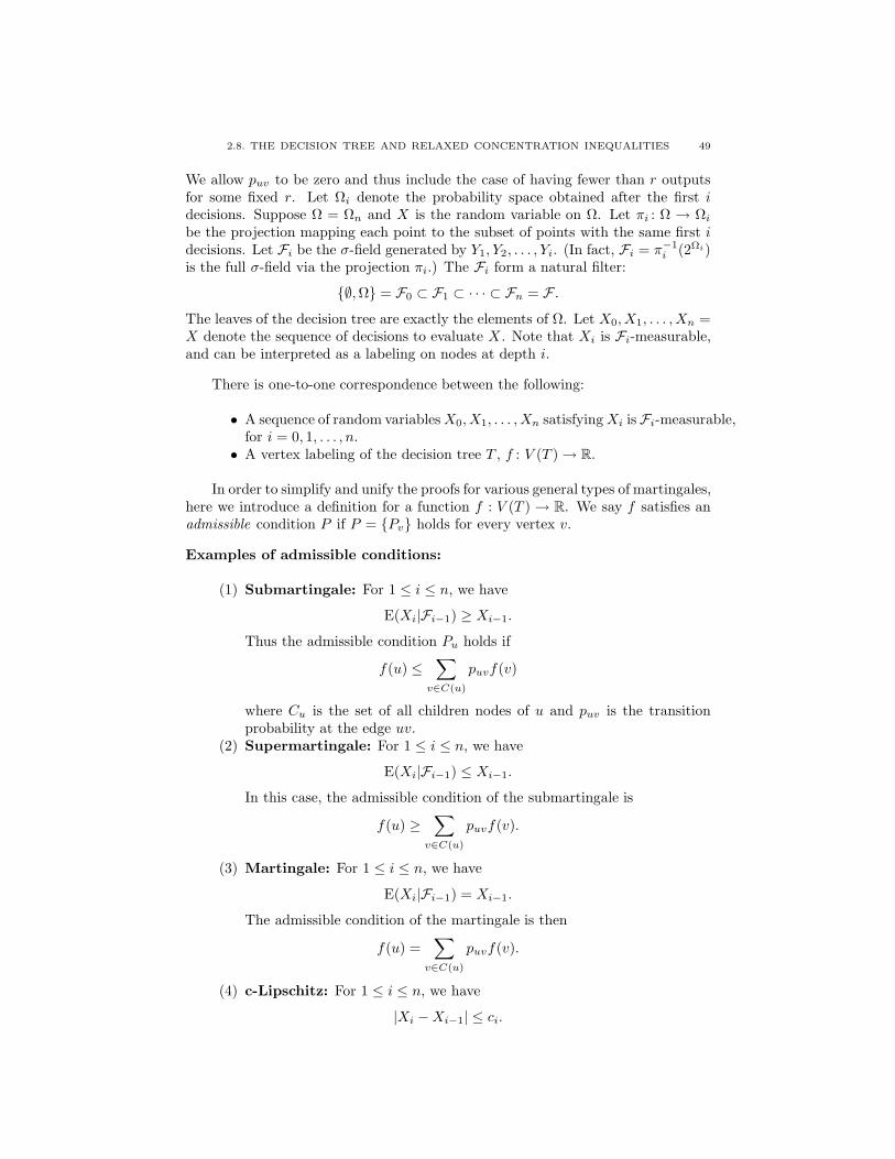
In order to simplify and unify the proofs for various general types of martingales,here we introduce a definition for a function f : V (T ) → R. We say f satisfies anadmissible condition P if P = Pv holds for every vertex v.

Examples of admissible conditions:

(1) Submartingale: For 1 ≤ i ≤ n, we have

E(Xi|Fi−1) ≥ Xi−1.

Thus the admissible condition Pu holds if

f(u) ≤∑

v∈C(u)

puvf(v)

where Cu is the set of all children nodes of u and puv is the transitionprobability at the edge uv.

(2) Supermartingale: For 1 ≤ i ≤ n, we have

E(Xi|Fi−1) ≤ Xi−1.

In this case, the admissible condition of the submartingale is

f(u) ≥∑

v∈C(u)

puvf(v).

(3) Martingale: For 1 ≤ i ≤ n, we have

E(Xi|Fi−1) = Xi−1.

The admissible condition of the martingale is then

f(u) =∑

v∈C(u)

puvf(v).

(4) c-Lipschitz: For 1 ≤ i ≤ n, we have

|Xi −Xi−1| ≤ ci.


The admissible condition of the c-Lipschitz property can be described asfollows:

|f(u) − f(v)| ≤ ci, for any child v ∈ C(u)

where the node u is at level i of the decision tree.(5) Bounded Variance: For 1 ≤ i ≤ n, we have

Var(Xi|Fi−1) ≤ σ2i

for some constants σi.The admissible condition of the bounded variance property can be

described as:∑v∈C(u)

puvf2(v) − (

∑v∈C(u)

puvf(v))2 ≤ σ2i .

(6) General Bounded Variance: For 1 ≤ i ≤ n, we have


where σi, φi are non-negative constants, and Xi ≥ 0. The admissiblecondition of the general bounded variance property can be described asfollows:∑

v∈C(u)

puvf2(v) − (

∑v∈C(u)

puvf(v))2 ≤ σ2i + φif(u), and f(u) ≥ 0

where i is the depth of the node u.(7) Upper-bounded: For 1 ≤ i ≤ n, we have

Xi − E(Xi|Fi−1) ≤ ai +M

where ai’s, and M are non-negative constants. The admissible conditionof the upper bounded property can be described as follows:

f(v) −∑

v∈C(u)

puvf(v) ≤ ai +M, for any child v ∈ C(u)

where i is the depth of the node u.(8) Lower-bounded: For 1 ≤ i ≤ n, we have

E(Xi|Fi−1) −Xi ≤ ai +M

where ai’s, and M are non-negative constants. The admissible conditionof the lower bounded property can be described as follows:

(∑

v∈C(u)

puvf(v)) − f(v) ≤ ai +M, for any child v ∈ C(u)

where i is the depth of the node u.

For any labeling f on T and fixed vertex r, we can define a new labeling fr asfollows:

fr(u) =f(r) if u is a descendant of r,f(u) otherwise.

A property P is said to be invariant under subtree-unification if for any treelabeling f satisfying P , and a vertex r, fr satisfies P .


We have the following theorem.

Theorem 2.34. The eight properties as stated in the preceding examples —submartingale, supermartingale, martingale, c-Lipschitz, bounded variance, generalbounded variance, upper-bounded, and lower-bounded — are all invariant undersubtree-unification.

Proof. We note that these properties are all admissible conditions. Let Pdenote any one of these. For any node u, if u is not a descendant of r, then fr andf have the same value on v and its children nodes. Hence, Pu holds for fr since Pu

does for f .

If u is a descendant of r, then fr(u) takes the same value as f(r) as well asits children nodes. We verify Pu in each case. Assume that u is at level i of thedecision tree T .

(1) For supermartingale, submartingale, and martingale properties, we have∑v∈C(u)

puvfr(v) =∑

v∈C(u)

puvf(r)

= f(r)∑

v∈C(u)

puv

= f(r)= fr(u).

Hence, Pu holds for fr.(2) For c-Lipschitz property, we have

|fr(u) − fr(v)| = 0 ≤ ci, for any child v ∈ C(u).

Again, Pu holds for fr.(3) For the bounded variance property, we have∑

v∈C(u)

puvf2r (v) − (

∑v∈C(u)

puvfr(v))2 =∑

v∈C(u)

puvf2(r) − (

∑v∈C(u)

puvf(r))2

= f2(r) − f2(r)= 0≤ σ2

i .

(4) For the general bounded variance property, we have

fr(u) = f(r) ≥ 0.

∑v∈C(u)

puvf2r (v) − (

∑v∈C(u)

puvfr(v))2 =∑

v∈C(u)

puvf2(r) − (

∑v∈C(u)

puvf(r))2

= f2(r) − f2(r)= 0≤ σ2

i + φifr(u).


(5) For the upper-bounded property, we have

fr(v) −∑

v∈C(u)

puvfr(v) = f(r) −∑

v∈C(u)

puvf(r)

= f(r) − f(r)= 0≤ ai +M.

for any child v of u.(6) For the lower-bounded property, we have∑

v∈C(u)

puvfr(v) − fr(v) =∑

v∈C(u)

puvf(r) − f(r)

= f(r) − f(r)= 0≤ ai +M,

for any child v of u.

Therefore, Pv holds for fr and any vertex v.

For two admissible conditions P and Q, we define PQ to be the property,which is only true when both P and Q are true. If both admissible conditionsP and Q are invariant under subtree-unification, then PQ is also invariant undersubtree-unification.

For any vertex u of the tree T , an ancestor of u is a vertex lying on the uniquepath from the root to u. For an admissible condition P , the associated bad set Bi

over Xi’s is defined to be

Bi = v| the depth of v is i, and Pu does not hold for some ancestor u of v.Lemma 2.35. For a filter F

∅,Ω = F0 ⊂ F1 ⊂ · · · ⊂ Fn = F ,suppose each random variable Xj is Fi-measurable, for 0 ≤ i ≤ n. For any admis-sible condition P , let Bi be the associated bad set of P over Xi. There are randomvariables Y0, . . . , Yn satisfying:

(1) Yi is Fi-measurable.(2) Y0, . . . , Yn satisfy condition P .(3) x : Yi(x) 6= Xi(x) ⊂ Bi, for 0 ≤ i ≤ n.

Proof. We modify f and define f ′ on T as follows. For any vertex u,

f ′(u) =f(u) if f satisfies Pv for every ancestor v of u including u itself.f(v) v is the ancestor with smallest depth so that f fails Pv.

Let S be the set of vertices u satisfying

• f fails Pu,• f satisfies Pv for every ancestor v of u.


It is clear that f ′ can be obtained from f by a sequence of subtree-unifications,where S is the set of the roots of subtrees. Furthermore, the order of subtree-unifications does not matter. Since P is invariant under subtree-unifications, thenumber of vertices that P fails decreases. Now we will show f ′ satisfies P .

Suppose to the contrary that f ′ fails Pu for some vertex u. Since P is invariantunder subtree-unifications, f also fails Pu. By the definition, there is an ancestor v(of u) in S. After the subtree-unification on the subtree rooted at v, Pu is satisfied.This is a contradiction.

Let Y0, Y1, . . . , Yn be the random variables corresponding to the labeling f ′.Then the Yi’s satisfy the desired properties.

The following theorem generalizes Azuma’s inequality. A similar but morerestricted version can be found in [81].

Theorem 2.36. For a filter F

∅,Ω = F0 ⊂ F1 ⊂ · · · ⊂ Fn = F ,suppose the random variable Xi is Fi-measurable, for 0 ≤ i ≤ n. Let Bi denote thebad set associated with the following admissible conditions:

E(Xi|Fi−1) = Xi−1

|Xi −Xi−1| ≤ ci

where c1, c2, . . . , cn are non-negative numbers. Let B = ∪ni Bi denote the union of

all bad sets. Then we have

Pr(|Xn −X0| ≥ λ) ≤ 2e− λ2

2Pn

i=1 c2i + Pr(B).

Proof. We use Lemma 2.35 which gives random variables Y0, Y1, . . . , Yn sat-isfying properties (1)-(3) in the statement of Lemma 2.35. Then it satisfies

E(Yi|Fi−1) = Yi−1

|Yi − Yi−1| ≤ ci.

In other words, Y0, . . . , Yn form a martingale which is (c1, . . . , cn)-Lipschitz. ByAzuma’s inequality, we have

Pr(|Yn − Y0| ≥ λ) ≤ 2e− λ2

2Pn

i=1 c2i .

Since Y0 = X0 and x : Yn(x) 6= Xn(x) ⊂ ∪i=1nBi = B, we have

Pr(|Xn −X0| ≥ λ) ≤ Pr(|Yn − Y0| ≥ λ) + Pr(Xn 6= Yn)

≤ 2e− λ2

2Pn

i=1 c2i + Pr(B).

For c = (c1, c2, . . . , cn) a vector with positive entries, a martingale is said to benear-c-Lipschitz with an exceptional probability η if∑

i

Pr(|Xi −Xi−1| ≥ ci) ≤ η.(2.9)

Theorem 2.36 can be restated as follows:


Theorem 2.37. For non-negative values, c1, c2, . . . , cn, suppose a martingaleX is near-c-Lipschitz with an exceptional probability η. Then X satisfies

Pr(|X − E(X)| ≥ a) ≤ 2e− a2

2Pn

i=1 c2i + η.

Now, we can use the same technique to relax all the theorems in the previoussections.

Here are the relaxed versions of Theorems 2.23, 2.28, and 2.30.


∅,Ω = F0 ⊂ F1 ⊂ · · · ⊂ Fn = F ,suppose a random variable Xi is Fi-measurable, for 0 ≤ i ≤ n. Let Bi be the badset associated with the following admissible conditions:

E(Xi | Fi−1) ≤ Xi−1



where σi, ai and M are non-negative constants. Let B = ∪ni=1Bi be the union of all

bad sets. Then we have

Pr(Xn ≥ X0 + λ) ≤ e− λ2

2(Pn

i=1(σ2i+a2

i)+Mλ/3) + Pr(B).


∅,Ω = F0 ⊂ F1 ⊂ · · · ⊂ Fn = F ,suppose a non-negative random variable Xi is Fi-measurable, for 0 ≤ i ≤ n. LetBi be the bad set associated with the following admissible conditions:

E(Xi | Fi−1) ≤ Xi−1


Xi − E(Xi|Fi−1) ≤ M

where φi and M are non-negative constants. Let B = ∪ni=1Bi be the union of all


Pr(Xn ≥ X0 + λ) ≤ e− λ2

2((X0+λ)(Pn

i=1 φi)+Mλ/3) + Pr(B).



E(Xi | Fi−1) ≤ Xi−1



where σi, φi, ai and M are non-negative constants. Let B = ∪ni=1Bi be the union of


Pr(Xn ≥ X0 + λ) ≤ e− λ2

2(Pn

i=1(σ2i+a2

i)+(X0+λ)(

Pni=1 φi)+Mλ/3) + Pr(B).


For submartingales, we have the following relaxed versions of Theorems 2.25,2.29, and 2.32.



E(Xi | Fi−1) ≥ Xi−1



where σi, ai and M are non-negative constants. Let B = ∪ni=1Bi be the union of all


Pr(Xn ≤ X0 − λ) ≤ e− λ2

2(Pn

i=1(σ2i+a2

i)+Mλ/3) + Pr(B).



E(Xi | Fi−1) ≥ Xi−1


E(Xi|Fi−1) −Xi ≤ M

where φi and M are non-negative constants. Let B = ∪ni=1Bi be the union of all


Pr(Xn ≤ X0 − λ) ≤ e− λ2

2(X0(Pn

i=1 φi)+Mλ/3) + Pr(B).

for all λ ≤ X0.



E(Xi | Fi−1) ≥ Xi−1



where σi, φi, ai and M are non-negative constants. Let B = ∪ni=1Bi be the union of


Pr(Xn ≤ X0 − λ) ≤ e− λ2

2(Pn

i=1(σ2i+a2

i)+X0(

Pni=1 φi)+Mλ/3) + Pr(B),

for λ < X0.


The best way to see the powerful effect of the concentration and martingaleinequalities, as stated in this chapter, is to check out many interesting applications.Indeed, the inequalities here are especially useful for estimating the error bounds inthe random graphs that we shall discuss in subsequent chapters. The applicationsfor random graphs of the off-line models are easier than those for the on-line models.The concentration results in Chapter 3 (for the preferential attachment scheme) andChapter 4 (for the duplication model) are all quite complicated. For a beginner,a good place to start is Chapter 5 on classical random graphs of the Erdos-Renyimodel and the generalization of random graph models with given expected degrees.An earlier version of this chapter has appeared as a survey paper [36] and includessome further applications.

old and new concentration inequalitiesfan/complex/ch2.pdf · chapter 2 old and new concentration...

Documents