oil price volatility and u.s. macroeconomic performance

OIL PRICE VOLATILITY AND U.S. MACROECONOMIC PERFORMANCE

TIMOTHY J. CONSIDINE+

This study uses a model with explicit energy sector linkages to estimate the macroeconomic impacts of the I986 collapse in energy prices. The model combines features of neoclassical macroeconomics to estimate final demand spending and of general equilibrium analysis to estimate substitution possibilities. The model allows price and wage rigidities yet permits interfuel and input substitutions. The simulation results suggest three conclusions. First, the most significant macroeconomic impact of the I986 oil price reduction is the sharp drop in inflation. Second, output and employment gains are relatively small due to the sharp drop in energy sector output. Finally, the estimated gain in real output due to lower energy prices is close to the output loss resulting from the trade deficit increase during I986.This may be one reason why no substantial increase in economic growth occurred following the 1986 collapse in energy prices.

I. INTRODUCTION

The 1986 plunge in oil prices casts doubt on some prevalent notions con- cerning energy markets and their interaction with the economy. First, one common view is that world oil reserves are fixed so that as consumption rises, oil prices will increase-perhaps erratically, but on average faster than overall inflation. Because of the recent surge in U.S. oil imports, these expectations for higher prices prompt some analysts to warn of future oil supply disruptions. Some analysts argue for preventive measures, such as energy taxes, as a way to reduce demand-and thus imports.

The 1986 price collapse surprised many observers. Some analysts, in fact, now consider it an aberration and continue to foresee rising real energy prices (Gately. 1986). Real oil prices from 1859 to 1986. however, resemble a ran- dom walk (Considine, 1986). Given the extraordinary increase in oil prices from 1979 to 1981, one may view the 1986 plunge as a correction to the long-term average. The historical record also indicates that the post-World War I1 period of oil price stability is unusual. The recent period-from 1973 to the present-resembles the era spanning the late 19th and early 20th cen- turies, when market control was in contention and price volatility resulted.

*College of Earth and Mineral Sciences, The Pennsylvania State University. University Pack, Pa. An earlier version of this paper was presented at the 62nd Annual Western Economic Association International Conference, Vancouver, B.C., July 1987, in a session organized by Deborah A. Ott, Federal Energy Regulatory Commission.

83 Contemporary Policy Issues Vol. VI, July 1988

84 CONTEMPORARY POLICY ISSUES

The second notion on which doubt was cast is that lower oil prices are unambiguously “good” for the U.S. economy. Although the estimates vary widely, many studies have shown that higher energy prices impose costs on the economy in the form of higher inflation, lower output, and higher unemployment. Appealing to symmetry, this argument implies that lower oil prices generate benefits for the economy. Energy taxes siphon off some of these benefits, however. Indeed, macroeconomic costs figured strongly in the Reagan administration’s recent opposition to oil import fees.

Clearly, the 1986 plunge in oil prices was a key factor in the consumer price index’s (CPI’s) rising only 1.9 percent in 1986-the lowest rate in 20 years. Growth in output and employment, however, did not accelerate sub- stantially. Growth in real gross national product changed very little-from 3.0 percent in 1985 to 2.9 percent in 1986. And employment growth ac- celerated slightly, from 2.0 to 2.3 percent.

By contrast, Hickman et al. (1987) find that during the first year after a 20 percent reduction in oil prices, inflation drops and output rises about 0.5 percentage point. These changes approach roughly 1 percent during sub- sequent years. The 1986 oil price decline was more than twice as large. Presumably, then, the macroeconomic impacts should have been even larger. Have other factors offset the presumably stimulative effects of lower oil prices? Or is the macroeconomic response to oil price changes inherently asymmetric?

The third notion is that large increases or decreases in energy prices impose adjustment costs on the economy. For example, firms investing in energy-efficient capital would be less profitable and thus less competitive under lower energy prices (Hickman et al., 1987). Amore obvious adjustment problem involves delays in efficiently allocating resources among different sectors of the economy. The plight of the oil and gas industry during 1986 is one example. Capital and labor resources that would have gone to the energy industry under higher energy prices now are free to flow to other sectors. This resource allocation may take some time due to delays in obtaining information. During the last boom, the oil and gas industry encountered bottlenecks in attracting resources from other sectors of the economy.

This paper examines these latter two issues by simulating a macroeconomic model explicitly incorporating energy sector linkages into the determination of aggregate output and prices. The findings support the notion that lower energy prices are good for the U.S. economy. However, the resulting employment and output losses in the energy sector are significant and thus should be considered. The relationship between energy prices and the economy is discussed in section 11. The model’s theoretical structure and its empirical specification are described in sections I1 and 111. respectively. The model simulation results are presented in section IV, and policy implications are drawn in section V.

CONSIDINE OIL PRICES AND U.S. MACROECONOMIC PERFORMANCE 85

II. ENERGY PRICES AND ECONOMIC ACTIVITY

During the 1970s. the temporary presence of rapid inflation with high unemployment-i.e., stagflation-prompted a reassessment of macroeconomic theory. The traditional view was that rising inflation results from excessive aggregate demand due to either too much fiscal stimulus or too much monetary stimulus. Stagflation was considered the result of the economy’s adjusting from its overheated position.

Many economists now view oil price shocks as another cause of stagflation. Indeed, the rational expectations school views unanticipated shocks, such as Organization of Petroleum Exporting Countries (OPEC)-imposed price increases, as the primary reason that output and prices vary from their long-term growth paths. Higher oil prices increase the costs of producing goods and services throughout the economy. These costs may be passed on to final product prices, resulting in inflation. As real purchasing power and aggregate spending decline, output falls and unemployment rises.

The relationship between stagflation and energy prices is controversial. Traditional macroeconomic models do not predict stagflation resulting from expenditure shocks or monetary shocks. For example, Keynesian models- in which the rates of price inflation and wage inflation depend on the degree of capacity utilization-predict a positive relation between inflation and capacity utilization. Monetarists argue that, assuming the classical conditions of full information and full employment, an import price increase is con- verted to price inflation only if the money supply increases. Both views depend on microeconomic assumptions about how labor markets and resource markets function. Consequently, an effort has been made to provide macroeconomics with microeconomic foundations (Bruno, 1984; Gordon, 1984).

Changing energy prices influence consumption decisions and production decisions through their effects on purchasing power and relative prices. These shifts in relative prices and real income alter the supply and demand for goods and services throughout the economy. Different levels for prices and employment result since factor inputs are not perfectly mobile and since wages and prices are not completely flexible in the short run.

The U.S. economy’s adjustment to energy price changes involves the interaction of supply and demand forces and their mutual influence on wages and prices. One may classify these adjustments into three areas: consumer spending, producer decisions, and wage and price adjustment. In addition, the economy’s adjustment to energy price changes is intertwined with monetary and fiscal policies (Pindyck, 1980).

A. Consumers Changes in real energy prices affect the composition of consumer outlays.

Given price-inelastic short-run energy demand, a rapid fall in energy prices


reduces the share of energy expenditures in total consumer outlays. Unless offset by price increases for other items or by a decrease in real income, either savings or consumption of other goods and services rises in the short run.

These shifts in the composition of consumption have a feedback effect on the production side of the economy. Changes in consumption for non- energy goods and services caused by changing energy prices translate into different levels of receipts, output, and employment for various sectors of the economy.

B. Producers Non-energy producers adjust their demand for factors of production to

these shifts in final product demand. As relative factor prices change, input levels are adjusted to minimize costs. These substitutions among fuels and other inputs, such as labor and capital, play a key role in the cost push in- flationary impact of higher energy prices. As output is adjusted to the new levels of demand and relative factor costs, wages and capital returns adjust. Hence, the production-side response to energy prices influences personal income.

A different rate of capacity utilization influences investment. Output effects stemming from shifts in consumer demand and relative factor costs could be an important channel through which energy prices influence investment among non-energy producers.

The investment and production activities of energy producers also are important. As energy producers reduce exploration, development, and production in response to lower energy prices, aggregate investment, employment, and income diminish. Naturally, the reverse occurs as energy prices rise.

C. Prices and Wages The major economic mechanisms transmitting energy price changes to the

overall price level are firm pricing behavior, government programs, and wage demands. To the extent that non-energy producers engage in cost-markup pricing, lower energy prices indirectly result in lower producer prices. These lower prices indirectly reduce the CPI, which also falls directly from energy price reductions. A lower CPI reduces outlays for indexed programs and wage demands. Lower wage rates feed back to production costs.

D. Monetary and Fiscal Policies If energy prices affect inflation and output, then they also influence tax

revenues and thus disposable income. Now that brackets are indexed to inflation, only real income gains are taxed at the margin. Energy producers’ royalties and corporate taxes also change. On the outlay side, government expenditures on goods and services change in response to a changing price level. Outlays for direct payments to individuals also change due to cost-of-

CONSIDINE: OIL. PRICES AND U.S. MACROECONOMIC PERFORMANCE 87

living adjustments in Social Security and other benefit programs. In addition, if unemployment falls under lower energy prices, then outlays for unemployment compensation decline.

The response of monetary policy to energy price changes also is important. As energy prices decrease, consumers and firms lower their transactions demand for money. If the Federal Reserve Bank does not reduce the money supply, interest rates fall.

111. MODEL OVERVIEW

Macroeconomic modeling of oil price shocks generally falls into two broad groups: traditional (income/expenditure) macroeconomic models and general equilibrium models. The Hudson-Jorgenson (1974) model typifies the latter approach. General equilibrium models explicitly estimate substitution possibilities but assume that prices and wages adjust fully each period so as to ensure full employment. One advantage of the more eclectic traditional macroeconomic models is that they consider unemployment as well as price and wage rigidities. The drawback is that such models generally fail to consider the role of energy in aggregate production. The model used below synthesizes these two approaches. It allows wage and price rigidities but explicitly accounts for interfuel and input substitutions in production. The model originally was developed for estimating the economic impacts of natural gas decontrol (Considine, 1983).

Most macroeconomic models consider only final demand expenditures since such costs essentially are equivalent to income. The production side of the economy is not examined explicitly. Given a relatively stable composition of production activities, such an approach can be quite useful. But large swings in relative prices create sectoral imbalances. To understand the macroeconomic implications of oil price shocks, one should consider the production side along with the demand side of the economy.

All three model components-production, final demand, and wages and prices-are solved simultaneously. The production side of the economy is represented by cost functions describing substitution possibilities among fuels and between energy and non-energy inputs. The cost functions have two important linkages with the final demand section of the model. First, the composition of final demand determines the level of sectoral output. Second, the cost functions provide a production-side estimate of income, which in turn is a key force in demand. The third major part of the model involves the determination of prices, wages, and interest rates. Again, the cost functions play a key role. Energy price indices are computed from the cost functions and then used to predict product prices. The latter are used to predict prices for investment and consumption goods.

The advantage of this approach is that interfuel and other input substitutions are allowed in determining prices. Thus, the model estimates both the


direct and the indirect effects of energy prices on the price level and on relative final demand prices. These price effects, together with real output and monetary policy, determine the interest rate level. Investment, consumer durable purchases, and use of capital relative to use of labor and energy in turn are influenced by interest rates.

The model’s level of aggregation reflects the diversity of energy use and allows one to estimate any output and employment effects that the energy sector generates in response to changes in energy prices and energy demand. The production side is broken down into the five major energy-consuming sectors (commercial, manufacturing, transportation, agriculture, and con- struction) and the two major energy-supplying sectors (mining and utilities). The equations are estimated with annual data reported by the Department of Commerce and the Department of Energy from 1960 to 1979. The model predicts gross domestic product, prices, wages, employment, and interest rates based on exogenously given oil prices, oil and natural gas production, government spending, tax rates, and money supply.

IV. MODEL SPECIFICATION

The central problem in estimating the macroeconomic impacts of energy prices is that changing energy prices shift relative prices throughout the economy. The impact of these relative price movements on the level and composition of income and output are the central interactions that the model examines. In addition, the model considers the dynamic adjustment of prices, employment, and output. Some researchers (Gordon, 1984; Bruno, 1984) view the rigidity of real wages as a key factor behind any adjustment problems that oil price shocks cause. The following subsections discuss briefly the model’s empirical specification.

A. Final Demand Consumption is divided into two major categories: energy expenditures

and non-energy expenditures. Household energy expenditures are disaggregated into spending on each of electricity, natural gas, heating oil, and gasoline. Non-energy consumption is divided into three categories: services, nondurables, and durables.

The household demand for fuels is specified in three steps. First, aggregate household energy expenditures are determined. Second, these expenditures are separated into heating fuels and transportation fuels. Finally, the heating fuel aggregate is separated into electricity, natural gas, and oil. The model employs these separability assumptions to reduce the number of parameters that must be estimated. In the simulation of the entire model, these steps are

1. For a listing of the equations and elasticities appearing in two unpublished appendices, contact the author.

CONSIDINE OIL PRICES AND US. MACROECONOMIC PERFORMANCE 89

linked together by energy prices and energy expenditures so that each stage of the allocation process is related to all other stages.

Non-energy expenditures are disaggregated into durables, nondurables, and services. These estimates then are used to predict demand for non- energy-producing sectors. Similarly, residential energy expenditures predicted from the fuel demand equations are a component of revenues for the energy sector.

Real expenditures on services are specified as a function of real per capita disposable income and the price of services relative to the aggregate deflator for personal consumption. Real consumption of nondurables is also predicted on the basis of income and relative prices. Purchases of durables are specified as a function of real per capita disposable income and short- term interest rates.

Total investment is separated into four categories: residential producer durables, nonresidential producer durables, nonresidential structures, and investment in the oil and gas sector. Total nonresidential investment is used to predict the demand for manufactured goods. Investment in the oil and gas sector is specified as a function of the value of proven fossil fuel reserves. Spending for durable equipment is a function of the lagged stock of equipment and aggregate output. Nonresidential investment in structures outside the mining sector is specified as a function of the first differences in output, the cost of capital, and the investment in structures lagged one period. Residential investment depends on lagged values for disposable income less transfers and interest rates.

B . Production Structure The production side of the model is specified by assuming that a “well-

behaved” cost function exists in addition to the underlying production function. The functional form adopted in estimating these cost share equations is based on the logistic function (Considine, 1984). The logistic functional form has three properties useful in forecasting. First, the predicted shares always are positive. Many linear share models yield negative share predictions, particularly if large changes in relative prices occur (Considine, 1987). The second reason is that this form ensures downward-sloping demand curves over a wide range of relative prices. Finally, adding up is guaranteed. This is important for modeling energy-economy interactions because aggregate energy expenditures should be consistent with national income. Forecasts from single-equation energy demand equations could imply energy expenditures too high relative to national income. Other share models also offer adding up but do so at the cost of not ensuring downward-sloping demand and positive shares.

The cost share equations allow for the partial adjustment of input quan- tities. Adjustment of factor demand to price changes is constrained by tech-


nological factors and by adjustment of the capital stock and other fixed factors of production. In addition, because producers often make input decisions on the basis of expected prices, their responses to relative price changes are not immediate. These two features-price expectations and adjustment costs-characterize producers’ gradual response to shifts in relative prices.

The dynamic cost share equations are estimated for the commercial, manufacturing, and transportation sectors, and for the demand for oil and natural gas in the electric utility sector. The cost share equations are estimated in two steps. (1) Interfuel substitution possibilities are determined. (2) Labor, capital, and aggregate energy substitution possibilities are determined based on the aggregate energy price index computed in step (1) along with wages and capital rental rates. Weak separability is assumed among individual fuels and labor and capital. This assumption implies that while the cost-minimizing combination of fuels is independent of the capital-labor combination, the aggregate energy level is not.

C . Prices, Wages, and Interest Rates The response of prices and wages to energy price changes is a critical ele-

ment of energy-economy interactions. The linkages between spending and sectoral output levels also are important. This subsection discusses the specification of various submodels predicting product price deflators, nominal wage rates, and the level of input expenditures for the production side of the economy.

The commercial, manufacturing, and transportation cost functions require estimates of the cost and input price levels. For estimation purposes, the product price deflator, the nominal wage rate, and the level of real expenditures on inputs are specified for each of these sectors as a simultaneous system. Prices and wages for the remaining sectors are specified in single- equation form.

A cost-markup formulation is used to specify the equations for the implicit product deflators. Generally, product prices are specified as a function of labor, capital, energy, and material costs: labor productivity: and the output level. Therefore, shifts in relative factor costs are explicitly considered in determining production-side prices. The exact formulation varies by sector. For example, commercial product prices are a function of wage rates, energy prices (computed from the commercial energy submodel), productivity, and lagged real commercial output. Among the product price models, this last term was the only aggregate demand variable that was significant and had the correct sign.

Nominal wages are specified as a function of consumer prices, labor productivity, and unemployment (Sargan, 1964). Again, the final model specification varies by sector. For example, the nominal commercial wage rate is specified as a function of the CPI, the aggregate unemployment rate,


commercial labor productivity, and the lagged rate of change in wages. In the full-model simulation, the productivity variable is computed from the commercial cost function.

The linkages between the final demand side and the cost functions are es- tablished with an equation for total input expenditures. Real commercial expenditures on labor, capital, and energy are specified as a function of commercial product prices, consumption net of energy, and government expenditures. Manufacturing input expenditures depend on investment, manufacturing product prices, and purchases of consumer durables. Transportation cost is linked to the level of transport prices as well as to commercial and manufacturing output.

The product price deflators by sector then are used to construct an aggregate product price deflator. The latter is an explanatory variable in simple dynamic models of consumption prices and investment prices. The final product price deflator equations are similar to those used in the University of Michigan macroeconomic model (Hymans and Shapiro, 1974). The CPI is related to prices for each of services, durables, and nondurables, and to the residential energy price index, which is computed from the residential energy demand equations.

Finally, interest rates are determined by solving a Klein-Goldberger type money demand equation in which the M1 definition of money in real terms is regressed on the three-month Treasury bill rate, real gross domestic product, and the lagged money supply. Long-term interest rates are determined by assuming a fixed yield curve spread. Given assumptions regarding monetary growth, one can estimate the impact of oil price changes on interest rates based on the model’s estimates of the associated impacts on inflation and real growth.

Induced changes in overall fiscal stimulus are represented by changes in personal tax payments. Tax revenues depend on the tax base and tax rates. The base is determined by tax preferences and by the income and profit levels. Tax rates are set by law. In 1985 and 1986, tax rates were indexed to inflation so that real income gains are taxed-thus reducing bracket creep. The tax equations used in the model explicitly consider tax bracket index- ing (Ribe and O’Connell, 1983).

V. MACROECONOMIC ANALYSIS OF THE 1986 OIL PRICE COLLAPSE

With a healthy dose of skepticism, this model is used here to examine the macroeconomic impacts of the 1986 oil price reduction. Some assumptions apply to the analysis. First. the oil price used is the average domestic first purchase price of crude oil. This price fell from an average of $24.09 per barrel in 1985 to $12.66 in 1986. or 47.4 percent. Accompany- ing this price decline was an often overlooked 25.5 percent decline in the


average wellhead price of natural gas, from $2.51 per thousand cubic feet in 1985 to $1.87 in 1986.

Another critical assumption is the domestic oil and gas supply response. Total petroleum production fell 345.000 barrels per day during 1986, or more than 3 percent. Natural gas production dropped more than 800 billion cubic feet, or roughly 4 percent.

For a large proportion of the labor force, wages are either directly or indirectly indexed to the price level. Thus, during oil price increases, wages would be adjusted to the higher price level. Whether this adjustment keeps pace with inflation is an empirical question. In the US., considerable evidence exists that real wages fall as energy prices rise (Mork, 1980; Pin- dyck, 1980). What happens to nominal wages when energy prices drop?

Two characteristics of the labor market suggest that nominal wages are inflexible downward. First, workers may have implicit contracts with their employers in which workers provide long-term service in return for stable permanent income. Second, given the uncertainty of energy prices and the price level, employers may seek to avoid any adjustment costs associated with frequent wage rate changes. Nevertheless, much empirical evidence suggests that the growth in nominal wages would decrease as a result of oil price reductions. This adjustment would take time, however, and could be contingent on the permanence of such energy price reductions. Conse- quently, in the model simulation, nominal wages are assumed to be inflexible downward so that lower energy prices do not reduce nominal wages. This assumption is important in that it affects the adjustment of the price level and real wages in response to lower energy prices. For example, assume a base case in which nominal wage growth is 4 percent and inflation is 3 percent. Real wages would rise 1 percent (4 - 3). Now, assume an energy price reduction that reduces inflation to 2 percent. Given our assumption that nominal wage growth is unaffected, real wages would rise 2 percent (4 - 2).

On the other hand, if nominal wage growth slowed to 3 percent, inflation would drop even more since wages are the largest component of production costs. For the sake of argument, assume that the price level does not change under this lower nominal wage growth-i.e., inflation is zero. In this case, real wages would rise 3 percent (3 - 0). Hence, real wages rise under lower energy prices but not as much as they do if nominal wages fall. In addition, downward rigidity in nominal wages implies that the price level may drop less than it would rise for the same percentage change in energy prices. This is one potential source of asymmetry in the macroeconomic impacts of oil price changes.

Given these assumptions, the model is simulated under lower oil and gas prices and the results are compared with a base forecast. Energy prices prevailing during 1985 are held constant in the base forecast for 1986. Predicted growth in gross domestic product (GDP) is 2.8 percent in 1985


and 2.2 percent in 1986. Employment growth is 2.4 percent in 1985 and 2.0 percent in 1986. And the GDP deflator rises 2.6 and 3.1 percent in 1985 and 1986. respectively.

The model then is simulated under the 1986 energy price drop. Oil and gas prices prevailing in 1986 are assumed to remain at those levels in 1987 so as to isolate any lagged effects. Monetary policy is assumed to be neutral in response to this price decline. Accordingly, the nominal level of M1 is held constant. Thus, any interest rate changes result from shifts in money demand caused by the energy price shock.

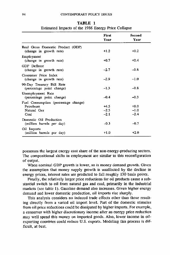
Economic growth increases and inflation drops in response to lower energy prices. The CPI falls slightly less than 3 percentage points (see table 1). Roughly 2.2 percentage points of this 2.9 percentage point drop results directly from lower energy prices. The remaining 0.7 percentage point drop is the indirect effect that lower energy costs have on prices for non-energy goods and services.

The gain in real gross domestic output is only 1.2 percent. Because double-deflated measures of output can be misleading, employment often is considered a better measure of the real effects of energy price shocks (Darby, 1982; Bruno, 1984). The increase in employment is roughly 0.7 percent-considerably less than the gain in real output. During the second year, output gains are minimal while employment growth is slightly higher (see table 1).

The small gains in employment and output under lower oil prices reflect a large shift in the composition of employment and output. Energy consumers-individuals as well as businesses-have more money to spend on other goods and services, while energy companies have less. U.S. oil and gas expenditures, at wellhead values, were slightly less than $182 billion in 1985. After the decline in oil and gas prices, this amount dropped to about $105 billion in 1986. Of this $77 billion change, more than half-about $42 billion-represents a reduction in domestic oil and gas revenues. This revenue decline causes some big reductions in mining employment and capital spending. The predicted reduction in the mining sector’s employment level is 97,000. Capital spending by the energy sector is predicted to fall 28 percent. In addition, the estimated reduction in GDP originating from the mining sector is nearly 7 percent. This alone reduces total GDP nearly 0.3 percentage point in 1986. From just the reduction in mining sector output, the base forecast growth of 2.2 percent in GDP is reduced to 1.9 percent.

Output from other sectors of the economy is stimulated from the oil price reduction. Of the estimated 1.2 percentage point increase in GDP growth, 0.9 percentage point results from higher output in the services sector. The rise in manufacturing output contributes only 0.2 percentage point to the overall output gain. Reduced capital spending by the energy sector reduces some of the output gains resulting from lower manufacturing energy costs. The remaining gains originate primarily from the transportation sector, which


TABLE 1 Estimated Impacts of the 1986 Energy Price Collapse

First Second Year Year

Real Gross Domestic Product (GDP) (change in growth rate)

Employment (change in growth rate)

GDP Deflator (change in growth rate)

Consumer Price Index (change in growth rate)

90-Day Treasury Bill Rate (percentage point change)

Unemployment Rate (percentage point change)

Fuel Consumption (percentage change) Petroleum Natural Gas Coal

(million barrels per day)

(million barrels per day)

Domestic Oil Production

Oil Imports

t1.2

+0.7

-2.7

-2.9

-1.3

-0.4

t4.5 -2.5 -2.1

-0.3

+1 .o

+0.2

+0.4

-0.8

-1 .o

-0.8

-0.3

t8.0 -1 .o -2.4

-0.7

+2.0

possesses the largest energy cost share of the non-energy-producing sectors. The compositional shifts in employment are similar to this reconfiguration

When nominal GDP growth is lower, so is money demand growth. Given the assumption that money supply growth is unaffected by the decline in energy prices, interest rates are predicted to fall roughly 130 basis points.

Finally, the relatively larger price reductions for oil products cause a substantial switch to oil from natural gas and coal, primarily in the industrial markets (see table 1). Gasoline demand also increases. Given higher energy demand and lower domestic production, oil imports rise sharply.

This analysis considers no induced trade effects other than those resulting directly from a varied oil import level. Part of the domestic stimulus from oil price reductions could be dissipated by higher imports. For example, a consumer with higher discretionary income after an energy price reduction may well spend this money on imported goods. Also, lower income in oil- exporting countries could reduce U.S. exports. Modeling this process is dif- ficult, at best.

of output.


Nevertheless, an informal comparative method can yield some insights. Deterioration in the trade deficit reduced the growth in gross national product about 1.1 percentage points in 1986. As suggested above, lower oil prices added about 1.2 percentage points to the GDP growth rate. This comparison, along with the lackluster growth in output during 1986, suggests that a substantial portion of the stimulus from lower oil prices could have been offset by further deterioration in the trade balance.

VI. CONCLUSIONS AND POLICY IMPLICATIONS

Volatile oil prices will continue to have major impacts on the economy. This analysis of the 1986 collapse in petroleum and natural gas prices suggests three principal conclusions. First, the most significant macroeconomic impact is the sharp but temporary drop in inflation. Second, the output and employment gains from the oil price decline are much smaller than the impacts on the price level, due mostly to the reduction in energy sector output. Indeed, the decline in oil and gas production during 1986 was larger than that predicted by many analysts, but then so was the decline in oil prices. Third, the estimated real output gains resulting from lower oil prices are of the same magnitude as the output losses due to the increase in the trade deficit during 1986. This may be one reason why a substantial increase in economic growth did not occur following the 1986 collapse in oil prices.

The notion that lower energy prices are “good” for the U.S. economy should be treated with caution since the energy sector generates a substantial share of national income. Furthermore, during the transitional reallocation of resources within the economy, aggregate economic activity may indeed slow down. Economic policymakers then must face the dilemma of offsetting deflationary pressures at the risk of future inflation. These pressures are temporary, however, so that discretionary policy shifts in response to oil price shocks may be counterproductive.


REFERENCES

Bruno, M., “Raw Materials, Profits, and the Productivity Slowdown,” Quarterly Journal of

Considhe, T. J., Natural Gas Wellhead Pricing Policies: Implications for the Federal Budget, US.

, ‘The Use of Linear Logit Models for Dynamic Input Demand Systems,” Review of

, “A Long Term Perspective on Oil Markets,” U.S. Economic Report, World Informa-

“Estimating the Demand for Energy and Natural Resource Inputs: Trade-Offs in Global

Darby, M. R., ‘The Price of Oil and World Inflation and Recession,” American Economic Review,

Gately, D., “Lessons from the 1986 Oil Price Collapse,” Brmkings Papers on Economic Activity,

Gordon, R. J., “Supply Shocks and Monetary Policy Revisited,” American Economic Review, May

Hickman, B. G., H. G. Huntington, and J. L. Sweeney, Macroeconomic Impacts of Energy Shocks, North Holland, Amsterdam, 1987.

Hudson, E. A., and D. W. Jagenson, “U.S. Energy Policy and Economic Growth, 1975-2000,” Bell Journal of Economics, Autumn 1974.

Hymans. S. H., and H. T. Shapiro, ‘“Ihe Structure and Properties of the Michigan Quarterly Econometric Model of the US. Economy,” International Economic Review, October 1974, 632-653.

Mork, K. A., and R. E. Hall, “Energy Prices, Inflation, and Recession, 1974-1975,” Energy Jour- nal, Autumn 1980.

Pindyck, R. S., “Energy Price Increases and Macroeconomic Policy,” Energy Journal, October 1980, 1-20.

%be, F. B., and K. OConnell, Forecasting Individual Income Tar Revenues: A Technical Analysis, U.S. Congressional Budget Wice, Special Study, August 1983.

Sargan, J. D., “Wages and Prices in the United Kingdom: A Study in Econometric Methodology,” in P. E. Hart, G. Mills, and K. Whitaker, eds., Econometric Analysis for National Economic Planning, Butterworth, London, 1964.

Economics, Fetnuary 1984, 1-29.

Congressional Budget Of€ice, April 1983.

Economics and Statistics. August 1984, 434-443.

tion Services, Bank of America, April 1986.

Properties,” Department of Mineral Economics, Pennsylvania State University, May 1987.

September 1982,738-751.

Spring 1986.

1984, 38-43.

oil price volatility and u.s. macroeconomic performance

Documents