oil and us stock market shocks: implications for canadian
TRANSCRIPT

Working Papers in Economics & Finance2021-07
Oil and US stock market shocks: implications for Canadian equities
Reinhold Heinlein, University of the West of England Sco9 M. R. Mahadeo, University of Portsmouth
Portsmouth Business School h9ps://www.port.ac.uk/about-us/structure-and-governance/organisaGonal-structure/our-academ-ic-structure/faculty-of-business-and-law/portsmouth-business-school
Faculty of Business and Law

Oil and US stock market shocks: implications for Canadian equities
Reinhold Heinleina, Scott M. R. Mahadeob
aBristol Business School, University of the West of England, BS16 1QY, United Kingdom. Email: [email protected] Business School, University of Portsmouth, PO1 3DE, United Kingdom. Email: [email protected]
Abstract
Oil and US stock market shocks are expected to be relevant for Canadian equities, as Canada is an oil-exporter adjacentto the US. We evaluate how the relationship between Canadian stock market indices and such external shocks changeunder extraordinary events. To do this, we subject statistically identified oil and S&P 500 market shocks to a surprisefilter, which detects shocks with the greatest magnitude occurring over a given lookback period; and an outlier filter,which detects extrema shocks that exceed a normal range. Then, we examine how the dependence structure betweenshocks and Canadian equities change under the extreme surprise and outlier episodes through various co-momentspillover tests. Our results show that co-moments beyond correlation are important in reflecting the changes occurringin the relationships between external shocks and Canadian equities in extreme events. Additionally, the differencesin findings under extreme positive and negative shocks provide evidence for asymmetric spillover effects from theoil and US stock markets to Canadian equities. Moreover, the observed heterogeneity in the relationships betweendisaggregated Canadian equities and shocks in the crude oil and S&P 500 markets are useful to policymakers forrevealing sector-specific vulnerabilities, and provide portfolio diversification opportunities for investors to exploit.
Keywords: Canada; oil market; spillover; stock market
JEL classification: C32; G15; Q43
1. Introduction
Canada is a top energy producer, with its position shifting between fourth and fifth in the global rankings over
the last 40 years1. Along with being in close geographic proximity to each other, the US is unquestionably
Canada’s principal trading partner. Moreover, the vast majority of Canada’s petroleum and natural gas exports are
destined for the US market (EIA, 2019). Thus, oil and the US are arguably two of the most important external markets 5
for Canada. Hence, our study analyses the channels through which extreme spillover shocks from both the oil and
US stock markets can affect Canadian equities. As stock market activity is a leading indicator of business cycles and
particularly so in the trough (Bosworth et al., 1975), it can be useful for policymakers to understand the impending real
sector ramifications of exogenous developments on a recipient country through the performance of the stock market
when unexpected events occur. Additionally, investors trading in either hard commodities and/or holding a portfolio 10
of assets which consists of interests in both the US and Canada can benefit from this line of research.
In this paper, we first apply the strategy of Herwartz and Plodt (2016) and Herwartz (2018) to statistically identify
international crude oil market supply and demand shocks and other shocks to the US stock market proposed in the
1Data accessed from eia.gov/international/rankings in January 2021.
Preprint submitted to Working Papers in Economics and Finance, Portsmouth Business School, University of Portsmouth July 4, 2021

theoretical model of Kilian and Park (2009). The advantages of using this statistical identification strategy is that
the structural shocks are orthogonal and the higher order moment dependencies between shocks are also minimised.15
Moreover, much has changed with the increasing financialisation of oil in recent times (Creti et al., 2013; Zhang
and Broadstock, 2020). Therefore, it becomes important to examine the plausibility of delay restrictions based on
economic theory when labelling meaningful shocks in the crude oil and financial markets suggested in Kilian and
Park (2009) in more recent datasets by using a statistically motivated identification approach. We show that these
structural shocks identified through independent components are consistent with those derived from the recursive20
structure implied by Kilian and Park (2009). Furthermore, from the impulse response analysis we document additional
evidence that the two estimation approaches closely align.
We then propose filtering the identified shocks into relatively quiet and extreme episodes to inform our under-
standing of how market relationships change in extraordinary times. Hamilton (1996) argues that it is the surprise
increases in oil prices over the preceding year which is of consequence to the economy, while Akram (2004) suggests25
that it is outlier oil prices exceeding a normal range which matters most. Such premises sit well with the finance
literature, which posits that unprecedented events arising from a stable environment is a hallmark of the contagion
phenomenon (Kaminsky et al., 2003). As such, we build on the work of Mahadeo et al. (2019b) who augment such
established non-linear oil price measures for sorting oil market shocks into quiet and extreme episodes. Hence, we
are able to empirically timestamp extraordinary surprise and outlier scenarios in both the international crude oil and30
US stock markets.
Using these quiet and extreme episodes as discrete subsamples, we evaluate whether correlations between Cana-
dian equities and structural oil and US stock market shocks change under extreme shocks across various co-moment
spillover channels. This step further consolidates approaches employed in two empirical oil-finance studies. One,
based on Broadstock and Filis (2014), is to explicitly estimate the relationship between structural oil market shocks35
suggested in Kilian (2009) and stock market returns. In the context of our analysis of Canadian equities, we extend
this idea to the SVAR model of Kilian and Park (2009) to also acquire other shocks to the US stock market. The other
study we build on is Mahadeo et al. (2019a), who use recently introduced co-moment contagion tests in Fry et al.
(2010) and Fry-McKibbin et al. (2014) to analyse how the relationship between oil and financial markets change in a
small oil-exporter under extreme conditions in the oil market. We include an additional co-moment contagion channel40
(i.e, co-kurtosis) introduced in Fry-McKibbin and Hsiao (2018), and instead of oil returns as the source market vari-
able we use shocks from the crude oil and US stock markets. A principal advantage of the various co-moment tests we
employ is that they do not involve the specification of complex economic models, requiring large datasets on trade and
economic fundamentals, in order to gain valuable insights into the linkages between a source and recipient market in
the wake of a shock (Fry-McKibbin et al., 2018). By incorporating the aforementioned modifications to these previous45
studies, we aim to contribute valuable insights into the relationship between shocks from the international crude oil
and US stock markets and the Canadian stock returns.
In addition to assessing the spillover effects from shocks in these relevant external markets on Canada’s headline
2

equity index - the Toronto Stock Exchange (TSX) Composite, we also consider the relationship between such shocks
and the sector level equities of this index. In so doing, we can determine the winners and losers when extreme 50
shocks occur, and gain further insights into market resilience and vulnerabilities. Instead of a focus of the relationship
between crude oil market shocks and the headline stock market index in multiple countries (see, inter alia, Jones and
Kaul, 1996; Filis et al., 2011; Kang and Ratti, 2013; Kang et al., 2015b; Boldanov et al., 2016; Antonakakis et al.,
2017; Heinlein et al., 2020), another strand of the literature examines the impact of oil price shocks on sector equities
and certain sectors of the economy. With specific reference to the Canadian housing market, Kilian and Zhou (2018) 55
demonstrate that oil price shocks raise real estate demand and real house prices not only in oil-rich provinces but in
oil-poor regions as well. Some recent studies on the impact of structural crude oil market shocks on disaggregated
stock returns include Sakaki (2019) for the US and Mishra and Mishra (2020) for India. The former study modifies the
Kilian and Park (2009) SVAR model for identifying shocks from the crude oil market and other shocks to the US stock
market, by substituting the returns of the composite US stock index with the returns of US sectoral stock indices. Their 60
impulse response analyses illustrate that oil supply and aggregate demand shocks have a positive effect on sector level
stock returns, while oil-specific demand shocks adversely affects stock returns for all sector equities except energy
and utilities. On the other hand, the latter study uses an alternative SVAR model to Kilian and Park (2009) suggested
by Ready (2018), and estimate the time varying relationship between these shocks and sector equities in India. Their
results show oil demand shocks have positive effects on all sector equities. 65
Our analysis on how the relationship between Canadian equities and structural oil and US stock market shocks
change, in extreme shock episodes compared to quiet periods, across various co-moment spillover channels is subse-
quently summarised. First, while there is a weak correlation between oil supply shocks and the real TSX composite
returns, which is consistent with the diminished role of oil supply shocks documented in the literature, we observe that
supply shocks affect these returns through co-skewness and co-kurtosis channels. Second, there are contagion effects 70
from global aggregate demand shocks to Canadian equities illustrated by the rise in correlations and several statisti-
cally significant spillover channels during negative extreme global aggregate demand shocks, while this relationship is
relatively unremarkable in periods of positive extreme global aggregate demand shocks. Third, both positive and neg-
ative extreme oil-specific demand shocks exhibit contagion effects on Canadian equities. Penultimately, the strongest
market relationships are noted between shocks to the US stock market and Canadian equities, and changes in this 75
relationship manifest in higher co-moments beyond the linear correlation channel. Lastly, the relationship between
disaggregated Canadian equities and the oil and US stock market shocks are heterogeneous across the various sectors
of this recipient market. Our spillover test results are found to be robust to alternative specifications, in both the
duration of the surprise filter and the bandwidth of the outlier filter, for identifying discrete quiet and extreme shock
episodes. This line of work is useful to policymakers for identifying systemic and sectoral vulnerabilities to shocks 80
from external markets, and for investors in formulating portfolio diversification strategies.
The rest of the paper is organised as follows. In Section 2, we provide coverage of the literature on the role of
commodity markets and the US on Canadian equities. Subsequently, we explain our empirical steps and describe the
3

data used in Section 3. We then present, analyse, and discuss our findings in Section 4. Section 5 concludes the paper.
2. Literature on the effects of oil and US stock markets on Canadian equities85
In this section, we consolidate some of the salient literature covering the influence of the crude oil and US markets
on Canadian equities. Many researchers have highlighted the impact of US developments on the Canadian real and
financial sectors. Canadian and US economies are highly integrated, and the structure and regulation of stock markets
in the two countries are similar. The stock markets share the same trading hours and some companies listed on
Canadian stock markets are inter-listed on US markets. A strand of literature has studied the extent to which these90
two markets are financially integrated (see, for example, Jorion and Schwartz, 1986, and Mittoo, 1992). Such studies
employ CAPM and APT frameworks, whereby findings suggest a move from segmentation to integration of markets
over time.
In Karolyi (1995), bi-variate GARCH models are used to study the dynamics of returns and volatility of the S&P
500 and the TSE 3002 markets. In the BEKK specification of the model no statistically significant spillovers from95
lagged TSE 300 returns to future S&P 500 returns cannot be rejected, while lagged S&P 500 returns are relevant for
future TSE 300 returns. In all model specifications, the authors find a strong response of Canadian equity returns to
S&P 500 shocks.
A further study applying M-GARCH models in the context of US/Canadian stock markets is Racine and Ackert
(2000). They find significant cross-market volatility dependencies, with a correlation in volatility for the S&P 500 and100
Toronto 35 stock index of 0.679. Interestingly, when they split their sample, January 1988 to March 1993, in half, the
second part of the sample shows a lower correlation between markets compared to the first part. They state a declining
correlation in their conclusion, although the total sample considered is short.
From a forecasting perspective, Rapach et al. (2013) show that lagged US stock returns help to predict returns of
major international markets. Working with monthly data from 1980:02 to 2010:12 and Granger causality tests, they105
give in-sample and out-of-sample evidence of the predictive power of lagged US returns on Canadian returns, among
other markets. Wang et al. (2018) show that US stock volatility can predict volatility of other markets. Their proposed
model is superior in forecasting 1-day ahead of the Canadian S&P TSX Composite index volatility compared to
benchmark models.
We turn the emphasis now from the relationship between US and Canadian equities towards the influence of the110
oil market on Canada. Elder and Serletis (2009), Rahman and Serletis (2012), and Bashar et al. (2013) all examine oil
price uncertainty in Canada. The first study employs a SVAR with multivariate GARCH-in-Mean; while the second
uses a VARMA, GARCH-in-Mean, asymmetric BEKK model; and the third uses alternative SVAR models. Across
all studies, it is consistently illustrated that rising oil price uncertainty leads to a reduction in Canadian economic
2The TSE 300 has been replaced by the S&P TSX Composite Index on May 1st , 2002.
4

activity. 115
Another strand of literature has exploited big data approaches to evaluate the impact of international shocks on
the Canadian economy. For instance, Vasishtha and Maier (2013) employ a factor-augmented VAR model, using
monthly data from January 1985 to May 2008 and across 261 series, to examine how the sources of global shocks
influence Canada. Their results show that Canada is vulnerable to foreign economic activity and commodity prices
but is comparatively more isolated to global inflation and interest rates. In another example, using a combination 120
of structural dynamic factor and VAR models, Charnavoki and Dolado (2014) estimate the dynamic responses of
Canadian macroeconomic indicators to global commodity market shocks. Their analysis utilises a quarterly dataset
which spans 1975 to 2010 and makes use of 281 variables. They show that positive global demand and negative com-
modity supply shocks lead to commodity price increases, and generate favourable external balances and commodity
currency effects. These authors also find a Dutch disease effect3 in response to commodity price increases resulting 125
from negative commodity supply shocks.
There are also insightful papers on the relationship between oil and the stock market that cover multiple countries,
which includes Canada. In the remainder of this section, we place the spotlight on the results relating to Canada
from such studies. One such study by Jones and Kaul (1996) find that the Canadian stock market reaction to oil price
shocks, which is similar to the US but dissimilar to Japan and the UK, is rational - oil price shocks influence on the 130
stock market is entirely explained through current and expected future real cash flows. In another study, Kang and
Ratti (2013) use an extension of the SVAR model introduced by Kilian (2009) to disentangle the international crude oil
market disturbances into supply and demand shocks. They do so by appending two additional variables to the bottom
of the recursive identification structure in the contemporaneous matrix of the SVAR, i.e. economic policy uncertainty
and stock returns. Their results show that oil price shocks and economic policy uncertainty are interrelated, and that 135
a rise in economic policy uncertainty leads to a significant reduction in real Canadian stock returns. Their results for
Canada are in line with the US, but are much less pronounced than their findings for Europe. In yet another study,
Kang et al. (2015b) use a mixture innovation time-varying parameter VAR model to examine structural oil market
shocks on stock returns. Their results demonstrate that in Canada (and Europe), oil supply and oil-specific demand
shocks are a greater source of volatility than in the US. However, global aggregate demand shocks are the main source 140
of stock market volatility in Canada, and this finding is consistent for the US and Europe as well.
Filis et al. (2011), Boldanov et al. (2016), and Antonakakis et al. (2017) all investigate the relationship between
oil and stock markets of multiple oil-exporting and importing countries using different approaches, and all include
Canada in their analyses. In the first study, a dynamic conditional correlations (DCC) model is used to examine the
changes in the oil-stock market relationship during key events in the international crude oil market. They document 145
that correlations do not differ between oil-exporters and importers. A BEKK model is used in the second study,
which contrastingly finds heterogeneity in correlations between oil-exporters and oil-importers. Their specific results
3The Dutch disease characterises the adverse effects a booming tradeable resource sector has on the non-boom tradeable sector, particularlythrough the appreciation of the real exchange rate. See, inter alia, Corden (1984, 2012) for further context.
5

for Canada (and Norway) suggests that time varying correlations between the volatilities of oil prices and the stock
market are negatively correlated, which is a contrast to the positive correlations reported in the case of oil-importers.
The third study utilises an extension of the Diebold and Yilmaz (2014) dynamic connectedness measure based on150
structural forecast error variance decompositions, and reports both between and within country differences in both
the strength and direction of the relationship between oil and stock markets for oil-exporters and oil-importers. Their
specific analysis for Canada imply that in turbulent conditions, the transmission of shocks to the stock market are
primarily driven by global aggregate demand shocks, but this source of transmission becomes much less pertinent in
tranquil conditions.155
In a recent study, Heinlein et al. (2020) assess the relationship between oil and stock markets for a heterogeneous
selection of oil-exporters and importers in the onset of the COVID-19 pandemic. They use local Gaussian correlations
with high frequency intraday data to determine whether market connections increase between crude oil and stock
returns in the wake of the crisis. Their results show that, even with such high frequency data, oil-exporting countries
experience comparatively stronger oil-stock market correlations compared to importers in both pre-crisis and crisis160
periods. Among the other oil-exporters in the analysis (i.e., Norway and Russia), the relationship between oil and
stock returns for Canada is relatively lower in the wake of the global pandemic.
3. Methods and data
Our empirical procedure consists of four steps. The first step documents how we disentangle shocks in the interna-
tional crude oil and US stock markets. In the second step, we outline two approaches for filtering these shocks into165
discrete quiet and extreme episodes. For the third step, we explain the regressions used to adjust the returns of the
Canadian equity indices for market fundamentals and describe the resulting data series. Finally, the fourth step illus-
trates various co-moment tests for evaluating whether the relationship between the identified shocks and the various
returns of Canadian equity indices change during extreme episodes compared to relatively quiet conditions.
Monthly data are used for all empirical steps, as this is the highest frequency at which the identifying assumptions170
made about demand and supply shocks in the crude oil market are valid (see, e.g., Kilian, 2009; Kilian and Park,
2009). Our period of investigation is January 1988 to April 2020, which is dictated by the availability of the Canadian
equity indices for the third step of our analysis. Combined, the first and second steps of identifying oil and US stock
market shocks, as well as filtering the data into quite and extreme episodes require approximately three preceding
years of data to prime these procedures. We further describe the data attributes below.175
3.1. Identifying structural oil and S&P 500 market shocks through independent components
We estimate a structural vector autoregression model (SVAR) based on monthly data, from 1985:1 to 2020:4, for the
global oil and US stock market following Kilian and Park (2009), which is represented in Eq. (1):
6

yt = ν +
24∑i=1
Aiyt−i + Bεt, t = 1, . . . ,T (1)
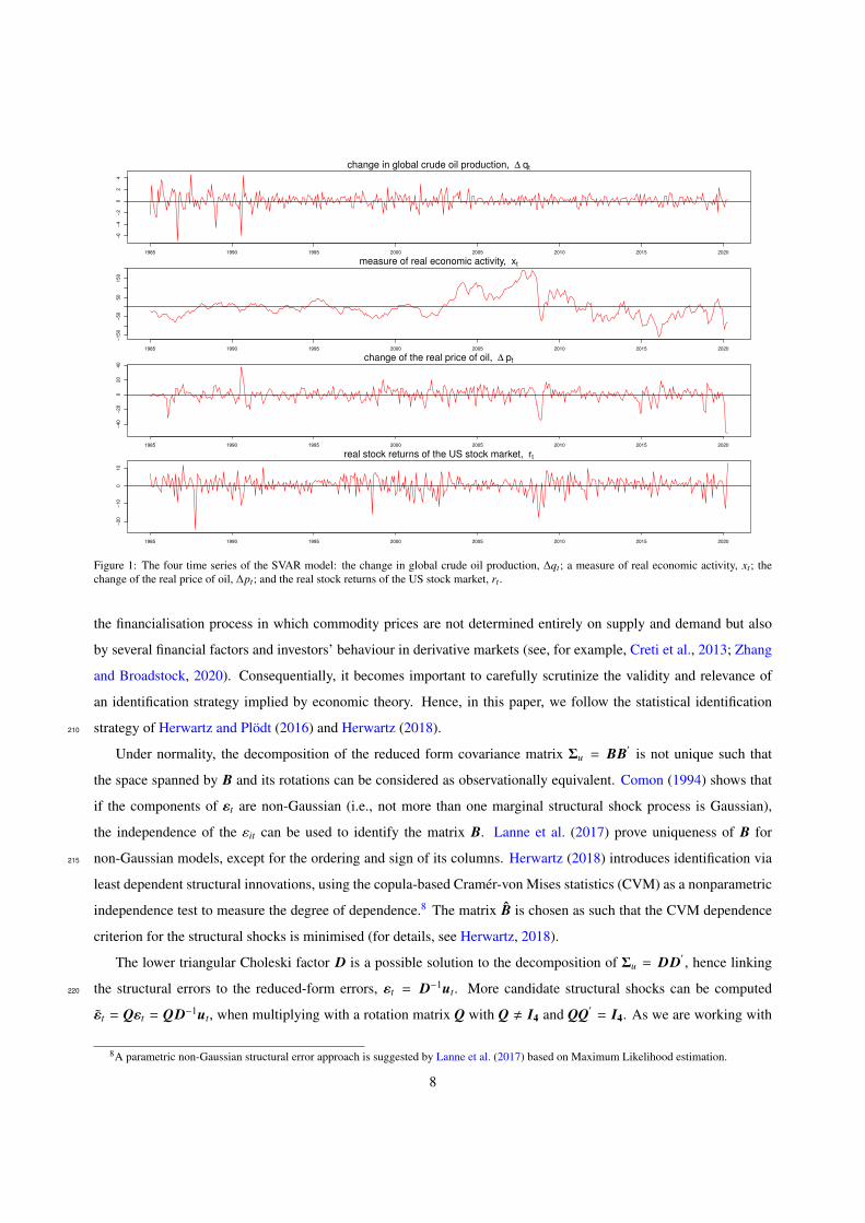
where the vector yt = (∆qt, xt,∆pt, rt)′ includes the change in global crude oil production4, ∆qt; a measure of world 180
demand for commodities, xt, for which we use the global index of real economic activity in industrial commodity
markets suggested in Kilian (2009, 2019)5; the change of the real price of oil, ∆pt, for which we use the US crude oil
imported acquisition cost by refiners, expressed in constant 2015 prices 6; and the real stock returns of the US stock
market, rt, for which we use the S&P 500 market index returns also deflated with 2015 prices7. Figure 1 shows the
raw data for these four series. We take a moment to justify the use of these variables in the context of our application 185
to Canada. Although in 2018 Canada was the world’s fourth largest producer of petroleum, other related downstream
liquids, and natural gas (EIA, 2019), the international crude oil market activity is considered sufficient to capture the
information content across these hydrocarbon commodity markets. This is because natural gas prices and contracts
are commonly indexed to crude oil prices (Zhang and Broadstock, 2020). In addition, the S&P 500 market index
is considered to be the most appropriate indicator for assessing the influence of the US stock market on Canadian 190
equities, due to its size and prominence on global financial markets (see, e.g., Phillips and Shi, 2020).
Furthermore, the structural shocks, εt, in Eq. (1) are uncorrelated across equations and over time with mean zero
and unit covariance matrix, Σε. The reduced form residuals, ut = Bεt, are linear functions of the structural innovations
and Cov(ut) = Σu = Bεtε′
t B′
= BΣεB′
= BB′
. Up to 24 lags are included in the estimation of Eq. 1, as is conventional
with specification of SVAR models for capturing the dynamics in the international crude oil market (see, e.g., Kilian, 195
2009; Kilian and Park, 2009; Kilian and Murphy, 2014; Kang et al., 2015a; Baumeister and Kilian, 2016a,b).
The model of the global crude oil market comprises four types of structural shocks, which are labelled as oil
supply shock (εs), aggregate demand shock (εad), oil-specific demand shock (εosd), and other shocks to stock returns
(εr). To identify the impact of the structural shocks on the variables in the system, Kilian and Park (2009) have
applied economic theory to justify the use of a recursive form in the B matrix. Some of the main premises of their 200
SVAR model is a vertical short run oil supply curve, whereby demand-side shocks do not contemporaneously affect
the global oil supply as it is generally costly for oil producers to respond to high frequency demand innovations; due
to the sluggishness in global real economic activity, this variable does not respond to oil-specific demand shocks in
the same month; and that developments in the international crude oil market are treated as predetermined for the US
stock market within the same month (for further details, see Kilian, 2009; Kilian and Park, 2009). In recent times, 205
4World crude oil production in thousands of barrels per day is obtained from the US Energy Information Administration (EIA), available fromeia.gov/opendata, and accessed in September 2020.
5The global measure of real economic activity is obtained from Lutz Kilian’s website, available atsites.google.com/site/lkilian2019/research/data-sets, and accessed in September 2020.
6Refiners acquisitions cost per barrel of imported crude oil, accessed in September 2020, is also obtained from the US EIA ateia.gov/dnav/pet/hist/LeafHandler.ashx?n=pet&s=r1300 3&f=m. The oil price data is expressed in constant 2015 prices using the US CPI ob-tained from fred.stlouisfed.org/series/CPIAUCSL, also accessed in September 2020, and converted into percent changes.
7S&P 500 index is obtained from Yahoo Finance, available at finance.yahoo.com/quote, and accessed in September 2020. Like oil prices, thisseries is adjusted for inflation using the US CPI with a 2015 base year. Returns are subsequently computed as the logarithmic-differencing of thereal stock market index times 100.
7
change in global crude oil production, ∆ qt
1985 1990 1995 2000 2005 2010 2015 2020
−6
−4
−2
02
4
measure of real economic activity, xt
1985 1990 1995 2000 2005 2010 2015 2020
−150
−50
50
150
change of the real price of oil, ∆ pt
1985 1990 1995 2000 2005 2010 2015 2020
−40
−20
020
40
real stock returns of the US stock market, rt
1985 1990 1995 2000 2005 2010 2015 2020
−20
−10
010
Figure 1: The four time series of the SVAR model: the change in global crude oil production, ∆qt; a measure of real economic activity, xt; thechange of the real price of oil, ∆pt; and the real stock returns of the US stock market, rt .
the financialisation process in which commodity prices are not determined entirely on supply and demand but also
by several financial factors and investors’ behaviour in derivative markets (see, for example, Creti et al., 2013; Zhang
and Broadstock, 2020). Consequentially, it becomes important to carefully scrutinize the validity and relevance of
an identification strategy implied by economic theory. Hence, in this paper, we follow the statistical identification
strategy of Herwartz and Plodt (2016) and Herwartz (2018).210
Under normality, the decomposition of the reduced form covariance matrix Σu = BB′
is not unique such that
the space spanned by B and its rotations can be considered as observationally equivalent. Comon (1994) shows that
if the components of εt are non-Gaussian (i.e., not more than one marginal structural shock process is Gaussian),
the independence of the εit can be used to identify the matrix B. Lanne et al. (2017) prove uniqueness of B for
non-Gaussian models, except for the ordering and sign of its columns. Herwartz (2018) introduces identification via215
least dependent structural innovations, using the copula-based Cramer-von Mises statistics (CVM) as a nonparametric
independence test to measure the degree of dependence.8 The matrix B is chosen as such that the CVM dependence
criterion for the structural shocks is minimised (for details, see Herwartz, 2018).
The lower triangular Choleski factor D is a possible solution to the decomposition of Σu = DD′
, hence linking
the structural errors to the reduced-form errors, εt = D−1ut. More candidate structural shocks can be computed220
εt = Qεt = QD−1ut, when multiplying with a rotation matrix Q with Q , I4 and QQ′
= I4. As we are working with
8A parametric non-Gaussian structural error approach is suggested by Lanne et al. (2017) based on Maximum Likelihood estimation.
8

a K = 4 dimensional system, the rotation matrix can be parameterised as the product of 6 orthogonal Givens rotation
matrices, K(K − 1)/2, leading to the optimisation of a 6-dimensional vector of rotation angles. This identification via
least dependent innovations is capable to identify the link matrix B except for column permutations and column signs.
If needed, we switch the columns of the matrix B by comparing and aligning the resulting impulse responses with 225
those impulse responses achieved by using the lower triangular Choleski factor D. This way we achieve an economic
meaningful labelling of the structural shocks in a statistical identification procedure.
3.2. Filtering shocks into discrete quiet and extreme episodes
We adopt two alternative measures to sort the statistically identified shocks into discrete outcomes of extreme and
quiet episodes. One measure is based on the idea suggested by Hamilton (1996), who argues that it is actually surprise 230
oil price increases over the preceding year which are of consequence to the economy rather than increases which
are simply corrections for previous price declines. It becomes straightforward to use this measure to also obtain
surprise oil price decreases, especially in analyses involving oil-exporters such as Canada. Furthermore, capturing
unexpected events arising from a stable oil market environment integrates comfortably with the literature on the
causes of spillovers. For instance, Kaminsky et al. (2003) characterise surprise shocks in a source market as one of 235
the unholy trinities of a contagion phenomenon. Therefore, it is also simple to extend the filter posited by Hamilton
(1996) to acquire relatively quiet and extreme surprise shock episodes, across all four identified shocks (εs, εad, εosd,
and εr), such that:
surprise+i,t =
1, if εi,t > max(0, εi,t−1, εi,t−2, ..., εi,t−12)
0, if 0 ≤ εi,t ≤ max(0, εi,t−1, εi,t−2, ..., εi,t−12), i = s, ad, osd, r, (2)
surprise−i,t =
1, if εi,t < min(0, εi,t−1, εi,t−2, ..., εi,t−12)
0, if 0 ≥ εi,t ≥ min(0, εi,t−1, εi,t−2, ..., εi,t−12), i = s, ad, osd, r, (3) 240
where surprise+i,t (surprise−i,t) is an indicator variable with 0 and 1 in Eq. (2) (Eq. (3)) representing the relatively quiet
and extreme positive (negative) surprise shock episodes, respectively. The periods which are found to be consistently
quiet (0) across all the four structural shocks, such that there exists no extreme positive or negative outlier shock
episodes, forms a mutually quiet sample. This mutually quiet sample will provide the basis of how we will evaluate
whether market relationships change in the presence of extreme shocks. In particular, we test whether various co- 245
moments between external shocks and Canadian equity returns differ under shock episodes classified as extreme
positive (negative) surprises compared to all other relatively quieter positive (negative) shock periods.
The second measure we use to sort the identified shocks into categories of extreme and quiet episodes is motivated
by Akram (2004) that it is the extreme oil prices outside a normal range which are of consequence to the economy. It is
also straightforward to apply this idea to the four identified structural shocks to obtain extreme outlier episodes in the 250
9

oil and US financial markets. However, the band of stable oil prices, of USD 14 to USD 20, used in Akram (2004) is a
feature of oil markets prior to the 21st century. Hence, we use the standard deviation (σi) of the structural shocks (εi)
to provide context of what is considered quiet and extreme. Using σ is appealing because it does not require imposing
priors about the typical range of values of the different structural shocks, which can be difficult to establish. As testing
for asymmetric responses to positive and negative shocks is a cornerstone of applied macroeconomics, especially oil255
empirics, we can further disaggregate extreme outlier shocks to also evaluate these cases. Given that σi = 1 for all εi,
the filters in Eqs. (4) and (5) are applied to each of the four identified shocks to sort values into relatively quiet and
extreme outlier episodes:
outlier+i,t =
1, if εi,t > 1
0, 0 ≤ εi,t ≤ 1, i = s, ad, osd, r, (4)
outlier−i,t =
1, if εi,t < −1
0, 0 ≥ εi,t ≥ −1, i = s, ad, osd, r, (5)260
where outlier+i,t (outlier−i,t) takes the form of an indicator variable with 0 and 1 in Eq. (4) (Eq. 5) representing the
relatively quiet and extreme positive (negative) outlier shock episodes, respectively. Once again, values which are
found to be consistently 0 for all four shocks will form a mutually quiet sample to determine if linkages vary under
extreme scenarios. In this instance, we test whether co-moments between external shocks and Canadian equity returns
change under shock episodes classified as extreme positive (negative) outliers compared to all other relatively quieter265
positive (negative) periods.
3.3. Estimating returns net of market fundamentals for Canadian equity indices
We work with the residuals, εk,t, from the generic regression in Eq. (6) to represent the returns of the real Canadian
equity indices adjusted for the macroeconomic environment:
rCANk,t = αk + Σn
j=1βk, jrCANk,t− j + Σn
j=1γ jIRCANt− j + Σn
j=1λ jIRUSt− j + εk,t (6)270
where k denotes a given real Canadian equity index so that the returns, rCANk,t , are the logarithmic difference of a
particular index times 100. The regressors used to control for lead-lag effects follow the contagion literature, which
include lags of the returns of a given real Canadian equity index, rCANk,t− j; Canadian short term interest rates, IRCAN
t− j ,
for which we use Canada’s interbank rate9; and US interest rates, IRUSt− j , for which we use the US effective federal
9Canadian 3-month rates and yields are obtained from the FRED database, available at fred.stlouisfed.org/series/IR3TIB01CAM156N, andaccessed in September 2020.
10

funds rate10. Interest rates are commonly used to account for market fundamentals, as they reflect information about 275
both macroeconomic developments and the policy environment (Forbes and Rigobon, 2002). We include lags of both
Canadian and US interest rates, to respectively control for domestic and foreign activity. An optimal lag length, n, for
these single equation regression models are selected by the Schwarz information criterion (SIC).
We estimate the returns net of market fundamentals as described in Eq. 6 for twelve Canadian equity market in-
dices. These include the S&P Toronto Stock Exchange (TSX) Composite, the headline Canadian equity market index, 280
as well as the eleven sector indices. The sector equities are defined along the Global Industrial Classification Standard
(GICS) Level 1 taxonomy, which are a subset of the constituents comprised in the parent S&P TSX Composite, and
consists of equities on the Consumer Discretionary, Consumer Staples, Energy, Financials, Health Care, Industrials,
Information Technology, Materials, Real Estate, Telecommunication, and Utilities Sectors. SIC suggests an optimal
lag length of 2 months across all twelve regressions for adjusting the Candian equity returns. 285
Canadian equity indices data are obtained from the Bloomberg terminal and deflated using Canada’s CPI11. As
previously discussed, our period of analysis is 1988:1 to 2020:4, determined by the Canadian equity indices data
availability. This therefore implies that data for priming the surprise shock filters in the second step are needed 12
months in advance, i.e. January 1987. As a consequence, the first step of statistically identifying structural shocks
requires data from December 1984, i.e. 25 months which include: 1 month for the computing the percentage changes 290
in world crude oil supply, oil prices, and the stock market; as well as a lag length of 24 months in estimating oil and
US stock market shocks.
Figure 2 illustrates the returns, net of market fundamentals, for the real S&P TSX Composite and its 11 GICS
Level 1 real S&P TSX sector equities. Firstly, the returns of the real TSX Composite is punctuated with spikes during
the key contemporary global financial crises such as the Asian financial crisis (late 1990s), the dotcom crash (early 295
2000s), the 2008 Global Financial Crisis (GFC), and the COVID-19 pandemic (2020). Secondly, the returns of the
real TSX Consumer Discretionary index shows higher volatility in the wake of global financial crises. On the other
hand, the real TSX Consumer Staples returns appears to be relatively more stable as might be expected. The real
equity returns of the TSX Energy, Finance, Materials, Real Estate, and Utilities Sectors all convey larger fluctuations
for international events like the Asian financial crisis, the GFC, and COVID-19. However, as anticipated, the real 300
equity returns of the IT and Telecommunications Sectors were particularly hard hit when the dotcom bubble burst but
perhaps more resilient in the COVID-19 pandemic in comparison to spikes observed in other sectors, due to working
from home and lock-down polices which rely on such technologies. The salient features of the real returns of the TSX
Industrial Sector index resembles that of the Composite Index, while the real Health Sector equity returns experienced
larger swings in the latter half of the 2010s. 305
10The US federal funds rate data are also obtained from the FRED database, available at fred.stlouisfed.org/series/DFF, and accessed in Septem-ber 2020.
11Canadian stock market data are expressed in constant 2015 prices obtained from fred.stlouisfed.org/series/CPALCY01CAM661N, and bothsets of data were accessed in September 2020.
11

S&P TSX composite
1990 1995 2000 2005 2010 2015 2020
−20
−10
05
10
consumer discretionary
1990 1995 2000 2005 2010 2015 2020
−30
−20
−10
010
20
consumer staples
1990 1995 2000 2005 2010 2015 2020
−15
−10
−5
05
energy sector
1990 1995 2000 2005 2010 2015 2020
−40
−20
010
20
financial sector
1990 1995 2000 2005 2010 2015 2020
−30
−20
−10
010
health sector
1990 1995 2000 2005 2010 2015 2020
−60
−20
020
40
industrial sector
1990 1995 2000 2005 2010 2015 2020
−20
−10
05
10
information technology
1990 1995 2000 2005 2010 2015 2020
−60
−40
−20
020
40
materials sector
1990 1995 2000 2005 2010 2015 2020
−30
−10
010
20
real estate
1990 1995 2000 2005 2010 2015 2020
−30
−20
−10
010
telecommunication services
1990 1995 2000 2005 2010 2015 2020
−10
010
20
utilities sector
1990 1995 2000 2005 2010 2015 2020
−15
−10
−5
05
10
Figure 2: Returns net of market fundamentals for the real S&P TSX Composite and the corresponding real Level 1 GICS sector equities.
3.4. Spillover channels from oil and the S&P 500 market shocks to Canadian equities
To analyse whether the relationship between Canadian equities, and oil and S&P 500 market shocks change under
extreme episodes, we adopt linear, asymmetric, and extremal dependence tests employed in Fry-McKibbin and Hsiao
(2018)12. The following notation are used in the specification of the dependence tests: zi is the standardised scaling
of εi, which are the statistically identified structural residuals, where i denotes the various source of the shocks: oil310
supply, aggregate demand, oil-specific demand, or other shocks to the US stock market (hereafter called S&P 500
market shocks). zk is the standardised scaling of εk, which are the residuals of Eq. (6) representing the returns adjusted
for market fundamentals, where k is a given real Canadian equity index. Tx and Ty are the sample sizes, such that xt
are the time periods of quiet shocks which come from the aforementioned mutually quiet sample (0) defined by either
the surprise filters (i.e., Eqs. 2 and 3) or outlier filters (i.e., Eqs. 4 and 5); and yt are the time periods of surprise or315
outlier shock episodes, which can be positive or negative. µix (µkx) and µiy (µky) are the sample means of εi,xt (εk,xt )
and εi,yt (εk,yt ), respectively; and σix (σkx) and σiy (σky) are the corresponding sample standard deviations. Finally, as
correlation coefficients are widely known to become spuriously over-inflated in the presence of heteroskedasticity, a
correction is used in all dependence tests to scale the volatility in extreme shock episodes conditional of the volatility
experienced in quiet shocks given by:320
12Fry-McKibbin and Hsiao (2018) put forward the co-kurtosis channels of extremal dependence and also consolidates into their analysis thelinear and asymmetric dependence contagion tests introduced in Fry et al. (2010), as well as the co-volatility channel of extremal dependenceproposed in Fry-McKibbin et al. (2014).
12

ρy|xi =ρy√
1 + ((σ2i,y − σ
2i,x)/σ2
i,x)(1 − ρ2y)
(7)
whereσ2i,x (σ2
i,y) is the variance of a given shock in quiet (extreme) episodes and ρy is the Pearson correlation coefficient
between a given shock and the returns of a Canadian equity index in extreme shock episodes.
3.4.1. Linear dependence
To evaluate whether there is a change in correlation between a given external shock and a Canadian equity index, dur- 325
ing quiet and extreme shock episodes, we employ a two-sided version of the Forbes and Rigobon (2002) significance
test suggested in Fry et al. (2010):
CR11(i→ k) =
(ρy|xi − ρx√
Var(ρy|xi − ρx)
)2
(8)
where ρy|xi is the heteroskedasticity corrected correlation coefficient between an external shock and Canadian equities
during extreme episodes; ρx is the Pearson correlation in the quiet sample. 330
3.4.2. Asymmetric dependence
We employ the co-skewness contagion tests introduced in Fry et al. (2010), to analyse whether there is a statistically
significant difference between quiet and extreme shock episodes about how the (i) mean of extreme shocks (denoted
as z1i ) affect the volatility of real Canadian equity returns (denoted as z2
k), as specified in Eq. (9); and (ii) volatility of
extreme shocks (denoted as z2i ) affect the mean of real Canadian equity returns (denoted as z1
k), as specified in Eq. (10): 335
CS 12(i→ k; z1i , z
2k) =
(ψy(z1
i , z2k) − ψx(z1
i , z2k)√
(4ρ2y|xi
+ 2)/Ty + (4ρ2x + 2)/Tx
)2
(9)
CS 21(i→ k; z2i , z
1k) =
(ψy(z2
i , z1k) − ψx(z2
i , z1k)√
(4ρ2y|xi
+ 2)/Ty + (4ρ2x + 2)/Tx
)2
(10)
where the parameters ψx(zmi , z
nk) and ψy(zm
i , znk) are defined as:
ψx(zmi , z
nk) =
1Tx
Tx∑t=1
(εi,xt − µix
σix
)m(εk,xt − µkx
σkx
)n
(11) 340
ψy(zmi , z
nk) =
1Ty
Ty∑t=1
(εi,yt − µiy
σiy
)m(εk,yt − µky
σky
)n
(12)
13
where zm (zn) is the standardised returns for market i (k) in the CS 12 (CS 21) test version and squared standardised
returns in the CS 21 (CS 12) test version.
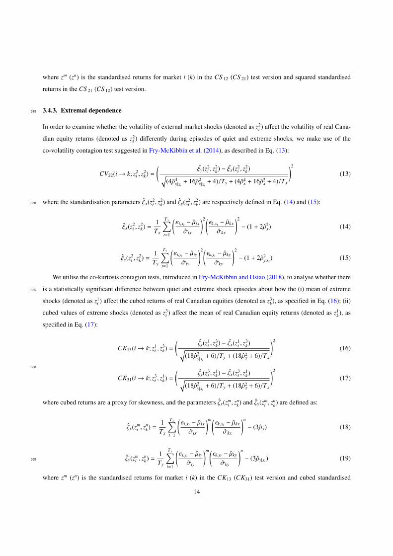
3.4.3. Extremal dependence345
In order to examine whether the volatility of external market shocks (denoted as z2i ) affect the volatility of real Cana-
dian equity returns (denoted as z2k) differently during episodes of quiet and extreme shocks, we make use of the
co-volatility contagion test suggested in Fry-McKibbin et al. (2014), as described in Eq. (13):
CV22(i→ k; z2i , z
2k) =
(ξy(z2
i , z2k) − ξx(z2
i , z2k)√
(4ρ4y|xi
+ 16ρ2y|xi
+ 4)/Ty + (4ρ4x + 16ρ2
x + 4)/Tx
)2
(13)
where the standardisation parameters ξx(z2i , z
2k) and ξy(z2
i , z2k) are respectively defined in Eq. (14) and (15):350
ξx(z2i , z
2k) =
1Tx
Tx∑t=1
(εi,xt − µix
σix
)2(εk,xt − µkx
σkx
)2
− (1 + 2ρ2x) (14)
ξy(z2i , z
2k) =
1Ty
Ty∑t=1
(εi,yt − µiy
σiy
)2(εk,yt − µky
σky
)2
− (1 + 2ρ2y|xi
) (15)
We utilise the co-kurtosis contagion tests, introduced in Fry-McKibbin and Hsiao (2018), to analyse whether there
is a statistically significant difference between quiet and extreme shock episodes about how the (i) mean of extreme355
shocks (denoted as z1i ) affect the cubed returns of real Canadian equities (denoted as z3
k), as specified in Eq. (16); (ii)
cubed values of extreme shocks (denoted as z3i ) affect the mean of real Canadian equity returns (denoted as z1
k), as
specified in Eq. (17):
CK13(i→ k; z1i , z
3k) =
(ζy(z1
i , z3k) − ζx(z1
i , z3k)√
(18ρ2y|xi
+ 6)/Ty + (18ρ2x + 6)/Tx
)2
(16)
360
CK31(i→ k; z3i , z
1k) =
(ζy(z3
i , z1k) − ζx(z3
i , z1k)√
(18ρ2y|xi
+ 6)/Ty + (18ρ2x + 6)/Tx
)2
(17)
where cubed returns are a proxy for skewness, and the parameters ζx(zmi , z
nk) and ζy(zm
i , znk) are defined as:
ζx(zmi , z
nk) =
1Tx
Tx∑t=1
(εi,xt − µix
σix
)m(εk,xt − µkx
σkx
)n
− (3ρx) (18)
ζy(zmi , z
nk) =
1Ty
Ty∑t=1
(εi,yt − µiy
σiy
)m(εk,yt − µky
σky
)n
− (3ρy|xi ) (19)365
where zm (zn) is the standardised returns for market i (k) in the CK13 (CK31) test version and cubed standardised
14

returns in the CK31 (CK13) test version.
3.4.4. Evaluating the null hypothesis of the dependence tests
The linear, asymmetric, and extremal dependence tests, under their respective null hypotheses of no changes in the
correlation, co-skewness, co-volatility, and co-kurtosis during quiet and extreme shock episodes, are asymptotically 370
distributed as:
CR11,CS 12,CS 21,CV22,CK13,CK31(i→ k)d−→ χ2
1.
As our sample sizes in the dependence tests are relatively small and the splits between extreme and calm periods
are unequal, it is not optimal to use the asymptotic critical values. In the case of short crisis periods, the linear test,
CR11, tends to be oversized while the higher moment tests, CS 12,CV22 and CK13, tend to be undersized, see Fry- 375
McKibbin et al. (2019). On these grounds we simulate critical values. When conducting simulating exercises, under
the null hypothesis, we use sample sizes for the extreme and quiet shock periods identical to our applications, as
implied by the surprise and outlier filters. The results of the critical values obtained from the simulation exercises,
based on 50,000 replications, are presented in Table A.3 for the conventional levels of statistical significance (i.e., 1%,
5%, and 10% levels). 380
4. Results and discussion
4.1. Comparison of identification strategies of the oil and S&P 500 market shocks
Jarque–Bera tests for normality on the reduced-form residuals of the VAR show that there is strong evidence against
the null hypothesis of normality for all four components of the model, see Table 1. Hence, identification through
independent components is an adequate identification technique.13385
Table 1: Jarque–Bera normality tests.
Component Skewness Kurtosis JB statistic p-value
u1t -0.476 8.176 461.610 0.000
u2t -0.632 6.608 243.650 0.000
u3t -0.219 4.701 51.459 0.000
u4t -0.533 3.720 27.553 0.000
13We use the R package ‘svars’ of Lange et al. (2019).
15

The estimated impact matrices of the recursive-Cholesky approach D and of the identification-through-independent-
components approach Bcvm reads as:
D =
0.764 0 0 0
0.466 13.268 0 0
−0.908 0.886 6.659 0
−0.008 0.199 0.244 3.695
Bcvm =
0.735 −0.028 0.175 −0.113
1.542 12.964 −2.411 −0.030
−2.345 2.254 5.926 −0.504
0.399 0.287 0.662 3.616
.
We compare the structural shocks obtained from the statistical identification strategy of Herwartz and Plodt (2016)
and Herwartz (2018), with the theoretical approach suggested in Kilian and Park (2009), in Figure 3, and note that the
results are qualitatively consistent. We further investigate the impulse response functions of these two identification390
strategies, in Figure 4, and observe a close alignment in the dynamics between the approaches across a forecast horizon
of 15 months. The similarity in dynamics shows that the correct column permutation has been chosen in the statistical
approach.
Oil supply shocks, εs
1990 1995 2000 2005 2010 2015 2020
−6
−4
−2
02
4
Aggregate demand shocks, εad
1990 1995 2000 2005 2010 2015 2020
−6
−4
−2
02
Oil−market specific demand shocks, εosd
1990 1995 2000 2005 2010 2015 2020
−4
−2
02
4
Other shocks to stock returns, εr
1990 1995 2000 2005 2010 2015 2020
−4
−2
01
23
Figure 3: Structural shocks comparison of different identification approaches. Blue line: shocks of a model identified as a recursive structure. Redline: shocks computed from a model which has been identified through independent components.
16

2 4 6 8 10 12 14
0.0
0.4
0.8
εs −> ∆ qt
2 4 6 8 10 12 14
−0.1
00.0
00.1
0
εad −> ∆ qt
2 4 6 8 10 12 14
−0.1
00.0
50.1
5
εosd −> ∆ qt
2 4 6 8 10 12 14
−0.1
00.0
00.1
0
εr −> ∆ qt
2 4 6 8 10 12 14
−3
−1
01
2
εs −> xt
2 4 6 8 10 12 14
812
16
20
εad −> xt
2 4 6 8 10 12 14
−2
02
46
εosd −> xt
2 4 6 8 10 12 14
−2
01
23
4
εr −> xt
2 4 6 8 10 12 14
−2.5
−1.5
−0.5
0.5
εs −> ∆ pt
2 4 6 8 10 12 14
−1
01
2
εad −> ∆ pt
2 4 6 8 10 12 140
24
68
εosd −> ∆ pt
2 4 6 8 10 12 14
−0.5
0.0
0.5
1.0
εr −> ∆ pt
2 4 6 8 10 12 14
−0.4
0.0
0.4
εs −> rt
2 4 6 8 10 12 14
−0.4
0.0
0.4
εad −> rt
2 4 6 8 10 12 14
−0.4
0.0
0.4
0.8
εosd −> rt
2 4 6 8 10 12 14
01
23
4
εr −> rt
Figure 4: Impulse response comparison of different identification approaches. Blue line: responses of a model identified as a recursive structure.Red line: responses computed from a model which has been identified through independent components.
We prefer using the statistical identification strategy, because it does not rely on strict zero restrictions derived from
economic theory. Further, under the statistical identification strategy the structural shocks are not just orthogonal but 395
the higher order moment dependencies between shocks are also minimised.
4.2. Evidence of spillover effects from oil and S&P 500 market shocks to Canadian equities
We now turn to our main research question of this paper - do various co-moments between real Canadian equity
returns and shocks from the crude oil and US stock markets differ under extreme shock episodes compared to quiet
periods? Due to the variations in quiet and extreme sample sizes produced by the positive and negative surprise and 400
outlier shock filters in Eqs. (2), (3) (4), and (5), we use simulated critical values to evaluate the null hypothesis of “no
contagion” across the various co-moment channels.
For both the surprise and outlier shock filters, Tx and Ty in Table 2 show the sample sizes of the amount of months
distributed between quiet and extreme shocks, respectively. Out of the overall sample of 375 months (i.e., 1988:4 -
2020:4), the sum of positive and negative Tx samples in the case of each of the four shocks are equal to 206 (115) 405
mutually quiet months under the surprise (outlier) filter. The remainder 169 (260) extreme episodes are distributed
across positive and negative oil supply (os), global aggregate demand (gd), oil-specific demand (od), and S&P 500
market (sp) shocks, denoted in months by Ty, with the possibility of overlaps where some months experience multiple
types of extreme shocks.
17

4.2.1. Implications for the S&P TSX Composite Index410
Table 2 shows that, over all periods of time, the highest positive (lowest negative) returns in the real S&P TSX
Composite are experienced when the S&P 500 market exhibits extreme positive (negative) shocks. These findings
are similar for both the surprise and outlier shock filters, and illustrates the synchronisation between the financial
markets of Canada and the US. Additionally, the return volatility of the real TSX Composite Index is typically higher
under extreme shock episodes in the crude oil and S&P 500 markets relative to quiet shock episodes 14. Furthermore,415
for each of the four identified shocks, returns volatility of the TSX Composite is higher under negative episodes
compared to positive episodes. As stock return volatility is a proxy for market uncertainty (see, e.g., Bloom et al.,
2007), higher volatility in extreme shock episodes reflect the fear associated with such events in the TSX market. The
largest return volatility values in the real TSX Composite occur under negative oil supply and demand shocks. These
aforementioned findings, regarding the return volatility of the real TSX Composite, are the same across both surprise420
and outlier filters.
From the spillover test results produced with the surprise and outlier filters, a general consistency is also observed
in Table 2. However, there is a tendency for the outlier filter to provide additional spillover channels from the oil and
S&P 500 markets to the TSX Composite relative to the surprise filter. Furthermore, the results are in line with the
contagion literature, that co-moments beyond the correlation channel are important in reflecting the changes occurring425
between market relationships in times of extreme events (see, e.g., Fry et al., 2010; Fry-McKibbin and Hsiao, 2018).
There is also strong evidence to support asymmetric spillover effects from oil and US financial market shocks to
Canadian equities, as noted by difference in findings under extreme positive and negative shocks.
We find a weak and (for the most part) negative correlation between oil supply shocks and the TSX composite
under quiet/extreme, positive/negative, and surprise/outlier oil supply shock episodes. Although oil supply shocks430
are thought to become irrelevant in the recent literature (see, e.g., Broadstock and Filis, 2014 and references within),
asymmetric and extremal dependence channels detect changes in the relationship between oil supply shocks and the
TSX Composite in extreme episodes.
Turning to the relationship between global aggregate demand side shocks and the TSX Composite, contagion ef-
fects are noted under extreme negative episodes, while extreme positive global aggregate demand side shocks appear435
comparatively inconsequential. This is evidenced by a generally weak relationship between global aggregate demand
shocks and the TSX Composite, which becomes stronger and positive under extreme negative episodes, in both sur-
prise and outlier shocks. Our results align with Antonakakis et al. (2017), who also document that global aggregate
demand shocks only matter in Canada during turbulent periods but the effects of such shocks are muted in tranquil
conditions. However, the correlation coefficient corrected for heteroskedasticity underscores the upward bias in the440
linear correlation coefficient during the high volatility associated with extreme episodes. Nevertheless, even after
14The one exception where return volatility in the real TSX Composite is higher in the quiet episodes is observed under positive oil-specificdemand shocks using the surprise filter.
18

19
Table 2: Spillover tests from shocks in the crude oil and S&P 500 markets to the adjusted returns of real S&P TSX Composite Index based on thesurprise and outlier shock filter.
Surprise shock filter
ospos osneg gdpos gdneg odpos odneg sppos spneg
Tx 107 99 111 95 107 99 113 93Ty 34 29 27 39 34 32 29 29µx 0.721 -0.411 0.577 -0.290 0.669 -0.354 1.623 -1.580µy -1.072 -0.771 0.045 -0.807 1.373 -1.275 3.704 -5.203σx 3.248 3.605 3.543 3.324 3.550 3.302 3.044 3.122σy 5.694 6.814 3.728 4.582 2.871 5.989 3.103 5.857ρx -0.109 -0.065 0.027 0.003 0.166 -0.157 0.314 0.457ρy -0.049 0.009 -0.030 0.366 0.406 0.423 0.495 0.636ρy|xi -0.031 0.003 -0.017 0.158 0.275 0.234 0.457 0.543
CR11 0.295 0.336 0.095 1.614 0.617 8.521∗∗ 0.888 0.464CS 12 0.661 0.042 0.379 21.620∗∗∗ 1.375 7.944∗∗∗ 1.652 0.512CS 21 0.735 1.709 0.041 18.312∗∗∗ 2.555∗ 24.596∗∗∗ 2.591∗ 0.340CV22 1.664 0.000 0.228 91.016∗∗∗ 6.064∗∗∗ 52.590∗∗∗ 4.036∗∗ 0.001CK13 4.944∗∗ 2.115∗ 0.327 62.485∗∗∗ 0.551 44.276∗∗∗ 1.777∗ 0.769CK31 4.014∗∗ 22.799∗∗∗ 0.858 100.552∗∗∗ 11.567∗∗∗ 102.444∗∗∗ 4.477∗∗ 0.122
Outlier shock filter
ospos osneg gdpos gdneg odpos odneg sppos spneg
Tx 54 61 61 54 57 58 70 45Ty 57 48 43 48 55 58 54 65µx 0.613 0.321 0.889 -0.029 0.873 0.051 1.164 -0.640µy -0.135 -1.232 0.310 -0.698 1.296 -0.519 3.382 -4.996σx 2.677 3.342 2.836 3.208 3.178 2.863 2.911 2.932σy 4.591 5.480 3.648 4.270 3.290 5.391 3.161 4.750ρx -0.112 -0.236 0.132 0.046 0.021 -0.283 0.149 0.251ρy -0.138 -0.066 -0.128 0.374 0.318 0.294 0.469 0.461ρy|xi -0.083 -0.018 -0.064 0.109 0.202 0.124 0.364 0.310
CR11 0.034 2.960 1.766 0.196 1.363 9.140∗∗∗ 2.180 0.146CS 12 1.276 0.008 3.355∗∗ 26.992∗∗∗ 0.813 21.284∗∗∗ 6.164∗∗∗ 8.348∗∗∗
CS 21 3.401∗ 3.590∗∗ 0.259 33.529∗∗∗ 13.248∗∗∗ 23.760∗∗∗ 8.510∗∗∗ 3.028∗
CV22 0.027 0.000 0.002 176.352∗∗∗ 5.843∗∗ 146.538∗∗∗ 16.419∗∗∗ 6.841∗∗∗
CK13 0.209 3.002∗∗ 1.600 104.609∗∗∗ 1.982 49.867∗∗∗ 4.945∗∗ 7.965∗∗∗
CK31 23.764∗∗∗ 45.658∗∗∗ 2.461∗ 248.299∗∗∗ 42.118∗∗∗ 235.226∗∗∗ 26.297∗∗∗ 6.489∗∗∗
Notes: ∗ significant at 10% level, ∗∗ significant at 5% level, ∗∗∗ significant at 1% level.We apply simulated critical values, see Table A.3.

correcting for this over-inflation, all co-moment spillover channels, with the sole exception of the linear correlation
channel, indicate that the dependence structure between the source shock and the recipient market change.
For the relationship between oil demand shocks and the TSX Composite, a weak positive correlation in quiet
periods becomes relatively stronger under extreme positive shocks in the cases of both surprise and outlier filters. Co-445
skewness, co-kurtosis, and co-volatility dependence tests provide evidence of spillover effects in the extreme positive
oil demand episodes. Under negative oil demand shocks, the correlation between the TSX composite and oil demand
shocks switches from negative in quiet periods to positive in extreme episodes. All spillover channels detect changes
in this relationship between quiet and extreme episodes during both negative oil demand surprise and outlier shocks.
The results from demand side shocks (both global aggregate demand and oil demand) are in line with the findings of450
Kilian and Park (2009) on the impact of oil price shocks on the US stock market that it is demand side shocks which
have a greater consequence for markets compared to supply side shocks.
With regards to the relationship between the S&P 500 market shocks and the TSX Composite, a relatively moder-
ate and positive interdependence becomes stronger under extreme conditions. This is consistent for both positive and
negative S&P 500 market shocks, as well as for both surprise and outlier approaches. The various co-moment depen-455
dence test results suggest that the outlier shock filter provide stronger evidence of spillover effects than the surprise
shock filter. Again, it is the channels beyond linear correlation which are significant and once more underscores the
importance of asymmetric and extremal dependence tests in analysing the relationship between markets under stress.
4.2.2. Implications for the sector equities of the S&P TSX Composite Index
Similar to the results of the parent composite index, the findings for the sector equities obtained using the surprise and460
outlier shocks are generally consistent with the tendency to convey additional spillover channels across the various
co-moments. We subsequently highlight the main results obtained from the sectoral analysis using the surprise and
outlier shock filters, respectively presented in Tables A.4 and A.5.
Of all extreme episodes, the 11 real TSX Composite GISC Level 1 Sectors all experienced the lowest returns
during the negative S&P 500 market shocks. The real TSX Consumer Discretionary, Consumer Staples, Energy, and465
Financial Sectors all experienced the highest return volatility under negative oil-specific demand shocks. However, for
the real TSX Industrial, IT, Telecommunications, and Utilities Sectors, the highest return volatility are recorded under
negative oil supply shocks. These observations about the summary statistics are consistent across both the surprise
and outlier filters. However, the real TSX Health, Materials, and Real Estate Sector equities conveyed differences
between surprise and outlier filters for periods where the highest return volatility occurred.470
Out of the four main types of shocks, the TSX Consumer Discretionary Sector is more correlated with oil-specific
demand and S&P 500 market shocks; and the TSX Consumer Staples Sector is more correlated with S&P 500 market
shocks. The TSX Consumer Discretionary Sector shows more spillover channels detected in comparison to the TSX
Consumer Staples Sector across samples obtained using the surprise and outlier shock filters. Such results are the-
20

oretically consistent with the idea that the Consumer Discretionary Sector is sensitive to extreme market conditions 475
whereas the Consumer Staples Sector is relatively more stable (unchanged) in the wake of an extreme shock compared
to quiet periods. This is particularly evident during negative global aggregate and positive oil-specific demand shocks.
The results for the TSX Energy Sector equities show, as one might expect, that changes in the co-moments between
shocks and this sector index primarily relate to extreme negative global aggregate and oil-specific demand side shocks.
For the relationship between TSX Financial Sector equities and shocks from the crude oil and US stock markets, cor- 480
relations are strongest under extreme positive and negative oil demand shocks, as well as under extreme negative
S&P 500 market shocks. Turning to the TSX Health, Industrial, IT, Materials, and Telecommunications Sectors, the
correlation between each of these sector indices and S&P 500 market shocks are stronger when compared to relation-
ship between these indices and crude oil market shocks. In the case of the TSX Real Estate Sector equities, with the
exception of positive global aggregate demand shocks, the crude oil market is found to be the source of spillovers for 485
this sector market. From the TSX Utilities Sector results, most spillover activity occurs in the relationship between
this sector index and oil demand shocks under negative episodes.
4.2.3. Robustness analysis
We test the sensitivity of the results from the various dependence tests to alternative specifications in the filters for
identifying discrete quiet and extreme shocks. For instance, in the case of the definition of surprise shocks correspond- 490
ing to major increases or decreases in a shock over the preceding 12 months, we also consider the cases 9 months
and 15 months. With respect to the outlier shocks for classifying extreme episodes as values exceeding 1 SD band,
we also consider the cases of 1.2 and 1.5 SD bands. The overall results from both filters for identifying surprise and
outlier shocks are robust to such alternative specifications in these rules15.
5. Conclusion 495
Our paper contributes to the literature by consolidating various empirical procedures into an original approach to
investigate the channels through which Canadian equities are affected by extreme spillover shocks from two of the
most important external markets of this country - the international crude oil and S&P 500 markets. To do this, we
first disentangle structural shocks from these external markets through independent components. Comparisons of
the structural shocks and impulse response functions implied by the statistically identified strategy and a theoretical 500
SVAR are found to closely align, yet pursuing the former strategy has advantages of orthogonality and a minimisation
of higher order moment dependencies between the estimated shocks.
Subsequently, we filter the statistically identified oil and S&P 500 market shocks into discrete quiet and extreme
episodes. This is achieved using two different approaches: a surprise filter, which detects major shocks occurring
15The results from the robustness analysis can be made available upon request to the authors.
21

over the preceding year; and an outlier filter, to detect extreme shocks outside a normal range of values. These505
discrete filters fit well with the contagion literature, which advocates that it is the unprecedented shocks from a stable
environmental that gives rise to an increase in cross-market linkages. We then use the periods of quiet and extreme
shocks to construct sub-samples for constructing spillover tests through multiple co-moment channels. These tests
evaluate whether correlation, co-skewness, co-volatility, and co-skewness between Canadian equity returns and shocks
from the crude oil and S&P 500 markets change during quiet and extreme shock episodes.510
We show that although oil supply shocks and Canadian equities are weakly correlated, the former can influence the
latter through certain higher co-moment channels. We also find contagion effects between global aggregate demand
shocks and Canadian equities, since only negative extreme shocks lead to a rise in correlation and the detection
of many statistically significant spillover channels. Regarding the relationship between oil-specific demand shocks
and Canadian equities, episodes of positive and negative extreme values in such shocks exhibit contagion effects.515
Moreover, we observe that compared to all shocks, market correlations are highest in the relationship between S&P
500 market and Canadian equities. Additionally, from the relationship between oil and S&P 500 market shocks and
disaggregated Canadian equities, our results suggest heterogeneity across various sectors. This type of research can
benefit Canadian policymakers interested in both systemic and sector vulnerability and resilience to external shocks.
It is also useful to stock market participants with interests in US, Canadian, international commodity markets seeking520
to optimise their portfolio choice.
Disclaimer
We declare that this research did not receive any specific grant from funding agencies in the public, commercial, ornot-for-profit sectors.
References525
Akram, Q.F., 2004. Oil prices and exchange rates: Norwegian evidence. The Econometrics Journal 7, 476–504.
Antonakakis, N., Chatziantoniou, I., Filis, G., 2017. Oil shocks and stock markets: Dynamic connectedness under the prism of recent geopolitical
and economic unrest. International Review of Financial Analysis 50, 1–26.
Bashar, O.H., Wadud, I.M., Ahmed, H.J.A., 2013. Oil price uncertainty, monetary policy and the macroeconomy: The Canadian perspective.
Economic Modelling 35, 249–259.530
Baumeister, C., Kilian, L., 2016a. Forty years of oil price fluctuations: Why the price of oil may still surprise us. Journal of Economic Perspectives
30, 139–60.
Baumeister, C., Kilian, L., 2016b. Understanding the decline in the price of oil since June 2014. Journal of the Association of Environmental and
Resource Economists 3, 131–158.
Bloom, N., Bond, S., Van Reenen, J., 2007. Uncertainty and investment dynamics. The Review of Economic Studies 74, 391–415.535
Boldanov, R., Degiannakis, S., Filis, G., 2016. Time-varying correlation between oil and stock market volatilities: Evidence from oil-importing
and oil-exporting countries. International Review of Financial Analysis 48, 209–220.
Bosworth, B., Hymans, S., Modigliani, F., 1975. The stock market and the economy. Brookings Papers on Economic Activity 1975, 257–300.
22

Broadstock, D.C., Filis, G., 2014. Oil price shocks and stock market returns: New evidence from the United States and China. Journal of
International Financial Markets, Institutions and Money 33, 417–433. 540
Charnavoki, V., Dolado, J.J., 2014. The effects of global shocks on small commodity-exporting economies: lessons from Canada. American
Economic Journal: Macroeconomics 6, 207–37.
Comon, P., 1994. Independent component analysis, a new concept? Signal Processing 36, 287–314.
Corden, W.M., 1984. Booming sector and Dutch disease economics: Survey and consolidation. Oxford Economic Papers 36, 359–380.
Corden, W.M., 2012. Dutch disease in Australia: Policy options for a three-speed economy. Australian Economic Review 45, 290–304. 545
Creti, A., Joets, M., Mignon, V., 2013. On the links between stock and commodity markets’ volatility. Energy Economics 37, 16–28.
Diebold, F.X., Yilmaz, K., 2014. On the network topology of variance decompositions: Measuring the connectedness of financial firms. Journal of
Econometrics 182, 119–134.
EIA, 2019. Country analysis executive summary: Canada. US Energy Information Administration ver. Oct. 2019.
Elder, J., Serletis, A., 2009. Oil price uncertainty in Canada. Energy Economics 31, 852–856. 550
Filis, G., Degiannakis, S., Floros, C., 2011. Dynamic correlation between stock market and oil prices: The case of oil-importing and oil-exporting
countries. International Review of Financial Analysis 20, 152–164.
Forbes, K.J., Rigobon, R., 2002. No contagion, only interdependence: Measuring stock market comovements. The Journal of Finance 57, 2223–
2261.
Fry, R., Martin, V.L., Tang, C., 2010. A new class of tests of contagion with applications. Journal of Business & Economic Statistics 28, 423–437. 555
Fry-McKibbin, R., Hsiao, C.Y.L., 2018. Extremal dependence tests for contagion. Econometric Reviews 37, 626–649.
Fry-McKibbin, R., Hsiao, C.Y.L., Martin, V.L., 2018. Global and regional financial integration in east asia and the asean. The North American
Journal of Economics and Finance 46, 202–221.
Fry-McKibbin, R., Hsiao, C.Y.L., Martin, V.L., 2019. Joint tests of contagion with applications. Quantitative Finance 19, 473–490.
Fry-McKibbin, R., Hsiao, C.Y.L., Tang, C., 2014. Contagion and global financial crises: Lessons from nine crisis episodes. Open Economies 560
Review 25, 521–570.
Hamilton, J.D., 1996. This is what happened to the oil price-macroeconomy relationship. Journal of Monetary Economics 38, 215 – 220.
Heinlein, R., Legrenzi, G.D., Mahadeo, S.M., 2020. Energy contagion in the covid-19 crisis. CESifo Working Paper 8345.
Herwartz, H., 2018. Hodges–Lehmann detection of structural shocks–an analysis of macroeconomic dynamics in the Euro area. Oxford Bulletin
of Economics and Statistics 80, 736–754. 565
Herwartz, H., Plodt, M., 2016. The macroeconomic effects of oil price shocks: Evidence from a statistical identification approach. Journal of
International Money and Finance 61, 30–44.
Jones, C.M., Kaul, G., 1996. Oil and the stock markets. The Journal of Finance 51, 463–491.
Jorion, P., Schwartz, E., 1986. Integration vs. segmentation in the Canadian stock market. The Journal of Finance 41, 603–614.
Kaminsky, G.L., Reinhart, C.M., Vegh, C.A., 2003. The unholy trinity of financial contagion. Journal of Economic Perspectives 17, 51–74. 570
Kang, W., Ratti, R.A., 2013. Oil shocks, policy uncertainty and stock market return. Journal of International Financial Markets, Institutions and
Money 26, 305–318.
Kang, W., Ratti, R.A., Yoon, K.H., 2015a. The impact of oil price shocks on the stock market return and volatility relationship. Journal of
International Financial Markets, Institutions and Money 34, 41–54.
Kang, W., Ratti, R.A., Yoon, K.H., 2015b. Time-varying effect of oil market shocks on the stock market. Journal of Banking & Finance 61, 575
S150–S163.
Karolyi, G.A., 1995. A multivariate GARCH model of international transmissions of stock returns and volatility: The case of the United States and
Canada. Journal of Business & Economic Statistics 13, 11–25.
Kilian, L., 2009. Not all oil price shocks are alike: Disentangling demand and supply shocks in the crude oil market. American Economic Review
99, 1053–69. 580
Kilian, L., 2019. Measuring global real economic activity: Do recent critiques hold up to scrutiny? Economics Letters 178, 106–110.
23
Kilian, L., Murphy, D.P., 2014. The role of inventories and speculative trading in the global market for crude oil. Journal of Applied Econometrics
29, 454–478.
Kilian, L., Park, C., 2009. The impact of oil price shocks on the US stock market. International Economic Review 50, 1267–1287.
Kilian, L., Zhou, X., 2018. Oil prices, exchange rates and interest rates. Unpublished .585
Lange, A., Dalheimer, B., Herwartz, H., Maxand, S., 2019. svars: An R package for data-driven identification in multivariate time series analysis.
Journal of Statistical Software .
Lanne, M., Meitz, M., Saikkonen, P., 2017. Identification and estimation of non-Gaussian structural vector autoregressions. Journal of Econometrics
196, 288–304.
Mahadeo, S.M.R., Heinlein, R., Legrenzi, G.D., 2019a. Energy contagion analysis: A new perspective with application to a small petroleum590
economy. Energy Economics 80, 890–903.
Mahadeo, S.M.R., Heinlein, R., Legrenzi, G.D., 2019b. Tracing the genesis of contagion in the oil-finance nexus. CESifo Working Paper 7925 .
Mishra, S., Mishra, S., 2020. Are Indian sectoral indices oil shock prone? An empirical evaluation. Resources Policy , 101889.
Mittoo, U.R., 1992. Additional evidence on integration in the Canadian stock market. The Journal of Finance 47, 2035–2054.
Phillips, P.C., Shi, S., 2020. Real time monitoring of asset markets: Bubbles and crises, in: Handbook of Statistics. Elsevier. volume 42, pp. 61–80.595
Racine, M.D., Ackert, L.F., 2000. Time-varying volatility in Canadian and US stock index and index futures markets: A multivariate analysis.
Journal of Financial Research 23, 129–143.
Rahman, S., Serletis, A., 2012. Oil price uncertainty and the Canadian economy: Evidence from a VARMA, GARCH-in-Mean, asymmetric BEKK
model. Energy Economics 34, 603–610.
Rapach, D.E., Strauss, J.K., Zhou, G., 2013. International stock return predictability: What is the role of the United States? The Journal of Finance600
68, 1633–1662.
Ready, R.C., 2018. Oil prices and the stock market. Review of Finance 22, 155–176.
Sakaki, H., 2019. Oil price shocks and the equity market: Evidence for the S&P 500 sectoral indices. Research in International Business and
Finance 49, 137–155.
Vasishtha, G., Maier, P., 2013. The impact of the global business cycle on small open economies: A FAVAR approach for Canada. The North605
American Journal of Economics and Finance 24, 191–207.
Wang, Y., Pan, Z., Wu, C., 2018. Volatility spillover from the US to international stock markets: A heterogeneous volatility spillover GARCH
model. Journal of Forecasting 37, 385–400.
Zhang, D., Broadstock, D.C., 2020. Global financial crisis and rising connectedness in the international commodity markets. International Review
of Financial Analysis 68, 101239.610
24

Appendix A.
Table A.3: Simulated critical values, 50,000 repetitions.
Tx 107 99 111 95 107 99 113 93Ty 34 29 27 39 34 32 29 29
CR11
10% 3.201 3.320 3.421 3.065 3.201 3.223 3.341 3.3125% 4.739 4.952 5.162 4.503 4.739 4.797 5.024 4.8831% 8.930 9.576 10.241 8.308 8.930 9.102 9.886 9.312
CS 12
10% 2.272 2.218 2.150 2.347 2.272 2.273 2.168 2.2195% 3.268 3.181 3.088 3.356 3.268 3.217 3.126 3.1401% 5.800 5.514 5.541 5.821 5.800 5.602 5.551 5.482
CV22
10% 1.887 1.808 1.774 1.941 1.887 1.857 1.814 1.7715% 2.725 2.588 2.540 2.825 2.725 2.699 2.585 2.6061% 5.345 4.955 4.771 5.582 5.345 5.165 5.002 4.994
CK13
10% 1.839 1.716 1.672 1.900 1.839 1.789 1.715 1.7225% 2.770 2.569 2.497 2.852 2.770 2.708 2.594 2.5711% 5.624 5.404 5.137 5.960 5.624 5.621 5.431 5.383
Tx 54 61 61 54 57 58 70 45Ty 57 48 43 48 55 58 54 65
CR11
10% 2.926 2.985 3.042 2.967 2.960 2.933 2.942 2.9445% 4.236 4.324 4.375 4.326 4.232 4.212 4.236 4.2191% 7.500 7.633 7.689 7.612 7.478 7.468 7.436 7.531
CS 12
10% 2.364 2.353 2.320 2.331 2.374 2.380 2.358 2.3605% 3.411 3.350 3.337 3.383 3.411 3.439 3.379 3.3731% 5.971 5.858 5.811 5.837 5.999 6.022 5.898 5.845
CV22
10% 1.965 1.962 1.925 1.915 1.960 1.999 2.037 1.9715% 2.963 2.926 2.865 2.898 2.987 3.041 3.036 2.9601% 6.050 5.995 5.817 5.934 6.049 6.065 6.147 6.061
CK13
10% 1.999 1.966 1.928 1.947 2.020 2.025 2.057 1.9665% 3.016 2.968 2.914 2.914 3.010 3.019 3.095 2.9751% 6.060 6.084 6.054 6.061 6.121 6.162 6.202 6.019
Notes: We simulated critical values 10% (weak), 5% (moderate), and 1%(strong) levels of statisticalsignificance, respectively, which corresponds to asymptotic χ2
1 critical values of 2.706, 3.841 and 6.635.The top panel replicates the sample sizes for the Surprise shock filter and the bottom panel the samplesizes for the Outlier shock filter.
25

Table A.4: Spillover tests from shocks in the crude oil and S&P 500 markets to the adjusted returns of real S&P TSX GICS Sector indices basedon the surprise shock filter.
ospos osneg gdpos gdneg odpos odneg sppos spneg
S&P TSX consumer discretionary sector index
µx 0.489 -0.545 0.653 -0.780 0.214 -0.247 1.303 -1.600µy -0.895 0.114 -0.291 0.070 0.754 -0.682 3.778 -5.762σx 3.777 3.851 3.659 3.918 3.790 3.896 3.211 3.951σy 7.080 5.516 3.910 4.107 4.227 7.792 4.836 6.965ρx -0.014 -0.020 0.000 0.141 -0.013 -0.070 0.174 0.386ρy 0.117 0.086 0.208 0.283 0.425 0.479 0.352 0.458ρy|xi 0.075 0.028 0.118 0.119 0.290 0.271 0.322 0.375
CR11 0.374 0.170 0.681 0.033 4.545∗ 6.418∗∗ 0.728 0.006CS 12 0.441 0.004 1.652 2.430∗ 3.006∗ 20.402∗∗∗ 14.587∗∗∗ 0.473CS 21 1.413 6.714∗∗∗ 1.326 7.665∗∗∗ 2.890∗ 41.432∗∗∗ 10.930∗∗∗ 0.327CV22 0.363 0.416 0.093 9.562∗∗∗ 2.029∗ 172.023∗∗∗ 20.836∗∗∗ 1.127CK13 13.421∗∗∗ 1.450 1.121 3.195∗∗ 1.160 122.489∗∗∗ 7.749∗∗∗ 0.502CK31 4.753∗∗ 56.781∗∗∗ 2.115∗ 41.217∗∗∗ 6.442∗∗∗ 161.253∗∗∗ 22.707∗∗∗ 0.029
S&P TSX consumer staples sector index
µx 0.024 -0.265 0.145 -0.418 0.181 -0.434 0.280 -0.594µy -0.353 -0.425 0.053 0.295 0.225 0.036 1.790 -2.572σx 3.079 3.506 3.345 3.207 3.217 3.347 3.175 3.372σy 4.410 4.278 2.864 3.957 2.637 5.073 2.975 4.558ρx 0.036 -0.093 0.073 0.144 -0.081 -0.116 0.189 0.172ρy -0.029 0.163 0.131 -0.074 0.234 0.127 0.420 0.273ρy|xi -0.018 0.054 0.074 -0.030 0.153 0.066 0.386 0.218
CR11 0.141 1.568 0.000 2.123 2.593 1.815 1.419 0.071CS 12 2.934∗ 0.416 0.200 0.004 0.247 0.843 0.570 0.691CS 21 4.864∗∗ 7.258∗∗∗ 0.229 0.139 0.071 10.705∗∗∗ 4.467∗∗ 0.000CV22 3.344∗∗ 1.292 0.348 2.389∗ 0.126 3.886∗∗ 0.694 0.280CK13 0.575 2.130∗ 0.357 0.025 0.029 1.224 0.487 0.430CK31 22.640∗∗∗ 44.490∗∗∗ 0.005 6.547∗∗∗ 1.376 42.041∗∗∗ 3.043∗∗ 0.632
S&P TSX energy sector index
µx 0.282 -0.597 0.465 -0.848 0.352 -0.673 1.300 -1.891µy -0.922 1.820 1.628 -1.623 3.697 -3.448 1.782 -4.730σx 4.982 5.534 5.170 5.302 5.276 5.216 5.277 4.702σy 8.912 9.118 5.841 6.813 5.245 9.376 5.341 9.350ρx 0.000 -0.096 0.041 0.014 0.156 0.014 0.130 0.172ρy 0.047 -0.206 -0.234 0.230 0.570 0.435 0.466 0.354ρy|xi 0.030 -0.069 -0.133 0.096 0.409 0.241 0.430 0.285
CR11 0.042 0.054 1.486 0.453 3.590∗ 2.874 3.463∗ 0.459CS 12 3.140∗ 0.021 0.023 5.524∗∗ 1.633 35.207∗∗∗ 0.973 0.709CS 21 0.582 0.146 0.072 12.190∗∗∗ 0.531 27.953∗∗∗ 1.512 0.084CV22 2.011∗ 1.157 3.223∗∗ 22.072∗∗∗ 0.352 176.408∗∗∗ 0.916 0.005CK13 13.569∗∗∗ 0.578 1.702∗ 13.817∗∗∗ 0.793 121.443∗∗∗ 0.000 0.024CK31 2.029∗ 0.956 0.134 57.692∗∗∗ 1.334 157.567∗∗∗ 1.378 0.024
Continued on next page
26

Table A.4 – Continued from previous page
ospos osneg gdpos gdneg odpos odneg sppos spneg
S&P TSX financial sector index
µx 0.805 -0.574 0.545 -0.328 0.419 -0.156 1.401 -1.386µy -2.024 -0.194 -0.110 -0.619 1.453 -1.416 3.868 -5.229σx 3.898 3.363 3.678 3.704 3.760 3.644 3.529 3.339σy 5.784 7.532 4.455 4.533 3.769 7.887 3.608 7.374ρx 0.052 0.038 -0.062 -0.069 0.102 0.034 0.263 0.305ρy -0.125 0.075 -0.051 0.377 0.361 0.440 -0.018 0.579ρy|xi -0.080 0.025 -0.028 0.163 0.243 0.245 -0.016 0.488
CR11 0.821 0.013 0.055 3.602∗ 0.981 2.467 2.165 1.640CS 12 0.270 0.296 0.928 5.656∗∗ 0.531 0.460 0.055 2.954∗CS 21 3.335∗∗ 6.676∗∗∗ 0.385 19.582∗∗∗ 1.516 19.533∗∗∗ 0.425 0.021CV22 0.091 0.130 0.039 84.957∗∗∗ 1.069 6.645∗∗∗ 0.000 0.679CK13 0.727 6.308∗∗∗ 0.100 66.094∗∗∗ 0.001 14.943∗∗∗ 5.850∗∗∗ 6.881∗∗∗CK31 13.714∗∗∗ 65.085∗∗∗ 0.095 95.819∗∗∗ 3.707∗∗ 73.974∗∗∗ 0.463 0.042
S&P TSX health sector index
µx 1.275 -0.536 1.269 -0.606 1.329 -0.594 2.196 -1.772µy 1.443 0.528 -4.628 0.387 -0.081 -0.724 1.438 -5.815σx 9.316 8.822 8.886 9.299 10.013 7.938 9.358 8.329σy 9.384 12.538 8.760 7.344 16.591 10.897 16.745 10.955ρx 0.013 -0.020 0.013 0.081 -0.165 0.104 -0.055 0.182ρy -0.024 0.220 -0.065 -0.037 0.113 0.330 0.285 0.461ρy|xi -0.015 0.074 -0.036 -0.015 0.073 0.177 0.259 0.378
CR11 0.038 0.631 0.117 0.638 2.692 0.301 2.993 1.524CS 12 0.392 0.123 0.008 0.787 2.686∗ 2.647∗ 4.250∗∗ 0.085CS 21 7.088∗∗∗ 2.861∗ 0.810 0.355 2.880∗ 5.375∗∗ 0.567 0.044CV22 0.009 0.058 0.314 3.326∗∗ 11.008∗∗∗ 16.612∗∗∗ 4.882∗∗ 0.076CK13 14.493∗∗∗ 0.468 0.026 10.633∗∗∗ 0.835 5.161∗∗ 5.170∗∗ 0.115CK31 8.294∗∗∗ 31.169∗∗∗ 0.035 1.135 10.015∗∗∗ 39.826∗∗∗ 1.138 0.058
S&P TSX industrial sector index
µx 0.450 -0.628 0.671 -0.932 0.431 -0.608 1.647 -2.152µy -0.583 -0.403 -0.021 -0.695 0.405 -0.007 4.332 -5.665σx 3.874 5.081 3.810 5.108 4.342 4.659 3.566 4.686σy 5.359 6.873 5.694 5.249 4.427 5.968 4.370 5.776ρx 0.017 0.157 0.116 -0.046 -0.017 0.016 0.166 0.399ρy 0.008 0.112 0.070 0.162 0.325 0.381 0.222 0.733ρy|xi 0.005 0.037 0.039 0.067 0.217 0.207 0.201 0.646
CR11 0.006 1.078 0.292 0.857 2.639 2.026 0.036 4.495∗CS 12 0.042 0.037 2.023 0.394 0.272 4.023∗∗ 0.019 0.000CS 21 1.371 4.729∗∗ 0.006 0.098 0.999 17.125∗∗∗ 2.951∗ 0.030CV22 0.341 3.314∗∗ 1.407 2.350∗ 0.779 26.991∗∗∗ 0.065 1.586CK13 0.077 4.216∗∗ 1.696∗ 6.930∗∗∗ 0.029 7.315∗∗∗ 0.140 4.743∗∗CK31 3.705∗∗ 72.814∗∗∗ 1.323 1.025 4.746∗∗ 70.337∗∗∗ 7.178∗∗∗ 0.223
Continued on next page
27

Table A.4 – Continued from previous page
ospos osneg gdpos gdneg odpos odneg sppos spneg
S&P TSX information technology sector index
µx 1.709 -0.291 0.998 0.456 1.749 -0.334 3.458 -2.545µy 0.460 -6.735 -3.471 -0.875 1.479 0.472 6.813 -7.692σx 8.680 9.089 9.340 8.428 9.356 8.322 8.629 8.150σy 10.988 18.115 10.516 12.636 8.825 8.071 8.597 11.194ρx -0.019 -0.086 -0.142 -0.077 0.113 -0.158 0.181 0.437ρy 0.043 0.063 0.314 0.052 -0.106 0.222 0.435 0.579ρy|xi 0.027 0.021 0.181 0.021 -0.068 0.116 0.400 0.487
CR11 0.100 0.830 5.210∗∗ 0.654 1.549 4.176∗ 1.785 0.139CS 12 2.862∗ 0.405 0.127 0.356 0.036 0.857 0.113 0.010CS 21 0.010 0.194 0.186 0.332 0.954 6.397∗∗∗ 3.070∗ 0.089CV22 3.815∗∗ 1.001 0.685 4.307∗∗ 0.492 0.023 3.222∗∗ 0.117CK13 1.484 2.326∗ 4.350∗∗ 31.615∗∗∗ 0.740 9.174∗∗∗ 0.003 0.077CK31 0.959 4.104∗∗ 0.440 1.593 4.559∗∗ 21.068∗∗∗ 3.596∗∗ 0.028
S&P TSX materials sector index
µx 0.092 -0.183 0.258 -0.389 -0.053 -0.027 1.573 -2.000µy -0.630 0.501 1.093 -1.392 1.345 -0.659 3.155 -4.543σx 6.423 6.547 6.555 6.383 6.626 6.328 6.128 6.360σy 9.666 9.460 6.864 8.301 4.574 7.427 5.747 10.102ρx -0.159 -0.135 0.143 0.037 0.134 -0.237 0.107 0.142ρy -0.131 -0.010 -0.125 0.516 0.101 0.036 0.546 0.316ρy|xi -0.084 -0.003 -0.070 0.238 0.066 0.019 0.508 0.253
CR11 0.279 1.282 2.252 2.699 0.218 3.778∗ 7.011∗∗ 0.436CS 12 0.077 0.022 0.029 48.862∗∗∗ 0.012 3.105∗ 16.792∗∗∗ 2.423∗CS 21 0.082 1.317 0.023 32.461∗∗∗ 1.164 2.647∗ 11.662∗∗∗ 0.094CV22 4.248∗∗ 0.017 3.426∗∗ 306.002∗∗∗ 0.109 5.766∗∗∗ 47.961∗∗∗ 0.001CK13 0.830 0.607 3.310∗∗ 248.748∗∗∗ 0.024 0.042 56.868∗∗∗ 4.619∗∗CK31 0.776 10.861∗∗∗ 0.906 188.805∗∗∗ 5.669∗∗∗ 19.834∗∗∗ 16.892∗∗∗ 0.010
S&P TSX real estate sector index
µx -0.088 -0.198 0.013 -0.320 0.271 -0.586 0.798 -1.282µy -1.607 -0.865 0.934 -0.338 0.508 -0.249 3.726 -4.738σx 4.631 3.960 4.161 4.496 4.351 4.245 4.384 3.952σy 9.274 5.732 5.072 6.332 3.526 8.661 5.554 8.253ρx 0.123 -0.006 -0.073 0.125 0.016 0.017 0.154 0.105ρy -0.249 -0.075 -0.018 0.407 0.434 0.480 0.256 0.280ρy|xi -0.161 -0.025 -0.010 0.179 0.297 0.271 0.233 0.224
CR11 3.895∗ 0.026 0.197 0.199 3.944∗ 3.619∗ 0.189 0.473CS 12 0.798 0.946 0.554 16.781∗∗∗ 0.243 54.764∗∗∗ 2.608∗ 0.077CS 21 9.429∗∗∗ 5.184∗∗ 0.093 19.984∗∗∗ 2.578∗ 34.479∗∗∗ 0.556 0.008CV22 6.469∗∗∗ 0.596 0.111 151.688∗∗∗ 6.648∗∗∗ 272.979∗∗∗ 0.021 2.348∗CK13 1.145 0.682 0.438 97.595∗∗∗ 0.404 194.356∗∗∗ 0.786 0.210CK31 19.737∗∗∗ 48.254∗∗∗ 0.016 118.896∗∗∗ 7.598∗∗∗ 176.472∗∗∗ 0.822 0.089
Continued on next page
28

Table A.4 – Continued from previous page
ospos osneg gdpos gdneg odpos odneg sppos spneg
S&P TSX telecommunication services sector index
µx 0.606 -0.175 0.591 -0.190 0.702 -0.278 1.218 -0.968µy -1.792 -1.296 -0.495 -0.065 0.029 0.774 2.728 -2.458σx 4.502 5.093 4.899 4.672 4.651 4.928 4.729 4.632σy 3.774 5.808 3.417 4.035 4.538 5.477 3.447 5.372ρx -0.197 0.137 -0.042 0.106 0.022 -0.160 0.369 0.353ρy -0.250 -0.100 -0.083 -0.114 -0.008 0.044 0.071 0.368ρy|xi -0.161 -0.033 -0.047 -0.047 -0.005 0.023 0.064 0.297
CR11 0.064 2.142 0.001 1.601 0.034 1.869 2.717 0.122CS 12 0.516 2.026 1.020 0.246 0.084 1.680 3.528∗∗ 0.015CS 21 0.338 0.287 0.619 9.116∗∗∗ 3.084∗ 8.300∗∗∗ 3.489∗∗ 2.015CV22 0.439 2.414∗ 0.200 8.512∗∗∗ 0.985 3.470∗∗ 17.898∗∗∗ 0.459CK13 4.073∗∗ 2.644∗∗ 6.664∗∗∗ 0.000 2.064∗ 4.812∗∗ 20.405∗∗∗ 1.306CK31 6.989∗∗∗ 0.051 0.655 30.026∗∗∗ 6.082∗∗∗ 17.911∗∗∗ 5.658∗∗∗ 1.100
S&P TSX utilities sector index
µx -0.128 -0.373 -0.313 -0.167 -0.548 0.082 0.219 -0.810µy -0.446 0.360 0.739 -0.269 0.309 -0.201 1.997 -1.904σx 3.293 3.644 3.589 3.320 3.826 2.999 3.357 3.516σy 3.568 5.357 2.686 4.597 3.353 4.566 4.111 3.836ρx 0.175 -0.015 0.122 0.068 -0.030 -0.279 0.155 -0.040ρy -0.140 -0.056 0.106 0.061 0.230 0.179 0.145 0.281ρy|xi -0.089 -0.018 0.059 0.025 0.151 0.093 0.131 0.224
CR11 3.398∗ 0.001 0.193 0.128 1.538 8.087∗∗∗ 0.016 2.313CS 12 0.019 0.087 0.219 0.395 0.896 5.833∗∗∗ 3.873∗∗ 0.724CS 21 2.159 0.494 0.163 0.028 1.557 18.897∗∗∗ 1.383 0.014CV22 0.498 1.228 1.569 0.398 0.049 22.398∗∗∗ 2.724∗∗ 0.549CK13 1.036 1.105 0.750 3.644∗∗ 0.009 1.866∗ 1.595 2.634∗∗CK31 3.805∗∗ 5.251∗∗ 0.001 0.167 0.456 62.184∗∗∗ 1.596 0.010
Notes: ∗ significant at 10% level, ∗∗ significant at 5% level, ∗∗∗ significant at 1% level.We apply simulated critical values, see Table A.3.
29

Table A.5: Spillover tests from shocks in the crude oil and S&P 500 markets to the adjusted returns of real S&P TSX GICS Sector indices basedon the outlier shock filter.
ospos osneg gdpos gdneg odpos odneg sppos spneg
S&P TSX consumer discretionary sector index
µx 0.603 0.449 1.054 -0.081 0.832 0.216 1.168 -0.485µy 0.328 -0.604 -0.004 -0.348 0.604 0.266 3.054 -4.987σx 3.731 3.122 3.299 3.457 3.645 3.158 3.182 3.534σy 4.597 4.892 4.015 4.270 4.217 6.794 4.090 5.460ρx 0.015 -0.085 0.020 0.220 -0.164 -0.225 0.142 0.161ρy -0.039 -0.038 0.042 0.258 0.370 0.343 0.322 0.364ρy|xi -0.023 -0.010 0.021 0.072 0.238 0.146 0.243 0.238
CR11 0.060 0.317 0.000 1.211 6.753∗∗ 7.246∗∗ 0.454 0.228CS 12 0.623 0.010 0.388 1.538 3.771∗∗ 64.305∗∗∗ 34.436∗∗∗ 0.001CS 21 2.396∗ 7.951∗∗∗ 1.290 8.095∗∗∗ 11.207∗∗∗ 55.021∗∗∗ 10.982∗∗∗ 2.609∗CV22 0.534 1.079 0.298 6.237∗∗∗ 7.189∗∗∗ 511.143∗∗∗ 93.914∗∗∗ 0.383CK13 0.305 1.608 2.646∗ 2.432∗ 3.684∗∗ 216.313∗∗∗ 31.605∗∗∗ 10.656∗∗∗CK31 30.555∗∗∗ 88.798∗∗∗ 3.064∗∗ 78.826∗∗∗ 40.569∗∗∗ 436.525∗∗∗ 57.429∗∗∗ 4.035∗∗
S&P TSX consumer staples sector index
µx -0.073 0.172 0.155 -0.054 0.215 -0.099 0.129 -0.055µy 0.104 -0.094 0.351 0.286 -0.026 0.345 1.437 -2.213σx 3.412 2.828 2.958 3.286 3.361 2.850 3.123 3.106σy 3.808 3.790 2.846 4.262 3.092 4.477 3.275 4.446ρx 0.169 -0.028 -0.216 0.146 -0.141 -0.135 0.160 0.206ρy -0.085 0.135 0.024 -0.054 0.137 0.032 0.347 0.090ρy|xi -0.051 0.037 0.012 -0.015 0.085 0.013 0.263 0.057
CR11 2.026 0.236 2.501 1.339 2.136 1.126 0.474 0.852CS 12 3.614∗∗ 0.769 0.447 0.000 0.785 2.685∗ 2.904∗ 0.453CS 21 7.833∗∗∗ 16.078∗∗∗ 4.044∗∗ 0.006 1.622 9.411∗∗∗ 3.030∗ 0.225CV22 16.195∗∗∗ 4.046∗∗ 0.124 1.294 1.112 12.246∗∗∗ 0.600 1.211CK13 1.532 2.982∗∗ 0.050 0.137 0.176 1.128 1.010 2.560∗CK31 76.325∗∗∗ 147.419∗∗∗ 0.437 5.319∗∗ 2.720∗ 95.028∗∗∗ 6.819∗∗∗ 2.289∗
S&P TSX energy sector index
µx -0.215 -0.006 0.712 -1.026 0.290 -0.492 0.651 -1.279µy -0.157 0.972 1.160 -1.112 3.386 -2.543 2.791 -3.462σx 5.087 5.616 4.765 5.854 5.518 5.201 5.491 4.960σy 5.718 7.888 6.307 5.950 5.815 8.113 5.483 7.635ρx -0.007 -0.239 0.206 0.135 0.078 -0.204 0.045 0.246ρy -0.009 -0.225 -0.114 0.304 0.378 0.347 0.196 0.185ρy|xi -0.005 -0.062 -0.057 0.086 0.243 0.148 0.145 0.117
CR11 0.000 1.981 3.307∗ 0.121 1.155 6.436∗∗ 0.424 0.656CS 12 0.241 0.000 0.013 16.775∗∗∗ 1.991 54.359∗∗∗ 0.279 3.365∗CS 21 0.025 1.266 0.041 22.318∗∗∗ 9.654∗∗∗ 37.879∗∗∗ 6.636∗∗∗ 0.321CV22 1.704 0.506 0.520 64.427∗∗∗ 0.348 439.863∗∗∗ 1.486 2.853∗CK13 0.028 0.833 0.181 28.873∗∗∗ 0.131 236.933∗∗∗ 0.463 4.868∗∗CK31 6.339∗∗∗ 16.698∗∗∗ 0.354 175.946∗∗∗ 12.540∗∗∗ 407.281∗∗∗ 13.459∗∗∗ 2.033∗
Continued on next page
30

Table A.5 – Continued from previous page
ospos osneg gdpos gdneg odpos odneg sppos spneg
S&P TSX financial sector index
µx 0.671 0.209 0.853 -0.056 0.624 0.232 1.202 -0.781µy -0.163 -1.126 -0.314 -0.191 0.910 -0.839 3.529 -4.481σx 3.583 3.127 3.198 3.464 3.603 3.082 3.264 3.126σy 5.062 6.171 4.299 4.397 3.903 6.660 3.928 5.695ρx -0.007 -0.044 -0.154 -0.033 0.045 0.047 0.151 0.090ρy -0.241 -0.033 -0.071 0.427 0.351 0.350 0.040 0.428ρy|xi -0.147 -0.009 -0.036 0.127 0.224 0.150 0.029 0.285
CR11 0.792 0.068 0.657 1.258 1.340 0.522 0.630 1.392CS 12 0.841 0.012 0.688 11.026∗∗∗ 0.033 4.958∗∗ 0.001 13.888∗∗∗CS 21 6.142∗∗∗ 6.610∗∗∗ 1.515 29.778∗∗∗ 12.737∗∗∗ 30.321∗∗∗ 0.292 6.674∗∗∗CV22 9.946∗∗∗ 1.697 0.031 162.751∗∗∗ 3.715∗∗ 53.735∗∗∗ 0.189 27.122∗∗∗CK13 4.275∗∗ 4.742∗∗ 0.487 62.550∗∗∗ 0.884 17.732∗∗∗ 0.001 62.542∗∗∗CK31 66.964∗∗∗ 136.794∗∗∗ 1.166 231.419∗∗∗ 27.344∗∗∗ 217.174∗∗∗ 0.567 9.113∗∗∗
S&P TSX health sector index
µx 1.964 0.615 1.772 0.657 1.648 0.855 2.610 -0.869µy 2.521 -1.478 -3.245 0.530 -0.234 -1.116 3.716 -5.112σx 6.627 8.278 8.420 6.446 8.580 6.423 7.319 7.483σy 7.872 10.831 13.774 8.562 16.089 9.170 9.266 10.004ρx -0.042 -0.096 -0.120 0.145 -0.385 -0.111 -0.089 0.073ρy -0.185 0.065 -0.044 0.008 0.114 0.145 0.021 0.368ρy|xi -0.112 0.018 -0.022 0.002 0.071 0.059 0.015 0.241
CR11 0.203 0.733 0.438 1.056 10.407∗∗∗ 1.458 0.450 1.014CS 12 0.038 0.238 7.670∗∗∗ 1.864 0.785 4.768∗∗ 2.593∗ 0.047CS 21 6.730∗∗∗ 3.995∗∗ 0.014 0.885 9.609∗∗∗ 8.171∗∗∗ 0.080 2.445∗CV22 0.392 0.001 0.016 9.258∗∗∗ 27.892∗∗∗ 50.839∗∗∗ 0.013 0.656CK13 1.844 7.106∗∗∗ 33.316∗∗∗ 7.096∗∗∗ 0.521 7.451∗∗∗ 2.119∗ 0.001CK31 42.510∗∗∗ 69.215∗∗∗ 0.041 1.084 33.688∗∗∗ 98.455∗∗∗ 0.048 4.584∗∗
S&P TSX industrial sector index
µx 0.713 0.887 1.214 0.345 1.272 0.347 1.620 -0.462µy 0.293 -1.695 0.188 -0.841 0.527 -0.333 3.464 -5.437σx 3.836 3.903 3.764 3.941 4.000 3.685 3.689 3.805σy 4.802 6.701 5.028 4.860 4.379 5.681 4.356 5.546ρx -0.004 -0.067 0.211 0.000 -0.164 -0.049 0.174 0.221ρy -0.054 -0.024 -0.045 0.158 0.214 0.178 0.289 0.480ρy|xi -0.032 -0.006 -0.023 0.043 0.134 0.073 0.217 0.325
CR11 0.031 0.204 2.617 0.092 3.714∗ 0.742 0.080 0.434CS 12 1.865 0.088 0.008 2.689∗ 0.070 4.066∗∗ 0.839 5.913∗∗∗CS 21 2.104 7.598∗∗∗ 0.160 2.066 6.279∗∗∗ 18.149∗∗∗ 0.740 5.293∗∗CV22 0.065 2.249∗ 0.014 0.050 1.244 43.758∗∗∗ 1.137 7.043∗∗∗CK13 1.250 0.956 1.239 6.234∗∗∗ 1.719 12.612∗∗∗ 0.122 1.582CK31 17.137∗∗∗ 124.912∗∗∗ 2.853∗ 16.283∗∗∗ 18.804∗∗∗ 153.157∗∗∗ 9.407∗∗∗ 11.595∗∗∗
Continued on next page
31

Table A.5 – Continued from previous page
ospos osneg gdpos gdneg odpos odneg sppos spneg
S&P TSX information technology sector index
µx 1.982 0.467 1.996 0.255 2.486 -0.106 2.840 -1.405µy 1.028 -5.541 -1.706 0.634 1.446 0.589 6.324 -9.974σx 7.373 9.262 9.456 7.061 7.531 9.104 8.176 8.240σy 10.704 15.352 10.469 12.361 9.925 9.754 9.756 14.097ρx 0.016 -0.186 -0.064 0.022 -0.043 -0.155 0.043 0.327ρy 0.031 0.037 0.008 0.084 -0.028 0.018 0.302 0.349ρy|xi 0.018 0.010 0.004 0.023 -0.017 0.007 0.227 0.228
CR11 0.000 2.279 0.209 0.000 0.026 1.370 1.449 0.440CS 12 14.628∗∗∗ 0.621 0.676 4.556∗∗ 0.163 0.276 0.022 0.250CS 21 0.000 1.328 0.787 0.356 0.788 1.671 7.749∗∗∗ 0.744CV22 1.523 0.954 1.345 2.563∗ 0.166 0.236 12.988∗∗∗ 0.263CK13 2.354∗ 2.521∗ 0.010 14.764∗∗∗ 0.036 13.794∗∗∗ 0.006 0.086CK31 2.079∗ 17.765∗∗∗ 0.663 6.978∗∗∗ 7.469∗∗∗ 24.207∗∗∗ 23.278∗∗∗ 5.157∗∗
S&P TSX materials sector index
µx -0.303 0.813 0.923 -0.426 0.282 0.296 0.971 -0.772µy -0.672 -0.308 1.264 -2.566 1.499 0.316 2.609 -4.616σx 6.017 6.685 6.257 6.493 6.686 6.116 6.236 6.517σy 8.871 7.897 6.829 7.537 5.479 7.862 5.804 8.520ρx -0.121 -0.241 0.203 -0.143 0.188 -0.215 -0.014 -0.160ρy -0.126 -0.038 -0.132 0.420 0.057 0.032 0.425 0.123ρy|xi -0.076 -0.010 -0.066 0.125 0.035 0.013 0.327 0.078
CR11 0.086 3.329∗ 3.429∗ 3.615∗ 1.011 2.811 5.071∗∗ 2.062CS 12 0.843 0.717 1.115 47.560∗∗∗ 1.933 3.110∗ 8.958∗∗∗ 5.192∗∗CS 21 2.535∗ 3.059∗ 0.202 63.324∗∗∗ 2.855∗ 0.377 17.988∗∗∗ 4.225∗∗CV22 2.208∗ 0.262 0.284 512.601∗∗∗ 1.482 9.567∗∗∗ 74.995∗∗∗ 6.702∗∗∗CK13 1.044 1.912 0.641 333.663∗∗∗ 2.743∗ 0.606 57.619∗∗∗ 10.501∗∗∗CK31 5.296∗∗ 27.305∗∗∗ 1.201 425.974∗∗∗ 11.362∗∗∗ 26.920∗∗∗ 49.607∗∗∗ 2.123∗
S&P TSX real estate sector index
µx 0.070 0.069 -0.165 0.334 0.001 0.137 0.482 -0.572µy 0.039 -0.487 0.417 -0.431 0.434 -0.492 2.459 -3.724σx 5.619 4.333 4.432 5.519 5.605 4.271 5.066 4.763σy 5.804 4.837 4.709 5.394 4.614 7.166 4.710 7.064ρx 0.106 -0.185 -0.117 0.082 0.025 -0.140 0.102 0.131ρy -0.426 -0.038 -0.023 0.439 0.195 0.316 0.437 0.202ρy|xi -0.271 -0.010 -0.012 0.132 0.121 0.134 0.337 0.128
CR11 5.768∗∗ 1.812 0.509 0.125 0.379 3.769∗ 2.501 0.000CS 12 17.072∗∗∗ 2.538∗ 0.491 28.028∗∗∗ 0.780 65.831∗∗∗ 2.806∗ 2.924∗CS 21 29.483∗∗∗ 7.730∗∗∗ 1.275 44.484∗∗∗ 7.797∗∗∗ 55.917∗∗∗ 2.167 0.025CV22 119.571∗∗∗ 5.790∗∗ 1.251 391.582∗∗∗ 3.152∗∗ 720.941∗∗∗ 0.416 0.325CK13 33.084∗∗∗ 1.132 0.057 229.257∗∗∗ 0.032 379.969∗∗∗ 0.403 1.305CK31 168.235∗∗∗ 135.486∗∗∗ 0.365 352.623∗∗∗ 22.857∗∗∗ 529.841∗∗∗ 8.066∗∗∗ 0.114
Continued on next page
32

Table A.5 – Continued from previous page
ospos osneg gdpos gdneg odpos odneg sppos spneg
S&P TSX telecommunication services sector index
µx 0.741 0.359 0.640 0.424 1.229 -0.140 0.409 0.740µy -1.448 -1.226 0.397 -0.121 -0.611 1.478 2.888 -3.311σx 3.774 3.522 3.589 3.710 3.708 3.453 3.978 3.048σy 4.222 5.371 3.899 4.421 4.942 5.360 4.825 5.238ρx -0.105 0.075 -0.108 -0.106 0.166 0.090 0.251 0.108ρy -0.129 -0.132 -0.276 -0.026 0.065 0.044 0.217 0.236ρy|xi -0.077 -0.036 -0.142 -0.007 0.040 0.018 0.161 0.151
CR11 0.032 0.687 0.052 0.499 0.684 0.265 0.373 0.068CS 12 0.812 0.001 0.259 2.115 0.022 0.090 0.846 0.285CS 21 0.611 0.133 0.106 4.584∗∗ 2.626∗ 3.655∗∗ 0.004 1.322CV22 1.044 3.525∗∗ 2.672∗ 0.711 0.327 0.001 0.035 2.130∗CK13 4.291∗∗ 0.508 11.437∗∗∗ 1.451 9.657∗∗∗ 0.267 0.714 3.667∗∗CK31 16.317∗∗∗ 1.496 0.087 23.994∗∗∗ 13.069∗∗∗ 35.749∗∗∗ 0.072 1.985∗
S&P TSX utilities sector index
µx -1.083 0.304 -0.461 -0.219 -0.535 -0.163 -0.170 -0.622µy 0.435 0.239 0.520 -0.272 -0.312 0.687 1.595 -1.614σx 3.081 3.682 3.420 3.550 3.781 3.154 3.307 3.728σy 3.292 4.291 3.346 4.061 3.999 3.934 3.942 4.178ρx 0.335 -0.032 -0.008 0.015 -0.013 -0.064 0.128 -0.032ρy -0.232 -0.068 0.070 0.070 0.318 0.198 0.160 0.036ρy|xi -0.141 -0.018 0.035 0.019 0.202 0.082 0.118 0.023
CR11 10.491∗∗∗ 0.011 0.085 0.001 1.906 1.057 0.004 0.104CS 12 2.405∗ 0.325 0.303 3.901∗∗ 0.405 12.778∗∗∗ 1.222 0.382CS 21 4.815∗∗ 0.441 1.814 0.786 8.382∗∗∗ 20.542∗∗∗ 0.154 0.644CV22 0.102 5.206∗∗ 0.167 0.034 0.356 85.526∗∗∗ 0.371 0.018CK13 0.090 1.642 1.216 5.292∗∗ 2.667∗ 24.949∗∗∗ 2.006 0.876CK31 17.889∗∗∗ 7.935∗∗∗ 1.689 6.147∗∗∗ 13.454∗∗∗ 199.002∗∗∗ 2.963∗ 1.011
Notes: ∗ significant at 10% level, ∗∗ significant at 5% level, ∗∗∗ significant at 1% level.We apply simulated critical values, see Table A.3.
33