1

Offshore Oilfield Development Planning under

Uncertainty and Fiscal Considerations

Vijay Gupta1 and Ignacio E. Grossmann

2

Department of Chemical Engineering, Carnegie Mellon University

Pittsburgh, PA 15213

Abstract

The objective of this paper is to present a unified modeling framework to address the issues of

uncertainty and complex fiscal rules in the development planning of offshore oil and gas fields

which involve critical investment and operational decisions. In particular, the paper emphasizes

the need to have as a basis an efficient deterministic model that can account for various

alternatives in the decision making process for a multi-field site incorporating sufficient level of

details in the model, while being computationally tractable for the large instances. Consequently,

such a model can effectively be extended to include other complexities, for instance endogenous

uncertainties and a production sharing agreements. Therefore, we present a new deterministic

MINLP model followed by discussion on its extensions to incorporate generic fiscal rules, and

uncertainties based on recent work on multistage stochastic programming. Numerical results on

the development planning problem for deterministic as well as stochastic instances are discussed.

A detailed literature review on the modeling and solution methods that are proposed for each

class of the problems in this context is also presented.

Keywords: Multi-period optimization, Planning, Offshore Oil and Gas, Multistage Stochastic,

Endogenous, Production Sharing Agreements (PSAs)

1 Introduction

The development planning of offshore oil and gas fields has received significant attention in

recent years given the new discoveries of large oil and gas reserves in the last decade around the

1 E-mail: vijaygup@andrew.cmu.edu 2 To whom all correspondence should be addressed. E-mail: grossmann@cmu.edu

2

world. These have been facilitated by the new technologies available for exploration and

production of oilfields in remote locations that are often hundreds of miles offshore.

Surprisingly, there has been a net increase in the total oil reserves in the last decade because of

these discoveries despite increase in the total demand (BP, Statistical review Report 2011).

Therefore, there is currently a strong focus on exploration and development activities for new oil

fields all around the world, specifically at offshore locations. However, installation and operation

decisions in these projects involve very large investments that potentially can lead to large

profits, but also to losses if these decisions are not made carefully.

With the motivation described above, the paper addresses the optimal development planning

of offshore oil and gas fields in a generic way and discusses the key issues involved in this

context. In particular, a unified modeling framework (Fig. 1) is presented starting with a basic

deterministic model that includes sufficient level of detail to be realistic as well as

computationally efficient. Moreover, we discuss the extension of the model for incorporating

uncertainty based on multistage stochastic programming, and fiscal rules defined by the terms of

the contract between oil companies and governments.

Figure 1: A unified framework for Oilfield Development planning under uncertainty and

complex fiscal rules

The planning of offshore oil and gas field development represents a very complex problem

and involves multi-billion dollar investments (Babusiaux et al., 2007). The major decisions

involved in the oilfield development planning phase are the following:

(a) Selecting platforms to install and their sizes

(b) Deciding which fields to develop and what should be the order to develop them

(c) Deciding which wells and how many are to be drilled in the fields and in what sequence

(d) Deciding which fields are to be connected to which facility

Basic Model: Oilfield

Development Planning under

Perfect Information

Include Fiscal Calculations

within the basic model

Uncertainty in Model

Parameters

Stochastic Programming

formulation without/with Fiscal

considerations

3

(e) Determining how much oil and gas to produce from each field

Therefore, there are a very large number of alternatives that are available to develop a

particular field or group of fields. However, these decisions should account for the physical and

practical considerations, such as the following: a field can only be developed if a corresponding

facility is present; nonlinear profiles of the reservoir to predict the actual flowrates of oil, water

and gas from each field; limitation on the number of wells that can be drilled each year due to

availability of the drilling rigs; long-term planning horizon that is the characteristics of the these

projects. Therefore, optimal investment and operations decisions are essential for this problem to

ensure the highest return on the investments over the time horizon considered.

By including all the considerations described above in an optimization model, this leads to a

large scale multiperiod MINLP problem. The extension of this model to the cases where we

explicitly consider the fiscal rules (Van den Heever et al. (2000) and Van den Heever and

Grossmann (2001)) and the uncertainties, especially endogenous uncertainty cases (Jonsbraten et

al. (1998), Goel and Grossmann (2004, 2006), Goel et al. (2006), Tarhan et al. (2009, 2011) and

Gupta and Grossmann (2011)), can lead to a very complex problem to solve. Therefore, an

effective model for the deterministic case is essential. On one hand such a model must capture

realistic reservoir profiles, interaction among various fields and facilities, wells drilling

limitations and other practical trade-offs involved in the offshore development planning, and on

the other hand can be used as the basis for extensions that include other complexities, especially

fiscal rules and uncertainties as can be seen in Figure 1.

The paper starts with a brief background on the basic structure of an offshore oilfield site and

major reservoir features. Next, a review of the various approaches considered in the literature for

optimal oilfield development under perfect information is outlined. The key strategic/tactical

decisions and details to be included with a generic deterministic model for multi-field site are

presented. Given the importance of the explicit consideration of the uncertainty in the

development planning, the recent work on the multistage stochastic programming approaches in

this context is highlighted. Furthermore, based on the above unified framework and literature

review, discussions on the extension of the proposed deterministic model to incorporate

uncertainty and generic fiscal rules within development planning are also presented. Numerical

results on several examples ranging from deterministic to stochastic cases for this planning

problem are reported.

4

2 Background

(a) Basic elements of an offshore oilfield planning

The life cycle of a typical offshore oilfield project consists of following five steps:

1) Exploration: This activity involves geological and seismic surveys followed by

exploration wells to determine the presence of oil or gas.

2) Appraisal: It involves drilling of delineation wells to establish the size and quality of the

potential field. Preliminary development planning and feasibility studies are also

performed.

3) Development: Following a positive appraisal phase, this phase aims at selecting the most

appropriate development plan among many alternatives. This step involves capital-

intensive investment and operations decisions that include facility installations, drilling,

sub-sea structures, etc.

4) Production: After facilities are built and wells are drilled, production starts where gas or

water is usually injected in the field at a later time to enhance productivity.

5) Abandonment: This is the last phase of an oilfield development project and involves the

decommissioning of facility installations and subsea structures associated with the field.

Given that most of the critical investment decisions are usually associated with the

development planning phase of the project, this paper focuses on the key decisions during this

phase of the project.

An offshore oilfield infrastructure (Fig. 2) consists of various production facilities such as

Floating Production, Storage and Offloading (FPSO), Tension Leg platform (TLP), fields, wells

and connecting pipelines to produce oil and gas from the reserves. Each oilfield consists of a

number of potential wells to be drilled using drilling rigs, which are then connected to the

facilities through pipelines to produce oil. There is two-phase flow in these pipelines due to the

presence of gas and liquid that comprises oil and water. Therefore, there are three components,

and their relative amounts depend on certain parameters like cumulative oil produced.

The field to facility connection involves trade-offs associated to the flowrates of oil and gas,

piping costs, and possibility of other fields to connect to that same facility. The number of wells

that can be drilled in a field depends on the availability of the drilling rig that can drill a certain

number of wells each year.

5

The facilities and piping connections in the offshore infrastructure are often in operation over

many years. It is therefore important to anticipate future conditions when designing an initial

infrastructure or any expansions. This can be accomplished by dividing the planning horizon, for

example, 20 years, into a number of time periods with a length of 1 year, and allowing

investment and operating decisions in each period, which leads to a multi-period planning

problem.

(b) Development planning Problem Specifications

We assume in this paper that the type of offshore facilities connected to fields to produce oil

and gas are FPSOs (Fig. 3). The extension for including Tension Leg Platform (TLP) is

straightforward but for simplicity we only consider FPSOs with continuous capacities and ability

to expand them in the future. These FPSO facilities cost multi-billion dollars depending on their

sizes, and have the capability of operating in remote locations for very deep offshore oilfields

(200m-2000m) where seabed pipelines are not cost effective. FPSOs are large ships that can

process the produced oil and store it until it is shipped to the onshore site or sales terminal.

Processing includes the separation of oil, water and gas into individual streams using separators

located at these facilities. Each FPSO facility has a lead time between the construction or

expansion decision, and its actual availability. The wells are subsea wells in each field that are

drilled using drilling ships. Therefore, there is no need to have a facility present to drill a subsea

well. The only requirement to recover oil from it is that the well must be connected to a FPSO

facility.

Figure 2: A Complex Offshore Oilfield Infrastructure

6

In this paper, we consider a typical offshore oilfield infrastructure (Figure 4) as a reference to

model the problem of oilfield development planning. In particular, given are a set of oil fields F

= {1,2,…f} available for producing oil using a set of FPSO (Floating, Production, Storage and

Offloading) facilities, FPSO = {1,2,…fpso}, that can process the produced oil, store and offload

it to the other tankers. Each oilfield consists of a number of potential wells to be drilled using

drilling rigs, which are then connected to these FPSO facilities through pipelines to produce oil.

The location of production facilities and possible field and facility allocation itself is a very

complex problem. In this work, we assume that the potential location of facilities and field-

facility connections are given. In addition, the potential number of wells in each field is also

given. Note that each field can be potentially allocated to more than one FPSO facility, but once

the particular field-connection is selected, the other possibilities are not considered. Furthermore,

each facility can be used to produce oil from more than one field. We assume for simplicity that

there is no re-injection of water or gas in the fields.

Figure 3: FPSO (Floating Production Storage and Offloading) facility

FPSO FPSO

Field Field

Field

Field

Oil/Gas

Production

Figure 4: A typical offshore oilfield infrastructure

7

The problem considers strategic/tactical decisions to maximize the total NPV of the project

under given constraints. The proposed model, as explained in the next section, focuses on the

multi-field site presented here and includes sufficient details to account for the various trade-offs

involved without going into much detail for each of these fields. However, the proposed model

can easily be extended to include various facility types and other details in the oilfield

development planning problem.

When oil is extracted from a reservoir oil deliverability, water-to-oil ratio (WOR) and gas-to-

oil ratio (GOR) change nonlinearly as a function of the cumulative oil recovered from the

reservoir. The initial oil and gas reserves in the reservoirs, as well as the relationships for WOR

0

2

4

6

8

10

12

14

0 0.5 1

x (k

stb

/d)

fc

Oil Deliveribility per well

x(F1-FPSO1)

x(F1-FPSO2)

0

0.5

1

1.5

2

2.5

3

0 0.5 1

WO

R (

stb

/stb

)

fc

Water-oil-ratio

wor(F1-FPSO1)

wor(F1-FPSO2)

0

0.2

0.4

0.6

0.8

1

1.2

0 0.5 1

GO

R (

kscf

/stb

)

fc

Gas-oil-ratio

gor(F1-FPSO1)

gor(F1-FPSO2)

Figure 5: Nonlinear Reservoir Characteristics for field (F1) for 2 FPSO facilities (FPSO 1 and 2)

(a) Oil Deliverability per well for field (F1)

(b) Water to oil ratio for field (F1) (b) Gas to oil ratio for field (F1)

8

and GOR in terms of fractional recovery (fc), are estimated from geologic studies. Figures 5 (a) –

(c) represent the oil deliverability from a field per well, WOR and GOR versus fractional oil

recovered from that field.

The maximum oil flowrate (field deliverability) per well can be represented as a 3rd

order

polynomial equation (a) in terms of the fractional recovery. Furthermore, the actual oil flowrate

(xf ) from each of the wells is restricted by both the field deliverability , (b), and facility

capacity. We assume that there is no need for enhanced recovery, i.e., no need for injection of

gas or water into the reservoir. The oil produced from the wells (xf ) contains water and gas and

their relative rates depend on water-to-oil ratio (worf) and gas-to-oil ratio (gorf) that are

approximated using 3rd

order polynomial functions in terms of fractional oil recovered (eqs. (c)-

(d)). The water and gas flowrates can be calculated by multiplying the oil flowrate (xf ) with

water-to-oil ratio and gas-to-oil ratio as in eqs. (e) and (f), respectively. Note that the reason for

considering fractional oil recovery compared to cumulative amount of oil is to avoid numerical

difficulties that can arise due to very small magnitude of the polynomial coefficients in that case.

1,1

2

,1

3

,,1 )()( dfccfcbfcaQ fffftff

d

f

f (a)

d

ff Qx

f (b)

ffffffff dfccfcbfcawor ,2,2

2

,2

3

,2 )()(

f (c)

ffffffff dfccfcbfcagor ,3,3

2

,3

3

,3 )()(

f (d)

fff xworw

f (e)

fff xgorg

f (f)

The next section reviews several approaches to model and solve the development planning

problem in the literature for the deterministic case where all the model parameters are assumed

to be known with certainty. A generic MINLP model for oilfield development planning is

presented next taking the infrastructure and reservoir characteristics presented in this section as

reference.

9

3 Development Planning under Perfect Information

The oilfield investment and operation planning has traditionally been modeled as LP (Lee and

Aranofsky (1958), Aronofsky and Williams (1962)) or MILP (Frair, 1973) models under certain

assumptions to make them computationally tractable. Simultaneous optimization of the

investment and operation decisions was addressed in Bohannon (1970), Sullivan (1982) and

Haugland et al. (1988) using MILP formulations with different levels of details in these models.

Behrenbruch (1993) emphasized the need to consider a correct geological model and to

incorporate flexibility into the decision process for an oilfield development project.

Iyer et al. (1998) proposed a multiperiod MILP model for optimal planning and scheduling of

offshore oilfield infrastructure investment and operations. The model considers the facility

allocation, production planning, and scheduling within a single model and incorporates the

reservoir performance, surface pressure constraints, and oil rig resource constraints. To solve the

resulting large-scale problem, the nonlinear reservoir performance equations are approximated

through piecewise linear approximations. As the model considers the performance of each

individual well, it becomes expensive to solve for realistic multi-field sites. Moreover, the flow

rate of water was not considered explicitly for facility capacity calculations.

Van den Heever and Grossmann (2000) extended the work of Iyer et al. (1998) and proposed

a multiperiod generalized disjunctive programming model for oil field infrastructure planning for

which they developed a bilevel decomposition method. As opposed to Iyer and Grossmann

(1998), they explicitly incorporated a nonlinear reservoir model into the formulation but did not

consider the drill-rig limitations.

Grothey and McKinnon (2000) addressed an operational planning problem using an MINLP

formulation where gas has to be injected into a network of low pressure oil wells to induce flow

from these wells. Lagrangean decomposition and Benders decomposition algorithms were also

proposed for the efficient solution of the model. Kosmidis et al. (2002) considered a production

system for oil and gas consisting of a reservoir with several wells, headers and separators. The

authors presented a mixed integer dynamic optimization model and an efficient approximation

solution strategy for this system.

Barnes et al. (2002) optimized the production capacity of a platform and the drilling

decisions for wells associated with this platform. The authors addressed this problem by solving

a sequence of MILPs. Ortiz-Gomez et al. (2002) presented three mixed integer multiperiod

10

optimization models of varying complexity for the oil production planning. The problem

considers fixed topology and is concerned with the decisions involving the oil production

profiles and operation/shut in times of the wells in each time period assuming nonlinear reservoir

behavior.

Lin and Floudas (2003) considered the long-term investment and operations planning of the

integrated gas field site. A continuous-time modeling and optimization approach was proposed

introducing the concept of event points and allowing the well platforms to come online at

potentially any time within planning horizon. Two-level solution framework was developed to

solve the resulting MINLP problems which showed that the continuous time approach can

reduce the computational efforts substantially and solve problems that were intractable for the

discrete-time model.

Kosmidis et al. (2005) presented a mixed integer nonlinear (MINLP) model for the daily well

scheduling in petroleum fields, where the nonlinear reservoir behaviour, the multiphase flow in

wells and constraints from the surface facilities were simultaneously considered. The authors

also proposed a solution strategy involving logic constraints, piecewise linear approximations of

each well model and an outer approximation based algorithm. Results showed an increase in oil

production up to 10% compared to a typical heuristic rules widely applied in practice.

Carvalho and Pinto (2006) considered an MILP formulation for oilfield planning based on

the model developed by Tsarbopoulou (2000), and proposed a bilevel decomposition algorithm

for solving large scale problems where the master problem determines the assignment of

platforms to wells and a planning subproblem calculates the timing for the fixed assignments.

The work was further extended by Carvalho and Pinto (2006) to consider multiple reservoirs

within the model.

Barnes et al. (2007) addressed the optimal design and operational management of offshore oil

fields where at the design stage the optimal production capacity of a main field was determined

with an adjacent satellite field and a well drilling schedule. The problem was formulated as an

MILP model. Continuous variables involved individual well, jacket and topsides costs, whereas

binary variables were used to select individual wells within a defined field grid. An MINLP

model wad proposed for the operational management to model the pressure drops in pipes and

wells for multiphase flow. Non-linear cost equations were derived for the production costs of

each well accounting for the length, the production rate and their maintenance. Operational

11

decisions included the oil flowrates, the operation/shut-in for each well and the pressures for

each point in the piping network.

Gunnerud and Foss (2010) considered the real-time optimization of oil production systems

with a decentralized structure and modeled nonlinearities by piecewise linear approximations,

resulting in a MILP model. The Lagrange relaxation and Dantzig–Wolfe decomposition methods

were studied on a semi-realistic model of the Troll west oil rim which showed that both the

approaches offers an interesting option to solve the complex oil production systems as compared

to the fullspace method.

(a) Key issues and Discussions

The work described above uses a deterministic approach to address the oilfield development

planning problem, and considers a sub-set of decisions under certain assumptions to ease the

computational burden. One such approach used is to optimize the production profiles and other

operation related decisions assuming that the investment decisions have already been fixed.

Other simplifying approaches include optimizing the decisions associated with a field or a

facility independent of decisions for other fields, optimizing investment and operation decisions

assuming linear or piece-wise linear reservoir behavior, simplified reservoir characteristics, etc.

In this paper, we emphasize the need to include the following details and decisions in the

deterministic model for it to be more realistic and consider various trade-offs to yield optimal

investment and operations decisions in a multi-field setting:

1) All three components (oil, water and gas) should be considered explicitly in the

formulation to consider realistic problems for facility installation and capacity decisions.

2) Nonlinear reservoir behavior in the model should be approximated by nonlinear functions

such as higher order polynomials to ensure sufficient accuracy for the predicted reservoir

profiles.

3) Reservoir profiles should be specific to the field-facility connections.

4) The number of wells should be a variable for each field to capture the realistic drill rig

limitations and the resulting trade-offs among various fields.

5) The possibility of expanding the facility capacities in the future, and including the lead

times for construction and expansions for each facility are essential to ensure realistic

investments.

12

6) Reservoir profiles should be expressed in such a way so that non-convexities can be

minimized in the model for it to be computationally efficient.

7) The planning horizon should be long enough, typically 20-30 years.

Notice that the inclusion of the other details in the model could further improve the quality of

decisions that are made. However, the model may become computationally intractable for the

deterministic case itself. Therefore, it is assumed that accounting for the above details will

provide a model that while being computationally tractable, is realistic.

(b) Proposed Deterministic Development Planning Model

We outline in this section the proposed MINLP model (Gupta and Grossmann, 2011), in

which we incorporate all the features mentioned above. The model takes the infrastructure (Fig.

4) and reservoir characteristics (Eq. (a)-(f)) presented in the earlier section as reference. With the

objective of maximizing the NPV considering a long-term planning horizon, the key investment

and operations decisions included in the proposed multi-period planning model are as follows:

(i) Investment decisions in each time period include which FPSO facilities should be

installed or expanded, and their respective installation or expansion capacities for oil,

liquid and gas, which fields should be connected to which FPSO facility, and the number

of wells that should be drilled in a particular field given the restrictions on the total

number of wells that can be drilled in each time period over all the given fields.

(ii) Operating decisions include the oil/gas production rates from each field in each time

period.

It is assumed that all the installation and expansion decisions occur at the beginning of each

time period, while operation takes place throughout the time period at constant conditions. There

is a limit on the number of expansions for each FPSO facility, and lead time for its initial

installation and expansion decision. The above decisions should satisfy the following set of

constraints:

Economic Constraints: The gross revenues, based on the total amount of oil and gas produced,

and total cost based on capital and operating expenses in each time period are calculated in these

constraints. Capital costs consist of the fixed FPSO installation cost, variable installation and

expansion costs, field-FPSO connection costs and well drilling costs in each time period, while

total operating expenses depend on the total amount of liquid and gas produced.

13

Reservoir Constraints: These constraints predict the reservoir production performance for each

field in each time period. In particular, the oil flow rate from each well for a particular FPSO-

field connection to be less than the deliverability (maximum oil flow rate) of that field. The

cumulative water and cumulative gas produced by the end of time period from a field, are

represented by a polynomial in terms of fractional oil recovery by the end of time period, and are

further used to calculate individual water and gas flowrates. The cumulative oil produced is also

restricted by the recoverable amount of oil from the field. The other way to incorporate water

and gas flow rates is to use the water-oil-ratio and gas-oil-ratio profiles directly in the model,

eqs. (c)-(d). However, it will add bilinear terms in the model, eqs. (e)-(f).

Field-FPSO Flow constraints: It includes the material balance constraints for the flow between

fields and FPSOs. In particular, the total oil flow rate from field in time period is the sum of the

oil flow rates over all FPSO facilities from this field, which depends on the oil flow rate per well

and number of wells available for production. Total oil, water and gas flowrates into each FPSO

facility, at time period from all the given fields, is calculated as the sum of the flow rates of each

component over all the connected fields.

FPSO Capacity Constraints: These equations restrict the total oil, liquid and gas flow rates into

each FPSO facility to be less than its corresponding capacity in each time period. The FPSO

facility capacities in each time period are computed as the sum of the corresponding installation

and expansion capacities taking lead times into considerations. Furthermore, there are

restrictions on the maximum installation and expansion capacities for each FPSO facility.

Well drilling limitations: The number of wells available in a field for drilling is calculated as the

sum of the wells available at the end of the previous time period and the number of wells drilled

at the beginning of time period. The maximum number of wells that can be drilled over all the

fields during each time period and in each field during complete planning horizon, are restricted

by the respective upper bounds.

Logic Constraints: Logic constraints include the restrictions on the number of installation and

expansion of a FPSO facility, and possible FPSO-field connections during the planning horizon.

Other logic constraints are also included to ensure that the FPSO facility can be expanded, and

the connection between a field and that facility and corresponding flow can occur only if that

facility has already been installed by that time period.

14

The proposed non-convex MINLP model for offshore oilfield planning involves nonlinear

and non-convex constraints that can lead to suboptimal solutions when solved with a method that

assumes convexity (e.g. branch and bound, outer-approximation). The detailed description of the

model is outlined in Gupta and Grossmann (2011) with two possibilities of MINLP formulations.

MINLP Model 1 consists of bilinear terms in the formulation involving WOR, GOR and oil flow

rates. MINLP model 2 includes univariate polynomials that represent reservoir profiles in terms

of cumulative water and gas produced. In addition, some constraints that involves bilinear terms

with integer variables that calculates the total oil flow rate from a field as the multiplication of

the number of available wells in the field and oil flow rate per well, are also present. However,

this MINLP formulation (Model 2) can be reformulated into an MILP using piecewise

linearizations and exact linearizations with which the problem can be solved to global optimality

(Gupta and Grossmann, 2011).

Table 1 summarizes the main features of these MINLP and reformulated MILP models. In

particular, the reservoir profiles and respective nonlinearities involved in the models are

compared in the table. Realistic instances involving 10 fields, 3 FPSO’s and 20 years planning

horizon have been solved and comparisons of the computational performance of the proposed

MINLP and MILP formulations are presented in the paper. The computational efficiency of the

proposed MINLP and MILP models have been further improved by binary reduction scheme that

yield an order of magnitude reduction in the solution time. A large scale example is explained in

the results section 6 of this paper.

Table 1: Comparison of the nonlinearities involved in 3 model types

Model 1 Model 2 Model 3

Model Type MINLP MINLP MILP

Oil Deliverability 3rd order polynomial 3rd order polynomial Piecewise Linear

WOR 3rd order polynomial - -

GOR 3rd order polynomial - -

wc - 4th order polynomial Piecewise Linear

gc - 4th order polynomial Piecewise Linear

Bilinear Terms N*x

N*x*WOR

N*x*GOR

N*x None

MILP Reformulation Not Possible Possible Reformulated MILP

15

Remarks:

The proposed non-convex MINLP model yields good quality solutions in few seconds when

solving with DICOPT directly even for large instances. There are various trade-offs involve in

selecting a particular model for oilfield problem. In case that we are concerned with the solution

time, especially for the large instances, it would be better to use DICOPT on the MINLP

formulations directly to obtain good quality solutions with modest computational times, although

global optimality is not guaranteed. If computing times are of no concern, one may want to use

the MILP approximation models that can yield better solutions, but at a higher computational

cost as explained in the results section.

Furthermore, these MILP solutions also provide a way to assess the quality of the suboptimal

solutions from the MINLPs, or finding better once using its solution for the original problem.

These MINLP or MILP models can further be used as the basis to exploit various decomposition

strategies or global optimization techniques for solving the problems to global optimality.

Moreover, the deterministic model proposed in the paper is very generic and can either be used

for simplified cases (e.g. linear profiles for reservoir, fixed well schedule, single field site etc.),

or extended to include other complexities as discussed in the following sections.

4 Incorporating Uncertainty in the Development Planning

In the previous section, one of the major assumptions is that there is no uncertainty in the model

parameters, which in practice is generally not true. There are multiple sources of uncertainty in

these projects. The market price of oil/gas, quantity and quality of reserves at a field are the

most important sources of the uncertainty in this context. The uncertainty in oil prices is

influenced by the political, economic or other market factors. The uncertainty in the reserves on

the other hand, is linked to the accuracy of the reservoir data (technical uncertainty). While the

existence of oil and gas at a field is indicated by seismic surveys and preliminary exploratory

tests, the actual amount of oil in a field, and the efficacy of extracting the oil will only be known

after capital investment have been made at the field. Both, the price of oil and the quality of

reserves directly affect the overall profitability of a project, and hence it is important to consider

the impact of these uncertainties when formulating the decision policy. However, the problem

that addresses the issue of uncertainty within development planning is very challenging due to

the additional complexity caused by the model size and resulting increase in the solution time.

16

Although limited, there has been some work that accounts for uncertainty in the problem of

optimal development of oil and/or gas fields. Haugen (1996) proposed a single parameter

representation for uncertainty in the size of reserves and incorporates it into a stochastic dynamic

programming model for scheduling of oil fields. However, only decisions related to the

scheduling of fields were considered. Meister et al. (1996) presented a model to derive

exploration and production strategies for one field under uncertainty in reserves and future oil

prices. The model was analyzed using stochastic control techniques.

Jonsbraten (1998) addressed the oilfield development planning problem under oil price

uncertainty using an MILP formulation that was solved with a progressive hedging algorithm.

Aseeri et al. (2004) introduced uncertainty in the oil prices and well productivity indexes,

financial risk management, and budgeting constraints into the model proposed by Iyer and

Grossmann (1998), and solved the resulting stochastic model using a sampling average

approximation algorithm.

Jonsbraten (1998b) presented an implicit enumeration algorithm for the sequencing of oil

wells under uncertainty in the size and quality of oil reserves. The author uses a Bayesian

approach to represent the resolution of uncertainty with investments. Both these papers consider

investment and operation decisions for one field only. Lund (2000) addressed a stochastic

dynamic programming model for evaluating the value of flexibility in offshore development

projects under uncertainty in future oil prices and in the reserves of one field using simplified

descriptions of the main variables.

Cullick et al. (2003) proposed a model based on the integration of a global optimization

search algorithm, a finite-difference reservoir simulation, and economics. In the solution

algorithm, new decision variables were generated using meta-heuristics, and uncertainties were

handled through simulations for fixed design variables. They presented examples having

multiple oil fields with uncertainties in the reservoir volume, fluid quality, deliverability, and

costs. Few other papers, (Begg et al. (2001), Zabalza-Mezghani et al. (2004), Bailey et al.

(2005), Cullick et al. (2007)), have also used a combination of reservoir modeling, economics

and decision making under uncertainty through simulation-optimization frameworks.

Ulstein et al. (2007) addressed the tactical planning of petroleum production that involves

regulation of production levels from wells, splitting of production flows into oil and gas

17

products, further processing of gas and transportation in a pipeline network. The model was

solved for different cases with demand variations, quality constraints, and system breakdowns.

Elgsæter et al. (2010) proposed a structured approach to optimize offshore oil and gas

production with uncertain models that iteratively updates setpoints, while documenting the

benefits of each proposed setpoint change through excitation planning and result analysis. The

approach is able to realize a significant portion of the available profit potential, while ensuring

feasibility despite large initial model uncertainty.

However, most of these works either consider the very limited flexibility in the investment

and operations decisions or handle the uncertainty in an ad-hoc manner. Stochastic programming

provides a systematic framework to model problems that require decision-making in the presence

of uncertainty by taking uncertainty into account of one or more parameters in terms of

probability distribution functions, (Birge and Louveaux, 1997). This area has been receiving

increasing attention given the limitations of deterministic models. The concept of recourse action

in the future, and availability of probability distribution in the context of oilfield development

planning problems, makes it one of the most suitable candidates to address uncertainty.

Moreover, extremely conservative decisions are usually ignored in the solution utilizing the

probability information given the potential of high expected profits in the case of favorable

outcomes.

In the next section, we first provide a basic background on the stochastic programming.

Furtheremore, given the importnace of uncertianty in the reserves sizes and its quality (decision-

dependent uncertianty) that directly impact the profitabiltiy of the project, a detailed review of

the model and solution methods recently proposed are discussed (Goel and Grossmann (2004),

Goel et al. (2006), Tarhan et al. (2009)).

(a) Basics Elements of Stochastic Programming

A Stochastic Program is a mathematical program in which some of the parameters defining a

problem instance are random (e.g. demand, yield). The basic idea behind stochastic

programming is to make some decisions now (stage 1) and to take some corrective action

(recourse) in the future, after revelation of the uncertainty (stages 2,3,…). If there are only two

stages, then the problem corresponds to a 2-stage stochastic program, while in a multistage

stochastic program the uncertainty is revealed sequentially, i.e. in multiple stages (time periods),

18

and the decision-maker can take corrective action over a sequence of stages. In the two-stage and

multistage case the cost of the decisions and the expected cost of the recourse actions are

optimized.

The problems are usually formulated under the assumption that uncertain parameters follow

discrete probability distributions, and that the planning horizon consists of a fixed number of

time periods that correspond to decision points. Using these two assumptions, the stochastic

process can be represented with scenario trees. In a scenario tree (Figure 6-a) each node

represents a possible state of the system at a given time period. Each arc represents the possible

transition from one state in time period t to another state in time period t+1, where each state is

associated with the probabilistic outcome of a given uncertain parameter. A path from the root

node to a leaf node represents a scenario.

An alternative representation of the scenario tree was proposed by Ruszczynski (1997) where

each scenario is represented by a set of unique nodes (Figure 6-b). The horizontal lines

connecting nodes in time period t, mean that nodes are identical as they have the same

information, and those scenarios are said to be indistinguishable in that time period. These

horizontal lines correspond to the non-anticipativity (NA) constraints in the model that link

different scenarios and prevent the problem from being decomposable. The alternative scenario

tree representation allows to model the uncertainty in the problem more effectively.

Jonsbraten (1998) classified uncertainty in Stochastic Programming problems into two broad

categories: exogenous uncertainty where stochastic processes are independent of decisions that

are taken (e.g. demands, prices), and endogenous uncertainty where stochastic processes are

affected by these decisions (e.g. reservoir size and its quality). Notice that the resulting scenario

tree in the exogenous case is decision independent and fixed, whereas endogenous uncertainty

(a) Standard Scenario Tree with uncertain parameters θ1 and θ2 (b) Alternative Scenario Tree

θ2=2 θ2=1 θ1=1

θ1=2 θ1=1

3 4 1, 2

t=1

t=2

2

t=3 1 2 3 4

θ2=2 θ2=1

θ1=2 θ1=2 θ1=1

θ1=1

θ1=1

θ1=1

Figure 6: Tree representations for discrete uncertainties over 3 stages.

19

problems yield a decision-dependent scenario tree. In the process systems area, Ierapetritou and

Pistikopoulos (1994), Clay and Grossmann (1997) and Iyer and Grossmann (1998) solved

various production planning problems that considered exogenous uncertainty and formulated as

the two-stage stochastic programs. Furthermore, detailed reviews of previous work on problems

with exogenous uncertainty can be found in Schultz (2003) and Sahinidis (2004). These

approaches for exogenous uncertainty can directly be exploited for the oilfield development

planning problem under oil/gas price uncertainty. In this paper, we focus on the endogenous

uncertainty problems where limited literature is available.

In the next section, we review the development planning problem using a multistage

stochastic programming (MSSP) approach with endogenous uncertainty, where the structure of

scenario tree is decision-dependent.

(b) Development planning under Endogenous Uncertainty

Most previous work in planning under uncertainty has considered exogenous uncertainty

where stochastic processes are independent of decisions (e.g., demands, prices). In contrast, there

is very limited work in problems in which the stochastic processes are affected by decisions, that

is with endogenous uncertainty.

Decisions can affect stochastic processes in two different ways (Goel and Grossmann, 2006).

Either they can alter the probability distributions (type 1), or they can be used to discover more

accurate information (type 2). In this paper, we focus on the type 2 of endogenous uncertainty

where the decisions are used to gain more information, and eventually resolve uncertainty.

Ahmed (2000), Vishwanath et al. (2004) and Held et al. (2005) considers type 1 decision-

dependent uncertainty. Ahmed (2000) presented examples on network design, server selection,

and facility location problems with decision-dependent uncertainties that are reformulated as

MILP problems, and solved by LP-based branch-and-bound algorithms. Vishwanath et al. (2004)

addressed a network problem having endogenous uncertainty in survival distributions. The

problem is a two-stage stochastic program in which first-period investment decisions are made

for changing the survival probability distribution of arcs after a disaster. The aim is to find the

investments that minimizes the expected shortest path from source to destination after a disaster.

Held et al. (2005) considered the problem that includes endogenous uncertainty in the structure

of a network. In each stage of this problem, an operator tries to find the shortest path from a

20

source to a destination after some of the nodes in the network are blocked. The aim is to

maximize the probability of stopping the flow of goods or information in the network.

Another way the decisions can impact the stochastic process is that they can affect the

resolution of uncertainty or the time uncertainty resolves (type 2). Type 2 uncertainty can further

be classified into two categories.

Immediate Uncertainty Resolution:

The first category of type 2 decision-dependent uncertainty assumes that the revelation of

accurate information (resolution of endogenous uncertainty) occurs instantaneously (Pflug

(1990); Jonsbraten et al. (1998); Goel and Grossmann (2004, 2006); Goel et al. (2006); Boland et

al. (2008)).

Pflug (1990) addressed endogenous uncertainty problems in the context of discrete event

dynamic systems where the underlying stochastic process depends on the optimization decisions.

Jonsbraten et al. (1998) proposed an implicit enumeration algorithm for the problems in this

class where decisions that affect the uncertain parameter values are made at the first stage.

In the context of oilfield development planning, Goel and Grossmann (2004) considered a

gas field development problem under uncertainty in the size and quality of reserves where

decisions on the timing of field drilling were assumed to yield an immediate resolution of the

uncertainty, i.e. the problem involves decision-dependent uncertainty as discussed in Jonsbraten

et al. (1998). The alternative scenario tree representation described earlier is used as a key

element to model the problem in this work. Linear reservoir models, which can provide a

reasonable approximation for gas fields, were used. In their solution strategy, the authors used a

relaxation problem to predict upper bounds, and solved multistage stochastic programs for a

fixed scenario tree for finding lower bounds. Goel et al. (2006) later proposed the theoretical

conditions to reduce the number of non-anticipativity constraints in the model. The authors also

developed a branch and bound algorithm for solving the corresponding disjunctive/mixed-integer

programming model where lower bounds are generated by Lagrangean duality. The proposed

decomposition strategy relies on relaxing the disjunctions and logic constraints for the non-

anticipativity constraints.

Boland et al. (2008) applied multistage stochastic programming to open pit mine production

scheduling, which is modeled as a mixed-integer linear program. These authors consider the

21

endogenous uncertainty in the total amount of rock and metal contained in it, where the

excavation decisions resolve this uncertainty immediately. They followed a similar approach as

Goel and Grossmann (2006) for modeling the problem, with the exception of eliminating some

of the binary variables used in the general formulation to represent conditional nonanticipativity

constraints. Furthermore, they solved the model in full-space without using a decomposition

algorithm. These authors also compared the fullspace results for this mine-scheduling problem

with the one where non-anticipativity constraints were treated as ‘lazy constraints’ during the

solution in CPLEX.

Colvin and Maravelias (2008, 2010) presented several theoretical properties, specifically for

the problem of scheduling of clinical trials having uncertain outcomes in the pharmaceutical

R&D pipeline. These authors developed a branch and cut framework to solve these MSSP

problems with endogenous uncertainty under the assumption that only few non-anticipativity

constraints be active at the optimal solution.

Gupta and Grossmann (2011) proposed a generic mixed-integer linear multistage stochastic

programming model for the problems with endogenous uncertainty where uncertainty in the

parameters resolve immediately based on the investment decisions. The authors exploit the

problem structure and extend the conditions by Goel and Grossmann (2006) to formulate a

reduced model to improve the computational efficiency in fullspace. Furthermore, several

generic solution strategies for the problems in this class are proposed to solve the large instances

of these problems, with numerical results on process networks examples.

Ettehad et al. (2011) presented a case study for the development planning of an offshore gas

field under uncertainty optimizing facility size, well counts, compression power and production

policy. A two-stage stochastic programming model was developed to investigate the impact of

uncertainties in original gas in place and inter-compartment transmissibility. Results of two

solution methods, optimization with Monte Carlo sampling and stochastic programming, were

compared which showed that the stochastic programming approach is more efficient. The models

were also used in a value of information (VOI) analysis.

Gradual uncertainty Resolution:

The second category of decision-dependent uncertainty of type 2 assumes that uncertainty

resolves gradually over time because of learning (Tarhan and Grossmann (2008); Solak (2007);

22

Tarhan et al. (2009); Stensland and Tjøstheim (1991); Dias (2002); Jonsbraten (1998); Harrison

(2007)).

Stensland and Tjøstheim (1991) have worked on a discrete time problem for finding optimal

decisions with uncertainty reduction over time and applied their approach to oil production.

These authors expressed the uncertainty in terms of a number of production scenarios. Their

main contribution was combining production scenarios and uncertainty reduction effectively for

making optimal decisions. Dias (2002) presented four propositions to characterize technical

uncertainty and the concept of revelation towards the true value of the variable. These four

propositions, based on the theory of conditional expectations, are employed to model technical

uncertainty.

Jonsbraten (1998) considered gradual uncertainty reduction where all uncertainty is assumed

to resolve at the end of the project horizon. The author used a decision tree approach for

modeling the problem where Bayesian statistics are applied to find the probabilities of branches

in the decision tree that are decision dependent. The author also proposed an algorithm that relies

on the prediction of upper and lower bounds. Harrison (2007) used a different approach for

optimizing two-stage decision making problems under uncertainty. Some of the uncertainty was

assumed to resolve after the observation of the outcome of the first stage decision. The author

developed a new method, called Bayesian Programming, where the corresponding integrals were

approximated using Markov Chain Monte Carlo simulations, and decisions were optimized using

simulated annealing type of meta-heuristics.

Solak (2007) considered the project portfolio optimization problem that deals with the

selection of research and development projects and determination of optimal resource allocations

under decision dependent uncertainty where uncertainty is resolved gradually. The author used

the sample average approximation method for solving the problem, where the sample problems

were solved through Lagrangean relaxation and heuristics.

Tarhan and Grossmann (2008) considered the synthesis of process networks with

uncertainties in the yields of the processes, which are resolved gradually over time depending on

the investment and operating decisions. In the context of oilfield development planning problem,

Tarhan et al. (2009) address the planning of offshore oil field infrastructure involving

endogenous uncertainty in the initial maximum oil flowrate, recoverable oil volume, and water

breakthrough time of the reservoir, where decisions affect the resolution of these uncertainties.

23

The authors extend the work of Goel and Grossmann (2004) and Goel et al. (2006) but with three

major differences.

i. Model focuses on a single field consisting of several reservoirs rather than multiple

fields. However, more detailed decisions such as the number, type, and construction

decisions for infrastructure are considered.

ii. Nonlinear, rather than linear, reservoir models are considered. Nonlinear reservoir

models are important because Goel and Grossmann (2004) focused on gas fields, for

which linear models are often an adequate approximation, while for oil fields

nonlinear reservoir models are required.

iii. The resolution of uncertainty is gradual over time instead of being resolved

immediately. Compared to the instantaneous uncertainty resolution, gradual

resolution gives rise to some challenges in the model, including the underlying

scenario tree and the nonanticipativity constraints.

Tarhan et al. (2009) developed a multistage stochastic programming framework that was

modeled as a disjunctive/mixed-integer nonlinear programming model consisting of individual

non-convex MINLP subproblems connected to each other through initial and conditional non-

anticipativity constraints. A duality-based branch and bound algorithm was proposed taking

advantage of the problem structure and globally optimizing each scenario problem

independently. An improved solution approach was also proposed that combines global

optimization and outer-approximation to optimize the investment and operations decisions

(Tarhan et al. (2011)).

(c) Discussions

The explicit modeling of endogenous uncertainty in the multistage stochastic programming

framework, and the proposed duality based branch and bound solution strategies (Goel et al.

2006, Tarhan et al. 2009, 2011) can be very useful for the oilfield development planning

problem. The examples considered in these papers show considerable improvement in the

expected NPV compared to the solution where uncertainty is handled by simply using expected

values of the parameters (expected value solution). The added value of stochastic programming

is due to the more conservative initial investment strategy compared to the expected value

solution. In particular, stochastic programming solution proposes higher investments only when

24

the uncertainty parameters are found to be favorable. Moreover, stochastic programming based

model generate solutions that not only provides higher expected net present values, but also

offers more robust solutions with respect to the uncertainties that are not included explicitly in

the uncertainty space. The stochastic solutions have low risk in terms of probability of leading to

a negative NPV as compared to expected value solution. These results support the advantage of

using stochastic programming approach for development planning of oilfields.

The model considered by Goel et al. (2006) is for gas fields only, where linear reservoir

profiles is a reasonable assumption. The model considers multiple fields but facility expansions

and well drilling decisions are not considered. On the other hand, the model considered in

Tarhan et al. (2009) assumes either gas/water or oil/water components for a single field and

single reservoir at a detailed level. Hence, its extension to realistic multiple field instances can be

expensive to solve with this model. Also, the model cannot be reformulated as an MILP for

solving large instances to global optimality.

Therefore, the proposed deterministic model, (Gupta and Grossmann, 2011), presented in the

earlier section can be used as a basis to incorporate uncertainty in the decision-making process

(either exogenous or endogenous) under the proposed unified framework (Fig. 1). The model

includes multiple fields, oil, water and gas, nonlinear reservoir behavior, well drilling schedule

and facility expansions and lead times to represent realistic oilfield development project while

being computationally tractable for large instances. The interaction among various fields,

possibility of capacity expansions, lead-times and well drilling decisions allows incorporating

recourse actions in a more practical way. Moreover, the model is suitable for either immediate

(Goel et al. 2006) or gradual uncertainty resolution (Tarhan et al. 2009) using multistage

stochastic program as the underlying model.

However, there are still certain points in the proposed uncertainty modeling approaches and

solution algorithms in these papers (Goel et al. 2006, Tarhan et al. 2009) for which there is scope

for further improvement:

1. The duality based branch and bound method can further be improved e.g. use of logic

inference during the generation of cuts in the branch and bound tree, robust procedure to

generate feasible solution from the solution of Lagrangean dual, use of parallel

computing and scenario reduction algorithms to solve large instances etc.

25

2. Other solution approaches (e.g. Gupta and Grossmann (2011)) for multiage stochastic

problems with endogenous uncertainties can be explored.

3. Some heuristic approaches and model approximations can be explored to handle the

realistic large scale development planning problems with uncertainty.

4. The importance of considering other uncertain parameters, most notably oil price, might

be interesting to consider.

5. The decision maker is assumed to be risk neutral in the proposed models where the

objective is to maximize the expected net present value. In reality with such huge

investments, companies are interested in models that consider not only uncertainty but

also the risk explicitly, which can make the problem even more challenging to solve (You

et al. 2009).

6. The available reservoir simulators ECLIPSE (Schlumberger, 2008) could be incorporated

into the model to improve the accuracy of the reservoir profiles, although the potential

computational expense would be too large.

7. Although the real options methods, (Lund (1999, 2005), Kalligeros (2004), Dias (2004)),

seems to be limited to the number of decisions and the flexibility to incorporate complex

system structures, some insight about its advantages and disadvantages over stochastic

programming methods would be worth investigating.

It should also be noted that the development planning models are not intended to solve only

once to plan for next 20-30 years. Instead the model can be updated and resolved multiple times

as more information reveals.

5 Development Planning with Fiscal Considerations

In previous sections, we considered the development planning problem under perfect information

and proposed a deterministic model that can be applied to a project with multiple fields.

Furthermore, we also outlined the multistage stochastic approaches to incorporate uncertainty

and their solution methods. The deterministic model, (Gupta and Grossmann, 2011), can be used

a basis to incorporate uncertainty according to the unified framework (Fig. 1).

Including fiscal considerations, (Van den Heever and Grossmann (2001), Lin and Floudas

(2003)), as part of the investment and operation decisions for the oilfield development problem

can significantly impact the optimal investment and operations decisions and actual NPV.

26

Therefore, in this section we extend the proposed deterministic model that considers multiple oil

and gas fields with sufficient detail to include generic complex fiscal rules in development

planning under the proposed framework (Fig. 1). We first consider the basic elements of the

various types of contracts involved in this industry, review the work in this area and provide a

generic approach to include these contracts terms in the model.

(a) Type of Contracts

There are a variety of contracts that are used in the offshore oil and gas industry (World

Bank, 2007). These contracts can be classified into two main categories:

I. Concessionary System: A concessionary (or tax and royalty) system usually

involves royalty, deduction and tax. Royalty is paid to the government at a certain

percentage of the gross revenues each year. The net revenue after deducting costs

becomes taxable income on which a pre-defined percentage is paid as tax. The total

contractor’s share involves gross revenues minus royalty and taxes. The basic

difference as compared to the production sharing agreement, is that the oil company

obtains the title to all of the oil and gas at the wellhead and pay royalties, bonuses,

and other taxes to the government.

II. Production Sharing Agreements: The revenue flow in a typical Production Sharing

Agreement can be seen as in Figure 7. Some portion of the total oil produced is kept

as cost oil by the oil company for cost recovery purposes after paying royalties to the

government that is a certain percentage of the oil produced. There is a cost recovery

ceiling to ensure revenues to the government as soon as production starts. The

remaining part of the oil called profit oil is divided between oil company and the host

government. The oil company needs to further pay income tax on its share of profit

oil. Hence, the total contractor’s (oil company) share in the gross revenue comprises

of cost oil and contractor’s profit oil share after tax. The other important feature of a

PSA is that the government owns all the oil and transfers title to a portion of the

extracted oil and gas to the contractor at an agreed delivery point. Notice that the cost

oil limit is one of the key differences with a concessionary system.

27

The specific rules defined in such a contract (either PSA or concessionary) between

operating oil company and host government determine the profit that the oil company can keep

as well as the royalties and profit share that are paid to the government. These profit oil splits,

royalty rates are usually based on the profitability of the project (progressive fiscal terms), where

cumulative oil produced, rate of return, R-factor etc. are the typical profitability measures that

determine the tier structure for these contract terms.

In particular, the fraction of total oil production to be paid to the government in terms of

profit share, royalties are to be calculated based on the value of one or more profitability

parameters (e.g. cumulative production, daily production, IRR, etc.), specifically in the case of

progressive fiscal terms. The transition to the higher profit share, royalty rates is expressed in

terms of tiers that are a step function (g) linked to the above parameters and corresponding

threshold values. For instance, if the cumulative production is in the range of first tier,

11 UxcL t , the royalty R1 will be paid to the government, while if the cumulative production

reaches in tier 2, royalty R2 will need to be paid, and so on. In practice, as we move to the higher

tier the percentage share of government in the total production increases. Notice that if the fiscal

Figure 7: Revenue flow for a typical Production Sharing Agreement

Production

Cost Oil Profit Oil

Contractor’s Share Government’s

Share

Total Government’s Share Total Contractor’s Share

Contractor’s after-

tax Share

Income

Tax

Royalty

28

terms are not linked to the specific parameters, e.g. royalties, profit share are the fixed

percentage of total production, then the tier structure is not present in the problem.

)(

4:

3:

2:

1:

443

333

322

111

g

TierUxcLR

TierUxcLR

TierUxcLR

TierUxcLR

RateRoyalty

Given that the resulting royalties and/or government profit oil share can be a significant

amount of the gross revenues, it is critical to consider these contracts terms explicitly during

oilfield planning to access the actual economic potential of such a project. For instance, a very

promising oilfield or block can turn out to be a big loss or less profitable than projected in the

long-term if significant royalties are attached to that field, which was not considered during the

development planning phase involving large investments. On the contrary, there could be the

possibility of missing an opportunity to invest in a field that has very difficult conditions for

production and looks unattractive, but can have favorable fiscal terms resulting in large profits in

the long-term. In the next section we discuss how to include these rules within a development

planning model.

(b) Development Planning Model with Fiscal Considerations

The models and solutions approaches in the literature that consider the fiscal rules within

development planning are either very specific or simplified, e.g. one field at a time, only one

component, simulation or meta-heuristic based approaches to study the impact of fiscal terms

that may not yield the optimal solutions (Sunley et al. (2002), Kaiser, M.J. and A.G. Pulsipher

(2004), World Bank (2007), Tordo (2007)).

Van den Heever et al. (2000), and Van den Heever and Grossmann (2001) used a

deterministic model to handle complex economic objectives including royalties, tariffs, and taxes

for the multiple gas field site. These authors incorporated these complexities into their model

through disjunctions as well as big-M formulations. The results were presented for realistic

instances involving 16 fields and 15 years. However, the model considers only gas production

and the number of wells were used as parameters (fixed well schedule) in the model. Moreover,

the fiscal rules presented were specific to the gas field site considered for the study, but not in the

generic form. Based on the continuous time formulation for gas field development with complex

29

economics of similar nature as Van den Heever and Grossmann (2001), Lin and Floudas (2003)

presented an MINLP model and solved it with a two stage algorithm.

With the motivation for optimal investment and operations decisions in a realistic situation

for offshore oil and gas field planning project, we incorporate the generic fiscal terms described

earlier within proposed planning models (MINLP and MILP) and unified framework (Fig. 1).

Notice that we focus on the progressive production sharing agreement terms here that covers the

key elements of the most of the available contracts, and represent one of the most generic forms

of fiscal rules. Particular fiscal rules of interest can be modeled as the specific case of this

representation.

The objective here is to maximize the contractor’s NPV which is the difference between total

contractor’s revenue share and total cost occurred over the planning horizon, taking discounting

into consideration. The idea of cost recovery ceiling is included in terms of min function (h) to

limit the amount of total oil produced each year that can be used to recover the capital and

operational expenses. This ceiling on the cost oil recovery is usually enforced to ensure early

revenues to the Govt. as soon as production starts.

),min( tCR

ttt REVfCRCO t (h)

Moreover, a sliding scale based profit oil share of contractor that is linked to some parameter,

for instance cumulative oil production, is also included in the model. In particular, disjunction (i)

is used to model this tier structure for profit oil split which states that variable tiZ , will be true if

cumulative oil production by the end of time period t, (Gupta and Grossmann, 2012), lies

between given tier thresholds iti UxcL , i.e. tier i is active and split fraction POif is used to

determine the contractor share in that time period. The disjunction (i) in the model is further

reformulated into linear and mixed-integer linear constraints using the convex-hull formulation

(Lee and Grossmann, 2000).

iti

t

PO

i

beforetax

t

ti

iUxcL

POfConSh

Z ,

t (i)

We assume that only profit oil split is based on a sliding scale system, while other fractions

(e.g. tax rate, cost recovery limit fraction) are fixed parameters. Furthermore, the proposed model

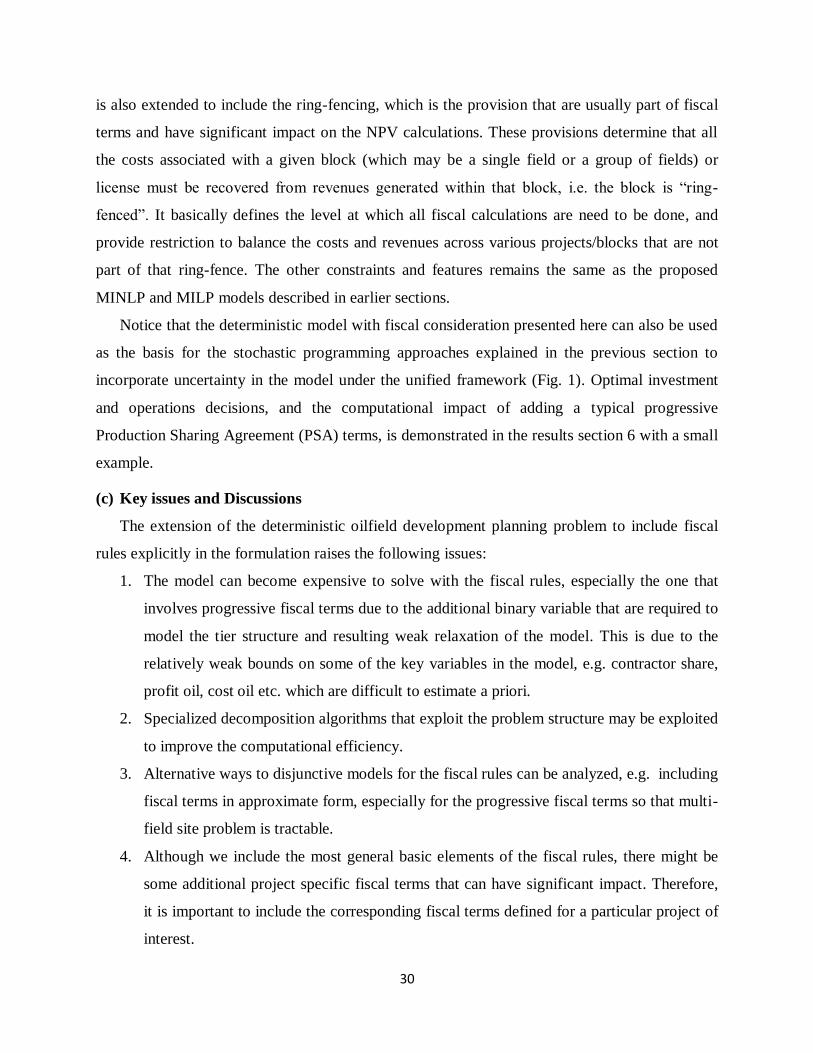
30

is also extended to include the ring-fencing, which is the provision that are usually part of fiscal

terms and have significant impact on the NPV calculations. These provisions determine that all

the costs associated with a given block (which may be a single field or a group of fields) or

license must be recovered from revenues generated within that block, i.e. the block is “ring-

fenced”. It basically defines the level at which all fiscal calculations are need to be done, and

provide restriction to balance the costs and revenues across various projects/blocks that are not

part of that ring-fence. The other constraints and features remains the same as the proposed

MINLP and MILP models described in earlier sections.

Notice that the deterministic model with fiscal consideration presented here can also be used

as the basis for the stochastic programming approaches explained in the previous section to

incorporate uncertainty in the model under the unified framework (Fig. 1). Optimal investment

and operations decisions, and the computational impact of adding a typical progressive

Production Sharing Agreement (PSA) terms, is demonstrated in the results section 6 with a small

example.

(c) Key issues and Discussions

The extension of the deterministic oilfield development planning problem to include fiscal

rules explicitly in the formulation raises the following issues:

1. The model can become expensive to solve with the fiscal rules, especially the one that

involves progressive fiscal terms due to the additional binary variable that are required to

model the tier structure and resulting weak relaxation of the model. This is due to the

relatively weak bounds on some of the key variables in the model, e.g. contractor share,

profit oil, cost oil etc. which are difficult to estimate a priori.

2. Specialized decomposition algorithms that exploit the problem structure may be exploited

to improve the computational efficiency.

3. Alternative ways to disjunctive models for the fiscal rules can be analyzed, e.g. including

fiscal terms in approximate form, especially for the progressive fiscal terms so that multi-

field site problem is tractable.

4. Although we include the most general basic elements of the fiscal rules, there might be

some additional project specific fiscal terms that can have significant impact. Therefore,

it is important to include the corresponding fiscal terms defined for a particular project of

interest.

31

In a forthcoming paper, we will discuss the details of the generic model for the development

planning problem with fiscal considerations and ways to improve its computational efficiency,

(Gupta and Grossmann, 2012).

6 Examples

In this section we consider a variety of the examples for the oilfield development planning

problem that covers deterministic, stochastic and complex fiscal features as discussed in the

earlier sections.

(a) Instance 1: Deterministic Case

In this section we present an example of the oilfield planning problem assuming that there is

no uncertainty in the model parameters. We compare the computational results of the various

MINLP and MILP models proposed in the respective section (see Gupta and Grossmann, 2011

for more details).

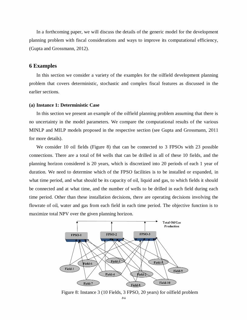
We consider 10 oil fields (Figure 8) that can be connected to 3 FPSOs with 23 possible

connections. There are a total of 84 wells that can be drilled in all of these 10 fields, and the

planning horizon considered is 20 years, which is discretized into 20 periods of each 1 year of

duration. We need to determine which of the FPSO facilities is to be installed or expanded, in

what time period, and what should be its capacity of oil, liquid and gas, to which fields it should

be connected and at what time, and the number of wells to be drilled in each field during each

time period. Other than these installation decisions, there are operating decisions involving the

flowrate of oil, water and gas from each field in each time period. The objective function is to

maximize total NPV over the given planning horizon.

Figure 8: Instance 3 (10 Fields, 3 FPSO, 20 years) for oilfield problem

32

The problem is solved using the DICOPT 2x-C solver for MINLP Models 1 and 2, and

CPLEX 12.2 for MILP Model 3. These models were implemented in GAMS 23.6.3 and run on

Intel Core i7 machine. The optimal solution of this problem that corresponds to reduced MINLP

Model 2-R solved with DICOPT 2x-C, suggests to install all the 3 FPSO facilities in the first

time period with their respective liquid (Figure 9-a) and gas (Figure 9-b) capacities. These FPSO

facilities are further expanded in future when more fields come online or liquid/gas flow rates

increases as can be seen from these figures.

After initial installation of the FPSO facilities by the end of time period 3, these are

connected to the various fields to produce oil in their respective time periods for coming online

as indicated in Figure 10. The well installation schedule for these fields (Figure 11) ensures that

the maximum number of wells drilling limit and maximum potential wells in a field are not

0

100

200

300

400

500

600

700

800

1 3 5 7 9 11 13 15 17 19

Q

liq (

kstb

/d)

Year

Liquid Capacity

fpso1

fpso2

fpso3

0

50

100

150

200

250

300

350

400

1 3 5 7 9 11 13 15 17 19

Qga

s (M

MSC

F/d

)

Year

Gas Capacity

fpso1

fpso2

fpso3

0

2

4

6

8

10

12

14

1 3 5 7 9 11 13 15 17 19

Nu

mb

er o

f W

ells

Year

Well Drilling Schedule f1 f2 f3 f4 f5 f6 f7 f8 f9 f10

Figure 9: FPSO installation and expansion schedule

(a) Liquid capacities of FPSO facilities (b) Gas capacities of FPSO facilities

Figure 10: FPSO-field connection schedule Figure 11: Well drilling schedule for fields

33

violated in each time period t. We can observe from these results that most of the installation and

expansions are in the first few time periods of the planning horizon. The total NPV of the project

is $30946.39M.

Tables 2-3 represent the results for the various model types considered for this instance.

DICOPT performs best in terms of solution time and quality, even for the largest instance

compared to other solvers as can be seen from Table 2. There are significant computational

savings with the reduced models as compared to the original ones for all the model types in

Table 3. Even after binary reduction of the reformulated MILP, Model 3-R becomes expensive to

solve, but yields global solutions, and provides a good discrete solution to be fixed/initialized in

the MINLPs for finding better solutions.

Table 2: Comparison of various models and solvers for Instance 1

Model 1 Model 2

Constraints 5,900 10,100

Continuous Var. 4,681 6,121

Discrete Var. 851 851

Solver

Optimal NPV

(million$)

Time (s) Optimal NPV

(million$)

Time (s)

DICOPT 31297.94 132.34 30562.95 114.51

SBB 30466.36 4973.94 30005.33 18152.03

BARON 31297.94 >72,000 30562.95 >72,000

Table 3: Comparison of models 1, 2 and 3 with and w/o binary reduction

Model 1 Model 1-R Model 2 Model 2-R Model 3-R

Constraints 5,900 5,677 10,100 9,877 17,140

Continuous Var. 4,681 4,244 6,121 5,684 12,007

Discrete Var. 851 483 851 483 863

SOS1 Var. 0 0 0 0 800

NPV(million$) 31297.94 30982.42 30562.95 30946.39 30986.22

Time(s) 132.34 53.08 114.51 67.66 16295.26

*Model 1 and 2 solved with DICOPT 2x-C, Model 3 with CPLEX 12.2

We can see from Table 4 that the solutions from the Models 1 and 2 after fixing discrete

variables based on the MILP solution (even though it was solved within 10% of optimality

tolerance) are the best among all other solutions obtained in Table 2. Therefore, the MILP

approximation is an effective way to obtain near optimal solution for the original problem.

Notice also that the optimal discrete decisions for Models 1 and 2 are very similar even though

34

they are formulated in a different way. However, only Model 2 can be reformulated into an

MILP problem that gives a good estimate of the near optimal decisions for these MINLPs.

Table 4: Improved solutions (NPV in million$) for Models 1 and 2 using Model 3-R solution

Model 1 Model 1 (fixed

binaries from

Model 3-R)

Model 2 Model 2 (fixed

binaries from

Model 3-R)

31297.94 31329.8136 30562.95 31022.4813

(b) Instance 2: Stochastic Case

In this example, we consider the planning of offshore oilfield under decision-dependent

uncertainty which resolves gradually as a function of investment and operations decisions.

A single reservoir (Figure 12) for 10 years planning horizon is considered that involves

decisions about the number, capacity, and installation schedule of FPSO/TLP facilities; the

number and drilling schedule of subsea/TLP wells; and the oil production profile over time. The

objective is to maximize the expected NPV value. The problem data, details and solution

methods are reported in Tarhan et al. (2009).

The uncertainties in the initial maximum oil flowrate, the size of the reservoirs, and the water

breakthrough time are represented by discrete distributions consisting of high and low values

resulting in eight scenarios (Table 5).

Figure 12: Offshore oilfield Infrastructure for instance 2

35

Table 5: Scenario representation for example 2

Scenarios

Initial

Productivity per

well (kbd)

Reservoir Size

Water

breakthrough

time

1 10 300 5

2 10 300 2

3 20 300 5

4 20 300 2

5 10 1500 5

6 10 1500 2

7 20 1500 5

8 20 1500 2

The specific rules used for describing the uncertainty resolution are as follows:

The appraisal program is completed when a total of three wells are drilled in one reservoir,

which not only gives the actual value for the initial maximum oil flowrate, but also provides the

posterior probabilities of reservoir sizes depending on the outcome. The uncertainty in reservoir

size can be resolved if either a total of nine or more wells are drilled, or production is made from

that reservoir for a duration of 1 year. Uncertainty in the water breakthrough time is resolved

after 1 year of production from the reservoir.

The comparison of model statistics given in the paper shows that the size of the full space

model increases exponentially as a result of the increase in the number of binary variables for

representing uncertainty resolution and the nonanticipativity constraints that relate the decisions

in indistinguishable scenarios.

The proposed branch-and-bound algorithm in Tarhan et al. (2009) required 23 h because, at

each node, 40 MINLP problems were solved to global optimality. A total of seven nodes were

traversed, and the best feasible solution was found at node 5. The computational efficiency of the

method is further improved by combining global optimization and outer-approximation within

proposed duality based branch and bound based algorithm (Tarhan et al. 2011).

The expected value solution proposes building five small FPSO and two TLP facilities and

drilling nine subsea wells in the first year. These decisions resolve the uncertainty in the initial

productivity and reservoir size. Depending on the values of the reservoir size and initial

productivity, different decisions are implemented. This expected value approach gives an

objective function value of $5.81 × 109. The optimal stochastic programming solution yields an

36

expected net present value of $6.37 × 109, which is higher than the expected value solution

($5.81 × 109). The multistage stochastic programming solution proposes building two small

FPSO and one TLP facility, and drilling nine subsea wells in the first year. Uncertainty in the

initial oil flowrate and reservoir size is resolved after nine wells have been drilled. For scenarios

5 and 6, the solution proposes building four more small FPSO facilities, one large FPSO facility,

and five TLP facilities and drilling 12 subsea and three TLP wells. For scenarios 7 and 8, the

solution proposes building six more small FPSO facilities and one TLP facility and drilling six

subsea wells.

The added value of stochastic programming is due to the conservative initial investment

strategy compared to the expected value solution strategy. The stochastic programming approach

considers all eight scenarios before making the initial investment. Therefore, it proposes building

two small FPSO facilities instead of five and one TLP facility instead of two. Also, it builds

more facilities and drills wells only after it determines that the reservoir size is 1500 Mbbl. A

comparison of net present values of the expected value solution and stochastic programming

shows that the added value of stochastic programming comes from handling the downside risk

much better than the expected value solution.

(c) Instance 3: Development planning with Complex Fiscal Rules

Optimal investment and operations decisions, and the computational impact of adding a

typical progressive Production Sharing Agreement (PSA) terms for a deterministic case of the

oilfield planning problem is demonstrated here.

0%

20%

40%

60%

80%

100%

0 200 400 600 800 1000

% P

rofi

t o

il Sh

are

of

Co

ntr

acto

r

Cumulative Oil Production (MMbbl)

Figure 13. Contractor’s Profit oil share for Example 3

37

In this instance, we consider 5 oilfields that can be connected to 3 FPSO’s with 11 possible

connections (Gupta and Grossmann, 2012). There are a total of 31 wells that can be drilled in the

5 fields, and the planning horizon considered is 20 years. There is a cost recovery ceiling and 4

tiers (see. Fig. 13) for profit oil split between the contractor and host Government that are linked

to cumulative oil production, which defines the fiscal terms of a typical progressive Production

Sharing Agreement.

Table 6 compares the results of the proposed MILP (Model 3) and reduced MILP models

(Model 3-R) with progressive PSAs for this example. We can observe that there is significant

increase in the computational time with fiscal consideration for the original MILP formulation

(Model 3), which takes more than 10 hours with a 14% of optimality gap as compared to the

reduced MILP model (Model 3-R), which terminates the search with a 2% gap in reasonable

time. In contrast, Model 3-R without any fiscal terms can be solved in 189.8 seconds. Therefore,

including fiscal rules within development planning can make the problem much harder to solve

due to the additional binary variables that are required to model tiers, and resulting weak

relaxation.

Note that on contrary the fiscal terms without tier structure, for instance fixed percentage of

profit share, royalty rates, may reduce the computational expense of solving the deterministic

model directly without any fiscal terms instead. Surprisingly, the problem with flat 35% of the

profit share of contractor is solved in 72.64s which is even smaller than the solution time for

deterministic case without any fiscal terms (189.8s). On the other hand, the problem with 2 tiers

instead of 4 as considered above is solved in 693.71s which is more than the model without fiscal

terms and less than the model with 4 tiers. Therefore, the increase in computational time while

including fiscal rules within development planning is directly related to the number of tiers

(steps) that are present in the model to determine the profit oil shares or royalties.

Table 6. Computational Results for Example 3

Model Constraints Continuous

Variables

Discrete

Variables

NPV

($Million)

Time (s)

Model 3 with PSA 9474 6432 727 2,183.63 >36,000

Model 3-R with PSA 9363 6223 551 2,228.94 1,163.7

The optimal solution from Model 3-R with fiscal considerations suggests installing 1 FPSO

facility with expansions in the future (see Fig. 14), while Fig. 15 represents the well drilling

schedule for this example. The tiers 2, 3 and 4 for profit oil split become active in years 6, 8 and

38

12, respectively, based on the cumulative oil production profile during the given planning

horizon.

Conclusions

In this paper, we have first reviewed a new generic model for offshore oil and gas field

infrastructure investment and operational planning considering multiple fields, three components

(oil, water and gas), facility expansions decisions, well drilling schedules and nonlinear reservoir

profiles. The detailed model and its reformulations to improve the computational efficiency have

been discussed. Furthermore, to address the issue of uncertainty in key model parameters, recent

work on multiage stochastic programming based approaches was highlighted. Discussion on the

extensions of the proposed deterministic model to incorporate uncertainties and generic fiscal

rules in a unified framework, and possible complications was presented. Numerical results on

development planning problems involving perfect information or uncertainty were reported, as

well as the handling of fiscal considerations, specifically Production Sharing Agreements. It is

0

50

100

150

200

250

0 5 10 15 20

MM

SC

F/d

Year

0

100

200

300

400

500

600

700

0 5 10 15 20

kst

b/d

Year

0

2

4

6

8

10

0 5 10 15 20

Num

ber

of

Wel

ls

Year

f1

f2

f3

f4

f5

Figure 14. Liquid and Gas capacities of FPSO 3

facility

Figure 15. Well drilling schedule for Example 3

(a) Liquid capacity (b) Gas capacity

39

hoped that this paper has shown that there has been very significant progress in the mathematical

programming models for offshore development planning.

References

1. Ahmed, S., 2000. Strategic planning under uncertainty: Stochastic integer programming

approaches. Ph.D. thesis, University of Illinois at Urbana-Champaign.

2. Aronofsky JS, Williams AC. The use of linear programming and mathematical models in

underground oil production. Manage Sci. 1962; 8:394–407.

3. Aseeri, A., Gorman, P., Bagajewicz, M. J. Financial risk management in offshore oil

infrastructure planning and scheduling. Ind. Eng. Chem. Res. 2004, 43, 3063–3072.

4. Babusiaux, D., Favennec, J. P., Bauquis, P. R., Bret-Rouzaut, N., and Guirauden, D.

(2007). Oil and Gas Exploration and Production: Reserves, costs, contracts. Technip

edition, 2007, chap. 4.

5. Bailey, W. J.; Couet, B.; Wilkinson, D. Field Optimization Tool for Maximizing Asset

Value. SPE ReserVoir EVal. Eng. 2005, 8 (1), 7–21.

6. Barnes, R., Linke, P., Kokossis, A. Optimization of oil-field development production

capacity. European symposium on computer aided process engineering, 2002, vol. 12 (p.

631).

7. Barnes, R.J., Kokossis, A. and Shang, Z. An integrated mathematical programming

approach for the design and optimisation of offshore fields. Computers and Chemical

Engineering, 31, Issues 5-6, 2007, 612-629.

8. Begg, S. H., Bratvold, R., Campbell, J. C. Improving Investment Decisions Using A

Stochastic Integrated Asset Model Presented at the SPE Annual Technical Conference

and Exhibition, New Orleans, LA, Sep 30-Oct 3, 2001; Paper SPE 71414.

9. Behrenbruch, P. Offshore oilfield development planning. J. Pet. Technol. 1993, 45 (8),

735–743.

10. Birge, J. R., Louveaux, F., 1997. Introduction to stochastic programming. New York,

NY: Springer.

11. Bohannon J. A linear programming model for optimum development of multi-reservoir

pipeline systems. J Petrol Tech. 1970;22:1429–1436.

12. Boland, N., Dumitrescu, I., Froyland, G., 2008. A multistage stochastic programming

approach to open pit mine production scheduling with uncertain geology.

http://www.optimizationonline.org/DBHTML/2008/10/2123.html.

13. BP Statistical Review of World Energy, 2011.

14. Caroe, C.C., Schultz, R., 1999: Dual decomposition in stochastic integer programming.

Oper. Res. Lett. 24, 37–45.

15. Carvalho, M., Pinto, J. M. A bilevel decomposition technique for the optimal planning of

offshore platforms. Brazilian J. Chem. Eng. 2006a, 23, 67–82.

40

16. Carvalho, M., Pinto, J. M. An MILP model and solution technique for the planning of

infrastructure in offshore oilfields. J. Pet. Sci. Eng. 2006b,51, 97–110.

17. Clay, R. L., Grossmann, I. E., 1997. A disaggregation algorithm for the optimization of

stochastic planning models. Computers and Chemical Engineering 21 (7),751-774.

18. Colvin, M., Maravelias, C. T., 2008. A stochastic programming approach for clinical trial

planning in new drug development. Computers and Chemical Engineering 32 (2008)

2626–2642

19. Colvin, M., Maravelias, C.T., 2010. Modeling methods and a branch and cut algorithm

for Pharmaceutical Clinical Trial Planning using Stochastic Programming, European

Journal of Operational Research, 203 (2010) 205–215.

20. Cullick, A. S., Heath D., Narayanan K., April J., Kelly J. Optimizing Multiple-Field

Scheduling and Production Strategy with Reduced Risk. Presented at the SPE Annual

Technical Conference and Exhibition, Denver, CO, Oct 5-8, 2003; Paper SPE 84239.

21. Cullick, A. S., Cude, R., and Tarman, M. 2007. Optimizing Field Development Concepts

for Complex Offshore Production Systems, Paper SPE 108562-MS presented at Offshore

Europe, Aberdeen, Scotland, U.K., 4-7 September.

22. Dias, M. A. G., 2004. Valuation of exploration and production assets: an overview of real

options models. Journal of Petroleum Science and Engineering 44 (1-2), 93-114.

23. Elgsæter, S. M., O. Slupphaug, Johansen T. A. A structured approach to optimizing

offshore oil and gas production with uncertain models. Comput. Chem. Eng. 2010, 34(2),

163-176.

24. Ettehad, A., Jablonowski, C. J., Lake, L. W. Stochastic Optimization and Uncertainty

Analysis for E&P Projects: A Case in Offshore Gas Field Development, Offshore

Technology Conference, 2011.

25. Goel, V., Grossmann, I. E. A stochastic programming approach to planning of offshore

gas field developments under uncertainty in reserves. Comput. Chem. Eng. 2004, 28 (8),

1409–1429.

26. Goel, V., Grossmann, I. E. A class of stochastic programs with decision dependent

uncertainty. Mathematical Programming, 2006, 108(2–3, Ser. B), 355–394.

27. Goel, V., Grossmann, I. E., El-Bakry, A. S., Mulkay, E. L. A novel branch and bound

algorithm for optimal development of gas fields under uncertainty in reserves. Comput.

Chem. Eng. 2006, 30, 1076-1092.

28. Grothey, A., McKinnon, K., 2000. Decomposing the optimization of a gas lifted oil well

network. Tech Rept. MS 00-005, Department of Mathematics and Statistics, University

of Edinburgh.

29. Gunnerud, V., Foss, B. Oil production optimization – A piecewise linear model, solved

with two decomposition strategies. Computers and Chemical Engineering, 2010, 34,

1803–1812.

30. Gupta, V., Grossmann, I. E. Solution strategies for multistage stochastic programming

with endogenous uncertainties. Comput. Chem. Eng. 2011, 35, 2235–2247.

41

31. Gupta, V., Grossmann, I. E. An Efficient Multiperiod MINLP Model for Optimal

Planning of Offshore Oil and Gas Field Infrastructure. I&EC Research, 2011, Submitted

for publication.

32. Gupta, V., Grossmann, I. E. Optimal Development Planning of Offshore Oil and Gas

Field Infrastructure under Complex Fiscal Rules. Proceedings of Foundations of

Computer-Aided Process Operations (FOCAPO 2012), In press.

33. Gupta, V., Grossmann, I. E. Modeling and Solution strategies for Offshore Oilfield

Development Planning under Complex Fiscal Rules. Working paper,2012.

34. Haugen, K. K., 1996. A stochastic dynamic programming model for scheduling of

offshore petroleum fields with resource uncertainty. European Journal of Operational

Research 88 (1), 88–100.

35. Haugland, D., Hallefjord, Å.; Asheim, H. Models for Petroleum Field Exploitation. Eur.

J. Oper. Res. 1988, 37, 58.

36. Held, H., Woodruff, D. L., 2005. Heuristics for multi-stage interdiction of stochastic

networks. Journal of Heuristics 11 (5-6), 483-500.

37. Ierapetritou, M. G., Pistikopoulos, E. N., 1994. A novel optimization approach of

stochastic planning models. Industrial and Engineering Chemistry Research 33, 1930-

1942.

38. Iyer, R. R., Grossmann, I. E., 1998. A bilevel decomposition algorithm for long-range

planning of process networks. Industrial and Engineering Chemistry Research 37 (2),

474-481.

39. Iyer, R. R., Grossmann, I. E., Vasantharajan, S., Cullick, A. S. Optimal planning and

scheduling offshore oilfield infrastructure investment and operations. Ind. Eng. Chem.

Res. 1998, 37, 1380–1397.

40. Jonsbraten, T. W. Oil-field optimization under price uncertainty. Journal of the

Operational Research Society,1998, 49, 811.

41. Jonsbraten, T., 1998. Optimization models for petroleum field exploitation. PhD thesis,

Norwegian School of Economics and Business Administration.

42. Jonsbraten, T. W.; Wets, R. J. B.; Woodruff, D. L. A class of stochastic programs with

decision dependent random elements. Ann. Oper. Res. 1998, 82, 83–106.

43. Kaiser, M.J. and A.G. Pulsipher. Fiscal System Analysis: Concessionary and Contractual

Systems Used in Offshore Petroleum Arrangements. US Department of the Interior

Mineral Management Services MMS 2004-016, 1-78.

44. Kosmidis, V., Perkins, J., Pistikopoulos, E., 2002. A mixed integer optimization strategy

for integrated gas/oil production. In: European Symposium on Computer Aided Process

Engineering. Vol. 12.

45. Kosmidis, V. D.; Perkins, J. D.; Pistikopoulos, E. N. Optimization of Well Oil Rate

Allocations in Petroleum Fields. Ind. Eng. Chem. Res. 2004, 43, 3513.

42

46. Kosmidis, V. D., Perkins, J. D., Pistikopoulos, E. N. A mixed integer optimization for the

well scheduling problem on petroleum fields. Computers & Chemical Engineering

Journal, 2005, 29, 1523–1541.

47. Lee AS, Aronofsky JS. A linear programming model for scheduling crude oil production.

J Petrol Tech. 1958;10:51–54.

48. Lee, S., Grossmann, I. E. New algorithms for nonlinear generalized disjunctive

programming. Computers and Chemical Engineering 2000, 24 (9-10), 2125-2141.

49. Ligero, E. L., Xavier, A. M., Schiozer, D. J. Value of information during appraisal and

development of petroleum fields. Presented at the 18th

International Congress of

Mechanical Engineering, Ouro Preto, MG Brasil, Nov 6-11, 2005.

50. Lin, X., Floudas, C. A. A Novel Continuous-Time Modeling and Optimization

Framework for Well Platform Planning Problems. Optim. Eng. 2003, 4 (1-2), 65–95.

51. Lund, M. W. 1999. Real options in offshore oil field development projects, Proceedings

3rd

International Conference on Real Options, 6-8 June Wassenaar, Holland.

52. Lund, M. W. Valuing Flexibility in Offshore Petroleum Projects. Ann. Oper. Res. 2000,

99 (1-4), 325–349.

53. Lund, D., 2005. How to analyze the investment–uncertainty relationship in real options

models? Review of Financial Economics 14, 311–322.

54. Ortiz-Gomez, A., Rico-Ramirez, V., & Hernandez-Castro, S. Mixed-integer multiperiod

model for the planning of oil-field production. Comput. Chem. Eng.,2002, 26(4–5), 703.

55. Ozdogan, U.; Horne, R. N. Optimization of well placement under time-dependent

uncertainty. SPE Reservoir Eval. Eng. 2006, 9 (2), 135–145.

56. Pflug, G. Ch., 1990. Online optimization of simulated markovian processes. Mathematics

of Operations Research Res. 15, No.3, 381-395.

57. Rico-Ramirez V., Grossmann I. E., Tarhan B., Hernández-Castro S., Segovia-Hernández

J. G. An Approach to the Representation of Gradual Uncertainty Resolution in Stochastic

Multiperiod Planning. Computer Aided Chemical Engineering, 26, 2009, 713-718.

58. Ruszczynski, A., 1997. Decomposition methods in stochastic programming. Math.

Programming (Ser. B) 79, 333-353.

59. Sullivan J. A computer model for planning the development of an offshore gas field. J

Petrol Tech. 1982;34:1555–1564.

60. Sahinidis, N.V., 2004. Optimization under uncertainty: State-of-the-art and

opportunities. Comput. Chem. Eng. 28 (6–7), 971–983.

61. Schultz, R., 2003. Stochastic programming with integer variables. Mathematical

Programming 97 (1–2), 285–309.

62. Solak, S., 2007. Efficient solution procedures for multistage stochastic formulations of

two problem classes. PhD thesis, Georgia Institute of Technology.

63. Sunley, E. M., T. Baunsgaard, and D. Simard. 2002. “Revenue from the Oil and Gas

Sector: Issues and Country Experience.” IMF Conference Paper.

43

64. Tarhan, B., Grossmann, I. E., 2008. A multistage stochastic programming approach with

strategies for uncertainty reduction in the synthesis of process networks with uncertain

yields. Computers and Chemical Engineering 32, 766-788.

65. Tarhan, B., Grossmann, I.E., Goel, V. Stochastic programming approach for the planning

of offshore oil or gas field infrastructure under decision- dependent uncertainty. Ind. Eng.

Chem. Res. 2009, 48(6), 3078–3097.

66. Tarhan, B., Grossmann, I.E., Goel, V. Computational strategies for non-convex

multistage MINLP models with decision-dependent uncertainty and gradual uncertainty

resolution. Ann. Oper. Res., 2011, DOI: 10.1007/s10479-011-0855-x.

67. Tordo, S. 2007. Fiscal Systems of Hydrocarbons: Design Issues.Working Paper 123/07,

World Bank, Washington, D.C.

68. Tsarbopoulou, C. Optimization of oil facilities and oil production. M.Sc. Dissertation,

University College London, London, U.K., 2000.

69. Ulstein, N. L., Nygreen, B.; Sagli, J. R. Tactical planning of offshore petroleum

production. Eur. J. Oper. Res. 2007, 176, 550–564.

70. Viswanath, K., Peeta, S., Salman, S. F., 2004. Investing in the links of a stochastic

network to minimize expected shortest path length. Tech. rep., Purdue University.

71. van den Heever, S. A.; Grossmann, I. E. An iterative aggregation/disaggregation

approach for the solution of a mixed integer nonlinear oilfield infrastructure planning

model. Ind. Eng. Chem. Res. 2000, 39, 1955–1971.

72. van den Heever, S. A., Grossmann, I. E., Vasantharajan, S.; Edwards, K. Integrating

complex economic objectives with the design and planning of offshore oilfield

infrastructures. Comput. Chem. Eng. 2000, 24, 1049–1055.

73. van den Heever, S. A., Grossmann, I. E. A Lagrangean Decomposition Heuristic for the

Design and Planning of Offshore Hydrocarbon Field Infrastructures with Complex

Economic Objectives. Ind. Eng. Chem. Res. 2001, 40, 2857–2875.

74. World Bank. 2007. “Contracts for Petroleum Development – Part 1-3.” Petroleum Sector

Briefing Note No. 7.

75. You F., Wassick J. M., Grossmann I. E. Risk management for global supply chain

planning under uncertainty: models and algorithms. AIChE J. 2009, 55, 931–946.

76. Zabalza-Mezghani, I.; Manceau, E.; Feraille, M.; Jourdan, A. Uncertainty management:

From geological scenarios to production scheme optimization. J. Pet. Sci. Eng. 2004, 44,

11–25.