office of structures bridge scour program chapter …gishydro.eng.umd.edu/sha_april2011/ch 11 scour...

OFFICE OF STRUCTURES

BRIDGE SCOUR PROGRAM

CHAPTER 11 APPENDIX A

ABSCOUR 9

USERS MANUAL

PART 1: DERIVATION OF METHODOLOGY

APRIL 2011

APRIL 2011

Preface ABSCOUR 9, Build 2.3 is the current version of this program as of January 2011 and all

previous versions should be discarded. The user is advised to check the web site below

for any revisions to the program:

http://www.gishydro.umd.edu

The material presented in this ABSCOUR Users Manual has been carefully researched

and evaluated. It is being continually updated and improved to incorporate the results of

new research and technology. However, no warranty expressed or implied is made on the

contents of this program or the user‟s manual. The distribution of this information does

not constitute responsibility by the Maryland State Highway Administration or any

contributors for omissions, errors or possible misinterpretations that may result from the

use or interpretation of the materials contained herein.

Significant Changes to ABSCOUR 9 Build 2.3:

1. Update the help file system to incorporate revisions based on OOS policies and

experience.

2. Revise the critical velocity for the Piedmont Zone (SHA modified Neill‟s critical

velocity curves) based on USGS field study of ABSCOUR using abutment scour

measurements of bridges in South Carolina)

3. Revise the recommended calibration/safety factors for ABSCOUR also based on

the USGS study noted above

4. Revise the computation for pressure flow based on the vertical blockage of the

flow by the structure superstructure (FHWA Research)

5. Current layered soil algorithm for contraction scour has been extended to the

abutment scour.

6. Revise pier local scour to include layered soil condition.

7. Implement pier scour option 4 that automatically solves for the worst case pier

scour condition, considering both uncontracted and contracted channel bed

conditions. Flow depth, flow velocity and soil properties will be automatically

revised based on the appropriate pier scour options and conditions.

8. Add a utility unit for abutment scour to consider the effect on scour if the

channel moves into the abutment. The input data can be directly imported from

the appropriate ABSCOUR run.

9. Change ABSCOUR default file extension to “asc”. The old extension will

remain visible on the file list. This will enable user to import files from older

ABSCOUR runs.

10. See also the History of Changes included in the back of this Appendix

Questions regarding the use of the ABSCOUR Program should be directed to the Office

of Structures, Structure Hydrology and Hydraulics Division

APRIL 2011

Maryland SHA Office of Structures

BRIDGE SCOUR PROGRAM (ABSCOUR 9) APPENDIX A - USERS MANUAL, PART 1

CAPABILITIES AND LIMITATIONS

ABSCOUR is a computer program developed by the Office of Structures for estimating

and evaluating scour at bridges and bottomless arch culverts. The program serves as an

analytical tool to assist the user in identifying and utilizing the appropriate bridge

geometry, hydraulic factors and soils/rock characteristics to estimate scour at structure

foundations. The program is not an expert system. The accuracy of the answers obtained

(scour depths) depends on the accuracy of the input information, the selection of the most

appropriate analytical methods available in the program and the user‟s judgment.

However, careful attention to the guidance in the manual should result in reasonable

estimates of scour. Design considerations for scour should include other factors than

scour depths as discussed in this Appendix and in Chapter 11.

The ABSCOUR 9 Program applies the methodologies and equations set forth in the

FHWA Manual 18, Evaluating Scour at Bridges with two exceptions:

An updated method recently developed by the FHWA Hydraulics Laboratory is

used to compute pressure scour

ABSCOUR 9 computes a combined contraction and local scour value at

abutments, rather than computing these elements separately and then adding them

together as is done in HEC-18. A recent NCHRP study (NCHRP 24-20) has

adopted the ABSCOUR approach and obtained reasonable estimates of abutment

scour. It is our view that the ABSCOUR approach (computing a combined

contraction and local scour value at abutments) is likely to be adopted by the

hydraulics community in the future.

Verification and calibration efforts of the ABSCOUR 9 methodology have been an on-

going effort over the last 10 years. These efforts include:

Several cooperative studies with FHWA utilizing the J. Sterling Jones Hydraulic

Laboratory in McLean, Virginia,

Two cooperative studies with the US Geological Survey using a database of

measurements of clear water abutment scour collected at South Carolina Bridges.

Continuing evaluation of the method within the Office of Structures on a bridge

by bridge basis over the last 10 years to determine ways and means of improving

the accuracy of the results and to facilitate its use by others. The Office of

Structures provides periodic workshops on the use of the program.

PROGRAM CAPABILITIES

1 Estimate contraction scour under a bridge for left overbank, channel and right

overbank using Laursen‟s live bed scour equation, and/or the option of either

Laursen‟s clear water scour equations or a modified Neill‟s competent velocity

equations for clear water scour (as calibrated using the USGS database in South

Carolina,

APRIL 2011

2 Estimate contraction and abutment scour for multiple layers of channel bed

materials

3 Estimate scour for complex and simple piers using a method based on the FHWA

HEC-18 equations,

4 Print input and output information for the scour report,

5 Plot the scour cross-section for the scour report,

6 Estimate scour for open channel and pressure flow conditions,

7 Estimate scour in cohesive soils and rock,

8 Estimate scour in bottomless arch culverts,

9 Estimate minimum D50 rock riprap sizes for design, based on the FHWA HEC 23

equations for abutments and piers,

10 Permit easy changes to hydraulic and soil parameter inputs in order to conduct

sensitivity analyses of the estimated scour depths.

11 Allow user the option to select various scour parameters rather than use the

standard values incorporated in the ABSCOUR program.

USER ASSISTANCE

1 Help screens and text files in the ABSCOUR Program to define, illustrate and

explain each input parameter, using the F-1 key or the Help File,

2 Background on the concepts used to develop the ABSCOUR methodology,

3 Over-ride features to allow the user to modify the program logic,

4 Simple and fast procedures to conduct sensitivity analyses of input parameters,

5 Engineers in the Office of Structures are available to provide user assistance upon

request.

OUTPUT FILES

1. A detailed report summarizing the factors considered in the scour computations.

2. Plots of the Approach Section, Bridge Section and Scour Cross-Section under the

bridge to a user defined scale for a plotter or to a dxf file for use in Microstation.

This includes a scour cross-section for combinations of abutments and piers, and a

comparison of the ABSCOUR cross-section with the corresponding HEC-RAS

cross-section.

LIMITATIONS

1 The accuracy of the scour computations is dependent upon the experience and

judgment of the user in the selection of input data and appropriate analytical

methods. The methods selected for analysis need to be consistent with the field

conditions as reflected in the input data and with appropriate hydraulic and

sediment transport concepts.

2 Ideally, a 3-D model would be helpful to determine hydraulic flow conditions and

to estimate scour, whereas the hydraulic data used to provide the input data is

typically a 1-D model. ABSCOUR contains subroutines that permit the user to

modify the hydraulic data (which are based on conveyance) to consider a more

conservative flow (worst case) distribution under the bridge for purposes of

estimating scour. The user needs to verify that the hydraulic model (typically

APRIL 2011

HEC-RAS) provides for a reasonable flow distribution upstream, through and

downstream of the bridge.

3 Calibration studies have been conducted, in cooperation with the US Geological

Survey, for estimating clear water scour for fine-grained sands and for cohesive

materials typical of the Piedmont. More accurate methods are available through

use of the EFA (Erosion Function Apparatus) to measure the critical velocity of

Shelby tube samples through a laboratory procedure. Limited calibration studies

have been made, to the best of our knowledge, for coarse-grained bed materials.

4 Available methods for estimating scour in rock (Erodibility Index Method) have

had limited verification and need to be applied with judgment.

5 There are many variables that will have an effect on scour at a bridge. ABSCOUR

will address a limited number of these conditions. The user is provided with

flexibility through overrides and other mechanisms to expand the range of

conditions which can be analyzed by ABSCOUR. The user is encouraged to

make a critical review of the estimated scour depths to verify that the numbers

look reasonable. If the ABSCOUR analysis does not appear to be reasonable, and

there are no detectable errors in the input data or the computations, the user is

encouraged to get in touch with the Office of Structures for guidance. Improper

use of over-rides is a common source of errors in using ABSCOUR.

It is the SHA‟s experience that the ABSCOUR Program, when applied with appropriate

consideration of the site conditions and scour parameters, will give reasonable results for

bridges over small and medium-sized channels typical of Maryland streams.

We have not as yet had the opportunity to apply ABSCOUR to a major river crossing,

outside of the calibration studies in South Carolina. However, the basic predictive

equations for pier scour and contraction scour are essentially the same as those used in

HEC-18. The concept of combining abutment scour and contraction scour together as

first utilized in ABSCOUR more than 10 years ago is now being considered by the

FHWA and is being used in on-going NCHRP research studies. We would expect that

the ABSCOUR model would give reasonable results on larger rivers where the

ABSCOUR channel and flood plain cross-section can be used to represent the river

channel and flood plain.

We were unable to get the ABSCOUR program to provide reasonable answers for bridge

abutments in the wide swamps and wetlands in the non-tidal coastal zone in South

Carolina. The preliminary studies indicate that the calculated ABSCOUR Kv values may

be too low for such sites. We have developed an alternative approach for evaluating clear

water abutment scour on streams which have characteristics similar to those of the

Coastal (Non-tidal) Zone of South Carolina.

Calibration Study Results

APRIL 2011

The information presented in the following plots reflects the results of the USGS

clear water calibration studies for ABSCOUR 9 in the Piedmont Zone of South

Carolina. The characteristics of this zone are considered typical for many Maryland

upland streams.

The South Carolina bridges were divided into two categories depending on the width of

the flood plain at the bridge for the 100-year flood: 1. Smaller streams with flood plain

widths of under 800 feet (black dots) and 2. Larger streams with flood plain widths

greater than 800 feet (white dots). For the smaller streams, using an adjustment factor

(safety factor) of 0.8 still results in an over-prediction of abutment scour for all of the

bridges in this category. For the larger streams an adjustment factor of 1.0 results in an

over-prediction of all but two bridges. There were certain unique features at these two

bridges which could not be modeled by the ABSCOUR program. (In both cases, deep

abutment scour occurred at one abutment and zero scour at the other abutment, indicating

a flow distribution condition not evident in the hydraulic analysis). This information has

been used in developing guidance for selection of the calibration factor (safety factor) in

ABSCOUR 9.

Please note that the study did not address live-bed scour.

APRIL 2011

PIEDMONT PHYSIOGRAPHIC REGION

CHARACTERISTICS OF THE SOUTH CAROLINA STREAMS

USED IN THE CALIBRATION STUDIES

TABLE 1 Range of Selected Stream Characteristics for Measurements of Clear-Water Abutment

Scour Collected at 129 Bridges in the Piedmont and Coastal Plain of South Carolina

Properties for Full Cross

Section Upstream of Bridge

Range

value

Drainage

area

(miles2)

Channel

slope

(ft/ft)

aAverage

cross

section

velocity

(ft/s)

aAverage

cross

section

depth

(ft)

a Cross

section

top

width

(ft)

a, b Unit

width

flow at

bridge

(cfs/ft)

Median

grain

size

(mm)

Observed

abutment-

scour

depth

(ft)

Observed

contraction-

scour depth

(ft)

Piedmont (90 abutment and 66 contraction scour measurements)

Minimum 11 0.00037 0.49 3.4 213 6.7 < 0.062 0.0 0.0

Median 82 0.0012 1.80 7.3 711 29.7 0.091 1.0 0.8

Maximum 677 0.0024 4.38 15.8 2663 72.9 1.19 18.0 4.5

Coastal Plain (104 abutment and 42 contraction scour measurements)

Minimum 6 0.00007 0.25 2.1 463 3.8 < 0.062 0.0 0.0

Median 54 0.0006 0.47 4.7 2154 17.7 0.19 8.4 2.0

Maximum 8,830 0.0024 0.94 16.3 28952 51.5 0.78 23.6 3.9

a Parameter was estimated with the 100-year flow. b Determined by ABSCOUR program.

APRIL 2011

CALIBRATION OF ABSCOUR 9 FOR THE COASTAL REGION OF

SOUTH CAROLINA

As indicated in the table above, the South Carolina Coastal Zone is characterized by wide

swampy wetlands and there was no clearly defined main channel and flood plain at many

of the bridge crossings. In general, it was difficult to model ABSCOUR for this type of

crossing, and the correlation studies between measured and predicted scour depths were

not adequate to recommend that ABSCOUR be used as a design method for this kind of

condition.

Maryland has few watersheds that are similar to the upland (non-tidal) coastal region in

South Carolina. An alternative approach is presented in Appendix A, Part 2, Attachment

5.

APRIL 2011

USERS MANUAL

FOR THE SHA BRIDGE SCOUR PROGRAM (ABSCOUR)

TABLE OF CONTENTS Preface…………………………………………………………………………..…………

Capabilities and Limitations……………………………….…………………..…….…...

Table of Contents ………………………………………………………………………..

PART 1: DEFINITIONS AND DERIVATION OF THE ABSCOUR METHODOLOGY

I. OVERVIEW ....................................................................................................... 12

A. LIVE BED SCOUR.

B. CLEAR WATER SCOUR.

C. SELECTION OF SCOUR TYPE

II. CONTRACTION SCOUR ............................................................................... 13

A. LAURSEN‟S LIVE BED CONTRACTION SCOUR EQUATION

B. MODIFICATION FOR PRESSURE FLOW

C. DEVELOPMENT OF THE ABUTMENT SCOUR EQUATIONS

C.1 Upstream Approach Section, Section 1

C.2 Bridge (Contracted) Section

C.3. Computation of Velocity for Contraction Scour Computations

C.4 Contraction Scour Computations for Abutment with a Short Setback

(Method A)

C.5. Determination of k2

C.6 Critical Shear Stress and Boundary Shear Stress

III. ABUTMENT SCOUR ..................................................................................... 23

A. ADJUSTMENT FACTOR FOR VELOCITY: 1-D AND 2-D MODELS

B. ADJUSTMENT FACTOR: SPIRAL FLOW AT ABUTMENT TOE

C. LOCAL ABUTMENT SCOUR EQUATION FOR VERTICAL WALL

ABUTMENTS

D. ADJUSTMENT OF ABUTMENT SCOUR FOR PRESSURE FLOW

E. COMPUTATION OF ABUTMENT SCOUR DEPTH (ABSCOUR

PROGRAM)

F. OTHER ADJUSTMENTS TO THE ABUTMENT SCOUR DEPTH

F.1 Adjustment Factor, Kt, for Abutments with Wing wall and Spill-through

Slopes

F.2 Adjustment Factor Ke for Embankment Skew Angle

F.3 Adjustment Factor, FS, for Calibration/Safety

G. FINAL SCOUR ELEVATION…………………….…….……………………

APRIL 2011

IV. CLEAR WATER SCOUR EQUATIONS ..................................................... 29

A. CONTRACTION SCOUR

B. ABUTMENT SCOUR

V. COMPUTATIONAL PROCEDURES………………………………………33

VI. HISTORY OF CHANGES TO ABSCOUR………………………………… 34

VII. REFERENCES…………………………………………………………..……37

PART 2: GUIDELINES FOR APPLYING THE ABSCOUR PROGRAM

I. Introduction ........................................................................................................... 2

II. Development of the Input Data for the ABSCOUR Model ............................. 3

A. STEP ONE - HYDRAULIC MODEL ................................................................ 4

A.1 Water Surface Profile

A.2 Development of ABSCOUR Model Cross-sections

B. STEP TWO -PROJECT INFORMATION MENU ............................................ 5

B.1 Project Name and Description

B.2 Over-Rides

C. STEP THREE - APPROACH SECTION ........................................................... 7

C.1 Enter Approach Section Data

D. STEP FOUR - DOWNSTREAM BRIDGE DATA.......................................... 12

D.1 Enter the Downstream Bridge Data

E. STEP FIVE - UPSTREAM BRIDGE DATA…………………………………16

E.1 Enter the Upstream Bridge Data

F. STEP 6 PIER DATA……………………………………………...……… . ..20

G. STEP 7 ACTUAL SECTIONS ………………………………………… …...21

III. COMPUTATIONS AND PROGRAM OUTPUT INFORMATION .......... 24

A. ABSCOUR Output............................................................................................ 24

B. ABSCOUR PROGRAM LOGIC ...................................................................... 33

C. EVALUATION OF THE PROGRAM OUTPUT ........................................... 34

C.1 Overrides

C.2 Bridge Section Data

C.3 Contraction Scour Table

C.4 Abutment Scour Table

C.5 Scour Depth Elevation

C.6 Scour Cross-Section

C.7 Evaluation of the Computed Scour Values

APRIL 2011

IV QUESTIONS TO CONSIDER-REVIEW OF THE ABSCOUR OUTPUT 38

V. COMPUTATION OF PIER SCOUR ............................................................... 39

VI. UTILITY MODULE ........................................................................................ 48

A. RIPRAP

B. CRITICAL VELOCITY

C. SCOUR IN ROCK

C.1 Application of the Erodibility Index Method

D. STREAM POWER CALCULATIONS

E. ERODIBILITY INDEX CALCULATIONS

E.1 COMPUTING THE ERODIBILITY INDEX FOR ROCK

E.2 DESIGN PROCEDURE

F. ABUTMENT SCOUR CONSIDERING FUTURE MOVEMENT OF

CHANNEL

ATTACHMENT 1: COMPUTATION OF THE VELOCITY OF FLOW USED

IN THE ABUTMENT SCOUR COMPUTATIONS. ...................................................... 55

I. COMPUTATION OF VELOCITY AND SCOUR

II. EXAMPLE PROBLEM 1

III. COMPUTATION OF CONTRACTION SCOUR

A. Short Setback - CASE A in Figure A1-1

B. Intermediate Setback of 70 Feet -Wide Overbank Section - CASE B in Figure

A1-1

C. Long Setback CASE C in Figure A1-1

D. Special Case Intermediate Setback-Narrower Overbank -

CASE D in Figure A1-1

ATTACHMENT 2: COMPLEX APPROACH FLOW CONDITIONS…….………….64

I. EXAMPLE 1 - TYPICAL FLOW DISTRIBUTION

II. EXAMPLE 2 - UNBALANCED FLOW CONDITION

III. EXAMPLE 3 - BEND IN THE RIVER

IV. EXAMPLE 4 - CONFLUENCE UPSTREAM OF BRIDGE

ATTACHMENT 3: CALIBRATION/ SAFETY FACTORS... …………………… ….68

ATTACHMENT 4: CRITICAL VELOCITIES IN COHESIVE SOILS………..…..… 70

ATTACHMENT 5: ESTIMATING CONTRACTION AND ABUTMENT SCOUR

IN SELECTED WETLANDS………………....……….………….71

APRIL 2011

PART 1: DERIVATION OF THE ABSCOUR METHODOLOGY

I. OVERVIEW

A. LIVE BED SCOUR

The method presented in this guideline for estimating live-bed abutment scour is based

on Laursen‟s contraction scour equation as presented in the FHWA Publication HEC No.

18, Fourth Edition. (1). This equation was originally derived by Straub (2) considering

that the shear stresses (and thus the rates of sediment transport) in an uncontracted section

and a contracted section are the same. It assumes a long contracted channel where the

flow is considered to be uniform and the scour depth is constant across the channel

section.

The contracting flow at the entrance corner of a channel constriction differs significantly

from the conditions described above. The flow velocity across the channel is not

uniform. The velocity near the edge of the constriction is faster than that in the

midstream. Because of this higher velocity and its associated turbulence, the scour depth

near the edge or corner of the constriction is usually deeper than in the center of the

channel. The flow pattern at the upstream corner of an abutment will be similar to the

flow at the entrance corner of a contracted channel, when the bridge approach roads

obstruct overbank flow or the abutment constricts the channel. Local abutment scour can

be expected to be deeper than the contraction scour in the center of the channel.

Laursen‟s contraction scour equation is used as the basis for developing equations for

estimating local abutment scour. Velocity variations caused by the flow contraction and

spiral flow at the toe of the abutment are considered in developing the equations.

B. CLEAR WATER SCOUR

The User has the options of selecting Laursen‟s clear water scour equation or a modified

(by Maryland SHA) version of Neill‟s competent velocity procedure based on the

calibration studies of ABSCOUR conducted by the USGS.

C. SELECTION OF TYPE OF SCOUR TO BE EXPECTED

The ABSCOUR program will make a selection as to whether the type of scour to be

expected at the structure will be live-bed or clear-water, based on the input provided by

the user. However, our experience has been that this input information is often

incomplete or incorrect, leading to erroneous program computations. The

recommendation of the Office of Structures is that a geomorphologist should make this

determination based on his field review of the stream and watershed characteristics, and

include this information in the geomorphology report.

APRIL 2011

II. CONTRACTION SCOUR

A. LAURSEN‟S LIVE BED CONTRACTION SCOUR EQUATION

Laursen‟s equation for estimating scour in a contracted section in a simple rectangular

channel can be expressed in the following form:

y2/y1 = (W2/W1) k2

(1-1)

Where:

y1 = flow depth in the approach section

y2 = total flow depth in the contracted section (y2 = y1 + ys, where ys. is the

scour depth)

W1 = channel width of the approach section

W2 = channel width of the contracted section

k2 = experimental constant related to sediment transport (originally identified as

by Laursen).

These dimensions are illustrated in Figure 1-1

Figure 1-1

Plan View of Approach and Bridge Sections

Please note that this equation is a simplified form of Equation 1-1 in HEC-18 for a

contraction of a constant flow in a rectangular channel with a uniform bed-material.

The ratio of q2/ q1 may be substituted for W1/ W2, and Equation 1-1 may be rewritten as:

APRIL 2011

y2/y1 = (q2/q1)k2

(1-2)

where:

q1 = unit discharge in the approach section

q2 = unit discharge in the contracted (bridge) section

y1 = total flow depth in the approach section

y2 = total flow depth in the contracted (bridge) section

k2 = experimental constant related to sediment transport

Equation 1-2 is a comparative equation, equating the rates of sediment transport at the

uncontracted and contracted sections. The equation applies to the live-bed condition to

the extent that the shear stresses in the two sections are considered equal. The application

of this equation can be extended to clear water scour for the special case where the shear

stresses in the two sections are both equal to the critical shear stress. The contracted

section, Section 2, is best represented for most cases as the downstream end of the bridge

where the flow is contracted and uniform. The upstream uncontracted section, Section 1,

should be selected at a point upstream where the flow is uniform and not influenced by

the bridge contraction. The directions in the HEC-RAS program regarding ineffective

flow areas can be used as a guide in selecting the approach section.

B. MODIFICATION FOR PRESSURE FLOW

If the bridge is subject to pressure flow, Equation 1-2 needs to be modified to account for

the additional contraction scour caused by the pressure flow:

y2/y1 = (q2/q1)k2

* kp (1-2a)

where:

kp is the pressure flow coefficient ( See Eq.1-25, Section III.D of Part 1.

All other values are the same as in Equation 1-2.

C. DEVELOPMENT OF THE ABUTMENT SCOUR EQUATIONS

The following guidance is offered in developing the abutment scour equations and in

explaining the information needed for application of the abutment scour (ABSCOUR)

method to compute contraction and abutment scour.

C.1 Upstream Approach Section, Section 1

Section 1 is the upstream approach section. Convert the actual cross-sections from the

water surface profile model program to ABSCOUR model cross-sections for the subareas

of the left overbank, main channel and right overbank. Represent each subarea as a

rectangle having a width and average depth. Obtain the top width (T) and flow area (A)

of each subarea from the output tables of the water surface profile model. Compute the

hydraulic depth of flow for each subarea as y = A/T. The computation of hydraulic depth

APRIL 2011

and top width from the HEC-RAS model is acceptable for Section 1, but is not

appropriate for Section 2, as explained below. Figure 1-2 shows an example of an

approach section.

Water Surface

y1

y1 y1

Left Overbank

(Looking D/S)

Right Overbank

(Looking D/S)

Main

Channel

W1

W1 W1

Figure 1-2: Definition sketch for the Approach Section (Looking Downstream)

(Please note that W and T may be used interchangeably in figures and equations to

designate a channel or floodplain width)

The ABSCOUR estimating procedure is based on the consideration that the cross-section

at the approach section remains constant in the reach between the approach section and

the upstream bridge section. Select the upstream model cross-section with this

consideration in mind. Guidance on modeling complex approach flow conditions is

presented in Attachment 2 of this Users Manual. For bridges located on bends, the

distribution of contraction scour needs to be assessed with regard to the effect of

bendway scour (7).

Verify that values used for y (depth), V (velocity), T (width), q (discharge per foot of

width) and Q (discharge) are consistent to assure that Q = VA (where A = area = T*y)

and q = V*y for each cross-section subarea.

C.2 Bridge (Contracted) Section

All measurements relative to bridge widths, abutment setbacks, etc, should be made

perpendicular to the flow in the channel and on the flood plains. This consideration is

most important for bridges skewed at an angle to the channel.

As indicated in Figure 1-3, the actual cross-section under the bridge needs to be

converted into the ABSCOUR Cross-section. A detailed step-by-step procedure is used

to do this as explained in Part 2, Step Four of this manual.

APRIL 2011

Figure 1-3

Definition Sketch for Bridge Section (Looking Downstream)

(Please note that W and T may be used interchangeably in figures and equations to

designate a channel or floodplain width)

A basic limitation of the HEC-RAS program is that it distributes flow under the bridge by

conveyance calculations. This approach does not take into account the three dimensional

flow patterns observed in the field at bridge contractions. For scour calculations, it is

important to account for the high local flow velocities and turbulence near the abutments

caused by the contracting flow in the overbank areas upstream of the bridge. Findings

from recent field surveys and laboratory studies of compound channels indicate that, for

bridges with abutments near the channel banks, the overbank flow converges into the

channel with rapid acceleration and high turbulence.

Converging flows under bridges with abutments near the channel banks tend to mix and

distribute uniformly, with higher local velocities observed at abutments. On the other

hand, if the abutment is set well back from the channel bank near the edge of the flood

plain, the overbank flow and the main channel flow tend to remain separated from each

other and do not mix as the flow passes under the bridge. This concept is applied in the

ABSCOUR model for purposes of computing velocities of flow.

C.3. Computation of Velocity for Contraction Scour Computations

This section explains how the velocity of flow is computed for the various conditions that

occur at Section 2, the Bridge Section Figure 1-4 illustrates the various scour parameters

addressed in this section.

APRIL 2011

Correction Factor for Low

Chord Submergence

ys

(yo)adj (y2)adj (yo)

Contraction Scour Elevation – Left Overbank (includes aggradation/degradation)

Average Bank

Slope

Z:1

Long term

Degradation (Aggradation)

Left Overbank Main

Channel

Right

Overbank

(y2)adj (yo)=

(yo)adj

ys

Correction Factor for Low

Chord Submergence

Contraction Scour Elevation – Channel (includes aggradation/degradation)

Long term


Setback

Figure 1-4

Definition Sketch for Contraction Scour Computations at Section 2, Bridge Section

Please recall from Equation 1-2 (or Equation1-2a for pressure flow) as depicted below,

that the unit discharge (q2) must be determined in order to compute the live bed total flow

depth (y2) under the bridge and that (q2) = V*yo .

y2/y1 = (q2/q1)k2

(1-2)

y2/y1 = (q2/q1)k2

* kp (1-2a)

Referring to Figure 1-4 above, once the total flow depth y2 is calculated, the contraction

scour depth can be computed as the total scour depth (y2) minus the original flow depth

(yo) or:

ys = y2 - yo (1-2b)

The final contraction scour depth is computed as:

Final ys = ys * FS (1-2c)

where FS = Factor of safety.

The discussion below describes the various methods for computing the velocity of flow

under the bridge for various site conditions so that the contraction scour can be

determined.

APRIL 2011

Method A Short Setback: When an abutment is set back a distance from the

channel bank no greater than five times the depth of flow in the channel, it is defined

as a “short setback.” For short setbacks, uniform mixing of flow is assumed so that

the velocity of flow is the same throughout the waterway area at the downstream end

of the bridge (Section 2). The average velocity of flow (Vave) under the bridge is

computed as:

Vave = Q / A (1-3)

where:

Q = total flow under the bridge, and

A = sum of the channel and flood plain flow areas under the bridge as measured

from bridges plans.

The unit discharge per foot (q) is computed as:

q2 = V ave * yo (1-4)

where:

yo = hydraulic depth of flow on the flood plain or in the channel = A/T, where T

is the top width of the subarea.

Note that the value of yo will be different for the left overbank, channel and right

overbank areas (Refer to Figure 1-3). It is computed as waterway area (A) of the

subarea divided by the top width (T) of the subarea. The downstream water surface

elevation input by the user serves as the datum for measuring the hydraulic depth and

for all other vertical measurements at Section 2.

The flow depth of scour, y2, is defined as the distance from the water surface to the

scoured channel bed elevation and the actual scour depth (ys) is defined as ys= y2 - yo

(Refer to Figure 1-4). In the immediate area of the channel banks, there is a transition

in the flow depth yo between the channel and the flood plain. The User selects the

bank slope „Z‟ (1 vertical to Z horizontal) in the vicinity of the bridge in order to

approximate the actual ground elevation more closely in the bank area. The flow

depth in the bank area is designated as (yo)adj, and is computed by ABSCOUR using

Equation 1-5:

(yo)adj = yo + (setback)/Z (1-5)

where

(yo)adj = adjusted Section 2 overbank flow depth before scour.

yo.. = downstream section average channel flow depth before scour

setback = the distance from the edge of channel to the face of the abutment for

vertical and wing wall types or toe of the slope for a spill-through

slope

Z = bank full slope where Z is the horizontal dimension and 1 is the

vertical dimension

APRIL 2011

Method B Intermediate Setback: This method for computing velocity applies

where the Abutment Setback is greater than 5 times hydraulic depth of the channel,

but less than 75% of the flood plain width. For this method, the program makes an

interpolation to compute the velocity of flow on the overbank between Method A

(Equation 1-3), the short setback, and Method C, the long setback (Equation1-7). The

average velocity at the overbank area is adjusted by the following equations:

Vmix = Q/A (short setback) at a setback distance of 5 yo (1-6a)

Vo = Q / Ao (long setback) at a setback of 0.75 Wo (1-6c)

(Va)o = Vmix- ( V mix-Vo) *(Setback-5*yo) /(0.75*Wo-5*yo) (1-6d)

where:

yo = flow depth in channel

Wo = width of overbank flood plain under bridge

Vmix = the velocity of the totally mixed flow condition., i.e., average total flow

under bridge for the short setback case where setback = 5*yo

Vo = the overbank flow velocity assuming a separate flow condition (i.e.

long setback condition)

(Va)o = the average overbank velocity for this medium setback case

This method provides for a smooth transition between the short and long setback

cases. For narrow flood plains, there is a special case where 0.75Wo is less than

5yo; accordingly, the program will select Method A, short setback for the

analysis. This special case is discussed in Attachment 1.

Method C Long Setback: This method for computing velocity applies where the

setback distance of the abutment from the channel bank is greater than seventy five

percent of the flood plain width. For this case, the assumption is made that the flow

on the flood plain at the approach section remains on the flood plain as it flows under

the bridge. Similarly, the flow in the main channel at the approach section remains in

the channel under the bridge. Accordingly, the following relationship will hold true

for flows on either the right or left flood plain subsections for the approach section (1)

and the bridge section (2):

Q1 = Q2

q1 W1 = q 2 W2

q 2 = q1 *W1 /W2 (1-7)

The discharge, Q1, in any cross-section subarea of Section 1 (channel, overbank area)

is obtained from the HEC-RAS program, and the unit discharge, q1, is computed as

Q1 /W1. W1 and W2 are obtained from the HEC-RAS program or from bridge plans.

APRIL 2011

The flow velocity under the bridge for any subarea is computed as:

V2= q 2 / yo2 (1-8)

where yo2 is the flow depth under the bridge

Modeling Flow Conditions for Different Setbacks of the Left and Right

Abutments: It is likely that situations will occur where one abutment will meet the

criteria for analysis by Method A, Short Setback, and the other abutment for analysis

by Method C Long Setback or Method B, Intermediate Setback. For such cases,

computations for the left and right abutments are treated separately. As an example,

assume that the left flood plain is set back from the channel a distance of more than

75 % of the width of the flood plain, (Method C analysis) and the right abutment is

set back from the channel a distance less than five channel flow depths (Method A

analysis). The ABSCOUR program will compute scour for the left abutment using

unit discharges computed only for the left overbank (V = Q overbank/A overbank). The

ABSCOUR program will compute scour for the right abutment using unit discharges

computed for mixed flow where:

V mix= (Q channel + Q right overbank)/(A channel +A right overbank). (1-9)

There are actually 16 different combinations of channel characteristics and of the

abutment setbacks considered in the ABSCOUR calculations. Numerical

examples are presented in Attachment 1, Section III of this manual.

C.4 Contraction Scour Computations for Abutment with a Short Setback (Method A)

When the abutment has no setback (is at the channel bank), the scour at the overbank will

be equal to that for channel. When the setback is small, the scour at the overbank will be

very close to the scour in the channel. However, due to the idealization of channel and

overbank flow into the rectangular shapes for the ABSCOUR cross-section, the

calculated overbank scour may be based on clear water scour (as determined from the

Approach Section calculations) when it is actually subject to live bed scour conditions

from the main channel. There is obviously a transition zone between the no setback case

and the case where the abutment is set well back on the flood plain.

The limit of the transition zone is defined as five times the flow depth in the downstream

channel. When there is no setback, the channel scour flow depth (y2) is used for the

contraction scour.

When the abutment setback on the flood plain exceeds the limit of the transition zone,

separate flow is assumed between the channel and the flood plain, and contraction scour

is computed directly using the procedure described for the medium setback or the long

setback.

When the setback is within this transition zone of from zero to 5yo, the following scheme

is used to compute contraction scour:

APRIL 2011

1. ABSCOUR separately calculates both clear water scour flow depth and live bed

scour flow depth for (1) the channel section and (2) the overbank section at a

distance of 5 yo.

2. The channel contraction scour flow depth (y2) is the scour when the setback is

equal to or less than zero - that is no setback case.

3. The overbank contraction scour flow depth (y2) is the overbank scour when the

setback is located on the flood plain beyond the channel banks a distance equal to

5 times the flow depth in the downstream channel (SB = 5yo)

There are four combination of overbank scour which may occur in the transition zone:

1. Clear water scour with no setback

2. Clear water scour with setback = 5yo

3. Live bed scour with no setback

4. Live bed scour with setback = 5yo

The computed overbank contraction scour will be interpolated between these four cases,

depending on the setback distance and the scour type (live-bed or clear water at overbank

and channel).

For example, when the channel is live bed and the overbank is clear water, then the

overbank contraction scour for the actual setback (between 0 and 5 times channel flow

depth) will be interpolated between case 3 ( live bed scour with no setback) and case 2

(clear water scour with setback = 5yo). The interpolation depends on the distance that the

abutment is set back from the channel bank and the scour type at the overbank and

channel sections.

A parabolic interpolation is used for the contraction scour flow depth calculation (y2)

since this method provides for a smooth transition that approximates the scour depths

computed through the application of Laursen‟s contraction scour equations. The

contraction scour flow depth is modified as necessary to take into account the effect of

any pressure scour and to apply a safety factor to the design (See Attachment 1).

Next, the abutment scour flow depth (y2a) is computed directly from the interpolated

contraction scour value as indicated by Equation 1-10. A detailed discussion of

Equations 1-10 through 1-12 and the derivation of kf and kv

+ are presented in Section III, Abutment Scour. The abutment scour equations are

introduced here primarily to present the complete process for computing scour for the

short setback method.

y2a = ( kf * (kv)k2

) * (total contraction flow depth) (1-10)

As described earlier, modifications to the total contraction scour to account for pressure

flow are applied to the total contracted flow depth prior to making the computation of

APRIL 2011

Equation 1-10. The unadjusted abutment scour depth (ysa) is computed as:

(ysa) = y2a - (yo)adj (1-11)

where:

(yo)adj = flow depth before scour occurs.

The final or adjusted abutment scour depth (ysa)adj is computed as:

(ysa)adj = kt * ke *FS * ysa (1-12)

where:

kt = modification for abutment shape

ke = modification for embankment skew

FS = factor of safety

y sa = initial abutment scour estimate noted above (ysa = y2a - (yo) adj)

C.5. Determination of k2 or :

The value of k2 ( ) in Equation 1-2 varies from 0.637 to 0.857 depending on the critical

shear stress of bed material to the boundary shear stress in the normal channel section.

For clear-water flow it is 0.857 and for live-bed flows it is less depending on the ratio of

shear stress to the critical shear stress of the bed material. Laursen (2) established the

variation of -value as a function of c/ 1 as shown in Figure 2.24 in ASCE Manual on

Sedimentation (2). This curve may be approximated by the following equation:

k2 or = 0.11( c/ 1 + 0.4)2.2

+ 0.623 (1-13)

Where c is the critical shear stress and 1 is the boundary shear stress in the upstream or

normal channel section. If c is equal to or greater than 1, then clear water scour can be

expected to take place at the bridge, and the value of k2 ( ) should be selected as 0.857.

Please note that current ABSCOUR recommendation is to evaluate the condition of live-

bed vs. clear water scour as a part of the stream morphology report.

C.6 Critical Shear Stress and Boundary Shear Stress

Critical shear stress, c, may be calculated by several methods. For non-cohesive

materials and for fully developed clear-water scour, Laursen (1) used the following

simple empirical equation developed for practical use:

c = 4D50 (1-14)

where:

D50 is the median particle size (ft.) in the section (channel bed or overbank area)

under consideration. On overbank areas, estimating the critical shear stress (lbs/

sq. ft.) may also involve consideration of the flood plain vegetation.

The boundary shear stress, 1, in the approach channel or overbank subarea may be

APRIL 2011

calculated as:

1 = y1S ave

(1-15)

where:

lbs/ft3, in the English system

y1 = flow depth or hydraulic depth of the reach approximated by the

depth at the approach section, and

Save = the average energy slope between the approach section and the downstream

section. (Refer to Part 2, Section C.1).

III. ABUTMENT SCOUR

Figure 1-5 illustrates the various factors used in the evaluation of abutment scour.

Correction Factor for

Low Chord Submergence

(ysa)adj

(yo)adj (y2a)adj

ysa

(yo)

Abutment Scour Elevation (includes aggradation/degradation)

Average Bank

Slope

Z:1

Long term


Left Overbank

Main

Channel

Right

Overbank

Setback

Figure 1-5: Definition Sketch for Abutment Scour Computations at Section 2,

Bridge Section (Looking Downstream)

A. ADJUSTMENT FACTOR FOR VELOCITY

The simple model depicted in Figure 1-1 and the accompanying analysis applies only to a

long contraction where the flow velocity is considered uniform. For flow constricted by

an abutment, the velocity across the section is not uniform, and the velocity at the face of

the abutment is higher. To compute abutment scour, the contraction scour equations

need to be modified to account for the higher velocity and resulting deeper scour which

occurs at the abutment.

APRIL 2011

The two-dimensional potential flow pattern around a rectangular abutment was used for

evaluating the velocity distribution across the contracted section. A study of the velocity

distribution in this constricted section (3, 4) applying the principles of potential flow

revealed that the ratio of the velocity at the toe of the abutment to the mean velocity of

the flow in the contracted section of a simple rectangular channel can be approximated by

the following equation:

kv = 0.8(q1/q2)1.5

+ 1 (1-16a)

where:

kv = is a factor based on a comparison of the velocity at the abutment toe with

the average velocity in the adjacent contracted section.

q1 = average unit discharge in the approach section, and

q2 = average unit discharge in the bridge section.

Equation 1-16a applies to a simple contraction, where the unit discharge of the approach

section is less than that in the contraction, q1<q2. The values of kv should be limited to

the range of values between 1.0 and 1.8. If the computed value is less than 1.0, use a

value of 1.0; if the computed value is greater than 1.8, use a value of 1.8.

Computation of kv for 2-D flow models

If the ABSCOUR user selects a 2-D model instead of a 1-D model such as HEC-RAS for

the hydraulic analysis, kv should be computed by a different procedure. The 2-D model

can be used to measure directly the velocity of flow at the face or toe of the abutment

(V face). Referring back to equation 1-16a, kv is a factor based on the comparison of the

flow at the abutment toe and the average flow in (Vave) in the adjacent contracted section.

Both of these parameters are calculated by the 2-D model. The procedure to calculate kv

is described below:

1. Select the override option for 2-D flow on the Project Information Card

2. Step 1 above will open two cells on the Downstream Bridge Data Card:

1 Enter the calculated/measured flow velocity at the abutment face/toe in the

cell designated Vface

2 Enter the calculated/measured average flow velocity in the adjacent

contracted section in the cell designated Vave

3. The ABSCOUR program will then calculate kv using Equation 1-16b:

kv = Vface/Vave 1-16b

Please Note that Equations 17-19 have been deleted; they are not missing from the

manual.

APRIL 2011

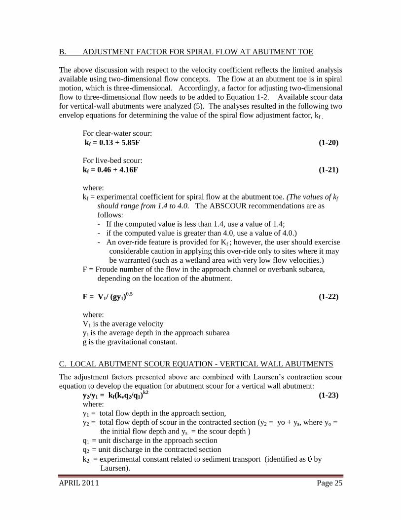
B. ADJUSTMENT FACTOR FOR SPIRAL FLOW AT ABUTMENT TOE

The above discussion with respect to the velocity coefficient reflects the limited analysis

available using two-dimensional flow concepts. The flow at an abutment toe is in spiral

motion, which is three-dimensional. Accordingly, a factor for adjusting two-dimensional

flow to three-dimensional flow needs to be added to Equation 1-2. Available scour data

for vertical-wall abutments were analyzed (5). The analyses resulted in the following two

envelop equations for determining the value of the spiral flow adjustment factor, kf .

For clear-water scour:

kf = 0.13 + 5.85F (1-20)

For live-bed scour:

kf = 0.46 + 4.16F (1-21)

where:

kf = experimental coefficient for spiral flow at the abutment toe. (The values of kf

should range from 1.4 to 4.0. The ABSCOUR recommendations are as

follows:

- If the computed value is less than 1.4, use a value of 1.4;

- if the computed value is greater than 4.0, use a value of 4.0.)

- An over-ride feature is provided for Kf ; however, the user should exercise

considerable caution in applying this over-ride only to sites where it may

be warranted (such as a wetland area with very low flow velocities.)

F = Froude number of the flow in the approach channel or overbank subarea,

depending on the location of the abutment.

F = V1/ (gy1)0.5

(1-22)

where:

V1 is the average velocity

y1 is the average depth in the approach subarea

g is the gravitational constant.

C. LOCAL ABUTMENT SCOUR EQUATION - VERTICAL WALL ABUTMENTS

The adjustment factors presented above are combined with Laursen‟s contraction scour

equation to develop the equation for abutment scour for a vertical wall abutment:

y2/y1 = kf(kvq2/q1)k2

(1-23)

where:

y1 = total flow depth in the approach section,

y2 = total flow depth of scour in the contracted section (y2 = yo + ys, where yo =

the initial flow depth and ys = the scour depth )

q1 = unit discharge in the approach section

q2 = unit discharge in the contracted section

k2 = experimental constant related to sediment transport (identified as by

Laursen).

APRIL 2011

D. ADJUSTMENT OF ABUTMENT SCOUR DEPTH FOR PRESSURE FLOW

For conditions of pressure flow, Equation 1-23 needs to be adjusted to account for the

effect of pressure flow by multiplying by the pressure coefficient, kp:

y2/y1 = (kf *(kv*q2/q1)k2

)* kp (1-24)

The pressure coefficient, kp, has been determined experimentally (6). Preliminary

conclusions suggest that kp be applied within the following limits:

kp = 0.9*F1 -0.16

(1-25)

where:

F1 = Froude Number for the flow blocked by the bridge superstructure.

= V/ (g*d1)0.5

g = acceleration due to gravity (32.2 ft/ sec2

)

d1 = vertical blockage of flow caused by bridge superstructure (See Figure 1-6)

= yu - h , yu being the depth of the upstream water surface and h being the

distance from the ground to the lower chord of the bridge. Please note that

d1 should be limited to the flow actually blocked by the bridge (parapet

or bridge deck) and should not include the depth of flow overtopping

the bridge.

The values of kp should range from 1.0 to 1.15. If the computed value is less than 1.0,

use a value of 1.0. Cases of severe submergence are defined where the depth of flow

above the low chord is greater than 40% of the flow depth as measured from the channel

bottom to the low chord (d1/h > 0.4), See Figure 1-6. For this case, the value of kp should

be multiplied by a factor of 1.15. If the computed value of kp exceeds 1.15, use a value

of 1.15.

Figure 1-6

Definition Sketch for Pressure Scour

APRIL 2011

E. COMPUTATION OF ABUTMENT SCOUR DEPTH (ABSCOUR PROGRAM)

The ABSCOUR program computes abutment scour as:

y2a = kf*(kv )k2

* y2 (1-26)

where:

y2, the contraction scour flow depth, is defined by either Equation 1-2 (no

pressure flow) or 1-2a (pressure flow) as appropriate.

For conditions of open channel flow or pressure flow at a bridge, using the depths

determined from Equation 1-11, the unadjusted abutment scour depth is:

ysa = y2a - (yo) adj (1-27)

where:

ysa = unadjusted abutment scour depth,

y2a = depth of flow at the bridge abutment after scour has occurred

(yo)adj = initial depth of flow at the bridge abutment, prior to the occurrence of

scour. As noted earlier, the adjustment factor is applied to modify flow

depths affected by the bank slope.

F. OTHER ADJUSTMENTS TO THE ABUTMENT SCOUR DEPTH, ysa

The final abutment scour depth, (ysa) adj is determined from the following adjustments:


where:



FS = factor of safety.

ysa = initial scour estimate from Equations 27 = y2a - (yo) adj

Please note that these adjustment factors (See FHWA Manual HEC-18) are applied

to the initial abutment scour depth to arrive at a final abutment scour depth and

elevation.

The adjustment factors are described below:

F.1 Adjustment Factor, kt, for Abutments with Wing wall and Spill-through Slopes

The scour depth estimated from Equation 1-23 for vertical wall abutments is adjusted by

the program for spill-through slopes and wing-wall abutments by multiplying by the

adjustment factor kt. The factor is computed on the basis of the ratio of the horizontal

APRIL 2011

offset provided by the spill-through slope or wing wall to the total length of the abutment

and approach embankment in the flood plain. This factor serves to account for the more

streamlined flow condition provided by the wing wall or spill-through slope.

The abutment shape factors in HEC-18 Table 8.1 (0.55 for spill-through abutment and

0.82 for wing wall abutment) apply to short abutments. As the length of the abutment

and approach road in the flood plain increase, the effect of a spill-through slope in

reducing scour is decreased. For long approach road sections on the flood plain, this

coefficient will approach a value of 1.0. Similarly, scour for vertical wall abutments with

wing walls on short abutment sections is reduced to 82 percent of the scour of vertical

wall abutments without wing walls. As the length of this abutment and approach road in

the flood plain increase, the effect of the wing wall in reducing scour is also decreased.

For long approach road sections in the flood plain, kt will approach a value of 1.0. Refer

to Part II of this report for a definition sketch of the ABSCOUR Shape Factor as SF =

X1/X2 (Please note the terminology for shape factor, SF, should not be confused with the

safety/calibration factor used elsewhere in the ABSCOUR methodology).

For a spill-through slope abutment:

kt = 0.55 +0.05 (( 1/SF) - 1) (1-29)

For abutments with wing walls:

kt = 0.82 + 0.02((1/SF) - 1) (1-30)

If SF < 0.1, then kt = 1.0

Detailed information on the selection of the Shape Factor, SF, is provided in Part 2,

Section E, Upstream Bridge Data.

F.2 Adjustment Factor ke for Embankment Skew Angle

For highways embankments skewed to flood plain flow, a correction factor, ke, is

computed to account for the effect of the embankment skew on abutment scour. The

embankment skew angle, is the angle between the direction of flow and the centerline

of the roadway (bridge) at the left or right abutment:

ke = ( ^0.13 (1-31)

This value will be usually different for each abutment. Note that the embankment skew

may not be the same as the skew angle of the abutment. The effect of the abutment skew

angle is taken into account by using the flow width that is normal to the flow.

F.3 Adjustment Factor, FS, for Calibration/Factor of Safety

In developing the ABSCOUR equations for estimating abutment scour, available

information from laboratory studies collected by the consultant firm of GKY and

Associates was used as a means of calibrating the model. These laboratory tests were

conducted in simple rectangular straight channels (laboratory flumes) with uniform flow.

APRIL 2011

A total of 126 data points were used to develop the envelop equation describing the

average value of the coefficient for the spiral flow adjustment factor, kf . Use of the

envelope curve provides for a limited factor of safety in the calculations.

In addition, the results of the calibration studies conducted by the USGS comparing

measured vs. computed abutment scour depths have provided additional information

regarding the accuracy of computed contraction scour and abutment scour depths.

However, each stream crossing represents a unique situation. For practical design of new

structures, use of a safety factor may be prudent to take into account the effect of the

complex flow patterns which can be expected to occur at bridges Recommendations

regarding the selection of a safety factor are described in Attachment 3.

G. FINAL SCOUR ELEVATION

Elev. of Bottom of Scour Hole = Water surface elevation - (yo)adj - (ysa)adj (1-32)

Please note that Equation 1-32 takes into account all factors in Equations 1-5 through

1-28. The user must modify these values where aggradation/ degradation or channel

movement is a consideration.

IV. CLEAR WATER SCOUR EQUATIONS

A. CONTRACTION SCOUR

Clear-water Contraction Scour

Laursen‟s contraction scour equation in the form of Equation 1-2 assumes the bed

materials and the shear stresses in the approach and the contracted sections are the same.

Where the bed material of the approach section is not the same as the contracted section,

Equation 1-2 should not be used. Where the upstream section is covered with vegetation

and no sediment is transported (clear water scour), or where there is a limited supply of

bed load available, the Maryland clear water scour curves (based on Neill‟s concept) may

be used in determining contraction scour. Recent findings of several stream morphology

reports indicate that clear water scour may be the expected type of scour in many

Maryland streams The bed material in the contracted section will be eroded until (1) the

bed shear is reduced to its critical value, or (2) the flow depth increases until it reaches

the depth where the mean velocity is reduced to the value of the critical velocity.

Section 2, the downstream side of the bridge, is used to define the parameters for

estimating clear water contraction and abutment scour. Flow depth y2 and flow velocity

V2 are determined for the appropriate portion of Section 2 under consideration. The basic

concept used in the computations is that scour will continue until the bed material has the

stability to resist the flow. At this depth, the flow velocity is reduced to the critical

velocity of the bed material, and V2 = Vc . This basic relationship can be expressed as:

y2 = (V2/ Vc ) (yo)adj

ys = (y2 - (yo)adj ) FS

APRIL 2011

Where:

y2 = yc = flow depth in contracted channel when bed shear is at the critical value.

(yo)adj = initial flow depth before scour

V2 = flow velocity before scour

Vc = critical velocity of bed material

FS = safety/ calibration factor

For conditions of clear-water scour, the following equations are used in the ABSCOUR

program to solve for y2. These equations were originally developed from Neill‟s

competent velocity curves, Reference 11, and modified as a result of the findings of the

USGS studies of abutment scour in South Carolina streams.

Modified Neill Critical Velocity Curves for the Piedmont Zone

EQUATION D50 RANGE(ft) PIEDMONT ZONE

1 0.1 ≤ D50 Vc = 11.5 d^0.167 D50^0.33

2 0.01≤ D50< 0.1 Vc = [ 11.5 d^(0.123/D50^0.2)] D50^0.35

3 0.0001≤ D50< 0.01 Vc = [ 11.5 d^(0.123/D50^0.2)] D50^0.35

Note:

1. D50 = 50% particle size of channel/flood plain bed: d = flow depth

2. If D50< 0.0005 ft, Vc = constant at D50 = 0.0005 ft.

3. If computed Vc< 1.0 fps, then set Vc =1

APRIL 2011

The following relationship applies to the above equations:

y2 = y1 + ys (1-37)

where:

y1 = flow depth before scour

y2 = flow depth after scour

ys = contraction scour depth below stream bed.

If pressure flow conditions exist, the value of y2 is increased as:

y2 (modified) = kp * y2 . (1-38)

The value of kp is explained in Section III D.

B. ABUTMENT SCOUR

Once the clear water contraction scour value is determined, clear water abutment scour

(y2a) can be calculated as:

y2a = ( kf (kv)0.857

) y2 (1-39)

where:

y2 = clear water contraction scour depth determined from Equations 1-34 to 1-36.

kf is dependent on the intensity of the spiral flow in the approach flow, and is

calculated as explained in Part I, Section III B.

kv is related to the contraction ratio of the approach flow and is calculated as

explained in Part I, Section III A.

The final or adjusted abutment scour depth (ysa)adj for clear water scour is computed in

the same manner as for live bed abutment scour, Equation 1-12:


where:



FS = factor of safety

y sa = initial abutment scour estimate noted above (ysa = y2a - (yo) adj)

Consolidated Clear-water Abutment Scour Equation

The following ABSCOUR clear-water abutment scour equation for clear water abutment

scour was developed by Stephen Benedict, USGS, in his report (referenced above) on the

ABSCOUR program, comparing predicted vs. measured abutment scour depths at South

APRIL 2011

Carolina Bridges:

FSadjyV

qkkkkky o

cpfvetsa

2857.0

Where

ysa is the scour depth at the abutment, in feet;

tk is a coefficient for abutment shape that ranges from 0.55 to 1.00;

ke is a coefficient for abutment skew;

kv is a coefficient to account for the increase in flow velocity at the abutment that

ranges from 1.0 to 1.8

q2 is the unit-width flow, in cubic feet per second per foot, under the bridge; please

note that q2/ Vc is equal to y2

kf is a coefficient to account for turbulence at the abutment that ranges from 1.4 to

4.0;

kp is a pressure flow coefficient

Vc is the critical velocity of the bed material for the computed scour depth

yo adj is the initial flow depth before scour

FS is a calibration/safety factor

CRITICAL VELOCITIES IN COHESIVE SOILS

There are as yet no definitive data available for determining critical velocities in cohesive

soils. In an unpublished paper (Permissible Shear Stresses/Critical Velocities, 2005)

Sterling Jones, Research Engineer, FHWA, has collected and commented on various

methods available in the literature regarding this subject. The Office of Structures has

conducted limited tests of critical velocities in cohesive soils using the EFA Apparatus in

the SHA Soils Lab. On the basis of this existing information, the Office of Structures

recommends the following:

1 For preliminary guidance on estimates of critical velocities in cohesive soils, use

the figure below developed from information in Neill‟s “Guide to Bridge

Hydraulics, Second Edition, June 2001” (Please note that three plots are presented

for low, medium and high resistance to flow velocities. Each plot contains the

values excerpted from Neill‟s tables which are connected by straight lines. There

is also a curve drawn to fit the data for each plot which can be used in a spread

sheet application of the method.

2 For more refined estimates of the critical velocity of cohesive soil layers at a

bridge site, take Shelby Tube samples of the various soil layers and test them in

an EFA Apparatus.

APRIL 2011

0

1

2

3

4

5

6

7

8

0 5 10 15 20 25

FLOW DEPTH (ft)

CO

MP

ET

EN

T M

EA

N V

EL

OC

ITY

, (fp

s)

High Resistance - very stiff

to hard soils

Avg. Resistance - medium

stiff to stiff soils

Low Resistance - very

soft or soft soils

V. COMPUTATIONAL PROCEDURES

The computational procedures in the ABSCOUR program described above have been

developed on the basis of straight channels with rectangular cross sections. Actual

stream channels and flood plains are likely to vary significantly from these geometric

shapes. The Engineer needs to apply judgment when using the ABSCOUR methodology

to evaluate scour at an actual bridge crossing. The ABSCOUR User‟s Guide presented in

Part 2 of this paper discusses ways to input data and interpret output data so as to achieve

a reasonable estimate of contraction, pier and abutment scour for cases where the channel

is not straight or where there is a complex flow distribution in the approach channel.

APRIL 2011

VI History of Other Changes to ABSCOUR

August 18, 2006 o Change the lower bound of the kf (spiral flow coefficient) from 1.0 to 1.4

based on studies of clear water scour in the FHWA flume at the Turner

Fairbanks Highway Research Laboratory.

o Modify the recommended procedure in the medium setback case for

evaluating the flow distribution under the bridge.

June 15, 2006 o Change downstream bridge soil D50 input cell to allow layered soil input.

o Utilize an iterated contraction scour elevation calculation so as to

determine the appropriate soil layer to contain the scour at the over-bank

and the channel.

o Calculate the live-bed and clear-water scour for the channel and over-

banks. The contraction scour flow depth depends on the approach section

scour type (live-bed or clear-water). If it is clear-water, then the clear-

water scour flow depth is used. If it is the live-bed scour, then the smaller

of the live-bed and clear-water scour flow depth will be used. This is to

account for the armoring effect due to the coarse sediments. A warning

will be issued when it is live-bed scour and bridge D50 of the control soil

layer is less than 1/10 of the approach D50. This approach also applies to

the interpolation scheme of the short setback case.

o Apply the layered soil and live-bed scour flow depth changes to the

bottomless culvert.

o When the water does not reach abutment, the output is N/A for the

abutment scour. However, the scour result drawing still shows the

abutment scour. This problem is fixed by using the contraction scour

elevation at the abutment in this case.

o Change the help topics to reflect the changes above.

January 11, 2006 o Revise help context and interface of the program in response to

suggestions received from participants at the recent ABSCOUR course

o Revise suggested Safety Factor

August 1, 2005 o Revise abutment spiral flow adjustment factor Kf based on updated test

data

o Add override option for 2-D flow velocity at abutment face and add option

for the cross-section orientation.

o Add actual approach and downstream bridge cross-section. Allow sections

to be imported from existing HEC-RAS project file. On the cross-section

drawing, superimpose the ABSCOUR cross-section with the actual cross-

section for checking ABSCOUR input data. Add tools to calculate the

flow geometry and the flow distribution based on the actual cross-section

and the results can be used as the ABSCOUR input.

o Update help context.

o

APRIL 2011

September 30, 2004 o Revise short setback contraction scour parabolic interpolation equation

exponent from 2.5 to 1.0<= (4.5-z) <=4.0.

o For Kv computation use the unit width discharge of the approach section

(q1) and bridge section (q2) and not the special average unit discharge

q1avg for kv and q2avg for kv as in previous version. This has a major

impact to Kv and the abutment scour depth.

o Add HECRAS discharge under bridge and Override discharge under

bridge. No more overtopping flow / flow adjustment. Revise the program

input data structure so that the previous version input file will be read such

that the Q1-Qovertoppint=HECRAS discharge. The input file is backward

compatible. If user leaves override discharge blank, no override discharge

will be shown in the output. If user do input override discharge, program

will check the total of HECRAS discharge and total of override discharge,

if the difference is no less than 1 cfs, then the program will issue an input

error message. If the total discharge under the bridge is larger than the

total discharge of the approach, program issue an error. Revise the help

context to reflect this change. Output total discharge at the approach and

under the bridge for estimate the overtopping discharge.

o When 5y0>0.75W, the output of the method of computing flow velocity

will be labeled as "short setback" although it is a special case.

o If one of the final abutment scour is less 5 feet, then the program will

output "Recommended minimum abutment scour depth" as 5 feet. This

will be followed by an output line labeled as "Control abutment scour

depth". These two additional output lines only occur when one of the

abutment's final scour depth is less than 5 feet.

o Change bank slope upstream of bridge fro "Z H: 1 V" to "Z=H/V" in both

input and output.

o Change the output line "Scour depth at abutment (y2a) adj" to "Abut.

scour flow depth (y2a) adj" to make it clear that (y2a) adj is the flow depth

not the scour depth.

o When Voverbank>Vchannel program issues a warning.

May 5, 2003 o Flow velocity under the bridge

o Change contraction scour interpolation from linear to parabolic

o Apply safety factor to contraction scour

o No interpolation for abutment scour, instead use the interpolated

contraction scour and apply the necessary correction factors

o Allow live bed scour for bottomless culvert

o Include rock scour in the utility menu

March 13, 2003 o Change approach energy slope to average energy slope between approach

section and bridge section

o Add [F1] help for the average energy slope with illustration

February 20, 2003

APRIL 2011

o Pier scour: (Kh pier) may become negative based on Equation in HEC-18

Figure 6.5. This revision limits the (Kh pier) to 0 as minimum.

o Pier scour: Revise grain roughness of the bed to D84 from D85 and only

echo this input when pier local scour case 2 is selected.

o ABSCOUR: In calculating Kv, when q2 average become zero or negative

due to uneven overtopping flow, set Kv=1.

December 23, 2002 o boundary shear has been changed to match HEC-RAS. A new input item,

energy slope at approach section, is required.

o Clear water scour equation has been revised for D50<=0.001 feet based on

the information from South Carolina.

o Delete multiple columns option in pier scour unit

APRIL 2011

VII. REFERENCES

1. FHWA, “Evaluating Scour at Bridges,” HEC No. 18, Fourth Edition, May 2001

2. Vanoni, Vito A., Manual on Sedimentation, Sedimentation Engineering, ASCE

Hydraulic Division, 1975.

3. Kirchhoff, Robert H., Potential Flows, Computer Graphic Solutions, Marcel Dekker,

Inc. New York, 1985.

4. Milne-Thomson, L. M., Theoretical Aerodynamics, Fourth Edition, Macmillan,

London, 1968.

5. Palaviccini, M., “Scour Predictor Model at Bridge Abutments,” Doctor of Engineering

Dissertation, The Catholic University of America, Washington, D.C., 1993.

6. Chang, Fred, (1) “Analysis of Pressure Scour,” Unpublished Research Report, 1995.

and (2) FHWA Pressure Flow Scour Data, 2009

7. Maynord, Steven T., Toe Scour Estimation in Stabilized Bendways, Technical Note,

ASCE Journal of Hydraulic Engineering, August, 1996.

8. Maryland State Highway Administration, Office of Structures, Manual for Hydrologic

and Hydraulic Design, September 2009

9. Peggy A. Johnson, Pier Scour at Wide Piers, ASCE North American Water and

Environment Congress, June 1996.

10. FHWA, “Bridge Scour and Stream Instability Countermeasures,” HEC No. 23,

Second Edition, March 2001

11. “Guide to Bridge Hydraulics”, Second Edition, Transportation Association of

Canada, 2001.

12. Evaluation of the Maryland Abutment-Scour Equation using Selected Threshold-

Velocity Methods. November, 2008 Stephen T. Benedict, US Geological Survey

13. USGS, Clear-Water Abutment and Contraction Scour in the Coastal Plain and

Piedmont Provinces of South Carolina, 1996 to 1999, Water Resources Report 03-4064

office of structures bridge scour program chapter …gishydro.eng.umd.edu/sha_april2011/ch 11 scour...

Documents