September 2011 1

OFFICE OF STRUCTURES MANUAL ON HYDROLOGIC AND HYDRAULIC DESIGN

CHAPTER 10 APPENDIX A HYDRAULICS OF TIDAL BRIDGES

September 2011

September 2011 2

Hydraulics of Tidal Bridges

Introduction

The Maryland SHA conducts hydraulic studies for proposed new and replacement structures over

tidal waters. In addition, the SHA frequently evaluates the adequacy of existing tidal bridges for

vulnerability to scour damage. This presentation outlines the methods recommended for use in

conducting the hydraulic analyses of existing and proposed tidal bridges.

Recent studies by the Corps of Engineers predict the likelihood of significant sea level rise along

the Maryland shoreline over the next century. The Office of Structures is in the process of

evaluating how the SHA should respond to this potential in the design of highways and

structures. Futures guidance will be included in Chapter 10 Appendix B.

The following general principles have evolved as the SHA, Office of Structures, has gained

experience in evaluating tidal bridges:

The SHA concurs with the observations of C.R. Neill (Reference 4) that "rigorous

analysis of tidal crossings is difficult and is probably unwarranted in most cases, but

in important cases consideration should be given to enlisting a specialist in tidal

hydraulics".

New structures over tidal waters typically are designed to span the tidal channel and

adjacent wetlands. Such designs do not significantly constrict the tidal flow, and

consequently minimize the extent of contraction scour. A primary concern about scour

for these bridges is the extent of local pier scour, and in some cases protection of

abutments and approach roads from local scour and/or wave ride-up.

However, many existing tidal bridges or replacement in kind structures may have smaller

waterway openings with resulting high velocities and significant contraction, pier and

abutment scour during storm tides.

Currents of storm tides in unconstricted channels are usually about 1 to 3 feet per second.

Most of the tidal bridges in Maryland are located on the Chesapeake Bay or on estuaries or inlets

tributary to the Bay. Previous studies commissioned by FEMA (Reference 12) have defined the

elevation of the 100-year and 500-year storm tide elevations throughout the bay area. Studies by

the SHA have identified a storm tide period of 24 hours, based on measured historic storm tides

on the bay.

With this information, and the hydrologic study of flood runoff from upland drainage areas, the

SHA conducts hydraulic studies of tidal bridges following Neill's method as outlined in FHWA

Hydraulic Engineering Circular 18 (Reference 13). There are several judgments that need to be

made in this regard:

September 2011 3

1. If riverine flow prevails, HEC-RAS should be used to make the hydraulic analysis

2. If tidal flow prevails (that is, if the elevation of the flow through the bridge is determined

by downstream tide elevations) the procedure described in this chapter can be used

through the application of the computer program TIDEROUT 2.

3. There are cases, discussed later on in this chapter, such as tidal flow between an island

and the mainland, where special procedures must be used to conduct the study.

Datum for use in Tidal Studies

The old FEMA studies that OBD uses to obtain storm tide elevations were based on the NGVD

datum of 1929. SHA has adopted the NAVD datum of 1988 for the design of its facilities. In

conducting tidal studies, it is important to convert the FEMA data (NGVD datum) to the SHA

data (NAVD datum) prior to running the TIDEROUT2 analyses. Typically, the NAVD datum is

lower than the NGVD datum for tidal areas tributary to the Bay. The following methodology

described below and illustrated in Table 1 is suggested for making this conversion:

Table 1 Example to Illustrate Use of Tidal Station Data

Table 1 reflects the conversion process for a bridge site on the Eastern Shore. To

understand the conversion process, it is helpful to think of there being three separate

gages at a tidal gauging station. The first gauge is the local datum for the station. The

second gauge is for the NGVD datum and the third gauge is for the NAVD datum. The

conversion from the NGVD datum to the NAVD datum involves the following steps.

For this example bridge site, the latitude is N38.33 degrees and the longitude is West

76.21 degrees

1. Obtain the 100-year storm tide elevation for the site from FEMA maps. In this

September 2011 4

case it is 6.0 feet

2. Go to web page (http://geodesy. noaa.gov/TOOLS/Vertcon/vertcon.html. Input

the latitude and longitude and the NGVD storm tide elevation of 6.0 feet. Read

directly the conversion from the NGVD elevation to the NAVD elevation. In this

case, the NAVD elevation corresponding to the NGVD elevation of 6.0 feet is

5.24 feet. These elevations are depicted for the 100-year storm tide in Table 1.

They are used to define the high tide for the tidal hydrograph. Please note that tide

data is rounded off to the nearest one-tenth of a foot.

3. The next step is to determine the low tide for the tidal hydrograph. This can be

obtained from the following web site:

http://www.ngs.noaa.gov/newsys-cgi-bin/ngs_opsd.prl

Go to the bottom of the web page, insert the latitude and longitude for the bridge

site and hit submit. A number of gaging station sites will be listed. Go to the

second set of Stations (PID stations that have all necessary information and select

a station:

The PIDs below do have the necessary information required to create an

image of the tidal and orthometric heights. GV0155 N375948 W0762750HV0238 N383431 W0760420HV0369 N381906 W0762713HV0365 N381904 W0762713HV0001 N383428 W0760425HU0640 N382904 W0754922HV0371 N381909 W0762713GV0156 N375945 W0762749HV0237 N383431 W0760426GV0157 N375947 W0762752HV0236 N383420 W0760437HV0239 N383431 W0760420HV0367 N381905 W0762715

Submit

For this example, Station HVO 371 was selected at random. The print out of the

station data is listed below:

September 2011 5

The NAVD 88 and the NGVD 29 elevations related to MLLW were computed from Bench Mark, TIDAL 10 STA

89, at the station.

Displayed tidal datums are Mean Higher High Water(MHHW), Mean High Water (MHW), Mean Tide Level(MTL),

Mean Sea Level (MSL), Mean Low Water(MLW), and Mean Lower Low Water(MLLW) referenced on 1983-2001

Epoch.

Plot the information provided on the Table 1 format. Note that the NGVD datum is 0.05 feet

above the local datum and the NAVD Datum is 0.85 feet above the local datum. Therefore there

is a difference of 0.8 feet between the two datums and NAVD elevations must be lowered 0.8

feet to match the NGVD elevations.

As noted above, there will be minor differences between the statistical information obtained from

different NOAA stations and we recommend rounding all values to the nearest tenth of a foot.

Once the information in Table 1 is compiled, the information on the tidal hydrograph can be

computed as outlined below in Table 2

September 2011 6

TABLE 2

NGVD ELEVATION (ft) NAVD ELEVATION (ft)

100-YEAR PEAK TIDE

ELEVATION

6.0 6- 0.8 = 5.2

LOW TIDE ELEVATION

(MLLW)

-0.05 -0.85

TIDAL RANGE -0.05 TO 6.0 -0.85 TO 5.2

TIDAL AMPLITUDE 3.0 ‘ 3.0

MEAN TIDE ELEVATION (6 + 0.05)/2 = 3.0 (5.2-0.85)/2 =2.2

ACCESSING THE NOAA WEB SITE FOR NAVD88 ELEVATIONS AT TIDAL STATIONS. An alternative approach to the procedure discussed above is to obtain NAVD 88 elevations at tidal stations directly from the NOAA Web site. The procedure is discussed below using as an example the tidal station for Solomon’s Island:

1) Go to NOAA map that displays tidal stations: http://tidesandcurrents.noaa.gov/gmap3/ 2) Zoom in or zoom out, pan etc. to get a better view 3) Click on the station marker(In this case Solomon’s Island). You should see a “balloon” listing various current and tide links to other reports. 4) Click on datums You should see a report with NAVD elevations on various station data – See below: ================================================================= Aug 26 2011 17:57 GMT ELEVATIONS ON STATION DATUM National Ocean Service (NOAA) Station: 8577330 T.M.: 0 W Name: Solomons Island, MD Units: Feet Status: Accepted (Apr 17 2003) Epoch: 1983-2001 Datum: STND

September 2011 7

Datum Value Description --------- -------- ---------------------------------------- MHHW 5.20 Mean Higher-High Water MHW 5.05 Mean High Water NAVD88 4.57 North American Vertical Datum of 1988 MSL 4.48 Mean Sea Level MTL 4.47 Mean Tide Level DTL 4.46 Mean Diurnal Tide Level MLW 3.88 Mean Low Water MLLW 3.72 Mean Lower-Low Water STND 0.00 Station Datum GT 1.47 Great Diurnal Range MN 1.17 Mean Range of Tide DHQ 0.15 Mean Diurnal High Water Inequality DLQ 0.16 Mean Diurnal Low Water Inequality HWI 6.90 Greenwich High Water Interval (in Hours) LWI 0.93 Greenwich Low Water Interval (in Hours) Maximum 8.00 Highest Observed Water Level Max Date 19550813 Highest Observed Water Level Date Max Time 03:48 Highest Observed Water Level Time Minimum 0.00 Lowest Observed Water Level Min Date 19621231 Lowest Observed Water Level Date Min Time 23:00 Lowest Observed Water Level Time HAT 5.58 Highest Astronomical Tide HAT Date 20010820 Highest Astronomical Tide Date HAT Time 07:36 Highest Astronomical Tide Time LAT 3.21 Lowest Astronomical Tide LAT Date 19960121 Lowest Astronomical Tide Date LAT Time 13:30 Lowest Astronomical Tide Time Tidal Datum Analysis Period: 01/01/1983 - 12/31/2001 Click HERE for further station information including New Epoch products.

September 2011 8

Evaluating Existing Tidal Bridges

In order to develop a cost-effective method of rating tidal bridges, the SHA developed a

screening process to identify low risk bridges. The basic tool used in this screening process is the

classification system outlined below:

Classification of Tidal Bridges

Following the guidance presented by Neill (Reference 4), tidal bridges are categorized into three

main types based on geometric configurations of bays and estuaries and the flow patterns at the

bridges:

1. bridges in enclosed bays or lagoons,

2. bridges in estuaries, and

3. bridges across islands or an island and the mainland.

Please Refer to the FHWA Hydraulic Engineering Circular 18, May 2001, Evaluating Scour at

Bridges or Neill’s Guide to Bridge Hydraulics, Second edition, June 2001 for further discussion

of these categories.

SHA has also classified tidal waterways to take into account whether:

•there is a single inlet or multiple inlets,

•there is a planned or existing channel constriction at the bridge crossing,

•river flow or tidal flow predominates for the anticipated worst-case condition for scour, and

•tidal flow or wind establishes the anticipated worst-case condition for scour for Category 3

bridge crossings.

Category 1. Bridges in enclosed bays or across bay inlets.

In tidal waterways of this type, runoff from upland watersheds is limited, and the

flow at the bridge is primarily tidal flow.

For an enclosed bay with only one inlet, the tidal flow must enter and exit through the inlet, and

the hydraulic analysis is relatively straightforward using an SHA modification of Neill’s tidal

prism method. If there are multiple inlets to the bay, special studies must be made to determine

the portion of the tidal prism that flows through each inlet for the design conditions.

If a highway crossing constricts a tidal waterway, there is a significant energy loss (head

differential) at the structure. SHA has developed a program called TIDEROUT 2 to route the

tidal flow through the bridge (Reference 14) for conditions of no constriction as well as

significant constriction. This software is included in the Office of Structures Manual for

Hydrologic and Hydraulic Design.

The purpose of the analysis is to (1) determine the maximum velocity of flow through the bridge

and the corresponding flow depth and (2) determine anticipated maximum high water for storm

September 2011 9

tides. These values are then used in the bridge design and scour estimating procedures.

Category 2. Bridges in Estuaries.

Flow in estuaries consists of a combination of riverine (upland runoff) flow and tidal flow. The

ratio of these flows varies depending upon the size of the upland drainage area, the surface area

of the tidal estuary, the magnitude and frequency of the storm tide and the magnitude, frequency,

shape and lag time of the flood hydrograph.

Group A includes those bridges over channels where the flow is governed primarily by riverine

flow (90% or more of the total flow).

Group B includes bridges on estuaries where the flow is affected by both riverine and tidal flow.

Group C includes bridges over estuaries where 90% or more of the flow consists of tidal flow.

The hydraulic analysis of bridges in Category 2 (Groups A, B and C) is similar to the analysis

used for Category 1, with the additional consideration of the upland flow. Where the flow

conditions are controlled by the tide, TIDEROUT 2 can be used for the analysis. However, if

riverine flow predominates and establishes the water surface profile at the bridge for worst-case

conditions, HEC-RAS should be used to conduct the hydraulic analysis. In some cases, the

engineer may determine by inspection which flow condition predominates. Such examples

include;

The Woodrow Wilson Bridge at Alexandria, VA. where the riverine flow from the huge

11,000 square mile Potomac River watershed is many times greater than the tidal flow in

the Potomac River above the bridge. HEC-RAS was used here to evaluate the flow

conditions at the bridge.

The Wallace Creek crossing described in Example 1 of this chapter where the riverine

flow is small in comparison with the riverine flow and TIDEROUT 2 is used to evaluate

the hydraulic flow conditions.

It is not always obvious as to which hydraulic flow condition (tidal or riverine) will control and

judgment must be used to select the appropriate method. In some cases, it may be necessary to

use both methods to analyze the flow for worst-case conditions. The table below provides

guidance in regard to selection of the appropriate hydraulic model.

TABLE 3 Selection of Hydraulic Variables for Tidal Analysis

Flow Conditon Model Qmax Tailwater

Q riverine

HEC-RAS

and/or

TIDEROUT2

as appropriate

Q max = Q riverine If tidal data

available at bridge

use MLLT datum

If HEC-RAS

tailwater > MLLT

datum, use

HECRAS

September 2011 10

Tailwater.

Q riverine + Q tidal

HEC-RAS

and/or

TIDEROUT 2

As appropriate

Q max = Q riverine

+Q tidal max

If tidal data

available at bridge

use Mean storm

tide elevation

If HEC-RAS

tailwater > Mean

storm tide

elevation, use

HECRAS

Tailwater

Category 3 Bridges connecting two islands or an island and the mainland.

The hydraulic analysis of bridges in this category is almost entirely dependent on the site

conditions, and no general guidelines have been developed for such locations. The effect of wind

often becomes a primary consideration at these locations. The analysis of such tidal problems

should be undertaken by Engineers knowledgeable about tidal hydraulics.

Category 4 Bridges where the bridge creates a constriction in the tidal flow and the site

conditions are also vulnerable to wind set up at the bridge

Guidance on evaluating this condition is presented later on in the Appendix and in Example 2.

The SHA Screening Process.

The SHA is using the following process to rate tidal bridges for Item 113, Scour Critical Bridges:

1. The location of each bridge is plotted on USGS topographic maps or NOAA navigation

charts. Preliminary information is collected on the tidal waterway, upland drainage basin

the highway crossing using the Tidal Bridge Data and Analysis Worksheet (Figure 2).

2. A preliminary estimate is made of the depths and velocities of storm tides, taking into

account the expected contribution to the flow of flood runoff from the upland drainage

basin. (TIDEROUT 2 can be used to conduct this analysis)

3. An SHA "Phase 2" study is made of each bridge. The bridge plans and files are reviewed,

along with the Phase 1 Channel Stability Study conducted by the U.S. Geological Survey.

This step may or may not include another bridge site inspection by the hydraulic

engineers/interdisciplinary team.

4. The structure is rated for Item 113 based on the foregoing information. Generally,

September 2011 11

structures on deep foundations with no history of scour will be rated as low risk when the

preliminary hydraulic analysis indicates that the velocity of flow and anticipated scour is

low. In those locations where estimated velocities are high, additional studies are made

to determine the degree of risk of scour damage.

DESIGN PROCEDURES FOR EVALUATING TIDAL FLOW THROUGH BRIDGES

The steps for evaluating tidal flow through bridges are outlined below for each of the categories

of tidal waterways introduced above. Examples and Case Histories are presented later in this

Appendix to illustrate the application of each of the design approaches..

Hydraulic analysis of tidal waterways can be complex due to its unsteady, nonlinear and three-

dimensional nature. The complexity is further enhanced by the uncertainty surrounding the

interaction of tidal flows and runoff events. Several numerical, analytical and physical modeling

techniques are available in the literature to address the hydraulic complexity of tidal waterways.

However, SHA has determined that it is not generally cost-effective to utilize such sophisticated

methods to evaluate tidal bridges in Maryland, particularly where tidal currents are low and

resulting scour is minimal.

Hydraulic Analysis of Category I Tidal Bridges

The following approach is recommended for structures over tidal waterways with insignificant

riverine flow.

The tidal flow rate through a channel that is relatively unconstricted by a bridge opening depends

on the rate at which the bay side of the bridge is "filled" or "emptied", since the head differential

between the ocean and bay sides of the bridge is expected to be small, the maximum discharge

through the bridge opening is computed as follows:

where

Qmax = maximum discharge in a tidal cycle, cu. ft./sec

VOL = volume of water in the tidal prism between high and low tide levels, ft3

T = tidal period, seconds

Using the maximum tidal flow rate, Qmax , the velocities for scour evaluation can be determined

using a hydraulic model, or by simply dividing this flow rate by the area of the bridge opening at

the mean elevation of the tidal flow being analyzed. (Neill’s concept utilizes an ideal tide cycle

represented by a cosine curve for a tidal basin upstream of the bridge with vertical sides.) For

this condition, the maximum discharge (in an unconstricted channel) occurs at an elevation

halfway between high tide and low tide. Flow velocities and depths can be determined from this

information, and scour depths can be estimated using information from the soils investigations.

T

VOL 3.14 = Q

max (I.1)

September 2011 12

TIDEROUT 2 can also be used to analyze tidal bridges in this category by inputting a value of

zero for riverine flow.

SHA uses a different form of this equation:

where

Qmax = maximum discharge in a tidal cycle, cu. ft./sec

As = surface area of the tidal basin at mid tide.

H = difference in elevation between high and low tide levels, ft3

T = tidal period, seconds

Equations I.1 and I.2 are based on the same principle. The only difference is Eq. I.1 requires the

tidal basin volume between high tide and low tide, and Eq. I.2 requires the tidal basin water

surface area at mid tide elevation. TIDEROUT 2 can also be used in this category by inputting a

value of zero for riverine flow.

Hydraulic Analysis of Category II Tidal Bridges

Tidal flow through a contracted bridge waterway opening may be treated as flow through an orifice,

in which an energy loss is encountered. Generally, the flow through an orifice is expressed in terms

of the area of the waterway opening and the difference in the water-surface elevations across the

contracted section as:

where

Qo = flow through the bridge (cfs),

Cd = discharge coefficient,

Ac = bridge waterway cross-sectional area, (ft2),

Hs = water-surface elevation upstream of the bridge (ft),

Ht = tidal elevation downstream of the bridge (ft), and

g = 32.2 (ft/s2).

Using the principle of continuity of flow, the discharge through a contracted section of a tidal

estuary can be analyzed as follows:

T

HAs 3.14 = Q

*max

(I.2)

)H-H( 2g A C = Q tscd0 (II.1)

September 2011 13

The amount of tidal flow is determined from the change in the volume of water in the tidal

basin over a specified period. This is calculated by multiplying the surface area of the

upstream tidal basin (As) by the drop in elevation over the specified time.

Qtide = As dHs/dt (II.1)

The total flow approaching the bridge is equal to the sum of the tidal flow and the riverine

flow, and the total flow passing through the bridge is calculated from Equation II.1.

Equation II.2 is derived by setting these flows equal to each other:

where

Q = riverine flow (cfs), and

As= surface area of tidal basin upstream of the bridge (ft2).

Equation II.2 is solved by routing the combined tidal flow and riverine flow through the bridge.

This involves a trial and error process that has been incorporated into the TIDEROUT program.

For a given initial condition, t1, all terms with subscript 1 are known. For t=t2, the downstream tidal

elevation (Ht2), riverine discharge (Q2), and waterway cross-sectional area (Ac2) are also known or

can be calculated from the tidal elevation. Only the water-surface elevation (Hs2) and the surface

area (As2) of the upstream tidal basin remain to be determined. Since the surface area of the tidal

basin is a function of the water-surface elevation, the elevation of the tidal basin at time t2 (Hs2) is

the only unknown term in Equation II.3. Its value can be determined by trial-and-error to balance

the values on the right and left sides of Equation II.3.

The change of the water-surface elevation with time for the downstream side of the bridge due to

the storm tide is determined from Equation II.4 (See Equation 75 of Section 4.6.4 in

Reference 13) and illustrated in Figure 3.

where

T = tidal period, selected as 24 hours for Maryland,

A = one-half of the tidal range, ft.

)H-H( 2g A C = dt

HdA + Q tscd

ss (II.2)

)2

H+H-

2

H+H2g()

2

A+A(C=

t

H-H

2

A+A+

2

Q+Q t2t1S2S1C2C1d

S2S1S2S121 (II.3)

y = ACos 2π(t-tp)/T +MEL (II.4)

September 2011 14

y = tidal elevation (ft), and

t = time (hr).

tp = peak time (hrs), and

MEL = midtide elevation (ft.)

TIDEROUT2 uses the following method for computing discharge.

The discharge coefficient, Cd, is the product of the coefficient of contraction, Cc, and the velocity

coefficient, Cv: Cd = Cc * Cv. The velocity coefficient is assumed to be 1.0 for this analysis. The

area of flow in the downstream contracted section of the bridge is then equal to the area of the flow

as it enters the bridge times the coefficient of contraction, Cc.

The downstream area of flow corresponding to the tidal elevation is used in the routing procedure

for the orifice flow condition.

If the difference in hydraulic grade line across the contracted section exceeds one-third of the flow

depth, upstream of the bridge (d), the flow will pass through critical depth. The discharge then will

be limited to that corresponding to the critical flow condition, which can be expressed as:

where

Qcr = critical discharge (cfs).

Acr = critical flow area (ft2)

dcr = critical depth (ft)

d = flow depth upstream of bridge ft.

g = 32.2 ft/s2

If (Qc - Q) is negative, it means that more water is flowing into the tidal basin than is flowing out

through the bridge, and the water-surface elevation will rise in the tidal basin.

Hydraulic Analysis of Category III Tidal Bridges

The hydraulic analysis of bridges in this category is almost entirely dependent on the site

conditions, and no general guidelines have been developed for such locations. The effect of wind

often becomes a primary consideration at these locations. The analysis of such tidal problems

should be undertaken by Engineers knowledgeable about tidal hydraulics. An example of a the

analysis of a Category III tidal bridge is provided in the case history section of this Appendix

Hydraulic Analysis of Category IV Tidal Bridges Affected by Wind

H2g A = H2g A C = Q downstreamupstreamdo (II.5)

gd 3

2 A = gd A = Q crcrcrcr

(II.6)

September 2011 15

Wind Effects on Tidal Basin Water Level

In a large tidal basin in flat coastal areas, steady wind causes a rise in water level on the leeward

side of the basin. A corresponding fall in the water surface occurs on the windward side. The rise

in water level is called wind set-up and the corresponding fall is called wind set-down.

Estimation of Wind Setup and Set Down

The TIDEROUT2 Program was designed to compute a combination of tidal flow and riverine

flow through a bridge without regard to the effect of the wind. However, wind conditions can

have a significant effect on the velocity of flow through the bridge, and therefore on the extent of

scour. This section presents a method for taking wind conditions into effect in running the

TIDEROUT2 program. Wind setup refers to the rise or piling up of water (measured in feet) at

the highway/bridge facility due to a sustained wind blowing towards the highway. Wind setdown

refers to a drop in the water surface elevation (measured in feet) of a waterway on the downwind

side of the bridge

Design Wind

The design wind needs to be selected in order to estimate wind setup and wind set down.

Reference 5 presents information regarding wind speeds 30 ft above the ground for various

recurrence intervals for the Maryland area. This reference depicts isolines of the highest winds

associated with return periods of 50, 100 and 500-years as determined from this study.

The return period corresponds to the average interval of time for which a given event will occur

(Reference 5). When the return period (Tr) is given, the probability of encounter (Ep) can be

obtained for a given period of time, such as design life (L). using Equation S-1

Ep=1-(1-1/Tr)^L (S-1)

Recommendations for selecting the design wind are presented in Table 4 below. These

values were computed using Equation S-1 and assuming a design service life of 80 years for

typical SHA structures.

Table 4 Recommended Design Wind

(Data obtained from Reference 5)

DESIGN EVENT

DESIGN LIFE

RECOMMENDED DESIGN WIND (MPH)

20-YEAR

OR LESS

FLOOD

50-YEAR

FLOOD

EVENT

100-YEAR

FLOOD

EVENT

500-YEAR

FLOOD

(Estimated)

50 OR LESS 63 67 71 76

80 RECOMMENDED 64 71 77 85

100 64 74 79 88

September 2011 16

Selection of the Fetch

Most of the bridges in Maryland are situated in waterways that have both a deep section (over 10

feet) and a shallow section (10 feet or less). When estimating the fetch of water to use in the

design calculations for wind setup, as described below, the fetch for the deep water and the fetch

for shallow water should be measured separately. The wind creates independent circulation

patterns in the waterway for the different depths so that the setup and fetch for the deep water and

shallow water portions of the waterway would be different, The fetch most representative of the

waterway in the vicinity of the bridge should be selected for the calculation of the wind setup.

Estimation of Wind Setup in Shallow Water (average water depths of 10 feet or less)

Wind setup and set down are unsteady phenomena. They vary with the time and direction of the

wind. The simplified equation presented below for wind setup in a shallow basin assumes that

magnitude of the wind velocity is constant , and continues to blow in the same direction.

Actually, the wind direction can be expected to shift, especially for hurricanes that travel through

Maryland in a generally Northerly direction. Assuming the wind direction is a constant and is in

alignment with the direction of the fetch provides for a worst-case analysis.

The equation from Reference 6 is presented below.

S = 0.00117*(F*Cos θ)/D)*V^2 (S-2)

Where

S= setup (ft) which is the difference in water level between the two ends of the fetch.

The set-up is used in the TIDEROUT 2 program to determine flow quantities and

velocities through the bridge.

F= Fetch (miles); The recommended fetch length for equation S-2 is the length of the

shallow water portion ( depth of ten feet or less) of the waterway

Θ=angle between the wind and the fetch. Assume θ = zero

D= average depth of the shallow water fetch (ft); obtained from navigational

charts

V= design wind velocity (mile per hour) from Table A1.

Estimation of Wind Setup in Deep Water (average water depths of 10 feet or more)

The USACE Shore Protection Manual (Reference 6) presents the general equation for the slope

of the water surface due to a wind stress in a steady state as:

dz/dx = (τs + τb)/(γ d) (S-3)

where

dz/ds = water surface slope

τs = wind shear stress

September 2011 17

τb = bottom shear stress

γ = unit weight of water

d = mean water depth

This equation was further simplified by substituting shear stresses in terms of wind velocity to:

dz/dx = 0.00000178*(V30)^2.22/(γ d) (S-4)

where V30 = wind velocity at 30 ft above the water surface (Table A1), in ft/sec

Set-up for deep-water channels is then calculated as:

S = (dz/dx)*F = 0.00000178*F*(V^2.22)/(γ*d) (S-5)

where

S= setup (ft) which is the difference in water level between the two ends of the fetch.

The set-up is used in the TIDEROUT 2 program to determine flow quantities and

velocities through the bridge.

F= Fetch (miles); the recommended fetch length for equation S-5 is the length of the

deep-water portion ( depth of ten feet or more) of the waterway.

V= design wind velocity (miles per hour) from Table A1.

γ = unit weight of water = 62.4 lbs/ cu. ft.

d= average depth of the deep water fetch (ft); obtained from navigational charts

DESIGN PROCEDURE

The following examples and case histories illustrate the methods discussed above for the

different conditions encountered at a highway crossing of a tidal waterway. The examples present

methodologies for analyzing tidal flow, with and without consideration of the effects of winds.

The case histories provide insight into special conditions requiring a more detailed analysis of the

hydraulic conditions existing at the bridge.

Example 1: Analysis of Tidal Flow at a Type 1 Bridge Waterway Crossing . The bridge

September 2011 18

and its approaches lie between an enclosed low wetland and the open sea. Wind effect is not

considered in this example.

Background

The Route 335 bridge over Wallace creek is a typical example of the many State highways

located in low lying tidal marsh areas. The drainage area of the tidal basin is a marsh of about

0.68 square miles ( 19,000,000 sq. ft.) bordered by a water divide on the west, a slightly higher

land elevation on the north, and Rt. 335 on the south and the east. This is a Type 1 crossing (after

Neill) between an enclosed low wetland and the open water of the Bay. The roadway is designed

to accommodate traffic for normal day weather. The elevations along the roads range from 3 to

five ft (NAVD) except that the approaches near the bridge and the bridge are raised to an

elevation of 6 ft.. Please refer to page 2 for a discussion of the conversion of an NGVD datum to

a NAVD datum.

The TIDEROUT 2 program is used to analyze flow through the bridge. The following data are

required:

1. Tidal Data- The storm tide elevation may be obtained from FEMA maps. For this

location, the 100-year tidal storm elevation is 6 feet (NGVD). Information from a

nearby gage is needed to convert the NGVD elevations to NAVD elevations, and

Station HVO239 (about seven miles from Wallace Creek) is used for this purpose.

The station information indicates that the difference between the NGVD

datum and the NAVD datum is 1.02 – 0.26 = 0.76 feet. Therefore the 100-

year storm tide elevation of 6.0 feet NGVD will be 6.0 – 0.76 = 5.24

NAVD.

The Mean Low Low Tide elevation will be – 1.02 ft. NAVD

Based on this information, the following 100-year tide data can be

computed for the NAVD Datum:

- Tidal range = 5.24 - (- 1.02) = 6.26

- Tidal amplitude = ½ range = 3.13

- Mean tide elevation = 6.26 – 3.13 = 2.11

2. A 12-hour tidal period is typically used for daily tides and a 24-hour period for

storm tides. The unsteady tidal flow is analyzed as a cosine curve using the tidal

amplitude and period as described previously in this chapter.

3. Routing Time. The routing period is a variable selected by the user, but a typical

value of 0.1 or 0.2 hour is recommended. Making this period too long will cause

problems in the solving of the routing equations and lead to inaccurate answers.

4. Roadway elevations are needed to evaluate overtopping flow. These are normally

available from SHA maps drawn to a scale of 1” = 200 feet. The typical weir flow

coefficient for a broad crested weir ( highway) as obtained from HEC-RAS is 2.5

September 2011 19

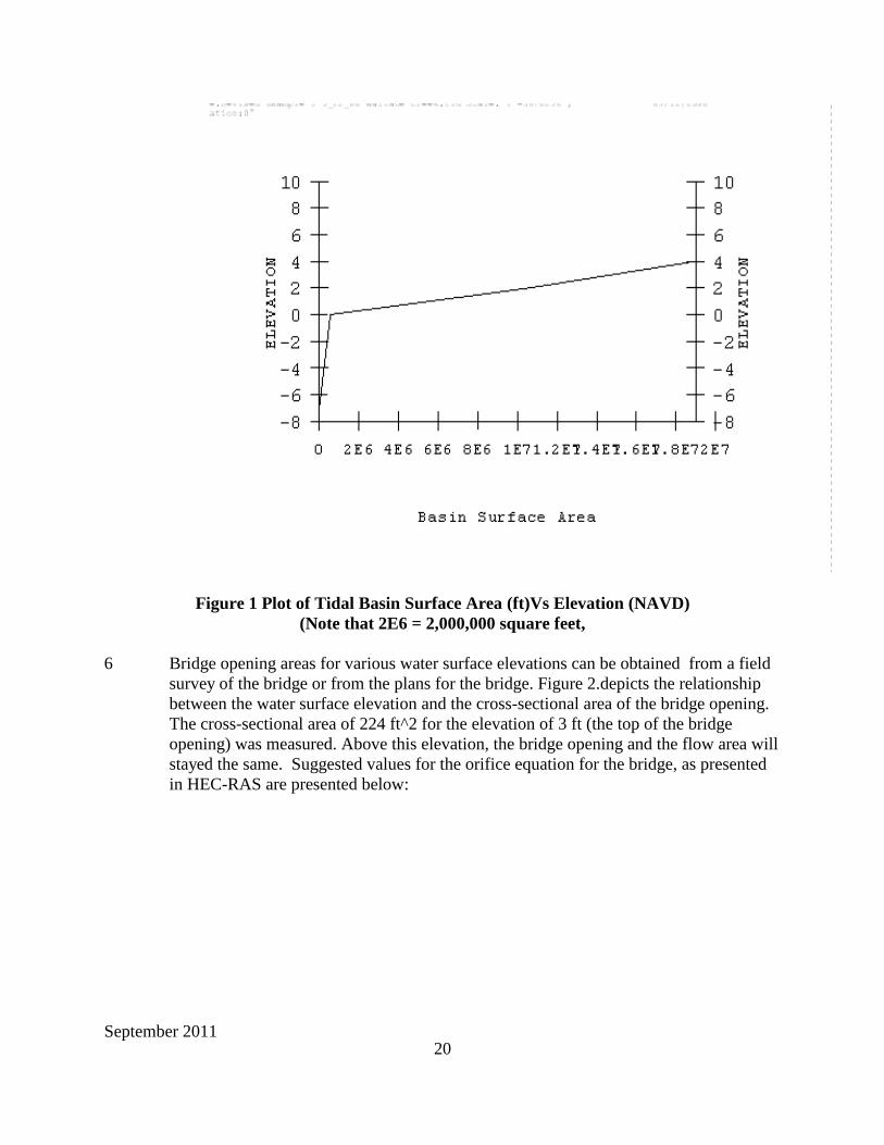
5. Surface area of the tidal basin at different elevations (Figure 1).

Tidal basin data can be obtained from contour maps. For low and flat wetland

areas, they may have to be obtained from larger scale maps of 1:2400

of which the contour interval is 2 ft or smaller. For the Wallace Creek bridge a

1:2400 scale contour map was used to measure the surface areas for the tidal basin

for elevations 0, 2 and 5 ft (NAVD).

The deepest elevation of the tidal basin is at the bridge where the channel bottom

is at the elevation of -6.8 ft.(NAVD) The water surface area of the basin at this

point will be zero. The surface areas of the tidal basin at 0, 2, and 8 ft elevations

were obtained by planimetering a 1 in=200 ft contour map to be 551,000;

10,600,000 and 19,000,000 ft^2 respectively. Above 4 feet, the basin water

surface area is assumed to be enclosed.

September 2011 20

Figure 1 Plot of Tidal Basin Surface Area (ft)Vs Elevation (NAVD)

(Note that 2E6 = 2,000,000 square feet,

6 Bridge opening areas for various water surface elevations can be obtained from a field

survey of the bridge or from the plans for the bridge. Figure 2.depicts the relationship

between the water surface elevation and the cross-sectional area of the bridge opening.

The cross-sectional area of 224 ft^2 for the elevation of 3 ft (the top of the bridge

opening) was measured. Above this elevation, the bridge opening and the flow area will

stayed the same. Suggested values for the orifice equation for the bridge, as presented

in HEC-RAS are presented below:

September 2011 21

TABLE 5 SUGGESTED ORIFICE FLOW COEFFIFICENTS (FROM HEC-RAS)

UPSTREAM

CONDITION

DOWNSTREAM

CONDITION

Cd

AVERAGE VALUE

FREE FLOW FREE FLOW FREE FLOW W2/W1*

PRESSURE FLOW SUBMERGED FREE FLOW 0.4

PRESSURE FLOW SUBMERGED SUBMERGED 0.8

*NOTE: W2 = Net bridge opening width; W1 = Upstream flow width. For free flow, Use a

minimum value of Cd =0.6

Figure 2 Elevation (NAVD) Vs Bridge Waterway Area (square feet)

Assumed Starting Condition: 100-yr storm tide; (Neither wind setup nor wind set down will

be considered for this discussion) The following tidal information is used as computed in the

previous section for TIDAL DATA

.

September 2011 22

1. Starting bridge headwater elevation for the tidal basin: The User has the

flexibility of selecting this value. Typically, a starting elevation is selected

equal to the elevation of the 100-year storm tide as determined from the

FEMA maps. For Wallace Creek the 100-year storm tide elevation is 5.24 feet

NAVD. ( In some cases, a different elevation may be selected if the User

desires to evaluate different peaking times for the tidal hydrograph and the

riverine hydrograph).

2. Mean tide elevation:. The mean storm tide elevation is 3.13 ft NAVD (See

page 16 tidal data)..

3. Stream Flow Data: No inflow is expected from other basins because the basin

is enclosed.. However, the hydrology of the basin is complex, and some flow

may occur into the basin as a result of the variation in the tidal flow between

basins. Therefore, a constant discharge of 50 cfs is assumed for this example,

For crossings of estuaries with larger riverine flows, the user has the option of

inputting a hydrograph or using the TIDEROUT2 program to generate a

hydrograph.

Discussion: The data described above is determined and entered into the TIDEROUT2 Program.

TIDEROUT2 will then route the tidal prism through the structure. The output table lists average

bridge velocity and flow depth for each of the time steps selected for analysis. The worst-case

hydraulic condition (typically the flow condition with the highest velocity) is then selected for the

hydraulic analysis

TIDEROUT 2 PRINTOUT

Wallace Creek with no wind setup

September 2011 23

Figure 1 Input Data

Figure 2 Tidal Basin Data

Figure 3 Bridge Opening Data

Figure 4 Roadway Data

September 2011 24

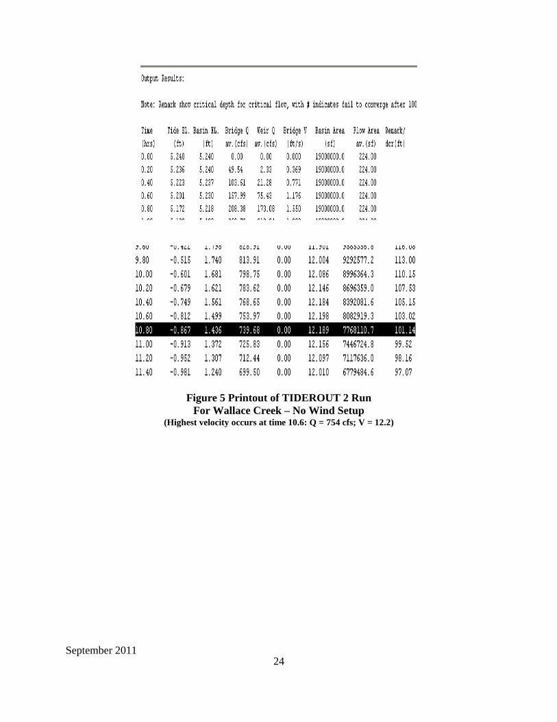
Figure 5 Printout of TIDEROUT 2 Run

For Wallace Creek – No Wind Setup (Highest velocity occurs at time 10.6: Q = 754 cfs; V = 12.2)

September 2011 25

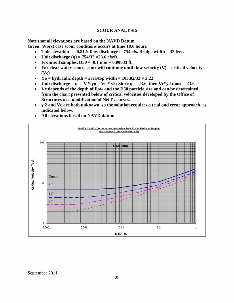
SCOUR ANALYSIS

Note that all elevations are based on the NAVD Datum.

Given: Worst case scour conditions occurs at time 10.6 hours

Tide elevation = - 0.812: flow discharge is 754 cfs. Bridge width = 32 feet.

Unit discharge (q) = 754/32 =23.6 cfs/ft.

From soil samples, D50 = 0.1 mm = 0.00033 ft.

For clear water scour, scour will continue until flow velocity (V) = critical veloci ty

(Vc)

Yo = hydraulic depth = area/top width = 103.02/32 = 3.22

Unit discharge = q = V * yo = Vc * y2; Since q = 23.6, then Vc*y2 must = 23.6

Vc depends of the depth of flow and the D50 particle size and can be determined

from the chart presented below of critical velocities developed by the Office of

Structures as a modification of Neill’s curves.

y 2 and Vc are both unknown, so the solution requires a trial and error approach. as

indicated below.

All elevations based on NAVD datum

Modified Neill's Curve for Non-cohesive Soils in the Piedmont Region

See Chapter 11 for Cohesive Soils

1

10

100

0.0001 0.001 0.01 0.1 1

D 50 - ft.

Cri

tical V

elo

cit

y (

fps)

Depth

50’

20’

10’

5'

D 50 - mm

September 2011 26

trial

number Q assumed y2 Vc calculated Comment

unit discharge

Total

contraction

Critical

velocity from

chart

unit

discharge

From

TIDEROUT 2 scour depth (=) Y2*Vc

1 23.6 10 2.8 28 y2 too high

2 23.6 8 2.5 20 y2 too low

3 23.6 9 2.7 24.3 close enough

Trial and Error Solution to determine total scour depth, y2

(flow depth plus contraction scour depth)

The total contraction scour depth (y2) is computed as 9 feet = Elevation – 9.8 (NAVD)

The contraction scour depth (ys) is then computed as:

ys = y2 – yo = 9 – 3.22 = 5.8 feet.

The ABSCOUR equation for the total depth of abutment scour (y2a) is:

y2a = Kv * Kvk2

(y2)

where Kf = vortex factor for turbulence ~ 1.4 for tidal waterways

Kvk2

= velocity factor ~ 1.0 for tidal waterways

y2a = 1.4 *1.0* 9 = 12.6 feet = Elevation -13.4 (NAVD)

The abutment scour depth (y2s) is computed as:

y2s = y2a – yo = 12.6 – 3.2 = 9.4 feet.

September 2011 27

Example 2: Analysis of Tidal Flow at a Bridge and Its Approaches for a Secondary Road

through a Low Wetland Area. Wind effect is considered

This example uses the same information as Example 1. The conditions in Example 1 are

modified to account for the potential for wind setup at the bridge.

ESTIMATION OF WIND SETUP

Location: MD 335 over Wallace Creek, Dorchester County

Given:

Wind speed for 100 yr for a bridge designed for 80-yr life is 77 MPH. (from H&H

Manual, Chapter 10, Appendix A, Table A1)

Fetch length of the tidal basin upstream of the bridge is approximately 5,000 ft (0.95 mi)

Average water depth is 3 ft (Shallow depth)

Use a value of θ equal to zero. This is the worst case because it assumes that the wind is

blowing straight down the fetch in the direction of the bridge

Estimate the wind setup:

Use Equation S5 in the above-mentioned manual

Total setup S=0.00117*(F*Cosθ)/D)V^2

=0.00117*(0.95Cos 0)/3)77^2=2.2 ft

(This value is the difference in elevation between the upper end of the fetch and the

bridge.)

The total wind setup is the difference in water levels between the two ends of the fetch. This

total wind setup is divided in the following manner between the wind setup at the bridge

and the wind set down at the upstream end of the fetch; If the total setup is evenly divided,

the setup will be 1.1 ft at the bridge and the set down will be 1.1 ft at the upstream end of the

fetch. However, considering that the water will pile up like a wave against the roadway, a more

conservative approach is recommended. A judgment is made to use the wind setup at the bridge

of 1.3 ft (by adding 0.2 ft to 1.1 ft) and a set down of 0.9 ft at the upwind start of the fetch (by

subtracting 0.2 ft from 1.1 ft). Please note that this difference of 1.3 - (- 0.9) adds up to the total

setup calculated By Equation S5.

In order to incorporate these values in the TIDEROUT2 program, the following procedure is

recommended (See Figure 3, Wind Setup and Setdown).

September 2011 28

Wind is blowing from the tidal basin to the Bay, creating wind set up and wind set down.

1. Assume that the ebb tide is to be analyzed, starting at the elevation of the high tide in the

basin (This is the typical case)

September 2011 29

2. Compute wind setup at the bridge (1.3 feet as indicated above)

3. Add the value of the setup to the value of the storm tide elevation at high tide. Input this

value as the (modified) starting bridge headwater elevation on the project data card. For this

example, we add 1.3 to the high tide elevation of 5.24 NAVD (Example 1)for a tide elevation

of 6.54

4. Use the mean tide elevation input on the project data card one-half of the storm tide elevation

as computed for Wallace Creek Example 1. This value is 3.8 feet NAVD)

5. Compute the setdown for the fetch on the downwind side of the bridge. (This is assumed to

be zero due to the great volume of water in the bay)

6. Subtract the setdown from the mean tide elevation. For the Wallace Creek example, the

downwind fetch is the Chesapeake Bay itself and it is likely that a body of water this large

will have a setdown value of zero. Subtract the value of the set down from the mean tide

elevation to obtain the modified mean tide elevation. Use a zero setdown value.

Modified mean tide elevation = 2.11 – 0.0 = 2.11

7. Run the program using these modified values and indicate that the analysis incorporates wind

setup and setdown

TIDEROUT 2 PRINTOUT FOR EXAMPLE 2

Wallace Creek with wind setup of 1.3 feet; no wind set down

Figure 1 Input Data

September 2011 30

Figure 2 Tidal Basin and Bridge Opening Data

Figure 3 Roadway Elevation Data

September 2011 31

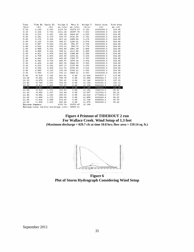
Figure 4 Printout of TIDEROUT 2 run

For Wallace Creek. Wind Setup of 1.3 feet (Maximum discharge = 829.7 cfs at time 10.8 hrs; flow area = 159.14 sq. ft.)

Figure 6

Plot of Storm Hydrograph Considering Wind Setup

September 2011 32

Figure 7

Tailwater- Headwater Relationship at the Bridge

Discussion

For this particular comparison of the tidal flow at Wallace Creek for conditions of no wind

Example 1) and wind (Example 2), the wind effect is not significant with regard to the maximum

velocity of flow through the bridge and resulting scour depths. The reason for this is that Route

335 is a low road and is overtopped by high tides. Most of the tidal flow goes over the road so

the effect of the wind setup is small. This would not be the case for a high road built to an

elevation above the 100-year storm tide. In this case, the tide would pile up along the roadway

embankment within the tidal waterway and create a greater head differential across the bridge

with a resulting greater velocity of flow through the bridge.

The effect of wind set up and set down may be important for highway crossings of tidal waters

tributary to the Chesapeake Bay and should be considered in the analysis. Judgment is needed in

the applications of these values because of (1) the many variables involved in computing the

setup and setdown and (2) the application of these values to the tidal analysis. It is unlikely that

the theoretical condition predicted by the wind setup equations will actually occur at the bridge.

Nevertheless, it is reasonable to make the estimate and to consider the wind in the hydraulic

design.

A comparison of the output tables will show that the worst-case scour conditions for Examples 1

and 2 are the same; therefore the scour analysis for Example 2 will be the same as Example 1 for

this particular set of conditions.

September 2011 33

CASE HISTORIES

A. Maryland Route 33 over Knapp’s Narrows

At the confluence of the Choptank River and the Chesapeake Bay lies a 13-mile long peninsula

stretching southward into the bay, Its southern tip is separated from the rest of the peninsula by a

200-ft wide channel, called Knapp’s Narrows. This lower island, 3.5-mile long, is called Tilghman

Island. MD Route 33 Bridge crosses the Knapp’s Narrows, connecting the peninsula with the

island.

The flow through the Knapp’s Narrows is controlled by the difference in the water surface

elevations on the eastern and western shores of the Tilghman Island. The water surfaces are

influenced by the tide, wind setup, and wave setup. Since the peninsula intrudes into a wide bay,

the tides affect the waters on both sides of the island to an equal degree; consequently, the water

surface difference is small. On this basis, it is concluded that the flow through the Knapp’s Narrows

caused by the tides, including storm tides, will be insignificant. The difference in water surface

elevations between the eastern and western shores of Tilghman Island is affected primarily by

winds.

1. Wind Setup

Wind blowing over the water exerts a drag force on the surface and causes a pile-up of water on the

shore, often called a wind setup. The height of wind setup depends on the wind velocity, water

depth, and fetches distance. For steady, 2-D cases, the general equation for the slope of the water

surface due to wind can be expressed in the following form (Reference 6)

where dx

dz = water surface slope, ft/ft

T s = wind shear stress, lb/ ft2

T B = bottom shear stress , lb/ ft2

d = water depth, ft

For (TS + TB), Keulegan (Reference 7) gave a simplified equation:

The value of TS can be approximated from the relation experimentally obtained by Sibul and

Johnson (Reference 8) as:

62.4d

T + T =

dx

dz Bs (III.1)

T 1.25 = T + T SBS (III.2)

September 2011 34

Where V30 = wind velocity measured at 30 ft above sea surface, ft/s.

The values of V30 can be obtained from various sources. For this case history, it was extracted from

Thom's (Reference 10) study of extreme winds in the U.S.

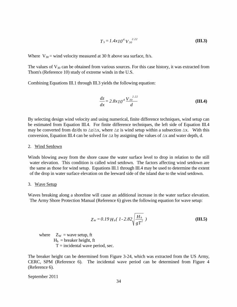
Combining Equations III.1 through III.3 yields the following equation:

By selecting design wind velocity and using numerical, finite difference techniques, wind setup can

be estimated from Equation III.4. For finite difference techniques, the left side of Equation III.4

may be converted from dz/dx to Δz/Δx, where Δz is wind setup within a subsection Δx. With this

conversion, Equation III.4 can be solved for Δz by assigning the values of Δx and water depth, d.

2. Wind Setdown

Winds blowing away from the shore cause the water surface level to drop in relation to the still

water elevation. This condition is called wind setdown. The factors affecting wind setdown are

the same as those for wind setup. Equations III.1 through III.4 may be used to determine the extent

of the drop in water surface elevation on the leeward side of the island due to the wind setdown.

3. Wave Setup

Waves breaking along a shoreline will cause an additional increase in the water surface elevation.

The Army Shore Protection Manual (Reference 6) gives the following equation for wave setup:

where ZW = wave setup, ft

Hb = breaker height, ft

T = incidental wave period, sec.

The breaker height can be determined from Figure 3-24, which was extracted from the US Army,

CERC, SPM (Reference 6). The incidental wave period can be determined from Figure 4

(Reference 6).

V 101.4x = T 30

2.22-6S (III.3)

d

V 102.8x =

dx

dz 30

2.22

8- (III.4)

) gT

H2.82-1 (H 0.19 = Z 2

bbW (III.5)

September 2011 35

For most design conditions, this equation will give wave setup values of about 0.15 Hb.

4. Hydraulics of Flow in Knapp’s Narrows

The flow in the Knapp’s Narrows is controlled by the difference in the water surface elevations on

the eastern and western shores of the Tilghman Island. The difference in the water-surface

elevation is the sum of wind setup, wind setdown, and wave setup.

The following step-by step method was used in calculating (1) the wind setup on the eastern shore

and the wind setdown on the western shore of the Tilghman Island, and (2) hydraulic parameters in

the Knapp’s Narrows for the storm conditions:

Step 1 Determination of Design Wind and Check Wind

Wind setup is an unsteady phenomenon affected by wind speed and duration. The setup increases

with an increase in time and ultimately reaches its maximum height. Equations III.1 through III.4

deal with the wind setup in its final stage when the setup becomes steady. Therefore, in estimating

wind setups design wind speed as well as the sustain time of the wind need to be determined. The

distribution of extreme winds in the United States (Reference 11) and the magnitude of maximum

hurricane winds (Reference 10) were reviewed. Based on this review, the storm winds were

selected to be 80 and 110 mile/hr, respectively, for the 100-and 500-year storms with a sustained

time of 12 hours (Reference 11).

(Note: This case history was analyzed in 1993 for which the wind speeds for the analysis was set

slightly higher than those suggested in Table A1 of this manual.)

Step 2 Computation of Wind Setup

Wind setup increases with the fetch over which the wind blows. The fetch measured to the east of

the Tilghman Island is longer than the fetch to the west. Therefore, storm wind blowing from the

east toward the Tilghman Island was used for the calculation of the maximum wind setup and

setdown. Wind from the east would pile up the water on the eastern shore and lower the water

surface on the western shore. The Choptank River estuary is about four miles wide with an

average water depth of about 30 ft at the confluence with the Chesapeake Bay south of the

Tilghman Island. Due to this large estuary opening, some water in the estuary will move to the

south into the Chesapeake Bay and not contribute to the water piling-up against the eastern shore

of the island. Based on this supposition, the flow pattern of the water out of the estuary was

estimated from a NOAA Chart, and the effective fetch distance was determined as 25,000 ft.

The fetch distance was divided into ten equal sections and the water depth in each section was read

from NOAA Sounding Map. Then, the wind setup was determined for each section by using

Equation III.4. Finally, the total wind setup was calculated by taking the summation of all the

section values. The total wind setup was found to be 2.27 ft and 4.25 ft, respectively, for the wind

velocities of 80 mph and 110 mph.

September 2011 36

Step 3 Computation of Wind Setdown

The east wind causes the water in the Chesapeake Bay to move from the eastern shore (which is the

western shore of the Tilghman Island) toward western shore. The water on the eastern shore

experiences setdown and that on the western shore experiences setup. The total water-surface

differential between the eastern and western shores of Chesapeake Bay can be determined in the

same way as described in Step 2. Since the water from the eastern shore would be moved to pile up

on the western shore, the rise of water surface from the still water surface will be approximately the

average value of setups. More accurate estimates of the setup and setdown can be made by finding

the average water surface as illustrated in Figure 5. Values of setup and setdown are then measured

from this average water surface. The wind setdown on the western shore of the Tilghman Island is

estimated as 1.3 ft and 2.6 ft, respectively, for 80 mph and 110 mph storm winds.

Step 4 Computation of Wave Setup

The procedures described in the US. Army Shore Protection Manual was used in determining the

wave setup. A wave setup of 0.6 ft and 0.7 ft, respectively, was calculated for the 100-year wind

of 80 mph and the 500-year wind of 110 mph.

Step 5 Calculation of Total Water-Surface Difference

The estimated total water-surface difference between the eastern shore and the western shore of the

Tilghman Island is determined by summing the wind setup and wave setup on the eastern shore and

the wind setdown on the western shore:

For 80 mph wind For 110 mph wind

Wind Setup 2.27 ft 4.25 ft

Wind Setdown 1.30 2.60

Wave Setup 0.60 0.70

Total 4.17 ft 7.55 ft

Step 6 Determination of Flow Velocity

To determine the flow velocity in the channel of the Knapp’s Narrows, the water-surface difference

between the eastern shore and the western shore of the Tilghman Island was set equal to the total

energy loss of the flow through the channel. The 200-ft wide channel has been dredged to an

average depth of about 10 ft. The channel is narrowed to a width of 100 feet at the bridge with an

average water depth of about 17 feet. The total length of channel is 2,400 ft. The total energy loss

includes the entrance loss at the channel inlet, the contraction and expansion losses at the bridge,

the exit loss at the outlet of the channel, and the friction loss. For the friction loss, the Manning

equation with the coefficient of n = 0.025 was used.

The analysis resulted in the flow velocities in the channel to be 5.4 ft/s and 7.3 ft/s, respectively, for

the 100- and 500-year storm winds.

September 2011 37

The above noted velocities and depth were used to evaluate the scour potential at the bridge.

B. Route 445 Bridge onto Eastern Neck Island.

The Eastern Neck Island consists of a three-mile delta formed in the Chesapeake Bay by the

Chester River estuary, Figure 8. The island stretches southward from the mainland. The Chester

River flows from the Northeast toward the island and then turns southward at Ringgold Point near

the northeast corner of the island. At the southern tip of the island, the river makes a 180 degree

turn and discharges into Chesapeake Bay at Love Point. The island is separated from the mainland

at the north by a waterway. The Route 445 Bridge crosses this waterway at the narrowest opening.

This channel connects the water of the Chester River on the east side of the bridge at Ringgold

Point to the water in the Chesapeake Bay on the west side to the river at Love Point. Therefore, the

flow at the bridge is controlled by the difference in the water surface levels of the Chester River

between the Ringgold Point and Love Point. This unusual geometric configuration of the area

surrounding the bridge creates an interesting but complex hydraulic condition that requires special

attention in evaluating the extent of scour to be expected at the bridge.

The following approach was used in the hydrologic and hydraulic analysis of the flow at the bridge:

A. Hydrology

As the flow in the Chester River estuary is the combination of the storm runoff from the river

basin and tidal flow, the storm runoffs and tides need to be investigated.

Step 1. Determination of The 100-Year Flood

The USGS regression equation (Reference 1)was used to estimate the magnitude of the 100-year

flood in the Chester River. The 100-year flood was determined as 29,000 cfs, and the 500-year

flood of 49,000 cfs was determined by multiplying the 100-year flood by a factor of 1.7.

Step 2. Determination of Storm Tides

Tidal information at Love Point of Kent Island, compiled by NOAA, was used to determine the

heights of storm tides. Since Love Point is located only about 4 miles west of the bridge in the same

water, the tidal information of Love Point was considered adequate for this investigation.

According to this compiled report, the extreme storm tide was estimated equal to be 7.2 ft above the

Mean Sea Level (MSL) at Love Point. The 500-year storm tide was estimated from studies of Davis

(Reference 2) and Ho (Reference 3) to be 9.3 ft above mean low water.

B. Hydraulics

The waterway at the bridge is sharply contracted and the flow is similar to the flow through an

orifice. Therefore, the orifice equation was used in determining the flow velocity at the bridge. The

September 2011 38

following procedures were followed:

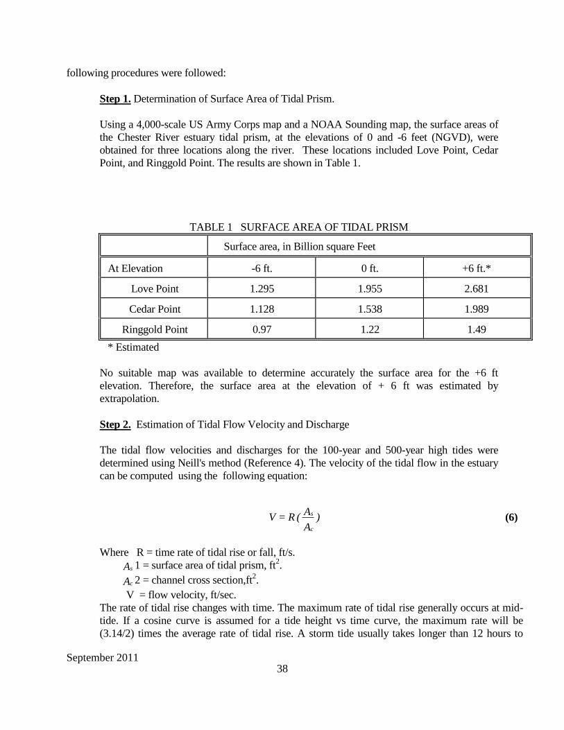
Step 1. Determination of Surface Area of Tidal Prism.

Using a 4,000-scale US Army Corps map and a NOAA Sounding map, the surface areas of

the Chester River estuary tidal prism, at the elevations of 0 and -6 feet (NGVD), were

obtained for three locations along the river. These locations included Love Point, Cedar

Point, and Ringgold Point. The results are shown in Table 1.

TABLE 1 SURFACE AREA OF TIDAL PRISM

Surface area, in Billion square Feet

At Elevation -6 ft. 0 ft. +6 ft.*

Love Point 1.295 1.955 2.681

Cedar Point 1.128 1.538 1.989

Ringgold Point 0.97 1.22 1.49

* Estimated

No suitable map was available to determine accurately the surface area for the +6 ft

elevation. Therefore, the surface area at the elevation of + 6 ft was estimated by

extrapolation.

Step 2. Estimation of Tidal Flow Velocity and Discharge

The tidal flow velocities and discharges for the 100-year and 500-year high tides were

determined using Neill's method (Reference 4). The velocity of the tidal flow in the estuary

can be computed using the following equation:

Where R = time rate of tidal rise or fall, ft/s.

As 1 = surface area of tidal prism, ft2.

Ac 2 = channel cross section,ft2.

V = flow velocity, ft/sec.

The rate of tidal rise changes with time. The maximum rate of tidal rise generally occurs at mid-

tide. If a cosine curve is assumed for a tide height vs time curve, the maximum rate will be

(3.14/2) times the average rate of tidal rise. A storm tide usually takes longer than 12 hours to

)A

A( R = V

c

s (6)

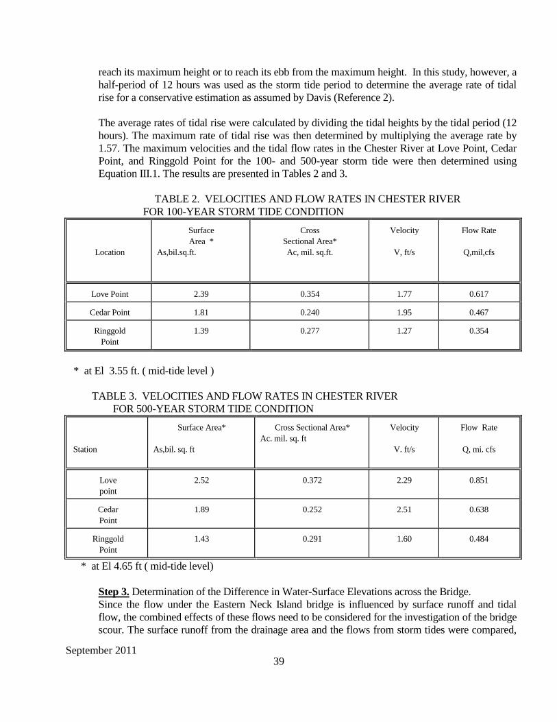
September 2011 39

reach its maximum height or to reach its ebb from the maximum height. In this study, however, a

half-period of 12 hours was used as the storm tide period to determine the average rate of tidal

rise for a conservative estimation as assumed by Davis (Reference 2).

The average rates of tidal rise were calculated by dividing the tidal heights by the tidal period (12

hours). The maximum rate of tidal rise was then determined by multiplying the average rate by

1.57. The maximum velocities and the tidal flow rates in the Chester River at Love Point, Cedar

Point, and Ringgold Point for the 100- and 500-year storm tide were then determined using

Equation III.1. The results are presented in Tables 2 and 3.

TABLE 2. VELOCITIES AND FLOW RATES IN CHESTER RIVER

FOR 100-YEAR STORM TIDE CONDITION

Location

Surface

Area *

As,bil.sq.ft.

Cross

Sectional Area*

Ac, mil. sq.ft.

Velocity

V, ft/s

Flow Rate

Q,mil,cfs

Love Point 2.39 0.354 1.77 0.617

Cedar Point 1.81 0.240 1.95 0.467

Ringgold

Point

1.39 0.277 1.27 0.354

* at El 3.55 ft. ( mid-tide level )

TABLE 3. VELOCITIES AND FLOW RATES IN CHESTER RIVER

FOR 500-YEAR STORM TIDE CONDITION

Station

Surface Area*

As,bil. sq. ft

Cross Sectional Area*

Ac. mil. sq. ft

Velocity

V. ft/s

Flow Rate

Q, mi. cfs

Love

point

2.52 0.372 2.29 0.851

Cedar

Point

1.89 0.252 2.51 0.638

Ringgold

Point

1.43 0.291 1.60 0.484

* at El 4.65 ft ( mid-tide level)

Step 3. Determination of the Difference in Water-Surface Elevations across the Bridge.

Since the flow under the Eastern Neck Island bridge is influenced by surface runoff and tidal

flow, the combined effects of these flows need to be considered for the investigation of the bridge

scour. The surface runoff from the drainage area and the flows from storm tides were compared,

September 2011 40

and the surface runoff was found to be less than 10% of the tidal flows. In view of the unlikely

possibility that the two peak discharges would coincide and considering the insignificant amount

of surface runoff, the surface runoff was subsequently neglected from further analysis.

Using the HEC-2 program, the Chester River flow was routed from Love Point to Ringgold Point

for the 100- and 500-year high tide conditions to determine the water surface differences between

these two points. Tidal flow is of a non-uniform nature. The flow increases along the river toward

the point of discharge into the bay. For each section, the corresponding tidal discharge estimated

in Step 2 (Tables 2 and 3) was used as input discharge in executing the HEC-2 program. The

starting water-surface elevation at the Love Point was set at the mid-tide elevation.

The following results were obtained. The water surface differences between the Ringgold Point

and the Love Point for the storm tide conditions were:

100-year high tide condition: h = 0.51 ft.

500-year high tide condition: h = 0.74 ft.

Step 4. Determination of Flow Velocity

The flow at the bridge is sharply contracted to form a flow condition similar to that of orifice

flow; therefore, to determine the flow velocity at the bridge, the orifice equation below was used:

where V = Flow velocity, ft/s

C = Velocity Coefficient

g = 32.2 ft/sec2

h = Water Surface Difference, ft.

The difference in water surface elevations across the bridge is approximately the same as the

water surface difference in the Chester River between Love Point and Ringgold Point as

calculated in Step 3.

The velocity coefficients for various orifices can be found in any fluid mechanics text. For a

streamlined orifice with a minimum energy loss, the velocity coefficient may be as high as 0.98.

For the flow at the Eastern Neck Island Bridge, considering energy losses attributed to the bents,

the velocity coefficient was assumed to be 0.9. With this assumption, the velocities of the flow

at the bridge were determined as:

100-year high tide condition: v = 5.16 ft/s

500-year high tide condition: v = 6.21 ft/s.

The above noted velocities were used to evaluate the scour potential at the bridge.

2ghC=V (7)

September 2011 41

References

1.U.S.Geological Survey, 1983, Report on Investigations No.35; Characteristics of Stream Flow in

Maryland, by D.H. Carpenter.

2.Davis, S. R., 1990, Scour Evaluation Study, MD Rt. 450 over Severn River, Scour Evaluation

Report to MD State Highway Administration.

3.Ho, F. R., 1976, Hurricane Tide Frequencies Along the Atlantic Coast, Proc. ASCE, 15th

Conference on Coastal Engineering, Honolulu.

4.Roads and Transportation Association of Canada ( RTAC), 1973, Guide to Bridge Hydraulics,

Edited by C.R. Neill, University of Toronto Press.

5.Gaythwaite, J., 1986, Marine Environment and Structural Design, Van Nostrand Reinhold Co.

6.U.S. Army Shore Protection Manual, Vol. 1, USACE, CERC, 1977.

7.Keulegan, G. H., "Wind Tides in Small Closed Channels," National Bureau of Standards, J. of

Research, Vol. 1.46, #5, May 1951.

8.Sibul, O. J., and Johnson, J. W., "Laboratory Studies of Wind Tides in Shallow Water, "Proc.

ASCE, WW-1, Vol. 83, April, 1957.

9.Gaythwaite, J., Marine Environment and Structural Design, Van Nostrand Reinhold Co., 1981.

10.Thom, H.C.S., "New Distributions of Extreme Winds in the U.S.," Proc. ASCE, St-7, Vol. 94,

July 1968.

11.National Oceanic and Atmospheric Administration, "Meteorological Criteria for Standard

Project Hurricane and Probable Maximum Hurricane Winds, Gulf and East Coast of the United

States.", U.S. Department of Commerce, NOAA Tech. Rept. NWS 23, 1979.

12.Virginia Institute of Marine Science, A Storm Surge Model Study, Volumes 1 and 2, Glouster

Point, Virginia, 1978.

13.Federal Highway Administration, Hydraulic Engineering Circular No. 18, Evaluating Scour at

Bridges, Fourth Edition, May 2001.

14.Maryland State Highway Administration, TIDEROUT 2, September 2004, Software program for

evaluating combined riverine and tidal flow at a bridge and considering overtopping flows.