of sussex dphil thesissro.sussex.ac.uk/51654/1/mascagni,_giulia.pdf · iii university of sussex...
TRANSCRIPT

A University of Sussex DPhil thesis
Available online via Sussex Research Online:
http://sro.sussex.ac.uk/
This thesis is protected by copyright which belongs to the author.
This thesis cannot be reproduced or quoted extensively from without first obtaining permission in writing from the Author
The content must not be changed in any way or sold commercially in any format or medium without the formal permission of the Author
When referring to this work, full bibliographic details including the author, title, awarding institution and date of the thesis must be given
Please visit Sussex Research Online for more information and further details
Tax revenue mobilisation in Ethiopia
Giulia Mascagni
Submitted for the degree of Doctor of PhilosophyDepartment of EconomicsUniversity of SussexNovember 2013

iii
UNIVERSITY OF SUSSEX
Giulia Mascagni, Doctor of Philosophy
Tax revenue mobilisation in Ethiopia
Summary
This thesis analyses tax revenue mobilisation in Ethiopia. The main research questionmotivating the thesis regards the existence of a crowding out effect of foreign aid ondomestic public revenue. Throughout the research we are also able to identify otherconstraints and opportunities for tax revenue mobilisation in Ethiopia, to shed light onbroader budget dynamics and to provide firm-level evidence on effective tax rates in theEthiopian manufacturing sector.
The thesis therefore contributes to the current debate on tax revenue mobilisation inAfrica by providing comprehensive evidence from Ethiopia, using longer time series thanmost other studies in this literature. Moreover it provides a new theoretical framework toanalyse the aid-tax relation. In addition it contributes to the very small evidence base ontaxation at the firm level in Africa by virtually doubling the literature and by proposinga theoretical framework for further research.
The thesis starts with a qualitative analysis of the Ethiopian fiscal history between1960 and 2009. This chapter is based on a descriptive analysis of Ethiopian fiscal data,on the study of secondary sources and on in-depth qualitative interviews.
On the basis of this deep understanding of the Ethiopian context, the thesis proceedsby developing a theoretical framework to explain the possible substitution effect betweenaid and tax. An empirical estimation of the model stemming from the theory shows thataid is positively associated with tax revenues. Other determinants of the tax ratio toGDP are found to be: trade openness, the manufacturing sector, the agricultural sectorand governance.
The following chapter takes a broader look at budget dynamics by using the cointe-grated VAR methodology. The results confirm the positive relation between aid and tax.In addition we find evidence for the existence of a domestic budget equilibrium and for apositive association between aid and capital expenditure in particular.
Finally the thesis takes a microeconomic look at taxation by analyzing effective taxrates amongst Ethiopian firms. I find that while tax incentives are widely used in Ethiopia,they do not seem to be affected by lobbying or political connections of the firm.

iv
Acknowledgements
The process of writing this thesis has been more challenging and exciting than I could
expect when I started.
Throughout the PhD I felt very lucky to be able to count on the wise advice and
invaluable guidance of my two supervisors: Alan Winters and Andy MacKay. They pro-
vided not only guidance and advice on my thesis, but also great inspiration on the role
that high quality economic research can have in development policy. I am particularly
thankful to Alan for being always understanding and supportive to my ventures in the
job market and in the field. I know this sometimes required a great deal of patience from
him. At the same time he was able to bring me back to the thesis and to provide the
necessary motivation when that was most needed. During these years he taught me much
more than ‘just’ how to do research. His intellectual integrity, serious commitment, and
continuous availability even at his busiest times have set a very high standard for me to
evaluate both myself and the people around me.
This thesis would have not been possible without the support of my Ethiopian friends.
They did not only help me to get access to data and information, but also to get to
know their beautiful country and culture. I am particularly grateful to the Ethiopian
Development Research Institute (EDRI) that offered excellent hospitality and support
while I was in Addis. The EDRI staff made me feel at home during my fieldwork. A
special thanks also goes to everyone who supported my work at the Ministry of Finance
and Economic Development, the National Bank of Ethiopia, Addis Ababa University,
and Ethiopian Economic Association. This thesis and my experience in Ethiopia have
benefited immensely from their generosity. Betam amasegenalen.
During the PhD I had the great opportunity to discuss my research with experts
and practitioners in the field. These conversations were truly thought provoking. I am
particularly grateful to those who agreed to be formally interviewed and who provided
invaluable insight into the topic of my research. In particular I would like to thank the
staff who helped me at the Italian Cooperation, the International Monetary Fund, the
World Bank, the OECD, the UK Department for International Development and the

v
European Commission.
The chapters of this thesis were presented at conferences and seminars throughout the
years. I received many useful comments on these occasions, which helped me to identify the
main weaknesses of my work, to think about possible solutions, and eventually to improve
this thesis. I am especially thankful to the faculty of the Department of Economics at
Sussex who were always available to offer good advice and help. I am also grateful to
the PhD colleagues that offered both technical help and moral support in the challenging
times of my PhD. A special thanks goes to Emilija Timmis, my co-author. She proved not
only to be a great person to work with but also a fantastic company once the work was
finished, usually with a glass of wine as a reward for a long day spent in a London cafe.
I was blessed with the support of a number of wonderful people in these years. My
brothers and my extended family in Bologna (which goes well beyond blood ties!) have
provided invaluable support at difficult times. They probably do not know how much they
contributed to the completion of this thesis. I also feel particularly lucky to have in my life
an exceptional friend like Chia, who has always been there to share the happy moments
and to comfort me in the difficult ones. I am blessed with many other friends who have
been there for me in the highs and lows of these years. They are truly amazing people,
and they know who they are. Last but not least, Andy provided patient support in the
most difficult times of the PhD and made the last years in Brighton happier than I could
ever imagine.
Finally I would have surely not even embarked in such an ambitious project if I did
not have the constant support and encouragement of my parents. They always pushed me
to do my best and to think about my work as a passion rather than a duty. They are the
most inspiring people I have ever known and this thesis is dedicated especially to them.

vi
Contents
List of Tables x
List of Figures xiv
1 Introduction 1
1.1 Background . . . . . . . . . . . . . . . . . . . . . . . . . . . . . . . . . . . . 1
1.2 Approach . . . . . . . . . . . . . . . . . . . . . . . . . . . . . . . . . . . . . 4
1.2.1 Why Ethiopia? . . . . . . . . . . . . . . . . . . . . . . . . . . . . . 6
1.3 Structure and overview . . . . . . . . . . . . . . . . . . . . . . . . . . . . . 8
2 A fiscal history of Ethiopia: aid dependence and taxation 1960-2009 11
2.1 Introduction . . . . . . . . . . . . . . . . . . . . . . . . . . . . . . . . . . . . 11
2.2 Methodology . . . . . . . . . . . . . . . . . . . . . . . . . . . . . . . . . . . 13
2.3 The Imperial period: 1941 - 1974 . . . . . . . . . . . . . . . . . . . . . . . . 16
2.3.1 Taxation in the agricultural sector . . . . . . . . . . . . . . . . . . . 16
2.3.2 Other taxes: trade, consumption and the industrial sector . . . . . . 18
2.3.3 Increasing revenue needs and development planning . . . . . . . . . 19
2.3.4 Borrowing and external assistance . . . . . . . . . . . . . . . . . . . 21
2.3.5 Opposition movements and the decline of the regime . . . . . . . . . 22
2.4 The Derg: 1974 - 1991 . . . . . . . . . . . . . . . . . . . . . . . . . . . . . . 24
2.4.1 The revolution and its opponents . . . . . . . . . . . . . . . . . . . . 25
2.4.2 External relations and aid . . . . . . . . . . . . . . . . . . . . . . . . 30
2.4.3 Fiscal trends . . . . . . . . . . . . . . . . . . . . . . . . . . . . . . . 32
2.5 The Ethiopian People’s Revolutionary Democratic Front: 1991 - today . . . 35
2.5.1 Transition and ethnic federalism: 1991-1998 . . . . . . . . . . . . . . 35
2.5.2 Economic policies in the 90s . . . . . . . . . . . . . . . . . . . . . . . 37
2.5.3 The war with Eritrea and the TPLF crisis: 1998-2002 . . . . . . . . 39
2.5.4 Consolidation and reform . . . . . . . . . . . . . . . . . . . . . . . . 41

vii
2.5.5 External relations . . . . . . . . . . . . . . . . . . . . . . . . . . . . 44
2.5.6 Tax revenue mobilisation . . . . . . . . . . . . . . . . . . . . . . . . 47
2.6 Implications for tax and aid: four underlying factors . . . . . . . . . . . . . 53
2.7 Conclusion . . . . . . . . . . . . . . . . . . . . . . . . . . . . . . . . . . . . 60
Appendices 62
2.A Quotas and price controls . . . . . . . . . . . . . . . . . . . . . . . . . . . . 63
2.B Interviews . . . . . . . . . . . . . . . . . . . . . . . . . . . . . . . . . . . . . 64
3 Aid and taxation: theory and evidence from Ethiopia 65
3.1 Introduction . . . . . . . . . . . . . . . . . . . . . . . . . . . . . . . . . . . . 65
3.2 Literature review . . . . . . . . . . . . . . . . . . . . . . . . . . . . . . . . . 67
3.3 Data and empirical methodology . . . . . . . . . . . . . . . . . . . . . . . . 71
3.3.1 The data . . . . . . . . . . . . . . . . . . . . . . . . . . . . . . . . . 71
3.3.2 Ethiopian context and some descriptives . . . . . . . . . . . . . . . . 72
3.3.3 Empirical framework and challenges . . . . . . . . . . . . . . . . . . 73
3.4 Results . . . . . . . . . . . . . . . . . . . . . . . . . . . . . . . . . . . . . . . 76
3.4.1 First step: the long run . . . . . . . . . . . . . . . . . . . . . . . . . 76
3.4.2 Second step: the short run . . . . . . . . . . . . . . . . . . . . . . . 79
3.4.3 The usual omitted ‘suspect’: governance . . . . . . . . . . . . . . . . 80
3.5 Robustness . . . . . . . . . . . . . . . . . . . . . . . . . . . . . . . . . . . . 85
3.5.1 Endogeneity and reverse causality . . . . . . . . . . . . . . . . . . . 85
3.5.2 Structural breaks . . . . . . . . . . . . . . . . . . . . . . . . . . . . . 91
3.5.3 Estimation in logs . . . . . . . . . . . . . . . . . . . . . . . . . . . . 98
3.6 Unpacking the effects: tax types and tax composition . . . . . . . . . . . . 98
3.7 The positive aid-tax relation: interpretation . . . . . . . . . . . . . . . . . . 103
3.8 Conclusions and policy implications . . . . . . . . . . . . . . . . . . . . . . 106
Appendices 108
3.A Critical summary of existing theories . . . . . . . . . . . . . . . . . . . . . . 109
3.B Summary of variables . . . . . . . . . . . . . . . . . . . . . . . . . . . . . . 112
3.C Stationarity . . . . . . . . . . . . . . . . . . . . . . . . . . . . . . . . . . . . 113
3.D Autocorrelation tests . . . . . . . . . . . . . . . . . . . . . . . . . . . . . . . 117
3.E Multicollinearity . . . . . . . . . . . . . . . . . . . . . . . . . . . . . . . . . 118
3.F Influential observations . . . . . . . . . . . . . . . . . . . . . . . . . . . . . . 120
3.G Non linearities . . . . . . . . . . . . . . . . . . . . . . . . . . . . . . . . . . 123
viii
3.H Granger causality test . . . . . . . . . . . . . . . . . . . . . . . . . . . . . . 125
3.I Results from estimation in logs . . . . . . . . . . . . . . . . . . . . . . . . . 126
4 Fiscal effects of aid in Ethiopia: a CVAR analysis 127
4.1 Introduction . . . . . . . . . . . . . . . . . . . . . . . . . . . . . . . . . . . . 127
4.2 Literature review . . . . . . . . . . . . . . . . . . . . . . . . . . . . . . . . . 129
4.3 Data . . . . . . . . . . . . . . . . . . . . . . . . . . . . . . . . . . . . . . . . 135
4.4 Descriptive statistics and context . . . . . . . . . . . . . . . . . . . . . . . . 137
4.5 The methodology: CVAR . . . . . . . . . . . . . . . . . . . . . . . . . . . . 139
4.5.1 The unrestricted VAR . . . . . . . . . . . . . . . . . . . . . . . . . . 140
4.5.2 VECM representation of the VAR . . . . . . . . . . . . . . . . . . . 141
4.6 The UVAR: specification and misspecification tests . . . . . . . . . . . . . . 143
4.6.1 Deterministic components . . . . . . . . . . . . . . . . . . . . . . . . 143
4.6.2 Lag length determination . . . . . . . . . . . . . . . . . . . . . . . . 145
4.6.3 Residual plots . . . . . . . . . . . . . . . . . . . . . . . . . . . . . . . 146
4.6.4 Residual autocorrelation . . . . . . . . . . . . . . . . . . . . . . . . . 148
4.6.5 Residual heteroskedasticity and normality tests . . . . . . . . . . . . 149
4.6.6 Goodness of fit . . . . . . . . . . . . . . . . . . . . . . . . . . . . . . 150
4.6.7 Parameter constancy . . . . . . . . . . . . . . . . . . . . . . . . . . . 150
4.7 Determination of cointegration rank . . . . . . . . . . . . . . . . . . . . . . 150
4.7.1 The Johansen test . . . . . . . . . . . . . . . . . . . . . . . . . . . . 151
4.7.2 Additional information to determine r . . . . . . . . . . . . . . . . . 152
4.7.3 Economic interpretability of the results . . . . . . . . . . . . . . . . 154
4.8 Long run identification . . . . . . . . . . . . . . . . . . . . . . . . . . . . . . 155
4.8.1 Long run exclusion . . . . . . . . . . . . . . . . . . . . . . . . . . . . 156
4.8.2 Testing for stationarity of xt . . . . . . . . . . . . . . . . . . . . . . 157
4.8.3 Testing restrictions on β . . . . . . . . . . . . . . . . . . . . . . . . . 158
4.8.4 Test for a zero restriction in α: weak exogeneity . . . . . . . . . . . 162
4.8.5 Test for unit vectors in α . . . . . . . . . . . . . . . . . . . . . . . . 163
4.9 CVAR: long run structure and results . . . . . . . . . . . . . . . . . . . . . 164
4.9.1 Results . . . . . . . . . . . . . . . . . . . . . . . . . . . . . . . . . . 165
4.9.2 Interpretation . . . . . . . . . . . . . . . . . . . . . . . . . . . . . . . 166
4.10 Short run structure . . . . . . . . . . . . . . . . . . . . . . . . . . . . . . . . 168
4.11 An alternative model with disaggregated expenditure . . . . . . . . . . . . . 170
4.12 Conclusions . . . . . . . . . . . . . . . . . . . . . . . . . . . . . . . . . . . . 174

ix
Appendices 176
4.A Stationarity tests . . . . . . . . . . . . . . . . . . . . . . . . . . . . . . . . . 177
4.B The MA representation . . . . . . . . . . . . . . . . . . . . . . . . . . . . . 180
4.C Misspecification tests for UVAR k = 1 . . . . . . . . . . . . . . . . . . . . . 183
4.D Results from UVAR k = 2 . . . . . . . . . . . . . . . . . . . . . . . . . . . . 184
4.E Graphs of unrestricted beta relations . . . . . . . . . . . . . . . . . . . . . . 185
4.F LR results with just identifying restrictions . . . . . . . . . . . . . . . . . . 187
4.G Lag length determination for system 2 . . . . . . . . . . . . . . . . . . . . . 188
4.H Misspecification tests for UVAR k = 2, system 2 . . . . . . . . . . . . . . . 189
4.I Residual plots for system 2 . . . . . . . . . . . . . . . . . . . . . . . . . . . 191
4.J LR results for system 2 with r = 4 . . . . . . . . . . . . . . . . . . . . . . . 193
4.K LR results for system 2 without dummies . . . . . . . . . . . . . . . . . . . 194
5 Tax incentives, lobbying and political connections: firm level evidence
from Ethiopia 195
5.1 Introduction . . . . . . . . . . . . . . . . . . . . . . . . . . . . . . . . . . . . 195
5.2 Literature review . . . . . . . . . . . . . . . . . . . . . . . . . . . . . . . . . 197
5.3 Theoretical framework and hypotheses . . . . . . . . . . . . . . . . . . . . . 202
5.3.1 The average effective tax rate . . . . . . . . . . . . . . . . . . . . . . 203
5.3.2 The explanatory variables . . . . . . . . . . . . . . . . . . . . . . . . 205
5.3.3 Core model and research questions . . . . . . . . . . . . . . . . . . . 208
5.4 Data and variables . . . . . . . . . . . . . . . . . . . . . . . . . . . . . . . . 209
5.4.1 Sample selection . . . . . . . . . . . . . . . . . . . . . . . . . . . . . 213
5.5 The Ethiopian context and descriptive statistics . . . . . . . . . . . . . . . . 214
5.5.1 The Ethiopian context and corporate tax legislation . . . . . . . . . 214
5.5.2 Descriptive statistics . . . . . . . . . . . . . . . . . . . . . . . . . . . 216
5.6 Empirical framework . . . . . . . . . . . . . . . . . . . . . . . . . . . . . . . 223
5.7 Results . . . . . . . . . . . . . . . . . . . . . . . . . . . . . . . . . . . . . . . 226
5.7.1 FEM . . . . . . . . . . . . . . . . . . . . . . . . . . . . . . . . . . . . 229
5.7.2 Goodness of fit and fixed effects . . . . . . . . . . . . . . . . . . . . . 232
5.7.3 Between estimator . . . . . . . . . . . . . . . . . . . . . . . . . . . . 233
5.7.4 Results on tax payments . . . . . . . . . . . . . . . . . . . . . . . . . 237
5.7.5 Exploring the effect of negative profit . . . . . . . . . . . . . . . . . 240
5.8 Robustness . . . . . . . . . . . . . . . . . . . . . . . . . . . . . . . . . . . . 242
5.8.1 Influence of 2003 and alternative ETR measure . . . . . . . . . . . . 242
x
5.8.2 The use of sales as a measure of size . . . . . . . . . . . . . . . . . . 243
5.8.3 Selection problems . . . . . . . . . . . . . . . . . . . . . . . . . . . . 243
5.8.4 Change in ETR threshold . . . . . . . . . . . . . . . . . . . . . . . . 246
5.9 Summary of results: main findings . . . . . . . . . . . . . . . . . . . . . . . 247
5.10 Conclusion . . . . . . . . . . . . . . . . . . . . . . . . . . . . . . . . . . . . 250
Appendices 252
5.A Treatment of current and deferred tax in the literature . . . . . . . . . . . . 253
5.B Summary statistics of relevant variables . . . . . . . . . . . . . . . . . . . . 254
5.C Discussion of events in 2002 and 2003 . . . . . . . . . . . . . . . . . . . . . 255
5.D Distribution of ETR by firm size over time . . . . . . . . . . . . . . . . . . 257
5.E The determinants of profit . . . . . . . . . . . . . . . . . . . . . . . . . . . . 258
5.F Analysis of fixed effects . . . . . . . . . . . . . . . . . . . . . . . . . . . . . 259
5.G Tables with coefficients for region and sector dummies . . . . . . . . . . . . 261
5.H Results including loss variable . . . . . . . . . . . . . . . . . . . . . . . . . . 263
5.I Tables for robustness checks . . . . . . . . . . . . . . . . . . . . . . . . . . . 264
6 Conclusions 272
6.1 Main findings and reflections on thesis . . . . . . . . . . . . . . . . . . . . . 272
6.2 Implications for research and practice . . . . . . . . . . . . . . . . . . . . . 276
6.3 Further research . . . . . . . . . . . . . . . . . . . . . . . . . . . . . . . . . 278
Bibliography 280
xi
List of Tables
2.1 Selected indicators averaged by political era . . . . . . . . . . . . . . . . . . 23
3.1 First step: LR results from tax equation . . . . . . . . . . . . . . . . . . . . 78
3.2 MacKinnon critical values . . . . . . . . . . . . . . . . . . . . . . . . . . . . 79
3.3 Short run results from tax equation (2nd step) . . . . . . . . . . . . . . . . 81
3.4 SR results with governance . . . . . . . . . . . . . . . . . . . . . . . . . . . 84
3.5 IV estimation with lagged grants and loans . . . . . . . . . . . . . . . . . . 87
3.6 LR equation with structural breaks . . . . . . . . . . . . . . . . . . . . . . . 94
3.7 SR equation with structural breaks . . . . . . . . . . . . . . . . . . . . . . . 96
3.8 Tax types LR equations: direct, indirect and trade tax . . . . . . . . . . . . 100
3.9 Tax types SR equations: direct, indirect and trade tax . . . . . . . . . . . . 102
3.B.1Summary of variables . . . . . . . . . . . . . . . . . . . . . . . . . . . . . . 112
3.C.1Results of Dickey-Fuller GLS test for trend-stationarity: levels . . . . . . . 113
3.C.2Results of Dickey-Fuller GLS test for stationarity: 1st difference . . . . . . 113
3.C.3Results of Kwiatkowski-Phillips-Schmidt-Shin test for trend-stationarity:
levels . . . . . . . . . . . . . . . . . . . . . . . . . . . . . . . . . . . . . . . . 114
3.C.4Results of Kwiatkowski-Phillips-Schmidt-Shin test for stationarity: 1st dif-
ference . . . . . . . . . . . . . . . . . . . . . . . . . . . . . . . . . . . . . . . 114
3.C.5Results of Clemente, Montanes, Reyes unit root test with two structural
breaks: levels . . . . . . . . . . . . . . . . . . . . . . . . . . . . . . . . . . . 115
3.C.6Results of Clemente, Montanes, Reyes unit root test with two structural
breaks: 1st diff . . . . . . . . . . . . . . . . . . . . . . . . . . . . . . . . . . 116
3.D.1Autocorrelation tests (first step) . . . . . . . . . . . . . . . . . . . . . . . . 117
3.D.2Autocorrelation tests (second step) . . . . . . . . . . . . . . . . . . . . . . . 117
3.E.1Tolerance and VIF . . . . . . . . . . . . . . . . . . . . . . . . . . . . . . . . 119
3.F.1Tax regression without influential observations . . . . . . . . . . . . . . . . 122
3.G.1Non linearities: inclusion of squared terms . . . . . . . . . . . . . . . . . . . 124

xii
3.H.1Results of Granger causality test . . . . . . . . . . . . . . . . . . . . . . . . 125
3.I.1 Estimation in logs: LR and SR . . . . . . . . . . . . . . . . . . . . . . . . . 126
4.2.1 Summary of CVAR fiscal literature . . . . . . . . . . . . . . . . . . . . . . . 132
4.6.1 Lag reduction test . . . . . . . . . . . . . . . . . . . . . . . . . . . . . . . . 146
4.6.2 Information criteria for lag length determination . . . . . . . . . . . . . . . 146
4.6.3 Autocorrelation test . . . . . . . . . . . . . . . . . . . . . . . . . . . . . . . 149
4.6.4 Multivariate heteroskedasticity and normality tests . . . . . . . . . . . . . . 149
4.6.5 Univariate heteroskedasticity and normality tests . . . . . . . . . . . . . . . 150
4.7.1 Quantiles of the simulated rank test distribution . . . . . . . . . . . . . . . 152
4.7.2 Johansen test for determination of cointegration rank . . . . . . . . . . . . 152
4.7.3 The roots of the companion matrix . . . . . . . . . . . . . . . . . . . . . . . 153
4.8.1 Test of LR exclusion . . . . . . . . . . . . . . . . . . . . . . . . . . . . . . . 157
4.8.2 Test for stationarity: shift dummies included . . . . . . . . . . . . . . . . . 158
4.8.3 Test for stationarity: shift dummies excluded . . . . . . . . . . . . . . . . . 158
4.8.4 Hypothesis testing on β . . . . . . . . . . . . . . . . . . . . . . . . . . . . . 160
4.8.5 Test of weak exogeneity . . . . . . . . . . . . . . . . . . . . . . . . . . . . . 163
4.8.6 Test of unit vector in alpha . . . . . . . . . . . . . . . . . . . . . . . . . . . 164
4.9.1 LR results on beta . . . . . . . . . . . . . . . . . . . . . . . . . . . . . . . . 167
4.9.2 LR results on alpha . . . . . . . . . . . . . . . . . . . . . . . . . . . . . . . 167
4.10.1Short run results . . . . . . . . . . . . . . . . . . . . . . . . . . . . . . . . . 170
4.10.2Residual covariance matrix . . . . . . . . . . . . . . . . . . . . . . . . . . . 170
4.11.1LR results on beta with disaggregated expenditure . . . . . . . . . . . . . . 172
4.11.2LR results on alpha with disaggregated expenditure . . . . . . . . . . . . . 173
4.A.1Results of Dickey-Fuller GLS test for stationarity: logs . . . . . . . . . . . . 177
4.A.2Results of Dickey-Fuller GLS test for stationarity: logs 1st diff . . . . . . . 177
4.A.3Results of Kwiatkowski-Phillips-Schmidt-Shin test for stationarity: logs . . 178
4.A.4Results of Kwiatkowski-Phillips-Schmidt-Shin test for stationarity: logs 1st
diff . . . . . . . . . . . . . . . . . . . . . . . . . . . . . . . . . . . . . . . . . 178
4.A.5Results of Clemente, Montanes, Reyes unit root test with two structural
breaks: logs . . . . . . . . . . . . . . . . . . . . . . . . . . . . . . . . . . . . 179
4.A.6Results of Clemente, Montanes, Reyes unit root test with two structural
breaks: logs 1st diff . . . . . . . . . . . . . . . . . . . . . . . . . . . . . . . . 179
4.B.1The MA representation and decomposition of the trends . . . . . . . . . . . 181
4.B.2Beta orthogonal: the loadings of the common trends . . . . . . . . . . . . . 182
xiii
4.B.3The long run impact matrix C . . . . . . . . . . . . . . . . . . . . . . . . . 182
4.C.1Autocorrelation test . . . . . . . . . . . . . . . . . . . . . . . . . . . . . . . 183
4.C.2Multivariate heteroskedasticity and normality tests . . . . . . . . . . . . . . 183
4.C.3Univariate heteroskedasticity and normality tests . . . . . . . . . . . . . . . 183
4.D.1Alpha coefficients from UVAR . . . . . . . . . . . . . . . . . . . . . . . . . . 184
4.D.2Beta coefficients from UVAR . . . . . . . . . . . . . . . . . . . . . . . . . . 184
4.D.3Π matrix from UVAR . . . . . . . . . . . . . . . . . . . . . . . . . . . . . . 184
4.F.1LR results on beta with just identifying restrictions . . . . . . . . . . . . . 187
4.F.2LR results on alpha with just identifying restrictions . . . . . . . . . . . . . 187
4.G.1Lag reduction test . . . . . . . . . . . . . . . . . . . . . . . . . . . . . . . . 188
4.G.2Information criteria for lag length determination . . . . . . . . . . . . . . . 188
4.H.1Autocorrelation test . . . . . . . . . . . . . . . . . . . . . . . . . . . . . . . 189
4.H.2Multivariate heteroskedasticity and normality tests . . . . . . . . . . . . . . 189
4.H.3Univariate heteroskedasticity and normality tests . . . . . . . . . . . . . . . 190
4.J.1 LR results on beta for system 2 and r = 4 . . . . . . . . . . . . . . . . . . 193
4.J.2 LR results on alpha for system 2 and r = 4 . . . . . . . . . . . . . . . . . . 193
4.K.1LR results on beta for system 2 without dummies . . . . . . . . . . . . . . 194
4.K.2LR results on alpha for system 2 without dummies . . . . . . . . . . . . . . 194
5.2.1 Results on size in the literature . . . . . . . . . . . . . . . . . . . . . . . . . 199
5.4.1 Explanatory variables . . . . . . . . . . . . . . . . . . . . . . . . . . . . . . 212
5.4.2 Sample by year . . . . . . . . . . . . . . . . . . . . . . . . . . . . . . . . . . 213
5.5.1 Regional distribution of firms and origin of tax take . . . . . . . . . . . . . 217
5.5.2 Sector distribution of firms and origin of tax take . . . . . . . . . . . . . . . 218
5.5.3 Correlation matrix: ETR and core variables . . . . . . . . . . . . . . . . . . 221
5.5.4 ETR by size quintiles . . . . . . . . . . . . . . . . . . . . . . . . . . . . . . 221
5.5.5 Transition matrix: 5 size quantiles . . . . . . . . . . . . . . . . . . . . . . . 222
5.5.6 Transition matrix for public ownership . . . . . . . . . . . . . . . . . . . . . 222
5.7.1 Pooled OLS, FEM, REM and BE results . . . . . . . . . . . . . . . . . . . . 227
5.7.2 Post-estimation tests . . . . . . . . . . . . . . . . . . . . . . . . . . . . . . . 228
5.7.3 FE estimation results . . . . . . . . . . . . . . . . . . . . . . . . . . . . . . . 230
5.7.4 BE results with regions . . . . . . . . . . . . . . . . . . . . . . . . . . . . . 234
5.7.5 BE results with sector dummies . . . . . . . . . . . . . . . . . . . . . . . . . 235
5.7.6 Tax payments: OLS, FEM, REM and BE results . . . . . . . . . . . . . . . 239
5.7.7 Post-estimation tests . . . . . . . . . . . . . . . . . . . . . . . . . . . . . . . 239

xiv
5.7.8 Tax payments: results including profit squared, lagged and dummies . . . . 241
5.B.1Summary statistics . . . . . . . . . . . . . . . . . . . . . . . . . . . . . . . 254
5.E.1Determinants of profits: Pooled OLS, FEM, REM and BE . . . . . . . . . . 258
5.F.1Explaining the fixed effects . . . . . . . . . . . . . . . . . . . . . . . . . . . 260
5.G.1BE results with sector dummies . . . . . . . . . . . . . . . . . . . . . . . . . 261
5.G.2BE results with regions . . . . . . . . . . . . . . . . . . . . . . . . . . . . . 262
5.H.1BE with loss variable . . . . . . . . . . . . . . . . . . . . . . . . . . . . . . . 263
5.I.1 Results without years 2003 and 2004 . . . . . . . . . . . . . . . . . . . . . . 264
5.I.2 FE estimation results with sales as a measure of size . . . . . . . . . . . . . 265
5.I.3 BE results with regions and sales as a measure of size . . . . . . . . . . . . 266
5.I.4 BE results with sectors and sales as a measure of size . . . . . . . . . . . . . 267
5.I.5 Results imputing zeroes for missing observations of tax . . . . . . . . . . . . 268
5.I.6 Results with all variables lagged, except tax . . . . . . . . . . . . . . . . . . 269
5.I.7 Results with ETR < 2 . . . . . . . . . . . . . . . . . . . . . . . . . . . . . . 270
5.I.8 Results with ETR < 2 but constrained to a maximum of 1 . . . . . . . . . 271

xv
List of Figures
1.1 Ratio of tax revenue to GDP in Ethiopia and in Africa . . . . . . . . . . . . 5
1.2 ODA as a share of GDP in Ethiopia and in Africa . . . . . . . . . . . . . . 7
1.3 ODA per capita in Ethiopia and in Africa . . . . . . . . . . . . . . . . . . . 7
2.1 Composition of domestic revenue . . . . . . . . . . . . . . . . . . . . . . . . 19
2.2 GDP composition: selected sectors as a share of total . . . . . . . . . . . . 28
2.3 Trends in fiscal variables . . . . . . . . . . . . . . . . . . . . . . . . . . . . . 31
2.4 Budget deficit as a share of GDP . . . . . . . . . . . . . . . . . . . . . . . . 33
2.5 GDP per capita at constant prices . . . . . . . . . . . . . . . . . . . . . . . 38
2.6 Growth rate of GDP at constant prices . . . . . . . . . . . . . . . . . . . . . 43
2.7 Aid dependency: grants and loans as a share of total expenditure . . . . . . 45
2.8 Deviations from three-years moving average of grants and tax . . . . . . . . 51
3.1 Plot of tax, grants and loans . . . . . . . . . . . . . . . . . . . . . . . . . . 72
3.2 Deviations from three-year moving average of tax and aid . . . . . . . . . . 73
3.3 Plot of ICRG indicators . . . . . . . . . . . . . . . . . . . . . . . . . . . . . 82
3.4 CUSUM graph (LR) . . . . . . . . . . . . . . . . . . . . . . . . . . . . . . . 92
3.5 CUSUMSQ graph (LR) . . . . . . . . . . . . . . . . . . . . . . . . . . . . . 92
3.6 Grant rolling estimates (LR) . . . . . . . . . . . . . . . . . . . . . . . . . . 93
3.7 Loan rolling estimates (LR) . . . . . . . . . . . . . . . . . . . . . . . . . . . 93
3.8 CUSUM graph(SR) . . . . . . . . . . . . . . . . . . . . . . . . . . . . . . . . 97
3.9 CUSUMSQ graph (SR) . . . . . . . . . . . . . . . . . . . . . . . . . . . . . 97
3.10 Grant rolling estimates (SR) . . . . . . . . . . . . . . . . . . . . . . . . . . . 97
3.11 Loan rolling estimates (SR) . . . . . . . . . . . . . . . . . . . . . . . . . . . 97
3.12 Plot of tax types . . . . . . . . . . . . . . . . . . . . . . . . . . . . . . . . . 99
4.4.1 Trends in domestic and foreign revenue . . . . . . . . . . . . . . . . . . . . 138
4.4.2 Trends in public expenditure . . . . . . . . . . . . . . . . . . . . . . . . . . 139

xvi
4.6.1 Residual plots . . . . . . . . . . . . . . . . . . . . . . . . . . . . . . . . . . . 147
4.7.1 Illustration of the roots of the companion matrix . . . . . . . . . . . . . . . 153
4.7.2 Trace test statistics . . . . . . . . . . . . . . . . . . . . . . . . . . . . . . . . 154
4.E.1Graphs of unrestricted beta relations . . . . . . . . . . . . . . . . . . . . . . 185
4.I.1 Residual plots for system 2 . . . . . . . . . . . . . . . . . . . . . . . . . . . 191
5.5.1 Histogram of ETR . . . . . . . . . . . . . . . . . . . . . . . . . . . . . . . . 219
5.5.2 Evolution of ETR in time . . . . . . . . . . . . . . . . . . . . . . . . . . . . 220
5.C.1Evolution of income in time . . . . . . . . . . . . . . . . . . . . . . . . . . . 256
5.C.2Evolution of sales in time . . . . . . . . . . . . . . . . . . . . . . . . . . . . 256
5.D.1Scatter plot of profits and sales . . . . . . . . . . . . . . . . . . . . . . . . . 257
5.F.1Plot of fixed effects . . . . . . . . . . . . . . . . . . . . . . . . . . . . . . . . 259

1
Chapter 1
Introduction
This thesis looks at tax revenue mobilisation in Ethiopia, a central issue in African coun-
tries and particularly in those, like Ethiopia, where tax revenue still falls well below the
target level of 15% of GDP1. The central question motivating the thesis is how foreign aid
influences tax revenue mobilisation in Ethiopia and, more specifically, whether a crowding
out effect occurs. The thesis not only answers this question using the case of Ethiopia,
but also it goes further by looking at other determinants of the ratio of tax revenue to
GDP, at broader fiscal dynamics, and at the tax take at the firm level.
1.1 Background
This research originally stems from a personal interest for aid effectiveness, which remains
one of the areas of research most central to the policy debate regarding developing countries
but yet far from providing clear-cut answers (Arndt et al., 2010; Rajan and Subramanian,
2008; Bourguignon and Sundberg, 2007). One of the reasons for this lack of consistency
in empirical results is that the focus has often been on aid’s effects on economic growth,
although the link between aid and final outcomes is likely to be indirect and thus possibly
weak. In the words of Bourguignon and Sundberg (2007), the aid effectiveness debate
needs to ‘open the black box’ and explore the mechanism, or ‘causality chain’, that leads
from aid to improved outcomes.
In this context, the focus on the fiscal effects of aid is a way to identify more direct
linkages of foreign assistance to policy. Since aid is increasingly flowing to governments’
1Adam and Bevan (2004) mention a consensus around a tax ratio of 15-20% for post-stabilizationcountries. International Monetary Fund (2005) suggest that a tax ratio of 15% is a reasonable target formost low-income countries.

2
budgets2, and decisions on the budget are the core of fiscal policy, a direct link between
aid and fiscal outcomes is plausible. Some authors suggested that the analysis of the fiscal
effects of aid is indeed a prerequisite for the analysis of its macroeconomic effects more
generally (McGillivray and Morrissey, 2000).
One of the potentially adverse fiscal effects of aid is to crowd out tax revenues. The
idea of a possible substitution effect between aid and tax revenues was already postulated
in 1963 by Kaldor (Kaldor, 1963), who argued that developing countries should and can
primarily rely on domestic rather than foreign revenues. “Foreign aid is likely to be fruitful
only when it is a complement to domestic effort, not when it is treated as a substitute for
it” (Kaldor, 1963). A substitution effect may happen for many reasons, chiefly because
aid may be a less politically costly source of revenue than taxation. Therefore the relation
between aid and taxation is crucial in the assessment of its effectiveness and I take it as a
central theme for this thesis.
However tax revenue mobilisation is not only important in relation to aid. Higher
reliance on taxation stimulates governments in developing countries to establish a social
contract with their citizens whereby they pay taxes in exchange for a series of services
and guarantees from the state (Moore, 1998; Brautigam et al., 2008). When governments
tax, they are implicitly being accountable to taxpayers on the way resources are spent, as
well as on the effectiveness and equity of such expenditure. This ‘internal’ accountability
(as opposed to ‘external’ accountability to donors) is the basis for democratic dialogue,
state building and institutional development. It also has clear implications in terms of tax
compliance. Moreover in presence of high levels of investment, necessary to meet ambitious
development goals, tax revenue mobilisation becomes a prerequisite for sustainability.
Schools and public infrastructure can be built today, perhaps with foreign resources, but
it will be up to the state to ensure teachers’ salaries are paid and infrastructure maintained.
In the context of African countries, tax revenue mobilisation should also be a central
part of the aid scaling-up scenario (Gupta et al., 2006), since it is the only real candidate
as a feasible exit strategy from foreign aid. While aid is still projected to increase, and
certainly so in Ethiopia, a scenario of scaled down aid in the long run is possible. Even if
such a scenario may only realize relatively far into the future, it is relevant and necessary
for African countries to prepare for it by putting in place an effective tax system that
2This is certainly the case for general and sector budget support, but also for other programs that arefinanced by donors through the government’s budget. This is the case of Protection of Basic Services inEthiopia, for example.

3
ensures enough resources for the state to sustain the development process. This is not to
say that aid should stop flowing to Africa. However it must be the final goal of development
aid itself to decrease its share to GDP and public expenditure, in favor of an increased
role of domestic revenues. This not only would allow sustainability, but also it would
encourage ownership, independence of policy making and it would reduce the volatility
and unpredictability that are typically associated with foreign aid3.
Donors have become more and more aware of the importance of tax revenue mobili-
sation, particularly in the wake of the global financial crisis that has exposed the dangers
of aid volatility and the need to ensure effectiveness for the aid that is provided. Donors’
support to tax mobilisation has focused both on tax policy, such as the introduction of
VAT, and on tax administration issues, such as the establishment of revenue authorities4.
The increased attention that tax revenue mobilisation has received in recent years
is shown, for example, by the African Economic Outlook and the African Development
Bank’s annual meeting of 2010, both focused on the theme of public resource mobilisation
and aid (OECD and African Development Bank Group, 2010); the creation of the African
Tax Administration Forum, inspired by the ‘International Conference on Taxation, State
Building and Capacity Development in Africa’ held in South Africa in August 2008; the
OECD Global Forum on Transparency and Exchange of Information for Tax Purposes
(OECD, 2012); and a recent report by the UK House of Commons on this theme (House
of Commons International Development Committee, 2012). On its part, Ethiopia has
recognised the importance of tax revenue mobilisation in its new development plan, the
Growth and Transformation Plan (GTP). The GTP foresees an increase in tax revenue
of about 25% a year in nominal terms, to reach a tax share of GDP of 15% by 2015.
Given that Ethiopia’s tax share stood at about 11% of GDP at the beginning of the GTP
period, this objective is certainly ambitious. The plan also recognizes that the main source
of finance for investment and development expenditure in general will have to be domestic
rather than external, and increasingly so.
Since aid and taxation are deeply intertwined in developing countries, it is crucial to
explore their relation in detail. Therefore the main research question motivating this thesis
is whether aid crowds out efforts to mobilise tax revenue in Ethiopia. However other as-
pects matter for tax revenue mobilisation and they are also explored in this thesis. Specific
3See Bulir and Hamann (2008) for evidence on the higher volatility of aid with respect to domesticrevenue.
4See Fjeldstad (2013) for a review of donors’ support to strengthen tax systems in developing countries.

4
additional research questions are outlined clearly at the beginning of each chapter. These
relate for example to the role of tax bases in the economy such as trade openness, the
manufacturing sector and agriculture. While trade and manufacturing are usually deemed
‘easy’ to tax due to high accessibility and visibility, fiscal incentives and exemptions may
prevent a full exploitation of these tax bases. Trade and manufacturing are included in
the econometric model estimated in chapter 3, and chapter 5 takes a closer look at the
microeconomic level in the manufacturing sector. Furthermore taxation in the agricul-
tural sector is particularly problematic in presence of high levels of subsistence. When
this variable is included in the model estimated in chapter 3, I find that it is negatively
associated in particular with domestic tax revenues.
1.2 Approach
Tax revenue mobilisation is a multifaceted issue that has attracted the attention of both
economists and political scientists. While the former group has often focused on the
econometric analysis of tax effort and on the mix of tax types, amongst others, the lat-
ter has looked at the relation with state building and institutional development. Both
aspects, the political and the economic one, are important for policy-oriented research.
The econometric analysis can provide ‘hard facts’ about the role of tax bases and aid or
of the determinants of the tax take at the micro level, in our case. The political analysis
can explain these results in the country specific context and connect them to important
political economy dynamics that are difficult to measure, and therefore to include in a
quantitative exercise. So both aspects are relevant and insightful, yet no single method
can encompass them in a comprehensive way.
This thesis therefore adopts a mix of analytical tools to study tax revenue mobilisation
in Ethiopia, encompassing both quantitative and qualitative methods. This choice is
not only grounded on the nature of the topic analyzed, but also on the willingness to
keep the analysis policy oriented. Since tax revenue mobilisation is so central to the
policy debate on developing countries, this thesis aims at contributing to it as well as
to the academic literature. To this aim, I always try to complement econometric results
with qualitative information obtained from an in-depth analysis of primary and secondary
sources of information, including interviews to policy makers and experts. The bulk of the
qualitative analysis is reported at the beginning of the thesis, in chapter 2, to set the stage
for the quantitative chapters. However relevant elements from the qualitative analysis are
referred to throughout the thesis as appropriate. In particular the qualitative analysis

5
complements the econometric exercises by informing the design of empirical models and
by allowing an interpretation of results that is deeply rooted in the Ethiopian context.
As far as the econometric exercises are concerned, preference is generally given to the
simplest econometric methods that are able to yield indications on the research questions
motivating each chapter. This approach is also motivated by the policy orientation of this
research, that favors results that are easy to interpret and communicate. Moreover the
mixed methods approach is applied also within the econometric chapters, that encompass
both macroeconomic and microeconomic analysis therefore offering a comprehensive view
on tax revenue in Ethiopia.
On the macroeconomic side, chapters 3 and 4 use time series econometrics and par-
ticularly cointegration techniques that allow the distinction between short run and long
run effects. They use Ethiopian macroeconomic data from the Ministry of Finance and
Economic Development from 1960 to 2009. This is a longer time series than most studies
of this kind and it therefore allows potentially more robust inference. Moreover the unique
history of independence of Ethiopia contributed to the early development of modern fiscal
institutions and data collection activities. Partly because of this, Ethiopia today reports
the highest Statistical Development Index in Africa, together with South Africa (OECD
and African Development Bank Group, 2010). This dataset therefore represents a strength
of the analysis, particularly in the African context.
Figure 1.1: Ratio of tax revenue to GDP in Ethiopia and in Africa
.1.15
.2.25
.3rat
io of
total
tax to
GDP
1995 2000 2005 2010year
Africa EthiopiaLow Income Africa North AfricaSub-Saharan Africa
Source: author’s calculations using data from the African Economic Outlook 2010 and Africa DevelopmentIndicators.
On the microeconomic side, chapter 5 brings a microeconomic view to a topic largely
debated in the macroeconomic literature. By looking at effective tax rates, i.e. the ratio

6
of tax payments to income at the firm level, it essentially mirrors at the microeconomic
level the tax share (of GDP) that was analyzed previously at the macroeconomic level.
The adoption of a case study approach allows the connection of the macroeconomic and
microeconomic results in the context of the broader Ethiopian context. Moreover by
focusing only on one country this thesis is able to offer a highly comprehensive and in-
depth analysis on tax revenue in Ethiopia, that partly overcomes the limits inherent to
cross country studies.
1.2.1 Why Ethiopia?
The case study approach motivates the focus of this thesis on Ethiopia, which is a good
setting for studying tax revenue mobilisation for a few reasons. First of all the country
still has a lower tax share (of GDP) than any grouping of African countries5, as shown in
figure 1.1. In addition it is still highly reliant on trade taxation, more so than other African
countries (OECD and African Development Bank Group, 2010). This indicates that the
desired shift from trade to domestic taxation (in the context of trade liberalization) has
not fully occurred in Ethiopia. Given the level and structure of taxation in Ethiopia, the
analysis of tax revenue mobilisation is particularly relevant to this country. Moreover in a
context of low domestic revenue, it is all the more important to ensure that aid does not
have the adverse effect of crowding out tax.
As for aid, Ethiopia is widely considered an ‘aid darling’ since foreign assistance (official
development assistance, ODA, as a share of GDP) has been higher than in other Sub-
Saharan African (SSA) countries since the mid 80s (see figure 1.2). Moreover foreign
assistance is projected to increase further in the coming years. For example the UK’s
Department for International Development (DFID) has identified Ethiopia as one of its
focus countries in the aid review of 2011, which implies sustained and increased amounts
of aid. This focus is grounded on the fact that Ethiopia is ‘good value for money’6, as it
ranks in the top 5% of countries with the highest ‘need-effectiveness’ index (Department
for International Development, 2011).
However while Ethiopia today receives more aid as a share of GDP than other SSA
countries (figure 1.2), this figure has been lower than other low-income African countries
5In figure 1.1, ‘Africa’ includes all African countries; ‘Low Income Africa’ includes countries classifiedas low income by the World Bank; ‘North Africa’ includes Algeria, Egypt, Lybia, Morocco, Sudan andTunisia; ‘Sub-Saharan Africa’ includes all other countries.
6Howard Taylor, former head of DFID in Ethiopia, was quoted as saying that the review of UK aidin the world has shown that Ethiopia is ‘good value for our money’, thus justifying aid increases (DerejeFeyissa, 2011).

7
Figure 1.2: ODA as a share of GDP in Ethiopia and in Africa
0.05
.1.15
ODA a
s a sh
are of
GDP
1960 1970 1980 1990 2000 2010year
Ethiopia Low Income AfricaSub-Saharan Africa
Source: author’s calculations using data from OECD and Africa Development Indicators.
(except for a few years in the early 2000s). Moreover ODA per capita in Ethiopia has
always been lower than both the SSA average and the low-income countries average (see
figure 1.3). This may be expected in the context of a large country (with about 80 million
people it is the second largest population in Sub-Saharan Africa) that however is still one
of the poorest in the world7.
Figure 1.3: ODA per capita in Ethiopia and in Africa
010
2030
40OD
A per
capit
a
1960 1970 1980 1990 2000 2010year
Ethiopia Low Income AfricaSub-Saharan Africa
Source: author’s calculations using data from OECD and Africa Development Indicators.
Finally Ethiopia is a country with very ambitious development goals. The GTP foresees
7Ethiopia ranks 171st out of 184 countries for GDP per capita in purchasing power parity in 2013.

8
an annual GDP growth of 11% in constant terms during the planning period. This high
growth is largely fuelled by high levels of investment, that in turn require large amounts
of domestic resources to be financed and sustained. Last but not least, data in Ethiopia
is better than in other African countries, therefore allowing more robust econometric
results. It therefore seems timely and relevant to study tax revenue mobilisation in the
case of Ethiopia.
1.3 Structure and overview
This thesis is structured around four substantive chapters, from 2 to 5, while chapter 6
draws some broad conclusions from them.
The research starts in chapter 2 with a qualitative analysis of aid and taxation in
Ethiopia from an historical perspective, covering the period 1960-2009 which is also the one
considered in the econometric analysis of chapters 3 and 4. The inclusion of this chapter
is motivated by a strong belief that understanding the local context can represent a great
value in understanding empirical results and in drawing conclusions that are consistent
with the country-specific context. The main contribution of this chapter to the literature
is to provide a fiscal history of Ethiopia that was not available before in these terms for
the period considered. In addition it contributes to the thesis by setting the stage for the
subsequent econometric analysis, that often refers back to this chapter for relevant in depth
qualitative elements. The analysis is based on the desk study of a rich set of secondary
sources, including published articles and reports but also unpublished documents collected
in the field. Moreover the analysis gains additional insight thanks to about 20 in-depth
interviews to policy makers and experts8. I identify four underlying factors in Ethiopian
history that are relevant to tax revenue mobilisation and particularly to its relation with
aid. Moreover they are relevant in the design of the econometric models and particularly
as regards exogeneity and structural breaks. These factors are: the the long tradition
of statehood and continuity; the history of independence from colonial powers; political
commitment and ambition in development plans; and the relative costs of taxation and
aid.
On the basis of this in-depth analysis of the country context, chapter 3 provides an
analysis of the tax share (of GDP) in Ethiopia. These two chapters (2 and 3) are highly
complementary, as they both look primarily at the aid-tax relation, with the aim of fully
8To these formal interviews are to be added another 20 informal or preliminary interviews.

9
exploiting the advantages of a case study approach using both quantitative and qualitative
methods. The analysis of chapter 3 is based on a tax effort equation estimated using
Ethiopian data with an error correction model (ECM). I find that aid has a positive effect
on the tax share that is robust to the inclusion of governance, a usual source of omitted
variable bias, and to other potential problems such as endogeneity. While the focus is
on aid, other tax determinants are included to control for the effects of changes in the
main tax bases. Trade and the manufacturing sector are found to have a positive effect on
the tax share, that is particularly strong for the latter. The coefficient on agriculture is
largely non-significant in the aggregate tax equation, probably due to contrasting positive
and negative effects found when running separate regressions respectively for trade and
domestic (direct and indirect) taxes.
The following chapter (4) takes a broader look at fiscal dynamics by including ex-
penditure in the analysis. The empirical methodology is the cointegrated VAR (CVAR)
model that allows the estimation of a set of simultaneous long run relations as well as rich
short run dynamics. The main advantage of adopting a CVAR is its a-theoretical nature,
that relies instead of a rich set of tests for model specification. Moreover by estimating
simultaneous equations, the CVAR does not require an a priori definition of variables as
endogenous or exogenous. The drawback is that this method, by estimating a large number
of parameters, is highly demanding on the data and the results are often model-specific.
However by using the Ethiopian data, with more observations than normally available
in the African context, we are able to obtain results that are robust to different model
specifications. Three main results stem from the analysis. Firstly, we find evidence for
the existence in Ethiopia of a long run domestic budget equilibrium that does not include
aid. Secondly we find a positive relation between aid variables (grants and loans) and
expenditure, that is particularly strong between grants and capital expenditure. Last but
not least, we confirm the previous result of a positive relation between aid (both grants
and loans) and taxation therefore finding no evidence of a substitution effect.
It is useful at this point to underline briefly the differences and complementarities
between the single equation (ECM) model estimated in chapter 3 and the CVAR of chapter
4. While the former is more structural, the latter is largely a-theoretical and it allows
testing all the assumptions and restrictions that are imposed on the model. Both have
advantages and disadvantages. On the one hand, the main disadvantage of single equation
models is that they assume the exogeneity of explanatory variables and this assumption is
often difficult to test empirically. On the other hand, CVAR is highly reliant on the data

10
and it may therefore yield fragile results in small samples where only few degrees of freedom
are allowed. As far as advantages are concerned, single equation models allow the inclusion
of more variables that are potentially relevant other than fiscal ones alone. While the effect
of trade, manufacturing and agriculture on tax is less contentious in the literature than
that of aid, it is nonetheless valuable to provide evidence on these aspects at the country
level. Moreover their inclusion allows considering tax in perspective, by controlling for
available tax bases9. On the other hand the CVAR allows the exploration of broader
fiscal dynamics that include expenditure and potentially deficit, that are excluded from
the ECM model, and the behavior of tax revenue in the budget process. Therefore these
two approaches, while partly overlapping, offer complementary insights and are therefore
both valuable to the purpose of this thesis. The consistency in the results regarding aid
and taxation also confirms the robustness of this positive relation.
Chapter 5 takes a microeconomic view on the tax take by looking at effective tax rates
(ETRs), broadly defined as tax payments as a ratio of profits at the firm level. The chap-
ter focuses on corporate taxation, that in Ethiopia contributes 17% to total tax revenue
and about half of total direct taxes. This is a rather substantial contribution particularly
considering that the manufacturing sector, the main but not only contributor of corpo-
rate taxation, represents only 5% of GDP in the country. Corporate taxation is therefore
already a substantial contributor to total revenues and, perhaps more importantly, it has
the potential to contributing even more to the government’s budget in the future as the
manufacturing sector develops further. The analysis of ETRs contributes to the literature
both by introducing a theoretical framework that was not available before, and by provid-
ing evidence on taxation at the firm level in Africa that is largely under-represented in this
literature. I find that tax incentives are very generous in Ethiopia, with most firms paying
ETRs that are well below the statutory tax rate. However the ETR does not seem to be
affected by lobbying or political connections. On the contrary, size and public ownership
are associated with higher effective tax rates in Ethiopia.
Finally chapter 6 provides an overview of the conclusions of this thesis, drawing on
the more detailed discussion presented at the end of each chapter both in the conclusion
sections and in the interpretation/summary of results sections.
9This is also reinforced by the use of the tax ratio to GDP as a dependent variable rather than the logof the deflated value of tax revenue as in the CVAR.
11
Chapter 2
A fiscal history of Ethiopia: aid
dependence and taxation
1960-2009
2.1 Introduction
Tax revenue mobilisation in Africa is attracting increasing attention due to its central
role in financing development plans, in alleviating aid dependence and in establishing a
social contract between the government and citizens (OECD and African Development
Bank Group, 2010; Brautigam et al., 2008; OECD, 2008). This topic has been studied by
academics from different disciplines, as it is multifaceted in nature, and particularly by
economists and political scientists. This chapter aims at bridging those two complementary
areas of research by providing an in depth qualitative analysis of taxation and aid in
Ethiopia in the context of the economic analysis presented in the other chapters of this
thesis.
The qualitative analysis sheds light on the political economy of fiscal policy and aid
in Ethiopia between 1960 and 2009, a period for which detailed fiscal data is available.
The main focus is on exploring the existence of a substitution effect between aid and tax,
whereby large inflows of aid may discourage the government’s efforts towards tax revenue
mobilisation. While going through the Ethiopian fiscal history, the elements that drive
fiscal dynamics are underlined and explained in the specific political and cultural context
of Ethiopia.
The bulk of this chapter (sections 2.3, 2.4 and 2.5) provides a review of Ethiopian
fiscal history that, to the best of my knowledge, is not available in such comprehensive

12
terms for the period considered. This part is based on secondary sources as well as on
the documents and data collected during 18 months of fieldwork between 2009 and 2012.
In addition in-depth interviews were carried out during the fieldwork, adding primary
information to the historical account (see section 2.2 for more details on the methodology).
The interviews cover particularly the most recent history of which more interviewees have
direct experience.
The historical review and the insights obtained during the interviews allow the iden-
tification of four inter-related underlying factors in Ethiopian history that influence the
aid-tax relation, as well as fiscal policy more generally (see section 2.6). The analysis finds
no evidence of a substitution effect between tax and aid and it shows that the existence
of such an effect would be particularly ill-grounded in the Ethiopian context.
This chapter therefore contributes to the literature in three ways. Firstly it provides
a review of the Ethiopian fiscal history that was only available in separate documents,
sometimes of difficult access, and not in a comprehensive single research. Secondly it
provides an in-depth original analysis of the aid-tax relation in Ethiopia, supported by
historical facts an by insights obtained in the interviews. Finally, it provides a bridge be-
tween political and economic analysis by underlining elements that are useful to carry out
a meaningful econometric exercise. In particular it helps in defining the theoretial struc-
ture and the restrictions that often have to be applied in macroeconomic models. This is
important in the context of relatively short time series, where the confirmation of econo-
metric results by a solid qualitative analysis can help validating them. In addition it allows
the interpretation of the results in a way that is realistic and consitent with the country
context, which allows providing more solid conclusions and policy recommendations.
Research questions
Based on this background, this chapter aims at answering the following research quesitons:
• What has been historically the relation between tax and aid? Is a substitution effect
occurring in Ethiopia?
• How does this historical background influence that relation today?
• What have been the main drivers and constraints to tax revenue mobilisation be-
tween 1960 and 2009?
13
2.2 Methodology
The analysis is largely based on a long period of fieldwork carried out during 18 months
spent in Addis Ababa between 2009 and 20121. During this time I worked closely with
government officials and functionnaires with a long experience of macroeconomic analysis
to put together my dataset. I also conducted numerous discussions and formal interviews
with relevant actors.
The fieldwork covered the following three phases. First, necessary information and
data was collected and organized in a consistent format. This process involved many
meetings and discussions that allowed me to obtain a first understading of fiscal policy
and aid in Ethiopia as well as to establish relations with a number of relevant actors, many
of which would be future interviewees. Secondly, the fiscal data was used to carry out a
preliminary descriptive and econometric analysis and the other information was reviewed
and organized. On the basis of this preliminary analysis I prepared the interview guide for
the formal interviews, also including the issues emerging from meetings and discussions.
The timing of the formal interviews after the initial qualitative and quantitative analysis
was completed allowed a more specific focus on the results and on their interpretation.
Finally, the interviews were carried out and the information collected was organized and
analysed. This last step is supported by an in depth review of the literature on the eco-
nomic history of Ethiopia and of other relevant documents, reports and tax laws collected
in the field. The study of these documents was largely carried out in preparation of the
interviews but it was systematically elaborated in the last stage of the process.
As far as the formal interviews are concerned, the choosen format is that of in-depth or
un-structured interviews. These in practice take the form of a conversation that pursues
a precise purpose (Ritchie and Lewis, 2003). This “conversation” is based on an interview
guide that allows the researcher to be flexible in terms of the order of the questions and
topics, which is mostly driven by the issues brought up by the interviewee and by the
natural flow of the conversation. All questions are asked as open questions, thus avoiding
any type of suggestion of possible answers. An initial general question is usually followed
by related and more detailed follow-up ones. Assumptions and hypotheses are formulated
as questions to assess their acceptability before proceeding further. On certain occasions
interviewees were asked about specific results obtained in the quantitative exercise and
1Most of the field research was carried out while I was affiliated as Resident Researcher to the EthiopianDevelopment Research Institute (EDRI), a local research institute to which I am deeply grateful for theircontinued support throughout my research.

14
their possible interpretation. The interviews normally lasted for 45 minutes, net of the
initial introductions (where necessary) and explanation of the process.
The broad themes included in the interview guide are the following.
• Fiscal policy and reform, with a particular focus on taxation. This section
includes in particular questions on the sustainability of fiscal policy, revenue targets,
tax composition, the objectives of tax policy and reform, and the constraints to tax
revenue mobilisation.
• The characteristics of aid in Ethiopia and the relation with donors. This
includes the following sub-themes: the type and quality of the relation with donors,
conditionality and influence in policy making, predictability and reliability, the de-
terminants of variations in aid flows, aid modalities incuding in particular grants
and loans.
• The relation between domestic revenue mobilisation and aid. This section
was mostly focussed on the interviewee’s perception of this relation and on the
possible channels that would explain it, including in particular: capacity building,
technical assistance, the effect of aid on the tax base, and trade liberalization.
To these three main themes are to be added questions that explore more specifically the
historical perspective on these topics. These questions were asked only to people who have
an academic background in history, to those who have a long experience in the country
and to those who have been working in relevant government institutions for long periods
of time in the years considered. Clearly these categories are often overlapping.
As far as interviewees are concerned, they belong to three categories: government
officials, donor agencies and international organizations, and independent experts. The
boundary between these categories is often blurry as it is fairly common for government
employees to join international organizations at a certain stage of their career. This adds
an interesting element to interviews as these persons have a good understanding of both
the government and the donors’ perspective. In addition I had the great opportunity to
interview a few persons who have been involved in macroeconomic policy, and particularly
fiscal policy, for as long as three decades as well as foreigners whose experience in Ethiopia
dates back as far as the early 60s.
The institutions involved in the interview process were, amongst others, the Ministry
of Finance and Economic Development (MOFED), the National Bank of Ethiopia (NBE),
the World Bank, the International Monetary Fund, the European Commission and DFID,

15
as well as experts from Addis Ababa University, the Ethiopian Economics Association and
the Ethiopian Developent Research Institute, or independent experts. The most senior
relevant person was interviewed in most cases, typically at the director or head of division
level, as well as officials of lower seniority when they had a specific expertise on the topic.
I finally ran 19 formal interviews for which I have records. To these are to be addeed
over 20 informal or preliminary interviews carried out throughout the period and for which
written records have been kept. It is important to note that although all formal interviews
are recorded, such records as well as the names of the interviewees will not be disclosed.
Therefore any reference to interviews in this chapter is made in a way that makes it very
difficult to trace the identity of the interviewee2.
Although no systematic attempt was made to validate responses, two methods were
used to partially cross-validate the results from the interviews and thus to make sure they
correspond to reality. First, the same questions were typically asked to more than one
person within the same institution, and across institutions. While differences in perception
across institutions may be expected, within the same institution answers should be largely
in line. This was indeed the case, and the main themes emerging from the analysis were
also lagely shared across institutions. Secondly, after receiving an answer to one of the
overall questions, follow up questions were asked to gain additional insight but also to
test whether the answer had a solid and consistent basis. In addition, where possible,
any information obtained in the interviews was cross validated with available documents,
reports, and published material.
The main reference period is 1960 - 2009 which is also the temporal frame of the
broader economic research, including the econometric analysis. However this chapter also
briefly discusses events before and after these years when they provide relevant elements
for understanding tax revenue mobilisation and aid in Ethiopia.
Interviews are at the core of the analysis particularly for the last period of Ethiopian
history (section 2.5). For earlier years (sections 2.3 and 2.4) the analysis is based mainly on
an elaboration of secondary sources that are cited throughout. However original elements
from interviews are included also in sections 2.3 and 2.4 and particularly they were useful
in allowing a consistent reading of the history along the theme of this research.
2For more details on institutions that took part in interviews see appendix 2.B.

16
2.3 The Imperial period: 1941 - 1974
The imperial history of Ethiopia dates back several centuries and although there are
interesting fiscal aspects to it, here we only focus on the period following the Italian
invasion of 1935 - 41 and until the 1974 revolution that led to the overthrow of the
Emperor. When the Italians invaded Ethiopia in 1935 Haile Selassie had already been in
power for a few years and he left the country as a result. It was only in 1941 that he came
back to Ethiopia and the empire was re-established, together with many of the institutions
and laws that have shaped fiscal policy for over three decades. However it is important
to note that fiscal policy was already perceived as an important issue before the Italian
invasion, and the 1931 Constitution stated that:
“The receipts of the Government Treasury, of whatever nature they may be,
shall be expended in conformity with the annual budget fixing the sums placed
at the disposal of each Ministry.”
This quote shows that the concept of budget as an instrument to connect revenues and
expenditures was already present before the invasion, although it was formally imple-
mented only in the early 40s. This section is mainly based on secondary sources referenced
throughout, unless otherwise stated.
2.3.1 Taxation in the agricultural sector
The agricultural sector during the Imperial period was particularly important not only
for its contribution to the economy but also because land was the basis of power. The
traditional system of land tenure in Ethiopia is essentially based on the concepts of gult and
rist. The former refers to the land assigned to landlords who had the task of administering
it and who could extract tributes (gebbar) from tenants. The latter refers to the actual
ownership of the land, that was given to peasants/tenants on the condition that they would
fulfil their gebbar obligations. Under this arrangement rist ownership was considered
permanent and it was inheritable, although in fact it was still conditional. Gebbar was
usually paid by offering between one third and one half of the produce, labor services
and gifts (Shiferaw Bekele, 1995; Brietzke, 1976). This system created a clear distinction
between peasants and landlords, in addition to being often regarded as exploitative.
While this description of the land tenure system is highly simplified, it provides a
basis for understanding the structure underlying the tax system. In fact upon the return
of the Emperor in 1941 the process of modernization included the substitution of gebbar

17
obligations with taxes payable in cash, introduced with the 1941 Land Tax Proclamation3.
Generally the modernization process involved the gradual reduction of the administrative
powers of landlords and it culminated with the abolition of gult in 1966. The process also
involved the privatization of land, or “absolutization” of rist.
In this context, the revised Land Tax Proclamation of 1944 further exhacerbated the
divide between landlords and peasants. By providing for a tax exemption for the original
landowner, the law essentially favored absentee landlordism which was rapidly becoming
a problem as landlords preferred to move to urban centers and engage in the growing
manufacturing and construction sectors. In addition an exemption was provided also for
the Ethiopian (Coptic) Christian Church that possessed a large amount of land. This
provision not only meant foregoing substantial revenues but also allowing the Church to
extract its own tributes from its land.
In addition an income tax was introduced in 1943 including personal incomes, rents
and business profits, and providing for exemptions to foster investment. An attempt to
introduce a tax on agricultural income was made in 1967 with the Agricultural Income
Tax Proclamation. This proclamation was partly intended to address the demands for
more equity stemming from the popular movements (see section 2.3.5). The proclamation
finally was only a watered down and poorly implemented version of the original intention,
due to great opposition from landlords (Shwab, 1970; Brietzke, 1976). Popular protests
also expressed opposition to the new law, such as the 1968 tax revolt in Gojjam4. Notwith-
standing these problems, Eshetu Chole (1984) holds that this tax still fared better than
the land tax in terms of revenue generation. Indeed the share of direct taxes in total tax
revenue increased from an average of 22% in the five years before 1968 to 30% in the five
years after (see figure 2.1).
Generally however direct taxation in agriculture performed poorly both in terms of
revenue generation and of equity (Brietzke, 1976; Eshetu Chole, 1984). In addition Brietzke
(1976) holds that the traditional tenures remained essentially unaffected by reform. This is
certainly true in terms of the exploitation of peasants, particularly in terms of extraction of
resources. Landowners were largely shifting the tax burden on to the farmers who instead
were experiencing a heavy tax burden for which they saw little in return. In addition
3The Land Tax Proclamation provided for tax payments to vary according to the type of land, partic-ularly: fertile, semi-fertile and poor (Shwab, 1970).
4The Gojjamis saw the law as a threat to the ancestral right of the people to the land (Clapham, 1988;Brietzke, 1976) and opposed land measurement provisions that would have implied a higher tax burden(Eshetu Chole, 1984; Shwab, 1970).

18
exemptions and fiscal incentives were benefiting the growing commercial agricultural sector
which was also largely reliant on peasant’s exploitation (Clapham, 1988). As a result the
Imperial Government became increasingly disconnected from the countryside, with little
support and only weak links to the political interests there (Clapham, 1988; Shiferaw
Bekele, 1995).
2.3.2 Other taxes: trade, consumption and the industrial sector
Direct taxation was mainly levied in the traditional sector in rural areas, as the ‘modern’
industrial sector was still largely underdeveloped. The Italians never really had an indus-
trial plan for Ethiopia and therefore the decade after 1941 was mainly characterized by
restoration and reconstruction in this sector. The Imperial government quickly recognised
the importance of foreign investment for industrial development and it issued in 1950 the
“Notice for the encouragement of foreign capital investment” (Shiferaw Bekele, 1995). In
this context a number of fiscal incentives were set for foreign investors and particularly
exemptions from business income tax, duty free imports and guarantees regarding the
possibility of remitting a proportion of profits. In the following decade Ethiopia expe-
rienced accelerated industrialization and a doubling of manufacturing production. This
was due not only to fiscal incentives and the government’s direct involvement (see de-
velopment plans in section 2.3.3), but also to the federation with Eritrea in 1952 where
industrialization was much more advanced (Shiferaw Bekele, 1995).
Notwithstanding relatively high growth rates, the manufacturing sector in 1964/65
was only contributing 3.1% to GDP (see figure 2.2) and it was mainly in foreign hands.
Moreover it was only bringing little benefit in terms of employment. The failure to boost
manufacturing has also been linked to the traditional land tenure system that was pre-
venting the creation of domestic savings necessary to finance investment (Shiferaw Bekele,
1995). All this meant that the manufacturing sector was indeed not contributing much to
revenue.
As a result of the little tax revenue obtained though direct taxation, the imperial
regime was relying more on trade and indirect taxes. The high reliance on trade taxes
appears rather clearly in figure 2.1 that plots the shares of revenue types of total revenue.
This is also confirmed by a higher share of this type of tax on total revenue under the
Emperor than during other regimes (see table 2.1).
Trade taxation was based on the 1943 Customs and Export Duties Proclamation.
Import duties were the most important source of revenue, contributing 78% of trade taxes

19
Figure 2.1: Composition of domestic revenue
0.2
.4.6
.81
1960
1961
1962
1963
1964
1965
1966
1967
1968
1969
1970
1971
1972
1973
1974
1975
1976
1977
1978
1979
1980
1981
1982
1983
1984
1985
1986
1987
1988
1989
1990
1991
1992
1993
1994
1995
1996
1997
1998
1999
2000
2001
2002
2003
2004
2005
2006
2007
2008
2009
Non-tax Direct taxIndirect tax Trade tax
Note: Variables are calculated as a share of total revenue. Source: author’s calculations using data fromthe Ministry of Finance and Economic Development
on average between 1949 and 1974. This is consistent with the main industrial strategy of
the time, based on import substitution and naturally reflected in high tariffs on imports
(Shiferaw Bekele, 1995). However the revenue generating potential of import duties was
not fully exploited because of the increase in exemptions aimed at promoting industrial
development (Eshetu Chole, 1984). Export taxes were levied mainly on coffee and this
introduced an element of instability due to volatility of prices in the international coffee
market.
Domestic indirect taxation aimed at generating revenue and at protecting the domestic
economy by granting lower rates for domestic products. Revenue was generated with
taxes on alcohol, salt, fuel, tobacco and other excises on mass consumption goods, such
as sugar and textiles, with large revenue-generating capacity (Shwab, 1970; Eshetu Chole,
1984). The most important source of indirect tax revenue however were transaction taxes,
introduced in 1951 and combined with a turnover tax and a tax on construction works in
1963 (Shwab, 1970; Eshetu Chole, 1984). Finally, a stamp duty was introduced in 1957
but it did not generate much revenue.
2.3.3 Increasing revenue needs and development planning
The modernization of the fiscal system was indeed a priority for the Emperor, as proved
by the number of laws and reforms implemented in the early 40s. Eshetu Chole (1984)
holds that the system in place four years after the return of the Emperor was essentially
the same as the one that could be observed in the 70s, although clearly there were changes
20
and innovations in the meantime. The effort in tax revenue mobilisation, though with
many difficulties, was sustained during the Imperial period and it was mainly driven by
two elements: the expansion of the state and increased development expenditure. The first
element entailed the great increase in the military and in the civilian bureaucracy that were
both receiving salaries in cash, besides other benefits (Shiferaw Bekele, 1995). A strong
professional army was particularly needed in the context of tensions with insurgents in the
newly annexed Eritrea (federation happened in 1952) and a border dispute with Somalia
that escalated to an armed conflict in 1964.
The second element pushing the increase of revenues was increased development ex-
penditure, which in turn contributes also to explain the need for an expanded bureaucracy.
Development planning became a central issue in the international debate in the 50s and
Ethiopia, as a founding member of the UN, was well part of it. The country started
working on sectoral programmes already in 1945 with the 10-years industrial develop-
ment programme developed with the support of the US Development Assistance Mission
(Shiferaw Bekele, 1995).
These programs paved the way for the three 5-year development plans prepared under
the Imperial regime and particularly referring to the periods 1958-62, 1963-67 and 1968-
19735. The planning process and implementation improved over the years, also thanks to
the high involvement of foreign advisors throughout all the plans (Shiferaw Bekele, 1995).
Foreign resources were also largely used to finance all three plans and Shiferaw Bekele
(1995) reports that the first one was financed by a third by foreign resources. Note that
these figures are not comparable with the grants data we use because it is not clear what
proportion of the financing of the plans was going through the Treasury.
The plans were a great step forward as they were setting clear goals and economic ob-
jectives. However their implementation experienced several difficulties and some observers
thought the government’s commitment to development was purely cosmetic, giving only
an appearance of progress (Levine, 1961). Notwithstanding these difficulties and doubts,
some effort was made to give a clearer direction in development. This includes at least
awareness on the importance of domestic revenue mobilisation, as shown by the following
quotes from the Third Five Year Development Plan (1968-1973) .
“The plan calls for a growth of total tax revenue by almost 15% per year on
average, or about 1.4 times faster than the growth of monetary production and
5The fourth development plan, starting from 1974, was never implemented for obvious reasons.

21
income.”
“A central concern of the plan is the effective mobilisation of adequate financial
resources. [. . . ] This means in particular an emphasis on general Government
and public sector finances to increase effectively the volume of public savings
available to provide investment finance.”
Finally, an element emerging clearly from the development planning process was the
need to improve the quality and quantity of data available in the country. The scaling up
efforts in data collection led to the establishment of the Central Statistical Office (CSO)
in 1961. The CSO engaged from the very beginning on more precise estimates of the
national accounts as well as on several national surveys to collect demographic and other
socio-economic data. The first census survey took place in 1961 in Ethiopian urban centers
(Shiferaw Bekele, 1995).
2.3.4 Borrowing and external assistance
The great increase in expenditure needs also raised more interest in borrowing and external
assistance as sources of revenue.
Figure 2.4 shows that deficits are registered in each year after the mid-60s, when
the government started making more systematic use of domestic borrowing to finance
its budget (Shiferaw Bekele, 1995). However deficit was still much smaller in magnitude
than in later regimes (see average deficit figures by regime in table 2.1). By the early
60s Ethiopia was also rather independent in terms of economic policy in general, having
adopted its own currency in the mid-50s and officially established its central bank (National
Bank of Ethiopia) in 1963.
As far as external relations are concerned, there is little doubt that Ethiopia stands
as a special case in Africa due to its independence from colonial powers. While this
ensured a high degree of autonomy, it also meant that Ethiopia in the post-colonial period
did not have a ‘patron’ that would provide aid and lobby for her in the international
arena. However Haile Selassie benefited from a high international standing and had strong
external relations. Amongst others Ethiopia was a member of the League of Nations since
1923, to which the Emperor appealed personally upon the Italian invasion of 1936; it is
one of the founding members of the United Nations; and the Emperor had close ties with
the USA that are well documented in Vestal (2011).
Immediately after liberation the most influential country in Ethiopia was certainly
Britain. The 1942 Anglo-Ethiopian Agreement was providing for financial assistance but

22
also for great policy influence, to the extent that some observers likened the country to a
British protectorate (Shiferaw Bekele, 1995). This situation was not well received by the
Emperor and the agreement was ended in 1944, one year before its expiry, and replaced
by a new one where the economic content was much more limited (Shiferaw Bekele, 1995).
The 1942 agreement provided for budget support in the form of grants that how-
ever were limited in amount (Eshetu Chole, 1984) and that were soon overshadowed by
increased American assistance (Shiferaw Bekele, 1995). Americans established a peer-to-
peer relationship with Ethiopia6 and they actively supported independence from Britain.
Americans also provided technical assistance on tax administration and policy, amongst
other areas (Bahru Zewde, 2008). In return, the US obtained an ally in the Horn and the
Kagnew military telecommunications station in Eritrea that was only closed in 1977 when
the Americans fully withdrew from Ethiopia.
Besides the US, Ethiopia could count on bilateral assistance from the Federal Republic
of Germany, the Soviet Union, Czechoslovakia and Yugoslavia. Multilateral organizations
such as the World Bank (WB), the World Food Program and other UN agencies were
also active in the county. UN experts in the 60s and a WB team in 1973 visited the
country specifically to give recommendations on the tax system. These focussed on the
need to improve progressivity and to reform land taxation, and the WB team in particular
underlined the issue of exemptions, de jure or de facto, for commercial agriculture and
landlords (Eshetu Chole, 1984).
Generally however over the period external aid remained always and consistently lower
than the Ethiopian requests, although foreign grants and loans together were contributing
a fifth of total expenditure on average during the Imperial period (see table 2.1).
2.3.5 Opposition movements and the decline of the regime
A central characteristic of the Imperial style of government, which is indeed also a strong
trait of the Ethiopian political culture in general, is related to distrust, secretiveness and
suspicion (Levine, 1961; Clapham, 1988; Medhane Tadesse and Young, 2003). Levine
(1961) describes this system of mutual spying and constant shuffling of political appoint-
ments that was aimed at minimizing organized dissent and at ensuring loyalty to the
Emperor. This climate greatly frustrated the growing educated elite that found itself in a
purely passive and subordinate role.
6This relation was formalized in 1943 with the Mutual Aid Agreement and later confirmed with theTreaty of Amity and Economic Relations of 1951.

23
Table 2.1: Selected indicators averaged by political era
Indicator Description Imperial Derg EPRDF
GDP per capita (ETB) 1001.2 995.8 1141.9GDP growth growth rate of GDP at con-
stant prices3.4 1.7 6.5
Agriculture sector’s share of GDP 71.3 59.3 49.9Manufacturing sector’s share of GDP 3.7 5.5 5.1Trade openness (import+export) / GDP 10.5 13.4 29.4Fiscal pressure on trade Trade taxes / (ex-
port+import)21.5 23.1 14.8
Tax share share of GDP 5.3 9.2 9.6Tax growth tax revenue growth rate 11.5 8.7 18.5Grants share of GDP 1.0 1.8 3.0Loans share of GDP 0.7 1.9 2.9Aid dependency (loans + grants) / total ex-
penditure21.1 19.7 28.2
Non-tax revenue share of GDP 0.9 3.3 3.8Deficit share of GDP 0 -2.1 -1.4Direct tax share of total tax revenue 25.9 36 34.5Indirect tax share of total tax revenue 30.7 29.1 23.6Trade taxes share of total tax revenue 43.4 34.9 41.9
Note: Author’s calculations using data from MOFED. Constant GDP was used at the denominator ofsector shares, trade openness, to calculate GDP growth and GDP per capita. Current GDP was used tocalculate shared of tax, loans, grants, and deficit.
The Emperor was indeed troubled by the idea that someone could get enough power
to challenge him (Levine, 1961). This fear materialized in a failed military coup d’etat
in 1960 aiming at establishing a more democratic and progressive government, and at
starting economic and political reforms to truly modernize the country. Even if the coup
eventually failed, it had great political impact. The Emperor accelerated the reform
process, particularly with the Tax Proclamation of 1961, the Investment Decree of 1963,
the Investment Proclamation of 1966, the Agriculatural Income Tax Proclamation of 1967,
as well as the establishment of the Confederation of Ethiopian Labor Unions (CELU) in
1962.
Notwithstanding these reforms, the underlying tensions were far from resolved. First of
all the implementation of the new laws was only half-hearted and the privileges of landlords
were largely maintained, including fiscal ones (see section 2.3.1). Tax rebellions in Bale
in 1964 and most notably in Gojjam in 1968 (Chege, 1979; Brietzke, 1976; Mengisteab,
1990) are examples of the growing discontent. The land tenure system not only was largely
considered exploitative, with a great fiscal burden on the peasantry and growing class
inequality (Gilkes, 1975), but also it was seen as an obstacle to agricultural development.
These tensions were further fuelled by economic decline in the 60s and 70s due to the
closure of the Suez canal in 1967 and the 1973 oil crisis which contributed to the loss of

24
competitiveness of Ethiopia as well as increasing prices. Gilkes (1975) estimates that in
1973 prices rose by 20% and that in the first quarter of 1974 alone, the price rise was
equivalent to an annual rate of 80%. Finally the famine in 1973 exposed the inadequacy,
or the unwillingness, of the Government to reach to rural areas and provide the basic
services and food that were desperately needed in the affected areas (Clapham, 1988).
The fall of the Emperor was eventually the result of a series of mutinies, strikes and
demonstrations that characterized the last year of the Imperial regime. The masses de-
manded the sacking of corrupt officials, democracy, pay increments, administrative re-
forms, the right of association and better working conditions. Last but not least the
agrarian question was at the centre of the debate, with the slogan “Land to the Tiller”
(Economic and Political Weekly, 1978; Chege, 1979; Gilkes, 1975). However the revolu-
tion was largely an urban process and the peasantry remained mostly an inert audience
to it (Chege, 1979; Clapham, 1988). Protests culminated in the month-long general strike
called by CELU in March 1974 and they did not stop until the Emperor was deposed on
12th September 1974. By this time the Derg7, the military junta that would rule Ethiopia
until 1991, was largely present in the high ranks of government (Gilkes, 1975; Economic
and Political Weekly, 1978).
The details on the revolution that characterized the transition between the Imperial
period and the Derg, as well as the main actors involved, are described in section 2.4.1.
2.4 The Derg: 1974 - 1991
The Derg regime took power in 1974 and it was led for most of the period by Mengistu Haile
Mariam. It has been divided by some observers (Clapham, 1989; Keller, 1985) in three
periods, as follows. The mobilisation period (1974-78) started with the toppling of the old
regime and it was characterized by the struggle for power of the different actors involved
in the revolution. The regime was at this time mainly concerned with its survival. In the
campaign period (1978-1984) the main traits of the regime emerged, such as centralization
and collectivization, although state institutions were still at an embryonic state. The plan
period (1984-1991) was characterized by the establishment of socialist institutions as well
as the scaling up of planning efforts. While this periodization is not strictly followed in
7At this time the military junta was not yet known as Derg but as Military Coordinating Committee(MCC). The MCC was established in June 1974 and it essentially translated into the Provisional MilitaryGovernment (PMG) after the coup in September 1974. The PMG was the predecessor of the Derg andthe demarcation line between the two is virtually non-existent.

25
this section, the events discussed can easily be traced back to it.
2.4.1 The revolution and its opponents
The 1974 revolution that overthrew the Emperor saw two main driving forces: the urban
class, represented by CELU and the Ethiopian People’s Revolutionary Party (EPRP),
and the armed forces. During the revolution the two forces shared a common target: the
autocracy and the feudal system. However in 1974 the EPRP was still young and lacked
the organization and leadership necessary to be the vanguard of the movement (Chege,
1979; Economic and Political Weekly, 1978). The armed forces took advantage of this
vacuum of power and established themselves as the leading force of the revolution.
In 1974 the new military government took power in Ethiopia and it declared itself
anti-capitalist, anti-imperialist and anti-Marxist, under a rather general slogan “Ethiopia
Tikdem”, or “Ethiopia first”. Despite its role in leading the revolution, it was clear from
the beginning that the Derg lacked a social base as well as legitimization amongst ethinc
groups (Economic and Political Weekly, 1978; Chege, 1979; Gilkes, 1975). Indeed the
divergence in ideals between the two forces of the revolution became quickly and painfully
clear in the aftermath of the revolution.
Both CELU and EPRP, along with students, opposed the military regime since the
beginning with massive demonstrations of discontent organized across the country. This
dissent was met by the repression of the regime in what is known as ‘Red Terror’, that
caused massive bloodshed between 1975 and 1978. Both CELU and EPRP were neutral-
ized through assassinations and detention. The fomer was eventually replaced with the
All-Ethiopia Trade Union that became essentially just a repressive arm of the regime.
The students also paid a high price for their resistence, facing armed repression and
group executions throughout the spring of 1977 (Markakis and Ayele, 1977). The zemecha
program carried out in those years was officially aimed at improving literacy and health
in the context of the land reform by displacing students to rural areas. However some ob-
servers note that it may have had the hidden goal of avoiding assembly and demonstrations
at universities (Gilkes, 1975; Brietzke, 1976).
In addition the Derg was opposed by ethnic minorities that after centuries of Amhara
domination were becoming increasingly sensitive. While at the beginning the military
regime did not have a clear ethnic connotation, it was perceived to be Amhara dominated
and indeed this perception proved true in later years (Chege, 1979; Clapham, 1988; Gilkes,
1982). Naturally the slogan ‘Ethiopia First’ and the nationalist ideology of the Derg was
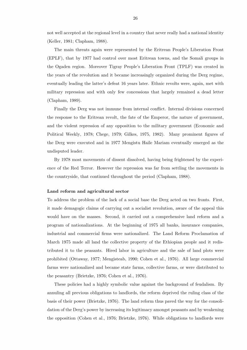
26
not well accepted at the regional level in a country that never really had a national identity
(Keller, 1981; Clapham, 1988).
The main threats again were represented by the Eritrean People’s Liberation Front
(EPLF), that by 1977 had control over most Eritrean towns, and the Somali groups in
the Ogaden region. Moreover Tigray People’s Liberation Front (TPLF) was created in
the years of the revolution and it became increasingly organized during the Derg regime,
eventually leading the latter’s defeat 16 years later. Ethnic revolts were, again, met with
military repression and with only few concessions that largely remained a dead letter
(Clapham, 1989).
Finally the Derg was not immune from internal conflict. Internal divisions concerned
the response to the Eritrean revolt, the fate of the Emperor, the nature of government,
and the violent repression of any opposition to the military government (Economic and
Political Weekly, 1978; Chege, 1979; Gilkes, 1975, 1982). Many prominent figures of
the Derg were executed and in 1977 Mengistu Haile Mariam eventually emerged as the
undisputed leader.
By 1978 most movements of dissent dissolved, having being frightened by the experi-
ence of the Red Terror. However the repression was far from settling the movements in
the countryside, that continued throughout the period (Clapham, 1988).
Land reform and agricultural sector
To address the problem of the lack of a social base the Derg acted on two fronts. First,
it made demagogic claims of carrying out a socialist revolution, aware of the appeal this
would have on the masses. Second, it carried out a comprehensive land reform and a
program of nationalizations. At the beginning of 1975 all banks, insurance companies,
industrial and commercial firms were nationalized. The Land Reform Proclamation of
March 1975 made all land the collective property of the Ethiopian people and it redis-
tributed it to the peasants. Hired labor in agriculture and the sale of land plots were
prohibited (Ottaway, 1977; Mengisteab, 1990; Cohen et al., 1976). All large commercial
farms were nationalized and became state farms, collective farms, or were distributed to
the peasantry (Brietzke, 1976; Cohen et al., 1976).
These policies had a highly symbolic value against the background of feudalism. By
annuling all previous obligations to landlords, the reform deprived the ruling class of the
basis of their power (Brietzke, 1976). The land reform thus paved the way for the consoli-
dation of the Derg’s power by increasing its legitimacy amongst peasants and by weakening
the opposition (Cohen et al., 1976; Brietzke, 1976). While obligations to landlords were

27
annuled, taxes to the government were still due. Initially the 1967 Agricultural Income
Tax Proclamation remained in effect since that did not depend upon ownership (Brietzke,
1976), but it was later replaced by the Rural Land Fee and Agricultural Activities Income
Tax Proclamation in 1976.
The new legislation also provided for the creation of peasants associations (PAs) and
urban dwellers associations (kebele) throughout the country. Their main role was to imple-
ment the land reform and to coordinate the redistribution of land (Ottaway, 1977). More
generally they were local administrative units, also in charge of collecting taxes (Ottaway,
1977; Mengisteab, 1990; Cohen et al., 1976; Brietzke, 1976). However capacity was low at
the local level and the government committed to reducing illiteracy through the zemecha
and other campaigns. Indeed illiteracy was reduced from 90% in 1973 to 65% in 1981
(Griffin, 1992).
As the reform was being implemented, three main forms of agricultural production
emerged: family farms, cooperatives and state farms. Peasant or family farms remained
the most widespread mode of production, occupying over 90% of the cultivated area, and
they were organized in peasants associations. Cooperatives started to be more forcefully
promoted by the Government after 1978, along with collectivization, but the expected
growth in this sub-sector never occurred, neither in terms of quantity nor of productivity.
Finally state farms stem from what were commercial farms before the nationalization of
1975 (Griffin, 1992; Keller, 1985; Clapham, 1987). The agricultural development strategy
of the government was largely focussed on state farms and cooperatives, despite them
being less productive than family farms (Mengisteab, 1990; Clapham, 1987). Consequently
they were allocated the lion’s share of public resources, including a more favourable tax
treatment than family farms (Ottaway, 1977; Mengisteab, 1990).
Manufacturing sector
The manufacturing sector was also involved in the nationalization program, as all large
scale industries were put under the control of the Ministry of Industry8 in 1976 (Wubneh,
1990; Griffin, 1992). Private initiative was generally discouraged, including legal restric-
tions for capital investments (Griffin, 1992). Since the nationalization program did not
provide for any compensation, foreign investment stopped flowing into the country. Any
incentive to improve profitability was slashed by top marginal tax rate as high as 89%.
8The Ministry of Industry in turn was under the Office of the National Committee for Central Planning(ONCCP).

28
In addition all the after-tax profits of state firms were to be transfered to the government
(see section 2.4.3).
Besides government policy, the private sector suffered also because of internal conflicts
that led not only to the destruction of some factories in Eritrea and in the East, but also
to shortage of raw materials and spare parts, difficulties in transport, the lack of foreign
exchange and power shortages (Griffin, 1992).
However Eshetu Chole (2004) holds that the performance of the industrial sector was
still more respectable than that of agriculture. This is confirmed by national accounts
data that indeed show an average growth rate in the agricultural sector of 1.5% as com-
pared to 3.8% in manufacturing over the Derg period. Despite this better performance
manufacturing remained only a marginal contributor to GDP under the Derg, as shown
in figure 2.2, although its share was larger than in the Imperial period (see table 2.1).
As a result of bad economic policies, both in the agricultural and in the industrial
sectors, GDP per capita was generally lower in the first years of the Derg than at the end
of the Imperial rule (see figure 2.5).
Figure 2.2: GDP composition: selected sectors as a share of total
Source: author’s calculations using data from the Ministry of Finance and Economic Development
Consolidation and planning
Starting from 1979, with the establishment of the Committee for Organizing the Party of
the Workers of Ethiopia (COPWE), the Derg put a systematic effort in building the insti-
tutions of a socialist state (Keller, 1985). The whole process however was slow, directed
from the top, and it fully reflected existing power structures (Keller, 1985, 1981; Gilkes,

29
1982).
In 1984 the Workers Party of Ethiopia (WPE) was launched and a new constitution was
introduced in 1987, formally establishing the People’s Democratic Republic of Ethiopia.
Both the constitutional process and the formation of the party were attempts of the Derg to
gain political legitimization for the increasingly unpopular military ruling class. However
no concessions were made on the demands of opposition groups and thus the process could
at best deliver an appearance of representation (Clapham, 1988).
On the planning side, the Office of the National Committee for Central Planning
(ONCCP) was part of the new institutional setup and it was aimed at taking the lead
on economic development. A decade after the revolution, it launched in 1984 the Derg’s
first development plan: the Ten Years Development Plan. The timing of its launch was
particularly unfortunate, as a major famine broke out in 1984 therefore implying a shift of
all national efforts towards the emergency. The famine also accelerated the villagization
and resettlement campaigns that were essentially representing the core of development
policy before the 10-year plan (Keller, 1985; Clapham, 1987). The weakness of the plan’s
design and implementation was exposed by a consistent shift of public expenditure away
from development and services towards control functions. This is particularly the case of
military expenditure that was needed to maintain the Derg’s authority (Clapham, 1988;
Eshetu Chole, 2004).
As the consolidation process continued and power concentrated increasingly in Mengistu’s
hands, continuity with the Imperial regime became more clear. In fact the central thesis
of Clapham (1988) is that:
“There has been a revolution. Much has changed. But a sense of what has
changed, and how, is to be gained only through an appreciation of continuity.”
This continuity in particular entailed the political culture and style of administration,
based on personal relations, suspicion and the lack of independent institutions; nation-
alism expressed in the slogan “Ethiopia First”, that can be compared to Haile Selassie’s
vision of “Greater Ethiopia” (Keller, 1985); and the cult of personality and centralism in
decision making that increasingly developed within the Derg. The strong state and the
attitudes towards political authority developed under the Imperial regime were in fact not
an obstacle but rather an advantage of the new military government and a determinant
of the success of the revolution (Clapham, 1988).
The Derg finally never obtained legitimacy and support from the people. An attempted
coup in 1989 and the military losses in Tigray and Eritrea, that by the late 80s were fully
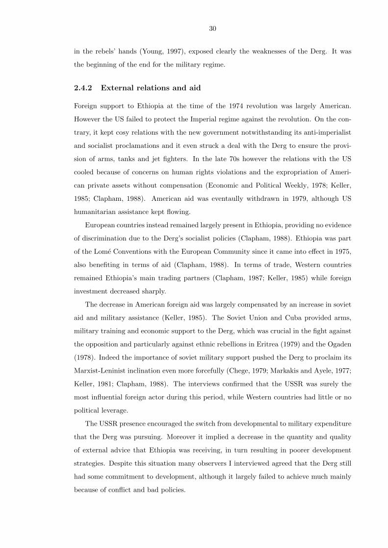
30
in the rebels’ hands (Young, 1997), exposed clearly the weaknesses of the Derg. It was
the beginning of the end for the military regime.
2.4.2 External relations and aid
Foreign support to Ethiopia at the time of the 1974 revolution was largely American.
However the US failed to protect the Imperial regime against the revolution. On the con-
trary, it kept cosy relations with the new government notwithstanding its anti-imperialist
and socialist proclamations and it even struck a deal with the Derg to ensure the provi-
sion of arms, tanks and jet fighters. In the late 70s however the relations with the US
cooled because of concerns on human rights violations and the expropriation of Ameri-
can private assets without compensation (Economic and Political Weekly, 1978; Keller,
1985; Clapham, 1988). American aid was eventaully withdrawn in 1979, although US
humanitarian assistance kept flowing.
European countries instead remained largely present in Ethiopia, providing no evidence
of discrimination due to the Derg’s socialist policies (Clapham, 1988). Ethiopia was part
of the Lome Conventions with the European Community since it came into effect in 1975,
also benefiting in terms of aid (Clapham, 1988). In terms of trade, Western countries
remained Ethiopia’s main trading partners (Clapham, 1987; Keller, 1985) while foreign
investment decreased sharply.
The decrease in American foreign aid was largely compensated by an increase in soviet
aid and military assistance (Keller, 1985). The Soviet Union and Cuba provided arms,
military training and economic support to the Derg, which was crucial in the fight against
the opposition and particularly against ethnic rebellions in Eritrea (1979) and the Ogaden
(1978). Indeed the importance of soviet military support pushed the Derg to proclaim its
Marxist-Leninist inclination even more forcefully (Chege, 1979; Markakis and Ayele, 1977;
Keller, 1981; Clapham, 1988). The interviews confirmed that the USSR was surely the
most influential foreign actor during this period, while Western countries had little or no
political leverage.
The USSR presence encouraged the switch from developmental to military expenditure
that the Derg was pursuing. Moreover it implied a decrease in the quantity and quality
of external advice that Ethiopia was receiving, in turn resulting in poorer development
strategies. Despite this situation many observers I interviewed agreed that the Derg still
had some commitment to development, although it largely failed to achieve much mainly
because of conflict and bad policies.
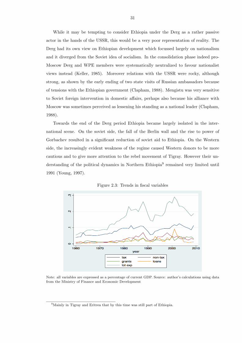
31
While it may be tempting to consider Ethiopia under the Derg as a rather passive
actor in the hands of the USSR, this would be a very poor representation of reality. The
Derg had its own view on Ethiopian development which focussed largely on nationalism
and it diverged from the Soviet idea of socialism. In the consolidation phase indeed pro-
Moscow Derg and WPE members were systematically neutralized to favour nationalist
views instead (Keller, 1985). Moreover relations with the USSR were rocky, although
strong, as shown by the early ending of two state visits of Russian ambassadors because
of tensions with the Ethiopian government (Clapham, 1988). Mengistu was very sensitive
to Soviet foreign intervention in domestic affairs, perhaps also because his alliance with
Moscow was sometimes perceived as lessening his standing as a national leader (Clapham,
1988).
Towards the end of the Derg period Ethiopia became largely isolated in the inter-
national scene. On the soviet side, the fall of the Berlin wall and the rise to power of
Gorbachev resulted in a significant reduction of soviet aid to Ethiopia. On the Western
side, the increasingly evident weakness of the regime caused Western donors to be more
cautious and to give more attention to the rebel movement of Tigray. However their un-
derstanding of the political dynamics in Northern Ethiopia9 remained very limited until
1991 (Young, 1997).
Figure 2.3: Trends in fiscal variables
Note: all variables are expressed as a percentage of current GDP. Source: author’s calculations using datafrom the Ministry of Finance and Economic Development
9Mainly in Tigray and Eritrea that by this time was still part of Ethiopia.

32
2.4.3 Fiscal trends
The 1974 revolution sparked demands from the masses both in the urban centers and in
more remote ethnic communities. These political demands were readily directed to the
military government itself as soon as it took power. Indeed Clapham (1988) holds that
“the major effect of revolution was [. . . ] not that the state apparatus was weakened, but
that it was required to do much more.” This increased role of the state implied a need to
increase public resources and it was largely in line with the socialist ideology embraced by
the new regime.
Figure 2.3 shows clearly that since its establishment in 1974 the Derg has increased
both tax revenue and expenditure. The former is particularly impressive considering that
the new regime had neither full control on the country nor popular support in its early
years. It is therefore plausible that the increase in revenue was more the result of coercion
and intimidation than of a genuine social contract, particularly given the contemporaneous
shrinking of the development and services budget in favor of military expenditure.
Non-tax revenues also increased significantly, initially due to the expropriations carried
out in the first years of the regime (Clapham, 1989) and to the contribution of state firms
to the budget through ‘government investment income’. This represented the transfer of
post-tax profits to the government, so that state enterprises contributed both through
tax and non-tax revenue. In addition the government was extracting surplus from the
agricultural sector using a system of quotas and price controls, although these resources
did not show in the budget (see appendix 2.A for more details).
Despite the increase in revenues, the government was still experiencing a resource gap
resulting in increasing levels of debt (Eshetu Chole, 2004). The increase in budget deficit
appears clearly in figure 2.4 that shows an increase in the use of this instrument exactly
starting from the 1974 revolution. As far as foreign debt is concerned, the situation
deteriorated so much that in 1990 payments of all debt obligations were frozen except
those to international financial institutions and other critical ones (Eshetu Chole, 2004).
All fiscal variables, and particularly tax, non tax revenue and expenditure, seem to peak
in 1988/89 then decrease steadily until the end of the regime in 1991. This decline is due to
the deteriorating economic, military and political situation in the country. The economic
crisis is essentially the result of over a decade of poor economic policies, including the
overextension of the state in the economy, a bad investment climate, and the deterioration
of terms of trade (Eshetu Chole, 2004). Militarily the Derg was suffering huge losses and
defeats in the north and the morale of the armed forces was quickly deteriorating. This
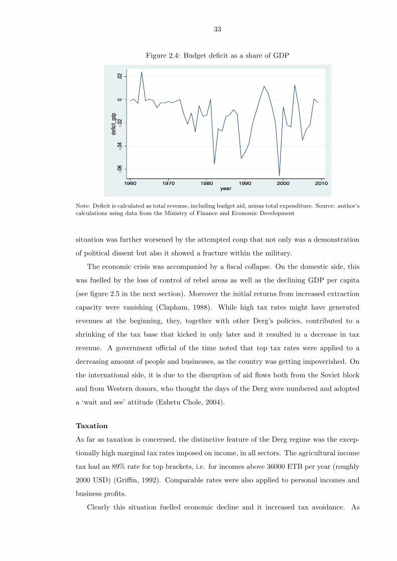
33
Figure 2.4: Budget deficit as a share of GDP
Note: Deficit is calculated as total revenue, including budget aid, minus total expenditure. Source: author’scalculations using data from the Ministry of Finance and Economic Development
situation was further worsened by the attempted coup that not only was a demonstration
of political dissent but also it showed a fracture within the military.
The economic crisis was accompanied by a fiscal collapse. On the domestic side, this
was fuelled by the loss of control of rebel areas as well as the declining GDP per capita
(see figure 2.5 in the next section). Moreover the initial returns from increased extraction
capacity were vanishing (Clapham, 1988). While high tax rates might have generated
revenues at the beginning, they, together with other Derg’s policies, contributed to a
shrinking of the tax base that kicked in only later and it resulted in a decrease in tax
revenue. A government official of the time noted that top tax rates were applied to a
decreasing amount of people and businesses, as the country was getting impoverished. On
the international side, it is due to the disruption of aid flows both from the Soviet block
and from Western donors, who thought the days of the Derg were numbered and adopted
a ‘wait and see’ attitude (Eshetu Chole, 2004).
Taxation
As far as taxation is concerned, the distinctive feature of the Derg regime was the excep-
tionally high marginal tax rates imposed on income, in all sectors. The agricultural income
tax had an 89% rate for top brackets, i.e. for incomes above 36000 ETB per year (roughly
2000 USD) (Griffin, 1992). Comparable rates were also applied to personal incomes and
business profits.
Clearly this situation fuelled economic decline and it increased tax avoidance. As
34
emerged from interviews, nobody had any incentive to increase their income, individuals
and private businesses alike, given that the benefit would accrue mainly to a state that
was delivering little in return. There is no doubt that this attitude contributed to the
economic decline that became apparent in the last years of the regime.
However the Derg could count on relatively easy to collect taxes such as indirect and
trade ones. These were relatively easy to administer, as they were collected respectively
at the factory gate and at the border. Moreover the large state sector, including farms
and enterprises, was a source of both tax and non-tax revenue. Finally most taxes were
collected in urban centers that largely remained under government control even when the
guerrilla was ongoing in the countryside (Young, 1997; Clapham, 1988).
As far as agricultural taxation is concerned, two main tax types were levied: the
agricultural income tax and the land use tax. These were introduced by the Derg and
they largely replaced the previous system of obligations. The contribution of agricultural
taxation to state revenue more than doubled in the early years of the Derg (Markakis,
1989). However tax incidence in rural areas after the reform is estimated at 5% (Griffin,
1992) and Eshetu Chole (2004) holds that generally the agricultural sector was not an
important source of tax revenue. Although peasants were requested to pay tax, they
received little in return as most resources were directed to state farms (Markakis, 1989).
Family farms were also discriminated in terms of the land use tax, that was levied
irrespective of location or soil fertility. The annual rate was 10 Birr (about 0.5 USD) for
those who were not members of cooperatives, 5 Birr for those who were members and 2
Birr per hectare for state farms (Eshetu Chole, 2004). The tax was levied per holding and
regardless of the plot size. Also falling on the agricultural sector were trade taxes, with
the coffee sector being one of the main sources of revenue. Clapham (1987) reports that
the share of export price paid to producers fell from 67% before the revolution to 33%
afterwards. Notwithstanding this heavy burden on producers, little evasion was possible
given the tight controls of the government which included internal customs to prevent
smuggling (Clapham, 1987).
In a last attempt to gain popularity, and realizing the declining international standing
of socialism, the Derg tried to introduce some degree of liberalization in the economy
starting from 1988. In particular this entailed the expansion of fiscal incentives for invest-
ment, including exemptions from custom duties and income tax. Moreover in 1990 the top
marginal income tax rate was reduced from 89% to 59% (Eshetu Chole, 2004). However
the reform of the dying regime was too little and too late.

35
2.5 The Ethiopian People’s Revolutionary Democratic Front:
1991 - today
Throughout the Derg regime liberation movements had been active in the country and
particularly the Tigray People’s Liberation Front (TPLF) and the Eritrean People’s Liber-
ation Front (EPLF), the two forces that eventually led to the defeat of the military regime.
After 16 years of armed struggle starting in 1975, they finally reached Addis Ababa in
May 1991. Recognising the defeat, which to many observers had been just a matter of
time for a couple of years, Mengistu fled to Zimbabwe. Proving its weakness, the facade
of political institutions the Derg had created, including the Worker’s Party of Ethiopia,
valished instantly upon the fall of the regime (Markakis, 2011).
2.5.1 Transition and ethnic federalism: 1991-1998
The TPLF not only played a central role in defeating the Derg, but it also deeply shaped
Ethiopian politics after 1991. During the armed struggle it developed strong local ties,
through its fighters who were living in very modest conditions with the peasantry. The
TPLF could also count on a very strong organizational, administrative and military appa-
ratus used to administer the liberated territories under the Derg and to keep the military
regime confined to urban areas. In 1980-82, the TPLF controlled about 80% of the ter-
ritory in Tigray where 90% of the people lived (Young, 1997). The military progress
however was compromised by the famine of 1984 that completely disrupted the TPLF’s
activity. The organizational skills developed in the 80s proved crucial when the front had
to govern the whole country. Finally, the TPLF had a well developed ideology based on
revolutionary change, democracy, transparency, collective leadership and the refusal of a
cult of personality for a single leader.
Aware of the need to give itself a national standing in view of the weakening and
eventual defeat of the Derg, the TPLF promoted the creation of the Ethiopian People’s
Revolutionary Democratic Front (EPRDF) in 1989. The EPRDF, which is still governing
Ethiopia today, is an umbrella organization composed of different ethnic-based fronts and
parties, including the Amhara, Oromo, Tigrayans and Southern People. The EPRDF
initially embraced a Marxist ideology that however was later softened to ensure alliances
in the West (Young, 1997; Hagmann and Abbink, 2011).
While the experience of the struggle was crucial to the TPLF and EPRDF success,
it also posed some difficulties as regards the transition from a guerrilla movement to a

36
national government. First of all, there was a need for national representativeness beyond
the northern provinces. Secondly some of the traditional practices of the EPRDF, such
as the system of evaluation of the leadership10, found opposition amongst bureaucrats at
the national level. Thirdly the rise to power of EPRDF resulted in a gradual distancing
of its leadership from its peasant base, that was ever more anxious to see its demands
met as well as improvements in terms of poverty and development (Young, 1997; Medhane
Tadesse and Young, 2003).
Since the transitional conference that eventually formalized the EPRDF government
with Meles Zenawi as President, the focus was largely on ethnic groups and nationalities.
The EPRDF essentially accepted the right of self determination “up to and including
secession”, which was enshrined in the 1994 Constitution. Indeed in 1994 Eritrea separated
from Ethiopia following a referendum that resulted in a staggering 99.8% of the votes in
favor of independence (Young, 1997). In 1992 regional elections were held where ethnic
groups were allowed to choose leaders from their own background (Young, 1997; Abbink,
2011). Elected officials were trained in EPRDF special schools on the party’s program and
then sent back to the regional level (Markakis, 2011). In the meantime EPRDF troops
and officials were sent to the periphery to ensure control and administrative support.
The only challenge for the new government was the Oromo Liberation Front (OLF) that
never collaborated with the EPRDF and boycotted the 1992 elections. General elections
were held in 1995, resulting in an overwhelming EPRDF victory, the establishment of the
Federal Democratic Republic of Ethiopia and the confirmation of Meles Zenawi as leader
(now Prime Minister).
As in the case of the Derg, the EPRDF benefited from the legacy of a strong state which
was used as an administrative base rather than being dismantled. Indeed kebeles11 were
maintained and they later became a central tool for government control in the periphery.
The challenge therefore was the democratization and legitimization of a state that was
largely inherited by the Derg (Young, 1997).
Ethnic federalism
The most important characteristic of the new government by far was the decentralization
of the state and the introduction of ethnic federalism. The level of ambition and radical
10The evaluation system adopted during the armed struggle was called gim gimma and it was essentiallya process of popular critical evaluation aimed at assessing the front’s policies, programme, leadership andconduct (Medhane Tadesse and Young, 2003; Hagmann and Abbink, 2011).
11Kebeles are the lowest level of decentralized public administation.

37
change of the federalist project cannot be underestimated, as underlined by two intervie-
wees with a long experience in Ethiopia. This is enshrined in a quote from Meles, from
an interview released in 2010 at the 5th International Conference of Federalism 12:
“Unlike other developmental states [. . . ], the approach here is for massive grass-
roots mobilisation. You can’t have massive grassroots mobilisation on the basis
of a national uniform plan. It has to vary not only from region to region but also
from village to village, because the circumstances in each village are unique.
So the national plan, the national framework, is just that: a framework on the
basis of which every village will have to write its own story, but a story that
will add up into the national development plan.”
Partly because of its ambitious and innovative character, the implementation of the
federalist project encountered a few challenges from the very beginning. These included the
definition of ethnic groups, the adoption of local languages, and the legitimization of the
new administration in areas where the EPRDF was less rooted than Tigray such as Oromia,
Amhara and Southern regions. As a result, often the EPRDF had to get actively involved
in creating the conditions for decentralization, with training and propaganda (Markakis,
2011). Easing the capacity constraints at the local level was in the mandate of the Ministry
of Federal Affaires that also ensured the involvement of the central government in regional
affaires (Abbink, 2011).
While ethnic federalism was clearly the main feature of the EPRDF period, and in-
deed it was de facto in place already in 1991, full implementation and operationalization
were rather challenging throughout the 90s. The project was then complemented with
the woreda-level13 decentralization started in the early 2000s and characterized by more
administrative than ethnic salience. This process entailed the multiplication of woredas
across the country and it thus involved a huge increase in local resource needs both in
terms of human resources and financing.
2.5.2 Economic policies in the 90s
The Ethiopian economy taken up by the EPRDF in 1991 was in dire conditions (Markakis,
2011). Figure 2.5 shows that GDP per capita had been decreasing ever since the mid 80s.
A few years after taking power Meles Zenawi, aware of the centrality that economic poli-
12See www.ethiopianfederalism.org.13Woredas are the local level of administration at a further decentralized level below Regions.

38
cies would have, started a degree in economics at the Open University in Britain and
instructed cabinet officials and fellow guerrilla soldiers to do the same. He later continued
his education at the Erasmus University in Rotterdam and his thesis titled “African devel-
opment: dead ends and new beginnings”, completed in 2004, is still a reference document
for understanding the economic policies of Ethiopia (Gill, 2010).
Figure 2.5: GDP per capita at constant prices
Source: author’s calculations using data from the Ministry of Finance and Economic Development
In the early 90s however the Government was still dealing with political issues, not
least the establishment of ethnic federalism. Partly to ensure Western support and partly
to distinguish itself from the previous regime, the EPRDF declared its intent to move
towards a market economy, although the real commitment was unclear (Eshetu Chole,
2004). In this context, in the early 90s the EPRDF started a process of liberalization and
privatization under the auspices of the international financial institutions. Financial and
technical support was provided already in 1991 by the African Development Bank, the
European Community, the World Bank and the International Monetary Fund, that later
supported also the Structural Adjustment Program (SAP) of 1993-96.
One of the sectors to be liberalized, at least partly, was the financial sector that so
far had been dominated by the Commercial Bank of Ethiopia. Reforms in the early 90s
allowed the private sector to engage in banking and insurance, although this was restricted
to Ethiopian nationals (Alemayehu Geda, 2011). The liberalizations involved also the
agricultural sector, reintroducing hired labour and eliminating restrictions to plot size
(Markakis, 2011). The EPRDF also encouraged capitalist farming and the establishment
of larger plots, particularly in the lowland areas (Young, 1997). However public land

39
ownership was maintained and even given a constitutional basis. The need to increase
productivity of smallholders and the importance of industrialization were enshrined in
the Agricultural Development Led Industrialization (ADLI), a long term strategy that
entailed a focus on agriculture and that continued to shape development efforts for many
years hence (Alemayehu Geda, 2011).
Privatizations were also carried out but its implementation was slow, also due to the
lack of private investors. This slow progress is part of the reason for delayed payments
under the SAP, which after the first tranche of 1993 were frozen for 23 months (see figure
2.8). The privatizations often resulted in the transfer of ownership from the state to
members of the party or party affiliates14 (Markakis, 2011). Since the role of the party in
the economy was formally outside the state proper, the issue did not raise the complaints
of the international community. A truly private sector therefore remained limited, also
due to the lack of faith that the EPRDF had in it as a promoter of development.
While some effort was made towards liberalization, the interviewees with direct expe-
rience of this period hold that the process was undertaken reluctantly and half-heartedly.
The EPRDF was still essentially anchored to marxist ideals and it did not have faith in a
purely market oriented economy. Indeed the limits of the liberalization process were very
clear for the Ethiopian government. A few issues remained non-negotiable then, and still
are not today, such as public land ownership, the liberalization of telecommunications and
the international opening of the financial sector. This tendency to a large role of the public
sector will become more clear with the emergence of the idea of developmental state.
2.5.3 The war with Eritrea and the TPLF crisis: 1998-2002
The late 90s and early 2000s represented a turning point for the EPRDF and they marked
the emergence of its current profile.
In 1998 war erupted with Eritrea over a border dispute, after years of rather peaceful
relations. This caused the suspension of aid disbursements to Ethiopia on grounds of a
‘peace conditionality’ based on the view that development aid could not be delivered to
a country that was scaling up its military spending, which Ethiopia was indeed doing
massively during the war (Gill, 2010; Markakis, 2011).
While the war was raging the country, bad rains in the area of Wollo and in the Somali
14One example is the Endowment Fund for the Rehabilitation of Tigray (EFFORT) established by theTPLF in 1995. EFFORT was a conglomerate of industrial, financial and service enterprises meant to helpthe reconstruction of Tigray. Other regions later followed this example and established similar bodies.

40
region caused acute food shortages. Since aid was not available, or at least was much short
of what was needed, the affected people had to sell their assets and thus they became even
more vulnerable to the subsequent drought (Hammond and Maxwell, 2002). There is little
doubt that the war with Eritrea was a major reason for the slow response of donors to
what was called an ‘averted famine’, although many in the affected areas suffered of severe
malnutrition and died as a consequence (Hammond and Maxwell, 2002).
A truce was eventually reached in 2000 with the mediation of the Organization of the
African Union (OAU) and the United Nations. An agreement was reached on the border
issue in 2001 and aid resumed. However the tension with Eritrea remained high and the
two countries suspended all relations.
One of the consequences of the war was the emergence within the party of two factions.
The first one, led by Meles and eventually prevailing, was more sensitive to international
pressure and it was thus in favor of a conciliatory approach that would lead to an early
ending to the conflict. The second faction was for a full scale offensive against Eritrea
(Medhane Tadesse and Young, 2003). The war was certainly one of the causes of the 2001
TPLF crisis, but not the only one.
The tension within the party was further exacerbated on the occasion of one of the
TPLF’s customary evaluations. The main themes of discussion, presented by Meles, were
the decaying of the TPLF leadership, the increasing distance from its constituency and the
concerns over the influence of foreign powers in Ethiopia (Medhane Tadesse and Young,
2003). These were far reaching and delicate themes that indeeed sparked a heated debate
from which Meles emerged as the undisputed leader (Medhane Tadesse and Young, 2003).
The crisis marked a turning point in the history of the EPRDF for at least three
reasons. First, the emergence of a strong single leader implied a shift away from collec-
tive leadership and towards centralism. Secondly it underlined the need for the EPRDF
to improve national legitimacy, thus softening the ethnic discourse. The focus switched
from ethnicity to poverty and economic development. This entailed a massive increase
in resources for development and service delivery at the woreda level starting in 2001.
Notably devolution of powers to the woreda level had no ethnic salience as it was a purely
administrative process. Thirdly the attention moved from political to economic issues, in
a partial ideological shift. The government was now willing to be integrated in the world
economy and to open to capitalism, which was never clearly indicated before. However
the EPRDF maintained some central features, such as the central role of the state in the
economy, the commitment to federalism, public ownership of land, and support for the

41
peasants (Medhane Tadesse and Young, 2003). Moreover the link between the party an
the state strengthened even more after the crisis.
In this context, foreign relations were enhanced as Meles was seen as a moderate
modernizer (Markakis, 2011). The role of donors was crucial in determining the fate of
the war, and thus in the crisis as well, with the imposition of the ‘peace conditionality’.
The government coming out of the 2001 crisis was certainly a good ally of the West but
also a more assertive and confident one than donors had gotten used to during the 90s.
2.5.4 Consolidation and reform
As the political challenges were overcome, the government could fully focus on economic
issues. The underlying ideology for economic policy in the 2000s was that of a develop-
mental state. This concept is largely in line with the idea of revolutionary democracy15
that characterized the TPLF/EPRDF since the struggle and that after 2002 was more
forcefully opposed to liberal democracy. The ambiguous relation between the idea of
developmental state and the opening to the market economy caused some tension with
international donors. However Meles was not willing to compromise and he remained un-
persuaded by the validity of applying liberalism to a developing economy. His view was
reinforced by the support of prominent economists like Joseph Stiglitz who was not only
his mentor but also a personal friend (Gill, 2010; Dereje Feyissa, 2011). In 2008, during a
two hours questions session following the presentation of his thesis on the developmental
state16, Meles reportedly said17:
“We in Ethiopia very nicely and politely have rejected a number of neoliberal
prescriptions given to us, and we have lived to tell the story”
In this context of renewed confidence the government also reappropriated the political
space for reform that was largely limited before 2001, as suggested by a top government
official with a long experience with the EPRDF. The Civil Service Reform started in 1996
was revived in the early 2000s. The overarching objective was to create a qualified and
technically prepared civil service, including in the area of tax administration (MOFED,
15Revolutionary democracy was the ideology adopted by the TPLF/EPRDF to promote democratizationin Ethiopia and the empowerment of ethnic groups. The concept has its roots in Leninism, though it isinfused with democratic principles (Abbink, 2011). Indeed it postulates the need for a strong vanguardparty, ruling in the name of the rural masses, the commitment to the right of self-determination, theintertwining between the party and the state, and their dominant role in politics, the economy and society(Abbink, 2011; Hagmann and Abbink, 2011).
16“Dead ends and new beginnings” is Meles’s thesis where the concept of developmental state is outlined.17Cited in (Gill, 2010).
42
2002). In 2002 a major reform was carried out in the area of taxation as well, that had
received only marginal attention since 1991. The reform represented a major effort to
improve revenue mobilisation that was falling short of the needs stemming from adminis-
trative reforms, decentralization and the re-militarization carried out during the late 90s.
Notwithstanding the rocky relations with the IMF, the area of taxation was actually one
in which there was much agreement and indeed the IMF, along with other donors, played
a crucial role in supporting the tax reform (see section 2.5.6 for details).
The renewed confidence of the EPRDF after the 2001 crisis may also help explain the
liberal approach adopted towards the 2005 elections. The run up to the elections was
marked by much fervor, with the emergence of partisan newspapers and publicly broad-
casted debates (Markakis, 2011; Gill, 2010). Many interviewees remember the absolute
confidence of the EPRDF to win the elections that were seen more as an opportunity
for broad endorsement and fine-tuning than for a radical change. The opposition par-
ties, opposed to federalism and supporting more liberal economic policies, eventually lost
the elections after a heated debate in which both sides claimed victory. In the months
following the elections tension was high and violence erupted in the streets in November
2005, causing 200 deaths (Markakis, 2011). International donors, particularly the EU,
adopted a hard line against the Government and the situation quickly escalated to a per-
sonal confrontation between Meles and Ana Gomes, the electoral mission’s chief observer
(Gill, 2010). The political ferment preceeding the 2005 elections was never seen again,
with essentially no organized opposition operating in the country since then (Markakis,
2011).
Although the government won the elections, the result was a major blow as the oppo-
sition succeeded in getting a substantial number of votes. This shock prompted a moment
of reflection and evaluation within the EPRDF leadership. This process resulted in a rein-
forcement of the developmental state as the main ideology of the EPRDF. In the aftermath
of the 2005 elections it became even more clear that the government’s legitimacy would be
based on its strong and effective role in development and poverty reduction in the name of
the people of Ethiopia. The renewed focus on national development also sped up the move
from ethnicity to nationalism already underway in the EPRDF since the early 2000s.
It is in this context that the government engaged in a ‘big push’ towards GDP growth
and economic development that emerged clearly in the 2005 Plan for Accelerated and
Sustained Development to End Poverty (PASDEP) and even more so in the 2010 Growth
and Transformaiton Plan (GTP). The new enemy was now poverty and the nation was

43
called to unite towards its eradication.
Figure 2.6: Growth rate of GDP at constant prices
Source: author’s calculations using data from the Ministry of Finance and Economic Development
Following the developmental state thesis, the government scaled up massively its efforts
in infrastructure development. One of the best examples of this are the dams currently
being built, including the Great Ethiopian Reinassance dam on the Blue Nile River. No-
tably this dam, which will be the biggest of its kind in Africa, is fully funded with domestic
resources since donors did not want to get involved due to the dispute with other countries
regarding the Nile waters. This dam emerged in many interviews as a symbol of Ethiopian
independence and pride.
On the agricultural side progress was made to attract foreign investors in commercial
agriculture. Land lease contracts were stipulated in the context of what is internationally
labelled ‘land grab’ or ‘the second scramble for Africa’. These contracts entail very low
tax rates on profits and exemptions are granted for several years since establishment
(Markakis, 2011). In both cases of land lease to foreign investors and the construction of
dams, the process is largely controlled from the top, thus confirming the growing tendence
to centralism.
The ‘big push’ for development expenditure and economic growth is reflected in GDP
figures that show staggering growth rates, consistently at double digit since the economy
recovered from the 2001-2002 drought (see figure 2.6). Figure 2.5 shows that GDP per
capita doubled since the early 2000s. While these figures are partly justified by the projects
and scaling up of service delivery at the woreda-level, they are also the object of much
criticism by the IFIs as well as academics (Dercon and Zeitlin, 2009). The IFIs have

44
argued that GDP figures are largely inflated and the continuous confrontation with the
WB’s former Country Director Ken Ohashi was mentioned several times in the interviews.
In conclusion, it seems like the EPRDF went gradually back to the tradition of central-
ism that was typical of the previous regimes. The thesis of transformation and continuity
developed in Clapham (1988) is therefore picked up again by observers of today’s Ethiopia
such as Abbink (2011). Moreover Markakis (2011) holds that this tradition of authori-
tarianism and centralism inherited from the imperial period is precisely one of the two
obstacles that Ethiopia is still to overcome, together with the integration of the lowlands
populations in the periphery of the state.
2.5.5 External relations
Since aid and the relation with donors18 was a central part of the interviews, this section
is largely based on interviews to both government and donors officials.
After 1991 Ethiopia has received increasing amounts of aid, in the context of develop-
ment programs such as the 1991 Emergency Recovery and Reconstruction Program and
the 1993 SAP. As reported in table 2.1, grants and loans amount to about 3% of GDP
each in the EPRDF period, adding up to a 6% for all aid. In terms of aid dependecy,
defined as total aid (loans and grants) as a share of total expenditure, the average in the
EPRDF period is 28% (see table 2.1). Figure 2.7 shows that aid indeed increased as a
source of governemnt funding in correspondence with the SAP. While these figures may
seem high, it is worth noting that aid per capita was only 211 ETB per head in 2009/2010
(equivalent to about 7.5 GBP).
In the 90s the government engaged in the liberalization process described in section
2.5.2 as part of a “strategic softening” of EPRDF ideology (Dereje Feyissa, 2011). This
not only allowed the party to obtain funds for reconstruction and new allies, but also to
draw a clear distinction with the Derg, notwithstanding several ideological similarities.
Despite the fact that the development strategy in the 90s was largely dictated by donors,
the EPRDF was able to draw clear lines for what it was willing to accept. An interviewee
put it rather neatly, dividing policy dialogue in three categories. The first one is the area
of agreement, including topics like health and education. The second one is the area of
18Ethiopia has received over the period more multilateral than bilateral aid, with the main multilateraldonors being the World Bank (IDA), the UN system (UNICEF, UNDP and WFP for emergency assistance),the European Union and the African Development Bank. On the bilateral side the largest bilateral donorshave historically been the United States, Japan, Italy and Canada, with also Germany, The Netherlands,Norway and the UK playing an important role.

45
Figure 2.7: Aid dependency: grants and loans as a share of total expenditure
Source: author’s calculations using data from the Ministry of Finance and Economic Development
compromise, where ideas proposed by the donors may be adopted even if the government
is not really enthusiastic about it as long as they are in line with the government’s vision.
The third one is the ‘no-go’ area and it includes topics like the liberalization of the financial
sector, of telecommunications and the privatization of land. In this area no compromise
was reached even in the 90s.
The first clear rupture in donor-government relations occurred in 1998 when donors
stopped aid to Ethiopia because of the war with Eritrea, which also coincided with the
‘averted famine’. This rupture fuelled the Ethiopian government’s perception that donors
were unreliable and not trustworthy as they abandoned the country at a time of need.
Moroever the relations with foreigners were at the centre of the TPLF debate thus sparking
a strong willingness to maintain control and independence over policy making. Indeed the
problem of the government was to “maximize the inflow of resources (so it can finance as
much as possible), while giving up as little sovereignty (in terms of control over the policy
agenda) as possible” (Furtado and Smith, 2007).
When donors came back to the country in 2000, the approach to development was
shifting towards untied budget support, the use of country systems and a stronger fo-
cus on ownership (Dereje Feyissa, 2011). The first poverty reduction strategy program,
the Sustainable Development and Poverty Reduction Program (SDPRP), adopted in the
early 2000s, had a strong focus on untied budget support. This is reflected in figure 2.7
that shows increased foreign presence in the budget at this time, sustained by the strong
commitment to development of the Ethiopian government that was providing a ‘posi-

46
tive development story’ for donors. However this commitment was not the only element
attracting donors and perhaps not the most important one either.
The terrorist attacks of September 11th 2001 reinforced the strategic significance that
Ethiopia had lost with the end of the Cold War, but that had already been revived by
the bombings of US embassies of Nairobi and Dar es Salam in 1998 (Dereje Feyissa,
2011). With the start of the war on terror Ethiopia became a crucial ally of the US in
a region (the Horn) of political instability and extreme islamist tendencies. During my
interviews with the donor community, even the most technocratic institutions recognised
that geopolitical factors are the main determinants of aid in the country. An interviewee
put it rather clearly: “donors want to stay in Ethiopia for two reasons: first, development
objectives and poverty reduction; second, strategic interests. But really, the order is more
realistically reversed.” This view is confirmed in virtually all interviews within the donor
community and it is also supported in Furtado and Smith (2007) when they state that:
“Changes in the level of donor assistance to Ethiopia have been driven over-
whelmingly by political and geopolitical considerations [. . . ]. These factors,
rather than anything the government has consciously done to manage the aid
agenda, have largely determined the level of aid inflows.”
As capacity constraints were still a major issue both in the center and in the periphery,
the US$483 million Public Sector Capacity Building Program (PSCAP) was launched in
2004. PSCAP was aimed at improving public service delivery at all levels of the public
administration, increasing citizen participation and enhancing good governance and ac-
countability in the public sector. One of its six workstreams is focussed on taxation and it
entailes reinforced collaboration with donors on tax reform and revenue mobilisation, for
example including twinning programs between tax authorities in Ethiopia and the UK.
A second rupture occurred in 2005 when donors condemned the post-election violence
and withdrew untied budget support, which by that time was planned to be scaled up from
US$375 to US$500 million (Furtado and Smith, 2007). In a climate of renewed distrust
and tension, donors rather quickly came up with a solution in the form of a project,
the Protection of Basic Services (PBS), that was going to become the largest of its kind
in Africa. The largest component of PBS provides for service delivery at the local level
through the government’s financial management system and particularly through the block
grant to the regions. PBS more recently funded a project aimed at increasing transparency
and accountability that entailed the publication of the local administration’s budget in
public places such as churches, mosques and kebeles. Disclosure and dissemination of
47
budget information was also supported by the use of media such as TV and radio, as well
as budget literacy trainings for citizens at the woreda and kebele level.
An official from a major donor agency noted that, far from being a punishment for the
2005 events, PBS turned out to result in more and better aid for Ethiopia. Not only did the
program reinforce the local service delivery that the government was pursuing strongly as
a mean to reduce poverty and to increase legitimacy, but also it caused the disappearance
of donors (in terms of visibility) as all the improvements at the local level were seen as
achievements of the government. In addition the increased focus on service delivery meant
a closure of the arenas for policy dialogue on broader macroeconomic issues, that were
present under untied budget support. The government welcomed this development that
however donors might have not fully foreseen.
As a result of the ruptures in donor-government relations, the 1998 and 2005 being only
two of them19, and the the long tradition of independence and statehood, it is not surpris-
ing that donors in Ethiopia have little influence over policy and the development agenda.
This not only emerged during the interviews but is also confirmed by several scholars
(Abbink, 2011; Furtado and Smith, 2007). For example, it is recognised by donors that
the conditionality provided under PBS is hardly enforced and enforceable, besides being
rather soft. Moreover the assertiveness of the government towards ‘traditional donors’ is
certainly enhanced by the emergence of new donors and most notably China.
Generally the Ethiopian government over the years has shown a great degree of own-
ership over the development process that has somehow put donors in an uneasy situation.
On the one hand they would like to have a voice in policy making. On the other hand
ownership is precisely what donors wanted to promote under the Paris Declaration on
Aid Effectiveness, amongst others. They are therefore not in a position to criticize the
government for taking the ownership that they should rather encourage.
2.5.6 Tax revenue mobilisation
The new government in 1991 was able to take over the remains of the administrative appa-
ratus relatively quickly. Both officials and observers consistently confirmed that the state
was actually functioning throughout the transition with as little as one week of admin-
19For example, the Ethiopian government had several disagreements with the IMF and notably it isnot a ‘program country’ of the IMF, which is therefore only covering a surveillance and advisory role inthe country. The reason for this, emerging in the interviews, is that Ethiopia is not willing to take theconditions and pressure on policy making that an IMF loan would entail. Disagreement also emerged whendonors refused to fund big hydroelectric projects such as the Reinassance Dam that is seen as a centerpieceof the country’s development strategy.

48
istrative ‘blackout’. However the fiscal situation inherited from the Derg was disastrous.
Not only revenue was low and decreasing for three years in a row, but also arrears on debt
payments kept accumulating. A top government official suggested that at the beginning
of the EPRDF period debt was a central concern of the new government, more pressing
than increasing revenue. Indeed the government succeeded both in reducing deficit (see
figure 2.4) and in incrasing revenues that in 1992 increased by 36% and still at a sustained
double digit rate until the war with Eritrea in 1998. These great improvements in fiscal
policy were partly due to the very low level of tax collections under the ‘fiscal collapse’ of
the Derg, that was relatively easily reversed with the start of the new regime; and partly
to the fact that the EPRDF by the early 1990s had already good control of many regions
in Ethiopia where instead the Derg had almost no authority anymore. Moreover the dis-
mantlement of the huge Derg’s military apparatus decreased expenditures substantially,
therefore contributing to decreasing deficit.
Although progress was made in increasing revenue from the historical lows of the
Derg, the EPRDF performance remained weak for a number of reasons. First, revenue
generation had certainly suffered from the secession of Eritrea, that was more industrialized
than Ethiopia, and from the dismantling of nationalized firms. Moreover tax revenue
mobilisation was constrained by the desire to keep the fiscal burden on peasants low,
who were the main constituency of the EPRDF (Young, 1997). Last but not least the
90s were a period of great political change, as noted in section 2.5.2, thus limiting both
the capacity and the policy space for reform. Tax policy was no exception and a high
ranking government official described the EPRDF’s attitude towards it as “relaxed” in
the 90s. The reasons for this, he explained, were the low expenditure needs20 and the
limited capacity to implement programs, by which he meant political space too. Indeed
the top marginal tax rates were kept at Derg’s levels until 1994, at 59% on businesses
income and still 89% on personal income (Eshetu Chole, 2004).
However a few policy changes were carried out by the EPRDF in this period. Proclama-
tion 107/1994 amended the previous income tax law (Proclamation 173/1961 and amend-
ments) and brought maximum marginal tax rates to 35%. In two separate proclamations in
1995 and 1997 also the tax on rural land and agricultural income was reviewed, introducing
tax exemptions for two consecutive 5-year periods for agricultural investors (Alemayehu
Geda and Abebe Shimeles, 2005). These were adjustments of tax law rather than major
20The great demilitarization process following the fall of the Derg was surely a major determinant ofdecreased expenditure needs.

49
reforms, with the other relevant tax event being the introduction of the turnover tax whose
implementation however was phased in over a few years.
The war with Eritrea further distracted the government’s attention from economic
issues and indeed it captured virtually all the national efforts until 2000. Observers close
to the government remember that little or no attention was given to the economic situation
at that time, let alone fiscal policy. Revenue generation stagnated between 1998 and 1999
(see figures 2.3 and 2.8) and deficit increased to an historical high (see figure 2.4). However
the increase in deficit was also due to the food shortages that the government had to meet
with increased borrowing as foreign aid was not available until the end of hostilities in
2000.
It is in the early 2000s, in the context of a more peaceful political setting and a renewed
commitment to developement, that tax revenue mobilisation became a higher priority for
the government. Revenue needs increased massively: the increased militarization achieved
during the war was going to be sustained, the woreda-level decentralization and the in-
frastructure projects implemented in the context of a developmental state also required
huge resources. Since the delivery of services at the local level was becoming a basis for
legitimacy, finding resources for development plans became even more pressing.
It is in this context that the major tax policy reform of the EPRDF period took place
in 2002. The reform entailed both an income tax proclamation (Proclamation 286/2002)
and a law on indirect tax (Proclamation 285/2002). The former further decreased the
higher marginal income tax rate from 35% to 30% and introduced various deductions for
the calculation of business profits. In addition it included Tax Identification Numbers
(TIN) that had to be assigned to all businesses and individual taxpayers in urban areas.
A generous set of incentives for investment, both foreign and domestic, was provided
for. Amongst these were tax holidays that also include a regional development element,
providing for longer periods of exemption for investments in more remote regions.
The main innovation of the second proclamation was surely the introduction of the
Value Added Tax (VAT) starting from 2003, that was meant to substitute previous indirect
taxes (i.e. sales and turnover tax). Other taxes were also introduced in the early 2000s
such as the surtax on imports, the withholding tax on income and the interest tax, while
taxes on exports were brought to zero starting from 2003.
Implementation of the reform however was difficult, particularly as far as the VAT
and TIN are concerned. Indeed figure 2.3 shows that the tax share (of GDP) actually
decreased following the reform. This decline was explained by government officials by

50
implementation problems due to the lack of taxpayer’s collaboration and capacity con-
straints in the government. Not only did the reform find the resistance of taxpayers, but
also of the tax administration that, a top government official explained, was not happy
about improved systems of collection that would undermine the unofficial benefits that tax
officials were able to extract from a mismanaged system. A foreign observer noted that
the government, rather optimistically, hoped that the business sector would come forward
upon the introduction of TIN and VAT while instead it backed off through tax evasion
and avoidance.
Interestingly a top government official noted that while the rural sector had a strong
tradition of tax compliance, notwithstanding its low contribution to revenue, urban areas
did not. What is sometimes referred to as the ‘modern sector’, to distinguish it from
agriculture, had a relatively short history in Ethiopia and it had little compliance culture,
not fully perceiving the need to contribute to the government’s revenue. The disengage-
ment of the EPRDF from the private sector, at least in the 90s, might have contributed
to reinforcing this problem.
The government of Ethiopia in the 2000s was fully aware that domestic financing
had to have an increasingly important role with respect to foreign resources. Not only
was foreign assistance insufficient to cover the incresingly ambitious development plans,
but also donors were increasingly seen with suspicion and distrust particularly after the
experience of the war with Eritrea. Aid had proved to be volatile (see figure 2.8) and the
donors’ willingness to influence the policy dialogue was more and more unwelcome. A few
government officials I interviewed noted that aid is neither sustainable nor predictable, also
due to the determination of the Ethiopian government to set its own development agenda
that donors may not always agree upon (e.g. Great Reinassance Dam). Domestic resources
instead are perceived to be under the control of the government thus offering a more stable
source of revenue and, perhaps more importantly, one over which the government has
undisputed decision power. Figure 2.8 shows clearly that tax revenue is less volatile than
aid.
This is the spirit with which the governemnt engaged in the administrative tax re-
form of 2008 and 2009. First of all tax administration was unified under the Ethiopian
Revenue and Customs Authority (ERCA) that was taking over the activity of the Federal
Inland Revenue, the Ethiopian Custom Authority and the National Lottery Administra-
tion, previously controlled by the Ministry of Revenue. This greatly improved the status
and effciency of revenue administration that was now managed under a single and in-
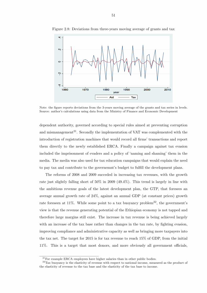
51
Figure 2.8: Deviations from three-years moving average of grants and tax
Note: the figure reports deviations from the 3-years moving average of the grants and tax series in levels.Source: author’s calculations using data from the Ministry of Finance and Economic Development
dependent authority, governed according to special rules aimed at preventing corruption
and mismanagement21. Secondly the implementation of VAT was complemented with the
introduction of registration machines that would record all firms’ transactions and report
them directly to the newly established ERCA. Finally a campaign against tax evasion
included the imprisonment of evaders and a policy of ‘naming and shaming’ them in the
media. The media was also used for tax education campaigns that would explain the need
to pay tax and contribute to the governemnt’s budget to fulfill the development plans.
The reforms of 2008 and 2009 succeded in increasing tax revenues, with the growth
rate just slightly falling short of 50% in 2009 (49.4%). This trend is largely in line with
the ambitious revenue goals of the latest development plan, the GTP, that foresees an
average annual growth rate of 24%, against an annual GDP (at constant prices) growth
rate foreseen at 11%. While some point to a tax buoyancy problem22, the government’s
view is that the revenue generating potential of the Ethiopian economy is not tapped and
therefore large margins still exist. The increase in tax revenue is being achieved largely
with an increase of the tax base rather than changes in the tax rate, by fighting evasion,
improving compliance and administrative capacity as well as bringing more taxpayers into
the tax net. The target for 2015 is for tax revenue to reach 15% of GDP, from the initial
11%. This is a target that most donors, and more obviously all government officials,
21For example ERCA employees have higher salaries than in other public bodies.22Tax buoyancy is the elasticity of revenue with respect to national income, measured as the product of
the elasticity of revenue to the tax base and the elasticity of the tax base to income.
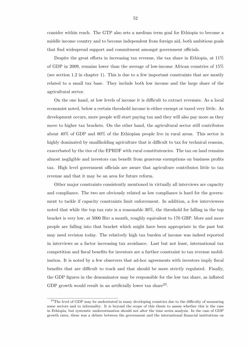
52
consider within reach. The GTP also sets a medium term goal for Ethiopia to become a
middle income country and to become independent from foreign aid, both ambitious goals
that find widespread support and commitment amongst government officials.
Despite the great efforts in increasing tax revenue, the tax share in Ethiopia, at 11%
of GDP in 2009, remains lower than the average of low-income African countries of 15%
(see section 1.2 in chapter 1). This is due to a few important constraints that are mostly
related to a small tax base. They include both low income and the large share of the
agricultural sector.
On the one hand, at low levels of income it is difficult to extract revenues. As a local
economist noted, below a certain threshold income is either exempt or taxed very little. As
development occurs, more people will start paying tax and they will also pay more as they
move to higher tax brackets. On the other hand, the agricultural sector still contributes
about 40% of GDP and 80% of the Ethiopian people live in rural areas. This sector is
highly dominated by smallholding agriculture that is difficult to tax for technical reasons,
exacerbated by the ties of the EPRDF with rural constitutencies. The tax on land remains
almost negligible and investors can benefit from generous exemptions on business profits
tax. High level government officials are aware that agriculture contributes little to tax
revenue and that it may be an area for future reform.
Other major constraints consistently mentioned in virtually all interviews are capacity
and compliance. The two are obviously related as low compliance is hard for the govern-
ment to tackle if capacity constraints limit enforcement. In addition, a few interviewees
noted that while the top tax rate is a reasonable 30%, the threshold for falling in the top
bracket is very low, at 5000 Birr a month, roughly equivalent to 170 GBP. More and more
people are falling into that bracket which might have been appropriate in the past but
may need revision today. The relatively high tax burden of income was indeed reported
in interviews as a factor increasing tax avoidance. Last but not least, international tax
competition and fiscal benefits for investors are a further constraint to tax revenue mobil-
isation. It is noted by a few observers that ad-hoc agreements with investors imply fiscal
benefits that are difficult to track and that should be more strictly regulated. Finally,
the GDP figures in the denominator may be responsible for the low tax share, as inflated
GDP growth would result in an artificially lower tax share23.
23The level of GDP may be understated in many developing countries due to the difficulty of measuringsome sectors and to informality. It is beyond the scope of this thesis to assess whether this is the casein Ethiopia, but systemtic underestimation should not alter the time series analysis. In the case of GDPgrowth rates, these was a debate between the government and the international financial institutions on

53
Last but not least, many interviews pointed to the importance of private sector com-
panies that carry out large investment project and that have strong links with the state
and the party. They suggested that a full assessment of fiscal discipline should take into
account these actors that may be accumulating debt. Unfortunately data on this sector is
not readily available and therefore this analysis focuses only on the public budget.
2.6 Implications for tax and aid: four underlying factors
The fiscal history of Ethiopia outlined in the previous sections allows the identification
of at least four related underlying factors in Ethiopian history and culture that deeply
influence the relation between revenue generation and aid. While these factors have been
present throughout Ethiopian history, they emerged more clearly in the 2000s.
Before describing in detail the underlying factors however, it is useful to note that
during the interviews I asked all interviewees if they thought aid and tax are treated as
substitutes in Ethiopia. The vast majority of them was convinced that aid does not have
a disincentive effect on tax and that the two variables are not treated as substitutes. A
few foreign observers who have been working on and in Ethiopia for decades noted that
substitution of tax with aid would not be in the Ethiopian character, and this is discussed
more in the next paragraphs. When asked about the nature of the relationship between
aid and tax, many interviewees pointed to a positive relation based on the role of aid in
easing the capacity constraint of the government and in supporting economic development.
Only a few interviewees thought that either aid has no effect on tax or has a negative
one. However even they agreed on the possible channels for a positive effect, namely
capacity and development, and on the validity of the underlying factors presented here in
the Ethiopian context. Indeed the discussion so far has shown that Ethiopia has always had
foreign advisors on tax matters, thus making the capacity channel particularly plausible.
The underlying factors are discussed in the following paragraphs; they are certainly
related and in some cases even overlapping concepts.
Tradition of statehood and continuity
We have shown throughout this chapter that the long tradition of stethood, interrupted
only by a few years of Italian invasion, is one of Ethiopia’s most valuable assets. Bahru
Zewde, a Professor of history at Addis Ababa University, holds that transitions in Ethiopia
the credibility of double digit growth rates.

54
were always characterized by administrative continuity and that during the transition of
1991 Ethiopia remained without a government for only one week24. The presence of a
strong state and administrative apparatus certainly allowed the Derg and the EPRDF to
undertake, within a few month since their establishment, radical reforms such as, respec-
tively, the land reform and ethnic federalism.
In addition to the administrative apparatus, continuity regards also the culture of
power and the political environment. Many scholars agree that the way authority is
exercised has changed little in Ethiopian history, although certainly much has changed
otherwise. Clapham (1988) notes that the following description of the Ethiopian leader,
used to describe the Emperor, fits very well Mengistu too.
“The leader was required to be both omnipresent and omnicompetent, capable
of intervening at will in the smallest details of any aspect of administration,
and his personal involvement was normally essential where any innovation was
involved.”
This quote may well describe the late Prime Minister Meles Zenawi as well, who was
reportedly fully involved in decision making in virtually all areas of policy. Indeed Abbink
(2011) argues that the thesis on transformation and continuity developed by Clapham
(1988) still holds in contemporary Ethiopia. Many observers interviewed in the context
of this research agree with that view, although under the EPRDF the tendency towards
centralism developed mostly in the second decade of its rule (see section 2.5.4).
This political culture is not confined to the leadership and it would be simplistic to
think that it is only imposed from the top. Instead it is largely embedded in popular
culture, as shown in Lefort’s research in rural Ethiopia in the run up to the 2005 elections
(Lefort, 2007). The author shows that peaceful electoral competition was inconceivable
in rural areas, with peasants concerned about voting for the winning side to ensure their
welfare and even their survival. In their view, the fact that opposition was able to campaign
freely in 2005 meant that the government had abdicated (Lefort, 2007). Along similar lines,
Young (1997) notes that the lack of transparency in the first years of EPRDF rule was
criticized much more by foreigners than by Ethiopians.
Finally continuity can be observed also in aid, at least in terms of flows. American
aid kept flowing in socialist Ethiopia for a few years after the 1974 revolution and when
it was withdrawn it was largely compensated with European and Soviet assistance. The
24From Professor Bahru Zewde’s keynote lecture on the “Dynamics of political succession in Ethiopia”at the 18th International Conference of Ethiopian Studies on November 1st 2012 in Dire Dawa, Ethiopia.
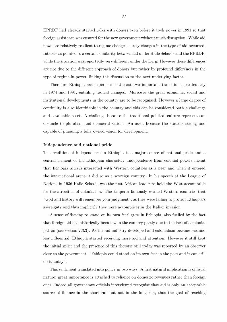
55
EPRDF had already started talks with donors even before it took power in 1991 so that
foreign assistance was ensured for the new government without much disruption. While aid
flows are relatively resilient to regime changes, surely changes in the type of aid occurred.
Interviews pointed to a certain similarity between aid under Haile Selassie and the EPRDF,
while the situation was reportedly very different under the Derg. However these differences
are not due to the different approach of donors but rather by profound differences in the
type of regime in power, linking this discussion to the next underlying factor.
Therefore Ethiopia has experienced at least two important transitions, particularly
in 1974 and 1991, entailing radical changes. Moreover the great economic, social and
institutional developments in the country are to be recognised. However a large degree of
continuity is also identifiable in the country and this can be considered both a challenge
and a valuable asset. A challenge because the traditional political culture represents an
obstacle to pluralism and democratization. An asset because the state is strong and
capable of pursuing a fully owned vision for development.
Independence and national pride
The tradition of independence in Ethiopia is a major source of national pride and a
central element of the Ethiopian character. Independence from colonial powers meant
that Ethiopia always interacted with Western countries as a peer and when it entered
the international arena it did so as a sovreign country. In his speech at the League of
Nations in 1936 Haile Selassie was the first African leader to hold the West accountable
for the atrocities of colonialism. The Emperor famously warned Western countries that
“God and history will remember your judgment”, as they were failing to protect Ethiopia’s
sovreignty and thus implicitly they were accomplices in the Italian invasion.
A sense of ‘having to stand on its own feet’ grew in Ethiopia, also fuelled by the fact
that foreign aid has historically been low in the country partly due to the lack of a colonial
patron (see section 2.3.3). As the aid industry developed and colonialism became less and
less influential, Ethiopia started receiving more aid and attention. However it still kept
the initial spirit and the presence of this rhetoric still today was reported by an observer
close to the government: “Ethiopia could stand on its own feet in the past and it can still
do it today”.
This sentiment translated into policy in two ways. A first natural implication is of fiscal
nature: great importance is attached to reliance on domestic revenues rather than foreign
ones. Indeed all governemnt officials interviewed recognise that aid is only an acceptable
source of finance in the short run but not in the long run, thus the goal of reaching
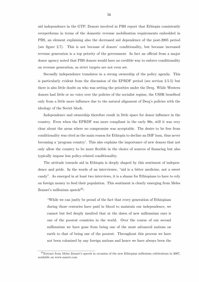
56
aid independence in the GTP. Donors involved in PBS report that Ethiopia consistently
overperforms in terms of the domestic revenue mobilisation requirements embedded in
PBS, an element explaining also the decreased aid dependence of the post-2005 period
(see figure 2.7). This is not because of donors’ conditionality, but because increased
revenue generation is a top priority of the government. In fact an official from a major
donor agency noted that PBS donors would have no credible way to enforce conditionality
on revenue generation, as strict targets are not even set.
Secondly independence translates in a strong ownership of the policy agenda. This
is particularly evident from the discussion of the EPRDF period (see section 2.5.5) but
there is also little doubt on who was setting the priorities under the Derg. While Western
donors had little or no voice over the policies of the socialist regime, the USSR benefited
only from a little more influence due to the natural alignment of Derg’s policies with the
ideology of the Soviet block.
Independence and ownership therefore result in little space for donor influence in the
country. Even when the EPRDF was more compliant in the early 90s, still it was very
clear about the areas where no compromise was acceptable. The desire to be free from
conditionality was cited as the main reason for Ethiopia to decline an IMF loan, thus never
becoming a ‘program country’. This also explains the importance of new donors that not
only allow the country to be more flexible in the choice of sources of financing but also
typically impose less policy-related conditionality.
The attitude towards aid in Ethiopia is deeply shaped by this sentiment of indepen-
dence and pride. In the words of an interviewee, “aid is a bitter medicine, not a sweet
candy”. As emerged in at least two interviews, it is a shame for Ethiopians to have to rely
on foreign money to feed their population. This sentiment is clearly emerging from Meles
Zenawi’s millenium speech25:
“While we can justly be proud of the fact that every generation of Ethiopians
during those centuries have paid in blood to maintain our independence, we
cannot but feel deeply insulted that at the dawn of new millennium ours is
one of the poorest countries in the world. Over the course of our second
millennium we have gone from being one of the most advanced nations on
earth to that of being one of the poorest. Throughout this process we have
not been colonized by any foreign nations and hence we have always been the
25Extract from Meles Zenawi’s speech in occasion of the new Ethiopian millenium celebrations in 2007,available on www.nazret.com
57
authors of our destiny, both our successes and failures. [...] A thousands years
from now, when Ethiopians gather to welcome the fourth millennium, they
shall say that the eve of the third millennium was the beginning of the end of
dark ages in Ethiopia. They shall say that the eve of the third millennium was
the beginning of Ethiopian renaissance.”
All this is crucial in understanding why the Ethiopian government might not just treat
aid and tax as substitutes in an opportunistic manner, as deeper historical and cultural
aspects are at work here.
Political commitment and ambition
Linked to the issue of independence and national pride is the continued commitment of
Ethiopian governments to development. While the EPRDF is the first Ethiopian govern-
ment to make development its foremost objective, a closer look at the history as well as
the interviews reveal that such a commitment was already present before. The discussion
on the commitment to development clearly is not meant to overshadow events such as
the Red Terror or the failure of the Imperial regime to tackle the 1973 famine that killed
tens of thousands of people. It is rather one of many elements emerging from Ethiopian
history, that is relevant for this research.
While the commitment to development under Haile Selassie has sometimes been de-
scribed as a mere facade (see section 2.3.5), the Imperial development plans are likely to
be the first ones in Africa and the government at the time has taken practical steps to
increase revenues to fund a growing public administration (see section 2.3.3). In his speech
at the League of Nations in 1936 the Emperor declared:
“For 20 years past, either as Heir Apparent, Regent of the Empire, or as
Emperor, I have never ceased to use all my efforts to bring my country the
benefits of civilization [. . . ]. ”
As far as the Derg is concerned, a few interviews and informal conversations surpris-
ingly pointed to an underlying commitment of the military government too. However,
they argue, the military regime was not able to pursue this commitment for two reasons.
First the Derg had no capacity to implement such a plan as it was largely composed by
military forces with little understanding of economic policy. An interviewee also noted
that the training for governemnt officials at that time was largely provided by the USSR
and it was of lower quality than that provided by Americans under Haile Selassie. Sec-
ondly the Derg was too occupied with repressing the continuous challenges and opposition

58
it faced, thus not being able to engage in development. While this is only the view of
a few Ethiopians, it was fairly consistent across interviewees with different backgrounds.
What is written in history is that the Derg came to power with a socialist agenda based on
land redistribution and modernization, as opposed to the exploitative feudal system. In
addition the most serious attempt of the Derg to engage in a development plan was largely
spoiled by the 1984 famine thus making its implementation very difficult, even assuming
a genuine commitment to it.
However it is certainly under the EPRDF that the commitment to development became
more prominent and central in the policy agenda. The TPLF’s, and later EPRDF’s,
ideology has always been linked to the struggle for development in rural areas and indeed
the leadership is highly committed to it, as confirmed in all interviews. The ambitious
development plans of the last decade are largely in line with this commitment. Moreover
the fact that the government is delivering at the local level (through the woreda-level
decentralization and PBS) is helping tax compliance as the people start seeing a return
for their tax payment, in what might be seen as an embryonic and implicit form of social
contract.
The ambition, sometimes deemed excessive, and the commitment of the Ethiopian
govenment deeply shape the aid-tax relation. As a top government official noted: “if more
aid flows into the country, domestic resources do not have to decrease. Instead the project
can expand. Aid and tax would only be treated as substitutes if a country does not have a
vision”, he argued, which is not the case for Ethiopia. On the contrary the fact that aid is
available makes the ambitious government’s plan possible because now the resources are
available, matched with the domestic ones, to deliver it. Projects that would have taken
a long time to be financed can now be actually realised with joint domestic and foreign
resources. In other words, there seem to be excess demand for funds in Ethiopia. In this
context aid and tax are complements rather than substitutes.
Taxation and aid: relative costs
The last underlying factor is the relative cost of tax and aid, which is sometimes cited as
the reason for substitution. In particular, the argument goes, when governments have to
decide how to finance their plans they will first choose aid and then fill the gap with as
little tax as possible. This may be the result of a higher political cost of tax whereas aid
is “free” money. This argumet is particularly ill grounded in the Ethiopian case, for at
least two reasons.
First, I have shown that aid in Ethiopia is not ‘free’ and indeed conditionality and

59
aid dependence represent a heavy burden for leaders. Mengistu was wary his leadership
appearing to be dependent on foreign actors, which would have undermined his image as
a strong national leader (see section 2.4.2). This sentiment is even stronger under the
EPRDF, especially after the 2001 TPLF crisis when foreign influence played a crucial role
and was one of the areas of criticism towards the faction led by Meles (see section 2.5.3).
As far as conditionality is concerned, the interviews revealed that conditions on eco-
nomic policy, including revenue performance, are not stringent nor really enforceable in
Ethiopia. Indeed donors seem to be reluctant to leave the country or to stop aid because
of economic conditions, although they may be the cause of delays in disbursment. So the
burden is not as much attached to the aid that is given, but to the fact that it is not
possible to get all the assistance that Ethiopia would want, and might partly be able to
obtain, precisely because the cost attached to additional funds (in terms of conditionality)
would be too high. This is of course true unless donors are willing to increase aid to
Ethiopia for other reasons, such as geopolitical ones.
The issue of delayed disbursement brings us to another element often cited by intervie-
wees: aid predictabilty. At least two top government officials noted explicitly that it is very
difficult to make plans based on aid because it is an unpredictable and unreliable source of
revenue. They argue that this became ever more clear after the 2005 elections. Another
interviewee observed that it is dangerous to rely heavily on an unpredictable source of
financing like aid for the huge development projects of Ethiopia. That, he argued, makes
the country too vulnerable as these projects are of foremost importance. This links to the
example of dams, widely cited as an example of projects that donors are not willing to
fund though they are central in the government’s strategy.
The second reason is related to the cost of raising tax. I asked questions about the
political cost of increasing tax revenue in many interviews and the general consensus, both
on the donors and government side, is that such a cost is not a big concern. First of all
the government is acting mainly on expanding the tax base, including fighting evasion and
expanding the tax net. Tax rates on the other hand have only been decreased under the
EPRDF. This generates solid grounds for the government to argue that the increase in tax
revenue is essentially fair and it is aimed at bringing everyone in the tax net to contribute
their fair share. It is a matter of equality that everyone has to pay tax, and this reasoning
is also being promoted with tax education campaigns and increased dialogue on taxation
at the kebele level.
In addition the long tradition of centralization and statehood is playing an important

60
role. The Derg for example was able to extract revenues because of its authoritarian na-
ture that the population would generally comply with, particularly after the experience
of the Red Terror. Even during the Imperial regime, a top official noted, people in ru-
ral areas were used to paying tax. Failing to do so would be an act of dissent and, he
explained, nobody would dare. Even if we have shown that landlords could exert some
resistance in paying tax (see sections 2.3.1), peasants did not have the power to do so.
This legacy clearly remained in today’s Ethiopia, although the culture of compliance is
not as rooted in urban areas. While the perceived high tax burden creates some discontent
amongst businesses and individuals, it seems far from providing the basis for serious up-
rising particularly in the context of slow progress on democratization and pluralism. The
government’s view is that the fiscal burden is generally not a concern since the economy
is growing fast and the full revenue potential is still not tapped.
Finally, the great political and economic importance of the EPRDF’s development
plan is at work again here. A high official in a major donor agency noted that the cost
of increasing tax revenue is still much lower than the cost of not delivering the plan, and
other interviewees have talked along these lines although less explicitely.
2.7 Conclusion
This chapter reviewed the Ethiopian fiscal history over the period 1960 - 2009, focussing
on domestic revenues and aid. The analysis shows that in Ethiopia there does not seem to
be a substitution effect between tax and aid, therefore answering the first research question
(see section 5.1). This chapter shows that there are at least four underlying factors that
make the existance of such a substitution effect particularly ill grounded in the case of
Ethiopia. These underlying factors are supported by historical facts and episodes presented
throughout the chapter. The analysis of the EPRDF period in particular shows how these
factors, that are present throughout the whole period considered, are developed more
consciously and clearly in the political discourse in the 2000s. By doing this, the analysis
sheds light on the second research question.
Finally the analysis allows understanding the political economy underlying the ob-
served variations in fiscal variables, answering the last question raised in section 5.1.
Amongst others, the small contribution of agriculture to tax revenue emerges throughout
the period; while trade has been a sector where substantial revenue has been generated.
Thus the qualitative analysis also offers a solid basis for the econometric analysis, which is
complementary to it. Particularly a number of issues remain to be explored with quantita-

61
tive tools, such as the estimation of the effect of agriculture and manufacturing shares on
tax revenue mobilisation. In addition an econometric analysis is needed to assess whether a
significant relation exists between aid and tax and particularly whether a positive relation
can be supported by the data.
The analysis fills a gap in the literature by presenting a consistent and comprehensive
reading of the Ethiopian economic history that is geared towards revenue mobilisation
and aid. Moreover, by showing the importance of social, cultural and economic factors in
defining the aid-tax relationship, it underlines the value of complementing a quantitative
analysis with in depth qualitative elements. In this sense this chapter overcomes the limits
of the existing economic literature that, by largely focussing on econometric aspects, fails
to fully exploit the potential for a case study analysis.

62
Appendices

63
2.A Quotas and price controls
Quotas and price controls were widely used under the Derg as a surplus extraction mech-
anism. They can ultimately be seen as a way to finance government’s plans since they
are effectively a subsidy for urban consumption at the expense of producers. However
they did not strictly represent a source of revenue for the government’s budget, thus not
showing up either in tax or non-tax revenue.
The central institution implementing quotas and price controls was the Agricultural
Marketing Corporation (AMC), established in 1976. Partly as a response to increasing food
prices and food shortages in urban areas, in 1978/79 the AMC introduced grain quotas.
This imposed on peasants associations an obligation to transfer a part of their produce,
namely 7%, to the government at a given price. This was a large proportion considering
that the marketable output in Ethiopia was only 20% of the output of foodgrains (Griffin,
1992). However quotas were not set uniformly and their enforcement was quite arbitrary,
therefore there are variations in estimates on how much was sold to the AMC in quotas
(Eshetu Chole, 2004).
Cooperatives and state farms were forced to sell only through the AMC while private
producers were required to only sell part of their output (estimated at 4%) to the AMC
(Griffin, 1992; Clapham, 1987). This clearly created a further disincentive for joining
cooperatives. Perhaps more indicative is the fact that private merchants were required
to sell 50% of their grain purchases to the AMC (Eshetu Chole, 2004). The grains thus
obtained were sold mostly to kebeles, state enterprises and the armed forces.
Surplus extraction was working through price controls, that were normally set by the
AMC largely below market prices, by 50% for some major crops such as maize and teff
(Griffin, 1992; Clapham, 1987). While the initial benefits of the land reform are not to be
underestimated, there is no doubt that they were at least partly eroded by this system of
quotas, besides the general impovrishment (Griffin, 1992). The exploitative system of the
feudal era was now replaced by other forms surplus extraction from the peasantry.
Moreover the AMC retained control over fertilizer and it did discriminate against
private peasants with respect to its price. As a result fertilizer was used a lot more in
state farms relative to their share of the agricultural sector. All this made peasants ever
more disenchanted and detached from the regime.

64
2.B Interviews
The full list of interviewees will not be disclosed, as agreed with those who took part
in the interviews. However the following list indicated the main institutions involved in
the consultation. Usually more than one person from each of the institutions above was
interviewed, with at least one at the level of directors or heads of division. In addition,
independent experts and academics took part in interviews.
• Addis Ababa University
• Department for International Development (UK)
• Ethiopian Development Research Institute
• Ethiopian Economics Association
• European Commission
• International Monetary Fund
• Ministry of Finance and Economic Development
• National Bank of Ethiopia
• Prime Ministers Office
• PBS Secretariat
• USAID
• World Bank, Ethiopia Office
65
Chapter 3
Aid and taxation: theory and
evidence from Ethiopia
3.1 Introduction
This chapter provides an empirical analysis of the relation between aid and taxation in
Ethiopia, using a unique dataset of 50 annual observations. This is a longer series than
those used in most of the literature1. The main hypothesis explored is the existence of
a crowding out effect of aid on tax revenues. In addition to the aid-tax relation, this
chapter offers insights into the role of tax determinants such as the manufacturing sector,
agriculture and trade.
I fully exploit the case study approach by complementing the econometric analysis
with an in depth knowledge of the country specific context, grounded on the qualitative
analysis of chapter 2. Not only the qualitative analysis allows the interpretation of the
results in a more informed and relevant way. It also informs the econometric exercise
by offering a deeper understanding of issues such as endogeneity and structural breaks.
Given the limited attention given to the country context in the majority of the econometric
literature on this topic, this approach represents a novelty.
Ethiopia has received increasing amounts of aid in recent years and it is often considered
an ‘aid darling’. While per capita aid is still below the African average, the share of aid
to GDP is relatively high compared to Sub-Sarahan Africa2. Perhaps most importantly,
Ethiopia has been identified by some donors as a focus country for increased aid flows in
1This is true for the literature focussing on case studies and using annual observations.2Also see the introduction to this thesis in chapter 1.

66
coming years. For example DFID identified Ethiopia as one of its focus countries in its aid
review of 2011, as it ranked in the first 5% of countries with the highest ‘need-effectiveness’
index (Department for International Development, 2011). At the same time tax revenues
amount to only about 11% of GDP, a share that is well below the average for low income
African countries (and for any other grouping of African countries, as shown in chapter 1).
This situation coupled with the centrality of domestic revenue in financing the Growth and
Transformation Plan (GTP, the current five-year development plan), makes the analysis
of the relation between tax and aid central and relevant for the policy debate in Ethiopia.
This analysis provides evidence for a positive effect of aid on tax revenues, that is mostly
explained by the role of aid in building capacity at the national level.
To gain a deeper understanding on the aid-tax relation, this chapter explores the role
of aid heterogeneity in terms of grants and loans. These are sometimes thought to have
different effects due to the need for repayment for the latter, while the former would create
fiscal space without giving rise to future liabilities (Gupta et al., 2004; Morrissey et al.,
2006; Benedek et al., 2012). I find some support for this hypothsis in the long run, where
loans have a stronger positive effect than grants. However there is still no evidence of a
negative effect of grants in the long run, only of a weaker but still positive one. In the
short run both grants and loans have a positive and significant effect.
Moreover by including other tax determinants in the analysis I find that manufacturing
has a strong positive effect on tax revenues, probably due to its role as tax collector besides
that of tax payer3. In addition agriculture does not appear to have a significant effect on
aggregate tax, but it affects negatively domestic taxes. Trade has the expected positive
effect. These results, while somewhat secondary with respect to those on aid, offer insights
into the possible challenges and opportunities for a stronger tax revenue mobilisation,
which is a top policy priority under the GTP.
Therefore this chapter is driven by the following three research questions, that are
reported in order of priority:
• Is aid a disincentive to tax revenue mobilisation?
• Does aid heterogeneity matter (i.e. grants and loans)?
• What are the determinants of the tax share in Ethiopia?
3Firms collect collect taxes on wages and on consumption that are then transfered to the state.

67
3.2 Literature review
The literature on tax effort is based on the analysis of the determinants of the tax share
(sometimes also referred to as tax effort), defined as total tax revenue collection as a share
of GDP. It is mostly based on cross country analyses using data from international sources
(e.g. Government Finance Statistics by the IMF or the World Development Indicators
from the WB) to ensure comparability across countries. Part of this literature has been
specifically focussed on the relation between tax and aid, without finding a consensus on
the sign and significance of that effect.
The tax effort literature has its roots in the early studies conducted within the Inter-
national Monetary Fund (Chelliah, 1971; Chelliah et al., 1975; Tait et al., 1979). They
identify the core tax determinants that are still largely used in this literature today, and
namely: mining share, trade openness (export + imports), GDP per capita and agricul-
tural share. They use mainly cross-section estimation techniques often applied to averaged
data on different periods. Typically a tax effort index is computed as the ratio between
the actual tax share and the predicted one from the econometric model. This index is
used for guidance in evaluating the fiscal performance of the countries considered. Tanzi
(1992) largely confirms these early results by using cross section time series data for 88
countries. He finds that half the variation in the tax share can be attributed to those core
variables, with the addition of the foreign debt share of GDP.
The most important theoretical contribution to this literature certainly is the article
by Heller (Heller, 1975), that develops the framework largely used today in most of the
literature (see appendix 3.A for a critical summary of it). Heller’s framework originally
focussed on variables from the public budget alone including tax, aid, borrowing, and
expenditure. His empirical estimation of the model on cross section-time series data from
11 African countries underlines a negative effect of aid on tax effort. This framework is
further tested in the fiscal response literature that includes mostly country case studies
such as Franco-Rodriguez et al. (1998), Machado (2009), Mavrotas and Ouattara (2006),
Franco-Rodriguez (2000), and Osei et al. (2003). The results on aid in this litreature are
contrasting, with the former three articles finding a negative effect on tax revenue and the
latter two a positive one4.
The seminal work of Heller (1975) is further developed and expanded by Leuthold
4For a detailed review of fiscal response studies using the cointegrated VAR methodology, see chapter4.

68
(1991) and Ghura (1998) to provide the theoretical basis for tax effort models, including
also the quality of institutions and macroeconomic policies along with aid. The former
study provides an empirical application on a panel of eight African countries observed
over 9 years. The author disaggregates tax revenue in direct and indirect taxes and finds
a positive effect of foreign grants on the former and a negative one on the latter. Ghura
(1998) also focuses on African countries, again over a relatively short period between 1985
and 1996. He finds that aid has an adverse effect on tax revenue. However he underlines
that endogeneity may be a problem if grants are directed towards less performing coun-
tries (therefore with higher needs) where the tax share is lower. The author also finds
that corruption and macroeconomic policies are important determinants of the tax share.
Mahdavi (2008) further expands the theoretical famework by adding new sets of explana-
tory variables related to demographics and labor force characteristics; administrative and
enforcement costs; the macroeconomic environment; and the political environment and
corruption. This rich specification is estimated using an unbalanced panel dataset of 43
developing countries observed over the period 1973-2002. The paper finds that aid still
has a negative and significant (at the 10% level) effect even after all the other variables
are included in the model.
Providing a more positive picture on aid, Gupta (2007) suggests that aid has a positive
effect on tax revenue and that this result is even stronger for low income countries. He
uses a bigger sample than previous studies, including 150 developing countries observed
over 25 years. Stotsky and WoldeMariam (1997) focus particularly on the effect of IMF
programs on tax effort in the receiving country, failing to find strong support for a beneficial
effect. Other studies in this tradition have focussed also on corruption and the institutional
environment (Bird et al., 2008; Imam and Jacobs, 2007), or on natural resources (Bornhorst
et al., 2008). As far as other tax determinants are concerned, these studies generally find
a negative effect of agricultural share in GDP, a positive effect of trade openness, a weak
positive effect of manufacturing, and contrasting results on GDP per capita.
Some studies have looked specifically at aid heterogeneity, particularly disaggregating
it in grants and loans. As underlined in Gupta et al. (2004), loans may have a positive effect
on tax effort because of the need for repayment while grants may instead be expected to
crowd out domestic revenue, therefore having an expected negative effect. This hypothesis
is tested on a dataset of 107 low and middle income countries from 1970 to 2000. The
results on the variables related to the tax base (namely agriculture, industry, trade and
income) are in line with the literature. The hypothesis on grants and loans is confirmed

69
by finding the expected coefficients to be significant. Morrissey et al. (2006) estimated a
similar specification using a comparable sample over the period 1975-2000 and confirmed
these results: loans have a positive and significant effect on tax revenue, grants have a
smaller negative and significant effect, so that the combined effect (when the two variables
are combined in total aid) is a positive but non-significant coefficient. When lagged aid is
used however, to account for possible endogeneity, the negative effect of grants becomes
non-significant and total aid is found to have a positive effect on tax effort. Teera and
Hudson (2004) reach a similar result, finding a positive but not significant result on the
aid variable. By using interaction terms the authors also find that the importance of trade
and manufacturing in influencing the tax share decreases as countries get richer.
More recently there has been a renewed interest in the estimation of the aid-tax rela-
tion, perhaps also sparked by a reflection on the existing evidence. In particular Carter
(2013) provides a critical summary of the literature on the aid-tax relation underlining
its methodological problems and other limitations. He provides new estimates, partly ad-
dressing the methodological concerns, that provide no evidence of a negative effect of aid
on tax revenues perhaps also due to the increased attention of donors to domestic revenue
mobilisation. Benedek et al. (2012) try to address specifically some of these concerns,
particularly as regards endogeneity. They use a panel of 118 countries over 1980-2009
and a number of econometric methodologies including GMM. The results show a negative
coefficient on grants that however is weakening over time, particularly when compared to
the results of Gupta et al. (2004) that found a larger coefficient. They also estimate sep-
arate regressions for disaggregated tax types. While aid has a negative effect on most tax
types, it has a positive relation with trade taxes. Clist and Morrissey (2011) use a large
sample of developing countries and find that aid has a positive effect on tax revenue after
the mid-80s when there appears to be a break in the relation. This break corresponds to a
stronger emphasis on conditional lending in the international debate and it may indicate
the success of conditionality in stimulating fiscal reforms. To address endogeneity, the
authors use lagged aid (in addition to current aid in a separate specification) and find
a positive result on both grants and loans after 1985. Aid lagged two years is also used
as an instrument, yielding similar results. Mkandawire (2011) focuses on the effect of
the colonial heritage on tax effort in a cross section of African countries, using averaged
data over four-year intervals in the period 1984-2004. The author argues that the colonial
status of African countries has implications in terms of taxation that can still be observed
in today’s tax systems. While aid it is not the focus of the analysis, it is still included

70
in the model and it is found to have a positive, although weak, effect on the tax share.
This result is confirmed even when its lagged value is used as an instrument to account
for endogeneity. Other recent papers largely confirm the results on the tax determinants
related to the tax base, although they find no evidence of a significant relation between
aid and taxation (Drummond et al., 2012; Le et al., 2012).
While cross country studies are prevalent in this literature, they also suffer from lim-
itations due to the heterogeneity in the effect of aid amongst countries. Carter (2013)
argues that due to this heterogeneity, estimates of averaged effects are unstable and they
are of limited policy interest. One possible way forward indicated in the paper is the in-
creased reliance on country case studies that can also include interviews with government
officials. This is the approach adopted in this research and it is in this niche that I aim to
contribute.
So far there are only few studies of tax effort that take a case study approach. Amongst
these, Ezemenari et al. (2008) analyses Rwanda and it finds a small negative effect of
aid. The paper also contributes to the literature by providing a theoretical framework
alternative to Heller (1975) that is discussed in appendix 3.A. Other country studies have
focussed mostly on the fiscal variables alone, following more the fiscal response tradition
than the tax determinants literature (Hisali and Ddumba-Ssentamu, 2013; Martins, 2010;
Osei et al., 2005; Bwire, 2013). They generally provide evidence of a positive effect of aid
and they are reviewed in detail in chapter 4.
Contribution
This chapter contributes to the literature by providing a country study on Ethiopia, in
a literature largely dominated by cross-country studies. I provide evidence for a positive
relation between aid and taxation, therefore contributing to a debate that is still far from
settled.
By complementing econometric evidence with qualitative information, I show the ad-
vantages of a case study approach. This is reinforced by in depth interviews of govern-
ment and donor agencies officials that are specifically aimed at understanding the aid-tax
relation. Since this approach is rather rare in the literature, it represents an original
contribution aimed at overcoming the limits of the cross-country literature.
71
3.3 Data and empirical methodology
The data used to investigate the research questions outlined in section 3.1 is Ethiopian
time series from 1960 to 20095. The characteristics of this data, as well as the data
generating environment are discussed in the next two sections. The last section describes
the empirical model used to analyse this data and it discusses some econometric challenges.
3.3.1 The data
The Ethiopian dataset spans 50 years, from 1960 to 2009. By relying on 50 annual ob-
servations, this exercise can count on a larger sample than other country-level studies
working with annual data. In a small sample context, even adding a few observations
adds robustness to the results. This dataset is therefore a crucial asset for this analysis.
The dataset was compiled exclusively from national sources, and particularly from the
National Accounts data originally compiled by the Ministry of Finance and Economic
Development (MOFED). Using a single national source presents two advantages. First,
it allows consistency in the data that cannot be fully ensured when mixing data sources.
This is particularly the case of aid figures that may present huge discrepancies across
different datasets, as discussed in the next paragraphs. Secondly the national data is used
for policy making, thus making it more relevant than international datasets.
The use of national data is particularly important in the case of aid measures, namely
grants and loans. The national figures used in this exercise consist only of aid that flows
through the government budget (i.e. the Treasury). This includes, but it is not limited
to, budget support. The use of this data for aid is not only sensible in terms of data
consistency but it is also relevant to the research questions presented in section 3.1. Indeed
the component of aid flowing to the budget is the closest substitute to tax revenue and it
is therefore the one that is more likely represent a disincentive or substitution effect. Of
course there are issues related to aid fungibility, but nonetheless it seems reasonable to
consider this component of aid as the most relevant one for the analysis. This is reinforced
by the fact that budget data is the one used by policymakers when taking fiscal decisions
and it is the portion of aid that they are fully aware of.
The national aid figures are smaller than the ones reported by OECD-DAC6. This
5These are more specifically 1960/61 and 2009/2010, that are the Gregorian calendar years that corre-spond to the relevant Ethiopian years. The Ethiopian calendar is 7 years behind the Gregorian one and itstarts in September.
6For example the grants figure is about a fourth of the corresponding OECD-DAC one.

72
discrepacy is due to items within grants that are not disbursed through the government
system, mainly humanitarian and emergency aid that in Ethiopia can be rather substantial
due to the constant threat of drought and famine. Moreover items that are not included
in the budget grant figure are, for example, projects managed by donors and grants to
NGOs.
The national aid figure today is largely dominated by the Protection of Basic Services
(PBS) project, described in chapter 2. Other programs disbursed through the Treasury are
for example the Public Sector Capacity Building Program (PSCAP), the Productive Safety
Net Program (PSNP) and other funds aimed at specific sectors such as infrastructure.
All variables are measured as a share of GDP, except for GDP per capita (log of
constant GDP per capita) and the GDP gap (percentage deviation of GDP from trend).
A summary of the variables used in this analysis is reported in appendix 3.B.
3.3.2 Ethiopian context and some descriptives
A full qualitative analysis of the Ethiopian context and a detailed description of the data is
provided in chapter 2, therefore I will highlight here only a few elements that are relevent
when carrying out the econometric exercise.
Figure 3.1: Plot of tax, grants and loans
0.05
.1.15
1960 1970 1980 1990 2000 2010year
tax grantsloans
Note: all variables are expressed as a percentage of current GDP. Source: author’s calculations using datafrom the Ministry of Finance and Economic Development.
The unique Ethiopian history of independence is translated in fiscal terms in the im-
portance assigned to tax revenue mobilisation by all governments that have ruled Ethiopia
over the period considered (see chapter 2 for a complete account).

73
As far as aid is concerned, Ethiopia has received budget aid throughout the whole
period. Moreover foreign technical assistance has been provided to Ethiopia throughout
the period, initially on the basis of the early sectoral and multi-year development plans of
Haile Selassie. Even in the first imperial period, missions from the UN, the WB and the
US provided advice in the field of taxation, amongst others (see chapter 2). Still today
taxation is one of the areas of greatest agreement between the government and donors, in
a relation that is often characterized by confrontation and contrasting views.
Figure 3.1 shows a plot of tax, grants and loans over the period, all measured as a share
of GDP. The first message from the picture is that tax is a much larger source of revenue in
the government’s budget than grants and loans. Secondly the figure does not immediately
suggest a negative relation between tax revenue and the aid variables. Moreover figure
3.2 reports the 3-year moving average of aid (aggregated grants and loans, for the sake
of clarity) and tax, showing that the former is much more volatile than the latter thus
making it a more unpredictable source of revenue.
Figure 3.2: Deviations from three-year moving average of tax and aid
Note: the figure reports deviations from the 3-years moving average of the grants and tax series in levels.Source: author’s calculations using data from the Ministry of Finance and Economic Development
3.3.3 Empirical framework and challenges
The Ethiopian time series are used to estimate a standard tax effort equation, stemming
from the literature. Equation 3.1 is largely in line with other studies in this literature,
where A is aid, later disaggregated in grants and loans, NT is non tax revenue, Agri is
the agriculture, Manuf is manufacturing, Trade is trade openness, and GDPpc is GDP
per capita. Appendix 3.B reports a more detailed descrition of these variables. Some

74
specifications add to these core variables a cycle variable (GDPgap) and dummies to
reflect changes in regime.
T = b0 + b1A + b2NT + b3Agri + b4Manuf + b5Trade + b6GDPpc (3.1)
In equation 3.1 tax revenue is determined by variables that are proxy measures of compo-
nents of the tax base, so the equation is largely in line with the cross-country tax effort
literature. The theoretical basis for equation 3.1 is provided by Heller-type models, par-
ticularly as developed in the literature for example by Leuthold (1991) and Ghura (1998)
(see section 3.2 and appendix 3.A for more details). The Heller-type fiscal response models
focus largely on the effects of aid on spending, and revenue (including aid and tax) is re-
quired to finance spending. In Heller (1975) and other early papers aid does not enter the
government utility function, but it is later introduced by Franco-Rodriguez et al. (1998)
where aid and tax are allowed to affect differently government utility.
In a time series setting, variables may present trends. If the variables of interest move
together in the long run, they may be cointegrated and this issue is discussed below. As
far as short run dynamics are concerned, trends in the data become irrelevant since first
differences are used in the empirical estimation. In particular equation 3.1 can be estimated
using a cointegration model that allows separating the long run (LR) and short run (SR)
effects. I use the two-step procedure suggested by Engle and Granger (1987). The Engle-
Granger (EG) procedure requires the series to be integrated of the same order in levels
(first step) and to be stationary in first difference (second step). To this end three tests for
stationarity are used: the Augmented Dickey-Fuller test (dfgls), the Kwiatkowski-Phillips-
Schmidt-Shin test (kpss), and the Clemente, Montanes, Reyes unit root test (clem). The
last one in particular allows for the presence of up to two structural breaks7 and it is
therefore useful in the Ethiopian case where breaks may be expected in correspondence
with regime changes8. It is important to remember however that the clem test is not a
test for structural breaks as such but instead it only analyses the properties of a single
series (Perron and Vogelsang, 1992). The results of the stationarity tests show that all
7The Zivot-Andrews test can only take into account one break (Zivot and Andrews, 1992).8In the clem test the breaks are not imposed a priori but are estimated by the test. Using this test
is particularly important because Dickey-Fuller style tests may confuse non-stationarity with structuralbreaks. In other words, in presence of structural breaks, the residuals will display a clear pattern and theclassic unit root tests are not able to reject the null hypothesis of non-stationarity (Ghosh, 1999).

75
variables are I(1)9. They are reported and discussed in appendix 3.C.
The first step of the EG procedure identifies long run relations and it involves the
variables in level, and more specifically as shares of GDP. Cointegration occurs when the
relation between those non-stationary variables produces stationary residuals. If this is
the case the series move together in time and they form a long-run equilibrium. The test
for cointegration proposed by Engle and Granger is therefore esentially a stationarity test
on the residuals similar to the Dickey-Fuller test10. Since this statistic does not follow the
standard distribution, the MacKinnon critical values are used (MacKinnon, 2010). When
residuals are not serially independent the test includes lags of the first difference of the
residual and this version of the test is known as the Augmented Engle Granger (AEG)
test.
The second step of the procedure identifies short run effects. Here the variables are
included in first difference and they are therefore stationary, provided that they are I(1).
The lagged residual from the first step is also included as an error correction term (ECT),
indicating the adjustment to LR equilibrium.
As far as econometric challenges are concerned, two issues are of particular interest:
endogeneity and structural breaks.
Endogeneity regards in particular the aid variables and the short run equations since
LR cointegrating relation is superconsistent (Engle and Granger, 1987). Concerns are
raised in the literature based on the idea that aid may be given to countries with higher
needs, which may happen to be also those countries with a lower potential to raise taxes
due to low levels of income. If this is the case, a negative spurious relation would indeed be
observed between aid and tax. This however is a concern more in relation to cross-country
studies than in a time series setting. In time series analysis endogeneity may stem from a
possible detrimental effect of aid on domestic institutions that would therefore undermine
the administrative basis for an effective fiscal system, resulting again in a spurious negative
relation. Moreover aid flows may respond to government’s decisions in terms of fiscal
and economic policies, rewarding ‘good’ policies with increased financial assistance. If
donors believe that increasing tax revenue is a ‘good’ policy and reward government that
succeed in doing so, a spurious positive relation would occur. However this case seems
9The grants variable shows some stationarity in levels that however disappears in the dfgls test withone lag and when treated in conjunction with loans in the aid variable. The series is treated as I(1), alsoto ensure consistency with other variables.
10The test regresses the first difference of the residuals from the first step (LR) equation on the laggedlevel of these residuals, without a constant. The test statistic is a simple OLS t-statistic on the laggedresidual.
76
particularly ill-grounded in the Ethiopian case. The following quote (Furtado and Smith,
2007) summarizes the argument for this, which is also exposed in more detail in chapter
2 and in section 3.5.1.
“Changes in the level of donor assistance to Ethiopia have been driven over-
whelmingly by political and geopolitical considerations [. . . ]. These factors,
rather than anything the government has consciously done to manage the aid
agenda, have largely determined the level of aid inflows.”
Endogeneity is discussed in detail in section 3.5.1 and an instrumental variable approach
is proposed. Moreover the role of the institutional environment and governance are ex-
plicitely taken into account in section 3.4.3.
Turning to structural breaks, they are particularly expected in correspondence with
the regime changes of 1974 and 1991. Two shift dummies are therefore included in the
regressions presented in section 3.4 and this issue is explored in more detail in section
3.5.2. The dummies capture the Derg (1975-1990) and EPRDF (1991-2009) regimes,
with the Imperial period (1960-1974) being excluded and thus representing the reference
period. While breaks need to be taken into account, it is important to keep in mind the
elements of continuity outlined in chapter 2. This is particularly relevant in the case of the
administrative apparatus, that was largely inherited by successive regimes. While breaks
can be expected in 1974 and 1991, section 3.5.2 explores the possibility of breaks other
than these without however finding any evidence for it.
3.4 Results
This section presents the main results from the estimation of equation 3.1 using the Engle-
Granger two step procedure. It is divided in two sections that report respectively the long
run and short run results.
3.4.1 First step: the long run
Table 3.1 reports the long run (LR) results for different specifications of the empirical
model, using all variables in levels11. Cointegration amongst these variables is crucial to
ensure consistent estimates and to proceed to the next step of the Engle-Granger proce-
dure. Therefore table 3.1 also includes the AEG test statistics at the bottom, for testing
11Mostly as a percentage of GDP, except GDP per capita and the GDP gap.

77
cointegration. These test statistics are to be compared with the MacKinnon critical values
reported in table 3.2 and calculated using the Stata program module devised by Schaffer
(2010). The null hypothesis is no cointegration, so rejection would provide evidence that
the series are indeed cointegrated.
The first column of table 3.1 reports the full specification excluding regime dummies.
However the AEG test statistic shows that this regression does not produce stationary
residuals, therefore indicating the lack of cointegration. Since structural breaks may pro-
duce a pattern in the residuals, therefore making them non-stationary, column two includes
regime dummies and with these the system is cointegrated. Indeed this regression passes
the AEG test with 0 lags. Further lags in this case are not needed because the residuals
do not show evidence of autocorrelation12. The regime dummies are therefore included in
all remaining specifications.
The third column excludes the GDP gap variable over concerns of a possible built-in
negative correlation with the dependent variable due to GDP being at the denominator of
the tax share. This may also explain the negative coefficient on GDP gap that indicates
a countercyclical behavior of tax revenue and that may be somewhat puzzling. Dropping
the GDP gap has little impact on the results but it does allow grants to reach the 10%
significance threshold. Note that this specification passes the cointegration test also when
one lag is included, although zero lags would be sufficient since autocorrelation is rejected
(see table 3.D.1 in appendix 3.D for autocorrelation tests on the LR equation). Given
its superior cointegration properties and the little impact of dropping the potentially
problematic GDPgap variable, column three represents the preferred specification13.
Finally specifications 4 and 5 take multicollinearity into account by including alterna-
tively agri and trade that are found to be the variables most affected by this issue (see
appendix 3.E for a detailed analysis).
For all specifications a test for homoskedasticity (White and Breusch-Pagan tests) is
run and it provides no evidence of a problem. The residuals also pass the normality tests.
The R2 for all LR equations is rather large, ranging from 0.86 to 0.92, which may be
expected in presence of cointegration.
The results on the aid variables are consistently positive across specifications, with
loans seemingly driving the positive effect of aggreagate aid as it is always significant
12Table 3.D.1 in appendix 3.D shows autocorrelation tests for the LR equation. They also show thatautocorrelation disappears once regime dummies are included.
13This specification is used to compute the error correction term (ECT) for the second step of theEngle-Granger procedure and it is the basis of robustness checks.

78
Table 3.1: First step: LR results from tax equation
(1) (2) (3) (4) (5)
grants 0.116 0.293 0.325* 0.325 0.248(0.52) (1.65) (1.78) (1.48) (1.56)
loans 0.215 0.305*** 0.413*** 0.428*** 0.397***(1.62) (2.81) (4.31) (3.74) (4.24)
non-tax 0.260 0.194 0.163 0.304* 0.154(1.60) (1.53) (1.26) (2.02) (1.19)
agri 0.053 0.064 0.052 -0.038(0.88) (1.09) (0.87) (-0.56)
manuf 1.366*** 0.766** 0.736** 0.167 0.548**(4.00) (2.48) (2.31) (0.48) (2.35)
trade 0.087** 0.116*** 0.144*** 0.134***(2.09) (3.29) (4.34) (4.32)
GDPpc 0.023 0.016 -0.007 0.039** -0.011(1.09) (0.79) (-0.39) (2.46) (-0.66)
GDP gap -0.028* -0.025*(-1.88) (-1.91)
Derg 0.019*** 0.017*** 0.017*** 0.015***(4.10) (3.61) (3.06) (3.58)
EPRDF 0.004 -0.003 0.003 -0.007(0.51) (-0.42) (0.41) (-1.25)
Constant -0.204 -0.152 0.012 -0.207 0.087(-1.41) (-0.95) (0.08) (-1.34) (0.80)
Observations 50 50 50 50 50r2 0.86 0.92 0.91 0.87 0.91
Augmented Engle-Granger test for cointegration0 lags -4.086 -6.363 -6.706 -6.687 -6.5821 lag -3.638 -5.734 -6.326 -5.884 -6.1992 lags -2.563 -4.745 -5.017 -4.708 -4.726
Note: t statistics in parentheses; * p < 0.10, ** p < 0.05, *** p < 0.01. All variables are included in levels,i.e. as a share of GDP except GDPpc and GDPgap. The dependent variable in all columns is the taxshare.

79
except for column 1. Grants are significant only in specfication 3 at the 10% level. In
particular a percentage point increase in the share of grants to GDP is associated with
a 0.3 percentage points increase in the tax share, and the corresponding result for loans
is 0.4 (specification 3). These findings are largely in line with the literature using the
disaggregation between grants and loans, where the latter is found to have a stronger and
positive effect.
Agriculture displays its expected negative coefficient only once multicollinearity is tack-
led, in specification 4, although it remains non-significant. Manufacturing and trade dis-
play the expected positive and significant coefficients which are confirmed in all specifica-
tions. In particular manufacturing has a large coefficient, implying that a percentage point
increase in the manufacturing share of GDP is associated with a 0.7 increase in the tax
share. This may be due to the fact that firms act as tax collectors, both for wage taxes and
for indirect taxes. GDP per capita has a mostly positive coefficient that however is only
significant in specification 4, suggesting that a 1% increase in GDP per capita increases
the tax share by 0.04 percentage points.
Table 3.2: MacKinnon critical values
k (excl. constant) 10% 5% 1%
k=8 -5.328 -5.708 -6.478k=9 -5.623 -6.011 -6.800k=10 -5.907 -6.304 -7.112
Note: Critical values valid also for AEG with lags.
3.4.2 Second step: the short run
Having found cointegration in the first step, it is now possible to proceed to the second
step (SR)14. The variables are now made stationary by first differencing15.
Table 3.3 reports the SR results, starting in column 1 from the same specification as
the LR one in column 3 of table 3.1. Let us note at the outset that overall the SR results
are largely in line with the LR ones. Both aid variables still display positive coefficients
in all specifications. Moreover in the short run both grants and loans are significant in all
specifications, confirming that they both have a beneficial effect on tax effort. The effect
of grants in the SR is larger in magnitude in all specifications. In particular, a percentage
point increase in the share of grants in GDP is associated with a 0.4 percentage points
14Specification 3 of table 3.1 is used to compute the ECT.15For stationarity test on the variables in first difference, see appendix 3.C.

80
increase in the tax share and the corresponding figure for loans is 0.25 (in the specification
of column 1). Both coefficients are robust to changes in specification.
Column 2 considers a dynamic structure by including lags of grants and loans. The
lags are not significant and their inclusion has only a small impact on the aid variables.
Their coefficients are still positive although smaller than the contemporaneous ones, as it
may be expected. In column 3 the GDP gap is brought in the equation, with a negative
and significant coefficient consistent with the LR result. Although multicollinearity is not
flagged as a problem (see appendix 3.E), columns 4 and 5 replicate the last two specifi-
cations of table 3.1 for completeness. Therefore trade and agri are included alternatively.
Tests of autocorrelation and heteroskedasticity are carried out on all specifications and
provide no evidence of the presence of these problems16.
Trade is still significant and positive in all specifications, indicating that a percentage
point increase in trade openness is associated with 0.2 percentage points increase in the
tax share. Manufacturing in the short run is only significant at the 10% level in the
last two specifications, while agriculture never reaches significance. This may imply that
the structure of the economy, that is partly captured by these two variables, influences
the tax share mostly in the long run. The regime dummies are not significant in any of
the specifications, again indicating that they matter mostly in the LR. Finally, the error
correction term (ECT) has the expected negative sign in all specifications and it indicates
a quick adjustment to the LR equilibrium within one year.
3.4.3 The usual omitted ‘suspect’: governance
Governance is certainly the most obvious candidate as an omitted variable, that may result
in endogenity. Indeed the relation between governance and taxation is well established in
the literature on taxation and state building (OECD, 2008; Brautigam et al., 2008). Gov-
ernance may also be thought to be related with aid, as donors can reasonably be worried
about the effect of corruption and other bad administrative practices on aid spending.
Governance can be included using the International Country Risk Guide (ICRG) data
on political risk which is available from 1985 to 2012. To the best of my knowledge, this
is the longest available series of governance indicators. Given that its inclusion results in
halving an already small sample, this variable was not included in the previous results.
However it can be used to get a sense of the bias that its omission may induce. While the
16See autocorrelation tests for the SR equation in table 3.D.2, appendix 3.D.

81
Table 3.3: Short run results from tax equation (2nd step)
(1) (2) (3) (4) (5)
non-tax -0.043 -0.053 -0.005 0.060 -0.035(-0.34) (-0.37) (-0.04) (0.38) (-0.27)
grants 0.434*** 0.491*** 0.434*** 0.186 0.426***(3.32) (3.02) (3.83) (1.25) (3.30)
L.grants 0.110(0.72)
loans 0.254*** 0.242** 0.179** 0.176* 0.262***(2.98) (2.64) (2.34) (1.70) (3.16)
L.loans 0.016(0.15)
agri 0.066 0.047 -0.074 0.122(0.60) (0.40) (-0.72) (0.91)
manuf 0.838 0.711 0.347 1.251* 0.595*(1.61) (1.27) (0.74) (1.97) (1.83)
trade 0.207*** 0.212*** 0.173*** 0.210***(4.71) (4.62) (4.40) (4.85)
GDPpc -0.005 -0.005 0.057* -0.001 0.007(-0.16) (-0.16) (1.86) (-0.02) (0.29)
Derg 0.001 0.001 0.003 0.000 0.002(0.45) (0.35) (1.15) (0.14) (0.59)
EPRDF -0.002 -0.003 -0.002 0.001 -0.003(-0.86) (-0.97) (-0.85) (0.38) (-1.12)
ECT -0.955*** -0.992*** -0.963*** -0.705*** -0.973***(-5.56) (-5.02) (-6.47) (-3.48) (-5.81)
GDP gap -0.059***(-3.68)
Constant 0.000 0.000 -0.002 0.001 -0.000(0.06) (0.10) (-0.79) (0.33) (-0.18)
Obs. 49 48 49 49 49r2 0.61 0.62 0.71 0.38 0.60
Note: t statistics in parentheses; * p < 0.10, ** p < 0.05, *** p < 0.01. All variables are included in firstdifference an the dependent variable is the tax share in all columns.

82
resulting sample is smaller, it is still sufficient to obtain indicative estimates.
The ICRG political risk variable is a measure of governance comprising the following 12
indicators (weights in brackets): government stability (12), socioeconomic conditions (12),
investment profile (12), internal conflict (12), external conflict (12), corruption (6), military
in politics (6), religious tensions (6), law and order (6), ethnic tensions (6), democratic
accountability (6), bureaucracy quality (4). The maximum rating for each country is 100,
that indicates very low political risk and the highest level of governance.
In particular two different variables from the ICRG dataset are used: the full indicator
(icrg) and the indicator excluding the two conflict components (icrgnc). These indicators
are rescaled to take values from 0 to 1. The reason for excluding conflict is that it may not
be strictly related to governance and it may have a different effect on tax than governance.
For instance if taxes are increased at times of war because of increased financing needs,
a higher ICRG indicator (i.e. less conflict) would be associated with a lower tax share.
On the contrary the effect of governance on tax postulated in the literature is generally
positive: better working institutions are better able to collect taxes and to overcome
compliance problems. Having established in theory the relation between governance and
taxation, endogeneity may arise when the former is also related with aid.
Figure 3.3 plots these two series and shows that indeed there is some variability in the
ICRG indicators for Ethiopia over the period considered.
Figure 3.3: Plot of ICRG indicators
Source: International Country Risk Guide
Table 3.4 reports estimates using the full sample in column 1, to allow comparison
with previous results. Column 2 reports the same estimates, still excluding the ICRG

83
indicators, on the period from 1985 onwards to allow a direct comparison in the same
time period. Note that only one shift dummy is included in this sub-sample since only
one regime change occurs. Columns 3 and 4 report the results of two regressions including
respectively icrg and icrgnc.
Both governance variables display the expected positive and significant coefficients.
This result confirms the importance of governance in determining the tax share. Most im-
portantly however the results on aid variables are only marginally changed by the inclusion
of governance. The coefficients on grants and loans remain significant and of comparable
magnitude with those of column 2, thus confirming the existence of a positive effect. In the
case of loans the new estimates including ICRG data are both smaller, thus suggesting the
presence of a small positive bias. However in the case of grants it is not clear whether the
small bias would be positive (as indicated when using icrg) or negative (as when including
icrg).
It is worth noting that the positive effect of the Derg dummy becomes significant when
the governance variables are included. This is due to a purely statistical effect, where the
dummy captures the jump shown in figure 3.3 while the coefficients on governance capture
variations within the periods (i.e. Derg and EPRDF).
A further confirmation of the existence of a small positive bias due to the omission of
governance can be obtained using the following standard formula (Greene, 2008), applied
to the aggregate aid figure.
E[b|x, z] = β +cov(x, z)
var(z)γ (3.2)
In equation 3.2, b is the estimated coefficient, x is the potentially endogenous variable (i.e.
aid), z is the omitted variable (i.e. governance) and γ is the coefficient that z would have
if it was not omitted. So the sign of the bias is determined by two elements: the effect of
z on the dependent variable and the sign of the covariance between the x and z. All these
variables are available from the previous estimation and using ICRG data. For the sake of
simplicity the calculation is done using the aggregate aid figure, also considering that the
bias on the disaggregated grants and loans coefficients is already clear from table 3.4. The
true coefficient of aid and the size of the bias can therefore be calculated by substituting
as follows:
b = β +0.093
160.004(0.001) (3.3)
The equation provides further evidence on the presence of a small and positive bias (i.e.
the second term on the LHS) due to the omission of governance, consistent with the

84
Table 3.4: SR results with governance
(1) (2) (3) (4)Full sample 1985-on 1985-on 1985-on
non-tax -0.043 0.011 -0.099 -0.072(-0.34) (0.06) (-0.75) (-0.49)
grants 0.434*** 0.469** 0.424*** 0.478***(3.32) (2.82) (3.42) (3.46)
loans 0.254*** 0.350*** 0.314*** 0.314***(2.98) (3.28) (3.94) (3.50)
agri 0.066 -0.077 0.059 0.062(0.60) (-0.49) (0.49) (0.44)
manuf 0.838 0.081 0.691 0.752(1.61) (0.11) (1.25) (1.17)
trade 0.207*** 0.180*** 0.176*** 0.191***(4.71) (3.28) (4.33) (4.16)
GDPpc -0.005 0.036 -0.004 -0.003(-0.16) (0.91) (-0.14) (-0.09)
Derg 0.001 0.006 0.016*** 0.013**(0.45) (1.06) (3.28) (2.45)
EPRDF -0.002 . . .(-0.86) . . .
ECT -0.955*** -0.830** -0.821*** -0.953***(-5.56) (-2.94) (-3.92) (-3.98)
icrg 0.060***(3.64)
icrgnc 0.062**(2.77)
Constant 0.000 -0.004 -0.033*** -0.025***(0.06) (-1.33) (-4.01) (-3.15)
Observations 49 25 25 25r2 0.61 0.65 0.82 0.77
Note: t statistics in parentheses; * p < 0.10, ** p < 0.05, *** p < 0.01. All variables are included infirst difference and the dependent variable is the tax share in all columns. The first column uses the fullsample, the others use a sub-sample starting in 1985.

85
results in table 3.4. However this bias is negligible and it does not substantially affect the
aid estimates. Indeed the results are essentially unaltered when the ICRG indicators are
included in the equation.
A caveat of this analysis using ICRG data is that any result only refer to the period
1985-2009 and they may therefore not be fully generalizable to the whole period.
3.5 Robustness
Having presented the main results, this section checks their robustness to a number of
econometric and data issues. Despite having taken into account the effect of governance
as a possible omitted factor in section 3.4, endogeneity remains a possible econometric
issue and it is therefore discussed in further detail in section (3.5.1). In addition struc-
tural breaks may also be a concern, given the presence of three different political regimes
throughout the period. While it is reasonable to assume breaks in correspondence of
regime changes, tests are also performed to check other possible breaks in the relation
(section 3.5.2). Finally, section 3.5.3 checks the robustness of the results to the choice of
using variables as a share of GDP and it presents results using logs instead.
Additional problems that may affect the results are influential observations and non-
linearities. The former in particular may be an issue in presence of exceptional events
that indeed occurred in Ethiopia in the period considered, such as droughts and famines.
These events may cause disruptions in tax payments and large inflows of aid, therefore
potentially affecting the relation. This issue however does not appear to determine the
results, that are robust to dropping the observations that are potentially problematic (for
more details see results and discussion in appendix 3.F).
The second problem may rise from the possible non-linearities in the aid-tax relation.
To tackle this, quadratic terms are included in both in the LR and SR equations. Only
mild evidence is found of a decreasing effect of grants, which would be consistent with the
idea that the marginal benefit of aid is decreasing with the amount of aid. These results
are reported in appendix 3.G.
The remainder of this section focuses specifically on endogenity and structural breaks.
3.5.1 Endogeneity and reverse causality
The endogeneity of aid is a common concern in the tax effort literature, as discussed in
sections 3.2 and 3.3. In the cointegration framework endogeneity would be a problem
only in the SR, since the LR equilibrium relation is characterized by superconsistency
86
(Engle and Granger, 1987). In presence of endogeneity, the SR coefficients could pick up
spurious effects due to omitted variables or simple correlations in which causality cannot
be established.
A common way to test for endogeneity in a time series setting is the Granger causality
test (Granger, 1969). When applied to the Ethiopian series, with particular attention to
the aid variables, the test shows that both grants and loans Granger-cause tax. However
this test suffers from several limitations such as its purely statistical nature, therefore
ignoring suggestions from economic theory, and its focus on the temporal dimension only.
Appendix 3.H reports the test results and it discusses them.
This section starts by discussing possible instrumenting strategies and by providing
2SLS results. It continues by exploring the nature of endogeneity in the specific case of
Ethiopia, using qualitative information including interviews to donors and government
officials.
IV estimation
Finding a valid instrumenting strategy for aid is generally a difficult task, and it is an even
harder one in a time series setting. Not only the proposed instrument should be measured
with available data for the whole period considered, but also it is required to vary in time.
This difficulty is further exacerbated when the analysis focuses on a developing country,
where data availability is usually more problematic and relatively long time series are rare.
Given this difficulty in finding an appropriate instrument for aid, the literature com-
monly uses its lagged value to decrease concerns over endogeneity (Gupta et al., 2004;
Morrissey et al., 2006; Clist and Morrissey, 2011; Mkandawire, 2011). This is also the
main instrumenting strategy used here and particularly two lags are used as instruments.
Table 3.5 reports the results of the first stage and second stage regressions respectively
in the first two and last two columns. As regards the first stage, the results show clearly
that the instruments are better fit to explain grants than loans. In the case of loans the
proposed instruments may not be associated with the problem variable, therefore violating
one of the standard conditions for a relevant IV, (Cameron and Trivedi, 2009). The weaker
the association of the IV with the problem variable, the weaker the identification.
Instruments that are marginally relevant are weak instruments and they make esti-
mation much less precise, thus inflating standard errors and resulting in less satisfactory
t-statistics. The partial R2 provides a test for weak instruments as it captures the ex-
planatory power of the instruments once all other variables are controlled for. The partial
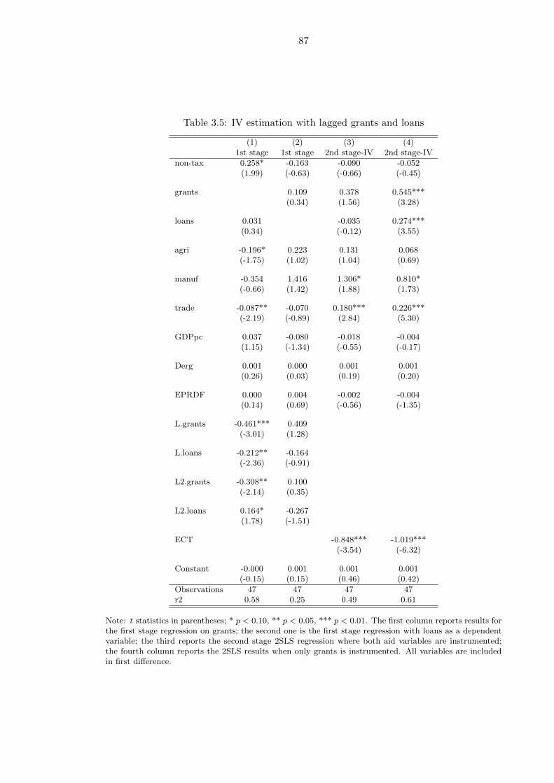
87
Table 3.5: IV estimation with lagged grants and loans
(1) (2) (3) (4)1st stage 1st stage 2nd stage-IV 2nd stage-IV
non-tax 0.258* -0.163 -0.090 -0.052(1.99) (-0.63) (-0.66) (-0.45)
grants 0.109 0.378 0.545***(0.34) (1.56) (3.28)
loans 0.031 -0.035 0.274***(0.34) (-0.12) (3.55)
agri -0.196* 0.223 0.131 0.068(-1.75) (1.02) (1.04) (0.69)
manuf -0.354 1.416 1.306* 0.810*(-0.66) (1.42) (1.88) (1.73)
trade -0.087** -0.070 0.180*** 0.226***(-2.19) (-0.89) (2.84) (5.30)
GDPpc 0.037 -0.080 -0.018 -0.004(1.15) (-1.34) (-0.55) (-0.17)
Derg 0.001 0.000 0.001 0.001(0.26) (0.03) (0.19) (0.20)
EPRDF 0.000 0.004 -0.002 -0.004(0.14) (0.69) (-0.56) (-1.35)
L.grants -0.461*** 0.409(-3.01) (1.28)
L.loans -0.212** -0.164(-2.36) (-0.91)
L2.grants -0.308** 0.100(-2.14) (0.35)
L2.loans 0.164* -0.267(1.78) (-1.51)
ECT -0.848*** -1.019***(-3.54) (-6.32)
Constant -0.000 0.001 0.001 0.001(-0.15) (0.15) (0.46) (0.42)
Observations 47 47 47 47r2 0.58 0.25 0.49 0.61
Note: t statistics in parentheses; * p < 0.10, ** p < 0.05, *** p < 0.01. The first column reports results forthe first stage regression on grants; the second one is the first stage regression with loans as a dependentvariable; the third reports the second stage 2SLS regression where both aid variables are instrumented;the fourth column reports the 2SLS results when only grants is instrumented. All variables are includedin first difference.

88
R2 in the grants equation is 0.3 whereas for the loans equation is 0.1, thus confirming
the low validity and relevance of the IV in the latter case. A more formal test for weak
instruments (Stock and Yogo, 2005) confirms that the proposed instruments are weak for
loans but not for grants17.
Having established that the IV may not be valid for loans, columns three and four
instrument respectively both variables and only grants, for which the IV appears valid.
When both variables are instrumented, loans becomes largely non-significant with a large
standard error (0.3, almost ten times larger than the coefficient) which could be expected.
The coefficient on grants is positive but also non-significant, with a more precise estimate
and a smaller standard error (0.24). When only grants is instruemnted (column 4), its
coefficient is positive and significant with a magnitude that is relatively similar to the OLS
estimate of 0.43418.
The 2SLS results therefore provide evidence for the robustness of the positive coefficient
of grants in the SR to endogeneity, while the IV estimates are not satisfactory for loans.
However the Granger causality test did not flag any concern for loans while it indicated
the possibility of reverse causality for grants (see appendix 3.H). The combined evidence
therefore suggests that estimates are fairly robust to endogeneity. Biases may occur, but
they appear to be small. However it should be noted that the instruments used here suffer
from limitations on validity, and therefore the issue of endogeneity is not fully tackled.
Chapter 4 will address these concerns more systematically.
The IV estimates can be compared to the OLS ones (those showed in table 3.3) to
assess the extent of endogeneity. Two tests are performed and they provide consistent
results: the Hausman test and the Durbin-Wu-Hausman test19. The former finds that
the difference in coefficients between the two methods is not systematic (p-value: 0.99),
therefore supporting the OLS estimates on efficiency grounds. The latter confirms this
result, failing to reject the null hypothesis of exogeneity of the aid variables with p-values
of 0.29 (Durbin score chi2) and 0.41 (Wu-Hausman F statistic).
17The hypothesis of weak instruments cannot be rejected for the former but it can for the latter at the10% level, with F-statistic of 1.5 for loans and 8.7 for grants, to be compared with a 10% critical value of7.5.
18The coefficient estimated with 2SLS is larger than the OLS one, thus indicating a small negative bias.While the IV estimate should not be taken as a precise point estimate, it may be compared with the resultsobtained when including governance in section 3.4.3. As far as grants are concerned, the exercise withICRG data did not show a clear indication on the sign of the bias. Therefore the ICRG and IV resultsare largely consistent. The fact that all estimates (OLS, IV and including ICRG) are of comparable inmagnitude supports the robustness of a positive effect of grants.
19The first test requires homoskedasticity while the second one allows for heteroskedasticity.

89
Qualitative evidence
In addition to econometric tests and techniques, qualitative evidence may help explaining
the nature of endogeneity in Ethiopia and assessing the extent to which it is indeed a
problem. This qualitative analysis is supported by interviews to government officials and
donor agencies, therefore allowing for great insight into the working of the aid-tax relation
in the Ethiopian context.
Chapter 2 shows that Ethiopia since 1960 has received aid for reasons largely other
than economic ones. To the extent that aid is driven by political and strategic reasons in
donor countries, it is exogenous to the Ethiopian government’s decision making process
that determines the tax share conditional on a number of variables.
This discussion does not aim at arguing that donors disburse money regardless of the
country level conditions. Clearly they want to see ‘value for money’ and thus they do
care about basic economic indicators as well as fiscal policy. However conditionality in
Ethiopia is rather mild, due to weak enforceability and a relatively low bargaining power
of donors (see chapter 2 for a full discussion on this). Strong ownership and leadership on
the government’s side means that policy objectives and conditions need to be in line with
its priorities to be acceptable. This is largely recognised by donors as well, as confirmed in
the interviews. So for example fiscal discipline and relatively low corruption are part of the
Ethiopian institutional tradition and not a response to donor preferences, perhaps with
the aim of receiving more aid. This situation is not particularly surprising in a country
with a long institutional tradition and a history of independence from colonial powers.
An example of mild conditionality is PBS, which indeed does condition aid on service
delivery, something of which the government is very enthusiastic about. Chapter 2 shows
that this focus on services not only is in line with government’s objectives, but also it
allows it to gain legitimacy and popularity amongst citizens as well as largely wiping off
the discussion table broader economic policies.
Still using the example of PBS, let us consider conditionality on the revenue side. In
principle PBS imposes additionality, as foreign funds have to be matched by government
resources. I asked donors about the enforcement of this principle and in particular what
would happen if the government does not adhere to it. They confirmed that there is no
actual way to enforce additionality. However this has not been a problem in Ethiopia so
far, as the Government has consistently overperformed on the revenue targets. Indeed
increasing revenue is first and foremost a priority of the government thus making strict
conditionality on revenue irrelevant.

90
As far as economic factors are concerned, they do not seem to influence aid either.
For example Ethiopia has experienced very high inflation in the past 5 years and while
donors have been critical of this, aid has increased. Similarly the case of liberalizations is
emblematic (see chapter 2 for more details). Although the governemnt has systematically
refused to open up to donors requests in this area, there has been no consequence on aid
flows.
So aid does not seem to be driven by economic factors in Ethiopia. It is interesting that
even the most technical of the donor agencies involved in the interviews confirmed that it
is indeed political and stretegic reasons that really matter in Ethiopia, while donors can
always turn a blind eye on economic issues. Ethiopia benefits from a strategic geographical
position that allows easy access to the Middle East as well as a good base for commu-
nications and military operations. For example the American Kagnew communications
station, inaugurated well before the period considered here, was a crucial listening post
in the Korean war, World War Two and during the Cold War (see chapter 2 and Wrong
(2005)). The strategic importance of Ethiopia was then reinforced during the Cold War
and as a result of the increased terrorist threat following the attacks to US embassies in
Nairobi and Dar es Salaam in 1998 and the New York attacks of September 11th 2001.
To the strategic considerations is to be added the fact that Ethiopia is home to millions
of African poor, being a large country and still one of the poorest in the world. All this
explains why donors are reluctant to leave Ethiopia even when economic and political
conditions deteriorate.
One relevant example is the aftermath of the 2005 elections. While many donors
pointed to violations of human rights as well as irregularities in the election process,
aid was only temporarily suspended. One immediate ‘punishment’ was the end of budget
support that however was promptly replaced by PBS. Under this project (PBS is a project
although some similarities exist with tied budget support) aid could not only be restored
quickly after the interruption, but also it increased in the following years.
In conclusion, domestic economic and political factors do not seem to play a role
in determining variations in aid flows. The qualitative elements discussed here indeed
suggest that aid in Ethiopia seems to be only weakly or not at all determined by economic
or political governance (thus potentially raising concerns about the omitted variable bias)
or by the tax share itself (thus resulting in reverse causality). Instead it is more plausible
to explain aid flows with the political and strategic needs of donor countries, therefore
making them exogenous to the domestic decision making process.
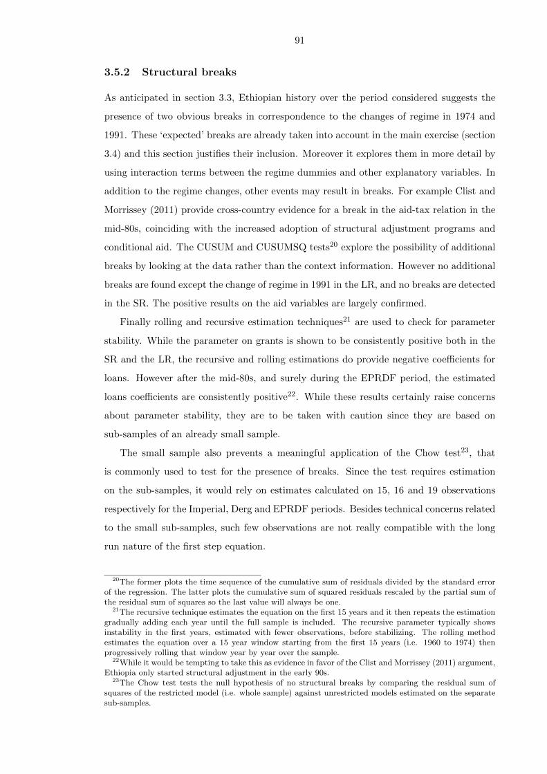
91
3.5.2 Structural breaks
As anticipated in section 3.3, Ethiopian history over the period considered suggests the
presence of two obvious breaks in correspondence to the changes of regime in 1974 and
1991. These ‘expected’ breaks are already taken into account in the main exercise (section
3.4) and this section justifies their inclusion. Moreover it explores them in more detail by
using interaction terms between the regime dummies and other explanatory variables. In
addition to the regime changes, other events may result in breaks. For example Clist and
Morrissey (2011) provide cross-country evidence for a break in the aid-tax relation in the
mid-80s, coinciding with the increased adoption of structural adjustment programs and
conditional aid. The CUSUM and CUSUMSQ tests20 explore the possibility of additional
breaks by looking at the data rather than the context information. However no additional
breaks are found except the change of regime in 1991 in the LR, and no breaks are detected
in the SR. The positive results on the aid variables are largely confirmed.
Finally rolling and recursive estimation techniques21 are used to check for parameter
stability. While the parameter on grants is shown to be consistently positive both in the
SR and the LR, the recursive and rolling estimations do provide negative coefficients for
loans. However after the mid-80s, and surely during the EPRDF period, the estimated
loans coefficients are consistently positive22. While these results certainly raise concerns
about parameter stability, they are to be taken with caution since they are based on
sub-samples of an already small sample.
The small sample also prevents a meaningful application of the Chow test23, that
is commonly used to test for the presence of breaks. Since the test requires estimation
on the sub-samples, it would rely on estimates calculated on 15, 16 and 19 observations
respectively for the Imperial, Derg and EPRDF periods. Besides technical concerns related
to the small sub-samples, such few observations are not really compatible with the long
run nature of the first step equation.
20The former plots the time sequence of the cumulative sum of residuals divided by the standard errorof the regression. The latter plots the cumulative sum of squared residuals rescaled by the partial sum ofthe residual sum of squares so the last value will always be one.
21The recursive technique estimates the equation on the first 15 years and it then repeats the estimationgradually adding each year until the full sample is included. The recursive parameter typically showsinstability in the first years, estimated with fewer observations, before stabilizing. The rolling methodestimates the equation over a 15 year window starting from the first 15 years (i.e. 1960 to 1974) thenprogressively rolling that window year by year over the sample.
22While it would be tempting to take this as evidence in favor of the Clist and Morrissey (2011) argument,Ethiopia only started structural adjustment in the early 90s.
23The Chow test tests the null hypothesis of no structural breaks by comparing the residual sum ofsquares of the restricted model (i.e. whole sample) against unrestricted models estimated on the separatesub-samples.
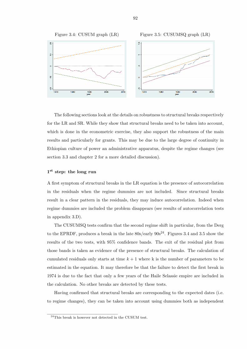
92
Figure 3.4: CUSUM graph (LR) Figure 3.5: CUSUMSQ graph (LR)
The following sections look at the details on robustness to structural breaks respectively
for the LR and SR. While they show that structural breaks need to be taken into account,
which is done in the econometric exercise, they also support the robustness of the main
results and particularly for grants. This may be due to the large degree of continuity in
Ethiopian culture of power an administrative apparatus, despite the regime changes (see
section 3.3 and chapter 2 for a more detailed discussion).
1st step: the long run
A first symptom of structural breaks in the LR equation is the presence of autocorrelation
in the residuals when the regime dummies are not included. Since structural breaks
result in a clear pattern in the residuals, they may induce autocorrelation. Indeed when
regime dummies are included the problem disappears (see results of autocorrelation tests
in appendix 3.D).
The CUSUMSQ tests confirm that the second regime shift in particular, from the Derg
to the EPRDF, produces a break in the late 80s/early 90s24. Figures 3.4 and 3.5 show the
results of the two tests, with 95% confidence bands. The exit of the residual plot from
those bands is taken as evidence of the presence of structural breaks. The calculation of
cumulated residuals only starts at time k + 1 where k is the number of parameters to be
estimated in the equation. It may therefore be that the failure to detect the first break in
1974 is due to the fact that only a few years of the Haile Selassie empire are included in
the calculation. No other breaks are detected by these tests.
Having confirmed that structural breaks are corresponding to the expected dates (i.e.
to regime changes), they can be taken into account using dummies both as independent
24This break is however not detected in the CUSUM test.

93
variables and in interaction terms. The latter in particular is useful to identify the effect
of breaks on the parameters of interest, namley those on the aid variables25. Table 3.6
reports the LR regression without and with regime shift dummies respectively in columns
1 and 2. Columns 3 and 4 add the interaction terms with the aid variables, respectively
without and with the shift dummies. In columns 3 and 4 therefore the parameter on the
variable refers to the reference period, i.e. Haile Selassie’s regime, while the coefficients
for other regimes are obtained by summing the coefficients on the original variable and on
the relevant interaction term.
The results in table 3.6 show that both grants and loans seem to have negative, though
largely non-significant coefficients in the first period and positive ones later. While loans
and its interaction terms are non-significant individually, they are jointly significant (F(3,
38) = 5.25, p-value: 0.004). However this is not the case for grants and its interaction
terms, for which the test of joint significance cannot reject the null (F(3, 38) = 1.07,
p-value: 0.373).
Figure 3.6: Grant rolling estimates (LR) Figure 3.7: Loan rolling estimates (LR)
Having identified the presence of structural breaks, parameter stability is assessed
across the period using a specification that includes regime dummies26. Rolling estimates
are obtained using rolling 15-years windows starting from the period 1960-1974. The
year on the horizontal axis is therefore the starting year of the rolling estimation. These
estimates are then plotted in figures 3.6 and 3.7 to assess the stability of parameters.
While informative, these results are to be taken with caution since each estimate is only
relying on 15 observations. Both parameters show a period of instability at the beginning
25This exercise is repeated for all variables in the model but the results are not reported for simplicity.The Derg dummy and its interaction terms are generally the most significant ones. The previous resultsare largely confirmed.
26The specification used as a basis for rolling and recursive estimation corresponds to column 3 in table3.1.
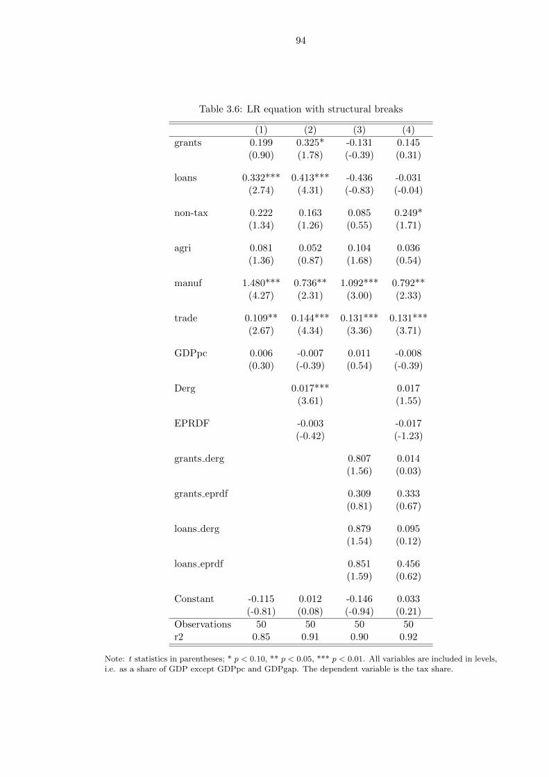
94
Table 3.6: LR equation with structural breaks
(1) (2) (3) (4)
grants 0.199 0.325* -0.131 0.145(0.90) (1.78) (-0.39) (0.31)
loans 0.332*** 0.413*** -0.436 -0.031(2.74) (4.31) (-0.83) (-0.04)
non-tax 0.222 0.163 0.085 0.249*(1.34) (1.26) (0.55) (1.71)
agri 0.081 0.052 0.104 0.036(1.36) (0.87) (1.68) (0.54)
manuf 1.480*** 0.736** 1.092*** 0.792**(4.27) (2.31) (3.00) (2.33)
trade 0.109** 0.144*** 0.131*** 0.131***(2.67) (4.34) (3.36) (3.71)
GDPpc 0.006 -0.007 0.011 -0.008(0.30) (-0.39) (0.54) (-0.39)
Derg 0.017*** 0.017(3.61) (1.55)
EPRDF -0.003 -0.017(-0.42) (-1.23)
grants derg 0.807 0.014(1.56) (0.03)
grants eprdf 0.309 0.333(0.81) (0.67)
loans derg 0.879 0.095(1.54) (0.12)
loans eprdf 0.851 0.456(1.59) (0.62)
Constant -0.115 0.012 -0.146 0.033(-0.81) (0.08) (-0.94) (0.21)
Observations 50 50 50 50r2 0.85 0.91 0.90 0.92
Note: t statistics in parentheses; * p < 0.10, ** p < 0.05, *** p < 0.01. All variables are included in levels,i.e. as a share of GDP except GDPpc and GDPgap. The dependent variable is the tax share.

95
of the period. The coefficient on grants then settles on mostly positive values, while the
one on loans becomes positive from the late 80s.
The plots of coefficients obtained using recursive estimation (not reported here for
simplicity) are largely consistent with the results from the rolling estimation.
2nd step: the short run
Contrary to the LR case, in the SR no autocorerlation is detected regardless of whether
the regime dummies are included or not. This suggests that structural breaks are not
present in the SR and indeed the CUSUM and CUSUMSQ tests confirm it. The test
results, reported in figures 3.8 and 3.9, show no evidence of structural breaks in the short
run as the plotted residuals lie inside the 95% confidence interval.
Although the analysis of residuals offers no evidence of the presence of structural
breaks, it may still be useful to check for the effect of interaction terms between regime
dummies and the aid variables27. Table 3.7 reports the results using the regime dummies
both as independent variables and in interactions terms. The coefficient on grants is
positive in all periods, generally with a larger magnitude in the Haile Selassie period.
Loans instead have a negative coefficient in the first period that turns positive in the
remaining two periods, with the EPRDF interaction term being always significant at the
10% level. A test of joint significance of grants and loans and their respective interaction
terms shows that they are both jointly significant28.
Parameter stability is explored using rolling estimation (in this section) and recursive
estimates (results not reported for simplicity) on a 15 years window29. Consistently with
LR results, the coefficient on grants is always positive as shown in figure 3.10. Its magni-
tude decreases as the window moves to more recent years. The coefficient on loans (figure
3.11), also in line with the long run, shows some negative estimates between the late 60s
and the early 80s when it becomes consistently positive. The coefficient of loans therefore
shows more instability than the one on grants.
27As before, interaction terms are also included for other explanatory variables although the results arenot reported here. The previous results are largely confirmed and the interaction terms, as well as thedummies included as independent variables are never significant.
28Grants: F(3, 34) = 4.02, p-value: 0.015; loans: F(3, 34) = 4.15, p-value: 0.013.29Estimates are based on the SR specification reported in column 1 of table 3.3.

96
Table 3.7: SR equation with structural breaks
(1) (2) (3) (4)
non-tax -0.042 -0.043 -0.022 -0.012(-0.33) (-0.34) (-0.17) (-0.09)
grants 0.415*** 0.434*** 0.637 0.490(3.21) (3.32) (1.01) (0.74)
loans 0.241*** 0.254*** -0.576 -0.640(2.88) (2.98) (-1.14) (-1.22)
agri 0.127 0.066 0.163 0.090(1.32) (0.60) (1.55) (0.73)
manuf 1.064** 0.838 1.177** 0.903(2.23) (1.61) (2.37) (1.63)
trade 0.190*** 0.207*** 0.188*** 0.207***(4.61) (4.71) (4.63) (4.69)
GDPpc -0.023 -0.005 -0.025 -0.006(-0.92) (-0.16) (-0.98) (-0.21)
Derg 0.001 0.001(0.45) (0.24)
EPRDF -0.002 -0.003(-0.86) (-0.95)
grants derg -0.016 0.088(-0.02) (0.13)
grants eprdf -0.278 -0.082(-0.43) (-0.12)
loans derg 0.569 0.645(1.01) (1.10)
loans eprdf 0.869* 0.953*(1.70) (1.78)
ECT -0.928*** -0.955*** -0.967*** -0.973***(-5.49) (-5.56) (-5.44) (-5.41)
Constant 0.000 0.000 0.001 0.001(0.27) (0.06) (0.53) (0.35)
Observations 49 49 49 49r2 0.59 0.61 0.65 0.66
Note: t statistics in parentheses; * p < 0.10, ** p < 0.05, *** p < 0.01. All variables are included in firstdifference and the dependent variable is the tax share.

97
Figure 3.8: CUSUM graph(SR) Figure 3.9: CUSUMSQ graph (SR)
Figure 3.10: Grant rolling estimates(SR) Figure 3.11: Loan rolling estimates (SR)
98
3.5.3 Estimation in logs
A further robustness check regards the way variables are measured, namely as shares of
GDP. GDP figures are based on surveys and other estimates of economic activities. They
may therefore be imprecise or change in time because of better estimation techniques. In
addition GDP figures have been at the center of a heated debate in recent years, with
many forign observers doubting their validity (Dercon and Zeitlin, 2009). The analysis is
therefore repeated with the variables in logs instead of shares of GDP, to check whether
it is indeed the denominator that drives the results.
Stationarity is tested for all variables and they all turn out to be I(1). It is therefore
possible to proceed with the cointegration procedure as in the previous analysis. Table
3.I.1 in appendix 3.I reports the results for both the LR and SR.
The LR specification in logs still passes the Engle-Granger test for cointegration and it
is therefore possible to carry out the standard two-step procedure. The results are robust
to a different variable definition that excludes GDP at the denominator. Indeed previous
results are largely confirmed when repeating the estimation in logs and particularly so for
the aid variables that are positive and significant in all specifications. In particular a 1%
increase in grants is associated with a 0.1% increase in tax revenue in the short run, while
a 1% increase in loans would have a smaller effect of 0.05% on tax revenue.
Note that now the coefficient on the GDP gap is non-significant and positive, confirm-
ing the hypothesis that the negative and significant coefficient found in section 3.4 may
be due to a built-in correlation with GDP at the denominator of the dependent variable.
Indeed when tax is measured as a log, rather than a share of GDP, the GDP gap is not
significant anymore.
The coefficients on other variables are largely similar to previous estimates. The only
noteworthy change is the positive coefficient on agriculture, that is now significant whereas
manufacturing fails to reach significance in all specifications.
3.6 Unpacking the effects: tax types and tax composition
Having carried out the analysis using the aggregate tax share, this section turns to the
individual tax types to check if the identified effects run through a particular one of these.
There are potentially various channels through which aid relates to tax revenue. For
example aid may provide foreign exchange to purchase imports that, if taxed, contribute
to increasing tax revenue. Aid may also provide support to tax reform aimed at increasing
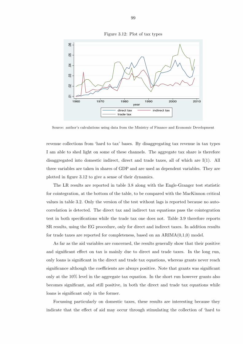
99
Figure 3.12: Plot of tax types
.01.02
.03.04
.05.06
1960 1970 1980 1990 2000 2010year
direct tax indirect taxtrade tax
Source: author’s calculations using data from the Ministry of Finance and Economic Development
revenue collections from ‘hard to tax’ bases. By disaggregating tax revenue in tax types
I am able to shed light on some of these channels. The aggregate tax share is therefore
disaggregated into domestic indirect, direct and trade taxes, all of which are I(1). All
three variables are taken in shares of GDP and are used as dependent variables. They are
plotted in figure 3.12 to give a sense of their dynamics.
The LR results are reported in table 3.8 along with the Engle-Granger test statistic
for cointegration, at the bottom of the table, to be compared with the MacKinnon critical
values in table 3.2. Only the version of the test without lags is reported because no auto-
correlation is detected. The direct tax and indirect tax equations pass the cointegration
test in both specifications while the trade tax one does not. Table 3.9 therefore reports
SR results, using the EG procedure, only for direct and indirect taxes. In addition results
for trade taxes are reported for completeness, based on an ARIMA(0,1,0) model.
As far as the aid variables are concerned, the results generally show that their positive
and significant effect on tax is mainly due to direct and trade taxes. In the long run,
only loans is significant in the direct and trade tax equations, whereas grants never reach
significance although the coefficients are always positive. Note that grants was significant
only at the 10% level in the aggregate tax equation. In the short run however grants also
becomes significant, and still positive, in both the direct and trade tax equations while
loans is significant only in the former.
Focussing particularly on domestic taxes, these results are interesting because they
indicate that the effect of aid may occur through stimulating the collection of ‘hard to
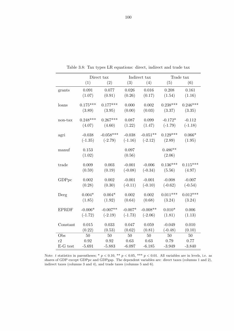
100
Table 3.8: Tax types LR equations: direct, indirect and trade tax
Direct tax Indirect tax Trade tax(1) (2) (3) (4) (5) (6)
grants 0.091 0.077 0.026 0.016 0.208 0.161(1.07) (0.91) (0.26) (0.17) (1.54) (1.16)
loans 0.175*** 0.177*** 0.000 0.002 0.238*** 0.246***(3.89) (3.95) (0.00) (0.03) (3.37) (3.35)
non-tax 0.248*** 0.267*** 0.087 0.099 -0.172* -0.112(4.07) (4.60) (1.22) (1.47) (-1.79) (-1.18)
agri -0.038 -0.058*** -0.038 -0.051** 0.129*** 0.066*(-1.35) (-2.79) (-1.16) (-2.12) (2.89) (1.95)
manuf 0.153 0.097 0.486**(1.02) (0.56) (2.06)
trade 0.009 0.003 -0.001 -0.006 0.136*** 0.115***(0.59) (0.19) (-0.08) (-0.34) (5.56) (4.97)
GDPpc 0.002 0.002 -0.001 -0.001 -0.008 -0.007(0.28) (0.30) (-0.11) (-0.10) (-0.62) (-0.54)
Derg 0.004* 0.004* 0.002 0.002 0.011*** 0.012***(1.85) (1.92) (0.64) (0.68) (3.24) (3.24)
EPRDF -0.006* -0.007** -0.007* -0.008** 0.010* 0.006(-1.72) (-2.19) (-1.73) (-2.06) (1.81) (1.13)
Constant 0.015 0.033 0.047 0.059 -0.049 0.010(0.22) (0.53) (0.62) (0.81) (-0.48) (0.10)
Obs 50 50 50 50 50 50r2 0.92 0.92 0.63 0.63 0.79 0.77E-G test -5.691 -5.883 -6.097 -6.185 -3.949 -3.840
Note: t statistics in parentheses; * p < 0.10, ** p < 0.05, *** p < 0.01. All variables are in levels, i.e. asshares of GDP except GDPpc and GDPgap. The dependent variables are: direct taxes (columns 1 and 2),indirect taxes (columns 3 and 4), and trade taxes (columns 5 and 6).
101
tax’ handles, such as income and profits, whereas ‘easy to tax’ ones (i.e. consumption
through indirect taxes) are already tapped30. This may also explain the non-significant
coefficient in the indirect tax equation. In this context the introduction of the VAT, that
was strongly supported by the international financial institutions, may play a minor role
because it largely replaced pre-existing sales taxes. Figure 3.12 shows that in the early
90s indirect and trade taxes (both considered ‘easy to collect’) increased substantially
while direct taxation lagged behind. This would support the view that income taxes are
more difficult to raise, because of administrative capacity but also political constraints.
In this context the stimulus effect of aid may happen both through technical assistance
aimed at increasing local capacity; and through the interantional backing of donors and
international financial institutions that may give legitimacy to politically difficult reforms.
Since trade is certainly considered ‘easy to tax’, this argument would however not be
informative in explaining the positive coefficient of loans in the trade tax equation. That
posive effect may instead be due to the increased availability of foreign exchange allowed
through aid, that may fuel imports and in turn trade taxes. Note that the positive effect
of aid on trade taxes is documented also elsewhere in the literature (Benedek et al., 2012).
Another interesting result is the coefficient on agriculture, that was consistently non-
significant in all specifications notwithstanding its expected negative effect. Agriculture
is generally found to have a negative effect on domestic direct and indirect taxes, as
expected, while it has a positive effect on trade taxes, consistently with other studies in
the literature (Aizenman and Jinjarak, 2009). The negative effect becomes significant once
manufacturing is dropped both in the LR and SR equations, thus improving precision in
the estimates (see appendix 3.E on multicollinearity)31. In the aggregate tax equation this
expected negative effect of agriculture is probably offset by the positive one through trade
taxes, thus making the coefficient largely non-significant. The positive sign on agriculture
in the trade tax equation may be due to export taxes that have been largely reliant on
agricultural exports, most notably coffee. Indeed Ethiopian exports are largely agricultural
products and up to 2002/2003, when export taxes were eliminated, they represented an
important source of revenue.
30Aizenman and Jinjarak (2009) provide a cross country analysis of the effects of globalization on ‘easy tocollect’ and ‘difficult to collect’ taxes. In their classification, the former category includes trade taxes andseignorage, whereas the second one includes domestic direct (income, profits) and indirect (sales, VAT)taxes. However in the case of Ethiopia indirect taxes have been always considered ‘easy to collect’, asexplained throughout chapter 2. Therefore it seems legitimate to consider only direct taxes on income andprofits as ‘hard to tax’ in the discussion here.
31The equation excluding agriculture is not reported here for simplicity but it yields coefficients of thesame sign and significance for other variables.

102
Table 3.9: Tax types SR equations: direct, indirect and trade tax
Direct tax Indirect tax Trade tax(1) (2) (3) (4) (5) (6)
non-tax 0.110** 0.117** 0.036 0.028 -0.201** -0.140(2.08) (2.35) (0.49) (0.40) (-2.15) (-1.45)
grants 0.089* 0.088* 0.020 0.021 0.209** 0.188(1.74) (1.74) (0.27) (0.30) (2.12) (1.37)
loans 0.140*** 0.144*** -0.011 -0.015 0.033 0.064(4.11) (4.43) (-0.23) (-0.33) (0.56) (0.88)
agri -0.033 -0.047* -0.089 -0.070* 0.157*** 0.039(-0.73) (-1.69) (-1.41) (-1.78) (2.94) (1.00)
manuf 0.084 -0.118 0.750*(0.40) (-0.39) (1.87)
trade 0.039** 0.040** 0.027 0.026 0.094*** 0.096***(2.32) (2.43) (1.14) (1.11) (4.62) (4.24)
GDPpc 0.012 0.014 0.018 0.014 -0.025 -0.005(1.00) (1.38) (1.03) (0.98) (-1.50) (-0.35)
ECM -0.726*** -0.739*** -0.927*** -0.916***(-4.85) (-5.11) (-5.57) (-5.65)
Constant -0.000 -0.000 -0.000 -0.000 0.001 0.000(-0.23) (-0.31) (-0.23) (-0.17) (0.93) (0.06)
Dummies yes yes yes yes yes yes
Obs 49 49 49 49 49 49r2 0.58 0.58 0.50 0.49 - -
Note: t statistics in parentheses; * p < 0.10, ** p < 0.05, *** p < 0.01. All variables are included in firstdifference. The dependent variables are: direct taxes (columns 1 and 2), indirect taxes (columns 3 and4), and trade taxes (columns 5 and 6). In the case of direct and indirect taxes, the results are fromt hesecond step of the EG procedure. For trade taxes the results are obtained using and ARIMA(0,1,0) model.Regime dummies for the Derg and EPRDF period are included in all equations.

103
Finally, an alternative approach to gaining insights into tax composition is to use a
variable that indicates the share of domestic taxes (i.e. direct and domestic indirect) to
total revenue. Tax composition, as defined here, is a central issue in developing countries
where trade taxes still represent the lion’s share of tax revenue. This is indeed the case
in Ethiopia where in the last year of the sample trade taxes still contributed over 40% to
total tax revenue, and over the whole period that share peaked at 56%. The international
community has been concerned with the possibility of a shift towards domestic taxes and
this idea has been at the basis also of the adoption of VAT by an increasing number of
countries (Keen and Ligthart, 2002; Keen and Simone, 2004). Tax composition is used as
a dependent variable, however this exercise did not yield satisfactory results or additional
insight. It is therefore not reported here.
3.7 The positive aid-tax relation: interpretation
The main result of the analysis is a strong rejection of the disincentive effect that is
sometimes argued in the context of the aid effectiveness debate. I show that aid is instead
positively associated with the tax share. The positive effect is generally confirmed for both
grants and loans, with some differences that are discussed later in this section.
This postive relation implies that aid and tax are not treated as substitutes but that
instead increases in aid are associated with increases in taxes. Indeed aid may influence tax
collection by contributing to improving the tax administration (thus decreasing adminis-
trative costs, for example by promoting the introduction of IT systems) and by providing
international legitimacy for tax reform (thus decreasing political costs). Its coefficient
in the reduced form equation is therefore the result of a negative effect due to possible
substitution and a positive one through the reduction of the costliness of raising tax. The
empirical results from Ethiopia suggest that the latter positive effect is larger than the
possible negative one.
Turning to aid heterogeneity, while grants and loans appear to have both a positive
effect on tax revenue, some differences emerge from the analysis. The idea developed in the
literature (Gupta et al., 2004) that loans may stimulate tax mobilisation more than grants
because of repayment, is partly confirmed. In the long run loans are always significant
while grants only reach the 10% level in one specification. Despite this, no evidence can
be provided for a LR detrimental effect of grants on tax effort. The coefficient on grants
is consistently positive, also when rolling estimates are provided in section 3.5.2 both for
the LR and SR.

104
In the short run both aid variables are significant above the 5% level and still positive,
with grants having a larger coefficient than loans. This may suggest that grants are used
mainly to release short run constraints in the administration, thus allowing a contempo-
raneous increase in tax revenue. Moreover both coefficients (grants and loans) are robust
to the inclusion of governance in the equation, to capture institutional factors that are
excluded from the main equations. The coefficient of grants in particular is also robust
to taking into account endogeneity with IV estimation, while a satisfactory instrument
cannot be found for loans.
A disaggregation of tax revenue into direct, indirect and trade taxes, shows that the
positive effect of aid occurs primarily through direct and trade taxes. In the case of
direct taxes, the explanation may be related to the beneficial effect of aid in supporting
the increased mobilisation of ‘hard to collect’ taxes such as those on income and profits.
Instead ‘easy to collect’ taxes such as those on consumption may already be tapped, thus
not benefiting as much from aid. This explanation would not be appropriate in the case
of trade taxes however, where the positive effect may be due to the provision of foreign
exchange through aid.
In the Ethiopian context, the positive effect can be explained by two elements in
particular: capacity building and matching32. Indeed capacity is the most widely cited
constraint to tax revenue mobilisation in interviews, both with government officials and
with donors. Aid is likely to have an effect on this capacity constraint thanks to technical
assistance, additional resources for tax administration and external advisors. Ethiopia
has received external advice and support in the area of taxation across the whole period,
including assistance from the US, UN and WB during the Imperial period (see chapter
2). More recently taxation has remained one of the few policy areas of strong cooperation
between donors and the government, while on other macroeconomic policies disagreement
often occurs. For this reason the positive effect of aid through various capacity building
activities is fully consistent with the Ethiopian context. By making the administration
more efficient, aid may also contribute to making taxation less costly thus resulting in an
increase in tax revenue.
At least three examples exist today in Ethiopia of this foreign role in the area of
32Other possible explanations can be provided for a positive effect of aid on tax revenue, which I howeverbelieve being secondary to capacity building and matching. For example aid may increase marketablesurplus due to better infrastructure and thus increase revenue through indirect taxes on goods. It couldalso imply an increase in aid-related imports that, while largely duty-free, may still imply an increase intrade tax revenues.
105
taxation. The first one is the Public Sector Capacity Building program (PSCAP), one of
the 6 themes of which is precisely taxation. Secondly PBS funds, amongst other things,
projects aimed at raising awareness on tax issues, with the final objective of increasing
compliance (see chapter 2). Indeed at least two interviewees mentioned that a basic
knowledge about the budget process and what taxes are used for can help overcoming
compliance and evasion problems. Finally the IMF has had a crucial advisory role both in
the 2002 reform, that amongst other things introduced the VAT, and in the 2008 reforms
(see chapter 2).
The second possible explanation is that the government is matching foreign resources
with internal ones. This may happen because of two reasons. The most obvious one is that
donors may require the governemnt to do so. While this is indeed the case, for example
under PBS that includes an additionality clause, it does not seem that donors are really
driving the matching effect. This is confirmed by the consistent over-performance of the
Government of Ethiopia with respect to the revenue targets under PBS.
The second reason for matching is related to the specific historical and cultural char-
acteristics of Ethiopia. Ethiopia is the only country in Africa to have never been colonized
and this is deeply rooted in the national culture and pride. Not only does this translate
in great policy ownership and a heavy weight attached to aid conditions and external
influence; but also it implies a tradition of independence and a feeling that the country
can ‘stand on its own feet’. In this sense, as emerged also in a few interviews, having
to rely on foreign funding to deal with domestic development challenges is a shame for
Ethiopians. It means that the country is not able to ‘feed its population’ and to respond to
its basic needs. This sentiment is clear in some of the speeches of the late Prime Minister
Meles Zenawi who ruled Ethiopia for 20 years, and it is at the basis of the willingness
of the Government to match foreign resources with domestic ones. In fact aid may even
set an incentive for tax revenue mobilisation not only because of the possible dependence
and shame coming with it, but also because it makes the ambitious development project
happen. Again, this emerged in many interviews. Ethiopia has ambitious development
projects that would be hard to implement only with domestic resources. The fact that aid
is available makes the project realistic and feasible, thus giving momentum to domestic
revenue mobilisation efforts.
The positive relation between aid and tax is reinforced by the fact that they are not
treated as substitutes in Ethiopia but rather as complements. In addition to the elements
discussed previously (i.e. independence, national pride, external influence) aid volatility

106
and unpredictability also prevent them to be substitutes. A plot of the three-year moving
average of the tax and aid series shows very clearly that the latter is a much more volatile
source of revenue than tax (see figure 3.2). Many interviewed government officials argue
that it is not a sustainable source of funding because its little reliability makes it difficult
to plan ahead.
3.8 Conclusions and policy implications
This chapter provided evidence on a positive relation between aid and tax in Ethiopia.
The use of in depth qualitative information, that represents a novelty in the literature, is
used to explain the results in the specific context of Ethiopia. Given the country-specific
historical and political context, a positive relation between aid and tax seems particularly
well grounded in Ethiopia and examples are provided throughout the chapter.
The main conclusion of the analysis is the presence of a strong and positive relation
between aid and taxation, that is particularly robust for grants (particulalry to structural
breaks and endogeneity). The positive results on grants and loans are robust to the
inclusion of governance, that is often omitted from time series analyses of tax effort. As
far as aid heterogeneity is concerned, grants and loans both have a positive sign although
they present some differences in their LR and SR effects that are discussed in section 3.7.
The first policy implication is therefore that in the case of Ethiopia a crowding out
effect of aid should not be a source of concern for donors. I find no evidence in Ethiopia
of such a negative effect of aid on tax effort or of the opportunistic behavior that would
result in a substitution between tax and aid. Instead the results support the idea that
aid has been effective in supporting the administration and in strengthening institutions
in the field of taxation.
In addition, the inclusion of other tax determinants in the analysis allows drawing a
few broader conclusions and policy implications.
Firstly the effect of manufacturing is very large and significant, particularly in the
long run equation. Its coefficient exceeds unity in some specifications, implying that a
percentage point increase in the share of manufacturing in GDP results in an even higher
increase in the tax share. For example the coefficient of 0.7 (in the preferred LR equation,
column 3 in table 3.1) suggests that for each percentage point increase in the manufacturing
share, 70% of it goes into increased tax. Besides arguments related to the high visibility
and accessibility of manufacturing firms, this large effect may be due to the fact that
firms act as tax collectors, as they transfer to the state taxed levied on employees’ salaries

107
and on consumption. This result, by indicating the strong revenue generating potential
of the manufacturing sector, underlines that industrial development has fiscal advantages
in addition to the better documented benefits in terms of employment, formality and
structural transformation.
Secondly trade displays the expected positive and significant coefficient in virtually
all specifications. This is a confirmation of the major role that trade plays as a tax
base in many developing countries, and particulalry in Ethiopia. Indeed Ethiopia is one
of the African countries with the highest share of trade taxes in total revenue (OECD
and African Development Bank Group, 2010). This clearly has implications in terms of
trade liberalization. While the increase in trade flows would bring about more revenue, a
decrease in tax rates may have an adverse revenue impact at least in the short term. It is
therefore important to understand the balance between these two opposite effects and to
provide for alternative sources of revenue in order to alleviate the possible negative effects
of liberalization, particularly in countries like Ethiopia that are highly reliant on trade
taxes.
Thirdly agriculture does not seem to have a significant effect on the aggregate tax
share due to its contrasting effects on different tax types. While a positive effect is found
for trade taxes, the expected negative one occurs for domestic direct and indirect taxes.
This result is particularly worrying in the context of the efforts of developing countries
to switch away from trade taxes towards domestic revenue (Keen and Simone, 2004).
The agricultural sector may represent a possible opportunity for future reform to increase
its revenue generation capacity, especially as commercial agriculture develops. However
the subsistance and remoteness that characterize this sector are likely to remain major
constraints to tax revenue mobilisation in Ethiopia.
Finally, also in line with much of the literature, the analysis largely fails to find a
significant effect of GDP per capita.

108
Appendices

109
3.A Critical summary of existing theories
Two main models have been developed for the analysis of tax determinants and its relation
with aid, namely Heller (1975) and Ezemenari et al. (2008).
Most empirical analyses of tax determinants are based on the theoretical framework
developed initially by Heller in his seminal work (Heller, 1975). These include, amongst
others, Mahdavi (2008), Leuthold (1991), Ghura (1998), Gang and Khan (1991), Franco-
Rodriguez et al. (1998), Osei et al. (2003), and Mosley et al. (1987).
Heller’s original model is based on the maximization of the public sector decision
maker’s utility function under the constraint that total revenues (including borrowing)
should equal total expenditures. The utility function is represented by deviations of ac-
tual fiscal aggregates from target levels, and it is specified in a quadratic form so that
marginal utility diminishes as the actual variables rise above the target levels. In this
framework taxation is the policy instrument and it is therefore endogenous, while aid is
considered exogenous. Franco-Rodriguez et al. (1998) later expanded the model to allow
for endogenous aid. This original version of the model is the basis for fiscal response studies
that typically only take into account fiscal variables (and growth in some cases). However
this model has progressively been abandoned in favor of more a-theoretical approaches
such as VAR and CVAR models.
Heller’s original model largely inspired the theoretical framework developed in Leuthold
(1991) in the context of a single equation model of tax determinants. While the author
still estimates a target for tax revenue, along Heller’s lines, other variables are included
besides purely fiscal ones. In particular, variables representing the tax base are used and
namely income, agriculture, mining and trade (imports + exports). Ghura (1998) further
expanded Leuthold’s model to include also corruption and economic policies and Mahdavi
(2008) added further sets of variables to it. This framework is the basis for most empirical
works focussing on a single equation for the tax share. These models are also referred to
as tax effort studies because of the possibility to obtain an index of tax effort based on
the ratio between actual and predicted tax share.
While the model developed by Heller has been used and developed by many authors,
it is also subject to criticism. The two main points of this critique are the functional form
and the computation of targets.
First, Binh and McGillivray (1993) note that meeting the target levels does not maxi-
mize utility in the original model and they suggest a change in the quadratic loss function
that allows overcoming this problem. However even with this modification, the model still

110
implies the same effect on utility from overshooting or undershooting the target. This is
clearly unrealistic. Feeny (2006) modifies the theoretical model to allow for asymmetries
in policy preferences and finds that although this issue is of great theoretical interest, it
implies few empirical consequences.
The second criticism regards the computation of targets. The way it is done in Heller
(1975) is not convincing, as target values are predicted using lags of the actual value, or
other variables for which theoretical justification is weak. Moreover, as pointed out in
White (1994), it is important to analyze the R2 of such auxiliary regressions. On the one
hand a high value might simply mean that the actual value of the variable is very close to
the target. This would reduce the meaningfulness of deviations from the target since it is
estimated from the actual value. On the other hand, a small R2 indicates a poor fit of the
equation thus casting doubts on the validity of such targets.
Moreover the target values thus estimated do not necessarily meet the constraint of
budget balance, as borrowing is set to zero. A possible solution would be to estimate the
target values of revenue and expenditure and allow borrowing to be different from zero
and thus fill the gap. Therefore the working of the model is heavily reliant on the targets
that are determined in a way that is of dubious validity. In fact White (1994) even argues
that the way in which targets are derived is a statistical artifact that leads to erroneous
results in Gang and Khan (1991).
Departing completely from Heller’s framework, Ezemenari et al. (2008) developed a
model to analyze the effects of aid on tax and on public investment. The model is based on
an intertemporal expenditure function, that describes the demand side of the economy and
that “denotes the minimum expenditure (in present value) required to achieve a given level
of utility at constant consumer prices and public good provision” (Ezemenari et al., 2008);
and on a revenue function that represents the production side of the economy and that
depends on the factors of production and prices. These two functions are then detailed
and developed to describe the economy more specifically. No trade occurs in this economy
and two periods are considered. The policy instruments are the tax rate and the share of
public investment in total spending. Direct taxes are levied through a lump-sum tax that
is exogenous and therefore the policy instrument is the consumption tax rate alone.
Three main propositions stem from the model and namely:
• An increase in foreign aid would reduce the proportion of government revenue that
is allocated for public investment;
• Under certain conditions, an increase in foreign aid reduces the optimal level of

111
consumption tax rate;
• An increase in foreign aid increases the provision of the public good and, under
certain conditions, it also increases both public and private investments.
These propositions stem from assumptions and conditions derived mathematically by the
authors. While some of them are clear and plausible, others are less straightforward.
In fact the paper fails to connect complex theoretical considerations to the reality of
developing countries by explaining their plausibility in that context. Moreover, while
clearly some simplification is necessary in a complex theoretical exercise, the exclusion of
trade and direct taxation from the model represents a serious shortcoming. Indeed it is
well known that trade is a major tax base in developing countries. In addition it is mainly
in the area of direct taxes that tax benefits and exemptions take place (i.e. fiscal benefits
for businesses). By looking only at the consumption tax rate, the paper fails to include in
the analysis some of the most important aspects of taxation in developing countries.
The model suggests two equations to be estimated empirically, one for tax revenue and
one for public investment. Interestingly the tax equation obtained is very similar to the one
used in Heller-type models. Moreover the dependent variable in the empirical tax equation
is the tax share, that includes all taxes and not only consumption ones. This implies a
weak link between the theory and the empirics, as they focus on different variables. This
also prevents to fully exploit the theory in interpreting the empirical results.
In conclusion this model brings some interesting elements to the analysis, namely the
intertemporal dimension and the effect of aid on the share of public investment. Moreover
it underlines the importance of moving away from the Heller framework and it offers
a valuable contribution in this direction. However it does not seem to allow a better
understanding of tax determinants than the standard tax effort models and it may not be
suitable to providing a complete analysis of taxation in Africa.

112
3.B Summary of variables
Table 3.B.1: Summary of variables
Name Definition Mean St. dev. Min Max
tax Total tax revenueas a share of GDP
.082 .024 .039 .124
dirtax Direct tax rev-enue as a share ofGDP
.028 .012 .010 .048
indtax Indirect tax rev-enue as a share ofGDP
.022 .006 .010 .036
tradetax Trade tax revenueas a share of GDP
.032 .011 .014 .061
grants Foreign grants asa share of GDP
.020 .012 0 .047
loans Foreign loans as ashare of GDP
.020 .016 .002 .092
trade Imports and ex-port as a share ofGDP
.187 .111 .085 .504
agri Agriculture shareof GDP
.591 .099 .415 .784
manuf Manufacturingshare of GDP
.048 .010 .026 .065
GDPpc Log of constantGDP per capita
6.946 .154 6.733 7.494
GDPgap Percentage devia-tion of GDP fromtrend (Hodrick-Prescott filter)
0 .134 -.312 .416
taxcomp Direct and in-direct domestictaxes as a share oftotal tax revenue
.600 .085 .439 .780
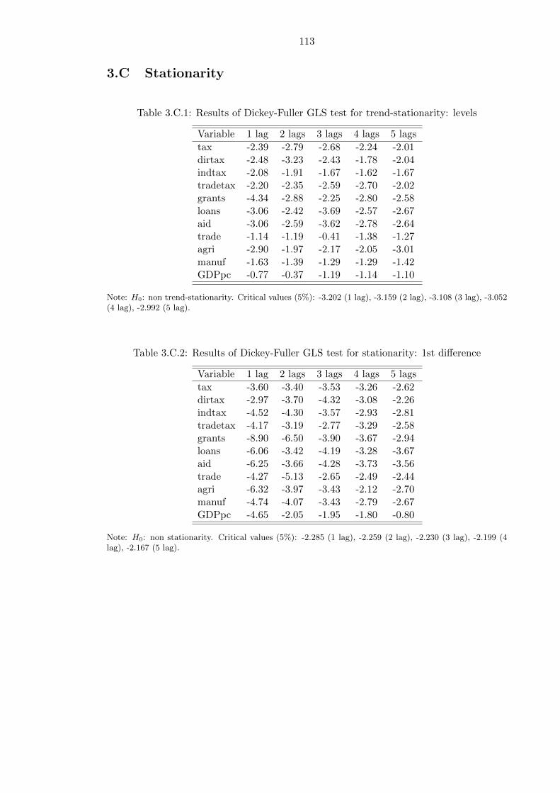
113
3.C Stationarity
Table 3.C.1: Results of Dickey-Fuller GLS test for trend-stationarity: levels
Variable 1 lag 2 lags 3 lags 4 lags 5 lags
tax -2.39 -2.79 -2.68 -2.24 -2.01dirtax -2.48 -3.23 -2.43 -1.78 -2.04indtax -2.08 -1.91 -1.67 -1.62 -1.67tradetax -2.20 -2.35 -2.59 -2.70 -2.02grants -4.34 -2.88 -2.25 -2.80 -2.58loans -3.06 -2.42 -3.69 -2.57 -2.67aid -3.06 -2.59 -3.62 -2.78 -2.64trade -1.14 -1.19 -0.41 -1.38 -1.27agri -2.90 -1.97 -2.17 -2.05 -3.01manuf -1.63 -1.39 -1.29 -1.29 -1.42GDPpc -0.77 -0.37 -1.19 -1.14 -1.10
Note: H0: non trend-stationarity. Critical values (5%): -3.202 (1 lag), -3.159 (2 lag), -3.108 (3 lag), -3.052(4 lag), -2.992 (5 lag).
Table 3.C.2: Results of Dickey-Fuller GLS test for stationarity: 1st difference
Variable 1 lag 2 lags 3 lags 4 lags 5 lags
tax -3.60 -3.40 -3.53 -3.26 -2.62dirtax -2.97 -3.70 -4.32 -3.08 -2.26indtax -4.52 -4.30 -3.57 -2.93 -2.81tradetax -4.17 -3.19 -2.77 -3.29 -2.58grants -8.90 -6.50 -3.90 -3.67 -2.94loans -6.06 -3.42 -4.19 -3.28 -3.67aid -6.25 -3.66 -4.28 -3.73 -3.56trade -4.27 -5.13 -2.65 -2.49 -2.44agri -6.32 -3.97 -3.43 -2.12 -2.70manuf -4.74 -4.07 -3.43 -2.79 -2.67GDPpc -4.65 -2.05 -1.95 -1.80 -0.80
Note: H0: non stationarity. Critical values (5%): -2.285 (1 lag), -2.259 (2 lag), -2.230 (3 lag), -2.199 (4lag), -2.167 (5 lag).
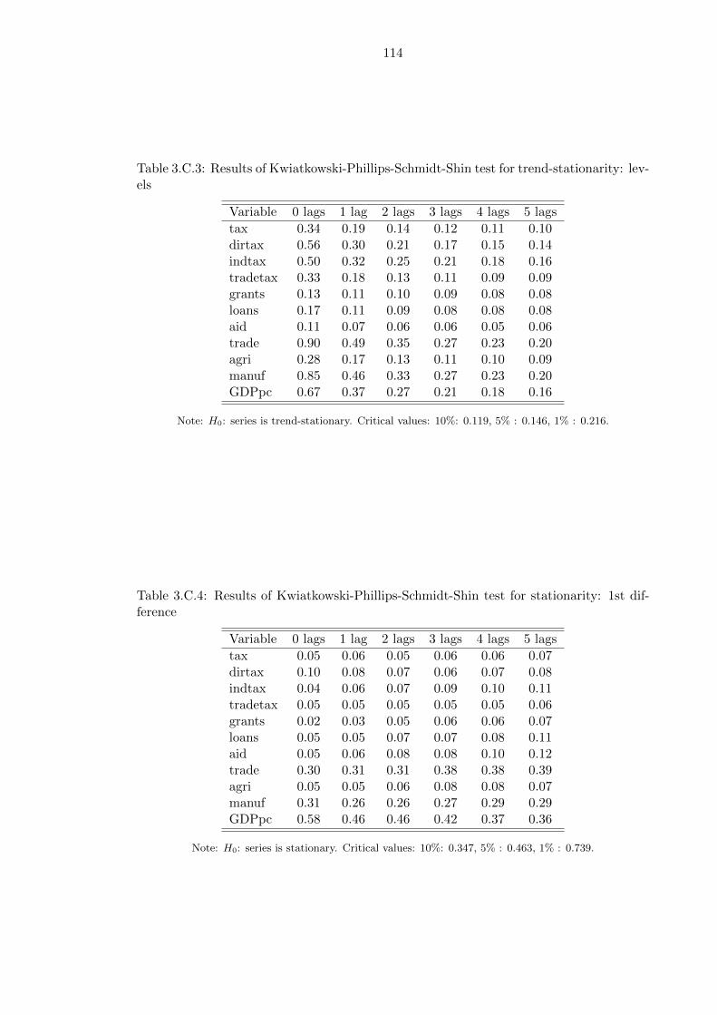
114
Table 3.C.3: Results of Kwiatkowski-Phillips-Schmidt-Shin test for trend-stationarity: lev-els
Variable 0 lags 1 lag 2 lags 3 lags 4 lags 5 lags
tax 0.34 0.19 0.14 0.12 0.11 0.10dirtax 0.56 0.30 0.21 0.17 0.15 0.14indtax 0.50 0.32 0.25 0.21 0.18 0.16tradetax 0.33 0.18 0.13 0.11 0.09 0.09grants 0.13 0.11 0.10 0.09 0.08 0.08loans 0.17 0.11 0.09 0.08 0.08 0.08aid 0.11 0.07 0.06 0.06 0.05 0.06trade 0.90 0.49 0.35 0.27 0.23 0.20agri 0.28 0.17 0.13 0.11 0.10 0.09manuf 0.85 0.46 0.33 0.27 0.23 0.20GDPpc 0.67 0.37 0.27 0.21 0.18 0.16
Note: H0: series is trend-stationary. Critical values: 10%: 0.119, 5% : 0.146, 1% : 0.216.
Table 3.C.4: Results of Kwiatkowski-Phillips-Schmidt-Shin test for stationarity: 1st dif-ference
Variable 0 lags 1 lag 2 lags 3 lags 4 lags 5 lags
tax 0.05 0.06 0.05 0.06 0.06 0.07dirtax 0.10 0.08 0.07 0.06 0.07 0.08indtax 0.04 0.06 0.07 0.09 0.10 0.11tradetax 0.05 0.05 0.05 0.05 0.05 0.06grants 0.02 0.03 0.05 0.06 0.06 0.07loans 0.05 0.05 0.07 0.07 0.08 0.11aid 0.05 0.06 0.08 0.08 0.10 0.12trade 0.30 0.31 0.31 0.38 0.38 0.39agri 0.05 0.05 0.06 0.08 0.08 0.07manuf 0.31 0.26 0.26 0.27 0.29 0.29GDPpc 0.58 0.46 0.46 0.42 0.37 0.36
Note: H0: series is stationary. Critical values: 10%: 0.347, 5% : 0.463, 1% : 0.739.

115
Table 3.C.5: Results of Clemente, Montanes, Reyes unit root test with two structuralbreaks: levels
variable break 1 break 2 test stat
tax 1974 1990 -3.890.01 0.39 .
dirtax 1976 1990 -3.850.00 0.47 .
indtax 1977 1989 -6.760.00 0.00 .
tradetax 1987 1991 -3.550.06 0.00 .
grants 1982 1998 -6.690.00 0.00 .
loans 1998 2003 -2.120.00 0.00 .
aid 1979 1998 -4.990.00 0.00 .
trade 1990 2002 -3.650.00 0.00 .
agri 1976 1995 -2.680.10 0.01 .
manuf 1976 1989 -3.580.01 0.02 .
GDPpc 1981 2002 -2.760.10 0.00 .
Note: H0: presence of unit root, i.e. non stationarity. Critical value for last column statistic: -5.49 (5%).P-values for statistical significance of the break are reported under the estimated break year.

116
Table 3.C.6: Results of Clemente, Montanes, Reyes unit root test with two structuralbreaks: 1st diff
variable break 1 break 2 test stat
tax 1987 1990 -8.610.00 0.00 .
dirtax 1987 1991 -5.630.00 0.00 .
indtax 1964 1990 -9.810.05 0.55 .
tradetax 1975 1992 -8.870.22 0.12 .
grants 1966 1999 -7.700.01 0.62 .
loans 1992 2000 -8.110.86 0.00 .
aid 1998 2002 -7.010.00 0.00 .
trade 1990 2001 -8.510.00 0.20 .
agri 1983 1989 -3.540.01 0.01 .
manuf 1982 1989 -9.710.08 0.61 .
GDPpc 1983 2001 -3.760.30 0.00 .
Note: H0: presence of unit root, i.e. non stationarity. Critical value for last column statistic: -5.49 (5%).P-values for statistical significance of the break are reported under the estimated break year.

117
3.D Autocorrelation tests
Table 3.D.1 reports results for autocorrelation tests and particularly the Durbin-Watson
test, that require all variables to be strictly exogenous, as well as the alternative Durbin
and Breusch-Godfrey tests that instead do not require strict exogeneity. The tests are run
for the first three specifications of table 3.1, and they show that indeed autocorrelation is
not detected once structural breaks are modeled in specifications 2 and 3.
Table 3.D.1: Autocorrelation tests (first step)
specification test stat p-value result
(1)Durbin-Watson 1.00 n.a. reject
Durbin’s alternative 11.102 0.001 rejectBreusch-Godfrey 10.862 0.001 reject
(2)Durbin-Watson 1.837 n.a. inconclusive
Durbin’s alternative 2.26 0.790 can’t rejectBreusch-Godfrey 0.093 0.760 can’t reject
(3)Durbin-Watson 1.927 n.a. inconclusive
Durbin’s alternative 0.008 0.930 can’t rejectBreusch-Godfrey 0.010 0.920 can’t reject
H0 for all tests = no serial correlation.
Table 3.D.2: Autocorrelation tests (second step)
dummies test stat p-value result
noDurbin-Watson 1.641 n.a. inconclusive
Durbin’s alternative 2.469 0.116 cannot rejectBreusch-Godfrey 2.918 0.088 cannot reject
yesDurbin-Watson 1.665 n.a. inconclusive
Durbin’s alternative 2.070 0.150 cannot rejectBreusch-Godfrey 2.596 0.107 cannot reject
H0 for all tests = no serial correlation.
‘Dummies’ in the first column refers to the regime shift dummies.

118
3.E Multicollinearity
Multicollinearity occurs when two regressors co-vary thus making the estimation less pre-
cise as it is not easy to identify the separate effect of the two variables. When there is
perfect multicollinearity, the problem becomes one of identification rather than of precision
only. In tax determinants models, multicollinearity typically concerns GDP per capita and
the agricultural share. However it may occur also between agriculture and manufacturing
or trade.
Multicollinearity can be detected using two techniques. First, the R2 of the main
regression is compared with the R2 of auxiliary regressions of one regressor on the others.
An R2 from the latter equation that is larger than the former, suggests the presence of
multicollinearity.
Secondly variance inflation factors (VIF) may be used, and their inverse is called the
tolerance. The critical thresholds for these values vary and researchers use 5, 10 or 20 for
VIF.
Table 3.E.1 reports tolerance (1/V IF ) and V IF values for the LR and SR equations.
The problem seem to occur mostly in the LR while VIFs for the second step, with variables
in first difference, are very low. In the LR equation the most problematic variables seem
to be agriculture and trade, both with VIFs exceeding the 5 and 10 threshold. This
is confirmed by looking at the R2 from auxiliary regressions of these variabls on other
regressors that indeed is very high, respectively at 0.965 and 0.908 for agri and trade.
Particularly the R2 from the agriculture auxiliary regression is higher than any of the R2
obtained in the first stage regressions (see table 3.1). This and the high VIF shown in
table 3.E.1 confirm that multicollinearity affects this variable in particular. Indeed when
multicollinearity is taken into account in table 3.1 its coefficient changes sign from positive
to the expected negative one although it is still largely non-significant.
As far as the second step is concerned (last two columns of table 3.E.1), VIFs are much
lower and they do not flag a problem, being all well below even the 5 threshold.
.

119
Table 3.E.1: Tolerance and VIF
1st step 2nd stepVariable VIF (1/VIF) VIF (1/VIF)
Agri 17.26 0.058 2.97 0.337
Trade 10.11 0.099 1.39 0.718
Manuf 5.52 0.181 2.71 0.369
GDPpc 4.51 0.181 1.59 0.630
Non tax 3.98 0.251 1.24 0.806
Grants 3.59 0.279 1.32 0.760
Loans 2.00 0.499 1.12 0.893
Mean VIF 6.71 1.70

120
3.F Influential observations
Two methods are used to identify outliers and influential observations: deviations from the
three-year moving average of aid (main variable of interest) and standardized residuals.
The first method allows the identification of the three highest negative deviations in 1977,
1983, and 2005; and the three highest positive ones in 1998, 1978 and 1993. These dates
can easily be matched with relevant events in Ethiopia and in particular:
• 1977 and 1978 are marked by the total withdrawal of US aid in response to the
newly established Derg regime. In 1978 the Ogaden war involved a scale-up of
Soviet support that largely substituted US aid.
• 1983 appears as a large negative deviation probably due to the high moving average in
that period, due to the famine erupting right after that time, in 1984, that attracted
much international support.
• 1993 is the year in which Ethiopia engages in its first Structural Adjustment Program
that brought to the country a large amount of loans.
• 1998 is the year in which the war with Eritrea starts.
• 2005 is marked by the elections and particularly the following rupture in relations
with donors that brought to the withdrawal of direct budget support.
Secondly, the three lowest and highest standardized residuals from the LR and SR
equations are identified as follows:
• In the long run equation the largest standardized residuals are in 1975, 2008 and
1984 (negative); and 1963, 2003 and 1983 (positive).
• The largest standardized residuals produced by the short run equation are in 2005,
1991 and 1984 (negative); and 1963, 2001 and 1997 (positive).
The years identified are easily traced back to historical events such as the 1984 famine, the
2005 elections and the reform momentum in the early 60s following the attempted coup.
Moreover high residuals are observed in correspondence of the regime change in 1991, the
war with Eritrea (1997 and 2001), and the tax reforms of 2008 that were accompanied by
a more assertive approach to tax enforcement.
Table 3.F.1 reports the long run and short run results for three different specifications.
The first one is the preferred specification including all observations, and the LR and SR

121
results are reported in the columns marked (1). The second specification excludes the
years identified using the 3-years MA of aid, and the results are reported in the columns
marked (2). Finally the observations with highest standardized residuals are excluded and
the results reported in the columns marked (3) are obtained.
The coefficients on the aid variables appear to be robust to the exclusion of these obser-
vations. The coefficient on grants remains similar, both in magnitude and significance,
both in the SR and LR. The coefficient on loans also seems robust to dropping outliers
although it is not significant in the SR equation once observations with high standardized
residuals are dropped (SR equation, column 3). The results on other variables are largely
in line with the previous results.

122
Table 3.F.1: Tax regression without influential observations
(1) (2) (3) (1) (2) (3)LR LR LR SR SR SR
grants 0.325* 0.290 0.246* 0.434*** 0.460*** 0.565***(1.78) (1.60) (1.87) (3.32) (3.49) (5.12)
loans 0.413*** 0.416*** 0.400*** 0.254*** 0.273*** 0.073(4.31) (4.34) (5.90) (2.98) (3.09) (1.04)
non-tax 0.163 0.220 0.254** -0.043 0.040 -0.046(1.26) (1.51) (2.50) (-0.34) (0.32) (-0.55)
agri 0.052 0.070 0.013 0.066 0.001 0.105(0.87) (1.20) (0.30) (0.60) (0.01) (1.12)
manuf 0.736** 0.792** 0.445* 0.838 0.299 0.937**(2.31) (2.43) (1.93) (1.61) (0.61) (2.33)
trade 0.144*** 0.172*** 0.080*** 0.207*** 0.304*** 0.260***(4.34) (4.08) (3.11) (4.71) (5.98) (7.26)
GDPpc -0.007 -0.015 0.026 -0.005 0.018 -0.007(-0.39) (-0.81) (1.66) (-0.16) (0.61) (-0.26)
Derg 0.017*** 0.015*** 0.020*** 0.001 0.001 0.003(3.61) (3.05) (5.90) (0.45) (0.34) (1.62)
EPRDF -0.003 -0.003 0.002 -0.002 -0.002 -0.002(-0.42) (-0.47) (0.38) (-0.86) (-0.95) (-0.76)
Constant 0.012 0.049 -0.174 0.000 -0.000 -0.001(0.08) (0.36) (-1.41) (0.06) (-0.20) (-0.62)
Obs 50 44 44 49 43 43r2 0.91 0.93 0.96 0.61 0.70 0.80
Note: t statistics in parentheses; * p < 0.10, ** p < 0.05, *** p < 0.01. Columns marked (1) reportthe main results for allowing comparison; columns marked (2) report the results obtained by droppingobservations with high deviations from the aid 3-year moving average; columns marked (3) report theresults on a sample where observations with high standardized residuals were dropped.

123
3.G Non linearities
To account for possible non-linearities, I try to include quadratic terms for the aid variables
in the LR ans SR equations. Once the quadratic terms are included in the LR, cointegra-
tion can still be found accrding to the Engle-Granger test that yields a statistic of -6.684
against a 5% critical value of -6.588. Both in the LR and in the SR the inclusion of the
squared terms makes the aid variables, along with the additional terms, non-significant.
However the squared terms and the aid variables are significant when tested jointly (i.e.
grants and grants2, and loans and loans2), except for grants in the long run equation.
The p-values resulting from the F-tests for joint significance are 0.243 (LR) and 0.001 (SR)
for grants; and 0.004 (LR) and 0.013 (SR) for loans.
The squared grants variable has a negative coefficient both in the LR (though non
significant) and in the SR, thus offering some weak support of decreasing marginal benefits
as outlined in the theory.

124
Table 3.G.1: Non linearities: inclusion of squared terms
(1) (2) (3) (4)LR LR SR SR
grants 0.325* 0.344 0.434*** 0.570(1.78) (0.68) (3.32) (1.08)
grants2 -0.102 -0.798(-0.01) (-0.09)
loans 0.413*** 0.356 0.254*** -0.014(4.31) (1.11) (2.98) (-0.06)
loans2 0.640 2.857(0.19) (1.28)
non-tax 0.163 0.168 -0.043 -0.013(1.26) (1.23) (-0.34) (-0.10)
agri 0.052 0.054 0.066 0.072(0.87) (0.86) (0.60) (0.61)
manuf 0.736** 0.751** 0.838 0.939*(2.31) (2.10) (1.61) (1.75)
trade 0.144*** 0.144*** 0.207*** 0.201***(4.34) (4.17) (4.71) (4.37)
GDPpc -0.007 -0.007 -0.005 -0.004(-0.39) (-0.41) (-0.16) (-0.14)
Derg 0.017*** 0.017*** 0.001 0.001(3.61) (3.45) (0.45) (0.48)
EPRDF -0.003 -0.003 -0.002 -0.002(-0.42) (-0.34) (-0.86) (-0.83)
ECT -0.955*** -0.976***(-5.56) (-5.64)
Constant 0.012 0.014 0.000 0.000(0.08) (0.10) (0.06) (0.03)
Observations 50 50 49 49r2 0.91 0.91 0.61 0.63
t statistics in parentheses
* p < 0.10, ** p < 0.05, *** p < 0.01
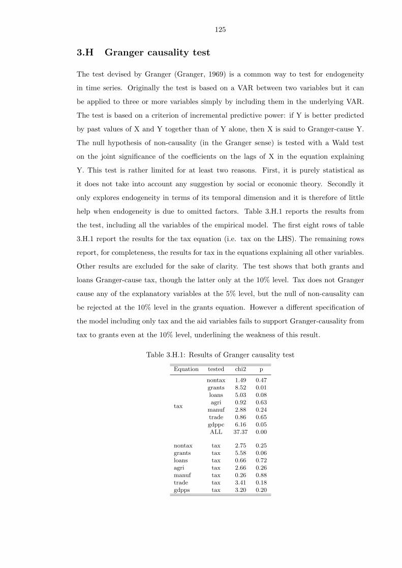
125
3.H Granger causality test
The test devised by Granger (Granger, 1969) is a common way to test for endogeneity
in time series. Originally the test is based on a VAR between two variables but it can
be applied to three or more variables simply by including them in the underlying VAR.
The test is based on a criterion of incremental predictive power: if Y is better predicted
by past values of X and Y together than of Y alone, then X is said to Granger-cause Y.
The null hypothesis of non-causality (in the Granger sense) is tested with a Wald test
on the joint significance of the coefficients on the lags of X in the equation explaining
Y. This test is rather limited for at least two reasons. First, it is purely statistical as
it does not take into account any suggestion by social or economic theory. Secondly it
only explores endogeneity in terms of its temporal dimension and it is therefore of little
help when endogeneity is due to omitted factors. Table 3.H.1 reports the results from
the test, including all the variables of the empirical model. The first eight rows of table
3.H.1 report the results for the tax equation (i.e. tax on the LHS). The remaining rows
report, for completeness, the results for tax in the equations explaining all other variables.
Other results are excluded for the sake of clarity. The test shows that both grants and
loans Granger-cause tax, though the latter only at the 10% level. Tax does not Granger
cause any of the explanatory variables at the 5% level, but the null of non-causality can
be rejected at the 10% level in the grants equation. However a different specification of
the model including only tax and the aid variables fails to support Granger-causality from
tax to grants even at the 10% level, underlining the weakness of this result.
Table 3.H.1: Results of Granger causality test
Equation tested chi2 p
tax
nontax 1.49 0.47grants 8.52 0.01loans 5.03 0.08agri 0.92 0.63
manuf 2.88 0.24trade 0.86 0.65gdppc 6.16 0.05ALL 37.37 0.00
nontax tax 2.75 0.25grants tax 5.58 0.06loans tax 0.66 0.72agri tax 2.66 0.26manuf tax 0.26 0.88trade tax 3.41 0.18gdpps tax 3.20 0.20
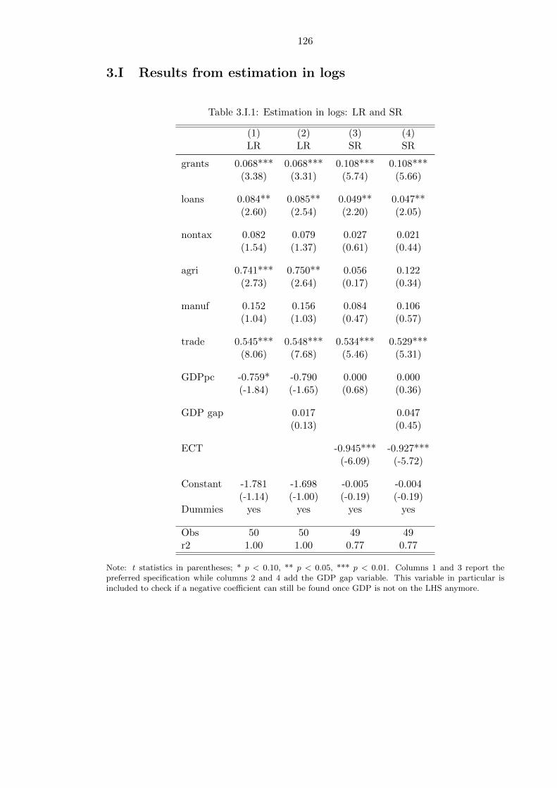
126
3.I Results from estimation in logs
Table 3.I.1: Estimation in logs: LR and SR
(1) (2) (3) (4)LR LR SR SR
grants 0.068*** 0.068*** 0.108*** 0.108***(3.38) (3.31) (5.74) (5.66)
loans 0.084** 0.085** 0.049** 0.047**(2.60) (2.54) (2.20) (2.05)
nontax 0.082 0.079 0.027 0.021(1.54) (1.37) (0.61) (0.44)
agri 0.741*** 0.750** 0.056 0.122(2.73) (2.64) (0.17) (0.34)
manuf 0.152 0.156 0.084 0.106(1.04) (1.03) (0.47) (0.57)
trade 0.545*** 0.548*** 0.534*** 0.529***(8.06) (7.68) (5.46) (5.31)
GDPpc -0.759* -0.790 0.000 0.000(-1.84) (-1.65) (0.68) (0.36)
GDP gap 0.017 0.047(0.13) (0.45)
ECT -0.945*** -0.927***(-6.09) (-5.72)
Constant -1.781 -1.698 -0.005 -0.004(-1.14) (-1.00) (-0.19) (-0.19)
Dummies yes yes yes yes
Obs 50 50 49 49r2 1.00 1.00 0.77 0.77
Note: t statistics in parentheses; * p < 0.10, ** p < 0.05, *** p < 0.01. Columns 1 and 3 report thepreferred specification while columns 2 and 4 add the GDP gap variable. This variable in particular isincluded to check if a negative coefficient can still be found once GDP is not on the LHS anymore.

127
Chapter 4
Fiscal effects of aid in Ethiopia: a
CVAR analysis
4.1 Introduction
This chapter1 explores the public budget’s dynamics in Ethiopia, particularly focussing on
the fiscal effects of aid. It therefore takes a broader perspective than chapter 3 by looking
at the budget as a whole rather than focussing on tax revenue and its determinants. In
particular the expenditure side of the budget is also considered here, as well as its long
run relation with both domestic and foreign sources of revenue.
To this purpose we use the cointegrated vector auto-regressive (CVAR) methodology
that allows estimating simultaneous equations, thus being better suitable to describe bud-
get dynamics than single equation models. Moreover this methodology allows for the
existance of multiple long run relations that may indeed be expected once all budget
variables are taken into account2.
Since the VAR model is highly demanding of the data and the inclusion of an additional
variable would imply a large increase in the number of parameters to be estimated, we
include only a maximum of 5 variables in the model. The bulk of the chapter discusses
a model of tax, non-tax revenue, grants, loans and total expenditure. We also estimate
an alternative system that looks at public expenditure in more detail by disaggregating
it into the capital and recurrent components. In this alternative system tax and non-tax
revenue are aggregated into domestic revenue. The estimation of the two systems also
1This chapter is based on co-authored work with Emijlia Timmis (University of Nottingham).2For a more detailed discussion on the differences and complementarity between CVAR and single
equation models, see the introduction to this thesis.

128
allows a robustness check and indeed the two sets of results are largely consistent.
Our results provide evidence for the existence of a domestic budget equilibrium that is
robust to different specifications. Moreover we find that both aid variables (i.e. grants and
loans) are positively related to tax revenue in the long run, thus failing to provide evidence
for a disincentive or substitution effect. In addition we find that foreign aid is positively
related with expenditure, and more so with grants than loans. The disaggregation of
expenditure shows that this result is largely driven by capital expenditure, that is also
more strongly associated to grants than loans. In the case of recurrent spending instead
the effects of the two aid variables is more similar.
One of the key advantages of our study over similar CVAR applications for Africa
lies in our data. In particular we use annual data from 1960 to 2009 compiled by the
Ministry of Finance and Economic Development (MOFED) of Ethiopia3. Not only the
series are longer than those used in most other studies in the literature, but also they are
obtained from a single domestic source. By using national data we are able to capture the
recipient’s measure of aid, which is what is effectively disbursed through the budget and
what the government is aware of. Therefore it is the component and the measure of aid
most relevant for the analysis of its fiscal effects.
The CVAR framework allows us to test a rich set of hypothesis on aid and budget
dynamics, which can be summarized in four broad issues of interest.
Firstly, we explore the existence of a domestic budget equilibrium that would include
only domestic variables and exclude aid. The existence of such a domestic equilibrium
implies that the government makes long term plans based on domestic sources, while
aid is an addition to such pre-existing long run relation. The question of whether aid
is part of the budget process or rather it is an external source of financing that relaxes
an existing domestic budget constraint is also closely related to the issue of exogeneity,
which is discussed throughout the chapter. This issue is also relevant in the context of aid
volatility and predictability, which make it harder for governments to take aid into account
in their spending plans and therefore to make it part of the long run budget equilibrium.
Secondly we can expect a positive relation of aid with expenditure. To which extent
they are related and whether aid is spent for the intended purpose are issues that can be
explored empirically. In particular the latter issue has been the focus of fungibility studies
that have tried to establish if aid was spent for its intended purpose. However a definition
3Note that since we are taking logs and since the first three observations for grants are very close tozero, the effective sample is 1963-2009.

129
of what is exactly to be considered the ‘good’ way to spend aid in terms of components
of public expenditure is still a contentious issue (McGillivray and Morrissey, 2000).
Thirdly aid can influence tax revenue and, amongst others, it may discourage tax effort
to the extent that it may provide a politically cheaper source of revenue than taxation.
This, in theory, is particularly the case for grants than for loans, since the latter require
re-payment in the future (Gupta et al., 2004; Morrissey et al., 2006; Benedek et al., 2012).
However this view is rather simplistic since aid may also help in strengthening tax admin-
istration and improving tax policy, besides the possible positive effects through income,
as argued in chapter 3.
Finally, aid may not be all spent in additional public expenditure but also be used
to decrease borrowing. Since aid relaxes the domestic budget constraint (i.e. the budget
equilibrium excluding aid variables), the government can now achieve the same level of
expenditure with less domestic borrowing.
This chapter therefore explores the four hypothesis outlined above and, more specifi-
cally, is guided by the following research questions.
• Does the budget balance hold as an equilibrium relation in the long run?
• Is aid part of that long run equilibrium relation?
• Does aid discourage tax revenue?
• Does aid increase spending?
• Which components of spending are most affected by aid?
• Does aid heterogeneity (i.e. grants and loans) matter and what are the differences
in the behavior of the two aid components?
4.2 Literature review
The literature on the fiscal effects of aid is largely based on the seminal work of Heller
(1975) that set the theoretical basis for fiscal response models. This type of model in
particular look at the effect of aid on fiscal aggregates including expenditure (recurrent
and capital), domestic revenue (typically tax, but also non-tax revenue) and deficit. The
framework is based on the maximization of the government’s utility function, represented
by deviations of actual fiscal aggregates from target levels. The utility function is specified
in a quadratic form so that marginal utility diminishes as the actual variables rise above

130
the targets4. The fiscal response model is then estimated empirically, after the target
values have also been estimated using available data.
Criticism to this framework involved both theoretical and empirical issues5. As far as
the former is concerned, Binh and McGillivray (1993) note that meeting the targets does
not necessarily maximize utility and that it is not realistic to assume a perfectly symmetric
objective function where overshooting or undershooting the targets has the same effect on
utility. On the empirical side, targets are often estimated using lagged values of the actual
variable and other variables for which the theoretical justification is weak, which casts
doubts on their validity.
Parallel to fiscal response models, another related strand of the literature is concerned
with the estimation of tax effort models, or models of tax determinants. These are typically
focused on a single equation explaining the tax share of GDP with aid and a number of
other explanatory variables (as done in chapter 3). While tax effort models precede Heller’s
seminal work (Chelliah, 1971; Chelliah et al., 1975), they were further developed to include
the fiscal response theoretical framework (Leuthold, 1991; Ghura, 1998; Mahdavi, 2008).
The early studies focused mainly on tax determinants such as agriculture, mining and
trade, then the interest shifted more towards aid and its effect on tax revenue mobilisation
(Morrissey et al., 2006; Benedek et al., 2012; Clist and Morrissey, 2011). While results
on tax determinants are rather un-contentious, the ones on aid are contrasting in the
literature with evidence available for both a positive and a negative effect of aid on tax
revenue.
With the aim of overcoming the problems inherent with Heller’s framework and with
single equation models, the CVAR has attracted increasing attention in the analysis of
fiscal dynamics6. Indeed the CVAR has at least two advantages with respect to other
approaches in the literature: first, it does not require a theoretical structure and the
calculation of targets, and secondly it does not impose exogeneity but it rather allows the
researcher to test for it. In practice however economic theory is often invoked in the design
of a CVAR particularly as regards restrictions to be applied to the model, that can then
be tested empirically. Since the estimation of simultaneous equations for the long run and
short run involves a large number of parameters, the CVAR ideally requires large samples.
4Note that in this framework overshooting or undershooting the targets gives the same utility.5See chapter 3 for a more detailed critical discussion of Heller’s theoretical framework.6However the CVAR is not a good substitute for tax effort models that typically include a larger number
of variables. Such relatively large set of variables could hardly be accommodated in a CVAR model in thecontext of the typically small samples available for developing countries.

131
As this is often not the case in developing countries, only a limited number of variables
are usually included to preserve degrees of freedom. Since we are carrying out a CVAR
analysis of fiscal dynamics in a developing country, we focus on this particular literature
in the following paragraphs.
Table 4.2.1 summarizes the studies of the fiscal literature that use CVAR and for
each of them reports some details about the variables and data used, including the data
transformation (in parenthesis in the data column). It is to be noted here that other
studies in the literature use CVAR on developing countries but they are excluded from
this detailed review because they do not focus on fiscal dynamics. These are for example:
Mavrotas (2002), looking at the effect of aid on growth; M’Amanja and Morrissey (2006)
on aid, investment and growth in Kenya; and Juselius et al. (2011) exploring the effect of
aid on key macroeconomic variables in a panel of African countries. Since a substantial
part of aid flows into the public budget, an analysis of the fiscal effects of aid can be seen
as a prerequisite to understanding the macroeconomic effectiveness of aid (McGillivray
and Morrissey, 2000; Lloyd et al., 2009). In this sense, by focusing on the fiscal variables
we are therefore making a step back with respect to the literature on the macroeconomic
effects of aid.
Before getting into the details of the individual papers, a couple of general elements
emerge from table 4.2.1. First of all, most papers use a very limited number of observations,
reaching a maximum of 39 years. The exception to this is Martins (2010) that can rely on
a larger sample due to the use of quarterly data for Ethiopia. While quarterly data allows
the author to increase the sample size and conveniently to consider only a period of relative
political stability while preserving the number of observations, our approach is in favor of
annual data instead. The reason for this is twofold. Indeed quarterly data for Ethiopia
is available but it is not reliable as it is only compiled seriously after the introduction of
the Protection of Basic Services (PBS) project in 2005 when donors became more careful
about monitoring and reporting. In addition budget decisions are taken annually and
intra-year dynamics do not necessarily add relevant information. Therefore, while we take
the Martins (2010) paper as a reference point, as it analyses Ethiopia as well, we depart
from it both by using annual data and by exploiting deeper qualitative information about
the country context.
The second general element emerging from the literature is the small number of vari-
ables included in the models. In particular most studies include only 4 or maximum 5
variables to preserve the robustness of estimates with an already limited number of degrees

132
Table 4.2.1: Summary of CVAR fiscal literature
Paper Country Obs. Variables Data
FagernasandSchurich(2004)
Malawi 31 Loans , grants, ODA,domestic borrowing,domestic revenue, de-velopment expendi-ture, recurrent ex-penditure
National, WDI, IMFStatistical Appen-dices (levels in localcurrency at constantprices)
FagernasandRoberts(2004a)
Uganda 26 Loans, grants, ODA,domestic borrowing,domestic revenue, de-velopment expendi-ture, recurrent ex-penditure, total ex-penditure
National, IMF (levelsin local currency atconstant prices)
FagernasandRoberts(2004b)
Zambia 27 Loans, grants, ODA,domestic borrowing,domestic revenue, de-velopment expendi-ture, recurrent ex-penditure
WDI, IMF-IFS,OECD-DAC aiddata (levels in localcurrency at constantprices)
M’Amanjaet al.(2005)
Kenya 39 Expenditure, tax, aid(grants and loans),growth National(logs)
Osei et al.(2005)
Ghana 33 Expenditure (capitaland recurrent), tax,aid, domestic bor-rowing
IMF (fiscal variables)and OECD-DAC aiddata (levels in USDat constant prices)
Lloyd et al.(2009)
Developingcountries
30 Foreign financing,capital expenditure,recurrent expendi-ture, tax revenue,domestic borrowing
WB’s World Devel-opment Indicators(deflated nomi-nal value in localcurrency)
Martins(2010)
Ethiopia 60 Development ex-penditure, currentexpenditure, domes-tic revenue, grants,loans, domesticborrowing
National (deflatednominal value)
Bwire(2013)
Uganda 37 Expenditure, aid,tax, domestic bor-rowing
National (fiscal vari-ables) and OECD-DAC aid data (de-flated nominal value)
of freedom. Note that the studies on Malawi, Zambia and Uganda include the variables re-
ported in table 4.2.1 alternatively in different models, also with a maximum of 5 variables
for each model and most commonly only using 4 (Fagernas and Schurich, 2004; Fagernas
and Roberts, 2004a,b). The exception again is Martins (2010) with 6 variables, the inclu-
sion of which is probably allowed by the larger sample. All papers exclude one or more
variables from the analysis, to avoid estimating an identity, and most commonly domestic
borrowing and/or non-tax revenue.
Furthermore it is to be noted that the variables can be included either in levels or in

133
logs, with the former being prevalent in the studies reported in table 4.2.1. In the larger
CVAR literature however log transformation is quite common and it is used for example
in Juselius et al. (2011) and M’Amanja and Morrissey (2006). In either case, variables are
always deflated to reflect constant rather than current values.
Finally a general element emerging throughout the literature is the importance of
considering the country context in designing the CVAR system, particularly when the
number of observations is small. In particular knowledge of the historical and political
context can help in two related ways. Firstly it can explain variations and large residuals
emerging from the analysis with detailed qualitative information. Secondly it can help in
designing the deterministic components of the CVAR, such as dummies and shifts that
are necessarily related to country-specific events (political, economic or natural). These
country-specific elements are included, for example, in the analysis presented in Juselius
et al. (2011) and Bwire (2013).
Moving on to the detailed results of each paper, we follow a chronological order.
The set of studies by ODI/DFID on Malawi, Uganda and Zambia were inspired by
an early version of Osei et al. (2003), which was published in 2005 and is reviewed in the
next paragraph. They all adopt the same approach of estimating a set of different models
based on the CVAR methodology, including different sets of variables. In Fagernas and
Roberts (2004b) however all series resulted to be stationary and therefore only a simple
VAR, rather than a CVAR, was implemented. We therefore focus on the results of the
other two papers. Fagernas and Roberts (2004a) find that in Uganda both grants and
loans have the expected positive effect on total expenditure, with grants having a stronger
positive impact on the development component than on the current one of expenditure. In
addition a long run positive effect of aid on domestic revenue can be identified, while the
effect on domestic borrowing is negligible instead. The evidence from Malawi (Fagernas
and Schurich, 2004) is largely in line with that on Uganda. In particular both grants and
loans are shown to have a positive impact on development expenditure while the results
are less clear in the case of recurrent expenditure. In addition there is no solid evidence
that aid discourages tax effort in Malawi.
Osei et al. (2005) focus on the impact of aid on fiscal policy in Ghana using two models:
one with aggregate expenditure and the second one further disaggregated into capital and
recurrent expenditure. In both cases they provide support for strong exogeneity of foreign
aid. The main finding is that aid in Ghana is associated with beneficial policy responses.
In particular it increased tax effort and it decreased domestic borrowing. The evidence

134
seems to suggest that aid and domestic borrowing are treated as substitutes and that it
is therefore difficult to identify direct effects of aid on expenditure as these are likely to
be mediated by borrowing and tax variations. However aid in Ghana results in increased
current rather than capital expenditure, contrary to the evidence from Uganda and Malawi
(Fagernas and Schurich, 2004; Fagernas and Roberts, 2004a).
The evidence from Kenya presented in M’Amanja et al. (2005) relates fiscal variables
to growth. In particular the authors find that government expenditure has a positive effect
on GDP growth while no significant influence is found for tax. Aid disaggregation into
grants and loans offers insights into the different effects of these aid components. While
grants are positively associated with growth in the long run, loans seem to be treated as
a substitute for taxes and to finance fiscal deficits. They therefore have negative effects in
the long run. The paper concludes that in the case of Kenya a negative effect of aid on tax
effort is a potential obstacle to aid effectiveness and that grants seem to be a preferable
aid modality than loans.
Martins (2010) focuses on Ethiopia using quarterly data and disaggregating both ex-
penditure and aid but leaving domestic revenue aggregated (i.e. tax and non-tax revenue).
Domestic borrowing is included as well and estimating an identity is avoided by exclud-
ing a number of residual items. The paper finds that aid has a positive relation with
development expenditure that includes mainly capital expenditure but also certain ‘de-
velopmental’ items under the recurrent heading. In particular aid adjusts to variations in
expenditure, thus suggesting that donors follow expenditure decisions of the government
by financing increased expenditure. In addition domestic borrowing is found to be the
most adjusting item thus compensating for variations in aid and other revenues. Finally
no evidence is found for the idea that aid discourages tax effort in Ethiopia and the gov-
ernment finances its expenditure with revenues in the following order: domestic revenue,
aid and borrowing.
Finally the most recent CVAR paper on fiscal dynamics is included in Bwire’s PhD
thesis (2013) on Uganda. The author finds that aid in Uganda is associated with beneficial
policy responses and particularly with increased spending and tax effort, and decreased
borrowing. Moreover the paper finds that tax revenue is the main driver of spending
plans, thus being the main pushing force in the system. Contrary to Osei et al. (2005),
the exogeneity of aid cannot be empirically supported in the case of Uganda. Finally the
order of preference for resources to finance the budget is in line with the results in Martins
(2010) and namely domestic revenue, aid and domestic borrowing.
135
Therefore, whilst the discussed studies do not find much negative fiscal effects of aid,
they show that the underlying mechanisms differ across countries and thus justify the
case-study approach.
4.3 Data
Data availability and reliability is often a major problem in African countries and even
more so when time series are concerned. This problem is further exhacerbated by the use
of CVAR which is by definition an approach highly reliant on the data rather than on
economic theory.
Given the uniqueness of Ethiopia’s history of national independece (see chapter 2),
modern fiscal institutions have a longer history than in other African countries. The
reform process started by Emperor Haile Selassie in the 1940s had fiscal policy at its core
(see chapter 2 for more details), and indeed early fiscal data dates back to 1949. The
efforts for data collection, also reinforced by monitoring needs in the context of multi-year
development plans, led to the establishment of the Central Statistical Office in 1961. By
that time, which also corresponds to the beginning of our sample, Ethiopia had a well-
established tradition in collecting data, particularly fiscal data. In fact today Ethiopia has
the highest Statistics Capacity Index in Africa, together with South Africa (OECD and
African Development Bank Group, 2010).
Our Ethiopian dataset includes 50 annual observations from 1960 to 20097 and it was
compiled in Ethiopia on the basis of data from the Ministry of Finance and Economic
Development (MOFED). To the best of our knowledge, this is a longer series of annual
data than any other study in the literature. Using exclusively national data sources has
several advantages. First of all, the data is more likely to be consistent as it comes from
a single source. Secondly, it is the one used for government decision making and it is
therefore relevant from a policy perspective. Finally, it includes a measure of aid that
represents the portion included in the government’s budget. We believe this is the most
relevant component when assessing the fiscal effects of aid as it is most directly related to
fiscal variables, as well as being the one that the government is fully aware of.
Note that in considering budget aid we include budget support but also other sources
of aid that flow through the budget. In particular budget support was withdrawn in 2005
7The Ethiopian calendar year starts in September and it is 7 years behind the Gregorian calendar.These years therefore correspond more precisely to 1960/61 and 2009/2010 in the Gregorian calendar.

136
due to the tensions in the aftermath of the elections and it has never been restored since
then. However other types of aid have been introduced and most notably the Protection
of Basic Services (PBS). While PBS is a project, it flows through the budget and it fully
uses the country systems thus having some similarities with general budget support. While
only budget aid is considered, it is still possible to further disaggregate it into grants and
loans.
Furthermore total expenditure can be disaggregated into capital and recurrent. We
keep this distinction without further manipulation although that would be possible along
the lines of Martins (2010). While the distinction between developmental expenditure
and pure government consumption is theoretically appealing, it is very difficult to impute
single expenditure items to one or the other broad category. An obvious example is
the one of salaries for employees in the public sector. Some components of this item
may be considered developmental expenditure while others may be pure consumption.
While some simple distinctions can be made (e.g. recurrent expenditure in health and
education) it is not obvious which items should be labelled as developmental and which
ones as consumption expenditure. We therefore prefer to keep the original government’s
classification as a basis for disaggregation of public expenditure.
Finally we disaggregate domestic revenue into tax and non-tax revenue, that we show
display rather different characteristics. Domestic borrowing is excluded because a full
series is only available from 1974. Moreover its inclusion would not be possible given the
log transformation discussed in the next paragraph.
Variables are usually included in a CVAR system either in levels (Bwire, 2013; Martins,
2010; Osei et al., 2005) or in logarithmic transformation (Juselius et al., 2011; M’Amanja
et al., 2005). Both options are explored and a logarithmic transformation is eventually
chosen since it is superior in terms of model fit, as well as autocorrelation and normality
in the residuals.
The log transformation does not pose any problem as long as the variables are strictly
positive and not too close to zero. This is the case for all variables except for the first
three years of the grants series that reports values very close to zero. These first three
years are therefore dropped from the sample. The inclusion of domestic borrowing would
indeed represent a challenge in the log transformation since it presents several negative
values.
Finally, all the series are tested for trend-stationarity and particularly using the Aug-
mented Dickey-Fuller, the Kwiatkowski-Phillips-Schmidt-Shin and the Clemente-Montanes-
137
Reyes tests. The first two test for trend-stationarity while the last one allows, and esti-
mates the date of, structural breaks in the single series. The tests provide enough empirical
evidence to treat all series as I(1) and the results are shown in appendix 4.A8.
4.4 Descriptive statistics and context
This section describes the variables underlying the analysis, namely the fiscal variables
transformed in logs. The discussion focuses only on the elements emerging particularly
from figures 4.4.1 and 4.4.2 that are relevant for the CVAR modelling and for the in-
terpretation of results, while a more complete historical account is reported in chapter
2.
Two major events occurred during the period and namely the regime changes in 1974
and 1991, respectively from the Imperial regime of Haile Selassie to the military junta
known as the Derg, and from the Derg to the Ethiopian People’s Revolutionary Democratic
Front (EPRDF). The differences between these three regimes are likely to influence our
analysis and they are therefore taken into account by allowing for two regime shifts in
1974 and 1991.
As far as budget dynamics are concerned, it is important to note that the conception
of government budget in Ethiopia was already present well before the start of our sample.
However it is only in the early 1940s that the modern institutions of Ethiopia are set up,
including those related to fiscal policy, mainly driven by the need for reconstruction and
development following the end of the Italian occupation (more details available in chapter
2).
The Derg regime came to power in 1974 following a socialist revolution against the
exploitative feudal system of the Imperial period (more details available in chapter 2).
Perhaps because of its coercive methods and its strategy of terror, the Derg could extract
increasing domestic revenue motivated primarily by expanded military expenditure and
an increasing role of the state in the economy. Indeed figures 4.4.1 and 4.4.2 show that
both domestic revenues and expenditure increased in the second half of the 70s.
These initial fiscal gains however were later eroded by the Derg’s poor economic policies
and by military losses in the late 80s. This resulted in a deteriorating fiscal situation at
8A note is due on loans and tax. The former seems to show trend-stationarity according to the Aug-mented Dickey-Fuller test when using 1 lag. At higher lags and in the other two tests the series results to beI(1). The latter seems to still be non-stationary in first difference when using the Augmented Dickey-Fullertests. However the kpss test with lags and the clem tests show evidence for tax being I(1). Therefore webelieve we have enough evidence to proceed by treating all series as I(1).

138
the end of the 1980s that appears clearly in figures 4.4.1 and 4.4.2. Both revenues and
expenditures decreased, including foreign grants and loans. The decline in international
assistance was due to a ‘wait and see’ attitude of donors that were not willing to support
a government that grew increasingly oppressive and whose days were deemed numbered.
The fiscal collapse of the late 80s is reflected also in a deterioration in budget balance at
that time.
Figure 4.4.1: Trends in domestic and foreign revenue
24
68
10
1960 1970 1980 1990 2000 2010year
tax nontaxgrants loans
Source: Authors’ calculations based on data provided by the Ministry of Finance and Economic Develop-ment
Foreign aid still flowed to Ethiopia under the Derg, including from Western donors
(see chapter 2 for more details). Indeed figure 4.4.1 shows that both foreign grants and
loans increased rather markedly in the late 70s in correspondence with scaled up Soviet
aid, also aimed at supporting the Derg in the Ogaden war against Somali groups.
When the EPRDF took power in 1991, it had already a long history as an organized
guerrilla movement (particularly the TPLF, see chapter 2 for details). This high level of
internal organization and the strength of the existing Ethiopian institutional apparatus
allowed the new government to take over the public administration with little disrup-
tion. This is confirmed in figures 4.4.1 and 4.4.2 that show both domestic revenue and
expenditure recovering rather quickly after the change of regime.
The EPRDF was supported in the reconstruction and economic adjustment process by
Western donors, particularly by the International Financial Institutions that contributed
through Structural Adjustment Programs (SAPs) in the 90s. Indeed an increase in loans
appears rather clearly in figure 1. However the eruption of the conflict with Eritrea in 1998
triggered a ‘peace conditionality’ that resulted in many donors leaving Ethiopia until the

139
armed confrontation ended in 2000/2001. This year was also marked by a famine particu-
larly in the Somali region, that donors responded to with great delay due to the conflict.
The peace conditionality resulted in increased deficit during the war years, used not only
to finance military expenditure but also to face the food shortages. The decrease in loans
following the peace conditionality and the subsequent increase once such conditionality
was lifted in the early 2000s, are both visible in figure 4.4.1.
Figure 4.4.2: Trends in public expenditure
46
810
12
1960 1970 1980 1990 2000 2010year
total exp. capital exp.recurrent exp.
Source: Authors calculations based on data provided by the Ministry of Finance and Economic Develop-ment
4.5 The methodology: CVAR
The CVAR methodology is used here to analyse budget dynamics in the context of a
budget identity such as the one reported in equation 4.1.
TAX + NONTAX + LOANS + GRANTS + BOR = REXP + CEXP (4.1)
The CVAR methodology is particularly useful in the analysis of budget dynamics for
at least two reasons. Firstly the mechanism for the budget process does not have to be
specified a priori, and therefore the CVAR can let the data speak on the dynamics that
drive the process. In this sense the CVAR is a-theoretical. This is a clear advantage
with respect to the fiscal response literature, that assumes the existence of targets that
the government would like to meet and that drive the process. However the existence
of such targets and the mechanism for setting them are not based on empirical analysis

140
or testing. Secondly the CVAR methodology does not require the a priori distinction
between exogenous and endogenous variables that instead can and will be tested. This is
particularly relevant as regards the endogeneity of aid that is a common concern in the
tax effort literature.
Besides these advantages, it is important to note that this methodology has also a few
caveats. First of all the CVAR is very demanding on the data and therefore the number of
variables should be as limited as possible to allow estimation and inference, particularly
in small samples. Moreover the CVAR lends itself to the“build-up of type I errors in a
general-to-specific modeling strategy” (Lloyd et al., 2009). Finally the results are often
largely dependent on the chosen model and since different researchers may choose different
ones, they could potentially reach different conclusions (Lloyd et al., 2009). For this reason
we estimate a number of models that are alternative to our preferred specification (mostly
reported in the appendix) and that support the robustness of our results.
The CVAR is also a good method for analyzing time series that are trending, as they
are in our case (see figures 4.4.1 and 4.4.2). This trending behavior and the presence of
a unit root in our series may give rise to cointegration (i.e. stationary combinations of
system variables). When this is the case, it is possible to separate the long run (LR) and
short run (SR) dynamics, as well as to test the existence of LR equilibrium relationships.
Moreover the CVAR framework allows for a rich set of tests to make sure the model is
specified correctly and to test all the assumptions that are normally imposed a priori,
most notably exogeneity.
Using the data described in section 4.3, we therefore analyze fiscal dynamics in Ethiopia
using a cointegrated VAR (CVAR) model, or vector error correction model (VECM). The
basic VAR framework is based on the estimation of a set of simultaneous equations, one for
each variable in the system, where the explanatory variables are the lags of the dependent
variable and of all the other variables in the system. All variables are treated as potentially
endogenous.
4.5.1 The unrestricted VAR
We first formulate a five-dimensional VAR(k) model where k = 1, . . . , t − k and xt =
[exptot, tax, nontax, grants, loans], the lower case indicating logs of the original variables
and k the selected lag length. The unrestricted VAR model is essentially a reformulation

141
of the covariances in the data9 and it can be summarized as follows:
xt = Π1xt−1 + · · ·+ Πkxt−k + ΦDt + εt t = 1, , T (4.2)
where xt is a p × 1 vector of endogenous variables, with p = 5 in our case; Dt is a
vector of deterministic components (such as a constant µ, a trend, and dummy variables)
with a vector of coefficients Φ; k denotes the selected lag length; εt is a p × 1 vector of
unobservable error terms, that are assumed to be serially uncorrelated, have a zero mean,
a time-invariant positive definite covariance matrix Ω, and are INp(0,Ω); and Πk are p×p
matrices of coefficients to be estimated. Since VAR describes the variation in xt as a
function of lagged values of the process, but not the current values, all information about
the contemporaneous effects between the variables is contained in the residual covariance
matrix Ω (with dimensions p × p). Note that the INp(0,Ω) assumption about the errors
is consistent with economic agents who are rational in the sense that they do not make
systematic errors when they make plans for time t based on the available information at
(t− 1) (Juselius, 2006, p.46).
If the assumption that X = [x1, x2, . . . , xT ] is multivariate normal IN(µ,Σ) is correct,
then it follows that the kth order VAR process is linear in parameters; has constant param-
eters; and has normally distributed errors εt (Juselius, 2006, p.45-46). These assumptions
can and will be tested in section 4.6. If the tests reveal that the model does not satisfy
the assumptions it is possible to modify it to achieve a ‘well behaved’ version, for example
by including dummies or by changing the measurement of the variables (Juselius, 2006,
p.47). Following this procedure, we finally obtain a well specified model so that reliable
statistical inference can be ensured10.
4.5.2 VECM representation of the VAR
In presence of non-stationarity in the variables, the VAR can be specified in terms of their
first difference and that would be stationary if xt is integrated of order 1, i.e. xt ∼ I(1).
The VECM representation of the VAR includes both the stationary first difference of
9The parameters [Π1,Π2, ,Π(T−1)] = Σ12Σ(−1)22 where Σ12 represents a covariance matrix between
y(1,t) = xt and y(2,t) = x(t−1), x(t−2), . . . , x1, X0 (where X0 is the vector of initial values). This illus-trates that VAR is essentially a reformulation of the covariances in the data (Juselius, 2006, p.46).
10“Simulation studies have shown that valid statistical inference is sensitive to violation of some of theassumptions, such as parameter non-constancy, autocorrelated residuals (the higher, the worse) and skewedresiduals, while quite robust to others, such as excess kurtosis and residual heteroscedasticity” (Juselius,2006, p.47).

142
variables in xt(∆xt) and their value in levels (xt), thus preserving both the long run and
short run information in the data. In particular the error correction form of the VAR
(VECM or CVAR) is represented by the following equation:
∆xt = Πxt−1 +
k−1∑i=1
Γi∆xt−i + ΦDt + εt (4.3)
where Π and Γi are matrices of, respectively, long run and short run coefficients11; and
εt ∼ IN(0,Ω).
The VECM representation illustrates that if variables are found to be I(1), and macroe-
conomic variables usually are, we are regressing stationary variables (∆xt) on unit-root
processes (xt−1). In such case, the estimated coefficients are spurious. However, if some
variables in the system are driven by the same persistent shocks, there may exist linear
combinations of these variables that are integrated of the lower order than the variables
themselves (i.e. I(0)). These linear combinations would represent cointegrated relations,
βxt, and could be interpreted as the long-run steady-state relationships. When cointegra-
tion exists, Π has reduced rank r < p and it is defined as follows:
Π = αβ (4.4)
where α and β are p× r matrices (with r < p), βxt defines the stationary long-run cointe-
grating relationships (r× 1), and α denotes the adjustment coefficients to the equilibrium
error. Intuitively, if all xt ∼ I(1) and ∆xt ∼ I(0), then a full rank in Π would be logically
inconsistent as it would imply that xt must be stationary12. On the other hand r = 0
implies that each variable in xt is non-stationary and it is driven by its own individual
stochastic trend and therefore no cointegration exists. In this case a simple VAR model
with the variables in first difference would not imply any loss in long run information.
The determination of r, the cointegration rank, is discussed in section 4.7. This choice
is crucial for all the subsequent estimation and for the economic interpretation of the
results. Indeed the r cointegrating relations can be interpreted as steady state equilibrium
relations to which the system adjusts. The identification of these relations and their
parameters α and β, i.e. the long run structure, is discussed in section 4.8. Furthermore
11In particular, Π =∑k
i=1 Πi − Ip and Γi = −∑k
j=i+1 Πj with i = 1, . . . , k − 1.12The VECM representation of the VAR with full rank in Π and xt ∼ I(1) would imply that a stationary
variable ∆xt equals a non stationary variable xt−1, lagged stationary variables ∆xt−1 and a stationaryerror term. Since a stationary variable cannot equal a non-stationary variable, either Π = 0 or it wouldhave reduced rank.

143
the long run structure is identified by imposing restrictions on the cointegrating relations.
In order to allow inference, each of the LR relations requires one normalization and r − 1
restrictions on the β coefficients.
Expressing the VAR in its VECM form allows identifying long run relations, or the
steady state to which the process is pulled, defined by βxt − β0 = 0. The forces α
represent adjustment and they activate as soon as the process is out of steady state, i.e.
when βxt − β0 6= 0. The VECM can be complemented with a moving average (MA)
representation that identifies the pushing forces of the system. However in our case a
clear identification of the MA side is not feasible, as discussed in appendix 4.B.
4.6 The UVAR: specification and misspecification tests
This section is concerned with the specification of the unrestricted VAR (UVAR) model
and the related misspecification tests. First, we choose and justify the deterministic com-
ponents Dt including constant terms, trends and dummy variables. Secondly we assess
the necessary lag length k and we test for misspecification, particularly focusing on the
analysis of residuals. Finally we check for goodness of fit and for parameter constancy.
Note that “the residual autocorrelation tests and the ARCH tests are derived under the
assumption of normally distributed errors and the normality tests are derived under the
assumption of independent and homoscedastic errors” (Juselius, 2006, p.77). In addition
the lag length criteria are only valid under the assumption correctly specified model.
Therefore the misspecification test procedure, in search of the correctly specified model,
is rather iterative. Following this procedure we finally obtain a well specified model.
4.6.1 Deterministic components
The deterministic components include constant terms, trends and dummy variables. They
define the CVAR model specification in a way that influences all the subsequent analysis.
This section therefore considers them carefully and it justifies our choice.
As far as the constant terms and trends are concerned, we choose a model where the
constant term is unrestricted, therefore allowing a non-zero mean both in the LR and
SR relations13. The non zero mean in the SR relations, i.e. E(∆xt) 6= 0 implies that
there are linear trends in the variables. This is consistent with a unit root process in the
13There are five possible models to define the constant and trend terms, discussed in Juselius (2006,p.100). The model that fits our data better is model three, which is described in this section.

144
variables where xt ∼ I(1) and ∆xt ∼ I(0). However there is neither a trend in the SR
equations nor in the cointegrating space, meaning that the trends in the variables cancel
out in the cointegrating relations. This is indeed our case, as confirmed in the analysis of
residuals carried out in the next sections. In addition the exclusion of a trend from the
cointegrating space is discussed in section 4.8.1 and the results from the exclusion test
confirm the validity of this choice.
As far as dummy variables are concerned, three types can be considered: a mean shift
dummy (0, 0, 0, 1, 1, 1, ), a permanent intervention dummy (0, 0, 0, 1, 0, 0, ), and a transitory
shock dummy (0, 0, 0, 1,−1, 0, 0, )14. Capturing significant interventions and events with
dummies allows avoiding large residuals that may result in a violation of the normality
assumption. There are two main ways to decide on what dummies to include: to set them
according to knowledge of events that are significant enough to have to be taken into
account in the model or, in case such a priori knowledge is not available, to look at large
residuals in the data (for the latter see section 4.6.3). In the case of Ethiopia between 1960
and 2009 it is rather straightforward to identify two important shifts corresponding to the
political regime changes of 1974 and 1991. These events are likely to influence the analysis
due to the radical shift in some policies between successive regimes (details available in
chapter 2). However it is important to note that although change and transformation
has undoubtedly occurred in Ethiopia in both regime shifts, there are some important
elements of continuity (see section 4.4 and chapter 2).
Therefore, once they are taken into account using regime shift dummies, the two shifts
do not impair the validity of our statistical analysis. The first shift dummy takes value
of 1 after 1974 and zero otherwise, and the second shift dummy is ‘switched on’ in 1991
(taking a value of one thereafter and zero beforehand).
While we are confident that the deterministic components discussed here are well
specified, we also test the robustness of our results to different choices. Our main results
do not change when we specify differently the constant and trend terms as in the next
most plausible option15. Moreover they do not change substantially when we consider
other dates for the regime shifts, namely the years immediately before or after the chosen
ones.
14See Juselius (2006, p.102).15This would be model two in the discussion in Juselius (2006, p.100).

145
4.6.2 Lag length determination
Having included the deterministic components discussed in the previous section, we now
turn to the lag length determination of such specified model. Including the correct deter-
ministic components at this stage is necessary because the lag length determination tests
are only valid under the assumption of a correctly specified model, in terms of regime
shifts and constant parameters16 (Juselius, 2006, p.71). We use the standard lag length
determination procedure that relies on a likelihood ratio lag reduction test and on two
information criteria (Juselius, 2006, p.71).
The lag reduction test compares the null hypothesis of lag truncation at k against the
alternative hypothesis of k + 1. Accepting the null implies that there are no significant
coefficients at lag k + 1. The test uses the effective sample size, therefore the number
of observations available when using the maximum lag length considered. We consider a
maximum of five lags and therefore the effective sample for the test is 1968-2009. Note
that Juselius (2006, p.72) argues that “a lag length of two is in most cases sufficient to
describe a very rich dynamic structure even in a small-dimensional system” and we are
therefore comfortable with testing a maximum lag of five. As shown in table 4.6.1 the
lag reduction test always rejects the null, therefore suggesting the maximum lag length
(5). However the test does not use any penalizing factor for additional parameters to be
estimated and it is therefore not particularly suitable in small samples.
Instead the information criteria (IC) reported in table 4.6.2, namely Schwartz (SC)
and Hannan-Quinn (H-Q), include different penalizing factors related to the additional
number of parameters required by adding more lags. The SC criteria suggests a lag length
of one, while the H-Q criteria suggests (k = 3)17. The LM tests, reported in the last two
columns of the same table, indicate the presence of ‘left-over’ residual autocorrelation at
k = 1 with a p-value of 0.055. This would violate the basic assumptions of the model
and indeed when we try to estimate an unrestricted VAR (UVAR) with k = 1 and p = 5
we find an unsatisfactory model specification since multivariate normality is rejected, as
it is the null of homoscedastic errors of order one and two (see misspecification tests for
UVAR(k=1) in appendix 4.C). At the lag length of two the LM test does not detect
any autocorrelation. Moreover (k = 2) seems to provide a good description of the data
generating process as well as satisfactory results from misspecification tests (see sections
4.6.4 and 4.6.5). Given this information and our preference for simple models to preserve
16Constancy in the parameters is checked in section 4.6.7 and largely confirmed.17The lag length corresponding to the highest value of the IC is the suggested one.
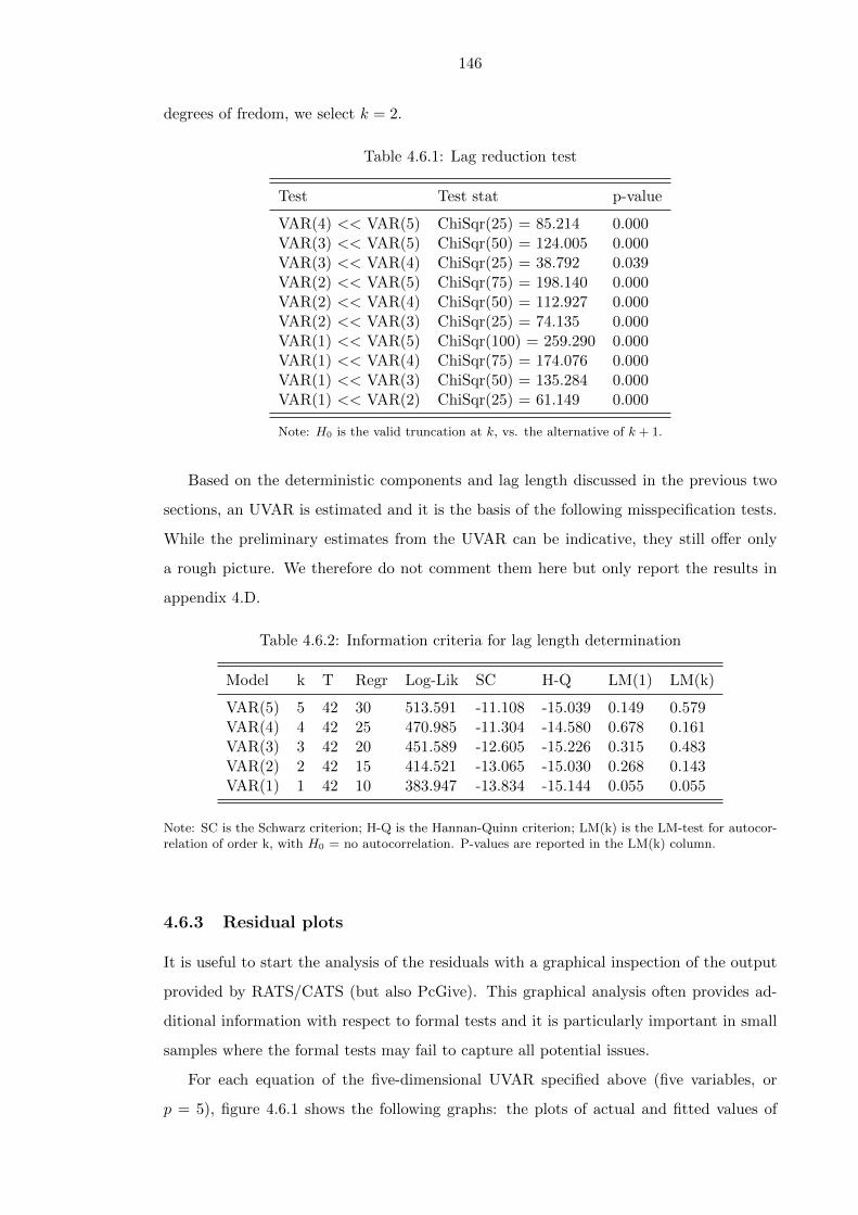
146
degrees of fredom, we select k = 2.
Table 4.6.1: Lag reduction test
Test Test stat p-value
VAR(4) << VAR(5) ChiSqr(25) = 85.214 0.000VAR(3) << VAR(5) ChiSqr(50) = 124.005 0.000VAR(3) << VAR(4) ChiSqr(25) = 38.792 0.039VAR(2) << VAR(5) ChiSqr(75) = 198.140 0.000VAR(2) << VAR(4) ChiSqr(50) = 112.927 0.000VAR(2) << VAR(3) ChiSqr(25) = 74.135 0.000VAR(1) << VAR(5) ChiSqr(100) = 259.290 0.000VAR(1) << VAR(4) ChiSqr(75) = 174.076 0.000VAR(1) << VAR(3) ChiSqr(50) = 135.284 0.000VAR(1) << VAR(2) ChiSqr(25) = 61.149 0.000
Note: H0 is the valid truncation at k, vs. the alternative of k + 1.
Based on the deterministic components and lag length discussed in the previous two
sections, an UVAR is estimated and it is the basis of the following misspecification tests.
While the preliminary estimates from the UVAR can be indicative, they still offer only
a rough picture. We therefore do not comment them here but only report the results in
appendix 4.D.
Table 4.6.2: Information criteria for lag length determination
Model k T Regr Log-Lik SC H-Q LM(1) LM(k)
VAR(5) 5 42 30 513.591 -11.108 -15.039 0.149 0.579VAR(4) 4 42 25 470.985 -11.304 -14.580 0.678 0.161VAR(3) 3 42 20 451.589 -12.605 -15.226 0.315 0.483VAR(2) 2 42 15 414.521 -13.065 -15.030 0.268 0.143VAR(1) 1 42 10 383.947 -13.834 -15.144 0.055 0.055
Note: SC is the Schwarz criterion; H-Q is the Hannan-Quinn criterion; LM(k) is the LM-test for autocor-relation of order k, with H0 = no autocorrelation. P-values are reported in the LM(k) column.
4.6.3 Residual plots
It is useful to start the analysis of the residuals with a graphical inspection of the output
provided by RATS/CATS (but also PcGive). This graphical analysis often provides ad-
ditional information with respect to formal tests and it is particularly important in small
samples where the formal tests may fail to capture all potential issues.
For each equation of the five-dimensional UVAR specified above (five variables, or
p = 5), figure 4.6.1 shows the following graphs: the plots of actual and fitted values of

147
∆xi,t, i = 1, . . . , p (top left panel); the autocorrelogram of order 11 (top right panel); the
standardized residuals (bottom left panel); and the empirical and normal distributions
(bottom right panel). The graphs do not signal any particular issues. However it is
worth noting that larger residuals can be identified for grants and loans during the war
with Eritrea between 1998 and 2001 when donors partly left the country because of their
disagreement over the war. The 1983/84 famine can also be spotted in terms of a large
residual in some of the graphs. These events may be good candidates for transitory shock
dummies in case they pose problems for normality. However this does not seem to be the
case here, as shown in section 4.6.5, and we therefore prefer a parsimonious specification
that does not include these dummies.
Figure 4.6.1: Residual plots

148
4.6.4 Residual autocorrelation
As the VAR methodology is based on the idea of decomposing the variation in the data
into a systematic part describing the dynamics in the model and an un-systematic random
part, the assumption of uncorrelated residuals, and hence its test, is an important one. In
addition all the χ2 and F tests are derived under the assumption of independent errors,
the violation of which would result in the distribution of these tests deviating from χ2 and
F in unknown ways (Juselius, 2006, p.74).
The key test used to detect residual autocorrelation is the LM test of jth order auto-
correlation, calculated using an auxiliary regression of estimated VAR residuals, (εt), on
the k-lagged variables, xt−1, xt−2, . . . , xt−k, and the jth lagged VAR residual (εt−j). The
LM test is then calculated as a Wilks ratio test with a small-sample correction and it
is approximately distributed as χ2 with p2 degrees of freedom where p is the number of
variables in the model18. H0 assumes no (left-over) autocorrelation in the residuals.
Intuitively if the test suggests that there are significant autocorrelations left in the
model, agents’ plans for t based on the information available at t − 1 would deviate
systematically from the actual realizations (Juselius, 2006, p.74). The results in table
4.6.3 show no residual autocorrelation up to the 4th order.
18For more details see (Juselius, 2006, p.74).

149
Table 4.6.3: Autocorrelation test
Test Test statistic p-value
LM(1) ChiSqr(25) = 30.981 0.190LM(2) ChiSqr(25) = 29.974 0.225LM(3) ChiSqr(25) = 32.086 0.156LM(4) ChiSqr(25) = 17.479 0.864
Note: H0 is no autocorrelation.
4.6.5 Residual heteroskedasticity and normality tests
The test for residual heteroskedasticity is the mth order ARCH test described in (Juselius,
2006, p.74). Tables 4.6.4 and 4.6.5 show that no ARCH effects were detected respectively
at multivariate or univariate level, as the null of homoscedastic errors can never be rejected.
Table 4.6.5 also shows univariate normality tests where the null of normality could
never be rejected, also confirming that it is not necessary at this point to include transitory
shock dummies to account for large residuals. The null of multivariate normality cannot
be rejected, with p-value 0.111. While this p-value is not particularly far from the 10%
threshold, our results do not indicate any particular departures from normality in terms of
skewness (expected to be around 0) or kurtosis (expected to be around 3) in the univariate
tests19.
Table 4.6.4: Multivariate heteroskedasticity and normality tests
Test Test statistic p-value
Test for ARCH
LM(1) ChiSqr(225) = 218.679 0.606LM(2) ChiSqr(450) = 483.740 0.131LM(3) ChiSqr(675) = 689.582 0.340LM(4) ChiSqr(900) = 675.000 1.000
Test for normality
ChiSqr(10) = 15.635 0.111
Note: H0 is homoskedastic errors for the LM tests and normally distributed errorsfor the ChiSqr test.
19Juselius (2006, p.76-77) notes that VAR estimates are more sensitive to deviations from normality dueto skewness than to excess kurtosis.

150
Table 4.6.5: Univariate heteroskedasticity and normality tests
Variable Skewness Kurtosis ARCH(2) Normality R2
exptot 0.323 2.491 0.078 (0.962) 1.402 (0.496) 0.677tax -0.212 3.874 1.408 (0.490) 4.547 (0.103) 0.571nontax -0.125 2.438 3.078 (0.215) 0.310 (0.856) 0.509grants -0.425 3.482 0.114 (0.945) 2.566 (0.277) 0.511loans 0.193 2.437 2.578 (0.276) 0.599 (0.741) 0.518
Note: p-values in parenthesis when relevant. H0 is homoskedastic errors for the ARCHtests and normally distributed errors for the normality test.
4.6.6 Goodness of fit
The measure for goodness of fit in the VAR model is the trace correlation, defined in
Juselius (2006, p.73). The trace correlation for our model is 0.518 and it can be roughly
interpreted as an average R2 for the p VAR equations. CATS also calculates an R2 for
each of the p equations and these are reported in table 4.6.5. Indeed when the variables
are integrated of order one, the R2 is only meaningful when the dependent variable is
given as ∆xt.
4.6.7 Parameter constancy
Since parameter constancy is a pre-requisite for lag length determination and a useful
feature for the model, we carry out a battery of tests based on the model specified so far20.
For details on the tests we refer to Juselius (2006, p.150). When discussing parameter
constancy, “it is also important to realize that it is just a question of looking carefully
enough to find non-constancy in at least some directions of essentially any empirical model.
The important issue is whether the deviation from constancy is serious enough to warrant a
re-specification of the model” (Juselius, 2006, p.150). In our case the parameter constancy
tests do not show evidence of non-constant parameters.
4.7 Determination of cointegration rank
The determination of cointegration rank r is crucial in the CVAR analysis, as it influences
all the subsequent econometric analysis by dividing the data into r pulling and p−r push-
ing forces, corresponding respectively equilibrium relations and common driving trends.
20Results not reported here for simplicity.
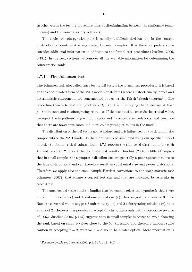
151
In other words the testing procedure aims at discriminating between the stationary (equi-
librium) and the non-stationary relations.
The choice of cointegration rank is usually a difficult decision and in the context
of developing countries it is aggravated by small samples. It is therefore preferable to
consider additional information in addition to the formal test procedure (Juselius, 2006,
p.131). In the next sections we consider all the available information for determining the
cointegration rank.
4.7.1 The Johansen test
The Johansen test, also called trace test or LR test, is the formal test procedure. It is based
on the concentrated form of the VAR model (or R-form) where all short-run dynamics and
deterministic components are concentrated out using the Frisch-Waugh theorem21. The
procedure then is to test the hypothesis Hr : rank = r, implying that there are at least
p−r unit roots and r cointegrating relations. If the test statistic exceeds the critical value,
we reject the hypothesis of p − r unit roots and r cointegrating relations, and conclude
that there are fewer unit roots and more cointegrating relations in the model.
The distribution of the LR test is non-standard and it is influenced by the deterministic
components of the VAR model. It therefore has to be simulated using our specified model
in order to obtain critical values. Table 4.7.1 reports the simulated distribution for each
Hr and table 4.7.2 reports the Johansen test results. Juselius (2006, p.140-141) argues
that in small samples the asymptotic distributions are generally a poor approximations to
the true distributions and can therefore result in substantial size and power distortions.
Therefore we apply also the small sample Bartlett corrections to the trace statistic (see
Johansen (2002)) that ensure a correct test size and that are indicated by asterisks in
table 4.7.2.
The uncorrected trace statistic implies that we cannot reject the hypothesis that there
are 2 unit roots (p − r) and 3 stationary relations (r), thus suggesting a rank of 3. The
Bartlett-corrected values suggest 3 unit roots (p−r) and 2 cointegrating relations (r), thus
a rank of 2. However it is possible to accept this hypothesis only with a borderline p-value
of 0.062. Juselius (2006, p.145) suggests that in small samples is better to avoid choosing
the rank based on small p-values close to the 5% threshold and therefore imposes some
caution in accepting r = 2, whereas r = 3 would be a safer option. More information is
21For more details see Juselius (2006, p.116-17, p.131-145).

152
explored in the next sections to support this decision.
Table 4.7.1: Quantiles of the simulated rank test distribution
p - r r Mean S.E. 50% 75% 80% 85% 90% 95%
5 0 58.617 10.052 58.135 65.396 67.284 69.383 71.789 75.4454 1 39.213 8.459 38.395 44.636 46.095 48.066 50.244 54.1543 2 23.243 6.861 22.499 27.299 28.671 30.263 32.258 35.8652 3 10.956 4.491 10.305 13.485 14.408 15.503 16.910 19.0761 4 1.963 1.939 1.364 2.722 3.221 3.782 4.611 5.855
Note: the deterministic specification includes an unrestricted constant and 2 level shifts in 1974and 1991. Number of replications (N): 2500; length of random walks (T): 400.
Table 4.7.2: Johansen test for determination of cointegration rank
p− r r Eig.Value Trace Trace* Frac95 P-Value P-Value*
5 0 0.561 102.992 89.825 75.445 0.000 0.0034 1 0.459 65.973 57.488 54.154 0.003 0.0253 2 0.364 38.306 34.598 35.865 0.026 0.0622 3 0.265 17.927 15.413 19.076 0.075 0.1551 4 0.087 4.095 3.549 5.855 0.123 0.163
Note: asterisks denote Bartlett-corrected values.
4.7.2 Additional information to determine r
Four additional pieces of information can be used to determine r and namely: the char-
acteristic roots of the model, the t-values of the α coefficients, the recursive graphs of the
trace statistic, and the graphs of the cointegrating relations22.
First, table 4.7.3 reports the p × k = 10 characteristic roots of the model with r = 3
and figure 4.7.1 illustrates them in the unit circle. If the third cointegrating vector is non-
stationary and therefore wrongly included in the model, then the largest characteristic
root will be close to the unit circle. With r = 3, the modulus of the largest characteristic
root is 0.690 as reported in table 4.7.3. Although in small samples it is difficult to make a
sharp distinction between unit roots, near unit roots, and ‘very stationary’ roots (Juselius,
2006, p.145), we believe that the largest root in our case is far enough from the unit circle
not to be considered a unit root23.
Secondly we look at the t-values of the alpha coefficients of the UVAR. The idea behind
this is that ideally we want to lose as little as possible of the information in Π when choosing
22For more details see Juselius (2006, p.48-52, 131-145).23Note that the modulus of the largest characteristic root for a model with r = 2 is 0.584.

153
Figure 4.7.1: Illustration of the roots of the companion matrixRoots of the Companion Matrix
-1.0 -0.5 0.0 0.5 1.0
-1.0
-0.5
0.0
0.5
1.0Rank(PI)=3
Table 4.7.3: The roots of the companion matrix
Real Imaginary Modulus Argument
Root1 1.000 0.000 1.000 0.000Root2 1.000 0.000 1.000 0.000Root3 0.690 -0.000 0.690 0.000Root4 -0.291 0.481 0.562 2.115Root5 -0.291 -0.481 0.562 -2.115Root6 0.340 0.400 0.525 0.866Root7 0.340 -0.400 0.525 -0.866Root8 0.395 -0.000 0.395 0.000Root9 -0.272 0.260 0.376 2.379Root10 -0.272 -0.260 0.376 -2.379
r. If all of the t-values of the α coefficients in the rth relation are small, say less than 2.6,
then one would not gain a lot by including the rth vector as a cointegrating relation in the
model (Juselius, 2006, p.142). The higher critical value is needed because in the UVAR
we have not yet established which βxt vectors are stationary. Since the t-values for the α
coefficients corresponding to a non-stationary βxt are not distributed as a Student’s t, it is
more appropriate to consider a value between Student’s t and Dickey-Fuller’s τ (Juselius,
2006, p.122).
Appendix 4.D shows the α coefficients from our basic UVAR. In the third relation
(Alpha 3) almost all coefficients are significant and thus show adjustment. Instead in the
fourth relation (Alpha 4) only one coefficient may be considered significant. These results
show that by choosing r = 2, thus excluding the third relation (Alpha 3), we would loose

154
important information. The choice of r = 3 seems therefore preferable.
Thirdly we look at the recursive graphs of the trace statistic (figure 4.7.2), noting that
the recursively calculated components of the trace statistic (in the lower panel of figure
4.7.2) should grow linearly for all stationary relations (r) but stay constant for the unit
root processes (p − r) (Juselius, 2006, p.142). The graph contains a unit root rejection
line at 1. However for small samples, and accounting for the Bartlett correction, this line
should be shifted to approximately 1.25 (Juselius, 2006, p.145). The figure confirms that
there are three stationary relations, and thus it supports r = 3.
A fourth source of information is provided by the graphs of the possible cointegrating
relations from the UVAR (reported in appendix 4.E). In particular if the graph of a
supposedly stationary relation shows clear signs of non-stationarity, it may be necessary
to reconsider the choice of r or try to re-specify the model. The graphs for the first three
Beta relations do not provide strong evidence against a choice of r = 3 although Beta(3)
is more difficult to judge around 1991.
In conclusion, we are rather confident that a choice of r = 3 fits the data reasonably
well and it is indeed supported by the majority of tests and evidence presented in this
section. This choice is also confirmed by the parameter constancy tests of the model with
r = 3, that do not signal any particular problem (Juselius, 2006, p.145).
Figure 4.7.2: Trace test statistics
4.7.3 Economic interpretability of the results
One of the elements to consider when evaluating the cointegration rank is the economic
interpretability of the results (Juselius, 2006, p.142). This section therefore assesses the
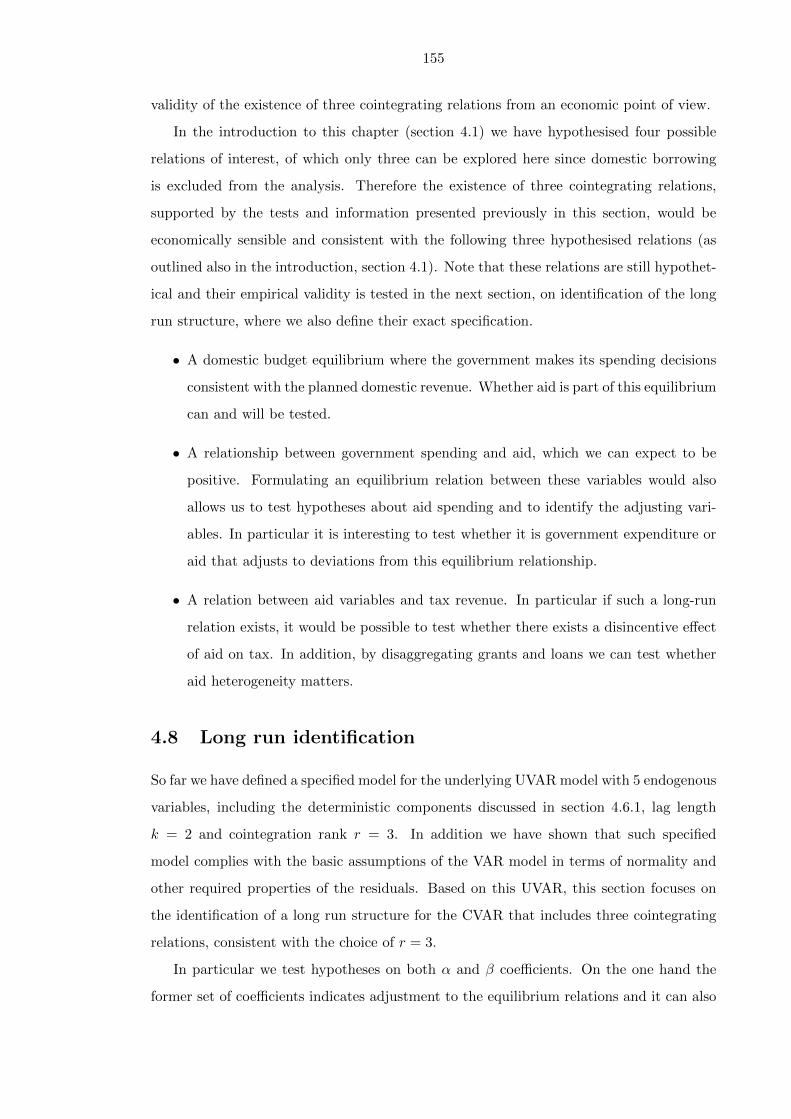
155
validity of the existence of three cointegrating relations from an economic point of view.
In the introduction to this chapter (section 4.1) we have hypothesised four possible
relations of interest, of which only three can be explored here since domestic borrowing
is excluded from the analysis. Therefore the existence of three cointegrating relations,
supported by the tests and information presented previously in this section, would be
economically sensible and consistent with the following three hypothesised relations (as
outlined also in the introduction, section 4.1). Note that these relations are still hypothet-
ical and their empirical validity is tested in the next section, on identification of the long
run structure, where we also define their exact specification.
• A domestic budget equilibrium where the government makes its spending decisions
consistent with the planned domestic revenue. Whether aid is part of this equilibrium
can and will be tested.
• A relationship between government spending and aid, which we can expect to be
positive. Formulating an equilibrium relation between these variables would also
allows us to test hypotheses about aid spending and to identify the adjusting vari-
ables. In particular it is interesting to test whether it is government expenditure or
aid that adjusts to deviations from this equilibrium relationship.
• A relation between aid variables and tax revenue. In particular if such a long-run
relation exists, it would be possible to test whether there exists a disincentive effect
of aid on tax. In addition, by disaggregating grants and loans we can test whether
aid heterogeneity matters.
4.8 Long run identification
So far we have defined a specified model for the underlying UVAR model with 5 endogenous
variables, including the deterministic components discussed in section 4.6.1, lag length
k = 2 and cointegration rank r = 3. In addition we have shown that such specified
model complies with the basic assumptions of the VAR model in terms of normality and
other required properties of the residuals. Based on this UVAR, this section focuses on
the identification of a long run structure for the CVAR that includes three cointegrating
relations, consistent with the choice of r = 3.
In particular we test hypotheses on both α and β coefficients. On the one hand the
former set of coefficients indicates adjustment to the equilibrium relations and it can also

156
offer insights on weak exogeneity. If one or more variables are found to be weakly exoge-
nous, it is possible to proceed with partial models in the well-specified long run structure
of the CVAR24. On the other hand, β coefficients define the long run equilibrium relations
to which the system is pulled back when it is out of steady state. By testing hypotheses
on β we can test for LR exclusion, stationarity of single variables and of relations between
variables. The latter is equivalent to testing the existence of long run equilibrium relations.
It also allows us to identify the possible identifying and over-identifying restrictions to be
imposed on the cointegrating relations and thus give indications on the LR structure.
4.8.1 Long run exclusion
The possibility that some variables should be excluded from the LR structure can be
explored through a test for a zero row restriction on β. If this hypothesis is accepted, the
variable can be excluded from the cointegration space without losing information. More
formally, the likelihood ratio procedure tests the null of a zero restriction for one variable
on all β vectors (β = 0) against the alternative of no restriction on β (β 6= 0)25.
Table 4.8.1 reports the test statistic and the associated p-value for the long-run exclu-
sion for each variable for all possible choices of r. For our choice of cointegrating rank,
r = 3, the long-run exclusion tests suggest that none of the endogenous variables should
be excluded from the cointegrating space and thus from the long-run relations. There
is, however, some borderline evidence for potential long-run exclusion of the 1991 shift
dummy26. Given the p-value of 0.055, very close to the 5% threshold, we decide to keep
this dummy in the LR system. This choice is confirmed by looking at the Π matrix from
the estimated UVAR (see appendix 4.D) that provides no clear signs for any of the vari-
ables or shift dummies to be excluded since their coefficients are significant for at least one
equation. Moreover the inclusion of both dummies is justified by qualitative information
on the two regime shifts in the Ethiopian context (see chapter 2).
Finally, the exclusion test can also be used to confirm the validity of our choice to
exclude a trend from the cointegrating space (see section 4.6.1 on deterministic compo-
nents). This test confirms that the trend is not required for our specified system for any
choice of r.
24Partial models would treat the identified exogenous variables explicitly as such in the empirical model.25Note that this test does not impose identifying restrictions yet.26The acceptance of exclusion of the shift dummy form the cointegrating relations would imply that the
mean shift cancels out in the cointegrating relations.

157
Table 4.8.1: Test of LR exclusion
r 5% C.V. exptot tax nontax grants loans 1991 1974
1 3.841 6.988 3.820 0.083 6.348 6.432 0.023 7.748(0.008) (0.051) (0.773) (0.012) (0.011) (0.880) (0.005)
2 5.991 14.029 11.057 6.517 12.934 8.175 1.464 13.076(0.001) (0.004) (0.038) (0.002) (0.017) (0.481) (0.001)
3 7.815 20.543 15.231 11.814 16.359 10.550 7.593 17.170(0.000) (0.002) (0.008) (0.001) (0.014) (0.055) (0.001)
4 9.488 29.845 24.371 18.638 24.689 19.429 15.863 24.233(0.000) (0.000) (0.001) (0.000) (0.001) (0.003) (0.000)
Note: LR-test, Chi-Square(r), P-values in brackets. H0 is a zero row restriction in beta, theacceptance of which implies that the variable can be excluded from the cointegrating space.
4.8.2 Testing for stationarity of xt
In section 4.3 we have stated that all variables are I(1), according to ‘traditional’ sta-
tionarity tests such as Dickey-Fuller GLS, the Kwiatkowski-Phillips-Schmidt-Shin and the
Clemente-Montanes-Reyes tests. In this section we look into this issue further by using the
CVAR framework, that allows testing whether each variable is stationary by itself around
the mean. In the CVAR framework and for r = 3, the test is implemented by imposing
restrictions on one cointegrating relation such that only the variable of interest and the
deterministic components are included. The other two cointegrating vectors are left un-
restricted. The likelihood ratio test (ChiSq(5-r)) tests the null hypothesis of stationarity.
Note that the test results are sensitive to both the choice of rank, r, and the inclusion
of the deterministic components. We therefore report the results for all choices of rank
and with shift dummies both included in (table 4.8.2) and excluded (table 4.8.3) from the
cointegrating relations.
For the cointegration rank of our choice (r = 3) the stationarity tests seem to suggest
that non-tax revenue, loans, and possibly government spending are stationary around the
mean, allowing for two mean shifts. However the stationarity hypothesis is rejected for
each variable with r = 2. Mean-stationarity is also rejected for all variables for all choices
of rank when the shift dummies are excluded.
It is important to note that the small size of our sample may play an important role
here. Indeed the order of integration is a statistical approximation (xt ∼ I(1)) and it
is often difficult to make clear-cut distinctions, particularly in a small sample (Juselius,
2006, p.18-19). The issue is further aggravated by the imposition of two mean shifts in
an already small sample. Indeed when excluding the shift dummies all variables appear

158
non-stationary27. The small sample size may also imply a problem of degrees of freedom,
as at this stage we are still estimating a large number of parameters (no restrictions have
been applied yet). Indeed for r = 2, and therefore allowing for more degrees of freedom,
all variables appear to be non-stationary.
Given the discussion above and the visual inspection of the data (see graphs in section
4.4), we remain inclined to treat all variables as I(1). This choice is also confirmed by the
‘traditional’ stationarity tests reported in appendix 4.A.
Table 4.8.2: Test for stationarity: shift dummies included
r DGF 5% C.V. exptot tax nontax grants loans
1 4 9.488 21.021 24.328 16.523 22.114 18.204(0.000) (0.000) (0.002) (0.000) (0.001)
2 3 7.815 12.200 14.988 7.902 12.811 8.954(0.007) (0.002) (0.048) (0.005) (0.030)
3 2 5.991 4.926 7.741 0.872 5.646 1.984(0.085) (0.021) (0.647) (0.059) (0.371)
4 1 3.841 4.953 7.560 0.727 4.760 0.658(0.026) (0.006) (0.394) (0.029) (0.417)
Note: LR-test, Chi-Square(5-r), P-values in brackets. H0 is stationarity.
Table 4.8.3: Test for stationarity: shift dummies excluded
r DGF 5% C.V. exptot tax nontax grants loans
1 6 12.592 32.274 32.239 32.214 32.951 29.707(0.000) (0.000) (0.000) (0.000) (0.000)
2 5 11.070 23.096 22.889 23.099 23.642 20.372(0.000) (0.000) (0.000) (0.000) (0.001)
3 4 9.488 15.811 15.685 16.145 16.498 13.153(0.003) (0.003) (0.003) (0.002) (0.011)
4 3 7.815 9.565 9.481 10.492 10.350 7.037(0.023) (0.024) (0.015) (0.016) (0.071)
Note: LR-test, Chi-Square(5-r), P-values in brackets. H0 is stationarity.
4.8.3 Testing restrictions on β
In this section we test different restrictions on the beta vectors to obtain indications on the
stationarity of possible combinations of variables and therefore their possible inclusion in
27It is also possible that the two shifts in the mean in such a small sample account for the otherwiseaccepted trend-unit-root behaviour.

159
the long run system as equilibrium relations. Essentially this procedure is an exploration
of cointegration properties of the variables (Juselius, 2006, p.191). If a relation is not found
to be stationary at this point, it may not be sensible for it to enter the LR structure.
More formally the test procedure involves imposing zero restrictions on some variables
in a given beta vector, allowing the remaining parameters to be estimated and keeping
the other two cointegrating relationships unrestricted. The null hypothesis is then the
stationarity of a particular relation which, if accepted, suggests that the tested relation
is a possible candidate for inclusion amongst the three cointegrating relations in the final
LR structure. Note that the results at this point are not final, since the coefficients are
estimated in a system that is not fully specified. We will therefore not discuss them
at length, although we can still judge whether they are plausible and consistent with
expectations. For each tested relation we impose one normalization28 and two restrictions
at least, which is what will be needed for LR identification. However when only two
restrictions are imposed (in addition to one normalization) the relation is just-identified
and therefore the p-value is 1 by construction, i.e. restrictions are not testable (Juselius,
2006, p.189).
Table 4.8.4 tests a number of possible relations and the last column reports the p-
value for the null of stationarity. The goal is not only to find stationarity but also to
assess the reducibility of relations, i.e. if it is possible to drop one additional variable
from the relation while preserving stationarity. By testing different specifications of the
possible cointegrating relations we can also assess their stability in terms of the sign and
magnitude of coefficients.
The table is organized around the expected relations formulated in sections 4.1 and
4.7.3 and namely: budget equilibrium, aid and expenditure, and aid and tax. As far as
the budget equilibrium is concerned, H1 includes all the variables that can be expected
to be part of that equilibrium. The relation is just identified as only two zero restrictions
on the shift dummies are included. Relations H2 to H6 impose further restrictions on
this relation and indeed it is possible to reduce the budget equilibrium relation until H7.
This relation is stationary with a p-value 0.692 and it only includes the domestic budget
variables, namely public expenditure, tax and non-tax revenue. It suggests that both
revenue variables are positively related with expenditure, as expected. Regime dummies
28Note that normalisation is not counted as a restriction and can be done on different variables in therelation without changing the ratio between the coefficients, as long a s one normalises on statisticallysignificant coefficient.

160
Table 4.8.4: Hypothesis testing on β
HP exptot tax nontax grants loans 1991 1974 p-value
Budget equilibrium
H1 1 -0.703 -0.275 -0.013 -0.051 0 0 1H2 1 -0.696 -0.338 0.001 0 0 0 0.391H3 1 -0.719 -0.281 0 -0.045 0 0 0.765H4 1 -0.731 -0.189 0 0 -0.177 -0.156 1H5 1 -0.694 -0.330 0 0 -0.021 0 0.426H6 1 -0.689 -0.347 0 0 0 0.016 0.409H7 1 -0.695 -0.338 0 0 0 0 0.692
Irreducibility of the budget equilibrium relation
H8 1 -10.875 0 0 0 0 0 0.001H9 1 -0.785 0 0 0 -0.385 -0.361 0.630H10 1 0 -0.738 0 0 0 0 0.003H11 1 0 -2.958 0 0 2.933 2.881 0.461
Aid and expenditure
H12 1 0 0 -0.761 -0.452 0.784 -0.145 1H13 1 0 0 -0.807 -0.558 0.993 0 0.8693H14 1 0 0 -0.607 -0.012 0 -0.715 0.0203H15 1 0 0 -0.325 -0.873 0 0 0.0030H16 1 0 0 -0.494 0 -0.258 -0.744 0.0575H17 1 0 0 0 1.342 -2.794 -2.491 0.3849
Aid and taxation
H18 0 1 0 -0.910 -0.712 1.709 0.449 1H19 0 1 0 -0.884 -0.393 1.135 0 0.628H20 0 1 0 -0.686 0.308 0 -0.856 0.017H21 0 1 0 -4.428 10.636 0 0 0.002H22 0 1 0 -0.559 0 0 0 0.002H23 0 1 0 0 -2.101 0 0 0.005
Note: the p-values refer to the stationarity test on the residuals of the corresponding relations, thusindicating whether the relations are stationary and therefore valid as long run relations. H0 is stationarity.Rows in bold indicate possible valid specifications for the long run relations.
can be excluded from this relation, indicating that the domestic budget equilibrium exists
regardless of the regime changes. This is consistent with the thesis of continuity across
periods mentioned in section 4.4 (see also chapter 2). By testing relations H8 to H11 we
show that H7 is irreducible since by imposing a further zero restriction on tax or non-tax
revenue, stationarity is rejected (unless regime dummies are brought back in the relation).
When examining the relation between aid and expenditure, the domestic revenue vari-
ables are restricted to zero and the expected positive relation is confirmed. H12 is just
identified, while H13 to H15 test zero (over-identifying) restrictions on the dummy vari-
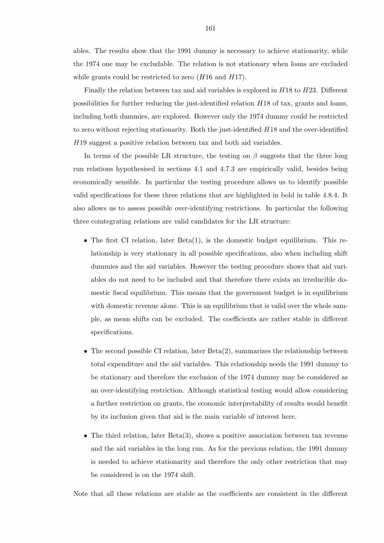
161
ables. The results show that the 1991 dummy is necessary to achieve stationarity, while
the 1974 one may be excludable. The relation is not stationary when loans are excluded
while grants could be restricted to zero (H16 and H17).
Finally the relation between tax and aid variables is explored in H18 to H23. Different
possibilities for further reducing the just-identified relation H18 of tax, grants and loans,
including both dummies, are explored. However only the 1974 dummy could be restricted
to zero without rejecting stationarity. Both the just-identified H18 and the over-identified
H19 suggest a positive relation between tax and both aid variables.
In terms of the possible LR structure, the testing on β suggests that the three long
run relations hypothesised in sections 4.1 and 4.7.3 are empirically valid, besides being
economically sensible. In particular the testing procedure allows us to identify possible
valid specifications for these three relations that are highlighted in bold in table 4.8.4. It
also allows us to assess possible over-identifying restrictions. In particular the following
three cointegrating relations are valid candidates for the LR structure:
• The first CI relation, later Beta(1), is the domestic budget equilibrium. This re-
lationship is very stationary in all possible specifications, also when including shift
dummies and the aid variables. However the testing procedure shows that aid vari-
ables do not need to be included and that therefore there exists an irreducible do-
mestic fiscal equilibrium. This means that the government budget is in equilibrium
with domestic revenue alone. This is an equilibrium that is valid over the whole sam-
ple, as mean shifts can be excluded. The coefficients are rather stable in different
specifications.
• The second possible CI relation, later Beta(2), summarizes the relationship between
total expenditure and the aid variables. This relationship needs the 1991 dummy to
be stationary and therefore the exclusion of the 1974 dummy may be considered as
an over-identifying restriction. Although statistical testing would allow considering
a further restriction on grants, the economic interpretability of results would benefit
by its inclusion given that aid is the main variable of interest here.
• The third relation, later Beta(3), shows a positive association between tax revenue
and the aid variables in the long run. As for the previous relation, the 1991 dummy
is needed to achieve stationarity and therefore the only other restriction that may
be considered is on the 1974 shift.
Note that all these relations are stable as the coefficients are consistent in the different

162
specifications where stationarity is accepted.
Interestingly when aid is included in the LR relations, and namely in the relations with
expenditure and tax, at least the 1991 shift dummy is needed to achieve stationarity. First
of all, this confirms our choice to keep it in the system despite the borderline result for
its excludability in section 4.8.1. Secondly, this result is largely in line with the Ethiopian
historical context. While we have argued that the administrative apparatus showed some
signs of continuity between regimes, and indeed the domestic budget equilibrium does not
require dummies to achieve stationarity, aid has changed more decidedly across regimes.
Particularly in 1991 foreign presence switched from the socialist influence of the Soviet
block to the liberal prescriptions of Western donors and institutions. The inclusion of the
1991 dummy therefore fits the historical events very well. While the 1974 regime shift also
had implications in terms of aid (see chapter 2), they were surely less dramatic than in
1991. Moreover there are only a few observations before 1974, therefore contributing to
making this dummy excludable from the second and third relations.
4.8.4 Test for a zero restriction in α: weak exogeneity
We now move on to testing restrictions on α, and particularly long run weak exogeneity.
The testing procedure here is focused on a model that is not yet identified. Therefore
the goal is more to identify the possibility of adopting a partial model, treating one or
more variables as exogenous, rather than to assess exogeneity per se. For the latter aim
in particular the test is repeated for the identified model presented in section 4.9.
In the CVAR context, a variable is said to be weakly exogenous in the long run param-
eters if it is not adjusting to the LR equilibrium error given by the cointegration relations.
This can be tested as zero row restriction in alpha for an individual variable, and therefore
the null hypothesis is no adjustment or weak exogeneity. A zero row in alpha, if accepted,
defines a common driving trend as the cumulated sum of the empirical shocks to the ex-
ogenous variable29. An exogenous variable therefore can be seen as having influenced the
long-run stochastic path of the other variables without itself having been influenced by
them. Note that to be compatible with r = 3, there can be at most 2 (= p− r) zero rows
in alpha (Juselius, 2006, p.194).
Table 4.8.5 shows that for our choice of r = 3, tax revenue is signalling some potential
29For a more detailed discussion on common driving trends and the MA representation, see appendix4.B.

163
long-run weak exogeneity30. While weak exogeneity of tax is possible, this result may sim-
ply indicate slow adjustment. Loans also exhibit some signs of long-run weak exogeneity
although the null can only be accepted with a rather small p-value of 0.073. For neither
of the two potentially exogenous variables identified could the null of weak exogeneity be
accepted with confidence, since the p-values are never larger than 0.1. Given the weak
evidence for exogeneity, we therefore do not proceed with partial models. However weak
exogeneity is re-assessed in our identified LR structure to identify possible common driving
trends (for a detailed discussion on common driving trends see appendix 4.B).
Table 4.8.5: Test of weak exogeneity
r DGF 5% C.V. exptot tax nontax grants loans
1 1 3.841 1.189 0.919 7.240 3.745 1.732(0.276) (0.338) (0.007) (0.053) (0.188)
2 2 5.991 5.434 1.115 8.179 6.970 3.732(0.066) (0.573) (0.017) (0.031) (0.155)
3 3 7.815 11.981 6.340 14.330 9.868 6.968(0.007) (0.096) (0.002) (0.020) (0.073)
4 4 9.488 21.232 11.385 18.414 16.179 16.413(0.000) (0.023) (0.001) (0.003) (0.003)
Note: LR-Test, Chi-Square(r), P-values in brackets. H0 is a zero row restriction in alphaand therfore weak exogeneity.
4.8.5 Test for unit vectors in α
In the previous section we have tested a zero row restriction in α, indicating no adjustment
and therefore weak exogeneity. Here instead we test for a unit vector in alpha, which is a
mirror image of the test of the weak exogeneity. It considers whether a variable is purely
adjusting to the long-run equilibrium error. If this is the case, the shocks to this variable
only have transitory but no permanent effects on any of the variables in the system,
therefore without any contribution to common driving trends (Juselius, 2006, p.200-201).
The results reported in table 4.8.6 suggest that government spending may be accepted
as purely adjusting to CI relations, and this would be supported for both neighbouring
choices of rank (2 or 4). These results offer some insight on the behaviour of variables and
they may also be indicative in the choice of normalization.
Note that while the previous results on weak exogeneity do not allow for clear cut
30The null would be more strongly accepted for r=2 but rejected for r=4.
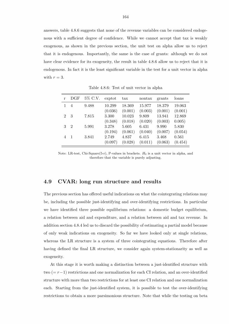
164
answers, table 4.8.6 suggests that none of the revenue variables can be considered endoge-
nous with a sufficient degree of confidence. While we cannot accept that tax is weakly
exogenous, as shown in the previous section, the unit test on alpha allow us to reject
that it is endogenous. Importantly, the same is the case of grants: although we do not
have clear evidence for its exogeneity, the result in table 4.8.6 allow us to reject that it is
endogenous. In fact it is the least significant variable in the test for a unit vector in alpha
with r = 3.
Table 4.8.6: Test of unit vector in alpha
r DGF 5% C.V. exptot tax nontax grants loans
1 4 9.488 10.299 18.369 15.977 18.379 19.063(0.036) (0.001) (0.003) (0.001) (0.001)
2 3 7.815 3.300 10.023 9.809 13.941 12.869(0.348) (0.018) (0.020) (0.003) 0.005)
3 2 5.991 3.278 5.605 6.431 9.990 5.830(0.194) (0.061) (0.040) (0.007) (0.054)
4 1 3.841 2.749 4.837 6.415 3.468 0.561(0.097) (0.028) (0.011) (0.063) (0.454)
Note: LR-test, Chi-Square(5-r), P-values in brackets. H0 is a unit vector in alpha, andtherefore that the variable is purely adjusting.
4.9 CVAR: long run structure and results
The previous section has offered useful indications on what the cointegrating relations may
be, including the possible just-identifying and over-identifying restrictions. In particular
we have identified three possible equilibrium relations: a domestic budget equilibrium,
a relation between aid and expenditure, and a relation between aid and tax revenue. In
addition section 4.8.4 led us to discard the possibility of estimating a partial model because
of only weak indications on exogeneity. So far we have looked only at single relations,
whereas the LR structure is a system of three cointegrating equations. Therefore after
having defined the final LR structure, we consider again system-stationarity as well as
exogeneity.
At this stage it is worth making a distinction between a just-identified structure with
two (= r−1) restrictions and one normalization for each CI relation, and an over-identified
structure with more than two restrictions for at least one CI relation and one normalization
each. Starting from the just-identified system, it is possible to test the over-identifying
restrictions to obtain a more parsimonious structure. Note that while the testing on beta

165
(section 4.8.3) indicated possible restrictions, these need to be tested in the context of
a system of 3 CI relations. As suggested by Juselius (2006, p.189), “if a relationship is
stationary it does not generally make sense to add more variables”. This, together with
the possibility of releasing additional degrees of freedom, makes the adoption of over-
identifying restrictions preferable.
4.9.1 Results
Tables 4.9.1 and 4.9.2 report the results for the over-identified system, whereas the ones for
the just-identified model are reported in appendix 4.F. The three cointegrating relations
included are:
• Beta(1): domestic budget equilibrium, corresponding to H7 in table 4.8.4;
• Beta(2): the aid-expenditure relation, corresponding to H12;
• Beta(3): the aid-tax relation, corresponding to H19.
The stationarity of this system is accepted with p-value 0.849 (ChiSqr(3) = 0.803) and
normality is also accepted with a p-value of 0.068 (ChiSqr(10) = 17.323), thus ensuring
valid inference. We imposed three over-identifying restrictions: both regime dummies in
Beta(1) and the 1974 dummy in Beta(3)31.
Table 4.9.1 shows the beta vectors before normalization and the the matrix of beta
coefficients for the three CI relations, while table 4.9.2 reports the matrix of alpha coeffi-
cients. Beta coefficients define the LR equilibrium relations between the variables included.
Normalization of the β vectors is always done on a significant variable32. In addition to
this statistical criterion, normalization is also decided to ease economic interpretability33.
Note however that the results of the normalized beta should still be read as a vector and
not as causal effects, since pushing and pulling forces still have to be determined.
The α coefficients capture adjustment behavior. In particular the adjusting variables
are those with a higher (significant) t-ratio in the αmatrix. The sign of the alpha coefficient
should be the opposite of the corresponding beta to ensure equilibrium correction. In
31Results of a system with just two over-identifying restrictions, namely the two dummies in beta 1, arelargely consistent with the ones presented here.
32Note also that the test of a unit vector in α showed some support for expenditure to be adjusting, thussupporting the decision to normalize on it in Beta(1) and Beta(2). As for Beta(3), the testing on alpha insection 4.8.5 suggests, though weakly, that tax is the most adjusting between the three variables included.
33Contrary to a regression model, a change in the normalization will not change the ratio between thecoefficients (Juselius, 2006, p.120).

166
our system this is the case for all significant alpha, therefore signalling no over-shooting
behavior.
The results in Beta(1) confirm the domestic budget equilibrium where tax and non-tax
revenue are both positively associated with total expenditure, the former more strongly
than the latter both in terms of significance and magnitude. The most adjusting variable
in this relation is expenditure, followed by tax.
Beta(2) shows a relation between expenditure and aid variables, where grants are
more strongly related to expenditure than loans. Both shift dummies are included and
significant, indicating a positive shift of the mean in 1974 and a negative one in 1991. The
most adjusting variable is non-tax revenue, followed by grants and, though less strongly,
loans.
Beta(3) shows that tax revenue is positively associated with both aid variables, and
more so with grants than loans both in terms of significance and magnitude. When the
tax relation is out of equilibrium, it is mainly non-tax revenue to adjust, followed by total
expenditure34. The 1991 shift is significant and it implies a negative mean shift in the tax
relation following the fall of the Derg regime.
In terms of weak exogeneity, the previous results (section 4.8.4) are largely confirmed.
In particular it is possible to accept weak exogeneity of loans with a p-value of 0.131
(ChiSqr(6) = 9.843)35.
4.9.2 Interpretation
Generally all relations identified here are economically sensible and they correspond to
our expectations. The domestic budget equilibrium is confirmed as a stationary relation,
excluding aid and both regime dummies. This implies that such an ‘internal’ relation exists
in Ethiopia regardless of the regime. The ‘internal’ budget equilibrium is consistent with
the elements of continuity that caracterized in the political and administrative environment
in Ethiopia throughout the period (see chapter 2). Moreover aid does not appear to be
necessarily part of the long run budget equilibrium. This is consistent with the general
feeling amongst Ethiopian policy makers that aid is not a reliable source of revenue and it
is preferable to rely on domestic revenues instead (for a more detailed discussion on this
34Tax, grants and loans signal some overshooting behaviour in the third relation, as the corresponding αand β have the same sign. However the α are not significant for any of the variables and the combined co-efficients of the overshooting variables are still lower than the significant adjusting ones, thus compensatingthe overshooting (though non-significant) behaviour and ensuring the stability of the system.
35Results available from the authors.
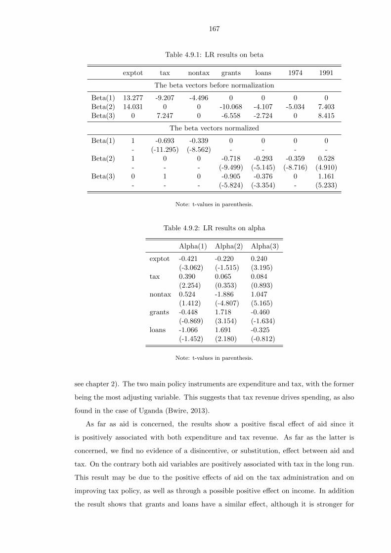
167
Table 4.9.1: LR results on beta
exptot tax nontax grants loans 1974 1991
The beta vectors before normalization
Beta(1) 13.277 -9.207 -4.496 0 0 0 0Beta(2) 14.031 0 0 -10.068 -4.107 -5.034 7.403Beta(3) 0 7.247 0 -6.558 -2.724 0 8.415
The beta vectors normalized
Beta(1) 1 -0.693 -0.339 0 0 0 0- (-11.295) (-8.562) - - - -
Beta(2) 1 0 0 -0.718 -0.293 -0.359 0.528- - - (-9.499) (-5.145) (-8.716) (4.910)
Beta(3) 0 1 0 -0.905 -0.376 0 1.161- - - (-5.824) (-3.354) - (5.233)
Note: t-values in parenthesis.
Table 4.9.2: LR results on alpha
Alpha(1) Alpha(2) Alpha(3)
exptot -0.421 -0.220 0.240(-3.062) (-1.515) (3.195)
tax 0.390 0.065 0.084(2.254) (0.353) (0.893)
nontax 0.524 -1.886 1.047(1.412) (-4.807) (5.165)
grants -0.448 1.718 -0.460(-0.869) (3.154) (-1.634)
loans -1.066 1.691 -0.325(-1.452) (2.180) (-0.812)
Note: t-values in parenthesis.
see chapter 2). The two main policy instruments are expenditure and tax, with the former
being the most adjusting variable. This suggests that tax revenue drives spending, as also
found in the case of Uganda (Bwire, 2013).
As far as aid is concerned, the results show a positive fiscal effect of aid since it
is positively associated with both expenditure and tax revenue. As far as the latter is
concerned, we find no evidence of a disincentive, or substitution, effect between aid and
tax. On the contrary both aid variables are positively associated with tax in the long run.
This result may be due to the positive effects of aid on the tax administration and on
improving tax policy, as well as through a possible positive effect on income. In addition
the result shows that grants and loans have a similar effect, although it is stronger for

168
the former. The non-significant alpha coefficients on tax, grants and loans in the third CI
relation do not give clear indications about the possible direction of causality.
Moreover both in Beta(2) and in Beta(3) grants seem to be more related to the fiscal
variables than loans, thus suggesting a larger beneficial effect of such aid modality. It may
be useful to point out that over the period the share of grants and loans on total aid has
been roughly equal, with grants increasing more substantially than loans only in the last
years of the sample (see figure 1).
As far as the effect of aid on expenditure is concerned, the coefficients show that, for
example, a 1% increase in grants is associated with a 0.72% increase in total expenditure36.
Given that the nominal amount of grants is substantially smaller than expenditure, these
figures suggest that expenditure increased by more than the amount of grants. Impor-
tantly, this is consistent with a positive association between aid and tax. For example,
at 2010 values, an increase in grants of 124 million ETB is associated with a 501 million
ETB increase in total expenditure.
In addition the adjustment coefficients in the second relation, between aid and expen-
diture, show that both grants and loans are adjusting while expenditure is not. This may
suggest that in the positive relation between aid and expenditure, causality may run from
the latter to the former. Such behavior may be indicative of a donor disbursement rule
whereby donors increase aid in response to commitment from the government in terms of
increased expenditure (consistently with the results in Martins (2010)).
Although we cannot draw conclusions on borrowing, we can still draw some indications
on its stationarity. Indeed since our system that excludes borrowing (therefore capturing it
in the residuals) is stationary, it must follow that borrowing is stationary too. This means
that the government does not systematically increase borrowing, which would imply a
non-stationary behaviour.
4.10 Short run structure
The short run structure of a CVAR model has some important differences from the LR
identification. First of all, while the CI relations in our model are r = 3 LR equilib-
rium relations between endogenous variables with the same time index, the SR equations
are p = 5 relations between p current variables (∆xt); (p × (k − 1)) lagged variables
36Note that the log transformation does not allow a more straightforward interpretation in terms ofchanges in nominal amounts.

169
∆xt−i, (i = 1, . . . , k − 1); and r lagged equilibrium errors β(xt−1) from the identified LR
structure. Identification of the short-run structure requires (p− 1) restrictions on each of
the simultaneous equations37.
Two other important differences exist with respect to the LR identification. First of all,
the distinction between endogenous and exogenous variables may change SR identification
whereas it did not change the LR structure that is rather based on vectors. Secondly, iden-
tification of the SR structure requires uncorrelated residuals, whereas no such requirement
existed in the LR structure. Therefore the residual covariance matrix plays an important
role in the SR structure. In particular uncorrelated residuals of a short-run structural
model may be interpreted as estimated shocks, whilst large off-diagonal elements in the
covariance matrix can be a signal of significant current effects between the system variables
(Juselius, 2006, p.230). Indeed “the VAR model can be considered a reduced form model
in the SR dynamics in the sense that potentially important current (simultaneous) effects
are not explicitly modeled but are left in the residuals” (Juselius, 2006, p.230). The high
correlation coefficients in the residual covariance matrix may also be due to the omission
of relevant variables.
The just-identified short run structure is heavily over-parameterised. This section re-
ports only a parsimonious system, following the SR identification strategy of parsimonious
parameterisation discussed in Juselius (2006, chapter 13). In particular the estimated co-
efficients with small t-statistics (p− value > 0.10) were set to zero. Since there are some
non-negligible correlation coefficients in the residual covariance matrix (see table 4.10.2),
the interpretation of the short-run equations as causal relationships should be taken with
caution. The results are shown in table 4.10.1 where the first column (labeled ‘Y’) indi-
cates the dependent variable of the equation, the number in parentheses are t-values and
CI1, CI2 and CI3 correspond respectively to Beta 1, 2 and 338. The 30 over-identifying
restrictions were accepted with a p-value of 0.5 (LR test of over-identifying restrictions:
Chisq(30) = 29.325).
The government expenditure equation shows positive association with past changes of
foreign grants and loans, albeit with limited magnitude. The negative coefficient on CI1 is
consistent with the adjustment of government expenditure to the long-run internal budget
equilibrium found in the LR structure.
37See Juselius (2006), chapter 13, for more details.38Note that exptot is not reported in the columns as it does not enter any of the SR equations according
to the parsimonuois parametrization strategy discussed before.

170
Table 4.10.1: Short run results
Y tax ntax grants loans CI1 CI2 CI3 1991 1974
exptot 0 0 0.16 0.11 -0.58 0.25 0 0 0.16- - (4.32) (4.49) (-5.58) (6.02) - - (2.02)
tax 0 0.20 0.08 0 0.46 -0.17 0.17 -0.26 0- (3.60) (1.84) - (2.83) (-2.51) (3.31) (-2.66) -
nontax 0 0 0.24 0.16 0 0 0.19 0 0.42- - (2.43) (2.19) - - (2.12) - (1.69)
grants 0 0 0 0 0 0 4.46 0 0- - - - - - (3.96) - -
loans -1.14 0 0.48 0 -1.74 0.74 0 0 0(-2.57) - (2.79) - (-3.47) (3.70) - - -
Note: t-values in parenthesis.
In the SR tax adjusts to all three CI relations and it responds positively to changes
in grants, consistently with the LR results. Also non-tax revenue responds positively to
both aid variables.
Grants do not seem to be adjusting to any of the other variables in the short run,
except for reacting to the third cointegrating relation. This is consistent with the alpha
matrix in the LR and it may suggest the exogeneity of grants in the SR.
Loans seem to follow grants, and respond to changes in the past changes in tax. The
variable also seems to adjust to the first two equilibrium errors.
Table 4.10.2: Residual covariance matrix
exptot tax nontax grants loans
texp 0.089tax 0.356 0.010ntax 0.409 -0.162 0.248
grants -0.039 0.104 -0.009 0.320loans 0.408 0.170 -0.043 0.122 0.420
4.11 An alternative model with disaggregated expenditure
Having identified the fiscal effects of aid on tax and expenditure, we now turn to exploring
the latter in more detail by further disaggregating capital and recurrent expenditure.
Given the weak results on the short run and the difficulty to identify common trends (for
a more detailed discussion, including the MA side, see appendix 4.B), in this section we
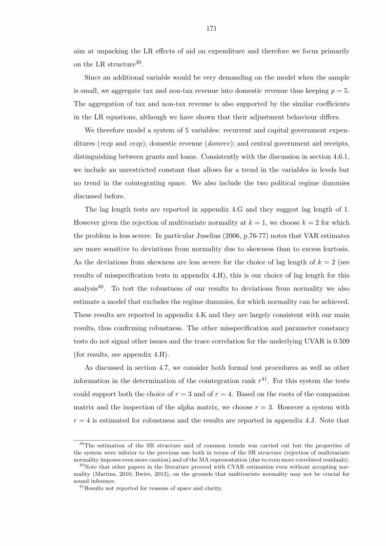
171
aim at unpacking the LR effects of aid on expenditure and therefore we focus primarily
on the LR structure39.
Since an additional variable would be very demanding on the model when the sample
is small, we aggregate tax and non-tax revenue into domestic revenue thus keeping p = 5.
The aggregation of tax and non-tax revenue is also supported by the similar coefficients
in the LR equations, although we have shown that their adjustment behaviour differs.
We therefore model a system of 5 variables: recurrent and capital government expen-
ditures (rexp and cexp); domestic revenue (domrev); and central government aid receipts,
distinguishing between grants and loans. Consistently with the discussion in section 4.6.1,
we include an unrestricted constant that allows for a trend in the variables in levels but
no trend in the cointegrating space. We also include the two political regime dummies
discussed before.
The lag length tests are reported in appendix 4.G and they suggest lag length of 1.
However given the rejection of multivariate normality at k = 1, we choose k = 2 for which
the problem is less severe. In particular Juselius (2006, p.76-77) notes that VAR estimates
are more sensitive to deviations from normality due to skewness than to excess kurtosis.
As the deviations from skewness are less severe for the choice of lag length of k = 2 (see
results of misspecification tests in appendix 4.H), this is our choice of lag length for this
analysis40. To test the robustness of our results to deviations from normality we also
estimate a model that excludes the regime dummies, for which normality can be achieved.
These results are reported in appendix 4.K and they are largely consistent with our main
results, thus confirming robustness. The other misspecification and parameter constancy
tests do not signal other issues and the trace correlation for the underlying UVAR is 0.509
(for results, see appendix 4.H).
As discussed in section 4.7, we consider both formal test procedures as well as other
information in the determination of the cointegration rank r41. For this system the tests
could support both the choice of r = 3 and of r = 4. Based on the roots of the companion
matrix and the inspection of the alpha matrix, we choose r = 3. However a system with
r = 4 is estimated for robustness and the results are reported in appendix 4.J. Note that
39The estimation of the SR structure and of common trends was carried out but the properties ofthe system were inferior to the previous one both in terms of the SR structure (rejection of multivariatenormality imposes even more caution) and of the MA representation (due to even more correlated residuals).
40Note that other papers in the literature proceed with CVAR estimation even without accepting nor-mality (Martins, 2010; Bwire, 2013), on the grounds that multivariate normality may not be crucial forsound inference.
41Results not reported for reasons of space and clarity.

172
Table 4.11.1: LR results on beta with disaggregated expenditure
cexp rexp domrev grants loans 1974 1991
The beta vectors before normalization
Beta(1) 9.297 1.978 -15.508 0.000 0.000 0.000 0.000Beta(2) 7.273 0.000 0.000 -6.450 -1.295 -5.124 1.241Beta(3) 0.000 10.457 0.000 -3.743 -2.103 -4.941 -0.480
The beta vectors normalized
Beta(1) -0.599 -0.128 1.000 0.000 0.000 0.000 0.000(-14.093) (-1.839) (.NA) (.NA) (.NA) (.NA) (.NA)
Beta(2) 1.000 0.000 0.000 -0.887 -0.178 -0.705 0.171(.NA) (.NA) (.NA) (-15.030) (-3.097) (-6.878) (2.062)
Beta(3) 0.000 1.000 0.000 -0.358 -0.201 -0.472 -0.046(.NA) (.NA) (.NA) (-7.824) (-4.616) (-6.132) (-0.746)
Note: t-values in parenthesis.
with r = 4 it is possible to also test robustness of our main system, since all the previous
CI relations can be included. The results are largely consistent with the rest of the analysis
and they therefore provide support for robustness.
As before, the long run structure is identified according to the testing on alpha and
beta42 as well as economic interpretability. Tables 4.11.1 and 4.11.2 show the results for
an identified LR structure with over-identifying restrictions and r = 3, that is accepted as
stationary with a p-value of 0.564.
The first CI relation corresponds to the domestic budget equilibrium previously iden-
tified and it therefore confirms the validity of that result in a different system. The
equilibrium between government spending and domestic revenue is confirmed regardless
of the change in regime, since both dummies are restricted to zero. As expected, domes-
tic revenue is positively associated with both recurrent and capital expenditure, but more
strongly so with the latter. Recurrent expenditure is found to be the single most adjusting
variable, in Beta(1) as well as in the other CI relations.
Beta(2) and Beta(3) roughly correspond to the second CI in the previous system, but
now the aid variables are related separately to capital and recurrent expenditure respec-
tively. To ensure consistency with our previous system, these CI relations include both
regime dummies. Consistently with the previous results, the 1974 dummy has a positive
effect on the relation between aid and both components of spending while the 1991 dummy
42Results on tests on alpha and beta not reported for reasons of space and clarity.

173
Table 4.11.2: LR results on alpha with disaggregated expenditure
Alpha(1) Alpha(2) Alpha(3)
cexp 0.214 -0.222 -0.114(0.529) (-1.168) (-0.419)
rexp 0.842 0.329 -0.585(4.978) (4.142) (-5.126)
domrev -0.163 0.081 -0.248(-0.726) (0.770) (-1.638)
grants 0.078 0.750 0.557(0.129) (2.644) (1.366)
loans 0.415 -0.207 0.531(0.439) (-0.467) (0.832)
Note: t-values in parenthesis.
has a negative effect when significant. Note that a further over-identifying restriction could
be imposed on the non-significant 1991 dummy in Beta(3) without changing the results.
Generally, the results confirm the positive relation of both loans and grants with both
components of public expenditure. The disaggregation however shows that the strongest
effect in terms of magnitude and significance is that of grants on capital expenditure.
Grants are also more related to current expenditure but the difference with the coefficient
on loans is less marked in Beta(3) than in Beta(2).
The positive and strong relation between grants and capital expenditure is consistent
with other findings in the literature (Fagernas and Schurich, 2004; Fagernas and Roberts,
2004a; Martins, 2010). On the one hand this result may seem counter intuitive: indeed it
may be reasonable for loans to be more related to the more ‘productive’ capital expenditure
since they have to be repaid in the future. In practice however loans to Ethiopia are
largely concessional, making repayment an issue rather distant in time that therefore
might not have direct policy implications. On the other hand grants may come with more
conditionality, in the form of pressure to spend on productive capital rather than recurrent
(‘consumption’) expenditure, precisely because they do not require repayment. The idea
that capital spending is preferable to recurrent expenditure may be slowly fading in the
international debate. However, in a historical perspective, this distinction may be behind
the result of grants being mostly associated with capital expenditure. Moreover the donor
disbursement rule identified before it is confirmed here, with grants being the second most
adjusting variable after rexp. This suggests that donors back a commitment to increased
domestic capital expenditure with grants.

174
4.12 Conclusions
This chapter shed light on the fiscal effects of aid in Ethiopia and in particular it answered
the research questions raised in section 4.1 on the hypothesized effects of aid. To do so
we used a CVAR methodology that proved particularly useful to disentangle the complex
dynamics that occur in the government budget process. The analysis showed that all
the basic assumptions of the CVAR model are satisfied, thus making this methodology
suitable for the analysis of our Ethiopian data as well as allowing valid inference.
In particular we provide evidence for the existence of a domestic budget equilibrium
that includes domestic revenues and government expenditure, but excludes aid. The do-
mestic budget equilibrium is confirmed in the two systems estimated in this chapter as well
as in the alternative systems used for checking robustness. This relation holds regardless
of the regime changes across the whole period considered. By looking at adjustment coeffi-
cients we also find that spending plans are mainly driven by tax revenue, while expenditure
is the most adjusting variable.
Moreover we find no evidence of a negative effect of aid on tax revenue, which implies
that the government of Ethiopia does not substitute taxes with aid nor is it discouraged
in its tax efforts. On the contrary we find a positive and robust relation between tax
revenue and both grants and loans in the LR, which is largely confirmed in the short run
structure too. This relation may be explained by a beneficial effect of aid in improving
tax administration and strengthening domestic institutions. Indeed throughout the whole
period the government of Ethiopia has received foreign advice on tax matters and this
remains today one of the policy areas of highest agreement between the government and
donors. Moreover Ethiopia’s history of independence from colonial powers has profoundly
shaped the national character and pride, making financial independence a core priority of
the current government. As a consequence, the case for a substitution or tax displacement
effect of aid is particularly ill-grounded in Ethiopia as confirmed by this analysis.
In addition both aid variables are found to have a positive and robust relation with
public expenditure. This relation is stronger between capital expenditure and grants
in particular, as shown in the alternative system using disaggregated expenditure data.
This finding is consistent with the results in the literature and with the idea that donors
may have a preference for grants to be spent on the more productive capital expenditure
rather than on ‘consumption’ recurrent expenditure. We are also able to identify a donor
disbursement rule whereby donors back proven commitment to increased expenditure with
additional funding, particularly grants.

175
As far as exogeneity is concerned, we are not able to provide clear-cut results. However
we find some evidence for weak exogeneity of loans in the long run. In addition the lack of
a short run effect on grants of other variables in the system may support grants exogeneity
in the SR structure. These results however need to be taken with caution as the direction
of causality remains difficult to establish, particularly in the LR relation between tax and
aid.
All the results presented here are robust to different changes in the system, which is
particularly valuable in the CVAR context where results are often very model-specific. We
are able to test and confirm all the underlying statistical assumptions of the VAR model,
more so in our main system than in the alternative one, thus supporting the validity of our
results. Moreover by using exclusively national data sources we can avoid problems related
to the different international measures of aid and capture exactly the component that is
most relevant for the analysis of its fiscal effects. Our dataset also presents an advantage
in terms of the length of the time series available, which is the longest in the CVAR
fiscal literature43. Last but not least, the findings of this chapter are largely rooted and
consistent with the Ethiopian context and with the qualitative evidence on the political
economy of the country.
In conclusion, our analysis of the fiscal effects of aid in Ethiopia does not provide any
evidence of adverse effects. On the contrary aid in Ethiopia had beneficial effects both
in terms of domestic revenue and government expenditure, and it has not impaired the
existence of a domestic budget equilibrium.
43This is true for studies using annual data, while by using quarterly data it is possible to increase thenumber of observations even further.

176
Appendices

177
4.A Stationarity tests
Table 4.A.1: Results of Dickey-Fuller GLS test for stationarity: logs
variable 1 lag 2 lag 3 lag 4 lag 5 lag
exptot -2.05 -2.02 -2.16 -1.72 -2.26capexp -2.33 -2.20 -2.18 -2.33 -1.96recexp -2.79 -2.69 -2.91 -2.39 -3.24tax -1.02 -1.28 -1.13 -1.00 -0.89nontax -2.55 -2.65 -3.33 -2.87 -2.41domrev -2.02 -2.74 -1.67 -1.62 -1.97grants -2.56 -1.82 -1.84 -2.07 -1.83loans -3.91 -2.96 -3.65 -3.04 -2.56
Note: H0: non-stationarity. Critical values (5%): -3.223 (1 lag), -3.176 (2 lag), -3.120 (3 lag), -3.059 (4lag), -2.993 (5 lag).
Table 4.A.2: Results of Dickey-Fuller GLS test for stationarity: logs 1st diff
variable 1 lag 2 lag 3 lag 4 lag 5 lag
exptot -3.36 -2.47 -2.39 -1.60 -1.38capexp -2.51 -1.65 -1.12 -0.96 -0.54recexp -2.62 -1.93 -1.83 -1.29 -1.38tax -1.38 -1.07 -0.80 -0.55 -0.04nontax -3.34 -1.94 -1.92 -1.89 -1.45domrev -1.35 -1.87 -1.30 -0.56 -0.49grants -2.63 -1.51 -1.18 -1.14 -0.90loans -2.96 -1.53 -1.44 -1.18 -0.98
Note: H0: non-stationarity. Critical values (5%): -2.306 (1 lag), -2.277 (2 lag), -2.245 (3 lag), -2.211 (4lag), -2.178 (5 lag).

178
Table 4.A.3: Results of Kwiatkowski-Phillips-Schmidt-Shin test for stationarity: logs
variable 0 lag 1 lag 2 lag 3 lag 4 lag 5 lag
exptot 0.25 0.15 0.11 0.10 0.09 0.08capexp 0.23 0.15 0.11 0.10 0.09 0.09recexp 0.17 0.10 0.08 0.07 0.06 0.06tax 0.44 0.25 0.19 0.16 0.14 0.13nontax 0.30 0.18 0.13 0.12 0.11 0.10domrev 0.25 0.15 0.11 0.10 0.09 0.09grants 0.44 0.29 0.23 0.19 0.17 0.16loans 0.26 0.18 0.16 0.15 0.14 0.15
H0: series is trend stationary
Critical values: 10%: 0.119, 5% : 0.146, 1% : 0.216.
Table 4.A.4: Results of Kwiatkowski-Phillips-Schmidt-Shin test for stationarity: logs 1stdiff
variable 0 lag 1 lag 2 lag 3 lag 4 lag 5 lag
exptot 0.13 0.13 0.13 0.13 0.14 0.15capexp 0.09 0.11 0.12 0.14 0.14 0.16recexp 0.06 0.05 0.06 0.06 0.06 0.07tax 0.62 0.49 0.42 0.40 0.39 0.40nontax 0.04 0.04 0.04 0.04 0.05 0.06domrev 0.40 0.30 0.25 0.25 0.26 0.27grants 0.04 0.06 0.09 0.10 0.09 0.12loans 0.02 0.03 0.04 0.05 0.06 0.07
H0: series is trend stationary
Critical values: 10%: 0.347, 5% : 0.463, 1% : 0.739.

179
Table 4.A.5: Results of Clemente, Montanes, Reyes unit root test with two structuralbreaks: logs
variable break 1 break 2 test stat
exptot 1972 1991 -2.150.06 0.01 .
capexp 1991 2002 -1.660.08 0.04 .
recexp 1972 1991 -2.810.02 0.00 .
tax 1974 1990 -0.690.18 0.01 .
nontax 1972 1990 -2.990.01 0.01 .
domrev 1972 1990 -1.680.04 0.00 .
grants 1976 2001 -2.430.00 0.00 .
loans 1976 1990 -2.980.01 0.01 .
Note: H0 is the presence of unit root, i.e. non stationarity; Critical value for last column statistic: -5.49(5%); P-values for statistical significance of the break are reported under the estimated break year.
Table 4.A.6: Results of Clemente, Montanes, Reyes unit root test with two structuralbreaks: logs 1st diff
variable break 1 break 2 test stat
exptot 1981 1990 -8.300.97 0.00 .
capexp 1981 1990 -10.950.99 0.00 .
recexp 1990 1998 -6.850.06 0.92 .
tax 1987 1990 -7.560.99 0.00 .
nontax 1987 1993 -8.220.99 0.03 .
domrev 1987 1990 -6.041.00 0.00 .
grants 1977 2000 -9.460.01 0.04 .
loans 1990 2002 -6.260.32 1.00 .
Note: H0 is the presence of unit root, i.e. non stationarity; Critical value for last column statistic: -5.49(5%); P-values for statistical significance of the break are reported under the estimated break year.

180
4.B The MA representation
The MA representation describes the non-stationary movement of the variables according
to the common driving trends that represent the cumulated sum of the shocks to the
system. If all variables in the system are stationary, either because they are I(0) or be-
cause the reduced rank condition holds, the VAR can be inverted so that xt, t = 1, , T , is a
function of past and present shocks, εt−j , j = 0, 1, , k initial values X0, and the determinis-
tic components, Dt. In particular the resulting alpha orthogonal coefficients represent the
common trends, or cumulated shocks, that drive the process, while the corresponding beta
orthogonal coefficients represent how these shocks load into the variables in the system.
“The autoregressive formulation is useful for expressing hypotheses on economic behavior,
whereas the moving average representation is useful when examining the properties of the
process” (Juselius, 2006, p.48). In particular, the MA representation allows us to identify
the common trends that drive the process.
The MA representation is another way to look at the LR dynamics and it is based
on the chosen LR structure. The identification of common trends is highly reliant on the
existence of weakly exogenous variables in the LR system. Given that we did not find
enough evidence to impose weak exogeneity conditions, nor did we have strong indications
that government spending is purely adjusting, the results in this section are to be taken
with caution.
Similar to the identification of the long-run relations, one normalisation and (p−r−1)
restrictions for each of the (p− r = 2) common trends are required. These just-identifying
restrictions would not change the likelihood function and therefore are untestable, but
allow us to get the t-statistics for the estimated parameters. The moving average repre-
sentation of our model with five endogenous variables and rank choice of r = 3 corresponds
to p−r = 2 stochastic trends driving the system. The identification of the MA side follows
the previously found signals that tax and loans may be considered more weakly exogenous
than other variables, although this result was weak. In addition the inspection of unre-
stricted alpha orthogonal coefficients also supports the normalization of the first common
stochastic trend (CT) on tax, and of the second one on loans.
These two possible CT are estimated and table 4.B.1 shows the non-normalized alpha
orthogonal vectors and the normalized CT. Table 4.B.2 shows the loading of the CT on
the variables in the system. In particular the shocks on loans seem to mainly affect, or
load into, aid variables, while the first CT affects mainly the domestic fiscal variables.
In addition through the C matrix (table 4.B.3), it is possible to infer the overall effects
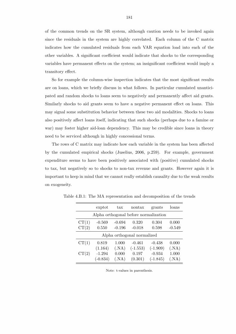
181
of the common trends on the SR system, although caution needs to be invoked again
since the residuals in the system are highly correlated. Each column of the C matrix
indicates how the cumulated residuals from each VAR equation load into each of the
other variables. A significant coefficient would indicate that shocks to the corresponding
variables have permanent effects on the system; an insignificant coefficient would imply a
transitory effect.
So for example the column-wise inspection indicates that the most significant results
are on loans, which we briefly discuss in what follows. In particular cumulated unantici-
pated and random shocks to loans seem to negatively and permanently affect aid grants.
Similarly shocks to aid grants seem to have a negative permanent effect on loans. This
may signal some substitution behavior between these two aid modalities. Shocks to loans
also positively affect loans itself, indicating that such shocks (perhaps due to a famine or
war) may foster higher aid-loan dependency. This may be credible since loans in theory
need to be serviced although in highly concessional terms.
The rows of C matrix may indicate how each variable in the system has been affected
by the cumulated empirical shocks (Juselius, 2006, p.259). For example, government
expenditure seems to have been positively associated with (positive) cumulated shocks
to tax, but negatively so to shocks to non-tax revenue and grants. However again it is
important to keep in mind that we cannot really establish causality due to the weak results
on exogeneity.
Table 4.B.1: The MA representation and decomposition of the trends
exptot tax nontax grants loans
Alpha orthogonal before normalization
CT(1) -0.569 -0.694 0.320 0.304 0.000CT(2) 0.550 -0.196 -0.018 0.598 -0.549
Alpha orthogonal normalized
CT(1) 0.819 1.000 -0.461 -0.438 0.000(1.164) (.NA) (-1.553) (-1.909) (.NA)
CT(2) -1.294 0.000 0.197 -0.934 1.000(-0.834) (.NA) (0.301) (-1.845) (.NA)
Note: t-values in parenthesis.
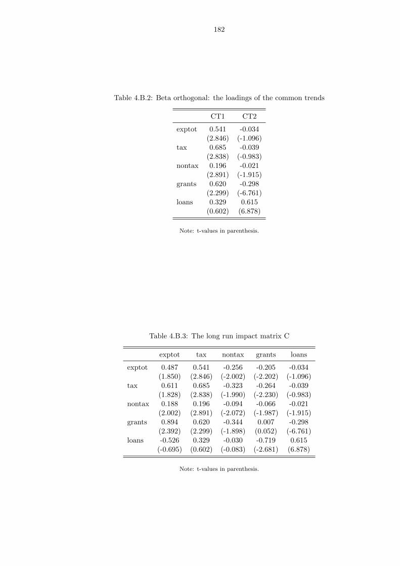
182
Table 4.B.2: Beta orthogonal: the loadings of the common trends
CT1 CT2
exptot 0.541 -0.034(2.846) (-1.096)
tax 0.685 -0.039(2.838) (-0.983)
nontax 0.196 -0.021(2.891) (-1.915)
grants 0.620 -0.298(2.299) (-6.761)
loans 0.329 0.615(0.602) (6.878)
Note: t-values in parenthesis.
Table 4.B.3: The long run impact matrix C
exptot tax nontax grants loans
exptot 0.487 0.541 -0.256 -0.205 -0.034(1.850) (2.846) (-2.002) (-2.202) (-1.096)
tax 0.611 0.685 -0.323 -0.264 -0.039(1.828) (2.838) (-1.990) (-2.230) (-0.983)
nontax 0.188 0.196 -0.094 -0.066 -0.021(2.002) (2.891) (-2.072) (-1.987) (-1.915)
grants 0.894 0.620 -0.344 0.007 -0.298(2.392) (2.299) (-1.898) (0.052) (-6.761)
loans -0.526 0.329 -0.030 -0.719 0.615(-0.695) (0.602) (-0.083) (-2.681) (6.878)
Note: t-values in parenthesis.

183
4.C Misspecification tests for UVAR k = 1
Table 4.C.1: Autocorrelation test
Test test statistic p-value
LM(1) ChiSqr(25) = 32.662 0.140LM(2) ChiSqr(25) = 31.307 0.179LM(3) ChiSqr(25) = 24.642 0.483LM(4) ChiSqr(25) = 29.883 0.229
Note: Variables are measured in logs of deflated values. The null of no autocorrelation cannot be rejectedfor all four lags.
Table 4.C.2: Multivariate heteroskedasticity and normality tests
Test test statistic p-value
Test for ARCH
LM(1) ChiSqr(225) = 262.498 0.044LM(2) ChiSqr(450) = 505.577 0.036LM(3) ChiSqr(675) = 690.000 0.336LM(4) ChiSqr(900) = 714.603 1.000
Test for Normality
ChiSqr(10) = 19.375 0.036
Note: Variables are measured in logs of deflated values. The null of homoskedastic errors is rejected at thefirst two lags. Normality is rejected when only one lag is used.
Table 4.C.3: Univariate heteroskedasticity and normality tests
Variable Skewness Kurtosis ARCH(1) Normality R2
exptot 0.490 4.114 0.208 (0.648) 5.203 (0.074) 0.563tax -0.089 4.169 0.011 (0.916) 6.622 (0.036) 0.405nontax -0.114 2.391 0.515 (0.473) 0.389 (0.823) 0.432grants -0.195 2.881 0.155 (0.694) 0.533 (0.766) 0.539loans 0.292 2.616 0.359 (0.549) 0.904 (0.636) 0.409
Note: P-values in parenthesis when relevant. Variables are measured in logs of deflated values.

184
4.D Results from UVAR k = 2
Table 4.D.1: Alpha coefficients from UVAR
Variable Alpha(1) Alpha(2) Alpha(3) Alpha(4) Alpha(5)
exptot -0.023 -0.044 -0.033 -0.000 -0.004(-2.267) (-4.303) (-3.197) (-0.014) (-0.356)
tax 0.018 0.010 -0.046 0.016 -0.016(1.427) (0.764) (-3.564) (1.276) (-1.235)
nontax -0.119 0.024 -0.077 0.015 0.033(-4.340) (0.877) (-2.812) (0.536) (1.185)
grants 0.122 -0.090 -0.073 0.075 0.039(3.282) (-2.416) (-1.966) (2.004) (1.060)
loans 0.114 -0.123 -0.144 -0.131 0.017(2.257) (-2.430) (-2.851) (-2.597) (0.327)
Note: t-values in parenthesis.
Table 4.D.2: Beta coefficients from UVAR
exptot tax nontax grants loans 1991 1974
Beta(1) 14.465 -7.072 -0.404 -3.874 -1.650 -0.124 -4.601Beta(2) 8.717 -8.519 -4.150 2.553 0.633 -1.438 1.858Beta(3) -2.545 0.733 1.434 0.973 1.143 -2.914 -1.702Beta(4) -0.769 4.787 -1.412 -2.337 1.691 0.801 -2.027Beta(5) 2.256 1.985 -1.981 -1.542 -0.203 -1.098 0.711
Table 4.D.3: Π matrix from UVAR
exptot tax nontax grants loans 1991 1974
exptot -0.650 0.512 0.154 -0.049 -0.027 0.167 0.079(-3.651) (4.048) (2.962) (-0.859) (-0.956) (4.586) (1.350)
tax 0.418 -0.199 -0.105 -0.104 -0.045 0.147 -0.033(1.890) (-1.270) (-1.631) (-1.475) (-1.307) (3.260) (-0.449)
nontax -1.258 0.718 -0.248 0.364 0.142 0.182 0.719(-2.651) (2.129) (-1.792) (2.405) (1.909) (1.873) (4.612)
grants 1.202 0.284 0.036 -1.010 -0.224 0.344 -0.729(1.871) (0.623) (0.190) (-4.924) (-2.223) (2.621) (-3.449)
loans 1.084 -0.461 0.410 -0.614 -0.656 0.459 -0.230(1.244) (-0.745) (1.610) (-2.207) (-4.794) (2.576) (-0.803)
Note: t-values in parenthesis.

185
4.E Graphs of unrestricted beta relations
Figure 4.E.1: Graphs of unrestricted beta relations
Beta1'*Z1(t)
1965 1967 1969 1971 1973 1975 1977 1979 1981 1983 1985 1987 1989 1991 1993 1995 1997 1999 2001 2003 2005 2007 2009-3-2-101234
Beta1'*R1(t)
1965 1967 1969 1971 1973 1975 1977 1979 1981 1983 1985 1987 1989 1991 1993 1995 1997 1999 2001 2003 2005 2007 2009-3
-2
-1
0
1
2
3
Beta2'*Z1(t)
1965 1967 1969 1971 1973 1975 1977 1979 1981 1983 1985 1987 1989 1991 1993 1995 1997 1999 2001 2003 2005 2007 2009-4-3-2-10123
Beta2'*R1(t)
1965 1967 1969 1971 1973 1975 1977 1979 1981 1983 1985 1987 1989 1991 1993 1995 1997 1999 2001 2003 2005 2007 2009-3
-2
-1
0
1
2
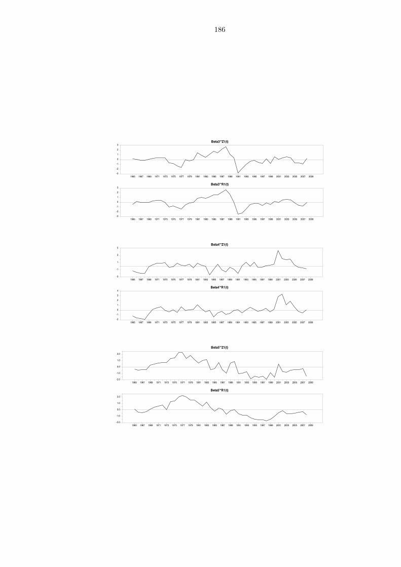
186
Beta3'*Z1(t)
1965 1967 1969 1971 1973 1975 1977 1979 1981 1983 1985 1987 1989 1991 1993 1995 1997 1999 2001 2003 2005 2007 2009-3
-2
-1
0
1
2
3
Beta3'*R1(t)
1965 1967 1969 1971 1973 1975 1977 1979 1981 1983 1985 1987 1989 1991 1993 1995 1997 1999 2001 2003 2005 2007 2009-3
-2
-1
0
1
2
3
Beta4'*Z1(t)
1965 1967 1969 1971 1973 1975 1977 1979 1981 1983 1985 1987 1989 1991 1993 1995 1997 1999 2001 2003 2005 2007 2009-3
-1
1
3
5
Beta4'*R1(t)
1965 1967 1969 1971 1973 1975 1977 1979 1981 1983 1985 1987 1989 1991 1993 1995 1997 1999 2001 2003 2005 2007 2009-2
-1
0
1
2
3
4
Beta5'*Z1(t)
1965 1967 1969 1971 1973 1975 1977 1979 1981 1983 1985 1987 1989 1991 1993 1995 1997 1999 2001 2003 2005 2007 2009-2.0
-1.0
0.0
1.0
2.0
Beta5'*R1(t)
1965 1967 1969 1971 1973 1975 1977 1979 1981 1983 1985 1987 1989 1991 1993 1995 1997 1999 2001 2003 2005 2007 2009-2.0
-1.0
0.0
1.0
2.0

187
4.F LR results with just identifying restrictions
Table 4.F.1: LR results on beta with just identifying restrictions
exptot tax nontax grants loans 1974 1991
The beta vectors before normalization
Beta(1) 52.359 -38.258 -9.918 0.000 0.000 -8.176 -9.283Beta(2) 163.433 0.000 0.000 -124.391 -73.864 -23.766 128.215Beta(3) 0.000 10.466 0.000 -10.463 -7.447 4.696 17.881
The beta vectors normalized
Beta(1) 1.000 -0.731 -0.189 0.000 0.000 -0.156 -0.177(.NA) (-18.193) (-7.015) (.NA) (.NA) (-3.211) (-5.037)
Beta(2) 1.000 0.000 0.000 -0.761 -0.452 -0.145 0.785(.NA) (.NA) (.NA) (-7.386) (-4.704) (-0.771) (4.927)
Beta(3) 0.000 1.000 0.000 -1.000 -0.712 0.449 1.709(.NA) (.NA) (.NA) (-4.833) (-3.877) (1.169) (5.137)
Note: t-values in parenthesis.
Table 4.F.2: LR results on alpha with just identifying restrictions
Alpha(1) Alpha(2) Alpha(3)
exptot -0.773 0.132 -0.045(-3.214) (0.679) (-0.419)
tax 0.599 -0.133 0.192(1.942) (-0.536) (1.381)
nontax 0.860 -2.180 1.211(1.318) (-4.150) (4.127)
grants -1.158 2.328 -0.997(-1.264) (3.158) (-2.423)
loans -1.357 2.302 -0.857(-1.075) (2.264) (-1.510)
Note: t-values in parenthesis.

188
4.G Lag length determination for system 2
Table 4.G.1: Lag reduction test
test test stat p-value
VAR(4) << VAR(5) ChiSqr(25) = 105.487 0.000VAR(3) << VAR(5) ChiSqr(50) = 152.346 0.000VAR(3) << VAR(4) ChiSqr(25) = 46.860 0.005VAR(2) << VAR(5) ChiSqr(75) = 206.752 0.000VAR(2) << VAR(4) ChiSqr(50) = 101.265 0.000VAR(2) << VAR(3) ChiSqr(25) = 54.406 0.001VAR(1) << VAR(5) ChiSqr(100) = 253.858 0.000VAR(1) << VAR(4) ChiSqr(75) = 148.371 0.000VAR(1) << VAR(3) ChiSqr(50) = 101.512 0.000VAR(1) << VAR(2) ChiSqr(25) = 47.106 0.005
Table 4.G.2: Information criteria for lag length determination
Model k T Regr Log-Lik SC H-Q LM(1) LM(k)
VAR(5) 5 42 30 532.201 -11.994 -15.925 0.346 0.637VAR(4) 4 42 25 479.458 -11.707 -14.983 0.128 0.051VAR(3) 3 42 20 456.028 -12.816 -15.437 0.042 0.649VAR(2) 2 42 15 428.825 -13.746 -15.711 0.367 0.336VAR(1) 1 42 10 405.272 -14.849 -16.159 0.288 0.288
SC: Schwarz CriterionH-Q: Hannan-Quinn CriterionLM(k): LM-Test for autocorrelation of order k

189
4.H Misspecification tests for UVAR k = 2, system 2
Table 4.H.1: Autocorrelation test
Test test statistic p-value
LM(1) ChiSqr(25) = 21.508 0.664LM(2) ChiSqr(25) = 26.459 0.383LM(3) ChiSqr(25) = 29.378 0.248LM(4) ChiSqr(25) = 25.606 0.429
Note: Variables are measured in logs of deflated values. The null of no autocorrelation cannot be rejectedfor all four lags.
Table 4.H.2: Multivariate heteroskedasticity and normality tests
Test test statistic p-value
Test for ARCH
LM(1) ChiSqr(225) = 193.465 0.937LM(2) ChiSqr(450) = 457.196 0.397LM(3) ChiSqr(675) = 675.000 0.493LM(4) ChiSqr(900) = 675.000 1.000
Test for Normality
ChiSqr(10) = 22.777 0.012
Note: Variables are measured in logs of deflated values. The null of homoskedastic errors cannot be rejectedat any lags. Normality is rejected.

190
Table 4.H.3: Univariate heteroskedasticity and normality tests
Variable Skewness Kurtosis ARCH(2) Normality R2
cexp -0.136 3.471 0.957 (0.620) 2.469 (0.291) 0.511rexp -0.133 4.986 3.547 (0.170) 12.630 (0.002) 0.693domrev -0.717 3.639 2.968 (0.227) 4.239 (0.120) 0.537grants -0.328 2.907 0.119 (0.942) 1.032 (0.597) 0.506loans 0.006 2.454 1.046 (0.593) 0.089 (0.956) 0.518
Note: Variables are measured in logs of deflated values. P-values in parenthesis when relevant.

191
4.I Residual plots for system 2
Figure 4.I.1: Residual plots for system 2

192

193
4.J LR results for system 2 with r = 4
Table 4.J.1: LR results on beta for system 2 and r = 4
cexp rexp domrev grants loans 1974 1991
The beta vectors before normalization
Beta(1) 98.569 14.935 -159.126 0.000 0.000 0.000 0.000Beta(2) -99.862 0.000 0.000 92.391 69.390 0.000 -79.102Beta(3) 0.000 -13.297 0.000 4.860 3.095 5.634 0.000Beta(4) 0.000 0.000 -150.345 91.698 72.382 0.000 -79.167
The beta vectors normalized
Beta(1) -0.619 -0.094 1.000 0.000 0.000 0.000 0.000(-127.005) (-12.584) (.NA) (.NA) (.NA) (.NA) (.NA)
Beta(2) 1.000 0.000 0.000 -0.925 -0.695 0.000 0.792(.NA) (.NA) (.NA) (-6.937) (-7.324) (.NA) (4.283)
Beta(3) 0.000 1.000 0.000 -0.366 -0.233 -0.424 0.000(.NA) (.NA) (.NA) (-10.011) (-6.184) (-6.916) (.NA)
Beta(4) 0.000 0.000 1.000 -0.610 -0.481 0.000 0.527(.NA) (.NA) (.NA) (-6.785) (-7.519) (.NA) (4.244)
Note: t-values in parenthesis.
Table 4.J.2: LR results on alpha for system 2 and r = 4
Alpha(1) Alpha(2) Alpha(3) Alpha(4)
cexp -8.776 -5.773 -0.770 8.862(-2.241) (-2.349) (-2.354) (2.397)
rexp 4.091 2.368 -0.227 -3.308(2.499) (2.306) (-1.658) (-2.141)
domrev -2.235 -1.191 -0.312 1.984(-1.047) (-0.889) (-1.752) (0.985)
grants 10.338 7.114 1.658 -10.352(1.681) (1.844) (3.231) (-1.784)
loans -22.158 -14.096 -0.836 22.037(-2.755) (-2.793) (-1.244) (2.902)
Note: t-values in parenthesis.
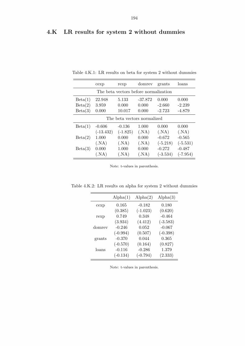
194
4.K LR results for system 2 without dummies
Table 4.K.1: LR results on beta for system 2 without dummies
cexp rexp domrev grants loans
The beta vectors before normalization
Beta(1) 22.948 5.133 -37.872 0.000 0.000Beta(2) 3.959 0.000 0.000 -2.660 -2.239Beta(3) 0.000 10.017 0.000 -2.723 -4.879
The beta vectors normalized
Beta(1) -0.606 -0.136 1.000 0.000 0.000(-13.432) (-1.825) (.NA) (.NA) (.NA)
Beta(2) 1.000 0.000 0.000 -0.672 -0.565(.NA) (.NA) (.NA) (-5.218) (-5.531)
Beta(3) 0.000 1.000 0.000 -0.272 -0.487(.NA) (.NA) (.NA) (-3.534) (-7.954)
Note: t-values in parenthesis.
Table 4.K.2: LR results on alpha for system 2 without dummies
Alpha(1) Alpha(2) Alpha(3)
cexp 0.165 -0.182 0.180(0.385) (-1.023) (0.620)
rexp 0.749 0.348 -0.464(3.934) (4.412) (-3.583)
domrev -0.246 0.052 -0.067(-0.994) (0.507) (-0.398)
grants -0.370 0.044 0.365(-0.570) (0.164) (0.827)
loans -0.116 -0.286 1.379(-0.134) (-0.794) (2.333)
Note: t-values in parenthesis.
195
Chapter 5
Tax incentives, lobbying and
political connections: firm level
evidence from Ethiopia
5.1 Introduction
This chapter takes a microeconomic perspective on tax revenue mobilisation by looking at
the tax take at the firm level in Ethiopia. In particular the focus is on the determinants
of effective tax rates (ETR), broadly defined as the ratio of business profit taxes paid by
the firm to its income (The Tax Policy Center, 2011). They are a measure of the tax
burden on firms, or of the tax take for each firm, according respectively to the firms’ or
the government’s point of view. The main aim of this chapter is to understand what
determines ETRs, including both legal provisions, such as the statutory tax rate and tax
benefits, and the firm’s activity in terms of lobbying and political connections. By doing
this I aim at identifying possible constraints to tax revenue mobilisation at the firm level
in Ethiopia and potential areas for reform.
The focus of the analysis is on business profit tax. While this is not the only tax paid
by firms, it is the most relevant one since it is the only one diretly paid by the firm. Other
taxes, such as labour income taxes and social contributions, are paid by the firm on behalf
of employees while others, such as indirect taxes, are eventually charged on the consumer
through an increase in prices. Therefore firms are primarily affected by business profits
tax, that is also the policy instrument used for fiscal incentives such as exemptions and
tax holidays.
Business profit taxes in Ethiopia amount to 17% of total tax revenue and to about
196
half (49%) of direct taxes. They are therefore already a substantial share of total revenue
and, perhaps more importantly, they have the potential to contribute even more to the
government’s budget in the future. Indeed the manufacturing sector in Ethiopia is still
rather limited in size, as in other African countries, and it contributed only about 5%
to GDP in 20091. Therefore business profits tax can reasonably be expected to become
increasingly important, as the manufacturing sector expands as foreseen in the current
development plan (GTP, Growth and Transformation Plan).
Moreover business profits tax has received much attention particularly in the debate on
international tax competition, tax evasion and the interaction of international tax systems
both in advanced and developing economies. On the one hand in advanced economies the
main concern of the literature is to provide evidence on the equity in the distribution of
the tax burden, and particularly on whether big corporations pay their fair share of tax
(see for example Citizens for Tax Justice (1985)). On the other hand, developing countries
face the additional challenge, along with equity, to ensure a sufficient level of tax revenue
to carry out the basic functions of the state and more generally to finance development
expenditure.
In presence of a relatively small tax base for business profits tax, it is particularly
important to ensure that tax competition and tax benefits do not harm the efforts to-
wards increased domestic revenue mobilisation in Africa. Many low income countries have
adopted exemptions to attract investment and this has indeed reduced the tax base. This
in turn may imply a higher tax burden for those who do pay tax and thus stronger in-
centives to evade (Gauthier and Reinikka, 2006). In this context, the general consensus
on the objectives of tax reform revolves around three broad elements: increasing the tax
base, reducing tax rates, and reducing exemptions and exceptions to a minimum deemed
necessary. Ethiopia has worked towards these principles with the 2002 tax reform that
brought the corporate tax rate down from 35% to 30% and introduced stricter rules on tax
evasion, which ultimately should result in an increased tax base. Increasing the tax base
however is not only a tax policy issue but also an industrial policy one. As far as tax policy
is concerned, and besides the fight against evasion, a general reduction of exemptions will
also lead to an increase of the tax base since it would increase firms’ taxable income.
In this context, this chapter contributes to the policy debate and to the literature
1Note that business income tax is levied on the industrial sector as a whole and not only on themanufacturing sector, thus including for example utilities and construction besides manufacturing, and onlarge agricultural projects as well.

197
in three ways. Firstly it offers a quantification of effective tax rates and an estimate of
the effects of its determinants, including lobbying and political connections. Evidence
on business profits tax for Africa is extremely rare, as only two other studies have been
carried out on African countries but with much smaller samples (Gauthier et al., 2002;
Gauthier and Reinikka, 2006). This evidence is useful to assess the potential for increasing
tax revenue from the manufacturing sector and it represents a starting point for policy
reform.
Secondly a unique census dataset is used, including firms observed over 14 years from
1996 to 2009, thus having a substantial advantage with respect to other studies on Africa.
This long panel potentially allows better estimates than other studies in the litertaure
both because of a larger sample size and the possibility of accounting for firm fixed effects.
The availability of data in the African context is ensured by the use of surveys rather than
accounting data for listed firms, which is more commonly used in the ETR literature (see
sections 5.2 and 5.4). This choice is discussed in section 5.4.
Finally this chapter contributes to the literature by paving the way for further studies
on effective tax rates in Africa and more generally in developing countries. Section 5.3
proposes a theoretical framework that guides the analysis and that can potentially be the
basis for other similar studies. Providing evidence on ETR that is specific to Africa is
particularly important in light of the findings in Abbas et al. (2012), showing that the
continent presents different trends in corporate income taxation than other regions of the
world. They show that not only the tax base has narrowed in Africa, but also that the
widespread use of tax incentives has brought effective tax rates close to zero in many
countries. This chapter is therefore a first step in providing country specific evidence on
the level of effective tax rates, particualrly for the case of Ethiopia.
Finally, this research is particularly relevant at a time when tax revenue mobilisation
is widely recognized as one of the objectives of aid and development policy (House of
Commons International Development Committee, 2012).
5.2 Literature review
The firm level literature in Africa has developed in the last two decades particularly
since the World Bank enhanced its effort in collecting firm level data, thus allowing more
empirical work that is widely reviewed in Bigsten and Soderbom (2005). The focus has
been mainly on firms’ performance, its determinants and its constraints (Carlin et al., 2006;
Siba and Soderbom, 2011; Bigsten and Gebreeyesus, 2007; Dollar et al., 2005; Fafchamps

198
and El Hamine, 2004), as well as trade and exports (Bigsten et al., 1999; Elbadawi et al.,
2006; Bigsten et al., 2009). However this literature is only marginally concerned with
corporate taxation2. Therefore the main reference literature for this work is the one
specifically focussed on ETR, that is reviewed in this section in detail.
The ETR literature originates in the Unites States to inform and influence policy
making about existing inequities in the tax system. Citizens for Tax Justice carried out
a number of descriptive studies, amongst which Citizens for Tax Justice (1985), arguing
that large corporations in America were not paying their fair share of tax. The early
literature focuses exclusively on the ETR-size relation using largely descriptive techniques
rather than regression analysis (Zimmerman, 1983; Porcano, 1986; Wang, 1991; Kern and
Morris, 1992). All these studies focus on the US and the results are conflicting. Particularly
Zimmerman (1983) finds a positive relation between size and ETR while Porcano (1986)
finds a negative one. Wilkie and Limberg (1990) explained the difference in these results
on the basis of the empirical methodology. Later Kern and Morris (1992) showed that
the results from Zimmerman (1983) are more robust than those in Porcano (1986), but
that the effect of size decreased in the late 80s and it then became insignificant. Wang
(1991) argues that net operating losses (NOL) should be included in the analysis to avoid
a positive bias. Gupta and Newberry (1997) confirm this view and they argue that the
omission of NOL may induce a positive bias in size to the extent that small firms are
more likely to incur losses due to their lower diversification. Stickney and McGee (1982)
introduce more variables in the descriptive analysis, namely capital intensity, leverage,
extent of foreign operations, natural resource involvement. They find that size does not
play an important role in explaining differences in ETRs but leverage and capital intensity
are negatively associated with it.
The article by Gupta and Newberry (1997) is the first attempt at providing a multi-
variate regression analysis using panel data. In particular the authors add to the analysis
variables related to the capital structure, such as capital intensity and leverage; to the asset
mix, namely inventory intensity; and other variables such as firms’ performance (namely
ROA, the return on assets) and the firm’s extent of involvement in research and devel-
opment activities. The authors support the results in Zimmerman (1983) and Kern and
Morris (1992) by finding a positive and significant relation between ETR and size before
2The only area of this literature concerned with taxation is the work on tariffs. For example Bigsten et al.(2009) use Ethiopian data to show that tariff reductions have a positive effect on total factor productivity.Moreover they find that the reduction of tariffs further results in smaller and more capital-intensive firms.

199
a tax reform occurred in 1986. After this reform however the relation turns to negative,
and still significant. However when the authors consider only the subsample of firms with
longer histories, they find that size does not have a significant effect either before or after
the 1986 reform. Capital intensity and research and development intensity are consistently
significant and negative across specifications, while firms’ performance and the asset mix
have a positive and significant coefficient.
Finally research on the US has also focused on state level revenue, a literature that is
comprehensively reviewed in Hofmann (2002). For example Gupta and Mills (2002) look
at the effect of multistate tax planning on the ETR but they also include other variables
in the regression. They find a positive and significant coefficient on size although it is
not robust to changes in specification. Capital intensity is always negative but never
significant.
The literature on the USA discussed so far is summarized in the first part of table
5.2.1. The table focuses on the results on size, that are the most conflicting ones in the
literature. Despite the disagreement on the effect of this variable, most results support a
positive relation in the US. Table 5.2.1 also includes studies on other advanced countries
and emerging economies, reported respectively in the second and third part of the table.
Table 5.2.1: Results on size in the literature
Reference country effect of size
Zimmerman (1983) USA +Porcano (1986) USA -Kern and Morris (1992) USA +Omer et al. (1993) USA +Stickney and McGee (1982) USA n.s.Gupta and Newberry (1997) USA n.s.Gupta and Mills (2002) USA +
Holland (1998) UK +Wilkinson et al. (2001) New Zealand +Richardson and Lanis (2007) Australia -
Kim and Limpaphayom (1998) Pacific -Derashid and Zhang (2003) Malaysia -Adhikari et al. (2006) Malaysia -Guha (2007) India -Wu et al. (2012) China +
Note: n.s. means that size did not result to be significant
As far as other advanced economies are concerned, Holland (1998) finds that in the UK
generally a negative relation exists between ETR and size although firms in the highest

200
decile have larger ETR. The author also finds evidence of sectoral differences in that firms
in the mining sector face higher ETRs. Wilkinson et al. (2001) focus on the effect of the
1993 reform of the dividend imputation system in New Zealand. They find that size has a
positive but not always significant effect. This result however is contradicted, in the case
of Australia, by Richardson and Lanis (2007) who find a negative and significant effect
there. Otherwise the results of both Wilkinson et al. (2001) and Richardson and Lanis
(2007) are largely consistent and in line with the literature, particularly as far as leverage
(−), capital intensity (−) and performance (+) are concerned.
As far as developing countries are concerned, the ETR literature has developed only
recently and mostly on emerging Asian economies. Kim and Limpaphayom (1998) is the
first attempt at providing some evidence on ETR and firm size for the emerging countries
of the Pacific. In particular the authors use data for all firms, excluding financial ones,
listed in the stock exchange in Hong Kong, Korea, Malaysia, Taiwan and Thailand. The
authors focus on size and they test whether the political cost hypothesis, postulating a
positive relation between ETR and size3, is applicable to developing countries. Supported
by a negative coefficient on size, they suggest that while this hypothesis may be valid
in the US, it is not for developing countries. Indeed governments in the latter group of
countries may require more the cooperation of big firms to achieve national economic goals
and therefore they would provide fiscal incentives for big firms (thus resulting in a negative
relation between ETR and size). This study in addition confirms that firms’ performance
has a positive effect on ETRs but fails to find a significant relation with leverage.
Taking up the indication in Kim and Limpaphayom (1998) that industry effect may be
an important determinant, Derashid and Zhang (2003) focus on sectoral differences in ETR
in Malaysia. The sectors are defined relatively broadly and, for example, manufacturing
is considered a sector in itself, along with mining, finance and construction. Sectoral
differences are found to matter, with the manufacturing sector paying less tax than any
other sector. The negative result on size for Pacific countries is confirmed here, although
it is not robust. Leverage and capital intensity have the expected negative effect, while
performance has a negative coefficient contrary to the rest of the literature. This last
result and the one on size set a basis for the authors to suggest that indeed significant
differences may exist between developed and developing countries.
Adhikari et al. (2006) use a dataset of Malaysian firms listed in the Kuala Lumpur
3For more details on the political cost hypothesis also see section 5.3.
201
Stock Exchange and observed over a 10-year period. This article adds to the ‘standard’
variables two measures of political connections, on the grounds that these would be cru-
cial in ensuring a more favorable tax treatment. The first is the percentage of government
ownership in a firm. The second is a proxy based on informal ties of a firms directors with
leading politicians. The results for both measures are negative and significant, suggesting
that indeed these variables should be included in the model. The results previously found
on Malaysia on capital intensity (−), leverage (−) and performance (−) are confirmed.
None of the sector dummies is significant except for the one on the manufacturing sector
that has a negative coefficient. Wu et al. (2012) expand the evidence on political con-
nections by studying Chinese listed firms from 1999 to 2007. To capture this aspect, the
authors first distinguish between publicly and privately owned firms. They then obtain
a proxy for politically connected managers based on whether they previously served in
the government or in the military. They find that the presence of politically connected
managers help private firms obtain tax benefits but that it does not have any effect for
state owned enterprises. This may suggest that these enterprises can already benefit from
connections just by being publicly owned. While previous results for developing countries
are confirmed, size here displays a positive and significant coefficient across all models.
The authors also include growth to capture performance and managers’ characteristics
(age and education) but find no significant effect in neither.
Moreover Guha (2007) uses a database of Indian manufacturing firms and finds that
size has a negative coefficient, and the usual results on capital intensity and leverage
are confirmed. In addition the author includes, along with the standard variables, also a
measure of export intensity measured as the ratio of as exports to total sales. This variable
is found to have a negative coefficient, thus suggesting that firms that export more also
benefit more from tax incentives. It is worth noting that although Gupta and Newberry
(1997) did not include this variable, they suggested that foreign operations should be
taken into account. Along these lines Bauman and Schadewald (2001) adopt a descriptive
approach to explore how the activity of American firms in jurisdictions with different tax
regulations affects ETR.
Last but not least, it is important to note that throughout the literature an effort has
been made to identify the effect of tax reform on ETRs (Gupta and Newberry, 1997; Wu
et al., 2012; Richardson and Lanis, 2007; Guha, 2007; Wilkinson et al., 2001) by including
either a variable that captures its effect or its interaction with size, to check whether
reform was successful in tackling possible inequalities in the system, or both.
202
As far as Africa is concerned, very few studies have looked in detail at ETR and they
have not been fully in line with the literature reviewed here. The work that is closest to
the ETR literature for Africa is an article by Gauthier and Reinikka (2006), using survey
data from Ugandan firms. The authors estimate a system of three simultaneous equations
using 3SLS methods to explore the effect of size on firms’ tax payments. However they
depart from the literature in two ways. First, they consider tax payments including also
social security contributions and sales tax/value added tax along with corporate income
tax. By doing this the effective tax rate paid by the firm is largely inflated, mainly due
to sales tax/VAT. Indeed the authors show that of the 6.6% average tax burden (share
of sales value), five percentage points are represented by sales tax. Secondly the authors
do not estimate the direct effect of size on ETR but they look at the indirect effect
through exemptions and evasion. This exercise is possible thanks to specific information
on tax evasion and exemptions in the datset that however contains a limited number of
observations (147 when looking specifically at ETR).
Contribution
This chapter contributes to the ETR literature in two ways. Firstly it provides evidence
on Africa, which is extremely scarce so far. The importance of providing regional specific
evidence has been highlighted in the literature. Moreover it has already been suggested
that Africa may display different patterns (Abbas et al., 2012), thus the further relevance
of expanding the literature to this region. Secondly, it brings an economic perspective to
a theme largely debated in accounting journals. While the accounting concepts are taken
into consideration, a theoretical framework is developed both to specify the economic
mechanisms that define effective tax rates and to allow a clear formulation of testable
hypotheses. More generally, this work aims at shedding light on corporate taxation in
Africa, a topic largely recognized for its relevance but at the same time virtually ignored
in the empirical firm-level literature.
5.3 Theoretical framework and hypotheses
The main actors in this theoretical framework are the government and firms. The former
produces a complex system of tax laws and regulations that reflect its objectives and the
political negotiation with firms. Within this system, all firms face the same statutory tax
rate but they may have different ETRs and thus a different tax burden. It is also possible
that, keeping the tax system constant, the ETR faced by the same firm changes in different

203
periods according to differences in behavior. In other words, while firms respond to the
overall tax system as set out by laws and regulations, the actual ETR they face is a result
of their action.
The remainder of this section goes into details regarding the definition and determi-
nants of ETR (section 5.3.1); it describes the explanatory variables that are expected to
influence the ETR (section 5.3.2); and it proposes the empirical model and the testable
hypotheses stemming from the theoretical discussion (section 5.3.3).
5.3.1 The average effective tax rate
As anticipated in the introduction (section 5.1), the effective tax rate for firms is defined as
corporate income tax payments divided by pre-tax income, which essentially corresponds
to profits. The standard choice in the literature is to only include income tax in the
numerator, namely business profit tax. This is justified by the focus on exemptions and
other fiscal benefits, since special regimes and industrial policy mostly take place in the
area of corporate income tax. This is indeed the case in Ethiopia, where fiscal incentives
are set mainly through the business profits tax. The concept of tax expenditures captures
this aspect of public policy. In particular, they are defined as “revenue losses attributable
to tax provisions that often result from the use of the tax system to promote social goals
without incurring direct expenditures” (The Tax Policy Center, 2011). These goals may
include for example the development of a particular sector, incentives to investment in
general or in a particular region.
By ETR the literature usually refers to the average effective tax rate, as defined in
this section, as opposed to the marginal effective tax rate. The latter is defined as the
percentage of the expected return on an additional investment that is expected to be
paid in tax (Spooner, 1986). Change in behavior, including incentives to investment, are
usually achieved through marginal tax rates. However the use of the average ETR instead
is grounded on computational simplicity and on the fact that it is better suited to assess
the overall tax burden of a firm. The remainder of the chapter therefore refers to ETR as
average effective tax rates.
As far as the numerator of the ETR is concerned, the tax payment of a firm in a given
year is the sum of current and deferred tax where the latter includes reductions and the
effect of tax credits (Stickney, 1979). Deferred tax is an accounting concept4 emerging
4It does not refer to parts of the tax bill that authorities allow the firm to pay with a delay.

204
from differences between the time when expenses and revenues are included in accounting
calculations and the time when they are included in tax calculations5. In this chapter
the ETR is defined using the whole tax payment, therefore including both components.
Studies that adopt different measures of tax payments (including or excluding, partly or
entirely, deferred tax) to check for robustness, generally find that the results are consistent
regardless of the measure used. Therefore they suggest that this issue is not a concern in
this analysis. For a more detailed discussion on the treatment of current and deferred tax
in the literature, see appendix 5.A. The extent of deferred tax also depends on the specific
provisions of the tax system and they are explored in detail for Ethiopia in section 5.5.1.
As far as the denominator of the ETR is concerned, it is useful to clarify the difference
between pre-tax (or book) income and taxable income. The former is essentially revenue
net of costs of production and other expenses, therefore essentially capturing profits, and
it can be used as an indicator of firms’ performance as well. The difference with tax-
able income essentially lies in exclusions, exemptions, tax holidays and other deductions.
These include for example accelerated depreciation or investment tax credits that allow a
deduction of certain investment items from taxable income. The statutory tax rate is then
applied to taxable income. The elements that determine the difference between book in-
come and taxable income are generally referred to as tax preferences (Wilkie, 1988). Most
studies in the literature use book income at the denominator although Stickney (1979)
suggests the use of estimated taxable income at the denominator. This is computationally
burdensome when all necessary information on tax preferences is not readily available.
Moreover by taking the ratio of tax payments on taxable income one should obtain the
statutory tax rate, if no evasion and/or corruption is taking place.
Based on these definitions, the average effective tax rate can be described by the
following formula:
ETR =TPay
PTI=
(PTI − TP )τ
PTI(5.1)
where:
TPay = tax payment
PTI = pre-tax income (or profits)
5The most common case of deferred tax is depreciation that usually occurs more slowly for accountingpurposes than for tax purposes. One extreme case is the UK between 1972 and 1984, where a 100%depreciation allowance was applied on machinery and plant in the year of purchase. This gives rise to asituation where the depreciation is charged slowly for accounting purposes but the tax reduction is takenimmediately (James and Nobes, 2009). In this extreme example, the deferred tax is the portion of theimmediate tax reduction that is spread over the years of accounting depreciation.
205
TP = tax preferences
τ = statutory tax rate
Equation 5.1 can be rewritten as follows:
ETR =TPay
PTI= (1− TP
PTI) · τ (5.2)
Equation 5.2 shows that the effective tax rate is essentially composed of two elements: the
statutory tax rate and the share of tax preferences on pre-tax income. The first one does
not vary across firms in the same year. However it may vary in time as a result of tax
reform. The second one is essentially a measure of tax benefits normalized on profits. If
all firms face the same tax benefits, this share would not vary across firms. However this is
normally not the case, as tax preferences are available for example for firms that operate
in certain sectors or regions, or that engage in certain types of investment. In addition
the behavior of firms differ, influencing this share as well6. This ratio can therefore be
expected to vary both across firms and in time. Equation 5.2 implies that, holding TP
constant, an increase in profit increases the ETR. Similarly, holding PTI constant, an
increase in tax preferences decreases the ETR. The main insight is therefore that the ETR
is influenced not only by the statutory tax rate and tax preferences, but also by pre-tax
income if TP and PTI are not perfectly correlated (Wilkie, 1988).
5.3.2 The explanatory variables
Based on equation 5.2, the next paragraphs identify what are the variables that influence
the ETR, or more precisely its components on the RHS of the equation. These are namely:
the statutory tax rate (τ) and the share of tax preferences ( TPPTI ).
As far as the statutory tax rate is concerned, it is possible to capture its effect by
including tax reform as an explanatory variable. This essentially captures the same infor-
mation as the statutory tax rate, provided that it does not vary across firms but only in
time. Tax reform was carried out in Ethiopia in 2002 and one of the main provisions was
a decrease of the statutory tax rate from 35% to 30% (see section 5.5 for more details).
Theoretically, such a policy has the effect of decreasing the ETR. The reality may not
be as straightforward however. First, tax reform is usually comprehensive and includes
6Differences in ETRs across firms may be due to timing or to ‘permanent’ differences. The former refersto deferred taxes and it will fade away in the future while the latter will not. In this sense they can becalled ‘permanent’ although they can vary in time (Spooner, 1986). By including all tax expense, i.e. bothcurrent and deferred, the timing differences should be canceled.

206
many different aspects of tax policy that may have different effects on the ETR. The in-
terpretation of the coefficient on reform has to take into account all of these aspects. It
is therefore crucial to understand the relevant tax reform in detail (see section 5.5). A
second and related point refers to the Laffer curve, that postulates an inverse U shaped
relation between the statutory tax rate and tax revenue (Laffer, 2004). This is explained
by the fact that a decrease in the tax rate has two effects: an arithmetic and an economic
one. The arithmetic effect leads to a decrease in tax revenue by the amount of the decrease
in the tax rate. The economic effect is instead an increase in tax revenue due to a greater
incentive to work and make profits and generally to an increase in the tax base. The
Laffer curve in itself does not postulate if a decrease in tax rates will increase or decrease
tax revenue. The tax response depends on various factors, including the tax system in
place, the ease of movement to and from informality, and characteristics of the productive
factors. However the curve shows that a positive effect of a cut of the tax rate is entirely
possible and sensible (Laffer, 2004).
The share of tax preferences can be influenced by firms in two main ways: tax min-
imizing strategies and lobbying. First they can and do adopt tax minimizing strategies
(Hofmann, 2002) that involve most notably choices on investment, financing and capital
intensity. For example, a firm may invest in a more energy efficient technology or in a
certain region, knowing that there are fiscal benefits attached to it. More generally new
investments may benefit from tax preferences. Firms can also decide the level of financial
leverage to minimize tax. Finally capital intensive firms may have lower ETRs because of
tax-deductible interest payments and accelerated depreciation relative to the assets’ life
(Derashid and Zhang, 2003).
Secondly firms can affect ( TPPTI ) by lobbying the government to obtain additional fiscal
benefits, resulting in an incrase in TP . Lobbying is difficult to measure but its effect
can be captured in practice by three variables: public ownership, size and age. It has
been shown that accounting for political connections is important in understanding the
mechanisms through which firms can obtain fiscal benefits and more generally a favorable
treatment, for example in competing for government contracts (Faccio, 2006; Fisman,
2001). Obtaining government contracts in turn would have fiscal benefits, as for example
in the case of Ethiopia revenues obtained from the government are exempted. One of the
most common indicators for political connections is public ownership, as it may grant more
direct channels to government officials. Ideally managers’ personal connections would be
included in the analysis as well, to identify the potential for effective lobbying. However

207
data on this variable is not easy to obtain and only two of the reviewed papers include
such personal connections (Adhikari et al., 2006; Wu et al., 2012). Size can also influence
the ability and the effectiveness of lobbying. In particular the ‘political power hypothesis’
postulates a negative relation between ETR and size, on the grounds that larger firms
enjoy a higher bargaining power in negotiating with the government and that they have
greater resources to devote to tax minimizing strategies (Richardson and Lanis, 2007).
Age can also influence lobbying because older firms may have a more established network
of connections.
Finally it may be useful to note that tax evasion is not directly included in the equation
because of its unobservability and lack of data. However it may be possible to identify
variables that are likely to influence it. In particular size and public ownership can influ-
ence the probability and extent to which firms engage in tax evasion, besides influencing
lobbying. As far as size is concerned, and opposed to the negative effect postulated by
the political power hypothesis, the ‘political cost hypothesis’ postulates a positve relation
between ETR and size instead (Zimmerman, 1983). This relation is explained by the
greater visibility of large firms that makes it more difficult for them to escape the tax
net through evasion. Along the same lines, public ownership may also have an effect on
evasion because of higher visibility to authorities. For example public owned firms may
employ persons who are directly related to the government, therefore tightening up the
control from within.
The fact that public ownership and size affect both tax preferences, though lobbying,
and evasion should be kept in mind when interpreting the results. In the case of size, the
sign of the relation with ETR would be different if the channel is lobbying or tax evasion,
respectively negative according to the political power hypothesis and positive according
to the political cost one. In the case of public ownership, if the effect occurs through
lobbying a lower ETR can be expected (i.e. negative relation) while if it occurs through
evasion the coefficient would be positive.
So far the ‘core variables’ of the model have been identified as: reform, capital intensity,
financing decisions, investment, public ownership, age and size. In addition to these, there
may be other variables that are less directly related with the (TP/PTI) ratio but that
are worth including in the model to check their significance. First, firms’ performance
may influence the ETR and it can be captured, amongst others, by growth in sales or the
presence of losses7. The expected effect of performance indicators on the ETR however
7Note that net operating losses (i.e. negative profits) in one year influence the ETR in the future when

208
is unclear. On the one hand governments might want to put obstacles to large firms to
avoid them being too powerful (i.e. negative relation between performance and ETR). On
the other hand they may also want to set incentives for them due to their contribution to
growth and employment (i.e. positive relation).
Moreover foreign connections in terms of export or of presence of foreign capital may
matter, according to the government’s views on exports and foreign investment. Finally
some characteristics of the owners, besides the public or private nature, may be relevant
to include. In particular the number of owners is considered.
5.3.3 Core model and research questions
The framework discussed in the previous sections leads to a reduced form equation that
stems from equation ?? and that is the basis of the econometric exercise.
ETR = α+ β1SIZE + β2CAPINT + β3INV EST + β4PUBLIC+
+ β5AGE + β6REFORM + ε (5.3)
Equation 5.6 represents the ‘core model’ for the analysis and henceforth it is referred to
as the baseline equation. To this model are going to be added other control variables such
as growth, loss, export, foreign capital and owners. Section 5.4 describes the data used to
capture each of these variables in detail.
Estimation of the baseline equation and its extensions can shed light on the following
research questions, that correspond to the testable hypotheses underlying the analysis.
1. Which hypothesis is more appropriate in explaining the ETR-size relation in Ethiopia:
the political cost hypothesis or the political power hypothesis?
2. Can political connections, through public ownership, help firms reduce their tax
burden?
3. Reform: can a reduction of the statutory tax rate have a positive effect on the ETR?
loss carryforwards are allowed. In the case of Ethiopia, losses can be carried forward for three years (seesection 5.5.1).

209
5.4 Data and variables
The data used in this chapter is the census of Ethiopian firms in the manufacturing sector
collected by the Central Statistical Agency, namely the Large and Medium Manufacturing
Industry Survey (LMMIS). The LMMIS is a unique dataset in the African context as
it provides panel data for a large number of firms observed over 14 years, from 1996 to
20098. This data is also used in other studies in the literature although not for analysing
tax-related issues (Melese and Waldkirch, 2011; Bigsten et al., 2011, 2009; Bigsten and
Gebreeyesus, 2007; Soderbom, 2011; Siba and Soderbom, 2011).
The use of census data is not common in the ETR literature, as the usual source of
information is financial statements for firms listed in the stock exchange. Data from finan-
cial statements however is not available, nor necessarily relevant, in the African context.
In the case of Ethiopia, as of today there is no stock exchange9. In other part of Africa
where a stock exchange exists, only few firms are usually listed. This is the case for many
of Ethiopia’s neighbours such as Kenya (50 firms), Tanzania (11 firms) and Rwanda (4
firms). This selection is likely not to be representative of the industrial sector and it may
therefore include firms that are systematically different from the population as a whole. In
this context census data is preferable as it provides consistent information for the whole
population of firms thus avoiding selection problems, at least at the source. Moreover
the data included in the LMMIS is still based on accounting forms and it includes all the
variables that are necessary for an analysis of ETRs. In addition a clear advantage of the
LMMIS dataset is to follow a large number of firms over a relatively long time period,
that is rather rare in the African context.
The LMMIS dataset includes establishments that engage 10 persons or more and that
use power driven machinery10. As the survey is designed to consider only large and
medium enterprises, it excludes small and micro ones. At the national level in 2009 large
and medium manufacturing represented 70% of the total contribution of manufacturing
to GDP (at constant prices)11. Given the focus on corporate taxation, considering this
8Note that Ethiopia uses the Ethiopian calendar, that is different than the Gregorian one in two mainways: it is seven years behind the Gregorian calendar and it runs from September to August. The first yearin the LMMIS dataset therefore corresponds to 1995/96 and to the Ethiopian Fiscal Year (EFY) 1988.
9There was some form of exchange during the Imperial period that was dismantled by the socialistregime and never opened again (Tsegaye, 2012).
10The number of persons engaged is not necessarily the same as the number of employees, as the formercan include for example members of the family working in the firm without a salary. Moreover changesin employment may arise between the time the firm is selected into the survey and the time the survey isactually carried out. Therefore firms can be observed to employ less than 10 persons.
11Author’s calculation from data provided by the Ministry of Finance and Economic Development.

210
type of enterprises is important and relevant, as they represent the bulk of manufacturing
produciton in Ethiopia.
The LMMIS dataset includes information on taxes12 paid by firms in the survey year,
including a disaggregation between business profits tax and indirect taxes13. Note that
indirect taxation amounts to about 80% of the total tax take from firms. This may
be due to the fact that indirect taxes are relatively easier to collect and they face less
opposition from interest groups as they are levied on a large group of mostly non-organized
consumers. In addition, fiscal incentives occur mostly as reductions on the business tax
burden therefore contributing to explain the lower contribution of this tax type. Total tax
payments (business profit tax) as reported in the LMMIS allow the computation of ETRs.
However attention should be paid to the possibility of delays in tax collection, reflected in
such measure of tax payments, due to exceptional circumstances. This may be the case
for example at the peak of the famine in 2002, as shown in section 5.5. Time dummies are
one way to capture these exceptional events and robustness is discussed in section 5.8.
The ETR is obtained by taking the ratio of business profits tax payments to profits.
Only observations for which tax data is available, i.e. non-missing, can be considered
to avoid intruducing errors in the dataset. The possibility that missing values on tax
are really zeroes, when all other variables are non-missing, is explored in the robustness
section to check whether this choice affets the results (see section5.8). The denominator
of the ETR, profits (or a close proxy of it), is calculated as the total value of sales and
other revenues minus the following14:
• Total wages and benefits to employees;
• Total value of raw materials, spare parts and auxiliary materials;
• Other industrial costs;
• Non industrial costs, including for example commercial and marketing costs;
• The change in the value of fixed assets between the beginning and the end of the
year.
12Tax data includes all tax paid at both the federal and regional level. The regional components is muchsmaller than the federal one, contributing only about 20% of total tax revenue. Business profits tax leviedon large corporations accrues to the central government by law.
13The distinction between current and deferred tax is therefore ignored and they are both included inthe measure of total tax payments.
14The calculation of profits is restricted to observations for which all the necessary variables are available,to avoid mis-calculations due to missing values.

211
Turning to explanatory variables, the LMMIS data allows me to measure all the vari-
ables identified in the theoretical framework of section 5.3. Firstly size can be measured
using sales or employment15. These variables are usually transformed in natural loga-
rithms to reduce skewness. The use of sales would introduce exogenous changes due to
inflation and not to actual changes in the size of a firm. This is particularly important
in Ethiopia, where inflation has often reached double-digit figures in recent years. The
preferred measure of size is therefore the number of employees which is the measure used
in the main results in section 5.7. The value of sales is also used to test for robustness in
section 5.8.
Secondly capital intensity is defined as the ratio of fixed assets to labor. This measure
differs from the one most commonly used in the ETR literature, namely the ratio of fixed
assets to total assets. However it is commonly used in the firm-level literature using
LMMIS data (Bigsten and Gebreeyesus, 2007; Bigsten et al., 2009; Melese and Waldkirch,
2011; Soderbom, 2011) and it is also used in the ETR context, for example in Stickney
and McGee (1982).
Note that leverage cannot be measured, as an indicator of financing decisions, due to
lack of data. However some information on financing decisions can be included in two
ways. On the one hand, the percentage of foreign capital in total capital is included. On
the other hand, capital intensity may also capture part of the effect of leverage, which
would go in the same direction. This is because more capital-intensive firms may have
higher debts to finance their fixed assets and because they can offer a collateral. Note
also that the financial sector in Ethiopia is not particularly developed and therefore the
level of leverage may be expected to be generally lower, and less relevant, than in other
countries.
Moreover investment in fixed assets is included as a percentage of existing fixed assets.
This is expected to have a negative sign as investment often benefits from fiscal incentives.
Export is included as the ratio of exports to total sales, as in Guha (2007). Growth in
employment is also included as an indicator of performance. Political connections are
captured through public ownership. Since census data is anonymous, it is impossible to
proxy the management’s personal connections using LMMIS data. The measure of age
can be obtained using the year of commencement of operations, that is reported in the
survey questionnaire. As a few inconsistencies are present in the data, the mode of this
15Total assets may also be used to measure size. However the LMMIS data reports only fixed assets andnot total assets.

212
Table 5.4.1: Explanatory variables
Variable Description Expected sign
Size Log of number of employees + / -Size (sales) Log of deflated sales value + / -Capital intensity Value of fixed assets in mil-
lions /number of employees-
Investment Investment in fixed assets /fixed assets at the beginningof the period
-
Reform Dummy=1 after 2002 +Public ownership(political connec-tions)
Dummy =1 for any publicownership
-
Export Export / sales -Foreign capital Percentage of foreign capital
on total initial capital-
Age Years since establishment -Owners Number of owners + / -Loss Dummy=1 if profits ≤ 0 in
any year-
Profits Log of profits +Growth Growth in employment + / -Sector Dummies for sectors of opera-
tionsRegion Dummies for Ethiopian re-
gionsYear Year dummies
variable is used16.
Furthermore, the effect of reform is captured by including a dummy that takes the
value of 1 after 2002. This dummy is preferred to the inclusion of the statutory tax rate
because the 2002 tax reform in Ethiopia went well beyond a decrease in the tax rate.
Therefore using the latter would be misleading, while inclusion of both would result in
perfect collinearity. The reform dummy essentially captures the same information but it
is more easily and correctly interpreted.
Finally a dummy variable captures the occurrance of losses by taking the value 1 if the
firm ever incurred in losses in its history and 0 otherwise. Although this variable is not
part of the core model, it is used in some specifications (see section 5.7.5) to capture the
16To verify the validity of this choice, I check whether firms are observed before the birth year thusidentified. In 99% of cases all other variables are not observed before the firm’s birth, thus confirming thischoice. An alternative to taking the mode would be to use the earliest year available. The two measuresare largely the same but choosing the earliest year introduces a few mistakes when there are typing errorsin the data.

213
effect of negative profits that is otherwise excluded from the analysis. Indeed Wang (1991)
and Gupta and Newberry (1997) suggest that losses should be included in the regression
as a determinant of the ETR since they generally can be carried forward and offset future
profits (see section 5.5 for details on carryforwards in Ethiopia).
The LMMIS data spans from 1996 to 2009, with a gap of only one year in 1997. Despite
the relatively long period covered, firms are typically observed only for a few years, with
an average of 4.4 years. Table 5.4.2 shows how the sample changes in each year. A firm
is coded as a new entry if it was missing in year t− 1 but is observed17 in year t. A firm
is coded as exiting in year t if it is not observed in that year but was observed in t − 1.
Table 5.4.2 also reports the number of observations in which profits are negative and the
sample size for which all the core variables are available.
Table 5.4.2: Sample by year
year entry exit profit< 0 sample
1996 - - 116 4571998 285 183 184 4201999 139 130 202 3542000 176 188 208 4172001 143 110 229 4822002 275 122 240 5832003 75 440 121 2362004 176 127 122 102005 110 205 96 2502006 284 116 143 2182007 291 242 140 2312008 367 164 161 2012009 411 363 157 259
5.4.1 Sample selection
The sample is composed of 750 firms and 3300 firm-year observations, with an average
of 4.4 years per firm. Clearly the sample size may change according to the variables
included in the different specifications and therefore the number of observations, as well
as the number of establishments (N g), is always reported in the tables. This sample is
17That is, if not all variables used for the computation of profits are observed. While this may notaccurately reflect movements into and out of buiness, it does reflect whether the firm enters or exits thesample in a given year. Similar results are obtained when entry and exit are coded according ot whetherfirms report any sales.

214
comparable to those used in other studies in the literature using LLMIS data18, with some
differences due to the specific requirements for this analysis. In particular tax variables,
including disaggregated tax data (business profits and indirect tax), are not used in other
studies in the literature. The calculation of the profit variable is also demanding in terms
of data and not all firms report information on investment, ownership and export. Given
the high data requirement for this study, only establishments that report a high degree
of the information required in the questionnaire can be included in the sample. Selection
problems are discussed in section 5.8.
Firms enter the sample according to two main criteria related to the measure of ETR.
First, only observations with positive or zero profits are included. This is in line with
the ETR literature and it is justified by the fact that including negative profits at the
denominator would result in negative ETRs. This would be difficult to interpret and not
particularly sensible. More details on this issue can be found in section 5.5 and the effect
of negative profits is also explored in section 5.7.3. Secondly, and again in line with the
ETR literature, observations that report an ETR larger than 1 are excluded. While this
can happen for a number of reasons (see for example Derashid and Zhang (2003) and
Zimmerman (1983)), it would however potentially bias the estimates. As a result, 43
observations are dropped from the sample. The robustness of the results to this choice is
discussed in section 5.819.
5.5 The Ethiopian context and descriptive statistics
5.5.1 The Ethiopian context and corporate tax legislation
The data used in this study spans from 1996 to 2009, a period of relative political and
institutional stability. After the fall of the Derg regime in 1991, the country has always
18With respect to other studies using LMMIS, three years of data are added and particularly 2007,2008 and 2009. While direct comparisons may not be sensible because the variables used are different,it may be useful to note that the sample size is in line with the literature going from a maximum of6500 to a minimum of 1100 observations. For example Melese and Waldkirch (2011) use about 6500observations, Bigsten et al. (2011) about 4800, Bigsten et al. (2009) 6000, Bigsten and Gebreeyesus (2007)3800, Soderbom (2011) 5400, (Siba and Soderbom, 2011) 2000 and (Soderbom, 2011) reaches a minimumof 1100 observations in some specifications.
19Other unrealistic observations are excluded: those reporting a growth rate larger than 10 (10 obser-vations), those that report a value for exports that is larger than the value of sales (19 observations), andthose for which new investment is larger than 10 times the existing value of fixed assets (21 observations).Note that firms that are only observed for one period are naturally dropped to allow the exploitationof the time dimension of the panel dataset. This is the case for 20% of observations, corresponding to53% of firms that could potentially be included. These observations would necessarily be dropped in theestimation of a fixed effects model (FEM).

215
been governed by a coalition of parties known as EPRDF (Ethiopian People’s Revolution-
ary Democratic Front) under the leadership of Meles Zenawi until his death in 2012. At
the beginning of the sample period, tax policy was regulated by Proclamation 107/1994
that provided for tax rates on business profits of a flat 35% for incorporated businesses
and varying according to a schedule with a maximum tax rate of 35% for other entities.
In 2002 the Government of Ethiopia issued a major reform of the tax system that in-
troduced a number of important changes20. Three of them are discussed here in particular.
First, the new law on income tax (Proclamation 286/2002) decreased the tax rate to a flat
30% for incorporated businesses. Other taxpayers were instead following a schedule with
a maximum rate of 35%. In particular, the law distinguishes three types of businesses:
• Schedule A: businesses with legal personality regardless of their annual sales revenue
and other businesses having annual sales revenue of 500000 ETB or more.
• Schedule B: businesses with no legal personality and with annual sales revenue be-
tween 100000 and 500000 ETB.
• Schedule C: any other business not classified in A or B, that is without legal person-
ality and whose annual sales are less than 100000 ETB.
The flat 30% rate applies to categories A and B, that are also required to maintain proper
books of accounts on an accrual basis. A schedule with a maximum rate of 35% instead
applies only to category C. Although this information is not reported in the questionnaire,
all firms in the sample are expecetd to be in either category A or B.
As noted already in section 5.3, tax policy complements these statutory tax rates with
a number of tax preferences allowed by the government in separate regulations. Amongst
these, all revenue obtained from the federal, regional or local governments is exempted as
well as those from the National Bank of Ethiopia. Moreover the government can grant tax
credits in form of a tax deduction of a percentage of the investment or as an exemption
for investment in underdeveloped areas.
Secondly, as part of the reform of 2002, the Government of Ethiopia scaled up its
efforts to ensure compliance and to fight tax evasion. One of the provisions aimed at this
objective is the introduciton of the Tax Identification Number for all taxpayers, particu-
larly businesses. Whether the TIN in particular would have a large effect in this sample
20The main references for this section are Tesfaye (2008), Mengesha (2008) and the three proclamationsGovernment of Ethiopia (1994), Government of Ethiopia (2002b), and Government of Ethiopia (2002a).

216
is unclear as medium and large enterprises were already registered at the Ministry of In-
dustry and Trade before the reform. However the increased effort in fighting tax evasion
is likely to affect the firms in the sample.
Thirdly, although this is not directly relevant for this analysis, an important innovation
of the 2002 reform was the introduction of VAT with Proclamation 285/2002. The VAT
mainly substituted the sales taxes and the turnover tax that firms were already subject
to before the reform. The 2002 reform was therefore a comprehensive one, that shows
the commitment of the government to increase tax revenue with the broader objective of
financing its ambitious development plans.
Two additional elements of the tax system in Ethiopia are relevant for this analysis: loss
carryforwards and depreciation rules. The former refers to the possibility for businesses
to use the loss in one period to offset profits in later periods. This practice is commonly
accepted and Ethiopia is no exception. In particular losses can be carried forward for the
next three tax periods, but only a maximum of two three-year periods is allowed. This
confirms the validity of the loss variable as a proxy for loss carryforwards, particularly as
the average period over which firms are observed is 4.4 years. So a loss incurred in time
t=1 can be carried forward untill time t=4 unless another loss is recorded in the same
period, in which case these losses can be carried forward only until time t=7.
Depreciation rules are relevant because they are one of the most important elements in
determining the difference between current tax and deferred tax (James and Nobes, 2009).
While depreciation is usually faster for tax purposes than for accounting ones, the extent
to which they differ determines the importance of deferred tax (see appendix 5.A for a
more detailed discussion on the treatment of deferred tax). The details on depreciation
in the Ethiopian tax law are rather complex but for the purpose of this analysis it is
sufficient to note that depreciation rates vary from 5% to 20% according to the type of
asset21. These rates are in line with accounting principles and they therefore do not imply
particular difficulties in terms of deferred and current tax.
5.5.2 Descriptive statistics
This section presents a descriptive analysis of the sample used, as defined in section 5.4.1.
So for example firm-year observations with negative profits are not included, unless ex-
plicitely stated. The variables considered here are particularly those of the core model,
21For example, the rate allowed on buildings and construction is 5%, on intangible assets 10%, onmachinery and vehicles 20%.

217
and summary statistics for all variables are reported in appendix 5.B.
Tax take by region and sector
Before getting into the details of the ETR and other variables, it is useful to look at
the regional and sectoral composition of firms in the sample. Table 5.5.1 and 5.5.2 show
regional and sectoral distributions, in terms of number of observations and of percentage
of income tax take from that region or sector. The tables include figures for both the
most recent year only, 2008-2009, and for all the years pooled together. In the latter
case, figures in the tax take column are the mean contribution of a region or sector to
the total tax take over all years. In the case of regions, a zero is reported when firms are
observed in a particular region but their contribution is very small, while the minus sign
indicates that no observations are available for that region. This is indeed the case for
Benishangul-Gumuz that has no observation in the sample in any of the years considered.
Afar, Somali and Gambela all have only few observations in the pooled sample and none
at all in 2009. This should not come as a surprise since these regions are particularly
remote and not easily accessible, therefore not making them an attractive location for
manufacturing enterprises. The table shows that firms are largely concentrated in Addis
Ababa and Oromia, with most firms in Oromia probably concentrated in the areas just
outside the capital. These two regions together account for the bulk of observations and
for about 90% of the total tax take.
Table 5.5.1: Regional distribution of firms and origin of tax take
year 2009 mean - all years
Regions % of obser-vations
% of totaltax take
% of obser-vations
% of totaltax take
Addis Ababa 66.5 34.2 63.3 37.0Oromia 17.7 53.6 14.4 53.3SNNPR 3.7 0.01 7.5 5.6Amhara 4.3 5.3 6.3 4.7Tigray 3 4.2 3.0 0.9Dire Dawa 1.8 0.3 3.4 0.1Harari 3 2.2 1.6 2.2Afar - - 0.3 0.9Somali - - 0.3 0Gambela - - 0.2 0Benishangul - - - -
As far as sectors are concerned, only the top sectors in Ethiopia are considered for

218
simplicity, defined as those that most firms in the sample work in. Sectors are defind
using ISIC codes at the four-digit level. The sectors considered in table 5.5.2 represent
70% of all observations in 2009 and 63% in the pooled sample. They also account for
about half the total tax take in Ethiopia. The top taxpayer sector in the table, with
a contribution of over one fifth of the total tax share, is ‘Liquors’ and more precisely
‘Manufacture of malt liquors and malt’ that predominantly includes beer. In 2009 this
was the second most contributing sector, after the manufacture of cement (ISIC 2694)
which contributed 27% of the total tax take. Note that this sector is not the same as
‘Cement’ in the table, that instead refers to articles in cement and to ISIC code 2695. The
third and fourth most contributing sectors, ‘Plastic’ and ‘Soap’ in the table, report much
lower shares. These figures point to a high concentration of the tax take in a few sectors.
Table 5.5.2: Sector distribution of firms and origin of tax take
year 2009 mean - all years
Sector % of obser-vations
% of totaltax take
% of obser-vations
% of totaltax take
Print 14.02 3.28 10.56 4.51Plastic 13.41 5.44 5.45 2.45Soap 6.71 5.24 3.19 9.22Furniture 6.71 1.66 12.93 3.72Flour 5.49 1.95 4.90 1.11Bakery 5.49 1.47 8.97 3.29Leather 4.88 1.69 1.92 1.62Liquors 3.66 21.75 1.98 13.47Footwear 3.66 0.56 5.11 0.71Paints 3.05 3.42 1.76 1.90Cement 3.05 0.80 5.90 3.14
Total 70.12 47.27 62.67 45.14
Note: sectors correspond to the ISIC codes in parenthesis: Print (2200), Plastic (2520), Soap (2424),Furniture (3610), Flour (1531), Bakery (1541), Leather (1910), Liquors (1553), Footwear (1920), Paints(2422), Cement (2695).
Descriptive analysis of effective tax rates
Turning now to ETRs more specifically, figure 5.5.1 reports the histogram of the effective
tax rate for the pooled sample. The figure shows clearly that most firms in the sample are
subject to an effective tax rate that is well below the statutory one. The great majority
of firms in the pooled sample (95%) paid an effective tax rate below 30%, that represents
roughly the statutory rate (note that this was 35% before the reform of 2002). This figure

219
is confirmed when looking at 2009, the most recent year in the sample, with 93% of firms
facing an ETR lower than the statutory rate in that year. Indeed many firms both in the
pooled sample and in 2009 alone face very low ETRs. More than half of all firms in the
pooled sample are below an arbitrary ETR threshold of 5% and the corresponding figure
for 2009 is 27%. These figures indicate clearly a large discrepancy between the ETR and
the statutory tax rate. This descriptive evidence confirms the importance in Africa, and
particularly in Ethiopia, of special regimes and tax preferences that has been pointed out
in the literature (for example by Abbas et al. (2012)) and in the policy debate.
Figure 5.5.1: Histogram of ETR
Note: The figure refer to the pooled sample of all firm-year observations.
Figure 5.5.2 shows the evolution in time of the ETR in the sample. It confirms again
that the ETR is generally lower than the statutory rate in all years, although there are
a few cases where the ETR is higher than the statutory rate and in a few rare cases
substantially so. This may be explained with tax arrears or plain mistakes in the data.
These cases however are only 115 observations out of about 3,300, therefore representing
a relatively small minority of cases. A comparison of means revelas that these outliers (in
terms of the ETR) have a higher mean value of sales and profits.
The most striking feature of the graph is the sharp drop and subsequent increase in
the ETR in years 2003 and 2004. The drop in 2003, which corresponds to 2002/2003
due to the difference between the Ethiopian and Gregorian calendar, may be explained
by the historical situation at the time. Indeed this period is marked by one of the most
devastating droughts and famines in the history of Ethiopia, and surely the most important
one in the period considered. One explanation might thus be that the government was
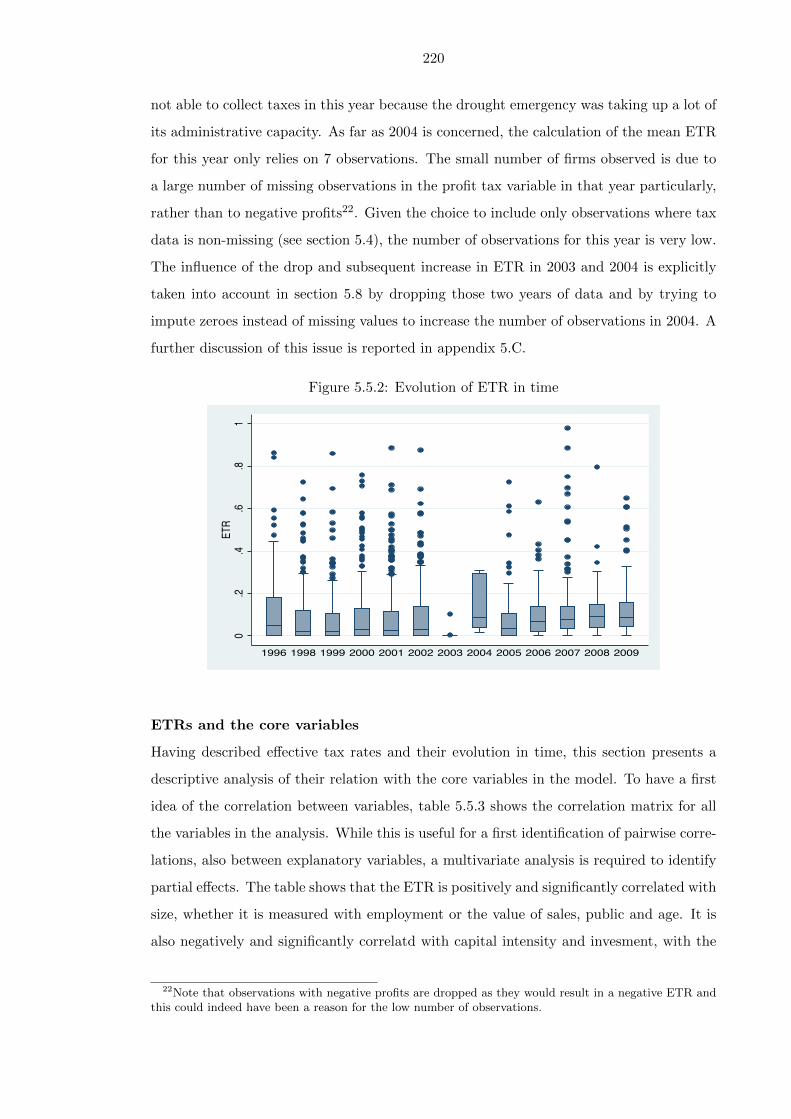
220
not able to collect taxes in this year because the drought emergency was taking up a lot of
its administrative capacity. As far as 2004 is concerned, the calculation of the mean ETR
for this year only relies on 7 observations. The small number of firms observed is due to
a large number of missing observations in the profit tax variable in that year particularly,
rather than to negative profits22. Given the choice to include only observations where tax
data is non-missing (see section 5.4), the number of observations for this year is very low.
The influence of the drop and subsequent increase in ETR in 2003 and 2004 is explicitly
taken into account in section 5.8 by dropping those two years of data and by trying to
impute zeroes instead of missing values to increase the number of observations in 2004. A
further discussion of this issue is reported in appendix 5.C.
Figure 5.5.2: Evolution of ETR in time
0.2
.4.6
.81
ETR
1996 1998 1999 2000 2001 2002 2003 2004 2005 2006 2007 2008 2009
ETRs and the core variables
Having described effective tax rates and their evolution in time, this section presents a
descriptive analysis of their relation with the core variables in the model. To have a first
idea of the correlation between variables, table 5.5.3 shows the correlation matrix for all
the variables in the analysis. While this is useful for a first identification of pairwise corre-
lations, also between explanatory variables, a multivariate analysis is required to identify
partial effects. The table shows that the ETR is positively and significantly correlated with
size, whether it is measured with employment or the value of sales, public and age. It is
also negatively and significantly correlatd with capital intensity and invesment, with the
22Note that observations with negative profits are dropped as they would result in a negative ETR andthis could indeed have been a reason for the low number of observations.

221
latter relation being largely expected. As far as the explanatory variables are concerned,
the correlation matrix suggest that public firms are significantly bigger than private ones
and generally older.
Table 5.5.3: Correlation matrix: ETR and core variables
ETR empl sales cap. int. invest public age
ETR 1size (empl) 0.13 1size (sales) 0.09 0.86 1cap. int. -0.11 0.04 0.25 1invest -0.06 0.03 0.04 0.05 1public 0.18 0.59 0.50 -0.04 0.01 1age 0.17 0.47 0.36 -0.14 0.05 0.45 1
Taking a closer look on size, table 5.5.4 shows the ETR by quintiles calculated both
using employment and deflated sales value. The quintiles are calculated on the pooled
sample (upper panel of table 5.5.4) and on the last two years of data only (lower panel)
to avoid picking up time effects23. The table confirms a linear positive relation between
size and the ETR, with the latter increasing rather consistently across quintiles. It also
shows that ETRs are higher in the last two years of data with respect to the pooled
sample, pointing to an increased capacity of the state of extracting revenues from the
manufacturing sector and/or to increased profitability of firms. In addition the graphs in
appendix 5.D report the distribution of ETR by firm size over time.
Table 5.5.4: ETR by size quintiles
Size 1 2 3 4 5 tot
Pooled sample
Employment 6.8 7.3 7.2 9.9 10.5 8.3Sales 7.1 7.0 7.6 8.6 10.3 8.2
2008 - 2009
Employment 8.5 10.4 11.3 11.8 13.3 11.1Sales 8.7 10.8 9.5 12.5 13.9 11.1
Exploiting the time series properties of the dataset, it is possible to explore the mo-
bility of firms across values of selected variables24. In particular tables 5.5.5 and 5.5.6
23It may be that firms are getting bigger in time on average and taking quintiles in the pooled samplemay just capture observations for older years in the lower quintiles and for most recent ones in the higherquintiles.
24Transition matrices show the transition probabilities, i.e. the change in one categorical variable over

222
look respectively at the probability of transitioning between quintiles of size and between
private/public ownership in any two consecutive years. Table 5.5.5 shows that firms do
not move much across quintiles of size25, with the majority of observations in the table
lying in the diagonal, therefore indicating no change in size qiuntile. When firms do move
they are most likely to do so in the next nearest quintile. Note that size can also vary
within a quintile and this mobility is not captured in table 5.5.5. Mobility between pri-
vate and public ownership is also limited, with only 2% of firms that are initially private
switching to public and 12% switching in the opposite direction (see transition matrix in
table 5.5.6).
Table 5.5.5: Transition matrix: 5 size quantiles
1 2 3 4 5 Total
1 72.81 22.48 4.07 0.43 0.21 1002 18.69 61.23 17.69 2.39 0.00 1003 1.26 13.00 69.60 15.09 1.05 1004 0.19 1.30 10.22 79.00 9.29 1005 0.00 0.18 0.73 5.14 93.94 100
Total 29.84 7.63 20.63 21.9 20 100
Table 5.5.6: Transition matrix for public ownership
Private Public Total
Private 1,775 35 1,810(98.07) (1.93) (100)
Public 87 633 720(12.08) (87.92) (100)
Total 1,862 668 2,530(73.60) (26.40) (100)
Finally it is worth noting that the average ETR in the years after the reform was 9.9%,
higher than the pre-reform average of 7.7%. The dispersion of ETR however was relatively
stable before and after the reform, in terms of standard deviation.
A descriptive analysis of negative profits
As noted in section 5.4.1, observations with negative profits are excluded from the sample
as they would pose interpretation probelms in the econometric analysis. It is however
useful to explore these observations in a descriptive manner to identify possible patterns
time.25However, note that firm size may not change but quintile boundaries may be moved in differnt years.

223
that may determine selection problems (see section 5.8). Of all the firm-year observations
for which there is enough information to calculate profits, 23% report a value equal or
smaller than zero. This corresponds to 116 establishments and 19% of all firms observed.
These are largely concentrated in Addis Ababa that is in fact over represented in this
sub-sample of firms with zero or negative profits, with 60% of these firms based in the
capital as opposed to 53% of all observations on profits. The positive relation between
size and profits suggests that smaller firms are more likely to incur in losses and that
therefore in the sample relatively larger firms are over-represented with respect to the
whole population.
Perhaps not surprisingly, firms with negative or zero profit pay on average 16 times less
taxes (in absolute value) than firms with positive income. While it is not straightforward
why these firms still pay tax, this may be due to arrears in tax payments, delays in tax
collection or adjustments in tax calculations.
Going back to the main sample, it is useful to identify the determinants of profits, as
these relations would indirectly influence the ETR through its denominator. To this aim,
appendix 5.E reports the results of auxiliary regressions of profits on the other explanatory
variables. However the results from these regressions are to be interpreted only on a
descriptive level as simple associations. The results show a positive relation of profits with
all explanatory variables, although not so clearly for age.
5.6 Empirical framework
Panel data is characterized by the co-existence of a cross-sectional dimension, namely N
units i, in this case firms, and a time series dimension, namely T time periods t. Its
main advantage is that by observing units over time, it allows taking into account firm
specific unobservable effects that may otherwise result in biased estimates. There are in
particular three types of unobservables: individual varying but time invariant variables,
such as managerial ability and corporate culture; time varying but individual invariant
variables, such as particular events in the regulatory or institutional environment faced by
firms; and both individual varying and time varying variables. The first two can be taken
into account with panel data analysis, and namely with a fixed effects model (FEM) or a
random effects model (REM).
Generally, a panel data model with fixed effects can be summarized as follows26, where
26The discussion on available models for panel data draws largely on Baltagi (2005) and Wooldridge

224
i = 1, . . . , N denotes the cross sectional units and t = 1, . . . , T denotes the time dimension
and β and xit are vectors of respectively coefficients and variables.
yit = α+ βxit + uit (5.4)
where
uit = µi + νit (5.5)
In equation 5.4, the unobservable firm specific µi is captured in the error term along with
the true error νit. This would result in biased and inconsistent OLS estimates of β if µi
is also related to the explanatory variables (i.e. if Corr(xit, µi) 6= 0). Instead panel data
models, by taking into account the heterogeneity between units, allow the identification
of the effects of the observable variables, given the unit-specific unobservables.
In a FEM context, the firm specific effects can be eliminated by de-meaning27. Esti-
mates thus obtained are called within estimates (βwithin) as they exploit variations within
the unit, over time. Note that this procedure eliminates all time invariant effects, both
observed and unobserved. Therefore if the x vector contains a variable such as location
or sector, that are not expected to vary in time, they would be cancelled along with the
unobservables.
The model described so far is also called the ‘one way error component model’ and it
takes into account only unobservables that are unit specific. The ‘two way error component
model’28 takes into account also unobservables that are time specific but do not vary across
firms (Baltagi, 2005). These may be for example effects related to the environment where
individuals or firms operate, that are indeed potentially relevant. These time specific
effects can be captured by time dummies.
In addition to the within variation, panel data also allows the estimation of a between
estimator (βbetween) that exploits only the variation between groups. This is implemented
essentially by taking averages for each unit over time. While the between estimator looks
at differences between firms, the within estimator explores variations within a firm over
time. Since both variations are potentially intersting, both estimators are implemented in
this exercise.
When all unobserved variables can be considered collectively as a significant random
(2009).27This is what is done here. Two other approaches yield largely equivalent results: including N − 1
dummies for each firm (i.e. LSDV) or first differencing.28In this case the error term would look as follows, where λt is the time specific effect: uit = µi +λt +νit.

225
variable, a random effects model (REM) can be used. One of the main differeces between
FEM and REM is that the latter requires all unobservables to be uncorrelated with the
included explanatory variables in all time periods. This is a strong assumption and it
should be evaluated carefully when choosing between the two models. The choice between
FEM and REM should be based on the research question, on the characteristics of the
data and on the plausibility of the assumption of independence of the unobservables from
x.
In this case a FEM approach seems to be more appropriate for at least two related
reasons. Firstly the expected unobservables are related to managerial ability and the firm’s
culture and reputation. While these variables can change in time, they can be expected
to be largely time-invariant in a relatively short period like the one considered here. Note
that while the panel spans over 14 years, the average number of years over which firms
are observed in the sample is 4.4 (see section 5.4.1). Secondly, these unobservables are
expected to be related to the x thus breaking the REM assumption. For example, it is
reasonable to expect managerial ability to be positively related with size.
Notwithstanding the a priori preference for FEM, both models are estimated and the
Hausman test is used to identify the most appropriate one. Essentially the test compares
the estimates derived under REM and FEM, exploiting the fact that if the unobserved
effects are related to the x then βGLS is biased and inconsistent. The null is that the
difference in coefficients is not systematic. Therefore the test can be interpreted in a
simplistic manner as supporting adoption of the FEM if H0 is rejected or of the REM if it
cannot be rejected. It is important to note that the rejection of the null only implies that
the REM is not consistent but not that the FEM is necessarily the correct model to use.
A final note is due on endogeneity. It is argued in section 5.3 that the theoretical
relation between the explanatory variables and the ETR goes from the former to the
latter. The identification of this causal relation lies in the difference between the tax
system and the effective tax rate. While the former may have an effect on how firms
behave, the latter is determined by the extent to which firms can and do exploit the tax
preferences and legal loopholes set out in the tax system. While the tax system is the
same for all firms, the ETR is firm-specific and it may also change in time for the same
firm. However despite the theoretical framework, endogeneity may still be an issue29. The
use of instrumental variables is limited by data availability. Moreover GMM methods are
29Some papers in the literature have looked at the effect of ETRs on size, recognising however thepossibilty of reverse causality (Da Rin et al., 2010).

226
not particularly suitable due to the unbalanced nature of the panel data and the costliness
of such methods in terms of observations, particularly when T is small.
5.7 Results
This section starts by considering a few models that only include the core variables and
namely: size30, capital intensity, investment, public ownership, reform, age (see section
5.3). This is the core model shown in equation 5.6, that is reported here again for conve-
nience.
ETR = α+ β1SIZE + β2CAPINT + β3INV EST + β4PUBLIC+
+ β5AGE + β6REFORM + ε (5.6)
The dependent variable is always the effective tax rate, calculated as discussed in section
5.3 and 5.4. The four econometric models outlined in section 5.6 and namely OLS, FEM,
REM and BE, are estimated and the results are reported in table 5.7.1. Note that in the
BE regression reform is excluded since this variable displays only variation in time and
not across firms.
As far as size is concerned, the significant result using FEM suggests a positive, though
small, effect of size. The variable is transformed in logs and the interpretation of its
coefficient, taking the FEM as an example, would suggest a 0.009 percentage point increase
in the ETR when size increases by 1%. The coefficient on capital intensity is always
negative and mostly significant. An increase of 1 point in capital intensity (measured as
fixed assets in millions per employee) is associated with a 3.5 percentage point decrease in
the ETR in specification (2). Investment has the expected negative and significant sign,
with 1 percentage point more investment (as a share of total assets) decreasing the ETR
by 1.4 percentage points. This effect is in line with the commonly adopted policy objective
of promoting investment through fiscal incentives. The public ownership dummy always
displays a positive coefficient that is always significant except in the FEM specification.
The lack of significance in the FEM may be due to the small degree of variation that public
displays over time (see table 5.5.6 in section 5.5). The tax reform of 2002 seems to have had
a positive and significant effect, increasing the effective tax rate by 2.1 to 3.7 percentage
30Note that throughout this section only the number of employees is used as a measure of size. Howeverrobustenss to this choice is checked by using the value of sales in section 5.8.
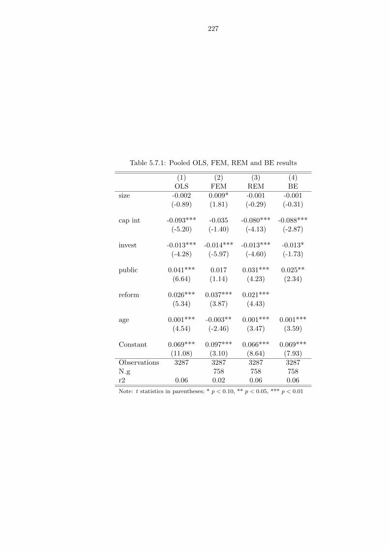
227
Table 5.7.1: Pooled OLS, FEM, REM and BE results
(1) (2) (3) (4)OLS FEM REM BE
size -0.002 0.009* -0.001 -0.001(-0.89) (1.81) (-0.29) (-0.31)
cap int -0.093*** -0.035 -0.080*** -0.088***(-5.20) (-1.40) (-4.13) (-2.87)
invest -0.013*** -0.014*** -0.013*** -0.013*(-4.28) (-5.97) (-4.60) (-1.73)
public 0.041*** 0.017 0.031*** 0.025**(6.64) (1.14) (4.23) (2.34)
reform 0.026*** 0.037*** 0.021***(5.34) (3.87) (4.43)
age 0.001*** -0.003** 0.001*** 0.001***(4.54) (-2.46) (3.47) (3.59)
Constant 0.069*** 0.097*** 0.066*** 0.069***(11.08) (3.10) (8.64) (7.93)
Observations 3287 3287 3287 3287N g 758 758 758r2 0.06 0.02 0.06 0.06
Note: t statistics in parentheses; * p < 0.10, ** p < 0.05, *** p < 0.01

228
points, according to the different estimates. Remember that the reform decreased the
statutory tax rate from 35% to 30% and it paved the way for increased efforts in tax
enforcement. The positive coefficient may therefore suggest a behavior consistent with
the Laffer curve or merely the increased effort in enforcement entailed in the reform, or a
combination of both. The coefficient on age is significant in all specifications and mostly
positive, with the exception of the FEM that estimates a negative effect. However note
that in the FEM model, looking at within variations for a firm in time, the age variable
is essentially a trend variable.
Two tests are available to identify the correct model, the results of which are reported
in table 5.7.2. First, the F-test for the joint significance of the fixed effects compares the
pooled OLS model with the LSDV model with firm dummies. This test rejects the null
and therefore supports the significance of fixed effects. Second, the Hausman test supports
the superiority of FEM to REM as the latter yields incosistent estimates.
Furthermore, table 5.7.2 reports the results of the autocorrelation and heteroskedas-
ticity tests for the preferred FE model. The Wooldridge test for autocorrelation in panel
data suggests that no autocorrelation is present in the data. The modified Wald statistic
for groupwise heteroskedasticity (Greene, 2008) considers firms as groups and strongly
rejects the null of homoskedasticity. Therefore clustered standard errors are reported in
the result tables.
Table 5.7.2: Post-estimation tests
Test H0 Test statistic P value
F test H0: all fixed effectsare equal to zero
F(6,757) = 12.26 0.000
Hausman test H0: difference be-tween FEM andREM is not system-atic
chi2(6) = 20.09 0.003
Wooldridge test H0: no first-orderautocorrelation
F(1, 326) = 0.103 0.748
Wald test H0: homoskedastic-ity
chi2 (758) = 8.8e+36 0.000
Note: Wooldridge and Wald test are performed on the FE model.
In conclusion, the model of choice is the fixed effect model. This choice is not only
supported by the test statistics described above but also by the possibility of taking into
account firm-specific effects that are unobserved but that are likely to affect the effective

229
tax rate. These may for example be the firm’s culture and the quality of management,
besides the factors explored in section 5.7.3 such as location and sector. The following
discussion will therefore focus on the FEM and BE. In particular the latter allows taking
into account the time invariant but observable variables, such as location and sector, that
are necessarily excluded from the FEM.
5.7.1 FEM
Table 5.7.3 reports the results from the FEM, including the baseline specification already
shown in table 5.7.1 and other estimated equations augmented with control variables and
year dummies. The table also includes, at the bottom, a few statistics that are useful
when commenting the results. In particular, both the number of firm-year observations
and the number of firms (N g) included in each regression are reported. Furthermore the
table includes the three R-squared of the FEM model: within (r2), between (r2 b) and
overall (r2 o). Finally the table reports the value of rho, which is the fraction of variance
in the error term due to the fixed effects, and the F-statistic for the joint significance of
the fixed effects. These statistics are explained and discussed in detail in section 5.7.2.
The first specification in table 5.7.3 reports the baseline equation estimated with a
FEM, the results of which were already discussed previously. Specification (2) adds an
interaction term between reform and size, which aims at capturing the extent to which
tax reform tackles the possible inequalities emerging from the effect of size on ETR. The
coefficient obtained is not significant, although it is jointly significant with size (F( 2,
757) = 7.50, p-value = 0.0006). This suggests that reform may have had an effect on the
relation between size and ETR, particularly further increasing the positive effect already
observed on size. In other words, the positive coefficient on the interaction term suggests
that after the reform the (positive) effect related to the politcal cost hypothesis is even
stronger than the (negative) one implied in the political power hypothesis. According to
this interpretation, the 2002 reform would have made it even harder for large firms to
obtain fiscal benefits or to escape the tax net through evasion. However the very low
t-statistic of the interaction term imposes caution in interpreting this result.
The next specification (3) adds year dummies to the baseline equation, that may be
useful to capture special conditions in the environment faced by firms. The inclusion of
year dummies however results in dropping the reform variable, as it essentially captures
the same variation. The table does not report all coefficients for year dummies for the sake
of simplicity and readability. However two of them are significant in all specifications and
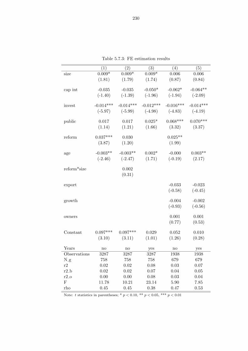
230
Table 5.7.3: FE estimation results
(1) (2) (3) (4) (5)
size 0.009* 0.009* 0.009* 0.006 0.006(1.81) (1.79) (1.74) (0.87) (0.84)
cap int -0.035 -0.035 -0.050* -0.062* -0.064**(-1.40) (-1.39) (-1.96) (-1.94) (-2.09)
invest -0.014*** -0.014*** -0.012*** -0.016*** -0.014***(-5.97) (-5.99) (-4.98) (-4.83) (-4.19)
public 0.017 0.017 0.025* 0.068*** 0.070***(1.14) (1.21) (1.66) (3.32) (3.37)
reform 0.037*** 0.030 0.025**(3.87) (1.20) (1.99)
age -0.003** -0.003** 0.002* -0.000 0.003**(-2.46) (-2.47) (1.71) (-0.19) (2.17)
reform*size 0.002(0.31)
export -0.033 -0.023(-0.58) (-0.45)
growth -0.004 -0.002(-0.93) (-0.56)
owners 0.001 0.001(0.77) (0.53)
Constant 0.097*** 0.097*** 0.029 0.052 0.010(3.10) (3.11) (1.01) (1.26) (0.28)
Years no no yes no yes
Observations 3287 3287 3287 1938 1938N g 758 758 758 679 679r2 0.02 0.02 0.08 0.03 0.07r2 b 0.02 0.02 0.07 0.04 0.05r2 o 0.00 0.00 0.08 0.03 0.04F 11.78 10.21 23.14 5.90 7.85rho 0.45 0.45 0.38 0.47 0.53
Note: t statistics in parentheses; * p < 0.10, ** p < 0.05, *** p < 0.01

231
in particular 2003 and 2005. The negative and significant coefficient on the former should
not come as a surprise, as revenues dropped sharply in that year probably as a result of
the famine emergency (see section 5.5). The negative coefficient on 2005 on the other
hand may be explained by the elections that took place in that year, as the government
may have decreased temporarily the fiscal burden in the pre-election period.
The results including the year dummies are largely in line with the previous two speci-
fications (1 and 2). However the model now provides a better fit, with a within R-squared
of 8%. While this value is still low, it indicates that the inclusion of time dummies in-
creases considerably the explanatory power in these regressions. Moreover both capital
intensity and public ownership are now significant, although at the 10% level, with the
expected negative and positive signs respectively. The most remarkable change however is
in the coefficient on age that now turns to positive and still significant. This change may
be due to the fact that age in a FEM context essentially captures a trend rather than only
age itself. When time dummies are included, and they have mostly negative signs, the
coefficient on age turns to positive. It indicates that one more year in the age of a firm
is associated with an ETR 0.2 percentage points higher. This positive result is consistent
with the one on size, as the rationale for older and larger firms to face higher ETRs is based
on visibility in both cases. Note that age and size are strongly and positively correlated
in the sample, as shown in table 5.5.3.
Specifications (4) and (5), add three control variables that may influence the ETR
respectively without and with time dummies. None of these controls is significant and
their inclusion also results in a sharp drop in the number of available observations, as
many firms do not report the necessary information. However their inclusion, and the
resulting smaller sample, do not change the main findings on the core variables either
in terms of sign or of magnitude. The negative sign on growth may be interpreted as a
fiscal advantage that firms have when they grow more, perhaps because they have more
bargaining power as national ‘champions’. The share of export in total sales is also negative
although not significant, indicating a fiscal advantage of exporters.
As far as the core variables are concerned, size is significant at the 10% level only
when controls are not included. However the coefficient remains positive and of compara-
ble magnitude in all specifications. This lack of strong significance of size may be due to
its limited variability in time (see table 5.5.5), that therefore implies that its effect may
partly be picked up as a fixed effect in a FEM context. It may also be the result of the co-
existing counteracting effects of the political power hypothesis (negative) and the political
232
cost hypothesis (positive). The effect of capital intensity remains negative across speci-
fications, although not always significant, with the coefficient being larger in magnitude
when controls are added. The estimates of the effect of investment are largely consistent,
being always negative, significant at the 1% level and of virtually the same magnitude in
all specifications. Public is the dummy for public ownership that is also meant to capture
political connections. This variable is significant only when year dummies and/or controls
are added to the equation. The coefficient is consistent across specifications in that it is
always positive, although both significance and magnitude vary. It indicates that publicly
owned firms, far from having a fiscal advantage, face higher ETRs than privately owned
ones. As noted previously (see table 5.5.6), the variable only varies little over time thus
partly explaining its lack of significance in some FEM specifications31.
Finally, the reform dummy is always significant and positive, except when the inter-
action term with size is included. However an F-test of joint significance of reform and
its interaction with size shows that the two variables are significantly different from zero
when considered jointly. These results suggests that reform succedded in increasing ETRs
despite providing for a decrease in the statutory tax rate.
5.7.2 Goodness of fit and fixed effects
This section focuses on some of the statistics reported at the bottom of the results table
5.7.3, starting from the three R-squared. In a FEM context, these are calculated on the
basis of the empirical model discussed in section 5.6.
In particular the R-squared measures the (squared) correlation between the predicted
values from the model and the actual values of the dependent variable. It therefore rep-
resents the fraction of the variation in the dependent variable that is explained by the
equation. Since the fixed effects (FE) are included in the error term, their explanatory
power is not taken into account in the calculation of the R-squared. The R-squared within
is therefore the portion of the variation of y that is explained by the model, excluding
the fixed effects. The exclusion of fixed effects from the computation of the R-squared is
one reason why the R-squared can be low in FE models. The R-squared between would
thus be interpreted as the fraction of the variation between units that is explained by the
variables in the model, excluding fixed effects. Therefore if FE have a high explanatory
31As public is correlated with age and size, with older and bigger firms more likely to be in publicownership, a further check can be done by dropping these variables to check whether it becomes thensignificant. This is not the case, through the coefficient remains positive. For the sake of simplicity, theseresults are not reported as they would add very little information to the table.
233
power for the variation across units, the R-squared between will be very low.
In this case, the within R-squared ranges from about 2% to 8%. The explanation relies
partly in the exclusion of the fixed effects. This is clear when comparing these figures with
the R-squared obtained when estimating the core model with LSDV, which is 40%. LSDV
estimation of the core model is equivalent to specification 1 in table 5.7.3 but its R-squared
takes into account the explanatory power of the fixed effects32.
Furthermore, rho measures the fraction of the variance of the whole error term (µi +
νit) that is explained by the fixed effects components (µi). It therefore gives an indication
of the explanatory power of the fixed effects. The value of rho indicates that the fixed
effects explain about half of the variance of the whole error in the FEM, thus confirming
once again their importance in the equation.
Since the F statistic and the rho confirm the importance of the fixed effects, it is useful
to explore them further. A first indication can be obtained by plotting them as in the figure
reported in appeddix 5.F that also includes a normal distribution for reference. Moreover it
is possible to bring them on the LHS and regress them on the other explanatory variables.
Their predicted values are obtained from the FEM core model with year dummies. As
they do not vary in time but only across firms, the between estimator is used. The results
are reported in appendix 5.F. The fixed effects appear to be consistently related negatively
with size and age while other variables do not display significant coefficients, except for
public (positive) but only when region dummies are included.
5.7.3 Between estimator
The analysis based on FEM does not include variables such as foreign initial capital,
location and sector dummies because they are fixed in time and they would therefore be
dropped in the FE model. They can however be included when using a between estimator,
that exploits the variation between cross-sectional units rather than within them. One
of the advantages of BE models is that, by taking average values for each firm, they
smooth out spikes in the data and they also reduce the effect of the possible lags discussed
in appendix 5.C. Since the sample does not provide enough subsequent observations to
sensibly use period averages, as could be done with longer time series, only time averages
for the whole period are considered in the BE model.
Tables 5.7.4 and 5.7.5 report respectively the results of the baseline model augmented
32In the LSDV model the fixed effects are included as a set of dummies amongst the regressors, ratheras part of the error term as in the standard FEM procedure performed by STATA.

234
with, alternatively, region and sector dummies33. The dummies are included alternatively
to avoid the overspecification of the model. In addition the same control variables discussed
in section 5.7.1 are also included here.
Table 5.7.4: BE results with regions
(1) (2) (3) (4)
size -0.001 -0.012*** -0.004 -0.005**(-0.31) (-2.77) (-1.51) (-2.03)
cap int -0.088*** -0.149*** -0.057** -0.082***(-2.87) (-2.97) (-2.32) (-2.76)
invest -0.013* -0.005 -0.012* -0.017**(-1.73) (-0.72) (-1.72) (-2.36)
public 0.025** 0.108*** 0.038*** 0.041***(2.34) (6.00) (3.23) (3.90)
age 0.001*** 0.000 0.001** 0.001***(3.59) (0.06) (2.19) (3.10)
foreign capital 0.016(0.82)
export 0.009 -0.039(0.21) (-1.40)
growth -0.003 0.002(-0.63) (0.39)
owners -0.002(-0.95)
Constant 0.069*** 0.119*** 0.094*** 0.098***(7.93) (7.03) (8.80) (10.18)
Regions no yes yes yes
Observations 3287 655 2625 3287N g 758 420 733 758r2 0.06 0.18 0.10 0.13
Note: t statistics in parentheses; * p < 0.10, ** p < 0.05, *** p < 0.01
33The tables including the coefficients for region and sector dummies are reported in appendix 5.G.

235
Table 5.7.5: BE results with sector dummies
(1) (2) (3) (4)
size -0.001 -0.007 0.000 -0.002(-0.31) (-1.60) (0.09) (-0.58)
cap int -0.088*** -0.152*** -0.053** -0.071**(-2.87) (-2.88) (-2.03) (-2.23)
invest -0.013* -0.004 -0.008 -0.012*(-1.73) (-0.51) (-1.12) (-1.66)
public 0.025** 0.095*** 0.026** 0.031***(2.34) (5.29) (2.22) (2.94)
age 0.001*** 0.000 0.001** 0.001***(3.59) (0.16) (2.47) (3.52)
foreign capital 0.018(0.90)
export 0.003 -0.037(0.06) (-1.31)
growth -0.005 0.000(-0.98) (0.09)
owners -0.002(-0.98)
Constant 0.069*** 0.087*** 0.059*** 0.065***(7.93) (4.58) (5.01) (6.08)
Sectors no yes yes yes
Observations 3287 655 2625 3287N g 758 420 733 758r2 0.06 0.15 0.06 0.11
Note: t statistics in parentheses; * p < 0.10, ** p < 0.05, *** p < 0.01

236
Starting from size, it is useful to consider how the coefficient behaves once the dum-
mies are included, both in table 5.7.4 and 5.7.5. This variable has a small and negative
coefficient, mostly not significant. The lack of significance indicates that the effect of size
may occur mostly within firms (as in the FEM model) rather than between firms. The
negative coefficient is only significant when region dummies are included, although not
in all specifications. While the result needs to be taken with caution due to the lack of
significance in most specifications, it is not necessarily at odds with the FEM result. It
indicates that generally larger firms can obtain lower ETR (though this negative effect is
largely non-significant). However within the life of a firm, and in the small variability in
terms of size, as firms grow bigger they are more visible and therefore face a higher ETR.
Since the variability in size is not very high, it is likely that over the sample relatively
big firms remain bigger and smaller firms remain smaller as they mostly move to adjacent
quintiles (see table 5.5.5).
Capital intensity and investment retain their negative and significant coefficients, par-
ticularly in specification (4) of both tables where the maximum number of observations
is used. Public is now always significant and the positive sign found in table 5.7.3 is con-
firmed. The magnitude of the coefficient is also similar to the one obtained with the FEM,
suggesting that public ownership is associated with a 3.1 to 4.1 percentage points higher
ETR (in specification 4 of tables 5.7.4 and 5.7.5). The coefficient on age is positive and
mostly significant, consistently with the FEM results with year dummies. This confirms
the fact that age in a FEM context may essentially capture a trend rather than age in itself,
if time is not controlled for with year dummies. However the coefficient remains small,
with an additional year in the firm’s age corresponding to a 0.1 percentage point increase
in the ETR. This positive coefficient fails to support the idea that older and more estab-
lished firms are more able to lobby the government and therefore to obtain lower ETR.
On the contrary older firms experience higher ETR, perhaps because of higher visbility.
Specification (2) in both table 5.7.4 and 5.7.5 includes all the additional control vari-
ables also discussed in section 5.7.1 as well as initial foreign capital. The results show that
all these controls are not significant. Moreover the sample size decreases dramatically by
including them, and this is particularly due to owners and foreign capital. These two
variables are therefore dropped in (3), thus increasing the sample size but still not finding
significance for either growth or export in either of the two tables. Remember that controls
are not found to be significant in the FE model either. Finally, specification (4) includes
only the core variables and the region dummies in table 5.7.4 or the sector dummies in

237
table 5.7.5.
As far as regions are concerned, the dummy for Addis Ababa is excluded and therefore
all the results are to be interpreted as deviations from this benchmark34. Regional dum-
mies mostly have negative coefficients (results reported in appendix 5.G), suggesting that
Addis Ababa faces a higher ETR than other more remote regions. This is probably due
ot the higher visibility and accessibility of firms in the capital, as discussed also in section
5.5.2. Afar and Tigray are exceptions in that firms there face a higher ETR, respectively
by 5 and 2.4 percentage points (results reported in appendix 5.G). However these two
positive coefficients are not significant. It is important to note that firms are mostly con-
centrated in Addis Ababa and Oromia (see section 5.5) and thus other regions may only
have a few observations. This is the case for Gambela, that has a large negative coefficient
which however is driven by only 6 observations in the sample. The negative effect is not
surprising however, given that firms operating in remote regions, such as Gambela, can
benefit from fiscal incentives.
As far as sectors are concerned, the dummies included refer to the top manufacturing
sectors in Ethiopia, that together account for over 50% of the sample (also see section
5.5)35. This implies that smaller sectors are omitted and thus the coefficients can be
interpreted against this group of minor sectors. Significant coefficients can be found only
for bakery and media, with firms in these two sectors facing higher ETRs by respectively
4.3. and 3.4 percentage points (results reported in appendix 5.G). Note that the sectors
considered here are based on the 4-digit level of the ISIC code and that only manufacturing
firms are considered, while other studies in the literature include the industrial sector as
a whole where manufacturing altogether is one of the sub-sectors (Derashid and Zhang,
2003).
5.7.4 Results on tax payments
This section turns the focus from the ETR to tax payments, therefore only considering
the numerator of the ETR. These are essentially the amount of tax that firms pay and
they represent, when aggregated, the tax take. The exercise on tax payments follows
directly from the previous sections and it is based on a log transformation of the depen-
34Note that Beneshangul is also omitted because there are no observations from this region. This shouldbe no surprise as the region is remote, not easily accessible and mostly focussed on agriculture.
35The sectors included in the BE regression represent 53,83% of observations in the pooled sample andthey are: plastic, furniture, print, footwear, flour, bakery, cement.

238
dent variable36. This allows bringing profits to the RHS of the equation with the other
explanatory variables and to assess its impact on tax payments. Note that profits could
not be included in the core model because of its arithmetic negative correlation with the
dependent variable.
Table 5.7.6 reports the results for all different models using the log transformation.
The dependent variable is always the log of business profit tax payment and profits in
the RHS is transformed in logs. Model specification is checked, as before, using the
F test that confirms joint significance of the fixed effects and the Hausman test that
confirms the superiority of FEM with respect to REM (see rows 1 and 2 in table 5.7.7).
Heteroskedasticity and autocorrelation are checked for the preferred FEM model, and the
results are reported in table 5.7.7. The first test (row 3 in table 5.7.7) confirms the presence
of cluster-level heteroskedasticity in the FEM model and therefore clustered errors are used
in column (2). The Wooldridge test can only reject the null at the 10% level but not at the
5% level. Therefore specification (3) reports a FE model where first order autoregression
is allowed for. Column (5) reports results obtained using the between estimator.
Using the FEM and BE specification, table 5.7.8 explores in more detail the effect of
profit by including its squared value and its lag. Specification (1) shows that the lag is
positive and significant. The surprising result in column (1) is the negative and significant
coefficient on reform, which so far was always found to have a positive and significant
effect. Specification (2) checks whether reform picks up an income effect by including
an interaction term between the two variables. Indeed the interaction is negative and
significant while reform now turns positive although not significant. The two variables
however are jointly significant with and F-test statistic F (2, 521) = 6.96 and a p-value of
0.001. This may suggest that the negative effect of reform in column 1 is probably due
to an income effect after 2002. In particular, the interaction term indicates that after the
reform, the effect of an increase profit is still to increase tax expenditure but not by as
much as it did before the reform. Reform in itself instead now seems to have a positive
effect on tax payments.
Furthermore specification (3) checks for non-linearities in the effect of profit by includ-
ing its squared value. Its coefficient is indeed significant and positive in all subsequent
specifications. It is noteworthy that in the FEM specification in column (3) its inclusion
makes the sign on profit become negative though non-significant, although it is still jointly
36The ETR is transformed in logs as follows, where tax is short for tax payment: log(ETR) =log( tax
income) = ln(tax) − ln(income)

239
Table 5.7.6: Tax payments: OLS, FEM, REM and BE results
(1) (2) (3) (4) (5)OLS FEM FEM-AR REM BE
profit 0.798*** 0.604*** 0.619*** 0.699*** 0.759***(38.06) (13.54) (21.12) (31.32) (21.74)
size 0.289*** 0.329*** 0.200** 0.388*** 0.299***(8.14) (4.38) (2.45) (9.81) (4.91)
cap int -0.385 -0.329 0.233 0.149 0.741(-1.24) (-0.88) (0.45) (0.46) (1.28)
invest -0.248*** -0.160*** -0.132*** -0.206*** -0.244**(-6.21) (-4.11) (-3.21) (-5.67) (-2.55)
public 0.749*** 0.535*** 0.393*** 0.612*** 0.651***(9.23) (3.64) (3.15) (6.53) (4.19)
reform 0.152** -0.159 0.140 0.135**(2.53) (-1.24) (1.02) (2.33)
age 0.005*** 0.054*** 0.039*** 0.009*** 0.010***(2.84) (3.68) (3.27) (3.58) (3.25)
Constant -1.340*** 0.256 0.966*** -0.561*** -1.046***(-7.22) (0.39) (7.30) (-2.65) (-3.53)
Observations 2228 2228 1563 2228 2228N g 665 524 665 665r2 0.84 0.34 0.79 0.83 0.85
Note: t statistics in parentheses; * p < 0.10, ** p < 0.05, *** p < 0.01
Table 5.7.7: Post-estimation tests
Test H0 Test statistic P value
F test H0: all fixed effectsare equal to zero
F(7,664) = 51.73 0.000
Hausman test H0: difference be-tween FEM andREM is not system-atic
chi2(7) = 40.61 0.000
Wald test H0: homoskedastic-ity
chi2 (665) = 2.1e+34 0.000
Wooldridge test H0: no first-orderautocorrelation
F(1, 200) = 2.793 0.0962
Note: Wooldridge and Wald test are performed on the FE model.
significant when considered with its squared value (F (2, 664) = 102.87, p−value = 0.000).
The combination of a negative coefficient on profit and a positive one on profit squared

240
implies a non-linear relation between profit and tax payments, and particularly a U-shaped
one. In other words, as firms move to higher profit levels, they first face decreasing tax
payments and then increasing ones. Moreover the results suggest that this relationship
exists only within firms and not across firms. Columns 4 to 6 show that in the latter case
instead as profit increases, tax payments increase exponentially.
Note that, considering the flat statutory tax rate which is applied in Ethiopia, a 1%
increase in profit should result in a (1% × 35%) increase in tax payments at all levels of
income. Instead the results suggest the presence of tax preferences at low levels of profit
that fade away at higher levels. Moreover they suggest that generally when firms have
high profits, a further increase makes tax payments increase exponentially.
Finally sector and region dummies are not included in the table for the sake of clar-
ity. As far as the former is concerned, significant and negative coefficients are found for
furniture and concrete. As far as regions are concerned, the coefficients are all negative
and mostly significant, except for Tigray that have a positive but non-significant coeffi-
cient. This confirms that firms in Addis, the excluded category, face generally higher tax
payments.
5.7.5 Exploring the effect of negative profit
Finally this section takes into account the effect of negative profits, that is losses that firms
may suffer in one or more year. Remember from section 5.4.1 that only observations where
profit is positive are included in the sample. However losses may be a determinant of ETRs
and thus they should be included in the equation, as suggested by Wang (1991) and Gupta
and Newberry (1997). The loss dummy described in section 5.4 is therefore included in
a BE model, as it varies across firms but not in time. The dummy should capture the
presence of loss carryforwards, discussed in section 5.4 and 5.5. Appendix 5.H reports
results of different specifications estimated with BE and including loss along with other
control variables and dummies. The introduction of the loss variable does not change
the coefficients of the baseline specification. Moreover the variable has a consistently
negative coefficient, though not significant, indicating that firms that incur losses face
lower ETR. This result is largely expected, also due to the possibility of carrying forward
losses as stated in the Ethiopian tax law (see section 5.5). However the loss variable is
never significant in any of the specifications, thus suggesting that its inclusion may not be
necessary.

241
Table 5.7.8: Tax payments: results including profit squared, lagged and dummies
(1) (2) (3) (4) (5) (6)FEM FEM FEM BE BE BE
profit 0.637*** 0.655*** -0.202 0.334** 0.208 0.277(11.34) (11.54) (-0.95) (1.97) (1.25) (1.59)
profit lag 0.169*** 0.166***(3.80) (3.71)
profit sq. 0.031*** 0.017** 0.022*** 0.019***(3.93) (2.56) (3.44) (2.81)
size 0.125 0.127 0.324*** 0.267*** 0.182*** 0.227***(1.13) (1.15) (4.36) (4.32) (2.94) (3.62)
cap int -1.066 -0.990 -0.545 0.502 0.205 0.470(-1.11) (-1.01) (-1.32) (0.86) (0.36) (0.77)
invest -0.133*** -0.142*** -0.163*** -0.232** -0.194** -0.228**(-3.26) (-3.46) (-4.11) (-2.44) (-2.06) (-2.40)
public 0.484*** 0.448*** 0.558*** 0.618*** 0.799*** 0.667***(2.99) (2.71) (3.88) (3.99) (5.19) (4.26)
reform -0.502*** 0.661 -0.167(-2.72) (1.14) (-1.31)
reform*profit -0.078**(-2.21)
age 0.098*** 0.103*** 0.048*** 0.010*** 0.008*** 0.010***(3.75) (4.01) (3.36) (3.30) (2.68) (3.33)
Constant -2.393** -2.706** 5.448*** 1.665 2.804** 2.213*(-2.24) (-2.54) (3.66) (1.52) (2.58) (1.95)
Regiondummies no no no no yes no
Sectordummies no no no no no yes
Observations 1414 1414 2228 2228 2228 2228N g 522 522 665 665 665 665r2 0.36 0.36 0.35 0.85 0.86 0.85
Note: t statistics in parentheses; * p < 0.10, ** p < 0.05, *** p < 0.01

242
5.8 Robustness
5.8.1 Influence of 2003 and alternative ETR measure
As noted in section 5.5, the ETR in Ethiopia is affected by the famine as it drops dramat-
ically in 2003 to increase sharply the following year. To check whether the main results
are sensitive to these spikes, the two years 2003 and 2004 are dropped and the model
re-estimated. Results from selected FEM and BE specifications are reported in table 5.I.1
of appendix 5.I. All results are essentially confirmed thus suggesting that the spikes corre-
sponding to the famine do not determine them. While the results are generally confirmed
in magnitude, sign and significance, a note may be useful on reform, size and age. Firstly
once the two years of famine are dropped, the reform dummy becomes negative and sig-
nificant at the 10% level in the baseline FEM specification. Therefore this result does
not seem to be robust, indicating that the reform dummy may be picking up the effect of
other events (most notably the famine) occurring in the same years. Second, the positive
and significant result on size is confirmed in the FEM specification, and the coefficient is
slightly larger now. In addition a positive, though largely insignificant, result is also found
in the BE model except in the specification where region dummies are included. This
suggests that the negative effect of size previously found in the BE specifications is not
robust and indeed it was largely non-significant in the main results. Thirdly the results
are indicative as regards the ‘age puzzle’ whereby age changed sign in the FE and BE
results. In particular they show that the negative coefficient found in the previous FEM
results is not robust to dropping the years of famine, as its coefficient is instead confirmed
positive and significant as in other specifications (BE results in tables 5.7.4 and 5.7.5,
results on tax payments in tables 5.7.6 and 5.7.8, and FEM results with year dummies in
table 5.7.3).
Appendix 5.I also includes two additional tables. The first one (table 5.I.5) re-estimates
the equation on a sample where zeroes were imputed for the tax variable when it is missing
but all other variables are non-missing. This increased the sample by 655 observations,
particularly in those years with more missing tax observations. The results are generally
robust and size is positive and significant at the 5% level in all FEM specifications. How-
ever reform again does not appear to be robust. Secondy table 5.I.6 tackles the possible
concern of a lag in the data, discussed in appendix 5.C, by replacing all variables except
tax with their lags. The results are largely non significant, therefore suggesting that no
relation exists between tax and the lagged explanatory variables. This supports the idea
that a lag does not occur in the data, as argued in appendix 5.C.

243
5.8.2 The use of sales as a measure of size
As mentioned in section 5.4, size can be measured either in terms of employment or
sales. While the former measure is adopted throughout the analysis, this section tests for
the robustness of that choice by replicating the results using the values of sales instead of
employment. As noted before, sales may capture the exogenous effect of inflation together
with the actual size. This problem cannot be entirely accounted for, as different sectors
experience different price dynamics and are more or less influenced by the national price
shocks. However it is possible to partly correct for the effect of inflation by deflating
the sales variable using the GDP deflator calculated on the aggregated national data on
the large and medium manufacturing sector. This data is provided by the Ministry of
Finance and Economic Development (MoFED) from 1997, thus excluding the first year of
the Ethiopian dataset. This explains why the sample size is slightly smaller than in the
previous analysis.
The FEM and BE models are re-estimated and the results are reported in appendix 5.I.
The results of the previous analysis are largely confirmed, thus supporting their robustness
to changes in the measure of size. As far as sales are concerned, the variable is mostly
non-significant. The signs and magnitudes previously found for size however are largely
confirmed, particularly a positive coefficient in the FEM and a negative one in the BE. The
only significant result is in the BE model when regional dummies are included, consistently
with the main results. The results on all other variables are esentially confirmed and in
the case of reform, investment, age and all the sets of dummies they are virtually the same.
5.8.3 Selection problems
An analysis of ETRs necessarily includes only firms that do report tax information, par-
ticularly profit tax. First of all, it is useful to note that the firms included in the sample
represent 95% of the total reported profit tax take in the survey and they therefore ac-
count for the bulk of the fiscal contribution of the manufacturing sector37. However there
remains a natural question about the possible selection bias: are firms that omit the tax
information systematically different from those who do report it?
A common way to deal with sample selection is the Heckman procedure. This proce-
dure can be used in cases where the dependent variable is observed only if a criteria defined
in terms of some random variable Z is met. However an instrument is required to identify
37This is true as far as the tax take reported in the survey is concerned.

244
the selection equation, which should both be a good predictor of selection and have no
association with the outcome variable in the unrestricted population, after adjustment for
other predictors of Y. In this case unfortunately such an instrument is not available and
it is therefore not possible to correct for selection using the Heckman procedure.
However a simple and intuitive approach can offer some indications on selection: test-
ing the equality of means in the explanatory variables in the sample and in the whole
population. This can be done by using the explanatory variables that are available for
firms that do not report tax information. Thus, two samples are compared: the one used
in the ETR analysis, that includes the tax variable, and that of firms that report all vari-
ables but profit tax. They are named respectively sample 1, i.e. the sample used in this
work, and 2, i.e. the observations that are excluded from the analysis. A t-test can then
be used to test the null of the difference between the mean of specific variables in samples
1 and 2 to be zero. This test is performed for each of the core variables, except reform.
The tests reveal that for most variables the means are statistically different between
the two samples. In particular, firms included in the ETR analysis are bigger, both in
terms of sales and employment, less capital intensive, more likely to be public and older.
However there seem to be no statistically significant difference in terms of investment
share.
Note that these differences may be due to the fact that observations with negative
profits are excluded, rather than to whether firms report or not tax information. It is
possible to get indications regarding the source of selection by repeating all tests on samples
defined on the basis of the availability of tax information rather than the ETR38. This
may not be directly useful as regards the selection problem in the ETR analysis but it may
give indications as to where selection comes from, namely from the profit or tax variables
that compose the ETR. In this case the difference in means is still statistically significant
for capint, public and age. However in the case of size there seem not to be a significant
difference between the two samples, at least when employment is used as a measure of
size39. This may suggest that the result found before, of firms in the used sample being
bigger, is driven by the fact that observations with negative profit are excluded. Finally,
now also the difference in investment is statistically significant, with firms reporting tax
information investing less than others.
38Note that to obatain the ETR not only tax information needs to be available but also a positive profitvalue.
39Note however that when sales is used as a measure of size, the t-test shows that firms that report taxinformation are smaller than those do not, and this difference is statistically significant.

245
The t-tests therefore show that firms in the sample are generally bigger than those in
the whole population, as well as being older and more likely to be public. In fact the three
variables are related as shown in table 5.5.3. First of all this means that the results may
only be applicable to the upper end of the population of large and medium enterprisees
that are considered. Bigger firms may be selected into the sample simply because they
complete questionnaires more fully. This may be because their larger resources, in terms
of staff, organization and managerial systems, allow them to reply to questionnaires at a
lower cost. Indeed bigger firms are more likely to have information readily available and
dedicated departments for administrative issues that can provide detailed answers to the
enumerators. Moreover, as they are more visible, bigger firms may generally find it harder
to hide tax information to authorities and thus they would benefit less from not releasing
information to enumerators. Remember that the Central Statistical Agency, which collects
this data, is a governmental organization.
Another problem related to selection is attrition, as the panel used here is very un-
balanced. Indeed attrition rates are high in the dataset and they may create a problem if
attrition is non-random, similarly to the discussion above on selection. The LMMIS datase
presents high levels of entry and exit in each year, which are due to actual movements into
and out of business, as well as to possible issues with the quality of data collection. To
address this issue in the calculation of attrition rates, I use 4-years intervals: from 1996 to
2001 (5 years), from 2002 to 2005 (4 years), and from 2006 to 2009 (4 years). I thus define
attrition as the situation where a firm is observed in any year of the first period, but in
none of the second period40. Between the first and the second period attrition occurs in
47% of the sample, while 53% of firms are observed in both periods. Between the second
and the third period, the attrition rates is 26%, with 74% of firms being observed in both
periods. The substantial drop in attrition in the most recent part of the sample may be
due to both better economic conditions in Ethiopia and to improved data quality. As
in the case of selection, attrition is only problematic if it is non-random. Following the
previous discussion on selection, I adopt a simple and intuitive approach to test whether
firms that exit the sample are systematically different from those who stay in the period
before exit, when both groups are observed. Indeed a battery of simple t-tests on the
difference in means between the two groups reveal that firms that exit are smaller, both
in terms of sales and number of employees, and less profitable, than those that survive.
40More specifically, existance is defined as the availability of information (i.e. non-missing) on either thevalue of sales or the number of employees in that year.
246
The tests therefore suggest that attrition may cause bias in favour of larger and more
profitable firms, as in the case of selection discussed before. There are potentially a number
of techniques that can be used for correction for attrition, such as inverse probability
weights. However this technique to correct for attrition requires the identification of
an instrument that determines attrition but not the outcome variable, similarly to the
Heckman procedure. Such variable is not available in this case, therefore making this type
of correction not implementable. Imputation procedures are another option to address the
issue of missing data. However they present several challenges (see, for example, Cameron
and Trivedi (2005)) and they are beyond the scope of this thesis.
5.8.4 Change in ETR threshold
It is sometimes recommended (Omer et al., 1990) to test the robustness of results to
different ETR measures. While this cannot be done with the Ethiopian data, it is however
possible to check for robustness to different ETR thresholds. The choice adopted here, as
explained in section 5.4.1, is to drop all observations in which the ETR is larger than one.
This is standard in the literature and it is also intuitively sensible. However there may be
instances in which the ETR is larger than 1 and indeed Kim and Limpaphayom (1998)
use a threshold of 2 instead. Moreover Derashid and Zhang (2003) explain that in the
process of consolidation between firms, profits and losses of subsidiaries are combined but
a tax liability may still arise on the profits. Zimmerman (1983) explains the possibility of
an ETR larger than one with timing issues, in the instance that an asset sold in one year
at gain is only recognised for tax purposes in the following year thus resulting in a change
in the numerator but not in the denominator. Even considering these cases however an
ETR larger than 2 can reasonably be considered unrealistic and therefore be attributed
to a mistake in the data.
The robustness of the results to changes in the upper ETR threshold is therefore
checked by including in the sample also 26 observations with ETR larger than 1 but
smaller than 2. The results are reported in table 5.I.7 of appendix 5.I. In addition table
5.I.8 (appendix 5.I) implements an alternative option, namely including observations with
ETR larger than one but setting their value to 1. The main results are generally confirmed,
although significance and magnitude do change in some specifications. This robustness
check broadly suggests that the results are robust to changes in the ETR threshold, as all
variables generally retain their sign and a magnitude comparable with previous results.

247
5.9 Summary of results: main findings
This chapter provides evidence on effective tax rates in Ethiopia, a country where tax
preferences are widely used to promote investment and equitable regional development.
In addition to these policy objectives, the chapter aims at identifying the effect of lobbying
and political connections on the ETR. A few exercises are carried out in sections 5.7 and
5.8 which add to the descriptive analysis of section 5.5. It is therefore useful at this stage
to summarize all the findings and to identify the main trends emerging from the analysis.
First of all, it is shown in section 5.5 that ETRs in Ethiopia are indeed very low, with
a substantial proportion of firms paying less than 5% of their profit in tax. This confirms
the idea that in Africa, and specifically in Ethiopia, tax preferences are widely used to
reduce the tax burden on firms well below the statutory tax rate. In terms of tax revenue
mobilisation, this may imply that not all the revenue potential of the manufacturing
sector is tapped. Some of the sources of tax preferences are identified in section 5.7 and
particularly the promotion of investment and regional development. Investment is found
to have a negative and mostly significant coefficient across all specifications. Moreover
firms operating in disadvantaged regions such as Gambela and S.N.N.P.R.41 are able to
obtain lower ETRs and this is indeed enshrined in tax regulations to promote equitable
regional development. In addition a consistently negative and mostly significant result is
found for capital intensity. This may capture the effect of leverage, as discussed in section
5.4, to the extent that more capital intensive firms can access credit more easily thanks
to the availability of a collateral.
While it is possible to identify some sources of tax preferences that are indeed expected
as they are part of the tax code, this exercise aims at exploring also the less official
dynamics that may make some firms pay less thanks to lobbying, corruption or tax evasion.
While these elements are not easily pinned down in a precise manner, this analysis allows
nonetheless the identification of some aspects of it.
Firstly by including size it is possible to test whether larger firms are able to better
lobby the government and obtain lower ETRs (political power hypothesis) or if, instead,
they are easier preys of fiscal rules because of their higher visibility (political cost hy-
pothesis). The results on size are rather weak and sometimes contradictory. This may be
due to the offsetting effects that size may capture in a reduced form model (see section
5.3), and particularly the counteracting effects of the political power and the political
41Southern Nations, Nationalities, and Peoples’ Region.

248
cost hypotheses. While FEM estimation yields mostly a positive coefficient on size, some
specifications of the BE model yield negative ones that however are mostly not significant
(except when regional dummies are included). Moreover these negative results are not
robust to dropping the years of famine (see table 5.I.1 in the appendix).
The contradiction between the FEM and the BE results may be plausible however.
FEM results suggest that increasing size in the life of a firm does not allow it to obtain
lower ETRs, in fact the opposite as it may make it more visible and thus increase its
ETR. Nevertheless it may still be true that firms that are bigger on average can have a
small benefit in terms of ETR, as suggested by the BE model, particularly once regional
differences are accounted for42. Indeed table 5.5.5 shows that the majority of firms stay in
the same size quintile or move to the bordering one. It is therefore plausible that smaller
firms remain relatively smaller even when they grow in size, while larger firms remain
relatively bigger despite changes in size. This limited mobility across size quintiles may
help reconcile the different results of FEM and BE models that indeed to capture different
aspects of the question.
Therefore, the evidence on size does not provide much support for the political power
hypothesis. Even considering the negative coefficient in the BE model, the effect is very
small and largely non-significant. Size is instead found to have a more consistently positive
within effect in FEM specifications (see tables 5.7.3, 5.7.6 and 5.I.1) thus offering more
support for the political cost hypothesis. Moreover the positive coefficient is strengthened
in magnitude and significance when the two years of famine are dropped. Furthermore
the political cost hypothesis is supported also by the results on age, that are consistently
positive once time effects are taken into account (see table 5.7.3) or the years of famine
dropped (see 5.I.1 in appendix). This essentially answers the first of the three research
questions asked at the end of section 5.3.
In terms of interpretation, a positive or non-significant coefficient means that larger
firms face a higher ETR through increased visibility or that size does not matter in deter-
mining the ETR. In other words the government is not being lobbied, or not effectively
so, by large firms to obtain fiscal benefits. Kim and Limpaphayom (1998) suggest that
this situation may occur particularly when the power balance between the public and the
private sector tends more towards the former as the government is able to maintain its
42However the fact that this negative coefficient is largely insignificant without region dummies makesit rather unreliable, also considering that it is actually positive though not significant in two of the BEspecifications where the two years of famine are dropped (table 5.I.1).

249
power and hold big corporations accountable rather than being influenced by them. This
may be the case in advanced economies also thanks to the activity of civil society orga-
nizations, such as Citizens for Tax Justice in the US. However similar organizations are
rare in developing countries. A positive or insignificant relation may be plausible in the
case of Ethiopia given its tradition of socialism and strong statehood. In this context, the
balance of power between public and private is surely leaning more towards the former.
Finally note that only the manufacturing sector is considered, while the political cost
and political power hypotheses may be more relevant for other sectors such as finance,
construction and utilities (Wilkie and Limberg, 1990)43.
Secondly the inclusion of public ownership aims at capturing the effect of political
connections on the ETR. Publicly owned firms in Ethiopia may be expected to have lower
ETRs for different reasons, such as widespread corruption or preferential treatment in
competition for government contracts (Faccio, 2006). However the coefficient on public
is consistently positive and mostly significant. This suggests that, far from representing
a fiscal advantage, the presence of the public sector in a firm increases the control over
its tax affaires and therefore it actually increases its effective tax rate. This effect is
still significant once sectoral and regional differences are accounted for. This essentially
answers the second research question by providing evidence that political connections do
not help firms obtain lower ETR. Instead publicly owned firms face higher ETRs, a result
that can be explained by higher control ‘from within’ and by the higher visibility of public
firms.
Therefore the results on size and public suggest that, although tax preferences are
indeed generous in the manufacturing sector in Ethiopia, they are not influenced by the
lobbying of larger firms or by political connections. The last statement clearly is true
to the extent that public captures the effect of political connections, which is argued in
section 5.3.
Finally reform has a positive effect on the ETR across specifications, but it is not
robust to dropping the two years of famine. This may indicate the difficulty of identifying
the effect of the 2002 reform since a major famine broke out the following year, thus
resulting in confounded effects. However section 5.5 shows that the average ETR is higher
in the pre-reform period then in the post-reform one. Moreover the tax payments exercise
43Note that lobbying may originate in specific sectors that are more organized than others. Howeverthere is no evidence that size captures sector differences as it is non-significant both when dummies areincluded and when they are not, except when regional dummies are included.

250
in section 5.7.4 shows that, once the interaction between profit and reform is taken into
account, the positive coefficient is confirmed. Therefore to answer the third research
question, the results provide some (weak) evidence for a positive effect of the 2002 reform
on the ETR in Ethiopia. Given that the statutory rate was decreased with the reform,
this may be due to a behaviour consistent with the Laffer curve or to the increased effort
in tax enforcement and in the fight to tax evasion. Or it may be a result of a combination
of both elements.
5.10 Conclusion
Effective tax rates in Africa are often thought of as being very low, because of tax incentives
and fiscal benefits. This chapter provided an empirical investigation of this issue by
quantifying the tax payments of firms and thus the extent of tax preferences in Ethiopia.
I find that tax preferences play a major role but that there is no evidence that they are
influenced by lobbying and political connections. A number of econometric exercises and
a descriptive analysis have allowed replying to the research questions that motivated this
study (see section 5.9). However it needs to be stressed that both the quality of data and
the weakness of some results impose caution in drawing policy implications. The empirical
findings are supported by descriptive and qualitative elements that are presented in this
chapter and in the broader context of this thesis.
The main contribution of this chapter is that it adds to the very small literature on
ETR in Africa by virtually doubling it. This chapter offers for the first time evidence
on corporate taxation in Ethiopia and particularly on effective tax rates. In this sense,
this work aims at setting the basis for further research rather than being conclusive in
itself. I show that there is some potential in analysing ETRs in the context of Africa,
in the broader area of tax revenue mobilisation that has been largely focussed on the
macroeconomic level so far.
Three issues arose in this work and they are summarized here as directions for future
research. Firstly the availability and quality of data is probably the main challenge in
studying taxation at the firm level in Africa. More effort should be put in developing
and exploiting the existing sources of data, perhaps complementing them with additional
information useful for the analysis of ETRs, such as additional variables on political con-
nections. The industrial sector as a whole would ideally be considered to explore the
differences between manufacturing and, for example, finance, construction and utilities.
Secondly the theoretical framework and the econometric methodology used here could be
251
applied to other existing datasets that so far have been analysed in a less comprehensive
way. Last but not least, the research on ETRs should be expanded to other countries in
Africa. This would allow exploring the existence of common and distinctive patterns in
the continent against which the results presented here could also be compared. Indeeed,
as argued in Derashid and Zhang (2003), different regions in the world have different poli-
cies, levels of development and characteristics. These elements affect the results and they
should be included in a meaningful interpretation that takes into account the context.

252
Appendices

253
5.A Treatment of current and deferred tax in the literature
Based on the difference between current and deferred tax, ETRs can be calculated using
three definitions of tax payments in the numerator:
1. only current tax
2. total tax payments, including current and deferred
3. current tax plus a portion of deferred tax
As far as the last definition is concerned, one option is to include only the proportion of
the deferred tax that is payable in the short term. Alternatively the calculation could
be based on the present value of deferred taxes. A third option is to subtract from tax
expense only the change in deferred tax (Omer et al., 1990). The implementation of the
third definition requires a large amount of data and it poses a computational challenge,
particularly when survey data as opposed to accounting data is used (Spooner, 1986).
Some studies in the literature use current tax only, such as Kern and Morris (1992); Omer
et al. (1993); Stickney and McGee (1982); Zimmerman (1983); Porcano (1986). However
other authors, such as Kim and Limpaphayom (1998), use total tax payments arguing
that deferred taxation is not widely used in Asian countries and indeed many companies
do not even report this information. When using total tax payments, Omer et al. (1990)
recommend the use of deferred tax expense rather than deferred tax change to avoid the
introduction of systematic differences in ETR that the authors also find to be related to
size.
Some studies in the literature follow the suggestion in Omer et al. (1990) and use the
different ETR measures to check for robustness. Generally they find consistent results
regardless of the measure used (Omer et al., 1993; Derashid and Zhang, 2003), therefore
suggesting that it is not a critical apect for the validity of the analysis. Moreover section
5.5 shows that the issue of deferred taxes may not be substantial in the case of Ethiopia
therefore making total tax payments a good variable for computing the ETR.
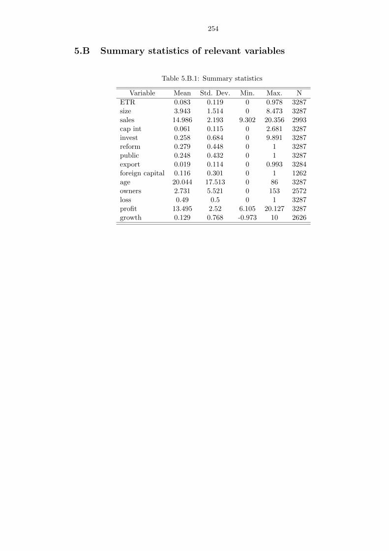
254
5.B Summary statistics of relevant variables
Table 5.B.1: Summary statistics
Variable Mean Std. Dev. Min. Max. N
ETR 0.083 0.119 0 0.978 3287size 3.943 1.514 0 8.473 3287sales 14.986 2.193 9.302 20.356 2993cap int 0.061 0.115 0 2.681 3287invest 0.258 0.684 0 9.891 3287reform 0.279 0.448 0 1 3287public 0.248 0.432 0 1 3287export 0.019 0.114 0 0.993 3284foreign capital 0.116 0.301 0 1 1262age 20.044 17.513 0 86 3287owners 2.731 5.521 0 153 2572loss 0.49 0.5 0 1 3287profit 13.495 2.52 6.105 20.127 3287growth 0.129 0.768 -0.973 10 2626

255
5.C Discussion of events in 2002 and 2003
Exploring further the issue of the drop and subsequent increase in ETR in 2003-2004 ,
figures 5.C.1 and 5.C.2 show that both profits and sales experience a sharp decline in 2002,
a year earlier than the observed drop in ETR. Two brief historical notes may help clarifying
this. Firstly, while the peak of the drought was reached with the famine of 2002/03, its
roots lie in the previous year. In fact the famine was officially recognized only at a stage
when the drought had already heavily hit in the areas concerned. In 2002, faulty rains
had disrupted production and caused an increase in malnutrition and decimation of herds.
This already precarious situation, particularly in pastoralist areas, paved the way for the
disastrous effects of the subsequent drought (Gill, 2010; Hammond and Maxwell, 2002).
Second, in the early 2000s military tension was high between Ethiopia and Eritrea although
the war was formally finished with the December 2000 peace agreement. Although a
Boundary Commission agreed on a verdict in 2002, it was not until 2005 that both countries
formally agreed to this verdict and that Ethiopia withdrew its troops. Given the complex
situation of the time, it is not straightforward, and it may not even be correct, to attribute
the sharp decrease in sales and profits to either the drought or military tension at the
Eritrean border.
The difference in the timing of response of sales (2002) and tax (2003) however may
be explained by the different factors that affect them. Indeed it may be possible that
while profits and sales are already heavily affected by the war and the drought leading to
the famine, the ETR may instead be affected by collection delays due to the emergency
in 2003. Moreover there is historical evidence for Ethiopia that during times of internal
conflict, as the early 2000s, industrial production can be disrupted because of difficulties
in transport, delays in deliveries of raw materials and other inputs, and power shortages.
In fact while the income tax take in absolute value may have decreased in those years,
there is no reason for the ETR to decrease. If anything, in times of war tax rates may
increase to finance military operations. In 2003 on the other hand, the intervention of
donors and the management of the emergency might have caused a congestion in the
public administration and thus a delay in tax collection.
The discussion above provides some support for the possibility of a different timing of
the drop in profits and ETR. However it is important to consider the possibility of a lag in
the data using detailed information from the survey and the tax legislation. First of all, it
is worth noting that the survey is designed to contain data referring to the same survey year
and thus lags should not occur. As far as tax law is concerned, firms are required to send

256
their tax declaration, together with the accounts and supporting documents, two to four
months after the closure of the fiscal year (according to the accounting requirements and
the type of books of accounts kept by the firm). This would then be between September
and December. At this time firms have to pay tax as they already have an estimation of
the amount due that will be then verified by the tax authority. Notwithstanding the 2002
tax reform, the procedure and timing remain essentially unchanged. The survey is then
carried out in June, and data is collected for the previous year. At this point firms have
closed the accounts for the previous year and they are also able to report the amount of
tax paid. Enumerators visit the firms and they fill in the questionnaire which is mostly in
the form of tables that contain the data on sales, inputs, etc. The discussion between the
enumerator and the firm is focused on a single fiscal year, thus implying the absence of a
lag.
Given the details of data collection and particularly its timing, it seems therefore
unlikely that the survey actually reports lagged tax data in a systematic manner. However
this cannot be asserted with certainty and surely not for 2003, when the data may suggest
the presence of a lag in collection. However this year can reasonably be treated as an
exception and indeed no other major event occurred in the period considered that could
have caused a delay in tax collection.
Figure 5.C.1: Evolution of income intime Figure 5.C.2: Evolution of sales in time

257
5.D Distribution of ETR by firm size over time
Figure 5.D.1: Scatter plot of profits and sales
0.2
.4.6
.80
.2.4
.6.8
0.2
.4.6
.80
.2.4
.6.8
1996 1998 1999 2000
2001 2002 2003 2004
2005 2006 2007 2008
2009
Mean
of E
TR by
quan
tiles
Graphs by year
Note: the plots report ETR by quantiles (20) of firm size, calculated using the number of employees in log.

258
5.E The determinants of profit
Table 5.E.1: Determinants of profits: Pooled OLS, FEM, REM and BE
(1) (2) (3) (4)OLS FEM REM BE
size 1.171*** 0.471*** 1.006*** 1.291***(57.43) (7.08) (37.68) (35.54)
cap int 4.967*** 1.535*** 3.600*** 5.932***(24.69) (3.34) (17.42) (14.07)
invest 0.366*** 0.333*** 0.328*** 0.658***(11.02) (8.66) (11.95) (6.54)
public 0.499*** 0.341*** 0.497*** 0.183(7.26) (3.04) (6.03) (1.26)
reform 0.915*** 0.671*** 0.787***(16.92) (8.14) (16.34)
age -0.002 0.026** 0.002 -0.003(-1.16) (2.58) (0.95) (-1.15)
Constant 8.139*** 10.665*** 8.697*** 7.795***(116.48) (31.53) (90.29) (64.80)
Observations 3287 3287 3287 3287N g 758.00 758.00 758.00r2 0.74 0.24 0.78
t statistics in parentheses* p < 0.10, ** p < 0.05, *** p < 0.01

259
5.F Analysis of fixed effects
Figure 5.F.1: Plot of fixed effects

260
Table 5.F.1: Explaining the fixed effects
(1) (2) (3) (4) (5)
size -0.008*** -0.007*** -0.011*** -0.008*** -0.010***(-3.10) (-2.90) (-4.51) (-3.14) (-4.04)
cap int -0.027 -0.019 -0.018 -0.007 -0.001(-0.90) (-0.88) (-0.84) (-0.29) (-0.06)
invest 0.002 0.001 -0.001 0.001 -0.001(0.34) (0.21) (-0.21) (0.22) (-0.19)
public 0.004 0.006 0.020** 0.012 0.023**(0.39) (0.60) (2.03) (1.22) (2.25)
age -0.001*** -0.001*** -0.001*** -0.001*** -0.001***(-5.17) (-5.54) (-6.07) (-5.64) (-6.09)
export -0.015 -0.009 -0.011 -0.004(-0.61) (-0.36) (-0.45) (-0.18)
growth 0.001 0.002 0.001 0.002(0.21) (0.60) (0.32) (0.57)
loss -0.008 -0.009 -0.006 -0.007(-1.33) (-1.57) (-1.06) (-1.18)
Constant 0.049*** 0.050*** 0.077*** 0.049*** 0.066***(5.72) (5.75) (7.99) (4.63) (6.01)
Region dummies no no yes no yes
Sector dummies no no no yes yes
Observations 3287 2625 2625 2625 2625N g 758.00 733.00 733.00 733.00 733.00r2 0.08 0.09 0.15 0.14 0.18
t statistics in parentheses
* p < 0.10, ** p < 0.05, *** p < 0.01

261
5.G Tables with coefficients for region and sector dummies
Table 5.G.1: BE results with sector dummies
(1) (2) (3) (4)size -0.001 -0.007 0.000 -0.002
(-0.31) (-1.60) (0.09) (-0.58)
cap int -0.088*** -0.152*** -0.053** -0.071**(-2.87) (-2.88) (-2.03) (-2.23)
invest -0.013* -0.004 -0.008 -0.012*(-1.73) (-0.51) (-1.12) (-1.66)
public 0.025** 0.095*** 0.026** 0.031***(2.34) (5.29) (2.22) (2.94)
age 0.001*** 0.000 0.001** 0.001***(3.59) (0.16) (2.47) (3.52)
foreign capital 0.018(0.90)
export 0.003 -0.037(0.06) (-1.31)
growth -0.005 0.000(-0.98) (0.09)
owners -0.002(-0.98)
plastic 0.004 -0.001 0.001(0.17) (-0.10) (0.06)
furniture -0.007 -0.004 -0.007(-0.48) (-0.36) (-0.79)
print 0.032* 0.019 0.034***(1.85) (1.49) (3.06)
footwear 0.000 0.006 -0.003(0.01) (0.36) (-0.20)
flour -0.015 0.005 -0.002(-0.52) (0.35) (-0.15)
bakery 0.027* 0.041*** 0.042***(1.74) (3.69) (4.38)
cement -0.020 0.002 -0.015(-0.90) (0.12) (-1.27)
Constant 0.069*** 0.087*** 0.059*** 0.065***(7.93) (4.58) (5.01) (6.08)
Observations 3287 655 2625 3287N g 758.00 420.00 733.00 758.00r2 0.06 0.15 0.06 0.11
Note: t statistics in parentheses; * p < 0.10, ** p < 0.05, *** p < 0.01

262
Table 5.G.2: BE results with regions
(1) (2) (3) (4)size -0.001 -0.012*** -0.004 -0.005**
(-0.31) (-2.77) (-1.51) (-2.03)
cap int -0.088*** -0.149*** -0.057** -0.082***(-2.87) (-2.97) (-2.32) (-2.76)
invest -0.013* -0.005 -0.012* -0.017**(-1.73) (-0.72) (-1.72) (-2.36)
public 0.025** 0.108*** 0.038*** 0.041***(2.34) (6.00) (3.23) (3.90)
age 0.001*** 0.000 0.001** 0.001***(3.59) (0.06) (2.19) (3.10)
foreign capital 0.016(0.82)
export 0.009 -0.039(0.21) (-1.40)
growth -0.003 0.002(-0.63) (0.39)
owners -0.002(-0.95)
afar -0.052 0.051 0.050(-0.56) (1.08) (1.11)
tigray -0.014 0.027 0.024(-0.40) (1.52) (1.59)
amhara 0.003 -0.021 -0.036***(0.16) (-1.63) (-3.19)
oromia -0.018 -0.027*** -0.027***(-1.21) (-2.79) (-3.21)
somalie -0.058 -0.078* -0.080**(-1.05) (-1.84) (-2.09)
snnpr -0.059*** -0.051*** -0.051***(-3.02) (-4.39) (-4.88)
gambela -0.194** -0.125** -0.131**(-2.03) (-2.06) (-2.39)
harari -0.021 -0.029 -0.031(-0.57) (-0.99) (-1.19)
diredawa -0.083*** -0.064*** -0.061***(-3.19) (-3.34) (-3.53)
Constant 0.069*** 0.119*** 0.094*** 0.098***(7.93) (7.03) (8.80) (10.18)
Observations 3287 655 2625 3287N g 758.00 420.00 733.00 758.00r2 0.06 0.18 0.10 0.13
Note: t statistics in parentheses; * p < 0.10, ** p < 0.05, *** p < 0.01

263
5.H Results including loss variable
Table 5.H.1: BE with loss variable
(1) (2) (3) (4) (5)
size -0.001 -0.001 -0.011** -0.002 0.000(-0.31) (-0.24) (-2.28) (-0.81) (0.03)
cap int -0.088*** -0.085*** -0.133** -0.041 -0.058**(-2.87) (-2.77) (-2.52) (-1.59) (-2.29)
invest -0.013* -0.013* -0.004 -0.012* -0.010(-1.73) (-1.82) (-0.53) (-1.73) (-1.38)
public 0.025** 0.025** 0.109*** 0.040*** 0.023**(2.34) (2.39) (5.93) (3.38) (2.00)
age 0.001*** 0.001*** -0.000 0.001** 0.001**(3.59) (3.63) (-0.03) (2.18) (2.52)
loss -0.008 -0.009 -0.007 -0.006(-1.39) (-0.94) (-1.04) (-0.97)
foreign capital 0.020(1.05)
owners -0.002(-1.01)
export 0.017 -0.029 -0.040(0.38) (-1.04) (-1.44)
growth -0.003 0.001 0.000(-0.58) (0.29) (0.06)
Constant 0.069*** 0.072*** 0.110*** 0.081*** 0.070***(7.93) (8.02) (5.45) (6.39) (7.00)
Region dummies no no yes yes no
Sector Dummies no no yes yes no
Observations 3287 3287 655 2625 2625N g 758.00 758.00 420.00 733.00 733.00r2 0.06 0.07 0.20 0.12 0.04
Note: t statistics in parentheses; * p < 0.10, ** p < 0.05, *** p < 0.01
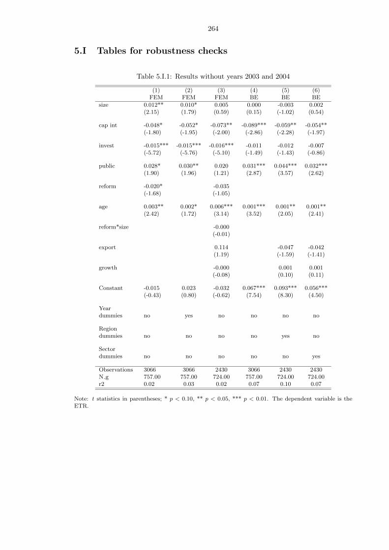
264
5.I Tables for robustness checks
Table 5.I.1: Results without years 2003 and 2004
(1) (2) (3) (4) (5) (6)FEM FEM FEM BE BE BE
size 0.012** 0.010* 0.005 0.000 -0.003 0.002(2.15) (1.79) (0.59) (0.15) (-1.02) (0.54)
cap int -0.048* -0.052* -0.073** -0.089*** -0.059** -0.054**(-1.80) (-1.95) (-2.00) (-2.86) (-2.28) (-1.97)
invest -0.015*** -0.015*** -0.016*** -0.011 -0.012 -0.007(-5.72) (-5.76) (-5.10) (-1.49) (-1.43) (-0.86)
public 0.028* 0.030** 0.020 0.031*** 0.044*** 0.032***(1.90) (1.96) (1.21) (2.87) (3.57) (2.62)
reform -0.020* -0.035(-1.68) (-1.05)
age 0.003** 0.002* 0.006*** 0.001*** 0.001** 0.001**(2.42) (1.72) (3.14) (3.52) (2.05) (2.41)
reform*size -0.000(-0.01)
export 0.114 -0.047 -0.042(1.19) (-1.59) (-1.41)
growth -0.000 0.001 0.001(-0.08) (0.10) (0.11)
Constant -0.015 0.023 -0.032 0.067*** 0.093*** 0.056***(-0.43) (0.80) (-0.62) (7.54) (8.30) (4.50)
Yeardummies no yes no no no no
Regiondummies no no no no yes no
Sectordummies no no no no no yes
Observations 3066 3066 2430 3066 2430 2430N g 757.00 757.00 724.00 757.00 724.00 724.00r2 0.02 0.03 0.02 0.07 0.10 0.07
Note: t statistics in parentheses; * p < 0.10, ** p < 0.05, *** p < 0.01. The dependent variable is theETR.
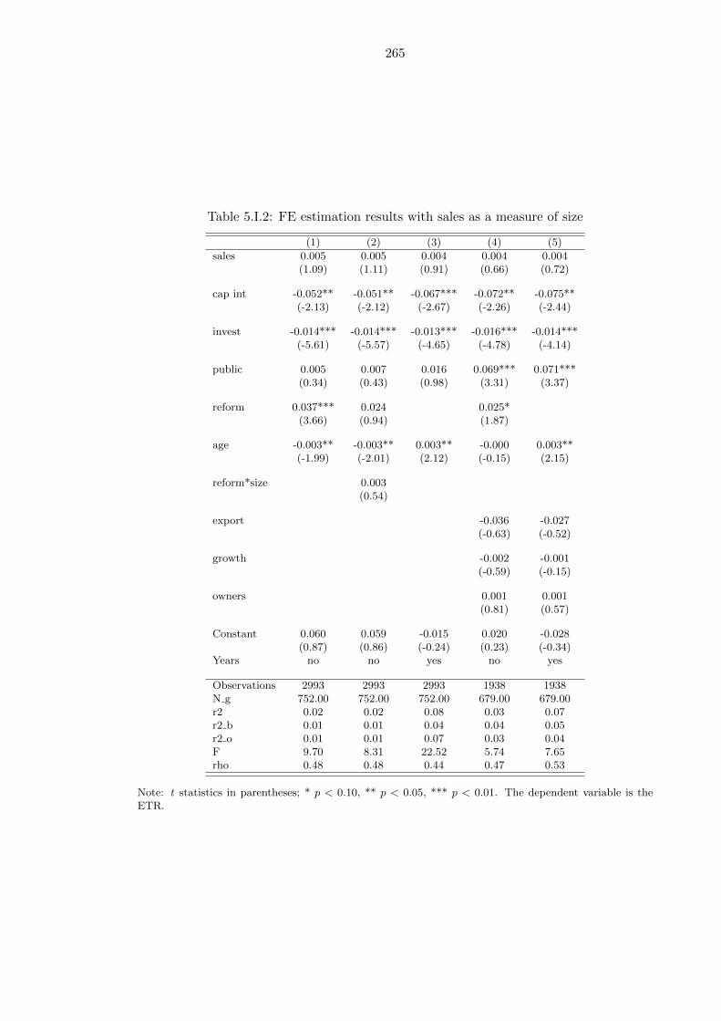
265
Table 5.I.2: FE estimation results with sales as a measure of size
(1) (2) (3) (4) (5)
sales 0.005 0.005 0.004 0.004 0.004(1.09) (1.11) (0.91) (0.66) (0.72)
cap int -0.052** -0.051** -0.067*** -0.072** -0.075**(-2.13) (-2.12) (-2.67) (-2.26) (-2.44)
invest -0.014*** -0.014*** -0.013*** -0.016*** -0.014***(-5.61) (-5.57) (-4.65) (-4.78) (-4.14)
public 0.005 0.007 0.016 0.069*** 0.071***(0.34) (0.43) (0.98) (3.31) (3.37)
reform 0.037*** 0.024 0.025*(3.66) (0.94) (1.87)
age -0.003** -0.003** 0.003** -0.000 0.003**(-1.99) (-2.01) (2.12) (-0.15) (2.15)
reform*size 0.003(0.54)
export -0.036 -0.027(-0.63) (-0.52)
growth -0.002 -0.001(-0.59) (-0.15)
owners 0.001 0.001(0.81) (0.57)
Constant 0.060 0.059 -0.015 0.020 -0.028(0.87) (0.86) (-0.24) (0.23) (-0.34)
Years no no yes no yes
Observations 2993 2993 2993 1938 1938N g 752.00 752.00 752.00 679.00 679.00r2 0.02 0.02 0.08 0.03 0.07r2 b 0.01 0.01 0.04 0.04 0.05r2 o 0.01 0.01 0.07 0.03 0.04F 9.70 8.31 22.52 5.74 7.65rho 0.48 0.48 0.44 0.47 0.53
Note: t statistics in parentheses; * p < 0.10, ** p < 0.05, *** p < 0.01. The dependent variable is theETR.
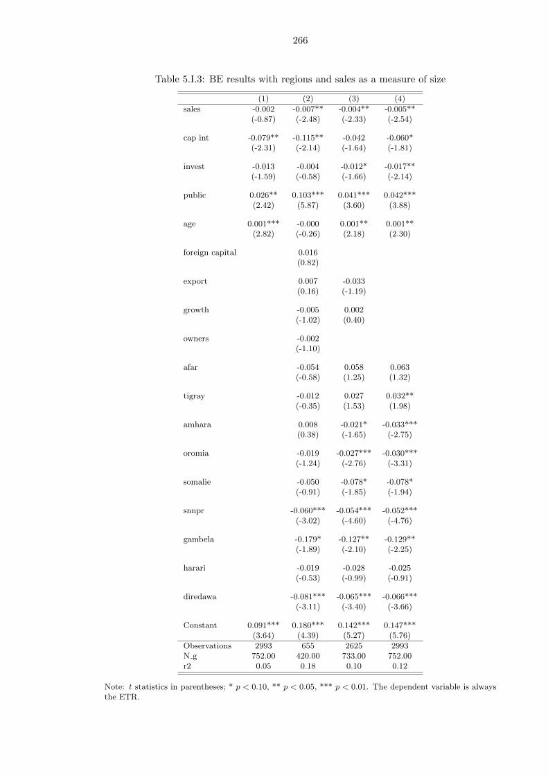
266
Table 5.I.3: BE results with regions and sales as a measure of size
(1) (2) (3) (4)
sales -0.002 -0.007** -0.004** -0.005**(-0.87) (-2.48) (-2.33) (-2.54)
cap int -0.079** -0.115** -0.042 -0.060*(-2.31) (-2.14) (-1.64) (-1.81)
invest -0.013 -0.004 -0.012* -0.017**(-1.59) (-0.58) (-1.66) (-2.14)
public 0.026** 0.103*** 0.041*** 0.042***(2.42) (5.87) (3.60) (3.88)
age 0.001*** -0.000 0.001** 0.001**(2.82) (-0.26) (2.18) (2.30)
foreign capital 0.016(0.82)
export 0.007 -0.033(0.16) (-1.19)
growth -0.005 0.002(-1.02) (0.40)
owners -0.002(-1.10)
afar -0.054 0.058 0.063(-0.58) (1.25) (1.32)
tigray -0.012 0.027 0.032**(-0.35) (1.53) (1.98)
amhara 0.008 -0.021* -0.033***(0.38) (-1.65) (-2.75)
oromia -0.019 -0.027*** -0.030***(-1.24) (-2.76) (-3.31)
somalie -0.050 -0.078* -0.078*(-0.91) (-1.85) (-1.94)
snnpr -0.060*** -0.054*** -0.052***(-3.02) (-4.60) (-4.76)
gambela -0.179* -0.127** -0.129**(-1.89) (-2.10) (-2.25)
harari -0.019 -0.028 -0.025(-0.53) (-0.99) (-0.91)
diredawa -0.081*** -0.065*** -0.066***(-3.11) (-3.40) (-3.66)
Constant 0.091*** 0.180*** 0.142*** 0.147***(3.64) (4.39) (5.27) (5.76)
Observations 2993 655 2625 2993N g 752.00 420.00 733.00 752.00r2 0.05 0.18 0.10 0.12
Note: t statistics in parentheses; * p < 0.10, ** p < 0.05, *** p < 0.01. The dependent variable is alwaysthe ETR.
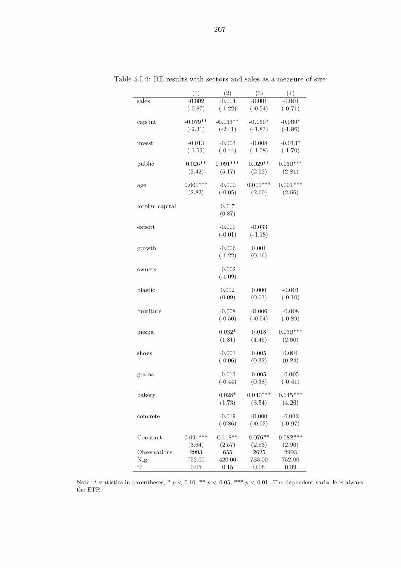
267
Table 5.I.4: BE results with sectors and sales as a measure of size
(1) (2) (3) (4)
sales -0.002 -0.004 -0.001 -0.001(-0.87) (-1.22) (-0.54) (-0.71)
cap int -0.079** -0.133** -0.050* -0.069*(-2.31) (-2.41) (-1.83) (-1.96)
invest -0.013 -0.003 -0.008 -0.013*(-1.59) (-0.44) (-1.08) (-1.70)
public 0.026** 0.091*** 0.029** 0.030***(2.42) (5.17) (2.52) (2.81)
age 0.001*** -0.000 0.001*** 0.001***(2.82) (-0.05) (2.60) (2.66)
foreign capital 0.017(0.87)
export -0.000 -0.033(-0.01) (-1.18)
growth -0.006 0.001(-1.22) (0.16)
owners -0.002(-1.09)
plastic 0.002 0.000 -0.001(0.09) (0.01) (-0.10)
furniture -0.008 -0.006 -0.008(-0.50) (-0.54) (-0.89)
media 0.032* 0.018 0.030***(1.81) (1.45) (2.60)
shoes -0.001 0.005 0.004(-0.06) (0.32) (0.24)
grains -0.013 0.005 -0.005(-0.44) (0.38) (-0.41)
bakery 0.028* 0.040*** 0.045***(1.73) (3.54) (4.26)
concrete -0.019 -0.000 -0.012(-0.86) (-0.02) (-0.97)
Constant 0.091*** 0.118** 0.076** 0.082***(3.64) (2.57) (2.53) (2.90)
Observations 2993 655 2625 2993N g 752.00 420.00 733.00 752.00r2 0.05 0.15 0.06 0.09
Note: t statistics in parentheses; * p < 0.10, ** p < 0.05, *** p < 0.01. The dependent variable is alwaysthe ETR.

268
Table 5.I.5: Results imputing zeroes for missing observations of tax
(1) (2) (3) (4) (5) (6)FEM FEM BE BE BE est6
size 0.014*** 0.010** 0.013* -0.003 -0.006** -0.001(3.28) (2.29) (1.96) (-1.25) (-2.50) (-0.36)
capint -0.015 -0.027 -0.058* -0.056** -0.012 -0.008(-0.60) (-1.12) (-1.78) (-2.47) (-0.69) (-0.42)
invest -0.011*** -0.011*** -0.010*** -0.014** -0.013** -0.011*(-5.38) (-5.00) (-4.21) (-2.43) (-2.24) (-1.79)
public 0.010 0.019 -0.003 0.018** 0.031*** 0.020*(0.81) (1.64) (-0.21) (1.99) (2.89) (1.85)
reform -0.014** -0.026(-2.05) (-1.33)
age -0.000 -0.001 0.002 0.001*** 0.001*** 0.001***(-0.06) (-0.87) (1.27) (4.34) (2.65) (3.02)
ref size 0.000(0.11)
export 0.011 -0.026 -0.031(0.28) (-1.15) (-1.35)
growth -0.006 0.002 0.001(-1.47) (0.60) (0.31)
years no yes no no no no
regions no no no no yes no
sectors no no no no no yes
Constant 0.022 0.060** 0.004 0.064*** 0.089*** 0.050***(0.87) (2.39) (0.10) (8.68) (9.46) (4.76)
Observations 3942 3942 3157 3942 3157 3157N g 852.00 852.00 819.00 852.00 819.00 819.00r2 0.01 0.09 0.01 0.06 0.09 0.06
Note: t statistics in parentheses; * p < 0.10, ** p < 0.05, *** p < 0.01. The dependent variable is alwaysthe ETR.

269
Table 5.I.6: Results with all variables lagged, except tax
(1) (2) (3) (4) (5)FEM FEM BE BE BE
L.size -0.015 -0.017 0.006 0.003 0.004(-0.87) (-0.91) (0.65) (0.33) (0.39)
L.cap int -0.325* -0.364** -0.167 -0.152 -0.151(-1.95) (-2.22) (-1.45) (-1.31) (-1.24)
L.invest 0.062 0.061 -0.009 -0.018 -0.010(0.75) (0.71) (-0.41) (-0.79) (-0.44)
public -0.034 -0.007 -0.051 -0.035 -0.049(-0.51) (-0.12) (-1.45) (-0.96) (-1.38)
reform 0.104***(2.67)
L.age -0.010 0.008** 0.002** 0.002** 0.002**(-1.57) (2.24) (2.30) (2.51) (2.25)
years no yes no no no
regions no no no yes no
sectors no no no no yes
Constant 0.367*** 0.008 0.086*** 0.095*** 0.102***(2.91) (0.10) (2.87) (2.77) (2.69)
Observations 1563 1563 1563 1563 1563N g 577.00 577.00 577.00 577.00 577.00r2 0.01 0.03 0.02 0.05 0.03
Note: t statistics in parentheses; * p < 0.10, ** p < 0.05, *** p < 0.01. The dependent variable is alwaysthe ETR.

270
Table 5.I.7: Results with ETR < 2
(1) (2) (3) (4) (5) (6)FEM FEM FEM BE BE BE
size 0.008 0.007 0.008 -0.004 -0.011** -0.006(0.95) (0.82) (0.77) (-1.01) (-2.16) (-1.22)
cap int 0.005 -0.014 -0.031 -0.096** -0.048 -0.061(0.15) (-0.42) (-0.62) (-2.14) (-1.13) (-1.37)
invest -0.016*** -0.014*** -0.015*** -0.026** -0.022* -0.018(-5.80) (-4.89) (-4.11) (-2.39) (-1.78) (-1.51)
public 0.014 0.023 0.005 0.028* 0.058*** 0.037*(0.91) (1.52) (0.28) (1.82) (2.92) (1.89)
reform 0.043*** 0.033(3.12) (0.83)
age -0.004** 0.002 -0.004** 0.001** 0.000 0.000(-2.11) (1.09) (-2.12) (2.28) (0.57) (0.75)
reform*size 0.002(0.27)
export 0.066 -0.042 -0.057(0.76) (-0.88) (-1.20)
growth -0.013 0.008 0.007(-1.54) (0.95) (0.77)
Constant 0.131*** 0.050 0.141** 0.098*** 0.137*** 0.113***(2.95) (1.12) (2.37) (7.59) (7.56) (5.67)
Yeardummies no yes no no no no
Regiondummies no no no no yes no
Sectordummies no no no no no yes
Observations 3313 3313 2643 3313 2643 2643N g 758.00 758.00 737.00 758.00 737.00 737.00r2 0.01 0.04 0.02 0.03 0.05 0.03
Note: t statistics in parentheses, * p < 0.10, ** p < 0.05, *** p < 0.01. The dependent variable is the ETR.Owners and forcap are excluded from the set of control variables because they are always non-significantand their inclusion would also reduce considerably the sample size.
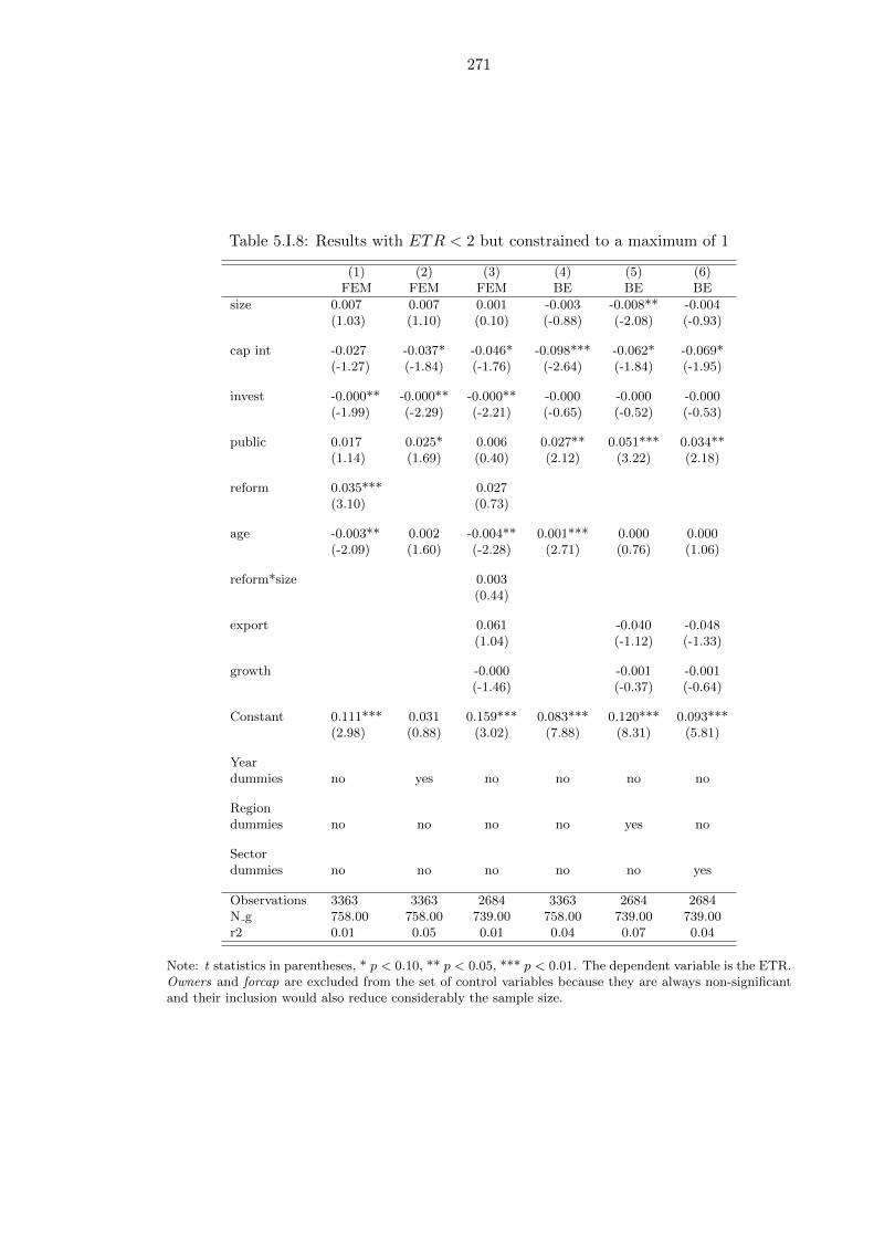
271
Table 5.I.8: Results with ETR < 2 but constrained to a maximum of 1
(1) (2) (3) (4) (5) (6)FEM FEM FEM BE BE BE
size 0.007 0.007 0.001 -0.003 -0.008** -0.004(1.03) (1.10) (0.10) (-0.88) (-2.08) (-0.93)
cap int -0.027 -0.037* -0.046* -0.098*** -0.062* -0.069*(-1.27) (-1.84) (-1.76) (-2.64) (-1.84) (-1.95)
invest -0.000** -0.000** -0.000** -0.000 -0.000 -0.000(-1.99) (-2.29) (-2.21) (-0.65) (-0.52) (-0.53)
public 0.017 0.025* 0.006 0.027** 0.051*** 0.034**(1.14) (1.69) (0.40) (2.12) (3.22) (2.18)
reform 0.035*** 0.027(3.10) (0.73)
age -0.003** 0.002 -0.004** 0.001*** 0.000 0.000(-2.09) (1.60) (-2.28) (2.71) (0.76) (1.06)
reform*size 0.003(0.44)
export 0.061 -0.040 -0.048(1.04) (-1.12) (-1.33)
growth -0.000 -0.001 -0.001(-1.46) (-0.37) (-0.64)
Constant 0.111*** 0.031 0.159*** 0.083*** 0.120*** 0.093***(2.98) (0.88) (3.02) (7.88) (8.31) (5.81)
Yeardummies no yes no no no no
Regiondummies no no no no yes no
Sectordummies no no no no no yes
Observations 3363 3363 2684 3363 2684 2684N g 758.00 758.00 739.00 758.00 739.00 739.00r2 0.01 0.05 0.01 0.04 0.07 0.04
Note: t statistics in parentheses, * p < 0.10, ** p < 0.05, *** p < 0.01. The dependent variable is the ETR.Owners and forcap are excluded from the set of control variables because they are always non-significantand their inclusion would also reduce considerably the sample size.
272
Chapter 6
Conclusions
This thesis analyses tax revenue mobilisation in Ethiopia in a comprehensive way, encom-
passing qualitative and quantitative elements as well as macroeconomic and microeconomic
perspectives. The issue of tax revenue mobilisation is particularly relevant in Ethiopia as
the tax share there still falls below the average of other African countries and the target
level of 15%. This relevance is reflected in the top priority that the government has given
to taxation in the Growth and Transformation Plan (GTP) and in the increasing attention
that donors are paying to this topic. Given the deep intertwining of taxation and aid, and
the need to ensure that aid is spent effectively, the relation between aid and taxation is a
central theme to this thesis.
This thesis contributes both to the literature and to the policy debate. Firstly, by
providing evidence on the Ethiopian experience, it shows the advantages of a case study
approach as a way to overcome the limits of the cross-country literature. By focussing on
a single country, the analysis can explicitely recognize that taxation is a multifaceted issue
by adopting a set of different methodological tools, yet ensuring coherence in the case study
context. Secondly this thesis contributes to the policy debate by providing evidence of a
positive relation between aid and taxation that is robust to the use of different methods
and specifications. Last but not least it makes a conceptual contribution by providing
a theoretical framework to think about the tax take at the microeconomic level, in the
context of the analysis of effective tax rates in chapter 5.
6.1 Main findings and reflections on thesis
The main finding of this thesis is the positive relation between aid and tax in Ethiopia. The
investigation of this relation is the main research question motivating this work and is a

273
strong common thread that links particularly chapters 2, 3, and 4. While the three chapters
are motivated by the same core question, they take different approaches to answering it.
Chapter 2 reports a qualitative analysis including an historical account of taxation and
aid in Ethiopia during the period for which data is available. This historical account,
largely based on secondary sources, is complemented with primary information obtained
during in-depth interviews to high-level officials in the Government of Ethiopia and in
donor agencies, as well as independent experts. In chapter 3 I estimate a tax effort
model in a case study context, which is a novelty in a literature largely dominated by
cross-country studies. The tax effort framework has the advantage of putting the aid-
tax relation in the economic context and perspective of the country analysed, both by
taking variables in shares of GDP and by including proxies of the tax base as control
variables. Chapter 4 takes a CVAR approach, where only fiscal variables are included, in
log transformation. This approach has the important advantage, with respect to chapter
3, of taking into account endogeneity by estimating simultaneous equations. By analysing
tax effort and aid from these different perspectives, this thesis provides a unique in-depth
and comprehensive analysis of this issue in the Ethiopian context.
The main explanation provided for the positive relation between aid and tax is capacity
building and technical assistance, through which aid can decrease both administrative costs
(by, for example, introducing IT systems that make the tax administration more effective
and efficient) and political costs (by having the international backing of foreign donors,
the government may be able to increase legitimacy of tax reform). While a portion of this
capacity building is captured by the financial flows that I am measuring, not all of it is.
This is particularly the case of policy advice and of programs that are not delivered through
the government’s budget. While these parts of capacity building are not captured in my
measure of aid, they are explored in chapter 2. Moreover the intensity of these activities
is likely to be highly correlated with the amount of financial flows into the budget, as
they both depend on the quality of relations between the government and donors. This
explanation, based on capacity building, is also consistent with the results obtained in the
disaggregated tax equations in chapter 3 (section 3.6), where aid appears to be mostly
associated with direct and trade taxes. In the case of direct taxes, aid may influence the
ability of the government to collect taxes from ‘hard to tax’ handles. In addition, given
the ambitious nature of the government’s development plans and their centrality to its
political legitimacy, the availability of foreign resources may give momentum to increased
tax revenue mobilisation; it may even represent an incentive for it, due to the ‘shame of

274
aid’ rooted in Ethiopian culture.
Since endogeneity of the aid variables is likely the greatest limitation of this work, it
is worth reflecting on how the various econometric methods adopted in this thesis help
tackling it. In a time series setting the problem is somewhat mitigated with respect to
the cross-country case, particularly in presence of cointegration. In both chapters 3 and
4 cointengration can be confirmed and therefore the long run results do not suffer from
concerns related to endogeneity. Clearly however in the case of the ECM in chapter 3, it
is difficult to make causal statements. This is particularly true in the short run part of
the exercise where the issue needs to be explicitly tackled. I take a number of measures
to address endogeneity in the short run part of the ECM. First, I adopt an instrumental
variable approach. A number of possible instrumental variables are tested but most of
them are not satisfactory in terms of validity. Moreover the time series context makes the
identification of an instrument even harder, due to limitations in data availablity for the
relatively long period considered. The best available solution is the use of lags, that are
valid instruments at least for grants. While the limitations of the use of lags are noted in
chapter 3, it is at least partly reassuring that the main results are largely confirmed. In
addition I address the possibility of an omitted variable problem by including the variable
that may be the main source of bias: governance. Secondly, I use the qualitative evidence
from chapter 2 to explore the possible sources of endogeneity in the specific context of
Ethiopia. In section 3.5.1, drawing larlegy from chapter 2, I argue that aid decisions are
largely exogenous to the government decision making process in Ethiopia. However it is
really in chapter 4 that this issue can be fully addressed, since the CVAR framework allows
the estimation of simultaneous equations without making assumptions about endogeneity.
In addition to confirming the previous results on aid and tax, the CVAR methodology
provides some evidence for the exogeneity of loans, particularly in the identified system,
and no support for the endogeneity of grants, that appear the least adjusting variable
in the tests for a unit vector in alpha (see section 4.8.5). Therefore the main result of
this thesis, showing a positive relation between aid and tax, is largely supported by all
chapters. Endogeneity does not seem to affect it in any substantial way, although causality
cannot be established with absolute confidence.
The discussion on endogeneity clearly exemplifies how chapters 2, 3, and 4 are highly
complementary to each other, while adding specific insights to the thesis.
Chapter 2 bridges the qualitative and quantitative sides of tax revenue mobilisation,
particularly by underlining the political and cultural aspects of the aid-tax relation. It

275
therefore serves the econometric analysis in two ways, besides representing a contribution
by itself. Firstly it helps in designing the econometric models of chapters 3 and 4 and
in understanding the econometric challenges that they present. Most notably, it sheds
light on the nature and extent of regime changes that may lead to structural breaks.
Secondly the analysis of chapter 2 is useful in interpreting the econometric results and in
ensuring that the conclusions are consistent with the Ethiopian context, which is all the
more important in presence of small samples.
Chapter 3 offers a broader insight into tax revenue mobilisation in the context of the
Ethiopian economy, taking into account the effect of different tax bases. By doing this
it offers important insights into how the sectoral composition of the economy influences
tax revenue mobilisation. While trade is confirmed as a major positive determinant of
the tax share, agriculture has a negative effect on domestic taxes (direct and indirect) in
particular. This effect is only clear in the disaggregated tax equations since the expected
negative sign is contrasted by the positive effect on trade taxes in the aggregate tax
equation. Furthermore manufacturing is found to have a large and significant effect on
the tax share, due not only to the higher visibility and accessibility of this sector but also
to the fact that firms act as a tax collectors for indirect and employment taxation.
Chapter 4 contributes to the thesis by including other fiscal variables in the equation,
most notably public expenditure that is further disaggregated into recurrent and capital
spending. By doing this, it offers a broader view on the fiscal dynamics in Ethiopia. It
provides evidence of a long-run domestic budget equilibrium that excludes foreign aid. This
implies that the government makes long term plans based on domestic sources, treating aid
as an addition to such pre-existing long run relation. By looking at adjustment coefficients
we also find that spending plans are mainly driven by tax revenue, while expenditure is
the most adjusting variable. In addition we find that government spending is positively
associated with both aid variables and this relation is particularly strong between capital
expenditure and grants, as shown in our ‘alternative system’. Finally we identify a donor
disbursement rule whereby donors back proven commitment to increased expenditure with
additional funding, particularly grants.
Therefore, while the three chapters are strongly linked by a common research question,
each of them explores different specific issues and provides additional contributions to the
main research question on aid and tax.
Finally chapter 5 is somehow different from the previous three chapters since it takes a
microeconomic perspective by focussing on the manufacturing sector, while the rest of the

276
thesis is largely focussed on the macro level. However this chapter is actually connected
to chapter 3 and it somehow stems from that analysis. In fact the effective tax rate
essentially mirrors the tax to GDP ratio at the firm level, particularly in the manufacturing
sector. Moreover the analysis of business taxation follows from the importance of the
manufacturing sector as a determinant of the tax share emerging from chapter 3. Business
profits tax represents already a substantial share of total revenue in Ethiopia, and it is
likely to play an increasingly important role as industrial development unfolds (see chapter
1). Moreover chapter 5 draws largely from the qualitative work summarised in chapter 2,
particularly as regards tax legislation and the role of the business sector in the Ethiopian
economy.
By focusing on ETRs, I am able to quantify tax payments by firms and assess the
extent of tax preferences in Ethiopia. I find that tax incentives are indeed generous in the
Ethiopian manufacturing sector, with most firms facing an ETR well below the statutory
rate. The econometric exercise allows the identification of some of the regulatory sources of
tax preferences such as regional development and incentives for investment. However the
analysis explores also less official sources of tax preferences such as lobbying and political
connections. While these elements are not easily pinned down in a precise manner, this
analysis nonetheless allows the identification of some aspects of it. By using proxies to
capture these aspects, I find that effective tax rates do not seem to be influenced by the
lobbying of larger firms or by political connections. These results support the ‘political
cost hypothesis’, postulating a positive relation between visibility, and particualrly size,
and tax payments. This hypothesis is particularly plausible in the Ethiopian context where
the socialist tradition has resulted in a larger role of the state and in a perception of the
private sector as purely rent seeking, as discussed in chapter 2.
6.2 Implications for research and practice
The main implication for further research stemming from this thesis regards the impor-
tance of using mixed methods, including both qualitative and quantitative analysis. The
three quantitative chapters, namely 3, 4 and 5, benefit hugely from a deep understanding
of the Ethiopian context both in the design phase of the analysis and in the interpreta-
tion of results. Moreover the in-depth analysis of taxation in Ethiopia allows this thesis
to make a substantial contribution to the existing knowledge on taxation and aid in the
specific context of Ethiopia, attempting to take into account all the economic, political
and cultural factors at play.

277
As far as the implications for empirical analysis are concerned, this thesis shows the
potentially valuable contribution that time series analysis can offer even in a small sample
setting. While parsimony and caution are due when using small samples, chapters 3 and
4 show that the main result of a positive relation between aid and tax is robust not only
to changes in specifications but also to the adoption of different methods. They therefore
make a case for further research at the macroeconomic level in Africa, despite criticism
related to data quality and small samples. Indeed I show that this type of research can
provide answers to policy relevant questions that are central to the debate on African
development. Moreover as African countries continue improving their statistics, studies
like the ones presented here should become more common and increasingly robust.
As far the microeconomic empirical side is concerned, chapter 5 shows that the analysis
of taxation at the micro level is feasible and it can provide useful insights. Clearly the
analysis can be much improved and a few important caveats remain in terms of data
availability and methods. Despite these issues however I believe it is valuable to quantify
the extent of fiscal incentives, that are often presented as one of the main obstacles to
tax revenue mobilisation in Africa. Moreover, despite problems with measurement, the
analysis of ETR can offer some indications on the role of lobbying and political connections.
The analysis presented in chapter 5 is clearly far from being exhaustive in itself. It rather
aims at being a starting point for further research on this potentially important, and still
largely underdeveloped, area of economic research.
Last but not least, this thesis has a few policy implications. The main result is the
positive relation between aid and taxation in Ethiopia. In terms of policy, it implies
that donors should not be concerned about adverse fiscal effects of aid in Ethiopia, or
at least not as far as taxation is concerned. Therefore the argument of a crowding out
effect is particularly ill-grounded in the Ethiopian case and it cannot be used to justify
lower aid levels1. This analysis has shown that aid instead is beneficial to tax revenue
mobilisation and therefore support to tax policy and administration should continue to
be a priority in the development agenda. Donors can play an important role in domestic
revenue mobilisation by providing international support to politically difficult reform, by
building capacity, and by offering advice on both tax policy and administration reforms.
As this thesis started with a comparison of tax and aid in Ethiopia with the broader
African context, it is useful to reflect on the validity of my results for other countries in
1Ethiopia is not facing the threat of decreasing aid flows today, but it may be in the future in thecontext of a possible scaling down of aid (Gupta et al., 2006).
278
Africa. While I have argued that the case of Ethiopia is unique, it shares with other coun-
tries the common challenge of increasing domestic revenue while receiving large amounts of
aid. Moreover the Ethiopian uniqueness, while it is deeply rooted in the national culture,
becomes less and less distinctive as the colonial legacy looses its importance over time;
and as African countries become more willing and able to be independent from foreign
influence.
In terms of the other tax determinants, the agricultural sector emerges as a constraint
to increasing the tax share and particularly as far as domestic taxes are concerned. While
subsistence in agriculture is widespread in Ethiopia, reforms to increase the tax contribu-
tion from this large sector should be considered, including a review of the land tax. On
the other hand the manufacturing sector represents an opportunity for increasing the tax
share. Not only is this sector ‘easier to tax’ because of its higher visibility and accessibility
than, for example, the agricultural sector; it also acts as a collector of taxes on salaries
and goods therefore having a large revenue generating potential.
While the manufacturing sector is found to be already beneficial to tax revenue, it has
the potential to become increasingly important as a tax contributor. Chapter 5 shows
that tax benefits are widely used in the manufacturing sector, but they do not seem
to be influenced by lobbying and political connections. The balance between providing
incentives for industrial development and mobilising public revenue is to be considered
carefully by policy makers in Ethiopia, and different policy options need to be evaluated.
6.3 Further research
Besides representing a stand-alone work, this thesis has also prompted many ideas for
future research and for refining the existing analysis. I mention here only a few of the
ones I hope to develop following this thesis.
Chapter 2 can certainly be refined by focusing more on specific issues or a time period
(e.g. the EPRDF period alone), to become fully a stand alone piece without the ancillary
role of providing support for the rest of the thesis.
The CVAR analysis of chapter 4 could be further developed by including growth in
the system, and aggregating fiscal variables in more general headings such as domestic
revenue, expenditure and aid. This would give additional and interesting insights into the
relation of both aid and fiscal variables with economic growth.
The analysis of tax revenue mobilisation was largely carried out at the national level
in this thesis. However Ethiopia presents a federal structure that implies also revenue

279
collection and other fiscal powers for the regions. An analysis of the fiscal dynamics at
the sub-national level would provide additional insight into a layer of government that
may become increasingly important in revenue collection. Moreover the fiscal effects of
the block grant that the central government provides to the regions could be evaluated.
Last but not least, the effective tax rate exercise should be both refined by looking for
additional data to capture political connections and by exploring further interaction effects
between explanatory variables. Moreover a similar analysis could be carried out for other
countries with available data to build up a body of evidence on corporate taxation in Africa.
This would be useful in two ways. Firstly such body of African research could be compared
with evidence from other regions of the world to evaluate whether Africa displays different
patterns. Secondly it would allow a comparison of country level experiences on firm-level
taxation within Africa. I believe there is great potential in carrying out a similar anlaysis
of ETR using administrative data (i.e. tax returns), particuarly given the limitations of
firm-level surveys. In further developing this analysis with new and better data, chapter 5
represents a first step and the theoretical framework is potentially a good basis for further
research.

280
Bibliography
Abbas, S. M. A., Klemm, A., Bedi, S., and Park, J. (2012). A partial race to the bottom:
corporate tax developments in emerging and developing economies. IMF Working Paper
WP/12/28, International Monetary Fund.
Abbink, J. (2011). Ethnic-based federalism and ethnicity in Ethiopia: reassessing the
experiment after 20 years. Journal of Eastern African Studies, 5(4):596–618.
Adam, C. and Bevan, D. (2004). Fiscal policy design in low-income countries. In Addison,
T. and Roe, A., editors, Fiscal Policy for development. Palgrave MacMillan.
Adhikari, A., Derashid, C., and Zhang, H. (2006). Public policy, political connections,
and effective tax rates: longitudinal evidence from Malaysia. Journal of accounting and
public policy, 25(5):574–595.
Aizenman, J. and Jinjarak, Y. (2009). Globalization and developing countries - a shrinking
tax base? Journal of development studies, 45(5).
Alemayehu Geda (2011). Macroeconomic performance in post-Derg Ethiopia. Northeast
African Studies, 8(1):159–204.
Alemayehu Geda and Abebe Shimeles (2005). Taxes and tax reform in Ethiopia, 1990-
2003. Research paper 2005/65, UNU-WIDER.
Arndt, C., Jones, S., and Tarp, F. (2010). Aid and growth: have we come full circle?
Journal of globalization and development, 1:1–29.
Bahru Zewde (2008). Society, state and history: selected essays. Addis Ababa University
Press.
Baltagi, B. H. (2005). Econometric analysis of panel data. John Wiley and sons Ltd.
Bauman, C. and Schadewald, M. (2001). Impact of foreign operations on reported effective

281
tax rates: interplay of foreign taxes, U.S. taxes and U.S. GAAP. Journal of international
accounting, auditing and taxation, 10:177–196.
Benedek, D., Crivelli, E., Gupta, S., and Muthoora, P. (2012). Foreign aid and revenue:
still a crowding out effect? IMF Working Paper WP/12/186, International Monetary
Fund.
Bigsten, A., Collier, P., Dercon, S., Fafcharnps, M., Gauthier, B., Gunning, J. W.,
Habarurema, J., Isaksson, A., Oduro, A., Oostendorp, R., Pattillo, C., and Soderbom,
M. (1999). Exports of African manufactures: macro policy and firm behaviour. Journal
of International Trade and Economic Development, 8:53–71.
Bigsten, A. and Gebreeyesus, M. (2007). The small, the young, and the productive:
determinants of manufacturing firm growth in Ethiopia. Economic Development and
Cultural Change, 55:813–840.
Bigsten, A., Gebreeyesus, M., Siba, E., and Soderbom, M. (2011). The effects of agglomer-
ation and competition on prices and productivity: evidence for Ethiopia’s manufacturing
sector. Mimeo, University of Gothenburg.
Bigsten, A., Gebreeyesus, M., and Soderbom, M. (2009). Gradual trade liberalization and
firm performance in Ethiopia. Mimeo, University of Gothenburg.
Bigsten, A. and Soderbom, M. (2005). What have we learned from a decade of manu-
facturing enterprise surveys in Africa? Policy Research Working Paper 3798, World
Bank.
Binh, T. N. and McGillivray, M. (1993). Foreign aid, taxes and public investment. a
comment. Journal of Development Economics, 41:173–176.
Bird, R. M., Martinez-Vazquez, J., and Torgler, B. (2008). Tax effort in developing
countries and high income countries: the impact of corruption, voice and accountability.
Economic analysis and policy, 38:55–71.
Bornhorst, F., Gupta, S., and Thornton, J. (2008). Natural resource endowments, gov-
ernance, and the domestic revenue effort: evidence from a panel of countries. IMF
Working Paper WP/08/170, International Monetary Fund.
Bourguignon, F. and Sundberg, M. (2007). Aid effectiveness - opening the black box.
American Economic Review, 97:316–321.
282
Brautigam, D., Fjeldstad, O.-H., and Moore, M. (2008). Taxation and state building in
developing countries: capacity and consent. Cambridge University Press.
Brietzke, P. (1976). Land reform in revolutionary Ethiopia. The Journal of Modern
African Studies, 14:637–660.
Bulir, A. and Hamann, A. J. (2008). Volatility of development aid: from the frying pan
to the fire? World Development, 36:2048–2066.
Bwire, T. (2013). Aid, fiscal policy and macroeconomy of Uganda: a CVAR approach.
PhD thesis, University of Nottingham.
Cameron, A. C. and Trivedi, P. K. (2005). Microeconometrics Methods and Applications.
Cambridge University Press.
Cameron, A. C. and Trivedi, P. K. (2009). Microeconometrics using STATA. STATA
Press.
Carlin, W., Schaffer, M., and Seabright, P. (2006). Where are the real bottlenecks? A
Lagrangian approach to identifying constraints on growth from subjective survey data.
CERT Discussion Paper 0604, Heriot Watt University.
Carter, P. (2013). Does foreign aid displace domestic taxation? Journal of Globalization
and Development, 4:1–47.
Chege, M. (1979). The revolution betrayed: Ethiopia 1974-77. The Journal of Modern
African Studies, 17:359–380.
Chelliah, R. J. (1971). Trends in taxation in developing countries. Staff papers, Interna-
tional Monetary Fund.
Chelliah, R. J., Baas, H. J., and Kelly, M. R. (1975). Tax ratios and tax effort in developing
countries. Staff papers, International Monetary Fund.
Citizens for Tax Justice (1985). Corporate taxpayers and corporate freeloaders: four
years of continuing, legalized tax avoidance by America’s largest corporations 1981-84.
Technical report, Citizens for Tax Justice.
Clapham, C. (1987). Revolutionary socialist development in Ethiopia. African Affaires,
86:151–165.
Clapham, C. (1988). Transformation and continuity in revolutionary Ethiopia. Cambridge
University Press.

283
Clapham, C. (1989). The state and revolution in Ethiopia. Review of African Political
Economy, (44):4–17.
Clist, P. and Morrissey, O. (2011). Aid and tax revenue: signs of a positive effect since
the 80s. Journal of international development, 23:165–180.
Cohen, J., Goldsmith, A., and Mellor, J. (1976). Rural development issues following
Ethiopian land reform. Africa Today, 23:7–28.
Da Rin, M., Giacomo, M. D., and Sembenelli, A. (2010). Corporate taxation and the size
of new firms: evidence from Europe. Journal of the European Economic Association,
8:606–616.
Department for International Development (2011). Bilateral aid review: technical report.
UK Department for International Development.
Derashid, C. and Zhang, H. (2003). Effective tax rates and the “industrial policy” hy-
pothesis: evidence from Malaysia. Journal of international accounting, auditing and
taxation, 12:45–62.
Dercon, S. and Zeitlin, A. (2009). Rethinking agriculture and growth in Ethiopia: a
conceptual discussion. Mimeo.
Dereje Feyissa (2011). Aid negotiation: the uneasy “partnership” between the EPRDF
and the donors. Journal of Eastern African Studies, 5:788–817.
Dollar, D., Hallward-Driemeier, M., and Mengistae, T. (2005). Investment climate and
firm performance in developing economies. Mimeo, University of Chicago.
Drummond, P., Daal, W., Srivastava, N., and Oliveira, L. E. (2012). Mobilizing revenue
in Sub-Saharan Africa: empirical norms and key determinants. IMF Working Paper
WP/12/108, International Monetary Fund.
Economic and Political Weekly (1978). Revolution and counter-revolution in Ethiopia.
Economic and Political Weekly, 13:461–472.
Elbadawi, I., Mengistae, T., and Zeufack, A. (2006). Market access, supplier access, and
Africa’s manufactured exports: an analysis of the role of geography and institutions.
World Bank Policy Research Working Paper 9342, World Bank.
Engle, R. F. and Granger, C. W. J. (1987). Co-integration and error correction: represen-
tation, estimation, and testing. Econometrica, 55:251–76.

284
Eshetu Chole (1984). Towards a history of the fiscal policy of the pre-revolutionary
Ethiopian state: 1941-74. Journal of Ethiopian Studies, 17:88–106.
Eshetu Chole (2004). Underdevelopment in Ethiopia. OSSREA.
Ezemenari, K., Kebede, E., and Lahiri, S. (2008). The fiscal impact of foreign aid in
Rwanda: a theoretical and empirical analysis. Policy research working paper, World
Bank.
Faccio, M. (2006). Politically connected firms. The American Economic Review, 96:369–
386.
Fafchamps, M. and El Hamine, S. (2004). Firm productivity, wages, and agglomeration
externalities. CSAE Working Paper 2004-32, University of Oxford.
Fagernas, S. and Roberts, J. (2004a). The fiscal effects of aid in Uganda. ESAU Working
Paper 9, Overseas Development Institute.
Fagernas, S. and Roberts, J. (2004b). The fiscal effects of aid in Zambia. ESAU Working
Paper 10, Overseas Development Institute.
Fagernas, S. and Schurich, C. (2004). The fiscal effects of aid in Malawi. ESAU Working
Paper 7, Overseas Development Institute.
Feeny, S. (2006). Policy preferences in fiscal response studies. Journal of international
development, 18:1167–1175.
Fisman, R. (2001). Estimating the value of political connections. The American Economic
Review, 91:1095–1102.
Fjeldstad, O.-H. (2013). Taxation and development: a review of donor support to
strengthen tax systems in developing countries. Working Paper 2013/010, UNU-
WIDER.
Franco-Rodriguez, S. (2000). Recent developments in fiscal response with an application
to Costa Rica. Journal of international development, 12:429–441.
Franco-Rodriguez, S., Morrissey, O., and McGillivray, M. (1998). Aid and the public
sector in Pakistan: evidence with endogenous aid. World Development, 26:1241–1250.
Furtado, X. and Smith, W. J. (2007). Ethiopia: aid, ownership and sovreignty. GEG
working paper 2007/28, Global Economic Governance Programme.

285
Gang, I. N. and Khan, H. A. (1991). Foreign aid, taxes and public investment. Journal
of Development Economics, 34:355–369.
Gauthier, B. and Reinikka, R. (2006). Shifting tax burdens through exemptions and
evasion: an empirical investigation of Uganda. Journal of African economies, 15(3):373–
398.
Gauthier, B., Soloaga, I., and Tybout, J. (2002). A firm’s-eye view of commercial policy
and fiscal reforms in Cameroon. The World Bank economic review, 16(3).
Ghosh, M. (1999). Structural break and unit root in macroeconomic time series: evidence
from a developing economy. The Indian Journal of Statistics, 61:318–336.
Ghura, D. (1998). Tax revenue in Sub-Saharan Africa: Effects of economic policies and
corruption. IMF Working Paper WP/98/135, International Monetary Fund.
Gilkes, P. (1975). Ethiopia - a real revolution?, the world today. The World Today,
31:15–23.
Gilkes, P. (1982). Building Ethiopia’s revolutionary party. MERIP reports.
Gill, P. (2010). Famine and foreigners: Ethiopia since Live Aid. Oxford University Press.
Government of Ethiopia (1994). Proclamation 107/1994. Federal Negarit Gazeta of the
Federal Democratic Republic of Ethiopia.
Government of Ethiopia (2002a). Proclamation 285/2002. Federal Negarit Gazeta of the
Federal Democratic Republic of Ethiopia.
Government of Ethiopia (2002b). Proclamation 286/2002. Federal Negarit Gazeta of the
Federal Democratic Republic of Ethiopia.
Granger, C. W. J. (1969). Investigating causal relations by econometric models and cross
spectral methods. Econometrica, 37:424–438.
Greene, W. H. (2008). Econometric Analysis. Pearson Education.
Griffin, K. (1992). The economy of Ethiopia. The Macmillan Press.
Guha, A. (2007). Company size and effective corporate tax rate: study on Indian private
manufacturing companies. Economic and Political Weekly, 42:1869–1874.
Gupta, A. S. (2007). Determinants of tax revenue efforts in developing countries. IMF
Working Paper WP/07/184, International Monetary Fund.

286
Gupta, S., Clemens, B., Pivovarsky, A., and Tiongson, E. (2004). Foreign aid and revenue
response: does the composition of aid matter? In Gupta, S., Clemens, B., and Inchauste,
G., editors, Helping countries develop: the role of fiscal policy. International Monetary
Fund.
Gupta, S. and Mills, L. F. (2002). Corporate multistate tax planning: benefits of multiple
jurisdictions. Journal of Accounting and Economics, 33:117–139.
Gupta, S. and Newberry, K. (1997). Determinants of the variability in corporate effective
tax rates: evidence from longitudinal data. Journal of accounting and public policy,
16:1–34.
Gupta, S., Powell, R., and Yang, Y. (2006). Macroeconomic challenges of scaling up aid
to Africa: a checklist for practitioners. Washington: International Monetary Fund.
Hagmann, T. and Abbink, J. (2011). Twenty years of revolutionary democratic Ethiopia,
1991 to 2011. Journal of Eastern African Studies, 5:579–595.
Hammond, L. and Maxwell, D. (2002). The Ethiopian crisis of 1999-2000: lessons learned,
questions unanswered. Disasters, 26:262–279.
Heller, P. (1975). A model of public fiscal behaviour in developing countries: aid, invest-
ment and taxation. American Economic Review, 65:429–445.
Hisali, E. and Ddumba-Ssentamu, J. (2013). Foreign aid and tax revenue in Uganda.
Economic Modelling, 30:356–365.
Hofmann, M. A. (2002). The state corporate income tax: a synthesis of recent research.
Journal of Accounting Literature, 21:76–119.
Holland, K. (1998). Accounting policy choice: the relationship between corporate tax
burdens and company size. Journal of business finance and accounting, 25:265–288.
House of Commons International Development Committee (2012). Tax in developing
countries: increasing resources for development. Fourth report of session 2012-13, House
of Commons.
Imam, P. A. and Jacobs, D. F. (2007). Effect of corruption on tax revenues in the Middle
East. IMF Working Paper WP/07/270, International Monetary Fund.
International Monetary Fund (2005). Monetary and fiscal policy design issues in low-
income countries. Washington: International Monetary Fund.

287
James, S. and Nobes, C. (2009). The economics of taxation. Pearson Education.
Johansen, S. (2002). A small sample correction for the test of cointegrating rank in the
vector autoregressive model. Econometrica, 70(5):A Small Sample Correction for the
Test of Cointegrating Rank in the Vector Autoregressive Model.
Juselius, K. (2006). The cointegrated VAR model: methodology and applications. Advanced
Texts in Econometrics. Oxford University Press.
Juselius, K., Moller, N. F., and Tarp, F. (2011). The long-run impact of foreign aid in 36
African countries. UNU-WIDER Working Paper 2011/51, UNU-WIDER.
Kaldor, N. (1963). Will underdeveloped countries learn to tax? Foreign Affairs, 41:410–
419.
Keen, M. and Ligthart, J. E. (2002). Coordinating tariff reduction and domestic tax
reform. Journal of international economics, 56:489–507.
Keen, M. and Simone, A. (2004). Tax policy in developing countries: some lessons from the
1990s and some challenges ahead. In Gupta, S., Clemens, B., and Inchauste, G., editors,
Helping countries develop: the role of fiscal policy. International Monetary Fund.
Keller, E. J. (1981). The revolutionary transformation of Ethiopia’s twentieth century
empire. The Journal of Modern African Studies, 19(2):307–335.
Keller, E. J. (1985). State, party and revolution in Ethiopia. African Studies Review,
28(1):1–17.
Kern, B. B. and Morris, M. H. (1992). Taxes and firm size: the effect of tax legislation
during the 1980s. Journal of the American Taxation Association, 14:80–96.
Kim, K. A. and Limpaphayom, P. (1998). Taxes and firm size in Pacific-basin emerging
economies. Journal of international accounting, auditing and taxation, 7:47–68.
Laffer, A. B. (2004). The laffer curve: past, present and future. Backgrounder paper 1765,
The Heritage Foundation.
Le, T. M., Moreno-Dodson, B., and Bayraktar, N. (2012). Tax capacity and tax effort:
extended cross-country analysis from 1994 to 2009. Policy Research Working Paper
6252, World Bank.
Lefort, R. (2007). Powers - mengist - and peasants in rural Ethiopia: the May 2005
elections. Journal of Modern African Studies, 45:253–273.

288
Leuthold, J. H. (1991). Tax shares in developing economies. a panel study. Journal of
Development Economics, 35:173–185.
Levine, D. (1961). Haile Selassie’s Ethiopia: mith or reality? Africa Today, 8:11–14.
Lloyd, T., McGillivray, M., Morrissey, O., and Opoku-Afari, M. (2009). The fiscal effects
of aid in developing countries: a comparative dynamic analysis. In Mavrotas, G. and
McGillivray, M., editors, Development aid. A fresh look. Palgrave Macmillan.
Machado, R. (2009). Aid and fiscal policy in Nicaragua: a fiscal response analysis. Journal
of international development, 22:483–502.
MacKinnon, J. G. (2010). Critical values for cointegration tests. Queen’s Economics
Department Working Paper 1227, Queen’s University.
Mahdavi, S. (2008). The level and composition of tax revenue in developing countries:
evidence from unbalanced panel data. International Review of Economics and Finance,
17:607–617.
M’Amanja, D., Lloyd, T., and Morrissey, O. (2005). Fiscal aggregates, aid and growth
in Kenya: a vector autoregressive (VAR) analysis. CREDIT Research paper 05/07,
CREDIT.
M’Amanja, D. and Morrissey, O. (2006). Foreign aid, investment, and economic growth
in Kenya: a time series approach. CREDIT Research paper 05/06, CREDIT.
Markakis, J. (1989). Revolution in Ethiopia: 15 years on. Review of African Political
Economy, (44):1–3.
Markakis, J. (2011). Ethiopia: the last two frontiers. Eastern Africa Series. James Currey.
Markakis, J. and Ayele, N. (1977). Class and revolution in Ethiopia. Review of African
Political Economy, (8):99–108.
Martins, P. M. G. (2010). Fiscal dynamics in Ethiopia: the cointegrated VAR model
with quarterly data. Economics Department Working Paper Series 9-2010, University
of Sussex.
Mavrotas, G. (2002). Aid and growth in India: some evidence from disaggregated aid
data. South Asia Economic Journal, 3:19–48.

289
Mavrotas, G. and Ouattara, B. (2006). Aid disaggregation and the public sector in aid-
recipient economies: some evidence from Cote D’Ivoire. Review of Development Eco-
nomics, 10:434–451.
McGillivray, M. and Morrissey, O. (2000). Aid fungibility in assessing aid : red herring or
true concern? Journal of international development, 12:413–428.
Medhane Tadesse and Young, J. (2003). TPLF: Reform or decline? Review of African
Political Economy, 30(97):389–403.
Melese, M. and Waldkirch, A. (2011). Foreign participation, productivity and transition
in a least developed country: firm-level evidence. Mimeo, Colby College.
Mengesha, G. W. (2008). Tax accounting in Ethiopian context.
Mengisteab, K. (1990). Ethiopia: Failure of land reform and agricultural crisis. Greenwood
Press.
Mkandawire, T. (2011). On tax effort and colonial heritage in Africa. Journal of develop-
ment studies, 46(10):1647–1669.
MOFED (2002). Ethiopia: sustainable development and poverty reduction program. Min-
istry of Finance and Economic Development, Federal Democratic Republic of Ethiopia.
Moore, M. (1998). Death without taxes: democracy, state capacity, and aid dependence in
the fourth world. In Robinson, M. and White, G., editors, The democratic developmental
state: politics and institutional design. Oxford University Press.
Morrissey, O., Islei, O., and M’Amanja, D. (2006). Aid loans versus aid grants: are the
effects different? CREDIT Research paper 06/07, CREDIT.
Mosley, P., Hudson, J., and Horrell, S. (1987). Aid, the public sector and the market in
less developed countries. The Econmic Journal, 97:616–41.
OECD (2008). Governance, taxation and accountability: issues and practices. DAC
guidelines and reference series, OECD.
OECD (2012). The global forum for transparency and exchange of information for tax
purposes. Information brief, OECD.
OECD and African Development Bank Group (2010). African Economic Outlook 2010:
public resource mobilization and aid. OECD and African Development Bank Group.

290
Omer, T. C., Molloy, K. H., and Ziebart, D. A. (1990). Measurement of effective corporate
tax rates using financial statement information. Journal of the American Taxation
Association, 13(1):57–72.
Omer, T. C., Molloy, K. H., and Ziebart, D. A. (1993). An investigation of the firm size
- effective tax rate relation in the 80s. Journal of accounting, auditing and finance,
8(2):167–182.
Osei, R., Morrissey, O., and Lloyd, T. (2003). Modelling the fiscal effects of aid: an
impulse response analysis for Ghana. CREDIT Research paper 03/10, CREDIT.
Osei, R., Morrissey, O., and Lloyd, T. (2005). The fiscal effects of aid in Ghana. Journal
of international development, 17:1037–1053.
Ottaway, M. (1977). Land reform in Ethiopia 1974-1977. African Studies Review, 20(3):79–
90.
Perron, P. and Vogelsang, T. J. (1992). Testing for a unit root in a time series with a
changing mean: corrections and extensions. Journal of business and economic statistics,
10(4):467–470.
Porcano, T. M. (1986). Corporate tax rates: progressive, proportional or regressive. Jour-
nal of the American Taxation Association, 7(2):17–31.
Rajan, R. G. and Subramanian, A. (2008). Aid and growth: what does the cross-country
evidence really show? The Review of Economics and Statistics, 90(4):643–665.
Richardson, G. and Lanis, R. (2007). Determinants of the variability in corporate effective
tax rates and tax reform: evidence from Australia. Journal of accounting and public
policy, 26(6):689–704.
Ritchie, J. and Lewis, J. (2003). Qualitative research practice: a guide for social science
students and researchers. SAGE Publications Ltd.
Schaffer, M. (2010). egranger: Engle-Granger (EG) and Augmented Engle-Granger (AEG)
cointegration tests and 2-step ECM estimation. Stata command.
Shiferaw Bekele (1995). An economic history of Ethiopia: the Imperial era 1941-1974.
Codesria.
Shwab, P. (1970). The tax system of Ethiopia. The American Journal of Economics and
Sociology, 29(1):77–88.
291
Siba, E. and Soderbom, M. (2011). The performance of new firms: evidence from
Ethiopia’s manufacturing sector. Mimeo, University of Gothenburg.
Soderbom, M. (2011). Firm size and structural change: a case study of Ethiopia. Mimeo,
University of Gothenburg.
Spooner, G. M. (1986). Effective tax rates from financial statements. National Tax Journal,
29:293–306.
Stickney, C. P. (1979). Analysing effective corporate tax rates. Financial ananlysis Jour-
nal, 35(4):45–54.
Stickney, C. P. and McGee, V. E. (1982). Effective corporate tax rates the effect of size,
capital intensity, leverage, and other factors. Journal of accounting and public policy,
1(2):125–152.
Stock, J. H. and Yogo, M. (2005). Testing for weak instruments in linear IV regression. In
Andrews, D. W. K. and Stock, J. H., editors, Identification and inference for econometric
models: essays in honor of Thomas Rothenberg. Cambridge University press.
Stotsky, J. G. and WoldeMariam, A. (1997). Tax effort in Sub-Saharan Africa. IMF
Working Paper WP/97/107, International Monetary Fund.
Tait, A., Eichengreen, B., and Gratz, W. (1979). International comparisons of taxation
for selected developing countries. Staff papers, International Monetary Fund.
Tanzi, V. (1992). Structural factors and tax revenue in developing countries: a decade of
evidence. In Goldin, I. and Winters, A., editors, Open Economies: Structural Adjustment
and Agriculture. Cambridge University press.
Teera, J. M. and Hudson, J. (2004). Tax performance: a comparative study. Journal of
international development, 16(6):785–802.
Tesfaye, M. (2008). Ethiopian tax accounting: theory and practice.
The Tax Policy Center (2011). The tax policy briefing book. Urban Institue and Brookings
Instutution.
Tsegaye, E. (2012). Ethiopian stock exchange imperative. Addis Fortune, 12(621).
Vestal, T. M. (2011). The lion of Judah in the new world: Emperor Haile Selassie of
Ethiopia and the shaping of America’s attitudes toward Africa. ABC-CLIO.

292
Wang, S. W. (1991). The relation between firm size and effective tax rates: a test of firm’s
political success. The accounting review, 66(1):158–169.
White, H. (1994). Foreign aid, taxes and public investment. a further comment. Journal
of Development Economics, 45(1):155–163.
Wilkie, P. J. (1988). Corporate average effective tax rates and inferences about relative
tax preferences. Journal of the American Taxation Association, 10(1):75–88.
Wilkie, P. J. and Limberg, S. T. (1990). The relationship between firm size and effective
tax rate: a reconciliation of Zimmerman [1983] and Porcano [1986]. Journal of the
American Taxation Association, 11(2):76–91.
Wilkinson, B. R., Cahan, S. F., and Jones, G. (2001). Strategies and dividend imputation:
the effect of foreign and domestic ownership on average effective tax rates. Journal of
international accounting, auditing and taxation, 10(2):157–175.
Wooldridge, J. M. (2009). Introductory econometrics. A modern approach. South Western,
Cengage Learning.
Wrong, M. (2005). I didn’t do it for you: how the world used and abused a small African
nation. HarperCollins Publishers.
Wu, W., Wu, C., Zhou, C., and Wu, J. (2012). Political connections, tax benefits and firm
performance: evidence from China. Journal of accounting and public policy, 31(3):277–
300.
Wubneh, M. (1990). State control and manufacturing labor productivity in Ethiopia. The
journal of developing areas, 24(3):311–326.
Young, J. (1997). Peasant revolution in Ethiopia: the Tigray People’s Liberation Front
1975-1991. Cambridge University Press.
Zimmerman, J. L. (1983). Taxes and firm size. Journal of accounting and economics,
5:119–149.
Zivot, E. and Andrews, D. (1992). Further evidence on the Great Crash, the oil-price
shocks, and the unit-root hypothesis. Journal of Business and Economic Statistics,
10(3):251–270.