OECD DEVELOPMENT CENTRE

Background Paper

for the

Global Development Outlook 2010

Shifting Wealth: Implications for Development

GROWTH, INEQUALITY AND POVERTY

REDUCTION IN DEVELOPING COUNTRIES:

RECENT GLOBAL EVIDENCE

by

Augustin Kwasi FOSU

Deputy Director, UN University-World Institute for Development Economics Research (UNU-WIDER),

Helsinki, Finland; honorary RDRC Research Fellow, University of California-Berkeley, USA; and honorary

BWPI Research Associate, University of Manchester, UK. No institution of affiliation is responsible for the

views expressed herein.

March 2010

2

GLOBAL DEVELOPMENT OUTLOOK BACKGROUND PAPERS

This series of background papers was commissioned for the Global Development Outlook 2010: Shifting Wealth and the Implications for Development. These papers have been contributed by the Non-Residential Fellows of the Global Development Outlook, eminent scholars from developing and emerging countries, to provide insight and analysis on the areas covered by the main report. The opinions expressed and arguments employed in this document are the sole responsibility of the author and do not necessarily reflect those of the OECD or of the governments of its member countries.

Comments on this paper would be welcome and should be sent to the OECD Development Centre, 2 rue André Pascal, 75775 PARIS CEDEX 16, France; or todev.contact@oecd.org. Documents may be downloaded from the OECD Development Centre website www.oecd.org/dev/gdo, or obtained via e-mail (dev.contact@oecd.org).

©OECD (2010)

Applications for permission to reproduce or translate all or part of this document should be sent to rights@oecd.org

3

Acknowledgement I am grateful to Jan-Erik Antipin for valuable research assistance and to three anonymous referees for helpful comments.

4

Abstract

The study presents the recent global evidence on the transformation of economic growth to poverty reduction in developing countries, with emphasis on the role of income inequality. The focus is on the period since the 1990s when growth in these countries has generally surpassed that of the advanced economies. Both regional and country-specific data are analysed for the USD1.25 and USD2.50 poverty ratios using the most recent World Bank poverty data. The study finds that on average income growth has been the major driving force behind both the declines and increases in poverty. The study, however, documents substantial regional and country differences that are masked by this ‘average’ dominant-growth story. While in the majority of countries, growth was the major factor behind falling or increasing poverty, inequality, nevertheless, played the crucial role in poverty behavior in a large number of countries. And, even in those countries where growth has been the main driver of poverty-reduction, further progress could have occurred under relatively favorable income distribution. For more efficient policymaking, therefore, idiosyncratic attributes of countries should be emphasized. In general, high initial levels of inequality limit the effectiveness of growth in reducing poverty while growing inequality reduces poverty directly for a given level of growth. It would seem judicious, therefore, to accord special attention to reducing inequality in certain countries where income distribution is especially unfavorable. Unfortunately, though, additional evidence in the present study points to the limited effects of growth and inequality-reducing policies in low-income countries.

5

Growth, Inequality, and Poverty Reduction in Developing Countries: Recent Global Evidence

1. Introduction

The last two decades have witnessed the economic emergence of developing countries, which have generally exhibited GDP growth rates in excess of those prevailing in the developed countries. This process has been particularly apparent since the middle 1990s, when this gap has been increasing. Much of this ‘shifting wealth’ has also been translated to increasing human development, such as poverty reduction. There has been a tremendous reduction in poverty globally, with a substantial part of this attributable to China. But even when China is omitted from the sample, poverty reduction is still considerable (Chen and Ravallion, 2008). This record of achievement has, however, been far from uniform, with many countries experiencing little poverty reduction or even increasing poverty. Part of this disappointing performance is attributable to dismal growth, as in many African countries in the 1980s and early 1990s, for example. High and growing income inequality, as in many Latin American countries historically, could also prove to be a major culprit.

In China, where poverty reduction has been quite substantial, further reduction could have arguably still occurred in the absence of the increasing income inequality accompanying growth (Ravallion and Chen, 2007). And, even among African countries where the lack of growth appears to have been the main culprit generally, there are considerable disparities in terms of the ability of countries to transform growth to poverty reduction (Fosu, 2008, 2009). For example, Botswana has experienced tremendous income increases, even by global standards, but the growth has been transformed to only minimal reduction in poverty. In contrast, Ghana has succeeded in translating its relatively modest growth to considerable poverty reduction. The difference in the levels of income inequality between the two countries appears to explain much of this disparity in performance (Fosu, 2009).

Similarly in Latin America, Costa Rica cut its USD1 poverty rate1 from 21.4 per cent in 1981 to 2.4 per cent in 2005. Over the same period, however, Brazil reduced its poverty rate from 17.1 per cent to 7.8 per cent. Although a major portion of this differential poverty reduction between the two countries was attributable to per capita GDP growth, which was more than twice in Costa Rica than in Brazil, a substantial portion was likely due to the higher Gini coefficient of about 0.58 for Brazil as compared to 0.47 for Costa Rica. Indeed, Bolivia presents the extreme case for illustrative purposes; while its mean monthly income increased slightly fromUSD175.1 (2005 PPP-adjusted) in 1990 to USD203.5 in 2005, the poverty rate at the USD1 standard actually rose from 4.0 per cent to 19.6 percent over the same period, thanks to the high Gini coefficient and, perhaps more importantly, to a considerable rise in the Gini coefficient from 0.42 to 0.58 during the period (World Bank, 2008).

In explaining, therefore, how the substantial growth in developing countries may have contributed to improving human development, particularly poverty reduction, it is crucial to understand the role of (income)

1 The ‘$1 standard’ is defined here as the daily $1.25 2005 PPP-adjusted income currently adopted by the World Bank as

representing the $1 standard (Chen and Ravallion, 2008; Ravallion et al, 2009). Similarly the ‘$2 standard’ is the daily

$2.50 2005 PPP-adjusted income. The $1 and $1.25 ($2 and $2.50) standards will be used interchangeably herein.

6

inequality in the growth-poverty nexus (e.g., Fosu, 2009; Kalwij and Werschoor, 2007; Ravallion, 1997; World Bank, 2006b). That inequality influences growth’s transformation to poverty reduction, furthermore, suggests that even with the same level of growth, countries would face different likelihoods of attaining goal 1 of the Millennium Development Goals (MDG1) of halving poverty by 2015. Indeed, instead of the current 7 per cent average annual GDP growth that is generally accepted as the required rate for many developing countries to attain MDG1, there would be country-specific thresholds depending on the distribution of income inequality across countries (Fosu, 2009).

Based on the most recent global panel data from the World Bank (see Chen and Ravallion, 2008), the present paper presents evidence on poverty performance for the various major regions of the world since 1980. It explores the extent to which the generally strong growth of developing countries, especially since the mid-1990s, may have been translated to poverty reduction. Provided herein also is evidence on the relative contributions of inequality and growth to the inter-temporal behavior of poverty by country for a large global sample.

Since the 1980s, the poverty rate has been trending considerably downward globally (World Bank, 2006a). A strand of the literature maintains that growth has been the main driver of this reduction, with income distribution playing no special role (e.g., Dollar and Kraay, 2002). Nonetheless, attention to the importance of income distribution in poverty reduction has also been growing (e.g. Bruno et al, 1998; World Bank, 2006b). At the country level, a number of studies have decomposed the effects of inequality and income on poverty (e.g. Datt and Ravallion, 1992; Kakwani, 1993). Both Datt and Ravallion (1992) and Kakwani (1993) estimate substantial contributions by distributional factors as well as by growth. Regionally, based on cross-country African data, Ali and Thorbecke (2000) find that poverty is more sensitive to income inequality than it is to the level of income.

Several papers, furthermore, emphasize the importance of inequality in determining the responsiveness of poverty to income growth (e.g. Adams, 2004; Easterly, 2000; Ravallion, 1997). Based on the specification that the growth elasticity of poverty decreases with inequality, Ravallion (1997) econometrically tested the "growth-elasticity argument" that while low inequality helps the poor share in the benefits of growth it also exposes them to the costs of contraction. Similarly, Easterly (2000) evaluated the impact of the Bretton Woods Institutions’ programs by specifying growth interactively with inequality in the poverty-growth equation and found that the effect of the programs was enhanced by lower inequality. Moreover, while focussing on appropriately defining growth, Adams (2004) nonetheless provides elasticity estimates showing that the growth elasticity of poverty is larger for the group with the smaller Gini coefficient (less inequality)2.

Despite the above and other related studies, there appears to be limited recent comprehensive comparative global evidence on the transformation of growth to poverty reduction in developing countries. The few recent exceptions include Kalwij and Verschoor (2007) (hereafter K&V), who present regional estimates. K&V find that there are considerable differences across regions in the income elasticity of poverty, mainly as a result of cross-regional disparities in income inequalities as well as in cross-regional growths in incomes. They also report substantial regional differences in the inequality elasticity. That study, however, is based on a much smaller and earlier sample that ends in 1998. Moreover, the poverty rate at the USD2-per-day standard was the only measure analysed by K&V, mainly because of their interest in maximising the representation of 2 We adopt here the convention of an absolute-valued elasticity.

7

countries from Eastern Europe and Central Asia where the poverty rate at the USD1 level has been minimal. Nor do K&V explore possible country-specific differences.

Fosu (2009) fills the above gap somewhat with comparative evidence for SSA. Using 1980-2004 data from World Bank (2007), the author estimates several models of the poverty function for the USD1 level and obtains comparative values for both income and inequality elasticities of poverty for SSA versus non-SSA. That study finds considerably lower elasticity values for SSA than for non-SSA, respectively. It additionally estimates the income elasticity for a number of SSA countries in the World Bank database and reports a large variation across countries, mainly as a result of inequality-level differences.

Based on the most recent global panel data from the World Bank (see Chen and Ravallion, 2008), the present paper first sheds light on the poverty performance versus growth since 1980 for all the major regions of the world. It then focuses on the more recent period since the mid-1990s when developing countries have grown relatively fast. The study explores how this overall strong growth has been translated to human development in the form of poverty reduction. This exploration is conducted for the major regions of the world and for a select global sample of 80 countries for which sufficient comparative data exist. Of particular interest is the country-specific role of inequality, as well as income, in the transformation process. The exercise is conducted for both the USD1.25 and USD2.50 standards.

Inter alia, the paper estimates the responsiveness of poverty headcount ratio to growth regionally and by country, based on region and country-level inequality and income attributes. This exercise should, thus, inform the policy debate on MDG1, in particular. More generally, though, the paper’s country-specific focus provides a useful comparative analysis that transcends the usual cross-country and cross-region emphases. In the final analysis, the challenge is at the country level where policymakers must seek the optimal mix of emphases on economic growth versus inequality, in order to generate the greatest amount of poverty reduction. The findings of the present analysis should, therefore, prove useful especially for policymaking not only regionally but also at the country level.

2. Comparative trends in growth and poverty

A. Regional GDP growth and poverty reduction, 1981-95 vs. 1996-2005

We present in this section the regional trends in GDP and poverty for the periods: 1981-1995 and 1996-2005. The sample period begins in 1981 when much of the global poverty data becomes available. These two sub-periods are chosen to reflect the dichotomy of the growth pattern of developing countries. The latter sub-period reflects relatively strong growth for this country group. Indeed, there is acceleration in the growth gap between developing (low and middle-income) countries and developed (high-income) countries during this latter period (Figure 1)3.

3 Note, though, from this Figure that there was a similar increasing gap from the 1960s until the mid-1970s, when the

gap declined until the early 1990s, before the more recent acceleration began about the mid-1990s.

8

Figure 1. Trend in Developing-Developed Countries’ GDP Growth Gap

LMY

-HIC

, %

1960 1970 1980 1990 2000

-20

24

6

Notes: LMY and HIC are ‘low & middle-income’ and ‘high-income’ countries, respectively. LMY-HIC is the GDP growth of

LMY less GDP growth of HIC. The solid line depicts the actual values of (LMY-HIC) and the dotted line is the fitted values

from a 3rd-order polynomial time trend. (Data source: World Bank WDI Online 2009b)

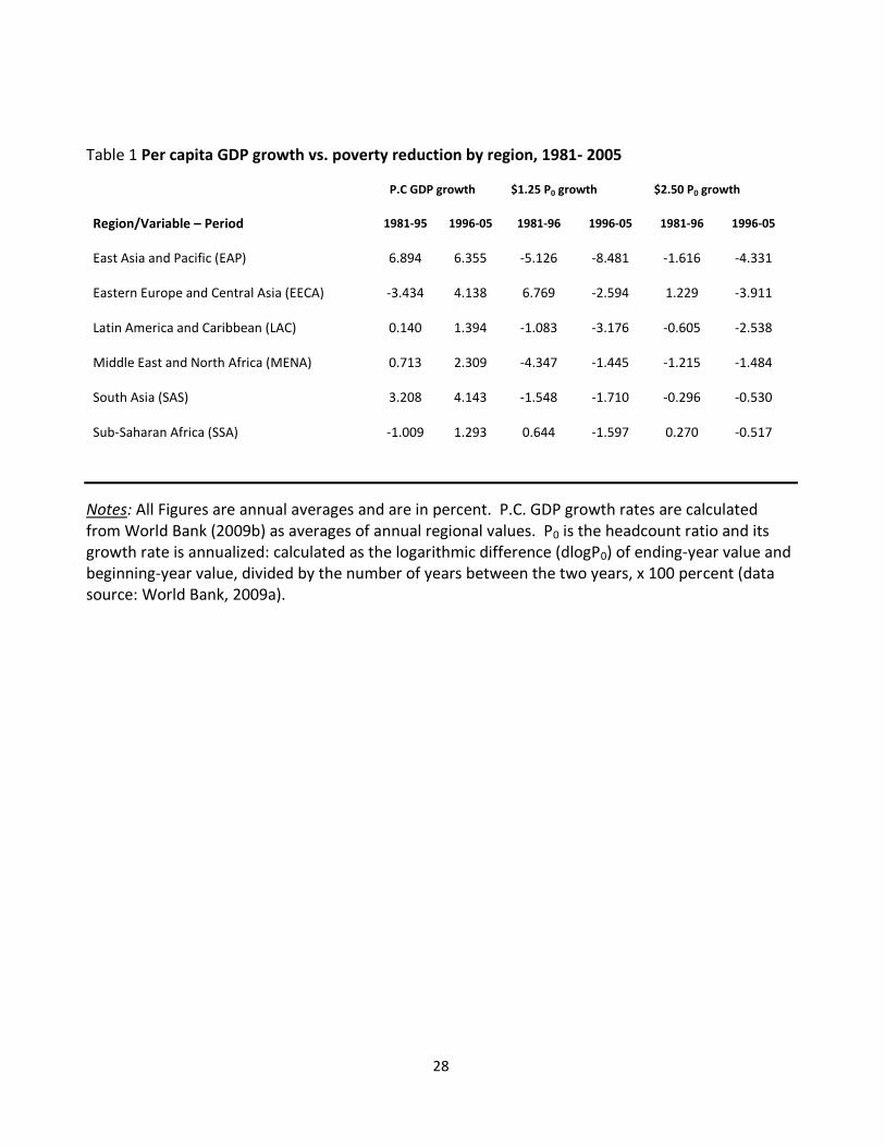
To provide a general picture of how GDP growth rates may have been translated to poverty reduction since 1981, and particularly since the mid-1990s, we report in Table 1 the 1981-95 and 1996-2005 regional averages of per capita GDP growth and annualized growth rates of the headcount ratio based on the USD1 (USD1.25) and USD2 (USD2.50) standards4. The six regions are: East Asia and the Pacific (EAP), Eastern Europe and Central Asia (EECA), Latin America and the Caribbean (LAC), Middle East and North Africa

(MENA), South Asia (SAS), and sub-Saharan Africa (SSA).

[See all Tables from page 28 onwards.]

Several observations are in order. First, EAP registered spectacular per capita GDP growth, resulting in substantial poverty reductions over both sub-periods. Second, for EECA, the large per-capita GDP decline in the first period seems to account for the considerable increase in the poverty rate during that period; conversely, a substantial decrease in the poverty rate during the latter period accompanied that period’s strong economic growth. Third, considerable poverty reduction seems to

4 The annualised growth rates are calculated as the logarithmic differences between the poverty rates between 1996

and 2005, divided by the frequency of the intervening years.

9

have resulted from the rather modest GDP growth in LAC, especially during the latter period. Fourth, the moderate GDP growth of MENA was transformed to an appreciable poverty reduction in the early period, but the stronger growth in the latter period resulted in only a modest poverty reduction.

In the case of SAS, the substantial GDP growths in both sub-periods appear to have been translated to only moderate poverty reduction. Finally, for SSA the per capita GDP decline in the first period seems to account for the poverty rise during that period; conversely, poverty reduction in the latter period appears to have resulted from appreciable economic growth that period. Interestingly, the rates of poverty decline since the mid-1990s were about the same between the SSA and SAS, despite the latter’s much stronger GDP growth.

The above observations suggest regional differences in the responsiveness of poverty to GDP growth. For example, the finding of SAS’s relatively modest poverty reduction despite strong GDP growth in both sub-periods points to three possible explanations: (1) GDP growth did not sufficiently reflect actual income growth;5 (2) the responsiveness of poverty to income growth was weak; or (3) inequality may have increased. In contrast, the substantial reductions in poverty in EAP seem as expected, given the region’s spectacular growth. Understanding such inter-regional discrepancies in the transformation of GDP growth to poverty reduction, however, would require a deeper analysis of the poverty function, which we shall conduct in a subsequent section.

B. Poverty trends by region and for the ‘emerging giants’

To shed further light on the trends in the global picture of poverty, Table 2 presents in greater detail the regional evidence corresponding to the two poverty standards. In addition to the six regions, evidence is provided for the two most populous countries and ‘emerging giants’, China and India. For the six regions, the Table presents USD1.25 and USD2.50-standard headcount ratios for 1981, 1996 and 2005; these years span the 1981-2007 period for which country data are sufficiently reliable to produce the regional averages (World Bank, 2009a)6. Table 2 also reports statistics for these same years in the case of China. Evidence is presented for both rural and urban sectors as well as for the overall economy, computed as a population-weighted mean of the two sectors. For India, the years are 1983, 1994 and 2005, since these are the specific years spanning the 1981-2007 period for which relatively reliable survey data are available.

Reported in Table 2 are the annualized means of the changes in levels (percentage changes) and logarithmic differences (growth rates) in the poverty rates for the two sub-periods: early 1980s to mid-1990s and mid-1990s to 2005. These sub-periods are the first decade and a half and the last

5 ‘Income’ refers to the PPP-adjusted income from World Bank (2009), derived from per capita consumption from

household surveys or the interpolated private consumption from national accounts (Chen and Ravallion, 2008). 6 Regional poverty data are available for other years over 1981-2007 as well, but we have opted to interpolate between the selected years for the growth rates, in order to provide comparable analysis for the two sub-periods of analysis.

10

decade, respectively, with the latter period corresponding roughly to when developing countries generally grew substantially and faster than the advanced countries, as hitherto observed above.

Consider first the poverty trends at the USD1.25 standard. In 2005, poverty was highest in SSA and lowest in MENA and EECA. Between 1981 and 2005, it declined for all regions except EECA, where the initial value was rather small to begin with. Among the remaining regions, in percent (logarithmic change) terms, the greatest reduction in poverty is observed for EAP, followed by MENA, LAC, SAS and SSA, in that order. There are differences across time, though. During 1981-1996, for example, poverty increased for EECA and SSA but declined for all other regions. In 1996-2005, however, poverty decreased for all regions. The largest decline (in percent terms) was in EAP, followed by LAC and EECA, then by SAS, SSA and MENA. Moreover, the fall in poverty was faster in the latter period in all regions except MENA, which had a low level of poverty to start with. Thus, for all practical purposes, the last decade has witnessed reductions in the poverty rate, at least at the USD1.25 level, for all regions of the world.

In terms of the ‘emerging giants’, China’s poverty rate at the USD1.25 level fell in both sub-periods but faster in the second period for both the urban and rural sectors. India’s poverty also fell in both periods but more rapidly in the second period for only the rural sector, though the decline was sufficient for translating into a faster poverty reduction for the whole economy. China’s poverty also fell much faster than India’s in both sub-periods, overall and by sector. Furthermore, poverty in China decreased substantially more in the urban than in the rural sector, further exacerbating the urban-rural difference over time. For India, the decline was faster in the urban area during the first period, but the reverse was the case in the latter period. It is also noteworthy that poverty fell less in India than in the SAS region generally for each of the sub-periods. Moreover, poverty reduction in India during the latter period was about the same as that in SSA, despite the fact that India’s GDP growth was much faster than SSA’s.

We now consider poverty trends at the USD2.50 standard. The observations are generally similar to those above for the USD1.25, though there are some differences as well. During the entire 1981-2005 period, poverty declined the most in EAP and the least in SSA. It rose during 1981-1996 for EECA and SSA but fell in all regions during 1996-2005. The lowest declines in the latter period were in SAS and SSA (about equally), though the poverty rate in 2005 was highest in SAS, not in SSA, contrary to the finding at the USD1.25 standard.

Considering the two emerging giants, again, poverty at the USD2.50 standard fell faster in the second period for both China and India. Furthermore, China’s poverty declined much faster than India’s during both sub-periods. The poverty rate at this standard for China also fell more rapidly in urban than in rural areas in both periods. India’s poverty similarly fell faster in the urban area than in the rural sector in both periods, in contrast with the above observation at the USD1.25 level where the decline was faster in the rural area in the latter period. Furthermore, in 2005 India’s poverty at the USD2.50 standard was slightly higher than that in SAS as a whole and was about

11

5 percentage points higher than that in SSA. Finally, the decline in India’s poverty was slightly less than that in either SAS or SSA during the latter period.

C. Current poverty rates: global evidence by country

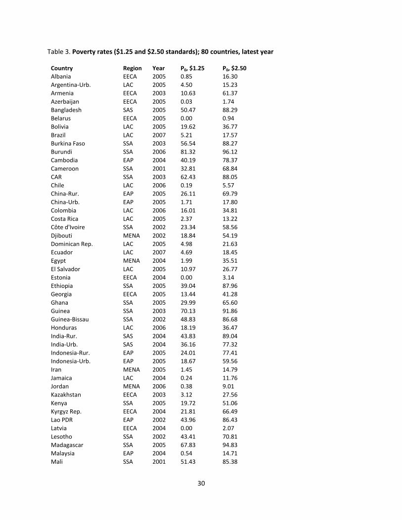
For the 80 countries that have sufficient data for the early-mid-1990s and also for the 2000s, we first examine the distributions of their poverty rates in the latest year in the 21st century for which data are available7. This is done in Table 3. We find that at the USD1.25 standard, the poverty rate ranges from 0.0 per cent in Belarus (2005), Estonia (2005) and Latvia (2005) to 88.5 per cent in Tanzania (2000), with a median of 17.9 per cent.

In terms of the emerging giants, China’s urban and rural poverty rates at the USD1.25 standard are 1.7 per cent and 26.1 per cent, respectively, with the latter above the ‘global’ median of 17.9 per cent. Thus, extreme poverty has become essentially a rural phenomenon in China.

In the case of India, at 43.8 per cent and 36.2 per cent, respectively, the rural and urban poverty rates are well above the ‘global’ median. It appears then that for India the strong GDP growth in the more recent period may not have similarly reduced poverty. Similar observations hold for the USD2.50 poverty standard. Here the range is from 0.9 per cent in Belarus to 98.2 per cent in Tanzania, with a median of 47.7 per cent. For the emerging giants, China’s respective urban and rural poverty rates are 17.8 per cent and 34.8 per cent, which are both below the ‘global’ median. In contrast, at 77.3 per cent and 89.0 per cent, respectively, India’s urban and rural poverty rates are both substantially above the ‘global’ median, as in the case at the USD1.25 standard.

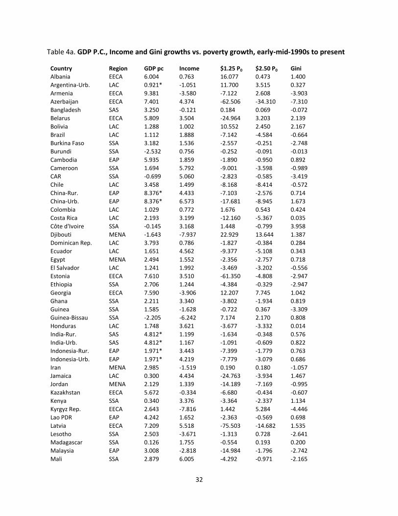
D. Growth vs. poverty reduction by country, early-mid-1990s to present For the global sample of 80 countries Table 4a presents, over the early-mid-1990s to the present, data on per capita GDP and income growths, and on the growth of poverty at both the USD1.25 and USD2.50 standards. Also reported in the Table are data on the growth of inequality, represented by the Gini coefficient. The goal here is to assess how GDP growth or income growth may have been translated to poverty reduction at the country level. For many of these countries, reasonably strong

7 This selection criterion is intended to ensure that we can also consistently analyse changes in the poverty rate over

time for the same set of countries. The wider interval of early-mid-1990s is used as the starting point in order to include as many countries as possible in the sample, for a number of the countries had data in the early but not in the mid 1990s, and vice versa. Note that the average over the starting period could not be used due to the need for annualizing. The closest year to 1996 with data within 1990-1996 is selected as the starting year, as most of the countries have data for the mid-1990s but not for the earlier 1990s. The latest year in the 21

st century for which data are available is used as

the end-period for the analysis.

12

GDP growth seems to have been translated to substantial poverty reduction: (e.g. Azerbaijan, Brazil, Cameroon, Chile, China, Costa Rica, Ecuador, Egypt, El Salvador, Estonia, Ghana, Honduras, Indonesia, Jamaica, Jordan, Kenya, Latvia, Mali, Mauritania, Moldova, Pakistan, Poland, Romania, Russian Federation, Senegal, Sri Lanka, Swaziland, Thailand, Tunisia, Uganda, Ukraine, and Vietnam). In several other countries, however, strong GDP growth was accompanied by only modest poverty reduction, either because the growth did not result in similar increases in income or because inequality increased to thwart the transformation process (e.g., Albania, Georgia, India, Iran, Kyrgyz Republic, Mongolia, and Yemen). As one of the major emerging economies, India is of particular interest here. Its per-capita GDP grew at a stellar annual average rate of nearly 5.0per cent, and yet the average annual rate of poverty reduction was only 1.6 per cent and 1.1 per cent for the rural and urban sectors, respectively. Furthermore, although the Gini coefficient increased during that period, it was quite modest8. Apparently, the main culprit appears to be the minimal increase in income resulting from the strong GDP growth (Table 4a). But even if income growth sufficiently reflected GDP changes, there is the issue of the transformation of income growth to changes in poverty. This process is likely to differ by country. To better illustrate this country-specific linkage, we order by deciles the 80 sample countries with respect to their GDP and income per capita growth rates, on the one hand, and the poverty rates, on the other. The results are summarised in Table 4b as country ‘poverty transformation efficiency’ vectors; the first two coordinates indicate the decile rankings of per-capita GDP and income growths, respectively, and the last two coordinates the respective growths of the USD1.25 and USD2.50-level poverty rates9. For example, the (2, 8, 10, 9) vector for Albania means that the country was in the 2nd and 8th top deciles for per-capita GDP and income growths, respectively, but in the 10th and 9th top deciles for the USD1.25 and USD2.50 poverty standards, respectively. Hence, Albania performs rather poorly in transforming GDP growth to poverty reduction, with the rather weak income reflection of GDP as the main explanation. With respect to the emerging giants, a similar observation can be made about India, in that its stellar performance on GDP growth is poorly translated to income growth and poverty reduction, though income growth seems to fairly reflect its record of poverty reduction. For China, on the other hand, there appears to be a fair reflection by income growth of GDP growth, though the country’s performance on poverty reduction, relative to its growth performance, is somewhat below par. In contrast, countries like Azerbaijan, Jamaica, Latvia, Mexico, Poland, the Russian Federation, Tunisia, Ukraine and Venezuela do quite well in transforming their GDP growths to poverty reduction. And, in the other extreme, Georgia’s GDP growth places it in the top decile but the country performs among the worst decile on income and poverty reduction.

8 At 0.58 and 0.82 the respective mean annualized growth rates of the Gini coefficient for the rural and urban sectors

are less than one-half percentage point above the mean or median of the sample of 80 countries (Table 4a). 9 A lower-number decile for the GDP or income growth indicates a grouping of higher-growth countries, while a lower-number decile for the poverty rates indicates a grouping of larger poverty-reduction countries.

13

3. Transforming growth to poverty reduction – a quantitative assessment

The above discussion suggests that differences in regional or country experiences in poverty reduction may be attributable in considerable part to disparities in growth rates. Consistent with an important strand of the literature (e.g. Dollar and Kraay, 2002), therefore, growth is a powerful force for reducing poverty. Nonetheless, as the above discussion also shows, there are many countries where GDP or income growth may not adequately be translated to poverty reduction. For example, a number of countries registered only modest poverty reductions despite strong growth, and conversely.

An increasing number of studies have shown, for example, that inequality may play a crucial role in the transformation of growth to poverty reduction (e.g. Adams, 2004; Bourguignon, 2003; Easterly, 2000; Epaulard, 2003; Fosu, 2008, 2009; Kalwij and Verschoor, 2007; Ravallion, 1997). In particular, Fosu (2009) finds that initial inequality differences can lead to substantial cross-country disparities in the income-growth elasticity of poverty not only between SSA and other regions but also even among SSA countries. In general, less inequality would imply a greater (absolute) value of the elasticity, so that a larger amount of poverty reduction would emanate from a given level of growth10.

We explore herein the global evidence on the transformation of income growth to poverty reduction, with inequality serving as an important intermediation factor. Following Bourguignon (2003), Epaulard (2003), Fosu (2009), and Kalwij and Verschoor (2007), we estimate the following income-poverty transformation equation, which can be derived from the assumption that income is log-normally distributed11.

(1) p = b1 + b2y + b3yGI + b4y(Z/Y) + b5g + b6 gGI + b7 g(Z/Y) + b8GI + b9Z/Y

where p is the growth in the poverty rate, y is income growth, g is growth in the Gini coefficient, GI is the initial Gini coefficient (expressed in logarithm), Z/Y is the ratio of the poverty line Z to income Y (expressed in logarithm), and bj (j=1,2,…,9) are the respective coefficients to be estimated.

The coefficient b2 is anticipated to have a negative sign, so that an increase in income growth should reduce poverty growth, ceteris paribus. In contrast, b3 is expected to be positive, for a higher level of initial inequality would decrease the rate at which growth acceleration is transformed to poverty reduction. The coefficient b4 should be positive as well, consistent with the hypothesis, based on the lognormal income distribution, that a larger income (relative to the poverty line) would have

10 Note, though, that a perverse outcome is conceivable, since redistributing from the non-poor to the poor in a very

low-income economy could actually increase the poverty rate, so that less inequality might engender greater poverty in such countries; see Fosu (2010), for example, for an elaboration of this point. 11 For details of the derivation, see Bourguignon (2003), Epaulard (2003), and Kalwij and Verschoor (2007). Note that other specifications also resulted in similar results (see Fosu, 2009).

14

associated with it a higher income-growth elasticity12. (Bourguignon 2003; Epaulard, 2003; Fosu, 2009; and Kalwij and Verschoor, 2007)

The sign of b5 is theoretically positive, for a worsening income distribution is expected to increase poverty, ceteris paribus. In contrast, b6 cannot generally be signed; however, it would be negative if there is a diminishing effect of the poverty-increasing effect of rising inequality. The sign of b7 would also be negative, as in a relatively low-income economy (high Z/Y) improving income distribution (lowering g) might exacerbate poverty by increasing the likelihood of more people falling into poverty. Finally, b8 and b9 are likely to be positive; rising initial inequality or increasing the poverty line relative to income should, ceteris paribus, exacerbate poverty, respectively, though these coefficients do not affect the income or inequality elasticity of poverty. (Bourguignon 2003; Epaulard, 2003; Fosu, 2009; and Kalwij and Verschoor, 2007)

From equation (1), the respective income and inequality elasticities are obtained as: (2) Ey = b2 + b3GI + b4Z/Y

(3) Eg = b5 + b6GI + b7Z/Y

Hence, given the above expected signs, Ey and Eg are anticipated to be negative and positive, respectively, so that rising growth should decrease the growth of poverty, while inequality increases would exacerbate poverty increases. It is conceivable, though, that perverse signs of the elasticities could occur. For example, in a highly unequal (high GI) and low-income (high Z/Y) economy, the magnitude of the combined positive-signed b3 and b4 could actually overwhelm the magnitude of the negative-signed b2. Similarly, in such an economy, Eg could be negative. These two elasticities, which are estimated next, would be crucial in determining what happens to poverty reduction over time in a given economy.

4. Data, estimation and results

The data used in the present analysis are derived from the most recent World Bank global database13 which yields at most 392 usable unbalanced panel observations involving some 123 countries over 1977-200714. Separate regression equations are estimated for the USD1.25 and USD2.50 poverty standards. Summary statistics by region for the poverty rates, income inequality (Gini coefficient) and mean income are reported in the appendix Table A115. Note that the averages

12 We shall ignore the sign and adopt the convention of referring to the income elasticity by its magnitude. 13 See World Bank, 2009. 14 There are 320 and 392 usable observations for the $1.25 and $2.50 poverty standards, respectively. 15 We do not report the summary data for the growth rates because they would not be reliable, as the periods are not

standardized across observations. That is, growth rates are calculated over different period lengths depending on data availability, so that their averages are not technically reliable.

15

are non-weighted and, due to missing data, sample composition may vary over time. Hence, only the statistics for the entire sample period are reported for the various regions. Note, nonetheless, that the respective regional sample poverty rates presented in Table A1 are strikingly close to the population-weighted values shown earlier in Table 2.

Using the above unbalanced panel data, equation (1) is estimated by applying three procedures: random-effects (RE), country fixed-effects, and generalised method of moments (GMM)16. Following Kalwij and Verschoor (2007), various versions of the equation are estimated, with special attention paid to the regional effects. Note that all the level variables used in the estimation are expressed in (natural) logarithm, while the growth variables are the logarithmic changes. Due to its ability to control for possible endogeneity of the explanatory variables17, the GMM results are selected as the most preferred and are reported in the text as Tables 5.1 and 5.2, for the USD1.25 and USD2.50 standards, respectively. The regression results seem rather similar between the two poverty standards, and show that all the estimated coefficients are as expected. The estimates also suggest that any variation in the income and inequality elasticities across regions, and presumably across countries, is mainly attributable to differences in attributes. In particular, model (5) suggests that once the poverty function is fully specified, there are little regional differences with respect to the income elasticity, similarly to the finding in Kalwij and Verschoor (2007)18. Based on results from this model in Tables 5.1 and 5.2, we use equations (2) and (3) to estimate the income and inequality elasticities. For the USD1.25 poverty standard we obtain: (4) Ey = -9.757 + 2.307 GI + 1.333 Z/Y

(5) Eg = 14.391 -3.649 GI – 2.754 Z/Y

And, for the USD2.50 poverty standard, we obtain:

(6) Ey = -8.178 + 1.902 GI + 0.912 Z/Y

(7) Eg = 5.336 – 1.155 GI – 1.513 Z/Y

It is deducible from equations (4) and (6) that the income elasticity (in absolute value) decreases with initial inequality, GI, and with Z/Y. Hence, regions/countries with lower initial levels of

16 Only the GMM results are, however, reported here. The other (FE and RE) estimates are very similar to the GMM and

can be made available by the author upon request. 17 Because income and inequality may be endogenously determined GMM, which controls for endogeneity, may be

particularly applicable here. 18 The Hansen J test suggests that the instruments are generally ‘valid’ in all the models except for model (3). An F test

furthermore indicates that one cannot reject the null hypothesis that the coefficients of the regional variables are not different between models (4) and (5), a result that is qualitatively buttressed by the virtual across-model equality of SEE and uncentred R

2, especially in Table 5.1.

16

inequality and higher incomes relative to the poverty line would exhibit larger poverty responsiveness to income changes. Similarly, from equations (5) and (7), we deduce that regions/countries with lower initial inequality levels or larger incomes relative to the poverty line would also possess high values of the inequality elasticity. Conversely, low-income, high-inequality localities would have both low (absolute-valued) income and inequality elasticities.

Estimates of the income and inequality elasticities, generated from equations (4) - (7), are reported for the various regions in Table 6, for both the USD1.25 and $2.50 poverty standards.19 Since the country composition likely changes over time, the sample statistics for the sub-periods may not be reliable. We, therefore, focus on the elasticity estimates for the overall 1981-2007 period. According to the income elasticity estimates, the greatest responsiveness of poverty to income growth is exhibited by EECA, followed by LAC and MENA with similar values, then by EAP, and followed closely by SAS, with the least value displayed by SSA. These results appear to hold for both poverty standards; though, as to be expected, the respective elasticities are lower for the USD2.50 poverty standard than for the USD1.25. The differences in income elasticity by region seem to be driven by differences in inequality, but also by disparities in income levels. For example, for both poverty standards, the highest elasticity enjoyed by the EECA is attributable to the fact that the region exhibits both the lowest initial inequality and the highest mean income. LAC’s moderate elasticity is driven by high mean income and high inequality, which tend to counteract one another, while MENA’s moderate elasticity is attributable to both modest income and moderate inequality. Meanwhile, EAP’s and SAS’s moderate-to-low elasticity (absolute) values are explained by their relatively low mean incomes and moderate levels of inequality. Finally, SSA exhibits the lowest income elasticity, thanks to both its low income and high inequality.

The regional comparison of inequality elasticity estimates, also shown in Table 6, is similar between both poverty standards and mirrors the pattern observed for the income elasticity. That is, EECA exhibits the largest value, suggesting that its poverty rate is the most prone to distributional changes in income distribution, followed by LAC and MENA, then by EAP, and subsequently by SAS, with SSA displaying the least responsiveness. As in the case of the income elasticity, EECA’s high value of the inequality elasticity is attributable to both its low level of inequality and high income; LAC’s moderate value results from its high income counteracted by high inequality, while MENA’s moderate elasticity derives from both modest income and moderate inequality. EAP’s and SAS’s low-to-moderate values are attributable to their relatively low incomes and moderate levels of inequality. Finally, the smallest estimated value of the inequality elasticity for SSA is explained by high inequality and low mean income.

19 Elasticity estimates based on the FE and RE models are similar to those of the GMM; however, they are not reported here for reasons of parsimony but can be made available by the author upon request.

17

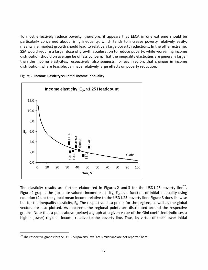
To most effectively reduce poverty, therefore, it appears that EECA in one extreme should be particularly concerned about rising inequality, which tends to increase poverty relatively easily; meanwhile, modest growth should lead to relatively large poverty reductions. In the other extreme, SSA would require a larger dose of growth acceleration to reduce poverty, while worsening income distribution should on average be of less concern. That the inequality elasticities are generally larger than the income elasticites, respectively, also suggests, for each region, that changes in income distribution, where feasible, can have relatively large effects on poverty reduction.

Figure 2. Income Elasticity vs. Initial Income Inequality

Income elasticity, Ey, $1.25 Headcount

Global

Glo

ba

l

EA

P

EE

CA

LA

C

ME

NA

SA

S

SS

A

0,0

2,0

4,0

6,0

8,0

10,0

12,0

0 10 20 30 40 50 60 70 80 90 100

Gini, %

Ey

The elasticity results are further elaborated in Figures 2 and 3 for the USD1.25 poverty line20. Figure 2 graphs the (absolute-valued) income elasticity, Ey, as a function of initial inequality using equation (4), at the global mean income relative to the USD1.25 poverty line. Figure 3 does likewise but for the inequality elasticity, Eg. The respective data points for the regions, as well as the global vector, are also plotted. As apparent, the regional points are distributed around the respective graphs. Note that a point above (below) a graph at a given value of the Gini coefficient indicates a higher (lower) regional income relative to the poverty line. Thus, by virtue of their lower initial

20 The respective graphs for the USD2.50 poverty level are similar and are not reported here.

18

inequality levels, SAS, EAP and SSA would have all exhibited higher income and inequality elasticities than LAC, respectively, were it not for LAC’s higher income.

Figure 3. Inequality Elasticity vs. Initial Income Inequality

Inequality elasticity, Eg, $1.25 Headcount

Global

Glo

ba

l

EA

P

EE

CA

LA

C

ME

NA

SA

S

SS

A

0,0

2,0

4,0

6,0

8,0

10,0

12,0

14,0

16,0

18,0

0 10 20 30 40 50 60 70 80 90 100

Gini, %

Eg

These regional estimates, however, confound the intra-regional heterogeneity. In the case of SSA, Fosu (2009) finds a considerable variation in both the income and inequality elasticities among countries. As the author argues, SSA countries with very high levels of inequality may require a relatively large emphasis on income distribution as a way of boosting the income elasticity via decreasing inequality. Thus, the appropriate approach would be rather country-specific.

Table A2 in the appendix presents estimates of the income and inequality elasticities for all the 123 countries in the World Bank database for both the USD1.25 and USD2.50 poverty standards. These estimates are based on the latest year for which a given country has data and may, therefore, not be strictly comparable across countries. Nevertheless, we can draw some fairly general conclusions.

19

First, the income elasticity estimates are nearly all negative21, suggesting that income growth would reduce poverty for practically all countries for both poverty standards. Second, nearly all the inequality elasticity estimates are positive22; thus, increases in inequality would, in general, raise poverty. Third, the estimated elasticites at the USD1.25 standard are, respectively, larger than at the USD2.50 standard, as to be expected, since moving people out of poverty at the higher poverty line would require greater effort. Fourth, consistent with the above regional observations, the elasticities are generally largest for the EECA countries and lowest for the SSA countries. Indeed, the hitherto observed regional orderings appear to hold23. Fifth, as earlier observed above for the regions, the inequality elasticity seems to be appreciably larger than the respective income elasticity at the country level, especially at the USD1.25 poverty level; however, this observation does not seem to hold generally at the USD2.50 standard24.

We now focus on the results for the two emerging giants. China exhibits much larger income and inequality elasticities in the urban than in the rural sector. This finding holds for both poverty standards and implies that economic growth in the urban area would be more readily translated to poverty reduction, but then poverty in that sector would also be relatively susceptible to the poverty-increasing effect of rising inequality. In India, however, the reverse appears to be the case, with the income and inequality elasticities slightly larger in the rural area generally25. Finally, India’s estimated elasticities are appreciably less than China’s, respectively, especially for the urban sector.

5. Explaining poverty reduction by country, early-mid-1990s to present

A main objective of the current paper is to examine how the recent substantial growth of developing countries, especially relative to the advanced economies, may have been translated to human development such as poverty reduction. The above elasticity estimates for the 123 countries inform us of the expected reduction in poverty in response to increasing growth in income or in inequality for the particular year for which a given elasticity estimate is provided. For current policy purposes, these estimates are the most pertinent.

To meet the above objective of explaining recent growth performance and poverty reduction, however, we need to situate the elasticity estimates in the relevant period. The income and 21 The only exception is Liberia and for the $2.50 standard; the result is attributable to the country’s low mean income that was appreciably below the poverty line. 22 The exceptions are: Liberia, for both of the poverty standards; and Burundi, Guinea, Malawi, Mozambique, Rwanda,

Tanzania and Zambia, where the mean incomes are appreciably below the $2.50 poverty line. Note, however, that the magnitudes of these negative estimates are generally rather small. 23 The few exceptions include Haiti and Nepal whose income elasticity estimates seem lower than the average for SSA, for instance. 24 This difference in results between the two poverty standards is attributable to the much larger partial effect of the

inequality on poverty at the USD1.25 than at the USD2.50 level [compare intercepts in equations (5) and (7) with the intercepts of equations (4) and (6)]. 25 The only exception is the estimated inequality elasticity at the USD2.50 level, which is slightly larger for the urban sector.

20

inequality elasticities are, therefore, recomputed over the early-mid-1990s for the select global sample of 80 countries, using equations (4) – (7).26 The results are presented in Tables A3.1 and A3.2 of the appendix, respectively, for the USD1.25 and USD2.50 standards27. Also reported are the mean annualised growths in income, inequality and poverty, as we are interested in the extent to which the observed poverty changes might be decomposable into income and inequality factors.

According to Tables A3.1 and A3.2, the income elasticity estimates are generally negative while those of the inequality elasticity are positive, as anticipated28. Hence, income increases or inequality decreases in a given country would be translated to poverty reduction over the period of the analysis: the early-mid-1990s to the present. Note from these Tables also that the magnitudes of the elasticites tend to be, respectively, larger for the USD1.25 than for the USD2.50 standard, as to be expected.

To shed further light on the differential abilities of the various countries in transforming economic growth to poverty reduction since the early-mid-1990s, the income and inequality elasticity estimates are ordered by country in Tables 7.1 and 7.2 for the USD1.25 and USD2.50 poverty standards, respectively. These results show that a country with a high (absolute) value of income elasticity also tends to exhibit a high value of inequality inelasticity, as already observed above for the ‘current-year’ estimates29. This is primarily because countries with large incomes (relative to the poverty line) displayed high magnitudes of both elasticities [equations (2) and (3)]. The implication of the result, as earlier observed, is that lower-income countries would require greater income

26 As explained earlier, the 80 countries were selected according to the following criteria: In each case, the starting date is the latest year for which there is data within 1990-96, and the ending date is the latest year within 2000-2007. The selection criteria are designed to maximize the number of included countries while providing a reasonable degree of period standardization. Although the current method does not achieve perfect comparability across countries, it represents a reasonable attempt to explain recent poverty reduction by country for a large global sample. Given differences of year-coverage across countries, all statistics are annualized by dividing by the number of years between the end points for each country. 27 These are the values reported under columns A and C of Tables A3.1 and A3.2, respectively. Note that the estimates

under columns B and D are illustrative only; they are indicative of the importance of initial inequality alone, with the role of income suppressed. 28 For the USD1.25 standard, CAR appears the only exception with a positive value for the income elasticity; at the

USD2.50 standard, the two exceptions are CAR and Guinea. There are several exceptions for the inequality elasticity estimates, though: CAR, Guinea, Mali, Mozambique, and Swaziland for the USD1.25 standard (column C of Table A3.1); and Burkina Faso, Burundi, CAR, Guinea, Madagascar, Mali, Mozambique, Niger, Swaziland and Zambia for the USD2.50 standard (Table A3.2, column C). The main rationale for the ‘perverse’ results is that these countries had appreciably lower mean incomes than the poverty line, hence the greater preponderance of exceptions under the USD2.50 standard. 29 Note that countries with the highest (absolute) values of the income elasticity are in decile 1, while those with the

highest values of inequality elasticity are in decile 10. This convention is adopted in order to highlight the fact that the effects of income and inequality on poverty changes generally had opposite signs. Note also that the absolute magnitudes of the elasticities could not be used here, since some countries may have the opposite sign, as indicated above.

21

growth for a given expected poverty reduction; however, these countries would also need to be less concerned about inequality increases, and conversely. We now present in Tables 8.1 and 8.2, for the USD1.25 and USD2.50 standards, respectively, the evidence on the relative contributions of income and inequality changes to poverty reduction, by country, during the early-mid-1990s to the present. For better clarity of interpretation, this reporting is done separately for countries exhibiting poverty reduction and for those experiencing increases in poverty. The results show that, on average, income growth primarily drove both poverty declines and increases. Among countries experiencing poverty reduction, income growth was responsible for practically 100 per cent of the predicted poverty reduction for both poverty standards. And, in the case of countries exhibiting poverty increases, negative income growth contributed on average 74 per cent and 85 per cent of the predicted poverty increases for the USD1.25 and USD2.50 standards, respectively.

There are, however, major differences across countries. Brazil, for instance, experienced substantial poverty reduction, thanks to the favorable changes in both income and inequality (increasing income and decreasing inequality), though a larger proportion emanated from income growth: 63 per cent versus 37 per cent for either poverty standard (Tables 8.1 and 8.2). Azerbaijan’s poverty decline also resulted from both income growth and a decrease in inequality, but with the primary reduction actually coming from income distribution: 30 (39) per cent for income versus 70 (61) per cent for inequality for the USD1.25 (USD2.50) standard.

Rising inequality seems, however, to have thwarted the poverty-reduction efforts of increasing income in a number of countries. China’s tremendous poverty decline would have been even higher without an increase in inequality. The country’s USD1.25 poverty rate in the rural sector would have been predicted to have fallen annually by 7.9 per cent instead of 6.6 per cent (Table 8.1). More dramatically, rising inequality in the urban sector reduced the rate of poverty declines by some 6.7 percentage points annually (Table 8.1). Similarly at the USD2.50 poverty level, increases in inequality considerably reduced the rates of predicted poverty reduction in both sectors of the economy (Table 8.2).

Indeed, rising inequality led to increases in poverty overall in several countries, despite the poverty-reduction impact of income growth, such as in: Albania, Bolivia, and Cote d’Ivoire (Table 8.1). In a number of countries, however, reduced growth was responsible for rising poverty, notwithstanding increasingly favorable income distribution over time, including: Armenia, Iran, Kyrgyz Republic, Mongolia, and Yemen (Table 8.1). And, in many cases, both income levels and their distribution worsened to engender a worsening poverty picture, such as in: Argentina-urban, Djibouti, Georgia, Guinea Bissau, South Africa, and Tanzania for both poverty standards (Tables 8.1 and 8.2).

22

6. Some country simulation illustrations

India: Linkage between GDP and income matters.

As already discussed above, India’s relatively modest poverty reduction since the mid-1990s resulted primarily from the modest income growth despite its substantial GDP growth. If income had grown at the same rate as (per capita) GDP of 4.8 per cent annually (Table 4a), then the (predicted) contribution of growth to poverty reduction (USD1.25 standard) would have been more than 10.0 per cent30, instead of less than 2.5 per cent, annually (Table 8.1).

Bolivia: Rising inequality hurts.

Bolivia’s USD1.25 poverty rate has risen by 10.5 per cent annually since the mid-1990s, despite a 1.0 per cent annual income growth, thanks to a worsening income distribution (Table A3.1). Suppose income inequality had not changed. Then (predicted) poverty would have fallen annually by 3.2 per cent instead of rising by 7.6 per cent (Table 8.1).

Russian Federation: Falling inequality helps.

The (USD2.50) poverty rate of the Russian Federation fell by 12.3 per cent (7.9 per cent predicted) annually as of the mid-1990s despite its meagre annual income growth rate of 0.54 per cent, because its income inequality fell by 2.3 per cent annually (Table A3.2). In the absence of this favourable income distribution, poverty would be predicted to fall by only 1.1 per cent (Table 8.2).

Burkina Faso vs. Chile: Low income is a bane; high income is a boon.

Burkina Faso (BF) had a lower level of inequality than Chile did (Gini coefficient of 0.51 vs. 0.55), its inequality has decreased much faster than Chile’s since the mid-1990s (2.75 per cent vs. 0.57 per cent annually), while both countries grew equally at 1.5 per cent annually (sources: Table A3.1 and World Bank, 2009a). Yet, Chile managed to reduce (USD1.25) poverty by 8.2 per cent annually compared with BF’s of 2.6 per cent (Table A3.1). This difference is due to BF’s relatively low income (USD40.8 vs. USD387.2 monthly). If BF had enjoyed the same level of income as Chile, its respective income and inequality elasticities would have been –3.82 and 6.5131, instead of –0.794 and 0.260 (Table A3.1); and, predicted poverty reduction would be 23.63 per cent32, compared with the currently predicted reduction of 1.94 per cent (Table 8.1).

30 That is, 4.8(-2.2) = -10.6 for rural and 4.8(2.1) = -10.1 for urban.

31 That is, based on equations (4) and (5), respectively, -9.757 + 2.307(ln 51) + 1.333 ln(37/387.2) = -3.82 and 14.391 –

3.649 (ln 51) – 2.754 ln(37/387.2) = 6.51. 32 That is, (-3.82)(1.5) + (6.51)(-2.75) = -23.63.

23

Conclusion

The current study has shed light on the transformation of economic growth to poverty reduction in developing countries during the more recent period when these countries have generally experienced relatively strong growth. Using the most recent comparable data from World Bank (2009a), we first presented evidence on GDP growth, income growth, and poverty reduction since the 1980s for the various regions of the world: EAP, EECA, LAC, MENA, SAS and SSA. The regional evidence is provided for two periods: 1981 to mid-1990s and mid-1990s to the present, with a focus on the latter sub-period when the recent acceleration of the GDP growth gap between developing countries and developed countries appears to have begun. Also examined is a global sample of 80 countries for which available data would permit reasonably comprehensive comparative analysis.

The paper finds that, except for EECA, poverty measured at both the USD1 (USD1.25 2005 PPP-adjusted income) per day and USD2 (USD2.50 2005 PPP-adjusted income) per day decreased for all regions during the entire 1981-2005 period. Similarly, with the exception of MENA, all regions exhibited greater reductions in poverty in the later sub-period. Two regions, EECA and SSA, showed increases in poverty rates during the earlier sub-period; however, poverty has declined for all regions since the mid-1990s.

The greatest poverty reduction during 1981-2005 occurred in EAP, LAC, EECA, SAS, SSA and then MENA, in that order for the USD1.25 standard; at the USD2.50 standard, the order was EAP, EECA, LAC, MENA, then SAS and SSA (about the same). Qualitatively, the observed patterns of poverty decline at the regional level appear to correspond well with the GDP growth over both sub-periods. During 1981-1995, EECA and SSA experienced rising poverty rates in response to negative per capita GDP growth, while the remaining regions registered both positive GDP growth and poverty reduction.

In the later sub-period, per capita GDP increased for all regions. Furthermore, those regions experiencing higher GDP growth also tended to exhibit greater declines in poverty. The rate at which GDP growth was translated to poverty reduction, however, appears to differ across regions. The rate seemed rather low for SAS, especially at the USD2.50 standard. This weak transformation rate appears to emanate from a poor relationship between GDP and income growths.

As the two most populous nations and ‘emerging giants’, the performance of China and India has received special attention in the present study. While both countries have registered substantial poverty reductions since 1981, the rate of decrease is much larger for China than for India. Income growth in India has been rather minimal despite its substantial per-capita GDP performance. Once this phenomenon is taken into account, India’s relatively modest poverty reduction, especially during the mid-1990s to the present, is not unusual.

In contrast, income growth in China seems to better reflect its GDP growth. Moreover, while relatively large in both sectors, the bulk of poverty decline in China was in the urban sector,

24

rendering current poverty essentially a rural phenomenon. To a lesser degree, a similar observation holds for India, where the urban bias is observed at the USD2.50 level; at the USD1.25 level, however, the rate of poverty reduction was actually larger for the rural than urban sector during the later sub-period.

The study then concentrates on the global sample of 80 countries for which sufficient data were available for the early-mid-1990s to the present (2000s). We find that there is a wide range of observed relationships between income growth and poverty reduction, that is, even if GDP growth correctly reflected income growth. For the majority of the countries, income growth seemed to be a reasonable reflection of the observed poverty reduction. A number of countries, however, exhibited strong income growth but low poverty reduction, and conversely. Apparently, income inequality was a major mediating factor for these countries. Also of importance was the level of income (relative to the poverty line), which tended to increase the responsiveness of poverty reduction to both income and inequality changes. Indeed, the measure of ‘relative income-poverty transformation efficiency’ presented in the current paper reveals some surprising results. In particular, the transformation of income growth to poverty reduction in China may not be that efficient after all. Given the spectacular income growth in the country, more poverty declines could have been achieved by China, a result that is consistent with previous findings (e.g. Ravallion and Chen, 2007).

The paper subsequently estimated the responsiveness of poverty to income and inequality: income and inequality elasticities. Estimating the elasticities based on the latest year for which data were available for the 123 countries in the World Bank database, we find a large cross-country variation of responsiveness poverty to both income and inequality.

For cross-country comparability, and to better analyse the translation of income growth to poverty reduction during the more recent period when developing countries grew rather substantially, the elasticities were also computed for the early-mid-1990s for the 80 countries. Again, as expected, we observe a large range of cross-country values for either elasticity. In addition to initial income inequality differences, disparities in income levels played an important role in the responsiveness of poverty reduction to income growth and inequality increases in many countries. Higher-income countries exhibited a greater ability to transform a given growth rate to poverty reduction, ceteris paribus, simply because they enjoyed higher incomes relative to the poverty line. Such countries would also enjoy larger inequality elasticities, suggesting that increasing inequality would be more deleterious to poverty in these countries than in their lower-income counterparts.

Conversely, poor countries with low incomes would require greater efforts on both income growth and decreases in poverty to reduce their poverty levels. Yet it is these countries that must urgently reduce their poverty levels. Inter alia, this quandary suggests not only that low-income countries must try harder internally, but also that a reasonable case can be made for external assistance.

25

Despite major differences in the roles of income and inequality in changes in the poverty picture since the mid-1990s, some generalities seem in order. First, most of the 80 countries (about 75 per cent) experienced poverty reduction. Second, on average, nearly all of this success could be attributable to income growth rather than inequality changes. Third, among the countries experiencing rising poverty rates, most of this record was, on average, attributable to income declines: 74 per cent by income versus 26 per cent by inequality for the USD1.25 standard, and 85 per cent by income versus 15 per cent by inequality for the USD2.50 standard.

These results are in concert with previous studies that extol the dominant virtues of growth (e.g. Dollar and Kraay, 2002). While analytically appealing, this growth-dominant ‘average’ story is, however, inadequate. We have documented herein major differences across countries globally. In some sense, our findings are consistent with Ravallion’s (2001) that looking beyond the averages can uncover country-specific differences in what happens to inequality during growth. We have gone a step further by estimating the implications of such differences for poverty reduction by region and for a large number of countries, using the most recent poverty dataset of the World Bank.

What the current results suggest, then, is that pro-poor growth may require some understanding of idiosyncratic country attributes33. After all, policies are by and large country-specific, and the present study does indeed find that there are substantial cross-country differences in the transformation of GDP or income growth to poverty reduction, depending on the income and inequality profiles of countries. Understanding these country-specific profiles is, therefore, crucial in crafting appropriate polices for most efficiently achieving poverty reduction globally.

33 There is a large volume of the literature on pro-poor poverty; for a recent review, see Grimm et al. (2007).

26

References

Adams, R. H. (2004). “Economic growth, inequality and poverty: Estimating the growth elasticity of

poverty,” World Development 32(12), 1989-2014.

Ali, A. A. and E. Thorbecke (2000). "The State and Path of Poverty in Sub-Saharan Africa: Some Preliminary

Results," Journal of African Economies, Vol. 9, AERC Supplement 1, 9-40.

Bourguignon, F. (2003), “The growth elasticity of poverty reduction: Explaining heterogeneity across

countries and time periods,” in Eicher, T. S. and S. J. Turnovsky (Eds.), Inequality and Growth: Theory

and Policy Implications (pp.3-26). Cambridge, MA: MIT Press.

Bruno, M., M. Ravallion, and L. Squire (1998). “Equity and Growth in Developing Countries: Old and New

Perspectives on Policy Issues,” in V. Tani and K.-Y. Chu (Eds.), Income Distribution and High Growth,

Cambridge, MA: MIT Press.

Chen, S and M. Ravallion (2008), “The Developing world is Poorer than We Thought, But No Less

Successful in the Fight against Poverty,” Poverty Research Paper No. 4703, World Bank.

Datt, G. and M. Ravallion (1992). "Growth and Redistribution Components of Changes in Poverty: A

Decomposition to Brazil and India in the 1980s," Journal of Development Economics, Vol. 38, pp. 275-295.

Dollar, D. and A. Kraay (2002). “Growth is Good for the Poor,” Journal of Economic Growth, 7(3), 195-225.

Easterly, W. (2000). "The Effect of IMF and World Bank Programs on Poverty," Washington, DC: World Bank,

mimeo.

Epaulard, A. (2003), “Macroeconomic Performance and Poverty Reduction,” IMF Working Paper No.

03/72.

Fosu, A.K. (2008), “Inequality and the Growth-Poverty Nexus: Specification Empirics Using African Data,” Applied Economics Letters, 15, pp. 563-566.

Fosu, A.K. (2009), “Inequality and the Impact of Growth on Poverty: Comparative Evidence for Sub-Saharan Africa,” Journal of Development Studies, 45(5), 726-745.

Fosu, A.K. (2010), “The Effect of Income Distribution on the Ability of Growth to Reduce Poverty: Evidence from Rural and Urban African Economies,” American Journal of Economics and Sociology, July, forthcoming.

27

Grimm, M., Klasen, S. and A. McKay (2007), eds., Determinants of Pro-poor Growth in Developing Countries: Analytical Issues and Findings from Country Studies, London: Palgrave-McMillan (2007).

Kakwani, N. (1993). "Poverty and Economic Growth with Application to Cote d'Ivoire," Review of Income and Wealth, Vol. 39, 121-139. Kalwij, A. and A. Werschoor (2007), “Not by Growth Alone: The Role of the Distribution of Income in Regional Diversity in Poverty Reduction,” European Economic Review, 51, pp. 805-829. Ravallion, M. (1997), “Can High Inequality Developing Countries Escape Absolute Poverty?” Economics Letters, 56, pp. 51-57.

Ravallion, M. (2001), “Growth, Inequality and Poverty: Looking Beyond Averages,” World Development, 29(11), 1803- 1815.

Ravallion, M. and S. Chen (2007), “China’s (Uneven) Progress against Poverty,” Journal of Development Economics, 82, pp. 1-42.

Ravallion, M., Chen, S. and P. Sangraula (2009), “Dollar a Day Revisited,” World Bank Economic Review, 23(2), 163-184.

World Bank (2006a). Global Monitoring Report 2006, Washington DC: World Bank, 2006.

World Bank (2006b). “Equity and Development,” World Development Report 2006, Washington DC:

World Bank, 2006.

World Bank (2007), POVCAL Online, 2007.

World Bank (2008). POVCAL Online 2008.

World Bank (2009a). POVCAL Online 2009.

World Bank (2009b). World Development Indicators Online 2009.

28

Table 1 Per capita GDP growth vs. poverty reduction by region, 1981- 2005

P.C GDP growth $1.25 P0 growth $2.50 P0 growth

Region/Variable – Period 1981-95 1996-05 1981-96 1996-05 1981-96 1996-05

East Asia and Pacific (EAP) 6.894 6.355 -5.126 -8.481 -1.616 -4.331

Eastern Europe and Central Asia (EECA) -3.434 4.138 6.769 -2.594 1.229 -3.911

Latin America and Caribbean (LAC) 0.140 1.394 -1.083 -3.176 -0.605 -2.538

Middle East and North Africa (MENA) 0.713 2.309 -4.347 -1.445 -1.215 -1.484

South Asia (SAS) 3.208 4.143 -1.548 -1.710 -0.296 -0.530

Sub-Saharan Africa (SSA) -1.009 1.293 0.644 -1.597 0.270 -0.517

Notes: All Figures are annual averages and are in percent. P.C. GDP growth rates are calculated from World Bank (2009b) as averages of annual regional values. P0 is the headcount ratio and its growth rate is annualized: calculated as the logarithmic difference (dlogP0) of ending-year value and beginning-year value, divided by the number of years between the two years, x 100 percent (data source: World Bank, 2009a).

29

Table 2. Trends in poverty (headcount ratio) by region, 1981-2005 Level (%) Mean annual change (%) Mean annual log-difference (%)

A. $1.25 standard 1981 1996 2005 1981-1996 1996-2005 1981-1996 1996-2005

EAP 77.67 36.00 16.78 -2.78 -2.14 -5.13 -8.48

EECA 1.67 4.61 3.65 0.20 -0.11 6.77 -2.59

LAC 12.87 10.94 8.22 -0.13 -0.30 -1.08 -3.18

MENA 7.87 4.10 3.60 -0.25 -0.06 -4.35 -1.45

SAS 59.35 47.05 40.34 -0.82 -0.75 -1.55 -1.71

SSA 53.37 58.78 50.91 0.36 -0.87 0.64 -1.60

China 84.02 36.37 15.92 -3.18 -2.27 -5.58 -9.18

China (Rural) 94.08 49.48 26.11 -2.97 -2.60 -4.28 -7.10

China (Urban) 44.48 8.87 1.71 -2.37 -0.80 -10.75 -18.29

1983 1994 2005 1983-1994 1994-2005 1983-1994 1994-2005

India 55.51 49.40 41.64 -0.56 -0.71 -1.06 -1.55

India (Rural) 57.78 52.46 43.83 -0.48 -0.78 -0.88 -1.63

India (Urban) 48.25 40.77 36.16 -0.68 -0.42 -1.53 -1.09

B. $2.50 standard

1981 1996 2005 1981-1996 1996-2005 1981-1996 1996-2005

EAP 95.38 74.85 50.69 -1.37 -2.68 -1.62 -4.33

EECA 15.22 18.30 12.87 0.21 -0.60 1.23 -3.91

LAC 31.58 28.84 22.95 -0.18 -0.65 -0.61 -2.54

MENA 38.96 32.47 28.41 -0.43 -0.45 -1.21 -1.48

SAS 92.55 88.53 84.41 -0.27 -0.46 -0.30 -0.53

SSA 80.89 84.23 80.40 0.22 -0.43 0.27 -0.52

China 99.54 76.40 48.08 -1.54 -3.15 -1.76 -5.15

China (Rural) 100.00 88.00 69.79 -0.80 -2.02 -0.85 -2.58

China (Urban) 97.75 52.07 17.80 -3.05 -3.81 -4.20 -11.93

1983 1994 2005 1983-1994 1994-2005 1983-1994 1994-2005

India 91.52 89.94 85.70 -0.14 -0.39 -0.16 -0.44

India (Rural) 92.81 92.51 89.04 -0.03 -0.32 -0.03 -0.35

India (Urban) 87.39 82.68 77.32 -0.43 -0.49 -0.50 -0.61

Notes: EAP = East Asia and Pacific; EECA = Eastern Europe and Central Asia; LAC = Latin America and the Caribbean; MENA = Middle East and North Africa; SAS = South Asia; and SSA = Sub-Saharan Africa. (Source: World Bank, 2009a.).

30

Table 3. Poverty rates ($1.25 and $2.50 standards); 80 countries, latest year Country Region Year P0, $1.25 P0, $2.50

Albania EECA 2005 0.85 16.30

Argentina-Urb. LAC 2005 4.50 15.23

Armenia EECA 2003 10.63 61.37

Azerbaijan EECA 2005 0.03 1.74

Bangladesh SAS 2005 50.47 88.29

Belarus EECA 2005 0.00 0.94

Bolivia LAC 2005 19.62 36.77

Brazil LAC 2007 5.21 17.57

Burkina Faso SSA 2003 56.54 88.27

Burundi SSA 2006 81.32 96.12

Cambodia EAP 2004 40.19 78.37

Cameroon SSA 2001 32.81 68.84

CAR SSA 2003 62.43 88.05

Chile LAC 2006 0.19 5.57

China-Rur. EAP 2005 26.11 69.79

China-Urb. EAP 2005 1.71 17.80

Colombia LAC 2006 16.01 34.81

Costa Rica LAC 2005 2.37 13.22

Côte d'Ivoire SSA 2002 23.34 58.56

Djibouti MENA 2002 18.84 54.19

Dominican Rep. LAC 2005 4.98 21.63

Ecuador LAC 2007 4.69 18.45

Egypt MENA 2004 1.99 35.51

El Salvador LAC 2005 10.97 26.77

Estonia EECA 2004 0.00 3.14

Ethiopia SSA 2005 39.04 87.96

Georgia EECA 2005 13.44 41.28

Ghana SSA 2005 29.99 65.60

Guinea SSA 2003 70.13 91.86

Guinea-Bissau SSA 2002 48.83 86.68

Honduras LAC 2006 18.19 36.47

India-Rur. SAS 2004 43.83 89.04

India-Urb. SAS 2004 36.16 77.32

Indonesia-Rur. EAP 2005 24.01 77.41

Indonesia-Urb. EAP 2005 18.67 59.56

Iran MENA 2005 1.45 14.79

Jamaica LAC 2004 0.24 11.76

Jordan MENA 2006 0.38 9.01

Kazakhstan EECA 2003 3.12 27.56

Kenya SSA 2005 19.72 51.06

Kyrgyz Rep. EECA 2004 21.81 66.49

Lao PDR EAP 2002 43.96 86.43

Latvia EECA 2004 0.00 2.07

Lesotho SSA 2002 43.41 70.81

Madagascar SSA 2005 67.83 94.83

Malaysia EAP 2004 0.54 14.71

Mali SSA 2001 51.43 85.38

31

Mauritania SSA 2000 21.16 56.79

Mexico LAC 2006 0.65 9.27

Moldova EECA 2004 8.14 42.76

Mongolia EAP 2005 22.38 64.24

Morocco MENA 2007 2.50 24.38

Mozambique SSA 2002 74.69 93.91

Nepal SAS 2003 55.12 84.81

Nicaragua LAC 2005 15.81 41.34

Niger SSA 2005 65.88 90.92

Nigeria SSA 2003 64.41 89.70

Pakistan SAS 2004 22.59 76.24

Panama LAC 2006 9.48 23.11

Paraguay LAC 2007 6.45 19.98

Peru LAC 2006 7.94 25.38

Philippines EAP 2006 22.62 56.08

Poland EECA 2005 0.10 1.67

Romania EECA 2005 0.75 7.73

Russian Fed. EECA 2005 0.16 4.08

Senegal SSA 2005 33.50 72.35

South Africa SSA 2000 26.20 50.73

Sri Lanka SAS 2002 13.95 53.55

Swaziland SSA 2000 62.85 86.97

Tanzania SSA 2000 88.52 98.16

Thailand EAP 2004 0.40 20.50

Tunisia MENA 2000 2.55 21.05

Turkey EECA 2005 2.72 14.70

Uganda SSA 2005 51.53 83.72

Ukraine EECA 2005 0.10 1.37

Uruguay-Urb. LAC 2006 0.02 8.39

Venezuela LAC 2006 3.53 15.71

Vietnam EAP 2006 21.45 61.85

Yemen EAP 2005 17.53 61.69

Zambia SSA 2004 64.29 87.26

Mean 23.27 47.70

Median 17.86 50.90

Min 0.00 0.94

Max 88.52 98.16

SD 23.99 32.00

Quintiles

1 1.33 14.77

2 8.94 31.91

3 22.04 61.50

4 44.93 85.59

__________________________________________________________________________________ Notes: These are the 80 countries with data for 2000 or onward, as well as data in the early-mid-1990s (1990-1996); see the text for details of the selection criteria. P0 is the headcount ratio. Year indicated in parentheses is the latest year for which there is data. (Data source: World Bank, 2009a.)

32

Table 4a. GDP P.C., Income and Gini growths vs. poverty growth, early-mid-1990s to present Country Region GDP pc Income $1.25 P0 $2.50 P0 Gini

Albania EECA 6.004 0.763 16.077 0.473 1.400

Argentina-Urb. LAC 0.921* -1.051 11.700 3.515 0.327

Armenia EECA 9.381 -3.580 -7.122 2.608 -3.903

Azerbaijan EECA 7.401 4.374 -62.506 -34.310 -7.310

Bangladesh SAS 3.250 -0.121 0.184 0.069 -0.072

Belarus EECA 5.809 3.504 -24.964 3.203 2.139

Bolivia LAC 1.288 1.002 10.552 2.450 2.167

Brazil LAC 1.112 1.888 -7.142 -4.584 -0.664

Burkina Faso SSA 3.182 1.536 -2.557 -0.251 -2.748

Burundi SSA -2.532 0.756 -0.252 -0.091 -0.013

Cambodia EAP 5.935 1.859 -1.890 -0.950 0.892

Cameroon SSA 1.694 5.792 -9.001 -3.598 -0.989

CAR SSA -0.699 5.060 -2.823 -0.585 -3.419

Chile LAC 3.458 1.499 -8.168 -8.414 -0.572

China-Rur. EAP 8.376* 4.433 -7.103 -2.576 0.714

China-Urb. EAP 8.376* 6.573 -17.681 -8.945 1.673

Colombia LAC 1.029 0.772 1.676 0.543 0.424

Costa Rica LAC 2.193 3.199 -12.160 -5.367 0.035

Côte d'Ivoire SSA -0.145 3.168 1.448 -0.799 3.958

Djibouti MENA -1.643 -7.937 22.929 13.644 1.387

Dominican Rep. LAC 3.793 0.786 -1.827 -0.384 0.284

Ecuador LAC 1.651 4.562 -9.377 -5.108 0.343

Egypt MENA 2.494 1.552 -2.356 -2.757 0.718

El Salvador LAC 1.241 1.992 -3.469 -3.202 -0.556

Estonia EECA 7.610 3.510 -61.350 -4.808 -2.947

Ethiopia SSA 2.706 1.244 -4.384 -0.329 -2.947

Georgia EECA 7.590 -3.906 12.207 7.745 1.042

Ghana SSA 2.211 3.340 -3.802 -1.934 0.819

Guinea SSA 1.585 -1.628 -0.722 0.367 -3.309

Guinea-Bissau SSA -2.205 -6.242 7.174 2.170 0.808

Honduras LAC 1.748 3.621 -3.677 -3.332 0.014

India-Rur. SAS 4.812* 1.199 -1.634 -0.348 0.576

India-Urb. SAS 4.812* 1.167 -1.091 -0.609 0.822

Indonesia-Rur. EAP 1.971* 3.443 -7.399 -1.779 0.763

Indonesia-Urb. EAP 1.971* 4.219 -7.779 -3.079 0.686

Iran MENA 2.985 -1.519 0.190 0.180 -1.057

Jamaica LAC 0.300 4.434 -24.763 -3.934 1.467

Jordan MENA 2.129 1.339 -14.189 -7.169 -0.995

Kazakhstan EECA 5.672 -0.334 -6.680 -0.434 -0.607

Kenya SSA 0.340 3.376 -3.364 -2.337 1.134

Kyrgyz Rep. EECA 2.643 -7.816 1.442 5.284 -4.446

Lao PDR EAP 4.242 1.652 -2.363 -0.569 0.698

Latvia EECA 7.209 5.518 -75.503 -14.682 1.535

Lesotho SSA 2.503 -3.671 -1.313 0.728 -2.641

Madagascar SSA 0.126 1.755 -0.554 0.193 0.200

Malaysia EAP 3.008 -2.818 -14.984 -1.796 -2.742

Mali SSA 2.879 6.005 -4.292 -0.971 -2.165

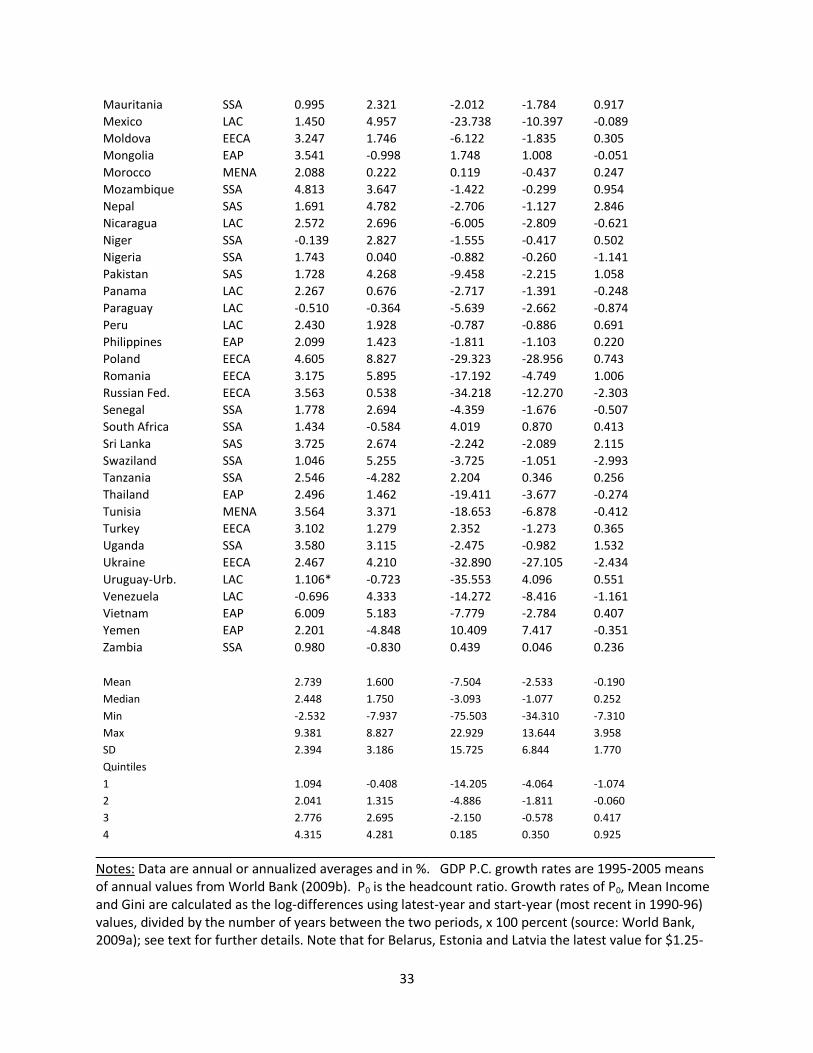
33

Mauritania SSA 0.995 2.321 -2.012 -1.784 0.917

Mexico LAC 1.450 4.957 -23.738 -10.397 -0.089

Moldova EECA 3.247 1.746 -6.122 -1.835 0.305

Mongolia EAP 3.541 -0.998 1.748 1.008 -0.051

Morocco MENA 2.088 0.222 0.119 -0.437 0.247

Mozambique SSA 4.813 3.647 -1.422 -0.299 0.954

Nepal SAS 1.691 4.782 -2.706 -1.127 2.846

Nicaragua LAC 2.572 2.696 -6.005 -2.809 -0.621

Niger SSA -0.139 2.827 -1.555 -0.417 0.502

Nigeria SSA 1.743 0.040 -0.882 -0.260 -1.141

Pakistan SAS 1.728 4.268 -9.458 -2.215 1.058

Panama LAC 2.267 0.676 -2.717 -1.391 -0.248

Paraguay LAC -0.510 -0.364 -5.639 -2.662 -0.874

Peru LAC 2.430 1.928 -0.787 -0.886 0.691

Philippines EAP 2.099 1.423 -1.811 -1.103 0.220

Poland EECA 4.605 8.827 -29.323 -28.956 0.743

Romania EECA 3.175 5.895 -17.192 -4.749 1.006

Russian Fed. EECA 3.563 0.538 -34.218 -12.270 -2.303

Senegal SSA 1.778 2.694 -4.359 -1.676 -0.507

South Africa SSA 1.434 -0.584 4.019 0.870 0.413

Sri Lanka SAS 3.725 2.674 -2.242 -2.089 2.115

Swaziland SSA 1.046 5.255 -3.725 -1.051 -2.993

Tanzania SSA 2.546 -4.282 2.204 0.346 0.256

Thailand EAP 2.496 1.462 -19.411 -3.677 -0.274

Tunisia MENA 3.564 3.371 -18.653 -6.878 -0.412

Turkey EECA 3.102 1.279 2.352 -1.273 0.365

Uganda SSA 3.580 3.115 -2.475 -0.982 1.532

Ukraine EECA 2.467 4.210 -32.890 -27.105 -2.434

Uruguay-Urb. LAC 1.106* -0.723 -35.553 4.096 0.551

Venezuela LAC -0.696 4.333 -14.272 -8.416 -1.161

Vietnam EAP 6.009 5.183 -7.779 -2.784 0.407

Yemen EAP 2.201 -4.848 10.409 7.417 -0.351

Zambia SSA 0.980 -0.830 0.439 0.046 0.236

Mean 2.739 1.600 -7.504 -2.533 -0.190

Median 2.448 1.750 -3.093 -1.077 0.252

Min -2.532 -7.937 -75.503 -34.310 -7.310

Max 9.381 8.827 22.929 13.644 3.958

SD 2.394 3.186 15.725 6.844 1.770

Quintiles

1 1.094 -0.408 -14.205 -4.064 -1.074

2 2.041 1.315 -4.886 -1.811 -0.060

3 2.776 2.695 -2.150 -0.578 0.417

4 4.315 4.281 0.185 0.350 0.925

_____________________________________________________________________________________ Notes: Data are annual or annualized averages and in %. GDP P.C. growth rates are 1995-2005 means of annual values from World Bank (2009b). P0 is the headcount ratio. Growth rates of P0, Mean Income and Gini are calculated as the log-differences using latest-year and start-year (most recent in 1990-96) values, divided by the number of years between the two periods, x 100 percent (source: World Bank, 2009a); see text for further details. Note that for Belarus, Estonia and Latvia the latest value for $1.25-

34

standard P0 is reported as 0; for the purpose of computing the growth rate, this value has been approximated by 0.001. This approximation suggests that the corresponding estimates should be viewed with some caution.

35

Table 4b. ‘Poverty transformation efficiency’, by country

Country Efficiency Vector Country Efficiency Vector

Albania (2, 8, 10, 9) Kyrgyz Rep. (5, 10, 9, 10)

Argentina-Urb. (9, 9, 10, 10) Lao PDR (3, 6, 6, 7)

Armenia (1, 10, 3, 9) Latvia (1, 1, 1, 1)

Azerbaijan (1, 2, 1, 1) Lesotho (5, 10, 7, 9)

Bangladesh (4, 8, 8, 8) Madagascar (9, 5, 8, 8)

Belarus (2, 3, 2, 3) Malaysia (4, 9, 2, 5)

Bolivia (8, 7, 10, 10) Mali (4,1, 5, 6)

Brazil (8, 5, 4, 2) Mauritania (9, 5, 7, 4)

Burkina Faso (4, 6, 6, 8) Mexico (8, 2, 2, 1)

Burundi (10, 7, 8, 8) Moldova (4, 6, 4, 5)

Cambodia (2, 5, 7, 6) Mongolia (3, 9, 9, 9)

Cameroon (7, 1, 3, 3) Morocco (6, 8, 8, 7)

CAR (10, 1, 6, 6) Mozambique (2, 4, 7, 7)

Chile (3 , 6, 3, 2) Nepal (7, 2, 6, 5)

China-Rur. (1, 2, 4, 4) Nicaragua (5, 4, 4, 3)

China-Urb. (1, 1, 3, 2) Niger (10, 4, 7, 7)

Colombia (9, 7, 9, 9) Nigeria (7, 8, 8, 8)

Costa Rica (6, 4, 2, 2) Pakistan (7, 3, 3, 4)

Côte d'Ivoire (10, 4, 9, 6) Panama (6,. 8, 6, 5)

Djibouti (10, 10, 10, 10) Paraguay (10, 8, 4, 4)

Dominican Rep. (3, 7, 7, 7) Peru (6, 5, 8, 6)

Ecuador (8 , 2, 3, 2) Philippines (6, 6, 7, 5)

Egypt (5, 6, 6, 3) Poland (2, 1, 1, 1)

El Salvador (8, 5, 5, 3) Romania (4, 1, 2, 2)

Estonia (1, 3, 1, 2) Russian Fed. (3, 8, 1, 1)

Ethiopia (5, 7, 5, 7) Senegal (7, 5, 5, 5)

Georgia (1, 10, 10, 10) South Africa (8, 9, 10, 9)

Ghana (6, 3, 5, 4) Sri Lanka (3, 5, 6, 4)

Guinea (8, 10, 10, 9) Swaziland (9, 2, 5, 6)

Guinea-32.Bissau (10, 9, 8, 9) Tanzania (5, 10, 9, 8)

Honduras (7, 3, 5, 3) Thailand (5, 6, 2, 3)

India-Rur. (2, 7, 7, 7) Tunisia (3, 4, 1, 1)

India-Urb. (2, 7, 8, 6) Turkey (4, 7, 9, 5)

Indones-Rur. (7, 4, 4, 5) Uganda (3, 4, 6, 6)

Indones-Urb. (7, 3, 3, 3) Ukraine (5, 3, 1, 1)

Iran (4, 9, 9, 8) Uruguay-Urb. (8, 9, 2, 10)

Jamaica (9, 2, 1, 3) Venezuela (10, 2, 2, 1)

Jordan (6, 6, 3, 2) Vietnam (1, 1, 4, 4)

Kazakhstan (2, 8, 4, 7) Yemen (6, 10, 10, 10)

Kenya (9, 3, 5, 4) Zambia (9, 9, 9, 8)

Notes: ‘Efficiency Vector’ has the deciles ranks as coordinates. For example Albania’s Efficiency Vector of (2, 8, 10, 9) means that the country’s deciles ranks are 2, 8, 10 and 9, respectively, on per-capita GDP growth, per-capita income growth, poverty reduction at the $1.25 standard and poverty reduction at the $2.50 standard.

36

Table 5.1 Inequality, Income Growth and Poverty – GMM regression results, 1980-2007: $1.25

Variable/Model (1) (2) (3) (4) (5) Constant -0.046 -0.007 -0.022 -0.447 -0.204 (-1.28) (-0.72) (-2.05) (-2.87) (-1.73)

dlog Yit -0.330 -9.757 (-3.89) (-4.14)

dlog Yit x log Git-1 1.844 2.307 (1.64) (3.54)

dlog Yit x log(Z/Yit-1) 1.525 1.333 (6.57) (6.43)

dlog Git 1.714 13.161 14.391 (3.86) (3.09) (4.22)

dlog Git x log Git-1 -3.178 -3.649 (-2.80) (-3.97)

dlog Git x log(Z/Yit-1) -2.681 -2.754 (-5.97) (-7.06)

log Git-1 0.123 0.055 (2.80) (1.67)

log(Z/Yit-1) 0.025 0.011 (2.24) (1.24)

dlog Yit x region dummy

East Asia and Pacific (EAP) -1.470 -1.436 -7.598

-4.31 (-3.76) (-1.90)

Latin America and the Caribbean (LAC) -1.213 -0.821 -7.393

(-2.10) (-1.69) (-1.64)

East Europe and Central Asia (EECA) -2.554 -2.040 -8.026

(-3.11) (-1.69) (-2.05)

Middle East and North Africa (MENA) 0.134 -2.475 -8.594

(0.04) (-1.90) (-1.97)

South Asia (SAS) -1.523 -1.062 -7.432

(-2.52) (-2.09) (-1.86)

Sub-Saharan Africa (SSA) -0.598 -0.452 -9.140

(-2.48) (-1.17) (-2.11)

N 320 320 320 320 320

Uncentered R2 0.11 0.34 0.41 0.64 0.64

SEE 0.307 0.265 0.252 0.196 0.196

Hansen J 0.238a 8.164

b 25.157

c 13.367

d 27.888

e

[0.63] [0.23] [0.01] [0.42] [0.06]

__________________________________________________________________________________ Notes:The dependent variable is the log-difference of headcount ratio ($1.25 / day); heteroscedastic robust t-statistics in parentheses; Hansen J statistic tests for over-identification of instruments (p-values in brackets). All regressors involving dlog Yit are considered endogenous and are instrumented. All models are estimated using 2-step GMM. aCritical value, χ2

0.05(1) = 3.84;instruments: logYit-1 and dlogPOPit. bCritical value, χ2

0.05(6) = 12.59; instruments: regional dummy variables, logYit-1 interacted with dummy variables and dlogPOPit.

cCritical

37

value is χ20.05(12) = 21.02; instruments: regional dummy variables, logYit-1 and logGit-1 interacted with

regional dummy variables and dlogPOPit. dCritical value, χ2

0.05(13) = 22.36; instruments: regional dummy variables, logYit-1 and logGit-1 interacted with regional dummy variables, dlogPOPit, logYit-1 x logGit-1, logYit-1 x log(Z/Yit-1) and logGit-1 x logGit-1.

eCritical value, χ20.05(18) = 28.87; instruments: same as listed in d.

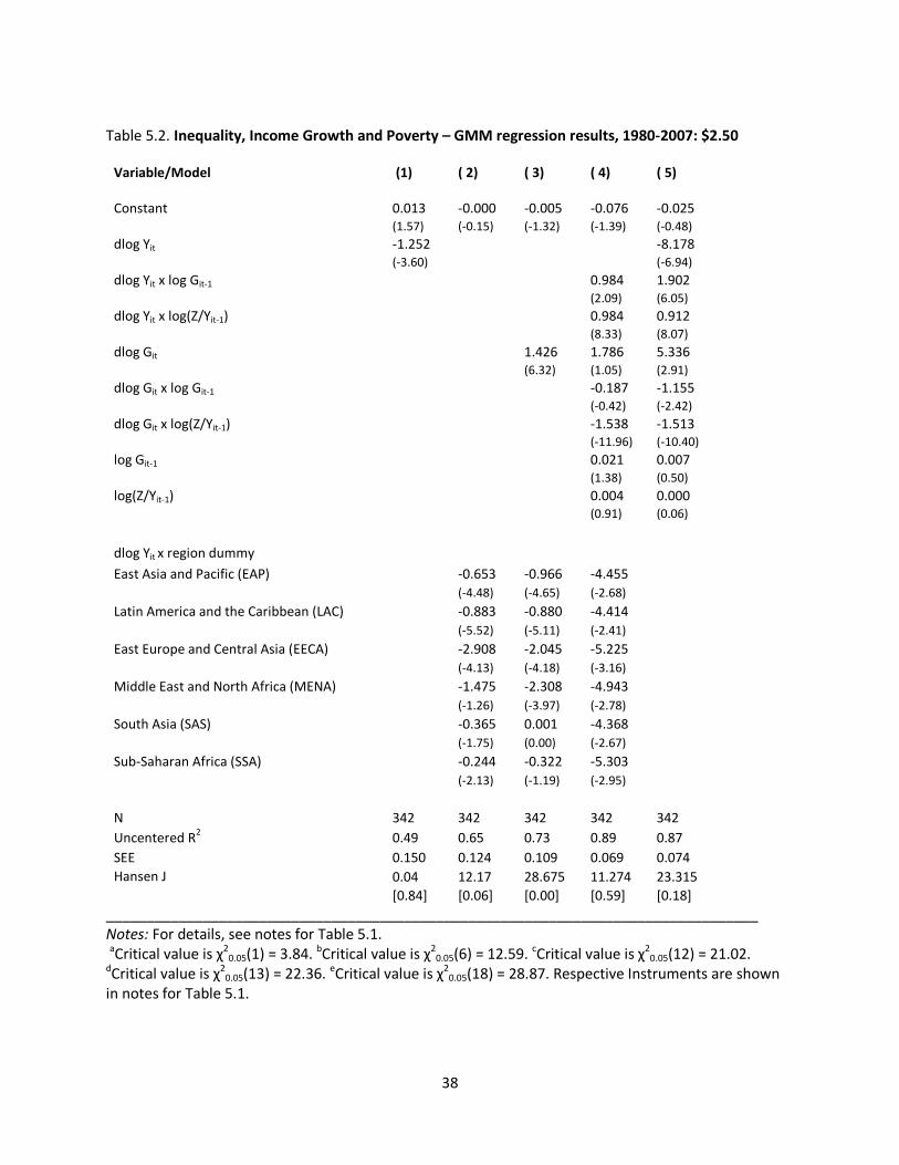
38

Table 5.2. Inequality, Income Growth and Poverty – GMM regression results, 1980-2007: $2.50

Variable/Model (1) ( 2) ( 3) ( 4) ( 5) Constant 0.013 -0.000 -0.005 -0.076 -0.025 (1.57) (-0.15) (-1.32) (-1.39) (-0.48)

dlog Yit -1.252 -8.178 (-3.60) (-6.94)

dlog Yit x log Git-1 0.984 1.902 (2.09) (6.05)

dlog Yit x log(Z/Yit-1) 0.984 0.912 (8.33) (8.07)

dlog Git 1.426 1.786 5.336 (6.32) (1.05) (2.91)

dlog Git x log Git-1 -0.187 -1.155 (-0.42) (-2.42)

dlog Git x log(Z/Yit-1) -1.538 -1.513 (-11.96) (-10.40)

log Git-1 0.021 0.007 (1.38) (0.50)

log(Z/Yit-1) 0.004 0.000 (0.91) (0.06)

dlog Yit x region dummy

East Asia and Pacific (EAP) -0.653 -0.966 -4.455

(-4.48) (-4.65) (-2.68)

Latin America and the Caribbean (LAC) -0.883 -0.880 -4.414

(-5.52) (-5.11) (-2.41)

East Europe and Central Asia (EECA) -2.908 -2.045 -5.225

(-4.13) (-4.18) (-3.16)

Middle East and North Africa (MENA) -1.475 -2.308 -4.943

(-1.26) (-3.97) (-2.78)

South Asia (SAS) -0.365 0.001 -4.368

(-1.75) (0.00) (-2.67)

Sub-Saharan Africa (SSA) -0.244 -0.322 -5.303

(-2.13) (-1.19) (-2.95)

N 342 342 342 342 342

Uncentered R2 0.49 0.65 0.73 0.89 0.87

SEE 0.150 0.124 0.109 0.069 0.074

Hansen J 0.04 12.17 28.675 11.274 23.315

[0.84] [0.06] [0.00] [0.59] [0.18]

_________________________________________________________________________________ Notes: For details, see notes for Table 5.1. aCritical value is χ2

0.05(1) = 3.84. bCritical value is χ20.05(6) = 12.59. cCritical value is χ2

0.05(12) = 21.02. dCritical value is χ2

0.05(13) = 22.36. eCritical value is χ20.05(18) = 28.87. Respective Instruments are shown

in notes for Table 5.1.

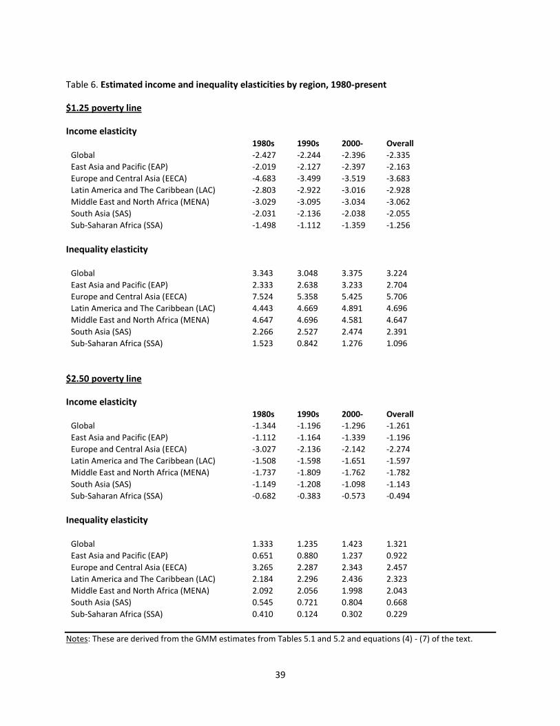
39

Table 6. Estimated income and inequality elasticities by region, 1980-present

$1.25 poverty line

Income elasticity 1980s 1990s 2000- Overall

Global -2.427 -2.244 -2.396 -2.335

East Asia and Pacific (EAP) -2.019 -2.127 -2.397 -2.163

Europe and Central Asia (EECA) -4.683 -3.499 -3.519 -3.683

Latin America and The Caribbean (LAC) -2.803 -2.922 -3.016 -2.928

Middle East and North Africa (MENA) -3.029 -3.095 -3.034 -3.062

South Asia (SAS) -2.031 -2.136 -2.038 -2.055

Sub-Saharan Africa (SSA) -1.498 -1.112 -1.359 -1.256

Inequality elasticity

Global 3.343 3.048 3.375 3.224

East Asia and Pacific (EAP) 2.333 2.638 3.233 2.704

Europe and Central Asia (EECA) 7.524 5.358 5.425 5.706

Latin America and The Caribbean (LAC) 4.443 4.669 4.891 4.696

Middle East and North Africa (MENA) 4.647 4.696 4.581 4.647

South Asia (SAS) 2.266 2.527 2.474 2.391

Sub-Saharan Africa (SSA) 1.523 0.842 1.276 1.096

$2.50 poverty line

Income elasticity 1980s 1990s 2000- Overall

Global -1.344 -1.196 -1.296 -1.261

East Asia and Pacific (EAP) -1.112 -1.164 -1.339 -1.196

Europe and Central Asia (EECA) -3.027 -2.136 -2.142 -2.274

Latin America and The Caribbean (LAC) -1.508 -1.598 -1.651 -1.597

Middle East and North Africa (MENA) -1.737 -1.809 -1.762 -1.782

South Asia (SAS) -1.149 -1.208 -1.098 -1.143

Sub-Saharan Africa (SSA) -0.682 -0.383 -0.573 -0.494

Inequality elasticity

Global 1.333 1.235 1.423 1.321

East Asia and Pacific (EAP) 0.651 0.880 1.237 0.922

Europe and Central Asia (EECA) 3.265 2.287 2.343 2.457

Latin America and The Caribbean (LAC) 2.184 2.296 2.436 2.323

Middle East and North Africa (MENA) 2.092 2.056 1.998 2.043

South Asia (SAS) 0.545 0.721 0.804 0.668

Sub-Saharan Africa (SSA) 0.410 0.124 0.302 0.229

Notes: These are derived from the GMM estimates from Tables 5.1 and 5.2 and equations (4) - (7) of the text.

40

Table 7.1. Countries in deciles on income and inequality elasticities, early-to-mid 1990s, $1.25 poverty standard

Decile Income elasticity Inequality elasticity Decile Income elasticity Inequality elasticity

(min-max) (min-max) (min-max) (min-max)

1. Albania Burkina Faso 6. Armenia Azerbaijan

Argentina-Urb. CAR Côte d'Ivoire China-Urb.

Belarus Guinea India-Rur. Colombia

Estonia Madagascar Indonesia-Rur. Ecuador

Latvia Mali Kyrgyz Rep. El Salvador

Romania Mozambique Pakistan Kyrgyz Rep.

Ukraine Swaziland South Africa Moldova

Uruguay-Urb. Zambia Sri Lanka Thailand

2. Chile Burundi 7. Bangladesh Brazil

Georgia Lesotho India-Urb. Egypt

Iran Nepal Indonesia-Urb. Jordan

Jamaica Niger Kenya Morocco

Malaysia Nigeria Lao PDR Paraguay

Poland Senegal Mauritania Tunisia

Russian Fed. Tanzania Nicaragua Venezuela

Turkey Uganda Philippines Yemen

3. Bolivia Cambodia 8. Cambodia Bolivia

Costa Rica Cameroon Cameroon Costa Rica

Djibouti China-Rur. China-Rur. Djibouti

Kazakhstan Ethiopia Ethiopia Dominican Rep.

Mexico Ghana Ghana Kazakhstan

Morocco Guinea-Bissau Honduras Mexico

Peru Indonesia-Urb. Tanzania Panama

Yemen Vietnam Vietnam Peru

4. China-Urb. Bangladesh 9. Burundi Albania

Dominican Rep. Honduras Guinea-Bissau Chile

Egypt India-Rur. Lesotho Georgia

Jordan India-Urb. Nepal Iran

Panama Kenya Niger Jamaica

Paraguay Lao PDR Nigeria Malaysia

Tunisia Mauritania Senegal Poland

Venezuela Pakistan Uganda Turkey

5. Azerbaijan Armenia 10. Burkina Faso Argentina-Urb.

Brazil Côte d'Ivoire CAR Belarus

41

Colombia Indonesia-Rur. Guinea Estonia

Ecuador Mongolia Madagascar Latvia

El Salvador Nicaragua Mali Romania

Moldova Philippines Mozambique Russian Fed.

Mongolia South Africa Swaziland Ukraine

Thailand Sri Lanka Zambia Uruguay-Urb.

Notes: Country categorization into deciles is based on the ‘overall’ income and inequality elasticities presented in the appendix Tables A3.1. Growth rates are calculated using the latest observation of period 1990-1996 and the most recent 2000s value. Countries are arranged alphabetically in each decile.

42

Table 7.2; Countries by decile on income and inequality elasticities, early-to-mid 1990s, $2.50 poverty standard

Decile Income elasticity Inequality elasticity Decile Income elasticity Inequality elasticity

(min-max) $2.50 (min-max) $2.50 (min-max) $2.50 (min-max) $2.50 1. Albania CAR 6. Armenia Armenia Argentina-Urb. Burundi Bangladesh Ecuador Belarus Guinea Côte d'Ivoire Egypt Estonia Madagascar Ecuador El Salvador Latvia Mali India-Rur. Kyrgyz Rep. Romania Mozambique Indonesia-Rur. Moldova Ukraine Niger Kyrgyz Rep. South Africa Uruguay-Urb. Swaziland Pakistan Thailand

2. Djibouti Burkina Faso 7. Cambodia Colombia Georgia Nepal China-Rur. Djibouti Iran Nigeria India-Urb. Jordan Jamaica Senegal Indonesia-Urb. Kazakhstan Kazakhstan Tanzania Lao PDR Morocco Poland Uganda Mauritania Tunisia Russian Fed. Vietnam Philippines Venezuela Turkey Zambia South Africa Yemen

3. Bolivia Cambodia 8. Ethiopia Bolivia Chile Cameroon Ghana Costa Rica Costa Rica China-Rur. Honduras Georgia Egypt Ethiopia Kenya Jamaica Malaysia Ghana Nepal Paraguay Morocco Guinea-Bissau Nicaragua Peru Peru Lao PDR Tanzania Poland Yemen Lesotho Vietnam Romania

4. China-Urb. Bangladesh 9. Burundi Albania Dominican Rep. India-Rur. Cameroon Brazil Jordan India-Urb. Guinea-Bissau Dominican Rep. Mexico Indonesia-Rur. Lesotho Iran Panama Indonesia-Urb. Niger Malaysia Paraguay Kenya Nigeria Mexico Tunisia Mauritania Senegal Panama Venezuela Pakistan Uganda Turkey

5. Azerbaijan Azerbaijan 10. Burkina Faso Argentina-Urb. Brazil China-Urb. CAR Belarus Colombia Côte d'Ivoire Guinea Chile El Salvador Honduras Madagascar Estonia

43

Moldova Mongolia Mali Latvia Mongolia Nicaragua Mozambique Russian Fed. Sri Lanka Philippines Swaziland Ukraine Thailand Sri Lanka Zambia Uruguay-Urb.

Notes: Country categorization into deciles is based on the ‘overall’ income and inequality elasticities presented in the appendix Tables A3.2. Growth rates are calculated using the latest observation of period 1990-1996 and the most recent 2000s value. Countries are arranged alphabetically in each decile.

44

Table 8.1. Poverty ($1.25 Headcount ratio) growth, contribution of inequality and mean income growth to poverty reduction, early-mid-1990s-present A. Countries experiencing poverty reduction

A B A + B

Country Region Povg EY*dlnY EG*dlnG Pred Povg

Armenia EECA -7.122 8.580 -13.363 -4.783

Azerbaijan EECA -62.506 -11.656 -27.118 -38.774

Belarus EECA -24.964 -17.208 16.707 -0.501

Brazil LAC -7.142 -5.505 -3.198 -8.704

Burkina Faso SSA -2.557 -1.220 -0.715 -1.936

Burundi SSA -0.252 -0.881 -0.007 -0.888

Cambodia EAP -1.890 -3.354 1.813 -1.541

Cameroon SSA -9.001 -8.362 -1.497 -9.859

CAR* SSA -2.823 1.454 6.023 7.476

Chile LAC -8.168 -5.124 -3.304 -8.428

China-Rur. EAP -7.103 -7.872 1.268 -6.603

China-Urb. EAP -17.681 -19.252 6.686 -12.566

Costa Rica LAC -12.160 -10.217 0.181 -10.036

Dominican Rep. LAC -1.827 -2.453 1.434 -1.020

Ecuador LAC -9.377 -12.016 1.402 -10.614

Egypt MENA -2.356 -4.829 3.228 -1.601

El Salvador LAC -3.469 -5.377 -2.338 -7.714

Estonia EECA -61.350 -14.269 13.219 -1.050

Ethiopia SSA -4.384 -1.848 -4.188 -6.035

Ghana SSA -3.802 -5.636 1.463 -4.173

Guinea* SSA -0.722 0.722 2.081 2.803

Honduras LAC -3.677 -6.394 0.032 -6.362

India-Rur. SAS -1.634 -2.650 1.466 -1.184

India-Urb. SAS -1.091 -2.438 2.056 -0.382

Indonesia-Rur. EAP -7.399 -7.968 2.048 -5.920

Indonesia-Urb. EAP -7.779 -8.254 1.559 -6.694

Jamaica LAC -24.763 -14.958 7.789 -7.169

Jordan MENA -14.189 -4.137 -4.806 -8.943

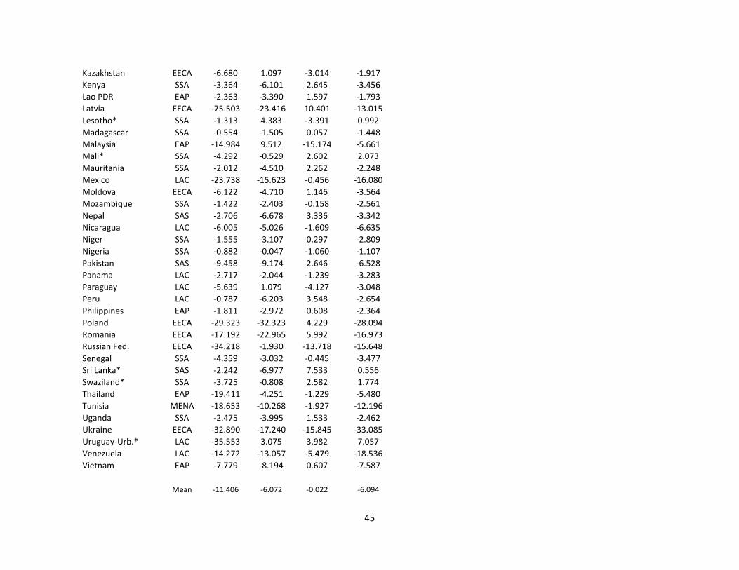
45

Kazakhstan EECA -6.680 1.097 -3.014 -1.917

Kenya SSA -3.364 -6.101 2.645 -3.456

Lao PDR EAP -2.363 -3.390 1.597 -1.793

Latvia EECA -75.503 -23.416 10.401 -13.015

Lesotho* SSA -1.313 4.383 -3.391 0.992

Madagascar SSA -0.554 -1.505 0.057 -1.448

Malaysia EAP -14.984 9.512 -15.174 -5.661

Mali* SSA -4.292 -0.529 2.602 2.073

Mauritania SSA -2.012 -4.510 2.262 -2.248

Mexico LAC -23.738 -15.623 -0.456 -16.080

Moldova EECA -6.122 -4.710 1.146 -3.564

Mozambique SSA -1.422 -2.403 -0.158 -2.561

Nepal SAS -2.706 -6.678 3.336 -3.342

Nicaragua LAC -6.005 -5.026 -1.609 -6.635

Niger SSA -1.555 -3.107 0.297 -2.809

Nigeria SSA -0.882 -0.047 -1.060 -1.107

Pakistan SAS -9.458 -9.174 2.646 -6.528

Panama LAC -2.717 -2.044 -1.239 -3.283

Paraguay LAC -5.639 1.079 -4.127 -3.048

Peru LAC -0.787 -6.203 3.548 -2.654

Philippines EAP -1.811 -2.972 0.608 -2.364

Poland EECA -29.323 -32.323 4.229 -28.094

Romania EECA -17.192 -22.965 5.992 -16.973

Russian Fed. EECA -34.218 -1.930 -13.718 -15.648

Senegal SSA -4.359 -3.032 -0.445 -3.477

Sri Lanka* SAS -2.242 -6.977 7.533 0.556

Swaziland* SSA -3.725 -0.808 2.582 1.774

Thailand EAP -19.411 -4.251 -1.229 -5.480

Tunisia MENA -18.653 -10.268 -1.927 -12.196

Uganda SSA -2.475 -3.995 1.533 -2.462

Ukraine EECA -32.890 -17.240 -15.845 -33.085

Uruguay-Urb.* LAC -35.553 3.075 3.982 7.057

Venezuela LAC -14.272 -13.057 -5.479 -18.536

Vietnam EAP -7.779 -8.194 0.607 -7.587

Mean -11.406 -6.072 -0.022 -6.094

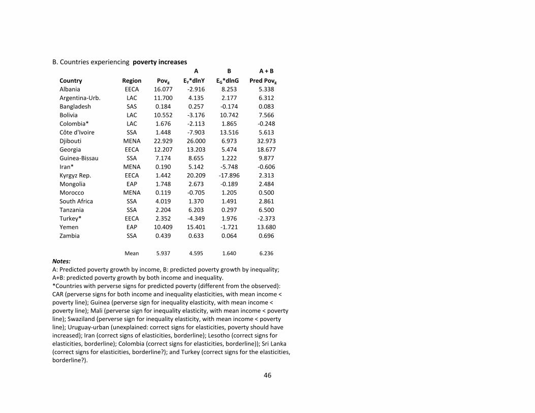
46

B. Countries experiencing poverty increases

A B A + B

Country Region Povg EY*dlnY EG*dlnG Pred Povg

Albania EECA 16.077 -2.916 8.253 5.338

Argentina-Urb. LAC 11.700 4.135 2.177 6.312

Bangladesh SAS 0.184 0.257 -0.174 0.083

Bolivia LAC 10.552 -3.176 10.742 7.566

Colombia* LAC 1.676 -2.113 1.865 -0.248

Côte d'Ivoire SSA 1.448 -7.903 13.516 5.613

Djibouti MENA 22.929 26.000 6.973 32.973

Georgia EECA 12.207 13.203 5.474 18.677

Guinea-Bissau SSA 7.174 8.655 1.222 9.877

Iran* MENA 0.190 5.142 -5.748 -0.606

Kyrgyz Rep. EECA 1.442 20.209 -17.896 2.313

Mongolia EAP 1.748 2.673 -0.189 2.484

Morocco MENA 0.119 -0.705 1.205 0.500

South Africa SSA 4.019 1.370 1.491 2.861

Tanzania SSA 2.204 6.203 0.297 6.500

Turkey* EECA 2.352 -4.349 1.976 -2.373

Yemen EAP 10.409 15.401 -1.721 13.680

Zambia SSA 0.439 0.633 0.064 0.696

Mean 5.937 4.595 1.640 6.236

Notes: A: Predicted poverty growth by income, B: predicted poverty growth by inequality; A+B: predicted poverty growth by both income and inequality. *Countries with perverse signs for predicted poverty (different from the observed): CAR (perverse signs for both income and inequality elasticities, with mean income < poverty line); Guinea (perverse sign for inequality elasticity, with mean income < poverty line); Mali (perverse sign for inequality elasticity, with mean income < poverty line); Swaziland (perverse sign for inequality elasticity, with mean income < poverty line); Uruguay-urban (unexplained: correct signs for elasticities, poverty should have increased); Iran (correct signs of elasticities, borderline); Lesotho (correct signs for elasticities, borderline); Colombia (correct signs for elasticities, borderline)); Sri Lanka (correct signs for elasticities, borderline?); and Turkey (correct signs for the elasticities, borderline?).

47

Table 8.2. Poverty ($2.50 Headcount ratio) growth, contribution of inequality and mean income growth to poverty reduction, early-mid-1990s-present A. Countries experiencing poverty reduction

A B A + B

Country Region Povg EY*dlnY EG*dlnG Pred Povg

Azerbaijan EECA -34.310 -6.751 -10.520 -17.271

Brazil LAC -4.584 -2.916 -1.657 -4.573

Burkina Faso* SSA -0.251 -0.220 0.384 0.164

Burundi SSA -0.091 -0.403 0.004 -0.398

Cambodia EAP -0.950 -1.720 0.530 -1.189

Cameroon SSA -3.598 -3.553 -0.476 -4.028

CAR* SSA -0.585 3.331 3.724 7.054

Chile LAC -8.414 -2.864 -1.695 -4.559

China-Rur. EAP -2.576 -4.267 0.218 -4.049

China-Urb. EAP -8.945 -11.826 2.341 -9.485

Costa Rica LAC -5.367 -5.804 0.087 -5.717

Côte d'Ivoire* SSA -0.799 -4.468 5.227 0.759

Dominican Rep. LAC -0.384 -1.367 0.704 -0.663

Ecuador LAC -5.108 -6.359 0.681 -5.678

Egypt MENA -2.757 -2.929 1.272 -1.657

El Salvador LAC -3.202 -2.877 -1.130 -4.007

Estonia EECA -4.808 -8.786 6.054 -2.733

Ethiopia SSA -0.329 -0.862 -0.870 -1.732

Ghana SSA -1.934 -2.827 0.374 -2.454

Honduras LAC -3.332 -2.816 0.015 -2.801

India-Rur. SAS -0.348 -1.555 0.362 -1.194

India-Urb. SAS -0.609 -1.348 0.625 -0.724

Indonesia-Rur. EAP -1.779 -4.790 0.492 -4.298

Indonesia-Urb. EAP -3.079 -4.432 0.461 -3.972

Jamaica LAC -3.934 -8.820 3.551 -5.269

Jordan MENA -7.169 -2.362 -2.226 -4.589

Kazakhstan EECA -0.434 0.660 -1.277 -0.617

Kenya SSA -2.337 -2.844 1.114 -1.729

Lao PDR EAP -0.569 -1.931 0.377 -1.554

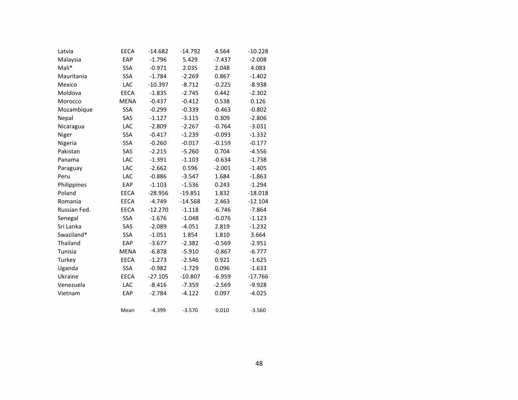
48

Latvia EECA -14.682 -14.792 4.564 -10.228

Malaysia EAP -1.796 5.429 -7.437 -2.008

Mali* SSA -0.971 2.035 2.048 4.083

Mauritania SSA -1.784 -2.269 0.867 -1.402

Mexico LAC -10.397 -8.712 -0.225 -8.938

Moldova EECA -1.835 -2.745 0.442 -2.302

Morocco MENA -0.437 -0.412 0.538 0.126

Mozambique SSA -0.299 -0.339 -0.463 -0.802

Nepal SAS -1.127 -3.115 0.309 -2.806

Nicaragua LAC -2.809 -2.267 -0.764 -3.031

Niger SSA -0.417 -1.239 -0.093 -1.332

Nigeria SSA -0.260 -0.017 -0.159 -0.177

Pakistan SAS -2.215 -5.260 0.704 -4.556

Panama LAC -1.391 -1.103 -0.634 -1.738

Paraguay LAC -2.662 0.596 -2.001 -1.405

Peru LAC -0.886 -3.547 1.684 -1.863

Philippines EAP -1.103 -1.536 0.243 -1.294

Poland EECA -28.956 -19.851 1.832 -18.018

Romania EECA -4.749 -14.568 2.463 -12.104

Russian Fed. EECA -12.270 -1.118 -6.746 -7.864

Senegal SSA -1.676 -1.048 -0.076 -1.123

Sri Lanka SAS -2.089 -4.051 2.819 -1.232

Swaziland* SSA -1.051 1.854 1.810 3.664

Thailand EAP -3.677 -2.382 -0.569 -2.951

Tunisia MENA -6.878 -5.910 -0.867 -6.777

Turkey EECA -1.273 -2.546 0.921 -1.625

Uganda SSA -0.982 -1.729 0.096 -1.633

Ukraine EECA -27.105 -10.807 -6.959 -17.766

Venezuela LAC -8.416 -7.359 -2.569 -9.928

Vietnam EAP -2.784 -4.122 0.097 -4.025

Mean -4.399 -3.570 0.010 -3.560

49

B. Countries experiencing poverty increases

A B A + B

Country Region Povg EY*dlnY EG*dlnG Pred Povg

Albania EECA 0.473 -1.826 3.478 1.652

Argentina-Urb. LAC 3.515 2.434 1.082 3.517

Armenia* EECA 2.608 4.591 -5.798 -1.207

Bangladesh SAS 0.069 0.147 -0.044 0.103

Belarus* EECA 3.203 -11.339 7.023 -4.316

Bolivia LAC 2.450 -1.833 4.943 3.110

Colombia* LAC 0.543 -1.109 0.945 -0.164

Djibouti MENA 13.644 15.438 3.060 18.498

Georgia EECA 7.745 7.864 2.437 10.301

Guinea SSA 0.367 -0.079 2.496 2.417

Guinea-Bissau SSA 2.170 3.373 0.460 3.833

Iran MENA 0.180 2.988 -2.717 0.271

Kyrgyz Rep. EECA 5.284 10.554 -8.791 1.763

Lesotho* SSA 0.728 1.319 -1.514 -0.195

Madagascar* SSA 0.193 -0.381 -0.041 -0.423

Mongolia EAP 1.008 1.566 -0.071 1.495

South Africa SSA 0.870 0.678 0.749 1.427

Tanzania SSA 0.346 3.091 0.003 3.094

Uruguay-Urb. LAC 4.096 1.853 1.954 3.807

Yemen EAP 7.417 8.991 -0.771 8.219

Zambia SSA 0.046 0.082 -0.018 0.064

Mean 2.712 2.305 0.422 2.727

Notes: A: Predicted poverty growth by income; B: predicted poverty growth by inequality; A+B is predicted poverty both income and inequality. *Countries with perverse signs for predicted poverty growth (different from the observed): Similar reasons as in Table 8.1; note that there are a few more countries with perverse elasticity signs for the $2.50 standard due to the greater likelihood of mean income falling below the poverty line.

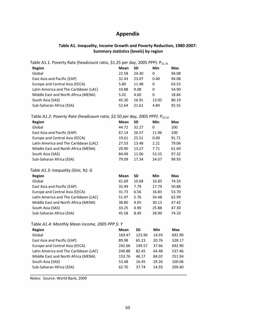
50

Appendix

Table A1. Inequality, Income Growth and Poverty Reduction, 1980-2007: Summary statistics (levels) by region

Table A1.1. Poverty Rate (headcount ratio, $1.25 per day, 2005 PPP): P$1.25

Region Mean SD Min Max

Global 22.58 24.30 0 94.08

East Asia and Pacific (EAP) 32.43 23.07 0.40 94.08

Europe and Central Asia (EECA) 5.80 11.48 0 63.53

Latin America and The Caribbean (LAC) 10.88 9.08 0 54.90

Middle East and North Africa (MENA) 5.02 4.60 0 18.84

South Asia (SAS) 45.30 16.91 13.95 80.19

Sub-Saharan Africa (SSA) 52.64 21.61 4.84 92.55

Table A1.2: Poverty Rate (headcount ratio, $2.50 per day, 2005 PPP): P$2.50

Region Mean SD Min Max

Global 44.72 32.27 0 100

East Asia and Pacific (EAP) 67.14 26.57 11.96 100

Europe and Central Asia (EECA) 19.61 25.51 0.00 91.71

Latin America and The Caribbean (LAC) 27.53 13.48 2.21 79.06

Middle East and North Africa (MENA) 29.90 13.27 7.71 61.69

South Asia (SAS) 84.49 11.06 53.55 97.32

Sub-Saharan Africa (SSA) 79.09 17.34 24.07 99.93

Table A1.3: Inequality (Gini, %): G

Region Mean SD Min Max

Global 41.69 10.68 16.83 74.33

East Asia and Pacific (EAP) 35.99 7.79 17.79 50.88

Europe and Central Asia (EECA) 31.73 6.56 16.83 53.70

Latin America and The Caribbean (LAC) 51.97 5.76 34.48 62.99

Middle East and North Africa (MENA) 38.80 4.05 30.13 47.42

South Asia (SAS) 33.25 4.90 25.88 47.30

Sub-Saharan Africa (SSA) 45.58 8.49 28.90 74.33

Table A1.4: Monthly Mean income, 2005 PPP $: Y

Region Mean SD Min Max

Global 169.47 123.90 14.93 692.90

East Asia and Pacific (EAP) 89.98 65.23 20.76 328.17

Europe and Central Asia (EECA) 242.66 149.57 37.66 692.90

Latin America and The Caribbean (LAC) 240.88 82.45 64.48 537.46

Middle East and North Africa (MENA) 153.76 46.17 84.02 251.94

South Asia (SAS) 53.48 16.45 29.26 100.06

Sub-Saharan Africa (SSA) 62.70 37.74 14.93 209.40

_______________________________________________________________ Notes: Source: World Bank, 2009

51

Table A2. Estimated income and inequality elasticities for all countries at the latest data-year (in parentheses), $1.25 and $2.50 poverty standards

Elasticity Elasticity

Country Region Income Inequality Income Inequality

$1.25 $1.25 $2.50 $2.50

Albania (´05) EUCA -3.623 5.625 -2.217 2.443

Algeria (´95) MENA -3.067 4.553 -1.815 1.911

Angola (´00) SSA -1.036 0.923 -0.262 0.348

Argentina-Urb (´05) LAC -3.624 6.091 -2.084 3.052

Armenia (´03) EUCA -2.693 3.730 -1.574 1.422

Azerbaijan (´05) EUCA -4.934 7.582 -3.333 2.945

Bangladesh (´05) SAS -1.994 2.267 -1.101 0.603

Belarus (´05) EUCA -4.879 8.033 -3.131 3.623

Benin (´03) SSA -1.765 1.963 -0.896 0.564

Bhutan (´03) SAS -2.108 2.886 -1.068 1.235

Bolivia (´05) LAC -2.619 4.184 -1.347 2.133

Bosnia-Herzegovina (´04) EUCA -4.456 7.436 -2.761 3.506

Botswana (´93) SSA -1.891 2.731 -0.834 1.374

Brazil (´07) LAC -3.458 5.855 -1.939 3.003

Bulgaria (´03) EUCA -4.223 6.730 -2.668 2.947

Burkina Faso (´03) SSA -1.549 1.544 -0.740 0.355

Burundi (´06) SSA -1.310 0.854 -0.632 -0.172

Cambodia (´04) EAP -1.846 2.219 -0.925 0.773

Cameroon (´01) SSA -1.944 2.491 -0.972 0.976

Cape Verde (´01) SSA -2.272 3.310 -1.156 1.532

CAR (´03) SSA -1.176 0.879 -0.453 0.071

Chad (´02) SSA -1.369 1.176 -0.615 0.157

Chile (´06) LAC -3.936 6.780 -2.285 3.463

China-Rur. (´05) EAP -2.339 3.065 -1.312 1.106

China-Urb. (´05) EAP -3.499 5.429 -2.116 2.380

Colombia (´06) LAC -2.717 4.392 -1.412 2.251

Colombia-Urb (´91) LAC -3.166 5.174 -1.762 2.570

Comoros (´04) SSA -1.365 1.704 -0.457 0.855

Congo, Dem. Rep. (´05) SSA -1.268 1.092 -0.510 0.205

Congo, Rep. (´05) SSA -1.329 1.288 -0.532 0.366

Costa Rica (´05) LAC -3.659 6.099 -2.126 3.007

Côte d'Ivoire (´02) SSA -2.112 2.931 -1.060 1.287

Croatia (´05) EUCA -5.860 10.101 -3.790 4.791

Czech Rep. (´96) EUCA -5.679 9.599 -3.704 4.417

Djibouti (´02) MENA -2.449 3.414 -1.353 1.390

Dominican Rep. (´05) LAC -3.215 5.246 -1.805 2.587

Ecuador (´07) LAC -3.322 5.560 -1.850 2.831

Egypt (´04) MENA -3.198 4.718 -1.936 1.922

El Salvador (´05) LAC -3.012 4.820 -1.667 2.348

Estonia (´04) EUCA -4.283 7.085 -2.641 3.319

Ethiopia (´05) SSA -2.331 2.839 -1.367 0.824

Gabon (´05) SSA -2.997 4.586 -1.715 2.065

Gambia, The (´03) SSA -1.863 2.391 -0.897 0.971

Georgia (´05) EUCA -2.695 3.944 -1.514 1.699

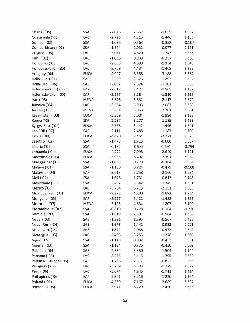
52

Ghana (´05) SSA -2.046 2.657 -1.055 1.032

Guatemala (´06) LAC -2.725 4.313 -1.446 2.135

Guinea (´03) SSA -1.026 0.563 -0.352 -0.107

Guinea-Bissau (´02) SSA -1.844 2.032 -0.977 0.531

Guyana (´98) LAC -3.071 4.820 -1.743 2.256

Haiti (´01) LAC -1.036 0.938 -0.257 0.368

Honduras (´06) LAC -2.605 4.098 -1.354 2.043

Honduras-Urb. (´86) LAC -2.769 4.434 -1.468 2.223

Hungary (´04) EUCA -4.997 8.358 -3.188 3.864

India-Rur. (´04) SAS -2.239 2.676 -1.297 0.754

India-Urb. (´04) SAS -2.052 2.524 -1.101 0.850

Indonesia-Rur. (´05) EAP -2.617 3.422 -1.565 1.137

Indonesia-Urb. (´05) EAP -2.387 3.284 -1.310 1.318

Iran (´05) MENA -3.546 5.632 -2.117 2.572

Jamaica (´04) LAC -3.584 5.903 -2.087 2.868

Jordan (´06) MENA -3.661 5.853 -2.201 2.681

Kazakhstan (´03) EUCA -3.309 5.004 -1.994 2.123

Kenya (´05) SSA -2.287 3.277 -1.185 1.465

Kyrgyz Rep. (´04) EUCA -2.568 3.442 -1.496 1.241

Lao PDR (´97) EAP -2.111 2.488 -1.187 0.709

Latvia (´04) EUCA -4.470 7.464 -2.771 3.520

Lesotho (´02) SSA -1.478 1.713 -0.600 0.687

Liberia (´07) SSA -0.172 -0.985 0.294 -0.794

Lithuania (´04) EUCA -4.292 7.098 -2.649 3.321

Macedonia (´03) EUCA -3.955 6.497 -2.391 3.062

Madagascar (´05) SSA -1.083 0.778 -0.364 0.084

Malawi (´04) SSA -1.160 0.724 -0.479 -0.108

Malaysia (´04) EAP -3.613 5.758 -2.166 2.634

Mali (´01) SSA -1.648 1.731 -0.813 0.445

Mauritania (´95) SSA -2.427 3.342 -1.345 1.331

Mexico (´06) LAC -3.704 6.213 -2.151 3.085

Moldova, Rep. (´04) EUCA -2.892 4.200 -1.693 1.724

Mongolia (´05) EAP -2.557 3.422 -1.488 1.233

Morocco (´07) MENA -3.125 4.834 -1.807 2.190

Mozambique (´02) SSA -0.819 0.228 -0.184 -0.220

Namibia (´93) SSA -1.619 2.391 -0.584 1.356

Nepal (´03) SAS -1.381 1.395 -0.567 0.425

Nepal-Rur. (´84) SAS -1.676 1.441 -0.933 0.021

Nepal-Urb. (´84) SAS -1.842 2.038 -0.972 0.542

Nicaragua (´05) LAC -2.468 3.753 -1.278 1.806

Niger (´05) SSA -1.149 0.832 -0.433 0.051

Nigeria (´03) SSA -1.134 0.776 -0.430 0.002

Pakistan (´04) SAS -2.552 3.350 -1.504 1.144

Panama (´06) LAC -3.246 5.415 -1.795 2.760

Papua N. Guinea (´96) EAP -1.788 2.317 -0.822 0.993

Paraguay (´07) LAC -3.209 5.303 -1.779 2.672

Peru (´06) LAC -3.074 4.945 -1.711 2.414

Philippines (´06) EAP -2.301 3.216 -1.220 1.364

Poland (´05) EUCA -4.339 7.167 -2.689 3.337

Romania (´05) EUCA -3.941 6.229 -2.450 2.735

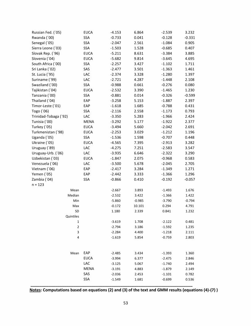
53

Russian Fed. (´05) EUCA -4.153 6.864 -2.539 3.232

Rwanda (´00) SSA -0.733 0.041 -0.128 -0.331

Senegal (´05) SSA -2.047 2.561 -1.084 0.905

Sierra Leone (´03) SSA -1.503 1.528 -0.685 0.407

Slovak Rep. (´96) EUCA -5.211 8.631 -3.384 3.885

Slovenia (´04) EUCA -5.682 9.814 -3.645 4.695

South Africa (´00) SSA -2.257 3.427 -1.102 1.711

Sri Lanka (´02) SAS -2.477 3.501 -1.363 1.461

St. Lucia (´95) LAC -2.374 3.328 -1.280 1.397

Suriname (´99) LAC -2.721 4.287 -1.448 2.108

Swaziland (´00) SSA -0.988 0.661 -0.276 0.080

Tajikistan (´04) EUCA -2.532 3.390 -1.465 1.230

Tanzania (´00) SSA -0.881 0.014 -0.326 -0.599

Thailand (´04) EAP -3.258 5.153 -1.887 2.397

Timor-Leste (´01) EAP -1.618 1.685 -0.788 0.431

Togo (´06) SSA -2.116 2.558 -1.173 0.793

Trinidad-Tobaga (´92) LAC -3.350 5.283 -1.966 2.424

Tunisia (´00) MENA -3.292 5.177 -1.922 2.377

Turkey (´05) EUCA -3.494 5.660 -2.042 2.691

Turkmenistan (´98) EUCA -2.253 3.029 -1.212 1.196

Uganda (´05) SSA -1.536 1.598 -0.707 0.448

Ukraine (´05) EUCA -4.565 7.395 -2.913 3.282

Uruguay (´89) LAC -4.275 7.251 -2.583 3.547

Uruguay-Urb. (´06) LAC -3.935 6.646 -2.322 3.290

Uzbekistan (´03) EUCA -1.847 2.075 -0.968 0.583

Venezuela (´06) LAC -3.500 5.678 -2.045 2.705

Vietnam (´06) EAP -2.417 3.284 -1.349 1.271

Yemen (´05) EAP -2.442 3.333 -1.366 1.296

Zambia (´04) SSA -0.866 0.410 -0.192 -0.057

n = 123

Mean -2.667 3.893 -1.493 1.676

Median -2.532 3.422 -1.366 1.422

Min -5.860 -0.985 -3.790 -0.794

Max -0.172 10.101 0.294 4.791

SD 1.180 2.339 0.841 1.232

Quintiles

1 -3.619 1.708 -2.122 0.481

2 -2.794 3.186 -1.592 1.235

3 -2.284 4.400 -1.218 2.111

4 -1.619 5.854 -0.759 2.803

Mean EAP -2.485 3.434 -1.393 1.360

EUCA -3.994 6.377 -2.475 2.846

LAC -3.125 5.067 -1.740 2.494

MENA -3.191 4.883 -1.879 2.149

SAS -2.036 2.453 -1.101 0.782

SSA -1.549 1.681 -0.699 0.536

________________________________________________________________________ Notes: Computations based on equations (2) and (3) of the text and GMM results (equations (4)-(7) )

54

Table A3.1. Income and inequality elasticities vs. poverty reduction since the early-mid-1990s, for the 80 countries, $1.25 poverty standard

Period 1990-96 Period 1990-96 Early-Mid-1990s to 2000s

Income Inequality Poverty rate

Income elasticity Inequality elasticity growth Growth growth

Country Region A B C D E F G

Albania EECA -3.822 -1.979 5.896 2.089 0.763 1.400 16.077

Argentina-Urb. LAC -3.935 -0.876 6.663 0.345 -1.051 0.327 11.700

Armenia EECA -2.397 -1.005 3.423 0.548 -3.580 -3.903 -7.122

Azerbaijan EECA -2.665 -1.557 3.710 1.422 4.374 -7.310 -62.506

Bangladesh SAS -2.112 -1.870 2.416 1.916 -0.121 -0.072 0.184

Belarus EECA -4.911 -2.668 7.812 3.179 3.504 2.139 -24.964

Bolivia LAC -3.169 -1.132 4.956 0.749 1.002 2.167 10.552

Brazil LAC -2.915 -0.342 4.816 -0.501 1.888 -0.664 -7.142

Burkina Faso SSA -0.794 -0.699 0.260 0.065 1.536 -2.748 -2.557

Burundi SSA -1.164 -1.668 0.556 1.596 0.756 -0.013 -0.252

Cambodia EAP -1.804 -1.348 2.033 1.091 1.859 0.892 -1.890

Cameroon SSA -1.444 -0.884 1.513 0.356 5.792 -0.989 -9.001

CAR SSA 0.287 -0.261 -1.762 -0.629 5.060 -3.419 -2.823

Chile LAC -3.419 -0.501 5.779 -0.249 1.499 -0.572 -8.168

China-Rur. EAP -1.776 -1.754 1.777 1.732 4.433 0.714 -7.103

China-Urb. EAP -2.929 -2.093 3.996 2.269 6.573 1.673 -17.681

Colombia LAC -2.736 -0.444 4.396 -0.339 0.772 0.424 1.676

Costa Rica LAC -3.194 -0.907 5.118 0.393 3.199 0.035 -12.160

Côte d'Ivoire SSA -2.495 -1.439 3.415 1.235 3.168 3.958 1.448

Djibouti MENA -3.276 -1.441 5.029 1.238 -7.937 1.387 22.929

Dominican Rep. LAC -3.121 -0.730 5.052 0.113 0.786 0.284 -1.827

Ecuador LAC -2.634 -0.641 4.090 -0.027 4.562 0.343 -9.377

Egypt MENA -3.111 -1.830 4.499 1.853 1.552 0.718 -2.356

El Salvador LAC -2.700 -0.684 4.205 0.040 1.992 -0.556 -3.469

Estonia EECA -4.066 -1.569 6.598 1.441 3.510 2.004 -61.350

Ethiopia SSA -1.485 -1.249 1.421 0.934 1.244 -2.947 -4.384

Georgia EECA -3.380 -1.419 5.254 1.202 -3.906 1.042 12.207

Ghana SSA -1.687 -1.357 1.787 1.105 3.340 0.819 -3.802

Guinea SSA -0.444 -1.041 -0.629 0.605 -1.628 -3.309 -0.722

Guinea-Bissau SSA -1.387 -0.641 1.512 -0.027 -6.242 0.808 7.174

Honduras LAC -1.766 -0.483 2.372 -0.278 3.621 0.014 -3.677

India-Rur. SAS -2.210 -2.021 2.544 2.156 1.199 0.576 -1.634

India-Urb. SAS -2.089 -1.599 2.501 1.487 1.167 0.822 -1.091

Indonesia-Rur. EAP -2.314 -2.182 2.683 2.410 3.443 0.763 -7.399

Indonesia-Urb. EAP -1.956 -1.500 2.274 1.330 4.219 0.686 -7.779

Iran MENA -3.386 -1.064 5.438 0.641 -1.519 -1.057 0.190

Jamaica LAC -3.374 -1.279 5.309 0.981 4.434 1.467 -24.763

Jordan MENA -3.090 -1.061 4.828 0.636 1.339 -0.995 -14.189

Kazakhstan EECA -3.286 -1.622 4.962 1.524 -0.334 -0.607 -6.680

Kenya SSA -1.807 -0.742 2.333 0.132 3.376 1.134 -3.364

Kyrgyz Rep. EECA -2.586 -0.567 4.025 -0.144 -7.816 -4.446 1.442

55

Lao PDR EAP -2.052 -1.878 2.288 1.928 1.652 0.698 -2.363

Latvia EECA -4.244 -1.965 6.774 2.067 5.518 1.535 -75.503

Lesotho SSA -1.194 -0.290 1.284 -0.583 -3.671 -2.641 -1.313

Madagascar SSA -0.858 -0.918 0.285 0.411 1.755 0.200 -0.554

Malaysia EAP -3.376 -0.822 5.534 0.259 -2.818 -2.742 -14.984

Mali SSA -0.088 -0.706 -1.202 0.075 6.005 -2.165 -4.292

Mauritania SSA -1.943 -1.044 2.466 0.610 2.321 0.917 -2.012

Mexico LAC -3.152 -0.709 5.127 0.080 4.957 -0.089 -23.738

Moldova EECA -2.698 -1.600 3.757 1.489 1.746 0.305 -6.122

Mongolia EAP -2.678 -1.677 3.679 1.610 -0.998 -0.051 1.748

Morocco MENA -3.171 -1.293 4.883 1.004 0.222 0.247 0.119

Mozambique SSA -0.659 -1.001 -0.166 0.542 3.647 0.954 -1.422

Nepal SAS -1.396 -1.385 1.172 1.149 4.782 2.846 -2.706

Nicaragua LAC -1.864 -0.455 2.590 -0.322 2.696 -0.621 -6.005

Niger SSA -1.099 -1.316 0.591 1.040 2.827 0.502 -1.555

Nigeria SSA -1.174 -0.938 0.929 0.442 0.040 -1.141 -0.882

Pakistan SAS -2.150 -1.855 2.501 1.892 4.268 1.058 -9.458

Panama LAC -3.025 -0.441 4.995 -0.345 0.676 -0.248 -2.717

Paraguay LAC -2.967 -0.758 4.720 0.157 -0.364 -0.874 -5.639

Peru LAC -3.217 -0.975 5.133 0.501 1.928 0.691 -0.787

Philippines EAP -2.089 -1.061 2.759 0.636 1.423 0.220 -1.811

Poland EECA -3.662 -1.724 5.688 1.685 8.827 0.743 -29.323

Romania EECA -3.895 -2.168 5.956 2.388 5.895 1.006 -17.192

Russian Fed. EECA -3.589 -0.863 5.956 0.323 0.538 -2.303 -34.218

Senegal SSA -1.125 -0.836 0.878 0.281 2.694 -0.507 -4.359

South Africa SSA -2.344 -0.391 3.612 -0.423 -0.584 0.413 4.019

Sri Lanka SAS -2.609 -1.625 3.562 1.529 2.674 2.115 -2.242

Swaziland SSA -0.154 -0.286 -0.863 -0.589 5.255 -2.993 -3.725

Tanzania SSA -1.448 -1.633 1.160 1.542 -4.282 0.256 2.204

Thailand EAP -2.908 -0.985 4.489 0.516 1.462 -0.274 -19.411

Tunisia MENA -3.047 -1.193 4.675 0.845 3.371 -0.412 -18.653

Turkey EECA -3.399 -1.160 5.419 0.793 1.279 0.365 2.352

Uganda SSA -1.282 -1.254 1.000 0.942 3.115 1.532 -2.475

Ukraine EECA -4.095 -1.879 6.509 1.930 4.210 -2.434 -32.890

Uruguay-Urb. LAC -4.254 -1.082 7.224 0.670 -0.723 0.551 -35.553

Venezuela LAC -3.013 -0.963 4.717 0.481 4.333 -1.161 -14.272

Vietnam EAP -1.581 -1.510 1.493 1.347 5.183 0.407 -7.779

Yemen EAP -3.177 -1.279 4.902 0.981 -4.848 -0.351 10.409

Zambia SSA -0.762 -0.542 0.296 -0.184 -0.830 0.236 0.439

n=80

Mean -2.425 -1.183 3.395 0.829 1.600 -0.128 -7.504

Median -2.622 -1.107 3.694 0.709 1.750 0.270 -3.093

Min -4.911 -2.668 -1.762 -0.629 -7.937 -7.310 -75.503

Max 0.287 -0.261 7.812 3.179 8.827 3.958 22.929

SD 1.088 0.533 2.170 0.843 3.186 1.759 15.725

Quintiles

1 -3.304 -1.640 1.394 0.073 -0.408 -1.008 -14.205

2 -2.921 -1.302 2.572 0.532 1.315 -0.028 -4.886

3 -2.135 -0.995 4.493 1.018 2.695 0.456 -2.150

4 -1.434 -0.705 5.157 1.552 4.281 0.964 0.185

56

Notes: A: Overall income elasticity, B: Income elasticity attributable to initial inequality; C: Overall inequality elasticity, D: Inequality elasticity attributable to initial inequality; E: Annualized (log-difference) growth of mean income; F: Annualized (log-difference) growth of inequality; G: Annualized (log-difference) growth of the poverty rate. For each country the latest year in 1990-1996 is used as the start-year and the most recent year with data in the 2000s as the end-year; details in text. Note that for Belarus, Estonia and Latvia, the latest $1.25 headcount ratio value is 0 and has been replaced with 0.001 in order to compute the growth rates (source provides data for .01 in some cases). Elasticities are based on equations (4) – (7) of the text and country data.

57

Table A3.2. Income and inequality elasticities vs. poverty reduction since the early-mid-1990s, for the 80 countries, $2.50 poverty standard

Period 1990-96 Period 1990-96 Early-Mid-1990s to 2000s

Income Inequality

Poverty rate

Income elasticity Inequality elasticity growth growth Growth

Country Region A B C D E F G

Albania EECA -2.394 -1.766 2.485 1.442 0.763 1.400 0.473

Argentina-Urb. LAC -2.317 -0.856 3.312 1.219 -1.051 0.327 3.515

Armenia EECA -1.283 -0.962 1.485 0.954 -3.580 -3.903 2.608

Azerbaijan EECA -1.543 -1.418 1.439 1.231 4.374 -7.310 -34.310

Bangladesh SAS -1.209 -1.676 0.613 1.387 -0.121 -0.072 0.069

Belarus EECA -3.236 -2.334 3.284 1.787 3.504 2.139 3.203

Bolivia LAC -1.828 -1.067 2.281 1.018 1.002 2.167 2.450

Brazil LAC -1.544 -0.416 2.495 0.622 1.888 -0.664 -4.584

Burkina Faso SSA -0.143 -0.711 -0.140 0.801 1.536 -2.748 -0.251

Burundi SSA -0.532 -1.509 -0.334 1.286 0.756 -0.013 -0.091

Cambodia EAP -0.925 -1.245 0.595 1.126 1.859 0.892 -0.950

Cameroon SSA -0.613 -0.862 0.481 0.894 5.792 -0.989 -3.598

CAR SSA 0.658 -0.349 -1.089 0.894 5.060 -3.419 -0.585

Chile LAC -1.911 -0.547 2.965 0.702 1.499 -0.572 -8.414

China-Rur. EAP -0.963 -1.580 0.305 0.702 4.433 0.714 -2.576

China-Urb. EAP -1.799 -1.859 1.399 1.329 6.573 1.673 -8.945

Colombia LAC -1.436 -0.500 2.226 0.674 0.772 0.424 0.543

Costa Rica LAC -1.814 -0.882 2.452 0.905 3.199 0.035 -5.367

Côte d'Ivoire SSA -1.410 -1.321 1.321 1.172 3.168 3.958 -0.799

Djibouti MENA -1.945 -1.322 2.207 1.173 -7.937 1.387 13.644

Dominican Rep. LAC -1.739 -0.736 2.481 1.173 0.786 0.284 -0.384

Ecuador LAC -1.394 -0.663 1.985 0.772 4.562 0.343 -5.108

Egypt MENA -1.887 -1.643 1.772 0.772 1.552 0.718 -2.757

El Salvador LAC -1.445 -0.698 2.033 0.793 1.992 -0.556 -3.202

Estonia EECA -2.503 -1.428 3.021 1.237 3.510 2.004 -4.808

Ethiopia SSA -0.693 -1.164 0.295 1.076 1.244 -2.947 -0.329

Georgia EECA -2.013 -1.303 2.339 1.161 -3.906 1.042 7.745

Ghana SSA -0.847 -1.253 0.457 1.131 3.340 0.819 -1.934

Guinea SSA 0.049 -0.992 -0.754 0.973 -1.628 -3.309 0.367

Guinea-Bissau SSA -0.540 -0.663 0.569 0.772 -6.242 0.808 2.170

Honduras LAC -0.778 -0.532 1.100 0.693 3.621 0.014 -3.332

India-Rur. SAS -1.297 -1.800 0.628 1.490 1.199 0.576 -0.348

India-Urb. SAS -1.156 -1.452 0.760 1.463 1.167 0.822 -0.609

Indonesia-Rur. EAP -1.391 -1.933 0.645 1.252 3.443 0.763 -1.779

Indonesia-Urb. EAP -1.051 -1.370 0.672 1.544 4.219 0.686 -3.079

Iran MENA -1.967 -1.011 2.571 1.202 -1.519 -1.057 0.180

Jamaica LAC -1.989 -1.188 2.420 1.091 4.434 1.467 -3.934

Jordan MENA -1.765 -1.008 2.237 0.982 1.339 -0.995 -7.169

Kazakhstan EECA -1.978 -1.471 2.104 1.263 -0.334 -0.607 -0.434

Kenya SSA -0.842 -0.746 0.983 0.823 3.376 1.134 -2.337

Kyrgyz Rep. EECA -1.350 -0.602 1.977 0.823 -7.816 -4.446 5.284

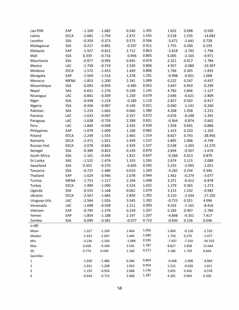
58

Lao PDR EAP -1.169 -1.682 0.540 1.391 1.652 0.698 -0.569

Latvia EECA -2.681 -1.754 2.972 1.435 5.518 1.535 -14.682

Lesotho SSA -0.359 -0.373 0.573 0.596 -3.671 -2.641 0.728

Madagascar SSA -0.217 -0.891 -0.207 0.911 1.755 0.200 0.193

Malaysia EAP -1.927 -0.812 2.712 0.863 -2.818 -2.742 -1.796

Mali SSA 0.339 -0.716 -0.946 0.805 6.005 -2.165 -0.971

Mauritania SSA -0.977 -0.995 0.945 0.974 2.321 0.917 -1.784

Mexico LAC -1.758 -0.719 2.530 0.806 4.957 -0.089 -10.397

Moldova EECA -1.572 -1.453 1.449 0.806 1.746 0.305 -1.835

Mongolia EAP -1.569 -1.516 1.378 1.291 -0.998 -0.051 1.008

Morocco MENA -1.853 -1.200 2.181 1.099 0.222 0.247 -0.437

Mozambique SSA -0.093 -0.959 -0.485 0.952 3.647 0.954 -0.299

Nepal SAS -0.651 -1.276 0.109 1.145 4.782 2.846 -1.127

Nicaragua LAC -0.841 -0.509 1.230 0.679 2.696 -0.621 -2.809

Niger SSA -0.438 -1.219 -0.185 1.110 2.827 0.502 -0.417

Nigeria SSA -0.436 -0.907 0.140 0.921 0.040 -1.141 -0.260

Pakistan SAS -1.233 -1.663 0.666 1.380 4.268 1.058 -2.215

Panama LAC -1.633 -0.497 2.557 0.672 0.676 -0.248 -1.391

Paraguay LAC -1.638 -0.759 2.289 0.831 -0.364 -0.874 -2.662

Peru LAC -1.840 -0.938 2.435 0.939 1.928 0.691 -0.886

Philippines EAP -1.079 -1.009 1.100 0.982 1.423 0.220 -1.103

Poland EECA -2.249 -1.555 2.465 1.314 8.827 0.743 -28.956

Romania EECA -2.471 -1.921 2.449 1.537 5.895 1.006 -4.749

Russian Fed. EECA -2.078 -0.845 2.929 1.537 0.538 -2.303 -12.270

Senegal SSA -0.389 -0.823 0.149 0.870 2.694 -0.507 -1.676

South Africa SSA -1.161 -0.456 1.815 0.647 -0.584 0.413 0.870

Sri Lanka SAS -1.515 -1.474 1.333 1.265 2.674 2.115 -2.089

Swaziland SSA 0.353 -0.370 -0.605 0.595 5.255 -2.993 -1.051

Tanzania SSA -0.722 -1.480 0.010 1.269 -4.282 0.256 0.346

Thailand EAP -1.629 -0.946 2.078 0.944 1.462 -0.274 -3.677

Tunisia MENA -1.753 -1.117 2.104 1.048 3.371 -0.412 -6.878

Turkey EECA -1.990 -1.090 2.524 1.032 1.279 0.365 -1.273

Uganda SSA -0.555 -1.168 0.062 1.079 3.115 1.532 -0.982

Ukraine EECA -2.567 -1.683 2.859 1.392 4.210 -2.434 -27.105

Uruguay-Urb. LAC -2.564 -1.026 3.545 1.392 -0.723 0.551 4.096

Venezuela LAC -1.698 -0.928 2.211 0.993 4.333 -1.161 -8.416

Vietnam EAP -0.795 -1.379 0.239 1.207 5.183 0.407 -2.784

Yemen EAP -1.854 -1.188 2.197 1.207 -4.848 -0.351 7.417

Zambia SSA -0.099 -0.581 -0.077 0.723 -0.830 0.236 0.046

n=80

Mean -1.327 -1.109 1.404 1.056 1.600 -0.128 -2.533

Median -1.423 -1.047 1.444 1.040 1.750 0.270 -1.077

Min -3.236 -2.334 -1.089 0.595 -7.937 -7.310 -34.310

Max 0.658 -0.349 3.545 1.787 8.827 3.958 13.644

SD 0.774 0.439 1.160 0.271 3.186 1.759 6.844

Quintiles

1 -1.930 -1.486 0.284 0.804 -0.408 -1.008 -4.064

2 -1.631 -1.208 1.053 0.954 1.315 -0.028 -1.811

3 -1.193 -0.954 2.088 1.136 2.695 0.456 -0.578

4 -0.644 -0.715 2.468 1.287 4.281 0.964 0.350

59

Notes: A: Overall income elasticity, B: Income elasticity attributable to initial inequality; C: Overall inequality elasticity, D: Inequality elasticity attributable to initial inequality; E: Annualized (log-difference) growth of mean income; F: Annualized (log-difference) growth of inequality; G: Annualized (log-difference) growth of the poverty rate. For each country the latest year in 1990-1996 is used as the start-year and the most recent year with data in the 2000s as the end-year; details in text. Note that for Belarus, Estonia and Latvia, the latest $1.25 headcount ratio value is 0 and has been replaced with 0.001 in order to compute the growth rates (source provides data for .01 in some cases). Elasticities are based on equations (4) – (7) of the text and country data.