observation of bilinear systems with application to biological control

Automatica, Vol. 13, pp. 243-254. Pergamon Press, 1977. Printed in Great Britain

Observation of Bilinear Systems with Application to Biological Control*

DARRELL W I L L I A M S O N t

Although biological sensors are not available for on-line control of microbial cell growth in waste treatment and fermentation systems, an observable bilinear model permits the use of an on-line observer to estimate the unmeasurable variables.

Key Word Index Observability; observers; bilinear; biological control: modelling.

Summary--ln this paper a system of bilinear equations is derived which under appropriate conditions model the microbial cell- growth and product formation of various waste treatment and fermentation systems. Given the available measurements, the problem of obtaining an asymptotic estimate of the state of the system is considered. Necessary and sufficient conditions for the observability of a general system of bilinear equations are also derived. As accurate biological sensors do not often exist the results are significant for the on-line control of these biological processes.

l. INTRODUCTION

LINEAR models are frequently used to approximate the dynamic nature of nonlinear processes. While linear models are convenient they are in many cases inadequate. This is particularly true in modelling biological processes.

The continuous cultivation of micro-organisms has been used in bacteriological research[l], the fermentation industry[2] and in the biological treatment of urban wastes[3,9]. An extensive development of mathematical models beginning with the work of Monod[-4] has proceeded over the past 25 years. More recently[5] with the advent of computers and the availability of sophisticated detecting and measuring devices, models and model parameters have been more accurately determined.

However th~se sophisticated measuring devices are almost entirely restricted for use in the laboratory and can not be used for on-line measurement for purposes of control. For example, the measurement of biomass is usually made by optical means in a turbidistat where a voltage signal proportional to the total amount of solid in the culture is produced. In many cases it actually is the concentration of the active cells which is the important factor. As pointed out in [6, 7] the state of the art in the control of biological processes is still

*Received 17 November 1975; revised 7 June 1976. The original version of this paper was presented at the 6th IFAC Congress on Control Technology in the Service of Man which was held in Boston, Cambridge MA during August 1975. The published Proceedings of this IFAC Meeting may be ordered from: Instrument Society of America, 400 Stanwix Street, Pittsburgh, PA 15222, U.S.A. or John Wiley, Baffins Lane, Chichester, Sussex, U.K. This paper was recommended for publication in revised form by associate editor P. Kokotovic.

tDepartment of Systems and Control, School of Electrical Engineering, University of New South Wales, Australia.

243

deficient in reliable and accurate sensors. There is still no reliable active biomass sensor. No sensor exists which can be sterilised for use as a continuous carbon substrate sensor. Frequently no sensor exists for monitoring product concentrations that is both continuous and can withstand repeated sterili- sations.

The growth of cells in a continuous culture is maintained by the supply of fresh nutrient, or industrial waste in the case of waste treatment plants. The growth is usually accompanied by the formation of products, e.g. methane gas. Certain products and nutrients are either soluble in the culture or are given off in gaseous form, with minimal absorption. That is accurate on-line measurements can be made which will determine the total biomass concentration, and/or a nutrient concentration, e.g. oxygen uptake rate, and a product formation, e.g. carbon dioxide evolution rate. The problem that we consider in this paper is: given the available measurements how can we obtain on-line estimates of the other components of biomass, substrate and product formation.

In the next section based on existing models we formulate a general bilinear model of microbial cell- growth and product formation. We then in later sections analyse the structure of this model and show that provided the system is 'suitably observable' with respect to the available measurements an on-line observer system can be built whose outputs asymptotically estimate the required components.

2. BIOLOGICAL MODEL

A complete understanding of the chemical, physical and biological mechanisms involved in various biological processes is unknown and is not likely to be available. Existing models can be divided into two parts: the first part describes the rate of cell growth and the second part the rate of product synthesis.

Let re(t) = concentration of cells in a

continuous mass cu l t u r e

u ( t )= flow rate of fresh nutrient into the growth vessel of unit volume

244 D. WILL1AMSON

and

;'It l= specific growth rate

~h,,{t l - : v ~ m,,lt ) - - ltlt )m~(t }-- )'2nl,~{l )

th~,(t )= r2mo(t ) -u( t )me(t )

12.3!

Then based on mass balance it follows that

ph(t )=?,( t )m(t ) -u( t )m( t ).

Further, if

s(t) = substrate concentration in growth vessel

(2.1~

s, =cons tant concentration of nutrient flow- ing into growth vessel

,~{t) = _-~/3_ m, (t) - u(t )s(t) + s,u (t) kl

where

m~(t) = active cell concentration

me(t) = nonliving cell concentration

and

and

k~ = constant yield

then

g(t)= -~-'(!-~m(tj-u(t)s(t)+s,u(t). (2.2) kj

These two basic equations appear frequently[8] in the literature as a model of microbial growth.

The specific growth rate 7 is in general a function of the substrate concentration s, and the environmental conditions, e.g. temperature and pH. In industrial applications the growth rate is frequently optimised over these environmental conditions and then the environmental conditions are held fixed, by approximate closed loop feedback control, at the optimal values. We shall assume in this paper that environmental conditions are constant. Then if the nutrient substrate s is in unlimited supply ?(s )=7, ,=cons tant , However, if the substrate is in growth limiting concentrations only, then by the Monod model[4] of growth rate

"fm S ) , ( s ) . . . . . . .

s+ks

m,(t) + m~(t) = total cell concentration.

Although these two components can be identified in a laboratory, sensors for on-line measurements can measure only the total biomass[7].

We shall now consider a model for product synthesis. Probably the best known and useful of these is the model of Luedeking and Piret[10] originally developed for the batch fermentation of glucose to lactic acid. They discovered that the instantaneous rate of acid formation, /5, could be related to the instantaneous rate of bacterial growth, rh, and to the bacterial density, m as follows

l~=ad~ + flm

where e, fl are constant for constant temperature and pH. A modified equation considered in [11] for penicillin production (p) is

/5 = :~rh +/ /m -6p (2.4)

where the term - 6 p represents~a first order penicillin destruction mechanism.

Equations (2.1)-(2.4) can be expressed in the form

21(t)=(Al +u(t)Bl)xl(t)+blu(tt (2.5a)

where ks is a positive constant. In batch processes, i.e. when u(t ) - O, conditions do not remain constant since the nutrient concentration is continually decreasing. However in practice in a continuous process where we are operating at a high growth rate, 7(s)=constant is often a good approximation. Later in section 6 we consider an extension to nonlinear growth rates.

In equation (2.1), re(t) actually represents the active cell concentration and not the total solids concentration. As pointed out in [9] in the analysis of the treatment of whey discharge, the proportion of active cells in the sludge mass could be as low as ten per cent. A more accurate model of biomass is ~hen

22(f ) =:Fx2(t ) 4- G1x 1 (t) -I- 1~221 {l)+ ~2ult)

(.,qlt)~R",x2(t)~R ~) (2.5b)

where all the matrices are constant. In general many cells, substrates and products may be present in the culture. The state x 1 represent all the cell and substrate concentrations and the state x 2 all the product concentrations. The model may be further generalised by the addition of a term, Ep(t), to equation (2.5a) which represents the formation of products which inhibit the production of cells. This inhibitory effect can be considerable in batch processes, i.e. u(t)=-O, but is often negligible in continuous cultures where the product is removed.

Observation of bilinear systems with application to biological control 245

Rearranging equation (2.5) we obtain Measurements:

2~ (t) = (A, + u(t)B 1 )x I (t) + Ep(t) + blu(t)

2 2 (t) = Fx 2 (t) + (G + u(t)D)x I (t) + b2u(t ) (x I (0)6R" and x2(0)E R' (2.6a)

are both unknown)

where

G = G 1 + G 2 A I , D = G 2 B 1 and b2---~2+G2b 1.

We assume that certain measurements Yl (t) and Y2 (t) are available where

yl (t )=c' lxl (t )e R

Y2 (t) = c'2x 2 (t) ~ R. (2.6b)

We also assume based on practical considerations that the flow rate u(t) is non negative and bounded. That is, there exists a constant m o < zo such that

0 < u(t) < mo. (2.6c)

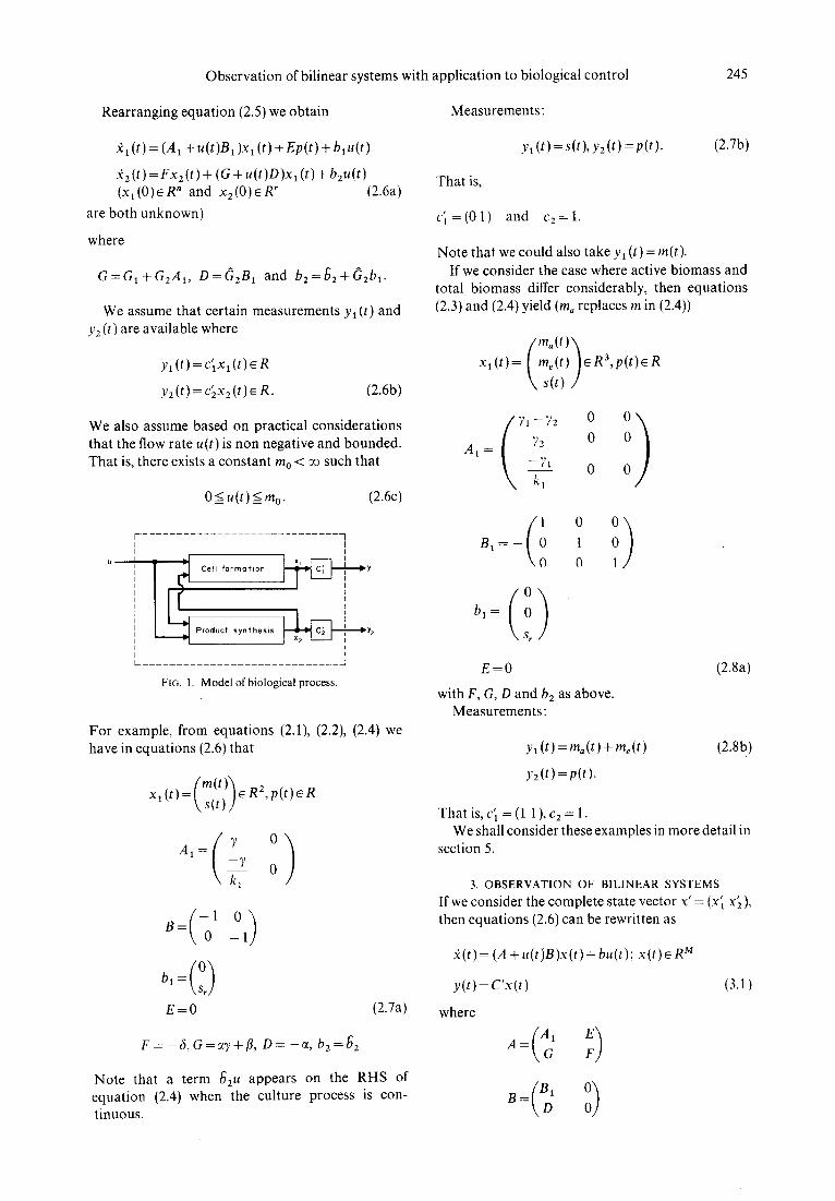
- " 1 ~1~ Cell f .... *ion

Vl Product synthesis

FIG. 1. Model of biological process.

• Yl

P~

For example, from equations (2.1), (2.2), (2.4) we have in equations (2.6) that

X1 (t ) = ( 7 ~ I ) ~ R2, p(t )6 R

o

o) :(o)

E=O

F = - 6 , G=oty + fl, D=-c~ , b2=~ 2

(2.7a)

Note that a term 6zu appears on the RHS of equation (2.4) when the culture process is continuous.

Yl ( t ) = S( t ) , Y2 ( t ) = p ( t ) . (2.7b)

That is,

c' 1= (01 ) and c2=1.

Note that we could also take y~ (t) = re(t). If we consider the case where active biomass and

total biomass differ considerably, then equations (2.3) and (2.4) yield (ma replaces m in (2.4))

i/ma(t)"~ Xl(t)= [ m e ( t ) l ~ R 3 , p ( t ) 6 R

\ s(t) /

A l = 72 0

- - Y l o

o o) B I = - l 0

0 1 (0) ba = 0

S r

E = 0

with F, G, D and b 2 as above. Measurements:

(2.8a)

y,( t)=m.(t)+me(t)

y2(t)=p(t) .

(2.8b)

That is, c'1 = (1 1 ), cz = 1. We shall consider these examples in more detail in

section 5.

3. O B S E R V A T I O N O F B I L I N E A R S Y S T E M S

If we consider the complete state vector x ' = (x' 1 x~), then equations (2.6) can be rewritten as

2 ( t )= (A + u(t )B )x(t ) + bu(t ); x(t )~ R M

y(t )=C'x(t ) (3.1)

where

246 D. WILLIAMSON

\C2/

and all parameters are assumed constant. For a general bilinear system of the type

described by equation (3.1) we say that 2(t) is an estimate of x(t) if

lim t]~?(t ) - x(t)ll = 0

The estimate is said to be asymptotic if there exists a constant 2o independent of u(t) such that

It~¢;(t)-x(t)ll<e -~°' (t>O)

The existence of 2o which is independent of u(t) is necessary in control problems where we need to separate the two tasks of obtaining a state estimate ~(t), and choosing a feedback control law

u(t)= f ( x ( t ) )+u~ t (t)

for some external signal ue~,( • ). In controlling the process the actual control implemented is

u(t j= f (-~(t ) ) + Ue~t(t ),

and so u(t) is not a priori known, unless of course open loop control is implemented.

The existence of an observer system that provides an estimate 2 (0 is closely related to the question of observability of system (3.1) ([19], [20]). It is also well known that the forcing term bu(t) does not affect observability of the initial state x(0), and so for this purpose we may assume b = 0. Let ~# denote the set of all Lipshitz continuous functions. Then for all x(O) and all u ~ ~k" the output of system (3.1) (for b = O) can be expressed as

y(t, x(0); u) = C'O0(t, 0;u)

where

qh(t, 0; u) = ( A + u(t )B )O(t, 0; u);

• (0, 0, u) = IM

for all t => O. If any two such states are indistinguish- able for all u e',Y, the system is unobserrable. Likewise, given any x~(O), the system is said to be observable with respect to u on [0, t l] if:

y(t: xa (0!, u )= ylt; xb (0). u)

for some x b (0) and all t e [0, t~ ] implies x a (0) = x b (0). For an input u(t), more specific conditions for observability can be established as follows. Recall from D'Angelo [14] that the time varying system

2( t )=L( t )x ( t ) ; x(O)~R M

y( t )=C'x( t ) ; y ( t )~R t (+)

is completely observable on the interval [0, t l] if, for specified tl, the initial state x(0) can be determined from a knowledge ofy( t ) on [0, tl].

The system is said to be totally observable on the interval [0, t~] if it is completely observable on every subinterval of [0, il]. The M x M{' observability matrix O(t) is defined as

where

0(t) = [C AC.. . A M- ~C]

d A - / - : ( t ) + ~ t .

The matrix O(t) provides algebraic criteria for determining whether or not a system is observable.

Theorem (D'Angelo). The system (t) with L(t) differentiable M - 2 times almost everywhere on [0, t l] is completely observable on ~_0, t l] if 0(t) has rank M almost everywhere on some finite subinterval of the interval [0, t 1].

Theorem (D'Angelo). The system (t) with L(t) differentiable M - 2 times on [0, t l] is totally observable on [0, t l ] if and only if the observability matrix O(t) has rank M almost everywhere on the interval [0, tl].

If O(t) has rank M everywhere on [0, t l] then the system (?) is said to be uniformly observable on [0, t~]. In this case it follows that the state x(t 2) at the instant t=t2 can be determined from a knowledge of the output y(tz t at that instant.

Likewise, the bilinear system (3.1) is completely (totally, uniformly) observable with respect to u on [0, t l] if the matrix O(u) exists almost everywhere (everywhere, everywhere) and has rank M almost everywhere (almost everywhere, everywhere) where

and I M denotes the M-dimensional identity matrix. Two distinct states x~,(O),xh(O) are said to be

indistin.euishable by u if

y(t; x~(O), u) = y(t; xb(O), u)

and

O(u)=[CAC. . .A M 1C]

d A = (A + u(t)B) +7- .

clt


Clearly, the form of observability depends on the existence of the derivatives

(k) for k= 1,2,.. M - 2 /,4 "'

systems a necessary and sufficient condition for observability for all inputs u(t) can be established. The result can be extended to include the multi-output case by considering an appropriate observable canonical form for the pair {A, C}.

and on the rank of 0(u). Henceforth, by observability of (3.1), we shall

mean complete observability with respect to u on the infinite interval I-0, ~ ) . The results can be directly extended to other forms of observability on other intervals.

If system (3.1) is observable for some u then it follows that it is completely observable except for at most a finite class of inputs. For example, the system

Lemma 1 The bilinear system

2 ( t ) = ( A + u ( t ) B ) x ; x ( t j e R "

y(t)=c'x(t); y(t)~R

is observable if and only if there exists a constant nonsingular transformation P such that

: ~ ( t ) = 22 0 2 3

(i ° !)} +u( t ) 0 x(t)

0

21 # 2 2 # ) ' 3

y(t )=(O 1 1)x(t)

is observable for all inputs u(t) which do not satisfy

(23 -- 22)/~(t) + (22 +/~123 --2122 -- 22/~ 3)u(t) = 0.

In connection with the biological control problem one often has a choice as to the form of input u(t). For example, in fermentation systems piece- wise continuous controls would suffice. This is useful from the point of view of practical implemen- tation, and has computational advantages with respect to the estimator design• In fact if u(t) can take on at most a finite number of constant values

~/0, U l , . . . , U p ,

then system (3.1) is observable if

rank [C' L'kC... (L~,)M-xC] = M

for k=0 , 1 . . . . . p

where L k = ,4 + UkB. However, in other applications, such as waste treatment systems, the input u(t) may be continuously varying. In this case it is important to know whal classes of inputs lead to un- observability since this will be relevant to problems of ill-conditioning and sensitivity associated with the observer design.

For the case of general single output bilinear

t O 0

PAP- 1 = l 0

O , , •

al) a2

1 a n

PBP- 1 t b;1 bl2 ... b , . )

= b22 b2.,, • 0

0 ... 0 b,, /

and

c'P -1 = [ 0 . . . 0 1]

Proof (i) If such a transformation exists, then with L=A +u(t)B we have

O'(u) =

(c) c ' L

c'L 2 + c'L

t c'P- 1 t = c'P- 1 (PLP- 1 )

c'P- 1 (PLP- 1 )2 + c'P- 1 (PLP- 1 P

which is of the form

- 0 0 0 1 -

0 0 1 *

1 * *

0 1

1 * *

for some elements (*) which depend on u. This matrix clearly has rank n for all u.

248 D. WHI,IA MSON

(ii) Conversely , if the system is uniformly observable, it is observable when ult}=-O. That is, there

exists a t r ans fo rmat ion Pl such thai

Pl AP~ 1 =

1 a . _ j

and

which implies

(l +l~bk t.k- 2 --fibk,k 2)Axk-2

k 1

+ E i = 1

( i ~ k 2)

(l~tbk, i - - U b k - 1, i )A. 'c. i = O.

After successive differentiations, we obta in k equa- t ions

c ' P i - 1 = [ 0 0 1 ] .

Let PIBP 11 = [bu]" We now show that if b~s # 0 for

some i>j, then for all tl > t o there exists a funct ion u(t) such that some c o m p o n e n t Xq(t) of x(t) is not observable at t = t I which gives a cont rad ic t ion .

Let k be the largest integer such that bks 4= 0 for some 0 < i < k < n. Then since

- - ,1¢'

J I n - k - 1)

3 )

r I I

i

0

i

A:,) _-o

where R is a k x k matr ix whose componen t s ri~(u, ft... ) are the coefficients of Ax~ ob ta ined above. In par t icular , the coefficient of Axq in the #h

0 l ! X k

1 * ' x k + 1

ipi I

X n

it follows that the componen t s x/ ( t ) for / > k are observable for all t>to and all u(t). That is, given

y , ) . , . . . . . I n - l ) at t = t ~ ~,,

and two possible states

2'=LCq22.. .2,) 2' = (ycl yc2... 2n)

equa t ion (i.e. r/,q) includes the addi t ive term

(/) bkq for q < k,

/L

and no o ther term involving higher der ivat ives of u. Hence if bkq # 0 for some q < k we can choose

at t = t I , it follows that

Ax i = xj - xj = 0 for k ~. j ~ n.

F h e n at t = t 1

k - 1

A2 s=Ax i ~+u y" baiAxi for l < j < k i=1

which implies (] = k)

k - 2

( l+ubk,k-l)Axk 1+~ Y', bkiAxi=O. i - 1

Differentiat ing the above equa t ion gives

k- 1

AXk l = A X k 2 + u E b k - l , i A x i i = l

- atd ( uk~lbkiAxi)i_,

t l ( t l ), f i ( t l ) . . . . . ( ~ ) ( t 1 )

such that the qth column of R is zero at t = t 1 . Tha t is, Axq(t) is not necessari ly zero at t = t 1 .

Q.E.D.

The necessity condi t ion of this l emma corrects an error made in an earl ier p a p e r [ l 8].

The i n p u t - o u t p u t re la t ionship of bi l inear systems which are observable for all inouts u(t) can then be de termined. In the case of second order systems we have observabi l i ty for all u(t) if the i n p u t - o u t p u t re la t ionship is of the form

f(t) + [a 2 + u(t)bl 1] 9(t)

+ [a l +u(t)(b~2 +a2b11 ) ]y( t )

d + b22[bl, u 2 (t)y(t) + dt u (t)y(t)] = v (t)


for some function v(t) depending on u(t), and for all t such that fi(t) exists.

described by equations (2.6) (and (3.1)) if we consider observability with respect to the scalar output

Example 1 Consider the cell growth equations (2.7) of section

2; viz.

+=,( o' +(%

:) - l J J \ s ( t ) /

y(t) =s(t)

where k~, 7 and s, are constant. The input-output description for all t such that fi(t) exists is given by

; ( t ) + (u(t ) - y )~( t ) - yu( t )y(t ) + (u 2 (t )y(t )

d - - + ~ u ( t ) y ( t ) )=v( t )

g(t) =o¢ly I (t) -]-~2Y2 (t)

for appropriate choice of constants ~1, ~2.

4. OBSERVER DESIGN Given any input u e ~//, equation (3. l) is a linear time varying system

2 ( t ) = L ( t ) x ( t ) + b u ( t ) ; x ( t ) e R M

y ( t ) = C ' x ( t ) (4.1)

where L ( t ) = A + u ( t ) B for which standard conditions of observability can be applied. Johnson[ l 7] has shown that when {L(t), C} represent an observable process (in general, C can also be time varying) in the sense that for all ~ > 0 and all t, there exists 6 (e) > 0 such that

61 < j'~p + ~ ¢'(r, t o + e )CC'@(z, t o +~)dr

where

where

v ( t ) = s , a ( t ) - 7s , u ( t ) + s~u 2 ( t ) .

Hence, by the previous lemma, the system is observable for all inputs u(t).

An equivalent input-output description is then given by

2 ' ( t )= { ( Ol ?7)

+<o t)}.,,,+(°,), ,, y( t )= (0 1)x, (t)

(3.2)

where

Xl( t )= ix11( t )S t t ) )

and

x l l ( t )=g + T s - u s - v

?

kl - - - - m + ( 7 - 2 u ) s + u s , - v .

Therefore given the measurement s(t), if an asymptotic estimate ~11(t) is available, then an asymptotic estimate rh(t) can be obtained.

Lemma 1 may also be useful for examining~ observability of the multi-output biological model

¢(t , t o) = L( t )~( t , t o); ¢(to, t o ) - I M

then an observer system exists which provides a uniformly asymptotically stable estimate with arbitrary settling time for the transient response. A general linear observer structure of order M (observers of order M - m also exist) is given by

.~ = K 1 (t)2 + K 2 (t)y + bu

where

K , (t) = L ( t ) - K 2 ( t )C'

K=(t)=½B-'(t)CQU) (4.2)

and

B(t ) = - B(t )L(t ) - E(t )B(t )

- R ( t ) + C Q ( t ) C ' (4.3)

(R(t), Q(t) arbitrary real, symmetric, positive definite matrices). The solution of the linear matrix equation (4.3) may be expressed as

B(t ) =@'(to, t )Bo@(to, t)

-~oO'(r, t)R (r)¢(~, t)d~

+ J",o ¢' (~, t )C Q (z)C'e (~, t) dr.

This approach has the disadvantage that the solution B (t) for some choice of R (t), Q (t) cannot be

250 D. WILLIAMSON

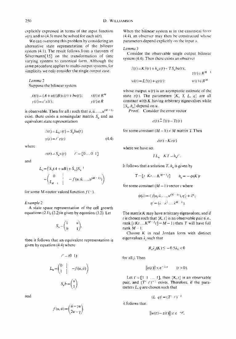
explicitly expressed in terms of the input function u(t), and so (4.3) must be solved for each u(t).

We can overcome this problem by considering an alternative state representat ion of the bilinear system (4.11. The result follows from a theorem of Silvermann[15] on the t ransformat ion of time varying systems to canonical form. Although the same procedure applies to mult i -output systems, for simplicity we only consider the single output case.

Lemma 2 Suppose the bilinear system

2(t)= (A +u(t)B)x(t)+ bu(t): y( t )=c 'x ( t ) ;

x ( t ) e R M

v ( t )~R

is observable. Then for all t such that fi,// . . . . . u IM- ~) exist, there exists a nonsingular matrix S, and an equivalent state representat ion

When the bilinear system is in the canonical form (4.4), an observer may then be constructed whose parameters depend explicitly on the input ,.

Lemma 3 Consider the observable single output bilinear

system (4.4). Then there exists an observer

}(t) =K2( t ) + h,,y(t)+ TS, bu(t);

w(t ) = E£(t ) + qy(t ) :

z ( t )~R M

w( t )~R M

whose output w(t) is an asymptotic estimate of the state z(t). The parameters {K, T, L, q} are all constant with K having arbi t rary eigenvalues while [S~,h,l depend on u.

Proof Consider the error vector

e(t) ~=2(t)-Tz(t)

where

and

5(t) = L,,z(t) + S, bu(t)

y ( t ) = / ' z ( t )

z ( t )= S ,x( t ) / ' = [ 0 . . . 0 l ]

L,, = [S,,(A + u B ) + 8,,]S,~

= (IM0_, - f (u, ,i . . . . . u ~M- ~'))

for some M-vector valued function f ( • ).

(4.4)

Example 2 A state space representat ion of the cell growth

equations (2. l), (2.2)is given by equation (3.2). Let

then it follows that an equivalent representat ion is given by equat ion (4.4) where

/ ' = ( 0 l )

(0 ) L , = ,I - f ( u , l ~ )

l i

for some constant (M - 1 ) × M matrix T. Then

O(t)=Ke(t)

where we have set

T L u - K T = hu/ '.

It follows that a solution T, h u is given by

T = [ t K t . . . K M-*t] h , = - O ( K ) t

for some constant (M - 1 ) vector t where

~(2) = </(u, ~i . . . . . u ~ '~' - ~'), ~l > + 2":

r / = ( 2 22 . . . 2 M l).

The matrix K may have arbi t rary eigenvalues, and if t is chosen such that {K, t} is an observable pair (i.e., rank [ t K t . . . K M - 2 t ] = M - 1) then T will have full rank M - l.

Choose K in real Jordan form with distinct eigenvalues 2i such that

ReXj(K)<= -0 .5) . 0 < 0

for allj. Then

Ile(t)tp :e (,>0).

Let t ' = [ 1 1 ... I], then {K,t} is an observable pair, and (T' / ) - ~ exists. Therefore, if the parameters L, q are chosen such that

and

fi -Tu~ f ( u ' f i ) = \ 2 u _ T / "

it follows that

(L q ) '= (T ' /)-1

IIw( )-z.lll e- o


and so w(t) provides an asymptotic estimate of z(t) where 2o is independent of u (t).

Q.E.D. Example 3

Using the rel~resentation (3.2) we have from lemma 3 that an asymptotic estimate 2(t) ofx~ (t) is provided by

~(t) = - 0.52o~(t ) + h~y (t) + s,u(u - 7 - 0-52o)

w(t) = (~(t) + 0.5&y(t)~ y(t) /

where

hu = (7 + 2o)U - 0.520 (~ + 0.52o) - fi

( T = [ 1 -0 .520] ) .

It can be seen that although the observer is independent of the derivatives of the output y(t), as it must be since noise will also be present in a practical situation, the observer parameters do depend on the derivatives of the input u(t). If the input is noise free this will present no difficulties. Likewise, if derivatives of u (t) fail to exist at certain instants t~, t2, t3 . . . . (such as in bang-bang control taws) then this problem can also be overcome in a practical situation by eliminating the inputs fi,/i . . . . . u(M- a) to the observer at those instants. This would correspond to re-initialising the observer state at

t = t l , t z , t 3 , . . .

and provided the switching instants are not too frequent, or alternatively, 2o is made sufficiently large, asymptotic state estimates will be obtained for

t 1 < t < t z , t 2 < t < t 3 , etc. Actual differentiation of the system u can also be

overcome by augmenting the system with M - l integrators as illustrated in Fig. 2. From the point of view of optimal control design, augmenting the system with integrators is equivalent to placing constraints on the derivatives of the input[16]. In a waste treatment system this would correspond to having several storage tanks, as is often the case, buffering the effluent before it is neutralised.

Let us now return to the bilinear model, equation (2.6), developed in section 2 for cell formation and

s y s t e m ] • y

~t g ( ~, U,...., U (M-~))

FIG. 2. Augmented system.

product synthesis. If this equation is then written in the form of equation (3.1), the results of this and the previous section may be used to examine observability and construct an observer. However, if the product inhibition effect, as represented by the term Exz(t), can be neglected, as is often the case in continuous processes, or is directly measurable, i.e. E = kc'2 for some vector k, a simpler observer design can be accomplished. In this case a constant linear estimator can be used to estimate the states x 2(t) and a bilinear estimator is only required to provide an estimate of Xl(t ). This can save considerable computational effort.

Theorem. Consider the system

Xl (t) ---- (A 1 + u(I)B 1 )x(t) + Ex 2 (t) + b 1 u(t)

x2(t) =Fx2(t ) + (G + u(t)D)x I (t) + b2u(t )

y, (t)=c'lxx (t)

y2(t)=c'2x2(t)

O<=u(t)<mo

where the initial states x 1 (0) ~ R" and x 2 (0) s R" are unknown. Suppose the bilinear subsystem

O1 (t)= (A a + u(t)B x )t/1 (t);

yl(t)=ci~l(t)

is observable, in the sense of section 3, and the linear subsystem

02(t)=Frlz(t); y2(t)=c'2q2(t)

is also observable. Then provided the product inhibition term Ex2 (t) is measurable, i.e. E = kc'z for some vector k, there exists matrices

{KI, h., 7"1, Su, g2 , T2, h2, L~, L2, ql, q2}

which define an observer system

~1 (t) = g 1)~1 ( t ) Jr- huy 1 (t) + T 1 Suky 2 (t)

+ T1S, btu(t)

:~2 (t) =K2~ 2 (t) + T 2 (G + u(t)D)w 1 (t) + h2y 2 (t)

+ T2b2u(t)

w 1 (t) = S~ -1 (E,21 (t) + qlYl (t))

w 2 (t) = E2~ 2 (t) + q2Y2 (t)

where

~l ( t )e Rn- l,fc2(t)ff R "-1

252 D. WIt.LIAMSON

such that: given any constant 2 0 > 0,

[]w, (t)--Xl (t)H -ze ~,~'

and

Ilw (t)-x2(t)il e --*°' it>o)

where

i.e.

when

'o= ,llT lltllGIl÷moltDII)

d dt (lle2It)ll~) < - ;-°]le:(t)ll~

for all t such that ti,/i . . . . , t?" ~1

exist.

Proof (Constructive). Under the hypothesis of observability of the bilinear subsystem, there exists a transformation S, such that

Ile (t)ll> ....... A1 --/-0

Then from (iii),

l t w 2 t t ) - x 2 ( t ) l l ~r. e ~,'.

z l ( t ) ~=S,xl(t)

is given by

21 (t) = L , z t ( t )+ S , (Exz( t ) + b~u(t ));

) ' l ( t ) = / " z l ( t )

where L , , / ' are defined as in lemma 2. Since E = kc' 2, an asymptotic estimate is given by w 1 (t) above. This follows by considering the error vector

e, ( t )~2 t ( t ) - T 1Z 1 (t)

and choosing {K 1, h,, T 1, LI, ql} as in lemma 3 so that

I I S , , w , ( t ) - =,(t)ll ~e-*, ' '

which implies since IlSu 1tt is bounded that

] ] W l ( t ) - x , ( t ) ] l < . l e-~o'.

Now suppose {K2, T2, h2, L2, q2} are constant and chosen such that

{i) K2 is in real Jordan form with

Re2i(K2}<= --0.521 < - - 0 . 5 2 0 < 0 forall j.

(ii) T 2 F - K 2 T 2 = h 2 c 2. (iii) ( L 2 q 2 ) ' = ( ~ c 2 } 1

Then the error vector

C 2 (t) ~ 22 (t) - - T2x 2 (t)

is governed by

e2 (t) =K2e 2 (t) + ~ (G + u(t)D)(w~ (t) - x 1 (t)).

Therefore since u(t) is bounded

Since the pair {F, c2} is observable a solution ~t T2, h2} is given by

T2=P[t2 K2t2 ... K~2 lt2] ; h2=-O2(K2) t2

where r.-1

j= l

S r - - | d e t ( s I - K 2 ) = +f ir_is r + . . . +fl ls+/ /o

and P is the nonsingular transformation such that

{PFP 1,c2P-I

is in observable canonical form, i.e., similar structure to L u, / ' in lemma 3.

Q.E.D. Given the available measurement of substrate

concentration s(t) for the biological model of equation (2.7) we have constructed by means of examples l, 2, and 3 a first order observer that provides an asymptotic estimate of the cell concentration re(t).

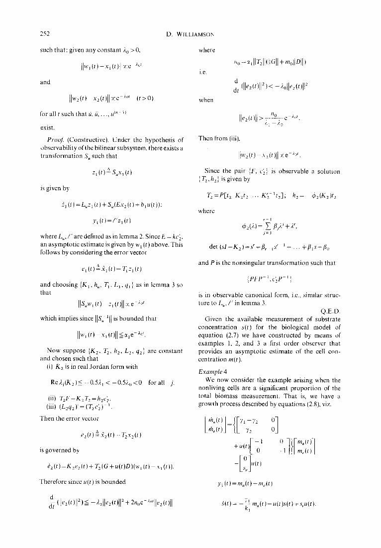
Example 4 We now consider the example arising when the

nonliving cells are a significant proportion of the total biomass measurement. That is, we have a growth process described by equations (2.8), viz.

[ lha(t)] --)'2

+ u (t)[ ; 1 -0 ] t [m"( t : 1 1 j)l_ me (t

+[°Z, Ls~J

y l ( t ) = m , ( t ) + m , , ( t )

d (lie2 (t)l121 - 2, Ile2 It )112 + 2noe-~°'[[e 2 (t)[] dt ~(t ) = u(t )s(t ) + s,u(t ). - ~ m . ( t ) -


The third order system as represented by the state vector

[m, ( t )m~( t ) s ( t ) ] '

Hence

Ile(t)ll ~ l e -~'

is not uniformly observable from the measurement y~. We therefore have partitioned the system into a second order system, which is uniformly observable from ya, and a first order system. The approach is first to estimate ma(t) from y l ( t ) , and use this to estimate s(t). We omit the design of an observer to estimate m,( t ) since this is analogous to examples 1 3. Instead we assume an estimate w(t) of m~(t) has been obtained such that

I Iw(t)- m~(t )ll <= %e- ~o,

Consider the equation

(20 > 0).

' 9 . e(t ) = - ~ w(t ) - u (t )z(t ) + sru(t )

then the error vector

e ( t ) a = z ( t ) - s ( t )

is governed by

~(t ) = - ~- (w(t ) - ma(t ) ) - u(t )e(t ). tel

So

d (lie(t)112)= _ 2u(t)lleU)112 dt

271 e ' ( t ) ( w ( t ) - m o ( t ) ) . kl

Now, u(t) is a bounded flow rate; that is,

O < u ( t ) < m o.

Assume in addition that u(t)>=6o>O for all t>0 . Then

d ([le(t)ll) 2 < _ 26o[le(t)112 + 2noe- ,o,[le(t)l[ dt =

where 2 = minimum (2 o, ao). That is, we are able to obtain an estimate of the substrate concentration s(t), but the rate of estimation depended on 6 o where 0 < 6 o < u(t). If this rate is not fast enough, i.e. 6 o is too small, for control purposes, the substrate concentration would have to be directly measured.

5. AN EXTENSION TO N O N L I N E A R

G R O W T H RATES

As pointed out in section 2 if the nutrient substrate s is in unlimited supply the cell growth rate 7 is constant. When the substrate is in growth limiting concentrations, then 7 depends in a nonlinear way on s. One such dependence is expressed by the Monod model. But if we operate the processes at a high growth rate, then again 7 constant is a good approximation. The observation problem when the growth rates are constant has been treated in the previous sections.

If the growth rates are nonlinear, then A 1 and F in equations (2.6) are functions of x 1 and x 2 re- spectively. No general results can be stated in this case and each problem must be examined in its own right.

One technique that we now illustrate is not as restrictive as it first appears. Typically in biological processes cells m i grow at the expense of some particular substrate Sk, and for u ( t ) = 0 the growth rate of mj is proportional to the rate of depletion of s k. This is illustrated in equations (2.1), (2.2). Consider again these equations, viz.

rh(t) = 7m(t) - u( t )m( t )

7 s(t)= kl m ( t ) - u ( t ) s ( t ) + s r u ( t )

where k 1 , s r are constants and 7 = 7 ( s , m ) . Define the new state x ( t ) a= re( t )+ kls( t ) , then

~ ( t ) = - u ( t ) x ( t ) + k , s , u ( t ) ; x(0) unknown.

Consider an observer

when

I F/1 ~. 710~0 ~

=<-2)~, lie(t)l ?

Ile t)lL_->ao"_°21

2(t ) = - u(t )z(t ) + kl sru( t )

and define the error

e(t) a=z ( t ) - x ( t ) .

Then

~(t)= - u ( t ) e ( t ) .

254 D. WII.IJAMSON

t h e flow rate u is nonnegative. Assume further that

u( t )>~50>0

for all t > 0. Then

d di- le ( t )12 = - H( t } l c ( t ) [ 2 ~_ - ~5 0 l e ( t ) l : .

So

example considered the growth rate 7 could be an3 function of cell ',tnd substratc concentrati,,ns. The key rcquiremen,* was f'ol u( / )=0 that " be pr(~- pm tional 1,~ ~!te rate of depletion of the substrate s.

The resuh,_, of this paper are at present being applied to the on-line computer control and optimtzation c,f alcohol (ethanol) production. This is a project which recently began at the thdversity of N.S.W. in the Departmenl of Biological ]ech- nology.

le(t)l: le(O)lZe- o ' (t O)

and le(t)t approaches zero asymptotically with rate 6 o. Therefore if s ( t ) (or m ( t ) ) is available for measurement, an asymptotic estimate

th ( t ) = z ( t ) - k t s ( t )

(or kt,~(t l = z ( t ) - m ( t ) ) can be obtained.

6. D I S C U S S I O N A N D C O N C L U S I O N S

Based on existing theories we have formulated a model, equation (2.6), describing microbial cell growth and product synthesis in continuous cultures. This is essentially a two stage process in which cells are grown and then the product synthesised. A term was included that represented the inhibiting effect of the formation of products on the cell growth.

In the model, environmental conditions, such as temperature and pH, were assumed constant. We also assumed that the various cell growth rates were constant. Given certain measurements we then formulated the observability problem. From the system theoretic point of view, necessary and sufficient conditions (lemma 1) in terms of the system parameters were derived for observability of a bilinear system for all inputs u( t ) . An observer which avoided differentiation of signals was then constructed whose outputs asymptotically esti- mated the remaining cell, substrate and product concentration.

Although the rate of estimation can be a p r i o r i specified the faster the estimation the less tolerant these systems will be to noise measurements. A trade off must then be made. Because of the terms involving the product of control and state variables more quantitative results of performance in the presence of noise cannot at present be obtained.

An extension of the observation problem when the growth rates are nonlinear was considered in section 5. We illustrated a technique which is often useful for the treatment of these problems. In the

REFERENCES [1] H. MOSER: The Dynamics of bacterial population main-

tained in the chemostat. Carnegie lnsl. Washington Publ. 614(1958).

[12] A.J.C. OLSEN: Manufacture of bakers yeast by continuous fermentation. Continuous culture of microorganisms. Soc. Chem. Ind. Mono 12, New "fork, MacMillan (19611.

[3] J. F. ANI)R~WS: Dynamic model of the anaerobic digestion process. J. Sanitary Eng. Dip. Pr,,c. Am. Sot'. Civil Eng. 95, (1969}.

[4] J. MONOD: ka Technique de cultures continues: thdnric cl applications. Ann. Inst. Pasteur 79, (4) (1950)

[5] D. BOtiRDAUD and C. FOttArD: Identification and optimization of batch culture fermentation processes. Is* European Cm?ll o,1 Computer Control and Fermentation, Dijon, France { 19731.

[6] A. E. HUMPHREY: Rationale for and principles ol computer-coupled fermentation systems. Ist European ('anti on Contputer Control and Fermentation. Dijon, France (19731.

[7] A.G. LANE: Instrumentation in computer control of a pilot plant. 1st European Conll on Computer Control and Fermentation, Dijon, France (1973).

[8] G. D'ANs, D. GOTTLIt!B and P. KoK()rot \lE: Optimal control of bacterial growth. Pro(. IFAC 5th ~brhl Congress, Paris, France (19721.

[9] G. J. S~,WARDS and G. A. HOLDER: Aerobic biological treatment of anaerobically digested whey. 2nd National Chem. Eng. Cot!1~ Queensland (1974).

['10] R. LUEDEKIN(i and E. L. PINET: Akinetie study of the lactic acid fermentation. J. Biochem. ~'~4ier~hioI. Te~h. Eng. I, 393 (1959L

[1 t] A. CONSTANTINIDkS, J. L. SPEN('ER and E. L. G ~,l)t.N. JR.: Optimisation of batch fermentation processes. Develop- ment of mathematical models R~r batch penicillin fermen- tations. Bioteeh. Bioeng. xii, 803 830 (1970).

[12] R. E. KaLMa, N: Mathematic description of linear dynami- cal systems. J. Siam. I (2)(1963).

[13] T. E. [~ORr~4ANN and D. WIEUAMSON: Design of low-order observers for linear feedback control laws. IEEE Trans. Aut. Control AC-17, {3) June ( 1972}.

[_14] H.D. ANGELO: Linear Time-karying Systems:/tnalysis and Sjnthesis. Allyn & Bacon, Boston (19701.

[15] M. StLVERMANN: Transformation of time-variable systems to canonical form. IEEE Trans. Aut. Control AC-I1, (2) April (1966).

[16] J. B. MOORE and B. D. O. ANDERSON: Optimal linear control with input derivative constraints. Proc. IEE 144, {12) Dec. (19671.

[.17] G. W. JOHNSON: A deterministic theory of estnnation and control. Proc. Joint Aut. Control Cot![~, June (1970).

[18] D. WU.LJA'4SON: Modelling and observation of microbial growth processes. Proc. IFAC Sixth Worht Congress, Boston, Aug. (1975).

['19] B. A. FRELeK and D. L. ELLtOTT: Optimal observation for variable structure systems. Proc. IFAC August (1975).

[20] S. HARA and K. Kul,,tJra: Minimal order state observers l\)r bilinear systems. Int. J. Control (to appearL

observation of bilinear systems with application to biological control

Documents