Bilinear Pairings in Cryptography

Master thesis#603

by

Dennis Meffert<d.meffert@student.science.ru.nl>

at

Radboud Universiteit Nijmegen

Computing Science Department

Toernooiveld 1

6525 ED Nijmegen

The Netherlands

supervised by

dr. W. Bosma

dr. D.C. van Leijenhorst

May 24, 2009

1

Abstract

This thesis consists of two sections. The first section is devoted to the mathematics of pairings. Ellip-tic and hyperelliptic curves over finite fields are described, as well as rational functions and divisorson such curves. The Weil pairing on elliptic curves, and the Tate pairing on elliptic and hyperellipticcurves are explained with a computational approach in mind.

The second section introduces bilinear pairings in a cryptographic setting. First their relation to thediscrete logarithm problem in finite fields is investigated. Then we illustrate how bilinear pairingsgive rise to new mathematical problems which can be used as a base for secure cryptosystems. Weconclude with a description of several cryptosystems based on bilinear pairings.

2

3

Acknowledgements

First of all I would like to thank my supervisors, Wieb Bosma and Dick van Leijenhorst, for theirguidance during the writing of this thesis and for their helpful comments on the text. Thanks isalso due to Ken Madlener for the many fruitful discussions we have had about cryptography. On apersonal note I would like to thank my parents for their support.

4

5

Contents

1 Introduction 81.1 Thesis outline . . . . . . . . . . . . . . . . . . . . . . . . . . . . . . . . . . . . . . . . . 8

2 Elliptic and Hyperelliptic Curves 102.1 Projective Space . . . . . . . . . . . . . . . . . . . . . . . . . . . . . . . . . . . . . . . 102.2 Algebraic Curves . . . . . . . . . . . . . . . . . . . . . . . . . . . . . . . . . . . . . . . 102.3 Rational Functions . . . . . . . . . . . . . . . . . . . . . . . . . . . . . . . . . . . . . . 112.4 Divisors . . . . . . . . . . . . . . . . . . . . . . . . . . . . . . . . . . . . . . . . . . . . 122.5 Elliptic Curves . . . . . . . . . . . . . . . . . . . . . . . . . . . . . . . . . . . . . . . . 14

2.5.1 Definition . . . . . . . . . . . . . . . . . . . . . . . . . . . . . . . . . . . . . . . 142.5.2 Computing the group law . . . . . . . . . . . . . . . . . . . . . . . . . . . . . . 152.5.3 Group structure . . . . . . . . . . . . . . . . . . . . . . . . . . . . . . . . . . . 162.5.4 Rational functions on elliptic curves . . . . . . . . . . . . . . . . . . . . . . . . 17

2.6 Hyperelliptic Curves . . . . . . . . . . . . . . . . . . . . . . . . . . . . . . . . . . . . . 182.6.1 Definition . . . . . . . . . . . . . . . . . . . . . . . . . . . . . . . . . . . . . . . 182.6.2 Jacobian . . . . . . . . . . . . . . . . . . . . . . . . . . . . . . . . . . . . . . . . 192.6.3 Computing the group law . . . . . . . . . . . . . . . . . . . . . . . . . . . . . . 202.6.4 Group structure . . . . . . . . . . . . . . . . . . . . . . . . . . . . . . . . . . . 212.6.5 Example . . . . . . . . . . . . . . . . . . . . . . . . . . . . . . . . . . . . . . . . 212.6.6 Rational functions on hyperelliptic curves . . . . . . . . . . . . . . . . . . . . . 22

3 Pairings 233.1 Weil Pairing . . . . . . . . . . . . . . . . . . . . . . . . . . . . . . . . . . . . . . . . . . 23

3.1.1 Definition . . . . . . . . . . . . . . . . . . . . . . . . . . . . . . . . . . . . . . . 233.1.2 Properties . . . . . . . . . . . . . . . . . . . . . . . . . . . . . . . . . . . . . . . 243.1.3 Computation . . . . . . . . . . . . . . . . . . . . . . . . . . . . . . . . . . . . . 243.1.4 Modifications . . . . . . . . . . . . . . . . . . . . . . . . . . . . . . . . . . . . . 27

3.2 Tate-Lichtenbaum Pairing . . . . . . . . . . . . . . . . . . . . . . . . . . . . . . . . . . 273.2.1 Definition . . . . . . . . . . . . . . . . . . . . . . . . . . . . . . . . . . . . . . . 283.2.2 Properties . . . . . . . . . . . . . . . . . . . . . . . . . . . . . . . . . . . . . . . 283.2.3 Computation . . . . . . . . . . . . . . . . . . . . . . . . . . . . . . . . . . . . . 303.2.4 Modifications . . . . . . . . . . . . . . . . . . . . . . . . . . . . . . . . . . . . . 31

3.3 Hyperelliptic Tate-Lichtenbaum Pairing . . . . . . . . . . . . . . . . . . . . . . . . . . 323.3.1 Definition . . . . . . . . . . . . . . . . . . . . . . . . . . . . . . . . . . . . . . . 32

6

3.3.2 Properties . . . . . . . . . . . . . . . . . . . . . . . . . . . . . . . . . . . . . . . 323.3.3 Computation . . . . . . . . . . . . . . . . . . . . . . . . . . . . . . . . . . . . . 323.3.4 Elliptic versus Hyperelliptic Pairings . . . . . . . . . . . . . . . . . . . . . . . . 34

4 Discrete Logarithm Problem 354.1 Problems . . . . . . . . . . . . . . . . . . . . . . . . . . . . . . . . . . . . . . . . . . . 35

4.1.1 Relating the problems . . . . . . . . . . . . . . . . . . . . . . . . . . . . . . . . 354.2 Protocols . . . . . . . . . . . . . . . . . . . . . . . . . . . . . . . . . . . . . . . . . . . 36

4.2.1 Diffie-Hellman key exchange . . . . . . . . . . . . . . . . . . . . . . . . . . . . . 364.2.2 Digital Signature Algorithm . . . . . . . . . . . . . . . . . . . . . . . . . . . . . 37

4.3 Attacks . . . . . . . . . . . . . . . . . . . . . . . . . . . . . . . . . . . . . . . . . . . . 374.4 Elliptic Curve Discrete Logarithm Problem . . . . . . . . . . . . . . . . . . . . . . . . 38

4.4.1 Attacks . . . . . . . . . . . . . . . . . . . . . . . . . . . . . . . . . . . . . . . . 384.5 Hyperelliptic Curve Discrete Logarithm Problem . . . . . . . . . . . . . . . . . . . . . 39

4.5.1 Attacks . . . . . . . . . . . . . . . . . . . . . . . . . . . . . . . . . . . . . . . . 404.6 Practical Considerations . . . . . . . . . . . . . . . . . . . . . . . . . . . . . . . . . . . 40

5 Pairing-Based Cryptography 425.1 Abstract Pairings . . . . . . . . . . . . . . . . . . . . . . . . . . . . . . . . . . . . . . . 425.2 Complexity Assumptions . . . . . . . . . . . . . . . . . . . . . . . . . . . . . . . . . . . 43

5.2.1 Bilinear Diffie-Hellman . . . . . . . . . . . . . . . . . . . . . . . . . . . . . . . . 435.2.2 Gap Diffie-Hellman Groups . . . . . . . . . . . . . . . . . . . . . . . . . . . . . 445.2.3 Pairing Inversion . . . . . . . . . . . . . . . . . . . . . . . . . . . . . . . . . . . 44

5.3 Choosing groups and mappings . . . . . . . . . . . . . . . . . . . . . . . . . . . . . . . 45

6 Pairing-Based Protocols 466.1 Three-Party Key Exchange . . . . . . . . . . . . . . . . . . . . . . . . . . . . . . . . . 466.2 Identity Based Encryption . . . . . . . . . . . . . . . . . . . . . . . . . . . . . . . . . . 47

6.2.1 Introduction . . . . . . . . . . . . . . . . . . . . . . . . . . . . . . . . . . . . . 476.2.2 Security models . . . . . . . . . . . . . . . . . . . . . . . . . . . . . . . . . . . . 486.2.3 The Boneh-Franklin identity based encryption scheme . . . . . . . . . . . . . . 526.2.4 Other identity based encryption schemes . . . . . . . . . . . . . . . . . . . . . . 58

6.3 Short Signatures . . . . . . . . . . . . . . . . . . . . . . . . . . . . . . . . . . . . . . . 606.3.1 Introduction . . . . . . . . . . . . . . . . . . . . . . . . . . . . . . . . . . . . . 606.3.2 Security models . . . . . . . . . . . . . . . . . . . . . . . . . . . . . . . . . . . . 616.3.3 The Boneh-Lynn-Shacham short signature scheme . . . . . . . . . . . . . . . . 646.3.4 The Boneh-Boyen short signature scheme . . . . . . . . . . . . . . . . . . . . . 65

7 Conclusions 68

7

Chapter 1

Introduction

Bilinear pairings were originally brought to the cryptographic community by Menezes, Okamoto andVanstone with their MOV attack [38]. As it turns out pairings can be used to transport the discretelogarithm problem on a certain class of elliptic curves over a finite field to the discrete logarithmproblem on a smaller finite field, where a sub-exponential index calculus attack can be used to attackthe problem. However, it was the publication of an identity based encryption scheme (by Boneh andFranklin [10]) based on bilinear pairings that triggered a real upsurge in the popularity of pairingsamong cryptographers. Following Boneh and Franklin, a lot of cryptosystems based on pairings havebeen proposed which would be hard to construct using more conventional cryptographic primitives.At this moment, pairing-based cryptography is a highly active field of research, with several hundredsof publications.

The goal of this thesis is to provide an overview of the most active topics of research in pairings. Thematerial is presented in two parts. In the first part we will look at the mathematical foundations ofbilinear pairings. In the second part we will describe how pairings can be applied in cryptographicsettings. The reader is assumed to have knowledge of basic abstract algebra, but the theory of ellipticand hyperelliptic curves necessary to understand pairings is covered in this thesis.

1.1 Thesis outline

The outline of the thesis is as follows.

• Chapter 2. In this chapter we provide a short introduction to elliptic and hyperelliptic curves,as well as some concepts from algebraic geometry such as divisors and rational functions.

• Chapter 3. Here we introduce bilinear pairings mathematically. The Weil pairing is defined forelliptic curves and the Tate pairing is defined in both the elliptic and the hyperelliptic curvesetting.

• Chapter 4. This chapter describes the discrete logarithm problem for (hyper)elliptic curve andhow bilinear pairings are related to this.

• Chapter 5. Here the mathematical problems that arise from bilinear pairings are outlined.

8

• Chapter 6. In this chapter we give an overview of several cryptographic protocols that usebilinear pairings.

• Chapter 7. This chapter concludes the thesis with some final remarks.

9

Chapter 2

Elliptic and Hyperelliptic Curves

In this chapter we first define elliptic curves, describe the group structure on the set of points onan elliptic curve and look at some important theorems. Then we generalize to hyperelliptic curvesand see how to define a similar group structure on the Jacobian. We also describe rational functionson curves and divisor theory. Most of the results in this chapter come from [5], [4], [48], [37] and [39].

2.1 Projective Space

Let K be a field. Consider the equivalence relation ∼ defined on K3 \ {(0, 0, 0)} given by

(X,Y, Z) ∼ (λX, λY, λZ)

for every λ ∈ K∗. This means two points are considered equal if one is a scalar multiple of the other.We denote the equivalence class of (X,Y, Z) by [X : Y : Z].

Definition 2.1. The set of all equivalence classes is called the projective plane over K

P2K := { [X : Y : Z] | X,Y, Z ∈ K but not X = Y = Z = 0 }.

The set of equivalence classes where Z 6= 0 is a copy of K2 because [X : Y : Z] is equivalent to[XZ : YZ : 1]. If Z = 0, then either X 6= 0 or Y 6= 0. If X 6= 0 then [X : Y : 0] is equivalent to [1 : YX : 0].Now suppose X = 0. Then Y 6= 0 and [0 : Y : 0] is equivalent to [0 : 1 : 0]. In other words, the setof equivalence classes where Z = 0 is the union of a copy of K with a single point. If you think ofthe projective plane as the set of lines passing through the origin in K3, the latter set of equivalenceclasses is usually referred to as the line at infinity.

2.2 Algebraic Curves

Definition 2.2. Let K be a field. An affine algebraic curve (or simply affine curve) over K is anequation f(x, y) = 0, where f is a polynomial in x and y with coefficients in K. Solutions of thisequation are points on the curve. A K-rational point is a point (x, y) on the curve where x and y areelements of K.

10

We will make extensive use of the following notation. If C : f(x, y) = 0 is an affine curve, then C refersto the equation f(x, y) = 0. We write C/K to indicate that C is defined over the field K. We denotethe set of K-rational points with C(K).

Definition 2.3. A singular point or smooth point on the curve is a point (x, y) on the curve whereboth partial derivatives of f vanish. In other words, a point (x, y) where f(x, y) = ∂f

∂x = ∂f∂y = 0. If a

curve has no singular points, then we say the curve is non-singular.

Definition 2.4. A polynomial is homogeneous of degree d if every term has degree d in the variables.For example, xy2 − 2x2z + 8z3 is homogeneous of degree 3 in the variables x, y, z. We can make anypolynomial in two variables x, y homogeneous in three variables x, y, z by multiplying each term withpowers of z. This is known as homogenization. For example, homogenizing xy + 4x − y3 + 1 yieldsxyz + 4xz2 + y3 + z3.

Let K be a field and C : f(x, y) = 0 an affine curve defined over K and let F (x, y, z) be the homog-enization of f . Suppose F is homogeneous of degree d. The polynomial F cannot be evaluated in aprojective point [x0 : y0 : z0] ∈ P2

K since [x0 : y0 : z0] = [λx0 : λy0 : λz0] but F (x0, y0, z0) does notnecessarily equal F (λx0, λy0, λz0). In fact

F (λx0, λy0, λz0) = λdF (x0, y0, z0).

However, this equality also shows it does make sense to verify if F is zero when evaluated in (x0, y0, z0).Thus, the set of projective points on the curve defined by the equation F (x, y, z) = 0:

{[x : y : z] ∈ P2K

∣∣F (x, y, z) = 0}

is well defined. This way, given an affine curve we can obtain a projective curve by homogenizing thecorresponding polynomial. The projective curves we are going to use always have one single point atinfinity, so for convenience we will be working with affine coordinates from now on and simply addthe point at infinity to the set of points on the curve. We go back to the projective model when weneed to investigate the exact behaviour of certain functions in the point at infinity.

2.3 Rational Functions

Let C be a curve defined over a finite field K = Fq by the following equation

fC(x, y) = 0.

When we are interested in the way polynomial functions behave on the points of C, it makes sense toconsider functions g1 and g2 “equivalent” if and only if g1(x, y) = g2(x, y) for every (x, y) ∈ C(K).

Definition 2.5. Following this line of thought, we define the coordinate ring

K[C] := K[x, y]/〈fC〉

where 〈fC〉 is the ideal generated by the polynomial fC(x, y). If fC is irreducible over K (which will bethe case for the curves we are interested in) then 〈fC〉 is a prime ideal and hence K[C] is an integraldomain. Consequently, there is a corresponding field of fractions, which is called the field of rationalfunctions on C, notated K(C).

11

Zeroes and Poles

In this section we introduce zeroes and poles of rational functions and their multiplicity. Several factsare stated without proof or even some of the intuition behind it, but a rigorous treatment of theseconcepts can be found in [31] and [43].

Definition 2.6. A rational function f ∈ K(C) is regular at a point P ∈ C(K) if it can be representedas a quotient g/h, where g, h ∈ K[C] and h(P ) 6= 0. A rational function f has a pole at the point P ifit is not regular at P . It has a zero at the point P if it is regular at P and if g(P ) = 0, so f(P ) = 0.

The set of functions that are regular in a point P ∈ C(K) is a subring of K(C) and is known as thelocal ring of C at P . It is usually denoted OC,P . The local ring OC,P is also obtained by localizingthe ring K[C] at MP , where MP = {f ∈ K[C] | f(P ) = 0}, which is a maximal ideal. Since OC,P is alocal ring, it has a unique maximal ideal, given by mP = {f ∈ OC,P | f(P ) = 0}. A generator for thisideal, traditionally denoted π, is said to be a uniformizing parameter for P .

Definition 2.7. For a point P ∈ C(K), every regular function f ∈ OC,P can be written as f = πnu,where π is a uniformizing parameter for P , n is an integer and u is a unit and u(P ) 6= 0,∞. Thisvalue n is the multiplicity or order of f at P , and it does not depend on the choice of π. It is alsogiven by n = max{k ∈ Z | f(P ) ∈ mk

p}. The multiplicity of f at P is denoted ordP (f). If ordP (f) > 0then f has a zero of order n at P . If ordP (f) < 0 then f has a pole of order n at P . We can extendthis concept to all rational functions. If f ∈ K(C) and f 6= 0 then f = g

h for some g, h ∈ OC,P . Themultiplicity of f in a point P is then defined to be ordP (f) = ordP (g) − ordP (h). If f = 0 thenordP (f) =∞.

Example 2.1. Let C : y2−x3+x = 0 be an affine curve over R and P = (0, 0) ∈ C(R). A uniformizingparameter for P is y. Let f(x, y) = x ∈ R(C). Then f has a zero at P and ordP (f) = 2, becausex = (x3 + x) x

x3+x = y2 1x2+1 .

These definitions do not provide any real insight in how to actually calculate multiplicities or uni-formizing parameters, but in a later section we will give explicit formulae for both of these in the caseof (hyper)elliptic curves.

2.4 Divisors

This section describes divisors on curves [48]. Divisors will be used in the construction of a grouplaw on hyperelliptic curves, which is covered in the next section. Moreover, they are essential in thedefinition of bilinear pairings in the next chapter.

A divisor A is a formal sum of points on C

A :=∑P∈C

nP (P )

where nP ∈ Z and nP 6= 0 for only a finite number of points. The set of divisors of an affine curveforms a free abelian group generated by the points on C, known as the divisor group of C which isnotated Div(C).

12

Degree of a divisor

The degree of a divisor A is given bydegA :=

∑P∈C)

nP .

The set of divisors of degree zero is a subgroup of Div(C) and is defined as follows:

Div0(C) := {A ∈ Div(C) | degA = 0 }.

Divisor of a function

We can associate a divisor with a rational function of a curve by counting the multiplicities of thezeros and poles of the points in the function. Let f ∈ K(C)∗. The divisor of the function f is definedby

(f) :=∑P∈C

ordP (f)(P )

It follows that (fg) = (f) + (g) and (f/g) = (f)− (g) for every f, g ∈ K(C)∗

Theorem 2.1. Let f ∈ K(C)∗. Then deg(f) = 0.

A proof of this theorem can be found in [31].

Evaluating rational functions in a divisor

Let f ∈ K(C) and A =∑P∈C(K) nP (P ) ∈ Div(C). We define the evaluation of f in A as follows

f(A) :=∏

P∈C(K)

f(P )nP

Principal divisors

A divisor A ∈ Div(C) is called a principal divisor if there is a non-zero rational function f ∈ K(C)∗

such that A = (f). It is easy to show that the set of principal divisors forms a subgroup of Div(C).Construct a mapping

K(C)∗ −→ Div(C)f 7−→ (f)

This is clearly a group homomorphism, as (fg) = (f) + (g) and ( 1f ) = −(f). It follows that the

image of this mapping, which is the set of principal divisors, is a subgroup of Div(C)0. We denote thissubgroup Prin(C).

Equivalence of divisors

We can define an equivalence relation on divisors by considering divisors A and B linearly equivalentif their difference is a principal divisor:

A ∼ B ⇐⇒ A− B = (f) for some f ∈ K(C)∗.

It follows that A is a principal divisor if and only if A ∼ (0).

13

The Picard group or divisor class group is defined as follows:

Pic(C) := Div(C)/Prin(C).

Thus, two divisors are in the same divisor class if they are equivalent up to addition with a principaldivisor.

Support of a divisor

Let A =∑P∈C nP (P ) be a divisor. The support of A is the set of points on the curve appearing in

the sum. Formally:supp(A) := {P ∈ C |nP 6= 0 }.

Effective divisors

A divisor A =∑P∈C nP (P ) is said to be effective if nP ≥ 0 for all P ∈ C.

2.5 Elliptic Curves

In this section we will define elliptic curves. These results come from [?].

2.5.1 Definition

Let K be an algebraically closed field, and consider the following equation defined over P2K , known as

the projective Weierstrass equation

Y 2Z + a1XY Z + a3Y Z2 = X3 + a2X

2Z + a4XZ2 + a6Z

3

with coefficients a1, a2, a3, a4, a6 ∈ K.In order to find the solutions of this equation in P2

K we first take a look at the points where Z = 0(the line at infinity). Substituting Z = 0 in the equation yields X3 = 0, which means the curve onlyintersects the line at infinity in the point [0 : 1 : 0]. We will refer to this point as the point at infinity,denoted ∞. Now suppose Z 6= 0. Any solution is of the form [XZ : YZ : 1], which means we might aswell use only two variables to describe such a point. First we divide the Weierstrass equation by Z3

Y 2

Z2+ a1

XY

Z2+ a3

Y

Z=X3

Z3+ a2

X2

Z2+ a4

X

Z+ a6.

Then we substitute x = XZ and y = Y

Z to obtain the affine Weierstrass equation

y2 + a1xy + a3y = x3 + a2x2 + a4x+ a6.

This process is known as dehomogenization. Using the affine form we can refer to points satisfyingthis equation without having to use projective coordinates. A point satisfying the equation is noweither the point at infinity ∞ or a point of the form (x, y) with x, y ∈ K.

14

If the curve given by an affine Weierstrass equation

E : y2 + a1xy + a3y − x3 − a2x2 − a4x− a6 = 0

is non-singular, then E is an elliptic curve.

The notation described in the previous section on algebraic curves also applies here. If E is an ellipticcurve we use the notation E/K to indicate that it is defined over the field K. When we write E(K)we refer to the set of solutions (x, y) with x, y ∈ K together with the point of infinity ∞.

If char(K) 6= 2, 3 the Weierstrass equation can be simplified through a change of variables into anequation of the form:

y2 = x3 + ax+ b

When char(K) = 2 not all terms can be eliminated resulting in an equation in one of the followingforms:

y2 + xy = x3 + ax2 + b or y2 + xy = x3 + ax+ b

Finally, if char(K) = 3, the simplified equation is in the following form:

y2 = x3 + ax2 + b or y2 = x3 + ax+ b

The resulting form in the cases where char(K) = 2 or 3 depends on a quantity known as the j-invariantwhich we will not define here. For a complete overview of how to do these substitutions we refer to[48].

2.5.2 Computing the group law

Through a process known as chord-and-tangent composition, points on an elliptic curve can be added,giving again another point on the curve. This method is best illustrated geometrically over R.

Adding two distinct points P and Q on this curve is done by “drawing” a line through them. Thisline will intersect the curve in a third point −R, which can be reflected in the x-axis to get the pointR. Addition on the curve is defined by P + Q = R. If the line through P and Q is vertical (i.e. ifQ = −P ) it will intersect the curve at infinity and thus P + (−P ) =∞. Adding a point P to itself isdone in a similar fashion. Instead of drawing a line through two distinct points, we now draw the linetangent to the point P . This line again intersects the curve in a third point −R which is reflected togive P + P = R, or the line intersects the curve at infinity in which case P + P =∞. The process ofadding two points is visualized in figure 2.1 on an elliptic curve E defined over R.

This can also be described algebraically. Reflecting a point P = (x, y) is done by simply inverting they coordinate: −P = (x,−y). Addition of two distinct points works as follows. Let P = (x1, y1) andQ = (x2, y2) be distinct points such that P 6= −Q. The slope of the line through P and Q is given byλ = y1−y2

x1−x2. Now we can calculate the coordinates of P + Q = R = (x3, y3) by reflecting third point

of intersection:x3 = λ2 − x1 − x2

y3 = −y1 + λ(x1 − x3)

15

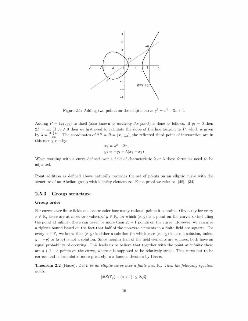
Figure 2.1: Adding two points on the elliptic curve y2 = x3 − 3x+ 1.

Adding P = (x1, y1) to itself (also known as doubling the point) is done as follows. If y1 = 0 then2P = ∞. If y1 6= 0 then we first need to calculate the slope of the line tangent to P , which is givenby λ = 3x2

1+a2y1

. The coordinates of 2P = R = (x3, y3), the reflected third point of intersection are inthis case given by:

x3 = λ2 − 2x1

y3 = −y1 + λ(x1 − x3)

When working with a curve defined over a field of characteristic 2 or 3 these formulas need to beadjusted.

Point addition as defined above naturally provides the set of points on an elliptic curve with thestructure of an Abelian group with identity element ∞. For a proof we refer to [48], [34].

2.5.3 Group structure

Group order

For curves over finite fields one can wonder how many rational points it contains. Obviously for everyx ∈ Fq there are at most two values of y ∈ Fq for which (x, y) is a point on the curve, so includingthe point at infinity there can never be more than 2q + 1 points on the curve. However, we can givea tighter bound based on the fact that half of the non-zero elements in a finite field are squares. Forevery x ∈ Fq we know that (x, y) is either a solution (in which case (x,−y) is also a solution, unlessy = −y) or (x, y) is not a solution. Since roughly half of the field elements are squares, both have anequal probability of occuring. This leads us to believe that together with the point at infinity thereare q + 1 + ε points on the curve, where ε is supposed to be relatively small. This turns out to becorrect and is formulated more precisely in a famous theorem by Hasse:

Theorem 2.2 (Hasse). Let E be an elliptic curve over a finite field Fq. Then the following equationholds:

|#E(Fq)− (q + 1)| ≤ 2√q.

16

A proof is given in [48].

The value #E(Fq)− (q + 1) is known as the trace of Frobenius and is usually denoted t.

Torsion subgroups

Like in every additive group, the addition of points on the curve induces a scalar multiplication ofpoints. For n ∈ Z and P a point on an elliptic curve, we define:

nP =

P + P + . . .+ P︸ ︷︷ ︸n times

, if n > 0

(−P ) + (−P ) + . . .+ (−P )︸ ︷︷ ︸n times

, if n < 0

∞, if n = 0

The order of a point P is the smallest positive integer n such that nP = ∞. If the order of a pointP divides n (i.e. if nP = ∞), then P is called an n-torsion point. The set of K-rational n-torsionpoints forms a subgroup, the n-torsion group, denoted E(K)[n]. The following theorem gives us somevaluable information about the structure of an n-torsion group.

Theorem 2.3. Let E/Fpm be an elliptic curve and let n ∈ Z be a prime coprime to p. Then the orderof E(Fpm)[n] is n2 and E(Fpm)[n] ∼= Z/nZ⊕ Z/nZ.

For a special class of curves the n-torsion group is trivial when n is a power of the characteristic of thefield over which the curve is defined. We will first define this class of curves. Let E/K be an ellipticcurve, where K = Fpm . If p | t, where t is the trace of Frobenius of E , then E is called supersingular.

2.5.4 Rational functions on elliptic curves

The following is explained in detail in [39]. Suppose E/K : y2 +a1xy+a3y = x3 +a2x2 +a4x+a6 is an

elliptic curve. Observe that every polynomial f(x, y) ∈ K[E ] can be written in the form a(x) + b(x)y,by rearranging terms and replacing any occurrence of y2 by x3 + a2x

2 + a4x+ a6 − a1xy − a3y. Thisform can be used to define the degree of f , which we will be needed in determining the orders of zeroesand poles of f as well as the behaviour of f in ∞.

Definition 2.8. Let f(x, y) = a(x) + b(x)y 6= 0 be polynomial function in K[E ]. Then the degree off is defined to be

deg(f) = max{2 degx(a), 3 + 2 degx(b)}

where degx denotes the usual degree of a polynomial in x, taking degx(0) =∞.

The behaviour of rational functions on E in the point at infinity is defined as follows.

Definition 2.9. Let f = g/h ∈ K(E). If deg(g) < deg(h) then we define f(∞) = 0. If deg(g) > deg(h)we say f is not defined at ∞. If deg(g) = deg(h) then f(∞) is defined to be the ratio of the leadingcoefficients of g and h.

A uniformizing parameter π for a point P ∈ E(K) can be found as follows. If P = ∞ then chooseπ = x/y. If P = (xP , 0) then choose π = y. If P = (xP , yP ), yP 6= 0 then choose π = x − xP . Theorder of a rational function f at P can now be determined by writing f = πnu with n ∈ Z and u aunit, u(P ) 6= 0,∞, as described earlier.

17

2.6 Hyperelliptic Curves

In this section we define hyperelliptic curves. These results come from [39].

2.6.1 Definition

A hyperelliptic curve C over a field K is a curve given by the equation:

y2 + h(x)y = f(x)

where f is a monic polynomial of degree 2g + 1 and h is a polynomial of degree ≤ g, for a certaing ≥ 1. This number g is called the genus of the curve. We require the curve to be non-singular, whichmeans the partial derivatives given by

∂C∂x

= h′(x)y − f ′(x) and∂C∂y

= 2y + h(x)

should not vanish simultaneously. The curves with genus 1 are exactly the elliptic curves, whichmeans hyperelliptic curves are a generalization of elliptic curves. As a consequence, the theorems anddefinitions that follow in the next sections also hold for elliptic curves.

As with elliptic curves, we use the notation C/K to indicate that C is defined over a field K. We willwrite C to refer to the set of solutions together with a point of infinity ∞ and use C(K) to denote theset of solutions with coordinates in K (i.e. the K-rational points). If char(K) = 2, then h(x) 6= 0. Ifchar(K) 6= 2, then we can assume h(x) = 0 without loss of generality. If h(x) = 0 then f(x) has norepeated roots in K. For a proof of these facts we refer to [39].

If P = (x, y) is a point on C, then ι(P ) = (x,−y − h(x)) is also a point on C, sometimes denoted P

and referred to as the opposite of P . The map ι is called the hyperelliptic involution, and a point forwhich ι(P ) = P is called a ramification point or special point. If ι(P ) 6= P then P is said to be anordinary point.

In the section on elliptic curves we gave a bound on the number of points on the curve by statingHasse’s theorem. This theorem can be reformulated so it also applies to hyperelliptic curves.

Theorem 2.4 (Hasse-Weil). Let C be a hyperelliptic curve of genus g over a finite field Fq. Then thefollowing equation holds:

|#C(Fq)− (q + 1)| ≤ 2g√q.

Unlike in elliptic curves, the points on a genus > 1 curve do not have the structure of a group.However, in what follows we will see there is a group law defined over another object that we canassociate with the curve.

2.6.2 Jacobian

The (degree 0 part of the) divisor class group is defined as the set of degree zero divisors modulo theprincipal divisors:

Pic0(C) := Div0(C)/Prin(C).

18

If A is a degree zero divisor then we denote the divisor class of A by A. The zero degree divisor classgroup is isomorphic to an object known as the Jacobian variety on C, which is why the divisor classgroup is sometimes simply referred to as the Jacobian and denoted Jac(C).

A divisor A is said to be semi-reduced if it is of the form

A =∑P∈C

nP (P )− (∑P∈C

nP )(∞)

and if A satisfies for all P in the sum:

1. P 6=∞

2. nP ≥ 0

3. if P = ι(P ) and nP > 0 then nP = 1

4. if P 6= ι(P ) and nP > 0 then nP = 0

If in addition∑P∈C nP ≤ g, where g is the genus of the curve, then A is said to be reduced.

Example 2.2. Let C be a curve of genus 2 such that P1, P2, P3 ∈ C and Pi 6= Pj for any i, j ∈ {1, 2, 3}.Then (P1) + 2(P2) + (P3) − 4(∞) is a semi-reduced divisor and (P1) + (P2) − 2(∞) is a reduceddivisor.

It turns out that every zero degree divisor is linearly equivalent to exactly one reduced divisor, whichmeans every divisor class can be uniquely represented by a reduced divisor. For a given divisor classA we define ρ(A) to be the unique reduced divisor of the class. In addition we define ε(A) to be theeffective part of this divisor (i.e. ρ(A) = ε(A)− d(∞), where d is the degree of ε(A)).

Remark 2.1. In the elliptic curve case the Jacobian is isomorphic to the group of points on the curve.The isomorphism E → Pic0(E) is given by P 7→ (P )− (∞).

Storing reduced divisors is done by representing them as a pair of polynomials. This representationis known as the Mumford representation. Let C/K be a hyperelliptic curve and A =

∑P∈C nP (P )−

(∑P∈C nP )(∞) a reduced divisor. We use the notation xP and yP for the coordinates of a point

P ∈ C. Now we can uniquely represent A by a pair of polynomials a, b ∈ K[x]. The first polynomiala is defined as follows:

a(x) =∏P∈C

(x− xP )nP .

The second polynomial b is defined as the unique polynomial satisfying the following properties:

1. deg b < deg a ≤ g,

2. for all P ∈ C such that nP > 0: b(xP ) = yP ,

3. b is a solution of the congruence b2 + hb ≡ f (mod a).

A reduced divisor represented by polynomials a and b will be denoted div(a, b).

19

2.6.3 Computing the group law

The elements of the divisor class group have the structure of an Abelian group. The identity elementof this group is the divisor class represented by the reduced divisor with Mumford representationdiv(1, 0). The inverse of an element div(a, b) is div(a,−b − h). We describe an algorithm to adddivisor classes, due to Cantor. Assuming Mumford representation it adds two divisors in reducedform and returns the sum of the divisors in reduced form. It is far from efficient, but works for curvesof arbitrary genus. For fixed genus it is possible to derive much more efficient algorithms that do notneed to invoke the extended Euclidian algorithm.

Algorithm 1: Cantor’s Algorithm

Input: Reduced divisors div(a1, b1) and div(a2, b2).Output: Reduced divisor div(a3, b3) = div(a1, b1) + div(a2, b2).

// Calculate the sum of the divisors.

d1 ← gcd(a1, a2) = e1a1 + e2a2

d← gcd(d1, b1 + b2 + h) = c1d1 + c2(b1 + b2 + h)s1 ← c1e1

s2 ← c1e2

s3 ← c2

a3 ← a1a2/d2

b3 ← (s1a1b2 + s2a2b1 + s3(b1b2 + f))/d (mod a3)

// Make sure the result is in reduced form.

while deg a3 > g doa3 ← (f − hb3 − b23)/a3

b3 ← −h− b3 (mod a3)end

Consult [37] for a proof of correctness of this algorithm.

2.6.4 Group structure

Group order

For elliptic curves the order of the group is simply the number of points on the curve. For hyperellipticcurves the points do not have the structure of a group, so we need to determine the order of the divisorclass group instead. Obviously when a hyperelliptic curve is defined over a finite field the Jacobianhas finite order, since there is only a finite amount of polynomials usable as a representation of adivisor class. For an elliptic curve E/K, the group of points contains a subgroup of K-rational points:E(K) ⊆ E(K). Similarly, the divisor class group of a hyperelliptic curve C/K contains a subgroupwith K-rational divisor classes, but the concept of a rational divisor is a bit more complicated.

Formally, a divisor A =∑P∈C nP (xP , yP ) is K-rational if A =

∑P∈C nP (σ(xP ), σ(yP )) for every

σ ∈ Gal(K,K). It is important to realize that this is not the same as requiring each point in thesupport of A to have coordinates in K. However, a principal divisor is K-rational if and only if it is

20

the divisor of a rational function with coefficients in K. Also, if a divisor class with representativediv(a, b) is K-rational, then the polynomials a, b have coefficients in K. The group of K-rationaldivisor classes in the divisor class group is denoted Pic0

K(C) and is a subgroup of Pic0(C).

The following theorem gives a bound on the order of the divisor class group of a curve defined over afinite field with q elements.

Theorem 2.5 (Weil). Let C/Fq be a hyperelliptic curve of genus g. Then

(√q − 1)2g ≤ #Pic0

Fq(C) ≤ (

√q + 1)2g.

Torsion subgroups

The following definitions are essentially the same as the definitions of the torsion subgroups of thegroup of points on an elliptic curve. Using the group law on the divisor class group a reduced divisorA can be repeatedly added to itself. For n ∈ Z we define:

nA =

A+A+ . . .+A︸ ︷︷ ︸n times

, if n > 0

(−A) + (−A) + . . .+ (−A)︸ ︷︷ ︸n times

, if n < 0

∞, if n = 0

The order of a reduced divisor A is the smallest positive integer n such that nA = 0, where 0 is thedivisor with empty support. The divisors with order dividing n form a subgroup denoted Pic0(C)[n].The K-rational divisors with order dividing n form a subgroup denoted Pic0

K(C)[n].

2.6.5 Example

Let C be a hyperelliptic curve defined by the equation y2 = x5+x3+1. Then C(F3) = {∞, (0, 1), (0, 2), (1, 0) }.Now let F32 = F3/(x2 − x − 1) and let α be a root of the polynomial x2 − x − 1 in F32 . ThenC(F32) = {∞, (0, 1), (0, 2), (1, 0), (α+ 1, 1), (α+ 1, 2), (2, α+ 1), (2, 2α+ 2), (2α+ 2, 1), (2α+ 2, 2) }.

Table 2.1: Pic0F3

(C)Reduced divisor Mumford representation

0 div(1, 0)(0, 2)− (∞) div(x, 2)2(0, 2)− 2(∞) div(x2, 2)(α+ 1, 1) + (2α+ 1, 1)− 2(∞) div(x2 + 1, 1)(0, 1) + (1, 0)− 2(∞) div(x2 + 2x, 2x+ 10)(1, 0)− (∞) div(x+ 2, 0)(0, 1) + (0, 2)− 2(∞) div(x2 + 2x, x+ 2)(α+ 1, 2) + (2α+ 1, 2)− 2(∞) div(x2 + 1, 2)2(0, 1)− 2(∞) div(x2, 1)(0, 1)− (∞) div(x, 1)

21

The divisor class group over F3 is shown in 2.1. It contains two reduced divisors as representativesthat have non-F3-rational points in their support. However, they are F3-rational divisors. Also noticethe polynomials in the Mumford representation all have coordinates in F3.

Let A1 = (0, 2)− (∞) = div(x, 2) and A2 = 2(0, 1)− 2(∞) = div(x2, 1). We are going to compute thereduced divisor in the class A1 + A2 using Cantor’s algorithm. First we use the extended Euclidianalgorithm to calculate d1 = gcd(a1, a2) = gcd(x, x2) = 1 · x+ 0 · x2 = e1a1 + e2a2. Similarly, we thencalculate d = gcd(d1, b1 + b2 +h) = gcd(x, 1 + 2 + 0) = gcd(x, 0) = 1 ·x+ 0 · 0 = c1d1 + c2(b1 + b2 +h).Now s1 = c1e1 = 1, s2 = c1e2 = 0 and s3 = c2 = 0. Then a3 = a1a2/d

2 = x3/x2 = x andb3 = (s1a1b2 + s2a2b1 + s3(b1b2 + f))/d (mod a)3 = (x+ 0 + 0)/x = 1 (mod a)3. Since deg a3 = 1 ≤ 2we are done and the reduced divisor in the class A1 +A2 = (0, 1)− (∞) = div(x, 1).

2.6.6 Rational functions on hyperelliptic curves

As with elliptic curves, the following can assist [39]. Suppose C/K : y2+h(x)y = f(x) is a hyperellipticcurve of genus g. Similar to the elliptic curve case, every polynomial f(x, y) ∈ K[C] can be written inthe form a(x) + b(x)y, by rearranging terms and replacing any occurrence of y2 by f(x)− h(x)y.

Definition 2.10. Let f(x, y) = a(x) + b(x)y 6= 0 be polynomial function in K[C]. Then the degree off is defined to be

deg(f) = max{2 degx(a), 2g + 1 + 2 degx(b)}

where again degx denotes the usual degree of a polynomial in x, taking degx(0) =∞.

The behaviour of rational functions on C in the point at infinity is now defined exactly the same asin the elliptic curve case.

A uniformizing parameter π for a point P ∈ C(K) can be found as follows. If P = ∞ then chooseπ = xg/y. If P = P then choose π = y. If P = (xP , yP ), yP 6= 0 then choose π = x− xP .

22

Chapter 3

Pairings

A pairing is map e : G1 × G2 → GT where G1, G2 and GT are groups (usually cyclic of the sameprime order). In some instances the pairing is symmetric: G1 = G2. When G1 6= G2 the pairing issaid to be asymmetric. In this chapter we describe how to construct pairings on elliptic curves andthe divisor class group of hyperelliptic curves.

3.1 Weil Pairing

The Weil pairing was introduced by Andre Weil in 1940 [52] and has proven to be a useful tool in thestudy of elliptic curves. There are several definitions of the Weil pairing which are all closely relatedbut not exactly equivalent. We will not focus on these differences here and stick to the definition thatallows for straightforward extraction of an algorithm to compute it.

3.1.1 Definition

The Weil pairing is a function that maps a pair of points in an n-torsion group of an elliptic curve toan nth root of unity in some extension field of the field the curve was defined over. More specifically,let E/Fq be an elliptic curve and let n be a prime divisor of #E(Fq) coprime to char(Fq). The Weilpairing is a map

e : E(Fq)[n]× E(Fq)[n]→ F∗q .

Sometimes we will use the notation en instead of e to specify directly the order of the torsion groupon which the pairing is defined.

The Weil pairing maps points to a certain extension field Fqk , which should be large enough to makesure E(Fqk) contains all n-torsion points (so in reality we do not need the full algebraic closure of Fq).The embedding degree is the degree k of this field extension. When n - q − 1, then k is the smallestinteger such that n | qk − 1, or equivalently, the smallest integer such that Fqk contains all nth rootsof unity. If n | q− 1 then in some instances k = 1, but in other instances k = n. From now on we willassume n - q − 1, since this is the case in most practical situations.

23

Let P,Q ∈ E(Fqk)[n]. To define e(P,Q), we first need a divisor AP ∼ (P )− (∞) and a divisor AQ ∼(Q)− (∞). We require that AP and AQ have disjoint support. First note that since nP = nQ =∞ itfollows that nAP ∼ n(P )− n(∞) and nAQ ∼ n(Q)− n(∞) are principal divisors. As a consequenceof this, there exist rational functions fP and fQ such that (fP ) = nAP and (fQ) = nAQ. We can nowdefine the Weil pairing as:

e(P,Q) :=fP (AQ)fQ(AP )

The result of the pairing is independent of the divisors chosen and thus the Weil pairing is well-defined.

3.1.2 Properties

The following theorems state that the Weil pairing is a bilinear, alternating and non-degenerate map-ping. A proof of these properties is given in [48].

Theorem 3.1. The Weil pairing is linear in both arguments:

e(P +Q,R) = e(P,R)e(Q,R) for all points P,Q,R

ande(P,R+ S) = e(P,R)e(P, S) for all points P,R, S.

Theorem 3.2. The Weil pairing is alternating:

e(P,Q) = e(Q,P )−1 for all points P,Q.

As a consequence, the self-pairing of a point P is always 1:

e(P, P ) = e(P, P )−1 = 1 for all points P.

Theorem 3.3. The Weil pairing is non-degenerate:

e(P,Q) = 1 for all points Q if and only if P =∞.

3.1.3 Computation

We describe how to compute the Weil pairing using an algorithm by Victor Miller [40]. The paperin which the algorithm is described was never published but is cited very frequently. We will use themethod as described in [10] and employ the same notation.

The first step is to find divisors AP ∼ (P ) − (∞) and AQ ∼ (Q) − (∞). To do so, choose randomR1, R2 ∈ E(Fqk)[n] and let AP = (P + R1) − (R1) and AQ = (Q + R2) − (R2). These are suitablechoices, since the difference of AP and (P )− (∞) is indeed a principal divisor:

AP −((P )− (∞)

)=((P +R1)− (R1)

)−((P )− (∞)

)= (P +R1)− (R1)− (P ) + (∞)

and similarly, the difference of AQ and (Q)− (∞) is a principal divisor.

24

To evaluate e(P,Q) we now have to compute

fP (AQ)fQ(AP )

=fP((Q+R2)− (R2)

)fQ((P +R1)− (R1)

) =fP (Q+R2)fQ(P +R1)

· fQ(R1)fP (R2)

.

The main problem in computing the Weil Pairing is finding functions fP and fQ such that (fP ) = nAPand (fQ) = nAQ. We show how to construct fP iteratively. The same method is used to constructfQ. First define the function fi for i ≥ 1 such that

(fi) = i(P +R1)− i(R1)− (iP ) + (∞).

Since P is a n-torsion point, it follows that

(fn) = n(P +R1)− n(R1)− (nP ) + (∞) = n(P +R1)− n(R1) + (∞) = nA.

Lemma 3.1. Let P,R1 ∈ E(Fqk)[n] be the points as described above, and let i and j be positive integerssuch that i 6= j. Suppose l is a function such that l(x, y) = 0 is the equation of the line joining thepoints iP and jP and suppose v is a function such that v(x, y) = 0 is the equation of a vertical linethrough the point (i+ j)P . Then

fi+j = fi · fj ·l

v

Proof. We use the divisors of the functions to prove the equality. First note that since l intersects thecurve at the points iP , jP and −(i+ j)P the divisor of l is given by

(l) = (iP ) + (jP ) + (−(i+ j)P )− 3(∞).

The line v intersects the curve at the points (i+ j)P and −(i+ j)P , which means the divisor of v isgiven by

(v) = ((i+ j)P ) + (−(i+ j)P )− 2(∞).

Writing down the divisor of fifj lv yields the equality needed to prove the lemma:

(fifj lv ) = (fi) + (fj) + (l) − (v)=

(i(P +R1) − i(R1) − (iP ) + (∞)

)+(

j(P +R1) − j(R1) − (jP ) + (∞))

+((iP ) + (jP ) + (−(i+ j)P ) − 3(∞)

)−(

((i+ j)P ) + (−(i+ j)P ) − 2(∞))= (i+ j)(P +R1) − (i+ j)(R1) − (iP )− (jP ) + 2(∞) +

(iP ) + (jP ) + (−(i+ j)P )− 3(∞) − ((i+ j)P ) − (−(i+ j)P ) + 2(∞)= (i+ j)(P +R1) − (i+ j)(R1) − ((i+ j)(P )) + (∞)= (fi+j).

Constructing fP this way and then evaluating it in AQ would be unwieldy, because fn becomes verycomplex for high n. Therefore when computing the Weil Pairing we do not store the actual expres-sions of the functions, but immediately evaluate them at each step. To arrive at fn we use the binaryrepresentation of n = [nm, nm−1, . . . , n0]2 and use the double-and-add method. We initialize fi to f1and iterate through the bits starting at m− 1 going down to 0. At each iteration we either double i

25

(if the corresponding bit is 0) or we double i and add 1 (if the corresponding bit is 1). Meanwhile wecalculate the corresponding fi by using the recursion fi+j = fifj

lv . After the final iteration i will be

equal to n and we will have obtained fn.

For this method to work, we need to be able to directly calculate the evaluation of f1 in AQ. For-tunately, the function f1 can be explicitly constructed. First note that the divisor of f1 is givenby

(f1) = (P +R1)− (R1)− (P ) + (∞).

Now let l(x, y) = 0 be the equation of the line going through the points P and R1. Then the divisorof l is given by

(l) = (P ) + (R1) + (−(P +R1))− 3(∞).

Let v(x, y) = 0 be the vertical line going through the point P +R1. Then the divisor of v is given by

(v) = (P +R1) + (−(P +R1))− 2(∞).

It follows that

(v)− (l) = (P +R1) + (−(P +R1))− 2(∞)− (P )− (R1)− (−(P +R1)) + 3(∞)= (P ) + (R1)− (P +R1) + (∞)= (f1).

As a consequence

f1(AQ) =v(Q+R2)l(Q+R2)

· l(R2)v(R2)

.

Combining these ideas leads to an efficient algorithm for computing fP (AQ), which is outlined asfollows.

Algorithm 2: Miller’s Algorithm [Weil pairing]

Input: P,Q,R1, R2,m, [nm, . . . , n1, n0]2 = n.Output: fP (AQ).l← line through P and R1

v ← vertical line through P +R1

f ← v(Q+R2)l(Q+R2)

· l(R2)v(R2)

T ← P

for i = m− 1 to 0 dol← tangent line at Tv ← vertical line through 2Tf ← f2 · l(Q+R2)

v(Q+R2)· v(R2)l(R2)

T ← 2Tif ni = 1 then

l← line through T and P

v ← vertical line through T + P

f ← f · f1 · l(Q+R2)v(Q+R2)

· v(R2)l(R2)

T ← T + Pend

end

26

Computing fQ(AP ) is done by modifying the algorithm in the obvious way. The Weil pairing isevaluated by running Miller’s algorithm twice. The first time to compute fP (AQ) and the secondtime to compute fQ(AP ). Dividing them gives the final result.

3.1.4 Modifications

In order for the Weil pairing to be useful in cryptography it needs to be slightly adapted. Firstof all we want the Weil Pairing to satisfy a stronger notion of non-degeneracy. In its current formnon-degeneracy means that for every P 6= ∞ there is at least one Q such that e(P,Q) 6= 1 and viceversa. We would like the pairing to be strongly non-degenerate, which means the self-pairing shouldnot be trivial (i.e. e(P, P ) 6= 1 for P 6= ∞). Unfortunately, from the alternating property we knowthat e(P, P ) = 1. Then, from bilinearity it follows e(P,Q) = 1 when P and Q are linearly dependent.

We also would like the pairing to be defined on cyclic groups instead of the product of two cyclicgroups such as the n-torsion group of an elliptic curve. We can restrict the inputs to a cyclic subgroupof the n-torsion group, but then the pairing would be trivial on all inputs as they are all linearlydependent. The obvious solution is to take the inputs from separate cyclic subgroups of the n-torsiongroup. As we shall see, this also solves the problem of strong non-degeneracy.

Let E/Fq be an elliptic curve, n a prime coprime to char(Fq) such that E(Fq) contains a point of ordern, and k the embedding degree. If Pg and Qg are linearly independent points, they generate the fulln-torsion group of E (i.e. 〈Pg, Qg〉 = E(Fq)[n]). Let G1 = 〈Pg〉 and G2 = 〈Qg〉. If we restrict theinputs of the Weil pairing as follows

e : G1 ×G2 → F∗qk

then the pairing satisfies the strong non-degeneracy property.

A practical problem here is to actually find points in G1 and G2, but this can be solved if there existsa distortion map on E [4]. A distortion map φ : E → E maps a point P to a point φ(P ) such thatP and φ(P ) are linearly independent. For supersingular curves these distortion maps can always becomputed. We can use this property to obtain a symmetric strongly non-degenerate pairing, knownas the the modified Weil Pairing e(P,Q) : G1 ×G1 → F∗qk . It is defined as follows:

e(P,Q) := e(P, φ(Q))

3.2 Tate-Lichtenbaum Pairing

The Tate pairing, or Tate-Lichtenbaum pairing was introduced to cryptography by Frey and Ruck[44] for the purpose of transporting the discrete logarithm problem on the divisor class group of acurve C/Fq to the multiplicative group of some extension of its field of definition. However, after thearrival of pairing based cryptography, it was quickly proposed as an alternative to the Weil pairing,as its computation is less costly. In this section we will define the Tate pairing for elliptic curves andgive an efficient way to compute it. In the next section we will generalize the pairing to hyperelliptic

27

curves. Obviously the hyperelliptic version of the pairing can be used on elliptic curves as well, but thesimplification of the computation in the elliptic case is significant enough to justify separate treatment.

3.2.1 Definition

Like the Weil pairing, the Tate pairing can be defined in terms of evaluations of rational functions indivisors. Let E/Fq be an elliptic curve defined over a finite field and fix a prime n coprime to char Fqsuch that n | #E(Fq). Let Fqk be the smallest extension field of Fq containing the set of nth roots ofunity. Then k is the smallest integer such that n | qk − 1 (the embedding degree). We first define

nE(Fq) := {nP | P ∈ E(Fq)}.

The quotient group E(Fq)/nE(Fq) is the set of equivalence classes of points in E(Fq) where points areconsidered equivalent if their difference is a point of order n. The quotient group F∗q/(F∗q)n is the setof equivalence classes of field elements where two elements are considered equivalent if they are thesame up to multiplication with an nth power. This quotient group is isomorphic to µn (the group ofnthroots.The Tate pairing is a map

t : E(Fqk)[n]× E(Fqk)/nE(Fqk)→ F∗qk/(F∗qk)n.

Similar to the Weil pairing, sometimes we will use the notation tn to indicate the order of the torsiongroup.

Let P ∈ E(Fqk)[n] andQ ∈ E(Fqk), whereQ is a representative of an equivalence class in E(Fqk)/nE(Fqk).To define t(P,Q) we first need a divisor AQ ∼ (Q) − (∞) and a function fP such that (fP ) =n(P )−n(∞). We require AQ and (fP ) to have disjoint support to ensure the evaluation of fP in AQis not equal to zero. We can now define the Tate Pairing of P and Q as:

t(P,Q) := fP (AQ).

3.2.2 Properties

We prove that the Tate pairing is a bilinear and non-degenerate mapping. Then we show that weneed an embedding degree larger than 1 to get non-trivial self-pairings.

Theorem 3.4. The Tate pairing is bilinear:

t(P +Q,R) = t(P,R)t(Q,R) for all points P,Q ∈ E(Fqk)[n] and R ∈ E(Fqk)/nE(Fqk).

and

t(P,R+ S) = t(P,R)t(P, St) for all points P ∈ E(Fqk)[n] and R,S ∈ E(Fqk)/nE(Fqk).

Proof. We give the proof as described in [4]. Let fP and fQ be functions such that (fP ) = n(P )−n(∞)and (fQ) = n(Q)−n(∞). Let AR ∼ (R)− (∞) be a divisor with support disjoint to {∞, P,Q, P +Q}.Then

t(P,R) = fP (AR) and t(Q,R) = fQ(AR).

28

Now let g be a function such that (g) = (P +Q)− (P )− (Q) + (∞). Note that

(fP fQgn) = (fP ) + (fQ) + n(g)= n(P ) + n(Q)− 2n(∞) + n(P +Q)− n(P )− n(Q) + n(∞)= n(P +Q)− n(∞).

This means the function fP fQgn is suitable for use in computation of t(P +Q,R):

t(P +Q,Rt) = fP fQgn(AR) = fP (AR)fQ(AR)g(AR)n = t(P,R)t(Q,R)g(AR)n.

In other words, t(P,R)t(Q,R) and t(P +Q,R) are equivalent up to a multiplication with a nth power.This means they are equivalent in the quotient group K∗/(K∗)n, proving linearity in the first factor.

Now choose divisors AR ∼ (R) − (∞) and AS ∼ (S) − (∞). Let fP be a function such that (fP ) =n(P )− n(∞). Then

t(P,R) = fP (AR) and t(P, S) = fP (AS).

Note that AR +AS ∼ (R+ S)− (∞), since

(R+ S)− (∞)−AR −AS = (R+ S)− (∞)− (R) + (∞)− (S) + (∞)= (R+ S)− (R)− (S) + (∞).

which clearly is a principal divisor. This means AR + AS is suitable for use in computation oft(P,R+ S), leading us to the equation

t(P,R+ S) = fP (AR +AS) = fP (AR)fP (AS) = t(P,R)t(P, S)

proving linearity in the second factor.

Theorem 3.5. The Tate Pairing is non-degenerate. If P ∈ E(Fqk)[n] then

t(P,Q) = 1 for all Q if and only if P =∞.

Similarly, if Q ∈ E(Fqk)/nE(Fqk) then

t(P,Q) = 1 for all P if and only if Q =∞.

For a proof, see [29].

Theorem 3.6. If k > 1 (where k is the embedding degree), then self-pairings of points in E(Fq)[n] aretrivial. As a result of bilinearity it follows that if k > 1, then the pairing of any two linearly dependentpoints in E(Fq)[n] is trivial.

Proof. Let P ∈ E(Fq)[n], fP ∈ Fq(E) such that (fP ) = n(P ) − n(∞), and AP ∈ Div(E) such thatAP ∼ (P )−(∞). Then t(P, P ) = fP (AP ) ∈ F∗q . Since F∗q is a group of order q−1 and gcd(n, q−1) = 1(because k > 1) it follows that F∗q = (F∗q)n. As a consequence, t(P, P ) is an nth power and vanishesin the quotient group F∗q/(F∗q)n.

29

3.2.3 Computation

The same approach as used in Miller’s algorithm for computing the Weil Pairing can be used forefficiently computing the Tate Pairing. In computing the Tate Pairing the main problem is to constructa function f such that (f) = n(P ) − n(∞). Again, we can build this function iteratively using thedouble-and-add method. First we define a function fi for i ≥ 1 such that

(fi) = i(P )− (iP )− (i− 1)(∞).

Since P is a n-torsion point, it follows that

(fn) = n(P )− (nP )− (n− 1)(∞) = n(P )− n(∞) = (f).

Note that(f1) = (P )− (P )− 0(∞) = 0

which means f1 = 1.

Lemma 3.2. Let P ∈ E(Fqk)[n], and let i and j be positive integers. Suppose l is a function suchthat l(x, y) = 0 is the equation of the line between the points iP and jP and suppose v is a functionsuch that v(x, y) = 0 is the equation of vertical line through the point (i+ j)P . Then

fi+j = fi · fj ·l

v

Proof. Recall from the lemma used in computing the Weil Pairing the divisors of l and v:

(l) = (iP ) + (jP ) + (−(i+ j)P )− 3(∞)(v) = ((i+ j)P ) + (−(i+ j)P )− 2(∞)

Writing down the sum of the divisors results in the equality:

(fifj lv ) = (fi) + (fj) + (l) − (v)=

(i(P ) − (iP ) − (i− 1)(∞)

)+(

j(P ) − (jP ) − (j − 1)(∞))

+((iP ) + (jP ) + (−(i+ j)P ) − 3(∞)

)−(

((i+ j)P ) + (−(i+ j)P ) − 2(∞))= (i+ j)(P ) − (iP ) − (jP ) − (i+ j − 2)(∞) +

(iP ) + (jP ) + (−(i+ j)P ) − 3(∞)−((i+ j)P ) − (−(i+ j)P ) + 2(∞))

= (i+ j)(P )− ((i+ j)P )− (i+ j − 1)(∞)= (fi+j).

Recall from the definition of the Tate Pairing that we also need a divisor AQ ∼ (Q) − (∞) withsupport disjoint from (fP ). Let R ∈ E(K)[n] such that R 6=∞, P,−Q,P −Q. Then a valid choice forAQ is (Q+R)− (R). We can now compute t(P,Q) = fP (AQ) using Miller’s algorithm. Note that itis slightly simpler than the version for the Weil Pairing due to the fact that f1 = 1.

30

Algorithm 3: Miller’s Algorithm [Tate Pairing]

Input: P,Q,R,m, [nm, . . . , n1, n0]2 = n.Output: fP (AQ).f ← 1T ← P

for i = m− 1 to 0 dol← tangent line at Tv ← vertical line through 2Tf ← f2 · l(Q+R)

v(Q+R) ·v(R)l(R)

T ← 2Tif ni = 1 then

l← line through T and P

v ← vertical line through T + P

f ← f · l(Q+R)v(Q+R) ·

v(R)l(R)

T ← T + Pend

end

3.2.4 Modifications

Throughout this section, let E/Fq be an elliptic curve, n a prime coprime to char(Fq) such that E(Fq)contains a point of order n, and k the embedding degree.

For practical applications of the Tate pairing, it is desirable to have the output be an element of themultiplicative group of a finite field instead of a coset in the quotient group F∗qk/(F∗qk)n. To achievethis we can raise the result to the power (qk − 1)/n. In the literature this process is referred to asthe final exponentiation. The exponentiated pairing which maps directly into F∗qk is called the reducedTate pairing :

t′(P,Q) := t(P,Q)(qk−1)/n

To obtain a symmetric bilinear map from the Tate pairing we have to make sure both inputs comefrom the same group. At first this may seem like a problem since the second input of the Tate pairingis not a n-torsion point on the curve, but a coset in the quotient group E(Fqk)/nE(Fqk). Fortunately,if we assume that E(Fqk) contains no elements of order n2, then E(Fqk)[n] can be identified withE(Fqk)/nE(Fqk).

Finally, assuming the existence of a distortion map φ on E , we can apply the same modification tothe Tate pairing as we did to the Weil pairing (assuming k > 1) to obtain a symmetric stronglynon-degenerate map defined on cyclic groups. Let Pg ∈ E(Fq)[n] and G1 = 〈Pg〉. Then the modifiedTate pairing is a map t(P,Q) : G1 ×G1 → F∗qk , defined as follows:

t(P,Q) := t′(P, φ(Q))

31

3.3 Hyperelliptic Tate-Lichtenbaum Pairing

In this section we generalize the Tate-Lichtenbaum pairing to the divisor class group of a hyperellipticcurve. Most of the results are derived from [28], [21] and [16].

3.3.1 Definition

Let C/Fq be a hyperelliptic curve, n a prime coprime to char(Fq) with n | #Pic0Fq

(C), and again k thesmallest integer such that n | qk − 1 (the embedding degree).

The hyperelliptic Tate pairing is a map

t : Pic0F

qk(C)[n]× Pic0

Fqk

(C)/nPic0F

qk(C)→ F∗qk/(F∗qk)n.

Let AP and AQ be divisor classes with respective representatives AP and AQ such that supp(AP ) ∩supp(AQ) = ∅. Let fAP

be a function such that (fAP) = nAP . Then we define the Tate pairing of

AP and AQ as follows:t(AP ,AQ) = fAP

(AQ)

The requirement of AP and AQ having disjoint support is to make sure the evaluation of fAPin AQ

is not zero. Notice how this is a straightforward generalization of the Tate pairing on elliptic curves,where we take AP = (P )− (∞) and AQ ∼ (Q)− (∞) to pair two points P and Q.

It can be shown that this pairing is also well-defined.

3.3.2 Properties

The hyperelliptic Tate pairing satisfies the same properties as the elliptic Tate pairing (i.e. bilinearityand non-degeneracy).

3.3.3 Computation

Again, let C/Fq be a hyperelliptic curve, n a prime coprime to char(Fq) such that n | #Pic0F

qk(C),

where k is the embedding degree. For AP ∈ Pic0F

qk(C)[n] and AQ ∈ Pic0

Fqk

(C)/nPic0F

qk(C), we will

describe how to compute t(AP ,AQ).

The first difficulty in the pairing computation is the choice of divisors as representative of the divisorclasses. Computing the group operation of the divisor class is done with reduced divisors in Mumfordrepresentation, but we cannot use the reduced representative for both inputs in the pairing evaluationbecause two reduced divisors do not have disjoint support. Indeed, for any two divisor classes APand AQ we have ∞ ∈ supp(ρ(AP )) ∩ supp(ρ(AQ)) (recall ρ(A) denotes the reduced divisor in A).Fortunately, if we impose certain constraints on the function fAP

we can evaluate fAPin ε(AQ) (the

effective part of the reduced divisor in AQ). For details of these constraints we refer to [28] and [21].However, if we assume that k > 1 and AP ∈ Pic0

Fq(C)[n], then this constraint is not necessary. From

now on we will assume this is the case.

32

Let A = ρ(AP ). Again, we build fA iteratively. Let fi be a function such that

(fi) = iA− ρ(iA).

It is important to realize that iA is obtained using multiplication by i in the group Div(C), and iA isobtained using multiplication by i in the group Pic0(C)[n]. Since A is an n-torsion element of Pic0(C)we have:

(fn) = nA− ρ(nA) = nA.

Also:(f1) = A− ρ(A) = 0

which means f1 = 1.

Lemma 3.3. Let A = ρ(AP ), and let i and j be positive integers. Furthermore, suppose giA,jA is afunction such that (giA,jA) = ρ(iA) + ρ(jA)− ρ(iA+ jA). Then

fi+j = fi · fj · giA,jA.

Proof.(fifjg) = (fi) + (fj) + (giA,jA)

= iA− ρ(iA) + jA− ρ(jA) + ρ(iA) + ρ(jA)− ρ(iA+ jA)= (i+ j)A− ρ((i+ j)A).= (fi+j).

The function g can be obtained from Cantor’s algorithm as follows. Assume we are using Cantor’salgorithm to calculate the sum of two reduced divisors Ai and Aj represented by [a1, b1] and [a2, b2],respectively. The result of the algorithm is a reduced divisor Ai+j = ρ(Ai +Aj). After the first partof the algorithm we have obtained a semi-reduced divisor A′i+j represented by [a′3, b

′3], satisfying

A′i+j = Ai +Aj − (d).

In the second part of the algorithm the divisor is reduced to a divisor Ai+j represented by [a3, b3],satisfying

Ai+j = A′i+j − ((y − b′3)/a3). (3.1)

Substituting 3.1 in 3.2 gives us

Ai+j = Ai +Aj − (d)− ((y − b′3)/a3) = Ai +Aj − (d(y − b′3)/a3). (3.2)

This shows we can take g = d(y−b′3)a3

.

The full algorithm is thus as follows. Note that the inputs AP and AQ are the reduced representativesof the input divisor classes.

33

Algorithm 4: Miller’s Algorithm [Hyperelliptic Tate Pairing]

Input: AP ,AQ,m, [nm, . . . , n1, n0]2 = n.Output: fAP

(ε(AQ).f ← 1T ← APfor i = m− 1 to 0 do

T ← 2T extracting gT,T (using Cantor’s algorithm)f ← f2 · g(ε(AQ))if ni = 1 then

T ← T +A1 extracting gT,AP(using Cantor’s algoritm)

f ← f · g(ε(AQ))end

end

Just as with the elliptic version, we can raise the result to the power (qk−1)/n to obtain the truncatedTate pairing which maps to the group Fqk .

3.3.4 Elliptic versus Hyperelliptic Pairings

One of the main reasons of considering pairings for hyperelliptic curves is the fact that it is thenpossible to choose from a larger variety of embedding degrees [23]. Also, when working out specialcases of addition formulae in genus 2 it is possible to outperform the group arithmetic on ellipticcurves. However, it seems the speed of a hyperelliptic pairing computation is more costly and can inmost instances be matched by the speed of an elliptic pairing computation [21]. Regarding the size ofgroup elements, for non-supersingular curves it seems the elements in G2 are larger in the hyperellipticcurve case, as the size of the elements depends on the embedding degree. The conclusion is that inpractice, elliptic curves are more efficient then hyperelliptic curves for general pairing applications.[21]

34

Chapter 4

Discrete Logarithm Problem

This chapter is dedicated to the discrete logarithm problem and closely related problems like Diffie-Hellman. These problems and the protocols arising from them, require a cyclic Abelian group. Tra-ditionally, in these problems the group of choice is the multiplicative group of a finite field Fq, soin the first sections we will use a multiplicative notation for the groups. When we will move theseproblems to the group of an elliptic curve or hyperelliptic curve we will switch to additive notation.It is shown how pairings can be used in certain instances to attack protocols based on the discretelogarithm problem in (hyper)elliptic curves.

4.1 Problems

From now on, let G be an Abelian group. In G we can define the following closely related problems.

Definition 4.1. The discrete logarithm problem (DLP) is the problem of finding the least positiveinteger a such that the equation h = ga holds, when the elements g, h ∈ G are given, provided thisinteger exists (i.e. when h ∈ 〈g〉).

This problem is believed to be computationally hard. We use the notation DLPg to refer to the problemof computing discrete logarithms with respect to a base g ∈ G, and we write DLPG to refer to theproblem of computing DLPg for any g ∈ G. The same convention is used for the rest of the problemsto be defined in this chapter.

Definition 4.2. Closely related to the discrete logarithm problem is the Diffie-Hellman problem(DHP). This is the problem of finding gab when g, ga, gb ∈ G are given. This problem is sometimes alsoreferred to as the computational Diffie-Hellman problem (CDH).

Definition 4.3. There is also an easier decisional version, called the decision Diffie-Hellman problem(DDH), which is the problem of deciding if h = gab when g, ga, gb, h ∈ G are given.

4.1.1 Relating the problems

Obviously if you can solve CDH then you can also solve DDH. This relation is denoted CDHG −→ DDHG.More specifically, it means that if there is an algorithm A that solves CDHG in polynomial time, thenit is possible to construct an algorithm with access to A that solves DDHG in polynomial time. We also

35

say CDHG is a stronger problem than DDHG. This notation will be used throughout the entire chapterto describe polynomially bounded reductions of one problem to another.

Another relation that obviously holds is DLPG −→ CDHG (given g, ga, gb you can take discrete loga-rithms to obtain a and b which allows you to compute gab). It is not known if the converse is true –nobody really knows if it is possible to obtain gab from ga and gb without first determining either a or b.

As shown in [15], if you can efficiently compute the discrete logarithm with respect to a single elementh in a cyclic group G, then you can efficiently compute the discrete logarithm with respect to anyh ∈ G. The same holds for the computational Diffie-Hellman problem:

Proposition 4.1. Let G be a cyclic group of prime order p. For any generator g ∈ G we have:DLPG ←→ DLPg and CDHG ←→ CDHg.

Proof. Suppose we can solve DLPg for a certain g ∈ G. Let h ∈ G. We show we can solve DLPh, whichproves we can solve DLPG. Suppose we are given x = ha ∈ G and we would like to find a. Let h = gb.Then x = ha = (gb)a = gba. We can solve DLPg so we can obtain ba as well as b. Then a is easilyobtained by computing b−1 (mod p). This proves DLPG ←− DLPg.

Now suppose we have an algorithm A which solves CDHg for a certain g ∈ G. We use the notationA(g, gc, gd) = gcd. Let h ∈ G. We show we can solve CDHh, which proves we can solve CDHG. Supposewe are given h, hc and hd ∈ G. We need to compute hcd. Since g is also a generator for G we knowthat h = gx for a certain x. Then hc = (gx)c = gxc and hd = (gx)d = gxd. We now computeA(g, gxc, gxd) = gx

2dc. Also, using approximately log p calls to A we can calculate gxp−2

= gx−1

.Then A(g, gx

−1, gx

2dc) = gx−1x2dc = gxdc = hcd. This proves CDHG ←− CDHg.

The relations DLPG −→ DLPg and CDHG −→ CDHg obviously hold.

4.2 Protocols

The Diffie-Hellman problem can be used as the basis for several cryptographic protocols. In thissection we will shortly describe two of these protocols [5].

4.2.1 Diffie-Hellman key exchange

One application of CDH is the Diffie-Hellman key exchange protocol. Suppose two people, traditionallynamed Alice and Bob, want to share a secret key (which is a random element in some group). Sharingthis secret needs to be done by communicating over an insecure channel and should not require anyprior interaction between the two parties. Assuming the agreement between the two parties on agroup G of large prime order with generator g, and also the hardness of CDH in G, the sharing of asecret key can be done in one round using the following steps:

1. Alice generates a random positive integer a, which should be less than the group order. Theinformation she sends to Bob is:

ga.

The integer a is kept private.

36

2. Bob also generates a random positive integer b, which should be less than the group order. Theinformation he sends to Alice is:

gb.

The integer b is kept private.

After these two steps Alices computes (gb)a = gab and Bob computes (ga)b = gab. This shared secretgab cannot be recovered without solving CDH in G, because any eavesdropper watching the insecurechannel only has the following information:

G, g, ga and gb

4.2.2 Digital Signature Algorithm

Another famous application of CDH is the Digital Signature Algorithm. This protocol requires a groupG of large prime order p with generator g and a bijective mapping f : G→ Z/pZ. Suppose Bob wantsto sign a message m ∈ Z/pZ with his private key x, which is a positive integer less than p, the order ofthe group G. Using the following scheme, the authentication of the message can be established usingBob’s public key h = gx:

1. Bob generates a random positive integer k, such that k ≤ p and computes a = gk. He thencomputes the solution b to the congruence

m = −xf(a) + kb (mod p).

The information he sends to Alice is:m, a and b.

2. Alice first computes

u = mb−1 (mod p) and v = f(a)b−1 (mod p)

To establish the authenticity of the message, she needs to verify that gugb = a:

guhv = gmb−1gvx = gmb

−1+xf(a)b−1= g(m+xf(a))b−1

= gkbb−1

= gk = a.

4.3 Attacks

There exist several algorithms to compute the discrete logarithm. Some of them are designed to workonly in the multiplicative group of a finite field. Others are more general and can be used in arbitrarygroup settings. The fastest general attacks are the Pollard-ρ and baby-step giant-step methods. Therunning time of both methods is O(

√n) (where n is the size of the group), which is exponential in

the input length (i.e. the number of digits in n). These methods are often also referred to as squareroot methods. The fastest attack specifically tailored to the multiplicative group of a finite field is theindex-calculus attack. Its running time is sub-exponential in the input length.

37

Pohlig-Hellman

In addition to the aforementioned attacks, Pohlig and Hellman observed that in order to solve DLP ina finite group G, it is only necessary to solve DLP in the subgroups of prime power order in G. Thissimplification is based on the chinese remainder theorem. In other words, the security of a protocolbased on DLP in a group does not depend on the order of the group but on the largest prime factor ofthe order of the group.

4.4 Elliptic Curve Discrete Logarithm Problem

The discrete logarithm can be stated in any Abelian group, including the group of points on an ellipticcurve. Its use was first suggested independently by Koblitz [35] and Miller [41].

Definition 4.4. Let E/Fq be an elliptic curve, P ∈ E(Fq) and let n be the order of the group of pointsE(Fq). Note that E(Fq) is generally not a cyclic group, but we can still compute the discrete logarithm(with respect to P ) of points in the cyclic subgroup generated by P . More specifically, given Q ∈ 〈P 〉,the elliptic curve discrete logarithm problem (ECDLP) is the problem of finding the integer a such that

Q = aP.

The main advantage of the group of points on an elliptic curve, compared to the multiplicative groupof a finite field, is that there is no known sub-exponential algorithm (like the index-calculus method)to solve the discrete logarithm problem. This means we can use smaller groups that offer the samelevel of security. In practice, for this to be true we need to avoid certain types of elliptic curves as wewill see in the next section.

4.4.1 Attacks

Obviously, all the general square root methods can be applied to attack the elliptic curve discretelogarithm problem as well. However, there is no known analogue of the index-calculus method forelliptic curves. In what follows, we will see there are two types of curves where the group of pointscarry additional structure which allows for a more efficient computation of the discrete logarithm.

MOV attack

The discrete logarithm problem on an elliptic curve can be reduced to the discrete logarithm problemon the multiplicative group of some extension field of the finite field over which the curve is defined.If the extension field is reasonably small, it could be more efficient to solve the discrete logarithmproblem there using the sub-exponential index-calculus method. The transportation of the discretelogarithm problem is realized with the Weil pairing, and the degree of the required field extension isthe embedding degree. As a consequence, supersingular elliptic curves are especially vulnerable to thisattack (recall that supersingular curves have an embedding degree no larger than 6). This method isdue to Menezes, Okamoto and Vanstone and is usually referred to as the MOV attack [38]. It worksas follows.

38

Let E/Fq be a supersingular elliptic curve and let P be a point of order n. Let e : 〈P 〉 × 〈P 〉 → F∗qk

denote the modified Weil pairing, where k is the embedding degree. We can obtain the discretelogarithm a of Q ∈ 〈P 〉 as follows. First compute e(P,Q) = e(P, aP ) = e(P, P )a. The integer acan then be found by calculating the discrete logarithm in F∗qk with respect to e(P, P ). Note thatwe are using the modified Weil pairing which makes use of a distortion map ensuring that e(P, P ) 6= 1.

If E/Fq is not supersingular we have to use the unmodified Weil pairing e : E(Fqk)[n]×E(Fqk)[n]→ F∗qk .As a consequence, e(P, P ) = 1 is not a generator of F∗qk . As an alternative, we need to find anS ∈ E(Fqk)[n] such that e(Q,S) is a generator of F∗qk . A method to find such a point S is given in[33], but for a random elliptic curve the embedding degree is too large for the MOV-attack to be useful.

It is also interesting to note that the existence of a bilinear map e : G1 × G1 → GT implies thatDDH is easy in G1. Suppose we are given P, aP, bP,Q ∈ G1 where 〈P 〉 = G1. To solve DDH we needto decide if Q = abP . In order to do so, we evaluate e(aP, bP ) = e(P, P )ab. If Q = abP then alsoe(P,Q) = e(P, abP ) = e(P,Q)ab. Thus, solving DDH is simply done by comparing the two pairingevaluations e(aP, bP ) and e(P,Q). A group where CDH is hard but DDH is easy is known as a gapDiffie-Hellman group and such a group allows for some interesting cryptographic protocols [42], oneof which we will be covered in a later chapter.

Anomalous attack

When an elliptic curve E/Fpm has a trace of Frobenius equal to 1 the number of points on the curveequals pm. In this case the elliptic curve is said to be anomalous and there exists an efficient reductionwhich enables an attacker to solve the discrete logarithm problem on E in polynomial time [49]. Thismethod works by transporting the discrete logarithm problem on E to the discrete logarithm problemon the additive group of Fp, where the discrete logarithm problem can be solved in linear time. Theactual attack will not be described here, as it requires theory beyond the scope of this thesis.

GHS attack

This attack works for some elliptic curves defined over a finite field of characteristic two. It was shownby Gaudry, Hess and Smart [25] that the elliptic curve discrete logarithm problem on an elliptic curveE/F2n can be reduced to the discrete logarithm problem on an associated hyperelliptic curve C/F2m

where m < n (i.e. the associated hyperelliptic curve is defined over a smaller field). This is donethrough a process known as the Weil descent. In some instances, where the genus of C is large enough,there exists a sub-exponential algorithm to solve the discrete logarithm in C. This will be describedin the next section.

4.5 Hyperelliptic Curve Discrete Logarithm Problem

When elliptic curve groups were begun to be used in cryptography, a natural question that arose isif it can be generalized to hyperelliptic curves. Koblitz proposed this in 1989 [36]. The discretelogarithm problem on hyperelliptic curves is defined in the divisor class group of the curve.

39

Definition 4.5. Let C/Fq be a hyperelliptic curve and let A1 ∈ Pic0Fq

(C) and A2 ∈ 〈A1〉. Thehyperelliptic curve discrete logarithm problem (HCDLP) is the problem of finding the integer a suchthat

A2 = aA1.

Recall that for a hyperelliptic curve C/Fq of genus g the following relation holds: |Pic0Fq

(C)| ∼ qg. Asa consequence, the use of higher genus curves can be advantageous, because the complexity of thegeneric attacks on the discrete logarithm problem is then O(

√qg). In other words, the divisor class

group of a higher genus curve has a large group order, while arithmetic is kept in the relatively smallfinite field. However, we shall see that the discrete logarithm problem on curves with genus > 4 isvulnerable to a non-generic attack.

4.5.1 Attacks

Just as with the elliptic curve case, there are several attacks specifically tailored to operate in thedivisor class group of a hyperelliptic curve as well.

Frey-Ruck attack

The Frey-Ruck attack [44] is a generalization of the MOV attack on ECDLP. Instead of using the Weilpairing we use the hyperelliptic Tate pairing to transport an instance of the discrete logarithm problemin the divisor class group to an instance of the discrete logarithm problem in the multiplicative groupof the finite field over which the curve is defined. Again, solving the discrete logarithm problem inthe latter group is only feasible if the embedding degree of the curve is small enough.

Ruck attack

The Ruck attack [?] is a generalization of the anomalous attack on ECDLP. Let C/Fpn be a hyperellipticcurve. If the divisor class group of C has a subgroup of order p, then the discrete logarithm problemcan be solved in this subgroup using at most O(log p) operations in Fpn . The actual attack will notbe described here, as it requires the theory beyond the scope of this thesis.

Index-Calculus

Contrary to elliptic curves, there is an analogue of the index-calculus attack for hyperelliptic curves[4]. The effectiveness of this attack depends on the size of the genus compared to the size of thefinite field. A description of this attack will be omitted here, but it is important to note that it issignificantly faster than the square root methods on hyperelliptic curves of genus ≥ 4. For this reason,only hyperelliptic curves of genus 2 and 3 should be used for cryptographic purposes.

4.6 Practical Considerations

In this section we will compare the security of elliptic and hyperelliptic curve cryptosystems withthe security of conventional cryptosystems when both are based on the discrete logarithm problem.With conventional we mean the group of choice is the multiplicative group of a finite field, though italso provides an indication of the security of other cryptosystems such as RSA, since the best known

40

algorithms for integer factorization and the best known algorithms for computing discrete logarithmsin a finite field are of the same complexity.

From the theorem of Weil we know the divisor class group of an hyperelliptic curve C/Fq of genusg has at most (

√q + 1)2g elements. Using this upper bound the running time of the fastest discrete

logarithm methods isO((√q + 1)g

).

The running time of the index-calculus attack in a finite field Fp is [46]

O(

exp(c(ln p)1/3(ln ln p)2/3)).

Comparing these running times allows us to derive the size of the finite field to use in both situationsthat yield the same level of security. Since the group elements are represented using finite fieldelements, this also indicates the key size. For example, if we use a 1024-bit key in conventionalmethods, we take p = 21024 and solve the equation for q and g = 1 to obtain a key size of 174 bits foruse in elliptic curve cryptography, and for g = 2 to obtain a key size of 80 bits for use in hyperelliptic(genus 2) curve cryptography. A comparison of key sizes for genus 1, 2 and 3 curves needed to matchsecurity levels for the corresponding key size used in conventional cryptography is listed in 4.1. Thesenumbers show that (hyper)elliptic curve based cryptography becomes relatively more advantageousas the key size increases.

Table 4.1: Key Sizes (in bits)Conventional Elliptic Curve Genus 2 Curve Genus 3 Curve256 94 47 32512 128 64 431024 174 87 582048 234 117 784096 313 157 1058192 417 209 13916384 554 277 185

41

Chapter 5

Pairing-Based Cryptography

In this chapter we describe how pairings give rise to a plethora of mathematically hard problems whichcan be used as the basis of a cryptographic scheme.

5.1 Abstract Pairings

It is possible to create cryptographic primitives based purely on the properties of an abstract pairing,without thinking about the actual instantiations of the groups and the mapping. The advantageof this is that one can focus solely on the cryptographic aspects of the systems and deal with themathematical implementation later. However, in doing so it is also easy to make invalid assumptionsabout certain properties of pairings. Examples include: hashing onto the associated groups can bedone efficiently, elements of the groups can be represented efficiently or the group operation itself canbe implemented efficiently. This issue is discussed in [24]. In the first sections of this chapter we willconsider abstract pairings and the problems arising from them. In a later section we discuss suitablechoices of groups and pairings.

Let G1, G2, GT be cyclic groups of large prime order q. We write G1 and G2 additively and GT

multiplicatively. Recall that a pairing is a mapping

e : G1 ×G2 → GT

satisfying the property of bilinearity, which means the following should hold:

e(aP, bR) = e(P,R)ab, for allP ∈ G1, Q ∈ G2 and all a, b ∈ Z

A pairing is admissible if the mapping is also non-degenerate and computable. Non-degeneracy meansthe mapping cannot be the trivial map which sends every pair of elements of G1 and G2 to the identityelement of GT . Because all are groups of prime order, it follows that if P is a generator of G1 andQ is a generator of G2, then e(P,Q) is a generator of GT . A mapping is said to be computable if analgorithm exists which can efficiently compute e(P,Q) for any P,Q ∈ G1. If G1 = G2 then the pairingis said to be symmetric. Otherwise it is said to be asymmetric.

42

5.2 Complexity Assumptions

From now on, let G1, G2 and GT be cyclic groups of prime order n, and e : G1 ×G2 → GT a bilinearpairing. We will always assume it is non-degenerate and efficiently computable.

5.2.1 Bilinear Diffie-Hellman

The bilinear version of the Diffie-Hellman problem comes in a variety of flavours [50].

Originally, the Bilinear Diffie-Hellman Problem (BDH) is defined in the setting of a symmetric pairingof cyclic groups (i.e. G1 = G2). It is the problem of computing e(P, P )abc when P, aP, bP, cP ∈ G1

are given. This problem is sometimes also referred to as the computational bilinear Diffie-Hellmanproblem (CBDH).

Just as with the regular Diffie-Hellman Problem there is also an easier version, known as the de-cision bilinear Diffie-Hellman problem (DBDH). This is the problem of deciding if e(P, P )abc = r

when P, aP, bP, cP ∈ G1 and r ∈ GT are given. In a modified version the problem is to decide ife(P, P )ab/c = r instead.

These problems can be generalized to the setting of asymmetric pairings. Assume G1 6= G2 and letG1 be generated by P1 and G2 be generated by P2. Given values i, j, k ∈ {1, 2}, the most generalversion (BDHi,j,k) is defined as follows. Given P1, P2, aPi, bPj , cPk, compute e(P1, P2)abc. Some articlesmention the BDH-1 and BDH-2 problems, which are equivalent to the BDH1,1,2 and the BDH1,2,2 problems,respectively.

Some pairing based protocols require the existence of an efficiently computable group homomorphismϕ : G2 → G1 for the security proof to hold. The BDHϕi,j,k problem is defined the same as the BDHi,j,kproblem, except that the adversary now has access to an oracle which computes values under theisomorphism ϕ.

Given j, k ∈ {1, 2}, the (bilinear) co-Diffie-Hellman Problem (coBDHj,k) is the problem of computinge(P1, P2)abc when aP1, aP2, bPj and cPk are given.

The following reductions between these problems exist [50] (where A −→ B means: if there exists anefficient algorithm to solve A, there exists an efficient algorithm to solve B):

• BDHi,j,k ←→ BDHi′,j′,k′ and BDHϕi,j,k ←→ BDHϕi′,j′,k′ if i+ j + k = i′ + j′ + k′.

• BDHϕi,j,k −→ BDHϕi′,j′,k′ if i+ j + k ≤ i′ + j′ + k′

• BDHi,j,k −→ BDHϕi,j,k

• BDHi,j,k ←− BDHϕi,j,k if ϕ exists and is efficiently computable

• BDHi,j,k −→ coBDHj,k −→ BDHϕ2,j,k

• CDH −→ BDHi,j,k for every i, j, k ∈ {1, 2}

43

5.2.2 Gap Diffie-Hellman Groups

A gap Diffie-Hellman group is a group where the CDH problem is hard, but where the DDH problemis easy [12]. Such a group can be used to construct a signature scheme (see the next chapter). Itis possible to realize a gap Diffie-Hellman group using a bilinear pairing. If e : G1 × G1 → GT

is a bilinear pairing, then DDHG1 is easy. Indeed, let P, aP, bP, cP ∈ G1. Then due to bilinearitye(aP, bP ) = e(cP, P ) ⇐⇒ e(P, P )ab = e(P, P )c ⇐⇒ ab = c. The CDH problem in G1 is still assumedto be hard, making G1 a gap Diffie-Hellman group.

5.2.3 Pairing Inversion

The following can be found in [22]. It is important to investigate the hardness of the problem ofinverting a pairing, as this has consequences for the security of cryptosystems based on pairings, andeven on cryptosystems based on exponentiation in finite fields. In this section we describe some ofthe consequences of being able to invert pairings.

The fixed argument pairing inversion 1 problem (FAPI-1) is the problem of finding a Q ∈ G1 such thate(P,Q) = r when P ∈ G1 and r ∈ GT are given. Similarly, the fixed argument pairing inversion 2problem (FAPI-2) is the problem of finding a P ∈ G1 such that e(P,Q) = r when Q ∈ G1 and r ∈ GTare given. A pairing e is said to be strong-invertible with respect to P if we can efficiently solve FAPI-1for any r ∈ GT , when P ∈ G1 is given. Similarly, e is said to be strong-invertible with respect to Q ifwe can efficiently solve FAPI-2 for any r ∈ GT , when Q ∈ G2 is given.

The generalized pairing inversion problem (GPI) is the problem of finding P and Q ∈ G1 such thate(P,Q) = r when r ∈ GT is given. A pairing e is said to be weak-invertible if we can efficiently solveGPI for any r ∈ GT .

To see why it is important to investigate the difficulty of the pairing inversion problems, consider thefollowing reductions:

• FAPI-1 −→ GPI

• FAPI-2 −→ GPI

• FAPI-1 −→ DDHG1

• FAPI-2 −→ DDHG2

• FAPI-1 −→ BDH-1

• FAPI-2 −→ BDH-2

• FAPI-1 and FAPI-2 −→ CDHG1 and CDHG2 and CDHGT

Computing pairings is done in two stages. In the first stage a divisor is evaluated in a functionusing Miller’s Algorithm. In the second stage the result is exponentiated. However, some pairingscan be computed without the exponentiation, and in this case the hardness of the pairing inversionproblem depends entirely on the hardness of inverting Miller’s algorithm. In these cases it is shown

44

that inverting Miller’s algorithm is hard. On the other hand there are cases where inverting theexponentiation is hard but where inverting Miller’s algorithm is easy (see [22]). In other words, itseems that inverting pairings in two stages is infeasible. It is also shown in [22] that methods invertinga pairing in a single step are infeasible. Thus, so far pairing based protocols seem to be secure.

5.3 Choosing groups and mappings

When a cryptographic protocol requires a symmetric pairing, one should choose a supersingular curvewith distortion map. In [10] an example of such a curve and distortion map is given. The curveE : y2 = x3 + 1 with p ≡ 2 (mod 3) is a supersingular curve. To obtain a distortion map, let1 6= ζ ∈ Fp2 be a solution of x3 − 1 = 0 ∈ Fp2 . The distortion map ϕ : E → E is the mapping(x, y) 7→ (ζx, y). It takes a point P ∈ E(Fp) to a point ϕ(P ) ∈ E(Fp2) such that P and ϕ(P ) arelinearly independent. The modified Weil or Tate pairing as described in chapter 3 can be used as asymmetric pairing.

On the other hand, when a cryptographic protocol requires an asymmetric pairing, then one shouldchoose an ordinary curve. There exist several methods of constructing ordinary curves with prescribedembedding degree. These methods are summarized in [19].

45

Chapter 6

Pairing-Based Protocols

In this chapter we describe some of the more important cryptographic protocols based on bilinear pair-ings. In the first section we describe a protocol by Joux which allows three parties to share a secretkey in one round. In the second section we focus on identity based encryption, which is probably themost well known application of pairings. In the last section we describe two short signature schemesbased on pairings. This is however just a tiny selection of the available pairing based cryptographicprotocols. Pairings have proven to be applicable far beyond fundamental cryptographic primitivessuch as encryption and signatures.

6.1 Three-Party Key Exchange

The Diffie-Hellman Key Exchange protocol can be extended to three parties, but this would requiremultiple rounds. Joux [32] described a protocol based using a bilinear pairing where only one roundis needed to establish a secret key between three parties. The protocol assumes all parties agreedin advance on two groups G1 and GT , an element P ∈ G1 and a bilinear map e : G1 × G1 → GT .Assuming the hardness of the Bilinear Diffie-Hellman problem in these groups, key agreement is doneusing the following steps:

1. Alice generates a random positive integer a. The information she broadcasts is:

aP.

2. Now Bob also generates a random positive integer b. The information he broadcasts is:

bP

3. And finally, Carol generates a random positive integer c. The information she broadcasts is:

cP

After these steps everyone can compute e(P, P )abc, because by bilinearity we have

e(P, P )abc = e(aP, bP )c = e(bP, cP )a = e(aP, cP )b

46

This shared secret e(P, P )abc cannot be recovered without solving BDH, because any eavesdropperwatching the insecure channel only has the following information, which is an instance of BDH:

G1, GT , e, P, aP, bP and cP

6.2 Identity Based Encryption

6.2.1 Introduction

Identity-based encryption (IBE) is probably the most celebrated application of pairings in cryptogra-phy. In 1984 Shamir [47] envisioned a cryptographic scheme in which the public key is the identity ofthe user (e.g. his e-mail address) instead of some random generated number. Any string can be usedas the public key, as long as it undeniably identifies the user. The obvious advantage of this is that iteliminates the need for users to look up public keys in a directory and the use of certificates binding thepublic key to an identity. Since the public key cannot be generated, it follows that the correspondingprivate key needs to be derived from the public key. Because of this property there is a need for atrusted third party that extracts private keys using another secret which nobody else knows. Thisthird party is known as the key generation center. Users can obtain the private key corresponding totheir identity from the key generation center over a secure channel, once the authenticity of the useris established.

Even though the concept of IBE is now over two decades old, the first working implementation wasnot realized until 2001, by Boneh and Franklin [10]. Since it is based on pairings and single-handedlyresponsible for the sudden enormous rise of interest in pairings in cryptography, we will be focusingon this system in this section.

Definition 6.1. Formally, an identity based encryption scheme IBE is specified by four randomizedalgorithms (S,X , E ,D) [1]:

• S (setup). This algorithm takes a security multiplier k as input and returns params (the mathe-matical objects used in encryption, decryption and key extraction including the message spaceM and the ciphertext space C) and master-key (which will be used by the key generation centerto extract private keys). The system parameters are public as they are required for encryption,and the master key is only known to the key generation center.

Notation: 〈params,master-key〉 ← S(1k).

• X (extract). This algorithm takes an identity ID ∈ {0, 1}∗, params and master-key as input. Itreturns the corresponding private key dID.

Notation: dID ← X (params,master-key, ID).

• E (encrypt). This algorithm takes as input a message M ∈ M, an identity ID ∈ {0, 1}∗ andparams. It returns the ciphertext C ∈ C which is the encryption of M with the public key ID.

Notation: C ← E(params, ID,M).

47

• D (decrypt). This algorithm takes as input a ciphertext C ∈ C, a private key dID (which belongsto an identity ID ∈ {0, 1}∗) and params. It returns the plaintext M ∈M which is the decryptionof C with the private key dID.

Notation: M ← D(params, dID, C).

We also require the scheme to be consistent [1]:

∀M ∈M : D(params, dID, E(params, ID,M)) = M ⇐⇒ dID = X (params,master-key, ID).

Applications of identity based encryption

As noted in [10], one advantage of identity based encryption over classical public key cryptographyis that key revocation is much easier. For example, if daily key expiration is desired the system couldbe setup in such a way that identities are padded with the current date (i.e. Alice sends an encryptedmessage to Bob using the public key “bob@company.com — [current-date]”). The private key gener-ator would then only allow Bob on that specific date to extract the corresponding private key. Thiswould also allow Alice to send a message to Bob he can only open on a future date, possibly beforehe even joined the network. In a traditional public key infrastructure this would be impossible sincethe public and private key are generated simultaneously.

The same mechanism can be used to easily manage user credentials in a corporate setting. If Alicesends a message encrypted using the public key “bob@company.com — [date] — clearance=secret”,then Bob would only be able to decrypt the message if he has the required security clearance on thespecified date. The credentials can be easily granted and revoked by the private key generator.

Another interesting application of IBE noted in [10] is delegation of decryption keys. In this appli-cation the setting is a bit different. Suppose Bob runs his own IBE infrastructure and controls theprivate key generation center. Instead of using Bob’s identity as a public key, Alice now uses thecurrent date as a public key when sending an encrypted message. Since Bob runs the private keygenerator he can extract the private key needed to decrypt messages encrypted by any public key. IfBob goes on a trip and takes his laptop, he can extract the private key for every day on the trip andinstall these on his laptop instead of the master key. If the laptop is then stolen, only the keys usablefor the duration of the trip are compromised.

6.2.2 Security models

The security proofs of the cryptographic schemes that are covered in this chapter make use of severaldifferent notions of security. In this section we will describe the security notions common in publickey cryptography, and show how they can be adapted to suit identity based encryption.

Notions of security in public key cryptography

In defining notions of security [2] it is useful to distinguish between security goals and attack models.The security goal we will consider is indistinguishability of encryptions (IND), which intuitively means

48

an adversary should not be able to retrieve any information about a plaintext M when he is given thecorresponding ciphertext C. The attack models we will consider are:

1. Chosen-plaintext attack (CPA). In this attack model the adversary can encrypt arbitrary plain-texts at will.

2. Chosen-ciphertext attack (CCA1). In this attack model the adversary not only is able to encryptarbitrary plaintexts at will, he also gets access to a decryption oracle allowing him to obtain thedecryption of any ciphertext, but only before being given the challenge ciphertext.

3. Adaptive chosen-ciphertext attack (CCA2). In this attack model the adversary is again ableto encrypt plaintexts and is given access to a decryption oracle, but in this attack model theadversary has access to the oracle even after being challenged on the ciphertext.

These security notions can be formally defined with a game simulating an attack against a publickey encryption scheme. We will not give the definitions here, but instead intuitively describe how toextend these notions to the setting of identity based encryption and formally define those.

Notions of security in identity based encryption

The security goals in identity based encryption remain the same. However, to keep security as tight aspossible, in the attack models we will in addition allow the adversary access to a key extraction oraclewhich returns the private key corresponding to any identity. Also, the adversary is challenged on anidentity of his choice, as opposed to some randomly generated public key. Obviously, the identity hewishes to be challenged on may not have been used in any key extraction oracle query. Similar topublic key cryptography, IND-ID-CCA2 is the strongest and most desirable notion of security. This isjustified in [1].

Definition 6.2. We can define IND-ID-CCA2 formally using the following game between a challengerand an adversary which is used to simulate an attack against a scheme IBE, which is a straightforwardextension of the formal definition for IND-CCA2.

• Setup. The challenger runs S(1k) for a given security multiplier k, gives the adversary params

and keeps master-key to itself.

• Phase 1. The adversary is allowed to do decryption and key extraction queries. In a keyextraction query the adversary sends the challenger a public key IDi. The challenger computesdIDi ← X (params,master-key, IDi) and sends it to the adversary. In a decryption query theadversary sends the challenger a public key IDi and a ciphertext Ci. The challenger first computesdIDi ← X (params,master-key, IDi) and then Mi ← D(params, dIDi , Ci), which is sent to theadversary. The adversary does not have to commit to the list of queries in advance; each querycan depend on the result of former queries. The adversary decides when phase 1 is over.

• Challenge. The adversary picks a public key ID and two messages M0,M1 ∈ M on whichhe wants to be challenged. The public key may not have appeared in one of the key ex-traction queries of phase 1. The challenger picks a random bit b ∈ {0, 1} and obtains C ←E(params, ID,Mb). C is sent to the adversary.

49

• Phase 2. The same as Phase 1, but in the key extraction queries ID is not allowed and in thedecryption queries ID and C are not allowed simultaneously. The adversary decides when phase2 is over.

• Guess. The adversary outputs his guess b′ ∈ {0, 1} and wins the game if b = b′.

If an adversary A takes pure random guesses then Pr[b = b′] = 12 . Thus, the advantage of A in

attacking the scheme is defined as:

AdvA(k) =∣∣∣∣Pr[b = b′]− 1

2

∣∣∣∣where the probability is over the random bits used by both the challenger and the adversary.

A function ε : N→ R is said to be negligible if:

∀c ≥ 0 ∃kc ∈ N ∀k ≥ kc : ε(k) ≤ k−c.

We consider IBE to be secure in the sense of IND-ID-CCA2 if AdvA is negligible as a function of k forevery polynomially bounded adversary A.

Definition 6.3. IND-ID-CPA is defined using a similar game. This time the adversary does not haveaccess to a decryption oracle in phase 1 and phase 2.

• Setup. The challenger runs S(1k) for a given security multiplier k, gives the adversary params

and keeps master-key to itself.

• Phase 1. The adversary is allowed to do key extraction queries. In a key extraction query the ad-versary sends the challenger a public key IDi. The challenger computes dIDi ← X (params,master-key, IDi)and sends it to the adversary. The adversary does not have to commit to the list of queries inadvance; each query can depend on the result of former queries. The adversary decides whenphase 1 is over.

• Challenge. The adversary picks a public key ID and two messages M0,M1 ∈ M on whichhe wants to be challenged. The public key may not have appeared in one of the key ex-traction queries of phase 1. The challenger picks a random bit b ∈ {0, 1} and obtains C ←E(params, ID,Mb). C is sent to the adversary.

• Phase 2. The same as Phase 1, but in the key extraction queries ID is not allowed. Theadversary decides when phase 2 is over.

• Guess. The adversary outputs his guess b′ ∈ {0, 1} and wins the game if b = b′.

Again, the advantage of A in attacking the scheme is defined as:

AdvA(k) =∣∣∣∣Pr[b = b′]− 1

2

∣∣∣∣where the probability is over the random bits used by both the challenger and the adversary.

We consider IBE to be secure in the sense of IND-ID-CPA if AdvA is negligible as a function of k forevery polynomially bounded adversary A. This is also known as semantic security.

50

Complexity assumptions

As with any cryptographic scheme, the security of identity based encryption systems depends on thehardness of certain mathematical problems. One of the problems very often associated with pairingbased protocols is the BDH problem, which was discussed in the previous chapter. However, we stillhave to define precisely what it means when we assume BDH is “hard”. We use the following definitions,as given in [10].

Definition 6.4. An algorithm A is said to have advantage ε in solving BDH in 〈G1, GT , e〉 if

Pr[A(P, aP, bP, cP ) = e(P, P )abc

∣∣∣ a, b, c← (Z/qZ)∗, P ← G∗1

]≥ ε.

The notation x← X means that x is randomly sampled from a probability distribution X. If X is afinite set then x is sampled uniformly at random from X.

If no polynomially bounded algorithm has non-negligible advantage in solving BDH in 〈G1, GT , e〉 thenwe say BDH is hard in 〈G1, GT , e〉. For the asymptotic formulation we require an algorithm thatgenerates the groups.

Definition 6.5. A bilinear group generator is a randomized algorithm with the following properties:

1. It takes a security parameter k ∈ Z+.

2. It runs in polynomial time in k.

3. It outputs a prime number q, the description of three groups G1, G2, GT of order q and thedescription of an admissible bilinear map e : G1 ×G2 → GT .

The description of the groups G1, G2 and GT should include generators P1, P2 and g respectively,and a polynomial time (in k) algorithm to compute the group action. The size of the groups shoulddepend on the size of k (i.e. q should be a random prime of k bits). The description of the bilinearmap e should include a polynomial time algorithm to compute e. If G is a bilinear group generator,then we denote the output of G by G(1k) = 〈q,G1, G2, GT , e〉.

Definition 6.6. Assuming the existence of a bilinear group generator G, we can formalize the as-sumption of the hardness of BDH. The advantage of an algorithm A in solving BDH for G is defined asfollows:

AdvBDH

G,A(k) = Pr

[A(q,G1, G2, GT , e, P, aP, bP, cP ) = e(P, P )abc

∣∣∣∣∣ 〈q,G1, G2, GT , e〉 ← G(1k),P ← G∗1, a, b, c← (Z/qZ)∗

]

However, it is usually said an algorithm has advantage ε(k) in solving BDH for G if AdvBDH

G,A(k) ≥ ε(k). Iffor any randomized polynomial time (in k) algorithm A we have that AdvBDH

G,A is a negligible function,then G is said to satisfy the BDH-assumption and BDH is said to be hard in groups generated by G.

Similarly, we can define the BDHi,j,k assumption.

51

Random oracles

The identity based encryption scheme we will be focusing on uses random oracles as hash functions.A random oracle is a function which maps inputs to truly uniformly chosen outputs, but always mapsthe same input to the same output every time it is invoked. Random oracles are very often usedto represent an ideal hash function H : {0, 1}∗ → {0, 1}k, where {0, 1}∗ is the space of finite binarystrings. Of course, random oracles do not really exist in practice, but they can be very useful in secu-rity proofs of cryptographic schemes. The idea is to design a cryptosystem which uses random oraclesfor hash functions, prove its security and then replace the random oracles with real hash functions.Obviously, the proof of security does not hold formally for the system with real hash functions, but theinstantiation of the oracle by a real hash function should merely be a heuristic, trusted to be securebased on experience with the actual hash function used, because breaking the protocol is then thoughtto reveal previously unknown flaws of these well studied hash functions. When a cryptographic systemusing random oracles is proven to be secure in this sense it is said to be secure in the random oraclemodel. This paradigm is developed by Bellare and Rogaway [3] and has led to the design of severalprotocols that are both efficient and provably secure.

Even though the random oracle methodology seems to be very useful by allowing the designer tofocus on the structure of the protocol without having to get lost in details, it seems it also allows thedesigner to arrive at wrong conclusions regarding the security of the protocol. In [14] it is shownthere exist cryptographic systems that are secure in the random oracle model but fail to have any realsecure implementation at all. In fact, they show that any protocol secure in the random oracle modelcan be slightly adapted to have no secure implementation at all, while retaining the level of securityin the random oracle model. They arrive at the conclusion that the random oracle methodology isnot a sound method of abstracting protocols for use in security analysis. For this reason the authorsof the first identity based encryption scheme encouraged the search for a scheme which can be provento be secure without random oracles.

6.2.3 The Boneh-Franklin identity based encryption scheme

The first fully functional identity-based encryption scheme was given by Boneh and Franklin [10]. Inthis section we will describe this system. In the original paper the authors construct the system instages. They first describe a simpler version of the scheme, BasicIdent, which is secure against chosenplaintext attacks in the random oracle model. The system is then transformed using a technique ofFujisaki and Okamoto [20] to a system FullIdent which is shown to be secure against adaptive chosenciphertext attacks in the random oracle model, assuming the hardness of BDH in the groups and pairinginvolved.

Definition

The BasicIdent scheme is defined by the following algorithms:

S (setup). Let k be the desired security parameter.

52

- Generate two cyclic groups G1 and GT of prime order q and a pairing e : G1 ×G1 → GT . Thesize of these groups should depend on the security parameter k. In addition, pick a randomgenerator P ∈ G1, a random element s ∈ (Z/qZ)∗ and let Ppub = sP .

- Pick cryptographic hash functions H1 : {0, 1}∗ → G∗1 and H2 : GT → {0, 1}n for some n ∈ Z.For the security proof to work, these hash functions need to be random oracles.

- Let params = 〈q,G1, GT , e, n, P, Ppub, H1, H2〉 and master-key = s. The message space is M ={0, 1}n and the ciphertext space is C = G∗1 × {0, 1}n.

- Return 〈params,master-key〉.

X (extract). Let ID ∈ {0, 1}∗ be the public key to extract the corresponding private key from and lets be master-key.

- Compute QID = H1(ID) and dID = sQID ∈ G∗1.

- Return dID.

E (encrypt). Let ID ∈ {0, 1}∗ be the public key to use for encryption and let M ∈M be the plaintextto encrypt.

- Compute QID = H1(ID).

- Pick a random r ∈ (Z/qZ)∗.

- Compute gID = e(QID, Ppub) ∈ GT .

- Compute C = 〈rP,M ⊕H2(grID)〉.

- Return C.

D (decrypt). Let C = 〈U, V 〉 ∈ C be encrypted with public key ID and let dID be the correspondingprivate key.

- Compute V ⊕H2(e(dID, U))) = M .

- Return M .

The key element here is that both the sender and receiver are able to compute e(QID, P )rs, which isused to mask the plaintext. The sender knows sP and generates r so he can compute e(QID, rsP ) =e(QID, P )rs. The receiver on the other hand knows sQID and rP so he is able to compute e(sQID, rP ) =e(QID, P )rs. Since QID = tP for some t ∈ (Z/qZ)∗ it follows that anyone who is able to recover theplaintext can compute e(P, P )rst from P, rP, sP and tP , which is equivalent to solving an instance ofthe BDH problem.

The hash function H1 is used to generate QID = tP , where t should be a secret, so it follows that itshould be possible to hash onto G1. This means it should be possible to take a random element fromG1 without having computed the discrete logarithm of this element with respect to P .

Theorem 6.1. BasicIdent is consistent.

Proof. Let ID ∈ {0, 1}∗, M ∈ M be a message, dID = X (params, s, ID) = sQID a private key and〈U, V 〉 = E(params, ID,M) the encryption of M . Then

U = rP and V = M ⊕H2(e(QID, Ppub)r) = M ⊕H2(e(QID, sP )r

53

Consequently,

D(params, dID, 〈U, V 〉) = V ⊕H2

(e(dID, U)

)= M ⊕H2

(e(QID, sP )r

)⊕H2

(e(sQID, rP )

)= M.

Using a technique due to Fujisaki-Okamoto [20], BasicIdent is transformed into a system with astronger level of security. This system, named FullIdent, is described by the following algorithms:

S (setup). Let k be the desired security parameter.

- Generate two cyclic groups G1 and GT of prime order q and a pairing e : G1 ×G1 → GT . Thesize of these groups should depend on the security parameter k. In addition, pick a randomgenerator P ∈ G1, a random element s ∈ (Z/qZ)∗ and let Ppub = sP .

- Pick cryptographic hash functions H1 : {0, 1}∗ → G∗1, H2 : GT → {0, 1}n for some n ∈ Z,H3 : {0, 1}n × {0, 1}n → (Z/qZ)∗ and H4 : {0, 1}n → {0, 1}n. For the security proof to work,these hash functions need to be random oracles.

- Let params = 〈q,G1, GT , e, n, P, Ppub, H1, H2, H3, H4〉 and master-key = s. The message space isM = {0, 1}n and the ciphertext space is C = G∗1 × {0, 1}n × {0, 1}n.

- Return 〈params,master-key〉.

X (extract). Let ID ∈ {0, 1}∗ be the public key to extract the corresponding private key from and lets be master-key.

- Compute QID = H1(ID) and dID = sQID ∈ G∗1.

- Return dID.

E (encrypt). Let ID ∈ {0, 1}∗ be the public key to use for encryption and let M ∈M be the plaintextto encrypt.

- Compute QID = H1(ID).

- Pick a random σ ∈M and let r = H3(σ,M).

- Compute gID = e(QID, Ppub) ∈ GT .

- Compute C = 〈rP, σ ⊕H2(grID),M ⊕H4(σ)〉.

- Return C.

D (decrypt). Let C = 〈U, V,W 〉 ∈ C be encrypted with public key ID and let dID be the correspondingprivate key.

- Reject the ciphertext if P /∈ G∗1.

- Compute V ⊕H2(e(dID, U)) = σ ⊕H2(grID)⊕H2(e(dID, rP )) = σ.

- Compute W ⊕H4(σ) = M .

- Let r = H3(σ,M). If U 6= rP then the ciphertext is forged and should be rejected, otherwise Mis the decryption of C.

54

- Return M .

The encryption is similar to the encryption in BasicIdent. Instead of using the pairing computationgrID to generate a bit string that masks the plaintext, the pairing computation is used in the same wayto mask another random bit string σ, which is in turn used to mask the plaintext. This constructionallows the system to verify if any given ciphertext is really the result of applying the encryption al-gorithm to a bit string. Forged ciphertexts are thus rejected, preventing an adversary to learn anyinformation about the plaintext he could obtain by creating slightly modified versions of a ciphertext(i.e. by flipping small amounts of bits) and examining the resulting decryptions. (In essence, this iswhat makes FullIdent secure against adaptive chosen ciphertext attacks.)

Theorem 6.2. FullIdent is consistent.

Proof. Let ID ∈ {0, 1}∗, M ∈ M be a message, dID = X (params, s, ID) = sQID a private key and〈U, V 〉 = E(params, ID,M) the encryption of M . Then

U = rP, V = σ ⊕H2

(e(QID, Ppub)r

), and W = M ⊕H4(σ)

Consequently,

D(params, dID, 〈U, V,W 〉) = W ⊕H4

(V ⊕H2

(e(dID, U)

))= M ⊕H4(σ)⊕H4

(σ ⊕H2

(e(QID, Ppub)r

)⊕H2

(e(dID, U)

))= M ⊕H4(σ)⊕H4

(σ ⊕H2

(e(QID, sP )r

)⊕H2

(e(sQID, rP )

))= M ⊕H4(σ)⊕H4(σ)= M.

Security

The BasicIdent scheme is proven secure in the random oracle model against IND-ID-CPA attacks(assuming the hardness of BDH) using the following theorem. Due to its length the proof is notincluded here.

Theorem 6.3 (4.1 in [10]). Suppose the hash functions H1 and H2 are random oracles. ThenBasicIdent is a semantically secure identity based encryption scheme ( IND-ID-CPA) assuming BDH ishard in groups G1, GT with bilinear pairing e. Concretely, suppose there is a polynomially boundedIND-ID-CPA adversary A that has non-negligible advantage ε(k) against the scheme BasicIdent. Thenthere is an algorithm B that runs in polynomial time and solves BDH in groups G1 and GT with bilinearpairing e with non-negligible advantage.

Intuitively, efficiently attacking BasicIdent allows one to efficiently solve BDH which contradicts theBDH hardness assumption. In the proof in [10] the efficiency of the security reduction is as follows.Suppose the advantage of A against FullIdent is ε. If A makes at most qE > 0 private key extractionqueries and qH2 > 0 hash queries to H2, then the advantage of B is at least 2ε(k)

e(1+qE)·qH2, where e is

the base of the natural logarithm. The running time of B is O(time(A)).

The FullIdent scheme is proven secure in the random oracle model against IND-ID-CCA2 attacks (as-suming the hardness of BDH) using the following theorem. Again, the proof is omitted here.

55

Theorem 6.4 (4.4 in [10]). Let the hash functions H1, H2, H3 and H4 be random oracles. ThenFullIdent is IND-ID-CCA2-secure assuming BDH is hard in groups G1, GT with bilinear pairing e. Con-cretely, suppose there is a polynomially bounded IND-ID-CCA2 adversary A that has non-negligibleadvantage against the scheme FullIdent. Then there is an algorithm B that runs in polynomial timeand solves BDH in groups G1 and GT with bilinear pairing e with non-negligible advantage.

Again, intuitively this means efficiently attacking FullIdent allows one to efficiently solve BDH whichcontradicts the BDH hardness assumption. The efficiency of the security reduction is as follows. Supposethe advantage of A against FullIdent is ε. If A makes at most qE > 0 private key extraction queries,at most qD decryption queries and at most qH2 , qH3 , qH4 hash queries to H2, H3, H4 repsectively, thenthe advantage of B is at least

2FOadv

(ε(k)

e(1 + qE + qD), qH4 , qH3 , qD

)/qH2

and the running time of B is at most

FOtime(t(k), qH4 , qH3),

whereFOadv(ε(k), qH4 , qH3 , qD) =

12qH4 + qH3)

[(ε(k) + 1)(1− 2/q)qD − 1]

andFOtime(t(k), qH4 , qH3) = t(k) +O((qH4 + qH3) · n),

where q is the order of the groups G1 and GT and n is the length of σ.

Generalization

The FullIdent scheme can further modified to allow the more general setting of asymmetric pairings.This allows for a greater variety of curves and we can use. We follow the construction as given in[50]. First we have to fix four variables i, j, k, l ∈ {1, 2} that decide for certain elements if they are tobe chosen from G1 or G2. These variables redefine the following sections in the protocol:

(i) The generator P ∈ G1 is replaced with generators P1 ∈ G1 and P2 ∈ G2, and now the publicparameter is chosen to be Ppub = sPi ∈ Gi.

(j) The cryptographic hash function H1 : {0, 1}∗ → G1 becomes a function H1 : {0, 1}∗ → Gj .

(k) The first element of the ciphertext tuple rP ∈ G1 becomes rPk ∈ Gk.

(l) The private key dID ∈ G∗1 is now chosen such that dID = sQID ∈ Gl or dID = φ(sQID) ∈ Gl.

There are certain restrictions on the actual choice of i, j, k and l. For instance, since QID ∈ Gj andPpub ∈ Gi we generally need to have i 6= j, because the encryption requires a pairing computationof Ppub and QID. However, if φ is efficiently computable, then the pairing of φ(Ppub) and QID or thepairing of φ(QID) and Ppub could be used instead, also allowing the choice of i = j = 2. Similarly, thedecryption requires a pairing computation of rPk and dID, so we generally require k 6= l. If φ is effi-ciently computable we can use the pairing of φ(rPk) and dID or the pairing of φ(dID) and rPk instead,

56

in which case the choice of k = l = 2 is also allowed. Also note that if j = 1, then dID = sQID ∈ Gjand thus l = 1. If j = 2, then generally l = 2, unless φ is efficiently computable, in which casedID = φ(sQID) ∈ G1 (i.e. l = 1) is also allowed. Finally, in the security proof (Lemmas 4.2 and 4.6in [10]) the random oracle H1 is simulated by computing Qt = btPj and dt = btPpub = btsPj , whileone of the equalities dt = sQt or dt = φ(sQt) should also hold. This means i = j or if φ is efficientlycomputable i = 2 and j = 1.

Accounting for these restrictions, we can see that if φ is not efficiently computable, then (i, j, k, l) hasto be (2, 1, 2, 1). If φ is efficiently computable then (i, j, k, l) can be selected from

(2, 2, 2, 2), (2, 2, 2, 1), (2, 1, 2, 1), and (2, 2, 1, 2).

In the previous chapter we concluded that BDHφi,j,k is harder than BDHφi′,j′,k′ if i+ j + k ≤ i′ + j′ + k′,so it is best to choose (2, 1, 2, 1) or (2, 2, 1, 2). This results in the following full description of the scheme:

S (setup). Let k be the desired security parameter.

- Generate three cyclic groups G1, G2 and GT of prime order q and a pairing e : G1 ×G2 → GT .The size of these groups should depend on the security parameter k. In addition, pick a randomgenerator P2 ∈ G2, a random element s ∈ (Z/qZ)∗ and let Ppub = sP2.

- Pick cryptographic hash functions H1 : {0, 1}∗ → G∗j , H2 : GT → {0, 1}n for some n ∈ Z,H3 : {0, 1}n × {0, 1}n → (Z/qZ)∗ and H4 : {0, 1}n → {0, 1}n. For the security proof to work,these hash functions need to be random oracles.

- Let params = 〈q,G1, G2, GT , e, n, P2, Ppub, H1, H2, H3, H4〉 and master-key = s. The messagespace is M = {0, 1}n and the ciphertext space is C = G∗k × {0, 1}n × {0, 1}n.

- Return 〈params,master-key〉.

X (extract). Let ID ∈ {0, 1}∗ be the public key to extract the corresponding private key from and lets be master-key.

- Compute QID = H1(ID)

- Compute dID = sQID ∈ G∗j- Return dID.

E (encrypt). Let ID ∈ {0, 1}∗ be the public key to use for encryption and let M ∈M be the plaintextto encrypt.

- Compute QID = H1(ID).

- Pick a random σ ∈M and let r = H3(σ,M).

- Do one of the following:

1. Compute gID = e(QID, Ppub) ∈ GT , if j = 1.

2. Compute gID = e(φ(Ppub), QID) ∈ GT , if j = 2.

- Compute C = 〈rPk, σ ⊕H2(grID),M ⊕H4(σ)〉.

- Return C.

57

D (decrypt). Let C = 〈U, V,W 〉 ∈ C be encrypted with public key ID and let dID be the correspondingprivate key.

- Reject the ciphertext if P2 /∈ G∗2.

- Do one of the following:

1. Compute V ⊕H2(e(dID, U)) = σ, if j = 1.

2. Compute V ⊕H2(e(U, dID)) = σ, if j = 2.

- Compute W ⊕H4(σ) = M .

- Let r = H3(σ,M). If U 6= rP then the ciphertext is forged and should be rejected, otherwise Mis the decryption of C.

- Return M .

If φ is not efficiently computable then the security reduces to the BDHφ2,1,2 problem or the coBDH1,2

problem, which is a somewhat weaker result. If φ is efficiently computable, then the security reducesto the BDHφ2,1,2 problem or the BDHφ2,2,1 the problem, but since φ is not just given as an oracle to theadversary but is now actually computable, these are equal to the BDH2,1,2 problem and the BDH2,2,1

problem, respectively.

6.2.4 Other identity based encryption schemes

Following the Boneh-Franklin scheme, lots of other identity based encryption have been proposed.Some try to improve on the level of efficiency or security, others try to adapt special types of publickey cryptosystems (e.g. hierarchical schemes, fuzzy schemes, etc.) to the setting of identity basedencryption. In this section we give a short overview of some important systems that have beendeveloped. For the actual construction and security proof of the systems we refer to their respectivearticles.

Identity based encryption without random oracles

Because the random oracle model is quite controversial, an important open problem after the con-struction of the Boneh-Franklin scheme was to develop an identity based encryption scheme which isprovably secure in the standard model. As a first step towards this goal, Canetti et al. [13] createan identity based encryption scheme which is provably secure without random oracles, although ina slightly weaker security model. In this weakened model, known as selective identity security, anadversary needs to commit to the identity he wishes to attack in advance. In the standard identitybased model, the adversary is allowed to adaptively choose his target identity. The security of thescheme depends on the hardness of the DBDH problem and the construction is quite inefficient.

As an improvement, Boneh and Boyen [6] created two efficient identity based encryption schemes,both provably secure in the selective-identity model and also without resorting to random oraclemethodology. The first system can be extended to an efficient hierarchical identity based encryptionsystem (see next section) and its security is based on the DBDH problem. The second system is moreefficient, but its security reduces to the non-standard DBDHI problem.

58

A later construction due to Boneh and Boyen [7] is proven fully secure without random oracles. Itssecurity reduces to the DBDH problem. However, the scheme is impractical and was merely given as atheoretical construct to prove that there indeed exist fully secure identity based encryption schemeswithout having to resort to random oracles.

Finally, Waters [51] improves on this result and constructs a modification of the scheme which isefficient and fully secure without random oracles. Its security also reduces to the DBDH problem.

Hierarchical identity based encryption

The concept of hierarchical identity based encryption was first introduced by Horwitz and Lynn [30].In traditional public key infrastructures there is a root certificate authority, and possibly a hierarchyof other certificate authorities. The root authority can issue certificates to authorities on a lower leveland the lower level certificate authorities can issue certificates to users. To reduce workload, a similarsetup could be useful in the setting of identity based encryption. In identity based encryption thetrusted party is the private key generator. A natural way to extend this to a two-level hierarchicalbased encryption is to have a root private key generator and domain private key generators. Userswould then be associated with their own primitive identity plus the identity of their respective domain,both arbitrary strings. Users can obtain their private key from a domain private key generator, whichin turn obtains its private key from the root private key generator. More levels can be added to thehierarchy by adding subdomains, subsubdomains, etcetera.

The first hierarchical identity based encryption scheme with an arbitrary number of levels is given byGentry and Silverberg [26]. It is an extension of the Boneh-Franklin scheme and its security dependson the hardness of the BDH problem. It also uses random oracles.

Boneh and Boyen managed to construct a hierarchical based encryption scheme without random or-acles based on the BDH problem, but it is secure in the weaker selective-ID model [6].

In the aforementioned constructions, the time needed for encryption and decryption grows linearly inthe hierarchy depth, thus becoming less efficient at complex hierarchies. In [9], Boneh, Boyen andGoh give a hierarchical identity based encryption system in which the decryption time is the sameat every hierarchy depth. It is selective-ID secure without random oracles and based on the BDHE

problem.

Fuzzy identity based encryption

In [45], Sahai and Waters give a fuzzy identity based encryption system. In fuzzy identity basedencryption, identities are viewed as a set of descriptive attributes, instead of a string of characters.The idea is that private keys can decrypt messages encrypted with the public key ω, but also messagesencrypted with the public key ω′ if d(ω, ω′) < ε for a certain metric d and a fault tolerance value ε.One valuable application of fuzzy identity based encryption is the use of biometric identities. Sincetwo measurements of the same biometric (e.g. an iris scan) will never be exactly the same, a certainamount of error tolerance is required when using such measurements as keys. The security of theSahai-Waters scheme reduces to the modified DBDH problem.

59

Identity based encryption schemes without pairings

Another identity based encryption scheme that was published around the same time as the Boneh-Franklin scheme (but turned out to be invented several years earlier) is due to Cocks. The security ofthe system is based on the quadratic residuosity problem modulo a composite N = pq where p, q ∈ Zare prime [17]. Unfortunately, this system produces very large ciphertexts compared to the pairingbased systems and thus is not very efficient.

Recently, Boneh et. al. constructed another identity based encryption system that is not based onpairings [11]. It is related to the Cocks system since the security of it is also based on the quadraticresiduosity problem. The system is space efficient but encryptions are slow. It is proven secure in therandom oracle model.

6.3 Short Signatures

6.3.1 Introduction

Digital signatures are used to authenticate messages in an electronic environment. The concept wasfirst described in 1976 by Diffie and Hellman [18]. Since then, several practical signature schemes havebeen proposed, but RSA and DSA are the most frequently used schemes today. Both RSA and DSAgenerate relatively long signatures. In low-bandwidth communication environments, the signaturesshould be as short as possible. For example, a signature printed on a postage stamp or a signaturecommunicated over the telephone cannot be as long as 320 bits, which is a typical keysize in today’simplementation of DSA (due to the required security level). In this section we describe two pairingbased signature schemes that provide much shorter signatures while offering similar levels of security.

Definition 6.7. Formally, a signature scheme is specified by four randomized algorithms (I,G,S,V):

• I (setup). This algorithm takes a security multiplier k as input and returns system parametersparams.

Notation: params〉 ← I(1k).

• G (key generation). When invoked by user A, this algorithm takes the system parameters asinput and returns a public key PA (which will be used to verify signatures) and a secret key SA

(which will be used to produce signatures).

Notation: 〈PA, SA〉 ← G(params).

• S (sign). This algorithm takes a message M ∈ M and a secret key SA and returns a signatureσ.

Notation: σ ← S(params,M, SA).

• V (verify). This algorithm takes a message M ∈ M, a signature σ and a public key PA andverifies if σ is a valid signature produced by the secret key SA that belongs to the public key PA

for the message M . It returns valid is the signature is valid, and invalid otherwise

60

Notation: V(params,M, σ, PA).

Remark 6.1. Usually signature schemes are described by three algorithms instead of four. The setupalgorithm is then omitted and the key generation algorithm takes the security multiplier instead. Also,system parameters are not explicitly passed as arguments to the sign and verify algorithms, but aresimply assumed to be available.

6.3.2 Security models

Notions of security in signature schemes

To be able to have signature schemes that are provably secure, we first need a formal definition ofsecurity. We consider the security models for signature schemes as described by Goldwasser et. al. intheir seminal paper [27].

Similar to the security models for encryption, we distinguish between security goals and attack models.Possible goals an adversary could have against a signature scheme of a user A are:

1. Total break. Recovering the secret key of A.

2. Universal forgery. Being able to forge a signature for any message.

3. Selective forgery. Forging a signature for a particular message chosen a priori by the adversary.

4. Existential forgery. Forging a signature for at least one message that has not been signed before.The adversary has no control over the message.

5. Strong existential forgery [8]. Forging a signature for at least one message. The message mayhave been signed before, but the forged signature should be a new signature. The adversary hasno control over the message.

These goals are in decreasing order of hardness (e.g. a total break of the signature scheme impliesany type of forgery). Therefore, signature schemes resisting existential forgery are the most desirablesystems in terms of security.

Remark 6.2. To “forge” a signature for a message M means to produce a new signature for M .Obtaining a valid signature for M from A does not constitute forgery.

The attack models describe how much information is accessible to the adversary:

1. Key-only attack. In this attack model the adversary only knows the public key of A.

2. Known message attack. In this attack model the adversary is given a set of valid signaturesfor a set of messages M1,M2, . . . ,Mn. The adversary is also given the messages, but he cannotchoose them.

3. Generic or weak chosen message attack. In this attack model the adversary is given a set of validsignatures for a set of messages M1,M2, . . . ,Mn. These messages are chosen by the adversarybut the entire list of messages is fixed before the adversary learns the corresponding signaturesand before the adversary even sees the public key of A. Therefore, this attack is the same againstevery user.

61

4. Direct chosen message attack. In this attack model the adversary is given a set of valid signaturesfor a set of messages M1,M2, . . . ,Mn. These messages are chosen by the adversary and thistime the adversary is allowed to construct the list of messages after learning the public key ofthe user A. The attack is still non-adaptive - the attacker only sees the signatures after fixingthe entire list.

5. Adaptive chosen message attack. This attack model is the most general. The adversary is givenaccess to an oracle that computes signatures of A for any message. This attack is adaptive - theoracle queries can depend on the results of previous oracle queries.

The adaptive chosen message attack is the most natural attack and being able to successfully performsuch an attack implies being able to successfully perform any of the other attacks. The usual notion ofsecurity employed is resistance against existential forgery under adaptive chosen message attacks, butin some situations resistance against strong existential forgery under adaptive chosen message attacksis desirable.

Definition 6.8. A formal security definition can be given as follows. Consider the following game,played by an adversary A and a challenger:

• Setup. The challenger runs G(1k) for a given security multiplier k, gives the adversary thepublic key P and keeps the secret key S to itself.

• Signature Queries. The adversary is allowed to do sign queries. In such a query the adversarysends the challenger a message M ∈ M. The challenger computes σi ← S(Mi, SA) and sendsσi to the adversary. The adversary does not have to commit to the list of queries in advance;each query can depend on the result of former queries. The adversary decides when this phaseis over.

• Output. The adversary outputs a pair (M,σ) and wins the game if

1. V(M,σ, PA) = valid.

2. M /∈ {M1,M2, . . . ,Mn}.

The advantage of the adversary A attacking the signature scheme is defined as follows:

AdvA(k) = Pr[V(M,σ, PA) = valid]

where the probability is taken over the random bits used by both the challenger and the adversary.

We consider the signature scheme to be secure against existential forgery under adaptive chosenmessage attacks if AdvA is negligible as a function of k for every polynomially adversary A.

Complexity assumptions

The security of the short signature schemes we will describe rely on the following complexity assump-tions.

62

Definition 6.9. An algorithm A is said to have advantage ε in solving co-CDH in (G1, G2) if

Pr[A(P2, aP2, Q) = aQ

∣∣∣ a← (Z/pZ)∗, Q← G∗1

]≥ ε.

Definition 6.10. An algorithm A is said to have advantage ε in solving q-SDH in (G1, G2) if

Pr

[A(P1, xP1, . . . , x

qP1, P2, xP2) =(c,

1x+ c

P1

) ∣∣∣ x← (Z/pZ)∗,P1 ← G∗1, P2 ← G∗2

]≥ ε.

These problems are said to be hard in groups (G1, G2) if no polynomially bounded algorithm hasnon-negligible advantage in solving the problems in (G1, G2). The asymptotic formulation of theseassumption requires a bilinear group generator again, as defined in the previous section.

Definition 6.11. Assuming the existence of a bilinear group generator G, the advantage of an algo-rithm A in solving co-CDH for G is defined as follows:

Advco-CDH

G,A (k) = Pr

[A(q,G1, G2, GT , e, P2, aP2, Q) = aQ

∣∣∣∣∣ 〈q,G1, G2, GT , e〉 ← G(1k),Q← G∗1, a← (Z/qZ)∗

].

If for any randomized polynomial time (in k) algorithmA we have that Advco-CDH

G,A is a negligible function,then G is said to satisfy the co-CDH-assumption and co-CDH is said to be hard in groups generated by G.

Definition 6.12. Assuming the existence of a bilinear group generator G, the advantage of an algo-rithm A in solving q-SDH for G is defined as follows:

Advq-SDH

G,A (k) = Pr

A(p,G1, G2, GT , e, P1,

xP1, . . . , xqP1, P2, xP2)

=(c,

1x+ c

P1

)∣∣∣∣∣〈p,G1, G2, GT , e〉 ← G(1k),P1 ← G∗1, P2 ← G∗2x← (Z/pZ)∗

.If for any randomized polynomial time (in k) algorithm A we have that Advq-SDH

G,A is a negligible func-tion, then G is said to satisfy the q-SDH-assumption and q-SDH is said to be hard in groups generatedby G.

6.3.3 The Boneh-Lynn-Shacham short signature scheme

The Boneh-Lynn-Schacham (or BLS) signature scheme [12] is one of the earlier pairing based proto-cols. It offers signature lengths half the size of signatures generated by DSA, but at a similar level ofsecurity. We describe the revised version which uses an asymmetric pairing.

Definition

The BLS-scheme is originally constructed using any Gap co-Diffie-Hellman pair, but since we arefocusing on pairing based cryptography we will translate the algorithms to the pairing based setting:

I (setup). Let k be the desired security parameter.

63

- Generate three cyclic groups G1, G2 and GT of prime order and a pairing e : G1 × G2 → GT .The size of these groups should depend on the security parameter k. In addition, pick a randomgenerator P ∈ G1 and a random generator Q ∈ G2.

- Pick cryptographic hash functions H : {0, 1}∗ → G∗1. For the security proof to work, this hashfunction needs to be a random oracle.

- Let params = 〈G1, G2, GT , e, n, P,Q,H〉. The message space is M = {0, 1}n.

- Return params.

G (key generation).

- Pick a random x ∈ Z/pZ and compute V = xQ ∈ G2.

- The public key is V , and the secret key is x.

- Return 〈V, x〉.

S (sign). Let M ∈M be the message to sign and let x be the secret key.

- Compute R = H(M) ∈ G1.

- Compute σ = xR ∈ G1.

- Return σ.

V (verify). Let M ∈M be a message, σ ∈ G1 a signature and v ∈ G2 a public key.

- Compute R = H(M) ∈ G1.

- Return valid if e(σ,Q) = e(R, V ). Otherwise, return invalid.

Any adversary has access to the public key xQ ∈ G2 and the generators P ∈ G1 and Q ∈ G2. Forginga signature means creating an element xR ∈ G1 when R ∈ G1 is given which is equivalent to solvingthe co-CDH problem in (G1, G2), which is assumed to be hard. On the other hand, xR ∈ G1 is a validsignature generated using the public key yQ ∈ G2 if x = y. Thus, verifying a signature is equivalentto solving the co-DDH problem in (G1, G2), which is easy due to the existence of the efficiently com-putable pairing.

Theorem 6.5. The BLS-scheme is consistent.

Proof. Let M ∈M be a message and σ ∈ G1 be a signature on this message generated by the signingprocedure using the public key V . We need to show that the

V(params,M, V ) = valid.

Indeede(σ,Q) = e(xR,Q) = e(R,Q)x and e(R, V ) = e(R, xQ) = e(R,Q)x.

The scheme becomes efficient when we instantiate it with groups that allow a short representation ofelements. Luckily, elliptic curves (i.e. G1 and G2 are subgroups of the group of points on an ellipticcurve E/Fq) have a short representation. Instead of taking σ as the signature, we can store just thex-coordinate of σ. In the verification algorithm we simply pick a point σ having said x-coordinate.Since there could be two points having this x-coordinate it is possible we have picked −σ instead.Therefore, to preserve consistency of the scheme we also accept a signature if e(σ,Q)−1 = e(R, V ).

64

Security

The security of the scheme in the random oracle model is proven by the following theorem.

Theorem 6.6 (3.2 in [12]). Suppose the hash function H is a random oracle. Then the signaturescheme on (G1, G2) is secure against existential forgery under an adaptive chosen-message attackassuming co-CDH is hard in (G1, G2). Concretely, suppose there is a forger algorithm A that hasnon-negligible advantage against the signature scheme and runs in polynomial time. Then there isan algorithm B that solves co-CDH in (G1, G2) with non-negligible advantage and runs in polynomialtime.

Intuitively, this theorem states that being able to efficiently forge a signatures allows one to efficientlysolve co-CDH in (G1, G2), which contradicts the co-CDH hardness assumption. The efficiency of thesecurity reduction in the proof in [12] is as follows. Suppose A has advantage ε against the signaturescheme and runs in time t. Suppose A makes at most qs > 0 signature queries and at most qH > 0hash queries to H. Then the constructed algorithm B solves co-CDH in (G1, G2) with advantage ε′

and runs in time t′ such that

ε ≥ e(qs + 1) · ε′ and t ≤ t′ − cG1(qH + 2qs),

where cG1 is a constant that depends on G1. Here e is the base of the natural logarithm.

6.3.4 The Boneh-Boyen short signature scheme

Another short signature scheme based on pairings is due to Boneh en Boyen [8]. The signatures arejust as short as the signatures in the BLS-scheme and the scheme is much more efficient. The securityis not based on random oracles, but uses the Strong Diffie-Hellman (SDH) problem as a complexityassumption. The scheme is proven to be existentially unforgable against an adaptive chosen messageattack.

Definition

The signature scheme is defined by the following set of algorithms:

I (setup). Let k be the desired security parameter.

- Generate three cyclic groups G1, G2 and GT of prime order q and a pairing e : G1 ×G2 → GT .The size of these groups should depend on the security parameter k.

- Let params = 〈q,G1, G2, GT , e〉. The message space is M = Z/qZ.

- Return params.

G (key generation).

- Pick random generators P1 ∈ G1 and P2 ∈ G2, and random integers x, y ∈ (Z/qZ)∗.

- Compute U = xP2 ∈ G2 and V = yP2 ∈ G2 Also compute z = e(P1, P2) ∈ GT .

- The public key is the tuple 〈P1, P2, U, V, z〉 and the secret key is the tuple 〈P1, x, y〉.

65

- Return 〈〈P1, P2, U, V, z〉, 〈P1, x, y〉〉.

S (sign). Let m ∈ Z/qZ be the message to sign and let 〈P1, x, y〉 be the secret key.

- Pick a random r ∈ (Z/qZ)− {x+my }.

- Compute σ = (x+m+ yr)−1P1 ∈ G1 (the inverse (x+m+ yr)−1 is computed modulo p.

- Return 〈σ, r〉.

V (verify). Let m ∈ Z/qZ be a message, 〈σ, r〉 a signature and 〈P1, P2, U, V, z〉 a public key.

- Return valid if e(σ, U +mP2 + rV ) = z. Otherwise, return invalid.

Theorem 6.7. The Boneh-Boyen signature scheme is consistent.

Proof. Let m ∈ Z/qZ be a message and 〈σ, r〉 be a signature on this message generated the signingprocedure using the public key 〈P1, P2, U, V, z〉. We need to show that

V(params,M, 〈P1, P2, U, V, z〉) = valid.

Indeede(σ, U +mP2 + rV ) = e

((x+m+ yr)−1P1, xP2 +mP2 + ryP2

)= e((x+m+ yr)−1P1, (x+m+ ry)P2

)= e(P1, P2

)(x+m+yr)−1(x+m+yr)

= e(P1, P2

)= z.

Security

The security of this signature scheme depends on a the strong Diffie-Hellman assumption, which isthe discrete logarithm analogue of the strong RSA assumption. The SDH assumption is new and notas well studied as the BDH assumption, so in order to build confidence in this assumption, the authorsderive a lower bound on the on the computational complexity of an algorithm solving q-SDH in genericgroups [8]. The signature scheme is proven to be secure in the standard model (i.e. without the useof random oracles) using the following theorem.

Theorem 6.8 (3.2 in [8]). The signature scheme on (G1, G2) is secure against existential forgeryunder an adaptive-chosen message attack assuming q-SDH is hard in (G1, G2). Suppose there isa forger algorithm A that has non-negligible advantage against the signature scheme and runs inpolynomial time. Then there is an algorithm B that solves q-SDH in (G1, G2) with non-negligibleadvantage and runs in polynomial time.

Intuitively, this theorem states that being able to efficiently forge a signatures allows one to efficientlysolve q-SDH, which contradicts the q-SDH hardness assumption. The efficiency of the security reductionin the proof in [8] is as follows. Suppose A has advantage ε against the signature time and runs intime t. Suppose A makes at most qs > 0 signature queries. Then the constructed algorithm B solvesq-SDH in (G1, G2) with advantage ε′ and runs in time t′ such that

q > qs, ε ≥ 2(ε′ +qsp

) ≈ 2ε′, and t ≤ t′ − θ(q2T )

where T is the maximum time for a multiplication in G1 and G2.

66

Chapter 7

Conclusions

We have defined elliptic and hyperelliptic curves over finite fields and shown how to compute thegroup operation on them.

The Weil pairing and Tate-Lichtenbaum pairing are efficiently computable bilinear mappings definedon elliptic and hyperelliptic curves. It seems the Tate-Lichtenbaum pairing on elliptic curves is themost efficient and practical pairing to use. We have shown how to compute both pairings using Miller’salgorithm.

Using the group law on elliptic and hyperelliptic curves, it is possible to define the discrete logarithmproblem on these curves. On curves with a low embedding degree (i.e. supersingular curves), pairingscan be used to reduce the problem to the discrete logarithm problem on a finite field, where sub-exponential attacks can be used.

We have shown how pairings give rise to mathematical problems (e.g. the bilinear Diffie-Hellmanproblem) that can be used as the basis for cryptographic schemes. We have discussed the conse-quences of being able to invert pairings.

Pairings can be used to create interesting cryptographic protocols. For instance, they can be used tocreate a novel cryptographic scheme, known as identity based encryption, for which currently no otherpractical construction is known. In addition, pairings can be used to construct a signature schemethat has very short signature representations.

67

Bibliography

[1] Nuttapong Attrapadung, Yang Cui, Goichiro Hanaoka Hideki Imai, Kanta Matsuura, Peng Yang,and Rui Zhang, Relations among notions of security for identity based encryption schemes, LATIN2006: Theoretical Informatics, 7th Latin American Symposium, vol. 3887, Springer-Verlag, 2006,pp. 130–141.

[2] Mihir Bellare, Anand Desai, David Pointcheval, and Phillip Rogaway, Relations among notionsof security for public-key encryption schemes, CRYPTO ’98: Proceedings of the 18th AnnualInternational Cryptology Conference on Advances in Cryptology (London, UK), Springer-Verlag,1998, pp. 26–45.

[3] Mihir Bellare and Phillip Rogaway, Random oracles are practical: A paradigm for designingefficient protocols, ACM Conference on Computer and Communications Security, 1993, pp. 62–73.

[4] I. Blake, G. Seroussi, N. Smart, and J. W. S. Cassels, Advances in elliptic curve cryptography(london mathematical society lecture note series), Cambridge University Press, New York, NY,USA, 2005.

[5] Ian F. Blake, G. Seroussi, and N. P. Smart, Elliptic curves in cryptography, Cambridge UniversityPress, New York, NY, USA, 1999.

[6] D. Boneh and X. Boyen, Efficient selective-ID secure identity-based encryption without randomoracles, Advances in Cryptology (EUROCRYPT 2004), LNCS, vol. 3027, Springer, 2004, pp. 223–238.

[7] , Secure identity based encryption without random oracles, Proceedings of Crypto 2004,Lecture Notes in Computer Science, Springer-Verlag, 2004.

[8] , Short signatures without random oracles, Lecture Notes in Computer Science (EURO-CRYPT’04), vol. 3027, Springer, 2004, pp. 382–400.

[9] D. Boneh, X. Boyen, and E. Goh, Hierarchical identity based encryption with constant size ci-phertext, Proceedings of Eurocrypt ’05, 2005.

[10] Dan Boneh and Matt Franklin, Identity-based encryption from the Weil pairing, Lecture Notesin Computer Science 2139 (2001), 213–??

68

[11] Dan Boneh, Craig Gentry, and Michael Hamburg, Space-efficient identity based encryption with-out pairings, FOCS ’07: Proceedings of the 48th Annual IEEE Symposium on Foundations ofComputer Science (Washington, DC, USA), IEEE Computer Society, 2007, pp. 647–657.

[12] Dan Boneh, Ben Lynn, and Hovav Shacham, Short signatures from the Weil pairing, LectureNotes in Computer Science 2248 (2001), 514–??

[13] R. Canetti, S. Halevi, and J. Katz, A forward-secure public-key encryption scheme, Advances inCryptology (Eurocrypt 2003). Lecture Notes in Computer Science, vol. 2656, Springer-Verlag,2003, pp. 255–271.

[14] Ran Canetti, Oded Goldreich, and Shai Halevi, The random oracle methodology, revisited, J.ACM 51 (2004), no. 4, 557–594.

[15] J. Cheon and D. Lee, Diffie-hellman problems and bilinear maps, Cryptology ePrint Archive:Report 2002., 2002.

[16] YoungJu Choie and Eunjeong Lee, Implementation of the tate pairing on hyperelliptic curves ofgenus 2, vol. 2791, 2004, pp. 97–111.

[17] Clifford Cocks, An identity based encryption scheme based on quadratic residues, Proceedings ofthe 8th IMA International Conference on Cryptography and Coding. Lecture Notes in ComputerScience, vol. 2260, 2001.

[18] Whitfield Diffie and Martin E. Hellman, New directions in cryptography, IEEE Transactions onInformation Theory IT-22 (1976), no. 6, 644–654.

[19] D. Freeman, M. Scott, and E. Teske, A taxonomy of pairing-friendly elliptic curves, Preprint,2006.

[20] Eiichiro Fujisaki and Tatsuaki Okamoto, Secure integration of asymmetric and symmetric en-cryption schemes, Lecture Notes in Computer Science 1666 (1999), 537–554.

[21] Steven Galbraith, Florian Hess, and Frederik Vercauteren, Hyperelliptic pairings, Lecture Notesin Computer Science, vol. 4575, Springer, 2007, pp. 108–131.

[22] , Aspects of pairing inversion, IEEE Transactions on Information Theory, 2008, pp. 5719–5728.

[23] Steven D. Galbraith, Supersingular curves in cryptography, Lecture Notes in Computer Science2248 (2001), 495–??

[24] Steven D. Galbraith, Kenneth G. Paterson, and Nigel P. Smart, Pairings for cryptographers,Discrete Appl. Math. 156 (2008), no. 16, 3113–3121.

[25] P. Gaudry, F. Hess, and N. P. Smart, Constructive and destructive facets of Weil descent onelliptic curves, Journal of Cryptology: the journal of the International Association for CryptologicResearch 15 (2002), no. 1, 19–46.

69

[26] Craig Gentry and Alice Silverberg, Hierarchical id-based cryptography, ASIACRYPT ’02: Pro-ceedings of the 8th International Conference on the Theory and Application of Cryptology andInformation Security (London, UK), Springer-Verlag, 2002, pp. 548–566.

[27] Shafi Goldwasser, Silvio Micali, and Ron L. Rivest, A digital signature scheme secure againstadaptive chosen-message attacks, SIAM Journal on Computing 17 (1988), no. 2, 281–308.

[28] R. Granger, F.Hess, R. Oyono, N. Theriault, and F. Vercauteren, Ate pairing on hyperellipticcurves, Advances in Cryptology (2007), 430–447.

[29] F. Hess, A note on the tate pairing of curves over finite fields, Arch. Math, 2004, pp. 28–32.

[30] Jeremy Horwitz and Ben Lynn, Toward hierarchical identity-based encryption, Theory and Ap-plication of Cryptographic Techniques, 2002, pp. 466–481.

[31] Klaus Hulek, Elementary algebraic geometry, American Mathematical Society, 2000.

[32] Antoine Joux, A one round protocol for tripartite diffie-hellman, ANTS-IV: Proceedings of the4th International Symposium on Algorithmic Number Theory (London, UK), Springer-Verlag,2000, pp. 385–394.

[33] Kanayama, Kobayashi, Saito, and Uchiyama, Remarks on elliptic curve discrete logarithm prob-lems, TIEICE: IEICE Transactions on Communications/Electronics/Information and Systems(2000).

[34] Anthony W. Knapp, Elliptic curves, Mathematical Notes, vol. 20, Princeton University Press,1992.

[35] Neil Koblitz, Elliptic curve cryptosystems, Mathematics of Computation, vol. 48, 1987, pp. 203–209.

[36] , Hyperelliptic cryptosystems, J. Cryptol. 1 (1989), no. 3, 139–150.

[37] Neil Koblitz, Alfred J. Menezes, Yi-Hong Wu, and Robert J. Zuccherato, Algebraic aspects ofcryptography, Springer-Verlag New York, Inc., New York, NY, USA, 1998.

[38] Alfred Menezes, Scott Vanstone, and Tatsuaki Okamoto, Reducing elliptic curve logarithms tologarithms in a finite field, STOC ’91: Proceedings of the twenty-third annual ACM symposiumon Theory of computing (New York, NY, USA), ACM Press, 1991, pp. 80–89.

[39] Alfred J. Menezes, Yi-Hong Wu, and Robert J. Zuccherato, An elementary introduction to hy-perelliptic curves, 1996.

[40] Victor S. Miller, Short programs for functions on curves, IBM Thomas J. Watson ResearchCenter, 1986.

[41] , Use of elliptic curves in cryptography, Lecture notes in computer sciences; 218 on Ad-vances in cryptology—CRYPTO 85 (New York, NY, USA), Springer-Verlag New York, Inc., 1986,pp. 417–426.

70

[42] Tatsuaki Okamoto and David Pointcheval, The gap-problems: A new class of problems for thesecurity of cryptographic schemes, PKC ’01: Proceedings of the 4th International Workshop onPractice and Theory in Public Key Cryptography (London, UK), Springer-Verlag, 2001, pp. 104–118.

[43] Grace Orzech and Morris Orzech, Plane algebraic curves, Marcel Dekker, Inc., 1981.

[44] Hans-Georg Ruck, On the discrete logarithm in the divisor class group of curves, Math. Comput.68 (1999), no. 226, 805–806.

[45] Amit Sahai and Brent Waters, Fuzzy identity based encryption, Lectures Notes in ComputerScience, vol. 3494, Springer, 2005, pp. 457–473.

[46] Oliver Schirokauer, Damian Weber, and Thomas F. Denny, Discrete logarithms: The effectivenessof the index calculus method, ANTS, 1996, pp. 337–361.

[47] Adi Shamir, Identity-based cryptosystems and signature schemes, Advances in Cryptology, Pro-ceedings of CRYPTO ’84, Lecture notes in Computer Science, 1984, pp. 47–53.

[48] Joseph H. Silverman, The arithmetic of elliptic curves, Graduate Texts in Mathematics, vol. 106,Springer, 1986.

[49] N. P. Smart, The discrete logarithm problem on elliptic curves of trace one, Journal of Cryptology:the journal of the International Association for Cryptologic Research 12 (1999), no. 3, 193–196.

[50] Nigel Smart and Frederik Vercauteren, On computable isomorphisms in efficient asymmetricpairing based systems, 2007, pp. 538–547.

[51] B. Waters, Efficient identity-based encryption without random oracles, Advances in Cryptology– EUROCRYPT 2005, Lecture Notes in Computer Science, vol. 3404, 2005, pp. 114–127.

[52] Andre Weil, Sur les fonctions algebriques a corps de constantes finis., C. R. Academie des Sci-ences, 1946.

71