oblique & expansion waves
TRANSCRIPT

1EDUNEX ITB
1
18 October 2021
Fakultas Teknik Mesin dan Dirgantara
Oblique & Expansion Waves
OBLIQUE SHOCK WAVES
AE3110 Aerodynamics 1
Dr. -ing. Mochammad Agoes M. ST. MSc.Ema Amalia, ST., MT.
Pramudita Satria Palar, ST, MT, PhD
2EDUNEX ITB
2
WEEK 9
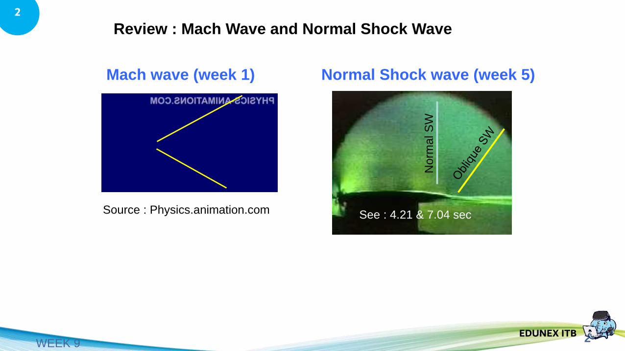
Mach wave (week 1)
Review : Mach Wave and Normal Shock Wave
Source : Physics.animation.com
Normal Shock wave (week 5)
See : 4.21 & 7.04 sec
Norm
al S
W

3EDUNEX ITB
3
WEEK 9
Mach wave (week 1)
Review : Mach Wave and Normal Shock Wave
𝜇 Mach angle
𝜇 = 𝑠𝑖𝑛−11
𝑀𝑎
𝑉
𝑀∞ > 1.0 𝑀∞ > 1.0
▪ Isentropic
▪ It is only function of 𝑴∞
▪ streamline is straight
▪ Non-isentropic
▪ It is only function of 𝑴∞
▪ streamline is straight
𝑀∞ > 1.0 𝑀∞ < 1.0
𝜅 = 90𝑜
Normal Shock wave (week 5)
Supersonic Supersonic Supersonic Subsonic
What does it happen when the angle is in between ?
𝜇 ≪ 𝛽 ≪ 𝜅 𝛽
Oblique SW
If It is only function of 𝑴∞ ?
4EDUNEX ITB
4
WEEK 9
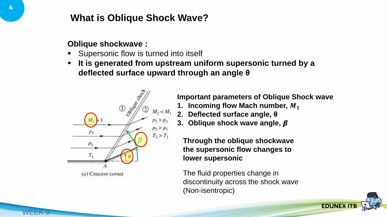
What is Oblique Shock Wave?
Oblique shockwave :
▪ Supersonic flow is turned into itself
▪ It is generated from upstream uniform supersonic turned by a
deflected surface upward through an angle θ
Important parameters of Oblique Shock wave
1. Incoming flow Mach number, 𝑴𝟏
2. Deflected surface angle, θ
3. Oblique shock wave angle, 𝜷
𝛽 Through the oblique shockwave
the supersonic flow changes to
lower supersonic
The fluid properties change in
discontinuity across the shock wave
(Non-isentropic)
5EDUNEX ITB
5
WEEK 9
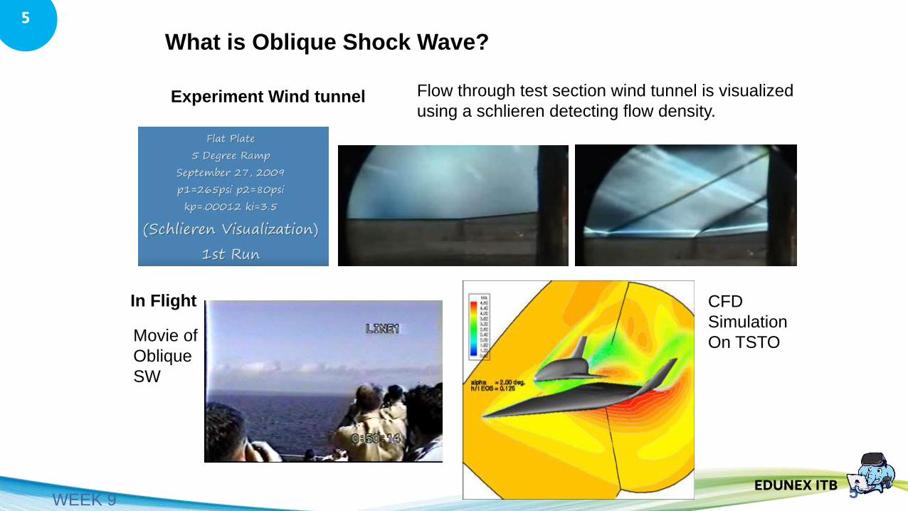
What is Oblique Shock Wave?
Experiment Wind tunnel Flow through test section wind tunnel is visualized
using a schlieren detecting flow density.
In Flight
Movie of
Oblique
SW
CFD
Simulation
On TSTO
6EDUNEX ITB
6
WEEK 9
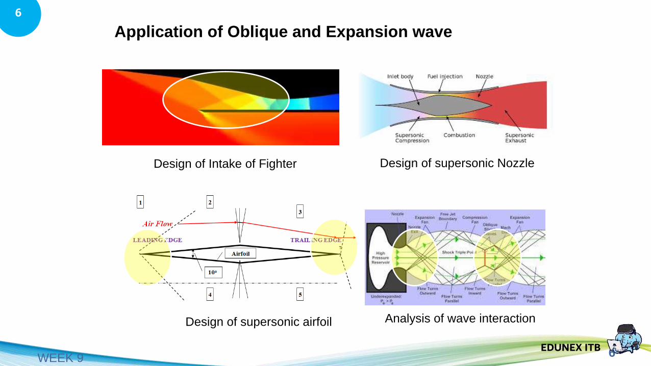
Application of Oblique and Expansion wave
Design of Intake of Fighter
Analysis of wave interaction Design of supersonic airfoil
Design of supersonic Nozzle
7EDUNEX ITB
7
WEEK 9
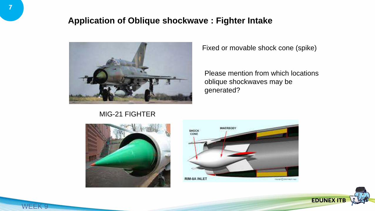
Application of Oblique shockwave : Fighter Intake
MIG-21 FIGHTER
Fixed or movable shock cone (spike)
Please mention from which locations
oblique shockwaves may be
generated?
8EDUNEX ITB
8
WEEK 9
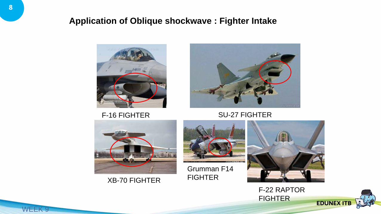
Application of Oblique shockwave : Fighter Intake
F-16 FIGHTER SU-27 FIGHTER
XB-70 FIGHTER
Grumman F14
FIGHTER
F-22 RAPTOR
FIGHTER
9EDUNEX ITB
9
WEEK 9
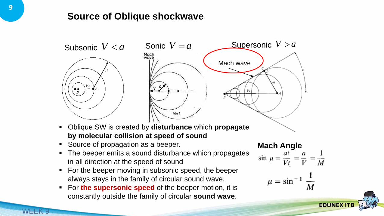
Source of Oblique shockwave
aV Subsonic aV =Sonic Supersonic aV
Mach wave
Mach Angle
▪ Oblique SW is created by disturbance which propagate
by molecular collision at speed of sound
▪ Source of propagation as a beeper.
▪ The beeper emits a sound disturbance which propagates
in all direction at the speed of sound
▪ For the beeper moving in subsonic speed, the beeper
always stays in the family of circular sound wave.
▪ For the supersonic speed of the beeper motion, it is
constantly outside the family of circular sound wave.
10EDUNEX ITB
10
WEEK 9
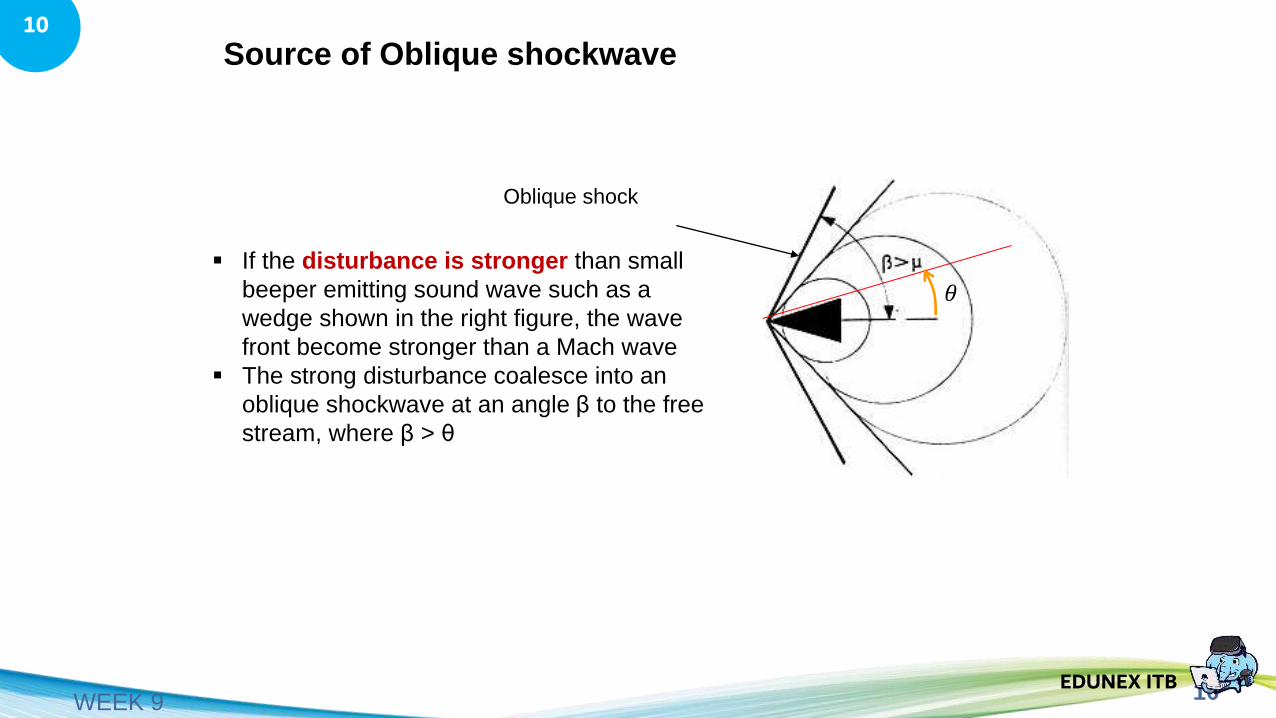
Source of Oblique shockwave
Oblique shock
▪ If the disturbance is stronger than small
beeper emitting sound wave such as a
wedge shown in the right figure, the wave
front become stronger than a Mach wave
▪ The strong disturbance coalesce into an
oblique shockwave at an angle β to the free
stream, where β > θ
𝜃
11EDUNEX ITB
11
WEEK 9
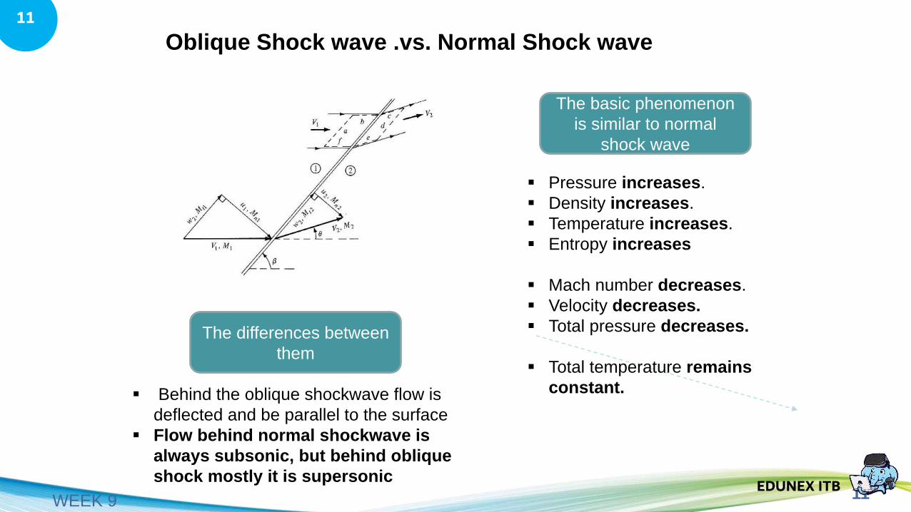
Oblique Shock wave .vs. Normal Shock wave
The basic phenomenon
is similar to normal
shock wave
▪ Pressure increases.
▪ Density increases.
▪ Temperature increases.
▪ Entropy increases
▪ Mach number decreases.
▪ Velocity decreases.
▪ Total pressure decreases.
▪ Total temperature remains
constant.
The differences between
them
▪ Behind the oblique shockwave flow is
deflected and be parallel to the surface
▪ Flow behind normal shockwave is
always subsonic, but behind oblique
shock mostly it is supersonic

12EDUNEX ITB
12
WEEK 9
Governing Equation for Oblique Shockwave
Assumptions:
▪ The flow is steady.
▪ The flow is adiabatic.
▪ There are no viscous effect on
the side of the control volume.
▪ There are no body forces.
Fixed Control volume approach (Eulerian)
flow is steady
Continuity equation
13EDUNEX ITB
13
WEEK 9
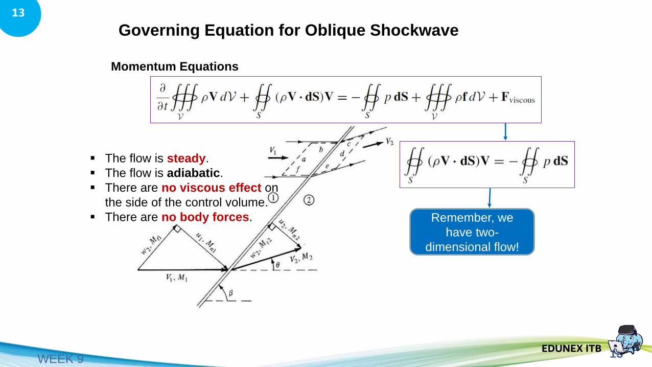
Governing Equation for Oblique Shockwave
▪ The flow is steady.
▪ The flow is adiabatic.
▪ There are no viscous effect on
the side of the control volume.
▪ There are no body forces.
Momentum Equations
Remember, we
have two-
dimensional flow!
14EDUNEX ITB
14
WEEK 9
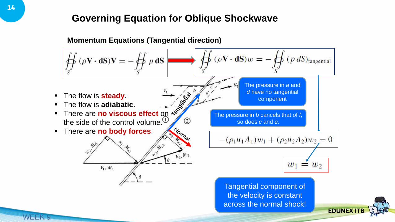
Governing Equation for Oblique Shockwave
▪ The flow is steady.
▪ The flow is adiabatic.
▪ There are no viscous effect on
the side of the control volume.
▪ There are no body forces.
Momentum Equations (Tangential direction)
The pressure in b cancels that of f,
so does c and e.
The pressure in a and
d have no tangential
component
Tangential component of
the velocity is constant
across the normal shock!
15EDUNEX ITB
15
WEEK 9
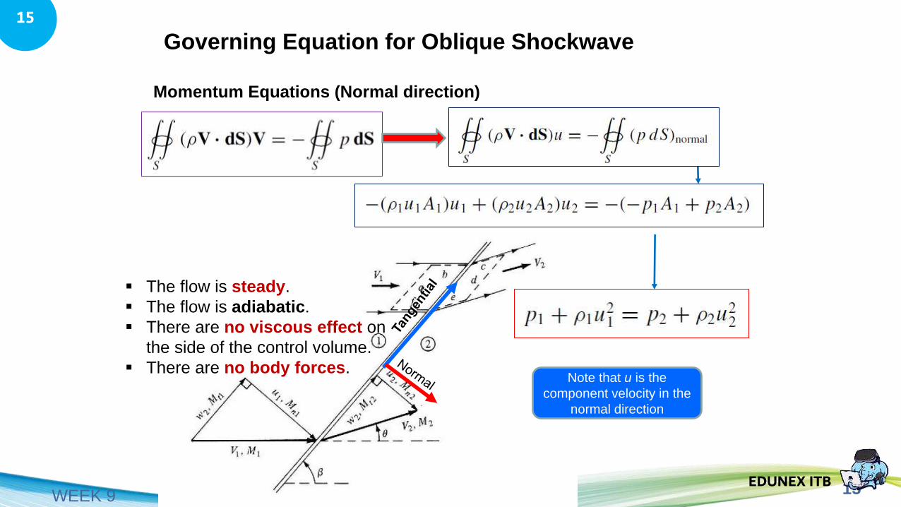
Governing Equation for Oblique Shockwave
▪ The flow is steady.
▪ The flow is adiabatic.
▪ There are no viscous effect on
the side of the control volume.
▪ There are no body forces.
Momentum Equations (Normal direction)
Note that u is the
component velocity in the
normal direction
16EDUNEX ITB
16
WEEK 9
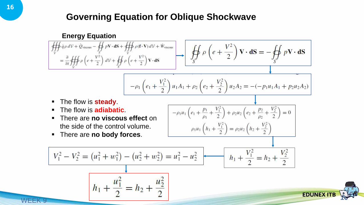
Governing Equation for Oblique Shockwave
▪ The flow is steady.
▪ The flow is adiabatic.
▪ There are no viscous effect on
the side of the control volume.
▪ There are no body forces.
Energy Equation
17EDUNEX ITB
17
WEEK 9
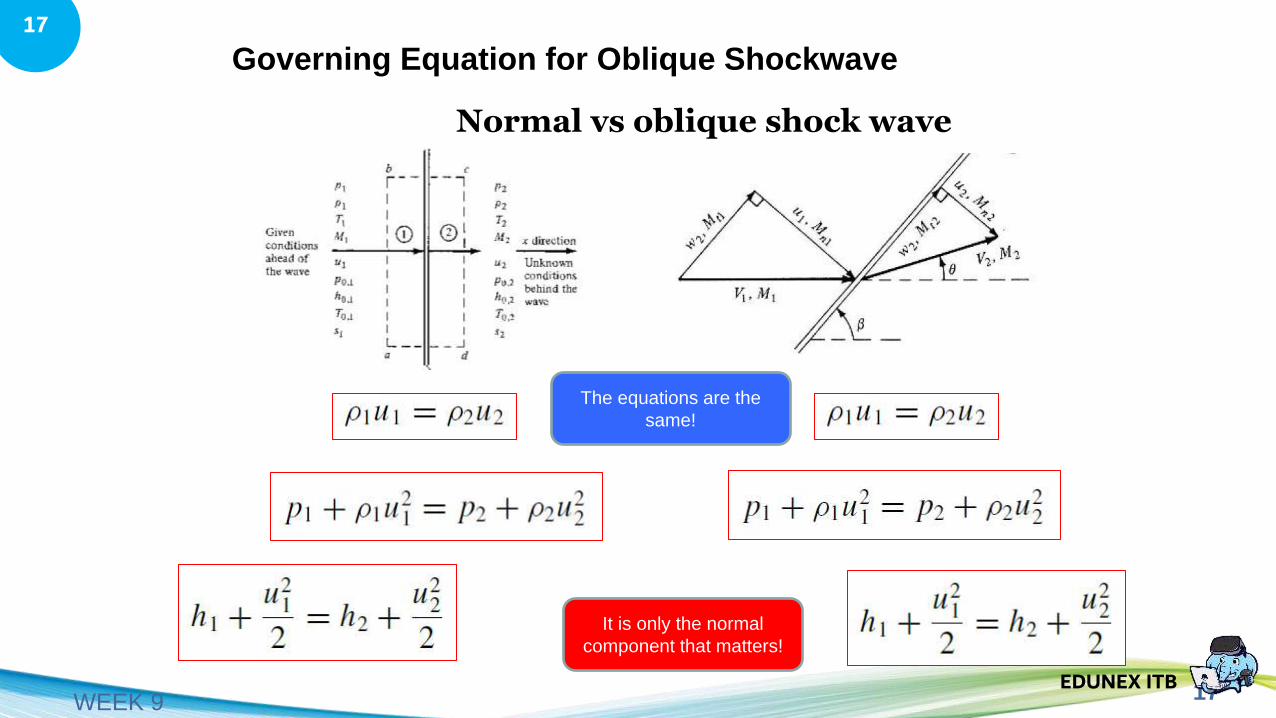
Governing Equation for Oblique Shockwave
Normal vs oblique shock wave
The equations are the
same!
It is only the normal
component that matters!
18EDUNEX ITB
18
WEEK 9
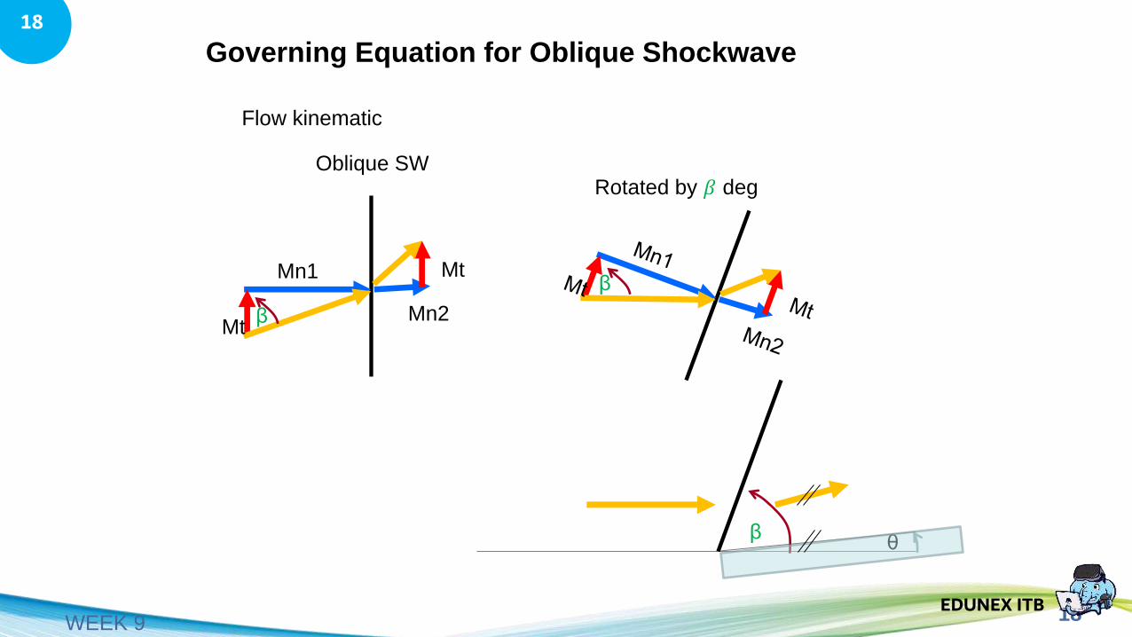
Governing Equation for Oblique Shockwave
Oblique SW
Mn2
Mn1 Mt
Mt
Rotated by 𝛽 deg
β
β
θβ
Flow kinematic

19EDUNEX ITB
19
WEEK 9
Governing Equation for Oblique Shockwave
β
From Normal shock wave relation
Left side kinematic
relation 𝑀𝑛1 = 𝑀1 sin 𝛽
M1
Right side
kinematic relation
𝑀2 =𝑀𝑛2
sin(𝛽 − 𝜃)
Left side Right side
𝑀22 𝑠𝑖𝑛2 𝛽 − 𝜃 =
2 + (𝛾 − 1)𝑀12 𝑠𝑖𝑛2 𝛽
2𝛾 𝑀12 𝑠𝑖𝑛2 𝛽 − (𝛾 − 1)
𝜌2𝜌1
=(𝛾 + 1)𝑀1
2 𝑠𝑖𝑛2 𝛽
2 + (𝛾 − 1)𝑀12 𝑠𝑖𝑛2 𝛽
𝑝2𝑝1
= 1 +2𝛾
(𝛾 + 1)𝑀1
2 𝑠𝑖𝑛2 𝛽 − 1
20EDUNEX ITB
20
WEEK 9
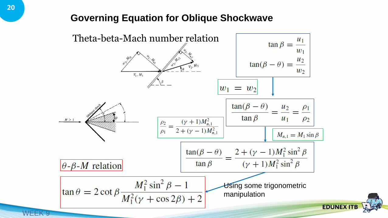
Governing Equation for Oblique Shockwave
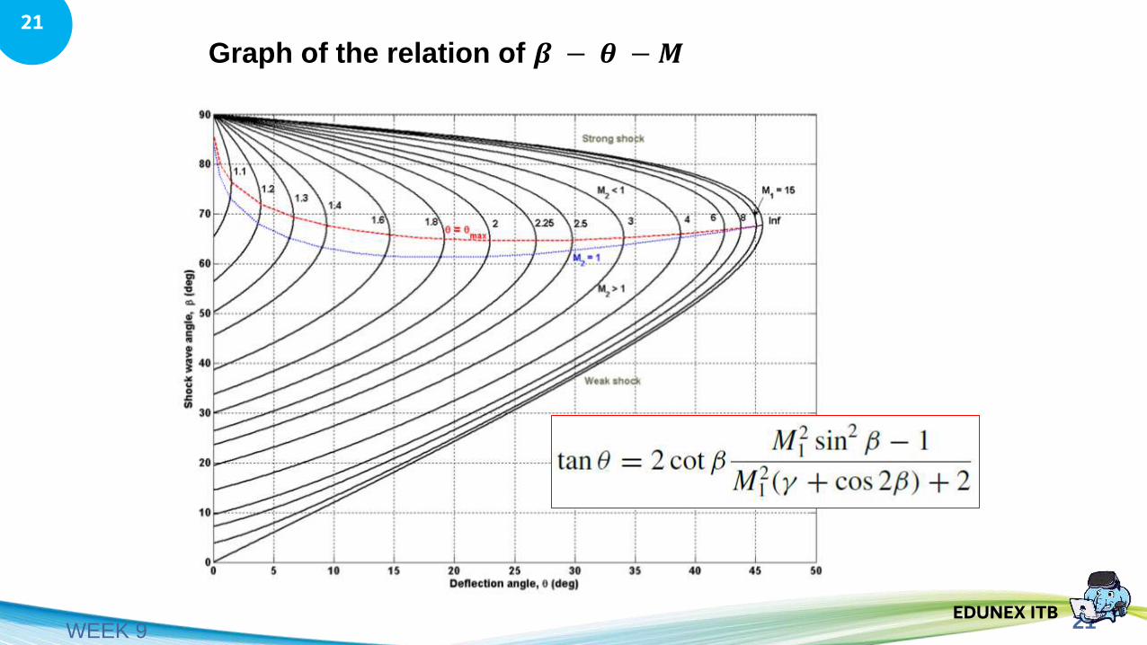
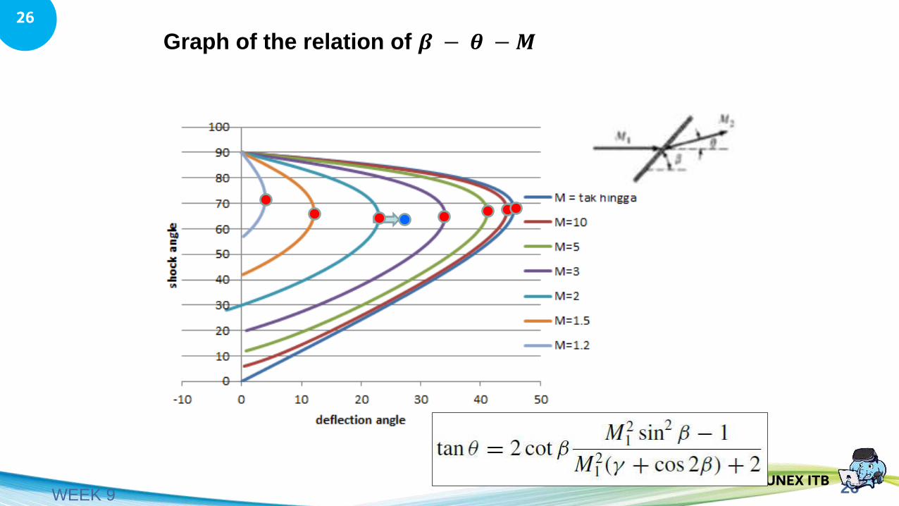
Theta-beta-Mach number relation
Using some trigonometric
manipulation
21EDUNEX ITB
21
WEEK 9
Graph of the relation of 𝜷 − 𝜽 −𝑴
22EDUNEX ITB
22
WEEK 9
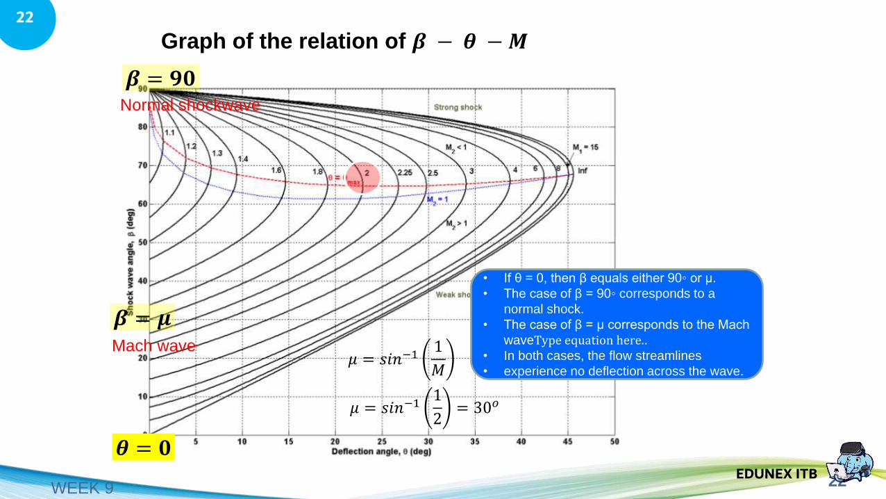
Graph of the relation of 𝜷 − 𝜽 −𝑴
• If θ = 0, then β equals either 90◦ or μ.
• The case of β = 90◦ corresponds to a
normal shock.
• The case of β = μ corresponds to the Mach
waveType equation here.. • In both cases, the flow streamlines
• experience no deflection across the wave.
𝜽 = 𝟎
𝜷 = 𝝁
𝜷 = 𝟗𝟎
Mach wave
Normal shockwave
𝜇 = 𝑠𝑖𝑛−11
𝑀
𝜇 = 𝑠𝑖𝑛−11
2= 30𝑜
23EDUNEX ITB
23
WEEK 9
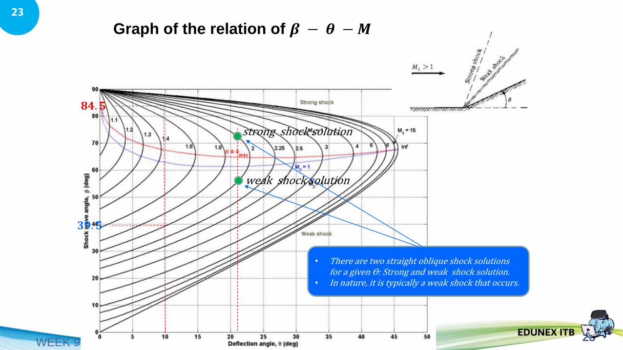
Graph of the relation of 𝜷 − 𝜽 −𝑴
• There are two straight oblique shock solutions for a given ϴ: Strong and weak shock solution.
• In nature, it is typically a weak shock that occurs.
weak shock solution
strong shock solution
𝟖𝟒. 𝟓
𝟑𝟗. 𝟓
24EDUNEX ITB
24
WEEK 9
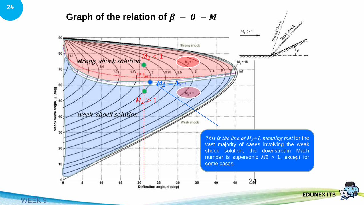
Graph of the relation of 𝜷 − 𝜽 −𝑴
24
This is the line of M2=1, meaning that for the
vast majority of cases involving the weak
shock solution, the downstream Mach
number is supersonic M2 > 1, except for
some cases.
𝑀2 > 1
𝑀2 < 1
𝑴𝟐 = 𝟏
weak shock solution
strong shock solution
25EDUNEX ITB
25
WEEK 9
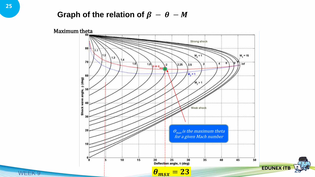
Graph of the relation of 𝜷 − 𝜽 −𝑴
ϴmax is the maximum theta for a given Mach number
Maximum theta
𝜽𝒎𝒔𝒙 = 𝟐𝟑
26EDUNEX ITB
26
WEEK 9
Graph of the relation of 𝜷 − 𝜽 −𝑴
27EDUNEX ITB
27
WEEK 9
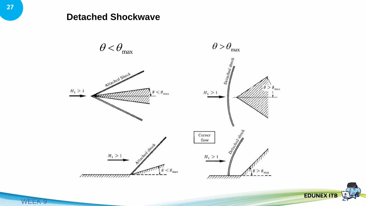
Detached Shockwave
max max
28EDUNEX ITB
28
WEEK 9
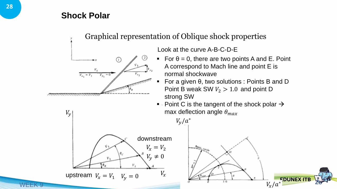
Shock Polar
Graphical representation of Oblique shock properties
𝑉𝑥
𝑉𝑦
𝑉𝑥 = 𝑉1
𝑉𝑦 ≠ 0
𝑉𝑦 = 0
𝑉𝑥 = 𝑉2
upstream
downstream
𝑉𝑥/𝑎∗
𝑉𝑦/𝑎∗
▪ For θ = 0, there are two points A and E. Point
A correspond to Mach line and point E is
normal shockwave
▪ For a given θ, two solutions : Points B and D
Point B weak SW 𝑉2 > 1.0 and point D
strong SW
▪ Point C is the tangent of the shock polar →
max deflection angle 𝜃𝑚𝑎𝑥
Look at the curve A-B-C-D-E
29EDUNEX ITB
29
WEEK 9
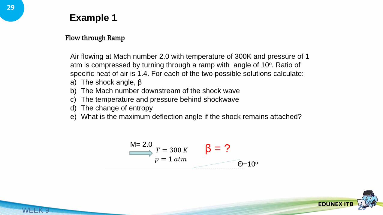
Example 1
Flow through Ramp
Air flowing at Mach number 2.0 with temperature of 300K and pressure of 1
atm is compressed by turning through a ramp with angle of 10o. Ratio of
specific heat of air is 1.4. For each of the two possible solutions calculate:
a) The shock angle, β
b) The Mach number downstream of the shock wave
c) The temperature and pressure behind shockwave
d) The change of entropy
e) What is the maximum deflection angle if the shock remains attached?
Θ=10o
M= 2.0β = ?𝑇 = 300 𝐾
𝑝 = 1 𝑎𝑡𝑚
30EDUNEX ITB
30
WEEK 9
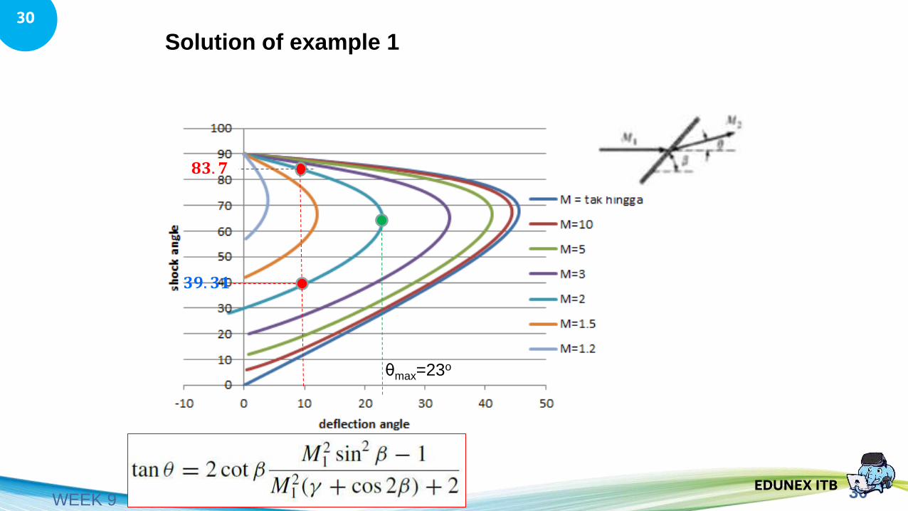
Solution of example 1
𝟖𝟑. 𝟕
𝟑𝟗. 𝟑𝟏
θmax=23o
31EDUNEX ITB
31
WEEK 9
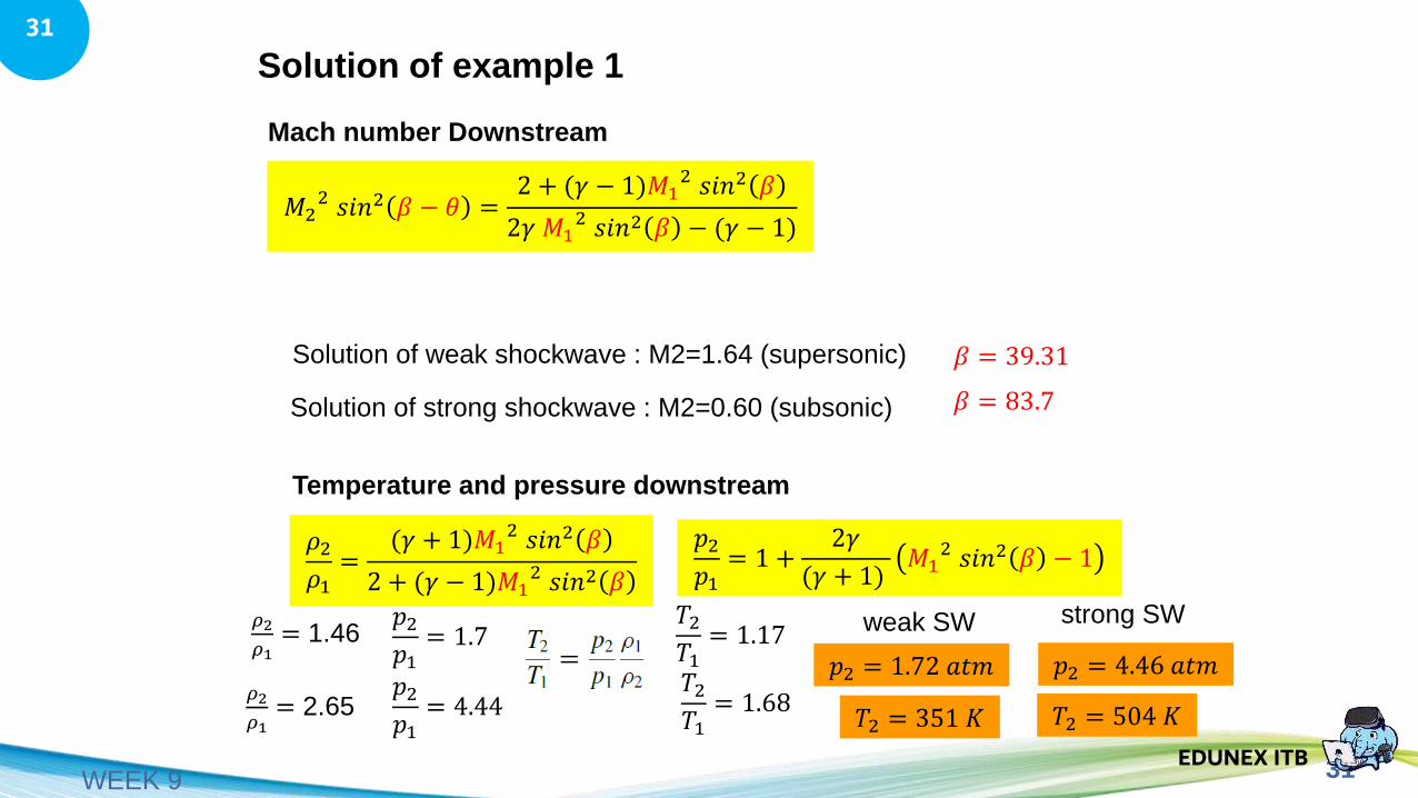
Solution of example 1
Mach number Downstream
𝑀22 𝑠𝑖𝑛2 𝛽 − 𝜃 =
2 + (𝛾 − 1)𝑀12 𝑠𝑖𝑛2 𝛽
2𝛾 𝑀12 𝑠𝑖𝑛2 𝛽 − (𝛾 − 1)
Solution of weak shockwave : M2=1.64 (supersonic)
Solution of strong shockwave : M2=0.60 (subsonic)
Temperature and pressure downstream
𝜌2𝜌1
=(𝛾 + 1)𝑀1
2 𝑠𝑖𝑛2 𝛽
2 + (𝛾 − 1)𝑀12 𝑠𝑖𝑛2 𝛽
𝑝2𝑝1
= 1 +2𝛾
(𝛾 + 1)𝑀1
2 𝑠𝑖𝑛2 𝛽 − 1
𝜌2
𝜌1= 2.65
𝑝2𝑝1
= 4.44𝑇2𝑇1
= 1.68
𝑝2 = 1.72 𝑎𝑡𝑚
𝑇2 = 351 𝐾
weak SW
𝑝2 = 4.46 𝑎𝑡𝑚
strong SW
𝑇2 = 504 𝐾
𝜌2
𝜌1= 1.46
𝑝2𝑝1
= 1.7𝑇2𝑇1
= 1.17
𝛽 = 39.31
𝛽 = 83.7
32EDUNEX ITB
32
WEEK 9
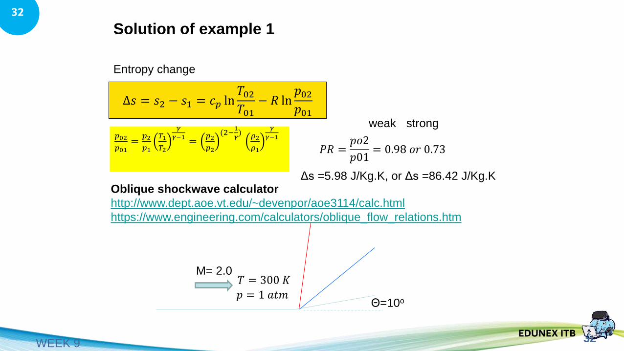
Solution of example 1
Entropy change
∆𝑠 = 𝑠2 − 𝑠1 = 𝑐𝑝 ln𝑇02𝑇01
− 𝑅 ln𝑝02𝑝01
𝑝02
𝑝01=
𝑝2
𝑝1
𝑇1
𝑇2
𝛾
𝛾−1=
𝑝2
𝑝2
(2−1
𝛾) 𝜌2
𝜌1
𝛾
𝛾−1
𝑃𝑅 =𝑝𝑜2
𝑝01= 0.98 𝑜𝑟 0.73
weak strong
Δs =5.98 J/Kg.K, or Δs =86.42 J/Kg.KOblique shockwave calculator
http://www.dept.aoe.vt.edu/~devenpor/aoe3114/calc.html
https://www.engineering.com/calculators/oblique_flow_relations.htm
Θ=10o
M= 2.0𝑇 = 300 𝐾
𝑝 = 1 𝑎𝑡𝑚
33EDUNEX ITB
33
WEEK 9
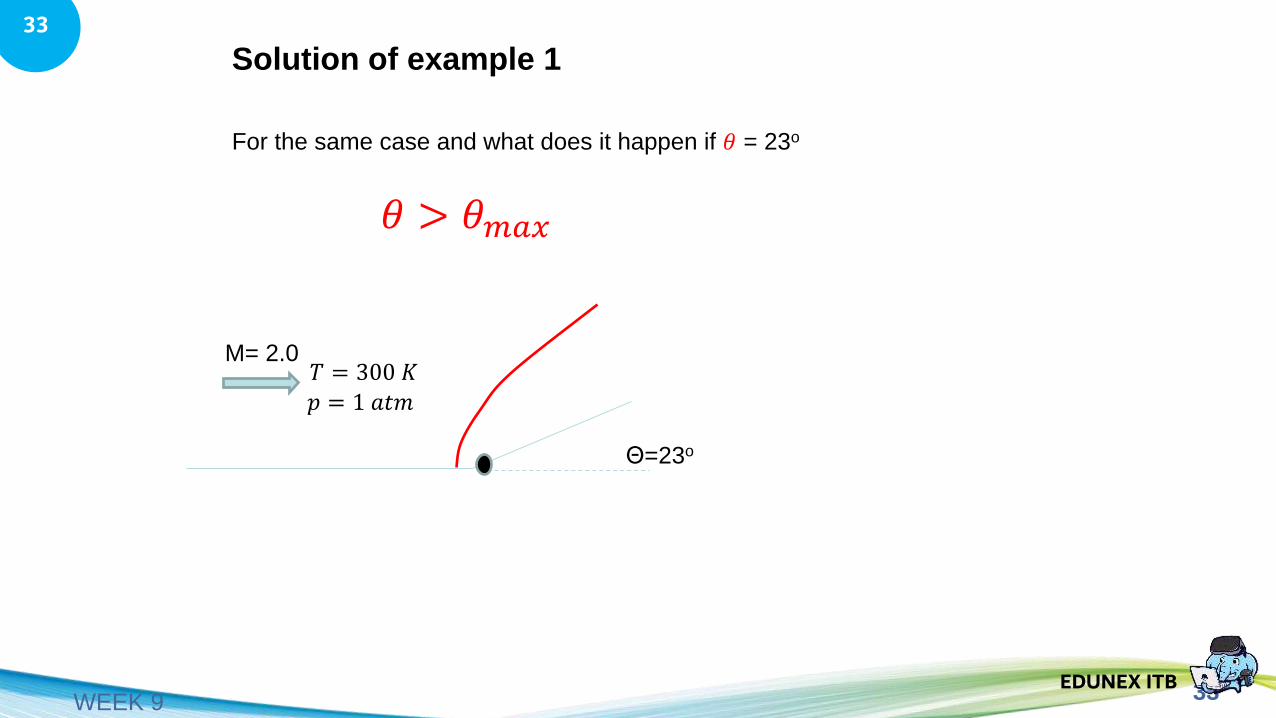
Solution of example 1
For the same case and what does it happen if 𝜃 = 23o
Θ=23o
M= 2.0𝑇 = 300 𝐾
𝑝 = 1 𝑎𝑡𝑚
𝜃 > 𝜃𝑚𝑎𝑥
34EDUNEX ITB
34
WEEK 9
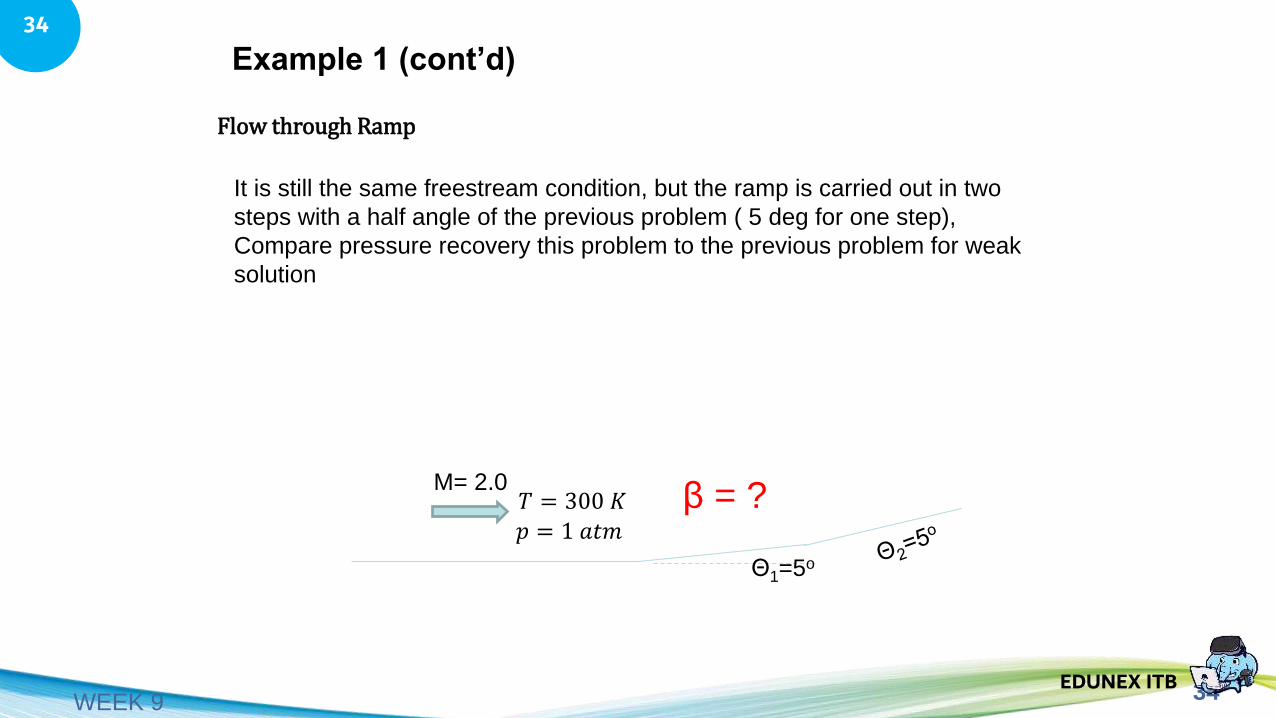
Example 1 (cont’d)
Flow through Ramp
It is still the same freestream condition, but the ramp is carried out in two
steps with a half angle of the previous problem ( 5 deg for one step),
Compare pressure recovery this problem to the previous problem for weak
solution
Θ1=5o
M= 2.0β = ?𝑇 = 300 𝐾
𝑝 = 1 𝑎𝑡𝑚
35EDUNEX ITB
35
WEEK 9
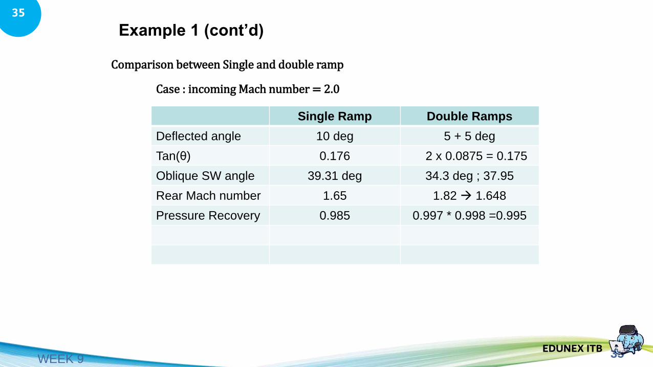
Example 1 (cont’d)
Comparison between Single and double ramp
Single Ramp Double Ramps
Deflected angle 10 deg 5 + 5 deg
Tan(θ) 0.176 2 x 0.0875 = 0.175
Oblique SW angle 39.31 deg 34.3 deg ; 37.95
Rear Mach number 1.65 1.82 → 1.648
Pressure Recovery 0.985 0.997 * 0.998 =0.995
Case : incoming Mach number = 2.0
36EDUNEX ITB
36
WEEK 9
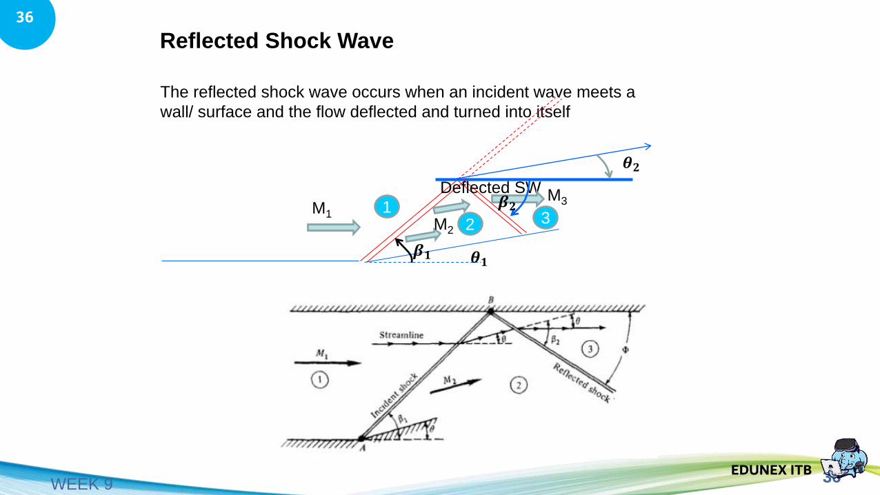
Reflected Shock Wave
The reflected shock wave occurs when an incident wave meets a
wall/ surface and the flow deflected and turned into itself
M1
Deflected SW
12 3M2
M3
𝜽𝟏𝜷𝟏
𝜽𝟐
𝜷𝟐
37EDUNEX ITB
37
WEEK 9
Reflected Shock Wave
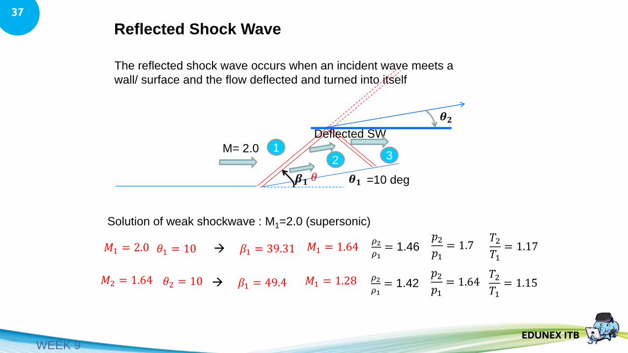
The reflected shock wave occurs when an incident wave meets a
wall/ surface and the flow deflected and turned into itself
=10 deg
M= 2.0
Deflected SW
12 3
𝜽𝟐
𝜽𝟏𝜷𝟏
Solution of weak shockwave : M1=2.0 (supersonic)
𝛽1 = 39.31𝜃1 = 10 𝑀1 = 1.64→𝑀1 = 2.0
𝛽1 = 49.4𝜃2 = 10 𝑀1 = 1.28→𝑀2 = 1.64
𝜌2
𝜌1= 1.46
𝑝2𝑝1
= 1.7𝑇2𝑇1
= 1.17
𝜌2
𝜌1= 1.42
𝑝2𝑝1
= 1.64𝑇2𝑇1
= 1.15
𝜃
38EDUNEX ITB
38
WEEK 9
Shock Wave Interactions with zero slip line
M1 12 3M2
M3
𝜽𝟏𝜷𝟏
𝜷𝟐
𝜽𝟏𝜷𝟏
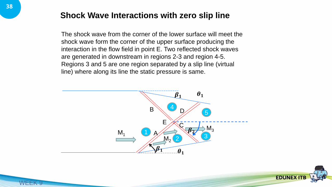
The shock wave from the corner of the lower surface will meet the
shock wave form the corner of the upper surface producing the
interaction in the flow field in point E. Two reflected shock waves
are generated in downstream in regions 2-3 and region 4-5.
Regions 3 and 5 are one region separated by a slip line (virtual
line) where along its line the static pressure is same.
E
A
B
C
D4
5
39EDUNEX ITB
39
WEEK 9
1 2
3 4
4’
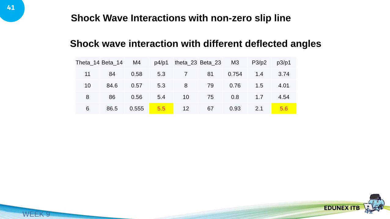
Shock Wave Interactions with non-zero slip line
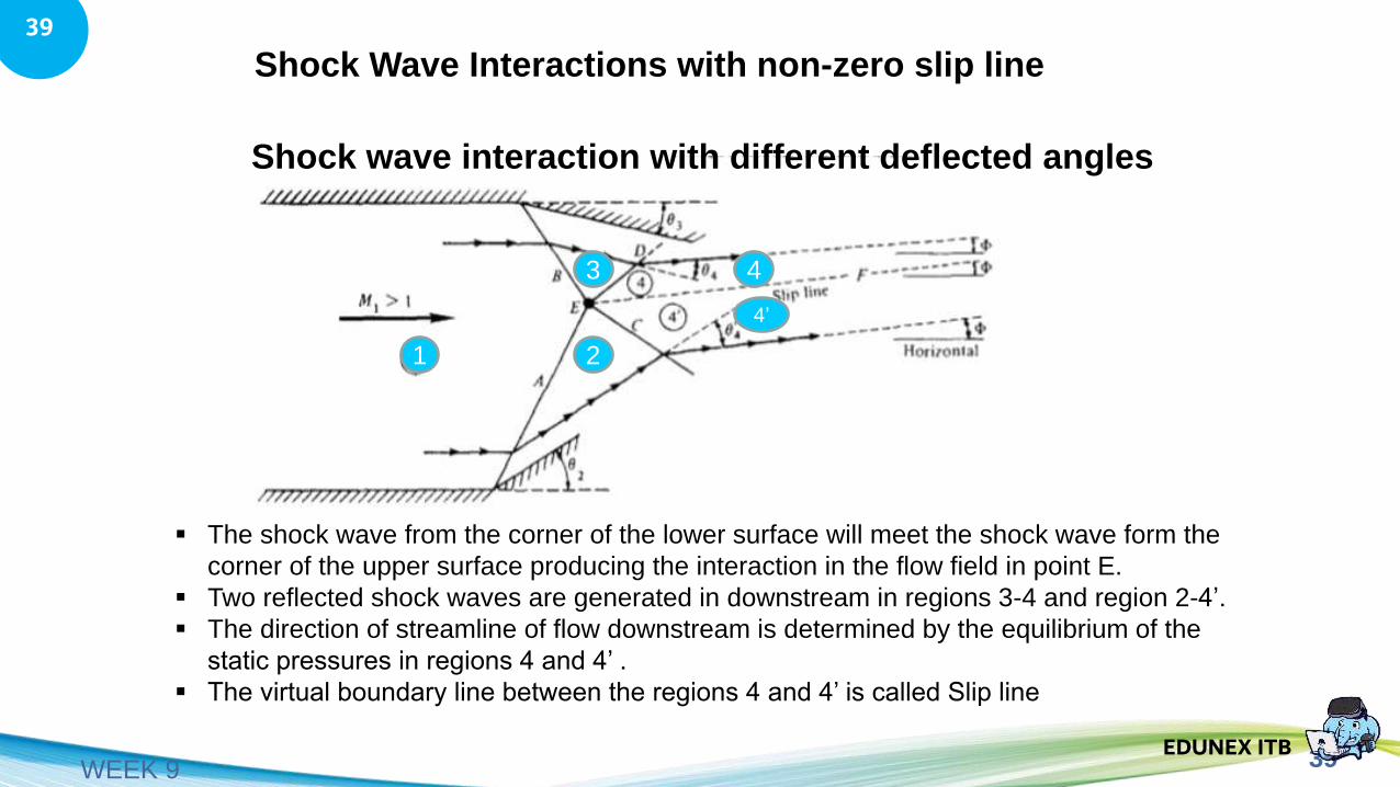
Shock wave interaction with different deflected angles
▪ The shock wave from the corner of the lower surface will meet the shock wave form the
corner of the upper surface producing the interaction in the flow field in point E.
▪ Two reflected shock waves are generated in downstream in regions 3-4 and region 2-4’.
▪ The direction of streamline of flow downstream is determined by the equilibrium of the
static pressures in regions 4 and 4’ .
▪ The virtual boundary line between the regions 4 and 4’ is called Slip line
40EDUNEX ITB
40
WEEK 9
Shock Wave Interactions with non-zero slipline
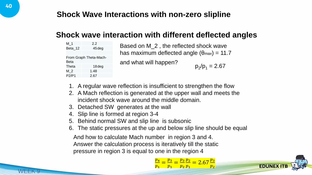
Shock wave interaction with different deflected anglesM_1 2.2
Beta_12 45deg
From Graph Theta-Mach-
Beta
Theta 18deg
M_2 1.48
P2/P1 2.67
Based on M_2 , the reflected shock wave
has maximum deflected angle (θmax) = 11.7
and what will happen?
1. A regular wave reflection is insufficient to strengthen the flow
2. A Mach reflection is generated at the upper wall and meets the
incident shock wave around the middle domain.
3. Detached SW generates at the wall
4. Slip line is formed at region 3-4
5. Behind normal SW and slip line is subsonic
6. The static pressures at the up and below slip line should be equal
And how to calculate Mach number in region 3 and 4.
Answer the calculation process is iteratively till the static
pressure in region 3 is equal to one in the region 4
𝑝4
𝑝1=
𝑝3
𝑝1=
𝑝3
𝑝2
𝑝2
𝑝1= 2.67
𝑝3
𝑝2
p2/p1 = 2.67
41EDUNEX ITB
41
WEEK 9
Shock Wave Interactions with non-zero slip line
Shock wave interaction with different deflected angles
Theta_14 Beta_14 M4 p4/p1 theta_23 Beta_23 M3 P3/p2 p3/p1
11 84 0.58 5.3 7 81 0.754 1.4 3.74
10 84.6 0.57 5.3 8 79 0.76 1.5 4.01
8 86 0.56 5.4 10 75 0.8 1.7 4.54
6 86.5 0.555 5.5 12 67 0.93 2.1 5.6
42EDUNEX ITB
42
WEEK 9
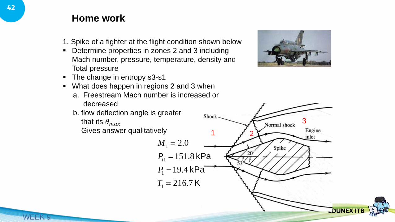
Home work
1. Spike of a fighter at the flight condition shown below
▪ Determine properties in zones 2 and 3 including
Mach number, pressure, temperature, density and
Total pressure
▪ The change in entropy s3-s1
▪ What does happen in regions 2 and 3 when
a. Freestream Mach number is increased or
decreased
b. flow deflection angle is greater
that its 𝜃𝑚𝑎𝑥
Gives answer qualitatively
K
kPa
kPa
7.216
4.19
8.151
0.2
1
1
1
1
=
=
=
=
T
P
P
M
t
1 2
3
43EDUNEX ITB
43
WEEK 9
WEEK 2