nx 9 thermal solver tmg reference manual · 2014-10-06 · to use tmg features from outside the nx...
TRANSCRIPT

NX 9 Thermal Solver TMG Reference Manual

Proprietary & Restricted Rights Notice
© 2013 Maya Heat Transfer Technologies Ltd. All Rights Reserved. This software and related documentation are proprietary to Maya Heat Transfer Technologies LTD.
All trademarks belong to their respective holders.
MPICH2 Copyright Notice
+ 2002 University of Chicago
Permission is hereby granted to use, reproduce, prepare derivative works, and to redistribute to others. This software was authored by:
Mathematics and Computer Science Division Argonne National Laboratory, Argonne IL 60439
(and)
Department of Computer Science University of Illinois at Urbana-Champaign
GOVERNMENT LICENSE
Portions of this material resulted from work developed under a U.S. Government Contract and are subject to the following license: the Government is granted for itself and others acting on its behalf a paid-up, nonexclusive, irrevocable worldwide license in this computer software to reproduce, prepare derivative works, and perform publicly and display publicly.
DISCLAIMER
This computer code material was prepared, in part, as an account of work sponsored by an agency of the United States Government. Neither the United States, nor the University of Chicago, nor any of their employees, makes any warranty express or implied, or assumes any legal liability or responsibility for the accuracy, completeness, or usefulness of any information, apparatus, product, or process disclosed, or represents that its use would not infringe privately owned rights.
Portions of this code were written by Microsoft. Those portions are Copyright (c) 2007 Microsoft Corporation. Microsoft grants permission to use, reproduce, prepare derivative works, and to redistribute to others. The code is licensed "as is." The User bears the risk of using it. Microsoft gives no express warranties, guarantees or conditions. To the extent permitted by law, Microsoft excludes the implied warranties of merchantability, fitness for a particular purpose and non-infringement.
METIS Copyright and License
The TMG solver uses the METIS library with permission. METIS, Copyright (1997) The Regents of the University of Minnesota. A copy of the METIS reference manual is located at [NX_installation]\NXCAE_extras\tmg\install\metis-manual.pdf in your NX distribution. Related

papers are available at http://www.cs.umn.edu/~metis, while the primary reference is “A Fast and Highly Quality Multilevel Scheme for Partitioning Irregular Graphs”. George Karypis and Vipin Kumar. SIAM Journal on Scientific Computing, Vol. 20, No. 1, pp. 359—392, 1999.
Mesa 7.5.2 Copyright (C) 1999-2007 Brian Paul All Rights Reserved.
Permission is hereby granted, free of charge, to any person obtaining a copy of this software and associated documentation files (the "Software"), to deal in the Software without restriction, including without limitation the rights to use, copy, modify, merge, publish, distribute, sublicense, and/or sell copies of the Software, and to permit persons to whom the Software is furnished to do so, subject to the following conditions:
The above copyright notice and this permission notice shall be included in all copies or substantial portions of the Software.
THE SOFTWARE IS PROVIDED "AS IS", WITHOUT WARRANTY OF ANY KIND, EXPRESS OR IMPLIED, INCLUDING BUT NOT LIMITED TO THE WARRANTIES OF MERCHANTABILITY, FITNESS FOR A PARTICULAR PURPOSE AND NONINFRINGEMENT. IN NO EVENT SHALL BRIAN PAUL BE LIABLE FOR ANY CLAIM, DAMAGES OR OTHER LIABILITY, WHETHER IN AN ACTION OF CONTRACT, TORT OR OTHERWISE, ARISING FROM, OUT OF OR IN CONNECTION WITH THE SOFTWARE OR THE USE OR OTHER DEALINGS IN THE SOFTWARE.
Qwt MayaMonitor is based in part on the work of the Qwt project (http://qwt.sf.net).

Table of Contents
i
Table of Contents Introduction ................................................................................................................ 1
Section 1: Input Cards ................................................................................................ 2
Card 1 – Title Card – Required ................................................................................................................ 5 Card 2a – Program Control Card – Required ........................................................................................... 6 Card 2b – Analyzer Control Card – Optional......................................................................................... 12 Card 4a – Single NODE Cards – Optional ............................................................................................. 18 Card 4b – Multiple Node Generation Cards – Optional ......................................................................... 19 Card 4c – New Local Coordinate System Cards – Optional .................................................................. 22 Card 4d – Third Level Node Generation Card – Optional ..................................................................... 25 Card 5a – Element Cards – Optional ...................................................................................................... 26 Card 5b – Multiple Element Generation Cards – Optional .................................................................... 38 Card 5c – Third Level Element Generation Card – Optional ................................................................. 42 Card 5d – Space Element Generation Card – Optional .......................................................................... 44 Card 6 – View Factor, Solar View Factor, Earth, Orbit, and Convective
Conductance Request Cards – Optional .............................................................................................. 48 Card 6a – View Factor Request Cards – Optional ................................................................................. 49 Card 6b – Solar View Factor Request Card – Optional ......................................................................... 53 Card 6d – Earth Card – Optional ............................................................................................................ 55 Card 6e – Thermal Coupling Request Card – Optional ......................................................................... 57 Card 6f – MESH Redefinition – Optional .............................................................................................. 86 Card 6g – Symmetric View Factors Request Card – Optional ............................................................... 90 Card 6h – Symmetric Elements List Card – Optional ............................................................................ 91 Card 6j – View Factor Merging Card ..................................................................................................... 94 Card 6k – Orbit Definition Card – Optional........................................................................................... 96 Card 6l – Additional Orbital Parameters ORBADD Card – Optional ................................................. 100 Card 6m – Minimum Allowable View Factor VFMIN Card – Optional ............................................. 105 Card 6n – Heat Flux View Factor Requests to Radiative Sources – Optional ..................................... 106 Card 6o – Symmetric Elements List Continuation Card – Optional .................................................... 111 Card 6p – Spinning Definition in Orbit Card – Optional ..................................................................... 112 Card 6q – Spinning Request Card – Optional ...................................................................................... 113 Card 6r – View Factor Request Cards in an Enclosure – Optional ...................................................... 115 Card 6s – Diffuse Sky View Factor Request Card – Optional ............................................................. 117 Card 6t – ORBDEF1-ORBDEF7 Orbit and Attitude Modeling Request Cards
– Optional .......................................................................................................................................... 119 Card 6u – DIURNAL1-6 Solar Heating Modeling Request Cards – Optional .................................... 138

Table of Contents
ii
Card 6v - Hemicube View Factor Method Activation Card - Optional ............................................... 152 Card 6w – Monte Carlo Method Activation Card - Optional ............................................................... 153 Card 6x – Thermal Coupling Rotational Periodicity Card - Optional .................................................. 156 Card 7 – Element Merging and Renumbering Cards ........................................................................... 157 Card 8 – Element Elimination Cards – Optional .................................................................................. 159 Card 9 - ALIGN Align Vector Definition - Optional ........................................................................... 161 Card 9 - ARPARAM Articulation Parameters - Optional .................................................................... 162 Card 9 - ARRAYTYPE Array Variable Definition Card - Optional ................................................... 163 Card 9 - ARRAYDATA Array Variable Definition Card - Optional .................................................. 168 Card 9 - ARTICUT Articulation Definition - Optional ....................................................................... 169 Card 9 - AXISYMM Axisymmetric Element Creation Card - Optional .............................................. 170 Card 9 - DESCRIP Character String Descriptor Cards - Optional ....................................................... 174 Card 9 - EAREAED Area Proportional Edge Conductance – Optional .............................................. 175 Card 9 - EAREAFA Area Proportional Face Conductance - Optional ................................................ 177 Card 9 - ELEMQED Element Edge Heat Fluxes - Optional ................................................................ 179 Card 9 - ELEMQEL Element Heat Generation - Optional .................................................................. 181 Card 9 - ELEMQFA Element Face Heat Fluxes - Optional ................................................................. 182 Card 9 – FMHDEF - Free Molecular Heating Request Cards – Optional ........................................... 184 Card 9 - FREEFACE Element Free Face Generation Card - Optional ................................................ 187 Card 9 – GENERIC Generic Entity Cards – Optional ......................................................................... 190 Card 9 – GPARAM Parameter Card - Optional ................................................................................... 192 Card 9 – GRAVITY Gravity Definition Cards - Optional ................................................................... 193 Card 9 - HYDENV Hydraulic Element Environment Definition Card -
Optional ............................................................................................................................................. 195 Card 9 - INCLAXI Include Axisymmetric Elements Definition Card -
OBSOLETE ....................................................................................................................................... 197 Card 9 - INTERP Analyzer Table Interpolation - Optional ................................................................. 198 Card 9 - JOINT Articulation Joint Definition - Optional ..................................................................... 201 Card 9 - KEEPDEL Element Keep/Delete Cards - Optional ............................................................... 203 Card 9 - LAYER Layer Property Definition Card - Optional .............................................................. 206 Card 9 - MAT Material Property Definition Card - Optional .............................................................. 209 Card 9 - MATCHANGE Material Property Change Card – Optional ................................................. 215 Card 9 - MATVEC Material Orientation Definition Card - Optional .................................................. 216 Card 9 - MCV Moving Control Volume Fluid Elements - Optional ................................................... 219 Card 9 - NAME Cards - Optional ........................................................................................................ 221 Card 9 - NAME2 - Group Name Description - Optional ..................................................................... 224 Card 9 - NODEQ Nodal Heat Source - Optional ................................................................................. 225 Card 9 - NODESINK Sink Nodes - Optional....................................................................................... 226 Card 9 – OPTICAL Surface Properties - Optional ............................................................................... 227

Table of Contents
iii
Card 9 - PARAM Parameter Card - Optional ...................................................................................... 228 Card 9 – PELTIER Peltier Device Card - Optional ............................................................................. 267 Card 9 - PHASE Phase Change Elements - Optional .......................................................................... 270 Card 9 - PRINT Analyzer Printout Codes - Optional .......................................................................... 271 Card 9 - PROP Physical Property Definition Cards - Optional ........................................................... 278 Card 9 - PSINK Pressure Sink Definition Cards - Optional ................................................................ 284 Card 9 – PSPROP1 Plane Stress Elements for Blades Card - Optional ............................................... 285 Card 9 – PSPROP2 Plane Stress Elements for Holes Card - Optional ................................................ 286 Card 9 - QNODE Heat Loads - Optional ............................................................................................. 287 Card 9 – RELTEMP Relative Temperature Correction - Optional ...................................................... 290 Card 9 - RENUMN, RENUME Node and Element Renumbering - Optional ..................................... 291 Card 9 – REPORTER for Group Reports – Optional .......................................................................... 292 Card 9 - REPEAT Additional Card Generation - Optional .................................................................. 294 Card 9 - REVNODE or REVNOM Reversed Element Creation - Optional ........................................ 295 Card 9 – ROT_FX Rotational Effects Definition - Optional ............................................................... 297 Card 9 – ROTATION Rotation Load Definition - Optional ................................................................ 299 Card 9 – ROTPER Thermal Rotational Periodicity Definition - Optional .......................................... 300 Card 9 - SINK Sink Elements - Optional ............................................................................................. 302 Card 9 - STEP Solution Steps Control Card - Optional ....................................................................... 304 Card 9 - SYMM Symmetry Definition Card - Optional ...................................................................... 307 Card 9 - TABDATA Analyzer Table Data Cards - Optional ............................................................... 308 Card 9 - TABTYPE Table Variable Type Definition Card - Optional ................................................ 310 Card 9 – THERMAL_VOID Thermal Void Zone Definition - Optional ............................................ 317 Card 9 - THERMST Analyzer Thermostat Definition - Optional ........................................................ 319 Card 9 - TINIT Initial Temperatures - Optional ................................................................................... 322 Card 9 – TOTTEMP Total Temperature Effects Definition - Optional ............................................... 324 Card 9 – TSTREAM Thermal Stream Definition - Optional ............................................................... 325 Card 9 - VARIABLE Variable Definition Card - Optional ................................................................. 329 Card 9 - VECTOR Vector Definition Card - Optional ........................................................................ 330 Card 9 – VOID_NONGEOM Void Non-Geometric Element Definition -
Optional ............................................................................................................................................. 331 Card 9 – WDINIT Initial Water Mass Accumulation per Unit Area – Optional ................................. 333 Card 9 - XCAP Capacitances - Optional .............................................................................................. 334 Card 9 - XCIRC Circular Element Definition Card - Optional ............................................................ 335 Card 9 - XCOND Conductances - Optional ......................................................................................... 337 Card 9 – ZONE_CONVECTION Thermal Convecting Zone Definition -
Optional ............................................................................................................................................. 341 Card 10 - User-Written Subroutines USER1 and USERF - Optional .................................................. 343

Table of Contents
iv
Section 2: Files ....................................................................................................... 386
Section 3: Modules ................................................................................................ 407
Analyzer Module .................................................................................................................................. 407 Steady State Analysis Flowchart .......................................................................................................... 408 Transient Analysis Flowchart ............................................................................................................... 416 Hydraulic Network Flowchart .............................................................................................................. 432 ANS2TMG Module ............................................................................................................................. 474 COND and CONN2 Modules .............................................................................................................. 475 CONDN Module .................................................................................................................................. 482 GRAYB Module .................................................................................................................................. 496 HEMIVIEW Module ............................................................................................................................ 502 MAIN, DATACH and ECHOS Modules ............................................................................................. 511 MEREL Module ................................................................................................................................... 512 NEVADA Module ............................................................................................................................... 517 POWER Module .................................................................................................................................. 519 REFORM Module ................................................................................................................................ 523 RSLTPOST Module ............................................................................................................................. 531 TMG2ANS Module ............................................................................................................................. 535 TMGINT Module ................................................................................................................................. 536 VUFAC Module ................................................................................................................................... 541 References ............................................................................................................................................ 575

Introduction
1
Introduction In most situations, a thermal model can be defined and solved using NX Thermal Analysis from within the NX environment. The thermal model is built using the NX interface. The results can then be displayed and analyzed within NX using the built-in post-processing functionality. Before solving, all thermal models and their operational data are translated into a TMG input file. This process is transparently integrated into the TMG interface. Under normal circumstances it is unnecessary to know how it works. However, advanced users may occasionally need access to TMG functions that are unavailable from within the NX interface. To do so, some knowledge of TMG’s underlying structure is required, since individual commands and data sets must be inserted directly into the TMG input file. This document describes the format and contents of the input file and the output files, and gives an overview of how TMG’s various modules interact. The document is divided into three main sections:
• The first section describes the format and content of the TMG input file (or data deck). It describes in details all TMG input cards. An overview of the input file format is shown below.
• The second section gives a list of all files created during a TMG run with a brief summary of their content.
• Finally, the last section explains the function of all TMG modules that are executed during a TMG run

Input File Format Overview
2
Section 1: Input Cards Input File Format Overview
To use TMG features from outside the NX environment, you must place instructions and data directly into TMG’s input file (also known as the data deck). This can be done with any text editor. In most cases, a single input file (always called INPF) is created in the following manner:
1. Build a thermal model using TMG within NX. 2. Set run time options to only build an input file in the TMG thermal analysis task. 3. Select the solve button in the TMG thermal analysis task.
This creates the file INPF in the directory from which NX was run. When the TMG input file is complete, the model can be solved by entering tmg at the operating system’s command prompt where the input file resides and selecting TI for interactive thermal solve. You can also create the TMG data deck from an empty file by using any text editor or user written code that produces the proper TMG input file format. Only very advanced users should attempt this. TMG's input deck, INPF, consists of 10 different Card types, separated by –1 Delimiter Cards. Only the first two Card types, and the ten –1 Delimiter Cards are mandatory.
Data Deck Format
Card 1 Title Card – Mandatory –1 (Delimiter Card) Card 2a Program Control Card – Mandatory Card 2b Analyzer Control Card – Optional –1 (Delimiter Card) Card 3 Plot Card – Obsolete –1 (Delimiter Card) Card 4 Node Cards – Optional –1 (Delimiter Card) Card 5 Element Cards – Optional –1 (Delimiter Card) Card 6 View Factor & Thermal Coupling Cards – Optional –1 (Delimiter Card) Card 7 Element Merging Cards – Optional

Input File Format Overview
3
–1 (Delimiter Card) Card 8 Element Elimination Cards – Optional –1 (Delimiter Card) Card 9 Additional Model Parameter Cards – Optional –1 (Delimiter Card) Card 10 User–written subroutines for the Analyzer – Optional –1 (Delimiter Card)
Input Convention
1. Input is in free format. Blanks or commas may separate data fields. 2. Data may be either a mnemonic or a numerical value. A mnemonic may be a code, a
symbolic variable, or a group name. Group names are mnemonic symbols that represent groups of elements. Group names are defined with Card 9 NAME Cards, and may be used instead of element numbers. The liberal use of group names is encouraged, since it makes both data input and output more legible. Symbolic variables are mnemonic symbols that represent numerical values defined with Card 9 VARIABLE Cards. Whenever a symbolic variable is encountered in the data deck, its numerical value is substituted.
3. Delimiter Cards and lines starting with mnemonic codes must start in column 1. 4. No line may exceed 90 characters.
Expressions 1. Expressions enclosed in brackets may be used instead of numerical values on Cards 4
through 9. Several levels of brackets may be used, but the length of the expression must not exceed 29 characters.
2. The operators +, –, /, *, and ** (exponentiation) may be used. 3. There must be no spaces inside the brackets.
Comment Cards and Fields Comment Cards may appear anywhere in the data stream after the Title Card. Comment Cards must have the letter C or a dollar sign ($) in the first column. Comments may also be entered on the Data Cards themselves, following a dollar sign ($).
Examples: $ THIS IS A COMMENT CARD 1,10.6,11,12.8 $ INPUT FORMAT EXAMPLE WITH COMMA SEPARATORS

Input File Format Overview
4
1 10.6 11 12.8 $ SAME WITH BLANK SEPARATORS 401 1.0 2 (3*(5.2/2.8+1)) $ USE OF AN EXPRESSION GENER 2 2 1 10 1 0 0 0 1 0 $ MNEMONIC CODE NAME XSISTOR 5 $ CARD 9 NAME CARD VARIABLE %HEATIN .5 $ CARD 9 SYMBOLIC VARIABLE CARD QNODE XSISTOR %HEATIN $ SYMBOLIC VARIABLE & GROUP NAME QNODE XSISTR2 (%HEATIN*.5) $ SYMBOLIC VARIABLE IN AN EXPRESSION

Card 1 – Title Card
5
Card 1 – Title Card – Required TITLE
Must not exceed 70 characters, and must be the first Card in the data deck.
Example: WHITE ALUMINUM T IN SPACE

Card 2a - Program Control Card
6
Card 2a – Program Control Card – Required M, N, MESH, RK, IST, KSP, SIGMA, PSUN, IA, TLIN, PIR
M M is the program control parameter that defines which modules are to be run. Different values of M may be summed to run different modules. For example, if M = 3 = 1+2, the COND module and the VUFAC module will be run. M = 0
TMG executes the MAIN, DATACH and ECHOS modules, which performs data checking. This option is always performed.
M = 1 TMG executes the COND module to calculate capacitances, conductive conductances, and hydraulic resistances from geometry. Two options exist for calculating conductances from geometry: the older element center method, and the element CG method (recommended). The latter can be specified with a Card 9 PARAM COND NEW option.
M = 2 TMG executes the VUFAC module to calculate view factors, solar view factors, Earth view factors, albedo factors, and thermal couplings. For this option, you also need to specify Card 6 Request Cards.
M = 4 TMG executes the GRAYB module to calculate radiative conductances from view factors. There is a caveat: If there are no Card 6 view factor requests, and it is not a restart run (i.e. there are no files MODLF or VUFF present), then the GRAYB module is not run.
M = 8 This is an obsolete option, which is not recommended. It executes the GRAYB module to calculate the solar spectrum gray body view factor matrix from view factors, which can be used to calculate solar spectrum heat loads in the POWER module. Any existing solar spectrum gray body view factor matrix on file VUFF will be overwritten.
M = 16 This is an obsolete option, which is not recommended. It executes the GRAYB module to calculate the IR spectrum gray body view factor matrix from view factors, which can be used to calculate IR spectrum heat loads in the POWER module. Any existing IR spectrum gray body view factor matrix on file VUFF will be overwritten.
M = 32 TMG executes the POWER module to calculate collimated (sun) solar spectrum heat loads. Solar view factors, view factors, and the PSUN parameter are necessary for this calculation.

Card 2a - Program Control Card
7
There is a caveat: If there are no Card 6 solar spectrum view factor (solar view factor, orbital view factor, heat flux view factor) requests, and it is not a restart run (i.e. there are no files MODLF or VUFF present), then the POWER module is only entered but not executed.
M = 64 TMG executes the POWER module to calculate IR spectrum heat loads. Earth view factors, view factors, and the PIR parameter are necessary for this calculation. There is a caveat: If there are no Card 6 solar spectrum view factor (solar view factor, orbital view factor, heat flux view factor) requests, and it is not a restart run (i.e. there are no files MODLF or VUFF present), then the POWER module is only entered but not executed.
M = 128 TMG executes the POWER module to calculate diffuse solar spectrum (e.g., albedo) heat loads. Albedo factors or heat flux view factors, view factors, and the PSUN parameter are necessary for this calculation. There is a caveat: If there are no Card 6 solar spectrum view factor (solar view factor, orbital view factor, heat flux view factor) requests, and it is not a restart run (i.e. there are no files MODLF or VUFF present), then the GRAYB module is only entered but not executed.
N N is the input/output format control parameter. N = 0
None of the options below is selected. N = 8
NASTRAN format input, all of Card 4 is a NASTRAN bulk data deck. N = 16
NASTRAN format output. If the Analyzer is run, NASTRAN element temperatures are written on file FMODLF.
N = 512 The VUFAC module does not write the details of the view factor calculations on file REPF in order to reduce its size.
N = 1024 Card 4 and 5 data is read from file VUFF.
Any combination of these options may be executed by summing their codes.
MESH MESH specifies the element subdivision parameter for view factor shadowing, ray tracing, and Card 6e thermal coupling calculations by the VUFAC module. Unshadowed view factors and solar view factors are calculated exactly and are not affected by the MESH value.

Card 2a - Program Control Card
8
MESH may be 0, 1, 2, 3, 4, or 5. For MESH = 0 no subdivision is performed. For MESH > 0 each beam is subdivided into MESH line segments, and each planar element into NV*MESH2 triangular sub–elements, where NV is the number of nodes (as shown below).
The Card 6f MESH Redefinition Card overrides the MESH parameter value.
RK is used by the GRAYB module with Gebhardt's (but not Oppenheim's) Method to eliminate insignificant radiative conductances, or to connect them to element KSP. A radiative conductance is considered insignificant if its gray body view factors to both elements are less than abs(RK) times the largest gray body view factor of either element to a non-space element. RK must be between –1 and 1. If RK > 0, the conductance is eliminated, except if it is connected to a space element defined on a Card 5 SPACE Card. If RK < 0, it is connected to element KSP, unless KSP is a space element. RK = 0 defaults to RK = 1E-4. Typically, RK = .05 can thin out the radiative conductances without significantly affecting accuracy.
Beam MESH=0
Quadrilateral MESH=0
Beam MESH=1
Triangle MESH=0
Triangle MESH=1
Quadrilateral MESH=1
Triangle MESH=2
Beam MESH=2
Quadrilateral MESH=2

Card 2a - Program Control Card
9
IST Obsolete.
KSP KSP is used by the GRAYB module either to create residual view factors = 1 – VFSUM for Gebhardt's method when the view factors do not sum to unity. Generally view factors do not sum to unity because of approximations made during the shadowing calculation process. KSP = 0
Creates self–view factors = 1 – VFSUM, i.e., the elements are made to see themselves. This option works well when there are a lot of low–emissivity elements present.
KSP = 1000000 Has the effect of adjusting the gray body view factors to compensate residual view factors. This is an obsolete method, and it does not work with Oppenheim's Method.
KSP = NSP creates view factors = 1 – VFSUM to element NSP. NSP must be the Card 5d space element number. If multiple enclosures exist, then each enclosure is flagged as being able to see space or not. An enclosure is characterized as being able to see space if at least element of that enclosure sees a space element. If an enclosure does not see space, the KSP = 0 option is used for that enclosure. This way, the creation improper space couplings from enclosures that do not see space is avoided, and inside and outside enclosures can be safely mixed.
KSP = 2000000 is similar to KSP=NSP, except that the space element number is obtained from the Card 5d Space Element Card.
KSP = 3000000 attempts to iteratively adjust the shadowed view factors proportionately to reduce the residual view factors. This is the recommended option.
SIGMA SIGMA is the Stefan-Boltzmann constant value in approximate units, e.g., 0.1714E-8 Btu/(hr*ft2*R4), or 5.6696E-8/(m2* K4), or 3.6577E-11W/(in2*K4).
PSUN PSUN is the collimated solar spectrum radiative source's (sun's) power output per unit area arriving at the element. PSUN is used by the POWER module in solar spectrum heat load calculations (M = 32 or M = 128).

Card 2a - Program Control Card
10
Typical values are 429+_7 Btu/hr/ft2 or 1353+_21 W/M2.
IA Used if a sinda85 output is requested with Card 9 PARAM SINDA85. If IA=0, a transient format output is created on file sinda85.dat. If IA=-99990, then a steady-state format output is created on file sinda85.dat.
TLIN
TLIN = (T1+T2)(T12+T2
2) is used by the MEREL module to linearize radiative conductances
during substructuring and Card 9 PARAM THIN model thinning operations. Only conductances that are connected to both radiative and conductive conductances are linearized. T1 is the typical estimated absolute temperatures of the elements to be eliminated, and T2 is the typical absolute temperature of their environments.
PIR is the heat load per unit area leaving the surface of the Earth. PIR is used by the POWER module (M = 64) to calculate Earth heat loads. A typical value for PIR for Earth heat load calculations is 75 BTU / hr / ft2 or 236 W / M2.
Notes: All parameters of Card 2a must be present. Zeros may be used for the parameters not used. Restart. runs may be performed using previously calculated data.
1. The most common type of restart run is rerunning the Analyzer after all the model parameters (conductances, capacitances, thermal couplings, radiative heat inputs) have been calculated from geometry. For this option, you should use M = 0 and make sure files MODLF and tmggeom.dat are present.
2. The second most common type of restart is to use re-use previously calculated radiative geometric view factors (e.g. view factors, solar view factors, etc.) For this option, make sure files VUFF and tmggeom.dat are present from the previous run, delete all Card 6 requests for calculating view factors and solar view factors etc. (but not thermal coupling requests), and M should be the value used in the previous run.
3. Other types of restart runs are also possible, e.g. when you wish to calculate additional view factors. For this type of run newly calculated data is appended to files MSGF, VUFF, REPF, and MODLF. However, on file VUFF the newly calculated data will supersede earlier data whereas on file MODLF (capacitances, conductances, heat loads) newly calculated data will be added to existing data. If necessary, file MODLF may be cleared of unwanted previous results with Card 9 KEEPDEL Cards.

Card 2a - Program Control Card
11
Card 2a Example: 7 0 1 0 0 84 1.713E–9 440 0 26463592 80 $ CARD 2A $ The VUFAC, GRAYB and COND modules will be executed.

Card 2b – Analyzer Control Card
12
Card 2b – Analyzer Control Card – Optional GRADNT, TABS, DTP, DT, TST, TF, TRDMP
This Card runs the Analyzer to calculate temperatures. Its parameters are interpreted according to whether the run is steady–state or transient.
Steady–State Runs
GRADNT is the convergence criterion. Convergence is achieved when GRADNT > TDMAX, where TDMAX is the maximum temperature difference between two iterations. GRADNT must be > 0. GRADNT = 0 defaults to 0.001. An additional energy balance convergence criterion may be specified on a Card 9 PARAM ENGBAL Card. If GRADNT=-9, then the Analyzer is not run.
TABS is the temperature of absolute zero. It is used to evaluate radiative conductances and air densities for hydraulic elements. It can be > 0 or < 0, e.g., +273 or +460.
DTP is the number of iterations between printouts. DTP = 0 defaults to a single printout at the end of the run.
DT is the iteration damping parameter. DT should be between 0 and 1. DT = 0 defaults to 1.0. At each iteration, for each element, an equilibrium temperature Teq (at which the element is in thermal equilibrium with its neighbors) is calculated. Tnew is then the mixture of Teq and the temperature Told of the previous iteration:
T DT T T DTnew old eq= − +( )1
Larger DT values speed up convergence for well–behaved models. Smaller DT values increase stability. If hydraulic elements are used in the model, smaller DT values, e.g. 0.3, are recommended.
TST is the time value at which the time–dependent heat load and sink temperature boundary conditions are evaluated for the run. If all boundary conditions are specified as CONSTANT, i.e. there are no time-dependent boundary conditions specified, TST = 0 may be used.

Card 2b – Analyzer Control Card
13
If time–dependent parameters are defined in tables on TABDATA Cards, TST must not exceed the largest time value of the table. If TST = –89990, an integrated average of the time-dependent heat loads with TIME values >0 is used for boundary conditions.
TF is the maximum number of iterations.
TRDMP TRDMP is ignored for steady-state runs.
Transient Runs
GRADNT GRADNT = –2
The explicit exponential forward differencing integration technique is used. The temperature of an element at time t + dt is calculated from the temperatures heat loads and conductance values at time t. At time t the equilibrium temperature Teq and the RC value for each element are calculated, where RC is the element's capacitance divided by the sum of its conductances. The new temperature T(t + dt) is calculated by:
T t dt T t T t T t eeq
dtRC( ) ( ) ( ( ) ( ))( )+ = + − −−
1
The exponential forward differencing technique is unconditionally stable for all values of dt, but does not conserve the energy of the system, which may lead to erroneous results with dt >> RCMIN, where RCMIN is then the smallest non–zero RC value in the model. Performance of the algorithm is degraded if zero capacitance elements are present, because the temperatures of zero-capacitance elements are calculated iteratively at each integration time step.
GRADNT = –3 The explicit forward differencing integration technique is used:
)))(()(()()(RCdttTtTtTdttT eq −+=+
The forward differencing technique is first-order accurate and conserves the energy of the system, but may become unstable if dt >RCMIN. If this option is used, it is a good idea to set DT = 0. However, this can often yield very small integration time steps, which may result in excessively long runs. Since this method is explicit (no iterations are performed) for models containing only non-zero capacitance elements, it is quite efficient if a reasonable integration time step can be specified.

Card 2b – Analyzer Control Card
14
The temperatures of zero-capacitance elements are calculated iteratively at each integration time step, resulting in slower runs.
GRADNT = –4 The implicit forward–backward or Crank–Nicolson technique is used:
RCdtdttTdttTtTtT
tTdttT eqeq
+−++
−+=+
2)()(
2)()(
)()(
where RC is the time constant of the element. T(t + dt) is calculated iteratively, because Teq(t + dt) has to be estimated at each time step. The default value for the maximum number of iterations is 100, but this may be changed on a Card 9 PARAM NLOOP Card. The temperature converge criterion for the iterations defaults to .001, but this may be overridden with a Card 9 PARAM TDIFS Card. A warning message is issued if the maximum number of iterations is exceeded. This method is unconditionally stable for all values of dt. Picking a reasonable integration time step dt can be tricky. If DT = 0 is used, the integration time step defaults to RCMIN/2, which is generally too small, yielding very long runs. However, large integration time steps can result in inaccuracies and lack of convergence. dt = DT should be specified explicitly, typically as the largest time interval for which each element's temperature rise can be safely considered to be linear.
GRADNT = –5
The implicit variable α method is used:
( )RCdtdttTdttTtTtTtTdttT eqeq ))()(())()()(1(()()( +−++−−+=+ αα
where α is the degree of implicitness of the method. α defaults to 1 (backward differencing technique), but may be specified at any value with a Card 9 PARAM ALPHA Card. For α = 0 this defaults to the forward differencing technique, and for α = .5 to the forward-backward differencing technique. For large integration time steps the default backward differencing technique generally yields more accurate results than the Crank-Nicolson technique. Otherwise, the same rules apply to specifying DT. This is the recommended integration algorithm.
GRADNT = –6
The fully implicit integration method is used. It is similar to the implicit variable α method (GRADNT = -5), except that all heat loads, capacitances, and conductances are updated in every iteration of the nonlinear solve loop of the transient run.
GRADNT = –9 The Analyzer is not run.

Card 2b – Analyzer Control Card
15
TABS TABS is the absolute temperature, see above.
DTP DTP is the elapsed time between printouts. DTP = 0 results in a single printout at the end of the run. DTP may be interpolated from tables (see Card 9 INTERP, TABTYPE, and TABDATA Cards) or defined in a user–written subroutine. If DTP is a negative integer, (e.g. –5), then a printout will occur every DTP’th time step.
DT DT specifies the integration time step parameter dt. DT may also be interpolated from tables (see Card 9 INTERP, TABTYPE, and TABDATA Cards), or defined in a user–written subroutine. DT = 0
defaults the integration time step to RCMIN/2. DT > RCMIN
the solution may become unstable with the forward differencing technique. DT < 0
Sets the integration time step to DT RCMIN /2, i.e., a constant multiple of RCMIN.
TST TST is the starting time of a transient run.
TF TF is the final time of the run.
TRDMP is the transient iteration damping parameter, equivalent to DT of steady–state runs. TRDMP = blank defaults to 1.0.
Notes: 1. For further details on the Analyzer, refer to the section ANALYZER Module. For details on
table interpolation and other Analyzer options please see Card 9. 2. Temperatures are written on file TEMPF at each DTP printout interval.
Initial temperatures default to zero, unless specified by Card 9 TINIT Cards or if a file TEMPF is present at the start of a run, in which case the set of temperatures whose time

Card 2b – Analyzer Control Card
16
value is closest to the TST parameter are used as the starting temperatures. This is useful for defining the initial temperatures for transient runs, or for restarting steady–state runs that have not completely converged. TINIT Cards override temperatures specified in a TEMPF file.
3. Temperature printouts are specified with Card 9 PRINT Cards. 4. Temperature boundary conditions are specified with Card 9 SINK Cards. Heat load
boundary conditions may be calculated from geometry (orbital heat loads), or specified with Card 9 QNODE Cards. Both temperature and heat load boundary conditions may be specified to be table-dependent with Card 9 INTERP Cards or varied in a user–written subroutine.
5. A number of techniques may be used speed solution convergence for steady–state runs. If you find that your model has not converged, or is converging too slowly, you must first determine the cause of the problem:
• Specify Card 9 PRINT TRACE, PRINT ILUTRACE, and PRINT HYDTRACE Cards. These will at each iteration print a summary both to the screen and to file REPF, from which you will be able to determine whether your model is converging too slowly, or whether the solution is oscillating.
• Specify a Card 9 PRINT HFGROUP Card. This will print the values of each conductance and the elements it connects to file REPF. This is generally an extremely useful tool for model debugging.
If you find your solution is oscillating, try the following: • If you have a very nonlinear model that is oscillating, try lowering the DT parameter to
0.3 or lower. If you have a hydraulic model that is oscillating, specify a low hydraulic damping parameter with card 9 PARAM HYDDAMP.
• You may have ill–conditioning, which occurs when the sum of the conductances of some elements is much larger than the conductances for the rest of the model. You can get the conductance sums from the PRINT HFGROUP printout on file REPF.
• If your steady-state model is converging slowly, try increasing the DT parameter to 1. 6. A number of techniques are also available to speed up slow transient runs. The most
common cause is a small integration time step. Often this is because the default DT = 0 is specified, and RCMIN is very small. To get around this, specify a physically realistic DT value (e.g. DT=TF/100 or DT=TF/1000) and use an implicit technique. To determine a suitable DT for your model, re–run your problem with DT/2, and compare the results. If the results are unacceptably different, lower your DT. Lower DT values should yield more accurate results.
Another possible cause of slow transient runs is that the temperature difference convergence criterion of 0.001 is too tight. You can alter it with a Card 9 PARAM TDIFS Card, but make sure your accuracy is acceptable.

Card 2b – Analyzer Control Card
17
Card 2b Example: 0 -273 0 0 0 100 $ STEADY STATE, 100 ITERATIONS, DEFAULT DAMPING $ PARAMETER IS USED -3 -273 10 0 0 20 $ TRANSIENT RUN, FORWARD DIFFERENCING PRINTOUT $ EVERY 10 UNITS. TOTAL TIME = 20 UNITS, $ INTEGRATION TIME STEP = 20 UNITS.

Card 4a - Single Node Cards
18
Card 4a – Single NODE Cards – Optional N, X1, X2, X3
N
is the node number, 1 ≤ N ≤ 999999. A node is a point in space defined by its coordinates.
X1, X2, X3: are the (X, Y, Z) coordinates of the node in the Cartesian (local or global) coordinate system, or
the (R, φ, Z) coordinates of the node in the local cylindrical coordinate system defined by Card 4c, or
the (R, θ, φ) coordinates of the node in the local spherical coordinate system, which is defined by Card 4c. θ is the angle in degrees the radius vector makes with the local Z axis, φ is the angle in degrees the projection of the radius vector on the local XY plane makes with the local X axis (CCW is positive).
Notes: • Node number duplication is not permitted. • Node dimensions should not exceed 0.5E6.

Card 4b - Multiple Node Generation Cards
19
Card 4b – Multiple Node Generation Cards – Optional KODE, NA, NB, NDA, NDB, DA1, DA2, DA3, DB1, DB2, DB3
KODE KODE = GEN (or –5)
NA is the number of nodes in the A direction.
NB is the number of nodes in the B direction.
NDA is the node number increment in the A direction, must be > 0.
NDB is the NODE number increment in the B direction, must be > 0.
DA1, DA2, DA3
are the (X, Y, Z) or (R, φ, Z) or (R, θ, φ) increments for the generated nodes in the A direction.
DB1, DB2, DB3
are the (X, Y, Z) or (R, φ Z) or (R, θ φ,) increments for the generated nodes in the B direction.
Note: A Card 4b following a Card 4a generates a matrix of NA * NB nodes. The nodes start with the coordinates and number of the Card 4a node. It is possible to generate nodes on a rectangular flat plane, a polar flat plane, a cylinder, a cone, a sphere, or other complex shapes.

Card 4b - Multiple Node Generation Cards
20
Card 4b Example 1: 1 0 0 0 GEN 3 2 1 10 1 0 0 0 2 0
In a Cartesian coordinate system the above two Cards are equivalent to the following six Cards. 1 0 0 0 2 1 0 0 3 2 0 0 11 0 2 0 12 1 2 0 13 2 2 0
Card 4b Example 2: 1 1 0 0 GEN 6 3 1 10 0 60 0 0 0 1
In a cylindrical coordinate system the above two Cards will generate 6*3 nodes on the surface of a cylinder of unit radius at increments of PHI = 60 degrees and Z = 1. Node numbers are incremented by 1 in the PHI direction and by 10 in the Z direction.
Card 4b Example 3: 1 1 30 0
1 2 3
11 12 13
1 1
2
X
Y
Starting Node

Card 4b - Multiple Node Generation Cards
21
GEN 6 5 1 10 0 0 60 0 30 0
In a spherical coordinate system the above two Cards will generate 30 nodes on the surface of a sphere of unit radius at increments of φ= 60 and θ= 30. node numbers are incremented by 1 in the φdirection and by 10 in θ direction.

Card 4c – New Local Coordinate System Cards
22
Card 4c – New Local Coordinate System Cards – Optional KODE, N1, N2, N3
KODE = SCART (or –2) creates a Cartesian coordinate system. = SCYL (or –3) creates a cylindrical coordinate system. = SSPHER (or –4) creates a spherical coordinate system.
N1 is a previously defined node, where the origin of the new coordinate system is located.
N2 is a previously defined node, which lies along the new Z axis.
N3 is a previously defined node, which lies in the new XZ plane, on its +X side (e.g., along the new +X axis).
Notes: This card creates a new coordinate system, using three previously defined nodes to define the orientation of its axes and the location of its origin. All node Cards following this Card will be in the new coordinate system, until a new Card 4c is encountered. The default is the Cartesian global coordinate system. If N1, N2, and N3 are all blank, the location of the origin and the orientation of the new local coordinate system are not altered from their current value, only the type of the coordinate system changes, depending on the value of KODE.

Card 4c – New Local Coordinate System Cards
23
Card 4c Example: –1 $ STARTING CARD 4 DATA $ 1 1.0 0.0 0.0 $ THESE 3 NODES ARE USED TO DEFINE THE NEW LOCAL 2 1.0 0.0 1.0 $ COORDINATE SYSTEM. BY DEFAULT THEY ARE IN THE 3 2.0 0.0 0.0 $ GLOBAL CARTESIAN COORDINATE SYSTEM. $ $ THE NEXT CARD 4C CREATES A NEW CYLINDRICAL COORDINATE $ SYSTEM WHOSE ORIGIN LIES AT (1.0 0.0 0.0) OF THE $ GLOBAL COORDINATE SYSTEM AND WHOSE AXES ARE PARALLEL $ TO THE AXES OF THE GLOBAL COORDINATE SYSTEM. $ SCYL 1 2 3 $ $ THE NEXT CARD IS A NODE IN THE NEW CYLINDRICAL $ COORDINATE SYSTEM, WITH COORDINATES R = 2, PHI = 45, $ Z = 1. THE COORDINATES OF THIS NODE IN THE GLOBAL $ COORDINATE SYSTEM WILL BE(2.414, 1.414, 1.0). $ 4 2.0 45.0 1.0 -1

Card 4c – New Local Coordinate System Cards
24

Card 4d – Third Level Node Generation Card
25
Card 4d – Third Level Node Generation Card – Optional KODE, NC, NDC, DC1, DC2, DC3
This Card, when it follows a Card 4b, which in turn follows a Card 4a, creates a matrix of NA*NB*NC nodes in the A, B, and C directions. Card 4b generates the nodes on a plane in the A and B directions. Card 4d generates NC of these planes in the C direction.
KODE = GEN3RD (or –7)
NC is the number of nodes in the C direction.
NDC is the node number increment.
DC1, DC2, DC3
are the (X,Y,Z), or (R, θ, Z), or (R, θ φ) increments of the node coordinates in the C direction, depending on the coordinate system defined on Card 4c.
Example: 1 0 0 0 $ IN THE GLOBAL CARTESIAN COORDINATE GEN 4 2 1 10 1 0 0 0 1 0 $ SYSTEM CREATES 4*4*2 = 32 NODES GEN3RD 4 100 0 0 1 $ ON TWO PARALLEL PLATES
Node Generation
1 2 3 4
Z
X
Y
101 102 103 104
201 202 203 204
301 302 303 304
11 12 13 14
111 112 113 114
211 212 213 214
311 312 313 314

Card 5a – Element Cards
26
Card 5a – Element Cards – Optional N, TYPE, MAT, FRONTOPTPROP, PROP, NODE1, NODE2,….
Card 5a defines the elements from which TMG calculates conductive, convective, and radiative, conductances and hydraulic resistances. The TYPE parameter and the number of its nodes (between 1 and 8) define the shape of an element. Elements may be spherical lump masses, cylindrical beams, triangles, quadrilaterals, tetrahedra, wedges, or hexahedra.
N
N is the element number, 1 ≤ N ≤ 9999999.
TYPE defines the element type. TYPE may be SURFACE, SOLID, MIDSIDE, NONTHERM, FLOWSEC, BLSTART, AMBIENT, DUCT, FLOWRES, FANPUMP, FLOWCON, STREAM or of the form On.
= SURFACE specifies that a lump mass, beam, or planar element. A SURFACE element can support capacitance, conductive conductance, radiative
conductance, and thermal coupling calculations. Internal angles must be < 180 degrees. The orientation of a SURFACE element's surface normal is determined by the ordering of its nodes. If the element is so viewed that its nodes are seen to be in a counter–clockwise order, the element surface normal points towards you.
= On This is a special type of SURFACE element, where the reverse side optical properties are
N1 N4 N3
N2 N1 N2 N1 N2 N1
N3
Beam Triangle - surface normal out of plane of paper if nodes are seen in counter-clockwise order
Quadrilateral - surface normal out of plane of paper if nodes are seen in counter-clockwise order
1-node lump mass

Card 5a – Element Cards
27
defined on Card 9 OPTICAL Card n (e.g. O10). The front side surface properties may be defined with an OPTICAL Card ID in the FRONTOPTPROP field.
= SOLID (or –9) specifies that it is a solid tetrahedron, wedge, or hexahedron. The COND module calculates capacitances and conductances to adjacent solid and planar elements. The nodes of a non-tetrahedron solid element must be input in a specific order. For wedges the 4th node must be above the 1st node. For hexahedra the 5th node must be above the 1st node.
= MIDSIDE (or –11) specifies that the element is parabolic and lists the midside nodes. The MAT, FRONTOPTPROP, PROP and MAT fields are ignored. If a parabolic element is specular and if ray tracing is performed, the curvature of the element will be taken into account for the calculation of the reflected ray direction.
= NONTHERM (or -12) specifies that the element will not take part in the thermal calculations, but can be referenced as a characteristic element for Card 6e free convection options
N2 Tetrahedron
N1
N3
N4
Wedge
N1 N2
N4 N5
N6
N3
Hexahedron
N1 N2
N3 N4
N5 N7 N8
N6
Pyramid
N1 N2
N3 N4
N5

Card 5a – Element Cards
28
Hydraulic Elements
Hydraulic elements are used to model heat transfer and pressure drops in 1–D duct flow networks. Hydraulic elements may be 1–node FLOWSEC, BLSTART, or AMBIENT elements, or 2–node DUCT, FLOWRES, and FANPUMP elements. 1–node hydraulic elements define the fluid and the duct cross–sectional properties. For 2–node hydraulic elements the COND module connects the element CG to its ends with equal flow resistances to model pressure drops and 1–way conductances to model heat transported by the fluid. Temperatures and total pressures are computed at both the CG's and ends of hydraulic elements. Gas densities are computed with the Ideal Gas Law. The nominal and initial flow directions are defined to occur in the direction from NODE1 to NODE2.
BLSTART or FLOWSEC
AMBIENT
FLOWRES
DUCT
FLOWSEC AMBIENT
AMBIENT
FLOWSEC
FANPUMP FLOWRES DUCT
DUCT
DUCT DUCT
AMBIENT
FLOWSEC
DUCT
FLOWRES
DUCT DUCT DUCT

Card 5a – Element Cards
29
The environmental properties (standard temperature & pressure, gravity, AMBIENT element pressure & temperature) are specified on a Card 9 HYDENV Card. Gravity value and direction specified on the HYDENV Card are used to calculate the buoyancy forces and free convection heat transfer coefficients. Buoyancy effects may be turned off with the Card 9 PARAM NOBUOY option. Total pressure boundary conditions are specified on Card 9 PSINK Cards and on AMBIENT elements. Flow boundary conditions are specified on FANPUMP elements. Convective heat transfer between surface elements and hydraulic elements is modeled with the Card 6e NEARCx options. During each thermal steady–state iteration or transient time step the complete hydraulic element network is solved in a separate iterative solution loop. The convergence criterion for this iterative loop may be specified with a Card 9 PARAM PDMAX Card.
= FLOWSEC (or –2450) A 1-node FLOWSEC element defines a duct cross–sectional area, hydraulic diameter, and fluid properties at its location. FLOWSEC elements are automatically created at the ends of 2-node hydraulic elements that do not have one specified. At free ends, AMBIENT elements are created. If MAT and PROP fields are set to 0, the material properties are set to those of the immediately upstream 1–node hydraulic element. Thus FLOWSEC properties are propagated downstream until a new FLOWSEC or BLSTART element is encountered. A FLOWSEC or BLSTART element must be specified wherever 3 or more 2-node hydraulic elements meet. FLOWSEC elements may not be referenced on Card 6e NEARCx convective thermal couplings.
= BLSTART (or –2451) A BLSTART element is similar to a FLOWSEC element, but it also defines the start of the boundary layer for the downstream hydraulic elements. A BLSTART element is useful for calculating heat transfer coefficients for a flat plate in free stream (Card 6e NEARC4) or duct flow with boundary layer (Card 6e NEARC12).
= AMBIENT (or –2452) A 1-node AMBIENT element specifies the properties of the ambient fluid. There must be at least one AMBIENT element present in a hydraulic model. AMBIENT elements define temperature and pressure boundary conditions with values are specified on the HYDENV Card. These values may be updated through table interpolation or a user–written subroutine. AMBIENT elements can act as inlets or exhausts to hydraulic networks. The area and hydraulic diameter are very large, hence the computed velocities and dynamic pressures will be near zero.

Card 5a – Element Cards
30
The PROP field is ignored for AMBIENT elements.
= DUCT (or –2000) For 2-node DUCT elements TMG computes length–dependent flow resistances. A DUCT element may be a straight duct, or a diffuser or a nozzle if it has different cross-sectional areas at its ends. A flow resistance multiplier may be specified on the PROP Card to model roughness effects. The pressure–flow relationship for a FLOWRES or a DUCT element is defined by:
MASSFLlRESVKLOSSDELTA IJPT ==2
2
ρ
where: DELTAPT is the total pressure drop over the 2–node element, > 0 when the total pressure at NODE1 is > than the total pressure at NODE2. V is the flow velocity at the narrower end. ρ is the fluid density at the narrower end. MASSFL is the mass flow through the element. RESIJ is the hydraulic flow resistance computed for a smooth duct.
KLOSS = R*K*KTABLE is the head loss factor. KTABLE is the table-dependent hydraulic flow resistance multiplier specified on the PROP Card (default = 1). R is the head loss factor computed for fully developed flow in a smooth duct. K is a head loss factor multiplier specified on the PROP Card (default = 1).
The MAT field is ignored for DUCT elements.
= FLOWRES (or –2002) A FLOWRES element is similar to a DUCT element, except that the computed flow resistance is length–independent. R = 1 for a FLOWRES element in the above equation. FLOWRES elements may be used to model losses over elbows, exits, entrances, and orifices. Exit and entrance total pressure drops may be modeled with either FLOWRES or DUCT elements. The difference is that for FLOWRES elements the KLOSS factor is totally specified on the PROP Card, while for DUCT elements it is automatically calculated whenever if an abrupt area change is encountered. Some typical KLOSS values are presented below (See Notes). The MAT field is ignored for FLOWRES elements.

Card 5a – Element Cards
31
PLAIN DUCT ENTRANCE KLOSS = 0.93
FLANGED DUCT ENTRANCE KLOSS = 0.49
ROUNDED DUCT ENTRANCE KLOSS = 0.04
SHARP DUCT ENTRANCE KLOSS = 2.70
TURN - KLOSS = 0.86 – 1.50
EXHAUST TO ATMOSPHERE KLOSS = 1.0
Typical FLOWRES Element Head Loss Factors

Card 5a – Element Cards
32
= FANPUMP (or –2003) A FANPUMP 2–node hydraulic element is used to specify a flow boundary condition such as total pressure rise, mass flow, volumetric flow, and flow velocity. These values are specified on the PROP Card. The outlet is at defined at NODE1, inlet is atNODE2. The MAT field of a FANPUMP element is ignored. The total pressure rise boundary condition DELTAPT over a FANPUMP element is modeled with:
KTABLEKDELTAPT *= where: K is a multiplier defined on the PROP Card, and KTABLE is a value interpolated from the table specified on the PROP Card. For this table, the dependent variable code on the Card 9 TABTYPE Card must be DELTAPT.
DELTAPT is considered > 0 when the total pressure at the inlet is lower than the one at the outlet. Note that this definition is the opposite of the one adopted for the FLOWRES and DUCT elements.
The mass flow boundary condition through a FANPUMP element is modeled with: KTABLEKMASSFL *=
The dependent variable code on the TABTYPE Card must be MASSFL. The mass flow is considered positive if it flows from inlet to outlet.
The volumetric flow rate boundary condition VOLUME through the element is modeled with:
KTABLEKVOLUME *= The dependent variable code on the TABTYPE Card must be VOLUME. Volumetric flow rate is considered positive if it flows from inlet to outlet.
The velocity boundary condition at the narrower end of the FANPUMP element is modeled with:
KTABLEKVELOC *= The dependent variable code on the TABTYPE Card must be VELOC. Velocity is positive if it flows from NODE1 to NODE2.
Stream elements Stream elements are similar to hydraulic elements in that they describe advective heat transfer due to fluid mass flow, but they give a more flexible way to directly control the fluid mass flow distribution with only minimal user input for the element properties and boundary conditions. Unlike the regular hydraulic elements they do not have flow resistance, cross-sectional, or fluid conduction properties and do not model pressure drops. Their pressure is not defined unless it is set explicitly with Card 9 PSINK cards. Stream elements include 2-node STREAM and 1-node

Card 5a – Element Cards
33
FLOWCON elements. FLOWCON elements, which define the fluid material properties, must be assigned to all nodes of the stream network (including free ends). Stream elements may not have fluid flow connections (may not share a node) with regular hydraulic elements. For stream elements that do not have explicitly defined mass flows, the mass flows are solved for so that to best match all the mass flow boundary conditions in a given stream network while optimizing mass flow continuity (minimizing the mass flow imbalances at the junction points) throughout the network and, for under-constrained problems, also optimizing flow equality between different inflow or outflow branches of each network junction. Mass flow imbalances at network junctions are permitted (over-constrained problems with conflicting boundary conditions), but a warning is issued for junctions where such imbalances are significant (greater than 1 percent). To prevent a mass flow imbalance at a given junction from causing a heat flow imbalance in the thermal solve, a compensating mass flow injection or loss is added internally at that junction, assuming the temperature of the extra mass flow to be the same as the calculated temperature at the junction. Because of their unset cross sectional properties, stream elements have undefined fluid velocities and Reynolds numbers. They also cannot be used in thermal coupling Card 6e requests with convection NEARCx options. For other thermal coupling request options they can only be referenced in the secondary element selections, unless the coupling request is of CONVSN, CONVLP, XCOND, NEAR, or NEARLP type. The stream fluid material capacitance is used for calculating advection conductances, but not for modeling stream element heat capacitances, which are taken to be zero, in transient runs.
= FLOWCON (or –2450) A 1-node FLOWCON element defines a stream fluid properties at its location. FLOWCON elements should be created at all nodes referenced in the STREAM elements, including the free ends. Though a FLOWCON element is defined synonymously to a FLOWSEC element, it is distinguished by that its PROP field should always be defined (not set to 0) and should reference a valid FLOWCON PROP card instead of a FLOWSEC one. If the MAT field is set to 0, the material properties are set to those of the immediately upstream 1–node hydraulic element.
= STREAM (or –2003) A 2-node STREAM element is used to either specify a mass flow boundary condition or to simply define the fluid flow path (inter-node connections) in the stream network, depending on the PROP card used. A STREAM element is synonymous to a FANPUMP hydraulic element except that it references a STREAM PROP card, which is similar to a FANPUMP PROP card except that it can only have either a mass flow definition (not total pressure rise, volumetric flow, or flow velocity) or no flow boundary condition at all. The outlet is defined at NODE1 and the inlet is at NODE2. The MAT field of a STREAM element is ignored.

Card 5a – Element Cards
34
MAT MAT may be 0, or a mnemonic of the form Mm (e.g., M10), where m is a material property id of a Card 9 MAT Card. For non–hydraulic elements MAT = 0 defaults to the default material properties. For hydraulic elements MAT = 0 defaults to the properties of the immediately upstream 1–node hydraulic element.
FRONTOPTPROP FRONTOPTPROP may be 0 or a mnemonic of the form On (e.g. O10), where n is an optical property number referencing a Card 9 OPTICAL Card. If FRONTOPTPROP is 0 and TYPE is SURFACE, then the optical surface properties are taken form the Card 9 MAT Card specified in the MAT field.
PROP PROP may be 0 or a mnemonic of the form Pp (e.g., P12), where p is a physical property number referencing a Card 9 PROP Card. A PROP Card is mandatory for SURFACE, FLUID, DUCT, FANPUMP, FLOWRES, FLOWCON, and STREAM elements.
A Hydraulic Element Example: Consider the problem of air flow between two circuit boards, driven by a fan located at the outlet. Inlet and exhaust are to the atmosphere. The flow path is defined as follows:
1–node elements are specified at nodes except the one at the end of the circuit board. It is not necessary to define one here because the duct profile is the same as at the 1–node element upstream, and one will automatically be created with the correct upstream duct profile of FLOWSEC element 3003. Since the air inlet to the circuit boards is the ambient air, the 1–node element before the inlet is AMBIENT element 3001. Since the fan outlet is to the atmosphere, the element at the end of the
CIRCUIT BOARD
CIRCUIT BOARD 2
FLOWSEC 3007
AMBIENT 3009
AMBIENT 3001
FLOWSEC 3003
3002 FLOWRES
3004 DUCT
3006 FANPUMP
3008 DUCT

Card 5a – Element Cards
35
flow path is AMBIENT element 3009. A FLOWRES element is used to model the length–independent entrance flow resistance. The outlet resistance is modeled with a DUCT element, which undergoes a rapid change in cross section, in effect becoming a diffuser, but it could also have been modeled with a FLOWRES element. The flow between the two circuit boards is modeled with a DUCT element. Its flow resistance values are calculated assuming fully developed flow in a smooth duct. A flow resistance multiplier value of 2.0 is entered to account for anticipated surface roughness effects. The fan is modeled with a FANPUMP element, whose characteristics are entered into a table referenced on the PROP Card.
Example: RTEST667 CARD 5A EXAMPLE - FLOW IN A SINGLE CHANNEL -1 3 0 0 0 0 0 0 0 0 0 0 $ CARD 2A M=1+2 - VUFAC + $ $ COND MODULES RUN 0 273 0 0 0 200 -1 -1 1 -.0254 0 0 $ AMBIENT NODE 2 0 0 0 11 1 0 0 12 1 .00254 0 13 1 .00254 .15 14 1 0 .15 3 .254 0 0 4 .30 0 0 5 .33 0 0 31 0 -.01 -.075 GEN 2 2 1 2 .254 0 0 0 0 .15 GEN3RD 2 10 0 .02 0 -1 $ CARD 5A ELEMENT DEFINITIONS $ 1 SURFACE M1 0 P1 31 32 34 33 $ BOARD ELEMENT 1 2 SURFACE M1 0 P1 41 42 44 43 $ BOARD ELEMENT 2 $ $ 1-NODE HYDRAULIC ELEMENT DEFINITIONS $ 3001 AMBIENT M2 0 P8 1 $ AMBIENT ELEMENT IS $ $ AT ENTRANCE 3003 FLOWSEC M2 0 P2 2 $ FLOWSEC ELEMENT AT $ $ BOARD INLET

Card 5a – Element Cards
36
9900 FLOWSEC M2 0 P2 3 $ FLOWSEC AT FAN INLET 3007 FLOWSEC M2 0 P3 4 $ FAN OUTLET AREA 3009 AMBIENT M2 0 P8 5 $ AMBIENT ELEMENT AT EXHAUST $ $ 2-NODE HYDRAULIC ELEMENT DEFINITIONS $ 3002 FLOWRES 0 0 P4 1 2 $ ENTRANCE RESISTANCE 3004 DUCT 0 0 P5 2 3 $ DUCT BETWEEN CIRCUIT BOARDS 3006 FANPUMP 0 0 P6 3 4 $ FANPUMP 3008 FLOWRES 0 0 P7 4 5 $ EXIT RESISTANCE $ $ TO ATMOSPHERE 4000 0 M1 0 P1 11 12 13 14 $ QUAD ELEMENT DEFINES $ $ DUCT PROFILE -1 $ CARD 6 CARD $ $ FORCED CONVECTION CONDUCTANCES $ AREA BOARDS 0 0 FLUID 0 1 NEARC1 -1 -1 -1 $ CARD 9 CARDS $ NAME BOARDS 1 2 $ BOARD ELEMENTS GROUP NAME NAME FLUID 3001 3009 $ FLUID ELEMENTS GROUP NAME HYDENV 101351 20 9.81 180 0 $ ENVIRONMENT IN SI UNITS TABTYPE 1 VOLUME TIME $ CONSTANT VOLUME FAN TABDATA 1 .002 0 $ SINGLE TABDATA CARD QNODE BOARDS 20 $ BOARD DISSIPATION 20 W PRINT 1 9999 TEMP $ PRINTOUT CARDS PRINT 1 9999 HFGROUP MAT 1 KTHERM 0 $ MAT CARD FOR BOARDS PROP 1 SHELL 0 $ PROP CARD FOR BOARDS MAT 2 RHO 1.207 $ MAT CARD FOR FLUID MAT 2 CPP 1007 $ MAT CARD FOR FLUID MAT 2 KTHERM .0263 $ MAT CARD FOR FLUID MAT 2 VISC 1.85E-5 $ MAT CARD FOR FLUID $ $ MAT CARD FOR AMBIENT ELEMENTS $ PROP 2 FLOWSEC 0 0 4000 $ PROP CARD FOR BOARD INLET. $ $ DUCT PROFILE DEFINED AT $ $ $ DUCT PROFILE DEFINED AT $ $ ELEMENT 4000 PROP 3 FLOWSEC .001 $ FAN OUTLET AREA = .001

Card 5a – Element Cards
37
PROP 4 FLOWRES .83 $ ENTRANCE RSISTANCE = .83 PROP 5 DUCT 2 $ DUCT RESISTANCE MULTIPLIER=2 PROP 6 FANPUMP 1 1 $ FANPUMP REFERENCES TABLE 1 PROP 7 FLOWRES 1 $ EXIT RESISTANCE 1.0 PROP 8 AMBIENT $ AMBIENT PROP CARD -1 -1

Card 5b – Multiple Element Generation Cards
38
Card 5b – Multiple Element Generation Cards – Optional KODE, NA, NB, NDA, NDB, (NDVA(I), I = 1, MM), (NDVB(I), I = 1, MM)
A Card 5b following a Card 5a Starting Element generates a matrix of NA*NB elements with the properties of the Starting Element.
KODE KODE = GEN (or –5), or GENCL (or –6), or GENCLA (or –9)
KODE=GEN generates elements on open surfaces and in open volumes (e.g., on flat or unclosed curved planes, rectangular volumes, and half cylinders).
KODE=GENCL generates elements on closed surfaces and in closed volumes (e.g. spheres, cylinders). The last (NA'th) element's nodes in each row are joined to the nodes of the first element for each row to close the surface. Beam elements: the first node of the first element is joined to the second node of the NA'th (last) element of each of the NB rows. Triangular elements: the first and third nodes of the first element are joined to the second and third nodes of the NA'th element respectively. To approximate a circle with a series of triangular elements, the third node should fall on the center of the circle. Quad elements: the first and fourth nodes of the first element are joined to the second and third nodes of the NA'th element respectively. Wedge elements: the first, third, fourth, and sixth nodes of the first element are joined to the second, third, fifth, and sixth nodes of the NA'th element respectively. If a solid cylinder is modeled with wedges, the third and sixth nodes of the wedges should fall on the axis of the cylinder. Hexahedra: the first, fourth, fifth, and eighth nodes of the first element are joined to the second, third, sixth, and seventh nodes of the NA'th element respectively.
KODE=GENCLA Also generates elements on closed surfaces and volumes, but the nodes of the NA'th element that are joined to the first element of each row differ from those of the GENCL option. Triangular elements: the second and third nodes of the first element are joined to the first and third nodes of the NA'th element respectively. To approximate a circle with a series of triangular elements, the third node should fall on the center of the circle. Wedge elements: the first, second, and third nodes of the first element are joined to the fourth, fifth, and sixth nodes of the NA'th element respectively.

Card 5b – Multiple Element Generation Cards
39
Hexahedra: the first, second, third, and fourth nodes of the first element are joined to the fifth, sixth, seventh and eighth nodes of the NA'th element respectively.
NA is the number of elements in the A direction (in a row).
NB is the number of elements in the B direction (number of rows).
NDA is the element number increment in the A direction.
NDB is the element number increment in the B direction.
NDVA(I) is the I'th node number increment in the A direction.
NDVB(I) is the I'th node number increment in the B direction.
MM is the number of nodes of each element, which may be from 1 to 8, and must equal the number of nodes of the Starting Element.

Card 5b – Multiple Element Generation Cards
40
Card 5b Example 1:
Quad elements in two rows of three are generated.
1 0 0 0 $ STARTING NODE GEN 4 3 1 4 1 0 0 0 1 0 $ 4*3 NODES ARE GENERATED –1 1 0 M1 0 P1 1 2 6 5 $ ELEMENT 1, STARTING CARD 5A ELEMENT GEN 3 2 1 3 1 1 1 1 4 4 4 4 $ CARD 5B GENERATES 6 ELEMENTS IN 2 ROWS OF 3
Card 5b Example 2:
This example produces six rectangular elements in two rows of three that define a triangular cross–section tube.
$ CYLINDRICAL COORDINATE SYSTEM DEFINED SCYL 1 .577 0 0 $ STARTING NODE 1 $ 9 NODES GENERATED, 120 DEGREES APART, AT Z = 0, 1, AND 2. GEN 3 3 1 3 0 120 0 0 0 1 –1 1 0 M1 0 P1 1 2 5 4 $ STARTING ELEMENT GENCL 3 2 1 3 1 1 1 1 3 3 3 3 $ GENERATES 6 ELEMENTS IN 2 ROWS OF 3.
6
5
4
3
2
1
1
2 3 4
5 6 7
8 9
6 5 4
3 2 1
1 2 3 4
5 6 7 8
9 10 11 12

Card 5b – Multiple Element Generation Cards
41
Card 5b, Example 3: 12 rectangular elements in 2 rows of 6 are generated, on the surface of a cylinder of radius 1 and height 2.
SCYL $ CYL. COORDINATE SYSTEM CARD 4C. 1 1 0 0 $ STARTING NODE 1 GEN 6 3 1 10 0 60 0 0 0 1 –1 1 0 M1 0 P1 1 2 12 11 $ STARTING ELEMENT 1 GENCL 6 2 1 10 1 1 1 1 10 10 10 10 $ CARD 4B GENERATES $ $ 12 ELEMENTS, 1 THRU 6 $ $ AND 11 THRU 16.

Card 5c – Third Level Element Generation Card
42
Card 5c – Third Level Element Generation Card – Optional KODE, NC, NDC, (NDVC(I), I = 1, MM)
A Card 5c preceded by a Card 5b and a Card 5a generates a matrix of NA*NB*NC elements with the properties of the Card 5a element. Card 5b defines the elements to be generated in the A and B directions, Card 5c defines them for the C direction.
KODE KODE = GEN3RD (or –7)
NC is the number of elements in the C direction.
NDC is the element number increment in the C direction.
NDVC(I) is the I'th node number increment in the C direction.
MM is the number of nodes in each element, which may be from 1 to 8, and must be equal to the number of nodes of the Starting Element.
Card 5c Example: This example generates 8 solid elements 1, 2, 11, 12, 101, 102, 111, 112. $ CARD 4 CARDS – GLOBAL CARTESIAN COORDINATE SYSTEM $ IS IN EFFECT. 1 0 0 0 $ STARTING NODE GEN 3 3 1 10 1 0 0 0 1 0 $ CARD 4B GENERATES 3*3 = 9 NODES GEN3RD 3 100 0 0 1 $ CARD 4C GENERATES 3*9 = 27 NODES –1 $ CARD 5 CARDS. 8 SOLID ELEMENTS ARE GENERATED. 1 SOLID M1 0 P1 1 2 12 11 101 102 112 111 $ CARD5A STARTING EL.

Card 5c – Third Level Element Generation Card
43
GEN 2 2 1 10 1 1 1 1 1 1 1 1 10 10 10 10 10 10 10 10 $CARD5B 4 EL. GEN3RD 2 100 100 100 100 100 100 100 100 100 $CARD 5C 8 EL.
1
1 2 3
2 2
12
112
102 102 101
13
23
123
223
X
Y
Z
101
201
102
202
211
221
212
222
203
213
113
103

Card 5d – Space Element Generation Card
44
Card 5d – Space Element Generation Card – Optional KODE, NSP, DIV
KODE = SPACE (or –8)
NSP is an element number or a group name from a single–element group. NSP must not conflict with other elements in the model and must not exceed the maximum allowable element number.
DIV is an optional integer subdivision parameter.
Notes:
• This Card generates a set of large inward-facing black elements forming an enclosure about the origin. If the model is not axisymmetric, these elements form a tetrahedron or a cube. For axisymmetric models a large cylinder is created about the origin. The number of elements on the circumference of the cylinder is 3*T1, where T1 is the number of tangential elements specified on the Card 9 AXISYMM Card.
• If DIV is blank or zero, then four triangular space elements form a large tetrahedron about the origin. These are assigned the sequential numbers NSP, NSP + 1, NSP + 2, and NSP + 3. If DIV is > 0, then six large square faces are created which form a cube about the origin. Each face is further subdivided into DIV**2 square elements, with DIV elements along each edge. The elements on the faces are assigned the group names SPACE+X, SPACE-X, SPACE+Y, SPACE-Y, SPACE+Z, SPACE-Z. In addition, all the space elements created are assigned the group name SPACE.
• All points on a space element are at a distance > 1.E6 from the origin.
• All the space elements are automatically merged into element NSP by the MEREL module.
• A Card 9 SINK Card should be used to define NSP's temperature.
• If Card 2a KSP=NSP, then for each element a residual view factor equal to 1- the sum of the view factors will be created to element NSP.

Card 5d – Space Element Generation Card
45
Card 5d Example: SPACE 2001

Card 6
48
Card 6 – View Factor, Solar View Factor, Earth, Orbit, and Convective Conductance Request Cards – Optional
Description of Card 6 Card 6 data consists of requests for the VUFAC module to calculate thermal couplings, or geometrical radiation parameters, which may be view factors, solar view factors, Earth view factors, or albedo factors. To run VUFAC, on Card 2a M = 2 must be specified. For an element to be recognized by the VUFAC module it must be a SURFACE or a hydraulic element. If an element is referenced on a Card 9 PARAM NORAD Card, it will not take part in radiation calculations, but will be recognized for thermal coupling calculations. If duplicate radiation parameters are written on file VUFF because of sequential runs, only the last ones will be considered valid. However, all the duplicated thermal couplings written on file MODLF are considered to be valid.

Card 6a – View Factor Request Cards
49
Card 6a – View Factor Request Cards – Optional L, N1, N2, FLAG, REVN1, REVN2, SPACE
L is the type of view factor calculation request. L may be VFSALL, VFNALL, VFS12, VFN12, VFS1ALL, and VFN1ALL. VFSALL (or 1)
VFSALL calculates all the view factors with shadowing, starting with the view factor from N1 to N2, and following the order in which the elements are defined on Card 5a. To calculate all the view factors leave all fields except the first one blank.
VFNALL (or 2) VFNALL is the same as VFSALL with no shadowing.
VFS12 (or 3) If N1 and N2 are element numbers, VFS12 calculates a single view factor from N1 to N2 with shadowing. If N1 and N2 are both group names, all the view factors from the elements of N1 to the elements of N2 will be calculated. For this option, the REVN1, REVN2, and SPACE fields may also be active.
VFN12 (or 4) VFN12 is the same as VFS12 with no shadowing.
VFS1ALL (or 5) If N1 is an element number, VFS1ALL calculates all the view factors for N1 with shadowing, starting with the view factor from N1 to N2 and following the order in which the elements are defined on Card 5a. N2 = blank calculates all view factors for N1. If N1 is a group name, all view factors for the elements of N1 will be calculated. For this option, the REVN1, REVN2, and SPACE fields may also be active.
VFN1ALL (or 6) is the same as VFS1ALL with no shadowing.
N1 may be an element number or a group name.
N2 may be an element number, group name, or blank.
Card 6a – View Factor Request Cards
50
FLAG may be: blank or 0, VFTRACE (or –3.4E5).
VFTRACE uses ray–tracing to calculate view factor if specular and/or transparent surfaces are present. Please see discussion below.
REVN1 REVN1 may be 0, or an element number, or a group name, and it specifies that the reverse sides of the REVN1 element(s) are to be added to the N1 elements. It is applicable for L = VFN12, VFS12, VFS1ALL or VFN1ALL.
REVN2 REVN2 may be 0, or an element number, or a group name, and it specifies that the reverse sides of the REVN2 element(s) are to be added to the N2 elements. It is applicable for L = VFN12, VFS12, otherwise it must be blank or 0.
SPACE may be the code SPACE, or blank or 0. SPACE is applicable only for L = VFN12, VFS12, VFS1ALL, VFN1ALL. If L = VFN12 or VFS12 and SPACE is present, then the space elements of Card 5d are added to the N2 group. If L = VFN1ALL or VFS1ALL and SPACE is present, then the space elements of Card 5d are added to the N1 group.
Notes: • Restart Option:
If VFSALL or VFNALL are used, and the VUFAC module stops prematurely, e.g. at the view factor of elements J1 to J2, the rest may be calculated in a restart run by using the same L, N1 = J1 and N2 = J2. The previously created file VUFF must be present, the new view factors will be automatically appended to it.
• Accuracy Check: The GRAYB module performs a view factor calculation accuracy check by summing the view factors for each element. The view factor sum should be close to 1. Compensation for view factor calculation inaccuracy is provided by the Card 2a KSP parameter. View factor calculation accuracy may be controlled with a Card 6f MESH ERROR Card. If the N=512 option is not specified on Card 2a, the view factor module will write a detailed view factor calculations report on file REPF. You may use this to debug your model.

Card 6a – View Factor Request Cards
51
• No Shadowing and No Radiation Flags: The Card 9 PARAM NOSHADOW option can be used to specify non-shadowing elements. The Card 9 PARAM NORAD option can be used to specify SURFACE elements that take part only in convective conductance calculations and not radiative calculations. The Card 9 PARAM NOSOLAR option can be used to specify elements that will not take part in solar spectrum calculations.
• VFTRACE OPTION If the VFTRACE option is specified view factors are calculated with ray–tracing whenever specular and/or transparent surfaces are encountered. If specular and/or transparent surfaces are present the effect of VFTRACE is increased accuracy in two areas: radiative couplings between elements, and the diffusely reflected component of incident solar radiation or radiation originating from Card 6n heat flux view factors. Ray-tracing is always performed for directly incident component of solar radiation and Card 6n heat flux view factor requests. If the VFTRACE option is not specified, view factors are calculated with the assumption that all surfaces reflect incident radiation diffusely. It is important to note the ray-tracing is Cpu-intensive and its benefits in increased accuracy are often negligible. If transparency/specularity values are specified only in the solar spectrum of an element on Card 9 MAT and MAT2 Cards, they are considered by default to be valid for the IR spectrum as well. If the IR spectrum transparency or specularity is also specified, a separate set of view factors will be calculated for the IR spectrum as well. The view factors calculated with ray-tracing are written on file VUFF with the mnemonic BVF. They are distinguished from view factors calculated without ray-tracing by the following:
1. For view factors calculated without ray-tracing the flag in the TIME field is -1.E36, for view factors calculated with ray-tracing in the solar spectrum the flag is -1.1E36, and for view factors calculated with ray-tracing in the IR spectrum the flag is -1.2E36.
2. The area specified in the AR field is not the area of the element, but its area multiplied by the factor (1-specularity/transmissivity). The emissivity and absorptivity values in the E and A values divided by (1-specularity/transmissivity).
• Calculating view factors in an enclosure. For calculating all the view factors in an enclosure with VfxENC Cards, please see Card 6r.

Card 6a – View Factor Request Cards
52
Card 6a Examples: VFSALL $ ALL VIEW FACTORS ARE CALCULATED WITH SHADOWING VFS12 ENC ENC $ ONLY THE VIEW FACTORS WITHIN THE ENCLOSURE $ WHOSE ELEMENTS ARE ASSOCIATED WITH THE NAME $ ENC ARE CALCULATED MESH 1 $ ALL THE VIEW FACTORS ARE CALCULATED WITH MESH = 1 VFSALL MESH 2 VFS1ALL SHIELD $ THEN ALL THE VIEW FACTORS TO THE GROUP OF $ ELEMENTS CALLED SHIELD ARE RECALCULATED FOR $ GREATER ACCURACY WITH MESH = 2 VFS12 4 5 $ VIEW FACTOR FROM ELEMENT 4 TO 5 IS CALCULATED

Card 6b – Solar View Factor Request Card
53
Card 6b – Solar View Factor Request Card – Optional L, N1, THETAS, PHIS, TIME, PSUN, REVN1
L L is the type of solar view factor calculation request. L may be SOLS1, SOLN1, SOLSALL, and SOLNALL. SOLS1 (or 7)
calculates a single solar view factor with shadowing for element or group N1. SOLN1 (or 8)
is the same as L = SOLS1 with no shadowing. SOLSALL (or 9)
calculates solar view factors with shadowing for all elements starting with element N1, in the order the Card 5 elements occur. For solar view factors to all elements, N1 should be 0.
SOLNALL (or 10) is the same as L = SOLSALL with no shadowing.
THETAS THETAS is the angle in degrees the sun vector makes with the Z axis. The sun vector is defined as a unit vector at the origin pointing towards the sun.
PHIS PHIS is the angle in degrees the projection of the sun vector on the XY plane makes with the X axis. (CCW is positive).
TIME TIME defines the time when a solar view factor occurs. TIME can be blank, or the flag CONSTANT for constant heat loads. TIME = blank defaults to CONSTANT.
PSUN PSUN is optional, it defines the solar constant for the view factor request. PSUN overrides the Card 2a default PSUN value. If PSUN is 0 or blank, the Card 2a PSUN value will be used. If PSUN is Tn or -n, where n is a table number (e.g. T10 or -10), and n is a table whose dependent variable is QNODE, and TIME = CONSTANT, then the PSUN value will be interpolated from the table n by the Analyzer during run time.

Card 6b – Solar View Factor Request Card
54
REVN1 is applicable for L = SOLS1 or SOLN1, otherwise it must be blank or 0. REVN1 may be 0 or an element or a group name, and the reverse sides of the REVN1 element(s) are added to the N1 elements.
Notes: • The sun is modeled as a collimated point source at a distance of 1.E6 from the origin, and
pointing towards it. • Solar view factor calculations to the space elements are not performed, and space elements
do not cause shadowing. For elements to be considered non–shadowing space elements, their nodes must be at distances > 1.E6, to prevent them from shadowing the sun. See Card 5d.
• If duplicate solar view factor requests are present to the same element, the first one takes precedence.
Card 6b Examples: SOLS1 3 45 38 12 $ SOLAR VF WITH SHADOWING FOR EL. 3 TIME = 12 SOLSALL 0 45 38 12 $ SOLAR VF'S FOR ALL ELEMENTS, TIME = 12
Card 6b Sun vector convention
Origin of Global
Coordinate System
THETAS
PHIS
X
Y
Sun
Z

Card 6d – Earth Card
55
Card 6d – Earth Card – Optional L, HR, ALB, THETAE, PHIE, TIME, PIR, PIRSUBSOLAR
L = EARTHN (or 12),
albedo factor and Earth view factor calculations will be performed with no shadowing. = EARTHS (or 13),
the above will be performed with shadowing.
HR HR is the H/R value, where H is the distance from the origin to the Earth's center, and R is the Earth's radius. The Earth's radius is equal to 3441 nautical miles, 3963 miles, or 6378 km.
ALB ALB is the albedo value, typically 0.35. Albedo is the solar reflectivity (1–absorptivity) of the Earth. If ALB = 0, no albedo factors or Earth view factors will be calculated, and the Earth Cards will be used for solar eclipse calculations only.
THETAE THETAE is the angle in degrees the Earth vector makes with the Z axis. The Earth vector is a unit vector at the origin pointing towards the center of the Earth.
PHIE is the angle in degrees the projection of the Earth vector on the XY plane makes with the X axis (positive CCW).
TIME is the time at which the Earth's position is defined by the Earth Card. TIME can be blank, or the flag CONSTANT.
PIR PIR is optional, it defines the heat load per unit area leaving the planet. PIR overrides the Card 2a default PIR value. If PIR is blank, the Card 2a PIR value will be used.
PIRSUBSOLAR PIRSUBSOLAR is optional, it defines the heat load per unit area leaving the surface of the dark side of the planet. Alternatively, the PIRSUBSOLAR value can be defined on the Card

Card 6d – Earth Card
56
9 PARAM PIRSUBSOLAR Card. If neither is present, PIRSUBSOLAR=PIR will be used.
Notes: • The Earth Card defines the position and albedo of the Earth at a particular TIME. It is used
for albedo factor, Earth view factor, and solar eclipse calculations. These are performed only for those elements that appear on Solar View Factor Request Cards 6b with the same TIME parameters as on the Earth Card. An Earth Card without a corresponding Solar View Factor Request Card will be ignored.
• Earth is modeled with its center at a distance of .8E6 from the origin, with a radius of .8E6/HR.
Card 6d Example: SOLSALL 0 30.0 40.0 8.0 EARTHS 1.1 .35 20.0 30.0 8.0
Solar view factor, albedo factor, and Earth view factor calculations will be performed for all the elements TIME = 8
Card 6d Earth vector convention
Origin of Global
Coordinate System
THETAE
PHIE
X
Y
Earth
Z

Card 6e - Thermal Coupling Request Card
57
Card 6e – Thermal Coupling Request Card – Optional L, N1S, N1F, N1D, N2S, N2D, HN1, KODE, EXP, P1, VX, VY, VZ
L L = AREA (or 11) Card 6e creates conductances that are fixed or area-proportional between two sets of elements N1 and N2. Card 6e is active only if the VUFAC module is run (Card 2a M = 2). Only the following types of elements are recognized:
• Card 5a SURFACE elements with emissivity ≥ 0, or flagged as NORAD with the PARAM NORAD Card.
• 2-node hydraulic or stream elements or 1-node AMBIENT elements. Solid elements are not recognized. Two conductance generation options are available. The NEARx (recommended) options connect the N1 elements to the nearest of the N2 elements. The non-NEARx options generate conductances according to a specified numbering scheme. Electrical couplings may also be created. An electrical coupling is similar to a thermal coupling, except that it takes part in the electrical network calculations, and not in the thermal network calculations. An electrical coupling is a linear thermal coupling that references a table (through the EXP parameter) whose dependent variable on the Card 9 TABTYPE Card is ELECRES. The value of the electrical coupling will be the value of the thermal coupling multiplied by the value interpolated from the table.
The Non-NEARx Options
N1S N1S defines the N1 elements. It may be an element number or a group name. If N1S is an element number, the N1 elements start with N1S, end with N1F, and are incremented by N1D. N1D = 0 defaults to N1D = 1.
N2S The N2 elements start with N2S and are incremented by N2D, corresponding to N1S and N1D. If N2S is a group name, it is interpreted to be the first element of the group, and it must be a Card 5a element. For the CONVASN and CONVSN options N2S is a table number specifying a time vs temperature behavior.

Card 6e - Thermal Coupling Request Card
58
N2D If N1S and N2S are both group names, N2D is the ID number of the Card 9 DESCRIP Card associated with this request. If N1S and N2S are both element numbers, N2D is an increment value described above.
HN1 HN1 is a coefficient associated with element N1.
KODE is a mnemonic. COND (or 1)
creates a linear conductance = A(N1)*HN1/RL. RL is the distance between the CG's of N1 and N2.
CONV (or 0) creates a linear conductance = A(N1)*HN1 between elements N1 and element N2. EXP (optional) is a conductance multiplier table number. The dependent variable on its TABTYPE Card must be COND.
CONV1W (or 34) creates a linear 1-way conductance = A(N1)*HN1 between elements N1 and element N2. A(N1) is the area of N1. N2 is affected by the N1 elements, while the N1 elements are not affected by N2.
CONVASN (or 21) creates a linear conductance = A(N1)*HN1 between the N1 elements and a SINK element whose temperature history is described by table N2S. The number of the SINK element is assigned during run-time. EXP is an optional table number for a conductance multiplier. The dependent variable on its TABTYPE Card must be COND. N2S is a table number specifying a time vs temperature behavior.
CONVLP (or 23) creates linear conductances for beam elements. The N1 elements must be beam elements and the resulting conductance is equal to LENGTH(N1)HN1. EXP is an optional table number for a conductance multiplier. The dependent variable on its TABTYPE Card must be COND.
CONVSN (or 20) creates a linear conductance = HN1 between the N1 elements and a SINK element whose temperature history is described by table N2S. The number of the SINK element is assigned during run-time.

Card 6e - Thermal Coupling Request Card
59
EXP is an optional table number for a conductance multiplier. The dependent variable on its TABTYPE Card must be COND. N2S is a table number specifying a time vs temperature behavior.
CSERIES (or 6) creates a conductance = A(N1)*HN1 in series with the already existing linear conductance between N1 and N2, thereby reducing it. EXP is an optional table number for a table-dependent conductance multiplier. The dependent variable on its TABTYPE Card must be COND.
CYLINDASN (or 3834) Free convection coupling(s) from element(s) N1 on the surface of a cylinder are created, convecting to a SINK element whose temperature history is described by table N2S. The fluid is assumed to surround, i.e. be both above and below the element. The SINK element ID is assigned during run-time. N1D is the material ID of the fluid, must be present as a Card 9 MAT Card. If it is zero, the fluid properties are obtained from the HYDENV Card. HN1 is the convection coefficient multiplier. EXP is the diameter of the cylinder. The EXP=SELF option is not valid for this correlation. P1 must be the length of the cylinder. VX, VY, VZ are the directional components of the unit axis vector of the cylinder.
FREE (or 4) creates a free convection conductance = A(N1)*HN1. Heat flow through it is calculated with:
EXPNNNNNN TTTTHNNAQ )(*)(*1*)1( 212121 −−=
EXP = blank defaults to .25. FREECONVASN (or 3835)
creates a free convection conductance = A(N1)*HN1 between the N1 elements and a SINK element whose temperature history is described by table N2S. The SINK element ID is assigned during run-time. The fluid is assumed to surround, i.e. be both above and below the element. Heat flow through it is calculated with:
EXPNNNNNN TTTTHNNAQ )(*)(*1*)1( 212121 −−=
EXP = blank defaults to .25. FORCEDCASN (or 3837)
Forced convection coupling(s) from element(s) N1 on the surface of a cylinder in cross flow are created, convecting to a SINK element whose temperature history is described by table N2S. The SINK element ID is assigned during run-time.

Card 6e - Thermal Coupling Request Card
60
N1D is the material ID of the fluid, must be present as a Card 9 MAT Card. If it is zero, the fluid properties are obtained from the HYDENV Card. HN1 is the convection coefficient multiplier. EXP is the velocity of the flow. P1 is 0. VX is the diameter of the cylinder.
FORCEDPASN (or 3836) Forced convection coupling(s) from element(s) N1 on the surface of a flat plate are created, convecting to a SINK element whose temperature history is described by table N2S. The SINK element ID is assigned during run-time. N1D is the material ID of the fluid, must be present as a Card 9 MAT Card. If it is zero, the fluid properties are obtained from the HYDENV Card. HN1 is the convection coefficient multiplier. EXP is the velocity of the flow. P1 may be the code TOP, BOTTOM, or BOTH, depending on whether the top, bottom, or both side(s) of the plate convect. VX is the length of the plate in the direction of the flow.
FORCEDSASN (or 3838) Forced convection coupling(s) from element(s) N1 on the surface of a sphere in cross flow are created, convecting to a SINK element whose temperature history is described by table N2S. The SINK element ID is assigned during run-time. N1D is the material ID of the fluid, must be present as a Card 9 MAT Card. If it is zero, the fluid properties are obtained from the HYDENV Card. HN1 is the convection coefficient multiplier. EXP is the velocity of the flow. P1 is 0. VX is the diameter of the sphere.
INCCHNLASN (or 3840) A free convection coupling from the element(s) N1 on the inner surface of either wall of an inclined open parallel plate channel is created, convecting to a SINK element whose temperature history is described by the table N2S. The SINK element ID is assigned during run-time. N1D is the material ID of the fluid, must be present as a Card 9 MAT Card. If it is zero, the fluid properties are obtained from the HYDENV Card. EXP is the distance between the walls of the channel. P1 is the length of the channel.

Card 6e - Thermal Coupling Request Card
61
VX, VY, VZ are the directional components of the vector of the surface normal of the walls of the channel.
INTER (or 12) defines the N1 elements to be interface resistance elements. If N1 is a planar element surface coated onto the surface of a solid element I, and a conductance of value GIN1 is calculated between them by the COND module, GIN1 is reduced to G1N1new:
1)1(1
11
11
HNNAGIN
G newIN
+=
If N1 lies at the interface of two solid elements then GIN1 is reduced to:
1)1(21
11
11
HNNAGIN
G newIN
+=
With this option you can model with zero-thickness planar elements the interface resistance of a thin glue line. If the N1 elements are beams, they must be connected to the edges of planar elements, and their area per unit length should be 1. EXP is an optional table number for a table-dependent conductance multiplier. The dependent variable on its TABTYPE Card must be COND.
INTERB (or 44) defines the N1 elements to be interface resistance elements. INTERB behaves the same way as the INTER option, except for beam elements. If the N1 elements are interface beam elements between two shell elements, the interface conductance between the two shells is proportional to the length of the interface beam element, not its surface area (as with the INTER option). If a conductance of value GIN1 is calculated between the two shell elements by the COND module, GIN1 is reduced to G1N1new:
1)1(1
11
11
HNNLGIN
G newIN
+=
INTER2 (or 42) creates interface conductances between the N1 and N2 elements where they are connected conductively. Conductive connection means the adjacent elements share the same nodes. The PARAM COND NEW option must be used. HN1 is the interface conductance value per unit length for shells, per unit area for solids, and interface conductance value for beams.

Card 6e - Thermal Coupling Request Card
62
If N1A is a shell element conductively connected to one of the shell elements of N2, the effective conductance GbN1 between N1A and the beam boundary element that is shared by N1A and the N2 element it is connected to is reduced to GbN1new:
1)1(11
1
1
1
HNANLG
G
bN
newbN
+=
where: L(N1A) is the length of the beam boundary element joining N1A and the element of the N2 group.
If N1A is a solid element conductively connected to one of the solid elements of N2, the effective conductance GbN1 between N1A and the shell boundary element that is shared by N1A and the N2 element it is connected is reduced to GbN1new:
1)1(11
1
1
1
HNANAG
G
bN
newbN
+=
where: A(N1A) is the area of the boundary element joining N1A and the N2 group.
If N1A is a beam element conductively connected to one of the beam elements of N2, the effective conductance of value GbN1 between N1A and the lump mass boundary element that is shared by N1A and the N2 element it is connected is reduced to GbN1new:
111
1
1
1
HNG
G
bN
newbN
+=
EXP is an optional table number for a table-dependent conductance multiplier. The dependent variable on its TABTYPE Card must be COND.
INTER2TOT (or 43) creates interface conductances between the N1 and N2 elements where they are connected conductively. Conductive connection means the adjacent elements share the same nodes. The PARAM COND NEW option must be used. HN1 is the total interface conductance value created between the N1 and N2 elements. If N1A is a shell element conductively connected to one of the shell elements of N2, the effective conductance GbN1 between N1A and the beam boundary element that is shared by N1A and the N2 element it is connected to is reduced to GbN1new:
1)1(1
1
1
1
HNANLLTOT
G
G
bN
newbN
+=
where:

Card 6e - Thermal Coupling Request Card
63
L(N1A) is the length of the beam boundary element joining N1A and the element N2. LTOT is the total length of the boundary between the N1 and N2 groups.
If N1A is a solid element conductively connected to one of the solid elements of N2, the effective conductance GbN1 between N1A and the shell boundary element that is shared by N1A and the N2 element it is connected is reduced to GbN1new:
1)1(1
1
1
1
HNANAATOT
G
G
bN
newbN
+=
where: A(N1A) is the area of the boundary element joining N1A and the N2 group. ATOT is the total area of the boundary between the N1 and N2 groups.
If N1A is a beam element conductively connected to one of the beam elements of N2, the effective conductance of value GbN1 between N1A and the lump mass boundary element that is shared by N1A and the N2 element it is connected is reduced to GbN1new:
11
1
1
1
HNNTOT
G
G
bN
newbN
+=
where: NTOT is the number of connections where the N1 group joins the N2 group.
EXP is an optional table number for a table-dependent conductance multiplier. The dependent variable on its TABTYPE Card must be COND.
INTERTOT (or 35) defines the N1 elements to be interface resistance elements. HN1 is the total interface conductance for all the interface elements N1. If N1 is a planar element surface coated onto the surface of a solid element I, and a conductance of value GIN1 is calculated between them by the COND module, GIN1 is reduced to G1N1new:
1)1(1
11
11
HNNAATOT
GIN
G newIN
+=
where ATOT1 is the total area of all the N1 elements. If N1 lies at the interface of two solid elements then GIN1 is reduced to:
1)1(21
11
11
HNNAATOT
GIN
G newIN
+=
With this option you can model with zero-thickness planar elements the interface resistance of a thin glue line.

Card 6e - Thermal Coupling Request Card
64
If the N1 elements are beams, they must be connected to the edges of planar elements, and their area per unit length should be 1. EXP is an optional table number for a table-dependent conductance multiplier. The dependent variable on its TABTYPE Card must be COND.
INTERBTOT (or 45) defines the N1 elements to be interface resistance elements. INTERBTOT is similar to INTERTOT, except for beam elements that lie at the interface of shell elements. For these, the interface conductance is proportional to the length of the beam element, not its surface area (as with the INTERTOT option). If a conductance G1N1 is calculated between the two shells be the COND module, G1N1 is reduced to G1N1new
1)1(1
1
1
1
HNANLLTOT
G
G
N
newN
+=
MERGE (or 27) merges elements N1 with the first element of N2, such that the N2 elements are left and the N1 element numbers disappear during Analyzer runs. As a rule, N2 should only contain a single element.
PLATEASN (or 3831) Free convection coupling(s) from the top/bottom/both side(s) of element(s) N1 on a plate are created to a SINK element whose temperature history is described by table N2S. The fluid is assumed to surround, i.e. be both above and below the element. The SINK element ID is assigned during run-time. N1D is the material ID of the fluid, must be present as a Card 9 MAT Card. If it is zero, the fluid properties are obtained from the HYDENV Card. HN1 is the convection coefficient multiplier. EXP is the characteristic length. Typically this should be the distance along the plate connecting its highest and lowest points. Alternatively, EXP may be the code SELF, in which case the vector components VX, VY, and VZ, as well as the characteristic length are calculated from the geometry of the group N1. P1 may be the code TOP, BOTTOM, or BOTH, indicating the side of the plate that convects. If P1 is BOTH, two separate thermal couplings are created, one from each side of the plate. VX, VY, VZ are the directional components of the unit vector of the surface normal of the plate.
PLATEHASN (or 3832) Free convection coupling(s) from the top/bottom/both side(s) of element(s) N1 on a horizontal plate are created to a SINK element whose temperature history is described by table N2S. The fluid is assumed to surround, i.e. be both above and below the element. The SINK element ID is assigned during run-time.

Card 6e - Thermal Coupling Request Card
65
N1D is the material ID of the fluid, must be present as a Card 9 MAT Card. If it is zero, the fluid properties are obtained from the HYDENV Card. HN1 is the convection coefficient multiplier. EXP is the characteristic length = area/perimeter of the plate. Alternatively, EXP may be the code SELF, in which case the characteristic length is calculated from the geometry of the group N1. P1 may be the code TOP, BOTTOM, or BOTH, indicating the side of the plate that convects. If P1 is BOTH, two separate thermal couplings are created, one from each side of the plate.
RAD (or 2) creates a radiative conductance parameter R.
)1(1)1( NeHNNAR = If the emissivities of the N1 and N2 elements are table-dependent, the value of R is adjusted at run-time.
)2()2()1(1)1(
NefirstNeNeHNNAR =
where: efirst(N2) is the first emissivity value in the table for element N2 e(N1) is the emissivity value for element N1 e(N2) is the emissivity value for element N2 HN1 is the gray body view factor from N1 to N2
RAD2 (or 36) creates a radiative conductance parameter R.
1)1( HNNAR = If the emissivities of the N1 and N2 elements are table-dependent, the value of R is adjusted at run-time.
)2()1()2()1(1)1(
NefirstNefirstNeNeHNNAR =
where: efirst(N1) is the first emissivity value in the table for element N1 efirst(N2) is the first emissivity value in the table for element N2 e(N1) is the emissivity value for element N1 e(N2) is the emissivity value for element N2 HN1 is the (effective emissivity of the N1elements)*(gray body view factor from N1 to N2)
RAD3 (or 50)

Card 6e - Thermal Coupling Request Card
66
creates a radiative conductance parameter R. EXPHNNAR 1)1(=
If the emissivities of the N1 and N2 elements are table-dependent, the value of R is adjusted at run-time.
)2()1()2()1(1)1(
NefirstNefirstNeNeHNNAR =
where: efirst(N1) is the first emissivity value in the table for element N1 efirst(N2) is the first emissivity value in the table for element N2 e(N1) is the emissivity value for element N1 e(N2) is the emissivity value for element N2 HN1 is the gray body view factor from N1 to N2 EXP is the specified emissivity
RADASN (or 24) creates a radiative conductance parameter R between the N1 elements and a SINK element whose temperature history is described by table N2S.
1)1( HNNAR = The SINK element number is assigned during run-time. If the emissivity of element N1 is table-dependent, the value of R is adjusted at run-time.
)1()1(1)1(
NefirstNeHNNAR =
where: efirst(N1) is the first emissivity value in the table for element N1 e(N1) is the emissivity value for element N1 HN1 is the (effective emissivity of N1)*(gray body view factor from N1 to N2).
RADASN2 (or 29) creates a radiative conductance parameter R between the N1 elements and a SINK element whose temperature history is described by table N2S.
)1(1)1( NeHNNAR = The SINK element number is assigned during run-time. where:
e(N1) is the emissivity value for element N1, may be table-dependent. HN1 is the gray body view factor from N1 to N2
RADASN3 (or 3839)

Card 6e - Thermal Coupling Request Card
67
creates a radiative conductance parameter R between the N1 elements and a SINK element whose temperature history is described by table N2S.
EXPHNNAR 1)1(= The SINK element number is assigned during run-time. If the emissivity of element N1 is table-dependent, the value of R is adjusted at run-time.
)1()1(1)1(
NefirstNEXPeHNNAR =
where: efirst(N1) is the first emissivity value in the table for element N1 e(N1) is the interpolated emissivity value for element N1 HN1 is the gray body view factor from N1 to N2 EXP is the specified emissivity.
RADTOT (or 26) creates radiative conductances between the elements of N1 and N2 such that the elements of N1 are coupled to the average temperature of N2 and the elements of N2 are coupled to the average temperature of N1. For each element pair N1 and N2, two thermal conductance parameters created, one between N1 and N2AVG, and another between N2 and N1AVG.
1212
21
)2()2(1)1()1(
NNAVGNN
AVGNN
GBVFNeNARHNNeNAR
==
where: HN1 is the specified gray body view factor between the N1 and N2 elements, i.e. the fraction of the radiation emitted by the N1 elements and absorbed by the N2 elements. N2AVG is a newly created element whose temperature is the average temperature of the N2 elements. N1AVG is a newly created element whose temperature is the average temperature of the N1 elements. GBVFN2N1 is the gray body view factor between the N2 and N1 elements, i.e. the fraction of the radiation emitted by N1 and absorbed by N2. GBVFN2N1 is computed from the emissivities and areas of the N1 and N2 elements and HN1. If the emissivities are table-dependent, the first value of the table is used to compute GBVFN2N1. e(N1) is the emissivity of element N1 e(N2) is the emissivity of element N2
If the emissivities are table-dependent, their values are computed at runtime. The value of GBVFN2N1 is not recomputed at runtime.
RADTOT2 (or 39)

Card 6e - Thermal Coupling Request Card
68
creates radiative conductances between the elements of N1 and N2 such that the elements of N1 are coupled to the average temperature of N2 and the elements of N2 are coupled to the average temperature of N1. HN1 is ignored. For each element pair N1 and N2, two thermal conductance parameters created:
1212
2121
)2()2()1()1(
NNAVGNN
NNAVGNN
GBVFNeNARGBVFNeNAR
==
where: GBVFN1N2 is the gray body view factor between the N1 and N2 elements, i.e. the fraction of the radiation emitted by the N1 elements and absorbed by the N2 elements. GBVFN1N2 is computed assuming the N1 and N2 elements are located on two opposing very close parallel plates. If the emissivities are table-dependent, the first values of the tables are used. N2AVG is a newly created element whose temperature is the average temperature of the N2 elements. N1AVG is a newly created element whose temperature is the average temperature of the N1 elements. GBVFN2N1 is the gray body view factor between the N2 and N1 elements, i.e. the fraction of the radiation emitted by the N1 elements and absorbed by the N2 elements. GBVFN2N1 is computed from the emissivities and areas of the N1 and N2 elements. If the emissivities are table-dependent, the first values of the tables are used to compute GBVFN2N1. e(N1) is the emissivity of element N1 e(N2) is the emissivity of element N2
If the emissivities are table-dependent, their values are computed at runtime. The values of GBVFN2N1 and GBVFN1N2 are not recomputed at runtime.
RADTOT3 (or 41) creates radiative conductances between the N1 and N2 element such that the elements of N1 are coupled to the average temperature of N2 and the elements of N2 are coupled to the average temperature of N1. For each element pair N1 and N2, two thermal conductance parameters created:
1212
21
)2()2(1)1(
NNAVGNN
AVGNN
GBVFNeNARHNNAR
==
where: HN1 is the specified e(N1)*GBVFN1N2 value between the N1 and N2 elements, GBVFN1N2 is the gray body view factor between the N1 and N2 elements, i.e. the fraction of the radiation emitted by the N1 elements and absorbed by the N2 elements. N2AVG is a newly created element whose temperature is the average temperature of the N2 elements.

Card 6e - Thermal Coupling Request Card
69
N1AVG is a newly created element whose temperature is the average temperature of the N1 elements. GBVFN2N1 is the gray body view factor between the N2 and N1 elements, i.e. the fraction of the radiation emitted by N1 and absorbed by N2. GBVFN2N1 is computed from the emissivities and areas of the N1 and N2 elements and N1. If the emissivities are table-dependent, the first value of the table is used. e(N2) is the emissivity of element N2
If the emissivities are table-dependent, their values are computed at runtime. The values of GBVFN2N1 and GBVFN1N2 are not recomputed at runtime.
)2()2()2()1(
)1(1)1(
122
12
21
NefirstGBVFNeNAR
NefirstNeHNNAR
NNAVGNN
AVGNN
=
=
where: efirst(N1) is the first emissivity value in the table for element N1 efirst(N2) is the first emissivity value in the table for element N2 e(N1) is the interpolated emissivity value for element N1 e(N2) is the interpolated emissivity value for element N2
RESISTANCE (or 33) creates a linear conductance = A(N1)/(HN1*ATOT1) EXP is an optional table number for a conductance multiplier. The dependent variable on its TABTYPE Card must be COND. ATOT1 is the sum of the areas of all the elements N1.
RSERIES (or 7) creates a radiative conductance = A(N1)*Emissivity*(N1)*HN1 in series with the already existing radiative conductance between N1 and N2, reducing it.
SOLAR (or 16) writes a solar view factor Card on VUFF with area A(N1) absorptivity(N1), solar view factor HN1, and TIME = EXP.
SPHEREASN (or 3833) Free convection coupling(s) from element(s) N1 on the surface of a sphere are created, convecting to a SINK element whose temperature history is described by table N2S. The fluid is assumed to surround, i.e. be both above and below the element. The SINK element ID is assigned during run-time. N1D is the material ID of the fluid, must be present as a Card 9 MAT Card. If it is zero, the fluid properties are obtained from the HYDENV Card. HN1 is the convection coefficient multiplier.

Card 6e - Thermal Coupling Request Card
70
EXP is the diameter of the sphere. VIEWF (or 3)
writes a view factor with area A(N1), emissivity(N1), and view factor HN1 on file VUFF. XCOND (or 22)
creates a linear conductance = HN1. EXP is an optional table number for a conductance multiplier. The dependent variable on its TABTYPE Card must be COND.
The NEARx Options The NEARx options connect each of the N1 elements to the nearest of the N2 elements. The algorithm calculating which element is the nearest assumes the elements are parallel to each other, and partially or wholly overlap. The area for the thermal coupling ATC is always based on the primary selection area. It is calculated with the assistance of the Card 2a/Card 6f MESH parameter. Each element N1 is subdivided into MESH2*NV sub-elements, according to the approach described on Card 2a, where NV is the number of nodes of N1. For all the NEARx options described below, ATC is by default based on the areas of the primary sub-elements. If the OVERLAP or OVRFLP options are used, then ATC is the area of overlap between the primary element and the secondary element. If the thermal coupling request is not preceded by a Card 6f MESH card containing the term OVERLAP or OVERFLP, then each primary element sub-element is coupled to the nearest secondary element. For area dependant conductances, the area, ATC(N1), used for each coupling is based only on the proximity test and it is the area of the sub-element of the N1 element. The resulting conductances from the sub-elements of the N1 element to the same N2 element are summed. If the Card 6f MESH card preceding a thermal coupling request contains the term OVERLAP, then calculations are performed with the proviso that no thermal couplings are created for elements that do not overlap. An overlap test between each sub-element of each element from the N1 group and the elements in the N2 group is performed. The overlap test is done by projecting the primary element onto the secondary element. The normal used for the projection of the primary element is selected according to the rules described in Card 6f Mesh. Each sub-element of the primary selection is coupled to the nearest secondary overlapping element. For area dependant conductances, the area ATC(N1) used for each coupling is the area of the sub-element of the N1 element that has an overlap with an element from the secondary selection. The coupling is dependant on the normal used for the projection of each primary element onto the secondary group. The resulting conductances from the sub-elements of the N1 element to the same N2 element are summed.

Card 6e - Thermal Coupling Request Card
71
Similar rules apply when the thermal coupling request Card 6e is preceded by a Card 6f MESH card containing the expression OVERFLP, except that the primary N1 and secondary N2 groups are interchanged if the average area of the primary group is greater than the average area of the secondary group. The option to select the primary or the secondary normal for the overlap test is not available in this case. If the primary and secondary selections are flipped, the original primary normal is used for the overlap test and the area ATC is based on the original secondary selection area. The use of OVERFLP is no longer recommended. The minimum MESH value is 1, resulting in 4 sub-elements for a quadrilateral element. MESH=0 defaults to MESH=1. The maximum is MESH value 5, resulting in 100 sub-elements for a quadrilateral. If the Card 6f MESH RESET option is used, no subdivision is performed, and only a single conductance is calculated for each element. With this option, false diffusion will not occur. False diffusion is the phenomenon of unintended lateral heat transfer between adjacent N1 elements joined to the same N2 element.
N1S N1S defines the N1 elements. If N1S is an element number, the N1 elements start with N1S, end with N1F, and are incremented by N1D. N1D = 0 defaults to N1D = 1. If N1S is a group name (the preferred option), N1F and N1D must be 0.
N2S N2S must be a group name. For each element in the N1 set the elements to be coupled to it are chosen from this group, based on either the overlap or the proximity algorithm.
N2D If N1S and N2S are both group names, N2D is the ID number of the Card 9 DESCRIP Card associated with this request.

Card 6e - Thermal Coupling Request Card
72
HN1 HN1 is a coefficient associated with element N1. HN1 = 0 defaults to 1.
EXP EXP is a parameter associated with the NEAR, NEARA, NEARF and NEARCx options. Otherwise, it should be blank.
KODE NEAR (or 5)
creates a linear conductance = HN1. EXP is an optional table number for a conductance multiplier. The dependent variable on its TABTYPE Card must be COND.
NEARA (or 8) creates a linear conductance = ATC(N1)*HN1. ATC(N1) is the area of the overlap of N1 onto N2. EXP is an optional table number for a conductance multiplier. The dependent variable on its TABTYPE Card must be COND.
NEARAFU (or 38) Does exactly the same as NEARA, except the N2 elements must be hydraulic elements.
NEARA1W (or 32) creates a linear 1-way conductance = ATC(N1)*HN1. ATC(N1) is the area of the overlap of N1 onto N2. The elements N2 are affected by the N1 elements, while the N1 elements are not affected by the N2 elements.
NEARA1WTOT (or 49) creates a linear 1-way conductance = HN1*ATC(N1)/ATOT1. ATC(N1) is the area of the overlap of N1 onto N2. ATOT1 is the sum of the areas of all the elements N1. The elements N2 are affected by the N1 elements, while the N1 elements are not affected by the N2 elements.
NEARA1WTOT2 (or 48) creates a linear 1-way conductance = HN1*ATC(N1)/ATOT2. ATC(N1) is the area of the overlap of N1 onto N2. ATOT2 is the sum of all the overlap areas of N1 onto N2. The elements N2 are affected by the N1 elements, while the N1 elements are not affected by the N2 elements.
NEARAR (or 11) creates a radiative conductance parameter R.
1)1()1( HNNeNAR TC=
If the emissivities of N1 and N2 elements are table-dependent, R is adjusted at run-time.

Card 6e - Thermal Coupling Request Card
73
)2()2()1(1)1(
NefirstNeNeHNNAR TC=
where: efirst(N2) is the first emissivity value in the table for element N2 e(N1) is the emissivity value for element N1 e(N2) is the emissivity value for element N2 ATC(N1) is the area of the overlap of N1 onto N2. HN1 is the specified gray body view factor from N1 to N2.
NEARAR2 (or 37) creates a radiative conductance parameter R.
1)1( HNNAR TC=
where: ATC(N1) is the area of the overlap of N1 onto N2. HN1 is the (effective emissivity of N1)*(gray body view factor from N1 to N2)
NEARAR3 (or 40) creates a radiative conductance parameter R assuming the N1 and N2 elements lie on flat parallel plates very close to each other.
−+
=1
)2(1
)1(1
)1(
NeNe
NAR TC
If the emissivities N1 and N2 are table-dependent, the value of R is adjusted at run-time.
−+
=)2()1(
)2()1(
1)2(
1)1(
1)1(
NefirstNefirstNeNe
NefirstNefirst
NAR TC
where: ATC(N1) is the area of the overlap of N1 onto N2 efirst(N1) is the first emissivity value in the table for element N1 efirst(N2) is the first emissivity value in the table for element N2 e(N1) is the emissivity value for element N1 e(N2) is the emissivity value for element N2
NEARAS (or 9) creates a conductance = ATC(N1)*HN1 in series with the already existing linear conductance between N1 and N2, thereby reducing it. ATC(N1) is the area of the overlap of N1 onto N2.

Card 6e - Thermal Coupling Request Card
74
NEARF (or 14) creates a free convection conductance between N1 and N2. Heat flow through it is calculated by:
EXPNNNNTCNN TTTTHNNAQ )(*)(*1*)1( 212121 −−=
ATC(N1) is the area of the overlap of N1 onto N2. EXP = blank defaults to .25.
NEARLP (or 18) creates a linear conductance = LENGTH(N1)*HN1. N1 must be a beam element. EXP is an optional table number for a conductance multiplier. The dependent variable on its TABTYPE Card must be COND.
NEARM (or 13) creates a very large conductance, relative to other conductances in the model, between N1 and N2.
NEARP (or 15) creates a linear conductance = ATC(N1)*HN1/RL between N1 and N2. RL is the perpendicular distance between N1 and N2, N1 and N2 should lie on parallel planes. ATC(N1) is the area of the overlap of N1 onto N2. EXP is an optional table number for a conductance multiplier. The dependent variable on its TABTYPE Card must be COND.
NEARRES (or 31) creates a linear conductance = ATC(N1)/(HN1*ATOT1). ATC(N1) is the area of the overlap of N1 onto N2. ATOT1 is the sum of the areas of all the elements N1. EXP is an optional table number for a conductance multiplier. The dependent variable on its TABTYPE Card must be COND.
NEARRES2 (or 47) creates a linear conductance = ATC(N1)/(HN1*ATOT2). ATC(N1) is the area of the overlap of N1 onto N2. ATOT2 is the sum of all the overlap areas of N1 onto N2. EXP is an optional table number for a conductance multiplier. The dependent variable on its TABTYPE Card must be COND.
NEARS (or 10)

Card 6e - Thermal Coupling Request Card
75
creates a conductance = HN1 in series with the already existing linear conductance between N1 and N2, thereby reducing it.
NEARTOT (or 30) creates a linear conductance = HN1* ATC(N1)/ATOT1. ATC(N1) is the area of the overlap of N1 onto N2. ATOT1 is the sum of the areas of all the elements N1. EXP is an optional table number for a conductance multiplier. The dependent variable on its TABTYPE Card must be COND.
NEARTOT2 (or 46) creates a linear conductance = HN1* ATC(N1)/ATOT2. ATC(N1) is the area of the overlap of N1 onto N2. ATOT2 is the sum of all the overlap areas of N1 onto N2. EXP is an optional table number for a conductance multiplier. The dependent variable on its TABTYPE Card must be COND.
NEARVF (or 28) writes a black body view factor on file VUFF with a magnitude A(N1)*HN1/AN1. A(N1) is the area of the overlap when N1 is projected onto N2, and AN1 is the full area of element N1.
The Forced Convection NEARC Options The following NEARC options model forced convection to hydraulic elements. The N2 elements must be 2-node hydraulic elements. The forced convection conductance G is computed with:
1***)1( HNKThNAG TC=
where: h is the computed forced convection heat transfer coefficient. KODE may be NEARC1, NEARC4, or NEARC12. HN1 is a constant conductance multiplier. KT is the conductance multiplier interpolated from optional Card 9 table EXP. EXP = blank defaults to KT = 1. The dependent variable on table EXP's TABTYPE Card must be COND. ATC(N1) is the area of the overlap of N1 onto N2.
NEARC1 (or 3000) If N1 is planar, h is calculated assuming it lies on the wall of a duct with fully developed duct flow. If N1 is a beam element, h is calculated with free cylinder in cross flow correlations. If N1 is a lump mass element, h is calculated with sphere in free flow correlations.

Card 6e - Thermal Coupling Request Card
76
NEARC4 (or 3003)
h is calculated using a flat plate in free stream correlation. The distance to the leading edge of the plate is the length of the flow path from the center of the hydraulic element N2 to the first upstream BLSTART element. If there are no BLSTART elements specified, the leading edge is at the most upstream element. N1 must be planar.
NEARC12 (or 3012)
This is similar to NEARC1, but the length of the boundary layer from the beginning of the duct is taken into account. The boundary layer starts at the nearest upstream BLSTART element.
NEARC13 (or 3012) This is similar to NEARC1, but 2-node beam elements are treated not as beams perpendicular to the flow, but as equivalent area shell elements parallel to the flow (i.e. as if they were on the pipe wall).
The Free Convection Options The following NEARC options are associated with free convection and Card 5a hydraulic elements. Additional available free convection options are the Card 6a NEARF and FREE convection options (see above). The N1 elements must be shell elements. Except for the NEARC10, CONCYL, CONSPH, CAVITY, and CAVITYH options, the N2 elements may be 2-node hydraulic elements or 1-node AMBIENT elements.
N1 N2
BLSTART Element
N1 N1 N2 N1 N2 N2

Card 6e - Thermal Coupling Request Card
77
The fluid is assumed to be a gas, and the free convection conductance is computed with: 1*)1(* HNNAhG TC=
where: h is the computed free convection heat transfer coefficient. HN1 is a constant multiplier. ATC(N1) is the area the overlap of N1 onto N2.
NEARC6 (or 3100) For this option a characteristic element is defined, and TMG automatically selects the correlation appropriate for the characteristic element's geometry from the following correlation types:
• top surface of a horizontal flat plate • top surface of an angled flat plate • one side of a vertical flat plate • horizontal rods • vertical rods • angled rods • spheres
For the NEARC6 option the relative vertical positions of the N1 and N2 elements is important. Free convection is driven by gravity, therefore the N1 elements must be hotter than the N2 elements and be positioned below them, or they must be cooler and above them.

Card 6e - Thermal Coupling Request Card
78
EXP is the characteristic element whose shape determines the correlation type and characteristic length.
EXP should be a planar, spherical, or beam element with the shape of the full convecting surface on which N1 is located. EXP may also be the code SELF, in which case the characteristic element is N1 itself.
NEARC9 (or 3104) This option assumes free convection upward from the bottom surface of a hot horizontal plate, or downward from the top surface of a cold plate. The relative vertical positions N1 and N2 are important. Free convection will only occur if N1 is hotter than N2 and is below it, or is colder and above it.
EXP is the characteristic element whose shape determines the correlation type and characteristic length. EXP should be a planar, spherical, or beam element with the shape of the full convecting surface on which N1 is located. EXP may also be the code SELF, in which case the characteristic element is N1 itself.
NEARC10 (or 3105) This option models recirculation between two closely spaced parallel plates boxed in at their edges, whose areas are large compared to the distance separating them (e.g. two circuit boards). N1 and N2 must both be horizontal or vertical. If they are otherwise oriented, a warning message is printed and a vertical or horizontal assumption is made. The recirculating fluid properties are defined on the Card 5a AMBIENT elements.
N2
N1

Card 6e - Thermal Coupling Request Card
79
EXP is the characteristic element whose shape determines the correlation type and characteristic length. EXP should be a planar, spherical, or beam element with the shape of the full convecting surface on which N1 is located. EXP may also be the code SELF, in which case the characteristic element is N1 itself.
NEARC16 (or 3500) This is the preferred option for most applications. It is similar to NEARC6, except that the relative vertical position of the N2 and N1 elements is not taken into account. The N2 element is considered to "surround" the N1 elements, therefore free convection will always occur. If N1 is a horizontal plate colder than N2, the NEARC9 correlation is used, i.e. the cold air will flow downwards from the top surface of the plate. EXP is the characteristic element whose shape determines the correlation type and characteristic length. EXP should be a planar, spherical, or beam element with the shape of the full convecting surface on which N1 is located. EXP may also be the code SELF, in which case the characteristic element is N1 itself.
NEARC19 (or 3504). This is similar to the NEARC9 option, except that the relative vertical position of N1 and N2 is not taken into account. Free convection will always occur, since N2 is considered to "surround" N1. If N1 is colder than N2, the NEARC6 correlation (convection from the top surface of a plate) is used. EXP is the characteristic element whose shape determines the correlation type and characteristic length. EXP should be a planar, spherical, or beam element with the shape of the full convecting surface on which N1 is located. EXP may also be the code SELF, in which case the characteristic element is N1 itself.
NEARCIN (or 3107). Free convection couplings from the inside surface of a box N1 to an internal hydraulic element N2 are calculated. The orientation of the surface normal of N1 with respect to the gravity vector determines the correlation used.
N1
N2 N2
N1

Card 6e - Thermal Coupling Request Card
80
If the convecting surface is the roof of a box (the surface normal points downward), the NEARC6 correlation is used, and N2 is assumed to lie below N1. Convection will occur if N1 is colder than N2. If the convecting surface is the floor of a box (the surface normal points upward), the NEARC6 correlation is used, and N2 is assumed to be above N1. Convection will occur if N1 is warmer than N2. If the convecting surface is the wall of a box (the surface normal points sideways), the NEARC16 correlation is used. Convection in this case will always occur. EXP is the characteristic element whose shape determines the correlation type and characteristic length. EXP should be a planar, spherical, or beam element with the shape of the full convecting surface on which N1 is located. EXP may also be the code SELF, in which case the characteristic element is N1 itself.
NEARCOUT (or 3108)
Free convection couplings from the outside surfaces of a box N1 to a surrounding fluid (hydraulic element N2) are calculated. The orientation of the surface normal of N1 with respect to the gravity vector determines the correlation used. If the convecting surface N1 is the bottom of a box (the surface normal points downward), the NEARC19 correlation is used. Convection will always occur. If the convecting surface is the roof or side of a box (the surface normal points sideways or upward), the NEARC16 correlation is used. Convection will always occur. EXP is the characteristic element whose shape determines the correlation type and characteristic length. EXP should be a planar, spherical, or beam element with the shape of
NEARCIN Option – free convection from inside
surfaces of box to internal fluid element
NEARCOUT Option – free convection from outside
surfaces of box to external fluid element
Hydraulic element N2
Walls – N1 elements
Walls – N1 elements
Hydraulic element
N2

Card 6e - Thermal Coupling Request Card
81
the full convecting surface on which N1 is located. EXP may also be the code SELF, in which case the characteristic element is N1 itself.
PLATE (or 3801) A free convection coupling from the top/bottom/both side(s) of element(s) N1 on a plate is created to hydraulic or AMBIENT element N2. EXP is the characteristic length=area/perimeter of the plate. Alternatively, EXP may be the code SELF, in which case the vector components VX, VY, and VZ, as well as the characteristic length are calculated from the geometry of the group N1. N1D may be 0 or the material ID of the convecting fluid. If it is zero, the fluid properties are obtained from the HYDENV Card. P1 may be the code TOP, BOTTOM, or BOTH, indicating the side of the plate that convects. If P1 is BOTH, two separate thermal couplings are created, one from each side of the plate. VX, VY, VZ are the directional components of the vector of the surface normal of the plate.
PLATEH (or 3802) A free convection coupling from the top/bottom/both side(s) of element(s) N1 on a horizontal plate is created to hydraulic or AMBIENT element N2. N1D may be 0 or the material ID of the convecting fluid. If it is zero, the fluid properties are obtained from the HYDENV Card. EXP is the characteristic length = area/perimeter of the plate. Alternatively, EXP may be the code SELF, in which case the vector components VX, VY, and VZ, as well as the characteristic length are calculated from the geometry of the group N1. P1 may be the code TOP, BOTTOM, or BOTH, indicating the side of the plate that convects. If P1 is BOTH, two separate thermal couplings are created, one from each side of the plate. VX, VY, VZ are the directional components of the vector of the surface normal of the plate.
SPHERE (or 3803) A free convection coupling from element(s) N1 on the surface of a sphere is created, convecting to hydraulic/AMBIENT element N2. N1D may be 0 or the material ID of the convecting fluid. If it is zero, the fluid properties are obtained from the HYDENV Card. EXP is the diameter of the sphere.
CYLINDER (or 3804) A free convection coupling from element(s) N1 on the surface of a cylinder is created, convecting to hydraulic/AMBIENT element N2. N1D may be 0 or the material ID of the convecting fluid. If it is zero, the fluid properties are obtained from the HYDENV Card. EXP is the diameter of the cylinder.

Card 6e - Thermal Coupling Request Card
82
P1 must be the length of the cylinder. VX, VY, VZ are the directional components of the axis vector of the cylinder.
INCCHNL (or 3805) A free convection coupling from the element(s) N1 on the inner surface of either wall of an inclined open parallel plate channel is created, convecting to hydraulic element N2. N1D may be 0 or the material ID of the convecting fluid. If it is zero, the fluid properties are obtained from the HYDENV Card. EXP is the distance between the walls of the channel. P1 is the length of the channel. VX, VY, VZ are the directional components of the vector of the surface normal of the walls of the channel.
CAVITY (or 3806) A free convection coupling from the element(s) N1 on one wall of an inclined closed parallel plate cavity is created, convecting to the nearest element N2 on the other wall of the N1D may be 0 or the material ID of the convecting fluid. If it is zero, the fluid properties are obtained from the HYDENV Card. N1D may be 0 or the material ID of the convecting fluid. If it is zero, the fluid properties are obtained from the HYDENV Card. EXP is the distance between the walls of the cavity. If VX is the code SELF, then P1, VX, VY, VZ are automatically calculated from the elements N1. P1 is the length of the cavity. VX, VY, VZ are the directional components of the vector of the surface normal of the walls of the cavity.
CAVITYH (or 3807) A free convection coupling from the element(s) N1 on one wall of a horizontal closed parallel plate cavity is created, convecting to the nearest element N2 on the other wall of the cavity. N1D may be 0 or the material ID of the convecting fluid. If it is zero, the fluid properties are obtained from the HYDENV Card. EXP is the distance between the walls of the cavity. If VX is the code SELF, then P1, VX, VY, VZ are automatically calculated from the elements N1. P1 is the length of the cavity.
CONCYL (or 3808) A free convection coupling from the element(s) N1 on the outer cylinder of two concentric horizontal cylinders is created, convecting to the nearest element N2 on the inner cylinder. N1D may be 0 or the material ID of the convecting fluid. If it is zero, the fluid properties are obtained from the HYDENV Card.

Card 6e - Thermal Coupling Request Card
83
EXP is the diameter of the outer cylinder. P1 is the diameter of the inner cylinder.
CONSPH (or 3809) A free convection coupling from the element(s) N1 on the outer sphere of two concentric spheres is created, convecting to the nearest element N2 on the inner sphere. N1D may be 0 or the material ID of the convecting fluid. If it is zero, the fluid properties are obtained from the HYDENV Card. EXP is the diameter of the outer sphere. P1 is the diameter of the inner sphere.
The CFD NEARC21 - NEARC44 and NEARCB1-NEARCB4 Options These options are used to couple convecting printed circuit board elements to adjacent fluid elements for the ESC product. A number of special conditions apply:
• The NEARC21-24 and NEARCB1-4 options define convective couplings between the board and the fluid. N1S should be the group name for the board, N2S should be the group name for the fluid. They create couplings between the board and the fluid equal to:
1**)1( HNhNAG overlap=
where: A(N1)overlap is the area of the board element overlapping the area of the corresponding fluid element, less the area of all the components between the fluid and board elements. h is the heat transfer coefficient calculated by TMG. HN1 is a user-specified multiplier. G is the conductance between the board and nearest fluid element. N1F is the surface roughness value assigned to the circuit board for the NEARC21 - NEARC24 and NEARCB1-4 options only. N1D defines the type of mesh correction to be applied to the convective couplings for the NEARC21 - NEARC24 and NEARCB1-4 options only. N1D = 0 no mesh correction. N1D = 1 forced convection mesh correction. N1D = 2 natural convection mesh correction. N1D = 3 automatic determination of mesh correction. KODE may be NEARC21, NEARC22, NEARC23, or NEARC24.
NEARC21 (3921) or NEARCB1 (3931) calculates convective couplings with h(KODE, EXP) = 1 from the positive side of the board
NEARC22 (or 3922) or NEARCB2 (3932)

Card 6e - Thermal Coupling Request Card
84
This is similar to NEARC21, except that the couplings are from the negative side of the board.
NEARC23 (or 3923) or NEARCB3 (3933) Similar to NEARC21, except that h is computed by TMG.
NEARC24 (or 3924) or NEARCB4 (3933) Similar to NEARC22, except that h is computed by TMG.
• The only difference between the NEARCBx and NEARC2x options is the method of calculating the overlap area. The code of the thermal coupling for both on the file MODLF CNF Card will be 3921-3924.
• The NEARC41-44 options define the association between the components and the boards. N1S should be a group name for components; N2S should be the group name for the board they lie on. Note: The matching of the NEARC4x and NEARC2x components Cards is important. NEARC41 Cards will be associated only with NEARC21 Cards; NEARC42 Cards will be associated with NEARC22 Cards, etc. The NEARC41-44 option creates couplings between the component and the fluid equal to:
1**)1( HNhNAG =
where: A(N1) is the area of the component. h is the heat transfer coefficient calculated by TMG. The roughness value and mesh correction flag used to calculate h is the one specified for the corresponding board elements on the NEARC21 Card. HN1 is a user-specified multiplier. KODE may be NEARC41, NEARC42, NEARC43, or NEARC44.
NEARC41 (or 3941) Specifies components for NEARC21 couplings on positive side of board.
NEARC42 (or 3942) Specifies components for NEARC22 couplings on negative side of board.
NEARC43 (or 3943) Specifies components for NEARC23 couplings on positive side of board.
NEARC44 (or 3944) Specifies components for NEARC24 couplings on negative side of board.
Card 6e Examples: AREA 1 5 2 7 4 .36 CONV $ CONVECTIVE CONDUCTANCES ARE CREATED BETWEEN ELEMENTS $ 1 AND 7, 3 AND 11, 5 AND 15, WITH MAGNITUDES = AREAS

Card 6e - Thermal Coupling Request Card
85
$ OF 1, 3, AND 5 MULTIPLIED BY .36. AREA BOXTOP 0 0 BOARD1 0 1.6 NEARA $ CONDUCTANCES ARE CREATED BETWEEN THE ELEMENTS OF $ BOXTOP AND THE NEAREST ELEMENTS OF BOARD1, $ MAGNITUDE = AREA(BOXTOP)(1.6) AREA BOXTOP 0 0 AMBIENT 0 .36 CONV $ CONVECTIVE CONDUCTANCES ARE CREATED BETWEEN THE $ ELEMENTS OF BOXTOP AND THE SINGLE ELEMENT AMBIENT AREA GLUE 0 0 0 0 (.03/.001) INTER $ THE ELEMENTS OF GLUE (CONNECTING TWO SOLID ELEMENTS) $ ARE INTERFACE RESISTANCE ELEMENTS, WITH THERMAL $ CONDUCTIVITY OF .03 AND THICKNESS OF .001 AREA PLATE 0 0 AIR 0 FREE .33 $ FREE CONVECTION COND. ARE CREATED BETWEEN THE $ ELEMENTS OF PLATE & AIR AREA BOARD 0 0 FLUID 0 1 NEARC1 $ FORCED CONVECTION CONDUCTANCES CALCULATED $ FOR ELEMENTS OF BOARD AREA WALL 0 0 AIR 0 1 NEARC6 101 $ FREE CONVECTION CONDUCTANCES FROM THE WALLS OF A BOX $ TO THE AIR THE CHARACTERISTIC ELEMENT IS ELEMENT 101 AREA BOARD1 0 0 BOARD2 0 1 NEARC10 SELF $ FREE CONVECTION CONDUCTANCES CALCULATED BETWEEN $ TWO BOARDS

Card 6f - MESH Redefinition
86
Card 6f – MESH Redefinition – Optional L, M, ERR, gpname
This option defines the MESH elemental subdivision parameter for subsequent thermal coupling and radiation calculations, until a new MESH Card is encountered. The global MESH parameter is defined on Card 2a.
L L is the code MESH (or 14)
M may be: = ERROR (or -3), or = RESET (or -2), or = SINGLEONLY (or -4), or = TOLERANCE (or -5), or = an integer value
M=ERROR For this option the MESH value for subsequent radiation calculations is calculated from the value of ERR, where ERR is the target residual view factor for each element.
∑−=i
ijVF1ERR
where: VFij is the view factor from element i to element j
ERR should be between 0 and 1. Lower ERR values (e.g. .02) will result in higher MESH values, and vice versa. This option is not valid for Card 6e thermal coupling calculation request. If a thermal coupling request is encountered while this option is active, it will be performed with the Card 2a MESH value.
M=RESET Subsequent radiation requests are performed with the Card 2a MESH value, until another MESH Card is encountered. Subsequent Card 6e thermal coupling calculation requests are performed such that only a single conductance is calculated for each element in the primary N1 group, even when the element overlaps several other elements. ERR = OVERLAP

Card 6f - MESH Redefinition
87
Subsequent Card 6e thermal coupling calculations are performed with the proviso that no thermal couplings are created for elements that do not overlap. The overlap test is done by projecting the primary element N1 onto the secondary element N2. gpname specifies the normal used for the projection of N1onto N2. If gpname is PRIMARY, the overlap test uses the primary element normal for the projection. If gpname is SECONDARY or blank, the overlap test uses the secondary element normal for the projection. The surface normal of a beam element is the perpendicular to the beam axial direction that lies on the surface formed by the beam axial direction and the line joining the CG of the primary element and the CG of secondary element.
ERR = OVERFLP As with the ERR = OVERLAP option, subsequent Card 6e thermal coupling calculations are performed with the proviso that no thermal couplings are created for elements that do not overlap. With this option, the overlap test uses the secondary element normal for the projection of the primary element onto the secondary element In addition, the primary N1 and secondary N2 groups on Card 6e are interchanged if the average area of the primary group is greater than the average area of the secondary group, and the thermal coupling is of the NEAR type. This is done to minimize heat flow concentration effects. If the primary N1 and the secondary N2 groups are interchanged, the overlap test uses the original primary element normals for the projection of the primary elements onto the secondary elements. This option is not recommended.
M=SINGLEONLY This Card is ignored for radiation requests and is used only for thermal coupling requests. ERR = ON
This addresses the case when common elements exist in both the primary N1 and secondary N2 groups in a subsequent request. If a coupling is created between two elements which occur in both the primary N1 and secondary N2 groups, then its value is multiplied by .5, in order to compensate for the possible creation of duplicate thermal couplings.
ERR = OFF This is the default option. For subsequent Card 6e thermal coupling requests duplicate thermal couplings may be calculated for the same element if the primary and secondary groups N1 and N2 have common elements.
gpname is ignored.
M=TOLERANCE This Card is used only for subsequent Card 6e proximity-dependent (NEARx option) thermal coupling requests. ERR is a tolerance value. A thermal coupling will be calculated only if:
)2,1min(ERRD AA<
where:

Card 6f - MESH Redefinition
88
D is the distance between the primary N1 and secondary N2 elements A1,A2 are the areas of the primary N1 and secondary elements N2
gpname is ignored.
M=integer value This option defines the MESH value explicitly. M may be an integer from 0 to 20, and sets the value of the MESH parameter. ERR = SUNRAYS
This is a global parameter, all collimated solar spectrum calculations are performed with the specified MESH=M value.
ERR = EARTH This is a global parameter, all Earth view factor and albedo factor calculations are performed with the specified MESH=M value.
ERR = GROUPNAME This is a global parameter, all view factor and heat flux view factor calculations involving any element of the group gpname are performed with the specified M value.
ERR = SPACE This is a global parameter, all view factors to the Card 5d SPACE elements are performed with the specified MESH=M value.
ERR = OVERLAP Subsequent Card 6e thermal coupling calculations are performed with the proviso that no thermal couplings are created for elements that do not overlap. The overlap test is done by projecting the primary element N1 onto the secondary element N2. gpname specifies the normal used for the projection of N1onto N2. If gpname is PRIMARY, the overlap test uses the primary element normal for the projection. If gpname is SECONDARY or blank, the overlap test uses the secondary element normal for the projection. The surface normal of a beam element is the perpendicular to the beam axial direction that lies on the surface formed by the beam axial direction and the line joining the CG of the primary element and the CG of secondary element.
ERR = OVERFLP As with the ERR = OVERLAP option, subsequent Card 6e thermal coupling calculations are performed with the proviso that no thermal couplings are created for elements that do not overlap. With this option, the overlap test uses the secondary element normal for the projection of the primary element onto the secondary element In addition, the primary N1 and secondary N2 groups on Card 6e are interchanged if the average area of the primary group is greater than the average area of the secondary group, and the thermal coupling is of the NEAR type. This is done to minimize heat flow concentration effects. If the primary N1 and the secondary N2 groups are interchanged, the

Card 6f - MESH Redefinition
89
overlap test uses the original primary element normals for the projection of the primary elements onto the secondary elements. This option is not recommended.
Notes: • In general, higher MESH values result in more accurate computations.
• Unless otherwise specified, Card 6f overrides the default Card 2a MESH parameter.
• For a discussion of how the MESH parameter subdivides an element, please see Card 2a.
Card 6f Example: In the following example, all radiation calculations are performed with MESH=2, with the following exceptions: a) For element 100 the targeted view factor sum error is .02. b) For the elements of the group CRITICAL, MESH=3 is used. c) All solar spectrum calculations are performed with MESH=4. d) Card 6e thermal couplings will be created with a single coupling only. MESH ERROR .02 VFS1ALL 100 MESH 3 GROUPNAME CRITICAL MESH 2 VFSALL MESH RESET AREA N1 0 0 N2 0 1 NEARA MESH 4 SUNRAYS SOLSALL 0 0 0 0

Card 6g – Symmetric View Factors Request Card
90
Card 6g – Symmetric View Factors Request Card – Optional L, KODE
L SYMVREQ (or 15)
A combination of Cards 6g, Card 6h, Card 6o, and Card 6a VFx1ALL Cards may be used to calculate view factors for geometrically symmetric models more efficiently, by taking into account the model's symmetry. Card 6g sets the view factor merging flags.
KODE KODE is the symmetric view factor merging flag. KODE=ARCOMB (or 1)
merges the view factors and areas of the symmetric elements. This option should be used if all the boundary conditions and the calculated temperatures are also expected to be symmetrical. The symmetric elements defined on Cards 6h should also be merged with Cards 7.
KODE=REST (or 3) creates the remaining view factors of the model with no view factor merging. This option should be used if the calculated temperatures are not expected to be symmetrical.
Card 6g Example: SYMVREQ ARCOMB $ SYMMETRIC VIEW FACTORS WITH ELEMENT MERGING SYMNODES 11 12 13 14 $ N1 ELEMENT IS 11, 11,12,13,14 ARE SYMMETRIC SYMNODES 21 22 23 24 $ N1 ELEMENT IS 21, 21,22,23,24 ARE SYMMETRIC VFS1ALL 11 VFS1ALL 21 $ VIEW FACTORS FOR N1 ELEMENTS ARE CALCULATED

Card 6h Symmetric Elements List Card
91
Card 6h – Symmetric Elements List Card – Optional L, N1, N2, N3,....NN Option 1
L, GENER, N1S, INC1, N1N, INC2, N2N Option 2 This Card specifies a symmetrical model's properties for symmetric view factor calculations.
L L= SYMNODES (or 16)
N1 N1 is the N1 row element.
N2, N3...NN are the elements symmetrical with respect to the N1 row element. There is a maximum of 15 elements per Card, but Card 6o Continuation Cards may be used to extend this.
N1S, INC1, N1N, INC2, N2N N1S is the Starting Element for Option 2. Option 2 creates N2N Cards 6h, each N1 row element incremented by INC2. Each Card 6h contains N1N elements, incremented by INC1. The generated Cards have the format: SYMNODES, N1S, N1S+INC1, ....N1S+(N1N–1)*INC1 SYMNODES, N1S+INC2, N1S+INC2+INC1,....N1S+INC2+(N1N–1)*INC1 " " SYMNODES, N1S+(N2N–1)*INC2,.....N1S+(N2N–1)*INC2+(N1N–1)*INC1
N TANGENTIAL ELEMENTS, N = 4
N1
N1’ N1”
N4
N3
N2
N1 ROW
N2’
N2”

Card 6h Symmetric Elements List Card
92
Notes: For globally axisymmetric models (see Card 9 AXISYMM Card) Cards 6g and 6h need not be specified, they are automatically generated. Cards 6g and 6h may be used for view factor calculations only, not for other types of radiation view factors.
Modeling symmetrical models: 1. Create a symmetric model, with N tangential elements located at each level along the axis of
the model (see diagram). 2. Choose a row of elements and call it the N1 row. Each N1 row element must have N–1
other corresponding elements. 3. Specify with Cards 6h that elements N1, N2, N3,....NN, N1', N2', N3',.... NN', N1'',... etc.
are symmetric elements. There must be a Card 6h defined for each level, and all the elements of the model must be listed on Cards 6h. Each Card 6h must have exactly N elements on it, and the first element must be an N1 row element.
4. Calculate all the view factors for each N1 row element with Card 6a VFx1ALL Cards. This creates a partial set of view factors, for example the view factor from N2 to N3 will not be computed. TMG will automatically create the rest of the symmetric view factors. If the Card 6g the ARCOMB option is specified, create Card 7 Merging Cards to merge elements N1, N2, ...NN into element N1, elements N1', N2', ...NN' into element N1', etc.
Card 6h Example: 1 0 0 0 GEN 3 2 1 3 1 0 0 0 1 0 GEN3RD 2 10 0 0 1 $ CARD 4 NODES – THE CARTESIAN GLOBAL $ COORDINATE SYSTEM IS IN EFFECT –1 1 0 M1 0 P1 1 11 12 2 2 0 M1 0 P1 11 14 15 12 3 0 M1 0 P1 4 5 15 14 4 0 M1 0 P1 4 1 2 5 11 0 M1 0 P1 2 12 13 3 12 0 M1 0 P1 12 15 16 13 13 0 M1 0 P1 5 6 16 15 14 0 M1 0 P1 5 2 3 6 $ CARD 5 ELEMENTS, 1,2,3,4 ARE SYMMETRIC, $ AND 11,12,13,14 ARE SYMMETRIC. –1

Card 6h Symmetric Elements List Card
93
SYMVREQ ARCOMB $ CARD 6G, THE ELEMENTS WILL BE MERGED, $ ONE CARD 6H PER STATION, ALL ELEMENTS ARE LISTED SYMNODES 1 2 3 4 $ ELEMENT 1 IS AN N1 ROW ELEMENT SYMNODES 11 12 13 14 $ ELEMENT 11 IS AN N1 ROW ELEMENT VFN1ALL 1 $ VIEW FACTORS FOR N1 ELEMENT 1 VFN1ALL 11 $ VIEW FACTORS FOR N1 ELEMENT 11 –1 1 2 3 4 $ CARDS 7 MERGE ELEMENTS. 11 12 13 14 -1

Card 6j- View Factor Merging Card
94
Card 6j – View Factor Merging Card L, NM, NN2, NN3, NN4,... Option 1
L, GENER, N1S, INC1, N1N, INC2, N2N Option 2
L, NAME1 Option 3
L, NM, NAME2 Option 4
L L = VFMERGE (or 18)
N1S, INC1, N1N, INC2, N2N N1S is the Starting Element for Option 2. Option 2 creates N2N Cards 6j, each starting with an N1 element incremented by INC2. Each Card 6j contains N1N elements, incremented by INC1. The generated Cards have the format: VFMERGE, N1S, N1S+INC1, ....N1S+(N1N–1)*INC1 VFMERGE, N1S+INC2, N1S+INC2+INC1,....N1S+INC2+(N1N–1)*INC1 " " VFMERGE, N1S+(N2N–1)*INC2,.....N1S+(N2N–1)*INC2+(N1N–1)*INC1
NAME1, NAME2 are group names.
NM is an element number.
Notes: a) For Option 1 Card 6j merges the view factors, solar view factors, albedo factors, and Earth
view factors of elements NM, NN2, NN3,.. A new element NM is created, with an area equal to the sum of the areas. The radiative surface properties are set to the area–averaged values.
b) For Option 3 the elements of NAME1 are merged with the starting element of NAME1. For NX users, this is the element with the lowest element number. For non–NX users, the starting element is the first element defined on the Card 9 group name NAME Card.
c) For Option 4 all the elements of group NAME2 are merged into element NM. A new element NM is created, with an area equal to the sum of the areas. The radiative surface properties are set to the area–averaged values.

Card 6j- View Factor Merging Card
95
d) Card 6j differs from Card 7 in that element merging is performed for the radiative properties only. This is useful for reducing the size of the view factor matrix to be inverted by the GRAYB module. However, it results in less accurate radiative conductances.
e) Corresponding Card 7 Merging Cards should be present whenever Card 6j is used, to merge the non-radiative model parameters.
f) The use of the Card 7 Merging Card is recommended instead of Card 6j.
Card 6j Examples: VFMERGE 1 2 3 4 VFMERGE,GENER,1,1,5,10,2 INTO 1. $ ELEMENTS 2,3, AND 4 MERGED INTO 1. $ ELEMENTS 2,3,4,5 MERGED $ ELEMENTS 12,13,14,15 MERGED INTO 11.

Card 6k - Orbit Definition Card
96
Card 6k – Orbit Definition Card – Optional L, ORIENT, ALB, NINT, SUNDECL, ORBINCL, E, SMAR, OMEGA, ANGPER, PER, N1
This Card generates equivalent Card 6b Solar View Factor Request and Card 6d Earth Cards from the orbital parameters. Additional optional orbital parameters may be defined on an immediately following Card 6l. The planet does not have to be Earth.
L L is an orbit generation code. L may be ORBS1, ORBN1, ORBSALL, or ORBNALL. ORBS1 (or 19)
generates them with shadowing. ORBN1 (or 20)
generates them with no shadowing. ORBSALL (or 21)
generates them for all elements with shadowing. N1 = blank. ORBNALL (or 22)
generates them for all elements with no shadowing. N1 = blank.
ORIENT ORIENT is the vehicle coordinate system orientation flag. Different orientation flags may not be mixed within a single data deck. ORIENT may be PLANET, SUN, SURFACE, or STAR. PLANET (or 0)
the vehicle coordinate system is planet oriented. Its X axis points towards the center of the planet. Its Z axis is in the Northern half–space or in the plane of the equator. Its Y axis lies in the orbit plane.
SUN (or 1) the vehicle coordinate system is sun oriented. Its X axis points towards the sun. Its Z axis lies in the plane formed by the Sun vector and the North vector, such that it is positive Northward. Its Y axis completes the right–handed set.
SURFACE (or 2) the vehicle coordinate system is attached to the surface of the planet, and rotates with it. Its X axis points towards the center of the planet. Its Z axis points North and its Y axis points West. Only solar vectors are computed for this option; planet view factors are not computed.
STAR (or 3)

Card 6k - Orbit Definition Card
97
the vehicle coordinate system is star oriented. Its X axis points towards a star. Its Z axis lies in the Sun–North plane, positive Northward. Its Y axis completes the right–handed set. The star’s coordinates are defined on the ORBSADD Card.
ALB is the albedo value, e.g. .35. If ALB = 0, solar view factors with eclipse will be calculated without Earth or albedo factors. ALB is ignored for ORIENT=SURFACE.
NINT is the number of equally spaced subintervals into which the Card 6l orbit interval STARTANGLE to ENDANGLE is divided. The number of orbital positions is NINT + 1 + twice the number of eclipse points. Two calculations are performed for each eclipse point, one on each side of it, separated by a .1 degree interval.
SUNDECL is the sun's declination angle in degrees. SUNDECL is the angle between the sun vector, which points towards the sun, and the equatorial plane.
SUNDECL is > 0 in the Northern and < 0 in the Southern hemispheres. For Earth, –23.44 ≤ SUNDECL ≤ 23.44, and is = 0 at equinox.
ORBINCL is the orbit inclination angle in degrees, i.e. the angle between the orbit plane and the equatorial plane. ORBINCL is positive counterclockwise when looking towards the planet's center from the orbit ascending node. ORBINCL equals the latitude for ORIENT=SURFACE.
E
is the orbit eccentricity, 0 ≤ E ≤ 1. E = 0 is a circular orbit. E is ignored for ORIENT=SURFACE.
SMAR is the orbit semi major axis ratio, i.e. the ratio of the length of the orbit's semi major axis to the planet's radius. Earth's radius is 3441 nautical miles = 3963 miles = 6378 kilometers.

Card 6k - Orbit Definition Card
98
SMAR is ignored for ORIENT=SURFACE.
OMEGA is the angle between the reference line, which is the projection of the sun vector onto the equatorial plane (local noon), and the orbit ascending node, in degrees, measured in the equatorial plane. (Clarification note: this is not the same as the Right Ascension of Ascending Node, which is the angle measured from the Vernal Equinox, nor the Geographic Longitude of Ascending Node, which is the angle measured from the Prime Meridian.) OMEGA is positive when the equatorial plane is viewed from the North Pole (measured "East" from the reference line). OMEGA is ignored for ORIENT=SURFACE.
ANGPER is the periapsis angle in degrees, i.e. the angle between the ascending node and the perigee, measured in the orbit plane. Periapsis is the point in the orbit closest to the planet. ANGPER is positive in the direction of the spacecraft's motion. ANGPER is ignored for ORIENT=SURFACE.
PER is the period of the orbit in appropriate time units. PER is the length of a day for ORIENT=SURFACE.
N1 is the element (or elements if N1 is a group name) for which the calculations are performed. N1 must be blank for the ORBSALL and ORBNALL options.
Notes:
If a planet's radius RP and acceleration of gravity at its surface G (6378 km and 9.81 m/sec2 for Earth) are known, then the orbital period can be calculated:
( )232
1
2 SMARGRPER P
= π
The maximum and minimum altitudes above the center of the planet are:
apoapsisatRPESMARHPperiapsisatRPESMARHP
)1()1(
+=−=
Card 6k Example 1: ORBSALL PLANET 0 12 0 0 0 6.625 180 0 24.0

Card 6k - Orbit Definition Card
99
The spacecraft is in a geosynchronous (SMAR = 6.625, PER = 24) equatorial (ORBINCL = 0) orbit, during equinox (SUNDECL = 0). Solar eclipse calculations with shadowing (L = ORBSALL), but no Earth view factor or albedo factor calculations (ALB = 0) are performed every 2 hours (NINT = 12), plus just before and just after entering and exiting eclipse. The vehicle coordinate system's X axis points towards the Earth, its Z axis North, and its Y axis West (ORIENT = PLANET).
Card 6k Example 2: ORBSALL SURFACE 0 12 -23.5 45.55 0 0 0 0 24
The vehicle coordinate system is anchored to Earth at latitude of 45.5 degrees (Montreal).

Card 6l - Additional Orbital Parameters ORBADD Card
100
Card 6l – Additional Orbital Parameters ORBADD Card – Optional L, STARTANGLE, ENDANGLE, TIMEI, ANGX, ANGY, ANGZ, ORDER, DANGX, DANGY, DANGZ,
OMEGASTAR, PHISTAR, THETASTAR A Card 6l must follow a Card 6k Orbit Definition Card. If absent, all its parameters default to 0. ENDANGLE defaults to 360 degrees.
L L is the code ORBADD (or 23).
STARTANGLE STARTANGLE is the initial orbit position in degrees. STARTANGLE is measured in the orbit plane, starting from the periapsis, and is positive in the direction of the motion of the spacecraft. For ORIENT=SURFACE, STARTANGLE is the number of degrees the planet has rotated from local midnight for the start of the orbit. For a 6:00 AM start STARTANGLE should be 90 degrees.
ENDANGLE is the final orbit position in degrees. ENDANGLE is measured in the orbit plane, starting from the periapsis, and is positive in the direction of the motion of the spacecraft. For ORIENT=SURFACE, ENDANGLE is the number of degrees the planet has rotated from local midnight for the end of the orbit. For a 5:00 PM end ENDANGLE should be 255 degrees.
TIMEI is the TIME parameter value at STARTANGLE. If ENDANGLE–STARTANGLE = 360, TIMEI must be 0, i.e. a full orbit must start at TIMEI = 0.
ANGX, ANGY, ANGZ are the angles in degrees which define the orientation of the vehicle coordinate system (as defined by the ORIENT on Card 6k) at TIME = TIMEI with respect to the global (model’s) coordinate system. If the two coordinate systems coincide and are stationary relative to each other, i.e. DANGX, DANGY, DANGZ are blank, then ANGX, ANGY, ANGZ, and ORDER must also be blank.

Card 6l - Additional Orbital Parameters ORBADD Card
101
ORDER determines the order of the rotations by which the vehicle coordinate system is rotated into the global (model's) coordinate system. ORDER may be the codes: XYZ, XZY, YXZ, YZX, ZXY, or ZYX (or 1 to 6), defining the axes of rotation in the order the rotations are performed. For example, if ORDER is XZY, to arrive at the global coordinate system you must first rotate counterclockwise about the vehicle coordinate system's X axis by ANGX, then next about the new Z axis by ANGZ, then about the new Y axis by ANGY.
DANGX, DANGY, DANGZ are the rotational angle increments in degrees for ANGX, ANGY, ANGZ after one complete orbit. If these are blank or zero, the vehicle coordinate system is fixed with respect to the global coordinate system. For example, the rotation AX(t) about the X axis at TIME = t is computed with:
−
+=PERIOD
TIMEItDANGXANGXtAX )(
OMEGASTAR is the angle of the vernal equinox in degrees from the Reference Line. The vernal equinox is a vector along the line of intersection of the ecliptic and equatorial planes, pointing in the direction where the sun crosses the equator going Northwards.
PHISTAR is the angle between the projection of the star vector on the equatorial plane and the angle of the vernal equinox measured counter clockwise when looking southwards.
THETASTAR is the angle between the vector pointing towards the star and the North vector.
Card 6l Example: ORBSALL PLANET 0 12 0 0 0 6.625 180 0 24.0 $ CARD 6K EXAMPLE ORBADD 0 360 0 0 90 180 ZYX $ S/C ORIENTATION IN ORBIT
The spacecraft is in geosynchronous (SMAR = 6.625, PERIOD = 24) equatorial (ORBINCL = 0) orbit, during equinox (SUNDECL = 0). Solar eclipse calculations with shadowing (L = ORBSALL), are performed every 2 hours (NINT = 12), plus just before and just after entering and exiting eclipse. No Earth view factor or albedo factor calculations are performed (ALB = 0). The vehicle coordinate system's X axis points towards the Earth, its Z axis North, and its Y axis West (ORIENT = PLANET).

Card 6l - Additional Orbital Parameters ORBADD Card
102
The spacecraft's Z axis points away from the Earth, its Y axis is positive in the direction of the motion (towards East), and its X axis points southward. To get to the model's coordinate system, the vehicle coordinate system is rotated 180 degrees counterclockwise about its Z axis, then 90 degrees counterclockwise about its new Y axis.

Card 6l - Additional Orbital Parameters ORBADD Card
103
Orbit inclination angle ORBINCL
Orbit Parameters
Sun declination angle SUNDECL
Vernal equinox axis
Planet
Reference Line (local noon) Equator
Vehicle orbital path, direction of travel
Sun vector
Ascending node
Local noon to ascending node angle OMEGA +ve Eastward
Perigee - closest point to the planet
Periapsis angle ANGPER
North
Initial orbit position
Final orbit position STARTANGLE ENDANGLE
Direction of Sun’s motion at vernal equinox

Card 6l - Additional Orbital Parameters ORBADD Card
104
Vehicle Coordinate System Definition
ORIENT = PLANET Xv points towards the centre of the planet, Zv is in the Northern half-space, Yv is in the orbit plane.
North
Xv
Yv
Zv
ORIENT = SURFACE Xv points towards the centre of the Earth, Zv points Northwards, Yv points West. ORBINCL is the latitude.
North
Sun
Reference Line
Xv
Yv
Zv
SUNDECL
ORBINCL
ORIENT = PLANET Xv points towards the Sun. Zv lies in the Northern half-space, positive Northwards.
North
Sun
Reference Line
Xv
Yv
Zv
ORIENT = STAR Xv points towards the star. Zv lies in the Sun-North plane, positive northwards.
North
Sun
Reference Line
Xv
Yv
Zv
THETASTAR
OMEGASTAR
PHISTAR
Vernal Equinox
Xv

Card 6m - Minimum Allowable View Factor VFMIN Card
105
Card 6m – Minimum Allowable View Factor VFMIN Card – Optional L, VAL
L L = VFMIN (or 24)
VAL
VAL is a value. 0 ≤ VAL ≤1
Notes: 1. This Card sets a minimum value for unshadowed view factors, default = 1.0E-10.
If the estimated value of a view factor is < VAL for both elements, that view factor is not calculated. If it is calculated, and is < VAL, it is not written on file VUFF.
2. The value of VAL is in effect until a subsequent VFMIN Card is encountered. 3. A VFMIN Card can considerably speed up view factor calculations for large models.
However, care should be exercised in setting the value of VAL, since it can significantly affect the energy balance. A rule of thumb is that VAL < 1/10N is safe, where N is the number of elements in the model (or enclosure).
4. The difference between the Card 2a RK parameter and the VFMIN Card is that VFMIN prevents the calculation of small view factors, thus reduces run–time of the VUFAC module, while the RK parameter eliminates small radiative couplings caused by small gray body view factors for Gebhardt's Method. Both the VFMIN and RK options should be used together to save CPU time, since small radiative couplings will still be created by the GRAYB module, even though there may not be any small view factors in the model. For the Card 9 PARAM OPPENHEIM option the RK parameter is not available, only VFMIN is effective.
Card 6m Example: VFMIN .001 $ SETTING VAL FOR VIEW FACTORS OF ENCLOSURE 1 VFS12 ENC1 ENC1 VFMIN .0001 $ SETTING VAL FOR VIEW FACTORS OF ENCLOSURE 2 VFS12 ENC2 ENC2

Card 6n - Heat Flux View Factor Requests to Radiative Sources
106
Card 6n – Heat Flux View Factor Requests to Radiative Sources – Optional
L, N1, N2, POWER, TIME, AFLAG, REVN1, REVN2, POWERIR, THETA, PHI, ARRAYNO, DIRFLAG
L L= the type of heat flux view factor request. L may be SOURCES12, SOURCEN12, SOURCESALL, or SOURCENALL. SOURCES12 (or 25)
calculates a heat flux view factor from source element(s) N1 to element(s) N2 with shadowing. If N1 and N2 are both group names, all the heat flux view factors from the elements of N1 to the elements of N2 will be calculated.
SOURCEN12 (or 26) is the same as SOURCES12 with no shadowing.
SOURCESALL (or 27) calculates all the heat flux view factors for source element(s) N1 with shadowing, starting with the heat flux view factor to N2. N2 = 0 calculates all the heat flux view factors for source element(s) N1. If N1 is a group name, all the heat flux view factors for the elements of that group will be calculated.
SOURCENALL (or 28) is the same as SOURCESALL with no shadowing.
N1 N1 is the radiative source. N1 may be an element number or a group name.
N2 N2 is the element or group name of the element(s) for which the heat flux view factors are calculated. N2 must be set to 0 for the SOURCESALL and SOURCENALL Cards.
POWER POWER is the value of the solar spectrum heat load per unit time emitted by the N1 source elements. POWER may not be negative. To ensure that the specified amount of solar spectrum radiation is emitted by the N1 source elements and none of it is re-absorbed by them due to reflection, their absorptivity value will be set to zero in the POWER module.

Card 6n - Heat Flux View Factor Requests to Radiative Sources
107
If POWER is Tn, where n is a table number (e.g. T10), and n is a table whose dependent variable is QNODE, and TIME is CONSTANT, then the POWER value will be interpolated from the table n by the Analyzer during run time. For multispectral runs (Card 9 PARAM SPECTRA Card) the values of POWER and POWERIR are multiplied together to yield the heat load per unit time. If the sources are wavelength-dependent, either POWER or POWERIR must reference a table specifying the wavelength dependence.
TIME TIME specifies the time value when the heat flux view factors are defined. TIME may also be the flag CONSTANT (or –99990). If TIME is blank, it defaults to CONSTANT.
AFLAG AFLAG determines whether the values specified in the POWER and POWERIR fields are emitted heat loads per unit area, per element, or emitted by all the elements N1. = ABSOLUTE (or 0)
For this option POWER and POWERIR are the emitted power values for the element N1. = AREA (or 1), or
For this option POWER and POWERIR are the emitted power per unit area values for the element N1.
= TOTAL (or 2), For this option, if:
• POWER or POWERIR are of the form Tn, and • table n has the independent variable EID, or it has the independent variable OPERAT
and the dependent variable TABLE, and • one of the tables listed in n has the independent variable EID, then the heat load is calculated according to the following formula:
∑Ω
Ω= 1
)()(
)()()( N
iiAREAi
IAREAIFIH
where: H(I) is the heat load emitted per unit time by the radiating source element I, where I is a member of the group N1 Ώ(I) is the value interpolated from the table n for element I AREA(I) is the area of element I F is a multiplying factor, which is obtained by interpolation from the non-EID table if the independent variable is OPERAT. If the independent variables is EID, then F=1.
For the TOTAL option N1 must be a group name.

Card 6n - Heat Flux View Factor Requests to Radiative Sources
108
= blank, which defaults to AREA. = INCABSOLUTE (or 3), or = INCAREA (or 4), or =INCTOTAL (or 5) INCABSOLUTE, INCAREA, and INCTOTAL behave the same way as the ABSOLUTE, AREA, and TOTAL options, except that instead of view factors being calculated and written on VUFF, heat loads are written on MODLF. The magnitude of the heat loads is equal to what the elements would have absorbed had they all been perfectly black.
REVN1 REVN1 may be 0, blank, an element ID, or a group name. The reverse sides of the REVN1 element(s) are added to the N1 source elements.
REVN2 is applicable for L = SOURCES12 or SOURCEN12, otherwise it must be blank or 0. REVN2 may be 0 or an element or a group name, and the reverse sides of the REVN2 element(s) are added to the N2 elements.
POWERIR POWERIR is the IR spectrum heat load per unit time emitted by the source element(s). To ensure that the specified amount of IR spectrum radiation is emitted by the N1 source elements and none of it is re-absorbed by them due to reflection, their emissivity value will be set to zero in the POWER module. If POWERIR is Tn or -n, where n is a table number (e.g. T10 or -10), and n is a table whose dependent variable is QNODE, and TIME is CONSTANT, then the POWERIR value will be interpolated from the table n by the Analyzer during run time. For multispectral runs (Card 9 PARAM SPECTRA Card) the values of POWER and POWERIR are multiplied together to yield the heat load per unit time. If the sources are wavelength-dependent, either POWER or POWERIR must reference a table specifying the wavelength dependence.
THETA THETA is optional. If THETA is present, the sources send out only collimated rays. If THETA is not present, they send out rays in all directions. THETA is the angle in degrees between the direction of the collimated rays and the element surface normal. If THETA is not zero, then the elemental material coordinate system must be defined with Card 9 MATVEC Cards. If the source element N1 is a 1-node element, or DIRFLAG is 1, then THETA is interpreted to be in the global coordinate system.

Card 6n - Heat Flux View Factor Requests to Radiative Sources
109
PHI PHI is the angle in degrees between the projection of the collimated rays’ direction vector onto the material coordinate system’s XY plane and the X-vector of the material coordinate system, measured positive in the counterclockwise direction. If THETA is not zero, then the elemental material coordinate system must be defined with Card 9 MATVEC Cards. If the source element N1 is a 1-node element, or DIRFLAG is 1, PHI is interpreted to be in the global coordinate system.
ARRAYNO ARRAYNO is optional, and if specified, is the number of an array that contains a distribution vs angle data. If ARRAYNO is specified, the source N1 is considered to be direction-dependent. The angular distribution in the table is normalized over all solid angle such that the total power specified in the POWER and POWERIR fields is respected. Without the ARRAYNO table referenced, the diffuse source will provide a Lambertian power distribution. By specifying angular dependence in the table, other distributions can be defined. The intensity emitted by the radiative heat source in a given direction is calculated by multiplying the POWER and POWERIR values by the normalized value interpreted from the array, times the multiplier specified by AFLAG. The array must be specified with Card 9 ARRAYTYPE and ARRAYDATA Cards. The first independent variable must be DIR_INC, the second independent variable must be ANG_INC, and the dependent variable must be MULTIPLIER. A MATVEC Card must also be specified for each N1 source element to specify the material directional properties. DIR_INC is the angle in degrees of the emitted ray with respect to the material X axis, and ANG_INC is the angle in degrees of the emitted ray with respect to the material Z axis. If ARRAYNO is specified, the values of THETA and PHI are ignored.
DIRFLAG If DIRFLAG is blank or zero, then THETA and PHI are interpreted to be defined in the N1 elements’ material coordinate system. If DIRFLAG is 1, then THETA and PHI are interpreted to be in the global coordinate system.
Notes: This Card calculates heat flux view factors from radiative sources such as light sources. The calculation procedure is analogous to that of solar loads, with the heat flux view factors replacing the solar view factors. The following procedure should be used to calculate radiative heat loads from source elements. 1. Define the radiative source elements geometrically. Assign them a group name (e.g.
SOURCES) with a Card 9 NAME Card.

Card 6n - Heat Flux View Factor Requests to Radiative Sources
110
2. Request all the view factors with a Card 6a VFSALL Card. 3. Request the heat flux view factors with a Card 6n SOURCES Card. Set N1 to the source
group name, and specify the POWER and POWERIR parameters. Optionally, you may wish to specify the TIME and AFLAG parameters.
4. Set the Card 2a M parameter to 194 (= 2+64+128), plus whatever other options you wish to run. These options request that the VUFAC should be run to calculate the view factors and the heat flux view factors and that the POWER module should be run to calculate the heat loads and write them on file MODLF.
When heat flux view factors are written on file VUFF, the value in the view factor field is the calculated heat flux view factor multiplied by the POWER parameter.
Card 6n Example: SOURCES1ALL SOURCES 0 1.6 $ RADIATIVE HEAT FLUX VIEW FACTORS ARE $ CALCULATED TO ALL THE ELEMENTS FROM $ SOURCE ELEMENTS CALLED SOURCES. THE $ EMITTED HEAT LOAD HAS A VALUE OF 1.6 $ PER UNIT AREA. SOURCES12 SOURCA 2 2.5 10 ABSOLUTE $ RADIATIVE HEAT LOADS ARE CALCULATED FROM $ SOURCE SOURCA TO ELEMENT 2 TO AT TIME = 10. $ THE EMITTED HEAT LOAD FROM THE ELEMENTS OF $ SOURCA HAS A VALUE OF 2.5 PER ELEMENT.

Card 6o Symmetric Elements List Continuation Card
111
Card 6o – Symmetric Elements List Continuation Card – Optional L, N2, N3,....NN
L L= SYMNCONT (or 29)
N2, N3,....NN N2, N3,....NN are the elements of the symmetric model that are symmetrical with respect to the N1 element defined on a previous Card 6h. There is a maximum of 15 elements per Card, but any number of Card 6o Continuation Cards may be used. This Card is useful if the model's symmetry is greater than 15 – fold, i.e. if not all the symmetric elements fit on a single Card 6h. Any number of elements may be placed on a series of Cards 6o.
Card 6o Example: $ THE FOLLOWING CARDS DESCRIBE A MODEL WITH $ 35–FOLD SYMMETRY SYMVREQ ARCOMB SYMNODES 1 2 3 4 5 6 7 8 9 10 11 12 13 14 15 SYMNCONT 16 17 18 19 20 21 22 23 24 25 26 27 28 29 30 SYMNCONT 31 32 33 35 35 SYMNODES 101 102 103 104 105 106 107 108 109 11 111 112 113 114 SYMNCONT 115 116 117 118 119 120 121 122 123 124 125 126 127 128 SYMNCONT 129 130 131 132 133 135 135

Card 6p – Spinning Definition in Orbit Card
112
Card 6p – Spinning Definition in Orbit Card – Optional L, NPOS, VECTOR
This card is used to specify spinning of a spacecraft or a portion of a spacecraft in orbit. This card must follow the ORBADD card 6l of the corresponding orbit definition.
L L is the code ORBSPIN (or 30)
NPOS NPOS is the number of positions per spin. The minimum NPOS value is 2.
VECTOR VECTOR is the vector number referencing VECTOR card 9. This vector defines the spinning axis.
Notes: The ORBSPIN card is always associated with an orbit definition from ORBIT Cards 6k and an ORBADD Card 6l, or an ORBDEF Card 6t. The ORBSPIN card must follow the ORBADD Card 6l or the ORBDEF Card 6t of the corresponding orbit definition. If an ORBSPIN card is specified, SPIN1 or SPINALL cards are generated by the DATACH module for every orbit position specified in the corresponding orbit definition. If an ORBSPIN card is specified, the solar, earth, albedo, and black body view factors are averaged over each spin position.
Example 1: ORBSALL PLANET 0.35 12 0 0 0 1.1 0 0 3.6E+03 ORBADD 0 360 0 0 0 0 XYZ 0 0 0 ORBSPIN 8 1 $ THE ORBSPIN CARD DEFINIES SPINNING FOR THE WHOLE MODEL.
Example 2: ORBDEF1 1 S1 EARTH NADIR PVEL BUS 0 ORBDEF2 1 8.64E+04 6.37E+09 9810 ON .3 FLUX 2.36E+02 FLUX 0 ORBDEF3 1 1.3772E+03 SUNDECL 0 0 0 0 0 0 ORBDEF4 1 CLASSIC AMIN 1.9E+09 ECC 0 45.000 0 LTIME 18 ORBDEF5 1 0 0 -1 -1 0 0 1 0 0 ORBDEF6 1 FULL AN 0 0 360 12 ORBDEF7 1 0 0 0 0 0 0 0 ORBSPIN 8 2 $ THE ORBSPIN CARD DEFINES 8 POSITIONS FOR FRONT SIDES OF THE ELEMENT GROUP ‘BUS’ $ OVER WHICH THE VIEW FACTORS ARE AVERAGED. THE SPINNING AXIS IS VECTOR 2.

Card 6q – Spinning Request Card
113
Card 6q – Spinning Request Card – Optional L, N1, NPOS, VECTOR, TIME
This card is used to define spinning request for a model or a portion of a model.
L L is the type of spinning request. L may be SPINALL or SPIN1. SPINALL (or 32)
calculates all solar, earth, albedo, and black body view factors for a model that is in a spinning motion.
SPIN1 (or 31) calculates all solar, earth, albedo, and black body view factors for elements N1 that are in a spinning motion.
N1 is a group name for SPIN1 option. It is 0 for the SPINALL option.
NPOS is the number of positions per spin. The minimum NPOS value is 2.
VECTOR is the vector number referencing VECTOR card 9. This vector defines the spinning axis.
TIME is either blank or the flag CONSTANT. TIME = blank defaults to CONSTANT.
Notes: If an SPIN1 or SPINALL card is specified, the solar, earth, albedo view factors, and black body view factors are averaged over each spin position. If two or more objects, defined on different SPIN1 cards, are spinning then it is assumed that these objects are moving at the same spin rate. Spinning is not allowed on more than one spin axis. If SPIN1 cards have different number of spinning positions, a single NPOS value (the maximum of all) will be used for all cards. Spinning can be used in a model along with other features, such as articulation, ray-tracing, thermal couplings, hemicube and deterministic methods for view factor calculation, etc.
Example: SPINALL 0 8 10 CONSTANT

Card 6q – Spinning Request Card
114
VECTOR 10 0, 0, 0, 0, 0, 1 $ THE MODEL SPINS ABOUT VECTOR 10

Card 6r – View Factor Request Cards in an Enclosure
115
Card 6r – View Factor Request Cards in an Enclosure – Optional L, N1, N2, FLAG1,FLAG2
L L is the type of view factor calculation request. L may be VFSENC or VFNENC. VFSENC (or 33)
calculates all the view factors with shadowing in an enclosure specified by N1, N2 and FLAG1. Only the elements belonging to the enclosure are checked for potential shadowing, potentially resulting in considerable CPU savings.
VFNENC (or 34) is the same as VFSENC with no shadowing.
N1 may be an element number a group name, or 0. N1 specifies the elements whose front surfaces belong to the enclosure.
N2 may be an element number a group name, or 0. N2 specifies the elements whose reverse sides belong to the enclosure. The N2 elements’ reverse sides are specified on Card 9 REVNODE or REVNOM Cards.
FLAG1 may be blank, 0, or SPACE. SPACE (or -4)
SPACE specifies that the enclosure contains the space elements as well as the elements specified by N1 and N2.
FLAG2 may be blank, 0, or VFTRACE. If FLAG2 is VFTRACE, then ray-tracing is performed on the specular and transparent elements of the enclosure according to the rules described for the VFTRACE option of Card 6a.
Notes: • The VFSENC and VFNENC requests are very similar to the view factor request of Card 6a.
For further comments please see Card 6a.
Card 6r Examples: VFSENC FRONT BACK SPACE

Card 6r – View Factor Request Cards in an Enclosure
116
$ ALL VIEW FACTORS IN AN ENCLOSURE DEFINED BY THE FRONT $ SURFACES OF THE ELEMENTS FRONT, THE REVERSE SIDES $ OF THE ELEMENTS BACK, AND THE SPACE ELEMENT ARE CALCULATED.

Card 6s – Diffuse Sky View Factor Request Card
117
Card 6s – Diffuse Sky View Factor Request Card – Optional L, N1, N2, THETA, PHI, BETA, DIFFSKY, REFLG, PSUN, TIME
L is SKY (or 36)
N1 is the element number or group name of the elements whose front surface will receive diffuse radiation from the sky.
N2 is the element number or group name of the elements whose reverse surface will receive diffuse radiation from the sky. Reverse sides can be created with Card 9 REVNODE Card.
THETA is the angle in degrees the vector point towards zenith makes with the global Z axis.
PHI is the angle in degrees the projection onto the global XY plane of the vector pointing towards zenith makes with the global X axis. The counterclockwise direction is positive.
X
Y
Z
Zenith direction
Global coordinate
system
THETA
PHI
Sun vector
90-BETA

Card 6s – Diffuse Sky View Factor Request Card
118
BETA is the solar altitude angle in degrees, the angle from the horizontal to the sun vector.
DIFFSKY is the diffuse sky factor ratio, i.e. the diffuse sky flux on a horizontal plate divided by the direct normal solar flux.
REFLG is the ground reflectance.
PSUN is the value of the solar flux attenuated by the atmosphere incident upon a surface. If PSUN is 0, the card 2a PSUN value will be used. If PSUN is Tn or -n, where n is a table number (e.g. T10 or -10), and n is a table whose dependent variable is QNODE, and TIME = CONSTANT, then the PSUN value will be interpolated from the table n by the Analyzer during run time.
TIME is the TIME value when the solar heat flux occurs.
Notes: • This Card calculates the diffuse incident solar spectrum flux from the sky as well as that
reflected from the ground. The equation used is: ( )
Ω−+
+Ω+
=2
))cos(1))(sin((2
)cos(1( βDIFFSKYDIFFSKYPSUNfluxIncident
where: SIGMA is the surface elevation angle, i.e. the angle between the element surface normal and zenith. The reference for the equation is found in: ASHRAE Handbook, HVAC Applications 1995, SI edition, p. 30.1 to 30.5.
• The SKY Card generates equivalent ALB Cards on file VUFF. Shadowing calculations are not performed. Incident solar fluxes are not computed with the SKY Card, they need to be computed separately with a Card 6b SOLx Cards.
• Elements that cannot receive fluxes calculated by the SKY Card should be flagged with a Card 9 PARAM NOSOLAR option.

Card 6t – ORBDEF Orbit and Attitude Modeling Request Cards
119
Card 6t – ORBDEF1-ORBDEF7 Orbit and Attitude Modeling Request Cards – Optional
The ORBDEF1-ORBDEF7 Cards define an orbit and attitude modeling request. ORBDEF1 ID SHADOPT PNAME V1OPT V2OPT FRONTGRP REVGRP ORBDEF2 ID PLPERIOD PLRADIUS PLGRAV PLIRFLAG ALB IROPT1 IRVAL1
IROPT2 IVAL2 ORBDEF3 ID SOLFLUX SOLOPT SV1 SV2 SV3 SV4 SV5 SV6 ORBDEF4 ID BETA BETAOPT ALRADVAL BETAANGLE (beta angle orbit
option), or ORBDEF4 ID GEOSYNC LONGVALUE (geosynchronous orbits option), or ORBDEF4 ID ORBTYPE ALTOPT1 ALT1 ALTOPT2 ALT2 ORBINCL ANGPER
ANOPT ANVAL (for CLASSIC, SUNSYNC, SHUTTLE OR MOLNIYA options)
ORBDEF5 ID V1X V1Y V1Z V2X V2Y V2Z SATDIR SATLAT RASUN ORBDEF6 ID SEGTYPE STARTPOS STARTANGLE TIMEI ENDANGLE NINT ORBDEF7 ID ROTX ROTY ROTZ ROTRATE STARRA STARDECL ROTFLAG
All fields are required on all the Cards, except for the FRONTGRP and REVGRP on ORBDEF1, which may be blank. If the value in a field is to be ignored, please specify 0. A simpler alternate method is available in Cards 6k and 6l. It is helpful to reference the diagram at Card 6l when perusing these cards.
ID is the orbit and attitude modeling request number. ID is an integer value common to all associated ORBDEF Cards.

Card 6t – ORBDEF Orbit and Attitude Modeling Request Cards
120
ORBDEF1 ID SHADOPT PNAME V1OPT V2OPT FRONTGRP REVGRP - Major Orbit Parameters
FIELD VALUE DESCRIPTION ORBDEF1 ORBDEF1 or 41 mnemonic ID integer ID number
SHADOPT
S1 Shadowing for some elements N1 No shadowing for some elements SALL Shadowing for all elements NALL No shadowing for all elements
PNAME
MERCURY Planet Mercury VENUS Planet Venus EARTH Planet Earth MARS Planet Mars JUPITER Planet Jupiter SATURN Planet Saturn URANUS Planet Uranus NEPTUNE Planet Neptune PLUTO Planet Pluto GENERIC Generic planet MOON Moon
V1OPT
NADIR vector1 points to the nadir SUN vector1 points to the Sun STAR vector1 points in the star direction PVEL vector1 points in the velocity vector direction PNORMAL vector1 points along the orbit normal NORTH vector1 points North SOUTH vector1 points South
V2OPT
PVEL vector2 points close to the positive velocity vector direction PNORMAL vector2 points close to the positive orbit normal direction NORTH vector2 points close to the North direction SOUTH vector2 points close to the South direction NADIR vector2 points close to the nadir direction SUN vector2 points close to the Sun direction STAR vector2 points close to the star direction
FRONTGRP mnemonic or integer Element ID or group ID of front facing elements REVGRP mnemonic or integer Element ID or group ID of reverse facing elements

Card 6t – ORBDEF Orbit and Attitude Modeling Request Cards
121
SHADOPT Shadowing option to be used for the selected elements.
PNAME Planet name around which the spacecraft orbits. This field has the following effects:
• For planets other than the Moon or Mercury, the dark side IR radiation value is assumed to be the same as the front side radiation value. For the Moon and Mercury, an interpolation is performed between the front and reverse sides.
• For the planet Earth, options exist to specify the time of the year when the orbit occurs. In addition, it is necessary to specify only either the sun declination angle or the sun right ascension angle, as opposed to other planets, where both need to be specified. The reason is that the maximum and minimum sun declination angles are know to be 23.44 degrees.
V1OPT Flag for target1, the target with which vector1 is aligned. vector1 is the first of two vectors fixed with respect to the spacecraft (global) coordinate system needed to specify the alignment of the spacecraft with respect to the orbit.
• The components of vector1 are specified on the ORBDEF5 Card.
• If no rotation is specified on ORBDEF7, the spacecraft is so oriented that vector1 is always locked onto target1.
• If a rotation is specified on ORBDEF7, vector1 is aimed at its target only at time = 0. At subsequent times, the spacecraft is rotated about the rotation axis by the rate specified on ORBDEF7.
V2OPT Flag for target2, the target towards which vector2 is aimed. vector2 is the second of two vectors fixed with respect to the spacecraft (global) coordinate system needed to specify the alignment of the spacecraft with respect to the orbit.
• The components of vector2 are specified on the ORBDEF5 Card.
• The spacecraft will be aligned to minimize the angular deviation between vector2 and the spacecraft-to-target2 vector. However, it may not be achievable to have perfect alignment between the spacecraft-to-target2 vector and vector2. Then, the spacecraft will be oriented with respect to the orbit that:
o The spacecraft-to-target2 vector always lies in the plane of vector1 and a vector2. o The dot product of the spacecraft-to-target2 vector and vector2 is always positive.
If this is not possible, an error message will be issued.
FRONTGRP This is the single element ID or the group name of the front facing elements for which the orbital fluxes are to be calculated.

Card 6t – ORBDEF Orbit and Attitude Modeling Request Cards
122
• This field should blank if the SHADOPT is NALL or SALL.
• This field should be 0 if only a reverse group is selected.
REVGRP This is a single element ID or the group name of the elements for whose reverse sides orbital fluxes are to be calculated. The field should be blank or 0 if no reverse sides are to be included in the orbital flux calculations. If both FRONTGRP and REVGRP are blank or 0, and SHADOPT is S1 or N1, then orbital positions are computed, in case the orbit is referenced in an articulation object, but orbital heating is not taken into account.

Card 6t – ORBDEF Orbit and Attitude Modeling Request Cards
123
ORBDEF2 ID PLPERIOD PLRADIUS PLGRAV PLIRFLAG ALB IROPT1 IRVAL1 IROPT2 IVAL2 – Planet Parameters
FIELD VALUE DESCRIPTION ORBDEF2 ORBDEF2 or 42 Mnemonic ID integer ID number PLPERIOD real Planet period value PLRADIUS real Planet radius value PLGRAV real Planet gravity constant value
PLIRFLAG OFF Planet albedo and IR radiation are not calculated ON Planet albedo and IR radiation are calculated
ALB real
Albedo value. Alternatively, ALB may be of the form Tn, where n is a table number, referencing a TABTYPE Card. The dependent variable on the TABTYPE Card must be ALBEDO, and the independent variable LATITUDE. Latitude must be defined in degrees. If a table is specified, the Card 9 PARAM EXEARTH flag must also be set.
IROPT1 FLUX Front side planet IR radiation is specified as flux TEMP Front side planet IR radiation is specified as temperature
IRVAL1 real Front side planet IR radiation value
IROPT2 FLUX Reverse side planet IR radiation is specified as flux TEMP Reverse side planet radiation is specified as temperature
IRVAL2 real Reverse side planet IR radiation value
PLPERIOD Period of the planet’s rotation, i.e. the time in seconds for a complete rotation around its axis of rotation. For Earth this value is 86400 seconds.
PLRADIUS Planet radius value. For Earth this value is 6370.32 km.
PLGRAV Planet surface gravity value. For Earth this value is 9.81 m/s^2
PLIRFLAG Flag to indicate whether the planet IR and albedo are to be calculated or not.
ALB Planet albedo value. For Earth, the average value is 0.3.

Card 6t – ORBDEF Orbit and Attitude Modeling Request Cards
124
IROPT1 Flag to specify how the planet IR radiation value is specified (flux or temperature).
IRVAL1 Planet IR value in flux or temperature units For Mercury and the Moon, it is for the front side only.
IROPT2 Flag to specify how the planet IR radiation value is specified for the dark side of the planet (flux or temperature). For planets other than Moon and Mercury this field is ignored.
IRVAL2 IR radiation value (in flux or temperature units) for the dark side of Mercury and the Moon. The interpolation between the dark and light side is done according to the algorithm described on the Card 9 PARAM PIRSUBSOLAR Card. For other planets this should be 0.

Card 6t – ORBDEF Orbit and Attitude Modeling Request Cards
125
ORBDEF3 ID SOLFLUX SOLOPT SV1 SV2 SV3 SV4 SV5 SV6 – Solar and Orbit Parameters
FIELD VALUE DESCRIPTION ORBDEF3 ORBDEF3 or 43 mnemonic or 43 ID integer ID number
SOLFLUX real Solar flux value integer Solar flux table number for SOLOPT=TABLE
SOLOPT
SUNDECL SV1 is sun's declination angle in degrees MEQUI Planet is Earth, time is March equinox JSOL Planet is Earth, time is June solstice SEQUI Planet is Earth, time is September equinox DSOL Planet is Earth, time is December solstice SUNRA Planet is Earth, SV1 is sun right ascension angle in degrees DAY Planet is Earth, SV1 is day number for Earth for year (year=1999) GMT Planet is Earth, SV1 is day value TABLE SOLFLUX is a solar flux table number
SV1 integer Day number for SOLOPT=DAY or SOLOPT=GMT real Angle in degrees for SOLOPT=SUNDECL, SOLOPT=SUNRA 0 For all other SOLOPT options
SV2 integer Month for GMT option SV3 integer Year for GMT option SV4 integer Hour for GMT option SV5 integer Minutes for GMT option SV6 integer Seconds for GMT option
SOLFLUX Incident solar flux value at the planet, or table number of the time dependent solar flux value defined in Card 9 TABTYPE Card.
• If a table is defined, the dependent parameter on the TABTYPE Card must be QNODE, and the independent parameter must be TIME.
SOLOPT Flag for defining the sun’s angular position with respect to the planet.
• For planets other than Earth SOLOPT = SUNDECL must be used, and it is also necessary to define the sun right ascension angle on ORBDEF5 Cards.
Card 6t – ORBDEF Orbit and Attitude Modeling Request Cards
126
SV1 This field specifies the:
• Day number if SOLOPT = GMT (Greenwich Mean Time) or SOLOPT = DAY.
• Sun declination angle value in degrees for SOLOPT = SUNDECL. o This is the angle in degrees between the sun vector, which points towards the sun,
and the equatorial plane. It is > 0 in the Northern and < 0 in the Southern hemispheres. For Earth, the sun’s declination angle is between ±23.44 degrees. Please refer to the diagram at Card 6l.
• Sun's right ascension angle in degrees for SOLOPT = SUNRA. o The sun right ascension angle is the angle measured eastward from the vernal
equinox axis in the Earth's equatorial plane to the projection of the sun vector onto the equatorial plane.
o The vernal equinox is the time when the apparent position of the sun crosses the equator moving from south to north. The vernal equinox axis is a line from the Earth's center to the point where the sun crosses the equator moving from south to north.
SV1 must be 0 for all other options.
SV2 Month if SOLOPT = GMT, otherwise it must be 0.
SV3 Year if SOLOPT = GMT, otherwise it must be 0.
SV4 Hour if SOLOPT = GMT, otherwise it must be 0.
SV5 Minutes if SOLOPT = GMT, otherwise it must be 0.
SV6 Seconds if SOLOPT = GMT, otherwise it must 0.

Card 6t – ORBDEF Orbit and Attitude Modeling Request Cards
127
ORBDEF4 ID ORBTYPE ALTOPT1 ALT1 ALTOPT2 ALT2 ORBINCL ANGPER ANOPT ANVAL (Orbit Parameters for CLASSIC, SUNSYNC, SHUTTLE OR MOLNIYA options)
FIELD VALUE DESCRIPTION ORBDEF4 ORBDEF4 or 44 Mnemonic ID integer ID number
ORBTYPE
CLASSIC Classical Orbit SUNSYNC Sun Synchronous Orbit SHUTTLE Shuttle Orbit MOLNIYA Molniya Orbit
ALTOPT1
AMIN Minimum orbit altitude AMAX Maximum orbit altitude RMIN Minimum orbit radius RMAX Maximum orbit radius ECC Orbit eccentricity PER Orbit period
ALT1 real ALTOPT1 value
ALTOPT2
AMIN Minimum orbit altitude AMAX Maximum orbit altitude RMIN Minimum orbit radius RMAX Maximum orbit radius ECC Orbit eccentricity PER Orbit period
ALT2 real ALTOPT2 value ORBINCL real Orbit inclination in degrees ANGPER real Periapsis angle in degrees
ANOPT
LTIME Local time value at ascending node LNOON Angle between local noon and ascending node RAAN Right ascension angle of the ascending node LONGAN Geographic longitude of ascending node LONGSAT Longitude of S/C
ANVAL real Value defined by ANOPT

Card 6t – ORBDEF Orbit and Attitude Modeling Request Cards
128
ORBTYPE Flag to specify the type of orbit.
ALTOPT1 First of two flags necessary to specify the elliptical shape of the orbit.
ALT1 Orbit shape parameter value corresponding to ALTOPT1.
ALTOPT2 Second of two flags necessary to specify the elliptical shape of the orbit.
ALT2 Orbit shape parameter value corresponding to ALTOPT2.
ORBINCL Orbit inclination angle in degrees, which is the angle between the North vector and the normal to the orbit plane.
• When the orbit is so viewed that the spacecraft travels in the counterclockwise direction, the orbit normal points towards the viewer. If it travels in the clockwise direction, the orbit normal points away from the viewer.
• The ascending node is the point in planet’s equatorial plane where the spacecraft crosses the equator moving from South to North.
• ORBINCL is positive counterclockwise when looking towards the planet’s centre from the orbit ascending node. The orbit ascending node is the point where the orbit crosses the equatorial plane going Northwards. Please refer to the diagram at Card 6l.
ANGPER Periapsis angle in degrees, which is the angle in the plane of the spacecraft's orbit between the ascending node and the perigee of the orbit, measured in the direction of motion of the spacecraft.
• It is positive in the direction of motion of the spacecraft. Please refer to the diagram at Card 6l.
ANOPT Flag specifying the nature of the ascending node value.

Card 6t – ORBDEF Orbit and Attitude Modeling Request Cards
129
• If ANOPT = LTIME, ANVAL is the local time value in hours (0-24) at the ascending node position in the orbit.
• If ANOPT = LNOON, ANVAL is the angle in degrees of the ascending node from local noon. It is measured in the equatorial plane from the reference line to the ascending node, and is positive in the counterclockwise direction when the equatorial plane is viewed from the North Pole. It is the same as the angle OMEGA on the diagram at Card 6l.
o The reference line is the projection of the sun vector onto the equatorial plane. Please refer to the diagram at Card 6l
o The sun vector points towards the sun.
• If ANOPT = RAAN, ANVAL is the right ascension angle of the ascending node in degrees. Please refer to the diagram at Card 6l.
o The right ascension angle is the angle measured Eastward from the vernal equinox axis in the Earth's equatorial plane to the ascending node.
o The vernal equinox is the time when the apparent position of the sun crosses the equator moving from south to north. The vernal equinox axis is a line from the Earth's center to the point where the sun crosses the equator moving from South to North.
o The ascending node is the point in planet’s equatorial plane where the spacecraft crosses the equator moving from South to North.
• If ANOPT = LONGAN, ANVAL is the geographic longitude of the ascending node in degrees, measured from the Prime Meridian. The Prime Meridian is the line longitude at which longitude is 0 degrees.
• If ANOPT = LONGSAT, then ANVAL is the longitude of the spacecraft in degrees at the time specified in fields SV1-SV6 of the ORBDEF3 Card. This option is valid only if SOLOPT = GMT on the ORBDEF3 Card.
ANVAL Ascending node value corresponding to the ANOPT option.

Card 6t – ORBDEF Orbit and Attitude Modeling Request Cards
130
ORBDEF4 ID BETA BETAOPT ALRADVAL BETAANGLE (beta angle orbit option), or
FIELD VALUE DESCRIPTION ORBDEF4 ORBDEF4 or 44 mnemonic ID integer ID number ORBTYPE BETA Orbit beta angle mnemonic
BETAOPT ALT Orbit altitude mnemonic RADIUS Orbit radius mnemonic
ALRADVAL real Betaopt value BETAANGLE real Beta angle (orbit inclination in degrees)
BETAOPT Flag specifying the nature of ALRADVAL.
ALRADVAL Altitude or radius value corresponding to BETAOPT.
BETAANGLE Beta angle value in degrees. The beta angle is the minimum angle between the orbit plane and the sun vector,
• BETAANGLE must be between -90 and +90 degrees.
• BETAANGLE > 0 occurs when the spacecraft travels in the counterclockwise direction in its orbit when viewed from the sun, and BETAANGLE < 0 occurs when it travels in the clockwise direction.

Card 6t – ORBDEF Orbit and Attitude Modeling Request Cards
131
ORBDEF4 ID GEOSYNC LONGVALUE (geosynchronous orbits option), FIELD VALUE DESCRIPTION ORBDEF4 ORBDEF4 or 44 mnemonic ID integer ID number ORBTYPE GEOSYNC Geosynchronous orbit LONGVALUE real Longitude value in degrees
LONGVALUE Sub-spacecraft longitude value when SOLOPT = GMT on the ORBDEF3 Card. Otherwise it should be 0. The rationale for this is that for the geosynchronous option there is no ascending node value, LONGVALUE is used only for the orbital display option.

Card 6t – ORBDEF Orbit and Attitude Modeling Request Cards
132
ORBDEF5 ID V1X V1Y V1Z V2X V2Y V2Z SATDIR SATLAT RASUN – Spacecraft Orientation Parameters
FIELD VALUE DESCRIPTION ORBDEF5 ORBDEF5 or 45 mnemonic ID Integer ID number V1X real X component of vector1 in the global coordinate system V1Y real Y component of vector1 in the global coordinate system V1Z real Z component of vector1 in the global coordinate system V2X real X component of vector2 in the global coordinate system V2Y real Y component of vector2 in the global coordinate system V2Z real Z component of vector2 in the global coordinate system
SATDIR 1 For ORBDEF4 ANOPT = LONGSAT, S/C is ascending at the
LONGSAT position
2 For ORBDEF4 ANOPT = LONGSAT, S/C is descending at the LONGSAT position
SATLAT real S/C latitude (active for ORBDEF4 ANOPT = LONGSAT) RASUN real Right ascension angle of the sun in degrees
V1X X coordinate of vector1 on ORBDEF1 in the global coordinate system.
V1Y Y coordinate of vector1 on ORBDEF1 in the global coordinate system.
V1Z Z coordinate of vector1 on ORBDEF1 in the global coordinate system.
V2X X coordinate of vector2 on ORBDEF1 in the global coordinate system.
V2Y Y coordinate of vector2 on ORBDEF1 in the global coordinate system.
V2Z Z coordinate of vector2 on ORBDEF1 in the global coordinate system.

Card 6t – ORBDEF Orbit and Attitude Modeling Request Cards
133
SATDIR Flag specifying whether the spacecraft is ascending or descending when ORBDEF4 ANOPT = LONGSAT. Otherwise it should be 0.
SATLAT Spacecraft latitude in degrees if ORBDEF4 ANOPT = LONGSAT. Otherwise it should be 0.
RASUN Sun right ascension angle value in degrees if ORBDEF3 SOLOPT = SUNDECL for planets other than Earth (ORBDEF1 PNAME = EARTH). Otherwise it should be 0.
• The sun right ascension angle is the angle measured eastward from the Vernal equinox axis in the planet’s equatorial plane to the projection of the sun vector onto the equatorial plane.
• The vernal equinox is the time when the apparent position of the sun crosses the equator moving from south to north. The vernal equinox axis is a line from the Earth's center to the point where the sun crosses the equator moving from South to North.

Card 6t – ORBDEF Orbit and Attitude Modeling Request Cards
134
ORBDEF6 ID SEGTYPE STARTPOS STARTANGLE TIMEI ENDANGLE NINT – Full or Partial Orbit Parameters
FIELD VALUE DESCRIPTION ORBDEF6 ORBDEF6 or 46 mnemonic ID Integer ID number
SEGTYPE FULL Full orbit PARTIAL Partial orbit
STARTPOS
AN S/C starting position is defined w/rt ascending node DN S/C starting position is defined w/rt descending node LN S/C starting position is defined w/rt local noon LM S/C starting position is defined w/rt local midnight PE S/C starting position is defined w/rt perigee AP S/C starting position is defined w/rt apogee
STARTANGLE Real S/C starting angle w/rt the starting position TIMEI Real Initial computational time ENDANGLE Real S/C end angle w/rt starting position NINT Integer Number of orbital position or negative of table number value
SEGTYPE Flag specifying whether the orbit is full or partial.
STARTPOS Flag specifying the position from which the start angle (and end angle for a partial orbit) is referenced.
• Please refer to the diagram at Card 6l for the illustration of the PE option.
• For ORBDEF4 Card GEO option, only the LN and LM options are valid.
STARTANGLE Angle in degrees of the start position from the reference point defined in STARTPOS. The angle is measured in the orbit plane and is positive in the direction of motion of the spacecraft.
TIMEI Analysis time associated with the start angle of partial orbits. For full orbits it should be 0.

Card 6t – ORBDEF Orbit and Attitude Modeling Request Cards
135
ENDANGLE Angle in degrees of the end position from the reference point defined in STARTPOS for partial orbits. The angle is measured in the orbit plane and is positive in the direction of motion of the spacecraft. For full orbits it should be 0.
NINT Number of equal angular intervals at which the orbital fluxes will be calculated. If the angle positions are specified in a table, then:
• NINT must be < 0, and then the abs(NINT) is a table number defined in Card 9 TABTYPE and TABDATA Cards containing the angular positions.
• On the TABTYPE Card, the dependent variable must be ROTAT, and the independent variable must be TIME. On the TABDATA Cards the dependent variable must be an angle in degrees, while the value of the independent variable is ignored (it does not have to be time).

Card 6t – ORBDEF Orbit and Attitude Modeling Request Cards
136
ORBDEF7 ID ROTX ROTY ROTZ ROTRATE STARRA STARDECL ROTFLAG – Spacecraft Rotation Parameters
FIELD VALUE DESCRIPTION ORBDEF7 ORBDEF7 or 47 Mnemonic ID integer ID number ROTVX real X component of the rotation vector in S/C coordinate system ROTVY real Y component of the rotation vector in S/C coordinate system ROTVZ real Z component of the rotation vector in S/C coordinate system ROTRATE real Rotation of the S/C per orbit STARRA real Star right ascension angle STARDECL real Star declination
ROTFLAG 0 Constant rate Integer Table number specifying variable rate S/C angular rotation
ROTVX X component of the spacecraft rotation vector in the global coordinate system. Otherwise it should be 0.
ROTVY Y component of the spacecraft rotation vector in the global coordinate system. Otherwise it should be 0.
ROTVZ Z component of the spacecraft rotation vector in the global coordinate system. Otherwise it should be 0.
ROTRATE Rotation in degrees per complete orbit of the spacecraft about the specified axis of rotation. If there is no rotation, it should be 0.
STARRA Star right ascension angle value in degrees if ORBDEF1 V1OPT = STAR or V2OPT = STAR. Otherwise it should be 0.
• The star right ascension angle is the angle measured eastward from the vernal equinox axis in the planet’s equatorial plane to the projection of the star vector onto the equatorial plane.

Card 6t – ORBDEF Orbit and Attitude Modeling Request Cards
137
• The vernal equinox is the time when the apparent position of the sun crosses the equator moving from south to north. The vernal equinox axis is a line from the Earth's center to the point where the sun crosses the equator moving from south to north.
STARDECL Star declination in degrees if ORBDEF1 V1OPT=STAR or V2OPT=STAR. If not applicable it should be 0.
• The star declination angle is an angle in degrees measured from planet’s equatorial plane to the star vector. It is positive northward and negative southward and is between -90 and +90 inclusively.
• The star vector points to the star.
ROTFLAG Table number if the rotation rate is defined via a rotation vs time table.
• The table should be defined with a ROTAT vs TIME TABTYPE Card. If no table specified, ROTFLAG should be 0.

Card 6u – Diurnal Solar Heating Modeling Request Cards
138
Card 6u – DIURNAL1-6 Solar Heating Modeling Request Cards – Optional
This set of Cards defines a diurnal solar heating modeling request. Each request consists of six DIURNAL Cards, labeled DIURNAL1 – DIURNAL6. A diurnal heating request calculates solar and other heat flux view factors for a model located on a planet’s surface. DIURNAL1 ID SHADOPT PNAME V1OPT V2OPT FRONTGRP REVGRP DIURNAL2 ID V1X V1Y V1Z V2X V2Y V2Z DIURNAL3 ID LATITUDE SOLOPT VAL1 VAL2 DIURNAL4 ID FLUXOPT VAL1 VAL2 VAL3 VAL4 VAL5 DIURNAL5 ID NINT CALCOPT LOCTIME1 LOCTIME2 LOCTIME3 DIURNAL6 ID STARTOPT FINALOPT TIMEVAL SV1 SV2 SV3 FV1 FV2 FV3
All fields are required on all the Cards, except when otherwise specified. If the value in a field is to be ignored and cannot be blank, it must be zero.
ID Request number and is an integer value common to all associated DIURNAL Cards.

Card 6u – Diurnal Solar Heating Modeling Request Cards
139
DIURNAL1 ID SHADOPT PNAME V1OPT V2OPT FRONTGRP REVGRP
FIELD VALUE DESCRIPTION DIURNAL1 DIURNAL1 (or 61) Mnemonic. ID Integer Request ID number.
SHADOPT
S1 Calculations are done with shadowing for requested elements.
N1 Calculations are done without shadowing for requested elements.
SALL Calculations are done with shadowing for all elements. NALL Calculations are done without shadowing for all elements
PNAME
MERCURY Planet is Mercury. VENUS Planet is Venus. EARTH Planet is Earth. MARS Planet is Mars. JUPITER Planet is Jupiter. SATURN Planet is Saturn. URANUS Planet is Uranus. NEPTUNE Planet is Neptune. PLUTO Planet is Pluto. MOON Planet is the Moon. GENERIC Generic planet
V1OPT
SUN vector1 points towards the Sun. NORTH vector1 points North. SOUTH vector1 points South. EAST vector1 points East. WEST vector1 points West. ZENITH vector1 points towards the zenith. GRAVITY vector1 points towards the planet center.
V2OPT
SUN vector2 points approximately towards the Sun. NORTH vector2 points approximately towards North. SOUTH vector2 points approximately towards South. EAST vector2 points approximately towards East. WEST vector2 points approximately towards West. ZENITH vector2 points approximately towards the zenith. GRAVITY vector2 points approximately towards the planet center.
FRONTGRP Group name or integer Element ID or group name of front facing elements.
REVGRP Group name or integer
Element ID or group name of elements whose reverse side is to be included.

Card 6u – Diurnal Solar Heating Modeling Request Cards
140
SHADOPT Shadowing option to be used for the selected elements.
PNAME Planet name.
• For planets other than the Earth, both the sun declination angle and the sun right ascension angle must be specified.
• For planets other than Earth, the PNAME field has no effect, and is used for display purposes only.
• For Earth, only the sun declination angle needs to be specified.
V1OPT Flag for target1, the target vector1 is aligned with. vector1 is the first of two vectors fixed with respect to the model’s global coordinate system needed to specify the orbit.
• The model is so oriented that vector1 is locked onto target1.
• The components of vector1 are specified on the DIURNAL2 Card.
V2OPT Flag for target2, the target towards which vector2 is aimed. vector2 is the second of two vectors fixed with respect to the global coordinate system.
• A plane defined by vector1 and the origin-to-target2 vector is created.
• The model is so oriented that vector2 lies in this plane, and the angle between vector2 and the origin-to-target2 vector is minimal.
• The components of vector2 are specified on the DIURNAL2 Card.
FRONTGRP Element ID or the group name of the elements for whose front side the fluxes are to be calculated.
• Should be blank or 0 if the SHADOPT is NALL or SALL.
• This field should be 0 if only a reverse group is selected.
REVGRP Element ID or the group name of the elements for whose reverse sides fluxes are to be calculated.
• Should be blank or 0 if the SHADOPT is NALL or SALL.
• Should be blank or 0 if no reverse sides are to be included in the orbital flux calculations.

Card 6u – Diurnal Solar Heating Modeling Request Cards
141
Examples: DIURNAL1 ID NALL/SALL PNAME V1OPT V2OPT DIURNAL1 3 S1 EARTH SUN NORTH FRONTARR DIURNAL1 3 S1 EARTH SUN NORTH 0 REVARR DIURNAL1 3 SALL EARTH EAST NORTH

Card 6u – Diurnal Solar Heating Modeling Request Cards
142
DIURNAL2 ID V1X V1Y V1Z V2X V2y V2Z
FIELD VALUE DESCRIPTION DIURNAL2 DIURNAL2(or 62) mnemonic. ID Integer Request ID number. V1X Real X component of vector1 in the global coordinate system. V1Y Real Y component of vector1 in the global coordinate system. V1Z Real Z component of vector1 in the global coordinate system. V2X Real X component of vector2 in the global coordinate system. V2Y Real Y component of vector2 in the global coordinate system. V2Z Real Z component of vector2 in the global coordinate system.
Examples: DIURNAL2 3 1.0 1.0 1.0 2.0 3.0 4.0

Card 6u – Diurnal Solar Heating Modeling Request Cards
143
DIURNAL3 ID LATITUDE SOLOPT VAL1 VAL2
FIELD VALUE DESCRIPTION
DIURNAL3 DIURNAL3 (or 63) Mnemonic
ID Integer Request ID number. LATITUDE Real Latitude in degrees.
SOLOPT
SUNDECL Planet is Earth, VAL1 is the sun's declination in degrees. MEQUI Planet is Earth, time is March equinox. JSOL Planet is Earth, time is June solstice. SEQUI Planet is Earth, time is September equinox. DSOL Planet is Earth, time is December solstice. SUNRA Planet is Earth, VAL1 is solar right ascension angle in degrees. DAY Planet is Earth, VAL1 is the day number for year 1999.
DATE Planet is Earth, VAL1 is the day number and VAL2 is the month number for year 1999.
OTHER For a planet other than Earth, VAL1 is the sun declination angle and VAL2 is the sun right ascension angle.
VAL1
Integer Day number for DAY and DATE options.
Real Sun declination angle in degrees for SUNDECL and OTHER options. Sun right ascension angle in degrees for SUNRA option.
0 or blank For all other SOLOPT options.
VAL2 Integer Month number for DATE option. Real Sun right ascension angle in degrees for OTHER planets. 0 or blank For all other SOLOPT options.
LATITUDE The latitude angle in degrees of the model’s location on the planet.
SOLOPT Flag for defining the sun’s angular position with respect to the planet.
• For planets other than Earth, the OTHER option should be used.
VAL1
• Day number in the year 1999 if SOLOPT = DAY.
• Month for the year 1999 if SOLOPT = DATE.

Card 6u – Diurnal Solar Heating Modeling Request Cards
144
• Sun declination in degrees for SOLOPT = SUNDECL and SOLOPT = OTHER. The sun's declination is the angle between the solar vector and the equatorial plane, positive northwards.
• Solar right ascension angle in degrees for SOLOPT = SUNRA. o The solar right ascension angle is the angle measured eastward in the Earth's
equatorial plane from the vernal equinox axis to the projection of the sun vector onto the equatorial plane.
o The vernal equinox is the time when the apparent position of the sun crosses the equator moving from south to north. The vernal equinox axis is the line from the Earth's center to the point where the sun crosses the equator moving from south to north.
• Must be blank or 0 for all other options.
VAL2
• Month number in the year 1999 if SOLOPT = DATE.
• Solar right ascension angle in degrees if SOLOPT = OTHER.
• Must be blank or 0 for all other options.
Examples: DIURNAL3 3 44.6 OTHER 48.0 20.0 DIURNAL3 3 44.6 DATE 27 1 DIURNAL3 3 44.6 DAY 27 DIURNAL3 3 44.6 SUNRA 12.5
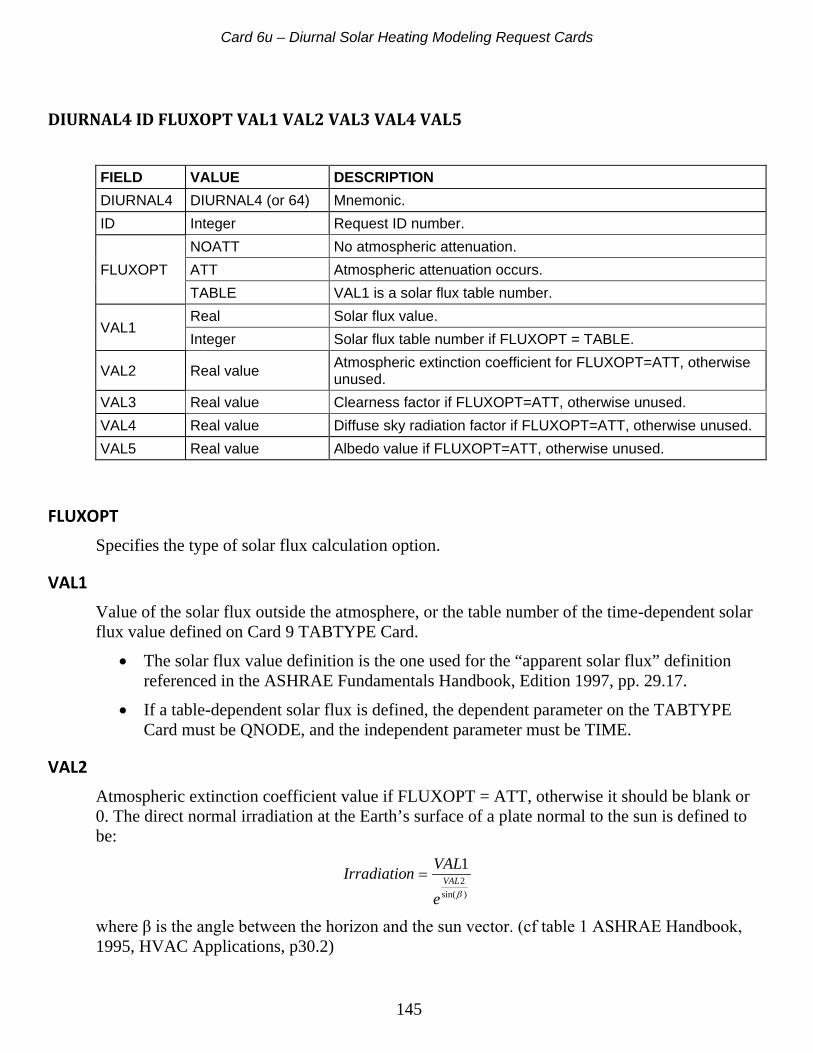
Card 6u – Diurnal Solar Heating Modeling Request Cards
145
DIURNAL4 ID FLUXOPT VAL1 VAL2 VAL3 VAL4 VAL5
FIELD VALUE DESCRIPTION DIURNAL4 DIURNAL4 (or 64) Mnemonic. ID Integer Request ID number.
FLUXOPT NOATT No atmospheric attenuation. ATT Atmospheric attenuation occurs. TABLE VAL1 is a solar flux table number.
VAL1 Real Solar flux value. Integer Solar flux table number if FLUXOPT = TABLE.
VAL2 Real value Atmospheric extinction coefficient for FLUXOPT=ATT, otherwise unused.
VAL3 Real value Clearness factor if FLUXOPT=ATT, otherwise unused. VAL4 Real value Diffuse sky radiation factor if FLUXOPT=ATT, otherwise unused. VAL5 Real value Albedo value if FLUXOPT=ATT, otherwise unused.
FLUXOPT Specifies the type of solar flux calculation option.
VAL1 Value of the solar flux outside the atmosphere, or the table number of the time-dependent solar flux value defined on Card 9 TABTYPE Card.
• The solar flux value definition is the one used for the “apparent solar flux” definition referenced in the ASHRAE Fundamentals Handbook, Edition 1997, pp. 29.17.
• If a table-dependent solar flux is defined, the dependent parameter on the TABTYPE Card must be QNODE, and the independent parameter must be TIME.
VAL2 Atmospheric extinction coefficient value if FLUXOPT = ATT, otherwise it should be blank or 0. The direct normal irradiation at the Earth’s surface of a plate normal to the sun is defined to be:
)sin(21
βVAL
e
VALnIrradiatio =
where β is the angle between the horizon and the sun vector. (cf table 1 ASHRAE Handbook, 1995, HVAC Applications, p30.2)

Card 6u – Diurnal Solar Heating Modeling Request Cards
146
VAL3 Clearness factor value if FLUXOPT = ATT, otherwise it should be blank or 0.
• The clearness factor is the ratio between the actual clear day direction radiation intensity at a specific location, and the intensity calculated for the standard atmosphere at the same location and date. (Ref: ASHRAE Handbook, 1995, HVAC Applications, pp. 30.5). Clearness values > 1 indicate a very dry and clear sky (e.g. at high altitudes) - and, conversely, very hazy and humid conditions if the value is < 1.
VAL4 Diffuse sky radiation factor if FLUXOPT = ATT, otherwise it should be blank or 0.
• This is the ratio of the diffuse solar flux originating from the sky incident upon a horizontal plate to the direct attenuated solar flux incident upon a plate normal to the sun vector. (cf table 1 ASHRAE Handbook, 1995, HVAC Applications, p30.2)
VAL5 Albedo value if FLUXOPT = ATT, otherwise, it should be blank or 0.
• Albedo is the fraction of the solar radiation reflected from the nearby ground.
Examples: DIURNAL4 3 ATT 1100.0 .15 .7 .16 .35 DIURNAL4 3 NOATT 1100.0 DIURNAL4 3 TABLE 10
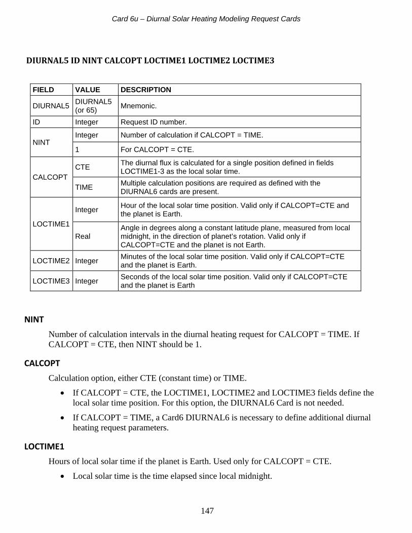
Card 6u – Diurnal Solar Heating Modeling Request Cards
147
DIURNAL5 ID NINT CALCOPT LOCTIME1 LOCTIME2 LOCTIME3
FIELD VALUE DESCRIPTION
DIURNAL5 DIURNAL5 (or 65) Mnemonic.
ID Integer Request ID number.
NINT Integer Number of calculation if CALCOPT = TIME.
1 For CALCOPT = CTE.
CALCOPT CTE The diurnal flux is calculated for a single position defined in fields
LOCTIME1-3 as the local solar time.
TIME Multiple calculation positions are required as defined with the DIURNAL6 cards are present.
LOCTIME1
Integer Hour of the local solar time position. Valid only if CALCOPT=CTE and the planet is Earth.
Real Angle in degrees along a constant latitude plane, measured from local midnight, in the direction of planet’s rotation. Valid only if CALCOPT=CTE and the planet is not Earth.
LOCTIME2 Integer Minutes of the local solar time position. Valid only if CALCOPT=CTE and the planet is Earth.
LOCTIME3 Integer Seconds of the local solar time position. Valid only if CALCOPT=CTE and the planet is Earth
NINT Number of calculation intervals in the diurnal heating request for CALCOPT = TIME. If CALCOPT = CTE, then NINT should be 1.
CALCOPT Calculation option, either CTE (constant time) or TIME.
• If CALCOPT = CTE, the LOCTIME1, LOCTIME2 and LOCTIME3 fields define the local solar time position. For this option, the DIURNAL6 Card is not needed.
• If CALCOPT = TIME, a Card6 DIURNAL6 is necessary to define additional diurnal heating request parameters.
LOCTIME1 Hours of local solar time if the planet is Earth. Used only for CALCOPT = CTE.
• Local solar time is the time elapsed since local midnight.

Card 6u – Diurnal Solar Heating Modeling Request Cards
148
• If the planet is not Earth, LOCTIME is the angular position in degrees measured from local midnight in the direction of the planet's rotation at constant latitude. Used only for CALCOPT = CTE option.
LOCTIME2 Minutes of the local solar time if the planet is Earth. Used only for CALCOPT = CTE.
LOCTIME3 Seconds of the local solar time if the planet is Earth. Used only for CALCOPT = CTE.
Examples: DIURNAL5 3 1 CTE 11 23 45 DIURNAL5 3 12 TIME

Card 6u – Diurnal Solar Heating Modeling Request Cards
149
DIURNAL6 ID STARTOPT FINALOPT TIMEVAL SV1 SV2 SV3 FV1 FV2
FIELD VALUE DESCRIPTION DIURNAL6 DIURNAL6 (or 66) Mnemonic. ID Integer Request ID number.
STARTOPT
LSTIME Fields SV1-3 define the start of the diurnal heating request.
SUNRISE The diurnal start position is at sunrise.
ANGLE The diurnal start position is at SV1 degrees from local midnight.
Blank A complete day is simulated and all subsequent fields must be blank.
FINALOPT
LSTIME Fields FV1-3 define the final position of the diurnal heating request.
SUNSET The diurnal heating end position is at sunset.
ANGLE The diurnal heating end position is at FV1 degrees from local midnight.
TIMEVAL Real Time value at the diurnal heating start position.
SV1 Integer Hour value of the local solar time at start of diurnal
heating request. STARTOPT = LSTIME only.
Real Start position in degrees from local midnight. STARTOPT = ANGLE only.
SV2 Integer Minute value of the local solar time at the start position. STARTOPT = LSTIME only.
SV3 Integer Second value of the local solar time at start position. STARTOPT = LSTIME only.
FV1 Integer Hour value of the local solar time at the end position. FINALOPT = LSTIME only.
Real End position in degrees from local midnight. FINALOPT = ANGLE only.
FV2 Integer Minute value of the local solar time at the end position. FINALOPT = LSTIME only.
FV3 Integer Second value of the local solar time at the position. FINALOPT = LSTIME only.

Card 6u – Diurnal Solar Heating Modeling Request Cards
150
STARTOPT Specifies whether the starting position of the diurnal heating request is defined in terms of local solar time, at sunrise, or in degrees from local midnight.
• If STARTOPT = LSTIME, then the fields SV1-SV3 define the starting position of the diurnal heating request in terms of local solar time.
• If STARTOP = SUNRISE, the start position is at the sunrise.
• If STARTOPT = ANGLE, then SV1 is the angle in degrees from local midnight to the start position. This angle is measured in the direction of the planet's rotation at constant latitude.
• If a complete day is simulated, then this field and the rest of the fields should be blank.
FINALOPT Specifies whether the final position of the diurnal heating request is defined in terms of local solar time, at sunset, or in degrees from local midnight.
• If FINALOPT = LSTIME, then the fields FV1-FV3 define the final position of the diurnal heating request in terms of local solar time.
• If FINALOPT = SUNSET, the diurnal heating request ends at sunset.
• If FINALOPT = ANGLE, then FV1 is the angle in degrees from local midnight to the end position of the diurnal heating request. This angle is positive when measured in the direction of the planet's rotation at constant latitude.
TIMEVAL Time value at the start position.
SV1
• If STARTOPT = LSTIME, then SV1 is the hour value of the local solar time at the start position.
• If STARTOPT = ANGLE, then SV1 is the angle in degrees from local midnight to the starting position. This angle is positive when measured in the direction of the planet's rotation at constant latitude.
SV2 Minute value of local solar time at the start position for STARTOPT = LSTIME. Otherwise, it should be zero or blank.
SV3 Seconds value of local solar time at the start position for STARTOPT = LSTIME. Otherwise, it should be zero or blank.

Card 6u – Diurnal Solar Heating Modeling Request Cards
151
FV1
• If FINALOPT = LSTIME, then FV1 is the hours value of the local solar time at the end position.
• If FINALOPT = ANGLE, then FV1 is the angle in degrees from local midnight to the end of the diurnal heating request. This angle is positive when measured in the direction of the planet's rotation at constant latitude.
FV2 Minutes value of local solar time at the end position for STARTOPT = LSTIME. Otherwise, it should be zero or blank.
FV3 Seconds value of local solar time at the end position for STARTOPT = LSTIME. Otherwise, it should be zero or blank.
Examples: $ For FULL DAY: DIURNAL6 3 $ For PARTIAL DAY: DIURNAL6 3 LSTIME LSTIME 0.0 0 0 0 12 0 0 DIURNAL6 3 LSTIME SUNSET 3600.0 1 0 0 DIURNAL6 3 LSTIME ANGLE 0.0 1 0 0 45.0 DIURNAL6 3 SUNRISE LSTIME 0.0 0 0 0 12 0 0 DIURNAL6 3 SUNRISE SUNSET 0.0 DIURNAL6 3 SUNRISE ANGLE 0.0 0 0 0 90.0 DIURNAL6 3 ANGLE LSTIME 0.0 30.0 0 0 12 0 0 DIURNAL6 3 ANGLE SUNSET 0.0 0.0 DIURNAL6 3 ANGLE ANGLE 0.0 10.0 0

Card 6v - Hemicube View Factor Method Activation Card
152
Card 6v - Hemicube View Factor Method Activation Card - Optional This Card toggles the use of the hemicube method to calculate view factor requests. If toggled ON, the HEMIVIEW module calculates view factor requests which follow this Card. If toggled OFF, view factors are calculated using the VUFAC module. To use the HEMIVIEW module, you must have a graphics card and operating system which supports the OpenGL graphics library, and you must have an active graphics display. During activation of the HEMIVIEW module, a small graphics window will appear which on your display, which is used to calculate the view factors.
L, TOGGLE, WINSIZE, OPTION
L = HEMI (or 35)
TOGGLE = ON (or 4)
all following VFS12, VFSALL, VFS1ALL, VFSENC Cards will be processed using the HEMIVIEW module.
= OFF (or 5) all following VFS12, VFSALL, VFS1ALL, VFSENC Cards will be processed using the VUFAC module
WINSIZE is the window size in pixels along each side of the square graphics window used by the hemicube method. More pixels yield greater accuracy, but result in increased computation time. The default and recommended value is 128.
OPTION specifies the hemicube/analytical method hybrid option. Currently, only OPTION=1 is supported. =1 performs only pure hemicube calculations

Card 6w – Monte Carlo Method Activation Card
153
Card 6w – Monte Carlo Method Activation Card - Optional This card toggles the use of the Monte Carlo method to calculate view factor requests, radiative heating requests, orbital heating, and diurnal heating requests. If toggled ON, the VUFAC module uses the Monte Carlo method to calculate view factor requests, radiative heating requests, orbital heating and diurnal heating requests which follow this Card. If toggled OFF, these view factors are calculated using the deterministic subdivision method. The Monte Carlo method can calculate view factors, orbital view factors, heat flux view factors, radiative couplings, or heat loads. It does so by sampling rays in random directions and following the ray paths to their termination.
L, TOGGLE, NRAYS, RAY_OPTION, VFTYPE, SEED, ERR, CL
L = MONTECARLO
TOGGLE = ON
all following Card 6 VFS12, VFSALL, VFS1ALL, VFSENC, SOURCExxx, DIURNALx, ORBIT, ORBDEFx, EARTHx, and SOLxxx cards will be processed by the VUFAC module using the Monte Carlo method.
= OFF all following cards will be processed with the VUFAC module using the standard deterministic subdivision method. The Monte Carlo method will not be active until it is toggled back on again.
NRAYS = number of rays to be launched.
Depending on the RAY_OPTION flag, the number of rays to be launched to or from an element will be either NRAYS (absolute) or NRAYS per unit area. For view factor requests and radiative source requests, NRAYS specifies the number of rays launched from each element. For environmental heating requests (solar, earth, orbit, or diurnal heating requests), NRAYS specifies the number of rays launched to each element.
RAY_OPTION =AREA
NRAYS rays per unit area are launched from or (in the case of environmental heating requests) to the element.
=ABSOLUTE

Card 6w – Monte Carlo Method Activation Card
154
NRAYS rays are launched per element. =ERROR
The ray density control is based on error criterion, i.e. more rays are launched until the specified error criterion ERR is satisfied to within a confidence level CL percentage.
VFTYPE =VF
View factors will be computed with the Monte Carlo method. This includes blackbody view factors, ray-traced view factors, heat flux view factors, earth, albedo, and solar view factors, provided those requests follow this card.
=HTFRAD Radiative couplings and heat loads will be computed with the Monte Carlo method. View factor requests result in the direct computation of radiative couplings. Heat flux view factor requests and environmental heating requests result in the direct computation of radiative heat loads.
SEED This value sets the pseudo-random number generator seed for the following Monte Carlo request. The seed is the first in number in a unique sequence of pseudo-random numbers, so re-using the same seed will yield identical results between runs (assuming identical TMG versions are run). The seed can be modified to study convergence of the Monte Carlo results. If the seed value is not entered, a default of zero is used.
ERR If RAY_OPTION = ERROR, then ERR is the error criterion value.
CL If RAY_OPTION = ERROR, then CL is the confidence level value expressed in percentage.
Notes:
• When the Monte Carlo option is active, ray tracing is automatically performed to all specular, diffuse, and transparent elements.
• When VFTYPE=HTFRAD, and view factors are requested with Card 6a VF type Cards, then radiative couplings are computed directly from the Monte Carlo ray tracing technique by the VUFAC module. This results in a radiative conductance matrix similar to that generated by using Gebhardt’s method from view factor data.
• When VFTYPE=HTFRAD, and heat flux view factors are requested with SOURCE or ORB type Cards, radiative heat loads are computed directly from the Monte Carlo ray tracing technique by the VUFAC module, and written as HTF cards into MODLF.
Card 6w – Monte Carlo Method Activation Card
155
• It is possible to mix methods, e.g. to compute radiative couplings of some radiative enclosures with the HTFRAD option, and then to the Monte Carlo method OFF, and to compute black body view factors for other enclosures. If you have selected the Oppenheim method, TMG will automatically use the Oppenheim method only for the enclosures for which black body view factors have been calculated.
• The default maximum number of rays cast per element is 20,000. This can be modified with the advanced Card 9 option GPARAM 4 305 NMAX.
• The Monte Carlo method makes use of a pseudo-random number generator. To modify the seed value for the random number generator, use the advanced option GPARAM 4 294 N.
Example: The following is a TMG model with two different enclosure type view factor requests: $ $ 1 – BUS_ENCLOSURE $ MONTECARLO ON 10000 ABSOLUTE VF VFSENC BUS_ENC 0 MONTECARLO OFF $ $ 2 – MIDDLE_ENCLOSURE $ MESH ERROR 9.000000E-01 VFSENC MIDDLE_ 0 $
The first TMG radiation request is an enclosure request which computes black body view factors between the elements in group “BUS_ENC”. It computes the black body view factors using the Monte Carlo ray tracing method, by casting 10,000 rays randomly from each element in the enclosure. The second TMG radiation request is an enclosure request which computes black body view factors between the elements of group “MIDDLE_”. It does not use the Monte Carlo method, rather, TMG’s standard deterministic subdivision method is used.

Card 6v - Hemicube View Factor Method Activation Card
156
Card 6x – Thermal Coupling Rotational Periodicity Card - Optional This Card specifies that thermal couplings should be rotationally periodic. This means that an average angle is computed between the primary and secondary group of the thermal coupling, about the specified axis of rotation. The secondary group is rotated back by that angle before thermal couplings are calculated.
L, TOGGLE, XO, YO, ZO, XDIR, YDIR, ZDIR
L = ROTATE (or 67)
TOGGLE = ON (or 4)
all subsequent thermal couplings will be treated as rotationally periodic. = OFF (or 5)
all subsequent thermal couplings will be treated normally.
XO, YO, ZO specifies the start location of the axis vector.
XDIR, YDIR, ZDIR specifies the direction of the axis vector.
Card 6x Example: $ GROUP2 is to be rotated about the z axis by the average angle between GROUP1 and $ GROUP2 before the thermal coupling is calculated. ROTATE ON 0.0 0.0 0.0 0.0 0.0 1.0 AREA GROUP1 0 0 GROUP2 0 1.000000E+02 NEARA ROTATE OFF

Card 7 – Element Merging and Renumbering Cards
157
Card 7 – Element Merging and Renumbering Cards M, NN2, NN3, NN4,... Option 1 element list maximum 13 elements per Card
NAME1, NAME2 Option 2 maximum 2 group names
NAME1 Option 3 single group name
NM, NAME2 Option 4 element + group name
NAME1, NN2 Option 5 group name + element
GENER, N1S, INC1, N1N, INC2, N2N Option 6 element generation Element merging/renumbering by the MEREL module consists of assigning one or more elements the element number of the starting element and automatically combining their conductances, capacitances, and heat loads. The resulting temperature will be the average of the merged elements. Element merging should be used only if the elements are closely coupled, or are expected to have similar temperatures. Element merging can reduce solution time by reducing the size of the model, and by eliminating high conductances that cause ill–conditioning.
Notes: • For Option 1 elements NN2, NN3, NN4,.. are merged into element NM. • For Options 2, NAME1 and NAME2 are group names and NM and NN2 are element
numbers. NAME1 may not start with the letter C. • For Options 2, 3, and 5 the elements of NAME1 and NAME2 are merged with the starting
element of NAME1. For NX users, this is the element with the lowest element number. For non–NX users, the starting element is the first element defined on the Card 9 group name NAME Card.
• For Option 4 all the elements are merged into element NM. • Option 5 generates N2N Option 1 format Cards, each with N1N elements:
$ N1S, N1S+INC1,....N1S+(N1N–1)INC1 N1S+INC2, N1S+INC2+INC1,...N1S+INC2+(N1N–1)INC1 N1S+(N2N–1)INC2,N1S+INC1+(N2N–1)INC2,..N1S+(N1N–1)INC1+(N2N–1)INC2 $
INC1 is the element number increment between the elements on the same line (between elements to be merged). N1N is the number of elements in each line (maximum 13).

Card 7 – Element Merging and Renumbering Cards
158
INC2 is the element number increment between the generated Cards (increment between elements to be merged to). N2N is the number of Cards generated.
• Elements may be merged to the nearest physical element with Card 6e NEARM option. • Elements connected with a conductance value > 1.0E10 are automatically merged. • The elements created by the Card 5d Space Element Card, and the reverse elements created
with the Card 9 REVNODE Card are automatically merged. • The temperatures of the merged elements are recovered by the automatic creation of
follower conductances. During the Analyzer run, the merged elements become SINK elements. This option may be disabled with the Card 9 PARAM NOMRECOV Card.
• Hydraulic elements and Card 9 MCV elements may not be merged into other elements. However, other elements may be merged into them.
• If elements with temperature-dependent specific heats or capacitances are merged, it is important to ensure that they all reference the same specific heat table.
Card 7 Examples: 10, 4, 5 $ ELEMENTS 4 AND 5 MERGED INTO ELEMENT 10 GENER, 201, 1, 3, 10, 3 $ ELEMENTS 202 AND 203 MERGED INTO 201 $ ELEMENTS 212 AND 213 MERGED INTO 211 $ ELEMENTS 222 AND 223 MERGED INTO 221 BOX1,BOX2 $ ELEMS ASSOCIATED WITH CARD 9 NAMES BOX1 $ AND BOX2 ARE MERGED INTO THE STARTING $ ELEMENT OF BOX1

Card 8 - Element Elimination Cards
159
Card 8 – Element Elimination Cards – Optional NE1, NE2, ... Option 1 - list of elements
NAME1 Option 2 - group name
GENER, N1S, INC1, N1N, INC2, N2N Option 3 - element generation
Element elimination by the MEREL module consists of the creation through substructuring a smaller but equivalent conductance–capacitance thermal model. For further details, please see Card 9 PARAM SUBSTR.
Notes: • Option 1 eliminates the elements NE1, NE2, ... from the model. The
maximum number of elements per Card is 13. • Option 2 eliminates elements of NAME1. NAME1 may not start with
the letter C. • Option 3 generates N2N Element Elimination Cards, each containing
N1N elements. The format is identical to the one described on Card 7.
Card 8 Example: 1,5,8,10 $ ELEMENTS 1,5,8, AND 10 ARE ELIMINATED FROM THE MODEL.

Card 9 - ALIGN Align Vector Definition
161
Card 9 - ALIGN Align Vector Definition - Optional KODE, N1, T1, T2, T3
KODE KODE = ALIGN(or 62)
N1 is a joint number (N1 from a Card 9 JOINT Card).
T1 is the orbit dependent direction defined on a Card 6t ORBDEF1 Card (NADIR, SUN, STAR, PVEL, PNORMAL, NORTH or SOUTH) which vector T2 is aligned with.
T2 T2 is a vector number (N1 from Card 9 VECTOR Card).
T3 T3 may be:
ALL for all defined orbit and modeling requests, or an ID number from an ORBDEF Card for single orbit and attitude modeling requests.
Notes: The ALIGN option minimizes the angle between the align vector and the vector to the object being pointed to, while respecting the constraints of the rotational joint. It requires Card 9 ARTICUT, JOINT, VECTOR and Card 6 orbit definition Cards to be present in INPF. An orbit is defined with either Card 6t ORBDEF cards, or Card 6b SOL card and Card 6d EARTH card.
Example: $ ALIGN VECTOR 2 WITH NORTH FOR ALL ORBITS JOINT 1 REVOLUT 0 1 VECTOR 1 0 0 0 -1 0 0 VECTOR 2 0 0 0 0 1 0 ARTICUT 1 SHELLS ALIGN 1 NORTH 2 ALL

Card 9 – ARPARAM Articulation Parameters
162
Card 9 - ARPARAM Articulation Parameters - Optional KODE, N1, T1, T2, T3
KODE KODE = ARPARAM (or 51)
N1 is the parameter type. It can only be TIME.
T1 is the starting time of the articulation movement.
T2 is the ending time of the articulation movement.
T3 is the interval of time when calculations of time-dependent view factors and radiative conductances are to be calculated for analysis.
Notes: When an ORBIT card is present in the input file, the articulation parameter card is not considered. The start time, end time and time interval are superseded by the values in the ORBIT card.
Example: ARPARAM TIME 0 10 0.5 $ ARTICULATION STARTS AT TIME 0, AND ENDS AT TIME 10. $ TIME DEPENDENT RADIATIVE CONDUCTANCES $ ARE CALCULATED AT EVERY HALF SECOND

Card 9 – ARRAYTYPE Array Variable Definition Card
163
Card 9 - ARRAYTYPE Array Variable Definition Card - Optional KODE, N1, T1, T2, T3
KODE KODE=ARRAYTYPE (or 53)
N1 N1 is the array number. An array cannot have the same number as a table in the model.
T1 T1 is the code for the first independent variable (X)
T2 T2 is the code for the second independent variable (Y)
T3 T3 is the code for the dependent variable (Z)
Mnemonic Code
Equiv. Num. Code Description of the Code
Dep. or Ind. Var.
ABSORPTIVITY 45 Solar absorptivity Dep. ANG_INC 120 Angle of incidence of a ray Ind. ANG_REF 122 Angle of reflection of ray Ind. BRDF 46 Value of the bidirectional reflectance distribution function at
ANG_INC and ANG_REF. Note that the BRDF array must be fully populated. BRDF are used only in conjunction with the Monte Carlo HTFRAD ray tracing option. Input BRDF data is normalized by TMG so that the integral of the probability density over all angles equals one.
Dep.
CAP 3 CAP is the capacitance of a single element. Dep. COND 1 COND is the current conductance value (linearized if non-
linear) if it is used as the independent variable. COND is a conductance multiplier when it is used as the dependent variable. The original conductance value is multiplied by the value interpolated from the table.
Dep.
CPP 2015 CPP is the specific heat at constant pressure at the element. The independent variable must be TEMP or TIME and referenced from a MAT Card.
Dep.
CURRENT 30 CURRENT is a current boundary condition specified for an electrical resistance element.
Dep.
DIR_INC 121 Direction of incidence of a ray Ind.

Card 9 – ARRAYTYPE Array Variable Definition Card
164
Mnemonic Code
Equiv. Num. Code Description of the Code
Dep. or Ind. Var.
ABSORPTIVITY 45 Solar absorptivity Dep. DELTAPT 2003 DELTAPT is the total pressure rise if it is referenced as
dependent variable from a PROP FANPUMP Card. DELTAPT is positive if there is a total pressure rise over the element, and it describes a flow boundary condition. DELTAPT is the total pressure drop if it is referenced from a PROP DUCT or PROP FLOWRES Card as the independent variable, positive if there is a total pressure drop over the element.
Dep.
E 18 E is the emissivity of an element. The independent variable code must be TEMP or TIME. Should be referenced from a MAT Card.
Dep.
ELECRES 31 ELECRES is the electrical resistivity specified for an electrical resistance element.
Dep.
FLOWRES 2002 FLOWRES is the hydraulic flow resistance multiplier referenced by a PROP FLOWRES or PROP DUCT Card.
Dep.
KTHERM 2017 KTHERM is the thermal conductivity of an element. The independent variable element must be the same as the dependent variable element. Should be referenced from a MAT Card.
Dep.
MASSFL 2005 MASSFL is the mass flow through a 2-node hydraulic element. If referenced from a FANPUMP or STREAM element, it must be the dependent variable and is then a flow boundary condition. If referenced from a PROP DUCT or PROP FLOWRES Card, it must be the independent variable. It is considered positive in the reference forward direction of the element.
Dep.
MULTIPLIER 84 MULTIPLIER is a multiplier value interpolated from the array. Dep. PTOTAL 2008 PTOTAL is the total pressure at a hydraulic element.
If it is the dependent variable, it must be referenced by a PSINK element, and is considered to be a boundary condition.
Dep. Ind.
QNODE 4 QNODE is the heat load into an element. If it is the independent variable, it is considered to be the total heat load into the element. If it is the dependent variable, it is summed with all other heat loads into the element, and is a boundary condition.
Dep.
RHOAMB 2012 RHOAMB is the density of the ambient fluid. Dep. RHO 2018 RHO is the density of a fluid in a hydraulic network. If RHO is
the dependent variable, it must be flagged as LIQUID on a MAT2 card.
Dep.
SPECULAR 83 Solar specular reflectivity of a surface Dep.

Card 9 – ARRAYTYPE Array Variable Definition Card
165
Mnemonic Code
Equiv. Num. Code Description of the Code
Dep. or Ind. Var.
ABSORPTIVITY 45 Solar absorptivity Dep. TEMP 2 TEMP is the temperature of an element.
If used as the dependent variable, the element must be a SINK or an AMBIENT element. If used as the independent variable, and the dependent variable is a conductance, the average temperatures of the two ends of the conductance are used as the independent variable.
Both
TIME 0 TIME is the time value during a transient run. TIME is considered to be periodic, with a period equal to the (largest-smallest) time value in the table.
Ind.
TPHASE 40 • Tphase is the phase change temperature of an element. Dep. TPRIME 101 • TPRIME is the temperature value of the first element of the
conductance. • If a Card 6e thermal coupling references a table whose
independent variable is TPRIME, the independent variable will be the temperature of the N1 (primary) element
Ind.
TRANSMISS 82 Solar transmissivity of a surface Dep. USER1ARR USER2ARR ... USER9ARR
91-99 USER1ARR…USER9ARR are codes for table interpolation to be used with the CALL USERARRAY routine in a Card 10 user-written subroutine.
Ind.
VELOC 2007 VELOC is the flow velocity through the hydraulic element. If referenced from a PROP FANPUMP Card it must be the dependent variable and is a flow boundary condition.
Dep.
VISC 2016 VISC is fluid viscosity. The independent variable code must be TEMP or TIME. It should be referenced from a MAT Card.
Dep.
VOLTAGE 29 VOLTAGE is voltage boundary conditions specified for an electrical resistance element.
Dep.
VOLUME 2004 VOLUME is volume flow through the hydraulic element. If referenced from a PROP FANPUMP Card, it must be the dependent variable and is a flow boundary condition. If referenced from a PROP DUCT or PROP FLOWRES Card, it must be the independent variable. It is considered positive in the referenced forward direction of the 2-node element.
Dep.
WAVELENGTH 116 WAVELENGTH is the wavelength value at which the spectrum-dependent dependent variable is defined. WAVELENGTH must be defined in microns μ, where 1 μ=1.E-8m.
Both
WAVELENGTHNUMBER
116 WAVELENGTHNUMBER is an integer (1,2,3..) used as the independent variable to define a wavelength-dependent spectrum. The dependent variable must be WAVELENGTH or TEMP.
Ind.
Notes: • This card describes the nature of the dependent and independent variables for array N1
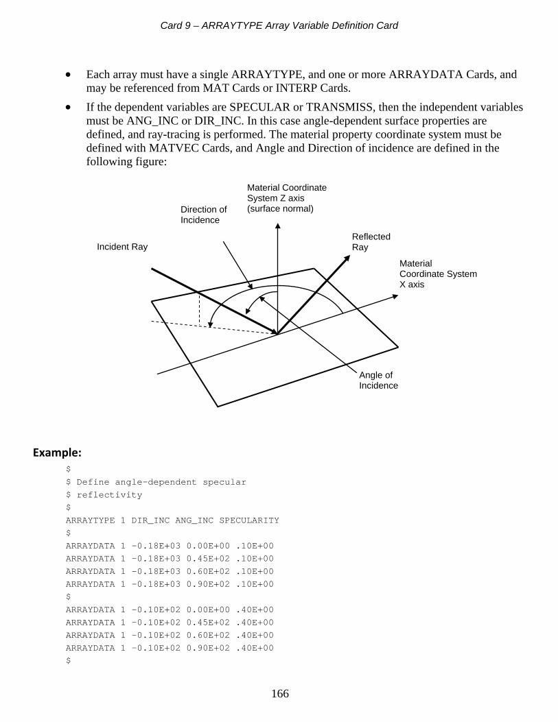
Card 9 – ARRAYTYPE Array Variable Definition Card
166
• Each array must have a single ARRAYTYPE, and one or more ARRAYDATA Cards, and may be referenced from MAT Cards or INTERP Cards.
• If the dependent variables are SPECULAR or TRANSMISS, then the independent variables must be ANG_INC or DIR_INC. In this case angle-dependent surface properties are defined, and ray-tracing is performed. The material property coordinate system must be defined with MATVEC Cards, and Angle and Direction of incidence are defined in the following figure:
Example: $ $ Define angle-dependent specular $ reflectivity $ ARRAYTYPE 1 DIR_INC ANG_INC SPECULARITY $ ARRAYDATA 1 -0.18E+03 0.00E+00 .10E+00 ARRAYDATA 1 -0.18E+03 0.45E+02 .10E+00 ARRAYDATA 1 -0.18E+03 0.60E+02 .10E+00 ARRAYDATA 1 -0.18E+03 0.90E+02 .10E+00 $ ARRAYDATA 1 -0.10E+02 0.00E+00 .40E+00 ARRAYDATA 1 -0.10E+02 0.45E+02 .40E+00 ARRAYDATA 1 -0.10E+02 0.60E+02 .40E+00 ARRAYDATA 1 -0.10E+02 0.90E+02 .40E+00 $
Material Coordinate System Z axis (surface normal)
Reflected Ray Incident Ray
Angle of Incidence
Direction of Incidence
Material Coordinate System X axis
Card 9 – ARRAYTYPE Array Variable Definition Card
167
ARRAYDATA 1 0.00E+00 0.00E+00 .50E+00 ARRAYDATA 1 0.00E+00 0.45E+02 .50E+00 ARRAYDATA 1 0.00E+00 0.60E+02 .50E+00 ARRAYDATA 1 0.00E+00 0.90E+02 .50E+00 $ ARRAYDATA 1 0.10E+02 0.00E+00 .60E+00 ARRAYDATA 1 0.10E+02 0.45E+02 .60E+00 ARRAYDATA 1 0.10E+02 0.60E+02 .60E+00 ARRAYDATA 1 0.10E+02 0.90E+02 .60E+00 $ ARRAYDATA 1 0.18E+03 0.00E+00 .90E+00 ARRAYDATA 1 0.18E+03 0.45E+02 .90E+00 ARRAYDATA 1 0.18E+03 0.60E+02 .90E+00 ARRAYDATA 1 0.18E+03 0.90E+02 .90E+00 $ $ Bidirectional reflectivity example $ ARRAYTYPE 2 ANG_INC ANG_REF BRDF ARRAYDATA 2 0.0 0.0 0.8 ARRAYDATA 2 0.0 44.9 0.8 ARRAYDATA 2 0.0 45.0 0.0 ARRAYDATA 2 0.0 90.0 0.0 $ ARRAYDATA 2 44.9 0.0 0.8 ARRAYDATA 2 44.9 44.9 0.8 ARRAYDATA 2 44.9 45.0 0.0 ARRAYDATA 2 44.9 90.0 0.0 $ ARRAYDATA 2 45.0 0.0 0.0 ARRAYDATA 2 45.0 44.9 0.0 ARRAYDATA 2 45.0 45.0 0.8 ARRAYDATA 2 45.0 90.0 0.8 $ ARRAYDATA 2 90.0 0.0 0.0 ARRAYDATA 2 90.0 44.9 0.0 ARRAYDATA 2 90.0 45.0 0.8 ARRAYDATA 2 90.0 90.0 0.8

Card 9 – ARRAYDATA Array Variable Definition Card
168
Card 9 - ARRAYDATA Array Variable Definition Card - Optional KODE, N1, T1, T2, T3
KODE KODE=ARRAYDATA (or 54 )
N1 N1 is the array number. An array cannot have the same number as a table in the model.
T1 T1 is the value for the first independent variable (X)
T2 T2 is the value for the second independent variable (Y)
T3 T3 is the value for the dependent variable (Z)
Notes: • This card defines the data points for array N1 for linear interpolation. • The data must represent a fully populated table, that is if there are n X values and m Y
values in the data there must be (m x n) ARRAYDATA Cards, for every X value there must be m Y values etc.
• Each array must have a single ARRAYTYPE, and one or more ARRAYDATA Cards, and may be referenced from MAT Cards or INTERP Cards.
• When data is required outside of the user supplied range the appropriate extreme data point(s) are used. No extrapolation occurs.
• If the dependent variable is angle of incidence then the dependent variable must lie in the range 0 through 90.
• If the dependent variable is direction of incidence then the dependent variable must lie in the range-180 through +180. Data outside of this range will be mapped into it.

Card 9 – ARTICUT Articulation Definition
169
Card 9 - ARTICUT Articulation Definition - Optional KODE, N1, T1, T2, T3
KODE KODE = ARTICUT (or 49)
N1 N1 is the joint number.
T1 T1 is a group name containing the articulating elements.
T2 T2 is the speed of rotation or translation. If the speed is table-dependent, T2 should be the mnemonic Tn (or the negative number -n), where n is the table number referencing TABTYPE and TABDATA Cards.
T3 T3 is a table multiplier (if T2 is a table), otherwise it is ignored. If T2 is not a table, T3 may be blank.
Notes: The articulation definition is used with a joint definition card 9 JOINT. The joint number of the articulation card is associated with the same joint number of the joint definition card. The group of elements refers to the elements of that joint only and not to the child joints. Refer to joint definition card 9 JOINT.
Example: ARTICUT 20 ARTICGRP 5. JOINT 20 REVOLUTE 0 10 VECTOR 10 0. 0. 0. 0. 0. 1. $ ELEMENTS IN GROUP ARTICGRP ROTATE AT A SPEED OF 5. DEGREES $ PER SECOND ABOUT VECTOR NUMBER 10
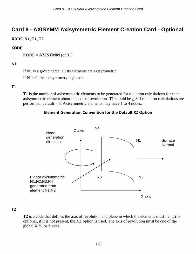
Card 9 – AXISYMM Axisymmetric Element Creation Card
170
Card 9 - AXISYMM Axisymmetric Element Creation Card - Optional KODE, N1, T1, T2
KODE KODE = AXISYMM (or 31)
N1 If N1 is a group name, all its elements are axisymmetric. If N1= 0, the axisymmetry is global.
T1 T1 is the number of axisymmetric elements to be generated for radiation calculations for each axisymmetric element about the axis of revolution. T1 should be > 8 if radiation calculations are performed, default = 8. Axisymmetric elements may have 1 to 4 nodes.
Element Generation Convention for the Default XZ Option
T2 T2 is a code that defines the axis of revolution and plane in which the elements must lie. T2 is optional, if it is not present, the XZ option is used. The axis of revolution must be one of the global X,Y, or Z axes.
Surface Normal
X axis
Planar axisymmetric N1,N2,N3,N4 generated from element N1,N2
Node generation direction N1
N4
N3 N2
Z axis

Card 9 – AXISYMM Axisymmetric Element Creation Card
171
= XZ, then the elements must be defined on the +X side of the XZ plane, and the rotation will be counterclockwise about the Z axis. This is the default. = YZ, then the elements must be defined on the +Y side of the YZ plane, and the rotation will be counterclockwise about the Z axis. = XY, then the elements must be defined on the +X side of the XY plane, and the rotation will be counterclockwise about the Y axis. = ZY, then the elements must be defined on the +Z side of the ZY plane, and the rotation will be counterclockwise about the Y axis. = YX, then the elements must be defined on the +Y side of the YX plane, and the rotation will be counterclockwise about the X axis. = ZX, then the elements must be defined on the +Z side of the ZX plane, and the rotation will be counterclockwise about the X axis. = X, then the elements and the X axis must lie on the same plane, and the rotation will be counterclockwise about the X axis. = Y, then the elements and the Y axis must lie on the same plane, and the rotation will be counterclockwise about the Y axis. = Z, then the elements and the Z axis must lie on the same plane, and the rotation will be counterclockwise about the Z axis.
Notes: 1. Internal Element Generation for Radiation Calculations
• For radiation calculations each 1- and 2-node axisymmetric element with an emissivity ≥ 0 generates T1 internal shell and beam elements in the counterclockwise direction about the axis of revolution. The first generated element is assigned the axisymmetric element number, the others are assigned unused element numbers reported on file REPF. A 1-node axisymmetric element generates T1 beam elements, a 2-node axisymmetric element generates T1 shell elements. The generated elements are merged with the axisymmetric element once the radiation parameters have been calculated.
• Hydraulic and 3 and 4-node elements are not expanded. • The Card 5d SPACE Card generates 3*T1 very large elements forming a closed
cylinder about the origin for radiation calculations. • The radiative surface properties of the axisymmetric elements are passed to the
generated elements. 2. Surface Normals of Axisymmetric Elements
Care should be taken with radiation calculations that the surface normals point in the correct directions.

Card 9 – AXISYMM Axisymmetric Element Creation Card
172
The direction of the surface normal of an expanded element is determined by the orientation of the nodes of its axisymmetric element with respect to the axis of revolution. This is done by first identifying the direction vector of the axisymmetric element, which is from node 1 to node 2. For NX users, this is readily identified with the element “first edge” switch. Next, the surface normal vector of the axisymmetric element is computed. This is the cross product (*) of the direction vector and the vector normal to the plane. For the default convention the plane normal is the Y-axis, hence the element surface normal will be the direction vector*Yaxis. The element surface normal lies in the XZ plane, and when it is revolved with the axisymmetric element it defines the orientations of the expanded element surface normals. Another way of visualizing the surface normal direction of the axisymmetric element is that if the direction vector of the axisymmetric element points in the same direction as the axis vector (i.e. their dot products are positive), and the axisymmetric element lies in the +XZ plane, the surface normal points inwards towards the axis. If their dot products are negative (as in diagram), the surface normal points away from the axis. If their dot products are zero, then if the direction vector points in the +X direction, the surface normal points in the +Z direction, if the direction vector points in the –X direction, the surface normal points in the –Z direction. If a 2-node axisymmetric shell elements lies on a solid, the surface normal of its front side will be automatically so oriented that it points out of the solid.
3. Physical Properties of Axisymmetric Elements Special considerations apply to the PROP Cards:
• For 1-node axisymmetric elements PROP BEAM should be specified. • For 2-node axisymmetric elements PROP SHELL should be specified. • For 3-4 node planar axisymmetric elements no PROP Card should be specified.
4. Additional Considerations
• Axisymmetric elements are both geometrically and thermally axisymmetric with respect to the axis of revolution, i.e. there can be no tangential thermal gradients.
• The model's symmetry is used to enhance the efficiency of the radiation calculations. Internally the Card 6 VFSALL/VFNALL Cards are replaced with equivalent VFS1ALL and VFN1ALL Cards. View factors are calculated only for the axisymmetric elements, the view factors for the expanded elements are generated from symmetry considerations. The view factors of the expanded elements are then merged.
• If view factor calculations are requested with VFS1ALL or VFN1ALL Cards, the results may be erroneous, unless a VFSALL request is also present.
• Circular elements may not be specified with XCIRC Cards for an axisymmetric model. • For conduction , capacitance, and Card 6e AREA Card calculations each axisymmetric
element is assumed to have the fully revolved shape about the axis of revolution.

Card 9 – AXISYMM Axisymmetric Element Creation Card
173
• Elements may be specified to be non-axisymmetric with the Card 9 PARAM NOAXISYM Card.
• If there is more than one AXISYMM card in the model, then the groups N1 must be exclusive.
• If N1 = 0, then all elements that are not part of other AXISYMM cards will be expanded according to the global AXISYMM card.
Example: AXISYMM 0 8 $ THE THERMAL MODEL IS GLOBALLY AXISYMMETRIC WITH $ RESPECT TO THE GLOBAL Z AXIS.

Card 9 – DESCRIP Character String Descriptor Cards
174
Card 9 - DESCRIP Character String Descriptor Cards - Optional KODE1, N1, T1
KODE2, N1, T2, T3, T4, T5, T6
KODE3, N1, T7, T8, T9, T10, T11, T12, T13
KODE1 = DESCRIP (or 36)
N1 is a descriptor number
T1 is a character string up to 40 characters long assigned to number N1. The string can be accessed from within Card 10 USERF and USER1 user-written subroutines with a CALL DESCRIP statement.
KODE2 = DESCAD1 (or 55)
T2, T3 T2, T3 are 8-character descriptor strings such as SINK or CONSTANT associated with the DESCRIP Card.
T4, T5, T6 T3, T4, T5 are all optional group names associated with the DESCRIP Card.
KODE3 = DESCAD2 (or 56)
T7, T8, T9, T10, T11, T12, T13 T7, T8, T9, T10, T11, T12, T13 are all optional constants associated with the DESCRIP Card.
Example: DESCRIP 46 BOISSY-NUEVO CORRELATION $ THE CHARACTER STRING "BOISSY-NUEVO $ CORRELATION" IS ASSIGNED THE DESCRIPTOR NUMBER 46.

Card 9 – EAREAED Area Proportional Edge Conductance
175
Card 9 - EAREAED Area Proportional Edge Conductance – Optional
KODE, N1, T1, T2, T3, T4, T5, T6, T7
KODE KODE = EAREAED (or 46)
N1 is an element number.
T1 is an edge number, as defined in the diagram associated with the FREEFACE Card. If the area proportional edge conductance is applied to a beam or axisymmetric shell, then T1 is ignored. If the area proportional edge conductance is applied to a shell or axisymmetric solid, then T1 is the edge number for which the conductance is applied.
T2 is 0.
T3 is the table number referencing TABTYPE and TABDATA Cards that define the temperature distribution of the reference temperature of the conductance.
T4 is 0.
T5 T5 is a length or area proportional nominal convective coefficient or a nominal emissivity for radiative coupling. For convective coupling, T5 is the nominal convective coefficient divided by the length of the edge of a beam or shell or the revolved area of the edge of an axisymmetric shell or an axisymmetric solid. For radiative coupling, T5 is the nominal emissivity of the beam, shell, axisymmetric shell or axisymmetric solid element.
T6 T6 is the code CONVASN for convective coupling or RADASN for radiative coupling.

Card 9 – EAREAED Area Proportional Edge Conductance
176
T7 T7 is the table number referencing TABTYPE and TABDATA cards that defines the variation of the convective coefficient for the CONVASN option or the variation of emissivity for the RADASN option. T7 is left blank for constant convective coefficient or constant emissivity.
Notes: When an EAREAED card is specified, a coupling is created from the element to a reference temperature described by table T3. This table can only be expressed as temperature versus time. For constant reference temperature, only one value must be specified in the table. For the CONVASN option, the convective coefficient is created by multiplying coefficient T5 by the length or area of the element and the interpolated value from table T7 if any. This table can only be expressed as conductance versus temperature. For the RADASN option, the reference emissivity specified by T5 is multiplied by the interpolated value from table T7 if any. This table can only be expressed as conductance versus temperature. When a convective or radiative coupling is created at an edge of a shell or an axisymmetric solid, a new beam or axisymmetric shell element is created and used to apply the coupling.
Examples: EAREAED 10 3 0 15 0 2.5 CONVASN TABTYPE 15 TEMP TIME TABDATA 15 20. 0. $ A CONVECTIVE COUPLING OF 2.5 PER UNIT LENGTH IS APPLIED BETWEEN EDGE 3 OF $ SHELL ELEMENT 10 AND A. CONSTANT REFERENCE TEMPERATURE OF 20. EAREAED 20 0 0 25 0 0.5 RADASN 30 TABTYPE 25 TEMP TIME TABDATA 25 0. 0. TABDATA 25 10. 1. TABTYPE 30 COND TEMP TABDATA 30 0.8 0. TABDATA 30 1.0 10. $ A RADIATIVE COUPLING OF NOMINAL EMISSIVITY OF 0.5 IS APPLIED TO BEAM ELEMENT 20. $ THE EMISSIVITY VARIES FROM 0.8 TO 1.0 AND IS MULTIPLIED BY THE NOMINAL VALUE. $ THE REFERENCE TEMPERATURE VARIES FROM 0 TO 10.

Card 9 – EAREAFA Area Proportional Face Conductance
177
Card 9 - EAREAFA Area Proportional Face Conductance - Optional KODE, N1, T1, T2, T3, T4, T5, T6, T7
KODE KODE = EAREAFA (or 47)
N1 N1 is an element number.
T1 T1 is a face number as defined in the diagram associated with the FREEFACE Card. If the area proportional face conductance is applied to a shell, then T1 is ignored. If the area proportional face conductance is applied to a solid, then T1 is the face number for which the conductance is applied.
T2 T2 is 0.
T3 T3 is the table number referencing TABTYPE and TABDATA cards that defines the temperature distribution of the reference temperature of the conductance.
T4 T4 is 0.
T5 T5 is an area proportional nominal convective coefficient or a nominal emissivity for radiative coupling. For convective coupling, T5 is the nominal convective coefficient divided by the area of the face of the shell or the solid. For radiative coupling, T5 is the nominal emissivity of the shell or solid element.
T6 T6 is the code CONVASN for convective coupling or RADASN for radiative coupling.
T7 T7 is the table number referencing TABTYPE and TABDATA cards that defines the variation of the convective coefficient for the CONVASN option or the variation of emissivity for the RADASN option. T7 is left blank for constant convective coefficient or constant emissivity.
Card 9 – EAREAFA Area Proportional Face Conductance
178
Notes: When an EAREAFA card is specified, a coupling is created from the element to a reference temperature described by table T3. This table can only be expressed as temperature versus time. For constant reference temperature, only one value must be specified in the table. For the CONVASN option, the convective coefficient is created by multiplying coefficient T5 by the area of the face of element and the interpolated value from table T7 if any. This table can only be expressed as conductance versus temperature. For the RADASN option, the reference emissivity specified by T5 is multiplied by the interpolated value from table T7 if any. This table can only be expressed as conductance versus temperature. When a convective or radiative coupling is created at a face of solid, a new shell element is created on the face and used to apply the coupling.
Examples: EAREAFA 10 3 0 15 0 2.5 CONVASN TABTYPE 15 TEMP TIME TABDATA 15 20. 0. $ A CONVECTIVE COUPLING OF 2.5 PER UNIT AREA IS APPLIED $ BETWEEN FACE 3 OF SOLID ELEMENT 10 AND A CONSTANT $ REFERENCE TEMPERATURE OF 20. EAREAFA 20 0 0 25 0 0.5 RADASN 30 TABTYPE 25 TEMP TIME TABDATA 25 0. 0. TABDATA 25 10. 1. TABTYPE 30 COND TEMP TABDATA 30 0.8 0. TABDATA 30 1.0 10. $ A RADIATIVE COUPLING OF NOMINAL EMISSIVITY OF 0.5 IS $ APPLIED TO SHELL ELEMENT 20. THE EMISSIVITY VARIES $ FROM 0.8 TO 1.0 AND IS MULTIPLIED BY THE NOMINAL $ VALUE. THE REFERENCE TEMPERATURE VARIES $ FROM 0. TO 10.

Card 9 – ELEMQED Element Edge Heat Fluxes
179
Card 9 - ELEMQED Element Edge Heat Fluxes - Optional KODE, N1, T1, T2, T3, T4
KODE KODE = ELEMQED (or 43)
N1 N1 is an element number.
T1 T1 is the element edge number as defined in the diagram associated with the FREEFACE Card. If the edge heat flux is applied to a beam or axisymmetric shell, then T1 is ignored. If the edge heat flux is applied to a shell or axisymmetric solid, then T1 is the edge number for which the heat flux is applied.
T2 T2 is the heat flux at the first end of the edge.
T3 T3 is the heat flux at the last end of the edge.
T4 T4 is the code CONSTANT if the heat flux is not table-dependent. T4 is a table number referencing TABTYPE and TABDATA cards for table-dependent heat flux.
Notes: For beam and shell elements, heat fluxes T2 and T3 are expressed as total heat per length. For axisymmetric shell and axisymmetric solid elements, T2 and T3 are expressed as total heat per area where the area is the surface area of the revolved edge. Heat flux cannot be applied to any other element type.
The total heat load is given by 2
32 TT + multiplied by the length of the edge or the area of the
revolved edge. For table-dependent heat flux, this nominal value is multiplied by the value interpolated from the table. When heat flux is applied to an edge of a shell or axisymmetric solid, a new beam of axisymmetric shell is created and the total heat is applied to this element as required.

Card 9 – ELEMQED Element Edge Heat Fluxes
180
Examples: ELEMQED 10 0 2.5 3.0 CONSTANT ELEMQED 20 3 0.6 0.7 10 TABTYPE 10 QNODE TEMP TABDATA 10 100. 0. TABDATA 10 200. 100. $ AN AVERAGE HEAT FLUX OF 2.75 IS APPLIED TO BEAM $ ELEMENT 10 NOMINAL HEAT FLUX OF .65 FOR ELEMENT 20 $ HEAT FLUX IS MULTIPLIED BY INTERPOLATED $ VALUE. HEAT FLUX VARIES FROM 100 to 200 $ OVER TEMPERATURE RANGE 0 TO 100.

Card 9 - ELEMQEL Element Heat Generation
181
Card 9 - ELEMQEL Element Heat Generation - Optional KODE, N1, T1, T2
KODE KODE = ELEMQEL (or 42)
N1 N1 is an element number.
T1 T1 is the heat load into N1.
T2 T2 is the code CONSTANT for constant heat load, or T2 is a table number referencing TABTYPE and TABDATA cards for table-dependent heat load.
Notes: For table-dependent heat load the total heat load into element N1 is the nominal heat load T1 multiplied by the value interpolated from table T2 for table-dependent heat load.
Examples: ELEMQEL 10 2.5 CONSTANT $ AN HEAT LOAD OF 2.5 IS APPLIED TO ELEMENT 10 ELEMQEL 20 .8 10 TABTYPE 10 QNODE TEMP TABDATA 10 3.10. TABDATA 10 3.5 100. $ HEAT LOAD ON ELEMENT 20 VARIES FROM 3. TO 3.5 OVER $ TEMPERATURE RANGE OF 10 TO 100 AND IS MULTIPLIED BY $ NOMINAL VALUE OF .8
Card 9 – ELEMQFA Element Face Heat Fluxes
182
Card 9 - ELEMQFA Element Face Heat Fluxes - Optional KODE, N1, T1, T2, T3, T4
KODE KODE = ELEMQFA (or 44)
N1 N1 is an element number.
T1 T1 is the element face number as defined in the diagram associated with the FREEFACE Card. If the face heat flux is applied to a shell element, then T1 is ignored. If the face heat flux is applied to a solid, then T1 is the face number for which the heat flux is applied.
T2 T2 is the shell option. If the heat flux is applied to a face of a shell, then T2 is 1. If it is applied to the reverse side of a shell it is 2. If it is applied to a face of a solid, then T2 is 0.
T3 T3 is the face heat flux applied to the element.
T4 T4 is the code CONSTANT if the heat flux is not table-dependent. T4 is a table number referencing TABTYPE and TABDATA cards for table-dependent heat flux.
Notes: Element face flux can only be applied to shell and solid elements. The total heat load is given by the heat flux multiplied by the area of the face of the element. For table-dependent heat flux, this nominal value is multiplied by the value interpolated from the table. When heat flux is applied to a face of a solid, a new shell element is created at that face and the total heat is applied to this element as required.
Example: ELEMQFA 10 0 1 3.0 CONSTANT $ A CONSTANT HEAT FLUX OF 3 IS APPLIED $ TO SHELL ELEMENT 10 ELEMQFA 20 4 0 2.5 10 $ NOMINAL HEAT FLUX OF 2.5 ON FACE 4

Card 9 – ELEMQFA Element Face Heat Fluxes
183
$ OF SOLID ELEMENT 20. TABTYPE 10 QNODE TEMP TABDATA 10 10. 0. TABDATA 10 20. 10. $ HEAT FLUX IS MULTIPLIED BY INTERPOLATED VALUE. $ HEAT FLUX VARIES FROM 10 to 20 OVER TEMPERATURE $ RANGE 0 TO 10.

Card 9 - FMHDEF – Free Molecular Heating Request Card
184
Card 9 – FMHDEF - Free Molecular Heating Request Cards – Optional
The FMHDEF1-FMHDEF3 Cards define a free molecular heating (FMH) request. FMHDEF1, ID, SHADOPT, TIME, FRONTGRP, REVGRP FMHDEF2, ID, HEATFLUXMODE, FLUX, VELOCITY, DENSITY FMHDEF3, ID, FMHACC, HEATFLUXDIR, VECX, VECY, VECZ, TX, TY, TZ
ID is the free molecular heating request number. ID is an integer value common to all associated FMHDEF Cards.
FMHDEF1, ID, SHADOPT, TIME, FRONTGRP, REVGRP
FIELD VALUE DESCRIPTION FMHDEF1 FMHDEF1 or 68 mnemonic ID integer ID number
SHADOPT FMHS1 Shadowing for some elements FMHSALL Shadowing for all elements
TIME Real value Time value CONSTANT Flag CONSTANT Blank blank (SHADOPT=FMHSALL) defaults to CONSTANT
FRONTGRP mnemonic or integer Element ID or group name of front facing elements REVGRP mnemonic or integer Element ID or group name of reverse facing elements

Card 9 - FMHDEF – Free Molecular Heating Request Card
185
FMHDEF2, ID, HEATFLUXMODE, FLUX, VELOCITY, DENSITY
FIELD VALUE DESCRIPTION FMHDEF2 FMHDEF2 or 69 mnemonic ID integer ID number
HEATFLUXMODE
FLUX The heat flux is entered by the user VELOCITY_DENSITY The velocity and density are entered by the user
DENSITY The density is entered by the user while the velocity is calculated from orbit
ALTITUDE_DENSITY The density is altitude dependent. The altitude and the velocity are calculated from orbit.
FLUX Real value Value for constant flux Table Table for time dependent flux
VELOCITY Real value Value for constant velocity Table Table for time dependent velocity
DENSITY Real value Value for constant density Table Table for time dependent density
FMHDEF3, ID, FMHACC, HEATFLUXDIR, VECX, VECY, VECZ, TX, TY, TZ
FIELD VALUE DESCRIPTION FMHDEF3 FMHDEF3 or 70 mnemonic ID integer ID number
FMHACC Real value FMH accommodation factor
HEATFLUXDIR VECTOR Direction defined by vector VECX, VECY, VECZ or
table TX, TY, TZ ORBIT Direction obtained from orbit definition

Card 9 - FMHDEF – Free Molecular Heating Request Card
186
Notes: The flux generated by free molecular heating is Q = Alpha * Rho * V^3 where Alpha is the accomodation factor, Rho is the density of the rarefied gas, and V is the velocity of the object. Free Molecular Heating only supports Monte Carlo ray tracing and the HTFRAD option for heat flux calculations.
Example: $ ---------------------- $ Free Molecular Heating $ ---------------------- $ MONTECARLO ON 2000 ABSOLUTE HTFRAD 0 FMHDEF1 1 FMHSALL CONSTANT FMHDEF2 1 FLUX 1.000000E+02 NONE 0 NONE 0 FMHDEF3 1 1.000000E+00 VECTOR 1.0 1.0 1.0 T42 T43 T44 MONTECARLO OFF

Card 9 - FREEFACE Element Free Face Generation Card
187
Card 9 - FREEFACE Element Free Face Generation Card - Optional KODE, N1, T1, T2, T3, T4, T5, T6, T7, T8, T9
KODE KODE = FREEFACE (or 64)
N1 is a group name. The elements generated by this Card will be assigned this group name.
T1 is a flag = 0 or 1. T1=0 means the element generated by this Card cannot radiate, T1=1 means they can. If the generated elements are beams or lump masses they cannot radiate.
T2 is an element number on whose face/edge an element is to be generated.
T3 is the face/edge number associated with element T2.
T4 is an element number on whose face/edge an element is to be generated (optional).
T5 is the face/edge number associated with element T4.
T6 is an element number on whose face/edge an element is to be generated (optional).
T7 is the face/edge number associated with element T6.
T8 is an element number on whose face/edge an element is to be generated (optional).
T9 is the face/edge number associated with element T8.

Card 9 - FREEFACE Element Free Face Generation Card
188
Notes: • This Card generates elements on the faces or edges of specified elements. The generated
elements are all assigned the group name N1, which may be used in the same way as other group names defined on the Card 9 NAME Cards.
• The orientation of shell elements generated on faces of solid elements is such that the shell elements face outwards. This allows them to radiate, provided the underlying element has a proper emissivity defined, and provided the generated element is not flagged as non-radiating with a Card 9 PARAM NORAD Card. Shell elements between generated between two solid elements, beams, and lump masses cannot radiate.
• In case an element already exists on a specified face, a new element will not be created. Instead, the existing element will be added to the group N1.
• If multiple FREEFACE requests exist for the same element face, only a single element will be generated, and it will be added to all the specified group names.
• A generated beam is assigned a surface area equal to the thickness of the underlying shell, and a generated lump mass is assigned the surface are of the underlying beam. If the generated beam or lump mass is connected to more than one element, it is randomly assigned the surface area of the one of the underlying elements.
• The numbering convention for the free faces and edges in relation to the nodes is as follows:
N1 N2
Top – face 2
Front – face 3
Left – face 6
Rear– face 5
Bottom – face 1
Right – face 4
N3 N4
N5 N6
N7 N8

Card 9 - FREEFACE Element Free Face Generation Card
189
Top – face 2
Front – face 3
Left – face 5
Bottom – face 1
Right – face 4
Front – face 2
Rear– face 4
Bottom – face 1
Right – face 3
N1 N2
N3
N4 N5
N6
N1 N2
N3
N4
Edge 2
Edge 1
Edge 3
Edge 1
Edge 3 Edge 4
Edge 2
N1 N2
N3
N1 N2
N3 N4

Card 9 GENERIC Generic Entity Card
190
Card 9 – GENERIC Generic Entity Cards – Optional GENERIC1 N1 String1
GENERIC2 N1 String2
GENERIC3 N1 Group1
GENERIC4 N1 Group2
GENERIC5 N1 R1, R2, R3, R4, R5, R6, R7, R8
GENERIC6 N1 I1, I2, I3, I4, I5, I6
N1 N1 is the ID associated with the GENERIC Cards.
String1 String1 is a character string if 80 characters or less.
String2 String2 is a character string if 80 characters or less.
GRP1 GRP1 is group name in NAME2 long format. It must exist in the INPF. Card GENRIC3 is optional.
GRP2 GRP2 is group name in NAME2 long format. It must exist in the INPF. Card GENRIC4 is optional.
R1-R8 R1-R8 are up to 8 real characters associated with the generic entity.
I1-I8 I1-I8 are up to 8 integer characters associated with the generic entity.
Notes: This Card defines a set of generic entities for the model. The generic entities may be accessed from the Analyzer in a user-written subroutine with CALL GENERIC.
Example: GENERIC1 5 This is string 1
GENERIC2 5 This is string 2

Card 9 GENERIC Generic Entity Card
191
GENERIC3 5 This is group name 1
GENERIC4 5 This is group name 2
GENERIC5 5 111.0 112.0 113.0 114.0 115.0 116.0 117.0 118.0
GENERIC6 5 121 122 123 124 125 126 127 128
NAME2 NAME1 This is group name 1
NAME2 NAME2 This is group name 2

Card 9 – GPARAM Parameter card
192
Card 9 – GPARAM Parameter Card - Optional KODE, N1, T1, T2
This Card defines or overrides run-time parameters for the model.
KODE KODE = GPARAM (or 41)
N1 N1 is an internal number referring to a TMG module.
T1 T1 is the parameter index in module N1.
T2 T2 is the parameter value.
Note: GPARAM cards are used to activate NX Thermal advanced parameters. A number of diferent GPARAM cards are also written to INPF by the NX Thermal preprocessing module. A list of these is given in the examples below.
Examples: GPARAM 0 21 1 $ The thermal postprocessor is run to output NX reports GPARAM 0 35 1 $ indicates NX reports on surfaces are refreshed GPARAM 0 36 1 $ indicates NX reports are refreshed GPARAM 1 153 1 $ Flag for file handling when NX reports are refreshed GPARAM 4 420 0 $ Allow all elements to shadow GPARAM 4 420 1 $ Limit shadowing checks to the requested enclosure GPARAM 12 725 0 $ Use first order formulation for quadrilateral shells GPARAM 12 792 0 $ Do not account for conduction in hydraulic fluid flow GPARAM 12 861 1 $ indicates the thermal solver will compute heatflow and/or view factor NX reports GPARAM 12 1084 1 $ Printout times match integration times GPARAM 12 1281 4 $ The thermal solver will use 4 threads in matrix assembly parallelization GPARAM 38 15 0 $ Use first order formulation for quadrilateral shells GPARAM 56 28 1 $ Activate on-screen rendering for the hemicube method GPARAM 56 30 0.05 $ Sum of disposed radiation view factors less than 0.05 GPARAM 1000 72 -2 $ Equivalent to PARAM CAPDIST OFF

Card 9 GRAVITY Gravity Definition Cards
193
Card 9 – GRAVITY Gravity Definition Cards - Optional KODE, N1, T1, T2, T3
KODE KODE = GRAVITY (or 98)
N1 is the GRAVITY card ID. Cards with the same ID reference the same Gravity definition.
T1 may be: = X (or 1) = Y (or 2) = Z (or 3) = MAGNITUDE (or 4)
T1 = X or Y or Z represents the X or Y or Z components of the gravity vector. If a component is constant, then its value is specified in T2. If it is table dependent, then T2 is a table multiplier and T3 has the form Tn (e.g. T25) where n is a table number referencing TABTYPE and TABDATA cards. The dependent variable on the TABTYPE card must be NUMBER, and the independent variable is TIME.
T1 = MAGNITUDE is the magnitude of the gravity acceleration. If the magnitude is constant, then its value is specified in T2. If it is table dependent, then T2 is a table multiplier and T3 has the form Tn (e.g. T25) where n is a table number referencing TABTYPE and TABDATA cards. The dependent variable on the TABTYPE card must be NUMBER, and the independent variable is TIME. When the MAGNITUDE card is present in a GRAVITY definition, it overrides the magnitude of the gravity vector defined through the X, Y, and Z components. In this case, the components provide the gravity direction only. When the MAGNITUDE card is not present in a GRAVITY definition, both the gravity direction and magnitude are derived from the X, Y, and Z components of the gravity vector.
Notes: If a GRAVITY definition is present, it overrides the gravity magnitude and direction in the HYDENV card.

Card 9 GRAVITY Gravity Definition Cards
194
If more than one GRAVITY definition is present, a warning is issued and only the first definition is retained.
Example: GRAVITY 1 X 0.0 GRAVITY 1 Y 0.0 GRAVITY 1 Z -1.0 GRAVITY 1 MAGNITUDE 1.0 T25 TABTYPE 25 NUMBER TIME TABDATA 25 9.81 0.0

Card 9 HYDENV Hydraulic Element Environment Definition Card
195
Card 9 - HYDENV Hydraulic Element Environment Definition Card - Optional KODE, N1, T1, T2, T3, T4, T5, T6
KODE KODE = HYDENV (or 25)
N1 N1 is the absolute (not gauge) value of the static pressure of the Card 5 AMBIENT elements. N1 also defines the zero gauge pressure and the standard pressure values at which the densities on the MAT Cards are defined. The nominal value for 1 atmosphere in SI units is 101,351 Newtons/m2.
T1 T1 is the temperature of the Card 5a AMBIENT elements and the standard temperature at which the fluid densities on MAT Card are defined. The nominal room temperature value in SI units is 20 C.
T2 T2 is the magnitude of the acceleration of gravity, 9.81 m/sec2 in SI units.
T3 T3 is the angle in degrees between the model's global Z axis and the gravity vector. Down is considered positive (i.e. if the Z axis points upwards, T3 should be 180).
T4 T4 is the angle in degrees between the X axis and the projection of the gravity vector on the global XY plane.
T5 T5 is optional – it may be the code SAMEMAT, or blank, or 0. If T5 is SAMEMAT, then the buoyancy forces for hydraulic networks are calculated by assuming the material of the AMBIENT element is the same as the material of the hydraulic element, and the buoyancy forces are driven solely by their temperature difference. For this option, it is not necessary to define a Card 5a AMBIENT element.
T6 T6 is optional. If T6 is SAMEMAT, then T6 may take on the format Tn (e.g. T136), were n is the number of a temperature vs time table, defined with a TABTYE and TABDATA Cards,

Card 9 HYDENV Hydraulic Element Environment Definition Card
196
describing the temperature of the AMBIENT environment. This is used for buoyancy calculations only.
Notes: This Card defines the properties of the ambient environment for hydraulic elements. It is mandatory if Card 5a hydraulic elements are present in the model.
Example: HYDENV 101351 20 9.81 180 0 SAMEMAT $ AMBIENT ENVIRONMENT DEFINED IN SI UNITS

Card 9 – INCLAXI Include Axisymmetric Elements Definition Card
197
Card 9 - INCLAXI Include Axisymmetric Elements Definition Card - OBSOLETE KODE, N1
KODE KODE = INCLAXI (or 58)
N1 N1 is a group name.
Notes: • This Card causes the axisymmetric elements generated for radiation calculations from the
axisymmetric elements of group N1 to also be included in the group N1. Please see the AXISYMM Card for an explanation of the axisymmetric element creation card.
• The INCLAXI Card is useful for creating thermal couplings between axisymmetric elements and non-axisymmetric elements. In this case, the Card PARAM AXIMERGE is also useful.
Example: The following example shows how the INCLAXI Card could be used together with PARAM AXIMERGE and AXISYMM to couple a group of non-axisymmetric elements to a group of axisymmetric elements generated from a group of axisymmetric elements. --Card 6-- $ $ Card 6e thermal coupling between non-axisymmetric GROUP1 and axisymmetric $ GROUP2 elements $ AREA GROUP1 0 3 GROUP2 0 1 NEARC23 $ --Card 9— $ $ Axisymmetric Card which expands all axisymmetric elements into 8 axisymmetric elements $ AXISYMM 0 8 $ $ GROUP1 are elements that are not axisymmetric $ PARAM NOAXISYM GROUP1 $ $ GROUP2 elements are automatically axisymmetric elements because of the $ AXISYMM Card above. $ INCLAXI GROUP2 $ $ The following merges all the axisymmetric elements in GROUP2 with the original $ axisymmetric elements. $ PARAM AXIMERGE

Card 9 – INTERP Analyzer Table Interpolation
198
Card 9 - INTERP Analyzer Table Interpolation - Optional KODE, N1, T1, T2, T3, T4
KODE KODE = INTERP (or 7)
N1 N1 is the element number, group name, or conductance number of the dependent variable. The interpolated variable is applied on N1. If N1 is a group name, the interpolated variable is applied on all the elements of the group, and T1 should be 0.
T1 T1 is the element number, group name, or conductance number of the independent variable. If T1 is a group name, the group must contain only a single element. T1 = 0 defaults to T1 = N1.
T2 T2 is a table number.
T3 T3 may be a multiplying factor for the interpolated variable. The dependent variable Y(I) at element I is computed by interpolation from the table T2 by:
)),1(,2(3)( ITXTTIY Ω=
where: Y(I) is the computed dependent variable at element I X(T1,I) is the independent variable at elements I and T1 I is an element number that is part of the group N1 Ώ(T2) represents the result of the interpolation procedure over table T2
T3 may be the code AREA (or 1E36), in which case the interpolated variable Y(I) is multiplied by the area of I.
)())(,2(4)( IAREAIXTTIY Ω=
T3 may be the code VOLUME (or 3E36), in which case the interpolated variable Y(I) is multiplied by the volume of I. For planar and beam elements the volume is calculated by multiplying the length or area by the cross-sectional area or thickness.
)())(,2(4)( IVOLUMEIXTTIY Ω=
Card 9 – INTERP Analyzer Table Interpolation
199
T3 may be the code TOTAL (or 2E36), in which case the interpolated variable (e.g. heat load) is redistributed among the elements of group N1 in proportion to their areas or volumes.
∑Ω
= 1
)(
)())(,2(4)( N
iiAV
IAVIXTTIY
where: AV(I) is either the volume (for solid elements) or area of element I (for shells and beams), or unity (for non-dimensional element), where I is a member of the N1 group. For the TOTAL option all the elements of group N1 must be of the same type, i.e. solid and non-solid elements may not be mixed.
If table T2 has the independent variable is EID, or its independent variable is OPERAT and its dependent variable is TABLE, and one of the tables listed in T2 has the independent variable EID, then Y(I) is calculated with a weighting factor Ώ(I) interpolated from the table whose independent variable is EID:
∑Ω
Ω= 1
)()(
)()(4)( N
iiAVi
IAVITIY
T4 T4 is a multiplying factor for the interpolated variable, effective only if T3 = AREA, VOLUME, or TOTAL. For all other options it defaults to 1.
Notes: • The value of the dependent variable is calculated by linear table interpolation at each
Analyzer iteration or time step and multiplied by T3 or T4. • Table T2 is defined with TABTYPE and TABDATA Cards. TABTYPE Cards define the
type of the independent and dependent variables, and TABDATA Cards contain the table data. Alternatively, T2 may reference a bivariate array defined by ARRAYTYPE and ARRAYDATA Cards.
• A conductance-dependent variable Y(N1) is evaluated differently from the above procedure: GORIGITXTTIY )),1(,2(3)( Ω=
where: GORIG is the conductance parameter calculated from geometry by the COND, GRAYB, or VUFAC modules, or created with XCOND Cards. N1 is the conductance number. The conductance number may be specified on XCOND Cards, or it may be automatically assigned. For this case, it may be obtained from REPF with a PRINT HFGROUP printout.
For this option, the TABDATA Cards of table T2 should contain a conductance multiplier. The dependent variable code on the TABTYPE Card of table T2 must be COND.

Card 9 – INTERP Analyzer Table Interpolation
200
• For a details on how the table data carried through to the SINDA file on file FMODLF, please see the description of the REFORM Module
• In addition to INTERP Cards, tables may also be referenced from Card 6e thermal couplings, user-written subroutines, PROP Physical Property Cards, and MAT Material Property Cards.
Examples: INTERP 2 1 3 3.0 TABTYPE 3 QNODE TEMP TABDATA 3 2 4 TABDATA 3 8 10 $ INTERPOLATES HEAT LOAD TO ELEMENT 2 AS A FUNCTION $ OF TEMP OF ELEMENT 1. FOR A TEMP OF 7.0 THE $ CALCULATED HEAT LOAD = 15 $ = 3*((7-4)/(10-4)*(8-2)+2)

Card 9 – JOINT Articulation Joint Definition
201
Card 9 - JOINT Articulation Joint Definition - Optional KODE, N1, T1, T2, T3
KODE KODE = JOINT (or 50)
N1 N1 is the joint number.
T1 T1 is the joint type. It can be REVOLUTE for a rotational joint or TRANSLATIONAL for a translational joint.
T2 T2 is a parent joint number. The parent joint number is zero when the joint is a primary joint. See below.
T3 T3 is a vector number. For a rotational joint, the elements rotate about the given vector. For a translational joint, the elements move along the given vector. See VECTOR card.
Notes: The movement of an articulating member is defined by both ARTICUT and JOINT Cards. An articulation may consist of multiple joints. These joints form a chain. An example of such a joint chain is a robotic arm. The multi-joint articulation is handled by assigning a parent to a joint to represent the relative movement. A parent of a joint can have its own parent. Only the first joint in a chain has no parent.
Element group 1
Element group 2
Fixed
Joint 2, parent is joint 1
Joint 1, no parent

Card 9 – JOINT Articulation Joint Definition
202
The joint definition is used with an articulation definition card 9 ARTICUT. The joint number of the joint definition card is associated with the same joint number of the articulation definition card.
Examples: ARTICUT 1 ARTICG1 5. JOINT 1 REVOLUTE 0 1 VECTOR 1 0. 0. 0. 0. 0. 1. $ $ ELEMENTS IN GROUP ARTICG1 ROTATE AT A SPEED OF 5 DEGREES PER SECOND ABOUT $ VECTOR 1. $ ARTICUT 2 ARTICG2 10. JOINT 2 REVOLUTE 1 2 VECTOR 2 1. 0. 0. 0. 0. 1. $ $ ELEMENTS IN GROUP ARTICG2 ROTATE AT A SPEED OF 10 DEGREES PER SECOND ABOUT $ VECTOR 2 RELATIVE TO ELEMENTS OF GROUP ARTICG1. THE ABSOLUTE MOVEMENT OF JOINT 2 $ IS THE MOVEMENT OF JOINT 2 RELATIVE TO JOINT 1 PLUS THE MOVEMENT OF JOINT 1.

Card 9 – KEEPDEL Element Keep/Delete Cards
203
Card 9 - KEEPDEL Element Keep/Delete Cards - Optional KODE, N1, T1, T2
KODE KODE = KEEPDEL (or 15)
N1 N1 is an element number, or a group name.
T1 T1 is another element number, or 0. T1 must be 0 if N1 is a group name.
T2 = DELETE (or -1)
All references to elements N1 through T1 will be deleted by the DATACH module, including Card 5 elements on INPF, the XCOND and XCAP Cards, and all references from files VUFF, MODLF, and MODLCF. N1 = T1 = 0 defaults to all elements.
= KEEP (or 1) This option is similar to DELETE, except that only the elements N1 through T1 are kept, all others are deleted. All conductances or view factors with N1 through T1 as one of their elements, are kept. In case of conflict between KEEP and DELETE requests, the KEEP option prevails. For example, if one element of a conductance is to be kept while the other is to be deleted, the conductance is kept. N1 = T1 = 0 defaults to all elements.
= ALBDEL (or -13) deletes all albedo heat loads from VUFF.
= BVFDEL (or -10) deletes all view factors from VUFF.
= CAPDEL (or -5) deletes capacitances from MODLF and INPF for elements N1 through T1. N1 = T1 = 0 defaults to all elements.
= CAPMDEL (or -19) deletes capacitances from MODLF only (not INPF) for elements N1 through T1. N1 = T1 = 0 defaults to all elements.

Card 9 – KEEPDEL Element Keep/Delete Cards
204
= CONDDEL (or -6) deletes all conductive conductances from MODLF.
= CONDEL (or -2) deletes conductive conductances, thermal couplings, and hydraulic flow resistances from MODLF and INPF for elements N1 through T1. N1 = T1 = 0 defaults to all elements.
= EVFDEL (or -14) deletes all Earth view factors from VUFF.
= HTFALBDEL (or -15) deletes all albedo heat loads from MODLF.
= HTFIRDEL (or -16) deletes all Earth IR radiative heat loads from MODLF.
= HTFSOLDEL (or -12) deletes all solar heat loads from MODLF.
= HTFSOLDEL (or -12) deletes all solar heat loads from MODLF.
= HVFDEL (or -20) deletes all heat flux view factors in all spectra from VUFF.
= NEARCDEL (or -8) deletes all thermal couplings from MODLF created with the Card 6e NEARCx options.
= NEARXDEL (or -7) deletes all thermal couplings and conductances including (radiative conductances) from MODLF created with the Card 6e NEARx, CONV, RAD, COND, CSERIES, RSERIES, and FREE options, but not those created with the NEARCx options.
= QDEL (or -4) deletes all radiative heat loads from MODLF.
= RADDEL (or -3) deletes radiative conductances from MODLF for elements N1 to T1, except those created by Card 6e radiative thermal couplings. N1 = T1 = 0 defaults to all elements.
= SVFDEL (or -11) deletes all solar view factors from VUFF.
Examples: KEEPDEL BOX 0 KEEP $ ONLY ELEMENTS OF BOX WILL BE KEPT $

Card 9 – KEEPDEL Element Keep/Delete Cards
205
KEEPDEL 30 35 DELETE $ ELEMENTS 30 THROUGH 35 WILL BE DELETED $ KEEPDEL 1 9999 RADDEL $ ALL RADIATIVE CONDUCTANCES DELETED $ KEEPDEL 1 8CONDEL $ ALL CONDUCTIVE CONDUCTANCES CONNECTED TO 1 THROUGH 8 $ DELETED FROM MODLF & MODLCF $ KEEPDEL 20 30 QDEL $ ALL HEAT LOADS TO 20 THROUGH 30 WILL BE $ DELETED FROM FILES MODLF AND MODLCF $ KEEPDEL 0 0SVFDEL $ ALL SOLAR VIEW FACTORS DELETED FROM VUFF

Card 9 – LAYER Layer Property Definition Card
206
Card 9 - LAYER Layer Property Definition Card - Optional KODE, N1, T1, T2, T3, T4, T5, T6, T7, T8
KODE = LAYER (or 67) A LAYER Card defines the layer properties of non-homogeneous multilayer Card 5 shell elements.
N1 is the LAYER Card ID. Must be the same as the associated PROP Card ID of the top element in the layer.
T1 is layer number. T1 must be > 1, since it references the layer below the top layer.
T2 is the MAT Card ID of the layer, in the form Mn, where n is he ID number.
T3 is the PROP Card ID of the layer in the form Pn, where n is the ID.
T4 is the OPTICAL Card ID of the front side of the layer, in the form On, where n is the ID. Must be zero if not used.
T5 is the OPTICAL Card ID of the reverse side of the layer, in the form On, where n is the ID. Must be zero if not used.
T6 is the is the principal material angle in degrees for orthotropic materials, measured relative to the principal material axis of the top layer, as defined on its it MATVEC Card. This requires that if a layer is orthotropic, the top layer should also be specified as an orthotropic element. Must be zero if not used.
T7 is the heat transfer coefficient that determines the magnitude of the transverse conductive coupling between the layers. If T7 is not zero, a conductive coupling of magnitude G is created between the element and the element of the layer above it.

Card 9 – LAYER Layer Property Definition Card
207
7)( TelementAREAG =
If T7 is zero, but the thermal conductivity of the element and the element above it are not, the transverse conductance is calculated from the layer thicknesses and thermal conductivities:
abovelayer
abovelayer
layer
layer
KTHERMt
KTHERMt
elementAREAG
_
_
22
)(
+=
If T7 is zero or blank, and either the thermal conductivity of the layer, or that of the layer above, is table-dependent, then, instead of creating a single conductance between the two layers, an additional calculation point is inserted between the layers, and a transverse conductance is created between this calculation point and the layer, and between this point and the layer above. If T7 has the value 1.E-20 or less, then no thermal coupling is created between the layers.
T8 defines the magnitude of the radiative conductance between the layer and the layer above. If T8 is neither zero nor blank, then a radiative conductance of magnitude Grad is created between the layers:
8)( TelementAREAGrad =
If T8 is zero or blank, and emissivities are defined for both the top surface of the layer and the reverse side of the layer above, view factors will be automatically requested between the layers. View factors from inner layers are calculated only to adjacent layers, and are set to unity. If T8 has the value 1.E-20 or less, then no radiative thermal coupling is created between the layers.
Description: Non-homogeneous multilayer elements are shell elements with different layers. Each layer may have different optical, physical, and material properties. Radiation, in-plane conduction, and conduction to an adjacent layer are supported by each layer. By contrast, all layers of homogeneous multilayer elements (defined with non-zero field T3 on a PROP Card for shell elements) have the same material and physical properties, the layers cannot radiate to each other, and in-plane conduction is supported only on the central layer. The following are the highlights of the way non-homogeneous multilayer elements are handled in TMG:
• An element is defined to be a non-homogeneous multilayer element if it has LAYER Cards defined. The LAYER Card ID (field N1) must be the same as the PROP Card ID of the top layer.
• Each LAYER Card generates a shell element behind the top layer, with MAT, OPTICAL, and PROP Card properties defined on the LAYER Card. The properties of the top layer

Card 9 – LAYER Layer Property Definition Card
208
are obtained from its own MAT, OPTICAL, and PROP Cards. The top layer does not have a LAYER Card.
• Each internal layer’s element is generated at the center of the layer, while each external (top and bottom) layer’s element is generated on its outer surface. Example: for a 4-layer element, with thicknesses t1, t2, t3, and t4, the distances from top to bottom between the elements will be (t1+t2/2), (t2/2+t3/2), (t3/2+t4). Note that the total thickness adds up to t1+t2+t3+t4.
• If a reverse side is specified on a Card 6 radiation request, e.g. on a Card 6r VFSENC Card, it will be interpreted to be the reverse side of the bottom layer.
• Reverse side elements for a layer are generated if its reverse side optical properties are defined on its OPTICAL or MAT Cards. For the top layer a reverse side may also be defined by a REVNODE Card.
• If a layer can conduct laterally, it will conduct to the corresponding layer of an adjacent multilayer element. For example, the third layer of a multilayer element conducts to an adjacent multilayer element’s third layer.
• “Hanging” layers do not conduct laterally – e.g. if a multilayer element has 4 layers and the adjacent element has only 3 layers, the 4th layer will not conduct the adjacent element.
• A layer’s thermal conductivities may be specified to be constant or table-dependent, isotropic or orthotropic.
• A beam element is connected to a multilayer element is considered to be connected to all its layers, i.e. a “short” is formed connecting the layers.
• A layer of a non-homogeneous multilayer element may not be specified to be a multilayer element.
• Temperature and heat load boundary conditions may be applied to specific layers. For details please see the SINK and QNODE Cards.
• The surface normals of adjacent non-homogeneous multilayer elements sharing common nodes should be oriented in a consistent direction, for example they should not point in opposite directions.
Example: The following is an example of a 3-layer non-homogeneous multilayer element, with the referenced MAT, PROP, and OPTICAL Cards. PROP 2 SHELL .6 $ PROP Card of top layer LAYER 2 2 M4 P6 O5 O6 0 $ Second layer of elements referencing PROP Card 2 LAYER 2 3 M4 P6 O5 O6 0 $ Third layer MAT 4 KTHERM .67 $ MAT Card of the layers OPTICAL 5 E .5 $ Front optical property OPTICAL 6 E .6 $ Rear optical property PROP 6 SHELL 3.7 $ PROP Card of the layers

Card 9 – MAT Material Property Definition Card
209
Card 9 - MAT Material Property Definition Card - Optional KODE, N1, keyword, value
A MAT Card defines the material properties of Card 5 elements. If a property is not defined, the default values apply.
KODE KODE = MAT (or 32)
N1 is the material number.
keyword keyword is the keyword for the property specified. Keyword Description ABLAT If value is ≠ 0, then the material can ablate. Only multilayer shells and
solids can ablate. TPHASE and HTLAT must be specified for ablative materials. If 1 > ABLAT > 0, (e.g. .5) then the material ablates, i.e. burns up during phase change. For homogeneous multilayer shells, once a shell layer has ablated, its conductance to adjacent layers is increased by a factor of 100,000, and its in-plane conductance and capacitance are set to 1.E-6 times its value. Similarly, once a solid element has ablated, its thermal conductivity is increased by a factor of 100,000, and its thermal capacitance is set to 1.E-6 times its value. If value > 1 and value is an integer, it is interpreted to be the material ID for the ablated phase. For this case charring is assumed to occur during ablation, and the material properties of the charred material are defined by value. A set of MAT Cards with material ID=value must be present for this option.
ABSORPTIVITY Surface absorptivity in solar spectrum. CAPAPH Specific heat above phase change temperature, may not be table-dependent.
To specify a table-dependent specific heat above the phase change temperature, specify the specific heat to be table-dependent.
COEFFTHERM Thermal expansion coefficient of the material. Not used. CPP Specific heat value at constant pressure.

Card 9 – MAT Material Property Definition Card
210
The nominal value for air in SI units is 1007 Nm/Kg/C. For water it is 4187 Nm/Kg/C. For aluminum it is 1088 Nm/Kg/C, and for steel 669 Nm/Kg/C.
E Emissivity. E may be replaced by the keyword NORAD (or -2.34) for materials that do not radiate.
ELECRES Electrical resistivity of material. Default is 0. HTLAT Latent heat per unit mass at phase change temperature. IRSPEC Surface specularity in the IR spectrum. IRTRANS Surface transmissivity in the IR spectrum. IREXTINCT IR spectrum extinction coefficient. If this property is specified for a solid
element, then during ray tracing calculations the IR spectrum strength of each ray traveling through the element is diminished by a fraction equal to:
)*(1 LENGTHIREXTINCTe −− where LENGTH is the length of the path of the ray through the element. IREXTINCT is ignored for shell, beam or lump mass elements. If a non-zero IREXTINCT or SOLAREXTINCT property is specified for
a solid element, it is automatically surface coated with transparent shell elements with reverse sides. The reduction in the value of the ray strength is considered to be due to absorption by the solid. The power absorbed in the solid element is assigned to the surface coated shell elements, rather than to the solid element itself.
IREFFRONT Index of refraction on the front surface of a transparent material for both the IR and solar spectra. If IREFFRONT is not specified, or is specified to be zero, it defaults to 1. For shell elements, IREFFRONT is the index of refraction on the front surface, and IREFBACK on the reverse side. The bending of a light going through the element ray and incident on the front surface a transparent element is calculated with Snell’s Law:
)sin()sin( thetafrontIREFBACK
IREFFRONTthetaback =
where: thetafront is the angle between the incident ray and the surface normal thetaback is the angle between the transmitted ray and the surface normal
If sin(thetaback) >1, transmission is not possible, and full reflection occurs.

Card 9 – MAT Material Property Definition Card
211
Each surface of solid elements with IREFFRONT >1 is automatically surface coated with two transparent shell elements: one facing the element, and one facing away. The index of refraction of the element facing the solid is assigned the value of IREFFRONT, and its reverse side is assigned the IREFFRONT value of the adjacent element. The IREFBACK value is ignored for solid elements. If there is no adjacent solid element, or the adjacent solid element does not have an index of refraction value specified, then it is assumed to be a free surface, and the reverse side is assigned an index of refraction value of unity. If the index of refraction through a solid is not uniform, a curved path is calculated for a ray traveling through the solid.
IREFBACK Index of refraction on the back surface of a transparent material. If IREFBACK is not specified or is set to 0, it defaults to IREFFRONT. IREFBACK is ignored for solid elements.
IRSCATTER Specifies the infrared spectrum scattering coefficient in a semi-transparent material. This is also sometimes referred to as the infrared spectrum macroscopic scattering cross section. The units of the scattering coefficient are length-1. Used only with Monte Carlo ray tracing.
IRREDIFF Infrared diffuse reflectivity. This value is only used when Monte Carlo ray tracing is to be performed and a BRDF table is to be specified for the bidirectional reflectivity of the material. The value should point to a table number.
KTHERM Thermal conductivity. A nominal value for air in SI units is .0263 W/m/C. For water it is .603 W/m/C, for pure aluminum 249 W/m/C, for steel 31 W/m/C.
KXX Orthotropic thermal conductivity in the material X direction, which is defined on MATVEC Cards. For each orthotropic element the material's orientation vectors must be defined on a corresponding MATVEC Card.
KYY Orthotropic thermal conductivity in the material Y direction, which is defined on MATVEC Cards.
KZZ Orthotropic thermal conductivity in the material Z direction, which is defined on MATVEC Cards.
PHASE Property describing phase of a hydraulic fluid. May be SOLID, LIQUID, or GAS. This option is valid for hydraulic networks only.
REMISS Emissivity of the reverse side of an element. Default value is –2.34. If REMISS > 0 is specified, reverse side elements will be automatically created for all the elements of this MAT Card similarly to the Card 9

Card 9 – MAT Material Property Definition Card
212
REVNODE Card T1=0 option, where the reverse and front sides are automatically merged, and the element numbers of the reverse sides are automatically assigned. In case of conflict with a reverse side specified on an existing REVNODE or REVNOM Card, the REVNODE or REVNOM Card definition will prevail.
RABSORP Absorptivity of reverse side of element. Default value is –2.34. RSOLSPEC Solar spectrum specularity on reverse side of element Default value is 0. RIRSPEC IR spectrum specularity on reverse side of element. Default value is 0. RHO Density.
For hydraulic elements, this is the density of the fluid at the standard temperature and pressure defined on the HYDENV Card.
The nominal value for air in SI units is 1.207 Kg/m3 at a pressure of 101,351 Newtons/m2 and temperature of 20 C. For water it is 1000 Kg/m3. For aluminum it is 2,700 Kg/m3, and for steel 7,850 Kg/m3. If the density of a hydraulic element is table-dependent, its PHASE value should be flagged as LIQUID.
SATRHO Saturation density of fluid. Used for CFD calculations only, e.g. when the saturation density of water is specified as a function of temperature for condensation analysis.
SOLAREXTINCT Solar spectrum extinction coefficient. If this property is specified for a solid element, then during ray tracing calculations the solar spectrum strength of each ray traveling through the element is diminished by a fraction equal to:
)*(1 LENGTHCTSOLAREXTINe −− where LENGTH is the length of the path of the ray through the element. SOLAREXTINCT is ignored for shell, beam or lump mass elements. If a non-zero IREXTINCT or SOLAREXTINCT property is specified for
a solid element, it is automatically surface coated with transparent shell elements with reverse sides. The reduction in the value of the ray strength is considered to be due to absorption by the solid. The power absorbed in the solid element is assigned to the surface coated shell elements, rather than to the solid element itself.
SOLARSCATTER Specifies the solar spectrum scattering coefficient in a semi-transparent material. This is also sometimes referred to as the solar spectrum macroscopic scattering cross section. The units of the scattering coefficient are length-1. Only used when Monte Carlo ray tracing is to be performed.
SOLREDIFF Solar diffuse reflectivity. This value is only used when Monte Carlo ray tracing is to be performed and a BRDF table is to be specified for the

Card 9 – MAT Material Property Definition Card
213
bidirectional reflectivity of the material. The value should point to a table number.
SPECULARITY Surface specularity in solar spectrum. TPHASE Phase change temperature for phase change material. TRANSMISS Surface transmissivity in solar spectrum. VISC Dynamic viscosity for 1-node hydraulic elements only. A nominal value for
air in SI units is 1.85E-5 Nsec/m2, for water .001 Nsec/m2. Default = 0.
value value is the specified value for the material property. If not specified, the default values are zero, except for the following: keyword Default value E NORAD (or -2.34) PHASE SOLID (or 1) TPHASE 1.E6 If a material is table or array dependent, for example its properties are described in table n, then value may be the mnemonic Tn (e.g. T210 for table or array 210). For multispectral runs, the IR spectrum properties only (E, IRSPEC, etc.) may be defined to be spectrum-dependent, where the dependent variable on the TABTYPE Card is WAVELENGTH. Within the same run, radiative properties may be defined to have constant IR and solar properties, or be wavelength dependent. TMG will automatically create the appropriate wavelength-dependent tables from IR and solar properties for multispectral runs where necessary, and the appropriate constant solar and IR properties from spectrum-dependent properties for non-multispectral runs. For further details, please see the Card 9 PARAM SPECTRA Card.
Notes: For each MAT Card N1 the 7-character group name _M0000N1 (e.g. _M00016 for MAT Card 16) is automatically created.
Example: $ CARD 5 101 SURFACE M2 0 P4 1 2 3 4 $ ELEMENT 101 HAS PROPERTIES DEFINED WITH MAT CARD 2 $ AND PROP CARD 4 | $ CARD 9 PROP 4 PLANAR 1.6 $ ELEMENTS WHICH REFERENCE PROP CARD 4 HAVE $ A THICKNESS OF 1.6

Card 9 – MAT Material Property Definition Card
214
$ MAT 2 RHO 2.6 MAT 2 CPP 7.8 MAT 2 E .6 MAT 2 ABSORPTIVITY .4 MAT 2 KTHERM 1.4 $ ELEMENTS WHICH $REFERENCE MAT CARD 2 HAVE $ DENSITY=2.6, SP. HEAT=7.8, EMISSIVITY=.6, $ ABSORPTIVITY=.4 AND THERMAL CONDUCTIVITY = 1.4 $ MAT 3 KTHERM T2 TABTYPE 2 KTHERM TEMP TABDATA 2 .6 -100 TABDATA 2 .5 0 TABDATA 2 .5 100 $ THERMAL CONDUCTIVITY OF MATERIAL 3 IS $ TEMP. DEPENDENT, DEFINED ON TABLE 2 $ $ This example shows infrared and solar diffuse reflectivity pointing to the $ same BRDF table. $ MAT 1 IRREDIF T002 MAT 1 SOLREDI T002 ARRAYTYPE 2 ANG_INC ANG_REF BRDF ARRAYDATA 2 0.0 0.0 0.8 ARRAYDATA 2 0.0 44.9 0.8 ARRAYDATA 2 0.0 45.0 0.0 ARRAYDATA 2 0.0 90.0 0.0 $ ARRAYDATA 2 44.9 0.0 0.8 ARRAYDATA 2 44.9 44.9 0.8 ARRAYDATA 2 44.9 45.0 0.0 ARRAYDATA 2 44.9 90.0 0.0 $ ARRAYDATA 2 45.0 0.0 0.0 ARRAYDATA 2 45.0 44.9 0.0 ARRAYDATA 2 45.0 45.0 0.8 ARRAYDATA 2 45.0 90.0 0.8

Card 9 - MATCHANGE Material Property Change Card
215
Card 9 - MATCHANGE Material Property Change Card – Optional KODE N1 T1 T2
KODE KODE= MATCHANGE (or 63) The MATCHANGE Card specified material properties for elements. It overrides material properties specified on MAT Card.
N1 N1 is the element number or group name whose material properties are to be changed. If N1 is of the 7-character format _Mxxxxx, where xxxxx is a MAT Card number (e.g. for MAT Card number 13 this would be _M00013) then the properties of the elements associated with MAT Card xxxxx will be changed.
T1 T1 is the material property code (e.g. ABSORPTIVITY). For material property codes please see the description of the Card 9 MAT Card.
T2 T2 is the material property value (e.g. .5). T2 is the material property value (e.g. .5) For rules on material property values, please see the description of the Card 9 MAT Card.
Example: $ The absorptivity of element 500 is specified to be 500. $ MATCHANGE 500 ABSORPTIVITY .5 $ $ The thermal conductivity of elements of group HEATER is specified to be .92 $ MATCHANGE HEATER KTHERM .92

Card 9 – MATVEC Material Orientation Definition Card
216
Card 9 - MATVEC Material Orientation Definition Card - Optional KODE, N1, T1, T2, T3, T4
KODE KODE = MATVEC (or 35) The MATVEC Card defines the material orientation of the principal axes of the orthotropic thermal conductivities KXX, KYY, KZZ of an orthotropic element whose values are defined on a MAT Card. If there are no corresponding KXX, KYY, KZZ properties defined, the MATVEC Card is ignored.
N1 N1 is an element number or a group name to which the MATVEC Card applies.
Option 1:
Defines the element material's principal directions in the element's local coordinate system.
T1 T1 is the angle THETA (degrees), which is the angle the material's thermal conductivity in the Xmat direction makes with nodes 1 and 2. The material's thermal conductivity in the Ymat direction lies in the plane of the element.
T2-T4 T2-T4 must all be blank.

Card 9 – MATVEC Material Orientation Definition Card
217
Option 2:
Defines the material's directions in the global coordinate system. Two vectors P1 and P2 are defined in the spherical global coordinate system. P1 defines the material's Zmat axis, while P2 lies on the material's XmatZmat plane on the +Xmat side of the plane.
T1 T1 is THETA1, the angle in degrees P1 makes with the global Z axis.
T2 T2 is PHI1, the angle in degrees the projection of P1 onto the global XY plane makes with the global X axis.
T3 T3 is THETA2, the angle in degrees P2 makes with the global Z axis.
T4 T4 is PHI2, the angle in degrees the projection of P2 onto the global XY plane makes with the global X axis.
Z
X
Y
THETA2
THETA1
P1 – Zmat Axis P2 – in +ve Xmat/Zmat plane
Global Coordinate System
PHI1
PHI2

Card 9 – MATVEC Material Orientation Definition Card
218
Examples: $CARD 5 345 SURFACE M1 0 P1 1 2 3 4 $ ELEMENT 345 THERMAL CONDUCTIVITIES DEFINED $ ON MAT CARD 1 | | $CARD 9 MAT 1 0 0 0 0 12 13 14 $ MATERIAL 1 IS ORTHOTROPIC, WITH THERMAL $ CONDUCTIVITIES OF 12, 13, AND 14 IN THE $ MATERIAL'S X, Y, AND Z DIRECTIONS. $ MATVEC 345 5 10 15 20 $ ELEMENT 345 HAS ITS MATERIAL AXES $ DEFINED IN GLOBAL SPHERICAL COORDINATES

Card 9 – MCV Moving Control Volume Fluid Elements
219
Card 9 - MCV Moving Control Volume Fluid Elements - Optional KODE, N1, T1, T2
KODE KODE = MCV (or 28)
N1 is an element number, or a group name.
T1 is an element number or 0, which defaults to T1 = N1. If N1 is a group name, T1 must be 0.
T2 is the capacitance flow rate, used for steady-state analysis only. T2 may be blank and is ignored for transient analysis.
Notes: 1. The MCV Card defines the elements N1 through T1 to be MCV (Moving Control Volume)
fluid elements. The temperature of an MCV element is calculated by computing its heat balance as it moves downstream to its next location.
2. The MCV method provides an alternative to the standard SCV (Stationary Control Volume) method for modeling one-dimensional pipe or duct fluid flow. The SCV method assumes the elements are stationary, and one-way conductances are used to model the heat carried into an element by the moving fluid. One-way conductances can be defined directly with XCOND Cards, or are automatically created for hydraulic networks. Where possible, the SCV method should be used to model fluid flow.
3. The major advantage of the MCV method is that it can model fluid flow with phase change, by defining the phase change properties of the element with PHASE or MAT Cards. Otherwise, it is a much more cumbersome technique.
4. With the MCV method, a special numbering sequence must be used. MCV fluid elements must be sequentially numbered in ascending order in each flow branch. Fluid flows from the lowest to the highest element number.
5. If transient analysis is performed with MCV Cards: a. All elements must be separated by equally spaced time intervals. The integration time
step DT specified on Card 2b must be the time it takes for the fluid to flow to the next downstream element.

Card 9 – MCV Moving Control Volume Fluid Elements
220
b. Only the -3 forward differencing or the -2 exponential forward differencing techniques may be specified on Card 2b.
c. Capacitances must be specified as usual for all MCV elements. Capacitances may be calculated from geometry or specified on XCAP Cards. Capacitances are ignored in steady-state analysis.
6. If steady-state analysis is performed, it is necessary to specify the T2 parameter on the MCV Card. T2 must be the mass rate of flow times the specific heat of the fluid (Btu/sec/F or W/C).
7. Fluid branching may be modeled with MCV elements. The first element in a branch must be connected to the main stream with a XCOND FOLLOWER Card.
8. MCV elements must not be merged or renumbered with Card 7. 9. MCV elements may not be used with the ILU solver.
Example: XCAP 3 7 3 $ ELEMENTS 3 TO 7 HAVE CAPACITANCES OF 3.0 $ MCV 3 7 $ ELEMENTS 3 TO 7 ARE MCV FLUID ELEMENTS. $ THE FLUID FLOWS FROM ELEMENT 3 TO 4, ETC.

Card 9 – NAME Cards
221
Card 9 - NAME Cards - Optional KODE, N1, T1, T2, T3
KODE KODE = NAME (or 21)
N1 N1 is the group name of a group of elements. Group names must be specified with 7 characters or less. Valid characters are printable ASCII, except for comma and space. Valid group names must start with a letter.
T1 T1 is an element number or another group name. If T1 is an element number, the group N1 will contain elements T1 through T2, in increments of T3. If T1 is a group name, then the group N1 includes with all the elements of T1.
T2 T2 may be an element number > T1. T2 may be blank, in which case T2 = T1. T2 may be the code REV for the case when T1 is a group name. For this case N1 will include not the elements of group T1, but their reverse sides. T2 may be the code TOP for the case when T1 is a group name. For this case N1 will include not the elements of group T1, but the top layer of their non-homogeneous multilayers. T2 may be the code MIDDLE for the case when T1 is a group name. For this case N1 will include not the elements of group T1, but the middle layer of their non-homogeneous multilayers. T2 may be the code BOTTOM for the case when T1 is a group name. For this case N1 will include not the elements of group T1, but the bottom layer of their non-homogeneous multilayers. T2 may be the code ALL for the case when T1 is a group name. For this case N1 will include not the elements of group T1, but all the layers of their non-homogeneous multilayers. T2 may be the code FROMTOP for the case when T1 is a group name. For this case N1 will include not the elements of group T1, but layer number T3 counting from top of their non-homogeneous multilayers.

Card 9 – NAME Cards
222
T2 may be the code FROMBOTTOM for the case when T1 is a group name. For this case N1 will include not the elements of group T1, but layer number T3 counting from bottom of their non-homogeneous multilayers.
T3 T3 is an element number increment or is blank, in which case T3 = 1. If T2 is the code FROMTOP or FROMBOTTOM, then T3 is a layer number.
Notes: 1. An element may be assigned many group names. During printout the name that comes first
alphabetically is printed. 2. If a nonexistent Card 5 geometrical element is referenced with group name, it is ignored.
Example: NAME BOXA 100 200 $ THIS CARD ASSOCIATES THE ELEMENTS 100 - 200 $ WITH THE NAME BOXA. REVNODE BOXA 1000 .1 .1 $ THIS DEFINES THE PROPERTIES OF THE REVERSE $ SIDES OF THE ELEMENTS OF BOX
In this example if a Card 5 element in the 100-200 range does not exist, its reverse side is not created.
3. If a group name references a range of Card 9 non-geometrical elements (e.g. on a QNODE or on an XCOND Card), all those elements will be created. Example:
QNODE BOXA 100 CONSTANT
will create constant heat loads to all the elements of BOXA (100-200, see above). If an element has not been defined previously, this Card will create it.
4. Where only a single element is acceptable, (e.g. for the element number of the dependent variable on an INTERP Card), a group name is interpreted as the first element of that group name.
5. The long format of the group name is specified on the NAME2 Card. If the long format is used, it must be enclosed in double quotes (“). For examples, please see the NAME2 Card.
6. It is possible to use the NAME Card to ensure that TMG-created elements start only above a certain number. For example, NAME KEEPOUT 1 100000 will ensure that all TMG-created elements will have element ID’s > 100000.
Examples: VFS12 OUTSIDE ALL $ CARD 6A REQUESTS ALL VIEW FACTORS FROM $ OUTSIDE OF A BOX

Card 9 – NAME Cards
223
$ AREA OUTSIDE 0 0 SPACE 0 1.0 CONV $ CARD 6E COUPLINGS FROM ELEMENTS 1001-1500 $ TO SPACE ELEMENT 2001 $ QNODE TOP 1.6 CONSTANT $ CARD 9 HEAT LOAD INTO ELEMENT 101 $ SINK SPACE -273 CONSTANT $ CARD 9 2001 IS A SINK ELEMENT $ REVNODE INSIDE 1000 .8 0 $ CARD 9 ELEMENTS 1001-1500 DEFINED $ NAME OUTSIDE 1001 1500 $ CARD 9 NAME CARDS NAME ALL 1 3000 NAME TOP 101 NAME BOX1 101 200 NAME BOX2 201 300 NAME SPACE 2001 NAME INSIDE 1 500 NAME FLUIDS 10 20 NAME BOX BOX1 $ THE NAME BOX IS ASSOCIATED NAME BOX BOX2 $ WITH ELEMENTS 101-200, 201-300.

Card 9 – NAME2 Cards - Group Name Definition
224
Card 9 - NAME2 - Group Name Description - Optional KODE, N1, T1
KODE KODE = NAME2 (or 59)
N1 is a short format group name.
T1 is the long format of the group name – must not exceed 80 characters.
Notes:
• This Card associates a description with the group name of N1, specified on the NAME Card. This Card associates long format group names with their short format versions, since a short format group name cannot exceed 7 characters.
• When referencing a group name on a Card you may use either the short format of the group name specified on a NAME Card, or the long format specified on NAME2 Card. If the long format is used, the group name must be enclosed in double quotes (“). See examples below.
• In case the long format is used on the Card to reference a group, and the long format name contains a double quote, it must be preceded by a backslash (\).
Examples: NAME2 TOPLOAD Heat load on box cover NAME TOPLOAD 101 105 QNODE TOPLOAD 1.6 CONSTANT $ NAME SIDELD 201 207 NAME2 SIDELD Side load QNODE “Side load” 1.7 $ NAME2 BOTLOAD Heat load on the “bottom” of the box QNODE “Heat loads on the \“bottom\” of the box”

Card 9 - NODEQ Cards - Nodal Heat Source
225
Card 9 - NODEQ Nodal Heat Source - Optional KODE, N1, T1, T2
KODE KODE = NODEQ (or 48)
N1 is a node number.
T1 is the heat load into N1.
T2 is the code CONSTANT for constant heat load, or a table number referencing TABTYPE and TABDATA cards for table-dependent heat load.
Notes: For table-dependent heat load the total heat load into node N1 is the nominal heat load T1 multiplied by the value interpolated from table T2 for table-dependent heat load. The nodal heat load is redistributed to connecting elements for the thermal analysis.
Examples: NODEQ 10 2.5 CONSTANT $ AN HEAT LOAD OF 2.5 IS APPLIED TO NODE 10 NODEQ 20 .8 10 TABTYPE 10 QNODE TEMP TABDATA 10 3.10. TABDATA 10 3.5 100. $ HEAT LOAD ON NODE 20 VARIES FROM 3. TO 3.5 OVER $ TEMPERATURE RANGE OF 10 TO 100 AND IS MULTIPLIED $ BY NOMINAL VALUE OF .8
Card 9 - NODESINK Sink Nodes
226
Card 9 - NODESINK Sink Nodes - Optional KODE, N1, T1, T2, T3
KODE KODE = NODESINK (or 45)
N1 is the sink node number.
T1 is the shell option. T1 is 0 if the sink node is applied at a node of a solid element. T1 is 1 if the sink node is applied at a node of a shell element.
T2 is the temperature of the sink node.
T3 is CONSTANT for constant sink node temperature.
Notes: Sink node temperatures are distributed to elements by the DATACH module. New beam elements are created at edges of shells and new shell elements are created at faces of solids when required. When sink node temperatures are translated to sink element temperature, the sink element temperature is the average of all sink node temperatures of the element. Sink element temperature always takes precedence over sink node temperature. As an example, if a shell exists at a face of a solid with a sink element temperature and sink node temperatures exist at every node of the shell, the sink element temperature will be used.
Example: NODESINK 10 0 30. CONSTANT $ NODE 10 HAS A TEMPERATURE OF 30

Card 9 – OPTICAL Surface Properties
227
Card 9 – OPTICAL Surface Properties - Optional KODE, N1, T1, T2
KODE KODE = OPTICAL (or 65)
N1 N1 is id of the optical surface property.
T1 T1 is code of the property. T1 may be the code for any surface optical property (e.g. ABSORPTIVITY, E, etc.) described on the MAT Card.
T2 T2 is the value of the property. If the property is table-dependent, T2 may take the form Tn, where n is the table number (e.g. T6 for table or array 6).
Notes: The OPTICAL Card provides an alternate way of specifying front and reverse side optical surface properties for elements. To define the front side properties of an element, the OPTICAL Card must be referenced in the FRONTOPTPROP field of a Card 5a. To define the reverse side properties of an element, the OPTICAL Card must be referenced in the REVOPTPROP field of a Card 5a. For further discussion, please see a description of the Card 5a. Properties such as TRANSMISSIVITY, IRTRANS, etc., which apply to both sides, are obtained from the OPTICAL Card that defines the front side properties and are ignored when defined on the reverse side on an element.
Example: $ Card 5 element with front and reverse side optical properties specified 256 REVOPTPROP=11 M6 13 P6 11 12 13 14 | | | $ Corresponding optical properties 11 and 13 OPTICAL 11 E .4 OPTICAL 11 ABSORPTIVITY .7 OPTICAL 13 E .7 OPTICAL 13 ABSORPTIVITY .5

Card 9 – PARAM Parameter Card
228
Card 9 - PARAM Parameter Card - Optional KODE, N1, T1, T2, T3
This Card defines several run-time parameters for the model.
KODE KODE = PARAM (or 22)
N1 = ACCEL (or 3), or = ADDBEAMENDS (or 111), or = ALPHA (or 17), or = ANADOMDEC (or 131), or = ANALYZVERSION (or 55), = AUTOCOAT (or 47), = AXIMERGE (or 75), = BACKTOBACK (or 60), = CAPDIST (or 72), or = CHECKPOINT (or 49), or = CINDA (or 65), or = CNVGTRA (or 37), or = COINCNODE (or 90), or = COMPILE (or 84), or = COMPRESS (or 36), or = COND (or 28), or = CONDENS (or 89), or = CSOLVE (or 32), or = DOMDEC (or 126), or = DTEMPMAX (or 86), or = ELECUPDATE (or 43), or = ELEMTYPE (or 115), or = ELIM1WAY (or 117), or = ENGBAL (or 10), or = ESATAN (or 66) = ESATANTMG (or 108) = EXEARTH (or 68)

Card 9 – PARAM Parameter Card
229
= FASTRANSIENT (or 44), or = FLAGPOLE (or 70), or = HEIDI (or 25), or = HYBRID (or 22), or = HYDEXPT (or 127), or = HYDLOOP (or 29), or = HYDDAMP (or 42), or = ILU (or 27), or = LASTTIME (or 99), or = LOCALDAMP (or 112), or = MODCOND (or 56), or = MPIALL, or =MPIVUFAC (or 120), or =MPIHEMIVIEW (or 121),or = MPIRSLTPOST (or 123), or = NEGCOND (or 26), or = NEVADA (or 50), or = NLOOP (or 2), or = NOAXISYM (or 23), or = NOBUOY (or 15), or = NOELREC (or 58) = NOEMIT (or 59) = NOMRECOV (or 14), or = NONIDEAS (or 54), or = NORAD (or 13), or = NOSHADOW (or 12), or = NOSOLAR (or 67), or = NOTCONN (or 98), or = OPPENHEIM (or 45), = OPPMERGE (or 80), = PATCH (or 77), = PDMAX (or 21), or = PECONV (or 61), or = PIRSUBSOLAR (or 52), or = QUARTIC (or 4), or

Card 9 – PARAM Parameter Card
230
= RADDOMDEC (or 124), or = RADSOLVE (or 118), or = REDUCE (or 69), or = RESTARTDIR (or 91), or = RESTART (or 91), or = RETRANS (or 36), or = REVINC (or 88), or = RUNSINDA (or 74), or = SCRMESG (or 38), or = SINDA (or 62), or = SINDA85 (or 64), or = SINKBND (or 128), or = SOLIDACC (or 1), or = SPECTRA (or 102), or = SUBSTR (or 5), or = TDEPORTHO (or 116), or = TDIFS (or 18), or = TEMPCONDITION (or 114), or = TEMPTARGET (or 119), or = THERMOSTAT (or 110), or = THIN (or 9), or = TMGVERSION (or 113), or = TRASYS (or 63), or = UNITS (or 73), or = USERDLL (or109), or = USRCNDADD (or 51), or = VFADJUSTALL (or 92)
Options:
PARAM ACCEL n T2
PARAM ACCEL OFF
PARAM ACCEL CHEBY This option is OBSOLETE.

Card 9 – PARAM Parameter Card
231
This option sets some of the iteration convergence accelerator parameters for Analyzer if the conjugate gradient solver is not used (Card 9 PARAM ILU OFF must be present). If the n and T2 parameters are specified, Aitken's accelerator is used. Every n'th iteration (default = 6) the ratio r between the last two temperature changes is computed for each element i;
2,1,
1,,
−−
−
−−
=nini
nini
TTTT
r
Then, if -1 < r < 1, a new temperature is extrapolated using the formula for summing an infinite geometric series:
T TT T
ri new i ni n i n
, ,, ,= +
−−−
− −2
1 2
1
1/(1-r) is the acceleration multiplier. Its maximum permitted value is T2. The default for T2 is 50. If T1 = OFF, the accelerator is disabled. If T1 = CHEBY, the Chebyshev accelerator is used instead of Aitken's. This method is based on computing accelerator parameters from the maximum and minimum eigenvalues of the convergence matrix. It is preferable to Aitken's Method for difficult, hard-to-converge models and for models with hydraulic elements.
PARAM ADDBEAMENDS This option creates two zero thickness quadrilateral shell elements at the free ends of radiating beams with emissivity=0 and absorptivity=0 facing outward. Their purpose is to close the ends of beams, to create radiative blockages for other elements. Since beam cross-sections are assumed to be circular, and the elements fit in the circle, their areas do not fully cover the beam ends.
PARAM ALPHA T1 This option sets the explicit-implicit weighting factor ALPHA to T1 for transient runs with the Card 2b GRADNT = - 5 option. At each integration time step the temperature at time t + dt is computed by:
dtdttdTALPHA
dttdTALPHAtTdttT )()()1()()( +
+−+=+
T1 must be bounded by 0 and 1. T1 = 0 defines a fully explicit and T1 = 1 a fully implicit algorithm. If a PARAM ALPHA Card is not present, the default is ALPHA = 1.
PARAM ANADOMDEC T1 This option activates distributed memory (MPI) parallel processing in the Analyzer module using domain decomposition approach. Each Analyzer process runs in its separate domain

Card 9 – PARAM Parameter Card
232
specific directory. Those directories are automatically created as mayampi_tmpdir1,2,.. subdirectories in the main run (solution) directory path (that path should exist on all the machines in the run, but it does not have to be on a network shared location.) Before launching the Analyzer module the domain decomposition (DOMDEC) module is run to partition the model into domains. Each domain has only a portion of the model’s full set of elements and conductances in its MODLCF file, which is written to the domain’s directory. The DOMDEC module also converts other input files of the Analyzer to their domain-specific versions that are placed in the domains’ directories. Upon the analyzer run completion the domain’s chunks of each of the solve results files (TEMPF, tmgrslt.dat, etc) are merged into the corresponding single (united) file in the main run directory. This option can be combined with parallel view factor calculations but not with PARAM DOMDEC or PARAM RADDOMDEC options. Compared to the PARAM DOMDEC option the PARAM ANADOMDEC method is applied to the Analyzer module only (GRAYB, POWER, and MEREL are run in serial) but provides more complete parallelization of that module and has no special restrictions on the models with which it can be used or on how the models are partitioned (for example, a single radiative enclosure could be split between multiple domains).
PARAM ANALYZVERSION T1 This option allows a different version of the analyzer module to be run. T1 is a number > 0, e.g. 6, in which case the executable tmg/exe/analyz6.exe will be run, instead of tmg/exe/analyz.exe.
PARAM AUTOCOAT T1 This option performs automatic surface coating on free edges and surfaces of specified elements. Free edges of shells are covered with beams whose surface areas are set to the thicknesses of the shells, and free surfaces of solids are covered with zero thickness shells. The material properties of the coating elements are set to the material properties of the elements they coat. No new element will be created on a free surface or edge that is already covered by an element. The surface normals of free surfaces point outwards. If T1 is a group name, only the elements of T1 are surface coated. The newly created elements are assigned the group name T1. If T1 is a blank, all elements are surface coated. If T1 is OFF, then all other PARAM AUTCOAT Cards are rendered null. If T1 is _SOLIDS, then all solid elements (and only solid elements) will be surface coated. No group names will be associated with the surface coated elements.
PARAM AXIMERGE This option merges all axisymmetric elements generated for radiation calculations into the axisymmetric elements themselves for thermal coupling calculations. Please see Card 9 INCLAXI Card. This option is OBSOLETE.
Card 9 – PARAM Parameter Card
233
PARAM BACKTOBACK This option creates reverse sides element with REVNODE Cards from all back-to-back Card 5 shell elements that share the same nodes but whose surface normals point in opposite directions.
PARAM CAPDIST T1 T2 If T1 is blank, then for the element CG method, this option redistributes capacitances and heat loads of solid elements only from the CG to the boundary elements, and eliminates the conductances from the CG to the boundaries. This is the default option. If T1 is SUBDIV, then the solid element is further subdivided into subelements with capacitances assigned to the faces of the subelements. This creates a denser conductance matrix and increases the accuracy of transient solutions (but not steady-state solutions), with a corresponding increase in Cpu time. If T1 is OFF, then the redistribution of the capacitances from the CG for solid elements does not occur. The capacitance and the elemental heat load are lumped at the CG, not at the boundary elements, and conductances from the CG to the boundary elements are created. This was the default option in previous releases. T2 may be a group name or element number, valid if T1 is SUBDIV. In that case only the elements specified in T2 are subdivided.
PARAM CENTRIFUG T1 T2 T3 T4 T5 T6 T7 T8 This option specifies that a group of solid or hydraulic elements undergo rotation about an axis. If the elements specified are hydraulic elements, a centrifugal body force is applied to the specified hydraulic elements. If the elements specified are solid elements, then advection is assumed to occur between the adjacent elements. 1-way conductances are created between the adjacent solid elements. T1 is a group name specifying the elements. If T1 =0, the centrifugal force applies to all hydraulic elements and advective 1-way conductances are created between all solid elements. T2 is the frequency of revolution multiplied by 2*Pi. For example, if the frequency of rotation is 600 rpm, then T2 would be 2*Pi*600/60=62.8 Rad/sec. The centrifugal effect on a 2-node hydraulic element is calculated by:
2)(2Pressure
21
222 rrT −
= ρ
where
ρ is the density of the fluid r1, r2 are the perpendicular distances from the ends of a 2 node hydraulic element to the axis of revolution.

Card 9 – PARAM Parameter Card
234
T3, T4, T5 are the i, j, k, components of a vector along the axis of revolution. If the vector points out of the paper, the direction of rotation is considered to be counterclockwise in the plane of the paper when looking at the paper. T6, T7, T8 are the global x, y, z coordinates of a point along the axis of revolution. The magnitude G1way of the 1-way advective conductance created between two adjacent solid elements is:
volCG pρ=way1
where: Cp is the specific heat of the material of the element that lies upstream vol is the volume the boundary element between the adjacent solids sweeps out in unit time when rotating at T2.
PARAM CHECKPOINT T1 T2 This option allows the creation of a checkpoint file at the completion of the run. T1 is an identity number that is appended to the name of the checkpoint file. For example, if T1 = 300, the checkpoint file is called CHECKPNT300. T2 is a flag = 0 or 1. If T2=1, a command line-driven interface is automatically run with each stand-alone checkpoint run allowing the user to modify specified entities. A checkpoint file contains the dump of all the data in memory of the Analyzer at the completion of the run. If the file is renamed CHKPNT, then the Analyzer can be re-run in a standalone mode using only the tmg/exe/analyz.exe and file CHKPNT. This allows the user to create stand-alone self-running objects of complete thermal models.
PARAM CINDA T1 T2 T3 T4 This option creates a CINDA format output. T1 must be 0. T1 may be a blank if T2 is blank. T2 is an optional file name, on which the CINDA format output is written. If T2 is blank, the output is written on file FMODLF. T3 and T4 are two element numbers, T4 > T3. If these are specified, TMG will attempt to create internal element numbers (e.g. boundary elements for the COND module, Oppenheim elements, etc.) within these limits.
PARAM CNVGTRA This option allows the TMG CFD product to be halted during the Analyzer run if the PAUSE button is pressed.

Card 9 – PARAM Parameter Card
235
PARAM COINCNODE T1 This option allows the merging of coincident nodes if they fall within a tolerance radius of T1 of each other.
PARAM COMPILE LAHEY This option specifies that the LAHEY Fortran compiler should be used to compile user-written subroutines.
PARAM COMPRESS This option specifies that the properties of the hydraulic elements will be calculated using compressible flow properties.
PARAM COND NEW T2 This option specifies what method is used to calculate conductive conductances. If the card is specified, the element CG method is used. If the card is omitted, the element center method is used. T2 is a flag. T2 = blank (default) is the same as T2=3. T2 = 1 is the old (obsolete) version of element CG method, characterized by no conductances between the CG and the boundary elements. T2 = 2 is another obsolete implementation of the element CG method. T2 = 3 is the up-to-date implementation of the element CG method.
PARAM CONDENS T1 This option is used for TMG CFD calculations only. It indicates that condensation and evaporation is modeled. T1 represents the material number for the condensate (e.g. water).
PARAM CSOLVE T1 This option enables the coupled solver for TMG CFD. T1 is a flag determining the coupled solver option. T1 = 1 is the flow only solution. T1 = 2 is the thermal only solution. T1 = 3 is the coupled solution, non-parallel option. T1 = 4 is the coupled solution, parallel option
PARAM DOMDEC T1 This Card is the same as PARAM RADDOMDEC except that the domain decomposition is extended so that the non-radiative elements and conductances are divided between domains as well, instead of being duplicated in full on every domain. Instead of separate/independent linear solves in the Analyzer module for different domains, a common parallel linear solve is done. In

Card 9 – PARAM Parameter Card
236
contrast to the PARAM RADDOMDEC option, the current option is meaningfully applicable to conduction-dominated models as well. T1 is an optional integer value that sets the level of overlap between the domains (if the field is empty, it defaults to 1). Value of 0 means that no additional domain overlap is introduced. Increasing the level of domain overlap by 1 means that each domain will be extended by a layer of out-of-domain elements that are directly connected (through non-radiative conductances) to the given domain elements. Increasing that value can improve iterative convergence of the ILU-BiCGStab linear solve, but it also increases the memory requirement and per-iteration computational cost for each domain.
PARAM DTEMPMAX T1 T2 This option allows the integration time step to be automatically increased during transient runs. T1 is the maximum allowable temperature change in a given integration time step. T1 may also be specified in a time-dependent table (please see the Card 9 TABTYPE Card). T2 is the maximum allowable integration time step. T2=0 or blank defaults to the Card 2b TF parameter, i.e. the time of the run. The minimum allowable integration time step is the Card 2b DT, parameter, or the integration time step calculated from a table. The algorithm first estimates the temperature change for each element. The integration time step value is then proportionally increased until the maximum estimated temperature change reaches T1, provided that:
• The slopes of all time-dependent boundary conditions are unchanged within the integration time step.
• Phase change does not occur on any element during the integration time step.
• The maximum estimated temperature change is ≤ T1.
PARAM ELECUPDATE T1 This option specifies that if an electrical resistance matrix is specified, the properties of the matrix should be updated with a frequency of T1. Default for T1 = 10. For further details on electrical resistance matrices please see the TABTYPE Card.
PARAM ELEMTYPE T1 T2 T3 This option associates the elements of a group to a specific element type. T1 is a group name T2 = 0 If T3 = FLUIDFACE, then the elements of group T1 are identified as fluid faces for CFD analysis.

Card 9 – PARAM Parameter Card
237
PARAM ELIM1WAY T1 This option ensures that if there is more than one 1-way conductance connected to a single element, such that the element influences the other element at the end of the 1-way conductance, then the smaller 1-way conductances are combined with the larger 1-way conductance, and the smaller 1-way conductance is replaced by a value equal to T1 times its value. T1 should be small number. This parameter can be used to eliminate false diffusion occurring with mesh misalignment when 1-way conductances are created with the PARAM CENTRIFUG option, or when a fluid velocity is specified on a PROP Card.
PARAM ENGBAL T1 T2 T2 may be blank, or the code FRACT. The ENGBAL option adds a system energy balance convergence criterion to steady-state Analyzer runs. Without PARAM ENGBAL the default convergence criterion is that the maximum temperature difference between any two iterations must be < the Card 2b GRADNT parameter. With PARAM ENGBAL the system energy balance criterion must also be fulfilled. The energy balance is equal to the sum of the heat inputs into the elements, plus the heat flowing from the sources, less the heat flowing into the sinks, less the heat remaining in the elements connected with one-way conductances. If T2 is blank, the energy balance must be < T1. If T2 is FRACT, the energy balance must be < T1 times the value of heat flowing into the sink elements. With the FRACT option T1 = .005 generally yields acceptable results.
PARAM ESATAN T1 T2 T3 T4 This option creates an ESATAN format output. T1 must be 0. T1 may be a blank if T2 is blank. T2 is an optional file name, on which the ESATAN format output is written. If T2 is blank, the output is written on file esatan.dat. T3 and T4 are two element numbers, T4 > T3. If these are specified, TMG will attempt to create internal element numbers (e.g. boundary elements for the COND module, Oppenheim elements, etc.) within these limits.
PARAM ESATANTMG T1 T2 This option defines the parameters for the ESATAN-TMG product. T1 is an ESATAN keyword, whose explanation may be found in the ESATAN User’s Manual. T2 may be blank, or a value. T1 may be SOLVE, then if T2=1, an end-to-end ESAN-TMG solve is created, if T2=2, an ESATAN input file is created, and if T2=3, a solution is run from the ESATAN input file. T1 may be TIMEO, then T2 is the start time value.

Card 9 – PARAM Parameter Card
238
T1 may be TIMEND, then T2 is the end time value. T1 may be OUTINT, then T2 is the output interval value. T1 may be DTIMEI, then T2 is the initial time step value. T1 may be NLOOP, then T2 is the maximum iteration count value. T1 may be RELXCA, then T2 is the temperature convergence criterion value. T1 may be DAMPT, then T2 is the temperature damping factor value. T1 may be INBALA, then T2 is the absolute energy balance criterion value. T1 may be INBALR, then T2 is the relative energy balance criterion value. T1 may be INBNDM, then T2 is the mean energy balance criterion value. T1 may be ARITH, then T2 is the arithmetic node factor value. T1 may be DTPMAX, then T2 is the maximum temperature change over time step value. T1 may be DTROCA, then T2 is the temperature error bound over time step value. T1 may be DTMIN, then T2 is the minimum time step value. T1 may be DTMAX, then T2 is the maximum time step value. T1 may be TABS, then T2 is the absolute temperature offset value. T1 may be STEFAN, then T2 is the Stefan-Boltzmann constant value. T1 may be CVTCA, then T2 is the cyclic temperature convergence criterion value. T1 may be CVDTCA, then T2 is the cyclic temperature ROC convergence criterion value. T1 may be PERIOD, then T2 is the cycle period value. T1 may be OUTPUT, then T2 is the output interval value during cyclic iterations value. T1 may be SOLVIT, then the successive point iteration (steady state solver) is specified. T1 may be SOLVFM, then the sparse matrix (steady state solver) is specified. T1 may be SOLVCG, then the conjugate gradient (steady state solver) is specified. T1 may be SLFRWD, then the forward difference (transient solver) is specified. T1 may be SLFWBK, then the standard Crank-Nicolson (transient solver) is specified. T1 may be SLCRNC, then the advanced Crank-Nicolson (transient solver)is specified. T1 may be SOLCYC, then the cyclic transient solver is specified.
PARAM EXEARTH T1 T2 With this option Earth view factors and albedo factors are created not by the default method of analytical formulation and table lookup, but by explicitly modeling the section of the Earth seen by the satellite as a segment of a faceted sphere, and calculating the Sun's reflections from the facets.

Card 9 – PARAM Parameter Card
239
T1 is the number of elements (facets) in the tangential direction. T2 is the number of elements in the radial direction. Although this method is more Cpu-intensive, it has the following advantages:
• If specular surfaces exist on the satellite, both albedo factors and Earth view factors will be ray-traced. This is not the case for the default method, where only incident solar radiation is ray-traced.
• More accurate shadowing calculations are performed for the albedo calculation than with the default method.
PARAM FASTRANSIENT T1 This is an OBSOLETE option. PARAM TDIFS should be used instead.
PARAM FLAGPOLE This option provides conductive paths between elements that are joined with a flagpole and hinge-door topologies. By default, TMG does not provide a thermal conductive path between elements for these topologies. The PARAM FLAGPOLE option is only applicable with the element CG method, activated by the PARAM COND NEW flag. A flagpole topology occurs when a beam element is joined to a solid or a shell at a corner only. Exceptions to flagpole topologies are:
• When the beam is non-conducting. • The attached shell is non-conducting. • The beam is connected with both its nodes to a shell. • The beam is flagpole-connected to a shell, but the shell has one or more conductive
beams running along its edge, and one of these beams is connected to the beam. • If a beam is attached to a combination of solids and shells at a node, it is assumed to be
attached only to a single solid. If it is attached to more than one shell at a node, it is considered to be attached to only one shell.
Once the flagpole situation is identified, a connection is made by merging the 1-node lump mass boundary element to the appropriate boundary element of the other element. This is identified as follows:
• If the other element is a conductive shell, the lump mass is merged to the center of one of the boundary elements at the shell's edges.
• If the other element is a solid, then the lump mass boundary element is merged to the CG of the shell boundary element on the face of the solid.
A hinge-door topology occurs when a shell is attached to one or more solids at only two of its nodes. Exceptions to hinge-door topologies are:

Card 9 – PARAM Parameter Card
240
• The shell is non-conducting. • The solid has a conductive shell on its surface joining the hinge-dooring shell at its
nodes. • The shell is a boundary element to another solid, i.e. it is fully connected with all its
nodes to the surface of another solid. The hinge-door topology is addressed by identifying the beam boundary element at the nodes, and joining this to an appropriate surface boundary element of the solid.
PARAM HEIDI T1 This option splits every quadrilateral element into two triangular elements. T1 is an increment (e.g. 1000) such that if element N is a quadrilateral element, it is split into two triangular elements N and N + T1. The details of the split are written on file HEIDISPLIT by the DATACH module.
PARAM HYDEXPT This option models each hydraulic element with an exponential temperature profile along the element length.
PARAM HYDLOOP T1 This option specifies that the maximum number of hydraulic loop iterations must not exceed T1. The default is 100.
PARAM HYDDAMP T1 This option specifies the damping parameter T1 for the hydraulic network. Default = Card 2b DT parameter.
PARAM HYBRID This is an obsolete option which specifies that the hybrid solver should be used if a steady state run is being performed. The hybrid solver is a combination of the substructuring option and the iterative solver. All elements connected by only linear conductances are automatically eliminated, creating a smaller model, which is then solved iteratively. The temperatures of the full model are then recovered at the end of the run. The PARAM HYBRID option is equivalent to the PARAM SUBSTR RADNODES option. It is ignored for transient runs.
PARAM ILU LFIL T2 T3 This is a recommended option which activates the ILU preconditioned conjugate gradient solver. If this option is used, the default PARAM ACCEL parameter is automatically set to OFF.

Card 9 – PARAM Parameter Card
241
The conjugate gradient solver is the default option. LFIL is the maximum number of terms generated for each row of the preconditioning matrix. LFIL defaults to 10. LFIL = -1 generates a diagonal preconditioning matrix. LFIL = -2 generates a unit preconditioning matrix. Higher LFIL values are more suitable for ill-conditioned matrices and increase the likelihood of convergence, but require more Cpu time. If convergence does not occur after 100 iterations within the conjugate gradient solver, the LFIL value is automatically increased by 10, until convergence is achieved. T2 is optional. It defines the conjugate gradient solver iteration convergence criterion, which defaults to 1.E-8. The conjugate gradient iterations are considered converged if the norm of the residual of vector [A]x-b divided by the norm of the vector b is less than T2. Once this convergence criterion is satisfied, an additional convergence criterion must also be satisfied: the difference in temperatures between iterations must be less than the amount specified by PARAM TDIFS (alternately specified by GRADNT in Card 2b for steady-state runs). This additional temperature difference convergence criterion has a stabilizing effect on the outer iteration convergence: it can be deactivated, however, by inserting the advanced parameter GPARAM 12 1394 0 in Card 9. T3 is optional. It defines the maximum number of allowable iterations. The default is 100.
PARAM LASTTIMEONLY This option specifies that only a single printout will be created for a transient run at the end of the run. It overrides all other options.
PARAM LOCALDAMP N1 T1 This option allows the specification of iteration damping parameters for selected elements only, as opposed to globally, as specified on Card 2b. N1 may be an element number or group name, and T1 is the iteration damping parameter that overrides the Card 2b value for the selected elements.
PARAM MODCOND T1 T2 T3 This option modifies the conductances for odd-shaped elements with the element CG method. Odd-shaped elements yield negative conductances. Large negative conductances can have two undesirable effects: convergence problems, and in unrealistic temperatures on the boundaries of the element. The latter is aggravated when the boundary lies on a free surface and can convect or radiate, and the thermal gradients in the element are large. To address this problem, the negative conductances of odd-shaped elements are automatically clipped during Analyzer runs, and a warning message is written on file MSGF.
Card 9 – PARAM Parameter Card
242
T1 sets the clipping threshold for elements that have a free surface boundary. The largest negative conductance in the element is clipped such that its absolute value will not exceed T1 times the sum of the conductances of the elements it is connected to.
T1 must be ≥ 0. T1 = 0 defaults to 1. T1 < 1 will modify more elements, T1 > 1 will modify fewer elements. T2 sets the clipping threshold for elements that do not have a free surface boundary. T2 must be ≥ 0. T2 = 0 or T2 = blank defaults to 10. T3 multiplies the default T1 and T2 values by T3.
PARAM MPIALL This option activates distributed memory parallel processing for HEMIVIEW and VUFAC modules, using the message passing interface (MPI) protocol for inter-processor communication, with the purpose of reducing the CPU time of view factor computations. This Card is meant to be an easier-to-use substitute for PARAM MPIHEMIVIEW and PARAM MPIVUFAC Cards. The parallel run can use either a single machine with multiple processors/cores or an interconneted set of multiple machines with one or more processors on each. This option requires a file named mayampi.hosts to be present in the thermal solve run directory. That file should list the host names of the machines to be used for the parallel run, one host name per line. The first line should contain the name of the machine the solve is launched from (the master machine). If multiple processes are to be used on any of the machines then that machine should be listed multiple number of times (on multiple lines). The total number of parallel processors launched equals the number of lines in the mayampi.hosts file. The TMG installation directory path should be valid on all of the machines in the run, which could be achieved by either placing the TMG executables in the same path on each machine local drive or installing TMG in a network shared location. The solve run directory does not have to be valid/accessible on any of the machines except the master one. The machines in the same parallel run should have compatible operating systems: one should neither mix Linux and Windows machines nor combine 32-bit with 64-bit machines. HEMIVIEW and VUFAC parallel processing uses dynamic load balancing, which allows efficient use of machines of different performance characteristics in the same run: faster machines will automatically receive more work load than the slower ones. For multi-host runs on Linux platform a secure shell installation (ssh command) should be available and configured to run without password prompt (that is, passwordless ssh should be enabled). On Windows platforms, one also needs to install MPICH2 (version 1.4.1p1) on each machine so that the MPICH2 process manager (SMPD) service is active on all the machines of the run (http://www.mpich.org/).
PARAM MPIVUFAC T1 T2 This Card activates the distributed-memory parallel processing feature for the VUFAC module in order to reduce the CPU time of view factor computations. Different view factors and related quantities (e.g. solar view factors) will be computed concurrently on different machines or different cores/CPUs of the same machine. T1 is a mandatory integer value, and should be set to the number of processes of the parallel run.

Card 9 – PARAM Parameter Card
243
T2 is optional. It is the name of the file that allows the specification of the machine host names, one per line. Multiple processors/cores on the same host can be specified by repeating the name of the host multiple times in the file. If T2 is blank, then a default machine file named mayampi.hosts will be sought first in the run directory. The number of lines in the machine file should be equal or larger than the requested number of processes T1. The same machine setup and machine file requirements apply as for the PARAM MPIALL option.
PARAM MPIHEMIVIEW T1 T2 This Card activates the distributed-memory parallel processing feature for the HEMIVIEW module, in order to reduce the CPU time of view factor computations. Different view factors will be computed concurrently on the graphic cards of different machines. T1 is a mandatory integer value, and should be set to the number of processes of the parallel run. T2 is optional. It is the name of the file that allows the specification of the machine host names, one per line. Multiple processors/cores on the same host can be specified by repeating the name of the host multiple times in the file. If T2 is blank, then a default machine file named mayampi.hosts will be sought first in the run directory. The number of lines in the machine file should be equal or larger than the requested number of processes T1. The same machine setup and machine file requirements apply as for the PARAM MPIALL option.
PARAM MPIRSLTPOST T1 T2 This Card activates the distributed-memory parallel processing feature for the RSLTPOST module in order to reduce the CPU time of the postprocessing computations. The data from different time steps of a transient run will be postprocessed concurrently on different parallel processes. T1 is a mandatory integer value, and should be set to the number of processes of the parallel run. T2 is optional. It is the name of the file that allows the specification of the machine host names, one per line. Multiple processors/cores on the same host can be specified by repeating the name of the host multiple times in the file. If T2 is blank, then a default machine file named mayampi.hosts will be sought in the run directory. The number of lines in the machine file should be equal or larger than the requested number of processes T1. The same machine setup and machine file requirements apply as for the PARAM MPIALL option. The current Card is best used with multiple processes on a single machine. If the same machine file is used as for PARAM MPIALL in a parallel run with multiple hosts having multiple cores each, then one can limit the RSLTPOST parallel processing to the master machine by listing all the master machine processes in the first lines of the machine file and then setting the T1 value to the number of the master machine processes.
Card 9 – PARAM Parameter Card
244
PARAM NEGCOND This option allows the COND Module using the element center method to write negative conductive conductances onto file MODLF instead of merging the two connected elements together.
PARAM NEVADA T1 T2 T3 T4 This option creates a NEVADA format output. T1 must be 0. T1 may be a blank if T2 is blank. T2 is an optional file name, on which the NEVADA format output is written. If T2 is blank, the output is written on file nevada.ren. T3 and T4 are two element numbers, T4 > T3. If these are specified, TMG will attempt to create internal element numbers (e.g. boundary elements for the COND module, Oppenheim elements, etc.) within these limits.
PARAM NLOOP T1 This option sets to T1 the maximum number of iterations during transient runs in an integration time. The default is 100. Convergence is achieved if the maximum temperature difference between two subsequent iterations is less than the value set by the PARAM TDIFS Card, default = .001. The steady state equivalent of PARAM NLOOP is the Card 2b TF parameter.
PARAM NOAXISYM T1 This option defines the group T1 to be non-axisymmetric elements, which allows the inclusion of non-axisymmetric elements in an axisymmetric model.
PARAM NOBUOY T1 This specifies that buoyancy pressures are not to be calculated for the hydraulic elements T1. T1 must be an element number or a group name. If T1 is blank, buoyancy is ignored for all elements.
PARAM NOELREC This option is similar to PARAM NOMRECOV; if Card 8 element elimination or PARAM SUBSTR substructuring is performed, then the temperatures of the eliminated elements are not recovered. The file MODLCF will also be much smaller. Postprocessing where all temperatures are needed should be avoided.
PARAM NOEMIT T1 This option specifies that the element(s) T1 and their reverse side elements cannot emit or receive radiation in the IR spectrum, or shadow other elements in all spectral bands, during radiation calculations of the VUFAC module. T1 may be a single element, or a group name.

Card 9 – PARAM Parameter Card
245
If reverse sides are defined with REVNOM or REVNODE Cards for the element(s) T1, they are considered to be non-emitting and non-shadowing as well. No view factors will be calculated for elements T1 and their reverse sides, hence no radiative couplings or radiative heat flux view factors will be calculated for them. This option is similar to PARAM NORAD. A possible use for PARAM NOEMIT is to define a set of perfectly transparent "mask" elements, which will fix the ray-tracing calculation mesh for all elements behind them.
PARAM NOMRECOV T1 T1 may be blank or a group name. With this option the temperatures of the merged elements of Card 7 are not recovered during Analyzer runs. By default they are automatically recovered. If T1 is blank, none of the merged elements’ temperatures are recovered. If T1 is a group name, only the temperatures of the elements specified in the group are not recovered. This option reduces the size of the output, but should not be used if any sort of post-processing is needed where the temperatures of all the elements are used.
PARAM NONIDEAS T1 T2 T3 T4 This option identifies the nodes or elements between T2 and T3 that were not created by the NX FEM Module. T1 may be ELEMENT or NODE. T2 is the starting element or node number. T3 is the ending element or node number. Blank or zero defaults to T2. T4 is an increment. Blank or zero default to1.
PARAM NORAD T1 T2 This specifies that the front sides of element(s) T1 and the reverse sides of element(s) T2 are not considered in any radiative calculations by the VUFAC module. They cannot emit or receive any radiation or shadow any other elements in all spectral bands. It is the equivalent of specifying NORAD to be the emissivity of a Card 5a geometrical element. T1 and T2 may be single elements, or 0, or group names. For the sake of backward compatibility, if T2 is blank, both the front and reverse sides of element(s) T1 are considered to be non-radiating.
PARAM NOSHADOW T1 This specifies that the element(s) T1 and their reverse sides (defined with REVNOM or REVNODE Cards) cannot shadow during radiation calculations of the VUFAC module. T1 may be a single element, or a group name.

Card 9 – PARAM Parameter Card
246
PARAM NOSOLAR T1 T2 This specifies that the front sides element(s) T1 and the reverse sides of element(s) T2 do not have any solar, Earth or albedo view factors calculated to them. However, they still shadow for Orbital, Sun or Earth requests. T1 and T2 may be single elements, 0, or group names.
PARAM NOTCONN T1 This specifies that element(s) T1 are not connected to other elements. The temperatures of the T1 elements are not used in calculating average, min, or max temperatures, and all T1 elements and their nodes are flagged as PARAM NONIDEAS. T1 may be an element or a group name.
PARAM OPPENHEIM T1 This option specifies that radiative couplings should be created with Oppenheim's Method instead of Gebhardt's Method if Card 2a M = 4. This is the recommended option. For each radiating element I a corresponding Oppenheim element I+T1 is created. A radiative coupling between I and its Oppenheim element is created with a magnitude equal to Area(I)*emissivity(I)/(1-emissivity(I)). The view factors VFIJ between elements I and J are transformed into radiative couplings equal to Area(I)*VFIJ between the corresponding Oppenheim elements I+T1 and J+T1. In case of element number conflict, an unused element number is assigned to the Oppenheim element instead of I+T1. The Card 2a RK parameter is ignored. Oppenheim's Method has several advantages over Gebhardt's Method.
1. Temperature-dependent emissivities are modeled exactly and efficiently, since only the radiative coupling between the element and its Oppenheim element needs to be updated.
2. The costly matrix inversion process necessary for Gebhardt's Method is bypassed. 3. The radiation matrices to be solved tend to be much smaller, resulting in faster solution
time. 4. The storage of the large gray body view factor matrix on file VUFF is bypassed.
For transient runs it is suggested that an implicit integration method should be employed, because of the presence of the many zero-capacitance Oppenheim elements solution times are costly with explicit techniques.
PARAM OPPMERGE T1 This option specifies that the Oppenheim elements of those elements that are merged should also be merged to speed up runs. T1 may be OFF or blank (the default). If T1 is OFF, the Oppenheim elements are not merged. By default the Oppenheim elements are merged.

Card 9 – PARAM Parameter Card
247
PARAM PATCH T1 T2 This option automatically merges adjacent Oppenheim elements in the MEREL module into a “patch” on both the front and reverse sides of elements, in order to reduce the temperature calculation time in the Analyzer module. The elements merged all center around a common node. Typically, 5-10 adjacent Oppenheim elements are merged. This option usually reduces the number of radiative conductances in large models by an order of magnitude, with generally only a slight reduction in accuracy. Oppenheim elements are merged only if:
• the elements associated with them are coplanar within a specified tolerance value, • their parent elements have the same emissivities, and • the topology is not that of a fence or a flagpole. One form of inaccuracy introduced by the merging of the Oppenheim elements is a “false diffusion” type heat flow between elements within a patch, caused by the elements’ common connection to the same Oppenheim element. This is usually negligible if the adjacent elements have similar temperatures. To reduce the false diffusion effect, negative corrective radiative conductances are introduced between elements within a patch. However, no corrective conductances are introduced if they have temperature-dependent emissivities. Any number of PARAM PATCH Cards may be used. T1 may be:
• A numerical value (e.g. 10), which specifies the angular tolerance in degrees. If T1 is blank or = 0, T1 default to 15 degrees. Adjacent elements whose surface normals differ by > T1 degrees will not have their Oppenheim elements patched together.
• The code NOPATCH, in which case T2 must be an element number or a group name. This specifies the elements to be excluded from patching.
• The code ONEPATCH, in which case T2 must be a group name. This option ensures that the Oppenheim elements of the elements specified in T2 are patched together.
• The code PATCHMAX specifies a maximum area threshold criterion for patching adjacent Oppenheim elements. T2 must be a group name. The smallest elemental area in T2 becomes the area threshold criterion. Elements with areas greater than this value will not have their Oppenheim elements patched together. The objective of this criterion is to prevent large elements from being patched together.
• The code PATCHSET specifies a set of elements that can only be patched to each other. T2 must be a group name specifying these elements. Any number of PARAM PATCH PATCHSET Cards may be present in the model.
PARAM PDMAX T1 This option specifies the convergence parameter for the pressure/flow solution of the hydraulic network.

Card 9 – PARAM Parameter Card
248
If T1 > 0, convergence occurs if the maximum total pressure difference between iterations is < T1, and no conductance clipping is performed. Lower T1 values increase the accuracy of the solution. If this Card is not present or T1 = 0 or blank, T1 defaults to 1% of the maximum total pressure difference in the model. If T1 < 0, then convergence occurs if the maximum total pressure difference between iterations is < abs(T1) times the maximum total pressure difference in the model, and no conductance clipping is performed. Convergence of the hydraulic network may be observed with the PRINT HYDTRACE Card.
PARAM PECONV T1 T2 T3 This option specifies a periodic convergence criterion for transient runs. If a transient run is cyclical with a period T2, then convergence is considered to has been achieved if the maximum temperature difference on any element between last two cycles is < T1. The run is then terminated. If T3 is blank or =0, then only the results of the last cycle are written on file tmgrslt.dat. If T3 =1, then all the results are written on tmgrslt.dat.
T2 should be ≤ the final time value specified on Card 2b TF.
PARAM PIRSUBSOLAR T1 This option specifies T1 to be the ratio of the IR emissive power of a planet at its subsolar point to its IR emissive power on the side opposite the subsolar point. This is used in planetary IR radiative heat flux calculations. Default for T1 is 1. The IR radiative heat fluxes incident on an element is calculated with:
−
+=AL
ALBTEVFPIRFluxIncident )11(
Where: PIR is the planet emissive power in the subsolar point ALB is the albedo factor AL is the albedo value EVF is the planet view factor
This option is useful if the planet surface temperature is a strong function of the incident solar radiation, for example on the Moon. This option is automatically invoked if the Moon or Mercury is specified as planets on the Card 6t ORBDEF Card.
PARAM QUARTIC With this option, if radiative conductances are present, the Analyzer solves a quartic equation for each element at each iteration to calculate elemental temperatures. Otherwise, the radiative conductances are linearized using the current temperature values.

Card 9 – PARAM Parameter Card
249
PARAM QUARTIC can increase stability and reduce the number of iterations needed to achieve solution. It should be used if some of the elements radiate at high temperatures or over large temperature differences. If the temperature differences are small, however, its overhead can increase solution run time. This option is OBSOLETE and is automatically disabled if the conjugate gradient solver is used.
PARAM RADDOMDEC This Card activates domain decomposition method of parallel processing of radiative conductances in GRAYB, POWER, MEREL, and Analyzer modules to enable solutions of large multi-enclosure radiative models that may require more memory than is available on a single machine. The original radiative model with multiple radiative enclosures will be decomposed and solved as a coupled set of submodels (domains) distributed over multiple directories on multiple machines. The model partitioning/decomposition are done automatically, by grouping radiative enclosures into domains so that the domains would be as nearly equal in their memory requirements as possible. While the set of radiative conductances is split (without overlap) between different domains, all the non-radiative conductances of the full model are passed in their entirety to each of the domain. This makes this option best suited for predominantly radiative models. This method is currently not supported (is automatically disabled) for models with spinning, articulation, CFD-coupled solves, or user1 subroutines. The PARAM RADDOMDEC card requires an additional input file named tmgdomdec.setup in the main run directory (where the simulation starts). That file should contain an alternating sequence of machine host names and absolute paths to domain-specific run directories, as hostname1 /abs/path/dir1 hostname2 /abs/path/dir2 … Here each directory path is defined locally with respect to the machine listed on the preceding line, even if that path is not directly accessible/mounted on other machines. This simplifies use of local/scratch disks for the distributed run. The main run directory should be accessible for reading and writing from every machine in the list. Note that the main run directory differs from the directory of the first (or any) domain. If the lowest level directory (e.g. “dir1” in “/abs/path/dir1”) does not exist, it will be created automatically, provided the upper level directory (“/abs/path/”) exists. The paths in the list should differ between each other in the physical location they correspond to, but not necessarily in their specification strings (e.g. when on same-named local disks of different machines). The MPI environment needs to be active for all machines listed in the tmgdomdec.setup, with the same requirements as for the PARAM MPIALL option. The number of host/directory entries in the tmgdomdec.setup input file determines the maximum allowed number of domains. The actual number of domains used depends on the

Card 9 – PARAM Parameter Card
250
number and relative sizes of enclosures in the model and cannot be larger than the total number of enclosures or much larger than the total number of view factors divided by the number of view factors in the largest enclosure. Action of this PARAM card is independent of (does not affect, is not affected by, and can be freely intermixed with) other parallel processing PARAM cards (PARAM MPIALL, PARAM MPIVUFAC, PARAM MPIHEMI, PARAM MPIRSLTPOST). While other parallel processing options are designed primarily for performance improvement, the present card aims to overcome the limitations on the model size (particularly on the number of radiative conductances) that are imposed by a single-machine memory limit. Depending on the model, the current method may not give any performance gain or could increase the overall execution time compared to if the same model is run without this PARAM on (due to a larger number of iterative updates and linear solves). But it enables execution of large models that do not fit into memory of any single machine the user may have available. PARAM RADDOMDEC changes the standard execution flow in the following way. After the Vufac module completes, an auxiliary module Domdec will be run to partition the original model into domains and to setup run directories and input files for running Grayb, Power, Merel, and Analyzer modules for each domain. Each of those modules will then be run in parallel via MPICH2 implementation of message passing interface (MPI), with different MPI processes running in different run directories. After completion of the Analyzer run, the solve results data will be gathered in the main run directory. The postprocessing module (RSLTPOST) will proceed as for a regular undistributed run. The DOMDEC module analyzes inter-element connectivity information (read from VUFF, MODLF, tmggeom.dat, and tmg49.dat files) and partitions the element list so that each element is assigned a single domain index. The connectivity matrix (“graph”) is constructed so that any two elements which are connected in any of the following ways: • radiative or follower conductance • merge card • free face card • different layers of the same multilayer element • front and reverse side of a transparent element are forced to belong to the same domain, by being merged into the same element (“vertex”) of the connectivity graph. Each vertex of the connectivity graphs is assigned a weight, mainly based on the number of view factors it encapsulates. To make domains as nearly equal in their total weights (numbers of view factors) as possible within reasonable computation time, the connectivity graph is partitioned using the METIS library ["A Fast and High Quality Multilevel Scheme for Partitioning Irregular Graphs". George Karypis and Vipin Kumar, SIAM Journal on Scientific Computing, Vol. 20, No. 1, pp. 359-392, 1999]. The obtained domains are then internally sorted by their size (the first domain is the largest). If any domains could be merged so that the resulting new domain is not larger than the largest existing one, that will be done as

Card 9 – PARAM Parameter Card
251
well. The partitioning step of the DOMDEC module writes the partitioning information to file partition.dat, which lists domain index for each element number, distinguishing radiative elements by negative sign of their domain index. The DOMDEC module is launched via MPI with different processes starting in the main run directory. After the partitioning step above completes (done only on the first process), the partitioning information is broadcasted to all other processes. Each process then reads the full VUFF and MODLF files from the main run directory and writes its own reduced (filtered) domain-specific copies of those files to the corresponding domain run directory. Other necessary TMG files (tmggeom.dat, tmg49.dat, etc) as well as partition.dat file are copied unmodified from the main directory to the distributed directories. In spite of being launched via MPI (for easier management of distributed execution), each process of GRAYB, POWER, and MEREL modules runs essentially as if it were a regular serial run but applied to the domain-specific VUFF and MODLF files, without any internal communication between processes (no MPI calls used). For those modules, the PARAM RADDOMDEC card is only taken into account when processing QNODE cards in the Merel module, which reads the partitioning information and excludes heat load (HTF) cards for out-of-domain radiative elements from writing to the MODLF file of its domain, to prevent double counting of those heat loads in the Analyzer module. The main interaction between different domains occurs at the Analyzer stage (via MPI calls). For optimal convergence, all elements of the model (even elements of other domains) are solved on every domain. The main difference from the undistributed run is that all the missing radiative conductances of each out-of-domain element are replaced by one effective conductance (equal to the sum of missing radiative conductances) from the element to an effective sink element (whose temperature is set as radiative-conductance-averaged temperature of the elements that would be connected to the given element through the missing conductances). In this way, the missing radiative conductances are accounted for via corrections to the diagonal elements and the right hand sides of the linearized heat balance equation. This implementation allows a given radiative element to have radiative conductances from more than one domain. For each radiative element, its heat load will be calculated as a sum of heat load contributions from all domains. The inter-domain synchronization of temperatures and the matrix correction terms is performed after each complete linear solve for temperatures. The Analyzer temperature solve results for all the elements of the full model (with partial exception for Oppenheim elements, see below) are written only by the first MPI process in the first domain directory. Upon completion of the Analyzer run, those files and some related ones (TEMPF, GTEMPF, PRESSF, tmgrslt.dat, tmgrslt2.dat, REPF, QNODEF, groups.unv) are copied to the main directory. Oppenheim elements are created independently on different domains (assigned zero domain index) and their element numbers and temperatures are meaningful only with respect to their corresponding domains (rather than the full model). The TEMPF file in the main directory includes Oppenheim elements (and their temperatures) from the first domain only. Each distributed TMG module starts with empty MSGF files in the domain-specific directories. After the module completes, its MSGF outputs in each directory are appended to the common

Card 9 – PARAM Parameter Card
252
MSGF file in the main run directory, domain after domain, in the order of domain enumeration. The information written to the REPF files stays in the domain-specific directories, with only the first domain’s REPF file being copied to the main directory. While the full updated domain-specific VUFF, MODLF, MODLCF, and tmggeom.dat files are not gathered back in the main directory, the extra HTF cards and the view factor sums written in the distributed runs are appended to the main directory MODLF and tmggeom.dat files, respectively, for postprocessing.
PARAM RADSOLVE This option calculates temperatures in the Analyzer model by solving the radiative and non-radiative matrices separately, passing boundary conditions back and forth. It is particularly effective with large radiative models, and ones where large radiative temperature differences and nonlinearities cause convergence problems. It is limited to non-articulating models using the Oppenheim’s Method. When the results are output, the Oppenheim element temperatures are transformed into equivalent far-field radiative temperatures, with a corrective heat load for energy balance. PARAM RADSOLVE is automatically activated with wavelength-dependent (PARAM SPECTRA Card) models. Using this option is often more efficient because:
• The radiation matrix is solved in T4, not T, which makes it well-behaved and linear. The non-radiation matrix is always solved in T. When the two matrices are combined, they need to be solved in T, which makes the resulting matrix non-linear. Thus the PARAM RADSOLVE option in effect eliminates radiative non-linearities, which makes it particularly effective for reducing the number of iterations when the radiation matrix is very non-linear, e.g. near cryogenic temperatures.
• PARAM RADSOLVE can be very effective when the model is ill-conditioned. This is because the radiation part of the matrix is very seldom ill-conditioned, but the radiation part is usually much larger than the solid part. Ill-conditioning requires larger preconditioning matrices with higher fill-in values, which reduces the performance of the solution. Using the PARAM RADSOLVE option confines the high-fill-in preconditioner to the much smaller solid portion of the matrix, resulting better solver performance.
PARAM REDUCE T1 T2 T3 This option creates a reduced finite-difference conductance/capacitance model between user-specified groups of elements during the Analyzer run. T1 is a group name of elements that are condensed into a finite difference node with label T2 in the reduced model. The reduced model is written out at the end of the run onto file INPF.reduced in INPF format. Model creation:

Card 9 – PARAM Parameter Card
253
• For a reduced model of n finite-difference nodes there must be n PARAM REDUCE Cards in the model, each specifying a separate group and label.
• Care should be taken that all elements of the model are specified on a PARAM REDUCE Card, none should be left out. In case some are left out, TMG will assign a single aggregate group for all left-out non-sink elements, and a separate group for each left-out SINK element.
• SINK elements of different temperatures should be specified in their own groups and should not be mixed with non-SINK elements. SINK elements of the same temperature may be grouped together.
• The reduced model contains: • TINIT Cards that specify the average temperature of the group at the printout
interval. • QNODE and XCAP Cards containing the total heat inputs and capacitances of the
groups at the time of the printout. For transient runs these may be written with time-dependent tables.
• XCOND RAD Cards to model direct radiative conductance paths between the groups. Their values are calculated by computing the heat flow through the radiative conductances between the groups of elements and dividing by the SIGMA*(TI**4-TJ**4). For transient runs these may be written with time-dependent tables.
• XCOND COND Cards to model direct conductive paths. Their values are computed by calculating the heat flow between the groups through all direct conductive paths and dividing by the temperature difference between them. For transient runs these may be written with time-dependent tables.
• XCOND COND Cards to model conductance paths not included in the direct conductance and radiative paths. For transient runs these may be written with time-dependent tables.
• If T3=1, XCOND FOLLOWER conductances to recover the temperatures of the original model. If this option is specified, care should be taken that the node number T2 is different from any element label in the model.
• SINK Cards to specify the temperature of temperature boundary condition groups. For transient runs these may be written with time-dependent tables.
• NAME Cards associating the group names with the assigned labels. • A PRINT 0 0 SUBTEMP Card to automatically create a file tmgtempe.unv to
recover element temperatures in NX format. The following example will create a three-node finite difference model between the three groups SPACE, ANTENNA, and DECK. PARAM REDUCE SPACE 2001 PARAM REDUCE ANTENNA 1 PARAM REDUCE DECK 2

Card 9 – PARAM Parameter Card
254
PARAM RESTART T1 T2 T3 This option governs the reuse and recalculation of different thermal model parameters during restarts. The Card 2a M parameter must =231. T1 is a mnemonic defining the type of thermal model parameter. T1 may be:
COND_CAP_FLUID for conductive conductances, capacitances, and hydraulic resistances calculated by the COND module, and the thermal model parameters with the mnemonics CON, CAP, and HYD on file MODLF.
THERMAL_COUPLINGS for thermal couplings calculated by Card 6e AREA Cards of the types: CONV, COND, RAD, VIEW, NEAR, CSERIES, RSERIES, NEARA, NEARAS, NEARS, NEARAR, INTER, NEARM, NEARP, SOLAR, NEARFOL, NEARLP, ABS, XCOND, CONVLP, RADTOT, MERGE, NEARVF, NEARTOT, NEARRES, NEARA1W, RESISTA, CONV1W, INTERTO, RAD2, NEARAR2, RADTOT2, NEARAR3, INTER2, INTER2T, INTERB, INTERBTOT and the thermal model parameters with the mnemonic CNF on file MODLF.
CONVECTION_COUPLINGS for thermal couplings calculated by Card 6e AREA Cards of the types: NEARAFU, NEARC1, NEARC4, NEARC5, NEARC12, NEARC13, FREE, NEARF, NEARC6, NEARC7, NEARC8, NEARC9, NEARC10, NEARCIN, NEARCOUT, NEARC16, NEARC19, PLATE, PLATEH, SPHERE, CYLIND, INCCHNL, CAVITY, CAVITYH, CONCYL, CONSPH, NEARC21, NEARC22, NEARC23, NEARC24, NEARC41, NEARC42, NEARC43, NEARC43, NEARC44, NEARCB1, NEARCB2, NEARCB3, NEARCB4 and the thermal model parameters with the mnemonic CNF on file MODLF.
BLACK_BODY_VIEW_FACTORS for view factors calculated the VUFAC and HEMIVIEW modules by requests of the types Card 6a and 6r, and the thermal model parameters with the mnemonics BVF on file VUFF. If previously calculated black body view factors were calculated with the ray-tracing VFTRACE option, and specular and transparent properties are present, they should be reused only if the specular and transparent properties have not changed from the previous run.
RADIATIVE_CONDUCTANCES for radiative conductances are calculated by the GRAYB module, and the thermal model parameters with the mnemonic RAD on file MODLF.
ORBITAL_VIEW_FACTORS

Card 9 – PARAM Parameter Card
255
for orbital view factors, calculated with Card 6 requests of the type Card 6b, 6d, 6k, 6l, 6n, 6s, 6t, and 6u, and the thermal model parameters with the mnemonics EVF, EVR, ALB, ALR, SVF on file VUFF. If specular and transparent properties are present, previously calculated orbital view factors should be reused only if the specular and transparent properties have not changed from the previous run.
HEAT_FLUX_VIEW_FACTORS for heat flux view factors, calculated with Card 6 requests of the type Card 6n, and the thermal model parameters with the mnemonics HVF and HVI on file VUFF. If specular and transparent properties are present, previously calculated heat flux view factors should be reused only if the specular and transparent properties have not changed from the previous run.
ORBIT_HEAT_FLUXES for orbital heat loads calculated with the Card 2a M=32, M=64, and M=128 options, and the thermal model parameters mnemonic HTF on file MODLF.
T2 is a flag governing the retention and reuse, or deletion of these parameters on files VUFF or MODLF. T2 may be the mnemonic:
REUSE or DELETE If only REUSE options are present, all parameters other than the ones specified to be reused are deleted. If only DELETE options are present, all parameters other than the ones specified to be deleted are reused. In case of a conflict between the REUSE and DELETE options, the REUSE option prevails.
T3 is a flag governing the recalculation or non-recalculation of these parameters. T3 may be the mnemonic:
CALC or NOCALC
PARAM RESTARTDIR T1 This option specifies the name of the directory T1 where the restart files VUFF, MODLF, and tmggeom.dat are located if a restart is being performed.
PARAM RETRANS T1 This option redefines the laminar to turbulent transition Reynolds Number for duct flow to T1. The default transition Reynolds Number is 2300.

Card 9 – PARAM Parameter Card
256
PARAM REVINC T1 This option specifies the reverse side increment T1 for all elements whose reverse side properties are defined on MAT Cards. The reverse side of element I will be I+T1. If this Card is not present, the reverse side numbering is automatically assigned.
PARAM RUNSINDA This option allows you to run any one of the SINDA versions, or ESATAN, to calculate temperatures instead of the Analyzer module. You have to customize the script tmg/com/runsinda.com or tmg/com/runsinda.cmd, and remember to specify the SINDA version with a PARAM SINDA or PARAM SINDA85 Card.
PARAM SCRMESG This option writes error/warning messages onto the screen for TMG CFD instead of onto MSGF.
PARAM SINDA T1 T2 T3 T4 This option creates an old COSMIC SINDA format output. T1 must be 0. T1 may be a blank if T2 is blank. T2 is an optional file name, on which the SINDA format output is written. If T2 is blank, the output is written on file FMODLF. T3 and T4 are two element numbers, T4 > T3. If these are specified, TMG will attempt to create internal element numbers (e.g. boundary elements for the COND module, Oppenheim elements, etc.) within these limits.
PARAM SINDA85 T1 T2 T3 T4 This option creates a SINDA format output. T1 must be 0. T1 may be a blank if T2 is blank. T2 is an optional file name, on which the SINDA85 format output is written. If T2 is blank, the output is written on file sinda85.dat. T3 and T4 are two element numbers, T4 > T3. If these are specified, TMG will attempt to create internal element numbers (e.g. boundary elements for the COND module, Oppenheim elements, etc.) within these limits.
PARAM SINKBND This option merges all boundary elements of a sink element to the original sink element. This has the effect of sinking all of those boundary elements to the sink temperature.

Card 9 – PARAM Parameter Card
257
PARAM SOLIDACC With this option, the conductive conductances of hexahedral or wedge-shaped solid elements that do not have unique element centers are calculated accurately by the COND module for the element center option. For the recommended element CG option this option is ignored. A solid element is will not have a unique element center if on one of its surfaces the perpendiculars from the edges do not meet at a single point. With PARAM SOLIDACC conductances are calculated by subdividing the element into tetrahedral sub-elements. The sub-element's element center closest to the solid element's CG is chosen as the element center, and all other sub-elements' element centers are eliminated with the star-delta transformation. If a PARAM SOLIDACC Card is not present (the default option), a unique element center is assumed near the CG for odd-shaped solid elements. This yields fewer conductances, but creates a less accurate conductance matrix. If the only solid elements present are tetrahedral, brick-shaped, or regular wedge-shaped, a PARAM SOLIDACC Card need not be used.
PARAM SPECTRA T1 T2 T3 T4 T5 T6 T7 T8 This option specifies that radiative couplings and radiative heat fluxes are to be calculated using spectrum-dependent optical properties in a multispectral run, instead of the standard gray-body assumption with two (IR and solar) bands. Multispectral runs should be specified only if wavelength-dependent optical properties are present, and more accurate results are desired. A separate radiative coupling matrix for radiative heat transfer between elements will be created for each band in the IR spectrum,, and separate radiative heat loads will be created for each band in the total spectrum. T1
specifies the number of bands into which the total spectrum is subdivided.
• T1 must be >1 for a multispectral run.
• If T1 =0, a standard gray body run is performed, just as if a PARAM SPECTRA Card were not present. Radiative couplings are calculated only for the IR spectrum, and radiative heat fluxes are calculated only in the IR and solar spectra. A PARAM SPECTRA Card’s presence is necessary for gray body runs only if wavelength-dependent optical properties are present in the model, in order to transform their properties into the equivalent solar and IR spectrum properties.
• T1 may take the form of Tn (e.g. T3), where n is a table number that specifies the wavelength breakpoints between the bands. The number of bands is then computed from the table.
o The independent variable on the TABTYPE Card must be WAVELENGTHNUMBER.
o The dependent variable must be TEMP or WAVELENGTH.

Card 9 – PARAM Parameter Card
258
o If the dependent variable is TEMP, then for each temperature specified in the table an equivalent wavelength is calculated, using Wien’s law for a radiating black body.
o If the dependent variable on the TABTYPE Card is WAVELENGTH, then the values on the TABDATA Card must be specified in units of μ (microns), where 1μ = 1.E-8m.
T2 is the constant in the equation for Planck`s spectral energy distribution, value of 14387.69 μK, or 25897.84 μR.
T3 specifies the method by which the spectrum is subdivided when T1 > 0.
• The radiative spectrum is considered to range from 0 ->λmax and λmax->1000λmax, where λmax is defined by T3. The spectrum 0 ->λmax is subdivided according to a method defined by T3, T5, and T6.
• For T3=MAXMINWAVE, T5 is the minimum wavelength of interest and T6 is the maximum wavelength of interest λmax, specified in μ (microns). The spectrum 0->T5 is a single band. The spectrum T5-> λmax is subdivided into T1 bands, with breakpoints chosen to avoid bands that would not radiate significantly. The spectrum λmax->1000λmax is a single band.
• For T3=MAXMINTEMP, T5 and T6 are the minimum and maximum temperatures of interest. For example, these may be specified to be room and lamp temperatures for models where radiative heating with lamps is calculated. The first band 0->λmin and the last band λmax->1000λmax are computed so that each one of them will radiate a power equal to 1/T1 using the spectral distribution for a black body at temperatures T5 and T6. The spectrum λmin->λmax is subdivided into T1-2 bands. The breakpoints between λmin and λmax are chosen to avoid “dead bands”, i.e. bands that will not radiate significantly.
• For T3=EQPOWER, λmax is calculated from temperature T5, and the spectrum 0->λmax is subdivided into T1-1 bands. λmax is so chosen that each band radiates the same power at the black body at temperature T5. T6 is ignored.
• For T3=EQBAND, T5 is the maximum wavelength of interest λmax, specified in μ. The spectrum 0->λmax is subdivided into T1-1 equal bands, and the spectrum λmax->1000λmax is a single band.
T4 is a wavelength value in μ (microns) that defines the breakpoint between the solar and IR spectra. T4 has a number of uses. • T4 permits the specification of optical properties using the standard gray body values in
the IR and solar spectra. It is thus not necessary to specify all optical properties as wavelength-dependent. For multispectral runs, for each pair of constant IR and solar

Card 9 – PARAM Parameter Card
259
spectrum optical properties (E and ABSORPTIVITY), (IRSPEC and SPECULARITY), (IRTRANS and TRANSMISSIVITY), (IREXTINCT and SOLAREXTINCT), (IRSCATTER and SOLARSCATTER), (IRREDIFF and SOLREDIFF), TMG creates equivalent wavelength-dependent property tables for each of the bands. For example: for an absorptivity-emissivity pair of properties, the emissivity value in the table in the wavelength band λi to λi+1 where λi+1 ≤T4 is set to the solar absorptivity value, in the band where λi ≥ T4 it is set to the emissivity value, and in the band where λi <T4> λi+1 it will be a weighted average of the emissivity and absorptivity. Note that wavelength-dependent optical properties should be defined only with IR spectrum mnemonics, not solar spectrum mnemonics. Thus, ABSORPTIVITY should not be defined as a function of wavelength, while E can be.
• For gray-body runs (T1=0) if wavelength-dependent optical properties are present, they are transformed into equivalent gray body solar and IR properties with T4.
• Radiative heat loads into elements from radiative sources (Card 6 SOURCE Cards) are calculated for all the bands in the spectrum 0 ->1000λmax.
• Radiative couplings for radiative heat transfer between elements are not calculated with discrete bands in the spectrum 0->λi where λi ≤T4. In other words, minimal radiation is assumed to occur in the solar spectrum. The fraction of radiation emitted by an element is summed with the lowest radiating band. To permit radiation in all bands, you can specify the ALLBAND option for T8.
• T4 is also used to modify the orbital solar spectrum (solar heat input and albedo) calculations. First, an internal power vs wavelength table is created from published measured solar data. Next, this table is modified so that the power emitted in the bands with the range λi to λi+1, where λi > T4, is set to 0, and is summed with the largest band where λi+1 ≤T4. Last, the table is non-dimensionalized to create a constant weighting factor for each band, where the weighting factor represents the fraction of energy emitted in that band.
• T4 is also used to modify the Earth IR spectrum for orbital calculations. First, an internal power vs wavelength table is created from the specified Card 2a PIR for the Earth. Next, an equivalent Earth temperature is calculated, assuming an Earth emissivity of .612. Next, a power vs wavelength table is created for this spectrum using Planck’s Law. Next, the table is so modified that the power emitted in the bands defined by the range λ i to λi+1, where λi+1 ≤ T4, is set to 0, and is summed with the lowest band where λ i >T4. Last, the table is non-dimensionalized to create a constant weighting factor for each band, where the weighting factor represents the fraction of energy emitted in that band.
• T4=0 defaults to T4=3μ. T5
The interpretation of T5 depends on the mnemonic T3. It is λmax for EQBAND, the black body temperature and EQPOWER, the minimum temperature of interest for MAXMINTEMP, and the minimum wavelength of interest for MAXMINWAVE.

Card 9 – PARAM Parameter Card
260
T6 The interpretation of T6 depends on the mnemonic T3. It is the maximum temperature of interest for MAXMINTEMP and the maximum wavelength of interest for MAXMINWAVE.
T7 is optional. If present, it must be a table specified as Tn (e.g. T5), where n is the table number in which the weighting factors for the spectrum-dependence of the sun is defined on TABTYPE and TABDATA Cards. The dependent variable on the TABTYPE Card must be PSUN, and the independent variable must be WAVELENGTH. The solar power magnitude in a particular band is calculated by interpolating a weighting factor from the table, and multiplying it by the PSUN value specified for that particular Card 6 request. If is T7=0, an internally generated solar power table is used.
T8
• May be blank, or • SINGLEIRSPECTRUM, in which case all the radiative couplings will be merged into
a single band, or • ALLBANDS, in which case all the bands radiate, including those in the solar spectrum.
PARAM SUBSTR T1 T2 T3 This option requests the MEREL module to reduce the number of elements with substructuring, and it specifies the elements not to be eliminated. Substructuring is a process that reduces the size of the model to be solved by performing a series of star-delta transformations before solving for temperatures. The information to recover the eliminated elements' temperatures is written on file MODLCRF. T1
is the element number or group name of element(s) not to be eliminated, or is the code RADNODES (or -2.34), in which case none of the elements connected to a radiative conductance is eliminated, or is 0 or blank if any element may be eliminated.
T2 may be GSUM (or 33), in which case those elements whose conductance sums is > T3 are eliminated. may be RCMIN (or 31), in which case all elements with RC values < T3 are eliminated, including zero-capacitance elements. RC is the element's capacitance divided by sum of its conductances. may be CMIN (or 32), in which case all elements with capacitance values < T3, including zero-capacitance elements, are eliminated.

Card 9 – PARAM Parameter Card
261
is blank T3
may be a value associated with T2 = GSUM, RCMIN, or CMIN, or is blank. The Analyzer calculates the temperatures of the eliminated elements of the reduced model in a single iteration at each printout interval. Several PARAM SUBSTR Cards may be used simultaneously. The elements to be eliminated are selected as follows:
• All elements specified on Card 8 and the T2 elimination criteria are eliminated. • Sink elements, MCV elements, phase change elements, hydraulic elements, elements
referenced on INTERP or THERMST Cards, and elements connected with one-way or non-linear non-radiative conductances are automatically kept.
• The element(s) of T1 are kept, even if a T1 element is requested to be eliminated on a Card 8 or by one of the T2 elimination criteria.
• If all the elements in a steady-state run are candidates for elimination, a single PARAM SUBSTR Card with T1 = T2 = T3 = blank will eliminate all the elements.
Substructuring can reduce Analyzer run times by solving a smaller and less ill-conditioned model that has larger RC values. Substructuring is especially useful when:
• High-conductance elements are eliminated in an ill-conditioned model. • Zero capacitance and small-RC elements that govern the integration time step are eliminated
for transient analysis. If the eliminated elements are connected to radiative conductances, the Card 2a SIGMA and TLIN parameters must be specified. Elements referenced in user-written subroutines must be kept by specifying them on a T1 parameter. Substructuring results are exact if the following conditions are met:
• The elements to be eliminated are joined to other elements by conductive conductances only, or by radiative conductances only, or by a mixture of the two with an exact value for TLIN.
• Steady-state analysis is used. • The PARAM THIN option is not used. If transient analysis is performed and non-zero capacitance elements are eliminated, the substructuring process will not be exact, since the order of the differential equations describing the model is changed. However, the error will generally be small if the eliminated element capacitances are comparatively small or their rates of change of temperature are small. For SINDA models, only the temperatures of the reduced model will be calculated. The recovery information on file MODLCRF is not transmitted to the SINDA file on file FMODLF.

Card 9 – PARAM Parameter Card
262
PARAM TDEPORTHO T1 With this Card T1 specifies the criterion for updating temperature-dependent orthotropic conductances. By default these conductances are updated only when the maximum temperature change for any temperature-dependent orthotropic element exceeds 20 degrees. Increasing this value speeds up Analyzer runs, decreasing this value increases the accuracy.
PARAM TDIFS T1 T2 This Card specifies the temperature iteration convergence criterion for steady-state runs, and transient runs when an implicit technique (Crank-Nicolson or backward) is used. Convergence is achieved if the maximum temperature difference for any element between two subsequent iterations is < abs(T1). This criterion is used both in the outer (nonlinear) iteration loop as well as in the linear solver activated by PARAM ILU. The steady state T1 default is the Card 2b GRADNT parameter, the transient default is .001. T2 specifies how the convergence criterion is applied. If T2 is blank or ALL, T1 applies to all elements. If T2 is CAPONLY, T1 applies only to elements with non-zero capacitances. If T2 is NONOPPENHEIM, T1 applies only to non-Oppenheim elements only. If T2 is IDEASONLY, T1 applies only to Card 5 elements. If T2 is an element number, T1 applies only to that element. If T2 is a group name, T1 applies only to that group name. If T2 is STEADYSTATE, T1 applies only to the solution control STEP cards with the
steady state solution type. Multiple PARAM TDIFS Cards may be used. In case of conflict, the tighter convergence criterion specified for the element is used.
PARAM TEMPCONDITION This Card ensures that at printout times no element temperature falls below the minimum SINK temperature or initial temperature. It is possible for an element temperature to fall below the minimum allowable temperature if the element is highly distorted, or because other nonlinearities occur.
PARAM TEMPDIFFTARGET T1 T2 This Card creates an additional stopping criterion for transient runs. T1 is an element number or group name of element(s), and T2 is a temperature difference. The run is considered to be completed when the difference in average temperature of T1 between two consecutive transient timesteps is less than T2.
Card 9 – PARAM Parameter Card
263
PARAM TEMPTARGET T1 T2 This Card creates an additional stopping criterion for transient runs. T1 is an element number or group name of element(s), and T2 is a temperature. The run is considered to be completed when the average temperature of T1 reaches the temperature T2 either from above or below.
PARAM THERMOSTAT T1 T2 T3 This is a global flag for thermostats and is used only if Card 9 THERMST Cards are present. The following options are available: If T1 is the code AVGTEMP, then all the heater elements are set to the average temperature
of the Thigh and Tlow values specified on the THERMST Card. This is a simple way to calculate heater power requirements. This is the default option for steady-state analysis if there are Card 9 THERMST Cards present but no PARAM THERMOSTAT Card. Please note that this can result in negative heat loads on the heaters, when the heater temperatures are below those of the environment.
If T1 is the code PROPORTIONAL, then all the thermostats are replaced by proportional controllers, with the temperature limits equal to the Thigh and Tlow values specified on the THERMST Card. Care should be taken for this option during steady-state analysis to use a low value for the Card 2b DT relaxation parameter to prevent oscillation of the solution.
If T1 is the code Q_EQUIV, then, if a steady-state run is performed, TMG will automatically perform multiple runs to calculate through sensitivity analysis the heater powers required to keep the sensors at the average of the Thigh and Tlow temperatures specified on the THERMST Card. If there are N thermostats in the model, N runs will be performed.
T2 is the temperature convergence criterion used for convergence for the Q_EQUIV option. By default T2 is 0.1 degrees. Otherwise it is ignored.
T3 is the maximum number of iterations performed for the Q_EQUIV option. Otherwise it is ignored. T3 defaults to 10. If the model has no non-linear conductances, there should be only two iterations.
PARAM THIN T1 This option eliminates insignificant conductances in the MEREL module. A conductance is considered insignificant if:
Gij < T1 * GSUMi, and Gij < T1 * GSUMj
Where: Gij is the conductance between elements I and J GSUMi is the sum of the conductances to element I GSUMj is the sum of the conductances to element J

Card 9 – PARAM Parameter Card
264
Radiative conductances are linearized with the Card 2a SIGMA and TLIN parameters during the thinning out process. T1 values above .01 should be used with caution; too many eliminated conductances may result in degradation of accuracy. Thinning can considerably reduce the run times of the Analyzer module if there are too many insignificantly small conductances present. This option also eliminates negative conductances, so it should be used with caution when the PARAM COND NEW option is in effect.
PARAM TMGVERSION T1 This option sets the defaults for a particular version number. For example, if a set of default parameters were changed in TMG version 13 from version 12, the Card PARAM TMGVERSION 12 will reset those parameters to those of version 12. The objective is to be able to perform comparison runs between two versions to evaluate the effects of a change in defaults.
PARAM TRASYS T1 T2 T3 T4 This option creates a TRASYS format output. T1 must be 0. T1 may be a blank if T2 is blank. T2 is an optional file name, on which the TRASYS format output is written. If T2 is blank, the output is written on file FMODLF. T3 and T4 are two element numbers, T4 > T3. If these are specified, TMG will attempt to create internal element numbers (e.g. boundary elements for the COND module, Oppenheim elements, etc.) within these limits.
PARAM UNITS T1 T2 T3 T4 T5 T6 This option specifies to TMG what units are being used. T1 is a numerical code, not in use at this time. T2 is the number of model’s length units that are in a meter. For example, if the model’s length units are in inches, T2=39.37 T3 is the number of the model’s force units that are in a Newton. For example, if the model’s force units are Kgf, then T3=1/9.81=.1019 T4 is the model’s temperature scaling factor with respect to Centigrade. For example, if the model’s temperature units are in Fahrenheit or Rankin, T4=1.8 T5 is the model’s temperature offset for absolute zero. For example, if the model’s temperature units are in Centigrade, T5=-273.15 T6 is the model’s time scaling units with respect to seconds. For example, if the model’s time is in hours, then T6=3600.

Card 9 – PARAM Parameter Card
265
The model’s units can be accessed from a user-written subroutine with CALL TUNITS. Please see the appropriate documentation in Card 10.
PARAM USERDLL This option allows you to bypass the use of the required Fortran compiler for user-written subroutines. Instead, it allows you to use another Fortran compiler. A dll will be created, and automatically linked into the code. An important limitation: You MUST have the following defined in your user-written subroutine: DOUBLE PRECISION T, TIME, DT Also, only TMG subroutines documented in the Reference Manual may be called.
PARAM USRCNDADD This option signals to the Analyzer that the user-written subroutine USER1 is called with KODE=5, and a set of new conductances are to be added to the Analyzer conductance matrix at run-time. For further description, please see the Card 10 CALL ADDCOND option.
PARAM VFADJUSTALL This option allows the proportional adjustment of all view factors when the Card 2a KSP=3000000 option is specified. Without this option only unshadowed view factors are adjusted. The benefit of using this option is that it increases the likelihood that after adjustment all the elements’ view factors sum to 1.
Examples: PARAM SOLIDACC $ CONDUCTIVE CONDUCTANCES BETWEEN ODD-SHAPED $ SOLID ELEMENTS WILL BE ACCURATELY CALCULATED $ PARAM NLOOP 200 $ THE NLOOP PARAMETER IS SET TO 200 $ PARAM ACCEL 10 100 $ THE ACCELERATOR PARAMETERS ARE REDEFINED $ PARAM QUARTIC $ THE FOURTH ROOT IS FOUND AT EACH ITERATION $ PARAM SUBSTR KEY GSUM .1 PARAM SUBSTR 0 RCMIN .01 PARAM RECOVER $ SUBSTRUCTURING AND RECOVERY ARE PERFORMED. $ THE ELEMENTS ASSIGNED TO KEY ARE KEPT. $ ELEMENTS WITH GSUM > .1 AND RCMIN < .01 $ ARE ELIMINATED.

Card 9 – PARAM Parameter Card
266
$ PARAM ENGBAL .001 $ THE ENERGY BALANCE MUST BE < .001 AT CONVERGENCE $ PARAM ENGBAL .01 FRACT $ ENERGY BALANCE MUST BE < .01 OF HEAT FLOW INTO SINKS
Card 9 – PELTIER Peltier Device Card
267
Card 9 – PELTIER Peltier Device Card - Optional KODE, GRPCOLD, GRPHOT, NPOLE, SEEBECK, GEOM, ELECRES, VOLT, CURRENT, KTHERM
KODE KODE = PELTIER (or 60)
GRPCOLD GRPCOLD is the group name of the cooled side elements of the Peltier device.
GRPHOT GRPHOT is the group name of the other ("hot") side elements of the Peltier device.
NPOLE NPOLE is the number of poles of the Peltier device.
SEEBECK SEEBECK is the value of the Seebeck coefficient of the Peltier device material. If SEEBECK is of the form Tn (e.g. T5), then n is a table number from which the Seebeck coefficient is interpolated. The table must be defined with Card 9 TABTYPE and TABDATA Cards. The independent variable may be TEMP, which is interpreted to be the average temperature of the hot and cooled sides, or TIME, and the dependent variable must be SEEBECK.
GEOM GEOM is the value of the geometrical parameter (Area/length of each semiconductor element) associated with the Peltier device.
ELECRES ELECRES is the value of the electrical resistivity of the Peltier device material. If ELECRES is of the form Tn (e.g. T7), then n is a table number from which the electrical resistivity is interpolated. The table must be defined with Card 9 TABTYPE and TABDATA Cards. The independent variable may be TEMP, which is interpreted to be the average temperature of the hot and cooled sides, or TIME, and the dependent variable must be ELECRES.
VOLT VOLT is the value of the applied voltage of the Peltier device. If VOLT is > 0, it is understood to be applied to the cooled side. Either VOLT or CURRENT must be zero.

Card 9 – PELTIER Peltier Device Card
268
Current and voltage in the Peltier device are related by:
ELECRESGEOMTTSEEBECK
NPOLEVOLTAGECURRENT cooledhot
−−= )(
2
If VOLT is of the form Tn (e.g. T7), then n is a table number from which the electrical resistivity is interpolated. The table must be defined with Card 9 TABTYPE and TABDATA Cards. The independent variable may be TEMP, which is interpreted to be the average temperature of the hot and cooled sides, or TIME, and the dependent variable must be VOLTAGE.
CURRENT CURRENT is the value of the current applied to the cooled side of the Peltier device. Either VOLT or CURRENT must be zero. If CURRENT is of the form Tn (e.g. T7), then n is a table number from which the electrical resistivity is interpolated. The table must be defined with Card 9 TABTYPE and TABDATA Cards. The independent variable may be TEMP, which is interpreted to be the average temperature of the hot and cooled sides, or TIME, and the dependent variable must be CURRENT.
KTHERM KTHERM is the value of the thermal conductivity of the Peltier device. If KTHERM is of the form Tn (e.g. T90), then n is a table number from which the thermal conductivity is interpolated as a function of the average temperature of the hot and cooled sides. The table must be defined with Card 9 TABTYPE and TABDATA Cards. The independent variable must be TEMP, and the dependent variable must be KTHERM.
Notes: • You can also model more complex Peltier device phenomena, with the CALL PELTIER
function with Card 10 user-written subroutines. • A conductive coupling of value ))()((2 KTHERMGEOMNPOLE is automatically introduced
between the cooled and hot sides. • This Card specifies the parameters for a Peltier device. Using these parameters, the
Analyzer module calculates the appropriate heat inputs to the cooled and hot sides of the device. The heat input QC applied to the cooled side and QH applied to the hot side of the device is calculated by:
++−=
GEOMELECRESCURRENTTTCURRENTSEEBECKNPOLEQC abscooled
2)(**2
2
++=
GEOMELECRESCURRENTTTCURRENTSEEBECKNPOLEQH abshot
2)(**2
2

Card 9 – PELTIER Peltier Device Card
269
where Tabs is the temperature offset from absolute zero.
Examples: $ CONSTANT COEFFICIENT PELTIER DEVICE PELTIER TCOLD THOT 127 2.02E-4 .00052 1.0E-5 12. 0 1.51 $ $ TABLE-DEPENDENT PELTIER DEVICE PELTIER TCOLD THOT 127 T1003 .00052 T1001 12. 0 T1002 TABTYPE 1003 SEEBECK TEMP TABDATA 1003 1.94E-4 -273 TABDATA 1003 1.94E-4 0 TABDATA 1003 2.02E-4 25 TABDATA 1003 2.10E-4 75 TABDATA 1003 1.79E-4 200 TABTYPE 1001 ELECRES TEMP TABDATA 1001 9.2E-6 -273 TABDATA 1001 9.2E-6 0 TABDATA 1001 1.76E-5 200 TABTYPE 1002 KTHERM TEMP TABDATA 1002 1.61 -273 TABDATA 1002 1.61 0 TABDATA 1002 2.09 200

Card 9 – PHASE Phase Change Elements
270
Card 9 - PHASE Phase Change Elements - Optional KODE, N1, T1, T2, T3
KODE KODE = PHASE (or 4), or
N1 N1 is the phase change element number, or a group name.
T1 T1 is the phase change temperature.
T2 T2 is the value of the element's latent heat.
T3 T3 is the ratio of the thermal capacitance above the phase change temperature to the thermal capacitance below the phase change temperature. If a temperature-dependent capacitance is specified in a table, this value is automatically updated.
Notes • This Card provides an alternate method of defining phase change properties for both
geometric and non-geometric elements. The preferred method of defining phase change properties for geometric elements is through MAT Cards.
• The capacitance of the N1 element(s) must be non-zero, they may be either created by the COND module from geometry or defined on XCAP Cards. The capacitance is interpreted to be the capacitance value below the phase change temperature.
• Phase change elements may be used in transient analysis, or in steady-state analysis with MCV elements to model phase change in fluid flow.
Example: XCAP 62 0 12 PHASE 62 50 80 2
Element 62 is a phase change element which has a phase change temperature of 50 degrees, latent heat of 80, and thermal capacitances of 12 and 2*12 = 24 below and above the phase change temperature respectively.

Card 9 – PRINT Analyzer Printout Codes
271
Card 9 - PRINT Analyzer Printout Codes - Optional KODE, N1, T1, T2, T3
KODE KODE = PRINT (or 6)
N1 is an element number (element from), or a group name. This Card prints out different parameters during Analyzer runs.
T1 is an element number (element to), or 0, which defaults to T1 = N1, or a group name.
T2 Options: ABSHEAT (or 16)
prints on file MSGF the absorbed heat values of the group names of N1 since the beginning of a transient run. N1 must be a group name, it cannot be an element number. The absorbed heat values Qabs are calculated by the formula:
))0()0()()(()( tTtCtTtCtQ jjjjabs −∑=
where j is an element belonging to the group, t0 is the time at the start of the run. t is the current time Cj is the capacitance of element j Qabs is the absorbed heat value Tj is the temperature of element j For sink elements, Qabs is the total heat absorbed by the sink element from the beginning of the run.
APPTEMP (or 115) prints the apparent temperature of an element onto a universal file. The apparent temperature of an element is equal to (emissivity**.25*(T(IOPP)+TABS)-TABS), where T(IOPP) is the temperature of its Oppenheim element, and TABS is the absolute temperature.
CAP (or 3) prints the capacitances for elements N1 through T1 on REPF.

Card 9 – PRINT Analyzer Printout Codes
272
COND (or 1) prints the conductance values with conductance numbers on REPF.
CONN (or 6) prints the connectivity model in NX format on tmgconn.unv.
ELDUCTTEMP (or 153) prints elemental temperatures for 1D fluid elements in NX format onto universal file tmgstreamtempe.unv.
ELECTRICAL (or 104) prints electrical network calculation results in NX format onto universal files voltages.unv and powerdensity.unv, and in TEMPF format onto POWERDENSITY.
ELFLUIDWALL (or 161) prints elemental fluid temperatures on walls, for thermal streams in NX format onto universal file tmgtstreamwallstempe.unv.
ELGRAD (or 65) prints elemental thermal gradient in NX format onto universal file tmggrade.unv.
ELHBAL (or 67) prints elemental heat balances in NX format onto universal file tmghbal.unv.
ELHTC (or 74) prints elemental heat transfer coefficients in NX format onto universal file tmghtc.unv.
ELHTF (or 63) prints elemental heat flux vector (thermal gradient times elemental thermal conductivity times thickness) in NX format onto universal file tmghtfe.unv.
ELMASSFL (or 78) prints elemental mass flows in NX format onto universal file tmgmasse.unv.
ELORBFL (or 76) prints elemental orbital heat fluxes in NX format onto universal files tmgabsf.unv, tmgincf.unv, tmgreff.unv.
ELORBVF (or 77) prints elemental solar, albedo, and Earth view factors in NX format onto universal file tmgorbvf.unv.
ELPRESS (or 72) prints elemental total pressures in NX format onto universal file tmgprese.unv.
ELQUAL (or 105)

Card 9 – PRINT Analyzer Printout Codes
273
prints elemental quality for phase change elements in NX format onto universal file tmgquale.unv.
ELREN (or 70) prints elemental Reynolds Numbers in NX format onto universal file tmgrene.unv.
ELRCPROD (or 118) prints elemental RC products, i.e. element’s capacitance divided by the sum of its conductances, in NX format onto universal file tmgrcprod.unv.
ELTEMP (or 61) prints element temperatures in NX format onto universal file tmgtempe.unv.
ELTMAX (or 106) prints elemental maximum and minimum temperatures and times of their occurrence in NX format onto universal file tmgtmaxe.unv.
ELTOTF (or 107) prints elemental heat loads and fluxes in NX format onto universal file tmgtotf.unv.
ELTOTTEMP_ABS (or 155) prints total absolute element temperatures for total temperature requests in NX format onto universal file tmgtottempabs.unv.
ELTOTTEMP_REL (or 159) prints total relative element temperatures for total temperature requests in NX format onto universal file tmgtottemprel.unv.
ELTOTTEMP_STAT (or 160) prints total static element temperatures for total temperature requests in NX format onto universal file tmgtottempsta.unv.
ELTRVTGR (or 143) prints elemental transverse temperature gradients on multilayers in NX format onto universal file tmgtrvtgre.unv.
ELVEL (or 68) prints elemental fluid velocities in NX format onto universal file tmgvele.unv.
ELVFENV (or 157) prints element environmental view factors in NX format onto universal file tmgvfenv.unv.
ELVFSUM (or 75) prints elemental view factor sums in NX format onto universal file tmgvfsum.unv.
FLUENCE (or 117)
Card 9 – PRINT Analyzer Printout Codes
274
prints elemental fluences in NX format onto universal file tmgfluence.unv. The fluence of an element is the total energy input into the element, which is accumulated over time. It is equal to the integral over time (from 0 to t) of q/A, where t is time, q is the power or heat load from both radiative and non-radiative sources, and A is the element area.
GRP2GRP (or 81) prints heat flows onto REPF between groups N1 and T1, both of which must be group names. This option is similar to the HFGROUP option, and is useful for model debugging. T1 may be the symbol *, in which case the heat flows from the group N1 to all the elements in the model will be printed. T1 may be the keyword _SINKS, in which case the heat flows from the group N1 to all the sink elements or groups are calculated. Heat flows through the different modes of heat transfer are calculated as follows:
1. Conductive heat flows are calculated only between groups that have direct conductive heat paths between each other, i.e. they share common edges or surfaces.
2. Convective heat flows are calculated by summing the heat flows through the non-radiative thermal couplings between the two groups.
3. Radiative heat flows are calculated by summing the heat flows through the radiative thermal couplings, plus the direct radiative couplings calculated by Gebhardt’s Method. If Oppenheim’s Method was used to calculate radiative heat transfer, a two-step method is used to calculate the heat flows. In step 1, all non-Oppenheim elements are set to be sinks of temperature of zero, except for the N1 elements, which are set to their proper temperatures. The temperatures of all Oppenheim elements are then computed with the CG solver, and QN1T1, the heat flow from N1 to T1, is calculated. In step 2, all non-Oppenheim element temperatures are set to zero except for the temperatures of the group T1, and QT1N1, the heat flow from T1 to N1, is calculated. The net radiative heat flow between the two groups is QN1T1 – QT1N1.
4. Average temperatures of the groups are calculated by simple averaging. 5. The equivalent radiative, convective, or conductive conductances are calculated by
dividing the appropriate heat flow between the groups by the difference in their average temperatures. In cases where large temperature gradients exist within a given group, this may yield counterintuitive results.
The functionality is identical to the CALL GRP2GRP option in the card 10 user-written subroutine.
HFGROUP (or 12) prints the heat flows through each conductance. The conductances are grouped by element number for easy model troubleshooting. HFGROUP also prints out details of the calculations for the hydraulic elements present in the model, and if there are electrical elements present (see TABTYPE Card), details of the voltage drop and power dissipation calculations.

Card 9 – PRINT Analyzer Printout Codes
275
HYDTRACE (or 81) prints to the screen and to file REPF the convergence behavior of the hydraulic solution loop.
ILUTRACE (or 80) prints to the screen and to file REPF the convergence behavior of the conjugate gradient solution loop.
IRRADILD (or 128) prints elemental irradiance heat load in NX format onto universal file tmgradf.unv. IRRADIFL (or 129) prints elemental irradiance heat flux in NX format onto universal file tmgradf.unv
The net radiative heat flux leaving a surface is equal to the difference between the radiosity and the irradiance:
Qnet = Qout – Qin The radiosity of a surface Qout is the outgoing radiative heat flux that consists of the emitted and reflected flux from that surface. The irradiance of a surface Qin is the incident radiative heat flux from all other surfaces.
QinTQout ρεσ += 4 where:
ε is the surface emissivity, σ is the Stefan-Boltzmann constant, T is the absolute surface temperature, ρ is the surface reflectivity.
MASSFL (or 2005) prints the mass flow through hydraulic elements N1 through T1 onto REPF.
NDDUCTTEMP (or 154) prints nodal temperatures for 1D fluid elements in NX format onto universal file tmgstreamtempn.unv.
NDFLUIDWALL (or 162) prints nodal fluid temperatures on walls, for thermal streams in NX format onto universal file tmgtstreamwallstempn.unv.
NDGRAD (or 66) prints the nodes' thermal gradient in NX format onto universal file tmggradn.unv.
NDHTF (or 64) prints the NODE heat flux vectors in NX format onto universal file tmghtfn.unv.

Card 9 – PRINT Analyzer Printout Codes
276
NDMASSFL (or 79) prints the nodal mass flows in NX format onto universal file tmgmassn.unv.
NDPRESS (or 73) prints the nodes' total pressures in NX format onto universal file tmgpresn.unv.
NDREN (or 71) prints the nodes' Reynolds Numbers in NX format onto universal file tmgrenn.unv.
NDTEMP (or 62) prints the node temperatures in NX format onto universal file tmgtempn.unv.
NDTRVTGR (or 144) prints nodal transverse temperature gradients on multilayers in NX format onto universal file tmgtrvtgrn.unv.
NDVEL (or 69) prints the nodes' fluid velocities in NX format onto universal file tmgveln.unv.
NETRADLD (or 124) prints elemental net radiative heat load in NX format onto universal file tmgradf.unv. NETRADFL (or 125) prints elemental net radiative heat flux in NX format onto universal file tmgradf.unv. PRESS (or 111)
prints the total pressure values for hydraulic elements N1 through T1 onto REPF. QNODE (or 4)
prints the heat loads to the elements N1 through T1 onto REPF. QUAL (or 14)
prints the quality (the fraction of the element in its higher temperature phase) values for phase change elements onto REPF.
RADIANCE (or 114 ) prints the radiance of an element onto a universal file. The radiance of an element is equal to Boltzmann’s constant*(T(IOPP)+TABS)**4/(2*3.14159), where T(IOPP) is the temperature of its Oppenheim element.
RADIOSLD (or 126) prints elemental radiosity heat load in NX format onto universal file tmgradf.unv. RADIOSFL (or 127) prints elemental radiosity heat flux in NX format onto universal file tmgradf.unv. RCPROD (or 11)

Card 9 – PRINT Analyzer Printout Codes
277
prints the RC products onto REPF for transient runs at the beginning of the run. This is useful for determining which element will create RCMIN and thereby govern the integration time step.
RTRACE (or 103) prints the results of ray-tracing for specular or transparent elements onto file TRACEF.
SUBTEMP (or 83) prints element temperatures in NX format onto universal file tmgtempe.unv during an Analyzer run. This is very similar to the ELTEMP option, which, however, creates the file subsequent to an Analyzer run.
TEMP (or 2) prints the temperatures for elements N1 through T1 onto REPF.
TRACE (or 15) prints to the screen and to file REPF the iteration number and maximum temperature of each iteration to track convergence. For transient runs the printout can become very large.
VFGROUP (or 102) prints the view factors for elements N1 through T1 to REPF.
T3 is an integer that represents the thermal output request ID of the PRINT card. If T3 is blank, the PRINT card is part of the GLOBAL thermal output request. A thermal output request is referenced by the STEP cards of type OUTPUT. For a given solution step (i.e. transient time interval), only the PRINT cards with the same thermal output request ID as the one referenced by the STEP OUTPUT card of the solution step are active.
Examples: PRINT 1 20 QNODE $ HEAT LOADS TO ELEMENTS 1 THROUGH 20 PRINTED $ PRINT 1 9999 TEMP $ ALL TEMPERATURES ARE PRINTED

Card 9 – PROP Physical Property Definition Cards
278
Card 9 - PROP Physical Property Definition Cards - Optional KODE, N1, T1, T2, T3, T4, T5, T6, T7, T8
This Card defines the physical properties of Card 5 elements (where applicable).
KODE KODE = PROP (or 33)
N1 N1 is the physical property number, referenced on a Card 5 element card.
T1 T1 is code: AMBIENT (or -2452)
for AMBIENT elements, BEAM (or 1)
for 2-node beam elements, BLSTART (or -2451)
for 1-node BLSTART hydraulic elements, DUCT (or -2000)
for 2-node DUCT hydraulic elements, FLOWCON (or -2450)
for 1-node FLOWCON hydraulic elements, FLOWRES (or -2002)
for 2-node FLOWRES hydraulic elements, FLOWSEC (or -2450)
for 1-node FLOWSEC hydraulic elements, FANPUMP (or -2003)
for 2-node FANPUMP hydraulic elements, LUMP (or 0)
for lump mass elements, MIDSIDE (or -11)
for elements that specifies the midside nodes of parabolic elements. SHELL (or 2)
Card 9 – PROP Physical Property Definition Cards
279
for planar 3- and 4-node shell elements, STREAM (or -2003)
for 2-node STREAM hydraulic elements,
For LUMP, BEAM, and SHELL elements:
T2 is the volume of 1-node elements. is the cross-sectional area of beam elements. is the thickness of shell elements. may be blank, which defaults to 0.
T3 is the surface area of a lump mass element. is the surface area per unit length of a beam element. may be blank, which defaults to 0 is the number of layers for SHELL elements, must be an odd number. This option creates homogeneous multilayer shell elements in the MEREL module, which have the following properties:
• The shell element is subdivided into T1 layers, where T1 is an odd number. The layers are equidistant from each other.
• The original shell element number is assigned to the middle layer, new element numbers are created for all additional layers. The layers numbers are written on REPF.
• The in-plane thermal conductive paths are assigned to the middle layer. • The capacitance of the element is equally subdivided between all the layers. • A heat load applied to the element becomes applied to the top layer of the element.
However, if the element is transparent in either the solar or IR spectra, the heat load is evenly distributed among the layers.
• Thermal couplings, equal to (area of element)*(thermal conductivity)/distance are created between the layers.
• The top and bottom layers are determined by the element orientation, such that the element normal will face out of the top layer.
• Thermal couplings and radiative conductances attached to the element are redefined to be attached to the top and bottom layers of the element.
Note that you may define nonhomogeneous multilayer shell elements with the Card 9 LAYER Card. Unlike homogeneous multilayer elements, nonhomogeneous multilayer elements support in-plane conduction and radiation between the layers.

Card 9 – PROP Physical Property Definition Cards
280
T4 is blank, or is the fluid flow velocity for the element. If T4 is not blank and the element center method is specified, the COND module will calculate equivalent 1-way conductances between adjacent element CG's to model the fluid flow. If the element CG method is specified, the CONDN module will calculate 1-way conductances between the boundary elements and the element CG. The magnitude of the 1-way conductance is equal to T4*T2*RHO*CP*L, where RHO and CP are the density and specific heat of the material, and L is the length of the projection onto a line perpendicular to the flow direction of the common side for the element center method, or boundary element for the element CG method. If the element is a beam element, the fluid flow is assumed to be parallel to the beam. The fluid flow direction is specified in T5 and T6.
T5 may be blank. If T4 is not blank, and T6 is not the code MATVEC, then T5 is the angle in degrees between the fluid flow direction vector and the global Z axis. If T6 is the code MATVEC, then flow direction is in the plane of the element. T5 is then the angle in degrees from the material’s X axis in the direction of the material’s Y axis that specifies the flow direction.
T6 may be blank. If T4 is not blank and T6 is not the code MATVEC, then T6 is the angle in degrees between the projection of the fluid flow direction vector onto the global XY plane and the global X axis.
T7 may be blank. If T7 is not blank, T7 is the nonstructural mass for LUMP elements, nonstructural mass per unit length for BEAM elements, and nonstructural mass per unit area for SHELL elements. The total mass of the element is the volume of the element times its density, plus its nonstructural mass. The capacitance of the element is calculated by multiplying its total mass with its specific heat.
T8 may be blank. If T8 is not blank, T8 is additional capacitance for LUMP elements, additional capacitance per unit length for BEAM elements, and additional capacitance per unit area for SHELL elements.

Card 9 – PROP Physical Property Definition Cards
281
The total mass of the element is the volume of the element times its density, plus its nonstructural mass. The capacitance of the element is calculated by multiplying its total mass with its specific heat, and summing it with the additional capacitance calculated from T8.
For FLOWSEC, BLSTART and AMBIENT hydraulic elements:
T2 is the duct cross-sectional area. If T2 = 0 the cross-sectional area is set to the surface area of element T4. For AMBIENT elements the cross-sectional area is set to 1.E22.
T3 is the hydraulic diameter. If T3 and T4 are both blank or 0, the hydraulic diameter is computed from the cross-sectional area T2, assuming a square cross-section. If T4 is not blank, the hydraulic diameter is obtained from T4. For AMBIENT elements the hydraulic diameter is set to 1.E11
T4 is the element number of a Card 5 planar element with the duct's cross-sectional profile. If T4 is not blank, the hydraulic diameter and cross-sectional area are both computed from the shape of element T4. If T2, T3, and T4 are all blank or zero, the properties are obtained from the immediately upstream FLOWSEC or BLSTART element.
T5 is the head loss of the flow through the element. If the element is connected to a single hydraulic element, i.e. it is at the end of the chain, the head loss will be applied to the DUCT or FLOWRES element connected to it. If the element is connected to two or more DUCT or FLOWRES elements, half the head loss will be applied to each of the connected elements.
T6 is ignored, may be blank.
T7 is ignored, may be blank.
T8 is ignored, may be blank.

Card 9 – PROP Physical Property Definition Cards
282
For FLOWRES, DUCT, and FANPUMP hydraulic elements:
T2 For FLOWRES and DUCT elements T2 is a flow resistance multiplier. If T3 is blank for FLOWRES elements, T2 reduces to the constant head loss factor KLOSS. For FANPUMP elements T2 multiplies the total pressure rise, mass flow, volumetric flow, or velocity value interpolated from Table T3. T2 = 0 or blank defaults 1.
T3 is a table number. T3 is optional for FLOWRES and DUCT elements. If present, it defines a table-dependent flow resistance (or head loss factor) multiplier, and the dependent variable on the TABTYPE Card must be FLOWRES. T3 is required for FANPUMP elements, it defines the flow boundary conditions (mass flow, volumetric flow, velocity, or total pressure rise). The dependent variable on the TABTYPE Card must be MASSFL, VOLUME, VELOC, or DELTAPT.
T4 T4 is ignored for non-DUCT elements, may be blank. For DUCT elements, T4 represents the absolute wall roughness (or sand-grain roughness) value on the wall off the hydraulic element. The flow resistance and heat transfer coefficients will be appropriately modified as a function of this roughness value. Smooth walls should be specified with T4 = 0.
T5 T5 is ignored for non-DUCT elements, may be blank. For DUCT elements that are not straight, T4 represents the radius of curvature. The flow resistance and heat transfer coefficients will be appropriately modified as a function of the curvature of the element.
T6 is ignored, may be blank.
T7 is ignored, may be blank.
T8 is ignored, may be blank.

Card 9 – PROP Physical Property Definition Cards
283
For FLOWCON hydraulic elements: All fields are ignored. The PROP FLOWCON card is only used to mark 1-node elements as belonging to a stream network.
For STREAM hydraulic elements:
T2 is a multiplier of the total mass value value interpolated from table T3. T2 = 0 or blank defaults to 1.
T3 is a table number or blank. If set, it defines the mass flow boundary condition. The dependent variable on the TABTYPE card must be MASSFL.
Notes: • For each PROP Card N1 the 7-character group name _P0000N1 (e.g. _P00016 for PROP
Card 16) is automatically created.
Example: $ CARD 5 101 0 M2 0 P4 1 2 3 4 $ CARD 5A ELEMENT 101 HAS ITS PROPERTIES DEFINED WITH $ MAT CARD 4 AND PROP CARD 5 | $ CARD 9 PROP 4 SHELL 1.6 $ ALL CARD 5A ELEMENTS WHICH REFERENCE $ PROP CARD 4 HAVE A THICKNESS OF 1.6

Card 9 – PSINK Pressure Sink Definition Cards
284
Card 9 - PSINK Pressure Sink Definition Cards - Optional KODE, N1, T1
KODE KODE = PSINK (or 27)
N1 is an element number, or a group name.
T1 T1 is the total (not static) pressure boundary condition value expressed as gauge (not absolute) pressure for hydraulic element(s) N1. T1 may be the code FPRESSF (or -1.E5), in which case the total pressure values are read from file PRESSF, which must be present.
Notes: You can define pressure boundary conditions for Card 5a hydraulic elements either with PSINK Cards or AMBIENT elements.
• For open-ended flow paths that start and end with an AMBIENT element the static pressure and temperature boundary conditions should be defined with AMBIENT elements and the HYDENV Card. Note that for open-ended paths there is no need to explicitly define an AMBIENT element, one is automatically created.
• If an element's total pressure boundary condition is specified in a table or a user-written subroutine, the element must be flagged as a PSINK element.
• Only a single PSINK Card may be present in the data deck if the FPRESSF option is used.
Examples: PSINK 0 FPRESSF $ TOTAL PRESSURE VALUES OF A PREVIOUS RUN ARE USED PSINK 1 10 $ ELEMENT 1 HAS TOTAL PRESSURE OF 10

Card 9 – PSPROP1 Plane Stress Elements Card
285
Card 9 – PSPROP1 Plane Stress Elements for Blades Card - Optional
KODE, N1, T1, T2, T3
KODE KODE = PSPROP1 (or 95)
N1 is the ID of the PSPROP1 card.
T1 is a group name whose elements are specified as plane stress elements.
T2 is the number of instances (or blades).
T3 is a code that defines the axis of revolution and the plane in which the plane stress elements lie. = XZ, the elements lie on the ZX plane and the axis of rotation is the Z-axis. = YX, the elements lie on the XY plane and the axis of rotation is the X-axis.
Example: PSPROP1 1 "1 - QUAD4 Plane Stress ZX" 5 XZ

Card 9 – PSPROP2 Plane Stress Elements for Holes Card
286
Card 9 – PSPROP2 Plane Stress Elements for Holes Card - Optional
KODE, N1, T1, T2, T3, T4, T5, T6, T7
KODE KODE = PSPROP2 (or 97)
N1 is the ID of the PSPROP2 card.
T1 is a group name whose elements are specified as plane stress elements.
T2 is the number of instances (or holes).
T3 is a code that defines the axis of revolution and the plane in which the plane stress elements lie. = XZ, the elements lie on the ZX plane and the axis of rotation is the Z-axis. = YX, the elements lie on the XY plane and the axis of rotation is the X-axis.
T4 is the hole radius.
T5, T6, T7 are the X, Y and Z coordinates of the hole center.
Example: PSPROP2 1 "5 - QUAD4 Plane Stress ZX" 4 XZ 2.500000E-02 7.500000E-02 0.000000E+00 2.500000E-02

Card 9 – QNODE Heat Loads
287
Card 9 - QNODE Heat Loads - Optional KODE, N1, T1, T2, T3, T4, T5
KODE KODE = QNODE (or 1)
N1 is an element number, or a group name.
T1 is the specified heat load, or heat load/area, or heat load/volume into N1.
T2 may be the specified time when the heat load occurs (this option is not recommended). T2 may not be < 0, unless T2=-99990. may be the code CONSTANT (or -99990) for constant heat loads. If T2 is blank it defaults to CONSTANT. may take the form Tn (e.g. T6), where n is a table number specified by TABTYPE and TABDATA Cards, and table n specifies a heat load multiplier. The total heat load will then be equal to the value interpolated from table Tn, times T1, times the geometrical multiplying factor computed from T3.
T3 blank, ABSOLUTE, or 0.
T1 is the heat load into element N1. AREA (or 1E36)
T1 is the heat load per unit area into element N1. LENGTH (or 4E36)
T1 is the heat load per unit length into element N1. This is applicable to beam elements only.
TOTAL (or 2E36) The heat load is redistributed among the elements of group N1 in proportion to their areas or volumes
∑Ω
= 1
)(
)())(,2(1)( N
iiAV
IAVIXTTIQ

Card 9 – QNODE Heat Loads
288
where: AV(I) is either the volume (for solid elements) or area of element I (for shells and beams), or unity (for non-dimensional element), where I is a member of the N1 group. All the elements of group N1 must be of the same type, i.e. solid and non-solid elements may not be mixed. Q(I) is the heat load to element I, which is a member of the group N1. Ώ(T2,I) is the interpolated variable where T2 is a table.
If T2 is a table, and table T2 has the independent variable is EID, or its independent variable is OPERAT and its dependent variable is TABLE, and one of the tables listed in T2 has the independent variable EID, then Q(I) is calculated with a weighting factor Ώ(I) interpolated from the table whose independent variable is EID:
∑Ω
Ω= 1
)()(
)()(1)( N
iiAVi
IAVITIQ
If N1 is a single element, the heat load is applied to the element. VOLUME (or 3E36)
T1 is the heat load per unit volume into element N1. For planar and beam elements the volume is calculated by multiplying the length or area by the cross-sectional area or thickness.
T4 Specifies the layer for multilayer elements. Non-homogeneous multilayer elements are specified on LAYER Cards, homogeneous multilayer elements are specified on PROP Cards. = 0, blank, or TOP, the element is not multilayer or heat load is applied to the top layer. = MIDDLE – heat load is applied to the middle layer. = BOTTOM – heat load is applied to the bottom layer. = ALL – heat load is applied to all the layers. = SPECIFY – heat load is applied to the T5’th layer, as counted from the bottom layer. T4=1 is the same as T4=BOTTOM.
T5 Layer number for T4=SPECIFY.
Notes: Orbital radiative heat loads calculated from geometry are automatically summed by the MEREL module with those specified on QNODE Cards.

Card 9 – QNODE Heat Loads
289
A T2 parameter value other than CONSTANT or a table number is not recommended if orbital heat loads are also calculated. This is because it is necessary to match with T2 all the orbital time parameters on QNODE Cards, otherwise errors can result. To get around this problem, it is recommended that you specify time-dependent heat loads on tables with INTERP, TABTYPE, and TABDATA Cards, or with user-written subroutines. This will avoid the problem of matching all the time values if orbital heat loads are also calculated.
Examples: QNODE 14 30 CONSTANT $ HEAT LOAD OF 30 IS ADDED TO ELEMENT 14 QNODE 14 30 8 AREA $ A HEAT LOAD = 30*AREA(14) IS ADDED TO ELEMENT 14 AT TI

Card 9 – RENUMN, RENUME Node and Element Renumbering
290
Card 9 – RELTEMP Relative Temperature Correction - Optional KODE, N1, T1
KODE KODE = RELTEMP (or 85)
N1 is an element number or group name to which relative temperature correction will be applied.
T1 may be a constant relative temperature correction. may be of the format Tn (e.g. T5), where n is a table number referencing a table whose dependent variable is TEMP.
Notes: The T1 field will be used to calculate relative temperature correction ∆T for all elements in N1. If a given element has a nonzero ∆T, then in the heat balance equations in the Analyzer solve, all the RELTEMP card relevant heat flows will use that element temperature shifted by ∆T, i.e. taking T + ∆T instead of T. The relevant heat flows include heat flows through convective thermal couplings as well as through all couplings between hydraulic elements and non-hydraulic elements. Relative temperature corrections are typically used in rotating machinery applications.
Examples: $ A relative temperature correction of 5.5 is applied to element 200. RELTEMP 200 5.5 $ A relative temperature correction of 7.0 is applied to the elements $ of group GROUP1. RELTEMP GROUP1 7.0

Card 9 – RENUMN, RENUME Node and Element Renumbering
291
Card 9 - RENUMN, RENUME Node and Element Renumbering - Optional
KODE, N1, T1, T2, T3, T4, T5…
KODE KODE = RENUMN (or 39), for which nodes are renumbered, or KODE = RENUME (or 38), for which elements are renumbered
N1 is an element or node number T1 is renumbered to for NX post-processing.
T1 is the element or node number N1 to be renumbered.
T2 is an element or node number T3 is renumbered to for NX post-processing.
T3 is the element or node number to be renumbered.
T4 is an element or node number T5 is renumbered to for NX post-processing.
Notes: This Card permits elements and nodes to be renumbered for NX post-processing. There is a maximum of 6 element pairs to a Card.
Examples: RENUMN 80005 101 80006 406 80008 203 $ NODE 101 IS RENUMBERED TO 80005, NODE 406 $ IS RENUMBERED TO 8008 ETC.

Card 9 – REPORTER Card for Group Reports
292
Card 9 – REPORTER for Group Reports – Optional KODE, N1, T1, T2, T3, T4, T5
KODE KODE = REPORTER (or 70) The REPORTER Card creates an output of different group properties and writes it onto a file. The report on a given group property provides the average, maximum and minimum values of the property requested.
N1 is the REPORTER Card type. = PRINT, the report is written onto GroupReport.html. For steady-state runs, a single output is produced. For transient runs, report outputs are written at each printout time and orbit calculation time of the run. = TRACK, the report is written onto TrackReportThermal.csv. Report outputs are written at each integration time. T1 must be GRTEMP. A graphical output is available as well to display the temperature variation during run time.
T1 is the group property requested. It can take the following codes: GRTEMP Temperatures GRLOAD Heat loads GRFLUX Heat fluxes GRPROP Physical properties GRORBVF Orbital or source view factors GRPHASE Phase change quality GRDUCT Duct flow data GRHEATMAPS Heat maps – heat flows between different groups connected to group T2 GRTDIF Temperature difference between groups T2 and T3 GRHEATFLOW Heat flow between groups T2 and T3 GRVIEWFACT View factors and RadK’s between groups T2 and T3
T2 is a group name.

Card 9 – REPORTER Card for Group Reports
293
T3 is a second group name for the GRTDIF, GRHEATFLOW, GRVIEWFACT options.
T4 may be blank or Tupperlimit for N1=PRINT and T1=GRTEMP. If the maximum temperature of T2 exceeds T4, the output line in the html report is highlighted in red.
T5 may be blank or Tlowerlimit for N1=PRINT and T1=GRTEMP. If the minimum temperature of T2 is below T4, the output line in the html report is highlighted in blue.

Card 9 – REPEAT Additional Card Generation
294
Card 9 - REPEAT Additional Card Generation - Optional KODE, N1, T1, T2
KODE KODE = REPEAT (or 11)
N1 is an element or conductance number limit
T1 is an element or conductance number increment
T2 is an element or conductance number increment
Notes: • This Card will generate a number of additional copies of the previous Card 9 Card in the
data deck, provided the previous Card 9 Card is an XCOND, XCAP, SINK, or QNODE Card.
• If the previous Card's N1 parameter is N1P, then additional Cards will be generated with N1 increasing in the series N1P, N1P+T1, N1P+2T1,…N1. For XCOND Cards, if the previous Card's T1 parameter is T1P, then the corresponding T1 parameters generated will be T1P, T1P+T2, T1P+2*T2,….etc.
Examples: SINK 30 0 CONSTANT REPEAT 33 1
will internally generate the following Cards: SINK 30 0 CONSTANT SINK 31 0 CONSTANT SINK 32 0 CONSTANT SINK 33 0 CONSTANT

Card 9 – REVNODE or REVNOM Reversed Element Creation
295
Card 9 - REVNODE or REVNOM Reversed Element Creation - Optional
KODE, N1, T1, T2, T3, T4
KODE KODE = REVNODE (or 13), if the element is merged with its reversed side element, or KODE = REVNOM (1013) if no merging is performed.
N1 is the element or group name whose reverse side is created
T1 is the element number increment. The element number of the reversed element will be N1 + T1. For T1 = 0, the reverse side element number is automatically assigned.
T2 is the emissivity of the reversed element. If T2 = SAME (or -99), all its IR spectrum properties are set to the same value as that of element N1. If T2 = MAT (or –98), then all the reverse side properties, including solar spectrum properties, will be obtained from the reverse side properties of the MAT or OPTICAL Card of the element N1.
T3 is the absorptivity of the reversed element. If T3 = SAME (or -99), its absorptivity is set to the same value as that of element N1. If a solar transmissivity is specified on the front side of the element, TMG will automatically set the solar transmissivity of the reverse side to the same value.
T4 is a group name for the reverse elements created, or is blank.
Notes: • This Card creates a reverse side element for each Card 5 element N1. Each new element has
the same nodes as N1, but their order is reversed, i.e. the reverse side element's surface normal will point in the opposite direction from N1. Reverse side elements for beams and lump masses are not created.
• REVNODE Cards are used to define reverse side elements for radiative enclosures.

Card 9 – REVNODE or REVNOM Reversed Element Creation
296
• The reverse element's thermal conductivity and specific heat are set to 0. • If an element N1 is specified as non-shadowing with a PARAM NOSHADOW Card, its
reverse side will also be non-shadowing.
Examples: REVNODE 100 1000 .06 SAME $ REVERSE ELEMENT 1100 IS CREATED, E = .06, $ ABSORPTIVITY = SAME AS 100, AND THE TWO ARE MERGED $ REVNODE 100 5000 .06 .15 $ REVERSE ELEMENT 5100 OF ELEMENT 100 IS CREATED WITH $ E = .06 AND ABSORPTIVITY = .15, AND THE TWO ARE MERGED $ REVNOM TOP 5000 .06 .15 $ REVERSE ELEMENTS ARE CREATED FOR THE ELEMENTS $ ASSOCIATED WITH TOP, AND ARE NOT MERGED

Card 9 – ROT_FX Rotational Effects Definition Cards
297
Card 9 – ROT_FX Rotational Effects Definition - Optional KODE, N1, T1, T2, T3
KODE KODE = ROT_FX (or 86)
N1 is the ROT_FX card ID. Cards with the same ID reference the same rotational effects definition.
T1 = ROT_FXS (or 121) The type of rotation effects is specified in T2. T2 may be either NEGLECT_ROT (neglect wall rotations) or CORRECT_ROT (correct for wall rotations) or RELTEMP_REF (relative temperature reference frame). = SWIRL (or 125) indicates the type of swirl to be used for total temperature corrections. T2 may be either VELOCITY (swirl velocity) or RATIO (swirl ratio) or DEL_TEMP (relative temperature difference). = SWIRL_VELOCITY (or 122) A swirl velocity is specified for total temperature corrections. If the swirl velocity is constant, then its value is specified in T2. If it is table dependent, then T2 is a table multiplier and T3 has the form Tn (e.g. T25) where n is a table number referencing TABTYPE and TABDATA cards. The dependent variable on the TABTYPE card must be VELOC, and the independent variable is TIME. = SWIRL_RATIO (or 123) A swirl ratio is specified for total temperature corrections. If the swirl ratio is constant, then its value is specified in T2. If it is table dependent, then T2 is a table multiplier and T3 has the form Tn (e.g. T25) where n is a table number referencing TABTYPE and TABDATA cards. The dependent variable on the TABTYPE card must be NUMBER, and the independent variable is TIME. = SWIRL_DEL_TEMP (or 124) A relative temperature difference is specified for total temperature corrections. If the relative temperature difference is constant, then its value is specified in T2. If it is table dependent, then T2 is a table multiplier and T3 has the form Tn (e.g. T25) where n is a table number referencing TABTYPE and TABDATA cards. The dependent variable on the TABTYPE card must be TEMP, and the independent variable is TIME.

Card 9 – ROT_FX Rotational Effects Definition Cards
298
Example: $ ------------------ $ Rotational effects $ ------------------ ROT_FX 1 ROT_FXS RELTEMP_REF ROT_FX 1 SWIRL VELOCITY ROT_FX 1 SWIRL_VELOCITY 2.000000E+04

Card 9 – ROTATION Rotation Load Definition Cards
299
Card 9 – ROTATION Rotation Load Definition - Optional KODE, N1, T1, T2, T3
KODE KODE = ROTATION (or 89)
N1 is the ROTATION card ID. Cards with the same ID reference the same rotation load definition.
T1 = TYPE (or 1) The type of rotation load is specified in T2. If T2 = GLOBAL, then the rotation load is applied to all elements. If T2 = LOCAL, then the rotation load is applied to a selection subset of elements. = SELECTION (or 2) The rotation load is applied to the elements of group T2. = AXIS (or 3) The axis of rotation is represented by a Card 9 VECTOR card. The ID of the referenced VECTOR card is specified in T2. = ANGULAR_RATE (or 4) The rotation angular rate is specified. If the angular rate is constant, then its value is specified in T2. If it is table dependent, then T2 is a table multiplier and T3 has the form Tn (e.g. T25) where n is a table number referencing TABTYPE and TABDATA cards. The dependent variable on the TABTYPE card must be ROTATION, and the independent variable is TIME.
Example: $ ------------- $ Rotation Load $ ------------- ROTATION 2 TYPE GLOBAL ROTATION 2 AXIS 1 ROTATION 2 ANGULAR_RATE 5.729578E+04 VECTOR 1 0.000000E+00 0.000000E+00 0.000000E+00 0.000000E+00 0.000000E+00 1.000000E+00

Card 9 –ROTPER Thermal Rotational Periodicity Definition Cards
300
Card 9 – ROTPER Thermal Rotational Periodicity Definition - Optional
KODE, N1, T1, T2, T3, T4
KODE KODE = ROTPER (or 87)
N1 is the ROTPER card ID. Cards with the same ID reference the same rotational periodicity definition.
T1 = TYPE (or 1) is the type of rotational periodicity. T2 may be CONDUCTIVE or RADIATIVE. = SELECTION (or 2) For rotational periodicity of type CONDUCTIVE, T2 and T3 are group names associated with the Master Region and the Slave Region selections, respectively. = AXIS (or 3) The axis of rotation is represented by a Card 9 VECTOR card. The ID of the referenced VECTOR card is specified in T2. = INSTANCE (or 4) The number of instances is specified in T2. It represents the number of times the geometry is duplicated around the axis of rotation. The rotation angle between two consecutive instances is 360 degrees divided by the number of instances T2. = ANGLE (or 5) The rotation angle in degrees that is used to duplicate the geometry around the axis of rotation is specified in T2. The equivalent number of instances is 360 divided by T2. = RESOLUTION (or 6) For rotational periodicity of type CONDUCTIVE, the resolution of the coupling that connects the master and slave regions is specified in T2. T2 may be ONETOONE or COARSE or MEDIUM or FINE or VERYFINE or FINEST. = OVERLAP (or 7) For rotational periodicity of type CONDUCTIVE, the option to connect only overlapping elements between the master and slave regions can be activated. T2 may be ON or OFF. = OVER_DIR (or 8)

Card 9 –ROTPER Thermal Rotational Periodicity Definition Cards
301
For rotational periodicity of type CONDUCTIVE, when the connect only overlapping elements is ON, the overlap projection direction is specified in T2. The normal of the primary (master) or secondary (slave) elements is used to determine the overlap area. T2 may be PRIMARY or SECONDARY.
Note: In a thermal rotational periodicity definition, either INSTANCE or ANGLE must be specified.
Example: $ $ -------------------------------------- $ Thermal Rotational Periodicity Objects $ -------------------------------------- $ $ Thermal Rotational Periodicity(2) ROTPER 3 TYPE RADIATIVE ROTPER 3 AXIS 1 ROTPER 3 ANGLE 6.000000E+01

Card 9 – SINK Sink Elements
302
Card 9 - SINK Sink Elements - Optional KODE, N1, T1, T2, T3, T4, T5
KODE KODE = SINK (or 5)
N1 is the sink element number, or a group name. If N1 is a group name, all its elements become sink elements. If N1 is ‘*’, and T1 is FTEMPF, then all the element specified on file T3 will be sinks with temperature history specified on file T3.
T1 may be the temperature of the sink element, or may be the code FTEMPF (or -10000), and the temperatures are read from file specified in T3.
T2 is the time when T1 occurs (this option is not recommended, and if used, T2 may not be < 0), or may be blank or the code CONSTANT, for which T1 is constant. If T2 is ‘*’, its value is ignored.
T3 may be blank or a file name. If T3 is a file name, and T1 is FTEMPF, then the temperatures are read from file T3. File T3 must have file TEMPF format. If T3 is blank, and T1 is FTEMPF, then the temperatures are read from file T3. File T3 must have file TEMPF format.
T4 Specifies the layer for multilayer elements. Non-homogeneous multilayer elements are specified on LAYER Cards, homogeneous multilayer elements are specified on PROP Cards. = 0, blank, or TOP, the element is not multilayer or temperature is applied to the top layer. = MIDDLE – temperature is applied to the middle layer. = BOTTOM – temperature applied to the bottom layer. = ALL – temperature is applied to all the layers.

Card 9 – SINK Sink Elements
303
= SPECIFY – temperature is applied to the T5’th layer from the bottom. T4=1 is the same as T4=BOTTOM.
T5 Layer number for T4=SPECIFY.
Notes: * A sink element's temperature is a boundary condition for the thermal model, which can be
changed in the user-written subroutine or with INTERP Cards. * A sink element temperature should not be adjusted with a follower conductance. * It is recommended that time-dependent sink element temperatures be specified on tables
with INTERP, TABTYPE, and TABDATA Cards, and not with the T1 parameter. * A sink element is flagged internally in the Analyzer by a negative capacitance. Thus, a sink
element may be changed to a non-sink element with a specified capacitance during a run, by changing its capacitance value. This may be accomplished only in a user-written subroutine.
* Sink temperature definitions should not be at absolute zero. This is physically unrealistic, and will cause convergence problems.
Examples: SINK 30 0 CONSTANT $ ELEMENT 30 IS DEFINED AS A SINK ELEMENT $ INTERP 30 0 1 1 $ ELEMENT 30 IS REFERENCED ON TABLE 1 TABTYPE 1 TEMP TIME $ TABLE 1 DEFINES A TIME-VARYING HISTORY $ TABDATA 1 20 0 $ ELEMENT 30 HAS TEMP. OF 20 AT TIME 0 $ TABDATA 1 40 100 $ ELEMENT 30 HAS TEMP. OF 40 AT TIME 100 $ SINK 20 100 CONSTANT $ ELEMENT 20 HAS A TEMPERATURE 100.0

Card 9 – STEP Solution Steps Control Card
304
Card 9 - STEP Solution Steps Control Card - Optional KODE, N1, T1, T2, T3
KODE KODE = STEP (or 94) The STEP cards allow you to set up a solution sequence so that different stages of the same simulation use different settings for the solution type (transient or steady state), integration time step, and printing step control. If present, they override the corresponding settings (DTP, DT, TST, TF) of the Analyzer Control Card 2b. The simulation stages corresponding to different STEP cards are executed in the order that those cards are written in the INPF file.
N1 is the STEP card ID. Cards with the same ID reference the same Solution Step.
T1 may be:
= TYPE (or 1)
= ENDTIME (or 2)
= TIMESTEP (or 3)
= DTEMPMAX (or 4)
= DTMIN (or 5)
= DTMAX (or 6)
= OUTPUT (or 7)
= PRINT (or 8)
T1 = TYPE defines the solution type for the given step. If T2 = STEADY (or 1) then the given step will be treated as steady state. If T2 = TRANSIENT (or 2) or blank then the step is to be treated as transient.
T1 = ENDTIME
specifies the value of end time of the solution step in T2. For steady state steps this is the time point where the steady state simulation is to be performed for the given step. If the step is of type transient when it covers the transient integration time interval from the end time of the

Card 9 – STEP Solution Steps Control Card
305
previous STEP card to the current step end time. The end time values of the first and last step are taken to be the initial and final time of the simulation and they override the TST and TF fields of Card 2b.
T1 = TIMESTEP
specifies how the transient integration time step is to be determined for the given solution step. If T2 = NUMBER (or 3) then the integration time step is a constant value equal to the total duration of the current time step interval (from previous solution step end time to the current solution step end time) divided by the integer value provided in T3 (if that value is 0 or absent then it will be taken as 1). If T2 = DT (or 4) then the integration time step is a constant value given in T3. If T2 = AUTOMATIC (or 5) then the integration time step is determined automatically using the PARAM DTEMPMAX method.
T1 = DTEMPMAX
When automatic time stepping is used, the maximum allowable temperature change of the PARAM DTEMPMAX method is specified in T2.
T1 = DTMIN
The lower limit on the integration time steps obtained during automatic time stepping is specified in T2.
T1 = DTMAX
The upper limit on the integration time steps obtained during automatic time stepping is specified in T2.
T1 = OUTPUT
If T2 = YES (or 1) then results printouts will be performed at each integration time step. By default, or if T2 = END (or 2), the results printout is done only at the end time of the solution step.
T1 = PRINT
The thermal output request ID that should be used for the given STEP card is specified in T2, unless it is set to GLOBAL (or -1).
Example: $ $ Solution Steps $ STEP 1 TYPE TRANSIENT STEP 1 ENDTIME 0.000000E+00

Card 9 – STEP Solution Steps Control Card
306
STEP 1 TIMESTEP NUMBER 100 STEP 1 OUTPUT END STEP 1 PRINT GLOBAL $ STEP 2 TYPE TRANSIENT STEP 2 ENDTIME 2.500000E+04 STEP 2 TIMESTEP DT 0.5 STEP 2 OUTPUT YES STEP 2 PRINT GLOBAL

Card 9 – SYMM Symmetry Definition Card
307
Card 9 - SYMM Symmetry Definition Card - Optional KODE, N1, T1, T2, T3, T4
KODE KODE = SYMM (or 40)
N1 N1 is the code MIRROR (or 32)
T1 T1 should be 0.
T2 is a node number.
T3 is a node number
T4 is a node number
Notes: This Card defines the plane of symmetry for a mirror-symmetrical model. The plane is defined by nodes T2,T3,T4. The positive side of the plane is the one where nodes T2,T3,T4 are seen in a counterclockwise order. The model is assumed to be symmetrical both geometrically and thermally. The effect of the Card is to create equivalent Card 7 Merging Cards for the symmetrically located elements.
Example: SYMM MIRROR 0 101 102 103 $ THE MODEL HAS MIRROR SYMMETRY WRT PLANE DEFINED $ BY NODES 101, 102, 103

Card 9 – TABDATA Analyzer Table Data Cards
308
Card 9 - TABDATA Analyzer Table Data Cards - Optional KODE, N1, T1, T2, T3
KODE KODE = TABDATA (or 9)
N1 is the table number
T1 is the value of the dependent variable
T2 is the value of the independent variable
T3 (optional) is the table number of the TABDATA Cards associated with the TABTYPE Card. If T3 is blank, the table number of the TABDATA Cards associated with the TABTYPE Cards is N1.
Notes: * This Card defines the data points of table N1 for linear interpolation by the Analyzer. Their
order in the data deck must be such that the independent variable T2 is monotonically increasing. Tables with a single data point return a constant value.
* If the independent variable is time, then the table is interpreted to be periodic, with a period equal to the (largest-smallest) time value in the table.
* Tables may be referenced from INTERP Cards, Card 10 user-written subroutines, Card 6e AREA Cards, MAT Material Property Cards, and PROP Physical Property cards.
* The nature of the data contained in a table is specified on its TABTYPE Card. * It is a good policy to extend tables beyond their expected range, to ensure that during
iteration the Analyzer does not exceed the table. If a table is exceeded its last value is used and an error message is written on file MSGF.
* For the special case when the independent variable code on the corresponding TABTYPE Card is OPERAT, and the dependent variable code is TABLE, the TABDATA Card may outline a sequence of operations involving interpolation, addition, subtraction, multiplication, division, and thermostat. For this option, the dependent variable must be a table number on the TABDATA Card, and the independent variable may be the code INTERP, ADD, SUBTRACT, MULTIPLY, DIVIDE, and THERMST. For a description of this option please see the Notes section on the TABTYPE Card description.

Card 9 – TABDATA Analyzer Table Data Cards
309
Examples: INTERP 3 2 6 1 TABTYPE 6 QNODE TEMP TABDATA 6 22.6 100 TABDATA 6 16.7 1000 $ TABLE 6 CONTAINS TEMPERATURE DEPENDENT HEAT LOADS $ FOR ELEMENT 3. THE HEAT LOAD VARIES FROM 22.7 $ TO 16.7 OVER THE TEMPERATURE RANGE 100 TO 1000

Card 9 – TABTYPE Table Variable Type Definition Card
310
Card 9 - TABTYPE Table Variable Type Definition Card - Optional KODE, N1, T1, T2
KODE KODE = TABTYPE (or 8)
N1 is the table number
T1 is the code for the dependent variable type
T2 is the code for independent variable type
Mnemonic Code
Equiv. Num. Code Description of the Code
Dep. or Ind. Var.
ALBEDO 72 • Albedo value Dep. CAP 3 • CAP is the capacitance of an element. Both COND 1 • If used as the independent variable, COND is the current
linearized conductance value. • COND is a conductance multiplier when it is used as the
dependent variable. The original conductance value is multiplied by the value interpolated from the table.
Both
CPP 2015 • CPP is the specific heat at constant pressure at the element.
• The independent variable must be TEMP or TIME and referenced from a MAT Card.
Dep.
CURRENT 30 • CURRENT is a current boundary condition specified for an electrical resistance element.
Dep.
DELTAPT 2003 • DELTAPT is the total pressure rise if it is the dependent variable for a FANPUMP hydraulic element. DELTAPT is a flow boundary condition and is considered positive if there is a total pressure rise over the element.
• DELTAPT is the total pressure drop if it is used as the independent variable for a DUCT or FLOWRES element. DELTAPT is then considered positive if there is a total pressure drop over the element.
• The table should be referenced from a PROP DUCT, PROP FLOWRES, or PROP FANPUMP Card.
Both
DT 16 • DT is the integration time step for transient runs. Dep.

Card 9 – TABTYPE Table Variable Type Definition Card
311
Mnemonic Code
Equiv. Num. Code Description of the Code
Dep. or Ind. Var.
DTEMPMAX 59 • DTEMPMAX is the maximum allowable temperature change during a transient run. Please see the description of the Card 9 PARAM DTEMPMAX Card. The independent variable must be TIME.
Dep.
DTP 17 • DTP is the printout time interval for transient runs. Dep. E 18 • E is the emissivity of an element.
• The independent variable code must be TEMP or TIME. • The table should be referenced from a MAT Card.
Dep.
EID 130 • The independent variable is the element number of the dependent variable.
Ind.
ELECRES 31 • ELECRES is the electrical resistivity specified for an electrical resistance element.
Dep.
FLOWRES 2002 • FLOWRES is the hydraulic flow resistance multiplier. • The table should be referenced from a PROP FLOWRES
or PROP DUCT Card.
Dep.
HTFL 19 • HTFL is heat flow through a conductance. Ind. INDEX 141 • INDEX is an index of a parameter value in specifying a list
of parameters of a function. • The dependent variable must be PARAMETER.
Ind.
KTHERM 2017 • KTHERM is the thermal conductivity of an element. Dep. KXX 2019 • KXX is the orthotropic thermal conductivity in the
material X direction. Dep.
KYY 35 • KYY is the orthotropic thermal conductivity in the material Y direction.
Dep.
KZZ 36 • KZZ is the orthotropic thermal conductivity in the material Z direction.
Dep.
LATITUDE 123 • Latitude value Ind. MASSFL 2005 • MASSFL is the mass flow through a 2-node hydraulic or
stream element. • If used as the dependent variable, then the table is a flow
boundary condition for a FANPUMP or STREAM element. The table should be referenced from a PROP FANPUMP or PROP STREAM Card.
• If used as the independent variable the table must reference a DUCT or FLOWRES hydraulic element.
• It is considered positive in the reference forward direction of the element.
Both
NUMBER 118 • NUMBER is a dimensionless quantity. It can be used with any type of dependent variable. It is mainly intended for use as a multiplier in table operations.
Dep.
OPERAT 135 • Independent variable on TABDATA Card is an operation. See Notes below.
Ind.

Card 9 – TABTYPE Table Variable Type Definition Card
312
Mnemonic Code
Equiv. Num. Code Description of the Code
Dep. or Ind. Var.
PARAMETER
120 • PARAMETER is a value of arbitrary dimensionality to describe a list of parameters of a function. The independent variable is a parameter index. The meaning and dimensionality of each PARAMETER value is determined by the type of function which references the PARAMETER vs. INDEX table.
• The independent variable must be INDEX.
Dep.
PDYN 2010 • PDYN is the dynamic pressure RHOV2/2 at a hydraulic element .
Ind.
PRINT 58 • With this option a printout is created during transient runs for all the time points specified in the table.
• The independent variable should be TIME. • An INTERP Card should be specified. • The value of the dependent variable on the TABDATA
card is ignored, only its sign matters. If the dependent variable is < 0, then calculations will be made at the corresponding time step value, but no printout will occur. If the dependent variable is ≥ 0, then printout will occur.
Dep.
PSTATIC 2009 • PSTATIC is the static pressure at the hydraulic element. Ind. PSUN 46 • PSUN is the Card 2a solar power per unit area parameter
at a particular time value. • Independent variable must be TIME.
Dep.
PTOTAL 2008 • PTOTAL is the total pressure at a hydraulic element. • If used as the dependent variable, the table must point to
a PSINK element, and is considered to be a boundary condition.
Both
QNODE 4 • QNODE is the heat load into an element. • If it is used the independent variable, it is considered to
be the total heat load into the element. • If it is used as the dependent variable, it is summed with
all other heat loads into the element, and is a boundary condition.
Both
REDUCT 2006 • REDUCT is the Reynolds Number based on hydraulic diameter.
Ind.
RELENGT 2013 • RELENGT is the Reynolds Number for a hydraulic element based on the distance from the start of the boundary layer to the element's CG.
• The boundary layer is considered to start at the immediately upstream BLSTART element.
Ind.
RHOAMB 2012 • RHOAMB is the density of the ambient fluid for hydraulic elements.
Both
RHO 2018 • RHO is the fluid density of the for a hydraulic element. • If RHO is used as the dependent variable, it must be
flagged as LIQUID on a MAT2 Card.
Both

Card 9 – TABTYPE Table Variable Type Definition Card
313
Mnemonic Code
Equiv. Num. Code Description of the Code
Dep. or Ind. Var.
ROTAT 32 • ROTAT is the angular rotation of an element in degrees. Dep. SEEBECK 60 • Temperature-dependent Seebeck coefficient. Dep. TABLE 117 • Interpolated variable is a table number. Dep. TDIF 22 • TDIF is the absolute value of the temperature difference
between the elements of a single conductance. • It can be used only when a conductance number
references the conductance. • The dependent variable must be COND.
Ind.
TEMP 2 • TEMP is the temperature of an element. • If used as the dependent variable, the element must be a
SINK or AMBIENT element. • If used as the independent variable, and the dependent
variable is a conductance, and the conductance number is the dependent variable value on the INTERP Card, then: • If the independent variable value on the INTERP Card
is the same as the dependent variable value, then average temperatures of the two ends of the conductance are used as the independent variable.
• If the independent variable value on the INTERP Card is the different from the dependent variable value, then temperatures of the independent variable value will be used as the independent variable.
Both
TEMPX 119 • TEMPX is the mean value of the solver calculated temperatures of all elements whose IDs are listed in the independent variable column of the table. This is meant for using element temperatures in table operations. The values in the dependent variable columns are ignored.
• The independent variable must be EID.
Dep.
THMCDISP 139 • THMCDISP is a contact gap distance for contact thermal couplings in thermomechanical coupling runs.
• The dependent variable must be COND.
Ind.
THMCPRES 140 • THMCPRES is a contact gap pressure for contact thermal couplings in thermomechanical coupling runs.
• The dependent variable must be COND.
Ind.
TIME 0 • TIME is the time value during a transient run. • The table is considered to be periodic, with a period equal
to the (largest-smallest) time value in the table.
Ind.
TPHASE 40 • Tphase is the phase change temperature of an element. Dep. TPRIME 101 • TPRIME is the temperature value of the first element of
the conductance. • If a Card 6e thermal coupling references a table whose
independent variable is TPRIME, the independent variable will be the temperature of the N1 (primary) element.
Ind.
TRANS 33 • TRANS is the translation of a point in units of length. Dep.

Card 9 – TABTYPE Table Variable Type Definition Card
314
Mnemonic Code
Equiv. Num. Code Description of the Code
Dep. or Ind. Var.
USERF 43 • USERF is a code for invoking a user-written function. • For this option, the value of the dependent variable is
evaluated with a user-written subroutine instead of table interpolation (see Card 10).
Ind.
USER1ARR USER2ARR | USER9ARR
91-99 • USER1ARR…USER9ARR are codes for table interpolation to be used with the CALL USERARRAY routine in a Card 10 user-written subroutine.
Ind.
VELOC 2007 • VELOC is the flow velocity through the hydraulic element.
• If the table referenced from a PROP FANPUMP Card it must be the dependent variable and is a flow boundary condition.
• If the table is referenced from a PROP DUCT or PROP FLOWRES element, it must be the independent variable.
• Velocity is considered positive in the referenced forward direction of the 2-node element.
Both
VISC 2016 • VISC is fluid viscosity. • The independent variable code must be TEMP or TIME. • The table should be referenced from a MAT Card.
Dep.
VOLTAGE 29 VOLTAGE is voltage boundary conditions specified for an electrical resistance element.
Dep.
VOLUME 2004 • VOLUME is volume flow through the hydraulic element. • If the table referenced from a PROP FANPUMP Card, it
must be the dependent variable and is a flow boundary condition.
• If the table referenced from a PROP DUCT or PROP FLOWRES Card, it must be the independent variable.
• The volume flow is considered positive in the referenced forward direction of the 2-node element.
Both
Notes: * This Card describes the nature of the dependent and independent variables of table N1. * Each table must be specified with a single TABTYPE and one or more TABDATA Cards. * Tables may be referenced form within user-written subroutines, Card 6e thermal coupling
Cards, and from INTERP, PROP, and MAT Cards. * Table Operations:
A sequence of interpolation, addition, subtraction, multiplication, and division operations on an element parameter may be performed with a single table if the table independent variable is OPERAT, and the dependent variable is TABLE on the TABTYPE Card. On the corresponding TABDATA Card the dependent variable must be table number, and the

Card 9 – TABTYPE Table Variable Type Definition Card
315
independent variable must be the mnemonic INTERP, ADD, SUBTRACT, MULTIPLY, DIVIDE, or THERMST. The first operation on the TABDATA Card must be INTERP. It is best to illustrate this with an example. INTERP 403 0 6 3.8 TABTYPE 6 TABLE OPERAT TABDATA 6 7 INTERP TABDATA 6 8 ADD TABTYPE 7 QNODE TIME TABDATA 7 6.2 0 TABTYPE 8 QNODE TIME TABDATA 8 3.0 0
The heat load of 34.96 to element 403 is evaluated from table 6 as follows: First, the value of 6.2 is computed by interpolation from table 7. Next, the value of 3.0 is computed by interpolation from table 8, and added to the value of 6.2, yielding 9.2. Finally, the result is multiplied by 3.8, yielding the value of 34.96. Another example to illustrate the usage of the mnemonic THERMST: THERMST 177 0 40.0 100.0 1001 ID QNODE 235 1.0 T101 ABSOLUTE TABTYPE 101 TABLE OPERAT TABDATA 101 1 INTERP TABDATA 101 1001 THERMST TABTYPE 1 QNODE TIME TABDATA 1 25.0 0.0 A heat load of 1.0, applied to element 235, is multiplied by the value interpolated from table operation 101. The first operation is an interpolation that returns a heat load multiplier of 25.0, which is subject to a thermostat identified with ID 1001 through the second operation. Thermostat 1001 is a dead zone thermostat with element 177 as a sensor, a cut-in temperature of 40 and a cut-off temperature of 100.
* Electrical resistance elements: 1. An element is specified to be an electrical resistance element by referencing it on an
INTERP Card that points to a table whose dependent variable is the ELECRES electrical resistivity, or specifying the electrical resistivity on a Card 9 MAT Card.

Card 9 – TABTYPE Table Variable Type Definition Card
316
Electrical resistances will be automatically calculated for these elements using the conduction shape factors calculated by the COND module.
2. Electrical resistance elements form an electrical network. At each iteration or time step voltage, current, and electrical power dissipations will automatically be performed for the electrical network.
3. The frequency with which the power dissipation of the electrical resistance elements is updated is specified on PARAM ELECUPDATE Card.
4. Conductances for the electrical network may also be specified with a Card 6e AREA thermal couplings that reference an ELECRES table. The magnitude of the electrical resistance is the electrical resistance interpolated from the table divided by the calculated thermal coupling value. An example of this the Card 6e NEARA coupling. If the Card references a table in its EXP field whose dependent variable is ELECRES, then the magnitude of the electrical resistance calculated between the N1 and N2 elements will be:
1)1( HNNAELECRESRelec =
Where: Relec is the electrical resistance calculated between the N1 and N2 elements. A(N1) is the area of the N1 element. HN1 is the multiplier specified on the Card. ELECRES is the electrical resistivity interpolated from the table.
5. Voltage and/or current boundary conditions may be specified with CURRENT and VOLTAGE tables. At least one voltage boundary condition must be specified for each separate electrical network.
6. Voltage drops are written onto file voltages.unv, and if the PRINT HFGROUP option is present, onto file REPF. Power dissipation is written onto file POWERDISS.unv.
Examples: TABTYPE 12 QNODE TEMP TABDATA 12 10 0 TABDATA 12 20 10 $ TABLE 12 CONTAINS HEAT LOAD VS TEMP DATA

Card 9 – THERMAL_VOID Thermal Void Zone Definition Card
317
Card 9 – THERMAL_VOID Thermal Void Zone Definition - Optional KODE, N1, T1, T2, T3
KODE KODE = THERMAL_VOID (or 91) defines a boundary condition that creates a thermal coupling between a group of selected elements and a Void Non-Geometric element.
N1 is the THERMAL_VOID card ID. Cards with the same ID reference the same Thermal Void Zone.
T1 may be: = SELECTION (or 1) = VOID_ELEM (or 2) = PRESSURE (or 3) = HTC (or 4) = ROT_FX (or 5)
T1 = SELECTION The thermal void is applied to a selection of elements that are represented by the group name T2.
T1 = VOID_ELEM The thermal void zone selection is coupled to a non-geometric element represented by VOID_NONGEOM cards. The ID of the referenced VOID_NONGEOM cards is specified in T2.
T1 = PRESSURE A pressure is specified for the thermal void zone. If the pressure is constant, then its value is specified in T2. If the pressure is table dependent, then T2 is a table multiplier and T3 has the form Tn (e.g. T25) where n is a table number referencing TABTYPE and TABDATA cards. The dependent variable on the TABTYPE card must be PTOTAL, and the independent variable is TIME.

Card 9 – THERMAL_VOID Thermal Void Zone Definition Card
318
T1 = HTC A heat transfer coefficient connecting the selected elements with the non-geometric element is specified. If the heat transfer coefficient is constant, then its value is specified in T2. If the heat transfer coefficient is table dependent, then T2 is a table multiplier and T3 has the form Tn (e.g. T25) where n is a table number referencing TABTYPE and TABDATA cards. The dependent variable on the TABTYPE card must be COND, and the independent variable is TEMP, TDIF, QNODE, CAP, or TIME.
T1 = ROT_FX The thermal void zone temperatures are corrected for rotational effects. The ID of the referenced ROT_FX cards is specified in T2.
Note: A void non-geometric element can be referenced by more than one thermal void zone.
Example: $ Thermal Void(1) NAME2 Thermal Thermal Void(1) NAME Thermal 655 762 1 THERMAL_VOID 1 SELECTION Thermal THERMAL_VOID 1 VOID_ELEM 3 THERMAL_VOID 1 PRESSURE 1.000000E+03 THERMAL_VOID 1 HTC 1.200000E+07 THERMAL_VOID 1 ROT_FX 1

Card 9 – THERMST Analyzer Thermostat Definition
319
Card 9 - THERMST Analyzer Thermostat Definition - Optional KODE, N1, T1, T2, T3, T4, T5, T6, T7, T8, T9, T10
KODE KODE = THERMST (or 10)
N1 is the element number or group name of the thermostat's temperature sensor. If N1 is a group name, then the sensor temperature is considered to be the average of the N1 elements.
T1 is the element number or group name where the thermostat's heater(s) are located. If T1 is a group name, a heater is placed on all the elements of the group.
T2 is the thermostat's cut-in temperature. If T6 is PID, i.e. the thermostat acts as a PID controller, then T2 is the set point of the controller.
T3 is the thermostat's cut-off temperature, T3 > T2 for heater control and T3 < T2 for cooler control.
T4 = 0 or blank, then the thermostat controls the total heat input into the element T1, including additional heat loads not specified in T4. = value, then it is a heat input, and the thermostat controls only this heat input to the element. If this value takes on the form Tn (e.g. T576), then n is a table number of a QNODE vs TIME table, specifying the time-dependent heat load value to the heaters. If T5=FAN, then T4 is not a heat input, but rather a user-assigned thermostat ID. If T5=ID, then T4 is not a heat input, but rather a user-assigned thermostat ID, that can be referenced in a table operation.
T5 is a mnemonic that characterizes the heat input T4 into element T1 if T4 > 0. = ABSOLUTE, then the heat input value T4 is specified for each element T1. = AREA, then the heat input value T4*area(T1) is specified for each planar, beam or lump mass element T1, and a heat input value of T4*volume(T1) is specified for each solid element T1. = TOTAL, then the elements of group T1 receive the total heat input T4.
Card 9 – THERMST Analyzer Thermostat Definition
320
= FAN, then the thermostat controls no heaters, and T4 is a user-assigned element ID.
T6 may be the code PROPORTIONAL, in which case the heat input Q to the heaters follows the relationship:
2)1(
3)1(223
))1(3(3)1(0
TNTQHTRQ
TNTTTT
NTTQHTRQ
TNTQ
<=
≥≥−
−=
>=
or it may be blank, in which case a thermostat with a dead zone is modeled, and:
2)1(3
2)1(3)1(0
TNTTateindeterminQTNTQHTRQTNTQ
>>=≤=≥=
or it may be the code PID, in which case a proportional PID controller is modeled. The heat inputs Q to the heaters are calculated as follows:
( ) QHTRQT
dttdeTdtteTteTQHTRQ
NTTte
≤≤
+++=
−=
∫ 010)(9)(8)(7
)1(2)(
where QHTR is the heat input to the heaters, defined by T4 and T5.
T7 is the gain if a PID controller is specified in T6, otherwise it is ignored.
T8 is the integral constant if a PID controller is specified in T6, otherwise it is ignored.
T9 is the derivative constant if a PID controller is specified in T6, otherwise it is ignored.
T10 is the bias if a PID controller is specified in T6, otherwise it is ignored.
Notes: * If T6 is blank, the thermostat models a dead zone between the cut-in and cut-out
temperatures, in which the ON/OFF state of the heater does not change. The heater is switched ON if the sensor temperature is below the cut-in temperature, and is switched OFF if the sensor temperature is above the cut-out temperature.

Card 9 – THERMST Analyzer Thermostat Definition
321
* If T6 is PROPORTIONAL, then the thermostat acts like a proportional controller between the temperatures T2 and T3.
* For cooler control, the negative heat load T4 must be of the form Tn, that references a table of QNODE versus TIME.
* A number of options exist for handling thermostats in steady state, all defined on a Card 9 PARAM THERMOSTAT Card. If a PARAM THERMOSTAT Card is not present, one is automatically created with the AVGTEMP option. With this option, the heaters are defined to be SINK elements, with the average temperature of the cut-in and cut-off temperatures. This is an approximation, but it allows the calculation of heat flows into the heaters for the defined conditions.
Examples: QNODE HEATERS 5 THERMST SENSOR1 HEATERS 70 72 $ A THERMOSTAT OPERATING BETWEEN TEMPERATURES 70 AND 72 DEGREES TURNS ON AND OFF $ THE HEAT LOAD OF 5 UNITS TO THE ELEMENTS HEATERS. THE TEMPERATURE IS SENSED AT $ THE ELEMENT SENSOR1. $ THERMST SENSOR1 HEATERS 70 72 100 TOTAL $ A THERMOSTAT OPERATING BETWEEN TEMPERATURES 70 AND 72 DEGREES TURNS ON AND OFF A $ TOTAL HEAT LOAD OF 100 TO THE ELEMENTS HEATERS. THE TEMPERATURE IS SENSED AT $ THE ELEMENT SENSOR1. THE INDIVIDUAL ELEMENTS WILL RECEIVE HEAT INPUTS IN $ PROPORTION TO THEIR AREAS.
Card 9 – TINIT Initial Temperatures
322
Card 9 - TINIT Initial Temperatures - Optional KODE, N1, T1, T2, T3, T4, T5
KODE KODE = TINIT (or 14) defines initial temperatures for the Analyzer run or the SINDA data deck. There are two input options:
Option 1
N1 is an element number or a group name for the elements whose initial temperatures are specified.
T1 is another element number or 0. T1 must be 0 if N1 is a group name.
T2 starting temperature for elements N1 through T1.
T3-T5 are ignored.
Option 2
N1 is the code FILE.
T1 is a filename from which the temperatures are read. The file must have file TEMPF format.
T2-T5 are ignored.
Option 3
N1 is the code STEADYSTATE. If this option is used, and Card 2b specifies a transient run, then a steady state run will be performed before the transient run with the options T1-T5 to calculate the initial temperatures.

Card 9 – TINIT Initial Temperatures
323
T1 is the equivalent of the Card 2b GRADNT parameter.
T2 is the equivalent of the Card 2b DTP parameter.
T3 is the equivalent of the Card 2b DT parameter.
T4 is the equivalent of the Card 2b TST parameter.
T5 is the equivalent of the Card 2b TF parameter.
Notes: * By default starting temperatures are read from file TEMPF. If file TEMPF is not present,
zero starting temperatures are assumed. * If TINIT Cards are present, they overwrite TEMPF. * For sink elements you must define temperatures on SINK Cards. Where they conflict with
the TINIT Cards, the SINK Card definitions prevail. * Initial temperatures should not be at absolute zero. This is physically unrealistic, and mat
cause convergence problems.
Examples: TINIT 1 20 15.0 $ ELEMENTS 1 THROUGH 20 HAVE STARTING TEMPF OF 15 $ TINIT 25 0 30.0 $ ELEMENT 25 HAS A STARTING TEMP OF 30 DEGREES $ TINIT BOX 0 30 $ THE ELEMENTS OF BOX HAVE STARTING TEMP OF 30 $ TINIT FILE TEMPPREV $ STARTING TEMPS ARE READ FROM FILE TEMPPREV

Card 9 – TOTTEMP Total Temperature Effects Definition Card
324
Card 9 – TOTTEMP Total Temperature Effects Definition - Optional KODE, N1, T1, T2, T3, T4
KODE KODE = TOTTEMP (or 93) defines total temperature effects on fluid duct elements.
N1 is the TOTTEMP card ID. Cards with the same ID reference the same Total Temperature Effects definition.
T1 may be: = SELECTION (or 1) = ROT_FX (or 2)
T1 = SELECTION Total temperature effects are applied to a selection of elements. T2 is a group name or element number of the fluid duct element(s). T3 is the group name of the convecting wall elements. For two-sided total temperature effects, it represents the group name of the convecting wall elements of the first side. For two-sided total temperature effects, T4 is the group name of the convecting wall elements of the second side.
T1 = ROT_FX The fluid duct temperatures are corrected for rotational effects. The ID of the referenced ROT_FX cards is specified in T2. This card is required for one-sided total temperature effects.
T1 = ROT_FXAB The fluid duct temperatures are corrected for rotational effects. The ID of the referenced ROT_FX cards is specified in T2. This card is defined for two-sided total temperature effects with the same rotational effects for both sides.
T1 = ROT_FXA or ROT_FXB is similar to ROT_FX. ROT_FXA and ROT_FXB reference the rotational effects for the first and second side of the two-sided total temperature effects, respectively.

Card 9 – TSTREAM Thermal Stream Definition Card
325
Card 9 – TSTREAM Thermal Stream Definition - Optional KODE, N1, T1, T2, T3
KODE KODE = TSTREAM (or 88)
N1 is the TSTREAM card ID. Cards with the same ID reference the same Thermal Stream.
T1 may be: = SELECTION (or 1) = DIRECTION (or 2) = MATERIAL (or 3) = MASSFLOW (or 4) = TINLET (or 5) = PRESSURE (or 6) = HTC or HTCA (or 7) = HTCB (or 8) = FLOWREVERSE (or 9) = ROT_FX or ROT_FXA (or 12) = ROT_FXB (or 13) = HEATPICKUP or HEATPICKUPA (or 14) = HEATPICKUPB (or 15) = IDINLET or IDINLETA (or 16) = IDINLETB (or 17)
T1 = SELECTION The thermal stream is applied to a selection of elements. T2 is a goup name or an element number. If the stream is two-sided, T3 is a group name or an element number for the second side.

Card 9 – TSTREAM Thermal Stream Definition Card
326
T1 = DIRECTION For thermal streams on faces, a direction is specified for the stream elements. The X, Y, and Z components of the vector representing the stream direction are specified in T2, T3, and T4, respectively.
T1 = MATERIAL The material ID of the fluid material in the thermal stream is specified in T2.
T1 = MASSFLOW A massflow is specified for the thermal stream. If the massflow is constant, then its value is specified in T2. If the massflow is table dependent, then T2 is a table multiplier and T3 has the form Tn (e.g. T25) where n is a table number referencing TABTYPE and TABDATA cards. The dependent variable on the TABTYPE card must be MASSFL, and the independent variable is TIME.
T1 = TINLET An inlet temperature is specified for the thermal stream. If the inlet temperature is constant, then its value is specified in T2. If the temperature is table dependent, then T2 is a table multiplier and T3 has the form Tn (e.g. T25) where n is a table number referencing TABTYPE and TABDATA cards. The dependent variable on the TABTYPE card must be TEMP, and the independent variable is TIME.
T1 = PRESSURE A pressure is specified for the thermal stream. If the pressure is constant, then its value is specified in T2. If the pressure is table dependent, then T2 is a table multiplier and T3 has the form Tn (e.g. T25) where n is a table number referencing TABTYPE and TABDATA cards. The dependent variable on the TABTYPE card must be PTOT, and the independent variable is TIME.
T1 = HTC A heat transfer coefficient connecting the selected elements with the stream is specified. If the heat transfer coefficient is constant, then its value is specified in T2. If the heat transfer coefficient is table dependent, then T2 is a table multiplier and T3 has the form Tn (e.g. T25) where n is a table number referencing TABTYPE and TABDATA cards. The dependent variable on the TABTYPE card must be COND, and the independent variable is TEMP, TDIF, QNODE, CAP, or TIME. If the thermal stream is two-sided, then HTC specifies the same heat transfer coefficient for both sides of the stream.
T1 = HTCA or HTCB is similar to HTC. HTCA and HTCB specify the heat transfer coefficient for the first and second side of the two-sided thermal stream, respectively.

Card 9 – TSTREAM Thermal Stream Definition Card
327
T1 = FLOWREVERSE indicates that flow reversal can be activated. If the original mass flow becomes negative, then the flow reversal conditions are activated. T2 may be MASSFLOW or TINLET. T2 = MASSFLOW If the massflow of the flow reversal conditions is constant, then its value is specified in T3. If it is table dependent, then T3 is a table multiplier and T4 has the form Tn (e.g. T25) where n is a table number referencing TABTYPE and TABDATA cards. The dependent variable on the TABTYPE card must be MASSFL, and the independent variable is TIME. T2 = TINLET If the inlet temperature of the flow reversal conditions is constant, then its value is specified in T3. If it is table dependent, then T3 is a table multiplier and T4 has the form Tn (e.g. T25) where n is a table number referencing TABTYPE and TABDATA cards. The dependent variable on the TABTYPE card must be TEMP, and the independent variable is TIME.
T1 = ROT_FX The stream temperatures are corrected for rotational effects. The ID of the referenced ROT_FX cards is specified in T2. If the thermal stream is two-sided, then ROT_FX references the same rotational effects for both sides of the stream.
T1 = ROT_FXA or ROT_FXB is similar to ROT_FX. ROT_FXA and ROT_FXB reference the rotational effects for the first and second side of the two-sided thermal stream, respectively.
T1 = HEATPICKUP Additional heat pickup in the fluid flowing in the stream is specified, as a heat power per unit area of the thermal stream selection. If the heat pickup is constant, then its value is specified in T2. If the heat pickup is table dependent, then T2 is a table multiplier and T3 has the form Tn (e.g. T25) where n is a table number referencing TABTYPE and TABDATA cards. The dependent variable on the TABTYPE card must be QNODE, and the independent variable is TEMP or CAP or TIME. If the thermal stream is two-sided, then HEATPICKUP specifies the same heat pickup for both sides of the stream.
T1 = HEATPICKUPA or HEATPICKUPB is similar to HEATPICKUP. HEATPICKUPA and HEATPICKUPB specify the heat pickup for the first and second side of the two-sided thermal stream, respectively.
T1 = IDINLET or IDINLETA For thermal streams on edges, the ID of the first element of the stream is specified in T2. If the stream is two-sided, then T2 is the first element ID in the first side of the stream.

Card 9 – TSTREAM Thermal Stream Definition Card
328
T1 = IDINLETB is similar to IDINLETA. It specifies the ID of the first element in the second side of a two-sided stream on edges.

Card 9 – VARIABLE Variable Definition Card
329
Card 9 - VARIABLE Variable Definition Card - Optional KODE, N1, T1
KODE KODE = VARIABLE (or 29)
N1 is a symbolic variable name. The variable name must start with a % sign, and must not exceed 29 characters.
T1 is the value of the symbolic variable.
Notes: * You can use symbolic variables anywhere in the data deck, except for Cards 1 and 2. Once a
symbolic variable is encountered, it is replaced with its value. * If you use symbolic variables in NAME Cards and other VARIABLE Cards its definition
must occur before its usage. Otherwise, it may occur anywhere. * You can access symbolic variables by the Card 10 user-written subroutine.
Examples: VARIABLE %AREA .5 VARIABLE %HEATIN .7 VARIABLE %XVAR 3.7 XCOND 101 102 %XVAR COND QNODE 5 (%HEATIN*%AREA) CONSTANT $ HEAT LOAD TO ELEMENT 5 = .35

Card 9 – VECTOR Vector Definition Card
330
Card 9 - VECTOR Vector Definition Card - Optional KODE, N1, T1, T2, T3, T4, T5, T6
KODE KODE = VECTOR (or 52)
N1 is the vector number.
T1, T2, T3 are the X, Y and Z coordinates of first point of vector.
T4, T5, T6 are X, Y and Z components of the vector that define the direction.
Notes: A vector Card defines the rotations or translational parameters for an articulating joint as well as the spinning axis for spinning spacecraft. VECTOR Cards are referenced from JOINT and ORBSPIN Cards.
Example: VECTOR 1 0. 0. 0. 0. 0. 1. $ VECTOR 1 HAS ITS ORIGIN AT ZERO AND IS ORIENTED $ IN THE Z DIRECTION.

Card 9 – VOID_NONGEOM Void Non-Geometric Element Definition Card
331
Card 9 – VOID_NONGEOM Void Non-Geometric Element Definition - Optional
KODE, N1, T1, T2, T3
KODE KODE = VOID_NONGEOM (or 90) defines a void non-geometric element that can be used as part of one or more thermal void zones.
N1 is the VOID_NONGEOM card ID. Cards with the same ID reference the same Non-Geometric Element.
T1 may be: = CAP_METHOD (or 4) = MAT (or 1) = HEAT_LOAD (or 2) = CAPACITANCE (or 3) = VOLUME (or 5)
T1 = CAP_METHOD This card describes the capacitance method specified for the Non-Geometric Element. T2 may be: T2 = NONE The Non-Geometric element has no capacitance. T2 = SPECIFY_CAP The Non-Geometric element capacitance is explicitly defined. Its value is specified in a separate VOID_NONGEOM card with T1 = CAPACITANCE. T2 = SPECIFY_VOL The Non-Geometric element capacitance is computed based on the volume of the element (specified in a separate VOID_NONGEOM card with T1 = VOLUME) and on the material properties (density and specific heat). The material ID is specified in a separate VOID_NONGEOM card with T1 = MAT.
Card 9 – VOID_NONGEOM Void Non-Geometric Element Definition Card
332
T1 = HEAT_LOAD A heat load is applied to the Non-Geometric element. If the heat load is constant, then its value is specified in T2. If the heat load is table dependent, then T2 is a table multiplier, and T3 has the form Tn (e.g. T25) where n is the table number referencing TABTYPE and TABDATA cards. When the heat load is variable, the dependent variable on the TABTYPE Card must be QNODE and the independent variable can be TEMP, or CAP, or TIME.
T1 = MAT A material is specified for the Non-Geometric element. Its ID is specified in T2.
T1 = CAPACITANCE A capacitance is defined for the Non-Geometric element, and its value is specified in T2. This value must be a constant.
T1 = VOLUME A volume is defined for the Non-Geometric element, and its value is specified in T2. This value must be a constant.
Example: VOID_NONGEOM 3 MAT 2 VOID_NONGEOM 3 HEAT_LOAD 1.000000E+07 VOID_NONGEOM 3 CAP_METHOD SPECIFY_CAP VOID_NONGEOM 3 CAPACITANCE 1.000000E+10

Card 9 – WDINIT-Water Accumulation Per Unit Area
333
Card 9 – WDINIT Initial Water Mass Accumulation per Unit Area – Optional
KODE, N1, T1, T2, T3
KODE KODE = WDINIT (or 61) defines initial water mass accumulation per unit area. There are two input options:
Option 1
N1 is an element number or a group name for the elements whose initial water mass accumulation is specified.
T1 is another element number or 0. T1 must be 0 if N1 is a group name.
T2 is the initial water mass accumulation per unit area, on the front side of elements N1 through T1.
T3 is the initial water mass accumulation per unit area, on the reverse side of elements N1 through T1.
Option 2
N1 is the code FILE.
T1 is a filename from which the initial water mass accumulation is read. The file must have file WATERDENSF format.
T2-T3 are ignored.

Card 9 – XCAP Capacitances
334
Card 9 - XCAP Capacitances - Optional KODE, N1, T1, T2, T3
KODE KODE = XCAP (or 2)
N1 is an element number, or a group name.
T1 is an element number or 0. T1 = 0 defaults to T1 = N1. If N1 is a group name, T1 must be 0.
T2 is the capacitance value of the elements N1 through T1 or of group N1.
T3 = AREA (or 1.E36) in which case the capacitance generated will be equal to T2*area of element, or = LENGTH (or 4.E36) in which case the capacitance generated will be equal to T2*length of beam element, or = VOLUME (or 3.E36), in which case the capacitance generated will be equal to T2*volume of element, or is blank.
Notes * This Card specifies capacitances for elements N1 through T1. Alternatively, capacitances
may be calculated from geometry by specifying non-zero specific heats and densities on MAT Cards for Card 5a elements.
* Capacitances calculated from geometry are summed with those specified on XCAP Cards by the MEREL module.
Examples: XCAP 3 5 3 $ ELEMENTS 3,4, AND 5 HAVE CAPACITANCES OF 3.0
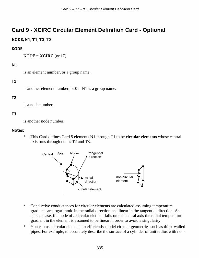
Card 9 – XCIRC Circular Element Definition Card
335
Card 9 - XCIRC Circular Element Definition Card - Optional KODE, N1, T1, T2, T3
KODE KODE = XCIRC (or 17)
N1 is an element number, or a group name.
T1 is another element number, or 0 if N1 is a group name.
T2 is a node number.
T3 is another node number.
Notes: * This Card defines Card 5 elements N1 through T1 to be circular elements whose central
axis runs through nodes T2 and T3.
* Conductive conductances for circular elements are calculated assuming temperature gradients are logarithmic in the radial direction and linear in the tangential direction. As a special case, if a node of a circular element falls on the central axis the radial temperature gradient in the element is assumed to be linear in order to avoid a singularity.
* You can use circular elements to efficiently model circular geometries such as thick-walled pipes. For example, to accurately describe the surface of a cylinder of unit radius with non-
Central Axis Nodes tangential direction
radial direction
circular element
non-circular element

Card 9 – XCIRC Circular Element Definition Card
336
circular elements, you need at least 8 tangential elements. With circular elements you can accurately model the cylinder with as few as 3 tangential elements.
* Lump mass and beam elements are not considered to be circular elements. * For view factor calculations performed by the VUFAC module, each circular element is
subdivided into a number of flat elements such that the angle subtended by an edge of a flat element does not exceed 45 degrees. If, however, an edge of a circular element exceeds 135 degrees that edge is subdivided into three equiangular line segments. View factors thermal couplings are calculated for these flat elements separately, and are then summed to yield the view factor and thermal coupling of the circular element.
* It is important to remember that view factor calculations assume uniform illumination over the element. If the circular element subtends too large an angle, this condition may not be fulfilled, and inaccurate results are obtained.
* Circular elements may not be defined as orthotropic elements. * It is highly recommended that circular elements have shapes that have edges along the radial
and tangential directions. * Circular elements may not be specified with XCIRC Cards for an axisymmetric model.

Card 9 – XCOND Conductances
337
Card 9 - XCOND Conductances - Optional KODE, N1, T1, T2, T3, T4, T5, T6
KODE KODE = XCOND (or 3)
N1 is an element number, or a group name. If N1 is a group name, a conductance of value T2 is generated between all the elements of the N1 and the element(s) of T1.
T1 is another element number, or a group name. If T1 is a group name, a conductance of value T2 is generated between the element(s) of the N1 and the elements of T1.
T2 is the value of the conductance between elements N1 and T1.
T3 is a code or a conductance number, or a table number. 1WAYC (or 2)
creates a one-way conductive conductance between elements N1 and T1. N1 will be affected by T1, but T1 will not be affected by N1. You can model fluid flow with one-way conductive conductances, where N1 is the downstream element, T1 is the upstream element, and T2 is the mass rate of flow times the fluid's specific heat (e. g. Btu/sec/F) flowing into element N1 from T1. If a chain of 1-WAYC conductances is present, they should all be of the same magnitude, and start and end in a SINK element. If this rule is not followed, an energy imbalance will show up on file MSGF.
1WAYR (or 3) creates a one-way radiative conductance of value T2 = (area* emissivity * gray body view factor) between elements N1 and T1. N1 will be affected by T1, but T1 will not be affected by N1.
CNVSN (or 8) adds a linear conductance between elements N1 and T1. The value of this conductance at run time is T2 times the value interpolated from table T4. If T5 is neither zero nor blank, then it is interpreted to be the ID of a temperature vs time table. This table defines the temperature history of a sink element whose element number is defined at run-time. The

Card 9 – XCOND Conductances
338
conductance is then created not between N1 and T1, but between the element N1 and this sink element.
CNVASN (or 9) adds a linear conductance between elements N1 and T1. The value of this conductance at run time is area(N1) times T2 times the value interpolated from table T4. If T5 is neither zero nor blank, then it is interpreted to be the ID of a temperature vs time table. This table defines the temperature history of a sink element whose element number is defined at run-time. The conductance is then created not between N1 and T1, but between the element N1 and this sink element.
CNVSNR (or 10) adds a linear conductance between the reverse side of element N1 and element T1. The value of this conductance at run time is T2 times the value interpolated from table T4. If T5 is neither zero nor blank, then it is interpreted to be the ID of a temperature vs time table. This table defines the temperature history of a sink element whose element number is defined at run-time. The conductance is then created not between N1 and T1, but between the reverse side of element N1 and this sink element.
CNVASNR (or 11) adds a linear conductance between the reverse side of element N1 and element T1. The value of this conductance at run time is area(N1) times T2 times the value interpolated from table T4. If T5 is neither zero nor blank, then it is interpreted to be the ID of a temperature vs time table. This table defines the temperature history of a sink element whose element number is defined at run-time. The conductance is then created not between N1 and T1, but between the reverse side of element N1 and this sink element.
COND (or 0) creates a linear conductive conductance of value T2 between elements N1 and T1.
CSERIES (or 5) adds a conductive conductance of value T2 in series with the linear conductances between elements N1 and T1, to reduce their value. This option can model contact conductances.
FOLLOWER (or 4) automatically makes T1 into a sink element with the temperature of N1. T1 should not be defined with a SINK Card. T2 is ignored.
FREE (or 7) creates a free convection conductance between elements N1 and T1. The heat flow through it is calculated with:
QN1T1 = T2(TN1 - TT1)(TN1 - TT1)T4

Card 9 – XCOND Conductances
339
where: TN1 is the temperature of element N1 TT1 is the temperature of element T1 QN1T1 is the heat flow through the conductance by the Analyzer module. T4 = blank defaults to T4 = 0.25.
RAD (or 1) creates a radiative conductance with T2 = (area * emissivity * gray body view factor) between elements N1 and T1.
RADSN2 (or 13) adds a radiative conductance between elements N1 and T1. The value of this conductance at run time is area(N1) times emissivity(N1) times T2 times the value interpolated from table T4. If T5 is neither zero nor blank, then it is interpreted to be the ID of a temperature vs time table. This table defines the temperature history of a sink element whose element number is defined at run-time. The conductance is then created not between N1 and T1, but between the element N1 and this sink element.
RADSN3 (or 12) adds a radiative conductance between elements N1 and T1. The value of this conductance at run time is area(N1) times T2 times the value interpolated from table T4. If T5 is neither zero nor blank, then it is interpreted to be the ID of a temperature vs time table. This table defines the temperature history of a sink element whose element number is defined at run-time. The conductance is then created not between N1 and T1, but between the element N1 and this sink element.
RADSNR2 (or 15) adds a radiative conductance between the reverse side of element N1 and element T1. The value of this conductance at run time is = (area(N1))*(emissivity of reverse side of N1)*(T2)*(the value interpolated from table T4). If T5 is neither zero nor blank, then it is interpreted to be the ID of a temperature vs time table. This table defines the temperature history of a sink element whose element number is defined at run-time. The conductance is then created not between N1 and T1, but between the reverse side of element N1 and this sink element.
RADSNR3 (or 14) adds a radiative conductance between the reverse side of element N1 and element T1. The value of this conductance at run time is area(N1) times T2 times the value interpolated from table T4. If T5 is neither zero nor blank, then it is interpreted to be the ID of a temperature vs time table. This table defines the temperature history of a sink element whose element number is defined at run-time. The conductance is then created not between N1 and T1, but between the reverse side of element N1 and this sink element.

Card 9 – XCOND Conductances
340
RSERIES (or 6) adds a radiative conductance of T2 = (area * emissivity * gray body view factor) in series with the radiative conductances between elements N1 and T1.
T3 > 15 a conductive conductance of value T2 is created between elements N1 and T1 with the conductance number T3.
T3 < -15 a radiative conductance with (area * emissivity * gray body view factor) value = T2 is created between elements N1 and T1 with the conductance number abs(T3). The T3 > 15 and T3 < 15 options pre-assign conductance numbers which are otherwise automatically assigned, so the conductances are referenced by user-written subroutines or INTERP Cards.
T4 is an exponent associated with a free convection conductance, or blank, or a table number associated with CNV-type conductances.
T5 is a table number associated with CNV-type conductances.
T6 is the number of DESCRIP Card associated with the XCOND Card (optional).
Examples: XCOND 3 4 2 COND $ CONDUCTIVE CONDUCTANCE OF VALUE 2.0 BETWEEN 3 AND 4 $ XCOND 5 6 7 RAD $ RADIATIVE CONDUNCTANCE OF VALUE 7 BETWEEN 5 AND 6 $ XCOND 8 9 0 FOLLOWER $ ELEMENT 9 FOLLOWS THE TEMPERATURE OF ELEMENT 8 $ XCOND 1 2 .5 FREE .33 $ FREE CONVECTION CONDUNCTANCE BETWEEN 1 AND 2

Card 9 – ZONE_CONVECTION Thermal Convecting Zone Definition Card
341
Card 9 – ZONE_CONVECTION Thermal Convecting Zone Definition - Optional
KODE, N1, T1, T2, T3
KODE KODE = ZONE_CONVECTION (or 92) defines a boundary condition that creates a convection coupling between a group of selected elements and a fluid environment.
N1 is the ZONE_CONVECTION card ID. Cards with the same ID reference the same Thermal Convecting Zone.
T1 may be: = SELECTION (or 1) = MAT (or 2) = PRESSURE (or 3) = TEMPERATURE (or 4) = HTC (or 5) = ROT_FX (or 6)
T1 = SELECTION The thermal convecting zone is applied to a selection of elements that are represented by the group name T2.
T1 = MAT The material ID of the fluid environment is specified in T2.
T1 = PRESSURE A pressure is specified for the thermal convecting zone. If the pressure is constant, then its value is specified in T2. If the pressure is table dependent, then T2 is a table multiplier and T3 has the form Tn (e.g. T25) where n is a table number referencing TABTYPE and TABDATA cards. The dependent variable on the TABTYPE card must be PTOTAL, and the independent variable is TIME.

Card 9 – ZONE_CONVECTION Thermal Convecting Zone Definition Card
342
T1 = TEMPERATURE A temperature is specified for the fluid environment. If the temperature is constant, then its value is specified in T2. If the temperature is table dependent, then T2 is a table multiplier and T3 has the form Tn (e.g. T25) where n is a table number referencing TABTYPE and TABDATA cards. The dependent variable on the TABTYPE card must be TEMP, and the independent variable is TIME.
T1 = HTC A heat transfer coefficient for the convection between the selected elements and the fluid environment is specified. If the heat transfer coefficient is constant, then its value is specified in T2. If the heat transfer coefficient is table dependent, then T2 is a table multiplier and T3 has the form Tn (e.g. T25) where n is a table number referencing TABTYPE and TABDATA cards. The dependent variable on the TABTYPE card must be COND, and the independent variable is TEMP, TDIF, QNODE, CAP, or TIME.
T1 = ROT_FX The thermal convecting zone temperatures are corrected for rotational effects. The ID of the referenced ROT_FX cards is specified in T2.
Example: $ Thermal Convecting Zone(1) NAME2 Thermal Thermal Convecting Zone(1) NAME Thermal 328 345 1 ZONE_CONVECTION 1 SELECTION "Thermal Convecting Zone(1)" ZONE_CONVECTION 1 MAT 2 ZONE_CONVECTION 1 PRESSURE 2.000000E+03 ZONE_CONVECTION 1 TEMPERATURE 1.0 T16 ZONE_CONVECTION 1 HTC 1.0 T8 ZONE_CONVECTION 1 ROT_FX 1

Card 10 - User-Written Subroutines USER1 and USERF
343
Card 10 - User-Written Subroutines USER1 and USERF - Optional
SUBROUTINE +USER1(GG,T,C,Q,QD,R,TIME,DT,IT,KODE,NOCON,MAXNO, +ICONV,DUM1,DUM2,DTP,TF) DIMENSION GG(*),QD(*),T(*),C(*),Q(*),R(*),ICONV(*) CHARACTER*7 NAME COMMON/TDMAX/TDMAX COMMON/PRTFLG/PRTFLG COMMON/IRUN/IRUN,IR(1) COMMON/MAXNOQ/MAXN1,MAXN2 COMMON/PARAMS/PARAMS(80000) COMMON/GRAV/GRAV,GV(3),TABS,RGAS,PSTD,TSTD,SIGMA SAVE | | RETURN END
USER1 is an optional FORTRAN 77 user-written subroutine that is automatically compiled and loaded with the Analyzer at run time. USER1 may call other subroutines. All user-written subroutines and user-defined common blocks should be called USER2, USER3, ..., to prevent name conflicts with the subroutines of the Analyzer. The first line after the ninth -1 Delimiter Card must start in column 7 with phrase SUBROUTINE. However, FUNCTION is also acceptable if SUBROUTINE USER1 appears later on. Note on variable type convention: In the following write-up the Fortran default convention for variable types is assumed. Variables starting with the letters (I-N) are assumed to be integers. Variables starting with the letters (A-H,O-Z) are assumed to be real, unless they are specifically specified to be double precision.

Card 10 - User-Written Subroutines USER1 and USERF
344
How USER1 is integrated into the Analyzer Module
IR(IRUN) not set
7. USER1 is entered with KODE = 2. You can modify the calculated temperatures.
10. Run completed?
9. USER1 is entered with KODE = 3 and IRUN is set to IRUN + 1. Check if IR(IRUN) is set or not.
1. Analyzer initialization - all conductances, capacitances, etc. are read in & placed into the proper arrays.
2. If Card 9 PARAM USRCNDADD is present, USER1 is entered with KODE=5. If CALL ADDCOND is present, new conductances are added to the matrix.
3. If hydraulic elements are present, the hydraulic iteration loop is entered. In this loop USER1 is entered once per hydraulic iteration with KODE = 4, during which you can modify total pressures and hydraulic flow resistances.
4. Analyzer evaluates conductances, performs table interpolation, and evaluates heat loads.
5. USER1 is entered with KODE = 1. You can modify conductances, capacitances, heat loads, sink temperatures, and other parameters which will be used for temperature calculation.
6. The Analyzer calculates temperatures for the next iteration or time step.
no yes
IR(IRUN) set
11. Run completed.

Card 10 - User-Written Subroutines USER1 and USERF
345
Explanation of the Parameters
C(K) C(K) is the capacitance of internal element K. If C(K) < 0, the element is a sink or some other type of special element such as MCV, and its temperatures are not computed with the normal heat balance equations but by some other technique such as table interpolation.
DT DT is the current integration time step for transient runs from Card 2b. DT by default is single precision. However, you may specify DT, T, and TIME to be passed as double precision variables to USER1, by specifying these variables to be double precision with the statement: DOUBLE PRECISION T,TIME,DT
DTP DTP is the printout time increment for transient runs from Card 2b.
GG(J) GG(J) is the current value of the resistance J, i.e. the inverse of the conductance J. If J is a radiative conductance, GG(J) is the inverse of its current linearized value, i.e. the temperature difference between its elements divided by the heat flow through it.
GRAV GRAV is the magnitude of the acceleration of gravity from the HYDENV Card.
GV(3) GV(3) is the unit gravity vector in global coordinates from the HYDENV Card.
IRUN IRUN is the current run number (e.g. 1, 2, etc.)
IR(IRUN) IR(IRUN) is the parameter to be set if you wish to perform run number IRUN, for IRUN > 1. Please see the example below on multiple runs.
Card 10 - User-Written Subroutines USER1 and USERF
346
IT IT is the current iteration counter value for steady-state runs.
KODE = 1 if the subroutine USER1 is entered just before calculating temperatures.
At this time you can alter model parameters (heat inputs, conductances, capacitances, sink temperatures) which can affect temperature calculation. Please see example below.
= 2 if it is entered just after calculating temperatures. At this time you can perform temperature postprocessing.
= 3 when the run is completed, = 4 when the subroutine is entered just before calculating total pressures for
hydraulic elements. = 5 If Card 9 PARAM USRCNDADD is present, USER1 is entered once
initially with KODE=5. If CALL ADDCOND is present, new conductances may be added to the matrix at this time.
MAXN1 MAXN1 is the number of non-hydraulic elements (cannot be changed).
MAXN2 MAXN2 is the number of hydraulic elements (cannot be changed).
MAXNO MAXNO is the number of elements (cannot be changed). MAXNO = MAXN1 + MAXN2. Note: If you have hydraulic elements in the model, and are creating and dimensioning arrays for elements, it is recommended that your array sizes be dimensioned to MAXNO + MAXN2, not MAXNO. The reason is that internally TMG partitions element numbers as follows: 1 to MAXN1 Thermal properties of non-hydraulic elements. MAXN1+1 to MAXN1+MAXN2 Thermal properties of hydraulic elements. MAXN1+MAXN2+1 to MAXN1+2*MAXN2 Pressure/flow properties of hydraulic elements.

Card 10 - User-Written Subroutines USER1 and USERF
347
NOCON NOCON is the number of conductances (cannot be changed).
PARAMS This is a general-purpose common block for analyzer parameters. PARAMS(249) is the largest Card 9 DESCRIP Card ID number. PARAMS(291) is the maximum element number in the model. PARAMS(292) is the maximum node number in the model.
PRTFLG PRTFLG is the print flag, 0 = OFF and 1 = ON. If PRTFLG is set to 1 when KODE = 2, the parameters specified on the PRINT Cards are printed for the current iteration or time step.
PSTD PSTD is the standard pressure from the HYDENV Card.
Q(K) Q(K) is the calculated heat load to internal element K. At each iteration or time step, Q(K) is recalculated. Thus, if you wish modify Q(K), you must do it every time USER1 is entered with KODE=1.
QD(K) QD(K) is the fraction of phase-change element K in its higher temperature phase. K is an internal element number.
R(J) R(J) is the conductance parameter of conductance J. R(J) is altered during the run only for temperature-dependent radiative conductances, otherwise it will remain constant. For conductive linear conductance the value of R(J) is the inverse of its initial conductance value, i.e. R(J) is a resistance. For a radiative conductance R(J) has the (area * emissivity * gray body view factor * Stefan-Boltzmann's constant) value. For Oppenheim's Method (specified with Card 9 PARAM OPPENHEIM) the gray body view factor between an element and its surface element is considered to be 1/(1-emissivity).

Card 10 - User-Written Subroutines USER1 and USERF
348
If you wish to change the value of a radiative coupling in a user-written subroutine, (e.g. because the emissivity is temperature dependent), you should change the value of both R(J) and GG(J) by a consistent factor (Rnew(J) = Rold(J) * f and GGnew(J) = GGold(J) / f). For a convective conductance R(J) is the inverse of the Card 6e A(N1) * HN1, i.e. projected area times the multiplier value.
RGAS RGAS is the Universal Gas Constant computed from the data of the Card 9 HYDENV Card.
SIGMA SIGMA is the Stefan-Boltzmann's Constant specified on Card 2a.
T(K) T(K) is the temperature of the internal element K, for internal element numbers ≤ MAXN1 + MAXN2. T(K) is the total pressure value of hydraulic internal element K for internal element numbers > MAXN1 + MAXN2. T(K) by default is in single precision. However, since the Analyzer calculates temperatures in double precision, you can take advantage of this if you do the following: T(K) by default is in single precision. However, since the Analyzer calculates temperatures in double precision, you can take advantage of this by specify that the T array is in double precision by including the following line: DOUBLE PRECISION T,TIME,DT The contents of the T array are as follows:
From To Description T(1) T(MAXN1) temperatures of non-
hydraulic elements T(MAXN1+1) T(MAXN1+MAXN2) temperatures of hydraulic
elements T(MAXN1+ MAXN2+1) T(MAXN1+2MAXN2) total pressure values of
the hydraulic elements

Card 10 - User-Written Subroutines USER1 and USERF
349
The total pressure and temperature values of the hydraulic element K are stored in the T array with an offset of MAXN2, i.e. the temperature stored in T(K), and its total pressure is stored in T(K + MAXN2). Both ICONV(K) and ICONV(K + MAXN2) will return the element's real element number.
TABS TABS is the absolute value of the absolute zero temperature (e.g. 273) specified on Card 2b. TABS is positive.
TDMAX TDMAX is the current value of the maximum temperature difference of any element between the current iteration and the previous one for steady-state runs. If TDMAX is set to 0 with KODE = 2 for steady state runs, the run is forced to terminate.
TIME TIME is the current time value for transient runs. TIME by default is single precision. However, you may specify DT, T, and TIME to be passed as double precision variables to USER1, by specifying these variables to be double precision with the statement: DOUBLE PRECISION T,TIME,DT
TIME has different values for different KODE values. For KODE=1 TIME is the value at the beginning of the integration time step. For KODE=2, 3, or 4 TIME is the value at the end of the integration time step.
TF TF is the final time of a transient run. TF is the maximum number of iterations for a steady state run. If TF is set to 0, the run is forced to terminate.
TSTD TSTD is the standard temperature from the HYDENV Card.

Card 10 - User-Written Subroutines USER1 and USERF
350

Card 10 - User-Written Subroutines USER1 and USERF
351
Access to Files You can access all files from USER1. Their pre-assigned numbers are:
File Unit number
TEMPF 2
INPF 89
MODLF 7
VUFF 8
FMODLF 16
MSGF 17
REPF 18
MODLCF 56
GTEMPF 62
INPF should not be modified. New files created with an OPEN statement should be numbered 20-40.

Card 10 - User-Written Subroutines USER1 and USERF
352
Special Functions and Subroutines The following special functions and subroutines are available: FUNCTION ARRAYINTERP(X,Y,Z,N) SUBROUTINE ADDCOND(ICONDNO,NC,GCOND) FUNCTION CAPAPH(K) FUNCTION CAPBPH(K) SUBROUTINE CHANGENODECOORDS(NODE,V) SUBROUTINE CONDNOS(K,ICONDNO,NC,KBEL,NBEL) SUBROUTINE CONDNOS2(NAME1,ICONDNO,NC) SUBROUTINE DESCRIP (DESC,ID,IDLENGTH,TYPE1,TYPE2,GRP1,GRP2,GRP3,NVAR,VAR, IUPD) SUBROUTINE FAN(K,RMASS) SUBROUTINE FASTSOLVE2(ICD,COND,ICOND,ITYPE,ISINK,PAR,IERR,X,B) SUBROUTINE FORMOUT (TITLE,FILENAME,ARRAY,TIME,ISDTP,CODE) SUBROUTINE GENERIC (N1,STRING1,STRING2,GRP1,GRP2,RARR,IARR,NID) SUBROUTINE GETLAYERS(K,NLAYERS,LAYERS) SUBROUTINE GRP2GRP (GROUPA,GROUPB,T,GG,R,C,HTFLOW,MAXNO+MAXN2,NOCON, PAR) FUNCTION HTLAT(K) FUNCTION HYDPROP(I,K) SUBROUTINE HYDPROPPUT(I,K,VALUE) FUNCTION ICONDELEM(IR) FUNCTION ICONV(K) FUNCTION IELEMTYPE(I,K) FUNCTION KCONV(I) SUBROUTINE LONGNAME(NAME1,A80,ID,LENGTH,ICODE) FUNCTION NAME(K) SUBROUTINE NAMAR(NAME,NAMARR,N)

Card 10 - User-Written Subroutines USER1 and USERF
353
FUNCTION NOCOND(N1,N2,LL) SUBROUTINE PELTIER (GRPCOLD,GRPHOT,NPOLE,SEEBECK,GEOMF,ELECRES,VOLT, CURRENT,RKTHERM,T,Q) SUBROUTINE READPROP2 (PROP,GEOM,NDGRID,GRID,KPROP,KGEOM,KNDGRID,KGRID) SUBROUTINE TCNAME(NAME1,NAME2,ICONDNO,NC) SUBROUTINE TINT(X,Y,N) SUBROUTINE THERMOSTAT(OP,IEL,IFLAG) FUNCTION TMGINT(X,XARRAY,YARRAY,N) SUBROUTINE TMGN12(J,K1,K2,LL) FUNCTION TPHASE(K) SUBROUTINE TUNITS (T1,T2,T3,T4,T5,T6) SUBROUTINE USERARRAY (IARRAY, K, VALUE, CODE) SUBROUTINE VARVAL(VARNAM,VAL)

Card 10 - User-Written Subroutines USER1 and USERF
354
VALUE = ARRAYINTERP(X,Y,Z,N) returns the interpolated real value from bivariate array N where the independent variables are X and Y. Z is not used at this time. X,Y,Z must be real values, N must be an integer. The bivariate array must be defined with Card 9 ARRAYTYPE and ARRAYDATA Cards.
CALL ADDCOND(ICONDNO,NC,GCOND) This routine adds new conductances to the conductance array at run-time. It can be used only if a Card 9 PARAM USRCNDADD Card is present and USER1 is entered with KODE=5. Since USER1 is entered with KODE=5 only once in the run, so you can add conductances only once. However, you can deactivate conductances any time during the run by setting their value to some arbitrarily low value such as 1.E-36.
GCOND is a real array that should be dimensioned to GCOND(NC). This is an input.
GCOND(L) is the L’th conductance to be added to the conductance matrix. GCOND(L) has the same units as the R array. Please note: for conductive conductances, GCOND(L) has the units of resistance, i.e. the inverse of conductance.
ICONDNO is an integer array that should be dimensioned ICONDNO(4,NC)
ICONDNO(1,L) contains the conductance number of the L'th conductance in the array. This value is returned.
ICONDNO(2,L) contains the first specified external element label. This is an input.
ICONDNO(3,L) contains the second specified external element label. This is an input.

Card 10 - User-Written Subroutines USER1 and USERF
355
ICONDNO(4,L) is the specified conductance type. This is an input.
= 0 if the conductance is conductive. GCOND(L) should have the units of resistance.
= 1 if the conductance is radiative. A radiative conductance values should be equal to the SIGMA*Area*Emissivity*gray body view factor value.
= 2 if it is a follower conductance. ICONDNO(3,L) will follow the temperature of ICONDNO(2,L).
= 6 if it is a 1-way radiative conductance. ICONDNO(3,L) is affected by ICONDNO(2,L), whereas ICONDNO(2,L) is not affected by ICONDNO(3,L).
= 7 if it is a 1-way conductive conductance. ICONDNO(3,L) is affected by ICONDNO(2,L), whereas ICONDNO(2,L) is not affected by ICONDNO(3,L).
NC is an integer, the number of conductances in arrays ICONDNO and GCOND. This is an input.
VALUE = CAPAPH(K) returns real value CAPAPH(K), the capacitance of phase change element with internal element K above its phase change temperature.
VALUE = CAPBPH(K) returns real value CAPBPH(K), the capacitance of phase change element with internal element K below its phase change temperature.
CALL CHANGENODECOORDS(NODE,V) This routine changes the coordinates of node NODE to V. V is a real vector of dimension 3, NODE is an integer. The conductive conductances of all elements connected to NODE will be changed appropriately.

Card 10 - User-Written Subroutines USER1 and USERF
356
CALL CONDNOS(K,ICONDNO,NC,KBEL,NBEL) This routine returns the conductive conductances (including the conductances connecting the boundary elements) and boundary elements associated with internal element number K for the element CG method. This method is preferred to the CALL TCNAME option for the element CG method. ICONDNO
Is an integer array containing the conductance parameters. ICONDNO must be dimensioned as ICONDNO(4,MAXC). The dimension MAXC is user-assigned, and should equal maximum expected number of conductances to be found for a single element.
ICONDNO(1,L) contains the conductance number of the L'th conductance in the array.
ICONDNO(2,L) contains one internal element label.
ICONDNO(3,L) contains the other internal element label.
ICONDNO(4,L) is reserved for future use.
NC is the number of returned conductances in array ICONDNO. NC is returned.
KBEL is an array that should be defined with the maximum dimension KBEL(MAXNO).
KBEL(L) contains the internal element number of the L’th boundary element of element K.
NBEL

Card 10 - User-Written Subroutines USER1 and USERF
357
is the number of boundary elements in array KBEL. NBEL is an integer, and it is returned.
CALL CONDNOS2(NAME1,ICONDNO,NC) This routine returns all the conductive conductances associated with the elements of group name NAME1, including the conductances connecting the boundary elements. CONDNOS2 can be used only with the element CG method.
ICONDNO is an integer array containing the conductance parameters. It must be dimensioned ICONDNO(4,MAXC). MAXC is user-assigned, and is determined by the maximum expected number of conductive conductances to be found. MAXC = MAXNO is generally a safe bet,
ICONDNO(1,L) contains the conductance number of the L'th conductance in the array.
ICONDNO(2,L) contains one internal element label.
ICONDNO(3,L) contains the other internal element label.
ICONDNO(4,L) contains the internal element label of the "parent element" to which the conductance belongs.
NC is an integer, the number of conductances returned in array ICONDNO.
NAME1 is a character variable, it is the group name of the elements whose internal conductances are desired. This is an input.

Card 10 - User-Written Subroutines USER1 and USERF
358
CALL DESCRIP (DESC,ID,IDLENGTH,TYPE1,TYPE2,GRP1,GRP2,GRP3,NVAR,VAR, IUPD)
This CALL statement accesses all the parameters associated with the Card 9 DESCRIP Card. DESC is the descriptor character string. It is a character variable, must be specified as CHARACTER*40. ID is an integer, it is the DESCRIP Card id number (N1 parameter). The maximum ID number is specified in PARAMS(249). IDLENGTH is an integer, it is the length of the character string DESC. TYPE1, TYPE2 are character strings associated with the DESCRIP Card (e.g. SINK and CONSTANT) specified on the DESCAD1 Card. Must be specified as CHARACTER*8. GRP1, GRP2, GRP3 are the group names specified on the DESCAD1 Card. They are character variables and their length must be 7 or fewer characters. NVAR is and integer, it is the number of variables in array VAR. VAR is a real array of length 7 containing the values specified on the DESCAD2 Card. IUPD is an integer flag that is returned. IUPD=1 if the descriptor parameters are updatable in a checkpoint run, otherwise IUPD=0.
CALL FAN(K,RMASS) imposes a mass flow of value RMASS in the positive direction through the hydraulic FANPUMP element with internal element number K. RMASS is a real, and K ins an integer variable.
CALL FASTSOLVE2(ICD,COND,ICOND,ITYPE,ISINK,PAR,IERR,X,B) This subroutine solves the matrix equation AX = B, using the preconditioned iterative biconjugate gradient method. It is a general-purpose matrix solver, and whose input parameters are independent of the data structure of the Analyzer. A

Card 10 - User-Written Subroutines USER1 and USERF
359
is the matrix whose elements are created from the conductances of arrays ICD and COND. The matrix A is internally created by FASTSOLVE2 from the conductances specified in ICD and COND.
X is the solution vector computed. On input, X is used as the initial estimate. X is real and must be dimensioned X(IMAX), where IMAX is the largest element number in the conductance array ICD. The X values of non-existent elements are returned with the value -1.2E34.
B is the input right hand side vector. B is real and must be dimensioned B(IMAX).
ICD is the input integer array of length ICOND that contains the connected element numbers of the conductances specified in COND. ICD must be dimensioned ICD(2,ICOND). ICD(1,L)
is the first element of the L'th conductance. ICD(2,L)
is the second element of the L'th conductance. The element numbers in ICD may be arbitrary, and not all elements need to exist.
COND is a real array of length ICOND. COND(L) contains the value of the L'th conductance. COND must be dimensioned COND(ICOND).
ITYPE is the input integer array of length ICOND that defines the conductance type in ICD. ITYPE must be dimensioned ITYPE(ICOND). ITYPE(L) ≥ 0 specifies an ordinary conductance. ITYPE(L) = -1 specifies a 1-way conductance, only element ICD(1,L) is affected.
ICOND is an integer, it is the number of conductances in ICD and COND.
ISINK

Card 10 - User-Written Subroutines USER1 and USERF
360
is an integer input array that flags those elements which have constant X boundary conditions. ISINK must be dimensioned ISINK(IMAX), where IMAX is the largest element number in the conductance array ICD. If element K is not a constant X boundary condition, ISINK(K) must = 0. If element K is a constant X boundary condition, ISINK(K) must = 1, and on return X will take on the value B(K).
IERR is an integer, it is the returned error flag = 1 for error, otherwise = 0.
PAR is a real control array of length 20. PAR(1)
is the input initial fill-in value estimate for the preconditioning matrix. = 0 defaults to 7. If convergence is not achieved, the fill-in value is updated in increments of 10 until convergence is achieved. = -1 uses the Jacobi preconditioner, where the preconditioning matrix consists of the inverse of the diagonal of the matrix A.
PAR(2) is the input tolerance value specified for eliminating small terms in the preconditioning matrix. = 0 defaults to .0001.
PAR(3) is the input convergence criterion. The solution is considered converged if norm(AX-B)/norm(B) < PAR(3), or if the PAR(10) convergence criterion is fulfilled. = 0 defaults to 1.E-8.
PAR(4) is the input maximum number of iterations. = 0 defaults to 200.
PAR(5) is the input flag that prints the convergence residual value to file MSGF and to the screen. = 0 defaults to no residuals printed.
PAR(6)
Card 10 - User-Written Subroutines USER1 and USERF
361
is reserved. PAR(7)
is output, on return contains the value of the convergence residual. PAR(8)
is output, on return contains the number of iterations completed. PAR(9)
is an input flag to re-use the previously created preconditioning matrix on exit. PAR(9) = 0 creates the preconditioning matrix. PAR(9) = 1 uses the previously created preconditioning matrix in order to save CPU time.
PAR(10) is not used.
PAR(11) is an input flag to increase performance for repeated re-entry. = 1 improves performance by saving all temporary arrays (but not the matrix A) created internally for subsequent re-use. = 0 does not save the arrays.
PAR(12) is an input flag to increase performance for reported re-entry with the same matrix but different B. = 1 saves all matrices, including the input matrix A created from ICD, for subsequent calculations with another B vector. PAR(12) = 0 does not.
The following example solves the matrix AX + B = 0: A = | -3 2 | | 1 -1 | and B = | 0 | | -100 | The matrix is can be expressed with 3 conductances: G21 = 1 G12 = 1 - one-way conductance ITYPE = -1. G11 = -1 Since G12 is a 1-way conductance, only row 1 is affected by G12, not row 2.

Card 10 - User-Written Subroutines USER1 and USERF
362
Example: FASTSOLVE2 EXAMPLE -1 0 0 0 0 0 0 0 0 0 0 0 0 273 0 0 0 1 -1 -1 -1 -1 -1 -1 -1 SINK 1 0 SINK 2 0 -1 SUBROUTINE USER1(GG,T,C,Q,QD,R,TIME,DT,IT, +KODE,NOCON,MAXNO,ICONV,DUM1,DUM2,DTP,TF) DIMENSION T(*),X(2),B(2),PAR(20),ICD(2,3) DIMENSION COND(3), ISINK(2),ITYPE(3) SAVE DATA PAR,X,B,ISINK,ITYPE/24*0.0,5*0/ ICOND=3 ICD(1,1)=2 ICD(2,1)=1 COND(1)=1 ICD(1,2)=1 ICD(2,2)=2 COND(2)=1 ITYPE(2)=-1 ICD(1,3)=1 ICD(2,3)=1 COND(3)=-1 B(2)=-100 CALL FASTSOLVE2(ICD,COND,ICOND,ITYPE,ISINK,PAR,IERR,X,B) T(1)=X(1) T(2)=X(2) RETURN END -1
CALL FORMOUT(TITLE,FILENAME,ARRAY,TIME,ISDTP,CODE) prints the values of the array ARRAY at time TIME in either file TEMPF format or NX element data set type 56 universal file format, depending on CODE. TITLE
must be a character variable < 40 characters.

Card 10 - User-Written Subroutines USER1 and USERF
363
If CODE = 'TEMPF', TITLE is ignored. FILENAME
must be a character variable < 12 characters. If CODE = 'IDEAS', the data is written on file FILENAME.unv. If CODE = 'TEMPF' the data is written on file FILENAME. The file FILENAME is opened in append mode, previous data is not destroyed.
ARRAY Is a real array, must have a length > MAXNO. ARRAY(K) is a value associated with internal element number K. If ARRAY(K) is assigned a value = -1.2E34, it is not printed.
ISDTP is an integer, it is the specific data type code, which must be from 0 to 18. If CODE = 'TEMPF', ISDTP is ignored. ISDTP = 0 is unknown. ISDTP = 5 is temperature, and ISDTP = 16 is heat gradient.
CODE Is a character variable, must be ‘IDEAS’ or ‘TEMPF’
Example: CALL FORMOUT('VOLTAGES FOR HEATER 12','VOLTS',V,TIME,0,'IDEAS')
CALL GENERIC(N1,STRING1,STRING2,GRP1,GRP2,RARR,IARR,NID) This routine returns the parameters associated with the GENERIC Card whose ID is N1. N1
is the GENERIC Card ID. STRING1
is the string entity associated with the GENERIC1 Card. String1 must be specified as A80.
STRING2
Card 10 - User-Written Subroutines USER1 and USERF
364
is the string entity associated with the GENERIC2 Card. String2 must be specified as A80.
GRP1 is the group name associated with associated with the GENERIC3 Card. GRP1 is in the short format, must be specified as A7 .
GRP2 is the group name associated with associated with the GENERIC4 Card. GRP2 is in the short format, must be specified as A7 .
RARR is the real array associated with associated with the GENERIC5 Card. RARR must be dimensioned as RARR(8) .
IARR is the integer array associated with associated with the GENERIC6 Card. IARR must be dimensioned as IARR(8) .
NID is the number of generic entities in the model
Example: CHARACTER*80 STRING1,STRING2 CHARACTER*7 GRP1,GRP2 DIMENSION IARR(8),RARR(8),IARR1(8),IARR2(8) CALL GENERIC(5,STRING1,STRING2,GRP1,GRP2,RARR,IARR,NID)
CALL GETLAYERS(K,NLAYERS,LAYERS) This routine returns the element numbers generated for homogeneous multilayer shell elements. A homogeneous multilayer shell element is defined by a non-zero T2 parameter on the Card 9 PROP SHELL Card. K
is an integer, it is the internal element number of the multilayer shell element whose layers are desired.
NLAYERS Is an integer, it is the number of layers of element K.
LAYERS(I),I=1...NLAYERS
Card 10 - User-Written Subroutines USER1 and USERF
365
LAYERS is an integer array, it must be dimensioned LAYERS(MAXLAYERS), where MAXLAYERS is the largest number of layers specified for any element in the model. LAYERS(I) is the I’th internal element label for the layers of element K. The layers are listed from bottom to top, i.e. LAYERS(1) is the internal element label of the bottom layer.
CALL GRP2GRP (GROUPA,GROUPB,T,GG,R,C,HTFLOW,MAXNO+MAXN2,NOCON, PAR)
This routine calculates the heat flow from element group GROUPA to element group GROUPB. GROUPA is a group name - must be defined as CHARACTER*7
and must be 7 characters long. GROUPB is a second group name - must be defined as
CHARACTER*7 and must be 7 characters long. HTFLOW is a real array of dimension 10 containing the calculated heat flows.
HTFLOW(1) contains the heat flow from GROUPA to GROUPB through conduction. GROUPA to GROUPB must be in contact to have conductive heat flow between them.
HTFLOW(2) contains the heat flow from GROUPA to GROUPB through radiation, including directly connected radiative conductances and through Oppenheim elements.
HTFLOW(3) contains the heat flow from GROUPA to GROUPB through directly connected forced convection conductances.
HTFLOW(4) contains the heat flow from GROUPA to GROUPB through directly connected free convection conductances.
HTFLOW(5) contains the heat flow from GROUPA to GROUPB through directly connected 1-way radiative conductances.
HTFLOW(6) contains the heat flow from GROUPA to GROUPB through directly connected 1-way conductive conductances.

Card 10 - User-Written Subroutines USER1 and USERF
366
HTFLOW(7) contains the heat flow from GROUPA to GROUPB through directly connected linear convective conductances.
HTFLOW(8) contains the heat flow from GROUPA to GROUPB through directly connected CFD-type conductances.
HTFLOW(9) contains the sum of HTFLOW(1) through HTFLOW(8).
HTFLOW(10) contains the equivalent conductance value between the two groups, calculated by dividing HTFLOW(9) by the difference of the average temperatures of GROUPA and GROUPB.
PAR is a real parameter array of dimension 4. PAR(1) = 1, the results of HTFLOW are printed onto REPF. PAR(2) = 1, then the heat flows through the individual
conductances are also printed. = 2, then only heat flows through all conductances is calculated and printed.
PAR(3) must be 0. PAR(4) must be 0.
VALUE = HTLAT(K) returns the real value HTLAT(K), the latent heat value of phase change element with internal element K. K is an integer.
VALUE = HYDPROP(I,K) returns the real value HYDPROP(I,K), the I’th hydraulic property of hydraulic internal element K. The hydraulic property values may be set with the HYDPROPPUT function described below. I, K are integers.
HYDPROP(1,K) is the total pressure value. HYDPROPPUT may be used for pressure sink elements only.
HYDPROP(2,K) is the static pressure value. HYDPROPPUT may not be used.

Card 10 - User-Written Subroutines USER1 and USERF
367
HYDPROP(3,K) is the dynamic pressure value. HYDPROPPUT may not be used.
HYDPROP(4,K) is the mass flow through K. HYDPROPPUT may not be used.
HYDPROP(5,K) is the volume flow through K. HYDPROPPUT may not be used.
HYDPROP(6,K) is the velocity through K. HYDPROPPUT may not be used.
HYDPROP(7,K) is the hydraulic diameter. HYDPROPPUT may not be used.
HYDPROP(8,K) is the fluid density. HYDPROPPUT may not be used.
HYDPROP(9,K) is the viscosity.
HYDPROP(10,K) is the duct cross-sectional area.
HYDPROP(11,K) is the specific heat.
HYDPROP(12,K) is the thermal conductivity.
HYDPROP(13,K) is the duct-based Reynolds Number. HYDPROPPUT may not be used.
HYDPROP(14,K) is the Reynolds Number based on the length to the nearest upstream BLSTART element. HYDPROPPUT may not be used.
HYDPROP(15,K) is the height. HYDPROPPUT may not be used.
HYDPROP(16,K)

Card 10 - User-Written Subroutines USER1 and USERF
368
is the Prandtl Number. HYDPROPPUT may not be used.
HYDPROP(17,K) is the imposed mass flow into K. HYDPROPPUT may not be used.
HYDPROP(18,K) is the fluid density at temperature TSTD and static pressure PSTD, calculated with the Ideal Gas Law.
HYDPROP(19,K) is the distance along the flow path from K to start of the nearest upstream BLSTART element. HYDPROPPUT may not be used.
HYDPROP(20,K) is the latent heat of element non-hydraulic element K - same HTLAT(K).
HYDPROP(21,K) is the phase change temperature of non-hydraulic element K - same TPHASE(K).
HYDPROP(22,K) is the capacitance above the phase change temperature of non-hydraulic element K - same as CAPAPH(K).
HYDPROP(23,K) is the capacitance below the phase change temperature of non-hydraulic element K - same as CAPBPH(K).
CALL HYDPROPPUT(I,K,VALUE) This routine sets the hydraulic property value type I of internal element K to VALUE. For the codes I please see the HYDPROP function above. I and K are integers, VALUE is real.
IELEM = ICONDELEM(IR) returns the integer value of the internal element number IELEM associated with conductive conductance number IR. IELEM is the element from

Card 10 - User-Written Subroutines USER1 and USERF
369
which the conductance was derived with the element CG conductance calculation method. If there is no such association (e.g. because the conductance is a thermal coupling) the value 0 is returned. IR must be an integer.
I = ICONV(K) returns the integer I, the external element number of the integer internal element K.
II = IELEMTYPE(I,K) Returns the integer II, the element type. I is an integer, it is external element number. K is an integer, and it is also returned. If K is not zero, K is the element associated with element I. The explanation of the return codes is as follows: II=-1 I does not exist in the model II=0 I is defined in NX II=1 I is a reverse side element associated with element K II=2 I is an Oppenheim element associated with element K II=3 I is an element surface coated on element K II=4 I is a homogeneous multilayer element of element K II=5 I is an Oppenheim element of reverse side of element K II=6 I is a space element II=7 I is a CFD element II=8 I is a TMG-created hydraulic element connected to K II=9 I is a TMG-created element connected to element K
K = KCONV(I) returns the integer K, the internal element number of integer external element number I. If I does not exist K = 0 is returned.

Card 10 - User-Written Subroutines USER1 and USERF
370
CALL LONGNAME(NAME1,A80,ID,LENGTH,ICODE) This routine associates the description string A80 associated with the group name NAME1. The description string is defined on a Card 9 NAME2 Card, which must be present in the input deck. NAME1 is the group name. NAME1 must be specified as CHARACTER*7. A80 is the descriptor string. A80 must be specified to be CHARACTER*80. LENGTH is the length of the description string A80. LENGTH is an integer. ID is the group name number. ID is an integer. ICODE is an input and must be specified to be an integer. ICODE may be 1, 2, or 3.
= 1 returns A80, ID, and LENGTH for the input NAME1. = 2 returns NAME1, ID, and LENGTH for the input A80. = 3 returns NAME1, A80, and LENGTH for the input ID.
The following returns the group name NAME1 associated with the descriptor string ‘You are so good looking!’. CHARACTER*80 A80 CHARACTER*7 NAME1 SAVE DATA KINIT/0/ IF(KINIT.EQ.0)THEN KINIT=1 CALL LONGNAME(NAME1, + ’You are so good looking!’,ID,LENGTH,2) END IF
VALUE = NAME(K) returns NAME(K), the group name of integer internal element K. NAME must be defined as CHARACTER*7. If K is associated with multiple group names, the first group name in an alphabetical sort is returned.

Card 10 - User-Written Subroutines USER1 and USERF
371
CALL NAMAR(NAME,NAMARR,N) returns the N internal element numbers associated with group NAME, and places them in integer array NAMARR. NAMARR should be dimensioned sufficiently large (e.g. MAXNO) to accept N element numbers. NAMARR and N are integers, NAME is a character variable. To save time, this subroutine should be called only once, at initialization time. Use the FORTRAN SAVE command to ensure the values of NAMARR are retained between entries to USER1. The following returns N1 and N2 element numbers associated with the group names 'GROUP1' and 'GROUP2'. DIMENSION NAMARR1(MAXNO),NAMARR2(MAXNO) SAVE DATA KINIT/0/ IF(KINIT.EQ.0)THEN KINIT=1 CALL NAMAR('GROUP1',NAMARR1,N1) CALL NAMAR('GROUP2',NAMARR2,N2) END IF
J = NOCOND(N1,N2,LL) returns J, the conductance number of conductance type LL between the external (not internal) element numbers N1 and N2. J, N1, N2, LL are all integers. N1, N2, and LL are all input. If the conductance does not exist, J = 0 is returned. LL may be:
= 0 for a linear conductance, = 1 for a radiative conductance, = 2 for a follower conductance (element N2 follows element N1), = 3 for a hydraulic element forced convection conductance, = 4 for a free convection conductance, = 5 for a hydraulic flow resistance, = 6 for a 1-way radiative conductance, = 7 for a 1-way conductive conductance. Conductance numbers are automatically assigned, but may be pre-assigned on an XCOND Card.

Card 10 - User-Written Subroutines USER1 and USERF
372
CALL PELTIER (GRPCOLD,GRPHOT,NPOLE,SEEBECK,GEOMF,ELECRES,VOLT, CURRENT,RKTHERM,T,Q)
This routine calculates the heat inputs to the hot and cold sides of a Peltier device. The algorithm used is derived from the Melcor handbook. If you use this routine, please note that you must have a Peltier Card present in the deck, and on this Peltier Card you must specify the VOLT and CURRENT parameters with zero values. The Peltier Card parameters will be overwritten by what you specify in the user-written subroutine. GRPCOLD
is the group name for the cold side. Must be a character variable. GRPHOT
is the group name for the cold side. Must be a character variable. NPOLE
is an integer, it is the number of poles of the device. SEEBECK
is the real value Seebeck coefficient. If SEEBECK is a negative whole number, e.g. –3.0, then the Seebeck coefficient will be interpolated from table 3. SEEBECK must be a real number, not an integer.
GEOMF is the geometric factor. GEOMF is real.
ELECRES is the electrical resistivity. If ELECRES is a negative whole number, e.g. –3.0, then the electrical resistivity will be interpolated from table 3. ELECRES must be a real number, not an integer.
VOLT is the applied voltage. VOLT is real.
CURRENT is the applied current. Either the applied voltage or the applied current must be zero. CURRENT must be a real number, not an integer.
RKTHERM is the thermal conductivity, it is a real value. If RKTHERM is a negative number, e.g. –3.0, then the electrical resistivity will be

Card 10 - User-Written Subroutines USER1 and USERF
373
interpolated from table 3. RKTHERM must be a real number, not an integer.
T is the temperature array – it is a real value.
Q is the heat input array– it is a real value.
CALL READPROP2 (PROP,GEOM,NDGRID,GRID,KPROP,KGEOM,KNDGRID,KGRID)
This routine reads the elemental properties from file VUFF. PROP
is a real array that must be dimensioned as PROP(10,MAXNO). PROP contains scalar variables associated with integer internal element K. PROP(1,K)
contains the area of lump mass, beam and shell elements, and volume of solid elements.
PROP(2,K) contains the emissivity.
PROP(3,K) contains the absorptivity.
PROP(4,K) contains the (thermal conductivity)*(cross-sectional area) of a beam, the (thermal conductivity*thickness) of a planar, and the thermal conductivity of solid internal element.
PROP(5,K) contains the (specific heat)*density*(cross-sectional area) of a beam, the (specific heat)*density*thickness of a planar, and the (specific heat)*density of solid internal element.
PROP(6,K) contains the hydraulic diameter.
PROP(7,K) contains the number of nodes.
GEOM

Card 10 - User-Written Subroutines USER1 and USERF
374
is a real array that must be dimensioned as GEOM(3,4,MAXNO). GEOM contains vector variables associated with internal element K. GEOM(1,1,K) to GEOM(3,1,K)
contain the X,Y,Z coordinates of the CG of internal element K. GEOM(1,2,K) to GEOM(3,2,K)
contain the X,Y,Z of the element center of internal element K. GEOM(1,3,K) to GEOM(3,3,K)
contain the X,Y,Z coordinates of the surface normal of internal element K.
GRID is a real array that must be dimensioned as GRID(3,MAXGRD). GRID(1,I), GRID(2,I), GRID(3,I)
contain the global X,Y,Z coordinates of node I. MAXGRD must be > PARAMS(292), i.e. the largest node number.
NDGRID Is an integer array that must be dimensioned as NDGRID(8,MAXNO). NDGRID(J,K)
contains the J'th node number of the internal element K. KPROP
is a CHARACTER*1 variable, the code 'Y' or 'N'. PROP is read only if KPROP = 'Y'. Otherwise, PROP need not be dimensioned.
KGEOM is a CHARACTER*1 variable, the code 'Y' or 'N'. GEOM is read only if KGEOM = 'Y'. Otherwise, GEOM need not be dimensioned.
KNDGRID is a CHARACTER*1 variable, the code 'Y' or 'N'. NDGRID is read only if KGRID = 'Y'. Otherwise, NDGRID need not be dimensioned.
KGRID is a CHARACTER*1 variable, the code 'Y' or 'N'. GRID is read only if KGRID = 'Y'. Otherwise, GRID need not be dimensioned.
The following reads in the arrays PROP and GEOM, but not NDGRID or GRID, which need not be dimensioned.
CALL READPROP2(PROP,GEOM,NDGRID,GRID,'Y','Y','N','N')

Card 10 - User-Written Subroutines USER1 and USERF
375
CALL TCNAME(NAME1,NAME2,ICONDNO,NC) returns the NC conductances of the model where one of the elements belongs to group name NAME1 and the other to NAME2. NC is an integer, it is a returned value. NAME1, NAME2
are character variable group names, must be ≤ 7 characters. If NAME2 is '*', all the conductances connected to NAME1 are returned.
ICONDNO is an integer array containing the conductance parameters. ICONDNO must be dimensioned as ICONDNO(4,MAXC), where the dimension MAXC is user-assigned, and must be greater than the maximum expected number of conductances to be found.
ICONDNO(1,L) contains the conductance number of the L'th conductance in the array.
ICONDNO(2,L) contains the internal element number of the conductance associated with the group name NAME1 (unless it is a 1-way conductive conductance, in which case it is the element number of the upstream element).
ICONDNO(3,L) contains the internal element number of the conductance associated with the group name NAME2 (unless it is a 1-way conductive conductance, in which case it is the element number of the downstream element).
ICONDNO(4,L) contains the conductance type code, which is:
= 0 for a linear (conductive or convective) conductance, = 1 for a radiative conductance, = 2 for a follower conductance, = 3 for a hydraulic element forced or free convection conductance, = 4 for a free convection conductance,

Card 10 - User-Written Subroutines USER1 and USERF
376
= 5 for a hydraulic flow resistance, = 6 for a 1-way radiative conductance, = 7 for a 1-way conductive conductance.
This routine should be called only once, at initialization time. The FORTRAN SAVE command should be used to ensure the values of ICONDNO are retained between entries to USER1. Note: If the element CG Method is used, TCNAME will not return all the conductive conductances associated with the elements, only the ones connected to the CG. The conductances between the boundary elements are not returned. To get all the conductive conductances associated with an element with the element CG Method, please use the CONDNOS or CONDNOS2 routines. The following example returns NC1 conductances between the group names GROUP1 and GROUP2, and NC2 conductances the group names GROUP3 and GROUP4. DIMENSION ICONDNO1(4,10000),ICONDNO2(4,10000) SAVE DATA KINIT/0/ IF(KINIT.EQ.0)THEN KINIT=1 CALL TCNAME('GROUP1','GROUP2',ICONDNO1,NC1) CALL TCNAME('GROUP2','GROUP3',ICONDNO2,NC2) END IF
CALL TINT(X,Y,N) returns the real interpolated value Y from the table N when the independent variable's value is X. must be real, and N must be an integer. The table N must be defined with TABTYPE and TABDATA Cards.
CALL THERMOSTAT(OP,IEL,IFLAG) sets or gets a thermostat flag. OP
is either ‘SET’ or ‘GET’ ‘SET’ sets the thermostat’s sensor flag to IFLAG ‘GET’ gets the current thermostat flag IFLAG
Card 10 - User-Written Subroutines USER1 and USERF
377
IEL is the external element number of the thermostat’s sensor.
IFLAG is the thermostat flag = 0 means thermostat is OFF = 1 means thermostat is ON
Y = TMGINT(X,XARRAY,YARRAY,N) returns the linearly interpolated value from an array. X
is the argument for which interpolation is performed. YARRAY
is the dependent variable array of length N XARRAY
is the independent variable array of length N
CALL TMGN12(J,K1,K2,LL) returns the conductance type code LL and the internal element numbers K1 and K2 for conductance J. LL is:
= -1 if the conductance does not exist, = 0 for a linear conductance, = 1 for a radiative conductance, = 2 for a follower conductance, = 3 for Card 6e NEARC forced or free convection conductances, = 4 for Card 9 XCOND FREE or Card 6e NEARF free convection conductances, = 5 for a hydraulic flow resistance, = 6 for a 1-way radiative conductance, = 7 for a 1-way conductive conductance.

Card 10 - User-Written Subroutines USER1 and USERF
378
VALUE = TPHASE(K) returns the real value TPHASE(K), the phase change temperature of phase change element with internal element K. K is an integer.
CALL TUNITS (T1,T2,T3,T4,T5,T6) This routine returns the parameters on the Card 9 PARAM UNITS Card. For explanation of these parameters, please see description of the PARAM UNITS Card. T1, T2, T3, T4, T5, T6 are all real values.
CALL USERARRAY (IARRAY,K,VALUE,CODE) This routine puts or gets the VALUE into user-defined array number IARRAY. IARRAY
may be an integer number 1-9. K
is an integer internal element number. VALUE
is the real value to be placed into location K of user-defined array number IARRAY.
CODE may be ‘PUT’ or ‘GET’.
An application for this routine is with table interpolation. Suppose that the following Card 9 Cards are present:

Card 10 - User-Written Subroutines USER1 and USERF
379
INTERP 5 5 3 1.0 TABTYPE 3 QNODE USER2ARR TABDATA 3 0.0 0.0 TABDATA 3 200.0 100.0 -1 CALL USER1( | | CALL USERARRAY (2,5,10.0,’PUT’) | | -1
Then when the user-written subroutine is called, value 10 is placed into location 5 of user-defined array 2. As a result, during table interpolation a heat load of 10 will be applied to element 5.
CALL VARVAL(VARNAM,VAL) returns the real value VAL of the symbolic variable VARNAM defined on a Card 9 VARIABLE Card. VARNAM is a character variable that must start with a % sign. If the variable name VARNAM is not defined on a VARIABLE Card, VAL = -1.2E34 is returned. The following returns X, the value of the symbolic variable name %VAR1.
CALL VARVAL('%VAR1',X)

Card 10 - User-Written Subroutines USER1 and USERF
380
Multiple Runs You can perform a maximum of 9999 Analyzer runs within a single run by defining the type of run (steady state or transient) in the IR array. In the first run, the IR array is initialized to -10000, except for IR(1), which is initialized to the value of the Card 2b GRADNT parameter (-2, -3, -4, or -5) if it is transient, and 0 if it is steady state. IRUN is the current run number. To perform subsequent runs, for each subsequent run n simply set the IR(n) value to the desired Card 2b GRADNT values. For example, The temperatures, heat loads, and total pressures of run n are written on files TEMPFn, QNODEFn, and PRESSFn. For example, let us suppose that we wish to perform three runs in a row: a steady state run to define initial temperatures with the boundary conditions defined at Card 2b TST = 0, then a transient run with Card 2b GRADNT = -3 until TF = 2, then another steady state run with the heat loads and sink element temperatures defined at TIME = 10. We would then do the following: SUBROUTINE +USER1(GG,T,C,Q,QD,R,TIME,DT,IT,KODE,NOCON,MAXNO, +ICONV,DUM1,DUM2,DTP,TF) DIMENSION GG(*),QD(*),T(*),C(*),Q(*),R(*),ICONV(*) CHARACTER*7 NAME COMMON/TDMAX/TDMAX COMMON/PRTFLG/PRTFLG COMMON/IRUN/IRUN,IR(1) COMMON/MAXNOQ/MAXN1,MAXN2 COMMON/PARAMS/PARAMS(80000) COMMON/GRAV/GRAV,GV(3),TABS,RGAS,PSTD,TSTD,SIGMA SAVE IF(KODE.EQ.3)THEN C C Define multiple runs when the first run is completed. C Set second run to transient, forward differencing method. C IR(2)=-3 C C Set third run to steady state. C IR(3)=0 END IF IF(IRUN.EQ.2)THEN C C Set final time of transient run for run 2 to 2, printout C interval to 0.5.

Card 10 - User-Written Subroutines USER1 and USERF
381
C TF=2 DTP=0.5 END IF IF(IRUN.EQ.3)THEN C C Set steady state iteration parameters for run 3. C The heat loads and Sink element temperatures are C defined at time = 10. The maximum number of C iterations is set to 100, and only final printout C is requested. C TIME=10 TF=100 DTP=0 END IF RETURN END
Example: -1 $ NINTH -1 DELIMITER CARD SUBROUTINE +USER1(GG,T,C,Q,QD,R,TIME,DT,IT,KODE,NOCON,MAXNO, +ICONV,DUM1,DUM2,DTP,TF) DIMENSION GG(*),QD(*),T(*),C(*),Q(*),R(*),ICONV(*) CHARACTER*7 NAME COMMON/TDMAX/TDMAX COMMON/PRTFLG/PRTFLG COMMON/IRUN/IRUN,IR(1) COMMON/MAXNOQ/MAXN1,MAXN2 COMMON/PARAMS/PARAMS(80000) COMMON/GRAV/GRAV,GV(3),TABS,RGAS,PSTD,TSTD,SIGMA SAVE IF(KODE.EQ.1)THEN C C Set heat load to element 10 to 20 for time > 100 C if temperature of element 30 < 15 degrees. C IF(TIME.GT.100.0.AND.T(KCONV(30)).LT.15) + Q(KCONV(10)))=20.0 ELSE C C Postprocessing - temperature of element 20 is 5 C degrees above that of 30 C T(KCONV(20))=T(KCONV(30))+5 END IF RETURN END

Card 10 - User-Written Subroutines USER1 and USERF
382
-1 $ TENTH DELIMITER CARD

Card 10 - User-Written Subroutines USER1 and USERF
383
SUBROUTINE USERF - Optional SUBROUTINE USERF(ITAB,IDEP,VDEP,CHARA, +GG,T,C,Q,QD,R,TIME,DT,IT,NOCON,MAXNO,ICONV,DTP,TF) DIMENSION GG(*),QD(*),T(*),C(*),Q(*),R(*),ICONV(*) CHARACTER*40 CHARA CHARACTER*7 NAME COMMON/TDMAX/TDMAX COMMON/PRTFLG/PRTFLG COMMON/IRUN/IRUN,IR(1) COMMON/MAXNOQ/MAXN1,MAXN2 COMMON/PARAMS/PARAMS(80000) COMMON/GRAV/GRAV,GV(3),TABS,RGAS,PSTD,TSTD,SIGMA SAVE
This subroutine provides a programmable extension for table interpolation. Its objective is to allow you to alter parameters taking into account more complex behavior than simple table interpolation. During at each iteration or integration time step USERF calculates the value of a dependent variable VDEP associated with element or conductance number IDEP. The nature of VDEP (e.g. heat input, conductance multiplier, etc.) is defined on TABTYPE Card ITAB or by the character string label defined on a Card 9 DESCRIP Card. The routine USERF is called whenever table interpolations are for tables whose independent variable code on the TABTYPE Card is USERF.
Parameter Explanation
ITAB Input parameter, it is the table number of a TABTYPE Card whose independent variable code is USERF.
IDEP Input parameter, the conductance or element number associated with dependent variable VDEP. Note: If the dependent variable is a property associated with a hydraulic element (e.g. mass flow), and element with internal number K is referenced, then IDEP will take on the value K+MAXN2 instead of K.

Card 10 - User-Written Subroutines USER1 and USERF
384
VDEP Output parameter, value of the dependent variable to be set in the subroutine.
CHARA Descriptive character string of maximum length 40 associated with the table number ITAB. The association is defined on a Card 9 DESCRIP Card. You can find the definition of the rest of the parameters in the CALL statement under the description of the USER1 subroutine
Example: $ CARD9 $ INTERP 10 0 4 1 $ CONDUCTANCE 10 IS MODIFIED BY $ USER FUNCTION DEFINED ON TABTYPE CARD 4 $ INTERP 12 0 3 1 $ CONDUCTANCE NUMBER 12 IS MODIFIED $ BY THE BOISSY-NUEVO CORRELATION $ DESCRIP 3 BOISSY-NUEVO CORRELATION TABTYPE 3 COND USERF TABTYPE 4 COND USERF -1 SUBROUTINE USERF(ITAB,IDEP,VDEP,CHARA, +GG,T,C,Q,QD,R,TIME,DT,IT,NOCON,MAXNO,ICONV,DTP,TF) C C This subroutine provides an alternative to table C interpolation functions. If the independent variable C code on TABTYPE card ITAB is "USERF", then instead of C performing table interpolation the Analyzer enters the C subroutine USERF. This way, table-dependent functions C may be replaced by user-written logic. C DIMENSION GG(*),QD(*),T(*),C(*),Q(*),R(*),ICONV(*) CHARACTER*40 CHARA IF(ITAB.EQ.4)THEN C C For conductance number IDEP the heat transfer C coefficient (conductance multiplier) is set to 2. C VDEP=2 ELSE IF(CHARA(1:24).EQ.'BOISSY-NUEVO CORRELATION') +THEN C C For the Boissy-Nuevo correlation the heat transfer C coefficient (conductance multiplier) is set to C 3.14 + time*10. Note how the parameter is accessed

Card 10 - User-Written Subroutines USER1 and USERF
385
C a descriptor field instead of a table number. C VDEP=3.14 + TIME*10 END IF RETURN END

Card 10 - User-Written Subroutines USER1 and USERF
386
Section 2: Files The main input file to TMG is INPF.
• Results are written on files VUFF, REPF, MODLF, FMODLF, MSGF, tmgrslt.dat and tmggeom.dat.
• For file to be used, it simply needs to be present at the start of the run. For restart runs, file tmggeom.dat needs to be present, and please see description of Card 2a.
• Scratch files used by TMG have the prefix scx, SCX or SC, such as SCX01, SCX09, etc. and are deleted after the run.
esatan.dat • esatan.dat is an ESATAN output format file created if Card 9 PARAM
ESATAN is specified.
FMODLF • FMODLF contains a thermal model in TRASYS, or SINDA formats,
or element or node temperatures in NASTRAN format. FMODLF is created if a Card 9 PARAM SINDA or PRAM TRASYS Card is present.
• The REFORM module writes on FMODLF. FMODLF is always appended to.
GTEMPF • GTEMPF is an output file that contains node temperatures. Its format is
identical to that of file TEMPF, except that the temperatures are node temperatures.
• GTEMPF is created from file TEMPF and the model's geometry by the TMGINT FE to FD interpolator module.
INPF • INPF is the primary input file used by the DATACH module. • No input line may exceed 90 columns. • All data on INPF is in free format, except for the optional NASTRAN
format section in Card 4.

Card 10 - User-Written Subroutines USER1 and USERF
387
MODLCF • MODLCF is a condensed version of file MODLF after addition of the
Card 9 model parameters, element merging, substructuring, and combining of heat loads, capacitances, and conductances. The format of MODLCF is identical to that of MODLF, with the following exceptions:
1. For capacitances VAL1 = capacitance value, VAL2 always = 1. 2. MODLCF contains the additional capacitances, conductances,
element sink temperatures, and heat loads specified on Card 9 XCOND, XCAP, SINK, and QNODE Cards. The Card 9 XCOND 1WAYC conductance is written with the mnemonic 1WC, and the 1WAYR conductance is written with the mnemonic 1WR.
3. There is only a single RDF Card present at the beginning of the file. 4. A series of time Cards with MNM = TIM, VAL1 = time value are
written at the end of the file. These contain the time values specified on Card 9 QNODE Cards and Card 6e radiation heat load requests.
5. All elements in the model are assigned a capacitance value with a MNM = CAP Card, which may be zero.
6. For merged elements follower conductances MNM = FOL are created, unless the Card 9 PARAM NOMRECOV option is specified.
7. Elements that have been eliminated with Card 8 and Card 9 PARAM SUBSTR substructuring and whose temperatures are to be calculated by the recovery process are set to be constant temperature MNM = SNK sink elements with a temperature of -1.E30.
• Sink Element Temperatures MNM = SNK I = element J = blank VAL1 = temperature of the sink element VAL2 = time when temperature occurs
• Follower Conductances MNM = FOL I = element whose temperature is to be followed J = element whose temperature follows that of element I VAL1 = 1.E-36

Card 10 - User-Written Subroutines USER1 and USERF
388
MODLF • MODLF contains all the thermal couplings, radiative, conductive,
hydraulic, and convective conductances, element capacitances, and heat loads calculated from elemental geometry and material and physical properties by the COND, GRAYB, VUFAC, and POWER modules.
• MODLF is always appended to. • MODLF is by default in binary format, however, it can be translated
into ASCII format by the AS option of the TMG Executive Menu utility tmg (type tmg as). Both binary and ASCII formats are equally acceptable to TMG; however, the binary is preferred, because there is no loss in precision. If MODLF is in ASCII format, its data can be read with the format (A3,2I6,9E11.4)
• Before each run, a run definition Card containing the run title and date is written in the format ('RDF',A80)
MNM, I, J, VAL1, VAL2, VAL3, VAL4, VAL5, VAL6, VAL7, VAL8, VAL9
• Heat Load Cards - created by the POWER and/or VUFAC modules MNM = HTF I = element receiving heat load if I < 1E6. = blank if element receiving heat load is > 1E6. J = blank. VAL1 = heat load value. VAL2 = time at which heat load occurs. VAL3 = blank if I < 1E6. = element receiving heat load if I > 1E6.
• Linear Thermal Couplings created by Card 6e COND, CONV, CONVASN, CONVLP, CONVSN, RESISTANCE, XCOND, NEAR, NEARA, NEARLP, NEARM, NEARP, NEARRES, NEARTOT options MNM = CNF I = element from, must be non-hydraulic element if I < 1E6 and
J < 1E6. = blank if I > 1E6 or J > 1E6. J = element to if I < 1E6 and J < 1E6. = blank if I > 1E6 or J > 1E6.
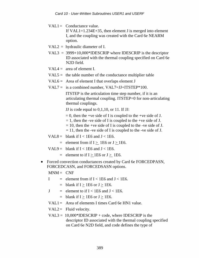
Card 10 - User-Written Subroutines USER1 and USERF
389
VAL1 = Conductance value. If VAL1=1.234E+35, then element J is merged into element I, and the coupling was created with the Card 6e NEARM option.
VAL2 = hydraulic diameter of I. VAL3 = 3999+10,000*IDESCRIP where IDESCRIP is the descriptor
ID associated with the thermal coupling specified on Card 6e N2D field.
VAL4 = area of element I. VAL5 = the table number of the conductance multiplier table VAL6 = Area of element I that overlaps element J VAL7 = is a combined number, VAL7=JJ+ITSTEP*100.
ITSTEP is the articulation time step number, if it is an articulating thermal coupling. ITSTEP=0 for non-articulating thermal couplings. JJ is code equal to 0,1,10, or 11. If JJ: = 0, then the +ve side of I is coupled to the +ve side of J. = 1, then the -ve side of I is coupled to the +ve side of J. = 10, then the +ve side of I is coupled to the -ve side of J. = 11, then the -ve side of I is coupled to the -ve side of J.
VAL8 = blank if I < 1E6 and J < 1E6. = element from if I > 1E6 or J > 1E6. VAL9 = blank if I < 1E6 and J < 1E6. = element to if I > 1E6 or J > 1E6.
• Forced convection conductances created by Card 6e FORCEDPASN, FORCEDCASN, and FORCEDSASN options. MNM = CNF I = element from if I < 1E6 and J < 1E6. = blank if I > 1E6 or J > 1E6. J = element to if I < 1E6 and J < 1E6. = blank if I > 1E6 or J > 1E6. VAL1 = Area of elements I times Card 6e HN1 value. VAL2 = Fluid velocity. VAL3 = 10,000*IDESCRIP + code, where IDESCRIP is the
descriptor ID associated with the thermal coupling specified on Card 6e N2D field, and code defines the type of

Card 10 - User-Written Subroutines USER1 and USERF
390
conductance and the relative vertical relationships of elements I and J. code may be:
= 3836 for the FORCEDPASN option, if the element convects from the top surface
= 3837 for the FORCEDCASN option = 3838 for the FORCEDSASN option
VAL4 = characteristic length for the FORCEDPASN option = diameter FORCEDCASN and FORCEDSASN options VAL5 = 0 VAL6 = Material ID of fluid VAL7 = 0 as a rule = 1 for the BOTTOM option of the FORCEDPASN option VAL8 = blank if I < 1E6 and J < 1E6. = element from if I > 1E6 or J > 1E6. VAL9 = blank if I < 1E6 and J < 1E6. = element to if I > 1E6 or J > 1E6.
• Forced Convection Conductances created by Card 6e NEARC1, NEARC4, NEARC12 options. MNM = CNF I = element from if I < 1E6 and J < 1E6, must be non-hydraulic
element. = blank if I > 1E6 or J > 1E6. J = element to if I < 1E6 and J < 1E6. = blank if I > 1E6 or J > 1E6. VAL1 = Overlapping area of elements I and J times Card 6e HN1
value. VAL2 = hydraulic diameter of I. VAL3 = conductance type code+10,000*IDESCRIP where
IDESCRIP is the descriptor ID associated with the thermal coupling specified on Card 6e N2D field. The conductance type code may be:
= 3000 NEARC1 DUCT flow. = 3001 NEARC1 DUCT flow for beam element. = 3002 NEARC1 DUCT flow for lump mass element. = 3003 NEARC4 Flat plate in free stream.
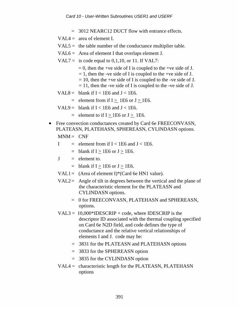
Card 10 - User-Written Subroutines USER1 and USERF
391
= 3012 NEARC12 DUCT flow with entrance effects. VAL4 = area of element I. VAL5 = the table number of the conductance multiplier table. VAL6 = Area of element I that overlaps element J. VAL7 = is code equal to 0,1,10, or 11. If VAL7:
= 0, then the +ve side of I is coupled to the +ve side of J. = 1, then the -ve side of I is coupled to the +ve side of J. = 10, then the +ve side of I is coupled to the -ve side of J. = 11, then the -ve side of I is coupled to the -ve side of J.
VAL8 = blank if I < 1E6 and J < 1E6. = element from if I > 1E6 or J > 1E6. VAL9 = blank if I < 1E6 and J < 1E6. = element to if I > 1E6 or J > 1E6.
• Free convection conductances created by Card 6e FREECONVASN, PLATEASN, PLATEHASN, SPHEREASN, CYLINDASN options. MNM = CNF I = element from if I < 1E6 and J < 1E6. = blank if I > 1E6 or J > 1E6. J = element to. = blank if I > 1E6 or J > 1E6. VAL1 = (Area of element I)*(Card 6e HN1 value). VAL2 = Angle of tilt in degrees between the vertical and the plane of
the characteristic element for the PLATEASN and CYLINDASN options.
= 0 for FREECONVASN, PLATEHASN and SPHEREASN, options.
VAL3 = 10,000*IDESCRIP + code, where IDESCRIP is the descriptor ID associated with the thermal coupling specified on Card 6e N2D field, and code defines the type of conductance and the relative vertical relationships of elements I and J. code may be:
= 3831 for the PLATEASN and PLATEHASN options = 3833 for the SPHEREASN option = 3835 for the CYLINDASN option
VAL4 = characteristic length for the PLATEASN, PLATEHASN options

Card 10 - User-Written Subroutines USER1 and USERF
392
= diameter for SPHEREASN and CYLINDASN options VAL5 = 0 = 0 for SPHEREASN, CYLINDASN options VAL6 = Material ID of fluid VAL7 = is 0 as a rule = 1 for the BOTTOM option of the PLATEASN and
PLATEHASN options VAL8 = blank if I < 1E6 and J < 1E6. = element from if I > 1E6 or J > 1E6. VAL9 = blank if I < 1E6 and J < 1E6. = element to if I > 1E6 or J > 1E6.
• Free Convection Conductances created by Card 6e NEARF and FREE options MNM = CNF I = element from if I < 1E6 and J < 1E6. = blank if I > 1E6 or J > 1E6. J = element to if I < 1E6 and J < 1E6. = blank if I > 1E6 or J > 1E6. VAL1 = Overlapping area of elements I and J times Card 6e HN1
value. VAL2 = Free convection exponent. VAL3 = 10,000*IDESCRIP where IDESCRIP is the descriptor ID
associated with the thermal coupling specified on Card 6e N2D field.
VAL4 = area of element I. VAL5 = ignored. VAL6 = Area of element I that overlaps element J. VAL7 = is code equal to 0,1,10, or 11. If VAL7:
= 0, then the +ve side of I is coupled to the +ve side of J. = 1, then the -ve side of I is coupled to the +ve side of J. = 10, then the +ve side of I is coupled to the -ve side of J. = 11, then the -ve side of I is coupled to the -ve side of J.
VAL8 = blank if I < 1E6 and J < 1E6. = element from if I > 1E6 or J > 1E6. VAL9 = blank if I < 1E6 and J < 1E6.

Card 10 - User-Written Subroutines USER1 and USERF
393
= element to if I > 1E6 or J > 1E6. • Free Convection Conductances created by Card 6e NEARC6, NEARC9,
NEARC10, NEARC16, NEARC19, NEARCIN, and NEARCOUT options. MNM = CNF I = element from if I < 1E6 and J < 1E6, must be non-hydraulic
element. = blank if I > 1E6 or J > 1E6. J = element to if I < 1E6 and J < 1E6. Except for NEARC10, J is
a hydraulic element. = blank if I > 1E6 or J > 1E6. VAL1 = Overlapping area of elements I and J times Card 6e HN1
value. VAL2 = hydraulic diameter. VAL3 = Code defining type of conductance, type of characteristic
element, angle of tilt, and relative vertical positions of elements I and J.
= 3104 NEARC9 Horizontal plate, downward facing. Element J is above element I.
= 3105 NEARC10 Vertical recirculating cavity. = 3106 NEARC10 Horizontal recirculating cavity. Element J is
above element I. = 3109 – 3199 NEARC6. Characteristic length is calculated
from geometry of characteristic plate element. Element J is above element I. The angle between the vertical and its projection onto the plate is VAL3–3109 degrees.
= 3209 – 3299 NEARC6. Characteristic length is calculated from geometry of characteristic beam element. Element J is above element I. The angle of axis of the beam element from the vertical is VAL3 – 3209 degrees.
= 3304 NEARC9 Horizontal plate, downward facing. Element I is above element J.
= 3306 NEARC10 Horizontal recirculating cavity. Element I is above element J.
= 3309-3399 NEARC6 Characteristic length is calculated from geometry of characteristic plate element. Element I is above element J. The angle of between the vertical and its projection onto the plate is VAL3-3309 degrees.

Card 10 - User-Written Subroutines USER1 and USERF
394
= 3409-3499 NEARC6 Characteristic length is calculated from geometry for characteristic beam element. Element I is above element J. The angle of the beam element from the vertical is VAL3-3409 degrees.
= 3509-3599 NEARC16 Characteristic length is calculated from geometry for characteristic plate element. The relative vertical positions of elements I and J are ignored. The angle between the vertical and its projection onto the plate is VAL3-3509 degrees.
= 3609-3699 NEARC16 Characteristic length is calculated from geometry for beam. The relative vertical positions of elements I and J are ignored. The angle between the vertical and its projection onto the plate is VAL3-3609 degrees.
VAL4 = area of element I. VAL5 = characteristic length. VAL6 = Area of element I that overlaps element J VAL7 = is code equal to 0,1,10, or 11. If VAL7:
= 0, then the +ve side of I is coupled to the +ve side of J. = 1, then the -ve side of I is coupled to the +ve side of J. = 10, then the +ve side of I is coupled to the -ve side of J. = 11, then the -ve side of I is coupled to the -ve side of J.
VAL8 = blank if I < 1E6 and J < 1E6. = element from if I > 1E6 or J > 1E6. VAL9 = blank if I < 1E6 and J < 1E6. = element to if I > 1E6 or J > 1E6.
• Free Convection Conductances created by Card PLATE, PLATEH, SPHERE, CYLINDER, INCCHNL, CAVITY, CAVITYH, CONCYL, and CONSPH options MNM = CNF I = element from if I < 1E6 and J < 1E6, must be non-hydraulic
element. = blank if I > 1E6 or J > 1E6. J = element to if I < 1E6 and J < 1E6. For PLATE, PLATEH,
SPHERE, CYLINDER options element J is a hydraulic element.
= blank if I > 1E6 or J > 1E6. VAL1 = Overlapping area of elements I and J times Card 6e HN1
value.

Card 10 - User-Written Subroutines USER1 and USERF
395
VAL2 = Angle of tilt in degrees between the vertical and the plane of the characteristic element for PLATE, CYLINDER, INCCHNL, and CAVITY options.
= 0 for PLATEH, SPHERE, CAVITYH, CONCYL, CONSPH options.
VAL3 = 10,000*IDESCRIP + code, where IDESCRIP is the descriptor ID associated with the thermal coupling specified on Card 6e N2D field, and code defines the type of conductance and the relative vertical relationships of elements I and J. code may be: = 3821 for the PLATE and PLATEH options, if the element convects from the top surface
= 3841 for the PLATE and PLATEH options, if the element convects from the bottom surface
= 3803 for the SPHERE option = 3804 for the CYLINDER option = 3805 for the INCCHNL option = 3806 for the CAVITY and CAVITYH options = 3808 for the CONCYL option = 3809 for the CONSPH option VAL4 = characteristic length for the PLATE, PLATEH options = diameter for SPHERE and CYLINDER options = spacing for the CAVITY, CAVITYH, INCCHNL options = smaller diameter for CONCYL and CONSPH options VAL5 = 1 for TOP and =2 for BOTTOM options of PLATE and
PLATEH = 0 for SPHERE, CYLINDER and CAVITYH options = larger diameter for CONCYL, CONSPH options = length for INCCHNL and CAVITY options VAL6 = The material number of the convecting fluid for the PLATE,
PLATEH, SPHERE, CYLINDER, INCCHNL CAVITY, CAVITYH, CONCYL, and CONSPH options.
VAL7 = is code equal to 0,1,10, or 11. If VAL7: = 0, then the +ve side of I is coupled to the +ve side of J. = 1, then the -ve side of I is coupled to the +ve side of J. = 10, then the +ve side of I is coupled to the -ve side of J. = 11, then the -ve side of I is coupled to the -ve side of J.

Card 10 - User-Written Subroutines USER1 and USERF
396
VAL8 = blank if I < 1E6 and J < 1E6. = element from if I > 1E6 or J > 1E6. VAL9 = blank if I < 1E6 and J < 1E6. = element to if I > 1E6 or J > 1E6.
• CFD conductances - created the Card 6e NEARC21-4, NEARC41-4 options MNM = CNF I = element from if I < 1E6 and J < 1E6, board or component
element. = blank if I > 1E6 or J > 1E6. J = element to if I < 1E6 and J < 1E6, CFD element. = blank if I > 1E6 or J > 1E6. VAL1 = Overlapping area of element I times HN1 value. VAL2 = roughness coefficient. VAL3 = code defining the type of conductance
= 3921 board to fluid conductance is specified with Card 6e NEARC21 option.
= 3922 board to fluid conductance is specified with Card 6e NEARC22 option.
= 3923 board to fluid conductance is specified with Card 6e NEARC23 option.
= 3924 board to fluid conductance is specified with Card 6e NEARC24 option.
= 3941 board to fluid conductance is specified with Card 6e NEARC41 option.
= 3942 board to fluid conductance is specified with Card 6e NEARC42 option.
= 3943 board to fluid conductance is specified with Card 6e NEARC43 option.
= 3944 board to fluid conductance is specified with Card 6e NEARC44 option.
VAL4 = code for evaluating the heat transfer coefficient - same as N1D code on Card 6e
VAL5 = table number for table multiplier. VAL6 = area of element I that overlaps element J. VAL7 = code equal to 0,1,10, or 11. If VAL7:
= 0, then the +ve side of I is coupled to the +ve side of J.

Card 10 - User-Written Subroutines USER1 and USERF
397
= 1, then the -ve side of I is coupled to the +ve side of J. = 10, then the +ve side of I is coupled to the -ve side of J. = 11, then the -ve side of I is coupled to the -ve side of J
VAL8 = blank if I < 1E6 and J < 1E6. = element from if I > 1E6 or J > 1E6. VAL9 = blank if I < 1E6 and J < 1E6. = element to if I > 1E6 or J > 1E6.
• Conductive Conductances created by the COND module MNM = CON I = element from if I < 1E6 and J < 1E6. = blank if I > 1E6 or J > 1E6. J = element to if I < 1E6 and J < 1E6. = blank if I > 1E6 or J > 1E6. VAL1 = conductance value. VAL2 = element number from which the conductances were
calculated, if element CG method was used. VAL3 = blank if I < 1E6 and J < 1E6. = element from if I > 1E6 or J > 1E6. VAL4 = blank if I < 1E6 and J < 1E6. = element to if I > 1E6 or J > 1E6.
• One-way Conductive Conductances created by the COND module MNM = CON I = blank J = blank VAL1 = conductance value. VAL2 = 0 VAL3 = downstream element number VAL4 = negative of upstream element number
• Radiative Conductances created by GRAYB module MNM = RAD I = element from if I < 1E6 and J < 1E6. = blank if I > 1E6 or J > 1E6. J = element to if I < 1E6 and J < 1E6. = blank if I > 1E6 or J > 1E6.

Card 10 - User-Written Subroutines USER1 and USERF
398
VAL1 = area*emissivity of element I*gray body view factor between I and J.
VAL2 = 1.0. VAL3 = 1.0. VAL4 = 1.0. VAL5 = -1.E36 if non-articulating radiative couplings. For
articulating radiative couplings VAL5 is the TIME value when the coupling occurs.
VAL6 = blank if I < 1E6 and J < 1E6. = element from if I > 1E6 or J > 1E6. VAL7 = blank if I < 1E6 and J < 1E6. = element to if I > 1E6 or J > 1E6.
• Radiative Thermal Couplings created by VUFAC module MNM = RAD I = element from if I < 1E6 and J < 1E6. = blank if I > 1E6 or J > 1E6. J = element to if I < 1E6 and J < 1E6. = blank if I > 1E6 or J > 1E6. VAL1 = area of element I. VAL2 = emissivity of element I. VAL3 = -12300 if the positive side of I is coupled to the positive side
of J. VAL3 = -12301 if the negative side of I is coupled to the positive side
of J. VAL3 = -12310 if the positive side of I is coupled to the negative side
of J. VAL3 = -12311 if the negative side of I is coupled to the negative
side of J. VAL4 = gray body view factor. VAL5 = -1.E36 VAL6 = blank if I < 1E6 and J < 1E6. = element from if I > 1E6 or J > 1E6. VAL7 = blank if I < 1E6 and J < 1E6. = element to if I > 1E6 or J > 1E6.
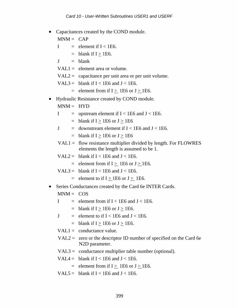
Card 10 - User-Written Subroutines USER1 and USERF
399
• Capacitances created by the COND module. MNM = CAP I = element if I < 1E6. = blank if I > 1E6. J = blank VAL1 = element area or volume. VAL2 = capacitance per unit area or per unit volume. VAL3 = blank if I < 1E6 and J < 1E6. = element from if I > 1E6 or J > 1E6.
• Hydraulic Resistance created by COND module. MNM = HYD I = upstream element if I < 1E6 and J < 1E6. = blank if I > 1E6 or J > 1E6 J = downstream element if I < 1E6 and J < 1E6. = blank if I > 1E6 or J > 1E6 VAL1 = flow resistance multiplier divided by length. For FLOWRES
elements the length is assumed to be 1. VAL2 = blank if I < 1E6 and J < 1E6. = element from if I > 1E6 or J > 1E6. VAL3 = blank if I < 1E6 and J < 1E6. = element to if I > 1E6 or J > 1E6.
• Series Conductances created by the Card 6e INTER Cards. MNM = COS I = element from if I < 1E6 and J < 1E6. = blank if I > 1E6 or J > 1E6. J = element to if I < 1E6 and J < 1E6. = blank if I > 1E6 or J > 1E6. VAL1 = conductance value. VAL2 = zero or the descriptor ID number of specified on the Card 6e
N2D parameter. VAL3 = conductance multiplier table number (optional). VAL4 = blank if I < 1E6 and J < 1E6. = element from if I > 1E6 or J > 1E6. VAL5 = blank if I < 1E6 and J < 1E6.

Card 10 - User-Written Subroutines USER1 and USERF
400
= element to if I > 1E6 or J > 1E6.
MSGF or MSGF.dat • MSGF contains all the program messages.
nevada.ren • nevada.ren contains the NEVADA format output file. nevada.ren is
created by the REFORM module when a Card 9 PARAM NEVADA Card is present.
POWERDENSITY • POWERDENSITY contains the power dissipation density of electrical
elements (if they exist) in TEMPF format. See Card 9 TABTYPE Card description.
POWERDENSITY.unv • POWERDENSITY.unv contains the power dissipation density of
electrical elements (if they exist) in NX universal file format.
PRESSF • PRESSF contains the computed total pressure PT(I) and mass flow
values MASSFL(I) for all the hydraulic elements in the model. • Data is written in format:
(I7,2E15.7)
and the data fields contain I, PT(I), MASSFL(I) for element I. • If I = -99999, then PT(I) represents the printout time. • If a Card 9 PSINK FPRESSF Card is present, all the hydraulic
elements are defined to be PSINK elements, with the constant pressures and constant mass flows read from file PRESSF.
QNODEF • QNODEF is an output file that contains elemental heat inputs. Its
format is identical to that of file TEMPF. • QNODEF is created by the Analyzer at each printout interval.

Card 10 - User-Written Subroutines USER1 and USERF
401
REPF • REPF contains details of calculations. • REPF is always appended to.
sinda85.dat • sinda85.dat is a SINDA85 format output file created if Card 9 PARAM
SINDA85 is specified.
TEMPF • File TEMPF contains the calculated temperatures at the end of a run.
The Analyzer writes data on TEMPF at the printout intervals defined by the Card 2b DTP parameter. Alternatively, other software may create TEMPF. e.g. SINDA, for post-processing by TMG.
• TEMPF is used for post-processing by the TMGINT, FRONT, and REFORM modules.
• Data is written on TEMPF in format: (I10,1PE23.15)
• If at the start of a run a file TEMPF is present, its data is used as the initial temperatures. If Card 9 TINIT Cards are also present, the temperatures of the TINIT Cards override those of file TEMPF. If it is not present, or contains an incomplete set of data, the Analyzer for the undefined elements assumes zero initial temperatures.
I, TEMP(I)
I is the element number. TEMP(I) is the temperature of element I. If I is -99999, TEMP(I) is the printout time value for subsequent temperatures.
tmggeom.dat • tmggeom.dat is a binary file that contains information about the
geometrical and other parameters of the model. • If restarts are performed tmggeom.dat should be present.
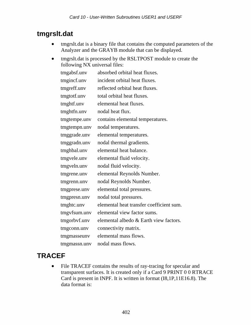
Card 10 - User-Written Subroutines USER1 and USERF
402
tmgrslt.dat • tmgrslt.dat is a binary file that contains the computed parameters of the
Analyzer and the GRAYB module that can be displayed. • tmgrslt.dat is processed by the RSLTPOST module to create the
following NX universal files: tmgabsf.unv absorbed orbital heat fluxes. tmgincf.unv incident orbital heat fluxes. tmgreff.unv reflected orbital heat fluxes. tmgtotf.unv total orbital heat fluxes. tmghtf.unv elemental heat fluxes. tmghtfn.unv nodal heat flux. tmgtempe.unv contains elemental temperatures. tmgtempn.unv nodal temperatures. tmggrade.unv elemental temperatures. tmggradn.unv nodal thermal gradients. tmghbal.unv elemental heat balance. tmgvele.unv elemental fluid velocity. tmgveln.unv nodal fluid velocity. tmgrene.unv elemental Reynolds Number. tmgrenn.unv nodal Reynolds Number. tmgprese.unv elemental total pressures. tmgpresn.unv nodal total pressures. tmghtc.unv elemental heat transfer coefficient sum. tmgvfsum.unv elemental view factor sums. tmgorbvf.unv elemental albedo & Earth view factors. tmgconn.unv connectivity matrix. tmgmasseunv elemental mass flows. tmgmassn.unv nodal mass flows.
TRACEF • File TRACEF contains the results of ray-tracing for specular and
transparent surfaces. It is created only if a Card 9 PRINT 0 0 RTRACE Card is present in INPF. It is written in format (I8,1P,11E16.8). The data format is:

Card 10 - User-Written Subroutines USER1 and USERF
403
IEL,VAL1,VAL2,VAL3,VAL4,VAL5,VAL6,VAL7,VAL8
• IEL is the element number that is hit. If IEL=0, and VAL1 = -99990, then VAL2 is the time value for the following trace.
• VAL1 is the strength of the ray in the solar spectrum • VAL2 is the strength of the ray in the IR spectrum • VAL3 is the optical path length for the ray from its origin. • VAL4 is the total distance the ray has traveled. • VAL5 is the X-coordinate of the ray where it hits. • VAL6 is the Y-coordinate of the ray where it hits. • VAL7 is the Z- coordinate of the ray where it hits. • VAL8 is the value of the index of refraction of the element it hits.
voltages.unv • voltages.unv is a universal file created by the Analyzer whenever
electrical elements are present.
VUFF • VUFF contains the model geometry elemental properties written by
ECHOS, the view factors, hat flux view factors solar view factors, albedo factors, and Earth view factors written by VUFAC, and the IR and solar spectrum gray body view factor matrices written by GRAYB. VUFF is always appended.
MNM, I, J, AR, E, TSA, VF, TIME, DD • MNM is the mnemonic code for the Card.
All Cards except for MNM = NGR, MNM = AXM, and MNM = RDF can be read with the format (A3,2I6,3E11.4,F11.7,2E11.4) = AXM for expansion of axisymmetric profile elements written by the
DATACH module. MNM = AXM can be read with the format (A3,10I6)
= ALB for albedo factors written by the VUFAC module. = ALR for albedo factors calculated with ray-tracing written by the
VUFAC module

Card 10 - User-Written Subroutines USER1 and USERF
404
= BVF for view factors written by the VUFAC module. = EVF for Earth view factors written by the VUFAC module. = EVR for Earth view factors calculated with ray-tracing written by the
VUFAC module = GRD for node coordinates X, Y, Z written by the ECHOS module. = HVF for solar spectrum heat flux view factors written by the VUFAC
module. = HVI for IR spectrum heat flux view factors written by the VUFAC
module. = IGM for the IR spectrum gray body view factor matrix. = NCC for the element center for circular elements written by the
ECHOS module. = NCG for the element's C.G written by the ECHOS module. = NDC for the element center for non-circular elements written by the
ECHOS module. = NGR for the node numbers for an element written by the ECHOS
module. MNM = NGR can be read with the format (A3,10I6)
= NPR for the elemental properties written by the ECHOS module. = NRM for the element's surface normal written by the ECHOS
module. For beam elements NRM is the axial unit vector pointing from node 1 to node 2.
= SVF for solar view factors written by the VUFAC module. = SGM for the solar spectrum gray body view factor matrix. = RDF for run definition Cards.
At the start of each run, a run definition Card written by the MAIN module containing the run title and date is written in the format ('RDF',A80) The Card 9 NAME group names, starting element, increment, and ending element, and group name number are written on file VUFF by the DATACH module with the format ('RDFGROUPNAMES',1X,A7,I9,I12,2I10) The Card 9 VARIABLE symbolic variable names and values are written on file VUFF by the DATACH module with the format ('RDFVARIABLENAME',1X,A31,E15.8)
Card 10 - User-Written Subroutines USER1 and USERF
405
= REV for reverse elements written by the DATACH module. • I is:
= element from, or = blank for nodes. = the profile element number for MNM = AXM.
• J is: = blank, or = element to, or = element number of the radiative source for heat flux view factors, or = node number for GRD. = the number of nodes for NGR. = the first expanded element number for MNM = AXM. The fourth
field represents the last expanded element number, and the fifth field represents the increment.
= the reverse element number for MNM = REV. • AR is:
= area or volume of element I, or = X coordinate for GRD, NDC, NCG, NCC, or NRM.
• E is: = emissivity of element I.
If E= -2.34, the element is recognized by the VUFAC module for area-proportional conductance calculations, but not for radiation. If E < 0, it is not recognized by the VUFAC module at all. If E =-1.23, it is assigned an area =0.
= Y coordinate for GRD, NDC, NCG, or NRM. • TSA is:
= TSA parameter (combined radiative solar spectrum property) of element I. = Z coordinate for GRD, NDC, NCG, NCC, or NRM.
• VF is: = view factor from I to J if MNM = BVF and MNM = HVF and TIME
= -1.E36 = gray body view factor from I to J if MNM = SGM or IGM

Card 10 - User-Written Subroutines USER1 and USERF
406
= solar view factor if MNM = SVF = albedo factor if MNM = ALB = Earth view factor if MNM = EVF = thermal conductivity times cross-sectional area, or thermal
conductivity times thickness, or thermal conductivity (for solid elements) of element I if MNM = NPR
= -1E30 if MNM = NPR for elements that are the reverse sides of other elements created by the Card 9 REVNODE Card, and for SPACE elements created with Card 5d. This ensures that follower conductances are created to recover the temperatures of these elements after they are merged. If VF < -1.E28, and MNM=NPR, then the element I is not recognized by the COND module for conduction calculations.
• TIME is: = time at which the view factor (MNM = BVF), solar view factor (MNM = SVF), Earth view factor (MNM = EVF), heat flux view factor (MNM = HVF), or albedo factor (MNM = ALB) occurs. TIME is = -1.E36, -1.1E36, or -1.2E36 for view factors (MNM = BVF) that will be used only for radiative conductance and gray body view factor calculations and are constant over time. TIME = -1.1E36 on a BVF Card is a flag indicates that the view factor was calculated with ray-tracing using the solar spectrum surface properties. The value in the AR field is equal to the area of the element multiplied by the factor (1-solar spectrum specularity/transparency). The values in the E and TSA fields are equal to the emissivity and absorptivity of the element divided by the factor 1/(1-solar spectrum specularity/transparency) respectively. If no IR spectrum properties were specified for the model, the view factors of this Card are considered valid for both the solar and IR spectra. If IR spectrum properties were calculated for the model, the view factors of this Card are considered valid for the solar spectrum only. TIME = -1.2E36 is a flag indicates that the view factor was calculated with ray-tracing using the IR spectrum surface properties. The value in the AR field is equal to the area of the element multiplied by the factor (1-IR spectrum specularity/transparency). The values in the E and TSA fields are equal to the emissivity and absorptivity of the element divided by the factor 1/(1-IR spectrum specularity/transparency) respectively.

Analyzer Module
407
Section 3: Modules Analyzer Module Function
The Analyzer module calculates state or transient temperatures and total pressures for thermal/hydraulic models. Heat paths are specified as thermal conductances, fluid flow paths as flow resistances. Boundary conditions specified are elemental heat loads, mass flows, sink temperatures, and total pressures. Parameters may be varied during solution time through table interpolation and with user–written FORTRAN subroutines. The Analyzer is run if a Card 2b Analyzer Control Card is present.
Steady State Analysis
If Card 2b GRADNT ≥ 0, steady state analysis is performed. The temperatures of non–sink elements are calculated iteratively. The flowchart of the steady-state algorithm is as follows:

Analyzer Module
408
Steady State Analysis Flowchart
Initialize model parameters, set iteration number n=0 Step 1
Solve hydraulic network for total pressures Step 2
Calculate conductances Gij,n Step 3
Table interpolation for heat inputs, temperature boundary conditions, and conductances Step 4
Add thermostat-controlled heat inputs Step 5
Increase iteration count to n+1 Step 6
Modify temperature-dependent orthotropic conductances Step 7
Add series conductances to conductances Step 8
Enter subroutine USER1 with KODE=1 to modify heat inputs, temperature boundary
conditions, and conductances Step 9

Analyzer Module
409
If printout flag is ON, recover substructured temperatures and print Step 13
Completion, print results. Step 17
Solve for temperatures Ti,n+1 Step 11
Perform heater sizing calculations Step 10
Enter subroutine USER1 with KODE=2 to modify temperatures Step 12
Yes, set IRUN=IRUN+1,
go to Step 2 Multiple runs?
No
Step 15
No, go to Step 2 Run
converged or iteration limit exceeded?
Yes
Step 14
Yes, IRUN=IRUN+1,
go to Step 2 Multiple runs?
No
Step 16
Enter USER1 with KODE=3
Step 14
Step 15

Analyzer Module
410
Step 1: Initialization
Initial values are assigned to all the element temperatures, conductances, and heat inputs. The initial temperatures default to zero unless a file TEMPF is present, or initial temperatures have been specified with Card 9 TINIT Cards, in which case these define the initial temperatures. For multilayer elements, the layer temperatures are initialized to the temperature of the middle layer. The temperatures of unitialized Oppenheim elements are initialized at the average temperature of the elements the Oppenheim element is connected to. If the element CG method is used, the boundary element temperatures are initialized to the weighted average temperatures of the elements they are connected to. For details on initialization of hydraulic elements, please refer to the Hydraulic Elements section. Time t at the start of the run is defined by the Card 2b TST parameter. If Card 9 PARAM USRCNDADD is present, the user-written subroutine is entered with KODE=5. At this time, you can add new conductances to the conductance matrix. If the element CG method is used, large negative conductances are modified according to the values set by Card 9 PARAM MODCOND.
Step 2: Calculation of Total Pressures for Hydraulic Elements Total pressures of hydraulic elements are calculated for the current iteration (please refer to the Hydraulic Elements section).
Step 3: Calculation of Conductances Convective and free convection conductances associated with hydraulic elements are updated as described in the Hydraulic Elements section. One-way conductances for hydraulic networks are updated by multiplying the mass flow values flowing through DUCT and FLOWRES elements with the specific heat. Conductive conductances for hydraulic elements are calculated from the CG to the boundary.
LKTHERMAG DUCT2
=

Analyzer Module
411
where: G is the conductance from the CG to the boundary ADUCT is the duct cross-section L is the length of the duct KTHERM is the thermal conductivity of the fluid
Free convection conductances specified on Card 6e and not associated with hydraulic elements are calculated with:
G GF T Tij n ij i n j nEXP
, , ,( )= −
where: Gij,n is the value of the conductance between elements i and j at iteration n i,n refers to the property of element i at iteration n Ti,n is the temperature of element i at iteration n Tj,n is the temperature of element j at iteration n GFij is the free convection conductance parameter EXP is the specified exponent
Step 4: Table Interpolation Next, linear table interpolations are performed. Heat inputs, SINK temperatures, and table-dependent conductances are evaluated. For further details please refer to Card 9 INTERP, TABDATA, and TABTYPE Cards. If the independent variable is greater than the largest value in the table, the last dependent variable is used, and a warning message is issued. If the independent variable is greater than the smallest value in the table, the first dependent variable is used. In other words, the first and last values of the table are extended beyond the table limits. If electrical elements are present, the electrical network is solved for voltage and current. The power dissipation in the electrical network is computed and summed with other heat inputs specified for the electrical elements. For further details please refer to the Card 9 TABTYPE Card. If the Card 9 PARAM CAPDIST OFF Card is not present, and the default element CG formulation is used, then the heat loads on solid elements are redistributed from the CG to the boundary elements. For tetrahedra, a uniform weighting factor is used. For wedges and hexahedra, the weighting factors are proportional to the areas of the boundary elements.

Analyzer Module
412
Step 5: Add Thermostat-controlled Heat Inputs Thermostats are transformed into proportional controllers. For proportional controllers, the heat input Q to the heaters follows the following relationship:
2)1(
3)1(223
))1(3(3)1(0
TNTQHTRQ
TNTTTT
NTTQHTRQ
TNTQ
<=
≥≥−
−=
>=
where: T(N1) is the sensor temperature QHTR is the maximum heater power T3 is the cut-out temperature for the proportional controller T2 is the cut-in temperature of the heater
Step 6: Increase Iteration Count to n+1
Step 7: Modify Temperature-dependent Orthotropic Conductances If orthotropic materials are present, all conductances associated with orthotropic elements are recalculated, provided the maximum temperature change of an orthotropic element has not exceeded 20 degrees. This value can be set with the Card 9 PARAM TDEPORTHO Card.
Step 8: Series Conductances If series or interface conductances (Card 6e INTER, INTERTOT, INTER2, INTER2TOT Card) are present the conductances the interface element is connected to are modified.
Step 9: Entering USER1 with KODE = 1 Next, the optional user–written subroutine USER1 is entered with KODE = 1. You can modify conductances, heat loads, etc. before calculating temperatures. For further details, please refer to Card 10 User–Written Subroutine.

Analyzer Module
413
Step 10: Perform Heater Sizing Calculations If a Card 9 THERMST Card is present, and if the T1 is the code Q_EQUIV, then a sensitivity analysis is performed to calculate the heater heat loads required to keep the sensors at the average of the Thigh and Tlow temperatures specified on the THERMST Card.
Step 11: Calculation of Temperatures The undamped temperature estimate Tiest,n+1 for iteration n+1 is calculated according to the method outlined in the section on the conjugate gradient solver below. Next, the temperatures Ti,n+1 for all elements i for the next iteration n+1 are computed with damping from Tiest,n+1.
T DT T T DTi n i n iest n, , ,( )+ += − +1 11
where: DT is the iteration damping factor from Card 2b, default = 0.5. Tiest,n+1 is the temperature estimate at iteration n+1 calculated with the CG solver.
Sink element and MCV element temperatures are not altered. Sink element temperatures may be altered through table interpolation or in USER1.
Step 12: Entering USER1 with KODE = 2: Once temperatures are calculated, USER1 is entered with KODE = 2. This gives the option to alter some of the calculated temperatures. For further details, please refer to Card 10 User–Written Subroutine.
Step 13: Printout and Recovery of Eliminated Element Temperatures Next, a check is made to determine whether the printout flag is set. The printout flag is set either with the Card 2b DTP parameter or through PRTFLG in USER1. If the printout flag and substructuring are performed through Card 8 element elimination or Card 9 PARAM SUBSTR Cards, the temperatures of the eliminated elements are recovered. The temperature recovery matrix is read in from file MODLCRF, and the heat loads of the eliminated elements are redistributed in the order the elements were eliminated, according to the method described in the section on the MEREL Module. Then, the temperatures Ti,n+1 of each eliminated elements i are computed in the reverse order they were eliminated. Next, printout is performed according to the specifications of Card 9 PRINT Cards. At every printout a set of results are written on files QNODEF, REPF, PRESSF, TEMPF, tmgrslt.dat and MSGF.

Analyzer Module
414
Step 14: Convergence Check Next, a run completion check is performed. A run is considered completed if the maximum number of iterations (defined on Card 2b TF parameter) is exceeded, or if convergence occurs. Convergence occurs if the maximum temperature difference between two subsequent iterations is less than the Card 2b GRADNT parameter, default = 0.001. If the Card 9 PARAM ENGBAL system energy balance criterion is set, this criterion must also be met for convergence to occur. For each sink element i a heat flow QSINKi is computed:
QSINK Q GTSUM T GSUMi n i n i n i n i n, , , , ,+ + + + += + −1 1 1 1 1
where: QSINKi,n+1 is the heat flowing into (or out of) the sink element i at iteration n+1. GSUMi,n is the sum of conductances Gij,n for element i. GTSUMi,n is the sum of the Tj,nGij,n for element i. GSUMCi,n is the sum of non-radiative conductances for element i GSUMRi,n is the sum of all GRij's for element i. GTSUMCi,n is the sum of the Tj,nGij,n for all non-radiative conductances for element i.
GTSUMRi,n is the sum of the Tj,n4GRij for all radiative conductances for element i. To satisfy the system energy balance criterion the following criterion must be met:
QSINK QSINK QTOT TIN OUT− − < 1
where: QSINKIN is the sum of the heat flows into the sink elements QSINKOUT is the sum of the heat flows out of the sink elements QTOT is the sum of the heat loads into the elements T1 is either an absolute value, defined on the Card 9 PARAM ENGBAL Card, or is a specified fraction of QSINKIN.
If convergence has not occurred, the cycle start again at Step 2.
Step 15: Enter USER1 with KODE = 3 for Multiple Runs Once the run is completed, USER1 is entered with KODE =3. At this time you can specify additional steady-state or transient runs by setting a flag in the array IR. For further details, please refer to Card 10 User-Written Subroutines.

Analyzer Module
415
If an additional run is specified, the program continues at Step 2 of either the steady state or transient algorithms. If there are subsequent runs, a printout on files TEMPFn, PRESSFn, and QNODEFn is created, where n is the run number.
Step 16: Completion If the run is completed, a final printout is performed.

Analyzer Module
416
Transient Analysis Flowchart
Initialize model parameters Step 1
Solve hydraulic network for total pressures Step 2
Add thermostat-controlled heat inputs Step 6
Enter subroutine USER1 with KODE=1 to modify heat inputs, temperature boundary
conditions, and conductances Step 9
Calculate conductances Gij,t Step 3
Calculate RCMIN, dt. If t≠TST and integration is implicit, set tcalc=t+dt. Otherwise set tcalc=t. Step 4
Table interpolation for heat inputs, temperature boundary conditions, and conductances at
t=tcalc Step 5
Modify temperature-dependent orthotropic conductances Step 7
Add series conductances to conductances Step 8

Analyzer Module
417
If printout flag is ON, recover substructured temperatures and print Step 14
Yes, set IRUN=IRUN+1,
go to Step 2
Completion, print results Step 18
Enter subroutine USER1 with KODE=2 to modify temperatures Step 13
Step 10
Printout, set tcalc=TST+dt
tcalc=TST?
Go to Step 5
Increment time to t+dt Step12
Yes
No
Multiple runs?
No
Step 17
No, go to Step 2 T=TF?
Yes
Step 15
Yes, IRUN=IRUN+1,
go to Step 2 Multiple runs?
No
Enter USER1 with KODE=3 Step 16
Solve for temperatures at Ti,t+dt Step11

Analyzer Module
418
Transient Analysis
If Card 2b GRADNT = –2, –3, –4, or –5, transient analysis is performed using the following algorithm:
Step 1: Initialization Initial values are assigned to all the element temperatures, conductances, and heat inputs. The initial temperatures default to zero unless a file TEMPF is present, or initial temperatures have been specified with Card 9 TINIT Cards, in which case these define the initial temperatures. For multilayer elements, the layer temperatures are initialized to the temperature of the middle layer. The temperatures of unitialized Oppenheim elements are initialized at the average temperature of the elements the Oppenheim element is connected to. If the element CG method is used, the boundary element temperatures are initialized to the weighted average temperatures of the elements they are connected to. For details on initialization of hydraulic elements, please refer to the Hydraulic Elements section. If Card 9 PARAM USRCNDADD is present, the user-written subroutine is entered with KODE=5. At this time, you can add new conductances to the conductance matrix. Time t at the start of the run is defined by the Card 2b TST parameter. If the element CG method is used, large negative conductances are modified according to the values set by Card 9 PARAM MODCOND. Conductive conductances for hydraulic elements are calculated from the CG to the boundary.
LKTHERMAG DUCT2
=
where: G is the conductance from the CG to the boundary ADUCT is the duct cross-section L is the length of the duct KTHERM is the thermal conductivity of the fluid

Analyzer Module
419
Step 2: Calculation of Total Pressures for Hydraulic Elements Total pressures of hydraulic elements are calculated for the current time step (please refer to the Hydraulic Elements section).
Step 3: Calculation of Conductances Convective and free convection conductances associated with hydraulic elements are updated as described in the Hydraulic Elements section. One-way conductances for hydraulic networks are updated by multiplying the mass flow values flowing through DUCT and FLOWRES elements with the specific heat. Free convection conductances specified on Card 6e and not associated with hydraulic elements are calculated with:
G GF T Tij t ij i t j tEXP
, , ,( )= −
where: Gij,t is the value of the conductance between elements i and j i,t refers to the property of element i at time t. Ti,t is the temperature of element i Tj,t is the temperature of element j GFij is the free convection conductance parameter EXP is the specified exponent
Step 4: Calculation of Integration Time Step dt, tcalc, and RCMIN Next, the integration time step dt is calculated, according to the specification of the Card 2b DT parameter.
• If DT > 0, dt is fixed at the value of DT
• If DT = 0, dt RCMIN=2
• If DT is < 0, dt DT RCMIN=2
where: RCMIN is the smallest value of in the model GSUMi,t is the sum of conductances Gij,t for element i.

Analyzer Module
420
Next, dt is checked to see if t + dt exceeds the time of the next printout interval, defined by the DTP and TF parameters of Card 2b. If t + dt is too large, dt is appropriately reduced. The parameter tcalc is defined. tcalc is the time value at which the heat loads and temperature boundary conditions are evaluated. For implicit methods when calculation the temperatures at time t+αdt, tcalc is t+αdt, where:
α is the explicit-implicit weighting factor, between 0 and 1.
For Crank-Nicolson α = .5, for forward and exponential forward differencing α = 0, and for backward differencing α = 1. When the initial values are to be printed, tcalc is set to TST.
Step 5: Table Interpolation at t=tcalc Next, linear table interpolations are performed. Heat inputs, SINK temperatures, and table-dependent conductances are evaluated. For further details please refer to Card 9 INTERP, TABDATA, and TABTYPE Cards. If the independent variable is greater than the largest value in the table, the last dependent variable is used, and a waning message is issued. If the independent variable is greater than the smallest value in the table, the first dependent variable is used. In other words, the first and last values of the table are extended beyond the table limits. If electrical elements are present, the electrical network is solved for voltage and current. The power dissipation in the electrical network is computed and summed with other heat inputs specified for the electrical elements. If series or interface conductances (Card 6e INTER Card) are present the appropriate conductance values are modified. If the Card 9 PARAM CAPDIST OFF Card is not present, and the default element CG formulation is used, then the heat loads and capacitances of solid elements are redistributed from the CG to the boundary elements. For tetrahedra, a uniform weighting factor is used. For wedges and hexahedra, the weighting factor are proportional to the areas of the boundary elements.
Step 6: Thermostats Next, if thermostats or PID controllers have been specified on Card 9 THERMST Cards, the heat load to each heater element is checked as to whether it should be zero or not. For PID controllers, the heat input Q to the heaters is calculated using the following equations:

Analyzer Module
421
QHTRQTdt
tdeTdtteTteTQHTRQ
NTTte
≤≤
+++=
−=
∫ 010)(9)(8)(7
)1(2)(
where: QHTR is the maximum heat input to the heaters. T2 is the controller’s set point T7 is the controller’s gain T8 is the integral constant T9 is the derivative constant T10 is the bias
For thermostats, a heater element is turned ON if the temperature Ti,t of the sensor element falls below the cut–in temperature of the thermostat. It is turned OFF if the sensor element temperature is above the cut–off temperature. If the sensor element temperature is between the cut–in and cut–off temperatures, the heater's ON/OFF status is not altered. For proportional controllers, the heat input Q to the heaters follows the following relationship:
2)1(
3)1(223
))1(3(3)1(0
TNTQHTRQ
TNTTTT
NTTQHTRQ
TNTQ
<=
≥≥−
−=
>=
where: T(N1) is the sensor temperature QHTR is the maximum heater power T3 is the cut-out temperature for the proportional controller T2 is the cut-in temperature of the heater
Step 7: Modify Temperature-dependent Orthotropic Conductances If orthotropic materials are present, all conductances associated with orthotropic elements are recalculated, provided the maximum temperature change of an orthotropic element has not exceeded 20 degrees.
Step 8: Series Conductances If series or interface conductances (Card 6e INTER, INTERTOT, INTER2, INTER2TOT Card) are present the conductances the interface element is connected to are modified.

Analyzer Module
422
Step 9: Entering USER1 with KODE = 1 Next, the optional user–written subroutine USER1 is entered with KODE = 1. You can modify conductances, heat loads, sink temperatures, and capacitances before calculating temperatures. For further details, please refer to Card 10 User–Written Subroutines.
Step 10: If tcalc=TST, initial printout is performed.
tcalc is then incremented to TST+αdt, and the program loops to Step 5 to recalculate boundary conditions.
Step 11: Calculation of Temperatures Next, the temperatures at time t + dt are calculated:
Explicit techniques (GRADNT = -2 and GRADNT = -3)
For the exponential forward differencing technique:
T T TEQ T e
TEQQ GTSUM
GSUMC
GSUM
i t dt i t i t i t
dt
i ti t i t
i t
i ti t
i t
i t, , , ,
,, ,
,
,,
,
( )( ),+
−
= + − −
=+
=
1 τ
τ
where:
τi,t is the time constant of the element TEQi,t is the equilibrium temperature the element would reach if all its neighboring element temperatures were constant. GSUMi,t is the sum of conductances Gij,t for element i at time t. GTSUMi,t is the sum of the Tj,tGij,t for element i at time t. GSUMCi,t is the sum of non-radiative conductances for element i at time t. GSUMRi,t is the sum of all GRij's for element i at time t. GTSUMCi,t is the sum of Tj,tGij,t for all non-radiative conductances for element i at time t.
GTSUMRi,t is the sum of the Tj,t4GRij for all radiative conductances for element i at time t. For the forward differencing technique:

Analyzer Module
423
T T TEQ T dti t dt i t i t i t
i t, , , ,
,
( )( )+ = + −τ
Implicit Techniques (GRADNT = –4 and GRADNT = –5)
For the implicit techniques all temperatures are calculated iteratively.
The implicit techniques are unconditionally stable if the explicit–implicit weighting factor α > .5. If the default conjugate gradient solver is used, Tiest,t+dt,n+1 is calculated using the technique described below, where:
Tiest,t+dt,n+1 is the estimated temperature of element i at iteration n+1 without damping calculated with the conjugate-gradient technique.
All parameters used at time t+dt are calculated using temperature and conductance values at iteration n. Next, damping is used to calculate the new set of temperatures:
T T TRDMP TRDMP Ti t dt n iest t dt n i t dt n, , , , , ,( )+ + + + += + −1 1 1
where: Ti,t+dt,n+1 is the temperature estimate of element i at iteration n+1 TRDMP is the transient damping parameter defined on Card 2b.
During iteration only the radiative conductances are updated, all other conductances are evaluated at t. The maximum number of iterations defaults to 100, and may be overridden on the Card 9 PARAM NLOOP Card. If the maximum number of iterations is reached, a warning message is written on file MSGF. If the Card 9 PRINT TRACE flag was set, the highlights of the current iteration are printed to the screen as well as to file REPF. Convergence is achieved when the maximum temperature difference between two subsequent iterations is less than the product TDIFS*TRDMP. TDIFS may be set on the Card 9 PARAM TDIFS Card, its default value = 0.001.
Initial temperature estimation for the implicit techniques
To accelerate convergence, the first iteration, Ti,t+dt,1 is estimated from the past behavior of the equilibrium temperature of the element.
T T TEQ TEQ dtdtpi t dt i t i t i t dtp, , , , , ,( )( )+ −= + −1 1
where:

Analyzer Module
424
dtp is the previous integration time step
Phase Change Calculations
Next, the temperatures of phase change elements modeled with Card 9 PHASE or MAT Cards are appropriately adjusted to account for the energy absorbed by the latent heat of absorption. For the explicit techniques this adjustment occurs at the completion of the first iteration only. For the implicit techniques it occurs at the completion of each iteration. The adjustment is as follows: 1. For each phase change element a quality QUALi,t+dt is defined, which is the fraction of the
element in its hotter phase. Initially, QUALi,t+dt is set to QUALi,t. If Ti,t is below the phase change temperature, QUALi,t = 0. If Ti,t is above the phase change temperature, QUALi,t = 1.
2. Next, a check is performed to see if phase change effects should be considered. Phase change effects are not considered if both Ti,t and Ti,t+dt both lie on the same side of the phase change temperature.
3. If phase change is considered, the energy flowing into the element over the integration time step is partitioned into three components: energy that affects its temperature below the phase change temperature, energy that affects its quality at the phase change temperature, and energy that affects its temperature above the phase change temperature. Using these three values, the temperature and the quality of the phase change element are appropriately adjusted.
Ablative elements are a subset of phase change elements. Once an ablative element enters its higher temperature phase, a determination is made whether it is considered to have burned up or merely changed properties. If the ABLAT parameter on the MAT card points to a change in material properties, the thermal conductivity capacitance are appropriately adjusted. If, instead, the element is considered to have burned up, then the capacitance is reduced by a factor of 1.E-6. For solid elements thermal conductivity is increased by a factor of 1.E5, for shell elements the in-plane thermal conductivity is set to zero, and the out-of-plane thermal conductivity is increased by a factor of 1.E5.
Analyzer Module
425
Step 12: Increment time to t+dt
Step 13: Entering USER1 with KODE = 2: Once temperatures are calculated, USER1 is entered with KODE = 2. This gives you the option to alter some of the calculated temperatures. For further details, please refer to Card 10 User–Written Subroutine.
Step 14: Printout and Recovery of Substructured Element Temperatures Next, the status of the printout flag is checked. The printout flag may be specified either through the Card 2b DTP parameter or through PRTFLG in USER1. If the printout flag has not been set, TMG proceeds to the next step. If the printout flag has been set and substructuring had been performed through Card 8 element elimination or Card 9 PARAM SUBSTR Cards, the temperatures of the eliminated elements is recovered. Next a printout is performed according to the specifications of Card 9 PRINT Cards. At every printout a set of results are written on file REPF and MSGF. The elemental heat loads are written on file QNODEF, and the temperatures on file TEMPF at the completion of the run. Total pressures and mass flows are written on file PRESSF.
Step 15: Run Completion Check Next, a run completion check is performed. A transient run is considered completed if t equals the Card 2b TF parameter.
Step 16: Enter USER1 with KODE = 3 for Multiple Runs Once the run is completed, USER1 is entered with KODE = 3. You can specify additional steady–state or transient runs, by setting a flag in the array IR. For further details, please refer to Card 10 User–Written Subroutine.

Analyzer Module
426
Step 17: Check for Multiple Runs If an additional run is specified, the program re–enters at either Step 2 of the steady state or transient algorithm.
Step 18: Completion, Print Results If there are subsequent runs, a printout on files TEMPFn, PRESSFn, and QNODEFn is created, where n is the run number.

Analyzer Module
427
Conjugate-Gradient Solver The CG solver uses the biconjugate gradient stabilized technique to solve for temperatures. The equations are placed into the matrix format:
[GG]T Bt + dt, n + 1 =
where:
[GG] is the conductance matrix Ti,t+dt,n+1 is the temperature vector estimate at conjugate iteration n+1 and time t+dt without damping. B is the right-hand side vector
Derivation of the conductance matrix GG
The energy balance equation for a transient run to be solved iteratively at iteration n+1 and time t + dt for element i can be cast in the form:
− −+ + − ∑ − ∑ + ∑ +
− + ∑ + ∑ − ∑ + ∑ +
− + ∑ =
+ ++
+ + + + + +
+ +
C T Tdt
Q T GC T GC T T GR
T T GR T GC T GC T T GR
T T GR
i t i t dt n i ti t dt j t ij i t ij j t ABS ij
i t ABS ij j t dt n ij i t dt n ij j t dt n ABS ij
i t dt n ABS ij
, , , ,, , , ,
, , , , , , ,
, ,
( )( )( ( )
( ) ) ( ) ( )
( ) )
1 4
41 1 1
4
14
1
0
α α
α
where: GCij is the sum of the non-radiative conductances between i and j n is the current iteration value Ci,t is the capacitance of the element. Ti,t+dt,n+1 is the temperature of element i at time t+dt and iteration n+1. The objective is to solve for Ti,t+dt,n+1. Ti,t is the temperature of element i at time t. GRij is the radiative conductance parameter for a radiative coupling between elements i and j, equal to its (Boltzmann’s Constant)(area)(emissivity)(gray body view factor) product value. α is the explicit-implicit weighting factor, between 0 and 1. For Crank-Nicolson α = .5, for forward and exponential forward differencing α = 0, and for backward differencing α = 1. For steady state analysis α = 1. dt is the integration time step. For steady state analysis dt = infinity. TABS is the absolute value of absolute zero.

Analyzer Module
428
Since the equation is non-linear, the Newton-Raphson Method is used. A first-order Taylor series expansion for ∑ ++ +( ), ,T T GRj t dt n ABS ij1
4 about Tj,t+dt,n and for ( ), ,T T GRi t dt n ABS ij+ + +14 Σ about
Ti,t+dt,n is performed:
∑ + = ∑ + ∑ + −+ + + + + + + +( ) ( ) ( ) ( ), , , , , , , , , ,T T GR GR T T GR T T T Tj t dt n ABS ij ij j t dt n ABS ij j t dt n ABS j t dt n j t dt n14 4 3
14
( ) ( ) ( ) ( ), , , , , , , , , ,T T GR T T GR T T T T GRi t dt n ABS ij i t dt n ABS ij i t dt n ABS i t dt n i t dt n ij+ + + + + + ++ ∑ = + ∑ + + − ∑14 4 3
14
Substituting into the energy balance equation yields: − −
+ +
− ∑ − ∑ + ∑ + −
+ ∑ + ∑ − ∑ +
∑ + + ∑ + − −
+ ++
+ + + +
+ + + + +
+
C T Tdt
Q
T GC T GC T T GR
T T GR T GC T GC
GR T T GR T T T T
T
i t i t dt n i ti t dt
j t ij i t ij j t ABS ij
i t ABS ij j t dt n ij i t dt n ij
ij j t dt n ABS ij j t dt n ABS j t dt n j t dt n
i t dt
, , , ,,
, , ,
, , , , ,
, , , , , , , ,
, ,
( )
( )( ( )
( ) ) (
( ) ( ) ( )
(
1
4
41 1
4 31
1
4
α
α
α
n ABS ij i t dt n ABS i t dt n i t dt n ijT GR T T T T GR+ ∑ − + − ∑ =+ + + +) ( ) ( ) ), , , , , ,4 3
14 0
Recasting this equation into the matrix form: [GG]T Bt + dt, n + 1 =
yields:
B
C Tdt
QGC T T GR T T
T T GR T T T T T
T T T T T
i
i t i ti t dt
ij j t i t ij j t ABS
i t ABS ij j t dt n ABS j t dt n ABS j t dt n
i t dt n ABS i t dt n ABS i t dt n
= −+
+ − ∑ − + ∑ + −
+ + ∑ − + + + +
+ − +
+
+ + +
+ + +
, ,,
, , ,
, , , , , , ,
, , , , , ,
( )( ( ) (( )
( ) )) ( ( ) ( )
( ) ( ) )
α
α α1 1
4
4
4
4 4 3
4 3
when i ≠ j:
GG GC GR T Tij ij ij i t dt n ABS= + ++4 3( ), ,
when i = j:
GGCdt
GC T T GRiji t
ij i t dt n ABS ij= − − ∑ − + ∑+,
, ,( )α
4 3
where: GGij is the matrix term of the i'th row and j'th column Bi is the right hand side
For sink temperatures: GGii = -1 Bi = -Ti,t

Analyzer Module
429
The matrix is solved with the biconjugate-stabilized version of the conjugate gradient technique (Ref. 2). The matrix convergence parameters can be set on Card 9 PARAM ILU. Convergence is considered to be achieved if the value of the norm of the expression below is < T2.
[ ] T2<
−B
BTGG
where: T2 is a convergence parameter specified on Card 9 PARAM ILU. T2 defaults to 1.E-8.
To accelerate convergence, an approximate inverse matrix is used as a preconditioner. The preconditioning matrix is created using the Incomplete Lower-Upper factorization method. LFIL is the maximum number of terms in each row of the preconditioning matrix, and its initial value defaults to 10. LFIL may be redefined on a Card 9 PARAM ILU Card. The preconditioning matrix is created once every 10 iterations for steady-state runs, and once every 10 integration time steps for transient runs. In addition, before every solution the diagonal terms of the GG matrix are checked to see if they have changed since the last time the preconditioning matrix was updated. If they have changed by more than 100%, the preconditioning matrix is automatically updated. If the conjugate gradient solver does not converge after 100 iterations, one of two actions is taken. If the pattern of convergence is good, then the maximum number of allowable iterations is increased to 200, 300, etc. If the pattern of convergence is not good, then the LFIL value of the preconditioning matrix is automatically increased in increments of 10 to a maximum value of 200, and the preconditioning matrix is re-created until convergence is achieved. If the forward differencing or exponential forward differencing methods are specified, then only a single iteration per time step is used as the default. This assumes that the conductance matrix remains constant during the integration time step.

Analyzer Module
430
Hydraulic Elements The function of hydraulic elements is to model mass and heat transport and the associated free and forced convection mechanisms in 1-dimensional duct network fluid flow. Each hydraulic element belongs to two coupled networks: the pressure/flow hydraulic network and the temperature/heat flow thermal network. The element is connected to the hydraulic network with flow resistances, and to the thermal network with convective and 1–way conductances. The two networks are bidirectionally coupled because convective and 1–way conductances are functions of the mass flow through the element, and buoyancy forces, density, and flow resistances are functions of temperature. Two types of hydraulic elements may be specified Card 5a: 1–node AMBIENT, FLOWSEC, and BLSTART elements, and 2–node DUCT, FLOWRES, and FANPUMP elements.
1-node hydraulic elements
A 1–node FLOWSEC hydraulic element defines the cross–sectional properties (area and hydraulic diameter) at its location. A BLSTART element is similar to a FLOWSEC element, except that it also defines the start of the boundary layer for convective conductance calculations. An AMBIENT element is a very large area pressure and temperature sink element used to define a flow boundary condition.
2-node hydraulic elements
A 2–node hydraulic element defines the total pressure drop or total pressure rise across it. A DUCT element models length–dependent pressure drops. A FLOWRES element models length–independent pressure drops. Mass flow, volume flow, velocity, and total pressure rise boundary conditions are defined on FANPUMP elements. The center of each 2–node hydraulic element is automatically connected to the upstream and downstream 1–node hydraulic elements with two equal hydraulic flow resistances and 1–way fluid flow thermal conductances. Optionally, convective conductances between 2–node hydraulic elements and other thermal elements may be defined with the Card 6e NEARCx options.

Analyzer Module
431
Flow branches
A flow branch is a series of connected 2-node hydraulic elements ending in either a 1–node hydraulic element or in a junction with two or more flow branches. The same forward direction should be specified for all the 2-node hydraulic elements in a flow branch, i.e. from node 1 to node 2. This is the assumed initial flow direction in the flow branch. In case of a direction inconsistency in the assumed flow direction, the orientation of a hydraulic element will be automatically reversed and a warning message will be given. Flow reversals due to pressure changes will also be automatically be computed. Each hydraulic element must have its cross–sectional and flow properties defined, for a 2–node hydraulic element these are defined by the 1–node elements at its ends. To define cross-sectional and flow properties for a flow branch, it is sufficient to specify a single 1-node hydraulic element at the most upstream location. New downstream FLOWSEC hydraulic elements with the same cross–sectional and fluid properties will be automatically created until a new FLOWSEC or BLSTART element is encountered.
AMBIENT elements
Each hydraulic element must have a path to either an AMBIENT element, or to an element whose total pressure is fixed with a Card 9 PSINK Card. Models with hydraulic elements must have at least one AMBIENT element defined. The hydraulic environment (ambient temperature, static pressure) must be defined with a Card 9 HYDENV Card. These will define the boundary conditions for AMBIENT elements. AMBIENT element at the dangling ends of a flow branches will be automatically created unless a FLOWSEC or BLSTART element is specified there.
Solution of the Hydraulic Network At each iteration or time step (see Step 2 of the steady state and transient algorithms) the hydraulic pressure–flow network is solved. The following algorithm is used:

Analyzer Module
432
Hydraulic Network Flowchart
Initialize hydraulic model parameters, mass flows. Set hydraulic loop iteration counter hn to 0.
Increase iteration counter to hn + 1.
Calculate densities, velocities, buoyancy pressures, static and dynamic pressures, Reynolds Numbers, centrifugal
pressures.
If buoyancy flag is ON, recalculate velocities, Mach numbers, static temperatures and pressures, densities, equivalent
compressible heat inputs.
Calculate flow resistances RESij
Perform clipping on flow resistances RESij
Perform mass flow and flow resistance table interpolation
Step 1
Step 2
Step 3
Step 4
Step 5
Step 6
Step 7

Analyzer Module
433
Step 1: Initialization
If mass flows have been calculated in a previous time step or iteration, then the previously calculated values are used. If no mass flows have yet been calculated for any of the hydraulic elements, all mass flows MASSFLIJ are initialized for 2–node hydraulic elements with a duct Reynolds Number = 10000. The first time the hydraulic loop is entered, the initial total pressures PT of non–PSINK elements are set to zero and the initial static pressures PS are set to zero gauge pressure.
No, go to Step 2
Enter USER1 with KODE = 4.
For each branch, calculate buoyancy, pressures, and sum flow resistances.
Calculate total pressures at endpoints of branches and mass flows in branches. Calculate mass flows
and total pressures in elements.
Has convergence occurred or has maximum number of iterations been
exceeded?
Total pressure/mass flow calculations completed.
Step 8
Step 9
Step 10
Step 11
Step 12
Analyzer Module
434
Step 2: Increase Iteration Counter
The iteration counter is increased.
Step 3: Calculate Densities, Buoyancy Forces, etc.
Next, if the mass flow through a flow resistance is entirely due to buoyancy forces, to increase the stability of the solution the change in mass flow from that of the previous iteration is multiplied by the Card 2b damping factor DT or TRDMP. Next, the duct Reynolds Numbers are computed.
Reduct = MASSFL DA
IJ duct
µ
Dduct is the hydraulic diameter of the element A is the cross–sectional area of the element µ is the viscosity of the fluid MASSFLIJ is the mass flow through a hydraulic flow resistance between elements I and J REduct is the duct Reynolds Number
The mass flows are then checked to see whether they fall outside the limits of 1 < REduct < 108. If the mass flows fall outside this limit, they are appropriately adjusted. Next, if the compressible flow option (Card 9 PARAM COMPRESS) is not specified, the density for gases is computed using the Ideal Gas Law:
ρ =+P
R T TS
U ABS( ) where:
ρ is the density at the element PS is the static pressure T is the temperature of the element TABS is the absolute temperature RU is the Universal Gas Constant
RU = P
T T
SENV
nominal ENV ABSρ ( )+
TENV is the standard temperature defined on the Card 9 HYDENV Card PSENV is the standard pressure defined on the CARD 9 HYDENV Card

Analyzer Module
435
ρnominal is the nominal fluid density defined on the Card 9 MAT Card for the AMBIENT elements
For liquids the change in density = 0. Next, in order to avoid large solution oscillations, a check is performed to see whether the change in density from that of the previous value brings the new computed density below 25% of the nominal density specified on the MAT Card for the element. If it does, the change in density is clipped. Then, the change in density is damped by multiplying it with the Card 2b DT or TRDMP parameter. Next, the buoyancy pressure rise over each 2-node hydraulic element is computed:
DELTA g DELTAPB ambient= −( )ρ ρ HEIGHT
where: DELTA PB is the buoyancy pressure increase over the element. g is the acceleration of gravity, defined on the Card 9 HYDENV Card. ρambient is the density of the ambient air at standard temperature and pressure, defined on Card 5a AMBIENT Card's MAT Card. DELTA HEIGHT is the difference in elevation between the two ends of the 2–node hydraulic element.
Next, the flow velocities are computed:
V = MASSFLA
IJ
ρ
where: V is the velocity
Next, the dynamic pressures are computed:
P VD =
ρ 2
2
where: PD is the dynamic pressure
Next, the static pressures are recomputed: P P PS T D= −
Centrifugal effects calculation
If a Card 9 PARAM CENTRIFUG Card is specified, DELTA PB is calculated by:

Analyzer Module
436
DELTAPB =−ω ρ2 2 21 2
2CG H H( )
where:
ρCG is the density at the CG of the element ω is the circular frequency of the centrifugal force H1,H2 are the perpendicular distances of the two ends of the hydraulic element from the axis of rotation.
Step 4: Compressible Flow Calculations
If the compressible flow option is specified with Card 9 PARAM COMPRESS, the density and static pressure calculations take into account compressible effects for all elements with Mach numbers > .1. The theoretical background can be found in Chapter 8, Ref. 13. For elements with Mach numbers > .1, the following procedure is followed. First, for each two-node hydraulic element I, the upstream velocity, density, and static pressure are calculated from the upstream temperature, mass flow, and total pressure:
PPT A PT A MASSFL R T T
A
PT A PT A MASSFL R T TA R T T
V MASSFL R T TPT A PT A MASSFL R T T
SUU U U U IJ U U ABS
U
UU U U U IJ U U ABS
U U U ABS
UIJ U U ABS
U U U U IJ U U ABS
=+ −
=+ −
=+ −
+
+
+
+
+
2 2 24
2 2 24
42 2 2
2 2 2
2 2 2
2 2 2
( )
( )( ( ))
( )( ( ( ))
ρ
)
where: VU is the upstream velocity, AU is the upstream cross-sectional area, ρU is the upstream density TU is the upstream temperature PSU is the upstream static pressure PTU is the upstream total pressure MASSFLIJ is the mass flow through the hydraulic element TABS is the absolute temperature RU is the Universal Gas Constant

Analyzer Module
437
Next, the upstream Mach number is calculated using the ratio of the specific heats and the upstream temperature :
MACH Vk R T TU
U
ratio U U ABS
=+( )
where: MACHU is the upstream Mach number, kratio is the ratio of the specific heat at constant pressure to the specific heat at constant volume (fixed at 1.4),
Next, the upstream stagnation temperature is computed:
T T T k MACHSU U ABS
ratio U= + +−( )( ( ) )1 1
2
2
where: TSU is the upstream stagnation temperature
Next, the net heat input per unit mass flow for the hydraulic element I is computed:
QQ GTSUM T GSUM MASSFL C T T
MASSFLunitI I I I IJ p U I
IJ
=+ − − −( )
where: Cp is the specific heat for the element. Qunit is the net heat input per unit mass flow for the hydraulic element GTSUMI is the sum of the conductances times connected element temperatures for element I QI is heat input into hydraulic element I GSUMI is the sum of the conductances of element I Qunit is the net heat input per unit mass flow for the hydraulic element I TI is the temperature of element I
Next, the downstream stagnation temperature TSD is computed:
T T QCpSD SU
unit= +
where: TSD is the downstream stagnation temperature. TSD is only affected by the heat input into the flow.
Next, the equivalent friction parameter KLOSSEQ for the hydraulic element is computed. For non-FANPUMP elements:
K KLOSSEQ LOSS=

Analyzer Module
438
and for FANPUMP elements:
K K PT PTPLOSSEQ LOSS
D U
D
= +−
where: PTD is the downstream total pressures of the FANPUMP element. KLOSSEQ is the equivalent friction parameter KLOSS is the head loss factor PD is the dynamic pressure of the element at its narrower end
Next, the differential equation for M2(x), the square of the Mach number at a normalized distance x along the hydraulic element is solved:
+
+
+
−
−
−+
= LOSSEQSU
SDratio
SU
SD
U
D
ratio
KTTxMk
TT
AA
xM
xMkxM
dxxdM ln)(lnln2
)(12
)()1(1)()( 2
2
22
2
where: AD is the downstream cross-sectional area.
M2(x) is the square of the Mach number at a distance x in the element Applying the boundary condition:
M MACHU2 20( ) =
where: MACHU is the upstream Mach number.
The downstream Mach number is then computed from:
MACH MD = 2 1( )
where: MACHD is the downstream Mach number
The following limitation is imposed: 0 1< <MACHD
When choke flow (MACHD ~ 1) occurs, a warning message is written on file MSGF. Next, the downstream temperature TD is estimated:

Analyzer Module
439
ABSratio
SU
Uratio
SDABSUD TkT
MACHk
TTTT −
−+
−+
+=
2)1(1
2)1(
1)(
2
2
where: TD is the downstream temperature.
Next, the downstream static pressure PSD is calculated:
P P A MACH
T TT T
A MACHSD SU U U
D ABS
U ABS
D D
=
++
where: PSD is the downstream static pressure PSU is the upstream static pressure
Next, the downstream velocity is computed:
V MACH k R T TD D ratio U D ABS= +( )
where: VD is the downstream velocity
Next, the downstream density is computed from:
ρDIJ
D D
MASSFLV A
=
where:
ρD is the downstream density. Next, in order to compute the downstream temperature using the standard temperature computational routines QCD is computed:
Q C T T Q MASSFLCD p D U unit IJ= − −( ( ) )ρ
where: QCD is an equivalent compressible heat input value which is applied to the immediately downstream 1-node hydraulic element to account for the compressible heating effects. QCD is summed with all the other heat inputs into the downstream element.
Next, the downstream total pressure is estimated:
PT P VD SD
D D= +ρ 2
2

Analyzer Module
440
where: PTD is the downstream total pressure
Next, the flow resistance RESIJ is computed for the duct:
RES P PMASSFLIJ
TU TD
IJ
=−
where: RESIJ is the value of the hydraulic flow resistance.
Next, the friction heating effects on the wall are computed. Due to friction, under adiabatic conditions the wall temperature will approximately equal the temperature of the stagnation temperature of the fluid. To model this effect, first the difference between the static and dynamic temperatures is computed for the 2-node hydraulic element I:
TDIFF T T k MACHI I ABS ratio
U= + −( )( )12
2
where: TDIFFI is the difference between the temperature and stagnation temperature of the fluid at the center of the element.
Next, for each wall element connected to the fluid element with convective conductance an additional heat input QWALLI is computed.
Q GSUM TDIFFWALLI I I=
where: QWALLI is the corrective heat input applied element I to account for the friction heating effects. To maintain energy conservation, QWALLI is also subtracted from QI.
Step 5: Calculation of Hydraulic Flow Resistances RESIJ
Next, if compressibility effects are not taken into account, flow resistances RESIJ are computed as described in the section on Evaluating Hydraulic Flow Resistances below.
Step 6: Clipping RESIJ
If the fractional change between two subsequent iterations in the value of a hydraulic flow resistance is greater than the hydraulic iteration damping parameter defined with Card 9 PARAM HYDDAMP (or the Card 2b DT or TRDMP parameter if a PARAM HYDDAMP is not present), the change in the flow resistance is appropriately clipped. This is done to avoid solution oscillations.

Analyzer Module
441
Step 7: Table Interpolation
Next, table interpolations are performed. Table interpolation may be used to multiply computed hydraulic flow resistances (see the section on Evaluating Hydraulic Flow Resistances below), and to calculate FANPUMP mass flows and pressure rises. Each 2–node FANPUMP element must reference a table, which is used to specify velocities, mass flows, or total pressure rise as a function of mass or volume flow through the element. Velocities and volume flows are transformed into mass flows using the fluid density and FANPUMP cross–sectional area values. These in turn are transformed into a mass flow couple -MASSFLIJ at the inlet and +MASSFLIJ at the outlet 1-node elements of the FANPUMP element. The FANPUMP element itself has an infinite hydraulic flow resistance. The total pressure at the center of the FANPUMP element is estimated to be the average value of the total pressures at the end elements. If total pressure rise DELTA PT as a function of mass flow is specified for a FANPUMP element, first the mass flows in and out of the end elements are computed from the current estimates of the flow resistances from the ends of the FANPUMP element and the total pressures of the elements they are joined to. Then, the DELTA PT value over the FANPUMP element is interpolated from the table using the average of these mass flow values. The PTCG value at the CG of the FANPUMP element is estimated to be the average of the total pressures values of the end elements. Last, the total pressures of the end elements are then computed to be PTCG + DELTA PT /2 and PTCG - DELTA PT /2, and the end elements are defined to be pressure sink elements.
Step 8: Entering USER1 with KODE = 4
Next, the user–written subroutine is entered with KODE = 4. At this time, you can alter hydraulic flow resistances and total pressures for sink elements.
Step 9: Branch Buoyancy Pressure Calculations
Next, the total buoyancy pressures δ, the total flow branch flow resistances RESTOT, and the buoyancy–driven mass flow MASSFLPB are computed for each flow branch.
MASSFLRESPB
TOT
DELTAPBTOT=
where:

Analyzer Module
442
MASSFLPB is the computed mass flow through the flow branch due to buoyancy effects in the flow branch. DELTAPBTOT is the sum of the buoyancy pressures in the flow branch computed by summing the buoyancy pressures of each element over the branch. RESTOT is the total hydraulic flow resistance of the flow branch.
Once MASSFLPB is computed, it is modeled as a mass flow couple +MASSFLPB and –MASSFLPB mass flow boundary conditions are added at the beginning and end 1-node elements of the flow branch.
Step 10: Calculation of Total Pressures and Mass Flows in Branches
Once the mass flow inputs and total pressure values for the pressure sink elements are defined, the matrix is simplified by reducing it to flow branches. Here the flow branches are as defined above, with the exception that the endpoints of a FANPUMP element are considered to consist of the start of a new flow branch. The purpose of the simplification is to reduce the size of the matrix to be solved. The simplification consists of summing the flow resistances in a flow branch. Next, the total pressures at the endpoints of each flow branch are computed from the mass balance equation, i.e. the sum of the mass flows into each hydraulic element must be zero.
MASSIN MASSFL
MASSFL PT PTRES
IE IE JEJE
IE JEIE JE
IE JE
+ =
=−
∑ ,
,,
0
hence:
MASSIN PT PT RESIE JE IE IE JEJE
+ − =∑ ( ) , 0
where: IE,JE are 1-node elements at the ends of a flow branch MASSINIE is the impressed mass flow into element I, computed from FANPUMP elements and from MASSFLPB couples. PTIE,PTJE are the total pressure values at elements IE and JE, where MASSFLIE,JE is the mass flow through hydraulic flow resistance RESIE,JE
This matrix equation is solved by a conjugate–gradient sparse matrix inversion routine.
Calculation of Mass Flows through Elements

Analyzer Module
443
Next, the total pressures PTI for each element I in each branch are calculated from the computed total pressures PTIE an PTJE. Starting from the end IE, the first total is computed:
PT PT MASSFL RESI IE IE JE I JE= + , ,
and so on. Next, the mass flows are computed:
MASSFL MASSFLIJ IE JE= ,
Step 11: Checking for Convergence
Next, if no clipping has been performed on any conductances, the maximum total pressure change for any element from that of the previous iteration is evaluated and is compared with PDMAX, the maximum allowable total pressure change for convergence to have occurred. PDMAX defaults to 1% of the difference between the maximum and minimum total pressure values in the model, but may be overridden on a Card 9 PARAM PDMAX Card. If the solution has not converged, the sequence of steps from Step 2 onwards are repeated. If the solution has not converged after the maximum number of iterations, a warning message is printed on file MSGF. The maximum number of iterations defaults to 100, however this may be overridden by a PARAM HYDLOOP Card. Convergence trace may be printed out with the PRINT HYDTRACE Card,
Evaluating Hydraulic Flow Resistances for Incompressible Flows Hydraulic resistances are modeled with 2–node hydraulic elements. FLOWRES elements model length–independent pressure drops, while DUCT elements model length–dependent pressure drops. For both, the non–linear flow resistance is determined by the KLOSS parameter.
PT PT K P RES MASSFLI J LOSS D IJ IJ− = =
hence:
RES K PMASSFLIJ
LOSS D
IJ
=
where: KLOSS is the head loss factor
For FLOWRES elements the KLOSS parameter is defined by: K K KLOSS PROP TABLE=

Analyzer Module
444
where: KPROP is the nominal head loss factor specified on the PROP Card KTABLE is a multiplying factor interpolated from table (default = 1)
For DUCT elements KLOSS is computed from: K K K RLOSS PROP TABLE F=
where: RF is the flow resistance factor computed for the element.
Three types of DUCT element configurations are possible: straight ducts, diffusers (where the flow widens), and nozzles (where the flow contracts). The flow direction and the ratio of the areas of the 1–node elements at its ends determine the type of DUCT element configuration.
Straight ducts
For straight ducts fully developed duct flow is assumed, and RF is computed from:
R fLDF
duct
=4
where: f is the Fanning friction factor Dduct is the hydraulic diameter of the duct = 4A/U A is the cross–sectional area of the duct U is the perimeter of the duct L is the length of the duct
In evaluating f, rectangular cross–section ducts are assumed. For laminar flow f is computed with the following approximate relationship (derived from data presented in Thermal Computations for Electronic Equipment by Gordon N. Ellison, Van Nostrand Reinhold Co., 1984).
2300Re1forRe
AD1024
f
2
<<
−
= ductduct
duct
For turbulent flow the following approximate relationships are used:(Handbook of Heat Transfer Fundamentals, 2nd. Ed., by Rohsenow, Hartnett, and Ganic, McGraw-Hill, 1985):
f for 2300 < Re
f for
= <
= < <
.Re.
ReRe .
/
/
079 30000
046 30000 1 6
1 4
1 5
ductduct
ductduct E

Analyzer Module
445
Nozzles and diffusers
For nozzles and diffusers the angles α and β are defined (Handbook of Hydraulic Resistance – Coefficients of Local Resistance and of Friction by I.E. Idel'chick, 1960):
−=
−=
D
D
LSISI
LSESE
221tan2
221tan2
β
α
where: SE1 is the larger side of the exit SE2 is the larger side of the inlet SI1 is the smaller side of the exit SI2 is the smaller side of the inlet LD is the length of the nozzle or diffuser
α is assumed >β. If α <β, the two are reversed. α can take on a maximum value of 40 degrees. If α > 40 degrees, α = 40 degrees is used. Next, a friction coefficient is defined:
+−=
2sin
1
2sin
1211
16fψ
2
FR βαAA
for β > .5 degrees, and
−=
−
=2
FR A2A11
21
A2A11
SI2SE1
2α4sin
fψ
for β < .5 degrees. where:
A1 is the area at the narrower end A2 is the area at the larger end ψFR is the friction coefficient
For diffusers, a shock and an expansion coefficient are defined at the narrower end:

Analyzer Module
446
2300Reductfor0Z
2300ReductforA2A11ψZ
2α4tanψ
EXP
2
EXPEXP
1.25
EXP
<=
>
−=
=
where:
ψEXP is the shock coefficient ZEXP is the expansion coefficient
Then the flow resistance factor for a diffuser is: R ZF FR EXP= +4Ψ
For nozzles a length to hydraulic diameter ratio is defined:
R LDLD =
1
where: D1 is the hydraulic diameter at the narrower end RLD is the length to hydraulic diameter ratio
Next, an interpolation parameter RINT is computed: R R RR R RR R
INT LD LD
INT LD LD
INT LD
= − < <= − < <= <
. .
. .
.
5 4 0 054 2 05 151 15
for for .
for .
Next, the parameter Z' is defined and the flow expansion coefficient ZEXP is calculated:
2300Refor0
2500Re2300for200
2300Re211'
2500Refor211'
50for50180
)50)(5.0('
50for50
5.0'
2
2
<=
<<
−
−=
>
−=
>−
−−+=
<
−=
ductEXP
ductduct
EXP
ductEXP
INTINT
INT
ZAAZZ
AAZZ
RRZ
RZ
αα
αα
Then the flow resistance factor for a nozzle is: R ZF FR EXP= +4Ψ

Analyzer Module
447
Duct Geometry Considerations for Rough and Curved Ducts For fully developed flow through straight, smooth ducts, TMG currently supports a wide range of friction factor and heat transfer correlations for different duct geometries. Corresponding reliable correlations for rough or curved ducts do not exist for all these geometries. Indeed, the only comprehensive set of correlations is for ducts with circular cross sections (pipes). To fully extend TMG’s geometry dependent correlations to rough and curved ducts, the following approximations are made:
=
circularsmooth,
circularrough,smoothrough f
fff
i) The coefficient for the rough duct is the coefficient for the smooth duct of the appropriate geometry times the ratio of the rough and smooth coefficients for circular geometry. i.e.,
ii) As above, the coefficient for the curved duct is the coefficient for the straight duct of the appropriate geometry, times the ratio of the curved and straight coefficients for circular geometry. An extra factor is also used to account for the increased length of the curved duct compared to the straight-line distance between the end nodes of the duct. i.e.,
where:
φ is the angle of the bend in degrees, R is the radius of curvature of the bend, and L is the straight-line distance between the end nodes of the element.
iii) The coefficients for circular geometry given above are evaluated using the hydraulic diameter of the duct. All correlations given in sections 3 to 5 are for circular ducts. Additionally, it is approximated that the flow is fully developed.
=
circularsmooth,
circularrough,smoothrough Nu
NuNuNu
LR
180ff
ffcircularstraight,
circularcurved,straightcurved
πφ
=
LR
180NuNu
NuNucircularstraight,
circularcurved,straightcurved
πφ
=

Analyzer Module
448
Rough Duct Correlations Friction Factors i.) Laminar Flow: Re < 2300 In the case of purely laminar flow, the roughness has no influence on the friction factor, which is given by
Re is the Reynolds number, given by ν
mh uD=Re .
ii.) Turbulent Flow Re ≥ 4000
It is noted that the experiments of Nikuradse are often cited as having identified three different friction factor regimes during turbulent flow in rough pipes. These experiments, however, were performed using smooth pipes with grains of sand of “uniform” size glued to them. His results are not typical for the roughness typically found in commercial rough pipes. Therefore, the results of Colebrooke, on which the Moody diagram is based are used over those of Nikuradse.
2
smooth 0.7Reln5635.1f
−
=
ii.a) For smooth circular pipes, the friction factor is of the form (Re)ff = . The most suitable correlation in t his regime is that given by Colebrook, ii.b) For rough pipes, the friction factor correlation is of the form
= Re,ff
hDε
The correlation by Jain is the most accurate explicit formula that approximates the original implicit correlation by Colebrooke. iii.) Transition to Turbulent Flow: 2300<Re < 4000
There is little accurate data for this region. We would like a function which creates a continuous transition from laminar to turbulent conditions. We use a linear joining function between the laminar and turbulent friction factors, given by
2
9.0rough Re5.422ln7372.14841.3f
−
+−=
hDε
)1(Re16f =
)2(
)3(

Analyzer Module
449
f4000 depends on the roughness. Nusselt Numbers The Nusselt number in rough ducts is only significantly different from smooth ducts in non-
laminar flow conditions. The following correlation is used for Re>2300.
where
6Pr1n6Pr0.68Prn 0.215
>=≤=
Curved Duct Correlations Head Loss Coefficients The pressure loss in a bend can be calculated with the total loss coefficient K as
Where K is given by
)10956.6f(1700
2300Re10956.6
)ff(23004000
2300Reff
34000
3
230040002300
−− ×−
−
+×=
−
−−
+=)5(
n
n
smooth
rough
S
4
ff
NuNu
=
=
4ff
4ff
smooth
rough
smooth
rough
≥
≤
2
2uKP ρ=∆
**
180444
KRD
fKD
LfD
LfK
hhh
curved +
=+==
πφ

Analyzer Module
450
Correlations for bends are generally given for K, fcurved, or K*. Here, we transform all correlations into expressions of the form fcurved/fstraight using the relations
and
+
=
1804
1804*
RD
f
RD
fK
ff
h
h
straight
curved
πφ
πφ
i.) Laminar Flow: Re < 2300 The Dean number is defined as
2/1
Re−
=
aRDe
where a=Dh/2. The following correlations are given by Idelchik for laminar flow:
ii.) Turbulent Flow: Re > 2300 Ito gives correlations for bends of discrete angles of 45, 90 and 180 degrees, while Idelchik gives more dubious looking correlations in general. The Idelchik correlations are, however within about 20% of the Ito correlations. The Ito correlations are used preferentially over Idelchik’s, in the range of validity. They are:
2/125.022
Re0076.00075.000873.091Re
+=<
−−−
aR
aRBK
aR φ
84.017.0
2
Re00241.091Re
=>
−
−
aRBK
aR φ
47.1
2.140.145−
+=°=
aRBφ where
175.065.0Re0.560050
−−
=<<
aRfDe curved
225.055.0Re6.21400600
−−
=<<
aRfDe curved
275.045.0Re25.150001400
−−
=<<
aRfDe curved
=
1804 RD
fK
ff
h
straight
curved
πφ
Analyzer Module
451
These correlations are valid over the range 2x10⁴<Re<4x10⁵ and 2<R/a<15. They are used with angles φ plus or minus 1 degree of the given discrete values (i.e., 44 to 46 degrees, 89 to 91 degrees, and 179 to 181 degrees). Outside of this range of validity, the Idelchik correlation is used: where for
9035.07.0,0.1800.100
)90(0088889.00.1,0.1001.900.1,1.909.89
)70(0077135.084573.0,9.8970)sin(9.0,70
38.0051.0*
φφ
φφφ
φφφφ
+=≤≤°
−+=<≤°=<<°
−+=≤<°=°≤
+=
B
BBBB
RaBK
Heat Transfer Correlations There appears to be no sufficiently general correlations for heat transfer coefficients in curved ducts. Observations are that for modest values of R/a, heat transfer in a 90 degree bend is increased by about 20%, and heat transfer in a 180 degree bend is increased by about 30%. As R/a gets higher, the effect should lessen, since the duct will become more and more “straight-like”. The following correlation is proposed:
( ) 180133.0
26102.60028.00.1φ
φφ−
−
×−+=
aR
NuNu
straight
curved
One–way Conductances For each flow resistance, a one–way conductance is created to model the heat transported by the fluid. The direction of the conductance is in the direction of the flow, and is updated every
52.4
96.1
0.1160.1180
2.1795.07.19,90
0.17.19,90
−
−
+=°=
+=<
°=
=>
°=
aRB
aRB
aR
BaR
φ
φ
φ

Analyzer Module
452
iteration. Flow reversals are automatically taken into account. The magnitude of the conductance is:
GIJ AVC= ρ p
where: GIJ is the magnitude of the one–way conductance
All properties are evaluated at the narrower end of a nozzle or a diffuser, unless it is a straight duct, in which case they are evaluated at the inlet.
Convective Conductances Associated with Hydraulic Elements Free and forced convection convective conductances associated with hydraulic elements are defined with the Card 6e NEARCx options. Three types of forced convection options can be specified: NEARC1, NEARC12 and NEARC4. Five types of free convection conductances can be specified: NEARC6, NEARC16, NEARC9, NEARC19, and NEARC10. For all except the NEARC10 option, a convective conductance is created between a solid surface element and a hydraulic element. For the NEARC10 option it is created between two parallel plates. The heat flow through a convective conductance is described by:
Q G T TG hA H K
NSNH NSNH NS NH
NSNH NS NS TABLE
= −=
( )
where: NS is the surface element NH is the hydraulic element QNSNH is the heat flowing between NS and NH TNS,TNH are the temperatures of NS and NH GNSNH is the convective conductance between NS and NH h is the heat transfer coefficient computed by TMG ANS is the area of element NS HNS is a user–specified multiplier, default = 1 KTABLE is a user–specified multiplier interpolated from a table, = 1 for default and for free convection

Analyzer Module
453
Forced Convection Conductances: NEARC1, NEARC12, NEARC4, FORCEDPASN, FORCEDCASN, FORCEDSASN Options
The NEARC1, NEARC12, FORCEDCASN, FORCEDSASN Options NEARC1 and NEARC12 are the most comprehensive of the forced convection options. They automatically selects different convective conductance correlations as a function of the element and duct geometries. If NS is a planar element, then:
DLDTD
DUCT
ductDL
DUCT
duct
DUCT
ductDL
duct
duct
ductduct
ductDT
p
NuTRTRNuNu
ADNu
AD
ADNu
TRTR
TR
Nu
KTHERMC
)1(
ductscircular,02.1for0.4
ductsrrectangula,02.1for56.489.7
2300Refor1
2000Refor0
2300Re2000for300
2000Re
PrRe023.
Pr
2
22
33333.8.0
−+=
>=
<−=
>=
<=
<<−
=
=
=µ
where: NuD is the duct Nusselt number for fully developed duct flow KTHERM is the thermal conductivity of the fluid REduct is the duct Reynolds Number, defined at the narrower end. Dduct is the duct hydraulic diameter, evaluated at the narrower end for nozzles or diffusers, ADUCT is the duct cross–sectional area, evaluated at the narrower end for nozzles or diffusers Pr is the fluid's Prandtl Number hmult is a length-correction factor = 1 for NEARC1, where fully developed flow is assumed.

Analyzer Module
454
For the NEARC12 option hmult is evaluated as a function of X/Dduct, where:
X is the distance from the element NS to the start of the boundary layer, which is at the nearest upstream BLSTART element, or, if one is not defined, the most upstream element.
The following table presents hmult for the turbulent case (REduct > 2300) (Fig. 26, PP 7–34, of Handbook of Heat Transfer Fundamentals, 2nd. Ed., by Rohsenow, Hartnett, and Ganic, McGraw–Hill, 1985):
X/Dduct 0.0 1.0 2.0 3.0 4.0 5.0 6.0 7.0 8.0 >10.0 hmult (turb)
2.2 2.4 1.85 1.45 1.4 1.32 1.23 1.2 1.15 1.05
For the laminar case, the following relationship is used (Fig. 26, PP 7–34, of Handbook of Heat Transfer Fundamentals, 2nd. Ed., by Rohsenow, Hartnett, and Ganic, McGraw–Hill, 1985):
0.02Xfor3.66
1)(1000X
9.4613.657h
0.02Xfor3.66
10.7X1.356h
PrReD2XX
0.488mult
0.333mult
ductduct
>
+=
<
−=
=
++
+
+
+
If NS is a beam element, then the correlation for a cylinder in cross flow (Thermal Analysis and Control of Electronic Equipment by Allan D. Kraus and Avram Bar–Cohen, hemisphere, 1993) is used:
NS
NS
NSNS
NS.67NSNS
0.40.4NS
NS.67NSNS
0.4NS
DKTHERMNu
h
μρVD
Re
100Refor)0.06ReRe(0.4PR0.35PRNu
100Refor)0.06ReRe(0.4PRNu
=
=
<++=
>+=
where:
NuNS is the Nusselt of element NS

Analyzer Module
455
DNS is the diameter of the element RENS is the Reynolds number at the element
This correlation is also used for the FORCEDCASN option. If the element is a sphere (Thermal Analysis and Control of Electronic Equipment by Allan D. Kraus and Avram Bar–Cohen, hemisphere, 1993):
NS
NS
.67NSNS
0.4NS
DKTHERMNu
h
)0.06ReRe(0.4PR2Nu
=
++=
This is also the correlation used for the FORCEDSASN option.
The NEARC4 Options
This correlation calculates the heat transfer coefficient using the flat plate in free stream correlation (Thermal Analysis and Control of Electronic Equipment by Allan D. Kraus and Avram Bar–Cohen, Hemisphere, 1993):
XKTHERMNu h
μρXV RE
3E5 for RERE.0288Pr Nu
3E5 RE 2E5forRETURBFR)Pr-.0288(1 RER)Pr.332(TURBF Nu
3E5 RE 2E5for 1E5
2E5 - RE TURBFR
2E5 REforRE.332Pr Nu
X
X
X .8
X.333
X
X .8
X.333.5
X.333
X
XX
X .5
X.333
X
=
=
>=
<<+=
<<=
<=
NuX is the plate Nusselt number REX is the plate Reynolds number
The FORCEDPASN Option For this option the following correlations are used (Holman, J.P., Heat Transfer, 7th ed., McGraw Hill Book Company, New York, 1990):

Analyzer Module
456
LNuKTHERM h
μρLV RE
6E5 for RERE.037Pr Nu6E5 RE 4E5forRETURBFR)Pr-.037(1 RER)Pr.664(TURBF Nu
6E5 RE 4E5for 2E5
4E5 - RE TURBFR
4E5 REforRE.664Pr Nu
.8.333
.8.333.5.333
.5.333
=
=
>=
<<+=
<<=
<=
where: L is the length of the plate in the direction of the flow.
Free Convection For free convection, the heat flow through a convective conductance is described by:
QNSNH = GNSNH(TNS – TNH) GNSNH = hEXPANSHNS
where: QNSNH is the heat flowing NS and NH TNS,TNH are the temperatures of NS and NH GNSNH is the convective conductance between NS and NH his the heat transfer coefficient computed by TMG ANS is the area of element NS HNS is a user–specified multiplier, default = 1 EXP is the number of the characteristic element, from which the characteristic length L is calculated h is the calculated free convection heat transfer coefficient
In h convection occurs only if:
• The surface element is hotter than the fluid element, and the fluid element is above the surface element.
• The surface element is colder than the fluid element, and the fluid element is below the surface element.
• The fluid element surrounds the surface element. Free convection conductances are calculated only for gases. Free convection in liquids may be modeled with the Card 6e NEARA option.

Analyzer Module
457
All of the correlations defined below were obtained from (Handbook of Heat Transfer Fundamentals, 2nd. Ed., by Rohsenow, Hartnett, and Ganic, McGraw–Hill, 1985). The following parameters are defined for the fluid:
2 for Pr
3.086)-1(.5Pr)(.11log-.111 RC
2 for Pr .074)-10(100Pr)(.1log.075 RC
2 for Pr 3
.088)-9(.5Pr)(.10log-.109 RC
2 for Pr 2.301
.077)-08(100Pr)(.1log.077 RC
).61Pr(1.13Pr RC
1000 for Pr .15 RC1000 for Pr .14 RC
Pr.492 1
.6705RC
)LT-abs(TARaμKTHERMT
Cpgρ A
10TS
10TS
10TC
10TC
.42.81
.22
TV
TH
TH
.44444.5625L
3NHNSA
A
2
A
>=
<+=
>=
<+
=
+=
>=<=
+
=
=
=
where: TA is the absolute temperature of the convecting element. Ra is the Rayleigh number L is the characteristic length of the element g is the acceleration of gravity KTHERM is the thermal conductivity of the fluid μ is the viscosity of the fluid Cp is the specific heat of the fluid Pr is the fluid’s Prandtl Number
The NEARC6 and NEARC16 Options
These options calculate free convection conductances for horizontal, vertical, and angled plates, horizontal, vertical, and angled rods, and spheres.

Analyzer Module
458
For each conductance request a characteristic element is specified. The characteristic element generally needs to be an element that has the shape and size of the full wall on which the element is located. The shape, size, and orientation of the characteristic element, not the convecting element itself, determines the correlation selected. For the NEARC6 option, free convection takes place only if the NS element is hotter than the NH element and is below it, or it is colder and is above it. The NS element is the solid element, the NH element is the fluid element. For the NEARC16 option (except for the horizontal flat plate correlation), their relative positions of NS and NH are ignored, the fluid is assumed to surround the convecting element.
Free Convection from a Sphere (SPHERE, NEARC6, NEARC16, SPHEREASN options)
LKTHERMNu h
)Nu (Nu Nu
Ra.878RC 2.0 Nu
Ra RC Nu
NS
)(1/66L
6TNS
.25LL
.333TST
=
+=
+=
=
where: L is the characteristic length, the diameter of the sphere NS is located on the solid NH is the fluid
Free Convection from a Vertical Flat Plate (NEARC6, NEARC16, PLATE, PLATEASN options)
A plate is considered vertical if it is within 10 degrees of the vertical.
LKTHERMNu h
)Nu (Nu Nu
Ra RC Nu
RaRC2.8 1ln
2.8 Nu
NS
)(1/66T
6LNS
.3333TVT
.25L
L
=
+=
=
+
=
where: L is the characteristic length, which is the height of the plate

Analyzer Module
459
For the NEARC6 option convection occurs only if TNS > TNH and NS is below NH, or if TNS < TNH and NS is below NH. For the NEARC16 and PLATE TOP/BOTTOM/BOTH options the fluid is assumed to surround the plate and convection always occurs. For the PLATE BOTH option, two separate convective thermal couplings are created, one from each side of the plate.
Free Convection from the Top Surface of a Horizontal Plate (NEARC6, NEARC16, PLATE, PLATEH, PLATEASN, PLATEHASN options)
A plate is considered horizontal if it is within 5 degrees of the horizontal.
LKTHERMNu h
)Nu (Nu Nu
Ra RC Nu
Nu1.4 1ln
1.4 Nu
Ra.835RC Nu
NS
.110T
10LNS
.3333THT
TT
L
.25L TT
=
+=
=
+
=
=
where: L is the characteristic length, equal to the area of the plate divided by its perimeter.
If TNS > TNH and NS is above NH, or if TNS < TNH and NS is above NH, then:
• For the NEARC16, PLATE TOP and PLATEH TOP options the NEARC9 correlation is used.
• For the NEARC6 option h=0 and convection does not take place.
Free Convection from plates at an angle (NEARC6, NEARC16, and PLATE, PLATEASN options)
The plate angle must be more that 10 degrees from the vertical, otherwise the vertical correlation is used. The plate also must be more than 5 degrees from the horizontal, otherwise the horizontal correlation is used. For the NEARC6, NEARC16, and PLATE TOP options, if TNS > TNH, the plate convects upward, and the following correlation is used:

Analyzer Module
460
LKTHERMNu h
)Nu (Nu Nu
Ra RC Nu)Nu,max(NuNu
Ra.835RC1.4 1ln
1.4 Nu
Racos(ANG)RC2.81ln
2.8 Nu
90) ANG RCRCarctanfor sin(ANG) RC RC
RCRCarctan ANG 90-for cos(ANG) RC RC
NS
)(1/66T
6LNS
.3333T T
L2L1L
.25L
L1
.25L
L2
3
TH
TV.333THT
3
TH
TV.333TVT
=
+=
=
=
+
=
+
=
<<
=
<<=
where: ANG is the angular deviation from the vertical in degrees L is the characteristic length, which is the length of the line formed when the gravity vector is projected onto the plate.
For the NEARC6, NEARC16, and PLATE TOP options, if TNS < TNH then h=0. For the PLATE BOTTOM option, the following method is used to calculate h:
First, the h1 is calculated for an upward facing plate, with Ra replaced by Rasin(ANG). Next, h2 is calculated for the downward facing plate, with Ra replaced by Rasin(ANG). Next, h3 is calculated for the vertical plate correlation, with Ra replaced by Racos(ANG). Finally, h=max(h1,h2,h3) is computed.
Free Convection from Horizontal Cylinders (NEARC6, NEARC16, CYLINDER, CYLINDASN options)
A cylinder is considered horizontal if it lies within 10 degrees of the horizontal.

Analyzer Module
461
LKTHERMNu h
)Nu (Nu Nu
Nu2Rf 1ln
2Rf Nu
Nu.13 - 1 Rf
Ra RC NuRa.772RC Nu
NS
.33.3T
3.3LNS
TT
L
.16TT
.333TCT
.25L TT
=
+=
+
=
=
=
=
where: L is the characteristic length, which is the diameter of the cylinder.
Free Convection from Vertical Cylinders (NEARC6, NEARC16, CYLINDER, CYLINDASN options)
A cylinder is considered vertical if it is within 10 degrees of the vertical.
LKTHERMNu h
10 DLfor
RaRC1.8 1lnD
1.8L Nu
LD Ra Ra
10DLfor
)9.1ln(Nu9.Nu
NuD2L
)Nu (Nu Nu
Ra RC Nu
Nu2.8 1ln
2.8 Nu
Ra RC Nu
NS
C.25
SLC
NS
4C
S
C
PNS
TTC
(1/6) 6T
6LP
.3333TVT
TT
L
LTT
=
>
+
=
=
<+
=
=
+=
=
+
=
=
ξξ
ξ
where: L is the characteristic length, the height of the cylinder

Analyzer Module
462
DC is the diameter of the cylinder
Free Convection from Cylinders at an Angle (NEARC6, NEARC16, CYLINDER, CYLINDASN options)
A cylinder is considered to be at an angle if it is more than 10 degrees away from the horizontal and more than 10 degrees away from the vertical.
LKTHERMNu h
Nu1.8 1ln
1.8 Nu
RaRCcos(ANG)LLsin(ANG)
.676R 1.228 .772 Nu
Lcot(ANG)
2L R
NS
TT
NS
.25L
.25
C1.23
PTT
CP
=
+
=
+
++=
=
where: L is the characteristic length, the diameter of the cylinder LC is the length of the cylinder ANG is the angular deviation from the vertical in degrees
Free Convection from the Bottom of a Horizontal Plate (NEARC9, NEARC19, PLATE BOTTOM and PLATEH BOTTOM, PLATEASN BOTTOM, PLATEHASN BOTTOM options)
LKTHERMNu
h
Nu NuNu2.5 1ln
2.5 Nu
Pr1.9 1
.527Ra Nu
NS
LNS
TT
L
(2/9).9
.2
TT
=
=
+
=
+
=
where: L is the characteristic length, which is the area of the plate divided by its perimeter

Analyzer Module
463
If TNS > TNH and NS is above NH, or if TNS < TNH and NS is above NH, then:
• For the NEARC9 option h = 0 and convection does not take place. • For the NEARC19, PLATE BOTTOM, and PLATEH BOTTOM, PLATEASN BOTTOM,
PLATEHASN BOTTOM options convection takes place, but the NEARC6 option's horizontal flat plate correlation is used. The plate is assumed to be completely surrounded by the fluid.
Convection Between Two Large Parallel Plates (NEARC10, CAVITY, CAVITYH options)
This correlation calculates the free convection coefficient between two closely spaced parallel plates, joined at their edges to create an enclosed cavity. The fluid properties used are those specified on the AMBIENT element’s MAT Card. NH here represents not the fluid element but the plate element on the other wall.
Correlation for vertical cavities (NEARC10, CAVITY):
For Pr <1:
.333T
.273
L
.3333
31.36
.293
CT
.0605Ra NuHEIGHT
RaL.242 Nu
Ra6310 1
.104Ra 1 Nu
=
=
+
+=
For PR > 1:
.3.1
.051T
.25.36
.051L
CT
RaHEIGHT
L.084Pr Nu
RaHEIGHT
L.36Pr Nu
1 Nu
=
=
=
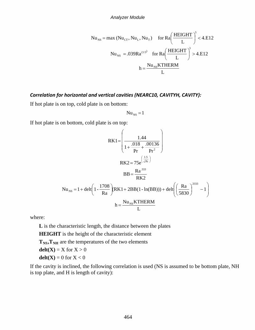
Analyzer Module
464
LKTHERMNu h
4.E12 L
HEIGHTRafor .039Ra Nu
4.E12 L
HEIGHTRafor )Nu ,Nu ,(Numax Nu
NS
3)(1/3
NS
3
TLCTNS
=
>
=
<
=
Correlation for horizontal and vertical cavities (NEARC10, CAVITYH, CAVITY):
If hot plate is on top, cold plate is on bottom: 1 Nu NS =
If hot plate is on bottom, cold plate is on top:
LKTHERMNu h
15830Radelt ln(BB)))-2BB(1 (RK1
Ra1708-1delt 1 Nu
RK2Ra BB
75e RK2
Pr.00136
Pr.018 1
1.44 RK1
NS
.3333
NS
.333
Pr1.5
2
=
−
++
+=
=
=
++=
where: L is the characteristic length, the distance between the plates HEIGHT is the height of the characteristic element TNS,TNH are the temperatures of the two elements delt(X) = X for X > 0 delt(X) = 0 for X < 0
If the cavity is inclined, the following correlation is used (NS is assumed to be bottom plate, NH is top plate, and H is length of cavity):

Analyzer Module
465
HL12for 7021HL6for 63
6HL3for 603HL1for 53
1for HL25LHHL
crit
crit
crit
crit
crit
≤=<≤=<≤=<≤=
<=
=
τττττ
NHNS
NHNS
T Tfor ANG90T Tfor ANG90
>+=>−=
ττ
−
=
−=
−
=
0<
−=
−=
1.6
15830Radelte
)Racos(170811.44deltd
15830
)Racos(deltc
degrees18 1.8for )Racos()81708sin(1.11.44deltb
)Racos(17081delta
3333.
3333.
τ
τ
τττ
τ
( )
LKTHERMNu h
degrees180 degrees 90for )sin()1Nu(1Nudegrees 90for )sin(NuNu
and 12for HL NuNu and 12for HL NuNu
)sin(NuNuNuNu
1.44de1Nu)Nu ,Nu ,max(Nu Nu
cab1Nu
NS
2NS
crit25.
2NS
crit4NS
crit1NS
4crit3
414
3
TLCT2
1
crit
crit
=
<<−+=><=
<>=<>=
=
+==
++=
τττττ
ττττ
τ τττ
τ

Analyzer Module
466
Free Convection between Horizontal Concentric Cylinders (CONCYL option)
For this option the convection is assumed to take place on the surface of the outer cylinder, therefore h is calculated as convecting from the outer to the inner cylinder.
( )
O
I
.25C
.6)(I
.6)(O
3
4
I
O
C
IO
LDFKTHERMDh
Pr.861PrRA.386F
DDL
RaDDln
Ra
2D-DL
=
+=
+
=
=
−−
where:
DO is the outer diameter DI is the inner diameter
Free Convection between Concentric Spheres (CONSPH option)
For this option the convection is assumed to take place on the surface of the outer sphere, therefore h is calculated as convecting from the outer to the inner sphere.
O
I
.25S
51.4)(I
1.4)(O
4IO
S
IO
LDKTHERMFD
h
Pr.861PrRa
.74F
)D(D)D(DRaLRa
2D-D
L
=
+=
+=
=
−−
where: DO is the outer diameter DI is the inner diameter

Analyzer Module
467
Free Convection from walls of an open inclined channel (INCCHNL option) and a hydraulic element
If the inclined channel is horizontal, then the horizontal cavity option is used. NS is here considered to be an element on either wall of the channel.
LKTHERMNu h
Ra2.87
Ra576
1Nu
H)RaLcos(ANGRa
NS
ANG2
ANG
NS
ANG
=
+
=
=
where:
L is the distance between the walls H is the length of the channel ANG is the angular deviation from the vertical in degrees
Calculation of heat flows between groups B and A using the heat flows through groups The heat from between two groups is the summary of 3 separate calculations: through directly connected conductances, through conductive conductances with the element CG method, and through Oppenheim radiative conductances. This calculation methodology is used by the printout options PRINT GRP2GRP, REPORTER PRINT GRHEATFLOW, REPORTER PRINT GRHEATMAPS, and PARAM REDUCE to calculate reduced models.
RADBACONDBAdirectBABA QQQQ ++=
Elements of group A
Elements of group B
QBA

Analyzer Module
468
Legend: QBA total heat flow from group B to group A through all conductances QdirectBA heat flow from group B to group A through conductances that connect the two groups
directly. Examples of these are conductive couplings with the element center method, radiative conductances calculated using Gebhardt’s method, and thermal coupling,
QCONDBA heat flow from group B to group A through boundary elements connecting the two groups if the element CG method is used
QRADBA heat flow from group B to group A through radiative conductances, if the Oppenheim Method is used
Calculation of heat flow between elements of group B and group A through direct conductances The heat flow between groups B and B via direct conductances is evaluated by summing the heat flow through all conductances connecting elements of group A and B directly. This is expressed by the following equation:
∑ −=k
AiBjABkdirectBA TTGQ )(
Legend: QdirectBA is the total heat flow from B to A through direct conductances (radiative,
conductive, thermal coupling, etc.), where one end of conductance lies in B, other in A
GABk is the k’th direct conductance between A and B TAi,TBj are the temperatures of the elements eAi and eBj, joined by the conductance GABk
Element eAi Temperature TAi
Element eBj Temperature TBj
Conductance GABk

Analyzer Module
469
Calculation of conductive heat flows between adjacent groups with the element CG method The conductive heat flow between adjacent groups when the CG conduction method is used is evaluated by summing the heat flows across the boundary elements common to groups A and B. The heat flow across each boundary element is the sum of heat flow through the conductances connecting the common boundary element to the other boundary elements on one side only, in group A or B. This is expressed by the following equation:
∑∑∑ −==k i
BbikABABiBbiki
CONDBAiCONDBA GTTQQ )(
Legend: QCONDBAi is the heat flowing from the element eBi to the element eAi through the common
boundary element eAbi
QCONDBA is the total heat flowing from all the elements of group B to the elements of group A through common boundary elements
TBbik is the temperature of the k’th boundary element of element eBi, excluding the boundary element eABi common to A and B
TBAi s the temperature of the common boundary element between elements eBi and eAi GBbikAB is the conductance from the k’th boundary element of element eBi to the common
boundary element eABb
Internal conductive conductances
Element eAi TAb1 Element eBi
TAb2
TAb3
TBb1
TBb2
TBb3
TABi
Boundary element eABi

Analyzer Module
470
Calculation of radiative heat flow between groups B and A if the Oppenheim Method is used This calculation is done in two in two steps. First, all real element temperatures are set to absolute 0 except for those of group B, which are maintained at the calculated values. The temperatures of all Oppenheim elements are calculated. The radiative heat flow from group B into group A at absolute 0 is then equal to the heat flow from the Oppenheim conductances of group A into the elements of group A. The process is then reversed and all temperatures, except those of group A, are maintained at absolute 0. This temperature field is used to compute the radiative heat exchange from group A to B at absolute 0 as explained in the above paragraph. The net radiative heat flow from B to A is the heat flow calculated in step 1 minus the heat flow calculated in step 2. The net heat flow is expressed in the equation below:
∑∑ −=i
BioBiozi
AioAiozRADBA GTGTQ
Legend: Subscript A elements associated to group A Subscript B elements associated to group B Subscript i index of elements in group A
TB1
GA1A1o
TA1
TB2
TA1o
TB2o
TB1o Group A element
Oppenheim element
Group B element
Oppenheim element
Group B element

Analyzer Module
471
Subscript o Oppenheim elements Subscript z index of element set maintained at absolute zero TAi temperature of element i in group A TAio temperature of the Oppenheim element of element i in group A GAio conductance between element eAi and its Oppenheim element TAioz temperature of the Oppenheim element of eAi, the i’th element of group A,
calculated with the following BC’s: 1) all non-Oppenheim elements (except group B) are sinks with absolute zero temperatures, 2) all the B elements are sinks set at their correct temperatures.
TBioz temperature of the Oppenheim element of eBi, the i’th element of group B, calculated with the following BC’s: 1) all non-Oppenheim elements (except group A) are sinks with absolute zero temperatures, 2) all the A elements are sinks set at their correct temperatures.
GBio conductance between element eBi and its Oppenheim element Accuracy issues with the calculation of equivalent conductances and ScriptFij Group-to-group equivalent conductances through each of the conductive mechanisms (radiative, conductive, and convective) are calculated from the heat flows between two groups with the following expression:
)( AB
BAtypeBAtype TT
QG
−=
Legend: GBAtype is the equivalent conductance for a particular heat transfer mechanism (conductive,
radiative, etc.) QBAtype is the heat flow through that mechanism TB,TA are the average group temperatures for groups B and A A typical printout on REPF looks like this:
Group-to-Group Heat Flow Report:
Temp Q Cap Description

Analyzer Module
472
Groupi: 54.73 5.8073E+02 3.2361E+00 Group B
Groupj: 25.00 1.0243E+02 1.0000E+30 Group A
Type Cond. value Heat Flow i->j ScriptFij Black Body Vfij
Conduction 0.0000E+00 0.0000E+00
Radiation 1.9522E+01 5.8039E+02 0.85 1.000004E+00
Linear Th. coupl. 1.1484E-02 3.4140E-01
Total 1.9534E+01 5.8073E+02
A group’s temperature is calculated by simple averaging. Since this definition is arbitrary, and is only accurate if the thermal gradients within a group are small, and conductances are computed from group temperatures, the conductances will be accurate only if the gradients within a group are small. If the local gradients within a group are large, conductances are not accurate, it is even possible to get negative conductance values for positive heat flows. ScriptFij is an alternate convention to the gray body view factor for defining the heat flow through a radiative conductance:
( )( )ijiij
jABSiABSijiRADij
viewfactorgraybodyemissivityScriptFTTScriptFAQ
=
−= )( 44
ScriptFij is a property that depends only on element surface properties and areas, not on the heat flows between groups. In the above output, ScriptFij is accurately calculated from optical and surface properties, not from heat flows between groups using the following algorithm:
∑∑
=
kkok
kkojko
ijGT
GTScriptF
where: Tjko is the temperature of the Oppenheim element of the k’th element of group j, calculated under the following conditions:
• all elements in group i are set to their correct temperatures,
• all other non-Oppenheim temperatures are set to absolute zero,
• all non-Oppenheim temperatures are sinks Tko is the temperature of the Oppenheim element of the k’th element of the group that includes all elements except the elements of group i, calculated under the above conditions.

Analyzer Module
473
However, because of the arbitrariness of the method for calculating group temperatures, the above equation in general will not be match the radiative heat flow calculation between groups, unless thermal gradients within a group are small.
References: 1. Applied Iterative Methods, Hageman, A.L., and Young. D.M., Academic Press, 1981 2. An Introduction to Hybrid Iterative Methods, H.A. van der Vorst and G.L.G. Sleijpen,
Proceedings of the International Workshop on Solution Techniques for Large-Scale Problems, CERCA Centre de Recherché en Calcul Appliqué, Montreal, Quebec, Canada, Sept. 26-28, 1994
3. Preconditioned Krylov Subspace Methods for CFD Applications, Y. Saad, University of Minnesota, Proceedings of the International Workshop on Solution Techniques for Large-Scale Problems, CERCA Centre de Recherche en Calcul Appliqué, Montreal, Quebec, Canada, Sept. 26-28, 1994

ANS2TMG Module
474
ANS2TMG Module Function
The ANS2TMG module transforms the ANSYS version 5 finite element model to TMG input file format or TMG geometry interpolation file VUFFE format.
Module Operation ANS2TMG accepts ANSYS version 5 FE model in ASCII file format, which can be generated from ANSYS by issuing CDWRITE command. For ANSYS version 5.5 you should include the UNBLOCKED option with the CDWRITE command. To translate an ANSYS FE model file into TMG input file format: 1. Create a TMG format include file, containing boundary conditions, analysis control and
other data. Call this file inpf.inc 2. Name your ANSYS input file file.cdb 3. Run the TMG Executive Menu from the operating system, and select the "RA - Merge
ANSYS and TMG files and run TMG". This operation will create a TMG input file INPF and run it.
To create TMG geometry interpolation file VUFFE format for temperature mapping postprocessing by the tmgint module by select "BI - Build interpolator geometry file" option. ANS2TMG translates the following ANSYS FE model identities into TMG FD model:
• ANSYS FE nodes are translated into TMG nodes. • ANSYS thermal elements are translated into TMG elements. The ANSYS element types
translated are: SURF19, SURF22, LINK32, LINK33, PLANE35, SHELL57, SELL63, PLANE67, LINK68, PLANE77, SOLID70, MASS71, SOLID87, and SOLID90.
• SURF19 and SURF22 are translated only when temperature has been defined as one of their degrees of freedom.
• The extra nodes from surface effect elements and higher order elements are ignored. • ANSYS thermal material property data are translated into TMG Card 9 MAT Cards. The
material properties translated are: density DENS, specific heat C, thermal conductivities KXX, KYY and KZZ, radiation emissivity EMIS. TMG will automatically assign a default solar absorptivity of -1E6 for each MAT Card.
For temperature-dependent material properties corresponding Card 9 TABTYPE and TABDATA Cards are generated. Thermal conductivity, C, and EMIS are translated into corresponding TABTYPE Card KTHERM, CPP and E codes. Density is always assumed to be constant. ANSYS real constants are translated into TMG Card 9 PROP Physical Property Cards.

COND and CONN2 Modules
475
COND and CONN2 Modules Function
The COND and CONN2 modules create capacitances, hydraulic resistances, and conductive conductances from geometry for the element center method. The COND and CONN2 modules are considered obsolete and the use of the CONDN module with the element center method is recommended. Output is written on file MODLF.
Conductive Conductance Calculations Conductances are computed between elements if their thermal conductivities are > 0. Elements may have the following shapes: Point (lump mass elements), Line (beam elements), Planar (triangular and quadrilateral elements). Solid (tetrahedron, wedge, and hexahedron). Conductances between elements are calculated by a four-step technique:
Step 1: Location of the Element Center and Elemental Subdivision
First, the element center locations are determined. For lump masses the element center is at the node. For beam elements the element center is at the CG. The element center of a beam is unique. For triangular elements the element center is at the meeting of the perpendicular bisectors of the edges. The element center of a triangle is unique. Planar quadrilateral elements are divided into two triangular sub-elements by connecting the opposite corners that form the largest angle sum. The element center of a quadrilateral is unique if the perpendicular bisectors of all the sides meet at a common point. This is the case with regularly shaped quadrilaterals, such as rectangles and isosceles trapezoids. If the element center is unique, the element has only a single sub-element. If a quadrilateral does not have a unique element center, the element center of the sub-element closest to the element CG is chosen to be the element center of the element. If a Card 9 PARAM SOLIDACC Card is present, or the material is orthotropic, solid elements are subdivided into tetrahedral sub-elements. The element a center of each sub-element is found at the meeting of the perpendiculars erected from the element centers of its surfaces.

COND and CONN2 Modules
476
A solid element has a unique element center if the element centers of all the sub-elements coincide. This occurs when each surface has a unique element center. This is so for elements whose surfaces are regular, i.e. triangles, rectangles, or isosceles trapezoids. Thus, tetrahedra have unique element centers, while wedges and hexahedra do only if all its surfaces are regular shapes. Solid elements with a unique element center have only a single sub-element. If a solid element does not have a unique element center, the element center of the sub-element closest to the element CG is chosen to be the element center of the element. If there is no Card 9 PARAM SOLIDACC Card present (the default option), the solid element is not subdivided, and a unique element center is assumed near its CG. This option yields fewer but less accurate conductive conductances. Where possible, elements with regular shapes should be used. This minimizes the number of conductances, thus speeding up solution times, and maximizes accuracy. Note that for certain element shapes (e.g. a triangle with an obtuse angle) the element center may fall outside the element. See diagram and discussion below.
Step 2: Calculation Sub-element Conductances
Next, the sub-elemental conductances Gi to the sub-element's boundaries are computed.
GKALi =
where: K is the thermal conductivity, L is:
• the distance from the element center to the ends of a beam, • the length of the perpendicular to the element's edge for a planar shell element • the length of the perpendicular to a surface for a solid element • is zero for a beam lying on the edge of a shell, or for a shell on the surface of a solid.
A is: • the cross-sectional area for a beam, • the (thickness)*(boundary length) for a planar shell element, • the boundary surface area of the surface for a solid element,
Gi is the elemental conductance for sub-element i. Note that when the element center falls outside the sub-element (e.g. for an obtuse angled triangle) L and Gi will be negative. In the example below, the conductance between side 1 and the element center will be negative.

COND and CONN2 Modules
477
Thick shell approximation
If solid elements have large (> 5) aspect ratios, i.e. they are thin as opposed to chunky, the thick shell approximation is used. The aspect ratio is defined as the longest edge divided by the approximate thickness. To calculate the approximate thickness value, the thickness direction is first found: this is the direction with the smallest average edge length. The average edge length in the thickness direction is then used as the approximate thickness. For wedge elements the thickness direction is the one from one triangular face to the other. In-plane conductances are then calculated as if the solid element were planar with a thickness equal to the mean thickness of the solid element. The through-thickness conductance is calculated as if the solid element were solid with a unique element center.
Step 3: Calculation of Conductances Between Sub-Elements
Next, the conductances between the element centers of connected sub-elements are calculated. Sub-elements are considered connected if they share common nodes along a face or an edge. Lump mass elements may be connected only to beam elements. Beam elements may be connected only to lump mass or other beam elements. Planar elements may be connected to lump mass elements or other beam elements along a common node, or they may be connected to planar elements if they share both nodes of an edge. Solid elements may be connected to planar elements or to other solid elements. For elements that meet only one other element at a boundary (e.g. solid joined to another solid), the conductances are summed in series:
2
1
3
Element centre

COND and CONN2 Modules
478
+
ji
ij
GG
G11
1
where:
Gij is the computed conductance between sub-elements i and j Gi is the conductance between the element center of sub-element i and the common boundary. Gij is the conductance between the element center of sub-element j and the common boundary,
If the sub-element meets meet more than one element at the boundary (e.g. three or more shell sub-elements sharing a common edge), the conductances between the sub elements are calculated by eliminating the boundary using the star-delta transformation for multi-branched stars:
where:
Gk is a conductance joined the boundary from sub-element k.
Negative conductances
If the element center of sub-element i falls outside its boundaries, a Gi < 0 will be computed, possibly resulting Gij < 0. If it falls inside another sub-element within the same element and Gij < 0, the two sub-element element centers will be merged and a warning message will be issued about approximate conductances. If it falls outside the element, a warning message is issued, and the conductance is replaced by a very large value, which will result in element merging by the MEREL module. A sub-element's element center falling outside the element also cause problems if the adjacent element it falls in has a different thermal conductivity or a different thickness. Incorrect conductances will then result.
Step 4: Elimination of Sub-Elements

COND and CONN2 Modules
479
Last, the sub-elements whose element centers are not the element centers of the element are eliminated by the CONN2 module. The elimination is performed by the star-delta transformation process, as described above. A side-effect of the star-delta elimination is that a large number of very small conductances may be generated between non-adjacent elements. To reduce their number, model thinning is performed in the CONN2 module to eliminate insignificant conductances. A conductance GIJ between elements I and J is considered insignificant if the following criteria are met:
• I and J do not share a common edge or boundary. • Gij < .001*Gitot • Gji < .001*Gitot Where:
Gitot is the sum of the conductances of element I Gjtot is the sum of the conductances of element J
The method by which conductances are created between non-adjacent elements is shown below. The boundary joining the two sub-element of element m is eliminated through the Y-delta transform, resulting in couplings between non-adjacent element i and j. Although the conductance map does not look physically realistic, it is mathematically correct.
For certain geometries, e.g. when two obtuse or right angled triangles are joined by their longest edges, a negative or infinite conductance may be computed. A warning message then is issued, and the conductance is replaced by a very large value, which will result in element merging by the MEREL module.
I
J
K
I
J
K
Eliminating a sub-element can yield conductances between non-adjacent elements

COND and CONN2 Modules
480
Circular elements
If the element is defined to be a circular element with a Card 9 XCIRC card, the element is re-mapped before the element center is located. The curved element is unfolded and stretched so that the calculated conductances will account for a logarithmic temperature variation in the radial direction.
Orthotropic Materials
If a solid element has an orthotropic thermal conductivity, then element is first proportionally stretched in the element’s material X, Y, and Z directions by the factors, √(kyykzz), √(kxxkzz), √(kyykxx) respectively before the conductance calculation, and the thermal conductivity value is set to 1. If a planar element has an orthotropic thermal conductivity, then element is first proportionally stretched in the element’s material X and Y directions by the factors √kyy, √kxx respectively before the conductance calculation, and the thermal conductivity value is replaced by the value √(kyykxx).
Axisymmetric Elements
If an element is an axisymmetric solid, it is treated as a planar element in the XZ plane that is stretched in the X direction by:
−
minmaxlog
min)max(2
XX
XXπ
and in the Z direction by:
min)max( XX −π
If it is an axisymmetric shell with a thickness t, it is treated as a beam with an equivalent cross-section of:
−
minmaxlog
min)max(2
XX
XXπ
where:
Xmax and Xmin are the maximum and minimum X (radial) dimensions of the element. If the material is also orthotropic, it is first stretched along the orthotropic axes as described

COND and CONN2 Modules
481
above.
Capacitance Calculations Capacitance calculations are performed only for elements that have specific heats > 0. An elemental capacitance is calculated by multiplying the (volume)*( specific heat)*(density).
Hydraulic resistance calculations Two hydraulic resistances are calculated between the CG of each 2-node hydraulic element and the 1-node hydraulic elements at its boundary. The value of the hydraulic resistance written on file MODLF with MNM = HYD is the flow resistance multiplier from the element PROP Card divided by the distance between the CG of the element and its ends.

CONDN Module
482
CONDN Module Function
The CONDN module creates capacitances, hydraulic resistances, and conductive conductances from geometry. Its functionality is identical to the COND module, but its approach is different. Whereas COND directly creates conductances between element centers, CONDN creates special boundary elements on each solid element’s surfaces, planar element's edges, and beam element's ends, and creates conductances between the centers of gravity (CG's) of the element and these boundary elements.
CONDN is activated by Card 2a M = 1 and Card 9 PARAM COND NEW. Output is written on MODLF.
Creation of Boundary Elements Boundary elements are the equivalent to:
• zero thickness shell elements created on the surfaces of solid elements, • zero radius beam elements on the edges of shell elements, and • zero radius lump mass elements on the end of beam elements. Boundary elements are not created if the surface or edge on which it is to be created is already occupied by another element, or if the element on which it is to be created has zero thermal conductivity.
Elemental Conductances for Beams The elemental conductance of a beam connects the CG of the beam to the boundary elements at its endpoints and is calculated with:
GKALij =
where: Gij is the conductance between the ends of the beam,
Boundary Elements

CONDN Module
483
k is the thermal conductivity, L is the distance from the element CG to one of the nodes, A is the cross-sectional area.
Elemental Conductances for Triangles To create the elemental conductances of a triangle the first step is to create a conductance matrix between only the boundary element CG's.
A linear internal temperature field is assumed within the element:
T x y a a x a y( , ) = + +1 2 3
The boundary element temperatures Tbi are defined at the midpoints of the edges: T x y T ib b bi i i
( ) = = 1,2,3
Substituting the boundary element temperatures into temperature field equation, the weighting factors eij of the coefficients a1, a2, a3 can be evaluated:
a e T e T e Ta e T e T e Ta e T e T e T
b b b
b b b
b b b
1 11 1 12 2 13 3
2 21 1 22 2 23 3
3 31 1 32 2 33 3
= + += + += + +
From the geometry of the element the coefficients bi and ci of the unit edge normal vectors Ni at the boundary elements and the length Li of each boundary element can be evaluated:
N2 N1
L2
q2 L1
Tb2 Tb1 g12 (xb2,yb2) (xb1,yb1)
q
q3
N3 L3 Tb3
g13 g23 (xb3,yb3)
Element geometry Conductance matrix between boundary elements

CONDN Module
484
N i jN i jN i j
1
2
3
( )( )( )
,
,
,
x y b cx y b cx y b c
b b
b b
b b
1 1 1 1
2 2 2 2
3 3 3 3
= +
= +
= +
The temperature gradient vector is constant over the triangle, and is expressed by: ′ = +T i ja a2 3
Expanding yields: )TeTeTeTeTeTeT(e bbbbbbb 333232231131323122121T' ++++++=
If the element has a thickness is t and thermal conductivity k, then using Fourier’s Law the heat flow qi into element at each boundary element can be evaluated using the dot product of the temperature gradient vector and the edge normal vector:
q ktL x yi i bi bi= − ′ ⋅T Ni( , )
Expanding yields: q ktL b e T e T e T c e Tb e T e Tq ktL b e T e T e T c e Tb e T e Tq ktL b e T e T e T c e Tb e T e T
b b b b b
b b b b b
b b b b b
1 1 1 21 1 22 2 23 3 1 31 1 32 2 33 3
2 2 2 21 1 22 2 23 3 2 31 1 32 2 33 3
3 3 3 21 1 22 2 23 3 3 31 1 32 2 33 3
= − + + + + += − + + + + += − + + + + +
( ( ) ( ))( ( ) ( ))( ( ) ( ))
Collecting terms:
q ktL T b e c e T b e c e T b e c eq ktL T b e c e T b e c e T b e c eq ktL T b e c e T b e c e T b e c e
b b b
b b b
b b b
1 1 1 1 21 1 31 2 1 22 1 32 3 1 23 1 33
2 2 1 2 21 1 31 2 2 22 2 32 3 2 23 2 33
3 3 1 3 21 1 31 2 3 22 3 32 3 3 23 3 33
= − + + + + += − + + + + += − + + + + +
( )( ( ) ( ) ( ))( )( ( ) ( ) ( ))( )( ( ) ( ) ( ))
However, the qi’s can also be expressed in terms of conductances between the boundary elements using Kirchoff’s Law:
q g T T g T Tq g T T g T Tq g T T g T T
b b b b
b b b b
b b b b
1 12 1 2 13 1 3
2 12 2 1 23 2 3
3 23 3 2 13 3 1
= − + −
= − + −= − + −
( ) ( )( ) ( )( ) ( )
Equating the above two sets of equations yields the expressions for gij: g ktL b e c eg ktL b e c eg ktL b e c e
12 1 1 22 1 32
13 1 1 23 1 33
23 2 2 23 2 33
= += += +
(((
)))
This conductance matrix is between the boundary elements only, and does not connect them to the CG.

CONDN Module
485
Optionally, of the Card 9 PARAM CAPDIST OFF is present, the conductance matrix is transformed into a conductance matrix between the element CG and the boundary element.
The two conductance matrices are equivalent, but the conductance matrix from the CG has 6 conductances, whereas the matrix between the boundary elements has only 3. To calculate the additional conductances from the CG to the boundary elements, it is recognized that the temperature at the CG of the triangle if the triangle has a linear temperature gradient is equal to the average temperature of the midpoints of the sides. This is possible only if:
G GG G
CG CG
CG CG
1 2
1 3
==
An additional constraint we impose is that the root mean square value of the sum of the conductances between the boundary elements is minimized. This yields the following equations:
∂+ +∂
=( )
( )G G G
G CG
122
132
232
1
0
The star-delta transformation is used to provide the other 3 equations:
Tb2
Tb3
Tb1 Tb2
Tb3
Tb1 G12
G23 G13
G1CG G2CG
G3CG
Conductance matrix between boundary elements
Transformed conductance matrix between CG and boundary elements

CONDN Module
486
G GG G G
G g
G GG G G
G g
G GG G G
G g
CG CG
CG CG CG
CG CG
CG CG CG
CG CG
CG CG CG
1 2
1 2 312 12
1 3
1 2 313 13
2 3
1 2 323 23
+ ++ =
+ ++ =
+ ++ =
For an equilateral triangle the element center method and the element CG method provide identical results.
Elemental Conductances for Tetrahedra The derivation of the conductance matrix for a tetrahedron is very similar to the derivation for a triangle. The first step is to create a conductance matrix between the boundary element CG's. A linear internal temperature field is assumed within the element:
T x y z a a x a y a z( , , ) = + + +1 2 3 4
The boundary element temperatures Tbi are defined at the midpoints of the edges: 4,3,2,1),,( == iTzyxT bibibibi
Substituting the boundary element temperatures into temperature field equation, the weighting factors eij of the coefficients a1, a2, a3 , a4 can be evaluated:
a e T e T e T e T
a e T e T e T e T
a e T e T e T e T
a e Tb e T e T e T
b b b b
b b b b
b b b b
b b b
1 11 1 12 2 13 3 14 4
2 21 1 22 2 23 3 24 4
3 31 1 32 2 33 3 34 4
4 41 1 42 2 43 3 44 4
= + + +
= + + +
= + + +
= + + +
From the geometry of the element the coefficients bi, ci, did, of the unit surface normal vectors Ni at the boundary elements and the area Ai of each boundary element can be evaluated:

CONDN Module
487
N i j k
N i j k
N i j k
N i j k
1( , , )
( , , )
( , , )
( , , )
x y z b c d
x y z b c d
x y z b c d
x y z b c d
b b b
b b b
b b b
b b b
1 1 1 1 1 1
2 2 2 2 2 2 2
3 3 3 3 3 3 3
4 4 4 4 4 4 4
= + +
= + +
= + +
= + +
The temperature gradient vector is constant over the element, and is expressed by: ′ = + +T i j ka a a2 3 4
Expanding yields:
kjiT'
444343242141
434333232131
424323222121
)TeTeTeT(e)TeTeTeT(e)TeTeTeT(e
bbbb
bbbb
bbbb
+++++++++++=
If the element has thermal conductivity k, then using Fourier’s Law the heat flow qi into element at each boundary element can be evaluated using the dot product of the temperature gradient vector and the surface normal vector:
q kA x y zi i bi bi bi= − ′ ⋅( ( , , ))T Ni
Expanding yields: q kA b e T e T e T e T c e T e T e T e T
d e T e T e T e T
q kA b e T e T e T e T c e T e T e T e Td e T e T e T e
b b b b b b b b
b b b b
b b b b b b b b
b b b
1 1 1 21 1 22 2 23 3 24 4 1 31 1 32 2 33 3 34 4
1 41 1 42 2 43 3 44 4
2 2 2 21 1 22 2 23 3 24 4 2 31 1 32 2 33 3 34 4
2 41 1 42 2 43 3 44
= − + + + + + + + ++ + +
= − + + + + + + + ++ + +
( ( ) ( ) ( ))
( ( ) ( ) ( T
q kA b e T e T e T e T c e T e T e T e Td e T e T e T e T
q kA b e T e T e T e T c e T e T e T e Td e T e T e T
b
b b b b b b b b
b b b b
b b b b b b b b
b b b
4
3 3 3 21 1 22 2 23 3 24 4 3 31 1 32 2 33 3 34 4
3 41 1 42 2 43 3 44 4
4 4 4 21 1 22 2 23 3 24 4 4 31 1 32 2 33 3 34 4
4 41 1 42 2 43
))
( ( ) ( ) ( ))
( ( ) ( ) (
= − + + + + + + + ++ + +
= − + + + + + + + ++ + 3 44 4+ e Tb ))
Collecting terms:

CONDN Module
488
q kA T b e c e d e T b e c e d eT b e c e d e T b e c e d e
q kA T b e c e d e T b e c e d eT b e c e d e T b e c e d e
q
b b
b b
b b
b b
1 1 1 1 21 1 31 1 41 2 1 22 1 32 1 42
3 1 23 1 33 1 43 4 1 24 1 34 1 44
2 2 1 2 21 2 31 2 41 2 2 22 2 32 2 42
3 2 23 2 33 2 43 4 2 24 2 34 2 44
= − + + + + + ++ + + + +
= − + + + + + ++ + + + +
( )( ( ) ( )( ) ( ))
( )( ( ) ( )( ) ( ))
3 3 1 3 21 3 31 3 41 2 3 22 3 32 3 42
3 3 23 3 33 3 43 4 3 24 3 34 3 44
4 4 1 4 21 4 31 4 41 2 4 22 4 32 4 42
3 4 23 4 33 4 43 4 4 24 4 34 4 44
= − + + + + + ++ + + + +
= − + + + + + ++ + + + +
( )( ( ) ( )( ) ( ))
( )( ( ) ( )( ) ( ))
kA T b e c e d e T b e c e d eT b e c e d e T b e c e d e
q kA T b e c e d e T b e c e d eT b e c e d e T b e c e d e
b b
b b
b b
b b
However, the qi’s can also be expressed in terms of conductances between the boundary elements using Kirchoff’s Law:
q g T T g T T g T T
q g T T g T T g T Tq g T T g T T g T Tq g T T g T T g T T
b b b b b b
b b b b b b
b b b b b b
b b b b b b
1 12 1 2 13 1 3 14 1 4
2 12 2 1 23 2 3 24 2 4
3 23 3 2 13 3 1 34 3 4
4 14 4 1 24 4 2 34 4 3
= − + − + −
= − + − + −= − + − + −= − + − + −
( ) ( ) ( )
( ) ( ) ( )( ) ( ) ( )( ) ( ) ( )
Equating the above two sets of equations yields the expressions for gij:
g kA b e c e d eg kA b e c e d eg kA b e c e d eg kA b e c e d eg kA b e c e d eg kA b e c e d e
12 1 1 22 1 32 1 42
13 1 1 23 1 33 1 43
14 1 1 24 1 34 1 44
23 2 2 23 2 33 2 43
24 2 2 24 2 34 2 44
34 3 3 24 3 34 3 44
= + += + += + += + += + += + +
( )( )( )( )( )( )
This conductance matrix is between the boundary elements only, and does not connect them to the CG. The elemental heat loads and capacitances are distributed to the four boundary elements with a weighting factor proportional to the sum of the conductances to the boundary element.

CONDN Module
489
( )
( )
( )
( )342423141312
142414tet4
342423141312
342313tet3
342423141312
242312tet2
342423141312
141312tet1
gggggggggCC
gggggggggCC
gggggggggCC
gggggggggCC
+++++++
=
+++++++
=
+++++++
=
+++++++
=
If the Card 9 PARAM CAPDIST OFF option is present, the matrix is transformed into a conductance matrix between the element CG and the boundary elements. The two conductance matrices are equivalent, but the conductance matrix from the CG has 10 conductances, whereas the matrix between the boundary elements has only 6. For this option, the elemental heat load and capacitance are concentrated at the CG. To calculate the four additional conductances, we use the fact that the CG temperature is equal to the average of the four temperatures at the CG's of the sides. This is possible only if:
G GG GG G
CG CG
CG CG
CG CG
1 2
1 3
1 4
===
An additional constraint we impose is that the root mean square value of the sum of the conductances between the boundary elements is minimized. This yields the following equation:
∂+ + + +
∂=(
( ))
G G G G GG CG
12 13 14 23 34
1
2 2 2 2 2 0
The star-delta transformation provides the other 6 equations:

CONDN Module
490
G GG G G G
G g
G GG G G G
G g
G GG G G G
G g
G GG G G G
G g
G GG G G G
G g
G GG G G G
G g
CG CG
CG CG CG CG
CG CG
CG CG CG CG
CG CG
CG CG CG CG
CG eCG
CG CG CG CG
CG CG
CG CG CG CG
CG CG
CG CG CG CG
1 2
1 2 3 412 12
1 3
1 2 3 413 13
1 4
1 2 3 414 14
2
1 2 3 423 23
2 4
1 2 3 424 24
3 4
1 2 3 434 34
+ + ++ =
+ + ++ =
+ + ++ =
+ + ++ =
+ + ++ =
+ ++ =
+
Calculation of Elemental Conductances for Quadrilaterals, Wedges, Pyramids, and Hexahedra
To calculate the conductance matrix for quadrilaterals, hexahedra and wedges these elements are first divided into triangular, tetrahedral and pyramidal subelements. For a quadrilateral the diagonally opposite nodes with the larger sum of the internal angles are connected.
Quadrilateral is subdivided into four elemental subtriangles joined at the CG

CONDN Module
491
Each hexahedron is subdivided into 6 pyramids with lines joining the CG of the hexahedron to each of the corners. Each wedge is subdivided in 3 pyramids and 2 tetrahedra by joining the CG of the element to the corners.
For each sub-element a conductance matrix is constructed similar to the procedure described above for triangles and tetrahedra, with the following exceptions:
• For wedges, pyramids, and hexahedra, the location of the calculation points on external faces is at the CG of the face.
• At internal faces the boundary condition of matching the heat fluxes is used. • The conductance matrix of pyramidal elements and sub-element is derived by
sub-dividing the pyramid into two tetrahedra, and applying the following conditions:
• The sum of the heat flows through the adjacent side of the two tetrahedra is zero.
• The thermal gradient normal to the quadrilateral face is the same for both tetrahedra (uniform heat flux on the quadrilateral face).
• The temperature at the CG of the quadrilateral face is equal to the area-weighted average temperature of the CG's of the two triangles subdividing that face.
Subdivision of a hexahedron Subdivision of a wedge

CONDN Module
492
The element conductance matrix is assembled by eliminating the calculation point at the CG of the internal faces using the star-delta transform. This yields a conductance matrix between the boundary elements. For quadrilaterals the resulting conductance matrix is further transformed by creating four more conductances between the CG and the boundary elements in the manner described above for the tetrahedron with the PARAM CAPDIST OFF option, by minimizing the root mean square value of the conductances between the boundary elements. The weighting factors for the conductances from the CG to the boundary elements are derived by assuming a parabolic temperature distribution within the element. The resulting size of the conductance matrix is 10 conductances for quads, 10 conductances for wedges and 15 conductances for hexes. For wedges and hexes, the capacitance and elemental heat loads are redistributed to the boundary elements at analysis time, for quads they remain concentrated at the CG. Optionally, if the Card 9 PARAM CAPDIST OFF is present, the conductance matrix between the boundary elements is transformed into a conductance matrix between the CG of the element and boundary elements, including conductance terms from the CG to the boundary elements. This is done in a manner similar to the method described above for the triangle and the tetrahedron, with an important exception. The root mean square value of the conductances between the boundary elements is minimized as before, however, the conductances between the CG and the boundary elements are not equal. For a solid element:
GG
A DA D
iCG
jCG
i j i
j i j
=sin( )sin( )
θθ
and for a quadrilateral: GG
L DA L
iCG
jCG
i j i
j i j
=sin( )sin( )
θθ
where: Di is the distance between the element CG and the CG of the boundary element
θi is the angle between the line joining the CG of the element to the boundary element and the surface normal of the boundary element.
This approach yields a conductance matrix identical to that of the element center method for rectangles and brick elements.

CONDN Module
493
Interface Conductances If an interface conductance between two adjacent elements is specified with a Card 6 INTER, ITERTOT, INTER2, INTER2TOT option, two parallel boundary elements are created on the adjacent elements by splitting the nodes of the interface element. The interface conductance equal to the area of the boundary element times the interface conductance is then created connecting the two boundary elements. If more than two elements are connected to the interface element, then conductances will be created between all the elements with a value equal to the total interface conductance value divided by the total number of elements.
Parabolic Elements Parabolic and linear elements are treated identically, the extra nodes on parabolic elements are only used in temperature recovery stage.
Temperature-dependent thermal conductivities If an element has a non-linear thermal conductivity specified in a table, a nominal value of 1 is used in the conductance calculation and the resulting conductances are multiplied by the interpolated conductance value during the Analyzer run.
Orthotropic Materials If a solid element has an orthotropic thermal conductivity, then element is first proportionally stretched in the element’s material X, Y, and Z directions by the factors √(kyykzz), √(kxxkzz), √(kyykxx) respectively before the conductance calculation, and the thermal conductivity value is set to 1. If a planar element has an orthotropic thermal conductivity, then element is first proportionally stretched in the element’s material X and Y directions by the factors √kyy, √kxx respectively before the conductance calculation, and the thermal conductivity value is replaced by the value √(kyykxx).

CONDN Module
494
Axisymmetric Elements If an element is an axisymmetric solid, it is treated as a planar element in the XZ plane that is stretched in the X direction by:
−
minmaxlog
min)max(2
XX
XXπ
and in the Z direction by:
min)max( XX −π
If it is an axisymmetric shell with a thickness t, it is treated as a beam with an equivalent cross-section of:
−
minmaxlog
min)max(2
XX
XXπ
where:
Xmax and Xmin are the maximum and minimum X (radial) dimensions of the element.
If the material is also orthotropic, it is first stretched along the orthotropic axes as described above.
Capacitance Calculations Capacitance calculations are performed only for elements that have specific heats > 0. An elemental capacitance is calculated by:
Capacitance = (volume)(specific heat)(density)
Hydraulic Resistance Calculation Two hydraulic resistances are calculated between the CG of each 2-node hydraulic element and the 1-node hydraulic elements at its boundary. The value of the

CONDN Module
495
hydraulic resistance written on file MODLF with MNM = HYD is the flow resistance multiplier from the element PROP Card divided by the distance between the CG of the element and its ends.
Comparison between CONDN and COND modules The following provides a brief comparison between the COND and CONDN conduction modules.
• CONDN creates conductances between boundary elements, whereas COND also creates conductances between element centers. For regular rectangular meshes, CONDN creates a much denser mesh.
• CONDN is more tolerant of odd element shapes. • For meshes which contain irregular elements CONDN generally produces
more accurate temperatures, especially if the thermal model includes radiation or convection effects. This is because that CONDN module allows TMG to calculate temperatures at the CG’s of the surface elements, which more accurately represent the average surface temperature of the radiating or convecting elements. In addition, the conductance matrix derivation for solid elements is much more accurate that that of COND, and CONDN allows the creation of negative conductances, while COND does not.

GRAYB Module
496
GRAYB Module Function
The GRAYB module creates the radiative conductances (Card 2a M = 4) and the IR (M = 16) and solar spectrum (M = 8) gray body view factor matrices. The radiative conductances may be calculated using the recommended Oppenheim's Method (activated with Card 9 PARAM OPPENHEIM) or Gebhardt's Method. The radiative conductances are written on file MODLF, and the gray body view factor matrices on file VUFF.
The Gray Body View Factor Radiative heat transfer between elements i and j is described by:
Q AVFG T T
A VFG T Tij i i ij i j
j j ji j i
- ( )
= −
= −
σ
σ
Ε
Ε
( )4 4
4 4
Where: Qi is the net radiative heat load from element i to element j. σ is Stefan-Boltzmann's constant. Ti,T are the absolute temperatures of elements i and j. Ei, Ej are the emissivities of elements i and j, defined on MAT Cards. Ai, Aj are the surface areas of elements i and j. VFGij is the gray body view factor from i to j, which is the fraction of the emitted or reflected radiant heat load leaving the surface i and absorbed by j after multiple diffuse reflections from all the elements. VFGji is the gray body view factor from j to i.
An important property associated with the gray body view factor is reciprocity:
E AVFG E A VFGi i ij j j ji=
Note the similarity to the view factor reciprocity property:
AVF A VFi ij j ji=
Another important property of the gray body view factor is that the sum of the gray body view factors for any element i is unity:
VFGij
j∑ = 1
The gray body view factor and the view factor are identical in an enclosure where all the
GRAYB Module
497
elements are black. An important difference between the view factors and the gray body view factors is that while self-view factors are zero for non-concave surfaces, gray body self-view factors are generally not zero, since reflections cause the elements to re-absorb some of the radiation that leaves their surfaces. In the IR spectrum gray body view factor calculation the absorptivity is equal to the emissivity. For solar spectrum calculations the emissivity values are replaced by the solar absorptivity values.
Enclosures The GRAYB module separates elements into enclosures. An enclosure is defined to be a set of elements that view each other and only each other. The advantages of enclosures are:
• Efficiency - the size of the radiation matrix to be inverted is reduced for Gebhardt's Method. • Model debugging - the elements belonging to each enclosure are written on REPF. This can
be used to verify that improper couplings between enclosures are not present.
KSP and the Residual View Factor Ri The residual view factor Ri for element i is:
R VFi ij= − ∑1
The ideal value of Ri is 0. Departures from this may occur because of the approximations in view factor calculations, or when an improper enclosure is defined, e.g. when i sees the back of another element. Very large departures are usually an indication of an improper model. The physical effect of Ri > 0 is to reduce the radiation leaving i, in effect making the surface more "concave".
TMG provides three methods of compensating for Ri ≠ 0:
• Create a self-view factor (KSP = 0). The effect of creating a self-view factor may be viewed as assuming the element is concave. Some of the radiation is incident on i itself, which is then reflected to the elements it sees in proportion to the view factors times the reflectivity
• Setting the residual view factor to an element (KSP > 0, KSP = element number). If KSP > 0, Ri is connected to element KSP, provided a view factor from that enclosure to

GRAYB Module
498
element KSP already exists. If it is does not, Ri is set to the self-view factor. This prevents the unwanted leakage of radiation from inside an enclosure to an element it cannot see. A new very large black element KSP is created in the enclosure. If KSP > 0, for each element i where Ri < 0 the KSP = 0 option is used. If KSP = 2E6, the space element number obtained from the Card 5d SPACE Card is substituted for the code 2E6.
• Approximate proportional adjustment of the view factors (KSP = 3E6). This is the recommended option. With this option, adjustment of the shadowed view factors only is performed iteratively to minimize the maximum Ri. The unshadowed view factors are assumed to be exact because it is assumed they were calculated with the accurate Exact Contour Integral Technique. At each iteration each shadowed view factor VFij is multiplied by the factor:
1
1 −+
−+
RA
A AR A
A Aij
i jj
i
i j
The Ri's are re-evaluated during each iteration. The iterations are halted when the maximum Ri is minimized.
Oppenheim's Method Oppenheim's Method, or otherwise known as the radiosity method, is the recommended approach. Oppenheim's Method consists of creating an artificial "Oppenheim element" I for each radiating element i, which may be visualized as an imaginary element floating above element i, and intercepting all radiation to it.
Radiative couplings to other elements AiVFij
Radiative coupling between I and i AiEi/(1-Ei) Element i
Oppenheim element I

GRAYB Module
499
A radiative coupling equal to
A EE
i i
i1−
is created between I and i, and each view factor VFij is transformed into a radiative coupling AiVFij between I and the Oppenheim element J of j. Oppenheim's Method is an alternative to Gebhardt's Method for calculating radiative couplings. It has several advantages:
• Temperature-dependent emissivities are handled more accurately and efficiently. This is because during temperature calculations only the radiative conductance AiEi/(1-Ei) between the Oppenheim element and the element itself needs to be modified.
• CPU performance is generally much improved for two reasons: the matrix inversion process of Gebhardt's Method is bypassed, and the number of radiative couplings is much generally much smaller. This is because in a given enclosure Gebhardt's Method creates a radiative coupling between every element, even if they cannot view each other.
• Accuracy is improved because the RK elimination of insignificant radiative couplings is bypassed.
• File sizes are generally smaller. Note: With Oppenheim's Method significant performance degradation can be expected during transient analysis with the explicit forward differencing method. This is because the Oppenheim elements are assigned zero capacitance, and the forward differencing method requires a full steady-state solution for the surface elements at each integration time step. However, no accuracy degradation is observed with the implicit time integration methods. Oppenheim's Method is invoked by specifying Card 9 PARAM OPPEHEIM T1. The corresponding Oppenheim element I for each element i are then assigned an element number equal to i + T1. In case of numbering conflict, an unused element number is assigned.
Gebhardt's Method Gray body view factors between the elements are calculated by Gebhardt's Method (Ref. 2). This method assumes that the radiation emitted by i and absorbed by j after multiple diffuse reflections is equal to the absorbed portion of the radiation directly incident upon j, plus the radiation reflected by all surfaces:
VFG E VF VF E VFGij j ij ik k kjk
= + −∑ ( )1
The reflected radiation is assumed to be reflected perfectly diffusely, i.e. it is reflected in proportion to the view factors of the element. If only geometric view factors are present on the

GRAYB Module
500
VUFF file, then even if an element has specular reflectivity, its reflectivity is treated as perfectly diffuse. If ray-traced view factors are present on VUFF through the use of the VFTRACE option, the equivalent reduced diffuse properties of the view factor matrix are used for elements that have specular or transmissive surface properties. In this case, the specular and transmissive effects have been accounted for during the ray-tracing procedure.
The RK Parameter Excessively weak radiative conductances calculated with Gebhardt's Method may be eliminated or connected to element Card 2a KSP through the use of a non-zero Card 2a RK parameter. For each element i and j the largest gray body view factors not connected to a Card 5d space element VFGimax and VFGjmax are found, and only those radiative conductances whose gray body view factors fulfill the two inequalities:
VFG RK VFGVFG RK VFG
ij i
ji j
> | > |
||
max
max
are written on file MODLF. All others are considered insignificant. The double inequality is necessary because when Ai << Aj the conductance may be insignificant for j but very important for i. If RK > 0 the insignificant radiative conductances are not written on file MODLF, unless the coupling is to space.
If RK < 0 and KSP ≠ 0 each insignificant coupling is replaced by two equivalent couplings, one from element i and one from element j, to element KSP, provided KSP is not a Card 5d space element. This technique is similar to the one described in (Ref. 1). The gray body view factor matrices are not affected by RK. It is necessary to exercise care with RK > 0 to avoid eliminating an excessive number of radiative couplings. RK = 1 eliminates all radiative couplings. RK = 0 defaults to RK=1.E-4.
Module Operation • First, the module reads from file VUFF all the areas, emissivities, and the appropriate
spectrum view factors. • If view factors are duplicated, the last one is used. • Next, the elements are separated into enclosures. • Next, the residual view factors are computed and, depending on the value of KSP, view

GRAYB Module
501
factor adjustment is performed. • Next, radiative couplings are calculated, either with Oppenheim's Method or Gebhardt's
Method. • Next, if Gebhardt's Method is specified, insignificant radiative couplings are eliminated or
joined to KSP. • Next, the radiative couplings are written on file MODLF with the mnemonic MNM = RAD. • Next, if the gray body matrices are being calculated with Gebhardt's Method, they are
written on file VUFF with the mnemonic MNM = IGM for the IR spectrum and MNM = SGM for the solar spectrum. For this operation, very small gray body view factors, where:
VFGij < 1.E – 6 VFGji < 1.E – 6
are ignored.
Angle Dependent Surface Properties For an element with angle dependent specular reflectivity or transmissivity the diffuse reflectivity is calculated as:
ρ ρ
ρ
ε
ε τ
di i si
di i i
= − −
= − −
1
1 or
Where:
ρdi is the diffuse reflectivity,
ρsi is the average specular reflectivity, calculated by averaging the data in the array, and τ is the average transmissivity, calculated by averaging the data in the array.

HEMIVIEW Module
502
HEMIVIEW Module Function
The HEMIVIEW module calculates diffuse blackbody view factors using the hemicube method, which allows computer graphics hardware to accelerate the calculations. All HEMIVIEW module requests start with Card 6v HEMI ON and end with HEMI OFF. Between these Cards is the body of the HEMIVIEW requests. Details of the calculations are written on files MSGF and REPF. Results are written on file VUFF.
The Difference between HEMIVIEW and VUFAC The VUFAC module calculates view factors with a combination of the contour integration and Nusselt sphere methods, using automatic elemental subdivision algorithm when shadowing occurs. View factors between elements are calculated one at a time. If shadowing occurs, the number of calculations required to compute the view factors varies roughly as the cube of the number of elements, which is very Cpu intensive. The HEMIVIEW module is much faster. It uses computer graphics techniques to graphically render the radiating elements onto the five sides of a hemicube (a half-cube) placed at the CG of an element, called the emitting element. The view factors from the emitting element to the other elements, called the receiving elements, are determined by post-processing the graphical images of the receiving elements projected onto each of the hemicube sides. The hemicube method is fast for two reasons: the number of renderings is linearly proportional to the number of elements, and the rendering calculations are performed with specialized fast graphics cards. The accuracy of the hemicube method is limited by the pixel resolution of the drawing area.
How It Works Cohen and Greenberg first proposed the hemicube algorithm, in which the five sides of an imaginary hemicube cover an element such that the center of the cube is at the centroid of the emitter element i (Figure 1a), and the top plane of the cube is parallel to the plane of the element. The faces of the hemicube are divided into equal size squares, referred to as pixels, with areas of dA. Each element j, called the receiver element, is graphically projected onto the faces of the hemicube, with the focus of the projection on the centroid of emitter element i. This projection is easily and efficiently performed within computer graphics hardware, with each hemicube face containing the rendered image of a section of the model. Each receiver element j is assigned a unique color, and a depth-buffer algorithm (Z-buffer) ensures that only the visible parts of overlapping elements appear in the final image. The rendered images on the five hemicube surfaces comprise the images of all the elements of the model surrounding the emitter element i. The pixel colors of these five images are post-

HEMIVIEW Module
503
processed to calculate the view factors of the emitter i to each element. Figure 1 (a and b) depicts two elements being rendered onto the surface of a hemicube, and the resulting pixel colors after the rendering process.
Figure 1. (a) Projection of two elements onto the Hemicube
Figure 1. (b) Pixel-resolution image of the elements on the Hemicube faces

HEMIVIEW Module
504
Calculation of View Factors Each pixel is associated with a pre-computed delta view factor ΔFp,
where the geometry is shown in Figure 2.
x p
z p
x p
y p
θ p θip
θ p r r
Figure 2: Geometry for determining pixel delta view
∆Ap
Emitting sub-element
θip
The vector r is from the eye position (CG of the emitting element i) to the CG of the pixel under consideration.θ ip is the angle between r and the emitter element normal.θ p is the angle between r and the normal to the hemicube plane on which the pixel lies. A pixel’s contribution to the view factor (Equations 3 & 5), is derived by assigning a local (x,y,z) coordinate system to the hemicube, and making the hemicube a unit height. Then, for pixels on the top plane of the hemicube,
2 2 1| | 1, cos cos . (2)p p ip pr x yr
θ θ= + + = =
Upon substitution of the above equation into Eq. (1), the view factor contribution of each pixel becomes:
222 )1( ++∆
=∆pp
pp yx
AF
π (3)
for top plane pixels of uniform area ∆A. Similarly, for the side plane pixels,
2 2 1| | 1, cos , cos (4)pp p ip p
zr y z
r rθ θ= + + = =
which yields:
222 )1( ++∆
=∆pp
ppp zy
AzF
π (5)
(1) ∆ ∆Fr
Apip p
p=cos cosθ θ
π 2

HEMIVIEW Module
505
The Rendering Procedure The rendering procedure is depicted in detail in Figure 3. First, the eye position, view direction, viewing frustum dimensions, and image plane location parameters are defined. The eye position is at the CG of the emitter element i. The view direction is perpendicular to each of the viewing planes, i.e. the sides of the hemicube. The top surface of the viewing frustum is a side of the hemicube, the bottom surface is a corresponding square or half-square located at the emitter CG. Next, the colors and vertex coordinates of the j elements are processed for rendering. Each receiver element, as well as its reverse side, is assigned a different color. Finally, a “draw” command is issued, and the graphic hardware draws the receiver element images on the five rendering planes, as seen from the position and perspective of the CG of the emitter element i.

HEMIVIEW Module
506
Start
Set eye position, view direction, and “up” direction for graphics
library
Select color for front or back side of the receiver, dependent on which side faces the emitter
Send element vertices to graphics library
Draw the image
Next element
Read pixel color from the image
Compute delta view factors
Compute sub view factors
Next view direction
Next viewpoint
Merge sub view factors
End
For each emitting patch
For each view direction
For each viewpoint in the patch
For each receiver element
Sort emitter and receive lists
Yes
Yes
Yes
Yes
No
No
No
No
Next emitting patch
Figure 3. Work flow of image rendering in HEMIVIEW

HEMIVIEW Module
507
Once these initial parameters are set, the algorithm loops over all the sides and all the all the receiver elements j, projecting them onto the five sides. If a reverse side is not defined, it is still projected onto the rendering planes, but the view factor to it are discarded and a warning message is issued. For greater accuracy and efficiency, only view factors from smaller to larger elements are considered. After the image has been rendered image is rendered, the view factors are computed by summing the pixels of different colors in each of the five views. The contribution of a pixel to the view factor fij between elements i and j of the hemicube view l (Equations 3 & 5) is computed with:
jkl
lk
kji HFf ∑∑ ∆=−
5
(6)
where ΔFlk is the delta view factor for pixel k of hemicube view l and H jk is the Heaviside
function which equals 1 when the color of pixel k matches the color of element j, and 0 otherwise.
Using the MESH Parameter The accuracy of a view factor calculated with the hemicube method decreases if two elements are close together, i.e. if the view factor between them is large. If one does not use a Card 6f MESH ERROR setting, then for each element i the following iterative procedure is employed. First, all the view factors are calculated with no elemental subdivision, i.e. the emitter element is not subdivided. Next, an evaluation is performed. If a view factor seen through the top viewing plane is > .03, or the view factor seen through the side viewing plane is > 0.3, a second run is performed, with the MESH parameter specified by the user. If desired, one can bypass this check of view factor values and enforce unconditional use of the specified MESH parameter by activating an Advanced Solver Parameter (EMS) or specifying the Card 9 GPARAM 56 38 1. If a Card 6f MESH ERROR value is defined, then, regardless of the above MESH parameter setting, the mesh size for the elemental subdivision is determined automatically for each element so that the view factor sum error would be approximately within the given MESH ERROR set tolerance. This is the recommended option since it allows maintaining consistent accuracy throughout a model with different element sizes and configurations in it, while also minimizing the computational cost to achieve a given overall accuracy level. The MESH ERROR algorithm uses a view factor sum error estimate that is based on view factor values calculated without elemental subdivisions, distances from a given element to its surrounding elements, and the area of the given element. That error estimate uses a view-factor weighted direction average of estimated view factor errors for all emitter-receiver element pairs for a given emitter element. The final view factor is calculated by summing the view factors of all the sub-elements:

HEMIVIEW Module
508
ilm
mji
iji dAf
Af ∑ −− =
1 (7)
where: dAl is the m’th incremental area of emitter element i fm
i-j is the view factor for the m’th incremental area of element i to element j. For details as to how the subdivision is performed as a function of the MESH parameter please see a description in the VUFAC module.
Choosing the Winsize Parameter The rendering window size is specified by the Card6v WINSIZE parameter. WINSIZE defines the number of pixels that can be drawn on the screen, and hence affects the accuracy of the view factor calculations, the maximum number of elements that can be drawn, and total CPU time the module may take. The total number of pixels for the top view is WINSIZE*WINSIZE, for the side view is WINSIZE2/2. The maximum number of colors (and hence the maximum number of elements that can be drawn, i.e. seen by a given element) is 5*WINSIZE2. Please note that more elements than this can exist in a model, provided that some of these elements shadow each other. A larger WINSIZE value will increase the accuracy of the calculation but will also increase the CPU time. The default WINSIZE value is 128, which corresponds to a maximum of 49,152 elements that can be seen by any given element through one of the viewing planes.
Allowable Element Types For the Allowable Element Types, please see the description of the for VUFAC module.
Ray-Tracing If ray-tracing is specified in the radiation request with the VFTRACE flag, the HEMIVIEW module will calculate black body view factors without ray-tracing. Ray-tracing, however, will be performed by the VUFAC module.
Operational Modes The HEMIVIEW module has two different operational modes: On-Screen and Off-Screen. In the Off-Screen mode there are options to use either the graphic card based rendering (to take advantage of hardware acceleration in the graphics card) or software based rendering (for

HEMIVIEW Module
509
cases where the loss of hardware acceleration can be compensated by better parallel processing performance or, on Linux platform, for use on machines that don’t have graphics cards or the X-server running). In On-Screen mode, a fixed size window is popped-up in the top corner of the left hand side of the screen and the images are directly rendered to the window. This window must not be obscured, and it cannot be resized. A disadvantage of the On-Screen mode is that it is less robust. The window must not be obscured, the computer cannot be locked, and no screen saver can be activated while the module is running. The On-Screen mode is currently available only on Windows platforms, as a non-default option. It can be activated either through an Advanced Solver Parameter (HOR), or through specifying the Card 9 GPARAM 56 28 1. In the Off-Screen mode, no popped-up window can be seen and the images are rendered directly to either the memory of the graphics card or the Cpu memory. On UNIX platforms, the graphic card is used through the pBuffer, which allows hardware accelerated rendering. On Windows platforms, by default, this is done with DIB (Device-Independent Bitmaps), which use software-based rendering without hardware acceleration in the graphic card. For graphic cards that support Windows-specific WGL pbuffer extension to OpenGL, the hardware accelerated rendering can be enabled in the Off-Screen mode on Windows platforms by specifying Card 9 GPARAM 56 28 -1. For newer graphic cards that support OpenGL Frame Buffer Objects (FBO) through the GL_EXT_framebuffer_object OpenGL extension, an FBO-based Off-Screen mode can be used for hardware accelerated rendering on both Windows and Linux platforms, by specifying Card 9 GPARAM 56 28 -2. Only one of those Card 9 GPARAM 56 28 X settings should be used in a given run. On Linux platform there is also an off-screen mode that exploits software rendering (in the Cpu memory) via the OSMesa API of the Mesa 3D Graphics Library (www.mesa3d.org). That option uses a different HEMIVIEW executable, which is statically linked to the OSMesa library and does not have any dependencies on either the presence of the graphic card or the X server running or the X libraries availability on the machines. To activate that option one can either add GPARAM 0 47 1 to Card 9 or set environment variable TMG_HEMI_OSMESA to ON (both of those settings are ignored on Windows platforms). When the graphic card based rendering is used, one may not get a performance advantage from HEMIVIEW multiprocessing with multiple HEMIVIEW processors per machine because those processes would be competing for the same graphic card resources. For HEMIVIEW performance diagnostics in different operational modes one can also use Card 9 GPARAM 56 41 1 setting, which will activate printing of some of the HEMIVIEW key timing statistics to the run standard output (not to the MSGF file).
Remote Rendering It is possible to specify rendering on a remote graphic card on a network. To do this, with either the On- or Off-Screen modes, the DISPLAY environmental variable must be properly set. Remote rendering is slower than local, especially on UNIX platforms, because X server is

HEMIVIEW Module
510
invoked to perform a series of actions such as encoding and decoding Open-GL commands, and the rendering is indirect. The most frequently encountered problem with remote rendering is the availability of the remote graphics card, especially on UNIX platforms. Often access to the card is not permitted, or there is no active display available. To enable access control on UNIX platforms, the local user must run ‘xhost + host_name’ where host_name is the machine name from which the connection request to the graphic card is made. Another problem often encountered with remote rendering is the unavailability of the display. The display is not available when the remote computer is off, when there is no local login session running using the local graphic card, or when the number of clients or graphic applications using the graphics card has reached its allowable limit. Any remote graphics card on the network can be used by HEMIVIEW. A robust procedure is used to ensure the availability of a graphics card. If the desired graphics card is not local, and is not defined with the user’s $DISPLAY variable, it can be specified by the environmental variable TMG_HEMI_DISP. HEMIVIEW first checks if TMG_HEMI_DISP is defined. If it is, HEMIVIEW tries to connect to it. If it is not defined, or the access to it is denied, HEMIVIEW tries to use the local display, i.e., the graphics card on the local host machine, the machine on which TMG is running. If this graphics card is not accessible, HEMIVIEW tries to use the display specified by the environment variable DISPLAY as the last resort. If no display is available after the above three steps, a FATAL error is issued and HEMIVIEW terminates.

MAIN, DATACH and ECHOS Modules
511
MAIN, DATACH and ECHOS Modules Function
The MAIN module reads the Card 2 Program Control Cards, and determines what modules are to be run. It then creates a procedure file SCX34 that runs the appropriate modules. The DATACH module:
• Checks the input data on file INPF for errors. • Transforms the nodes into the global coordinate system. • Creates elements and nodes from element and node generation Cards and Card 9
AXISYMM Cards. • Transforms NASTRAN format data into TMG input format. • Replaces file TEMPF if there are Card 9 TINIT Cards present. • Eliminates elements or conductances with Card 9 KEEPDEL Cards. • Create equivalent solar and Earth view factor Cards from Card 6 Orbit Generation Cards. • Automatically creates 1-node hydraulic at ends of 2-node hydraulic elements that do not
already have them. • Creates REVNODE and REVNOM reverse side elements. • Creates space elements. ECHOS calculates each element's CG, element center, area or volume, hydraulic diameter, and surface normal, and writes it on file VUFF, along with the location of the nodes.

MEREL Module
512
MEREL Module Function
The MEREL module performs element merging and elimination. MEREL creates the condensed model file MODLCF from file MODLF and Cards 7, 8, and 9.
Model Condensation The following options exist:
• Automatic combination • Element merging or renumbering • Substructuring • Model thinning
Automatic Combination The MEREL module automatically combines all parallel radiative (and conductive conductances, and sums all capacitances and heat loads.
Element Merging Element merging creates a simplified thermal model by merging elements whose temperatures are expected to be similar. Element merging is performed for:
• elements specified on Card 7, • elements connected with a linear conductance value ≥ 1.E10, • elements connected by the Card 6e NEARM option, • elements for which an infinite or negative conductance was calculated by the COND
module, • reverse side elements created with the Card 9 REVNODE option, • the elements created by the Card 5d SPACE Card. For all except the REVNODE and SPACE Card follower conductances (MNM = FOL) are written on file MODLCF to recover the merged elements' temperatures. If the Card 9 PARAM NOMRECOV option is specified, no follower conductances are created for the merged elements. Element merging is identical to element renumbering. When j is merged to i, all references to j are replaced by a reference to i, and parallel linear and radiative conductances, capacitances, and heat loads are combined. The elements of non-linear conductances (e.g. hydraulic resistances, convective conductances) are renumbered, but they are not added in parallel with each other.
MEREL Module
513
Elements are renumbered in all references to Card 9 INTERP Cards, PHASE Cards, SINK element Cards, and THERMST Cards. The following type of elements may not be merged with other elements:
• Card 5e hydraulic elements. • Card 9 MCV elements. However, other elements may be merged to them.
Substructuring After element merging, substructuring is performed if Cards 8 are present or a Card 9 PARAM SUBSTR Card is present. Substructuring reduces the thermal model to a smaller mathematically equivalent one by eliminating specified elements. Their temperatures are recovered at each printout interval. First, a list of elements to be eliminated is created:
• Sink elements, MCV elements, phase change elements, hydraulic elements, elements referenced on INTERP or THERMST Cards, and elements connected with one-way or non-linear convective conductances are not eliminated.
• The elements T1 specified on the PARAM SUBSTR Card are not eliminated. • On PARAM SUBSTR GSUM Cards elements with Gksum > T3 are eliminated. Gksum is the
conductance sum of k. • On PARAM SUBSTR T2 RCMIN Card, elements with capacitance/Gksum < T3 are
eliminated, including zero-capacitance elements. • On PARAM SUBSTR T2 CMIN Cards elements with capacitance values < T3, including
zero-capacitance elements, are eliminated. • Card 8 elements are eliminated. • If the PARAM SUBSTR RADNODES option or the equivalent PARAM HYBRID option
is used, all elements with radiative conductances are not eliminated. In case of conflict , the element is not eliminated. Next, the total conductance Gksum for each element k to be eliminated is calculated:
Gksum = ΣGik Radiative conductances are linearized with the Card 2a TLIN parameter:
Gik = σVFGkiTLINAkEk where:
TLIN = (Ti4 - Tk4)/(Ti - Tk) TLIN is the estimate specified on Card 2a, Gik is the conductance between elements i and k,

MEREL Module
514
Tk is the estimated average absolute temperature of k, Ti is the estimated average absolute temperature of the elements connected to k, Ak, Ai are the areas of elements k and i, Ei, Ek, are the emissivities of elements k and i, VFGik, VFGki are the gray body view factors from elements k to i and i to k, σ is the Stefan-Boltzmann constant from Card 2a.
Next, new equivalent conductances are calculated between elements i and j: Gij = GikGjk/Gksum
where: i, j are elements connected to element k, Gij is the new equivalent conductance between elements i and j. Gij set to be a radiative conductance if the smaller of Gik and Gjk is a radiative conductance. Gij is set to be a conductive conductance if the smaller of them is a conductive conductance.
The heat load into element k is redistributed among the connected elements: Qi(t) = Qk(t)(Gik/Gksum)
where: Qk(t) is the heat load into element k at time t, Qi(t) is the new redistributed heat load into element i at time t.
The capacitance of element k is redistributed among the connected elements with: Cpi = Cpk(Gik/Gksum)
where: Cpi is the new additional capacitance redistributed to element i, Cpk is the capacitance of element k.
As each element k is eliminated, Gksum, the element numbers i of the connected elements, and the connecting conductances Gik are written on the recovery file MODLCRF, in the order the elements k are eliminated. This is the temperature recovery matrix used by the Analyzer to recover the temperatures of the eliminated elements at each printout interval. The eliminated elements k are written on file MODLCF as sink SNK elements of constant temperature – 1.E30. This is a flag to the Analyzer that the temperatures of these elements are to be calculated with the recovery process.
Accuracy of the Substructuring Process The substructuring process yields a mathematically exact equivalent thermal model for steady state analysis if for each element k:
• all connected conductances are conductive, or

MEREL Module
515
• all connected conductances radiative, or If an element k is connected to a mixture of conductive and radiative conductances, the error introduced by an incorrect estimate of TLIN will be small if the element is either linear conductance or radiative conductance dominated. An is error introduced when the capacitances are redistributed, since this changes the order of the system of differential equations that describes the model. This error is small if:
dTCpk/(GksumTM) << 1 where:
dT is the maximum/ temperature rate of change element k would experience if it were not eliminated, TM is the maximum temperature change element k would experience if it were not eliminated.
Purpose of Substructuring The purpose of substructuring is to speed up solution time. Substructuring is best used in the following areas:
• Eliminating troublesome high-conductance elements that cause ill-conditioning to the conductance matrix and hence slow down iteration.
• Eliminating troublesome zero-capacitance elements that cause the transient analysis to slow down, or low-capacitance elements that govern the integration time step. This type of small time constant element is eliminated with the minimum error.
Substructuring may slow down solution time when the number of conductances is increased. To avoid this, in a given region eliminate as many connected elements as possible, and use the PARAM THIN option to eliminate insignificant conductances.
Model Thinning After element merging and substructuring, model thinning is performed if requested on a Card 9 PARAM THIN Card. This eliminates insignificant conductances from the matrix, in order to speed up solution time. Insignificant conductances may arise from specifying an excessively small Card 2a RK value, from too many odd-shaped solid elements, and as a result of substructuring. A conductance is considered insignificant if the following two conditions are met:
Gij < GisumT1 Gij < GjsumT1
Where: Gij is the conductance between elements i and j T1 is the user-specified thinning parameter

MEREL Module
516
Gisum is the sum of the conductances to element i Gjsum is the sum of the conductances of element i
Radiative conductances are linearized with TLIN.
NEVADA Module
517
NEVADA Module The NEVADA module converts a NEVADA input deck into an equivalent NX/TMG universal file. This translator consists primarily of a pre-processor which reads and parses a NEVADA data deck, a finite element mesher and a post processor which writes the surface mesh and material properties to an NX/TMG universal file.
• The NEVADA to NX/TMG universal file translator can be invoked through the TMG Executive Menu
• The user is prompted for: • NEVADA input file name • NX/TMG universal output file name • NEVADA translation control parameters
• Currently there exists 3 translation control parameters : -nomask : Specifying this parameter will cause the translator to skip NEVADA
mask surfaces. The default is to translate NEVADA mask surfaces to the NX/TMG universal file.
-nodiv : By default, the NEVADA translator will subdivide any NEVADA surface into multiple TMG elements, including NEVADA TRIANGLE and QUADRILATERAL surfaces. This process is required in order to guarantee reasonable aspect ratios for the resulting TMG elements. However, specifying this parameter will deactivate the NEVADA translator subdivision parameter for NEVADA TRIANGLE and QUADRILATERAL surfaces only.
-oneelem : Specifying this parameter will deactivate the NEVADA translator subdivision parameter for all NEVADA surfaces, consequently, each NEVADA surface will be translated as a single TMG element. Use of this parameter should be avoided.
• The NEVADA surface properties block is converted into an equivalent NX/TMG material. The following NEVADA properties are supported:
• Absorptance (Solar) • Emittance (IR) • Specularity (Solar) • Transmittance (Solar)
• The NEVADA surface description block is converted into equivalent NX/TMG nodes, elements and groups. Each NEVADA surface is meshed individually into multiple TMG finite elements. The number of finite elements created is dependent on the surface type. As a general rule, the resulting finite elements are created in such a way as to limit element

NEVADA Module
518
distortion. • The following NEVADA surface types are currently supported:
• Triangle • Quadrilateral • Ellipse • Sphere • Cylinder • Cone • Paraboloid • Box • Polygon • Offset paraboloid
• NEVADA surface normals are translated as follows: • NEVADA surface normal “IN” translated to an equivalent TMG element. • NEVADA surface normal “OUT” translated to a TMG element with reversed node
connectivity. • NEVADA surface normal “BOTH” translated to an equivalent TMG element along with
a corresponding reverse node definition. • In general, since a NEVADA surface will be composed of multiple TMG elements, there
will not be a one-to-one correspondence between the NEVADA surface node number and the TMG element label. The TMG labels are generated in sequential order beginning at 1. However, in order to allow the NEVADA user easy access to the original NEVADA surfaces once inside NX, two (2) groups are created for each NEVADA surface generated; the first is named after the NEVADA surface name and the second after the NEVADA surface node number.
• The concept of mask nodes is not recognized by TMG, however, the NEVADA translator will read in both NEVADA ordinary and mask nodes. The corresponding TMG elements will be of a different color, depending whether or not they correspond to ordinary nodes (green) or mask nodes (yellow). This color distinction between the TMG elements allows easy modification of the TMG model.
• The NEVADA Intermediate Coordinate System (ICS) block is also supported and will support any number of nested ICS definitions.

POWER Module
519
POWER Module Function
The POWER module calculates IR and solar spectrum radiative heat loads from the orbital view factors, heat flux view factors, and view factors of file VUFF. The heat loads are written on file MODLF.
Module Operation The following outlines the steps of the algorithm:
• First, the view factor matrix is read in from VUFF (MNM = BVF). • If TIME=-1.0E36 on the BVF Card, then the view factor applies to both to the IR and
solar spectra. • If TIME=-1.1E36 on the BVF Card, then the view factor was calculated by ray-tracing
with the VFTRACE option and it applies to the solar spectrum only. • If TIME=-1.2E36 on the BVF Card, then the view factor was calculated by ray-tracing
with the VFTRACE option and it applies to the IR spectrum only. • Next, the view factors are proportionately adjusted using the Card 2a KSP=3000000 method
(see description under the GRAYB Module) to minimize the view factor sum deviations from unity. However, the method differs slightly from that employed in the GRAYB module: All view factors are adjusted, not only the view factors calculated without shadowing. The reciprocity relationship of the view factors is still maintained after this adjustment.
• Next, the view factors are scaled to ensure their sum becomes 1. The reciprocity relationships between them is no longer maintained at this stage.
• Next, for each element i, the effective properties τieff, ρieff, and Eieff are calculated from the surface properties and self-view factors. The effective properties are the surface properties of the element adjusted for self-reflection and self-transmission. For table-dependent emissivities, the first emissivity value of the table is used to calculate these parameters. Note that for temperature-dependent emissivity tables, this will in general be the emissivity value for the lowest temperature.
• For source elements, Eieff is set to zero, to ensure none of the emitted heat flux is reabsorbed by the source itself.

POWER Module
520
)1(1
)1(1
0))1)(1()1()1(1(
)1())1)(1()1()1(1(
))1(()1(
)(11(
2
2
2iiiiii
2ii
iriririr
iiii
ieff
iririiiiriririiiiiiiiiiririri
iririeff
iririiiiriririiiiiiiiiiririri
iiririririririiiieff
iririiriririiiiiiririri
iririiriririiiiiieff
VM
VM
tracingraywithcalculatedwerefactorsviewtheifVVVEEVEVVE
VVVVEEVEVVE
VEVEEEE
VVVEEVEVVEVVEEEV
−=
−=
−=+−−−−−−−+−−+−
+−=
+−−−−−−−+−−+−+−−−−
=
+)−−)(1−−(1−)−−(1+)−−(1+−+)−−)(1−−(1−−−+−
=
ττττττ
ττ
τττττττ
τττττττττρ
τ
Where: τieff is the effective transmissivity of element i ρieff is the effective reflectivity of element i Eieff is the effective absorptivity of element i Mii is a multiplier associated with element i Mirir is a multiplier associated with the reverse side of element i Vii is the self-view factor of element i Virir is the self-view factor of the reverse side of element i τi is the transparency of element i Ei is the absorptivity of element i Eir is the absorptivity of the reverse side of element i
• Next, the distribution matrix D is created. The terms Dij consist of the sum of the reflectivity and transmissivity terms.
jiDjiVMVMD
ij
irjieffiririjieffiiij
==
≠+=
0τρ
Where: Virj is the view factor from the reverse side of element i to element j Vij is the view factor from the front side of element i to element j
• Next, the heat flux view factors are read in from VUFF. Optionally, these may be put through an adjustment algorithm to ensure the total energy specified on the Card 6 SOURCE Card is maintained.
• Next, for each heat flux view factor the energy packets qqi, qqitrace, qqiabs, and qqinc, qqispec, and qqitrans are calculated.

POWER Module
521
i
ispecitransiabsitraceiiinc
ispec
itrans
siiispec
iiitrans
iiiabs
itrace
siiiiitrace
iii
Eqqqqqqqqqq
factorsviewfluxheatraytracedforqqfactorsviewfluxheatraytracedforqq
factorsviewfluxheatraytracednonforqqqqfactorsviewfluxheatraytracednonforqqqq
qqEqqfactorsviewfluxheatraytracednonforqq
factorsviewfluxheatraytracedforVPSAqqVPSAqq
−−−−−
=
==
−=−=
=−=
+==
1)(
00
0)(
ρτ
ρτ
Where: qqiinc is the contribution to the total incident diffuse flux on element i of the heat flux view factor Vi. qqiabs is the portion of the incident flux absorbed by element i. Vi is the heat flux view factor, albedo factor, Earth view factor, or heat flux view factor to the element. Ai is the area of the element. For elements for which the Card 6 VFMERGE option was used, this is the merged area of the element. PS is the emitted power per unit area of the source element. PS is the PSUN parameter defined on Card 2a or on the Solar View Facto Request card for solar or albedo calculations, and the Card 2a PIR parameter for IR spectrum calculations. PS=1 for heat flux view factor calculations because Vi already includes the source element’s emited power per unit area.
• Next, a special case is addressed. If ray-tracing was not performed on heat flux view factors (this occurs if file VUFF MNM=EVF or MNM=ALB, i.e. albedo and Earth view factors calculated without the PARAM EXEARTH option), and element i is specular or transparent, then qqitrans is redistributed among the elements j the reverse side of i sees, and qqispec is redistributed among the elements j element i sees. The redistribution weighting factor used is the view factor from the reverse sides of element i to j, and the view factor from i to j respectively. The redistributed heat flux is considered as incident on element j. An approximation is made here: if the element j is transparent, then the portion of the redistributed energy packet that would be transmitted through element j will be absorbed by element j.
• Now we have initialized the process, and calculated all the diffusely incident fluxes qqiinc. Next, the diffusely incident flux for each element i is redistributed to all the elements it sees through reflection or transmission.

POWER Module
522
∑
∑=
+=
jjijinciinc
jieffjijinciabsnewiabs
Dqqqq
EDqqqqqq ,
Where: qqiabs is the new total absorbed energy calculated for i qqiinc is the new diffusely incident energy calculated for i Eieff is the effective absorptivity of element i
• For the first iteration, the transmissive portion of the D matrix is set to zero. The rationale for this is that all incident heat fluxes are considered to have been ray-traced, and thus transmission has already been taken into account.
• The above redistribution process continues iteratively until a maximum of 30 iterations, or until the absorbed energy is 99.99% of the total initial incident energy. If this convergence criterion is not reached, then the remaining unabsorbed energy is redistributed to all the element in proportion to their computed absorbed energies.
Output: To output the calculated heat inputs on file MODLF, first the string: 'RDF COLLIMATED SOLAR LOADS' or 'RDF IR LOADS' or 'RDF DIFFUSE SOLAR LOADS'
is written. The heat inputs and the appropriate TIME values when they occur are then written on file MODLF with the mnemonic (MNM = HTF).

REFORM Module
523
REFORM Module
Function The REFORM module transforms the conductance-capacitance model on file MODLCF into SINDA or ESATAN formats, or the geometry model into TRASYS or NEVADA formats. The formatted models are written on file FMODLF.
SINDA Output Format If Card 2a N = 1, capacitances, conductances, heat loads, and sink element temperatures are written on FMODLF in SINDA format. Only the SINDA TITLE DATA, NODE DATA, CONDUCTOR DATA, SOURCE DATA, ARRAY DATA, and VARIABLES 1 DATA blocks are written. You can also create SINDA85 format on file sinda85.dat by specifying a Card 9 PARAM SINDAVER SINDA85.
TITLE DATA BLOCK The Card 1 Title Data Card is entered here.
NODE DATA BLOCK Zero-capacitance elements become arithmetic nodes with a capacitance value = – 1.0. Some versions of SINDA require that at least one diffusion node (element with a non-zero capacitance) to be present. Therefore, if only arithmetic nodes are present, TMG will make the first arithmetic node into a diffusion node with a capacitance value of 1.E – 10. The group name of the element is entered on the comment field with a $ sign. If Card 8 element elimination or Card 9 PARAM SUBSTR substructuring is performed, only the reduced model is written into the NODE DATA BLOCK. The information to recover the temperatures of the eliminated elements is not transmitted by TMG to SINDA. If elements are merged with Card 7, the merged element numbers are written in the NODE DATA BLOCK, and their temperatures are recovered. You can model temperature-dependent specific heats by specifying the table number on the MAT Card and running the COND module. The elements will be

REFORM Module
524
flagged with as SIV. Table data will be translated into array data, with the array number set to the table number. Initial temperature values default to 0, unless they are defined on Card 9 TINIT Cards, or are present on file TEMPF. Card 9 SINK elements are translated into boundary nodes.
CONDUCTOR DATA BLOCK Conductors are numbered sequentially starting with the Card 2a IST parameter value. Radiative conductors are multiplied by the Card 2a SIGMA value. You can model temperature-dependent thermal conductivities by entering the thermal conductivity table number on the Card 9 MAT Card, and running the COND module. Temperature-dependent conductors will then be flagged as SIV. The thermal conductivity data is translated into array data, with the array number set to the Card 9 table number. TMG translates Card 6e thermal couplings into convective conductors. These are flagged as convective conductors in the comment field, and a convective conductance number array is created in the ARRAY DATA BLOCK. Temperature-dependent thermal couplings are translated into SIV type conductors and the tables are transformed into arrays. You can model fluid flow with Card 9 XCOND 1WAYC Cards.
SOURCE DATA BLOCK Constant elemental heat inputs are entered here. You can create constant heat inputs with:
• Card 9 QNODE Cards, with T2 = CONSTANT. • Specifying the TIME parameter on a Card 6 to be CONSTANT.
ARRAY DATA BLOCK This block contains the following data:
• Temperature-dependent thermal conductivities and specific heats from Card 9 MAT Cards.
• Temperature-dependent thermal couplings. • Temperature-dependent heat loads defined on Card 9 INTERP, TABDATA,
and TABTYPE Cards.

REFORM Module
525
• Time-dependent elemental heat load arrays for TIME ≥ 0 specified on Card 9 QNODE Cards, Card 9 INTERP, TABDATA, and TABTYPE Cards, or calculated from geometry (e.g. orbital heat loads).
• Time-dependent boundary element temperatures from Card 9 SINK Cards or Card 9 INTERP, TABDATA, and TABTYPE Cards.
• Group names.
VARIABLES 1 DATA BLOCK This block contains CALL DA11MC statements referencing time-dependent heat loads and boundary node temperatures. Constant heat loads specified on If element N1 is defined as following the temperature of N2 on a Card 9 XCOND FOLLOWER Card, or if the PARAM NOMRECOV option is not used and element merging is performed (which creates XCOND FOLLOWER Cards on file MODLCF), this is translated as TN1 = TN2.
CONSTANTS, EXECUTION, VARIABLES 2, OUTPUT DATA BLOCKS Default or blank parameters are entered into these data blocks.
TMG Cards Not Used by REFORM The REFORM Module ignores the following Cards when creating a SINDA deck:
• Card 2b. • Card 5 hydraulic elements. • Card 9 HYDENV Cards. • Card 9 MCV Cards. • Card 9 PHASE phase change element Cards. • Card 9 INTERP, TABDATA, and TABTYPE Cards, except as outlined
above. • Card 9 PRINT Cards. • Card 9 THERMST thermostat definitions. • Card 9 PARAM NLOOP, ACCEL, QUARTIC, ENGBAL, ALPHA,
NOBUOY, NOMRECOV, PDMAX, TDIFS Cards. • Card 9 XCOND FREE and Card 6e FREE Cards. • Card 9 XCOND Cards with T3 > 15 or T3 < 15.

REFORM Module
526
TRASYS Output Format If (Card 2a N = 2048), a TRASYS model is written on file FMODLF. The following rules are used:
• Lump mass elements are ignored. • Beam elements are transformed into TYPE = ELEM surfaces. The surface
area per unit length must be specified on the PROP Card. Furthermore, the elements may also be written as TYPE=CY surfaces by adding the following Card 9: GPARAM 7 1 1
• Triangular planar elements with emissivities ≥ 0 are transformed into TYPE = POLY surfaces.
• Planar quadrilateral elements with emissivities ≥ 0 are transformed into TYPE = POLY, TYPE = RECT, or TYPE = TRAP surfaces.
• The default is ACTIVE = TOP. If the reverse side of an element is created with a Card 9 REVNODE Card and the same radiative surface properties, ACTIVE = BOTH is used. ACTIVE = OUT is used for beam elements.
• Each element is assigned a TRASYS surface number, e.g. element 912 may be written as SURFN = 2. The association between 912 and surface number 2 is made at the end of the deck by an entry into the CORRESPONDENCE DATA block, e.g. 912 = 2. In order to avoid surface number conflicts, surface numbers are assigned sequentially in increments of 4 for TYPE = POLY surfaces. This is because internally TRASYS splits each ACTIVE = TOP quadrilateral POLY type surfaces into two and ACTIVE = BOTH into four sequentially numbered surfaces, making it necessary to leave space for the additional surface numbers.
• With NX you can create DISK, CONE, CYL, SPHERO, PARAB TRASYS surface types. To do this, generate a mapped mesh using higher order elements on a disk, cone, cylinder, spheroid, or paraboloid. Make the mesh (including the midside nodes) line up with the latitudes and longitudes, otherwise the elements will be transformed into TYPE = POLY. or other errors can result.
The orientation of the surfaces follows the standard TMG and NX convention, i.e. if the nodes are specified in a counterclockwise order, the element faces the viewer. REFORM Module

REFORM Module
527
NEVADA Output Format If a Card 9 PARAM NEVADA Card is present, a NEVADA model is written on file nevada.ren.
• Lump mass and beam elements are ignored. • Triangular planar elements with emissivities are transformed into NEVADA
triangle surfaces. • Quadrilateral planar elements with emissivities are transformed into
NEVADA quadrilateral surfaces. • The default surface normal is IN. If the reverse side of an element is created
with a Card 9 REVNODE Card and the same radiative surface properties, the surface normal is BOTH.
• Each NEVADA surface label is assigned the corresponding TMG element label.
• With NX you can create ELLIPSE, SPHERE, CYLINDER, CONE, PARABOLID and OFFSET PARABOLOID surface types. In order to do this, generate a mapped mesh using higher order elements on an ellipse, sphere, cylinder, cone or paraboloid. Make the mesh. However, it is imperative that the mesh (including the midside nodes) lines up with latitudes and longitudes of the underlying surface, otherwise the elements will be translated to either a TRIANGLE, QUADRILATERAL or POLYGON surface types.
• The orientation of the surfaces follows the standard NX/TMG right hand rule convention (i.e. if the nodes are specified in a counterclockwise order, the element normal faces the viewer).
ESATAN Output Format If a Card 9 PARAM ESATAN Card is present, then an ESATAN format thermal model is created on file esatan.dat. The following blocks are created: 1. $MODEL Data Block
The title is read from the first line of file MODLCF. 2. $NODES Data Block
Sink elements read from file MODLCF and defined on Card 9 SINK element Cards are transformed into B type boundary nodes. Other types of elements are transformed into D type diffusion nodes. The element's group name is read

REFORM Module
528
from file INP2F and becomes the node label. Initial temperatures T are created by Card 9 TINIT Cards, and are read from file TEMPF. Element capacitances, calculated from geometry by the COND module or specified on Card 9 XCAP Cards, are read from file MODLCF. Element area A, emissivity EPS, and solar absorptivity ALP are read from file VUFF. Constant heat inputs Q are read from file MODLCF. Time and temperature-dependent sink temperatures associated with Card 9 INTERP Cards are written as variable temperatures. Array SINKi in the $ARRAY Data Block is used for the interpolated temperature values, where i is the specified table number. Time and temperature-dependent heat inputs associated with Card 9 INTERP Cards are written as variable heat inputs. Array HEATi in the $ARRAY Data Block is used for the interpolated heat input values, where i is the specified table number. Element capacitances with temperature-dependent specific heats are written as variable capacitances. Array SPECIFICHEATi in the $ARRAY Data Block is used for the interpolated specific heat values, where i is the specified table number.
3. $CONDUCTORS Data Block Linear conductances read from file MODLCF and are transformed into GL type linear conductors. Linear conductances may be calculated by the COND module, by the VUFAC module with the Card 6e NEARA and CONV options, or specified on Card 9 XCOND COND Cards. Radiative conductances read from file MODLCF are transformed into GR type radiative conductors. Radiative conductances may be calculated from geometry by the GRAYB module, specified on Card 9 XCOND RAD Cards, or on Cards 6e with the NEARAR option. One–way conductances read from file MODLCF are transformed into GL type fluidic conductors. One–way conductances may be calculated by the COND module for Card 5a FLUID elements, or defined on Card 9 XCOND 1WAYC Cards.

REFORM Module
529
Follower conductances from file MODLCF, created by the MEREL module to recover the merged elements' temperatures, are transformed into GL type linear conductors. Follower conductances defined on Card 9 XCOND FOLLOWER Cards are not recognized. Conductive conductances with temperature-dependent thermal conductivities are written as variable conductances. Array CONDUCTIVITYi in the $ARRAY Data Block is used for the interpolated thermal conductivity values. Time and temperature-dependent conductances associated with Card 9 INTERP Cards are written as variable conductances. Array CONDUCTANCEi in the $ARRAY Data Block is used for the interpolated conductance values. Radiative conductances with temperature-dependent emissivities are written as variable conductances. Array EMISSIVITYi in the $ARRAY Data Block is used for the interpolated emissivity values.
4. $CONSTANTS Data Block TMG control parameters for steady state and transient runs are read from Card 2b and translated into equivalent ESATAN control constants.
5. $ARRAYS Data block Time–dependent heat loads read from file MODLCF are transformed into QVALi arrays. These may be defined on Card 9 QNODE Cards, or may be radiative heat loads calculated from geometry by the POWER module. Sink element temperatures read from file MODLCF are translated into TVALi arrays. The sink elements are defined on Card SINK Cards. Time and temperature-dependent sink temperatures defined on TABDATA Cards are translated into SINKi arrays, where i is the specified table number. Time and temperature-dependent heat inputs defined on TABDATA Cards are translated into HEATi arrays, where i is the specified table number. Temperature dependent-specific heats defined on TABDATA Cards are translated into SPECIFICHEATi arrays, where i is the specified table number. Temperature-dependent thermal conductivities defined on TABDATA Cards are translated into CONDUCTIVITYi arrays, where i is the specified table number.

REFORM Module
530
Time and temperature-dependent conductances defined on TABDATA Cards are translated into CONDUCTANCEi arrays, where i is the specified table number. Temperature-dependent emissivities defined on TABDATA Cards are translated into EMISSIVITYi arrays, where i is the specified table number.
6. $EXECUTION Operation Block If the value of GRADNT in Card 2b is positive, the steady state solver SOLVFM is called in the EXECUTION Block. If GRADNT is equal to (-2) or (-3), the forward differencing transient solver SLFRWD is called. If GRADNT is equal to (-4) or (-5), the Crank-Nicolson forward backward transient solver SLFWBK is called.
7. $OUTPUTS Operation Block The subroutine PRNDTB is called for the printout of the label and temperature of all nodes in a table format.

RSLTPOST Module
531
RSLTPOST Module
Function The RSLTPOST module reads raw data generated by the thermal solver, and creates results file(s) in a format suitable to the CAD platform being used, in order to visualize thermal results in post-processing.
Nodal Temperature Interpolation The purpose of the nodal interpolation is to obtain temperature values at the element nodes taking as input the temperatures at the solver calculation points (centers of gravity of elements and boundary elements), the heat flows through element boundaries, as well as element physical, material, and geometrical properties. One of the challenges of the TMG nodal interpolation problem is that there are many situations when it is not adequate to approximate the space distribution of temperatures around a given node with a single linear profile throughout the node-adjacent elements. Examples of such situations include (i) contacts between different conductivity materials, (ii) contacts between shells of different thickness, (iii) shells at angle (e.g. plane crossing), as well as (iv) boundaries with heat load applied to them (which means discontinuity of the heat flux vector and temperature gradient), and alike. Another requirement to the TMG nodal interpolation scheme is a good balance between accuracy/reliability and the computional performance for as many modeling situations as possible. To satisfy those requirements TMG uses an approach that could be named an adaptive piece-wise linear scheme. For accurate treatment of various special cases, such as (i)-(iv) that scheme allows multiple (element-specific) linear profile pieces to fit the temperature distribution around a given node. To avoid excessive computational overhead of that method for simpler interpolation cases the algorithms is made adaptive, so that it allows a number of different levels of approximation/simplification, with the optimal level of simplification automatically chosen for each given node, depending on the surroundings of the node. Piece-wise linear interpolation The TMG piece-wise linear interpolation scheme uses a linear temperature profile inside each internal element around a given node:

RSLTPOST Module
532
,)()()( 0)(
0)(
0)(
0 LzzTLyyTLxxTTT ez
ey
ex −+−+−+=
where 0T , 0x , 0y , 0z , are the temperature and coordinates of the node, L is a characteristic length scale, and )(
,,e
zyxT are e -dependent coefficients of the linear interpolation. Note that in the TMG solver it is also assumed that there is a linear temperature profile inside each internal element and all the coefficients (including 0T ) of that profile are fully determined by the temperatures of all the boundary elements. Yet, in the so determined coefficients, 0T is e -dependent as well, )(
00eTT = , that is, there
is no single well-defined value for the nodal temperature. To overcome that problem, in the above equation we impose a requirement that 0T is not e -dependent (the same 0T value is shared between all the internal elements adjacent to the node), but when determining the coefficients )(
,,e
zyxT we drop the constraint that the equation should reproduce all the boundary element temperatures of element e . We only require that it reproduces temperature values )(bT for the boundary elements b directly connected to the node,
,)()()( )(0
)()(0
)()(0
)()(0
bbez
bey
bex TLzzTLyyTLxxTT =−+−+−+
where )(bx , )(by , )(bz are the coordinates of boundary element b center of gravity. That is, we sacrifice the constraints coming from the boundary elements that are not connected to the chosen node directly, though belong to a node-adjacent internal element. That sacrifice also means that (in contrast to the TMG solver) coefficients )(
,,e
zyxT are node-specific, i. e. for the same e they can be different depending on which of the nodes of e is considered. Since the above equations are not sufficient to determine all of the unknowns, we also require that, similarly to a real physical system, there is a proper balance of heat coming in and out of each inter-element interface (that is, a boundary element), with the contributing heat flows expressed in terms of the element linear temperature profiles. For lower dimensional elements (e.g. shells) we also add a constraint that temperature gradient is zero along the element normal.

RSLTPOST Module
533
The above-described constraints provide a complete system of equations to determine all the unknowns 0T , )(
,,e
zyxT . Since that system is over-defined, it is treated as a fitting problem, using a least square fit procedure. Adaptive choice for the level of accuracy of the interpolation method Before using any least square fits the interpolation algorithm screens out various more trivial situations when adequate accuracy can be achieved already by much simpler means. In particular, if the input temperature range is very narrow, so that all the temperatures of the adjacent boundary elements fall within a 10-5 oC-wide interval (and there is more than just one internal element adjacent to the node) then we’ll just use a weighted average:
,1 2)(
2)()(
)0(
∑∑
=
b
bb
bb
d
dTT
without any further checks or compuations. The next level of complexity (and the next step in the computational routine) targets situations when all the input temperatures (from the node-adjacent boundary elements) fall well onto one linear profile. For this purpose, only the 3 or 4 (depending on the dimensionality of the problem) closest boundary elements are used to obtain a guess for a possible linear profile and then it is checked how well that linear profile can reproduce the temperature values of the rest of the points. If the errors are sufficiently small (and the gradient calculation has not failed) then the guess is accepted and no further checks/computations are done. The error is judged to be sufficiently small if the following criterion is satisfied for each adjacent boundary element:
[ ] ,1.0~ )0()()()( <+−− δTTTT bbb
where )(~ bT is the linear-profile-guess based prediction for the temperature value at the boundary element, and δ is either 0.1 of the boundary element temperature range width or is 10-3, whichever is greater.

RSLTPOST Module
534
The next step is to check if there are sufficient reasons to use the full complexity treatment. Those reasons mainly include: 1. Differences in the conductivity of the node-adjacent internal elements 2. Heat load on the boundary (nonzero right hand side in Eq. 3) meaning discontinuity of the heat flux vector at the boundary (except solar extinction situation, where such boundary-localized discontinuities would be somewhat unphysical). 3. Lower dimensional geometry with shells at some angle to each other or more than 2 internal elements sharing the same boundary element (e.g. crossing of two or more planes) 4. Contacts between shells of different thickness If none of the above special cases are identified, then the scheme will use a reduced complexity treatment that is based on the piece-wise linear fit, but omitting the dependence of the coefficients )(
,,e
zyxT on element index e . That simplification reduces the number of unknowns to 4. Finally, if any of special cases 1-4 above are present, then the full complexity (piece-wise linear) treatment described in the previous section is applied.

TMG2ANS Module
535
TMG2ANS Module
Function The TMG2ANS module translates the TMG node temperature results on GTEMPF to ANSYS version 5 input files.
Module Operation TMG2ANS is accessed by running the TMG executive menu from operating system and selecting "AN - Translate TMG data to ANSYS input file". You will be prompted for the output option. You can translate TMG node temperatures into either an ANSYS PREP7 command input file bftemp.dat or an ANSYS POST1 command input file dntemp.dat, or both. The TMG node temperature result file GTEMPF must exist, if it does not you can generate it from the TMG element temperature result file TEMPF with the TMG model interpolator TMGINT. For transient analysis results multiple dntemp files are written, with file extensions s01, s02 etc. Each file contains the result of a printout interval in the GTEMPF file. TMG node temperatures are written as PREP BF commands on bftemp.dat to be input into the ANSYS FE model as a body force for subsequent ANSYS structural or other types of analyses. At the end of BF commands, a PREP command LSWRITE is written. For transient analysis a TIME command is written at each printout interval, followed by BF commands and an LSWRITE command. You can use a text editor to modify the ANSYS commands written in the bftemp.dat file. TMG temperatures are written as DNSOL commands on dntemp.dat and dntemp.s01, dntemp.s02, etc. For transient analysis results the printout interval associated with each result set is written as ANSYS comments. The dntemp files can then be used by ANSYS for post-processing.

TMGINT Module
536
TMGINT Module
Function The TMGINT module is an interactive post–processor that can: 1. Calculate node temperatures for a TMG thermal model. 2. Map temperatures from a thermal model onto an external FE model with a
different mesh.
Calculation of Nodal Temperatures:
Module Operation Nodal temperature interpolation is invoked automatically when TMG is executed from NX. TMGINT may also be invoked from the TMG Executive Menu. To compute the nodal temperatures, TMGINT uses files VUFF, MODLF and TEMPF. Node temperatures are written onto file GTEMPF and FMODLF, plus the NX simulation universal file maptempn.unv.
Interpolation Process The node temperatures of the thermal model are calculated from the element temperatures in file TEMPF. For each thermal element connected to a node, a temperature is obtained by spatial interpolation, unless the element has zero conductivity or thickness. The node temperature is the conductance-weighted average of the connected elements’ temperatures. If all connected elements have a non-zero thermal conductivity, their temperatures are averaged. If the node has a one-node element, it is assigned the element’s temperature. If the node is attached to one or more sink elements, then the temperature of the node is the average temperature of the sink elements.

TMGINT Module
537
Temperature Mapping:
Module Operation Temperature mapping is invoked with the NX temperature map icon of the TMG application task panel. It can also be invoked by running TMGINT from the TMG Executive Menu. When invoked from NX, the options for temperature mapping may be chosen by selecting the “Settings” menu. When invoked from the TMG Executive Menu, TMGINT prompts the user for options. The external FE model must use the same global coordinate system as the thermal model, and both models should be geometrically congruent; however, they need not have the same mesh. If the thermal model is entirely axisymmetric, then the external FE model will be mapped taking into account the thermal model axisymmetry. The geometry of the external FE model may be read either from a TMG scratch file named scxtmg.dat, or from a VUFFE file. It is recommended to use the scratch file, however the VUFFE file is still supported to maintain backward compatibility. `scxtmg.dat’ is created automatically when the temperature map option is chosen from NX. To create it manually, load the external FE model in the NX active viewport, choose the TMG thermal analysis task, and type the command /AX SF in the NX prompt window. The options for temperature mapping include the following:
• Use a previously created association table; • Calculate of transverse temperature gradients; • Read transverse temperature gradient geometry data from a scratch file; • Refine search algorithm using zones; • Exclude thermal elements from search algorithm; • Bound mapped temperatures to the temperature of the associated elements; • Standard, ANSYS, or NASTRAN output.

TMGINT Module
538
Association Table When the temperature mapping is performed, TMGINT associates thermal elements to nodes and elements of the external FE model. The association relationship is stored in a file called assoc.dat, which may be edited by the user. The user has the option to recalculate the association, or to read the association from assoc.dat.
Transverse Temperature Gradients It is often the case that the thermal model of a thin plate is meshed using two adjacent sets of thin shell elements, modeling the two opposite sides of the plate, whereas the equivalent external FE structural model has only one set of corresponding thin shell elements. For such cases, transverse temperature gradients may be calculated. The external FE model’s elements may be associated with the two corresponding adjacent thermal elements, to allow both an average temperature and a transverse temperature gradient to be mapped onto the external FE model’s elements. To permit the calculation of transverse temperature gradients, the user must define sets of two groups of shell elements in the thermal model, corresponding, respectively, to the bottom and top surfaces across which the gradient will be calculated. The groups must be called TGBOTXX and TGTOPXX, where XX is a number between 1 and 99. The distance between the surfaces TGBOTXX and TGTOPXX, necessary for the transverse temperature gradient calculations, is calculated automatically. However, the user has the option of overriding some of these distance calculations by entering the distance between some the groups in a file called mapgrad.dat. The format of each line of this file must be XX PBOT PTOP Where:
XX corresponds to groups TGBOTXX and TGTOPXX. PBOT and PTOP are the distances from the neutral axis to TGBOTXX and TGTOPXX, respectively. PBOT should be negative, and PTOP positive.
If a group named EXCLUDETG is defined in the structural model, then nodes and elements of that group will not be assigned a transverse gradient.

TMGINT Module
539
Zones Zones can be used to refine and restrict the association algorithm. Each node or element of the external FE model will only be associated with an element of the thermal model if they belong to the same zone. Zones are defined by groups named TEZONXX for the thermal model, and SNZONXX for the external FE model. XX must be a number from 1 to 99. By default all nodes and elements in the external FE model and all elements of the thermal model belong to zone zero. If you are going to use zones, you must also export the FE model to an NX universal file. To do this, load the external FE model in the NX active viewport, click on File, Export, NX Simulation Universal File, and name the file scxmap.dat.
Exclude Thermal Elements Thermal elements can be excluded from the association algorithm by entering the elements to be excluded when this is prompted for by TMGINT.
Bound Mapped Temperatures It is possible that nodes or elements of the external FE model will be outside of the elements of the thermal model. This may lead to extrapolation, rather than interpolation, of the temperatures. The user has the option to let the program constrain the interpolated temperature to be bounded by the node and element center temperature of the thermal model.
Output Type Mapped temperatures are available in the files MAPTEMPF and MAPGTEMPF which are in TEMPF and GTEMPF formats, respectively. Element, nodal, and temperature gradient data for elements and nodes are also contained in the NX universal files maptempe.unv, maptempn.unv, and mapgrade.unv, and mapgradn.unv, respectively. The user can also select to output the data in the form of ANSYS or NASTRAN cards. These cards are written to the files ansys.dat, tempp1.dat, tempp3.dat, and ansnas.dat, according to what the user specifies.
TMGINT Module
540
Mapping Procedure The association algorithm searches for the thermal element closest to each node or element CG of the external FE model. The search algorithm may be restricted according to zones, and use of zones should significantly decrease the processing time for very large models. If the user elects to read the element association from assoc.dat, then the search algorithm is bypassed, and only the distances between associated nodes and elements are calculated. In either case, external FE model nodes or elements not inside the associated thermal elements are written to file tmgint.out, with the distance between them reported. If an associated thermal element belongs to a transverse temperature gradient group, TGBOTXX or TGTOPXX, then the algorithm searches for the next nearest thermal element from the other group. In this way, the external FE node or element is associated with two thermal elements, from which a gradient and average temperature can be calculated. Once the association process is completed, the temperatures of the external FE nodes and elements are generated by interpolating the temperatures of the associated thermal element.

VUFAC Module
541
VUFAC Module
Function The VUFAC module calculates view factors, orbital view factors (solar view factors, albedo view factors, Earth view factors), heat flux view factors, and thermal couplings. All VUFAC Module calculation requests are specified on Cards 6. For the VUFAC module to be run, Card 2a M must be = 2. Details of the calculations (e.g. ray-tracing, shadowing surfaces used, etc.) are written on file REPF. Card 2a N = 512 disables this output. Results are written on file VUFF.
Some basic concepts: View factors, etc.
TMG view factors have three main classifications: view factors, orbital view factors and heat flux view factors. View factors are calculated between elements, and are subclassified into ray-traced and non-ray-traced view factors. Orbital view factors are subclassified into solar view factors, Earth view factors and albedo view factors.
View factors Orbital view factors
Heat flux view factors
Non-ray-traced view
factors
Ray-traced view factors
Solar view factors
Earth view factors
Albedo view factors
TMG View factors

VUFAC Module
542
All TMG view factors’ magnitudes depend upon the geometric relationship between the elements, and, if there is ray-tracing involved, upon the specular and transmissive surface properties of the elements participating in the ray-tracing. All TMG view factors are calculated by the VUFAC module. They are written on file VUFF, and are used by the GRAYB and POWER modules to calculate radiative couplings and absorbed heat fluxes using Gebhardt's or Oppenheim's Method.
Definition of the View Factor The view factor VFij from element i to element j is defined as the fraction of the radiation emitted by i that arrives at j without any intermediate diffuse reflections (but including specular reflections and transmissions), assuming perfectly diffuse and uniform emission in all directions. View factors are subclassified into ray-traced and non-ray-traced view factors. The non-ray-traced view factor is the view factor between the two elements if no specular reflection or transmission occurs. It depends solely upon the geometrical relationship between the two elements and the shadowing elements between them. The ray-traced view factor is the view factor that also accounts for all specular reflections or transmissions between the two elements. View factor calculations are requested by Card 6a View Factor Request and Card 6r View Factor Request in an Enclosure Cards. If these Cards are specified without the VFTRACE option, only non-ray-traced view factors are calculated. If these Cards are specified with the VFTRACE option, then ray-traced view factors are calculated when specularly reflective and transmissive elements are present in the model. View factors are written on file VUFF with MNM = BVF. (Sometimes view factors are referred to as Black Body View Factors.)
View Factor Sum The view factor sum is calculated in the GRAYB module, and is written on file REPF. The theoretical view factor sum for an element is 1. However, because of model geometry imperfections and approximations made during shadowing calculations, this condition is not always fulfilled. The residual view factor:

VUFAC Module
543
Residual view factor = 1- view factor sum is an indication of the of accuracy of the view factor calculations. Residual view factors of -.05 to .05 (or less) are usually acceptable. Generally, view factor calculation accuracy may be increased by specifying higher elemental subdivision with the Card 6f MESH parameter. This can be achieved either by specifying the absolute MESH value, or the MESH ERROR criterion (see explanation below).
View Factor Reciprocity An important view factor property is reciprocity:
jjiiij AVFAVF =
where: VFij, VFji are the view factors from i to j and from j to i, and Ai, Aj are the areas of elements i and j.
Orbital View Factors An orbital view factor is the view factor of an element to an orbital radiative source (sun, Earth IR, Earth albedo). An orbital view factor may be an Earth view factor, an albedo view factor, or a solar view factor. Orbital view factors are requested by Card 6b Solar View Factor Request Cards, Card 6d Earth Cards, Card 6k and Card 6l Orbit Cards, or Card 6t ORBDEF Cards, or Card 6s SKY Cards, or Card 6u Diurnal Solar Heating Cards. The Solar View Factor and Earth Cards may be used when you want to specify specific positions of the sun and Earth at specific points in time. The Orbit, ORBDEF, SKY and Diurnal Solar Heating Cards create an environmental heating condition for which Solar View Factor and Earth Cards are generated internally within TMG from orbit specifications. Orbital view factors are written on file VUFF. Solar view factors are written with MNM = SVF, Earth view factors with MNM = EVF or MNM=EVR, and albedo view factors with MNM = ALB or MNM=ALR. EVF and ALB orbital view factors are written when no ray-tracing is performed from the planet. EVR and ALR orbital view factors are written when ray-tracing is performed using the Card 9 PARAM EXEARTH option.

VUFAC Module
544
Heat Flux View Factors A heat flux view factor is a view factor to a diffuse radiative heat source of arbitrary shape. Heat flux view factors are requested by Card 6n Heat Flux View Factor Request Cards. Solar spectrum heat flux view factors are written on file VUFF with MNM=HVF, and IR spectrum heat flux view factors are written with MNM=HVI.
Allowable Element Types Radiating elements may be defined with 1 to 4 corner nodes. The elements may be linear or parabolic.
• A 1-node element is a sphere, with a surface area defined on its PROP Card. • A 2-node element is a circular cylinder, with a surface area per unit length
defined on its PROP Card. • A 3- or 4-node element must be planar, unless it is a parabolic element. Its
surface normal orientation is defined by the ordering of its nodes on the Card 5a. If the nodes are seen in a counterclockwise order, the element faces the viewer. To model the reverse side of a planar element, you must create a separate element with a Card 9 REVNODE or REVNOM Card, or have the reverse side properties defined on its MAT Card. If an element has midside nodes defined, it will be considered as a parabolic element. During ray-tracing calculations the curvature of the parabolic elements will be considered when calculating the point of interception and the direction of the reflected rays.
• To be recognized by VUFAC, an element must be a Card 5a SURFACE element with a Card 9 MAT Card emissivity ≥ 0 or a NORAD flag, and must have a surface area > 0. Only elements with emissivities ≥ 0 take part in radiation calculations. Solid elements are not recognized by the VUFAC module. Hydraulic elements are recognized by the VUFAC module only for thermal coupling calculations.
• An element may be flagged as non-radiating with Card 9 PARAM NORAD or by having its emissivity defined with the NORAD flag, in which case it is ignored for radiative calculations by the VUFAC module, but is recognized for Card 6e thermal coupling calculations, even for creating radiative thermal couplings.

VUFAC Module
545
• An element may be flagged as non-shadowing with Card 9 PARAM NOSHADOW, in which case it will not shadow other elements during radiation calculations.
• An element may be flagged as non-emitting with a Card 9 PARAM NOEMIT, in which case neither it nor its reverse side can emit radiation or shadow radiation calculations by the VUFAC module. A use for PARAM NOEMIT is to define a set of perfectly transparent "mask" elements, which will fix the ray-tracing calculation mesh for all elements behind them.
• Elements with solar absorptivity values < 0 are not recognized for solar view factor, Earth view factor, or albedo view factor calculations.
Circular Elements If an element is specified as circular with a Card 9 XCIRC Card, the VUFAC module approximates the circular shape of the surface by creating a number of internal flat elements. The nodes of these internally generated elements facet the surface of the circular element. For user-defined XCIRC elements that subtend angles less than 135 degrees from the center of the circle, internal elements are created such that each one subtends an angle of no greater than 45 degrees. If the user-defined XCIRC element subtends an angle greater than 135 degrees from the center of the circle, it is subdivided into 4 elements. The view factors and areas of the internal elements are merged to create the view factor for the circular element.
Axisymmetric Elements If an element is specified to be axisymmetric with a Card 9 AXISYMM T1 Card, it lies in the XZ plane. To allow the calculation of 3D radiative phenomena, T1 planar elements rotated about the Z axis are created internally in TMG by the DATACH Module for each profile element defined on the XZ plane. T1 defaults to 8. The T1 elements' view factors and areas are merged by VUFAC.
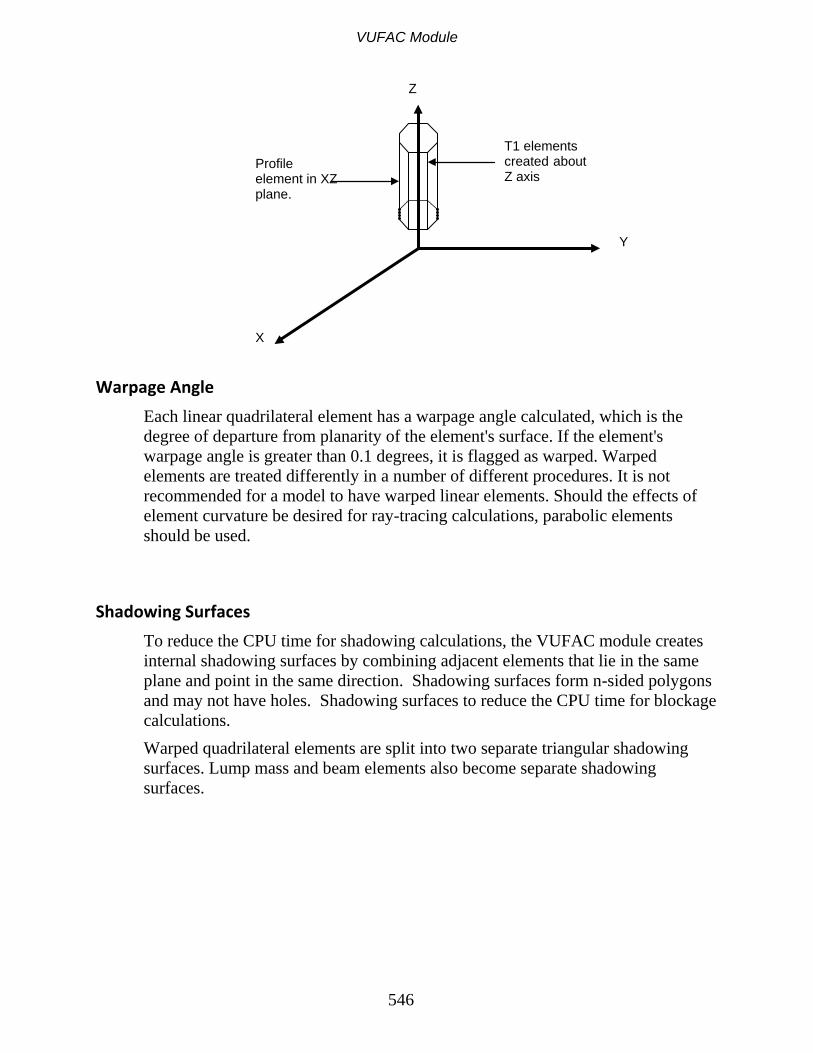
VUFAC Module
546
Warpage Angle Each linear quadrilateral element has a warpage angle calculated, which is the degree of departure from planarity of the element's surface. If the element's warpage angle is greater than 0.1 degrees, it is flagged as warped. Warped elements are treated differently in a number of different procedures. It is not recommended for a model to have warped linear elements. Should the effects of element curvature be desired for ray-tracing calculations, parabolic elements should be used.
Shadowing Surfaces To reduce the CPU time for shadowing calculations, the VUFAC module creates internal shadowing surfaces by combining adjacent elements that lie in the same plane and point in the same direction. Shadowing surfaces form n-sided polygons and may not have holes. Shadowing surfaces to reduce the CPU time for blockage calculations. Warped quadrilateral elements are split into two separate triangular shadowing surfaces. Lump mass and beam elements also become separate shadowing surfaces.
X
Y
Z
Profile element in XZ plane.
T1 elements created about Z axis

VUFAC Module
547
Elements flagged as non-shadowing with a Card 9 PARAM NOSHADOW are not included in shadowing surfaces.
Elemental Subdivision Algorithm For certain operations such as shadowing checks and ray-tracing elements need to be subdivided into sub-elements. The Card 2a or Card 6f MESH parameter governs the rules for the subdivision. A larger MESH parameter yields a larger number of sub-elements, resulting in more accurate the shadowing and ray-tracing calculations, with corresponding penalties in CPU time. The subdivision algorithm is shown below. If MESH > 0, planar elements are subdivided into MESH2*NV triangular sub-elements, where NV is the number of nodes. The element's centroid is joined to each of its nodes, and each triangle thus created is subdivided into MESH2 similar sub-triangles by subdividing each line segment into MESH equal parts. Lump mass elements are not subdivided. Beam elements are subdivided into MESH sub-elements.
Shadowing surface - all elements in same plane
Elements

VUFAC Module
548
If solar view factors are calculated for specular and transparent elements, the calculated MESH parameter value is multiplied by 5. This is to increase accuracy and reduce aliasing effects.
The View Factor Calculation Algorithm without Ray-Tracing The following outline the steps by which view factors are calculated without ray-tracing. Non-ray-traced view factors are calculated individually for each element pair i and j, following the order of the Card 6 requests. Orbital view factors are calculated from the viewing element i to the internal representation of the environmental source (the planet or the sun), which is considered to be element j. Heat flux view factors are calculated from viewing element i to the radiative source elements j.
Beam MESH=0
Quadrilateral MESH=0
Beam MESH=1
Triangle MESH=0
Triangle MESH=1
Quadrilateral MESH=1
Triangle MESH=2
Beam MESH=2
Quadrilateral MESH=2
VUFAC Module
549
Step 1: Viewing Check Before calculating view factors or orbital or heat flux view factors a viewing check is performed. The vertices of element i are examined to see whether they can be seen by the front surface of element j. Similarly, the vertices of element j are examined if they can be seen by element i. Both conditions need to be met for the elements to see each other. Lump mass elements cannot view each other if their nodes are coincident. Beam elements can not view each other if their axes fall on the same straight line.
Step 2: Preliminary View Factor Magnitude Check A preliminary view factor magnitude check is performed for view factor and heat flux view factor (but not solar view factor) calculations to see if the view factor is too small to be calculated. The minimum acceptable threshold value is defined a Card 6m VFMIN Card, and defaults to 1.E-10.
Step 3: Preliminary Shadowing Check If calculations with shadowing are requested, an initial shadowing check is performed on the shadowing surfaces to screen out shadowing surfaces that cannot possibly block the view of one element to the other. With Card 6 VFxENC Enclosure Card requests only shadowing surfaces that contain elements that belong to the enclosure are considered for screening. For this calculation lump mass and beam elements are transformed into equivalent rectangles. Each shadowing surface is subjected to the following tests:
• A clipping test in which a rectangular box is created around the two viewing elements, using their maximum and minimum global coordinates. If the maximum and minimum coordinates of the shadowing surface fall outside the box, it cannot possibly shadow.
• The shadowing surface's vertices are examined to see if they fall behind the front surface of either of the viewing elements. If they do, the surface cannot shadow.

VUFAC Module
550
• If the vertices of both viewing elements fall on the same side of the shadowing surface the surface cannot shadow.
Step 4: Calculating View Factors with No Shadowing If there are no shadowing surfaces between the elements i and j, the elements are not subdivided a special algorithm for computing unshadowed view factors is used to calculate the view factor VFij between them. The algorithm uses various techniques depending on the types of elements involved. If both viewing elements i and j are planar VFij is calculated with the contour integral technique (Ref. 1). This technique yields very accurate view factors. It consists of numerically integrating the following double integral around the perimeters of the two elements:
∫ ∫=Ci Cj
ij dCidCjCjCiSAi
VF ),(ln2
1π
where:
Ci,Cj are the paths around the perimeters of elements i and j S is the length of a line between two points on the perimeters of elements i and j
If the plane of element i cuts the plane of j, the shape of the cut element is modified to ensure the integration is performed only over the edges of the portions that see each other.
Line S
Integration around the perimeters of the two elements
i
j

VUFAC Module
551
View factors for spherical lump mass elements are calculated with an analytical expression without subdividing the sphere's surface into sub-elements. View factors for beam elements are calculated by transforming them into equivalent surface area hexagonal tubes, and using the exact contour integral technique with the planar sides. Once the view factor is calculated, if heat flux view factors were requested with Card 6n SOURCEx Cards, the view factor is multiplied by the POWER and POWERIR values specified on the Card before being written on VUFF.
Step 5: Calculation of the MESH Parameter If possibly shadowing surfaces have been found in Step 3, each element i and j is subdivided according to the Card 6f MESH parameter as discussed above. The MESH parameter may be user-specified, or automatically calculated, if the Card 6f MESH ERROR ERR option is used. For this option, the MESH parameter is calculated by:
MESH VF AERR NV A
ii i
j=
( )( )( )
MESH VFERR NV
ji
=( )( )
if j is not a space element
MESH MESHj i= if j is a space element
where: ERR is the maximum view factor sum error specified on Card 6f VFi is the maximum approximate estimated view factor between i and j, where element i is the smaller element. NV is average of the number of vertices of the elements i and j
The MESH values are rounded off to the nearest integer.
Step 6: Viewing and Blockage Check for Subelements If some shadowing surfaces have been identified as possibly shadowing, each element i and j is subdivided, and the incremental view factors DVFij from each sub-element DAi to each subelement DAj are calculated. The subdivision is governed by the Card 6f MESH parameter in the manner shown above. For view factor calculations element i is chosen to be the element with the smaller area. A viewing check is performed to verify that the front surface of each sub-element DAi can see the front surface of each subelement DAj.

VUFAC Module
552
If the plane of one of the triangular sub-elements cuts through the other subelement, the shape of the second subelement is appropriately modified to allow view factor calculations between only those portions that see each other. If either i or j is warped, then it is checked that the subelements are not shadowed by part of the warped element. The angle θ is calculated to be the angle between the vector joining the centroids of the two sub-elements and the surface normal of the warped element. Then:
DVFij = if warpage angle > 2
0 π θ−
Next, a blockage check is performed for each of the possible shadowing surfaces by checking if any of them intercepts the line joining the centroids of DAi and DAj. If a shadowing surface blocks, DVFij = 0.
Step 7: The Nusselt Sphere Technique
DA
DA
Element i Element j
DAj
DAi
Unit sphere
πDVFij

VUFAC Module
553
If both i and j are planar, and there is no blockage between the subelements, the Nusselt Sphere technique is used to calculate DVFij. The Nusselt Sphere technique is used because although it is a more approximate than the contour integral technique, it requires much less CPU time. The Nusselt Sphere uses a double projection method. First, a unit sphere (radius=1) is drawn around the CG of DAi (whose area is smaller than DAj). Next, the vertices of DAj are projected onto the sphere by drawing lines from the center of the sphere to the vertices. These vertex projections are then re-projected from the unit sphere onto the plane of DAi.
The area of this second projection equal to πDVFij. The Nusselt Sphere technique is most accurate if either DAi << DAj, or DAi is far away from DAj. If one of the elements is a beam, DVFij is calculated using the exact contour integral technique (not the Nusselt Sphere technique) between the sub-elements. This is because beam sub-elements tend to have high aspect ratios, and the assumption of small DAi does not necessarily hold. The incremental view factors DVFij are then summed to obtain VFij. If during the shadowing checks it turns out that: none of the possible shadowing surfaces does in fact shadow, and both i and j are planar, and VFij is sufficiently large (hence the accuracy of the Nusselt Sphere Technique is
suspect), then VFij is recalculated for greater accuracy with the exact contour integral technique. If heat flux view factors were requested with Card 6n SOURCEx Cards, the view factors are multiplied by the POWER and POWERIR values specified on the Card.
Step 8: Calculation of Solar View Factors If solar view factors are requested instead of view factors, and if Card 6d Earth Cards or Card 6k ORBIT Cards or Card 6t ORBDEF Cards are present, an eclipse check is first performed to see whether the Earth blocks the sun. To model the sun, an internal 1-node element is created from the sun angles at a distance of 1.E6 from the origin. The blockage checks between the element i and the sun are performed as discussed above.

VUFAC Module
554
If there is no eclipse, the incremental solar view factor for element i to the sun is:
DSVF DAAisun i
i=
cos( )θ
where: DSVFi is the incremental solar view factor of subelement DAi. θsun is the angle between the solar vector and the element's surface normal.
1-node elements are not subdivided. For a 1-node element: SVFi =.25
For a beam element:
DSVF DAAi
axis i
i=
sin( )θπ
where:
θaxis is the angle between the element's axis and the sun vector. At the end of the view factor calculation stage, the incremental solar view factors are summed and written as an array of solar view factors SVFi at each time interval.
Global coordinate system
X
Y
Z Sun vector
Zenith direction
σ
θ
π/2-β
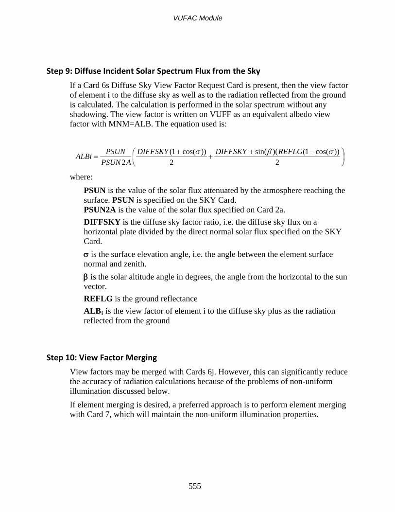
VUFAC Module
555
Step 9: Diffuse Incident Solar Spectrum Flux from the Sky If a Card 6s Diffuse Sky View Factor Request Card is present, then the view factor of element i to the diffuse sky as well as to the radiation reflected from the ground is calculated. The calculation is performed in the solar spectrum without any shadowing. The view factor is written on VUFF as an equivalent albedo view factor with MNM=ALB. The equation used is:
−+
++
=2
))cos(1()(sin(2
))cos(1(2
σβσ REFLGDIFFSKYDIFFSKYAPSUN
PSUNALBi
where: PSUN is the value of the solar flux attenuated by the atmosphere reaching the surface. PSUN is specified on the SKY Card. PSUN2A is the value of the solar flux specified on Card 2a. DIFFSKY is the diffuse sky factor ratio, i.e. the diffuse sky flux on a horizontal plate divided by the direct normal solar flux specified on the SKY Card. σ is the surface elevation angle, i.e. the angle between the element surface normal and zenith. β is the solar altitude angle in degrees, the angle from the horizontal to the sun vector. REFLG is the ground reflectance ALBi is the view factor of element i to the diffuse sky plus as the radiation reflected from the ground
Step 10: View Factor Merging View factors may be merged with Cards 6j. However, this can significantly reduce the accuracy of radiation calculations because of the problems of non-uniform illumination discussed below. If element merging is desired, a preferred approach is to perform element merging with Card 7, which will maintain the non-uniform illumination properties.

VUFAC Module
556
D
Special Topics The following pages detail special topics related to the VUFAC module.
View Factor Calculation Accuracy Considerations
The following table compares the accuracy of the contour integral technique with the Nusselt Sphere Technique with MESH = 1 and MESH = 2, and another popular technique called the Double Summation Technique (not used in TMG). The example is that of two parallel unit squares separated by a distance of D.
% Error vs. Separation Distance D for Two Parallel Unit Squares D Contour Integral Nusselt Sphere
MESH = 1 Nusselt Sphere MESH = 2
Double Summation MESH = 1
Double Summation MESH = 2
0.01 0.001 1.9 0.001 80000. 20000. 0.1 0.0002 10.6 4.7 865. 158. 1. 0.000005 5.6 1.3 8.5 1.94 10. 0 0.1 0.02 0.165 0.04
As the table shows, the accuracy of the contour integral technique is almost totally independent of geometry. The Nusselt Sphere technique has an error upper bound around 12% for MESH = 1, and 5% for MESH = 2, occurring when the elements are very close together. The double summation technique breaks down when the elements are very close together, unless they are divided into much smaller sub-elements.

VUFAC Module
557
Inaccuracies Due to Non-Uniform Illumination Radiation calculations with view factors assume uniform illumination over an element, and potentially significant errors may be introduced when this assumption is not fulfilled. Three good examples of the types of errors introduced by non-uniform illumination are the cylinder blockage problem, the fence problem, and the small area seeing a large area problem. In the cylinder blockage problem, radiation from element i cannot reach j because of blockage by cylinder k. However, if cylinder k is modeled as a single element and thus has a single reflecting surface, because of the uniform illumination assumption inherent in the view factor definition it is assumed that some of the radiation will be reflected onto j, which is clearly incorrect. To avoid this problem, if a cylinder can cause significant blockage then model its surface with a series of planar elements. A second common error is the fence blockage problem. Here i and i j cannot see each other because they are blocked by fence k. However, the edges of fence k do not line up with element l, which can see both i and j. Since both i and j are assumed to illuminate l uniformly, l will incorrectly reflect radiation from i to j. The solution here is to create a mesh so that the edge of l lines up with the edge of k, or, if this is not possible, use smaller elements along the projection of k. A third common error occurs when a small area sees a large area with a large view factor. Here element k is a small black area that is very close to reflective element i. Element i in turn has a large view factor to black element j. Then, very little of the radiation originating from k should be reflected away from i, most of it should bounce back to k and be re-absorbed. However, because the radiation incident upon i is assumed to be uniform, and radiation is reflected in proportion to the
i j k
l
i
i
j j
k
k
l
Cylinder blockage
Fence blockage
Small area sees large area

VUFAC Module
558
view factors, most of the radiation from k will be incorrectly computed to be reflected onto and absorbed by j. The solution here is to subdivide element i into smaller sub-elements. Highly reflective surfaces and coarse meshes generally aggravate problems due to non-uniform illumination.
Calculation of Earth View Factors without Ray-Tracing The Earth view factor EVFi is the element's view factor to Earth. To calculate EVFi, first, a preliminary viewing check is performed to see whether the element's surface sees any part of Earth. The location of the Earth is defined on a Card 6d, Card 6k, or Card 6t or Card 6u. Lump mass and beam elements can always see Earth. If the shadowing option is requested, a preliminary blockage check is performed to screen out the shadowing surfaces that cannot block the Earth. If after the screening some possibly shadowing surfaces exist, the Earth Blockage Factor is calculated:
• The Earth is sub-divided into 4*MESH2 subelements, while element i is subdivided into MESH2*NV sub-elements DAi.
• The view from each sub-element DAi to each Earth sub-element is then examined for blockage by checking whether any of the possibly shadowing surfaces interrupts their centroids' views of each other. The technique is the same as discussed above.
• An incremental Earth view factor DEVFi is calculated with the Nusselt Sphere Technique for each DAi.
• The Earth blockage factor is then defined as: •
∑∑∑∑
−=
m kmknb
m kmkb
i DEVF
DEVFEBF 1
where: DEVFmknb is the incremental view factor from the m'th subelement DAi of element i to the k'th subelement of Earth, calculated with the Nusselt Sphere Technique, calculated without blockage.

VUFAC Module
559
DEVFmkb is the incremental view factor from the m'th subelement DAi of element i to the k'th subelement of Earth, calculated with the Nusselt Sphere Technique, calculated with blockage. EBFi is the Earth blockage factor for element i
The Earth Blockage Factor = 1 if there is full blockage, and = 0 if there is no blockage.
After the Earth Blockage Factor is calculated, the unshadowed Earth view factor is calculated with the analytical expression of (Ref. 2) for the view factor from a small planar area to a very large sphere. Cylindrical 2-node elements are approximated as equivalent surface area square cross-section rods, and lump masses are approximated as equivalent area cubes. Then:
EVFi = (1-EBFi)(Unshadowed Earth view factor)
Calculation of Albedo Factors without Ray-Tracing The albedo view factor is defined by:
iEarthsuni dVFALBALB )cos(∫= θ
where: ALB is the Card 6d, Card 6k, or Card 6t or Card 6u albedo value ALBi is the albedo view factor of element i to the Earth θsun is the angle between the local Earth's surface normal and the sun vector dVFiEarth is the incremental view factor from element i to the Earth
An Albedo Blockage Factor is calculated similarly to the Earth Blockage Factor, except that each DEVFi is multiplied by the solar illumination weighting factor.
∑∑∑∑
−=
m kmknbk
m kmkbk
i DEVFSIWF
DEVFSIWFABF 1
where: SIWFk is the solar illumination weighting factor, equal to the solar view factor of the k'th Earth sub-element. ABFi is the Albedo Blockage Factor for element i
The albedo blockage factor = 1 if element i does not see any part of the Earth which reflects the sun.

VUFAC Module
560
The unshadowed albedo view factor is calculated by interpolating the tables of (Ref. 2), using the sun angle, Earth angle, and albedo value. Then:
ALBi = (1-ALBi)(Unshadowed albedo view factor)
Ray-Tracing
TMG's methodology for handling radiation in the presence of diffuse and transparent/specular surfaces
TMG's approach to handling a combination of diffuse, specular, and transmissive surfaces is to create a single view factor matrix to incorporate all these effects. This matrix is then used to calculate radiative couplings in the GRAYB module and heat absorption due to diffuse reflections and transmission in the POWER module with matrix methods such as Oppenheim's and Gebhardt's. Ray-tracing is performed in the VUFAC module when creating this matrix to account for specular reflection and transmission. Ray-tracing is performed automatically for solar view and heat flux view factors. For Earth and orbital view factors to be ray-traced, the PARAM EXEARTH option must be used. For element view factors to be ray-traced, the VFTRACE option must be used with the appropriate view factor request Card. The ray-tracing methodology is summarized as follows:
• If the receiver element j is fully diffuse, no rays are launched, but the standard view factor calculation algorithm is used to determine the strength (magnitude) of the energy incident on j that comes directly from i. This strength value is then stored with element j.
• If the receiver element j is specular or transparent, multiple rays are launched from source elements i to partially/fully specular/transparent receiver elements j. Both source and receiver elements are subdivided into sub-elements using the Card 6k MESH parameter, and a ray is traced from each sub-element of element i to each sub-element of element j. An energy packet for each spectrum (IR and solar) is created which follows the ray. The strength (magnitude) of the energy packet is equal to the area of the launching sub-element view factor between the sub-elements. The strengths of the incident energy packets are stored for each element.
• The rays are traced through multiple reflections and/or transmissions until they encounter a fully diffuse element, and then are not further traced.

VUFAC Module
561
The strengths of the incident energy packets are stored for each element. The strengths of the reflected/transmitted energy packets are reduced in magnitude proportional to the absorptivity and diffuse reflectivity of the elements.
• Once all elements are processed, the incident energy packets are summed to calculate the appropriate ray-traced view factors from elements i to j, including all specularly reflected and transmitted effects.
The view factor requests The ray-tracing process starts with a Card 6 view factor calculation request. The view factor request for which ray-tracing is done may be a:
• Card 6b Solar View Factor Request - ray-tracing is always done for solar view factors.
• Card 6n Heat Flux View Factor Request - ray-tracing is always done for heat flux view factors.
• Card 6a VFSALL View Factor Request with the VFTRACE flag. • Card 6r Enclosure View Factor Request with the VFTRACE flag. • Card 6k and Card 6t and Card 6u Orbit Cards: ray-tracing is always done for
solar view factors; but it is only done for albedo view factors and Earth view factors if the PARAM EXEARTH option is active.
Source element i Specular/transparent
receiver element j
CG of subelement
DAi
CG's of subelements DAj
Transmitted rays
Rays launched from source element i to receiver element j

VUFAC Module
562
Ray-Tracing with the PARAM EXEARTH option If the PARAM EXEARTH option is present, ray-tracing is done for Earth view factors and albedo view factors for a:
• Card 6k Orbit Definition Card • Card 6t ORBDEF Orbit and Attitude Modeling Request Cards • Card 6d Earth view factor requests • With the PARAM EXEARTH flag the Earth is modeled explicitly as a
separate set of shell elements for each orbital position in the appropriate location with respect to the model (please see a description of the Card 9 PARAM EXEARTH Card).
Choosing the source elements in a view factor request The elements i and j for which the calculations are performed are determined by the view factor requests. Element i is chosen from the specified set of source elements, and element j is chosen from the specified set of receiver elements.
• If Card 6n heat flux view factors are requested, the set of source and receiver elements are specified on the heat flux view factor request Card.
• If solar view factors are requested through Card 6b, Card 6k, Card 6t, or Card 6u, the source element i is the sun, and the receiver elements are specified on the on the solar view factor request Cards.
Earth modeled explicitly with shell elements
Sun
Reflected albedo/Earth IR ray
Specular/transmissive element
Transmitted/reflected ray

VUFAC Module
563
• If Card 6r view factors are requested with ray-tracing in an enclosure, the source elements and the receiver elements are both specified to be all the elements in the enclosure.
• If all the view factors in the model are requested with ray-tracing through Card 6a, then the source and receiver elements are both specified to be all the elements in the model.
• If albedo and Earth view factors are requested with the PARAM EXEARTH option with Cards 6k, 6d, or 6t, the source elements are the explicitly modeled Earth elements, and the receiver elements are the ones appropriately specified on the Card.
Viewing Checks and Elemental subdivision Steps 1 through 6 of the view factor calculation algorithm described above are followed to determine whether the two elements see each other. If element j is specular or transparent, the elements are subdivided as described above, even if there are no shadowing surfaces between them.
Calculation of energy packet strength To calculate the strength of the packets associated with the ray launched from DAi, an incremental view factor DVFij between subelements DAi and DAj is calculated as described above. For each non-zero DVFij, a ray packet of strength Strengthsolj in the solar spectrum and strength StrengthIRj in the IR is launched from the CG of the subelement DAi towards the CG of DAj: Strengthsol DA DVFiStrengthsol DA DVF POWERStrengthsol DA DVFStrengthsol DA DVF ALBStrengthIR DA DVFiStrengthIR DA DVF POWERIRStrengthIRStrengthIR DA DVF
j i j
j i ij
j j ij
j i ij sun
j i j
j i ij
j
j i ij
= for view factor calculations = for solar spectrum heat flux view factor calculations = for solar view factor calculations = ( ) for albedo factor calculations with PARAM EXEARTH = for view factor calculations = for IR spectrum heat flux view factor calculations = for solar view factor calculations =
cos θ
0 for Earth view factor calculations with PARAM EXEARTH

VUFAC Module
564
Where:
POWER is the solar spectrum energy per unit area emitted by the element i specified on Card 6n. POWERIR is the IR spectrum energy per unit area emitted by the element i specified on Card 6n. ALB is the albedo value specified for the Earth. θsun is the angle between the solar vector and the explicitly specified Earth element.
Accuracy considerations Accuracy and performance of ray-tracing strongly depend on the MESH parameter. The number of rays launched from an element varies as MESH4, since the rays are launched from each DAi subelement to each DAj subelement. The following table shows the number of rays launched from one quadrilateral element to another as a function of the MESH parameter:
Number of rays launched from quadrilateral source element i to quadrilateral element j.
MESH Number of rays launched
0 1
1 16
2 256
3 1296
4 4096
It is important to note that the cost of ray-tracing is only proportional to the number of specular/transparent elements in the model, since multiple rays are launched only towards them, and they are the ones that support reflected rays.

VUFAC Module
565
Calculation of reflected/transmitted energy packet strengths After the ray hits a specular or transparent element j, one or two new rays are launched from the point where the incident ray intersects DAj.
• If element j is only specular or transparent but not both, a single ray is launched.
• If element j is both specular and transparent (half-silvered mirror), then two new rays are launched from DAj: one ray is transmitted and one is reflected. For each of the newly launched rays, two energy packets (one in the solar and one in the IR spectrum) are tracked, for a total of four energy packets.
The new energy packets' strengths are computed as follows:
Strengthreflsol sol StrengthsolStrengthreflIR IR StrengthIRStrengthtranssol sol StrengthsolStrengthtransIR IR StrengthIR
j j
j j
j j
j j
= =
= =
ρρ
ττ
Where:
ρsolj is the specular reflectivity of the element j in the solar spectrum ρIRj is the specular reflectivity of the element j in the IR spectrum τsolj is the transparency of the element j in the solar spectrum τIRj is the transparency of the element j in the IR spectrum Strengthreflsol is the strength of the specularly reflected solar spectrum energy packet StrengthreflIR is the strength of the specularly reflected IR spectrum energy packet Strengthtranssol is the strength of the transmitted solar spectrum energy packet StrengthtransIR is the strength of the transmitted IR spectrum energy packet
Angle Dependent Surface Properties For some elements, specular reflectivity or transmissivity may be defined to be a function of angle of incidence. For these the specular reflectivity or transmissivity

VUFAC Module
566
are determined by linear interpolation of the data in the array referenced by the material property. If the incident angle falls outside the range defined in the array TMG uses the value at the nearest limit, it does not extrapolate.
The direction of incidence is determined by projecting the ray onto the plane defined by the element surface normal and then determining the angle between this projection and the material orientation vector for the element. Angle of incidence is the angle between the incoming ray and the surface normal.
Calculation of ray direction for reflected/transmitted rays For specular elements j, the new direction is calculated by assuming the angle of incidence is equal to the angle of reflection with respect to the local surface normal. For the transparent elements j, if the indices of refraction on both sides of the element are not specified or are equal, the direction of the transmitted ray is the same as the incident ray. However, if the indices of refraction are specified and are different, then a new direction for the ray's travel is calculated using Snell's Law:
sin ) )( = sin(θ θtrans
inc inc
trans
II
Where:
θinc is the angle the incident ray makes with the surface normal θtrans is the angle the transmitted ray makes with the surface normal Iinc is the index of refraction on the incident side of the element
Reflected Ray Incident Ray
Angle of Incidence
Direction of Incidence
Material Coordinate System Z axis

VUFAC Module
567
(specified on Card 9 MAT Card) Itrans is the index of refraction on the transmitted side of the element (specified on Card 9 MAT Card).
The index of refraction is assumed to be spectrum-independent, the element j is assumed to have the same indices of refraction in both the IR and solar spectra. If Iinc > Itrans, i.e. the ray goes from a dense to a less dense material, the computed sin(θtrans) may be > 1. For this case the material is assumed to reflect specularly, with the specular reflectivity equal to the transmissivity of the material. If element j is planar, the local surface normal is the same as the surface normal of the element.
Calculation of ray intercept and direction for curved elements If the element is curved, a more complex algorithm is used to compute the local surface normal, the point of interception, and the new ray direction. Curved elements are parabolic elements, defined by specifying the midside nodes of the sides with Card 5a MIDSIDE Cards. The shape of the surface is represented using the standard finite element parabolic shape functions. These describe the variations of x, y, and z on the surface as functions of 2 parameters: s and t. The equation for the shape of the surface is defined by curve-fitting the coordinates of the nodes. The following describes the procedure for calculating the local surface normal and the point of interception for parabolic elements: 1. Identify the sub-triangle within the element which the ray intersects.
Subdivision of quadrilateral into subtriangles

VUFAC Module
568
2. For quadrilaterals, select point at the parametric center of the element (s=0,
t=0) and determine its x, y, z coordinates. Using this point and the 8 element nodes, subdivide the quadrilateral into four quadrants. Subdivide each quadrant into two, yielding 8 subtriangles, and determine which subtriangle the ray intersects. If the element is a triangle, it is not subdivided, but is considered to be the intersecting subtriangle.
3. Subdivide the intersecting sub-triangle into 4 more subtriangles by connecting the midpoints of the sides. Determine which subtriangle the ray passes through. Calculate the surface normal of subtriangle and the intersection point with the ray, assuming the subtriangles are planar.
4. Further subdivide this sub-triangle in same manner into 4 sub-triangles, and determine which of these the ray intersects. Calculate the new intersection point and surface normal for this sub-triangle, assuming the sub-triangle is planar. Define a tolerance parameter D:
D length of side length of side=
1 + 2100
5. Compare results from the subdivision of Step 2 and Step 3, and if the intersection point has moved less than D and the angular change in surface normal is less than .01 radians, then stop. Otherwise sub-divide again and start with Step 2.
Subdivision of a triangle into subtriangles

VUFAC Module
569
6. If during the intersection calculations the ray does not intersect an element or a sub-triangle, then the element or sub-triangle is expanded in parametric space and the intersection calculation re-started. The expansion is applied recursively until an intersection is found or an internal limit is reached.
Once the point of intersection has been determined the reflected ray is calculated using the point of interception and the local surface normal. The new ray is then checked to see if it re-intersects the same element. The reflection/re-intersection procedures are repeated until a new ray does not re-intersect the element or 5 bounces are found. In the event of failure in the curved element processing TMG resorts to using the planar approximation to the element.
Location of the next intercepted element Once the direction and strengths of the ray launched from j are established, an artificial 1-node element k' is created at a very large distance along the ray. All the shadowing surfaces are then checked for interception of the ray originating at DAj and ending at k'. If more than one shadowing surfaces intercept, the one with the point of interception closest to DAj is chosen as the intercepting surface. Next, a search is done within the intercepting shadowing surface to identify the element k that is hit, and the coordinates of the interception point are computed. If the ray is not terminated, new strength values and directions are calculated in the manner described above, and the ray further continued.
Ray termination Ray termination occurs under the following circumstances:
• If none of the shadowing surfaces intercepts the ray, an improper model definition is assumed, and the ray is ignored and is assumed terminated in the space element.
• If view factors in an enclosure are requested, and an intercepting shadowing surface is found, but the intercepting shadowing surface is not inside the enclosure, an improper model definition is assumed and the ray is also ignored and is considered terminated.
• If the intercepted element k is diffuse, the ray-tracing for this ray is terminated.

VUFAC Module
570
• If the ray hits the back of an element whose reverse side is not defined, an improper model definition is assumed and the ray is terminated.
• If the energy packet strength is less than .001 of its original strength in both spectra, the ray is terminated.
Summation of the energy packets to calculate the ray-traced view factors Once the ray-tracing calculations are finished, the energy packets are summed to calculate the geometric view factors. For solar view factors, albedo view factors, Earth view factors, and heat flux view factors the geometric view factor is calculated by:
VF POWERA
DA DVF Riji
ii im ijk
k
N
= ∑
Where: N is the number of rays launched from source element i that arrive at
element j. VFji is the view factor from element j to source element I POWERi is the power per unit area of the emitting element = Card 6n POWERIR for IR spectrum heat flux view factor
calculations = Card 6n POWER for solar spectrum heat flux view factor
calculations = 1 for solar view factor calculations = ALBcos(θsun) for albedo view factor calculations Rijk is the reduction factor by which the strength of the k'th ray launched
from i is reduced after multiple reflections when it arrives at j m is the first element that the k'th ray hits DAiDVFim is the strength of the k'th ray launched from i For solar spectrum view factors, the view factor from element i to j is calculated with:
VFDA DVF R
Aiji im ijk
i soli soljk
N
= ( )1− −∑ ρ τ
For IR spectrum view factors, the view factor from element i to j is calculated with:

VUFAC Module
571
VFDA DVF R
Aiji im ijk
i IRi IRjk
N
= ( )1− −∑ ρ τ
In effect, the view factor is calculated for an area reduced by the sum of the specular reflectivity and transmissivity in each spectrum.
Ray-tracing through Solid Elements Solid elements are by default considered to be transparent, ray-tracing is considered to occur between shell, beam and lump elements. However, if the SOLAREXTINCT or IREXTINCT properties are defined for a solid elements, ray-tracing is performed within solid elements with the following methodology:
• Surface coating. In the DATACH module, all surfaces of all solid elements with SOLAREXTINCT or IREXTINCT properties are surface coated with perfectly transparent elements, unless a shell element already exists on that surface. These surface coated elements will also be considered to be the boundary elements for conduction calculations. Reverse sides are also created for these surface coated elements, which are ignored for conduction calculations. The index of refraction value assigned to the front surface of a surface coated element facing a solid element is the value specified as IREFFRONT on the MAT Card for the solid element. The index of refraction of the reverse side is taken from the adjacent solid element, or, if it is a free surface, is assigned the value 1. The IREFBACK field on the MAT Card is ignored for solid elements.
• Ray strength calculation. A ray striking one of these elements will be transmitted, and the strength of the transmitted ray will be diminished as it travels through the solid by a factor equal to: 1− −e EXT LENGTH( * ) where EXT is the specified extinction coefficient. The lost radiation is written as a view factor from the original source element incident upon the surface coated element the ray hits on the far side of the solid element.

VUFAC Module
572
• Index of refraction. If all the surface coated elements facing a solid have the same index of refraction, the solid element is considered to have a zero index of refraction gradient, and the ray path will be straight through it. If, however, there is a variation in the index of refraction (this can be achieved with Card 9 MATCHANGE Cards), then an index of refraction gradient will be calculated for the solid element, and an appropriate curved path will be calculated for the ray traveling through the solid. If a ray hits an internal surface coated element, it is always transmitted into the adjacent solid element. If it hits a surface coated element whose reverse side faces outwards, a determination is made based on Snell’s Law (see above) on whether it exits the solid material or total internal reflection occurs.
• Once the calculations are completed, view factors and solar view factors incident upon the surface coated elements are written onto VUFF. The POWER module will calculate heat fluxes for these elements, assuming the incident rays are perfectly absorbed by the surface coated elements.
Handling of Reciprocity In calculating view factors with ray-tracing, both VFij and VFji will in general be calculated. However, since the number of packets arriving at i from j will generally not be equal to the number of packets arriving at j from i, the reciprocity relationship AiVFij = AjVFji will as a rule not be fulfilled. The question is, which is more accurate: VFij or VFji?
To address this issue, if Ai ≥ 2Aj, then VFij (the view factor from the larger element) is discarded. If Aj ≤ Ai < 2Aj, then VFij is computed with averaging:
VF A VF A VFA
AA
AA
VF VF A VFA
AA
AA
iji ij j ji
i
i
j
j
i
ij ijj ji
i
i
j
j
i
=+
≥ ≥
=
22 2 if and
if 2 < or 2 <max( , )
Outputting of Results The calculated view factors are written on file VUFF with the following convention:
• Solar view factors are written in the solar spectrum only with the code MNM=SVF.

VUFAC Module
573
• Ray-traced albedo view factors are written with the code MNM = ALR. Albedo view factors that have not been ray-traced are written with the code MNM = ALB.
• Ray-traced Earth view factors are written with the code MNM = EVR. Earth view factors that have not been ray-traced are written with the code MNM = EVF.
• Heat flux view factors are ray-traced in both the IR and solar spectra. Heat flux view factors in the solar spectrum are written with the code MNM = HVF, while heat flux view factors in the IR spectrum are written with the code MNM = HVI.
• Both ray-traced and non-ray-traced view factors are written with MNM = BVF. View factors that have been ray-traced in the solar spectrum are written with the code TIME=-1.1E36. View factors that have been ray-traced in the IR spectrum are written with the code TIME=-1.2E36. View factors which have not been ray-traced (and hence apply to both spectra) are written with the code TIME = -1.0E36.
• Ray-traced view factors for elements that have specular or transparent surface properties are written with their areas, emissivities, and absorptivities redefined to take into account the reduction area. The following relationships are used:
A AA A
inewsol i soli soli
inewIR i IRi IRi
inewi
IRi IRi
inewi
soli soli
= − −= − −
=− −
=− −
( )( )
( )
( )
11
1
1
ρ τρ τ
ε ερ τ
α αρ τ
where: Ainewsol is the area written on file VUFF for solar spectrum view factors AinewIR is the are written on file VUFF for IR spectrum view factors εinew is the emissivity written on file VUFF for IR spectrum view factors αinew is the solar spectrum absorptivity written on file VUFF for
VUFAC Module
574
solar spectrum view factors.
Thermal Coupling Calculations Thermal couplings are calculated between elements N1 and N2 if requested by the Card 6e Cards. The VUFAC module must recognize element N1. N2 may be specified directly, or if one if the NEARx options is used, it may be automatically chosen by TMG to be the closest element to N1 from a pre-selected group of elements. Thermal couplings created by the Card 6e Card are written on file MODLF.

References
575
References 1. Chapter, John J., A Simplification Technique For Thermal Radiation In Gray
Enclosures, J. Of Spacecraft, Vol. 7, No. 12, pp1476, 1970. 2. Chapter, John J. et al, Simplified Radiation Analysis Using Modular
Enclosures, J. Of Spacecraft, Vol. 8, No. 9, pp1006, 1971. 3. Stevenson, J. A., and Grafton, J. C., Radiation Heat Transfer Analysis For
Space Vehicles, Report ASD61-119, 1961 (Wright Patterson Air Force Base). 4. Gebhardt, B. Unified Treatment For Thermal Radiation Transfer Processes -
Gray, Diffuse Radiators And Absorbers. ASME paper 57 - A - 34 (1957) 5. Sparrow, E. M. A New And Simpler Formulation For Radiative Angle Factors.
ASME Transactions, Journal Of Heat Transfer, Vol. 85, Series C, (1963), pp81.
6. Schornhorst, J. R., and Viskanta, R., An Experimental Examination Of The Validity Of The Commonly Used Methods Of Radiant Heat Transfer Analysis. Journal Of Heat Transfer, pp429. Nov. 1968
7. Handbook of Heat Transfer Fundamentals, 2nd. Ed., by Rohsenow, Hearten, & Janice, McGraw-Hill, 1985
8. Hageman, A.L., and Young. D.M., Applied Iterative methods, Academic Press, 1981
9. Thermal Analysis and Control of Electronic Equipment by Allan D. Kraus and Avram Bar-Cohen, Hemisphere, 1983
10. Handbook of Hydraulic Resistance - Coefficients of Local Resistance and of Friction by I.E. Idel'chik, 1960
11. Thermal Computations for Electronic Equipment by Gordon N. Ellison, Van Nostran Reinhold Co., 1984.
12. Cooling Techniques for Electronic Equipment, by Dave. S. Steinberg, Wiley-Interscience 1980.
13. The Dynamics and Thermodynamics of Compressible Fluid Flow, by Ascher H. Schapiro, The Ronald Press Co., 1953
14. An Introduction to Hybrid Iterative Methods, H.A. van der Vorst and G.L.G. Sleijpen, Proceedings of the International Workshop on Solution Techniques for Large-Scale Problems, CERCA Centre de Recherché en Calcul Appliqué, Montreal, Quebec, Canada, Sept. 26-28, 1994
15. Preconditioned Krylov Subspace Methods for CFD Applications, Y. Saad, University of Minnesota, Proceedings of the International Workshop on

References
576
Solution Techniques for Large-Scale Problems, CERCA Centre de Recherche en Calcul Appliqué, Montreal, Quebec, Canada, Sept. 26-28, 1994
16. Edwards, D.K. and Bertak, I.V. Imperfect Reflections In Thermal Radiation Heat Transfer, AIAA Paper 70-860, presented at the AIAA 5th Thermophysics Conference, LA, Ca., June 29-July 1, 1970
17. "A Fast and High Quality Multilevel Scheme for Partitioning Irregular Graphs". George Karypis and Vipin Kumar. SIAM Journal on Scientific Computing, Vol. 20, No. 1, pp. 359-392, 1999.