numerical study of interface reconstruction method in

HAL Id: hal-01863450https://hal.archives-ouvertes.fr/hal-01863450

Submitted on 28 Aug 2018

HAL is a multi-disciplinary open accessarchive for the deposit and dissemination of sci-entific research documents, whether they are pub-lished or not. The documents may come fromteaching and research institutions in France orabroad, or from public or private research centers.

L’archive ouverte pluridisciplinaire HAL, estdestinée au dépôt et à la diffusion de documentsscientifiques de niveau recherche, publiés ou non,émanant des établissements d’enseignement et derecherche français ou étrangers, des laboratoirespublics ou privés.

Numerical study of interface reconstruction method inunder-resolved regions of the flow for liquid jet primary

breakupAnirudh Asuri Mukundan, T. Menard, A. Berlemont, Jorge César Brändle de

Motta

To cite this version:Anirudh Asuri Mukundan, T. Menard, A. Berlemont, Jorge César Brändle de Motta. Numerical studyof interface reconstruction method in under-resolved regions of the flow for liquid jet primary breakup.ICLASS, 14th Triennial International Conference on Liquid Atomization and Spray Systems, Jul 2018,Chicago, United States. pp.1-8. hal-01863450

https://hal.archives-ouvertes.fr/hal-01863450

https://hal.archives-ouvertes.fr

ICLASS 2018, 14th Triennial International Conference on Liquid Atomization and Spray Systems, Chicago, IL, USA, July 22-26, 2018

Numerical study of interface reconstruction method in under-resolved regions of the flowfor liquid jet primary breakup

A. Asuri Mukundan*, T. Ménard, A. Berlemont, J. C. Brändle de MottaCNRS UMR6614–CORIA & Université de Rouen Normandie, Saint Étienne du Rouvray,

Rouen, [email protected], [email protected], [email protected], and

[email protected]

AbstractLiquid/gas interface reconstruction continues to be a challenge in the numerical study of liquid fuel atomization.This paper focuses on one such reconstruction method called moment of fluid (MOF) method intended specificallyfor interface reconstruction in under-resolved flow regions. MOF method gives two-fold advantage over volumeof fluid (VOF), level set (LS), and coupled level set volume of fluid (CLSVOF), such as: first, MOF preservesthe shape and orientation of interfaces that are commonly encountered in under-resolved regions of the flow, andsecond, it exhibits second-order accuracy in spatial resolution for multiple interface topologies. For various testcases considered in this paper, MOF has consistently proved to be more accurate than and at least as accurate asCLSVOF method.

Keywords: multiphase, moment of fluid, center of mass, volume fraction

IntroductionAtomization of injected liquid fuel in gas turbines and internal combustion (IC) engines play a major role in

the production of harmful pollutant emissions. This is due to the fact that the efficiency of liquid fuel combustionand production of pollutants has a direct dependency on the mixing between fuel and oxidizer, which in itselfresults from the cascade of the mechanisms initiated by the process of atomization of injected liquid fuel stream.Due to the multiphase characteristic and multi-physical aspect of the liquid fuel atomization, and often due to thepresence of highly turbulent environment, experimental investigations proves to be a challenging endeavor. Thismotivates the need for the development of numerical methods to study the atomization process.

An obvious requirement of these methods is least numerical error which will make it more trustable andsuitable to be used in detailed simulations such as direct numerical simulations (DNS) of liquid atomization [1–3].In addition, these numerical methods ideally must require less computational resources, thus not taxing even themost powerful supercomputers available today [4].

In the presence of complex topological structures encountered in liquid fuel atomization, the underlyingequations are stiff, thus the development and improvement of numerical methods to treat such structures hasbeen an active area of research. Of the many sharp interface reconstruction methods, volume of fluid (VOF)method [5–9], level set (LS) method [10–14], and their variant such as coupled level set volume of fluid (CLSVOF)method [1, 3, 15] have been proved to perform well on variety of canonical test cases. Although these validatedmethods prove to be successful in multiple applications, the geometrical property computations can still be inac-curate especially in the under-resolved regions of the flow. This results from the inaccurate computation of unitnormal of the interface in such regions. To mitigate this inaccuracy, a numerical interface reconstruction methodcalled moment of fluid (MOF) method [16] is developed in the in-house code ARCHER [1, 10, 17] and presentedin this work. MOF method has been proved – to preserve the orientation of the liquid/gas interface in the contextof multiphase flows [16, 18]; to be second-order accurate in spatial resolution [19].

The objectives of this paper are: to present MOF method for interface reconstruction in the context of in-compressible multiphase flows as a potential interface tracking technique, compare and contrast the results ofinterface reconstruction for various academic test cases between MOF and CLSVOF methods, and to emphasizethe relevance of the usage of the MOF method especially in the under-resolved regions flow regions.

Moment of Fluid (MOF) methodMOF method is an extension of VOF method for interface tracking in the context of multiphase flows. VOF

method uses only liquid volume fraction F (0th moment of the liquid volume) for tracking the interface in every*Corresponding author: [email protected]

1

mailto:[email protected]

14th ICLASS 2018 Interface Reconstruction using MOF method: Numerical Study

mixed computational cell. As a step further, MOF method tracks both the liquid volume fraction and coordinatesof the liquid center of mass (COM) xCOM (1st moment of liquid volume) for the interface reconstruction in eachsuch cell. A mixed computational cell, within this study, is defined as the cell in which 0 < F < 1 holds. Thedefinitions of the 0th and 1st moments of the liquid volume are given as

F =

∫ωdx∫

Ωdx, (1)

xCOM =

∫ωxdx∫

Ωdx

, (2)

where ω is the domain of the liquid packet inside the computational cell Ω. The availability of these two parametersestablishes a self-sufficiency of the required information to reconstruct the approximate interface in a cell thus,eradicating data requirement from its neigbours. This results in a uniform treatment of the internal and boundarycells in the mesh thus, yielding the resolution of the interface as high as that of the computational mesh itself.Within this work, the MOF method is developed in the in-house code ARCHER.

Interface ReconstructionThe commonly used piecewise linear interface calculation (PLIC) is employed in this work for approximating

the original interface. Thus, the equation of the approximated interface in 3D is given by ax + by + cz + d = 0,which represents the equation of a plane. In 2D, this equation becomes the equation of a line. The unit normal nof the interface is therefore expressed as n = [a, b, c]T . The shortest distance of the interface from the cell centeris characterized by the parameter d.

The interface reconstruction in MOF method is a constrained optimisation problem as described in [18]wherein n and d have to be determined simultaneously by the satisfaction of the two conditions

| F ref − F act(n, d) |= 0, and (3)

EMOF(n, d) = minEq. (3) holds

∥∥xrefCOM − xact

COM(n, d)∥∥

2. (4)

All the variables containing the superscript “ref” represents the variables pertaining to the original (reference) in-terface while those containing the superscript “act” represents the variables pertaining to the reconstructed (actual)interface. The explanation of these conditions is assisted through Figure 1. The shortest distance of the interface

n

d

xactCOM

xrefCOM

Figure 1: Mathematical Representation of MOF method

from the cell center d is determined by the volume conservation condition Equation (3). To this end, the linearapproximated interface (shown by dashed line in Figure 1) is constructed such that the volume of liquid is exactlythe same under reference (shown by solid line in Figure 1) and actual interface upto the machine precision. Thecomputation of optimal value of d is carried out using Newton-Raphson iterative method as described in Ménardet al [1]. The interface unit normal is then computed by minimising the error EMOF (also called distance de-fect) between the coordinates of the reference and the acutal COM of the liquid in the computational cell (c.f.Equation (4)).

In order to solve this minimisation problem, n is parameterised [18] using the polar coordinates as follows

n =

a

b

c

=

sin Φ cos Θ

sin Φ sin Θ

cos Φ

. (5)

2


Thus, the Equation (4) transforms into a non-linear least square problem for (Φ,Θ), i.e., finding (Φ∗,Θ∗) suchthat the error EMOF is minimum, i.e.,

EMOF(n, d) =∥∥g(Φ∗,Θ∗, d)

∥∥2

= minEq.(3) holds

∥∥g(Φ,Θ, d)∥∥

2, (6)

where g(Φ,Θ, d) = xrefCOM−xact

COM. Equation (6) is solved numerically for (Φ∗,Θ∗) using Gauss-Newton method.Once the optimal parametric angles (Φ∗,Θ∗) are known, the components of the unit normal [a, b, c]T can beretrieved using Equation (5). The new reference COM in each cell takes the value of the acutal COM pertaining tothe reconstructed interface using which the new values of the normal components are computed.

Interface AdvectionThe advection of interface in the case of MOF method involves advection of both reference liquid volume

fraction F ref and coordinates of reference COM xrefCOM. A directionally split numerical scheme is employed for

the advection of both quantities. The transport equation and numerical scheme implemented for the advectionare presented in the following subsections. Since the advection pertains solely to the reference quantities, thesuperscript “ref” will be dropped in volume fraction and the coordinates of the COM hereon.

Volume FractionThe advection equation for the volume fraction solved in ARCHER is given as

∂F

∂t+∇ · (Fu) = c (∇ · u); c =

1, F > 0.5

0, otherwise(7)

The algorithm proposed in the work of Weymouth and Yue [20] is implemented for the advection of the volumefraction. For more details on the finite difference discretization of the above equation and computation of volumefluxes across cell faces, the reader is referred to [20].

Centre of MassThe advection equation of the reference COM is given as

d

dt(xCOM) = u(xCOM), (8)

where u(xCOM) is the velocity field interpolated linearly from the face-centers of the computational cell to thelocation of the COM. This velocity is non-dimensionalized using the mesh spacing and the time step size ∆t =tn+1− tn, hence the velocity component becomes the local Courant-Friedrichs-Lewy (CFL) number. In this study,the COM is considered as a Lagrangian particle [16, Appendix A] that is associated with a liquid packet/parcel.

An Eulerian Implicit–Lagrangian Explicit (EI–LE) scheme [21] is employed in this study for solving Equa-tion (8). A first order integration scheme of this equation keeping constant velocity over the time step size ∆tyields,

xn+1COM = xnCOM + u(x∗COM) (9)

in which the mode of the scheme is Eulerian Implicit if x∗COM = xn+1COM and Lagrangian Explicit if x∗COM = xnCOM.

In order to have the consistency between the advection of liquid volume fraction and COM, the mode of the schemefor COM advection is switched between EI and LE for a Cartesian direction at each time step, i.e., if x−directionadvection of COM for tn → tn+1 is carried out using EI mode, then the x−direction advection of COM fortn+1 → tn+2 will be carried out in LE mode.

In this study, the coupling between the advections of the volume fraction and that of COM is carried out similarto that in the study of Jemison et al [18].

Results and DiscussionIn this section, the accuracy, order of convergence, and utility of the MOF interface reconstruction method are

analyzed using different canonical test cases. The choices of the validation tests considered in this study are madeso that the errors due to reconstruction and advection algorithms used in this study can be assessed. In each of thepresented tests, the reconstruction accuracy of MOF and CLSVOF algorithms are compared along with the orderof convergence of the error with respect to the spatial resolution of the mesh.

3


Since the advection errors are almost always accompanied with the reconstruction errors, these errors arereported and addressed using separate test cases for better evaluation of the performance of the reconstruction andadvection algorithm implemented in this study. In all the test cases presented in this work, a constant CFL numberof 0.5, periodic boundary conditions along x− and y−directions, and ∆x = ∆y = const. are used. The time stepsize ∆t is computed from the CFL number and the mesh spacing.

Translation testFollowing the work of Harvie and Fletcher [22], the advection of circular liquid droplet of radius r = 0.25

units placed at the center of a 1 × 1 domain is considered for analysing the errors due to reconstruction fromMOF and CLSVOF methods. The CLSVOF method developed by Ménard et al [1] is used in this study for thecomparison of results with MOF method. The advection is performed along x−direction with unit velocity suchthat the interface crosses the boundary and comes back to the same initial location at the final time step. Since thevelocity is uniform, obeys continuity equation and does not have any gradient in the domain, the errors arising atthe end of advection is purely from the reconstruction algorithm. This error is computed as

E =∑i,j

Aij | FnTi,j − F 0

i,j |, (10)

where Ai,j is the area of the cell, F 0 and FnT are the liquid volume fractions at the initial and final time iterationinstants respectively. The mesh resolutions considered in this test are 16 × 16, 32 × 32, 64 × 64, 128 × 128, and256 × 256. Figure 2 shows the initial interface (black line) and final interfaces (red line: MOF in left subfigure,

(a) MOF (b) CLSVOF

10−2 10−110−5

10−4

10−3 (∆x)2 ∼

∆x

E

MOFCLSVOF

(c) Error convergence for circle translation

Figure 2: 32× 32 mesh; Black line (nt = 0): Initial; Red line (nt = 128): MOF; Blue line (nt = 128): CLSVOF

blue line: CLSVOF in middle subfigure) of the circular liquid droplet after the advection for 32 × 32 mesh. Thecircle comes back to its initial location after 128 time advancement iterations for this mesh resolution. For suchinterface topology, it can be seen qualitatively that both MOF and CLSVOF methods have performed well. Fromthe error convergence plot shown in Figure 2c, it is quite obvious that both MOF and CLSVOF display second-order convergence rate.

Rotation TestThe same case as described in Rider and Kothe [23] is considered in which a circle of radius r = 0.15 units is

placed in a 1 × 1 domain with center at (0.5, 0.75), rotates around the center of the domain in a spatially varyingfield given by

u =π

3.14(0.5− y), and (11)

v =π

3.14(x− 0.5). (12)

In the exact solution, the circle retains its shape thus, this test assesses the efficiency of the EI–LE advectionalgorithm implemented in this study. The error in the numerical solution is computed using Equation (10) wherenT is the final time iteration at which the interface completes one full revolution around the center of the domain.The results of the error for the mesh resolutions 32 × 32, 64 × 64, and 128 × 128 are presented and compared inthe Figure 3 for MOF and CLSVOF reconstruction algorithms. The initial interface is depicted by black line, thefinal interfaces from MOF and CLSVOF reconstruction methods are depicted by red and blue lines respectively.

4


(a) 32× 32 (b) 64× 64 (c) 128× 128

10−2 10−110−6

10−5

10−4

∼ (∆x)2

∆x

E

MOFCLSVOF

(d) Error convergence for circle ro-tation

Figure 3: Initial and final interfaces of circle after one full rotation and error convergence plot

It can be observed from this figure that for such a simple advection problem, the advection schemes employed forthe volume fraction and COM in this study for MOF method is qualitatively more accurate than CLSVOF method.Furthermore, from Figure 3d for mesh resolutions from 16 × 16 to 128 × 128, it is observed that MOF methodexhibits second-order convergence rate and produces lower error than CLSVOF method.

Zalesak’s notched disk testIn this test, a slotted circle of fluid rotates around the center of the domain in a solenoidal velocity field. This

test is indeed an assessment of the efficiency of the reconstruction algorithm than that of the advection algorithm.Within this test, a slotted circle of radius r = 0.15 units having slot width of 0.06 units and slot length of

0.2 units is placed in a 1 × 1 domain with center of the circle located at (0.5, 0.75). The rotation of this slottedcircle is accomplished using velocity fields given in the Equations (11) and (12). Since this velocity is divergence-free throughout the domain, the interface of the Zalesak’s notched circular disk is expected to retain the originalshape at the end of rotation. The test ends when the first (anticlockwise) revolution of the slotted circular disk iscompleted. The resulting error between the exact and the reconstructed interface is then computed as

E =

∑i,j

| FnTi,j − F 0

i,j |∑i,j

| F 0i,j |

, (13)

where the definitions of F 0 and FnT remains the same as explained in the previous subsection. The results fromthis test are shown in Figure 4 for 32 × 32, 64 × 64, and 128 × 128 mesh resolutions. The initial interface isdepicted using black solid line, the final interface from MOF algorithm is depicted using red solid line while thatfrom CLSVOF algorithm is depicted using blue solid line.

(a) 32× 32 (b) 64× 64 (c) 128× 128

10−2 10−1

10−2

10−1

∼ (∆x)2

∆x

E

MOFCLSVOF

(d) Error convergence for Zalesakdisk rotation

Figure 4: Initial and final interface of Zalesak’s slotted disk after one full revolution and error convergence plot

It can be observed from Figures 4a to 4c, that the error in reconstruction is mainly concentrated in the re-gions of high curvature of the interface. Furthermore, it is obvious from from Figure 4d that the MOF method is

5


quantitatively more accurate in capturing the interface under a solenoidal velocity field than CLSVOF method.

Vortex in a box testThis test assesses the ability of an interface reconstruction method to represent the under-resolved structures

such as ligaments in a robust manner. In this test, a circular disk is made to undergo high amount of deformationunder a given velocity field. The following time reversing velocity field is prescribed over the whole 1× 1 domain

u = −2 sin2(πx) sin(πy) cos(πy) cos(πt/T ) (14)

v = 2 sin2(πy) sin(πx) cos(πx) cos(πt/T ) (15)

where T is the time period of reversal of the velocity field. In this study, T = 6 is chosen for the analysis ofthe interface reconstruction accuracy. This velocity field stretches and tears the initially circular fluid body as itbecomes progressively entrained by the vortex and comes back to its original shape at time t = T . The entrainmentis demonstrated as long thin fluid filament spiraling inward towards the vortex center. Unlike Zalesak’s notcheddisk test, the velocity field in this test is non-linear deeming this test to be a more realistic assessment for thereconstruction method.

The results of the interfaces are shown in Figure 5 for the mesh resolutions 64× 64, 128× 128, and 256× 256with the reference solution (depicted by black solid line in the subfigures) obtained on a 1024×1024 grid. The toprow in this figure pertain to the time instant t = T/2 corresponding to the maximum stretching of the fluid bodyand those at the bottom row pertain to the time instant t = T corresponding to the return to the original shape. The

(a) 64× 64 (b) 128× 128 (c) 256× 256

10−2 10−110−5

10−4

10−3

10−2

∼ (∆x)2

∆x

E

MOFCLSVOF

(d) Error convergence for vortex ina box test

Figure 5: Vortex in a box test; t = T/2 (top row) and t = T (bottom row) and error convergence plot

reconstruction algorithm proves to be robust in the smooth regions of the interface and it can be said qualitativelythat the results become better with the increase in mesh resolution at both the time instants of maximum stretch andat final time instant at which the interface returns back to its original shape. Figure 5d quantifies the reconstructionerror computed at time t = T when the interface returns to its initial shape. This error is computed according toEquation (10). From this figure, it can be seen that both MOF and CLSVOF reconstruction algorithms are of thesame level of accuracy in terms of reconstruction error. Once again, it can be seen that the MOF method exhibitsecond-order accuracy in spatial resolution.

Deformation of circular fluid body testA complex time reversing velocity field [24] given by

u = sin(4π(x+ 1/2)) sin(4π(y + 1/2)) cos(πt/T ) (16)v = cos(4π(x+ 1/2)) cos(4π(y + 1/2)) cos(πt/T ) (17)

6


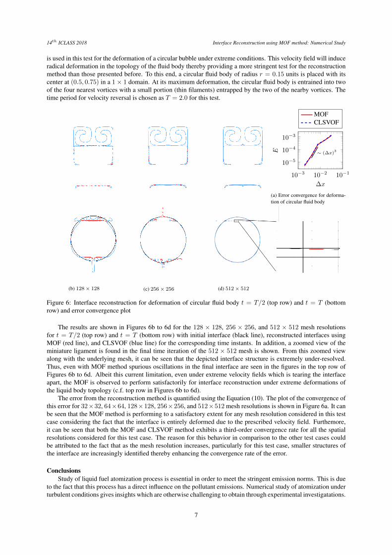
is used in this test for the deformation of a circular bubble under extreme conditions. This velocity field will induceradical deformation in the topology of the fluid body thereby providing a more stringent test for the reconstructionmethod than those presented before. To this end, a circular fluid body of radius r = 0.15 units is placed with itscenter at (0.5, 0.75) in a 1× 1 domain. At its maximum deformation, the circular fluid body is entrained into twoof the four nearest vortices with a small portion (thin filaments) entrapped by the two of the nearby vortices. Thetime period for velocity reversal is chosen as T = 2.0 for this test.

10−3 10−2 10−1

10−5

10−4

10−3

∼ (∆x)3

∆x

E

MOFCLSVOF

(a) Error convergence for deforma-tion of circular fluid body

(b) 128× 128 (c) 256× 256 (d) 512× 512

Figure 6: Interface reconstruction for deformation of circular fluid body t = T/2 (top row) and t = T (bottomrow) and error convergence plot

The results are shown in Figures 6b to 6d for the 128 × 128, 256 × 256, and 512 × 512 mesh resolutionsfor t = T/2 (top row) and t = T (bottom row) with initial interface (black line), reconstructed interfaces usingMOF (red line), and CLSVOF (blue line) for the corresponding time instants. In addition, a zoomed view of theminiature ligament is found in the final time iteration of the 512 × 512 mesh is shown. From this zoomed viewalong with the underlying mesh, it can be seen that the depicted interface structure is extremely under-resolved.Thus, even with MOF method spurious oscillations in the final interface are seen in the figures in the top row ofFigures 6b to 6d. Albeit this current limitation, even under extreme velocity fields which is tearing the interfaceapart, the MOF is observed to perform satisfactorily for interface reconstruction under extreme deformations ofthe liquid body topology (c.f. top row in Figures 6b to 6d).

The error from the reconstruction method is quantified using the Equation (10). The plot of the convergence ofthis error for 32×32, 64×64, 128×128, 256×256, and 512×512 mesh resolutions is shown in Figure 6a. It canbe seen that the MOF method is performing to a satisfactory extent for any mesh resolution considered in this testcase considering the fact that the interface is entirely deformed due to the prescribed velocity field. Furthemore,it can be seen that both the MOF and CLSVOF method exhibits a third-order convergence rate for all the spatialresolutions considered for this test case. The reason for this behavior in comparison to the other test cases couldbe attributed to the fact that as the mesh resolution increases, particularly for this test case, smaller structures ofthe interface are increasingly identified thereby enhancing the convergence rate of the error.

ConclusionsStudy of liquid fuel atomization process is essential in order to meet the stringent emission norms. This is due

to the fact that this process has a direct influence on the pollutant emissions. Numerical study of atomization underturbulent conditions gives insights which are otherwise challenging to obtain through experimental investigatations.

7


Within this work, MOF method was presented for reconstruction of liquid/gas interface in the context ofincompressible multiphase flows to the application of numerical analysis of primary breakup of liquid fuel. Thismethod involves computation of interface unit normal by reducing the defect in the first order moment of liquidvolume in a volume conservative manner. For various test cases presented in this study, MOF method proved tobe more accurate than and at least as accurate as that of CLSVOF method in terms of reconstruction error andpreservation of the shape and orientation of the interface topologies. Furthermore, MOF method demonstrated itssuperior capability of preserving the interface for topologies found in under-resolved flow structures such as thinfilaments and ligaments. This deems MOF method as an interface reconstruction method to be used in DNS forstudying primary atomization.

In future, development of a hybrid MOF–CLSVOF method for interface reconstruction is a promising im-provement thereby combining the advantages of both methods for interface reconstruction. MOF method requiresmore computational resources than CLSVOF method for the interface reconstruction mainly due to its unit normalcomputation from the COM. Thus, it is more prudent to use CLSVOF for interface reconstruction especially for thetopologies that are far less complicated making it more sensible to develop a hybrid MOF–CLSVOF method. Also,the volume fraction and COM of gas phase along with those pertaining to the liquid phase should be consideredfor optimal interface reconstruction in the next studies.

AcknowledgementsThe funding for this project from the European Union’s Horizon 2020 research and innovation programme

under the Marie Skłodowska-Curie grant agreement No. 675676 is gratefully acknowledged.

References[1] Ménard, T., Tanguy, S., and Berlemont, A. International Journal of Multiphase Flow 33(5):510–524 (2007).[2] Desjardins, O. and Pitsch, H. Atomization and Sprays 20(4):311–336 (2010).[3] Le Chenadec, V. and Pitsch, H. Atomization and Sprays 23(12):1139–1165 (2013).[4] Gorokhovski, M. and Herrmann, M. Annual Review of Fluid Mechanics 40:343–366 (2008).[5] Aulisa, E., Manservisi, S., Scardovelli, R., and Zaleski, S. Journal of Computational Physics 192(1):355–364

(2003).[6] López, J., Zanzi, C., Gómez, P., Faura, F., and Hernández, J. International Journal for Numerical Methods in

Fluids 58(8):923–944 (2008).[7] Hernández, J., López, J., Gómez, P., Zanzi, C., and Faura, F. International Journal for Numerical Methods in

Fluids 58:897–921 (2008).[8] Aniszewski, W., Ménard, T., and Marek, M. Computers & Fluids 97:52–73 (2014).[9] Owkes, M. and Desjardins, O. Journal of Computational Physics 332:21–46 (2017).[10] Tanguy, S. and Berlemont, A. International Journal of Multiphase Flow 31:1015–1035 (2005).[11] Desjardins, O., Moureau, V., and Pitsch, H. Journal of Computational Physics 227:8395–8416 (2008).[12] Herrmann, M. Journal of Computational Physics 227:2674–2706 (2008).[13] Herrmann, M. Atomization and Sprays 21(4):283–301 (2011).[14] Shinjo, J. and Umemura, A. International Journal of Multiphase Flow 37:1294–1304 (2011).[15] Le Chenadec, V. and Pitsch, H. Journal of Computational Physics 233:10–33 (2013).[16] Dyadechko, V. and Shashkov, M. Journal of Computational Physics 227:5361–5384 (2008).[17] Vaudor, G., Ménard, T., Aniszewski, W., Doring, M., and Berlemont, A. Computers and Fluids 152:204–216

(2017).[18] Jemison, M., Loch, E., Sussman, M., Shashkov, M., Arienti, M., Ohta, M., and Wang, Y. Journal of Scientific

Computing 54:454–491 (2013).[19] Li, G., Lian, Y., Guo, Y., Jemison, M., Sussman, M., Helms, T., and Arienti, M. International Journal for

Numerical Methods in Fluids 79:456–490 (2015).[20] Weymouth, G. D. and Yue, D. K.-P. Journal of Computational Physics 229:2853–2865 (2010).[21] Bnà, S., Cervone, A., Le Chenadec, V., and Sandro, M. In 11th International Conference of Numerical

Analysis and Applied Mathematics 2013, ICNAAM 2013, Rhodes, Greece, volume 1558, 875–878 (2013).[22] Harvie, D. J. E. and Fletcher, D. F. Journal of Computational Physics 162(1):1–32 (2000).[23] Rider, W. J. and Kothe, D. B. Journal of Computational Physics 141(2):112–152 (1998).[24] Smolarkiewicz, P. K. Monthly Weather Review 110:1968–1983 (1982).

8

numerical study of interface reconstruction method in

Documents