UCRL-ID- 135084

New VOF Interface Capturing and Reconstruction Algorithms

Peter Anninos

June 29,1999

This is an informal report intended primarily for internal or limited external distribution. The opinions and conclusions stated are those of the author and may or may not be those of the Laboratory. Work performed under the auspices of the U.S. Department of Energy by the Lawrence Livermore National Laboratory under Contract W-7405-ENG-48.

DISCLAIMER

This document was prepared as an account of work sponsored by an agency of the United States Government. Neither the United States Government nor the University of California nor any of their employees, makes any warranty, express or implied, or assumes any legal liability or responsibility for the accuracy, completeness, or usefulness of any information, apparatus, product, or process disclosed, or represents that its use would not infringe privately owned rights. Reference herein to any specific commercial product, process, or service by trade name, trademark, manufacturer, or otherwise, does not necessarily constitute or imply its endorsement, recommendation, or favoring by the United States Government or the University of California. The views and opinions of authors expressed herein do not necessarily state or reflect those of the United States Government or the University of California, and shall not be used for advertising or product endorsement purposes.

This report has been reproduced directly from the best available copy.

Available to DOE and DOE contractors from the Office of Scientific and Technical Information

P.O. Box 62, Oak Ridge, TN 37831 Prices available from (423) 576-8401

Available to the public from the National Technical Information Service

U.S. Department of Commerce 5285 Port Royal Rd.,

Springfield, VA 22161

New VOF Interface Capturing and Reconstruction Algorithms

Peter Anninos University of California, Lawrence Livermore National Laboratory, Livermore, CA 94550

(June 29, 1999)

Abstract

Several new methods are presented for the capturing and tracking of ma- terial boundary interfaces. All methods belong to the general Volume Of Fluid (VOF) approach, and vary from simple flow aligned algorithms to more complex geometric modeling. The performance of the different methods is evaluated by solving the advection equations for a variant of the canonical multi-fluid “ball & jacks” problem.

I. INTRODUCTION

Tracking the movement of free surfaces and interface boundaries between different ma- terials is of significant importance in many numerical hydrodynamical calculations. If the numerical methods are of low order, interfaces can be easily destroyed by the inherent dif- fusion in the algorithms. Higher order conventional advection techniques (e.g., second order upwind with monotonicity) can reduce the diffusion somewhat, but at the expense of in- troducing a front capturing procedure, though oscillations may still emanate from the front regions to corrupt the global solution. However, even higher order front capturing methods are not adequate for features with characteristic length scales of order a few grid cells, or for capturing sharp contact discontinuities in a single cell without specialized treatments. For problems with complex interactions at the interfaces, it is even more important to accurately track the boundaries in order to apply the necessary physical conditions arising from, say, free surface flows, surface and body tension, or even chemical reactive fronts.

A number of approaches have been developed over the past few decades to explicitly track interface boundaries and solve.the governing dynamical advective equations coupled with the appropriate hydrodynamics equations. These methods are designed to preserve discrete and discontinuous shapes without introducing averaging procedures, and thereby substantially reducing boundary diffusion and promoting more accurate numerical evolutions with much coarser resolution than allowed by front capturing methods. The algorithms presented in this paper belong to the Volume Of Fluid (VOF) method class [l-5]. In this approach, each material surface is reconstructed from the fractional volume of fluid content in each cell, eliminating the need to develop complex data and logic structures required by marker [6] or surface [7] tracking methods which generally introduce and evolve transitory nodal elements on unstructured boundary surfaces with Lagrangian techniques. VOF methods are also desirable in that they can easily handle global topological changes that may occur in the event of fragmentation processes and droplet mergers. Due to their robustness, simplicity,

and computational efficiency in terms of CPU time and memory allocation, VOF methods continue to be very widely used [8,9].

Several different methods from three distinctive grades of the VOF method class are presented in sections II and III, and subsequently compared for performance and error analysis in section IV. Some methods represent improvements to existing ideas, while others are new procedures designed for simplicity and for easy generalization to three-dimensional structured and unstructured meshes. The various methods and their relative performances are summarized for convenience in the final section V.

II. BASIC VOF CONCEPTS AND MATERIAL ORDERING SCHEME

The dynamical evolution of material interfaces for nonreactive flows is governed by the following set of advection equations, assuming the flow to be incompressible:

where M is the total number of materials, vj denotes the fluid velocity, and FI”l is the volume fraction occupied by the mth fluid material and is defined as a step function: Fl”l = 0 if the cell is empty of material m, Fl”l = 1 if the cell is completely filled with material m, and 0 < Fl”l = V[ml/VT < 1 in cells containing an interface boundary, where VT = C,“=, VLrn] is the total cell volume. The volume fraction is thus simply advected with the flow characteristics of the hydrodynamical system.

Equation (1) is solved using a six step upwind donor cell procedure with the following se- quence: (1) identify those cells containing an interface boundary by computing the maximum volume fraction of all materials and tagging the cells satisfying & < max(Flml) < 1 - F,, where the critical volume fraction F, is typically set to one percent (all remaining cells are treated in the same manner as a first order upwind method); (2) extract a 3 x 3 (in two dimensions) brick of cells centered on the donor cell; (3) estimate the orientation of the boundary surface (for all the methods other than the grid aligned models described below) using the volume fraction distribution within the extracted brick; (4) for the more general arbitrary surface orientation models (see below), shift the position of the boundary surface until the volume bounded by the interface surface and the cell faces matches the material volume fraction in the donor cell (of course this also requires a procedure to determine on which side of the surface the fluid lies); (5) compute the volume of fluid bounded by the donor cell faces, the reconstructed interface boundary, and the advection control volume set by the CFL constraint on the timestep (i.e., vAtAy for advection along the z-direction on uniform grids); (6) update the discretized advection equation from time levels n to n + 1,

by computing the fluxes from the bounded volume fractions as

(3)

(4)

2

where Vi[y] is the mth fluid material volume bounded in the spatial (i,j) cell by the interface surface &rd the advection control volume. Here it is assumed that the flow velocities are staggered spatially in relation to the volume fractions: velocities are face centered, volume fractions are cell centered. The volume fractions are then updated by

(5)

All of the steps outlined above are applied independently to each dimension of the problem using directional splitting to separate the two grouped volume terms in the right-hand-side of equation (5),

An important. element in multi-fl.uid calculations is the automatic and localized ordering of the different materials for advection. Since the VOF approach estimates fluxes from the distribution of volume fractions and advects more accurately those materials which fill the advection volume in the leading edge of the donor cell, one can obtain better results if the materials are ordered from highest downstream presence to highest upstream presence. This also conveniently allows for an effective accumulated fluid composition to be formed from materials of higher precedence, thereby filling the donor cell from the downstream to upstream direction, and eliminating the need to track interface boundaries on all sides of each material. A single composite volume fraction is defined as

Fjrnl = min 1, 2 FLel , [ I

(6) fkl

where Fjml denotes the volume fraction from the first m ordered materials. The six-step advection process is repeated for each composite group of materials to compute the accu- mulated fluxes J=irnl (or equivalently advection volumes). The individual material fluxes are recovered through the normalization procedure

designed to limit the total volume fraction from exceeding unity, and the individual volume fractions from becoming negative.

The materials are ordered into the four basic groups shown in Figure 1, plus an addi- tional fifth group to handle those materials not falling into any of the others. Basically the first group is the highest priority in the advection process since it stores the predom- inantly downstream materials. Using the simple notation F$&, FE1 and FL?, to denote the upstream, donor and downstream cells for material m respectively, fluids falling into this category satisfy FA?l < F, and (FE], F&lJ > F,, and represent a surface orientation essentially perpendicular to the flow field. The second group includes materials with surfaces aligned more parallel to the flow field and are characterized by (F$&, FE', FLTl) > F,.

The third group represents isolated fragments with (FLY,, FLY,) < F, and FE1 > F, which are advected prior to the dominantly upstream materials. Finally the fourth group includes trailing materials characterized by FhTl < F, and (Fh!,, FE]) > F,. However, it is en- tirely possible that more than one material can fall into each category, making it necessary

3

to implement a more quantitative procedure to order the fluids within each group. Since the general idea is to advect from leading to trailing edge materials, a simple calculation-of the normalized volume fraction gradient provides a convenient measure of priority. For groups 1, 2, and 4, the order parameter is defined as

P= F D+l-FD-1

FD

This parameter naturally increases (decreases) for higher volume fractions in the downstream (upstream) cells. It also increases in magnitude for smaller donor cell fractions when the upstream or downstream cells are saturated to unit fraction levels, reflecting the “steeper” nature of the interface surface. For the third group in which there is little or no fluid present in either the upstream or downstream cells, the appropriate order parameter is simply the volume fraction in the donor cell P = Fo.

III. NUMERICAL METHODS

The procedures described above make clear that the actual interface boundary is not tracked directly. Rather the boundaries are reconstructed locally from the evolved volume fraction content of each material within the donor cells. The process by which the sur- face is reconstructed suggests a natural classification of VOF algorithms into three distinct categories:

1. grid aligned models in which the interface is approximated as a piecewise constant or “staircase”-like surface and is basically aligned either parallel or perpendicular to the flow directional component (independently along each dimensional sweep),

2. flux corrected models that adjust one of the two aligned orientations (the parallel component) with a sloped line based on the local volume fraction distribution, and

3. arbitrary surface orientation models representing a more general approach which ap- proximates the surface as a piecewise linear, but arbitrarily oriented surface or plane.

A schematic exemplifying the first and third category models is shown in Figure 2. Several new (or in some cases improved or generalized) algorithms will be presented in

the following subsections, classified according to the three basic class methods and discussed from the simplest to the more complex. Numerical calculations will be postponed until the following section, where we compare results from each of the algorithm types.

A. Grid Aligned Models

I. Modified SLIC Methods

One of the earliest VOF algorithms (Simple Line Interface Calculation or SLIC) is at- tributed to Noh and Woodward [a]. The SLIC method assumes the interface surface is aligned either parallel or perpendicular to the flow vector component in each dimensional

4

sweep. The algorithm thus works well if the flow geometry is primarily aligned parallel to one coordinate direction or along the sum vector field. However, it can become -highly inaccurate for more complex geometries or off-axis translational and rotational flows (see, for example, references [lO,ll]).

By generalizing the SLIC algorithm to allow for “corner” turns within a single cell, it is possible to more closely represent tilted surface orientations with an adjustable volume fraction jump inside the donor cell, effectively increasing the curvature modeling capabilities at smaller subzone scales [12]. A modified SLIC-like algorithm with improved stability and accuracy is achieved by considering five different flow topologies as determined by the volume fractions in the three (upstream, donor, and downstream) cells. The fluid distributions corresponding to the five cases are shown in Figure 3 and defined by: FD-1 5 F,, Fo > F,, &+I 2 F, (Case A); FDB1 2 1 - F,, Fo 2 F,, F D+I 2 E (Case B); FD-I 2 F,, FD 2 F,, FD+~ 2 F, (Case C); FD-~ 2 1 - F,, FD > F,, FD+l 2 F, (Case D); and FD-r > F,, FD 2 F,, FD+~ 2 1 - F, (Case E). The corresponding flux formulas are easily derived by integrating the bounded volume of fluid and imposing the proper flux limiting constraints to automatically account for the corner adjusted flux and the locally available volume of fluid:

Case A : FDtlia E V,/Ay = min[FDAx, vAtFD+l], Case B : FD+r/z = Vo/Ay = min[FDAz, max(O, vAt - (1 - FD)Ax)], Case C : .9=~+r/z z Vo/Ay = VAtFD, Case D : FD+rjz f v~/Ay = min[FDAx, vAtFo+r+

max((1 - FD+l)vAt - (1 - FD)Ax, O)], Case E : FD+l/2 = vD/AY= min[FD+l VAt, FDAz - FD-~(Ax - UAt)].

(9)

Notice that these expressions are written explicitly for advection along the x-axis (the corresponding y-axis formulae are obtained simply by replacing Ax by Ay and assigning v to be the velocity along the y-axis). Equations (9) are also supplemented with the default value FD+rj2 = vA~FD if all of (Fo-1, FD, and FD+l) are less than or greater than F,, or if the volume fraction in any two adjacent cells are less than F,.

An alternative and more general (though also much simpler) implementation of plane corners is achieved by introducing four parameters (in 2D) representing the dimensions of two distinct blocks of fluid which run the length of the donor cell ,along the advection direction. Assuming a velocity vector pointing in the +x direction, the width and height dimensions of the two fluid blocks are denoted by 6x1, 6x2, 6yr and 61~2, with the block labeled with subscripts 1 (2) being more downstream (upstream) than the other. The height functions are’associated with volume fractions in the adjoining downstream and upstream cells: 6yr = F~+rny, and 6~2 = F&rAy. The width parameters are determined by the constraints

6x1 + 6x2 = Ax, (10)

and

6xr6yr-!- 6x26~2 = FDAxAY. (11)

The fluid flux is then defined as

.9=D+l/2 = VD/AY = FD+lvAt (12)

5

if uAt 5 6x1, or

.?=13+1/2 G V~/ny = ~x~FD+I + (vnt - SX~)FD-I (13)

otherwise, where

6x 1

= (FD -FD-I)~x F D+l- FD-I '

(14

For cases in which 6x1 < 0 or 6x1 > Ax the flux is simply set to v&FD. Together, equations (12) and (13) can account for each of the five cases in Figure 3, in addition to modeling corner turns for which neither of the the fluid blocks run cell edge to cell edge across the transverse direction. However, the two methods yield comparable results for the test problems considered here.

2. Donor/Acceptor Limiter

To present a more thorough comparison of the different algorithms in section IV, a slightly modified variant of the fairly popular donor/acceptor method of Hirt and Nichols [3] is included here for completeness. This approach utilizes a parameterized flux limiting formula to compute the amount of advected fluid as

.7-~+i/z = min[FvAt + max((1 - F)vAt - (1 - Fo)Ax, 0), FDAx], (15)

where F is determined by the slope of the interface boundary and the local fluid topology. The interface slope s is estimated from the volume fraction gradients centered on the donor cell by one of the several methods discussed in section III B 2. The parameter F is set to Fo for relatively flat surfaces in which ]sD] < s,, or to FD+l otherwise, where s, is a critical slope typically equal to 0.5 in order to delineate flat from steep surfaces. In addition, F = FD+I if FD+~ < F, and FD-~ > F,, or if F&l < F, and F D+i > F,, where F, is generally set to 0.4 and is used to enforce the steepness condition for reasonably filled donor-neighbor cells.

3. Monotonic Flux Fitting Approach

An altogether different approach to interface capturing that falls within this grid align- ment group is the idea of estimating volume fluxes from some simple constraints and mono- tonic curve fitting formulae. For example, as a fluid parcel passes through the donor cell, the flux volume necessarily passes from zero as the fluid first enters the cell, to a maximal value (equal to the advection control volume if the parcel is large enough), then decreases again to zero as the fluid exits the other side. Rather than attempting to compute exactly the fluid volume at each stage, one could instead model the curves only approximately using a monotonic function to fit the general behavior. Because the leading and trailing edge functions are necessarily different, the corresponding fluxes are fit separately with different formulas. Letting Fi+i,2 and G+rj2 respectively represent the leading and trailing edge fluxes for the one-dimensional problem along the x-direction, the following formulas

6

&2= ~D(3-~)+2F~(~-1)],At, (16)

&2= ~D(~-1)+2F~(~-~)]~ar, (17)

produce fairly robust approximations. The decision on which of the two formulae to apply is dictated by the sign of the local fluid volume gradient along the transport direction (the x-axis in this example): O,Fiyl < 0 for the leading edge, and O,F$] > 0 for the trailing edge. In practice this is carried out by monitoring both of the edge-centered gradients 6F+ = (FD+~ - &)/AX and 6F- = (FD - FD-i)/Ax, then applying the appropriate leading or trailing edge formulae, or simply setting -TDs1i2 = &vat if the product SF+&F- < 0. It is worth pointing out that equations (16) and (17) differ from the conventional second order monotonic van Leer [13] f ormula only by numerical constants, once the derivative expressions in the van Leer formula are expanded out and the proper volume fractions (either zero or one) are inserted at the outer boundaries of the fluid parcel.

Figure 4 shows a graph of both the leading and trailing edge normalized Aux fitting formulae, (16) and (17), as a function of volume fraction and for different advection control volumes. The curves lying above (below) the forty-five degree line represent the trailing (leading) edge results. Also shown are the corresponding second order upwind approxima- tions with the assumptions described above, and the exact fluxes derived by integrating the fluid volume in the donor cell for a single-dimensional flow. Considering the case of uAt = 0.6 for which the exact 1D analytic results are plotted with star symbols, and com- paring the dot-dashed lines with the connected open squares, it is clear that the flux fitting formulas are better approximations to the exact results. Deviations between the fitting formulas and the exact solutions range from essentially perfect agreement for nearly empty or filled cells, to roughly 20% in the worst case limits corresponding to volume fractions FD M vAt for trailing edges or FD z Ax - vAt for leading fluid elements. However, Figure 4 also suggests the possibility of formulating even more accurate fitting expressions than those presented here.

B. Flux Corrected Models

1. CALE

A common interface tracking algorithm found in many numerical codes developed at Lawrence Livermore National Laboratory is based on a variant of the SLIC and Wilson- LeBlanc methods due to Tipton 1141 that was primarily driven by numerical experiments and first surfaced in the CALE code. There are four main components to the algorithm: (1) the slope calculation to estimate surface orientations from the straight-line two-point gradient ratio, and to split materials into either series or parallel groups; (2) the SLIC-like treatment of leading edge only series flows; (3) a second order correction for parallel flows based on the maximum of the two edge-centered volume fraction gradients around the donor cell; and (4) the advection ordering of materials into three general groups, with the leading series and parallel materials collectively being the highest but equal priority, followed by the middle series materials, then the trailing series materials of the lowest priority order. Additionally,

7

the CALE method also includes several extra rules to further classify materials into either of the series or parallel groups. These rules lack rigor in general, but are found from numerical experiments to produce reasonable results. The basic components are outlined here to facilitate a clear comparison with a new alternative flux corrected procedure described in the following subsection.

2. Monotonic Flux Correction

The method described here represents a hybrid procedure designed to offer a compromise between the simplicity and speed of grid alignment models and the accuracy and stability of arbitrary surface orientation models. There are four main components to the algorithm: (I) the slope calculation to quantify the local flow geometry; (2) the advective treatment of steep surface orientations using SLIC-like rules for all leading, middle and trailing materials; (3) the second order treatment of locally shallow sloped geometries; and (4) the material ordering scheme described in section II for increased accuracy. Each of the four components are described below.

There are many ways to estimate the slope s of the interface boundary. The most straightforward procedure is to associate the slope with weighted volume fraction gradients in the extracted 3x3 brick centered on the origin of the donor cell. In general,

V&i SD f? si,j = -e = - X:=-I Wi+l,j+k&+l,j+k - CL=-, Wi-l,j+kFi-l,j+k IX:=--1 wi+e,j+lFi+e,j+l - C~,-.-l wi+e,j-lFi+e,j-1 ’ (18)

where wi,j is the weight factor that can differ for each cell in the 3x3 brick. The simple straight-line gradient (in which wi,j is unity on the four cells directly north, south, east and west of the donor cell, and zero everywhere else) does not work well in many cases as shown in section IV. Two variants that do work well include an uniformly weighted scheme in which wi,j is unity everywhere including the diagonal cells, and a weighted scheme in which the diagonal cells carry half the weight of the four centered cells.

In addition, an alternative technique useful for estimating the slope is based on the volume fraction centroid. In this approach, the interface boundary is associated with the vector normal to the line connecting the volume fraction centroid to the donor cell center

./ Xij ck-I ck-1 Xi+e,j+kfi+t,j+k

%’ = -z = - ci,-l ~~=-l yi+e,j+&+e,j+k ’ (19)

where (xi,j, yi,j) and (x&., $$) are the cell center and centroid coordinates from the donor cell origin. Although this generally provides a fairly good approximation of the surface orientation, the centroid calculation is most useful for determining on which side of the interface boundary that the fluid lies - a necessary ingredient in arbitrary surface orientation models (see below) for computing face-centered fluxes.

Once the slope is computed, the flow geometry is characterized locally as either parallel or series, depending on whether the slope is flat (Isi,jl < 1) or steep (Isi,jl > 1) and a few additional criteria based on the local volume fraction distribution. Materials that have been grouped as series are given the highest (lowest) priority in the advection sequence if the material is dominantly downstream (upstream) as described in section II. The volume flux

8

for this group of materials (Categories 1, 3 and 4 of Figure 1) is computed in a similar manner as the grid aligned methods presented in section III A 1. In particular, the fiux is assigned as

3 gilIz = min(vAt, FDAx), (20>

for leading and middle materials advected along the x-axis, or

3 gil,z = min(vAt, max(O, vht - (1 - FD)Ax)), (21)

for trailing materials. Fluids grouped as parallel are given intermediate priority as assigned to Category 2 materials (see Figure 1). The volume flux for this parallel component is estimated through a slight variant of the higher order monotonic flux fitting procedure discussed in section III A 3, and designed to account for a sloped interface analogous to a second order upwind procedure with monotonicity constraints. The flux in this case is

(22)

if (&I+, - FD) ( FD - FD-1) > 0 or PDyr,z = FDvAt otherwise (and constrained so as not to exceed the available fluid in the advection control volume). The free parameter c is typically set in the range 1 < c < 2. To prevent spurious features from forming at the transition cutoff slope (Is,] = l), the flux in cells with interface slopes in the range fijs,l 5 IsI < fUIscI is modified by a linearly weighted average

3 tram _ -per

D+1/2 - Di-l/2 + cpD:1,2 - 3%/2 (23)

where fU and fi are constants typically set to 3 and l/3 respectively..

C. Arbitrary Surface Orientation Models

I. Spherical Mapping

One of the more complex and time consuming elements of this method class is the problem of finding the location of the interface (once the slope is determined) so as to match the bounded volume to the donor cell volume fraction. The problem is linked to the many geometric permutations arising from various unique possible plane intersections, and is especially problematic for 3D and unstructured meshes. A possible means to overcome this limitation may be realized by mapping the donor grid cell onto a sphere (or more generally an ellipsoid) with the same total volume. This has the advantage that any interface surface orientation and position would be treated homologously. It is also potentially useful, and likely asymptotically more accurate, for arbitrary polygonal or polyhedral cells.

Letting r and rg represent the sphere radius and the perpendicular distance from the origin (at the center of the donor cell) to the interface boundary, the area A of the bounded region as shown in Figure 5 is given by

A T F=2-sin -1 To To ro 2 --- T T l- 7 ,

J 0

where r = m AxAy K to match the total circular and rectangular grid cell areas. It is important to note that the parameter r. can be either positive for bounded areas that do not cross the origin (basically less than half the area of the sphere), or negative if the bounded region includes the origin and accounts for more than half the area of the sphere. The bounded region is the domain containing the fluid and is determined by the location of the volume fraction centroid relative to the sphere center as discussed in section III B 2. Since the general idea is to devise an algorithm that does not require an iterative procedure to converge on the surface location, equation (24) is expanded out to third order in the smallness parameter E = ro/r

A F,AxAy 7= T2

which has the real root solution directly relating r. to Fo

TO - = -(U” + pqy r

cos (o/3) + x/Z (U” + (V1)1/6 sin (Q/3) ,

where

and

0 = tan-i 4 . m

( )

(25)

(26)

(27) cw

(29)

This expansion is fairly accurate and yields maximum errors of order 10% for the worst case scenarios in which E = fl. Equations (26) through (29) provide a means of directly locating a point on the line representing the interface surface with a bounded volume that is consistent with the volume fraction in the donor cell. This, together with the slope determined by the volume fraction gradients, completely defines the interface boundary without the need for iterative procedures or complex geometric modeling.

Since the smallness parameter is well defined and bounded in the radial domain, it is not a problem finding solutions to the third order polynomial equation. However, the intercept parameter in the usual linear equation is computed from a similarity solution of triangles involving ratios of the volume fraction gradients defining the slope, and can become singular in some cases. For example, the intercept along the y-axis is given by

10

and is undefined for steep slopes in which V,Filj --+ 0. Hence, the interface description is decomposed into two calculations: one using the y-axis intercept when ]si,j] 2 1 and the second using the x-axis intercept defined by

when ]SQ] > 1. Once the orientation and location of the interface surface are determined, the volume

Aux bounded by the interface and the advection control volume is computed as

VD 3D+l12 z - = FD

AY

where V,,, is the fluid volume bounded by the interface surface and the advection control volume, and V&l is the fluid volume bounded by the interface and the cell edges. This partitioned approach results in somewhat more accurate results then simply setting VD = V acv . The fluid side of the interface is easily determined separately for steep and parallel aligned slopes: For Is] 5 1, an arbitrary coordinate node (zN, yN) is defined to be on the fluid side of the donor cell if ye 5 SxN + b and yC < 0 or if yN 2 SxN + b and yC > 0, where (x,, yC) is the location of the volume fraction centroid and b is the y intercept as computed by equation (30). For Is] > 1, a node is defined to be on the fluid side if ZN 5 s-ryN - bs-’ and x, < 0 or if XN 2 s-iyN - bs-l and x, > 0.

2. Iterative Bisection

Youngs method [4] is perhaps the most popular algorithm in this arbitrary surface orien- tation class of solutions. It is certainly the method that has achieved a level of recognition to which new developing algorithms aspire. However, in its original form, the method is fairly complex to implement in 3D structured and in 2D arbitrary quadrilateral and polyg- onal grids. It is extremely complex for arbitrary hexahedral grids, and more so for general polyhedral grids in three dimensions. The method requires an elaborate system of tabu- lated geometric configurations and a logical decision-making process to account for all the possible orientations, intersections and geometrical volume shapes and calculations. The algorithm presented here eliminates the need to account for and compute in advance all the possible permutations and geometric possibilities, and should, in principle, be applicable to unstructured‘as well as structured meshes.

Given the interface slope as computed by one of the methods described in section IIIB 2, Youngs method can be generalized with the following procedures:

1. guess the intercept (along the x-axis for steep slopes or the y-axis for shallow slopes) for the linear equation representing the interface boundary,

2. locate the two (in 2D) cell edges which intersect the surface by scanning each of the edges in turn,

3. compute the fluid volume by adding a node to the center of the interface surface as a focal point for triangulating the bounded volume by connecting the node with the cell vertices on the fluid side as determined by the volume fraction centroid,

11

4. iterate on the intercept using a bisection procedure to shift the surface position until the bounded fluid volume in the donor cell and volume fraction match up,

5. compute the flux by a similar triangulation process on the volume bounded by the advection control volume and the converged interface surface.

The above generalized bisection algorithm represents the most sophisticated treatment of interface reconstruction presented in this paper. It thus offers a standard against which to compare the other faster and less complex methods.

IV. COMPARISON OF METHODS

The test problem against which all the methods presented in this paper are compared is a variant of the canonical “ball & jacks” problem. This particular problem is appropriate in that it consists of configuration geometries of both plane-fronted and curvature types: a two-dimensional cross or jack of width four cells (N w = 4) is placed within a spherical annulus also four cells thick in the radial direction. The composite object is then advected as a two-material flow in which the ball and jack components are (for most of the tests) treated as a single fluid, and the negative space is the second fluid. Results of solving the advection equations with a traditional second order upwind scheme with van Leer mono- tonicity is shown in Figure 6. Two separate calculations are presented to test translational and rotational advection. The translational evolution (top image) is performed to a phys- ical time of t = 50 on a 100 x 100 grid with unit cell widths and velocity components set to unity (wx = zlY = 1). The rotational test (bottom image) is carried out over a single complete revolution on a 50 x 50 grid with unit cell widths and velocities consistent with rigid-body rotation around the center of mass. The CFL timestep constraint is defined so that vAt = 0.6 in all the numerical evolutions. The displayed images in both cases represent filled regions outlined by volume fraction contour isovalues of F@ = 0.7, 0.5 and 0.3. Notice that in both evolutions the initial geometry loses its structure very early in the evolution, and the interface boundary completely diffuses away.

Figure 7 shows the corresponding results from the 5-rule grid aligned model of section IIIA 1. The top two images are results from advecting the object along the x-axis and into the diagonal direction. In general, grid aligned algorithms have the nice property that advection is nearly perfect for flows oriented perpendicular to the cell faces. The bottom left image shows the rotational result analogous to Figure 6. The bottom right image translationally evolves the same basic object, but uses eight zones to resolve across both the ball and jack widths, twice the grid resolution as the top right image. The apparent tapering effect evident in the spherical fronts of the top right image converges away with adequate cell coverage.

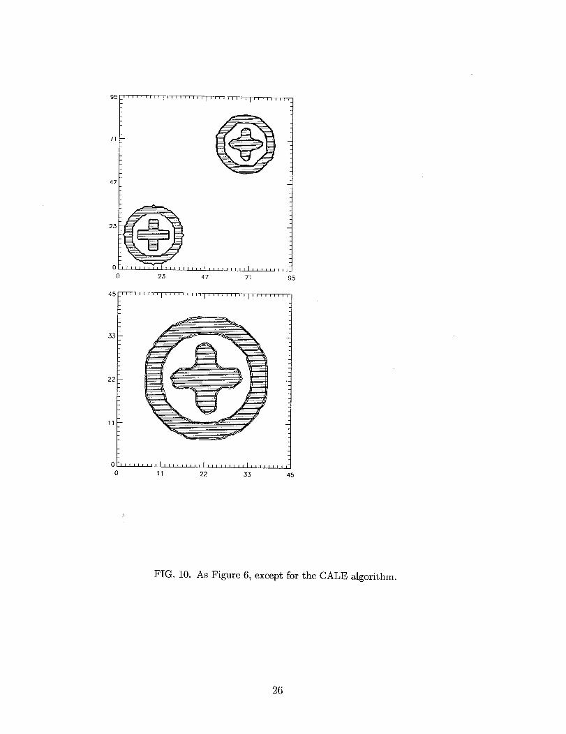
Figures 8 through 13 show analogous evolutions for each of the remaining algorithms: donor/acceptor limiter, monotonic flux fitting, CALE, monotonic flux corrected, spherical modeling, and the generalized iterative bisection methods respectively. Each figure shows results from the same diagonal translation (top images) and single revolution rigid-body rotation (bottom images) evolutions. The translation image shown for the spherical mapping algorithm (Figure 12) is generated from the advection of a 5-fluid system to confirm the robustness of the material ordering scheme, and to verify the stability of degenerate points

12

where several fluids meet in a single cell. The five fluids are represented by four different cross-hatched regions plus the exterior white space. Figure 13 displays two additional images in the bottom row distinguished by the method used to compute the interface slope. The image on the bottom left assigns the slope given by the vector normal to the line joining the donor cell center and the volume fraction centroid as described in section III B 2. The image on the bottom right is a result of assuming the slope to be given by the unweighted straight-line two-point gradients formed from only the east, west, north and south cells. All the other evolutions presented in this paper define the slope from a weighted gradient scheme that assigns a weight of one (two) to the diagonal (center) cells in the transverse direction as noted in section III B 2. Obviously the interface slope is not well represented by the simple one-dimensional gradient operator.

Notice that the monotonic flux fitting algorithm performs somewhat better visually than the other grid alignment models, especially for rotational motion. In addition, flux corrected models are of intermediate quality in representing both plane-fronted and curve-fronted flow geometries when compared to grid aligned and arbitrarily oriented surface models. This class of algorithms may, therefore, represent a good compromise between accuracy and efficiency. Of the two flux corrected models, the monotonic flux corrected algorithm appears more accurate and stable than the CALE algorithm when considering long term evolutions (see Figure 14). Finally, it is interesting to note that the spherical mapping approach appears quite good from accuracy and computational cost considerations (see also Table I), especially when compared to the more sophisticated and complex iterative bisection method.

For a quantitative description and comparison of these new algorithms, it is useful to carry out a more precise error analysis and convergence study. If perfect advection is as- sumed, the composite object can be translated or rotated analytically through a coordinate transformation and reconstructed on the grid at the same time corresponding to the final physical computation time. Numerical results can then be compared to analytically recon- structed solutions cell by cell with an averaged absolute measure of error

where FJ,y] and $71 are the numerical and analytical volume fraction solutions respectively. Errors are computed for each material over a region bounded by the radius (from the mass center) R < 4N w, where NW is the number of cells spanning the minimum width of the cross and annulus shapes. The radius 4Nw is the outer radius of the spherical ball, and is used as the upper bound so that error measurements can more closely represent actual interface cell errors, and are not arbitrarily biased to small numbers.

Table I shows each of the errors and relative CPU costs as computed from equation (33) for translational advection tests into the diagonal corner. The relative CPU cost is generally dependent on (and increases with) the volume filling factor of interface cells. CPU timings can therefore be quite different in general than shown here, especially for the more complex bisection method. Table II shows the corresponding errors for one-dimensional advection along the z-axis. Both tables compare the errors for each method and for two cell resolutions: NW = 4 and 8. As demonstrated by Table I, all methods converge at the expected linear truncation order characteristic of discontinuous flows in general. However, it is also evident from Table II that the grid aligned models (i.e., SL5 and DAL) are more

13

accurate and formally converge to second order for cases in which the flow is aligned along a grid axis.

The errors shown in Tables I and II correspond to a single physical time of t = 50. However, it is also important to assert the relative stability of these methods by plotting the error growth in time. Figure 14 shows the errors as computed by equation (33) at four different times: t = 50, 100, 150 and 200. Notice that the SL5 method appears the most sta,ble with the smallest absolute error and an effectively zero error growth to the three-digit precision of the calculations. The monotonic flux fitting method has the largest absolute error among the grid alignment methods (despite having the best visual appearance), but there is also room to improve on the fitting formulae as noted in section IIIA3. Finally we note that the CALE algorithm appears the most unstable and has an obvious problem in maintaining symmetry. In fact, if one runs this method for long periods of time, the interior cross shape can eventually be dissipated away. On the other hand, it should be kept in mind that all of these methods do prevent diffusion of the interface boundary as evidenced by the tightly grouped contour curves of different isovalues. As a result, they all also evolve with substantially smaller errors (about a factor of 3 as shown in Table I for 2D translational advection) than second order upwind methods with no interface capturing.

V. SUMMARY

Several new algorithms have been presented in this paper to capture and track interface boundaries between different material types. These methods range from simple flow and grid aligned models in which the surfaces are represented as piecewise constant functions, to more complex geometric models which represent boundaries as piecewise linear surfaces. In the directionally split numerical implementation adopted here, the flow aligned models behave better for essentially linear or plane-fronted structures. In fact, the most accurate methods (as identified by the error calculations of section IV) are generalizations of the basic SLIC algorithm presented in section III A 1 which evolve with essentially zero error growth to the three-digit precision of the error calculations. Although the more complex piecewise linear methods reproduce curved structures more accurately, they tend to round off sharp corners, which contributes to generally higher errors for plane-fronted shapes. However, these methods are relatively accurate and stable, and therefore preferred for curvilinear flows which need to be resolved with few grid cells. For situations in which the flow features are reasonably well resolved, say 6 - 8 cells to resolve a unit arc length, one might consider flow aligned models more suitable since they do converge.$o the proper curved surfaces with added zone coverage. They are also much simpler to code, faster to run, and more easily generalizable to 3D and unstructured meshes, though the spherical mapping technique for piecewise linear reconstruction has alot of these same advantages. On the other hand, flux corrected models which distinguish between flow geometries may represent a reasonable compromise since they have the advantage of speed and simplicity while improving on the curvature capturing problems of grid aligned models and the corner capturing deficiencies of the piecewise linear reconstruction methods.

14

ACKNOWLEDGMENTS

This work was performed under the auspices of the U.S. Department of Energy by Lawrence Livermore National Laboratory under Contract W-7405-Eng-48.

15

REFERENCES

[I] R. DeBar, Technical Report UCID-19683, Lawrence Livermore National Laboratory (1974)

[2] W.F. Noh and P.R. Woodward, In Lecture Notes in Physics; 59, A.I. van der Vooren and P. J. Zandbergen, editors, pages 330-340 (Springer-Verlag, 1976)

[3] C.W. Hirt and B.D. Nichols, J. Comput. Phys. 39, 201 (1981) [4] D.L. Youngs, In Numerical Methods for FLuid Dynamics, K.W. Morton and M.J.

Baines, editors (Academic Press, 1982) [5] N. Ashgriz and J.Y. Poo, J. Comput. Phys. 93, 449 (1991) [6] F. Harlow and J.E. Welch, Phys. F&ids 8, 2182 (1965) [7] S.O. Unverdi and G. Tryggvason, J. Comput. Phys. 100,25 (1992) [8] F.E. Pilliod and E.G. Puckett, preprint University of California, Davis [9] J.A. Greenough, D.T. Graves and P. Colella, preprint, Lawrence Livermore National

Laboratory (1999) [lo] R.L.Bell and E.S. Hertel, Technical Report SAND 92-1716, Sandia National Laboratory

(1992) [II] E.G. Puckett and J.S. Saltzman, Physica D 60, 84 (1992) [la] A.J. Chorin, J. Comput. Phys. 35, 1 (1980) 1131 B. van Leer, J. Comput. Phys. 23, 276 (1977) [14] R. Tipton, Technical Report, Lawrence Livermore National Laboratory (1994)

16

Upstream

FIGURES

Downstream

FIG. 1. Classification scheme for the ordering of materials in the advection step. Four general

categories are introduced to order fluids from the strongest downstream presence to the strongest upstream presence. In addition, a fifth category is used to capture those materials not belonging to any of the first four.

17

FIG. 2. Schematic representation of two of the three VOF class methods. The image to the left

displays how a grid aligned model utilizes piecewise constant surfaces oriented either parallel or perpendicular to the flow field to reconstruct the interface boundary (here it is assumed the velocity is positive and to the right). The image on the right shows a piecewise linear reconstruction of the interface that the more general arbitrary surface orientation models might produce.

18

Upstream Donor Downstream

Advection Volume FIG. 3.

The five different fluid volume topologies considered in the first of the two SLIC-like grid aligned algorithms.

19

0.8

s- Om6 -2 . X

s 0.4

0.2

0

/ - - - vAt = 0.4 - - - vAt = 0.6

/ - vAt=l.O o-----o vAt = 0.4 m------o vAt = 0.6 ~m-““;~’ vAt = 0.6

I I , , I I I I 0.6 0.8 1

Donor cell volume fraction F,

FIG. 4. Comparison of the normalized monotonic flux fitting formulas (represented by dashed

dot-dashed and solid lines) with the exact computed results (star symbols) and the exl panded second order van Leer expression (open circles and squares). The 45 degree line from the origin stretching to the opposite diagonal corner separates leading from trailing edge materials: the leading (trailing) curves lie below (above) the line. Both the leading and trailing edge calculations are normalized by the advection control volume (vat) and plotted as a function of the donor cell volume fraction Fo for different control volumes.

20

FIG. 5. Diagram of the spherical mapping approach to compute the interface boundary location

along the radial direction from the donor cell center. T is the radius of the sphere set to match the total area of the donor cell, and ~0 is the length of the vector starting from the origin and intersecting perpendicular to the boundary surface.

21

23

33 -

22-

11 -

FIG. 6. Advection of the “ball & jacks” problem using a conventional second order upwind method with van Leer monotonicity. Four grid cells cover the width of the jack and the radial thickness of the hol lowed spherical ball. The structure in the top image is initialized at t = 0 near the bottom left corner and advected with equal velocities V, = v.+, = 1 to a time of t = 50 on a 100 x 100 grid with unit cell widths. The bottom image is the same structure undergoing rigid-body rotation, and displayed after one revolution on a 50 x 50 grid. Both evolutions were performed with a CFL constant of 0.6. The images represent filled contour regions separated by isovalues of (0.7, 0.5 and 0.3) in the volume fraction.

22

0 0 0 23 47 71 95 0 23 47 71 95

FIG. 7. As Figure 6, except the 5-rule grid alignment model of section III A 1 is used to advect the interface. The top left image confirms nearly perfect advection for flow fields that are aligned with the grid orientation. The top right and bottom left images are the translational and rotational counterparts of Figure 6. The bottom right is the analogous evolution at double the grid resolution, using eight cells instead of four to span the width of the jack and hollowed sphere.

23

23

0

0 23 47 71 95

33-

22 -

11 -

orI9 II, ,, , ,I,,,,,,,,,I,,,,,,,,,~,,,,~,,,~,

0 11 22 33 45

FIG. 8. As F igure 6, except for the donor/acceptor lim iter algorithm of section IIIA 2.

24

23

0 0 23 47 71 95

33 -

22-

ll-

FIG. 9. As F igure 6, except for the monotonic flux fitting algorithm of section III A 3.

25

23

0

0 23 47 71 95

I-

33-

22 -

11 -

r-

FIG. 10. As F igure 6, except for the CALE algorithm.

26

23

0 23 47 71 95

-I

33 -

22 -

11 -

7

FIG. 11. As Figure 6, except for the monotonic flux corrected algorithm of section IIIB 2.

27

23

0 0 23 47 71 95

J

33 -

22 -

11 -

FIG. 12. As F igure 6, except for the spherical mapp ing mode l described in section III C 1. To demonstrate the robustness of the mu lti-fluid ordering scheme, the top image is a result of advecting five different fluids denoted by the distinct cross-hatched regions and the background white space.

28

0 23 47 71 95 0 II 22 33 45

0 0 0 23 47 71 95 0 23 47 71 95

FIG. 13. As Figure 6, except for the iterative bisection model of section IIIC 2. The top left and right images are the translational and rotational counterparts of Figure 6. The bottom left and right images are similar to the top left image, except the centroid method was used to estimate the interface slope in the left image, and the simple two-point gradient was used in the bottom right image. In all other evolutions, the slopes were calculated by the weighted gradient formula discussed in section IIIB 2.

29

0.14

0.12

0.10 ;j: Is i?-, 0.08 s! F Q

0.06

I I

0 . . .._.. 0 SLcj

D . . . . . . . . 0 DAL

0 ._.._.. + MFF

A--nCALE a---vMFC x---j< SPH U IT6

I I I I I I

A /

/ ,

, , / , ,/ / / / / /

40 60 80 100 120 140 160 180 200 Time

FIG. 14. Comparison of numerical errors for each of the methods presented in this paper. The errors are evaluated at four different times and plotted as a function of time along the horizontal axis to gauge the relative stability of each method.

30

TABLES

Method Error (NW =4) Error (NW =8) CPU (NW =4) uw2 0.30 0.14 1.17 SL5 0.033 0.016 1.0 DAL 0.038 0.022 0.96 MFF 0.084 0.043 1.04 CALE 0.064 0.03 1.0 MFC 0.049 0.024 1.05 SPH 0.048 0.024 1.09 ITB 0.048 0.023 1.30

TABLE I. Errors in the advection of the a-fluid “ball & jacks” problem at time t = 50 using a grid of size 100x100 (or 200x200 for the N w = 8 cases), CFL stability factor of 0.6, velocity components 0, = wY = 1, and unit cell widths. The second and third columns show the errors in a convergence study for which the structure dimensions differ only by the number of cells used to resolve the minimum width of the crosses and annulus (NW = 4 and 8 cells). Also shown in the fourth column is the relative cost effectiveness of each method compared to SL5 and as quantified by the CPU time on a Sun workstation. The method acronyms signify: second order upwind (UW2); 5-rule modified SLIC (SL5); donor/acceptor limiter (DAL); monotonic flux fitting (MFF); CALE algorithm (CALE); monotonic flux correction (MFC); spherical mapping (SPH); and iterative bisection (ITB);

Method Error (W =4) Error (W =8) uw2 0.19 0.089 SL5 0.0018 0.00046 DAL 0.0033 0.00086 MFF 0.047 0.024 CALE 0.0089 0.0044 MFC 0.037 0.018 SPH 0.026 0.013 ITB 0.024 0.012

TABLE II. Same as Table II, but for one dimensional flows in which the velocity component along the y-axis is set to zero.

31