726

Ser.B, 2007,19(6):726-735

NUMERICAL SIMULATION OF TWO-DIMENSIONAL DAM-BREAK FLOWS IN CURVED CHANNELS*

BAI Yu-chuan, XU Dong Institute for Sediment on River and Coast Engineering, School of Civil Engineering, Tianjin University, Tianjin 300072, China, E-mail: ychbai@tju.edu.cnLU Dong-qiang Shanghai Institute of Applied Mathematics and Mechanics, Shanghai University, Shanghai 200072, China (Received November 10, 2006; Revised April 17, 2007) ABSTRACT: Two-dimensional transient dam-break flows in a river with bends were theoretically studied. The river was modeled as a curved channel with a constant width and a flat bottom. The water was assumed to be an incompressible and homogeneous fluid. A channel-fitted orthogonal curvilinear coordinate system was established and the corresponding two-dimensional shallow-water equations were derived for this system. The governing equations with well-posed initial and boundary conditions were numerically solved in a rectangular domain by use of the Godunov-type finite-difference scheme, which can capture the hydraulic jump of dam-break flows. The comparison between the obtained numerical results and the experimental data of Miller and Chaudry in a semicircle channel shows the validity of the present numerical scheme. The mathematical model and the numerical method were applied to the dam-break flows in channels with various curvatures. Based on the numerical results, the influence of river curvatures on the dam-break flows was analyzed in details.

KEY WORDS: dam-break flow, shallow-water equations, channel bend, curvilinear coordinate, Godunov-type finite-difference scheme

1. INTRODUCTION With the development of hydraulic engineering,

more than 5 10× 4 large-scale dams have been constructed in the world, which are of benefit to power generation, farmland irrigation, canal

navigation, etc. However, the flooding disaster caused by dam failure is always a threat against lives and properties. Therefore, the prediction of dynamics of dam-break flows plays a vital role in the forecast and evaluation of flooding disasters, and is of long-standing interest for hydraulic engineers and researchers.

Dam-break flows can be studied by means of analytical, numerical and experimental methods. In practice, few raw data on dam-break flows are available due to the unpredictability of disasters. Therefore, the laboratory experiment is a key tool to understand the process of dam-break flows. Lauber and Hager[1,2] experimentally studied the dam-break flood propagating in straight channels with various bottom slopes. Miller and Chaudry[3] conducted an experiment in the channel composed of two straight segments connected by a 180° bend, and recorded the water levels of dam-break flows. Frazao and Zech [4] obtained experimentally both water levels and the velocity distribution in a channel with a 90° sharp bend. The experiment data obtained laid a solid basis for the verification of numerical models.

The main task of theoretical investigation on dam-break flows is to solve shallow-water equations. Because of the nonlinear nature of the equations, analytical methods are usually applied to the simplified one-dimensional problems [5,6], which provides us with a fundamental insight into the

* Project supported by the National Natural Science Foundation of China (Grant No. 40776045), Shanghai Leading Academic

Discipline Project (Grant No. Y0103) and the National Basic Research Program of China (973 Program, Grant No. 2007CB714101). Biography: BAI Yu-chuan (1967- ), Male, Ph. D., Professor

727

dam-break wave motion. One-dimensional numerical models are also widely used for large-scale flows [7-9], neglecting the river curvature and cross-sectional variation. To have a better simulation, two-dimensional numerical models have been rapidly developing in recent years with the advancement of computer technology, and finite-difference methods[10-13], finite-volume methods[14-16] and finite-element methods[17] are commonly used. Huang[18] developed an algorithm to take into account of non-uniform distributions of flow velocities and suspended sediment concentrations along water depth, which significantly enhanced the applicability of 2-D models in simulating open channel flows in channel bends. Three-dimensional numerical models have been employed to study the local properties of dam-break flows[19] , which remain a difficult task for the practical application in engineering.

Fruitful results have been achieved in recent years for dam-break flows with the aid of the finite-difference method which is a simple but applicable one for engineering practice. Most of the results obtained, however, are based on a rectangular domain due to the incapability of the finite-difference method in handling complex boundary conditions. As it is, rivers in nature are in the shape of narrow curved bends. To adapt the finite-difference method to complex river boundaries, a channel-fitted orthogonal curvilinear coordinate system is established in this article. Then the complex curved bend is transformed into a rectangular computational domain. The approach proposed here makes the finite-difference computation simpler and faster and is expected to be feasible for engineering application in consideration of the influence of river curvature on dam-break flows. The agreement between the numerical results in this article and the experimental data obtained by Miller and Chaudry[3] shows the validity of the present mathematical modeling.

2. GOVERNING EQUATIONS 2.1 Basic equations

For an incompressible, homogeneous fluid, the three-dimensional continuity and momentum equations in the Cartesian coordinate system are given as

0∇ =iV (1)

1 1pt ρ ρ

∂+ ∇ = − ∇ + ∇

∂i iV V V f τ (2)

where is the velocity vector, V f the body force

vector, the pressure, the deviatoric stress tensor, p τρ the density of fluid, and the time. t2.2 Coordinate transformation

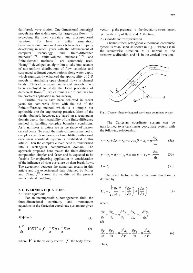
Channel-fitted orthogonal curvilinear coordinate system is established, as shown in Fig. 1, where s is in the streamwise direction, n is normal to the streamwise direction, and z is in the vertical direction.

Fig. 1 Channel-fitted orthogonal curvilinear coordinate system

The Cartesian coordinate system can be

transformed to a curvilinear coordinate system with the following relationship:

00 0 0

dΔ cosdyx x x x n x ns

β= + = − = − (3a)

0

0 0 0dΔ sindxy y y y n y ns

β= + = + = + (3b)

0z z= (3c)

The scale factor in the streamwise direction is defined by

2 2

s

2x y zHs s s∂ ∂ ∂⎛ ⎞ ⎛ ⎞ ⎛ ⎞= + +⎜ ⎟ ⎜ ⎟ ⎜ ⎟∂ ∂ ∂⎝ ⎠ ⎝ ⎠ ⎝ ⎠

(4)

where

220 0

2

dd

02

x x yx yn ns s s s s

∂ ∂∂ ∂= − = −

∂ ∂ ∂ ∂

(5)

2 20 0 0

2

dd

02

y x y xy ns s s s s

∂ ∂ ∂∂= + = −

∂ ∂ ∂ ∂n (6)

Thus,

728

22 2

0 02

d2d

0x x yx ns s s s

∂ ∂∂ ⎛ ⎞⎛ ⎞ = −⎜ ⎟ ⎜ ⎟∂ ∂ ∂⎝ ⎠ ⎝ ⎠+

222 0

2

dd

yns

⎛ ⎞⎜⎝ ⎠

⎟ (7)

22 2

0 02

d2d

y yy ns s s s

∂ ∂∂ ⎛ ⎞⎛ ⎞ = −⎜ ⎟ ⎜ ⎟∂ ∂ ∂⎝ ⎠ ⎝ ⎠0x+

22

2 02

dd

xns

⎛ ⎞⎜⎝ ⎠

⎟ (8)

2 2 2

2

11 2x y nns s R R∂ ∂⎛ ⎞ ⎛ ⎞ ⎛ ⎞+ = + − +⎜ ⎟ ⎜ ⎟ ⎜ ⎟∂ ∂⎝ ⎠ ⎝ ⎠ ⎝ ⎠

=

)

N

( 21 N− (9)

Finally, we have

1sH = − (10)

where nNR

= . The scale factors in the normal and

vertical directions can similarly be obtained as

2 2 2

1nx y zHn n n∂ ∂ ∂⎛ ⎞ ⎛ ⎞ ⎛ ⎞= + +⎜ ⎟ ⎜ ⎟ ⎜ ⎟∂ ∂ ∂⎝ ⎠ ⎝ ⎠ ⎝ ⎠

= (11a)

2 2 2

1zx y zHz z z∂ ∂ ∂⎛ ⎞ ⎛ ⎞ ⎛ ⎞= + +⎜ ⎟ ⎜ ⎟ ⎜ ⎟∂ ∂ ∂⎝ ⎠ ⎝ ⎠ ⎝ ⎠

= (11b)

Therefore, the convective acceleration operator

in the curvilinear coordinate system can be written as

[1

s s s sn z

u u u uu uN s n z∂ ∂ ∂

∇ = + + −− ∂ ∂ ∂

iu u

( )] [

1 1s n s n n

s nu u u u uu

N R N s n∂ ∂

+ +− − ∂

e +∂

( )2 1] [

1 1s s zs

z nu uuz N R N s

τ∂− +

∂ − − ∂e

( )2 ]

1zn znzz

zn z N Rτ ττ∂ ∂

+ −∂ ∂ −

e (12)

The divergence of deviatoric stress tensor is

written as

1[1

ss ns zs

N s n zτ τ τ∂ ∂ ∂

∇ = + +− ∂ ∂ ∂

iτ −

( )2 1] [

1 1ns ns nn

sN R N s nτ τ τ∂ ∂

+ + +− − ∂

e∂

( )1] [

1 1zn ss nn zs

nz N R N sτ τ τ τ∂ − ∂

− + +∂ − − ∂

e

( )2 ]

1zn znzz

zn z N Rτ ττ∂ ∂

+ −∂ ∂ −

e (13)

where , , , , ,ss nn zz zs zn nsτ τ τ τ τ τ are shear stresses and

ε is the turbulence viscosity coefficient. The pressure gradient is written as

11 s n

p p ppN s n z z∂ ∂ ∂

∇ = + +− ∂ ∂ ∂

e e e (14)

For the body force in Eq.(2), only the gravity is considered. Thus,

zg= −f e (15) where g is the gravitational acceleration.

Substituting Eqs.(12)-(15) into Eqs.(1)-(2) yields the three-dimensional equations describing the conservation of mass and momentum of incompressible flow in the curvilinear coordinates:

( )1 0

1 1s n n zu u u u

N s N R n z∂ ∂ ∂

− + + =− ∂ − ∂ ∂

(16)

( ) ( )21[

1s n s zs s u u u uu u

t N s n zρ

∂ ∂∂ ∂+ + +

∂ − ∂ ∂ ∂−

( )

2 1 1]1 1 1

s n ssu u pN R N s N s

τ∂∂+ + +

− − ∂ − ∂

∂+

729

( )2 01

sn sz sn

n z R Nτ τ τ∂ ∂

+ + =∂ ∂ −

(17)

( ) ( )21[1

s n n zn nu u u uu ut N s n z

ρ∂ ∂∂ ∂

+ + +∂ − ∂ ∂ ∂

+

( )2 2 1]

1 1s n ns nnu u p

N R n N s nτ τ− ∂∂

+ + + +− ∂ − ∂ ∂

( )0

1nz ss nn

z R Nτ τ τ∂ −

−∂ −

= (18)

( ) ( ) 21[ ]1

s n n zz zu u u uu ut N s n z

ρ∂ ∂∂ ∂

+ + +∂ − ∂ ∂ ∂

+

11

zs zn zzpgz N s n z

τ τ τρ ∂ ∂∂+ + + + +∂ − ∂ ∂ ∂

( )0

1zn

R Nτ

=−

(19)

Equation (16) is the continuity equation while Eqs.(17)-(19) are the momentum equations in the s, n and z directions, respectively. 2.3 Simplified equations

According to the physical characteristics of dam-break flows in natural conditions and corresponding assumptions [20], Eqs. (17)-(19) can be further simplified. Firstly, with the assumption of hydrostatic pressure distribution, the pressure gradient in the s and n directions can be obtained as

1 , 1 1

p g H p gN s N s n s

Hρ ρ∂ ∂ ∂= =

− ∂ − ∂ ∂ ∂∂

(20)

where H is the water surface elevation and can be obtained by , in which is the bed elevation.

bH h z= + bz

On the basis of the continuity equation and the above assumptions, the momentum equations can be simplified and integrated, and the shallow-water equations in the orthogonal curvilinear coordinate system are obtained, given as

( )( )

11 1

s nu h u hHt N s N R

∂∂+ −

∂ − ∂ −+

( ) 0nu hn

∂=

∂ (21)

( ) ( ) ( )21

1ss s

huhu hu ut N s n

∂∂ ∂ n+ + −∂ − ∂ ∂

( )21 1

s ns

u u h gh h SN R N s

∂⎛ ⎞= − −⎜ ⎟− − ∂⎝ ⎠−

( )11

zs b

Nτρ−

(22)

( ) ( ) ( )21

1n s n

huhu hu ut N s n

∂∂ ∂+ + −

∂ − ∂ ∂

( )

2 2

1s n

nu h u h hgh S

N R n− ∂⎛ ⎞= − −⎜ ⎟− ∂⎝ ⎠

−

( )zn bτρ

(23)

where su and are the integrated velocities in the

s and n direction respectively, h the water depth, nu

sS

and the channel bottom slope. (nS )zs bτ and

( )zn bτ are the component of shear stress, which can

be determined by

( ) 2 2zs f s n sb

C u u uτ ρ= + i (24a)

( ) 2 2zn f s n nb

C u u uτ ρ= + i (24b) where fC is the friction coefficient and can be computed with the Manning formula

2 4/31f nC M h

ρ−= − (25)

nM is the Manning roughness coefficient.

3. NUMERICAL SCHEME The above equations describing the movement of

dam-break flows forms a typical Riemann problem.

730

The water surface at the wave front changes sharply, and discontinuity and divergence may appear if the equations are directly discretized. Godunov[21] proposed a scheme for discretizing the Euler equations that the fluxes are taken to be piecewise constant over cell interfaces at each time step and locally exact solutions of the Riemann problem are applied at cell faces. It is felt that this Godunov-type scheme is suitable to deal with the dam-break flows. To do this, the partial differential equations shall be integrated over unit cells as follows:

1d d d d d d1 s nh s n hu n t hu s t

N+ +

−∫∫ ∫∫ ∫∫ −

( )

d d d 01

nu h s n tN R

=−∫∫∫ (26)

2 21 1d d d d1 2s shu s n hu gh n t

N⎛ ⎞+ +⎜ ⎟− ⎝ ⎠∫∫ ∫∫ +

( )2d d d d d1

s ns n

u u hhu u s t s n tN R

−−∫∫ ∫∫∫ =

1d d

1 1sg hS n tN N

− + −− −∫∫ ∫∫∫ i

( )

d d dzs b s n tτρ

(27)

1d d d d

1n shu s n hu u n tN

+−∫∫ ∫∫ n +

2 21 d d2nhu gh s t⎛ ⎞+ −⎜ ⎟

⎝ ⎠∫∫

( )2 2

d d d1s nu h u h s n t

N R−

=−∫∫∫

( )d d d d dzs b

nghS s t s n tτρ

− + −∫∫ ∫∫∫ (28)

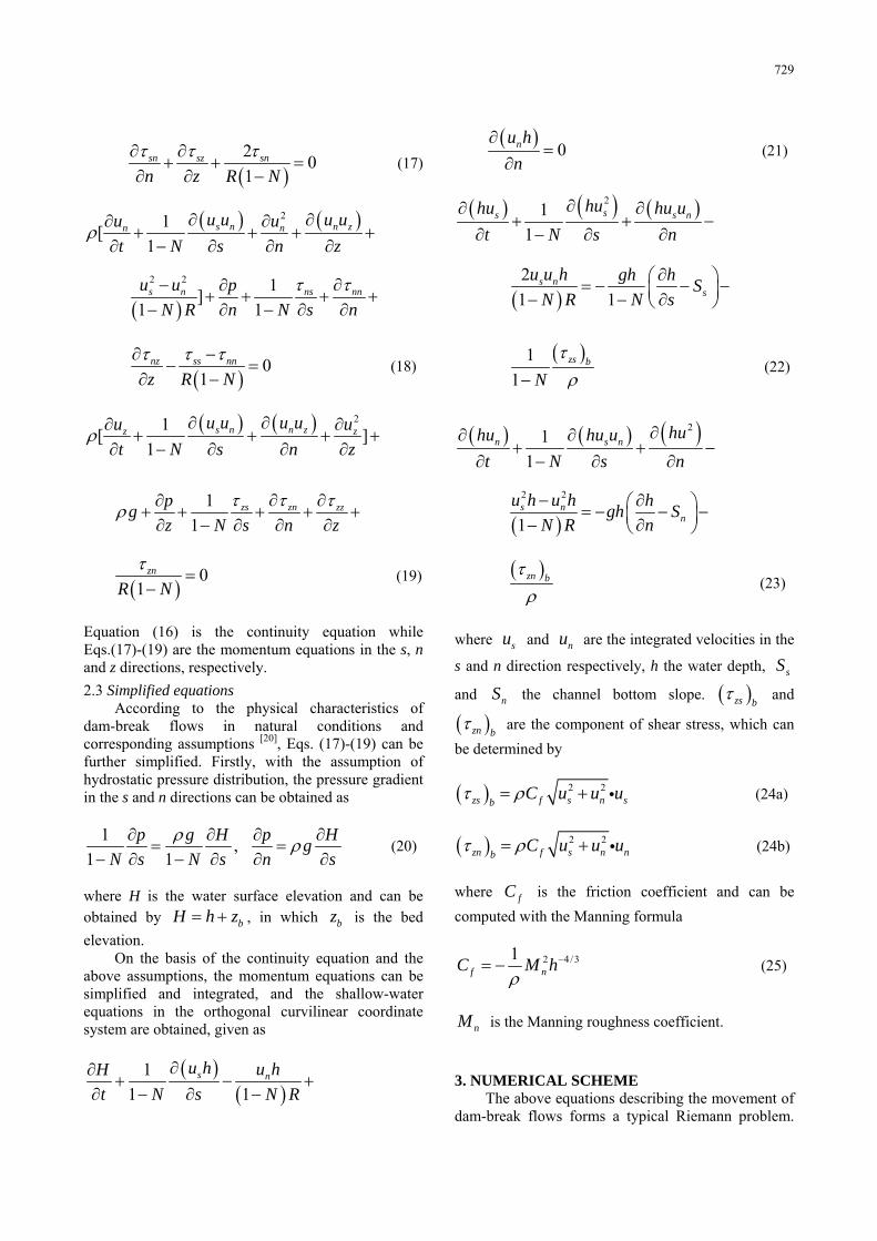
The scheme of grid and unit cell for

discretization is given in Fig.2. For convenience, the variables in the following are written in the conventional form as the Cartesian coordinate system. Next x and y represent the s and n directions respectively while denotes ( )( ,u v) ,s nu u .

Fig.2 Computational unit cells (a) and grids (b)

The valuables at cell interface are written in

uppercase letters while the valuables at cell center in lowercase letters. Δx and denote the grid size in the x and y directions respectively while the time step. By integrating Eqs.(26)-(28) on the hexahedron enclosed by

ΔyΔt

1mx x −= , 1 Δmx x x−= + ,

1ny y −= , 1 Δny y y−= + , st t= , and t t Δs t= + , the shallow-water equations are discretized as

11/ 2, 1/ 2 1/ 2, 1/ 2

Δ 1Δ 1

s sm n m n

th hx N

+− − − −= −

−i

( ), 1/ 2 1, 1/ 2

Δ[( ) ]Δm n m n

tHU HUy− − −

− − i

1/ 2, 1/ 2, 1[( ) ( ) ]m n m nHV HV− −− +−

( ) ( ) 1/ 2, 1

1Δ (29) 1 m n

t HVN R − −−

( ) ( )1

1/ 2, 1/ 2 1/ 2, 1/ 2

s s

m n m nhu hu+

− − − −= − Δ 1

Δ 1tx N−

i

2 2

, 1/ 2

12 m n

HU gH−

⎡⎛ ⎞+ −⎢⎜ ⎟⎝ ⎠⎣

731

2 2

1, 1/ 2

1 Δ2 Δm n

tHU gHy− −

⎤⎛ ⎞+ −⎥⎜ ⎟⎝ ⎠ ⎦

( ) ( )1/ 2, 1/ 2, 1m n m nHUV HUV

− −⎡ ⎤− +⎣ ⎦−

( )( )

1/ 2, 1/ 22 ΔΔ

1 1m n

UVH ttN R N

− − +− −

i

1/ 2, 1/ 21

1m n xgH SN− − −

−i

( )

1/ 2, 1/ 2

Δzx b

m n

tτρ

− −

⎡ ⎤⎢ ⎥⎣ ⎦

(30)

( ) ( )1

1/ 2, 1/ 2 1/ 2, 1/ 2

Δ 1Δ 1

s s

m n m n

thv hvx N

+

− − − −= −

−i

( ) ( ), 1/ 2 1, 1/ 2m n m nHUV HUV

− − −⎡ ⎤− −⎦⎣

2 21/ 2,

Δ 1[( )Δ 2 m n

t HV gHy −+ −

2 21/ 2, 1

1( )2 m nHV gH − −+ +]

( )( )

2 2

1/ 2, 1/ 2Δ1

m nU H V H

tN R

− −−

+−

1/ 2, 1/ 2Δ m n ytgH S− − −

( )1/ 2, 1/ 2

Δzx b

m n

tτρ

− −

⎡ ⎤⎢ ⎥⎣ ⎦

(31)

The treatment of the boundaries is very important

for the successful application of any numerical technique. For the solid boundary, a reflection boundary condition is adopted here,

2 1h h= , , v (32) 2 1u u= 2 1v= − The reflection procedure ensures that no flow

penetrate through the boundary by considering a hypothetical row of computational nodes at which the normal velocity is set to be the opposite to that of the

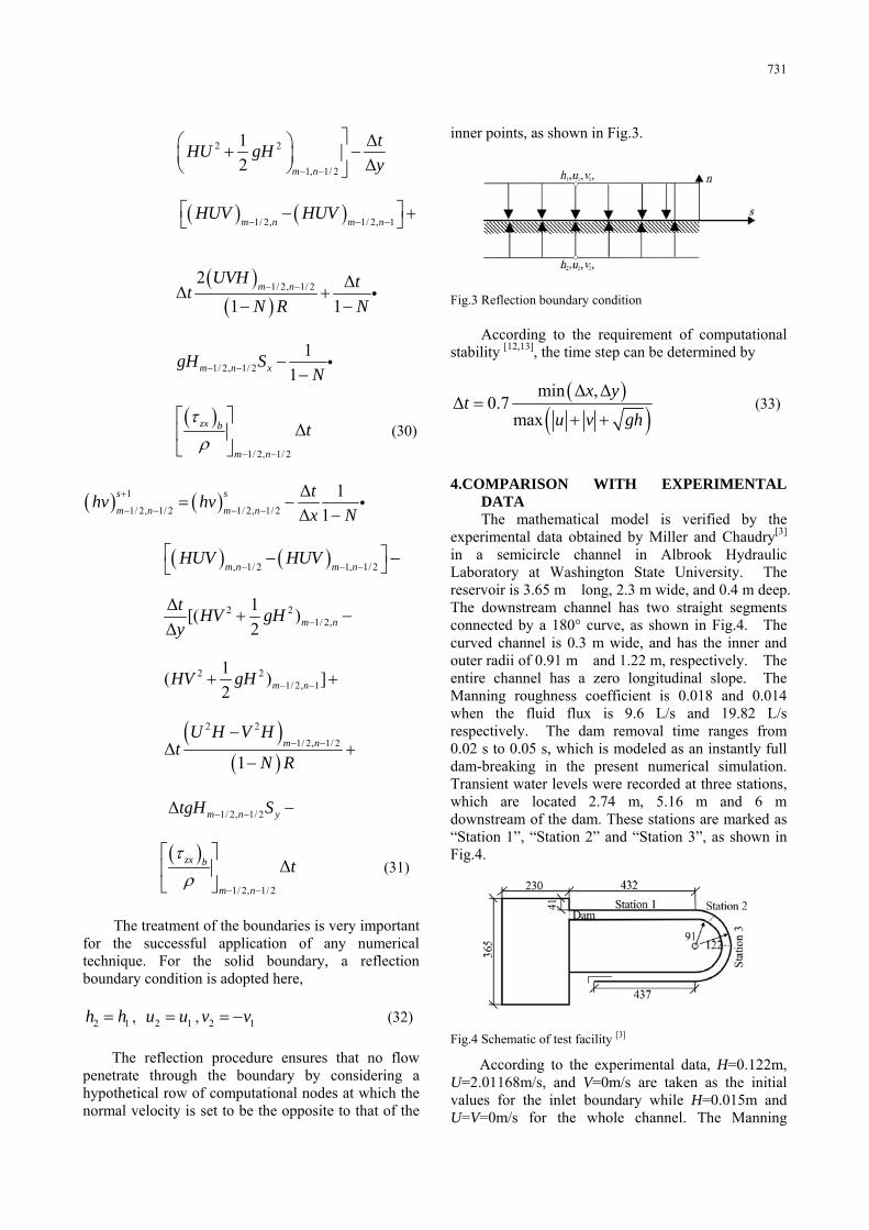
inner points, as shown in Fig.3. Fig.3 Reflection boundary condition

According to the requirement of computational

stability [12,13], the time step can be determined by

( )( )

min Δ ,ΔΔ 0.7

max

x yt

u v gh=

+ + (33)

4.COMPARISON WITH EXPERIMENTAL

DATA The mathematical model is verified by the

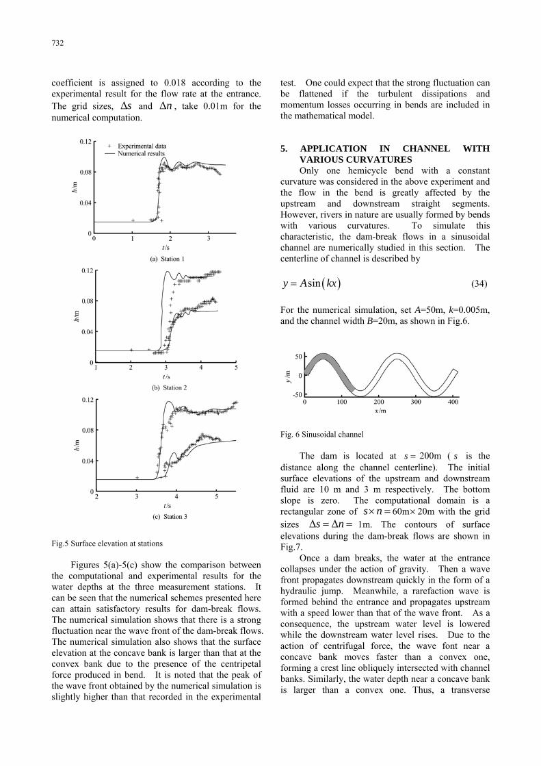
experimental data obtained by Miller and Chaudry[3] in a semicircle channel in Albrook Hydraulic Laboratory at Washington State University. The reservoir is 3.65 m long, 2.3 m wide, and 0.4 m deep. The downstream channel has two straight segments connected by a 180° curve, as shown in Fig.4. The curved channel is 0.3 m wide, and has the inner and outer radii of 0.91 m and 1.22 m, respectively. The entire channel has a zero longitudinal slope. The Manning roughness coefficient is 0.018 and 0.014 when the fluid flux is 9.6 L/s and 19.82 L/s respectively. The dam removal time ranges from 0.02 s to 0.05 s, which is modeled as an instantly full dam-breaking in the present numerical simulation. Transient water levels were recorded at three stations, which are located 2.74 m, 5.16 m and 6 m downstream of the dam. These stations are marked as “Station 1”, “Station 2” and “Station 3”, as shown in Fig.4.

Fig.4 Schematic of test facility [3]

According to the experimental data, H=0.122m, U=2.01168m/s, and V=0m/s are taken as the initial values for the inlet boundary while H=0.015m and U=V=0m/s for the whole channel. The Manning

732

coefficient is assigned to 0.018 according to the experimental result for the flow rate at the entrance. The grid sizes, and , take 0.01m for the numerical computation.

Δs Δn

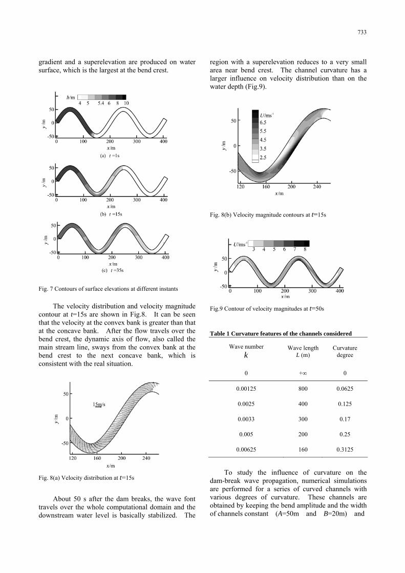
Fig.5 Surface elevation at stations

Figures 5(a)-5(c) show the comparison between

the computational and experimental results for the water depths at the three measurement stations. It can be seen that the numerical schemes presented here can attain satisfactory results for dam-break flows. The numerical simulation shows that there is a strong fluctuation near the wave front of the dam-break flows. The numerical simulation also shows that the surface elevation at the concave bank is larger than that at the convex bank due to the presence of the centripetal force produced in bend. It is noted that the peak of the wave front obtained by the numerical simulation is slightly higher than that recorded in the experimental

test. One could expect that the strong fluctuation can be flattened if the turbulent dissipations and momentum losses occurring in bends are included in the mathematical model. 5. APPLICATION IN CHANNEL WITH

VARIOUS CURVATURES Only one hemicycle bend with a constant

curvature was considered in the above experiment and the flow in the bend is greatly affected by the upstream and downstream straight segments. However, rivers in nature are usually formed by bends with various curvatures. To simulate this characteristic, the dam-break flows in a sinusoidal channel are numerically studied in this section. The centerline of channel is described by

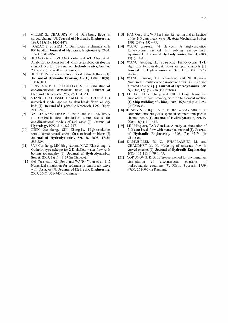
( )siny A kx= (34) For the numerical simulation, set A=50m, k=0.005m, and the channel width B=20m, as shown in Fig.6. Fig. 6 Sinusoidal channel

The dam is located at =s 200m ( s is the distance along the channel centerline). The initial surface elevations of the upstream and downstream fluid are 10 m and 3 m respectively. The bottom slope is zero. The computational domain is a rectangular zone of s n× = 60m×20m with the grid sizes Δ Δs n= = 1m. The contours of surface elevations during the dam-break flows are shown in Fig.7.

Once a dam breaks, the water at the entrance collapses under the action of gravity. Then a wave front propagates downstream quickly in the form of a hydraulic jump. Meanwhile, a rarefaction wave is formed behind the entrance and propagates upstream with a speed lower than that of the wave front. As a consequence, the upstream water level is lowered while the downstream water level rises. Due to the action of centrifugal force, the wave font near a concave bank moves faster than a convex one, forming a crest line obliquely intersected with channel banks. Similarly, the water depth near a concave bank is larger than a convex one. Thus, a transverse

733

gradient and a superelevation are produced on water surface, which is the largest at the bend crest.

Fig. 7 Contours of surface elevations at different instants

The velocity distribution and velocity magnitude

contour at t=15s are shown in Fig.8. It can be seen that the velocity at the convex bank is greater than that at the concave bank. After the flow travels over the bend crest, the dynamic axis of flow, also called the main stream line, sways from the convex bank at the bend crest to the next concave bank, which is consistent with the real situation. Fig. 8(a) Velocity distribution at t=15s

About 50 s after the dam breaks, the wave font

travels over the whole computational domain and the downstream water level is basically stabilized. The

region with a superelevation reduces to a very small area near bend crest. The channel curvature has a larger influence on velocity distribution than on the water depth (Fig.9). Fig. 8(b) Velocity magnitude contours at t=15s

Fig.9 Contour of velocity magnitudes at t=50s

Table 1 Curvature features of the channels considered

Wave number k

Wave length L (m)

Curvature

degree 　

0 +∞ 0

0.00125 800 0.0625

0.0025 400 0.125

0.0033 300 0.17

0.005 200 0.25

0.00625 160 0.3125

To study the influence of curvature on the

dam-break wave propagation, numerical simulations are performed for a series of curved channels with various degrees of curvature. These channels are obtained by keeping the bend amplitude and the width of channels constant (A=50m and B=20m) and

734

changing the wavelength of the bend L. The

curvature degree here is defined as AL

ξ = . The

curvature features of channels considered in this article are specified in Table 1.

The contours of surface elevations in these channels with various curvatures are shown in Fig.10 for the same instant t=28s. It can be seen from the figures that with the increase of curvature, the movement of dam-break flows becomes complex, and the longitudinal traveling speed (in x direction) becomes lower and lower. ξ=0 means a straight channel without bends, where the wave font is perpendicular to the bank and no superelevation of water surface will occur. In the sharp bend with ξ=0.3125, the wave font is obliquely intersected with banks and the superelevation occurs in a large range.

Fig.10 Contours of water depth in channels with various

curvatures at t=28s

For comparison, the surface elevations at the centerlines of channels with various curvatures at the instant t=28s are plotted in Fig.11. It can be seen that when ξ=0, the wave front is steep and the water surface between the wave font and the dam is smooth like the one-dimensional dam-break problem. When ξ≤0.125, the curve is basically overlapped with ξ=0, which indicates that a small curvature has little influence on dam-break wave propagation. When ξ=0.25, the influence of channel curvature on dam-break wave becomes significant, including the decrease of downstream water depth and the

fluctuation of wave surface, etc. However, the wave propagation speed is still unchanged. When ξ>0.25, the surface fluctuation is enhanced and the wave front is flattened. Furthermore, the wave propagation speed is lowered to a certain degree. The increasing energy dissipation due to the presence of curvatures may account for this phenomenon.

Fig.11 The surface elevations at the centerlines of channels

with various curvature degrees for the instant t=28s

6. CONCLUSION

Most rivers in nature are in the shape of narrow curved bends. To simulate dam-break flows in complex curved boundaries by the finite-difference method, a channel-fitted orthogonal curvilinear coordinate system has been established and two-dimensional shallow-water equations derived in this system through coordinate transformation, simplification and depth integration. The Godunov- type finite-difference scheme is used to discretize the governing equations derived in this article. Through the comparison between the numerical results obtained here and the well-known experimental data, the mathematical model proposed is verified. Furthermore, the mathematical model is feasible to simulate the water-surface superelevation that occurs in bends. The numerical simulation of dam-break flows in channels with various curvatures reveals that a small curvature has little influence on dam-break flows, while a greater curvature may lead to the decrease of downstream water depth and surface fluctuation, and an even greater curvature may lead to a lower wave propagation speed. REFERENCES [1] LAUBER G., HAGER W. H. Experiments to dam break

wave: horizontal channel [J]. Journal of Hydraulic Research, 1998, 36(3): 291-307.

[2] LAUBER G., HAGER W. H. Experiments to dam break wave: sloping channel [J]. Journal of Hydraulic Research, 1998, 36(3): 761-773.

735

[3] MILLER S., CHAUDRY M. H. Dam-break flows in curved channel [J]. Journal of Hydraulic Engineering, 1989, 115(11): 1465-1478.

[4] FRAZAO S. S., ZECH Y. Dam break in channels with 90° bend[J]. Journal of Hydraulic Engineering, 2002, 128(11): 956-968.

[5] HUANG Guo-fu, ZHANG Yi-fei and WU Chao et al. Analytical solutions for 1-D dam-break flood on sloping channel bed [J]. Journal of Hydrodynamics, Ser. A, 2005, 20(5): 597-603 (in Chinese).

[6] HUNT B. Perturbation solution for dam-break floods [J]. Journal of Hydraulic Division, ASCE, 1984, 110(8): 1058-1071.

[7] FENNEMA R. J., CHAUDHRY M. H. Simulation of one-dimensional dam-break flows [J]. Journal of Hydraulic Research, 1987, 25(1): 41-51.

[8] ZHANG H., YOUSSEF H. and LONG N. D. et al. A 1-D numerical model applied to dam-break flows on dry beds [J]. Journal of Hydraulic Research, 1992, 30(2): 211-224.

[9] GARCIA-NAVARRO P., FRAS A. and VILLANUEVA I. Dam-break flow simulation: some results for one-dimensional models of real cases [J]. Journal of Hydrology, 1999, 216: 227-247.

[10] CHEN Jian-zhong, SHI Zhong-ke. High-resolution semi-discrete central scheme for dam-break problems [J]. Journal of Hydrodynamics, Ser. B, 2005, 17(5): 585-589.

[11] PAN Cun-hong, LIN Bing-yao and MAO Xian-zhong. A Godunov-type scheme for 2-D shallow-water flow with bottom topography [J]. Journal of Hydrodynamics, Ser. A, 2003, 18(1): 16-23 (in Chinese).

[12] BAI Yu-chuan, XU-Dong and WANG Yu-qi et al. 2-D Numerical simulation for sediment in dam-break wave with obstacles [J]. Journal of Hydraulic Engineering, 2005, 36(5): 538-543 (in Chinese).

[13] HAN Qing-shu, WU Jia-hong. Reflection and diffraction of the 2-D dam break wave [J]. Acta Mechanica Sinica, 1992, 24(4): 493-499.

[14] WANG Jia-song, NI Han-gen. A high-resolution finite-volume method for solving shallow-water equation [J]. Journal of Hydrodynamics, Ser. B, 2000, 12(1): 31-41.

[15] WANG Jia-song, HE You-sheng. Finite-volume TVD algorithm for dam-break flows in open channels [J]. Journal of Hydrodynamics, Ser. B, 2003, 15(3): 28-34.

[16] WANG Jia-song, HE You-sheng and NI Han-gen. Numerical simulation of dam-break flows in curved and furcated channels [J]. Journal of Hydrodynamics, Ser. A, 2002, 17(1): 70-76 (in Chinese).

[17] LU Lin, LI Yu-cheng and CHEN Bing. Numerical simulation of dam breaking with finite element method [J]. Ship Building of China, 2005, 46(Suppl.): 246-252 (in Chinese).

[18] HUANG Sui-liang, JIA Y. F. and WANG Sam S. Y. Numerical modeling of suspended sediment transport in channel bends [J]. Journal of Hydrodynamics, Ser. B, 2006, 18(4): 411-417.

[19] LIN Ming-sen, TAO Jian-hua. A study on simulation of 3-D dam-break flow with numerical method [J]. Journal of Hydraulic Engineering, 1996, (7): 67-74 (in Chinese).

[20] DAMMULLER D. C., BHALLAMUDI M. and CHAUDHRY M. H. Modeling of unsteady flow in curved channel [J]. Journal of Hydraulic Engineering, 1989, 115(11): 1479-1495.

[21] GODUNOV S. K. A difference method for the numerical computation of discontinuous solutions of hydrodynamic equations [J]. Math. Sbornik, 1959, 47(3): 271-306 (in Russian).