CO CO rH CD Ö <

USAAML TECHNICAL REPORT 65-20

CURVED 1ET FLOWS

VOLUME II

May 1965

UuBli TIS1A E

U.S. ARMY AVIATION MATERIEL LABORATORIES

FORT EUSTIS. VIR6INIA

CONTRACT DA 44-177.AMC-238(T)

PETER R. PAYNE, INC.

F-pp^ ^fnüD

n^f. •;;'"■ pup

/^^y'

^f^^nnnnrfp rr:r\ ,.—, „ ^ r- ^ /—\ /C^ H? Li!;;ü> m

Ct4Jfr^ Voll IW^i^l^ In this section the shape integral is calculated for a number of idealized asym- metric distributions when, from Equation (195)

\

It is obvious from Equation (196) that (as long as viscous effects are unimpor- tant) maximum cushion pressure will be obtained when X is maximum. This implies that the maximum pressure peak must be on the cushion side of the jet centerline, as indicated in Figure 66.

"I

CUSHION PRESSURE LESS THAN SIMPLE THEORY

GREATER

Figure 66. Symmetric and Asymmetric Jet Total Head Profiles.

It should be remembered that the ratio

"TSTp mean

is entirely artificial; that is to say, it is not a true parameter, since it will change with the shape integral ( ^ ). This leads to a number of anomalies,

125

and indeed, the only reason for presenting the following results is the wide- spread use of the ratio &%A± P measurements.

The Jet Thickness Anomaly

as a means of reporting experimental

Sup^se now that a test nozzle has the geometry of Figure 67 and that an inst,,t has been placed in the nozzle, unknown to the experimenter. Thus a traverse across the (original) nozzle width ( 'fc ) gives the total head distribu- tion indicated in the figure. As a result, the unobservant experimenter com- putes the mean total pressure as

AP. » AP •Heouri

and the cushion pressure ratio as

AR Me«**

VKcux. T

AP, ^ KVA4C.

INSERT

\\\\\\\\\\\XL 4

/ / ///////////////'

Figure 67. Geometry for the Jet Thickness Anomaly.

The simple theory equation for ^-i)^ gives him

At - eCvfe)- C%y AP(

C'ir/4^ ♦M»**«. ^ ^R MJUc

126

The correct equation is

'ZC^'k) - ^-/R)

Thus the apparent ratio between experiment and theoretical results is

Experiment Theory

Thus, the unobservant experimenter would conclude that his measured ratio A^A, p^-mean exceeds the "theoretical" value. His belief would be illusory, however, and in the same way the limit cases of the total head distributions discussed below will show the misleading result that a jet should have all its energy concentrated at the inner boundary. While this conclusion is per- fectly correct so far as obtaining the maximum value of the ratio ( &Jfc,/&.P mean) is concerned, minimizing the mean total pressure has no physical Importance; it does not correspond to minimum jet power, for example.

Rectangular Total Head Distributions

AP

(i-t)K ***

urn*

- it rb < x <^) Figure 68. Two Rectangular Total Head

Distributions.

127

For the first of the two distributions sketched in Figure 68, it can be seen that as ^ % diminishes we encounter the physical limitation of reverse flow, which requires AA.< A^ . Since the jet static pressure gradient *^^. > O , this condition must occur at either J »^r or A • jit . For the first position,

But APt + 6%. = z&P**^ ;

For ^ - /yZi

Thus at **£ ) the limiting condition is

This limit is plotted in Figure 69, and the curves of cushion pressure ratio for the stepped distribution are plotted in Figure 70.

128

1.0

or

O H O <

O i—i H

S H l-H

Q

s

W

PH

< H O H

0.8

0.6

0.4

0.2

\\\\\\\

TOTAL HEAD DISTRIBUTION

IN JET

SOLUTION IS REAL IN THIS REGION

NO SOLUTION DUE TO REVERSED

FLOW

0 2 4 6 8

HEIGHT PARAMETER R/t

Figure 69. Solution Limits for the Rectangular Total Pressure Distribution.

10

129

1.4 1

1.2

i

I ^ ^

1.0

<

w

H

9

w

P.

o »—t

P U

0.8

0.6

0.4

0.2

4 6

HEIGHT PARAMETER #/t

10

Figure 70. Effect of a Stepped Rectangular Jet Total Head Distribution Upon Cushion Pressure.

130

A General Linear Variation

(-t<y<. t)

Iji/*)^ 'tyt) - t*£*i*p'

A = 11 + ^//>/?}

B'igure 71. General Linear Variation.

This case was first solved in Reference 13, from which Figure 72 was ab- stracted.

The reverse flow limitation can in this case be simplified to

BUt ^ * 4P - zaP

^c. < Z ~ Ml AP men* &?* tu****

& e/« * ^VAP.)

131

1.4

1.2

0* ^i.o

es w H §0.8

OH

0.6 8 CZ3 W

O X tD 0.4 ü

0.2

TOTAL HEAD DISTRIBUTION

IN JET

2 4 6

HEIGHT PA RAM ET EP. ß/t

10

Figure 72. Effect of a Linearly Varying Jet Total Head Distribution Upon Cushion Pressure.

132

This limit is superimposed on Figure 72 and is seen to confine the attainable cushion pressures to a fairly narrov/ band. However, a value of (A^/ßP mean) equal to 4/3 times the (uniform -A'? ) theory value is seen to be attainable at the limit ^A) -♦ 1«0'

A General Power Law Variation

This case includes that of Figure 71, when /l£. or 4r = 0 and also the constant total head case (-vu -*,<»0 ). It is based on the relationship

*pi v»u

although the actual value of !<■ does not influence the results.

M+7.

Figure 73. General Power Law Distribution.

133

It is obvious that the maximum cushion pressure (ai't/fc =1,0) will be twice the simple theory value, in the limit "W -**** .

CUSHION PRESSURE AS A RATIO OF MEAN TOTAL PRESSURE WITH A LINEAR VARIATION IN TOTAL PRESSURE ACROSS THE JET (EXPONENTIAL THEORY)

In this section the problem will be simplified by considering only a linear vari- ation of total pressure across the jet.

From Equation (164) cushion pressure is given by

^ - l*2*i^'H and the mean total pressure by

For a linear variation in Afx across the jet

where

Substituting in Equation (197),

(197)

^ - ij*^- (198)

134

4-

From Equation (198),

(199)

^ ' ^ • - -g- A• -- J*^I +-%). (200)

This expression is evaluated for various pressure ratios,

£^ » O / Vz , ^ Z oo t over the height range 0 < % ^ Xo

and is plotted in Figure 74.

For x^ * O J^Z » | | the expression reduces to 1 — e-

For AT -**■ oc* ^ oyp _>. o , the expression becomes

At values of the pressure ratio less than unity, that is to say, when

the solution is limited by the condition

AP.. > A^ ■

otherwise^here would be a reversal of flow in the jet next to the cushion. The existence of this limit was noted in the previous section.

That is

for real values.

135

1.4

1.2

1.0

i

•<.0.8

o H

§0.6

CO

en

ü

0.2

^M

\ 1 ^ .ee

\ 2.0

V ^-T.TMTTFOR 44- ^ 4^ 1

Iw 1.0^^^ ̂ f

A 1/2

S***J I / i / /

y

I ^ V / v\\.\ / \ vw /

\ ^m / ^'>c^\ / "•^^s /

^ N. 1 ^S 1 T^^^V i ^S^^^N 1 ^^« ^^^ h ^^ ^pj

0

Figure 74.

4 6 8

HEIGHT PARAMETER ^/^

Cushion Pressure as Affected by a Linear Distribution of Total Head Pressure in the Jet (Exponential Flow).

10

136

When the limit is reached.

o - .:**)-

> ■ t [' -('-•**)' and •I

This is computed and plotted in Figure 74. It will be seen that the limit is asymptotic to the curve for ^-/f3«, = 0 at great heights and reaches the value 1 when Q/fa = 1 at zero heights.

The results are replotted in Figure 75 for fixed heights with pressure ratio as abscissa.

THE EFFECT OF A LINEAR TOTAL HEAD VARIATION OF THE CUSHION PRESSURE PARAMETER ^Jjg^

Because of the large variation of A%/AfL with jet total pressure gradient, we are forced to conclude that the cusMon pressure parameter AJf defined in Equation (142) is a more meaningful measure of an annular jet's effective- ness.

Therefore, it is of interest to see how the cushion pressure parameter is af- fected by nonuniformity of total pressure distribution in the jet. Since this parameter is the measure of the pressure obtained in the cushion in relation to the energy supplied to the jet, the presence of a well-defined optimum would indicate the choice of jet structure to give the best operating performance.

For simplicity in computation we considered a distribution which gives a linear variation of total pressure across the jet. This may be defined by a pressure ratio ^ At* where the total pressure ^R varies from Ä^ at the out- side of tne jet to Afc. on ^e cushion side.

Then 4P^ * A^C» ^ ^ J^') (201)

137

es 5 c c

CS ^

>5 CO .O 05

s £

«■■'-« ü

o c H « :H -. CO O .M

si. S © •^ *J o

§1 & S *S w 2 1c ^ Ü G ^

LT t^

ä

m CO M

M

SHnSSaHd 1VX01 X3f NV3IM/3HnsS3Hd NOIHSHD

138

where *&- ~ AP/' — | .

Substituting for ^«x in the expression for cushion pressure, Equation (145) results in

(202)

We should then evaluate this expression over a range of values of the pressure ratio parameter yv- and the height parameter *y^ .

This is an excessively laborious computation which may properly be deferred until the value of the result is more clearly apparent. However, it is likely that the result will be intermediate between the two simpler cases in which rl = 0 (exponential flow) and /} = 1 (free-vortex flow).

Accordingly, these two cases were computed over the ranges

Variation in Cushion Pressure Parameter According to Exponential Flow Theory With a Linear Gradient of Total Pressure Across the Jet

The cushion pressure parameter is given by

Substituting

(203)

139

-^ -> Writing ^ - A —^ M

— i /'' '

r A [B, - ^«-c " - AB,)]

^

(204)

where

A = 'Vie

^ = e/^ - / ,

Note: Numerator is unreal when ^v- -«d "^•/^l— AB )

Der.ominator is unreal when ^v- < (^ i — B, J/l /\si ,

Since ^^ is essentially <o at both these limits, the denominator limit is effective because

>

Oetails of the actual computation are omitted from this report. It should be remarked that the expression in this form requires a numerical integration of the denominator for each point evaluated. Since this appears to be a mono- tonic type of function of **-, a sufficient accuracy may be obtained from a fairly small number of stations o ^"x * 1,

140

The computed values are presented in Table 3. These are plotted in Figure 76 as the broken lines, together with the results (full lines) from a similar computation for free-vortex flow described in the next section.

Variation in Cushion Pressure Parameter According to Free-Vortex Flow with a Linear Gradient of Total Pressure Across the Jet

In free-vortex flow «7 = Ijand we have for the cushion pressure parameter, from Equation (145)

0■* -^tl^i^ (%£**f*Jc%'H)äi'<te)] ^ The simple case when AR - constant was given by Equation (149).

Putting jfe£ » x and writing -^z = «u , we have R • %,*'*' so that

^ • ^^ '•

Then,

(i HO-f fff^stTctf,^ ^c ~C^^tzL*^X'+^)d*]d*'

J^—TT- ^ 7^ . (206)

The expression is evaluated over the ranges

and | <C «. ^. 4- •

141

TABLE 3

COMPUTED VALUES OF &/&,' ^fe FOR A LINEAR GRADIENT OF TOTAL PRESSURE ACROSS THE NOZZLE - EXPONENTIAL THEORY

Pc/Pa R/t = 0.25 (KJ3 1.0 2.0 4.0 10.0

5 4.35 2.67 1.43 0.675 0.283 0.0795

3 4.12

2 4.02 2.47 1.38 0.667 0.?83 0.082

1.5 3.81 2.30

1.25 3.70

1.00 4.075 x

0.95

0.925

0.800

0.687

0.600

0.418

0.400

0.228

0.200

0.095

2.26 1.27 0.639 0.279 0.081

2.21

2.48

X

1.25 0.630 0.276 0.0803

1.22

X

0.613 0.268 0.0807

0.602

X

0.263

0.249 X

0.0792

0.0760

0.0700

X

142

EXPONENTIAL FLOW . FREE-VORTEX FLOW

0.1 0.2 0.4 0.6 1.0 2.0 4.0 6.0

PRESSURE RATIO ACROSS JET A% /d£

10.0

Figure 76. Cushion Pressure Parameter With Linear Gradient of Total Pressure Across Jet - Free-Vortex and Exponential Flow.

143

As in the preceding case we omit details of the computation and give the result- ing values in Table 4. These are plotted in Figure 76 in conjunction with those from the exponential flow method. As before, we observe that the curves are bounded to the left by the condition that the denominator shall be wholly real.

Discussion of the Results

It is remarkable that the limit for real values seems to be the same for both cases. There is no very obvious reason why this should be so. The physical meaning, of course, is that the flow pattern near the inner (cushion side) boun- dary of the jet can not be maintained when the total head pressure Aß is re- duced to the local static pressure A-f»« • Therefore, the limit appears when Af^«Ab , assuming an absence of other disturbance to the flow locally. How- ever, the two methods give differing values of Afeat the same operating height and pressure ratio, and, if the limits do really coincide, the value of the cush- ion pressure parameter at the limit is a function only of the pressure ratio. It therefore depends upon other factors which are common to both methods. Fur- ther, it can be hopefully said that the same limit will apply to the Payne theory, intermediate between the two computed cases.

Considering first the curves for exponential flow, it is seen that a high value of the pressure ratio is favorable, though only slightly so. The effect is most marked at low height ratios, and there appears to be a minimum close to the reverse flow limit for heights below R/^ - 1. Here, too. the reverse flow limit is approaching asymptotically Pc/p =1, and since the exponential flow method is more valid at these low heights, this is clearly indicative of the ad- vantage of having ^c/f* much greater than unity for heavily loaded, low-flying GEMs.

At the other end of the scale, at tyfc = 10, the exponential method loses valid- ity. This curve has been plotted chiefly for comparison with the free-vortex result. This shows a gentle maximum at ^c/fi. ^ 1, which means simply that a uniform total pressure across the jet is more efficient than any linear varia- tion of pressure. Even so, the effect is slight and becomes less marked at low- er operating height ratios.

Therefore, the conclusion is that pressure gradient in the jet makes very little difference when fy^ is greater than 2, let us say.

These results suggest that it may not be worthwhile to work out the cases using the more precise model of the flow developed in this report, having regard to the computational difficulty using ordinary methods. This is a job for an elec- tronic computer, and, for the sake of completeness, it would be pleasant to see the result. However, it is fairly evident what this will be. Over the inter-

144

TABLE 4

COMPUTED VALUES OF ife^ • ^c FOR A LINEAR GRADIENT OF TOTAL PRESSURE ACROSS THE NOZZLE ~ FREE-VORTEX FLOW ( y = 1)

Pc/Pa R/t=2 3 4 6 10

5 0.905 0.492 0.330 0.186 0.0823

2 0.957 0.503 0.333 0.1885 0.0855

1 0.971 0.507 0.333 0.1870 0.875

0.8 0.960 0.508 0.335 0.1900 0.870

0.6 0.960 0.494 0.335 0.1885 0.868

0.57 0.960

x 0.40 0.492 0.332 0.1920 0.862

0.37

0.27

0.20

0.176

0.098 (limit for R/t = 9)

0.490 X

0.319 X

0.1935 0.833

0.1750 X

0.794 X

145

mediate range of height, the Payne model moves from approximation to the free- vortex result at the high end (R/fc, = 10) toward the exponential result at the low end. In the middle it will be between them, and, from the appearance of the curves, it will probably show only slight effects of pressure gradient with some advantage in having the pressure high on the cushion side. However, the effect will be slight.and one should not expect a gain of more than 10 percent or so from a pressure ratio 5:1, compared with a uniform pressure design.

In an earlier station,the effect of a total pressure gradient in the jet was exam- ined for free-vortex flow in terms of the parameter^aPMe<w,the cushion pressure ratio to the linear mean total pressure in the jet. This showed a larger effect than the present analysis; for instance, at ß-^fe- »■ 2L.

•>

s/y

*t-' H< Ah

© %:t> A%>_:78 ®^ -or' At^ -7* M -äP. «•CÄKf

Figure 77. Pressure Distributions in Jets.

Although these jets look the same, they arc absorbing different amounts of power.

Power ©c: 'I K (^^ 'H) <*% >

and this is greater when the higher total pressure is on the same side as the higher static { = cushion) pressure. Not surprisingly, the more powerful jet produces greater cushion pressure, which accounts for most, if not all, of the difference in ^■&-/^p •

This example serves to illustrate the superiority of the cushion pressure parameter as a criterion of cushion pressure achieved in proportion to power expended in the jet.

146

Chapter Six

VISCOUS MIXING EFFECTS IN THE ANNULAR JET

The first known treatment of the problem of viscous mixing effects in the annu- lar jet is due to Chaplin^0, who used a simple analysis to show that mixing al- ways causes a reduction in performance, relative to the idealized in viscid flow case.

It is doubtful whether real precision in the calculation of mixing effects can ever be achieved, because of the complexity of the induced flow fields. Nor can these effects be measured until a better understanding of annular jet flew mechanisms has been achieved, since it is impossible to say what portion of the observed loss is due to viscosity and what is due to nozzle diffusion and local flow distortions. The position is rather analogous to trying to measure the viscous drag of wings before the publication of Lanchester and Prandtl's lifting line theories, when the effects of aspect rntio on lift-curve slope and induced drag were unknown.

Reviewing the possible sources of loss which have to be separated from the vis- cous losses, if experimental data are to be obtained on the latter, we see that there are really only five:

1. Loss of cushion pressure due to nonuniformity of total head.

2. Loss of cushion pressure due to a local flow distortion, where the flow angle lr not the same as the geometrical nozzle angle.

3. Total pressure loss due to diffusion or separation in the nozzle.

4. Fundamental reduction in cushion pressure associated with a curved planform.

5. Experimental error; the latter may be

(a) simple errors in instrumentation or calibration,

(b) measurements at the wrong location (measuring "cushion pressure" near the jet, for example), or

147

(c) rig leakage, such as a twc-dimensional jet rig which has a low energy j-^t .iear the boundaries.

There are evidently enough hazards to render the unquestioning acceptance of published measurements quite impracticable, at least without a detailed analy- sis of the investigators test procedures and equipment. And the problem of eliminating ail but the viscous losses is correspondingly more difficult.

Figure 78 presents measurements of the cushion pressure ratio Afrc/^p,^^ made in three different investigations. There is obviously a significant differ- ence between the NASA model, which has a circular planform, and the two- dimensional rig results, and we might be tempted to assume that the difference in planform is the cause. The three-dimensional correction, of Equation (114) Indicates that this effect is small, however. Reference 16 also gives two meas- urements of the total head distribution across the nozzle of the Kuhn and Carter nozzle showing considerable distortion from the uniform condition. If we take a linear approximation to this distortion, we can extrapolate as shown in Figure 79. Using the theory of the previous chapter we can use this to obtain the change in cushion pressure, as shown in Figure 80. Note that although the Figure 79 extrapolation becomes progresoively less reliable as we move above -*><? -- 3.0, the importance of flow distortion becomes progressively less great, so that this inaccuracy is relatively unimportant.

Making these corrections to the data in Figure 78 gives the plot shown in Figure 81.

There is evidently still a significant difference between the two sets of points, and this is presumablv due to either a diffusion loss in the Reference 16 model nozzle, and/or to its jet not emerging at the nominal nozzle angle oi KP ~ 0 . What is clearly evident is that even the two-dimensional test rig results are well below the inviscid flow theory line, and most of this deficiency is presum- ably attributable to viscous mixing and nozzle diffusion loss effects. Certainly a negligible amount is due to the vertical flow angle diverging from the geometric angle, as shown by the very careful streamline plotting carried out in Reference 21, from which Figure 82 is abstracted.

We can approach the viscous mixing problem in at least two ways. The most elementary regards the passage of one stream of air over another as a "skin friction" problem which is exactly analogous to the passage of air over a solid surface. Unfortunately this approach gives numerical results only for the limit solution of stationary cushion air.

148

© BEN-CHIE YEN & KUHN & CARTER eT RAWLINGS & SEIVENO

\\\N\\

1.0

\

"5" 0.8 C i—i

H

0.6

O i—i

S o 4 D U

0.2 -

0 2 4 6

HEIGHT RATIO -//^

10

Figure 78. Some Experimental Measurements of the Cushion Pressure Parameter at O' = 0°.

149

6

At

2 4 6 8

HEIGHT PARAMETER J-/?

10

Figure 79. Assumed Equivalent Linear Total Head Distribution Across the Kuhn and Carter Model Jet.

150

-.03

Q < W K

< H O H

O

O

O H

g

-.02

1 < -.01

o H

W

w

Ü

4 6

HEIGHT PARAMETER ^/«f"

10

Figure 80. Increment of the Cushion Pressure Ratio Due to Total Head Distortion in the Kuhn and Carter Model.

151

1.0

0.8

0.6

g 0.4 cu

o 05 D Ü 0.2

4 6

HEIGHT RATIO J,/t

10

Figure 81. Data of Figure 78 With the Kuhn and Carter Results Corrected to Two-Dimensional Flow With Uniform Total Head.

152

c^bft <o K) ** "V CSj — o O o o C> O

1 1 1 1 1 1

cs?^

CM

Q O a o u Qi

CM

£ 2

o

T3 ß

o 0

i—i 0)

o

« »"3

> u 3 Ü

00

o u

fa

153

ffe-Ä

Attemsttv^y, Wi l^ki um a more detailed flow picture which accounts for the details of the flow entratemeiü process inside the cushion. At the present time there seems little point in investigating the finer details of the ambient air en- trainment, since this takes place at (approximately) ambient static pressure, and should not greatly influence the cushion pressure, therefore.

THE "AIR FRk.TION" CONCEPT

In Reference 3 it is shown thai the "effective skin friction loss " of a Jet of velocity ( -^J ) flowing over another stream of air (with velocity "^ ) is given apprcximateiy by a skin friction coefficient,

JVU

C ^ >C^} (>~Z.)

^j-

(207)

from the "^VCAC/ ^ measurements of Reference 22.

ntact with the cushion air is 5^. .the "friction If the length of the jet surtaee m vo iorce" is

y -gf ^c

c^c^ X-^j s AT. (208)

II dR is Hie i io/.zle toti:) iicad on the eushiou side

AP. ^^

c^c^o- ^O (209)

AR

From Equation (32), for conservation of total head ^

154 ■-.' ■■'...■.■

. '. ' ■■■.■■■■;■■,■.■; : ■ ■

,;f:

For thick jets, the mixing occurs in the region where the local static pressure is approximately equal to the cushion value.

-i (211)

AT / - CS^Cl- ö^pj-8-. ,212)

From Equation (101);

APN APj,^ AP, R Z"1-', (2i3)

and for uniform nozzle total head

AP AP "R ^ ^AFLJ ' (214)

The accuracy of the assumptions is such that we may as well use the inviscid value fo: Afe/Af*, inside the square root sign, when the jet is thick; that is, when ^.^ 1.0 say, so that

Afc - \ - Q|^,_ A^w^t (2^

Note from the geometry of Figure 41 that

s, - ^R. %:JL -a*0'"?- (2i6) er

155

When viscosity causes an appreciable reduction in **^ , we must solve Equa- tion (214) exactly. By squaring we have

In the quadratic solution to (217)

''2.

^Tc^ J ' (218)

^ ^

The minus root is the correct solution. As can be seen from Figure 83, the difference between Equations (215) and (219) is quite small.

This particular analysis cannot be extended into the "thin jet" regime because the concept of "skin friction" between two fluid streams, both of which are thick- er than the mixing zone between them, is then invalidated.

The theoretical limit is of course ^/. =5.2

yb/LIMIT ^■

As shown in Figure 83, this approach appears to give fair agreement with ex- periment for Jb-yfet 1.5, when we take the limit case of still cushion air

156

1.0

£«•

o H S 0.

CQ

ü

0.4

0.2

4 6

HEIGHT RATIO ^f/f

10

Figure 83. The "Air Friction" Theory of Viscous Losses in a Thick Jet Compared With Inviscid Flow Theory for 0 = 0°.

157

i'^t - 0). although the Kuhn and Carter points still fail below the line. Pre- sumably the true value of iJJ is somewhere between zero and unity, so that all points would fix'u it in the range o *- '^^•1.5, and prcsuniably the deficiency would then represent nozzle losses.

The air friction theory should show a loss in cushion pressure as the length of jet in contact with the cushion is increased. Some experimental work at Aeronutronic" , involving the use of rigid nozzle extensions, enables us to make a rough check on this hypothesis.

Some raw data from Reference 23 are displayed in Figure 84, in comparison with results obtained from conventional two-dimensional test rigs. The cushion pressure is shown to fall significantly when an extension is fitted, which does not agree with the Payne tests reported in a previous chapter. We presume this is due to some instrumentation error on the Aeronutronic rig.

When the inner extension is shortened or removed, more of the jet will be in contact with the cushion. Thus relative to the extended nozzle results of Fig- ure 84, the cushion pressure should be less than even the reduced values ob- tained with symmetrical extensions. As shown in Figure 85, this is in fact so, although the results can hardly be regarded as indicating a consistent trend.

Now from Equation (214) we can express the reduction in cushion pressure by the equation

(220)

A4 0r Ösf^A = ~ A^c CTr O - fMlg; jcrgc ) (221)

when Ö =0°, so that R* -4L .

For the geometry of Figure 85;

Asy4 - (So - -^OA; of course.

158

B 2 - JET, 2-D RIG | RAWLINGS AND € 1 -JET, 2-D RIG J SEIEND O 1 - JET, 2-D RIG BEN-CHIE YEN \\\\\\ i/

+ A/A

^ o. o

m ES

o m 0.

ü

0

3.0 NOZZLE EXTENSIONS 1.0 NOZZLE EXTENSIONS

4 6 8 HEIGHT PARAMETER <i/t

10

Figure 84. Effect of Nozzle Extensions on the Cushion Pressure Ratio (^ = 0°).

159

4/4 = 3.0

0.5 *//.

1.0

Jl/Jt = 1.0

0.5 4fc

1.0

Figure 85. Effect of Exposing the Inner Surface of the Jet When Nozzle Extensions Are Used (Ref- erence 23).

160

0.3

0.2

0.1

0 12 3 4

INCREASE IN JET SURFACE LENGTH A Se/t

Figure 86. Reduced Aeronutronic Data of Figure 85.

161

Equation (221) has been used to plot the expression

« * Mir

(222)

in Figure 86. The scatter is very large, as we would expect in analyzing this type of data. Nevertheless an appropriate trend is detectable and all points fall on or below the Cf = 0.16 curve, indicating "VT/O"- > 0- More- over, the -Cw/lv =1.0 points are noticably higher, on the average, than the JLef^r =3.0 ones; this again is reasonable because the entrained vortex now would be virtually parallel to the jet in the latter case.

A GENERAL THEORY OF MIXING LOSS

V-r_—--^^-g _^_^ y-/ /*/ 7 / / //// 7 / s /////// s

Figure 87. Mixing in the Annular Jet.

Under equilibrium conditions, it is generally agreed that viscous mixing causes the entrained flows illustrated in Figure 87. If 5^ and ^^ are distances along the jet surfaces on the cushion and ambient sides respectively, then from Reference 4, the entrained airflow ratio

-^ x

-w -wv;

-*w N

Z. z. KV^ [ -i* s. ]•

162

For continuity of mass flow, the entrained cushion air must return to the cushion:

and since some transfer of momentum has occurred, the momentum flux to am- bient of the main part of the jet is accordingly reduced.

This must result in the cushion pressure being less than the value predicted for inviscid flow. We can regard this either as being caused by a reduction of the mornenium flux to ambient (as in the previous section) or by a reduction in the curvature of the jet.

From a long term point of view, the best approach is likely to involve express- ing the local jet velocity distribution in a suitable analytic form (such as the error-function distribution), weighting it for the effect of varying static pressure, and solving the resulting equations for the inward and outward flows.

In the present analysis ve shall take a simpler approach, using the general con- cepts of Reference 4, but making the use of the general momentum relationship of Equation (101)

= 3: &h f?C

We shall also assume that mixing on the ambient side of the jet does not influ- ence 3£L , because there is nominally no pressure change, so that all mixing effects are attributable to the cushion.

The entrainment of cushion air reduces J^ by an amount A 3^ as explained in the previous section, so that we may write

% = ^c -AX - F

INVISC.t) C^ (223)

where r = a cushion entrainment term which will be discussed later.

The flow picture of Figure 87 is similar to that of an overfed jet, as indicated in Figure 88. However, the big difference is that we do not obtain as low a cushion pressure, unless all the primary vortex momentum ( ^ ) is dissipated CT, -0).

The momentum loss A«Xc ^s reaciily calculated when the entrainment function is known, and it is reasonable to assume that the momentum flux Oc into the cushion is equal to the momentum lost by the outgoing jet. Then knowing *Jv0

and J^ we know the mean effective velocity -v^ into the cushion.

163

N\\\\\\\\\V\\

».

• *

T*

^ =!r -^ X

(a) Conventional Overfed Jet.

■T^T-

^

1 ^

(IJ) Jet With Primary Vortex.

Figure 88. Two Ways of Portraying the Overfed Jet.

164

The momentum flux, 3^ , back to the jet is less than ^c because of skin friction losses against the ground plane and base plate and because of air friction between the outside of the vortex and the inner cushion air. The inner air may be stationary or there may be a secondary vortex; possibly the former is true of a finite planform, and the latter of a two-dimensional test rifr.. When a secondary vortex exists the air friction will be much less, of course.

We now proceed to express this chain of reasoning mathematically, assuming that entrainment takes place over <^y4 , where <^L is the distance over which entrainment occurs. (From Figure 82, for example, we might expect^ <t>^j|£).

Now#for mixing at constant static pressure (Figure 87)

JN * Jj + 3c (224)

or, in terms of average values>

-TW^-VH f-V^j -4- *0 ^C ;

*- * (225)

since the emnined air mass flow is run.^ ;

3;

^ (226)

and ^ s ^^e^)* + ^ ' -JN is the momentum flux at the nozzle. However, when the vehicle is

close to the ground, mixing occurs only on the innermost portions ui the jet, and it would be unrealistic to take J^i as the total value ( J^ ) for the whole jet, particularly in the zone of establishment ( <^^/t ^ 5'2)' We should rather weight -JJ, to be representative of the velocity and mass flow pertain- ing to that part of the jet in which mixing actually occurs.

Using the vortex assumptions of Reference 4, and denoting C^ Cfß. as the skin friction coefficients of the cushion air and ground respectively, then

165

referring to Figure 87

q^ - ^ ^ ^f^ "^ ^"^-^C . (227)

The skin friction on the base plate is here neglected as being negligible, and for convenience we assume that the skin friction in both the ground and cushion regions can be based on the "V^ velocity.

Then 3^ = To - «^ ^^•*'C

= P; -ifv^c(cf.^<=f*);

T - or = ^r^-e-<C<=fc - ^fc).

(228)

(229)

Thus from Fig re 88

•v X

-fuC ^ ^ / (230)

But from (210) and (224)

^f^ / J (231)

4.

where ^, and -wv^. are given by Equations (225) and (226). A^- and "^j are of course mean effective values.

(232)

166

The solution of Equation (232) can be accomplished in varying degrees of ac- curacy, depending upon how detailed we care to make the analysis of 31. and «tiU^ . Using the simple values given by Equations (225) and (226) and assum- ing uniform total head in the jet we can obtain a solution which is applicable at large values of>ß^.

Nu

AP AR I^»vi -C ^CtAP. U r*» >> AVJ M.,*..^ l-*"* * ^CtAFJ APi

(233)

The non-dimensional ratios

^ AP,'7 ? 2CtAf? ctC^r^r

must be known before Equation (233) can be evaluated. However, they are of second-order importance, since they appear only in the viscous correction to the exact solution, and they can be derived with sufficient accuracy from ex- ponential theory. We proceed as follows:

yz ~ &■ (234) C^o

at&tWf

The mass flow on the cushion side of the point <v is

(235)

(236)

167

Taking this value as average across the jet

<*(**&$ " ^_^ • <23T'

If the amount of the jet affected is the same* as the quantity of air entrained, then from Equation (236) and (237)

>v. ^ T ^- - % • ^e ~ ^ ) /^ - >fe ^ (238)

or

— • (239)

We can also calculate the average momentum flux and static pressure (Afa ) in the mixing zone, using the same approach.

-SC^A^" ^ i>tr V ^ ^^ (240)

4 j = g C^^- ^) . ^ (^-1^^;. (241)

Averaging across the jet

* Actually, for entrainment on one side of a jet, it can be shown that A"«^. = 1.2vn, . , using the Rouse data.

168

The local static pressure is

Thus, the arithmetric average in the region ^/Q. ^ %.^ '"^ is

(243)

and ^| - A^ ^ ^ / e -^ ^ J . (244)

Substituting these values in Equation (237)^

-C^C^^ (e^-U^ (245)

e

so that Equation (245) becomes

0+«y^ ^'^a' <2',6,

169 (^4^^).

Also, in the region <?^k ^L SZ.,

~K,

-vu

(247)

(248)

Substituting in (046),

AR- AP

—C^-*^)^ ( -**&., 0.««+% )

Note that the two viscous mixing terms tend to zero as 4£ /^r -r> Ö .

Within the order of accuracy of this analysis, a further simplification is possible, by ^rtue of the fact that O-'fe^A,,^ « l-o .

Thus, we can write

e - 1 o tc 4>^ K

(249)

A^

-VR

z, • (250)

For <|> A^. ^ 5.2 we use the normal equations for ^ and 'w«-'j which gives

170

% c-'*^

(251)

where ^ * O 6Z.(<j>% -I)'4" . (252)

Note that in the limit ^£ -> O ^

A^ ^^ A^ _ ^ ^n^ _ C^

AK APj

In practice the case of ^"^t ^ 5.2 rarely occurs, since it implies ■&/ > 10, approximately. Thus Equation (250) is of most interest.

This equation is plotted in Figure 89 for the case of & = 0°. It is evident that the loss in cushion pressure is very large when no secondary vortex exists, so that the full static air friction drag acts on the primary vortex. This ex- treme is unlikely in practice of course, but on the other hand, the secondary vortex cam >t be expected to be luss-free so that the lower limit will not be ap- proached either.

These limiting results are presented in Figure 90 in the conventional form of the cushion pressure ratio against height. The experimental points are seen to fall below the limit for i^. ^ 2.0, and it is thought that this deficiency probably represents diffusion losses in the nozzle, rather than a gross error

171

0.14

0.12

< ^ 0.10

Ü

o H W

g w CO

z o a p Ü

O w /->

08

06

04

02

^ ^ vvV> V v ^

ADDITIONAL LOSS DUE TO "AIR FRICTION" BETWEEN PRIMARY VORTEX AND STATIONARY CUSHION AIR

i kkHk^VT "^^l/OSS DUE TO PRIMARY VORTEX

SKIN FRICTION ONLY

IT I..OSS DUE TO REDUCTION IN JET MOMENTUM

4 6 HEIGHT PARAMETER 4/t

10

Figure 89. Theoretical Loss in Cushion Pressure Caused by Viscous Mixing {Q =0°).

172

1.0

0.8

0.6

et?

O >—i

H

Ui

m m

? 0.4

w

Ü 0.2

SECONDARY VORTEX

PR:MARY VORTEX

INVISCID THEORY

WITH ZERO-LOSi; SECONDARY VORTEX

WITH NO SECONDARY VORTEX; PRIMARY VORTEX HAS A LARGE

"AIR FRICTION" LOSS

Fiffire 90.

4 6 8

HEIGHT RATIO -A/t

Comparison of Viscous Mixing Theory With Experiment for & - 0°. (Experimei fal Points From Figure 84).

10

173

In the viscous mixing theory. Such diffusion losses are considered in the next chapter.

THE STATIC PRESSURE IN THE PRIMARY VORTEX

From Figure 88 the primary vortex pressure is

r- rc- ^C (253)

In general, J; < 3^ t due to friction losses. However, the air must flow back to the jet, so that we can never have the condition 3^ = 0. At the present time, therefore, since we are necessarily ignorant of the exact value of the entrainraent function w^ and the distance over which entrainment occurs, it seems sufficiently accurate to assume ^ s J^, and Ö] = 0 as the two extremes .

since jc - %3* = nL. .otaP (-^-^ -24^)i

Ar] e . Oie f ; (254)

^ I

I - r,v \ 4.JE: ^^ (255) i - e

where 0.16 is used when J| s 3^ , and half that value when tF^ = 0.

Equation (255) is plotted in Figure 91 together with the available experimental data. The nature of this particular measurement inevitably gives rise to a great deal of scatter unless the experiment is specially designed for it, and it is noteworthy that the two Hydronautics^ measurements, made during a pro- gram specially designed to study this effect, agree very well with the theory. The Aeronutronic data are very scattered, indicating the possibility of low ac- curacy, and the Iowa State data, while consistent, indicate much lower values than the other two. Thus a new and quite detailed experimental investigation is evidently necessary before any firm conclusions can be drawn.

174

ACTUAL PRESSURE VARIATION

ASSUMED VARIATION

1.0

.<JL0.8

2 | 0.6

W

(^0.4 X W H

O >

0.2

/ TH. A, ^ t b ^ -l

JET

^ter- -^^ t' s ^*JE c f a>>>

>>^G

h ■»■ c-i-Cc-t-t^ ' ^

G o i

■^ ^ ö "^^-u^

c

A

^

^^>1

S "^^

!

i \

A BEN-CHIE YEN

0 B. H. CARMICHAEL

0 CURTIS AND PFISTERER (KY DRONAUTICS )

0 2 4 6 8 HE/GHT PARAMETER ^t/^

Figure 91. Primary Vortex Pressure as a Function of Hover Height { 6 = 0°).

10

175

Chapter Seven

A SMALL PERTURBATION THEORY OF DIFFUSION LOSSES IN AN ANNULAR JET NOZZLE

V\\\\\\\\\\\\ NO DIFFUSION OCCURS

£N THIS REGION

T~7—///// //// / T > ' / / / / /

Figure 92. Basic Geometry of Nozzle Diffusion,

We come now to a second important source of loss; that due to the diffusion which occurs on the inside of the nozzle as the local velocity slows from

^/ to ^X

.^13 The existence of such a diffusion loss was postulated by Payne in 19Q4 " and was first measured in the present program. It appears to be a significant source of energy loss at normal operating heights but one which could easily escape experimental observation unless the experimenter was actually looking for it. (In this regard the Chaplin annular jet rig used by Payne, Inc. is a very powerful tool, because of its excellent flow distribution in the nozzle ducting upstream of the nozzle proper and because the pressure loss appears as a "gauge" reading .)

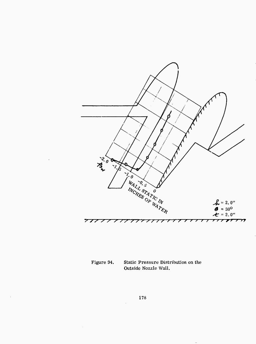
The existence of diffusion in the nozzle is easy to understand, of course, be- cause the jet must balance the cushion pressure, which is necessarily higher than the static pressure in the nozzle. Typical wall pressure distributions obtained with the Chaplin test rig are illustrated in Figures 93 and 94.

176

Figure 93. Static Pressure Distribution on the Inside Nozzle Wall.

177

^ 'Ct;*^ 0

4% 3 =30°

^e = 2.0" s s s s s s/ss/ss/zs/ ' s / ' ' 7 / > > / y? / n

Figure 94. Static Pressure Distribution on the Outside Nozzle Wall.

178

The present state of diffusion theory can hardly be regarded as satisfactory, of course. However, the theory developed in Chapter Two enables us to ob- tain an estimate if we assume that diffusion takes place at constant static pressure.

If iJ^ is the velocity of a filament in the nozzle, before diffusion starts, and -v* is the local velocity in the developed jet, then the total head loss &H is given by Equation (80)

^ { -^N ■ Z7f / (256)

where ^ A- = static pressure in the nozzle duct upstream of the diffusion section

äR = total pressure at the same station.

APPROXIMATE SOLUTION FOR A "STRAIGHT" NOZZLE

In this section we assume a conventional straight nozzle and an "exponential" jet with an initially constant total head distribution.

Thus AA , I - JZ . (257)

The mass flow is given by

r (jT^V

For simplicity, we define

Since -Ufc ^ (-&% 7^ )

^Vfe (258)

(259)

179

(260)

Also, since

From Equations (260) and (261),

4^ = ' - ^"■'V^R 45 J

# = ' - 'A- (261,

^ —^ • <262>

Note that AH =0 when

>^ - ^r (263)

(264)

Equation (262) is plotted in Figure iK, for a tvnical case.

This approach can be regarded as a "small uoiiurbation' analysis, in that we neglect the change in -Oi caused by the iuss m toti.l head. A moie exact treatment would result in larger calculated I». -,es.

MEAN TOTAL PRESSURE LOSS

The mean total head change will be given by

*p * A? - if, 4^ \

' " -f^lf " ^e ^^ y^ (265) AP APj

180

1.0

^3

2

s O

w

w w «

o o

0.8

0.6

0.4

0.2

1

TO TAL PRESSU LOSS

-rrrrf

RF

0.2 0.4 0.6 0.8

NONDIMENSIONAL DISTANCE ACROSS JET ~S/£

1.0

Figure 95. Approximate Total Pressure Loss Due to Diffusion iortyt = 1.0, in a Straight Nozzle. (Based on the Exponential Theory Static Pressure Distribution.)

181

£ - i - :^/>i -^-H'-^^O-A-**)]. JUPS v

11 (266)

The loss component of Equation (266) is plotted in Figure 96. At a height corresponding to ■'*&. = 2.0 for example, there is a 5% loss in mean total head. The actual cushion pressure loss will be somewhat greater than 5%, of course, because of the unfavorable Af^ gradient resulting, even though this is offset, to some extent, by the thickening of the jet. It will also be greater by virtue of the "small perturbation" assumption, as noted earlier.

It is interesting to note that the actual pressure loss measured in the Chaplin rig (Chapter Four) was 4%, instead of the theoretical figure of 2.5%.

TOTAL POWER LOSS DUE TO DIFFUSION

Power is defined as

/A*. ^d . ^67)

The power loss is

We are interested only in that part of the jet in which diffusion occurs, of course.

The power of this part is ,

I AtW -/^r'S- ■ }>

The power of the remainder of the jet is

182

y y,' J * (268)

0.10

^ 08

^1

w H W .06

s CO CO O J .04

w

S 02

12 3 4

HEIGHT PARAMETER /Gj/^

Figure 96. Mean Total Pressure Loss as a Function of the Height Parameter ^/^for a Straight Nozzle. (Based on Approximate Exponential Theory Static Pressure Distribution.)

183

^ -A)3' - J^Pj^y (269)

Tfaus^the total jet power is

The power before diffusion is

>PN - *P^«*' (271)

This must equal the first integral of Equation (270), indicating that the jet thickness Az,: is greater than the nozzle thickness. In fact, for continuity

Substitutin,! in (270) and dividing (270) by (271)

A/

This is exactly the same as Equation (266).

^/?'- ^^^V72»

184

Chapter Eight

COANDA JET FLOW

TV Figure 97. Basic Geometry.

From Equation (91), the equation governing Coanda flow can be taken as "free vortex" if the wall radius is constant; that is.

5^ ^

/ for which the general solution is

:*/£> [MZ^&uz +kl

(273)

(274)

when

m

185

(275)

(276)

mm^sm^^^um

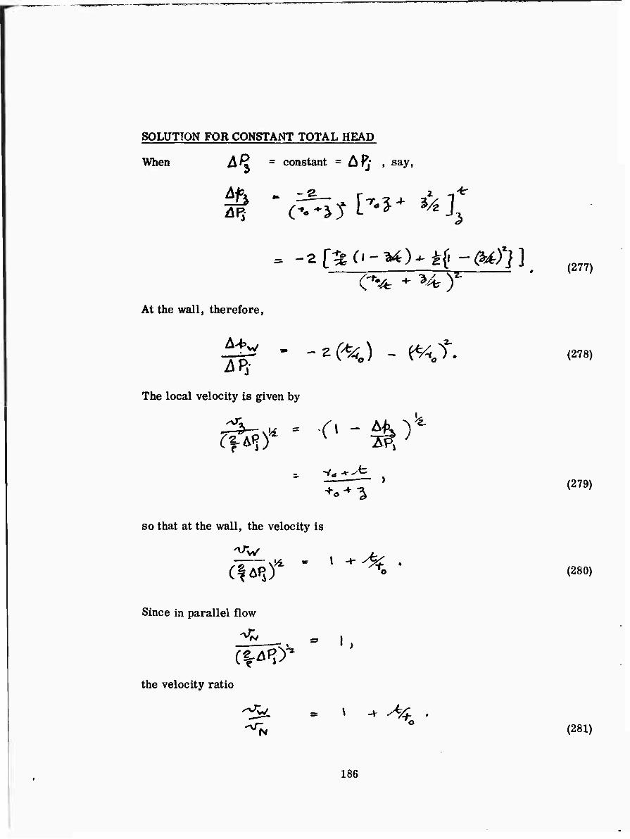
SOLUTION FOR CONSTANT TOTAL HEAD

When AR = constant = AR* , say,

At the wall, therefore.

A Pi ■2^) - <&A$

The local velocity is given by

^-^

~

so that at the wall, the velocity is

Since in parallel flow

' i>

the velocity ratio

'S/

(277)

(278)

(279)

(280)

(281)

186

This ratio is a measure of whether separation will occur when a straight sur- face follows a curved one, as in Figure £8.

THICK JET

DIFFUSION REGION

Figure 98. Separation of Coanda Flow.

Even if the diffusion is distributed, by careful blending of the radius and the straight section, we must expect separation when ',v'w<ArH>2.0 (-/*7^r0 > 1.0). When the flat section is merely tangential, separation can be expected to occur at a lower value. In all cases there will be some loss of jet total head, of course.

Figure 99, derived from Equation (278) gives the wall static pressure as a function of the jet thickness ratio ^/^ . In Reference 25 an experimental measurement is reported, in which a 1/8-inch jet, at an initial (nozzle) Mach number A 0.68, is deflected by a curved surface of radius 2.5 inches. The surface pressure is an average of

Apw

W = -0.1 .

The theoretical figure is, from Equation (278),

187

-1.2

0.1 0 2 0.3 0.4

JET THICKNESS PARAMETER tfa

Figure 99. Variation of Wall Pressure With the Jet Thickness Parameter t/j^ .

0.5

188

^JV = -2 x . 05 - (. 05)2

= -0.1025 .^

The agreement is therefore very good.

APPROXIMATE SOLUTION FOR THE BOUNDARY LAYER EFFECT

Let us define the loss of total head due to skin friction as

3>f - J%n-^<*i ' fiWh (282)

so that AI^ = AFJ - ^Ol} (283)

where <pC^J is understood to be finite and positive near the wall, but equal to z^ro over most of the jet. Substituting (283) in Equation (276),

.-a %\ifa^~'4^~ ffa^i (284)

This is the same as Equation (277) when ^ is large enough not to include the boundary layer. When "X = o ^ however, we have

SW" SR,WJö<, %Apy (285)

where 3>F ^ c^.^f^w1^

189

That is. IV ^ C^CAf* - Afw).

r* " 1 /(VVI3Cl!> ^^

-2P; ,NV,5C'> , (286) ——nr"2qr*A<r

This solution is only approximate, of course, but it does show how skin friction causes the wall static pressure to increase as the jet moves around the curved surface, and why the flow eventually separates.

We can obviously solve the equations for the case of viscous entrainment on the outer surface of the jet. In this case, AR decreases with increasing path length ^- "■ ^0 , and the thickness M increases. There is probably little point in doing this unless we use a realistic velocity distribution for the jet, however, and the magnitude of the task then renders it inappropriate for the present program. There does not seem to be any good reason why this approach should not adequately cover the Coanda flow problem, however, and enable both performance and stability to be predicted. Needless to say, such predictive ability would be highly valuable, not only where Coanda flow is required, but also where it is not desired.

From Equation (279),the local velocity in a (free vortex) Coanda flow is

^ r :v;:i (287)

After diffusion, this reduces to

'7) L ^ ^~ * " 'J ) (288) < ■ O (AfJ - MJ)3~

& H being the total head loss, which is given by Equation (80).

That is, *%P - 0 " ^)lC • " ^iP.) ; (289)

4H ' Jge^C« - 2£)1. (290,

190

—*mmm* < ■ ' •••*"——-

Let -a0 = ^C^ • ZIP , the nozzle dynamic head to ambient.

Then x . ix \,/fi- -.«- ÄH - Jä r i - (! - Av^p'^ ]

Noting that A^ * ^ and (Z^öPf)* = ^;;

(291)

(292)

I - AH/^ is obviouRly similar to the conventional diffuser loss (I ~ Vp ).

•• 27>- 2GIK - C^T'' =0, (293,

(294)

(295)

This function is plotted in Figure 100.

The average diffusion efficiency over the jet is therefore

^* E/^-'«)T^

^ -^At'-i^)v]%. (296)

(297)

191

- Jt %.= t+* im 1.0

0.8

0.6

0.4

0.2

^ N

k

k h 1

\

* 1 \ k

^ 1 \

h 5

i

k o

: k 1 k k k

1.0 1.1 1.2 1.3 1.4

LOCAL VELOCITY RATIO ^/^

Figure 100. Variation of Local Diffusion Efficiency -y With Local Velocity Ratio. *

1.5

192

As indicated in Figure 100, there is no solution when

That is, ^zA)*

or

^

\ I.** > 2 Oc-^).

This is most crit'cal at the wall ( "^ * 0 ^so that the requirement for a solution is

1 -^4 ^ ^ 'o

or ^. < 0-4\4. (298)

If we had used "small perturbation*4 theory, assuming that the total pressure loss did not reduce the velocity after diffusion, we should have obtained the result y^40 < 1.0 for a real solution. Note that the Equation (298) "stability" limit corresponds to

( Tor) =-1-0' (299) Substituting Equation (287) in (297)

^ = ^ e-^-feu1 -^tn%- (300)

Let X - **** X ̂ \

Then ,. s ^-»/4r ^ ^

193

i ^J-'VL'-^J*-1* •'<t

€ + t cvoh-^^^i^^ij- Now

m

** ' l-

»-v^

- i -i e^li + z*)

It can be shown that ft -♦- 1.0 as >^<e-*- 0, as should be expected.

194

X-

(301)

Chapter Nine

TWO-DIMENSIONAL FLOW IN A CURVED DUCT WITH CONSTANT TOTAL HEAD

The flow in a two-dimensional curved duct involves sudden diffusions when the curves are radii, tangential to straight ducts. These can be treated by the diffusion theory :eveloped in Chapter Two.

SUDDEN PRESSURE RISE ON THE

OUTSIDE WALL

\\\ ^ S

\_ SUDDEN DIFFUSION AS STATIC PRESSURE RETURNS TO THE STRAIGHT DUCT VALUE

PRESSURE DROPS ON THE INSIDE

WALL

Figure 101. Flow Separation in a Curved Duct.

The physical picture is illustrated in Figure 101. In real (three-dimensional) ducts, the pressure differential across the bend generates secondary flows in the boundary layer of the side walls, and sometimes in the middle as well, and these secondary flows can mask the simple picture shown in Figure 101.

In this chapter we confine our attention to the simplest possible case; a duct of constant thickness, which corresponds to the free-vortex flow of an annular jet. There is no reason why the more sophisticated general theory should not be ap- plied, of course, provided that we remember to include the equation for con- tinuity; that is, to take account of the variation in mean velocity as the dis- tance between the walls varies. This would enable us to solve problems of the type sketched in Figure 102 and to determine the optimum duct bend geometry for minimum loss.

In addition, there is no need to limit the theory to the constant total head case of this paper, of course.

195

Figure 102. Cases Solvable Using the General Theory Developed in This Investigation.

STATIC PRESSURE AND VELOCITY DISTRIBUTION

,N V S S S \ \

Figure 103. Assumed Geometry.

196

a**) XA.

The mass flow is

•^w O 1 -^r-K ^

But if the duct width before the bend is also JZ t

(303)

From Equation (91) the local static pressure in the bend is given by

& -t ^.äf. = ^_ Aß ;

The local velocity is

(304)

CV^-Jli1 . 005)

(306)

(307)

197

Equating (306) and (307),

■ K ' % - ^l ! I ^P) ^ . (308,

Substituting for K in Equation (304)

4P ■ (-"HJi^iT^iJ1 ' (309)

which tends to ^^Ap as ^o "* <30 •

From Equation (305) j

—3—\* * 1 0 v L!£flL^ , (310)

or, since -^ = Ä^p ^j _ Aj^p^

As ^-* ö

2^, « ^/^o (311)

^ —>. _L- —- «o .

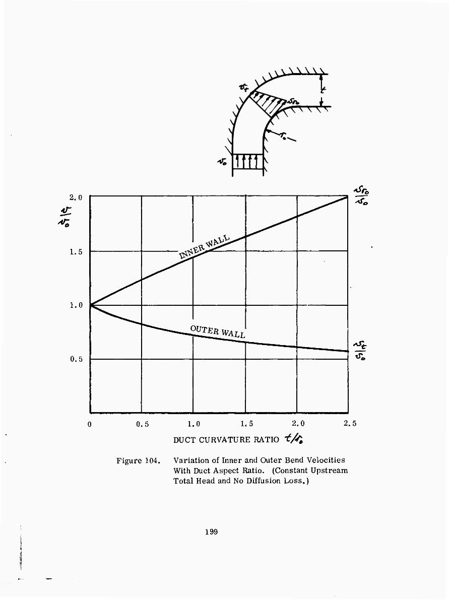
The wall velocity values given by Equation (311) are plotted in Figure 104.

THE CONSTANT VELOCITY STREAMLINE

A streamline exists, near the center of the duct, along which there is no change in velocity; that is, -"^ "- "^ • From Equation (311) this is given by *

198

\ \ \ \ \ \

2.0

5C -^

1.5

1.0

0.5

.L-«s*-' ^ "1 \^

^

f^ ■*^-^^( i^Si^L

0.5 1.0 1.5 2.0

DUCT CURVATURE RATIO 'tfa

/Ü^.

2.5

Figure 104. Variation of Inner and Outer Bend Velocities With Duct Aspect Ratio. (Constant Upstream Total Head and No Diffusion Loss.)

199

(y^ 0 'S

•• (%*\ s M'\ ' ■ -i> . <312>

In the limit ^5^ -^ 0 ^

as should be expected. The general solution to (312) is plotted in Figure 105.

MASS FLOW DISTRIBUTION AROUND THE BEND

By integrating Equation (310) across the duct on either side of the constant velocity streamline we can obtain expressions for the mass flow on either side of the constant velocity streamline.

^öure* ~ ^ fr* ^b-y^O l^J (313)

»v Tor**. ~ ~ T T-^

These Equations are plotted in Figure 106.

TOTAL HEAD LOSS ON THE OUTSIDE OF THE CONSTANT VELOCITY STREAMLINE

From Equation (80) the total head loss in a constant pressure diffusion is

(314)

(315)

200

1.0

fa** '«fc***r

0.8

0.6

0.4

0.2

^X

m CONST

0.5 1.0 1.5 2.0

DUCT CURVATURE RATIO tfa

2.5

Figure 105. Position of the Constant Velocity Streamline.

201

1.0

0.8

0.6

0.5

0.4

0.2

^OUTER j \ N \ \\

CONSTANT VELOCITY STREAMLINE

0.5 1.0 1.5 2.0

DUCT CURVATURE RATIO 't/s<>

2.5

Figure 106. Ratio of Mass Flow on One Side of the Constant Velocity Streamline to the Total Mass Flow.

202

Since A^n "£&) = -^o, this is more conveniently caressed as

"2-

^L ' C^ - ^ ^ • (316)

Substituting Equation (311),the mean loss is

^0^) ^g^Q^fa^felT)

TOTAL HEAD LOSS ON THE INSIDE OF THE CONSTANT VELOCITY STREAMLINE " " ^

For this case, Equation (315) becomes

But

(319)

203

(320)

•' ^« ^ 3»A J0 L(n Mty^o^j) J h*

MEAN TOTAL PRESSURE LOSS ACROSS THE DUCT

Summing Equations (317) and (320) across the entire duct

(f AH \ ~~ J^S , . (321)

Equation (321) is plotted in Figure 107.

THE LOSS INCREMENT DUE TO SKIN FRICTION

We can obtain an approximate figure for the total head loss due to skin friction from the relationship

^AHSF * c?[&■*.**<. * hde(■*.'Ao']

(322)

AH

- 0cf.-k. [< + T^^M^^^Of. -z

(324)

^, o -. This result is overplotted in Figure 107 for 0 = 90 and Ot = . 004.

204

0.14

0.12

0.10

1^ <l

a w H w

£ m en O

O < w K

< H O H

08

06

04

.02

0.5 1.0 1.5 2.0

DUCT CURVATURE RATIO -£/&

Figure 107. Average Total Head Loss Around a Constant Duct Thickness Bend.

205

COMPARISON WITH EXPERIMENT

The writers of this report are not aware of any two-dimensional flow meas- urements of curved duct losses, so that direct comparison with experiment is impossible. Reference 26 presents data for rectangular ducts of various finite aspect ratios and, as shown in Figure 108, these results fair into the two-dimensional solution very convincingly. However, an appropriately planned experimental program is essential before the basic hypothesis used in the foregoing analysis can be substantiated. Such a program would then permit embarkment upon the analysis of the secondary flows in the three- dimensional case.

It is perhaps worth pointing out that extensions of the present analysis to the more general case offer hope of defining duct bend shapes for minimum loss.

206

0.6

O EXPERIMENTAL DATA (R. A. WALLIS) B TWO-DIMENSIONAL FLOW THEORY

0.2 0.4 0,6

DUCT ASPECT RATIO -f/W

0.8

Figure 108. Comparison Between Theory and Experiment for a Right-Angle Bend.

fc = 2.0

1.0

207

Chapter Ten

FLOW INTO A TWO-DIMENSIONAL FLUSH INTAKE

XV^

yi-- (a) Actual intake flow.

^N

Figure 109. Flow Into a Flush Intake.

An intake which i. at right angles to the free-stream velocity is often highly desirable from a practical weight and size point of view, but is difficult to design for high intake efficiency. This is mainly because of the flow break- away which occurs on the leading edge of such an intake, as indicated in Figure 109(a), in contrast to the hoped-for inviscid flow picture of Figure 109(b). Even the latter would present problems, however, in that the

208

velocity would vary across the plane of the intake.

In this chapter we attempt to lay the foundations for the analysis of such flows, using the same basic approaches that have proven successful for curved jet flows. The subject is complicated by the important effect of the upstream boundary layer, and by separation due to sudden diffusion on the intake lip. Thus, although we shall develop the theory far enough to obtain closed form solutions, we will not attempt to "fill in" all the details, this being beyond the scope of the present program. Sufficient work has been done to indicate that this approach should yield good results, however, and to show that its use will improve our predictive abiliiy To cite c ly two examples, it is found that the "momentum drag" is not equal to the product of the free stream velocity and the intake mass flow, and that the efficiency of a horizontal intake will de- crease as the free-stream velocity increases, due to leading edge diffusion. Both these points might be of importance to a vehicle such as the XV-4A, for example.

^o —

LOW SPEED r^^/)

Figure 110. Flow Into a Flush Intake.

209

Two-dimensional flow into a flush intake must of necessity adhere to the body surface upstream of the intake, as illustrated in Figure 110. Thus, if the ex- ternal flow is undefined,so that the surface pressure distribution is unknown, we are unable to calculate the effects due to the tilt angle. For small angles these effects will presumably be of second order, however.

The flow illustrated in Figure 110 must satisfy the equation of curvilinear flow. That is,

^t -f ~Z~AK = -^ AR. (325) £i -**' <ly -^ 7> >

The curvature gradient ^ will depend upon the intake velocity ratio ( xlÄ-i^^u,^ ), as indicated in Figure 110, the flow direction being reversed from the conventional annular jet direction. If we retain the annular jet as- sumption of constant boundary radius, then solutions can be obtained in the same way as in the earlier chapters. It is possible that the constant radius assumption is an unnecessary restriction, however, and that the results can be made more general in future work.

Additionally, the free-vortex and exponential theory approximations are still of value; the firstjs applicable in the region ^t/tu.. •^Jsll. 0, and the second is correct as 'AX-^/^ -»> o • Yox M-S > 1.0, the general theory must be used.

MOMENTUM EQUATIONS

The geometry shown in Figure 110 assumes that a straight-walled duct follows the radiused inlet. Thus the line A-A theoretically makes a discontinuity at which the static pressure field changes, being some function of 5. above A-A and uniform below. In practice, the boundary layer will thicken on the upstream wall, of course, in such a way as to avoid this discontinuity. In fact, if the velocity at the % surface significantly exceeds the mean duct velocity, flow separation will occur at the point where the ^ radius is tangential to the duct.

Noting this reservation, the horizontal momentum balance for V ^ o gives

/ fV«^ = *aC^* -^O- (326)

210

If

then

(327)

^ ' '^ 4^#'' ^

Since

If we were to base the calculation of rf on continuity of mass flow, then

/7 * ^. , (330) yU~

This is not the same as Equation (329). Thus y differs depending on whether we assume conservation of momentum or mass flow. We do not know at the present time which is the more correct.

THE FLOW EQUATION FOR CONSTANT TOTAL HEAD

The total head distribution -AHw may be considered constant and equal to ( Afcf'ULo ) ^ ^e upstream boundary layer is of negligible thickness. The solution to (325) is therefore

211

^o*7V "^ ^f«Ccn ^73)^ (332)

^f V KfK k+o+lll (333)

/^f^C V J$,t"Z Ä +* * t*) ' (334)

INTAKE MASS FLOW

The local velocity Is

- c — ^tc e-J'- Thus the elemental mass flow is

(335)

^ ^ ^ ^ ^ f>^^ - r>-^o(."|^)(^; 73-

(336)

7 ^ 1 i^-o -^ y^rp^r-, ], (337)

212

/^>( appears as an arbitrary constant because the mass flow is arbitrary, so far as the intake is concerned. The actual value of '*»*,, depends upon the de- pression existing in the intake, due to the fan or other air-moving device.

Writing . ""^ß- ^ p/t/^i ;

Substitution of this in Equation (333) gives the static pressure distribution in terms of ^ and ( SJ-\/AK6 ) only, the latter being easily eliminated (Equation 330) for the case of conservation of mass flow.

THE FLOW CURVATURE PARAMETER ^ FOR CONSERVATION OF MOMENTUM

From Equation (334)

^

(340)

• (341)

Equating this to «^/^r , as in Equation (329)(the conservation of momentum criterion)

m 213

^ &^''* - ■ r ' (342)

This is explicit in the sense that defining «7 ana "'•^e: automatically de- fines the intake velocity ratio ( /*»., Ac^ ).

Since we cannot expect to have K>oO or ^^^ , these limits define the real range of VO values. In the latter case, vo = 0, of course, while for

oo .

The conservation of mass flow relationship for ^j is given by Equation (330). This is compared with Equation (347) in Figure 111, and the^difference be- tween the two is seen to be appreciable for low values of /**>% /cc0 . This may be interpreted as indicating a limitation of the constant flow radius as- sumption, or that the differential pressures A-J», and Ay^t act over a greater depth than the assumed value of "^ . The latter is felt to be most probable at the present time; but in the work which follows we derive solutions for the conservation of momentum case only, since the conservation of mass flow solutions turn out to be the same, except for the relationship between |9 and

THE STATIC PRESSURE DISTRIBUTION A>f>»

From Equations (334) and (339)^

^b- =1-22 (d^,\ ^ . (343)

Note that the intake velocity ratio does not appear explicitly.

From Equation (335) this gives

^ -". ^. -vw- ,^/c \^/ (344)

(_* ti^+iV ]

214

2.0

« W H W

S

S

o

FREE-VORTEX

EQUATION (342) - CONSERVATION OF MOMENTUM

1.0 2.0

MEAN VELOCITY RATIO /U, JAA<

rr f* Figure 111. Variation of ^ With«../^« .for Uniform Inflow (^ß = Constant).

215

LIMIT SOLUTIONS FOR </* O , ^*& = CONSTANT.

From the exponential theory solutions of Chapter Four

The local velocity is therefore

and the intake mass flow is *2. f

^•C'- I^X'-- 3-

Since -^ - f ^^ ^-, >

t/fZ

216

(346)

^ ' l -^-^c "• <-,

(348)

fT^^^ ^ * (349)

—^■'^ ) = —'' ^£P& ' (350)

Substituting in the static pressure and velocity equations,

KEe>< V ^a ^ v R/ - - ^^i^ <351)

-=? "^ * ST 7 =^fe " ' (352)

It is of interest to note that the local velocity ratio "^f ^MA, is independent of the flow ratio ('**-t/u,0 )• The function C^j^^L ) is plotted in Figure 112.

SOLUTIONS FOR »7« l-Q^ ^^- = CONSTANT

The free-vortex solutions of Chapter Four give

Jit~i *^ (353)

When ^. ^ O ^ Af^ * -A^ ^

-^P-^ ^t^V >

(354)

The local velocity is therefore

Hr_t- (355)

217

3.0

2.0

1^

2

Ü o w >

1.0

0

ssy//

= LOCAL VELOCITY

-</, = MEAN VELOCITY

1 3/4

1/2

1/4

0.2 0.4 0.6 0.8

POSITION ACROSS THE INTAKE l/t

1.0

Figure 112. Variation of Inlet Velocity With Intake Lip Radius. (Exponential Theory for *4O/M-*0O)

218

Thus,the mass flow is

4 f>^.o-^W^^.i (356)

■•^-|^f = c^X^/-0. (357)

Substituting this in the static pressure and velocity equations,

^ u^v[^(.-^)j" (358)

^ " ^. ^ - ^^^-/ ^ ^^_- . (359)

Once again the velocity ratio '^\/ULi is independent of ( ,•**■•/^»T, )• Equation (359) is plotted in Figure 113.

THE FLOW EQUATION WITH AN UPSTREAM BOUNDARY LAYER

When the upstream boundary layer is significant, in relation to the size of the intake, the total head distribution in the on-coming flow cannot be regarded as constant. Thus, Equation (331) now has the integral

J%* -7*?'^ ^ (36o)

instead of / (+* + ny ^-v (361)

21»

^ — = LOCAL VELOCITY

44, = MEAN VELOCITY

'X 2.0

2

H >—i

Ü O iJ w >

<

5

0

1 ST ALL

/ / j j j j j / / j

v x\

^ N few ^V

^

^ Ss

0.2 0.4 0.6 0.8

POSITION ACROSS THE INTAKE yk

J/4 1/2

1/4

1.0

Figure 113. Variation of Inlet Velocity With Intake Lip Radius. (Free-Vortex Theory ior*t9Lä'£rl. 0.)

220

In addition, the value of the curvature parameter { *f ) will be larger, from Equation (329).

The appearance of &K in the integral means that it must be analytic ( At? -"ftyj )f so that we have to make appropriate idealizations for ^(a ). There is nothing particularly difficult about this; we have already accomplished it for jet flows, but the reduction to numerical results is time- consuming, and is not within the terms of reference at the present program.

SOLUTION FOR A THIN UPSTREAM BOUNDARY LAYER

We may write 4R = -| f ^« "* &£%) (362)

where <^ C^) = 0 over most of the intake, but is finite when 5"* 0 • The

general solution to Equation (325) then becomes

(363)

Now, since ^C^) is only finite when "^ "■*" 0>

Note that this approximation improves as the boundary layer gets thinner, •^ gets larger, or v7 approaches 2.0 or zero.

Now at constant static pressure there is a simple relationship between the skin friction drag and the boundary layer momentum.

(364)

Jf

221

and writing A«o as'5|f'*A. ■ this becomes

^/l^-^^^^j^- C " " ' " " " ^ "' ' ~' ' '^ ^" ■ ■ " ' (365)

(366)

Thus, Equation (363) becomes

When ^ ' 0 ; ^''i * '4'',' '

rp-**o ir-** -^f^» if-***

^ . .. .^ ^ o^/.V^ ^

" (367)

Thus the square bracket replaces ( I ~" ^Vf-uJ") in the previous constant total head analysis, and the rest of the reasoning can be followed as before.

222

MOMENTUM DRAG

The momentum of the free-stream air swallowed by the intake is initially

i Now / o -. öLvi * -v*. •

Thus, the momentum drag can be written as R

•= >-««^» -^'o * (368)

This is quite different from the traditional value j**»'**'* , particularly if the intake is mounted some way back from the leading edge of a body or if there is any drag-producing structure (such as a sharply radiused leading edge) in front of it, whereby the mean velocity ^L0 is reduced. Even without drag effects, however, distortion of the velocity profile by the presence of the body will result in X differing from unity, and hence changing the momentum drag. It is easy to see from the studies of X in Chapter Two that this could influence the momentum drag by a factor of two in certain cases. Thus the reported mo- mentum drag anomalies may be nothing more than the use of an inapplicable analysis.

SOME EXPERIMENTAL MEASUREMENTS

The efficiency of a ram intake is usually stated as the ram pressure recovery ratio ( üf^ ). The flow is approximately one-dimensional; therefore the total pressure in the intake may be written as

7, - ^-^ .^

223

A* + (".) >tT" o

V ^:o / (369)

\^iere **^J is the mean static pressure rise relative to ambient and /<tj is the mean velocity in the intake.

Intake Power Efficiency

For a flush intake the ram pressure recovery ratio does not have precise meaning. Instead, as a measure of efficiency we consider the power content of the swallowed air in relation to its power at free stream velocity. Power over an area A is given by

? - f AP.^+b (370)

and we define the efficiency as

where i»^ is the mass flow into the intake.

That is,

Yl ~ Duct airflow power above ambient m

' Duct airflow power with no loss

If Zj-t. is constant over the duct area A, Equation (372) becomes

(372)

^f^< (373)

• o

and if AX-t is constant also, Equation (373) reduces to Equation (369). Thus, the iniake power efficiency and the ram pressure recovery ratio are identical under these conditions. However, the power efficiency has the advantage of

224

having an exact meaning, both in this special case and generally.

At low value of the free-stream velocity (/u.# -♦ 0), the efficiency has a large negative value since AP| will become negative when the free-stream total head is insufficient to compensate for losses in the duct.

Experimental Measurement of Intake Power Efficiency

As a simple experiment to establish the power efficiency for a two-dimensional flow, an intake was constructed in the floor of the Eiffel tunnel at Payne, Inc. The aperture was connected by a short length of ducting to an antechamber ex- hausted by the intake of a centrifugal blower. The general arrangement and di- mensions are shown in Figures 114 and 115. The air flow was examined by means of total and static pressure measurements at the throat of the intake, at the mouth of the intake, and at points near the tunnel floor upstream of the in- take. Additionally, the direction of the flow at the intake mouth was established.

These measurements were made with a directional probe. This instrument does not sense static pressure directly, and a calibration was necessary to obtain static pressure data.

Calibration of Yaw Probe, for Static Pressure Measurement

The sensing head of the yaw probe is cylindrical, 0.120-inch diameter, with three pressure tappings at anf'es approximately -30°, 0°, +30° to the refer- ence direction. The method of use consists of rotating the probe about its axis until the pressures in the side tappings are equal. The center tap (and reference direction) is then in line with the flow and senses the total pressure of the flow.

The pressure around a cylinder in incompressible flow is given by

>fcr s -fe 4 ^p.^eV (374)

where Cp is a coefficient depending only on angular position around the cylinder with respect to the flow direction. For the probe as used, the angu- lar position of the taps is constant and therefore Cp is constant. Thus, the common pressure in the side taps is given by

225

ssssjjjyyysyyySS/yyy/sssyy.tt ( { ( , , S-

TUNNEL FLOW

INTAKE FLOW

MOUTH THROAT

C s ' 's*

EXTRACTOR

Tv

/ /

f y s s s^s ̂ rr-

/ '/s/ ////

k- ^ PLENUM CHAMBER

"^7" //

/ / / / /

Figure 114. Arrangement of Intake in Floor of Wind Tunnel.

226

PROBE REACH 4.0"

TUNNEL WIDTH

MOUTH TRAVERSE

Figure 115. Location of Measuring Stations.

227

! - cP ^ -N^H^ ^ (375)

>wp was determined by setting up the probe in the main tunnel flow and measuring ^ - ^ ^ ^ _ ^ #

The actual values were

CZ^ - — O-CZ , (376)

In general

- o0.P

(377)

and /^r^ = - o-ttz-c-f,- ^ . (378)

In the tunnel experiments , ^H of Equation (371) is^ith respect to the tunnel static pressure ( ^"fco), representing the total pressure above am- bient sensed in the intake with forward motion 'vc0 . Thus, if AP is the measured total pressure with respect to room static >

228

Therefore.the expression for ''7 becomes

■x.

7 T y -^f^^, «£*. ^ y^R«., «^t

>^.^yü^

\ -V- --T—». / ^P-^-i ^"^ • (380)

Since ZJ P is essentially negative • »^^"-^s«*^- represents t'ne power lo«?t in the intake flow, and the term fc^ JA AR«,,«l«c may be called the power loss factor of the intake. Obviously as the tunnel speed is reduced the power loss factor becomes increasingly negative and leads to negative values of »^ . The experimental data are given on Figures 116, 117 and 118, showing the pressure and velocity distributions at the mouth and throat of the intake. The power loss factor was computed from the throat measurements.

Here the values were as follows:

/'* 2 Volume flow J -«H'«** = 16.0 ft / second Mass flow m, - /t/^«** = 0. 0373 slug/second/ft Power loss /*%Pu.<<*. = 37. 7 ft lb/second/ft Free stream power -g*^«& = 151 ft lb/second/ft Turnel speed -u^, = 90.0 ft/second Power loss factor '" ^ = 0. 25 Intake power efficiency M = 0. 75

Comparison with Theoretical Values

The velocity distribution in this intake mouth has been calculated by the methods of the previous section and is shown in Figures 119, 120 and 121.

In Figure 122 the experimental plot of the velocity normal to the intake plane is compared with the theoretical curve. The lack of agreement near the upstream wall is compared in Figure 123 with the velocity profile in the boundary layer in the tunnel 1 inch upstream of the start of the intake radius^and Figure 124 shows the total pressure gradient. The nominal thickness (where the velocity

229

-8

-6

W H

I o W K Ü i—i

55

CO

-4

-2

W pr*

L_ -O- THROAT

—X— MOUTH

1.0 0.5 0 0.5 1.0

INCHES FROM CENTER OF DUCT

Figure 116. Total and Static Pressures in Intake.

230

TUNNEL SPEED 90 FT./SEC.

150 r-

0.5 0 0.5

INCHES FROM CENTER OF DUCT

Figure 117. Velocity Vector Profile at Mouth of Intake.

231

TUNNEL SPEED 90 FT./SEC.

w

H ü O

W >

200

150

100

50

0

■^

^

MOUTH ^

TKROAT

k 0.5 0 0.5

INCHES FROM CENTER OF DUCT

Figure 118. Velocities at Mouth and at Throat of Intake.

232

^

^

H »—i

U o J i w >

Ü o

:

\

^\ -

^

,^=2.0

7 = i.0(

^r- ^;

EX PONENTIAL (^ =0)

0

VORTEX)

= 0.5

0.2 0.4 0.6 0.8

DISTANCE ACROSS INTAKE l/t

1.0

Figure 119. Theoretical Velocity Distributions for the Test Intake (Uniform Inflow).

233

3.0

2.0

If

H i—i

Ü O w >

<

o

1.0

7 = 0 (EXPONENTIAL THEORY)

= 0.5

FREE-VORTEX

1.0

MEAN VELOCITY RATIO 4*,/Mo './■<

y/t

0.2

0.4

— 0.6 0.8 1.0

2.0

Figure 120. Cross-Plot of Intake Velocity Ratio, as a Function of M, /M» , for the Test Intake. (Conservation of Momertum Correlation Between 'H and*^/*^.)

234

3.0

2.0

O H

o w >

g o

1.0

1^^^—m i ■■ i ■ ■ ■ ■■! ■ ■ -ii i. -i ■■» !■ - I»- i i i i -lu ■ ■ ■ ■ . ——^—^ ,

^

0

0.2

0.4

0.6

0.8 1.0

0 1.0

MEAN VELOCITY RATIO *,/*»

2.0

J'/A

Figure 121. Cross-Plot of Intake Velocity Ratio, as a Function of i^/Xf• , for the Test Intake. (Conservation of Mass Flow Correlation Between *t and &./M0 *)

235 *

200

u w w

>* H *—> u o w >

< u o

150

100

50

1

TUNNE = 90 F

L SPEED T. /SEC.

/

O*o-GH MSMSH^

^r-^'

^

A -^

y^

f

0.5 0 0.5 INCHES FROM CENTER OF DUCT

Figure 122. Comparison of Experimental and Theoretical Velocity at Mouth.

0.5 0 INCHES FROM TUNNEL FLOOR

(b)

"sr

0.5

lA —AJ'

0 0.5 ^ 0

INCHES FROM INTAKE WALL

Figure 123. Resemblance Between (a) Velocity Profile in Upstream Boundary Layer and (b) Velocity Difference (Theoretical-Experimental) Near Upstream Wall of Intake Throat.

236

is 0. 95 of the tunnel speed) is 0.14 inches and thus must be considered thick in proportion to the dimensions of the intake. The theoretical curve is thus not ap- plicable close to the boundaries, and the flow in the center should be increased to represent the practical case. This is sufficient to show the importance of the boundary layer in distributing intake flow.

The spanwise distribution of velocity across the duct (Figure 125) is fairly uni- form and the approximation to two-dimensional flow seems reasonably close.

Comparison With Zero Tunnel Speed Case

The velocity profile at the intake case for zero forward speed is shown in Figure 126 with the case from Figure 123 superimposed for comparison.

These show that the mass flows are almost identical, indicating that the amount of air swallowed by the intake is independent of forward speed. In the zero speed case the boundary layer is of course quite thin, being developed only over the length of the intake itself.

237

0 i.o o LOCAL TOTAL PRESSURE iN INCHES OF WATER

(a) Tunnel Speed Zero. (b) 90 Ft/Sec. Tunnel Speed.

Figure 124. Total Pressure in Upstream Boundary Layer.

150 Ft/Sec.

*

t t /

100 Ft/Sec.

Ö" *

* / / i

J

/ y

i

i

AXIS OF .TRAVERSE

> 50 Ft/Sec.

* *

> > / /

> >

*

<

12 3 4 5

DISTANCE ACROSS THE TUNNEL IN INCHES

Figure 125. Spanwise Distribution of Velocity at Mouth of Intake.

238

-G- 90 FT. /SEC. TUNNEL SPEED ZERO TUNNEL SPEED

150

w CO

H

H i—i

U o

>

100

50

\

I I f

0.5 0 0.5

INCHES FROM CENTER OF DUCT

Figure 126. Velocity at Throat of Intake - Tunnel Speed Zero and 90 Feet/Second.

239

Chapter Eleven

SOME GENERAL PROBLEMS OF A JET DISCHARGING ACROSS A FREE-STREAM FLOW

THRUST LOSS DUE TO MIXING

It was shown in Reference 3 that if a jet of mass flow ('»•'Ly ) mixes with an additional quantity of fluid (^my ) at a mixing static pressure A-f», , the augmentation is

Cj> r ^ _ Total momentum flux to ambient Jet momentum flux to the pressure A-f*,

£o^)Vf,, ^ ^C'-^^-^^s,)2 J (381)

where TV is the entrained fluid ratio.

•**« = primary jet velocity at the pressure A^>, ^D

= (dynamic head) efficiency of diffusion to ambient '0*l = velocity of secondary fluid before mixing.

This equation is quite general for incompressible flow; present indications are that compressibility effects are negligible so long as ^t, is subsonic.

When a jet is exhausted across a free-stream flow, the static pressure distri- bution in the region of the nozzle is quite complex. Generally it is greater than ambient in the forward portion of the jet ( A-jS)x in Figure 23 for example) so that A-fi is positive in Equation (381).

Close to the nozzle/we may take the relative static pressure as the free-stream dynamic head A^ f "^ on the high pressure side of the jet. On the rear side of the jet the static pressure will be ambient, or somewhat lower. Thus, the mean effective jet static pressure will be between these two extremes and will, in fact, be the arithmetric mean if the jet is thin in relation to its local radius of curvature. Thus, approximately

240

Af», - Aft = H.(>i*< );

Aft " ^(^.T and 5 = L^C^-O^r "*- » I"1. <382>

TMs equation does not account for the momentum lost by the air which is en- trained by the jet, a drag force which is obviously -vt.-m,^ . When this is included

r 3k 1 = uo-o'fö f + if- -w^. L •><> K~ l ^ J X:, (383)

Note that as 'vO/^ —*" 0 >

^..o (384)

As

it.

[?:]„,-fi^-']' which describes the effect of the pressure energy in the jet.

(385)

Equation (383) is plotted in Figure 127, where we see that, if the entrained air ratio (iv ) is large enough, the thrust recovery can be negative. The ap- parent thrust recovery can exceed unity only for very small values of "H- , and this is due only to the neglect of the pressure thrust term in the analysis.

It is not the primary purpose of this report to discuss jet drag, so that we shall not study the vari:.aon of (it ) with 'A*o/yr , beyond remarking that we can obviously accomplish this, using the results of the section on jet characteristics.

It seems that this mixing is the primary reason for the loss of propulsive thrust which occurs when a jet flap is deflected through a large angle. For complete- ness, however, we shall now review the other possible reasons for the "thrust anomaly".

241

1.0

w w S

W > o o -1.0

-2.0

Figure 127. Jet Drag Due to Entrainment in a 90 Degree Jet Flap.

242

When a jet of mass flow ( ^vj ) emerges from a body with a uniform velocity ^vw0 f we anticipate a thrust equal to the product ( -^.AJL^ ). This follows from Newton's law that force is equal to the rate of change of momentum; that is.

öUr «cc

the second derivative being zero in steady flow.

More precisely, if x<-#" is the local velocity in the jet exit plane, and Ztyj the local static pressure measured relative to ambient

A, - A/ r x f «- uAj ,

(386)

a relationship which can be applied to two- or three-dimensional flow.

SOURCES OF APPARENT JET DRAG COMMON TO ALL JET CONFIGURATIONS

The nozzle static pressure is usually assumed to be equal to ambient and this is usually a safe assumption for static conditions if it is well designed, and of con- stant section. If vena contracta occurs, however, or the nozzle is either con- vergent or divergent, then this assumption is invalid. / SFpARATED FLOW

(a) Nozzles for Which the Exit Plane Static Pressure is Essentially Ambient.

(b) Nozzles for Which the Exit Static Pressure is Greater Than Ambient.

Figure 128. Some Effects of Nozzle Shape on the Discharge Coefficient Under Static Conditions.

243

This obviously presents difficulties. In some experimental work with GEMs for example, it has been the practice to measure the supply air mass flow. The velocity is then obtained by dividing by the jet area Ay and nozzle force calculated from the expression

F~ (387)

If appreciable contraction occurs as the jet leaves the nozzle, such a calcula- tion could be as much as 40% in error, of course.

Thus, a first cause of jet drag can be a simple error in estimating the jet force. If the assumed value is fjj^ , and if the true value is f-j- , the ap- parent drag will be f - Fr , giving a drag coefficient increment.

^

= 2(4;XM^)T<-^). (388)

The Effect of Pressure Due to Free-Stream Flow

Major difficulties arise when the jet issues from a body immersed in a free stream flow, since the pressure term in Equation (387) is not now equal to ambient.

Figure 129. Jet Issuing From a Body in Inviscid Flow.

244

Consider the idealized case of a jet issuing from the rear of a body in inviscid flow, for example, as shown in Figure 129. If the total head of the jet is known ( AP, say).then its velocity is known from the relationship

AJ^- ~ [f C4Pi - ^f i ) J • (389)

Now the static pressure at the jet exit for a thin jet will be equal to the free- stream total head, provided that the rear is rounded. That is,

A*; = ^ ^<

For a nozzle thickness of (^t ), the jet mass flow will be

391)

k

From Equation (387) the jet force will be

The normal thrust ("Hij **-/ )N is the force of the jet when exhausting to ambient static pressure. That is,

From Equation (390)

(392)

245

^S1CJ)N ^ (394)

AR

The apparent jet drag is

'• ^ Ob

s- 0 (395)

This very simple result is perhaps what we would have intuitively suspected. By removing a small area (CZt ) of the body in order to permit a jet to emerge, we have reduced the forward acting pressure force on the body by Ct .J-PJU^

and replaced it by an equivalent jet pressure term.

The jet mass flow reduces with increasing ^^-o for constant jet total pressure. From Equation (391)

2±L ~ cte Cf ^ --:)

(i _ . 1 x'/z-

A^- ^ (396)

C' + tzff J"% • (397,

For the case of known ( >*•,' ) rather than constant ( ^Y ) we can calculate the apparent jet drag as follows:

246

From (394)

*>. = c:^. -^f^s. + ^f-^

(S *-iX' ^^f-T J

% • FN

= » - ^(^;

■

• * J); = -Of^ ^(-^/^

- • C>; ^ - cut

—— » s

(398)

(399)

a result identical to Equation (395) but of opposite sign.

In the case of ? body whose rear surface (at the ^_ ) is not normal to the free stream flow, the local pressure is K- 'tif'**-« , where K •<- 1.0 for a local angle of less than 90°. Equations (395) and (399) are then modified in that they are multiplied by the constant K.

The Effect of "Boundary Layer Pumping"

1—* -*;

T2mM££ .•\

Figure 130. Boundary Layer Entrainment in a Jet.

In a real (viscous) fluid, when a jet issues from the rear of a wing or body, or from anywhere except the leading edge, for that matter, it must entrain a boundary layer which has an average velocity lower than free-stream velocity.

Let us suppose that the boundary layer velocity (^u., ) is some arbitrary function of'S and that the body is slender enough for all static pressures to be essen- tiany ambient.

247

The equations governing the force on the symmetrical body are then

Force free-st ream momentum downstream of body

(jet momentum flux) - free-stream momentum upstream oi body

zi ^^ + zl r^ ~ zj&'t (400) w

&-

= C^j/^i) - l^^cje^i <*} - z/cty j * (4oi)

The skin friction force must be equal to the change in momentum flux of the boundary layer. That is,

^ = Z~°Je-~. ^ - ^JJ-'-i (402, el

Total force * ""^^l — ^sF,

Thus,when the mixing zone static pressure is ambient, there is no jet-induced effect on the skin friction drag of a slender body.

Jet-Induced Turbulence

If the rear of the wing or body from which a jet issues is of such a shape that the free-stream air cannot negotiate it without separation, then operation of the jet can result in a larger wake than for the "jet off" condition as indicated in Figure 131. Hence even if the final jet momentum flux is the same as at the nozzle, the total drag will increase, as a direct result of the presence of the jet.

248

(ammmim

(a) Jet Off. WAKE

(b) Jet On

Figure 131. Jet Influence on a Wake.

By analogy with a flat plate we should expect this drag to be of the form

'3>i (403)

\0 . This effect has been observed on an elliptical aerofoil with a 90 jet flap, in the two-dimensional tunnel, as reported in the introduction to this report.

Nozzle Diffusion Losses

An oblique jet in a free stream implies that a pressure differential is gener- ated across it. In fact, near the nozzle, the pressure differential across a 90° jet can be greater than the free-stream dynamic head.

249

SUDDEN DIFFUSION

ZONE

TZZZZZZr

(a) No Diffusion When Jet has no Static Pressure Gradient Across It.

(b) Jet Issuing into a Static Pressure Gradient Under- goes Rapid Diffusion on the High- Pressure Side.

Figure 132. Nozzle Diffusion Losses.

This implies that the jet flow on '.he high-pressure side of the nozzle suffers a sudden increase in static pressure, causing losses which are analogous to the Borda-Carnot "sudden diffusion" loss discussed earlier. For a known geometry this can obviously be evaluated by the use of Equation («0).

A SIMPLE HYPOTHESIS FOR JET PRESSURE IN A FREE-STREAM FLOW

Figure 133. Jet Flap in Inviscid Flow.

250

The problem of the shape of a jet flap in inviscid flow is theoretically solvable, even though the path of the jet depends upon the external flow field, which in turn depends upon the path of the jet. We could, for example, use a potential tank analog to obtain a solution. However, a closed-form analytic solution would be extremely difficult, if not impossible, to obtain.

When dealing with viscous fluids, we know that the total head in the jet falls rapidly as it moves away from the nozzle, due to entrainment. This does not necessarily imply that the jet sheet will have a greater curvature (giving re- duced circulation on the wing) however, because the total jet momentum flux is still conserved at constant static pressure. However, the problem is obviously even more complex than for inviscid flow, and in view of our ignorance on the subject A entrainment coefficients, we may well ask whether attempts to obtain such solutions are justifiable.

Figure 134. Smoke l\mnel Flow Observations of a Jet Flap.

Smoke tunnel observations of the flow around a jet flap indicate that the free streamlines "enter" the jet, almost without changing their direction (Figure 134). Certainly the flow picture seems quite different from the theoretical pic- ture of Figure 133. This then introduces the possibility of an attractive mathe- matical simplification analogous to the^A-o00* & hypothesis for swept-back wings and the Newtonian theory of hypersonic gas dynamics.

251

<M

Figure 135. Local Jet Geometry.

From Figure 135 the appropriate assumption is

Is*** *e> (404)

The change in momentum flux, normal to the initial direction, is evidently OfcT , so that the balance of pressure and momentum forces gives

or -r •f c<ro*& (405)

In other words, the product (-fO»19 ) is a constant. Because the center of curvature changes continuously along the curve, this seemingly simple equa- tion is difficult to transform to Cartesian coordinates. However, it can be plotted out graphically.

We note that

And since

/fc*^ ^

JU~®

(406)

e 0- c«» •ef. c^a &

252

~ & 1-4- /fc) * (407)

Then from (404) the local pressure is

ii+ * _^ ^ (408)

Thus for any jet shape, M «= T-'^, the horizontal pressure force component is

^*-

^

/AH^

(409)

so that the total pressure force is

where ^ is the maximum deflection the -^/ direction.

For an elliptical jet path, for example,

Z- ^^ (411)

-9C « f ^-^^^ (412)

253

which reduces to

•A^ ^ ^fc^A'Jf, + -<-]- _L_ . (413)

This function is plotted in Figure 136. Note that we have not attempted to determine the static pressure A^ behind the jet in this analysis.

SOME EXPERIMENTAL OBSERVATIONS

The behavior of a jet discharging normally into a free-stream air flow was examined using the flush intake in the floor of our two-dimensional tunnel with the air supply from a centrifugal blower discharging into the tunnel flow (Figure 137).

Total and static pressures were measured at three stations:

(1) Jet throat. (2) Jet outlet to tunnel. (3) Outlet from tunnel working section.

In addition, the static pressures at the tunnel wall at the working section entry and exit were measured.

The experiment was conducted at three different strengths of jet. Because of the interference with the free-stream flow, the free-stream velocity changed with the jet velocity. This is seen most clearly by considering the volume flow leaving through the tunnel driving fan with the jet at its various values.

Flows in Square Feet Per Second

Tunnel outflow 159 155 104.5 79.3

Jet inflow 0 8 12 20

Tunnel inflow 159 147 92.5 59.3

Velocities in Feet Per Second

Mean free-stream velocity 79.5 73 46.2 29.6

254

Mean jet velocity 0 41 62 103

Velocity ratio, jet/ free stream

0 0.56 1.34 2.88

All the measurements (except tunnel wall static pressures) were taken with the directional yaw probe described in a previous chapter, in conjunction with in- clined manometers. Under set conditions, pressures were steady and repeat- able. The data are plotted in Figures 137-143 without any smoothing or select- ive omission and the quality is such as to indicate a low incidence of random error.

255

^. / / /I i: -w.

Cl

J y y y s s J ........ H . ., . . .

9 *

J~L.

1.0

0.8

0.6

0.4

0.2

s- -^v*; •: 2/3 FOR CON STANT RADK JS

\

\

^

^- ^

*/h

Figure 136. Pressure Integral on the Upstream Side of a Jet Exhausted Normal to a Free-Stream Flow.

256

24" I *~ 18"

TUNNEL OUTFLOW

MEASURING STATIONS (1) TUNNEL OUTFLOW (2) JET MOUTH (3) JET THROAT

^c WALL TAPS

T a) T

16" 6"

TUNNEL INFLOW

<£) — C3>""

11.87" 879 JET OUTLET

^ Ij 87,. RADIUS IS 0. 75"

t JET INFLOW

PLENUM CHAMBER

Figure 137. Arrangement of Jet Discharging Through Floor of Wind Tunnel.

257

• • * d^jL

Ä H

Q *

PS 5

S J Z H <J 55 fe! 55 aS Q^ 10

OUTFLOW= = 155 Ft2/Sec.

•W =0.365 Slug/Sec. T = 25.0 Lb/Ft.

PRESSURES IN INCHES OF WATER -0.5 -1.0 -1.5

50 100 VELOCITY IN FT. /SEC.

150

20

24 J J I

/ S f / / /

FREE-STREAM

mFLOW = 147 Ft2/Sec. = 0.346 Slug/Sec. /Ft.

J"=25.4 Lb/Ft.

AXIS OF TRAVERSE

7\ /

/ / /

/

JET INFLOW= = 8.0 Ft2/Sec.

M = . 019 Slug/Sec. /Ft. T = 0.53 Lb/Ft.

Figure 138. Velocity and Pressure Distribution Downstream From Jet .(Jet/Free-Stream Velocity Ratio 0.56).

258

JlOO

(H 50

ü O

w >

0

0.5 0 0.5

INCHES FROM CENTER OF DUCT

W

fa O

w Ü s CO

H fa

•100

H i—i Ü O

fa >

50

Figure 139(a). Velocity and Pressure Distribution at Mouth of Jet. (Jet/Free-Stream Velocity Ratio 0.56).

1 B-,^. i

V-^ a4P a a

* is '' a ~ *A/ "

jj Ö- ■© < -2.0

« fa H

I fa O 09 fa K

GO

8 GO

ft 0.5 0 0.5

INCHES FROM CENTER OF DUCT

Figure 139(b). Velocity and Pressure Distribution in Jet Throat. (Jet/Free-Stream Velocity Ratio 0.56)

259

+0.5 PÄESSURES IN INCHES OF WATER

0 -0.5 -1.0 -1.5

50 100 150 VELOCITY IN FT./SEC.

OUTFLOW

#104.5 Ft2/Sec. * = 0.26 Slug/Sec. T = 15.3 Lb/Ft.

T^C X~^%

''*''' / / S r / / /

Ä£

FREE-STREAM INFLOW

92. 5 Ft2/Sec. « = 0.22 Slug/Sec. T = 10.1 Lb/Ft.

JET INFLOW / 12. 0 Ft2/Sec. /

#* = . 028 Slug/Sec. / J = 1.26 Lb/Ft. /

Figure 140. Velocity and Pressure Distribution Downstream From Jet. (Jet/Free- Stream Velocity Ratio 1. 34).

/ / /

260

150 +2.0

O 100

H i—( Ü O

w

50

0.5 0 0.5 INCHES FROM CENTER OF DUCT

h

fa o CO w

CO W OS

8 w 0.

100

w CO

fa

5 50

H i—i Ü o fa

Figure 141(a). Velocity and Pressure Distribution at Mouth of Jet. (Jet/Free-Stream Velocity Ratio 1.34).

AP

A4

-<-2.0 fa o CO fa a ü

^ w

-2.0 0.5 0 0.5

INCHES FROM CENTER OF DUCT

fa «

Figure 141(b). Velocity and Pressure Distribution in Jet Duct Throat. (Jet/Free-Stream Velocity Ratio 1.34).

261

PRESSURES IN INCHES OF WATER +0.5 0 -0.5 -1.0 -1.5

0 f ^ ^ ^ ^ ^

OUTFLOW 79. 3 Ft2/Sec.

X? = 0.186 Slug/Sec. T = 11.24 Lb/Ft.

10

15

20

24

/ /

JET INFLOW / 20.0 Ft2/Sec. /

& =0.041 Slug/Sec. T = 5.44 Lb/Ft.

Figure 142. Velocity and Pressure Distribution Downstream From Jet. (Jet/Free-Stream Velocity Ratio 2. 88).

262

TUNNEL FLOW

200

150

w CO

100

§ 50

>

B^«H UP

HH-%, ^

^»^ >-«-<or

■^

^V^

A+ r^^Ä^ >

+4.0

+2.0

-2.0

-4.0 0.5 0 0.5

INCHES FROM CENTER OF DUCT

Figure 143(a). Velocity and Pressure Distribution at Jet Mouth. (Jet/Free-Stream Velocity Ratio 2.88).

w H t O en w E U

tn W

263

200

150

ü W M

H'IOO

H ü O 50 W >

0

-j

AP X 'lSV^H^^M^^«___av__ ^

"^S

—

m^r^^ —-

ar*^> ̂ ^fr.

~— ^^

+4.0

+2.0

0

■2.0

-4.0

W H

t O co W K O 2:

M

0.5 0 0.5

INCHES FROM CENTER OF DUCT

Figure 143(b). Velocity and Pressure Distribution at Jet Throat. (Jet/Free-Stream Velocity Ratio 2.88).

264

RECOMMENDATIONS FOR FURTHER WORK

The program herein reported is rather diffuse in that, although the basic sub- ject is the equation for curvilinear flow, we have applied it to a number of practical applications. It could not, of course, be rigorously applied to all cases; therefore, most attention has been concentrated on the annular jet problem, since we were most familiar with this and since the annular jet problem posses ;es the greatest body of previous work, both theoretical and experimental.

As a result, it is believed that no further work is required in this area, except for the tidying up of loose ends. However, considerably more work remains to be done with intake flow and curved-duct flow; such an effort is important be- cause of the substantial reduction in losses which may be obtained.

Annular Jet Theory

The new kiviscid theory appears to be completely satisfactory, as far as it goes. In order to make the theory of maximum practical utility, it is recom- mended that a program be formalized in the following steps:

(a) Solve the in viscid flow annular jet equations for constant total pressure on a digital computer, and both tabulate and plot the results in conveni- ent form. The slide rule computations made for this report are unsatisfactory for general engi- neering use.

(b) Repeat the above calculations for a range of linear total pressure variations across the jet.

(c) Program the equations for the case of an arbi- trary total pressure distribution across the jet, and include both viscous mixing and diffusion pressure loss effects. Such a program, fully checked out and generally available, would con- stitute a valuable engineering design tool.

(d) Develop an optimum nozzle shape for minimum total pressure loss. The simple experiment reported in Appendix IV of this report shows

265

that even a very simple "pre-curving" of the flow gives a dramatic reduction in loss, and it is believed that a more sophisticated design would eliminate this loss.

(e) Examine the impact of the new theory on dy- namic motions of an annular jet GEM. The work so far done in viscous entrainment of the cushion air indicates strongly thatTulin's concepts of "underfed" and "overfed" jet op- eration are erroneous and that the preducted damping would be quite different if the airflow were considered as being intimately tied up with the primary vortex.

Intake Flow Theory

The application of curvilinear flow theory to the flow into a skewed intake has been undertaken only for the case of no upstream boundary layer or flow dis- tortion. While it explains all of the observed effects (including the low pressure recoveries) and the phenomenon of lip stall, it would require a separate pro- gram as lengthy as the present one, to "tie-up" the subject adequately in the same way as the annular jet theory has been rounded out. In view of the im- portance of this problem to many hardware applications, it is strongly suggest- ed that this be done.

Curved Duct Flow Theory

For rectangular ducts, the optimum curve shape for minimum diffusion loss must be investigated. Secondary flows due to finite aspect ratio have not been considered at all in this report, and this should obviously be done before a gen- eral theory of curved duct losses can be produced. Also, the work should be extended to include circular duct cross sections.

When such a general theory has been developed and adequately checked out by experiment, it would be possible to define optimum duct bend shapes for mini- mum loss. Needless to say, since ducts are used extensively in almost all aerospace hardware, the definition of low-loss shapes would be of almost uni- versal benefit.

266

Coanda Flow

The potentialities of Coanda flow around a curved surface are as yet unknown, because the phenomenon has still not been analyzed coherently. On general principles, it is felt that the present work should be extended, both theoreti- cally and experimentally, although there is (at the moment) no obvious hard- ware application in sight.

Diffusion Theory

The diffusion theory developed during this program appears to be a major breakthrough, even though it is not fully understood. In work not reported herein, for example, this theory has been applied to the in viscid flow around a cylinder and a sphere, and calculated drag coefficients have been obtained in virtually exact agreement with measured values.

There is a great need to find a "unifying theory" which relates this new ap- proach to the established boundary layer theory, to identify its limits of ap- plicability, and to understand its physical basis.

Jet Flap Theory

While significant steps have been made in understanding the jet flap problem and while the "thrust recovery" anomaly has been adequately resolved, there is obviously room for more work in this area. It ought to be possible to obtain the same precision in the theoretical description of the phenomenon as is now possible for the annular jet.

267

BIBLIOGRAPHY

1. Davidson, I. M., "The Jet-Flap," Journal of the Royal Aeronautical Society, 1956, page 25.

2. Stratford, B. S., "Mixing and the Jet Flap," Aeronautical Quarterly, Vol. VH, May 1956.

3. Payne, Peter R., "Viscous Mixing Phenomena with Particular Refer- ence to Thrust Augmentors," AIAA Paper No. 64-798, October 1964.

4. Viscous Mixing of Two-Dimeasional Jets with Particular Reference to Jets in Ground Proximity. USA TRECOM Technical Report 84-11, U. S. Army Transportation Research Command, Fort Eustis, Virginia, April 1964.

5. Schlichting, H., "Application of Boundary Layer Theory in Turbo- machinery, " Transactions of A. S. M. E., Journal of Basic Engineering, Series D, Vol. 81, No. 4r December 1959.

6. Lieblein, S., "Loss and Stall Analysis of Compressor Cascades," Transactions of A. S. M. E., Journal of Basic Engineering, Series D, Vol. 81, No. 3, September 1959.

7. Senoo, Yasutoshi, "Considerations on the Lifting Fan-Duct Systems of Ground Effect Machines," Proceedings of the National Meet- ing on Hydrofoils and Air Cushion Vehicles, I.A. S., Washington, D. C., September 1962.

8. Goldschmied, Fabio R., "An Approach to Turbulent Incompressible Separation and the Determination of Skin-Friction under Adverse Pressure Gradients," AIAA Paper No. 64-465, July 1964.

9. Chaplin, Harvey R., "Theory of the Annular Nozzle in Proximity to the Ground," David Taylor Model Basin, Aero Report 923, Washington, D. C., July 1957.

10. Cross, F. G., "Outstanding Problems of Air Cushion Vehicles," paper presented to Dansk Ingeniorforening, Copenhagen, Denmark, November 1961.

268

11. Stanton-Jones, R., "Some Design Problems of Hovercraft," IAS Paper No. 61-45, January 1961.

12. Pinnes, Robert W., "The Propulsion Aspects of Ground Effect Machines," Bureau of Naval Weapons Report No. RRSY-60-1. January 1960.

13. Payne, Peter R., "Annular Jet Theory, Part I - Jets with a Constant Total Head Distribution," Norman K. Walker Associates, Inc., Report No. 17. Contract No. NObs-90127, May 1964.

14. Strand, T., "Inviscid-Incompressible-Flow Theory of Static Peripheral Jets in Proximity to the Ground," Journal of the Aerospace Sciences, Vol. 28. No. 1, January 1961.

15. Schlichting, H., "Boundary Layer Theory," McGraw-Hill, New York, 1960.

16. Kuhn, Richard E., and Carter, Arthur W., "Research Related to Ground Effect Machines," Princeton Symposium on Ground Effect Phenomena, October 1959.

17. Hughes, D. L., "Air Cushion Craft Research at the University College of Swansea!*University of Wales, 1964.

18. Gabbay, E. J., "On the Coefficients of Contraction for Nozzles and Valve Openings," Doctorate Thesis in Theoretical Fluid Mechanics, University of London, 1960.

19. Preliminary Studies of the Application of Peripheral Fans to Ground Effect Machines, USA TRECOM Technical Report 64-10, U. S. Army Transportation Research Command, Fort Eustis, Virginia, April 1964.

20. Chaplin, Harvey R., "Effects of Jet Mixing on the Annular Jet," David Taylor Model Basin Report No. 1375, February 1959.

21. Yen, Ben-Chie, "Patterns of Flow Under a Two-Dimensional GEM, " Iowa Institute of Hydraulics Research, ONR Contract No. 1509(03), January 1962.

22. Albertson, M. L. , Dai, Y. B. , Jensen, R. A. , and Rouse, Hunter, "Diffusion of Submerged Jets," Transactions of the American Society of Civil Engineers, Vol. 115, 1950.

269

23. Rawlings, William L., and Seiveno, Donald H., "Program for Reduc- tion of Hydro-Skimmer Power Requirements," Aeronutronic Pub- lication No. U-1458, Contract No. NObs 84364, November 1961.

24. Experimental Investigation of the Viscous Effects on Balanced Jets in Ground Proximity. USA TRECOM Technical Report 63-61, U. S. Army Transportation Research Command, Fort Eustis, Virginia, October 1963.

25. Bailey, A. B., "Use of the Coanda Effect for the Deflection of Jet Sheets Over Smoothly Curved Surfaces," UTIA Technical Note No. 49, University of Toronto, August 1961.

26. Wallis, R. A., "Axial Flow Fans, " Academic Press, N. Y., 1961.

27. Fames, M. C., "Fundamentals of the Stability of Peripheral Jet Vehicles; Effect of Jet Thickness," Pneumo-Dynamics Report No. 6633-5, 1963.

270

DISTRIBUTION

US Army Materiel Command 7 US Army Mobility Command 4 US Army Aviation Materiel Command 5 US Strike Command 1 Chief of R&D, DA 3 US Army Transportation Research Command 69 USATRECOM Liaison Officer, US Army R&D Group (Europe) 1 US Army Engineer R&D Laboratories 4 US Army Human Engineering Laboratories 1 Army Research Office-Durham Z US Army Research Support Group 1 US Army Medical R&D Command 1 US Army Engineer Waterways Experiment Station 1 US Army Combat Developments Command Transportation Agency 1 US Army War College 1 US Army Command and General Staff College 1 US Army Transportation School 1 US Army Tank-Automotive Center 2 US Army Arctic Test Center 1 TC Liaison Officer, US Army Airborne, Electronics and Special

Warfare Board 1 US Army General Equipment Test Activity 1 Chief of Naval Operations 1 Bureau of Ships, D/N 1 Bureau of Naval Weapons 2 Bureau of Supplies and Accounts, D/N 1 US Naval Supply R&D Facility 1 US Naval Postgraduate School 1 David Taylor Model Basin 1 Marine Corps Landing Force Development Center 1 Marine Corps Educational Center 1 Marine Corps Liaison Officer, US Army Transportation School 1 Ames Research Center, NASA 2 NASA-LRC, Langley Station 2 Lewis Research Center, NASA 2 NASA Representative, Scientific & Technical Information Facility 2 Human Resources Research Office 2 US Army Standardization Group, Canada 2 Canadian Liaison Officer, US Army Transportation School 3 British Army Staff, British Embassy, Washington 4 US Army Standardisation Group, U. K. 1 Defense Documentation Center 20 US Government Printing Office 1

271

APPENDIX I

SCALE EFFECT IN ANNULAR JET FLOW

Scale effects can be studied experimentally without any need for hypotheses to explain them. Sufficient information is now available to indicate whether there is any very large variation of the cushion pressure ratio Aft Aft* wüh Reynolds number, and it seems that no such variation can be detected.

Little attention seems to have been devoted to this subject in the literature. In Reference IG, Kuhn and Carter suggest that "there are no first order scale effects... *', on the basis of tests with 4,8, and 42~inch-diameter models. How- ever, it is doubtful whether the differences in Reynolds numbers between these models were large enough for a scale effect trend to become larger than the ex- perimental scatter, particularly since additional variables are introduced by the use of three-dimensional models.

The comparison most free of extraneous variables is the two-dimensional flow case, and some recent English work now enables us to cover the range Re = 2 x 10 with two-dimensional rigs.

The results of Reference 17 are compared with the measurements of Rawlings and Seiven in Figure 144, and a very large scale effect is at first sight seen to be present. Although it is not ejcplicitly stated in Reference 17, however, it can be inferred that the jet total head is measured upstream of the actual noz- zle. Thus, even if the flow into the nozzle were perfect, we should still expect some loss from skin friction.

Let us use exponential theory to obtain a rough idea of this loss. The mass flow will be

(414)

so that the duct velocity is

^ * ?± * d^y .* -e. . (4i5)

273

r

wet

The skin friction force

fv - A 0py) Ct

Assuming Z^ = mean length of one nozzle wall,

(416)

(417)

» c (418)

This has been evaluated for ^ = 30° and Zpfe = 6.0, figures which are be- lieved to be about right for the Hughes rig. As shown in Figure 145, skin friction gives the same order of apparent A^Ap. variation with Rc as was actually observed.

It is concluded that the apparent scale effect is illusory, and that there is no ap- preciable variation in the range 2000 ^ ^c ^ 200,000. This is satisfactorily in accordance with mixing theory3, which indicates that scale has no effect on the turbulent or laminar mixing processes. It also emphasizes the need for measuring APj at the nozzle exit when appreciable skin friction loss is to be expected in the nozzle.

274

1.0

Q^0.8 5J

o

0.6

CO

ft 0.4

O i—i K en

o 0.2

0 2 4 6

HEIGHT PARAMETER A/t

10

Figure 144, Apparent Effect of Reynolds Number on the Cushion Pressure Ratio.

275

00 CD ^ (N

c o 10 CD o

• o

c a o •»s <i) ■4-> f) ^

••-4 3 u en fe CO

Q* ß U

2 & CQ d (1) o

i-H N 2 O

en 3

Z U

og t* ^1 9 rt t! a W <

« •

w i-(

ffl 0) S

CO Q J O Z tH w tf

&7/'</roiivH annssaHd NOIHSüD

276

APPENDIX n

ESTIMATION OF DRAG FROM TOTAL HEAD SURVEYS

r tfrom Chapter XXIV of Reference 15, the drag of a body is f iven by the momen- tum integral

. /'-►. _ ,. \ J . (419) D * Jt-fJ ^(^;-^,) o^

where A*, is the velocity measured well downstream of the body, and **£ is the free-stream velocity.

In a wind tunnel which draws air from ambient,

(420)

Substituting into Equation (419),

it«

-«ft

In most experiments ZiBL ^C A4, if the rake is sufficiently far downstream;

APH

-oo

This is the equation generally used in reduction of tunnel data.

277

APPENDIX m

A NOTE ON THE THEORY OF A FREE VORTEX

The classical theory of a vortex in in viscid flow, based on the irrotational pro- perties of an infinitely small fluid element, is very rigorous; see, for example, Chapter VII of Lamb. ♦ The basic results can be demonstrated much more sim- ply for two-dimensional flow, however, although at the expense of losing some of the rigor and elegance of the classical analyses of Helmholtz and Lord Kelvin.

Figure 146. Geometry of a Two-Dimensional Vortex.

For a balance between centrifugal and pressure forces on the element shown in Figure 146,

(pressure force) (centrifugal force).

(423)

* Sir Horace Lamb, "Hydrodynamics," Sixth Edition, Dover Publications, New York, 1932,

278

Sit ' t*4 (424)

But for conservation of total head,

O (425)

From Equation (425),

Xf ** **•*• (426)

+ •♦ ir^ . P.

If r is constant throughout the fluid, •'VfL. = 0. Thus, substituting Equation (426) for ytifat in Equation (424),

-Vf = constant. (428)

This is the classic relationship which is used in potential flow theory. However, there is another way of expressing Equations (424) and (425):

From Equation (425),

e^ - •e(p--t). (429)

Substituting fcr ^ in Equation (424),

«tr

279

That Is, ^kt -♦• ^ • + » ^ • f5 • (430)

This is identical with Equation (87) in the main body of the report. Thus, the general techniques developed are also applicable to the treatment of vortex fields, including the effects of viscosity.

Integrating Equation (430),

-to most problems, inviscid flow theory will apply at large values of 'f , where ä^y —* 0. Equation (431) then takes the form

where Jp*, is the ambient static pressure and r^ the total pressure in the vortex at large values of the radius.

Equation (431) may then be written as

(432) * - i/^' -(Po-K).

Equation (432) can be used to study such problems as vortex flow in a real (viscous) fluid.

280

APPENDIX IV

DIFFUSION LOSS MEASUREMENTS IN A PRE-CURVED NOZZLE

It was shown in the main body of the report that a diffusion loss occurs in the nozzle of an annular jet and that it is somewhat larger than predicted by theory. The theory is based upon the assumption that an initially straight flow curves suddenly to a radius ((? ), and, of course, there is no means of assuming that this is so in a straight nozzle.

With this in mind, we built a circular section fairing for the annular jet rig nozzle, as shown in Figure 147, in order to ensure that the air behaved as assumed in the theory. The total pressure was then measured by means of Kiel probe traverses, with and without this fairing in place.

The results plotted in Figure 147 show a marked reduction in loss when the fairing is fitted, the integrated loss now being almost exactly equal to the theoretical prediction. The experimental points do not lie along the theoret- ical curve, however, because the process of diffusion necessarily distorts the <L axis, and this is not taken into account in the theory.

It seems clear that if the fairing had been carefully blended into the nozzle to give a distributed total pressure rise (instead of being merely tangential to the nozzle surface), the total head loss would have been negligible.

281

m\>Ai

r/>//ttr///

ORIGINAL CONFIGURATION DATA POINTS Ä

ADDED FAIRING

/ / / f /

NEW CONFIGURATION DATA POINTS

« w H W s

W o a ö

0.3

0.2

O

0.1

THEORY

0.5 1.0 1.5 2.0

DISTANCE ACROSS NOZZLE IN INCHES

H W •-5

O M Q •—t CO

O i—t

E

Figure 147. To al Pressure Loss at the Exit Plane of an Annular Jet Nozzle.

282