numerical simulation of the response of the ocean...

Numerical Simulation of the Response of the

Ocean Surface Layer to Precipitation

SHAOWU BAO,1 SETHU RAMAN,1 and LIAN XIE1

Abstract—Numerical experiments were conducted to investigate the ocean’s response to the

precipitation. A squall line observed in TOGA COARE was simulated. The simulation reproduced some

of the observed ocean responses to the precipitation, such as the formation of a fresh water layer, surface

cooling and the variation of upper layer turbulent mixing. The precipitation-induced fresh layer can cause

the vertical turbulent diffusivities to decrease from the surface to a depth of about 11–13 meters within a

few hours. After the rainfall, the turbulence increases near the surface of the ocean due to the combined

effect of increased shear and wind forcing, but decreases with depth due to the development of a stable

layer. The main reason for the turbulence variation is the decrease in the vertical turbulence flux below the

surface fresh layer because of increased static stability. Sensitivity experiments reveal that the sea-surface

temperature increases faster after rainfall due to the formation of a shallow fresh water layer near the

surface.

Key words: Air-sea interaction, coupled model, ocean mixed layer.

1. Introduction

The region of the tropical western Pacific that has SST higher than 28 oC is called

the western Pacific warm pool. Because of the high SST, the western Pacific warm

pool supplies the atmosphere a large amount of heat and moisture that results in

substantial annual tropical precipitation. Western Pacific warm pool is a product of

regional air-sea interaction and it plays an important role in the global seasonal and

inter-annual climate variability such as El Nino and Southern Oscillation (ENSO).

Easterly trade winds prevail over most of the western equatorial Pacific. However

during boreal winters and springs the easterly trade winds are often interrupted by

strong westerly wind bursts (WWB), lasting from a couple of days to two or three

weeks. In recent years, the WWBs and their impacts, both local and remote, have

been investigated extensively (ZHANG and ROTHSTEIN, 1998; RICHARDSON et al.,

1999). It has been suggested that the WWB can generate eastward propagating

Kelvin waves, an important factor in the eastern Pacific warming during El Nino

1 Department of Marine, Earth and Atmospheric Sciences, North Carolina State University, Raleigh,

NC, 27695-8208, U.S.A. E-mail: [email protected]

Pure appl. geophys. 160 (2003) 2419–24460033 – 4553/03/122419 – 28DOI 10.1007/s00024-003-2402-4

� Birkhauser Verlag, Basel, 2003

Pure and Applied Geophysics

events. As for the local response, it is believed that the WWB could cause the

eastward surface jet (YOSHIDA, 1959). Observations have shown that the eastward

surface jet is often accompanied by a significant subsurface westward current. During

TOGA COARE IOP (Intensive Observation Period) experiment, subsurface

westward currents (SSWC) were observed during strong WWB episodes.

The importance of air-sea interaction in seasonal to inter-annual climate

prediction is well documented. However, the air-sea coupled processes and their

role in mesoscale to synoptic scale weather prediction on time scales from hours to

days over the western Pacific warm pool are not well understood. Mesoscale air-sea

interaction processes are important in regions with intense convection such as the

western Pacific warm pool (SUI et al., 1997).

It is apparent that the ocean and the atmosphere in the tropics communicate on

the mesoscale. However, the physical mechanisms are not well understood yet. The

progress was limited by the lack of high quality measurements of air-sea fluxes of

heat, moisture, and momentum in the warm pool region as well as by the difficulty

encountered by coupled models in simulating the air-sea interaction processes over

the western Pacific warm pool. In order to achieve a better understanding of the air-

sea interaction processes over the western Pacific warm pool, both the availability of

high quality measurements and the improvement of air-sea coupled models are

necessary. The TOGA/COARE (Tropical Ocean-Global Atmosphere/Coupled

Ocean-Atmosphere Response Experiment) was conducted from 1992 to 1993 over

the western Pacific warm pool (WEBSTER and LUKAS, 1992). One of its main

objectives was to describe and understand the principal processes responsible for the

coupling of the ocean and the atmosphere in the western Pacific warm pool system.

Data collected during the experiment provided investigators with information for a

better understanding of the air-sea interaction processes in the warm pool. However,

the development of the fully air-sea coupled models and the numerical experiments of

the coupled processes are still limited. It is well known that there is a lag in the

ocean’s response to the atmospheric forcing. Therefore, a valid question is as to how

important the mesoscale air-sea interaction processes are when the ocean’s response

time scale is much larger than that of the atmospheric forcing.

Our hypothesis is that the precipitation-induced low salinity stable layer may

play an important role in the mesoscale air-sea interaction processes. This stable

layer tends to isolate the rest of the mixed layer from the surface atmospheric

forcing. Consequently, downward transfer of the effects of the surface atmospheric

forcing (momentum, heat and salinity fluxes) is impeded by the stable surface layer

and their effects effectively limited within the top few meters. Therefore, the thin

top layer can respond more effectively to the surface atmospheric forcing. Thus the

response could be significantly faster than it would be without the precipitation

induced stable surface layer. Existence of the thin top layer in locations with

rainfall can also induce mesoscale circulations due to horizontal gradients in

sensible heat flux.

2420 Shaowu Bao et al. Pure appl. geophys.,

It has been observed that precipitation can cause the development of a fresh

stable layer at the surface (PRICE 1979; WIJESEKERA et al., 1999). SMYTH et al. (1997)

observed that associated with this low salinity layer, there is a rapid attenuation of

the turbulence below this stable layer; However, the turbulence increases in the

precipitation-induced stable layer near the surface. The authors suggested that the

turbulence production continues, and the vertical turbulent flux of the turbulent

kinetic energy (TKE) is substantially reduced, leading to the decay of the turbulence

below the surface precipitation-induced stable layer.

Observations reveal several features of the precipitation-induced fresh stable

layer. However, most of the observations were made after the precipitation stopped,

and therefore cannot describe the ocean’s response during the precipitation. The

sampling of rain rates is often made along a track, and thus provides only a one-

dimensional description of the oceanic response. Three-dimensional numerical

simulation is needed to investigate the temporal and spatial variations of the ocean’s

response to precipitation.

In this study, three-dimensional numerical simulations of the ocean’s response to

the westerly wind burst and precipitation are conducted. The simulation results are

compared to the observations. The difference in the ocean’s response with and

without precipitation is investigated. The mechanism by which the atmospheric

forcing changes the upper ocean turbulent mixing process is analyzed.

2. Model

POM (Princeton Ocean Model) is used in this study. Developed at Princeton

University, it contains an imbedded second moment turbulence closure model to

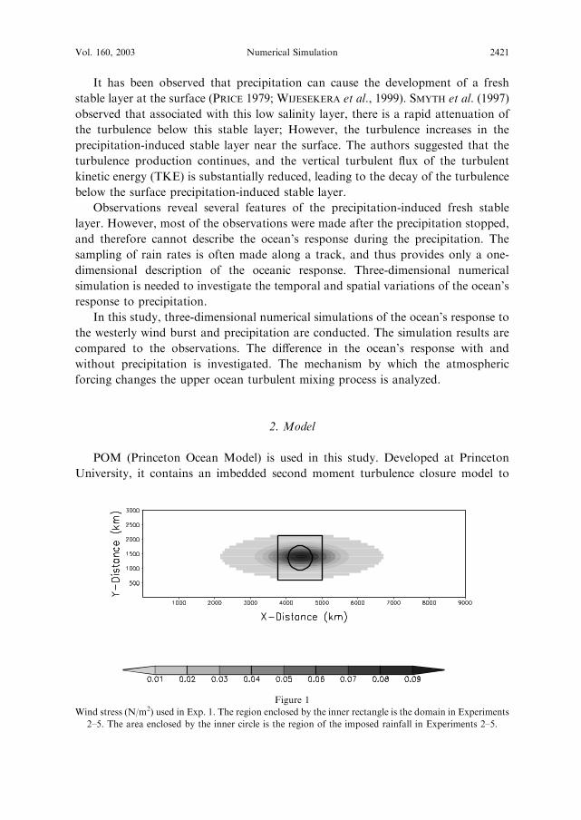
Figure 1

Wind stress (N/m2) used in Exp. 1. The region enclosed by the inner rectangle is the domain in Experiments

2–5. The area enclosed by the inner circle is the region of the imposed rainfall in Experiments 2–5.

Vol. 160, 2003 Numerical Simulation 2421

provide vertical mixing coefficients. It is a sigma coordinate model in that the vertical

coordinate is scaled by the water column depth. r ¼ z�gHþg is the vertical coordinate. z

is the conventional Cartesian vertical coordinate. D � H þ g where H is the bottom

topography that is constant in this study and g is the surface elevation. The

horizontal time differencing is explicit whereas the vertical differencing is implicit.

The latter eliminates time constraints for the vertical coordinate and permits the use

of fine vertical resolution in the surface and bottom boundary layers. The model has

a free surface and a split time step. The external mode portion of the model is two-

dimensional and uses a short time step based on the CFL condition and the external

wave speed. The internal mode is three-dimensional and uses a larger time step based

on the CFL condition and the internal wave speed. Complete thermodynamics have

been implemented. Details of the model are described by BLUMBERG and MELLOR

(1987) and KANTHA and CLAYSON (2000).

The finest horizontal resolution of this simulation is 10 km. A stretching vertical

grid scheme is used. Higher vertical resolution is used for the upper layers because the

ocean’s response to the surface atmospheric forcing such as precipitation associated

with squall lines, which last only a few hours, occurs mainly in the upper few meters

of the ocean. Below 50 meters, the ocean’s response is not significant. In this study,

the finest vertical resolution, at the upper-most layer, is about one meter. The

external mode time step is 20 seconds, and the internal mode has a time step of 600

seconds.

We assume that the initial temperature and salinity profiles are horizontally

homogeneous and the ocean is initially calm with no motion. The temperature and

salinity profiles are based on a global data set (LEVITUS et al., 1994; LEVITUS and

BOYER, 1994). February monthly average data at 165o E and 5o N are used. This

location is the center of the simulation domain.

The parameterization of the turbulent mixing processes is critical in the

simulation of the upper ocean boundary layer response to the atmospheric forcing.

The second moment turbulent closure model included in POM, often cited in the

literature as the Mellor-Yamada turbulent closure model (MELLOR and YAMADA,

1974, 1982), is widely used in geophysical fluid studies because it is relatively simple

and still retains much of the second moment accuracy.

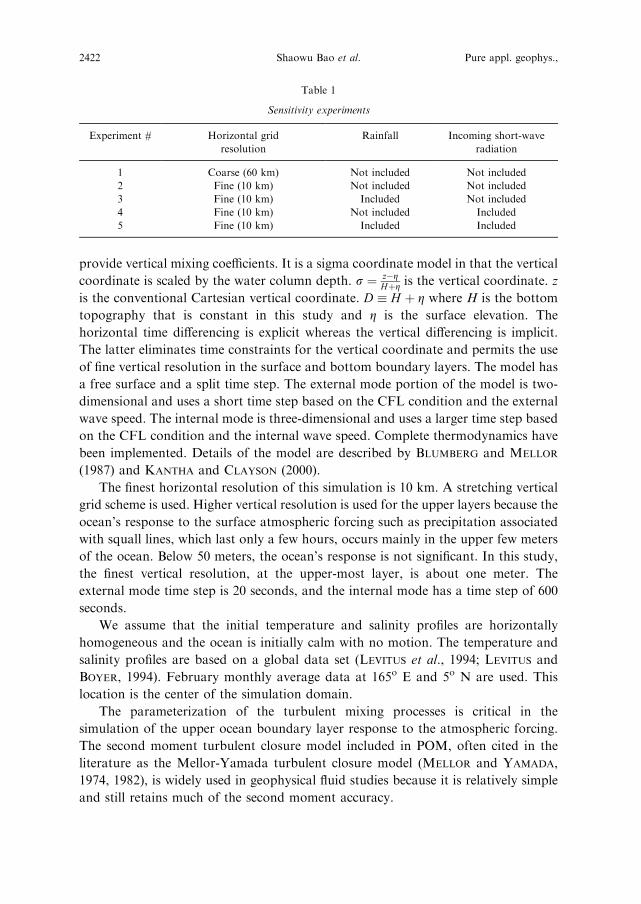
Table 1

Sensitivity experiments

Experiment # Horizontal grid

resolution

Rainfall Incoming short-wave

radiation

1 Coarse (60 km) Not included Not included

2 Fine (10 km) Not included Not included

3 Fine (10 km) Included Not included

4 Fine (10 km) Not included Included

5 Fine (10 km) Included Included


Figure 2

Simulated surface velocity fields in Exp. 1: (a) 3 days, (b) 5 days, (c) 10 days, (d) 15 days, (e) 20 days, (f) 30

days since the beginning of simulation.

Figure 3

Simulated surface zonal velocity, U (m/s), in Experiment 1: (a) 3 days, (b) 5 days, (c) 10 days, (d) 15 days,

(e) 20 days, (f) 30 days since the beginning of simulation. Positive values indicate eastward currents. Note

that wind stress is switched off on the 10th day.


Turbulent kinetic energy (TKE) and turbulent mixing length are predicted using

the following equations:

@q2D@t þ

@Uq2D@x þ

@Vq2D@y þ

@xq2D@r

¼ @@r

Kq

D@ q2

@r

h iþ 2Km

D@U@r

� �2þ @V@r

� �2h iþ 2g

q0Kh

@~qq@r�

2Dq3

B1l þ Fq ð1Þ

@q2lD@t þ

@Uq2lD@x þ @Vq2lD

@y þ@xq2lD@r

¼ @@r

Kq

D@ q2l@r

h iþ E1l

KmD

@U@r

� �2þ @V@r

� �2h iþ E3

gq0

Kh@~qq@r

n o~WW � 2Dq3

B1þ Fl ð2Þ

where g ¼ 9:8m s�2, q2 is the turbulent kinetic energy (TKE). ‘ is the turbulent

length scale and x is the velocity component normal to the sigma surface.~WW ¼ 1þ E2ðl=kLÞ, where von Karman constant k ¼ 0:4, L�1 ¼ ðg� zÞ�1þðH � zÞ�1. @~qq=@r �ð@q=@rÞ�ðc�2s @p

�@rÞ where cs is the speed of sound. B1, E1,

E2 and E3 are constants. U and V are zonal and meridional velocities. Fq and Fl are

diffusion terms of q2 and l, respectively.

The vertical kinematic viscosity and vertical diffusivity, Km and Kh, are defined

according to

Km ¼ qlSm; ð3ÞKh ¼ qlSh: ð4Þ

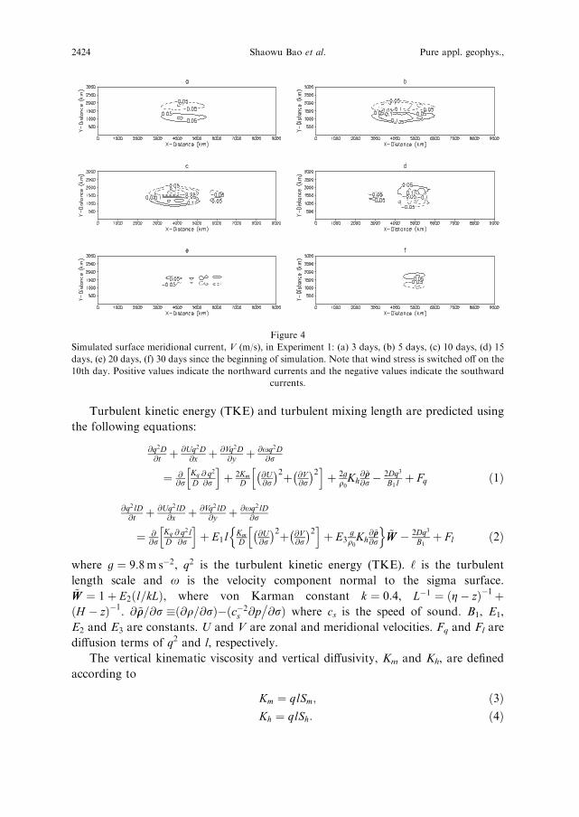
Figure 4

Simulated surface meridional current, V (m/s), in Experiment 1: (a) 3 days, (b) 5 days, (c) 10 days, (d) 15

days, (e) 20 days, (f) 30 days since the beginning of simulation. Note that wind stress is switched off on the

10th day. Positive values indicate the northward currents and the negative values indicate the southward

currents.


The coefficients, Sm and Sh are functions of Richardson number and Kq is the TKE

diffusivity.

During westerly Wind Burst events, the winds over the western Pacific warm pool

are mainly zonal. Impact of the meridional wind stress is relatively small compared to

the zonal ones (HARRISON and CRAIG, 1993). Therefore, in this study, only idealized

zonal wind stress is used. The wind stress field is imposed in the following form

(Fig. 1):

sðx; yÞ ¼ ramp � s0 � expf�ðx� x0=DxÞ2g expf�ðy � y0=DyÞ2g; ð5Þ

s0 is the maximum amplitude of stress. The variable ramp varies from 0 to 1 within

the first day of the simulation, thus the wind stress is switched on at the beginning of

the simulation and is increased to its maximum strength within one day. The same

value is then maintained for 10 days and then switched off. (x0,y0) is the center of the

simulation domain. Dx and Dy are the horizontal grid sizes.

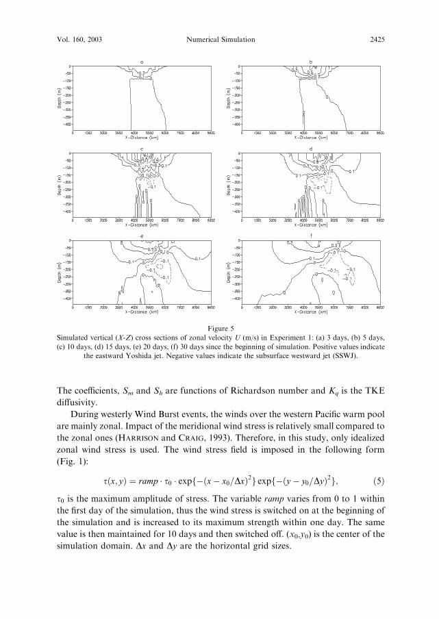
Figure 5

Simulated vertical (X-Z) cross sections of zonal velocity U (m/s) in Experiment 1: (a) 3 days, (b) 5 days,

(c) 10 days, (d) 15 days, (e) 20 days, (f) 30 days since the beginning of simulation. Positive values indicate

the eastward Yoshida jet. Negative values indicate the subsurface westward jet (SSWJ).


The rainfall-induced salinity flux (Fs) and heat flux (Ft) are given by:

Fs ¼ qIS0 ð6ÞFt ¼ qCpIðTa � T0Þ ð7Þ

where q is the water density, I is the rainfall intensity, S0 is the surface salinity, Cp is

specific heat of liquid water (4218 J K)1/kg), Ta is the atmospheric temperature and

T0 is the sea-surface temperature.

In this study, an idealized precipitation process is considered. The rainfall-

induced salinity flux and heat flux are included. The rainfall has an intensity of

15 mm/hour and covers a region enclosed by a circle with a radius of 100 km (Fig. 1).

The precipitation process lasts for five hours.

Figure 6

Simulated vertical (X-Z) cross sections of the differences between the salinities in Practical Salinity Unit

(psu) with and without rainfall (a) 2h, (b) 3h, (c) 4h, (d) 5h, (e) 6h, (f) 7h, (g) 8h, (h) 9h since the beginning

of simulation. The negative values indicate the rainfall-induced low salinity layer.


3. Experiment Design

A total of five experiments are conducted to study the effect of precipitation on

the upper ocean’s response (Table 1). In Exp. 1, the overall features of the

Westerly Wind Burst (WWB) and precipitation are simulated with a horizontal

resolution of 60 km and a finest vertical resolution of 10 m (top layer). The

simulation domain is 9000 km · 3000 km, and the integration time is 30 days.

However, the effect of the rainfall on the ocean’s response occurs mainly within the

top few meters of the ocean. In order to investigate the rainfall-induced effects and

their spatial variation, higher resolution numerical modeling is required. In

Experiments 2, 3, 4, and 5, the horizontal resolution is 10 km and the finest vertical

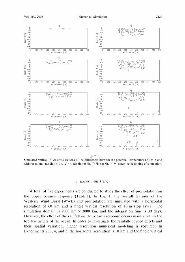
Figure 7

Simulated vertical (X-Z) cross sections of the differences between the potential temperature (K) with and

without rainfall (a) 2h, (b) 3h, (c) 4h, (d) 5h, (e) 6h, (f) 7h, (g) 8h, (h) 9h since the beginning of simulation.


resolution within the upper ocean is 1 meter. The domain covers a region of 1000

km · 1000 km and the integration time is 24 hours in Experiments 2–5. Effects of

the precipitation on the mixing processes of the upper ocean are investigated in

Experiments 2 and 3. Because the wind stress forcing remains after the formation

of the rainfall-induced fresh layer, effects of the precipitation on the vertical

transfer of the momentum are investigated. In Exp. 4 and Exp. 5, the effects of

rainfall on the vertical transfer of heat flux contributed by short-wave radiation are

investigated. In Exp. 4 and Exp. 5, the ocean receives a downward vertical heat

flux of 200 W/m2, a typical value for the location simulated in this study, due to

the idealized short-wave radiation.

Figure 8

Simulated vertical (X-Z) cross sections of the differences between density (kg/m3) with and without rainfall

(a) 2h, (b) 3h, (c) 4h, (d) 5h, (e) 6h, (f) 7h, (g) 8h, (h) 9h since the beginning of the simulation. Note that the

pattern of the density variation follows that of the salinity variation (see Fig. 6).


4. Results

4.1. Experiment 1: General Features of the Ocean’s Response to theWesterlyWind Burst

The wind stress generates an eastward surface Yoshida jet (YOSHIDA, 1959) as

indicated in Figures 2 and 3. Time series of the simulation results of the surface

velocity fields in Experiment 1 are shown in Figure 2. Time series of the simulation

results of the surface zonal velocity, U (m/s), in Experiment 1 are shown in Figure 3.

Positive values indicate eastward currents in Figure 3. The wind stress is switched off

on the 10th day. The eastward jet increases to its maximum strength in about 10

days, then begins to decrease due to the switch-off of the wind stress. The maximum

current reaches a value of 1.5 m/s.

The eastward jet causes meridional current, southward in the Northern

Hemisphere and northward in the Southern Hemisphere as shown in Figure 4.

The meridional velocities also reach their maximums just after the wind stresses are

switched off on the 10th day of the simulation and then begin to decrease. Simulated

maximum value of the meridional current is 0.35 m/s.

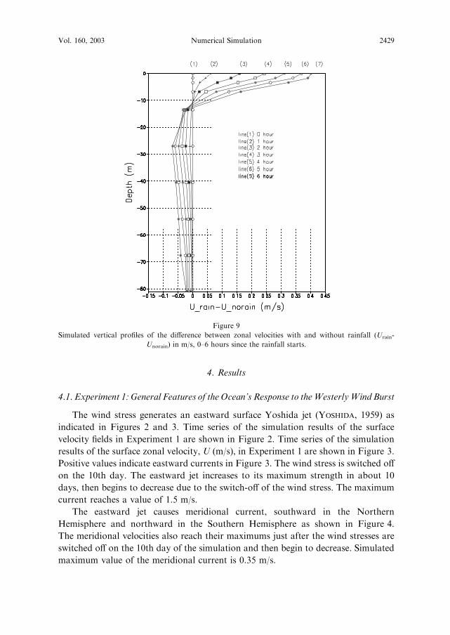
Figure 9

Simulated vertical profiles of the difference between zonal velocities with and without rainfall (Urain-

Unorain) in m/s, 0–6 hours since the rainfall starts.


Vertical X-Z cross section of zonal current U is shown in Figure 5. The

momentum spreads from the surface downward by two major processes: the mean

vertical velocity transport and the turbulent flux. The turbulent flux process plays a

greater role than the mean velocity transport. The eastward current causes a

convergence zone on the leading edge and a divergence zone on the trailing edge.

Because of mass continuity, the convergence and divergence caused by the surface

eastward jet generate the subsurface westward jet (SSWJ) below the eastward jet.

This feature agrees well with the observations (HISARD et al., 1970) and with other

simulations such as that by ZHANG and ROTHSTEIN (1998) using a general circulation

model originally developed by GENT and CANE (1989).

When the surface wind stress is switched off on the 10th day, there is no energy

source to drive the ocean surface current, consequently the surface eastward jet

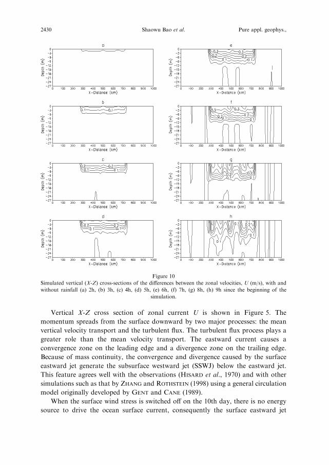
Figure 10

Simulated vertical (X-Z) cross-sections of the differences between the zonal velocities, U (m/s), with and

without rainfall (a) 2h, (b) 3h, (c) 4h, (d) 5h, (e) 6h, (f) 7h, (g) 8h, (h) 9h since the beginning of the

simulation.


begins to weaken. However, the upwelling and downwelling, which are the energy

sources of the SSWJ, still exist. Therefore, from Figure 5, it is apparent that the

SSWJ did not begin to weaken immediately after the surface wind stress is switched

off. It continues to increase, reaching its maximum on the 15th day, five days after

the wind stress is switched off.

4.2. Sensitivity to Rainfall (Experiments 2 and 3)

The (X Z) vertical cross section of the differences in the salinity and the potential

temperature between the simulation results with and without rainfall (Srain-Snorainand Train-Tnorain, respectively) are shown in Figures 6 and 7 respectively. It is clear

that immediately after the precipitation process started, the negative salinity

anomaly and negative temperature anomaly began to develop. The salinity anomaly

and the potential temperature anomaly are limited in the region where the

precipitation occurred. The magnitudes of the anomalies and the thickness of the

rainfall-induced fresh layer continued increasing with time until the precipitation

stopped. Then the precipitation-induced layer remains stable near the surface. The

magnitudes of the salinity and potential temperature anomalies are the highest near

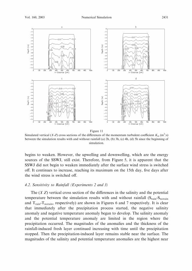
Figure 11

Simulated vertical (X-Z) cross sections of the differences of the momentum turbulent coefficient Km (m2/s)

between the simulation results with and without rainfall (a) 2h, (b) 3h, (c) 4h, (d) 5h since the beginning of

simulation.


the surface, and decrease with depth. The maximum salinity anomalies reach 0.3–

0.35 psu, and the maximum potential temperature anomalies reach 0.05oC just

before the precipitation stops. Four to five hours after the precipitation stops, the

magnitudes of the salinity and potential temperature anomalies at a depth of 2–3

meters, reach 0.15–0.2 psu and 0.04–0.05o C, respectively. This rainfall-induced

stable layer reaches a depth of about 11–13 meters within a few hours after the

precipitation stops.

A rainfall process with similar characteristics (intensity, range and duration) was

observed in December, 1992 as part of the Tropical Ocean Global Atmospheres/

Coupled Ocean Atmosphere Response Experiment (TOGA/COARE) in the western

Pacific warm pool, at 156oE and 2oS. The observed rainfall-induced negative salinity

anomaly reached a magnitude of 0.12 psu near the surface with a depth of about 2–3

meters. The magnitude of the corresponding rainfall-induced negative potential

temperature anomaly, measured also at a depth of 2–3 meters, reached 0.05o C at

about 5 hours after the formation of the rainfall-induced low salinity stable layer

(WIJESEKERA et al., 1999). Thus the simulation results agree well with the observations.

The magnitudes of salinity anomaly and potential temperature anomaly have

opposite effects on the density. The negative salinity anomaly tends to reduce the

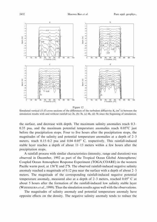
Figure 12

Simulated vertical (X-Z) cross sections of the differences of the turbulent diffusivity Kh (m2/s) between the

simulation results with and without rainfall (a) 2h, (b) 3h, (c) 4h, (d) 5h since the beginning of simulation.


density (making the upper layer more stable) while the negative potential temper-

ature anomaly tends to increase the density (making the upper layer unstable).

Figure 8 is the (X–Z) vertical cross section of the resulting density anomaly (qrain )qnorain). It is clear that (the negative) salinity anomaly has the dominant effect on the

density. The density anomaly essentially follows the pattern of the salinity anomaly.

The maximum magnitude of the density anomaly reached 0.3, or 1.4% of the

simulated value with no rain.

The rainfall-induced low salinity, low temperature and low-density layer has a

significant effect on the vertical turbulent transport of the momentum from the

surface atmospheric forcing. Differences in the vertical current profiles between the

no-rain case and the with-rain case (Fig. 9) are analyzed to investigate the effect of

the rainfall on the vertical turbulent transport. Horizontal positions of the profiles

are at the center of the rainfall region, which is also the center of the simulation

domain. It is clear from Figure 9 that immediately after the rainfall started, the zonal

velocity near the surface within the rainfall-induced fresh stable layer began to

increase, causing significant positive anomaly of U. The magnitude of the U anomaly

is at a maximum value of 0.35 m/s near the surface in five hours since the start of the

Figure 13

Simulated vertical (X-Z) cross sections of the momentum turbulent coefficient Km (m2/s) with rainfall (a)

2h, (b) 3h, (c) 4h, (d) 5h since the beginning of simulation. Note that under the rainfall-covered region Km

values become near zero due to the increased static stability.


rainfall event. Below a depth of 11–13 meters, which is also the lower boundary of

the rainfall-induced fresh stable layer, the anomaly turns negative. The magnitude of

the positive anomaly of U near the surface reaches 0.35 m/s at the fifth hour, a 55%

increase. It is markedly larger than that of the negative anomaly of U below a depth

of 11–13 meters, less than 0.1 m/s, about 10%. Similar features are found in other

precipitation regions as shown in the vertical cross-sections of the anomaly of the

zonal velocity (Urain-Unorain) (Fig. 10).

From Figures 9 and 10, it is clear that the lower part of the rainfall-induced layer

acts as a barrier and the effects of the surface atmospheric forcing cannot penetrate it.

This process causes that part of the ocean near the surface to respond to the

atmospheric forcing much faster than it would without the effects of rainfall.

As mentioned in Section 2 (the model), the vertical turbulent transport terms,

which cannot be resolved explicitly and therefore must be parameterized, are given

by @@r

KmD@U@r

� �, @@r

KhD@T@r

� �and @

@rKhD@S@r

� �. The vertical diffusivities of momentum and heat,

Km and Kh, respectively, play an important role in the estimation of the vertical

turbulent terms. Vertical cross sections of the anomalies of the simulated Km and Kh

are shown in Figures 11 and 12. It is apparent that the rainfall causes a significant

decrease in the values of Km and Kh. The magnitudes of the anomalies of Km and Kh

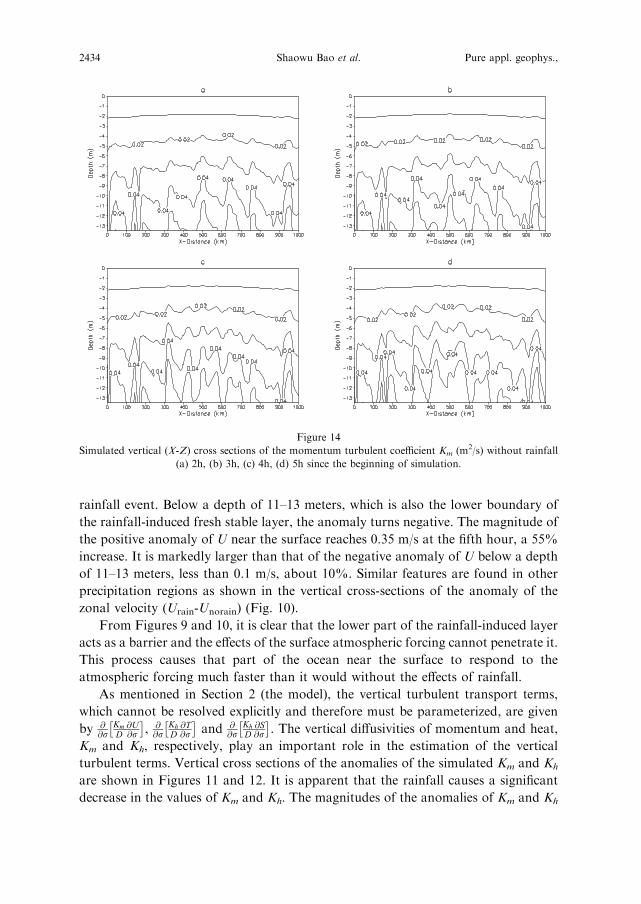
Figure 14

Simulated vertical (X-Z) cross sections of the momentum turbulent coefficient Km (m2/s) without rainfall

(a) 2h, (b) 3h, (c) 4h, (d) 5h since the beginning of simulation.


are at their minimum, near zero, at the surface, and increase with depth. At a depth

of about 11–13 meters, where the anomaly of U changes sign from positive to

negative, the magnitude of Km anomaly reaches a value of 0.05 m2/s, or 90% of the

value of Km, in four hours since the rainfall started. Kh anomaly shows a similar

pattern; its magnitude reaching a value of 0.065 m2/s or 90% of the value of the

initial Kh, at a depth of about 11–13 meters in four hours after the rainfall starts.

Vertical cross sections of Km with and without rainfall are shown in Figures 13 and

14 respectively.

It appears that the decrease in the simulated vertical diffusivity, Km, which

corresponds to an attenuation of the vertical turbulent mixing, could have caused the

effects of the surface atmospheric forcing to be concentrated near the sea surface.

Therefore, the effects of the surface rainfall-induced heat flux (cooling), salinity flux,

and the wind stress-induced momentum transport can reach a depth of 11–13 meters

only. The isolation of the surface rainfall-induced fresh stable layer from the rest of

the mixed layer also causes the surface layer to respond to the atmospheric forcing

considerably faster.

It will be of interest to investigate as to why the rainfall-induced fresh stable layer

tends to attenuate the vertical turbulent mixing. As mentioned in Section 2, the

Figure 15

Simulated vertical (X-Z) cross sections of the differences between the TKE buoyancy production terms

(m2/s3*10)7) with and without rainfall (a) 2h, (b) 3h, (c) 4h, (d) 5h since the beginning of simulation.


vertical turbulent diffusivities are determined by three factors: Turbulent kinetic

energy (TKE), turbulent length scale and Richardson number (Ri). The results of the

numerical experiments show that the rainfall-induced fresh stable layer has

significant effects on the TKE and Ri.

Equation (1) is used to predict the TKE. The left-hand side has temporal change

and horizontal and vertical advection terms. The right-handside terms are, from left

to right, the vertical turbulent flux, the shear production, the buoyancy production,

and the turbulent dissipation.

In the simulations that have a time scale of a few hours, the advection terms are

not as important as other terms. Therefore, the discussion will focus on the

production terms (buoyancy and shear), dissipation and the turbulent mixing term.

Due to the presence of the rainfall-induced low density layer, the density gradient

increases, leading to an increase in BruntVaisala frequency, and hence an increase in

static stability and a decrease in the buoyancy production of turbulence. Figure 15

shows the vertical cross section of the anomaly of the buoyancy production. It is

clear that for depths less than 11–13 meters, the anomaly of the turbulence buoyancy

production is negative, apparently caused by the stabilization of the surface fresh

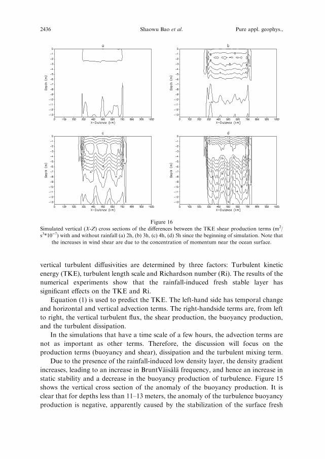
Figure 16

Simulated vertical (X-Z) cross sections of the differences between the TKE shear production terms (m2/

s3*10)7) with and without rainfall (a) 2h, (b) 3h, (c) 4h, (d) 5h since the beginning of simulation. Note that

the increases in wind shear are due to the concentration of momentum near the ocean surface.


layer. The magnitude of the anomaly is at maximum at about 3 meters. The

maximum anomaly of the buoyancy production term reaches a value of 6 · 10)7 m2/

s3, at the 4th hour.

At the beginning of the rainfall process, the direct effect of rainfall-induced

fresh layer is the stabilization of the upper layer, which tends to decrease the

turbulent production. The decrease of the turbulent production leads to the

attenuation of the vertical turbulent flux (Figs. 11 and 12), causing the momentum

to concentrate near the surface. Consequently, the shear production of turbulence

begins to develop, due to the increased velocity gradient between the rainfall-

induced fresh layer and the layer below it. Figure 16 is the vertical cross section of

the anomaly of shear production term. The magnitude of the positive anomaly of

shear production of turbulence is larger than that of the negative anomaly of the

buoyancy production of turbulence (Figs. 15 and 16). Thus the rainfall-induced

stable layer does not cause the total turbulence production (buoyancy production

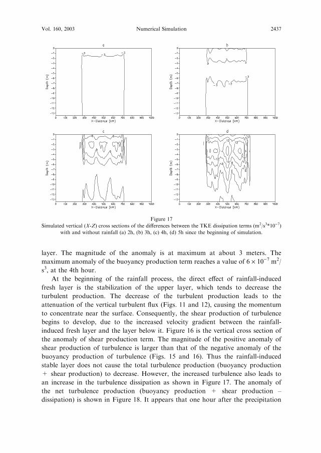
+ shear production) to decrease. However, the increased turbulence also leads to

an increase in the turbulence dissipation as shown in Figure 17. The anomaly of

the net turbulence production (buoyancy production + shear production –

dissipation) is shown in Figure 18. It appears that one hour after the precipitation

Figure 17

Simulated vertical (X-Z) cross sections of the differences between the TKE dissipation terms (m2/s3*10)7)

with and without rainfall (a) 2h, (b) 3h, (c) 4h, (d) 5h since the beginning of simulation.


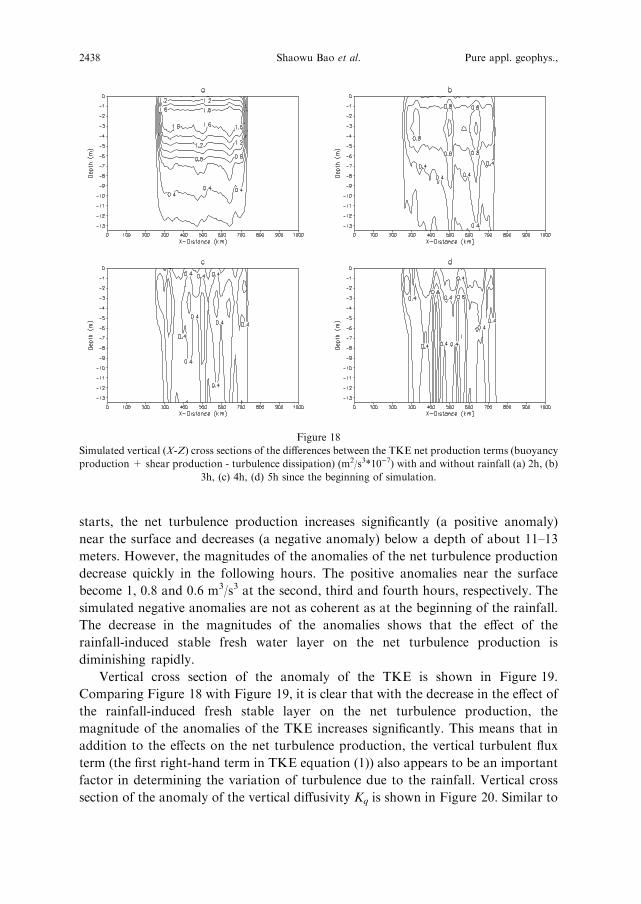
starts, the net turbulence production increases significantly (a positive anomaly)

near the surface and decreases (a negative anomaly) below a depth of about 11–13

meters. However, the magnitudes of the anomalies of the net turbulence production

decrease quickly in the following hours. The positive anomalies near the surface

become 1, 0.8 and 0.6 m3/s3 at the second, third and fourth hours, respectively. The

simulated negative anomalies are not as coherent as at the beginning of the rainfall.

The decrease in the magnitudes of the anomalies shows that the effect of the

rainfall-induced stable fresh water layer on the net turbulence production is

diminishing rapidly.

Vertical cross section of the anomaly of the TKE is shown in Figure 19.

Comparing Figure 18 with Figure 19, it is clear that with the decrease in the effect of

the rainfall-induced fresh stable layer on the net turbulence production, the

magnitude of the anomalies of the TKE increases significantly. This means that in

addition to the effects on the net turbulence production, the vertical turbulent flux

term (the first right-hand term in TKE equation (1)) also appears to be an important

factor in determining the variation of turbulence due to the rainfall. Vertical cross

section of the anomaly of the vertical diffusivity Kq is shown in Figure 20. Similar to

Figure 18

Simulated vertical (X-Z) cross sections of the differences between the TKE net production terms (buoyancy

production + shear production - turbulence dissipation) (m2/s3*10)7) with and without rainfall (a) 2h, (b)

3h, (c) 4h, (d) 5h since the beginning of simulation.


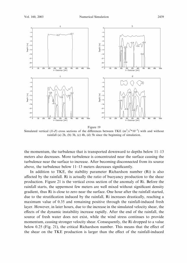
the momentum, the turbulence that is transported downward to depths below 11–13

meters also decreases. More turbulence is concentrated near the surface causing the

turbulence near the surface to increase. After becoming disconnected from its source

above, the turbulence below 11–13 meters decreases significantly.

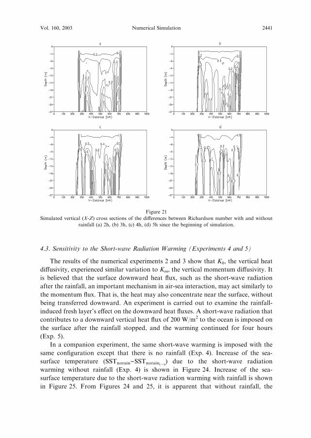
In addition to TKE, the stability parameter Richardson number (Ri) is also

affected by the rainfall. Ri is actually the ratio of buoyancy production to the shear

production. Figure 21 is the vertical cross section of the anomaly of Ri. Before the

rainfall starts, the uppermost few meters are well mixed without significant density

gradient, thus Ri is close to zero near the surface. One hour after the rainfall started,

due to the stratification induced by the rainfall, Ri increases drastically, reaching a

maximum value of 0.35 and remaining positive through the rainfall-induced fresh

layer. However, in later hours, due to the increase in the simulated velocity shear, the

effects of the dynamic instability increase rapidly. After the end of the rainfall, the

source of fresh water does not exist, while the wind stress continues to provide

momentum, causing stronger velocity shear. Consequently, the Ri dropped to a value

below 0.25 (Fig. 21), the critical Richardson number. This means that the effect of

the shear on the TKE production is larger than the effect of the rainfall-induced

Figure 19

Simulated vertical (X-Z) cross sections of the differences between TKE (m2/s2*10)3) with and without

rainfall (a) 2h, (b) 3h, (c) 4h, (d) 5h since the beginning of simulation.


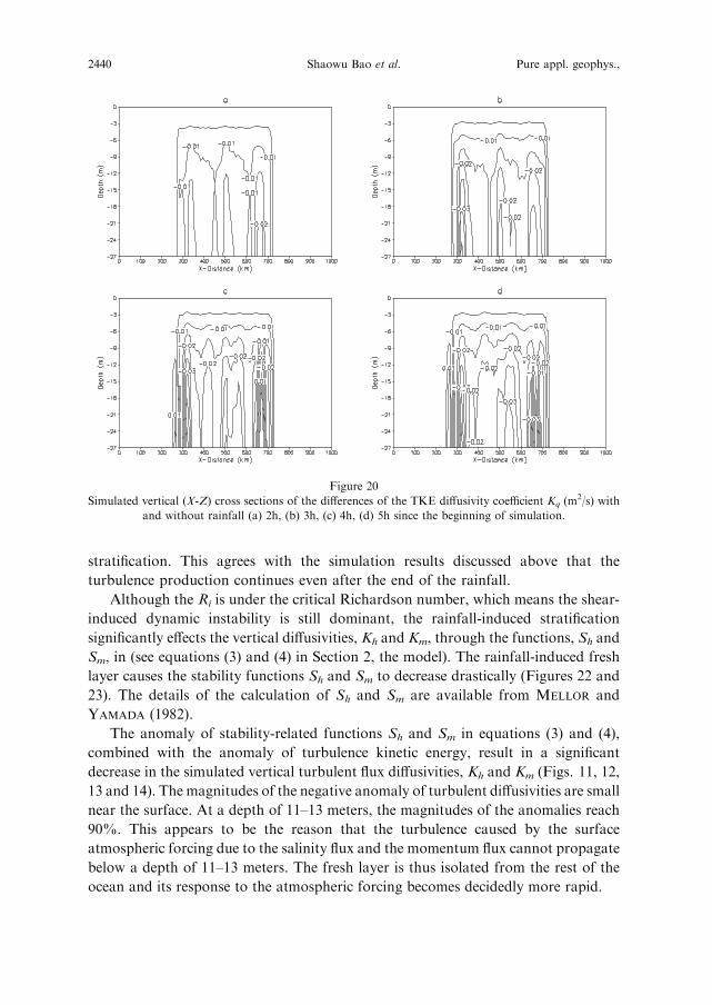
stratification. This agrees with the simulation results discussed above that the

turbulence production continues even after the end of the rainfall.

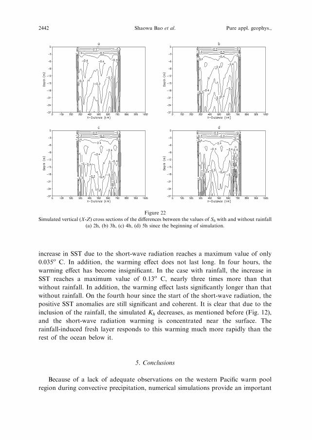
Although the Ri is under the critical Richardson number, which means the shear-

induced dynamic instability is still dominant, the rainfall-induced stratification

significantly effects the vertical diffusivities, Kh and Km, through the functions, Sh and

Sm, in (see equations (3) and (4) in Section 2, the model). The rainfall-induced fresh

layer causes the stability functions Sh and Sm to decrease drastically (Figures 22 and

23). The details of the calculation of Sh and Sm are available from MELLOR and

YAMADA (1982).

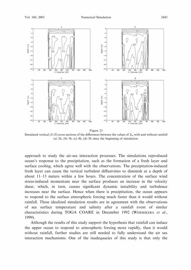
The anomaly of stability-related functions Sh and Sm in equations (3) and (4),

combined with the anomaly of turbulence kinetic energy, result in a significant

decrease in the simulated vertical turbulent flux diffusivities, Kh and Km (Figs. 11, 12,

13 and 14). The magnitudes of the negative anomaly of turbulent diffusivities are small

near the surface. At a depth of 11–13 meters, the magnitudes of the anomalies reach

90%. This appears to be the reason that the turbulence caused by the surface

atmospheric forcing due to the salinity flux and the momentum flux cannot propagate

below a depth of 11–13 meters. The fresh layer is thus isolated from the rest of the

ocean and its response to the atmospheric forcing becomes decidedly more rapid.

Figure 20

Simulated vertical (X-Z) cross sections of the differences of the TKE diffusivity coefficient Kq (m2/s) with

and without rainfall (a) 2h, (b) 3h, (c) 4h, (d) 5h since the beginning of simulation.


4.3. Sensitivity to the Short-wave Radiation Warming (Experiments 4 and 5)

The results of the numerical experiments 2 and 3 show that Kh, the vertical heat

diffusivity, experienced similar variation to Km, the vertical momentum diffusivity. It

is believed that the surface downward heat flux, such as the short-wave radiation

after the rainfall, an important mechanism in air-sea interaction, may act similarly to

the momentum flux. That is, the heat may also concentrate near the surface, without

being transferred downward. An experiment is carried out to examine the rainfall-

induced fresh layer’s effect on the downward heat fluxes. A short-wave radiation that

contributes to a downward vertical heat flux of 200 W/m2 to the ocean is imposed on

the surface after the rainfall stopped, and the warming continued for four hours

(Exp. 5).

In a companion experiment, the same short-wave warming is imposed with the

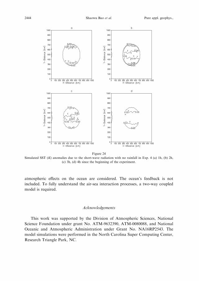
same configuration except that there is no rainfall (Exp. 4). Increase of the sea-

surface temperature (SSTnorain)SSTnoraint=0) due to the short-wave radiation

warming without rainfall (Exp. 4) is shown in Figure 24. Increase of the sea-

surface temperature due to the short-wave radiation warming with rainfall is shown

in Figure 25. From Figures 24 and 25, it is apparent that without rainfall, the

Figure 21

Simulated vertical (X-Z) cross sections of the differences between Richardson number with and without

rainfall (a) 2h, (b) 3h, (c) 4h, (d) 5h since the beginning of simulation.


increase in SST due to the short-wave radiation reaches a maximum value of only

0.035o C. In addition, the warming effect does not last long. In four hours, the

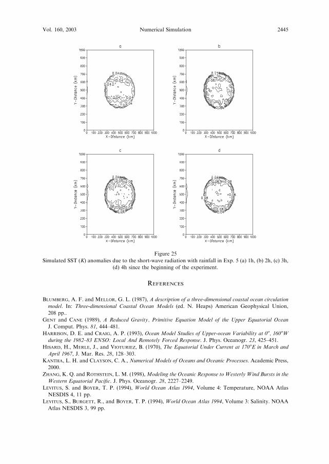
warming effect has become insignificant. In the case with rainfall, the increase in

SST reaches a maximum value of 0.13o C, nearly three times more than that

without rainfall. In addition, the warming effect lasts significantly longer than that

without rainfall. On the fourth hour since the start of the short-wave radiation, the

positive SST anomalies are still significant and coherent. It is clear that due to the

inclusion of the rainfall, the simulated Kh decreases, as mentioned before (Fig. 12),

and the short-wave radiation warming is concentrated near the surface. The

rainfall-induced fresh layer responds to this warming much more rapidly than the

rest of the ocean below it.

5. Conclusions

Because of a lack of adequate observations on the western Pacific warm pool

region during convective precipitation, numerical simulations provide an important

Figure 22

Simulated vertical (X-Z) cross sections of the differences between the values of Sh with and without rainfall



approach to study the air-sea interaction processes. The simulations reproduced

ocean’s response to the precipitation, such as the formation of a fresh layer and

surface cooling, which agree well with the observations. The precipitation-induced

fresh layer can cause the vertical turbulent diffusivities to diminish at a depth of

about 11–13 meters within a few hours. The concentration of the surface wind

stress-induced momentum near the surface produces an increase in the velocity

shear, which, in turn, causes significant dynamic instability and turbulence

increases near the surface. Hence when there is precipitation, the ocean appears

to respond to the surface atmospheric forcing much faster than it would without

rainfall. These idealized simulation results are in agreement with the observations

of sea surface temperature and salinity after a rainfall event of similar

characteristics during TOGA COARE in December 1992 (WIJESEKERA et al.,

1999).

Although the results of this study support the hypothesis that rainfall can induce

the upper ocean to respond to atmospheric forcing more rapidly, than it would

without rainfall, further studies are still needed to fully understand the air sea

interaction mechanisms. One of the inadequacies of this study is that only the

Figure 23

Simulated vertical (X-Z) cross sections of the differences between the values of Sm with and without rainfall



atmospheric effects on the ocean are considered. The ocean’s feedback is not

included. To fully understand the air-sea interaction processes, a two-way coupled

model is required.

Acknowledgements

This work was supported by the Division of Atmospheric Sciences, National

Science Foundation under grant No. ATM-9632390, ATM-0080088, and National

Oceanic and Atmospheric Administration under Grant No. NA16RP2543. The

model simulations were performed in the North Carolina Super Computing Center,

Research Triangle Park, NC.

Figure 24

Simulated SST (K) anomalies due to the short-wave radiation with no rainfall in Exp. 4 (a) 1h, (b) 2h,

(c) 3h, (d) 4h since the beginning of the experiment.


REFERENCES

BLUMBERG, A. F. and MELLOR, G. L. (1987), A description of a three-dimensional coastal ocean circulation

model. In: Three-dimensional Coastal Ocean Models (ed. N. Heaps) American Geophysical Union,

208 pp..

GENT and CANE (1989), A Reduced Gravity, Primitive Equation Model of the Upper Equatorial Ocean

J. Comput. Phys. 81, 444–481.

HARRISON, D. E. and CRAIG, A. P. (1993), Ocean Model Studies of Upper-ocean Variability at 0o, 160oW

during the 1982–83 ENSO: Local And Remotely Forced Response. J. Phys. Oceanogr. 23, 425–451.

HISARD, H., MERLE, J., and VIOTURIEZ, B. (1970), The Equatorial Under Current at 170oE in March and

April 1967, J. Mar. Res. 28, 128–303.

KANTHA, L. H. and CLAYSON, C. A., Numerical Models of Oceans and Oceanic Processes. Academic Press,

2000.

ZHANG, K. Q. and ROTHSTEIN, L. M. (1998),Modeling the Oceanic Response to Westerly Wind Bursts in the

Western Equatorial Pacific. J. Phys. Oceanogr. 28, 2227–2249.

LEVITUS, S. and BOYER, T. P. (1994), World Ocean Atlas 1994, Volume 4: Temperature, NOAA Atlas

NESDIS 4, 11 pp.

LEVITUS, S., BURGETT, R., and BOYER, T. P. (1994), World Ocean Atlas 1994, Volume 3: Salinity. NOAA

Atlas NESDIS 3, 99 pp.

Figure 25

Simulated SST (K) anomalies due to the short-wave radiation with rainfall in Exp. 5 (a) 1h, (b) 2h, (c) 3h,

(d) 4h since the beginning of the experiment.


MELLOR, G. L. and YAMADA, T. (1982), Development of a Turbulent Closure Model for Geophysical Fluid

Problems, Rev. Geophys. 20, 851–875.

PRICE, J. R. (1979), Observations of a Rain-formed Mixed Layer, J. Phys. Oceanogr. 9, 643–649.

RICHARDSON, R. A., GINIS ISSAC and ROTHSTEIN, L. M. (1999), A Numerical Investigation of the Local

Ocean Response to Westerly Wind Burst Forcing, in the Western Equatorial Pacific, J. Phys. Oceanogr.

29, 1334–1352.

SMYTH, W. D., ZAVIALOV, P. O. and MOUM, J. N. (1997), Decay of Turbulence in the Upper Ocean

Following Sudden Isolation from Surface Forcing, J. Phys. Oceanogr. 27, 820–822.

SUI, C. H., LI, X., LAU, K.-M., and ADAMEC, D. (1997), Multiscale Air–Sea Interactions during TOGA

COARE, Month. Weat. Rev. 125, 4, 448–462.

WEBSTER, P. J. and LUKAS, R. (1992), TOGA COARE: The Coupled Ocean-Atmosphere Response

Experiment, Bull. Amer. Meteor. Soc. 73, 1377–1416.

WIJESEKERA, H. W., PAULSON, C. A., and HUYER, A. (1999), The Effect of Rainfall on the Surface Layer in

the Western Equatorial Pacific during a Westerly Wind Burst, J. Phy. Oceanogr. 29, 612–632.

YOSHIDA, K. (1959), A Theory of the Cromwell Current (the Equatorial Undercurrent) and of the Equatorial

Upwelling, J. Oceanogr. Soc. Japan 15, 159–170.

(Received January 9, 2002, accepted June 7, 2002)

To access this journal online:

http://www.birkhauser.ch


numerical simulation of the response of the ocean...

Documents