numerical modelling of galvanic structural joints ... · numerical modelling of galvanic structural...
TRANSCRIPT
Numerical Modelling of Galvanic Structural Joints Subjected to Combined
Environmental and Mechanical Loading
by
Nitin Chandra Muthegowda
A Thesis Presented in Partial Fulfillment
of the Requirements for the Degree
Master of Science
Approved July 2015 by the
Graduate Supervisory Committee:
Kiran Solanki, Chair
Konrad Rykaczewski
Yang Jiao
ARIZONA STATE UNIVERSITY
August 2015
i
ABSTRACT
Dissimilar metal joints such as aluminum-steel joints are extensively used in automobile,
naval and aerospace applications and these are subjected to corrosive environmental and
mechanical loading resulting in eventual failure of the structural joints. In the case of
aluminum alloys under aggressive environment, the damage accumulation is
predominantly due to corrosion and is accelerated in presence of other metals. During
recent years several approaches have been employed to develop models to assess the
metal removal rate in the case of galvanic corrosion. Some of these models are based on
empirical methods such as regression analysis while others are based on quantification of
the ongoing electrochemical processes. Here, a numerical model for solving the Nernst-
Planck equation, which captures the electrochemical process, is implemented to predict
the galvanic current distribution and, hence, the corrosion rate of a galvanic couple. An
experimentally validated numerical model for an AE44 (Magnesium alloy) and mild steel
galvanic couple, available in the literature, is extended to simulate the mechano-
electrochemical process in order to study the effect of mechanical loading on the galvanic
current density distribution and corrosion rate in AE44-mild steel galvanic couple
through a multiphysics field coupling technique in COMSOL Multiphysics®. The model
is capable of tracking moving boundariesy of the corroding constituent of the couple by
employing Arbitrary Langrangian Eulerian (ALE) method.
Results show that, when an anode is under a purely elastic deformation, there is no
apparent effect of mechanical loading on the electrochemical galvanic process. However,
when the applied tensile load is sufficient to cause a plastic deformation, the local
ii
galvanic corrosion activity at the vicinity of the interface is increased remarkably. The
effect of other factors, such as electrode area ratios, electrical conductivity of the
electrolyte and depth of the electrolyte, are studied. It is observed that the conductivity of
the electrolyte significantly influences the surface profile of the anode, especially near the
junction. Although variations in electrolyte depth for a given galvanic couple noticeably
affect the overall corrosion, the change in the localized corrosion rate at the interface is
minimal. Finally, we use the model to predict the current density distribution, rate of
corrosion and depth profile of aluminum alloy 7075-stainless steel 316 galvanic joints,
which are extensively used in maritime structures.

iii
DEDICATION
I dedicate this dissertation to my mom, Chandra and dad, Muthegowda. Love you both to
the maximum.
iv
ACKNOWLEDGMENTS
I would like to express my sincere gratitude to the many people without whose support
this dissertation would not have materialized. First, I would like to thank my advisor prof.
K.N. Solanki, for his guidance, encouragement and belief in me throughout this
endeavor. Next, I would like to express my gratitude to my committee members prof.
Konrad Rykaczewski and prof. Yang Jiao for their support and helpful remarks to
improve my dissertation. I would like to extend special thanks to Mr. B. Gholami, Dr.
Bhatia, Dr. Adlakha, Mr. S. Turnage and Ms. M. Rajagopalan, for many engaging
conversations and discussions during my time.
v
TABLE OF CONTENTS
Page
LIST OF TABLES ........................................................................................................... viii
LIST OF FIGURES ........................................................................................................... ix
CHAPTER
1. MOTIVATION ............................................................................................................ 1
2. LITERATURE REVIEW ............................................................................................ 4
3. INTRODUCTION ....................................................................................................... 7
3.1 The Concept of Galvanic Corrosion: ................................................................... 7
3.1.1 Definition ............................................................................................................ 7
3.1.2 Fundamental Requirements ................................................................................ 9
3.1.3 Affecting Factors .............................................................................................. 10
3.2 Transport in Solution ............................................................................................... 11
3.2.1 Diffusion: .......................................................................................................... 11
3.2.2 Migration .......................................................................................................... 12
3.2.3 Nernst-Planck Equation .................................................................................... 14
3.2.3 Nernst Equations............................................................................................... 15
3.3 Kinetics Involved in Corrosion Process .................................................................. 17
vi
CHAPTER Page
3.3.1 Butler-Volmer Kinetics .................................................................................... 17
3.3.2 Polarization Curves........................................................................................... 19
3.3.3 Tafel Slope Constants ....................................................................................... 19
3.3.4 Corrosion Rate from Current Density .............................................................. 21
3.4 Effect of Mechanical Load on Galvanic Corrosion ................................................ 21
3.5 Galvanic Corrosion Rate Measurement .................................................................. 24
3.5.1 Immersion Experiment ..................................................................................... 24
3.5.2 Electrochemical Tests ....................................................................................... 25
4. METHODLOGY ....................................................................................................... 27
4.1 Governing Equations ............................................................................................... 27
4.2 Model and Finite Element Method.......................................................................... 29
4.3 Boundary Conditions............................................................................................... 30
4.4 Arbitrary Langrangian Eulerian (ALE) Method ..................................................... 31
5. RESULTS .................................................................................................................. 34
5.1 Galvanic Corrosion without Loading ...................................................................... 34
5.2 Effect of Electrolyte Depth ..................................................................................... 38
5.3 Effect of Solution Conductivity .............................................................................. 45
5.4 Effect of Area Ratio ................................................................................................ 51

vii
CHAPTER Page
5.5 Galvanic Corrosion under Mechanical Loading ..................................................... 56
5.5.1 Magnesium AE44 – Mild Steel Galvanic Couple ............................................ 56
5.5.2 Aluminum Alloy 7075-T6 and Stainless Steel 316 Joint: ................................ 68
6. CONCLUSION ......................................................................................................... 74
SCOPE .............................................................................................................................. 76
REFERENCES ................................................................................................................. 77
viii
LIST OF TABLES
Table Page
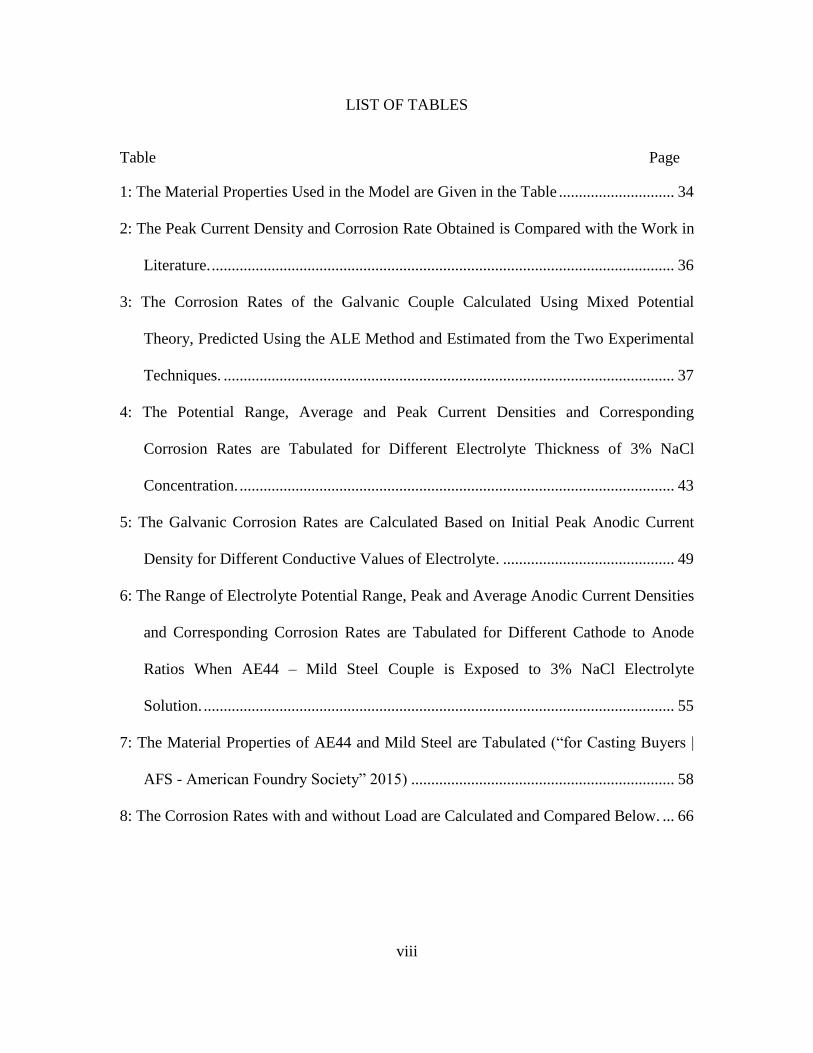
1: The Material Properties Used in the Model are Given in the Table ............................. 34
2: The Peak Current Density and Corrosion Rate Obtained is Compared with the Work in
Literature. .................................................................................................................... 36
3: The Corrosion Rates of the Galvanic Couple Calculated Using Mixed Potential
Theory, Predicted Using the ALE Method and Estimated from the Two Experimental
Techniques. ................................................................................................................. 37
4: The Potential Range, Average and Peak Current Densities and Corresponding
Corrosion Rates are Tabulated for Different Electrolyte Thickness of 3% NaCl
Concentration. ............................................................................................................. 43
5: The Galvanic Corrosion Rates are Calculated Based on Initial Peak Anodic Current
Density for Different Conductive Values of Electrolyte. ........................................... 49
6: The Range of Electrolyte Potential Range, Peak and Average Anodic Current Densities
and Corresponding Corrosion Rates are Tabulated for Different Cathode to Anode
Ratios When AE44 – Mild Steel Couple is Exposed to 3% NaCl Electrolyte
Solution. ...................................................................................................................... 55
7: The Material Properties of AE44 and Mild Steel are Tabulated (“for Casting Buyers |
AFS - American Foundry Society” 2015) .................................................................. 58
8: The Corrosion Rates with and without Load are Calculated and Compared Below. ... 66
ix
LIST OF FIGURES
Figure Page
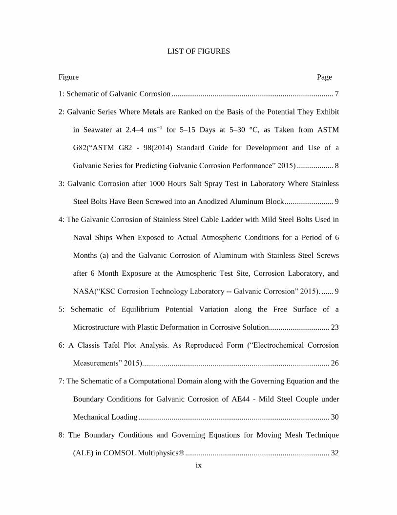
1: Schematic of Galvanic Corrosion ................................................................................... 7
2: Galvanic Series Where Metals are Ranked on the Basis of the Potential They Exhibit
in Seawater at 2.4–4 ms−1 for 5–15 Days at 5–30 °C, as Taken from ASTM
G82(“ASTM G82 - 98(2014) Standard Guide for Development and Use of a
Galvanic Series for Predicting Galvanic Corrosion Performance” 2015) ................... 8
3: Galvanic Corrosion after 1000 Hours Salt Spray Test in Laboratory Where Stainless
Steel Bolts Have Been Screwed into an Anodized Aluminum Block ......................... 9
4: The Galvanic Corrosion of Stainless Steel Cable Ladder with Mild Steel Bolts Used in
Naval Ships When Exposed to Actual Atmospheric Conditions for a Period of 6
Months (a) and the Galvanic Corrosion of Aluminum with Stainless Steel Screws
after 6 Month Exposure at the Atmospheric Test Site, Corrosion Laboratory, and
NASA(“KSC Corrosion Technology Laboratory -- Galvanic Corrosion” 2015). ...... 9
5: Schematic of Equilibrium Potential Variation along the Free Surface of a
Microstructure with Plastic Deformation in Corrosive Solution. .............................. 23
6: A Classis Tafel Plot Analysis. As Reproduced Form (“Electrochemical Corrosion
Measurements” 2015). ............................................................................................... 26
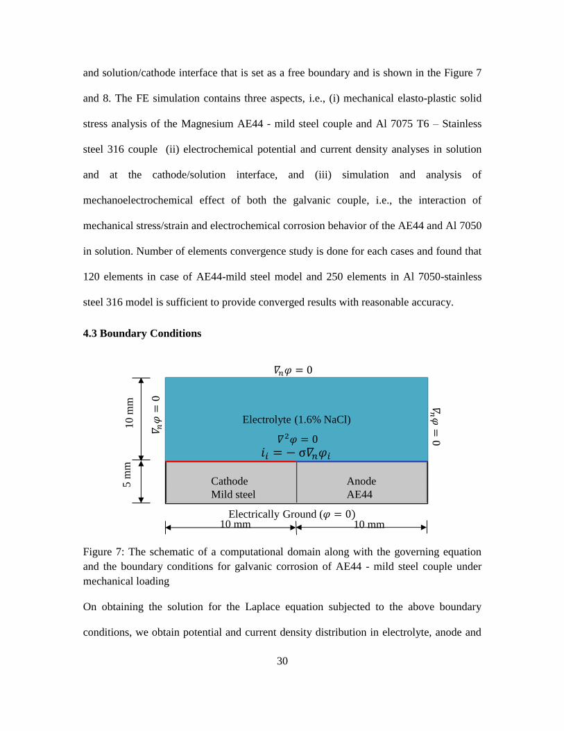
7: The Schematic of a Computational Domain along with the Governing Equation and the
Boundary Conditions for Galvanic Corrosion of AE44 - Mild Steel Couple under
Mechanical Loading .................................................................................................. 30
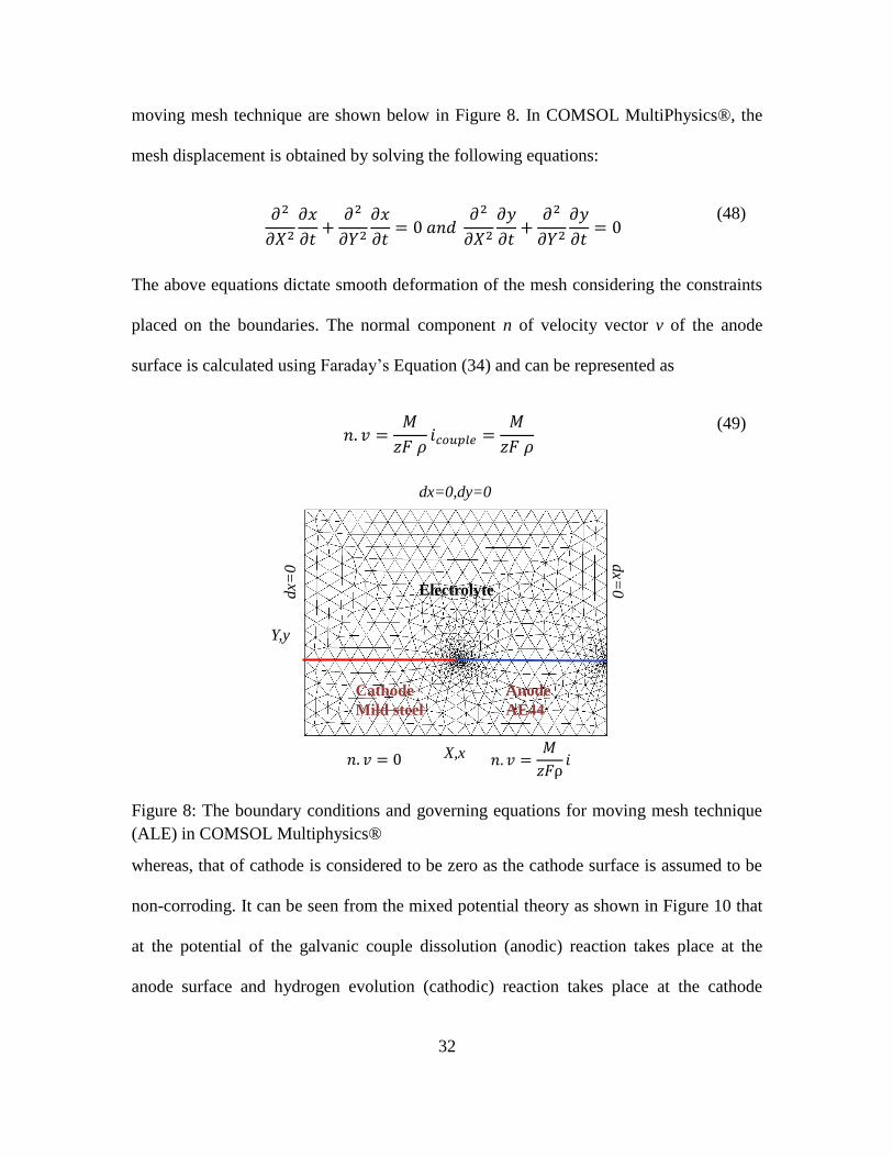
8: The Boundary Conditions and Governing Equations for Moving Mesh Technique
(ALE) in COMSOL Multiphysics® .......................................................................... 32
x
Figure Page
Figure 9: (a) The Schematic of a Computational Domain along with the Governing
Equation and the Boundary Conditions, (b) Cross Section of a Corroded Galvanic
Couple (Deshpande 2010a), (c) Surface Plot of Electrolyte Potential Gradient for
AE44–Mild Steel Galvanic Couple When Exposed to the Electrolyte Solution at t =
3 Days, (d) the Predicted Profile Using the Numerical Model and the Data Obtained
from the Immersion Experiment Conducted by Deshpande, after 3 Days of
Immersion in of 1.6 Wt% NaCl Electrolyte Solution (Electrical Conductivity of 2.5
Sm-1). ......................................................................................................................... 35
10: Polarization Behavior of Magnesium Alloy AE44 and Mild Steel, Reproduced from
(Deshpande 2010a). ................................................................................................... 36
11: The Predicted Surface Profile of Mg Alloy (AE44) from Numerical Model for
Different Electrolyte Thickness of 3% NaCl Concentration at t=3 Days. ................ 39
12: The Spatial Variation of Current Density of AE44-Mild Steel Couple for Different
Electrolyte Thickness of 3% NaCl Concentration. ................................................... 40
13: The Average and Peak Anodic Current Densities are Plotted Against Thickness of
Electrolyte of 3% NaCl Concentration. ..................................................................... 42
14: Surface Plot of Electrolyte Potential Gradient for AE44–mild Steel Galvanic Couple
When Exposed to the Electrolyte Solution of 3% NaCl Concentration with Different
Depth (a) 0.16 mm, (b) 0.64 mm and (c) 1.5 mm and (d) 10 mm. ............................ 44
15: The Predicted Surface Profile of AE44 from Numerical Model for Different
Conductivity of Electrolyte at t=3 Days. ................................................................... 46

xi
Figure Page
16: The Initial Spatial Current Density Variation of AE44–Mild Steel Galvanic Couple
Predicted Using the Numerical Model for Different Conductivity of the
Electrolyte. ............................................................................................................... 48
17: Surface Plot of Electrolyte Potential Gradient for AE44–Mild Steel Galvanic Couple
When Exposed to the Electrolyte Solution with Different NaCl Concentration (a)
0.25%, (b) 1.6% and (c) 10% at t = 3 Days. .............................................................. 50
18: The Predicted Profile Using the Numerical Model of AE44–mild Steel Galvanic
Couple When Exposed to 3% NaCl Electrolyte Solution for 72 Hours with Different
Area Ratios.. .............................................................................................................. 53
19: The Spatial Current Density Distribution for AE44-mild Steel Galvanic Couple When
Exposed to 3% NaCl Electrolyte Solution for Different Cathode to Anode Ratios.
The Area of the Anode is Kept Constant and Cathode Area is Varied to Obtain
Different Area. ........................................................................................................... 54
20: The Average and Peak Anodic Current Densities Are Plotted Against Different Area
Ratios When Exposed to an Electrolyte of 3% NaCl Concentration. ....................... 55
21: The Boundary Conditions for Static Stress Analysis of AE44 and Mild Steel
Couple. ...................................................................................................................... 57
22: The Effective Plastic Strain Distribution on Magnesium Alloy AE44 and Mild Steel
under a Tensile Load of 160 MPa. ............................................................................ 59
23: von Mises Stress Distribution on AE44 and Mild Steel under the Tensile Load. ...... 60

xii
Figure Page
24: The Variation of Plastic Strain and Hydrostatic Stress on the Surface of the Anode
(AE44) Is Plotted along the Distance from the Interface When Subjected to a Load
of 160 MPa. ............................................................................................................... 61
25: The Boundary Conditions and Governing Equations for Computational Domain (a)
and Moving Mesh Technique (ALE) (b) in Comsol Multiphysics® ........................ 62
26: The Depth Profile Predicted for Mg Alloy AE44 Using the Numerical Model for with
and Without Tensile Load of 160 MPa Conditions and Results Obtained from the
Immersion Experiment Conducted by Deshpande, after 3 Days of Immersion in of
1.6 Wt% Nacl Electrolyte Solution (Electrical Conductivity of 2.5 Sm-1). .............. 63
27: The Spatial Current Density Distribution on the Surface of Ae44-mild Steel Galvanic
When Exposed to 1.6% NaCl Electrolyte Solution Couple under Tensile Load
of 160 MPa and No Load Condition ......................................................................... 64
28: The Contour Plot of Norm Current Density Distribution on AE44–mild Steel
Galvanic Couple with (a) and Without (b) Tensile Load of 160 MPa, When Exposed
to the Electrolyte Solution of 1.6 % NaCl Concentration at t = 3 Days. ................... 65
29: The Contour Plot of Electrolyte Potential Distribution for AE44–Mild Steel Galvanic
Couple with (a) and without (b) Tensile Load of 160 MPa, When Exposed to the
Electrolyte Solution of 1.6 % NaCl Concentration at t = 3 Days. ............................. 66
30: The Boundary Conditions along with the Governing Equations are Provided in the
above Schematic of Galvanic Corrosion for Aluminum Alloy 7075-T6 and Stainless
Steel 316 Joint under a Tensile Load of 410 MPa. ................................................... 69
xiii
Figure Page
31: The Plastic Strain Distribution (a) and von Mises Stress Distribution (b) on
Aluminum Alloy 7075-T6 and Stainless Steel 316 Joint under a Tensile Load
of 100 Mpa. ............................................................................................................... 69
32: The Change in Total Electrode Thickness is Measured along the Length of the
Corroding Electrode Aluminum Alloy 7075-T6 with and without Tensile Load
of 300 MPa When Exposed to Electrolyte of 3% NaCl for 15 Days. ....................... 70
33: The Electrode Current Density Distribution of Aluminium Alloy 7075-T6 and
Stainless Steel 316 Joint under No Load and a Tensile Load of 300 MPa at
Time t = 15 Days. ...................................................................................................... 71
34: The Variation of Normalized Corrosion Current for Al 7050 T6 with Plastic Strain
Obtained from Polarization Experiment. ................................................................... 72
35: The Electrolyte Potential Distribution with (a) and without (a) Tensile Load of
110mpa at Time T=15 Days. ..................................................................................... 72

1
CHAPTER 1
1. MOTIVATION
Corrosion is a surface phenomenon known as the attack of metals or alloy by their
environment, as air, water or soil in chemical or electrochemical reaction to form more
stable compounds and this can result in structural failure and great economic loss.
Corrosion is a consideration in virtually all engineering applications. Each year,
industries invest time and money into trying to curtail the effects of corrosion. Many
different corrosive environments have been studied and monitored to develop corrosion
control methods (Revie 2011). The corrosion damage of equipment, production facilities,
infrastructure etc has severe consequences, including loss of property, interruption of
production, and outage of electricity, water etc. Such disruptions occur at a very high cost
to society. The corrosion cost is invariably high and was about 5% of U.S GDP(“Cost of
Corrosion Study Overview” 2015). The corrosion process of the metal is accelerated
when electrically coupled to a more noble metal and is known as galvanic corrosion.
As, with the increase in use of metals in all fields of technology, it is inevitable to have
dissimilar metal joints. The majority of aviation, automobile, electronics industries etc are
in the quest to find lighter metals to increase efficiency and performance, dissimilar metal
joints. An example of such effort was in the early 1980s when Volvo conducted a “Light
Component Project”, which resulted in a concept car (Mellde 1985). Galvanic corrosion
is one of the major hurdles to the use of magnesium parts in the automobile industry, and
it has acknowledged as a vital issue if magnesium is used in exterior components in a
vehicle (Isacsson et al. 1997). In many aircraft and aerospace vehicles the dissimilar
2
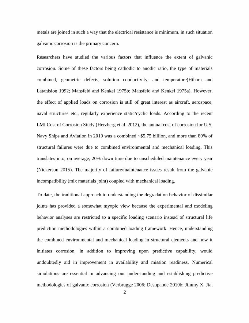
metals are joined in such a way that the electrical resistance is minimum, in such situation
galvanic corrosion is the primary concern.
Researchers have studied the various factors that influence the extent of galvanic
corrosion. Some of these factors being cathodic to anodic ratio, the type of materials
combined, geometric defects, solution conductivity, and temperature(Hihara and
Latanision 1992; Mansfeld and Kenkel 1975b; Mansfeld and Kenkel 1975a). However,
the effect of applied loads on corrosion is still of great interest as aircraft, aerospace,
naval structures etc., regularly experience static/cyclic loads. According to the recent
LMI Cost of Corrosion Study (Herzberg et al. 2012), the annual cost of corrosion for U.S.
Navy Ships and Aviation in 2010 was a combined ~$5.75 billion, and more than 80% of
structural failures were due to combined environmental and mechanical loading. This
translates into, on average, 20% down time due to unscheduled maintenance every year
(Nickerson 2015). The majority of failure/maintenance issues result from the galvanic
incompatibility (mix materials joint) coupled with mechanical loading.
To date, the traditional approach to understanding the degradation behavior of dissimilar
joints has provided a somewhat myopic view because the experimental and modeling
behavior analyses are restricted to a specific loading scenario instead of structural life
prediction methodologies within a combined loading framework. Hence, understanding
the combined environmental and mechanical loading in structural elements and how it
initiates corrosion, in addition to improving upon predictive capability, would
undoubtedly aid in improvement in availability and mission readiness. Numerical
simulations are essential in advancing our understanding and establishing predictive
methodologies of galvanic corrosion (Verbrugge 2006; Deshpande 2010b; Jimmy X. Jia,
3
Song, and Atrens 2006). However, there are few systematic numerical studies in the
literature on simulations of general galvanic corrosion processes, especially, to study the
effect of combined environmental and mechanical loading in galvanic coupled joints.

4
CHAPTER 2
2. LITERATURE REVIEW
Studies by Astley (Astley 1988), Adey and Niku (Adey and Niku 1988) have indicated
that numerical methods are promising for studying galvanic corrosion, and in particular
for predicting the galvanic current density distribution. There is an abundant amount of
analytical work reported in literature to investigate galvanic corrosion. Waber et al.
(Waber and Rosenbluth 1955; Waber 1955; Waber and Fagan 1956) have used linear and
equal corrosion kinetics (equal polarization parameter) for semi-infinite and parallel
anode and cathode surfaces. This work has been extended by Kennard and Waber
(Kennard and Waber 1970), by using unequal and linear polarization parameters for
anode and cathode surfaces and McCafferty (McCafferty 1977) has applied these unequal
and linear polarization parameters to circular systems. Galvanic corrosion over semi-
infinite coplanar surfaces has been investigated by Verbrugge (Verbrugge 2006) using
the conformal mapping technique. Lately, Song (Song 2010) has developed an analytical
approach to examine the galvanic corrosion in some practical applications such as steel–
aluminium joint exposed to bio-fuel, galvanic couple with corrosion inhibitors such as
passive spacer and a scratched organic coating. A numerical model solving the Laplace
and Nernst-Planck equations for a galvanic couple comprised of Al and Al4%Cu, has
been reported by Murer et al (Murer et al. 2010). They have compared model predictions
for current density with those obtained using Scanning Vibrating Electrode Technique
(SVET). Most of the numerical modelling work reported in the literature employs
boundary element method based commercial software called BEASY. Jia et al. (J. X. Jia,

5
Song, and Atrens 2007) have recently studied the influence of geometrical factors on the
galvanic current distribution for the magnesium alloy AZ91D coupled to steel was
investigated using a Boundary Element Method (BEM) model and experimental
measurements. All the above mentioned work considers stationary anode and cathode
surfaces. During galvanic corrosion, however, the corrosion rate is at its peak at the
junction of the galvanic couple and it decreases along the distance away from the junction
due to IR drop. Hence, the corroding material moves faster near the junction, resulting in
pit formation. Simulation of the movement of the corroding material requires explicit
tracking of the anodic interface. Bharadwaj et al. reported a methodology where the
governing equation for the electric potential was solved iteratively over a computational
domain varying due to galvanic corrosion. The new co-ordinates of the domain were
manually calculated on the basis of the corrosion rate/interface velocity. Arbitrary
Langrangian Eulerian (ALE) application mode in COMSOL Multi-Physics®, which is
capable of explicitly tracking the moving interface is used to determine the corrosion rate
and corroded surface profile of anode by Kiran B. Deshpande(Deshpande 2010b). The
numerical model results has already been compared to experimentally namely SVET
(Scanning Vibrating Electrode Technique) and the immersion technique by
Deshpande(Deshpande 2010a)(Deshpande 2010b). Galvanic corrosion of zinc and
aluminum coatings coupled with mild steel was simulated by Cross et al. using a time-
dependent finite element model (Cross, Gollapudi, and Schuh 2014). They obtained good
agreements with experimental measurements of open circuit potential without
considering any external mechanical load.
6
Xu and Cheng studied the effect of tensile load on steel pipeline corrosion for geometries
with initial defects(Xu and Cheng 2012b), (Xu and Cheng 2013). Moreover, effect of
defects with different simple geometries on distribution of local potential and current
density have been simulated using FEM and compared with experimental results (Xu and
Cheng 2014). They concluded that the mechanical-electrochemical interaction has
insignificant effect on corrosion rate under elastic deformation. Nevertheless, plastic
deformation at the defect, which can be considered as a local galvanic cell, can increase
the local activity of corrosion significantly and cause more stress concentration at the
defect. However, there has been no numerical study on effect of plastic deformation on
chemical processes involved in galvanic corrosion with explicitly tracking anodic
electrode dissolution in electrolyte. For this purpose, in the present work, we extend
Deshpande’s work to see the effect of loading and other factors such as area ratio,
electrolyte depth and conductivity on the galvanic corrosion rate and surface profile of
corroded anode. Initially, we replicate the Deshpande’s validated numerical
model(Deshpande 2010b) and then the mechanical-electrochemical interaction is
incorporated to the numeric model to see the effect of loading on rate of corrosion.
7
CHAPTER 3
3. INTRODUCTION
3.1 The Concept of Galvanic Corrosion:
This section gives a brief discussion about the basic concepts of galvanic corrosion and
electrochemical process involved in galvanic corrosion.
3.1.1 Definition
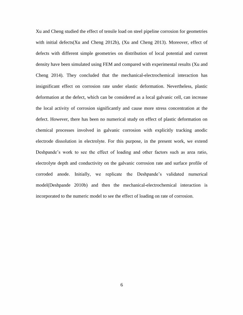
Bimetallic corrosion occurs when two metals, with different potentials, are in electrical
contact while immersed in an electrically conducting corrosive liquid, because the metals
have different natural potentials in the liquid, a current will flow from the anode (more
electronegative) metal to the cathode (more electropositive), which will increase the
corrosion on the anode. In general the corrosion which occur are similar to those that
would occur on single, uncoupled metal, but the rate of attack is increased depending on
the potential difference.
Figure 1: Schematic of Galvanic Corrosion

8
Figure 2: Galvanic series where metals are ranked on the basis of the potential they
exhibit in seawater at 2.4–4 m s−1 for 5–15 days at 5–30 °C, as taken from ASTM
G82(“ASTM G82 - 98(2014) Standard Guide for Development and Use of a Galvanic
Series for Predicting Galvanic Corrosion Performance” 2015)

9
Figure 3: Galvanic corrosion after 1000 hours salt spray test in laboratory where stainless
steel bolts have been screwed into an anodized aluminum block.
3.1.2 Fundamental Requirements
The main conditions required for galvanic corrosion
1. Potential difference between dissimilar materials (or other conductors, such a
graphite).
2. Electrical contact between dissimilar materials for electron transport (can be
direct contact or a secondary connection such as a common grounding path).
3. Exposure to conductive medium for ionic transport
Figure 4: The galvanic corrosion of stainless steel cable ladder with mild steel bolts used
in naval ships when exposed to actual atmospheric conditions for a period of 6 months (a)
and the galvanic corrosion of aluminum with stainless steel screws after 6 month
exposure at the Atmospheric Test Site, Corrosion Laboratory, and NASA(“KSC
Corrosion Technology Laboratory -- Galvanic Corrosion” 2015).
(a) (b)
10
3.1.3 Affecting Factors
Major Factors Affecting the rate of corrosion are
1. Electrode Potential: The value of the potential for any alloy, even in sea water, can
be changed by a variety of factors such as temperature, velocity, biocide treatment
etc. However, the relative ranking (Shown in the fig) of alloys remains largely
unchanged by these factors.
2. Electrode Efficiency: Some metals, such as titanium, are not very efficient at
reducing dissolved oxygen compared with copper alloys. eg cathode efficiency of
Ti and Cu alloys in reducing O2
or H2+
despite titanium being much more
electropositive.
3. Electrolyte: Electrolyte factors that have a major influence on bimetallic corrosion
are composition, pH and, in particular, electrical conductivity, which affects both
the intensity and distribution of corrosion, preferred PH for galvanic corrosion is
very small or very large (ie PH >> 7 or PH << 7).
4. Variable Potential: Polarization.
5. Area Ratio: The larger the cathode compared to the anode, the more oxygen
reduction can occur and, hence, the greater the galvanic current and, therefore,
corrosion.
6. Aeration and flow rate: The majority of practical situations involving bimetallic
corrosion arise in aqueous solutions under conditions where the cathodic reaction
is reduction of dissolved oxygen. As with single metal corrosion, bimetallic
11
corrosion is therefore partly dependent upon the rate at which oxygen can diffuse
to the surface from the bulk of the electrolyte.
7. Metallurgical condition and composition: In some cases differences in corrosion
potential can exist between coupled metals or alloys of nominally the same
composition. Subjection to cold working often tends to make a metal/alloy more
anodic. In some alloys heat treatment can produce galvanic differences.
3.2 Transport in Solution
During corrosion processes, species need to move around or be transported in solution. It
can be said that under some conditions the rate of corrosion depends on the speed of the
transport process. In galvanic corrosion, two transport processes occur, namely diffusion
and migration.
3.2.1 Diffusion:
Diffusion is a process where species move under the action of concentration gradient.
This process involves species moving from high to low concentration until even
concentration is achieved for all species. Two states of diffusion will be discussed, the
steady-state and the non-steady state.
The steady-state diffusion occurs when there is no change in the concentration of reactant
with time. The flux or flow of reactants under steady-state conditions can be represented
by Fick’s first law of diffusion(Fontana 1986).
𝐽(𝑥) = −𝐷𝑑𝐶(𝑥)
𝑑𝑥 (1)

12
where, J(x) is the flux or rate of movement of molecules across a unit area (mol m-2 s-1),
D is the diffusion coefficient (m2s-1), 𝑑𝐶(𝑥)
𝑑𝑥 is the concentration gradient. In this equation,
a negative sign is used because the diffusion occurs from a higher to a lower
concentration area.
The second type of diffusion is the non-steady or transient state. This is a process where
the concentration of species at any point changes with time. In this case, Fick’s second
law of diffusion applies:
𝜕𝐶
𝜕𝑡= −𝐷
𝜕2𝐶
𝜕𝑡2 (2)
3.2.2 Migration
Migration is the process where charged species are transported due to a local electrical
voltage gradient that exists over a distance in the solution, known as the potential
gradient:
𝑃𝑜𝑡𝑒𝑛𝑡𝑖𝑎𝑙 𝑔𝑟𝑎𝑑𝑖𝑒𝑛𝑡 =
𝑉
𝑥
(3)
where, V is the potential and x is the distance.
In this process, ions move or migrate due to a static electrical force depending on its
charge. The flux of ions due to migration is given by the equation below:
𝑀𝑖𝑔𝑟𝑎𝑡𝑖𝑜𝑛 𝑓𝑙𝑢𝑥 = 𝑧𝐹𝐷𝜐𝐶(𝑥)
𝑅𝑇 (4)
13
where, z is the charge on the ion, F is Faraday’s constant (96485 C mol-1), D is the
diffusion coefficient, R is the gas constant (8.314 J mol-1 K-1), T is the absolute
temperature (298 K), v is ion velocity, C(x) is the ion concentration.
Another transport process is convection, but we assume the conductive electrolyte to be
stationary hence neglect convection. In considering the concentration distribution of
species, the mass balance principle is applied, which states that the total concentration of
material in the system under study must be constant by the law of conservation of mass.
In the system under study, both mass transport and chemical reactions influence the
overall concentration distribution. Combining the effects of diffusion and migration, the
Nernst-Planck equation may be constructed(Perez 2004). The Nernst-Planck equation is a
conservation of mass equation describing the flux of chemical species in a medium under
the influence of an ionic concentration gradient and electrical potential distribution. In the
theory of dilute solution, the transport of aqueous ionic species is governed by the mass
balance equation which describes diffusion under concentration gradient and chemical
reaction. It extends Fick’s First Law of Diffusion for the case where diffusing particles
are influenced by electrostatic force. If the diffusing particles are themselves charged,
they influence the electric field on moving. The potential distribution therefore acts to
ensure that the solution remains close to electroneutrality at all points throughout the
domain. Regions of non-electroneutrality may exist in reality at interfaces with other
materials where static charges exist, but these regions are not explicitly considered. The
behavior of each species in solution is therefore governed by the Nernst-Planck law for
the case where electroneutrality is enforced.

14
3.2.3 Nernst-Planck Equation
Transport of species i can be represented by Nernst-Planck equation as,
𝑁𝑖 = 𝐷𝑖𝛻𝑐𝑖 − 𝑧𝑖𝐹𝑢𝑖𝑐𝑖𝛻𝜑 + 𝑐𝑖𝑉
(5)
where, 𝑁𝑖 is the flux, D is the diffusion coefficient, 𝑐𝑖 is the concentration of the species,
zi is the charge, F is the Faraday constant and 𝑢𝑖 is the mobility of species i, respectively
and φ is the electric potential and V is the velocity of solvent/electrolyte. In the above
equation, species flux is equated with the three additive fluxes associated with diffusion,
migration and convection.
The conservation of flux of species i can be written as,
𝜕𝑐𝑖
𝜕𝑡= −𝐷𝑖𝛻2𝑐𝑖 − 𝑍𝑖𝐹𝑢𝑖𝛻. (𝑐𝑖𝛻𝜙) + 𝛻. (𝑐𝑖𝑉) (6)
In the model, electroneutrality of the solution is assumed everywhere. The potential, V,
governed by Poisson’s equation, states:
𝛻2𝑉 =𝜎
𝜀 (7)
where, 𝜎 - charge density, 𝜀 - permittivity of the electrolyte. In this case, the excess
charge density is assumed to be zero at all points due to the assumption of
electroneutrality. Therefore as found by Sharland (Sharland, Jackson, and Diver 1989), it
is permissible to replace the Poisson’s equation by the equation of local charge neutrality,
∑ 𝑧𝑖[𝑖]𝑥 = 0
𝑖
(8)

15
where, [𝑖]𝑥is the concentration of species i at position x in the pit.
3.2.3 Nernst Equations
The First Law of Thermodynamics states that during a chemical reaction in an isolated
system, energy is conserved. The energy may be converted from one form to another.
The tendency of a reaction to proceed in a given direction can be explained through the
Gibbs free energy, G. The change in free energy ΔG is determined solely through the
initial and final states of the system. Reactions can proceed spontaneously only if the
total Gibbs free energy of the system decreases which means the free energy of the
reactants must be greater than the free energy of the products.
𝛥𝐺 = ∑𝜇𝑝𝑟𝑜𝑑𝑢𝑐𝑡𝑠 − ∑𝜇𝑟𝑒𝑎𝑐𝑡𝑎𝑛𝑡𝑠 (9)
where, 𝜇 is the chemical potential. Hence, if ΔG = 0 the reaction tends to proceed
spontaneously in the given direction; if ΔG=0 the reaction tends to proceed spontaneously
in the reverse direction and if ΔG=0, the reaction is in equilibrium which means it will
not have tendency to proceed in either direction.
Electrochemical cells generate electrical energy as a result of electrochemical reactions
and reactions can only proceed if the change in free energy ΔG=0,
𝛥𝐺 = 𝛥𝐺0 + 𝑅𝑇𝑙𝑛 (
𝑝𝑟𝑜𝑑𝑢𝑐𝑡 𝑜𝑓 𝑎𝑐𝑡𝑖𝑣𝑖𝑡𝑖𝑒𝑠 𝑜𝑓 𝑟𝑒𝑎𝑐𝑡𝑎𝑛𝑡𝑠
𝑝𝑟𝑜𝑑𝑢𝑐𝑡 𝑜𝑓 𝑎𝑐𝑡𝑖𝑣𝑖𝑡𝑖𝑒𝑠 𝑜𝑓 𝑝𝑟𝑜𝑑𝑢𝑐𝑡𝑠)
(10)
Considering a simple electrode reaction under equilibrium conditions
16
𝑂 + 𝑛𝑒− ⥦ 𝑅 (11)
Where O is the oxidized species, R the reduced species, and n is the number if electrons
associated with the reaction. If all the components of the reaction are in the standard
state, then the standard electrode potential for the reaction is defined by
𝜑𝑒𝑞0 = −∆𝐺0 /𝑛𝐹 (12)
where, ∆G0 is the Gibbs free energy for the reaction .
𝜑𝑒𝑞 = 𝜑𝑒𝑞
0 −𝑅𝑇
𝑧𝐹𝑙𝑛 (
𝑝𝑟𝑜𝑑𝑢𝑐𝑡 𝑜𝑓 𝑎𝑐𝑡𝑖𝑣𝑖𝑡𝑖𝑒𝑠 𝑜𝑓 𝑟𝑒𝑎𝑐𝑡𝑎𝑛𝑡𝑠
𝑝𝑟𝑜𝑑𝑢𝑐𝑡 𝑜𝑓 𝑎𝑐𝑡𝑖𝑣𝑖𝑡𝑖𝑒𝑠 𝑜𝑓 𝑝𝑟𝑜𝑑𝑢𝑐𝑡𝑠)
(13)
Equation (13) is the Nernst equation, used to describe the potential variation of the
electrode reaction at the equilibrium. The potential of the electrode changes according to
the concentration of the reduced and oxidized species.
𝜑𝑒𝑞 = 𝜑𝑒𝑞
0 −𝑅𝑇
𝑧𝐹𝑙𝑛 (
𝑝𝑟𝑜𝑑𝑢𝑐𝑡 𝑜𝑓 𝑎𝑐𝑡𝑖𝑣𝑖𝑡𝑖𝑒𝑠 𝑜𝑓 𝑟𝑒𝑎𝑐𝑡𝑎𝑛𝑡𝑠
𝑝𝑟𝑜𝑑𝑢𝑐𝑡 𝑜𝑓 𝑎𝑐𝑡𝑖𝑣𝑖𝑡𝑖𝑒𝑠 𝑜𝑓 𝑝𝑟𝑜𝑑𝑢𝑐𝑡𝑠)
(14)
Substituting into the equation above the gas constant, R = 8.314 J mol-1 K-1, the absolute
temperature T = 298 K and the Faraday’s constant F = 96485 Cmol-1, the equation below
is obtained
𝜑c,𝑒𝑞 = 𝜑c,𝑒𝑞
0 +0.0592
𝑧𝑙𝑛 (
𝑝𝑟𝑜𝑑𝑢𝑐𝑡 𝑜𝑓 𝑎𝑐𝑡𝑖𝑣𝑖𝑡𝑖𝑒𝑠 𝑜𝑓 𝑟𝑒𝑎𝑐𝑡𝑎𝑛𝑡𝑠
𝑝𝑟𝑜𝑑𝑢𝑐𝑡 𝑜𝑓 𝑎𝑐𝑡𝑖𝑣𝑖𝑡𝑖𝑒𝑠 𝑜𝑓 𝑝𝑟𝑜𝑑𝑢𝑐𝑡𝑠)
(15)

17
3.3 Kinetics Involved in Corrosion Process
3.3.1 Butler-Volmer Kinetics
Thermodynamics explains the concept of corrosion tendency, but it does not give any
idea on rate of corrosion, which is measured by kinetics principles. In practice we are
interested in the rate at which the corrosion reaction is taking place. The rate of a
chemical reaction can be defined as the number of moles of atoms reacting per unit time
and per unit surface of an electrode. In the case of an electrochemical reaction, which
involves charge transfer, the rate of reaction (corrosion) is calculated in terms of
equivalent current or charge transfer rate, which can presented by equation below
𝑖 = 𝑛𝐹𝑣 (16)
where, i is current density of charge-transfer (Am-2), n is number of mole of electron, F is
Faraday’s constant (96485 C mol-1), V is rate of reaction (mols-1m-2). Applying this
formula to the oxidation-reduction reaction representative of the corrosion of any metal at
equilibrium
𝑅𝑒𝑑 ⇋ 𝑂𝑋 + 𝑛𝑒+ (17)
When this reaction equilibrium is disturbed by either anodic or cathodic polarization, the
reaction rates are given by Arrhenius law.
𝐴𝑛𝑜𝑑𝑖𝑐 𝑟𝑒𝑎𝑐𝑡𝑖𝑜𝑛 𝑟𝑎𝑡𝑒: 𝑘𝑟𝑒𝑑𝐶𝑟𝑒𝑑𝑒𝑥𝑝
(−𝛥𝐺𝑎∗)
𝑅𝑇
(18)
18
𝐶𝑎𝑡ℎ𝑜𝑑𝑖𝑐 𝑟𝑒𝑎𝑐𝑡𝑖𝑜𝑛 𝑟𝑎𝑡𝑒: 𝑘𝑜𝑥𝐶𝑜𝑥𝑒𝑥𝑝
(−𝛥𝐺𝑐∗)
𝑅𝑇
(19)
𝛥𝐺𝑎∗ = 𝛥𝐺𝑎𝑐ℎ − 𝛼𝑛𝐹𝜂 (20)
𝛥𝐺𝑐∗ = 𝛥𝐺𝑐𝑐ℎ + (1 − 𝛼)𝑛𝐹𝜂 (21)
Where 𝑘𝑟𝑒𝑑 and 𝑘𝑜𝑥 are reduction and oxidation reaction rate constants respectively, 𝐶𝑟𝑒𝑑
and 𝐶𝑜𝑥 are concentrations of reacting species, 𝛥𝐺𝑎∗ and 𝛥𝐺𝑐∗ are activation energies of
anodic and cathodic reactions respectively, R is the gas constant and T is the temperature
in Kelvin (K). The electrochemical Gibbs energy of activation can be decomposed into
the Gibbs chemical activation energy 𝛥𝐺𝑐𝑐ℎ (which does not depend on the potential)
and electrical energy of charge transfer. The 𝜂 represents the change in potential at the
metal-electrolyte interface(𝛥𝐸 = 𝐸 − 𝐸𝑟𝑒𝑣), and 𝛼 is the coefficient of charge transfer (0
< 𝛼 < 0), which reflects the ratio of charge transfer between the two partial reactions,
anodic and cathodic. The reaction rates can be expressed by the anodic and cathodic
current densities, given below,
𝑖𝑎 = 𝑧𝐹 𝑘𝑟𝑒𝑑𝐶𝑟𝑒𝑑exp (−
𝛥𝐺𝑐𝑐ℎ
𝑅𝑇) 𝑒𝑥𝑝 (
𝛼𝑛𝐹𝜂
𝑅𝑇)
(22)
𝑖𝑐 = 𝑧𝐹 𝑘𝑜𝑥𝐶𝑜𝑥exp (−
𝛥𝐺𝑐𝑐ℎ
𝑅𝑇) 𝑒𝑥𝑝 (−
(1 − 𝛼)𝑛𝐹𝜂
𝑅𝑇)
(23)
For a reversible electrode at equilibrium, the current density becomes the exchange
current density, that is
19
𝑖𝑜 = 𝑧𝐹 𝑘𝑟𝑒𝑑𝐶𝑟𝑒𝑑 exp (−
𝛥𝐺𝑐𝑐ℎ
𝑅𝑇) = 𝑧𝐹 𝑘𝑜𝑥𝐶𝑜𝑥exp (−
𝛥𝐺𝑐𝑐ℎ
𝑅𝑇)
(24)
𝑖𝑜 = 𝑧𝐹 𝑘𝑟𝑒𝑑𝐶𝑟𝑒𝑑 exp (−
𝛥𝐺𝑐𝑐ℎ
𝑅𝑇) = 𝑧𝐹 𝑘𝑜𝑥𝐶𝑜𝑥exp (−
𝛥𝐺𝑐𝑐ℎ
𝑅𝑇)
(25)
𝑖 = 𝑖𝑎 − 𝑖𝑐 = 𝑖𝑜 [𝑒𝑥𝑝 (
𝛼𝑛𝐹
𝑅𝑇(𝐸 − 𝐸𝑟𝑒𝑣)) − 𝑒𝑥𝑝 (−
(1 − 𝛼)𝑛𝐹
𝑅𝑇(𝐸 − 𝐸𝑟𝑒𝑣))]
(26)
The equation (above add number) is called Butler-Volmer equation for an electrode
reaction. This relation between current density and overpotential is valid only when
reaction is governed only by charge transfer, and concentration polarization has no
effect(Revie 2008).
3.3.2 Polarization Curves
The kinetics of the electrochemical reactions at the interface between electrodes and
electrolyte can be quantified by current-potential curves, also known as polarisation
curves shown in Figure below. These curves are expressed as Butler-Volmer relations
between current density and over potential. When at equilibrium, the anodic and cathode
currents are equal to each other and no net current flows through the system (electrode),
i.e. the over potential is zero.
𝑖0 = |𝑖𝑎| = |𝑖𝑐| (27)
3.3.3 Tafel Slope Constants
When there is sufficient overpotential, the anodic or cathode current becomes negligible
depending upon whether the over potential is positive or negative respectively(Kear and
Walsh 2005). When η is anodic, that is positive, the second term in the Butler-Volmer
20
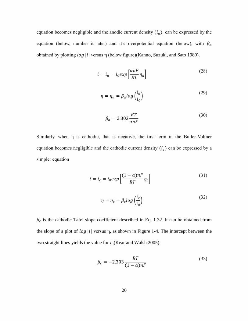
equation becomes negligible and the anodic current density (𝑖𝑎) can be expressed by the
equation (below, number it later) and it’s overpotential equation (below), with 𝛽𝑎
obtained by plotting 𝑙𝑜𝑔 |𝑖| versus η (below figure)(Kanno, Suzuki, and Sato 1980).
𝑖 = 𝑖𝑎 = 𝑖0𝑒𝑥𝑝 [
𝛼𝑛𝐹
𝑅𝑇𝜂𝑎]
(28)
𝜂 = 𝜂𝑎 = 𝛽𝑎𝑙𝑜𝑔 (
𝑖𝑎
𝑖0)
(29)
𝛽𝑎 = 2.303
𝑅𝑇
𝛼𝑛𝐹
(30)
Similarly, when η is cathodic, that is negative, the first term in the Butler-Volmer
equation becomes negligible and the cathodic current density (𝑖𝑐) can be expressed by a
simpler equation
𝑖 = 𝑖𝑐 = 𝑖0𝑒𝑥𝑝 [
(1 − 𝛼)𝑛𝐹
𝑅𝑇𝜂𝑐]
(31)
𝜂 = 𝜂𝑐 = 𝛽𝑐𝑙𝑜𝑔 (
𝑖𝑐
𝑖0)
(32)
𝛽𝑐 is the cathodic Tafel slope coefficient described in Eq. 1.32. It can be obtained from
the slope of a plot of 𝑙𝑜𝑔 |𝑖| versus η, as shown in Figure 1-4. The intercept between the
two straight lines yields the value for 𝑖0(Kear and Walsh 2005).
𝛽𝑐 = −2.303
𝑅𝑇
(1 − 𝛼)𝑛𝐹
(33)

21
3.3.4 Corrosion Rate from Current Density
The rate of corrosion can be calculated from current density using Faraday’s law(Tait
1994)
𝐶𝑅 =
𝑀
𝑧𝐹 𝜌𝑖𝑐𝑜𝑢𝑝𝑙𝑒
(34)
Where M is the molar mass of the corroding species, z electron number, F is the
Faraday’s constant, ρ is the density of the corroding species and icouple is the galvanic
current density in Am-2.
3.4 Effect of Mechanical Load on Galvanic Corrosion
As mentioned in the previous section, studying interaction of mechanical loading and
corrosion process leading to failure of material will be a particular focus in this research.
From a thermodynamic aspect, Gibbs function always grows with respect to increase in
the excessive pressure absolute value for an initially undeformed solid under compression
of tension. Each process of compression or tension can be considered as consisting of two
independent processes – one resulting in thermoelastic effects (low energy) and the other
responsible for strength properties of crystal (high energy). The first term can be
neglected as a higher order term in Gibbs function. It is shown that the hydrostatic part of
stress tensor affects the local value of the chemical potential of a certain point
independently of the direction of mechanical loading and that with an increase in
hydrostatic pressure, the mechanochemical activity is increased as well (Gutman 1994).

22
It is observed that elastic deformation caused by an external load decreases the
equilibrium electrical (electrode) potential of system with positive ions (𝜑𝑎,𝑒𝑞0 ) by
(Gutman 1994),
∆𝜑𝑎,𝑒𝑞
𝑒 = −∆𝑃𝑉𝑚
𝑧𝐹
(35)
where ∆𝜑𝑎,𝑒𝑞𝑒 is equilibrium potential shift of anode due to elastic deformation, Vm is
molar volume of the electrode, z is charge number, F is Faraday’s constant and ΔP is
magnitude of hydrostatic stress. Under plastic deformation, however, the change in
electrical potential can be governed by effective plastic strain εp (Gutman 1994),
∆𝜑𝑎,𝑒𝑞
𝑝 = −𝑇𝑅
𝑧𝐹𝑙𝑛 (
𝜐𝛼
𝑁0𝜀𝑝 + 1)
(36)
where ∆𝜑𝑎,𝑒𝑞𝑝
is equilibrium potential shift of anode due to plastic deformation, T is
absolute temperature, R is ideal gas constant (8.314 J/mol K), υ is the orientation-
dependent factor, α is a constant coefficient of 109 - 1011 cm-2 and N0 is the initial
dislocation density (Shintani et al. 2010; Klimanek and Pötzsch 2002)(Barlat et al. 2002)
before plastic deformation. Therefore, the overall equilibrium potential of anodic reaction
under continuous elasto-plastic deformation becomes (Gutman 1994),
𝜑𝑎,𝑒𝑞 = 𝜑𝑎,𝑒𝑞
0 −∆𝑃𝑉𝑚
𝑧𝐹−
𝑇𝑅
𝑧𝐹𝑙𝑛 (
𝜐𝛼
𝑁0𝜀𝑝 + 1)
(37)
We can assume that in case of metal dissolution, only the anodic current is affected by
the mechanical load directly. The above equations can be used in the governing equations
to couple the electrochemical and me process.

23
During plastic deformation, particularly, in the stage of strain hardening, the density of
mobile dislocations is increased with the increasing stress by activation of new
dislocations. The density of new dislocations, ΔN, is calculated (Gutman 1998)
𝛥𝑁 = 𝑁0[𝑒𝑥𝑝 (
𝑛𝛥𝜏
𝛼𝑘𝑁𝑚𝑎𝑥𝑇) − 1]
(38)
where N0 is the initial density of dislocations prior to plastic deformation, Δτ is the
hardening intensity, n is the number of dislocations in a dislocation pile-up, α is a
coefficient of 109–1011 cm−2, k is Boltzmann constant, Nmax is the maximum dislocation
density, and T is temperature. The plastic strain at the hardening stage can be expressed
by:
𝜀𝑝 =
𝑁0
𝛼𝜈[𝑒𝑥𝑝 (
𝑛𝛥𝜏
𝛼𝑘𝑁𝑚𝑎𝑥𝑇) − 1]
(39)
Figure 5: Schematic of equilibrium potential variation along the free surface of a
microstructure with plastic deformation in corrosive solution.
The theory illustrated by Gutman through Evans diagram, where a mechanical
deformation can lead to a redistribution of electrochemical heterogeneities and increasing

24
area for cathodic reaction. Moreover, an increase of slip steps, micro-cracks and surface
defects generated during plastic deformation would reduce the activation energy of
hydrogen evolution(Gutman 1994). The mechanoelectrochemical effect on cathodic
reaction can be described by:
𝑖𝑐 = 𝑖0,𝑐 (10
𝑚𝑖𝑠𝑒𝑠𝑉𝑚6𝐹(−𝑏𝑣) )
(40)
3.5 Galvanic Corrosion Rate Measurement
The measurement of corrosion is very essential and there are numerous ways to measure
the corrosion rate. Few of the methods employed in the work are mentioned below.
3.5.1 Immersion Experiment
Weight loss measurements:
The simplest way of measuring the corrosion rate of a metal is to expose the sample to
the test medium (e.g. sea water) and measure the loss of weight of the material as a
function of time. Although these tests are simple, there is no simple way to extrapolate
the results to predict the lifetime of the system under investigation.
Depth profiling:
In this method, the sample is exposed to the test medium (electrolyte) for a certain
duration and then the depth of corrosion is measured. There are various techniques to
measure the depth of corrosion, Auger Electron Spectroscopy (AES), Secondary Ion
Mass Spectrometry (SIMS), X-ray Photoelectron Spectroscopy (XPS) are few of the
many techniques.

25
3.5.2 Electrochemical Tests
Polarization Curves or Mixed Potential Theory:
As, galvanic corrosion works like a battery, the corrosion rates can be calculated by using
Faraday’s law as mentioned in Equation (40). Hence, we need to determine the galvanic
corrosion current. When reaction mechanisms for the corrosion reaction are known, the
corrosion currents can be calculated using Tafel Slope Analysis and a plot of log I versus
E is called a Tafel plot. The relationship between current density and potential of anodic
and cathodic electrode reactions under charge transfer control is given by the Butler-
Volmer equation. The Butler-Volmer relationship for current density is based on the
identifying the anodic and cathodic reactions that are taking place on each electrode. At
the equilibrium potential (zero overpotential) the anodic and cathodic currents are equal;
this point is known as the exchange current. However, when the overpotential is not equal
to zero, the anodic and cathodic currents are different. The current densities and tafel
slope constants are obtained by the Equations (27-33). The point of intersection of
anodic branch of an alloy with a lower Ecorr and cathodic branch of an alloy with a
higher Ecorr represents the corrosion potential and the current density of the galvanic
couple. Corrosion rate prediction obtained using this method is fairly accurate
when Ecorr of the constituent alloys are more than approximately 120 mV apart depending
on the slopes of the polarization curves, as reported by Hihara et al (Hihara and
Latanision 1992) and Hack (Baboian 2005) have previously used the mixed potential
theory approach in order to investigate galvanic corrosion of various couples using
sectional electrode technique.
26
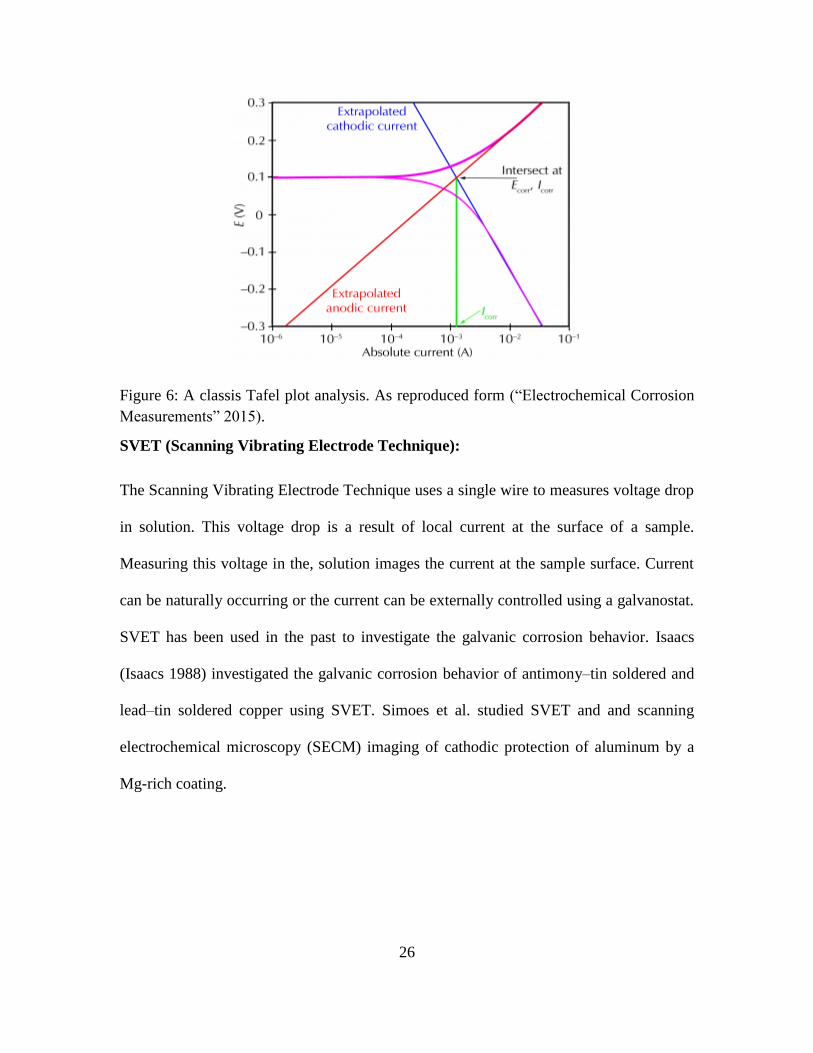
Figure 6: A classis Tafel plot analysis. As reproduced form (“Electrochemical Corrosion
Measurements” 2015).
SVET (Scanning Vibrating Electrode Technique):
The Scanning Vibrating Electrode Technique uses a single wire to measures voltage drop
in solution. This voltage drop is a result of local current at the surface of a sample.
Measuring this voltage in the, solution images the current at the sample surface. Current
can be naturally occurring or the current can be externally controlled using a galvanostat.
SVET has been used in the past to investigate the galvanic corrosion behavior. Isaacs
(Isaacs 1988) investigated the galvanic corrosion behavior of antimony–tin soldered and
lead–tin soldered copper using SVET. Simoes et al. studied SVET and and scanning
electrochemical microscopy (SECM) imaging of cathodic protection of aluminum by a
Mg-rich coating.
27
CHAPTER 2
4. METHODLOGY
4.1 Governing Equations
Transport of species i can be represented by Nernst-Planck equation as,
𝑁𝑖 = 𝐷𝑖𝛻𝑐𝑖 − 𝑧𝑖𝐹𝑢𝑖𝑐𝑖𝛻𝜑 + 𝑐𝑖𝑉 (41)
where, 𝑁𝑖 is the flux, D is the diffusion coefficient, 𝑐𝑖 is the concentration of the species,
zi is the charge, F is the Faraday constant and 𝑢𝑖 is the mobility of species i, respectively
and φ is the electric potential and V is the velocity of solvent/electrolyte. In the above
equation, species flux is equated with the three additive fluxes associated with diffusion,
migration and convection.
The conservation of flux of species i can be written as,
𝜕𝑐𝑖
𝜕𝑡= −𝐷𝑖𝛻2𝑐𝑖 − 𝑍𝑖𝐹𝑢𝑖𝛻. (𝑐𝑖𝛻𝜙) + 𝛻. (𝑐𝑖𝑉)
(42)
Now in the simplest case the following assumptions are made to simplify
1. Electrolyte solution is well mixed: no concentration gradient exists in the electrolyte
solution.
2. The solvent is incompressible: divergent of velocity leads to zero.
3. The solution is electro-neutral.
4. Dissolution reaction takes place at the anode surface whereas hydrogen evolution
reaction takes place at the cathode surface (which can be validated from the polarization
28
curves and the mixed potential theory). Thus, cathode surface is assumed to be not
corroding.
With the above assumptions, Equation (36) becomes:
𝛻2𝜑 = 0 (43)
The above equation takes the form of the Laplace equation for the electric potential and
represents the upper bound for the rate of corrosion, as transport by convection and by
diffusion are neglected (Verbrugge 2006).
Eq. above is solved over the electrolyte domain subject to boundary conditions, as shown
schematically in Fig. 4. The boundary conditions at the anode and the cathode surfaces
are vital in order to predict the correct corrosion rates. The polarization data obtained
experimentally for individual alloys (Fig. 2 and Fig. 3) are used as the boundary
condition for the anode and the cathode surfaces. The following boundary condition is
applied at the anode surface as shown in figure below
The general equations for defining distribution of current field in a solution during
electrochemical reactions are:
𝛻𝜙 = −
𝑓(𝜑)
(44)
where σ is the electrical conductivity of the electrolyte solution and 𝑓(𝜙) is the current
density of anodic (lower Ecorr) species. 𝑓(𝜑) is a piecewise linear interpolation function
which is obtained from the polarization curve (potential and current density data) of the
anodic species. The potential gradient is obtained by dividing the current density value
(corresponding to the potential field at anode and cathode) by the conductivity of the
29
electrolyte solution. Thus, the model is capable of handling non-linear boundary
conditions using a piecewise linear interpolation approach.
𝑖𝑖 = − 𝛻𝜑𝑖 (45)
4.2 Model and Finite Element Method
A finite element model is employed to solve the Laplace equation, Equation (43) using
boundary condition for an electrochemical process. The boundary conditions are given in
Figure 7 and 8. We use COMSOL Multiphysics® to solve the both electrochemical and
solid mechanics problem. COMSOL has a special module called Corrosion module
where a Corrosion Secondary interface can be chosen. It describes the current and
potential distributions in a corrosion cell under the assumption that the variations in
composition in the electrolyte are negligible. The interface can be combined with
interfaces modeling mass transport to describe concentration dependent (tertiary) current
distributions. The interfaces also describe how the geometry of the cell is affected due to
the deposition/dissolution of species on the electrodes. In COMSOL we couple the solid
mechanics module with the Corrosion module using multiphysics coupling field
technique. The mesh type used was triangular and an adaptive mesh refinement technique
was selected. A plane stain approximation and large plastic strain plasticity model with
isotropic hardening is used for solid mechanics problem. A solver of MUMPS (multi-
frontal massively parallel sparse) was selected for solution. In order to ensure reliability
of the FE modelling, all initial conditions were obtained from experimental tests or
accredited theoretical calculations (Deshpande 2010a). The boundary condition of
solution is that the solution boundary is electrically isolated, except the solution/anode
30
and solution/cathode interface that is set as a free boundary and is shown in the Figure 7
and 8. The FE simulation contains three aspects, i.e., (i) mechanical elasto-plastic solid
stress analysis of the Magnesium AE44 - mild steel couple and Al 7075 T6 – Stainless
steel 316 couple (ii) electrochemical potential and current density analyses in solution
and at the cathode/solution interface, and (iii) simulation and analysis of
mechanoelectrochemical effect of both the galvanic couple, i.e., the interaction of
mechanical stress/strain and electrochemical corrosion behavior of the AE44 and Al 7050
in solution. Number of elements convergence study is done for each cases and found that
120 elements in case of AE44-mild steel model and 250 elements in Al 7050-stainless
steel 316 model is sufficient to provide converged results with reasonable accuracy.
4.3 Boundary Conditions
Figure 7: The schematic of a computational domain along with the governing equation
and the boundary conditions for galvanic corrosion of AE44 - mild steel couple under
mechanical loading
On obtaining the solution for the Laplace equation subjected to the above boundary
conditions, we obtain potential and current density distribution in electrolyte, anode and
Anode
AE44
Cathode
Mild steel
Electrically Ground (
Electrolyte (1.6% NaCl)
10 mm 10 mm
10 m
m5
mm

31
cathode surfaces. Corrosion rate or interface velocity can then be calculated from current
density using Eq. (4). The ALE method is employed to incorporate the moving interface
during corrosion.
The general equations for defining distribution of current field in a solution during
electrochemical reactions are:
𝛻𝑖𝑖 = 𝑄𝑖 (46)
Since galvanic corrosion works like a battery, Faraday’s law applies. Hence it possible to
calculate the rate at which the metal is consumed at the anode
𝐶𝑅 =
𝑀
𝑧𝐹 𝜌𝑖𝑐𝑜𝑢𝑝𝑙𝑒
(47)
Where M is the molar mass of the corroding species, z is the electron number, F is the
faraday’s constant, ρ is the density of the corroding species and 𝑖𝑐𝑜𝑢𝑝𝑙𝑒 is the intensity of
coupling current.
4.4 Arbitrary Langrangian Eulerian (ALE) Method
ALE method is a moving mesh technique which enjoys the advantages of both Eulerian
and Langrangian frames of reference and can capture greater deformation with higher
resolution(Donea et al. 2004). ALE method comprises of two frames: a reference frame
with X, Y co-ordinates for a 2-D formulation and a spatial frame with x, y co-ordinates.
The reference frame has fixed co-ordinates while the spatial frame has co-ordinates
moving with time, subject to boundary conditions. We incorporate the ALE method using
COMSOL MultiPhysics®. The geometry and boundary conditions considered for this
32
moving mesh technique are shown below in Figure 8. In COMSOL MultiPhysics®, the
mesh displacement is obtained by solving the following equations:
𝜕2
𝜕𝑋2
𝜕𝑥
𝜕𝑡+
𝜕2
𝜕𝑌2
𝜕𝑥
𝜕𝑡= 0 𝑎𝑛𝑑
𝜕2
𝜕𝑋2
𝜕𝑦
𝜕𝑡+
𝜕2
𝜕𝑌2
𝜕𝑦
𝜕𝑡= 0
(48)
The above equations dictate smooth deformation of the mesh considering the constraints
placed on the boundaries. The normal component n of velocity vector v of the anode
surface is calculated using Faraday’s Equation (34) and can be represented as
𝑛. 𝑣 =
𝑀
𝑧𝐹 𝜌𝑖𝑐𝑜𝑢𝑝𝑙𝑒 =
𝑀
𝑧𝐹 𝜌
(49)
Figure 8: The boundary conditions and governing equations for moving mesh technique
(ALE) in COMSOL Multiphysics®
whereas, that of cathode is considered to be zero as the cathode surface is assumed to be
non-corroding. It can be seen from the mixed potential theory as shown in Figure 10 that
at the potential of the galvanic couple dissolution (anodic) reaction takes place at the
anode surface and hydrogen evolution (cathodic) reaction takes place at the cathode
X,x
Cathode
Mild steel
Anode
AE44
Electrolyte
dx=0,dy=0
dx=
0d
x=0
Y,y
33
surface. There are positive and negative current densities associated with anodic and
cathodic reactions, respectively. If the cathode boundary is also moved using the
equivalent boundary condition as applied to the anode surface, it depicts deposition
where cathode boundary is moved into the electrolyte solution due to negative current
density. In order to capture the realistic scenario of hydrogen evolution reaction where no
material is lost or accumulated, the cathode surface is assumed to be non-corroding.
34
CHAPTER 5
5. RESULTS
5.1 Galvanic Corrosion without Loading
Here we replicate the results from Deshpande’s work(Deshpande 2010b) on AE44
(Magnesium alloy) and mild steel galvanic couple exposed to 1.6 wt% NaCl solution, so
as to keep it as a base model and extend work on it. In his work, he has compared his
numerical model results with that of mixed potential theory and experimental results
based on immersion technique and SVET. The electric potential,𝐸𝑐𝑜𝑢𝑝𝑙𝑒 and the current
density,𝑖𝑐𝑜𝑢𝑝𝑙𝑒 of the galvanic couple are estimated from the intersection of the two
polarization curves of the individual constituent alloys. Deshpande (Deshpande 2010b)
modeled the electrodes (cathode and corroding anode) just as a moving line element but
here we model the electrodes as an entire 2 D block so as to apply load and to see the
effect of loading (strain) on galvanic corrosion. The current density of the galvanic
couple is a critical parameter since it forms the basis for corrosion rate estimation using
Faraday’s law (Tait 1994). The input for the simulations are obtained from the
polarization curves shown before in Figure 6. , and standard electrochemical properties
are used for AE44 and mild steel.
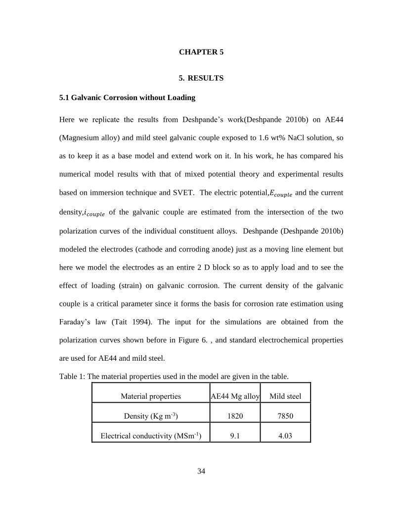
Table 1: The material properties used in the model are given in the table.
Material properties AE44 Mg alloy Mild steel
Density (Kg m-3) 1820 7850
Electrical conductivity (MSm-1) 9.1 4.03
35
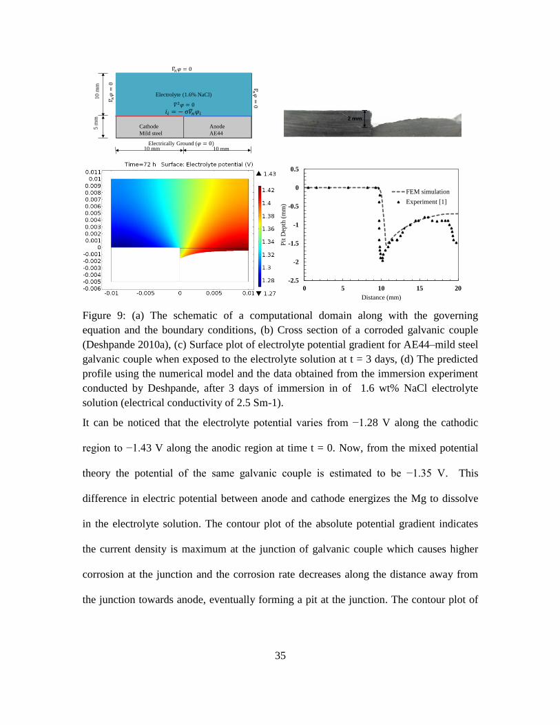
Figure 9: (a) The schematic of a computational domain along with the governing
equation and the boundary conditions, (b) Cross section of a corroded galvanic couple
(Deshpande 2010a), (c) Surface plot of electrolyte potential gradient for AE44–mild steel
galvanic couple when exposed to the electrolyte solution at t = 3 days, (d) The predicted
profile using the numerical model and the data obtained from the immersion experiment
conducted by Deshpande, after 3 days of immersion in of 1.6 wt% NaCl electrolyte
solution (electrical conductivity of 2.5 Sm-1).
It can be noticed that the electrolyte potential varies from −1.28 V along the cathodic
region to −1.43 V along the anodic region at time t = 0. Now, from the mixed potential
theory the potential of the same galvanic couple is estimated to be −1.35 V. This
difference in electric potential between anode and cathode energizes the Mg to dissolve
in the electrolyte solution. The contour plot of the absolute potential gradient indicates
the current density is maximum at the junction of galvanic couple which causes higher
corrosion at the junction and the corrosion rate decreases along the distance away from
the junction towards anode, eventually forming a pit at the junction. The contour plot of
-2.5
-2
-1.5
-1
-0.5
0
0.5
0 5 10 15 20P
it D
epth
(m
m)
Distance (mm)
FEM simulation
Experiment [1]
Anode
AE44
Cathode
Mild steel
Electrically Ground (
Electrolyte (1.6% NaCl)
10 mm 10 mm
10 m
m5
mm

36
electric potential of our model matches exactly as that of Deshpande’s(Deshpande 2010b)
as seen in Figure 9c.
Figure 10: Polarization behavior of Magnesium alloy AE44 and mild steel, reproduced
from (Deshpande 2010a).
Table 2: The peak current density and corrosion rate obtained is compared with the work
in literature.
Galvanic
Couple
Mixed Potential
Theory
Deshpande (1D, line
electrode)
ALE (2D electrodes)
Current
density
(Am-2)
Corrosion
rate
Current
density
(Am-2)
Corrosion
rate
Current
density
(Am-2)
Corrosion
rate
mm
y-1
nm
s-1
mm
y-1
nm
s-1
mm
y-1
nm
s-1
AE44–
mild
steel
96.05 231 7.33 87.35 210 6.67 87.05 209 6.64
The initial peak current density at the anodic region as predicted by the numerical model
is 87.05 Am−2 and the current density gradually decreases to around 31 A m−2 away from
the junction towards anode. The galvanic current density predicted by the mixed
37
potential theory is about 96 A m−2. The peak current density predicted at the junction of
from ALE is comparable with that of mixed potential theory (current is measured by
Scanning Vibrating Electrode Technique). The rate of corrosion values obtained by
modelling the entire electrodes is compared with that of Deshpande’s model(Deshpande
2010b) and experiment(Deshpande 2010a) and is tabulated in the Table 2. The profile of
the anode surface for AE44–mild steel couple after 3 days of constant exposure to the
electrolyte solution is shown in Figure 8a. It can be seen that a 1.6 mm deep pit at the
AE44 side of the galvanic couple is predicted by the numerical model which is compared
with results obtained from the immersion test, which is around 2 mm.
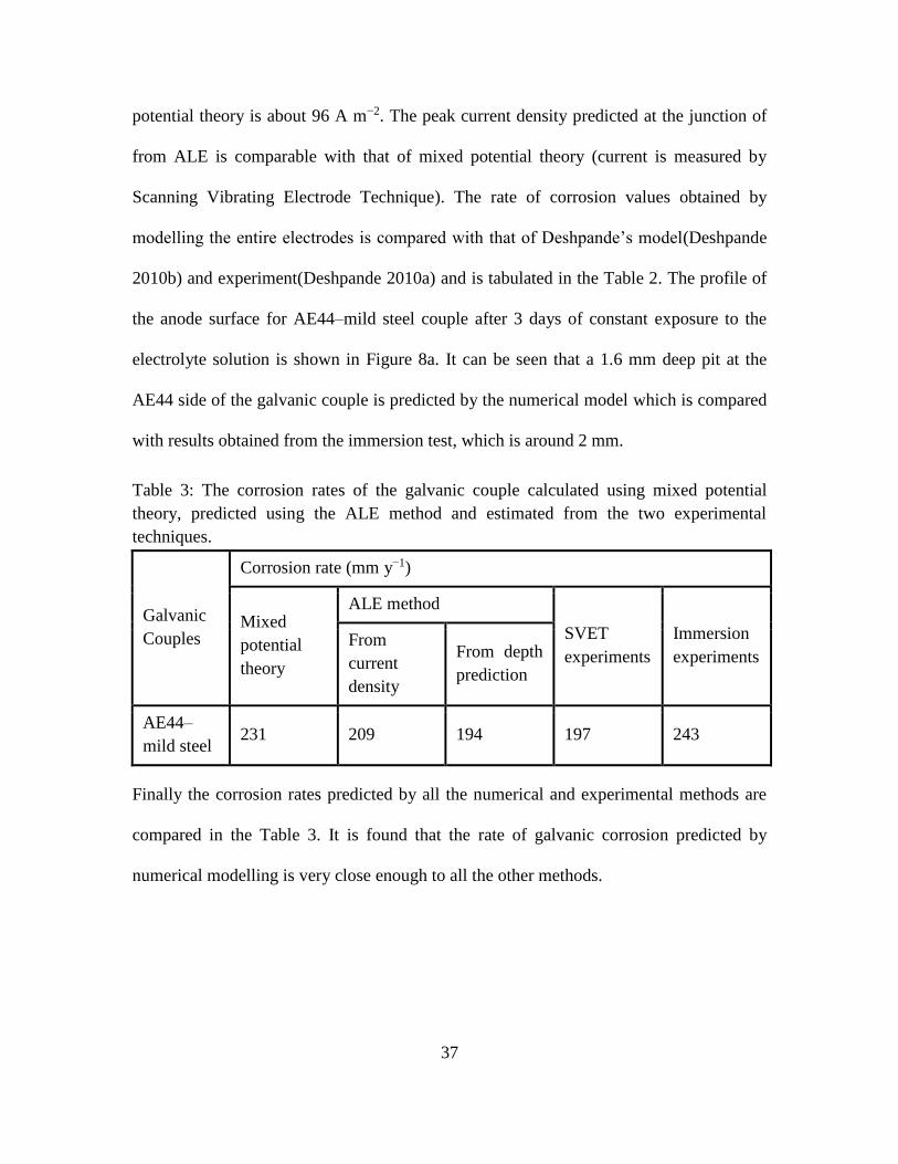
Table 3: The corrosion rates of the galvanic couple calculated using mixed potential
theory, predicted using the ALE method and estimated from the two experimental
techniques.
Galvanic
Couples
Corrosion rate (mm y−1)
Mixed
potential
theory
ALE method
SVET
experiments
Immersion
experiments From
current
density
From depth
prediction
AE44–
mild steel 231 209 194 197 243
Finally the corrosion rates predicted by all the numerical and experimental methods are
compared in the Table 3. It is found that the rate of galvanic corrosion predicted by
numerical modelling is very close enough to all the other methods.

38
5.2 Effect of Electrolyte Depth
If there is only a limited amount of electrolyte, the composition of the electrolyte may
significantly change as a result of electrochemical reactions. One important solution
factor is the thickness of thin-layer electrolytes, which is encountered in atmospheric
environments. The thickness of an electrolyte affects corrosion processes in several
different ways. First, it affects the lateral resistance of the electrolyte and, thus, affects the
potential and current distribution across the surface of the coupled metals. Second, it
affects the transport rate of oxygen across the electrolyte layer and, thus, the rate of
cathodic reaction. Third, it changes the volume and the solvation capacity of the
electrolyte and, thus, affects the formation of corrosion products.
One parameter that can easily be varied is the thickness of the electrolyte film. The effect
of electrolyte depth on galvanic corrosion is investigated using the numerical model
while maintaining equal surface area of both AE44 and mild steel and the conductivity of
electrolyte is maintained at 2.5 Sm-1 (1.6% NaCl). The electrolyte thickness is varied
from 0.16 mm to 10 mm. The depth profile obtained from numerical model solution for
different electrolyte thickness is shown below in the Figure 11.
39
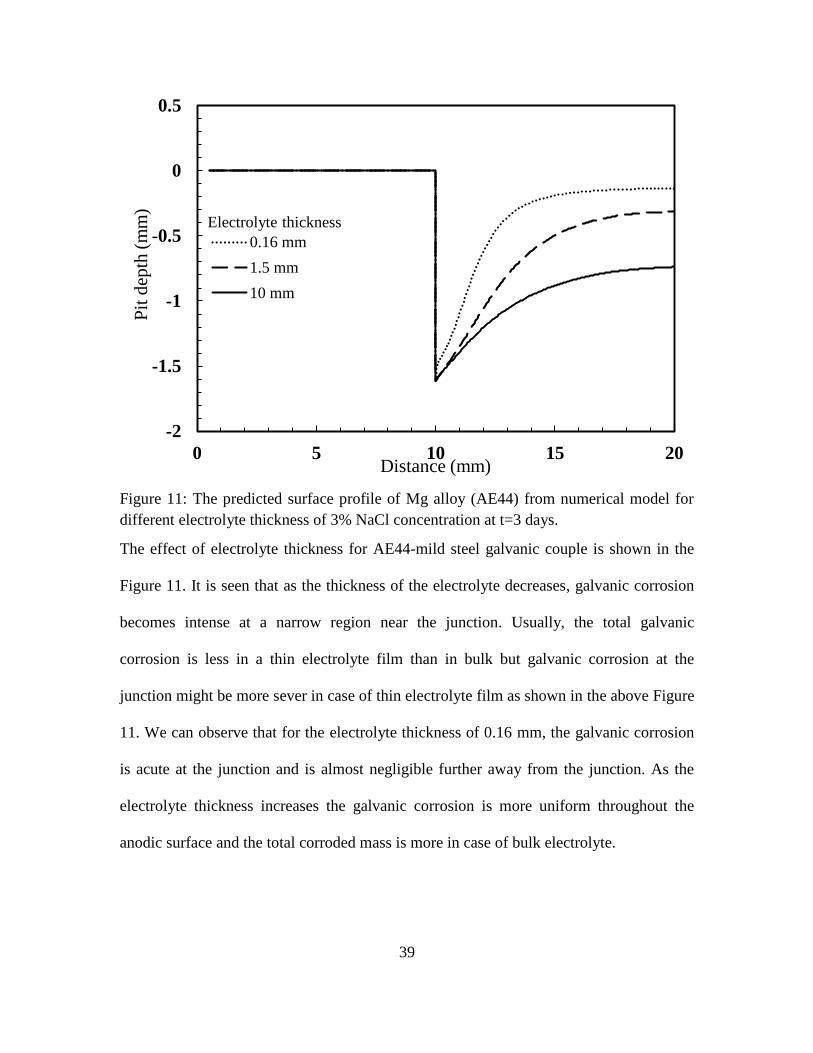
Figure 11: The predicted surface profile of Mg alloy (AE44) from numerical model for
different electrolyte thickness of 3% NaCl concentration at t=3 days.
The effect of electrolyte thickness for AE44-mild steel galvanic couple is shown in the
Figure 11. It is seen that as the thickness of the electrolyte decreases, galvanic corrosion
becomes intense at a narrow region near the junction. Usually, the total galvanic
corrosion is less in a thin electrolyte film than in bulk but galvanic corrosion at the
junction might be more sever in case of thin electrolyte film as shown in the above Figure
11. We can observe that for the electrolyte thickness of 0.16 mm, the galvanic corrosion
is acute at the junction and is almost negligible further away from the junction. As the
electrolyte thickness increases the galvanic corrosion is more uniform throughout the
anodic surface and the total corroded mass is more in case of bulk electrolyte.
-2
-1.5
-1
-0.5
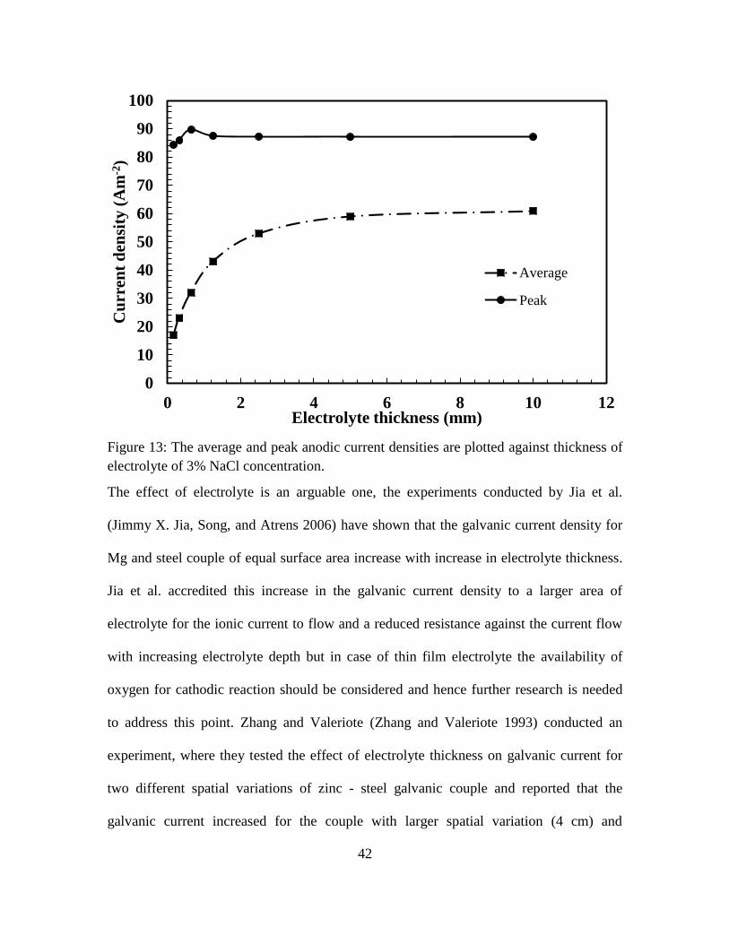
0
0.5
0 5 10 15 20
Pit
dep
th (
mm
)
Distance (mm)
0.16 mm
1.5 mm
10 mm
Electrolyte thickness
40
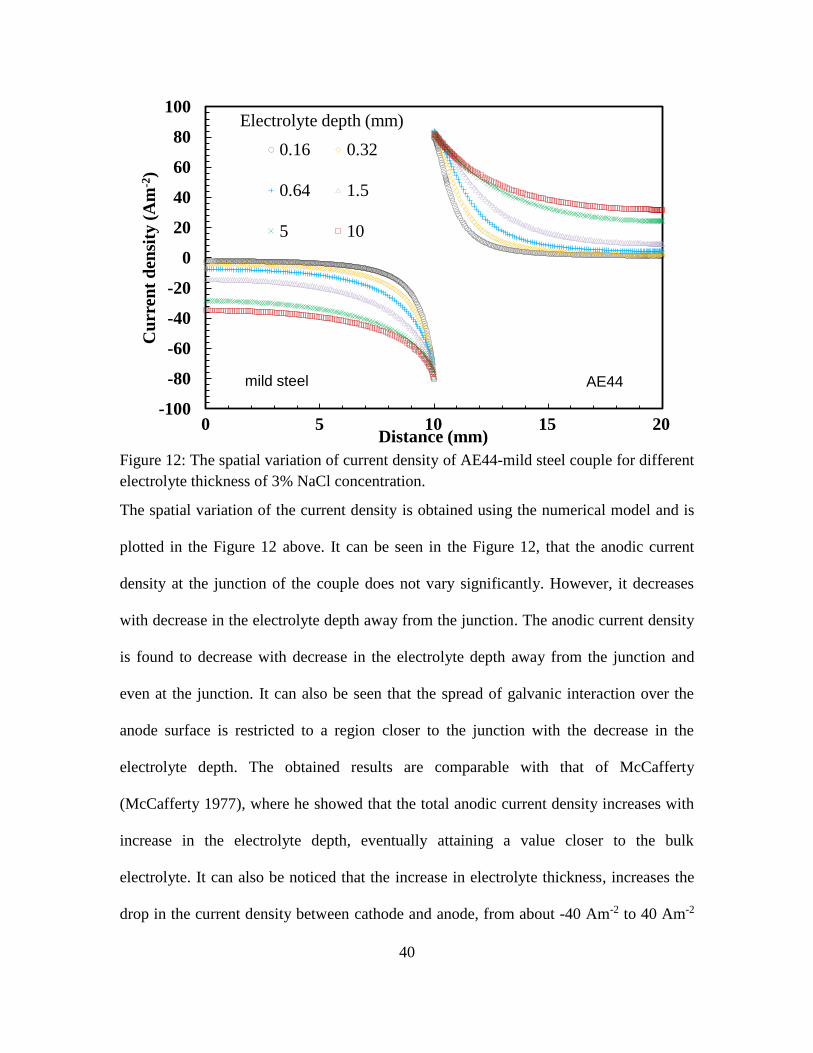
Figure 12: The spatial variation of current density of AE44-mild steel couple for different
electrolyte thickness of 3% NaCl concentration.
The spatial variation of the current density is obtained using the numerical model and is
plotted in the Figure 12 above. It can be seen in the Figure 12, that the anodic current
density at the junction of the couple does not vary significantly. However, it decreases
with decrease in the electrolyte depth away from the junction. The anodic current density
is found to decrease with decrease in the electrolyte depth away from the junction and
even at the junction. It can also be seen that the spread of galvanic interaction over the
anode surface is restricted to a region closer to the junction with the decrease in the
electrolyte depth. The obtained results are comparable with that of McCafferty
(McCafferty 1977), where he showed that the total anodic current density increases with
increase in the electrolyte depth, eventually attaining a value closer to the bulk
electrolyte. It can also be noticed that the increase in electrolyte thickness, increases the
drop in the current density between cathode and anode, from about -40 Am-2 to 40 Am-2
-100
-80
-60
-40
-20
0
20
40
60
80
100
-10 -5 0 5 10
Cu
rren
t d
ensi
ty (
Am
-2)
Distance (mm)
0.16 0.32
0.64 1.5
5 10
Electrolyte depth (mm)
AE44mild steel
-2.5
-2
-1.5
-1
-0.5
0
0.5
0 5 10 15 20
Pit
Dep
th (
mm
)
Distance (mm)
Experiment (Deshpande 2010)
Tensile load (160 Mpa)
No Load
41
for 10 mm electrolyte thickness and about -5 Am-2 to 5Am-2 for thin film electrolyte
(0.16 mm thickness), which results in higher overall corrosion.
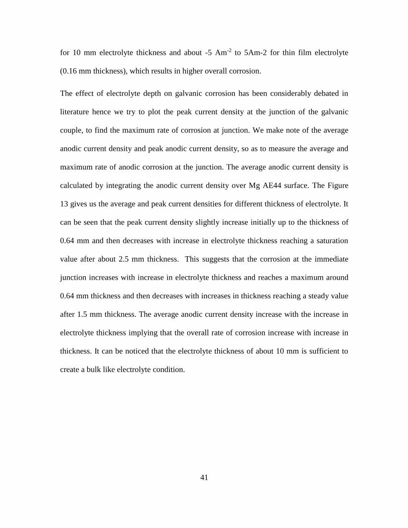
The effect of electrolyte depth on galvanic corrosion has been considerably debated in
literature hence we try to plot the peak current density at the junction of the galvanic
couple, to find the maximum rate of corrosion at junction. We make note of the average
anodic current density and peak anodic current density, so as to measure the average and
maximum rate of anodic corrosion at the junction. The average anodic current density is
calculated by integrating the anodic current density over Mg AE44 surface. The Figure
13 gives us the average and peak current densities for different thickness of electrolyte. It
can be seen that the peak current density slightly increase initially up to the thickness of
0.64 mm and then decreases with increase in electrolyte thickness reaching a saturation
value after about 2.5 mm thickness. This suggests that the corrosion at the immediate
junction increases with increase in electrolyte thickness and reaches a maximum around
0.64 mm thickness and then decreases with increases in thickness reaching a steady value
after 1.5 mm thickness. The average anodic current density increase with the increase in
electrolyte thickness implying that the overall rate of corrosion increase with increase in
thickness. It can be noticed that the electrolyte thickness of about 10 mm is sufficient to
create a bulk like electrolyte condition.
42
Figure 13: The average and peak anodic current densities are plotted against thickness of
electrolyte of 3% NaCl concentration.
The effect of electrolyte is an arguable one, the experiments conducted by Jia et al.
(Jimmy X. Jia, Song, and Atrens 2006) have shown that the galvanic current density for
Mg and steel couple of equal surface area increase with increase in electrolyte thickness.
Jia et al. accredited this increase in the galvanic current density to a larger area of
electrolyte for the ionic current to flow and a reduced resistance against the current flow
with increasing electrolyte depth but in case of thin film electrolyte the availability of
oxygen for cathodic reaction should be considered and hence further research is needed
to address this point. Zhang and Valeriote (Zhang and Valeriote 1993) conducted an
experiment, where they tested the effect of electrolyte thickness on galvanic current for
two different spatial variations of zinc - steel galvanic couple and reported that the
galvanic current increased for the couple with larger spatial variation (4 cm) and
0
10
20
30
40
50
60
70
80
90
100
0 2 4 6 8 10 12
Cu
rren
t d
ensi
ty (
Am
-2)
Electrolyte thickness (mm)
Average
Peak

43
decreased for smaller variation (3 mm) with increase in electrolyte thickness. They
attributed this opposite behavior to the fact that the current over the steel surface of the
smaller variation couple was oxygen-diffusion limited and was inversely proportional to
the electrolyte depth, while for the larger spatial variation, the current was not diffusion
limited and depended only on the potential of the steel surface.
Table 4: The potential range, average and peak current densities and corresponding
corrosion rates are tabulated for different electrolyte thickness of 3% NaCl concentration.
Electrolyte thickness (mm)
0.16 0.32 0.64 1.50 5.00 10.00
Minimum Potential (V) -1.10 -1.16 -1.20 -1.24 -1.30 -1.31
Maximum Potential (V) -1.48 -1.47 -1.46 -1.44 -1.42 -1.40
Potential range (V) 0.38 0.31 0.26 0.20 0.12 0.09
Average Current density (Am-2) 17.13 23.25 32.15 43.98 58.06 61.45
Peak Current density (Am-2) 84.37 85.96 89.65 87.86 87.14 87.06
Average Corrosion Rate (mmy-1) 41.25 55.99 77.43 105.92 139.82 147.99
Maximum Corrosion Rate (mmy-1) 203.18 207.01 215.90 211.59 209.86 209.66
The average rate of corrosion increases with the increase in electrolyte thickness
attributing to the increase in galvanic current with increase in area of electrolyte. The
maximum corrosion occurs at region of interface, where the current density is maximum.
The maximum rate of corrosion does not follow a conventional trend, initially it increases
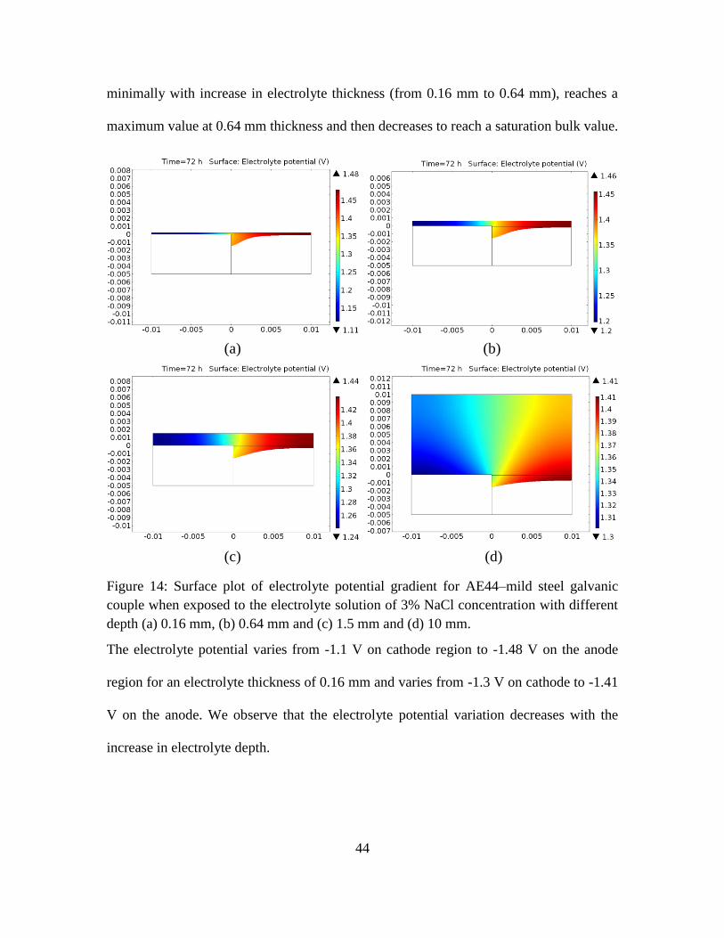
44
minimally with increase in electrolyte thickness (from 0.16 mm to 0.64 mm), reaches a
maximum value at 0.64 mm thickness and then decreases to reach a saturation bulk value.
Figure 14: Surface plot of electrolyte potential gradient for AE44–mild steel galvanic
couple when exposed to the electrolyte solution of 3% NaCl concentration with different
depth (a) 0.16 mm, (b) 0.64 mm and (c) 1.5 mm and (d) 10 mm.
The electrolyte potential varies from -1.1 V on cathode region to -1.48 V on the anode
region for an electrolyte thickness of 0.16 mm and varies from -1.3 V on cathode to -1.41
V on the anode. We observe that the electrolyte potential variation decreases with the
increase in electrolyte depth.
(a) (b)
(c) (d)

45
5.3 Effect of Solution Conductivity
Galvanic action of a bimetallic couple depends on the surface condition of the metals,
which, in turn, is determined by environmental conditions. A metal surface exhibits
different potentials in different electrolytes. A galvanic series provides information on the
polarity of a bimetallic couple but is environment-specific because the relative position of
each metal changes with solution. For instance, the corrosion rates of Magnesium and
mild steel in coupled and uncoupled conditions in several solutions vary. In all the
solutions, galvanic action results in protection of mild steel, but the amount of
Magnesium corrosion varies with solution composition. The difference in the corrosion
rates in magnesium sulfate and sodium sulfate solutions indicates the significant effect of
cations on the reaction kinetics. The conductivity of the electrolyte is a very important
factor because it determines the distribution of galvanic corrosion across the anode
surface. When conductivity is high, as in seawater, the galvanic corrosion of the anodic
metal is distributed uniformly across the surface. As the conductivity decreases, galvanic
corrosion becomes concentrated in a narrow region near the junction as shown below in
Figure 15. Usually, the total galvanic corrosion is less in a poorly conducting electrolyte
than in a highly conducting one.

46
Figure 15: The predicted surface profile of AE44 from numerical model for different
conductivity of electrolyte at t=3 days.
Here, different wt% NaCl solutions are considered to study the effect of conductivity on
galvanic corrosion rate and current density. As the salt concentration in the electrolyte
changes the conductivity of the electrolyte changes, so we vary the salt concentration
from 0.1% to 10% which varies the conductive of the electrolyte from 0.2 Sm-1 to 14 Sm-
1. We consider three different concentration of NaCl solutions, 0.5%, 1.6% and 10 %
which represent conductivity of solution as 0.5 Sm-1, 2.5 Sm-1 and 13.5 Sm-1
respectively(Weast and Ohio) 1975)[S-15 Results™ Test Report™ of Coralife] at 230C
room temperature. The conductivity was measured using a platinic conductivity cell. The
conductivity of a solution also depends upon temperature, hence we maintain standard
room temperature of 230 C or 296 K. The electrolyte thickness is about 10 mm
in order to assume corrosion in bulk electrolyte environment (as discussed in section 5.2,
-2.5
-2
-1.5
-1
-0.5
0
0.5
0 5 10 15 20
Pit
dep
th (
mm
)
Distance (mm)
Conductivity 0.5 S/m
(0.25% NaCl)
Conductivity 2.5 S/m
(1.6% NaCl)
Conductivity 13.5
S/m (10% NaCl)

47
an electrolyte thickness of around 10 mm is sufficient to create bulk like atmosphere for
the modeled couple).
The general trend observed for all electrolyte conductivity is that the galvanic corrosion
is more intense at the junction and then reduces as moved away from the intersection. It
can be seen in the Figure 15, that the overall galvanic corrosion more uniform thought the
length of anode and maximum when the conductivity of the electrolyte is high as in the
case of 10% NaCl solution with a conductivity of 13.5 Sm-1. In the case of low
conductive electrolyte (0.5 Sm-1), the galvanic corrosion is very intense at the proximity
of the junction and drastically reduces as we move away from the junction and can hardly
notice any corrosion away from the junction. It can be observed from the Figure 15, that
the corrosion at the junction is maximum for electrolyte with low conductivity (0.5 Sm-1).
The rate of corrosion at the junction is found to decrease with an increase in electrolyte
conductivity. The Figure 16 gives the initial current density distribution along the
electrode surface which can be used to calculate the initial rate at which the material is
depleted from the surface using Faraday’s equation, Equation (34). It can be seen from
the Figure 16, that the galvanic current distribution is more uniform for electrolyte with
high conductivity and hence we find more uniform corrosion throughout AE44 without
formation of steep pit for high conducting electrolyte (13.5 Sm-1). A sudden leap in the
current density is noticed for the electrolyte with low conductivity (0.5 Sm-1), hence we
can see concentrated corrosion at the junction resulting in a pit.

48
Figure 16: The initial spatial current density variation of AE44–mild steel galvanic
couple predicted using the numerical model for different conductivity of the electrolyte.
The peak anodic current density at the juncture is found to decrease with an increase in
electrolyte conductivity, whereas the average current density throughout the surface of
the anode increase with an increase in electrolyte conductivity. The initial corrosion rate
calculated using initial peak current density on the anode surface (at the junction) are
compared for different cases of electrolyte conductivity (different concentration) in the T
-100
-80
-60
-40
-20
0
20
40
60
80
100
0 5 10 15 20
Cu
rren
t d
ensi
ty (
Am
-2)
Distance (mm)
Conductivity 0.5 S/m
(0.25% NaCl)
Conductivity 2.5 S/m
(1.6% NaCl)
Conductivity 13.5 S/m
(10% NaCl)
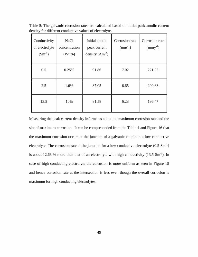
49
Table 5: The galvanic corrosion rates are calculated based on initial peak anodic current
density for different conductive values of electrolyte.
Conductivity
of electrolyte
(Sm-1)
NaCl
concentration
(Wt %)
Initial anodic
peak current
density (Am-2)
Corrosion rate
(nms-1)
Corrosion rate
(mmy-1)
0.5 0.25% 91.86 7.02 221.22
2.5 1.6% 87.05 6.65 209.63
13.5 10% 81.58 6.23 196.47
Measuring the peak current density informs us about the maximum corrosion rate and the
site of maximum corrosion. It can be comprehended from the Table 4 and Figure 16 that
the maximum corrosion occurs at the junction of a galvanic couple in a low conductive
electrolyte. The corrosion rate at the junction for a low conductive electrolyte (0.5 Sm-1)
is about 12.68 % more than that of an electrolyte with high conductivity (13.5 Sm-1). In
case of high conducting electrolyte the corrosion is more uniform as seen in Figure 15
and hence corrosion rate at the intersection is less even though the overall corrosion is
maximum for high conducting electrolytes.

50
Figure 17: Surface plot of electrolyte potential gradient for AE44–mild steel galvanic
couple when exposed to the electrolyte solution with different NaCl concentration (a)
0.25%, (b) 1.6% and (c) 10% at t = 3 days.
It can be observed from the Figure 17, that the electrolyte potential varies from −1.19 V
along the cathodic region to −1.46 V along the anodic region for the case (a) with the
electrolyte conductivity of 0.5 Sm-1 (vitiation of about 0.27 V). The variation of the
electrolyte potential reduces with the increase in electrolyte conductivity as shown in the
Figure 14. The potential varies for -1.27 V to -1.43 V for the case (b) with electrolyte
conductivity of 2.5 Sm-1 and variation further decreases from -1.33 V to -1.39 V for case
(c) with electrolyte conductivity of 13.5 Sm-1. Hence, higher the conductivity of
electrolyte lower the electrolyte potential variation.
(a) (b)
(c)

51
5.4 Effect of Area Ratio
When a piece of metal is freely corroding, the electrons generated at anodic areas flow
through the metal to react at cathodic areas exposed to the environment where they
restore the electrical balance of the system. The fact that there is no net accumulation of
charges on a corroding surface is quite important for understanding most corrosion
processes and ways to mitigate them. However, the absolute equality between the anodic
and cathodic currents expressed in the following equation does not mean that the current
densities for these currents are equal (Roberge, n.d.).
𝐼𝑎𝑛𝑜𝑑𝑖𝑐 = 𝐼𝑐𝑎𝑡ℎ𝑜𝑑𝑖𝑐 (50)
When the Equation (49) is expressed in terms of current densities by considering the
relative anodic (Sa) and cathodic (Sc) surface areas and their associated current densities ia
and ic expressed in units of Am-2, for example, it becomes clear that a difference in the
surface areas occupied by each reaction will have to be compensated by inequalities in
the current densities.
𝐼𝑎𝑛𝑜𝑑𝑖𝑐 = 𝑖𝑎𝑆𝑎 = 𝐼𝑐𝑎𝑡ℎ𝑜𝑑𝑖𝑐 = 𝑖𝑐𝑆𝑐 (51)
𝑖𝑎 = 𝑖𝑐
𝑆𝑐
𝑆𝑎
(52)
The implications of the surface area ratio Sc/Sa (cathode area to anode area) in the last
equation are particularly important in association with various forms of local cell
corrosion such as galvanic corrosion for which a large surface area ratio is a serious
aggravating factor. It is easy to understand that the effect of a certain amount of anodic
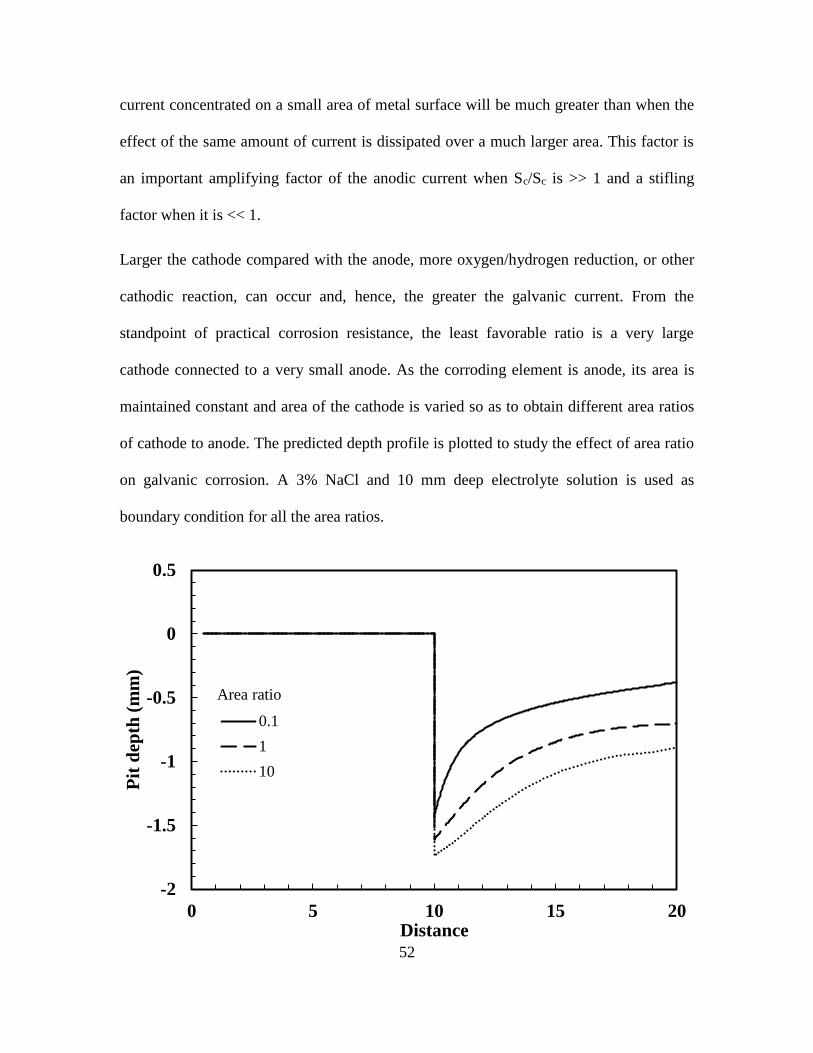
52
current concentrated on a small area of metal surface will be much greater than when the
effect of the same amount of current is dissipated over a much larger area. This factor is
an important amplifying factor of the anodic current when Sc/Sc is >> 1 and a stifling
factor when it is << 1.
Larger the cathode compared with the anode, more oxygen/hydrogen reduction, or other
cathodic reaction, can occur and, hence, the greater the galvanic current. From the
standpoint of practical corrosion resistance, the least favorable ratio is a very large
cathode connected to a very small anode. As the corroding element is anode, its area is
maintained constant and area of the cathode is varied so as to obtain different area ratios
of cathode to anode. The predicted depth profile is plotted to study the effect of area ratio
on galvanic corrosion. A 3% NaCl and 10 mm deep electrolyte solution is used as
boundary condition for all the area ratios.
-2
-1.5
-1
-0.5
0
0.5
0 5 10 15 20
Pit
dep
th (
mm
)
Distance
0.1
1
10
Area ratio

53
Figure 18: The predicted profile using the numerical model of AE44–mild steel galvanic
couple when exposed to 3% NaCl electrolyte solution for 72 hours with different area
ratios. The area of the anode is kept constant and cathode area is varied to obtain different
area ratios.
The obtain results convey that the rate of corrosion of AE44 increases with the increase
in area of the cathode (mild steel) and is very sensitive to change in area. It can be
observed from the above Figure 18, that the percentage (%) change in the thickness of
corroded metal at the metallic intersection (~19% change between 0.1 and 10 area ratio)
is much less when compared to that at the surface further away from the junction (~105
% change between 0.1 and 10 area ratio). We can also observe that the corrosion is
maximum at the interface irrespective of area ratios, hence considering area ratio as a
major factor in overall galvanic corrosion rather than localized corrosion at the junction.
The rate of corrosion at the junction of the couple does not vary as much as overall rate of
corrosion for different area ratios but the overall corrosion is much greater in case of
smaller anode can be further bolstered by observing the spatial current density
distribution shown in Figure 19. The influence of area ratio has been studied previously
by many, Jia et al. (Jimmy X. Jia, Song, and Atrens 2006) have studied the effect of
geometrical factors such as area ratio on galvanic current density of AZ91D Magnesium
alloy- to steel using experimental measurements and a BEM model which is in agreement
with the trend we observe.
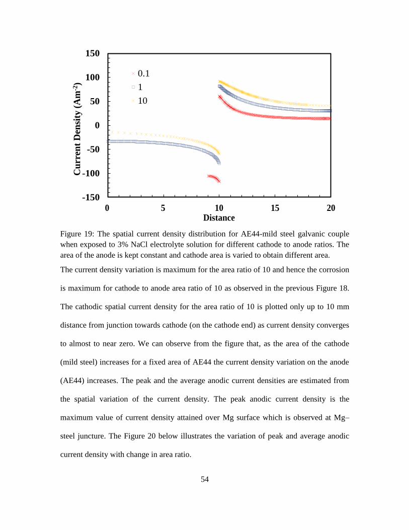
54
Figure 19: The spatial current density distribution for AE44-mild steel galvanic couple
when exposed to 3% NaCl electrolyte solution for different cathode to anode ratios. The
area of the anode is kept constant and cathode area is varied to obtain different area.
The current density variation is maximum for the area ratio of 10 and hence the corrosion
is maximum for cathode to anode area ratio of 10 as observed in the previous Figure 18.
The cathodic spatial current density for the area ratio of 10 is plotted only up to 10 mm
distance from junction towards cathode (on the cathode end) as current density converges
to almost to near zero. We can observe from the figure that, as the area of the cathode
(mild steel) increases for a fixed area of AE44 the current density variation on the anode
(AE44) increases. The peak and the average anodic current densities are estimated from
the spatial variation of the current density. The peak anodic current density is the
maximum value of current density attained over Mg surface which is observed at Mg–
steel juncture. The Figure 20 below illustrates the variation of peak and average anodic
current density with change in area ratio.
-150
-100
-50
0
50
100
150
-10 -5 0 5 10
Cu
rren
t D
ensi
ty (
Am
-2)
Distance (mm)
0.1
1
10
-2
-1.5
-1
-0.5
0
0.5
0 5 10 15 20
Pit
dep
th (
mm
)
Distance
0.1
1
10
Area ratio
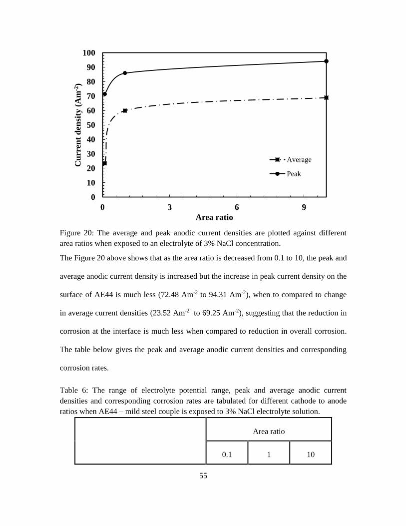
55
Figure 20: The average and peak anodic current densities are plotted against different
area ratios when exposed to an electrolyte of 3% NaCl concentration.
The Figure 20 above shows that as the area ratio is decreased from 0.1 to 10, the peak and
average anodic current density is increased but the increase in peak current density on the
surface of AE44 is much less (72.48 Am-2 to 94.31 Am-2), when to compared to change
in average current densities (23.52 Am-2 to 69.25 Am-2), suggesting that the reduction in
corrosion at the interface is much less when compared to reduction in overall corrosion.
The table below gives the peak and average anodic current densities and corresponding
corrosion rates.
Table 6: The range of electrolyte potential range, peak and average anodic current
densities and corresponding corrosion rates are tabulated for different cathode to anode
ratios when AE44 – mild steel couple is exposed to 3% NaCl electrolyte solution.
Area ratio
0.1 1 10
0
10
20
30
40
50
60
70
80
90
100
0 3 6 9
Cu
rren
t d
ensi
ty (
Am
-2)
Area ratio
Average
Peak
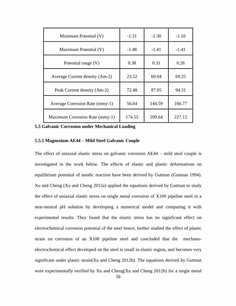
56
Minimum Potential (V) -1.31 -1.30 -1.10
Maximum Potential (V) -1.48 -1.41 -1.41
Potential range (V) 0.38 0.31 0.26
Average Current density (Am-2) 23.52 60.04 69.25
Peak Current density (Am-2) 72.48 87.05 94.31
Average Corrosion Rate (mmy-1) 56.64 144.59 166.77
Maximum Corrosion Rate (mmy-1) 174.55 209.64 227.12
5.5 Galvanic Corrosion under Mechanical Loading
5.5.1 Magnesium AE44 – Mild Steel Galvanic Couple
The effect of uniaxial elastic stress on galvanic corrosion AE44 – mild steel couple is
investigated in the work below. The effects of elastic and plastic deformations on
equilibrium potential of anodic reaction have been derived by Gutman (Gutman 1994).
Xu and Cheng (Xu and Cheng 2012a) applied the equations derived by Gutman to study
the effect of uniaxial elastic stress on single metal corrosion of X100 pipeline steel in a
near-neutral pH solution by developing a numerical model and comparing it with
experimental results. They found that the elastic stress has no significant effect on
electrochemical corrosion potential of the steel hence, further studied the effect of plastic
strain on corrosion of an X100 pipeline steel and concluded that the mechano-
electrochemical effect developed on the steel is small in elastic region, and becomes very
significant under plastic strain(Xu and Cheng 2012b). The equations derived by Gutman
were experimentally verified by Xu and Cheng(Xu and Cheng 2012b) for a single metal

57
corrosion and not galvanic corrosion. In this work, we apply the Gutman (Gutman 1994)
equations and develop a finite element model to study mechano-electrochemical effect on
galvanic corrosion of bimetallic Magnesium alloy AE44 and mild steel couple through
a multiphysics field coupling technique in COMSOL Multiphysics®.
Figure 21: The boundary conditions for static stress analysis of AE44 and mild steel
couple.
Here, the previous 2-D model used to study galvanic corrosion is coupled with
mechanical loading. The electrolyte part of the model is omitted and only the electrodes
are subjected to loading. The two electrodes are (AE44 and mild steel) are assumed to be
bonded together. We perform a stationary mechanical elasto-plastic solid stress analysis
on the galvanic couple. A tensile load of about 160 MPa is applied onto the anode end,
sufficient to cause plastic deformation in Magnesium AE44. The left end of the mild steel
is fixed. The boundary conditions and the dimensions are given in the Figure 21. We use
2-D triangular element with plane stain approximation and large plastic strain plasticity
Anode
AE44
Cathode
Mild steel
Electrolyte (1.6% NaCl)
Fix
ed
10 mm 10 mm
Fo
rce (MP
a)

58
model with isotropic hardening. The adaptive mesh refinement technique was utilized as
it eliminated mesh elongation and smearing to provide a smoother and better mesh
quality and direct (MUMPS) solver was used. The material properties assigned are
tabulated in the Table 6. The plastic strain is very important factor to consider while
studying the mechanoelectrochemical effect on galvanic corrosion given by Gutman’s
equations, Equation (37). Hence, the effective plastic strain and Von-Mises stress are the
main results to be analyzed. The solution obtained for the static study is shown in the
Figure 22 and 23.
Table 7: The material properties of AE44 and mild steel are tabulated (“For Casting
Buyers | AFS - American Foundry Society” 2015).
Material properties AE44 Mg alloy Mild steel
Density (Kg m-3) 1820 7850
Young's modulus (GPa) 45 205
Poisson's ratio 0.33 0.28
Initial yield stress (MPa) 142 470

59
Isotropic tangent modulus (GPa) 3.5 205
Electrical conductivity (MSm-1) 9.1 4.03
It can be observed from the Figure 22 that, only Magnesium alloy AE44 is plastically
deformed at the junction, as yield strength of AE44 (142 MPa from Table 6) is much less
than that of mild steel’s (470 MPa) and moreover while solving the corrosion problem,
we assume that external load on the specimen does not affect the current density in the
cathode and ion activity in the electrolyte, hence we choose a load sufficient enough to
plastically deform Magnesium alloy AE44. Due to the stress concentration at the
electrodes interface, the anode plastically deforms to a greater extent in the vicinity of the
junction and material away from junction is under elastic strain. The deformed anode is
shown in the Figure 22 and 23.
Figure 22: The effective plastic strain distribution on Magnesium alloy AE44 and mild
steel under a tensile load of 160 MPa.
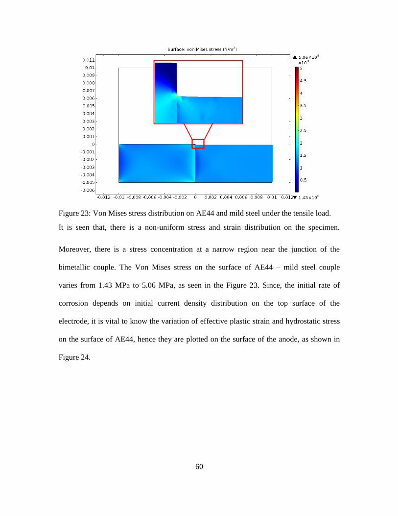
60
Figure 23: Von Mises stress distribution on AE44 and mild steel under the tensile load.
It is seen that, there is a non-uniform stress and strain distribution on the specimen.
Moreover, there is a stress concentration at a narrow region near the junction of the
bimetallic couple. The Von Mises stress on the surface of AE44 – mild steel couple
varies from 1.43 MPa to 5.06 MPa, as seen in the Figure 23. Since, the initial rate of
corrosion depends on initial current density distribution on the top surface of the
electrode, it is vital to know the variation of effective plastic strain and hydrostatic stress
on the surface of AE44, hence they are plotted on the surface of the anode, as shown in
Figure 24.
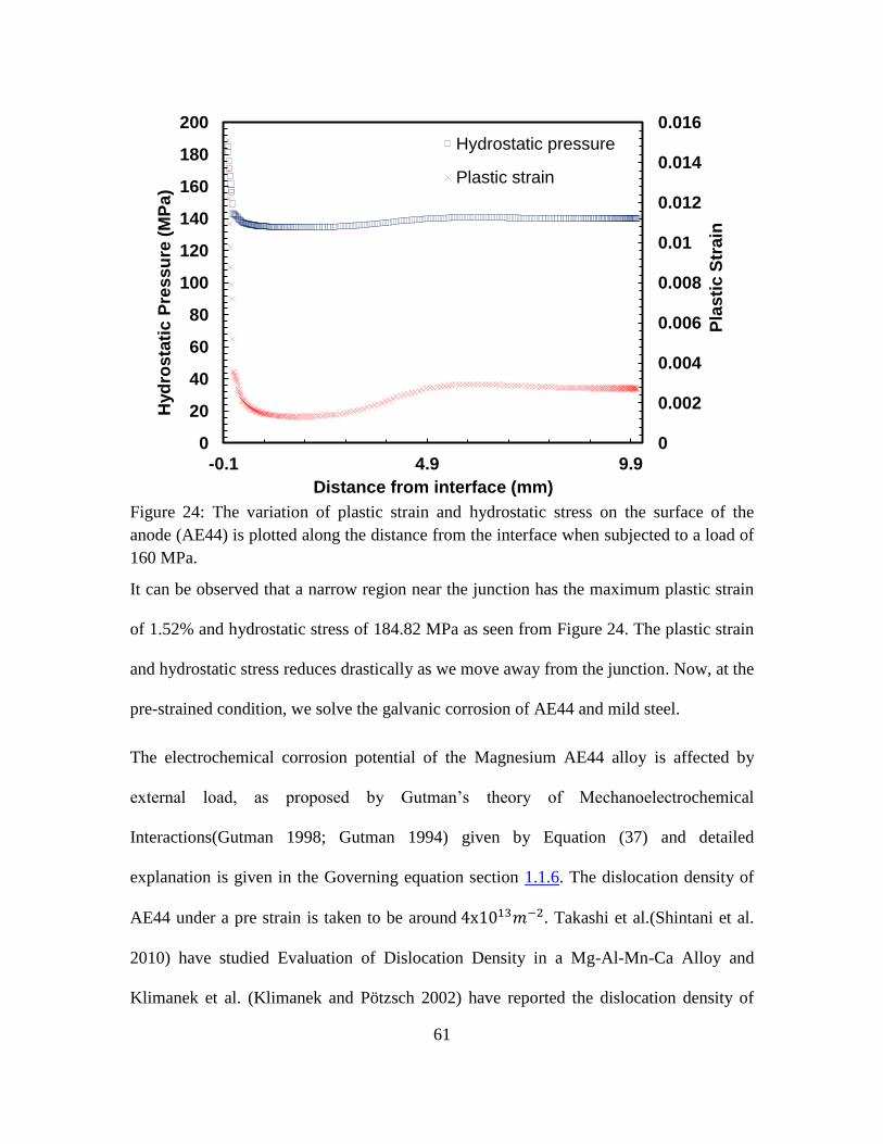
61
Figure 24: The variation of plastic strain and hydrostatic stress on the surface of the
anode (AE44) is plotted along the distance from the interface when subjected to a load of
160 MPa.
It can be observed that a narrow region near the junction has the maximum plastic strain
of 1.52% and hydrostatic stress of 184.82 MPa as seen from Figure 24. The plastic strain
and hydrostatic stress reduces drastically as we move away from the junction. Now, at the
pre-strained condition, we solve the galvanic corrosion of AE44 and mild steel.
The electrochemical corrosion potential of the Magnesium AE44 alloy is affected by
external load, as proposed by Gutman’s theory of Mechanoelectrochemical
Interactions(Gutman 1998; Gutman 1994) given by Equation (37) and detailed
explanation is given in the Governing equation section 1.1.6. The dislocation density of
AE44 under a pre strain is taken to be around 4x10¹³𝑚−2. Takashi et al.(Shintani et al.
2010) have studied Evaluation of Dislocation Density in a Mg-Al-Mn-Ca Alloy and
Klimanek et al. (Klimanek and Pötzsch 2002) have reported the dislocation density of
0
0.002
0.004
0.006
0.008
0.01
0.012
0.014
0.016
0
20
40
60
80
100
120
140
160
180
200
-0.1 4.9 9.9
Pla
sti
c S
tra
in
Hyd
ros
tati
c P
res
su
re (
MP
a)
Distance from interface (mm)
Hydrostatic pressure
Plastic strain
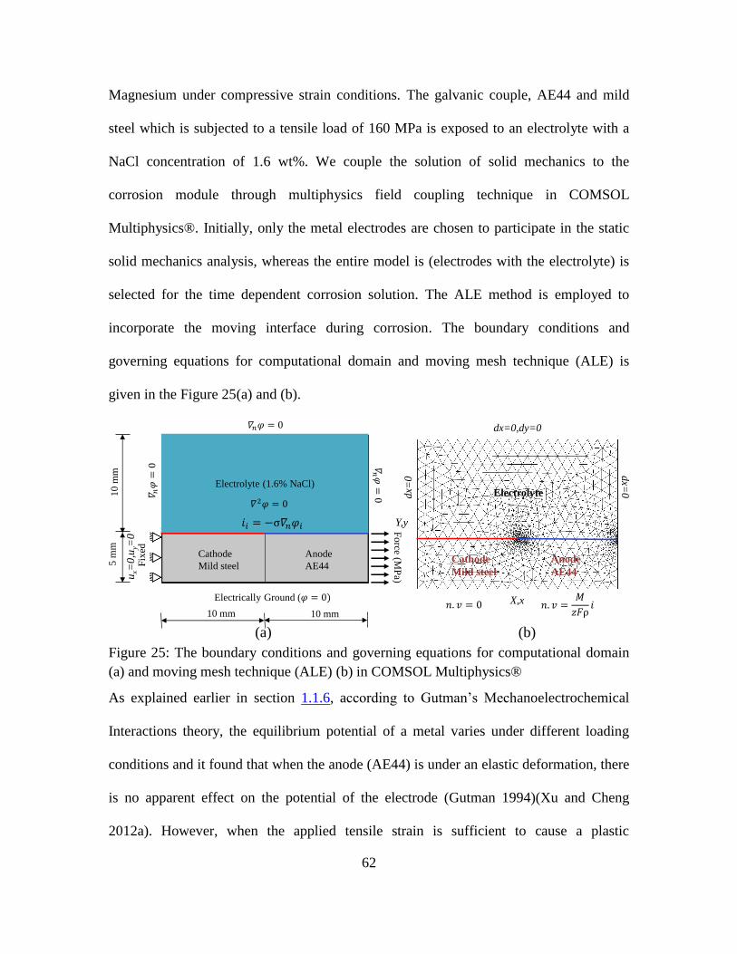
62
Magnesium under compressive strain conditions. The galvanic couple, AE44 and mild
steel which is subjected to a tensile load of 160 MPa is exposed to an electrolyte with a
NaCl concentration of 1.6 wt%. We couple the solution of solid mechanics to the
corrosion module through multiphysics field coupling technique in COMSOL
Multiphysics®. Initially, only the metal electrodes are chosen to participate in the static
solid mechanics analysis, whereas the entire model is (electrodes with the electrolyte) is
selected for the time dependent corrosion solution. The ALE method is employed to
incorporate the moving interface during corrosion. The boundary conditions and
governing equations for computational domain and moving mesh technique (ALE) is
given in the Figure 25(a) and (b).
Figure 25: The boundary conditions and governing equations for computational domain
(a) and moving mesh technique (ALE) (b) in COMSOL Multiphysics®
As explained earlier in section 1.1.6, according to Gutman’s Mechanoelectrochemical
Interactions theory, the equilibrium potential of a metal varies under different loading
conditions and it found that when the anode (AE44) is under an elastic deformation, there
is no apparent effect on the potential of the electrode (Gutman 1994)(Xu and Cheng
2012a). However, when the applied tensile strain is sufficient to cause a plastic
X,x
Cathode
Mild steel
Anode
AE44
Electrolyte
dx=0,dy=0
dx=
0
dx=
0
Y,y
(b)(a)
Anode
AE44
Cathode
Mild steel
Electrically Ground (
Electrolyte (1.6% NaCl)
10 mm 10 mm
Force (M
Pa)
Fix
ed
10
mm
5m
m
ux=
0,u
y=0
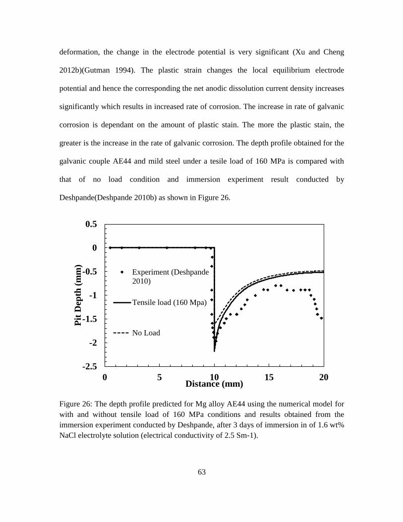
63
deformation, the change in the electrode potential is very significant (Xu and Cheng
2012b)(Gutman 1994). The plastic strain changes the local equilibrium electrode
potential and hence the corresponding the net anodic dissolution current density increases
significantly which results in increased rate of corrosion. The increase in rate of galvanic
corrosion is dependant on the amount of plastic stain. The more the plastic stain, the
greater is the increase in the rate of galvanic corrosion. The depth profile obtained for the
galvanic couple AE44 and mild steel under a tesile load of 160 MPa is compared with
that of no load condition and immersion experiment result conducted by
Deshpande(Deshpande 2010b) as shown in Figure 26.
Figure 26: The depth profile predicted for Mg alloy AE44 using the numerical model for
with and without tensile load of 160 MPa conditions and results obtained from the
immersion experiment conducted by Deshpande, after 3 days of immersion in of 1.6 wt%
NaCl electrolyte solution (electrical conductivity of 2.5 Sm-1).
-2.5
-2
-1.5
-1
-0.5
0
0.5
0 5 10 15 20
Pit
Dep
th (
mm
)
Distance (mm)
Experiment (Deshpande
2010)
Tensile load (160 Mpa)
No Load

64
It can be observed form the Figure 26, that the maximum and overall rate of corrosion is
more in case of plastically deformed anode (AE44). In the case of plastically deformed
anode, the rate of galvanic corrosion was to found to be maximum in the vicinity of the
junction due to the localization of plastic strain, as shown in Figure 22, 23 and 24. The
rate of corrosion is dictated by the current density distribution along the anode surface
and hence, we plot the spatial current density variation along the anode and cathode
surface. We compare the current density distribution for the cases with load and without
load in order study the effect of mechanical loading on spatial current density distribution
of AE44.
Figure 27: The spatial current density distribution on the surface of AE44-mild steel
galvanic when exposed to 1.6% NaCl electrolyte solution couple under tensile load of
160 MPa and no load condition.
It can be seen that that the current density on the AE44 surface under a tensile load of 160
MPa is 98.91 Am-2 at the vicinity of the junction and gradually decreases to about 34.51
-100
-80
-60
-40
-20
0
20
40
60
80
100
-10 -5 0 5 10
Cu
rren
t D
ensi
ty (
Am
-2)
Distance (mm)
Tensile Load of 160 Mpa
No Load

65
Am-2 as we move away, whereas the initial peak current density under no load condition
is about 87.05 Am-2 and gradually decrease to around 31 Am-2. This increase in current
density is due to the fact that the equilibrium potential decrease significantly under plastic
strain conditions as governed by the Equation (36). The reduced local equilibrium
potential increases the current density which in turn increases the rate of corrosion. The
change in local potential is significantly more in the plastic region, hence the corrosion
rate of AE44 is increased significantly at the proximate of intersection. The norm current
density contour plot is shown in the Figure 28 and it is seen that it varies from 900 Am-2
to 4.52 Am-2 on the electrode surface under the tensile load and varies from 740 Am-2 to
2.46 Am-2 under no load condition. The maximum norm current density is at the vicinity
of intersection for both the cases but relatively higher under loading.
Figure 28: The contour plot of norm current density distribution on AE44–mild steel
galvanic couple with (a) and without (b) tensile load of 160 MPa, when exposed to the
electrolyte solution of 1.6 % NaCl concentration at t = 3 days.
(b)(a)
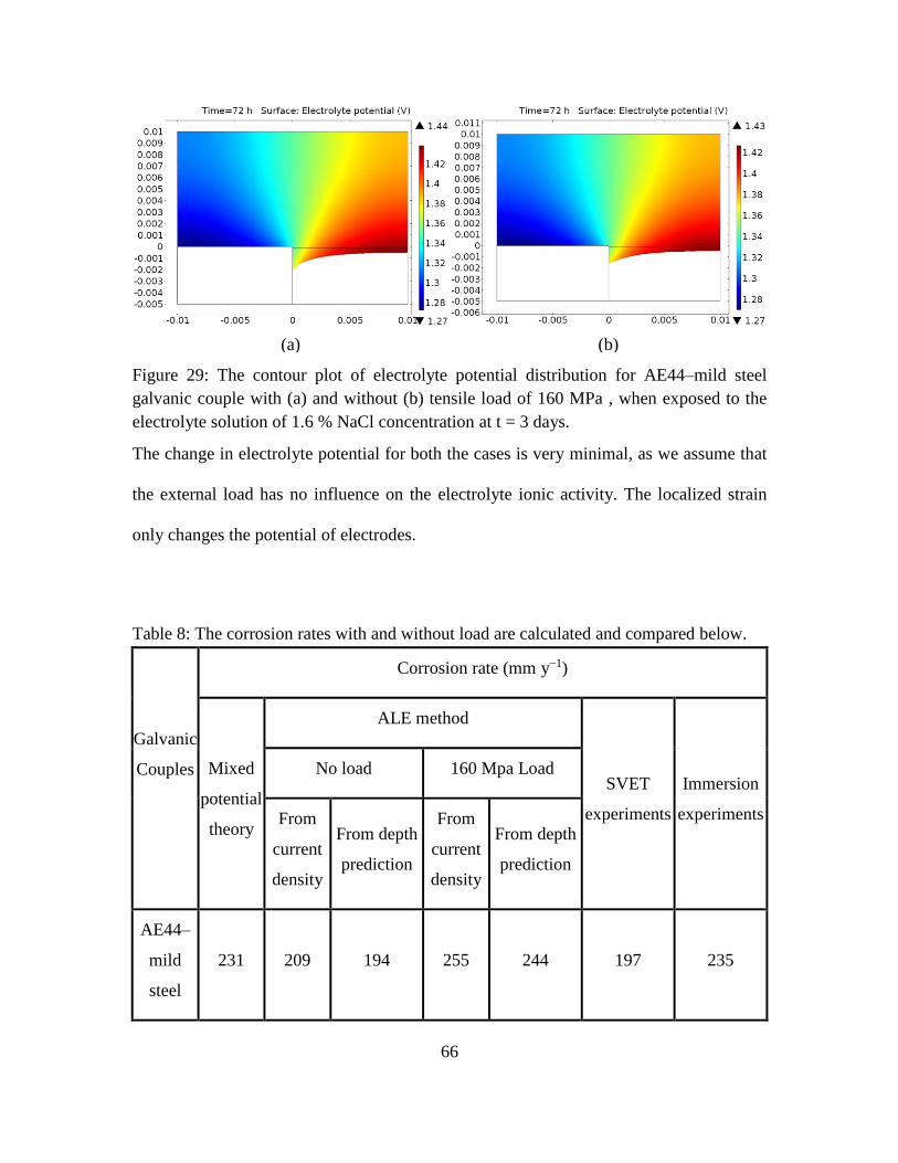
66
Figure 29: The contour plot of electrolyte potential distribution for AE44–mild steel
galvanic couple with (a) and without (b) tensile load of 160 MPa , when exposed to the
electrolyte solution of 1.6 % NaCl concentration at t = 3 days.
The change in electrolyte potential for both the cases is very minimal, as we assume that
the external load has no influence on the electrolyte ionic activity. The localized strain
only changes the potential of electrodes.
Table 8: The corrosion rates with and without load are calculated and compared below.
Galvanic
Couples
Corrosion rate (mm y−1)
Mixed
potential
theory
ALE method
SVET
experiments
Immersion
experiments
No load 160 Mpa Load
From
current
density
From depth
prediction
From
current
density
From depth
prediction
AE44–
mild
steel
231 209 194 255 244 197 235
(a) (b)

67
The rate of corrosion for the galvanic couple is calculated and is compared for with and
without load conditions and the experimental results conducted by
Deshpande(Deshpande 2010a). The corrosion rate is calculated from both current density
and pit growth captured by moving mesh technique (ALE).

68
5.5.2 Aluminum Alloy 7075-T6 and Stainless Steel 316 Joint:
The results obtained from galvanic corrosion of Aluminum Alloy 7075-T6 and Stainless
Steel 316 galvanic couple with and without tensile loading of 300 MPa are presented in
this section. The initial electrochemical parameters for FE simulation derived from the
Tafel plots. The Tafel plots are obtained from the experiments and exchange and limiting
current densities are obtained from the literature (McIntyre, n.d.),(Gereng 2015). In order
to show the capability of the numerical simulation in modeling the effect of mechanical
loading on corrosion process, a bolted plate, which acts as a galvanic cell in the presence
of saline electrolyte is considered. The anode and cathode are made of aluminum alloy
7075-T6 and stainless steel 316, respectively and the geometric model of the joint is
shown below Figure 30. Al 7075 plate is 1mm in thickness and 6mm in length. The joint
is exposed to the electrolyte of 3 wt% NaCl solution (5 Sm-1) for a period of 15 days.
The symmetry of the joint is used and only half the cross-section of the bolted plate is
modeled. The electrochemical properties are obtained from polarization experiment.
Standard mechanical properties of electrodes were used here. A triangular mesh with
adaptive mesh refinement is used and MUMPS (multi-frontal massively parallel sparse)
was selected for solution. The electrodes are perfectly bonded and zero flux is considered
at the cell boundary. Simulations with and without coupling external mechanical load
were carried out to demonstrate the influence of elasto-plastic deformation on corrosion
rate.
Initially a static mechanical elasto-plastic solid stress analysis is performed on the
galvanic couple to calculate the plastic strain and hydrostatic stress induced in the couple
due to external tensile load of 300 MPa. The load is chosen so as to plastically deform Al

69
7050 (yield strength is 400 MPa). Due to the stress concentration at the electrodes
interface, the anode plastically deforms in the vicinity of the cathode as see Figure 31.
The maximum plastic strain is about 3% at the intersection of Al and stainless steel due to
stress concentration and majority of the joint away from the joint is only under elastic
strain.
Figure 30: The boundary conditions along with the governing equations are provided in
the above schematic of galvanic corrosion for Aluminum Alloy 7075-T6 and Stainless
Steel 316 joint under a tensile load of 410 MPa.
Figure 31: The plastic strain distribution (a) and Von Mises stress distribution (b) on
Aluminum Alloy 7075-T6 and Stainless Steel 316 joint under a tensile load of 100 MPa.
The corrosion process is allowed for a period of 15 days to notice significant amount of
corrosion. It is evident from Figure 32, that the plastic deformation significantly increases
(a) (b)

70
the corrosion rate (change in thickness). The depth profile shows that the rate of galvanic
corrosion is increased significantly at the vicinity of junction due to the accumulation of
plastic strain at junction as seen in Figure 30. The rate of corrosion away from the
junction is not significantly affected. The elastic deformation, nevertheless, does not
distinctively affect the corrosion process, which is in accordance with reported
experiments.
Figure 32: The change in total electrode thickness is measured along the length of the
corroding electrode Aluminum Alloy 7075-T6 with and without tensile load of 300 MPa
when exposed to electrolyte of 3% NaCl for 15 days.
It can be noticed that the galvanic corrosion of the anode is amplified by the applied
external loading and higher corrosion of the electrode can be seen at the region with
higher plastic strain (higher stress concentration) as seen in Figure 32. It can be
concluded that the rate of corrosion is affected by amount of loading (plastic strain and
elastic strain) on the corroding electrode and it is found to increase with increase in
loading. The equilibrium potential shift of anode due to plastic deformation is governed
by Equation (36) and hence the total equilibrium potential of anode under plastic strain
-0.41
-0.36
-0.31
-0.26
-0.21
-0.16
-0.11
-0.06
-0.01
0 1 2 3 4
Pit
Dep
th (
mm
)
Distance (mm)
Tensile Load (300 Mpa)
no load
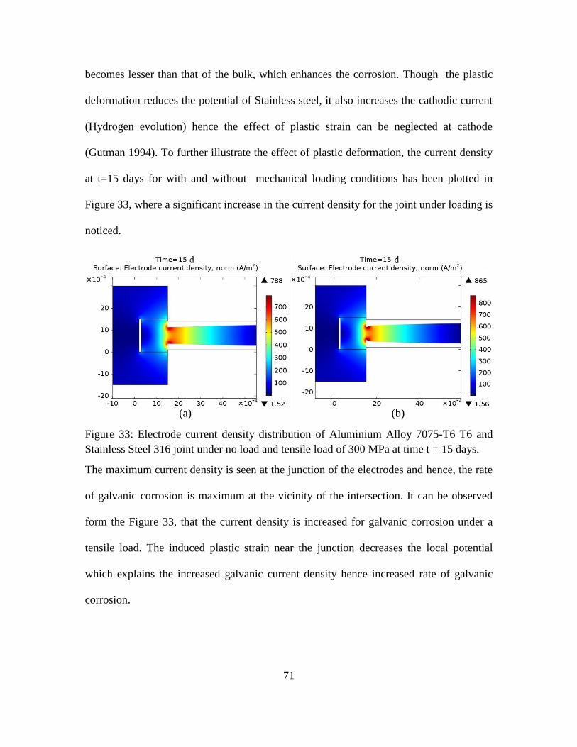
71
becomes lesser than that of the bulk, which enhances the corrosion. Though the plastic
deformation reduces the potential of Stainless steel, it also increases the cathodic current
(Hydrogen evolution) hence the effect of plastic strain can be neglected at cathode
(Gutman 1994). To further illustrate the effect of plastic deformation, the current density
at t=15 days for with and without mechanical loading conditions has been plotted in
Figure 33, where a significant increase in the current density for the joint under loading is
noticed.
Figure 33: Electrode current density distribution of Aluminium Alloy 7075-T6 T6 and
Stainless Steel 316 joint under no load and tensile load of 300 MPa at time t = 15 days.
The maximum current density is seen at the junction of the electrodes and hence, the rate
of galvanic corrosion is maximum at the vicinity of the intersection. It can be observed
form the Figure 33, that the current density is increased for galvanic corrosion under a
tensile load. The induced plastic strain near the junction decreases the local potential
which explains the increased galvanic current density hence increased rate of galvanic
corrosion.
(a) (b)
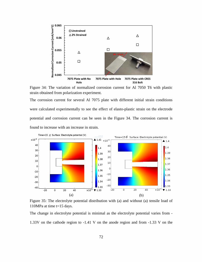
72
Figure 34: The variation of normalized corrosion current for Al 7050 T6 with plastic
strain obtained from polarization experiment.
The corrosion current for several Al 7075 plate with different initial strain conditions
were calculated experimentally to see the effect of elasto-plastic strain on the electrode
potential and corrosion current can be seen in the Figure 34. The corrosion current is
found to increase with an increase in strain.
Figure 35: The electrolyte potential distribution with (a) and without (a) tensile load of
110MPa at time t=15 days.
The change in electrolyte potential is minimal as the electrolyte potential varies from -
1.33V on the cathode region to -1.41 V on the anode region and from -1.33 V on the
2% strain
d
(a) (b)

73
cathode region to -1.41 on the anode region for with and without tensile loading
conditions.
74
CHAPTER 5
6. CONCLUSION
1. A numerical model for solving the Nernst-Planck equation, which captures the
electrochemical process is employed and this model is capable of tracking the moving
boundary for a 2-D electrode during galvanic corrosion and can handle nonlinear
boundary conditions. The current density and corrosion rates obtained for the
galvanic couple AE44 – mild steel were compared with those calculated by
Deshpande(Deshpande 2010b) from numerical model, mixed potential theory and
experimental techniques employing Scanning Vibrating Electrode Technique (SVET)
and immersion technique.
2. The electrolyte depth has a noticeable effect on surface profile and rate of corrosion
of AE44 – mild steel couple. The peak current density does not vary with the increase
in electrolyte depth but the average current density increased significantly with an
increase in depth attributing to a larger area for the current to pass and thus reduced
the resistance against the current flow. The overall corrosion of AE44 under deeper
electrolytes is found to increase but the corrosion at the proximate of the intersection
is not affected by the electrolyte depth.
3. The conductivity of the electrolyte significantly influences the rate of corrosion and
surface profile of AE44, especially near the junction. In low conducting electrolyte
(0.5 Sm-1) the galvanic current over the Magnesium was concentrated at a narrow
edge closest to the mild steel, resulting in a very steep spatial current distribution. The
spatial current density variation increased with decrease in conductivity of the
75
electrolyte and is more uniform in high conducting electrolyte (13.5 Sm-1). The
overall rate of corrosion increased with an increase in conductivity. The maximum
rate of corrosion at the vicinity of the junction decreased noticeably from 221.22
mmy-1 to 196.47 mmy-1 with an increase in conductivity from 0.5 Sm-1 to 13.5 Sm-1.
4. The cathode to anode area ratio has a significant effect on the corrosion rate. The
galvanic corrosion rate of AE44 increased appreciable with the decrease in mild steel
surface area but the change in galvanic corrosion rate at the junction was minimal.
5. The validated numerical model is extended to simulate the mechano-electrochemical
process through a multiphysics field coupling technique in order to study the effects
of mechanical loading on galvanic corrosion of AE44 – mild steel. Results show that,
when Magnesium alloy AE44 is under a purely elastic deformation, there is no
apparent effect of mechanical loading on the electrochemical galvanic process.
However, when the applied tensile load is sufficient to cause a plastic deformation,
the local galvanic corrosion activity at the vicinity of the interface is increased
remarkably and the rate of galvanic corrosion rate increased significantly with the
increase in plastic strain.
6. The mechano-electrochemically coupled numerical model was used to study the
effect of mechanical loading on Aluminum Alloy 7075-T6 and Stainless Steel 316
Joint. The plastic deformation significantly increased the galvanic current density on
Aluminum Alloy 7075-T6 resulting in enhanced corrosion of Aluminum especially at
the juncture where plastic stain is large.
76
SCOPE
The numerical model needs to be developed accounting for ionic species in the thin film
electrolyte solution in order to capture oxygen-diffusion limited reaction on cathode
surface, and thus the scope exists to carry out further investigations. Other geometrical
factors like shape of anode and cathode, insulation distance between anode and cathode
can also be studied. Experimental verification of the numerical results for the couple will
ascertain the numerical modeling technique and in future we intend to incorporate the
effect of concentration gradient into the mechano-electrochemical model. Further we
would look into localized forms of corrosion considering the effect of crystallographic
orientation and other surface defects of the underlying microstructural corrosion process,
leading to pit initiation and evolution.
77
REFERENCES
Adey, Ra, and Sm Niku. 1988. “Computer Modelling of Galvanic Corrosion.” In
Galvanic Corrosion, edited by Hp Hack, 96–96 – 22. 100 Barr Harbor Drive, PO
Box C700, West Conshohocken, PA 19428-2959: ASTM International.
http://www.astm.org/doiLink.cgi?STP26193S.
Astley, Dj. 1988. “Use of the Microcomputer for Calculation of the Distribution of
Galvanic Corrosion and Cathodic Protection in Seawater Systems.” In Galvanic
Corrosion, edited by Hp Hack, 53–53 – 26. 100 Barr Harbor Drive, PO Box
C700, West Conshohocken, PA 19428-2959: ASTM International.
http://www.astm.org/doiLink.cgi?STP26191S.
“ASTM G82 - 98(2014) Standard Guide for Development and Use of a Galvanic Series
for Predicting Galvanic Corrosion Performance.” 2015. Accessed July 6.
http://www.astm.org/Standards/G82.htm.
Baboian, R. 2005. Corrosion Tests and Standards: Application and Interpretation-
Second Edition. ASTM International. http://www.astm.org/doiLink.cgi?MNL20-
EB.
Barlat, F., M. V. Glazov, J. C. Brem, and D. J. Lege. 2002. “A Simple Model for
Dislocation Behavior, Strain and Strain Rate Hardening Evolution in Deforming
Aluminum Alloys.” International Journal of Plasticity 18 (7): 919–39.
doi:10.1016/S0749-6419(01)00015-8.
“Cost of Corrosion Study Overview.” 2015. Accessed July 8.
https://www.nace.org/Publications/Cost-of-Corrosion-Study/.
Cross, Samuel R., Srikant Gollapudi, and Christopher A. Schuh. 2014. “Validated
Numerical Modeling of Galvanic Corrosion of Zinc and Aluminum Coatings.”
Corrosion Science 88 (November): 226–33. doi:10.1016/j.corsci.2014.07.033.
Deshpande, Kiran B. 2010a. “Experimental Investigation of Galvanic Corrosion:
Comparison between SVET and Immersion Techniques.” Corrosion Science 52
(9): 2819–26. doi:10.1016/j.corsci.2010.04.023.
———. 2010b. “Validated Numerical Modelling of Galvanic Corrosion for Couples:
Magnesium Alloy (AE44)–mild Steel and AE44–aluminium Alloy (AA6063) in
Brine Solution.” Corrosion Science 52 (10): 3514–22.
doi:10.1016/j.corsci.2010.06.031.
Donea, J., Antonio Huerta, J.-Ph Ponthot, and A. Rodriguez-Ferran. 2004. Encyclopedia
of Computational Mechanics Vol. 1: Fundamentals., Chapter 14: Arbitrary
Lagrangian-Eulerian Methods. Wiley & Sons.
“Electrochemical Corrosion Measurements.” 2015. Accessed July 6.
http://www.gamry.com/application-notes/corrosion-coatings/basics-of-
electrochemical-corrosion-measurements/.
Fontana, Mars Guy. 1986. Corrosion Engineering. McGraw-Hill.

78
“For Casting Buyers | AFS - American Foundry Society.” 2015. Accessed July 6.
http://www.afsinc.org/buyer.cfm?navItemNumber=10373.
Gereng, Husnu. 2015. “Anticorrosive Properties of Date Palm (Phoenix Dactylifera L.)
Fruit Juice on 7075 Type Aluminum Alloy in 3.5% NaCl Solution.” Accessed
July 11. http://pubs.acs.org/doi/pdf/10.1021/ie301771u.
Gutman, E. M. 1994. Mechanochemistry of Solid Surfaces. Singapore ; River Edge, NJ:
World Scientific Pub Co Inc.
———. 1998. Mechanochemistry of Materials. Cambridge Int Science Publishing.
Herzberg, Eric F, Erica D Ambrogio, Clark L Barker, Evelyn F Harleston, William M
Haver, Norman T O’Meara, Ronald J Marafioti, Gregg L Stimatze, Andrew
Timko, and James C Tran. 2012. “The Annual Cost of Corrosion for Army
Ground Vehicles and Navy Ships.” LMI Report DAC2ITI.
Hihara, L. H., and R. M. Latanision. 1992. “Galvanic Corrosion of Aluminum-Matrix
Composites.” Corrosion 48 (7): 546–52. doi:10.5006/1.3315972.
Isaacs, H. S. 1988. “The Measurement of the Galvanic Corrosion of Soldered Copper
Using the Scanning Vibrating Electrode Technique.” Corrosion Science 28 (6):
547–58. doi:10.1016/0010-938X(88)90023-6.
Isacsson, Malte, Mats Ström, Holger Rootzén, and Otto Lunder. 1997. “Galvanically
Induced Atmospheric Corrosion on Magnesium Alloys: A Designed Experiment
Evaluated by Extreme Value Statistics and Conventional Techniques.” SAE
Technical Paper 970328. Warrendale, PA: SAE International.
http://papers.sae.org/970328/.
Jia, Jimmy X., Guangling Song, and Andrej Atrens. 2006. “Influence of Geometry on
Galvanic Corrosion of AZ91D Coupled to Steel.” Corrosion Science 48 (8):
2133–53. doi:10.1016/j.corsci.2005.08.013.
Jia, J. X., G. Song, and A. Atrens. 2007. “Experimental Measurement and Computer
Simulation of Galvanic Corrosion of Magnesium Coupled to Steel.” Advanced
Engineering Materials 9 (1-2): 65–74. doi:10.1002/adem.200600206.
Kanno, Ken-ichi, Masayuki Suzuki, and Yuichi Sato. 1980. “Tafel Slope Determination
of Corrosion Reaction by the Coulostatic Method.” Corrosion Science 20 (8–9):
1059–66. doi:10.1016/0010-938X(80)90084-0.
Kear, G., and F. C. Walsh. 2005. “The Characteristics of a True Tafel Slope.” Corrosion
and Materials 30 (6): 51–55.
Kennard, E., and J. T. Waber. 1970. “Mathematical Study of Galvanic Corrosion Equal
Coplanar Anode and Cathode with Unequal Polarization Parameters.” Journal of
The Electrochemical Society 117 (7): 880–85. doi:10.1149/1.2407662.
Klimanek, P., and A. Pötzsch. 2002. “Microstructure Evolution under Compressive
Plastic Deformation of Magnesium at Different Temperatures and Strain Rates.”
Materials Science and Engineering: A 324 (1–2): 145–50. doi:10.1016/S0921-
5093(01)01297-7.
79
“KSC Corrosion Technology Laboratory -- Galvanic Corrosion.” 2015. Accessed July 6.
http://corrosion.ksc.nasa.gov/galcorr.htm.
Mansfeld, F., and J. V. Kenkel. 1975a. “Galvanic Corrosion of A1 Alloys — II. Effect of
Solution Composition.” Corrosion Science 15 (3): 183–98. doi:10.1016/S0010-
938X(75)80008-4.
———. 1975b. “Galvanic Corrosion of Al alloys—III. The Effect of Area Ratio.”
Corrosion Science 15 (4): 239–50. doi:10.1016/S0010-938X(75)80019-9.
McCafferty, E. 1977. “Distribution of Potential and Current in Circular Corrosion Cells
Having Unequal Polarization Parameters.” Journal of The Electrochemical
Society 124 (12): 1869–78. doi:10.1149/1.2133178.
McIntyre, J. n.d. “McIntyre, J. F., S. M. Hoover, and K. A. Musselman. Galvanic
Corrosion of Al-7075-T6 and Steel-4340 Coupled to Brass QQ-B-626,360 and
Al-7075-T6 Coupled to Steel-4130 and Steel-4340: Exposure to Aqueous NaCl
and Salt-Fog Environments. No. NSWC/TR-86-26. NAVAL SURFACE
WEAPONS CENTER SILVER SPRING MD, 1986.”
Mellde, Rolf. 1985. “Volvo LCP 2000 Light Component Project.” SAE Technical Paper
850570. Warrendale, PA: SAE International. http://papers.sae.org/850570/.
Murer, Nicolas, Roland Oltra, Bruno Vuillemin, and Olivier Néel. 2010. “Numerical
Modelling of the Galvanic Coupling in Aluminium Alloys: A Discussion on the
Application of Local Probe Techniques.” Corrosion Science 52 (1): 130–39.
doi:10.1016/j.corsci.2009.08.051.
Nickerson, B. 2015. “US Naval Aviation – Operational Airframe Experience with
Combined Environmental and Mechanical Loading.” Corrosion Reviews to
appear.
Perez, Nestor. 2004. Electrochemistry and Corrosion Science. Springer Science &
Business Media.
Revie, R. Winston. 2008. Corrosion and Corrosion Control. John Wiley & Sons.
———. 2011. Uhlig’s Corrosion Handbook. John Wiley & Sons.
Roberge, Pierre R. n.d. Corrosion Basics: An Introduction. NACE International, 2006.
http://www.nace.org/cstm/Store/Product.aspx?id=612057cc-2a4b-4759-9710-
20c405584799.
Sharland, S. M., C. P. Jackson, and A. J. Diver. 1989. “A Finite-Element Model of the
Propagation of Corrosion Crevices and Pits.” Corrosion Science 29 (9): 1149–66.
doi:10.1016/0010-938X(89)90051-6.
Shintani, Takashi, Yoshinori Murata, Yoshihiro Terada, and Masahiko Morinaga. 2010.
“Evaluation of Dislocation Density in a Mg-Al-Mn-Ca Alloy Determined by X-
Ray Diffractometry and Transmission Electron Microscopy.” Materials
Transactions 51 (6): 1067–71. doi:10.2320/matertrans.M2010021.
80
Song, Guang-Ling. 2010. “Potential and Current Distributions of One-Dimensional
Galvanic Corrosion Systems.” Corrosion Science 52 (2): 455–80.
doi:10.1016/j.corsci.2009.10.003.
Tait, William Stephen. 1994. An Introduction to Electrochemical Corrosion Testing for
Practicing Engineers and Scientists. Clair, Racine, Wis.
Verbrugge, Mark. 2006. “Galvanic Corrosion over a Semi-Infinite, Planar Surface.”
Corrosion Science 48 (11): 3489–3512. doi:10.1016/j.corsci.2006.02.004.
Waber, James T. 1955. “Mathematical Studies of Galvanic Corrosion III . Semi‐infinite
Coplanar Electrodes with Equal Constant Polarization Parameters.” Journal of
The Electrochemical Society 102 (7): 420–29. doi:10.1149/1.2430111.
Waber, James T., and Bertha Fagan. 1956. “Mathematical Studies on Galvanic Corrosion
IV . Influence of Electrolyte Thickness on the Potential and Current Distributions
over Coplanar Electrodes Using Polarization Parameters.” Journal of The
Electrochemical Society 103 (1): 64–72. doi:10.1149/1.2430234.
Waber, James T., and Marshall Rosenbluth. 1955. “Mathematical Studies of Galvanic
Corrosion II . Coplanar Electrodes with One Electrode Infinitely Large and with
Equal Polarization Parameters.” Journal of The Electrochemical Society 102 (6):
344–53. doi:10.1149/1.2430058.
Weast, Robert C., and Chemical Rubber Company (Cleveland Ohio). 1975. CRC
Handbook of Chemistry and Physics: A Ready-Reference Book of Chemical and
Physical Data. Editor, Robert C. Weast. CRC Press.
Xu, L. Y., and Y. F. Cheng. 2012a. “An Experimental Investigation of Corrosion of X100
Pipeline Steel under Uniaxial Elastic Stress in a near-Neutral pH Solution.”
Corrosion Science 59 (June): 103–9. doi:10.1016/j.corsci.2012.02.022.
———. 2012b. “Corrosion of X100 Pipeline Steel under Plastic Strain in a Neutral pH
Bicarbonate Solution.” Corrosion Science 64 (November): 145–52.
doi:10.1016/j.corsci.2012.07.012.
———. 2013. “Development of a Finite Element Model for Simulation and Prediction of
Mechanoelectrochemical Effect of Pipeline Corrosion.” Corrosion Science 73
(August): 150–60. doi:10.1016/j.corsci.2013.04.004.
———. 2014. “Experimental and Numerical Studies of Effectiveness of Cathodic
Protection at Corrosion Defects on Pipelines.” Corrosion Science 78 (January):
162–71. doi:10.1016/j.corsci.2013.09.011.
Zhang, X. G., and E. M. Valeriote. 1993. “Galvanic Protection of Steel and Galvanic
Corrosion of Zinc under Thin Layer Electrolytes.” Corrosion Science 34 (12):
1957–72. doi:10.1016/0010-938X(93)90053-J.