numerical computations of the unsteady flow in a radial ...13299/fulltext01.pdf · numerical...
TRANSCRIPT

Numerical computations of the unsteady flow ina radial turbine.
by
Fredrik Hellstrom
March 2008Technical Reports from
Royal Institute of TechnologyKTH Mechanics
SE-100 44 Stockholm, Sweden

Akademisk avhandling som med tillstand av Kungliga Tekniska Hogskolan iStockholm framlagges till offentlig granskning for avlaggande av teknologielicentiatexamen fredagen den 28 mars 2008 kl 13.00 i sal E3, Osquarsbacke 14,Kungliga Tekniska Hogskolan, Vallhallavagen 79, Stockholm.
c©Fredrik Hellstrom 2008Universitetsservice US–AB, Stockholm 2008

Numerical computations of the unsteady flow in a radialturbine.
Fredrik Hellstrom 2008,KTH MechanicsSE-100 44 Stockholm, Sweden
Abstract
Non-pulsatile and pulsatile flow in bent pipes and radial turbine has beenassessed with numerical simulations. The flow field in a single bent pipe hasbeen computed with different turbulence modelling approaches. A comparisonwith measured data shows that Implicit Large Eddy Simulation (ILES) givesthe best agreement in terms of mean flow quantities. All computations with thedifferent turbulence models qualitatively capture the so called Dean vortices.The Dean vortices are a pair of counter-rotating vortices that are created inthe bend, due to inertial effects in combination with a radial pressure gradient.The pulsatile flow in a double bent pipe has also been considered. In the firstbend, the Dean vortices are formed and in the second bend a swirling motionis created, which will together with the Dean vortices create a complex flowfield downstream of the second bend. The strength of these structures will varywith the amplitude of the axial flow. For pulsatile flow, a phase shift betweenthe velocity and the pressure occurs and the phase shift is not constant duringthe pulse depending on the balance between the different terms in the Navier-Stokes equations.
The performance of a radial turbocharger turbine working under both non-pulsatile and pulsatile flow conditions has also been investigated by using ILES.To assess the effect of pulsatile inflow conditions on the turbine performance,three different cases have been considered with different frequencies and ampli-tude of the mass flow pulse and different rotational speeds of the turbine wheel.The results show that the turbine cannot be treated as being quasi-stationary;for example, the shaft power varies with varying frequency of the pulses for thesame amplitude of mass flow. The pulsatile flow also implies that the incidenceangle of the flow into the turbine wheel varies during the pulse. For the worstcase, the relative incidence angle varies from approximately −80◦ to +60◦. Aphase shift between the pressure and the mass flow at the inlet and the shafttorque also occurs. This phase shift increases with increasing frequency, whichaffects the accuracy of the results from 1-D models based on turbine mapsmeasured under non-pulsatile conditions.
For a turbocharger working under internal combustion engine conditions,the flow into the turbine is pulsatile and there are also unsteady secondaryflow components, depending on the geometry of the exhaust manifold situatedupstream of the turbine. Therefore, the effects of different perturbations at

the inflow conditions on the turbine performance have been assessed. For thedifferent cases both turbulent fluctuations and different secondary flow struc-tures are added to the inlet velocity. The results show that a non-disturbedinlet flow gives the best performance, while an inflow condition with a certainlarge scale eddy in combination with turbulence has the largest negative effecton the shaft power output.
Descriptors: Pulsatile flow, radial turbines, pipe flow, effects of inlet con-ditions, Large Eddy Simulation.
iv

Preface
This licentiate thesis in fluid mechanics consist of two parts. The first partgives an overview of the research area and a summary of the results. Thesecond part consists of 3 papers, which are adjusted to comply with the presentthesis format for consistency. However, their contents have not been changedcompared to published or submitted versions except for minor refinements. InChapter 7 of the first part of the thesis the respondent’s contribution to allpapers are stated.
March 2008, StockholmFredrik Hellstrom
v

vi

Contents
Abstract iii
Preface v
Chapter 1. Introduction 1
Chapter 2. Non-pulsatile and pulsatile internal flow 32.1. Flow in curved pipes 32.2. Internal pulsatile flow 5
Chapter 3. Turbochargers, with focus on the turbine 93.1. Performance parameters 93.2. The stator 113.3. The rotor 163.4. Turbine performance under pulsatile flow 19
Chapter 4. Methods 254.1. Governing equations 254.2. Turbulence 264.3. Numerical methods 274.4. Numerical accuracy and uncertainty 324.5. Comparison of computed and measured data 34
Chapter 5. Results 365.1. Non-pulsatile and pulsatile flow in curved pipes 365.2. Unsteady flow in a radial turbine 42
Chapter 6. Conclusions 566.1. Future work 57
Chapter 7. Papers and authors contributions 59
vii

Acknowledgements 62
References 63
Paper 1 73
Paper 2 93
Paper 3 117
viii

Part I
Overview and summary


CHAPTER 1
Introduction
A turbine is a flow device that extracts energy from a fluid by expanding itthrough a stator and rotor system and when the fluid passes the rotor with ahigh tangential velocity, it causes the rotor to rotate. The fluid can be a gasor a liquid depending on the applications. The turbine can be either a radialor an axial turbine. In axial turbines, the main flow direction at the inlet tothe rotor is parallel to the turbine shaft while for radial turbines, the main flowdirection at the inlet to the rotor is perpendicular to the shaft. Axial turbinescan be found in gas turbines, which are used for example for aircraft propulsion,power generation and ship propulsion. In a gas turbine, the working gas of theturbine is the exhaust gas from combustion chambers situated upstream of theturbine. The turbine, which may consist of several turbine stages, is used todrive the compressor stages, which are used to increase the amount of air to thecombustion chamber. The turbine can also drive a generator when it is usedfor power generation and propulsion systems on ships. Axial turbines are alsoused in power plants, and the working gas in this application can be steam,produced by a boiling process with different types of heat sources. In thisapplication, the turbine drives a generator. Another area where turbines areused is in hydroelectric power plants, where the working fluid is water. Oftenone uses also in this area radial (i.e. Francis) turbines. Radial turbines are alsoused in the aerospace area, where they are used for driving fuel pumps.
The area where radial turbines are used in largest numbers is probably inthe turbocharger application for Internal Combustion (IC) engines. In a tur-bocharger, the energy of the engine exhaust gas is extracted by expanding itthrough the turbine which drives the compressor by a shaft. This means thatthe wasted energy in the exhaust gas, which can be roughly 30-40 percent ofthe chemical energy released by the combustion, is used to increase the densityof the air admitted to the cylinder. Thereby the power output of the engine canbe increased or alternatively the engine size can be reduced, without decreas-ing the power output. If a turbocharged IC engine is compared with a naturalaspirated engine with the same power output, the turbocharged engine will besmaller, lighter and requires a smaller installation space. The turbochargedIC engine will also have a better efficiency, since the inertia of system is less
1
2 1. INTRODUCTION
and the friction losses are decreased due to smaller cylinders, valves etc. Thistechnique is called downsizing and can be used to meet the future demands onlower fuel consumption and emission levels with maintained, or even increased,power output. To be able to further increase the efficiency of the IC engine,the understanding of the highly pulsatile flow in the turbine part of the tur-bocharger must be improved. This knowledge will also be used to increase theefficiency of the turbine and also to develop a low order numerical model ofthe turbine to be used in numerical engine simulation tools. In this thesis, theperformance of the turbine working in both non-pulsatile and pulsatile flows isconsidered.
The main focus of the work has been on:
• The physics of pulsatile flow in bent pipes.• Assessment of the effects of inflow conditions on the turbine perfor-
mance.
For the later case, both the effects of pulsatile and non-pulsatile flow have beenassessed, with varying perturbations and unsteadiness applied at the inlet tothe turbine. The used method is time resolved three-dimensional numericalsimulations.
The work described in the thesis mark a contribution in understanding theflow in the turbine and its dependence on the inflow conditions. The latteraspect is of importance from engineering point of view; i.e. for the integrationof the turbo-charger in the car engine. By improved understanding of theflow, a better understanding the sources of losses in the turbine is achieved.The experience gained in the computational analysis shall hopefully help inimproving the modelling of such flows.
The remainder of the thesis is organized as follows: In Chapter 2 a briefoverview of the steady and unsteady flow in pipes is given. This chapter is fol-lowed by Chapter 3 where the features of turbochargers, with focus on the tur-bine part, are discussed. Chapter 4 consider the used methods. In Chapter 5,the most important results are presented followed by conclusions in Chapter 6.Finally, in Chapter 7, a short summary of the included papers is given.

CHAPTER 2
Non-pulsatile and pulsatile internal flow
The purpose of this chapter is to give a brief overview of the pulsatile internalflow in pipes since the flow in an exhaust system on an IC engine is highlypulsatile. The exhaust manifold, situated between the engine and the turbine,can be viewed as being made of straight and curved pipe sections. Therefore,the flow in bent pipe has also been considered. The frequency and the am-plitude of the pulsatile flow in the exhaust system will be determined by thenumbers of cylinders of the engine and at which operation point the engine isworking, i.e. the engine rotational speed and the throttle position. The ge-ometry of the exhaust manifold will also affect the flow into the turbine, sincesingle and double bends will introduce secondary flow, junctions will disturbthe flow and there are also pressure waves that will be reflected in the manifold.Therefore, a literature survey on the steady and unsteady flow in different pipeconfigurations has been conducted.
2.1. Flow in curved pipes
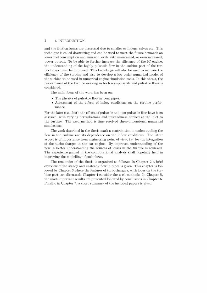
There are many applications where flow in bent pipes can be found, for examplepipe-lines, exhaust systems and the blood flow in arteries. One typical feature ofthe flow in bent pipes is the so called Dean vortices, which are a pair of counter-rotating vortices. When the flow enters the bend, the fluid is accelerated nearthe inner wall. Simultaneously, the fluid near the outer wall is decelerateddue to the adverse pressure gradient. This induces a secondary flow in thetransverse plane of the pipe. Further downstream, the centrifugal force inducesa second flow in the central part of the cross section from the inner wall to theouter wall and forms the two counter-rotating vortices, see Figure 2.1.
Sudo et al. (1998) investigated the steady turbulent flow in a circular-sectioned 90◦ bend. The curvature radius ratio, defined as the ratio betweenthe radius of the bend and the pipe radius, was four and the flow was assumedto be turbulent. At the inlet to the bend, ϕ=0◦, the primary flow acceleratesnear the inner wall. At ϕ=30◦ the secondary flow starts to develops into acounter rotating pair of vortices. Between ϕ=75◦ and 90◦ the primary flow isgreatly distorted and the turbulence intensity and Reynolds stresses increases.Downstream of the bend, the distribution of primary flow velocity gradually
3
4 2. NON-PULSATILE AND PULSATILE INTERNAL FLOW
Figure 2.1. The counter-rotating Dean vortices.
becomes smooth and the vortices breaks down, but the effect of secondary flowremains at 10 diameters downstream of the bend. Sudo & Hibara (2000) alsoperformed measurements on a 180◦ bend. The curvature radius was the sameas for the 90◦ bend. Upstream to ϕ=60◦ the flow in the two different geometriesshows similar characteristics. From ϕ=90◦ the secondary flow begins to weakenand meanders up and down in the central part of the tube. In this part of thebend, a low-velocity region exists in the middle and high velocity regions arelocated near the inner and outer walls.
Rutten et al. (2005) performed Large Eddy Simulations to investigate theturbulent flow through 90◦ pipe bend. The purpose of this investigation wasto see how long the extension must be to avoid distortion of the flow field fromthe bend at the inlet boundary. The conclusion from the investigation wasthat an extension length of three diameters is sufficient. The computed datais validated by comparing the first and second order statistical moments withPIV measurements by Brucker (1998). Power spectra of LES and PIV velocitysignals are also compared and the agreement of the numerical and experimentalresults is good. The computed flow field showed the counter-rotating Deanvortices, which are not of equal strength at all times and alternately dominatethe flow field. This alternately domination leads to alternately clockwise andanti-clockwise rotation of the flow close to the wall in the downstream tangent.
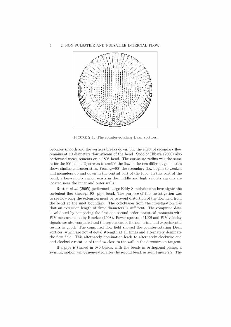
If a pipe is turned in two bends, with the bends in orthogonal planes, aswirling motion will be generated after the second bend, as seen Figure 2.2. The

2.2. INTERNAL PULSATILE FLOW 5
Figure 2.2. The swirl at the outlet of a double bent pipe.
swirling motion at the outlet of the second bend is not an effect of the Deanvortices from the first bend; it is an effect of the non-uniform axial velocitydistribution in radial direction at the inlet to second bend. If a non-uniformradial velocity distribution, with the maximal value rotated 90◦ with respectto the inner radius of the bend, is applied to the inlet to a single bend, thesecondary flow consist of one vortex at the outlet of the bend. When the flowwith high velocity and momentum enters the bend it is linked by the curvatureto the region where the momentum is lower which induces a swirling motion.Since very few articles where found for this geometry, a numerical investigationof the pulsatile flow in a double bent pipe was performed, and the results arediscussed in Chapter 5.
2.2. Internal pulsatile flow
An oscillating flow, which is a special type of pulsatile flow, only consists of thetime varying component, and hence the periodically time-averaged velocity iszero. Pulsatile flow is defined here as a flow that is composed of a steady com-ponent with a superimposed periodically varying temporal component. Thebehaviour of oscillating or pulsatile flow depends on the balance between theviscous effect and the acceleration of the fluid. The relative importance of theacceleration term relative to the viscous term in the momentum equation canbe expressed by the Womersley number, defined as:

6 2. NON-PULSATILE AND PULSATILE INTERNAL FLOW
α = r ·√
2π · fυ
(2.1)
where r is the pipe radius, f the frequency and υ is the kinematic viscosity. Asmall value of the Womersley number implies that the effects of unsteadinessare less important as compared to viscous effects. For low Womersley number(α <1), the velocity is nearly a quasi-steady Poiseuille flow which is in phasewith the pressure gradient. As the Womersley number increases, the velocitystarts to show a phase lag with respect to the pressure gradient. For all pulsat-ing flows, a phase shift between the axial flow and the pressure gradient occurs,see for example Dec et al. (1991) and Ramaprian & Tu (1983). For pure os-cillating very low Reynolds number flow the phase lag is 90◦ and for turbulentflow the phase lag is less than 90◦ according to Ramaprian & Tu (1983). Forpure oscillating very low Reynolds number flow, the ∂
∂t -term in the momentumequation (4.2) is balanced by the ∂p
∂xi-term. This can be showed by assuming
one-dimensional oscillating flow and that the pressure gradient is described by∂p∂x = p · eiωt where p is a constant and ω is the frequency of the oscillation.When this is inserted into the momentum equation (4.2) and solved for U , thefollowing result is obtained U = − ip
ω · eiωt. As can be seen, the phase shiftbetween the velocity and the pressure is 90◦. For pulsatile turbulent flow, thetime derivate term will be balanced both by the pressure gradient term andremaining terms in the momentum equations, including the Reynolds-stresses.Flow pulsations also affect the axial velocity profile in the pipe. The phase shiftbetween the pressure and the bulk velocity gives overshoots in boundary layerwhich depends on that the flow in the region near the wall has lower momen-tum than the bulk flow, and therefore, it is more sensitive to changes in theaxial pressure gradient. This effect increases with increasing frequency due tothe inertia effect. Ramaprian & Tu (1983) carried out an experimental studyof turbulent oscillatory flow in a long circular pipe. The oscillating frequenciescorrespond to a Womersley number of approximately 43 and 116, respectively.They compared the results with theoretical results for laminar oscillating pipeflow at the same frequency. The laminar flow shows sharper peaks of the over-shoots in the boundary layer than the turbulent flow. Also, the peaks occurcloser to wall for the theoretical laminar case. The experiments also show thatthe phase lag between pressure and velocity is smaller for turbulent flow thanfor the laminar flow. Dec et al. (1991) investigated a cyclic oscillating veloc-ity field in a tail pipe of a pulse combustor using Laser Doppler Velocimetry(LDV). The oscillating frequencies varied from 67 to 101 Hz and the ampli-tude was up to 5 times the mean velocity. The mean Reynolds number was3750. The turbulent flow shows a similar behaviour to the theoretical laminaroscillating pipe flow, with a phase shift between the pressure and the velocityand an overshoot near the wall. The flow near the wall reverses earlier than
2.2. INTERNAL PULSATILE FLOW 7
the flow in the core region. The laminar flow solution also shows a sharperovershoot relative to the core region profile, while the turbulent flow has asmoother axial velocity profile. The reason is, according to Dec et al. (1991),that in turbulent flow the additional momentum transport by the turbulencerapidly dissipates the oscillations. The turbulence intensity is uniform acrossthe core region of the flow, but the behaviour in the boundary layer has twodifferent modes. When the streamwise pressure gradient is adverse, the tur-bulent intensity increases from the core to a maximum in the boundary layerand then going to zero at the wall. When the pressure gradient is favourable,the turbulent intensity drops from the core value throughout the boundarylayer. The turbulent intensity also shows a maximum at times of zero-velocitycrossings. From the measured velocity profiles, the instantaneous wall shearstresses were calculated. A trend of increasing cycle-averaged wall shear stresswith increasing pulsation amplitude can be noted but no dependence on the fre-quency was found. The cycle-averaged wall shear stress is slightly greater thanthe wall shear stress predicted for steady turbulent flow at the same averagedmean Reynolds number.
For laminar pulsating flow in a bent pipe, the secondary flow changes ro-tational direction from being outward to inward in the centre when Reynoldsnumber is increased for a certain Womersley number. Hamakiotes & Berger(1988) showed using numerical computations, that the Dean vortices do changerotation direction when Re exceeds 300. The Womersley number was 15 andcurvature ratio was 1/7. The reversed vortices are called the Lyne vortices.Lyne (1970) showed analytically that the fluid is driven along the wall from theouter side to inner side under action of the pressure gradient in the same man-ner as for the Dean vortices. However, the pressure gradient in the boundarylayer is not balanced by the centrifugal forces, and at the edge of the boundarylayer, the flow returns centrifugally within in the boundary layer, and dragsthe fluid in the interior around in a pair of vortices, that are counter-rotatingcompared to the Dean vortex.
It may be expected that the heat transfer to or from a flow in a pipe shoulddepend on the pulsation frequency, since the pulsations will affect the boundarylayer. Both increase and decrease of the Nusselt number in pulsating flow hasbeen reported in the literature for different pulsation frequencies, amplitudesand mean Reynolds numbers. The Nusselt number is defined as the ratiobetween the convective and conductive heat transfer:
NuL =hcoef · L
kf(2.2)
hcoef is the heat-transfer coefficient, L is a characteristic length scale andkf is the thermal conductivity. Wang & Zhang (2005) performed numericalcomputations of turbulent pulsatile flow in a straight pipe with Uosc/Umean=3,

8 2. NON-PULSATILE AND PULSATILE INTERNAL FLOW
where the Womersley number was varied from 40 to 60. The results showedthat the axial pressure gradient has a phase lag of about 90◦ to the veloc-ity. The results also showed that the instantaneous velocity profile was flat atthe centre of the pipe. In the region between the core region and the wall avelocity overshoot occurred at some instants. These overshoots had a veloc-ity that was larger than the velocity in the core region, and more heat wastransported at these instances. The thermal boundary layer thickness variedwith the pulsation of the flow and was during a period, sometimes thinner andsometimes thicker than in a corresponding steady state flow case. The localNusselt number was, for different Womersley numbers, higher than it was forthe corresponding steady case. The heat transfer was greatly enhanced by thepulsative flow, especially in the entrance region. Wang and Zhang also showedthat the local instantaneous Nusselt number had its maximum when the ve-locity reached its peak value and the Nusselt number reached its lowest valuewhen the velocity was zero. The heat transfer was also enhanced when thevelocity amplitude of the pulse was increased. The results from Dec & Keller(1989) experiments with a pulse combustor fitted with a tail-pipe showed thatthe Nusselt number in oscillating flow was significantly higher than for steadyflow with the same mean Reynolds number. The experiments also showed thatthe Nusselt number increased with increasing frequency and pulsation ampli-tude. Habib et al. (2004) studied pulsatile pipe flow in a range of Re of 8 000< Re < 50 000 and both enhancement and reduction in mean Nusselt numberwas reported. The Nusselt number decreased for low pulsating frequency. Themaximum mean Nusselt number was obtained when the pulsating frequencywas in the vicinity of the turbulent bursting frequency. At this pulsating fre-quency, the interaction of the pulsations and the turbulent bursting increasedthe heat transfer, and hence the Nusselt number increased. These phenom-ena can be explained by the turbulent bursting model, which states that theviscous sublayer is unstable, and due to turbulent structures, its growth anddestruction occur periodically.
These different effects, such as the phase lag and increased heat transfer inpulsatile flow, will affect the performance of the radial turbine working underpulsatile flow conditions. The phase shift will imply that the static and dynamicpressure will be out of phase, which can affect the shaft power of the turbine.The pulsatile flow also increases the losses; for example the heat-losses to theambient. The losses due to viscous effects will probably also increase, duestronger shear layers. This will most probably imply that the turbine cannotbe treated as being a quasi-stationary flow device.

CHAPTER 3
Turbochargers, with focus on the turbine
Turbochargers can be used in many different applications, but they are allbased on the same principle. A turbocharger has four principal components,a compressor, a turbine, a shaft and bearings. The turbine part utilities theenergy from the hot gas that flows through the turbine and drives a compressorwhich will increase the density of the gas. The bearings support the shaft, andshaft seals are also required to separate the compressed air and the exhaustgases from the bearing lubrication system. Turbochargers can be found ondifferent types of internal combustion (IC) engines, from small four-stroke au-tomotive engines to large two-stroke marine diesel engines. For small internalcombustion engines, radial turbines are the most common type. Axial turbinesare used for large IC engines in marine and power generation applications. Therotational speed of the turbine is normally limited by the requirements of thecompressor and the maximum radius for a given rotational speed is limited bystructural reasons. This means, for turbines that normally are used for smallIC engines, that the radius of the turbine wheel must be small. For small axialturbines, this gives an unfavourable aspect ratio which will give rise to sec-ondary flows and tip leakages which will result in poor efficiency. Since axialturbines also are complicated and more expensive compared with radial tur-bines, the most common type of turbines for small IC engines is the radial type.Radial turbines can also deliver a larger specific power than an equivalent axialturbine. For small engines, like those used for passenger car, the pressure ratioover the compressor is about 2 and the speed can range up to about 300 000rpm.
3.1. Performance parameters
The fundamental parameters for turbines that define the performance are themass flow, the pressure ratio, the rotational speed, the efficiency and the poweroutput. The most important quantity for the turbine is the shaft power, PS ,which is defined here as
PS = TShaft · ω (3.1)
9

10 3. TURBOCHARGERS, WITH FOCUS ON THE TURBINE
where ω is the angular velocity and TShaft is the shaft torque. In thecomputations, the shaft torque is obtained by integrating the element forcesdue to the shear and pressure forces times the radial coordinate over the turbinewheel:
TShaft =∫
S
r × (f · n)dS (3.2)
Another important quantity is the turbine efficiency, ηis. Commonly onedefines the efficiency as the ratio of shaft power to the maximal isentropic powerof the driving gas flow:
ηis =PS
m · cp · T01 · (1− p2p01
γ−1γ )
(3.3)
where m is the mass flow, T01 and p01 is the total gas temperature andpressure before the turbine and p2 is the static pressure downstream of theturbine. cp is the specific heat and γ is the specific heat ratio. This definitionworks well for non-pulsatile flow and for pulsatile flow at moderate frequencies.For higher frequencies, the non-constant phase shift between the mass flow,pressure and shaft torque makes it impossible to define an isentropic efficiencyin a proper way.
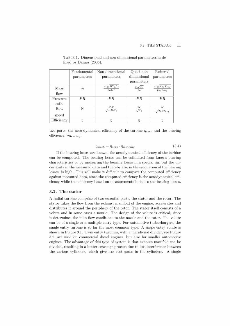
The fundamental parameters can either be predicted by using analytic orsemi-analytic models or by testing the turbocharger under controlled condi-tions. The fundamental parameters are often non-dimensionalized, see Table1, to take account for the inlet conditions and are often reported in com-pressor and turbine maps. Since the diameter, D for a particular turbine isconstant, it can be dropped. The turbines are also tested with the actual work-ing gas, and hence, the gas constant R and γ can also be dropped. By doingso, the quasi-non dimensional parameters are obtained. The performance canalso be reported as the referred parameters, which have the same units as thefundamental parameters. In the referred parameters, the inlet pressure andtemperatute are referred to reference values.
The performance of a turbine is tested in gas stand where the turbine isdriven by gas from an external compressor. The measurement can be performedboth with cold and hot gas. In the later case, fuel is injected and burnt in acombustion chamber upstream of the turbine. Since the rotational speed is veryhigh, it is very hard to directly measure the shaft power output of the turbine.Therefore, the compressor is throttled to control the load on the turbine, and bymeasuring the shaft speed, the inlet and outlet pressure, temperature and themass flow through the turbine and the compressor, respectively, the efficiency ofthe turbine can be computed. This efficiency is the mechanical efficiency, sincethe bearing losses are included. The mechanical efficiency can be divided into
3.2. THE STATOR 11
Table 1. Dimensional and non-dimensional parameters as de-fined by Baines (2005).
Fundamental Non dimensional Quasi-non Referredparameters parameters dimensional parameters
parameters
Mass mm√
RT0/γ
p0D2m√
T0p0
m√
T0/Tref
p0/pref
flowPressure PR PR PR PR
ratioRot. N N ·D√
γ·R·T0
N√T0
N√T0/Tref
speedEfficiency η η η η
two parts, the aero-dynamical efficiency of the turbine ηaero and the bearingefficiency, ηBearing;
ηmech = ηaero · ηBearing (3.4)
If the bearing losses are known, the aerodynamical efficiency of the turbinecan be computed. The bearing losses can be estimated from known bearingcharacteristics or by measuring the bearing losses in a special rig, but the un-certainty in the measured data and thereby also in the estimation of the bearinglosses, is high. This will make it difficult to compare the computed efficiencyagainst measured data, since the computed efficiency is the aerodynamical effi-ciency while the efficiency based on measurements includes the bearing losses.
3.2. The stator
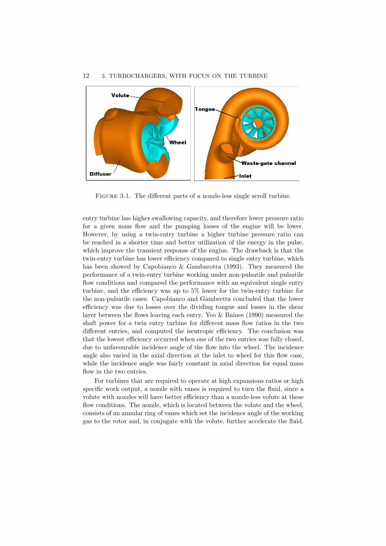
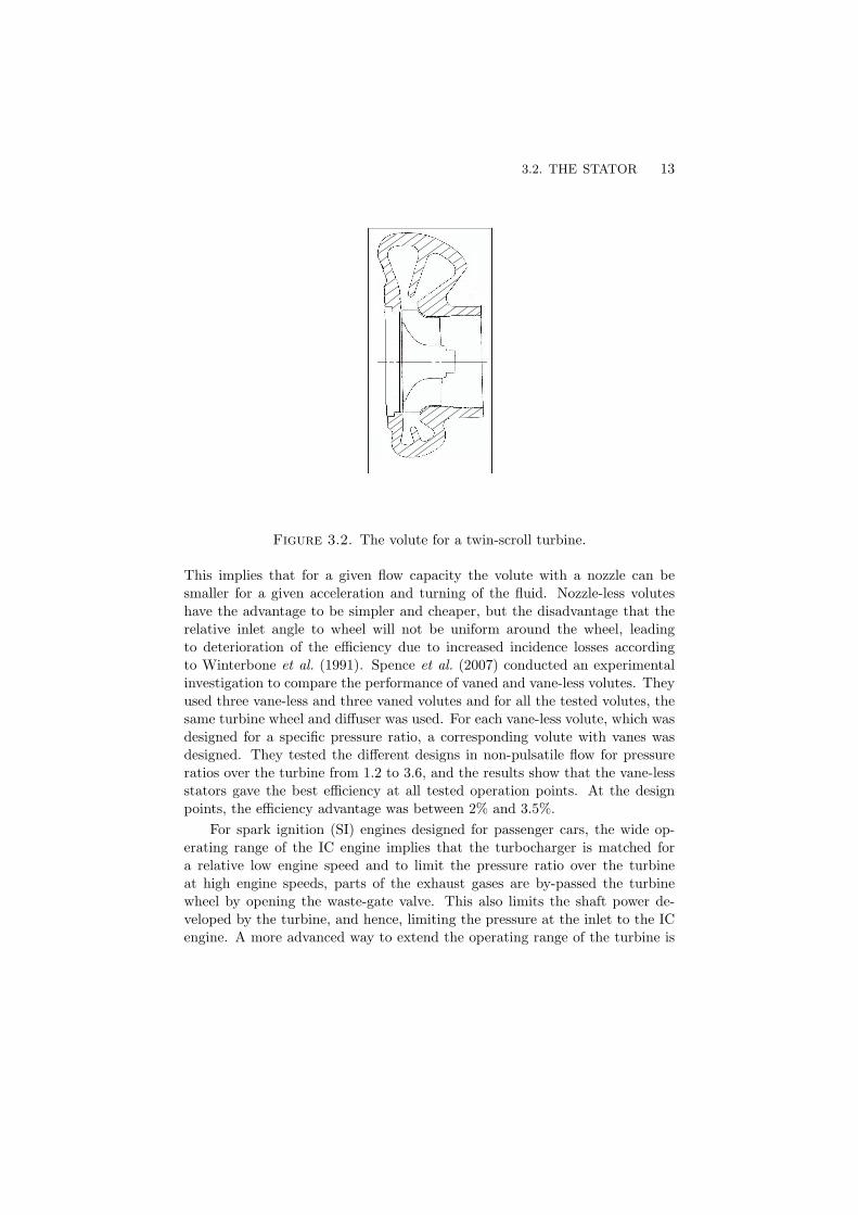
A radial turbine comprise of two essential parts, the stator and the rotor. Thestator takes the flow from the exhaust manifold of the engine, accelerates anddistributes it around the periphery of the rotor. The stator itself consists of avolute and in some cases a nozzle. The design of the volute is critical, sinceit determines the inlet flow conditions to the nozzle and the rotor. The volutecan be of a single or a multiple entry type. For automotive turbochargers, thesingle entry turbine is so far the most common type. A single entry volute isshown in Figure 3.1. Twin entry turbines, with a meridional divider, see Figure3.2, are used on commercial diesel engines, but also for smaller automotiveengines. The advantage of this type of system is that exhaust manifold can bedivided, resulting in a better scavenge process due to less interference betweenthe various cylinders, which give less rest gases in the cylinders. A single
12 3. TURBOCHARGERS, WITH FOCUS ON THE TURBINE
Figure 3.1. The different parts of a nozzle-less single scroll turbine.
entry turbine has higher swallowing capacity, and therefore lower pressure ratiofor a given mass flow and the pumping losses of the engine will be lower.However, by using a twin-entry turbine a higher turbine pressure ratio canbe reached in a shorter time and better utilization of the energy in the pulse,which improve the transient response of the engine. The drawback is that thetwin-entry turbine has lower efficiency compared to single entry turbine, whichhas been showed by Capobianco & Gambarotta (1993). They measured theperformance of a twin-entry turbine working under non-pulsatile and pulsatileflow conditions and compared the performance with an equivalent single entryturbine, and the efficiency was up to 5% lower for the twin-entry turbine forthe non-pulsatile cases. Capobianco and Gambretta concluded that the lowerefficiency was due to losses over the dividing tongue and losses in the shearlayer between the flows leaving each entry. Yeo & Baines (1990) measured theshaft power for a twin entry turbine for different mass flow ratios in the twodifferent entries, and computed the isentropic efficiency. The conclusion wasthat the lowest efficiency occurred when one of the two entries was fully closed,due to unfavourable incidence angle of the flow into the wheel. The incidenceangle also varied in the axial direction at the inlet to wheel for this flow case,while the incidence angle was fairly constant in axial direction for equal massflow in the two entries.
For turbines that are required to operate at high expansions ratios or highspecific work output, a nozzle with vanes is required to turn the fluid, since avolute with nozzles will have better efficiency than a nozzle-less volute at theseflow conditions. The nozzle, which is located between the volute and the wheel,consists of an annular ring of vanes which set the incidence angle of the workinggas to the rotor and, in conjugate with the volute, further accelerate the fluid.
3.2. THE STATOR 13
Figure 3.2. The volute for a twin-scroll turbine.
This implies that for a given flow capacity the volute with a nozzle can besmaller for a given acceleration and turning of the fluid. Nozzle-less voluteshave the advantage to be simpler and cheaper, but the disadvantage that therelative inlet angle to wheel will not be uniform around the wheel, leadingto deterioration of the efficiency due to increased incidence losses accordingto Winterbone et al. (1991). Spence et al. (2007) conducted an experimentalinvestigation to compare the performance of vaned and vane-less volutes. Theyused three vane-less and three vaned volutes and for all the tested volutes, thesame turbine wheel and diffuser was used. For each vane-less volute, which wasdesigned for a specific pressure ratio, a corresponding volute with vanes wasdesigned. They tested the different designs in non-pulsatile flow for pressureratios over the turbine from 1.2 to 3.6, and the results show that the vane-lessstators gave the best efficiency at all tested operation points. At the designpoints, the efficiency advantage was between 2% and 3.5%.
For spark ignition (SI) engines designed for passenger cars, the wide op-erating range of the IC engine implies that the turbocharger is matched fora relative low engine speed and to limit the pressure ratio over the turbineat high engine speeds, parts of the exhaust gases are by-passed the turbinewheel by opening the waste-gate valve. This also limits the shaft power de-veloped by the turbine, and hence, limiting the pressure at the inlet to the ICengine. A more advanced way to extend the operating range of the turbine is
14 3. TURBOCHARGERS, WITH FOCUS ON THE TURBINE
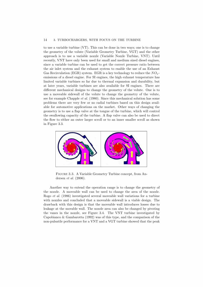
to use a variable turbine (VT). This can be done in two ways; one is to changethe geometry of the volute (Variable Geometry Turbine, VGT) and the otherapproach is to use a variable nozzle (Variable Nozzle Turbine, VNT). Untilrecently, VNT have only been used for small and medium sized diesel engines,since a variable turbine can be used to get the correct pressure ratio betweenthe air inlet system and the exhaust system to enable the use of an ExhaustGas Recirculation (EGR) system. EGR is a key technology to reduce the NOx-emissions of a diesel engine. For SI engines, the high exhaust temperature haslimited variable turbines so far due to thermal expansion and durability, butat later years, variable turbines are also available for SI engines. There aredifferent mechanical designs to change the geometry of the volute. One is touse a moveable sidewall of the volute to change the geometry of the volute,see for example Chapple et al. (1980). Since this mechanical solution has someproblems there are very few or no radial turbines based on this design avail-able for automotive applications on the market. Other ways of changing thegeometry is to use a flap valve at the tongue of the turbine, which will controlthe swallowing capacity of the turbine. A flap valve can also be used to directthe flow to either an outer larger scroll or to an inner smaller scroll as shownin Figure 3.3.
Figure 3.3. A Variable Geometry Turbine concept, from An-dersen et al. (2006).
Another way to extend the operation range is to change the geometry ofthe nozzle. A moveable wall can be used to change the area of the nozzle.Rogo et al. (1986) investigated several moveable wall variations for a turbinewith nozzles and concluded that a moveable sidewall is a viable design. Thedrawback with this design is that the moveable wall introduces losses due toleakage at the movable wall. The nozzle area can also be changed by pivotingthe vanes in the nozzle, see Figure 3.4. The VNT turbine investigated byCapobianco & Gambarotta (1992) was of this type, and the comparison of thenon-pulsatile performance for a VNT and a VGT turbine showed that the peak

3.2. THE STATOR 15
Figure 3.4. The variable vanes in nozzle for Variable NozzleTurbine, from Andersen et al. (2006).
efficiency was lower for VT compared to a fixed turbine. This is most likely dueto losses that the variable geometry systems induce due to leakage, wake lossesbehind the guiding vanes, separation, shocks and incidence losses, accordingto Capobianco & Gambarotta (1992) and Fukaya et al. (2000). But, the VTshowed better efficiency over a wider range, and of the two tested variableturbines, the VNT had the best efficiency. Andersen et al. (2006) investigatedthe performance of five different VNT and one VGT with the approximatelysame swallowing capacity, and they concluded that the VGT turbine is themost suitable variable turbine type for spark ignition engines. Some of theVNT had better efficiency at lower mass flow rates, but the VGT turbine hadthe best performance at high mass flow rates. They also investigated the coldstart emissions for all the tested variable turbines, and they concluded thata VT most likely requires better exhaust after-treatment system than a fixedsingle scroll turbine. The reason for the poor cold start emissions is the largermass and heat-transfer area. Due to lower efficiency at low mass flow ratescompared to a fixed geometry turbine, an IC engine with a VT will have largerpump losses at low engine rotational speeds, but this is compensated by thehigher boost pressure that can be achieved by a VT at low engine rotationalspeeds. A VT will also give better transient performance of the engine. Theturbocharger lag can also be decreased with VT which has been shown by Filipiet al. (2001).
Despite the many advantages with variable turbines, the most commontype used on IC engines for passenger cars is the nozzle-less single-entry waste-gated radial turbine due to the robust design and the relative low cost.
16 3. TURBOCHARGERS, WITH FOCUS ON THE TURBINE
3.3. The rotor
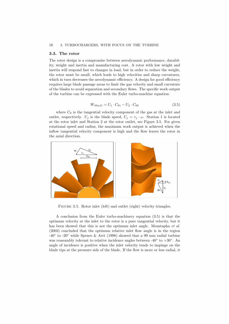
The rotor design is a compromise between aerodynamic performance, durabil-ity, weight and inertia and manufacturing cost. A rotor with low weight andinertia will respond fast to changes in load, but in order to reduce the weight,the rotor must be small, which leads to high velocities and sharp curvatures,which in turn decreases the aerodynamic efficiency. A design for good efficiencyrequires large blade passage areas to limit the gas velocity and small curvatureof the blades to avoid separation and secondary flows. The specific work outputof the turbine can be expressed with the Euler turbo-machine equation:
WShaft = U1 · Cθ1 − U2 · Cθ2 (3.5)
where Cθ is the tangential velocity component of the gas at the inlet andoutlet, respectively. Uj is the blade speed, Uj = rj · ω. Station 1 is locatedat the rotor inlet and Station 2 at the rotor outlet, see Figure 3.5. For givenrotational speed and radius, the maximum work output is achieved when theinflow tangential velocity component is high and the flow leaves the rotor inthe axial direction.
Figure 3.5. Rotor inlet (left) and outlet (right) velocity triangles.
A conclusion from the Euler turbo-machinery equation (3.5) is that theoptimum velocity at the inlet to the rotor is a pure tangential velocity, but ithas been showed that this is not the optimum inlet angle. Moustapha et al.(2003) concluded that the optimum relative inlet flow angle is in the region-40◦ to -20◦ while Spence & Artt (1998) showed that a 99 mm radial turbinewas reasonably tolerant to relative incidence angles between -40◦ to +30◦. Anangle of incidence is positive when the inlet velocity tends to impinge on theblade tips at the pressure side of the blade. If the flow is more or less radial, it
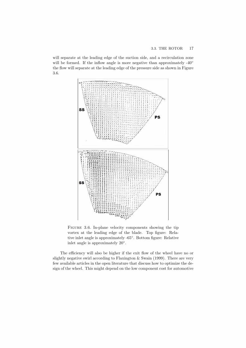
3.3. THE ROTOR 17
will separate at the leading edge of the suction side, and a recirculation zonewill be formed. If the inflow angle is more negative than approximately -40◦
the flow will separate at the leading edge of the pressure side as shown in Figure3.6.
Figure 3.6. In-plane velocity components showing the tipvortex at the leading edge of the blade. Top figure: Rela-tive inlet angle is approximately -65◦. Bottom figure: Relativeinlet angle is approximately 20◦.
The efficiency will also be higher if the exit flow of the wheel have no orslightly negative swirl according to Flaxington & Swain (1999). There are veryfew available articles in the open literature that discuss how to optimize the de-sign of the wheel. This might depend on the low component cost for automotive

18 3. TURBOCHARGERS, WITH FOCUS ON THE TURBINE
turbochargers, which imply the manufacturers use the cut-and-try techniques(Flaxington & Swain (1999)), and therefore they have large databases for differ-ent designs. Doran et al. (2001) studied the effects of different shroud profiles atdifferent operating points. In their experimental study, they used four differentshroud profile radius for a 99.0 mm radial inflow nozzle turbine. The resultsshowed that the largest shroud radius gave the best performance under mostconditions, but at the highest rotational speed, the most shaped shroud profilegave 3.5 percent points better efficiency. They also performed one dimensio-nal numerical analysis to examine the effect of shroud profile with respect toincidence angle. For negative incidence angles, a small radius of shroud cur-vature gave the best performance, while for positive inlet angles, the largestradius gave the best performance. No measurements or 3-dimesional numericalcomputations were conducted in order to explain the effects of different shroudprofiles.
Another way to increase the efficiency of the turbine is to use back sweptblades, which has for example been showed by Barr et al. (2006) by a numericalstudy for a turbine with an inlet tip diameter of 90 mm. They studied threedifferent back sweep blade angles; 0◦, 15◦ and 30◦. At design condition, theefficiency was almost equally, while at off-design conditions, the efficiency wasimproved by 2% for the 30◦ back sweep angle blade due to a strongly reducedtip vortex at the leading edge. The drawback of this design is that it increasesthe bending stresses in the blade, and therefore limits the used of back sweptblades. Palfreyman et al. (2002) studied the performance of four differentturbine wheel geometries for a mixed flow turbine, and they concluded thata reduced chord length (with 18.75%) gave the largest deterioration of theefficiency, followed by a reduced number of blades (from 12 to 10), and thenchanging the inlet blade angle. The size of the gap between the blade tip andshroud also affects the efficiency, since the pressure gradient over the bladedrives the flow over the tip and a jet and a tip vortex is created. Futral &Holeski (1970) performed an experimental study with the objective to studythe effects of tip clearance for a radial turbine. The wheel diameter was 152.9mm, which is quite large compared to the size of the wheel of an automotiveturbocharger. Tip clearance values of 0.25 to 7% of the passage height at therotor entrance and at the rotor exit were used. The results showed that anincrease of the axial tip clearance at the rotor entrance gave a decrease of thetotal efficiency of 0.15% for each percent increase of tip clearance. At the exitof the rotor, an increase of the radial tip clearance from 1% to 3% of the passageheight gave a decrease of the efficiency of 1.6% for each percent increase of tipclearance. For the range of 3% to 7% the decrease of efficiency was smaller, butstill, larger than the effect of increasing the radial gap at the entrance. But,the tip clearance height is not the only parameter that affects the flow over the
3.4. TURBINE PERFORMANCE UNDER PULSATILE FLOW 19
tip, and hence, the tip vortices and the losses that they introduce. Dambach& Hodson (2001) conducted an experimental investigation of the flow over theblade tip for different axial and radial tip-clearances for a radial turbine. Thetip gap was varied from 0.6% to 1.2% of the local blade height. They showedthat different blade tip gap height to blade width ratio gave different behaviourfor the tip leakage flow. If the ratio was below approximately 1
6 , the tip leakageflow was mixed with the boundary layer at the shroud, resulting in a tip leakageflow with low momentum, and hence, a less strong tip vortex at the suction side.If the ratio was larger than approximately 1
6 , the inertia effects dominated overthe viscous effects, and the momentum of tip leakage flow from the pressure tosuction side was higher, resulting in a stronger tip vortex. Also, they showedthat the pressure difference over the gap remains relatively constant for thetested tip gap heights.
For turbines working in pulsatile flow, mixed flow turbines have some ad-vantages compared to radial turbines. A mixed flow turbine is a turbine, withits leading edge of the blade inclined to the axial axis. This implies that theflow at the entrance to the wheel have both an axial velocity component anda radial velocity component. At higher mass flow rates, which is the same ashigher pressure ratio and lower U/Cs, mixed flow turbines have better effi-ciency compared to radial turbines due to less turning of the flow in the wheel.The turning process from the radial inlet to the axial outlet gives raise to lossesdue to secondary flow. The U/Cs ratio is called the blade speed ratio, and Uis the rotor tip speed and Cs defined as:
Cs =
√2 · cp · T01 · (1−
p2
p01
γ−1γ
) (3.6)
Mixed flow turbines have the maximum efficiency at a U/Cs ratio of ap-proximately 0.65, while a radial turbines have the best efficiency at blade speedratio of approximately 0.7 (Chen et al. (1997)). The efficiency also drops sub-stantially for U/Cs values below 0.7 for radial turbines, while mixed flow tur-bines can maintain high efficiency over a larger region of lower U/Cs ratios.
3.4. Turbine performance under pulsatile flow
As already mentioned, the flow in the exhaust system of an IC engine is highlypulsatile, and this affects the performance of the turbine. The performance ofturbines working under pulsatile flow conditions has been assessed by manyresearches by both different numerical methods and by experiments. A typicalfeature of turbines working in pulsatile flow is that when plotting the mass flowversus shaft torque, as been done in Figure 3.7, the trajectory form a closedloop, enclosing the quasi-stationary trajectory. The same is valid when plottingthe blade speed ratio U/Cs versus the efficiency. U/Cs varies during the pulse,

20 3. TURBOCHARGERS, WITH FOCUS ON THE TURBINE
since the rotational speed of the rotor is almost constant, whereas the variationof U/Cs is from low values of approximately 0.2 to high values above 1 (whenthe pressure ratio is equal to one, the isentropic velocity will be zero), which isfar away from the optimal value of approximately 0.7.
Figure 3.7. Computed shaft power vs. mass flow at inlet.
For turbines operating under pulsatile flow conditions, the mean efficiencyis lower compared to non-pulsatile flow conditions for the same mass flow andpressure ratio, but the instantaneous performance can be both higher and lower,see for example Winterbone et al. (1990), Winterbone et al. (1991), Dale & Wat-son (1986) and Capobianco & Gambarotta (1990). But it must be emphasizedthat it is very hard to compute the isentropic efficiency in an accurate way, dueto the phase shift between pressure and mass flow and the time it takes for theenergy to propagate from the measuring point to the turbine wheel. It is alsohard to measure the time dependent shaft power.
Winterbone et al. (1991) investigated the performance of a radial turbinein both non-pulsatile and pulsatile flow. The frequency of the pulsatile flowwas 35 Hz. To measure the time dependent shaft power, they used an hydraulicdynamometer in combination with the knowledge of the varying angular veloc-ity. The time resolved shaft torque is then the sum of the mean shaft torqueobtained from the hydraulic dynamometer and the product of the moment ofinertia of the rotating part and the time derivate of the angular velocity. Byanalyzing the measured pressure distribution around the volute for both non-pulsatile and pulsatile operating conditions, they concluded that the flow in
3.4. TURBINE PERFORMANCE UNDER PULSATILE FLOW 21
the turbine volute can be treated as being quasi-stationary, since the rate ofchange of pressure with respect to distance was much greater than it was withrespect to time. Since the shaft torque measurements were time-resolved, theycould compare them to the time resolved pressure traces at the inlet, and thephase lag between the pressure trace and the torque trace was about 40◦. Thetime this phase lag corresponds to, is larger than the pressure wave travel timefrom the inlet to the rotor, and hence the phase lag do not only depend onthe wave propagation time. Winterbone et al. also reported that the massflow pulses were approximately in phase with the pressure pulses, but the massflow trace was quite noisy, so it was hard to determine any phase shift. Therotational speed of the wheel varied with approximately 2% during the pulse.Wallace et al. (1969) investigated the effects of different frequencies, mass flowsand turbine speeds. They used a dynamometer to measure the shaft torqueof the turbine, and this dynamometer could be operated up to 100 000 rpm.The frequency of the pulsatile flow was varied from 16.7 Hz to 50 Hz, and theyconcluded that the turbine shaft torque first increased and then decreased withincreasing frequency. The shaft power diminished slightly with increasing massflow for constant rotational speed of the turbine wheel and mean inlet pressureto the turbine. Benson & Scrimshaw (1965) conducted experiments where thepulse frequency was varied from 30 Hz to 70 Hz, and the rotational speed ofthe turbine wheel was varied from 30 000 rpm to 60 000 rpm. The used turbinewas a nozzled radial turbine with twin entries. The results showed also thatthe efficiency increased up to a pulse frequency of 60 Hz, and then decreasedwith further increase in pulse frequency.
Dale & Watson (1986) measured the shaft power of a twin entry turbineworking in pulsatile flow. They concluded that the efficiency varied with vary-ing admissions in the two entries, where the lowest efficiency occurred when theflow entered only one of the two entries. For an operation point with a pulsefrequency of 40 Hz, the maximum deviation of the instantaneous efficiencyfrom the quasi-stationary assumption was up to 10%, with both higher andlower values than the efficiency from the quasi-stationary assumption. Kara-manis et al. (2001) concluded from an experimental study, that the deviationof isentropic efficiency from the quasi-stationary assumption was reduced asthe pulse frequency was increased for a mixed flow turbine. The frequency ofthe pulsatile flow was 40 Hz and 60 Hz, respectively. When they computed theisentropic efficiency, they applied a correction for the phase lag, which corre-sponded to the sonic travel time from the inlet to the wheel. The cycle-averagedefficiency was lower than the corresponding steady-state efficiency, due to thelarge variation of flow conditions. The incidence angle varied from -80◦ to 40◦
during the pulse. In the experiment conducted by Arcoumanis et al. (1999)the steady and unsteady performance of a mixed flow turbine was investigated
22 3. TURBOCHARGERS, WITH FOCUS ON THE TURBINE
for different rotational speeds of the wheel and with pulse frequencies of 40 Hzand 60 Hz. The results showed that the cycle averaged isentropic efficiencieswere higher for a mixed flow turbine compared to a radial turbine. By using acycle averaged efficiency, no phase shifting of the shaft torque is needed, whichis beneficial, since the time-resolved isentropic efficiency is strongly affected bythe size of the phase shift.
Lam et al. (2002) performed a time resolved 3-dimensional numerical studyof the pulsatile flow in a radial nozzled turbine. They used the frozen rotortechnique to model the rotation of the wheel. The results showed that in-stantaneous performance of the rotor under pulsatile conditions did not varysignificantly from the non-pulsatile conditions, and Lam et al. concluded thatthe wheel can be treated as a quasi-steady device, while the volute must betreated as a non quasi-stationary flow device. Palfreyman & Martinez-Botas(2005) investigated the pulsatile flow in a mixed flow turbocharger with numer-ical methods. They used a medium sized mixed flow nozzle-less turbine. Theyconcluded that the used method with explicit rotation of the wheel, better cap-tures the non quasi-stationary behaviour of the turbine than the method usedby Lam et al. (2002). But, this might also be an affect of that Palfreyman andMartinez-Botas used a nozzle-less turbine, without the damping the nozzlescan introduce, leading to a more uniform flow into the rotor. At the inlet tothe rotor, the incidence angle varied from −92◦ to +60◦, which will give raiseto losses, due to strong tip vortices at the leading edge of the blades. Theblade torque and the work output fluctuated substantially and with the fre-quency of the pulse. A perturbation with same frequency as the blade passagefrequency was also superimposed on the shaft torque trace, which is an effectof the blades passing the tongue. The velocity field within the turbine wheelalso varied substantially during the pulse due to poor flow guidance at the en-trance to the turbine wheel. The trajectory of the mass flow versus efficiencyshowed a hysteresis loop, which encapsulates the quasi-steady values. This is,according to Palfreyman and Martinez-Botas, due to the imbalance betweeninlet and outlet mass flow during the pulse and the “filling and emptying” ofthe volute as the turbine acts as a restriction. They also reported a phase lagbetween the computed isentropic work and the actual work.
One way to increase the work output of a turbine working in pulsatileflow is to use some type of active control of the turbine. This can be doneby controlling the throat inlet area to the wheel in accordance to the exhaustpulse. This improves the pressure ratio, especially at low mass flow. Pesiridis& Martinez-Botas (2006) tested a mixed flow turbine with a nozzle that wasable to alter to the throat inlet area to the turbine wheel. The variable nozzlewas of a sliding-wall type restrictor and it was possible to control the throatarea in phase and out of phase with the incoming pulses. The actuator was
3.4. TURBINE PERFORMANCE UNDER PULSATILE FLOW 23
an electrodynamic shaker. Tests were performed at two different frequencies ofthe pulsatile flow. Different phase settings between the pressure pulse and themovement of the nozzle were also tested. An increase in shaft power outputwith up to 7% was achieved with the active control system, but the efficiencywas lower for the turbine fitted with this type of active control system. Abetter design is to active control the incidence angle of the vanes in a vanednozzle. Rajoo & Martinez-Botas (2007) studied the performance of mixedflow turbines with moveable nozzle vanes. The movement of the nozzle vaneswas controlled in both a passive way and in an active way with an actuator.In the passive system, an increasing pressure in the volute opened the vanesagainst a pre-loaded spring, and when the pressure decreased, the vanes wereretracted. In this way, an increased area is obtained at high pressure, whilethe area is decreased at lower pressure. The passive system increased the shaftpower output (with 36% for the best case) during the period of the pulse whenthe mass flow was low, but reduced the maximum power. The cycle averagedpower was lower compared to a turbine with fixed vanes. Still the efficiency wasbetter for the turbine with a passive control system. For the active system,with a forced movement of the vanes, a small improvement of the efficiencywas achieved. The authors also concluded that of the tested control systems,a passive system with moveable nozzle vanes is probably the most beneficialsystem, especially for IC engines working with a narrow speed range.
When computing the isentropic efficiency and U/Cs, it is common to as-sume that the pressure at the outlet of the turbine is constant during thepulse. This assumption can be doubted; special for small turbines with a sizethat is common for automotive applications. Capobianco & Marelli (2005) in-vestigated the unsteady pulsatile flow in a four to one exhaust manifold anda nozzle-less radial turbine, and one of the conclusions was that the flow un-steadiness at the turbine outlet cannot be neglected due to the fact that themeasured pressure downstream of the turbine was not constant over a pulseperiod. The amplitude of the pressure variations was approximately 0.3 bar,and the amplitude of the pulse at the inlet to the turbine was for this caseapproximately 1.0 bar. The amplitude of the pressure variations downstreamof the turbine also increased when the waste-gate valve was opened, since themaximum pressure before the turbine was higher, due to an increased mass flowthrough the system. Capobianco & Gambarotta (1990) also studied the effectsof different waste-gate valve opening areas on the pressure pulses upstream anddownstream of the turbine, and the results showed that the pressure pulses atthe turbine inlet were unaffected by the waste-gate valve opening, while thepressure at the outlet of the turbine had a high frequency oscillation superim-posed. The frequency was about 3 kHz, but since neither the blade number northe rotational speed of the wheel was specified in the report, no conclusion of

24 3. TURBOCHARGERS, WITH FOCUS ON THE TURBINE
the source can be made. Benson (1974) also noticed pressure fluctuations down-stream of the turbine diffuser for pulsatile inlet conditions. He also concludedthat the non-steady performance of the turbine deviates from the quasi-steadyassumption. He based his result on measurements of the turbine performancefrom both non-pulsatile and pulsatile inlet conditions.
The only time resolved three-dimensional numerical investigation of theflow field and the performance of radial turbines working at rotational speedsthat are common for small automotive IC engines that has been found in theavailable literature has been performed by Lam et al. (2002). In their study,they used time resolved three-dimensional numerical computations to investi-gate the performance of a nozzled radial turbine with a rotor tip diameter of47.04 mm. They only investigated one operational point, where the frequencyof the pulsatile inlet flow corresponded to engine speed of 1600 rpm and theturbine rotational speed was set to 136 000 rpm. The tip gaps between theblades and the shroud was neglected, which of course affects the accuracy ofthe results. They also used the “frozen rotor” wheel modelling approach, whichimply that blade passage effects are not taken into account. No investigationsof the influence of different frequencies and amplitudes on the time-resolvedthree-dimensional flow field and the performance of radial turbines working atrotational speed in the range of approximately 80 000-300 000 rpm has beenfound. Therefore, a numerical study has been performed to investigate the ef-fects of different frequencies and amplitudes of the pulsatile flow at the turbineinlet. The results from the time-resolved three-dimensional computations havebeen analyzed with focus on the turbine performance and the flow field. Forthese computations, the secondary flow at the inlet was neglected. To assessthe effects of secondary flow at the inlet, a numerical study has also been per-formed with different perturbations applied at the inlet to the turbine. Thedifferent cases and the results are presented in Chapter 5.

CHAPTER 4
Methods
This chapter will start with a very brief overview of the governing equations; thecontinuity equation, the momentum equation and the energy equation. Theseequations form a model of incompressible and compressible flows of gases andliquids. These equations are non-linear, and there exist only a few laminarflow cases where these equations can be solved analytically. Instead, one canuse numerical techniques to solve the governing equations, which will also bebriefly discussed in this chapter.
4.1. Governing equations
The governing equations that describe the conservation of mass (4.1), momen-tum (4.2) and energy (4.3) are the Navier-Stokes (NS) equations and the energyequation complemented with the equation of state (4.4):
∂ρ
∂t+
∂
∂xj(ρ · uj) = 0 (4.1)
∂
∂t(ρ · ui) +
∂
∂xj(ρ · ui · uj) = − ∂p
∂xi+
∂τij
∂xj+ ρfi (4.2)
∂
∂t(ρ · h) +
∂
∂xj(ρ · uj · h) =
∂p
∂t+ uj
∂p
∂xj+ τij
∂ui
∂xj− ∂qj
∂xj+ Wext + qH (4.3)
p = ρ · T ·R (4.4)
where ρ is the density, p the pressure, T the temperature, xi the cartesiancoordinates, t the time, U = ui, i=1,3 is the velocity, fi the specific force, τij isthe viscous shear stress tensor, h is the specific enthalpy, R is the gas constantand qi is the heat flux. Wext is the work of external volume forces and qH is theheat source. The heat flux qi is modelled through Fourier’s law. The viscousshear stress tensor, τij is defined as:
τij = µ · ( ∂ui
∂xj+
∂uj
∂xi− 2
3δij ·
∂uk
∂xk) (4.5)
25

26 4. METHODS
4.2. Turbulence
When the flow reach a certain Reynolds number the flow goes from beinglaminar to turbulent. The Reynolds number is defined as
Re =U · L
υ(4.6)
where U is a characteristic velocity scale, L is a characteristic length scale andυ is the kinematic viscosity. Reynolds number is a dimensionless number thatdescribes the ratio between the inertial forces and the viscous forces. Thismeans that for low Re-number, the viscous forces are the predominant, andfor high Re-number, the inertial forces are dominant. For a pipe flow, thecharacteristic velocity is the bulk velocity and a typical length scale is thepipe diameter. With these characteristic quantities, a laminar pipe flow willbecome turbulent when the Re-number exceeds a certain value which dependson the particular set-up; i.e. approximately 2000 or larger, c.f. Carpinlioglu& Gundogdu (2001). One may define a critical Re-number based either ontheoretical (stability analysis) arguments or empirical data as is the case forthe pipe flow. Flows with Re-number larger than the critical Re-number, doesnot necessarily imply that it is a fully developed turbulent flow. Turbulent flowsare characterized by being time dependent and 3-dimensional where the flowat each location can be described by a mean velocity and a fluctuating part.Since the fluctuating part is irregular, only statistical methods can be used tocharacterize and quantify the flow properties. Another feature of turbulent flowis that the viscous forces dissipate the turbulent kinetic energy into heat. Theturbulent flow consists of eddies with different length scales, where the largesteddies are the most energetic ones. The large eddies have velocity and lengthscales of the same order as the mean flow. The large eddies are unstable andbreak up into smaller eddies. These smaller eddies in turn drive even smallereddies, until the scales where viscous dissipation becomes important. In thisway, energy is transferred from the larger scales to the smaller scales. Smalleddies are by nature independent of the boundary conditions and therefore havea universal and isotropic character. The larger eddies are characterised by theparticular flow and these eddies carry most of the turbulent kinetic energy.In the range between the energy bearing eddies and the small eddies, in thedissipative range, one finds a range of eddies (scales) that are dependent onlyof inertia and therefore one talks about the inertial subrange. The dominatingpart of turbulence production takes place in the energy containing range, whilealmost all dissipation occurs in the dissipation range. The transfer of energyfrom larger to smaller scales occurs mainly in the inertial subrange.

4.3. NUMERICAL METHODS 27
4.3. Numerical methods
Since the NS equations are non-linear, no general analytic solution exists; in-stead, numerical techniques can be used. By using a discretization practice,the NS equations are transferred into a system of non-linear algebraic equa-tions which than can be solved numerically. There are three main discretizationmethods that are used for fluid problems; the finite difference (FD) method,the finite element (FE) method and the finite volume method (FV). In all nu-merical studies presented in this thesis, the commercial general CFD solverSTAR-CD ver. 3.26 has been used. This code is based on the FV methods.
For the temporal discretization, two different schemes have been used,a first order implicit scheme and the Crank-Nicholson scheme. The implicitscheme has in principle no restrictions on the time step δt, but it must besmall enough so as to resolve the fluctuations and additionally to limit thetemporal approximation errors. The Crank-Nicholson scheme is of formal sec-ond order accuracy, but as for all central second-orders schemes, it is liableto introduce non-physical oscillations when the viscous smallest scales are notfully resolved. The Crank-Nicholson scheme can be blended with an implicitscheme. This will then lead to a reduction in the formal order of accuracy ofthe numerical scheme but with the gain of enhanced stability. When deter-mining the size of the time step it is important to consider the coupling to thespatial discretization and the speed which the information is propagating with(i.e. the local physical properties of the flow). This means that time step mustbe small enough to ensure that information can not propagate no more thanover a computational cell δx during a time step δt. This condition allows thenumerical scheme to track the propagation of physical information and it is ex-pressed in numerical analysis in form of the Courant condition (CFL) numberthat must be below 1:
CFL =|U | δtδx
≤ 1 (4.7)
where U = u± c is the physical propagation speed, with c being the speedof sound and u the convection velocity.
For the approximation of the spatial discretization of the convection terms,different schemes are available in the used code. Three of them have beenused, the first order Upwind Differencing (UD) scheme, the formal second or-der Monotone Advection and Reconstruction Scheme (MARS) and a blendedCentral Differencing (CD) scheme. The UD scheme is known to preserve thephysical bounds of the fluxes, but can in many cases lead to numerical dif-fusion. A second order scheme will better preserve steep gradients, but canalso introduce non-physical oscillations, known as numerical dispersion. TheMARS scheme employs a Total Variation Diminishing (TVD) scheme, making
28 4. METHODS
it particularly well suited to capture the strong gradients expected for thesecases. Since the MARS scheme is proprietary to CD-adapco, no details of thescheme can be found in the open literature. According to CD-adapco (2005)this scheme is the scheme that is least sensitive to solution accuracy to meshstructure and skewness of the available schemes in the used code. Since thedetails of the scheme are not known we have made extensive tests to assess itsaccuracy for problems of relevance to engine flows.
A modified version of the Pressure-Implicit with Splitting of Operators(PISO) method proposed in Issa (1986), Issa et al. (1986) and Issa et al. (1991)is implemented in the used code to solve the discretized governing equations ateach time step. One of the major differences is that the number of correctorstages is not limited to two, as being proposed in the original version; instead,the number of corrector stages is determined by the splitting error, which will,according to CD-adapco (2005), increase the accuracy and reliability of themethod.
4.3.1. Turbulence modelling
To resolve all scales of the turbulent flow the grid size and the time step mustbe smaller than the smallest length and time scale of the flow. This can be doneby fully resolved simulations, Direct Numerical Simulation, and in general, thecomputation cost will be proportional to Re3. This approach is not feasiblefor the applications studied in this work, since the required computationalresources are not available yet. Instead, the governing equations can be handledby two other methods, the Reynolds Averaged Navier Stokes (RANS) approachand the Large Eddy Simulation (LES) approach. In the RANS approach,the governing equations are expressed in terms of the mean quantities. Thebase line of the RANS equations is that the instantaneous flow field can bedivided into a time averaged part and a fluctuating part. With this insertedin the governing equations and averaged over time, the RANS equations areobtained, which describes the time averaged flow field. Due to the non-linearityof the NS equations, additional terms appear in the RANS equations; theReynolds stresses, ¯u′iu
′j . These terms represent the effect of the fluctuations
on the mean field. The Reynolds stresses cannot be expressed analytically interms of the mean variables and hence they have to be modelled in order to closethe equations. Turbulence models can be divided in several major categories,such as Eddy viscosity models and Reynolds stress based models. The eddyviscosity models are based on the turbulent-viscosity hypothesis which relatesthe Reynolds stresses to the mean velocity field as:
¯u′iu′j =
23kδij − υT
(∂Ui
∂xj+
∂Uj
∂xi
)(4.8)

4.3. NUMERICAL METHODS 29
where k is the turbulent kinetic energy and Ui is the mean flow velocitycomponents. To close this equation the turbulent viscosity, υT has to be ex-pressed in terms of the mean quantities. The most common turbulence modelsare the two equations models, which are based on transport equations. One ofthese models is the k-ε model, and in this model, the transport equations aresolved for the turbulent kinetic energy and its dissipation ε. From these twoquantities, the turbulent viscosity can be determined by the relation:
υT = Cµk2
ε(4.9)
Cµ is a model constant. There are also other alternatives of the stan-dard k-ε model, for example the Renormalisation Group (RNG) k-ε models,which has an additional term in the ε-equation to take into account the ef-fects of the mean flow on distortion of the turbulence. This model has beenused for all the RANS computations presented in this thesis. In the Reynolds-stress models, model transport equations are solved for the Reynolds stresses,uiuj and for the dissipation, ε. Since the Reynolds stresses are known, theturbulent-viscosity hypothesis is not needed. This has the advantage that ef-fects of anisotropy of the turbulence, streamline curvature, swirling motionsand high rate of strains are taken into account. Still, some terms in the Rey-nolds stress transport equations have to be modelled, with some more or lessrealistic assumptions. Unfortunately, there are no generally valid turbulencemodels. For plane boundary layer flow, most turbulence models work more orless well, simply since such simple flows are used for model calibration. On theother hand, the flow near a solid wall depends strongly on the shape of theboundary and the flow outside of the boundary layer. These effects make itdifficult to have generally valid models. Treatment of the near wall turbulenceis often done by using certain wall models. These models may work when thelocal flow conditions resemble those for which the model is calibrated for. Themost common wall model, is the so called (standard) wall function, which isbased on the log-law behaviour of the turbulent boundary layer on a plane wallat zero pressure gradient. Modifications to the logarithmic law of the wall totake into account effects of wall curvature and adverse pressure gradients havealso been proposed. A more advanced wall model, is the so called two-layermodel, where simplified turbulence models are used in the viscous region closeto walls whereas high Re turbulence model is used further away from the wall.
In LES, the large scales of the turbulent flow are resolved while the smallerscales are modelled. This implies that the resolved flow field is, in general, 3-dimensional and time dependent. These properties of LES makes it a naturalcandidate for handling the pulsatile flow in the turbine. In LES, the dependentvariables are low-pass filtered with a spatial filter. The filter width is definedthrough the smallest spatial resolution which can be related to the volume of
30 4. METHODS
the computational cell, V1/3cell , i.e. ∆=V
1/3cell . The governing equations for the
filtered variables have additional terms as compared to the original equations.These terms have to be expressed in terms of the filtered variables in orderto close the equations. In the momentum equation, the term that has to bemodelled is called the Sub-Grid-Scale stress (SGS-model). As for the RANSapproach, different SGS-models exist, and the first proposed is the Smagorinskymodel. In the Smagorinsky model, as in the RANS framework one introduces amodified viscosity and assumes that the effects of unresolved turbulence can beaccounted for in analogy with the molecular viscosity. Thus, the total viscosityis the sum of molecular and SGS-viscosities: υ = υPhysical + υSGS . υSGS isassumed to be proportional to the absolute value of the rate of strain tensorSij and the filter width:
υSGS = (Cs ·∆)2∣∣Sij
∣∣ (4.10)
where Cs is a model constant. It has long been known that the Smagorin-sky model is dissipative, especially in the near wall regions and when rotationaleffects are present. In analogy with the RANS-approach, one has also proposeda one equation eddy viscosity model, where a transport equation for the unre-solved turbulent kinetic energy is solved. In this model, υSGS is assumed to beproportional to the filter width and the unresolved turbulent kinetic energy:
υSGS = Ck ·∆ ·√
kSGS (4.11)
One may argue against this model in addition to the simple fact that ithas similar limitations as the Smagorinsky model. The small scales of turbu-lence are of local and universal character (i.e. independent on the particularproblem due to their small scale, except close to the wall). Therefore theSGS effects should be expressed by local variables and not through an ellipticpartial differential equation. Additionally, one may argue that the eddies ofdifferent scales interact with each other similarly if the scale ratio is similar.This is the foundation of several SGS models such as the scale similarity anddynamic models. In the SGS models based on the scale similarity hypothesis,the subgrid tensor is approximated by an analogous tensor computed from thesmallest resolved scales, c.f. Bardina et al. (1980). In the dynamic models,the SGS model coefficients are based on the local properties of the flow field,which implies that the coefficients are functions of space and time, c.f. Ger-mano et al. (1991) and Ghosal et al. (1995). Based on the same argumentone may also claim the error in neglecting the SGS terms is of second orderin the filter size. Thus, if the spatial resolution of the flow is high enough theSGS terms are small. In fact as the resolution is improved LES becomes DNS.With this in mind one may claim that for adequate resolution one may refrain

4.3. NUMERICAL METHODS 31
from using an explicit expression for the SGS terms. This is the foundationfor the so called Implicit LES, sometimes called ILES or MILES=MonotoneImplicit LES. The size of the SGS term is only one factor in the considerationsrelated to the modelling of the SGS terms. The SGS terms represent the effectof the small scales on the large ones. They should account for a net energytransfer from the resolved scales to the unresolved dissipative ones. Instanta-neously, they also act to transfer energy in the other direction, an effect thatis known and backscatter and which has not been quantified. Since the small-est scales are unresolved the SGS model should account for the dissipation.When no explicit SGS model is used, one may utilize the inherent dissipativeproperties of the numerical scheme, provided that the dissipation of the largerscales is negligible. It should be, however, emphasized that the accuracy ofthese methods depends of the grid size and numerical schemes. A first orderscheme implies that the cut-off frequency will be lower compared to a higherorder scheme since the artificial viscosity (dissipation) is higher for first orderschemes compared to second order schemes. But, for seconds order schemes,such as the central difference scheme, the odd derivate of the truncation errorcan introduce dispersion, which can result in non-physical oscillations in theflow field. The effect of these factors on the resolved scales is often small pro-vided that the grid resolution is fine as compared to the resolved scales that areof interest. Marginally resolved flows may of course suffer from lack of accuracysince the numerical dissipation is proportional to the grid spacing. A measureof the local resolution can be assessed by considering the local turbulent energyspectrum and the extent of the resolved inertial subrange.
A disadvantage with LES is that the boundary layers have to be resolvedto capture the dynamics in the near-wall regions. To be able to do this, thenear-wall region must be resolved which results in a very large number of gridpoints. As in the RANS case, different wall models have been proposed andthese can be divided into two categories:
• Modifying the SGS eddy viscosity in the region closest to the wall,for example a damping function of the viscosity or compute the eddyviscosity based on the logarithmic law of wall.
• Solve the one-dimensional boundary layer NS equations on a fine grid inthe near-wall region. The fine grid can also be a “grid-within-the grid”,where a one-dimensional grid is included in the cell layer closest to thewall.
In this thesis, the Implicit LES approach is used for almost all cases, andhence, no near-wall model is used at all. For the case where the Smagorinskymodel is used, a damping function is applied at the cell layer adjacent to thewall, where the filter width in this cell layer is defined as:
32 4. METHODS
∆ = min(κy,3√
Cell volume) (4.12)
y is defined as the distance form the wall to the adjacent cell centre and κ is aconstant.
4.3.2. Wheel modelling
In the turbine, the turbine wheel is rotating in relative to the stationary turbinehouse. This can be modelled by two different approaches:
• The Rotating Reference Frame technique (RRF)• Moving mesh technique.
In the RRF concept one uses a coordinate system that rotates with theturbine. Therefore, the Coriolis term is added to the Navier-Stokes equation.Since the housing of the turbine is not rotating, the computational domain con-tains also regions which are described in non-rotating coordinates. Hence theCoriolis terms are activated only in the region where rotation of the geometryoccurs.
In the moving mesh technique, also called the Sliding Mesh (SM) tech-nique, one part of the mesh is moving or rotating in relative to the stationarypart. At the interface between the moving and the stationary part, the movingmesh is made to slide past the stationary part. At the sliding interface, theconnectivity for cells on either side of the interface change at each time step.This is implemented in a way that there are no restrictions on the relative po-sition of the cell faces on either side of the sliding interface, i.e. cell faces acrossthe sliding interface do not to have a one-to-one correspondence. In order topreserve flux of mass, momentum and energy across the sliding interface and toavoid introducing non-physical perturbations, the interpolation over the slid-ing interface must be done in an appropriate way. The rotational speed of thewheel and cell sizes at the sliding interface will also determine the time step;the time step must be small enough to ensure that cells on both sides of thesliding interface do not pass each other completely during one time step.
4.4. Numerical accuracy and uncertainty
All numerical techniques are based on discrete approximations of the dependentvariables and thereby a discrete approximation to the governing equations. Thediscretization steps in both the time and space introduce errors. The errorscan be divided in four groups:
• Errors due to modelling errors in the governing equations.• Discretization errors, due to time and space discretization and the used
discretised representation of the dependent variables.

4.4. NUMERICAL ACCURACY AND UNCERTAINTY 33
• Errors in computing the discrete solution (i.e. convergence errors in thesolution process).
• Errors due to round-off error due to a limited number of significantdigits in the computations.
The influence of these different errors can be examined by performing nu-merical accuracy studies (using successively refined grids) and comparing theresults from the computations against measured or computed data. In thelatter case, data from DNS is often used.
The purpose of numerical accuracy studies is to state the order of accuracyof the used schemes. The numerical accuracy studies can also be used tocompute the uncertainty of the results. To investigate the numerical accuracyand the uncertainty, the GCI-method proposed by Celik (2005) was used. Theresults from these studies show that the order of accuracy for the used code isbetween 1 and 2, depending on the flow case and the used turbulence modellingapproach, see Paper 1 and Paper 2. This reflect the order of accuracy ofthe used schemes, where the formal second order MARS scheme is used forspatial discretization of the convection terms and a blended central differencescheme for the viscous terms. A blended Crank-Nicholson scheme was usedfor temporal discretization of the LES computations for the pipe cases and thefirst order Euler implicit temporal discretization and was used for the turbinecomputations and for the RANS computations. The GCI-method can also beused to estimate the uncertainty of the results. For the pipe-flow cases, theuncertainty of the computed velocity field at the finest grid was below 4% forthe LES computations for the single bend case, and for the RANS computationson the double bend case the uncertainty was below 9.6% for the finest grid.
For pulsatile flow, the evaluated quantity must be phase averaged. Thetotal number of samples can be computed with a formula given in Johansson& Alfredsson (1988) for a given a given sampling error ε:
ε(X) =1√N
xrms
Xm(4.13)
where N is the total number statistically independent samples, Xm is themean value and xrms is the root mean square value. Since the inflow conditionsfor the double bend pipe was pulsating, the velocities must be phase averagedin the LES computations, which implies that 400 cycles had to be computedif the sampling error should be below 1%, and hence no uncertainty has beencomputed for the pulsatile flow cases.
For the turbine computations, the numerical accuracy study was performedon simplified turbine geometry, where the complete wheel and only parts of thevolute and the diffuser were modelled to reduce the computational time. The

34 4. METHODS
rotational speed for the rotor was 97 897 rpm and a fixed mass flow was specifiedat the inlet.
Table 1. Computational accuracy study.
Grid Number Averaged Shaft Pressurenumber of cells cell torque drop
in the rotor size (mm) (Nm) (kPa)1 76 662 0.65 0.362 30.902 297 648 0.42 0.276 30.283 541 008 0.34 0.287 29.864 968 229 0.28 0.290 29.83
As can be seen in Table 1, the convergence for grid numbers 2, 3, and4 is monotone and the uncertainty for the shaft torque for the finest grid isabout seven percent and for the pressure drop 0.3%. The resolution for thecomputations for the complete turbine cannot be as fine as it was for grid 4in the accuracy study, due to the computation time. The used grid for thecomplete turbine has the same resolution of the wheel region as grid number 2in the accuracy study.
4.5. Comparison of computed and measured data
The numerical accuracy studies do not state if the used numerical methodcomputes the correct results or not. To do so, the results have to be compared tomeasured or computed data. In Paper 1, the computed results were comparedto measured data for the flow in a single bent pipe. The measurements wereperformed by Sudo et al. (1998), and the same geometry and bulk velocitywas used in the computations. Three different turbulence models were tested,a k − ε-RNG RANS turbulence model, Smagorinsky LES turbulence modeland Implicit LES and the results show that the Implicit LES gave the bestagreement with measured data, see Figure 5.3.
Since no measurements of the flow field for the used turbine were available,the computed performance for the turbine was compared to data that wasreported in the turbine map from the supplier for the actual turbine, c.f. Paper2. Keeping in mind the used wall boundary conditions, the uncertainty of theinlet conditions and the numerical uncertainty, the results show fairly goodagreement. In Paper 2 different causes for the differences in the results arediscussed.
The used code have also been used to investigate the performance and theflow field in turbines by Palfreyman & Martinez-Botas (2005), who investigated

4.5. COMPARISON OF COMPUTED AND MEASURED DATA 35
the flow field in a medium sized mixed flow turbocharger turbine for a pulsatingoperating condition. The unsteady RANS computations with the Sliding Meshtechnique were compared to experimental data and flow field measurementsby Laser Doppler Velocimetry (LDV). They concluded that the agreement forboth cycle averaged and instantaneous data was reasonable, but there remainedsome uncertainty over the used inlet conditions. Palfreyman et al. (2002) usedthe same code with a RNG k-ε turbulence model to compute the non-pulsatileflow field in a mixed flow turbine. They concluded that the computed flowfield agreed well with measured LDV data at the turbine exit. The turbineefficiency also agrees well with measured efficiency over the test range.
All this together show that the CFD code can be used to predict the per-formance of the turbine and that the code predicts the time resolved three-dimensional flow field in a reasonable way.

CHAPTER 5
Results
In this chapter, the most important and interesting results from the performedstudies will be discussed. To start with, the results from the pipe flow studyare presented, followed by the results from the investigation of the unsteadyflow into a radial turbine of a turbocharger.
5.1. Non-pulsatile and pulsatile flow in curved pipes
Two different geometries have been used in this study, see Figure 5.1. Onegeometry is similar to a runner on an exhaust manifold and the results from theinvestigation are used to get proper inlet conditions to the computations for theradial turbine. The results from the used code have also been compared to themeasured data from the experiments performed by Sudo et al. (1998). Whenverifying computations against measured data, it is always hard to know if theused inlet conditions are the same as in the experiment. For example, the decayof vortices and swirl in pipes is slow, which has been showed in different studies,see for example Anwer & Lai (1989), Mattingly & Yeh (1991), Steenbergen &Voskamp (1998) and Najafi et al. (2005). Therefore, an investigation of theinfluence of the inlet conditions on the flow field has also been carried out.
5.1.1. Method and computed cases
The Navier-Stokes equations have been solved numerically and different tur-bulence modeling approaches have been considered; the RANS and the LESapproach. In the RANS computations, the k- ε RNG turbulence model hasbeen used. The second order MARS scheme has been used for spatial dis-cretization of the non-linear terms. Euler implicit temporal discretization isemployed for integration of the momentum equations in time. The pressure isupdated in each time-step, through the PISO procedure.
For the LES computations, two different subgrid scale modelling approacheshave been used; the Smagorinsky model and Implicit LES. Different spatial dis-cretization schemes have been tested, where the central difference scheme givesoscillations. Even a blended central difference scheme introduced wiggles. The
36
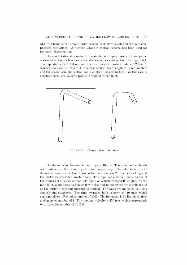
5.1. NON-PULSATILE AND PULSATILE FLOW IN CURVED PIPES 37
MARS scheme is the second order scheme that gives a solution without non-physical oscillations. A blended Crank-Nicholson scheme has been used fortemporal discretization.
The computational domain for the single bent pipe consists of three parts,a straight section, a bend section and a second straight section, see Figure 5.1.The pipe diameter is 104 mm and the bend has a curvature radius of 208 mm,which gives a radius ratio of 4. The first section has a length of 14.5 diametersand the second straight section has a length of 12.5 diameters. For this case, aconstant turbulent velocity profile is applied at the inlet.
Figure 5.1. Computation domains.
The diameter for the double bent pipe is 10 mm. The pipe has two bendswith radius r1=10 mm and r2=15 mm, respectively. The inlet section is 12diameters long, the section between the two bends is 2.5 diameters long andthe outlet section is 6 diameters long. This pipe has a similar shape as one ofthe runners of an exhaust manifold found on a turbocharged IC-engine. At thepipe inlet, a time resolved mass flow pulse and temperature are specified andat the outlet a constant pressure is applied. The walls are modelled as beingsmooth and adiabatic. The time averaged bulk velocity is 110 m/s, whichcorresponds to a Reynolds number of 8900. The frequency is 50 Hz which givesa Womersley number of 8. The maximal velocity is 250 m/s, which correspondsto a Reynolds number of 20 200.

38 5. RESULTS
5.1.2. Non-pulsatile flow in a single bent pipe
The time mean flow obtained from the LES computations shows that the Deanvortices are created at ϕ≈30◦, which is at the same location as reported in theexperiment performed by Sudo et al. (1998). At the exit of the bend, the timemean secondary flow consists of the counter-rotating Dean vortices with thecentres located in the lower part of the pipe, as shown in Figure 5.2. The axialvelocity has a C-shaped distribution in the cross-stream plane, with its maxi-mum at the outer part of the bend. The Dean vortices dominate the secondaryflow at the region downstream of the bend and the vortex cores are moving upagainst the centre of the pipe when they are convected downstream. 10 pipediameters downstream of the bend, the vortices have almost dissipated and theaxial velocity distribution is still C-shaped at this location. The instantaneoussecondary flow at the exit plane of the bend is not symmetric and at certaininstants up to 6 vortices, where two of them are counter-rotating with respectto the Dean vortices, is observed. The vortices are meandering in the cross-stream plane and the C-shaped axial velocity contour is meandering from oneside of the pipe to the other side and the Dean vortices at each side move upand down with varying strength. The axial velocity and the location of theDean vortices is varying with a Strouhal number of approximately 2, where theStrouhal number here is based on the bulk velocity and the pipe radius.
Figure 5.2. The counter-rotating Dean vortices at the outletof the bend. Contour: axial velocity component, vector: In-plane velocity components.

5.1. NON-PULSATILE AND PULSATILE FLOW IN CURVED PIPES 39
The comparison of the computed velocity profiles with the measured pro-files has been conducted at 3 different locations; half a diameter upstream ofthe bend, at the exit of the bend and half a diameter downstream of the bend.Half a diameter upstream of the bend, the deviations between the computedand measured velocity profiles are smaller than the measurement error. Atthe evaluation stations downstream the bend, the deviation is larger and theRANS computation could not capture the behaviour of the flow field, espe-cially at the inner wall, where the computed streamwise velocity is lower forall cases than it is in the measurement, see Figure 5.3. The time mean velocityprofiles from the LES computation without a subgrid scale model gives betteragreement with the measured velocity profiles at all evaluation stations, butthe LES computations over-predict the axial velocity at the outer part of thebend and under-predict the velocity in the centre part of the cross-section ofthe bend.
Despite the fact that the results from the RANS method give the largestdeviation from the measured velocities, this model is used to investigate theeffects of perturbations at the inlet. The reason is the long computation timesthat are required for the LES approach. Different inlet velocity profiles areapplied at the inlet to the single bend pipe. The imposed eccentricity and swirlare used to assess the sensitivity of the results to inlet perturbations. Thesetypes of perturbations are often found in experiments where the inlet pipe isshort and no fully developed turbulent pipe flow can develop. When comparingthe velocity profiles for the different cases with measured velocity profiles, itis clear that the case with the swirling motion gives the best agreement at theexit of the bend. One way to give a measure of the inlet effects is to comparethe Root Mean Square (RMS) value of the ∂U/∂ζ, where ∂U is the differencebetween the velocity profile obtained with a symmetric velocity profile anda non-symmetric or swirling velocity profile at a certain station. ∂ζ is thedifference in kinetic energy at the inlet for the symmetric inlet profile and anon-symmetric or swirling inlet profile. Table 1 shows the results from theanalysis at the exit of the bend and it is clear that inlet condition with swirlingflow gives the largest effect. In this case the flow field is rotated due to theswirling motion before the bend and hence, the low velocity region is turneda few degrees in the clockwise direction. This is also the inlet profile whichgives the best agreement with the measured velocity profiles downstream ofthe bend, indicate that there is probably a swirling secondary flow componentin the experimental case too.

40 5. RESULTS
Figure 5.3. Result from RANS and LES computations.Streamwise component half a diameter downstream of thebend.
Table 1. RMS value of ∂U/∂ζ at the exit of the bend.
Inlet profile Eccentric 1 Eccentric 2 Eccentric 3 SwirlRMS (∂U/∂ε) 0.093 0.046 0.16 0.55
5.1.3. Pulsatile flow in a double bent pipe
The pulsatile flow in the double bent pipe has been computed with both theRANS and the LES approach. In this section, the results from the LES com-putations are presented.
During the acceleration phase of the inlet velocity, the Dean vortices arecreated in the first bend. At the outer part of the entrance to the first bend arecirculation zone is located during the whole pulse period, except when flowreversal occurs. The recirculation is an effect of the adverse pressure gradient inthe streamwise direction at the outer wall. At the entrance to the second bend,the maximum velocity region is located at the inner wall, which means thatthe region of maximum velocity is rotated 90◦ from the exit of the first bend.The secondary flow downstream of the second bend is dominated by a swirlingmotion and the Dean vortices formed in the second bend. One of the Dean
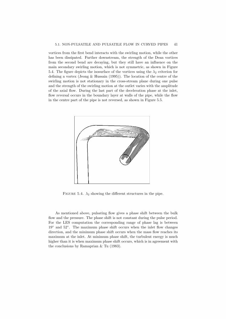
5.1. NON-PULSATILE AND PULSATILE FLOW IN CURVED PIPES 41
vortices from the first bend interacts with the swirling motion, while the otherhas been dissipated. Further downstream, the strength of the Dean vorticesfrom the second bend are decaying, but they still have an influence on themain secondary swirling motion, which is not symmetric, as shown in Figure5.4. The figure depicts the isosurface of the vortices using the λ2 criterion fordefining a vortex (Jeong & Hussain (1995)). The location of the centre of theswirling motion is not stationary in the cross-stream plane during one pulseand the strength of the swirling motion at the outlet varies with the amplitudeof the axial flow. During the last part of the deceleration phase at the inlet,flow reversal occurs in the boundary layer at walls of the pipe, while the flowin the centre part of the pipe is not reversed, as shown in Figure 5.5.
Figure 5.4. λ2 showing the different structures in the pipe.
As mentioned above, pulsating flow gives a phase shift between the bulkflow and the pressure. The phase shift is not constant during the pulse period.For the LES computation the corresponding range of phase lag is between19◦ and 52◦. The maximum phase shift occurs when the inlet flow changesdirection, and the minimum phase shift occurs when the mass flow reaches itsmaximum at the inlet. At minimum phase shift, the turbulent energy is muchhigher than it is when maximum phase shift occurs, which is in agreement withthe conclusions by Ramaprian & Tu (1983).
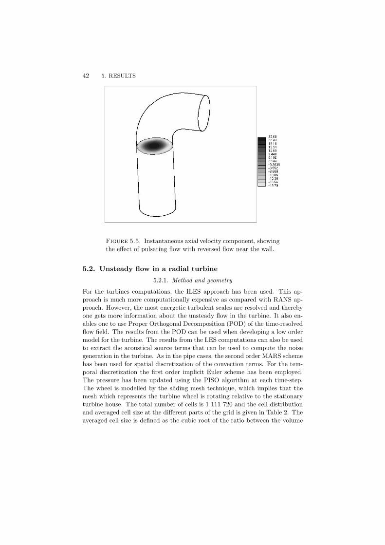
42 5. RESULTS
Figure 5.5. Instantaneous axial velocity component, showingthe effect of pulsating flow with reversed flow near the wall.
5.2. Unsteady flow in a radial turbine
5.2.1. Method and geometry
For the turbines computations, the ILES approach has been used. This ap-proach is much more computationally expensive as compared with RANS ap-proach. However, the most energetic turbulent scales are resolved and therebyone gets more information about the unsteady flow in the turbine. It also en-ables one to use Proper Orthogonal Decomposition (POD) of the time-resolvedflow field. The results from the POD can be used when developing a low ordermodel for the turbine. The results from the LES computations can also be usedto extract the acoustical source terms that can be used to compute the noisegeneration in the turbine. As in the pipe cases, the second order MARS schemehas been used for spatial discretization of the convection terms. For the tem-poral discretization the first order implicit Euler scheme has been employed.The pressure has been updated using the PISO algorithm at each time-step.The wheel is modelled by the sliding mesh technique, which implies that themesh which represents the turbine wheel is rotating relative to the stationaryturbine house. The total number of cells is 1 111 720 and the cell distributionand averaged cell size at the different parts of the grid is given in Table 2. Theaveraged cell size is defined as the cubic root of the ratio between the volume

5.2. UNSTEADY FLOW IN A RADIAL TURBINE 43
and the number of cells for each region. In the rotor region, only hexahedroncells have been used, while in the rest of the domain an unstructured grid hasbeen used with 95% hexahedron cells.
Table 2. Grid resolution.
Number of Averagedcells cell size (mm)
Volute 275 084 0.77Wheel 297 648 0.42Diffuser 538 988 0.71
Complete turbine 1 111 720 0.69
The turbine under consideration is a commercially available turbine witha size that is typical for a turbocharger mounted on a 2.0 litre IC engine of apassenger car. The turbine is a nozzle-less, 9 bladed radial turbine with thewaste-gate valve closed. The complete turbine and the turbine wheel are shownin Figure 5.6. The leading edge tip radius of the wheel is 22.10 mm and thetrailing edge tip radius is 18.75 mm.
Figure 5.6. The complete turbine geometry and the wheel.
The time-step for the non-pulsatile computations is 10−6 seconds whichcorresponds to a rotation of the wheel of 0.6◦/iteration. For the pulsatilecomputations, the time-step is 4 · 10−7 seconds.
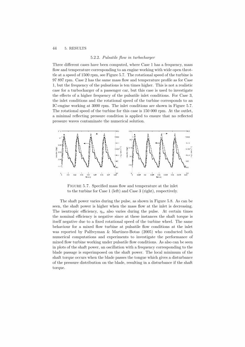
44 5. RESULTS
5.2.2. Pulsatile flow in turbocharger
Three different cases have been computed, where Case 1 has a frequency, massflow and temperature corresponding to an engine working with wide open throt-tle at a speed of 1500 rpm, see Figure 5.7. The rotational speed of the turbine is97 897 rpm. Case 2 has the same mass flow and temperature profile as for Case1, but the frequency of the pulsations is ten times higher. This is not a realisticcase for a turbocharger of a passenger car, but this case is used to investigatethe effects of a higher frequency of the pulsatile inlet conditions. For Case 3,the inlet conditions and the rotational speed of the turbine corresponds to anIC-engine working at 3000 rpm. The inlet conditions are shown in Figure 5.7.The rotational speed of the turbine for this case is 150 000 rpm. At the outlet,a minimal reflecting pressure condition is applied to ensure that no reflectedpressure waves contaminate the numerical solution.
Figure 5.7. Specified mass flow and temperature at the inletto the turbine for Case 1 (left) and Case 3 (right), respectively.
The shaft power varies during the pulse, as shown in Figure 5.8. As can beseen, the shaft power is higher when the mass flow at the inlet is decreasing.The isentropic efficiency, ηis also varies during the pulse. At certain timesthe nominal efficiency is negative since at these instances the shaft torque isitself negative due to a fixed rotational speed of the turbine wheel. The samebehaviour for a mixed flow turbine at pulsatile flow conditions at the inletwas reported by Palfreyman & Martinez-Botas (2005) who conducted bothnumerical computations and experiments to investigate the performance ofmixed flow turbine working under pulsatile flow conditions. As also can be seenin plots of the shaft power, an oscillation with a frequency corresponding to theblade passage is superimposed on the shaft power. The local minimum of theshaft torque occurs when the blade passes the tongue which gives a disturbanceof the pressure distribution on the blade, resulting in a disturbance if the shafttorque.

5.2. UNSTEADY FLOW IN A RADIAL TURBINE 45
Figure 5.8. Computed shaft power vs. mass flow at inlet forCase 1 (left) and Case 3 (right), respectively.
The flow field has only been investigated in detail for Case 1 and Case3, since the conditions of Case 2 is not encountered in engines for passengercars. The major difference between the flow fields in the volute for Case 1and Case 2, is that Case 2 has higher velocity in the volute due to the phaseshift between pressure and mass flow. The higher velocity in the volute forCase 2 implies that the inlet angle to the turbine wheel is different, which givesincidence losses, and hence, affects the shaft power in a negative way.
Figure 5.9. Relative incidence angle to the wheel for 90◦
azimuthal angle during one pulse. Case 1 to the left, Case 3to right.
The incidence angle to the wheel varies during the pulse, due to the varyingmass flow at the inlet. In Figure 5.9, the relative inlet angle for 90◦ azimuthalangle is plotted for Case 1 and Case 3. As can be seen, the inlet angle forCase 1 varies from approximately -85◦ to 60◦. For Case 3, the inlet anglevaries from approximately -67◦ to -25◦, which is more favourable. For Case

46 5. RESULTS
Figure 5.10. Snapshot of the in-plane relative velocity fieldat the inlet plane to the wheel, Case 1. The arrow shows thedirection of rotation. The top figure shows the flow field withlow mass flow through the turbine. The bottom figure showsthe flow field when the mass flow through the turbine is high.
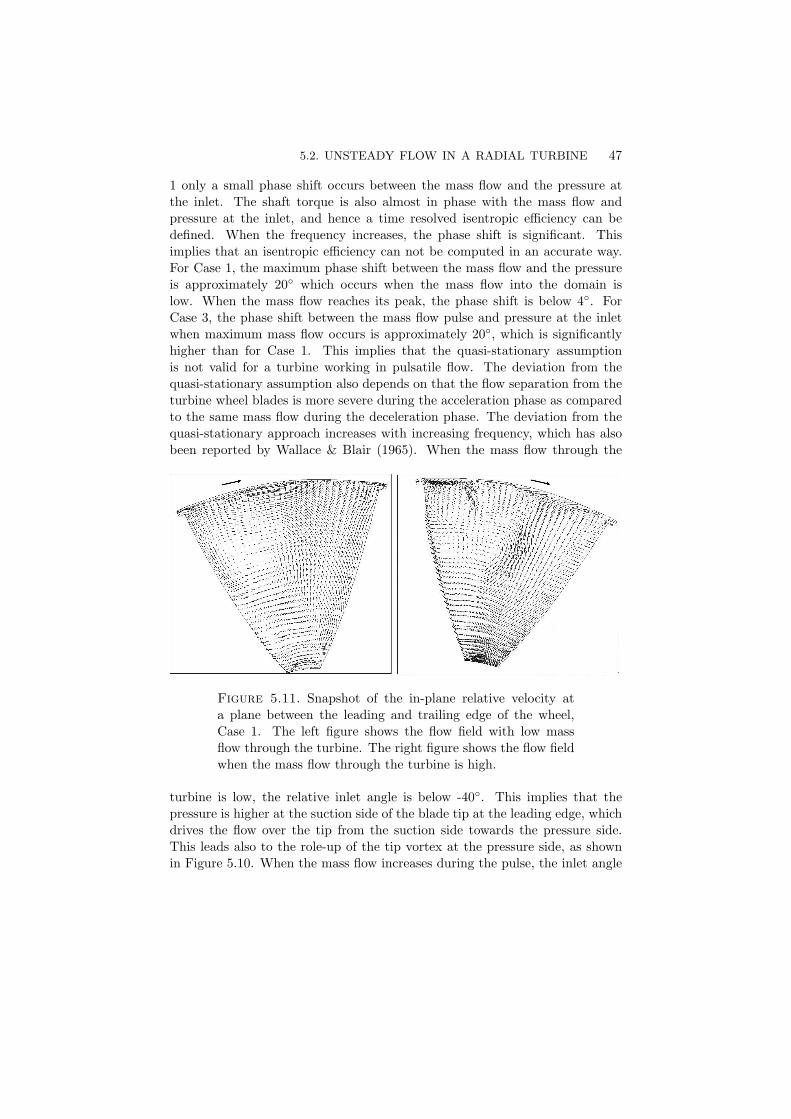
5.2. UNSTEADY FLOW IN A RADIAL TURBINE 47
1 only a small phase shift occurs between the mass flow and the pressure atthe inlet. The shaft torque is also almost in phase with the mass flow andpressure at the inlet, and hence a time resolved isentropic efficiency can bedefined. When the frequency increases, the phase shift is significant. Thisimplies that an isentropic efficiency can not be computed in an accurate way.For Case 1, the maximum phase shift between the mass flow and the pressureis approximately 20◦ which occurs when the mass flow into the domain islow. When the mass flow reaches its peak, the phase shift is below 4◦. ForCase 3, the phase shift between the mass flow pulse and pressure at the inletwhen maximum mass flow occurs is approximately 20◦, which is significantlyhigher than for Case 1. This implies that the quasi-stationary assumptionis not valid for a turbine working in pulsatile flow. The deviation from thequasi-stationary assumption also depends on that the flow separation from theturbine wheel blades is more severe during the acceleration phase as comparedto the same mass flow during the deceleration phase. The deviation from thequasi-stationary approach increases with increasing frequency, which has alsobeen reported by Wallace & Blair (1965). When the mass flow through the
Figure 5.11. Snapshot of the in-plane relative velocity ata plane between the leading and trailing edge of the wheel,Case 1. The left figure shows the flow field with low massflow through the turbine. The right figure shows the flow fieldwhen the mass flow through the turbine is high.
turbine is low, the relative inlet angle is below -40◦. This implies that thepressure is higher at the suction side of the blade tip at the leading edge, whichdrives the flow over the tip from the suction side towards the pressure side.This leads also to the role-up of the tip vortex at the pressure side, as shownin Figure 5.10. When the mass flow increases during the pulse, the inlet angle

48 5. RESULTS
increases and flow separation occurs at the suction side of the blade. The vortexdue to separation is much stronger than the tip vortex formed at the pressureside of the blade. The tip vortex formed at the leading edge detaches and isconvected downstream between the blades. Downstream between the blades,the secondary flow at high mass flow contains three different structures; thedetached tip vortex from the leading edge that is convected downstream, the tipvortex that is created between the blade tip and the shroud and a vortex thatis counter-rotating as compared to the tip vortices, as depicted in Figure 5.11.Between the blades, the pressure gradient drives the flow in the boundary-layerat the shroud from the pressure side towards the suction side. When the flowin the boundary-layer at the shroud is affected by the strong jet that is formedat the tip, it is deflected inwards between the blades and a vortex starts to rollup. The higher mass flow at the inlet for Case 3 implies that the Mach number
Figure 5.12. Snapshot of the velocity field in the diffuser,half a wheel diameter downstream of the trailing edge of thewheel, Case 1. The left figure shows the flow field with lowmass flow through the turbine. The right figure shows the flowfield when the mass flow through the turbine is high.
is higher. When the mass flow through the wheel reaches its maximum, ashock wave is formed between the leading edge of the blade and the wall at thetongue. The shock disturbs the flow, and the tip vortex at the suction side atthe leading edge where the shock occurs is very strong. Since the interval whensupersonic flow occurs in the volute only corresponded to a few blade passages,it does not deteriorate the shaft torque. The higher mass flow for Case 3 alsoresults in a stronger pressure gradient between the blades which gives a higherpower output. Despite the stronger pressure gradient, the tip vortices for Case
5.2. UNSTEADY FLOW IN A RADIAL TURBINE 49
3 are not as strong as for Case 1, depending on a more optimal inlet flow angleinto the wheel.
Downstream of the wheel, the centre line vortex has the direction of ro-tation opposite to direction of the rotation of the wheel when the mass flowthrough the turbine is high. For Case 3, this vortex is weaker as compared tothe centre line vortex for Case 1, due to a more favourable flow outlet angle forCase 3. When the mass flow is low for both cases, no coherent structures areobserved at the centre-line down-stream of the wheel, as shown Figure 5.12.
5.2.3. Effects of inlet perturbations
The effect of different perturbations at the inlet on the performance of a radialnozzle-less turbine has been assessed. Five different inlet conditions have beenconsidered. These are given in Table 3. For all cases, a turbulent velocityprofile and the temperature are specified at the inlet boundary and differentperturbations are added to this velocity profile. The mass flow at the inletto the turbine has been kept constant (equal to 0.08144 kg/s) by varying thevelocity. The temperature at the inlet has been set to 1000◦C for all cases.At the outlet, a non-reflective boundary condition is applied. The walls areassumed to be smooth and adiabatic.
Table 3. Computed cases.
Case Turbulence Secondary Strength ofintensity flow secondary flow
1 0% - -2 5% - -3 5% Dean 0.104 5% Swirl 0.285 5% Swirl 1.5
In Figure 5.13 the axial and azimuthal velocity components at the inlet tothe turbine are plotted for the different cases. For Case 1, no perturbationsare added. Case 2 had an inlet profile with turbulent fluctuations. The turbu-lence intensity for Cases 2-5 is 5% and the turbulent fluctuations at the inletboundary are created by the method proposed by Klein et al. (2003). Case3 has both turbulent fluctuations and secondary flow in the velocity profile,where the secondary flow consists of a pair of counter-rotating Dean vortices,see Figure 5.14. Cases 4 and 5 have, in addition to the turbulent fluctuations,a swirling motion added, where Case 5 has the stronger swirl. The strength ofthe swirl at the inlet is defined as the azimuthal velocity at the edge of the inlet

50 5. RESULTS
Figure 5.13. Axial and secondary velocity components at the inlet.
boundary divided by the axial bulk velocity. The strength of the Dean vorticesis defined as the area averaged value of the secondary component divided by theaxial component at the inlet. The strength of the secondary flow is obtainedfrom LES-computations of the pulsatile flow in a four to one exhaust manifold.
The evaluated data has been gathered for the last 4 of 20 revolutions ofthe turbine. This corresponds to 36 blade passages. This data have been usedfor the computing the time averages of the different parameters. In Figure 5.15
Table 4. Shaft power, available power at the inlet, isentropicefficiency, utility factor and pressure ratio.
Case PSHAFT PINLET ηis κ PR(kW) (kW)
1 5.02 82.18 0.66 0.061 1.412 4.34 82.14 0.66 0.053 1.343 4.41 82.26 0.64 0.054 1.364 4.40 82.12 0.66 0.053 1.355 4.05 82.35 0.64 0.048 1.32
the time resolved shaft power for the different cases is shown. The shaft powerfluctuates with a frequency that corresponds to the blade passage frequency.Fluctuations with lower frequencies are also present for all cases, depending onflow unsteadiness in the volute. In Table 4 the time averaged shaft power andtwo different ways of expressing the efficiency are given. For the time meanvalue of the shaft power, there are differences between the cases. The timemean shaft power for Case 5 is 19% lower than for Case 1, which is greaterthan the estimated numerical uncertainty. For Cases 2-4, the differences in theshaft power as compared to Cases 1 or 5 are of the same order as the numerical

5.2. UNSTEADY FLOW IN A RADIAL TURBINE 51
Figure 5.14. The secondary flow at the inlet plane for Case3 and 5, respectively.
uncertainty. Altogether, the computations show that different perturbations atthe inlet do affect the performance of the turbine. As can be seen in Table 4,the isentropic efficiency does not reflect the fact that the shaft power is almost20% lower for Case 5 as compared to Case 1. This is so since the isentropicefficiency also takes into account the energy content of the flow after the turbine,which can be used to drive a second turbo-charger. A better definition of theefficiency is the utility factor, κ. The utility factor is defined as:
κ =PSHAFT
PINLET(5.1)
This better reflect the effects of the perturbation at the inlet. In thisdefinition, PINLET is the available power at the inlet boundary, defined as:
PINLET =∫
Inlet
(12· ui · ui + h
)ρUndA (5.2)
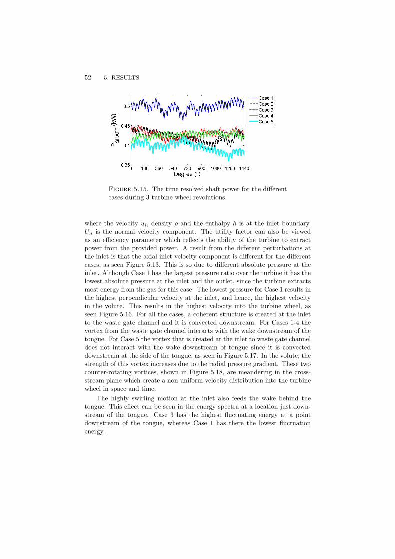
52 5. RESULTS
Figure 5.15. The time resolved shaft power for the differentcases during 3 turbine wheel revolutions.
where the velocity ui, density ρ and the enthalpy h is at the inlet boundary.Un is the normal velocity component. The utility factor can also be viewedas an efficiency parameter which reflects the ability of the turbine to extractpower from the provided power. A result from the different perturbations atthe inlet is that the axial inlet velocity component is different for the differentcases, as seen Figure 5.13. This is so due to different absolute pressure at theinlet. Although Case 1 has the largest pressure ratio over the turbine it has thelowest absolute pressure at the inlet and the outlet, since the turbine extractsmost energy from the gas for this case. The lowest pressure for Case 1 results inthe highest perpendicular velocity at the inlet, and hence, the highest velocityin the volute. This results in the highest velocity into the turbine wheel, asseen Figure 5.16. For all the cases, a coherent structure is created at the inletto the waste gate channel and it is convected downstream. For Cases 1-4 thevortex from the waste gate channel interacts with the wake downstream of thetongue. For Case 5 the vortex that is created at the inlet to waste gate channeldoes not interact with the wake downstream of tongue since it is convecteddownstream at the side of the tongue, as seen in Figure 5.17. In the volute, thestrength of this vortex increases due to the radial pressure gradient. These twocounter-rotating vortices, shown in Figure 5.18, are meandering in the cross-stream plane which create a non-uniform velocity distribution into the turbinewheel in space and time.
The highly swirling motion at the inlet also feeds the wake behind thetongue. This effect can be seen in the energy spectra at a location just down-stream of the tongue. Case 3 has the highest fluctuating energy at a pointdownstream of the tongue, whereas Case 1 has there the lowest fluctuationenergy.
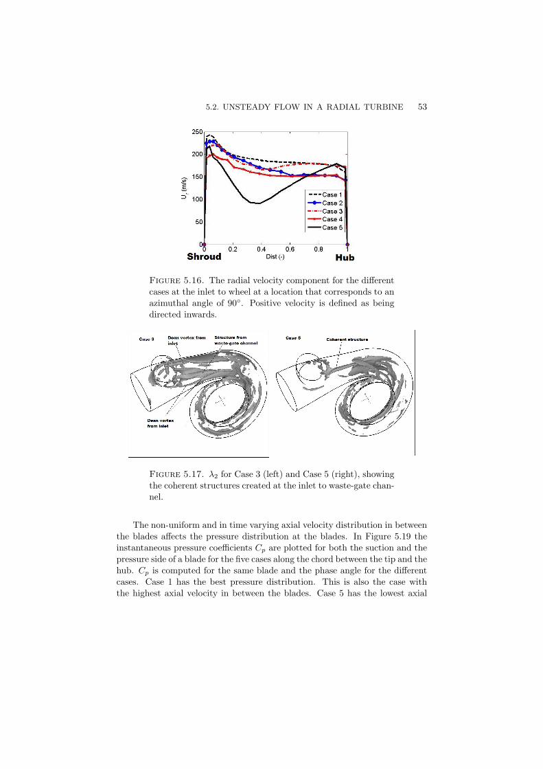
5.2. UNSTEADY FLOW IN A RADIAL TURBINE 53
Figure 5.16. The radial velocity component for the differentcases at the inlet to wheel at a location that corresponds to anazimuthal angle of 90◦. Positive velocity is defined as beingdirected inwards.
Figure 5.17. λ2 for Case 3 (left) and Case 5 (right), showingthe coherent structures created at the inlet to waste-gate chan-nel.
The non-uniform and in time varying axial velocity distribution in betweenthe blades affects the pressure distribution at the blades. In Figure 5.19 theinstantaneous pressure coefficients Cp are plotted for both the suction and thepressure side of a blade for the five cases along the chord between the tip and thehub. Cp is computed for the same blade and the phase angle for the differentcases. Case 1 has the best pressure distribution. This is also the case withthe highest axial velocity in between the blades. Case 5 has the lowest axial
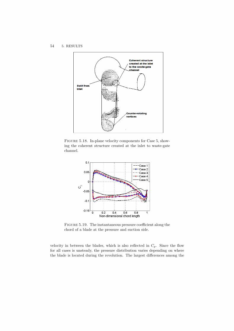
54 5. RESULTS
Figure 5.18. In-plane velocity components for Case 5, show-ing the coherent structure created at the inlet to waste-gatechannel.
Figure 5.19. The instantaneous pressure coefficient along thechord of a blade at the pressure and suction side.
velocity in between the blades, which is also reflected in Cp. Since the flowfor all cases is unsteady, the pressure distribution varies depending on wherethe blade is located during the revolution. The largest differences among the

5.2. UNSTEADY FLOW IN A RADIAL TURBINE 55
different cases are on the suction side, since this blade side is the most sensitiveto changes of the relative incidence angle.
The highest velocity for Case 1 in between the blades implies that this casehas the strongest azimuthal pressure gradient. This results in the strongesttip vortices at the leading edge of the blades. Case 5, which has the lowestvelocity in between the blades, has the weakest tip vortices. The secondaryflow structures in between the blades seem to have a secondary effect on theshaft power output.

CHAPTER 6
Conclusions
The unsteady flow in pipes and a radial turbine have been computed using LES.The purpose of the pipe flow computations was to study the non-pulsatile andpulsatile internal flow in curved geometries, which are relevant to the inlet tothe turbo-charger turbine. For one of the used geometries, a comparison withmeasured data has also been performed. The results show that an ImplicitLES turbulence modelling approach gives the best agreement with measuredvelocities among the tested turbulence modelling approaches. For the pulsatileflow a phase shift between the pressure and the bulk flow has been found.The phase shift varies during the pulse, depending on the balance between thedifferent terms in the momentum equation. The phase shift also implies thatflow in the boundary layer and in the core region of the pipe are out phase,since the low momentum flow in the boundary layer is more sensitive to changesin the axial pressure gradient than the flow in the core region. This results inan increased mixing in the region near the wall resulting in higher heat transferto the walls.
The bends in the pipe introduced secondary flow structures. In the firstbend, two counter-rotating vortices are created and the axial velocity compo-nent after the bend is not uniformly distributed. When this non-uniform axialvelocity distribution enters a second bend, situated in an orthogonal planedownstream of the first bend, a swirling motion is created downstream of thesecond bend. This swirling motion is also affected by the Dean vortices createdin the bends upstream. Since an exhaust manifold can be viewed as beingcomposed of straight and bent pipe sections, the flow into the turbine has non-negligible secondary flow structures in addition to the pulsatile axial flow. Thepulsatile flow in the turbine also increases the heat losses. This all togetherimplies that a turbocharger turbine for an IC-engine will have operation condi-tions that are far away from the conditions that they are designed and testedfor.
The effect of the pulsatile flow on the turbine performance has been assessedby conducting computation at different frequencies and mass flows. The majorconclusions of that study are as follows:
56
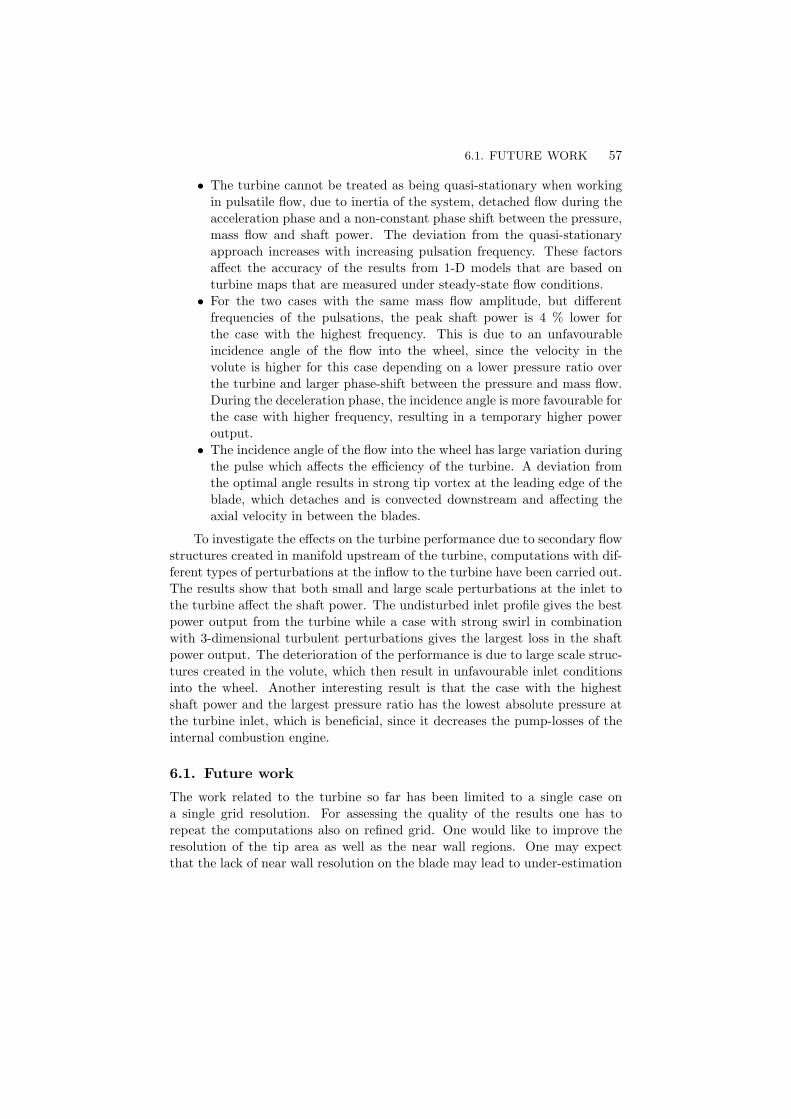
6.1. FUTURE WORK 57
• The turbine cannot be treated as being quasi-stationary when workingin pulsatile flow, due to inertia of the system, detached flow during theacceleration phase and a non-constant phase shift between the pressure,mass flow and shaft power. The deviation from the quasi-stationaryapproach increases with increasing pulsation frequency. These factorsaffect the accuracy of the results from 1-D models that are based onturbine maps that are measured under steady-state flow conditions.
• For the two cases with the same mass flow amplitude, but differentfrequencies of the pulsations, the peak shaft power is 4 % lower forthe case with the highest frequency. This is due to an unfavourableincidence angle of the flow into the wheel, since the velocity in thevolute is higher for this case depending on a lower pressure ratio overthe turbine and larger phase-shift between the pressure and mass flow.During the deceleration phase, the incidence angle is more favourable forthe case with higher frequency, resulting in a temporary higher poweroutput.
• The incidence angle of the flow into the wheel has large variation duringthe pulse which affects the efficiency of the turbine. A deviation fromthe optimal angle results in strong tip vortex at the leading edge of theblade, which detaches and is convected downstream and affecting theaxial velocity in between the blades.
To investigate the effects on the turbine performance due to secondary flowstructures created in manifold upstream of the turbine, computations with dif-ferent types of perturbations at the inflow to the turbine have been carried out.The results show that both small and large scale perturbations at the inlet tothe turbine affect the shaft power. The undisturbed inlet profile gives the bestpower output from the turbine while a case with strong swirl in combinationwith 3-dimensional turbulent perturbations gives the largest loss in the shaftpower output. The deterioration of the performance is due to large scale struc-tures created in the volute, which then result in unfavourable inlet conditionsinto the wheel. Another interesting result is that the case with the highestshaft power and the largest pressure ratio has the lowest absolute pressure atthe turbine inlet, which is beneficial, since it decreases the pump-losses of theinternal combustion engine.
6.1. Future work
The work related to the turbine so far has been limited to a single case ona single grid resolution. For assessing the quality of the results one has torepeat the computations also on refined grid. One would like to improve theresolution of the tip area as well as the near wall regions. One may expectthat the lack of near wall resolution on the blade may lead to under-estimation

58 6. CONCLUSIONS
of the separation regions and thereby also some viscous losses. One may alsoexpect that the separation bubbles are unsteady and this may interact andinduce further unsteadiness in the turbine. The underlying physics of sucheffects have to be further explored. Additionally, the effects of losses throughthe turbine housing have been neglected due to the use of adiabatic conditions.
One of the objectives of this work has been to better understand the dynam-ics of the flow in the turbine. This is expected to be done by utilizing ProperOrthogonal Decomposition (POD) that is an optimal expansion in orthogonalfunctions. The expansion is optimal in the sense that the kinetic energy ofthe flow can be expressed in minimal number of terms. We intend also to usesuch POD expansion to define a lower dimensional dynamical system. Thisis to be derived by applying a Galerkin projection of the POD expansion onthe governing equations. Such approach can be as efficient for simulation ascurrent 1-D tools but shall take into account the inherent 3-D characteristicsof the flow.
CHAPTER 7
Papers and authors contributions
Paper 1Numerical computations of steady and unsteady flow in bended pipes.F. Hellstrom & L. Fuchs.AIAA 2007-4350, 37th Fluid Dynamics Conference and Exhibit, Miami Fl.2007
The purpose of this work is to investigate the non-pulsatile and pulsatile flowin bent pipes. The results from one of the cases with different turbulence mod-elling approaches are compared with measured data. A study of the influenceof perturbations at the inlet is also performed. The work was performed byHellstrom under supervision by Prof. Fuchs. The results were presented at the37th Fluid Dynamics Conference and Exhibit, Miami, Florida, 2007 by Hell-strom.
Paper 2Numerical computations of pulsatile flow in a turbo-charger.F. Hellstrom & L. Fuchs.AIAA-2008-735, 46th Aerospace Sciences Meeting, Reno, 2008.
The objective of this work is to assess the effect of different pulsatile inletconditions on the turbine performance. Therefore three different cases withdifferent frequencies and mass flow pulses are considered. The performance ofthe turbine for the non-pulsatile computations is also compared with measuredperformance for the same geometry. The work was performed by Hellstromunder supervision by Prof. Fuchs. The results were presented at the 46thAerospace Sciences Meeting, Reno, 2008 by Hellstrom.
59

60 7. PAPERS AND AUTHORS CONTRIBUTIONS
Paper 3Effects of inlet conditions on the turbine performance of a radial turbine.F. Hellstrom & L. Fuchs.Submitted to ASME Turbo Expo 2008: Power for Land, Sea and Air June 9-13,2008, Berlin, Germany.
In this paper the effect of the different perturbations on the performance ofa radial nozzle-less turbine is assessed and quantified by using Large EddySimulations. Five different cases are considered, where the base case has anon-disturbed velocity profile applied at the inlet. The other cases has 3-dimensional turbulence added to the velocity profile. Three of the cases hasalso different secondary flow structures added at the inlet. The turbine perfor-mance is compared for the different cases and the flow field is investigated togive a better insight into the unsteady flow field and the effects from the differ-ent inlet conditions. The work was performed by Hellstrom under supervisionby Prof. Fuchs. The paper is submitted to ASME Turbo Expo 2008: Powerfor Land, Sea and Air June 9-13, 2008, Berlin, Germany.

61

Acknowledgements
First of all I would to thank my supervisor Professor Laszlo Fuchs for all en-couragement, support and guidance throughout this work.
I would also like to thank my employer GM Powertrain, Sweden AB, for makingmy PhD studies possible and I especially would like to thank my manager Dr.Reinmann, who gave me the possibility to conduct the PhD studies without anyinterruptions. Thanks also to Anna Svard and Per Birkestad for commentingmy manuscript.
The Swedish Emission Research Program is acknowledged for the financialsupport.
Last, but definitily least, I would like thank my wife and daughter for all thepatience and love.
62

References
Andersen, J., Karlsson, E. & Gawell, A. 2006 Variable turbine geometry on si
engines. SAE 2006 World Congress, Detroit, Michigan SAE 2006-01-0020.
Anwer, M. So, R. M. C. & Lai, Y. G. 1989 Pertubation and recovery from bend
curvature of a fully developd turbulent pipe flow. Physics of Fluid 1, 1387–1397.
Arcoumanis, C., Karamanis, N., Martinez-Botas, R. & Su, C. C. 1999 Un-
steady characteristics of a mixed-flow turbocharger turbine. IMechE paper no
C557/030 pp. 905–921.
Baines, C. N. 2005 Fundamentals of turbocharging. Concepts NREC, ISBN 0-
933283-14-8 .
Bardina, J., Ferziger, J. & Reynolds, W. 1980 Improved subgrid scale models
for large eddy simulation. AIAA Paper 80-1357 .
Barr, L., Spence, S. W. T., & McNally, T. 2006 A numerical study of the perfor-
mance characteristics of a radial turbine with varying inlet blade angle. ImechE
Conference Transactions from 8th International Conference on Turbochargers
and Turbocharging pp. 169–181.
Benson, R. 1974 Nonsteady flow in turbocharger nozzleless radial gas turbine. SAE
740739 pp. 1–11.
Benson, R. & Scrimshaw, K. 1965 An experimental investigation of non-steay flow
in a radial gas turbine. Instn Mech Engrs 180, 74–85.
Brucker, C. 1998 A time-recording piv-study of the swirl switching effect in a 90◦
bend flow. Proceedings of the Eight International Symposium on Flow Visualiza-
tions, Sorento, Italy .
Capobianco, M. & Gambarotta, A. 1990 Unsteady flow performance of tur-
bocharger radial turbines. C405/017, Proceeding of the Institute of Mechanical
Engineers, Fourth International Conference, Turbocharging and Turbochargers
pp. 123–132.
Capobianco, M. & Gambarotta, A. 1992 Variable geometry and waste-gated auto-
motive turbochargers: Measurements and comparision of turbine performance.
Transactions of ASME: Journal of Engineering for Gas Turbines and Power
114, 553–560.
Capobianco, M. & Gambarotta, A. 1993 Performance of a twin-entry automotive
63
64 REFERENCES
turbocharger turbine. ASME, 93- ICE-2. Energy-Sources Technology Conference
& Exhibition. pp. 1–10.
Capobianco, M. & Marelli, S. 2005 Transient performance of automotive tur-
bochargers: Test facility and preliminary experimental analysis. SAE 2005-24-
066, ICE 2005, 7th International Conference on Engines for Automobile .
Carpinlioglu, M. & Gundogdu, M. 2001 A critical review on pulsatile flow studies
directing towards future research topics. Flow measurements and Instrumenta-
tions 12, 165–174.
CD-adapco 2005 Methodology manual . STAR-CD Version 3.26.
Celik, I. B. 2005 Procedure for estimation and reporting of discretization er-
ror in cfd applications. Internal report, Mechanical and Aerospace Engi-
neering Department, West Virgina University, Morgantown Wv, USA, is-
Chapple, P., Flynn, P. F. & Mulloy, J. 1980 Aerodynamical design of fixed and
variable geometry nozzleless turbine casings. Transactions of the ASME Journal
Eng for Power 102, 141–147.
Chen, H., Baines, N. C. & Abidat, M. 1997 Exit traverse study of mixed-flow
turbines with inlet incidence variation. Proceedings of the Institute of Mechanical
Engineers 211 Part A, 461–475.
Dale, A. & Watson, N. 1986 Vaneless radial turbocharger turbine performance.
ImechE Conference Transactions; ”Turbochargers and Turbocharging”, London
pp. 65–76.
Dambach, R. & Hodson, H. 2001 Tip leakege flow in a radial inflow turbine with
varying gap height. Journal of Propulsion and Power 17, 644–650.
Dec, J. E. & Keller, J. O. 1989 Pulse combustor tail-pipe heat-transfer dependence
on frequency, amplitude and mean flow rate. Combustion and flame pp. 359–374.
Dec, J. E., Keller, J. O. & Hongo, I. 1991 Time-resolved velocities and turbulence
in oscillating flow of a pulse combustor tail pipe. Combustion and flame 83, 271–
292.
Doran, W. J., Spence, S. W. T. & Artt, D. W. 2001 Experimental performance
evaluation of a 99.0 mm radial inflow nozzled turbine with varying shroud pro-
files. Proceedings of the Institute of Mechanical Engineers: Journal of Power and
Energy 215, 267–280.
Filipi, Z., Wang, Y. & Addanis, D. 2001 Effect of variable geometry turbine (vgt)
on diesel engine and vehicle system transient respons. SAE 2001 World Congress,
Detroit, Michigan SAE 2001-01-1247, 1–19.
Flaxington, A. & Swain, E. 1999 Turbocharger aerodynamic design. Proceedings
of the Institute of Mechanical Engineers Vol 213 Part C, 43–57.
Fukaya, M., Watanabe, M. & Udagawa, T. 2000 Compressible turbulent flow
analysis on variable nozzle vanes and spacer in turbocharger turbine. SAE 2000
World Congress, Detroit, Michigan SAE 2000-01-0526.
Futral, S. M. & Holeski, D. E. 1970 Experimental results of varying the blade-
shroud clearence in a 6.02-inch radial-inflow turbine. Tech. Rep.. NASA TN
D-5513.
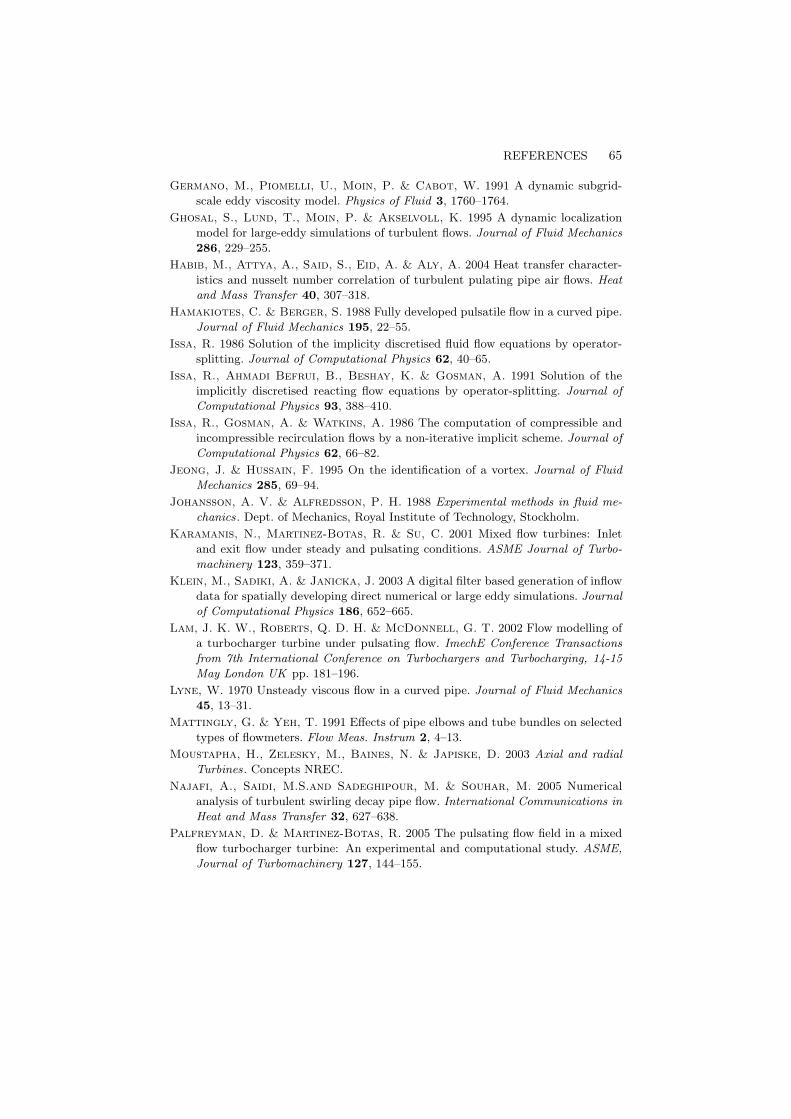
REFERENCES 65
Germano, M., Piomelli, U., Moin, P. & Cabot, W. 1991 A dynamic subgrid-
scale eddy viscosity model. Physics of Fluid 3, 1760–1764.
Ghosal, S., Lund, T., Moin, P. & Akselvoll, K. 1995 A dynamic localization
model for large-eddy simulations of turbulent flows. Journal of Fluid Mechanics
286, 229–255.
Habib, M., Attya, A., Said, S., Eid, A. & Aly, A. 2004 Heat transfer character-
istics and nusselt number correlation of turbulent pulating pipe air flows. Heat
and Mass Transfer 40, 307–318.
Hamakiotes, C. & Berger, S. 1988 Fully developed pulsatile flow in a curved pipe.
Journal of Fluid Mechanics 195, 22–55.
Issa, R. 1986 Solution of the implicity discretised fluid flow equations by operator-
splitting. Journal of Computational Physics 62, 40–65.
Issa, R., Ahmadi Befrui, B., Beshay, K. & Gosman, A. 1991 Solution of the
implicitly discretised reacting flow equations by operator-splitting. Journal of
Computational Physics 93, 388–410.
Issa, R., Gosman, A. & Watkins, A. 1986 The computation of compressible and
incompressible recirculation flows by a non-iterative implicit scheme. Journal of
Computational Physics 62, 66–82.
Jeong, J. & Hussain, F. 1995 On the identification of a vortex. Journal of Fluid
Mechanics 285, 69–94.
Johansson, A. V. & Alfredsson, P. H. 1988 Experimental methods in fluid me-
chanics. Dept. of Mechanics, Royal Institute of Technology, Stockholm.
Karamanis, N., Martinez-Botas, R. & Su, C. 2001 Mixed flow turbines: Inlet
and exit flow under steady and pulsating conditions. ASME Journal of Turbo-
machinery 123, 359–371.
Klein, M., Sadiki, A. & Janicka, J. 2003 A digital filter based generation of inflow
data for spatially developing direct numerical or large eddy simulations. Journal
of Computational Physics 186, 652–665.
Lam, J. K. W., Roberts, Q. D. H. & McDonnell, G. T. 2002 Flow modelling of
a turbocharger turbine under pulsating flow. ImechE Conference Transactions
from 7th International Conference on Turbochargers and Turbocharging, 14-15
May London UK pp. 181–196.
Lyne, W. 1970 Unsteady viscous flow in a curved pipe. Journal of Fluid Mechanics
45, 13–31.
Mattingly, G. & Yeh, T. 1991 Effects of pipe elbows and tube bundles on selected
types of flowmeters. Flow Meas. Instrum 2, 4–13.
Moustapha, H., Zelesky, M., Baines, N. & Japiske, D. 2003 Axial and radial
Turbines. Concepts NREC.
Najafi, A., Saidi, M.S.and Sadeghipour, M. & Souhar, M. 2005 Numerical
analysis of turbulent swirling decay pipe flow. International Communications in
Heat and Mass Transfer 32, 627–638.
Palfreyman, D. & Martinez-Botas, R. 2005 The pulsating flow field in a mixed
flow turbocharger turbine: An experimental and computational study. ASME,
Journal of Turbomachinery 127, 144–155.
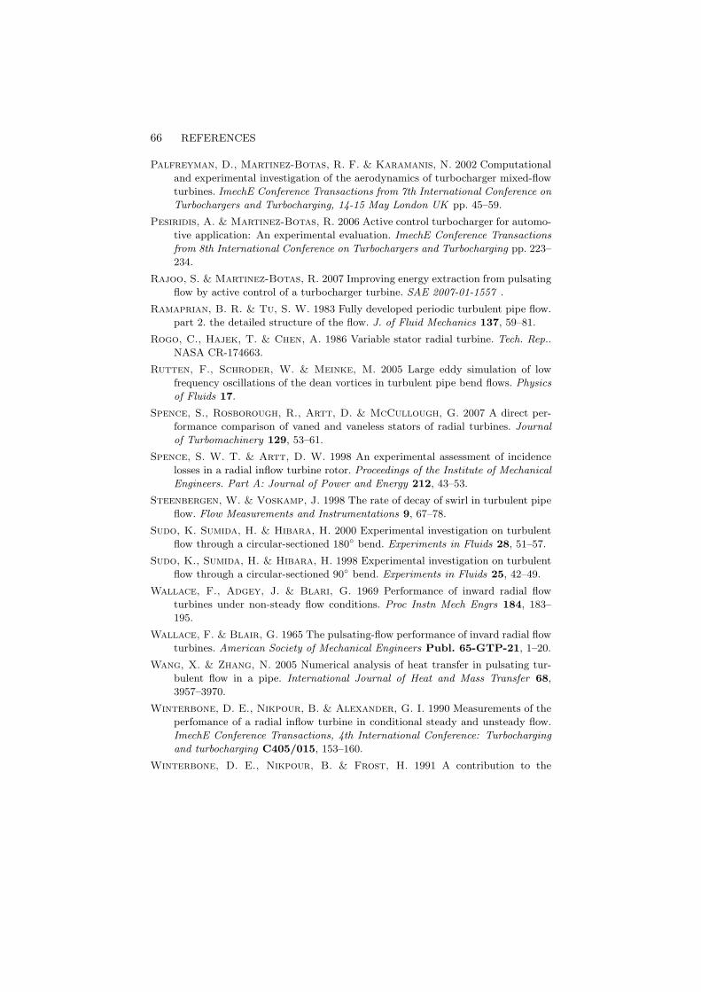
66 REFERENCES
Palfreyman, D., Martinez-Botas, R. F. & Karamanis, N. 2002 Computational
and experimental investigation of the aerodynamics of turbocharger mixed-flow
turbines. ImechE Conference Transactions from 7th International Conference on
Turbochargers and Turbocharging, 14-15 May London UK pp. 45–59.
Pesiridis, A. & Martinez-Botas, R. 2006 Active control turbocharger for automo-
tive application: An experimental evaluation. ImechE Conference Transactions
from 8th International Conference on Turbochargers and Turbocharging pp. 223–
234.
Rajoo, S. & Martinez-Botas, R. 2007 Improving energy extraction from pulsating
flow by active control of a turbocharger turbine. SAE 2007-01-1557 .
Ramaprian, B. R. & Tu, S. W. 1983 Fully developed periodic turbulent pipe flow.
part 2. the detailed structure of the flow. J. of Fluid Mechanics 137, 59–81.
Rogo, C., Hajek, T. & Chen, A. 1986 Variable stator radial turbine. Tech. Rep..
NASA CR-174663.
Rutten, F., Schroder, W. & Meinke, M. 2005 Large eddy simulation of low
frequency oscillations of the dean vortices in turbulent pipe bend flows. Physics
of Fluids 17.
Spence, S., Rosborough, R., Artt, D. & McCullough, G. 2007 A direct per-
formance comparison of vaned and vaneless stators of radial turbines. Journal
of Turbomachinery 129, 53–61.
Spence, S. W. T. & Artt, D. W. 1998 An experimental assessment of incidence
losses in a radial inflow turbine rotor. Proceedings of the Institute of Mechanical
Engineers. Part A: Journal of Power and Energy 212, 43–53.
Steenbergen, W. & Voskamp, J. 1998 The rate of decay of swirl in turbulent pipe
flow. Flow Measurements and Instrumentations 9, 67–78.
Sudo, K. Sumida, H. & Hibara, H. 2000 Experimental investigation on turbulent
flow through a circular-sectioned 180◦ bend. Experiments in Fluids 28, 51–57.
Sudo, K., Sumida, H. & Hibara, H. 1998 Experimental investigation on turbulent
flow through a circular-sectioned 90◦ bend. Experiments in Fluids 25, 42–49.
Wallace, F., Adgey, J. & Blari, G. 1969 Performance of inward radial flow
turbines under non-steady flow conditions. Proc Instn Mech Engrs 184, 183–
195.
Wallace, F. & Blair, G. 1965 The pulsating-flow performance of invard radial flow
turbines. American Society of Mechanical Engineers Publ. 65-GTP-21, 1–20.
Wang, X. & Zhang, N. 2005 Numerical analysis of heat transfer in pulsating tur-
bulent flow in a pipe. International Journal of Heat and Mass Transfer 68,
3957–3970.
Winterbone, D. E., Nikpour, B. & Alexander, G. I. 1990 Measurements of the
perfomance of a radial inflow turbine in conditional steady and unsteady flow.
ImechE Conference Transactions, 4th International Conference: Turbocharging
and turbocharging C405/015, 153–160.
Winterbone, D. E., Nikpour, B. & Frost, H. 1991 A contribution to the

REFERENCES 67
understanding of turbocharger turbine perfomance in pulsating flow. Interna-
tional Conference on Internal Combustion Research, Paper no C433/011. Inst.
of Mech. Engrs. pp. 19–28.
Yeo, J. H. & Baines, N. C. 1990 Pulsating flow and behaviour in a twin-entry
vaneless radial-inflow turbine. ImechE Conference Transactions, 4th Interna-
tional Conference: Turbocharging and turbocharging. C405/004, 113–122.