stable and accurate pressure approximation for …bobpego/preprints/ll4jcp.pdfstable and accurate...

Stable and accurate pressure approximation for

unsteady incompressible viscous flow

Jian-Guo Liu1, Jie Liu2, and Robert L. Pego3

Abstract

How to properly specify boundary conditions for pressure is a longstanding problem

for the incompressible Navier-Stokes equations with no-slip boundary conditions. An

analytical resolution of this issue stems from a recently developed formula for the

pressure in terms of the commutator of the Laplacian and Leray projection operators.

Here we make use of this formula to (a) improve the accuracy of computing pressure in

two kinds of existing time-discrete projection methods implicit in viscosity only, and

(b) devise new higher-order accurate time-discrete projection methods that extend a

slip-correction idea behind the well-known finite-difference scheme of Kim and Moin.

We test these schemes for stability and accuracy using various combinations of C0

finite elements. For all three kinds of time discretization, one can obtain 3rd-order

accuracy for both pressure and velocity without a time-step stability restriction of

diffusive type. Furthermore, two kinds of projection methods are found stable using

piecewise linear elements for both velocity and pressure.

Key words. time-dependent incompressible flow, projection method, timesplitting, third-order accuracy, backward facing step, driven cavity, flow pastcylinder, Stokes pressure, Leray projection.

AMS Subject Classifications. 76D05, 65M15, 65M60

1Department of Physics and Mathematics, Duke University, Durham, NC 27708. Email:

[email protected] of Mathematics, National University of Singapore, Singapore 117543. Email:

[email protected] of Mathematical Sciences and Center for Nonlinear Analysis, Carnegie Mellon

University, Pittsburgh, PA 15213. Email: [email protected]

1

2 J.-G. Liu, J. Liu & R. L. Pego

1 Introduction

We consider the Navier-Stokes equations (NSE) for incompressible fluid flow ina domain Ω in R

N (N = 2 or 3) with velocity specified on the boundary Γ = ∂Ω.We write the momentum equation and boundary conditions in the form

∂tu + ∇p = ν∆u + F in Ω, (1)

u = g on Γ. (2)

Here u is the fluid velocity, p the pressure, and ν = 1/Re is the kinematicviscosity coefficient, taken to be a fixed positive constant. We combine externalforcing f and nonlinear terms into one symbol F = f − u·∇u.

The pressure field p should ensure that the velocity is divergence-free, with

∇ · u = 0 in Ω. (3)

This incompressibility condition is the source of many difficulties associatedwith the numerical approximation of solutions of NSE, especially in the presenceof boundaries. Projection methods, deriving from classic work of Chorin andTemam, aim to deal efficiently with incompressibility through strategies thatinvolve the Helmholtz decomposition of an arbitrary vector field into a sum ofa gradient plus a divergence-free field. But for many years, projection methodswere plagued by large and poorly understood numerical boundary-layer errors.

The situation improved markedly with the formal analysis of Brown et al. [6],who explained why one could achieve second-order accuracy in time. One pointwe make in the present paper is that for no-slip boundary conditions, formalaccuracy and numerical boundary-layer errors at the time-discrete level can beunderstood rather simply in terms of the failure of commutativity between the(space-continous) Laplacian ∆ and the Leray-Helmholtz projection operator Ponto divergence-free vector fields.

The commutator ∆P −P∆ directly contributes a term to the Navier-Stokespressure, as we show in section 2. We will describe a formula for the pressure,in fact, that shows how it is necessarily determined from the current velocityand forcing fields by solving Poisson equations with appropriate boundary con-ditions. This formula underlies the proof in [19] of local-time well-posedness foran extended Navier-Stokes dynamics unconstrained by (3). This well-posednessproof shows that the pressure formula provides a rigorous resolution of the long-standing issue of how to properly specify boundary conditions for pressure. Fordiscussion of this issue see the book [12], and see the paper [27] for a recent andinteresting alternative.

Our goal here is to use the pressure formula to derive a number of improve-ments to numerical schemes for viscous incompressible flow. We will focus onsimple and efficient schemes that involve projection methods for time discretiza-tion, implicit in viscosity only. For numerical performance tests we use a varietyof C0 finite elements for spatial discretization. We anticipate that our study willhave a number of consequences for other kinds of time stepping and spatial dis-cretization, however. For example, if the Reynolds number is large enough so

Stable and accurate pressure approximation 3

that the time step is not severely restricted by diffusive stability criteria, onecan simply use explicit fourth-order Runge-Kutta time-stepping (like for a gaugemethod in [9]), since the pressure field is determined by current velocity andforcing.

There are several different kinds of projection methods. We will deal withthree types in this paper, which we classify as follows:

(1) Pressure approximation (PA) schemes involve determining an approxima-tion of the true pressure from the current velocity field. A key term in thepressure boundary conditions involves n·∇×∇×u, the normal componentof the curl of vorticity at the boundary. This term has appeared in thenumerical literature on projection methods for many years, starting withwork of Orszag, Israeli, and Deville [22] and Karniadakis et al. [17].

(2) Pressure update (PU) schemes involve using an existing pressure approxi-mation pn at time level n in determining pn+1. Such schemes go back tovan Kan [32], and include work by Bell et al. [5], Timmermans et al. [30]and Ren et al. [26]

(3) Slip correction (SC) schemes involve adjusting the boundary condition foran intermediate velocity to ensure that the Leray-projected velocity field(which is nominally divergence free) satisfies the desired boundary condi-tion to higher order. The well-known 2nd-order finite difference method ofKim and Moin [18] is of this type.

In brief, the main improvements that we propose in this paper involve (a) im-proved accuracy in computing the pressure in existing pressure-approximationand pressure-update projection methods, and (b) the derivation of new higher-order accurate slip-correction methods. Furthermore, our stability and accuracytests indicate that with PA or SC schemes, one may obtain up to 3rd-order accu-racy in time for both velocity and pressure with no diffusive time-step stabilityrestriction.

A potentially significant finding is that the PA and SC schemes which wetest exhibit good performance when discretizing space in simple ways—usingLagrange finite elements of equal order for velocity and pressure, for example.These (but not PU) schemes are stable even with piecewise-linear approximationfor both velocity and pressure. As is well known, this simple type of approxi-mation violates the classic inf-sup condition, a condition necessary for stabilityin traditional mixed steady-state formulations. Our tests suggest that the inf-sup condition may not be required for stability in time-dependent computationswith certain PA and SC schemes. The issue of obtaining good performancewithout the inf-sup condition is complex and subtle and worthy of further in-vestigation. For brevity, here we restrict ourselves to reporting a limited numberof numerical tests involving equal-order elements.

There is a large literature concerning projection methods, and discussion ofit here must necessarily be limited. We refer to [13] for a recent comprehensivereview. Many projection methods are closely related to the Navier-Stokes dy-namics extended by the pressure formula, and its implicit/explicit discretization


appearing in the work of Johnston & Liu [16]. We refer to [19] for discussion ofthese relations for the 2nd-order projection or time-splitting methods of Kim &Moin [18], Timmermans et al. [30], Henshaw & Petersson [14], Brown et al. [6],and the gauge method of E & Liu [9].

The Johnston-Liu scheme is essentially a pressure-approximation scheme, asare the higher-order schemes introduced by Karniadakis et al. [17]. Leriche etal. [21] recently tested the stability of many schemes from [17] for the Stokessystem in a 2D square domain with spectral collocation in space. They foundunconditional stability for a certain (3,2) HOS scheme that exhibits 3rd-ordertemporal accuracy for velocity. Here, we find similar behavior for slip-correctionand pressure-update schemes with finite-element spatial discretizations. More-over, using the pressure formula we find ways to recover full 3rd-order accuracyfor pressure as well as velocity. In this regard, it is important to maintain aclear distinction between the true Navier-Stokes pressure on the one hand, andthe potential that enforces zero divergence in the Helmholtz decomposition onthe other hand.

2 Pressure and well-posedness

We shall derive a very useful expression for the pressure based on a few identitiesinvolving the Leray-Helmholtz projection onto divergence-free fields.

The Laplace-Leray commutator. Recall that any square-integrable ve-locity field u has a unique Helmholtz decomposition

u = v + ∇φ, (4)

where v is L2-orthogonal to all square-integrable gradients:∫

Ωv ·∇q = 0 for all

q smooth enough. Then v is divergence-free and at the boundary has vanishingcomponent in the direction of the outward unit normal n:

∇ · v = 0 in Ω, n · v = 0 on Γ. (5)

We write v = Pu, defining the Leray-Helmholtz projection operator P , andwrite φ = Qu to denote the zero-mean potential field in (4), satisfying

∆φ = ∇ · u in Ω, n · ∇φ = n · u on Γ. (6)

That is, ∇φ = (I −P)u. Then ∆(I −P)u = ∆∇φ = ∇∆φ = ∇∇ ·u, and fromthis, the fact P∇ = 0, and the vector identity ∇×∇× u = ∆u −∇∇ · u, oneimmediately obtains the following identities described in [19]:

∆Pu = (∆ −∇∇·)u = −∇×∇× u, (7)

(∆P − P∆)u = (I − P)(∆ −∇∇·)u = −(I − P)∇×∇× u. (8)

Due to (8), we see that the commutator of the Laplacian and Leray projectionoperators is the gradient of a potential field pS(u) satisfying

pS(u) = Q(∆ −∇∇·)u, ∇pS(u) = (∆P − P∆)u. (9)


From (9) it follows that pS(u) is well-defined for all velocity fields with square-integrable second derivatives, and as discussed in [19], it is the unique zero-meansolution of the boundary value problem

∆pS(u) = 0 in Ω, n · ∇pS(u) = n · (∆ −∇∇·)u on Γ. (10)

Formulae for pressure. Suppose now that u is a solution of the Navier-Stokes equations (1)-(3). Suppose for simplicity at first that the boundary isno-slip, that is,

g = 0. (11)

Then u = Pu, but on the other hand, if we apply P to (1) and use (9) to sayP∆u = ∆Pu −∇pS(u), since P∇p = 0 what we find is that

∂tu = ν∆u − ν∇pS(u) + PF . (12)

Since P = I−∇Q, comparison of (12) with (1) immediately yields the expressionfor pressure that we seek, assuming it is normalized to mean zero: Necessarily,

p = νpS(u) + QF . (13)

This expression is explicit in terms of solutions of boundary value problemsinvolving the velocity and forcing fields, as in (10) and (6). We refer to pS(u) asthe Stokes pressure since the other terms vanish in the absence of forcing andnonlinear convection terms.

The expression (13) is altered as follows in case the boundary data g isnonzero and satisfies the natural compatibility condition

∫

Γ

n · g = 0 for t ≥ 0. (14)

Let R(g) denote the zero-mean harmonic function whose normal derivative atthe boundary is n · g, meaning that

∆R(g) = 0 in Ω, n · ∇R(g) = n · g on Γ. (15)

Now, if u satisfies (1), (2) and (3), then

u −∇R(g) = P(u −∇R(g)) = Pu, (16)

and applying P to (1) yields

∂t(u −∇R(g)) + ν∇pS(u) = ν∆u + PF . (17)

Hence the pressure is now given by

p = νpS(u) −R(∂tg) + QF . (18)

Finite-element computation of this pressure is best based on discretizationof the following equivalent weak-form characterization that involves only firstderivatives: For all test functions ψ with square-integrable gradient,

∫

Ω

∇p · ∇ψ =

∫

Γ

(ν(∇× u) · (n ×∇ψ) − (n · ∂tg)ψ) +

∫

Ω

F · ∇ψ. (19)


For sufficiently regular data, (18) is also equivalent to the single boundary valueproblem

∆p = ∇ · F in Ω, (20)

n · ∇p = −n · (ν∇×∇× u + ∂tg) + n · F on Γ. (21)

The appearance of the curl of vorticity in the boundary condition for pressureis familiar, dating back to Orszag et al. [22]. For purposes of analysis, how-ever, we most often use the operator representation in (18), which distinguishescontributions to pressure by source, particularly that from the Laplace-Leraycommutator.

Extended Navier-Stokes dynamics. There is a long history of usingvarious pressure Poisson equations like (20)-(21) in computation; see [27] fora discussion and further references. In this context, it is notable that (18)has recently been placed on a sound analytical footing in relation to Navier-Stokes well-posedness theory. It was proved in [19] that the initial-boundaryvalue problem is well-posed locally in time for equations (1) and (2) without thedivergence constraint (3)—instead using (19) to define the pressure. This wasdone in bounded domains with C3 boundaries, for suitably regular forcing andboundary data, and for any initial velocity uin having square-integrable gradientand satisfying the boundary condition (2), regardless of what its divergenceis. One obtains unique strong solutions with spatial second derivatives square-integrable in space-time.

The well-posedness theory of [19] involves using the pressure formula (19) toprove the stability of a basic implicit/explicit time-difference scheme for (1) thattreats the pressure and nonlinear terms explicitly in time, and only the viscosityterm implicitly. Bounds on the pressure gradient come from the following (es-sentially sharp) estimate for the Laplace-Leray commutator, or Stokes pressuregradient, which shows that for no-slip boundary conditions, the commutator isstrictly controlled at leading order by the viscosity term:

Theorem. Suppose Ω is a bounded domain with C3 boundary, and ε > 0. Thenthere is a constant C such that for all u that vanish on the boundary and havesquare integrable second derivatives,

∫

Ω

|∇pS(u)|2 ≤(

1

2+ ε

) ∫

Ω

|∆u|2 + C

∫

Ω

|∇u|2. (22)

We refer to (1) with (18) (or equivalently (17)) as the extended Navier-Stokesequations. For a general solution of these equations, it follows easily from (17),(10) and (5) that the divergence w = ∇ · u satisfies a diffusion equation withno-flux boundary conditions:

∂tw = ν∆w in Ω, n · ∇w = 0 on Γ. (23)

The divergence w ≡ 0 initially if and only if w ≡ 0 for all later time, andthis produces a solution of NSE including the incompressibility constraint. Thedynamics of the extended NSE extends the constrained dynamics of NSE in awell-posed manner off the “invariant manifold” of states satisfying (3).


3 Time discretization by projection methods

Since pressure is determined explicitly by (19) (or equivalently (18)), it isstraightforward to discretize the extended Navier-Stokes equations (1), (2) and(19) in time. To achieve efficiency at low to moderate Reynolds number, itis convenient to treat the viscosity term implicitly and treat the pressure andconvection terms explicitly. In this section we will describe three classes of timediscretizations of this type, and examine their formal accuracy in light of theformulae from the previous section that involve pressure. We treat semi-discreteschemes that are discrete in time and continuous in space. Time discretizationhas long been considered a main source of numerical boundary-layer error. Thisis already apparent in the studies by Orszag et al. [22] and Brown et al. [6], forexample, and is consistent with our numerical tests. We will discuss implemen-tation details for space discretization by finite elements in section 4.

It will be better to use a rotational form of the nonlinear term, writing

F = f − h, h = (∇× u) × u. (24)

This is different from the previous expression for F , but is related by the identity

u · ∇u = (∇× u) × u +1

2∇|u|2. (25)

The pressure formulae in (18)–(21) remain valid with the new F , the pressurechanging by a term 1

2|u|2 up to a constant.

For each kind of projection method, we will find a divergence-free approxi-mate velocity uj at time tj = j∆t by decomposing an intermediate velocity u

j∗

according to

uj∗ = uj + ∇qj , ∆qj = ∇ · uj

∗ in Ω, n · ∇qj = 0 on Γ. (26)

We denote the nonlinear terms corresponding to the divergence-free velocitiesuj by

hj = (∇× uj) × uj = (∇× uj∗) × (uj

∗ −∇qj). (27)

We will indicate backward differentiation formulas of order k and extrapolationformulas of order m using the notation

Dkun+1 =1

∆t

∑

j≥0

αkj un+1−j , Emun+1 =

∑

j≥1

βmj un+1−j . (28)

The nonzero coefficients for these formulae are listed in Table 1.

3.1 Slip-corrected projection methods

One can describe rather simple time-discrete schemes that formally achieve high-order accuracy without using any explicit approximation to pressure at all. Theidea is to adjust slip at the boundary, in a fashion similar to that in the classic2nd-order projection method of Kim & Moin [18].


αkj j = 0 j = 1 j = 2 j = 3 j = 4

k = 1 1 -1 0 0 0k = 2 3/2 -2 1/2 0 0k = 3 11/6 -3 3/2 -1/3 0k = 4 25/12 -4 3 -4/3 1/4

βmj j = 1 j = 2 j = 3 j = 4

m = 1 1 0 0 0m = 2 2 -1 0 0m = 3 3 -3 1 0m = 4 4 -6 4 -1

Table 1: Coefficients for backward-differentiation and extrapolation

To determine the approximate velocity un+1 at time tn+1 = (n+1)∆t, sup-pose that for all j ≤ n the decomposition (26) is available. Fix a pair of integers(k,m) with k ≥ m > 0. We discretize (1) in time using the kth-order backwarddifferentiation formula for the time derivative and kth-order extrapolation toapproximate hn+1. We use mth-order extrapolation to approximate ∇qn+1 onthe boundary. We update velocity by computing un+1

∗ and qn+1 to satisfy

1

∆t

αk0un+1

∗ +∑

j≥1

αkj un+1−j

= ν∆un+1∗ + fn+1 − Ekhn+1 in Ω, (29)

un+1∗ = gn+1 + ∇Emq

n+1 on Γ, (30)

∆qn+1 = ∇ · un+1∗ in Ω, n · ∇qn+1 = 0 on Γ. (31)

Then we can writeun+1 = un+1

∗ −∇qn+1. (32)

We refer to this scheme as the (k,m) SC scheme. (SC is for slip correction.)The case (k,m) = (3, 2) is perhaps most interesting, yielding 3rd-order accuracywith good stability in tests.

This scheme is just as efficient as many classic projection methods, involvingthe solution of one scalar Poisson equation in addition to N decoupled scalarelliptic equations for velocity per time step. Note that with finite-element dis-cretization, the quantities uj need not be computed every time step. One canuse u

j∗ − ∇qj for uj (j ≤ n) in (29), as in (27). Also note ∇ · un+1 = 0, and

n · un+1 = n · gn+1 on Γ, but tangential components of un+1 and gn+1 maynot match. Following the advice in [22] for avoiding a weak instability in theKim-Moin scheme, in implementing (30) one should enforce normal-componentmatching explicitly, requiring

n · un+1∗ = n · gn+1 and n × un+1

∗ = n × (gn+1 + ∇E2qn+1) on Γ, (33)

and not rely on the boundary conditions in (31).


Accuracy for velocity. Though the pressure is neglected in the step (29), it iseasy to see that the velocity un satisfies a formally kth-order-accurate discretiza-tion of the momentum equation in the following way. Apply the projection Pto (29), noting that n · uj = n · gj , hence as in (16),

Puj∗ = Puj = uj −∇R(gj). (34)

Because P∆un+1∗ = ∆Pun+1

∗ −∇pS(un+1∗ ) = ∆un+1−∇pS(u

n+1), we find that

DkPun+1 + ν∇pS(un+1) = ν∆un+1 + Pfn+1 − PEkhn+1, (35)

whence un+1 satisfies

Dkun+1 + ∇pn+1 = ν∆un+1 + fn+1 − Ekhn+1, (36)

wherepn+1 = νpS(u

n+1) −R(Dkgn+1) + Qfn+1 −QEkhn+1. (37)

Clearly (36) and (37) are kth-order accurate discretizations of (1) and (18)respectively.

Slip error. It remains to study the slip error in the boundary condition forun+1. From (30) and (32) it follows that this error is given by

un+1 − gn+1 = −∇(qn+1 − Emqn+1) on Γ. (38)

Comparing (29) and (36) we find (after writing α0 = αk0)

(α0

∆t− ν∆

)

qn+1 = pn+1. (39)

This equation together with (28) yields

(α0

∆t− ν∆

)

(qn+1 − Emqn+1) = pn+1 − Emp

n+1. (40)

Since pn consistently approximates the pressure p, the right-hand side of (40) isformally ∆tm∂m

t p plus higher-order terms. Since n ·∇qj = 0 on Γ, the quantity

q = qn+1 − Emqn+1 (41)

also satisfies n·∇q = 0, and we can infer from this boundary value problem thatq = O(∆tm+1) formally. (Indeed, if one knew rigorously that the right-handside takes values in a fixed interval [−M,M ] whereM = O(∆tm), then it followsfrom the maximum principle that the solution to (40) takes values in [−M, M ]with M = M∆t/α0 = O(∆tm+1).) Presuming the boundary and the data aresmooth, it is reasonable to expect that derivatives tangential to the boundaryare of the same order O(∆tm+1). Then the full gradient ∇q = O(∆tm+1) onthe boundary since the normal component is zero. We conclude that formallythe slip error un+1 − gn+1 is O(∆tm+1). This indicates that overall the orderof accuracy for un+1 is the minimum of k and m+ 1.


Approximate pressure. Though pressure is not computed explicitly in thescheme (29)-(32), an approximation pn+1 whose formal accuracy matches thatof velocity can be computed at negligible further cost and without solving anyfurther Poisson equations, by using (39) with (31). Namely we can set

pn+1 = pn+1 =α0

∆tqn+1 − ν∇ · un+1

∗ . (42)

This expression involves computed quantities and by (37) it is a consistent kth-order approximation to the pressure corresponding to un+1 from (18). Hence itshould approximate the true pressure with order of accuracy min(k,m+ 1).

Remarks. 1. It seems remarkable that equation (36) for the divergence-freevelocity un+1 is fully implicit with respect to Stokes pressure. Evidently thisis due to the commutator formula (9). The same thing naturally happens formany different kinds of projection and splitting methods.

2. We emphasize that the final projection step (32) should not be regardedas a fractional step that solves ∂tu + ∇p = 0. (For an interesting perspectiverelating fractional step methods to block LU decompositions see [24].) Thequantity qn+1 is not pressure times ∆t, despite its role in enforcing the zero-divergence condition for un+1. It is instructive to consider the error that occursif one takes the approximate pressure to be

pn+1 =α0

∆tqn+1,

a kind of approximation not uncommon in the literature. Supposing m+ 1 ≥ kfor convenience, the error in this approximation is evidently ν∇·un+1

∗ +O(∆tk).Put ε =

√

ν∆t/α0. From (29), the quantity w = ν∇ · un+1∗ satisfies

(1 − ε2∆)w = ε2∇ · (fn+1 − Ekhn+1) =: ε2a1 in Ω, (43)

n · ∇w = −n · ∇pn+1 =: a2 on Γ. (44)

Formally a1 and a2 are O(1). We expect a boundary layer, whose leading orderbehavior may be described by taking the boundary to be locally flat, a1 anda2 approximately constant, and presuming w depends only on the distance s tothe boundary. Then the leading-order solution in the boundary layer is

w ≈ ε2a1 − εa2e−s/ε. (45)

Thus in this case one expects pressure error of order O(∆t) in the interior, witha boundary layer error O(

√∆t). And since ∂sw ≈ a2 at s = 0, the pressure

gradient would have error O(1) at the boundary, as one can also see directlyfrom (42).

3. The slip correction incorporated into the boundary condition (30) is re-lated to the 2nd-order projection method of Kim & Moin [18] in the followingway. Corresponding to (29) Kim & Moin use a Crank-Nicholson time discretiza-tion for viscous terms and Adams-Bashforth for convective terms. Instead of(30) the boundary condition imposed on the intermediate velocity is

un+1∗ = gn+1 + ∆t∇φn, (46)


where ∆t φn in [18] corresponds to qn here, which is a first-order extrapolationapproximating qn+1. In [18], this boundary condition is derived in section 3 andappears two lines below (15). Equation (4) of [18] is a discretized version of (32)with qn+1 replaced by ∆t φn+1. The potential φn+1 is determined by solving adiscrete Poisson equation to enforce ∇ · Un+1 = 0 discretely. This is done ona staggered grid “without the need for boundary conditions for φn+1.” How-ever, equation (9) of [18], written after “incorporation of the velocity boundaryconditions,” indicates that the discretization is based on the single derivativeboundary condition

∆tn · ∇φn+1 = n · (un+1∗ − gn+1). (47)

(For a similar observation see [29]. To be precise, (9) is obtained using thereplacement

∆tφn+1(i, 1, k) − φ(i, 0, k)

x2(1) − x2(0)= un+1

2 (i,1

2, k) − un+1

2 (i,1

2, k),

which corresponds to (47).) If one follows the advice in [22] to modify (46) andexplicitly enforce normal-component matching as in (33), the condition (47)becomes n · ∇φn+1 = 0.

3.2 Pressure-approximation schemes

An alternative way to achieve 3rd-order accuracy efficiently and with good sta-bility involves approximating the pressure as determined by the formula (18).In particular, it was observed by Karniadakis et al. [17] (in a context involv-ing Adams-Moulton/Adams-Bashforth discretizations for formulas equivalent to(1), (2) and (20)–(21) but without the commutator formulae) that one can re-duce the accuracy of approximating the curl-curl term in the boundary condition(21). For the linear Stokes equations, Leriche et al. [21] studied the numericalperformance of a number of spectral collocation schemes from [17] based onbackward differentiation. Their results indicated unconditional stability using3rd-order backward differentiation together with 2nd-order extrapolation forthe curl-curl boundary condition. For a smooth test problem they obtained3rd-order accuracy for velocity but less for pressure (as discussed below).

The following time-discretization scheme is close to ones studied in [17, 21]:Let us use

hj∗ = uj

∗ · ∇uj∗ (48)

in place of (27). Fix a pair of integers (k,m) with k ≥ m > 0, and for conve-nience assume m + 1 ≥ k. (Again (k,m) = (3, 2) is particularly interesting.)We update the intermediate velocity un

∗ by succesively determining f , P and


un+1∗ to satisfy

f = fn+1 − Ekh∗n+1 − 1

∆t

∑

j≥1

αkj un+1−j

∗ , (49)

∆P = ∇ · f in Ω, (50)

n · ∇P = −n · (ν∇×∇× Emun+1∗ +

αk0

∆tgn+1) + n · f on Γ, (51)

αk0

∆tun+1∗ + ∇P = ν∆un+1

∗ + f in Ω, un+1∗ = gn+1 on Γ. (52)

We refer to this scheme as the (k,m) PA scheme (PA for pressure approxi-mation). As before, we do not compute the divergence-free velocity un+1 =un+1∗ − ∇qn+1 as in (31)-(32) in each time step, but only as needed—for the

final output, say. (Derivatives of un+1∗ have weak boundary layers, as we shall

see presently.)Accuracy for velocity. We can study accuracy by applying P to (52). What

P is does not matter, since P∇ = 0. Exactly as before, we get

Dkun+1 + ∇pn+1 = ν∆un+1 + fn+1 − Ekhn+1∗ , (53)

pn+1 = νpS(un+1) −R(Dkgn+1) + Qfn+1 −QEkhn+1

∗ . (54)

This yields kth-order accurate discretizations of (1) and (18) (anticipating thatthe difference between hj and hj

∗ does not matter, see below). But now the sliperror at the boundary is only due to the decomposition (26):

un+1 = gn+1 −∇qn+1 on Γ. (55)

If we recognize thatQuj

∗ = qj + R(gj), (56)

since uj + ∇qj = uj∗ = Pu

j∗ + ∇Qu

j∗ = uj − ∇R(gj) + ∇Qu

j∗, and we write

F n+1 = fn+1 − Ekhn+1∗ for simplicity, we see that equations (50)-(51) mean

P = νpS(Emun+1∗ ) − αk

0

∆tR(gn+1) + QF n+1 − 1

∆t

∑

j≥1

αkjQun+1−j

∗

= νpS(Emun+1) −R(Dkgn+1) + QF n+1 − 1

∆t

∑

j≥1

αkj q

n+1−j

= pn+1 − νpS(un+1 − Emun+1) − 1

∆t

∑

j≥1

αkj q

n+1−j . (57)

Since (52) means

Dkun+1∗ + ∇P = ν∆un+1

∗ + fn+1 − Ekhn+1∗ ,

comparing with (53) using uj∗ = uj + ∇qj yields

(α0

∆t− ν∆

)

qn+1 = νpS(un+1 − Emun+1), (58)


with n · ∇qn+1 = 0 on Γ. From this we see that qn+1 and ∇qn+1 are formallyO(∆tm+1), meaning that un+1 − gn+1 = O(∆tm+1) on Γ. Thus if m + 1 ≥k, both quantities un+1 and un+1

∗ are kth-order accurate approximations tovelocity. The former has zero divergence and the latter has no slip error.

The divergence wn+1 = ∇ · un+1∗ = ∆qn+1 can be expected to have a weak

boundary layer, however. This is because, by applying ∆ and taking the normalderivative at the boundary in (58), we find

(α0

∆t− ν∆

)

wn+1 = 0 in Ω, (59)

n · ∇wn+1 = n · ∇ ×∇× (un+1 − Emun+1) on Γ. (60)

A formal boundary layer analysis like that in remark 2 of the previous sectionyields (45) with a1 = 0 and a2 = O(∆tm), whence wn+1 ≈ O(∆tm)εe−s/ε withε =

√

ν∆t/α0. Therefore we expect the maximum norm to be O(√ν∆tm+1/2)

and the L2 norm to be O(ν3/4∆tm+3/4).

The presence of weak boundary layers in second derivatives of qn+1 promptsconcern over the accuracy of approximation of hj

∗, which replaces hj in (36).One has the identity

uj∗ · ∇uj

∗ − uj · ∇uj = (∇× uj) × (∇qj) +1

2∇(|uj

∗|2 − |uj |2). (61)

On the right-hand side, the first term is O(∆tm+1) and the second term is agradient. Then one sees Phj

∗ = P(uj · ∇uj) +O(∆tm+1) and since m+ 1 ≥ k,indeed (36) with hj

∗ for hj is a consistent kth-order accurate approximation to(1) in this case.

Approximate pressure. If k = m + 1, then the quantity P that appearsin (50)-(51) is not a fully kth-order-accurate approximation to the pressurecorresponding to (18). Using (58) in (57) yields

P = pn+1 −Dkqn+1 + νwn+1. (62)

The error in the boundary layer should be dominated by the last term, beingO(∆tm+1/2) in max norm (the one relevant for boundary forces) andO(∆tm+3/4)in L2 for fixed ν. This is quite consistent with the numerical results reportedin tables VIII and X of [21] for the pressure in the (3,2) HOS scheme of thatpaper, corresponding to k = 3, m = 2. Note that the error in ∇wn+1 and ∇Pshould be O(∆t2) in max norm in this case, in fact.

For the scheme (49)-(52), the quantities qj are not directly available. How-ever, the pressure approximation

pn+1 = pn+1 −Dkqn+1 = P − ν∇ · un+1

∗ (63)

is computable without solving a further Poisson equation. This should be a kth-order accurate approximation to the pressure corresponding to (18) for un+1.For, formally Dkq

n+1 = O(∆tk) because the qj are O(∆tm+1). The expression


(54) for pn+1 is evidently kth-order accurate except in the last term, where wehave hj

∗ instead of uj · ∇uj . But by the identity (61), the difference

Qhj∗ −Q(uj · ∇uj) = O(∆tk) +

1

2

(

|uj∗|2 − |uj|2

)

= O(∆tk). (64)

Thus we expect (54), and hence (63), to be kth-order accurate.Output. For output on time step N one probably wants to use the final

velocity uN∗ to compute a divergence-free velocity uN as in (31)-(32), and the

pressure pN that corresponds to uN via (18) (i.e., (20)-(21)).

3.3 Pressure-update methods

Methods that update pressure approximations from previous time steps havebeen introduced by a number of authors, especially including van Kan [32], Bellet al. [5], Timmermans et al. [30], and most recently Ren et al. [26], whosescheme is formally 3rd-order accurate. Here we describe a class of methods ofthis kind.

With basic notation as in the previous subsections, fix a pair of integers(k,m) with k ≥ m > 0, and suppose u

j∗, q

j and P j are known for j ≤ n. Withuj given by (26), we determine un+1

∗ , qn+1 and Pn+1 from the following.

1

∆t

αk0un+1

∗ +∑

j≥1

αkj un+1−j

+ ∇EmPn+1 = ν∆un+1

∗ + fn+1 − Ekhn+1,

(65)

un+1∗ = gn+1 on Γ, (66)

∆qn+1 = ∇ · un+1∗ in Ω, n · ∇qn+1 = 0 on Γ. (67)

Pn+1 = EmPn+1 +

(

αk0

∆t− ν∆

)

qn+1 (68)

The divergence-free velocity un+1 is given by (32) as usual. We refer to thisscheme as a (k,m) PU scheme. (PU for pressure update.) Timmermans etal. [30] introduced what is essentially a (2, 2) PU scheme. The scheme of [26] isa (3, 3) PU scheme.

Accuracy for velocity and pressure. Applying P , exactly as in subsection3.1 we find that un+1 satisfies (36), with pn+1 given exactly by (37). Thus thediscretization of the momentum equation is kth-order accurate. Subtracting(36) from (65), we find that

(α0

∆t− ν∆

)

qn+1 = pn+1 − EmPn+1. (69)

By (68) this means thatPn+1 = pn+1. (70)

Thus by (37) this scheme provides a kth-order accurate approximation pn+1 =Pn+1 to the pressure formula (18).


Slip error. It remains to consider the slip error un+1−gn+1 on the boundary.By (70) it follows that the right-hand side of (69) is ∆tm∂m

t p plus higher orderterms. Then formally qn+1 = O(∆tm+1) and the same holds for tangentialderivatives. By (32) it follows that the slip error un+1 − gn+1 = O(∆tm+1) onΓ, and this indicates kth-order accuracy overall for the scheme if m+ 1 ≥ k.

4 Spatial discretization by C0 finite elements

To obtain fully discrete schemes from the time-difference schemes above using C0

finite elements, a key idea is to treat the Stokes pressure (or curl-curl boundarycondition) by using the weak formulation in (19), as was done in [16]. But this isunnecessary for the ‘pressureless’ slip-corrected projection scheme of section 3.1,whose discretization is fairly straightforward—we only have to describe how wehandle the slip boundary condition.

We denote by 〈f, g〉 =∫

Ωfg the inner product in L2(Ω) and similarly

〈f, g〉Γ =∫

Γfg for the inner product in L2(Γ). Given a discretization pa-

rameter h > 0, we let Yh be a space of C0 finite elements for approximatingpressure and potentials, with Yh ⊂ H1(Ω)/R, the Sobolev space of functionswith square-integrable gradients, modulo constants. Also let Xh be a space ofC0 finite elements for approximating the velocity field, with Xh ⊂ H1(Ω,RN )having a nodal basis. Let X0,h = Xh ∩ H1

0 (Ω,RN ) be the subspace of Xh

consisting of vector fields that vanish on Γ.The decomposition (26) into a divergence-free field and a gradient field with

vanishing normal derivative at the boundary means that qj is determined (upto constants) by requiring

〈∇qj ,∇ψ〉 = 〈uj∗,∇ψ〉 − 〈n · uj

∗, ψ〉Γ ∀ψ ∈ H1(Ω)/R. (71)

For consistency the integral∫

Γn · u

j∗ must vanish. Given a discrete field

uj∗h ∈ Xh that we desire to satisfy n · u

j∗h = n · gj on Γ, where g satisfies

the consistency condition (14), we determine the corresponding discrete decom-position as follows. We find qj

h ∈ Yh to satisfy

〈∇qjh,∇ψh〉 = 〈uj

∗h,∇ψ〉 − 〈n · gj , ψ〉Γ ∀ψh ∈ Yh. (72)

Then we write Ujh = u

j∗h − ∇qj

h. This need not belong to Xh; the terms uj∗h

and ∇qjh can be handled separately throughout. For output, the vector field U

jh

may be L2-projected into Xh.Slip correction. To discretize the slip-correction schemes of section 3.1, we

suppose we have uj∗h and qj

h for all j ≤ n, and write

Hjh = (∇× u

j∗h) × U

jh = (∇× u

j∗h) × (uj

∗h −∇qjh). (73)

The discrete momentum equations for determining un+1

∗h are

αk0

∆t〈un+1

∗h ,vh〉 + ν〈∇un+1

∗h ,∇vh〉 = 〈F n+1

h ,vh〉 ∀vh ∈ X0,h, (74)


where

F n+1

h = fn+1 − EkHn+1

h − 1

∆t

∑

j≥1

αkj u

n+1−jh .

These equations suffice to determine un+1

∗h ∈ Xh once we specify discrete bound-ary conditions of the form

un+1

∗h = gn+1 + rn+1

h on Γh, (75)

where Γh is the collection of grid nodes on Γ. Then we find qn+1

h ∈ Yh by (72)and write un+1

h = un+1

∗h −∇qn+1

h as above.The terms rn+1

h lie in the space of boundary values of functions in Xh andapproximate ∇Emq

n+1

h , which lies in ∇Yh. For consistency with volume conser-vation, we require

n · rn+1

h = 0 on Γh. (76)

Consider a polygonal domain in 2D, whose boundary is the union of straightedges Γi. At corners where two edges meet, there are two independent normalsand this forces rn+1

h = 0. Along each edge Γi, the tangential component τ ·rn+1

h

must be found in the space Zih of tangential components of functions vh ∈ Xh

that satisfy τ ·vh = 0 at the endpoints of Γi. (When Xh is a space of Lagrangepiecewise polynomial finite elements, the space Zi

h is just a space of scalarLagrange piecewise polynomial elements on Γi that vanish at the two endpoints.)To determine τ ·rn+1

h , it is convenient to simply project the tangential derivativeτ · ∇Emq

n+1

h into Zih using the inner product in L2(Γi).

This procedure will generalize naturally to 3D polyhedral domains. Thecondition (76) forces rn+1

h = 0 at corners where 3 faces meet. Two componentsvanish along edges where two faces meet, and the tangential component can bedetermined by L2 projection of τ · ∇Emq

n+1

h for each edge separately. Thenthe two tangential components on faces can be determined by L2 projectionseparately for each face.

We mention an alternative (and more expensive) method of imposing bound-ary conditions that led to some stability problems in practice. Namely, in (75)we could simply take rn+1

n to be the L2 projection of ∇Emqn+1

h into Xh.Pressure approximation schemes. Discretization of the pressure-approximation

schemes from section 3.2 by C0 finite elements is based on the weak form equa-tion (19) for pressure, as was used in [16, 20]. With h

jh = u

j∗h · ∇u

j∗h and

writing

fh = fn+1 − Ekhn+1

h − 1

∆t

∑

j≥1

αjun+1−j∗h , (77)

we require Ph ∈ Yh to satisfy

〈∇Ph,∇ψh〉 = 〈ν∇×Emun+1

∗h ,n×∇ψh〉Γ−α0

∆t〈n ·gn+1, ψh〉+ 〈fh,∇ψh〉 (78)

for all ψh ∈ Yh. The momentum equations read

α0

∆t〈un+1

∗h ,vh〉 + 〈∇Ph,vh〉 + ν〈∇un+1

∗h ,∇vh〉 = 〈fh,vh〉 ∀vh ∈ X0,h, (79)

with the boundary conditions un+1

∗h = gn+1 on Γh.


5 Numerical tests in 1D

5.1 Single-mode Stokes flow in a periodic strip

To study stability and accuracy for the simplest kind of incompressible flows,we first consider the unsteady Stokes equations in the strip −1 < x < 1, y ∈ R,with boundary conditions at x = ±1:

∂tu + ∇pS(u) = ∆u + f , u|x=±1 = g, u|t=0 = u0. (80)

We set the force and boundary velocity to zero:

f = 0, g = 0, (81)

and look for normal-mode solutions that we write in the form

u(t, x, y) = eiξy−σt(u(x, ξ), iv(x, ξ)). (82)

Withµ =

√

ξ2 − σ, (83)

the equations reduce to the system

(∂2x − µ2)u = ∂xp, u|x=±1 = 0, (84)

(∂2x − µ2)v = ξp, v|x=±1 = 0, (85)

(∂2x − ξ2)p = 0, (∂xp− ξ∂xv)|x=±1 = 0. (86)

We see p = c1 sinh ξx+c2 cosh ξx. If for definiteness we take p as anti-symmetric,

p = sinh ξx, (87)

we find

u(x) = A

(

cosh ξx

cosh ξ− coshµx

coshµ

)

, A =ξ cosh ξ

ξ2 − µ2, (88)

v(x) = B

(

sinh ξx

sinh ξ− sinhµx

sinhµ

)

, B =ξ sinh ξ

ξ2 − µ2. (89)

Now, we compute that at x = ±1,

∂xp− ξ∂xv = ξ cosh ξ − ξ2 sinh ξ

ξ2 − µ2

(

ξ cosh ξ

sinh ξ− µ coshµ

sinhµ

)

.

Imposing the boundary condition ∂xp − ξ∂xv = 0 at x = ±1 and simplifyingleads to

ξ coth ξ − ξ2

ξ2 − µ2(µ cotµ− ξ coth ξ) = 0 (90)

which can be simplified to read µ tanhµ = ξ tanh ξ. This equation indeed implies∂xu − ξv = 0 by a simple calculation using (88) and (89). Since ξ is real, it isnot hard to see µ = iµ where µ is real and

−µ tan µ = ξ tanh ξ. (91)

In the numerical tests below, we will take ξ = 1, µ = 2.883355658589349, sothat µ tan µ+ ξ tanh ξ ≈ 0 numerically.


5.2 Single-mode stability tests

To investigate the stability of fully discrete k-step schemes, we write the schemeswith f = 0 and g = 0 as

A0un+1 + A1u

n + . . .+Akun+1−k = 0. (92)

Looking for a normal mode solution un = κnu, we require (∑k

j=0Ajκ

−j)u = 0

which is a polynomial eigenvalue problem for z = κ−1 . This can be rewrittenas a generalized eigenvalue problem as usual—e.g., for a 3-step scheme, k = 2and we require

0 I 00 0 I

−A3 −A2 −A1

u

κuκ2u

= κ

I 0 00 I 00 0 A0

u

κuκ2u

. (93)

The matrices Aj depend on ∆t as well as the finite elements being used.We calculated the eigenvalues of largest magnitude for the generalized eigen-

value problem (93) as a function of ∆t for fixed ξ = 1, using the Matlab functioneigs. The results are plotted in Figures 1–3 and are discussed below. We useda range of time steps varying from large (∆t = 1010) to small (∆t = 10−5). Thesolid curves in Figs. 1 and 2 are determined by the space-continuous normal-mode theory of Appendix A.

5.2.1 PA and SC schemes with m = 2.

The results for the (2,2) and (3,2) PA and SC schemes indicate that the eigenval-ues always have magnitude less than 1. We found this result insensitive to spatialresolution, and it holds with various finite-element pairs for spatial approxima-tion that were tested. This includes piecewise-polynomial approximations ofequal order for both velocity and pressure, including piecewise linear elements(P1/P1). Similar results were found also for piecewise quadratic (P2/P2) andquartic (P4/P4) elements. We will comment on the relation of these findings tothe standard inf-sup stability condition in the Conclusions section below.

This suggests unconditional stability for the (3,2) PA and SC schemes, whichinvolve reduced-order extrapolation of pressure or slip correction terms. The re-sult for the (3,2) PA finite-element scheme is consistent with the results reportedby Leriche et al. [21], in a square 2D domain with spectral collocation in space,using a ‘(3,2) HOS scheme’ that is equivalent to the (3,2) PA scheme at thetime-discrete level for the Stokes equations.

5.2.2 PA and SC schemes with m = 3.

We also tested (4,3) and (3,3) PA and SC schemes, which have unstable eigen-modes with |κ| > 1 when ∆t large. Only the results for (4,3) schemes are shown,since the (3,3) results are quite similar. Again we found the results rather in-sensitive to spatial resolution and the type of finite-element discretization.


The unstable eigenmodes were found to appear smooth and turn out to fitrather well a theory of normal modes for a space-continuous version of (92) forwhich an explicit dispersion relation can be written that relates κ to ∆t and ξ.See Appendix A for the details.

The theory indicates that for this single-mode problem, the (4,3) and (3,3)time-discrete schemes are stable for time steps ∆t less than a critical value ∆tcindependent of wave number ξ. Our numerical results suggest that this holdsindependent of spatial resolution. This means that these schemes in 1D do notappear to be subject to a stability restriction of diffusive type like ∆t ≤ Ch2,which becomes more restrictive as the grid is refined.

For the PA schemes this finding is not consistent with the correspondingresults of [21] for 2D square domains, where instability for all time steps wasfound for (4,3) and (3,3) HOS schemes. It is possible that instability for theseschemes is associated with presence of corners, so we performed numerical testsin a 2D domain with smooth boundary (a ring domain) that are described inthe next section.

5.2.3 PU schemes.

The results for pressure-update (PU) schemes are reported in Fig. 3 and have adifferent character. Of course, one has to augment equation (93) with pressurevariables for PU schemes. The (2,2) and (3,2) PU schemes appear uncondi-tionally stable only for the P2/P1 velocity/pressure finite element pair, whichsatisfies the standard inf-sup condition. With P1/P1 elements, these schemesare unstable for small ∆t, and almost neutrally stable (|κmax| ≈ 1) for larger ∆t,with neutral modes dominated by high-frequency oscillations in the pressure.

The (3,3) and (4,3) PU schemes are always unstable with P1/P1 elements.With P2/P1 elements, however, these schemes exhibit a window of stability,with instability for both small ∆t and for large ∆t. The lower threshhold forstability appears to get smaller as the spatial grid is refined, in a way we did notanalyze. (The (3,3) PU scheme was described and tested using finite differencesby Ren et al. [26].)

5.3 Single-mode accuracy tests

We checked the accuracy of various finite-element schemes using an explicitlyspecified smooth solution

(u, v, p) = g(t)eiky(u(x), iv(x), p(x)), g(t) = cos(t), (94)

where u(x), v(x), and p(x) are given by (88), (89) and (87), respectively. Thecomputational domain for x is [0.1, 0.9]. The forcing functions f and g aredetermined so that the Stokes equations (80) hold.

Temporal accuracy. In Tables 2–3, we take time steps ∆t = 0.02/2k for k = 0to 4 and integrate to T = 2 to do a temporal accuracy check. We use P5 finiteelements for both velocity and pressure. We refine the grid when reducing thetime step so that ∆t/h remains constant (= 1), to make spatial errors less than


10−5

10−3

10−1

101

103

105

107

109

0.5

0.6

0.7

0.8

0.9

1

1.1

∆t

(3,2) P1/P1(3,2) P2/P1(2,2) P1/P1(2,2) P2/P1(4,3) P1/P1(4,3) P2/P1

Figure 1: Largest magnitude of eigenvalue vs. ∆t. PA scheme. 30 elements foreach variable. Solid lines are theoretical results from Appendix A.

10−5

10−3

10−1

101

103

105

107

109

0.5

0.6

0.7

0.8

0.9

1

1.1

∆t

(3,2) P1/P1(3,2) P2/P1(2,2) P1/P1(2,2) P2/P1(4,3) P1/P1(4,3) P2/P1

Figure 2: Largest magnitude of eigenvalue vs. ∆t. SC scheme. 30 elements foreach variable. Solid lines are theoretical results from Appendix A.


10−5

10−3

10−1

101

103

105

107

109

0.6

0.8

1

1.2

1.4

1.6

∆t

(3,2) P1/P1(3,2) P2/P1(2,2) P1/P1(2,2) P2/P1(3,3) P1/P1(3,3) P2/P1(4,3) P1/P1(4,3) P2/P1

Figure 3: Largest magnitude of eigenvalue vs. ∆t. PU scheme. 30 elements foreach variable. Lines are interpolated to aid visualization.

temporal errors. The main quantity tabulated in all tables is − log10E, whereE is the quantity listed in the left-hand column. (This indicates the numberof essentially correct digits in the approximation.) In parentheses we also listthe local convergence rate α for E. In Tables 3–2 this is determined from theformula

α =log10(Ek−1/Ek)

log10(∆tk−1/∆tk)=

log10 Ek−1 − log10 Ek

0.3010 . . .. (95)

(Note log10 2 ≈ 0.3010. Values of α in the first column of the tables are basedon values of E for a larger time step not shown.) We only show results for thedivergence-free approximate velocity uh = (uh, vh). We use ph to denote thepressure obtained from solving a discrete version of (20)–(21), and will use ph todenote the approximate pressure obtained without solving any further Poissonequations—I.e., ph is based on (42) for SC schemes or (63) for PA schemes. Sincediscretization of these formulas yields discontinuities across element boundariesdue to the divergence term, we L2-project the result into the finite-elementpressure space to facilitate computation of gradient errors. (In a number ofcases we checked that one gets essentially the same results by computing errorselementwise without projecting.)

The results of the temporal accuracy check all show 3rd-order convergencein time consistent with the formal analysis, except for ∇ph in the SC scheme atthe finest resolution.

Spatial accuracy. Tables 4–7 contain results of tests of spatial accuracy usinguniform grids with element size h = 0.02/2k for k = 0, 1, 2, 3, 4, with time step∆t = h3/2 to minimize temporal error, and integrate to time T = 1. We useP2/P1 finite elements respectively for velocity and pressure in Tables 4 and 5,


and use P2 elements for both velocity and pressure in Tables 6 and 7.

For the (3,2) PA scheme with P2/P1 elements, all errors in Table 4 exhibitthe same convergence rate as interpolation. For the (3,2) SC scheme, however,the velocity errors in Table 5 exhibit fine-scale oscillations near the boundary,particularly the horizontal velocity, and the order of convergence is degraded.See the error plots in Fig. 4.

Results using P2 elements for all variables are in Tables 6 and 7. Note thatwhile the pressure gradient ∇ph exhibits 2nd-order accuracy in space (the sameorder as interpolation error for P2 elements), the pressure ph itself exhibits onlythe same 2nd-order accuracy, which is one order less than interpolation error.This may be due to a breakdown of the typical duality argument for optimalapproximation in the elliptic problem (10) that determines the Stokes pressure.The sharp estimate from [19] in (22) indicates that the Stokes pressure gradientis a second-order operator on the velocity field, and consequently the pressureis a first-order operator. The 2nd-order accuracy in space for pressure withP2 elements is consistent with this similarity to velocity gradients. We mightthen expect the pressure gradient to exhibit 1st-order accuracy (like secondderivatives of velocity) instead of the observed 2nd-order accuracy.

For the (3,2) PA scheme with P2/P2 elements, we remark that the errorp − ph is smaller than the error p − ph. But the former is dominated by grid-scale oscillations, resulting in gradient errors of similar magnitude.

The spatial convergence rates for the (3,2) SC scheme with the P2/P2 finiteelement pair are less than optimal for horizontal velocity and especially its gra-dient. The error u − uh appears to be dominated by high-frequency grid-scaleoscillations near the boundary. The pressure error p− ph based on the approxi-mation in (42) is also dominated by oscillations in this case. Note that only thevertical velocity vh is corrected by the projection step in this 1D problem—thehorizontal velocity is not affected by slip-correction.

E \ ∆t 0.01 0.005 0.0025 0.00125‖u− uh‖L∞ 7.2 (2.95) 8.1 (2.97) 9 (2.98) 9.9 (2.99)

‖∇(u− uh)‖L∞ 6.08 (2.95) 6.98 (2.97) 7.87 (2.98) 8.78 (2.99)‖v − vh‖L∞ 6.08 (2.95) 6.98 (2.97) 7.87 (2.98) 8.78 (2.99)

‖∇(v − vh)‖L∞ 5.19 (2.95) 6.08 (2.97) 6.98 (2.98) 7.88 (2.98)‖p− ph‖L∞ 4.77 (2.95) 5.67 (2.97) 6.56 (2.98) 7.49 (3.08)

‖∇(p− ph)‖L∞ 5.19 (2.95) 6.08 (2.97) 6.98 (2.98) 7.88 (2.98)‖p− ph‖L∞ 4.77 (2.95) 5.67 (2.97) 6.56 (2.98) 7.46 (2.98)

‖∇(p− ph)‖L∞ 5.19 (2.95) 6.09 (2.97) 6.98 (2.98) 7.72 (2.43)

Table 2: Temporal accuracy of the (3, 2) PA scheme in 1D. − log10E (and localorder α) vs ∆t. P5/P5 FE, T = 2, ∆t = h.


E \ ∆t 0.01 0.005 0.0025 0.00125‖u− uh‖L∞ 7.67 (2.87) 8.55 (2.92) 9.44 (2.95) 10.3 (2.98)

‖∇(u− uh)‖L∞ 6.69 (2.89) 7.57 (2.93) 8.46 (2.95) 9.35 (2.96)‖v − vh‖L∞ 6.69 (2.9) 7.57 (2.94) 8.46 (2.96) 9.36 (2.97)

‖∇(v − vh)‖L∞ 5.92 (2.92) 6.81 (2.95) 7.7 (2.97) 8.6 (2.97)‖p− ph‖L∞ 5.58 (2.95) 6.48 (2.97) 7.38 (2.98) 8.51 (3.78)

‖∇(p− ph)‖L∞ 5.92 (2.92) 6.81 (2.95) 7.7 (2.97) 8.59 (2.97)‖p− ph‖L∞ 5.59 (2.95) 6.48 (2.97) 7.38 (2.97) 8.25 (2.92)

‖∇(p− ph)‖L∞ 5.91 (2.91) 6.8 (2.93) 7.68 (2.92) 8.06 (1.28)

Table 3: Temporal accuracy of the (3, 2) SC scheme in 1D. − log10 E (and localorder α) vs ∆t. P5/P5 FE, T = 2, ∆t = h.

E \ h 0.8/80 0.8/160 0.8/320 0.8/640‖u− uh‖L∞ 7.74 (3.16) 8.68 (3.11) 9.61 (3.08) 10.5 (3.05)

‖∇(u− uh)‖L∞ 4.94 (2.01) 5.54 (2) 6.14 (2) 6.75 (2)‖v − vh‖L∞ 6.98 (3.29) 7.97 (3.27) 8.94 (3.25) 9.91 (3.21)

‖∇(v − vh)‖L∞ 4.49 (2.04) 5.1 (2.01) 5.7 (2) 6.31 (2)‖p− ph‖L∞ 3.88 (2.02) 4.49 (2) 5.09 (2) 5.69 (2)

‖∇(p− ph)‖L∞ 2.66 (1.02) 2.97 (1.01) 3.27 (1) 3.57 (1)‖p− ph‖L∞ 5.44 (2.75) 5.98 (1.82) 6.56 (1.9) 7.15 (1.97)

‖∇(p− ph)‖L∞ 2.67 (0.999) 2.97 (0.998) 3.27 (1) 3.57 (1)

Table 4: Spatial accuracy of the (3, 2) PA scheme in 1D. − log10E (and localorder α) vs ∆t. P2/P1 FE, T = 1, ∆t = h1.5.

E \ h 0.8/80 0.8/160 0.8/320 0.8/640‖u− uh‖L∞ 4 (1.68) 4.51 (1.69) 5.02 (1.7) 5.54 (1.71)

‖∇(u− uh)‖L∞ 1.49 (0.671) 1.7 (0.683) 1.91 (0.696) 2.12 (0.705)‖v − vh‖L∞ 6.71 (2.74) 7.54 (2.74) 8.36 (2.75) 9.18 (2.72)

‖∇(v − vh)‖L∞ 4.05 (1.78) 4.58 (1.78) 5.12 (1.78) 5.65 (1.77)‖p− ph‖L∞ 3.88 (1.99) 4.48 (1.99) 5.08 (2) 5.68 (2)

‖∇(p− ph)‖L∞ 2.66 (1.02) 2.97 (1.01) 3.27 (1.01) 3.57 (1)‖p− ph‖L∞ 5.35 (1.96) 5.95 (1.97) 6.55 (1.99) 7.15 (1.99)

‖∇(p− ph)‖L∞ 2.67 (0.998) 2.97 (0.997) 3.27 (0.999) 3.57 (0.999)

Table 5: Spatial accuracy of the (3, 2) SC scheme in 1D. − log10E (and localorder α) vs ∆t. P2/P1 FE, T = 1, ∆t = h1.5.


E \ h 0.8/80 0.8/160 0.8/320 0.8/640‖u− uh‖L∞ 7.75 (3.15) 8.68 (3.11) 9.61 (3.08) 10.5 (3.05)

‖∇(u− uh)‖L∞ 4.94 (2.01) 5.54 (2) 6.14 (2) 6.75 (2)‖v − vh‖L∞ 6.98 (3.29) 7.96 (3.27) 8.94 (3.25) 9.91 (3.21)

‖∇(v − vh)‖L∞ 4.49 (2.04) 5.1 (2.01) 5.7 (2) 6.31 (2)‖p− ph‖L∞ 3.89 (2.02) 4.49 (2.01) 5.1 (2) 5.7 (2)

‖∇(p− ph)‖L∞ 4.26 (2.02) 4.87 (2.01) 5.47 (2) 6.07 (2)‖p− ph‖L∞ 4.7 (2.16) 5.32 (2.06) 5.93 (2.02) 6.53 (2.01)

‖∇(p− ph)‖L∞ 2.01 (1) 2.31 (1) 2.61 (1) 2.92 (1)

Table 6: Spatial accuracy of the (3, 2) PA scheme in 1D. − log10E (and localorder α) vs ∆t. P2/P2 FE, T = 1, ∆t = h1.5.

E \ h 0.8/80 0.8/160 0.8/320 0.8/640‖u− uh‖L∞ 5.31 (1.94) 5.89 (1.94) 6.48 (1.95) 7.07 (1.96)

‖∇(u− uh)‖L∞ 2.6 (0.938) 2.89 (0.94) 3.17 (0.948) 3.46 (0.954)‖v − vh‖L∞ 7.41 (3) 8.31 (3) 9.21 (3) 10.1 (3)

‖∇(v − vh)‖L∞ 4.5 (2) 5.1 (2) 5.7 (2) 6.31 (2)‖p− ph‖L∞ 3.89 (1.99) 4.49 (1.99) 5.09 (2) 5.69 (2)

‖∇(p− ph)‖L∞ 4.29 (1.98) 4.88 (1.99) 5.48 (1.99) 6.08 (1.99)‖p− ph‖L∞ 3.7 (1.13) 4.05 (1.16) 4.41 (1.18) 4.77 (1.2)

‖∇(p− ph)‖L∞ 0.997 (0.119) 1.04 (0.154) 1.1 (0.178) 1.15 (0.193)

Table 7: Spatial accuracy of the (3, 2) SC scheme in 1D. − log10E (and localorder α) vs ∆t. P2/P2 FE, T = 1, ∆t = h1.5.


0 0.5 1−1

0

1x 10

−7u−uh

0 0.5 1−1

0

1x 10

−6v −vh

0 0.5 14.5

5

5.5x 10

−4p −ph

0 0.5 1−2

0

2x 10

−5p −ph

0 0.5 1−5

0

5x 10

−4u−uh

0 0.5 1−2

0

2x 10

−6v −vh

0 0.5 14.5

5

5.5x 10

−4p −ph

0 0.5 1−2

−1

0x 10

−5p −ph

0 0.5 1−2

0

2x 10

−7u−uh

0 0.5 1−1

0

1x 10

−6v −vh

0 0.5 14.5

5

5.5x 10

−4p −ph

0 0.5 1−2

0

2x 10

−4p −ph

0 0.5 1−2

0

2x 10

−5u−uh

0 0.5 1−1

0

1x 10

−8v −vh

0 0.5 14.5

5

5.5x 10

−4p −ph

0 0.5 1−5

0

5x 10

−4p −ph

Figure 4: From top to bottom: error plots for (3,2) PA-P2/P1, (3,2) SC-P2/P1,(3,2) PA-P2/P2, and (3,2) SC-P2/P2 schemes. 40 elements for each variable.∆t = h1.5 = 0.0028, T = 1.


6 Numerical tests in 2D

In this section, we report the results of tests on the stability, accuracy andbenchmark performance of the PA and SC finite-element schemes described insection 3 for several basic 2D examples. All the finite-element computations areperformed using Lagrange piecewise polynomial isoparametricC0 finite elementsof equal order for both velocity and pressure [28, 11]. For benchmark problemsincluding driven cavity flow, flow over a backward-facing step and flow past acylinder, for the most part we use piecewise quadratic (P2) elements.

Our stability and accuracy tests all use the same explicitly specified smoothsolution, given by

uex = cos(t) cos2(πx/2) sin(πy), (96)

vex = − cos(t) sin(πx) cos2(πy/2), (97)

pex = cos(t) cos(πx/2) sin(πy/2). (98)

We take ν = 1, and use forcing f and boundary values g for velocity determinedas necessary to yield the same exact solution in each case.

The finite element package we have implemented is in some sense an up-graded version of iFEM due to Long Chen (work in preparation, see http:

//math.uci.edu/~chenlong/). iFEM is an adaptive piecewise linear finite ele-ment package based on MATLAB. It uses a beautiful data structure to representthe mesh and also provides efficient MATLAB subroutines to manipulate themesh (e.g., see [8, 1]). In particular, local refinement and coarsening can be donefairly easily. For our purposes, we have extended it to isoparametric Lagrangeelements up to P5. The finite-element mesh is generated using DistMesh of Pers-son and Strang [23]. The contour plots on unstructured meshs are generated bythe MATLAB routine tricontour.m due to Engwirda [10].

6.1 Stability

We checked the nonlinear stability of several PA and SC finite element schemesby integrating the full NSE to time T = 10000. The domains (a square withhole and an annulus) and meshes used are shown in the left half of Figure 5. Ifany element has an edge on the circle, it is an isoparametric element. We used324 P2 finite elements (dof=740) for each variable.

With (3,2) PA and SC schemes, the computations were observed to remainstable to time T = 10000, for values of ∆t as large as 8 with errors no largerthan O(1). Similar results were obtained for these schemes with P1 (piecewiselinear) and with P4 finite elements.

The (3,3) and (4,3) PA and SC schemes in a square with hole were observedto have a time-step restriction for stability of possibly diffusive type. See Table 8.

For (3,3) and (4,3) PA and SC schemes in the annulus, we calculated theeigenvalues of largest magnitude using the Matlab function eigs, adapting theformalism of Section 5.2 to the fully discrete scheme in 2D. The largest magni-tude was observed to be less that 1 for ∆t less than a critical value ∆tc that


Figure 5: Finite-element meshes for stability and temporal accuracy checks.Square with hole: (x, y) | r2 ≤ x2 + y2, |x|, |y| ≤ R. Annulus: (x, y) | r2 ≤x2 + y2 ≤ R2. (r,R) = (0.2, 0.5).

∆tc \ N 0 1 2(3,3) P1/P1 0.0448 0.0155 0.00067(3,3) P2/P2 0.0002685 0.0000733 0.0000182(4,3) P1/P1 0.0485 0.0168 0.00074(4,3) P2/P2 0.0002909 0.0000805 0.0000200

Table 8: Largest time step for linear stability of PA schemes in a square withhole. N = number of refinements from grid in Fig. 5.

depends weakly on the mesh size, in the way reported in Table 9. These resultssuggest that the phenomenon observed for these schemes in 1D, namely stabilityfor small time steps independent of mesh size, may indeed hold also for smooth2D domains.

6.2 Temporal accuracy

We perform temporal accuracy checks in two different domains: an annulus,and a square with a hole. One has smooth boundary, and the other has corners.We use P4 isoparametric finite elements. The coarsest meshes used are picturedin Figure 5. These meshes were used with ∆t = 0.04 for Tables 10-12. When∆t is reduced by half, one triangle breaks into 4 triangles.

3rd-order schemes. We only show results for the (3,2) SC scheme, sinceresults for the PA scheme are similar. See Tables 10 and 11. The pressuregradient shows slightly degraded accuracy in the square with hole. In Fig. 6we show a mesh plot of the pressure error in the square with hole for the (3,2)PA and SC schemes. One sees steep gradients near the corners, where theformal analysis of section 3 evidently breaks down. Max-norm errors are stronglyaffected by behavior in the corner, and for this reason we tabulate L2 norms for


∆tc \ N 0 1 2(3,3) P1/P1 0.022 0.014 0.010(3,3) P2/P2 0.007 0.005 0.005(4,3) P1/P1 0.024 0.017 0.014(4,3) P2/P2 0.011 0.011 0.010

Table 9: Largest time step for linear stability of PA schemes in annulus. N =number of refinements from grid in Fig. 5.

pressure error and its gradient in Tables 10 and 11.

−0.5

0

0.5

−0.5

0

0.5−4

−2

0

2

4

x 10−5

p−ph

−0.5

0

0.5

−0.5

0

0.5−2

−1

0

1

2

x 10−4

p −ph

Figure 6: Pressure error in the square with hole for the (3,2) PA (left) and SC(right) scheme. ∆t = 0.02. 1296 P4 elements for each variable. T = 2. Onlyvalues at the vertices of triangles are used in the plots.

2nd-order schemes. For purposes of comparison, in Table 12 we provideresults of an accuracy check for a (2,1) SC scheme, which is formally 2nd-orderaccurate in time. We are not aware of previously published results using sucha finite element method, which is based on a time discretization close to theoriginal Kim-Moin finite-difference scheme described for a staggered grid in [18].Comparison of Tables 11 and 12 indicates that for this smooth test problem the3rd-order schemes are substantially more accurate than the 2nd-order (2, 1) SCscheme, with essentially the same cost. Note that here we have nonhomogeneousboundary conditions and are using P4 elements with an unstructured grid in adomain with corners and a hole.

4th-order scheme in a smooth domain. We also provide results ofan accuracy check for a (4,3) PA scheme in an annulus (which has smoothboundary) in Table 13. For stability reasons the largest time step we takeis ∆t = 0.01, smaller than that used in the previous tables. The coarsest


mesh used is that in Figure 5, used when ∆t = 0.01. The results demonstratebetter absolute accuracy than the (3,2) SC scheme in Table 10 for comparablestep sizes, but they fall short of 4th-order accuracy, especially for ∇ph, whoseabsolute accuracy is rather good but does not improve with refinement in thistest. It appears that the error in ph in Table 13 exhibits fine scale oscillationslike in Figure 4 for the (3,2) PA scheme with P2/P2 elements. The error in ph

and ∇ph decreases steadily, however.

E \ ∆t 0.02 0.01 0.005‖u− uh‖L∞ 5.76 (2.58) 6.66 (2.99) 7.57 (3.04)

‖∇(u− uh)‖L∞ 4.06 (2.93) 5.01 (3.13) 5.94 (3.1)‖p− ph‖L2 4.18 (2.5) 5.06 (2.93) 5.96 (2.98)

‖∇(p− ph)‖L2 3.68 (2.52) 4.56 (2.93) 5.45 (2.96)‖p− ph‖L2 4.17 (2.52) 5.06 (2.94) 5.96 (2.98)

‖∇(p− ph)‖L2 3.63 (2.8) 4.53 (2.99) 5.4 (2.92)

Table 10: Temporal accuracy, (3, 2) SC scheme in annulus. − log10E (and localorder α) vs ∆t. P4 isoparametric FE, T = 2.

E \ ∆t 0.02 0.01 0.005‖u− uh‖L∞ 5.74 (3.64) 6.64 (2.99) 7.56 (3.04)

‖∇(u− uh)‖L∞ 3.87 (3.44) 4.87 (3.31) 5.83 (3.2)‖p− ph‖L2 4.17 (3.71) 5.05 (2.94) 5.96 (3)

‖∇(p− ph)‖L2 3.53 (3.58) 4.38 (2.82) 5.21 (2.77)‖p− ph‖L2 4.16 (3.71) 5.05 (2.95) 5.96 (3)

‖∇(p− ph)‖L2 3.38 (3.5) 4.29 (3.03) 5.14 (2.82)

Table 11: Temporal accuracy, (3, 2) SC scheme in square with hole. − log10E(and local order α) vs ∆t. P4 isoparametric FE, T = 2.

6.3 Benchmark tests with finite elements

In this subsection, we test our schemes on the benchmark problems of drivencavity flow (with ν = 1/1000), flow over a backward facing step (with ν = 1/100and ν = 1/600) and flow past a cylinder (with ν = 1/1000). We use P1 finite-element or P2 and P4 isoparametric finite-element discretization. To save space,we only show results for the (3, 2) SC and (3,2) PA schemes. We emphasize the(3,2) SC scheme since the performance of the (3,2) PA scheme is always at leastas good.

For the driven cavity flow, we compute the flow in the domain [0, 1] × [0, 1]and start from rest, impulsively imposing horizontal velocity u = 1 on the topboundary for t > 0. Following [7], we plot the contours of vorticity with values[-5, -4, -3, -2, -1, -0.5, 0, 0.5, 1, 2, 3] and the contours of pressure with values[0.3, 0.17, 0.12, 0.11, 0.09, 0.07, 0.05, 0.02, 0, -0.002]. the pressure is set to


E \ ∆t 0.02 0.01 0.005‖u− uh‖L∞ 3.61 (1.9) 4.21 (1.99) 4.82 (2.04)

‖∇(u− uh)‖L∞ 2.09 (1.92) 2.69 (1.99) 3.3 (2.03)‖p− ph‖L2 2.02 (1.91) 2.61 (1.98) 3.22 (2.02)

‖∇(p− ph)‖L2 1.41 (1.84) 1.97 (1.87) 2.52 (1.84)‖p− ph‖L2 2.02 (1.91) 2.61 (1.98) 3.22 (2.02)

‖∇(p− ph)‖L2 1.41 (1.84) 1.97 (1.87) 2.52 (1.83)

Table 12: Temporal accuracy, (2, 1) SC scheme in square with hole. − log10E(and local order α) vs ∆t. P4 isoparametric FE, T = 2.

E \ ∆t 0.01 0.005 0.0025‖u− uh‖L∞ 8.42 9.52 (3.68) 10.6 (3.67)

‖∇(u− uh)‖L∞ 6.97 8.03 (3.52) 9.07 (3.45)‖p− ph‖L2 7.59 8.71 (3.72) 9.85 (3.79)

‖∇(p− ph)‖L2 6.39 7.56 (3.89) 8.66 (3.64)‖p− ph‖L2 7.57 8.7 (3.74) 9.84 (3.81)

‖∇(p− ph)‖L2 6.12 6.58 (1.54) 5.83 (-2.5)

Table 13: Temporal accuracy, (4, 3) PA scheme in annulus. − log10E (and localorder α) vs ∆t. P5 isoparametric finite elements are used. T = 2.

be zero at (0.5,0.5) which is the center of the cavity. (For the SC scheme, wereport the pressure computed from the final velocity field using (19), with theconvective form of the nonlinearity and not the rotational form which yields adifferent pressure.) The computational mesh is one more global refinement ofthe coarse mesh. We refer to computational results of [18, 7] for comparison.Although we use a rather coarse mesh, the vorticity and pressure contour plotsagree quite well with [7].

For the backward-facing step, we compute the flow in the domain

Ω = [0, L] × [−0.5, 0.5] \ [0, 0.5]× [−0.5, 0]

with no-slip boundary conditions everywhere except at the inflow boundaryx = 0 and the outflow boundary x = L. We take L = 8 when ν = 1/100,and take L = 20 when ν = 1/600. But we will only show results near thestep. We start from rest and gradually increase the boundary velocity (u, v)to (12y(1 − 2y), 0) at the inflow boundary and (−3y2 + 3/4, 0) at the outflowboundary, with no net influx at each time. The time-dependent function weused for gradually increasing velocity is (1 − cos(πt))/2 on [0, 1]. So, when t islarge, the mean inflow velocity is 1 which leads to Re=1/ν when we use twicethe step size as reference length. The computational mesh for ν = 1/600 isshown in Figure 7. Once the velocity field is obtained, we calculate the streamfunction and then show its contour plot. Once again, we obtain results thatagree rather well with [2, 18] using a rather coarse mesh.


For the flow past a cylinder, we follow the setup in [15]. Then the domainis [0, 2.2] × [0, 0.41]\(x − 0.2)2 + (y − 0.2)2 ≤ 0.052. (Note that the hole isslightly off-center.) The time dependent inflow and outflow profile

u(t, 0, y) = u(t, 2.2, y) = 0.41−2 sin(πt/8)(6y(0.41 − y), 0) (99)

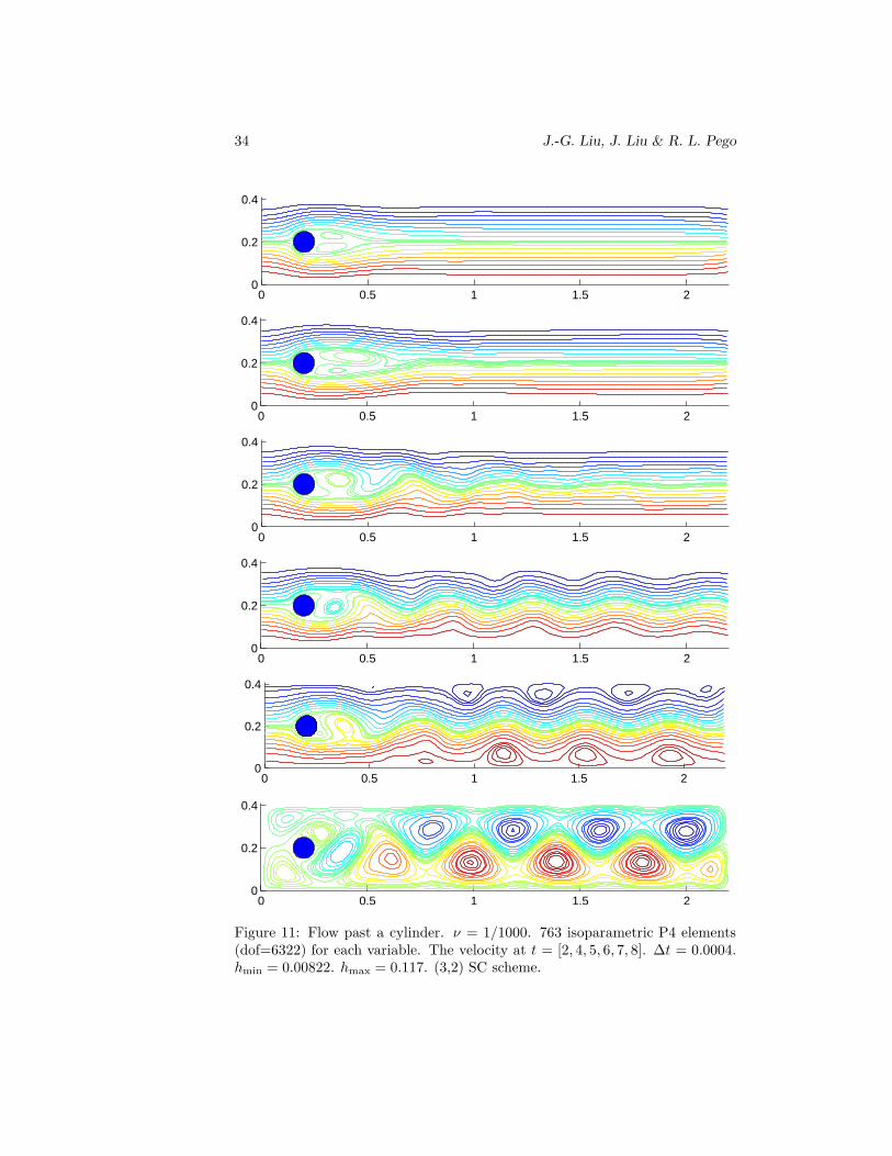
is prescribed. ν is chosen to be 1/1000. Based on the maximum velocity Umax =1 and the diameter of the cylinder L = 0.1, the Reynolds number of the flow is100. The computational mesh is shown in Figure 7 and the contour plot of thestream function at t=[2,4,5,6,7,8] is shown in Figure 11.

For comparison with [15] we also calculate the drag and lift coefficients,denoted by cd(t) and cl(t), which are the x and y components of the quantity

2

LU2max

∫

S

ν∂nu − p n , (100)

where S is the surface of the cylinder. Since our goal is to test the scheme,we faithfully calculate these quantities by surface integration, instead of trans-forming them into volume integrals, which is known to be more accurate. Wealso calculate when the maxima of cd and cl occur, and compute the pressuredifference between the front and the back of the cylinder

∆p(t) = p(t, 0.15, 0.2)− p(t, 0.25, 0.2). (101)

Since we use rotational form for the nonlinear term in the (3,0,2) and (3,1,1)calculations, the pressure we obtained is different from the standard pressureby 1

2|u|2. But because u vanishes on the cylinder surface, we have used our

pressure directly. As we have mentioned, we do not need to solve an extraPoisson equation to obtain this pressure.

The results for both the (3,0,2) and (3,2,0) schemes with P4 isoparametricelements are shown in Figure 12. Agreement with the reference results of [15]appears good, given that we use a grid roughly comparable to the coarsest grid(level 1) used in [15]. If we follow [15] and use [2.95092, 0.47795,−0.1116] asreference values for the maxima of cd, cl and ∆p(8), the relative errors of thosequantities are

[0.73%, 0.08%, 0.11%] and [0.11%, 0.25%, 0.02%]

for the (3,0,2) and (3,2,0) schemes respectively. We have also used P2 elementsinstead of P4, with the same time step ∆t = 0.0004, but with one global refine-ment of the mesh in Figure 7, so that the number of degrees of freedom remainsthe same. Then the relative errors in the maxima of cd, cl and ∆p(8) change to

[3.19%, 2.10%, 0.14%] and [0.33%, 1.65%, 0.40%]

for the (3,0,2) and (3,2,0) schemes respectively. We mention that if we increase∆t from 0.0004 to 0.0005, and keep the other parameters the same as in Fig-ure 11, the solution blows up around t = 3 (after about 6000 time steps).


Figure 7: Mesh used in backward facing step flow computation when ν = 1/600and in flow past a cylinder calculation when ν = 1/1000.

0 0.2 0.4 0.6 0.8 10

0.2

0.4

0.6

0.8

1−5 −5

−5

−4

−4

−4

−3

−3

−3

−3

−2

−2

−2

−2

−2

−2

−2−

2

−1

−1

−1

−1−

1

−0.5

−0.5

−0.5

−0.5

−0.

5−

0.5

0

0

0

0

0

0 0

0.5

0.5

0.5

0.5

0.5

0.5

0.5

1

1

1

1

1

1

1

1

1

2

2

2

2

2

2

2

23

3

3

3

3

33

0 0.2 0.4 0.6 0.8 10

0.2

0.4

0.6

0.8

1

−0.002

00.02

0.020.02

0.05

0.05

0.05

0.05

0.07

0.07

0.07

0.07

0.07

0.09

0.09

0.09 0.09

0.11

0.11

0.11

0.110.120.17

0 0.2 0.4 0.6 0.8 10

0.2

0.4

0.6

0.8

1−5 −5

−5

−4

−4

−4

−3

−3

−3

−3−2

−2

−2

−2

−2

−2

−2−

2−1

−1

−1 −1

−1

−0.5

−0.

5

−0.5

−0.5

−0.

5−

0.5

0

0

0

00

0 0

0.5

0.5

0.5

0.5

0.5

0.5

0.5

1

1

1

11

1

1

1

1

2

2

2

2

2

22

2

23

3

3

3

3

3

3

0 0.2 0.4 0.6 0.8 10

0.2

0.4

0.6

0.8

1

−0.002 0

0.02

0.02

0.02

0.05

0.05

0.05

0.05

0.07

0.07

0.07

0.07

0.07

0.09

0.09

0.09 0.09

0.11

0.11

0.11

0.110.12

Figure 8: Driven cavity, ν = 1/1000. P1/P1 with 8192 P1 elements (dof=4225)for each variable. hmin = 0.00594, hmax = 0.0397, ∆t = 0.006, T = 50. Top:(3,2) SC scheme. Bottom: (3,2) PA scheme. From left to right: vorticity contourplots, pressure contour plots.


0 0.5 1 1.5 2 2.5 3−0.5

0

0.5

S

X0 0.5 1 1.5 2 2.5 3

−0.5

0

0.5

S

X

Figure 9: Backward-facing step. ν = 1/100. P1/P1 with 6640 P1 elements(dof=3487) for each variable. hmin = 0.00783, hmax = 0.116, ∆t = 0.006,T = 20. X/S = 2.84. Left: (3,2) SC scheme. Right: (3,2) PA scheme.

0 1 2 3 4 5 6 7 8 9 10−0.5

0

0.5

X3

X1 X

2

S

0 1 2 3 4 5 6 7 8 9 10−0.5

0

0.5

S

X3

X1 X

2

Figure 10: Backward-facing step. ν = 1/600. 1700 P2 elements (dof=3925) foreach variable. hmin = 0.0186, hmax = 0.334, ∆t = 0.003, T = 120. Top: (3,2)SC scheme, X1/S = 8.86, X2/S = 15.5, X3/S = 9.9. Bottom: (3,2) PA scheme,X1/S = 8.86, X2/S = 15.55, X3/S = 9.9.


0 0.5 1 1.5 20

0.2

0.4

0 0.5 1 1.5 20

0.2

0.4

0 0.5 1 1.5 20

0.2

0.4

0 0.5 1 1.5 20

0.2

0.4

0 0.5 1 1.5 20

0.2

0.4

0 0.5 1 1.5 20

0.2

0.4

Figure 11: Flow past a cylinder. ν = 1/1000. 763 isoparametric P4 elements(dof=6322) for each variable. The velocity at t = [2, 4, 5, 6, 7, 8]. ∆t = 0.0004.hmin = 0.00822. hmax = 0.117. (3,2) SC scheme.


0 2 4 6 8−0.5

0

0.5

1

1.5

2

2.5

3

t(cd,max

)=3.9348, cd,max

=2.9293

t0 2 4 6 8

−0.5

−0.4

−0.3

−0.2

−0.1

0

0.1

0.2

0.3

0.4

0.5

t(cl,max

)=5.6932, cl,max

=0.47756

t0 2 4 6 8

−0.5

0

0.5

1

1.5

2

2.5

∆pmax

=2.3219, ∆p(8)=−0.11148

t

0 2 4 6 8−0.5

0

0.5

1

1.5

2

2.5

3

t(cd,max

)=3.9364, cd,max

=2.9541

t0 2 4 6 8

−0.5

−0.4

−0.3

−0.2

−0.1

0

0.1

0.2

0.3

0.4

0.5

t(cl,max

)=5.6928, cl,max

=0.47913

t0 2 4 6 8

−0.5

0

0.5

1

1.5

2

2.5

∆pmax

=2.3254, ∆p(8)=−0.11162

t

Figure 12: From left to right: the drag and lift coefficients cd, cl and pressuredifference between front and back of the cylinder ∆p for flow past a cylinderwith ν = 1/1000. Mesh is in Figure 7. ∆t = 0.0004. 763 isoparametric P4elements (dof=6322) for each variable. Top: (3,2) SC scheme. Bottom: (3,2)PA scheme.


7 Conclusions

The well-posed formula (18) that expresses pressure in terms of current velocityand forcing fields, via the Laplace-Leray commutator, has enabled us to studyin a rather simple way the formal accuracy of time-difference schemes for incom-pressible viscous flow. We used the commutator formula in (9) and the conceptof Stokes pressure to explain the accuracy of existing pressure-approximationand pressure-update projection methods, to devise improved approximations forcomputation of pressure, and to derive new higher-order slip-corrected projec-tion methods. The slip-correction methods are closely related to the originalKim-Moin scheme from [18] which was devised for a staggered finite-differencegrid. At the space-continuous level, the Kim-Moin scheme corresponds to a (2,1)SC scheme here with 2nd-order Crank-Nicolson time differencing and 1st-orderextrapolation for slip correction.

Stability. Our numerical tests indicate that, with no more cost than tradi-tional 2nd-order methods, one can achieve 3rd-order accuracy in time for bothvelocity and pressure, using (3,2) PA or SC schemes that retain stability withlarge time steps at low Reynolds number. In tests in smooth domains it ap-pears one may even achieve 4th-order accuracy using (4,3) PA or SC schemesfor the Stokes equations with a stability restriction on ∆t that appears inde-pendent of the spatial grid size h. In domains with corners, however, (4,3) and(3,3) schemes appear subject to a diffusive time-step restriction with the spatialdiscretizations that we tested.

In general it is not clear just how the implicit treatment of viscous termsenhances stability, but the effect naturally diminishes when viscosity becomessufficiently small. Our tests on benchmarks involve Reynolds numbers in thehundreds, and here we do encounter practical time step restrictions for sta-bility of (3,2) PA and SC schemes. For these tests we find that we needUmax∆t/hmin ≈ O(1) where hmin is the size of the smallest edge in the meshand each edge contains k+ 1 grid points for Pk elements. This appears roughlyconsistent with a CFL constraint based on the explicit treatment of convectionterms.

Accuracy. An interesting fact seen in our formal accuracy analysis is that theprojected (divergence-free) velocity satisfies a discretized momentum equationthat is fully implicit as regards the Stokes pressure (the viscous part of totalpressure). This is a consequence of the commutator formula in (9) and holds formany different projection and time-splitting methods. It does not mean thatwe need to solve a coupled system for velocity and pressure, however.

The formal analysis indicates that, as with any of the known projectionmethods, weak boundary layers usually remain in higher gradients of velocityand pressure. In the numerical tests for (3,2) PA and SC schemes, there aresome indications of degraded accuracy in such quantities, especially near cor-ners in the domain. Improved understanding and handling of corners would bedesirable. Future work is also needed to understand better the impact of spatialdiscretization on stability and error, especially near boundaries.


Finite elements and the inf-sup condition. A potentially important findingin this paper is that for PA and SC schemes we have observed good stabilityand accuracy in tests and benchmark problems using simple Lagrange finiteelements of equal order for velocity and pressure. This suggests that there isfar more flexibility in choosing methods for space discretization in schemes ofthis type than is traditionally possible for incompressible flow problems usingfinite elements without stabilization techniques (as in [3, 4], for example). Forthree-dimensional problems, for example, where complex mesh geometry maydemand a simple approach, a (2,2) or (2,1) PA scheme with piecewise linearelements (P1/P1) could be considered. (Our numerical tests for a smooth testproblem have indicated a substantial improvement in temporal accuracy with3rd-order schemes, however.) Alternatively, for situations that demand high ac-curacy, high-degree elements might be used without regard to velocity-pressurecompatibility.

Many traditional finite-element discretizations of mixed formulations of theStokes equations with divergence constraint require the spaces for velocity andpressure approximations to satisfy the inf-sup (Ladyzhenskaya-Babuska-Brezzi)condition: there should exist c > 0 independent of the discretization parameterh such that

infqh∈Yh

supvh∈Xh

〈∇ · vh, qh〉‖∇vh‖‖qh‖

≥ c > 0. (102)

The role of this condition is to ensure stability and accuracy for the pressureas determined by the mixed formulation. But as is well known, Lagrange finiteelements of equal order for velocity and pressure fail to satisfy this condition.

As we emphasized in section 2, however, the pressure is necessarily deter-mined by formula (18), for strong solutions of the Navier-Stokes boundary-valueproblem (1)-(3). This should mean that whenever one can compute an accu-rate velocity, one can compute an accurate pressure from the weak form (19) orthe Poisson BVP (20)-(21). The inf-sup condition (102) should play no role inthis. (See also [20] for more discussion, where stability of a C1 finite elementscheme for steady-state Stokes equations is proved, by using simply the Lax-Milgram lemma instead of the inf-sup condition.) But while our numerical testsare suggestive, we have no real reason why PA and SC schemes appear stableirrespective of the inf-sup condition, while PU schemes do not. Clearly, muchregarding the role of the inf-sup condition with regard to stability and accuracyof projection methods remains to be explained.

Comparisons. The new slip-correction schemes appear to have stability prop-erties similar to corresponding pressure-approximation schemes. In our imple-mentations, however, higher-order PA schemes seem to be somewhat more ro-bust than their SC counterparts in terms of spatial accuracy and accuracy nearboundaries and corners. Pressure-update (PU) schemes are somewhat simplerto describe and to code, but appear far less stable with finite element pairs thatviolate the inf-sup condition.

Finally, we remark that certainly one can consider schemes that combinethe pressure-approximation, slip-correction, and pressure-update strategies as


we have discussed. This may involve additional cost per time step, but it allowsone to use lower-order extrapolation while retaining accuracy in the overallscheme. Whether such combinations might yield gains in stability or mitigatedeficiencies in individual strategies remains to be seen.

Acknowledgments

This material is based upon work supported by the National Science Foundationunder grant nos. DMS 06-04420 and 09-05723 (RLP) and DMS 08-11177 (JGL),and partially supported by the Center for Nonlinear Analysis (CNA) underNational Science Foundation Grant Nos. 0405343 and 0635983. JL thanks L.Chen for the finite element package iFEM based on which the finite elementcalculations in this paper are done.

References

[1] J. Alberty, C. Carstensen and S. A. Funken, Remarks around 50 lines ofMatlab: short finite element implementation, Numer. Algorithms 20 (1999)117–137.

[2] B. F. Armaly, F. Durst, J. C. F. Pereira and B. Schonung, Experimentaland theoretical investigation of backward-facing step flow, J. Fluid Mech.127 (1983) 473-496.

[3] T. Barth, P. Bochev, M. Gunzburger and J. Shadid, A taxonomy of con-sistently stabilized finite element methods for the Stokes problem, SIAMJ. Sci. Comput. 25 (2004) 1585–1607.

[4] P. B. Bochev, C. R. Dohrmann and M. D. Gunzburger, Stabilization oflow-order mixed finite elements for the Stokes equations, SIAM J. Num.Anal. 44 (2006) 82–101.

[5] J. B. Bell, P. Colella and H. Glaz, A second-order projection method for theincompressible Navier-Stokes equations, J. Comp. Phys. 85 (1989) 257–283.

[6] D. L. Brown, R. Cortez and M. L. Minion, Accurate projection methodsfor the incompressible Navier-Stokes equations, J. Comp. Phys. 168 (2001)464–499.

[7] O. Botella and R. Peyret, Benchmark spectral results on the lid-drivencavity flow, Comput. & Fluids, 27 (1998) 421–433.

[8] L. Chen and C.-S. Zhang, A coarsening algorithm and multilevel precondi-tioners on adaptive grids by newest vertex bisection, submitted.

[9] W. E and J.-G. Liu, Gauge method for viscous incompressible flows, Com-mun. Math. Sci. 1 (2003) 317–332.

[10] D. Engwirda (2006). Contours for triangular grids (http://www.mathworks.com/matlabcentral/fileexchange/loadFile.do?

objectId=10408), MATLAB Central File Exchange. Retrieved Sept. 15,2008.


[11] M. S. Gockenbach, Understanding and Implementing the Finite ElementMethod, SIAM, Philadelphia, 2006.

[12] P. M. Gresho and R. L. Sani, Incompressible Flow and the Finite ElementMethod, vol. 2, Wiley, 2000.

[13] J. L. Guermond, P. Minev and J. Shen, An overview of projection methodsfor incompressible flows, Comput. Methods Appl. Mech. Eng. 195 (2006),no. 44-47, 6011–6045.

[14] W. D. Henshaw and N. A. Petersson, A split-step scheme for the incom-pressible Navier-Stokes equations, in Numerical simulations of incompress-ible flows (Half Moon Bay, CA, 2001), 108–125, World Sci. Publishing,River Edge, NJ, 2003.

[15] V. John, Reference values for drag and lift of a two-dimensional time-dependent flow around a cylinder, Int. J. Num. Meth. Fluids 44 (2004)777–788.

[16] H. Johnston and J.-G. Liu, Accurate, stable and efficient Navier-Stokessolvers based on explicit treatment of the pressure term, J. Comp. Phys.199 (2004) 221–259.

[17] G. E. Karniadakis, M. Israeli, S. A. Orszag, High-order splitting methodsfor the incompressible Navier-Stokes equations, J. Comp. Phys. 97 (1991)414-443.

[18] J. Kim and P. Moin, Application of a fractional-step method to incom-pressible Navier-Stokes equations. J. Comp. Phys. 59 (1985) 308–323.

[19] J.-G. Liu, J. Liu and R. Pego, Stability and convergence of efficient Navier-Stokes solvers via a commutator estimate, Comm. Pure Appl. Math. 60

(2007) 1443–1487.

[20] J.-G. Liu, J. Liu and R. Pego, Error estimates for finite-element Navier-Stokes solvers without standard inf-sup conditions, Chin. Ann. Math. Ser.B 30 (6) (2009) 743–768.

[21] E. Leriche, E. Perchat, G. Labrosse and M. O. Deville, Numerical eval-uation of the accuracy and stablity properties of high-order direct Stokessolvers with or without temporal splitting, J. Sci. Comput. 26 (2006) 25–43.

[22] S. A. Orszag, M. Israeli and M. Deville, Boundary conditions for incom-pressible flows. J. Sci. Comput. 1, (1986) 75–111.

[23] P.-O. Persson, G. Strang, A simple mesh generator in MATLAB. SIAMReview 46 (2004) 329–345.

[24] J. B. Perot, An analysis of the fractional step method. J. Comp. Phys. 108

(1993) 51–58.

[25] R. Peyret, Spectral methods for incompressible viscous flow. Applied Math.Sci. 148, Springer, New York, 2002.

[26] Y. Ren, Y. Jiang, M. Liu and H. Zhang, A class of fully third-order accurateprojection methods for solving the incompressible Navier-Stokes equations,Acta Mech. Sinica 21 (2005) 542-549.


[27] R. L. Sani, J. Shen, O. Pironneau and P. M. Gresho, Pressure boundarycondition for the time-dependent incompressible Navier-Stokes equations,Int. J. Numer. Methods Fluids 50 (2006) 673–682.

[28] R. Scott, Finite element techniques for curved boundaries, Thesis, Mas-sachusetts Institute of Technology, Cambridge, 1973.

[29] J. C. Strikwerda and Y. S. Lee, The accuracy of the fractional step method,SIAM J. Numer. Anal. 37 (1999), 37–47.

[30] L. J. P. Timmermans, P. D. Minev and F. N. Van De Vosse, An approximateprojection scheme for incompressible flow using spectral elements, Int. J.Numer. Methods Fluids 22 (1996) 673–688.

[31] L. N. Trefethen, Spectral methods in MATLAB. Software, Environments,and Tools 10, SIAM, Philadelphia, 2000.

[32] J. van Kan, A second-order accurate pressure-correction scheme for viscousincompressible flow. SIAM J. Sci. Stat. Comput., 7 (1986) 870–891

A Time-discrete normal modes in a strip

Here we describe how to determine normal-mode solutions for the time-discreteschemes of sections 3.1 (slip-correction) and 3.2 (pressure-approximation), inthe strip −1 ≤ x ≤ 1 as in Section 5.1. From this analysis we will get a stabilitycondition for the time step that is consistent with the numerical observationsfrom Figs. 1–2, namely that the (4,3) and (3,3) PA and SC schemes are stablefor time steps below a critical value independent of spatial grid size.

With zero forcing and boundary velocity and neglecting nonlinear terms, welook first for solutions of the time-discrete SC scheme (29)-(31) with the form

un = κnu(x, y) = κneiξy(u(x), iv(x))

with corresponding notation for un∗ and qn. We will find it convenient to define

Dk(z) =∑

j≥0

αkj z

j, Em(z) =∑

j≥1

βmj z

j .

We fix ν = 1. The SC scheme requires

1

∆t

αk0u∗ +

∑

j≥1

αkj u

= ∆u∗ in Ω, u∗ = Em(κ−1)∇q on Γ, (103)

u∗ = u + ∇q, ∇ · u = 0 in Ω, n · ∇qn+1 = 0 on Γ. (104)

We write separate equations for u and q as in section 3.1 by applying theprojection P and using the commutator relation (∆P − P∆)u∗ = ∇p, wherep = pS(u) is the Stokes pressure. The equations for u and q correspond to (36)


and (39) respectively, and take the form

(Dk(κ−1) − ∆)u + ∇p = 0, ∇ · u = 0 in Ω, (105)

∆p = 0 in Ω, n · ∇p = n · (∆ −∇∇·)u on Γ, (106)

u + (1 − Em(κ−1))∇q = 0 on Γ, (107)(

αk0

∆t− ∆

)

q = p in Ω, n · ∇q = 0 on Γ. (108)

With y-dependence proportional to eiξy in the strip −1 ≤ x ≤ 1, and with

µ(z) =√

ξ2 + Dk(z), λ =

√

ξ2 +αk

0

∆t, (109)

and z = κ−1, the equations become

(µ2 − ∂2x)

(

uv

)

+

(

∂x

ξ

)

p = 0, ∂xu− ξv = 0 (−1 < x < 1), (110)

(ξ2 − ∂2x)p = 0 (−1 < x < 1), ∂xp = ξ∂xv (x = ±1), (111)

u = 0, v + (1 − Em(κ−1))ξq = 0 (x = ±1), (112)

(λ2 − ∂2x)q = p (−1 < x < 1), ∂xq = 0 (x = ±1). (113)

We can separately study modes for which pressure, for example, has evenor odd symmetry. Looking first for the latter, we find that solutions withdivergence-free velocity tangent to the boundary take the form

p(x) = A sinh ξx (114)

u(x) = Bξ

(

cosh ξx

cosh ξ− cosh µx

cosh µ

)

, (115)

v(x) = B

(

ξ sinh ξx

cosh ξ− µ sinh µx

cosh µ

)

, (116)

q(x) = C

(

sinh ξx

ξ cosh ξ− sinhλx

λ coshλ

)

. (117)

On the boundaries x = ±1, these forms satisfy u = 0 and ∂xq = 0. The pressureboundary condition reads ∂xp = ξ∂xv = ∂2

xu, so it will automatically hold oncethe first component of (110a) is enforced. Imposing (110a) and the equation(113a) for q, we find that A, B and C are related by the linear equations

A+µ2 − ξ2

cosh ξB = 0, (118)

A− λ2 − ξ2

ξ cosh ξC = 0, (119)

so that (µ2 − ξ2)ξB+ (λ2 − ξ2)C = 0. Imposing the boundary condition (112b)for v and using this relation for B and C leads to the equation that determinesthe growth factor κ, which we write in the form

Fo(z,∆t, ξ) = 0, z = κ−1, (120)


with Fo defined via

Fo(z,∆t, ξ)

cosh µ= ξ tanh ξ − µ tanh µ− S(z)

(

ξ tanh ξ − ξ2

λtanhλ

)

, (121)

S(z) =∆t

αk0

Dk(z)(1 − Em(z)). (122)

The factor cosh µ is introduced in order to remove the poles arising from tanh µ.This makes Fo an entire (i.e., globally analytic) function of z.

For the mode with pressure having even symmetry, p = cosh ξx, similarcalculations lead to the dispersion relation

Fe(z,∆t, ξ) = 0, (123)

Fe(z,∆t, ξ)

µ sinh µ= ξ coth ξ − µ coth µ− S(z)

(

ξ coth ξ − ξ2

λcothλ

)

. (124)

Again, Fe is an entire function of z.It turns out that exactly the same single-mode dispersion relations govern

the time-discrete PA scheme.Numerical study via winding number. To count all unstable odd modes

(and similarly for even modes), for given values of ∆t and ξ, we want to countall solutions of (120) for which |z| < 1. From basic complex function theory,the number of solutions of (120) satisfying |z| < R, counting multiplicity, isthe winding number around zero of the closed curve Fo(Rγ,∆t, ξ), where γparametrizes the unit circle:

γ(θ) = eiθ, 0 ≤ θ ≤ 2π. (125)

If there are no zeros satisfying |z| = R, then the winding number is an integer,the total change in the complex argument divided by 2π. It turns out there isalways a trivial zero at z = 1, since Dk(1) = 0 and µ = ξ. It is convenient toremove this zero and scale amplitudes, by defining

F (z) =Fo(z,∆t, ξ)

1 − z, f(z) =

F (z)

(1 + |F (z)|)7/8.

(The parameter 7

8is just a convenient number close to 1.) Thus, the quantity

N(R) =1

2π

∫ 2π

0

d(

arg f(Reiθ))

, (126)

the winding number of f(Rγ) around zero, is the number of zeros of Fo satisfying|z| < R, excluding z = 1 (once, in case of higher multiplicity).

We compute the winding number N(R) numerically using a simple adaptivestepping algorithm. We evaluate fj = f(R exp iθj) for 0 ≈ θ0 < θ1 < . . . <θn = θ0 + 2π, and accumulate

∑nj=1

arg(fj/fj−1)/2π ≈ N . The values θj

are determined successively by doubling or halving the step θj+1 − θj to keep


|1 − fj+1/fj| within specified tolerances. This controls the relative change inarg f and |f |, and works well even when there is a zero of f very close to thecircle |z| = R.

Using bisection in R for N(R), we can then find rather accurately (to a tol-erance τ = 0.0005 with no difficulty) a value R for which the winding numbersatisfies N(R) = 0 < N(R+ τ). Then 1/R is approximately the largest magni-tude of any amplification factor κ for a mode with odd pressure in the space-continuous scheme. We perform the corresponding calculation for even pressuremodes and take the max. The results provide the solid curves in Figs. 1-2.

Recall that in Figs. 1-2, the results for the (3,3) and (4,3) schemes indicatethat for ξ = 1 there is a largest stable time step ∆tc > 0 independent of spatialresolution. The present normal mode theory suggests that this remains trueuniformly for all wave numbers ξ. We compute ∆tc as a function of ξ by fixingR = 1 and using bisection in ∆t to find the largest ∆t where N = 0. The resultsare plotted in Fig. 13, and indicate that ∆tc increases with ξ but remains strictlypositive in the limit ξ → 0. (For ξ = 0.01, ∆tc is 0.539 for the (4,3) scheme and0.349 for the (3,3) scheme.) For the (4,3) scheme with ξ = 1 the critical timestep ∆tc = 0.63 which compares well with the results in Figures 1 and 2.

0 0.5 1 1.5 2 2.5 3 3.5 40

1

2

3

4

5

6

7

(3,3)(4,3)

Figure 13: Largest stable time step ∆tcr vs. ξ according to normal-mode theory

stable and accurate pressure approximation for …bobpego/preprints/ll4jcp.pdfstable and accurate...

Documents