numerical calculations for electronic transport through
TRANSCRIPT

Numerical calculations forelectronic transport through
molecular systems
Robert Dahlke
Munchen 2004


Numerical calculations forelectronic transport through
molecular systems
Robert Dahlke
Dissertation
der Fakultat fur Physik
der Ludwig–Maximilians–Universitat
Munchen
vorgelegt von
Robert Dahlke
aus Aachen
Munchen, den 23. April 2004

Erstgutachter: Prof. Dr. Ulrich Schollwock
Zweitgutachter: Prof. Dr. Axel Schenzle
Tag der mundlichen Prufung: 8. Juli 2004
Contents
Zusammenfassung ix
1 Introduction 1
2 Description of charge transport 52.1 Perturbative approaches . . . . . . . . . . . . . . . . . . . . . 5
2.1.1 Rate equations . . . . . . . . . . . . . . . . . . . . . . 62.1.2 Bardeen formula . . . . . . . . . . . . . . . . . . . . . 82.1.3 Tersoff-Hamann formula . . . . . . . . . . . . . . . . . 92.1.4 Beyond the Tersoff-Hamann approximation . . . . . . . 10
2.2 Scattering approaches . . . . . . . . . . . . . . . . . . . . . . . 112.2.1 Definition of the scattering matrix . . . . . . . . . . . . 112.2.2 Landauer-Buttiker formalism . . . . . . . . . . . . . . 12
3 Quantum-chemical description of nanoscale systems 173.1 Ab-initio quantum-chemical methods . . . . . . . . . . . . . . 18
3.1.1 Separating nuclear and electronic problem . . . . . . . 183.1.2 Approximations to the electronic problem . . . . . . . 193.1.3 Approximations to the molecular orbitals . . . . . . . . 21
3.2 Density functional theory . . . . . . . . . . . . . . . . . . . . . 223.2.1 Hohenberg-Kohn formulation of DFT . . . . . . . . . . 233.2.2 Local density approximation . . . . . . . . . . . . . . . 243.2.3 Basis set . . . . . . . . . . . . . . . . . . . . . . . . . . 25
3.3 Semiempirical methods . . . . . . . . . . . . . . . . . . . . . . 253.3.1 Overview of methods in use . . . . . . . . . . . . . . . 263.3.2 Extended-Huckel method . . . . . . . . . . . . . . . . . 273.3.3 Concluding remarks . . . . . . . . . . . . . . . . . . . . 29
4 The Elastic-Scattering Quantum-Chemistry Method 314.1 Outline of the ESQC algorithm . . . . . . . . . . . . . . . . . 31
4.1.1 Algorithm step by step . . . . . . . . . . . . . . . . . . 32

iv Contents
4.1.2 Notes on calculations of conductance properties . . . . 344.1.3 Notes on STM image calculations . . . . . . . . . . . . 35
4.2 Detailed description of ESQC . . . . . . . . . . . . . . . . . . 354.2.1 Isolated semi-infinite leads . . . . . . . . . . . . . . . . 364.2.2 Connecting leads via a molecular region . . . . . . . . 424.2.3 Numerical implementation . . . . . . . . . . . . . . . . 45
5 Using molecules as electronic devices 495.1 Historical overview . . . . . . . . . . . . . . . . . . . . . . . . 49
5.1.1 Theoretical prediction . . . . . . . . . . . . . . . . . . 495.1.2 Experimental realisation . . . . . . . . . . . . . . . . . 51
5.2 Qualitative model for transport . . . . . . . . . . . . . . . . . 535.3 Recent experiments . . . . . . . . . . . . . . . . . . . . . . . . 545.4 Numerical calculations . . . . . . . . . . . . . . . . . . . . . . 55
5.4.1 Short summary of recent theoretical studies . . . . . . 565.4.2 Conduction properties of PDI devices . . . . . . . . . . 575.4.3 Discussion . . . . . . . . . . . . . . . . . . . . . . . . . 65
6 Understanding STM images 676.1 Introduction . . . . . . . . . . . . . . . . . . . . . . . . . . . . 67
6.1.1 Historical overview . . . . . . . . . . . . . . . . . . . . 676.1.2 Working principle . . . . . . . . . . . . . . . . . . . . . 686.1.3 Examples of STM images . . . . . . . . . . . . . . . . 70
6.2 Numerical STM image calculations . . . . . . . . . . . . . . . 716.2.1 Image contrast inversion . . . . . . . . . . . . . . . . . 716.2.2 Negative differential resistance . . . . . . . . . . . . . . 716.2.3 Electric field effects . . . . . . . . . . . . . . . . . . . . 736.2.4 Conformational analysis of self-organised monolayers . 75
Bibliography 81
Danksagung 91

List of Figures
2.1 Schematic representation of leads and defect . . . . . . . . . . 152.2 Occupation of energy levels within left and right contact . . . 16
4.1 Partitioning of the system into several parts . . . . . . . . . . 324.2 Discrete energy levels around the Fermi level . . . . . . . . . . 344.3 Splitting of the bulk region . . . . . . . . . . . . . . . . . . . . 374.4 Incoming and outgoing wave amplitudes . . . . . . . . . . . . 434.5 Graphite unit cell . . . . . . . . . . . . . . . . . . . . . . . . . 464.6 Super cell of graphite (side view) . . . . . . . . . . . . . . . . 474.7 Super cell of graphite (top view) . . . . . . . . . . . . . . . . . 47
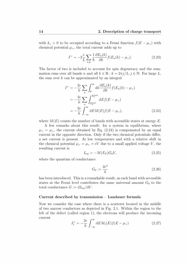
5.1 Example for a rectifying molecule . . . . . . . . . . . . . . . . 505.2 Energy versus distance diagram, no bias . . . . . . . . . . . . 515.3 Energy versus distance diagram, forward bias . . . . . . . . . 525.4 Energy versus distance diagram, reverse bias . . . . . . . . . . 525.5 Chemical structures . . . . . . . . . . . . . . . . . . . . . . . . 555.6 Structure of Cluster . . . . . . . . . . . . . . . . . . . . . . . . 595.7 Structure containing two, three, and four molecules . . . . . . 605.8 Spectrum and fit for one to four molecules . . . . . . . . . . . 615.9 Influence of molecular interaction . . . . . . . . . . . . . . . . 635.10 Influence of molecular interaction 2 . . . . . . . . . . . . . . . 645.11 IV –calculation . . . . . . . . . . . . . . . . . . . . . . . . . . 65
6.1 Working principle of an STM . . . . . . . . . . . . . . . . . . 696.2 STM-image collection . . . . . . . . . . . . . . . . . . . . . . . 706.3 Image contrast inversion . . . . . . . . . . . . . . . . . . . . . 726.4 Influence of tip-induced electric field . . . . . . . . . . . . . . 746.5 Two conformations of the same molecule . . . . . . . . . . . . 756.6 STM images of different molecular conformations . . . . . . . 766.7 Two different conformations . . . . . . . . . . . . . . . . . . . 786.8 Sample STM image calculations . . . . . . . . . . . . . . . . . 79

vi List of Figures

List of Tables
3.1 Time and energy scales for electrons and nuclei . . . . . . . . 19
4.1 Connexion between propagation properties and eigenvalues . . 42
5.1 Values for linear fit-parameter a . . . . . . . . . . . . . . . . . 62

viii List of Tables

Zusammenfassung
Thema der vorliegenden Arbeit ist die Beschreibung von Ladungstransport-eigenschaften molekularer Systeme, wenn diese das Verbindungsstuck zweierElektroden bilden. Einen technologischen Meilenstein setzte auf diesem Ge-biet die Rastertunnelmikroskopie (Binnig et al., 1981), mit der die gezielteUntersuchung von Transporteigenschaften einzelner, auf Oberflachen adsor-bierter Molekule moglich ist. Parallel dazu ermoglicht der immense Fort-schritt in der Miniaturisierung klassischer elektronischer Bauteile die Her-stellung von Zuleitungsstrukturen auf der Nanometerskala, die mit einzelnenoder nur wenigen Molekulen uberbruckt werden konnen (Reed et al., 1997).Es besteht die Hoffnung, mit solchen Systemen Schaltungselemente zu rea-lisieren, die heutigen elektronischen Bauteilen in Hinblick auf ihre Effizienzund den Grad ihrer Miniaturisierung deutlich uberlegen sein werden.
Experimente mit diesen molekularelektronischen Apparaten werfen dieFrage auf, wie sich die chemische Natur eines Molekuls sowie seine Kopplungan die Oberflache der Elektroden auf die Leitungseigenschaften auswirkt.Eine theoretische Beantwortung dieser Frage erzwingt eine quantenmechani-sche Beschreibung des Systems. Da trotz bedeutender Fortschritte bisher nurbeschrankt Ubereinstimmung zwischen den Ergebnissen besteht, handelt essich hierbei um ein aktuelles Gebiet der Grundlagenforschung.
Diese Arbeit beginnt mit einem Uberblick uber die gangigen Methodenzur theoretischen Beschreibung von Ladungstransport durch molekulare Sy-steme. Anschließend werden Methoden der Quantenchemie behandelt, dadiese in nahezu allen Ansatzen zur Beschreibung von elektronischem Trans-port durch molekulare Systeme Anwendung finden.
Auf diese allgemeinen Darstellungen folgt eine detaillierte Beschreibungdes numerischen Verfahrens, das im Rahmen dieser Dissertation implemen-tiert worden ist. Mit der vorliegenden Arbeit wird eine Verallgemeinerung derursprunglichen Methode eingefuhrt, die vormalige Einschrankungen bezuglichder betrachtbaren Systeme erfolgreich beseitigt.
Diese erweiterte Methode wird dann verwendet, um der durch Experimen-te von Dupraz, Beierlein und Kotthaus (2003) aufgekommenen Frage nachzu-gehen, welchen Einfluß verschiedene geometrische Anordnungen einer Gruppevon identischen Molekulen auf die Leitfahigkeitseigenschaften eines moleku-larelektronischen Apparats ausuben. Unsere Untersuchungen zeigen, daß sichdie Transporteigenschaften nur bei Bildung von Molekulgruppierungen mitbedeutender intermolekularer Wechselwirkung wesentlich von denen einzel-ner Molekule unterscheiden. Damit konnen wir Konsequenzen fur die Re-produzierbarkeit gewonnener Meßdaten aus der Stabilitat der Verbindungzwischen Molekul und Elektroden ableiten.

x Zusammenfassung
Abschließend befassen wir uns mit der Berechnung von Rastertunnelmi-kroskop-Bildern und prasentieren eigene Rechnungen, die im Rahmen einerKooperation mit Constable, Hermann et al. (2004) durchgefuhrt werden.Durch einen Vergleich mit experimentellen Bildern sollen verschiedene Kon-formationen eines auf Graphit adsorbierten Molekuls identifiziert werden. Dieenorme Große des Molekuls fuhrt zu einer Gesamtsystemgroße, die eine nu-merische Durchfuhrung der Algorithmen in der Praxis bisher scheitern ließ.Durch eine von uns eingefuhrte neuartige Berechnung sind wir in der Lage,erstmalig weitaus großere Systeme zu betrachten, als dies bisher moglich war.

Chapter 1
Introduction
The subject of this thesis is the description of charge transport properties ofmolecular systems, bridging two electrodes. Although electrical phenomenawere already known to the Ancient Greeks, systematic studies regardingstationary charge transport (i.e. electrical current) had not been possible untilthe year 1800, when Alessandro Volta succeeded in building the prototypeof today’s batteries. Shortly after Thomson (1897) discovered the electron,Drude (1900a,b) gave the first atomic model for electrical conduction bydescribing the electrons in a metal according to the kinetic theory of gases.Despite its success in explaining many observations, some properties of metalsmeasured at low temperatures, like the specific heat, drastically disagreewith the predictions of the model. The underlying classical concepts provedto be causing the disagreement. Therefore, detailed descriptions of chargetransport need to be based on quantum mechanics. In particular, this is truewhen transport through individual molecules is considered.
Experimentally, it has not been possible to measure the transport prop-erties of single molecules until about 20 years ago. The major difficulty was –and still is – the controlled attachment of an individual molecule to metallicor semiconducting leads, which is however necessary to apply a bias voltage.With the advent of scanning tunnelling microscopy, this type of measure-ments became feasible for the first time. Originally developed for obtainingtopographic surface images with atomic resolution (Binnig et al., 1981), se-lective studies of transport properties of individual molecules adsorbed onsurfaces can now be performed. Parallel to this development, the tremendousadvances in fabricating increasingly smaller semiconductor devices togetherwith experiments on self-assembling molecules, render it possible to buildlead contacts on the nanometer scale, which can be bridged by single or fewmolecules (Reed et al., 1997). There is hope for the realisation of circuitelements, built from such systems, which outclass today’s electronic circuits

2 1. Introduction
with respect to both efficiency and miniaturisation.As of today, this is still a field of intense fundamental research, the reason
being twofold: at first, the fabricated devices still lack reproducibility mainlybecause the deposition of molecules has to be performed in an uncontrollablefashion. Secondly, the impact on the measured conductance properties dueto both the chemical nature of the molecule itself and its bonding to the leadsurface is not consistently understood.
Because of this lack of understanding, intense theoretical studies go alongwith the experiments. The ultimate aim is to correlate the molecular elec-tronic structure with the conduction properties in a predictive manner, whichwould be a crucial step towards a directed design of molecular electronic de-vices.
This thesis is organised in the following way. In Chap. 2 we start byaddressing the question of how one can describe current across a molecularsystem, attached to a source and a drain lead. An overview of well-establishedtheoretical methods for dealing with this problem is given. We characterisethem in terms of underlying assumptions and applied approximations. Inparticular, we distinguish between two types of approaches, perturbativeones and those based on scattering theory. Among the perturbative meth-ods, we discuss the Tersoff-Hamann formula which gave the first theoreticalexplanation of scanning-tunnelling microscope images by relating them tothe local density of states of the substrate surface. We then motivate why itis necessary to go beyond this approximation which leads us to the scatter-ing approaches. They have in common that charge transport is attributedto the scattering from incoming electron waves to outgoing ones. This inter-pretation is known as the Landauer-Buttiker formalism which we describe indetail.
Next, we are concerned with the methods of quantum chemistry, as theyprovide means of describing molecular systems with respect to their atomiccomposition. This is why they are involved in almost any description of elec-tronic transport through molecular systems. In a sense they are the counter-part to so-called model Hamiltonians, the usual starting points in mesoscopicphysics, which more or less completely ignore the material specific part of asystem and are simple enough to allow for a proper many-body treatment.Quantum chemical methods, in contrast, take position and chemical naturefor each atom of the system into account, which results in complicated Hamil-tonians and therefore require a trade-off regarding the many-body nature ofthe problem to be made. One distinguishes ab-initio, density-functional andsemiempirical methods, each of which category is outlined in Chap. 3 withspecial attention to the approximations involved.
Following this general part, a detailed presentation of the numerical

3
method we have implemented for the study of charge transport throughmolecular systems is given in Chap. 4. It is based on the so-called elastic-scattering quantum-chemistry method, which was introduced by Sautet andJoachim (1988a). Originally, the method was derived in a one-dimensionalcontext, and although it was later extended to three dimensions, an anomalyof the one-dimensional case gave rise to a restriction of the systems which onewas able to study. With this thesis, a proper three-dimensional generalisa-tion of the method is introduced. By a thorough treatment of the underlyingscattering problem, we are able to lift the former restriction. In addition tothat, our generalised method is numerically more stable.
The remainder of this thesis is then devoted to the application of theo-retical methods to specific experimental situations. Content of Chap. 5 aremolecular electronic devices. We address the question raised by the experi-ments of Dupraz et al. (2003), how the conductance properties of a molecularelectronic device are influenced by a change in the geometrical alignment ofthe molecules bridging the electrodes. Our analysis reveals that the trans-port properties of a group of identical molecules differ from those of a sin-gle molecule only when inter-molecular interactions are considerably large.In particular, for those inter-molecular distances which are to be expectedfor typical self-assembled monolayers, such an effect does not occur. Onlyfor molecular clusters with distances almost as small as atomic distances, asignificant change in the conduction properties is observed. These clustersrepresent defects in the monolayer and can be produced when the couplingbetween molecules and lead surface is sufficiently weak. The strength of thecoupling mainly depends on the chemical type of the molecular group whichis responsible for the adsorption to the leads.
In Chap. 6 we consider scanning tunnelling microscope image calculations.After an introduction to the working principle of the device, we review recentnumerical studies which proved to be necessary in order to interpret exper-imental image data correctly. Then we present our own calculations from acooperation with Constable et al. (2004) to support the interpretation of re-cent STM images. The goal of the experiment is to identify different possibleconformations for a molecule when adsorbed on graphite. As the system un-der investigation is considerably large, we were able to produce the numericalimages only by introducing a special treatment for a large eigenvalue prob-lem, which cannot be solved sufficiently accurately by conventional methods.This is the first time that a method has been implemented that can performimage calculations for a system of that size.

4 1. Introduction

Chapter 2
Description of charge transport
The problem which we address in this chapter can be stated as follows: howto describe current across a molecular system, when it is attached to a sourceand a drain lead both having different chemical potentials? To this end thetheoretical methods which are in use for modelling electron tunnelling inmolecular systems are surveyed. These methods can be divided into twocategories: the ones which are based on perturbation theory and the oneswhich apply scattering theory.
Within the first category the solution for one part of the system is assumedto be known. Charge transport is described as the transition between suchknown states due to the influence of the rest of the system, which constitutesthe perturbing potential or enters via tunnelling matrix elements.
Scattering approaches take solutions to the entire system and distinguishbetween incoming states which move in direction of the molecular region andoutgoing states which move away from it. Charge transport is attributed tothe scattering from in-states to out-states. This interpretation is known asthe Landauer-Buttiker formalism.
In this chapter we first deal with perturbative methods, among which wedistinguish two different approaches. Then we turn to scattering methods ofwhich we discuss the basic principles. A full explanation of the approach wehave implemented, which belongs to the latter type, is deferred to Chap. 4.
2.1 Perturbative approaches
The central element of perturbation theory is a so-called unperturbed systemΣ0, described by a HamiltonianH0, for which one is in principle able to obtainthe eigenfunctions and eigenenergies exactly. This system is then perturbedby an interaction HamiltonianHint and this interaction is assumed to be small

6 2. Description of charge transport
as compared to the energy scales of the unperturbed system, so that one canexpand its influence into a converging power series. We refer to schemes whichfollow this classic form of perturbation theory as rate-equation approaches(Sec. 2.1.1). Within those H0 describes the molecular region only while Hint
describes the coupling to the leads.
All subsequent perturbative methods take a different viewpoint. Therethe unperturbed system consists not only of a single system but of two sys-tems (called Σ1 and Σ2 corresponding to source and drain lead1) which donot interact with each other. They are described by the Hamiltonians H1
and H2. The molecular region plays the role of the perturbing potential.Ordinary perturbation theory can not be applied because the eigenfunctionsfor both systems are not orthogonal. To overcome this problem one uses anapproach which relates back to Bardeen (1961) and is the content of Sec.2.1.2. With only a few further assumptions the Tersoff-Hamann formula(Sec. 2.1.3) can be derived, which historically constitutes the first theoreticalinterpretation of STM images. Finally we remark on methods going beyondthe Tersoff-Hamann approximation.
2.1.1 Rate equations
As mentioned in the introduction this first approach to electron transportdiffers from the following ones because the unperturbed system Σ0 consistsof a single molecule only, while the interaction part represents a connection tothe leads. It can therefore not be applied to STM image calculations, becausea molecular adsorbate can not be described without the substrate surfaceand furthermore, as an adsorbed molecule is hardly ever weakly coupled tothe substrate, perturbation theory is not applicable. Therefore this methodhas only been used to calculate conductance properties of single molecules,assuming a situation of weak coupling to the leads (Hettler et al., 2002,2003). Charge transport is related to the transition of electronic states fromthe molecular system Σ0 to states within the leads, due to the action of thecoupling.
Since within this approach one first treats the molecular system as beingisolated from the leads, it has the advantage that it allows for a detailedmany-particle description. The presentation follows Hettler et al. (2002).
1We have chosen numerical subscripts (instead of e.g. L and R for left and right lead)because they can easily be extended to more than two leads.

2.1 Perturbative approaches 7
The Hamiltonian
We think of the entire system as being divided into three parts, the molecularsystem Σ0, as well as two leads. The total Hamiltonian reads
H = H0 +Hint, (2.1)
where the isolated molecular part is described by H0 and the interaction partby Hint, which couples the molecule to the leads.
The molecular region is treated from a many-particle point of view andtherefore correlation effects can properly be accounted for by including two-body operators in H0. One of the well established tools for diagonalising sucha Hamiltonian like direct numerical diagonalisation can be used to obtainboth its spectrum and the corresponding electronic eigenfunctions.
The coupling term Hint merely consists of hopping terms from the leadto the molecule and vice versa. To be specific, the interaction Hamiltonianis supposed to be of the form
Hint =∑l=1,2
(Γ
2πρe
)1/2∑kσi
(tlic†iσalkσ + h.c.
), (2.2)
where the operators ciσ, c†iσ destroy and create electrons with spin σ in state
i of the molecule and the operators alkσ, a†lkσ act correspondingly in the leads
(l = 1, 2), with a dispersion relation E(lkσ) = Elk. The density of states
in the leads ρe is assumed to be constant. The parameters tli account for avariable coupling between the individual states. The interaction Hamiltoniancan be extended to also include a coupling to bosonic degrees of freedom(i.e. photons and/or phonons), which we do not consider here for simplicityreasons (see Hettler et al., 2002).
Master equation
With the diagonalisation of H0 obtained, a master equation is set up for theoccupation probabilities Ps of the molecular many-body states. Transitionrates can then be calculated using perturbation theory with respect to thecoupling constant Γ.
The transition rate wss′ between two molecular states s, s′ is composed ofthe tunnelling rates wl±
ss′ for electrons tunnelling from lead l to the molecule(+) or in the other direction (−), respectively:
wss′ =∑
l
(wl+ss′ + wl−
ss′). (2.3)

8 2. Description of charge transport
These tunnelling rates can be computed using the golden rule:
wl±ss′ =
2π
~|∑φl φ′
l
〈φ′l|〈s′|Hint|φl 〉|s〉δ(Eφl+ Es − Eφ′
l− Es′)|2, (2.4)
with |φl 〉 denoting states in lead l. If these lead states are assumed tobe occupied according to a Fermi function fl(E), then one can replace theexpression |
∑φlφ
′l〈φ′l|a
†lkσ|φl〉|2 by fl(E
lk)ρe and |
∑φlφ
′l〈φ′l|alkσ|φl〉|2 by [1 −
fl(Elk)]ρe. The in- and out-tunnelling rates thus become
wl+ss′ =
Γ
~fl(Es − Es′)
∑σ
|∑
i
tli〈s|c†iσ|s′〉|2, (2.5)
wl−ss′ =
Γ
~[1− fl(Es − Es′)]
∑σ
|∑
i
tli〈s|ciσ|s′〉|2. (2.6)
To obtain a stationary solution for the occupation probabilities Ps of themolecular states, they have to fulfil the following master equation
Ps = 0 =∑
s′
(wss′Ps′ − ws′sPs). (2.7)
Solving this system of equations yields the occupation probabilities Ps. Nowthe current from the molecule into one of the leads (say l) is proportional tothe net transition of states:
Il = e∑ss′
(wl+ss′Ps′ − wl−
s′sPs). (2.8)
In summary we note that this approach for calculating the current canbe used to treat the molecular system in great detail. This is achieved bytreating the surface of the leads, which are by themselves very complicatedobjects, as a simple perturbation to the molecular Hamiltonian. Thereforethe method is limited to the condition of weak coupling.
2.1.2 Bardeen formula
Now we change the viewpoint and consider two isolated systems, which dothis time correspond to macroscopic bulk material, i.e. the leads. Bardeen(1961) addressed this problem by considering two sets of states, which in thecase of STM correspond to states in the isolated substrate together with anadsorbate and the isolated STM tip. These states each solve the Schrodinger

2.1 Perturbative approaches 9
equation in their part of the system only. The matrix element for the transi-tion of a state Ψµ in the one region to a state Ψν in the other region is givenby
Mµν =
∫Ψ∗µ[H − Eν ]Ψνd
3r. (2.9)
In ordinary perturbation theory (H −Eν)Ψν would reduce to the perturbingpotential VintΨν . Here the situation is different: there is no perturbing po-tential and therefore the expression (H −Eν)Ψν vanishes in that part of thesystem where Ψν solves the Schrodinger equation, but it is non-zero in theother part of the system.
By partial integration, Bardeen was able to show that the expression inEq. (2.9) is proportional to the current operator applied to the states Ψµ andΨν :
Mµν = − ~2
2m
∫S
[Ψ∗µ∇Ψν −Ψν∇Ψ∗µ]d2r, (2.10)
where S is an arbitrary surface lying entirely within the barrier region sepa-rating the two systems. (The operator defined by the matrix elements Mµν
is referred to as the transfer Hamiltonian.)
Because the matrix element of the transition is proportional to the matrixelement of the current operator, it is justified to write the rate of tunnellingfrom state µ to state ν as:
Γµν =2π
~|Mµν |2δ(Eµ − Eν). (2.11)
This is the so-called Bardeen formula.
Although the Bardeen formula was originally derived in the context ofsuperconducting tunnelling, it became of great importance for the first in-terpretations of STM images, due to the work of Tersoff and Hamann.
2.1.3 Tersoff-Hamann formula
By applying the Bardeen formula to the case of STM imaging, Tersoff andHamann were able to show that the tunnelling current of an STM is pro-portional to the surface local density of states (LDOS) at the position of thetip evaluated at the Fermi energy (Tersoff and Hamann, 1983, 1985). Thisfamous result is obtained under the following assumptions: firstly perturba-tion theory in the tip-sample interaction must be applicable, secondly theapplied bias voltage as well as the temperature must be low, and finally theentire tip is considered to be merely a point probe.

10 2. Description of charge transport
The derivation is straightforward. Starting from Eq. (2.11), the currentbetween tip and sample is related to the tunnelling matrix elements betweeneigenstates of these two systems:
I =2πe
~∑µ,ν
f(Eµ)[1− f(Eν + eV )]|Mµν |2δ(Eµ − Eν), (2.12)
with
Mµν = 〈Ψµ|Vtip|Ψν〉.
Assuming low temperature and low voltage Eq. (2.12) can be approximatedas
I =2π
~e2V
∑µ,ν
|Mµν |2δ(Eµ − EF )δ(Eν − EF ). (2.13)
If the tip is simply taken to be a point probe located at r0, then the tunnellingmatrix element reduces to Ψµ(r0) and one arrives at the Tersoff-Hamannformula:
I ∝∑
µ
|Ψµ(r0)|2δ(Eµ − EF ). (2.14)
2.1.4 Beyond the Tersoff-Hamann approximation
The analytical expression (2.14) is appealing as it relates an STM imagedirectly to the surface electronic structure (note that it is not the electronicdensity, as Eq. (2.14) is evaluated at the Fermi energy only). However thereare situations where the underlying assumptions are not justified.
First of all it may be too crude to entirely neglect the electronic structureof the tip, for example when it has a substantial spatial modulation. Suchsituations are not well described by the Tersoff-Hamann formula, which as-sumes an s-state for the tip orbital. In these cases, the Bardeen formula (Eq.2.11) has to be evaluated numerically. This has been done for example byTsukada et al. (1990), who performed separate electronic structure calcula-tions for substrate and tip with an ab-initio method. Chen (1990a,b) hasstudied the influence of STM tips, for which a d-type orbital dominates thetunnelling process.
More severely, whenever a perturbative approach is questionable, theBardeen formula can not be applied at all. Perturbation theory most ob-viously fails in describing situations where the STM tip is used to activelymanipulate the sample surface. For example, it is possible to remove individ-ual molecules, adsorbed on the sample surface, by lowering the tip-surfacedistance at the position of that molecule below a certain critical value. Apart

2.2 Scattering approaches 11
from these extreme cases, perturbation theory is considered to become in-accurate long before the onset of such irreversible effects, i.e. for distanceslarger than those being involved in manipulation experiments.
Thus, there are relevant cases where perturbation theory itself breaksdown and alternative frameworks then have to be used which do not rely onweak coupling between parts of the system but treat the system as a singleentity. This will be considered in the next section.
2.2 Scattering approaches
To go beyond perturbation theory, where the tip influence is viewed as per-turbing the bulk potential and vice versa, it is necessary to treat the en-tire system containing tip and sample (for STM calculations) or containingmolecule and leads (for conductance calculations of molecules) in a unifiedway. One possible such framework is scattering theory (see e.g. Taylor, 1972).
To our knowledge, all non-perturbative theories for the STM imaging pro-cess solve the scattering problem in the single-particle approximation (Lucaset al., 1988; Sautet and Joachim, 1991; Doyen et al., 1993; Ness and Fisher,1997). This is because one needs a description of the system which ac-counts for small geometrical changes (i.e. movement of the tip). Explicitmany-particle formalisms are based on model Hamiltonians which containparameters that cannot be directly obtained from the spatial arrangementof the system. They are therefore not suited for our purpose and we restrictourselves to the single-particle approximation, too.
2.2.1 Definition of the scattering matrix
For the purpose of scattering theory, it is useful to decompose the systeminto a bulk region containing the leads (described by the Hamiltonian Hlead)and a defect region, being described by an external potential V (x). Thisdefect region has to be spatially localised, and its external potential V (x)(due to atomic cores and external fields if present) has to drop sufficientlyfast [V (x) ∼ O(|x|−p), for |x| → ∞ and p > 1].
Now consider a wave packet approaching the defect region, yet being faraway from it. Its wave function Ψ0(x, t0) can be expressed in terms of freesolutions φk, i.e. in eigenstates of Hlead (Bloch waves in our case). To bespecific, let its representation in terms of φk be
Ψ0(x, t0) =
∫d3k akφk(x), (2.15)

12 2. Description of charge transport
with ak peaked around some k0. In this representation, the time evolution ofEq. (2.15) will assume a very complicated form once the wave packet entersthe scattering region. However, one can define scattering states, which areeigenstates of the full Hamiltonian H = Hlead + V and therefore stationaryin time. The wave packet can also be expanded in terms of these scatteringstates and it can be shown that there exists a special choice these scatteringstates ψin
k (called in-states) for which the wave packet expansion coefficientsAk are identical to those of the expansion in terms of free solutions (Ak = ak).Therefore, as long as t0 is in the distinct past one has:
Ψ0(x, t0) =
∫d3kakψ
ink (x). (2.16)
A corresponding relation between free solutions and so-called out-states(which are also eigenstates to H = Hlead + V ) can be established by consid-ering a wave packet moving away from the defect region. In this sense, anyfree solution to Hlead is asymptotically equal to a scattering state (solutionto H = Hlead + V ).
The scattering problem can be formulated in the following way: How doeigenstates of Hlead evolve under the action of H = Hlead + V ? Put in otherwords: what is the probability amplitude of an incoming wave packet peakedaround k to evolve into an outgoing one peaked around k′ due to the actionof V ? This information is contained in the scattering matrix. Any eigenstateφk to Hlead is asymptotically equal to an in-state ψin
k . This in-state is aneigenstate to the full Hamiltonian Hlead +V and can also be expressed in thebasis of out-states. This basis transformation is described by the scatteringmatrix:
|ψoutk0〉 = S · |Ψin〉. (2.17)
As each out-state is again asymptotically equal to a free solution of Hlead, thescattering matrix describes in which way incoming free solutions are scatteredinto outgoing ones due to the action of V . The details of the scatteringproblem we are interested in together with a derivation of the scatteringmatrix directly from the Schrodinger equation is presented in Chap. 4.
The remaining question is how to obtain transport properties once thescattering matrix is known. This will be described in the next section.
2.2.2 Landauer-Buttiker formalism
Within the Landauer-Buttiker formalism (Buttiker et al., 1985), current isdescribed as a result of electron transmission through an impurity region ina single electron picture. This concept is presented here. We first consider

2.2 Scattering approaches 13
a single narrow conductor placed between two big contacts and derive thequantisation of conductance. We then consider the case of a scatterer placedbetween two narrow conductors and end up with the Landauer formula. Partsof the presentation follow Datta (1995).
Quantisation of conductance
To determine the current carried by a single electron, we start from theconservation of charge, which can be expressed via the equation of continuity:
∂t
∫ρd3x = −
∮ρv · dA. (2.18)
This equation must hold for any region in space. With the definition ofcurrent density j := ρv and using Gauss’ theorem, Eq. (2.18) can be writtenas
∂tρ+∇ · j = 0. (2.19)
The current dI through an infinitesimal small area dA is then defined asdI := j · dA. The current Ie which is produced by a single electron movingwith velocity ve = ven within a conductor of length L and cross sectionA = An (n being the unit normal) therefore is
Ie =−eve
L. (2.20)
Now what is the velocity ve of an electron? The electronic states within anarrow conductor belong to different bands n. Each of these bands is charac-terised by its dispersion relation En(k). For a narrow conductor along the z-axis, all wave vectors are of the form k = kez. If we take the wave function foran electron with wave vector k0 to be a Fourier composition of plane waves (allwithin a single band n) ψ(x, y, z, t) =
∫dkα(n, k)ψ(x, y) exp(ikz−iEn(k)t/~)
with coefficients α(n, k) peaked around k0, then the corresponding velocityis given by the group velocity i.e. the velocity of the maximum position ofthe wave package. The position of the maximum is located at the stationarypoint of the phase factor:
z =t
~∂En(k)
∂k
∣∣∣∣k=k0
(2.21)
and therefore
vn,k0 =1
~∂En(k)
∂k
∣∣∣∣k=k0
. (2.22)
The total current (in one direction) is produced by all electrons movingin that direction. Assuming the electronic states of the narrow conductor
14 2. Description of charge transport
with kz > 0 to be occupied according to a Fermi function f(E − µ>) withchemical potential µ>, the total current adds up to
I> = −2e
L
∑n,k
1
~∂En(k)
∂kf(En(k)− µ>). (2.23)
The factor of two is included to account for spin degeneracy and the sum-mation runs over all bands n and all k ∈ R : k = 2πj/L, j ∈ N. For large L,the sum over k can be approximated by an integral
I> = −2e
h
∑n
∫ ∞0
dk∂En(k)
∂kf(En(k)− µ>)
= −2e
h
∑n
∫ Emaxn
Eminn
dEf(E − µ>)
= −2e
h
∫ ∞−∞
dEM(E)f(E − µ>), (2.24)
where M(E) counts the number of bands with accessible states at energy E.A few remarks about this result: for a system in equilibrium, where
µ< = µ>, the current obtained by Eq. (2.24) is compensated by an equalcurrent in the opposite direction. Only if the two chemical potentials differ,a net current is present. At low temperature and with a relative shift inthe chemical potential µ> = µ< + eV due to a small applied voltage V , theresulting current is
Itot = −M(EF )G0V, (2.25)
where the quantum of conductance
G0 :=2e2
h(2.26)
has been introduced. This is a remarkable result, as each band with accessiblestates at the Fermi level contributes the same universal amount G0 to thetotal conductance G := dItot/dV .
Current described by transmission – Landauer formula
Now we consider the case where there is a scatterer located in the middleof two narrow conductors as depicted in Fig. 2.1. Within the region to theleft of the defect (called region 1), the electrons will produce the incomingcurrent
I>1 = −2e
h
∫ ∞−∞
dEM1(E)f(E − µ>) (2.27)

2.2 Scattering approaches 15
Region 1 Region 2
Figure 2.1: Schematic representation of the system. To the left and rightthere are wide contacts. The defect (in the middle) is coupled to them viasmall leads with a finite number of modes.
as we have calculated in the previous section (Eq. 2.24). Analogously, theincoming current from region 2 reads
I<2 = −2e
h
∫ ∞−∞
dEM2(E)f(E − µ<). (2.28)
At the defect each incoming wave is scattered in a different way, depending onits energy and the band it belongs to. This scattering redistributes the waveamplitude among all the accessible bands (numbered by M1(E) in region 1and M2(E) in region 2) and results in reflected amplitudes (within conductor1) and transmitted ones (within conductor 2). We introduce the scattering
coefficient sm←n(E ′, E) := am(E′)an(E)
, as the ratio of the scattered amplitude
am(E ′) within band m at energy E ′ in region 2 and the incident amplitudean(E) within band n at energy E in region 1. These scattering coefficients caneither be calculated by Green’s function techniques or by directly calculatingthe scattering matrix (see Sec. 2.2.1 and Sec. 4.2.2).
The current density associated with a wave of amplitude an(Ek) is propor-tional to |an(Ek)|2vn(k). This gives rise to the definition of the transmissionfunction T (E):
T (E) =∑n∈1
∑m∈2
∫Tm←n(E ′, E)dE ′,
Tm←n(E ′, E) = |sm←n(E ′, E)|2vm
vn
.
From now on, we will consider elastic scattering only. Therefore the integra-tion over E ′ can be performed trivially as all transmission coefficients withE ′ 6= E are zero. And because the scattering matrix is unitary for elasticscattering, the transmission function for transmission from conductor 1 to 2is identical to the one for transmission from conductor 2 to 1:
T (E) =∑n∈1
∑m∈2
Tm←n(E) =∑m∈2
∑n∈1
Tn←m(E). (2.29)

16 2. Description of charge transport
Because of charge conservation reflection is described by the function
Ri(E) := Mi(E)− T (E), (2.30)
where i labels conductor 1 or 2 respectively.When we replace M1(E) in Eq. (2.27) by T (E), then we obtain that
part of the outgoing current within conductor 2, which is produced by trans-mission from conductor 1. There is a second part due to reflection of theincoming current of conductor 2, which is obtained by replacing M2(E) inEq. (2.28) with R2(E). The outgoing current in conductor 2 is the sum ofboth contributions:
I>2 = −2e
h
∫[(T (E)f(E − µ>) +R2(E)f(E − µ<)] dE. (2.31)
The total current within conductor 2 now is the difference between incomingand outgoing currents I>
2 − I<2 :
Itot2 = −2e
h
∫[T (E)f(E − µ>) +R2(E)f(E − µ<)−M2(E)f(E − µ<)] dE
(2.30)= −2e
h
∫T (E)[f(E − µ>)− f(E − µ<)] dE. (2.32)
This is the so called Landauer formula (Landauer, 1957). Again we see that inequilibrium there will be no net current. Only if the two chemical potentialsare biased by an external voltage (see Fig. 2.2), a current can arise acrossthe scatterer.
E E
R T T
Figure 2.2: The occupation of energy levels within left and right contact atzero temperature. Because of an applied bias there is a net current producedby transmission across the defect.

Chapter 3
Quantum-chemical descriptionof nanoscale systems
Before we describe the basics of quantum-chemical methods for the descrip-tion of systems on the nanometer scale, we answer the question why we do notuse one of the standard models in physics commonly used for small systems,like the Hubbard or Anderson model.
When one deals with an electronic many-particle system, a complete so-lution starting from first principles is typically not possible. The hardestproblem is to treat the electron-electron correlations correctly. In practice,there are two possible approaches to this problem: either one applies ap-proximations with respect to these correlations, or one concentrates on theelectronic correlations only, thereby dropping all system dependent informa-tion, by discretising the Hilbert space and introducing free parameters de-scribing the interaction between neighbouring electrons. The latter approachprovides insight into effects merely produced by interaction and allows for aclassification of the underlying model with respect to the parameters. Whencompared to experimental results, the model parameters can be determinedand by this the system under investigation can be classified.
However, it is not always clear how the model parameters have to be ad-justed (or if the model is applicable in the first place), when some of the exper-imentally available parameters are varied. Therefore, the model-Hamiltonianapproaches are less suited for studying the influence of experimental detailslike small variations in the atomic structure or a change in chemical type.For example the scanning tunnelling microscope utilises the high sensitivityof the tunnelling current with respect to tiny changes in the tip position toobtain topographic surface information (see Chap. 6). A theoretical methodaiming to reproduce such images has to include the geometrical details ofthe setup and this is in practice only feasible when approximations to the

18 3. Quantum-chemical description of nanoscale systems
treatment of the electron-electron interactions are applied.Methods which aim to describe systems on the atomic scale are referred
to as quantum-chemical. During the years, starting in the late 1920’s withthe rise of quantum mechanics, a vast number of such methods has been de-veloped. As a first step one distinguishes between ab-initio and semiempiricalmethods. The first do not take any input parameters besides fundamentalphysical constants, while the semiempirical methods allow parameters to beeither taken from experiment or to be fit to best reproduce experimentallyaccessible observables. We first consider the ab-initio methods before we turnto the semiempirical ones.
3.1 Ab-initio quantum-chemical methods
As there is quite a number of so called ab-initio methods, it is helpfulto characterise them according to the underlying approximations to themany-particle problem. Thereby we are following Zulicke (1985), Szabo andOstlund (1996) and also Pople (1977).
3.1.1 Separating nuclear and electronic problem
Starting from the non-relativistic Hamiltonian for N electrons and M nuclei
H = −N∑
i=1
~2
2me
∇2i −
M∑n=1
~2
2Mn
∇2n −
N∑i=1
M∑n=1
e2Zn
|ri −Rn|(3.1)
+N∑
i=1
N∑j>i
e2
|ri − rj|+
M∑n=1
M∑m>n
e2ZnZm
|Rn −Rm|,
where Mn is the mass of nucleus n and Zn is its atomic number, the Born-Oppenheimer or adiabatic approximation (relating back to Born and Oppen-heimer, 1927) separates nuclear and electronic degrees of freedom. This ismotivated by the different time scales of their motion (see Tab. 3.1) and al-lows to factorise the total wave function Ψtot(r, R) := Ψnuc(R)Ψe(r, σ, {R}),where Ψnuc(R) is the nuclear wave function and Ψe(r, σ, {R}) the electronicone, depending explicitly on coordinates r and spin σ of all the N electrons,but where the nuclear positions R enter as fixed parameters only. One thenstudies the remaining electronic Hamiltonian
He = −N∑
i=1
~2
2me
∇2i −
N∑i=1
M∑n=1
e2Zn
|ri −Rn|+
N∑i=1
N∑j>i
e2
|ri − rj|(3.2)

3.1 Ab-initio quantum-chemical methods 19
electronic nuclearτe ≈ 10−15 · · · 10−16s τtrans ≈ 10−13 · · · 10−15s
Etrans ≈ 10−2 · · · 1eVEe ≈eV Evib ≈ 10−1 · · · 10−2eV
Erot ≈ 10−3eV
Table 3.1: Time and energy scales for electronic and nuclear dynamics
for a fixed set of nuclear coordinates {R}, and separately the nuclear Hamil-tonian
Hnuc =M∑
n=1
~2
2Mn
∇2n + Eeff, (3.3)
where the effective nuclear potential energy Eeff := Ee+∑M
n=1
∑Mm>n
e2ZnZm
|Rn−Rm| isthe sum of the nuclear potential energy and the electronic energy Ee obtainedfrom the solution of the Schrodinger equation using the Hamiltonian He
[Eq. (3.2)]. The Hamiltonian Hnuc [Eq. (3.3)] is used in the Schrodingerequation for the nuclear wave function to calculate vibrational, rotational,and translational modes of the nuclei.
In a typical quantum-chemical calculation a structure optimisation is per-formed as a first step by iteratively solving the Schrodinger equation forthe electronic and the nuclear wave functions. As such an iteration is timeconsuming, the electronic problem is not attacked in full detail. With theresulting coordinates for the atomic positions a detailed calculation of theelectronic properties follows, using Eq. (3.2) only, and we restrict ourselvesto this latter problem from now on, thereby dropping the electronic subscripte and the nuclear position vector R.
3.1.2 Approximations to the electronic problem
A complete solution to the Schrodinger equation together with the electronicHamiltonian of Eq. (3.2) results in eigenfunctions and the correspondingeigenenergies. Usually one is interested in ground state properties of thesystem, which require the calculation of the ground state wave function only.But still, the general problem is of course too hard to be solved exactly,and an approximate ansatz for the form of the wave function Ψ(r, σ) has tobe made, which includes some special assumptions regarding the dynamicalbehaviour of the electrons.
In Hartree-Fock theory the Pauli principle is taken into account by using

20 3. Quantum-chemical description of nanoscale systems
an anti-symmetrised product of orbital wave functions φ:
Ψ(r, σ) =1√N !
∣∣∣∣∣∣∣φ1(1) · · · φ1(N)
.... . .
...φN(1) · · · φN(N)
∣∣∣∣∣∣∣ , (3.4)
where φi(k) abbreviates φi(rkσk). This determinant contains the N lowestlying occupied orbitals.
With this ansatz for the wave function, the expectation value for theHamilton operator can be written as
〈H〉HF =∑
i
hi +1
2
∑ij
Jij −∑ij
1
2Kij (3.5)
hi = −∫φ∗i (1)
(~2
2me
∇2 +∑
n
e2Zn
|r1 −Rn|
)φi(1) d1 (3.6)
Jij =
∫ ∫|φ∗i (1)|2 · |φj(2)|2
|r1 − r2|d1d2 (3.7)
Kij =
∫ ∫φ∗i (1)φj(1)φ
∗j(2)φi(2)
|r1 − r2|d1d2, (3.8)
with J the Coulomb integral and K the exchange correlation integral.Configuration interaction (CI) methods release the restriction to a single
determinant wave function. They take sums of determinant wave functionswhich also include orbitals belonging to excited states. This results in moreaccurate but also very expensive calculations (Foresman and Frisch, 1996).
For spherically symmetric problems, such as determining the electronicconfiguration of isolated atoms, the Hartree-Fock method can be used to nu-merically generate atomic orbital wave functions, which are referred to asHartree-Fock atomic orbitals. The resulting N -particle wave function consti-tutes the best possible anti-symmetrised product of atomic orbitals for theHartree-Fock Hamiltonian, i.e. it minimises
E = min|Ψ〉
{〈H〉HF
〈Ψ|Ψ〉
}. (3.9)
For molecular systems, it is unfortunately out of question to determinethe best molecular orbital functions (as opposed to the atomic orbital func-tions), because the spherical symmetry is lost (Roothaan, 1951), and thus theHilbert space of possible functions is just too big. Therefore one additionallyhas to approximate the molecular orbitals.

3.1 Ab-initio quantum-chemical methods 21
3.1.3 Approximations to the molecular orbitals
One possible basis set for molecular orbital wave functions is a set of atomicorbitals. As one then deals with a linear combination of atomic orbitals, sucha choice is called LCAO. Atomic orbitals are of the following form:
φnlm(r, θ, φ) =∑
j
Cj,nlχj,nlm(r, θ, φ) (3.10)
χnlm = Rnl(r)Ylm(θ, φ)
Ylm(θ, φ) =
√2l + 1
4π
(l − |m|)!(l + |m|)!
P|m|l (cos(θ)) eimφ.
The Ylm are spherical harmonics and Pml (x) denotes the associated Legendre
polynomials, the ones corresponding to the s(l = 0) and p(l = 1) orbitalsbeing:
P 00 (x) = 1,
P 01 (x) = x, P 1
1 (x) =√
1− x2.
Within an LCAO treatment, the exact form of the radial wave functionRnl(r) is of great importance and commonly one of the following three choicesis being made:
• Slater type orbitals (STO): the radial part of the atomic orbital is takento have the same asymptotic decay as the hydrogen atomic wave func-tion (Slater, 1930), i.e.
Rnl(r) = Nrn−1e−ξlr, (3.11)
where N = 1√(2n)!
(2ξl)n+1/2 is a normalisation factor, chosen to let the
radial function fulfil∫r2RnlRnldr = 1.
• Gaussian functions : computationally more efficient than a STO is anexponential decay with a quadratic argument:
Rnl(r) = Nrn−1e−αlr2
, (3.12)
N =
(2n+1(2αl)
n+1/2
(2n− 1)!!√π
) 12
. (3.13)
Quite often STOs are being expanded into K Gaussian functions ofthe form (3.12) and then being termed Slater type orbitals at the K-Gaussian level: STO-KG (Pople, 1977).

22 3. Quantum-chemical description of nanoscale systems
• Hartree-Fock atomic orbitals : this choice is a LCAO approach in astrict sense, because these orbitals are optimised for the Hartree-Fockatomic problem. However, they generally result in less accurate valuesfor molecular problems as compared to STOs.
With an atomic orbital basis set chosen, a single molecular orbital ψ isnow a linear combination of all the atomic orbitals belonging to all the atomsof the molecule. If the latter are located at the spatial positions Ri, thensuch a combination assumes the form
ψ(r) =∑
i∈atoms
∑nlm
αinlmφ
inlm(r −Ri). (3.14)
The form of the total molecular wave function again depends on the levelof theory. For Hartree-Fock studies it is a single determinant as in Eq. (3.4).The expansion coefficients for the ground state wave function αi
nlm are finallyobtained by minimising the total energy according to Eq. (3.9).
3.2 Density functional theory
An approach alternative to the theory of electronic structure outlined above isthe so called density functional theory (DFT), ‘in which the electron densitydistribution n(r), rather than the many-electron wave function’ (Kohn, 1999,p. 1253) is the central quantity that one aims for. Its development began in1964 and 1965 with the two publications by Hohenberg and Kohn (1964), andby Kohn and Sham (1965) and was recognised by a Nobel Prize in Chemistryin 1998.
From the point of view of the Schrodinger equation, an electronic systemis uniquely specified by its external potential V . A complete solution to theassociated Hamiltonian
H = −N∑
i=1
~2
2m∇2
i +N∑
i=1
N∑j>i
e2
|ri − rj|+ V, (3.15)
where
V =N∑
i=1
V (ri) (3.16)
(together with appropriate boundary conditions) consists of its energy spec-trum and the corresponding N -particle eigenfunctions. The latter are ingeneral very complex quantities.

3.2 Density functional theory 23
Now DFT is based on the fact (see below) that there exists a one-to-onecorrespondence between the external potential V and the ground-state elec-tronic density n(r) of the electronic Hamiltonian for that potential. Becausemany ground-state properties of the system can be obtained directly fromthis ground-state density, one tries to solve for it.
We will only give a short introduction which is mainly intended to clarifysome of the naming conventions associated with the method.
3.2.1 Hohenberg-Kohn formulation of DFT
‘The ground-state density n(r) of a bound system of interacting electrons insome external potential V determines this potential uniquely’ (Kohn, 1999,p. 1259). The proof of this statement is quite simple and goes back toHohenberg and Kohn (1964).
From the correspondence between ground-state density and external po-tential it follows that the ground state energy of an interacting electronicsystem can be obtained by a variational principle, where the variation iswith respect to the density n(r), which is a simple function of just one spa-tial coordinate (Hohenberg and Kohn, 1964):
E0 = minn(r)
{EV [n(r)]}, (3.17)
where
EV [n(r)] =
∫V (r)n(r)dr + F [n(r)]. (3.18)
The latter functional F [n(r)] does not depend on V but contains the kineticenergy of the non-interacting electrons T [n(r)] and a second term specificto the electronic Coulomb interaction, which is not known exactly. Theso-called exchange-correlation energy functional Exc[n(r)] is now defined asthe difference between the unknown functional F and the kinetic energyfunctional T together with the Coulomb self-interaction:
F [n(r)] = T [n(r)] +1
2
∫n(r)n(r′)
|r − r′|drdr′ + Exc[n(r)]. (3.19)
Writing the density for a given number of N electrons as
n(r) =N∑
i=1
|φi(r)|2, (3.20)

24 3. Quantum-chemical description of nanoscale systems
where each φi(r) is normalised to unity, the Euler-Lagrange equations to Eq.(3.17) with Eqs. (3.18) and (3.19) take the form of N effective Schrodinger-like equations, which are named after Kohn and Sham (1965):(
− ~2
2m∇2 + Veff(r)
)φi(r) = εiφi(r), (3.21)
with an effective potential Veff and the exchange correlation potential Vxc
given as
Veff(r) = V (r) +
∫n(r′)
|r − r′|dr′ + Vxc(r), (3.22)
Vxc(r) =δ
δn(r)Exc[n(r)]
∣∣n(r)=n(r)
. (3.23)
The functions φi constituting the density n(r) are sometimes called Kohn-Sham orbitals. As Exc is now the only functional which remains unknown,one approximates it, most frequently by using the so-called local-densityapproximation.
3.2.2 Local density approximation
When introducing Eq. (3.21) Kohn and Sham (1965) already came up with asimple approximation for the exchange-correlation energy that is surprisinglyuseful. Let us denote the exchange-correlation energy density per electron ofa uniform electron gas by εxc(n). Within the local density approximation, theexchange-correlation energy density of a non-uniform electron distributionn(r) is taken to be a local function εxc(r), its value being identical to that ofa uniform electron gas with constant charge density n = n(r):
εxc(r) = εxc(n)∣∣n=n(r)
. (3.24)
Therefore, the explicit form of Exc is
ELDAxc [n(r)] =
∫n(r)εxc(n)
∣∣n=n(r)
d3r. (3.25)
The corresponding LDA exchange-correlation potential reads
V LDAxc (r) = εxc(n)
∣∣n=n(r)
+dεxc
dn. (3.26)
Although the approximation appears to be poor, it generally yields very ac-curate results. A commonly used parameterisation of εxc(n) based on Monte-Carlo simulations was given by Perdew and Zunger (1981).

3.3 Semiempirical methods 25
3.2.3 Basis set
With an explicit formula for the exchange-correlation potential, one finallyhas to choose a basis set for the Kohn-Sham orbitals. Analogously to theHartree-Fock method, they can be expanded in atomic wave functions. Moreoften one uses a plane waves basis set for the interstitial region between theatoms, while a separate solution of Eq. (3.21) is performed for the core regionaround each atom. Both types of wave functions then have to be matched atthe boundary of the atomic and the interstitial regions. This latter approachis known as the augmented plane wave (APW) method.
As the exact form of the wave function within the core region of eachatom is more or less irrelevant to the chemically interesting valence orbitalregion, it is more efficient to replace the exact core potential by approximatepseudopotentials. These pseudopotentials are more slowly varying and alsomuch weaker than the core potentials, and allow for an expansion of the wavefunctions into plane waves only.
With a basis set chosen, the Kohn-Sham equations (3.21) can be solvedself consistently, in close analogy to the Hartree-Fock method. Finally, wewant to note that the type of basis set resulting in the most accurate solutionsstrongly depends on the system under consideration. Therefore, a lot ofexperience is needed if one is interested in quantitative results. This does ofcourse hold for all ab-initio methods for electronic structure calculations.
3.3 Semiempirical methods
In contrast to both of the methods outlined above, which are extremely de-manding with respect to computational effort, semiempirical methods havebeen developed. The name semiempirical indicates that these methods havebeen parameterised to reproduce experimental results. They typically usethe same LCAO theory as ab-initio methods. However, many of the morecomplex integrals are removed or replaced using simple approximations. Em-pirical parameters and functions are used to compensate for the errors intro-duced by removing integrals.
We first name the most popular ones and characterise them accordingto their approximations and then give a detailed outline of one of them,namely the extended-Huckel method, which is the one we have implemented.Beside the references given in the text, a more detailed (but slightly outdated)description can be found in Scholz and Kohler (1981) and Zulicke (1985).

26 3. Quantum-chemical description of nanoscale systems
3.3.1 Overview of methods in use
The most famous examples of semiempirical methods are the extended Huckelmethod (which will be discussed in detail in Sec. 3.3.2) and the molecularorbital (MO) theory. The basic approximations of the latter method whichallow to neglect less important integrals of the Hartree-Fock method weredeveloped by Pople et al. in the 1950s and 1960s. A couple of methods arosefrom this period, the most restrictive being the CNDO-approximation (Com-plete Neglect of Differential Overlap, Pople and Segal, 1966) which completelyneglects two-electron interaction integrals. By maintaining the differentialoverlap between different orbitals for all integrals at a single atomic centrethe INDO-approximation is obtained (Intermediate Neglect of DifferentialOverlap, Pople et al., 1967), which improves upon the CNDO-approximationwhile still considerably reducing the computational effort as compared toab-initio methods. The least restrictive methods stemming from that eraapply the so called NDDO-approximation (Neglect of Diatomic DifferentialOverlap, Pople et al., 1965; Pople and Segal, 1965). Here the differential over-lap for orbitals of the same atom in two centre integrals is kept explicitly.Methods applying these approximations are still in use, although usually inmodifications intended for interpreting molecular spectra.
More suitable methods for the evaluation of energetic data and also forthe prediction of molecular geometries have been developed in the 1970s.The general idea was to not only apply an approximation simple enoughfor the desired calculation to be feasible but also to upgrade the accuracyof the results by introducing parameters that can be adjusted to fit exper-imental data. For the MINDO/3-method (Modified Intermediate Neglect ofDifferential Overlap/Version 3, Bingham et al., 1975a,b,c,d) the basic ap-proximations are similar to the INDO-approximation, but the atomic-orbitalexponents ξ are treated as free parameters which are being optimised dur-ing the course of minimisation. Despite the additional effort to determinethese parameters, the accuracy for quantities like the heat of formation andgeometry parameters for molecules containing heteroatoms (i.e. non-carbonatoms in organic molecules) is sometimes still quite low. These drawbackswere overcome by the MNDO-method (Modified Neglect of Differential Over-lap, Dewar and Thiel, 1977). It is based on the NDDO-approximation andadditionally improves upon the MINDO/3-method by freezing some of theparameters to values that were optimised using a least-square fit to a set ofexperimental values known to be otherwise represented poorly. But still, themethod fails to reproduce hydrogen bonds and activation energies tend to betoo large.
It took several years until a next generation of semiempirical methods

3.3 Semiempirical methods 27
was developed. To avoid terminology confusion with previous semiempiricalmethods (many of which we have not mentioned), entirely different nameswere adopted. These are AM1 (Austin Model 1, Dewar et al., 1985) andPM3 (MNDO Parametric Model no. 3, Stewart, 1989a,b). The new ideawas, instead of first identifying and then modifying the faulty approximationwhich causes the poor results, to rather add a new term with new parametersto the corresponding energy expression and fitting these to experimentalvalues. This approach has proven useful and AM1 or PM3 are nowadays themethods of choice if there is the need for a semiempirical quantum-chemicalmethod capable of producing results that are in quantitative agreement withexperiments.
3.3.2 Extended-Huckel method
The Huckel method was originally introduced to treat π-bonding in planarorganic molecules (Huckel, 1931a,b, 1932, 1933, 1937a,b). Given a moleculein the xy-plane, the idea was to use a 2pz basis set for each double bondedcarbon atom. This treatment has then been extended to non-π electronsystems with inclusion of all valence orbitals and is now being called theextended-Huckel method. It was originally developed by Hoffmann (1963).
LCAO ansatz
Making the ansatz that a wave function can be written as a linear combina-tion of atomic orbitals (LCAO), it assumes the general form
|Ψ〉 =∑
i
∑l
γil |φi
l〉, (3.27)
where i runs over all atoms (with spatial position Ri) of the system to bedescribed and l labels the orbitals of that atom. Expressed in this basis theone-particle Schrodinger equation reads∑
j,k
Hil,jkγjk = E
∑jk
Sil,jkγjk. (3.28)
Here we have introduced the overlap matrix Sil,jk := 〈φil|φ
jk〉 and the coeffi-
cients of the Hamiltonian are Hil,jk := 〈φil|H|φ
jl 〉.
Basis set
For an actual calculation it is necessary to represent the wave function in awell-suited analytic form. There is the obvious requirement that this basis set

28 3. Quantum-chemical description of nanoscale systems
should well represent the atomic orbitals, labelled by the principal quantumnumber n and the orbital quantum number l. But as there is a great numberof overlap integrals that have to be calculated, the basis set should also allowa fast calculation of these integrals. Therefore Slater type orbitals (STO)are commonly used, because they have the same asymptotic radial decay asthe atomic wave functions (Slater, 1930) and any overlap integral 〈φi|φj〉 canbe reduced to an analytic expression. Their explicit form was already givenin Eqs. (3.10) and (3.11). Expansion coefficients Cj,nl, ξl for various atomictypes can be found in the literature. We use parameters optimised for thedescription of valence orbitals (Hoffmann, 1963; Komiya et al., 1977).
Hamiltonian
The electronic Hamiltonian (3.2) can be split into two parts:
Hsingle =∑
n∈atoms
∑i∈n
− ~2
2me
∇2i −
e2Zn
|ri −Rn|+∑j∈n
j 6=i
e2
|ri − rj|
(3.29)
Hneglect =∑
n∈atoms
∑i∈n
−∑m6=n
e2Zm
|ri −Rm|+∑j /∈n
e2
|ri − rj|
(3.30)
+∑
n∈atoms
∑m>n
e2ZnZm
|Rn −Rm|.
Here i ∈ n denotes all electrons i belonging to atom n. The HamiltonianHsingle contains intra-atomic contributions only, while all contributions fromdifferent atoms are included in Hneglect. A one-electron method does ac-count for the energetic contributions contained in Hsingle but neglects theones corresponding to Hneglect. In the extended-Huckel method Hsingle can berepresented as a sum of one-electron operators:
Hsingle =∑
i
αic†ici +
∑i
∑j 6=i
βijc†icj . (3.31)
The coefficients αi and βij are called Coulomb integrals and resonance inte-grals, respectively.
The Coulomb integrals are usually parameterised using ionisation energiestaken from experiments and for the resonance integrals a number of formulashave been suggested. For example Wheland (1941) and also Mulliken et al.(1941) took βij = K ·Sij, whereas the choice βij = K ′ ·Sij(hii+hjj), K
′ = 1.75goes back to Hoffmann (1962, 1963); Wolfsberg and Helmholtz (1952). We

3.3 Semiempirical methods 29
use the latter one but with a different weighting: K ′ = k/2+a/2+a2 1−k2, k =
1.75, a = (hii−hjj
hii+hjj).
With a STO basis set the overlap matrix elements
Sij =
∫d3xφiφj (3.32)
can be reduced to analytic expressions which can be evaluated very efficiently.
Schrodinger equation
For a given molecular structure, described by the positions of all atoms,each atom is equipped with an atomic orbital function for all its valenceorbitals. These atomic orbitals are taken as a basis of the Hilbert space.The Hamiltonian matrix elements can then explicitly be calculated in thisrepresentation and the Schrodinger equation assumes the matrix form
Hγ = E · Sγ, (3.33)
where the vector γ contains the coefficients of the atomic orbitals. S is theoverlap matrix, which takes into account that orbitals at different atoms arenon-orthogonal in general. Equation (3.33) constitutes a generalised eigen-value problem which can be solved using standard methods of linear algebra.Instead of simply inverting S it is however advisable to compute S−1/2, whichexists uniquely for positive definite overlap matrices. Then Eq. (3.33) can betransformed to
S−1/2HS−1/2γ′ = Eγ′. (3.34)
Thus one obtains an eigenvalue problem for eigenvectors γ′ = S1/2γ. Fur-thermore this eigenvalue problem is symmetric, because S and also H aresymmetric matrices.
3.3.3 Concluding remarks
The previous section dealt with the extended-Huckel method, which we havechosen to implement although it is less accurate as compared to AM1 andPM3. The reason for this choice, besides the lesser computational effort,mainly is that we want to perform qualitative studies of considerably largesystems. To this end the extended-Huckel method is sufficient. However,it should be noted that there is no restriction to this choice. Any of themethods mentioned in this chapter could also be used, as they all provide aneffective single-particle Hamiltonian, which is the only input to the methodwe use for calculating transport through molecular systems (see Chap. 4).

30 3. Quantum-chemical description of nanoscale systems

Chapter 4
The Elastic-ScatteringQuantum-Chemistry Method
The original ESQC method ‘offers a means of studying the transmission ofelectrons through a defect embedded in an infinite, periodic chain’ (Roshd,1992, p. 8). It was first proposed by Sautet and Joachim (1988a,b,c) whostudied the transmission of electrons through a molecular switch. The infiniteand periodic chain in these studies was a conducting polymer, while the defectwas taken to be a benzene ring. The original, more or less one-dimensionalmethod, was then generalised in such a way that a defect could be embeddedin an infinite but periodic three-dimensional wire (Sautet and Joachim, 1991).This improvement allowed for the study of the tunnelling of electrons ina Scanning Tunnelling Microscope (STM), where the defect contains thesurface of the substrate together with a molecule adsorbed upon and theapex of the STM tip. The infinite and periodic wire represents the bulkregion of tip and substrate. However, in the original presentation the methodis restricted to the case that the two bulk regions are identical, which istypically not the case in real STM experiments.
In this chapter, we present a generalised version of ESQC (Dahlke andSchollwock, 2004), which overcomes the restriction to place the defect be-tween identical leads. Furthermore, it generalises the original setup of twoleads to an arbitrary number. These improvements are the result of a thor-ough treatment of the scattering problem as it is provided here.
4.1 Outline of the ESQC algorithm
The name already suggests that the method is based on the combination ofan exact solution to a scattering problem for a Hamiltonian which is obtained

32 4. The Elastic-Scattering Quantum-Chemistry Method
Figure 4.1: Partitioning of the system into individual parts, here for the caseof two leads (surrounded by boxes) being attached to the molecular regionwhich also contains the surface atoms of each lead.
from a quantum-chemical calculation. The basic principles of all scatteringapproaches have already been outlined in Sec. 2.2 while an introduction toquantum-chemical methods is provided in Chap. 3. The present chapter isdevoted to an in depth description of the ESQC method and also coversdetails of the implementation.
The method involves quite a large number of steps to finally obtain theconductance properties of a molecular system. Here we summarise thesesteps; the calculational details are contained in Sec. 4.2.
4.1.1 Algorithm step by step
As already described in Sec. 2.2 within a scattering approach the solutionsto the Schrodinger equation far away from the molecular region are asymp-totically equal to solutions of the isolated leads. To obtain these asymptoticstates the system is formally divided into several parts, one containing themolecular region and an additional part for each lead. For the case of twoleads, this partitioning is sketched in Fig. 4.1.
First the asymptotic states are calculated for each of the leads separately.Then the S-matrix for scattering of the incoming states into the outgoing ones

4.1 Outline of the ESQC algorithm 33
is calculated. Finally the current is calculated using the Landauer formula.Only the last two steps depend on the geometry of the molecular region.
1. The calculation of the scattering states for each isolated lead containsthe following steps which have to be performed only once:
• The periodic lead is split into identical layers.
• The spatial position and chemical nature of each atom within sucha layer has to be specified. Then the quantum-chemical calcula-tion is performed for two adjacent layers with appropriate bound-ary conditions (see below). This results in a layer-independentHamiltonian.
• With this Hamiltonian one performs a band-structure calculationto determine the Fermi energy.
• For a discrete set of energy values around the Fermi energy an op-erator describing the current properties is set up and transformedinto an eigenmode basis. The corresponding modes represent ei-ther incoming or outgoing scattering solutions.
The results for each discrete energy value can now be stored for reusingthem in calculations for different molecular setups.
2. The calculation of the scattering matrix involves the following steps:
• Spatial position and chemical nature of each atom within themolecular region enters the quantum-chemical calculation whichresults in the Hamiltonian for this part.
• The energy dependent scattering matrix is obtained by connect-ing the modes of each lead to the molecular region. This step isperformed for all the above chosen discrete energy values whichare within the energy window defined by the chemical potentialsof source and drain lead (see Fig. 4.2).
3. Finally the current is calculated in the following way:
• The value of the transmission function for each discrete energylevel is obtained by summing up the contribution to the scatteringmatrix from each channel.
• With the Landauer formula one obtains the current across themolecular region by an integration over these energies.

34 4. The Elastic-Scattering Quantum-Chemistry Method
drainsource
eV
E
Figure 4.2: Sketch of the set of discrete energy levels between the two chem-ical potentials of source and drain. At each of these energy levels the scat-tering matrix has to be calculated. The rectangular boxes represent thezero-temperature Fermi functions of source and drain lead.
It is noted here that the calculations can also be performed using Green’sfunction techniques (see e.g. Datta, 1995) which is equivalent to the scat-tering matrix approach (as shown by Fisher and Lee, 1981). We present thedetails of the calculation within the latter framework as then the contribu-tions from individual channels to the transmission function can be studiedeasily.
Before we go into the details of the steps outlined above we first wantto make some remarks about the differences between calculations for STMimages and calculations for conductance properties of molecules in molecularelectronic devices.
4.1.2 Notes on calculations of conductance properties
To obtain the conductance properties of a molecular electronic device (seeChap. 5), the current across the molecular region has to be calculated formany different applied source-drain voltages. Conductance properties canthen be obtained by numerically calculating the derivative of the currentwith respect to the applied voltage: G = dI
dV.
The entire ESQC-algorithm has to be executed for each value of applied

4.2 Detailed description of ESQC 35
voltage. To gain a proper resolution in voltage space one has to considerquite a large number of discrete energy levels between the chemical potentialsof source and drain electrode (see Fig. 4.2). And again for each of theseenergy levels, step two of the algorithm has to be performed. To increasethe accuracy of a conductance calculation one therefore has to increase thenumber of energy levels and the number of voltage steps. The limiting factoris usually not the computational time but rather the size of available systemmemory, because a matrix containing the current properties has to be keptin memory for each energy level and each lead.
4.1.3 Notes on STM image calculations
As explained in Chap. 6, an STM image is produced by recording the currentor the height of the STM tip while scanning over the sample surface. But theESQC algorithm results in the current value for a fixed geometry which in theSTM context corresponds to a fixed tip position. To obtain an STM imageof an entire surface region numerically, one has to model the tip movement.Then, for a finite number of tip positions the current calculation has to beperformed.
In order to obtain a reasonable image resolution the current calculationhas to be repeated a great many times. But because the calculations for eachfixed tip position do not dependent on each other this process can efficientlybe parallelised.
To keep the computational cost at a reasonable level, it is advisable totake only a few energy levels around the Fermi energy into account. For largemolecules adsorbed flat on top of the substrate one even has to restrict to asingle such level because due to their size, the Hamiltonian matrices alreadyuse up the entire system memory.
4.2 Detailed description of ESQC
As a first step of the ESQC-algorithm the system under consideration hasto be decomposed into distinct parts. These parts are described by thesame quantum-chemical method but several different calculations have to beperformed. The decomposition results in n+1-parts, where n is the number ofleads. Let us call them Σd, d ∈ {0, 1, . . . , n}. Σ0 contains the molecular regionand also the top most surface layers of each lead and Σd, d > 0 contains thesemi-infinite lead d (see Fig. 4.1 with n = 2). Periodic boundary conditionsin the directions perpendicular to the surface normal are used.
First we will restrict our attention to the semi-infinite leads, which in

36 4. The Elastic-Scattering Quantum-Chemistry Method
general will be different. In the outline of the ESQC-algorithm as givenabove this corresponds to step one.
4.2.1 Isolated semi-infinite leads
A microscopic description for each lead is obtained from quantum chemistry,which provides an effective one-particle Hamiltonian. By a tight-bindingapproximation and using the periodicity of the system, the semi-infinite leadHamiltonian assumes block tridiagonal form with finite dimensional blocks
Hd =∞∑
l=l0
∑i∈l
∑j<i
(Hd
llijc†dlicdlj + h.c.
)(4.1)
+∞∑
l=l0
∑i∈l
∑j∈l+1
(Hdl,l+1,ijc
†dlicd,l+1,j + h.c.)
Layer by layer, starting with the first layer not included in the molecularregion (named l0), the first term accounts for intra-layer interactions, whilethe second one describes the interaction between layers. The indices i andj run over the orbital basis set within each layer. The size of each layer ischosen such that only adjacent layers have non-zero interaction. It thereforedepends on the details of the tight-binding approximation. Figure 4.3 (a)sketches the partitioning of a lead into identical layers.
The Hamiltonian in Eq. (4.1) for one lead d is layer independent, if oneassumes periodicity, i.e. Hd
ll = Hdl0l0
and Hdl,l+1 = Hd
l0,l0+1. Therefore, weobtain the following infinite dimensional coupled system of equations:(
Md(E)γl + hd(E)γl+1 + h†d(E)γl−1
)= 0, ∀l ≥ l0 + 1, (4.2)
with Md(E) := Hdl0l0
− ESdl0l0
, hd(E) := Hdl0,l0+1 − ESd
l0,l0+1, and Sdll′ is the
overlap matrix between orbitals in layer l and layer l′ of lead d for cases whenone does not deal with an orthonormal basis set (otherwise Sd
ll′ = Id · δll′).
Band-structure calculation
Using Bloch’s theorem one can reduce the infinite dimensional system ofequations to an N×N -matrix equation (N being the number of orbital basisfunctions in one layer)(
Md(E) + hd(E)eik∆d + h†d(E)e−ik∆d
)γl(k,E) = 0, ∀l. (4.3)

4.2 Detailed description of ESQC 37
l
l + 1
l − 1
(a)
∆d
(b)
l
(c) (d)
Figure 4.3: (a) Part of the bulk region of a semi-infinite lead which is splitinto identical layers. (b) Each layer contains identical unit cells and periodicboundary conditions in the lateral direction are applied. (c) Zoom into theunit cell of one layer. The position of the atoms is indicated. (d) Each atomof the unit cell is equipped with a valence orbital basis set.

38 4. The Elastic-Scattering Quantum-Chemistry Method
With ∆d we denote the (lead dependent) lattice spacing and the layer coef-ficients γl obey the relation γl+1 = eik∆dγl. (From here on we will drop theenergy- and k-dependency of γ.)
Fixing the value of k Eq. (4.3) can also be written in the form
Hγl = E(k)Sγl, (4.4)
which is a generalised eigenvalue problem for E(k) with
H := Hdl0l0
+ eik∆dHdl0,l0+1 + e−ik∆dHd
l0+1,l0
S := Sdl0l0
+ eik∆dSdl0,l0+1 + e−ik∆dSd
l0+1,l0.
Whenever S is positive definite (which typical overlap matrices happen tobe), this equation can be transformed into a normal eigenvalue problem:
S−1/2HS−1/2xl = E(k)xl, (4.5)
xl := S1/2γl.
Solving for various values of k one obtains the dispersion relation or projectedband structure E(k) of the isolated lead. It should be noted here, that forefficiency (and also numerical accuracy) reasons it is advisable to reduce theN × N dimensional Eq. (4.5) to m different N2 × N2 (with N = m · N2)eigenvalue problems by again using Bloch’s theorem this time within thelateral direction, i.e. for all m values of k|| which are in accordance with thelateral periodic boundary conditions:
(H0
)ij
=m∑
c=1
eik||·Rc
(Hc
)ij. (4.6)
Here c runs over all cells within one layer and Rc denotes the spatial distanceto an (arbitrarily chosen) first cell (therefore R1 = 0). By H0 we denote thereduced N2×N2 dimensional Hamiltonian, and Hc contains the Hamiltonianelements for orbitals i in the first cell and orbitals j in cell c. An analogousreduction for the overlap matrix results in S0. Figure 4.3 (b) sketches theperiodicity of a single layer in lateral direction.
With the knowledge of the band structure of a lead, we can determine theFermi energy by successively filling up the one-particle states starting withthe lowest energy state. The conductance properties of the isolated lead aregoverned by states with energy values at the Fermi level, and these stateswill be determined next.

4.2 Detailed description of ESQC 39
Layer-to-layer propagator
To obtain the wave function belonging to a specific energy value E we againturn to Eq. (4.3). Defining λd := eik∆d one can easily see that it constitutesan N ×N quadratic eigenvalue problem in λd. It can be transformed into a2N × 2N linear eigenvalue problem:
Pd(E)
(γl
γl+1
)= λd
(γl
γl+1
), (4.7)
Pd(E) :=
[0 1
−h−1d h†d −h−1
d Md
]. (4.8)
The eigenvectors of this equation constitute Bloch waves for the semi-infinitelead. We call Pd(E) the layer-to-layer propagator because it also connectsthe coefficients of adjacent layers(
γl
γl+1
)= Pd(E)
(γl−1
γl
), (4.9)
where we have used Eq. (4.2).At a given energy E, each eigenvector constitutes an independent channel
and the eigenvalue λd contains information about its propagation along thelead. The eigenvalues come in pairs such that for each eigenvalue λ>, thereexists a corresponding eigenvalue λ< satisfying the relation λ> = 1/λ∗<, ascan be seen by transposing Eq. (4.3). Eigenvalues with |λ| 6= 1, i.e. complexk, belong to exponentially diverging solutions (see Eq. 4.9 and 4.7). Theseare of course non physical, as long as the lead is infinite. In semi-infinite leadshowever (which we are dealing with), exponentially decaying coefficients atthe boundary will contribute to the surface wave function and must not beneglected.
Current operator
We have already seen, that the modulus of an eigenvalue reveals informationabout the propagation properties of the corresponding Bloch wave. However,the contribution to the net current can not directly be seen from Eq. (4.5). Itdepends on the current density associated with a solution to the Schrodingerequation i~∂tSγ = Hγ and is obtained via the continuity equation. Theprobability amplitude |γ|2 for a stationary solution is constant in time
∂
∂tγ†Sγ =
i
~(γ†Hγ − γ†H†γ
)= 0, (4.10)

40 4. The Elastic-Scattering Quantum-Chemistry Method
because H and S are hermitian. For the probability amplitude at all layersbetween l1 and l2 one therefore has
0 =∂
∂t
l2∑l=l1
(γ†l γl )
=i
~
l2∑l=l1
γ†l (H −H)γl
=i
~(γ†l1−1h(E)γl1
+ γ†l1+1h†(E)γl1
− h.c.) (4.11)
+i
~(γ†l2−1h(E)γl2
+ γ†l2+1h†(E)γl2
− h.c.)
= 〈γ|l2, l2 + 1〉 i~
[0 −hh† 0
]〈l2, l2 + 1|γ〉
− 〈γ|l1 − 1, l1〉i
~
[0 −hh† 0
]〈l1 − 1, l1|γ〉,
with the projectors 〈l|γ〉 := γl . This gives rise to the definition of the currentoperator Wl for layer l as
Wl := |l, l + 1〉 i~
[0 −hh† 0
]〈l, l + 1|. (4.12)
Now let both ϕ and ϑ be solutions at fixed energy E with the eigenvalues λ1
and λ2 respectively. Because the expectation value for Wl is layer indepen-dent (Eq. 4.11) one has:
〈ϑ|Wl|ϕ〉 =〈ϑ|Wl+1|ϕ〉=λ1λ
∗2〈ϑ|Wl|ϕ〉. (4.13)
This equation describes the connection between the current properties of asolution ϕ and its eigenvalue λ.
Connection between eigenvalues and current properties
The current properties of each channel can be related to the correspondingeigenvalue. We start from Eq. (4.13):
〈ψ|Wj|φ〉 = λ∗1λ2〈ψ|Wj|φ〉.
Let us first consider |ψ〉 = |φ〉, i.e. λ1 = λ2, and therefore 〈ψ|Wj|φ〉 =|λ|〈ψ|Wj|φ〉. For each channel with eigenvalue |λ| 6= 1 one then must have

4.2 Detailed description of ESQC 41
〈ψ|Wj|ψ〉 = 0, i.e. this channel does not carry any current itself. This isconsistent with our terminology of an evanescent wave. If, however, |λi| = 1,then 〈ψ|Wj|ψ〉 is purely imaginary, because Wj is an anti-hermitian oper-ator. We can therefore define the velocity of a propagating wave to bevi := Im〈ψ|Wj|ψ〉.
Now we consider the case of two different solutions |ψ〉 6= |φ〉 and definev1,2 := 〈ψ|Wj|φ〉. If their eigenvalues do not satisfy λ1λ
∗2 = 1, then the
current between these two solutions is zero v1,2 = 0. So let us assume λ1 =1/λ∗2. Because if |λ1| > 1 then |λ2| < 1, a current can flow between anevanescent left going wave and an evanescent right going wave. But if werestrict ourselves to solutions with finite amplitudes in a semi-infinite lead,then either the left or right going wave amplitude must be zero. Therefore,evanescent waves do neither carry a current themselves nor do they exchangecurrent with other channels, that is they do not at all contribute to the netcurrent.
Finally, we are left with the case λ1 = 1/λ∗2, with |λ1| = |λ2| = 1. Thisis equivalent to λ1 = λ2, i.e. the case of degenerate eigenvalues. Thereforepropagating waves to degenerate eigenvalues do exchange current. That inturn means that the current of a superposition of two such waves does notnecessarily equal the sum of the two individual currents, which is problematicas we want to express the total current as a sum of independent channels.However, the propagating and evanescent waves were obtained by diago-nalising the propagator P . This transformation is unique up to rotationsin every degenerate eigenvalue subspace. Because W is anti-hermitian wecan diagonalise these subspaces and the resulting diagonal elements will bepurely imaginary. So the net current may be written as a summation over allthe individual contributions of propagating channels, only if these subspacerotations are performed.
Summarising, we have shown that the transformation U diagonalising thepropagator P (i.e U−1PU) can be chosen in such a way that the transforma-tion U †WU of the current operator is diagonal in the subspace of propagatingwaves with purely imaginary diagonal elements. All the other diagonal entriesare zero and the only non-zero non-diagonal elements belong to evanescentwaves in opposite directions. The relations between eigenvalue, current valueand propagation properties are summarised in Table 4.1.
Solutions for an isolated lead are linear combinations of propagating wavesin opposite directions, with the same amount of current being transportedin each direction, thus carrying no net current, and resulting in a standingwave.
We now define Λ> and Λ< as the two N ×N diagonal matrices composedof all incoming and outgoing eigenvalues Λ≷ := diag(λi
≷). The 2N × 2N -

42 4. The Elastic-Scattering Quantum-Chemistry Method
|λ| v description> 1 right< 1
0 evanescentleft
going wave
> 0 right≡ 1< 0
propagatingleft
going wave
Table 4.1: Summary of the connection between eigenvalue, current value andpropagation properties
matrix U , which diagonalises P :
U−1PU =
[Λ> 00 Λ<
], (4.14)
has the following quadratic block form:[U> U<
U>Λ> U<Λ<
]. (4.15)
After this transformation into the diagonal basis of the propagator, we caneasily obtain all physically relevant solutions of the infinite lead by specifyingthe amplitudes of all propagating waves at one lattice site.
Now that we have obtained a complete description of the transport prop-erties for all leads, we can turn our attention to the molecular region.
4.2.2 Connecting leads via a molecular region
Up to now, we have considered the isolated leads only. These are now as-sumed to be each coupled to the molecular defect region and thereby in-directly coupled to one another. We will use the same quantum-chemicaldescription for all three regions, the lead itself, the contact region, and themolecular region. The Hamiltonian for the lead itself has already been setup (Eq. 4.3). Thus, there are still two parts to be determined:
Hmol =∑i∈mol
(εi c†micmi +
∑j 6=i
Hmij c†micmj) (4.16)
Hcontact =∑
d∈leads
∑i∈l0
∑j∈mol
(Hdml0ijc
†dl0icmj + h.c.) (4.17)
The first Hamiltonian Hmol describes the molecular region in absence of theleads, while Hcontact describes the interaction between the top-most layers

4.2 Detailed description of ESQC 43
A
B C
D
Figure 4.4: Incoming and outgoing wave amplitudes
of each lead and the molecular region. Both Hamiltonians together withthe diagonalised layer-to-layer propagators for each lead will now be used tocalculate the transmission function.
Scattering matrix
We are interested in stationary solutions, which consist of an incoming prop-agating wave in one lead, being scattered among all the accessible outgoingchannels (propagating and evanescent ones). This information is containedin the scattering matrix S(
BC
)=
[S11 S12
S21 s22
]︸ ︷︷ ︸
=:S
(AD
), (4.18)
which determines the wave amplitudes of all outgoing waves B, C given theincoming ones A,D.
It is important to notice that the scattering matrix is always quadratic,because in each lead there are the same amount of incoming and outgoingchannels. This is opposed to the transfer matrix T , which connects theamplitudes of in- and outgoing waves C,D in one lead to the in- and outgoingwaves A,B of a second lead:(
CD
)= T
(AB
). (4.19)
This matrix is quadratic only if both leads have the same number of channels.It is then of the form (see Roshd, 1992)
T =
[F G†
G F †
](4.20)
and the relation to the scattering matrix is (Roshd, 1992)
S =
[−F †(−1)G F †(−1)
F−1 G†F †(−1)
]. (4.21)

44 4. The Elastic-Scattering Quantum-Chemistry Method
Methods calculating the scattering matrix via the transfer matrix (based onthe work of Sautet and Joachim, 1988b) fail, if two types of leads are used,because F then is no longer quadratic and can not be inverted. Therefore,one commonly takes source and drain lead to be identically constituted. Buteven in such cases, the method becomes numerically unstable, with increasingdistance between the molecular region and one lead, because the matrixelements of F and G (in Eq. 4.20) diverge exponentially, with increasinglead separation. Taking the inverse of F is therefore a numerically criticalprocedure. Both these problems are avoided by the direct calculation of thescattering matrix, which we will now present. This calculation is well definedwithout any restrictions to the number of leads and their composition. Thatmeans that it is not necessary to restrict to identical leads. Furthermore, itallows a numerically stable determination of the scattering matrix, even forweak coupling.
The part of the Hamiltonian containing the molecular region and its cou-pling to the leads can be written as
(H − ES)|ψ〉 =
h1 M1 0 0 τ †10 0 h2 M2 τ †20 τ1 0 τ2 M0
|ψ〉 = 0. (4.22)
(Using this order for the coefficients it is straight forward to extend all for-mulas to the general case of more than two leads.) The indices 1 and 2indicate source and drain lead surface layers, while the index 0 is used forthe molecular region. τ1,2 are the coupling matrices from source/drain to themolecules.
We now transform each lead into the basis of incoming and outgoingchannels (Eq. 4.14), i.e. we apply
U =
U1 0 00 U2 00 0 1
,with
U i =
[U i
> U i<
U i>Λi
> U i<Λi
<
]from the right to Eq. (4.22):
(H − ES)U =
A1> A1
< 0 0 τ †10 0 A2
> A2< τ †1
B1> B1
< B2> B2
< M0
, (4.23)

4.2 Detailed description of ESQC 45
with
Ai≷ = hiU
i≷ +MiU
i≷Λi
≷,
and
Bi≷ = τiU
i≷Λi
≷.
The first and third column act on the surface layer of the incoming channels,the second and fourth act on outgoing ones, while the fifth column, actingon the molecular region, remains unchanged.
The scattering matrix expresses the outgoing channel amplitudes in termsof the incoming ones. Therefore, we split the matrix of Eq. (4.23) into twoparts, one containing the outgoing columns, the other one containing theincoming ones as well as the molecular column:
Mout :=
A1< 0 τ †10 A2
< τ †2B1
< B2< M0
, Min :=
A1> 00 A2
>
B1> B2
>
.The first matrix Mout is a square matrix and by inverting it, we obtain thescattering matrix
S = −M−1out ·Min. (4.24)
4.2.3 Numerical implementation
Let us conclude this chapter with remarks about numerical efficiency. Withinthe innermost loop of the algorithm for calculating the transmission function,one has to calculate the scattering matrix. This is therefore the right place foroptimisation. The S-matrix as given in Eq. (4.24) is of the form X = A−1 ·Band citing the Numerical Recipes one ‘should LU decompose A and thenback-substitute with the columns of B instead of with the unit vectors thatwould give A’s inverse. This saves a whole matrix multiplication, and is alsomore accurate’ (Press et al., 1999, p. 49). Thus we restate the problem as
A ·X = B, (4.25)
which we have to solve for X.Now it should be noted that for calculating the transmission probability
we do not need the full scattering matrix (now called X), but only thosecolumn vectors, which correspond to incoming propagating waves from thesource lead. Say that we have d1 orbitals in each layer of the source leadand d2 in the drain lead. Then we have d1 + d2 incoming channels. Thenumber of propagating incoming channels p1 is always significantly smaller.

46 4. The Elastic-Scattering Quantum-Chemistry Method
Figure 4.5: The bulk graphite unit cell for one layer contains two atoms.Two layers are needed to generate a periodic super layer. Therefore, thesuper-layer unit cell contains four atoms.
And therefore, we do not need to substitute back all the d1 + d2 columnvectors of B, but only a small fraction, namely p1 � d1.
Let us consider an example: the primitive cell of graphite contains twoatoms, and two primitive layers are needed to build up a periodic super layer(see Fig. 4.5). Each of the carbon atoms is equipped with one 2s and three2p valence orbitals, i.e. the super-layer unit cell contains 16 orbitals. Fora 7 × 7 super layer of graphite (see Figs. 4.6 and 4.7) the total number oforbitals amounts to d1 = 7 ·7 ·16 = 784. However, the number of propagatingchannels is only of the order of ten: p1 ≈ 10 (the exact value depends on theenergy).

4.2 Detailed description of ESQC 47
Figure 4.6: When the unit cell is expanded to a 7× 7 super cell two graphitelayers are generated shown in side view.
Figure 4.7: Top view of the 7× 7 super cell containing 196 atoms.

48 4. The Elastic-Scattering Quantum-Chemistry Method

Chapter 5
Using molecules as electronicdevices
Within the last decade an increasing interest in molecular electronics hasdeveloped, with the expectation of realising molecular diodes and transistors.This is based on the progress in manipulation techniques, which now allow thecontrolled attachment of atomic scale structures like molecules to mesoscopicleads. With these new devices one is able to determine the conductanceproperties of molecular structures. Explaining and predicting the electronicbehaviour of such devices is an essential step towards their design and use asnanoscale electronic circuits.
This chapter starts with an historical overview, followed by a qualitativeexplanation of the occurrence of conductance peaks in molecular electronicdevices. We then briefly review some recent experiments and finally turnto our own numerical studies. We analyse possible answers to a questionraised in a recent experiment, using the elastic-scattering quantum-chemistrymethod and give a detailed discussion of our findings (which are publishedin Dahlke and Schollwock, 2004).
5.1 Historical overview
5.1.1 Theoretical prediction
The idea of using molecules as building blocks for electronic devices relatesback to the year 1974, when Aviram and Ratner suggested the ‘constructionof a very simple electronic device, a rectifier, based on the use of a singleorganic molecule’ (Aviram and Ratner, 1974, p. 277). Because commonsolid-state rectifiers are based on p–n junctions they argued that an organic

50 5. Using molecules as electronic devices
Figure 5.1: An example for a molecule which may act as a rectifier suggestedby (and taken from) Aviram and Ratner (1974). Mes on the right hand siderepresent methoxy groups (−OCH3) which constitute the donor region. Thequino groups (=0) on the left hand side provide the acceptor state while themethylene bridge (−CH2−) ensures insulation.
molecule, to show the properties of a rectifier, should consist of an electron-poor subunit on one side (acceptor) and an electron-rich subunit on theopposite side (donor). These subunits have to be effectively insulated fromone another to prevent a donor electron from occupying and thereby blockingthe acceptor state. As an example, they imagined a certain hemiquinonemolecule (shown in Fig. 5.1) to fulfil these requirements.
The energy versus distance diagram for a rectifying molecule is sketchedin Fig. 5.2. The acceptor state B on the left hand side of the molecule isrequired to lie at or slightly above the Fermi level. The donor state C on theright hand side has to lie below both the Fermi level and the acceptor stateB.
The energy diagram for the conducting direction is sketched in Fig. 5.3.As soon as an applied voltage becomes large enough for the source levels tooverlap with the acceptor level B of the molecule, electron transfer onto themolecule becomes possible. A similar situation on the opposite side enablestransfer from the donor level C to the drain lead. Finally, electron transferfrom the (now occupied) acceptor state B to the ionised donor state C con-sists of a two step process: elastic tunnelling from state B to a vibrationallyexcited Franck-Condon state of C is followed by a decay into the unexcitedstate C.
With reverse-biasing the asymmetric energy offset of acceptor and donorside prevents the above electron transfer process unless the Fermi level ofthe source lead (now on the right hand side) is raised to level D (see Fig.5.4). However, there is a second transfer process which consists of elastictunnelling from C to B and subsequent tunnelling from B into the drain

5.1 Historical overview 51
acceptor
metal metalmolecule
donor
CA
B
D
Figure 5.2: Schematic energy versus distance diagram for a molecular rec-tifier as suggested by Aviram and Ratner (1974). No bias voltage is applied.The unoccupied molecular level on the left hand side is lower lying com-pared to the one on the right hand side and therefore represents an electronacceptor state. The state on the right hand side represents a donor state.
lead. The voltage threshold for this latter process is governed by the energydifference between states B and C because elastic tunnelling can only occurwhen level B has been lowered in energy to be in resonance with level C.
When the threshold value involved for tunnelling in the forward directionis smaller than the one for tunnelling in the opposite direction, then themolecule acts as a rectifier. These threshold values do of course depend onthe details of the coupling between molecule and both leads as well as theelectronic structure of the molecule itself.
5.1.2 Experimental realisation
Because the molecule suggested by Aviram and Ratner (1974) does not coupleto metallic leads sufficiently strong, it was never used in experiments aim-ing to measure the conductance properties of molecules. It took more than20 years before one of the first experimental realisations succeeded. Geddeset al. (1990) were able to resolve a rectification effect in molecular films ontop of platinum surfaces. Later Metzger et al. (1997) were able to addressfewer molecules. They reported that ‘current-voltage measurements revealasymmetries in the DC electrical conductivity through Langmuir-Blodgettmultilayers and even monolayers of γ-(n-hexadecyl)quinolinum tricyanoquin-odimethanide, C16H33Q− 3CNQ’ (Metzger et al., 1997, p. 10455).
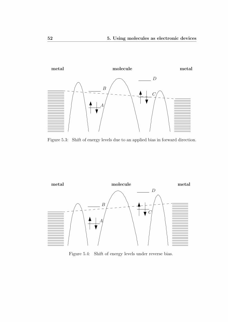
52 5. Using molecules as electronic devices
molecule metal
C
A
B
D
metal
Figure 5.3: Shift of energy levels due to an applied bias in forward direction.
molecule metalmetal
A
B
D
C
Figure 5.4: Shift of energy levels under reverse bias.

5.2 Qualitative model for transport 53
Measurements with a single conducting molecule were first reported byReed et al. (1997), and since then a lot of experiments using single or fewmolecules have been performed by various groups. Despite this experimentalsuccess, a detailed understanding of the connection between the molecularsetup of a device and its conduction properties is still lacking, and a lotof fundamental questions have not yet been answered. First of all, the ex-perimental results seem to be extremely sensitive to the fabrication process.Unfortunately the detailed structure of the molecular region is unknown, be-cause it is experimentally not observable. Therefore, numerical studies haveto assume a certain geometrical structure. However, all calculations tendto overestimate the observed magnitude of the current by up to one or twoorders of magnitude.
5.2 Qualitative model for transport
The model picture which was introduced by Aviram and Ratner to predicta molecular rectifier (Sec. 5.1.1) views the molecule as consisting of twospatially separated islands, each providing two relevant electronic levels. Thispicture was motivated by an analogy to semiconductor p-n junctions whereone deals with structures on the scale of micrometers.
Although molecular-electronic levels do indeed correspond to separatedmolecular orbitals, their spatial distance is on the atomic scale, i.e. of theorder of Angstrøms. Furthermore, both leads are only a few nanometersapart. In other words, the entire molecular junction is on the scale of (if notbelow) the interface region of standard semiconductor devices. The idea ofspatially separated energy levels, which are stable under perturbations suchas a strong coupling to the leads, the transfer of charge, or an applied biasvoltage, is therefore at least questionable.
Because the coupling between molecule and lead surface is produced bya chemical bond it will necessarily be strong. This invalidates the idea of aseparate island (let alone two islands) sitting between the contacts, as thelifetime of an additional charge on the molecule scales inversely with thecoupling to the leads. We rather think of the molecular region as inducing amodification of the potential gap between both leads. The molecular levels,shifted and broadened by the coupling to the leads, then allow for resonanttunnelling across the barrier region. The spatial location of the molecularorbitals does not provide a stable island, but it does influence the strengthof the coupling to the left and the right lead and this results in differentcouplings to each of them.

54 5. Using molecules as electronic devices
5.3 Recent experiments
As the experiments that measure conductance properties of molecular struc-tures vary not only in amount and chemical structure of the molecules in usebut also in the way these are attached to metallic or semiconducting leads,we want to give a short overview of the different setups in use. There arebasically three different types of devices in use: single or few molecules areaccessible in mechanically controllable break junction (MCB) experimentsand with the scanning tunnelling microscope (STM), while many moleculesare involved in sandwiched self-assembled monolayer (SAM) experiments.
For an explanation of the working principle of the STM we refer to Chap.6. MCB’s are produced by mechanically breaking a lithographically manu-factured small bridge connecting two leads. The spatial gap between bothleads is then tunable by piezo-electric techniques. When specific moleculesare deposited onto the device, a small fraction will be adsorbed in the gapregion and there is the chance that a few of them even bridge the gap. Byapplying a tunable voltage between both the leads, conductance propertiesof this molecular-electronic device can be measured.
Self-assembled monolayer devices are manufactured in a three step pro-cedure. First a single lead (typically having the form of a finger) is litho-graphically produced. Then a solution containing the molecules which areknown to self-assemble on top of the lead surface is spilt over the device, andwithin the time scale of hours a monolayer is built. In the final step, a secondlead is created on top of the molecular monolayer by beam epitaxy. Againconductance properties of the resulting device can be measured by biasingthe leads with an external voltage.
The observed properties depend not only on the molecular species bridg-ing the contacts but also on the exact geometry of the entire device. Theconductance measured with different setups can differ in orders of magnitudeand the qualitative voltage dependencies of the current ranges from simpleohmic behaviour to asymmetric behaviour and negative differential resistance(NDR).
Reed et al. (1997) have measured the conductance of a self-assembledmolecular monolayer bridging an MCB at room temperature, using moleculesof 1,4-benzene dithiol (i.e. having two thiol groups as can be seen in Fig. 5.5,which are known to couple strongly to Au-atoms). The conductance-voltage(CV ) characteristic was found to be symmetric with one peak in the voltagerange of 0−2V. They measured a current of the order of 50nA at a bias voltageof 2V, which they claim is produced by transport through one single activemolecule. Reichert et al. (2002) also used an MCB with molecules having twothiol groups, but being considerably longer. The measured current amplitude

5.4 Numerical calculations 55
SHHS
NCCN
Figure 5.5: Chemical structure of 1,4-benzene dithiol (top) and 1,4-phenylenediisocyanide (bottom).
was about 500nA at 1V for a single molecule, i.e. although the molecule wasmore than twice as long, the current was ten times larger.
With a different setup with an SAM sandwiched between two metallicleads Chen et al. (1999) have found negative differential resistance, namelyone peak at 2V in the IV curve. The molecule under investigation had onethiol group only and was attached to Au-leads at both ends. The measure-ments were taken at room temperature, and the measured current maximumwas of the order of 1nA.
Only recently, sandwiched SAM devices were studied at 4.2K (Lee et al.,2003; Dupraz et al., 2003), where 1,4-phenylene diisocyanide (PDI), a ben-zene ring with two isocyanide instead of thiol groups was used (see Fig. 5.5).The measurements exhibited currents of the order of 50 − 400nA. The CVcharacteristic for this molecule revealed more structure, in form of three tofive peaks within a voltage range of 1V. Such a behaviour was not observedwith previous devices containing other molecules.
In the next section we want to address the question whether the occur-rence of a large amount of conductance peaks within the SAM experiments iscontrary to the interpretation of such peaks being produced by resonant tun-nelling of electrons through individual molecular orbitals. Before doing so wefirst give an overview of other numerical studies which have been performedrecently.
5.4 Numerical calculations
Aiming to explain the various experimentally observed features of molecular-electronic devices, a number of theoretical methods have been invoked. Asone deals with a complex system, quite a number of effects are believed toinfluence the conductance properties. For example the external bias voltage,an induced electric field, and equilibrium charge transfer between moleculeand surface are believed to play an important role to name some of the effects.It has proven fruitful to analyse the influence of a single effect isolated from

56 5. Using molecules as electronic devices
the others.
5.4.1 Short summary of recent theoretical studies
Ab-initio calculations for the system studied experimentally by Reed et al.(1997) (see Sec. 5.3) were presented by DiVentra et al. (2000). Using ajellium model representing the gold leads, they were able to reproduce thecurrent-voltage characteristics qualitatively. However, the absolute magni-tude of the calculated current was about 2 orders of magnitude larger thanthe experimental values. Although they were able to reduce the currentvalue significantly by introducing a single gold atom between lead surfaceand molecule, the final current was still systematically too large. This in-dicates that numerical calculations need to take the atomic structure of thelead surface into account properly, in order to represent the geometry of thedevice accurately. The overestimation of the absolute magnitude of the cur-rent by most of the theoretical methods, is still an open problem (Emberlyand Kirczenow, 2001; Bauschlicher et al., 2003). An solution will also have toexplain the origin of the fairly large range of experimentally observed currentvalues (see Sec. 5.3).
Static charge transfer from the metal surface to the molecule was investi-gated by Xue et al. (2001). They found that such a charge transfer is presentand takes influence in that the molecular levels get shifted towards the Fermienergy compared to the position of the isolated molecule. This indicatesthat static charge transfer processes have to be accounted for, whenever aquantitative calculation of energy levels is aspired.
Along with an applied bias there will also be an electrostatic field acrossthe gap region. To be able to account for this external field, a self consistentprocedure together with a solution of the electrostatic problem was appliedby Brandbyge et al. (2002). Their results were in agreement with previouscalculations neglecting these effects. This indicates that approaches which areless sophisticated with respect to the electrostatic field should be sufficient.
Another interesting question is how the molecular orbital structure takesinfluence on the conductance properties. This has been studied by Seminarioet al. (2001); Darosa and Seminario (2001); Piccini et al. (2003). The aim is torelate different kinds of molecular orbital structures to certain conductancefeatures, which may allow one day to engineer molecules with predefinedconductance properties systematically.
The occurrence of negative differential conductance (NDC) has been stud-ied by Hettler et al. (2002, 2003). As already mentioned in Chapter 2 theyuse a rate equation based approach which is valid for weak coupling only.They argued that transitions between molecular levels around the Fermi en-

5.4 Numerical calculations 57
ergy can be forbidden due to different symmetry properties. This can resultin an isolated level which, if once occupied (via a photon assisted process)ends up blocking further transport. Negative differential conductance is thencaused by this blocking.
After this overview of the questions which have been investigated so far,we now consider a problem that occurred when interpreting the findings ofa recent experiment. This is the subject of the next section.
5.4.2 Conduction properties of PDI devices
Low temperature experiments with 1,4-phenylene diisocyanide (PDI) SAM’ssandwiched between two metallic leads have been performed by Lee et al.(2003) and Dupraz et al. (2003). They show several peaks in the CV -diagram.The typical voltage differences of these peaks are in the range of ∆U ≈ 0.2V(i.e. there are about 5 peaks within U = 0V and U = 1V). The commonlyadopted explanation for the occurrence of such peaks is the following. Eachmolecular orbital that enters the energy window, which is opened by theapplied voltage, enables resonant tunnelling. This increases the conductanceand therefore results in a peak within the CV -diagram.
Typically, the energy gap between molecular orbitals is in the range of∆E ≈ 1eV. In other words, for applied voltages up to U = 1V there should beonly a single accessible orbital per molecule, giving rise to only a single peakin the CV -diagram (assuming identical contributions from each molecule,which is motivated below). Therefore the following question arises: are theregeometrical alignments of the molecules which allow the additional peaks inthe CV diagram to be explained by resonant tunnelling through molecularorbitals as well?
Influence of changes in the molecular alignment to the transmissionspectrum
During the device fabrication, the step under least experimental control is theadsorption of the molecules onto the leads. Therefore the exact geometricalalignment of the molecular SAM is not exactly known. Furthermore, eventhe shape of both metallic lead surfaces may well be anything but regular andatomically flat. One therefore has to expect not only one specific but ratherquite a variety of molecular alignments to be produced within one device.As one is interested in the conduction properties of the resulting device as awhole, it is important to understand the influence of each type of geometricalalignment to the transmission function.

58 5. Using molecules as electronic devices
To this end, we have investigated three such possible alignments, whichwill be discussed separately.
1. When metal atoms are added on top of the molecular monolayer in arandom way, there might occur metallic clusters on top of the mono-layer. These affect the electronic configuration of the molecules in-dividually, and might therefore have an influence to the transmissionfunction.
2. In a SAM experiment, there is not just one molecule, but rather a fewhundred molecules involved. If the contribution to the transmissionfunction was different for each molecule, then T (E) would change qual-itatively, with a change in size of the mono-layer. We therefore analysehow the transmission functions depends on the number of moleculesinvolved.
3. The molecular monolayer may not be strictly periodic, but contain sev-eral defects. Within such a defect, the distance between two moleculescan be reduced, such that inter-molecular interactions are enhanced.Each of these defects will have a specific electronic structure and willtherefore influence the transmission function.
Influence of metallic clusters In the sandwich geometry, first the bottommetallic lead is created. Then the molecular mono-layer is adsorbed on top ofit by self-assembly. Finally the top metallic lead is build upon the molecularmono-layer. The exact shape of neither metallic surface is known and maybe anything but flat and regular.
It is likely that the surface atoms of the top metallic lead build up clusterson top of the molecular layer (as for example in Fig. 5.6 b). Which influencedo they have on the electronic configuration of the molecule they are incontact with? And do the clusters act as small molecules with new electroniclevels? In principle, there are three different influences which an Au clustercan have on the molecular-electronic structure: it introduces new electroniclevels, the existing molecular-electronic levels can be shifted, and the couplingbetween molecule and lead is reduced due to a increase in spatial separation.
The effect of a reduced coupling to the lead can clearly be seen in Fig.5.6 (c) where the amplitude of the transmission function is reduced withthe Au cluster added. This result is in full agreement with DiVentra et al.(2000). However, the peak positions themselves are hardly affected. Thiswas observed for several types of clusters similar to the one shown in Fig.5.6 and indicates that the shift of the molecular levels only slightly depends

5.4 Numerical calculations 59
(a)
(b)
(c)
Figure 5.6: (a) Structure of a molecule without cluster. (b) Structure of amolecule with a gold cluster on top. (c) Transmission function T (E) for bothstructures. The energy scale is relative to the HOMO-LUMO gap, such thatE = 0 corresponds to the middle of the gap.
on the exact geometry of the neighbouring Au atoms. Finally, there are noadditional peaks, which one might have expected because of the additionalelectronic levels of the cluster. The explanation of their absence is the fol-lowing: an electronic level gives rise to a peak in the transmission functiononly if the corresponding orbital wave function overlaps with both the topand bottom electrode. The overlap with that electrode which the clusteris attached to (say top electrode) is of course large. The overlap with thebottom electrode consists of two parts. The direct overlap and the indirectoverlap via the molecule. The direct overlap is negligible due to the largespatial separation. The indirect overlap is also negligible unless the energyof the cluster level coincides with a molecular energy level (otherwise thereis no molecular level to overlap with). But in that case, there already existsa transmission peak due to the molecule itself.
In summary, if transmission is already suppressed by the molecule (at alloff-resonant energies), it can either be further reduced by off-resonant tun-nelling through the cluster, or it can (at best) be left unchanged by resonanttunnelling through the cluster. Under no circumstances can transmission,once suppressed by the molecule, be afterwards increased by the cluster. Thisin turn means that metallic clusters cannot give rise to additional peaks inthe transmission spectrum.

60 5. Using molecules as electronic devices
Figure 5.7: The structure of two, three, and four molecules adsorbed withinan Au-9× 3 super cell. This setup was used to test the sum rule, Eq. (5.1).The results are shown in Fig. 5.8.
Mono-layer versus single molecule What do we expect the transmis-sion function T i(E) for i periodically arranged molecules to look like? As longas the inter-molecular interactions are small (compared to the intra-molecularones) the molecular levels of each molecule will not be significantly changed.Furthermore as the mono-layer consists of only one kind of molecule, allof them will have the same electronic structure. Therefore we expect eachmolecule to contribute roughly the same amount to the transmission func-tion:
T n(E) ≈∑
i
T 1(E) = nT 1(E), (5.1)
where i runs over all n adsorbed molecules. We do not expect the equationto be fulfilled exactly, because the electronic structure of each molecule willalways be a slightly affected by the presence of neighbouring molecules.
We calculated the transmission function for n=1 to 4 molecules withinan Au super cell of size 9× 3 (the structures are shown in Fig. 5.7). The dis-tance between the molecules is chosen to be a multiple of the closest Au-Auseparation aAu (d = 5.76A = 2aAu, with aAu = 2.88A). To our knowledge,the parameters of the PDI-SAM mono-layer have never been determined ex-perimentally, which is why we have to assume the above values. HoweverSTM studies (Zeng et al., 2002) and also theoretical calculations (Yourd-shahyan and Rappe, 2002) have been performed for alkanethiol mono-layers,and these parameters motivated our choice. According to structure optimi-sations the hollow-site adsorption is stronger than the top-site adsorption.The inter-molecular distance is taken from the observation of (Zeng et al.,2002).
As we have expected according to Eq. (5.1), the transmission functionshave the same amount of peaks, independently from the number of moleculespresent and at identical energetic positions (see Fig. 5.8 a). This result is also

5.4 Numerical calculations 61
(a) (b)
Figure 5.8: (a) Transmission function for one, two, three, and four PDImolecules (see Fig. 5.6 (a) and Fig. 5.8). (b) When plotted against each other,the transmission functions reveal a linear relationship: T i(E) = a(i, 4)T 4(E),where a(i, 4) ≈ i
4.
obtained for all larger distances of the molecules, where the inter-molecularinteraction is even smaller. Furthermore, the sum rule (Eq. 5.1) is indeedfulfilled, as shown in Fig. 5.8 (b), where each T i(E) is plotted against T 4(E)for i ∈ {1, 2, 3}. The calculated transmission values (300 discrete valueseach) clearly show a linear correlation. The straight lines are linear fits tothe data, and their slope does very well agree with the theoretically expectedvalue of a(n,m) = n/m. The deviation is below 6%, as can be seen in table5.1, where we summarise all the fitted values for T n(E) = a(n,m) · Tm(E).
We conclude the following: a monolayer, in which the inter-molecular dis-tance is large enough to not let inter-molecular interactions play a significantrole, has the same number of distinct electronic levels as a single molecule.These levels are then highly degenerate. A CV -diagram will therefore havethe same number of peaks. Only the net current will be increased by a fac-tor a(n,m) compared to the single molecule case. The mere fact that onedeals with a mono-layer instead of a single molecule does not imply that thetransmission function changes qualitatively.
Influence of molecular clusters We have seen that one does not observeadditional peaks in the transmission function as long as the inter-molecularinfluence is small; this is the case for distances which occur in typical SAMstructures (Zeng et al., 2002; Yourdshahyan and Rappe, 2002). We now in-vestigate cases, in which the molecular interactions are not negligible. This

62 5. Using molecules as electronic devices
n m a(n,m) an/m
− 1 σ
1 2 0.5188 3.76% 0.0141 3 0.3500 4.99% 0.0181 4 0.2649 5.96% 0.0212 3 0.6753 1.30% 0.0082 4 0.5117 2.34% 0.0153 4 0.7579 1.06% 0.011
Table 5.1: The fitted values for a(n,m) together with their deviation fromthe theoretical value a(n,m) := n/m and a measure for the quality of the fitσ, where σ2 := (N−1)−1
∑(T n(Ei)− a(n,m)Tm(Ei))
2 for N = 300 discreteenergy values T (Ei).
occurs for example when the periodic structure of the mono-layer is per-turbed by an additional molecule, such that a molecular cluster is formed.It is sufficient to study the transmission function of an isolated cluster only,because we have already seen that molecules in the periodic SAM arrange-ment do not influence each other. The sum of the transmission function forthe periodic SAM and the transmission function for the molecular cluster is,due to the sum rule, the total transmission function for defect and SAM.
We study the influence of a shorter distance between two, three, and fourmolecules on the transmission spectrum and relate it to the discrete energiesof the isolated molecules. The molecules are now separated by d = 2.88Awhich corresponds to the Au-Au atom spacing aAu. The atomic structure forthis calculation is shown in Fig. 5.9 (a), the resulting transmission functionsin Fig. 5.9 (b) and (c).
Upon reducing the molecular separation from d1 = 2aAu to d2 = aAu, thetransmission function qualitatively changes: the number of peaks roughlydoubles, and the new peak positions are different from the ones we have ob-tained in the previous calculations and do depend on the number of moleculesinvolved. This is an important point, because if there are several molecularclusters with different molecular distances, then they all give rise to peaksat different energy values. The resulting transmission function is the sumof the individual functions and will thus contain far more peaks than thetransmission function for the non perturbed periodic layer.
We now show that the new peaks are a result of the increase in molecularinteraction due to the decrease in spatial separation. For non-interactingmolecules, the molecular energies are identical and therefore degenerate. Aninteraction between molecules breaks this degeneracy, and therefore new en-
5.4 Numerical calculations 63
(a)
(b) (c)
Figure 5.9: (a) Two, three, and four molecules with a short inter-moleculardistance of d = aAu = 2.88A. (b) The transmission functions for two andthree molecules. (c) The transmission functions for three and four molecules.In contrast to all previous cases, the peaks are shifted with respect to eachother and there are also additional peaks. These changes are due to theincrease in inter-molecular interaction, which alters the electronic levels.

64 5. Using molecules as electronic devices
Figure 5.10: Magnification of the transmission functions for three and fourclosely spaced molecules from Fig. 5.9 (c). Additionally the discrete energylevels of the molecular region are plotted as points along the transmissionfunction. There corresponds at least one discrete energy level to each peak.A detailed discussion is given in the main text. Inset: Transmission function(original scale) for three and four closely spaced molecules (identical to Fig.5.9 c).
ergy levels occur. By performing a diagonalisation of the molecular Hamilto-nian (without leads), one can determine the levels of the molecular cluster.
In Fig. 5.10 we have again plotted the transmission function for threeand four molecules, this time together with the discrete energy levels of thecorresponding molecular cluster. The inset is identical to Fig. 5.9 (c), whilethe plot itself is a magnification, to better resolve the discrete energy levels(which are shown as points along the transmission function). Each of thetransmission peaks is related to at least one discrete energy value. But thereverse statement is not true: not each energy value can be related to a peakin the transmission function. Why is that? The discrete energies can onlygive rise to new peaks in the transmission function if they are not suppressedby a weak coupling to one of the leads. All levels which are not related toany peak belong to this category. If the position of the peak is shifted awayfrom a corresponding energy level, then this is due to the coupling betweenmolecules and leads. This coupling is absent in the diagonalisation of themolecular Hamiltonian, but is automatically included in the calculation ofthe transmission function.
Finally we show that the additional peak structure in the transmission

5.4 Numerical calculations 65
Figure 5.11: IV –calculation for a molecular region containing all threemolecular clusters shown in Fig. 5.9 (a). There are three distinct steps withinthe voltage range of 1V.
function for a scenario with an increased inter-molecular interaction gives riseto a number of steps in the IV -curve. Figure 5.11 contains an IV calculationfor a molecular structure containing all three molecular clusters shown in Fig.5.9 (a). In this calculation, the bias voltage V enters as a shift of the Fermilevels for source and drain lead: µ1 = µ2 + eV . The molecular energy hasbeen set to Em = µ1 − δEm − ηeV , where δEm is the zero bias displacementof the molecular levels and η = 0.5, because of the symmetric coupling tothe leads.
Compared to the experiments by Lee et al. (2003) and Dupraz et al. (2003)the number of steps in the IV –curve is well reproduced by our calculation.The obtained current is at least one order of magnitude larger than the ex-perimental values. This is a phenomenon common to all theoretical methodsbased on the Landauer formula (Emberly and Kirczenow, 2001; Bauschlicheret al., 2003). A satisfactory explanation for this discrepancy as well as forthe broad range of experimentally observed current values has not yet beenfound.
5.4.3 Discussion
We have shown that the peak structure of the transmission function is ro-bust against changes in the number of adsorbed molecules, as long as thedistance between molecules is considerably large (d & 6A). And also does

66 5. Using molecules as electronic devices
the exact shape of the top metallic lead not influence the qualitative struc-ture of the transmission function. Only if the distance between moleculesbecomes comparable to atomic length scales, inter-molecular interactions areno longer negligible and the transmission function undergoes a qualitativechange. Namely an additional peak structure occurs.
How does this finding compare to the experimental data? As we havepointed out in section 5.3, a more or less random peak structure was observedin the CV characteristic only in devices using molecules with two isocyanidegroups (Lee et al., 2003; Dupraz et al., 2003). In other devices moleculeswith at least one thiol group are typically used. These show significantly lesspeak structure.
We therefore give the following interpretation: The thiol group is knownto bind strongly to Au atoms. It is therefore likely, that thiol-based mono-layers stably adsorb to gold leads. Resulting periodic structures are thenrobust against distortions. The conductance of such structures is propor-tional to the corresponding single molecule conductance, i.e. the number ofmolecules involved changes the absolute value of the current only, not thepeak structure.
The random like peak structure in devices made up of isocyanide basedmolecules suggests that there are molecular clusters present in the mono-layer. These clusters might occur because the binding of an isocyanide groupto Au is considerably weaker compared to that of a thiol group, and weakerbinding results in a less robust periodic structure.
Chapter 6
Understanding STM images
In this chapter we present another application of the numerical method whichwe have implemented, namely the calculation of scanning tunnelling micro-scope (STM) images. Starting with an historical overview and a short intro-duction into the working principle of an STM, we consider experiments whichcan only be understood in accordance with theoretical calculations beyondthe Tersoff-Hamann approximation. We also present our own calculationsfrom a cooperation with Constable et al. (2004) to support the interpreta-tion of recent STM images. As the system under investigation is considerablylarge, we were able to produce the numerical images only by introducing aspecial treatment for a large eigenvalue problem, which cannot be solvedsufficiently accurately by conventional methods. This is the first time thata method has been implemented that can perform image calculations for asystem of that size.
6.1 Introduction
This section provides an introduction to the STM with respect to its history,its working principle, and some of its applications. We focus on experimentalaspects here, as the approaches in use to numerically calculate transportthrough molecular systems have already been discussed (see Chap. 2 and 4).Detailed reviews about theories specific to the STM can also be found in theliterature (Briggs and Fisher, 1999; Hofer and Foster, 2003).
6.1.1 Historical overview
The optical microscope can be used to obtain real-space images of structureswhich are too small to be visible to the unaided eye. However, its resolution

68 6. Understanding STM images
is restricted to objects larger than half the width of the wavelength of visiblelight (i.e. larger than roughly 250nm). Even smaller objects can be viewedusing electron microscopy. The transmission electron microscope (inventedby Knoll and Ruska, 1932a,b) detects electrons from a beam that was trans-mitted through the sample while the scanning electron microscope detectssecondary electrons which are emitted from the surface due to excitation by aprimary electron beam. Both methods are capable of resolving objects downto the scale of several nanometers by using electron beams with a wavelengthconsiderably smaller than that of visible light. They are invasive methods,because the highly energetic electron beam has to be directed onto and inter-act with the sample. Furthermore, the samples have to be viewed in vacuumto prevent the electrons from being scattered by air.
In 1981 the scanning tunnelling microscope was invented by Binnig et al.(1981, 1982). It was the first tool that allowed real-space images of surfacesto be obtained with atomic resolution and its inventors Gerd Binnig andHeinrich Rohrer were jointly awarded half of the 1986 Noble Price in Physics1.The STM is widely used in both industrial and fundamental research whereit serves as an instrument for analysing bare surfaces, adsorbates on topof surfaces and also for manipulating these adsorbates on the nanometerscale (Bartels et al., 1997). It can be operated at room temperature andatmospheric pressure although higher resolution is obtained under ultra-highvacuum conditions.
6.1.2 Working principle
Figure 6.1 shows a typical STM setup. An atomically sharp metallic tip isapproached to the surface under investigation. When the distance z betweensurface and tip is small enough (z < 10A) there is a measurable probabilityfor electrons to tunnel between tip and surface and vice versa. With anapplied voltage U the chemical potential of (say) the tip µ2 is lowered relativeto the chemical potential of the substrate µ1, and therefore each electronthat has tunnelled into the tip will equilibrate within the tip-bulk, therebycontributing to a tunnelling current. This current depends
• on the exact position of the tip,
• on the applied voltage,
• on the type of tip, surface, and (if present) adsorbate material,
1The other half was awarded to Ernst Ruska for his invention of the electron microscope.

6.1 Introduction 69
����������������������������������������������������������������������������������������������������������������������������������������������������������������������������������������������������������������������������������������������������������������������������������������������������������������������������������������������������������������������������������������������������������������������������������������������������������������������������������������������������������������������������������������������������������������������������������������������������������������������������������������������������������������������������������������������������������������������������������������������������������������������������������������������������������������������������������������������������������������������������������������������������������������������������������������������������������������������������������������������������������������������������������������������������������������������������������������������������������������������������������������������������������������������������������������������������������������������������������������������������������������������������������������������������������������������������������������������������������������������������������������������������������������������������������������������������������������������������������������������������������������������������������������������������������������������������������������������������������������������������������������������������������������������������������������������������������������������������������������������������������������������������������������������������������������������������������������������������������������������������������������������������������������������������������������������������������������������������������������������������������������������������������������������������������������������������������������������������������������������������������������������������������������������������������������������������������������������������������������������������������������������������������������������������������������������������������������������������������������������������������������������������������������������������������������������������������������������������������������������������������������������������������������������������������������������������������������������������������������������������������������������������������������������������������������������������������������������������������������������������������������������������������������������������������������������������
��������������������������������������������������������������������������������������������������������������������������������������������������������������������������������������������������������������������������������������������������������������������������������������������������������������������������������������������������������������������������������������������������������������������������������������������������������������������������������������������������������������������������������������������������������������������������������������������������������������������������������������������������������������������������������������������������������������������������������������������������������������������������������������������������������������������������������������������������������������������������������������������������������������������������������������������������������������������������������������������������������������������������������������������������������������������������������������������������������������������������������������������������������������������������������������������������������������������������������������������������������������������������������������������������������������������������������������������������������������������������������������������������������������������������������������������������������������������������������������������������������������������������������������������������������������������������������������������������������������������������������������������������������������������������������������������������������������������������������������������������������������������������������������������������������������������������������������������������������������������������������������������������������������������������������������������������������������������������������������������������������������������������������������������������������������������������������������������������������������������������������������������������������������������������������������������������������������������������������������������������������������������������������������������������������������������������������������������������������������������������������������������������������������������������������������������������������������������������������������������������������������������������������������������������������������������������������������������������������������������������������������������������������������������������������������������������������������������������������������������������������������������
I
z xy
y
T
U
T
Tunnel
x
Figure 6.1: The working principle of an STM device (taken from Aschauer,1999). Tip and surface are biased via an applied voltage in order to recorda small tunnelling current which depends on the tip position.
• as well as on several laboratory conditions such as temperature, pres-sure etc.
Because of the extreme sensitivity of the tunnelling current to the tipposition one can generate topographic surface images by scanning in lateraldirection over the sample. Thereby two different modes are possible. Surfaceswhich are known to be atomically flat can be scanned in the constant-heightmode, where the tunnelling current is measured as a function of lateral po-sition and fixed tip-surface distance z: I = I(x, y, z = const). The secondmode is the so-called constant-current mode, where during the scan acrossthe surface the tip-height is adjusted by a feedback loop, to fix the tunnellingcurrent at a chosen value. The different values for the tip height are recordedand make up the STM image: z = z(x, y, I = const). This latter mode istypically used when the surface structure is either not known or known tonot be entirely flat.
There is a third mode for STM operation which differs from the abovementioned ones in that it is not only used to image the surface but alsoto manipulate the position of adsorbed molecules. This can be achieved bydecreasing the tip-surface distance in the vicinity of the molecule below acertain critical value at which the tip influence becomes irreversible. Whenone deals with adsorbates building molecular monolayers, this can result inthe removal of a single molecule, i.e. it constitutes a controlled write opera-tion. With the above mentioned reversible constant-current mode a read-onlyoperation can also be performed.
These capabilities of the STM motivated intensive research within thelast decade aiming to build memory storage devices on the molecular or evenatomic level (Miller et al., 1997; Bennewitz et al., 2002). Nevertheless we

70 6. Understanding STM images
(a) (b)
(c)
Figure 6.2: A collection of images taken with an STM: (a) image of Rhodiumsurface 103Rh(111) (taken from Ohtani et al., 1988) (b) same surface with ben-zene molecules (C6H6) adsorbed (taken from Ohtani et al., 1988) (c) benzeneadsorbed on Platinum 195Pt(111) (taken from Weiss and Eigler, 1993).
restrict ourselves to reversible STM applications from now on.
6.1.3 Examples of STM images
A few representative images taken with an STM are shown in Fig. 6.2. Byscanning over clean surfaces, the orientation of the top layer can be deter-mined. In Fig. 6.2 (a) a step in the surface layer of Rh(111) can be identified.The image changes drastically when an adsorbate is present. In Fig. 6.2 (b)the same surface is shown, this time with benzene molecules adsorbed on top.They appear as hills with a dip in the middle. Another image of benzene,but adsorbed on Pt(111) and with a much higher resolution, is shown in Fig.6.2 (c).

6.2 Numerical STM image calculations 71
6.2 Numerical STM image calculations
As the STM technique was more and more established, it became obviousthat there are reproducible experimental effects which can not be explainedby the Tersoff-Hamann formula (see Sec. 2.1.3 and 2.1.4). In these cases,the underlying assumption that any influence of the tip can be ignored is nolonger justified. This section is devoted to cases in which it was necessary toperform numerical calculations beyond the Tersoff-Hamann approximationin order to explain experimental observations.
6.2.1 Image contrast inversion
Doyen et al. (1993) were able to show that the experimentally observed effectof image contrast inversion (Kopatzki and Behm, 1991; Schuster et al., 1991)can be explained by the influence of the tip potential at short tip-surfacedistances. They considered a bare metallic Palladium (Pd) surface.
First they calculated the local electronic density of states for the baresurface using DFT. Thereby they confirmed that it takes a maximum valueon top of a Pd surface atom, independently of the distance z from the surface.Above the hollow site the electronic density takes a minimum value.
In a second step, the STM tunnelling current was calculated. This wasdone using scattering theory for a periodically repeated Pd slab. The tipwas modelled via a localised attractive potential. They found that the localextrema of the tunnelling current coincide with the extrema of the density ofstates only for tip-surface distances larger than 3 A. For closer distances theimage contrast undergoes an inversion, and maxima of the tunnelling currentcorrespond to minima of the density of states. This image contrast inversionis shown in Fig. 6.3.
This effect can be explained as follows. With decreasing tip-surface dis-tance, the increasing interaction between the resonance state of the localisedtip potential and the delocalised surface states yields a splitting into bondingand anti-bonding states. Because of the d-type orbital structure of Pd thisinteraction is stronger for the hollow site than for the top site and so is thesplitting. The stronger bonding then results in a larger current for the hollowsite compared to the top site.
6.2.2 Negative differential resistance
Another example for the important influence of the tip electronic structureis the occurrence of negative differential resistance (NDR) in scanning tun-nelling spectroscopy experiments. In those experiments the bias voltage is

72 6. Understanding STM images
Figure 6.3: Calculation of the tunnelling current for two different distancesof the STM tip. The image contrast undergoes an inversion (i.e. currentmaxima become minima and vice versa) when the tip-surface distance isdecreased (taken from Doyen et al., 1993).

6.2 Numerical STM image calculations 73
tuned while the STM tip position is not changed. In this way the conduc-tance properties G(V ) = dI/dV of specific points above the surface can bemeasured.
Negative differential resistance cannot be explained within the Tersoff-Hamann approximation because the tunnelling current is taken to be directlyproportional to the applied voltage, such that the conductance is alwayspositive and constant.
Tsukada et al. (1991) addressed the phenomenon of NDR by using theBardeen formula together with first-principles electronic structure calcula-tions, which they performed for substrate and tip. Within their calculationsNDR occurred only when the STM current was dominantly produced by thetunnelling between a single tip state and a single substrate state both closeto the Fermi energy.
The mechanism of NDR is the following: for increasing but still smallapplied bias voltages, the broadening of the energy window which is beingintegrated over in the Bardeen formula, results in an increase of the tunnellingcurrent. Thus the conductance must be positive. By further increasing thebias voltage, the Fermi level offset between substrate and tip drives the twostates dominating the current off resonance. This leads to a decrease in thetunnelling matrix element Mij, because it involves the product of the LDOSof each of the two states, which is much reduced if the peak positions of thetwo LDOSs are shifted apart. A decrease of the total current and thereforea negative differential resistance is then obtained.
6.2.3 Electric field effects
The tip-induced electric field at the surface is, assuming a tip-sample sepa-ration of 5 − 10A and an applied voltage of 1V , of the order of 109Vm−1.Such an electric field can be expected to have a considerable effect onto theelectronic structure of the surface when its polarisability changes with spatialposition. This is for example the case when hydrocarbons, which are onlyslightly polarisable (εr ≈ 2), are adsorbed on silicon (εr ≈ 14) (Briggs andFisher, 1999).
When STM data from the bare silicon surface (Tromp et al., 1985) andfrom hydrocarbons adsorbed on silicon (Mayne et al., 1993) were compared,it was found that, although the molecules are adsorbed on top of the siliconsurface, they appear lower than the bare silicon surface dimers in the constantcurrent mode image. This can be explained by the influence of the tip inducedelectric field, which effectively pulls the electrons out of the regions with ahigher polarisability.
Numerical simulations neglecting the tip-induced electric field result in

74 6. Understanding STM images
Figure 6.4: Influence of the tip-induced electric field. The apparent heightof an adsorbed molecule can be changed. Hydrocarbons adsorbed on siliconappear as bumps (top figure) in calculations neglecting the electric field. Incontrast, when accounting for the field the adsorbed molecules correspond tolower regions of the STM image (bottom figure), in accordance with experi-ment (Ness and Fisher, 1997).
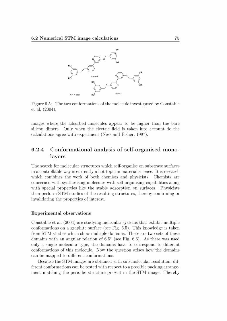
6.2 Numerical STM image calculations 75
Figure 6.5: The two conformations of the molecule investigated by Constableet al. (2004).
images where the adsorbed molecules appear to be higher than the baresilicon dimers. Only when the electric field is taken into account do thecalculations agree with experiment (Ness and Fisher, 1997).
6.2.4 Conformational analysis of self-organised mono-layers
The search for molecular structures which self-organise on substrate surfacesin a controllable way is currently a hot topic in material science. It is researchwhich combines the work of both chemists and physicists. Chemists areconcerned with synthesising molecules with self-organising capabilities alongwith special properties like the stable adsorption on surfaces. Physiciststhen perform STM studies of the resulting structures, thereby confirming orinvalidating the properties of interest.
Experimental observations
Constable et al. (2004) are studying molecular systems that exhibit multipleconformations on a graphite surface (see Fig. 6.5). This knowledge is takenfrom STM studies which show multiple domains. There are two sets of thesedomains with an angular relation of 6.5◦ (see Fig. 6.6). As there was usedonly a single molecular type, the domains have to correspond to differentconformations of this molecule. Now the question arises how the domainscan be mapped to different conformations.
Because the STM images are obtained with sub-molecular resolution, dif-ferent conformations can be tested with respect to a possible packing arrange-ment matching the periodic structure present in the STM image. Thereby

76 6. Understanding STM images
Figure 6.6: (a) Packing arrangement for trans-2 conformation. (b) STMimage of two domains differing in orientation by an angle of 6.5◦. (c) Ex-panded image of the domain corresponding to the trans-2 configuration. (d)Expanded image corresponding to the trans-1 configuration (images takenfrom Constable et al., 2004).
Constable et al. (2004) were able to uniquely relate each domain to a singleconformation (see Fig. 6.6).
However, details of the conformation concerning the angular direction ofthe bond between oxygen atom and the attached hydrocarbon chains (namedR in Fig. 6.5) remain unknown. Two different conformations are shown inFig. 6.7. Because the hydrocarbon chains do not show up in the STM imagesexplicitly, both conformations can be matched with the experiment. But itis believed that they give rise to different sub-molecular structures in theimages. Calculations can be used to predict the sub-molecular structure andby comparing the theoretical images with the ones obtained experimentally,it may be possible to pin down the conformational structure more strictly.
However, the algorithms for calculating STM images are limited to smallsystems, at least systems too small to contain the molecule of interest (Fig.6.7) and to our knowledge, no calculations have ever been published for amolecule of comparable size. This was also true for the ESQC method. Yetwe figured out the bottle neck of the calculation and by reformulating thecorresponding mathematical problem we succeeded in extending the methodto systems large enough for the molecule to fit into.

6.2 Numerical STM image calculations 77
Theoretical calculations
Because the molecule is wide spread on top of the graphite surface, a verylarge super cell has to be used. The size of this super cell in turn determinesthe dimension of the propagator matrix which enters the ESQC algorithm.This non-symmetric matrix has to be diagonalised, in order to obtain thepropagating channels (see Chap. 4). A straight forward diagonalisation usingstandard linear-algebra packages (LAPACK) proved to result in inaccurateeigenvalues. This affects the algorithm in a dramatic way: a significant lossin accuracy of the eigenvalues renders the entire method useless. This isbecause each eigenvalue, depending on its modulus, corresponds to a prop-agating or an evanescent incoming or outgoing solution. The method relieson an identical amount of incoming and outgoing solutions. Below a certainnumerical accuracy such an equal partitioning is no longer possible, resultingin the breakdown of the method.
By using the periodic nature in lateral direction of each lead explicitly,we were able to transform the diagonalisation procedure from a single stepdiagonalisation of a large quadratic 2NM matrix into N individual diagonal-isation steps each involving a 2M dimensional quadratic matrix only. Here Ncorresponds to the size of the super cell in units of the unit cell and M is thenumber of (valence) electrons contained in the latter. As M is independentof the system size (super cell size), so is the accuracy of the diagonalisationstep.
Only after the implementation of this exceedingly more accurate diag-onalisation procedure was it possible to consider a super cell large enoughfor the molecule to fit in. The remaining restriction is now imposed by theavailable computer memory (RAM). This allows, for the first time, theoreti-cal studies of such large molecules adsorbed on surfaces while still using anatomic description of the entire system.
Currently we are considering several conformations (two of which areshown in Fig. 6.7) of the molecules possibly involved in the above mentionedexperiments. Preliminary results are presented in Fig. 6.8. Each image is
obtained by scanning a region of size 30× 50A2
with a resolution of 60× 100points. As the calculation for a single point takes roughly 4 minutes on apresent-date PC, the total computer time for an entire image amounts toalmost two and a half weeks.
These calculations have to be considered as work in progress. So far wehave merely proven that calculations of this type are possible from a technicalpoint of view. Whether at all and for which parameter range the calculationsare in accordance with experiments remains to be seen. Further studiesconcerning the influence of parameters like molecule-substrate distance, tip-

78 6. Understanding STM images
Figure 6.7: Two different conformations of the molecule investigated by Con-stable et al. (2004). They enter as input to STM image calculations (see Fig.6.8).

6.2 Numerical STM image calculations 79
Figure 6.8: Sample STM image calculations for two different conformationsof the same molecule (which are shown in Fig. 6.7). The projected atomicpositions are plotted as black pixels, irrespective of their chemical type. Fur-ther studies are in order to finally perform calculations which can be relateddirectly to the experiments.

80 6. Understanding STM images
surface separation and molecule-surface orientation are in order to finallyperform calculations which can be related directly to the experiments. Thisis part of the future work which arises from the present thesis.

Bibliography
Aschauer, H. (1999). Scanrichtungsabhangigkeit bei STM-Aufnahmen vonAdsorbaten. Master’s thesis, LMU-Munchen. In German.
Aviram, A. and Ratner, M. A. (1974). Molecular rectifiers. Chemical PhysicsLetters, 29(2):277–283.
Bardeen, J. (1961). Tunneling from a Many-Particle Point of View. PhysicalReview Letters, 6(2):57–59.
Bartels, L., Meyer, G., and Rieder, K.-H. (1997). Basic Steps of Lateral Ma-nipulation of Single Atoms and Diatomic Clusters with a Scanning Tun-neling Microscope Tip. Physical Review Letters, 79(4):697–700.
Bauschlicher, C. W., Ricca, A., Mingo, N., and Lawson, J. (2003). On thecurrent flow for benzene-1,4-dithiol between two Au contacts. ChemicalPhysics Letters, 372(5-6):723–727.
Bennewitz, R., Crain, J. N., Kirakosian, A., Lin, J.-L., McChesney, J. L.,Petrovykh, D. Y., and Himpsel, F. J. (2002). Atomic scale memory at asilicon surface. Nanotechnology, 13:499–502.
Bingham, R. C., Dewar, M. J. S., and Lo, D. H. (1975a). Ground states ofmolecules. XXV. MINDO/3. Improved version of the MINDO semiem-pirical SCF-MO method. Journal of the American Chemical Society,97(6):1285–129.
Bingham, R. C., Dewar, M. J. S., and Lo, D. H. (1975b). Ground states ofmolecules. XXVI. MINDO/3 calculations for hydrocarbons. Journal of theAmerican Chemical Society, 97(6):1294–1301.
Bingham, R. C., Dewar, M. J. S., and Lo, D. H. (1975c). Ground statesof molecules. XXVII. MINDO/3 calculations for carbon, hydrogen, oxy-gen, and nitrogen species. Journal of the American Chemical Society,97(6):1302–1306.

82 Bibliography
Bingham, R. C., Dewar, M. J. S., and Lo, D. H. (1975d). Ground states ofmolecules. XXVIII. MINDO/3 calculations for compounds containing car-bon, hydrogen, fluorine, and chlorine. Journal of the American ChemicalSociety, 97(6):1307–1311.
Binnig, G., Rohrer, H., Gerber, C., and Weibel, E. (1981). Tunneling througha controllable vacuum gap. Applied Physics Letters, 40(2):178–180.
Binnig, G., Rohrer, H., Gerber, C., and Weibel, E. (1982). Surface Studiesby Scanning Tunneling Microscopy. Physical Review Letters, 49(1):57–61.
Born, M. and Oppenheimer, J. R. (1927). Zur Quantentheorie der Molekeln.Annalen der Physik, 84(20):457–484.
Brandbyge, M., Mozos, J.-L., Ordejon, P., Taylor, J., and Stokbro, K. (2002).Density functional method for nonequilibrium electron transport. PhysicalReview B, 65:165401.
Briggs, G. and Fisher, A. (1999). STM experiment and atomistic modellinghand in hand: individual molecules on semiconductor surfaces. SurfaceScience Reports, 33(1-2):3–81.
Buttiker, M., Imry, Y., Landauer, R., and Pinhas, S. (1985). Generalizedmany-channel conductance formula with application to small rings. Phys-ical Review B, 31(10):6207–6215.
Chen, C. J. (1990a). Origin of atomic resolution on metal surfaces in scanningtunneling microscopy. Physical Review Letters, 65(4):448–451.
Chen, C. J. (1990b). Tunneling matrix elements in three-dimensional space:The derivative rule and the sum rule. Physical Review B, 42(14):8841–8857.
Chen, J., Reed, M. A., Rawlett, A. M., and Tour, J. M. (1999). Large On-Off Ratios and Negative Differential Resistance in a Molecular ElectronicDevice. Science, 286(5444):1550–1552.
Constable, E. C., Hermann, B. A., Housecroft, C. E., Merz, L., and Scherer,L. J. (2004). Monitoring conformational diversity in self-organised mono-layers with scanning tunnelling microscopy at near atomic resolution.Chemical Communications, (8):928–929.
Dahlke, R. and Schollwock, U. (2004). Electronic transport calculationsfor self-assembled monolayers of 1,4-phenylene diisocyanide on Au(111)contacts. Physical Review B, 69(8):085324.

Bibliography 83
Darosa, P. A. and Seminario, J. M. (2001). Electron Transport through Sin-gle Molecules: Scattering Treatment Using Density Functional and GreenFunctions Theories. Journal of Physics C, 105:471–481.
Datta, S. (1995). Electronic Transport in Mesoscopic Systems. CambridgeUniversity Press, Cambridge, U. K.
Dewar, M. J. S. and Thiel, W. (1977). Ground states of molecules. 38. TheMNDO method. Approximations and parameters. Journal of the AmericanChemical Society, 99(15):4899–4907.
Dewar, M. J. S., Zoebisch, E. G., Healy, E. F., and Stewart, J. J. P. (1985).Development and use of quantum mechanical molecular models. 76. AM1:a new general purpose quantum mechanical molecular model. Journal ofthe American Chemical Society, 107(13):3902–3909.
DiVentra, M., Pantelides, S. T., and Lang, N. D. (2000). First-PrinciplesCalculation of Transport Properties of a Molecular Device. Physical ReviewLetters, 84(5):979–982.
Doyen, G., Drakova, D., and Scheffler, M. (1993). Green-function theory ofscanning tunneling microscopy: Tunneling current and current density forclean metal surfaces. Physical Review B, 47(15):9778–9790.
Drude, P. K. L. (1900a). Zur Elektronentheorie der Metalle. Annalen derPhysik, 1(3):566–614.
Drude, P. K. L. (1900b). Zur Elektronentheorie der Metalle. II. Teil. Annalender Physik, 3(11):369–403.
Dupraz, C. J. F., Beierlein, U., and Kotthaus, J. P. (2003). Low Temper-ature Conductance Measurements of Self-Assembled Monolayers of 1,4-Phenylene Diisocyanide. ChemPhysChem, 4(11):1247–1252.
Emberly, E. G. and Kirczenow, G. (2001). Models of electron transportthrough organic molecular monolayers self-assembled on nanoscale metalliccontacts. Physical Review B, 64(23):235412–235419.
Fisher, D. S. and Lee, P. A. (1981). Relation between conductivity andtransmission matrix. Physical Review B, 23(12):6851–6854.
Foresman, J. B. and Frisch, Æ. (1996). Exploring Chemistry with ElectronicStructure Methods. Gaussian, Inc. Pittsburgh, USA, second edition.

84 Bibliography
Geddes, N. J., Sambles, J. R., Jarvis, D. J., Parker, W. G., and Sandman,D. J. (1990). Fabrication and investigation of asymmetric current-voltagecharacteristics of a metal/langmuir–blodgett monolayer/metal structure.Applied Physics Letters, 56(19):1916–1918.
Huckel, E. (1931a). Quantentheoretische Beitrage zum Benzolproblem. I.Die Elektronenkonfiguration des Benzols und verwandter Verbindungen.Zeitschrift fur Physik, 70:204–286.
Huckel, E. (1931b). Quantentheoretische Beitrage zum Benzolproblem. II.Quantentheorie der induzierten Polaritaten. Zeitschrift fur Physik, 72:310–337.
Huckel, E. (1932). Quantentheoretische Beitrage zum Problem der aromatis-chen und ungesattigten Verbindungen. III. Zeitschrift fur Physik, 76:628–648.
Huckel, E. (1933). Die freien Radikale der organischen Chemie. Quanten-theoretische Beitrage zum Problem der aromatischen und ungesattigtenVerbindungen. IV. Zeitschrift fur Physik, 83:632–668.
Huckel, E. (1937a). Grundzuge der Theorie ungesattigter und aromatischerVerbindungen. Zeitschrift fur Elektrochemie, 43:752–788.
Huckel, E. (1937b). Grundzuge der Theorie ungesattigter und aromatischerVerbindungen. Zeitschrift fur Elektrochemie, 43:827–849.
Hettler, M., Schoeller, H., and Wenzel, W. (2002). Non-linear transportthrough a molecular nanojunction. Europhysics Letters, 57(4):571–577.
Hettler, M. H., Wenzel, W., Wegewijs, M. R., and Schoeller, H. (2003). Cur-rent Collapse in Tunneling Transport through Benzene. Physical ReviewLetters, 90(7):076805.
Hofer, W. A. and Foster, A. S. (2003). Theories of scanning probe micro-scopes at the atomic scale. Reviews of Modern Physics, 75(4):1287–1331.
Hoffmann, R. (1962). Theory of Polyhedral Molecules. I. Physical Fac-torizations of the Secular Equation. The Journal of Chemical Physics,36(2):2179–2189.
Hoffmann, R. (1963). An Extended Huckel Theory. I. Hydrocarbons. TheJournal of Chemical Physics, 39(1):1397–1412.

Bibliography 85
Hohenberg, P. and Kohn, W. (1964). Inhomogeneous Electron Gas. PhysicalReview B, 136(3):B864–B871.
Knoll, M. and Ruska, E. (1932a). Beitrag zur geometrischen ElektronenoptikI. Annalen der Physik, 12:607–640.
Knoll, M. and Ruska, E. (1932b). Beitrag zur geometrischen ElektronenoptikII. Annalen der Physik, 12:641–661.
Kohn, W. (1999). Nobel Lecture: Electronic structure of matter – wavefunctions and density functionals. Reviews of Modern Physics, 71(5):1253–1266.
Kohn, W. and Sham, L. J. (1965). Self-Consistent Equations Including Ex-change and Correlation Effects. Physical Review, 140(4A):A1133–A1138.
Komiya, S., Albright, T. A., Hoffmann, R., and Kochi, J. K. (1977). Thestability of organogold compounds. Hydrolytic, thermal, and oxidativecleavages of dimethylaurate(I) and tetramethylaurate(III). Journal of theAmerican Chemical Society, 99(26):8440.
Kopatzki, E. and Behm, R. J. (1991). STM imaging and local order of oxygenadlayers on Ni(100). Surface Science, 245(3):255–262.
Landauer, R. (1957). Spatial Variation of Currents and Fields Due to Lo-calized Scatterers in Metallic Conduction. IBM Journal of Research andDevelopment, 1(3):223–231.
Lee, J.-O., Lientschnig, G., Wiertz, F., Struijk, M., Janssen, R. A. J., Eg-berink, R., Reinhoudt, D. N., Hadley, P., and Dekker, C. (2003). Absenceof Strong Gate Effects in Electrical Measurements on Phenylene-BasedConjugated Molecules. Nano Letters, 3(2):113–117.
Lucas, A. A., Morawitz, H., Henry, G. R., Vigneron, J.-P., Lambin, P.,Cutler, P. H., and Feuchtwang, T. E. (1988). Scattering-theoretic approachto elastic one-electron tunneling through localized barriers: Application toscanning tunneling microscopy. Physical Review B, 37(18):10708–10720.
Mayne, A., Avery, A. R., Knall, J., Jones, T., Briggs, G., and Weinberg, W.(1993). An STM study of the chemisorption of C[2]H[4] on Si(001)(2 x 1).Surface Science, 284(3):247–256.
Metzger, R. M., Chen, B., Hopfner, U., Lakshmikantham, M. V., Vuillaume,D., Kawai, T., Wu, X., Tachibana, H., Hughes, T. V., Sakurai, H., Bald-win, J. W., Hosch, C., Cava, M. P., Brehmer, L., and Ashwell, G. J.

86 Bibliography
(1997). Unimolecular Electrical Rectification in HexadecylquinoliniumTricyanoquinodimethanide. Journal of the American Chemical Society,119(43):10455 –10466.
Miller, S. A., Turner, K. L., and MacDonald, N. C. (1997). Microelec-tromechanical scanning probe instruments for array architectures. RSI,68(11):4155–4162.
Mulliken, R. S., Rieke, C. A., and Brown, W. G. (1941). Hyperconjugation.Journal of the American Chemical Society, 63(1):41–56.
Ness, H. and Fisher, A. J. (1997). Influence of the tip-induced electric field onthe STM contrast of chemisorbed C2H4 . Physical Review B, 55(15):10081–10093.
Ohtani, H., Wilson, R. J., Chiang, S., and Mate, C. M. (1988). ScanningTunneling Microscopy Observations of Benzene Molecules on the Rh(111)-(3 x 3)(C6H6 + 2CO) Surface. Physical Review Letters, 60(23):2398–2401.
Perdew, J. P. and Zunger, A. (1981). Self-interaction correction to density-functional approximations for many-electron systems. Physical Review B,23(10):5048–5079.
Piccini, S., Selloni, A., Scandolo, S., Car, R., and Scoles, G. (2003). Elec-tronic properties of metal-molecule-metal systems at zero bias: A periodicdensity functional study. The Journal of Chemical Physics, 119(13):6729–6735.
Pople, J. A. (1977). Applications of Electronic Structure Theory, volume 4of Modern Theoretical Chemistry, chapter 1, pages 1–27. Plenum Press,New York.
Pople, J. A., Beveridge, D. L., and Dobosh, P. A. (1967). ApproximateSelf-Consistent Molecular Orbital Theory. V. Intermediate Neglect of Dif-ferential Overlap. The Journal of Chemical Physics, 47(2):2026–2033.
Pople, J. A., Santry, D. P., and Segal, G. A. (1965). Approximate Self-Consistent Molecular Orbital Theory. I. Invariant Procedures. The Journalof Chemical Physics, 43:S129.
Pople, J. A. and Segal, G. A. (1965). Approximate Self-Consistent Molecu-lar Orbital Theory. II. Calculations with Complete Neglect of DifferentialOverlap. The Journal of Chemical Physics, 43:S136.

Bibliography 87
Pople, J. A. and Segal, G. A. (1966). Approximate Self-Consistent MolecularOrbital Theory. III. CNDO Results for AB2 and AB3 Systems. The Journalof Chemical Physics, 44(3):3289–3296.
Press, W. H., Flannery, B. P., Teukolsky, S. A., and Vetterling, W. T. (1999).Numerical Recipes in C: The Art of Scientific Computing. CambridgeUniversity Press, Cambridge (U.K.), second edition.
Reed, M. A., Zhou, C., Muller, C. J., Burgin, T. P., and Tour, J. M. (1997).Conductance of a Molecular Junction. Science, 278(5336):252–254.
Reichert, J., Ochs, R., Beckmann, D., Weber, H. B., Mayor, M., andv. Lohneysen, H. (2002). Driving Current through Single OrganicMolecules. Physical Review Letters, 88(17):176804–176807.
Roothaan, C. C. J. (1951). New Developments in Molecular Orbital Theory.Reviews of Modern Physics, 23(2):69–89.
Roshd, D. (1992). Theoretical interpretation of Scanning Tunneling Micro-scope studies of adsorbates. Master’s thesis, University of Cambridge.
Sautet, P. and Joachim, C. (1988a). Electronic interference produced by abenzene embedded in a polyacetylene chain. Chemical Physics Letters,153(6):511–516.
Sautet, P. and Joachim, C. (1988b). Electronic transmission coefficient forthe single-impurity problem in the scattering-matrix approach. PhysicalReview B, 38(17):12238–12247.
Sautet, P. and Joachim, C. (1988c). The switching ability of a three-leveltight-binding system: the isolated and embedded case. The Journal ofChemical Physics, 21(21):3939–3957.
Sautet, P. and Joachim, C. (1991). Calculation of the benzene on rhodiumSTM images. Chemical Physics Letters, 185(1-2):23–30.
Scholz, M. and Kohler, H.-J. (1981). Quantenchemische Nahrungsverfahrenund ihre Anwendung in der organischen Chemie, volume 3 of Quanten-chemie. Dr. Alfred Huthig Verlag, Berlin. In German.
Schuster, R., Barth, J. V., Ertl, G., and Behm, R. J. (1991). Phase tran-sistions and domain-wall structures in the K/Cu(110) system: Scanning-tunneling-microscopy observations and Monte Carlo simulations. PhysicalReview B, 44(24):13689–13702.

88 Bibliography
Seminario, J. M., Zacarias, A. G., and Darosa, P. A. (2001). Analysisof a dinitro-based molecular device. The Journal of Chemical Physics,116(14):1671–1683.
Slater, J. C. (1930). Atomic Shielding Constants. Physical Review, 36(1):57–64.
Stewart, J. J. P. (1989a). Optimization of Parameters for Semi-EmpiricalMethods. I. Method. Journal of Computational Chemistry, 10:209.
Stewart, J. J. P. (1989b). Optimization of Parameters for Semi-EmpiricalMethods. II. Applications. Journal of Computational Chemistry, 10:221–264.
Szabo, A. and Ostlund, N. S. (1996). Modern Quantum Chemistry. DoverPublications, Inc. Mineola, New York.
Taylor, J. R. (1972). Scattering theory. John Wiley & Sons, Inc., New York.
Tersoff, J. and Hamann, D. R. (1983). Theory and Application for the Scan-ning Tunneling Microscope. Physical Review Letters, 50(25):1998–2001.
Tersoff, J. and Hamann, D. R. (1985). Theory of the scanning tunnelingmicroscope. Physical Review B, 31(2):805–813.
Thomson, J. J. (1897). Cathode Rays. Philosophical Magazine, 44:293.
Tromp, R. M., Hamers, R. J., and Demuth, J. E. (1985). Si(001) DimerStructure Observed with Scanning Tunneling Microscopy. Physical ReviewLetters, 55(12):1303–1306.
Tsukada, M., Kobayashi, K., and Ohnishi, S. (1990). First-principles the-ory of the scanning tunneling microscopy simulation. Journal of VacuumScience & Technology A, 8(1):160–165.
Tsukada, M., Kobayashi, K., Shima, N., and Isshiki, N. (1991). Scan-ning tunneling microscopy/scanning tunneling spectrosocopy simulationof Si(111)sqrt3-B surface. Journal of Vacuum Science & Technology B,9(2):492–494.
Weiss, P. S. and Eigler, D. M. (1993). Site dependence of the apparentshape of a molecule in scanning tunneling micoscope images: Benzene onPt{111}. Physical Review Letters, 71(19):3139–3142.

Bibliography 89
Wheland, G. W. (1941). The Resonance Energies of Unsaturated and Aro-matic Molecules. Journal of the American Chemical Society, 63(7):2025–2027.
Wolfsberg, M. and Helmholtz, L. (1952). The Spectra and Electronic Struc-ture of the Tetrahedral Ions MnO−4 , CrO−−4 , and ClO−4 . The Journal ofChemical Physics, 20(1):837.
Xue, X., Datta, S., and Ratner, M. A. (2001). Charge transfer and ”bandlineup”in molecular electronic devices: A chemical and numerical interpre-tation. The Journal of Chemical Physics, 115(9):4292–4299.
Yourdshahyan, Y. and Rappe, A. M. (2002). Structure and energetics ofalkanethiol adsorption on the Au(111) surface. The Journal of ChemicalPhysics, 117(2):825–833.
Zeng, C., Li, B., Wang, B., Wang, H., Wang, K., Yang, J., Hou, J. G., andZhu, Q. (2002). What can a scanning tunneling microscope image do forthe insulating alkanethiol molecules on Au(111) substrates? The Journalof Chemical Physics, 117(2):851–856.
Zulicke, L. (1973). Grundlagen und allgemeine Methoden, volume 1 of Quan-tenchemie. VEB Deutscher Verlag der Wissenschaften, Berlin. In German.
Zulicke, L. (1985). Atombau, chemische Bindung und molekulare Wechsel-wirkung, volume 2 of Quantenchemie. Dr. Alfred Huthig Verlag, Heidel-berg. In German.

90 Bibliography

Danksagung
An erster Stelle mochte ich Prof. Ulrich Schollwock danken. Er hatte dieIdee, das Thema der vorliegenden Arbeit zu behandeln, gab entscheidendeHilfestellungen und Impulse wahrend der Umsetzung des Vorhabens und ichverdanke ihm auch ungemein nutzliche Kontakte, die er zu anderen Arbeits-gruppen geknupft hat.
Xavier Bouju und Christian Joachim danke ich fur ihre Einladung nachToulouse und die freundliche Aufnahme in ihre Arbeitsgruppe wahrend mei-nes dortigen Aufenthalts.
Die Diskussionen mit Udo Beierlein und Christian Dupraz warfen wich-tige Fragen auf, die zu beantworten Teil der vorliegenden Arbeit wurde.Es hat sich gelohnt, die Kooperation uber den Rand des Fussballfeldes aufdas Gebiet der Physik zu erweitern. Die Zusammenarbeit mit Prof. BiancaHermann, aus einem CeNS Workshop hervorgegangen, hat schließlich dazugefuhrt, daß diese Arbeit auch einen Beitrag auf dem Gebiet leistet, das dieursprungliche Motivation dargestellt hat. Leo Merz danke ich fur die Daten,auf denen meine Berechnungen aufbauen.
Bei meinen jetzigen Zimmergefahrten, Corinna Kollath und DominiqueGobert, mochte ich mich fur ihre netten Ablenkungen bedanken. Insbesonde-re Dominique danke ich fur die Zeit, die er sich zum Korrekturlesen dieser Ar-beit genommen hat. Ebenso danke ich Michael Sindel fur seine Anregungen.Prof. Jan von Delft und allen Mitarbeitern, Doktoranden und Diplomandenseines Lehrstuhls danke ich fur die schone Zeit dort.
Bei Herrn Prof. Wagner bedanke ich mich dafur, daß ich lange Jahre diesehr nette Atmosphare an seinem Lehrstuhl genießen durfte. Dieser Dank giltsomit naturlich auch den ehemaligen Mitarbeitern, insbesondere SigmundStintzing, Claus Beisbart, Jens Schmalzing und Patrick Werner.
Schließlich mochte ich meinem Großvater danken, denn ohne ihn warenwohl manche Pfade in meinem Leben weniger glucklich verlaufen.
Ganz zum Schluß geht mein Dank an Carola Weiß mit dem Versprechen,daß wir die ganzen der Arbeit zum Opfer gefallenen Urlaube jetzt nachholenwerden!

92