electronic atomic and molecular calculations
TRANSCRIPT


Electronic Atomic and MolecularCalculations
Applying the Generator Coordinate Method
Else_EAMC-TRSIC_Prelims.qxd 4/19/2007 11:02 Page i

Cover Illustration
The R10(r) and R42(r) radial functions for Xe. The values in R10(r) are 785.7768, 782.8561, and
766.5602 for numerical HF, STOs, and GTOs, respectively.
Else_EAMC-TRSIC_Prelims.qxd 4/19/2007 11:02 Page ii

Electronic Atomic and Molecular Calculations
Applying the Generator Coordinate Method
Milan Trsic
and
Albérico B.F. da SilvaUniversidade de São Paulo
São Carlos, SP, Brazil
Amsterdam – Boston – Heidelberg – London – New York – Oxford – ParisSan Diego – San Francisco – Singapore – Sydney – Tokyo
Else_EAMC-TRSIC_Prelims.qxd 4/19/2007 11:02 Page iii

ElsevierRadarweg 29, PO Box 211, 1000 AE Amsterdam, The NetherlandsLinacre House, Jordan Hill, Oxford OX2 8DP, UK
First edition 2007
Copyright © 2007 Elsevier B.V. All rights reserved
No part of this publication may be reproduced, stored in a retrieval systemor transmitted in any form or by any means electronic, mechanical, photocopying,recording or otherwise without the prior written permission of the publisher
Permissions may be sought directly from Elsevier’s Science & Technology RightsDepartment in Oxford, UK: phone (+44) (0) 1865 843830; fax (+44) (0) 1865 853333;email: [email protected]. Alternatively you can submit your request online byvisiting the Elsevier web site at http://elsevier.com/locate/permissions, and selectingObtaining permission to use Elsevier material
Notice No responsibility is assumed by the publisher for any injury and/or damage to personsor property as a matter of products liability, negligence or otherwise, or from any useor operation of any methods, products, instructions or ideas contained in the materialherein. Because of rapid advances in the medical sciences, in particular, independent verification of diagnoses and drug dosages should be made
Library of Congress Cataloging-in-Publication DataA catalog record for this book is available from the Library of Congress
British Library Cataloguing in Publication DataA catalogue record for this book is available from the British Library
ISBN: 978-0-444-52781-3
Printed and bound in The Netherlands
07 08 09 10 11 10 9 8 7 6 5 4 3 2 1
For information on all Elsevier publicationsvisit our website at books.elsevier.com
Else_EAMC-TRSIC_Prelims.qxd 4/19/2007 11:02 Page iv

Dedication
Electronic, Atomic and Molecular Calculations – Applying the GeneratorCoordinate Method
I dedicate this book to my daughter Carmina and my sons Marcos and Manuel.
–Milan Trsic
I dedicate this book to my wife Sandra, my daughters Priscilla, Helen, and Vanessa, and my son Kevin.
–Albérico Borges Ferreira da Silva
Else_EAMC-TRSIC_DEDI.qxd 4/20/2007 6:46 AM Page v

This page intentionally left blank

Table of Contents
PREFACE . . . . . . . . . . . . . . . . . . . . . . . . . . . . . . . . . . . . . . . . . . . . . . . . . . . . . . . xi
ACKNOWLEDGEMENTS . . . . . . . . . . . . . . . . . . . . . . . . . . . . . . . . . . . . . . . . . . xiii
CHAPTER 1: INTRODUCTION . . . . . . . . . . . . . . . . . . . . . . . . . . . . . . . . . . . . . . . 1
CHAPTER 2: THE GENERATOR COORDINATE METHOD . . . . . . . . . . . . . . . . . 3
1. Introduction . . . . . . . . . . . . . . . . . . . . . . . . . . . . . . . . . . . . . . . . . . . . . . . . . . . . 32. Background for the Formulation of the Method . . . . . . . . . . . . . . . . . . . . . . . . . 33. Formulation of the Method . . . . . . . . . . . . . . . . . . . . . . . . . . . . . . . . . . . . . . . . 44. Applications in Nuclear Physics . . . . . . . . . . . . . . . . . . . . . . . . . . . . . . . . . . . . . 55. Some Alternative Proposals to the Generator Coordinate Method . . . . . . . . . . . 6
CHAPTER 3: ANALYTICAL AND NUMERICAL EXPERIMENTS FOR SIMPLE SYSTEMS . . . . . . . . . . . . . . . . . . . . . . . . . . . . . . . . . . . . . . . . . . . 9
1. Introduction . . . . . . . . . . . . . . . . . . . . . . . . . . . . . . . . . . . . . . . . . . . . . . . . . . . . 92. Analytical Solutions for the Griffin–Hill–Wheeler Equation . . . . . . . . . . . . . . . 93. Numerical Experiments for the Griffin–Hill–Wheeler Equation . . . . . . . . . . . . . 14
CHAPTER 4: THE GENERATOR COORDINATE HARTREE–FOCK FORMALISM . . . . . . . . . . . . . . . . . . . . . . . . . . . . . . . . . . . . . . . . . . . . . . . . . . . . 19
1. Introduction . . . . . . . . . . . . . . . . . . . . . . . . . . . . . . . . . . . . . . . . . . . . . . . . . . . . 192. The Background of the Hartree–Fock Scheme . . . . . . . . . . . . . . . . . . . . . . . . . . 193. The Generator Coordinate Hartree–Fock Method . . . . . . . . . . . . . . . . . . . . . . . . 214. Numerical Integration . . . . . . . . . . . . . . . . . . . . . . . . . . . . . . . . . . . . . . . . . . . . 225. First Applications to the He and Be Atoms . . . . . . . . . . . . . . . . . . . . . . . . . . . . 25
5.1. The He Atom with a Slater Orbital . . . . . . . . . . . . . . . . . . . . . . . . . . . . . . . 255.2. The He Atom with a Gaussian Orbital . . . . . . . . . . . . . . . . . . . . . . . . . . . . . 265.3. The Be Atom with GTOs . . . . . . . . . . . . . . . . . . . . . . . . . . . . . . . . . . . . . . 26
CHAPTER 5: DISCRETIZATION TECHNIQUES . . . . . . . . . . . . . . . . . . . . . . . . . . 31
1. Introduction . . . . . . . . . . . . . . . . . . . . . . . . . . . . . . . . . . . . . . . . . . . . . . . . . . . . 312. A Model Problem: The Harmonic Oscillator . . . . . . . . . . . . . . . . . . . . . . . . . . . 323. Discretization of the Griffin–Hill–Wheeler Equation
for the Harmonic Oscillator Problem . . . . . . . . . . . . . . . . . . . . . . . . . . . . . . . . . 34
Else_EAMC-TRSIC_contents.qxd 5/21/2007 21:56 Page vii

4. The Integral Discretization . . . . . . . . . . . . . . . . . . . . . . . . . . . . . . . . . . . . . . . . . 384.1. Introduction . . . . . . . . . . . . . . . . . . . . . . . . . . . . . . . . . . . . . . . . . . . . . . . . 384.2. The Harmonic Oscillator with Translated Gaussians . . . . . . . . . . . . . . . . . . 424.3. The Hydrogen Atom with a Gaussian Generator Function . . . . . . . . . . . . . . 44
5. A New Proposal for the Discretization of the Griffin–Hill–Wheeler–Hartree–Fock Equations . . . . . . . . . . . . . . . . . . . . . . . . . . . . . . . . . . . 465.1. Introduction . . . . . . . . . . . . . . . . . . . . . . . . . . . . . . . . . . . . . . . . . . . . . . . . 465.2. The Polynomial Integral Discretization . . . . . . . . . . . . . . . . . . . . . . . . . . . . 49
CHAPTER 6: ROLE OF THE WEIGHT FUNCTION IN THE DESIGN OF EFFICIENT BASIS SETS FOR ATOMIC AND MOLECULARNONRELATIVISTIC CALCULATIONS . . . . . . . . . . . . . . . . . . . . . . . . . . . . . . . 55
1. Introduction . . . . . . . . . . . . . . . . . . . . . . . . . . . . . . . . . . . . . . . . . . . . . . . . . . . . 552. Weight Function and the Generation of Universal Basis Sets . . . . . . . . . . . . . . . 56
2.1. Slater and Gaussian Universal Basis Sets for the Ground and Certain Low-lying Excited States of the Neutral Atoms from Hydrogen to Xenon . . . . . . . . . . . . . . . . . . . . . . . . . . . . . . . . . . . . . . 56
2.2. The Weight Functions . . . . . . . . . . . . . . . . . . . . . . . . . . . . . . . . . . . . . . . . . 612.3. Slater and Gaussian Universal Basis Sets for the Ground and Certain
Low-lying Excited States of Positive and Negative Ions of the Atoms from Hydrogen to Xenon . . . . . . . . . . . . . . . . . . . . . . . . . . . . . . . . . . . . . . 65
2.4 Role of the Weight Functions in the Evaluation of Total Electronic Energies . . . . . . . . . . . . . . . . . . . . . . . . . . . . . . . . . . . . . . . . . . . 72
3. Is the Generator Coordinate Weight Function a Distribution? . . . . . . . . . . . . . . . 754. The Future of Generating Basis Sets for Atomic and Molecular
Calculations Using the GCHF Method . . . . . . . . . . . . . . . . . . . . . . . . . . . . . . . . 76
CHAPTER 7: THE GENERATOR COORDINATE DIRAC–FOCK METHOD AND RELATIVISTIC CALCULATIONS FOR ATOMS AND MOLECULES . . . . . . . . . . . . . . . . . . . . . . . . . . . . . . . . . . . . 79
1. Introduction . . . . . . . . . . . . . . . . . . . . . . . . . . . . . . . . . . . . . . . . . . . . . . . . . . . . 792. The Generator Coordinate Dirac–Fock–Coulomb Formalism . . . . . . . . . . . . . . . 803. The Generator Coordinate Dirac–Fock Method and the
Generation of a Universal Gaussian Basis Set for the Relativistic Closed-Shell Atoms from Zinc to Nobelium . . . . . . . . . . . . . . . . . . . . . . . . . . . 87
4. The Generator Coordinate Dirac–Fock Method and the Generation of a Relativistic Universal Gaussian Basis Set for Atoms from Hydrogen to Nobelium . . . . . . . . . . . . . . . . . . . . . . . . . . . . . . . . . . . . . . . 934.1. Variational Prolapse Analysis for the Relativistic Universal
Gaussian Basis Set Generated with the Generator Coordinate Dirac–Fock Method . . . . . . . . . . . . . . . . . . . . . . . . . . . . . . . . . . . . . . . . . . 100
5. The Generator Coordinate Dirac–Fock–Breit Formalism . . . . . . . . . . . . . . . . . . 108
viii Table of Contents
Else_EAMC-TRSIC_contents.qxd 5/21/2007 21:56 Page viii

6. A Polynomial Version of the Generator Coordinate Dirac–Fock Method . . . . . . . . . . . . . . . . . . . . . . . . . . . . . . . . . . . . . . . . . . . . . . 113
7. The Polynomial Version of the Generator Coordinate Dirac–Fock Method and the Generation of Relativistic Adapted Gaussian Basis Sets . . . . . . . . . . . . 1197.1. Relativistic Adapted Gaussian Basis Sets for Hydrogen through Xenon . . . 1197.2. Relativistic Adapted Gaussian Basis Sets for Cesium through Radon . . . . . 135
CHAPTER 8: THE GENERATOR COORDINATE METHOD AND CONNECTIONS WITH NATURAL ORBITALS AND DENSITYFUNCTIONAL THEORY . . . . . . . . . . . . . . . . . . . . . . . . . . . . . . . . . . . . . . . . . . . 151
1. Introduction . . . . . . . . . . . . . . . . . . . . . . . . . . . . . . . . . . . . . . . . . . . . . . . . . . . . 1512. Natural Orbitals . . . . . . . . . . . . . . . . . . . . . . . . . . . . . . . . . . . . . . . . . . . . . . . . . 1513. An Integral Transform View of Natural Orbitals . . . . . . . . . . . . . . . . . . . . . . . . . 1514. Density Functional Theory . . . . . . . . . . . . . . . . . . . . . . . . . . . . . . . . . . . . . . . . 1565. First Applications of the Generator Coordinate Method to Density
Functional Theory . . . . . . . . . . . . . . . . . . . . . . . . . . . . . . . . . . . . . . . . . . . . . . . 157
FINAL REMARKS AND PERSPECTIVES . . . . . . . . . . . . . . . . . . . . . . . . . . . . . 163
APPENDIX: SELECTED UNIVERSAL AND ATOM-ADAPTED SLATER AND GAUSSIAN BASIS SETS FOR ATOMIC AND MOLECULAR CALCULATIONS . . . . . . . . . . . . . . . . . . . . . . . . . . . . . . . . 165
Appendix 1 . . . . . . . . . . . . . . . . . . . . . . . . . . . . . . . . . . . . . . . . . . . . . . . . . . . . . . 167Appendix 2 . . . . . . . . . . . . . . . . . . . . . . . . . . . . . . . . . . . . . . . . . . . . . . . . . . . . . . 169Appendix 3 . . . . . . . . . . . . . . . . . . . . . . . . . . . . . . . . . . . . . . . . . . . . . . . . . . . . . . 171Appendix 4 . . . . . . . . . . . . . . . . . . . . . . . . . . . . . . . . . . . . . . . . . . . . . . . . . . . . . . 175Appendix 5 . . . . . . . . . . . . . . . . . . . . . . . . . . . . . . . . . . . . . . . . . . . . . . . . . . . . . . 179
SUBJECT INDEX . . . . . . . . . . . . . . . . . . . . . . . . . . . . . . . . . . . . . . . . . . . . . . . . . 299
Table of Contents ix
Else_EAMC-TRSIC_contents.qxd 5/21/2007 21:56 Page ix

This page intentionally left blank

Preface
In 1975, during my first visit to Brazil (at that time I was a Research Associateat the University of Calgary, Calgary, Canada), I was a Visiting Professor for twomonths at the Federal University of Pernambuco, Recife, Brazil. I collaboratedwith Ron Adler, from the United States of America, and we published a paper inThe Journal of Chemical Physics on perturbation theory. At that time, ReinerDreizler, from the University of Frankfurt/M, was also visiting Recife. Reinerbeing a physicist tried to get me interested in the hot fields in physics. Amongother subjects he told me that the generator coordinate (GC) method raised inter-est in the physics community. We agreed that the application of the GC methodshould be feasible for electronic structure as well. So, in 1978, Reiner invited meas a Visiting Professor for six months to Frankfurt/M (1978 was also the year Imoved to a permanent position in São Carlos, São Paulo, Brazil). At that time,Reiner was the Head of the Institut für Theoretische Physik. As a result, togetherwith Chattopadhyay and Fink we published applications of the GC method to var-ious model problems, with emphasis in discretization techniques for the solutionof the Griffin–Hill–Wheeler (GHW) equation, and later on the study of one- andtwo-electron atoms in an electric field. At that time, the GC method was not ahigh-priority research subject for either of us and the mutual visits also servedthe additional purpose of cultivating our new friendship. Our collaboration cul-minated in our communication (with my student Mohallem) to the 1986 SanibelSymposia in Florida. That paper is the origin of what we now call the generatorcoordinate Hartree–Fock (GCHF) method.
I must acknowledge that in those days there were other groups applying theGHW equation or other integral transform methods to nonnuclear problems.Hoping not to omit anybody, I remember Thakkar and Smith in Kingston,Canada; Lathouwers and Van Leuven in Antwerp, Belgium; Laskowski andBrändas in Uppsala, Sweden; Galetti and Toledo Pizza in São Paulo, Brazil; andSomorjai and Bishop in Ottawa, Canada.
At this point, Reiner decided that he was not interested in getting involvedfurther in electronic structures, so I dare to say that the home of the GCHFmethod stayed in São Carlos.
In the following years, several bright graduate students were captivated by theGC theory and its applications, one of them being my colleague and coauthor ofthis book, Professor Albérico Borges Ferreira da Silva.
The emphasis of our work is on the role of the GC weight function in the designof atomic Slater-type functions (STFs) and Gaussian-type functions (GTFs) basis
Else_EAMC-TRSIC_Preface.qxd 4/19/2007 11:32 Page xi

sets, both universal and atom-adapted. In the Appendix, at the end of the book,we present our best STF and GTF basis sets, either for relativistic or nonrela-tivistic calculations.
Along the chapters of the book, the reader will note that there are open ques-tions, as is normal in any field of knowledge. One of them is certainly about abetter understanding of the weight function itself.
I would like to conclude with some other personal memories. Two scientistswho had a profound influence on my career were Professor Raymond Daudel, mydoctorate supervisor in Paris in 1966, and Professor Per-Olov Löwdin, my super-visor during my post-doctorate in Uppsala, 1972–1973. Both were very consid-erate men and inspired scientists and great educators of many generations.Daudel and others started the Centre de Mécanique Ondulatoire Appliqué at Ruedu Maroc (Daudel had been a student of de Broglie) under poor circumstancesafter the Second World War (the three of them used to sit on a board supportedby two chairs) but with deep knowledge of physics, chemistry, and mathematics.Löwdin at that time created the Quantum Chemistry Group at the UppsalaUniversity, where many students, post-doctoral fellows and Visiting Professorsstaged and spent sabbatical leaves. Both of them had a very special considerationfor young scientists coming from what at that time we called the Third World.
Other than my one-year stay in Uppsala, I had the privilege to participate inmany of the marvelous summer or winter institutes organized by Per-Olov (Pellefor many of us) in Sweden, Norway, and Florida. Devoted to the GC method,I used to tire Pelle claiming that we could surpass Rayleigh–Ritz. To this, Pellealways said: “when you discretize, you fall back in variation”; and I alwaysreplied: “not if you use integral discretization”.
M. TrsicSão Carlos, October 2006.
xii Preface
Else_EAMC-TRSIC_Preface.qxd 4/19/2007 11:32 Page xii

Acknowledgements
We wish to acknowledge the substantial contributions to the present day status ofthe generator coordinate Hartree–Fock (GCHF) and Dirac–Fock (GCDF) theo-ries and applications from master’s and PhD students, PD fellows, and collabo-rators. We are grateful for the recognition given to our GCHF work, which maybe verified by the citations.
We would like to acknowledge Professor José Rachid Mohallem, ProfessorJosé Ciríaco Pinheiro, Professor Francisco Elias Jorge, Dr. Hebert Florey Martinsda Costa, Dr. Rugles Cesar Barbosa, Dr. Moacyr Comar Jr., Dr. Luiz GuilhermeMachado de Macedo, and Dr. Roberto Luiz Andrade Haiduke for their veryspecial collaborations in the development and initial application of the GCHFmethod (J. R. Mohallem, H. F. M. da Costa, and J. C. Pinheiro), the GCDFmethod (F. E. Jorge) and the polynomial generator coordinate Hartree–Fock(pGCHF) and Dirac–Fock (pGCDF) methods (R. C. Barbosa, M. Comar, Jr., L. G. M. de Macedo, and R. L. A. Haiduke).
We also wish to state the efficient, helpful, and friendly dialog with represen-tatives of Elsevier. We ought to mention Ms. Joan Annuels, who was our contactand adviser for several months and when submitting the final manuscript.
Ms. Angela Marcia Deriggi Silva, our secretary of many years, typed most ofthe chapters efficiently, but, for family reasons, moved to another city beforecompletion of the project. Then, our former master’s student Wagner FernandoDelfino Angelotti, became responsible for finishing the typing and also drawingthe figures in TIF format. Wagner merits some further comments.
When Wagner entered the graduate programs in Physical Chemistry at theInstitute of Chemistry of São Carlos, University of São Paulo, under the super-vision of one of us (MT), he had received a bachelor’s degree in AppliedMathematics from the Federal University of São Carlos. My God, if that is whatmathematicians call “applied”, we can only hint at what they would consider“pure” mathematics. Anyway, Wagner had a solid background in Mathematics,was creative, and willing to learn. He passed the entrance examination in GeneralChemistry with such good marks that he received a fellowship during all the timehe worked on his master’s degree, and later approved Chemical Thermodynamicsand Quantum Chemistry subjects at the graduate level. Our research had much togain from his insights of Mathematical Physics.
We thank Dr. Flávia Pirola Rosselli and the graduate students Francisco dasChagas Alves Lima and Ranylson Marcello Leal Savedra for helping Wagnerwith the typing in the rush of the last days and for the final preparation of theappendix and figures.
Else_EAMC-TRSIC_ACKNO.qxd 4/20/2007 6:42 AM Page xiii

We certainly appreciate that Professor Roy Edward Bruns made the final readingof the English language.
The Brazilian agencies CNPq, FAPESP, and CAPES have generously supportedour research for long many years.
The Instituto de Química de São Carlos and the University of São Paulo haveprovided excellent conditions for the development of our research work.
xiv Acknowledgements
Else_EAMC-TRSIC_ACKNO.qxd 4/20/2007 6:42 AM Page xiv

Chapter 1
Introduction
What we now call Quantum Chemistry was initiated in the thirties of the lastcentury by Hartree, Fock, Born, Oppenheimer, Slater, and, perhaps, a few others.This was possible in the background of Quantum Mechanics, created in aspectacular intellectual explosion between 1926 and 1930 by a group of scientistsin various countries in Europe.
Since then, the evolution has been spectacular in new methodologies, concepts,and calculational capability: configuration interaction, many body perturbationtheory (MBPT), density functional theory (DFT), etc. Everyday, more powerfulcalculational accuracy and prediction ability has closely followed the evolution ofthe speed and capacity of computers. Mainframes and personal computers arecompeting for the market (the last gaining territory in some areas, as QuantumChemistry) and, recently, clusters may be making the bridge between these twotypes of hardware.
Perhaps the main representative of the enormous progress in computationalcapacity was the late Nobel Prize winner Professor Pople and the Gaussianpackage created by him and his large group of students and collaborators inPittsburgh.
In the middle of the last century, an innovative concept was introduced byWheeler and collaborators in the context of Nuclear Physics. They were trying tounderstand the collective motion of nucleons within the nuclei, so they introducedan � parameter controlling the limits of the confinement of the intranuclearparticles. This procedure is known as the generator coordinate method (GCM), �being the generator coordinate, an integration parameter.
Soon it was understood that the GCM was a variational procedure and that theintegral transform equation obtained by Wheeler and coworkers led to a morepowerful tool than the Rayleigh–Ritz (RR) variational method (well known andused to optimize exponents for Slater-type or Gaussian-type functions, linearcombination coefficients for Roothaan expansions for atoms and, mainly,molecules, and configuration interaction coefficients for different states). In theRR variation, the trial function depends on one or various � parameters, ��, andthe RR variational procedure would find the best value of �, say �0, so as to attainthe lower energy value of the system, within this framework.
Else_EAMC-TRSIC_ch001.qxd 4/19/2007 08:07 Page 1
The method developed by Wheeler and collaborators is more powerful than theformer. One starts again with a trial function, ��, but the GCM algorithm is anintegro-differential equation, often called the Griffin–Hill–Wheeler (GHW)equation, leading to an integral transform of the function, say,
(1.1)
thus, a new function is obtained. This function provides an energy that is a lowerbound to the RR minimum and the function � is, in principle, a better approxi-mation than ��0
to the exact solution of that particular Hamiltonian. It is apparent that such a powerful tool requires nontrivial mathematics, so it is
not surprising that very few analytical solutions for the GCM have been workedout (in fact, there are not many analytical solutions for RR either). In general,there is a need to resort to some kind of approximation scheme.
In this book we present the GCM and its applications in Quantum Chemistry.Chapter 2 presents the method as it was introduced in the context of NuclearPhysics. Chapter 3 describes some analytical and numerical experiments for simplesystems. Chapter 4 introduces the generator coordinate Hartree–Fock method for-mulation and some of its applications. Chapter 5 shows discretization techniquesand other approximate schemes for the solution of the GHW equation. Chapter 6discusses technical aspects of the application of the weight function for atomicbasis set design and shows the applications for molecular systems. Chapter 7 intro-duces the generator coordinate Dirac–Fock formalism and its applications inatomic and molecular relativistic calculations. Chapter 8 recognizes connections ofthe generator coordinate with natural orbitals and the DFT. Finally, in the Appendixwe show some selected basis sets, both relativistic and nonrelativistic, for quantumchemical calculations.
�� � �GHW ansatz �
2 Chapter 1
Else_EAMC-TRSIC_ch001.qxd 4/19/2007 08:07 Page 2

Chapter 2
The Generator Coordinate Method
1. Introduction
The Hartree–Fock theory [1], at its limit, may provide about 98% of the energyof an atom or molecule. Still, we wish for better, not only in the search for testingQuantum Mechanics, but also because the “small” 2% error may have the magni-tude of an ionization potential or an electronic transition.
Several alternatives are available if we endeavor to recover the missing portionof energy (correlation energy), such as many body perturbation theory (MBPT),density functional theory (DFT), and the variational configuration interaction(CI) method, often at the cost of nontrivial computational efforts.
Wheeler and collaborators [2], in the context of Nuclear Physics, showed in1953–1957 that the limit in the variational procedure capacity itself was not reached.As we indicated in the Introduction (Chapter 1), the generator coordinate method(GCM) introduces an integral transform capable, in principle, of finding the bestfunctional form for a given trial function through the Griffin–Hill–Wheeler (GHW)integral equation defined below.
2. Background for the Formulation of the Method
The GCM was introduced [2] in the field of Nuclear Physics. The proposition ofWheeler and collaborators was one of the first attempts to incorporate collectiveand single-particle nuclear motions into a single coherent quantum-mechanicalformulation.
The � parameter, which plays an important role in the method, is initiallyintroduced as a shape parameter of the nuclear liquid drop model, defining thesize and shape of the drop.
Physics and chemistry have been interacting and feeding each other withquestions and answers for centuries. However, the speed of interpenetration isvariable. Thus, until the introduction of what we now call the generator coordinateHartree–Fock (GCHF) method for atoms and molecules in 1986 [3] (see Chapter 4),the major part of the literature on the GCM dealt with the collective aspects ofnuclei. It started with the classical paper of Hill and Wheeler [2a], which aimed atrelating collective and single-particle aspects in the fission problem. The direct
Else_EAMC-TRSIC_ch002.qxd 4/19/2007 08:20 Page 3

application to the bound state case was pioneered by Griffin and Wheeler [2b], whoclearly recognized the GCM as a variational procedure. In Section 4 we review someof the literature in Nuclear Physics.
3. Formulation of the Method
Here, we shall follow closely the method presented by Griffin and Wheeler in1957 [2b]. We search for a solution to the Schrödinger equation:
(2.1)
where H is the Hamiltonian operator, � the eigenfunction, E the energy of thesystem, and x represents the space and spin coordinates. Then, a trial function�(x ;�) is chosen, where � represents one or several generator coordinates. Thetrial function � may be an approximate solution of Equation (2.1), or the exactsolution of a problem similar to Equation (2.1), or some other function appropri-ate for the case. Next, the integral transform function is built:
(2.2)
where f (�) is the weight function that needs to be determined. If the exact f (�)can be determined, then the integral transform in Equation (2.2) leads to theexact solution �.
The energy functional E can now be written,
(2.3)
The use of Equation (2.2) in Equation (2.3) gives
(2.4)
with the energy H (�,�) and overlap S (�,�) kernels defined as:
(2.5)
and
(2.6)
respectively.
S x x dx x x( , ) ( , ) ( , ) ( , ) ( , ) ,� � � � � ��� ��� � � ��∫
H H x dx x H x( , ) ( , ) ( , ) ( , ) ( , )� � � � � ��� ��� � � �x � � �∫
E f H f d d f S f d d� � �( ) ( , ) ( ) ( ) ( , ) ( ) ,� � � � � � � � � � � ��∫
E dx x H x x dx x x� � � � �� �( ) ( ) ( ) ( ) ( ).� ∫∫
� �( ) ( ) ( ; ) ,x d f x� � � �∫
H x x E x( ) ( ) ( ) ,� ��
4 Chapter 2
Else_EAMC-TRSIC_ch002.qxd 4/19/2007 08:20 Page 4

The generator wave function must now be chosen to make the integral anextreme value [see Equation (2.7)]:
(2.7)
The coefficients of �f �(�) and �f �(�) must vanish separately, because theseare two linearly independent variations. Thus, one arrives at the generator waveequation (often called GHW equation):
(2.8)
The analytical solution of the GHW equation for many electron atoms andmolecules (or many particle systems in general) is beyond present mathematicalcapabilities. Thus most applications have relied on either approximations, whichis the case for nuclei, or discretization techniques, as in the case of atoms andmolecules (see Chapter 5).
There seems to be only a few analytical solutions for the GCM, which wecomment upon in the next chapter.
4. Applications in Nuclear Physics
Certainly the early and numerous applications of the GCM arose in the field ofNuclear Physics. From the very beginning, the Nuclear Physics community gavepreference to the Gaussian overlap approximation (GOA) for the solution of theGHW equation.
In the GOA [4], the overlap kernel [Equation (2.6)] is replaced by a Gaussianfunction of the form
(2.9)
where the width � is often chosen as a function of the average of the GCMgenerator coordinate �� � (���)/2.
In the seventies, attempts were made to mobilize the GCM for the scatter-ing problem of complex particles as an alternative to the resonating groupmethod [5]. Considerable literature for the bound state has been reviewed byKlein [6], Villars [7], Brink [8], Mihailovich and Rosina [9], Wong [10], and,with specific emphasis on the scattering aspects, Giraud et al. [11]. We alsorefer to a conference held in Belgium in 1975 summarizing this topic [12].
S SaGaussian( , ) ( , ) exp
1
2 ( ),� � � �
� ��
� � ��⎡
⎣⎢
⎤
⎦⎥
⎧⎨⎪
⎩⎪
⎫⎬⎪
⎭⎪
� �H ES f d( , ) ( , ) ( ) 0.� � � � � �� �∫
0( ) ( , ) ( , ) ( ) . .
) ( ,� �
� ��
� � � � � � � � �
� � �E
d f d H ES f comp conj
f S
�
�
� �∫∫( )) ( )f d d� � �∫
The Generator Coordinate Method 5
Else_EAMC-TRSIC_ch002.qxd 4/19/2007 08:20 Page 5

More recent revisions may be found in the book by Ring and Schuck [13] andthe review by Bender et al. [4].
5. Some Alternative Proposals to the Generator Coordinate Method
In 1968, Somorjai and, later, Somorjai and Bishop [14] introduced an integraltransform method, closely related to GCM, for atomic and molecular systems.Somorjai was aware of the work of Wheeler and collaborators, but was critical ofthe use of Gaussian distributions for solving the integral equation.
The procedure to solve the integral transform employed by Somorjai andBishop was to choose a definite form for the weight function and then to use theupper and lower integration limits as variational parameters. In his first work onthe subject [14a], Somorjai employed Hulthen functions to represent 1s orbitalsfollowing a proposition by Parr and Wave [15]. The two-parameter Hulthenfunction, F�� (r), has the form
(2.10)
The identity,
(2.11)
shows that F�� is a linear combination of an infinite number of screened 1s func-tions, with orbital exponents ranging continuously in a variationally optimizedinterval [�, �]. Each 1s orbital has the same weight. Further, Somorjai rewritesthe finite integral transform [Equation (2.10)] as a general Laplace transform
(2.12)
thus recovering the form of the trial function of the GCM. In work to follow,Somorjai and other authors did not enter the GCM ansatz, but treated the func-tion f (x) in Equation (2.12) as having adjustable parameters. An extensive reviewof this method was later organized by Bishop and Schneider [16]. Also, in thiscontext, accurate correlated functions for two- and three-electron atomic systemswere obtained by Thakkar and Smith [17].
While the former solutions were certainly original and innovative, they maskedto some extent the full power of the integral transform. Still, they brought forwardthe possibility of the weight function being a distribution (the distribution character
F r f x e dxr x( ) ( ) ,0
� ��
∫
F r r e e e dxr r rx��
� �
�
�
( ) ,1� � �� � � �� ∫
F r e er r��
� �� �� � �1 .�
6 Chapter 2
Else_EAMC-TRSIC_ch002.qxd 4/19/2007 08:20 Page 6

of the weight function will be discussed in Chapter 6 of this book). Furthermore,their proposal of a weight function for the transform of a Gaussian orbital to aSlater orbital [14c] provided the path that facilitated one of the very few analyticalsolutions for the HW equation (see Chapter 3).
Some findings are often rediscovered, bringing always some new insight orperspective. Thus, in 1991 Flores put forward a proposition to calculate orbitalsas integrals over the exponential parameters [18] with a new set of basis func-tions, which, as the authors recognize, are too complicated to be competitive withcurrent bases employed in ab initio calculations. Still, the proposal is valid as anexperiment, although, as one may expect, numerical problems are not eliminated.In 1999 we proposed [19] that any Roothaan type expansion could be regardedas the discretization of an integral formulation.
Let us mention one parallel development of the GCM by Laskowski andBrändas [20] who introduced a self-consistent GCM in quantum lattice dynamics;applications show an interesting parallelism with the self-consistent random phaseapproximation.
References
1. D. R. Hartree, Proc. Cambridge Phys. Soc., 1928, 24, 89; D. R. Hartree, Proc.Cambridge Phys. Soc., 1928, 24, 111; D. R. Hartree, Proc. Cambridge Phys. Soc.,1928, 24, 426; V. Fock, Z. Phys., 1930, 81, 126.
2. (a) D. L. Hill, and J. A. Wheeler, Phys. Rev., 1953, 89, 1102; (b) J. J. Griffin, andJ. A. Wheeler, Phys. Rev., 1957, 108, 311.
3. J. R. Mohallem, R. M. Dreizler, and M. Trsic, Int. J. Quantum Chem. Symp., 1986,20, 45.
4. M. Bender, P. H. Heenen, and P. G. Reinhard, Rev. Modern Phys., 2003, 75, 121.5. H. Horiuch, Prog. Theor. Phys. (Kyoto), 1970, 43, 375; D. Zaikin, Nucl. Phys. A, 1971,
170, 584; T. Yukawa, Phys. Lett. B, 1972, 38, 1; T. Yukawa, Nucl. Phys. A, 1972, 186,127; T. Yukawa, Phys. Rev. C, 1973, 8, 1593; N. de Takacsy, Phys. Rev. C, 1972, 5,1883; F. Tabakin, Nucl. Phys. A, 1972, 182, 497; T. Flie�bach, Nucl. Phys. A, 1972, 194,625; C. W. Wong, Nucl. Phys. A, 1972, 197, 193; B. Giraud, and J. Letourneux, Nucl.Phys. A, 1972, 197, 410; B. Giraud, and J. Letourneux, Phys. Rev. Lett., 1973, 31, 399;P. Boche, and B. Giraud, Phys. Rev. Lett., 1972, 28, 1720; P. Boche, and B. Giraud,Nucl. Phys. A, 1983, 199, 160; W. Glöckle, Nucl. Phys. A, 1973, 211, 372.
6. A. Klein, In: Lectures in Theoretical Phsycis, Vol. 11 B, p. 1, eds. K. T. Mahanthappa,and W. E. Griffin, New York: Gordon and Breach, 1969; and in: Dynamic Structureof Nuclear States (Proc. Mont Tremblant Int. Summer School, 1971), p. 38, eds. D. J.Rowe et al., Toronto: University of Toronto Press, 1972.
7. F. Villars, School of Physics E. Fermi, Course 36, p. 14, 1966; and in: DynamicStructure of Nuclear States (Proc. Mont Tremblant Int. Summer School, 1971), p. 3,eds. D. J. Rowe et al., Toronto: University of Toronto Press, 1972.
8. D. M. Brink, Proc. Int. School of Physics E. Fermi, ed. C. Bloch, New York,Academic Press, Course 36, p. 247, 1966.
The Generator Coordinate Method 7
Else_EAMC-TRSIC_ch002.qxd 4/19/2007 08:20 Page 7
9. M. V. Mihailovich, and M. Rosina (eds), Fizika, 1973, 5 supplement, p. 1.10. C. W. Wong, Phys. Rep., 1975, 15, 283.11. B. Giraud, J. LeTourneux, and E. Osnes, Ann. Phys., 1975, 89, 359.12. P. Van Leuven, and M. Bouten (eds), Proceedings of the 2nd International Seminar
on the Generator Coordinate Method, Mol (Belgium), 1975.13. P. Ring, and P. Schuk, The Nuclear Many-Body Problem, New York: Springer, Inc.,
1980.14. (a) R. L. Somarjai, Chem. Phys. Lett., 1968, 2, 399; (b) R. L. Somorjai, Phys. Rev.
Lett., 1969, 23, 329; (c) D. M. Bishop, and R. L. Somorjai, J. Math. Phys., 1970, 11,1150.
15. R. G. Parr, and J. H. Wave, Prog. Theor. Phys. (Kyoto), 1966, 36, 854.16. D. M. Bishop, and B. E. Schneider, Int. J. Quantum Chem., 1975, 9, 67.17. A. J. Thakkar, and V. H. Smith, Phys. Rev. A, 1977, 15, 1; A. J. Thakkar, and V. H. Smith,
Phys. Rev. A, 1977, 15, 16; A. J. Thakkar, and V. H. Smith, Phys. Rev. A, 1977, 15, 2143.18. J. R. Flores, Chem. Phys. Lett., 1991, 182, 200; J. R. Flores, J. Com. Chem., 1992,
13, 1199.19. H. F. M. da Costa, M. Trsic, A. B. F. da Silva, and A. M. Simas, Eur. Phys. J. D, 1999,
5, 375.20. B. Laskowski, and E. Brändas, Phys. Rev., 1976, C13, 1741.
8 Chapter 2
Else_EAMC-TRSIC_ch002.qxd 4/19/2007 08:20 Page 8

Chapter 3
Analytical and Numerical Experiments for SimpleSystems
1. Introduction
This chapter belongs to the continuation of our presentation on the generatorcoordinate method (GCM) before we enter into the applications for atomic ormolecular systems; indeed, these last applications rely, in one way or another, onapproximate schemes, even if often providing reliable results. The very simpleproblems solved analytically have the merit to show in this chapter the bareansatz of the solution of the Griffin–Hill–Wheeler (GHW) equation, from whichthe energy eigenvalue(s) emerges as well as the weight function to be employedin the integral transform in Equation (2.11), allowing to obtain the exact functionof the system.
As for the numerical experiments shown in this chapter, the purpose is to raiseinterest in the implementation of approximations other than the discretizationtechniques preferred in quantum chemical applications or the Gaussian overlapapproximation (GOA), which has dominated applications in nuclear physics.
2. Analytical Solutions for the Griffin–Hill–Wheeler Equation
Perhaps, the first analytical solution for the GCM was a solution for the harmonicoscillator by Lathouwers and collaborators in 1976–1977 [1].
Soon afterwards, in a study of model problems, Dreizler, Trsic, and collabora-tors presented a trivial analytical solution for the para-helium independent parti-cle case [2]. The Hamiltonian of the system in atomic units is
(3.1)
where Z is the nuclear charge, r1 and r2 the distance of the electrons to thenucleus, and r12 the inter-electronic distance.
H x xZ
r
Z
r r( , )
1
2( )
1,1 2 1
222
1 2 12
�� � � � �� �
Else_EAMC-TRSIC_ch003.qxd 5/19/2007 20:59 Page 9

The most naïve model problem for the generator coordinate approach wouldbe a screened noninteracting two-electron system
(3.2)
where � is the screening parameter.The space symmetric ground-state function is
(3.3)
and the corresponding generator coordinate ansatz for the L�0, S�0 statewould be
(3.4)
The calculation of the Hamiltonian and overlap kernels is straightforward andcan be found in the basic literature on Quantum Mechanics or in References [3,4].
It is amusing that in this case one can show directly that the ground-state solutionof the GHW equation is
(3.5)
The solution of the GHW problem coincides thus with the result of thestraightforward variational approach using Equation (3.3) as a trial function. Thisresult can be understood in terms of the following statement. Writing theHamiltonian in Equation (3.1) as
(3.6)
one directly observes that the Hamiltonian kernel satisfies the relation
(3.7)� � � �H Z H Z( )5
16.0� �
⎛⎝⎜
⎞⎠⎟
H Z H Zr
( ) ( )1
,012
� �
E Z�� �5
16.
2⎛⎝⎜
⎞⎠⎟
f Z( )5
16,� � �� � �
⎛⎝⎜
⎞⎠⎟
⎛⎝⎜
⎞⎠⎟
� � � � �( , ) ( ) ( , ; ).1 2 1 2x x d f x��
x0∫
� ���
�( , ; )1 2
3( )1 2x x e r r� � �
h x xr r
( , )1
2
1
21 2 12
122
2
� � � � � �� �� �⎛
⎝⎜⎞⎠⎟
⎛⎝⎜
⎞⎠⎟
,
10 Chapter 3
Else_EAMC-TRSIC_ch003.qxd 5/19/2007 20:59 Page 10
The ground-state solution of the independent particle problem with the
Hamiltonian H0 �Z� � in terms of the GCM is expressed by Equation (3.5). This
observation seems to be initially due to Somorjai [5] in connection with integraltransform functions.
We now focus on another system: the exact solution of the hydrogen atomground state with a Gaussian trial function [6]; in spite of its seeming simplicity,this is probably the most elaborate analytical mathematical case solved so far forthe GCM. The “wrong” Gaussian trial function is intentionally chosen so as toillustrate the power of the GCM, which will bring the exact ground-state hydro-gen atom function and energy. Nonetheless, the mathematical effort for thisachievement is expressive indeed, indicating that, with present mathematicaltools, hardly more complex systems may have such exact kind of solution.
Thus, we start with a (unnormalized) Gaussian as trial function, i.e.,
(3.8)
This case was tested before by a discretization technique [2] leading to thevalue of �0.4994 a.u. and also with an algorithm for the optimal selection of thediscretization points [7], which converges to a quasi-exact numerical solution.The ordinary Rayleigh–Ritz (RR) method gives �0.4243 a.u.
It is straightforward to calculate the kernels for this case (a.u.)1
(3.9)
and
(3.10)
Lathouwers and Van Leuven [8] concluded that a direct solution of the GHWequation with the kernels above was not feasible. Through an integralHellmann–Feynman formulation, Hurley [9] arrived to an integral equationequivalent to the GHW equation, with kernels Equations (3.9) and (3.10),although resorting to a numerical scheme for its solution.
S( , ) ( ) .3 2 3 2� � � � �� �� � �
H ( , ) 3 ( ) ( )3 2 5 2 1� � � �� � � � � �� � � �� � � �2
� � �( , ) .2
r e r� �
5�16
Analytical and Numerical Experiments for Simple Systems 11
1Being the Laplace operator Hermitian, we can apply it for the calculation of H(�,�) in the following threeequivalent manners:
Curiously, three different explicit expressions (strictly symmetric) in � and � will be obtained. It is an interest-ing exercise in quantum mechanics to verify that in all three cases the very same final solution will be obtained.
� � � � � � � � � � � � � �� � �( , )( ( , )) ( ( , ) ( , )) ( ( , ) ) ( ,2 2r r d r r d r r� � � �� �) ( )) d�∫∫∫
Else_EAMC-TRSIC_ch003.qxd 5/19/2007 20:59 Page 11
In their integral-transform treatment for Gaussian functions for He-like atoms,Bishop and Somorjai [5c] arrived at the Laplace transform
(3.11)
where
(3.12)
Mohallem and Trsic [6] took advantage of the Laplace transform, Equations(3.11) and (3.12), and demonstrated that with the values q�1 and u�� �
12
� the exactsolution for the weight function and the ground-state wave function were found:
(3.13)
where
(3.14)
The result for the ground-state energy requires some additional effort too. Onecan now use Equations (3.14), (3.9), and (3.10) to integrate the GHW equation[see Equation (2.11)] explicitly:
(3.15)
and
(3.16)
With the change of variables
(3.17)� �� �y ,
S f d e d( , ) ( )2
( ) .0
3 2 3 2 1 4
0
� � � ��
� � � ��� ��
� � � � � ��
∫ ∫
H f d e d( , ) ( )3
2( )
(
0
1 2 5 2 1 4
0
3 21 2
� � � ��
� � � � �
� � �
��
� � � � � ��
� �
� �
�� �
∫ ∫
�� ��
� �� ��) 1
0
1 4∫ e d
f e( )1
2.3 2 (1 4 )�
�� �� � � � �
e f e dr r� ��
� ( ) ,2
0
� ��∫
G xe
x
q x
u( ) .
2 4
1�� �
�
g r e G x dxr( ) ( ) ,2
0
� ��
∫
12 Chapter 3
Else_EAMC-TRSIC_ch003.qxd 5/19/2007 20:59 Page 12

the GHW equation becomes
(3.18)
The above equation for � can now be solved with definite integral formulae [10]:
(3.19)
and
(3.20)
The Dp(z) are parabolic-cylinder functions and obey the recursion relation
(3.21)
Application of Equations (3.19) and (3.20) leads to the integration of Equation(3.18), i.e.,
(3.22)
The relation Equation (3.21) for p��3 and z� gives
(3.23)
Comparison of Equations (3.22) and (3.23) gives
.
On the one hand, the seemingly trivial transform of a Gaussian to an expo-nential and the correct hydrogen atom ground-state eigenvalue gives beautifulmathematical work with tools from the last century and perhaps from the 1800s.
���1
2
3 1 2 1 2 2 1 2 0.4 2 3D D D� � �� � �� � � � � �� � � �� � � �1
1��2���
3 1 2 1 2 2 1 2 0.4 2 3D D D� � �� � � �� � � � � �� � �� � � � �
D z zD z pD zp p p� �� � �1 1( ) ( ) ( ) 0.
X X e dX v e Dv v X vv
� � � � ��
� � ��� �1 1 2
0
1 2 22( ) 2 ( ) 2 . ∫ Γ � �
X X e dX v e Dv v X vv
� � � � ��
� � � � ��� �1 1 2
0
1 2 1 2 21 2( ) 2 ( ) 2 ∫ Γ � �
3 ( 1) 2 ( 1)5 2 41 2
1 1 2 4
00
���
� �y ye dy y y e dyy y� � �� � � �
�
� � � ��� ⎛
⎝⎜⎞⎠⎟ ∫∫
�� � � � � ��
� �( 1) .3 2 4
0
y ye dyy∫
Analytical and Numerical Experiments for Simple Systems 13
Else_EAMC-TRSIC_ch003.qxd 5/19/2007 20:59 Page 13

But the task was hard and one can feel that for more complicated systems we willhave to recur to other schemes. On the other hand, in the prize of the GCM wecomment that the common RR variation of a Gaussian gives a very poor approx-imation for the ground-state energy and not even a hint for the discovery of adifferent functional form.
3. Numerical Experiments for the Griffin–Hill–Wheeler Equation
In the subsequent chapters, we show what has been achieved with our presentmathematical capacities. Still, in what follows of this chapter we put forwardsome nonconclusive ideas for possible alternative paths of numerical or analyti-cal attempts to the solution of the GCM problem.
Let us first examine where integration by parts could lead us. We consider thatin Equations (3.9) and (3.10) H(�,�) and S(�,�) are Hermitian and the former aswell as f (�) belong to class C1 of functions (meaning basically continuous andthat the first derivative exists).
Integration by parts of Equation (2.11) gives
(3.24)
which we choose to write as
(3.25)
On the other hand, the derivation of Equation (2.11) leads to
(3.26)
Comparison of Equations (3.25) and (3.26) gives
(3.27)
thus
(3.28)
otherwise the trivial solution f(�)�0 would prevail.
H ES( , ) ( , ) 0� � � �� �
f H ES( ) ( , ) ( , ) 0,� � � � �� � �
df
H ES d f H ES�� ���
� � � � � ����
� � � �( )
( , ) ( , ) ( ) ( , ) ( , ) 0.� � � � � �∫∫
f H ES d f H ES
df
( ) ( , ) ( , ( ) ( , ) ( )
( )
� � � � � � ����
� � � �
�� ���
� �
�
� � �
�
) ,∫HH ES( , ) ( .� � � �� , )∫
d H ES f H ES
df
� ����
� � � � � � � � �
�� ���
f ( ) � �
�
( , ) ( , ) ( ) ( , ) ( , )
( )
� � �
�
∫HH ES( , ) ( , ) ,� � � �� ∫
14 Chapter 3
Else_EAMC-TRSIC_ch003.qxd 5/19/2007 20:59 Page 14
Equation (3.28) may be regarded as the continuous generalization of the secu-lar equation. In fact, in 1999 da Costa and collaborators [11] put forward thenotion that any liner combination of functions, e.g., Roothaan-type expansion,may be regarded as an implicit numerical integration of the GHW equation; thisobservation will be further considered in Chapter 6, where we discuss the role ofthe weight function.
Thus, me may write
(3.29)
with the understanding that S(�,�)�0 and that E ought to be independent from� and � at the end of any process in the search of the exact solution.
In what follows, we perform a numerical experiment with the same model casedescribed in Section 2 for the hydrogen atom.
With Equations (3.9) and (3.10) in this chapter for H(�,�) and S(�,�), weobtain the explicit expression
(3.30)
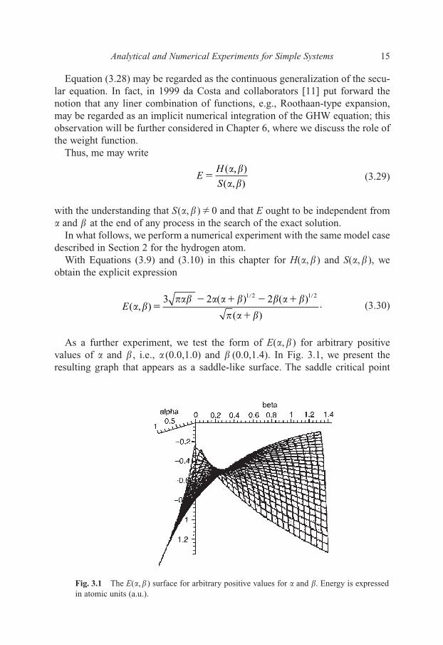
As a further experiment, we test the form of E(�,�) for arbitrary positivevalues of � and � , i.e., � (0.0,1.0) and � (0.0,1.4). In Fig. 3.1, we present theresulting graph that appears as a saddle-like surface. The saddle critical point
E( , )3 2 ( ) 2 ( )
( ).
1 2 1 2
� ���� � � � � � �
� � ��
� � � �
�
� �
EH
S�
( )
( , )
� �� �
,
Analytical and Numerical Experiments for Simple Systems 15
Fig. 3.1 The E(�,�) surface for arbitrary positive values for � and �. Energy is expressedin atomic units (a.u.).
Else_EAMC-TRSIC_ch003.qxd 5/19/2007 20:59 Page 15

leads to the values � 0 �0.2829421209 and � 0 �0.2829421210 and E(� 0,� 0) =�0.4244131813 a.u. This value is very close to the RR value of �0.4243 a.u.
To this point, we have relied largely on our recent work published in Advancesin Quantum Chemistry [12]. Nonetheless, it is legitimate to inquire whether inFig. 3.1 of Reference [12] the full potential of Equation (3.30) was achieved. Thisequation is supposed to be exact for the ground-state energy of the hydrogenatom, thus there should be a manner to extract the exact value from it.
We may further examine Equation (3.30). The previous paragraphs indicatethat values for � between 0.0 and 1.0 produce negative values for the energy.We arbitrarily set �� 1.0 and in Fig. 3.2 we plot the exact energy En � �1/2n2
and E(1.0,� ). The similarity between the two curves suggests that not only theground-state energy may be generated by this experiment, but excited-stateenergies as well.
As a continuation of our experiments, we set the following equation in a.u., i.e.,
(3.31)
so that we force E(1,�) to be equal to the exact expression for the energy. We thenscan values of n�1, 2, … and find the respective optimal values for �. These val-ues are then used in Equation (3.30) to obtain approximate eigenvalues for theexcited states. We remark that for n��, � converges to a value of 1.4.
Table 3.1 shows the exact energies for the ground and the first 11 excited levelsof the hydrogen atom together with the values calculated through Equations (3.30)
� �� � � �
��
� �1
2
3 2(1 ) 2 (1 )
(1 )(1, )2
1 2 1 2
nE
�� � � �� �
�
16 Chapter 3
Fig. 3.2 Plot of E(1,�) and En for various values of � and n.
Else_EAMC-TRSIC_ch003.qxd 5/19/2007 20:59 Page 16

Analytical and Numerical Experiments for Simple Systems 17
and (3.31), i.e., E(1,�), and the corresponding values of � for each case. As maybe observed, E(1,� ) mimics very accurately the exact values.
References
1. (a) L. Lathouwers, Ann. Phys., 1976, 102, 347; (b) L. Lathouwers, P. Van Leuven,and M. Bouten, Chem. Phys. Lett., 1977, 52, 439.
2. P. Chattopadhyay, R. M. Dreizler, M. Trsic, and M. Fink, Z. Phys. A, 1978, 285, 7.3. E. A. Hylleraas, Z. Phys., 1929, 54, 347.4. C. Eckart, Phys. Rev., 1930, 36, 878.5. (a) R. L. Somorjai, Chem. Phys. Lett., 1968, 2, 399; (b) R. L. Somorjai, Phys. Rev. Lett.,
1969, 23, 329; (c) D. M. Bishop, and R. L. Somorjai, J. Math. Phys., 1970, 11, 1150.6. J. R. Mohallem, and M. Trsic, Z. Phys. A, 1985, 322, 535.7. F. Arickx, J. Broekhove, E. Deumens, and P. Van Leuven, J. Chem. Phys., 1981, 39, 272.8. L. Lathouwers, and P. Van Leuven, Adv. Chem. Phys., 1982, 49, 115.9. A. C. Hurley, Int. J. Quant. Chem. Symp., 1967, 1, 677.
10. I. S. Gradshtein, and I. M. Ryzhik, Tables of Integrals, Series and Products, NewYork: Academic Press, 1965.
11. H. F. M. da Costa, M. Trsic, A. B. F. da Silva, and A. M. Simas, Eur. Phys. J. D, 1999,5, 375.
12. M. Trsic, W. F. D. Angelotti, and F. A. Molfetta, Adv. Quantum Chem., 2004, 47, 315.
Table 3.1
Comparison between exact and calculated hydrogen atom eigenvalues. Atomic units areemployed throughout
Eexact (a.u.) Ecalc (a.u.) �
�0.500000000000 �0.5000000000 0.3795056641�0.125000000000 �0.1250000000 0.9225340173�0.055555555556 �0.0555555556 1.128946441�0.031250000000 �0.0312500000 1.225896227�0.020000000000 �0.0200000000 1.278060772�0.013888888889 �0.0138888889 1.308955429�0.010204081632 �0.0102040816 1.328611873�0.007812500000 �0.0078125000 1.341829809�0.006172839506 �0.0061728395 1.351116767�0.005000000000 �0.0050000000 1.357877624�0.004132231405 �0.0041322314 1.362945568�0.003472222222 �0.0034722222 1.366838592
The purpose of this chapter is to suggest to the interested reader that there might still be open routes for further mathematicalinsights into GCM.
Else_EAMC-TRSIC_ch003.qxd 5/19/2007 20:59 Page 17

This page intentionally left blank

Chapter 4
The Generator Coordinate Hartree–FockFormalism
1. Introduction
In spite of its birth in nuclear physics [1], the generator coordinate method(GCM) found application also in other areas of physics [2–5].
It was probably only a matter of time that somebody would extend the inte-gral transform idea of Griffin, Hill, and Wheeler to the one-electron functionsof the Hartree–Fock (HF) scheme. So, at the 1986 Sanibel Symposia in Florida,Mohallem, Dreizler, and Trsic [6] presented the Griffin–Hill–Wheeler (GHW)version of the Hartree–Fock (GHWHF) equations [7].
This proposal opened a new route for very accurate calculations for atomic andmolecular systems, including ions.
In this work, example applications were for the He and Be atoms; it is inter-esting that from the beginning, the authors emphasized the role of the weightfunction, which actually has characterized the applications of the GCM. We alsoremark that the kernels in Reference [6] were calculated analytically.
Below we show, in part, the original proposition of Reference [6]. In Reference[6], the authors advocated for what was called variational discretization (seeChapter 5), which consisted in finding first the variational minimum for the ker-nel, and then to choose discretization points on the left and right of the optimalvalue. The strategy in Chapter 5 is to attempt the best numerical integration [6,8]of the GHW equation [see Equation (2.11)] in what since 1986 we call integraldiscretization.
2. The Background of the Hartree–Fock Scheme
In 1913, Bohr [9] presented his solution for the hydrogen atom as one of the mostimportant pillars of what we now call Old Quantum Theory. The energies calcu-lated with the Bohr model coincide with the exact values as obtained from theSchrödinger equation presented some 10 years later [10].
Of course, both Bohr and Schrödinger were aware of the ideas of the discretecharacter of spectra brought out by Planck [11]. Schrödinger, in particular, had
Else_EAMC-TRSIC_ch004.qxd 4/19/2007 08:50 Page 19
the inspiration of the attribution of wave character to the electron by Louis deBroglie in his thesis in 1924 [12].
These few years at the beginning of the 20th century were of an intenseintellectual activity in physics, mainly in Europe. Thus, since the Old QuantumTheory required several numerical adjustments to meet the criteria for theexperiment, in 1925 Heisenberg [13] presented the formalism of his QuantumMechanics, which allowed the treatment of both intensities and frequencies ofspectral lines of atomic systems. In the same year, Pauli [14] formulated hisexclusion principle, which required many-electron functions to be antisymmet-ric. It seems that Slater [15] was the first to write a many-electron wave functionas a determinant, thus providing a well-known and easy-to-handle algebraicstructure for these functions.
In 1928, Hartree [7a] created the self-consistent field method, in whichmany-electron systems are represented by one-electron functions, each depend-ing on the average field produced by the other electrons. Nevertheless, Hartreeemployed a simple product of one-electron functions, which lacks antisym-metry. Fock [7b] modified the self-consistent field method so as to includeexchange, which originates from antisymmetry of the many-electron function.Thus, this is the origin of the so-called Hartree–Fock scheme, which here werewrite in the framework of the GCM.
The purpose of this section is to provide a background for the theory to beintroduced in the following section, and certainly not to discuss in full the historyor formulation of Quantum Mechanics; the interested reader is referred to someappropriate literature [16].
Nevertheless, we do not wish to abandon this section without acknowledgingthe probabilistic interpretation of Quantum Mechanics as developed by Born [17]and the uncertainty principle enounced by Heisenberg [18].
The HF one-electron eigenvalue equation may be written as
(4.1)
where h0(1) is the sum of the one-electron kinetic energy operator and attractiveinteractions of the electron with the atomic nucleus or the molecular nuclei, withthe Coulomb Jj(1) and exchange Kj(1) operators defined as
(4.2)Je
rdj i j j i(1) (1) (2) (2) (1)
2
122� � � � �� �∫
⎡
⎣⎢
⎤
⎦⎥
h J Kj jj
i i i0 (1) (1) (1) (1) (1),� � �⎡⎣ ⎤⎦⎧⎨⎪
⎩⎪
⎫⎬⎪
⎭⎪∑ � � �
20 Chapter 4
Else_EAMC-TRSIC_ch004.qxd 4/19/2007 08:50 Page 20
and
(4.3)
The �i and �j are one-electron spin-functions. The �i Lagrange multipliersacquire in the HF theory the significance of one-electron energy eigenvalues,with e being the electron charge.
Equation (4.1) results from expressing the expectation value for the energywith a Slater determinant for the ground state and imposing the variationalprinciple.
In the following section, we extend the HF one-electron functions to integraltransform one-electron functions.
3. The Generator Coordinate Hartree–Fock Method
We choose the spatial one-electron functions for a 2n-electron system in theform
(4.4)
where �i(1, �) (STOs or GTOs) depend on the generator coordinate, �, and fi(�)are the unknown weight functions. With the trial function written as a Slaterdeterminant of the above orbitals, the minimization of the total energy withrespect to the weight functions fi(�) leads to the GHWHF equations
(4.5)
The overlap and Fock kernels are, respectively,
(4.6)
and
(4.7)F h J Kj jj
n
( , ) ( , ) 2 ( , ) ( , ) ,� � � � � � � �� � �⎡⎣ ⎤⎦∑
S i i( , ) (1, ) (1, )� � � �� � ��
� �F S f d i ni i( , ) ( , ) ( ) 0, 1, , .� � � � � � �� � �∫ …
� � � �i i if d i n(1) (1, ) ( ) , 1, , ,� �� …∫
Ke
rdj i j i j(1) (1) (2) (2) (1).
2
122� � � � �� �⎡
⎣⎢
⎤
⎦⎥
The Generator Coordinate Hartree–Fock Formalism 21
Else_EAMC-TRSIC_ch004.qxd 4/19/2007 08:50 Page 21

where
(4.8)
and the explicit expressions for the Coulomb, Jj(�,�), and exchange, Kj(�,�),kernels are
(4.9)
and
(4.10)
where
(4.11a)
and
(4.11b)
4. Numerical Integration
Equation (4.5) is solved by an iterative procedure, starting with an initial fi(�)[for instance, fi(�) � 0 or the solution of Equation (4.5) without the repulsionterms], with an arbitrary numerical criterion for convergence. During each iter-ation, the integrations are carried out using a discretization technique. In con-trast, with usual discretization procedures, which lead formally to the Roothaanequations, we propose to explore the continuous representation of the GCM,i.e., an accurate numerical integration of Equation (4.5) is attempted. This,besides formal refinements, allows us to avoid the optimization of the nonlin-ear parameters �. The straightforward procedure is to take a mesh of N equallyspaced points in �-space. Actually, we have used this rule for the He atom withSTOs. Nevertheless, for the case of GTOs, the weight functions fi(�) becomevery broad and we need a more sophisticated rule that permits us to useincreasing increments, ��, for increasing �. To attain this we relabel the gen-erator coordinate space [8]
(4.12a)� �� � �(log ) , 1A A
V ri j j i( , ; , ) (1, ) (2, ) (2, ) (1, ) .121� � � � � � � �� � � � ��� � � �
V ri j j i( , ; , ) (1, ) (2, ) (2, ) (1, )121� � � � � � � �� � � � ��� � � �
K d d f f Vj j j( , ) ( ) ( ) ( , ; , )� � � � � � � � � �� � � � � � �∫∫
J d d f f Vj j j( , ) ( ) ( ) ( , ; , )� � � � � � � � � �� � � � � � �∫∫
h hi i( , ) (1, ) (1) (1, )0� � � �� � �
22 Chapter 4
Else_EAMC-TRSIC_ch004.qxd 4/19/2007 08:50 Page 22

and
(4.12b)
where N is the number of discretization points, an option defining the size ofthe basis set and �� is the integration interval, also a matter of numericalchoice.
The values of �min and �max ��min � (N�1)�� are chosen so as to ade-quately cover the integration range of f (�).
The new generator coordinate � now spans the interval [��, ��], but theweight function becomes narrow and liable to discretization. An equally spacedmesh in the new interval is now enough for our purposes. This procedure is opti-mal with the use of GTOs as will be shown in Chapter 6.
This is clearly visualized by sketching the weight functions from a preliminarycalculation with arbitrary discretization parameters. We illustrate this point bythe plots of the 2s weight functions for Li, Be, Ne, and Ar in Fig. 4.1. This matterwill be further discussed in detail in Chapter 6.
The discretized version of the GHWHF equations becomes
(4.13)� �F S fk i k i
N
( , ) ( , ) ( ) 0.� � � � � �� � �
�
� �∑
� � ��k k k N� � � �min ( 1) , 1, , ,…
The Generator Coordinate Hartree–Fock Formalism 23
Fig. 4.1 The 2s Gaussian weight functions for Li, Be, Ne, and Ar atoms.
Else_EAMC-TRSIC_ch004.qxd 4/19/2007 08:50 Page 23

The matrix elements h(�k,��) and S(�k,��) have obvious definitions. TheJj(�k,��) and Kj(�k,��) are discretized at the same points:
(4.14a)
and
(4.14b)
The matrix elements of F are then set up and the diagonalization is madeby the method used in Reference [6]. The total energy is calculated fromeither
(4.15a)
or
(4.15b)
the obtained values being identical in all digits, where
(4.16a)
(4.16b)
and
(4.16c)K f f Kij i k i j k
N
k
N
� ( ) ( ) ( , ) .� � � �� �
�
∑∑
J f f Jij i k i j k
N
k
N
� ( ) ( ) ( , ) ,� � � �� �
�
∑∑
h f f hii i k i k
N
k
N
� ( ) ( ) ( , ) ,� � � �� �
�
∑∑
E h J Kii iij
n
iji
n
i
n
� � �2 (2 ),∑∑∑
E hi iii
n
� �( )�∑
K f fj k j m j n k m nn
N
m
N
( , ) ( ) ( ) ( , ; , ).� � � � � � � �� �
� � � � �V∑∑
J f f Vj k j m j n k m nn
N
m
N
( , ) ( ) ( ) ( , ; , )� � � � � � � �� �
� � � � �∑∑
24 Chapter 4
Else_EAMC-TRSIC_ch004.qxd 4/19/2007 08:50 Page 24

The mean value of r for the ith orbital is evaluated from
(4.17)
where
(4.18)
5. First Applications to the He and Be Atoms
5.1. The He Atom with a Slater Orbital
The generator functions are
(4.19)
for which the kernels are easily calculated as
(4.20)
and
(4.21)
Z is the nuclear charge and the Coulomb V(�,��;��,�) and exchange V(�,��;�,��)potentials are given by
(4.22)
where u�a�d and v�b�c.We choose the same discretization parameters for �, ��, � and �� (�min and ��
are the lowest value and the increment of the generator coordinate, respectively).The HF limit [7,19] is attained with few (nonoptimized) points.
V a b c du v u
u v
u v
u v
v( , ; , )
96
( )
1
3
1
3,
2
4 2 2��
��
� ��� ⎡
⎣⎢⎤⎦⎥
h S Z( , ) ( , ) 2 ( ) ;� � � � �� � �� � � �� � � �
S( , ) 8 ( )3� � � � �� � �
�( , ) exp( ),r r� �� �
r i r ii i i i( , ) ( , ) ( , ) .� � � �� � �
r f f ri i k i i k
N
k
N
� ( ) ( ) ( , ) ,� � � �� �
�
∑∑
The Generator Coordinate Hartree–Fock Formalism 25
Else_EAMC-TRSIC_ch004.qxd 4/19/2007 08:50 Page 25
5.2. The He Atom with a Gaussian Orbital
The generator functions are
(4.23)
with
(4.24)
and
(4.25)
The Coulomb and exchange potentials are given by
(4.26)
5.3. The Be Atom with GTOs
As a test of the continuous representation of the GCM, we employ the sameGaussian form for the 1s and 2s orbitals:
(4.27)
and
(4.28)
Except for the value of the nuclear charge, the kernels are the same as for He.Even in this early work, the authors remarked on the importance of the weight
function. However, we shall leave the discussion of its role until after the newconcepts of basis set design are presented in Chapter 6.
In Table 4.1, we show the main results obtained by Mohallem et al. [6] andcompare with the best calculations for He and Be available at the time, i.e.,
� � � �2s 22
0
( ) ( )exp( ) .r f r d� ��
∫
� � � �1s 12
0( ) ( )exp( )r f r d� �
�
∫
V a b c d a d b c a b c d( , ; , ) (2 ) ( )( )( ) .2.5 0.5� � � � � �� � ⎡⎣ ⎤⎦
h Z( , ) 3 ( ) (2 ) ( ).1.5 2.5� � � �� � � � � �� � � � � �⎡⎣ ⎤⎦
S( , ) ( ) 1.5� � � � �� � �� �
�( , ) exp( ),2r r� �� �
26 Chapter 4
Else_EAMC-TRSIC_ch004.qxd 4/19/2007 08:50 Page 26

The Generator Coordinate Hartree–Fock Formalism 27
Fig. 4.2 The weight functions for the (a) 1s and (b) 2s orbitals of the Be atom for Gaussiangenerator functions.
Table 4.1
Ground-state energies (atomic units) for He and Be for Slater (STO) and Gaussian(GTO) basis functions
GHW Equation HF
He STO �2.861679995612 �2.861679995612a
GTO �2.866167957 �28616692b
Be GTO �14.572780 �14.572368c
a Reference [20].b Reference [21].c Reference [21].
Else_EAMC-TRSIC_ch004.qxd 4/19/2007 08:50 Page 27

by Davies et al. [20] for Slater-type basis functions (STOs) and by Huzinaga [21]for Gaussian-type basis functions (GTOs). The values in Reference [6] wereobtained with trivial size matrices of 13�13 for the STOs and a 24 �24 for theGTOs. One can see that in this introductory work presented at the 1986 SanibelSymposia, the results were either competitive with or better than the alternativeresults available at the time.
Figs. 4.2 and 4.3 are likely to be the first GCM weight functions ever plotted.
References
1. D. L. Hill, and J. A. Wheeler, Phys. Rev., 1953, 89, 1102; J. J. Griffin, and J. A.Wheeler, Phys. Rev., 1957, 108, 311.
2. A. J. Thakkar, and V. M. Smith, Phys. Rev. A, 1977, 15, 1; A. J. Thakkar, and V. M.Smith, Phys. Rev., A, 1977, 15, 16.
3. L. Lathouwers, Ann. Phys., 1976, 102, 347; L. Lathouwers, P. Van Leuven, and M. Bouten, Chem. Phys. Lett., 1977, 52, 439.
4. B. Laskowski, and E. Brändas, Phys. Rev. C, 1976, 13, 1741.5. D. Galleti, and A. F. R. de Toledo Pizza, Phys. Rev. C, 1978, 17, 774; J. G. R. Tostes,
and A. F. R. de Toledo Pizza, Phys. Rev. A, 1983, 28, 538.6. J. R. Mohallem, R. M. Dreizler, and M. Trsic, Int. J. Quantum Chem. Symp., 1986,
20, 45.7. (a) D. R. Hartree, Proc. Cambridge Phys. Soc., 1928, 24, 89; D. R. Hartree, Proc.
Cambridge Phys. Soc., 1928, 24, 111; D. R. Hartree, Proc. Cambridge Phys. Soc.,1928, 24, 426; (b) V. Fock, Z. Phys., 1930, 61, 126.
28 Chapter 4
Fig. 4.3 The weight function for the 1s orbital of the He atom for the case of a Gaussiangenerator function.
Else_EAMC-TRSIC_ch004.qxd 4/19/2007 08:50 Page 28
8. J. R. Mohallem, Z. Phys. D, 1986, 3, 339; H. F. M. DaCosta, M. Trsic, A. B. F. da Silva,and A. M. Simas, Eur. Phys. J. D, 1999, 5, 375.
9. N. Bohr, Phil. Mag., 1913, 26, 1; N. Bohr, Phil. Mag., 1914, 27, 506.10. E. Schrödinger, Ann. Phys., 1926, 79, 361; E. Schrödinger, Ann. Phys., 1926, 80,
437; E. Schrödinger, Ann. Phys., 1926, 81, 109.11. M. Planck, Ann. Phys., 1901, 4, 553.12. L. de Broglie, Thesis, Paris, 1924; L. de Broglie, Ann. Phys., 1925, 3, 22.13. W. Heisenberg, Z. Phys., 1925, 33, 879.14. W. Pauli, Z. Phys., 1925, 31, 765.15. J. C. Slater, Phys. Rev., 1929, 34, 1293.16. For a discussion of the Hartree–Fock formulation, see, for instance, M. Weissbluth,
Atoms and Molecules, New York: Academic Press, 1978; for the fundation ofQuantum Mechanics, see, for example, E. Antletta, Fundation and Interpretation ofQuantum Mechanics: In the Light of a Critical-Historical Analysis of the Problemsand of a Synthesis of the Results, Hackensack: World Scientific PublishingCompany, Inc., 2002.
17. M. Born, Z. Phys., 1926, 37, 863; M. Born, Z. Phys., 1926, 38, 803.18. W. Heisenberg, Z. Phys., 1927, 43, 172.19. P. Chattopadhyay, R. M. Dreizler, M. Trsic, and M. Fink, Z. Phys., 1978, A285, 7.20. C. L. Davies, H. J. Jensen, and H. J. Mohkhorst, J. Chem. Phys., 1984, 80, 840.21. S. Huzinaga, J. Chem. Phys., 1965, 42, 1293.
The Generator Coordinate Hartree–Fock Formalism 29
Else_EAMC-TRSIC_ch004.qxd 4/19/2007 08:50 Page 29

This page intentionally left blank

Chapter 5
Discretization Techniques
1. Introduction
Since the generator coordinate method (GCM) was introduced by Griffin, Hill,and Wheeler in the context of nuclear physics [1], it is not surprising that earlyapplications between the fifties and the seventies of the last century were mainlyin that field.
As we have commented and exemplified in the previous pages, our presentmathematical capabilities prevent exact or analytical solutions for any nontrivialphysical or chemical system. Thus, from the initial days of the applications of theGCM, resort to approximations was mandatory.
In this chapter, we shall first discuss early studies on the discretization tech-niques for the Griffin–Hill–Wheeler (GHW) equation in physical and chemicalproblems. These studies were presented in the fifties to seventies of the last cen-tury, before the introduction of the generator coordinate Hartree–Fock (GCHF)method (Chapter 4). The interest in the preliminary approaches presented belowfocuses on model problems and emphasizes mathematical refinements. Also, theconcept of integral discretization (ID) and the recognition of the importance ofthe role of the weight function were recognized later. Thus, in this chapter weshall also discuss the origin and meaning of ID.
Finally, at the end of this chapter, we describe a very recent discretization tech-nique, which seems to be the most efficient proposed to date.
Perhaps the first attempts to solve the GHW integral equation via discretiza-tion techniques were due to Justin et al. [2].
A number of difficulties were reported concerning singularities of the weightfunction and negative eigenvalues of the overlap matrix. The first problem seemsto be linked with the use of the Gaussian overlap approximation (GOA) (see forinstance Reference [3]).
In 1978, Chattopadhyay et al. [4] applied the discretization technique tosimple model systems to obtain a more direct understanding of the intricacies ofthis methodology. This work stimulated further developments relying ondiscretization techniques as are described in this book. Here we reproduce thefindings of Reference [4] and comment on the context of present understandingof discretization techniques.
Else_EAMC-TRSIC_ch005.qxd 5/19/2007 21:07 Page 31

We note that orthogonality of the eigenfunctions of the GCM problem[Equation (2.4)] is expressed through the relations
(5.1)
while completeness of the basis requires
(5.2a)
with
. (5.2b)
The problem we choose for the illustration of practical rules in the numericaltreatment of the GHW equations is the harmonic oscillator in one dimension.We describe the oscillator problem via a “superposition” of square-well solu-tions. The kernels of the GHW equation can be obtained analytically. We usethis setup as a vehicle to investigate various points of the numerical approach(Section 3).
2. A Model Problem: The Harmonic Oscillator
The functions to be used for the generator coordinate ansatz of the harmonicoscillator problem are the solutions to the square-well problem
(5.3)
The eigenfunctions of this simple problem can be classified according toparity and energy. We note that the wave functions are
(5.4)
n�1,3,… for positive parity,
(5.5)�n xn x
x( )1
sin2
( ),2 2� ��
��
� �
�n xn x
x( )1
cos2
( ),2 2� ��
��
� �
V xx
x( )
0 .�
� �
�
��
⎧⎨⎪
⎩⎪
d S S� � � � � � � �� � � � �1( , ) ( , ) ( )∫
d d x S x x x� �� � � � � � ��( , ) ( , ) ( , ) ( )1� � � � �∫
dx x x f S f d di j i j ij� � � � � � � � �� �( ) ( ) ( ) ( , ) ( ) ,� �∫∫
32 Chapter 5
Else_EAMC-TRSIC_ch005.qxd 5/19/2007 21:07 Page 32

n�2,4,… for negative parity, and the energy (��m�1) as
(5.6)
in both cases.For convenience, the step function
(5.7)
has been used to represent the appropriate boundary conditions.The width of the square well is our generator coordinate. We thus describe the
well-known oscillator wave functions by superposition of the wave functions ofsquare wells with different widths.
The Hamiltonian and normalization kernels are easily evaluated. Writing theoscillator Hamiltonian as
(5.8)
with k being the force constant, we find, e.g., for the negative parity solutions,
(5.9)
(5.10)
for ���.
Hn n
kn
n
n
( , ) ( )2 ( )
sin2
( ) 2 8
(
2 1
2 2
2 2
2 2
� ���
�� � ����
� � ���
��
� ��
��
� �
�
�� ����
� � �� � �
�� �
2 2 2
2 2 2
2 2 3 2 2
)cos
2
8 ( + 3 )
( ) ( )s
�
��
��
n
n
n
⎧⎨⎩
⎡
⎣⎢
⎤
⎦⎥ iin
2
( , )
n
H
���
� �
⎫⎬⎭
�
Hn
kn
n( , )
8
2
12
1
2
2 2
2
2
2 2
2 2
� ��
���
�� � �
⎡
⎣⎢
⎤
⎦⎥
H k x�� �1
2
1
22 2
��
( ) 1 for 0
( ) 0 for 0
t t
t t
� �
� �
�
�n
n�
2 2
28
Discretization Techniques 33
Else_EAMC-TRSIC_ch005.qxd 5/19/2007 21:07 Page 33

(5.11)
(5.12)
for ���.We consider only the case k�1 throughout. One observes that a GOA would
not provide a good representation of these kernels.
3. Discretization of the Griffin–Hill–Wheeler Equation for theHarmonic Oscillator Problem
Since the GHW equation cannot, in general, be solved exactly, the solutionproceeds, in practice, by replacing the integration by summation. This discretiza-tion normally relies on application of the simplest form of Simpson’s rule,although more advanced numerical integration techniques are possible. Since therange of the generator coordinate includes, in most cases, infinite intervals, trun-cation of the sums involved is a second feature of the numerical approach. Withthe definitions
(5.13)
the GHW equation reduces to a standard (symmetric) eigenvalue problem in anonorthogonal representation
(5.14)
The solution of this problem involves two steps. One first solves the eigen-value problem
(5.15)
This step corresponds to solving the Fredhom equation of the second kind
(5.16)S b d b( , ) ( ) ( )� � � � ��∫
S b bij j ij
� .∑
[ ] 0, 1,...,1
H ES F i Nij ij jj
N
� � ��
∑
f FH HS S
i i
j i ji
j i ji
( )( , )
( , ) ,
� �� �� �
��
�
Sn
nSn( , ) ( )
4sin
2( , )2 1
2 2� ����
�� �
���
� �� ��
�� � ⎛⎝⎜
⎞⎠⎟
S( , ) 1� � �
34 Chapter 5
Else_EAMC-TRSIC_ch005.qxd 5/19/2007 21:07 Page 34

by a simple quadrature method, thus determining the geometrical components ofthe biorthogonal natural state expansion, as pointed out in detail by Lathouwers [5].
The second step involves diagonalization of the Hamiltonian in the basis ofEquation (5.15), respectively, Equation (5.16). Starting from the discretizedeigenvalue problem of the overlap kernel
(5.17)
one arrives at an orthogonal representation
(5.18)
where B is the matrix constructed from the eigenvectors, B~
its transpose, and �the diagonal matrix of eigenvalues.
If we multiply the matrix equation corresponding to Equation (5.14) from theleft with the matrix
(5.19)
we obtain the eigenvalue problem
(5.20)
where
(5.21)
F is the matrix of the discretized weight functions of Equation (5.13).Solution of the eigenvalue problem in Equation (5.15) readily gives the eigen-
values of the Hamiltonian, E, and the eigenvector matrix, C, from which theweight functions of the various eigenstates can be recovered by inversion
(5.22)
The actual eigenfunctions are then determined by integrating Equation (2.5)with the same numerical method as used in the discretization of the GHWequation.
We return to a closer look at the first step as expressed by Equations (5.15)and (5.16).
Some general properties of the eigenvalue spectrum of Equation (5.16) can bestated under the assumption that the kernel S(�,�) is Hermitian, nonnegative, andsquare integrable [5].
F DC� % .
A D H DC D F
��
%
.
( 1) 0,A E C� �
D B� � �� 1 2
� �� � � � �1 2 1 2 1,B S B%
B S B% �� ,
Discretization Techniques 35
Else_EAMC-TRSIC_ch005.qxd 5/19/2007 21:07 Page 35

A(1): The spectrum of eigenvalues is positive
A(2): The series ��n�1
2n converges and 0 is the only accumulation point of the
n eigenvalues.A(3): The sum rule
(5.23)
holds.The question arises about how far these properties are maintained in the
numerical approximation in Equation (5.15). In this case, one can view theoverlap kernel as a Gram-matrix to be constructed from a set of N vectors �i
in N-space
(5.24)
The following theorems [6] are available for the Gram-matrix:B(1): A necessary and sufficient condition for the linear dependence of thevectors �i is the vanishing of the Gram determinant
B(2): In case of linear dependence of the vectors, none of the eigenvalues arenegative. In the case of linear dependence, say there are k-independent vectors �i,one has N–K eigenvalues, which are zero.B(3): We have
(5.25)
Comparison of the statements (A) and (B) invites the following remarks:Negative eigenvalues of S, which are reported in the literature as a result of
carrying through the numerical procedure indicated here, are always a conse-quence of numerical errors. For the harmonic oscillator problem, this could beverified in each case by increasing the precision of the calculation.
The inherent structure of the exact spectrum with an accumulation point of eigen-values at the zero value will, however, eventually lead to numerical difficulties,without necessarily indicating proper linear dependence. This problem is solvedwhen we reject eigensolutions, which fall below a numerically acceptable limit, andnot reducing the dimensionality of the vector-space used in the numerical solution
nn
N
S��
trace( ).1
∑
S � 0.
S v vij i j� �( ).
� � �nn
S d��
�
( , )1
∫∑
1 ... 0.� �
36 Chapter 5
Else_EAMC-TRSIC_ch005.qxd 5/19/2007 21:07 Page 36

of Equation (5.15) as was repeatedly suggested in the literature [4]. The cost offollowing the former prescription is a loss of accuracy in all of the final solutions ofthe problems. The cost of following the latter prescription is mainly the loss of high-lying (in energy) solutions, which can be accepted in view of the general aim ofreproduction of the low-lying states of a given spectral problem.
The truncation of eigenstates of the overlap matrix can be discussed from amore quantitative point of view. Introducing the coordinate overlap [5]
(5.26)
one considers the eigenvalue problem
(5.27)
which has the same eigenvalues as the problem of Equation (5.16).The truncation prescription amounts to the statement
(5.28)
or equivalently
(5.29)
The final eigenstate (x) can be expanded directly in terms of the solutions ofthe eigenvalue problem of Equation (5.27)
(5.30)
From the relations
or
fcn
nn
22
1
,��
�
∑
fc
bn
nn
n
( ) ( )1 21
�
���
�
�
∑
� � �
�
( ) ( )
( ) ( , )
( ) (
1
1 21
x c y x
cb x d
f x
n nn
n
nn
n
�
�
�
�
�
��
�
∑
∑∫⎡
⎣⎢
⎤
⎦⎥ �
� ,, ) .� �d∫
y x y xn n c n( ) ( ) ( ).�� �
b bn
nn c
n
n
( )( )
( )1 2 1 2
�
� �
� ���
X x x y x dx y x( , ) ( ) ( ) ,� � ���∫
X x x x x d( , ) ( , ) ( , ) ,� � �� �� � ��∫
Discretization Techniques 37
Else_EAMC-TRSIC_ch005.qxd 5/19/2007 21:07 Page 37

one concludes, in the case || f ||2 is finite, that
(5.31)
The relative contribution of the eigensolutions of Equation (5.27) to the repre-sentation of the final eigenstates is governed by the factor n, which justifies theintroduction of the c value in Equations (5.28) and (5.29).
In Table 5.1, we present some results for the positive parity states of theharmonic oscillator. The generating functions in this case are given by thelowest positive parity solutions (n � 1) of the square-well problem. The resultsare comparable to those of negative parity states based on the generating func-tion with n � 2.
4. The Integral Discretization
4.1. Introduction
From the initial days of the GCHF method [7], we attempted the best numericalintegration of the Griffin–Hill–Wheeler–Hartree–Fock (GHWHF) equations,abandoning the variational discretization (VD), advocated earlier [4].
Nevertheless, it was Mohallem [8] who provided a formal background for theuse of the ID.
It is assumed that the kernel S(�,�) is square-integrable. The space spanned bythe generator function for all values of � is called HGC.
Typically, VD or ID implies truncation of HGC , and diagonalizing the H� operatorin this subspace of finite dimension N leads to the secular equation that providesthe optimum coefficients F N
i for the ⏐ N⟩ approximation to ⏐ ⟩:
(5.32) �NiN
ii
N
F��
�( )1
∑ .
c fn n
2 2.
38 Chapter 5
Table 5.1
Results for the positive parity states of the harmonic oscillator problem. Thegenerating function is given by Equation (5.4) with n � 1 (�0 � 0.2095, ��� 0.125,�n � 3.9595)
E1 E2 E3 E4 E5 E6
GCM 0.500 2.504 4.525 6.677 9.248 12.47Exact 0.5 2.5 4.5 6.5 8.5 10.5
Else_EAMC-TRSIC_ch005.qxd 5/19/2007 21:07 Page 38

Canonical orthonormalization [9] applied on the N vectors of this discretebasis leads to
(5.33)
(5.34)
(5.35)
where � n and u� ni are respectively eigenvalues and eigenvectors of the matrix S�S (�i,�j) (the bar indicates that the quantities are obtained from the discretebasis), i.e.,
(5.36)
It is straightforward to verify that the coefficients FNi are given by
(5.37)
Now, consider the vectors of an orthonormal basis, in the continuous repre-sentation, for HGC
(5.38)
with
(5.39)
One can verify that Equation (5.39) is a Fredholm equation of the first kind witha square-integrable kernel. It admits a numerical solution that may be written inthe form of Equation (5.36). Then vectors ⏐n⟩ and ⏐n� ⟩ may become arbitrarilyclose as N increases. In view of this, one can assume that a positive number canbe found so that the “strong” condition is fulfilled:
(5.40)n n N� � � 2 .
S u d un n n( , ) ( ) ( ).� � � � �∫ �
n d un
n�1
( ) ( )
� � �∫ �
Fc u
iN n ni
nn
N
�� 1∑ .
S u ui j njj
N
n ni( , )1
� � �
�∑ .
n un
ni ii
N
��
1( ) ,
1��∑
cnn
N2
1
1��
,∑
Nn
n
N
c n��1∑ ,
Discretization Techniques 39
Else_EAMC-TRSIC_ch005.qxd 5/19/2007 21:07 Page 39

Then,
(5.41)
where Equation (5.34) and the generalized triangular inequality wereemployed. This implies that the first term of inequality in Equation (5.41) maybecome as small as desired. Expansion of this term using Equations (5.35) and(5.38) gives
(5.42)
or, using Equation (5.37)
(5.43)
where the functions
(5.44)
are square-integrable (L2�). Actually, using the orthonormality of the un(�) functions,
it appears that the norm of the fN(�) functions is
(5.45)
since N is always finite.The convergence for ⏐ ⟩ is given by
(5.46) � � ���
lim ( ) ( ) ,N
Nf d� ∫ �
f dc
Nn
nn
N
( )2
2
1
� �∫ ∑� � ��
�
fc u
Nn n
nn
N
( )( )
1
��
�
�
∑
f d FN iN
ii
N
( ) ( ) ( )1
� � � �∫ ∑� ���
,
1 ( )( ) ( )
1 11�
� �
�
n
n n
nn
Nn ni
nn
N
ii
Nc ud
c u
� ��
∑∫ ∑∑⎡
⎣⎢⎢
⎤
⎦⎥⎥
� ��
c n n c n n
c n n n n N
nn
N
nn
N
nn
N
n
N
( ) ( )
,
1 1
11
� �
� � � � � �
� �
��
∑ ∑
∑∑
40 Chapter 5
Else_EAMC-TRSIC_ch005.qxd 5/19/2007 21:07 Page 40

where whether the limit and the integral commute or not depends on the relativedecrease of ⏐cn⏐
2 and n for the sum showed in Equation (5.45) [10].Equation (5.43) is fundamental in drawing the following conclusions. First, the
right-hand side does necessarily represent the discretization of the integral on theleft, but both sides merely generate approximations to the same vector ⏐ N⟩.
There are two cases to consider:(i) In favorable cases, when ⏐cn⏐
2 decreases faster than n, f(�) is (L2�) and the
GHW equation has Equation (5.14) as its real discretized version with a stablesolution for the discrete weight function. But to find the weight function throughdiscretization is often a task requiring intuition and the use of physical argu-ments. This is clearly only a technical problem that depends on the quality of theintegration scheme. For a poor integration, the coefficients should be worse thanthe VD values, whereas for a good integration it is expected that ID surpassesVD. This point is clarified in the application below.
(ii) In the opposite case, if n decreases faster than ⏐cn⏐2 in Equation (5.45), a
norm of the weight function increases without bound as N increases. When thedensity of the points in the mesh is raised the vectors show approximate lineardependence (ALD). This is often irrelevant in the first case, but very importanthere, since it implies numerical errors. The usual procedure is to establish a � ccut-off value for the eigenvalues of S below which the corresponding ⏐n� ⟩ is setequal to zero. The discrete version of the GHW equation in this case becomes
(5.47)
where N� � N � Nc, Nc denoting the number of vectors eliminated by the trun-cation. The solution for the weight functions tends to stabilize in some square-integrable fN�(�), in agreement with the results in Reference [10].
As argued in Reference [10], the singular character of f(�) is concomitantwith the importance of the vectors associated with small , which is a conse-quence of ALD, and truncation should be performed with care. The point hereis that in this case, VD seems to be just as incapable as ID in obtaining high-lying states.
In conclusion, in both the above cases, the only advantage of a full VD proce-dure seems to be possibly faster convergence to the energy of the state consid-ered, e.g., the ground state. The possible advantages of ID are explored below.
The conclusions above are now applied to two problems having exact solu-tions. Both have appeared in the literature [11,12] as examples of VD and so aresuitable for comparison with ID.
A simple Simpson rule is first considered for the discretization ofEquation (2.8). The disseminated rule of point picking around the variational
[ ]H ES fi j i jj
N
N j( , ) ( , ) ( ) 0,1
� � � � �� ��
�∑
Discretization Techniques 41
Else_EAMC-TRSIC_ch005.qxd 5/19/2007 21:07 Page 41
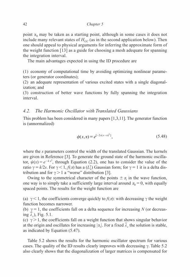
point �0 may be taken as a starting point, although in some cases it does notinclude many relevant states of HGC (as in the second application below). Thenone should appeal to physical arguments for inferring the approximate form ofthe weight function [13] as a guide for choosing a mesh adequate for spanningthe integration interval.
The main advantages expected in using the ID procedure are
(1) economy of computational time by avoiding optimizing nonlinear parame-ters (or generator coordinates);(2) an adequate representation of various excited states with a single diagonal-ization; and(3) construction of better wave functions by fully spanning the integrationinterval.
4.2. The Harmonic Oscillator with Translated Gaussians
This problem has been considered in many papers [1,3,11]. The generator functionis (unnormalized)
(5.48)
where the s parameters control the width of the translated Gaussian. The kernelsare given in Reference [3]. To generate the ground state of the harmonic oscilla-tor, (x)�e�k x2, through Equation (2.2), one has to consider the value of theratio ��k/2s. For ��1, f(�) has a (L2
�) Gaussian form; for ��1 it is a delta dis-tribution and for ��1 a “worse” distribution [3].
Owing to the symmetrical character of the points ��i in the wave function,one way is to simply take a sufficiently large interval around �0 �0, with equallyspaced points. The results for the weight function are
(a) ��1, the coefficients converge quickly to f(�): with decreasing � the weightfunction becomes narrower.(b) ��1, the coefficients fall on a delta sequence for increasing N (or decreas-ing �c), Fig. 5.1.(c) ��1, the coefficients fall on a weight function that shows singular behaviorat the origin and oscillates for increasing |�i|. For a fixed �c the solution is stable,as indicated by Equation (5.47).
Table 5.2 shows the results for the harmonic oscillator spectrum for variouscases. The quality of the ID results clearly improves with decreasing �. Table 5.2also clearly shows that the diagonalization of larger matrices is compensated for
�( , ) ,[ 2 ( ) ]2
x e s x� �� � �
42 Chapter 5
Else_EAMC-TRSIC_ch005.qxd 5/19/2007 21:07 Page 42
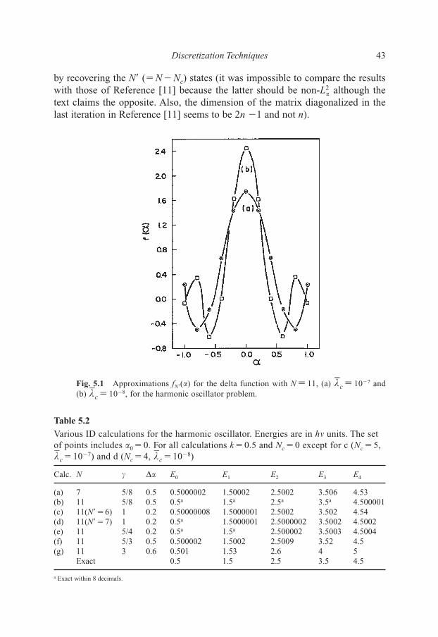
by recovering the N� (�N�Nc) states (it was impossible to compare the resultswith those of Reference [11] because the latter should be non-L2
� although thetext claims the opposite. Also, the dimension of the matrix diagonalized in thelast iteration in Reference [11] seems to be 2n �1 and not n).
Discretization Techniques 43
Fig. 5.1 Approximations fN�(�) for the delta function with N � 11, (a) �c � 10�7 and(b) �c � 10�8, for the harmonic oscillator problem.
Table 5.2
Various ID calculations for the harmonic oscillator. Energies are in h� units. The setof points includes �0 � 0. For all calculations k � 0.5 and Nc � 0 except for c (Nc � 5,�c � 10�7) and d (Nc � 4, �c � 10�8)
Calc. N � �� E0 E1 E2 E3 E4
(a) 7 5/8 0.5 0.5000002 1.50002 2.5002 3.506 4.53(b) 11 5/8 0.5 0.5a 1.5a 2.5a 3.5a 4.500001(c) 11(N��6) 1 0.2 0.50000008 1.5000001 2.5002 3.502 4.54(d) 11(N��7) 1 0.2 0.5a 1.5000001 2.5000002 3.5002 4.5002(e) 11 5/4 0.2 0.5a 1.5a 2.500002 3.5003 4.5004(f) 11 5/3 0.5 0.500002 1.5002 2.5009 3.52 4.5(g) 11 3 0.6 0.501 1.53 2.6 4 5
Exact 0.5 1.5 2.5 3.5 4.5
a Exact within 8 decimals.
Else_EAMC-TRSIC_ch005.qxd 5/19/2007 21:07 Page 43

4.3. The Hydrogen Atom with a Gaussian Generator Function
This problem is the starting point for calculations with Gaussian-type orbitals(GTOs) in quantum chemistry [14]. The calculations in Reference [14] are com-parable to the GCM except for the “brute force” optimization of the nonlinearparameters (in what follows, for the sake of comparison, these calculations willbe considered as versions of VD). Applied explicitly in the context of the GCM,this problem has been employed as a first test for discretization [4], VD [12], and,more recently, as an example of analytical integration of the GHW equation [15];for details see Chapter 3.
The (unnormalized) generator function for this case is
(5.49)
and the weight functions for all the s states are obtained from a well-known inte-gral transform between exponentials and Gaussians [16]. Since the weight func-tion in this case is L�
2, comparison with VD is of interest. The kernels are triviallyobtained and are shown in any of the GCM calculations for this problem. Beforepresenting the calculations, it must be noted that the limitation of the results inReference [5] (E0 ��0.4994 for N�50) should not be connected with the IDapproach, as proposed in Reference [12], but rather, owing to the choice of a highvalue for �c (approximately 10�8) and mainly to the choice of the mesh pointsaround �0, which restricts the integration interval to [0, 2�0], thus eliminatingmany relevant vectors for � > 2�0. By simply lowering �c (�10�15) and enlarg-ing the integration interval with different ��i (�min �0.01, ��i �10i�3, Ni �10, i�1,...,5), excellent results were obtained for the ground and first excited statein a 50-points calculations: respectively �0.4999998 and �0.12499996 (a.u.).
Nevertheless, this procedure does not allow the weight function to be obtained.The coefficients oscillate between positive and negative values with no definiteconvergence pattern. As the weight function is L2
� this problem is obviously dueto the integration technique. Actually, ID must be accomplished by relabeling
(5.50)
where a good (not optimal) value obtained for A in this case is 8.0. The dis-cretization interval becomes [��,��] but the weight function becomes narrowand liable to discretization in an equally spaced mesh in the new interval. This isvalid also for various excited states (for the ground and first excited states seeFig. 5.2). Also, this procedure eliminates the numerical problems due to ALD andone may use, in general, �c�0.
log, 1,
��
AA� �
�( , )2
r e r� �� �
44 Chapter 5
Else_EAMC-TRSIC_ch005.qxd 5/19/2007 21:07 Page 44
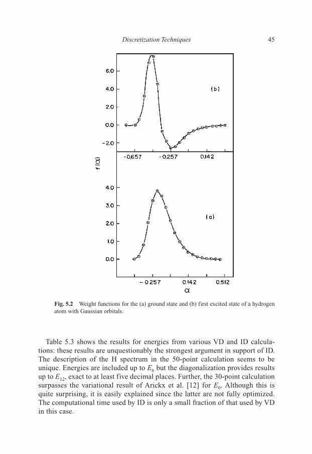
Table 5.3 shows the results for energies from various VD and ID calcula-tions: these results are unquestionably the strongest argument in support of ID.The description of the H spectrum in the 50-point calculation seems to beunique. Energies are included up to E6 but the diagonalization provides resultsup to E12, exact to at least five decimal places. Further, the 30-point calculationsurpasses the variational result of Arickx et al. [12] for E0. Although this isquite surprising, it is easily explained since the latter are not fully optimized.The computational time used by ID is only a small fraction of that used by VDin this case.
Discretization Techniques 45
Fig. 5.2 Weight functions for the (a) ground state and (b) first excited state of a hydrogenatom with Gaussian orbitals.
Else_EAMC-TRSIC_ch005.qxd 5/19/2007 21:07 Page 45

The fact that one obtains discretized weight functions has some implicationsfor quantum chemical techniques. It is a common belief in quantum chemistrythat Gaussians do not provide a good description of the wave function, in spite ofproviding accurate values for energy. However, the present approach seems toproduce a better wave function. This assumption is supported by results obtainedfor the cusp (0), mean values ⟨rn⟩, and lower bounds to E0 in Reference [17].
5. A New Proposal for the Discretization of the Griffin–Hill–Wheeler–Hartree–Fock Equations
5.1. Introduction
Ab initio electronic structure calculations for atoms and especially for moleculesare mostly carried out within the finite basis set expansion method of Roothaan[18]. Since the introduction of the basis set expansion method in Hartree–Fock(HF) theory, made by Roothaan [18], the search for ever more efficient basis setshas been a constant quest.
There is a considerable degree of freedom in choosing the basis functions foratomic and molecular calculations, as any complete set of functions can be emp-loyed. Although Slater-type functions (STFs) had been widely used as basis sets forcalculations with atoms and diatomic molecules, Gaussinan-type functions (GTFs)are invariably the popular choice as basis sets for polyatomic calculations.
The prime reason for the preference of GTFs as basis functions (basis sets)in polyatomic calculations lies in the fact that all the multicenter integrals canbe evaluated exactly by closed analytical formulas. However, a much largerbasis set of GTFs is needed than for the STF basis set because the GTFs behaveincorrectly both in the region near the nucleus (if a point nucleus model isused) and at long range.
46 Chapter 5
Table 5.3
Various VD and ID calculations for the H atom. Energies are in a.u. The set of pointsincludes �0 ��01578, with ���0.1 for (a) and ���0.08 for (b). First point (�min) ischosen to optimize (a) the spectrum and (b) the ground state
VD Ref. [12] ID ID ExactN = 30 N = 30 N = 50
�E0 0.49999999 0.4999999994 0.49999998 0.5�E1 � � 0.12499998 0.125�E2 � � 0.05555555 0.0555...�E3 � � 0.031249996 0.01325�E4 � � 0.019999997 0.02�E5 � � 0.01388887 0.013888...�E6 � � 0.010204080 0.010204082
Else_EAMC-TRSIC_ch005.qxd 5/19/2007 21:07 Page 46
The deficiencies cited above are relevant in nonrelativistic calculations basedon the Hartree–Fock–Roothaan (HFR) method [18], where the point nucleusapproximation is usually employed. Otherwise, when one employs the finitenucleus approximation, as commonly used in relativistic calculations, the use ofGTFs is the right choice, since relativistic calculations are based on the Diracequation whose solutions for an electron in a finite nucleus have been shown tobe Gaussian [19,20].
Owing to the popularity of the use of GTF basis sets, several groups haveattempted to develop techniques that are able to produce efficient GTF basis setsfor atomic and molecular calculations. Two of the most popular techniques in thedesign of GTF basis sets were the even-tempered [21] and the well-tempered [22]techniques. In 1986 another interesting and powerful technique to tailor basis setswas presented [7]. Initially, it was called as the generator coordinate version ofthe HF equations, and later became widely known as the generator coordinateHartree–Fock (GCHF) method.
Shortly, since the GCHF method was already presented in Chapter 4, theGCHF method is the result of employing the generator coordinate ansatz [1b] inthe independent particle model
(5.51)
where �k are the generator functions (they can be either STFs or GTFs), f k arethe weight functions, � is the generator coordinate, and n is the number of parti-cles. The k are then used to build the Slater determinant and calculate the meanvalue of the total energy (the energy expectation value).
The application of the variational principle to the energy expectation value(built with the one-electron functions k) leads to the GHWHF equations
(5.52)
where the k are the orbital eigenvalues and the Fock, F(�,�), and overlap, S(�,�),kernels are
(5.53)
and
(5.54)S k k( , ) (1, ) (1, ) .� � � �� � �
F h J Kj jj
N
( , ) ( , ) [2 ( , ) ( , )]� � � � � � � �� � �∑
[ ]F S f d k nk k( , ) ( , ) ( ) = 0, 1,..., ,� � � � � �� �∫
� � �k k kf d k n(1) (1, ) ( ) , 1,..., ,� ��∫
Discretization Techniques 47
Else_EAMC-TRSIC_ch005.qxd 5/19/2007 21:07 Page 47

The one-electron kernel, h(�,�), and the two-electron kernels, Coulomb Jk(�,�)and exchange Kk(�,�), are defined as
(5.55)
(5.56)
and
(5.57)
where
(5.58)
and
(5.59)
The GHWHF equations are integrated numerically through discretization witha technique that preserves the continuous representation (the integral character)of the GCHF method [8]. This technique is ID and was originally implementedin the GCHF method through a relabeling of the GC space, namely
(5.60)
where A is a scaling parameter determined numerically and the new coordinatespace � is discretized for each w atomic orbital symmetry (w = s, p, d, f, etc.) tak-ing into account an equally spaced numerical mesh, �(w)
k , so that
(5.61)
In Equation (5.61), N is the number of discretization points and �min and��(w) are the initial mesh point and the increment used to obtain the subsequentmesh points, respectively. The lowest (�min
(w) ) and highest (�max(w) ) points of the
mesh (� k(w)) are chosen so as to embrace the adequate integration range for the
weight function f k.
� ��kw k
ww w
Ak k N( )
( )
min( ) ( )In
( 1) , 1, , .� � � � ��
� K
��
� �ln
, 1,A
A
V rk j k j( , ; , ) (1, ) (2, ) (2, ) (1, ) .121� � � � � � � �� �� � � �
V rk j j k( , ; , ) (1, ) (2, ) (2, ) (1, )121� � � � � � � �� �� � � �
K V f f d dj j j( , ) ( , ; , ) ( ) ( ) ,� � � � � � � � � �� ∫∫ �
J V f f d dj j j( , ) ( , ; , ) ( ) ( ) ,� � � � � � � � � �� ∫∫ �
h hk k( , ) (1, ) (1) (1, ) ,� � � �� � �
48 Chapter 5
Else_EAMC-TRSIC_ch005.qxd 5/19/2007 21:07 Page 48

The choice of the generator coordinate � depends on the physical system understudy. For atomic systems, � can represent the atomic GTF exponents andaccording to Equation (5.61) the choice of the discretization points � k
(w) deter-mines the number of exponents � k
(w) of the GTF basis set for each w atomic orbitalsymmetry. The number of discretization points, N, defines the size of the GTFbasis set.
5.2. The Polynomial Integral Discretization
For over 10 years, the GCHF method was used successfully in the generation ofGTF basis sets of good quality for atoms with many electrons. Recently, a mod-ification in Equation (5.61) was proposed [23] to improve the way of obtainingGTF basis sets through the GCHF method. This modification permitted the useof the GCHF method to generate GTF basis sets of smaller size that were as accu-rate as those obtained with the original method.
Now, � k(w) in Equation (5.61) is discretized for each w atomic orbital symme-
try through the polynomial expansion
(5.62)
where each GTF exponent � k(w) is now determined by using the expression
(5.63)
In Equations (5.62) and (5.63), A is a scaling parameter to be determined numer-ically and k = 1, ..., N, where N is the number of discretization points, i.e., thesize of the GTF basis set, exactly as in the original GCHF method.
With the implementation of Equations (5.62) and (5.63) in the original GCHFmethod, the discretization of the GHWHF equations is now performed through anumerical mesh that is not equally spaced. Then, contrary to the original GCHFmethod, the GTF exponents are now generated through the numerical mesh, � k
(w),with the intervals, �� q
(w), not being equally spaced. This procedure makes theoptimization of the GTF exponents, � k
(w), in Equation (5.63) more flexible andmore efficient.
Although it is practical to perform numerical integration, the condition of anequally spaced numerical mesh in the original GCHF method always imposessome restrictions in the generation of exponents. For heavy atoms (atoms of thethird and fourth rows of the periodic table), the GCHF method was always able
� � � � �kw w w w wA k k k( )
min( )
1( )
2( ) 2
3( ) 3exp { ( 1) ( 1) ( 1)
.� � � � � � �
� ... ( 1) }.( )� ��qw qk
��
� � � �kw k
ww w w w
Ak k k( )
min( )
1( )
2( ) 2
3( ) 3ln
( 1) ( 1) ( 1)� � � � � � � �
�� � �... ( 1) ,( )�qw qk
Discretization Techniques 49
Else_EAMC-TRSIC_ch005.qxd 5/19/2007 21:07 Page 49
to generate accurate GTF basis sets of large size (very competitive with otheraccurate GTF basis sets published in the literature). In contrast, for light atoms(atoms of the first and second rows of the periodic table) the GCHF method wasnever able to generate accurate GTF basis sets of small and medium size [24].The accuracy of the GTF basis sets, generated with the original GCHF method,was always proportional to their size. This is the reason why other techniques(methods) were always able to present, mainly for light atoms, better GTF basissets of smaller size (and similar accuracy) than those obtained with the GCHFmethod [24].
The main goal of any method that is used for the generation of basis sets is thedesign of accurate basis sets of small size, as the computational cost of molecularcalculations depends directly on the size of the basis set employed. With the poly-nomial expansion presented in Equation (5.62), we will still be able to generateaccurate basis sets, but now they could be smaller than those obtained previouslywith the original GCHF method.
Another interesting aspect on the implementation of Equations (5.62) and(5.63) in the original GCHF method is that with an unequally spaced numericalmesh we can also segment Equation (5.62) before optimizing the GTF exponents,�k
(w). This is a very practical alternative as with the segmentation of Equation(5.62) we can use different sets of �min
(w) and �� q(w) for different regions in the
atom, i.e., a set with �min(w) and �� q
(w) to describe the inner shell electrons of theatom (the largest exponents), another set to describe the intermediate shell elec-trons, and another to describe the outer shell electrons (the smallest exponents).In practice, we can use as many segmentations as necessary depending only onthe total number of electrons in the atom and on the accuracy we are trying toattain for the HF energy.
In fact, we use the segmentation of Equation (5.62) as a complement to ourpolynomial expansion, since the use of segmentation comes from the necessityof truncating Equation (5.62). In practice, if one uses a very large number ofterms (complete set) in Equation (5.62) there will be no necessity of employingthe segmentation alternative.
Table 5.4 presents the ground-state HF energy results obtained for atoms ofthe first, second, and third rows of the periodic table with GTF basis sets gen-erated with the polynomial expansion implemented in the GCHF method. Hereit is interesting to explain how the basis set exponents are generated fromEquation (5.63) before discussing the results of Table 5.4. The letter k inEquation (5.63) represents the size of the basis set, i.e., the number of exponentsof the basis set, and it varies from 1 to the desired number of points (exponents)of the basis set for each w atomic orbital symmetry (w = s, p, d, f, etc.). The let-ter q represents the degree of the polynomial and, in practice, q values from 3 to4 are enough to generate basis sets for atoms of the first, second, and third rows.In Equation (5.63), each w atomic orbital symmetry will have a starting point
50 Chapter 5
Else_EAMC-TRSIC_ch005.qxd 5/19/2007 21:07 Page 50
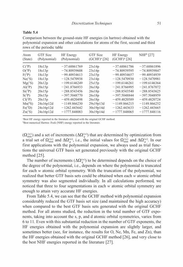
(�min(w) ) and a set of increments (�� q
(w)) that are determined by optimization froma trial set of �min
(w) and �� q(w), i.e., the initial values for �min
(w) and �� q(w). In our
first applications with the polynomial expansion, we always used as trial func-tions the universal GTF basis set generated previously with the original GCHFmethod [25].
The number of increments (�� q(w)) to be determined depends on the choice of
the degree of the polynomial, i.e., depends on where the polynomial is truncatedfor each w atomic orbital symmetry. With the truncation of the polynomial, werealized that better GTF basis sets could be obtained when each w atomic orbitalsymmetry was also segmented individually. In all calculations performed, wenoticed that three to four segmentations in each w atomic orbital symmetry areenough to attain very accurate HF energies.
From Table 5.4, we can see that the GCHF method with polynomial expansionconsiderably reduced the GTF basis set size (and maintained the high accuracy)when compared to the best GTF basis sets generated with the original GCHFmethod. For all atoms studied, the reduction in the total number of GTF expo-nents, taking into account the s, p, and d atomic orbital symmetries, varies from6 to 11. Even with this substantial reduction in the number of GTF exponents, theHF energies obtained with the polynomial expansion are slightly larger, andsometimes better (see, for instance, the results for O, Ne, Mn, Fe, and Zn), thanthe HF energies obtained with the original GCHF method [26], and very close tothe best NHF energies reported in the literature [27].
Discretization Techniques 51
Table 5.4
Comparison between the ground-state HF energies (in hartree) obtained with thepolynomial expansion and other calculations for atoms of the first, second and thirdrows of the periodic table
Atom GTF Size HF Energy GTF Size HF Energy NHFb [27](State) (Polynomial) (Polynomial) (GCHF)a [26] (GCHF)a [26]
C(3P) 18s13p �37.68861769 23s14p �37.68861786 �37.68861896O(3P) 18s13p �74.80939608 23s14p �74.80939595 �74.80939847F(2P) 18s13p �99.40934613 23s15p �99.40934657 �99.40934939Ne(1S) 18s13p �128.5470938 23s14p �128.5470930 �128.5470981Mg(1S) 20s12p �199.6146249 25s15p �199.6146261 �199.6146364Al(2P) 20s15p �241.8766933 26s18p �241.8766995 �241.8767072Si(3P) 20s15p �288.8543456 26s18p �288.8543540 �288.8543625S(3P) 20s15p �397.5048770 26s18p �397.5048844 �397.5048959Cl(2P) 20s15p �459.4820498 26s18p �459.4820589 �459.4820724Mn(6S) 24s16p12d �1149.866230 29s19p13d �1149.866215 �1149.866252Fe(5D) 24s16p12d �1262.443642 30s19p14d �1262.443633 �1262.443665Zn(1S) 24s16p12d �1777.848083 30s19p14d �1777.848065 �1777.848116
aBest HF energy reported in the literature obtained with the original GCHF method.bBest numerical Hartree–Fock (NHF) energy reported in the literature.
Else_EAMC-TRSIC_ch005.qxd 5/19/2007 21:07 Page 51
In Table 5.4, we can also see that the reduction in the total number of GTFexponents increases with the size of the atom, i.e., for the first-row atoms (C, O,F, and Ne), the reduction in the total number of GTF exponents, when comparedto the GTF size of the best GTF basis sets, obtained with the original GCHFmethod [17], varies between 6 and 7; for the second-row atoms (Mg, Al, Si, S,and Cl), this reduction varies between 8 and 9; and for the third-row atoms (Mn,Fe, and Zn), it varies from 9 to 11. This shows that the GCHF method with thepolynomial expansion works very well for light atoms, but its performance getsbetter when we are working with heavier atoms. This is the reason why the GCHFmethod with polynomial expansion has become extremely useful in the design ofrelativistic GTF basis sets, since in these cases we very often work with heavyatoms. The applications of the polynomial expansion in relativistic calculationswill be presented in Chapter 7.
Except for the cases where the polynomial energies are better (O, Ne, Mn, Fe,and Zn), we can see in Table 5.4 that the energy differences between our resultsand those obtained with the best original GCHF method [26] vary within anaccuracy of 10�6 and 10�7 hartree. When now we compare our results with thenumerical values [27] (last column in Table 5.4), we can see that the energy dif-ferences vary within the accuracy of 1015 to 10�7 hartree.
At this point it is interesting to mention that other authors have also employedthe idea of segmenting the space of the basis set exponents [28,29], but in a dif-ferent way compared to the methodology described above. One proposed the useof basis set segmentation in the even-tempered methodology with STFs [28] andthe other one was the first to propose the segmentation of basis set in the origi-nal GCHF method by using GTFs [29]. In both cases, the segmentation improvedthe energy results; and particularly for the work with GTFs [29], the HF energiesobtained for the atoms studied were not as accurate as the HF energy resultsobtained with our polynomial expansion. In fact, the difference between ourmethodology and the others is that we also use the idea of basis set segmentationin the polynomial expansion proposed in Equation (5.62).
The results displayed in Table 5.4 showed that the GCHF method with the poly-nomial expansion is a very powerful methodology to be employed in the design ofcompact and highly accurate GTF basis sets for atomic and molecular calculations.For sure, one of the great advantages of this methodology was the generation ofGTF basis sets to be used in relativistic atomic and molecular calculations, as wewill see in Chapter 7. The GTF basis set size is more critical in relativistic calcula-tions than in the nonrelativistic case, since it is not easy to have a good balancebetween size and accuracy when we are trying to generate relativistic GTF basissets by using the GC method [30–33], i.e., when the accuracy is quite satisfactory,the size is too large. Thus, the polynomial expansion became the basis of a method-ology capable of generating compact and highly accurate relativistic GTF basis setsby using the GC method, as we will show in Chapter 7.
52 Chapter 5
Else_EAMC-TRSIC_ch005.qxd 5/19/2007 21:07 Page 52
Concluding, we can say that the modification in the way of discretizing theGHWHF equations by the polynomial expansion presented in Equation (5.62)substantially improved the generation of Gaussian basis sets to be used in abinitio atomic and molecular calculations when we are employing the GCHFmethod. This new way of discretizing the GHWHF equations made the opti-mization of Gaussian exponents in the environment of the GCHF method moreflexible and more efficient, since it was able to considerably reduce the size ofthe Gaussian basis set to be generated with the GCHF method.
References
1. (a) D. L. Hill, and J. A. Wheeler, Phys. Rev., 1953, 89, 1102; (b) J. J. Griffin, and J. A. Wheeler, Phys. Rev., 1957, 108, 311.
2. D. Justin, M. V. Mihailovic, and M. Rosina, Nucl. Phys. A, 1971, 182, 54.3. M. Bender, P.-H. Heenen, and P.-G. Reinhard, Rev. Modern Phys., 2003, 75, 121.4. P. Chattopadhyay, R. M. Dreizler, M. Trsic, and M. Fink, Z. Phys. A, 1978, 285, 7.5. L. Lathouwers, Ann. Phys., 1976, 102, 347.6. R. Courant, and D. Hilbert, Methods of Mathematical Physics, New York:
Interscience, 1962.7. J. R. Mohallem, R. M. Dreizler, and M. Trsic, Int. J. Quantum. Chem. Symp., 1986,
20, 45.8. J. R. Mohallem, Z. Phys. D, 1986, 3, 339.9. P. O. Löwdin, Adv. Phys., 1956, 5, 1; L. Lathouwers, Int. J. Quantum Chem. Symp.,
1976, 10, 413.10. D. Galetti, and A. F. R. de Toledo Piza, Phys. Rev. C, 1978, 17, 774.11. J. Broeckhove, and E. Deumens, Z. Phys. A, 1979, 292, 243.12. F. Arickx, J. Broeckhove, E. Deumens, and P. Van Leuven, J. Comp. Phys., 1981,
39, 272.13. D. M. Bishop, and R. L. Somorjai, J. Math. Phys., 1970, 11, 1150.14. (a) S. Huzinaga, J. Chem. Phys., 1965, 42, 1293; (b) H. Sambe, J. Chem. Phys., 1965,
42, 1732.15. J. R. Mohallem, and M. Trsic, Z. Phys. A, 1985, 322, 535. 16. L. Lathouwers, and P. Van Leuven, Adv. Chem. Phys., 1982, 49, 115.17. J. R. Mohallem, and M. Trsic, Int. J. Quantum. Chem., 1988, 33, 555.18. C. C. J. Roothaan, Rev. Mod. Phys., 1951, 23, 69.19. Y. Ishikawa, R. Baretty, and R. C. Binning, Jr., Chem. Phys. Lett., 1985, 121, 130.20. Y. Ishikawa, and H. M. Quincy, Int. J. Quantum Chem. Symp., 1987, 21, 523.21. K. Ruedenberg, R. C. Raffanetti, and R. D. Bardo, Energy, Structure and Reactivity –
Proceedings of the 1972 Boulder Seminar Research Conference on TheoreticalChemistry, New York: Wiley, 1973.
22. S. Huzinaga, M. Klobukowski, and H. Tatewaki, Can. J. Chem., 1985, 63, 1812. 23. R. C. Barbosa, and A. B. F. da Silva, Mol. Phys., 2003, 101, 1073.24. A. B. F. da Silva, and M. Trsic, Can. J. Chem., 1996, 74, 1526.25. A. B. F. da Silva, H. F. M. da Costa, and M. Trsic, Mol. Phys., 1989, 68, 433.
Discretization Techniques 53
Else_EAMC-TRSIC_ch005.qxd 5/19/2007 21:07 Page 53

26. F. E. Jorge, and E. P. Muniz, Int. J. Quantum Chem., 1999, 71, 307.27. T. Koga, S. Watanabe, K. Kanayama, R. Yasuda, and A. J. Thakkar, J. Chem. Phys.,
1995, 103, 3000.28. T. Koga, H. Tatewaki, and A. J. Thakkar, Theor. Chim. Acta, 1994, 88, 273.29. F. E. Jorge, and E. V. R. de Castro, Chem. Phys. Lett., 1999, 302, 454.30. G. L. Malli, A. B. F. da Silva, and Y. Ishikawa, Phys. Rev. A, 1993, 47, 143.31. G. L. Malli, A. B. F. da Silva, and Y. Ishikawa, J. Chem. Phys., 1994, 101, 6829.32. F. E. Jorge, and A. B. F. da Silva, J. Chem. Phys., 1996, 104, 6278.33. F. E. Jorge, and A. B. F. da Silva, J. Chem. Phys., 1996, 105, 5503.
54 Chapter 5
Else_EAMC-TRSIC_ch005.qxd 5/19/2007 21:07 Page 54

Chapter 6
Role of the Weight Function in the Design ofEfficient Basis Sets for Atomic and MolecularNonrelativistic Calculations
1. Introduction
In this chapter, we will discuss the importance of the weight function of thegenerator coordinate Hartree–Fock (GCHF) method in the generation of basis setsfor atomic and molecular nonrelativistic calculations. The weight function has acentral role in finding basis set functions of good quality. In the GCHF method,the minimization of the total electronic energy is performed through the descrip-tion of the weight function, i.e., better described the weight function, the better isthe total electronic energy of the atomic or molecular system being studied.
The weight function of the GCHF method also had a central role in the gener-ation of universal basis sets. The idea of universal basis sets was first introducedin the literature in 1978 when a Slater universal basis set was presented by usingthe even-tempered formula [1,2]. Afterwards, other works (the first ones) werepublished applying the concept of universal basis sets [3–7].
The main interest in developing a universal basis set arose with the idea oftransferring integrals from one calculation to another [1]. This idea of transfer-ring integrals from one system to another is interesting but not practical. In fact,with the improvement of computers, it is easier to perform another calculationthan to store integrals and try to transfer them to other calculations. Moreover,transferring integrals from one system to another is only possible due to certainsimilarities between the atomic and molecular systems under study. As one willsee along this chapter, the GCHF is extremely useful in the generation of largeuniversal basis sets.
The first works with universal basis sets were able to generate a unique setof Slater-type functions (STFs) that was able to describe the atoms fromHelium (Z � 2) to Argon (Z � 18) [1,2]. Later, with the GCHF method we wereable to generate a unique set of Slater- and Gaussian-type functions (GTFs) todescribe the neutral atoms and respective positive and negative ions fromHydrogen (Z � 1) to Xenon (Z � 54) [8,9]. Actually, the works of References[8,9] present the largest universal Slater and Gaussian basis sets published so
Else_EAMC-TRSIC_ch006.qxd 5/4/2007 07:32 Page 55

far in the literature that were only generated from a unique set of basis functionexponents. After this achievement, we changed the idea of universal basis setsa bit; i.e., since it is not easy to generate a unique set of basis functionsexponents that can describe the total electronic energy for a large number ofatoms, we realized that this concept of universal basis set can be made flexibleby initially generating a unique set of basis set exponents and from it chooseonly the exponents that are really important to describe the total electronicenergy of a particular atom [10–12].
Here, we would like to remark that the most important work published sofar with the GCHF method and that uses this idea of making universal basissets flexible is the work of de Castro and Jorge [12]. They generated a univer-sal Gaussian basis set for the atoms from H (Z � 1) to No (Z � 102). The uni-versal Gaussian basis set exponents of Reference [12] are presented inAppendix 3.
Since the idea of this chapter is to show the role of the weight function of theGCHF method in the generation of basis sets, we will present this subject usingtwo classical examples: generation of the STF and GTF universal basis sets forthe neutral and ionic atomic species for the atoms from H to Xe [8,9]. InAppendixes 1 and 2, we present the GTF and STF universal basis set exponentsof Reference [8].
2. Weight Function and the Generation of Universal Basis Sets
2.1. Slater and Gaussian Universal Basis Sets for the Ground andCertain Low-lying Excited States of the Neutral Atoms from Hydrogen to Xenon
As already commented in the previous section, the GCHF method is tailored togenerate universal basis sets. This is true as with the integral discretization (ID)technique of the GCHF method [see Equations (4.12) in Chapter 4] we have a lotof flexibility to choose a universal mesh of the GCHF method that can describethe total electronic energy for a large number of atoms. Since with the ID tech-nique we do not have the cumbersome procedure of optimizing all the basis func-tion exponents, the search for a set of exponents that can describe the energy ofa large number of atoms becomes easier.
The first universal basis set generated with the GCHF method was presentedby Mohallem and Trsic in 1987 [13]. In that work they generated a universalGaussian basis set for the neutral atoms from Li (Z � 3) to Ne (Z � 10) [13].Afterwards, universal Slater and Gaussian basis sets generated with the GCHFmethod were presented for the neutral atoms from He (Z � 2) to Ag (Z � 18)[14] and for the neutral atoms and respective positive and negative ions fromH (Z � 1) to Xe (Z � 54) [8,9]. These last ones [8,9] are the largest universal
56 Chapter 6
Else_EAMC-TRSIC_ch006.qxd 5/4/2007 07:32 Page 56

STFs and GTFs presented in the literature so far, and the only case where, in fact,a unique set of STFs and GTFs exponents is able to describe a very large num-ber of atoms.
The (12s, 10p, 10d) universal Slater basis set of Reference [8] is generatedwith the following discretization parameters (i.e., orbital exponents):
Symmetry �min �� Ns �0.11 0.07 12p 0.00 0.07 10d �0.11 0.07 10
The (18s, 12p, 11d) universal Gaussian basis set of Reference [8] is generatedwith the following discretization parameters:
Symmetry �min �� Ns �0.55 0.16 18p �0.40 0.16 12d �0.55 0.16 11
�min, ��, and N are the discretization parameters of Equations (4.12).In Table 6.1 we show the total ground state Hartree–Fock (HF) energies for
both bases (Slater and Gaussian) and when possible we compare them with the
Role of the Weight Function in the Design of Efficient Basis Sets 57
Table 6.1
Total HF ground state energies (a.u.) obtained with the STF and GTF universal basesfor the neutral atoms from H (Z�1) to Xe (Z�54)
Atom State STF GTF Numerical [15](12s, 10p, 10d) (18s, 12p, 11d)
H 2S �0.4999990 �0.4999972 �0.5He 1S �2.8616794 �2.8616747 �2.8616800Li 2S �7.4327054 �7.4325533 �7.4327269Be 1S �14.573019 �14.572976 �14.573023B 2P �24.528977 �24.528672 �24.529061C 3P �37.688610 �37.688474 �37.688619N 4S �54.400921 �54.400709 �54.400934O 3P �74.809384 �74.809108 �74.809398F 2P �99.409341 �99.408974 �99.409349Ne 1S �128.54710 �128.54656 �128.54710Na 2S �161.85889 �161.85776 �161.85891Mg 1S �199.61457 �199.61356 �199.61463Al 2P �241.87368 �241.87044 �241.87671Si 3P �288.85383 �288.85101 �288.85436P 4S �340.71873 �340.71600 �340.71878S 3P �397.50482 �397.50163 �397.50490Cl 2P �459.48187 �459.47810 �459.48207Ar 1S �526.81717 �526.81241 �526.81751
(continued )
Else_EAMC-TRSIC_ch006.qxd 5/4/2007 07:32 Page 57

numerical HF values of Froese–Fisher [15], otherwise we show the best STFatom-optimized values of Clementi and Roetti [16] or the numerical results ofHuzinaga and Klobukowski [17].
In Table 6.2 we show the results for various low-lying excited states for theatoms from H (Z � 1) to Xe (Z � 54) and compare them with the values ofClementi and Roetti [16].
58 Chapter 6
K 2S �599.16429 �599.15586 �599.16479Ca 1S �676.75775 �676.74917 �676.75818Sc 2D �759.73544 �759.72531 �759.73572Ti 3F �848.40567 �848.39417 �848.40600V 4F �942.88403 �942.87129 �942.88433Cr 7S �1043.3558 �1043.3418 �1043.3552 [16]Mn 6S �1149.8653 �1149.8491 �1149.8662Fe 5D �1262.4424 �1262.4234 �1262.4437Co 4F �1381.4131 �1381.3905 �1381.4146Ni 3F �1506.8693 �1506.8427 �1506.8709Cu 2S �1638.9620 �1638.9315 �1638.9628 [16]Zn 1S �1777.8463 �1777.8115 �1777.8481Ga 2P �1923.2563 �1923.2153 �1923.2610Ge 3P �2075.3572 �2075.3125 �2075.3597As 4S �2234.2367 �2234.1882 �2234.2386Se 3P �2399.8655 �2399.8123 �2399.8676Br 2P �2572.4388 �2572.3800 �2572.4413Kr 1S �2752.0517 �2751.9861 �2752.0550Rb 2S �2938.3531 �2938.2756 �2938.3574Sr 1S �3131.5401 �3131.4544 �3131.5457Y 2D �3331.6766 �3331.5793 �3331.6842Zr 5F �3538.9995 �3538.8884 �3539.0096 [17]Nb 6D �3753.5846 �3753.4577 �3753.5977 [17]Mo 7S �3975.5329 �3975.3890 �3975.5495 [17]Tc 6S �4204.7400 �4204.6061 �4204.7887Ru 5F �4441.5154 �4441.3345 �4441.5395 [17]Rh 4F �4685.8544 �4685.6532 �4685.8817 [17]Pd 1S �4937.8915 �4937.6684 �4937.9210 [17]Ag 2S �5197.6682 �5197.4204 �5197.6985 [17]Cd 1S �5465.1036 �5464.8281 �5465.1331In 2P �5740.1368 �5739.8269 �5740.1691Sn 3P �6022.9043 �6022.5586 �6022.9317Sb 4S �6313.4600 �6313.0749 �6313.4853Te 3P �6611.7553 �6611.3266 �6611.7840I 2P �6917.9409 �6917.4681 �6917.9809Xe 1S �7232.0742 �7231.5613 �7232.1384
Table 6.1 Continued
Atom State STF GTF Numerical [15](12s, 10p, 10d) (18s, 12p, 11d)
Else_EAMC-TRSIC_ch006.qxd 5/4/2007 07:32 Page 58

Role of the Weight Function in the Design of Efficient Basis Sets 59
Table 6.2
Some low-lying HF-excited state energies (a.u.) obtained with the STF and GTFuniversal bases
Atom Configuration State STF GTF Optimized STF (12s, 10p, 10d) (18s, 12p, 11d) [16]
C |He| 2s22p2 1D �37.631327 �37.631141 �37.631325C |He| 2s22p2 1S �37.549530 �37.549172 �37.549582N |He| 2s22p3 2D �54.296155 �54.295947 �54.296158N |He| 2s22p3 2P �54.228090 �54.227878 �54.228089O |He| 2s22p4 1D �74.729248 �74.728976 �74.729223O |He| 2s22p4 1S �74.611002 �74.610735 �74.610978Si |Ne| 3s23p2 1D �288.81397 �288.81068 �288.81506Si |Ne| 3s23p2 1S �288.75584 �288.75168 �288.75853P |Ne| 3s23p3 2D �340.64877 �340.64581 �340.64875P |Ne| 3s23p3 2P �340.60310 �340.59993 �340.60320S |Ne| 3s23p4 1D �397.45229 �397.44905 �397.45221S |Ne| 3s23p4 1S �397.37463 �397.37127 �397.37450Sc |Ar| 4s13d2 4F �759.68851 �759.68849 �759.69860Ti |Ar| 4s23d2 1G �848.33198 �848.32046 �848.33198Ti |Ar| 4s23d2 1D �848.35829 �848.34677 �848.35823Ti |Ar| 4s23d2 3P �848.34823 �848.33672 �848.34818Ti |Ar| 4s23d2 1S �848.23057 �848.21902 �848.23057Ti |Ar| 4s13d3 5F �848.38595 �848.37459 �848.38600V |Ar| 4s23d3 2H �942.79865 �942.78589 �942.79882V |Ar| 4s23d3 2G �942.81973 �942.80698 �942.81991V |Ar| 4s23d3 2F �942.73615 �942.72338 �942.73633V |Ar| 4s23d3 2D �942.72243 �942.70966 �942.72261V |Ar| 4s23d3 4P �942.82008 �942.80733 �942.82008V |Ar| 4s23d3 2P �942.76040 �942.74764 �942.79882V |Ar| 4s13d4 6D �942.87949 �942.86689 �942.87951Cr |Ar| 4s23d4 1I �1043.1790 �1043.1648 �1043.1793Cr |Ar| 4s23d4 3H �1043.2221 �1043.2079 �1043.2223Cr |Ar| 4s23d4 3G �1043.1990 �1043.1848 �1043.1993Cr |Ar| 4s23d4 1G �1043.1084 �1043.0942 �1043.1087Cr |Ar| 4s23d4 3F �1043.1418 �1043.1276 �1043.1421Cr |Ar| 4s23d4 1F �1043.1108 �1043.0965 �1043.1110Cr |Ar| 4s23d4 5D �1043.3092 �1043.2951 �1043.3095Cr |Ar| 4s23d4 3D �1043.1669 �1043.1527 �1043.1672Cr |Ar| 4s23d4 1D �1043.0455 �1043.0313 �1043.0458Cr |Ar| 4s23d4 3P �1043.1418 �1043.1276 �1043.1421Cr |Ar| 4s23d4 1S �1043.0003 �1042.9860 �1043.0005Mn |Ar| 4s23d5 2I �1149.6626 �1149.6464 �1149.6629Mn |Ar| 4s23d5 2H �1149.6165 �1149.6002 �1149.6167Mn |Ar| 4s23d5 4G �1149.7225 �1149.7062 �1149.7228Mn |Ar| 4s23d5 2D �1149.5512 �1149.5349 �1149.5515Mn |Ar| 4s23d5 4F �1149.6265 �1149.6103 �1149.6268Mn |Ar| 4s23d5 2F �1149.6100 �1149.5937 �1149.6103Mn |Ar| 4s23d5 4D �1149.6877 �1149.6714 �1149.6879Mn |Ar| 4s23d5 2D �1149.5132 �1149.4969 �1149.5134
(continued )
Else_EAMC-TRSIC_ch006.qxd 5/4/2007 07:32 Page 59

60 Chapter 6
Mn |Ar| 4s23d5 4P �1149.7007 �1149.6845 �1149.7010Mn |Ar| 4s23d5 2P �1149.4123 �1149.3960 �1149.4123Mn |Ar| 4s23d5 2S �1149.5594 �1149.5431 �1149.5597Mn |Ar| 4s13d6 6D �1149.7431 �1149.7270 �1149.7432Fe |Ar| 4s23d6 1I �1262.2936 �1262.2746 �1262.2944Fe |Ar| 4s23d6 3H �1262.3430 �1262.3239 �1262.3437Fe |Ar| 4s23d6 3G �1262.3166 �1262.2975 �1262.3173Fe |Ar| 4s23d6 1G �1262.2122 �1262.1932 �1262.2129Fe |Ar| 4s23d6 3F �1262.2507 �1262.2317 �1262.2514Fe |Ar| 4s23d6 1F �1262.2149 �1262.1958 �1262.2156Fe |Ar| 4s23d6 3D �1262.2797 �1262.2607 �1262.2805Fe |Ar| 4s23d6 1D �1262.1392 �1262.1202 �1262.1399Fe |Ar| 4s23d6 3P �1262.2507 �1262.2317 �1262.2514Fe |Ar| 4s23d6 1S �1262.0864 �1262.0673 �1262.0871Fe |Ar| 4s13d7 5F �1262.3764 �1262.3575 �1262.3763Co |Ar| 4s13d8 4F �1381.3569 �1381.3345 �1381.3750Ni |Ar| 4s23d8 1G �1506.7548 �1506.7282 �1506.7560Ni |Ar| 4s23d8 1D �1506.7961 �1506.7695 �1506.7973Ni |Ar| 4s23d8 3P �1506.7805 �1506.7539 �1506.7817Ni |Ar| 4s23d8 1S �1506.5882 �1506.5616 �1506.5894Ni |Ar| 4s13d9 3D �1506.8224 �1506.7960 �1506.8224Cu |Ar| 4s23d9 2D �1638.9483 �1638.9176 �1638.9496Ge |Ar| 4s23d104p2 1D �2075.3179 �2075.2726 �2075.3208As |Ar| 4s23d104p3 2D �2234.1700 �2234.1213 �2234.1718As |Ar| 4s23d104p3 2P �2234.1265 �2234.0774 �2234.1283Se |Ar| 4s23d104p4 1D �2399.8168 �2399.7635 �2399.8185Se |Ar| 4s23d104p3 1S �2399.7448 �2399.6913 �2399.7466Y |Kr| 5s14d2 4F �3331.6612 �3331.5642 �3331.6550Zr |Kr| 5s04d4 5D �3538.9221 �3538.8112 �3538.9172Zr |Kr| 5s24d2 3F �3538.9850 �3538.8735 �3538.9821Nb |Kr| 5s04d5 6S �3753.5415 �3753.4149 �3753.5403Nb |Kr| 5s24d3 4F �3753.5389 �3753.4116 �3753.5394Mo |Kr| 5s04d6 5D �3975.3890 �3975.2455 �3975.3889Mo |Kr| 5s24d4 5D �3975.4267 �3975.2824 �3975.4280Tc |Kr| 5s04d7 4F �4204.6717 �4204.5102 �4204.6768Tc |Kr| 5s14d6 6D �4204.7609 �4204.5991 �4204.7669Ru |Kr| 5s04d8 3F �4441.4531 �4441.2726 �4441.4632Ru |Kr| 5s24d6 5D �4441.4633 �4441.2821 �4441.4746Rh |Kr| 5s04d9 2D �4685.8197 �4685.6187 �4685.8308Rh |Kr| 5s24d7 4F �4685.7740 �4685.5725 �4685.7892Pd |Kr| 5s14d9 3D �4937.8640 �4937.6406 �4937.8815Pd |Kr| 5s24d8 3F �4937.7536 �4937.5300 �4937.7709Ag |Kr| 5s24d9 2D �5197.4877 �5197.2396 �5197.5029
Table 6.2 Continued
Atom Configuration State STF GTF Optimized STF (12s, 10p, 10d) (18s, 12p, 11d) [16]
Else_EAMC-TRSIC_ch006.qxd 5/4/2007 07:32 Page 60

Role of the Weight Function in the Design of Efficient Basis Sets 61
From Tables 6.1 and 6.2, we can see that the universal STF total energy values arevery close to the numerical HF results and competitive with the excited state valuesof Clementi and Roetti. The performance of the universal GTF bases is almost asgood as in the STF case, at the expense of a somewhat larger basis set, as expected.
It is also interesting to notice from Tables 6.1 and 6.2 that both STF and GTFuniversal bases perform somewhat better for excited states than for ground stateswhen compared to the Clementi and Roetti results. The explanation is simple: theexponents of Clementi and Roetti are optimized for the ground state energy andare not optimal for excited states. However, the GCHF exponents generatedthrough the ID technique [see Equations (4.12)] are not biased and are equallyadequate for any property. In particular, the capacity of attaining excited stateswith the GC method was noticed in previous tests on model problems [18,19].
2.2. The Weight Functions
Here, it is relevant to discuss the behavior of the weight functions f(�) in thegeneration of the universal Slater and Gaussian basis sets of Reference [8]. InFigs. 6.1–6.6 we have plotted the GTF weight functions for the noble gases. Thecorresponding weight functions of the other atoms are comprised between the two
Fig. 6.1 The GTF 1s weight functions for the noble gases from He to Xe, and 2s fromNe to Xe.
Else_EAMC-TRSIC_ch006.qxd 5/4/2007 07:32 Page 61
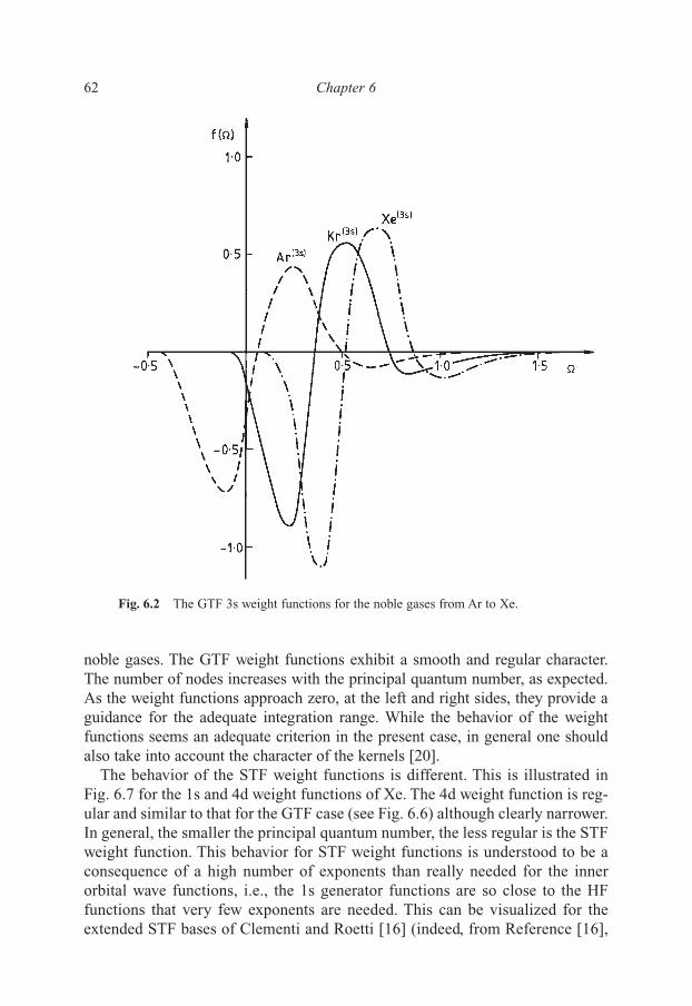
62 Chapter 6
noble gases. The GTF weight functions exhibit a smooth and regular character.The number of nodes increases with the principal quantum number, as expected.As the weight functions approach zero, at the left and right sides, they provide aguidance for the adequate integration range. While the behavior of the weightfunctions seems an adequate criterion in the present case, in general one shouldalso take into account the character of the kernels [20].
The behavior of the STF weight functions is different. This is illustrated inFig. 6.7 for the 1s and 4d weight functions of Xe. The 4d weight function is reg-ular and similar to that for the GTF case (see Fig. 6.6) although clearly narrower.In general, the smaller the principal quantum number, the less regular is the STFweight function. This behavior for STF weight functions is understood to be aconsequence of a high number of exponents than really needed for the innerorbital wave functions, i.e., the 1s generator functions are so close to the HFfunctions that very few exponents are needed. This can be visualized for theextended STF bases of Clementi and Roetti [16] (indeed, from Reference [16],
Fig. 6.2 The GTF 3s weight functions for the noble gases from Ar to Xe.
Else_EAMC-TRSIC_ch006.qxd 5/4/2007 07:32 Page 62
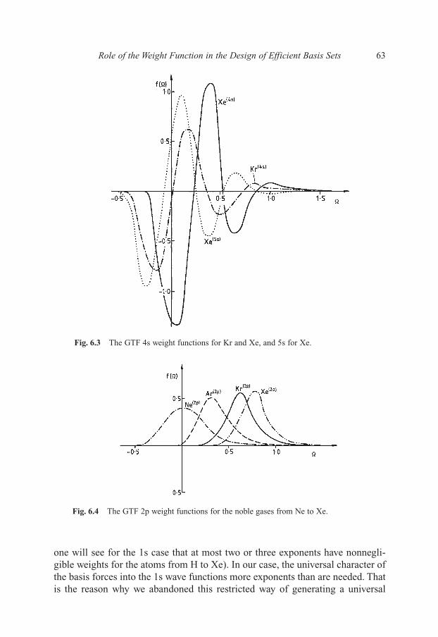
Role of the Weight Function in the Design of Efficient Basis Sets 63
one will see for the 1s case that at most two or three exponents have nonnegli-gible weights for the atoms from H to Xe). In our case, the universal character ofthe basis forces into the 1s wave functions more exponents than are needed. Thatis the reason why we abandoned this restricted way of generating a universal
Fig. 6.4 The GTF 2p weight functions for the noble gases from Ne to Xe.
Fig. 6.3 The GTF 4s weight functions for Kr and Xe, and 5s for Xe.
Else_EAMC-TRSIC_ch006.qxd 5/4/2007 07:32 Page 63
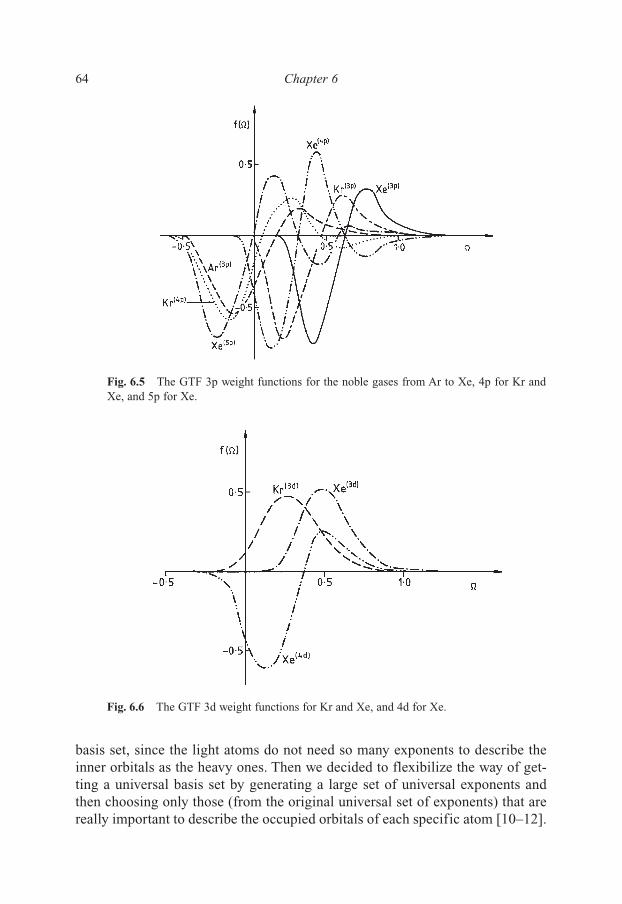
basis set, since the light atoms do not need so many exponents to describe theinner orbitals as the heavy ones. Then we decided to flexibilize the way of get-ting a universal basis set by generating a large set of universal exponents andthen choosing only those (from the original universal set of exponents) that arereally important to describe the occupied orbitals of each specific atom [10–12].
64 Chapter 6
Fig. 6.5 The GTF 3p weight functions for the noble gases from Ar to Xe, 4p for Kr andXe, and 5p for Xe.
Fig. 6.6 The GTF 3d weight functions for Kr and Xe, and 4d for Xe.
Else_EAMC-TRSIC_ch006.qxd 5/4/2007 07:32 Page 64

Certainly, the oscillating character of the STF 1s weight functions does nothamper the regular character of the wave functions. In Fig. 6.8 we plot the radialR10(r) and R42(r) functions for Xe with STFs, GTFs, and numerical HF functions[15]. At the scales employed, the three R42(r) functions are not distinguishablewhile for R10(r) they can be recognized at the origin. It is interesting to remarkthat the Gaussian R42(r) wave function, generated with the ID technique of theGCHF method [Equations (4.12)], has an adequate behavior at the origin.
2.3. Slater and Gaussian Universal Basis Sets for the Ground andCertain Low-lying Excited States of Positive and Negative Ions of the Atoms from Hydrogen to Xenon
After generating the STF and GTF universal basis sets for the neutral atoms fromH (Z�1) to Xe (Z�54) [8], we generated STF and GTF universal basis sets forthe positive and negative ions for the atoms from H to Xe as well [9].
The (12s, 10p, 10d) STF universal basis set for the positive ions from H toXe is generated with the following discretization parameters (i.e., orbitalexponents):
Symmetry �min �� Ns �0.11 0.07 12p 0.00 0.07 10d �0.11 0.07 10
Role of the Weight Function in the Design of Efficient Basis Sets 65
Fig. 6.7 The STF 1s and 4d weight functions for Xe.
Else_EAMC-TRSIC_ch006.qxd 5/4/2007 07:32 Page 65

66 Chapter 6
The (18s, 12p, 11d) GTF universal basis set for the positive ions from H to Xeis generated with the following discretization parameters:
Symmetry �min �� Ns �0.55 0.16 18p �0.40 0.16 12d �0.55 0.16 11
The (13s, 11p, 10d) STF universal basis set for the negative ions from H to Xeis generated with the following discretization parameters:
Symmetry �min �� Ns �0.21 0.07 13p �0.10 0.07 11d �0.05 0.07 10
Fig. 6.8 The R10(r) and R42(r) radial functions for Xe. The values in R10(r) are 785.7768,782.8561, and 766.5602 for numerical HF, STOs (Slater-type orbitals), and GTOs (Gaussian-type orbitals), respectively.
Else_EAMC-TRSIC_ch006.qxd 5/4/2007 07:32 Page 66

The (18s, 12p, 11d) GTF universal basis set for the negative ions from H to Xeis generated with the following discretization parameters:
Symmetry �min �� Ns �0.75 0.16 18p �0.55 0.16 12d �0.75 0.16 11
The basis (discretization parameters) for the STF and GTF positive ions fromH (Z�1) to Xe (Z�54) are the same as those we previously employed for the neu-tral atoms from H to Xe [8]. This coincidence was to be expected, as ionization pro-duces orbital contraction and thus the bases for the neutral atoms were adequate fordescribing the total energies for ground and low-lying excited states of the positiveions. For the negative ions, therefore, it was not possible to describe the total ener-gies by employing the same basis set as for the neutral atoms. This is a consequenceof the entry of one electron in the frontier atomic orbital, making it more diffusive;thus, lower values for �min are required for the STF and GTF universal bases.
In Tables 6.3–6.6 we present the total STF and GTF HF energies for the groundand low-lying excited states of the positive and negative ions from H to Xe. Ourresults are compared with the numerical results of Koga et al. [21] and only whennumerical results are not available they are compared with the atom-optimized val-ues of Clementi and Roetti [16]. One can see from Tables 6.3–6.6 that our STFenergy values (ground and low-lying excited states) compare very favorably with thenumerical results and the atom-optimized results of Clementi and Roetti, often beinglower than those obtained with the latter. Our GTF energies are only slightly abovethe STF values in spite of a rather modest increase in the number of basis functions.
In the case of positive ions (Tables 6.3 and 6.4), we notice a better perform-ance for both STF and GTF universal bases for the excited states than for theground states when compared with the Clementi and Roetti results [16]. Also, forthe positive and negative ions, the STF energy values are close to the numericalresults and competitive with the excited state values of Clementi and Roetti. Thiscapacity to describe excited states with the GC method has already been com-mented in other works [18,19].
We would also like to make a comparison between the STF energy resultsobtained for the ground state of cations and anions, and the STF energy resultsobtained by Koga et al. [22] using doubly even-tempered basis set for the sameionic species (the work of Koga et al. was published basically at the same timewe published our work [9] and Koga’s results are not included in Tables 6.3–6.6).Here it is important to pay attention to the fact that we are working with univer-sal STF basis set and thus the sizes of our basis sets are always the same, namely(12, 10p, 10d) for the cations and (13s, 11p, 10d) for the anions. In their work,Koga et al. worked with atom-adapted basis sets and thus their STF basis set sizeincreases with the increasing Z (atomic nuclear charge).
Role of the Weight Function in the Design of Efficient Basis Sets 67
Else_EAMC-TRSIC_ch006.qxd 5/4/2007 07:32 Page 67

68 Chapter 6
(continued )
Table 6.3
Certain total HF ground state energies (a.u.) obtained with the STF and GTF universalbases for the positive ions of the atoms from H (Z�1) to Xe (Z�54)
Ion Configuration State STF GTF Numerical [21](12s, 10p, 10d) (18s, 12p, 11d)
He� 1s1 2S �1.99999961 �1.99999304 �2.0Li� 1s2 1S �7.2364143 �7.2363955 �7.2364152Be� |He| 2s1 2S �14.277376 �14.277325 �14.277395B� |He| 2s2 1S �24.237574 �24.237467 �24.237575C� |He| 2s22p1 2P �37.292210 �37.292075 �37.292224N� |He| 2s22p2 3P �53.887994 �53.887733 �53.888005O� |He| 2s22p3 4S �74.372585 �74.372265 �74.372606F� |He| 2s22p4 3P �98.831700 �98.831309 �98.831720Ne� |He| 2s22p5 2P �127.81780 �127.81723 �127.81781Na� |He| 2s22p6 1S �161.676950 �161.676170 �161.676963Mg� |Ne| 3s1 2S �199.371747 �199.370717 �199.371810Al� |Ne| 3s2 1S �241.674587 �241.673312 �241.674670Si� |Ne| 3s23p1 2P �288.573013 �288.571210 �288.573131P� |Ne| 3s23p2 3P �340.349622 �340.347128 �340.349776S� |Ne| 3s23p3 4S �397.173104 �397.169882 �397.173183Cl� |Ne| 3s23p4 3P �459.048438 �459.044563 �459.048591Ar� |Ne| 3s23p5 2P �526.274229 �526.269378 �526.27534K� |Ne| 3s23p6 1S �599.01715 �599.01087 �599.01758Ca� |Ar| 4s1 2S �676.56959 �676.56129 �676.57001Sc� |Ar| 4s13d1 3D �759.53890 �759.52883 �759.53914Ti� |Ar| 4s13d2 4F �848.21678 �848.20529 �848.20340V� |Ar| 4s03d4 5D �942.67613 �942.66338 �942.67078Cr� |Ar| 4s03d5 6S �1043.1389 �1043.1249 �1043.1394Mn� |Ar| 4s13d5 7S �1149.6485 �1149.6322 �1149.6494Fe� |Ar| 4s13d6 6D �1262.1502 �1262.1314 �1262.2130Co� |Ar| 4s03d8 3F �1381.1273 �1381.1049 �1381.1288Ni� |Ar| 4s03d9 2D �1506.5895 �1506.5631 �1506.5911Cu� |Ar| 4s03d10 1S �1638.7265 �1638.6960 �1638.7282Zn� |Ar| 4s13d10 2S �1777.5658 �1777.5309 �1777.5675Ga� |Ar| 4s23d10 1S �1923.0579 �1923.0188 �1923.0597Ge� |Ar| 4s23d104p1 2P �2075.0846 �2075.0411 �2075.0865As� |Ar| 4s23d104p2 3P �2233.8863 �2233.8383 �2233.8883Se� |Ar| 4s23d104p3 4S �2399.5563 �2399.5033 �2399.5586Br� |Ar| 4s23d104p4 3P �2572.0426 �2571.9838 �2572.0452Kr� |Ar| 4s23d104p5 2P �2751.5642 �2751.4985 �2751.5674Rb� |Ar| 4s23d104p6 1S �2938.2157 �2938.1416 �2938.2199Sr� |Kr| 5s1 2S �3131.3680 �3131.2834 �3131.3738Y� |Kr| 5s2 1S �3331.4653 �3331.3679 �3331.4729Zr� |Kr| 5s14d2 4F �3538.7993 �3538.6879 �3538.8093Nb� |Kr| 5s04d4 5D �3753.3764 �3753.2498 �3753.3895Mo� |Kr| 5s04d5 6S �3975.3171 �3975.1735 �3975.3337Tc� |Kr| 5s14d5 7S �4204.5740 �4204.4118 �4204.5944Ru� |Kr| 5s04d7 4F �4441.2978 �4441.1171 �4441.3220Rh� |Kr| 5s04d8 3F �4685.6369 �4685.4357 �4685.6642Pd� |Kr| 5s04d9 2D �4937.6465 �4937.4232 �4937.6759
Else_EAMC-TRSIC_ch006.qxd 5/4/2007 07:32 Page 68

Role of the Weight Function in the Design of Efficient Basis Sets 69
Table 6.4
Certain HF low-lying excited state energies (a.u.) obtained with the STF and GTFuniversal bases for the positive ions of atoms from H (Z�1) to Xe (Z�54)
Ion Configuration State STF GTF Clementi–Roetti (12s, 10p, 10d) (18s, 12p, 11d) (CR) [16]
Sc� |Ar| 4s03d2 3F �759.50957 �759.49979 �759.50974Sc� |Ar| 4s2 1S �759.46186 �759.45138 �759.46197Ti� |Ar| 4s03d2 4F �848.18675a �848.17553 �848.18639Ti� |Ar| 4s23d1 2D �848.05617 �848.04427 �848.05622V� |Ar| 4s23d2 3F �942.49804 �942.48494 �942.49822Cr� |Ar| 4s13d4 6D �1043.0965a �1043.0823 �1043.0963Cr� |Ar| 4s23d3 4F �1042.8897 �1042.8752 �1042.8897Mn� |Ar| 4s03d6 5D �1149.5206a �1149.5046 �1149.5205Mn� |Ar| 4s23d4 5D �1149.3684 �1149.3519 �1149.3687Fe� |Ar| 4s23d5 6S �1262.1248 �1262.1054 �1262.1252Co� |Ar| 4s23d6 5D �1381.0080 �1380.9850 �1381.0089Ni� |Ar| 4s23d7 4F �1506.4310 �1506.4040 �1506.4317Cu� |Ar| 4s23d8 3F �1638.4780 �1638.4468 �1638.4791As� |Ar| 4s23d104p2 1D �2233.8375 �2233.7895 �2233.8390As� |Ar| 4s23d104p2 1S �2233.7662 �2233.7182 �2233.7677Se� |Ar| 4s23d104p3 2D �2399.4756 �2399.4227 �2399.4774Se� |Ar| 4s23d104p3 2P �2399.4226 �2399.3697 �2399.4245Br� |Ar| 4s23d104p4 1D �2571.9849 �2571.9262 �2571.9871Br� |Ar| 4s23d104p4 1S �2571.8993 �2571.8406 �2571.9014Zr� |Kr| 5s04d3 4F �3538.8015a �3538.6906 �3538.7663Zr� |Kr| 5s24d1 2D �3538.6994a �3538.5875 �3538.6948Nb� |Kr| 5s14d3 5F �3753.3496 �3753.2223 �3753.3505Nb� |Kr| 5s24d2 3F �3753.2047a �3753.0767 �3753.2028Mo� |Kr| 5s14d4 6D �3975.2345 �3975.0902 �3975.2362Mo� |Kr| 5s24d3 4F �3975.0440 �3974.8990 �3975.0459Tc� |Kr| 5s04d6 5D �4204.5435a �4204.3818 �4204.5228Tc� |Kr| 5s24d4 5D �4204.3038 �4204.1409 �4204.3129Ru� |Kr| 5s14d6 6D �4441.2545 �4441.0734 �4441.2678Ru� |Kr| 5s24d5 6S �4441.1075 �4440.9258 �4441.1216Rh� |Kr| 5s14d7 5F �4685.5523 �4685.3508 �4685.5672
Table 6.3 Continued
Ion Configuration State STF GTF Numerical [21](12s, 10p, 10d) (18s, 12p, 11d)
Ag� |Kr| 5s04d10 1S �5197.4511 �5197.2034 �5197.4813Cd� |Kr| 5s14d10 2S �5464.8491 �5464.5736 �5464.8786In� |Kr| 5s24d10 1S �5739.9507 �5739.6435 �5739.9784Sn� |Kr| 5s24d105p1 2P �6022.6520 �6022.3091 �6022.6783Sb� |Kr| 5s24d105p2 3P �6313.1407 �6312.7568 �6313.1659Te� |Kr| 5s24d105p3 4S �6611.4745 �6611.0467 �6611.5034I� |Kr| 5s24d105p4 3P �6917.5871 �6917.1148 �6917.6273Xe� |Kr| 5s24d105p5 2P �7231.6447 �7231.1320 �7231.7090
(continued )
Else_EAMC-TRSIC_ch006.qxd 5/4/2007 07:32 Page 69
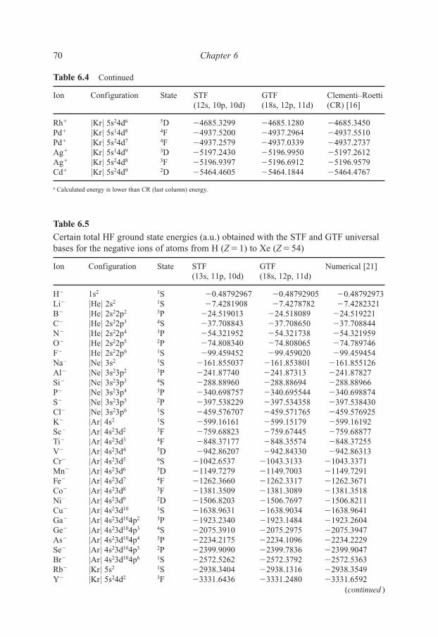
70 Chapter 6
Table 6.5
Certain total HF ground state energies (a.u.) obtained with the STF and GTF universalbases for the negative ions of atoms from H (Z�1) to Xe (Z�54)
Ion Configuration State STF GTF Numerical [21](13s, 11p, 10d) (18s, 12p, 11d)
H� 1s2 1S �0.48792967 �0.48792905 �0.48792973Li� |He| 2s2 1S �7.4281908 �7.4278782 �7.4282321B� |He| 2s22p2 3P �24.519013 �24.518089 �24.519221C� |He| 2s22p3 4S �37.708843 �37.708650 �37.708844N� |He| 2s22p4 3P �54.321952 �54.321738 �54.321959O� |He| 2s22p5 2P �74.808340 �74.808065 �74.789746F� |He| 2s22p6 1S �99.459452 �99.459020 �99.459454Na� |Ne| 3s2 1S �161.855037 �161.853801 �161.855126Al� |Ne| 3s23p2 3P �241.87740 �241.87313 �241.87827Si� |Ne| 3s23p3 4S �288.88960 �288.88694 �288.88966P� |Ne| 3s23p4 3P �340.698757 �340.695544 �340.698874S� |Ne| 3s23p5 2P �397.538229 �397.534358 �397.538430Cl� |Ne| 3s23p6 1S �459.576707 �459.571765 �459.576925K� |Ar| 4s2 1S �599.16161 �599.15179 �599.16192Sc� |Ar| 4s23d2 3F �759.68823 �759.67445 �759.68877Ti� |Ar| 4s23d3 4F �848.37177 �848.35574 �848.37255V� |Ar| 4s23d4 5D �942.86207 �942.84330 �942.86313Cr� |Ar| 4s23d5 6S �1042.6537 �1043.3133 �1043.3371Mn� |Ar| 4s23d6 5D �1149.7279 �1149.7003 �1149.7291Fe� |Ar| 4s23d7 4F �1262.3660 �1262.3317 �1262.3671Co� |Ar| 4s23d8 3F �1381.3509 �1381.3089 �1381.3518Ni� |Ar| 4s23d9 2D �1506.8203 �1506.7697 �1506.8211Cu� |Ar| 4s23d10 1S �1638.9631 �1638.9034 �1638.9641Ga� |Ar| 4s23d104p2 3P �1923.2340 �1923.1484 �1923.2604Ge� |Ar| 4s23d104p3 4S �2075.3910 �2075.2975 �2075.3947As� |Ar| 4s23d104p4 3P �2234.2175 �2234.1096 �2234.2229Se� |Ar| 4s23d104p5 2P �2399.9090 �2399.7836 �2399.9047Br� |Ar| 4s23d104p6 1S �2572.5262 �2572.3792 �2572.5363Rb� |Kr| 5s2 1S �2938.3404 �2938.1316 �2938.3549Y� |Kr| 5s24d2 3F �3331.6436 �3331.2480 �3331.6592
Rh� |Kr| 5s24d6 5D �4685.3299 �4685.1280 �4685.3450Pd� |Kr| 5s14d8 4F �4937.5200 �4937.2964 �4937.5510Pd� |Kr| 5s24d7 4F �4937.2579 �4937.0339 �4937.2737Ag� |Kr| 5s14d9 3D �5197.2430 �5196.9950 �5197.2612Ag� |Kr| 5s24d8 3F �5196.9397 �5196.6912 �5196.9579Cd� |Kr| 5s24d9 2D �5464.4605 �5464.1844 �5464.4767
a Calculated energy is lower than CR (last column) energy.
Table 6.4 Continued
Ion Configuration State STF GTF Clementi–Roetti(12s, 10p, 10d) (18s, 12p, 11d) (CR) [16]
(continued )
Else_EAMC-TRSIC_ch006.qxd 5/4/2007 07:32 Page 70
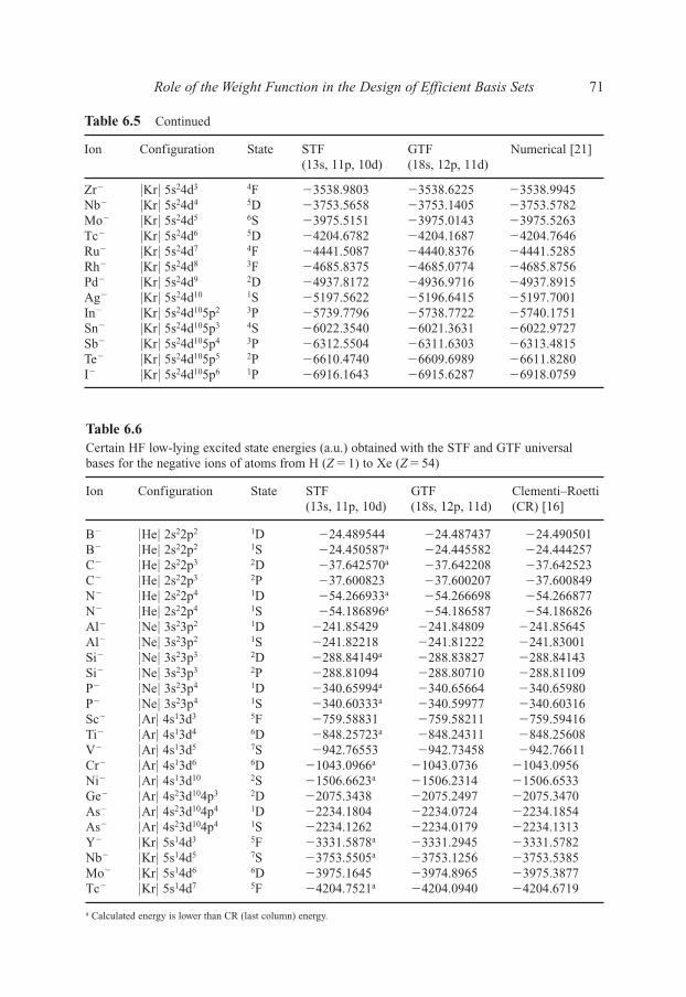
Role of the Weight Function in the Design of Efficient Basis Sets 71
Table 6.5 Continued
Ion Configuration State STF GTF Numerical [21](13s, 11p, 10d) (18s, 12p, 11d)
Zr� |Kr| 5s24d3 4F �3538.9803 �3538.6225 �3538.9945Nb� |Kr| 5s24d4 5D �3753.5658 �3753.1405 �3753.5782Mo� |Kr| 5s24d5 6S �3975.5151 �3975.0143 �3975.5263Tc� |Kr| 5s24d6 5D �4204.6782 �4204.1687 �4204.7646Ru� |Kr| 5s24d7 4F �4441.5087 �4440.8376 �4441.5285Rh� |Kr| 5s24d8 3F �4685.8375 �4685.0774 �4685.8756Pd� |Kr| 5s24d9 2D �4937.8172 �4936.9716 �4937.8915Ag� |Kr| 5s24d10 1S �5197.5622 �5196.6415 �5197.7001In� |Kr| 5s24d105p2 3P �5739.7796 �5738.7722 �5740.1751Sn� |Kr| 5s24d105p3 4S �6022.3540 �6021.3631 �6022.9727Sb� |Kr| 5s24d105p4 3P �6312.5504 �6311.6303 �6313.4815Te� |Kr| 5s24d105p5 2P �6610.4740 �6609.6989 �6611.8280I� |Kr| 5s24d105p6 1P �6916.1643 �6915.6287 �6918.0759
Table 6.6 Certain HF low-lying excited state energies (a.u.) obtained with the STF and GTF universalbases for the negative ions of atoms from H (Z�1) to Xe (Z�54)
Ion Configuration State STF GTF Clementi–Roetti(13s, 11p, 10d) (18s, 12p, 11d) (CR) [16]
B� |He| 2s22p2 1D �24.489544 �24.487437 �24.490501B� |He| 2s22p2 1S �24.450587a �24.445582 �24.444257C� |He| 2s22p3 2D �37.642570a �37.642208 �37.642523C� |He| 2s22p3 2P �37.600823 �37.600207 �37.600849N� |He| 2s22p4 1D �54.266933a �54.266698 �54.266877N� |He| 2s22p4 1S �54.186896a �54.186587 �54.186826Al� |Ne| 3s23p2 1D �241.85429 �241.84809 �241.85645Al� |Ne| 3s23p2 1S �241.82218 �241.81222 �241.83001Si� |Ne| 3s23p3 2D �288.84149a �288.83827 �288.84143Si� |Ne| 3s23p3 2P �288.81094 �288.80710 �288.81109P� |Ne| 3s23p4 1D �340.65994a �340.65664 �340.65980P� |Ne| 3s23p4 1S �340.60333a �340.59977 �340.60316Sc� |Ar| 4s13d3 5F �759.58831 �759.58211 �759.59416Ti� |Ar| 4s13d4 6D �848.25723a �848.24311 �848.25608V� |Ar| 4s13d5 7S �942.76553 �942.73458 �942.76611Cr� |Ar| 4s13d6 6D �1043.0966a �1043.0736 �1043.0956Ni� |Ar| 4s13d10 2S �1506.6623a �1506.2314 �1506.6533Ge� |Ar| 4s23d104p3 2D �2075.3438 �2075.2497 �2075.3470As� |Ar| 4s23d104p4 1D �2234.1804 �2234.0724 �2234.1854As� |Ar| 4s23d104p4 1S �2234.1262 �2234.0179 �2234.1313Y� |Kr| 5s14d3 5F �3331.5878a �3331.2945 �3331.5782Nb� |Kr| 5s14d5 7S �3753.5505a �3753.1256 �3753.5385Mo� |Kr| 5s14d6 6D �3975.1645 �3974.8965 �3975.3877Tc� |Kr| 5s14d7 5F �4204.7521a �4204.0940 �4204.6719
a Calculated energy is lower than CR (last column) energy.
Else_EAMC-TRSIC_ch006.qxd 5/4/2007 07:32 Page 71

72 Chapter 6
For the cations with s and p orbitals, Koga’s basis set size varies from (7s, 5p)to (11s, 7p) for C� through Ca�. For the cations with s, p, and d orbitals, Koga’sbasis size varies from (11s, 7p, 5d) to (13s, 12p, 8d) for Sc� through Xe�. In gen-eral, for the cations, our STF energy results are on average one decimal figuremore accurate than Koga’s results but, although our results are better for thecations lighter than Zr�, one has to recognize that Koga et al. used smaller basissets. From Zr� onwards, Koga’s basis set size becomes more similar to our uni-versal basis size (12s, 10p, 10d).
The average errors in our STF energies with respect to the numerical HF ener-gies for the cations are, respectively, 0.000012, 0.000121, 0.00136, and 0.02387millihartrees for the first, second, third, and fourth rows. The average errors in theenergies found by Koga et al. are 0.0004, 0.0063, 0.061, and 0.113 millihartreesfor the respective first-, second-, third-, and fourth-row cations.
For the anions, Koga’s basis set size varies from (8s, 6p) to (11s, 9p) for B�
through Cl�, and for K� it is (12s, 8p). For Sc� through I�, it varies from (12s, 8p,6d) to (14s, 13p, 9d). When we compare our STF energy results with Koga’sresults, we noticed that our results are on average one decimal figure more accu-rate than Koga’s results from H� to Se�. From Br� to Ag�, both STF basis setsizes becomes more similar and, in general, our results have the same accuracyas Koga’s results. From In� onwards, Koga’s results become more accurate thanour results, but we have to bear in mind that he worked with a slightly larger basisset (14s, 13p, 9d) than our universal basis set (13s, 11p, 10d).
The average errors in our STF energies with respect to the numerical HF limits for the anions are, respectively, 0.000044, 0.001757, 0.0026, and 0.3784millihartrees for the first, second, third, and fourth rows. Koga et al. found, for therespective first-, second-, third-, and fourth-row anions, the following averageerrors in the energies: 0.00068, 0.0063, 0.087, and 0.112 millihartrees.
In conclusion, we would like to say that a comparison of our results withKoga’s brings to attention the fact that when we are developing a universal basisset, instead of a fully optimized basis set, we face the penalty of using, mainlyfor lighter atomic systems (from H through Ca), a larger number of basisfunctions than a fully optimized basis set needs to obtain the same degree ofaccuracy. Indeed, our experience in developing universal basis sets alwaysshowed that this penalty is reduced when we work with atomic systems from thethird row on [8, 23–26].
2.4. Role of the Weight Functions in the Evaluation of Total ElectronicEnergies
Since the Griffin–Hill–Wheeler–Hartree–Fock (GHWHF) equations (seeChapter 4) are obtained from the minimization of the functional E with respectto the weight functions, fi, the description of fi governs the quest for the total
Else_EAMC-TRSIC_ch006.qxd 5/4/2007 07:32 Page 72

Role of the Weight Function in the Design of Efficient Basis Sets 73
energies for any atomic system. Achieving the best HF energy for an atomic sys-tem means obtaining the best description of fi through numerical integration, i.e.,the ID technique outlined in Chapter 4 (Section 4).
The quest for the best weight function associated with any atomic orbital isimplemented by the integral discretization described by Equations (4.12), and thediscretization parameters �min, ��, and N are responsible for attaining the bestweight function. When the GCHF method is employed to generate basis sets, thenumber of points N determines the size of the basis and, certainly, the larger thevalue of N, the lower is the ground state energy obtained. But the chosen value forN is a compromise between accuracy and size of the basis set.
In the section on “Weight Functions,” we presented a series of weight func-tions generated by the integration mesh of the neutral atoms from H through Xeand discussed some practical aspects and properties of the weight functions. Allthe observations we brought about in the aforesaid section are valid with respectto the weight functions of the positive and negative ions presented here but, atthis time, we add a few relevant remarks especially related to the ionic speciesand focus on the Gaussians weight functions.
In Fig. 6.9 we have plotted the Gaussian 2s weight functions for the isoelec-tronic species Be� and Li, and Be and Li�. It appears that the integration intervalwith �min ��0.55 is satisfactory for the Be� and Be species, but it is not adequatefor the alkaline atom, and it is particularly insufficient for the negative ion of Li.This is a feature that also appears for the highest occupied orbital of the other alka-line atoms considered, i.e., Na through Cs. For this reason, it was necessary to shift
Fig. 6.9 The 2s Gaussian weight functions for Be�, Be, Li, and Li�. The point �min ��0.55for s functions is indicated.
Else_EAMC-TRSIC_ch006.qxd 5/4/2007 07:32 Page 73

�min for the GTF universal basis set of the negative ions to �min ��0.75 for the ssymmetry (�min for s symmetry STF weight functions was shifted to �0.21). Thep and d symmetry weight functions also required a revision of the integration lim-its for the negative ions.
In Fig. 6.10, we show how the Gaussian 2s weight functions obtained for thespecies Li and Li� compare with the corresponding fully integrated weight func-tions. For both Li and Li�, the need for higher values of the weight functions tocompensate the truncation of the integration range surfaces. In view of our goalof generating “universal” (a unique set of exponents to be used for all atomsunder consideration) bases of tractable size, we opted to retain �min values that,in a few cases, did not accomplish a complete numerical integration. It is relevantto point out that this limitation of the �min values has little effect on the total HFenergy, even for the alkaline atoms and negative ions. Of course, the presentselection of lower limits for the numerical integration range should be reconsid-ered with caution if properties demanding very diffuse orbitals were of interest[20]. Otherwise, for most of the atoms and ions considered, the numerical inte-gration ranges are adequate. This is illustrated in Fig. 6.11 with the example ofthe Gaussian 2p weight functions for neutral and charged fluorine atoms.
Owing to the novelty of our procedure for the selection of basis set exponents,we provide some additional details on how a basis set is initially tailored with theGCHF method. Let us take as an example the tailoring of a universal basis set,nonetheless this recipe can be applied to any kind of basis set (universal or atom-adapted STF or GTF basis sets).
74 Chapter 6
Fig. 6.10 Comparison of the Gaussian 2s weight function for Li and Li� and the completeintegration range.
Else_EAMC-TRSIC_ch006.qxd 5/4/2007 07:32 Page 74

Since a universal basis set for H to Xe is desired, GCHF calculations for thesetwo and a few more sample atoms are performed with some small and arbitraryvalues for N. The plots of the weight functions indicate adequate ranges for thenumerical integration, i.e., the lowest (�min) and the highest (�max) values out-side which the weight functions for most atoms and occupied orbitals are negli-gible (a few very diffuse orbitals may demand even lower values for �min and�max but the inclusion of these would significantly enlarge the basis with littleor no influence for the total energy). Within this range, one chooses a constantincrement �� and the number of points N, which are mutually dependent. It isthe value of N that determines the size of the basis set, and certainly the largerthe value of N, the lower is the ground state energy. The chosen value of N is acompromise between accuracy and the basis set size to be handle in molecularcalculations.
Also, we would like to remark that since Equation (4.4) represents a continu-ous and infinite superposition, in the GCHF method we do not need to specifythe principal quantum numbers, n, for the various symmetries of the generatorfunctions, �i, as the weight functions, fi, distinguish the n states. Thus, all our uni-versal bases presented here consist of the simplest 1s, 2p, and 3d STFs or GTFs.
3. Is the Generator Coordinate Weight Function a Distribution?
Here, we would like to bring to the attention of the reader to the fact that theweight function of the GCHF method can be considered as a distribution
Role of the Weight Function in the Design of Efficient Basis Sets 75
Fig. 6.11 Plot of the 2p Gaussian weight functions for F�, F, and F�.
Else_EAMC-TRSIC_ch006.qxd 5/4/2007 07:32 Page 75

76 Chapter 6
function [27,28]. In Chapter 3 we showed that the trivial independent parti-cle model for para-helium [see Equation (3.2)] has a Dirac � distribution[Equation (3.5)] [19] as a solution for the weight function. One may wonderwhether all weight functions are distributions. Nonetheless, there is no uniquenotion of the distribution character of a function among mathematicians (seefor instance References [27,28]).
Following Reference [28], we may define a distribution f (x) symbolically by
(6.1)
provided that the integral exists. In this definition, we call �(x) a test function if�(x) is infinitely derivable belonging to C � (basically meaning that the deriva-tives of all orders exist and are continuous), and if �(x) should tend to zero out-side a finite interval (a,b).
Before we proceed further with our analogies, we stumble on the requirement�(x)�0 everywhere. While our 1s, 2p,… GTF weight functions do obey thisrequirement, 2s, 3p,… have nodes being nonpositive in some segments. It is notdifficult to understand this behavior since in our algorithm, we enter only with1s, 2p,… functions and the integration range given by the discretization of theexponents (i.e., the discretization parameters �min, ��, and N). Thus, the burdenof guarantying orthogonality between 1s and 2s, 2p and 3p, and so on is left forthe weight functions.
In an experiment in progress, entering initially in our algorithm with orthogo-nal bases we may expect all weight functions to be positive everywhere. We leavethis question open for further considerations, either by us or other interestedworkers.
4. The Future of Generating Basis Sets for Atomic and MolecularCalculations Using the GCHF Method
Along the years, the GCHF method became very popular and was the object ofhundreds of papers. Other researches have also contributed to the improvementof the method as well as in generating a large number of basis sets for atomicand molecular nonrelativistic calculations. We would like to cite some of theseworks (the main ones) and say that before the polynomial generator coordinateHartree–Fock (pGCHF) method presented in Chapter 5 (Section 5), other col-leagues tried to improve the way of generating basis sets with the GCHF methodby segmenting the integration space �, i.e., for the occupied s, p, d, etc. atomicorbitals they used different sets of �min and �� for a given Ns, Np, Nd, etc. (i.e.,the basis set size N for each atomic symmetry s, p, d, etc.). Then, for instance,
f x x dx( ) ( ) ,�∫
Else_EAMC-TRSIC_ch006.qxd 5/4/2007 07:32 Page 76
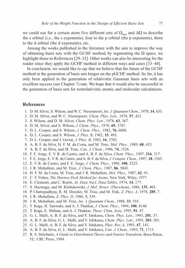
we could use for a certain atom five different sets of �min and �� to describethe s orbital (i.e., the s exponents), four to the p orbital (the p exponents), threeto the d orbital (the d exponents), etc.
Among the works published in the literature with the aim to improve the wayof obtaining basis sets with the GCHF method, by segmenting the � space, wehighlight those in References [29–32]. Other works can also be interesting for thereader since they apply the GCHF method in different ways and cases [33–44].
In conclusion, we would like to say that we believe that the future of the GCHFmethod in the generation of basis sets hinges on the pGCHF method. So far, it hasonly been applied in the generation of relativistic Gaussian basis sets with anexcellent success (see Chapter 7) rate. We hope that it would also be successful inthe generation of basis sets for nonrelativistic atomic and molecular calculations.
References
1. D. M. Silver, S. Wilson, and W. C. Nieuwpoort, Int. J. Quantum Chem., 1978, 14, 635.2. D. M. Silver, and W. C. Nieuwpoort, Chem. Phys. Lett., 1978, 57, 421.3. S. Wilson, and D. M. Silver, Chem. Phys. Lett., 1978, 63, 367.4. D. M. Silver, and S. Wilson, J. Chem. Phys., 1978, 69, 3787.5. D. L. Cooper, and S. Wilson, J. Chem. Phys., 1982, 76, 6088.6. D. L. Cooper, and S. Wilson, J. Phys. B, 1982, 15, 493.7. D. L. Cooper, and J. Gerrat, J. Phys. B, 1983, 16, 3703.8. A. B. F. da Silva, H. F. M. da Costa, and M. Trsic, Mol. Phys., 1989, 68, 433.9. A. B. F. da Silva, and M. Trsic, Can. J. Chem., 1996, 74, 1526.
10. F. E. Jorge, E. V. R. de Castro, and A. B. F. da Silva, Chem. Phys., 1997, 216, 317.11. F. E. Jorge, E. V. R. de Castro, and A. B. F. da Silva, J. Comput. Chem., 1997, 18, 1565.12. E. V. R. de Castro, and F. E. Jorge, J. Chem. Phys., 1998, 108, 5225.13. J. R. Mohallem, and M. Trsic, J. Chem. Phys., 1987, 86, 5043.14. H. F. M. da Costa, M. Trsic, and J. R. Mohallem, Mol. Phys., 1987, 62, 91.15. C. F. Fisher, The Hartree-Fock Method for Atoms, New York, Wiley, 1977.16. E. Clementi, and C. Roetti, At. Data Nucl. Data Tables, 1974, 14, 177.17. S. Huzinaga, and M. Klobukowski, J. Mol. Struct. (Theochem), 1986, 135, 403.18. P. Chattopadhyay, R. M. Dreizler, M. Trsic, and M. Fink, Z. Phys. A, 1978, 285, 7.19. J. R. Mohallem, Z. Phys. D, 1986, 3, 339.20. J. R. Mohallem, and M. Trsic, Int. J. Quantum Chem., 1988, 33, 555.21. T. Koga, H. Tatewaki, and A. J. Thakkar, J. Chem. Phys., 1994, 100, 8140.22. T. Koga, E. Shibata, and A. J. Thakkar, Theor. Chim. Acta, 1995, 91, 47.23. G. L. Malli, A. B. F. da Silva, and Y. Ishikawa, Chem. Phys. Lett., 1993, 201, 37.24. A. B. F. da Silva, G. L. Malli, and Y. Ishikawa, Chem. Phys. Lett., 1993, 203, 201.25. G. L. Malli, A. B. F. da Silva, and Y. Ishikawa, Phys. Rev. A, 1993, 47, 143.26. A. B. F. da Silva, G. L. Malli, and Y. Ishikawa, Can. J. Chem., 1993, 71, 1713. 27. R. S. Strichartz, A Guide to Distribution Theory and Fourier Transform, Boca Raton,
FL: CRC Press, 1994.
Role of the Weight Function in the Design of Efficient Basis Sets 77
Else_EAMC-TRSIC_ch006.qxd 5/4/2007 07:32 Page 77

28. E. Butkov, Mathematical Physics, Reading, MA: Addison–Wesley Publishing Co.,1968.
29. F. E. Jorge, and E. V. R. de Castro, Chem. Phys. Lett., 1999, 302, 454.30. E. V. R. de Castro, F. E. Jorge, and J. C. Pinheiro, Chem. Phys., 1999, 243, 1.31. J. C. Pinheiro, F. E. Jorge, and E. V. R. de Castro, Int. J. Quantum Chem., 2000, 78, 15.32. A. C. Neto, F. E. Jorge, and M. de Castro, Int. J. Quantum Chem., 2002, 88, 252.33. R. Custodio, M. Giordan, N. H. Morgon, and J. D. Goddard, Int. J. Quantum Chem.,
1992, 42, 411.34. R. Custodio, J. D. Goddard, M. Giordan, and N. H. Morgon, Can. J. Chem., 1992,
70, 580.35. N. H. Morgon, J. Phys. Chem. A, 1998, 102, 2050.36. I. N. Jardim, O. Treu, M. A. U. Martines, M. R. Davolos, M. Jafelicci, and J. C. Pinheiro,
J. Mol. Struct. (Theochem), 1999, 464, 15.37. J. C. Pinheiro, A. B. F. da Silva, and M. Trsic, J. Mol. Struct. (Theochem), 1997, 394,
107.38. J. C. Pinheiro, A. B. F. da Silva, and M. Trsic, Int. J. Quantum Chem., 1997, 63, 927.39. J. C. Pinheiro, F. E. Jorge, and E. V. R. de Castro, J. Mol. Struct. (Theochem), 1999,
491, 81.40. J. C. Pinheiro, M. Trsic, and A. B. F. da Silva, J. Mol. Struct. (Theochem), 2001, 539, 29.41. F. R. Sensato, R. Custodio, Q. B. Cass, E. Longo, M. Z. Hernandes, R. L. Longo, and
J. Andres, J. Mol. Struct. (Theochem), 2002, 589, 251.42. J. M. D. Trevas, and R. Custodio, J. Mol. Struct. (Theochem), 2001, 539, 17.43. H. F. M. da Costa, A. B. F. da Silva, J. R. Mohallem, A. M. Simas, and M. Trsic,
Chem. Phys., 1991, 154, 379.44. A. B. F. da Silva, and M. Trsic, Mol. Phys., 1993, 78, 1301.
78 Chapter 6
Else_EAMC-TRSIC_ch006.qxd 5/4/2007 07:32 Page 78

Chapter 7
The Generator Coordinate Dirac–Fock Methodand Relativistic Calculations for Atoms andMolecules
1. Introduction
In the recent years there has been a great interest in using Gaussian-typefunctions (GTFs) as basis set for relativistic calculations [1–5]. This is mainlydue to the work of Ishikawa et al. [1,4–7] who have emphasized that the imposi-tion of finite nuclear boundary conditions for solutions of the Dirac–Fock (DF)equations results in a solution that is Gaussian at the origin, and therefore theGTFs of integer power of r are appropriate basis functions for the finite nuclearmodel. The GTFs that satisfy the boundary conditions for the finite nucleus auto-matically satisfy the condition of the so-called kinetic balance for a finite speedof light [7].
In the beginning of the 1990s, da Silva et al. [8–12] presented universal Gaussianbasis sets for relativistic calculations. In that papers, the generator coordinateHartree–Fock (GCHF) method (developed initially for a nonrelativistic environ-ment, see Chapter 6) was employed to generate universal Gaussian function expo-nents and afterward use them in a relativistic code to assess their efficiency inproviding Dirac–Fock–Coulomb (DFC) and Dirac–Fock–Breit (DFB) atomic ener-gies. This procedure actually was first employed by Matsuoka and Huzinaga [13]who showed that orbital exponents optimized through the well-tempered schemefor nonrelativistic atoms (i.e., orbital exponents obtained from a nonrelativisticenvironment) can be carried over to relativistic calculations to produce wave func-tions close to the relativistic Hartree–Fock (HF) limit (or DF limit). Thus, insteadof optimizing the four well-tempered parameters �, �, �, and � anew in a DF codethey simply carried over the same optimized well-tempered exponents for a non-relativistic atom to the relativistic calculation since this procedure turned out to begood enough to produce DFC energy results close to those obtained by numericalsolution of the DF equations. After this pioneer work [13], instead of going throughthe cumbersome procedure of optimizing orbital exponents variationally inside ofa relativistic environment (code), that is far more expensive than their nonrelativis-tic counterpart, one could find several relativistic atomic calculations in the litera-ture following the Matsuoka–Huzinaga recipe [1–5,8–12].
Else_EAMC-TRSIC_ch007.qxd 5/4/2007 07:52 Page 79

The idea of Matsuoka and Huzinaga of employing GTFs exponents (originallyoptimized in a nonrelativistic environment and afterward use them to performrelativistic atomic and molecular calculations just adding to the original set ofnonrelativistic GTFs exponents a couple of larger exponents with the aim to bet-ter describe the behavior of the inner electrons that are closer to the finitenucleus) was extremely practical, but the idea of generating GTFs exponents inthe DF environment could not be forsaken. In fact, through the generation ofGTFs exponents directly from the DF environment we could obtain a more ade-quate set of GTFs exponents to be used in relativistic atomic and molecular cal-culations since they would be the GTFs exponents directly extracted (generated)from the DF formalism.
The idea of generating GTFs exponents directly from the DF environment wasachieved in 1996 when Jorge and da Silva published two papers introducing the gen-erator coordinate version of the DF equations that came to be named as “the gener-ator coordinate Dirac–Fock (GCDF) method” [14,15]. What we call the GCDFmethod comprises actually two formalisms, namely: “the generator coordinateDirac–Fock–Coulomb (GCDFC) formalism” [14] and “the generator coordinateDirac–Fock–Breit (GCDFB) formalism” [15].
2. The Generator Coordinate Dirac–Fock–Coulomb Formalism
For a close-shell (2M-electron) atom of nuclear charge Z, the unperturbedDirac–Coulomb (DC) Hamiltonian, HDC, in atomic units is
(7.1)
where hD(i) is the Dirac Hamiltonian of the ith electron and Vij is the instanta-neous Coulomb interaction between electrons i and j, namely
(7.2)
In Equation (7.2), rij is the distance between the ith and jth electrons and theDirac Hamiltonian, hD, in Equation (7.1) has the following form
(7.3)
where � and � are the Dirac matrices in conventional representation, namely
(7.4)��
��� �
�0
00 00 2I
⎛⎝⎜
⎞⎠⎟
⎛⎝⎜
⎞⎠⎟and .
h c c VD � � �� �p + 2nuc ,
V rij ij�1 ./
H h i V i jDC Di
iji j
� � �( ) , ,,
∑ ∑
80 Chapter 7
Else_EAMC-TRSIC_ch007.qxd 5/4/2007 07:52 Page 80

In the Dirac matrices � and � of Equation (7.4), the � are the 2�2 Pauli matri-ces and I is a 2 �2 unit matrix. In Equation (7.3), p is the momentum operatorand Vnuc is the potential energy due to the interaction between the nucleus and theith electron. Thus, the total energy is given by
(7.5)
where � is the normalized total wave function.The total wave function is an antisymmetrized combination of one-electron
orbitals defined as
(7.6)
where Pn�(r) and Qn�(r) are the large and small radial wave functions, respec-tively, and satisfy the orthonormality condition
(7.7)
where �nn� is the Kronecker delta. The orbitals �n�m(r,�,�) in Equation (7.6) forman orthonormal set and the choice of the phase in Equation (7.6) enables us to usereal radial functions for both large and small components [16]. The angular func-tions ��m(�,�) in Equation (7.6) are expressed in terms of the Clebsch–Gordoncoefficients, the normalized spherical harmonics and the two-component Paulispinors [16]. The quantum number � classifies the orbitals according to theirsymmetry species analogous to the orbital angular momentum in the nonrelati-vistic case.
In the DFC self-consistent-field (SCF) scheme, the behavior of an electron ina central field potential, V, is described by a radial equation of the form
(7.8)
where
(7.9)
with
(7.10)���
�� �d
dr r
FV c
c V c�
�
�
��
�
�
� 2 2
⎛⎝⎜
⎞⎠⎟
F n n n� � � �� �� ,
� �P r P r Q r Q r drn n n n nn� � � � ��� �( ) ( ) ( ) ( ) ,0
� � � �
�
� �� �∫
� �� �� ��
� �
� �n m
n m
n m
rr P r
ir Q r( , , )
( ) ( , )
( ) ( , ),
1
1�
�
��
�
��
⎛⎝⎜
⎞⎠⎟
E HDC� � � ,
Dirac–Fock Method and Relativistic Calculations 81
Else_EAMC-TRSIC_ch007.qxd 5/4/2007 07:52 Page 81
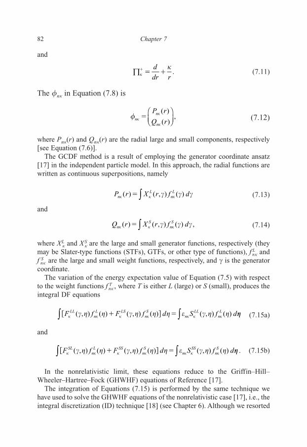
and
(7.11)
The �n� in Equation (7.8) is
(7.12)
where Pn�(r) and Qn�(r) are the radial large and small components, respectively[see Equation (7.6)].
The GCDF method is a result of employing the generator coordinate ansatz[17] in the independent particle model. In this approach, the radial functions arewritten as continuous superpositions, namely
(7.13)
and
(7.14)
where XL� and XS
� are the large and small generator functions, respectively (theymay be Slater-type functions (STFs), GTFs, or other type of functions), f L
n� andf S
n� are the large and small weight functions, respectively, and � is the generatorcoordinate.
The variation of the energy expectation value of Equation (7.5) with respectto the weight functions f T
n� , where T is either L (large) or S (small), produces theintegral DF equations
(7.15a)
and
(7.15b)
In the nonrelativistic limit, these equations reduce to the Griffin–Hill–Wheeler–Hartree–Fock (GHWHF) equations of Reference [17].
The integration of Equations (7.15) is performed by the same technique wehave used to solve the GHWHF equations of the nonrelativistic case [17], i.e., theintegral discretization (ID) technique [18] (see Chapter 6). Although we resorted
� �F f F f d S f dSLnL SS
nS
nSS
nS
� � � � � � �� � � ( , ) ( ) ( , ) ( ) ( , ) ( )� � ∫∫ .
� �F f F f d S f dLLnL LS
nS
nLL
nL
� � � � � � �� � � ( , ) ( ) ( , ) ( ) ( , ) ( )� � ∫∫
Q r X r f dnS
nS
� � �� � �( ) ( , ) ( ) ,� ∫
P r X r f dnL
nL
� � �� � �( ) ( , ) ( )� ∫
�nn
n
P r
Q r��
�
�( )
( ),
⎛⎝⎜
⎞⎠⎟
���� � �
d
dr r.
82 Chapter 7
Else_EAMC-TRSIC_ch007.qxd 5/4/2007 07:52 Page 82

to a discretization technique for the solution of Equations (7.15), the continuouscharacter of the original generator coordinate method (GCM) was retained. Thiswas achieved by simply choosing equally spaced discretization points in anattempt to find an adequate numerical integration of Equations (7.15). This pro-cedure characterizes the ID technique and it is implemented through a relabelingof the generator coordinate space, namely
(7.16)
To solve Equations (7.15) by discretization, and Pn�(r) and Qn�(r) become
(7.17)
and
(7.18)
The term f Tn�(�w)��w, where T stands for L or S in Equations (7.17) and (7.18),
may be regarded as expansion coefficients while {�w} becomes the set of basisexponents. Thus, basis set exponents are interpreted as a mesh of ID points.
The lowest (�min) and the highest (�max) values for the generator coordinateare chosen so as to embrace the adequate integration range for the f T
n�. Theformer values are related through
(7.19)
where N is the number of discretization points. In fact, the choice of the dis-cretization points determines the exponents of the basis functions and with the IDtechnique the cumbersome procedure of optimizing orbital exponents variation-ally is avoided since the GCDF method needs only a good numerical integrationto generate a set of exponents to adequately simulate Equations (7.15).
It is import to mention that at each iteration of the SCF procedure the integra-tions are implemented numerically through discretization. This procedure leadsformally to the Dirac–Fock–Roothaan (DFR) equations and therefore can be easilyimplemented in any DFR code.
After discretization, Equations (7.15) can be written in the matrix form as
(7.20)F f S f E� � � � �� ,
� � ��max min ( 1) ,� � �N
Q r X r fnS
w nS
w ww
� � �� � �( ) ( , ) ( ) .� �∑
P r X r fnL
w nL
w ww
� � �� � �( ) ( , ) ( )� �∑
� � ��ii
Ai A� � � � �
ln( 1), 1.min
�
Dirac–Fock Method and Relativistic Calculations 83
Else_EAMC-TRSIC_ch007.qxd 5/4/2007 07:52 Page 83

where the overlap matrix S� is given in a block-diagonal form
(7.21)
and the superscripts LL and SS are related to the large and small components,respectively.
The DF matrix can be written as
(7.22)
where the one-electron part o� is
(7.23)
The two-electron part t� , which consists of the matrices of two-electronCoulomb and exchange interactions, is given by
(7.24)
The one-electron matrix elements are given in terms of the generator coordi-nate � by
(7.25)
(7.26)
where TT is either LL or SS,
(7.27)
and
(7.28)�� � ���
�ijLS L
iS
jX rd
dr rX r dr� ��
�
( , ) ( , ) .0
⎛⎝⎜
⎞⎠⎟∫
�� � ���
�ijSL S
iL
jX rd
dr rX r dr� �
�
( , ) ( , ) ,0
⎛⎝⎜
⎞⎠⎟∫
S X r X r drijTT T
iT
j� � �� ���
( , ) ( , ) ,0∫
V X r V r X r drijTT T
iT
j� � �� ���
( , ) ( ) ( , ) ,nuc
0∫
tJ K K
K J K�� � �
� � �
�� �
� �
LL LL LS
SL SS SS
⎛⎝⎜
⎞⎠⎟
.
oV
V S�
� �
� � �
��
LL LS
SL SS SS
c
c c
�
� 2.
2
⎛⎝⎜
⎞⎠⎟
F o t� � �� � ,
SS 0
S��
�
�LL
SS0
⎛⎝⎜
⎞⎠⎟
84 Chapter 7
Else_EAMC-TRSIC_ch007.qxd 5/4/2007 07:52 Page 84

Dirac–Fock Method and Relativistic Calculations 85
The two-electron matrices, J�TT and K�
TT�, where the superscripts T and T� areeither L or S, have matrix elements of the form
(7.29)
and
(7.30)
The superscripts TT� represent a pair LS or SL. The Coulomb and exchange inte-grals in Equations (7.29) and (7.30) are given in terms of the generator coordi-nate � and in terms of the GTFs {XL
�} and {X S�} as
(7.31)
and
(7.32)
where
(7.33)
The density matrices are defined in terms of the generator coordinate � as
(7.34)
where f �T are the weight functions.
The GTFs generated with the GCDFC formalism satisfy the relativistic bound-ary conditions associated with the finite nuclear model for a finite speed of lightand conform to the so-called kinetic balance at the nonrelativistic limit.
In the uniform charge approximation of the finite nucleus, the potential insidethe nucleus is represented by (see Reference [7] and references therein)
(7.35)VZ
R
r
Rnucin
2
223 .�� �
⎛⎝⎜
⎞⎠⎟
⎛⎝⎜
⎞⎠⎟
D f fijTT T
iT
j� � �� �� ( ) ( ) ,
U r sr s r s
s r s r�
� �
� �( , ),
, .
1
1�
�
�
��
⎧⎨⎩
K X r X r U r s X s X sij kTT T
iT
kT
jT
� ��
� � � � �� � �,, ( , ) ( , ) ( , ) ( , ) (� � ��
l
,TT ,, ) ,00
�l
dr ds��
∫∫
J X r X r U r s X s X sij kTT TT T
iT
jT
kT
� ��
� � � � �� � �,, , ( , ) ( , ) ( , ) ( , ) (� � ��
l,, )
00
�l
dr ds��
∫∫
K j b jj D KijTT
kTT
ij kTT TT
k� � � � �
�
��
� �� � � ��
(2 1) ( ) .,,
l l
l
,∑∑
J j D J D JijTT
kTT
ij kTT TT
kTT
ij kT
� � � � � � �� �� �� � � �(2 1) ,0, ,
,0,�
l l l l
TT TT
k
, ���, ,l∑
Else_EAMC-TRSIC_ch007.qxd 5/4/2007 07:52 Page 85

In Equation (7.35), R is the nuclear radius given by [19]
(7.36)
where M is the atomic mass number. The potential outside the nucleus is givenby the Coulomb potential, V nuc
out ��Z/r. With this representation of the potential,the s1/2 solutions near the origin may be given as [5]
(7.37a)
and
(7.37b)
so that for �w arbitrary parameters we have
(7.38)
and
(7.39)
In Equations (7.37), P(r)/r has a finite value and zero slope at the originwhereas Q(r)/r vanishes there. Thus, in the finite nuclear model the GTF of inte-ger power of r are appropriate basis functions since the imposition of the finitenuclear boundary results in a solution that is Gaussian at the origin.
If, for instance, we choose for the s1/2 states the radial large-component basisset {X L
�} as a GTF of the form
(7.40)
then the condition of kinetic balance imposes the radial small-component basisset {X L
�} to be [20–22]
(7.41)
In Equations (7.40) and (7.41), NL and NS are normalization constants and �w isthe generator coordinate.
X rd
dr rX r N r rS
wL
w S w� ���
� �( , ) ( , ) exp( ).2 2� � � �⎡⎣⎢
⎤⎦⎥
X r N r rLw L w� � �( , ) exp( ),2� �
Q r b r b r r rw( ) exp( ).12
34 2 2� � � �L� �
P r r g r r rw( ) exp( )23 2� � � �L� �
Q r
rb r b r
( ),1 3
3� � �K
P r
rg r g r
( )1 2
24
4� � � + K
R M� � � 2.2677 10 ,5 1 3
86 Chapter 7
Else_EAMC-TRSIC_ch007.qxd 5/4/2007 07:52 Page 86
These kinetically balanced Gaussian basis functions are precisely of theform given in Equations (7.38) and (7.39). This is a consequence of the factthat the exponent of r in the Gaussian basis functions does not depend on thespeed of light. The kinetic balance simply guarantees that the solution of matrixDF equations approaches the correct nonrelativistic limit when c is taken toinfinity [7], and by itself does not guarantee an upper bound on the atomicrelativistic energy. But the combination of the kinetic balance condition withthe choice of the power of r in the Gaussian basis functions as an integer, asrequired by the boundary conditions when one uses the finite nuclear model, iscapable of reproducing the correct relativistic kinematics of an electron nearthe nucleus [23].
3. The Generator Coordinate Dirac–Fock Method and the Generation of a Universal Gaussian Basis Set for the Relativistic Closed-Shell Atoms from Zinc to Nobelium
The first application of the GCDF method in DFC calculations was in the gener-ation of a relativistic universal Gaussian basis set (RUGBS) for the closed-shellatoms from Zinc (Zn) through Nobelium (No) [14]. Here it is interesting toremember, as we have already mentioned in Chapter 6, that a universal basis setrepresents an unique set of basis function exponents that is able to describe alarge number of atoms. On the contrary, an adapted basis set means that for eachatom we have a different set of basis function exponents.
In that work [14], were performed DF-SCF calculations on all relativisticclosed-shell atoms with occupied d and f orbitals, i.e., all relativistic closed-shellatoms from Zn (Z � 30) up to No (Z � 102), and the finite nucleus model of uni-form proton-charge distribution and the restricted kinetic balance condition (one-to-one correspondence between the basis functions of large and smallcomponents) were employed in all of the calculations. The nuclear radius usedwas R�2.2677�10�5 M1/3, where M is the atomic mass number, and the speedof light, c, was assumed as 137.0370 a.u.
The 32 relativistic universal Gaussian exponents generated in this pioneerwork with the GCDFC formalism can be found in Reference [14]. Just for com-parison, we listed in Table 7.1 the DFC energies attained with the RUGBS,geometrical Gaussian basis sets (GGBS) [3], and numerical-finite-differenceprograms [3,10,11,19]. The third column in Table 7.1 (RUGBS size) indicates thenumber of exponents in each relativistic symmetry (s1/2, p1/2, p3/2, d3/2, d5/2, f5/2,and f7/2) taken from the 32 relativistic universal Gaussian exponents. For eachatomic system studied the number of exponents for each s, p, d, and f orbitalsymmetry was increased until the total DFC energy value was attained within anaccuracy comparable (or better) to that obtained with numerical-finite-differenceprograms.
Dirac–Fock Method and Relativistic Calculations 87
Else_EAMC-TRSIC_ch007.qxd 5/4/2007 07:52 Page 87

The 32 relativistic universal Gaussian exponents of Reference [14] were gen-erated by employing the ID technique of the GCDF method, i.e., in the newgenerator coordinate space, �, an equally spaced N-point mesh, �i, was cho-sen so as to obtain an adequate numerical integration range for the relativistics1/2, p1/2, p3/2, d3/2, d5/2, f5/2, and f7/2 symmetries for all atoms studied. The inte-gration range is characterized by the starting point �min, the increment ��, andthe maximum number of points N of the mesh �i. The optimum scaling param-eter A found for all calculations was 6.0.
From the results displayed in Table 7.1 we can see how powerful is the GCDFmethod in the generation of Gaussian basis functions exponents for relativisticcalculations. For the atoms Xe, Sm, W, Hg, Pb, Rn, Ra, Pu, and No, the total DFCenergies computed with the RUGBS are lower than those obtained by usingnumerical-finite-difference DF calculations (last column in Table 7.1). For theatoms Kr, Pd, and Yb, the total DFC energies were the same as those attained byusing numerical-finite-difference DF methods. For the atoms Zn, Ge, Sr, Cd, Sn,
88 Chapter 7
Table 7.1
Total Dirac–Fock–Coulomb (EDFC) energies (in hartree) for Zn (Z�30) through No (Z �102)
Atom Atomic RUGBS EDFC EDFC Numerical-Finite-Mass (M) Size (RUGBS)a (GGBS)b Difference (EDFC)
Zn 65.37 32s30p20d �1794.61338 �1794.61331 �1794.61340c
Ge 72.59 32s30p20d �2097.46672 �2097.46666 �2097.46675c
Kr 83.80 32s30p20d �2788.86168 �2788.86149 �2788.86168c
Sr 87.62 32s30p20d �3178.08131 �3178.08115 �3178.08133c
Pd 106.40 32s30p20d �5044.40343 �5044.40d
Cd 112.40 32s30p20d �5593.32279 �5593.32242 �5593.32286c
Sn 118.69 32s30p20d �6176.14096 �6176.14055 �6176.14105c
Xe 131.30 32s30p20d �7446.90026 �7446.89956 �7446.90018c
Ba 137.34 32s30p20d �8135.65000 �8135.64919 �8135.65006c
Sm 150.35 32s30p20d15f �10429.3726 �10429.2d
Yb 173.04 32s30p20d15f �14067.6811 �14067.7d
W 183.85 32s30p20d15f �16156.2494 �16156.2463 �16156.2484c
Hg 200.59 32s30p20d15f �19648.8712 �19648.8665 �19648.8692c
Pb 207.19 32s30p20d15f �20913.7211 �20913.7151 �20913.7184c
Rn 222.00 32s30p20d15f �23601.9780 �23601.9706 �23601.9742c
Ra 226.00 32s30p20d15f �25028.0218 �25028.0165e
Pu 242.00 32s30p20d15f �29656.5171 �29656.5122e
No 259.00 32s30p20d15f �36740.2908 �36740.2857f
aTotal DFC energies obtained by the relativistic universal Gaussian basis set (RUGBS).bEDFC obtained by using geometric Gaussian basis sets (Reference [3]).cEDFC obtained from Reference [3].dEDFC obtained from Reference [19].eEDFC obtained from Reference [10].fEDFC obtained from Reference [11].
Else_EAMC-TRSIC_ch007.qxd 5/4/2007 07:52 Page 88

and Ba, the total DFC energies were slightly above those attained with thenumerical-finite-difference DF results. The total DFC energies computed withthe RUGBS were consistently more accurate than those obtained by using theGGBS developed by Mohanti and Clementi [3] although our RUGBS be smallerin size than the GGBS [3]. Also, it is interesting to mention that in contrast to theRUGBS, the GGBS are not universal since for each atomic system displayed inTable 7.1 there is a different set of geometrical Gaussian exponents.
The surprising DFC energy results obtained for Xe, Sm, W, Hg, Pb, Rn, Ra,Pu, and No, when compared to numerical-finite-difference calculations, wereattributed to the proper representation of the wave function inside the nucleus dueto the higher numerical accuracy of the relativistic Gaussian basis functions gen-erated with the GCDF method. This evidence was not completely new since inprevious works Malli et al. [12] and Parpia and Mohanty [24] had already veri-fied the possibility of basis set functions be able to better represent the wavefunction inside the nucleus than the numerical-finite-difference methods avail-able by that time. Parpia and Mohanty [24] have also commented that the loweraccuracy of the finite-difference procedure is likely due to the far smaller num-ber of tabulation points in the region of the nuclear “skin,” and the problem getsworse when the atomic number increase since the orbital overlap with the atomicnucleus is known to increase rapidly with the increase of the atomic number.
Although the atomic systems studied [14] were different from those studiedby Parpia and Mohanty [24], the rapid contraction of the orbital wave functionfor very large atomic number was qualitatively similar. Parpia and Mohanty [24]also verified that their basis set calculations for Z � 70 provided lower DFCenergy results than their corresponding numerical-finite-difference calculations.From Table 7.1 we can see that a similar behavior was also found in our DFCcalculations since for Z � 74 we always were able to obtain DFC energy resultslower than the corresponding ones attained with numerical-finite-differencecalculations.
It is also interesting to mention that Malli et al. [12] and Parpia andMohanty [24] came up with the same evidence despite each one had used dif-ferent charge distribution. Malli et al. [12] represented the nucleus as a finitebody of uniform proton charge distribution, and Parpia and Mohanty [24]assumed that the nuclear charge density was distributed in the form of a Fermifunction. In our work[14] we have also used the same charge distribution asMalli et al. [12].
That pioneer work [14] was really important since it reinforced the fact thatsome improvements were needed to be made in relativistic numerical codes tocorrect their bad description for the relativistic kinematics of an electron insidethe nucleus. In 1997, Visscher and Dyall [25] presented in the literature the newrelativistic numerical results for finite-size nucleus models that seem to have cor-rected this problem.
Dirac–Fock Method and Relativistic Calculations 89
Else_EAMC-TRSIC_ch007.qxd 5/4/2007 07:52 Page 89

That time we attributed the high numerical accuracy of our RUGBS to the IDtechnique of the GCDF method, as with the ID technique the relativisticGaussian function exponents were generated by the discretization of the integralDF equations [Equations (7.15)] with the best numerical integration as a goal.In fact, a careful numerical integration of Equations (7.15) is able to providevery accurate Gaussian basis sets for relativistic calculations. Also, it is impor-tant to bring attention to the fact that the GCDF method is an algorithm wherebyGaussian basis sets can be generated directly from a relativistic environment(code) without variational exponent optimization.
Table 7.2 shows the convergence pattern for the Xe atom and from there wecan see that the use of the kinetic balance condition, along with the properboundary conditions imposed on the GTFs, accelerates the convergence and alsocontributes to the DFC energy stability. Also, we can see that the increasing num-ber of points in each s1/2, p1/2, p3/2, d3/2, and d5/2 symmetry rapidly favor the con-vergence of the total DFC energy to a value of �7446.90026 a.u., and by the timewe have reached Ns �32 (number of basis functions for s1/2 symmetry), Np �30(number of basis functions for p1/2 and p3/2 symmetries), and Nd �20 (number ofbasis functions for d3/2 and d5/2 symmetries) the total DFC energy has alreadyconverged to the energy limit of �7446.90026 a.u. Even if we go beyond Ns�32,Np �30, and Nd�20 there is no substantial improvement in the total DFC energy.
Tables 7.3–7.5 display the DFC orbital energies for Xe (Z�54), Rn (Z�86),and No (Z�102), respectively, obtained with the RUGBS. The third column inTables 7.3–7.5 shows the DFC orbital energies for Xe, Rn, and No obtained bynumerical-finite-difference DF calculations. From Tables 7.3–7.5 we can see thatthe DFC orbital energies obtained with the RUGBS for Xe, Rn, and No are ingood agreement when compared to the corresponding numerical-finite-differenceDF orbital energies.
90 Chapter 7
Table 7.2
Convergence pattern (in hartree) for the groundstate of Xe (Z � 54)
RUGBS Size (EDFC)a
30s27p18d �7446.89202030s27p20d �7446.89202630s28p20d �7446.89220131s28p20d �7446.89906231s29p20d �7446.89913231s30p20d �7446.89915332s30p20d �7446.90025632s31p20d �7446.90025932s32p20d �7446.900259
aEDFC represents the Dirac–Fock–Coulomb (DFC) energies.
Else_EAMC-TRSIC_ch007.qxd 5/4/2007 07:52 Page 90
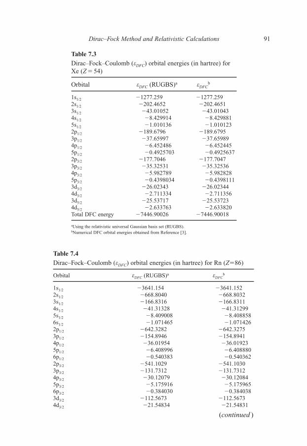
Dirac–Fock Method and Relativistic Calculations 91
Table 7.3
Dirac–Fock–Coulomb (DFC) orbital energies (in hartree) forXe (Z � 54)
Orbital DFC (RUGBS)a DFCb
1s1/2 �1277.259 �1277.2592s1/2 �202.4652 �202.46513s1/2 �43.01052 �43.010434s1/2 �8.429914 �8.4298815s1/2 �1.010136 �1.0101232p1/2 �189.6796 �189.67953p1/2 �37.65997 �37.659894p1/2 �6.452486 �6.4524455p1/2 �0.4925703 �0.49256372p3/2 �177.7046 �177.70473p3/2 �35.32531 �35.325364p3/2 �5.982789 �5.9828285p3/2 �0.4398034 �0.43981113d3/2 �26.02343 �26.023444d3/2 �2.711334 �2.7113563d5/2 �25.53717 �25.537234d5/2 �2.633763 �2.633820Total DFC energy �7446.90026 �7446.90018
aUsing the relativistic universal Gaussian basis set (RUGBS).bNumerical DFC orbital energies obtained from Reference [3].
Table 7.4
Dirac–Fock–Coulomb (DFC) orbital energies (in hartree) for Rn (Z�86)
Orbital DFC (RUGBS)a DFCb
1s1/2 �3641.154 �3641.1522s1/2 �668.8040 �668.80323s1/2 �166.8316 �166.83114s1/2 �41.31328 �41.312995s1/2 �8.409008 �8.4088586s1/2 �1.071465 �1.0714262p1/2 �642.3282 �642.32753p1/2 �154.8946 �154.89414p1/2 �36.01954 �36.019235p1/2 �6.408996 �6.4088806p1/2 �0.540383 �0.5403622p3/2 �541.1029 �541.10303p3/2 �131.7312 �131.73124p3/2 �30.12079 �30.120845p3/2 �5.175916 �5.1759656p3/2 �0.384030 �0.3840383d3/2 �112.5673 �112.56734d3/2 �21.54834 �21.54831
(continued )
Else_EAMC-TRSIC_ch007.qxd 5/4/2007 07:52 Page 91

92 Chapter 7
5d3/2 �2.189721 �2.1897703d5/2 �107.7594 �107.75954d5/2 �20.43896 �20.439135d5/2 �2.016612 �2.0167304f5/2 �9.194217 �9.1942324f7/2 �8.928509 �8.928566Total DFC energy �23601.9780 �23601.9742
aUsing the relativistic universal Gaussian basis set (RUGBS).bNumerical DFC orbital energies obtained from Reference [3].
Table 7.4 Continued
Orbital DFC (RUGBS)a DFCb
Table 7.5
Dirac–Fock–Coulomb (DFC) orbital energies (in hartree) for No (Z � 102)
Orbital DFC (RUGBS)a DFCb
1s1/2 �5526.516 �5526.5102s1/2 �1082.793 �1082.7903s1/2 �285.3977 �285.39674s1/2 �78.61882 �78.618095s1/2 �18.80527 �18.805066s1/2 �2.795032 �2.7951217s1/2 �0.2092464 �0.20931792p1/2 �1047.357 �1047.3553p1/2 �269.1022 �269.10134p1/2 �70.97112 �70.970355p1/2 �15.54233 �15.542246p1/2 �1.727430 �1.7275622p3/2 �808.7878 �808.78793p3/2 �212.1871 �212.18714p3/2 �55.21117 �55.211115p3/2 �11.43694 �11.437316p3/2 �1.049245 �1.0494473d3/2 �187.1341 �187.13414d3/2 �43.23725 �43.236995d3/2 �6.610122 �6.6104733d5/2 �176.4444 �176.44454d5/2 �40.45725 �40.457335d5/2 �5.985614 �5.9861444f5/2 �24.68849 �24.688305f5/2 �0.5665813 �0.56694594f7/2 �23.91509 �23.914985f7/2 �0.4690872 �0.4694412Total DFC energy �36740.2908 �36740.2857
aUsing the relativistic universal Gaussian basis set (RUGBS).bNumerical DFC orbital energies obtained from Reference [11].
Else_EAMC-TRSIC_ch007.qxd 5/4/2007 07:52 Page 92

Dirac–Fock Method and Relativistic Calculations 93
The GCDF method was the first algorithm capable of generating Gaussianbasis sets directly from the relativistic environment (code). In the GCDF method,the Gaussian function exponents are not parameters to be variationally optimizedas usual but they are generated by some criterion (the ID technique) for the inte-gration of the integral DF equations. The implementation of the ID technique(through the relabeling of the generator coordinate space [Equation (7.16)] forsolving the integral DF equations [Equations (7.15)]) other than allowing to spanthe relevant integration range (so that we can obtain universal basis sets) has theadvantage of avoiding variational exponent optimization.
This pioneer work with the GCDF method [14] had the merit to show that acareful numerical integration of the integral DF equations is able to providehighly accurate GTFs to be used in atomic and molecular relativistic calculations.
4. The Generator Coordinate Dirac–Fock Method and the Generation of a Relativistic Universal Gaussian Basis Set for Atoms from Hydrogen to Nobelium
Another important application of the GCDF method was in the generation of aRUGBS for the atoms from Hydrogen (Z�1) through Nobelium (Z�102) [26].In this application, the DFC calculations were performed by using the DFRATOMatomic program [27] and two nuclear models, namely: (a) the finite nucleus ofuniform proton-charge distribution and (b) the finite nucleus of Gaussian proton-charge distribution. In the finite nucleus model of uniform proton-charge distri-bution, the nuclear radius was given by [28]
(7.42)
where M is the atomic mass number. The speed of light, c, was assumed as137.0359895 a.u. [26].
The restricted kinetic balance condition [20] was assumed in all calculations,and the SCF equations for the average energy of configurations were solvedusing the Matsuoka’s method [29]. Also, the same Gaussian functions wereemployed to represent the following pairs of relativistic atomic orbital symme-tries: p1/2 and p3/2; d3/2 and d5/2; f5/2 and f7/2.
The RUGBS was obtained by searching the desired accuracy for the heaviestatom (Nobelium) with a basis set error lesser than 10 millihartree for this atom.The optimum discretization parameters found for Nobelium and applied todescribe all of the 102 atoms under study, i.e., from Hydrogen (H) throughNobelium (No), were �min and �� equal to �0.710 and 0.115, respectively. Theexponents of the RUGBS, obtained from these discretization parameters [seeEquation (7.16)], are shown in Appendix 4. Only the exponents of the basis set
R M� �5
30.836 0.570 (fm),1 3� �
Else_EAMC-TRSIC_ch007.qxd 5/4/2007 07:52 Page 93
94 Chapter 7
presented in Appendix 4 are used to describe all of the atomic orbital symmetries(s, p, d, and f).
The RUGBS functions for each atom were used to calculate the DFC total ener-gies from H through No with the two most popular nuclear models, i.e., the finitenucleus of uniform proton-charge distribution and the finite nucleus of Gaussianproton-charge distribution. The electronic configuration of each atom studied, thebasis set size, the DFC energies attained, and their errors with respect to numeri-cal DFC calculations [25] (i.e., the basis set error) are presented in Table 7.6.
The choice of the basis set functions for each atom studied (i.e., the basis settruncation process from H to No) was carried out trying to avoid the variationalprolapse and attain an accurate basis set (definition and more details on the vari-ational prolapse will be presented in Section 4.1).
To avoid variational prolapse, the Gaussian functions with the largest expo-nents were determined by means of an indirect analysis of the weight functions[see Equations (7.13) and (7.14)]. In the case of the GCM, the weight functionpresents a simple relationship with the atomic orbital coefficients [30]. Theatomic orbital coefficient analysis permitted a good description of the weightfunction behavior of the innermost atomic orbitals in regions close to the nucleus.Once the function with the largest exponent has been defined, the size of thebasis set is finally determined by the diffuseness of the electronic cloud for eachatom in its electronic configuration. Hence, different electronic configurations ofan atom may be represented by different sets of Gaussian function exponentsbased on its valence region characteristics.
Fig. 7.1 presents the basis set error of the RUGBS as a function of the atomicnumber for the electronic configuration related to the lowest DFC total energy ofeach atom from H to No. From Fig. 7.1 we can notice that the basis set errorobtained with both nuclear models is almost the same for all atoms studied,which is a clear indication that the RUGBS describes very well the region nearthe nucleus. The small deviations from a smooth increase of the basis set errorwith the atomic number are only due to the basis set truncation. Actually, webelieve that the basis set error behavior showed in Fig. 7.1 appears to be a char-acteristic of universal Gaussian basis sets obtained by the GCDF method due tothe use of a common ID interval, ��, for all atoms.
The largest basis set error observed in Table 7.6 is 8.8 millihartree for No (theatom with the largest atomic number). Such an error is very small considering thatthis atom presents a DFC total energy of approximately �36740 millihartree.However, the RUGBS error for lighter atoms is much smaller (for instance, it is3.6, 0.5, 0.1, 0.08, 0.008, and 0.0004 millihartree for Rn, Xe, Kr, Ar, Ne, and He,respectively). Therefore, these RUGBS errors assure that the RUGBS generatedwith the GCDF method is very accurate. The percentual errors observed for theseillustrative atoms are all around 0.00001–0.00002%, a fact that clearly reinforcesthe high accuracy of the RUGBS obtained with the GCDF method.
Else_EAMC-TRSIC_ch007.qxd 5/4/2007 07:52 Page 94

Dirac–Fock M
ethod and Relativistic C
alculations95
Table 7.6
Total DFC energies (in hartree) and basis set errors (in millihartree) for H (Z � 1) through No (Z � 102)
Atom Z M Configuration Basis Set Size Uniform Sphere Model Gaussian Model
EDFC Errora EDFC Errora
H 1 1 1s1 20s �0.50000660 0.00006 �0.50000660 0.00006He 2 4 1s2 19s �2.86181294 0.00038 �2.86181294 0.00038Li 3 7 [He]2s1 28s �7.43353311 0.00003 �7.43353311 0.00003Be 4 9 [He]2s2 27s �14.57589163 0.00007 �14.57589163 0.00007B 5 11 [He]2s22p1 26s18p �24.53655361 0.00063 �24.53655361 0.00063C 6 12 [He]2s22p2 26s17p �37.67603986 0.00087 �37.67603986 0.00088N 7 14 [He]2s22p3 25s17p �54.32772018 0.00172 �54.32772018 0.00172O 8 16 [He]2s22p4 25s17p �74.82498431 0.00179 �74.82498431 0.00179F 9 19 [He]2s22p5 25s16p �99.50160985 0.00543 �99.50160985 0.00544Ne 10 20 [He]2s22p6 24s16p �128.6919224 0.008 �128.6919224 0.008Na 11 23 [Ne]3s1 31s15p �162.0780736 0.014 �162.0780736 0.014Mg 12 24 [Ne]3s2 30s15p �199.9350572 0.010 �199.9350572 0.010Al 13 27 [Ne]3s23p1 29s25p �242.3307185 0.031 �242.3307185 0.031Si 14 28 [Ne]3s23p2 29s25p �289.4613330 0.005 �289.4613331 0.005P 15 31 [Ne]3s23p3 29s24p �341.4946524 0.016 �341.4946525 0.016S 16 32 [Ne]3s23p4 28s24p �398.5979070 0.023 �398.5979071 0.023Cl 17 35 [Ne]3s23p5 28s24p �460.9383709 0.013 �460.9383709 0.013Ar 18 40 [Ne]3s23p6 28s23p �528.6836783 0.084 �528.6836784 0.084K 19 39 [Ar]4s1 33s23p �601.5259384 0.015 �601.5259388 0.015Ca 20 40 [Ar]4s2 32s23p �679.7101100 0.051 �679.7101106 0.051Sc 21 45 [Ar]4s23d1 32s23p16d �763.3787110 0.027 �763.3787119 0.027
[Ar]4s13d2 32s23p17d �763.3016904 0.043 �763.3016913 0.044Ti 22 48 [Ar]4s23d2 32s22p16d �852.8197644 0.059 �852.8197657 0.060
[Ar]4s13d3 32s23p16d �852.7557010 0.055 �852.7557023 0.055V 23 51 [Ar]4s23d3 32s22p16d �948.1886159 0.040 �948.1886177 0.041
[Ar]4s13d4 32s22p16d �948.1359293 0.059 �948.1359311 0.059Cr 24 52 [Ar]4s23d4 32s22p15d �1049.638423 0.054 �1049.638426 0.054
[Ar]4s13d5 32s22p16d �1049.595992 0.042 �1049.595994 0.043
(continued )
Else_EAMC-TRSIC_ch007.qxd 5/4/2007 07:52 Page 95

96C
hapter 7
Mn 25 55 [Ar]4s23d5 32s22p15d �1157.321872 0.041 �1157.321875 0.043[Ar]4s13d6 32s22p16d �1157.288739 0.037 �1157.288743 0.037
Fe 26 56 [Ar]4s23d6 32s22p15d �1271.391943 0.037 �1271.391947 0.038[Ar]4s13d7 32s22p16d �1271.367364 0.035 �1271.367368 0.036
Co 27 59 [Ar]4s23d7 32s22p15d �1392.001787 0.036 �1392.001792 0.038[Ar]4s13d8 32s22p16d �1391.985140 0.035 �1391.985145 0.037
Ni 28 58 [Ar]4s23d8 32s22p15d �1519.305579 0.039 �1519.305586 0.041[Ar]4s13d9 32s22p15d �1519.296293 0.078 �1519.296300 0.081
Cu 29 63 [Ar]4s23d9 32s21p15d �1653.457268 0.101 �1653.457277 0.104[Ar]4s13d10 32s22p15d �1653.454996 0.067 �1653.455005 0.070
Zn 30 64 [Ar]4s23d10 32s21p15d �1794.612879 0.089 �1794.612890 0.093Ga 31 69 [Zn]4p1 31s29p14d �1942.563666 0.077 �1942.563682 0.082Ge 32 74 [Zn]4p2 31s29p14d �2097.470280 0.055 �2097.470300 0.061As 33 75 [Zn]4p3 31s28p14d �2259.441797 0.083 �2259.441822 0.090Se 34 80 [Zn]4p4 31s28p13d �2428.588115 0.119 �2428.588147 0.127Br 35 79 [Zn]4p5 30s28p13d �2605.023340 0.097 �2605.023379 0.106Kr 36 84 [Zn]4p6 30s28p13d �2788.860474 0.089 �2788.860523 0.101Rb 37 85 [Kr]5s1 34s27p13d �2979.804821 0.118 �2979.804894 0.119Sr 38 88 [Kr]5s2 34s27p12d �3178.079680 0.199 �3178.079770 0.199Y 39 89 [Kr]5s24d1 33s27p20d �3383.761550 0.165 �3383.761658 0.166
[Kr]5s14d2 33s27p21d �3383.699737 0.146 �3383.699845 0.146Zr 40 90 [Kr]5s24d2 33s27p20d �3597.083062 0.145 �3597.083191 0.146
[Kr]5s14d3 33s27p21d �3597.041249 0.147 �3597.041379 0.147Nb 41 93 [Kr]5s24d3 33s27p20d �3818.167951 0.154 �3818.168107 0.155
[Kr]5s14d4 33s27p20d �3818.148273 0.185 �3818.148430 0.185Mo 42 98 [Kr]5s24d4 33s26p20d �4047.136951 0.241 �4047.137142 0.242
[Kr]5s14d5 33s26p20d �4047.141104 0.262 �4047.141295 0.262Tc 43 98 [Kr]5s24d5 33s26p20d �4284.112918 0.225 �4284.113144 0.224
[Kr]5s14d6 33s26p20d �4284.142306 0.234 �4284.142532 0.233
Table 7.6 Continued
Atom Z M Configuration Basis Set Size Uniform Sphere Model Gaussian Model
EDFC Errora EDFC Errora
Else_EAMC-TRSIC_ch007.qxd 5/4/2007 07:52 Page 96

Dirac–Fock M
ethod and Relativistic C
alculations97
Ru 44 102 [Kr]5s24d6 33s26p20d �4529.213354 0.219 �4529.213625 0.219[Kr]5s14d7 33s26p20d �4529.269215 0.224 �4529.269487 0.223
Rh 45 103 [Kr]5s24d7 33s26p19d �4782.562252 0.245 �4782.562573 0.244[Kr]5s14d8 33s26p20d �4782.645740 0.227 �4782.646060 0.227
Pd 46 106 [Kr]5s24d8 33s26p19d �5044.279945 0.251 �5044.280326 0.251[Kr]5s14d9 33s26p19d �5044.392005 0.317 �5044.392386 0.317[Kr]5s04d10 29s26p20d �5044.400409 0.304 �5044.400790 0.303
Ag 47 107 [Kr]5s24d9 33s26p19d �5314.491791 0.281 �5314.492238 0.280[Kr]5s14d10 33s26p19d �5314.633528 0.314 �5314.633975 0.314
Cd 48 114 [Kr]5s24d10 33s26p19d �5593.317969 0.329 �5593.318510 0.327In 49 115 [Cd]5p1 32s32p18d �5880.430389 0.564 �5880.431022 0.560Sn 50 120 [Cd]5p2 32s32p18d �6176.126892 0.449 �6176.127644 0.445Sb 51 121 [Cd]5p3 32s31p18d �6480.517203 0.555 �6480.518078 0.549Te 52 130 [Cd]5p4 32s31p18d �6793.697409 0.511 �6793.698462 0.505I 53 127 [Cd]5p5 31s31p18d �7115.792434 0.550 �7115.793633 0.542Xe 54 132 [Cd]5p6 31s31p18d �7446.893528 0.511 �7446.894938 0.502Cs 55 133 [Xe]6s1 35s31p17d �7786.769498 0.553 �7786.771114 0.554Ba 56 138 [Xe]6s2 35s30p17d �8135.642505 0.611 �8135.644398 0.613La 57 139 [Xe]6s24f1 35s30p17d15f �8493.540705 0.691 �8493.542884 0.693
[Xe]6s25d1 35s30p20d �8493.642851 0.683 �8493.645031 0.685Ce 58 140 [Xe]6s24f2 35s30p17d15f �8860.994438 0.751 �8860.996943 0.753
[Xe]6s24f15d1 35s30p20d14f �8861.068172 0.808 �8861.070677 0.811Pr 59 141 [Xe]6s24f3 35s30p17d15f �9238.144815 0.835 �9238.147690 0.837Nd 60 144 [Xe]6s24f4 35s30p17d15f �9625.127610 0.932 �9625.130931 0.936Pm 61 145 [Xe]6s24f5 34s30p17d15f �10022.09039 1.16 �10022.09419 1.17Sm 62 152 [Xe]6s24f6 34s30p17d15f �10429.15743 1.24 �10429.16187 1.24Eu 63 153 [Xe]6s24f7 34s30p17d15f �10846.49871 1.29 �10846.50378 1.30Gd 64 158 [Xe]6s24f8 34s30p16d15f �11274.23533 1.66 �11274.24120 1.66
[Xe]6s24f75d1 34s30p20d15f �11274.22302 1.31 �11274.22889 1.31Tb 65 159 [Xe]6s24f9 34s30p16d15f �11712.53701 1.60 �11712.54371 1.60Dy 66 162 [Xe]6s24f10 34s30p16d15f �12161.53656 1.54 �12161.54423 1.55Ho 67 162 [Xe]6s24f11 34s30p16d15f �12621.40314 1.49 �12621.41183 1.50Er 68 168 [Xe]6s24f12 34s30p16d14f �13092.25880 1.68 �13092.26885 1.69Tm 69 169 [Xe]6s24f13 34s30p16d14f �13574.30401 1.64 �13574.31541 1.66
(continued )
Else_EAMC-TRSIC_ch007.qxd 5/4/2007 07:52 Page 97
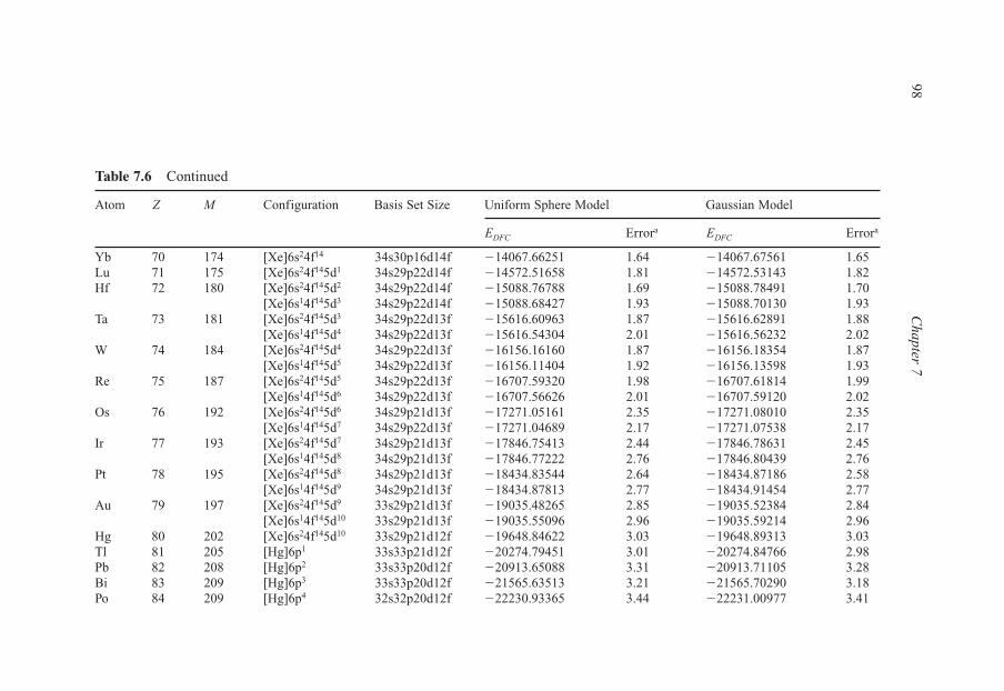
98C
hapter 7
Yb 70 174 [Xe]6s24f14 34s30p16d14f �14067.66251 1.64 �14067.67561 1.65Lu 71 175 [Xe]6s24f145d1 34s29p22d14f �14572.51658 1.81 �14572.53143 1.82Hf 72 180 [Xe]6s24f145d2 34s29p22d14f �15088.76788 1.69 �15088.78491 1.70
[Xe]6s14f145d3 34s29p22d14f �15088.68427 1.93 �15088.70130 1.93Ta 73 181 [Xe]6s24f145d3 34s29p22d13f �15616.60963 1.87 �15616.62891 1.88
[Xe]6s14f145d4 34s29p22d13f �15616.54304 2.01 �15616.56232 2.02W 74 184 [Xe]6s24f145d4 34s29p22d13f �16156.16160 1.87 �16156.18354 1.87
[Xe]6s14f145d5 34s29p22d13f �16156.11404 1.92 �16156.13598 1.93Re 75 187 [Xe]6s24f145d5 34s29p22d13f �16707.59320 1.98 �16707.61814 1.99
[Xe]6s14f145d6 34s29p22d13f �16707.56626 2.01 �16707.59120 2.02Os 76 192 [Xe]6s24f145d6 34s29p21d13f �17271.05161 2.35 �17271.08010 2.35
[Xe]6s14f145d7 34s29p22d13f �17271.04689 2.17 �17271.07538 2.17Ir 77 193 [Xe]6s24f145d7 34s29p21d13f �17846.75413 2.44 �17846.78631 2.45
[Xe]6s14f145d8 34s29p21d13f �17846.77222 2.76 �17846.80439 2.76Pt 78 195 [Xe]6s24f145d8 34s29p21d13f �18434.83544 2.64 �18434.87186 2.58
[Xe]6s14f145d9 34s29p21d13f �18434.87813 2.77 �18434.91454 2.77Au 79 197 [Xe]6s24f145d9 33s29p21d13f �19035.48265 2.85 �19035.52384 2.84
[Xe]6s14f145d10 33s29p21d13f �19035.55096 2.96 �19035.59214 2.96Hg 80 202 [Xe]6s24f145d10 33s29p21d12f �19648.84622 3.03 �19648.89313 3.03Tl 81 205 [Hg]6p1 33s33p21d12f �20274.79451 3.01 �20274.84766 2.98Pb 82 208 [Hg]6p2 33s33p20d12f �20913.65088 3.31 �20913.71105 3.28Bi 83 209 [Hg]6p3 33s33p20d12f �21565.63513 3.21 �21565.70290 3.18Po 84 209 [Hg]6p4 32s32p20d12f �22230.93365 3.44 �22231.00977 3.41
Table 7.6 Continued
Atom Z M Configuration Basis Set Size Uniform Sphere Model Gaussian Model
EDFC Errora EDFC Errora
Else_EAMC-TRSIC_ch007.qxd 5/4/2007 07:52 Page 98
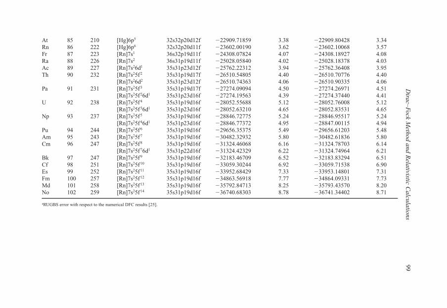
Dirac–Fock M
ethod and Relativistic C
alculations99
At 85 210 [Hg]6p5 32s32p20d12f �22909.71859 3.38 �22909.80428 3.34Rn 86 222 [Hg]6p6 32s32p20d11f �23602.00190 3.62 �23602.10068 3.57Fr 87 223 [Rn]7s1 36s32p19d11f �24308.07824 4.07 �24308.18927 4.08Ra 88 226 [Rn]7s2 36s31p19d11f �25028.05840 4.02 �25028.18378 4.03Ac 89 227 [Rn]7s26d1 35s31p23d12f �25762.22312 3.94 �25762.36408 3.95Th 90 232 [Rn]7s25f2 35s31p19d17f �26510.54805 4.40 �26510.70776 4.40
[Rn]7s26d2 35s31p23d12f �26510.74363 4.06 �26510.90335 4.06Pa 91 231 [Rn]7s25f3 35s31p19d17f �27274.09094 4.50 �27274.26971 4.51
[Rn]7s25f26d1 35s31p23d16f �27274.19563 4.39 �27274.37440 4.41U 92 238 [Rn]7s25f4 35s31p19d16f �28052.55688 5.12 �28052.76008 5.12
[Rn]7s25f36d1 35s31p23d16f �28052.63210 4.65 �28052.83531 4.65Np 93 237 [Rn]7s25f5 35s31p19d16f �28846.72775 5.24 �28846.95517 5.24
[Rn]7s25f46d1 35s31p23d16f �28846.77372 4.95 �28847.00115 4.94Pu 94 244 [Rn]7s25f6 35s31p19d16f �29656.35375 5.49 �29656.61203 5.48Am 95 243 [Rn]7s25f7 35s31p19d16f �30482.32932 5.80 �30482.61836 5.80Cm 96 247 [Rn]7s25f8 35s31p19d16f �31324.46068 6.16 �31324.78703 6.14
[Rn]7s25f76d1 35s31p22d16f �31324.42329 6.22 �31324.74964 6.21Bk 97 247 [Rn]7s25f9 35s31p19d16f �32183.46709 6.52 �32183.83294 6.51Cf 98 251 [Rn]7s25f10 35s31p19d16f �33059.30244 6.92 �33059.71538 6.90Es 99 252 [Rn]7s25f11 35s31p19d16f �33952.68429 7.33 �33953.14801 7.31Fm 100 257 [Rn]7s25f12 35s31p19d16f �34863.56918 7.77 �34864.09331 7.73Md 101 258 [Rn]7s25f13 35s31p19d16f �35792.84713 8.25 �35793.43570 8.20No 102 259 [Rn]7s25f14 35s31p19d16f �36740.68303 8.78 �36741.34402 8.71
aRUGBS error with respect to the numerical DFC results [25].
Else_EAMC-TRSIC_ch007.qxd 5/4/2007 07:52 Page 99
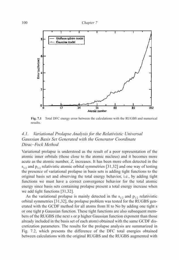
100 Chapter 7
4.1. Variational Prolapse Analysis for the Relativistic UniversalGaussian Basis Set Generated with the Generator CoordinateDirac–Fock Method
Variational prolapse is understood as the result of a poor representation of theatomic inner orbitals (those close to the atomic nucleus) and it becomes moreacute as the atomic number, Z, increases. It has been more often detected in thes1/2 and p1/2 relativistic atomic orbital symmetries [31,32] and one way of testingthe presence of variational prolapse in basis sets is adding tight functions to theoriginal basis set and observing the total energy behavior, i.e., by adding tightfunctions we must have a correct convergence behavior for the total atomicenergy since basis sets containing prolapse present a total energy increase whenwe add tight functions [31,32].
As the variational prolapse is mainly detected in the s1/2 and p1/2 relativisticorbital symmetries [31,32], the prolapse problem was tested for the RUGBS gen-erated with the GCDF method for all atoms from H to No by adding one tight sor one tight p Gaussian function. These tight functions are also subsequent mem-bers of the RUGBS (the next s or p higher Gaussian function exponent than thosealready included in the basis set of each atom) obtained with the same GCDF dis-cretization parameters. The results for the prolapse analysis are summarized inFig. 7.2, which presents the difference of the DFC total energies obtainedbetween calculations with the original RUGBS and the RUGBS augmented with
Fig. 7.1 Total DFC energy error between the calculations with the RUGBS and numericalresults.
Else_EAMC-TRSIC_ch007.qxd 5/4/2007 07:52 Page 100

a tight s or a tight p Gaussian function (EDFC –E�1DFC
tight). From Fig. 7.2 we can seethat the addition of a tight function almost always results in a correct convergenceof the DFC total energy for both nuclear models studied. However, a very smallincrease in the DFC total energy of 2 microhartree (at most) was observed with thefinite nucleus of uniform proton-charge distribution when we added tight s func-tions [from Cs (Z � 55) to Dy (Z � 66)] and tight p functions [from Yb (Z � 70)to Hg (Z � 80)]. The DFC total energy results with the Gaussian nucleus modeldid not present any evidence of variational prolapse (see Fig. 7.2).
To investigate the possibility of variational prolapse in more details, conver-gence tests were carried out for some representative atoms: No (Z �102), Rn(Z � 86), Hg (Z � 80), Yb (Z � 70), and Ba (Z � 56). These results are pre-sented in Tables 7.7–7.11, which show the DFC total energies and the 1s1/2 and2p1/2 orbital energies (1s1/2
and 2p1/2) obtained with the addition of up to three
tight functions to the s, p, d, or f symmetries in the basis set of these atoms.As can be seen from Tables 7.7–7.11, the DFC total energies always reduce
or eventually converge with the addition of tight d or f functions showing nosign of variational prolapse. These results were already expected since d and ffunctions represent electrons that are mainly in distant regions from the atomicnucleus [31]. Also, these results are in agreement with the idea that the varia-tional prolapse only possibly occurs in s1/2 and p1/2 relativistic orbital symmetries,
Dirac–Fock Method and Relativistic Calculations 101
Fig. 7.2 Total DFC energy differences between the calculations with the original RUGBSaugmented with one tight s or one tight p function (EDFC –E�1
DFCtight).
Else_EAMC-TRSIC_ch007.qxd 5/4/2007 07:52 Page 101
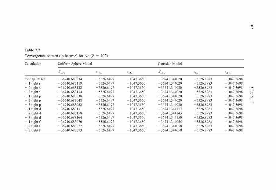
102C
hapter 7
Table 7.7
Convergence pattern (in hartree) for No (Z � 102)
Calculation Uniform Sphere Model Gaussian Model
EDFC 1s1/22p1/2
EDFC 1s1/22p1/2
35s31p19d16f �36740.683034 �5526.6497 �1047.3650 �36741.344020 �5526.8983 �1047.3698� 1 tight s �36740.683119 �5526.6497 �1047.3650 �36741.344020 �5526.8983 �1047.3698� 2 tight s �36740.683132 �5526.6497 �1047.3650 �36741.344020 �5526.8983 �1047.3698� 3 tight s �36740.683134 �5526.6497 �1047.3650 �36741.344020 �5526.8983 �1047.3698� 1 tight p �36740.683038 �5526.6497 �1047.3650 �36741.344020 �5526.8983 �1047.3698� 2 tight p �36740.683048 �5526.6497 �1047.3650 �36741.344020 �5526.8983 �1047.3698� 3 tight p �36740.683052 �5526.6497 �1047.3650 �36741.344020 �5526.8983 �1047.3698� 1 tight d �36740.683131 �5526.6497 �1047.3650 �36741.344117 �5526.8983 �1047.3698� 2 tight d �36740.683158 �5526.6497 �1047.3650 �36741.344143 �5526.8983 �1047.3698� 3 tight d �36740.683164 �5526.6497 �1047.3650 �36741.344150 �5526.8983 �1047.3698� 1 tight f �36740.683070 �5526.6497 �1047.3650 �36741.344055 �5526.8983 �1047.3698� 2 tight f �36740.683072 �5526.6497 �1047.3650 �36741.344058 �5526.8983 �1047.3698� 3 tight f �36740.683073 �5526.6497 �1047.3650 �36741.344058 �5526.8983 �1047.3698
Else_EAMC-TRSIC_ch007.qxd 5/4/2007 07:52 Page 102
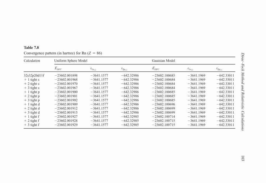
Dirac–Fock M
ethod and Relativistic C
alculations103
Table 7.8
Convergence pattern (in hartree) for Rn (Z � 86)
Calculation Uniform Sphere Model Gaussian Model
EDFC 1s1/22p1/2
EDFC 1s1/22p1/2
32s32p20d11f �23602.001898 �3641.1577 �642.32986 �23602.100685 �3641.1969 �642.33011� 1 tight s �23602.001968 �3641.1577 �642.32986 �23602.100684 �3641.1969 �642.33011� 2 tight s �23602.001970 �3641.1577 �642.32986 �23602.100684 �3641.1969 �642.33011� 3 tight s �23602.001967 �3641.1577 �642.32986 �23602.100684 �3641.1969 �642.33011� 1 tight p �23602.001900 �3641.1577 �642.32986 �23602.100685 �3641.1969 �642.33011� 2 tight p �23602.001901 �3641.1577 �642.32986 �23602.100685 �3641.1969 �642.33011� 3 tight p �23602.001902 �3641.1577 �642.32986 �23602.100685 �3641.1969 �642.33011� 1 tight d �23602.001909 �3641.1577 �642.32986 �23602.100696 �3641.1969 �642.33011� 2 tight d �23602.001912 �3641.1577 �642.32986 �23602.100699 �3641.1969 �642.33011� 3 tight d �23602.001913 �3641.1577 �642.32986 �23602.100699 �3641.1969 �642.33011� 1 tight f �23602.001927 �3641.1577 �642.32985 �23602.100714 �3641.1969 �642.33011� 2 tight f �23602.001928 �3641.1577 �642.32985 �23602.100715 �3641.1969 �642.33011� 3 tight f �23602.001929 �3641.1577 �642.32985 �23602.100715 �3641.1969 �642.33011
Else_EAMC-TRSIC_ch007.qxd 5/4/2007 07:52 Page 103

104C
hapter 7
Table 7.9
Convergence pattern (in hartree) for Hg (Z � 80)
Calculation Uniform Sphere Model Gaussian Model
EDFC 1s1/22p1/2
EDFC 1s1/22p1/2
33s29p21d12f �19648.846222 �3074.2217 �526.85407 �19648.893132 �3074.2406 �526.85413� 1 tight s �19648.846248 �3074.2217 �526.85407 �19648.893132 �3074.2406 �526.85413� 2 tight s �19648.846245 �3074.2217 �526.85407 �19648.893132 �3074.2406 �526.85413� 3 tight s �19648.846242 �3074.2217 �526.85407 �19648.893132 �3074.2406 �526.85413� 1 tight p �19648.846220 �3074.2217 �526.85407 �19648.893143 �3074.2406 �526.85414� 2 tight p �19648.846221 �3074.2217 �526.85407 �19648.893143 �3074.2406 �526.85414� 3 tight p �19648.846222 �3074.2217 �526.85407 �19648.893143 �3074.2406 �526.85414� 1 tight d �19648.846227 �3074.2217 �526.85407 �19648.893138 �3074.2406 �526.85413� 2 tight d �19648.846228 �3074.2217 �526.85407 �19648.893139 �3074.2406 �526.85413� 3 tight d �19648.846229 �3074.2217 �526.85407 �19648.893139 �3074.2406 �526.85413� 1 tight f �19648.846230 �3074.2217 �526.85407 �19648.893141 �3074.2406 �526.85413� 2 tight f �19648.846231 �3074.2217 �526.85407 �19648.893141 �3074.2406 �526.85413� 3 tight f �19648.846231 �3074.2217 �526.85407 �19648.893141 �3074.2406 �526.85413
Else_EAMC-TRSIC_ch007.qxd 5/4/2007 07:52 Page 104

Dirac–Fock M
ethod and Relativistic C
alculations105
Table 7.10
Convergence pattern (in hartree) for Yb (Z � 70)
Calculation Uniform Sphere Model Gaussian Model
EDFC 1s1/22p1/2
EDFC 1s1/22p1/2
34s30p16d14f �14067.662509 �2267.6459 �370.05413 �14067.675613 �2267.6513 �370.05414� 1 tight s �14067.662510 �2267.6459 �370.05413 �14067.675612 �2267.6513 �370.05413� 2 tight s �14067.662508 �2267.6459 �370.05413 �14067.675612 �2267.6513 �370.05413� 3 tight s �14067.662507 �2267.6459 �370.05413 �14067.675612 �2267.6513 �370.05413� 1 tight p �14067.662508 �2267.6459 �370.05413 �14067.675616 �2267.6513 �370.05414� 2 tight p �14067.662508 �2267.6459 �370.05413 �14067.675616 �2267.6513 �370.05414� 3 tight p �14067.662509 �2267.6459 �370.05413 �14067.675616 �2267.6513 �370.05414� 1 tight d �14067.662528 �2267.6459 �370.05413 �14067.675632 �2267.6513 �370.05414� 2 tight d �14067.662532 �2267.6459 �370.05414 �14067.675636 �2267.6513 �370.05414� 3 tight d �14067.662533 �2267.6459 �370.05413 �14067.675637 �2267.6513 �370.05414� 1 tight f �14067.662509 �2267.6459 �370.05413 �14067.675613 �2267.6513 �370.05414� 2 tight f �14067.662509 �2267.6459 �370.05413 �14067.675613 �2267.6513 �370.05414� 3 tight f �14067.662509 �2267.6459 �370.05414 �14067.675613 �2267.6513 �370.05414
Else_EAMC-TRSIC_ch007.qxd 5/4/2007 07:52 Page 105

106C
hapter 7
Table 7.11
Convergence pattern (in hartree) for Ba (Z � 56)
Calculation Uniform Sphere Model Gaussian Model
EDFC 1s1/22p1/2
EDFC 1s1/22p1/2
35s30p17d �8135.642505 �1383.8336 �209.08784 �8135.644398 �1383.8344 �209.08784� 1 tight s �8135.642503 �1383.8336 �209.08784 �8135.644398 �1383.8344 �209.08784� 2 tight s �8135.642503 �1383.8336 �209.08784 �8135.644398 �1383.8344 �209.08784� 3 tight s �8135.642503 �1383.8336 �209.08784 �8135.644398 �1383.8344 �209.08784� 1 tight p �8135.642504 �1383.8336 �209.08784 �8135.644399 �1383.8344 �209.08784� 2 tight p �8135.642504 �1383.8336 �209.08784 �8135.644399 �1383.8344 �209.08784� 3 tight p �8135.642504 �1383.8336 �209.08784 �8135.644399 �1383.8344 �209.08784� 1 tight d �8135.642506 �1383.8336 �209.08784 �8135.644399 �1383.8344 �209.08784� 2 tight d �8135.642506 �1383.8336 �209.08784 �8135.644400 �1383.8344 �209.08784� 3 tight d �8135.642506 �1383.8336 �209.08784 �8135.644400 �1383.8344 �209.08784
Else_EAMC-TRSIC_ch007.qxd 5/4/2007 07:52 Page 106

which can present an appreciable penetration into the nuclear region for atomicsystems with high Z [33]. The addition of tight d or f functions appears to onlyslightly disturb the energy of the 2p1/2 orbital just when the uniform spherenucleus model is employed, as noticed in Tables 7.8 and 7.10 for Rn (addition oftight f functions) and Yb (addition of tight d functions).
The convergence patterns for the addition of tight s or p functions show onlya small DFC total energy increase of 3 microhartree (at most) between two sub-sequent calculations when the uniform sphere nucleus model is adopted. TheDFC energy results obtained with the Gaussian nucleus model show an evenlower DFC energy increase with the addition of tight s functions to Rn and Yb(see Tables 7.8 and 7.10). For the orbital energies, only the 2p1/2
values areslightly disturbed by the addition of tight s functions to the Yb atom when theGaussian nucleus model is used. However, the increase in the DFC total energywith the addition of tight functions for all atoms studied is much smaller thanthe corresponding RUGBS error. The smallest basis set error for the atoms inTables 7.7–7.11 is 0.6 millihartree (for Ba atom). Thus, a DFC total energyincrease of 3 microhartree is 2000 times smaller than the basis set error, whichis a convincing argument in the direction to consider the RUGBS as free of vari-ational prolapse and apt to be employed in relativistic quantum chemical calcu-lations. Moreover, the increase observed in the DFC total energies in all caseswhen the Gaussian nucleus model was used is insignificant being equal to 0.1microhartree at most. Besides, convergence tests for the DFC total energies withthe addition of tight s and p Gaussian functions for both nuclear models werealso carried out for some lighter atomic systems (Xe, Cd, Kr, Zn, Ar, and Ne)with similar results. In fact, no variational prolapse was found indeed with theRUGBS generated with the GCDF method.
The good results obtained with the RUGBS are actually directly linked to theGCDF method. The great advantage of the GCDF method is that the ID tech-nique applied to Equations (7.15) works very well after a satisfactory choice ofthe GCDF parameters, its interval and limits. Hence, once these discretizationparameters are defined, the integral characteristics of Equations (7.15) are keptand the variational prolapse can be easily avoided by ensuring that the entire dis-cretization range for a certain atom is completely covered by the basis set func-tions we are generating.
Concluding, although the basis set size of the RUGBS can be consideredlarge for light atomic systems, it becomes much more competitive for heavieratoms. Only for comparison, the RUGBS size for No is 35s1/2, 31p1/2, 31p3/2,19d3/2, 19d5/2, 16f5/2, and 16f7/2 whereas the basis set developed by Tatewakiand Watanabe for H through Bi [34], and also without variational prolapse,has a size of 44s1/2, 44p1/2, 44p3/2, 36d3/2, 36d5/2, 32f5/2, and 32f7/2 functions andthe Gaussian exponents are different for each pair of relativistic atomic orbitalsymmetries: p1/2 and p3/2; d3/2 and d5/2; f5/2 and f7/2.
Dirac–Fock Method and Relativistic Calculations 107
Else_EAMC-TRSIC_ch007.qxd 5/4/2007 07:52 Page 107
5. The Generator Coordinate Dirac–Fock–Breit Formalism
Atomic and molecular DF calculations are usually based on an approximaterelativistic many-electron Hamiltonian, the DC Hamiltonian [16,35]. In the DCHamiltonian, the one-electron interactions are treated relativistically as a sum ofDirac’s one-electron Hamiltonians whereas the two-electron interaction is theusual nonrelativistic instantaneous electrostatic (Coulomb) repulsion. The instan-taneous Coulomb interaction between two electrons is not covariant and rela-tivistic corrections to this interaction are provided by quantum electrodynamics(QED) [36,37]. Addition of the frequency-independent Breit interaction
(7.43)
to the instantaneous Coulomb interaction “partially remedies” the lack of covari-ance of the DC Hamiltonian.
Some studies [5,38,39] demonstrated that the Breit interaction term can beincluded in the SCF procedure of the DF matrix calculations without any of thepossible difficulties that had been suggested [26]. Inclusion of the Breit termin the SCF process has the advantage that both Coulomb and Breit interactionsare included to the same order in the SCF potentials within the algebraicapproximation [40]. Besides, adding the Breit operator to the instantaneousCoulomb operator has the advantage that all effects through order �2 (where �is the fine-structure constant) are included in the zero-order Hamiltonian [41].The use of such a zero-order Hamiltonian in variational calculations naturallyleads to the DFB equations that include the Breit interaction as part of the two-body interactions.
In Section 2, we presented the integral version of the closed-shell DF equa-tions, known as the generator coordinate version of the closed-shell DF equationsor the GCDF method [14]. In the GCDF method, the integral DF equations aresolved through numerical integration and this is accomplished by discretizationpreserving the integral character of the GCDF method. This approach leads to anew view of basis set exponents to be used in relativistic atomic and molecularcalculations since in the GCDF method the basis set exponents are generated bydiscretization in a numerical integration procedure. This procedure is referred toas ID technique [18] in contrast to the procedure of optimizing orbital exponents.
Since in Section 2 we have presented the GCDFC formalism, it would be nat-ural to extend it to include the Breit interaction term [showed in Equation (7.43)]and consequently come up with a GCDFB formalism as well. This was done byJorge and da Silva in 1996 [15] and the GCDFB formalism made possible theGCDF method to perform DFB calculations.
To obtain the GCDFB equations, the frequency-independent Breit interaction(the Breit interaction term or simply the Breit term) is added to the unperturbed
B r r12 12 1 2 1 12 2 12 122(1 2 ) ( )( )�� � � � �� � � �� � � �r r
108 Chapter 7
Else_EAMC-TRSIC_ch007.qxd 5/4/2007 07:52 Page 108

DC Hamiltonian, HDC [Equation (7.1)]. As already commented, this “partiallyremedy” the lack of covariance of HDC leading to the Dirac–Coulomb–BreitHamiltonian (HDCB)
(7.44)
This approach inside the SCF treatment leads to the DFB-SCF equations [5]exactly as we did in Section 2 with GCDFC formalism [see Equations (7.8) to(7.21)].
Now with the inclusion of the Breit term [Equation (7.43)] in the GCDFC-SCFprocedure [14], the DFC matrix becomes the DFB matrix that can be written as
(7.45)
where the one-electron part, o�, and the two-electron part, t�, are the same matri-ces showed in Section 2 [see Equations (7.23)–(7.34)] and b� is
(7.46)
The Breit interaction matrices are given by
(7.47)
(7.48)
and
(7.49)
where Wv,TT�,T�T�ij,���l
in Equation (7.48) is given in terms of the generator coordinate � and in terms of the GTFs {X L
�} and {X S�} as
(7.50)
W X r X r U r s X s X sij kTT TT T
iT
kT
jT
� ��
� � � � �� � �,, , ( , ) ( , ) ( , ) ( , ) (� � ��
l,, )
( , ) ( , ) ( , ) ( , ) ( ,
00
�
� � �� � � � �
lds dr
X r X r U r s X s X s
r
Ti
Tk
Tj
T
∫∫�
� �� ��l) .
0
ds drr
��
∫∫
B j e D KijSS
k
SSk
LLij kSS LL
��
��
� � ��� �� �� �
�� �(2 1) ( , ) ,,
, ,
l
l l∑∑
B j f D K g DijSL
kLS
ij kSL LS
� � � � ��
� �� � � �� �� � � �� � �(2 1) ( , ) ( , ),, ,�
l l kkLS
ij kSL LS
k
Wl l
l
� ��
��,
, , ,��
�∑∑
B j e D KijLL
k
LLk
SSij kLL SS
��
��
� � ��� �� �� �
�� �(2 1) ( , ) ,,
, ,
l
l l∑∑
bB B
B B�� �
� �
�LL LS
SL SS
⎡
⎣⎢
⎤
⎦⎥ .
F o t b� � � �� � � ,
H h i V B i j .DCB Di
iji j
iji j
� � � �( ) ,, ,
∑ ∑ ∑
Dirac–Fock Method and Relativistic Calculations 109
Else_EAMC-TRSIC_ch007.qxd 5/4/2007 07:52 Page 109

The relativistic angular coefficients evLL(�,��), ev
SS(�,��), f v(�,��) and gv(�,��)are evaluated by using the technique described by Grant and Pyper [42].
The inclusion of the Breit term in the GCDF method enables us to apply it in DFBcalculations. The Breit term leads to changes in the orbitals and their energies, whichin turn modify the Coulomb interaction among the electrons in the SCF process.Now the “interference” between the Coulomb and Breit interactions and the result-ing orbital reorganization is taken into account in the GCDF-SCF procedure.
The first application of the GCDF method in DFB calculations was with aRUGBS obtained for the closed-shell atoms from Zinc (Zn) through Nobelium(No) [15]. That work reported DFB-SCF calculations on all relativistic closed-shell atoms with occupied d and f orbitals, i.e., all relativistic closed-shell atomsfrom Zn (Z�30) to No (Z�102).
The finite nucleus model of uniform proton-charge distribution and therestricted kinetic balance condition were also employed in all DFB calculations.The nuclear radius employed was R�2.2677�10�5 M1/3, where M is the atomicmass number, and the speed of light, c, used was 137.0370 a.u.
The 32 relativistic universal Gaussian exponents generated to perform thispioneer work with the GCDFB formalism can be found in Reference [15]. Theywere generated by employing the ID technique [Equation (7.16)] with the scal-ing parameter A�6.0 [15].
With the aim of comparison, Table 7.12 shows the DFC and DFB energies andalso the variational Breit interaction energy, EB, attained by using the RUGBS andanother universal GTF basis set [11]. The EB is the level shift in the total SCFenergy due to the inclusion of the Breit term in the GCDF-SCF process and it iscomputed as the difference EDFB � EDFC. The third column in Table 7.12 (RUGBSsize) indicates the number of exponents in each s1/2, p1/2, p3/2, d3/2, d5/2, f5/2, and f7/2
symmetry taken from the 32 relativistic universal Gaussian exponents generatedwith the GCDF method.
From Table 7.12 we can see the good performance of the GCDF method withthe RUGBS in providing DFB atomic energies. The EDFB obtained with theRUGBS were better than those (last column) obtained in a previous work byusing a universal GTF exponents generated from a nonrelativistic environment(code) [11]. Also in Table 7.12 (sixth column) we present the variational Breitinteraction (EB) energy for the atomic systems studied. The EDFC displayed inTable 7.12 (fifth column), used to assess EB, correspond to EDFC results obtainedpreviously with the GCDF method by using the GCDFC formalism [14].
The good numerical accuracy of the RUGBS in providing DFB energies wasattributed to the implementation of the ID technique inside the relativistic environ-ment (the GCDF method). With the ID technique, the Gaussian function exponentsare generated by discretization of Equations (7.15) (the integral DF equations)through a numerical integration procedure. In fact, a careful numerical integrationof Equations (7.15) will provide accurate Gaussian basis sets for relativistic atomic
110 Chapter 7
Else_EAMC-TRSIC_ch007.qxd 5/4/2007 07:52 Page 110
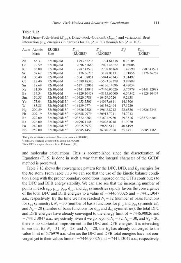
and molecular calculations. This is accomplished since the discretization ofEquations (7.15) is done in such a way that the integral character of the GCDFmethod is preserved.
Table 7.13 shows the convergence pattern for the DFC, DFB, and EB energies forthe Xe atom. From Table 7.13 we can see that the use of the kinetic balance condi-tion along with the proper boundary conditions imposed on the GTFs contributes tothe DFC and DFB energy stability. We can also see that the increasing number ofpoints in each s1/2, p1/2, p3/2, d3/2, and d5/2 symmetries rapidly favors the convergenceof the total DFC and DFB energies to a value of �7446.90026 and �7441.13047a.u., respectively. By the time we have reached Ns �32 (number of basis functionsfor s1/2 symmetry), Np �30 (number of basis functions for p1/2 and p3/2 symmetries),and Nd �20 (number of basis functions for d3/2 and d5/2 symmetries), the total DFCand DFB energies have already converged to the energy limit of �7446.90026 and�7441.13047 a.u., respectively. Even if we go beyond Ns�32, Np�30, and Nd�20,there is no substantial improvement in the DFC and DFB energies. It is interestingto see that for Ns �31, Np �28, and Nd �20, the EB has already converged to thevalue limit of 5.76979 a.u. whereas the DFC and DFB total energies have not con-verged yet to their values limit of �7446.90026 and �7441.13047 a.u., respectively.
Dirac–Fock Method and Relativistic Calculations 111
Table 7.12
Total Dirac–Fock–Breit (EDFB), Dirac–Fock–Coulomb (EDFC) and variational Breitinteraction (EB) energies (in hartree) for Zn (Z � 30) through No (Z � 102)
Atom Atomic RUGBS EDFB EDFC EBa EDFB
Mass Size (RUGBS)a (RUGBS)b (UGBS)c
Zn 65.37 32s30p20d �1793.85233 �1794.61338 0.76105Ge 72.59 32s30p20d �2096.51666 �2097.46672 0.95006Kr 83.80 32s30p20d �2787.43578 �2788.86168 1.42590 �2787.43571Sr 87.62 32s30p20d �3176.36275 �3178.08131 1.71856 �3176.36267Pd 106.40 32s30p20d �5041.08851 �5044.40343 3.31492Cd 112.40 32s30p20d �5589.48390 �5593.32279 3.83889Sn 118.69 32s30p20d �6171.72062 �6176.14096 4.42034Xe 131.30 32s30p20d �7441.13047 �7446.90026 5.76979 �7441.12988Ba 137.34 32s30p20d �8129.10458 �8135.65000 6.54542 �8129.10407Sm 150.35 32s30p20d15f �10420.0788 �10429.3726 9.2938Yb 173.04 32s30p20d15f �14053.5505 �14067.6811 14.1306W 183.85 32s30p20d15f �16139.0774 �16156.2494 17.1720Hg 200.59 32s30p20d15f �19626.2386 �19648.8712 22.6326 �19626.2346Pb 207.19 32s30p20d15f �20888.9979 �20913.7211 24.7232Rn 222.00 32s30p20d15f �23572.6264 �23601.9780 29.3516 �23572.6206Ra 226.00 32s30p20d15f �24996.1148 �25028.0218 31.9070Pu 242.00 32s30p20d15f �29615.8972 �29656.5171 40.6199No 259.00 32s30p20d15f �36685.1457 �36740.2908 55.1451 �36685.1365
aUsing the relativistic universal Gaussian basis set (RUGBS).bTotal DFC energies computed by using the RUGBS.cTotal DFB energies obtained from Reference [11].
Else_EAMC-TRSIC_ch007.qxd 5/4/2007 07:52 Page 111
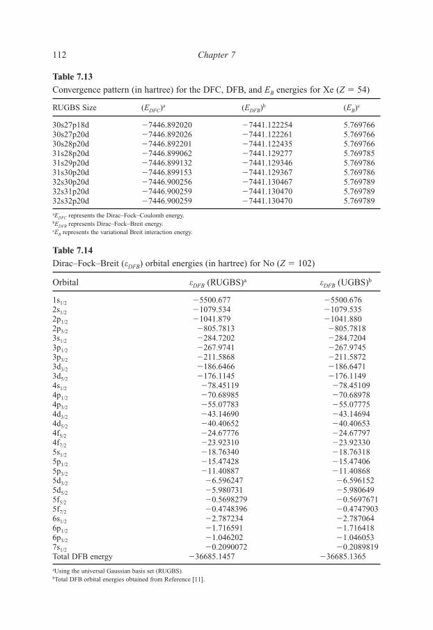
112 Chapter 7
Table 7.13
Convergence pattern (in hartree) for the DFC, DFB, and EB energies for Xe (Z � 54)
RUGBS Size (EDFC)a (EDFB)b (EB)c
30s27p18d �7446.892020 �7441.122254 5.76976630s27p20d �7446.892026 �7441.122261 5.76976630s28p20d �7446.892201 �7441.122435 5.76976631s28p20d �7446.899062 �7441.129277 5.76978531s29p20d �7446.899132 �7441.129346 5.76978631s30p20d �7446.899153 �7441.129367 5.76978632s30p20d �7446.900256 �7441.130467 5.76978932s31p20d �7446.900259 �7441.130470 5.76978932s32p20d �7446.900259 �7441.130470 5.769789
aEDFC represents the Dirac–Fock–Coulomb energy.bEDFB represents Dirac–Fock–Breit energy.cEB represents the variational Breit interaction energy.
Table 7.14
Dirac–Fock–Breit (DFB) orbital energies (in hartree) for No (Z � 102)
Orbital DFB (RUGBS)a DFB (UGBS)b
1s1/2 �5500.677 �5500.6762s1/2 �1079.534 �1079.5352p1/2 �1041.879 �1041.8802p3/2 �805.7813 �805.78183s1/2 �284.7202 �284.72043p1/2 �267.9741 �267.97453p3/2 �211.5868 �211.58723d3/2 �186.6466 �186.64713d5/2 �176.1145 �176.11494s1/2 �78.45119 �78.451094p1/2 �70.68985 �70.689784p3/2 �55.07783 �55.077754d3/2 �43.14690 �43.146944d5/2 �40.40652 �40.406534f5/2 �24.67776 �24.677974f7/2 �23.92310 �23.923305s1/2 �18.76340 �18.763185p1/2 �15.47428 �15.474065p3/2 �11.40887 �11.408685d3/2 �6.596247 �6.5961525d5/2 �5.980731 �5.9806495f5/2 �0.5698279 �0.56976715f7/2 �0.4748396 �0.47479036s1/2 �2.787234 �2.7870646p1/2 �1.716591 �1.7164186p3/2 �1.046202 �1.0460537s1/2 �0.2090072 �0.2089819Total DFB energy �36685.1457 �36685.1365
aUsing the universal Gaussian basis set (RUGBS).bTotal DFB orbital energies obtained from Reference [11].
Else_EAMC-TRSIC_ch007.qxd 5/4/2007 07:52 Page 112
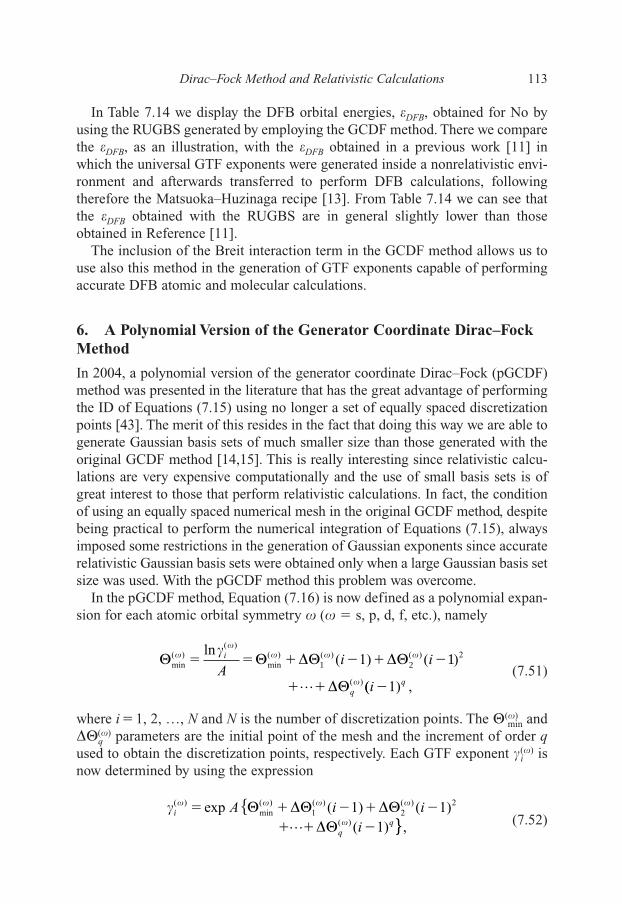
In Table 7.14 we display the DFB orbital energies, DFB, obtained for No byusing the RUGBS generated by employing the GCDF method. There we comparethe DFB, as an illustration, with the DFB obtained in a previous work [11] inwhich the universal GTF exponents were generated inside a nonrelativistic envi-ronment and afterwards transferred to perform DFB calculations, followingtherefore the Matsuoka–Huzinaga recipe [13]. From Table 7.14 we can see thatthe DFB obtained with the RUGBS are in general slightly lower than thoseobtained in Reference [11].
The inclusion of the Breit interaction term in the GCDF method allows us touse also this method in the generation of GTF exponents capable of performingaccurate DFB atomic and molecular calculations.
6. A Polynomial Version of the Generator Coordinate Dirac–FockMethod
In 2004, a polynomial version of the generator coordinate Dirac–Fock (pGCDF)method was presented in the literature that has the great advantage of performingthe ID of Equations (7.15) using no longer a set of equally spaced discretizationpoints [43]. The merit of this resides in the fact that doing this way we are able togenerate Gaussian basis sets of much smaller size than those generated with theoriginal GCDF method [14,15]. This is really interesting since relativistic calcu-lations are very expensive computationally and the use of small basis sets is ofgreat interest to those that perform relativistic calculations. In fact, the conditionof using an equally spaced numerical mesh in the original GCDF method, despitebeing practical to perform the numerical integration of Equations (7.15), alwaysimposed some restrictions in the generation of Gaussian exponents since accuraterelativistic Gaussian basis sets were obtained only when a large Gaussian basis setsize was used. With the pGCDF method this problem was overcome.
In the pGCDF method, Equation (7.16) is now defined as a polynomial expan-sion for each atomic orbital symmetry � (� � s, p, d, f, etc.), namely
(7.51)
where i�1, 2, …, N and N is the number of discretization points. The �(�)min and
��q(�) parameters are the initial point of the mesh and the increment of order q
used to obtain the discretization points, respectively. Each GTF exponent �i(�) is
now determined by using the expression
(7.52)� � � � �
�i( )
min( )
1( )
2( ) 2
( )
exp ( 1) ( 1)( 1)
� � � � �
� � �
A i iiq
q
�� �� ����L ,
� � �� ��
��
min( )
( )
min( ) ( ) ( ) 2
( )
ln( 1) ( )�
�� � �
�
�� � � � � �
� �
i
q
Ai i1 2 1
L (( 1) ,i q�
Dirac–Fock Method and Relativistic Calculations 113
Else_EAMC-TRSIC_ch007.qxd 5/4/2007 07:52 Page 113

where A is still a scaling parameter assumed here as being equal to 6.0 (exactly asin the original GCDF method [14,15]). Actually, the pGCDF method makes thegeneration of GTF exponents from the integral DF equations [Equations (7.15)]more flexible and more efficient allowing us to obtain smaller relativistic Gaus-sian basis sets without losing quality.
Before presenting and discussing the first applications with the pGCDFmethod, it is interesting to explain how the Gaussian basis set exponents are gen-erated from this methodology. The letter i in Equation (7.52) represents the indexof the basis set function, and it can vary from 1 to the number of points (size) ofthe basis set for each � atomic orbital symmetry. The letter q in Equation (7.52)represents the degree of the polynomial and, in practice, accurate relativisticenergies with small basis set sizes are obtained when q varies from 3 onward.Each � atomic orbital symmetry in Equation (7.52) has a starting point (�(�)
min)and a set of increments (��q
(�)), which are determined variationally.The number of increments (��q
(�)) to be determined variationally depends onthe choice of the polynomial degree, i.e., depends on where the polynomial istruncated for each atomic orbital symmetry. In fact, the truncation of the poly-nomial always implies in a less computational demanding process since we willhave less discretization parameters to optimize.
The first application of the pGCDF method was in the generation of Gaussianbasis sets for Helium- and Beryllium-like atomic species and for Kr and Xeatoms [43]. The basis sets developed to study these atomic systems were gener-ated employing the finite nucleus model of uniform proton-charge distributionand the restricted kinetic balance condition. The nuclear radius used wasR � 2.2677�10�5 M1/3, where M is the atomic mass number. The speed of light,c, was assumed as 137.0370 a.u. The SIMPLEX algorithm [44] was employed forthe optimization of the discretization parameters �(�)
min and ��q(�) and the poly-
nomial used in this first application of the pGCDF method had only the firstthree ��i
(�) parameters.The energy results obtained with the Gaussian basis sets developed by using the
pGCDF method for He- and Be-like species are presented in Tables 7.15 and 7.16along with previous results obtained with the original GCDF method [45], theeven-tempered scheme, and numerical finite-difference calculations [37,39].From Tables 7.15 and 7.16 we can see that the relativistic energies obtained withthe pGCDF basis sets present an excellent agreement with the corresponding onesobtained with other basis sets and numerical finite-difference calculations. TheDFC energy values (EDFC) obtained with the pGCDF basis sets are almost alwaysequal to or smaller than the numerical finite-difference results, except for Ar�14
and Sn�46 where the numerical finite-difference DFC energies are smaller by only1 microhartree. The DFC results obtained for He, Sn�48 and Be systems are notsurprising because energies smaller than finite-difference results have also beenfound in previous calculations [12,25]. The 1s and 2s orbital energies obtained in
114 Chapter 7
Else_EAMC-TRSIC_ch007.qxd 5/4/2007 07:52 Page 114

the DFC calculations, 1s(DFC) and 2s(DFC), are also presented in Tables 7.15 and7.16. The 1s(DFC) and 2s(DFC) obtained with the pGDCF basis sets are practicallyequal to the numerical finite-difference results.
In Tables 7.15 and 7.16 the Breit energies (EB), which are additionalcorrections to the DC energies [15], are also computed (EB � EDFB � EDFC).However, the direct comparison of EB is not so simple because numericalresults are referring to a first-order perturbative approach while the basis setsresults are calculated by means of the SCF procedure. Hence, the numericalvalues are almost always slightly larger than those calculated with the pGCDFbasis sets for at most 1.6 millihartree (Sn�46 specie) except for the Be atom.Moreover, the difference between the numerical perturbative and the SCFBreit energies increases with the atomic number, which was also noticed in
Dirac–Fock Method and Relativistic Calculations 115
Table 7.15
Calculated DF energies for He and He-like ions (in hartree)
Specie M pGCDF GCDF Even-temp- Numerical[45] ered [37] [37]
He 4.000 Size (N � 16)a (N � 22) (N � 16)EDFB �2.8617497 �2.8617499 �2.86174911s(DFB) �0.9179447 �0.9179449 �0.9179447EDFC �2.8618135 �2.8618137 �2.8618129 �2.86181341s(DFC) �0.9179907 �0.9179909 �0.9179907 �0.9179907EB �0.0000638 �0.0000638 �0.0000638 �0.0000638
Ne�8 20.179 Size (N � 18)b (N � 26) (N � 24)EDFB �93.970660 �93.970660 �93.9706591s(DFB) �43.96039 �43.96039 �43.96039EDFC �93.982768 �93.982768 �93.982767 �93.9827681s(DFC) �43.97190 �43.97190 �43.97190 �43.97190EB �0.012108 �0.012108 �0.012108 �0.012110
Ar�16 C 39.948 Size (N � 19)c (N � 31) (N � 25)EDFB �314.125616 �314.125617 �314.1256151s(DFB) �151.4794 �151.4794 �151.4794EDFC �314.199594 �314.199594 �314.199592 �314.1995941s(DFC) �151.5514 �151.5514 �151.5514 �151.5514EB �0.073978 �0.073977 �0.073977 �0.073998
Sn�48 118.690 Size (N � 19)d (N � 31) (N � 26)EDFB �2554.613472 �2554.613472 �2554.6134501s(DFB) �1260.137 �1260.137 �1260.137EDFC �2556.314089 �2556.314089 �2556.314067 �2556.3140711s(DFC) �1261.821 �1261.821 �1261.821 �1261.821EB �1.700617 �1.700617 �1.70062 �1.701930
a �(s)min ��0.396081326, ��1
(s) �0.140248553, ��2(s) ��5.27053896�10�3, and ��3
(s) �4.53948113�10�4.b �(s)
min �0.220040763, ��1(s) �0.116728474, ��2
(s) ��4.68915507�10�3, and ��3(s) �4.06654503�10�4.
c �(s)min �0.429481230, ��1
(s) �0.112178238, ��2(s) ��3.32833538�10�3, and ��3
(s) �2.92784498�10�4.d �(s)
min �0.768410105, ��1(s) �0.108423878, ��2
(s) ��2.01693410�10�3, and ��3(s) �2.04724523�10�4.
Else_EAMC-TRSIC_ch007.qxd 5/4/2007 07:52 Page 115

previous calculations [37–39]. Quiney et al. has pointed out that this differ-ence may be due to higher order covariant contributions that are included inthe SCF treatment and absent in the first-order perturbative approach [38].Total and orbital energies obtained in the DFB calculations performed withthe pGCDF basis sets (EDFB, 1s(DFB), and 2s(DFB)) always show an increasewhen compared with the respective DFC values (EDFC, 1s(DFC), and 2s(DFC)).
116 Chapter 7
Table 7.16
Calculated DF energies for Be and Be-like ions (in hartree)
Specie M pGCDF GCDF [45] Even-tempered Numerical [37,39] [37,39]
Be 9.000 Size (N�19)a (N�28) (N�20)EDFB �14.5751900 �14.5751899 �14.57518911s(DFB) �4.732941 �4.732941 �4.7329352s(DFB) �0.3093103 �0.3093100 �0.3093084EDFC �14.5758932 �14.5758931 �14.5758916 �14.57589201s(DFC) �4.733500 �4.733500 �4.733493 �4.7334982s(DFC) �0.3093233 �0.3093230 �0.3093211 �0.3093221EB �0.0007032 �0.0007032 �0.0007024 �0.0007025
Ne�6 20.000 Size (N� 21)b (N�31) (N�26)EDFB �110.242107 �110.242108 �110.2421071s(DFB) �40.57650 �40.57650 �40.576502s(DFB) �7.500461 �7.500461 �7.500461EDFC �110.255974 �110.255974 �110.255973 �110.2559741s(DFC) �40.58839 �40.58839 �40.58839 �40.588392s(DFC) �7.501339 �7.501339 �7.501339 �7.501339EB �0.013867 �0.013866 �0.013866 �0.013868
Ar�14 39.948 Size (N� 23)c (N�32) (N�28)EDFB �379.111136 �379.111136 �379.1111351s(DFB) �144.8599 �144.8599 �144.85992s(DFB) �31.24757 �31.24757 �31.24757EDFC �379.198185 �379.198185 �379.198184 �379.1981861s(DFC) �144.9363 �144.9363 �144.9363 �144.93632s(DFC) �31.25440 �31.25440 �31.25440 �31.25440EB �0.087049 �0.087048 �0.087049 �0.087073
Sn�46 118.690 Size (N�22)d (N�31) (N�30)EDFB �3157.780379 �3157.780379 �3157.7803751s(DFB) �1239.498 �1239.498 �1239.4982s(DFB) �297.7360 �297.7360 �297.7360EDFC �3159.833054 �3159.833054 �3159.833050 �3159.8330551s(DFC) �1241.327 �1241.327 �1241.327 �1241.3272s(DFC) �297.9260 �297.9260 �297.9260 �297.9260EB �2.052675 �2.052675 �2.052675 �2.054246
a�(s)min ��0.624833376, ��1
(s) �0.137382190, ��2(s) ��4.99453152 �10�3, and ��3
(s) �3.33086799�10�4.b�(s)
min ��0.116383875, ��1(s) �0.114958902, ��2
(s) ��3.66998448�10�3, and ��3(s) �2.69545268�10�4.
c�(s)min �0.0811216009, ��1
(s) �0.106378239, ��2(s) ��3.19868012�10�3, and ��3
(s) �2.08709916�10�4.d�(s)
min �0.503904776, ��1(s) �0.102278649, ��2
(s) ��1.92093673�10�3, and ��3(s) �1.57358600�10�4.
Else_EAMC-TRSIC_ch007.qxd 5/4/2007 07:52 Page 116
For the case of Be-like species, the effect of the Breit term over the 1s orbitalsis larger than for the 2s orbitals (see Table 7.16) as the major effect of the Breitinteraction is a large shift in the innershell orbital energies [37].
From Tables 7.15 and 7.16 we can see that the sizes of the pGDCF Gaussianbasis sets developed in this first application of the pGCDF method werealways smaller than those obtained with the original GCDF method (the basisset size reduction varies from 6 to 12). The same occurs when the comparisonis made with the even-tempered basis sets, except for the He atom where thebasis set sizes are equal. For all atomic systems, except the He atom, thepGCDF basis sets are smaller than the even-tempered ones by 1 to 8 functions.Also, from Tables 7.15 and 7.16 we can notice that the pGCDF methodbecomes more efficient as the atomic number increases (as can be seen for theSn ions), which is a great advantage because even larger basis set size reduc-tions can be expected for the heavier atoms in which the relativistic effects arefar more important. In fact, the great advantage of using the pGCDF methodis its efficacy in generating compact and accurate Gaussian basis sets for rel-ativistic calculations.
The basis set size reductions obtained in this first application of the pGDCFmethod may not appear so significant in absolute terms at a first glance, butconsidering that relativistic calculations employ a set of radial large and smallcomponents [see Equation (7.6)] the effect of any reduction in the basis set sizeis much more important than it should be in the nonrelativistic case. This canbe easily understood because the small component set is generated from thelarge component set [as required by the kinetic balance condition implicit inEquations (7.8)–(7.12) and exemplified in Equations (7.40) and (7.41)] since alinear combination of two small functions is originated from each single largefunction (one of larger and another of smaller angular momentum than theoriginal function).
The optimized parameters of the discretization grid appear to be similar foralike species (see footnotes of Tables 7.15 and 7.16) as could be expected forsuch simple systems. However, it must be noticed that the optimized discretiza-tion parameters depend on the number of basis set functions and these functionnumbers are different from one system to another. The �(�)
min parameter representsthe most diffuse basis set function while the first three ��q
(�) parameters areresponsible for a more effective discretization process. Hence, the general behav-ior of positive ��1
(�) and ��3(�) and negative ��2
(�) parameters (see footnotes ofTables 7.15 and 7.16) ensures that the intermediate region is treated with agreater density of discretization points (basis functions) than the extreme regions(the closer and the more distant regions from the atomic nucleus, i.e., the regionsof large and small exponents, respectively).
To test the ability of the pGCDF method in obtaining basis sets for neutralatoms with high atomic number, we also generated relativistic Gaussian basis
Dirac–Fock Method and Relativistic Calculations 117
Else_EAMC-TRSIC_ch007.qxd 5/4/2007 07:52 Page 117

sets for Krypton (Kr) and Xenon (Xe) atoms. The results presented in Table 7.17show that a basis set of similar quality to that obtained with the original GCDFmethod [46] to Kr and Xe can be reached with a basis set size reduction of 6 or7 functions in the s symmetry, 9 or 10 functions in the p symmetry, and 4 or 5functions in the d symmetry.
118 Chapter 7
Table 7.17
Calculated DF energies for Kr and Xe (in hartree)
Atom M pGCDF GCDF [46] Numerical [47]
Kr 83.80 Size 25s21p12da 32s30p16dEDFB �2787.43580 �2787.43583EDFC �2788.86169 �2788.86173 �2788.86168EB �1.42589 �1.42590
Xe 131.30 Size 26s23p14db 32s33p19dEDFB �7441.13067 –7441.13089EDFC �7446.90046 �7446.90068 �7446.90018EB �5.76979 �5.76979
a �(s)min��0.33092470, ��1
(s) �0.153672842, ��2(s) ��6.57488711�10�3, and ��3
(s) �2.47981003�10�4;�(p)
min��0.41419745, ��1(p)�0.154598157, ��2
(p) ��8.10877365�10�3, and ��3(p) �3.74648596�10�4;
�(d)min��0.16325250, ��1
(d)�0.151242915, ��2(d) ��1.05801395�10�2, and��3
(d)�8.01145811�10�4.b �(s)
min��0.34224311, ��1(s) �0.163510823, ��2
(s) ��6.97515448�10�3, and��3(s)�2.46105938�10�4;
�(p)min��0.43610911, ��1
(p)�0.162083531, ��2(p) ��8.15678377�10�3, and��3
(p)�3.37646697�10�4;�(d)
min��0.18026969, ��1(d)�0.145420061, ��2
(d)��8.81986701�10�3, and��3(d)�5.61867429�10�4.
Table 7.18
DFC orbital energies for Xe (in hartree)
Orbital pGCDF Numerical [47]
1s �1277.259 �1277.2592s �202.4652 �202.46513s �43.01050 �43.010434s �8.42995 �8.429885s �1.01016 �1.010122p �189.6796 �189.67953p �37.65996 �37.659894p �6.45253 �6.452445p �0.49260 �0.492562p �177.7046 �177.70473p �35.32530 �35.325364p �5.98284 �5.982835p �0.43983 �0.439813d �26.02340 �26.023454d �2.71138 �2.711363d �25.53714 �25.537234d �2.63381 �2.63382
Else_EAMC-TRSIC_ch007.qxd 5/4/2007 07:52 Page 118
Table 7.18 presents the DFC orbital energies for Xe. The agreement betweenthe numerical values and the results for the orbital energies of Xe is quite satis-factory (with deviations of less than 1 millihartree). These results reinforce thefact that the pGCDF method is able to generate compact relativistic basis setsthat represent not only the core region but also the valence region with similarquality in terms of energy, which is extremely important in relativistic molecularcalculations.
In fact, with the pGCDF method we are able to design accurate adaptedGaussian basis sets (AGBSs) to be used in DFC and DFB calculations withsmaller basis set sizes than those obtained with the original GCDF method [45]and the even-tempered formula [37,39]. The pGCDF method makes the genera-tion of Gaussian basis sets in the environment of the DF theory more flexible andmore efficient by allowing the use of a not equally spaced grid of points in theID technique [Equation (7.16)] of the GCDF method.
The results obtained for Helium- and Beryllium-like atomic species and for Krand Xe atoms showed that the pGCDF method is a very powerful methodologyto be used in the generation of compact and highly accurate relativistic Gaussianbasis sets. The pGCDF method is certainly computationally cheaper than the pro-cedure of optimizing all of the exponents since with the pGCDF method we needonly to optimize four or maybe six discretization parameters for each atomicorbital symmetry to reach an accurate relativistic energy.
7. The Polynomial Version of the Generator CoordinateDirac��Fock Method and the Generation of Relativistic AdaptedGaussian Basis Sets
7.1. Relativistic Adapted Gaussian Basis Sets for Hydrogen throughXenon
In this section, we present accurate relativistic adapted Gaussian basis sets(RAGBSs) for H (Z�1) through Xe (Z�54), generated with the pGCDFmethod, that can be used with two finite nuclear models: the uniform sphere andGaussian nucleus models [48]. The RAGBSs were also analyzed for the varia-tional prolapse by means of the addition of tight functions and no sign of varia-tional prolapse was found after a slight adjustment of the preoptimized pGCDFdiscretization parameters.
The DFC calculations were performed by using the DFRATOM atomic pro-gram [27] and two nuclear models: the finite nucleus of uniform proton-chargedistribution and the finite nucleus of Gaussian proton-charge distribution. In thefinite nucleus model of uniform proton-charge distribution, the nuclear radius isgiven by Equation (7.42) where M is the atomic mass number. The speed of light,c, used was 137.0359895 a.u. The restricted kinetic balance condition [20] was
Dirac–Fock Method and Relativistic Calculations 119
Else_EAMC-TRSIC_ch007.qxd 5/4/2007 07:52 Page 119
employed in all calculations and the SCF equations for the average energy ofconfigurations were solved using the Matsuoka’s method [29]. Also, the sameGaussian functions were employed to represent the following pairs of relativisticatomic orbital symmetries: p1/2 and p3/2; d3/2 and d5/2; f5/2 and f7/2.
The RAGBSs for atoms from Hydrogen (H) to Xenon (Xe) were generated bymeans of the pGCDF method including the first four parameters of the polyno-mial expansion in Equation (7.51), �(�)
min and ��q(�), where q �1, 2, and 3. The
use of only these four parameters has revealed to be a satisfactory alternative interms of computational effort and variational flexibility [43,49]. The �(�)
min
parameter is related to the most diffuse basis set function while each subsequentdiscretization point i (that corresponds to a GTF exponent) is generated througha combination of the increments ��1
(�), ��2(�), and ��3
(�). The RAGBS param-eter optimization process was carried out with the SIMPLEX algorithm [44] andthe RAGBSs were generated for every electronic configuration available forcomparison with the numerical DFC energy results of Visscher and Dyall [25].
The RAGBSs were also tested for variational prolapse problems with the twofinite nucleus models (the uniform sphere and Gaussian models) by the addition ofone tight s or one tight p Gaussian function for every atom from H to Xe. TheRAGBSs did not show any variational prolapse problem for atoms from H to Kr.However, a small prolapse of 0.1 millihartree, at most, was found initially in the s1/2
orbital symmetry of the remaining atoms (from Rb to Xe) with both nuclear mod-els. Thus, to solve this problem the preoptimized ��1
(S) parameter was increasedslightly so that the RAGBSs were developed to reach a satisfactory accuracy andat the same time ensure that variational prolapse problems were overcome. Theoptimal pGCDF parameters from H to Xe are presented in Table 7.19 and inAppendix 5 all of the Gaussian function exponents obtained with the pGCDFmethod for H through Xe are presented. Table 7.20 presents the RAGBS sizes, theDFC total energies, and the basis set errors with respect to the numerical DFCresults [25], i.e., the RAGBS errors.
The RAGBS errors are also illustrated in Fig. 7.3 as a function of the atomicnumber. These errors show, in general, a periodic behavior that increase withthe atomic number and the largest RAGBS errors were found for Ag (Z = 47)and Cd (Z = 48) atoms (1.5 millihartree). Moreover, the error behavior observedwith both nucleus models was similar although a slight difference is noticed foratoms from Ga (Z =31) onward. In addiction, the RAGBS errors for the He, Ne,Ar, Kr, and Xe noble gas atoms are 0.06, 0.22, 0.32, 0.9, and 1.2 millihartree,respectively. The largest error increase along the noble gas sequence is thatbetween Ar and Kr and this happens probably due to the filling of the first dsubshell.
A size comparison between the RAGBSs and a RUGBS developed previously[26], which is also free of variational prolapse, shows that the basis set sizes forH through Xe are much smaller for the case of the RAGBSs. For example, the
120 Chapter 7
Else_EAMC-TRSIC_ch007.qxd 5/4/2007 07:52 Page 120

Dirac–Fock M
ethod and Relativistic C
alculations121
Table 7.19
The pGCDF parameters for H (Z �1) through Xe (Z �54)a
Atom Z Configuration � �(�)min ��1
(�) ��2(�) ��3
(�)
H 1 1s1 s �4.30047807(–01) 1.58732967(–01) �6.46752224(–03) 1.89660077(–03)He 2 1s2 s �2.99298897(–01) 1.70182197(–01) �4.90207613(–03) 1.48926909(–03)Li 3 [He]2s1 s �7.23041451(–01) 1.79283569(–01) �9.66393960(–03) 7.35623572(–04)Be 4 [He]2s2 s �6.35904109(–01) 1.90764722(–01) �1.21337206(–02) 8.64987373(–04)B 5 [He]2s22p1 s �4.39039747(–01) 1.57686364(–01) �5.93691241(–03) 5.59773729(–04)
p �5.66616276(–01) 1.62721207(–01) �1.16744268(–02) 1.44305258(–03)C 6 [He]2s22p2 s �3.72472592(–01) 1.60793104(–01) �6.78833274(–03) 6.04142160(–04)
p �5.23640104(–01) 1.80846959(–01) �1.49904932(–02) 1.66039065(–03)N 7 [He]2s22p3 s �3.19192728(–01) 1.63066776(–01) �7.12497870(–03) 6.27449454(–04)
p �4.80283925(–01) 1.85563204(–01) �1.59779723(–02) 1.73692053(–03)O 8 [He]2s22p4 s �2.73411046(–01) 1.63174236(–01) �7.08758509(–03) 6.25123928(–04)
p �3.56895137(–01) 1.66594506(–01) �1.21120339(–02) 1.49161699(–03)F 9 [He]2s22p5 s �2.33117368(–01) 1.66570120(–01) �7.80829833(–03) 6.65674292(–04)
p �3.24151914(–01) 1.64649546(–01) �9.59494109(–03) 1.22896228(–03)Ne 10 [He]2s22p6 s �1.96977916(–01) 1.65512282(–01) �7.39599943(–03) 6.43274099(–04)
p �2.90116228(–01) 1.68122052(–01) �1.03548020(–02) 1.26914562(–03)Na 11 [Ne]3s1 s �5.99576487(–01) 1.83399268(–01) �9.28504958(–03) 4.98880067(–04)
p �2.46892482(–01) 1.75092001(–01) �1.44876394(–02) 1.68194488(–03)Mg 12 [Ne]3s2 s �5.42395766(–01) 1.76526053(–01) �8.46490055(–03) 4.70427984(–04)
p �1.68241163(–01) 1.59271627(–01) �9.62837111(–03) 1.29088640(–03)Al 13 [Ne]3s23p1 s �4.75376487(–01) 1.67778526(–01) �7.14546669(–03) 4.19150184(–04)
p �5.46222921(–01) 1.77264296(–01) �1.14775447(–02) 7.91942357(–04)Si 14 [Ne]3s23p2 s �4.24683919(–01) 1.67775010(–01) �7.26549368(–03) 4.28675923(–04)
p �4.99520927(–01) 1.76416646(–01) �1.23456269(–02) 8.63253368(–04)P 15 [Ne]3s23p3 s �3.81379202(–01) 1.69512837(–01) �8.32596160(–03) 4.86915608(–04)
p �4.62009824(–01) 1.65768573(–01) �9.65060844(–03) 7.01968717(–04)S 16 [Ne]3s23p4 s �3.45367712(–01) 1.65899855(–01) �7.73642086(–03) 4.66189764(–04)
p �4.32850598(–01) 1.68963813(–01) �1.03982936(–02) 7.54953208(–04)
(continued )
Else_EAMC-TRSIC_ch007.qxd 5/4/2007 07:52 Page 121

122C
hapter 7
Cl 17 [Ne]3s23p5 s �3.23059659(–01) 1.59594229(–01) �6.47143213(–03) 4.07924773(–04)p �3.88090196(–01) 1.66343507(–01) �1.06172117(–02) 7.83767270(–04)
Ar 18 [Ne]3s23p6 s �2.84492100(–01) 1.66764082(–01) �8.30178967(–03) 4.91742232(–04)p �3.69108236(–01) 1.66177234(–01) �1.04557188(–02) 7.69098226(–04)
K 19 [Ar]4s1 s �6.40383127(–01) 1.78771507(–01) �7.28531617(–03) 3.27562992(–04)p �3.38672371(–01) 1.65524805(–01) �1.02504929(–02) 7.60603098(–04)
Ca 20 [Ar]4s2 s �5.89982118(–01) 1.76163430(–01) �7.74966557(–03) 3.57974237(–04)p �2.79319818(–01) 1.59310661(–01) �9.91846593(–03) 7.68964061(–04)
Sc 21 [Ar]4s23d1 s �5.72086781(–01) 1.76694745(–01) �7.42702927(–03) 3.43352457(–04)p �2.50197788(–01) 1.58912820(–01) �9.59532576(–03) 7.49931723(–04)d �4.96718683(–01) 1.76083038(–01) �1.44839820(–02) 1.33618353(–03)
[Ar]4s13d2 s �5.90430487(–01) 1.81195122(–01) �7.51118959(–03) 3.37537150(–04)p �2.64421741(–01) 1.63454186(–01) �1.07238850(–02) 8.16194157(–04)d �5.47571330(–01) 1.77032835(–01) �1.22894383(–02) 1.02252946(–03)
Ti 22 [Ar]4s23d2 s �5.59456240(–01) 1.78789629(–01) �7.50002077(–03) 3.39258998(–04)p �2.29925854(–01) 1.62571949(–01) �1.08898166(–02) 8.41296361(–04)d �4.69663151(–01) 1.75382507(–01) �1.25234694(–02) 1.10819753(–03)
[Ar]4s13d3 s �5.81607722(–01) 1.81809644(–01) �7.74400573(–03) 3.48485403(–04)p �2.37026408(–01) 1.61904212(–01) �1.02998566(–02) 7.94564208(–04)d �4.92868997(–01) 1.76971381(–01) �1.34363987(–02) 1.13717297(–03)
V 23 [Ar]4s23d3 s �5.52230184(–01) 1.76296964(–01) �7.09759141(–03) 3.26013885(–04)p �2.07908399(–01) 1.60443088(–01) �1.05256926(–02) 8.25924227(–04)d �3.82512106(–01) 1.70679514(–01) �1.41271881(–02) 1.24084144(–03)
[Ar]4s13d4 s �5.67614644(–01) 1.85652857(–01) �8.33647255(–03) 3.67764404(–04)p �2.23053888(–01) 1.64210639(–01) �1.07441986(–02) 8.20903568(–04)d �4.58856970(–01) 1.77235725(–01) �1.36316375(–02) 1.15539223(–03)
Cr 24 [Ar]4s23d4 s �5.37501656(–01) 1.79073686(–01) �7.50271976(–03) 3.41163033(–04)p �1.88733186(–01) 1.60276147(–01) �9.99353776(–03) 7.94253065(–04)d �4.17328440(–01) 1.80954013(–01) �1.52250530(–02) 1.29156413(–03)
Table 7.19 Continued
Atom Z Configuration � �(�)min ��1
(�) ��2(�) ��3
(�)
Else_EAMC-TRSIC_ch007.qxd 5/4/2007 07:52 Page 122

Dirac–Fock M
ethod and Relativistic C
alculations123
[Ar]4s13d5 s �5.60233802(–01) 1.82633967(–01) �7.73048820(–03) 3.48038351(–04)p �1.98231318(–01) 1.61430059(–01) �1.00488533(–02) 7.84365279(–04)d �4.33861747(–01) 1.78261839(–01) �1.45509577(–02) 1.23090252(–03)
Mn 25 [Ar]4s23d5 s �5.28947477(–01) 1.80529993(–01) �7.83569594(–03) 3.55642888(–04)p �1.69063586(–01) 1.58857197(–01) �9.71222870(–03) 7.86003584(–04)d �4.04209498(–01) 1.83385691(–01) �1.54414654(–02) 1.26340154(–03)
[Ar]4s13d6 s �5.52106423(–01) 1.88917185(–01) �8.57188379(–03) 3.73259775(–04)p �1.80543821(–01) 1.60605149(–01) �9.87002971(–03) 7.77934497(–04)d �4.17537491(–01) 1.78815719(–01) �1.37464629(–02) 1.14868549(–03)
Fe 26 [Ar]4s23d6 s �5.22725816(–01) 1.80012923(–01) �7.71638202(–03) 3.51607280(–04)p �1.63374158(–01) 1.64668877(–01) �1.11449176(–02) 8.68382388(–04)d �3.46498319(–01) 1.71742687(–01) �1.35630919(–02) 1.18043769(–03)
[Ar]4s13d7 s �5.42185812(–01) 1.86941238(–01) �8.32017692(–03) 3.64589318(–04)p �1.64660597(–01) 1.63852940(–01) �1.07776934(–02) 8.37572740(–04)d �3.97273410(–01) 1.78533675(–01) �1.33473995(–02) 1.09993168(–03)
Co 27 [Ar]4s23d7 s �5.16514187(–01) 1.80790272(–01) �7.56210765(–03) 3.42333085(–04)p �1.43001921(–01) 1.66057532(–01) �1.17885915(–02) 9.12604243(–04)d �3.23518507(–01) 1.73578716(–01) �1.46415213(–02) 1.27519947(–03)
[Ar]4s13d8 s �5.39701524(–01) 1.82293628(–01) �7.68834079(–03) 3.44095930(–04)p �1.48672287(–01) 1.64314160(–01) �1.08104241(–02) 8.46087590(–04)d �3.74286963(–01) 1.80563389(–01) �1.42836881(–02) 1.18212093(–03)
Ni 28 [Ar]4s23d8 s �5.11168226(–01) 1.76730483(–01) �7.19286565(–03) 3.32555854(–04)p �1.24713700(–01) 1.62533463(–01) �1.09515438(–02) 8.67213003(–04)d �3.07728692(–01) 1.70850997(–01) �1.33691652(–02) 1.18600016(–03)
[Ar]4s13d9 s �5.29083449(–01) 1.86930020(–01) �8.32496819(–03) 3.67353378(–04)p �1.34129744(–01) 1.63622746(–01) �1.05419388(–02) 8.31932543(–04)d �3.60268208(–01) 1.74378063(–01) �1.20229629(–02) 1.01133120(–03)
Cu 29 [Ar]4s23d9 s �5.00031119(–01) 1.79869516(–01) �7.56819564(–03) 3.42759221(–04)p �1.10436150(–01) 1.62603446(–01) �1.05385039(–02) 8.44269316(–04)d �2.92687788(–01) 1.70653351(–01) �1.33045747(–02) 1.16581739(–03)
[Ar]4s13d10 s �5.25261580(–01) 1.83397050(–01) �7.71801410(–03) 3.45111261(–04)p �1.16983310(–01) 1.61416434(–01) �1.01283588(–02) 8.10488344(–04)d �3.39631141(–01) 1.79838871(–01) �1.34885703(–02) 1.11386082(–03)
(continued )
Else_EAMC-TRSIC_ch007.qxd 5/4/2007 07:52 Page 123

124C
hapter 7
Zn 30 [Ar]4s23d10 s �4.92899897(–01) 1.81970290(–01) �7.65424987(–03) 3.43945738(–04)p �9.42575773(–02) 1.63557999(–01) �1.10763080(–02) 8.79715889(–04)d �2.80639563(–01) 1.74377816(–01) �1.38388004(–02) 1.18580238(–03)
Ga 31 [Zn]4p1 s �4.38113822(–01) 1.79760353(–01) �7.64809307(–03) 3.46348428(–04)p �5.25040264(–01) 1.82778828(–01) �9.74902493(–03) 4.87086184(–04)d �2.31682708(–01) 1.57647291(–01) �9.78419272(–03) 9.00050604(–04)
Ge 32 [Zn]4p2 s �4.01533948(–01) 1.77998150(–01) �7.76095836(–03) 3.53203556(–04)p �4.87065931(–01) 1.77873222(–01) �9.34068865(–03) 4.80490682(–04)d �1.95942198(–01) 1.55397414(–01) �9.79471652(–03) 9.08916758(–04)
As 33 [Zn]4p3 s �3.71939006(–01) 1.70630869(–01) �6.80685473(–03) 3.23139213(–04)p �4.54278283(–01) 1.73187451(–01) �8.96261822(–03) 4.74657104(–04)d �1.57909942(–01) 1.55206801(–01) �1.08237652(–02) 1.01233602(–03)
Se 34 [Zn]4p4 s �3.44580809(–01) 1.67829557(–01) �6.61582373(–03) 3.16215484(–04)p �4.23100297(–01) 1.70558730(–01) �8.92301000(–03) 4.84411436(–04)d �1.34900991(–01) 1.56597938(–01) �1.18485387(–02) 1.11339990(–03)
Br 35 [Zn]4p5 s �3.20227475(–01) 1.67033525(–01) �6.67829527(–03) 3.21074322(–04)p �4.01012717(–01) 1.71061593(–01) �9.14136299(–03) 4.99473257(–04)d �1.08986297(–01) 1.58173004(–01) �1.33006093(–02) 1.24195838(–03)
Kr 36 [Zn]4p6 s �3.02549095(–01) 1.64823519(–01) �6.53012477(–03) 3.17960504(–04)p �3.78349192(–01) 1.69109433(–01) �9.41905626(–03) 5.23282131(–04)d �9.94031089(–02) 1.61401958(–01) �1.40845385(–02) 1.29037323(–03)
Rb 37 [Kr]5s1 s �6.55054412(–01) 1.89000000(–01) �7.39945603(–03) 2.57248753(–04)p �3.36722384(–01) 1.63028719(–01) �8.64755426(–03) 4.96189040(–04)d �6.14847465(–02) 1.56391854(–01) �1.37884760(–02) 1.29918254(–03)
Sr 38 [Kr]5s2 s �6.07465366(–01) 1.83000000(–01) �7.16820023(–03) 2.54055499(–04)p �3.08632340(–01) 1.62435084(–01) �9.02269594(–03) 5.27017766(–04)d �6.67111402(–02) 1.58882700(–01) �1.39339392(–02) 1.28814808(–03)
Y 39 [Kr]5s24d1 s �5.97323644(–01) 1.68000000(–01) �4.97875512(–03) 1.87946436(–04)p �2.79229724(–01) 1.53978071(–01) �7.17005460(–03) 4.35793619(–04)d �4.61990520(–01) 1.72380791(–01) �8.99953359(–03) 5.06293274(–04)
Table 7.19 Continued
Atom Z Configuration � �(�)min ��1
(�) ��2(�) ��3
(�)
Else_EAMC-TRSIC_ch007.qxd 5/4/2007 07:52 Page 124

Dirac–Fock M
ethod and Relativistic C
alculations125
[Kr]5s14d2 s �6.02762905(–01) 1.64000000(–01) �4.55386619(–03) 1.76745758(–04)p �2.82719439(–01) 1.53810966(–01) �7.13821188(–03) 4.34241969(–04)d �5.23723761(–01) 1.79344985(–01) �9.11865311(–03) 4.91590361(–04)
Zr 40 [Kr]5s24d2 s �5.84492154(–01) 1.69000000(–01) �5.23854457(–03) 1.96539557(–04)p �2.57395075(–01) 1.52760327(–01) �7.31227719(–03) 4.51344099(–04)d �4.36161217(–01) 1.68464955(–01) �8.88998316(–03) 5.30420482(–04)
[Kr]5s14d3 s �5.87186631(–01) 1.69000000(–01) �5.09756006(–03) 1.91157680(–04)p �2.64301951(–01) 1.54267024(–01) �7.35026734(–03) 4.50241751(–04)d �4.80902177(–01) 1.73716534(–01) �8.71540378(–03) 4.89818487(–04)
Nb 41 [Kr]5s24d3 s �5.68260973(–01) 1.70000000(–01) �5.47762126(–03) 2.03314374(–04)p �2.42971327(–01) 1.52904468(–01) �7.32374528(–03) 4.55822482(–04)d �4.08271343(–01) 1.68988202(–01) �9.51321722(–03) 5.71487586(–04)
[Kr]5s14d4 s �5.80325818(–01) 1.71000000(–01) �5.49225223(–03) 2.04157368(–04)p �2.46271146(–01) 1.53756392(–01) �7.49215909(–03) 4.62558600(–04)d �4.53193759(–01) 1.73155526(–01) �9.02974769(–03) 5.12726705(–04)
Mo 42 [Kr]5s24d4 s �5.56975262(–01) 1.70000000(–01) �5.54384659(–03) 2.05863252(–04)p �2.23298306(–01) 1.50430215(–01) �7.15288361(–03) 4.52433991(–04)d �3.91575130(–01) 1.67662100(–01) �9.55767941(–03) 5.79186724(–04)
[Kr]5s14d5 s �5.76034413(–01) 1.71000000(–01) �5.37776167(–03) 1.97366481(–04)p �2.31394318(–01) 1.53581250(–01) �7.63197613(–03) 4.73195104(–04)d �4.31222298(–01) 1.69834171(–01) �9.24936020(–03) 5.45519683(–04)
Tc 43 [Kr]5s24d5 s �5.50864794(–01) 1.72000000(–01) �5.75640547(–03) 2.09304402(–04)p �2.08126906(–01) 1.52756968(–01) �7.60282596(–03) 4.76793522(–04)d �3.75778218(–01) 1.65920173(–01) �9.24081975(–03) 5.59823282(–04)
[Kr]5s14d6 s �5.69469947(–01) 1.71000000(–01) �5.48765796(–03) 2.00163693(–04)p �2.17189261(–01) 1.51580119(–01) �7.21532151(–03) 4.55920038(–04)d �4.07174194(–01) 1.68611286(–01) �9.38068637(–03) 5.65836767(–04)
Ru 44 [Kr]5s24d6 s �5.48196791(–01) 1.72000000(–01) �5.75985046(–03) 2.08967502(–04)p �1.98950281(–01) 1.51819331(–01) �7.56639114(–03) 4.78333397(–04)d �3.59802225(–01) 1.66176918(–01) �9.67476355(–03) 5.97690340(–04)
[Kr]5s14d7 s �5.62670378(–01) 1.73000000(–01) �5.72974944(–03) 2.06956098(–04)p �2.02989625(–01) 1.52574579(–01) �7.47140326(–03) 4.70269724(–04)d �3.91126334(–01) 1.70995238(–01) �1.01044015(–02) 6.09788838(–04)
(continued )
Else_EAMC-TRSIC_ch007.qxd 5/4/2007 07:52 Page 125
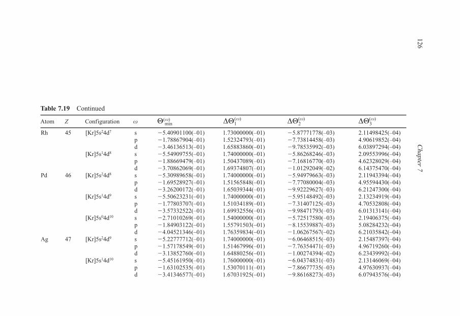
126C
hapter 7
Rh 45 [Kr]5s24d7 s �5.40901100(–01) 1.73000000(–01) �5.87771778(–03) 2.11498425(–04)p �1.78867904(–01) 1.52324793(–01) �7.73814458(–03) 4.90619852(–04)d �3.46136513(–01) 1.65883860(–01) �9.78535992(–03) 6.03897294(–04)
[Kr]5s14d8 s �5.54909755(–01) 1.74000000(–01) �5.86268246(–03) 2.09553996(–04)p �1.88669479(–01) 1.50437089(–01) �7.16816770(–03) 4.62328029(–04)d �3.70862069(–01) 1.69374807(–01) �1.01292049(–02) 6.14375470(–04)
Pd 46 [Kr]5s24d8 s �5.30989658(–01) 1.74000000(–01) �5.94979663(–03) 2.11943394(–04)p �1.69528927(–01) 1.51565848(–01) �7.77080004(–03) 4.95594430(–04)d �3.26200172(–01) 1.65039344(–01) �9.92229627(–03) 6.21247300(–04)
[Kr]5s14d9 s �5.50623231(–01) 1.74000000(–01) �5.95148492(–03) 2.13234919(–04)p �1.77803707(–01) 1.51034189(–01) �7.31407125(–03) 4.70532808(–04)d �3.57332522(–01) 1.69932556(–01) �9.98471793(–03) 6.01313141(–04)
[Kr]5s04d10 s �2.71010269(–01) 1.54000000(–01) �5.72517580(–03) 2.19406375(–04)p �1.84903122(–01) 1.55791503(–01) �8.15539887(–03) 5.08284232(–04)d �4.04521346(–01) 1.76359834(–01) �1.06267567(–02) 6.21035842(–04)
Ag 47 [Kr]5s24d9 s �5.22777712(–01) 1.74000000(–01) �6.06468515(–03) 2.15487397(–04)p �1.57178549(–01) 1.51467996(–01) �7.76354471(–03) 4.96719260(–04)d �3.13852760(–01) 1.64880256(–01) �1.00274394(–02) 6.23439992(–04)
[Kr]5s14d10 s �5.45161950(–01) 1.76000000(–01) �6.04374831(–03) 2.13146069(–04)p �1.63102535(–01) 1.53070111(–01) �7.86677735(–03) 4.97630937(–04)d �3.41346577(–01) 1.67031925(–01) �9.86168273(–03) 6.07943576(–04)
Table 7.19 Continued
Atom Z Configuration � �(�)min ��1
(�) ��2(�) ��3
(�)
Else_EAMC-TRSIC_ch007.qxd 5/4/2007 07:52 Page 126
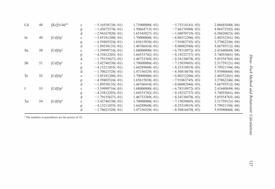
Dirac–Fock M
ethod and Relativistic C
alculations127
Cd 48 [Kr]5s24d10 s �5.16558138(–01) 1.71000000(–01) �5.75314141(–03) 2.06685840(–04)p �1.43675376(–01) 1.50664713(–01) �7.66176988(–03) 4.96472542(–04)d �2.94167020(–01) 1.65345827(–01) �1.04070719(–02) 6.58620823(–04)
In 49 [Cd]5p1 s �3.85181208(–01) 1.70000000(–01) �6.80312206(–03) 2.40352261(–04)p �4.59403524(–01) 1.65615838(–01) �7.91063745(–03) 3.57062246(–04)d �1.89530135(–01) 1.46766410(–01) �8.06082946(–03) 5.66795512(–04)
Sn 50 [Cd]5p2 s �3.59999716(–01) 1.68000000(–01) �6.78318972(–03) 2.41640849(–04)p �4.33812203(–01) 1.64553742(–01) �8.19232737(–03) 3.74055661(–04)d �1.79155627(–01) 1.46733369(–01) �8.34136078(–03) 5.85554765(–04)
Sb 51 [Cd]5p3 s �3.42746530(–01) 1.70000000(–01) �7.15039603(–03) 2.51759121(–04)p �4.13211855(–01) 1.64289048(–01) �8.25319019(–03) 3.79921194(–04)d �1.70621528(–01) 1.47156529(–01) �8.50816670(–03) 5.93980660(–04)
Te 52 [Cd]5p4 s �3.85181208(–01) 1.70000000(–01) �6.80312206(–03) 2.40352261(–04)p �4.59403524(–01) 1.65615838(–01) �7.91063745(–03) 3.57062246(–04)d �1.89530135(–01) 1.46766410(–01) �8.06082946(–03) 5.66795512(–04)
I 53 [Cd]5p5 s �3.59999716(–01) 1.68000000(–01) �6.78318972(–03) 2.41640849(–04)p �4.33812203(–01) 1.64553742(–01) �8.19232737(–03) 3.74055661(–04)d �1.79155627(–01) 1.46733369(–01) �8.34136078(–03) 5.85554765(–04)
Xe 54 [Cd]5p6 s �3.42746530(–01) 1.70000000(–01) �7.15039603(–03) 2.51759121(–04)p �4.13211855(–01) 1.64289048(–01) �8.25319019(–03) 3.79921194(–04)d �1.70621528(–01) 1.47156529(–01) �8.50816670(–03) 5.93980660(–04)
a The numbers in parentheses are the powers of 10.
Else_EAMC-TRSIC_ch007.qxd 5/4/2007 07:52 Page 127

128C
hapter 7Table 7.20
Total DFC energies (in hartree) and the basis set errors (in millihartree) for H (Z � 1) through Xe (Z � 54)a
Atom Z M Configuration Basis Sets Size Uniform Sphere Model Gaussian Model
EDFC Errora EDFC Errora
H 1 1 1s1 8s –0.500000 0.006 �0.500000 0.006He 2 4 1s2 8s �2.861753 0.060 �2.861753 0.060Li 3 7 [He]2s1 14s �7.433518 0.015 �7.433518 0.015Be 4 9 [He]2s2 14s �14.575859 0.033 �14.575859 0.033B 5 11 [He]2s22p1 14s9p �24.536522 0.033 �24.536522 0.033C 6 12 [He]2s22p2 14s9p �37.675986 0.055 �37.675986 0.055N 7 14 [He]2s22p3 14s9p �54.327633 0.089 �54.327633 0.089O 8 16 [He]2s22p4 14s9p �74.824873 0.113 �74.824873 0.113F 9 19 [He]2s22p5 14s9p �99.501458 0.157 �99.501458 0.157Ne 10 20 [He]2s22p6 14s9p �128.691711 0.220 �128.691711 0.220Na 11 23 [Ne]3s1 18s9p �162.077859 0.229 �162.077859 0.229Mg 12 24 [Ne]3s2 18s9p �199.934840 0.226 �199.934840 0.227Al 13 27 [Ne]3s23p1 18s13p �242.330593 0.156 �242.330593 0.156Si 14 28 [Ne]3s23p2 18s13p �289.461147 0.191 �289.461147 0.191P 15 31 [Ne]3s23p3 18s13p �341.494459 0.210 �341.494459 0.210S 16 32 [Ne]3s23p4 18s13p �398.597689 0.241 �398.597689 0.241Cl 17 35 [Ne]3s23p5 18s13p �460.938114 0.269 �460.938114 0.270Ar 18 40 [Ne]3s23p6 18s13p �528.683440 0.322 �528.683440 0.323K 19 39 [Ar]4s1 21s13p �601.525662 0.291 �601.525662 0.292Ca 20 40 [Ar]4s2 21s13p �679.709852 0.309 �679.709852 0.310Sc 21 45 [Ar]4s23d1 21s13p10d �763.378392 0.346 �763.378392 0.347
[Ar]4s13d2 21s13p10d �763.301374 0.359 �763.301375 0.360Ti 22 48 [Ar]4s23d2 21s13p10d �852.819418 0.405 �852.819418 0.407
[Ar]4s13d3 21s13p10d �852.755350 0.406 �852.755350 0.407V 23 51 [Ar]4s23d3 21s13p10d �948.188201 0.456 �948.188201 0.458
[Ar]4s13d4 21s13p10d �948.135523 0.465 �948.135524 0.467
Else_EAMC-TRSIC_ch007.qxd 5/4/2007 07:52 Page 128

Dirac–Fock M
ethod and Relativistic C
alculations129
Cr 24 52 [Ar]4s23d4 21s13p10d �1049.637960 0.517 �1049.637961 0.519[Ar]4s13d5 21s13p10d �1049.595498 0.536 �1049.595498 0.540
Mn 25 55 [Ar]4s23d5 21s13p10d �1157.321328 0.585 �1157.321329 0.589[Ar]4s13d6 21s13p10d �1157.288179 0.597 �1157.288180 0.600
Fe 26 56 [Ar]4s23d6 21s13p10d �1271.391315 0.665 �1271.391317 0.668[Ar]4s13d7 21s13p10d �1271.366712 0.687 �1271.366714 0.690
Co 27 59 [Ar]4s23d7 21s13p10d �1392.001053 0.770 �1392.001056 0.774[Ar]4s13d8 21s13p10d �1391.984377 0.798 �1391.984379 0.803
Ni 28 58 [Ar]4s23d8 21s13p10d �1519.304770 0.848 �1519.304773 0.854[Ar]4s13d9 21s13p10d �1519.295498 0.873 �1519.295501 0.880
Cu 29 63 [Ar]4s23d9 21s13p10d �1653.456441 0.928 �1653.456445 0.936[Ar]4s13d10 21s13p10d �1653.454059 1.004 �1653.454063 1.012
Zn 30 64 [Ar]4s23d10 21s13p10d �1794.611922 1.046 �1794.611928 1.055Ga 31 69 [Zn]4p1 21s17p10d �1942.563006 0.737 �1942.563015 0.749Ge 32 74 [Zn]4p2 21s17p10d �2097.469599 0.736 �2097.469611 0.750As 33 75 [Zn]4p3 21s17p10d �2259.441124 0.756 �2259.441142 0.770Se 34 80 [Zn]4p4 21s17p10d �2428.587454 0.780 �2428.587476 0.798Br 35 79 [Zn]4p5 21s17p10d �2605.022614 0.823 �2605.022644 0.841Kr 36 84 [Zn]4p6 21s17p10d �2788.859682 0.881 �2788.859722 0.902Rb 37 85 [Kr]5s1 25s17p10d �2979.804142 0.797 �2979.804220 0.793Sr 38 88 [Kr]5s2 25s17p10d �3178.079060 0.819 �3178.079156 0.813Y 39 89 [Kr]5s24d1 25s17p13d �3383.760793 0.922 �3383.760907 0.917
[Kr]5s14d2 25s17p13d �3383.698847 1.036 �3383.698961 1.030Zr 40 90 [Kr]5s24d2 25s17p13d �3597.082263 0.944 �3597.082399 0.938
[Kr]5s14d3 25s17p13d �3597.040330 1.066 �3597.040465 1.061Nb 41 93 [Kr]5s24d3 25s17p13d �3818.167133 0.972 �3818.167298 0.964
[Kr]5s14d4 25s17p13d �3818.147394 1.064 �3818.147557 1.058Mo 42 98 [Kr]5s24d4 25s17p13d �4047.136159 1.033 �4047.136358 1.026
[Kr]5s14d5 25s17p13d �4047.140237 1.129 �4047.140437 1.120Tc 43 98 [Kr]5s24d5 25s17p13d �4284.112048 1.095 �4284.112285 1.083
[Kr]5s14d6 25s17p13d �4284.141375 1.165 �4284.141613 1.152Ru 44 102 [Kr]5s24d6 25s17p13d �4529.212419 1.154 �4529.212704 1.140
[Kr]5s14d7 25s17p13d �4529.268212 1.227 �4529.268498 1.212
(continued )
Else_EAMC-TRSIC_ch007.qxd 5/4/2007 07:52 Page 129

130C
hapter 7
Rh 45 103 [Kr]5s24d7 25s17p13d �4782.561261 1.236 �4782.561597 1.220[Kr]5s14d8 25s17p13d �4782.644650 1.317 �4782.644988 1.299
Pd 46 [Kr]5s24d8 25s17p13d �5044.278850 1.346 �5044.279249 1.328106 [Kr]5s14d9 25s17p13d �5044.390952 1.370 �5044.391352 1.351
[Kr]5s04d10 25s17p13d �5044.399478 1.235 �5044.399875 1.218Ag 47 107 [Kr]5s24d9 25s17p13d �5314.490674 1.398 �5314.491144 1.374
[Kr]5s14d10 25s17p13d �5314.632339 1.503 �5314.632808 1.481Cd 48 114 [Kr]5s24d10 25s17p13d �5593.316844 1.454 �5593.317410 1.427In 49 115 [Cd]5p1 25s21p13d �5880.429953 1.000 �5880.430616 0.966Sn 50 120 [Cd]5p2 25s21p13d �6176.126359 0.982 �6176.127146 0.943Sb 51 121 [Cd]5p3 25s21p13d �6480.516731 1.027 �6480.517653 0.974Te 52 130 [Cd]5p4 25s21p13d �6793.696839 1.081 �6793.697948 1.019I 53 127 [Cd]5p5 25s21p13d �7115.791875 1.109 �7115.793138 1.037Xe 54 132 [Cd]5p6 25s21p13d �7446.892822 1.217 �7446.894310 1.130
a The RAGBS error with respect to the numerical DFC results [25].
Table 7.20 Continued
Atom Z M Configuration Basis Sets Size Uniform Sphere Model Gaussian Model
EDFC Errora EDFC Errora
Else_EAMC-TRSIC_ch007.qxd 5/4/2007 07:52 Page 130
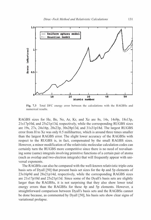
RAGBS sizes for He, Be, Ne, Ar, Kr, and Xe are 8s, 14s, 14s9p, 18s13p,21s17p10d, and 25s21p13d, respectively, while the corresponding RUGBS sizesare 19s, 27s, 24s16p, 28s23p, 30s28p13d, and 31s31p18d. The largest RUGBSerror from H to Xe was only 0.5 millihartree, which is around three times smallerthan the largest RAGBS error. The slight lower accuracy of the RAGBSs withrespect to the RUGBS is, in fact, compensated by the small RAGBS sizes.However, a minor modification of the relativistic molecular calculation codes cancertainly turn the RUGBS more competitive since there is no need of reevaluat-ing some (same) integrals involving primitive functions of a certain pair of atoms(such as overlap and two-electron integrals) that will frequently appear with uni-versal exponents.
The RAGBSs can also be compared with the well-known relativistic triple-zetabasis sets of Dyall [50] that present basis set sizes for the 4p and 5p elements of23s16p9d and 28s21p14d, respectively, while the corresponding RAGBS sizesare 21s17p10d and 25s21p13d. Since some of the Dyall’s basis sets are slightlylarger than the RAGBSs, it is not surprising that they also show lower totalenergy errors than the RAGBSs for these 4p and 5p elements. However, astraightforward comparison between Dyall’s basis sets and the RAGBSs cannotbe done because, as commented by Dyall [50], his basis sets show clear signs ofvariational prolapse.
Dirac–Fock Method and Relativistic Calculations 131
Fig. 7.3 Total DFC energy error between the calculations with the RAGBSs andnumerical results.
Else_EAMC-TRSIC_ch007.qxd 5/4/2007 07:52 Page 131

The energy difference results between the calculations with the originalRAGBS and the RAGBS augmented with one tight s or one tight p Gaussianfunction (EDFC –E�1
DFCtight) are presented in Fig. 7.4. The tight s or p function
added was always the next function right after those already chosen for the con-sidered atom, i.e., the next one from the set given by the pGCDF parameters inTable 7.19. From Fig. 7.4 we can see that the addition of one tight function withboth nuclear models always results in the lowering or convergence of the DFCtotal energy, including the atoms that had first presented signs of variationalprolapse in its s1/2 orbital symmetry (from Rb to Xe) and for which the ��1
(s)
parameter was slightly increased. These results show that it is possible to takeadvantage of the characteristics of the pGCDF method so as to eliminate thevariational prolapse problem from a basis set. This happens because ��1
(s) is apositive parameter that has the aim of ensuring a primary separation betweenthe ID points (Gaussian function exponents) that is adjusted by the combina-tion of the ��2
(s) and ��3(s) parameters depending on the atomic region (closer
or more distant regions from the nucleus). Thus, any increase of the ��1(s)
parameter will result in a corresponding separation increase of all discretiza-tion points into the atomic nucleus that will eventually overcome any previousbad description of the innermost atomic region responsible for the variationalprolapse.
132 Chapter 7
Fig. 7.4 Total DFC energy differences between the calculations with the RAGBS and theRAGBS augmented with one tight s or one tight p function (EDFC –E�1
DFCtight).
Else_EAMC-TRSIC_ch007.qxd 5/4/2007 07:52 Page 132

The DFC total energy reduction for H through Xe, upon the addition of onetight p function, is larger than the one for the addition of one tight s function,as shown in Fig. 7.4. Moreover, the energy difference behavior observed inFig. 7.4, between the two nuclear models for the addition of one tight s func-tion, becomes visually distinguished for the atoms from Ca (Z = 20) onward.When one tight p function is added, the distinct behavior between the twonuclear models is only seen for the atoms from Sn (Z = 50) onward. Hence,we suspect that Ca and Sn represent the limits where the s1/2 and p1/2 electroniccloud, respectively, begins to present a significant penetration into the nuclearregion resulting in the different behavior observed in Fig. 7.4 between the twofinite nucleus models studied (i.e., depending on the proton-charge distribu-tion characteristics of the nucleus model).
More detailed variational prolapse tests are shown in Tables 7.21–7.24 forsome selected atomic systems: Kr (Z = 36), Sr (Z = 38), Cd (Z = 48), and Xe(Z = 54). The DFC total energy behavior for these convergence patterns wasanalyzed by the addition of up to three tight Gaussian functions for s, p, or dsymmetries. As expected, the addition of tight d functions showed no sign ofvariational prolapse due to the negligible penetration of electrons in suchorbitals into the atomic nucleus [26,31,51]. Moreover, the addition of up to threetight s or p functions, with both nuclear models, also did not present any sign ofprolapse. The addition of up to three tight s functions was particularly importantin the case of Sr, Cd, and Xe since these atoms had previously presented pro-lapse in its s1/2 orbital symmetry. All these results allow us to assure that ourRAGBSs are totally free of variational prolapse and apt to be used in relativis-tic atomic and molecular calculations with both uniform sphere and Gaussiannucleus models.
Dirac–Fock Method and Relativistic Calculations 133
Table 7.21
Convergence pattern (in hartree) for Kr (Z�36)
Calculation Uniform Sphere Model Gaussian Model
EDFC EDFC
21s17p10d �2788.859682 �2788.859722�1 tight s �2788.859690 �2788.859753�2 tight s �2788.859690 �2788.859753�3 tight s �2788.859690 �2788.859753�1 tight p �2788.859798 �2788.859837�2 tight p �2788.859814 �2788.859854�3 tight p �2788.859815 �2788.859855�1 tight d �2788.859712 �2788.859752�2 tight d �2788.859713 �2788.859752�3 tight d �2788.859713 �2788.859752
Else_EAMC-TRSIC_ch007.qxd 5/4/2007 07:52 Page 133
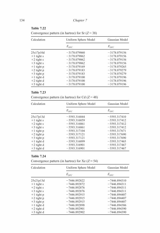
134 Chapter 7
Table 7.22
Convergence pattern (in hartree) for Sr (Z�38)
Calculation Uniform Sphere Model Gaussian Model
EDFC EDFC
25s17p10d �3178.079060 �3178.079156�1 tight s �3178.079062 �3178.079156�2 tight s �3178.079062 �3178.079156�3 tight s �3178.079062 �3178.079156�1 tight p �3178.079169 �3178.079265�2 tight p �3178.079183 �3178.079279�3 tight p �3178.079183 �3178.079279�1 tight d �3178.079100 �3178.079196�2 tight d �3178.079100 �3178.079196�3 tight d �3178.079100 �3178.079196
Table 7.23
Convergence pattern (in hartree) for Cd (Z �48)
Calculation Uniform Sphere Model Gaussian Model
EDFC EDFC
25s17p13d �5593.316844 �5593.317410�1 tight s �5593.316859 �5593.317412�2 tight s �5593.316861 �5593.317412�3 tight s �5593.316861 �5593.317412�1 tight p �5593.317104 �5593.317671�2 tight p �5593.317121 �5593.317690�3 tight p �5593.317121 �5593.317690�1 tight d �5593.316899 �5593.317465�2 tight d �5593.316901 �5593.317467�3 tight d �5593.316901 �5593.317467
Table 7.24
Convergence pattern (in hartree) for Xe (Z�54)
Calculation Uniform Sphere Model Gaussian Model
EDFC EDFC
25s21p13d �7446.892822 �7446.894310�1 tight s �7446.892872 �7446.894311�2 tight s �7446.892876 �7446.894311�3 tight s �7446.892876 �7446.894311�1 tight p �7446.892915 �7446.894407�2 tight p �7446.892915 �7446.894407�3 tight p �7446.892915 �7446.894407�1 tight d �7446.892898 �7446.894386�2 tight d �7446.892901 �7446.894390�3 tight d �7446.892902 �7446.894390
Else_EAMC-TRSIC_ch007.qxd 5/4/2007 07:52 Page 134

7.2. Relativistic Adapted Gaussian Basis Sets for Cesium throughRadon
RAGBSs for Cs (Z�55) through Rn (Z�86) were obtained by employing thepGCDF method with four parameters for each atomic orbital symmetry (�(�)
min
and ��q(�) with q =1, 2, and 3, where �� s, p, d, and f) [52] and the SIMPLEX
algorithm [44] was used to optimize the pGCDF discretization parameters. Thebasis set sizes for Cs through Rn were chosen by means of a preliminary analy-sis on the noble gas atom Rn and also taking into account the RAGBS size of Xe(25s21p13d) [48].
As expected, the initial optimized pGCDF parameters for Cs through Rnfurnished basis sets with prolapse in the s1/2 relativistic atomic orbital symme-try once this problem was detected in the atomic range from Rb (Z � 37) to Xe(Z � 54) with a prolapse of at most 0.1 millihartree [48]. Thus, since the atomicnumbers for Cs through Rn are larger than the ones studied before [48], the vari-ational prolapses found from Cs to Rn were also more pronounced and reached5.5 millihartree for Ra with the uniform sphere model. As before [48], the pro-lapse problem was solved by a slight increase of the ��1
(s) parameter thatimproves the description of the electrons closer to the nucleus (the innermostregion of the atom). Furthermore, a very small prolapse (0.01 millihartree forRa with the uniform sphere model) was also detected in the p1/2 symmetry fromTl (Z � 81) to Rn (Z � 86) and a subtle increase of the ��1
(p) parameter was alsoable to surpass the problem.
The optimal pGCDF discretization parameters, obtained after the adjustmentsof ��1
(s) and ��1(p) with the aim to overcome the variational prolapse, are given
in Table 7.25. All of the RAGBS exponents from Cs to Rn are presented inAppendix 5. Table 7.26 presents the DFC total energies, the RAGBS sizes, andits errors with respect to numerical results [25]. The RAGBS errors are illustratedin Fig. 7.5 as a function of the atomic number. From Fig. 7.5 we can see that theRAGBS errors behave in a periodic way and also increase with the atomic num-ber as the subshells are being filled, likewise to the behavior for the atoms fromH to Xe [48]. We can also notice from Fig. 7.5 that the RAGBS for Cs throughRn, as for H through Xe [48], showed lower errors with the Gaussian nucleusmodel than with the uniform sphere model as the atomic numbers are approxi-mately greater than 40, reaching a relative error of 1.3 millihartree for the heav-iest atoms. This can be rationalized since adapted basis sets are developed foreach atom with its own valence characteristics to attain the lowest basis set errorwith the possible smallest size. A small basis set requires that the most diffuseand the innermost regions in the atom be treated by a reduced number ofGaussian functions when compared to the intermediate region (this will be moreor less successful depending on the nuclear model adopted).
The RAGBS sizes from Cs to Rn are smaller than the ones of our prolapse-freeRUGBS that was obtained with the original GCDF method [26]. The RUGBS
Dirac–Fock Method and Relativistic Calculations 135
Else_EAMC-TRSIC_ch007.qxd 5/4/2007 07:52 Page 135

sizes for Ba, Yb, Hg, and Rn are 35s30p17d, 34s30p16d14f, 33s29p21d12f, and32s32p20d11f, respectively, while the corresponding RAGBS sizes are30s21p13d, 30s21p13d11f, 30s22p17d11f, and 30s27p17d11f. The size reduc-tion of the basis sets achieved by the pGCDF method in relation to the originalGCDF method for these illustrative atoms is in the range of 2�5 s functions,5�9 p functions, 3�4 d functions, and 0–3 f functions. In fact, the size differ-ence between the RUGBS and RAGBSs tends to reduce as the atomic numberincreases. Furthermore, the RUGBS errors for Ba, Yb, Hg, and Rn are 0.6, 1.6,3.0, and 3.6 millihartree, respectively, for the uniform sphere model, and can becompared with the RAGBS errors that are 0.9, 2.5, 2.9, and 4.5 millihartree,respectively, for the same nucleus model. Thus, such errors between bothapproaches are similar or, in other words, the RUGBS and the RAGBSs can beconsidered as having the same accuracy.
Another remark on the RAGBS sizes is that one more p function (22 insteadof 21) was added for the atoms from Lu (Z�71) to Hg (Z�80) to keep the basisset error below 5 millihartree. The electronic configurations with one electron inthe 5d subshell for La (Z�57), Ce (Z�58), and Gd (Z�64) required 15d insteadof 13d functions once the d electronic cloud is more diffuse in such configura-tions. The largest RAGBS errors are those for Rn (Z�86), i.e., 4.5 and 3.2 milli-hartree for the uniform sphere and the Gaussian models, respectively.
136 Chapter 7
Fig. 7.5 Total DFC energy error between the calculations with the RAGBSs and numericalresults.
Else_EAMC-TRSIC_ch007.qxd 5/4/2007 07:52 Page 136

Dirac–Fock M
ethod and Relativistic C
alculations137
Table 7.25
The pGCDF parameters for Cs (Z�55) through Rn (Z�86)a
Atom Z Configuration � �(�)min ��
1(�) ��
2(�) ��
3(�)
Cs 55 [Xe] 6s1 s �6.89309456(�01) 1.84500000(�01) �7.27838702(�03) 1.88656757(�04)p �3.73954597(�01) 1.54182625(�01) �7.10237528(�03) 3.43631331(�04)d �1.33627171(�01) 1.40010433(�01) �7.74851547(�03) 5.76592752(�04)
Ba 56 [Xe] 6s2 s �6.43427931(�01) 1.76500000(�01) �7.02749031(�03) 1.87869591(�04)p �3.59625691(�01) 1.58413113(�01) �7.83219906(�03) 3.71877331(�04)d �1.22352674(�01) 1.41353310(�01) �8.23617429(�03) 6.14459218(�04)
La 57 [Xe] 6s24f1 s �6.31540168(�01) 1.77300000(�01) �7.22990967(�03) 1.93851253(�04)p �3.30933707(�01) 1.57782436(�01) �7.71570635(�03) 3.67462664(�04)d �9.32342456(�02) 1.38683782(�01) �7.62257186(�03) 5.59506740(�04)f �4.49989016(�01) 1.46815349(�01) �4.38026134(�03) 3.10417177(�04)
[Xe] 6s25d1 s �6.23817882(�01) 1.75900000(�01) �7.22526889(�03) 1.95049252(�04)p �3.27841746(�01) 1.56745218(�01) �7.67231040(�03) 3.68657674(�04)d �4.55912743(�01) 1.68587229(�01) �8.47568117(�03) 4.25949785(�04)
Ce 58 [Xe] 6s24f2 s �6.25910415(�01) 1.76300000(�01) �7.20484855(�03) 1.93959558(�04)p �3.42177883(�01) 1.59174006(�01) �7.82366859(�03) 3.65879826(�04)d �6.70688664(�02) 1.30990723(�01) �6.23869509(�03) 4.88970430(�04)f �4.40600400(�01) 1.45481734(�01) �4.23799360(�03) 3.23719350(�04)
[Xe] 6s24f15d1 s �6.10850205(�01) 1.76500000(�01) �7.17401355(�03) 1.92132944(�04)p �3.32111124(�01) 1.58451270(�01) �7.83409698(�03) 3.69753823(�04)d �4.46240513(�01) 1.69350312(�01) �8.89767181(�03) 4.53370582(�04)f �3.50968316(�01) 1.34271521(�01) �3.79771186(�03) 3.06995978(�04)
Pr 59 [Xe] 6s24f3 s �6.20008675(�01) 1.78100000(�01) �7.29246162(�03) 1.94619959(�04)p �3.25339574(�01) 1.58518979(�01) �7.70667605(�03) 3.67393670(�04)d �7.23137980(�02) 1.31745194(�01) �6.06630476(�03) 4.90444807(�04)f �4.21335688(�01) 1.47026246(�01) �4.45187556(�03) 3.21449354(�04)
Nd 60 [Xe] 6s24f4 s �6.25819228(�01) 1.78700000(�01) �7.26198080(�03) 1.93059453(�04)p �3.22727881(�01) 1.57981471(�01) �7.65907905(�03) 3.63804882(�04)d �7.35878161(�02) 1.31115562(�01) �6.00293700(�03) 4.87121220(�04)f �4.07525146(�01) 1.47278947(�01) �4.61416931(�03) 3.20791228(�04)
(continued )
Else_EAMC-TRSIC_ch007.qxd 5/4/2007 07:52 Page 137

138C
hapter 7
Pm 61 [Xe] 6s24f5 s �6.24292825(�01) 1.74300000(�01) �6.59756092(�03) 1.75407365(�04)p �3.17981400(�01) 1.57194411(�01) �7.59651469(�03) 3.63591770(�04)d �6.34675207(�02) 1.30031680(�01) �6.04293610(�03) 4.91178568(�04)f �3.94105026(�01) 1.47958763(�01) �5.20613342(�03) 3.69779272(�04)
Sm 62 [Xe] 6s24f6 s �6.24665154(�01) 1.73800000(�01) �6.44921441(�03) 1.70898671(�04)p �3.10611106(�01) 1.60435984(�01) �7.66762180(�03) 3.61896639(�04)d �5.65387358(�02) 1.30142741(�01) �6.02615538(�03) 4.94350579(�04)f �3.75031681(�01) 1.51064017(�01) �6.12961434(�03) 4.34841334(�04)
Eu 63 [Xe] 6s24f7 s �6.19958906(�01) 1.76900000(�01) �6.52966007(�03) 1.69790644(�04)p �3.09193799(�01) 1.58949390(�01) �7.61749980(�03) 3.63995874(�04)d �5.13423063(�02) 1.32520135(�01) �5.84039491(�03) 4.60620984(�04)f �3.46318132(�01) 1.48917212(�01) �6.06505697(�03) 4.21986624(�04)
Gd 64 [Xe] 6s24f8 s �6.03213313(�01) 1.77500000(�01) �6.75107568(�03) 1.75941762(�04)p �3.04243681(�01) 1.56783061(�01) �7.08189014(�03) 3.41377839(�04)d �2.28591779(�02) 1.33774694(�01) �6.86008754(�03) 5.33697952(�04)f �2.85459648(�01) 1.50937479(�01) �7.38125161(�03) 5.07305790(�04)
[Xe] 6s24f75d1 s �5.93031341(�01) 1.78700000(�01) �6.74089038(�03) 1.73836839(�04)p �2.90022468(�01) 1.57129731(�01) �7.08802955(�03) 3.40421690(�04)d �4.37798776(�01) 1.90831332(�01) �1.23005179(�02) 6.11623021(�04)f �2.41595047(�01) 1.33850772(�01) �3.87083591(�03) 3.01316523(�04)
Tb 65 [Xe] 6s24f9 s �6.00636455(�01) 1.77600000(�01) �6.87613940(�03) 1.80027566(�04)p �2.84282739(�01) 1.56374730(�01) �7.06413913(�03) 3.41946454(�04)d �2.32279878(�02) 1.35509067(�01) �7.04765091(�03) 5.45865122(�04)f �2.66901117(�01) 1.51545336(�01) �7.23364106(�03) 5.13619927(�04)
Dy 66 [Xe] 6s24f10 s �6.00436041(�01) 1.77600000(�01) �6.88913657(�03) 1.80513074(�04)p �2.94004205(�01) 1.56309714(�01) �7.05405761(�03) 3.42021565(�04)d �2.21146294(�02) 1.35143879(�01) �7.02102552(�03) 5.53864950(�04)f �2.86089999(�01) 1.51360957(�01) �7.24815041(�03) 5.04203875(�04)
Ho 67 [Xe] 6s24f11 s �5.95940748(�01) 1.76900000(�01) �6.93934557(�03) 1.82863328(�04)p �2.89428253(�01) 1.56607553(�01) �7.06649068(�03) 3.40302523(�04)
Table 7.25 Continued
Atom Z Configuration � �(�)min ��
1(�) ��
2(�) ��
3(�)
Else_EAMC-TRSIC_ch007.qxd 5/4/2007 07:52 Page 138

Dirac–Fock M
ethod and Relativistic C
alculations139
d �2.31567398(�02) 1.36221543(�01) �6.91538754(�03) 5.39112469(�04)f �2.80357653(�01) 1.51761849(�01) �7.24726108(�03) 4.96550879(�04)
Er 68 [Xe] 6s24f12 s �5.87524295(�01) 1.75200000(�01) �6.90243734(�03) 1.83234525(�04)p �2.87510824(�01) 1.57176352(�01) �7.07336758(�03) 3.41170302(�04)d �2.21570953(�02) 1.36766975(�01) �7.20919689(�03) 5.54335932(�04)f �2.68523479(�01) 1.53359991(�01) �7.41688605(�03) 5.05928860(�04)
Tm 69 [Xe] 6s24f13 s �5.91380595(�01) 1.74800000(�01) �6.85438448(�03) 1.82227177(�04)p �2.78213410(�01) 1.56516855(�01) �7.10811764(�03) 3.40994132(�04)d �2.12816248(�02) 1.35541332(�01) �7.10417079(�03) 5.62463163(�04)f �2.74386254(�01) 1.58659080(�01) �7.94004377(�03) 5.15341382(�04)
Yb 70 [Xe] 6s24f14 s �5.88186810(�01) 1.73000000(�01) �7.13629598(�03) 1.93933315(�04)p �2.81562563(�01) 1.57203350(�01) �6.81925073(�03) 3.29283189(�04)d �2.39761361(�02) 1.37776507(�01) �7.32663964(�03) 5.72736797(�04)f �2.96757230(�01) 1.56793397(�01) �7.21869079(�03) 4.76510982(�04)
Lu 71 [Xe] 6s24f145d1 s �5.64926686(�01) 1.82600000(�01) �7.19504924(�03) 1.89644729(�04)p �2.50600848(�01) 1.50978899(�01) �6.84593447(�03) 3.13508924(�04)d �4.66318374(�01) 1.70193513(�01) �8.08701979(�03) 3.44770646(�04)f �1.95473248(�01) 1.42012116(�01) �6.58016448(�03) 5.06336533(�04)
Hf 72 [Xe] 6s24f145d2 s �5.46315490(�01) 1.82800000(�01) �7.17449235(�03) 1.87850347(�04)p �2.36815975(�01) 1.53543320(�01) �6.85873109(�03) 3.09753650(�04)d �4.42499286(�01) 1.63170149(�01) �7.28731870(�03) 3.18551448(�04)f �1.54788545(�01) 1.52137449(�01) �9.31285305(�03) 6.80048021(�04)
[Xe] 6s14f145d3 s �5.37530956(�01) 1.83600000(�01) �6.97397997(�03) 1.79673807(�04)p �2.49821181(�01) 1.53152048(�01) �6.88337425(�03) 3.11899328(�04)d �5.11978984(�01) 1.68737020(�01) �8.06810313(�03) 3.56226701(�04)f �1.69114075(�01) 1.48309179(�01) �8.79450113(�03) 6.39265251(�04)
Ta 73 [Xe] 6s24f145d3 s �5.32169635(�01) 1.79600000(�01) �7.06465401(�03) 1.87278576(�04)p �2.25487824(�01) 1.55842630(�01) �6.87048030(�03) 3.04998747(�04)d �4.30272436(�01) 1.64962678(�01) �7.94327230(�03) 3.59599333(�04)f �1.26677376(�01) 1.49936407(�01) �8.28727662(�03) 6.05125752(�04)
[Xe] 6s14f145d4 s �5.38656171(�01) 1.81400000(�01) �7.11918834(�03) 1.87328960(�04)p �2.31030902(�01) 1.55393654(�01) �6.92853055(�03) 3.07237653(�04)d �4.63392071(�01) 1.69260535(�01) �8.07946158(�03) 3.50489830(�04)
(continued )
Else_EAMC-TRSIC_ch007.qxd 5/4/2007 07:52 Page 139

140C
hapter 7
f �1.34369914(�01) 1.39061265(�01) �7.52960011(�03) 5.88738068(�04)W 74 [Xe] 6s24f145d4 s �5.26373310(�01) 1.83100000(�01) �7.23842661(�03) 1.88872912(�04)
p �2.13021676(�01) 1.51599407(�01) �6.90857249(�03) 3.13778804(�04)d �4.17825325(�01) 1.70687761(�01) �8.71140035(�03) 3.84054028(�04)f �9.13016434(�02) 1.43596835(�01) �7.93358341(�03) 5.81795040(�04)
[Xe] 6s14f145d5 s �5.27645066(�01) 1.84300000(�01) �7.17973059(�03) 1.85502971(�04)p �2.29520324(�01) 1.53956859(�01) �6.82521549(�03) 3.08752549(�04)d �4.63555144(�01) 1.69561457(�01) �8.08780486(�03) 3.51201651(�04)f �1.33424042(�01) 1.40174047(�01) �7.54791762(�03) 5.96438558(�04)
Re 75 [Xe] 6s24f145d5 s �5.21572883(�01) 1.85000000(�01) �7.23905153(�03) 1.86503966(�04)p �2.06073075(�01) 1.51912738(�01) �6.84705926(�03) 3.10483132(�04)d �3.99540165(�01) 1.69533950(�01) �9.46000618(�03) 4.27609929(�04)f �7.19160739(�02) 1.42293401(�01) �8.01388343(�03) 6.07199793(�04)
[Xe] 6s14f145d6 s �5.09772397(�01) 1.80900000(�01) �7.15701246(�03) 1.88100290(�04)p �2.10625658(�01) 1.53700260(�01) �6.89987393(�03) 3.10023808(�04)d �4.35469256(�01) 1.72982063(�01) �9.45747392(�03) 4.25023030(�04)f �7.82232257(�02) 1.40596036(�01) �7.45287329(�03) 5.82420231(�04)
Os 76 [Xe] 6s24f145d6 s �5.02894669(�01) 1.80700000(�01) �7.21629482(�03) 1.91084121(�04)p �1.82452891(�01) 1.51589494(�01) �6.91405064(�03) 3.16685768(�04)d �3.77734184(�01) 1.68733971(�01) �9.58427247(�03) 1.90094680(�04)f �6.96513836(�02) 1.39616585(�01) �8.43237097(�03) 3.13669040(�04)
[Xe] 6s14f145d7 s �4.97929096(�01) 1.80400000(�01) �7.18263452(�03) 4.50902790(�04)p �1.90763741(�01) 1.51841007(�01) �6.93277577(�03) 6.80843975(�04)d �4.09963048(�01) 1.71305282(�01) �9.53563698(�03) 1.88994629(�04)f �6.96347760(�02) 1.40512958(�01) �8.28041747(�03) 3.12068862(�04)
Ir 77 [Xe] 6s24f145d7 s �5.06128998(�01) 1.80300000(�01) �7.22799350(�03) 4.35274176(�04)p �1.94024323(�01) 1.50300332(�01) �6.87409349(�03) 6.62274502(�04)d �3.57001660(�01) 1.65921105(�01) �9.71126311(�03) 4.59985286(�04)f �6.88565771(�02) 1.40978489(�01) �8.85412587(�03) 6.88731831(�04)
[Xe] 6s14f145d8 s �5.09637806(�01) 1.80800000(�01) �7.19935170(�03) 1.89604896(�04)
Table 7.25 Continued
Atom Z Configuration � �(�)min ��
1(�) ��
2(�) ��
3(�)
Else_EAMC-TRSIC_ch007.qxd 5/4/2007 07:52 Page 140
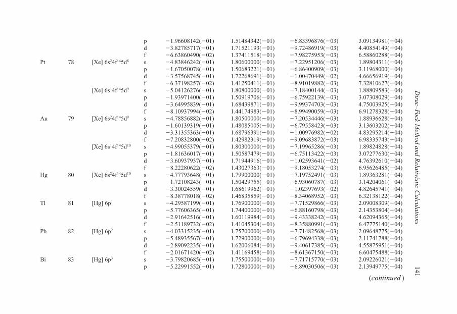
Dirac–Fock M
ethod and Relativistic C
alculations141
p �1.96608142(�01) 1.51484342(�01) �6.83396876(�03) 3.09134981(�04)d �3.82785717(�01) 1.71521193(�01) �9.72486919(�03) 4.40854149(�04)f �6.63860490(�02) 1.37411518(�01) �7.98275953(�03) 6.58860288(�04)
Pt 78 [Xe] 6s24f145d8 s �4.83846242(�01) 1.80600000(�01) �7.22951206(�03) 1.89804311(�04)p �1.67050078(�01) 1.50683221(�01) �6.86400909(�03) 3.11968000(�04)d �3.57568745(�01) 1.72268691(�01) �1.00470449(�02) 4.66656919(�04)f �6.37198257(�02) 1.41250411(�01) �8.91019882(�03) 7.32810627(�04)
[Xe] 6s14f145d9 s �5.04126276(�01) 1.80800000(�01) �7.18400144(�03) 1.88809583(�04)p �1.93971400(�01) 1.50919706(�01) �6.75922139(�03) 3.07308029(�04)d �3.64995839(�01) 1.68439871(�01) �9.99374703(�03) 4.75003925(�04)f �8.10937994(�02) 1.44174983(�01) �8.99490059(�03) 6.91278328(�04)
Au 79 [Xe] 6s24f145d9 s �4.78856882(�01) 1.80500000(�01) �7.20534446(�03) 1.88936628(�04)p �1.60139319(�01) 1.48085005(�01) �6.79558423(�03) 3.13603202(�04)d �3.31355363(�01) 1.68796391(�01) �1.00976982(�02) 4.83295214(�04)f �7.20832800(�02) 1.42982319(�01) �9.09683872(�03) 6.98335743(�04)
[Xe] 6s14f145d10 s �4.99055379(�01) 1.80300000(�01) �7.19965286(�03) 1.89824828(�04)p �1.81636017(�01) 1.50587479(�01) �6.75113422(�03) 3.07277630(�04)d �3.60937937(�01) 1.71944916(�01) �1.02593641(�02) 4.76392610(�04)f �8.22280622(�02) 1.43027363(�01) �9.18053274(�03) 6.95626485(�04)
Hg 80 [Xe] 6s24f145d10 s �4.77793648(�01) 1.79900000(�01) �7.19752491(�03) 1.89363281(�04)p �1.72108243(�01) 1.50429755(�01) �6.93060787(�03) 3.14204061(�04)d �3.30024559(�01) 1.68619962(�01) �1.02397693(�02) 4.82645741(�04)f �8.38778018(�02) 1.46835859(�01) �8.34068952(�03) 6.32138122(�04)
Tl 81 [Hg] 6p1 s �4.29587199(�01) 1.76900000(�01) �7.71529866(�03) 2.09008309(�04)p �5.77606365(�01) 1.74400000(�01) �6.88160798(�03) 2.14353804(�04)d �2.91642516(�01) 1.60119984(�01) �9.43338242(�03) 4.62094365(�04)f �2.51189732(�02) 1.41045304(�01) �8.35880991(�03) 6.47775140(�04)
Pb 82 [Hg] 6p2 s �4.03315235(�01) 1.75700000(�01) �7.71482568(�03) 2.09648775(�04)p �5.48935567(�01) 1.72900000(�01) �6.79694338(�03) 2.11741788(�04)d �2.89092235(�01) 1.62006084(�01) �9.40617385(�03) 4.55875951(�04)f �2.01671420(�02) 1.41169458(�01) �8.61367150(�03) 6.60475488(�04)
Bi 83 [Hg] 6p3 s �3.79820685(�01) 1.75500000(�01) �7.71715770(�03) 2.09226021(�04)p �5.22991552(�01) 1.72800000(�01) �6.89030506(�03) 2.13949775(�04)
(continued )
Else_EAMC-TRSIC_ch007.qxd 5/4/2007 07:52 Page 141

142C
hapter 7
d �2.91527320(�01) 1.62141461(�01) �9.48940053(�03) 4.61517961(�04)f �1.00985935(�02) 1.41944170(�01) �8.71357002(�03) 6.61010739(�04)
Po 84 [Hg] 6p4 s �3.64017592(�01) 1.79400000(�01) �7.73032648(�03) 2.04762261(�04)p �4.93510013(�01) 1.74900000(�01) �6.80541893(�03) 2.05926336(�04)d �2.26298477(�01) 1.55315397(�01) �9.59666420(�03) 4.83788384(�04)f �5.00568905(�03) 1.42011883(�01) �8.38077916(�03) 6.26379954(�04)
At 85 [Hg] 6p5 s �3.52727536(�01) 1.80200000(�01) �7.72522903(�03) 2.03454543(�04)p �4.72411339(�01) 1.73900000(�01) �6.88179644(�03) 2.09220729(�04)d �2.18559791(�01) 1.54287616(�01) �9.51650406(�03) 4.83509387(�04)f �1.62596305(�03) 1.43425593(�01) �8.43292357(�03) 6.10117280(�04)
Rn 86 [Hg] 6p6 s �3.34453526(�01) 1.80100000(�01) �7.73485697(�03) 2.03326769(�04)p �4.56637626(�01) 1.72000000(�01) �6.87350932(�03) 2.10783041(�04)d �2.19218026(�01) 1.56024563(�01) �9.90932638(�03) 4.97949780(�04)f �1.31091802(�03) 1.44417385(�01) �8.47418585(�03) 6.03346573(�04)
a The numbers in parentheses are the powers of 10.
Table 7.25 Continued
Atom Z Configuration � �(�)min ��
1(�) ��
2(�) ��
3(�)
Else_EAMC-TRSIC_ch007.qxd 5/4/2007 07:52 Page 142

Dirac–Fock M
ethod and Relativistic C
alculations143
Table 7.26
Total DFC energies (in hartree) and the basis set errors (in millihartree) for Cs (Z � 55) through Rn (Z � 86)
Atom Z M Configuration Basis Sets Size Uniform Sphere Model Gaussian Model
EDFC Errora EDFC Errora
Cs 55 133 [Xe] 6s1 30s21p13d �7786.769132 0.919 �7786.770800 0.868Ba 56 138 [Xe] 6s2 30s21p13d �8135.642200 0.916 �8135.644148 0.863La 57 139 [Xe] 6s24f1 30s21p13d11f �8493.540441 0.955 �8493.542669 0.908
[Xe] 6s25d1 30s21p15d �8493.642397 1.137 �8493.644626 1.090Ce 58 140 [Xe] 6s24f2 30s21p13d11f �8860.994060 1.129 �8860.996619 1.077
[Xe] 6s24f15d1 30s21p15d11f �8861.067756 1.224 �8861.070309 1.179Pr 59 141 [Xe] 6s24f3 30s21p13d11f �9238.144498 1.152 �9238.147431 1.096Nd 60 144 [Xe] 6s24f4 30s21p13d11f �9625.127308 1.234 �9625.130691 1.176Pm 61 145 [Xe] 6s24f5 30s21p13d11f �10022.09029 1.261 �10022.09414 1.216Sm 62 152 [Xe] 6s24f6 30s21p13d11f �10429.15735 1.318 �10429.16184 1.267Eu 63 153 [Xe] 6s24f7 30s21p13d11f �10846.49858 1.416 �10846.50371 1.373Gd 64 158 [Xe] 6s24f8 30s21p13d11f �11274.23544 1.551 �11274.24136 1.495
[Xe] 6s24f75d1 30s21p15d11f �11274.22261 1.723 �11274.22852 1.678Tb 65 159 [Xe] 6s24f9 30s21p13d11f �11712.53697 1.643 �11712.54372 1.587Dy 66 162 [Xe] 6s24f10 30s21p13d11f �12161.53641 1.694 �12161.54414 1.644Ho 67 162 [Xe] 6s24f11 30s21p13d11f �12621.40280 1.828 �12621.41157 1.758Er 68 168 [Xe] 6s24f12 30s21p13d11f �13092.25853 1.951 �13092.26864 1.896Tm 69 169 [Xe] 6s24f13 30s21p13d11f �13574.30353 2.122 �13574.31500 2.069Yb 70 174 [Xe] 6s24f14 30s21p13d11f �14067.66165 2.501 �14067.67484 2.419Lu 71 175 [Xe] 6s24f145d1 30s22p17d11f �14572.51662 1.773 �14572.53160 1.650Hf 72 180 [Xe] 6s24f145d2 30s22p17d11f �15088.76778 1.793 �15088.78496 1.649
[Xe] 6s14f145d3 30s22p17d11f �15088.68430 1.896 �15088.70147 1.757Ta 73 181 [Xe] 6s24f145d3 30s22p17d11f �15616.60969 1.811 �15616.62915 1.640
[Xe] 6s14f145d4 30s22p17d11f �15616.54312 1.934 �15616.56257 1.771W 74 184 [Xe] 6s24f145d4 30s22p17d11f �16156.16146 2.006 �16156.18360 1.809
[Xe] 6s14f145d5 30s22p17d11f �16156.11398 1.981 �16156.13612 1.786
(continued )
Else_EAMC-TRSIC_ch007.qxd 5/4/2007 07:52 Page 143

144C
hapter 7
Re 75 187 [Xe] 6s24f145d5 30s22p17d11f �16707.59299 2.192 �16707.61817 1.965[Xe] 6s14f145d6 30s22p17d11f �16707.56614 2.127 �16707.59134 1.878
Os 76 192 [Xe] 6s24f145d6 30s22p17d11f �17271.05175 2.211 �17271.08056 1.890[Xe] 6s14f145d7 30s22p17d11f �17271.04682 2.245 �17271.07558 1.968
Ir 77 193 [Xe] 6s24f145d7 30s22p17d11f �17846.75432 2.251 �17846.78687 1.882[Xe] 6s14f145d8 30s22p17d11f �17846.77274 2.242 �17846.80524 1.914
Pt 78 195 [Xe] 6s24f145d8 30s22p17d11f �18434.83555 2.478 �18434.87236 2.083[Xe] 6s14f145d9 30s22p17d11f �18434.87853 2.367 �18434.91531 2.000
Au 79 197 [Xe] 6s24f145d9 30s22p17d11f �19035.48280 2.699 �19035.52444 2.243[Xe] 6s14f145d10 30s22p17d11f �19035.55137 2.555 �19035.59300 2.096
Hg 80 202 [Xe] 6s24f145d10 30s22p17d11f �19648.84638 2.865 �19648.89380 2.356Tl 81 205 [Hg] 6p1 30s27p17d11f �20274.79483 2.687 �20274.84893 1.707Pb 82 208 [Hg] 6p2 30s27p17d11f �20913.65117 3.020 �20913.71252 1.809Bi 83 209 [Hg] 6p3 30s27p17d11f �21565.63502 3.319 �21565.70414 1.943Po 84 209 [Hg] 6p4 30s27p17d11f �22230.93324 3.853 �22231.01065 2.525At 85 210 [Hg] 6p5 30s27p17d11f �22909.71775 4.220 �22909.80475 2.865Rn 86 222 [Hg] 6p6 30s27p17d11f �23602.00097 4.548 �23602.10105 3.205
a The RAGBS error with respect to the numerical DFC results [25].
Table 7.26 Continued
Atom Z M Configuration Basis Sets Size Uniform Sphere Model Gaussian Model
EDFC Errora EDFC Errora
Else_EAMC-TRSIC_ch007.qxd 5/4/2007 07:52 Page 144
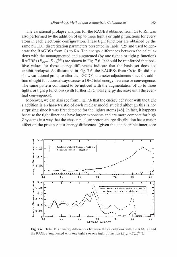
The variational prolapse analysis for the RAGBS obtained from Cs to Rn wasalso performed by the addition of up to three tight s or tight p functions for everyatom in each electronic configuration. These tight functions are obtained by thesame pGCDF discretization parameters presented in Table 7.25 and used to gen-erate the RAGBSs from Cs to Rn. The energy differences between the calcula-tions with the nonaugmented and augmented (by one tight s or tight p function)RAGBSs (EDFC –E�1
DFCtight) are shown in Fig. 7.6. It should be reinforced that pos-
itive values for these energy differences indicate that the basis set does notexhibit prolapse. As illustrated in Fig. 7.6, the RAGBSs from Cs to Rn did notshow variational prolapse after the pGCDF parameter adjustments since the addi-tion of tight functions always causes a DFC total energy decrease or convergence.The same pattern continued to be noticed with the augmentation of up to threetight s or tight p functions (with further DFC total energy decrease until the even-tual convergence).
Moreover, we can also see from Fig. 7.6 that the energy behavior with the tights addition is a characteristic of each nuclear model studied although this is notsurprising since it was first detected for the lighter atoms [48]. In fact, it happensbecause the tight functions have larger exponents and are more compact for highZ systems in a way that the chosen nuclear proton-charge distribution has a majoreffect on the prolapse test energy differences (given the considerable inner-core
Dirac–Fock Method and Relativistic Calculations 145
Fig. 7.6 Total DFC energy differences between the calculations with the RAGBS andthe RAGBS augmented with one tight s or one tight p function (EDFC –E�1
DFCtight).
Else_EAMC-TRSIC_ch007.qxd 5/4/2007 07:52 Page 145
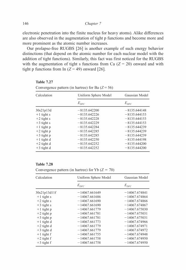
electronic penetration into the finite nucleus for heavy atoms). Alike differencesare also observed in the augmentation of tight p functions and become more andmore prominent as the atomic number increases.
Our prolapse-free RUGBS [26] is another example of such energy behaviordistinctions (that depend on the atomic number for each nuclear model with theaddition of tight functions). Similarly, this fact was first noticed for the RUGBSwith the augmentation of tight s functions from Ca (Z = 20) onward and withtight p functions from In (Z = 49) onward [26].
146 Chapter 7
Table 7.27
Convergence pattern (in hartree) for Ba (Z�56)
Calculation Uniform Sphere Model Gaussian Model
EDFC EDFC
30s21p13d �8135.642200 �8135.644148�1 tight s �8135.642226 �8135.644153�2 tight s �8135.642228 �8135.644153�3 tight s �8135.642229 �8135.644153�1 tight p �8135.642284 �8135.644239�2 tight p �8135.642285 �8135.644239�3 tight p �8135.642285 �8135.644239�1 tight d �8135.642250 �8135.644198�2 tight d �8135.642252 �8135.644200�3 tight d �8135.642252 �8135.644200
Table 7.28
Convergence pattern (in hartree) for Yb (Z � 70)
Calculation Uniform Sphere Model Gaussian Model
EDFC EDFC
30s21p13d11f �14067.661649 �14067.674841�1 tight s �14067.661686 �14067.674864�2 tight s �14067.661690 �14067.674866�3 tight s �14067.661690 �14067.674867�1 tight p �14067.661779 �14067.675030�2 tight p �14067.661781 �14067.675031�3 tight p �14067.661781 �14067.675031�1 tight d �14067.661773 �14067.674966�2 tight d �14067.661779 �14067.674971�3 tight d �14067.661779 �14067.674972�1 tight f �14067.661755 �14067.674948�2 tight f �14067.661758 �14067.674950�3 tight f �14067.661758 �14067.674950
Else_EAMC-TRSIC_ch007.qxd 5/4/2007 07:52 Page 146

Dirac–Fock Method and Relativistic Calculations 147
The magnitude of the energy decrease observed in a tight function augmenta-tion for each nucleus model (Fig. 7.6) depends, among other factors, on thedegree of penetration of such tight function into the nuclear region in compari-son with the functions already presented in the basis set, i.e., the functions of thebasis set before the addition of a tight function. As the uniform sphere model ischaracterized by a proton-charge distribution with uniform density strictly
Table 7.29
Convergence pattern (in hartree) for Hg (Z � 80)
Calculation Uniform Sphere Model Gaussian Model
EDFC EDFC
30s22p17d11f �19648.846385 �19648.893804�1 tight s �19648.846497 �19648.893809�2 tight s �19648.846509 �19648.893810�3 tight s �19648.846510 �19648.893810�1 tight p �19648.846433 �19648.893986�2 tight p �19648.846435 �19648.893987�3 tight p �19648.846435 �19648.893987�1 tight d �19648.846458 �19648.893878�2 tight d �19648.846462 �19648.893881�3 tight d �19648.846462 �19648.893882�1 tight f �19648.846408 �19648.893827�2 tight f �19648.846409 �19648.893828�3 tight f �19648.846409 �19648.893828
Table 7.30
Convergence pattern (in hartree) for Rn (Z � 86)
Calculation Uniform Sphere Model Gaussian Model
EDFC EDFC
30s27p17d11f �23602.000972 �23602.101045�1 tight s �23602.001089 �23602.101064�2 tight s �23602.001102 �23602.101066�3 tight s �23602.001103 �23602.101066�1 tight p �23602.000991 �23602.101050�2 tight p �23602.000993 �23602.101050�3 tight p �23602.000993 �23602.101050�1 tight d �23602.001055 �23602.101128�2 tight d �23602.001059 �23602.101132�3 tight d �23602.001059 �23602.101132�1 tight f �23602.001031 �23602.101104�2 tight f �23602.001033 �23602.101106�3 tight f �23602.001033 �23602.101106
Else_EAMC-TRSIC_ch007.qxd 5/4/2007 07:52 Page 147

148 Chapter 7
restricted inside the nuclear radius (after which this charge distribution goes sud-denly to zero) while the Gaussian nucleus shows a smooth reduction of the pro-ton-charge density with the radius, larger energy decrease values in the tight saddition are more likely to arise with the uniform sphere nucleus model (wherethe the proton-charge distribution is noncontinuous) than with the Gaussiannucleus model. However, for the tight p case (in which the exponents involved arenot so large as the s ones for any given atom and the energy differences are morecomparable) it is difficult to draw an explanation although from Hg (Z�80)onward the same behavior seen for the tight s appears to be present.
Furthermore, some atomic systems (Ba, Yb, Hg, and Rn) were selected toillustrate the prolapse analysis in more details by the addition of up to three tights, p, d, and f functions (see Tables 7.27–7.30). These tables show once more thatthe augmentation of tight d or f functions does not exhibit any sign of variationalprolapse since these kind of functions represent electrons that are too far from theatomic nucleus [26,31,48]. The already mentioned tight s or p addition pattern isalso shown in Tables 7.27–7.30 and from there we can see that the correct DFCtotal energy convergence shows that our RAGBSs generated from Cs to Rn donot present any sign of variational prolapse and are also apt to be used in rela-tivistic atomic and molecular calculations with both uniform sphere andGaussian nucleus models.
Other than the applications we have presented in this chapter with the GCDFand pGCDF methods for DFC and DFB calculations, the reader will find in theliterature other applications with the relativistic generator coordinate formalismin atomic and molecular DFC and DFB calculations [53�61].
Since the GCDF and pGCDF methods have been widely employed in the gen-eration of Gaussian basis sets to be used in relativistic atomic and molecular cal-culations [62–65], in Appendixes 4 and 5 one will find the ultimate universal andAGBSs generated with the GCDF and pGCDF methods for accurate relativisticatomic and molecular calculations.
Also, in the website www.iqsc.usp.br/basis-sets, one will find a whole descrip-tion of the relativistic Gaussian basis sets presented in this chapter.
References
1. Y. Ishikawa, H. Sekino, and R. C. Binning, Jr., Chem. Phys. Lett., 1989, 160, 206.2. S. Okada, and O. Matsuoka, J. Chem. Phys., 1989, 91, 4193.3. A. K. Mohanty, and E. Clementi, J. Chem. Phys., 1990, 93, 1829.4. Y. Ishikawa, Phys. Rev. A, 1990, 42, 1142.5. Y. Ishikawa, H. M. Quiney, and G. L. Malli, Phys. Rev. A, 1991, 43, 3270.6. Y. Ishikawa, R. Baretty, and R. C. Binning, Jr., Chem. Phys. Lett., 1985, 121, 130.7. Y. Ishikawa, and H. M. Quiney, Int. J. Quant. Chem. Symp., 1987, 21, 523.8. A. B. F. da Silva, G. L. Malli, and Y. Ishikawa, Chem. Phys. Lett., 1993, 203, 201.9. G. L. Malli, A. B. F. da Silva, and Y. Ishikawa, Chem. Phys. Lett., 1993, 201, 37.
Else_EAMC-TRSIC_ch007.qxd 5/4/2007 07:52 Page 148

10. A. B. F. da Silva, G. L. Malli, and Y. Ishikawa, Can. J. Chem., 1993, 71, 1713.11. G. L. Malli, A. B. F. da Silva, and Y. Ishikawa, Phys. Rev. A, 1993, 47, 143.12. G. L. Malli, A. B. F. da Silva, and Y. Ishikawa, J. Chem. Phys., 1994, 101, 6829.13. O. Matsuoka, and S. Huzinaga, Chem. Phys. Lett., 1987, 140, 567.14. F. E. Jorge, and A. B. F. da Silva, J. Chem. Phys., 1996, 104, 6278.15. F. E. Jorge, and A. B. F. da Silva, J. Chem. Phys., 1996, 105, 5503.16. Y.-K. Kim, Phys. Rev., 1967, 154, 17.17. A. B. F. da Silva, H. F. M. da Costa, and M. Trsic, Mol. Phys., 1989, 68, 433.18. J. R. Mohallem, Z. Phys. D, 1986, 3, 339.19. J. P. Desclaux, At. Data Nucl. Data Tables, 1973, 12, 311.20. Y.-S. Lee, and A. D. McLean, J. Chem. Phys., 1982, 76, 735; R. E. Stanton, and
S. Havriliak, J. Chem. Phys., 1984, 81, 1910.21. K. G. Dyall, I. P. Grant, and S. Wilson, J. Phys. B, 1984, 17, 1201.22. P. J. C. Aerts, and W. C. Nieuwpoort, Chem. Phys. Lett., 1986, 125, 83.23. A. Farazdel, W. M. Westgate, A. M. Simas, R. P. Sagar, and V. H. Smith, Jr., Int.
J. Quant. Chem. Symp., 1985, 19, 61.24. F. A. Parpia, and A. K. Mohanty, Phys. Rev. A, 1992, 46, 3735.25. L. Visscher, and K. G. Dyall, At. Data Nuc. Data Tables, 1997, 67, 207.26. R. L. A. Haiduke, L. G. M. de Macedo, and A. B. F. da Silva, J. Comput. Chem.,
2005, 26, 932.27. O. Matsuoka, and Y. Watanabe, Comput. Phys. Commun., 2001, 139, 218.28. W. R. Johnson, and G. Soff, At. Data Nuc. Data Tables, 1985, 33, 405.29. O. Matsuoka, J. Phys. Soc. Jpn., 1982, 51, 2263.30. H. F. M. da Costa, M. Trsic, A. B. F. da Silva, and A. M. Simas, Eur. Phys. J. D, 1999,
5, 375.31. H. Tatewaki, T. Koga, and Y. Mochizuki, Chem. Phys. Lett., 2003, 375, 399.32. H. Tatewaki, and Y. Mochizuki, Theor. Chem. Acc., 2003, 109, 40.33. H. Tatewaki, and Y. Watanabe, J. Comput. Chem., 2003, 24, 1823.34. H. Tatewaki, and Y. Watanabe, J. Chem. Phys., 2004, 121, 4528.35. G. W. F. Drake, and S. P. Goldman, Adv. At. Mol. Phys., 1988, 25, 393.36. H. Bethe, and E. E. Salpeter, Quantum Mechanics of One- and Two-Electron
Systems, Berlim: Springer-Verlag, 1957.37. Y. Ishikawa, Int. J. Quant. Chem. Symp., 1990, 24, 383.38. H. M. Quiney, I. P. Grant, and S. Wilson, J. Phys. B, 1987, 20, 1413.39. Y. Ishikawa, Chem. Phys. Lett., 1990, 166, 321.40. H. M. Quiney, In: Methods in Computational Chemistry, Vol. 2, ed. S. Wilson,
New York: Plenum, 1988.s41. J. Sucher, Phys. Scr., 1987, 36, 271; J. Sucher, Phys. Rev. A, 1980, 22, 348; M. Mittleman,
Phys. Rev. A, 1971, 4, 893.42. I. P. Grant, and N. C. Pyper, J. Phys. B, 1976, 9, 761.43. R. L. A. Haiduke, L. G. M. de Macedo, R. C. Barbosa, and A. B. F. da Silva, J. Comput.
Chem., 2004, 25, 1904.44. J. A. Nelder, and R. Mead, Comp. J., 1965, 7, 308.45. F. E. Jorge, M. T. Barreto, and A. B. F. da Silva, J. Mol. Struct. (Theochem), 1999,
464, 1.46. F. E. Jorge, T. B. Bobbio, and A. B. F. da Silva, Chem. Phys. Lett., 1996, 263, 775.
Dirac–Fock Method and Relativistic Calculations 149
Else_EAMC-TRSIC_ch007.qxd 5/4/2007 07:52 Page 149
150 Chapter 7
47. A. K. Mohanty, F. A. Parpia, and E. Clementi, In: Modern Techniques inComputational Chemistry: MOTECC-91, Chap. 4, Netherlands: Ed. ESCOM, 1991.
48. R. L. A. Haiduke, and A. B. F. da Silva, J. Comput. Chem., 2006, 27, 61.49. R. L. A. Haiduke, L. G. M. de Macedo, R. C. Barbosa, N. H. Morgon, and A. B. F.
da Silva, Int. J. Quantum Chem., 2005, 103, 529.50. K. G. Dyall, Theor. Chem. Acc., 2002, 108, 335.51. P. Pyykkö, Chem. Rev., 1988, 88, 563.52. R. L. A. Haiduke, and A. B. F. da Silva, J. Comput. Chem., 2006, 27, 1970.53. G. L. Malli, A. B. F. da Silva, and Y. Ishikawa, Can. J. Chem., 1992, 70, 1822.54. G. L. Malli, J. Styszynski, and A. B. F. da Silva, Int. J. Quantum Chem., 1995, 55, 213.55. F. E. Jorge, and A. B. F. da Silva, Can. J. Chem., 1996, 74, 1748.56. F. E. Jorge, and A. B. F. da Silva, J. Mol. Struct. (Theochem), 1997, 394, 101.57. F. E. Jorge, and A. B. F. da Silva, Z. Phys. D, 1997, 41, 235.58. F. E. Jorge, M. T. Barreto, and A. B. F. da Silva, Chem. Phys., 1997, 221, 45.59. L. G. M. de Macedo, R. C. Barbosa, and A. B. F. da Silva, Int. J. Quantum Chem.,
2005, 102, 1.60. L. G. M. de Macedo, N. H. Morgon, R. L. A. Haiduke, R. C. Barbosa, and A. B. F.
da Silva, Int. J. Quantum Chem., 2005, 103, 523.61. L. G. M. de Macedo, R. L. A. Haiduke, M. Comar, Jr., and A. B. F. da Silva,
Int. J. Quantum Chem., 2006, 106, 2790.62. G. L. Malli, and J. Styszynski, J. Chem. Phys., 1994, 101, 10736.63. J. Styszynski, and G. L. Malli, Int. J. Quantum Chem., 1995, 55, 227.64. G. L. Malli, and J. Styszynski, J. Chem. Phys., 1998, 109, 4448.65. R. L. A. Haiduke, M. Comer, Jr., and A. B. F. da Silva, Chem. Phys., 2006, 331, 173.
Else_EAMC-TRSIC_ch007.qxd 5/4/2007 07:52 Page 150
Chapter 8
The Generator Coordinate Method and Connections with Natural Orbitals and Density Functional Theory
1. Introduction
As was shown in Chapter 2, Griffin, Hill, and Wheeler [1] introduced the notionof continuity for the mathematical description of the structure of nuclei. As wehave been emphasizing in the chapters of this book, it appears that the mathe-matical description of continuity can be also applied to electronic systems aswell. These characteristics are slowly getting their space in the description of theelectronic structure of atoms and molecules, although they are not yet fullyunderstood. Also, there are areas in modern Quantum Chemistry in which thisnotion of continuity has not been tested or has had merely exploratory incursions.This is the case for natural orbitals and density functional theory (DFT), whichwill have our attention in this chapter.
2. Natural Orbitals
The idea of natural orbitals was introduced by the late Professor Per-OlovLöwdin in 1955 [2], as one of the many refinements brought by him in QuantumChemistry. Basically, the notion is to perform a configuration interaction (CI)calculation and, through a linear transform, cumulate the obtained correlationinformation into a single determinant. The early work in natural orbitals can beattributed to Löwdin and Shull [3]. In 1972, Davidson [4] discussed and updatedthe literature on natural orbitals.
For the reader interested in natural orbitals, we include a list of the latestapplications in both electronic and nuclear structures [5].
3. An Integral Transform View of Natural Orbitals
In 1990, da Costa et al. [6] published the first application of the generator coor-dinate method (GCM) to natural orbitals with the title “Generator CoordinateGaussian expanded Natural Orbitals”. The atomic species which illustrated thisapplication were: Li� (1S), Li0 (2S), Li� (1S), Be� (2S), Be0 (1S), and B� (1S).
Else_EAMC-TRSIC_ch008.qxd 5/21/2007 20:54 Page 151

The first applications of the generator coordinate Hartree–Fock (GCHF)method were in the generation of universal atomic basis sets [7,8] culminating inthe very accurate Slater type (STO) and Gaussian (GTO) universal bases for theatoms H to Xe [9]. In these applications, we employed a numerical integrationscheme and have retained the same in this chapter. The integration of theGriffin–Wheeler–Hartree–Fock (GWHF) equations is performed by discretiza-tion [10]. In later studies, the discretization technique was implemented using awell-defined technique, including relabeling of the generator coordinate �space [11], i.e.,
(8.1)
where A is the scaling factor. Relabeling narrows the weight function in the new� space and makes simple integration rules efficient. Thus, a given integrationrange is characterized by �min (lowest value), �� (constant increment), and M(the number of discretization points).
Although the complexity of the GC equations forces the use of numerical inte-gration, the continuous nature of the GCM was preserved in both the previousand present calculations. Thus the values of the integration parameters (�min, ��,and M) are chosen with the criterion of the best possible numerical integration.Note that discretization leads to a set of values of the generator coordinate � {�i},which corresponds to a set of generator coordinates (exponents) in the original �space {�i}.
The standard definition [2] of the first-order reduced density matrix is
(8.2)
where � is a normalized wave function. The first-order reduced density matrixcan be expanded in terms of continuous HF orbitals, i.e.,
(8.3)
with
(8.4)� � � �ij jdX dX X X X X� � � �1 1 1 1 1 1 1( ) ( , ) ( ) .∫ �
� � � �( , ) ( ) ( )1 1 1 1X X X Xi ij jij
� � ��∑
�( , ) (1 , , ) (1, , ) ,1 1 2X X N dX dX N NN� � �K K K� ��∫
�� �ln
, 1�
AA
152 Chapter 8
Else_EAMC-TRSIC_ch008.qxd 5/21/2007 20:54 Page 152
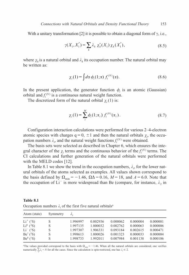
With a unitary transformation [2] it is possible to obtain a diagonal form of �, i.e.,
(8.5)
where �k is a natural orbital and �k its occupation number. The natural orbital maybe written as:
(8.6)
In the present application, the generator function �i is an atomic (Gaussian)orbital and fi
(N ) is a continuous natural weight function.The discretized form of the natural orbital �i (1) is:
(8.7)
Configuration interaction calculations were performed for various 2–4-electronatomic species with charges q�0, �1 and then the natural orbitals �i, the occu-pation numbers �i, and the natural weight functions fi
(N ) were obtained.The basis sets were selected as described in Chapter 6, which ensures the inte-
gral character of the �i terms and the continuous behavior of the fi(N ) terms. The
CI calculations and further generation of the natural orbitals were performedwith the MELD codes [12].
In Table 8.1 we show the trend in the occupation numbers, �i, for the lower nat-ural orbitals of the atoms selected as examples. All values shown correspond tothe basis defined by �min ��1.46, ���0.16, M�18, and A�6.0. Note thatthe occupation of Li� is more widespread than Be (compare, for instance, �2 in
� � �i i iN
M
f(1) (1; ( ) .( )� �l l
)l
∑
� � � �i i iNd f(1) (1; ) ( ).( )� �∫
� � � �( , ) ( ) ( ) ,1 1 1 1X X X Xk k kk
� � ��∑
Connections with Natural Orbitals and Density Functional Theory 153
Table 8.1
Occupation numbers �i of the first five natural orbitalsa
Atom (state) Symmetry �i
Li� (1S) S 1.996997 0.002936 0.000062 0.000004 0.000001Li0 (2S) S 1.997135 1.000032 0.002762 0.000063 0.000006Li� (1S) S 1.997307 1.906331 0.093184 0.002615 0.000471Be� (2S) S 1.998613 1.000026 0.001323 0.000033 0.000004Be0 (1S) S 1.998733 1.992011 0.007984 0.001138 0.000106
aThe values provided correspond to the basis with �min ��1.46. When all the natural orbitals are considered, one verifiesnumerically �
i�i �N for all the cases. Since the calculation is spin-restricted, one has �i � 2.
Else_EAMC-TRSIC_ch008.qxd 5/21/2007 20:54 Page 153
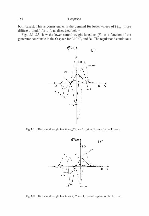
both cases). This is consistent with the demand for lower values of �min (morediffuse orbitals) for Li�, as discussed below.
Figs. 8.1–8.3 show the lower natural weight functions fi(N ) as a function of the
generator coordinate in the � space for Li, Li�, and Be. The regular and continuous
154 Chapter 8
Fig. 8.1 The natural weight functions fn(N ), n�1,..., 4 in � space for the Li atom.
Fig. 8.2 The natural weight functions fn(N ), n�1,..., 4 in � space for the Li� ion.
Else_EAMC-TRSIC_ch008.qxd 5/21/2007 20:54 Page 154

behavior of fi(N ) is well characterized. We have chosen to plot only the lower fi
(N )
values for better viewing, although higher weight functions have the same continu-ous character.
Since the generator function in Equation (8.6) is a 1s GTO, the orthogonalityof the various natural orbitals �i is ensured through the weight functions fi
(N ).Thus, one observes zero nodes for f1
(N ), one node for f2(N ), and so on.
There is some sort of a “structure” in the natural weight functions, which isnot encountered in the corresponding HF weight functions (for plots of HFweight functions see Chapter 6). For instance, f1
(N ) for Be (Fig. 8.3) basicallyshows the behavior of a 1s weight function in the region between � � �0.1and � � 1.0; but it has a second maximum at ca. � � �0.35. Thus, the n � 1natural orbital requires more diffuse (lower values of �) basis componentsthan an HF 1s orbital.
The demand for contracted basis components can be seen from the right-handside of Figs. 8.1–8.3, which our basis sets with �max � �min � (M–1)����min �17 � 0.16 reasonably satisfy. The left-hand side of Figs. 8.1 and 8.3 show that fordiffuse orbitals all fi
(N ) seem to terminate together at ca. �min ��0.80. As for Li�
(Fig. 8.2), there is a clear demand for very diffuse orbitals, i.e. ca. �min ��1.5.[Recall that from Equation (8.1) the generator coordinate (exponent) in � space is��exp(A�)�exp(6.0 �)].
Connections with Natural Orbitals and Density Functional Theory 155
Fig. 8.3 The natural weight functions fn(N ), n�1,..., 4 in � space for the Be atom.
Else_EAMC-TRSIC_ch008.qxd 5/21/2007 20:54 Page 155
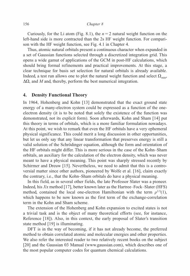
Curiously, for the Li atom (Fig. 8.1), the n�2 natural weight function on theleft-hand side is more contracted than the 2s HF weight function. For compari-son with the HF weight function, see Fig. 4.1 in Chapter 4.
Thus, atomic natural orbitals present a continuous character when expanded ina set of Gaussian functions selected through a discretized integration grid. Thisopens a wide gamut of applications of the GCM in post-HF calculations, whichshould bring formal refinements and practical improvements. At this stage, aclear technique for basis set selection for natural orbitals is already available.Indeed, a test run allows one to plot the natural weight function and select �min,��, and M and, thereby, perform the best numerical integration.
4. Density Functional Theory
In 1964, Hohenberg and Kohn [13] demonstrated that the exact ground stateenergy of a many-electron system could be expressed as a function of the one-electron density (it is to be noted that solely the existence of the function wasdemonstrated, not its explicit form). Soon afterwards, Kohn and Sham [14] putthis theory in terms of orbitals, which is a more familiar formulation nowadays.At this point, we wish to remark that even the HF orbitals have a very ephemeralphysical significance. This could merit a long discussion in other opportunities,but let us only say that any linear transformation that preserves energy is still avalid solution of the Schrödinger equation, although the form and orientation ofthe HF orbitals might differ. This is more serious in the case of the Kohn–Shamorbitals, an auxiliary for the calculation of the electron density, which was nevermeant to have a physical meaning. This point was sharply stressed recently bySchirmer and Dreuw [15]. Nevertheless, we need to admit that this is a contro-versial matter since other authors, pioneered by Wolfe et al. [16], claim exactlythe contrary, i.e., that the Kohn–Sham orbitals do have a physical meaning.
In this field, as in several other fields, the late Professor Slater was a pioneer.Indeed, his X� method [17], better known later as the Hartree–Fock–Slater (HFS)method, contained the local one-electron Hamiltonian with the term �1/3(1),which happens to be now known as the first term of the exchange-correlationterm in the Kohn and Sham scheme.
The extension of the Hohenberg and Kohn expansion to excited states is nota trivial task and is the object of many theoretical efforts (see, for instance,Reference [18]). Also, in this context, the early proposal of Slater’s transitionstate method [19] is illuminating.
DFT is in the way of becoming, if it has not already become, the preferredmethod to obtain correlated atomic and molecular energies and other properties.We also refer the interested reader to two relatively recent books on the subject[20] and the Gaussian 03 Manual (www.gaussian.com), which describes one ofthe most popular computer codes for quantum chemical calculations.
156 Chapter 8
Else_EAMC-TRSIC_ch008.qxd 5/21/2007 20:54 Page 156
5. First Applications of the Generator Coordinate Method toDensity Functional Theory
As we noted above, in 1951 Slater set the first step of the DFT by replacing theexchange term of the Hartree–Fock formulation with the exchange-correlation term
(8.8)
where �(1) is the one-electron density, in many applications represented by theoccupied atomic or molecular orbitals, i.e., for an even number of electrons
(8.9)
where �i are the one-electron functions (the expansion could alternatively bein terms of spin-orbitals). The value of the � parameter in the applicationsassumed two possible values depending on the origin of the deduction, i.e., � � 1.0 or � � 2/3. In 1972 [17], Slater raised the point that neither the value 2/3 nor the value 1.0 were necessarily optimal. One method to determinethe value of � was to force the HFS total energy for the ground state of anatomic system to equal the HF total energy [17]. Actually, in a popular versionof the HFS equations implemented in the seventies, the value employed was � � 0.7 [see, for instance, Reference 21]. This issue will be addressed in thecontext of the GCM below.
In 2004, Trsic et al. [22] applied the GCM in an innovative strategy, choosingthe parameter � in VX� in Equation (8.8) as the generator coordinate (in the stan-dard method the generator coordinate is part of the trial function, in general asan exponent of Gaussian- or Slater-type orbitals), thus, the generator coordinateis part of the Hamiltonian. The idea of the application of the GCM in the DFTwas proposed initially by Klaus Capelle in 2003 [23].
Trsic et al. [22] initiated a preliminary application of the GCM in DFT with aself-consistent field HF calculation for the He atom. We first obtain the best HFcalculation and then replace the exchange term by Slater’s X� potential [17] VX�,the simpler expression for DFT, but sufficient for this experiment. We interpret �as the generator coordinate and weight the exchange-correlation term for differentvalues of the parameter �, i.e.,
(8.10)
with N�4,�0 �0.25, and ���0.25 in our first experiment.
� � �i N i� � �0 ( ) ,�
� � �( ) 2 (1) (1),n i i
OCC� �∑
VX� � � ��� 3 (3 8 ) (1) ,1 3� �
Connections with Natural Orbitals and Density Functional Theory 157
Else_EAMC-TRSIC_ch008.qxd 5/21/2007 20:54 Page 157
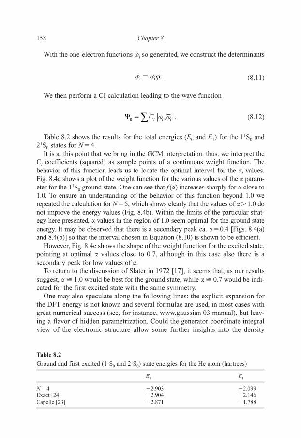
With the one-electron functions �i so generated, we construct the determinants
(8.11)
We then perform a CI calculation leading to the wave function
(8.12)
Table 8.2 shows the results for the total energies (E0 and E1) for the 11S0 and21S0 states for N�4.
It is at this point that we bring in the GCM interpretation: thus, we interpret theCi coefficients (squared) as sample points of a continuous weight function. Thebehavior of this function leads us to locate the optimal interval for the �i values. Fig. 8.4a shows a plot of the weight function for the various values of the � param-eter for the 11S0 ground state. One can see that f (�) increases sharply for � close to1.0. To ensure an understanding of the behavior of this function beyond 1.0 werepeated the calculation for N�5, which shows clearly that the values of ��1.0 donot improve the energy values (Fig. 8.4b). Within the limits of the particular strat-egy here presented, � values in the region of 1.0 seem optimal for the ground stateenergy. It may be observed that there is a secondary peak ca. ��0.4 [Figs. 8.4(a)and 8.4(b)] so that the interval chosen in Equation (8.10) is shown to be efficient.
However, Fig. 8.4c shows the shape of the weight function for the excited state,pointing at optimal � values close to 0.7, although in this case also there is asecondary peak for low values of �.
To return to the discussion of Slater in 1972 [17], it seems that, as our resultssuggest, � � 1.0 would be best for the ground state, while � � 0.7 would be indi-cated for the first excited state with the same symmetry.
One may also speculate along the following lines: the explicit expansion forthe DFT energy is not known and several formulae are used, in most cases withgreat numerical success (see, for instance, www.gaussian 03 manual), but leav-ing a flavor of hidden parametrization. Could the generator coordinate integralview of the electronic structure allow some further insights into the density
�0 , .� Ci i i� �∑
�i i i� �� .
158 Chapter 8
Table 8.2
Ground and first excited (11S0 and 21S0) state energies for the He atom (hartrees)
E0 E1
N�4 �2.903 �2.099Exact [24] �2.904 �2.146Capelle [23] �2.871 �1.788
Else_EAMC-TRSIC_ch008.qxd 5/21/2007 20:54 Page 158

functional properties? Also, since in DFT the excited states are a source ofadditional difficulties while GCM seems to generate excited states naturally, asshown in the very trivial example above, some understanding may be gained inthis case as well.
Connections with Natural Orbitals and Density Functional Theory 159
Fig. 8.4 The weight functions for the ground and the first excited states for the CIcalculation for N�4, (a) ground state for N�4 [Equation (8.10)]; (b) ground state for N�5; (c) excited state for N�4.
Else_EAMC-TRSIC_ch008.qxd 5/21/2007 20:54 Page 159

References
1. (a) D. L. Hill, and J. A. Wheeler, Phys. Rev., 1953, 89, 1102; (b) J. J. Griffin and J. A. Wheeler, Phys. Rev., 1957, 108, 311.
2. P. O. Löwdin, Phys. Rev., 1955, 97, 1474.3. P. O. Löwdin, and H. Shull, Phys. Rev., 1956, 101, 1730; H. Shull, and P. O. Löwdin,
J. Chem. Phys., 1955, 23, 1565; H. Shull, and P. O. Löwdin, J. Chem. Phys., 1959,30, 617; H. Shull, J. Chem. Phys., 1959, 30, 1405.
4. E. R. Davidson, Adv. Quantum Chem., 1972, 6, 235.5. A. I. Ermakov, A. E. Merkulov, A. A. Svechnikova, and V. V. Belouskov, J. Struct.
Chem., 2004, 45, 923; N. N. Lathiotakis, N. Helbig, and E. K. U. Gross, Phys. Rev.A, 2005, 72, 030501/1; B. Blaive, A. Julg, and A. Pellegatti, European Phys. J. B,2005, 47, 177; X. Z. Li, and J. Paldus, Int. J. Quantum Chem., 2005, 105, 672; S. Yamanaka, R. Takeda, M. Shoji, Y. Kitqgawa, H. Honda, and K. Yamaguchi, Int. J. Quantum Chem., 2005, 105, 605; D. Bressanini, G. Morosi, and S. Tarasco, J. Chem. Phys., 2005, 123, 204109/1; D. Van Neck, S. Rombouts, and S. Verdonck,Phys. Rev. C., 2005, 72, 054318/1; J. Ma, S. H. Li, and W. Li, J. Comp. Chem., 2006,27, 39; J. Cioslowski, and M. Buchowiecki, J. Chem. Phys., 2005, 123, 234102/1; L. Abrams, and C. D. Sherrill, Mol. Phys., 2005, 103, 3315; D. C. Thompson, and P. W. Ayers, Int. J. Quantum Chem., 2006, 106, 787; O. Gritsenko, and E. J. Baerends, J. Chem. Phys., 2006, 124, 054115/1; M. Sekiya, T. Noro, E. Miyoshi, Y. Osanai, and T. Koga, J. Comp. Chem., 2006, 27, 463.
6. H. F. M. da Costa, A. B. F. da Silva, M. Trsic, A. M. Simas, and A. J. A. Aquino, J. Mol. Struct. (Theochem)., 1990, 210, 63.
7. J. R. Mohallem, and M. Trsic, J. Chem. Phys., 1987, 86, 5043.8. H. F. M. da Costa, M. Trsic, and J. R. Mohallem, Mol. Phys., 1987, 62, 91.9. A. B. F. da Silva, H. F. M. da Costa, and M. Trsic, Mol. Phys., 1989, 68, 433.
10. P. Chattopadyay, R. M. Dreizler, M. Trsic, and M. Fink, Z. Phys. A, 1978, 285, 7.11. J. R. Mohallem, Z. Phys. D, 1986, 3, 339.12. The MELD codes were developed by E. R. Davidson, S. R. Langhoff, S. T. Elbert,
and L. E. Murchie, University of Indiana; the version employed in Reference [5] wasmodified by D. Feller, and D. C. Rawlings.
13. P. Hohenberg, and W. Kohn, Phys. Rev. B, 1964, 136, 864.14. W. Kohn, and L. J. Sham, Phys. Rev. A, 1965, 140, 1133.15. J. Schirmer, and A. Dreuw, Phys. Rev., Phys. Rev., 2007, 75, 022513.16. S. Wolfe, Z. Shi, C. E. Brion, J. Rolke, Y. Zeng, G. Cooper, D. P. Chong, and C. Hu,
Can. J. Chem., 2002, 80, 222.17. (a) J. C. Slater, Phys. Rev., 1951, 81, 385; (b) ibid., Phys. Rev., 1951, 82, 538; (c) ibid.,
Adv. Quantum Chem., 1972, 6, 1.18. E. K. U. Gross, L. N. Oliveira, and W. Kohn, Phys. Rev. A, 1988, 37, 2805; ibid., 37,
2809; ibid., 37, 2821; M. Petersilka, U. J. Gossmann, and E. K. U. Gross, Phys. Rev.Lett., 1996, 76, 1212; A. Nagy, Chem. Phys. Lett., 1998, 296, 489; A. Görling, Phys.Rev. A, 1999, 59, 3359.
19. J. C. Slater, and J. H. Wood, Int. J. Quantum Chem. Symp., 1971, 4, 3.
160 Chapter 8
Else_EAMC-TRSIC_ch008.qxd 5/21/2007 20:54 Page 160
20. R. M. Dreizler, and E. K. U. Gross, Density Functional Theory: An Approach tothe Quantum Many-Body Problem, Berlin: Springer, 1990; E. S. Kryachko, andE. V. Ludeña, Energy Density Functional Theory of Many-Electron Systems,Dordrecht: Kluwer Academic, 1990.
21. E. J. Baerendes, D. E. Ellis, and P. Ros, Chem. Phys., 1973, 2, 41; E. J. Baerends, andP. Ros, Chem. Phys., 1973, 2, 52; ibid, Chem. Phys., 1975, 8, 412; M. Trsic, T. Ziegler, and W. G. Laidlaw, Chem. Phys., 1976, 15, 383; T. Ziegler, A. Rauk, andE. J. Baerends, 1976, 16, 209; T. Ziegler, A. Rauk, and E. J. Baerends, Theoret. Chim.Acta (Berlin), 1977, 43, 261.
22. M. Trsic, W. F. D. Angelotti, and F. A. Molfetta, Adv. Quantum Chem., 2004, 47, 315.23. K. Capelle, J. Chem. Phys., 2003, 119, 1285.24. A. J. Takkar, and V. H. Smith, Phys. Rev. A, 1977, 15, 1; ibid., Phys. Rev. A, 1977,
15, 16.
Connections with Natural Orbitals and Density Functional Theory 161
Else_EAMC-TRSIC_ch008.qxd 5/21/2007 20:54 Page 161

This page intentionally left blank

Final Remarks and Perspectives
Along the pages of this book, we can witness an intimate connection betweenchemistry and physics through the generator coordinate (GC) ansatz. Of course,this interaction is present since the birth of both sciences and occurs in severalareas, although physics and chemistry are certainly distinct disciplines. One areathat is borderline indeed is Quantum Chemistry. Actually, quantum chemists donot feel at home (neither are they particularly welcome) in either community.When one of us (MT) was a post-doctoral fellow in the Quantum Chemistrygroup in Uppsala in the early seventies, the late Professor Per-Olov Löwdin usedto tell us how Professor John C. Slater died without ever being honored with theNobel Prize. Per-Olov (Pelle) had the clear notion that Slater was one (I mentionbriefly: Slater determinants, Slater orbitals, Slater’s rules, Xα method of thebuilders of Quantum Chemistry in the thirties, as soon as Quantum Mechanicswas well established). Pelle was a member of the Nobel Committee in Stockholmand would present Slater’s achievements to the Chemistry Committee. Theywould say: “well, this is really interesting, but this is physics”. So, the followingyear, Pelle would present his candidate to the Physics Committee and they said:“we can see the relevance of his work, but this is chemistry”. After 10 years, Pellegave up.
However, since mathematical intricacies of the GC algorithm requireinevitable approximate schemes for nontrivial systems, both communities areclearly differentiated by their preferences. The physicists preferred the Gaussianoverlap approximation, thus simplifying the model and then applying powerfulmathematical tools. The chemists opted to preserve the model and introduce sim-plifications in the algorithm (discretization techniques). Somebody once said:“the table of the chemist has four legs, and the table of the physicist has one legor an infinite number of legs”.
What is really interesting is that the GC method has become one important toolin the generation of accurate basis sets that have been currently used in relativis-tic and nonrelativistic calculations of atoms and molecules.
The secret of the GC method in the generation of accurate basis sets lies on howone discretizes the integral equation of the method, i.e., the Griffin-Hill-Wheeler(GHW) equation. The innovation in discretizing the GHW equation through anintegral discretization, instead of the usual variational discretization, allowed usto vary the space of the Slater- and Gaussian-function exponents in such a waythat it was possible to obtain universal as well as atom-adapted basis sets of highquality.
Else_EAMC-TRSIC_Remarks.qxd 5/21/2007 20:19 Page 163

It is for sure that the way of generating Slater- and Gaussian-function expo-nents employing the GC method was an innovation when compared to the tradi-tional way of optimizing all of the function exponents. The manner in which theSlater- and Gaussian-function exponents are generated by using the GC methodis also a step forward when we compare our methodology with the two other rel-evant methodologies developed to reach such a goal: the even-tempered and well-tempered formulas.
Certainly, the applications of the GC method in relativistic and nonrelativisticcalculations for atomic and, mainly, molecular systems may gain new perspec-tives with further improvements or, perhaps, with new methodological insights.
However, new analytical and numerical approaches, as exemplified in Chapter 3,may bring unexpected new possibilities. It is good to remember that new find-ings in Mathematics and numerical techniques require a time gap before beingapplied in chemistry and physics. At the end of Chapter 6, we also raise the needfor a better understanding of the weight function itself.
Also, adopting an optimistic perspective, the GC method may open a newvision of the elusive, and multiple, higher correction terms in DFT.
164 Final Remarks and Perspectives
Else_EAMC-TRSIC_Remarks.qxd 5/21/2007 20:19 Page 164

APPENDIX
SELECTED UNIVERSAL AND ATOM-ADAPTED SLATER
AND GAUSSIAN BASIS SETS FORATOMIC AND MOLECULAR
CALCULATIONS
Else_EAMC-TRSIC_appn1.qxd 5/19/2007 21:28 Page 165

This page intentionally left blank

Appendix 1
Universal Gaussian basis set for the ground [1] and certain low-lying excited [2]states of the neutral atoms and positive ions from Hydrogen (Z�1) throughXenon (Z�54).
Exp. # Symm. Exponents Symm. Exponents Symm. Exponents
1 S 0.036883 P 0.090718 D 0.0368832 0.096328 0.236928 0.0963283 0.251579 0.618783 0.2515794 0.657047 1.616074 0.6570475 1.716007 4.220696 1.7160076 4.481689 11.023176 4.4816897 11.704812 28.789191 11.7048128 30.569415 75.188628 30.5694159 79.838033 196.369875 79.838033
10 208.512710 512.858511 208.51271011 544.571910 1339.430764 544.57191012 1422.256537 3498.18660413 3714.50238314 9701.15277315 25336.46648516 66171.16016817 172818.98565418 451350.735373
References
1. A. B. F. da Silva, H. F. M. da Costa, and M. Trsic, Mol. Phys., 1989, 68, 433.2. A. B. F. da Silva, and M. Trsic, Can. J. Chem., 1996, 74, 1526.
Else_EAMC-TRSIC_appn1.qxd 5/19/2007 21:28 Page 167

This page intentionally left blank

Appendix 2
Universal Slater basis set for the ground [1] and certain low-lying excited [2]states of the neutral atoms and positive ions from Hydrogen (Z�1) throughXenon (Z�54).
Exp. # Symm. Exponents Symm. Exponents Symm. Exponents
1 S 0.516851 P 1.000000 D 0.5168512 0.786628 1.521962 0.7866283 1.197217 2.316367 1.1972174 1.822119 3.525421 1.8221195 2.773195 5.365556 2.7731956 4.220696 8.166170 4.2206967 6.423737 12.428597 6.4237378 9.776680 18.915846 9.7766809 14.879732 28.789191 14.879732
10 22.646380 43.816042 22.64638011 34.46691912 52.457326
References
1. A. B. F. da Silva, H. F. M. DaCosta, and M. Trsic, Mol. Phys., 1989, 68, 433.2. A. B. F. da Silva, and M. Trsic, Can. J. Chem., 1996, 74, 1526.
Else_EAMC-TRSIC_appn2.qxd 5/19/2007 22:10 Page 169

This page intentionally left blank

Appendix 3
Universal Gaussian basis set for the ground states [1] of the neutral atoms fromHydrogen (Z�1) through Lawrence (Z�103).
Exp. # Exponents
1 0.020000462 0.039163903 0.076688774 0.150168095 0.294051606 0.575797067 1.127496858 2.207807639 4.32321786
10 8.4655077811 16.5767315812 32.4597220813 63.5609952514 124.4619441915 243.7151194616 477.2306896117 934.4891347318 1829.8696247719 3583.1586684120 7016.3610943821 13739.0854166722 26903.1860743023 52680.4659115024 103156.2388554525 201995.3588238826 395537.1525668327 774520.9591527328 1516627.9887336729 2969784.6507943830 5815282.9419019131 11387194.5850785732 22297831.7330221933 43662492.6604555034 85497697.18196450
Else_EAMC-TRSIC_appn3.qxd 5/19/2007 22:22 Page 171
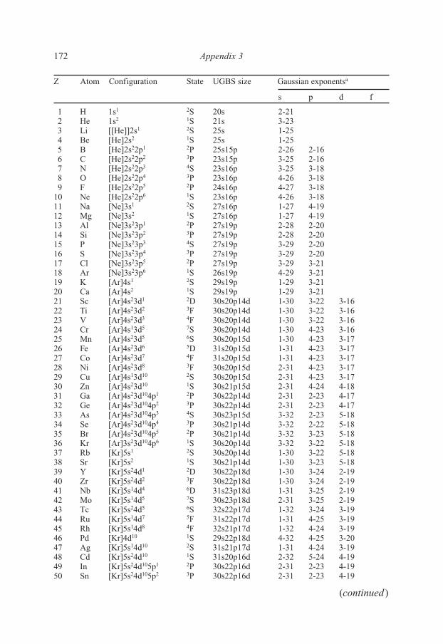
Z Atom Configuration State UGBS size Gaussian exponentsa
s p d f
1 H 1s1 2S 20s 2-212 He 1s2 1S 21s 3-233 Li [[He]]2s1 2S 25s 1-254 Be [He]2s2 1S 25s 1-255 B [He]2s22p1 2P 25s15p 2-26 2-166 C [He]2s22p2 3P 23s15p 3-25 2-167 N [He]2s22p3 4S 23s16p 3-25 3-188 O [He]2s22p4 3P 23s16p 4-26 3-189 F [He]2s22p5 2P 24s16p 4-27 3-18
10 Ne [He]2s22p6 1S 23s16p 4-26 3-1811 Na [Ne]3s1 2S 27s16p 1-27 4-1912 Mg [Ne]3s2 1S 27s16p 1-27 4-1913 Al [Ne]3s23p1 2P 27s19p 2-28 2-2014 Si [Ne]3s23p2 3P 27s19p 2-28 2-2015 P [Ne]3s23p3 4S 27s19p 3-29 2-2016 S [Ne]3s23p4 3P 27s19p 3-29 2-2017 Cl [Ne]3s23p5 2P 27s19p 3-29 3-2118 Ar [Ne]3s23p6 1S 26s19p 4-29 3-2119 K [Ar]4s1 2S 29s19p 1-29 3-2120 Ca [Ar]4s2 1S 29s19p 1-29 3-2121 Sc [Ar]4s23d1 2D 30s20p14d 1-30 3-22 3-1622 Ti [Ar]4s23d2 3F 30s20p14d 1-30 3-22 3-1623 V [Ar]4s23d3 4F 30s20p14d 1-30 3-22 3-1624 Cr [Ar]4s13d5 7S 30s20p14d 1-30 4-23 3-1625 Mn [Ar]4s23d5 6S 30s20p15d 1-30 4-23 3-1726 Fe [Ar]4s23d6 5D 31s20p15d 1-31 4-23 3-1727 Co [Ar]4s23d7 4F 31s20p15d 1-31 4-23 3-1728 Ni [Ar]4s23d8 3F 30s20p15d 2-31 4-23 3-1729 Cu [Ar]4s13d10 2S 30s20p15d 2-31 4-23 3-1730 Zn [Ar]4s23d10 1S 30s21p15d 2-31 4-24 4-1831 Ga [Ar]4s23d104p1 2P 30s22p14d 2-31 2-23 4-1732 Ge [Ar]4s23d104p2 3P 30s22p14d 2-31 2-23 4-1733 As [Ar]4s23d104p3 4S 30s23p15d 3-32 2-23 5-1834 Se [Ar]4s23d104p4 3P 30s21p14d 3-32 2-22 5-1835 Br [Ar]4s23d104p5 2P 30s21p14d 3-32 3-23 5-1836 Kr [Ar]3s23d104p6 1S 30s20p14d 3-32 3-22 5-1837 Rb [Kr]5s1 2S 30s20p14d 1-30 3-22 5-1838 Sr [Kr]5s2 1S 30s21p14d 1-30 3-23 5-1839 Y [Kr]5s24d1 2D 30s22p18d 1-30 3-24 2-1940 Zr [Kr]5s24d2 3F 30s22p18d 1-30 3-24 2-1941 Nb [Kr]5s14d4 6D 31s23p18d 1-31 3-25 2-1942 Mo [Kr]5s14d5 7S 30s23p18d 2-31 3-25 2-1943 Tc [Kr]5s24d5 6S 32s22p17d 1-32 3-24 3-1944 Ru [Kr]5s14d7 5F 31s22p17d 1-31 4-25 3-1945 Rh [Kr]5s14d8 4F 32s21p17d 1-32 4-24 3-1946 Pd [Kr]4d10 1S 29s22p18d 4-32 4-25 3-2047 Ag [Kr]5s14d10 2S 31s21p17d 1-31 4-24 3-1948 Cd [Kr]5s24d10 1S 31s20p16d 2-32 5-24 4-1949 In [Kr]5s24d105p1 2P 30s22p16d 2-31 2-23 4-1950 Sn [Kr]5s24d105p2 3P 30s22p16d 2-31 2-23 4-19
172 Appendix 3
(continued )
Else_EAMC-TRSIC_appn3.qxd 5/19/2007 22:22 Page 172

51 Sb [Kr]5s24d105p3 4S 30s22p16d 3-32 2-23 4-1952 Te [Kr]5s24d105p4 3P 30s23p16d 3-32 2-24 4-1953 I [Kr]5s24d105p5 2P 30s22p16d 3-32 3-24 4-1954 Xe [Kr]5s24d105p6 1S 31s22p16d 3-33 3-24 4-1955 Cs [Xe]6s1 2S 32s22p15d 1-32 3-24 5-1956 Ba [Xe]6s2 1S 32s22p16d 1-32 3-24 5-2057 La [Xe]6s25d1 2D 32s24p19d 1-32 3-26 2-2059 Pr [Xe]6s24f3 4I 32s22p16d12f 1-32 3-24 5-20 4-1560 Nd [Xe]6s24f 4 5I 32s22p16d12f 1-32 3-24 5-20 4-1561 Pm [Xe]6s24f5 6H 31s23p16d13f 1-31 3-25 5-20 4-1662 Sm [Xe]6s24f6 7F 33s22p16d12f 1-33 3-24 5-20 4-1563 Eu [Xe]6s24f7 8S 32s23p16d13f 1-32 3-25 5-20 4-1665 Tb [Xe]6s24f9 6H 33s23p16d13f 1-33 3-25 5-20 4-1666 Dy [Xe]6s24f10 5I 32s22p16d14f 1-32 3-24 5-20 4-1767 Ho [Xe]6s24f11 4I 32s23p16d14f 1-32 3-25 5-20 4-1768 Er [Xe]6s24f12 3H 33s22p16d13f 1-33 4-25 5-20 4-1669 Tm [Xe]6s24f13 2F 32s22p17d14f 1-32 4-25 5-21 4-1770 Yb [Xe]6s24f14 1S 32s22p17d13f 1-32 4-25 5-21 4-1671 Lu [Xe]6s24f145d1 2D 32s23p19d12f 1-32 4-26 2-20 5-1672 Hf [Xe]6s24f145d2 3F 32s22p18d12f 2-33 4-25 3-20 5-1673 Ta [Xe]6s24f145d3 4F 31s23p19d13f 2-32 4-26 3-21 5-1774 W [Xe]6s24f145d4 5D 31s23p19d12f 2-32 4-26 3-21 6-1775 Re [Xe]6s24f145d5 6S 31s23p19d12f 2-32 4-26 3-21 6-1776 Os [Xe]6s24f145d6 5D 32s23p18d12f 1-32 4-26 3-20 6-1777 Ir [Xe]6s24f145d7 4F 32s22p18d13f 2-33 3-24 4-21 6-1878 Pt [Xe]6s14f145d9 3D 32s23p18d13f 2-33 4-26 3-20 6-1879 Au [Xe]6s14f145d10 2S 32s22p18d12f 2-33 4-25 4-21 6-1780 Hg [Xe]6s24f145d10 1S 32s23p17d13f 2-33 4-26 4-20 6-1881 Tl [Xe]6s24f145d106p1 2P 32s23p18d13f 2-33 2-24 4-21 6-1882 Pb [Xe]6s24f145d106p2 3P 32s23p17d13f 2-33 2-24 4-20 6-1883 Bi [Xe]6s24f145d106p3 4S 32s25p17d12f 2-33 2-26 4-20 7-1884 Po [Xe]6s24f145d106p4 3P 32s23p18d13f 2-33 3-25 4-21 6-1885 At [Xe]6s24f145d106p5 2P 32s24p18d13f 3-34 3-26 4-21 6-1886 Rn [Xe]6s24f145d106p6 1S 32s25p17d13f 2-33 2-26 5-21 7-1987 Fr [Rn]7s1 2S 33s24p18d14f 1-33 3-26 4-21 7-2088 Ra [Rn]7s2 1S 33s23p18d14f 1-33 3-25 4-21 5-1889 Ac [Rn]7s26d1 2D 33s24p20d13f 1-33 3-26 3-22 7-1990 Th [Rn]7s26d2 3F 33s25p20d14f 1-33 3-27 3-22 7-2094 Pu [Rn]7s25f6 7F 33s25p19d15f 1-33 3-27 5-23 4-1895 Am [Rn]7s25f7 8S 33s25p19d14f 1-33 3-27 5-23 4-1798 Cf [Rn]7s25f10 5I 33s25p19d15f 1-33 3-27 5-23 4-1899 Es [Rn]7s25f11 4I 33s25p19d15f 1-33 3-27 5-23 4-18
100 Fm [Rn]7s25f12 3H 33s25p19d15f 1-33 3-27 5-23 4-18101 Md [Rn]7s25f13 2F 33s25p19d15f 1-33 3-27 5-23 4-18102 No [Rn]7s25f14 1S 32s25p19d15f 2-33 3-27 5-23 4-18103 Lr [Rn]7s25f146d1 2D 32s25p20d15f 2-33 3-27 3-22 5-19aThese numbers refer to the universal Gaussian exponents labels (Exp. #) shown in the previous table of this Appendix.
References
1. E. V. R. de Castro, and F. E. Jorge, J. Chem. Phys., 1998, 108, 5225.
Appendix 3 173
Z Atom Configuration State UGBS size Gaussian exponentsa
s p d f
Else_EAMC-TRSIC_appn3.qxd 5/19/2007 22:22 Page 173

This page intentionally left blank
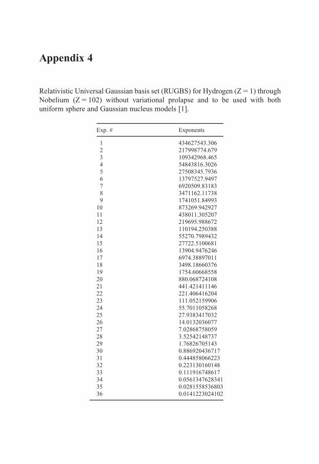
Appendix 4
Relativistic Universal Gaussian basis set (RUGBS) for Hydrogen (Z�1) throughNobelium (Z�102) without variational prolapse and to be used with bothuniform sphere and Gaussian nucleus models [1].
Exp. # Exponents
1 434627543.3062 217998774.6793 109342968.4654 54843816.30265 27508345.79366 13797527.94977 6920509.831838 3471162.117389 1741051.84993
10 873269.94292711 438011.30520712 219695.98867213 110194.25038814 55270.798943215 27722.510068116 13904.947624617 6974.3889701118 3498.1866037619 1754.6066855820 880.06872410821 441.42141114622 221.40641620423 111.05215990624 55.701105826825 27.938341703226 14.013203607727 7.0286875805928 3.5254214873729 1.7682670514330 0.88692043671731 0.44485806622332 0.22313016014833 0.11191674861734 0.056134762834135 0.028155853680336 0.0141223024102
Else_EAMC-TRSIC_appn4.qxd 4/20/2007 12:05 Page 175
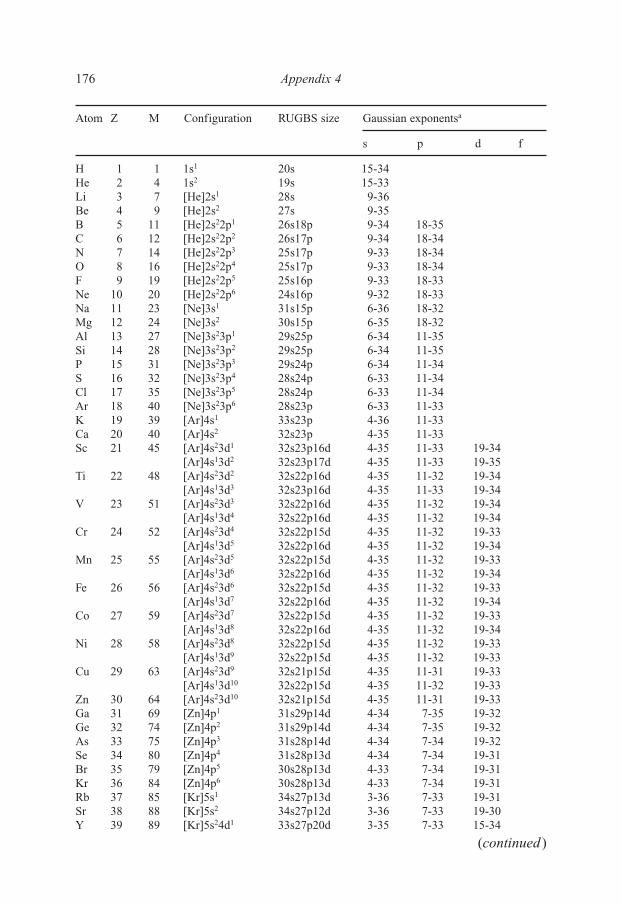
Atom Z M Configuration RUGBS size Gaussian exponentsa
s p d f
H 1 1 1s1 20s 15-34He 2 4 1s2 19s 15-33Li 3 7 [He]2s1 28s 9-36Be 4 9 [He]2s2 27s 9-35B 5 11 [He]2s22p1 26s18p 9-34 18-35C 6 12 [He]2s22p2 26s17p 9-34 18-34N 7 14 [He]2s22p3 25s17p 9-33 18-34O 8 16 [He]2s22p4 25s17p 9-33 18-34F 9 19 [He]2s22p5 25s16p 9-33 18-33Ne 10 20 [He]2s22p6 24s16p 9-32 18-33Na 11 23 [Ne]3s1 31s15p 6-36 18-32Mg 12 24 [Ne]3s2 30s15p 6-35 18-32Al 13 27 [Ne]3s23p1 29s25p 6-34 11-35Si 14 28 [Ne]3s23p2 29s25p 6-34 11-35P 15 31 [Ne]3s23p3 29s24p 6-34 11-34S 16 32 [Ne]3s23p4 28s24p 6-33 11-34Cl 17 35 [Ne]3s23p5 28s24p 6-33 11-34Ar 18 40 [Ne]3s23p6 28s23p 6-33 11-33K 19 39 [Ar]4s1 33s23p 4-36 11-33Ca 20 40 [Ar]4s2 32s23p 4-35 11-33Sc 21 45 [Ar]4s23d1 32s23p16d 4-35 11-33 19-34
[Ar]4s13d2 32s23p17d 4-35 11-33 19-35Ti 22 48 [Ar]4s23d2 32s22p16d 4-35 11-32 19-34
[Ar]4s13d3 32s23p16d 4-35 11-33 19-34V 23 51 [Ar]4s23d3 32s22p16d 4-35 11-32 19-34
[Ar]4s13d4 32s22p16d 4-35 11-32 19-34Cr 24 52 [Ar]4s23d4 32s22p15d 4-35 11-32 19-33
[Ar]4s13d5 32s22p16d 4-35 11-32 19-34Mn 25 55 [Ar]4s23d5 32s22p15d 4-35 11-32 19-33
[Ar]4s13d6 32s22p16d 4-35 11-32 19-34Fe 26 56 [Ar]4s23d6 32s22p15d 4-35 11-32 19-33
[Ar]4s13d7 32s22p16d 4-35 11-32 19-34Co 27 59 [Ar]4s23d7 32s22p15d 4-35 11-32 19-33
[Ar]4s13d8 32s22p16d 4-35 11-32 19-34Ni 28 58 [Ar]4s23d8 32s22p15d 4-35 11-32 19-33
[Ar]4s13d9 32s22p15d 4-35 11-32 19-33Cu 29 63 [Ar]4s23d9 32s21p15d 4-35 11-31 19-33
[Ar]4s13d10 32s22p15d 4-35 11-32 19-33Zn 30 64 [Ar]4s23d10 32s21p15d 4-35 11-31 19-33Ga 31 69 [Zn]4p1 31s29p14d 4-34 7-35 19-32Ge 32 74 [Zn]4p2 31s29p14d 4-34 7-35 19-32As 33 75 [Zn]4p3 31s28p14d 4-34 7-34 19-32Se 34 80 [Zn]4p4 31s28p13d 4-34 7-34 19-31Br 35 79 [Zn]4p5 30s28p13d 4-33 7-34 19-31Kr 36 84 [Zn]4p6 30s28p13d 4-33 7-34 19-31Rb 37 85 [Kr]5s1 34s27p13d 3-36 7-33 19-31Sr 38 88 [Kr]5s2 34s27p12d 3-36 7-33 19-30Y 39 89 [Kr]5s24d1 33s27p20d 3-35 7-33 15-34
176 Appendix 4
(continued )
Else_EAMC-TRSIC_appn4.qxd 4/20/2007 12:05 Page 176

[Kr]5s14d2 33s27p21d 3-35 7-33 15-35Zr 40 90 [Kr]5s24d2 33s27p20d 3-35 7-33 15-34
[Kr]5s14d3 33s27p21d 3-35 7-33 15-35Nb 41 93 [Kr]5s24d3 33s27p20d 3-35 7-33 15-34
[Kr]5s14d4 33s27p20d 3-35 7-33 15-34Mo 42 98 [Kr]5s24d4 33s26p20d 3-35 7-32 15-34
[Kr]5s14d5 33s26p20d 3-35 7-32 15-34Tc 43 98 [Kr]5s24d5 33s26p20d 3-35 7-32 15-34
[Kr]5s14d6 33s26p20d 3-35 7-32 15-34Ru 44 102 [Kr]5s24d6 33s26p20d 3-35 7-32 15-34
[Kr]5s14d7 33s26p20d 3-35 7-32 15-34Rh 45 103 [Kr]5s24d7 33s26p19d 3-35 7-32 15-33
[Kr]5s14d8 33s26p20d 3-35 7-32 15-34Pd 46 106 [Kr]5s24d8 33s26p19d 3-35 7-32 15-33
[Kr]5s14d9 33s26p19d 3-35 7-32 15-33[Kr]5s04d10 29s26p20d 3-31 7-32 15-34
Ag 47 107 [Kr]5s24d9 33s26p19d 3-35 7-32 15-33[Kr]5s14d10 33s26p19d 3-35 7-32 15-33
Cd 48 114 [Kr]5s24d10 33s26p19d 3-35 7-32 15-33In 49 115 [Cd]5p1 32s32p18d 3-34 4-35 15-32Sn 50 120 [Cd]5p2 32s32p18d 3-34 4-35 15-32Sb 51 121 [Cd]5p3 32s31p18d 3-34 4-34 15-32Te 52 130 [Cd]5p4 32s31p18d 3-34 4-34 15-32I 53 127 [Cd]5p5 31s31p18d 3-33 4-34 15-32Xe 54 132 [Cd]5p6 31s31p18d 3-33 4-34 15-32Cs 55 133 [Xe]6s1 35s31p17d 2-36 4-34 15-31Ba 56 138 [Xe]6s2 35s30p17d 2-36 4-33 15-31La 57 139 [Xe]6s24f 1 35s30p17d15f 2-36 4-33 15-31 19-33
[Xe]6s25d1 35s30p20d 2-36 4-33 15-34Ce 58 140 [Xe]6s24f 2 35s30p17d15f 2-36 4-33 15-31 19-33
[Xe]6s24f 15d1 35s30p20d14f 2-36 4-33 15-34 19-32Pr 59 141 [Xe]6s24f 3 35s30p17d15f 2-36 4-33 15-31 19-33Nd 60 144 [Xe]6s24f 4 35s30p17d15f 2-36 4-33 15-31 19-33Pm 61 145 [Xe]6s24f 5 34s30p17d15f 2-35 4-33 15-31 19-33Sm 62 152 [Xe]6s24f 6 34s30p17d15f 2-35 4-33 15-31 19-33Eu 63 153 [Xe]6s24f 7 34s30p17d15f 2-35 4-33 15-31 19-33Gd 64 158 [Xe]6s24f 8 34s30p16d15f 2-35 4-33 15-30 19-33
[Xe]6s24f 75d1 34s30p20d15f 2-35 4-33 15-34 19-33Tb 65 159 [Xe]6s24f 9 34s30p16d15f 2-35 4-33 15-30 19-33Dy 66 162 [Xe]6s24f10 34s30p16d15f 2-35 4-33 15-30 19-33Ho 67 162 [Xe]6s24f11 34s30p16d15f 2-35 4-33 15-30 19-33Er 68 69 168 [Xe]6s24f12 34s30p16d14f 2-35 4-33 15-30 19-32Tm 70 169 [Xe]6s24f13 34s30p16d14f 2-35 4-33 15-30 19-32Yb 174 [Xe]6s24f14 34s30p16d14f 2-35 4-33 15-30 19-32Lu 71 175 [Xe]6s24f145d1 34s29p22d14f 2-35 4-32 13-34 19-32Hf 72 180 [Xe]6s24f145d2 34s29p22d14f 2-35 4-32 13-34 19-32
[Xe]6s14f145d3 34s29p22d14f 2-35 4-32 13-34 19-32Ta 73 181 [Xe]6s24f145d3 34s29p22d13f 2-35 4-32 13-34 19-31
Appendix 4 177
Atom Z M Configuration RUGBS size Gaussian exponentsa
s p d f
(continued )
Else_EAMC-TRSIC_appn4.qxd 4/20/2007 12:05 Page 177

[Xe]6s14f145d4 34s29p22d13f 2-35 4-32 13-34 19-31W 74 184 [Xe]6s24f145d4 34s29p22d13f 2-35 4-32 13-34 19-31
[Xe]6s14f145d5 34s29p22d13f 2-35 4-32 13-34 19-31Re 75 187 [Xe]6s24f145d5 34s29p22d13f 2-35 4-32 13-34 19-31
[Xe]6s14f145d6 34s29p22d13f 2-35 4-32 13-34 19-31Os 76 192 [Xe]6s24f145d6 34s29p21d13f 2-35 4-32 13-33 19-31
[Xe]6s14f145d7 34s29p22d13f 2-35 4-32 13-34 19-31Ir 77 193 [Xe]6s24f145d7 34s29p21d13f 2-35 4-32 13-33 19-31
[Xe]6s14f145d8 34s29p21d13f 2-35 4-32 13-33 19-31Pt 78 195 [Xe]6s24f145d8 34s29p21d13f 2-35 4-32 13-33 19-31
[Xe]6s14f145d9 34s29p21d13f 2-35 4-32 13-33 19-31Au 79 197 [Xe]6s24f145d9 33s29p21d13f 2-34 4-32 13-33 19-31
[Xe]6s14f145d10 33s29p21d13f 2-34 4-32 13-33 19-31Hg 80 202 [Xe]6s24f145d10 33s29p21d12f 2-34 4-32 13-33 19-30Tl 81 205 [Hg]6p1 33s33p21d12f 2-34 3-35 13-33 19-30Pb 82 208 [Hg]6p2 33s33p20d12f 2-34 3-35 13-32 19-30Bi 83 209 [Hg]6p3 33s33p20d12f 2-34 3-35 13-32 19-30Po 84 209 [Hg]6p4 32s32p20d12f 2-33 3-34 13-32 19-30At 85 210 [Hg]6p5 32s32p20d12f 2-33 3-34 13-32 19-30Rn 86 222 [Hg]6p6 32s32p20d11f 2-33 3-34 13-32 19-29Fr 87 223 [Rn]7s1 36s32p19d11f 1-36 3-34 13-31 19-29Ra 88 226 [Rn]7s2 36s31p19d11f 1-36 3-33 13-31 19-29Ac 89 227 [Rn]7s26d1 35s31p23d12f 1-35 3-33 13-35 18-29Th 90 232 [Rn]7s25f 2 35s31p19d17f 1-35 3-33 13-31 18-34
[Rn]7s26d2 35s31p23d12f 1-35 3-33 13-35 18-29Pa 91 231 [Rn]7s25f 3 35s31p19d17f 1-35 3-33 13-31 18-34
[Rn]7s25f 26d1 35s31p23d16f 1-35 3-33 13-35 18-33U 92 238 [Rn]7s25f 4 35s31p19d16f 1-35 3-33 13-31 18-33
[Rn]7s25f 36d1 35s31p23d16f 1-35 3-33 13-35 18-33Np 93 237 [Rn]7s25f 5 35s31p19d16f 1-35 3-33 13-31 18-33
[Rn]7s25f 46d1 35s31p23d16f 1-35 3-33 13-35 18-33Pu 94 244 [Rn]7s25f 6 35s31p19d16f 1-35 3-33 13-31 18-33Am 95 243 [Rn]7s25f 7 35s31p19d16f 1-35 3-33 13-31 18-33Cm 96 247 [Rn]7s25f 8 35s31p19d16f 1-35 3-33 13-31 18-33
[Rn]7s25f 76d1 35s31p22d16f 1-35 3-33 13-34 18-33Bk 97 247 [Rn]7s25f 9 35s31p19d16f 1-35 3-33 13-31 18-33Cf 98 251 [Rn]7s25f10 35s31p19d16f 1-35 3-33 13-31 18-33Es 99 252 [Rn]7s25f11 35s31p19d16f 1-35 3-33 13-31 18-33Fm 100 257 [Rn]7s25f12 35s31p19d16f 1-35 3-33 13-31 18-33Md 101 258 [Rn]7s25f13 35s31p19d16f 1-35 3-33 13-31 18-33No 102 259 [Rn]7s25f14 35s31p19d16f 1-35 3-33 13-31 18-33
aThese numbers refer to the universal Gaussian exponents labels (Exp. #) shown in the previous table of this Appendix.
Reference
1. R. L. A. Haiduke, L. G. M. de Macedo, and A. B. F. da Silva, J. Comput. Chem., 2005,26, 932.
178 Appendix 4
(Continued)
Atom Z M Configuration RUGBS size Gaussian exponentsa
s p d f
Else_EAMC-TRSIC_appn4.qxd 4/20/2007 12:05 Page 178

Appendix 5
Relativistic adapted Gaussian basis sets for Hydrogen (Z�1) through Radon(Z�86) without variational prolapse and to be used with both uniform sphere andGaussian nucleus models [1,2].
Atom Exp. # Symm. Exponents
H 1 S� 0.4406498716E�032 0.6636101523E�023 0.1392971613E�024 0.3806525865E�015 0.1264794537E�016 0.4772690339E�007 0.1910319536E�008 0.7575227197E�01
Atom Exp. # Symm. Exponents
He 1 S� 0.1070160908E�042 0.1816369667E�033 0.4009745741E�024 0.1091195927E�025 0.3469587274E�016 0.1221681357E�017 0.4515012930E�008 0.1659957021E�00
Atom Exp. # Symm. Exponents
Li 1 S� 0.1395544240E�052 0.2559250298E�043 0.5742911768E�034 0.1535679448E�035 0.4765592080E�026 0.1671397863E�027 0.6451910321E�018 0.2669568833E�019 0.1153020595E�01
10 0.5062615733E�0011 0.2200663508E�0012 0.9222993773E�0113 0.3629347927E�0114 0.1305937900E�01
Else_EAMC-TRSIC_appn5.qxd 5/19/2007 21:38 Page 179

Atom Exp. # Symm. Exponents
Be 1 S� 0.2592322398E�052 0.4466184818E�043 0.9665712381E�034 0.2547163426E�035 0.7922856412E�026 0.2819584147E�027 0.1112866072E�028 0.4722060844E�019 0.2087984916E�01
10 0.9326238210E�0011 0.4078920936E�0012 0.1693245671E�0013 0.6467059123E�0114 0.2202835804E�01
Atom Exp. # Symm. Exponents Symm. Exponents Symm. Exponents
B 1 S� 0.6134113997E�05 P� 0.7833526734E�02 P� 0.7833526734E�022 0.1200911743E�05 0.1953316458E�02 0.1953316458E�023 0.2788380198E�04 0.6090838463E�01 0.6090838463E�014 0.7525280608E�03 0.2254806069E�01 0.2254806069E�015 0.2313509990E�03 0.9408218567E�00 0.9408218567E�006 0.7940469679E�02 0.4200588497E�00 0.4200588497E�007 0.2981915260E�02 0.1905267086E�00 0.1905267086E�008 0.1200789433E�02 0.8334566678E�01 0.8334566678E�019 0.5081700112E�01 0.3338336169E�01 0.3338336169E�01
10 0.2214980887E�0111 0.9745359636E�0012 0.4241708856E�0013 0.1789975554E�0014 0.7177360550E�01
Atom Exp. # Symm. Exponents Symm. Exponents Symm. Exponents
C 1 S� 0.8820854459E�05 P� 0.1320504565E�03 P� 0.1320504565E�032 0.1699873764E�05 0.3193206288E�02 0.3193206288E�023 0.3920047431E�04 0.9801835374E�01 0.9801835374E�014 0.1058495674E�04 0.3597672662E�01 0.3597672662E�015 0.3274646663E�03 0.1487339650E�01 0.1487339650E�016 0.1135721574E�03 0.6523991511E�00 0.6523991511E�007 0.4320816818E�02 0.2860037943E�00 0.2860037943E�008 0.1764415487E�02 0.1180390844E�00 0.1180390844E�009 0.7567133099E�01 0.4320320382E�01 0.4320320382E�01
10 0.3335123101E�0111 0.1478076207E�0112 0.6445264189E�0013 0.2705814623E�0014 0.1070097259E�00
180 Appendix 5
Else_EAMC-TRSIC_appn5.qxd 5/19/2007 21:38 Page 180

Atom Exp. # Symm. Exponents Symm. Exponents Symm. Exponents
N 1 S� 0.1401351315E�06 P� 0.1859743474E�03 P� 0.1859743474E�032 0.2624067184E�05 0.4421259099E�02 0.4421259099E�023 0.5915478395E�04 0.1344192809E�02 0.1344192809E�024 0.1569574270E�04 0.4909573736E�01 0.4909573736E�015 0.4792267175E�03 0.2023655418E�01 0.2023655418E�016 0.1646104514E�03 0.8842678572E�00 0.8842678572E�007 0.6219007758E�02 0.3847951163E�00 0.3847951163E�008 0.2526516732E�02 0.1566453985E�00 0.1566453985E�009 0.1079072747E�02 0.5603921587E�01 0.5603921587E�01
10 0.4736928316E�0111 0.2089539197E�0112 0.9055280987E�0013 0.3769130000E�0014 0.1473187948E�00
Atom Exp. # Symm. Exponents Symm. Exponents Symm. Exponents
O 1 S� 0.1873430055E�06 P� 0.3258352357E�03 P� 0.3258352357E�032 0.3509065321E�05 0.7860287126E�02 0.7860287126E�023 0.7908443093E�04 0.2387824255E�02 0.2387824255E�024 0.2096826726E�04 0.8657032665E�01 0.8657032665E�015 0.6394882041E�03 0.3549912629E�01 0.3549912629E�016 0.2193448358E�03 0.1560369119E�01 0.1560369119E�017 0.8273201617E�02 0.6967504630E�00 0.6967504630E�008 0.3355038877E�02 0.2995343169E�00 0.2995343169E�009 0.1430295253E�02 0.1174936697E�00 0.1174936697E�00
10 0.6267357458E�0111 0.2759944176E�0112 0.1194262049E�0113 0.4964881678E�0014 0.1938896151E�00
Atom Exp. # Symm. Exponents Symm. Exponents Symm. Exponents
F 1 S� 0.2555233727E�06 P� 0.4237660227E�03 P� 0.4237660227E�032 0.4661537654E�05 0.1076258801E�03 0.1076258801E�033 0.1032345759E�05 0.3320498487E�02 0.3320498487E�024 0.2709636429E�04 0.1190615440E�02 0.1190615440E�025 0.8229608559E�03 0.4746866855E�01 0.4746866855E�016 0.2823723015E�03 0.2013240100E�01 0.2013240100E�017 0.1068641943E�03 0.8690059309E�00 0.8690059309E�008 0.4355138717E�02 0.3652365399E�00 0.3652365399E�009 0.1866052559E�02 0.1429998806E�00 0.1429998806E�00
10 0.8207110892E�0111 0.3617376638E�0112 0.1560007202E�0113 0.6426601502E�0014 0.2469167094E�00
Appendix 5 181
Else_EAMC-TRSIC_appn5.qxd 5/19/2007 21:38 Page 181

Atom Exp. # Symm. Exponents Symm. Exponents Symm. Exponents
Ne 1 S� 0.3304419405E�06 P� 0.5189110622E�03 P� 0.5189110622E�032 0.6073887148E�05 0.1326904158E�03 0.1326904158E�033 0.1348906295E�05 0.4125911242E�02 0.4125911242E�024 0.3536576189E�04 0.1490360466E�02 0.1490360466E�025 0.1069579563E�04 0.5974633793E�01 0.5974633793E�016 0.3645983333E�03 0.2539435597E�01 0.2539435597E�017 0.1368769862E�03 0.1093267587E�01 0.1093267587E�018 0.5529718546E�02 0.4554456020E�00 0.4554456020E�009 0.2348957307E�02 0.1753980410E�00 0.1753980410E�00
10 0.1025154659E�0211 0.4491469876E�0112 0.1930256814E�0113 0.7950818958E�0014 0.3067054323E�00
Atom Exp. # Symm. Exponents Symm. Exponents Symm. Exponents
Na 1 S� 0.9043548154E�06 P� 0.6831690212E�03 P� 0.6831690212E�032 0.1639818742E�06 0.1599059339E�03 0.1599059339E�033 0.3545358381E�05 0.4805891231E�02 0.4805891231E�024 0.8977015057E�04 0.1745660153E�02 0.1745660153E�025 0.2614637520E�04 0.7213156019E�01 0.7213156019E�016 0.8603971384E�03 0.3191348865E�01 0.3191348865E�017 0.3141915985E�03 0.1423016805E�01 0.1423016805E�018 0.1250542711E�03 0.6019161957E�00 0.6019161957E�009 0.5328574608E�02 0.2273294727E�00 0.2273294727E�00
10 0.2387439317E�0211 0.1104746440E�0212 0.5185636456E�0113 0.2425218762E�0114 0.1109965236E�0115 0.4882897963E�0016 0.2027943936E�0017 0.7809882000E�0118 0.2739324245E�01
Atom Exp. # Symm. Exponents Symm. Exponents Symm. Exponents
Mg 1 S� 0.1133047393E�07 P� 0.9961517770E�03 P� 0.9961517770E�032 0.2092484084E�06 0.2461311345E�03 0.2461311345E�033 0.4577626972E�05 0.7500780754E�02 0.7500780754E�024 0.1166347144E�05 0.2691304102E�02 0.2691304102E�025 0.3403059182E�04 0.1085307903E�02 0.1085307903E�026 0.1117919316E�04 0.4695637400E�01 0.4695637400E�017 0.4065329498E�03 0.2080678800E�01 0.2080678800E�01
182 Appendix 5
(continued )
Else_EAMC-TRSIC_appn5.qxd 5/19/2007 21:38 Page 182
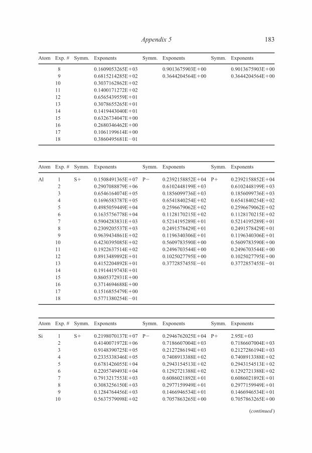
8 0.1609053265E�03 0.9013675903E�00 0.9013675903E�009 0.6815214285E�02 0.3644204564E�00 0.3644204564E�00
10 0.3037162862E�0211 0.1400171272E�0212 0.6565439559E�0113 0.3078655265E�0114 0.1419443040E�0115 0.6326734047E�0016 0.2680346462E�0017 0.1061199614E�0018 0.3860495681E�01
Atom Exp. # Symm. Exponents Symm. Exponents Symm. Exponents
Al 1 S� 0.1508491365E�07 P� 0.2392158852E�04 P� 0.2392158852E�042 0.2907088879E�06 0.6102448199E�03 0.6102448199E�033 0.6546164074E�05 0.1856099736E�03 0.1856099736E�034 0.1696583787E�05 0.6541840254E�02 0.6541840254E�025 0.4985059449E�04 0.2596679062E�02 0.2596679062E�026 0.1635756778E�04 0.1128170215E�02 0.1128170215E�027 0.5904283831E�03 0.5214195289E�01 0.5214195289E�018 0.2309205537E�03 0.2491578429E�01 0.2491578429E�019 0.9639434861E�02 0.1196340306E�01 0.1196340306E�01
10 0.4230395085E�02 0.5609783590E�00 0.5609783590E�0011 0.1922637514E�02 0.2496703544E�00 0.2496703544E�0012 0.8913489892E�01 0.1025027795E�00 0.1025027795E�0013 0.4152204892E�01 0.3772857455E�01 0.3772857455E�0114 0.1914419743E�0115 0.8605372931E�0016 0.3714694688E�0017 0.1516855479E�0018 0.5771380254E�01
Atom Exp. # Symm. Exponents Symm. Exponents Symm. Exponents
Si 1 S� 0.2198070137E�07 P� 0.2946762025E�04 P� 2.95E�032 0.4140071972E�06 0.7186607004E�03 0.7186607004E�033 0.9148390725E�05 0.2127286194E�03 0.2127286194E�034 0.2335338346E�05 0.7408913388E�02 0.7408913388E�025 0.6781426055E�04 0.2943154513E�02 0.2943154513E�026 0.2205749493E�04 0.1292721388E�02 0.1292721388E�027 0.7913217553E�03 0.6086021892E�01 0.6086021892E�018 0.3083256150E�03 0.2977159949E�01 0.2977159949E�019 0.1284764456E�03 0.1466946534E�01 0.1466946534E�01
10 0.5637579098E�02 0.7057863265E�00 0.7057863265E�00
Appendix 5 183
Atom Exp. # Symm. Exponents Symm. Exponents Symm. Exponents
(continued )
Else_EAMC-TRSIC_appn5.qxd 5/19/2007 21:38 Page 183
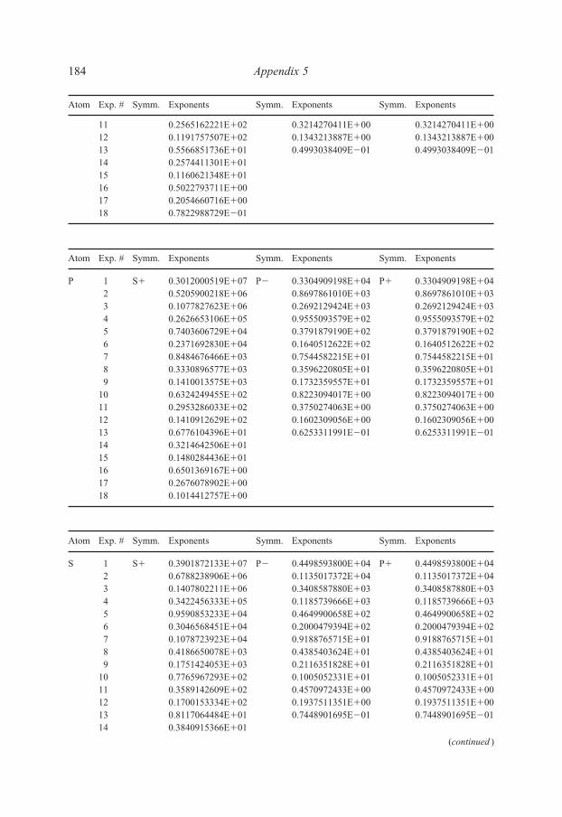
11 0.2565162221E�02 0.3214270411E�00 0.3214270411E�0012 0.1191757507E�02 0.1343213887E�00 0.1343213887E�0013 0.5566851736E�01 0.4993038409E�01 0.4993038409E�0114 0.2574411301E�0115 0.1160621348E�0116 0.5022793711E�0017 0.2054660716E�0018 0.7822988729E�01
Atom Exp. # Symm. Exponents Symm. Exponents Symm. Exponents
P 1 S� 0.3012000519E�07 P� 0.3304909198E�04 P� 0.3304909198E�042 0.5205900218E�06 0.8697861010E�03 0.8697861010E�033 0.1077827623E�06 0.2692129424E�03 0.2692129424E�034 0.2626653106E�05 0.9555093579E�02 0.9555093579E�025 0.7403606729E�04 0.3791879190E�02 0.3791879190E�026 0.2371692830E�04 0.1640512622E�02 0.1640512622E�027 0.8484676466E�03 0.7544582215E�01 0.7544582215E�018 0.3330896577E�03 0.3596220805E�01 0.3596220805E�019 0.1410013575E�03 0.1732359557E�01 0.1732359557E�01
10 0.6324249455E�02 0.8223094017E�00 0.8223094017E�0011 0.2953286033E�02 0.3750274063E�00 0.3750274063E�0012 0.1410912629E�02 0.1602309056E�00 0.1602309056E�0013 0.6776104396E�01 0.6253311991E�01 0.6253311991E�0114 0.3214642506E�0115 0.1480284436E�0116 0.6501369167E�0017 0.2676078902E�0018 0.1014412757E�00
Atom Exp. # Symm. Exponents Symm. Exponents Symm. Exponents
S 1 S� 0.3901872133E�07 P� 0.4498593800E�04 P� 0.4498593800E�042 0.6788238906E�06 0.1135017372E�04 0.1135017372E�043 0.1407802211E�06 0.3408587880E�03 0.3408587880E�034 0.3422456333E�05 0.1185739666E�03 0.1185739666E�035 0.9590853233E�04 0.4649900658E�02 0.4649900658E�026 0.3046568451E�04 0.2000479394E�02 0.2000479394E�027 0.1078723923E�04 0.9188765715E�01 0.9188765715E�018 0.4186650078E�03 0.4385403624E�01 0.4385403624E�019 0.1751424053E�03 0.2116351828E�01 0.2116351828E�01
10 0.7765967293E�02 0.1005052331E�01 0.1005052331E�0111 0.3589142609E�02 0.4570972433E�00 0.4570972433E�0012 0.1700153334E�02 0.1937511351E�00 0.1937511351E�0013 0.8117064484E�01 0.7448901695E�01 0.7448901695E�0114 0.3840915366E�01
184 Appendix 5
Atom Exp. # Symm. Exponents Symm. Exponents Symm. Exponents
(continued )
Else_EAMC-TRSIC_appn5.qxd 5/19/2007 21:38 Page 184

15 0.1771359150E�0116 0.7829354670E�0017 0.3261400044E�0018 0.1259076884E�00
Atom Exp. # Symm. Exponents Symm. Exponents Symm. Exponents
Cl 1 S� 0.3773813358E�07 P� 0.5437199854E�04 P� 0.5437199854E�042 0.7062520751E�06 0.1341039060E�04 0.1341039060E�043 0.1546880727E�06 0.3971626299E�03 0.3971626299E�034 0.3907454691E�05 0.1373100290E�03 0.1373100290E�035 0.1121742987E�05 0.5387523555E�02 0.5387523555E�026 0.3606428477E�04 0.2332250840E�02 0.2332250840E�027 0.1279581910E�04 0.1082945494E�02 0.1082945494E�028 0.4937281914E�03 0.5243597096E�01 0.5243597096E�019 0.2041545600E�03 0.2573887239E�01 0.2573887239E�01
10 0.8914640362E�02 0.1245183385E�01 0.1245183385E�0111 0.4050833683E�02 0.5771740891E�00 0.5771740891E�0012 0.1887570142E�02 0.2492046580E�00 0.2492046580E�0013 0.8887961105E�01 0.9743778804E�01 0.9743778804E�0114 0.4167386790E�0115 0.1917389540E�0116 0.8530294661E�0017 0.3616155587E�0018 0.1439401121E�00
Atom Exp. # Symm. Exponents Symm. Exponents Symm. Exponents
Ar 1 S� 0.4892715338E�07 P� 0.5945445814E�04 P� 0.5945445814E�042 0.8356017747E�06 0.1486551983E�04 0.1486551983E�043 0.1714726270E�06 0.4445856390E�03 0.4445856390E�034 0.4153824066E�05 0.1546984168E�03 0.1546984168E�035 0.1167000522E�05 0.6091817359E�02 0.6091817359E�026 0.3735729864E�04 0.2640668595E�02 0.2640668595E�027 0.1338668813E�04 0.1225638527E�02 0.1225638527E�028 0.5275649100E�03 0.5924720148E�01 0.5924720148E�019 0.2246443694E�03 0.2901387045E�01 0.2901387045E�01
10 0.1015415668E�03 0.1400075122E�01 0.1400075122E�0111 0.4786661050E�02 0.6475604412E�00 0.6475604412E�0012 0.2311925259E�02 0.2792338335E�00 0.2792338335E�0013 0.1124032865E�02 0.1091917884E�00 0.1091917884E�0014 0.5404557487E�0115 0.2524811674E�0116 0.1125893631E�0117 0.4708440270E�0018 0.1814178037E�00
Appendix 5 185
Atom Exp. # Symm. Exponents Symm. Exponents Symm. Exponents
Else_EAMC-TRSIC_appn5.qxd 5/19/2007 21:38 Page 185

Atom Exp. # Symm. Exponents Symm. Exponents Symm. Exponents
K 1 S� 0.7637240356E�07 P� 0.7444708484E�04 P� 0.7444708484E�042 0.1526038293E�07 0.1853667521E�04 0.1853667521E�043 0.3495680665E�06 0.5515745035E�03 0.5515745035E�034 0.9072231089E�05 0.1908415772E�03 0.1908415772E�035 0.2636277785E�05 0.7470446460E�02 0.7470446460E�026 0.8476989267E�04 0.3219090139E�02 0.3219090139E�027 0.2980877831E�04 0.1485733827E�02 0.1485733827E�028 0.1132863241E�04 0.7146254066E�01 0.7146254066E�019 0.4598542871E�03 0.3485408888E�01 0.3485408888E�01
10 0.1970385145E�03 0.1677162453E�01 0.1677162453E�0111 0.8807422351E�02 0.7747309688E�00 0.7747309688E�0012 0.4058747349E�02 0.3342638142E�00 0.3342638142E�0013 0.1905721321E�02 0.1310686266E�00 0.1310686266E�0014 0.9010100407E�0115 0.4239175679E�0116 0.1961523106E�0117 0.8821538921E�0018 0.3810771220E�0019 0.1562707432E�0020 0.6011978808E�0121 0.2144424942E�01
Atom Exp. # Symm. Exponents Symm. Exponents Symm. Exponents
Ca 1 S� 0.1067361002E�08 P� 0.9872550466E�04 P� 0.9872550466E�042 0.1961135964E�07 0.2389227675E�04 0.2389227675E�043 0.4194259900E�06 0.6960528282E�03 0.6960528282E�034 0.1030759745E�06 0.2374438434E�03 0.2374438434E�035 0.2873540040E�05 0.9225527827E�02 0.9225527827E�026 0.8970940255E�04 0.3971098732E�02 0.3971098732E�027 0.3096155748E�04 0.1842030650E�02 0.1842030650E�028 0.1166205198E�04 0.8956272083E�01 0.8956272083E�019 0.4732577134E�03 0.4439964701E�01 0.4439964701E�01
10 0.2042651132E�03 0.2182886334E�01 0.2182886334E�0111 0.9256944985E�02 0.1035284343E�01 0.1035284343E�0112 0.4348318700E�02 0.4607259169E�00 0.4607259169E�0013 0.2090058626E�02 0.1871361396E�00 0.1871361396E�0014 0.1014804072E�0215 0.4913554546E�0116 0.2342083773E�0117 0.1084939065E�0118 0.4821784128E�0019 0.2029611377E�0020 0.7987740350E�0121 0.2901644015E�01
186 Appendix 5
Else_EAMC-TRSIC_appn5.qxd 5/19/2007 21:38 Page 186
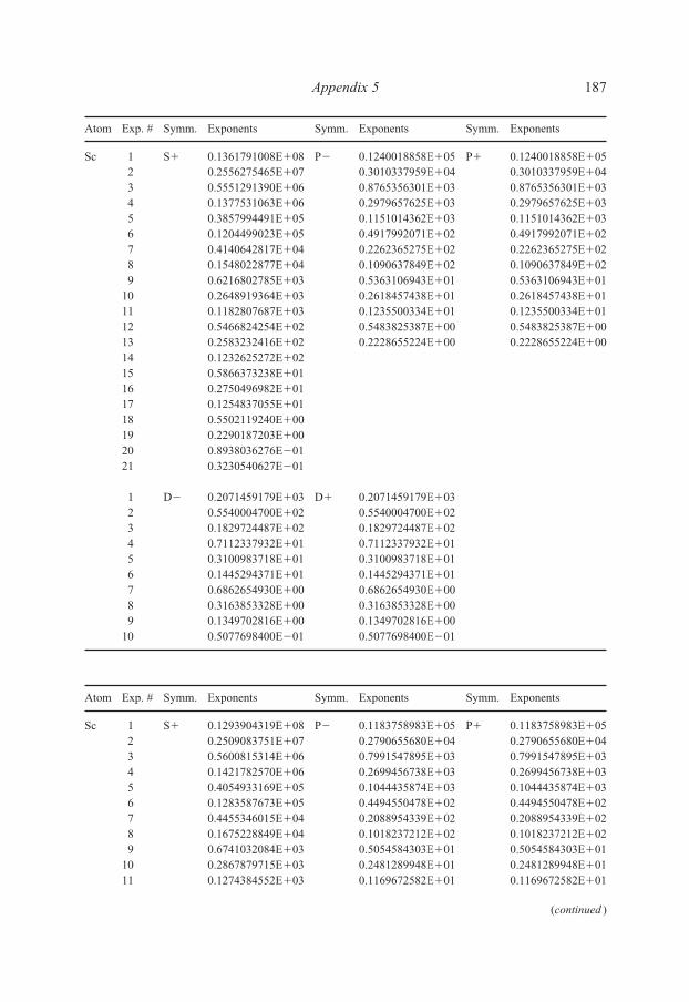
Atom Exp. # Symm. Exponents Symm. Exponents Symm. Exponents
Sc 1 S� 0.1361791008E�08 P� 0.1240018858E�05 P� 0.1240018858E�052 0.2556275465E�07 0.3010337959E�04 0.3010337959E�043 0.5551291390E�06 0.8765356301E�03 0.8765356301E�034 0.1377531063E�06 0.2979657625E�03 0.2979657625E�035 0.3857994491E�05 0.1151014362E�03 0.1151014362E�036 0.1204499023E�05 0.4917992071E�02 0.4917992071E�027 0.4140642817E�04 0.2262365275E�02 0.2262365275E�028 0.1548022877E�04 0.1090637849E�02 0.1090637849E�029 0.6216802785E�03 0.5363106943E�01 0.5363106943E�01
10 0.2648919364E�03 0.2618457438E�01 0.2618457438E�0111 0.1182807687E�03 0.1235500334E�01 0.1235500334E�0112 0.5466824254E�02 0.5483825387E�00 0.5483825387E�0013 0.2583232416E�02 0.2228655224E�00 0.2228655224E�0014 0.1232625272E�0215 0.5866373238E�0116 0.2750496982E�0117 0.1254837055E�0118 0.5502119240E�0019 0.2290187203E�0020 0.8938036276E�0121 0.3230540627E�01
1 D� 0.2071459179E�03 D� 0.2071459179E�032 0.5540004700E�02 0.5540004700E�023 0.1829724487E�02 0.1829724487E�024 0.7112337932E�01 0.7112337932E�015 0.3100983718E�01 0.3100983718E�016 0.1445294371E�01 0.1445294371E�017 0.6862654930E�00 0.6862654930E�008 0.3163853328E�00 0.3163853328E�009 0.1349702816E�00 0.1349702816E�00
10 0.5077698400E�01 0.5077698400E�01
Atom Exp. # Symm. Exponents Symm. Exponents Symm. Exponents
Sc 1 S� 0.1293904319E�08 P� 0.1183758983E�05 P� 0.1183758983E�052 0.2509083751E�07 0.2790655680E�04 0.2790655680E�043 0.5600815314E�06 0.7991547895E�03 0.7991547895E�034 0.1421782570E�06 0.2699456738E�03 0.2699456738E�035 0.4054933169E�05 0.1044435874E�03 0.1044435874E�036 0.1283587673E�05 0.4494550478E�02 0.4494550478E�027 0.4455346015E�04 0.2088954339E�02 0.2088954339E�028 0.1675228849E�04 0.1018237212E�02 0.1018237212E�029 0.6741032084E�03 0.5054584303E�01 0.5054584303E�01
10 0.2867879715E�03 0.2481289948E�01 0.2481289948E�0111 0.1274384552E�03 0.1169672582E�01 0.1169672582E�01
Appendix 5 187
(continued )
Else_EAMC-TRSIC_appn5.qxd 5/19/2007 21:38 Page 187

12 0.5843429843E�02 0.5141442170E�00 0.5141442170E�0013 0.2731402363E�02 0.2046343715E�00 0.2046343715E�0014 0.1285809941E�0215 0.6022320589E�0116 0.2772488139E�0117 0.1239415715E�0118 0.5315309000E�0019 0.2160364307E�0020 0.8221199158E�0121 0.2893848462E�01
1 D� 0.1184181440E�03 D� 0.1184181440E�032 0.3787208488E�02 0.3787208488E�023 0.1403033622E�02 0.1403033622E�024 0.5803339846E�01 0.5803339846E�015 0.2583224488E�01 0.2583224488E�016 0.1192706740E�01 0.1192706740E�017 0.5505613716E�00 0.5505613716E�008 0.2449015306E�00 0.2449015306E�009 0.1011822004E�00 0.1011822004E�00
10 0.3742456470E�01 0.3742456470E�01
Atom Exp. # Symm. Exponents Symm. Exponents Symm. Exponents
Ti 1 S� 0.1302524683E�08 P� 0.1535788547E�05 P� 0.1535788547E�052 0.2525880018E�07 0.3507922979E�04 0.3507922979E�043 0.5645888088E�06 0.9810760917E�03 0.9810760917E�034 0.1436945932E�06 0.3259387686E�03 0.3259387686E�035 0.4113703856E�05 0.1247948607E�03 0.1247948607E�036 0.1308596865E�05 0.5342338463E�02 0.5342338463E�027 0.4569353983E�04 0.2480771611E�02 0.2480771611E�028 0.1730117619E�04 0.1212298366E�02 0.1212298366E�029 0.7017205122E�03 0.6048480364E�01 0.6048480364E�01
10 0.3011731514E�03 0.2989122518E�01 0.2989122518E�0111 0.1351225070E�03 0.1419542861E�01 0.1419542861E�0112 0.6260288035E�02 0.6285029537E�00 0.6285029537E�0013 0.2958774982E�02 0.2516904992E�00 0.2516904992E�0014 0.1409212160E�0215 0.6681646098E�0116 0.3115509066E�0117 0.1411265920E�0118 0.6135059712E�0019 0.2528451688E�0020 0.9759156274E�0121 0.3484876988E�01
188 Appendix 5
Atom Exp. # Symm. Exponents Symm. Exponents Symm. Exponents
(continued )
Else_EAMC-TRSIC_appn5.qxd 5/19/2007 21:38 Page 188

1 D� 0.2244215807E�03 D� 0.2244215807E�032 0.6640364786E�02 0.6640364786E�023 0.2326283217E�02 0.2326283217E�024 0.9271507192E�01 0.9271507192E�015 0.4039512601E�01 0.4039512601E�016 0.1848724702E�01 0.1848724702E�017 0.8539922777E�00 0.8539922777E�008 0.3826025312E�00 0.3826025312E�009 0.1597451581E�00 0.1597451581E�00
10 0.5972653374E�01 0.5972653374E�01
Atom Exp. # Symm. Exponents Symm. Exponents Symm. Exponents
Ti 1 S� 0.1420630645E�08 P� 0.1438455617E�05 P� 0.1438455617E�052 0.2689067260E�07 0.3398921375E�04 0.3398921375E�043 0.5886866412E�06 0.9722039038E�03 0.9722039038E�034 0.1471906744E�06 0.3271316006E�03 0.3271316006E�035 0.4150893378E�05 0.1258385883E�03 0.1258385883E�036 0.1303825886E�05 0.5377849982E�02 0.5377849982E�027 0.4504700565E�04 0.2481328939E�02 0.2481328939E�028 0.1690566015E�04 0.1201207721E�02 0.1201207721E�029 0.6805652777E�03 0.5929080027E�01 0.5929080027E�01
10 0.2902220850E�03 0.2899807958E�01 0.2899807958E�0111 0.1294689764E�03 0.1365655618E�01 0.1365655618E�0112 0.5966602792E�02 0.6018392293E�00 0.6018392293E�0013 0.2805215729E�02 0.2411928524E�00 0.2411928524E�0014 0.1328723754E�0215 0.6261580922E�0116 0.2899116921E�0117 0.1302361257E�0118 0.5605737792E�0019 0.2283080553E�0020 0.8688571974E�0121 0.3051166126E�01
1 D� 0.1549566491E�03 D� 0.1549566491E�032 0.4800141881E�02 0.4800141881E�023 0.1755931844E�02 0.1755931844E�024 0.7281011420E�01 0.7281011420E�015 0.3284936661E�01 0.3284936661E�016 0.1547869249E�01 0.1547869249E�017 0.7311968019E�00 0.7311968019E�008 0.3323898752E�00 0.3323898752E�009 0.1395711111E�00 0.1395711111E�00
10 0.5196348690E�01 0.5196348690E�01
Appendix 5 189
Atom Exp. # Symm. Exponents Symm. Exponents Symm. Exponents
Else_EAMC-TRSIC_appn5.qxd 5/19/2007 21:38 Page 189

Atom Exp. # Symm. Exponents Symm. Exponents Symm. Exponents
V 1 S� 0.1402990488E�08 P� 0.1756100190E�05 P� 0.1756100190E�052 0.2752073598E�07 0.4007694684E�04 0.4007694684E�043 0.6196134971E�06 0.1117964263E�04 0.1117964263E�044 0.1582486835E�06 0.3700293487E�03 0.3700293487E�035 0.4531277461E�05 0.1410608132E�03 0.1410608132E�036 0.1437690565E�05 0.6012091214E�02 0.6012091214E�027 0.4995480969E�04 0.2780870137E�02 0.2780870137E�028 0.1878707708E�04 0.1355060948E�02 0.1355060948E�029 0.7558124667E�03 0.6752225347E�01 0.6752225347E�01
10 0.3214731553E�03 0.3339888805E�01 0.3339888805E�0111 0.1428742968E�03 0.1591846085E�01 0.1591846085E�0112 0.6557603176E�02 0.7096449700E�00 0.7096449700E�0013 0.3071996354E�02 0.2872362032E�00 0.2872362032E�0014 0.1451722804E�0215 0.6839699859E�0116 0.3175291751E�0117 0.1435576612E�0118 0.6246951934E�0019 0.2585901086E�0020 0.1006376552E�0021 0.3639291726E�01
1 D� 0.2406270350E�03 D� 0.2406270350E�032 0.7257124067E�02 0.7257124067E�023 0.2640954068E�02 0.2640954068E�024 0.1109004373E�02 0.1109004373E�025 0.5139036698E�01 0.5139036698E�016 0.2513079153E�01 0.2513079153E�017 0.1240242310E�01 0.1240242310E�018 0.5907215086E�00 0.5907215086E�009 0.2596778040E�00 0.2596778040E�00
10 0.1007540746E�00 0.1007540746E�00
Atom Exp. # Symm. Exponents Symm. Exponents Symm. Exponents
V 1 S� 0.1491401970E�08 P� 0.1653084457E�05 P� 0.1653084457E�052 0.2777091106E�07 0.3846914035E�04 0.3846914035E�043 0.6017095180E�06 0.1089220150E�04 0.1089220150E�044 0.1497045927E�06 0.3643091662E�03 0.3643091662E�035 0.4220705068E�05 0.1397466084E�03 0.1397466084E�036 0.1330719978E�05 0.5968905466E�02 0.5968905466E�027 0.4630099109E�04 0.2756105712E�02 0.2756105712E�028 0.1754470165E�04 0.1335704189E�02 0.1335704189E�029 0.7145027866E�03 0.6596346351E�01 0.6596346351E�01
10 0.3086130285E�03 0.3222855693E�01 0.3222855693E�0111 0.1395169989E�03 0.1512474339E�01 0.1512474339E�01
190 Appendix 5
(continued )
Else_EAMC-TRSIC_appn5.qxd 5/19/2007 21:38 Page 190

12 0.6514673960E�02 0.6619274877E�00 0.6619274877E�0013 0.3100709539E�02 0.2622850661E�00 0.2622850661E�0014 0.1484507772E�0215 0.7055162263E�0116 0.3284617696E�0117 0.1478311962E�0118 0.6347474205E�0019 0.2565898894E�0020 0.9636781804E�0121 0.3318398616E�01
1 D� 0.1898619291E�03 D� 0.1898619291E�032 0.5849779789E�02 0.5849779789E�023 0.2134578752E�02 0.2134578752E�024 0.8848950904E�01 0.8848950904E�015 0.3997737106E�01 0.3997737106E�016 0.1888058394E�01 0.1888058394E�017 0.8941929908E�00 0.8941929908E�008 0.4073780752E�00 0.4073780752E�009 0.1712578537E�00 0.1712578537E�00
10 0.6372732656E�01 0.6372732656E�01
Atom Exp. # Symm. Exponents Symm. Exponents Symm. Exponents
Cr 1 S� 0.1673696901E�08 P� 0.2220077820E�05 P� 0.2220077820E�052 0.3200196359E�07 0.5081811896E�04 0.5081811896E�043 0.7061887198E�06 0.1413134320E�04 0.1413134320E�044 0.1776541317E�06 0.4639219732E�03 0.4639219732E�035 0.5032760777E�05 0.1747371519E�03 0.1747371519E�036 0.1585914439E�05 0.7338149296E�02 0.7338149296E�027 0.5491130458E�04 0.3339111986E�02 0.3339111986E�028 0.2063566007E�04 0.1599929132E�02 0.1599929132E�029 0.8314107107E�03 0.7844729963E�01 0.7844729963E�01
10 0.3547476798E�03 0.3825118654E�01 0.3825118654E�0111 0.1583420499E�03 0.1802534786E�01 0.1802534786E�0112 0.7303175970E�02 0.7977676079E�00 0.7977676079E�0013 0.3438207804E�02 0.3222591911E�00 0.3222591911E�0014 0.1632012140E�0215 0.7715278492E�0116 0.3588251207E�0117 0.1621747118E�0118 0.7035881954E�0019 0.2894377148E�0020 0.1115215804E�0021 0.3975538656E�01
Appendix 5 191
Atom Exp. # Symm. Exponents Symm. Exponents Symm. Exponents
(continued )
Else_EAMC-TRSIC_appn5.qxd 5/19/2007 21:38 Page 191
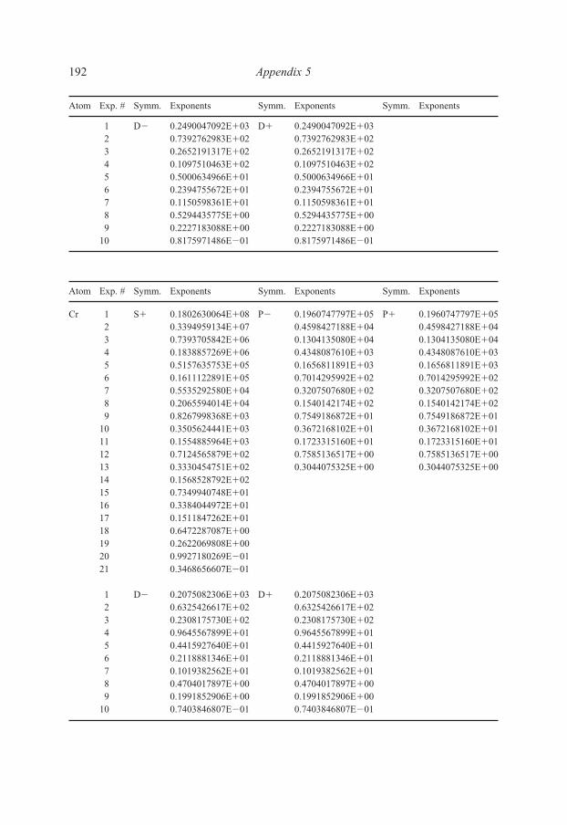
1 D� 0.2490047092E�03 D� 0.2490047092E�032 0.7392762983E�02 0.7392762983E�023 0.2652191317E�02 0.2652191317E�024 0.1097510463E�02 0.1097510463E�025 0.5000634966E�01 0.5000634966E�016 0.2394755672E�01 0.2394755672E�017 0.1150598361E�01 0.1150598361E�018 0.5294435775E�00 0.5294435775E�009 0.2227183088E�00 0.2227183088E�00
10 0.8175971486E�01 0.8175971486E�01
Atom Exp. # Symm. Exponents Symm. Exponents Symm. Exponents
Cr 1 S� 0.1802630064E�08 P� 0.1960747797E�05 P� 0.1960747797E�052 0.3394959134E�07 0.4598427188E�04 0.4598427188E�043 0.7393705842E�06 0.1304135080E�04 0.1304135080E�044 0.1838857269E�06 0.4348087610E�03 0.4348087610E�035 0.5157635753E�05 0.1656811891E�03 0.1656811891E�036 0.1611122891E�05 0.7014295992E�02 0.7014295992E�027 0.5535292580E�04 0.3207507680E�02 0.3207507680E�028 0.2065594014E�04 0.1540142174E�02 0.1540142174E�029 0.8267998368E�03 0.7549186872E�01 0.7549186872E�01
10 0.3505624441E�03 0.3672168102E�01 0.3672168102E�0111 0.1554885964E�03 0.1723315160E�01 0.1723315160E�0112 0.7124565879E�02 0.7585136517E�00 0.7585136517E�0013 0.3330454751E�02 0.3044075325E�00 0.3044075325E�0014 0.1568528792E�0215 0.7349940748E�0116 0.3384044972E�0117 0.1511847262E�0118 0.6472287087E�0019 0.2622069808E�0020 0.9927180269E�0121 0.3468656607E�01
1 D� 0.2075082306E�03 D� 0.2075082306E�032 0.6325426617E�02 0.6325426617E�023 0.2308175730E�02 0.2308175730E�024 0.9645567899E�01 0.9645567899E�015 0.4415927640E�01 0.4415927640E�016 0.2118881346E�01 0.2118881346E�017 0.1019382562E�01 0.1019382562E�018 0.4704017897E�00 0.4704017897E�009 0.1991852906E�00 0.1991852906E�00
10 0.7403846807E�01 0.7403846807E�01
192 Appendix 5
Atom Exp. # Symm. Exponents Symm. Exponents Symm. Exponents
Else_EAMC-TRSIC_appn5.qxd 5/19/2007 21:38 Page 192
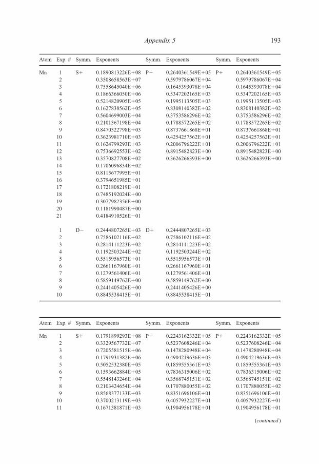
Atom Exp. # Symm. Exponents Symm. Exponents Symm. Exponents
Mn 1 S� 0.1890813226E�08 P� 0.2640361549E�05 P� 0.2640361549E�052 0.3508658563E�07 0.5979786067E�04 0.5979786067E�043 0.7558645040E�06 0.1645393078E�04 0.1645393078E�044 0.1866366050E�06 0.5347202165E�03 0.5347202165E�035 0.5214820905E�05 0.1995113505E�03 0.1995113505E�036 0.1627838562E�05 0.8308140382E�02 0.8308140382E�027 0.5604699003E�04 0.3753586296E�02 0.3753586296E�028 0.2101367198E�04 0.1788572265E�02 0.1788572265E�029 0.8470322798E�03 0.8737661868E�01 0.8737661868E�01
10 0.3623981710E�03 0.4254257562E�01 0.4254257562E�0111 0.1624799293E�03 0.2006796222E�01 0.2006796222E�0112 0.7536692553E�02 0.8915482823E�00 0.8915482823E�0013 0.3570827708E�02 0.3626266393E�00 0.3626266393E�0014 0.1706096834E�0215 0.8115677995E�0116 0.3794651985E�0117 0.1721808219E�0118 0.7485192024E�0019 0.3077982356E�0020 0.1181990487E�0021 0.4184910526E�01
1 D� 0.2444807265E�03 D� 0.2444807265E�032 0.7586102116E�02 0.7586102116E�023 0.2814111223E�02 0.2814111223E�024 0.1192503244E�02 0.1192503244E�025 0.5515956573E�01 0.5515956573E�016 0.2661167960E�01 0.2661167960E�017 0.1279561406E�01 0.1279561406E�018 0.5859149762E�00 0.5859149762E�009 0.2441405426E�00 0.2441405426E�00
10 0.8845538415E�01 0.8845538415E�01
Atom Exp. # Symm. Exponents Symm. Exponents Symm. Exponents
Mn 1 S� 0.1791899293E�08 P� 0.2243162332E�05 P� 0.2243162332E�052 0.3329567732E�07 0.5237608246E�04 0.5237608246E�043 0.7205581515E�06 0.1478280948E�04 0.1478280948E�044 0.1791931382E�06 0.4904219636E�03 0.4904219636E�035 0.5052532380E�05 0.1859555361E�03 0.1859555361E�036 0.1593662884E�05 0.7836315006E�02 0.7836315006E�027 0.5548143246E�04 0.3568745151E�02 0.3568745151E�028 0.2103424654E�04 0.1707880055E�02 0.1707880055E�029 0.8568377133E�03 0.8351696106E�01 0.8351696106E�01
10 0.3700213119E�03 0.4057932227E�01 0.4057932227E�0111 0.1671381871E�03 0.1904956178E�01 0.1904956178E�01
Appendix 5 193
(continued )
Else_EAMC-TRSIC_appn5.qxd 5/19/2007 21:38 Page 193

12 0.7791295063E�02 0.8401417904E�00 0.8401417904E�0013 0.3698221034E�02 0.3384892564E�00 0.3384892564E�0014 0.1763557228E�0215 0.8336120096E�0116 0.3853721384E�0117 0.1719106728E�0118 0.7301225742E�0019 0.2912885100E�0020 0.1077084572E�0021 0.3641995144E�01
1 D� 0.2433238431E�03 D� 0.2433238431E�032 0.7579631204E�02 0.7579631204E�023 0.2787053110E�02 0.2787053110E�024 0.1160691855E�02 0.1160691855E�025 0.5252957790E�01 0.5252957790E�016 0.2478831054E�01 0.2478831054E�017 0.1170271823E�01 0.1170271823E�018 0.5303519034E�00 0.5303519034E�009 0.2213705474E�00 0.2213705474E�00
10 0.8165722745E�01 0.8165722745E�01
Atom Exp. # Symm. Exponents Symm. Exponents Symm. Exponents
Fe 1 S� 0.2023710697E�08 P� 0.2828520028E�05 P� 0.2828520028E�052 0.3765837627E�07 0.6195586774E�04 0.6195586774E�043 0.8124714734E�06 0.1674435613E�04 0.1674435613E�044 0.2006738490E�06 0.5411784202E�03 0.5411784202E�035 0.5602892995E�05 0.2027317113E�03 0.2027317113E�036 0.1746125782E�05 0.8531694325E�02 0.8531694325E�027 0.5997677791E�04 0.3909349157E�02 0.3909349157E�028 0.2242011863E�04 0.1890394278E�02 0.1890394278E�029 0.9006221243E�03 0.9349799015E�01 0.9349799015E�01
10 0.3838839961E�03 0.4584344982E�01 0.4584344982E�0111 0.1714402744E�03 0.2159735819E�01 0.2159735819E�0112 0.7921071080E�02 0.9475354796E�00 0.9475354796E�0013 0.3738659720E�02 0.3752191784E�00 0.3752191784E�0014 0.1779965969E�0215 0.8440612276E�0116 0.3936456492E�0117 0.1782826057E�0118 0.7742607841E�0019 0.3183780267E�0020 0.1223993761E�0021 0.4344085610E�01
194 Appendix 5
Atom Exp. # Symm. Exponents Symm. Exponents Symm. Exponents
(continued )
Else_EAMC-TRSIC_appn5.qxd 5/19/2007 21:38 Page 194

1 D� 0.3194775408E�03 D� 0.3194775408E�032 0.9778159372E�02 0.9778159372E�023 0.3573014347E�02 0.3573014347E�024 0.1493886511E�02 0.1493886511E�025 0.6849359735E�01 0.6849359735E�016 0.3300473109E�01 0.3300473109E�017 0.1601919176E�01 0.1601919176E�018 0.7505636161E�00 0.7505636161E�009 0.3253578201E�00 0.3253578201E�00
10 0.1250564662E�00 0.1250564662E�00
Atom Exp. # Symm. Exponents Symm. Exponents Symm. Exponents
Fe 1 S� 0.1810495732E�08 P� 0.2640939689E�05 P� 0.2640939689E�052 0.3405804856E�07 0.5946635945E�04 0.5946635945E�043 0.7440208332E�06 0.1639314127E�04 0.1639314127E�044 0.1862916137E�06 0.5368288617E�03 0.5368288617E�035 0.5276478551E�05 0.2026269755E�03 0.2026269755E�036 0.1668543389E�05 0.8553646167E�02 0.8553646167E�027 0.5813973910E�04 0.3918346140E�02 0.3918346140E�028 0.2203183602E�04 0.1889977775E�02 0.1889977775E�029 0.8961281741E�03 0.9313606019E�01 0.9313606019E�01
10 0.3861279092E�03 0.4549788181E�01 0.4549788181E�0111 0.1739536986E�03 0.2137871158E�01 0.2137871158E�0112 0.8086811953E�02 0.9375486155E�00 0.9375486155E�0013 0.3828794136E�02 0.3723341475E�00 0.3723341475E�0014 0.1822164050E�0215 0.8603071042E�0116 0.3977039580E�0117 0.1776668806E�0118 0.7569949685E�0019 0.3036122228E�0020 0.1131318904E�0021 0.3865361904E�01
1 D� 0.2654543806E�03 D� 0.2654543806E�032 0.8473804319E�02 0.8473804319E�023 0.3163606712E�02 0.3163606712E�024 0.1327715654E�02 0.1327715654E�025 0.6020730666E�01 0.6020730666E�016 0.2835423059E�01 0.2835423059E�017 0.1332950691E�01 0.1332950691E�018 0.6012302975E�00 0.6012302975E�009 0.2500928033E�00 0.2500928033E�00
10 0.9221426338E�01 0.9221426338E�01
Appendix 5 195
Atom Exp. # Symm. Exponents Symm. Exponents Symm. Exponents
Else_EAMC-TRSIC_appn5.qxd 5/19/2007 21:38 Page 195
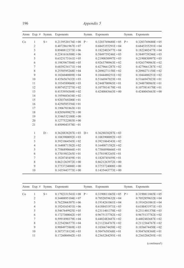
Atom Exp. # Symm. Exponents Symm. Exponents Symm. Exponents
Co 1 S� 0.2139520176E�08 P� 0.3203769680E�05 P� 0.3203769680E�052 0.4072861967E�07 0.6845355291E�04 0.6845355291E�043 0.8948812373E�06 0.1822402477E�04 0.1822402477E�044 0.2241616308E�06 0.5849759246E�03 0.5849759246E�035 0.6323173161E�05 0.2190830997E�03 0.2190830997E�036 0.1983967504E�05 0.9263790963E�02 0.9263790963E�027 0.6839234171E�04 0.4279661287E�02 0.4279661287E�028 0.2558595268E�04 0.2090271158E�02 0.2090271158E�029 0.1026040889E�04 0.1044480251E�02 0.1044480251E�02
10 0.4356567632E�03 0.5166947023E�01 0.5166947023E�0111 0.1934589060E�03 0.2448700965E�01 0.2448700965E�0112 0.8874527273E�02 0.1075814170E�01 0.1075814170E�0113 0.4153954369E�02 0.4240043663E�00 0.4240043663E�0014 0.1959683634E�0215 0.9203769200E�0116 0.4250585356E�0117 0.1906701863E�0118 0.8205699827E�0019 0.3346532180E�0020 0.1277522883E�0021 0.4509043578E�01
1 D� 0.3628838287E�03 D� 0.3628838287E�032 0.1083900092E�03 0.1083900092E�033 0.3921064543E�02 0.3921064543E�024 0.1640871582E�02 0.1640871582E�025 0.7586890666E�01 0.7586890666E�016 0.3701983265E�01 0.3701983265E�017 0.1820745459E�01 0.1820745459E�018 0.8621263972E�00 0.8621263972E�009 0.3753724008E�00 0.3753724008E�00
10 0.1435443773E�00 0.1435443773E�00
Atom Exp. # Symm. Exponents Symm. Exponents Symm. Exponents
Co 1 S� 0.1792331541E�08 P� 0.3190811065E�05 P� 0.3190811065E�052 0.3440895104E�07 0.7052859632E�04 0.7052859632E�043 0.7622066307E�06 0.1914261061E�04 0.1914261061E�044 0.1924165451E�06 0.6188431971E�03 0.6188431971E�035 0.5467649925E�05 0.2311401370E�03 0.2311401370E�036 0.1727300042E�05 0.9675137782E�02 0.9675137782E�027 0.5991890379E�04 0.4402483687E�02 0.4402483687E�028 0.2254286577E�04 0.2112364767E�02 0.2112364767E�029 0.9084975869E�03 0.1036674450E�02 0.1036674450E�02
10 0.3873718124E�03 0.5047658368E�01 0.5047658368E�0111 0.1726004942E�03 0.2365284295E�01 0.2365284295E�01
196 Appendix 5
(continued )
Else_EAMC-TRSIC_appn5.qxd 5/19/2007 21:38 Page 196

12 0.7937541947E�02 0.1034652083E�01 0.1034652083E�0113 0.3721175975E�02 0.4098214418E�00 0.4098214418E�0014 0.1756486261E�0215 0.8245174982E�0116 0.3801594276E�0117 0.1700445115E�0118 0.7288038124E�0019 0.2956174136E�0020 0.1120833100E�0021 0.3923409484E�01
1 D� 0.3090261061E�03 D� 0.3090261061E�032 0.9633774175E�02 0.9633774175E�023 0.3556425757E�02 0.3556425757E�024 0.1489927154E�02 0.1489927154E�025 0.6788414265E�01 0.6788414265E�016 0.3223603836E�01 0.3223603836E�017 0.1528984298E�01 0.1528984298E�018 0.6941773388E�00 0.6941773388E�009 0.2891091886E�00 0.2891091886E�00
10 0.1058511118E�00 0.1058511118E�00
Atom Exp. # Symm. Exponents Symm. Exponents Symm. Exponents
Ni 1 S� 0.2059279954E�08 P� 0.3571255933E�05 P� 0.3571255933E�052 0.3939334363E�07 0.7736220974E�04 0.7736220974E�043 0.8678259261E�06 0.2071601623E�04 0.2071601623E�044 0.2175431144E�06 0.6646523954E�03 0.6646523954E�035 0.6131427963E�05 0.2476482890E�03 0.2476482890E�036 0.1919915468E�05 0.1038651818E�03 0.1038651818E�037 0.6599444725E�04 0.4752695668E�02 0.4752695668E�028 0.2460583550E�04 0.2299783020E�02 0.2299783020E�029 0.9832747599E�03 0.1140649010E�02 0.1140649010E�02
10 0.4161197628E�03 0.5620526121E�01 0.5620526121E�0111 0.1842761335E�03 0.2666878078E�01 0.2666878078E�0112 0.8437771492E�02 0.1181060299E�01 0.1181060299E�0113 0.3947253059E�02 0.4731786813E�00 0.4731786813E�0014 0.1864109172E�0215 0.8781273462E�0116 0.4077125383E�0117 0.1843578614E�0118 0.8021967646E�0019 0.3319039515E�0020 0.1290199395E�0021 0.4656019181E�01
Appendix 5 197
Atom Exp. # Symm. Exponents Symm. Exponents Symm. Exponents
(continued )
Else_EAMC-TRSIC_appn5.qxd 5/19/2007 21:38 Page 197

1 D� 0.4325647814E�03 D� 0.4325647814E�032 0.1295554220E�03 0.1295554220E�033 0.4650796008E�02 0.4650796008E�024 0.1917448069E�02 0.1917448069E�025 0.8699652636E�01 0.8699652636E�016 0.4162167525E�01 0.4162167525E�017 0.2012027458E�01 0.2012027458E�018 0.9416777586E�00 0.9416777586E�009 0.4088670813E�00 0.4088670813E�00
10 0.1578086348E�00 0.1578086348E�00
Atom Exp. # Symm. Exponents Symm. Exponents Symm. Exponents
Ni 1 S� 0.2207905973E�08 P� 0.3607302845E�05 P� 0.3607302845E�052 0.4080382960E�07 0.7979958513E�04 0.7979958513E�043 0.8773249328E�06 0.2162495751E�04 0.2162495751E�044 0.2165787239E�06 0.6966899705E�03 0.6966899705E�035 0.6057918940E�05 0.2589682887E�03 0.2589682887E�036 0.1894698233E�05 0.1077877520E�03 0.1077877520E�037 0.6539162708E�04 0.4875297333E�02 0.4875297333E�028 0.2457685544E�04 0.2325598465E�02 0.2325598465E�029 0.9926796988E�03 0.1135437817E�02 0.1135437817E�02
10 0.4252332308E�03 0.5506555771E�01 0.5506555771E�0111 0.1906501094E�03 0.2574410868E�01 0.2574410868E�0112 0.8828670421E�02 0.1126029777E�01 0.1126029777E�0113 0.4167335927E�02 0.4471869836E�00 0.4471869836E�0014 0.1978715026E�0215 0.9326659152E�0116 0.4306690359E�0117 0.1922615574E�0118 0.8188966701E�0019 0.3284053113E�0020 0.1223748673E�0021 0.4181497734E�01
1 D� 0.3421361829E�03 D� 0.3421361829E�032 0.1097856105E�03 0.1097856105E�033 0.4080635851E�02 0.4080635851E�024 0.1694082296E�02 0.1694082296E�025 0.7574494428E�01 0.7574494428E�016 0.3517009330E�01 0.3517009330E�017 0.1635243207E�01 0.1635243207E�018 0.7341222552E�00 0.7341222552E�009 0.3068455783E�00 0.3068455783E�00
10 0.1151396836E�00 0.1151396836E�00
198 Appendix 5
Atom Exp. # Symm. Exponents Symm. Exponents Symm. Exponents
Else_EAMC-TRSIC_appn5.qxd 5/19/2007 21:38 Page 198

Atom Exp. # Symm. Exponents Symm. Exponents Symm. Exponents
Cu 1 S� 0.2127255449E�08 P� 0.4404416285E�05 P� 0.4404416285E�052 0.4065874207E�07 0.9514682989E�04 0.9514682989E�043 0.8971508971E�06 0.2530325972E�04 0.2530325972E�044 0.2257331876E�06 0.8035908742E�03 0.8035908742E�035 0.6397124307E�05 0.2956446863E�03 0.2956446863E�036 0.2016855197E�05 0.1222311516E�03 0.1222311516E�037 0.6987250232E�04 0.5508973202E�02 0.5508973202E�028 0.2627366273E�04 0.2625648174E�02 0.2625648174E�029 0.1059153209E�04 0.1283747781E�02 0.1283747781E�02
10 0.4521285067E�03 0.6245976813E�01 0.6245976813E�0111 0.2018696492E�03 0.2933585179E�01 0.2933585179E�0112 0.9311664007E�02 0.1290253058E�01 0.1290253058E�0113 0.4383003247E�02 0.5155005544E�00 0.5155005544E�0014 0.2079436251E�0215 0.9821772000E�0116 0.4561898323E�0117 0.2058040732E�0118 0.8907504255E�0019 0.3653363749E�0020 0.1402509114E�0021 0.4977777329E�01
1 D� 0.4424892568E�03 D� 0.4424892568E�032 0.1353235337E�03 0.1353235337E�033 0.4935411966E�02 0.4935411966E�024 0.2058381547E�02 0.2058381547E�025 0.9413554696E�01 0.9413554696E�016 0.4526678296E�01 0.4526678296E�017 0.2194707924E�01 0.2194707924E�018 0.1028768984E�01 0.1028768984E�019 0.4470704163E�00 0.4470704163E�00
10 0.1727125326E�00 0.1727125326E�00
Atom Exp. # Symm. Exponents Symm. Exponents Symm. Exponents
Cu 1 S� 0.2181663277E�08 P� 0.3903931661E�05 P� 0.3903931661E�052 0.4160661003E�07 0.8698937845E�04 0.8698937845E�043 0.9158663753E�06 0.2366106282E�04 0.2366106282E�044 0.2298271819E�06 0.7630176900E�03 0.7630176900E�035 0.6493434833E�05 0.2833320087E�03 0.2833320087E�036 0.2040120038E�05 0.1176645633E�03 0.1176645633E�037 0.7039623302E�04 0.5307782098E�02 0.5307782098E�028 0.2634874324E�04 0.2525958274E�02 0.2525958274E�029 0.1056553518E�04 0.1231723665E�02 0.1231723665E�02
10 0.4482791378E�03 0.5977268485E�01 0.5977268485E�0111 0.1987628938E�03 0.2803644498E�01 0.2803644498E�01
Appendix 5 199
(continued )
Else_EAMC-TRSIC_appn5.qxd 5/19/2007 21:38 Page 199
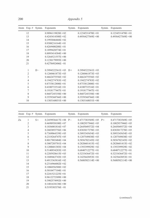
12 0.9096119828E�02 0.1234531470E�01 0.1234531470E�0113 0.4243414308E�02 0.4956427569E�00 0.4956427569E�0014 0.1993046468E�0215 0.9308216164E�0116 0.4269400208E�0117 0.1899428574E�0118 0.8095414384E�0019 0.3264521557E�0020 0.1230179995E�0021 0.4278492406E�01
1 D� 0.3994522561E�03 D� 0.3994522561E�032 0.1260461873E�03 0.1260461873E�033 0.4662475556E�02 0.4662475556E�024 0.1942274783E�02 0.1942274783E�025 0.8753812800E�01 0.8753812800E�016 0.4100733516E�01 0.4100733516E�017 0.1918177447E�01 0.1918177447E�018 0.8607245350E�00 0.8607245350E�009 0.3559368766E�00 0.3559368766E�00
10 0.1303168031E�00 0.1303168031E�00
Atom Exp. # Symm. Exponents Symm. Exponents Symm. Exponents
Zn 1 S� 0.2459936417E�08 P� 0.4717383569E�05 P� 0.4717383569E�052 0.4698958100E�07 0.1002957946E�05 0.1002957946E�053 0.1036001816E�07 0.2645049372E�04 0.2645049372E�044 0.2603893756E�06 0.8383017278E�03 0.8383017278E�035 0.7369064339E�05 0.3093345654E�03 0.3093345654E�036 0.2319264747E�05 0.1287549830E�03 0.1287549830E�037 0.8017883484E�04 0.5856702145E�02 0.5856702145E�028 0.3007205701E�04 0.2820601415E�02 0.2820601415E�029 0.1208601303E�04 0.1393399929E�02 0.1393399929E�02
10 0.5140934283E�03 0.6840712277E�01 0.6840712277E�0111 0.2285928615E�03 0.3233436472E�01 0.3233436472E�0112 0.1049463743E�03 0.1425643053E�01 0.1425643053E�0113 0.4913363816E�02 0.5680502114E�00 0.5680502114E�0014 0.2316966002E�0215 0.1086956588E�0216 0.5010477104E�0117 0.2241521225E�0118 0.9612272309E�0019 0.3902574992E�0020 0.1481634138E�0021 0.5195385376E�01
200 Appendix 5
Atom Exp. # Symm. Exponents Symm. Exponents Symm. Exponents
(continued )
Else_EAMC-TRSIC_appn5.qxd 5/19/2007 21:38 Page 200

1 D� 0.4896090922E�03 D� 0.4896090922E�032 0.1506536280E�03 0.1506536280E�033 0.5524649362E�02 0.5524649362E�024 0.2313584152E�02 0.2313584152E�025 0.1060185332E�02 0.1060185332E�026 0.5093949595E�01 0.5093949595E�017 0.2459032731E�01 0.2459032731E�018 0.1142802660E�01 0.1142802660E�019 0.4899320994E�00 0.4899320994E�00
10 0.1856601591E�00 0.1856601591E�00
Atom Exp. # Symm. Exponents Symm. Exponents Symm. Exponents
Ga 1 S� 0.2985493181E�08 P� 0.8866794085E�05 P� 0.8866794085E�052 0.5676531350E�07 0.2207419386E�05 0.2207419386E�053 0.1247892213E�07 0.6359554354E�04 0.6359554354E�044 0.3132442921E�06 0.2083419469E�04 0.2083419469E�045 0.8867195738E�05 0.7626399619E�03 0.7626399619E�036 0.2795576897E�05 0.3065065821E�03 0.3065065821E�037 0.9694459234E�04 0.1328991064E�03 0.1328991064E�038 0.3651974309E�04 0.6108729953E�02 0.6108729953E�029 0.1475940323E�04 0.2924899880E�02 0.2924899880E�02
10 0.6320214562E�03 0.1433464349E�02 0.1433464349E�0211 0.2832055542E�03 0.7065830310E�01 0.7065830310E�0112 0.1311485857E�03 0.3442108276E�01 0.3442108276E�0113 0.6198724536E�02 0.1628378915E�01 0.1628378915E�0114 0.2953268441E�02 0.7350902013E�00 0.7350902013E�0015 0.1400716852E�02 0.3111462844E�00 0.3111462844E�0016 0.6531750766E�01 0.1213422458E�00 0.1213422458E�0017 0.2957506166E�01 0.4284177573E�01 0.4284177573E�0118 0.1284172885E�0119 0.5280901849E�0020 0.2031254964E�0021 0.7217345702E�01
1 D� 0.5470614554E�03 D� 0.5470614554E�032 0.1785375907E�03 0.1785375907E�033 0.6714412694E�02 0.6714412694E�024 0.2817080571E�02 0.2817080571E�025 0.1276531244E�02 0.1276531244E�026 0.6048290480E�01 0.6048290480E�017 0.2900887663E�01 0.2900887663E�018 0.1363497443E�01 0.1363497443E�019 0.6080383309E�00 0.6080383309E�00
10 0.2490513328E�00 0.2490513328E�00
Appendix 5 201
Atom Exp. # Symm. Exponents Symm. Exponents Symm. Exponents
Else_EAMC-TRSIC_appn5.qxd 5/19/2007 21:38 Page 201

Atom Exp. # Symm. Exponents Symm. Exponents Symm. Exponents
Ge 1 S� 0.3189771503E�08 P� 0.1107106102E�06 P� 0.1107106102E�062 0.6004914335E�07 0.2707053178E�05 0.2707053178E�053 0.1311382250E�07 0.7670244705E�04 0.7670244705E�044 0.3280234043E�06 0.2475222597E�04 0.2475222597E�045 0.9279214430E�05 0.8941278692E�03 0.8941278692E�036 0.2931070349E�05 0.3553473254E�03 0.3553473254E�037 0.1020769602E�05 0.1527081580E�03 0.1527081580E�038 0.3869844136E�04 0.6974529486E�02 0.6974529486E�029 0.1576889568E�04 0.3327352393E�02 0.3327352393E�02
10 0.6819129708E�03 0.1629677277E�02 0.1629677277E�0211 0.3089970197E�03 0.8053989683E�01 0.8053989683E�0112 0.1448622083E�03 0.3947434160E�01 0.3947434160E�0113 0.6937598886E�02 0.1885822478E�01 0.1885822478E�0114 0.3351153716E�02 0.8630908798E�00 0.8630908798E�0015 0.1612086692E�02 0.3719373336E�00 0.3719373336E�0016 0.7625513961E�01 0.1483297502E�00 0.1483297502E�0017 0.3501985435E�01 0.5380463915E�01 0.5380463915E�0118 0.1541706988E�0119 0.6424057806E�0020 0.2501583112E�0021 0.8988684405E�01
1 D� 0.6209042224E�03 D� 0.6209042224E�032 0.2032514375E�03 0.2032514375E�033 0.7685666788E�02 0.7685666788E�024 0.3249060810E�02 0.3249060810E�025 0.1486113361E�02 0.1486113361E�026 0.7117923198E�01 0.7117923198E�017 0.3455026360E�01 0.3455026360E�018 0.1644885189E�01 0.1644885189E�019 0.7433535527E�00 0.7433535527E�00
10 0.3086173287E�00 0.3086173287E�00
Atom Exp. # Symm. Exponents Symm. Exponents Symm. Exponents
As 1 S� 0.3670050657E�08 P� 0.1331081188E�06 P� 0.1331081188E�062 0.7096475829E�07 0.3199940702E�05 0.3199940702E�053 0.1577357540E�07 0.8926607652E�04 0.8926607652E�044 0.3983659049E�06 0.2840645374E�04 0.2840645374E�045 0.1129917201E�06 0.1013707303E�04 0.1013707303E�046 0.3557716761E�05 0.3987971425E�03 0.3987971425E�037 0.1229148224E�05 0.1700256068E�03 0.1700256068E�038 0.4605673332E�04 0.7722864010E�02 0.7722864010E�029 0.1850060103E�04 0.3673864422E�02 0.3673864422E�02
10 0.7874631209E�03 0.1799398989E�02 0.1799398989E�0211 0.3510541707E�03 0.8920112952E�01 0.8920112952E�01
202 Appendix 5
(continued )
Else_EAMC-TRSIC_appn5.qxd 5/19/2007 21:38 Page 202
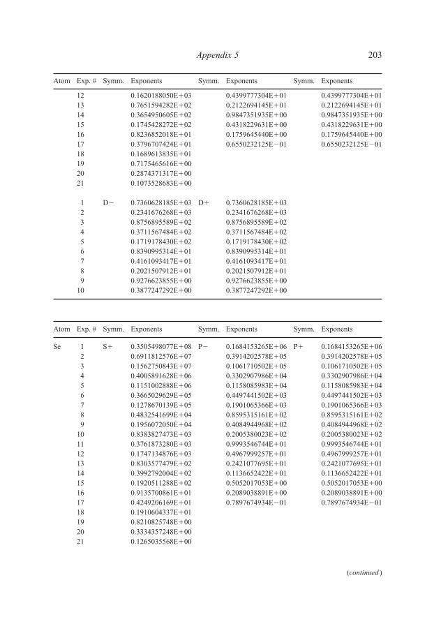
12 0.1620188050E�03 0.4399777304E�01 0.4399777304E�0113 0.7651594282E�02 0.2122694145E�01 0.2122694145E�0114 0.3654950605E�02 0.9847351935E�00 0.9847351935E�0015 0.1745428272E�02 0.4318229631E�00 0.4318229631E�0016 0.8236852018E�01 0.1759645440E�00 0.1759645440E�0017 0.3796707424E�01 0.6550232125E�01 0.6550232125E�0118 0.1689613835E�0119 0.7175465616E�0020 0.2874371317E�0021 0.1073528683E�00
1 D� 0.7360628185E�03 D� 0.7360628185E�032 0.2341676268E�03 0.2341676268E�033 0.8756895589E�02 0.8756895589E�024 0.3711567484E�02 0.3711567484E�025 0.1719178430E�02 0.1719178430E�026 0.8390995314E�01 0.8390995314E�017 0.4161093417E�01 0.4161093417E�018 0.2021507912E�01 0.2021507912E�019 0.9276623855E�00 0.9276623855E�00
10 0.3877247292E�00 0.3877247292E�00
Atom Exp. # Symm. Exponents Symm. Exponents Symm. Exponents
Se 1 S� 0.3505498077E�08 P� 0.1684153265E�06 P� 0.1684153265E�062 0.6911812576E�07 0.3914202578E�05 0.3914202578E�053 0.1562750843E�07 0.1061710502E�05 0.1061710502E�054 0.4005891628E�06 0.3302907986E�04 0.3302907986E�045 0.1151002888E�06 0.1158085983E�04 0.1158085983E�046 0.3665029629E�05 0.4497441502E�03 0.4497441502E�037 0.1278670139E�05 0.1901065366E�03 0.1901065366E�038 0.4832541699E�04 0.8595315161E�02 0.8595315161E�029 0.1956072050E�04 0.4084944968E�02 0.4084944968E�02
10 0.8383827473E�03 0.2005380023E�02 0.2005380023E�0211 0.3761873280E�03 0.9993546744E�01 0.9993546744E�0112 0.1747134876E�03 0.4967999257E�01 0.4967999257E�0113 0.8303577479E�02 0.2421077695E�01 0.2421077695E�0114 0.3992792004E�02 0.1136652422E�01 0.1136652422E�0115 0.1920511288E�02 0.5052017053E�00 0.5052017053E�0016 0.9135700861E�01 0.2089038891E�00 0.2089038891E�0017 0.4249206169E�01 0.7897674934E�01 0.7897674934E�0118 0.1910604337E�0119 0.8210825748E�0020 0.3334357248E�0021 0.1265035568E�00
Appendix 5 203
Atom Exp. # Symm. Exponents Symm. Exponents Symm. Exponents
(continued )
Else_EAMC-TRSIC_appn5.qxd 5/19/2007 21:38 Page 203
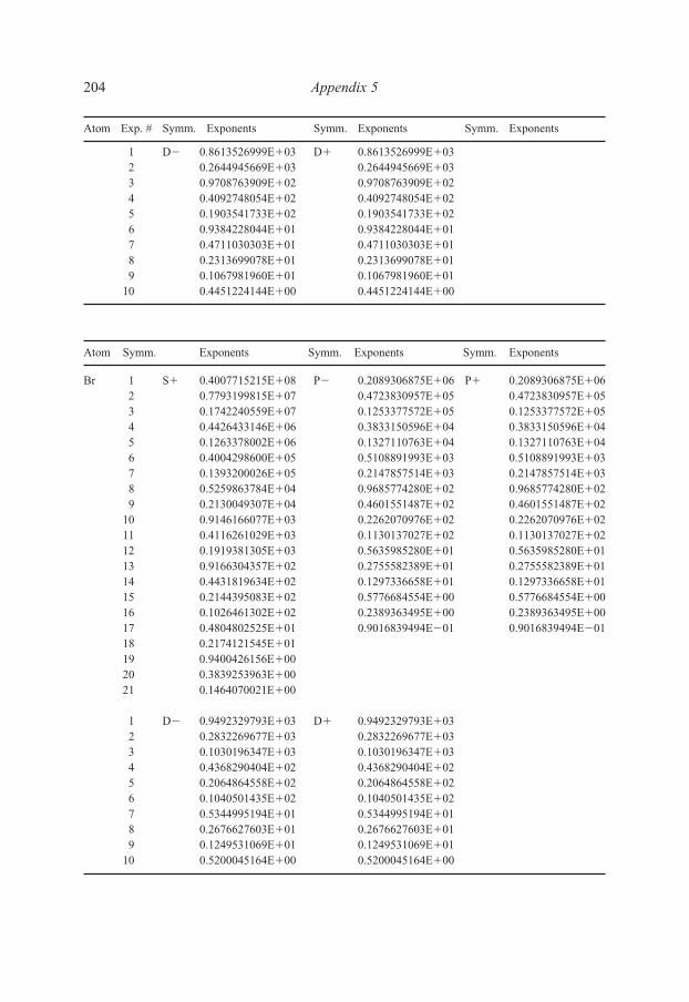
1 D� 0.8613526999E�03 D� 0.8613526999E�032 0.2644945669E�03 0.2644945669E�033 0.9708763909E�02 0.9708763909E�024 0.4092748054E�02 0.4092748054E�025 0.1903541733E�02 0.1903541733E�026 0.9384228044E�01 0.9384228044E�017 0.4711030303E�01 0.4711030303E�018 0.2313699078E�01 0.2313699078E�019 0.1067981960E�01 0.1067981960E�01
10 0.4451224144E�00 0.4451224144E�00
Atom Symm. Exponents Symm. Exponents Symm. Exponents
Br 1 S� 0.4007715215E�08 P� 0.2089306875E�06 P� 0.2089306875E�062 0.7793199815E�07 0.4723830957E�05 0.4723830957E�053 0.1742240559E�07 0.1253377572E�05 0.1253377572E�054 0.4426433146E�06 0.3833150596E�04 0.3833150596E�045 0.1263378002E�06 0.1327110763E�04 0.1327110763E�046 0.4004298600E�05 0.5108891993E�03 0.5108891993E�037 0.1393200026E�05 0.2147857514E�03 0.2147857514E�038 0.5259863784E�04 0.9685774280E�02 0.9685774280E�029 0.2130049307E�04 0.4601551487E�02 0.4601551487E�02
10 0.9146166077E�03 0.2262070976E�02 0.2262070976E�0211 0.4116261029E�03 0.1130137027E�02 0.1130137027E�0212 0.1919381305E�03 0.5635985280E�01 0.5635985280E�0113 0.9166304357E�02 0.2755582389E�01 0.2755582389E�0114 0.4431819634E�02 0.1297336658E�01 0.1297336658E�0115 0.2144395083E�02 0.5776684554E�00 0.5776684554E�0016 0.1026461302E�02 0.2389363495E�00 0.2389363495E�0017 0.4804802525E�01 0.9016839494E�01 0.9016839494E�0118 0.2174121545E�0119 0.9400426156E�0020 0.3839253963E�0021 0.1464070021E�00
1 D� 0.9492329793E�03 D� 0.9492329793E�032 0.2832269677E�03 0.2832269677E�033 0.1030196347E�03 0.1030196347E�034 0.4368290404E�02 0.4368290404E�025 0.2064864558E�02 0.2064864558E�026 0.1040501435E�02 0.1040501435E�027 0.5344995194E�01 0.5344995194E�018 0.2676627603E�01 0.2676627603E�019 0.1249531069E�01 0.1249531069E�01
10 0.5200045164E�00 0.5200045164E�00
204 Appendix 5
Atom Exp. # Symm. Exponents Symm. Exponents Symm. Exponents
Else_EAMC-TRSIC_appn5.qxd 5/19/2007 21:38 Page 204

Atom Exp. # Symm. Exponents Symm. Exponents Symm. Exponents
Kr 1 S� 0.4200639615E�08 P� 0.2325642133E�06 P� 0.2325642133E�062 0.8167577619E�07 0.5053851611E�05 0.5053851611E�053 0.1825121075E�07 0.1301169781E�05 0.1301169781E�054 0.4633823275E�06 0.3894897434E�04 0.3894897434E�045 0.1321494758E�06 0.1330231877E�04 0.1330231877E�046 0.4185028586E�05 0.5086823116E�03 0.5086823116E�037 0.1455014203E�05 0.2137334885E�03 0.2137334885E�038 0.5490358094E�04 0.9683310490E�02 0.9683310490E�029 0.2222939064E�04 0.4642150096E�02 0.4642150096E�02
10 0.9547215105E�03 0.2310879126E�02 0.2310879126E�0211 0.4300083951E�03 0.1172240450E�02 0.1172240450E�0212 0.2007969227E�03 0.5946429749E�01 0.5946429749E�0113 0.9610497644E�02 0.2960156615E�01 0.2960156615E�0114 0.4660926135E�02 0.1419092112E�01 0.1419092112E�0115 0.2264461277E�02 0.6429284965E�00 0.6429284965E�0016 0.1089563949E�02 0.2701404693E�00 0.2701404693E�0017 0.5132920224E�01 0.1033023502E�00 0.1033023502E�0018 0.2340610133E�0119 0.1021351518E�0120 0.4216302889E�0021 0.1627899483E�00
1 D� 0.1010594323E�04 D� 0.1010594323E�042 0.3007980499E�03 0.3007980499E�033 0.1096394627E�03 0.1096394627E�034 0.4671733172E�02 0.4671733172E�025 0.2221436683E�02 0.2221436683E�026 0.1125278848E�02 0.1125278848E�027 0.5796718461E�01 0.5796718461E�018 0.2898849209E�01 0.2898849209E�019 0.1343432765E�01 0.1343432765E�01
10 0.5507806445E�00 0.5507806445E�00
Atom Exp. # Symm. Exponents Symm. Exponents Symm. Exponents
Rb 1 S� 0.1877072370E�09 P� 0.2798814008E�06 P� 0.2798814008E�062 0.3771142117E�08 0.6144392290E�05 0.6144392290E�053 0.8578430665E�07 0.1589580691E�05 0.1589580691E�054 0.2189091295E�07 0.4760222471E�04 0.4760222471E�045 0.6208962017E�06 0.1620896305E�04 0.1620896305E�046 0.1939327926E�06 0.6164655436E�03 0.6164655436E�037 0.6609043898E�05 0.2572351173E�03 0.2572351173E�038 0.2434776926E�05 0.1156809548E�03 0.1156809548E�039 0.9607068606E�04 0.5507391010E�02 0.5507391010E�02
10 0.4022645846E�04 0.2726620398E�02 0.2726620398E�0211 0.1770923970E�04 0.1378924383E�02 0.1378924383E�02
Appendix 5 205
(continued )
Else_EAMC-TRSIC_appn5.qxd 5/19/2007 21:38 Page 205
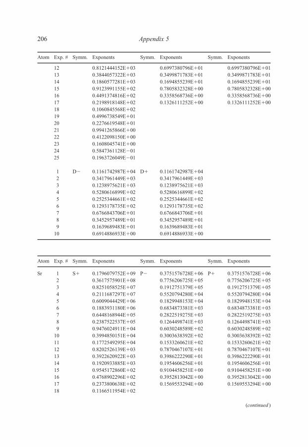
12 0.8121444152E�03 0.6997380796E�01 0.6997380796E�0113 0.3844057322E�03 0.3499871783E�01 0.3499871783E�0114 0.1860577281E�03 0.1694855239E�01 0.1694855239E�0115 0.9123991155E�02 0.7805832328E�00 0.7805832328E�0016 0.4491374816E�02 0.3358568736E�00 0.3358568736E�0017 0.2198918148E�02 0.1326111252E�00 0.1326111252E�0018 0.1060845568E�0219 0.4996738549E�0120 0.2276619548E�0121 0.9941265866E�0022 0.4122098150E�0023 0.1608045741E�0024 0.5847361128E�0125 0.1963726049E�01
1 D� 0.1161742987E�04 D� 0.1161742987E�042 0.3417961449E�03 0.3417961449E�033 0.1238975621E�03 0.1238975621E�034 0.5280616899E�02 0.5280616899E�025 0.2525344661E�02 0.2525344661E�026 0.1293178735E�02 0.1293178735E�027 0.6766843706E�01 0.6766843706E�018 0.3452957489E�01 0.3452957489E�019 0.1639689483E�01 0.1639689483E�01
10 0.6914886933E�00 0.6914886933E�00
Atom Exp. # Symm. Exponents Symm. Exponents Symm. Exponents
Sr 1 S� 0.1796079752E�09 P� 0.3751576728E�06 P� 0.3751576728E�062 0.3617575901E�08 0.7756206725E�05 0.7756206725E�053 0.8251058525E�07 0.1912751379E�05 0.1912751379E�054 0.2111687297E�07 0.5520794280E�04 0.5520794280E�045 0.6009044429E�06 0.1829948153E�04 0.1829948153E�046 0.1883931180E�06 0.6834873381E�03 0.6834873381E�037 0.6448168944E�05 0.2822519275E�03 0.2822519275E�038 0.2387522537E�05 0.1264498741E�03 0.1264498741E�039 0.9476024911E�04 0.6030248589E�02 0.6030248589E�02
10 0.3994850151E�04 0.3003638392E�02 0.3003638392E�0211 0.1772549295E�04 0.1533260621E�02 0.1533260621E�0212 0.8202526139E�03 0.7870467107E�01 0.7870467107E�0113 0.3922620922E�03 0.3986222290E�01 0.3986222290E�0114 0.1920933885E�03 0.1954606256E�01 0.1954606256E�0115 0.9545172860E�02 0.9104458251E�00 0.9104458251E�0016 0.4768902296E�02 0.3952813042E�00 0.3952813042E�0017 0.2373800638E�02 0.1569553294E�00 0.1569553294E�0018 0.1166511954E�02
206 Appendix 5
Atom Exp. # Symm. Exponents Symm. Exponents Symm. Exponents
(continued )
Else_EAMC-TRSIC_appn5.qxd 5/19/2007 21:38 Page 206

19 0.5607654173E�0120 0.2613053325E�0121 0.1169548636E�0122 0.4982177654E�0023 0.2001607796E�0024 0.7514940620E�0125 0.2612683855E�01
1 D� 0.1143517377E�04 D� 0.1143517377E�042 0.3412655823E�03 0.3412655823E�033 0.1248655031E�03 0.1248655031E�034 0.5347527531E�02 0.5347527531E�025 0.2559083652E�02 0.2559083652E�026 0.1306463104E�02 0.1306463104E�027 0.6792839420E�01 0.6792839420E�018 0.3434056192E�01 0.3434056192E�019 0.1611482579E�01 0.1611482579E�01
10 0.6701412009E�00 0.6701412009E�00
Atom Exp. # Symm. Exponents Symm. Exponents Symm. Exponents
Y 1 S� 0.1767964500E�09 P� 0.3634425755E�06 P� 0.3634425755E�062 0.4054630069E�08 0.8310790650E�05 0.8310790650E�053 0.1023450253E�08 0.2206397691E�05 0.2206397691E�054 0.2824109781E�07 0.6694940128E�04 0.6694940128E�045 0.8461693332E�06 0.2285691390E�04 0.2285691390E�046 0.2734358095E�06 0.8643368312E�03 0.8643368312E�037 0.9465366441E�05 0.3563932906E�03 0.3563932906E�038 0.3486301480E�05 0.1577406524E�03 0.1577406524E�039 0.1357061243E�05 0.7377545551E�02 0.7377545551E�02
10 0.5545011940E�04 0.3589391755E�02 0.3589391755E�0211 0.2362302923E�04 0.1788368686E�02 0.1788368686E�0212 0.1042222117E�04 0.8982702740E�01 0.8982702740E�0113 0.4729749186E�03 0.4477723939E�01 0.4477723939E�0114 0.2192959433E�03 0.2180692642E�01 0.2180692642E�0115 0.1031808919E�03 0.1021421507E�01 0.1021421507E�0116 0.4893343273E�02 0.4529762950E�00 0.4529762950E�0017 0.2323332386E�02 0.1872373260E�00 0.1872373260E�0018 0.1096927185E�0219 0.5115246609E�0120 0.2340125815E�0121 0.1043175134E�0122 0.4500721761E�0023 0.1866704422E�0024 0.7392629349E�0125 0.2776603233E�01
Appendix 5 207
Atom Exp. # Symm. Exponents Symm. Exponents Symm. Exponents
(continued )
Else_EAMC-TRSIC_appn5.qxd 5/19/2007 21:38 Page 207

1 D� 0.1227979574E�04 D� 0.1227979574E�042 0.4524991053E�03 0.4524991053E�033 0.1829007818E�03 0.1829007818E�034 0.7962857810E�02 0.7962857810E�025 0.3666588971E�02 0.3666588971E�026 0.1753394619E�02 0.1753394619E�027 0.8550777236E�01 0.8550777236E�018 0.4175652055E�01 0.4175652055E�019 0.2005026458E�01 0.2005026458E�01
10 0.9295597561E�00 0.9295597561E�0011 0.4085829371E�00 0.4085829371E�0012 0.1671910989E�00 0.1671910989E�0013 0.6254036317E�01 0.6254036317E�01
Atom Exp. # Symm. Exponents Symm. Exponents Symm. Exponents
Y 1 S� 0.1649678507E�09 P� 0.3540428693E�06 P� 0.3540428693E�062 0.3842600909E�08 0.8110372259E�05 0.8110372259E�053 0.9810150190E�07 0.2156069191E�05 0.2156069191E�054 0.2727640261E�07 0.6548357298E�04 0.6548357298E�045 0.8207223105E�06 0.2236972321E�04 0.2236972321E�046 0.2655459906E�06 0.8461711648E�03 0.8461711648E�037 0.9180244962E�05 0.3489281447E�03 0.3489281447E�038 0.3369585295E�05 0.1544204271E�03 0.1544204271E�039 0.1304797007E�05 0.7220632896E�02 0.7220632896E�02
10 0.5296517526E�04 0.3512031077E�02 0.3512031077E�0211 0.2239522809E�04 0.1749302041E�02 0.1749302041E�0212 0.9801100245E�03 0.8784264894E�01 0.8784264894E�0113 0.4411487856E�03 0.4378153787E�01 0.4378153787E�0114 0.2029190923E�03 0.2132221751E�01 0.2132221751E�0115 0.9478179965E�02 0.9989420474E�00 0.9989420474E�0016 0.4467122450E�02 0.4432263650E�00 0.4432263650E�0017 0.2110903022E�02 0.1833576551E�00 0.1833576551E�0018 0.9937631177E�0119 0.4631357285E�0120 0.2123152389E�0121 0.9513452788E�0022 0.4140148685E�0023 0.1738806000E�0024 0.7002939808E�0125 0.2687449912E�01
1 D� 0.1084407387E�04 D� 0.1084407387E�042 0.4034791886E�03 0.4034791886E�033 0.1634826444E�03 0.1634826444E�034 0.7086930822E�02 0.7086930822E�02
208 Appendix 5
Atom Exp. # Symm. Exponents Symm. Exponents Symm. Exponents
(continued )
Else_EAMC-TRSIC_appn5.qxd 5/19/2007 21:38 Page 208
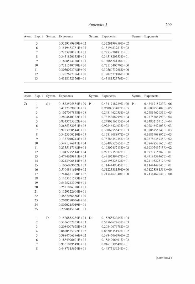
5 0.3229199959E�02 0.3229199959E�026 0.1519483781E�02 0.1519483781E�027 0.7253970181E�01 0.7253970181E�018 0.3451820553E�01 0.3451820553E�019 0.1608524138E�01 0.1608524138E�01
10 0.7211540770E�00 0.7211540770E�0011 0.3056073768E�00 0.3056073768E�0012 0.1202677186E�00 0.1202677186E�0013 0.4318152376E�01 0.4318152376E�01
Atom Exp. # Symm. Exponents Symm. Exponents Symm. Exponents
Zr 1 S� 0.1832595584E�09 P� 0.4341718729E�06 P� 0.4341718729E�062 0.4127169001E�08 0.9600953402E�05 0.9600953402E�053 0.1027097858E�08 0.2481462035E�05 0.2481462035E�054 0.2804610332E�07 0.7375388799E�04 0.7375388799E�045 0.8343755202E�06 0.2480216715E�04 0.2480216715E�046 0.2685382031E�06 0.9284642403E�03 0.9284642403E�037 0.9283960544E�05 0.3806755547E�03 0.3806755547E�038 0.3423500210E�05 0.1681908897E�03 0.1681908897E�039 0.1337040243E�05 0.7878635935E�02 0.7878635935E�02
10 0.5491396841E�04 0.3849852565E�02 0.3849852565E�0211 0.2355117568E�04 0.1930745713E�02 0.1930745713E�0212 0.1047275514E�04 0.9777715382E�01 0.9777715382E�0113 0.4794629841E�03 0.4919539467E�01 0.4919539467E�0114 0.2243996514E�03 0.2419522512E�01 0.2419522512E�0115 0.1066079062E�03 0.1144449045E�01 0.1144449045E�0116 0.5104861619E�02 0.5122338159E�00 0.5122338159E�0017 0.2446431390E�02 0.2134462040E�00 0.2134462040E�0018 0.1165101593E�0219 0.5475243309E�0120 0.2521036328E�0121 0.1129322604E�0122 0.4887056456E�0023 0.2028590056E�0024 0.8020215019E�0125 0.2998815154E�01
1 D� 0.1526852285E�04 D� 0.1526852285E�042 0.5356762263E�03 0.5356762263E�033 0.2084007678E�03 0.2084007678E�034 0.8820535192E�02 0.8820535192E�025 0.3984706396E�02 0.3984706396E�026 0.1884996601E�02 0.1884996601E�027 0.9161039549E�01 0.9161039549E�018 0.4487515624E�01 0.4487515624E�01
Appendix 5 209
Atom Exp. # Symm. Exponents Symm. Exponents Symm. Exponents
(continued )
Else_EAMC-TRSIC_appn5.qxd 5/19/2007 21:38 Page 209
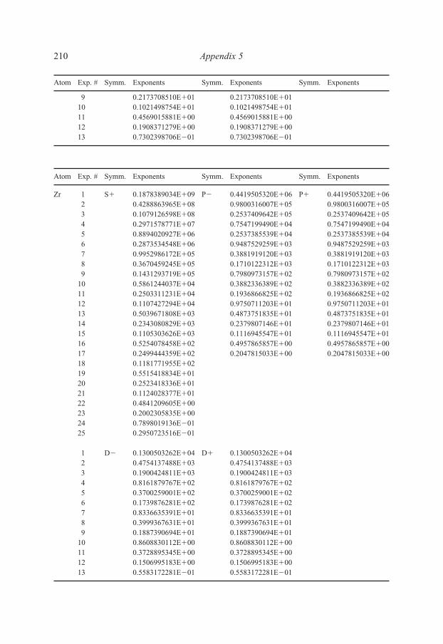
9 0.2173708510E�01 0.2173708510E�0110 0.1021498754E�01 0.1021498754E�0111 0.4569015881E�00 0.4569015881E�0012 0.1908371279E�00 0.1908371279E�0013 0.7302398706E�01 0.7302398706E�01
Atom Exp. # Symm. Exponents Symm. Exponents Symm. Exponents
Zr 1 S� 0.1878389034E�09 P� 0.4419505320E�06 P� 0.4419505320E�062 0.4288863965E�08 0.9800316007E�05 0.9800316007E�053 0.1079126598E�08 0.2537409642E�05 0.2537409642E�054 0.2971578771E�07 0.7547199490E�04 0.7547199490E�045 0.8894020927E�06 0.2537385539E�04 0.2537385539E�046 0.2873534548E�06 0.9487529259E�03 0.9487529259E�037 0.9952986172E�05 0.3881919120E�03 0.3881919120E�038 0.3670459245E�05 0.1710122312E�03 0.1710122312E�039 0.1431293719E�05 0.7980973157E�02 0.7980973157E�02
10 0.5861244037E�04 0.3882336389E�02 0.3882336389E�0211 0.2503311231E�04 0.1936866825E�02 0.1936866825E�0212 0.1107427294E�04 0.9750711203E�01 0.9750711203E�0113 0.5039671808E�03 0.4873751835E�01 0.4873751835E�0114 0.2343080829E�03 0.2379807146E�01 0.2379807146E�0115 0.1105303626E�03 0.1116945547E�01 0.1116945547E�0116 0.5254078458E�02 0.4957865857E�00 0.4957865857E�0017 0.2499444359E�02 0.2047815033E�00 0.2047815033E�0018 0.1181771955E�0219 0.5515418834E�0120 0.2523418336E�0121 0.1124028377E�0122 0.4841209605E�0023 0.2002305835E�0024 0.7898019136E�0125 0.2950723516E�01
1 D� 0.1300503262E�04 D� 0.1300503262E�042 0.4754137488E�03 0.4754137488E�033 0.1900424811E�03 0.1900424811E�034 0.8161879767E�02 0.8161879767E�025 0.3700259001E�02 0.3700259001E�026 0.1739876281E�02 0.1739876281E�027 0.8336635391E�01 0.8336635391E�018 0.3999367631E�01 0.3999367631E�019 0.1887390694E�01 0.1887390694E�01
10 0.8608830112E�00 0.8608830112E�0011 0.3728895345E�00 0.3728895345E�0012 0.1506995183E�00 0.1506995183E�0013 0.5583172281E�01 0.5583172281E�01
210 Appendix 5
Atom Exp. # Symm. Exponents Symm. Exponents Symm. Exponents
Else_EAMC-TRSIC_appn5.qxd 5/19/2007 21:38 Page 210
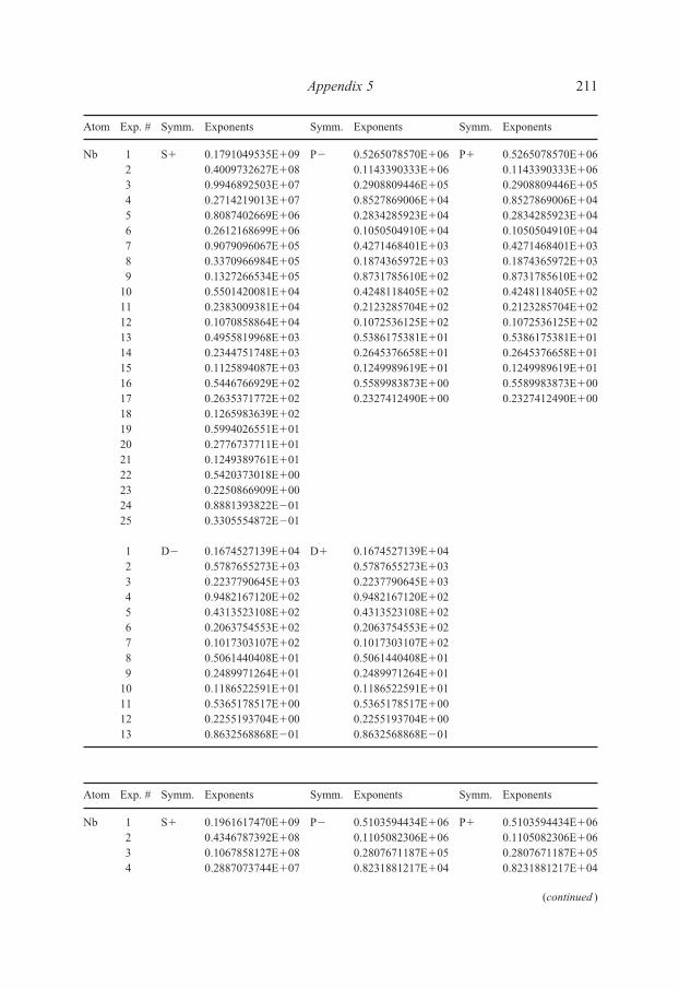
Atom Exp. # Symm. Exponents Symm. Exponents Symm. Exponents
Nb 1 S� 0.1791049535E�09 P� 0.5265078570E�06 P� 0.5265078570E�062 0.4009732627E�08 0.1143390333E�06 0.1143390333E�063 0.9946892503E�07 0.2908809446E�05 0.2908809446E�054 0.2714219013E�07 0.8527869006E�04 0.8527869006E�045 0.8087402669E�06 0.2834285923E�04 0.2834285923E�046 0.2612168699E�06 0.1050504910E�04 0.1050504910E�047 0.9079096067E�05 0.4271468401E�03 0.4271468401E�038 0.3370966984E�05 0.1874365972E�03 0.1874365972E�039 0.1327266534E�05 0.8731785610E�02 0.8731785610E�02
10 0.5501420081E�04 0.4248118405E�02 0.4248118405E�0211 0.2383009381E�04 0.2123285704E�02 0.2123285704E�0212 0.1070858864E�04 0.1072536125E�02 0.1072536125E�0213 0.4955819968E�03 0.5386175381E�01 0.5386175381E�0114 0.2344751748E�03 0.2645376658E�01 0.2645376658E�0115 0.1125894087E�03 0.1249989619E�01 0.1249989619E�0116 0.5446766929E�02 0.5589983873E�00 0.5589983873E�0017 0.2635371772E�02 0.2327412490E�00 0.2327412490E�0018 0.1265983639E�0219 0.5994026551E�0120 0.2776737711E�0121 0.1249389761E�0122 0.5420373018E�0023 0.2250866909E�0024 0.8881393822E�0125 0.3305554872E�01
1 D� 0.1674527139E�04 D� 0.1674527139E�042 0.5787655273E�03 0.5787655273E�033 0.2237790645E�03 0.2237790645E�034 0.9482167120E�02 0.9482167120E�025 0.4313523108E�02 0.4313523108E�026 0.2063754553E�02 0.2063754553E�027 0.1017303107E�02 0.1017303107E�028 0.5061440408E�01 0.5061440408E�019 0.2489971264E�01 0.2489971264E�01
10 0.1186522591E�01 0.1186522591E�0111 0.5365178517E�00 0.5365178517E�0012 0.2255193704E�00 0.2255193704E�0013 0.8632568868E�01 0.8632568868E�01
Atom Exp. # Symm. Exponents Symm. Exponents Symm. Exponents
Nb 1 S� 0.1961617470E�09 P� 0.5103594434E�06 P� 0.5103594434E�062 0.4346787392E�08 0.1105082306E�06 0.1105082306E�063 0.1067858127E�08 0.2807671187E�05 0.2807671187E�054 0.2887073744E�07 0.8231881217E�04 0.8231881217E�04
Appendix 5 211
(continued )
Else_EAMC-TRSIC_appn5.qxd 5/19/2007 21:38 Page 211
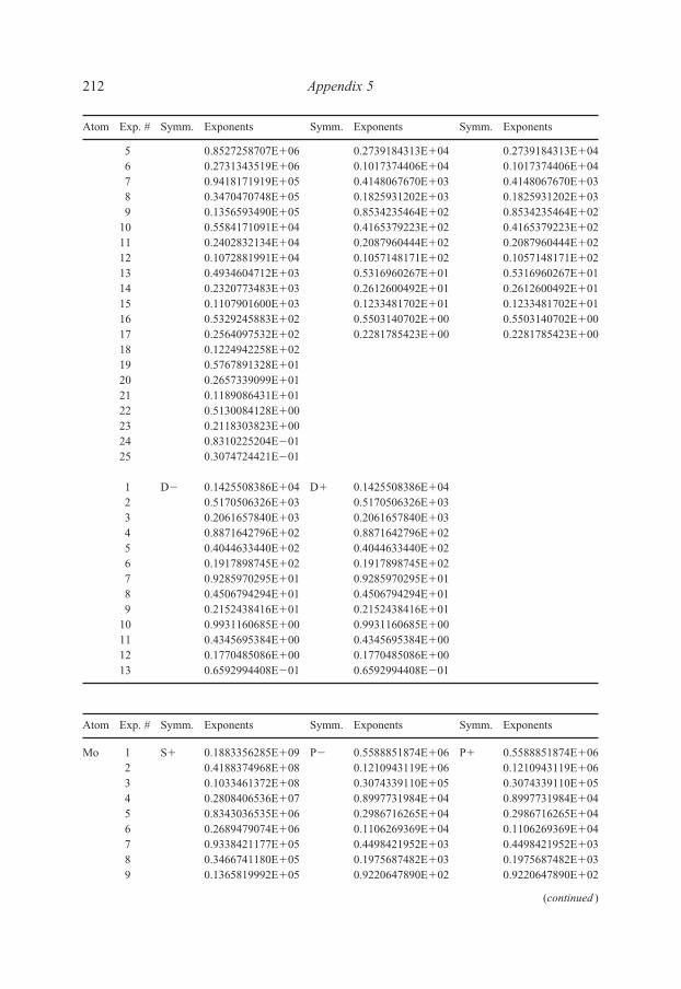
5 0.8527258707E�06 0.2739184313E�04 0.2739184313E�046 0.2731343519E�06 0.1017374406E�04 0.1017374406E�047 0.9418171919E�05 0.4148067670E�03 0.4148067670E�038 0.3470470748E�05 0.1825931202E�03 0.1825931202E�039 0.1356593490E�05 0.8534235464E�02 0.8534235464E�02
10 0.5584171091E�04 0.4165379223E�02 0.4165379223E�0211 0.2402832134E�04 0.2087960444E�02 0.2087960444E�0212 0.1072881991E�04 0.1057148171E�02 0.1057148171E�0213 0.4934604712E�03 0.5316960267E�01 0.5316960267E�0114 0.2320773483E�03 0.2612600492E�01 0.2612600492E�0115 0.1107901600E�03 0.1233481702E�01 0.1233481702E�0116 0.5329245883E�02 0.5503140702E�00 0.5503140702E�0017 0.2564097532E�02 0.2281785423E�00 0.2281785423E�0018 0.1224942258E�0219 0.5767891328E�0120 0.2657339099E�0121 0.1189086431E�0122 0.5130084128E�0023 0.2118303823E�0024 0.8310225204E�0125 0.3074724421E�01
1 D� 0.1425508386E�04 D� 0.1425508386E�042 0.5170506326E�03 0.5170506326E�033 0.2061657840E�03 0.2061657840E�034 0.8871642796E�02 0.8871642796E�025 0.4044633440E�02 0.4044633440E�026 0.1917898745E�02 0.1917898745E�027 0.9285970295E�01 0.9285970295E�018 0.4506794294E�01 0.4506794294E�019 0.2152438416E�01 0.2152438416E�01
10 0.9931160685E�00 0.9931160685E�0011 0.4345695384E�00 0.4345695384E�0012 0.1770485086E�00 0.1770485086E�0013 0.6592994408E�01 0.6592994408E�01
Atom Exp. # Symm. Exponents Symm. Exponents Symm. Exponents
Mo 1 S� 0.1883356285E�09 P� 0.5588851874E�06 P� 0.5588851874E�062 0.4188374968E�08 0.1210943119E�06 0.1210943119E�063 0.1033461372E�08 0.3074339110E�05 0.3074339110E�054 0.2808406536E�07 0.8997731984E�04 0.8997731984E�045 0.8343036535E�06 0.2986716265E�04 0.2986716265E�046 0.2689479074E�06 0.1106269369E�04 0.1106269369E�047 0.9338421177E�05 0.4498421952E�03 0.4498421952E�038 0.3466741180E�05 0.1975687482E�03 0.1975687482E�039 0.1365819992E�05 0.9220647890E�02 0.9220647890E�02
212 Appendix 5
Atom Exp. # Symm. Exponents Symm. Exponents Symm. Exponents
(continued )
Else_EAMC-TRSIC_appn5.qxd 5/19/2007 21:38 Page 212

10 0.5668537259E�04 0.4499001454E�02 0.4499001454E�0211 0.2460001944E�04 0.2257920831E�02 0.2257920831E�0212 0.1108072583E�04 0.1146741535E�02 0.1146741535E�0213 0.5142220474E�03 0.5798464551E�01 0.5798464551E�0114 0.2440418517E�03 0.2871953975E�01 0.2871953975E�0115 0.1175683640E�03 0.1370835446E�01 0.1370835446E�0116 0.5707035754E�02 0.6203873464E�00 0.6203873464E�0017 0.2770805728E�02 0.2619007049E�00 0.2619007049E�0018 0.1335544415E�0219 0.6343789730E�0120 0.2947533970E�0121 0.1329749587E�0122 0.5781803464E�0023 0.2405030629E�0024 0.9499989696E�0125 0.3537140435E�01
1 D� 0.1753542601E�04 D� 0.1753542601E�042 0.6035070644E�03 0.6035070644E�033 0.2329416325E�03 0.2329416325E�034 0.9875412327E�02 0.9875412327E�025 0.4503512508E�02 0.4503512508E�026 0.2163615919E�02 0.2163615919E�027 0.1072472756E�02 0.1072472756E�028 0.5371731798E�01 0.5371731798E�019 0.2662618664E�01 0.2662618664E�01
10 0.1279130540E�01 0.1279130540E�0111 0.5832794228E�00 0.5832794228E�0012 0.2472515261E�00 0.2472515261E�0013 0.9542155525E�01 0.9542155525E�01
Atom Exp. # Symm. Exponents Symm. Exponents Symm. Exponents
Mo 1 S� 0.1702220962E�09 P� 0.5749058874E�06 P� 0.5749058874E�062 0.3907235835E�08 0.1221468969E�06 0.1221468969E�063 0.9900772778E�07 0.3057504265E�05 0.3057504265E�054 0.2749974031E�07 0.8864463139E�04 0.8864463139E�045 0.8313087973E�06 0.2926444705E�04 0.2926444705E�046 0.2715718173E�06 0.1081514900E�04 0.1081514900E�047 0.9519405189E�05 0.4398765142E�03 0.4398765142E�038 0.3555101240E�05 0.1935694916E�03 0.1935694916E�039 0.1404511930E�05 0.9060511039E�02 0.9060511039E�02
10 0.5828334190E�04 0.4434859967E�02 0.4434859967E�0211 0.2522454063E�04 0.2231620515E�02 0.2231620515E�0212 0.1130514526E�04 0.1134947515E�02 0.1134947515E�0213 0.5209755513E�03 0.5735192429E�01 0.5735192429E�0114 0.2451100435E�03 0.2830992871E�01 0.2830992871E�01
Appendix 5 213
Atom Exp. # Symm. Exponents Symm. Exponents Symm. Exponents
(continued )
Else_EAMC-TRSIC_appn5.qxd 5/19/2007 21:38 Page 213

15 0.1169019333E�03 0.1341991936E�01 0.1341991936E�0116 0.5611944346E�02 0.6005970146E�00 0.6005970146E�0017 0.2692466741E�02 0.2494826493E�00 0.2494826493E�0018 0.1281878674E�0219 0.6013361805E�0120 0.2759788737E�0121 0.1230372698E�0122 0.5290712129E�0023 0.2178825404E�0024 0.8532490913E�0125 0.3154921795E�01
1 D� 0.1488058285E�04 D� 0.1488058285E�042 0.5248991670E�03 0.5248991670E�033 0.2056587928E�03 0.2056587928E�034 0.8776172593E�02 0.8776172593E�025 0.3999636478E�02 0.3999636478E�026 0.1908817442E�02 0.1908817442E�027 0.9354224636E�01 0.9354224636E�018 0.4615531708E�01 0.4615531708E�019 0.2248418983E�01 0.2248418983E�01
10 0.1060340442E�01 0.1060340442E�0111 0.4746757042E�00 0.4746757042E�0012 0.1977895277E�00 0.1977895277E�0013 0.7522032630E�01 0.7522032630E�01
Atom Exp. # Symm. Exponents Symm. Exponents Symm. Exponents
Tc 1 S� 0.1662857499E�09 P� 0.6977697206E�06 P� 0.6977697206E�062 0.3749132868E�08 0.1458916437E�06 0.1458916437E�063 0.9381492149E�07 0.3601998107E�05 0.3601998107E�054 0.2585865339E�07 0.1032278381E�05 0.1032278381E�055 0.7792205499E�06 0.3375483548E�04 0.3375483548E�046 0.2547786347E�06 0.1237959665E�04 0.1237959665E�047 0.8971009981E�05 0.5005573612E�03 0.5005573612E�038 0.3376159906E�05 0.2193429057E�03 0.2193429057E�039 0.1347831555E�05 0.1023908711E�03 0.1023908711E�03
10 0.5665089613E�04 0.5005094847E�02 0.5005094847E�0211 0.2488078682E�04 0.2518386242E�02 0.2518386242E�0212 0.1133274735E�04 0.1282144105E�02 0.1282144105E�0213 0.5313096253E�03 0.6492341272E�01 0.6492341272E�0114 0.2544656405E�03 0.3214114644E�01 0.3214114644E�0115 0.1235683403E�03 0.1529193460E�01 0.1529193460E�0116 0.6038227683E�02 0.6873058958E�00 0.6873058958E�0017 0.2946887609E�02 0.2868598712E�00 0.2868598712E�0018 0.1425598028E�02
214 Appendix 5
Atom Exp. # Symm. Exponents Symm. Exponents Symm. Exponents
(continued )
Else_EAMC-TRSIC_appn5.qxd 5/19/2007 21:38 Page 214

19 0.6784809115E�0120 0.3152919084E�0121 0.1419875514E�0122 0.6150034839E�0023 0.2542859433E�0024 0.9961212644E�0125 0.3669228500E�01
1 D� 0.1829435397E�04 D� 0.1829435397E�042 0.6377687147E�03 0.6377687147E�033 0.2483872236E�03 0.2483872236E�034 0.1059162483E�03 0.1059162483E�035 0.4846303461E�02 0.4846303461E�026 0.2331957801E�02 0.2331957801E�027 0.1156485581E�02 0.1156485581E�028 0.5793174308E�01 0.5793174308E�019 0.2872745775E�01 0.2872745775E�01
10 0.1382067976E�01 0.1382067976E�0111 0.6322089082E�00 0.6322089082E�0012 0.2694872367E�00 0.2694872367E�0013 0.1049082303E�00 0.1049082303E�00
Atom Exp. # Symm. Exponents Symm. Exponents Symm. Exponents
Tc 1 S� 0.1527345126E�09 P� 0.6408257593E�06 P� 0.6408257593E�062 0.3516999525E�08 0.1374165187E�06 0.1374165187E�063 0.8949244028E�07 0.3456662292E�05 0.3456662292E�054 0.2498330136E�07 0.1003380976E�05 0.1003380976E�055 0.7596844875E�06 0.3306264137E�04 0.3306264137E�046 0.2498084738E�06 0.1216588970E�04 0.1216588970E�047 0.8819461531E�05 0.4917639849E�03 0.4917639849E�038 0.3319009469E�05 0.2148067641E�03 0.2148067641E�039 0.1321834096E�05 0.9974461236E�02 0.9974461236E�02
10 0.5531182223E�04 0.4843430513E�02 0.4843430513E�0211 0.2414360188E�04 0.2419416869E�02 0.2419416869E�0212 0.1091439720E�04 0.1223021838E�02 0.1223021838E�0213 0.5073195137E�03 0.6154538146E�01 0.6154538146E�0114 0.2407232399E�03 0.3032957635E�01 0.3032957635E�0115 0.1157656281E�03 0.1439854847E�01 0.1439854847E�0116 0.5601920300E�02 0.6477753915E�00 0.6477753915E�0017 0.2708073329E�02 0.2716785899E�00 0.2716785899E�0018 0.1298436262E�0219 0.6130389849E�0120 0.2829653862E�0121 0.1267730142E�0122 0.5473172332E�0023 0.2260688645E�00
Appendix 5 215
Atom Exp. # Symm. Exponents Symm. Exponents Symm. Exponents
(continued )
Else_EAMC-TRSIC_appn5.qxd 5/19/2007 21:38 Page 215

24 0.8869563093E�0125 0.3281663649E�01
1 D� 0.1734804498E�04 D� 0.1734804498E�042 0.5980616418E�03 0.5980616418E�033 0.2304976751E�03 0.2304976751E�034 0.9731184542E�02 0.9731184542E�025 0.4409575618E�02 0.4409575618E�026 0.2101421517E�02 0.2101421517E�027 0.1031972721E�02 0.1031972721E�028 0.5116998495E�01 0.5116998495E�019 0.2510196726E�01 0.2510196726E�01
10 0.1193710444E�01 0.1193710444E�0111 0.5391906608E�00 0.5391906608E�0012 0.2266685308E�00 0.2266685308E�0013 0.8689583609E�01 0.8689583609E�01
Atom Exp. # Symm. Exponents Symm. Exponents Symm. Exponents
Ru 1 S� 0.1623681020E�09 P� 0.7400691181E�06 P� 0.7400691181E�062 0.3676656664E�08 0.1535315488E�06 0.1535315488E�063 0.9237014505E�07 0.3765899763E�05 0.3765899763E�054 0.2555460890E�07 0.1073512501E�05 0.1073512501E�055 0.7726784359E�06 0.3495699792E�04 0.3495699792E�046 0.2534271629E�06 0.1278118944E�04 0.1278118944E�047 0.8948808704E�05 0.5157508871E�03 0.5157508871E�038 0.3376508571E�05 0.2257676499E�03 0.2257676499E�039 0.1351120036E�05 0.1053799299E�03 0.1053799299E�03
10 0.5690839459E�04 0.5155253330E�02 0.5155253330E�0211 0.2504078461E�04 0.2598121628E�02 0.2598121628E�0212 0.1142461585E�04 0.1325890790E�02 0.1325890790E�0213 0.5364018055E�03 0.6734669475E�01 0.6734669475E�0114 0.2572330005E�03 0.3346620935E�01 0.3346620935E�0115 0.1250500416E�03 0.1599189441E�01 0.1599189441E�0116 0.6116381669E�02 0.7223004821E�00 0.7223004821E�0017 0.2987388966E�02 0.3030972142E�00 0.3030972142E�0018 0.1446133213E�0219 0.6886158878E�0120 0.3201333083E�0121 0.1442124150E�0122 0.6247773482E�0023 0.2583637723E�0024 0.1012172539E�0025 0.3728438227E�01
1 D� 0.2087625311E�04 D� 0.2087625311E�042 0.7049592191E�03 0.7049592191E�03
216 Appendix 5
Atom Exp. # Symm. Exponents Symm. Exponents Symm. Exponents
(continued )
Else_EAMC-TRSIC_appn5.qxd 5/19/2007 21:38 Page 216

3 0.2685630313E�03 0.2685630313E�034 0.1129677844E�03 0.1129677844E�035 0.5135047750E�02 0.5135047750E�026 0.2468716424E�02 0.2468716424E�027 0.1228542317E�02 0.1228542317E�028 0.6193791457E�01 0.6193791457E�019 0.3096178075E�01 0.3096178075E�01
10 0.1501943262E�01 0.1501943262E�0111 0.6919818702E�00 0.6919818702E�0012 0.2963499435E�00 0.2963499435E�0013 0.1154620528E�00 0.1154620528E�00
Atom Exp. # Symm. Exponents Symm. Exponents Symm. Exponents
Ru 1 S� 0.1614539079E�09 P� 0.7371120270E�06 P� 0.7371120270E�062 0.3676151529E�08 0.1548700830E�06 0.1548700830E�063 0.9274660363E�07 0.3834875677E�05 0.3834875677E�054 0.2573515073E�07 0.1100353659E�05 0.1100353659E�055 0.7795497434E�06 0.3597145955E�04 0.3597145955E�046 0.2558666533E�06 0.1317273979E�04 0.1317273979E�047 0.9032346863E�05 0.5312928512E�03 0.5312928512E�038 0.3403838236E�05 0.2320487095E�03 0.2320487095E�039 0.1359198632E�05 0.1079093780E�03 0.1079093780E�03
10 0.5708302497E�04 0.5253171600E�02 0.5253171600E�0211 0.2502680379E�04 0.2632169627E�02 0.2632169627E�0212 0.1136952918E�04 0.1334699711E�02 0.1334699711E�0213 0.5312299827E�03 0.6734078696E�01 0.6734078696E�0114 0.2533903125E�03 0.3323879388E�01 0.3323879388E�0115 0.1224698229E�03 0.1578091912E�01 0.1578091912E�0116 0.5953387491E�02 0.7085766232E�00 0.7085766232E�0017 0.2889079638E�02 0.2958396336E�00 0.2958396336E�0018 0.1389247111E�0219 0.6570349030E�0120 0.3033546477E�0121 0.1357158163E�0122 0.5839722293E�0023 0.2398833868E�0024 0.9337244226E�0125 0.3418315610E�01
1 D� 0.1914069549E�04 D� 0.1914069549E�042 0.6473621501E�03 0.6473621501E�033 0.2469160509E�03 0.2469160509E�034 0.1039034494E�03 0.1039034494E�035 0.4719059217E�02 0.4719059217E�026 0.2263038290E�02 0.2263038290E�027 0.1120999929E�02 0.1120999929E�02
Appendix 5 217
Atom Exp. # Symm. Exponents Symm. Exponents Symm. Exponents
(continued )
Else_EAMC-TRSIC_appn5.qxd 5/19/2007 21:38 Page 217

8 0.5611289438E�01 0.5611289438E�019 0.2776702514E�01 0.2776702514E�01
10 0.1328837355E�01 0.1328837355E�0111 0.6016671342E�00 0.6016671342E�0012 0.2521441700E�00 0.2521441700E�0013 0.9567885039E�01 0.9567885039E�01
Atom Exp. # Symm. Exponents Symm. Exponents Symm. Exponents
Rh 1 S� 0.1608087157E�09 P� 0.9104152671E�06 P� 0.9104152671E�062 0.3648913811E�08 0.1843480390E�06 0.1843480390E�063 0.9192627327E�07 0.4433733622E�05 0.4433733622E�054 0.2551708359E�07 0.1244406044E�05 0.1244406044E�055 0.7745171857E�06 0.4004473461E�04 0.4004473461E�046 0.2551132571E�06 0.1451606404E�04 0.1451606404E�047 0.9049618040E�05 0.5823738061E�03 0.5823738061E�038 0.3430962965E�05 0.2540584516E�03 0.2540584516E�039 0.1379696863E�05 0.1184059893E�03 0.1184059893E�03
10 0.5840183539E�04 0.5792302830E�02 0.5792302830E�0211 0.2582484915E�04 0.2922104658E�02 0.2922104658E�0212 0.1183888702E�04 0.1493607710E�02 0.1493607710E�0213 0.5583918234E�03 0.7599813834E�01 0.7599813834E�0114 0.2689153682E�03 0.3782024539E�01 0.3782024539E�0115 0.1312302327E�03 0.1808548111E�01 0.1808548111E�0116 0.6440019557E�02 0.8164873870E�00 0.8164873870E�0017 0.3154051576E�02 0.3419101061E�00 0.3419101061E�0018 0.1529931615E�0219 0.7294410123E�0120 0.3392474349E�0121 0.1527370895E�0122 0.6606437006E�0023 0.2724446234E�0024 0.1063091504E�0025 0.3895272296E�01
1 D� 0.2150541641E�04 D� 0.2150541641E�032 0.7278304844E�03 0.7278304844E�033 0.2782111434E�03 0.2782111434E�034 0.1175273656E�03 0.1175273656E�035 0.5368858880E�02 0.5368858880E�026 0.2595145965E�02 0.2595145965E�027 0.1298783347E�02 0.1298783347E�028 0.6585140718E�01 0.6585140718E�019 0.3309825836E�01 0.3309825836E�01
10 0.1613672001E�01 0.1613672001E�0111 0.7467130337E�00 0.7467130337E�0012 0.3209067509E�00 0.3209067509E�0013 0.1253282382E�00 0.1253282382E�00
218 Appendix 5
Atom Exp. # Symm. Exponents Symm. Exponents Symm. Exponents
Else_EAMC-TRSIC_appn5.qxd 5/19/2007 21:38 Page 218

Atom Exp. # Symm. Exponents Symm. Exponents Symm. Exponents
Rh 1 S� 0.1530625979E�09 P� 0.8575302407E�06 P� 0.8575302407E�052 0.3504866765E�08 0.1785166813E�06 0.1785166813E�063 0.8897645976E�07 0.4376991798E�05 0.4376991798E�054 0.2485441885E�07 0.1243116741E�05 0.1243116741E�055 0.7581946107E�06 0.4022157165E�04 0.4022157165E�046 0.2506859935E�06 0.1458104946E�04 0.1458104946E�047 0.8916110633E�05 0.5824690320E�03 0.5824690320E�038 0.3385638133E�05 0.2521638888E�03 0.2521638888E�039 0.1362225617E�05 0.1163564944E�03 0.1163564944E�03
10 0.5764009285E�04 0.5628176787E�02 0.5628176787E�0211 0.2545605676E�04 0.2806634670E�02 0.2806634670E�0212 0.1164587506E�04 0.1419112349E�02 0.1419112349E�0213 0.5477613257E�03 0.7155370016E�01 0.7155370016E�0114 0.2628890858E�03 0.3538372278E�01 0.3538372278E�0115 0.1277730917E�03 0.1687729129E�01 0.1687729129E�0116 0.6241882877E�02 0.7636624720E�00 0.7636624720E�0017 0.3041759674E�02 0.3223823956E�00 0.3223823956E�0018 0.1467543416E�0219 0.6957248303E�0120 0.3216534694E�0121 0.1439351534E�0122 0.6187242170E�0023 0.2535728001E�0024 0.9833479955E�0125 0.3581249121E�01
1 D� 0.1974411246E�04 D� 0.1974411246E�042 0.6692546256E�03 0.6692546256E�033 0.2562224176E�03 0.2562224176E�034 0.1083700640E�03 0.1083700640E�035 0.4952933321E�02 0.4952933321E�026 0.2392605319E�02 0.2392605319E�027 0.1194894499E�02 0.1194894499E�028 0.6034377274E�01 0.6034377274E�019 0.3014215098E�01 0.3014215098E�01
10 0.1456630473E�01 0.1456630473E�0111 0.6661198797E�00 0.6661198797E�0012 0.2819536598E�00 0.2819536598E�0013 0.1080487879E�00 0.1080487879E�00
Atom Exp. # Symm. Exponents Symm. Exponents Symm. Exponents
Pd 1 S� 0.1594112295E�09 P� 0.9621519759E�06 P� 0.9621519759E�062 0.3653200184E�08 0.1927135005E�06 0.1927135005E�063 0.9290400255E�07 0.4595249932E�05 0.4595249932E�054 0.2601885155E�07 0.1281404505E�05 0.1281404505E�05
Appendix 5 219
(continued )
Else_EAMC-TRSIC_appn5.qxd 5/19/2007 21:38 Page 219

5 0.7963810466E�06 0.4104828775E�04 0.4104828775E�046 0.2643742490E�06 0.1483840139E�04 0.1483840139E�047 0.9446461946E�05 0.5945851134E�03 0.5945851134E�038 0.3605432342E�05 0.2594342886E�03 0.2594342886E�039 0.1458713536E�05 0.1210817595E�03 0.1210817595E�03
10 0.6208597661E�04 0.5937719198E�02 0.5937719198E�0211 0.2758761853E�04 0.3005396319E�02 0.3005396319E�0212 0.1270043066E�04 0.1542327442E�02 0.1542327442E�0213 0.6011634570E�03 0.7883076506E�01 0.7883076506E�0114 0.2903507408E�03 0.3941947133E�01 0.3941947133E�0115 0.1420024680E�03 0.1894407161E�01 0.1894407161E�0116 0.6979073714E�02 0.8594782949E�00 0.8594782949E�0017 0.3420699832E�02 0.3616155811E�00 0.3616155811E�0018 0.1659333896E�0219 0.7905704745E�0120 0.3671315714E�0121 0.1649162921E�0122 0.7111356099E�0023 0.2921290027E�0024 0.1134531767E�0025 0.4133945335E�01
1 D� 0.2425662023E�04 D� 0.2425662023E�042 0.8068110627E�03 0.8068110627E�033 0.3046810970E�03 0.3046810970E�034 0.1277433595E�03 0.1277433595E�035 0.5814834501E�02 0.5814834501E�026 0.2810150844E�02 0.2810150844E�027 0.1409945097E�02 0.1409945097E�028 0.7181945609E�01 0.7181945609E�019 0.3631921130E�01 0.3631921130E�01
10 0.1783085381E�01 0.1783085381E�0111 0.8310675963E�00 0.8310675963E�0012 0.3595970206E�00 0.3595970206E�0013 0.1412532314E�00 0.1412532314E�00
Atom Exp. # Symm. Exponents Symm. Exponents Symm. Exponents
Pd 1 S� 0.1568006564E�09 P� 0.9477639491E�06 P� 0.9477639491E�062 0.3549218306E�08 0.1949596596E�06 0.1949596596E�063 0.8924411199E�07 0.4736098156E�05 0.4736098156E�054 0.2473743195E�07 0.1335892163E�05 0.1335892163E�055 0.7501083322E�06 0.4301701665E�04 0.4301701665E�046 0.2469186314E�06 0.1554786489E�04 0.1554786489E�047 0.8756093370E�05 0.6201635267E�03 0.6201635267E�038 0.3319400960E�05 0.2684046792E�03 0.2684046792E�03
220 Appendix 5
Atom Exp. # Symm. Exponents Symm. Exponents Symm. Exponents
(continued )
Else_EAMC-TRSIC_appn5.qxd 5/19/2007 21:38 Page 220

9 0.1334959260E�05 0.1239269472E�03 0.1239269472E�0310 0.5651990606E�04 0.6001732481E�02 0.6001732481E�0211 0.2499920110E�04 0.2997547931E�02 0.2997547931E�0212 0.1146326324E�04 0.1518020606E�02 0.1518020606E�0213 0.5407717486E�03 0.7663984761E�01 0.7663984761E�0114 0.2604410722E�03 0.3792629687E�01 0.3792629687E�0115 0.1270752176E�03 0.1808749804E�01 0.1808749804E�0116 0.6233533741E�02 0.8173577981E�00 0.8173577981E�0017 0.3050675321E�02 0.3441002492E�00 0.3441002492E�0018 0.1478127993E�0219 0.7036369396E�0120 0.3265667116E�0121 0.1466385121E�0122 0.6321835405E�0023 0.2596710223E�0024 0.1008451723E�0025 0.3674550455E�01
1 D� 0.2205627338E�04 D� 0.2205627338E�042 0.7535045759E�03 0.7535045759E�033 0.2897464749E�03 0.2897464749E�034 0.1227234754E�03 0.1227234754E�035 0.5602902388E�02 0.5602902388E�026 0.2698193567E�02 0.2698193567E�027 0.1341239986E�02 0.1341239986E�028 0.6734602003E�01 0.6734602003E�019 0.3342628712E�01 0.3342628712E�01
10 0.1604847661E�01 0.1604847661E�0111 0.7293696146E�00 0.7293696146E�0012 0.3070636497E�00 0.3070636497E�0013 0.1171857341E�00 0.1171857341E�00
Atom Exp. # Symm. Exponents Symm. Exponents Symm. Exponents
Pd 1 S� 0.1718569821E�09 P� 0.9959637868E�06 P� 0.9959637868E�052 0.3869939731E�08 0.1977549193E�06 0.1977549193E�063 0.9756676216E�07 0.4685017601E�05 0.4685017601E�054 0.2732309697E�07 0.1300314843E�05 0.1300314843E�055 0.8432531311E�06 0.4151378712E�04 0.4151378712E�046 0.2845480924E�06 0.1496910750E�04 0.1496910750E�047 0.1041580259E�06 0.5985664330E�03 0.5985664330E�038 0.4103352404E�05 0.2606122863E�03 0.2606122863E�039 0.1726090556E�05 0.1213100187E�03 0.1213100187E�03
10 0.7691954179E�04 0.5927490775E�02 0.5927490775E�0211 0.3602697694E�04 0.2985181329E�02 0.2985181329E�0212 0.1759570387E�04 0.1521420760E�02 0.1521420760E�02
Appendix 5 221
Atom Exp. # Symm. Exponents Symm. Exponents Symm. Exponents
(continued )
Else_EAMC-TRSIC_appn5.qxd 5/19/2007 21:38 Page 221

13 0.8890840636E�03 0.7704774438E�01 0.7704774438E�0114 0.4611115861E�03 0.3806761504E�01 0.3806761504E�0115 0.2435375539E�03 0.1801730108E�01 0.1801730108E�0116 0.1299547654E�03 0.8020756075E�00 0.8020756075E�0017 0.6951115636E�02 0.3297505788E�00 0.3297505788E�0018 0.3697622064E�0219 0.1940733476E�0220 0.9971358139E�0121 0.4975737283E�0122 0.2392461436E�0123 0.1099731075E�0124 0.4794593181E�0025 0.1967027419E�00
1 D� 0.1859683876E�04 D� 0.1859683876E�042 0.6372664379E�03 0.6372664379E�033 0.2458257609E�03 0.2458257609E�034 0.1043875042E�03 0.1043875042E�035 0.4771717948E�02 0.4771717948E�026 0.2296130126E�02 0.2296130126E�027 0.1137376005E�02 0.1137376005E�028 0.5671367785E�01 0.5671367785E�019 0.2783800444E�01 0.2783800444E�01
10 0.1315361957E�01 0.1315361957E�0111 0.5850590431E�00 0.5850590431E�0012 0.2395475371E�00 0.2395475371E�0013 0.8829003108E�01 0.8829003108E�01
Atom Exp. # Symm. Exponents Symm. Exponents Symm. Exponents
Ag 1 S� 0.1510571056E�09 P� 0.1067066851E�07 P� 0.1067066851E�072 0.3451946817E�08 0.2125277830E�06 0.2125277830E�063 0.8767365077E�07 0.5042778983E�05 0.5042778983E�054 0.2455766579E�07 0.1400194242E�05 0.1400194242E�055 0.7527469722E�06 0.4468942472E�04 0.4468942472E�046 0.2505450514E�06 0.1610472661E�04 0.1610472661E�047 0.8985214744E�05 0.6436770982E�03 0.6436770982E�038 0.3445147760E�05 0.2802740303E�03 0.2802740303E�039 0.1401376873E�05 0.1305965646E�03 0.1305965646E�03
10 0.6000682938E�04 0.6396593208E�02 0.6396593208E�0211 0.2683959734E�04 0.3234951620E�02 0.3234951620E�0212 0.1244261989E�04 0.1659292375E�02 0.1659292375E�0213 0.5932518955E�03 0.8479067793E�01 0.8479067793E�0114 0.2886614827E�03 0.4240112237E�01 0.4240112237E�0115 0.1422302211E�03 0.2038189899E�01 0.2038189899E�0116 0.7041727521E�02 0.9250899798E�00 0.9250899798E�00
222 Appendix 5
Atom Exp. # Symm. Exponents Symm. Exponents Symm. Exponents
(continued )
Else_EAMC-TRSIC_appn5.qxd 5/19/2007 21:38 Page 222
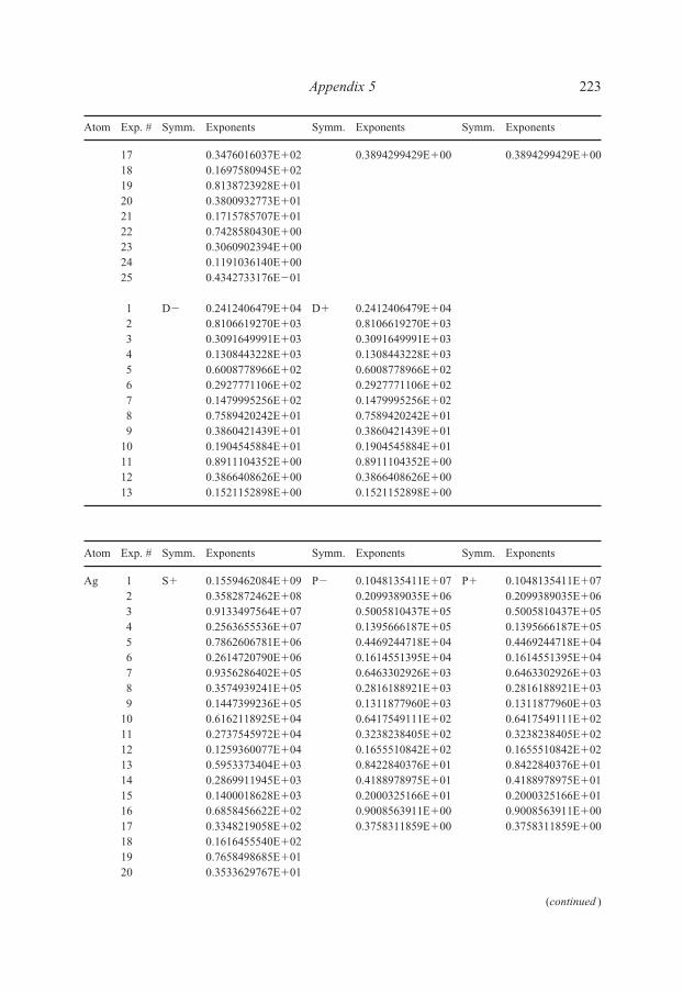
17 0.3476016037E�02 0.3894299429E�00 0.3894299429E�0018 0.1697580945E�0219 0.8138723928E�0120 0.3800932773E�0121 0.1715785707E�0122 0.7428580430E�0023 0.3060902394E�0024 0.1191036140E�0025 0.4342733176E�01
1 D� 0.2412406479E�04 D� 0.2412406479E�042 0.8106619270E�03 0.8106619270E�033 0.3091649991E�03 0.3091649991E�034 0.1308443228E�03 0.1308443228E�035 0.6008778966E�02 0.6008778966E�026 0.2927771106E�02 0.2927771106E�027 0.1479995256E�02 0.1479995256E�028 0.7589420242E�01 0.7589420242E�019 0.3860421439E�01 0.3860421439E�01
10 0.1904545884E�01 0.1904545884E�0111 0.8911104352E�00 0.8911104352E�0012 0.3866408626E�00 0.3866408626E�0013 0.1521152898E�00 0.1521152898E�00
Atom Exp. # Symm. Exponents Symm. Exponents Symm. Exponents
Ag 1 S� 0.1559462084E�09 P� 0.1048135411E�07 P� 0.1048135411E�072 0.3582872462E�08 0.2099389035E�06 0.2099389035E�063 0.9133497564E�07 0.5005810437E�05 0.5005810437E�054 0.2563655536E�07 0.1395666187E�05 0.1395666187E�055 0.7862606781E�06 0.4469244718E�04 0.4469244718E�046 0.2614720790E�06 0.1614551395E�04 0.1614551395E�047 0.9356286402E�05 0.6463302926E�03 0.6463302926E�038 0.3574939241E�05 0.2816188921E�03 0.2816188921E�039 0.1447399236E�05 0.1311877960E�03 0.1311877960E�03
10 0.6162118925E�04 0.6417549111E�02 0.6417549111E�0211 0.2737545972E�04 0.3238238405E�02 0.3238238405E�0212 0.1259360077E�04 0.1655510842E�02 0.1655510842E�0213 0.5953373404E�03 0.8422840376E�01 0.8422840376E�0114 0.2869911945E�03 0.4188978975E�01 0.4188978975E�0115 0.1400018628E�03 0.2000325166E�01 0.2000325166E�0116 0.6858456622E�02 0.9008563911E�00 0.9008563911E�0017 0.3348219058E�02 0.3758311859E�00 0.3758311859E�0018 0.1616455540E�0219 0.7658498685E�0120 0.3533629767E�01
Appendix 5 223
Atom Exp. # Symm. Exponents Symm. Exponents Symm. Exponents
(continued )
Else_EAMC-TRSIC_appn5.qxd 5/19/2007 21:38 Page 223

21 0.1575663656E�0122 0.6738117933E�0023 0.2742293036E�0024 0.1054039346E�0025 0.3796951417E�01
1 D� 0.2346979016E�04 D� 0.2346979016E�042 0.7895659183E�03 0.7895659183E�033 0.3002116891E�03 0.3002116891E�034 0.1262181656E�03 0.1262181656E�035 0.5740718302E�02 0.5740718302E�026 0.2763476398E�02 0.2763476398E�027 0.1377480561E�02 0.1377480561E�028 0.6955853675E�01 0.6955853675E�019 0.3481333914E�01 0.3481333914E�01
10 0.1689531345E�01 0.1689531345E�0111 0.7778703174E�00 0.7778703174E�0012 0.3324019509E�00 0.3324019509E�0013 0.1289823814E�00 0.1289823814E�00
Atom Exp. # Symm. Exponents Symm. Exponents Symm. Exponents
Cd 1 S� 0.1439742140E�09 P� 0.1244931229E�07 P� 0.1244931229E�072 0.3348673768E�08 0.2447399633E�06 0.2447399633E�063 0.8625844795E�07 0.5738086639E�05 0.5738086639E�054 0.2442528635E�07 0.1576049463E�05 0.1576049463E�055 0.7546671786E�06 0.4981394840E�04 0.4981394840E�046 0.2525326780E�06 0.1779706229E�04 0.1779706229E�047 0.9084365075E�05 0.7059919591E�03 0.7059919591E�038 0.3487024475E�05 0.3054521027E�03 0.3054521027E�039 0.1417644651E�05 0.1415846800E�03 0.1415846800E�03
10 0.6058990788E�04 0.6906484437E�02 0.6906484437E�0211 0.2702229748E�04 0.3482597556E�02 0.3482597556E�0212 0.1248250844E�04 0.1783170510E�02 0.1783170510E�0213 0.5927992346E�03 0.9106754616E�01 0.9106754616E�0114 0.2872818032E�03 0.4556731345E�01 0.4556731345E�0115 0.1410171291E�03 0.2194320661E�01 0.2194320661E�0116 0.6959330087E�02 0.9989447951E�00 0.9989447951E�0017 0.3427388764E�02 0.4222945359E�00 0.4222945359E�0018 0.1671968982E�0219 0.8019190456E�0120 0.3753521029E�0121 0.1701851812E�0122 0.7419040491E�0023 0.3086635897E�00
224 Appendix 5
Atom Exp. # Symm. Exponents Symm. Exponents Symm. Exponents
(continued )
Else_EAMC-TRSIC_appn5.qxd 5/19/2007 21:38 Page 224

24 0.1216475242E�0025 0.4507854673E�01
1 D� 0.2912502614E�04 D� 0.2912502614E�042 0.9458028609E�03 0.9458028609E�033 0.3518585675E�03 0.3518585675E�034 0.1464439958E�03 0.1464439958E�035 0.6659071375E�02 0.6659071375E�026 0.3230703890E�02 0.3230703890E�027 0.1633145019E�02 0.1633145019E�028 0.8400384867E�01 0.8400384867E�019 0.4293615799E�01 0.4293615799E�01
10 0.2129607002E�01 0.2129607002E�0111 0.1000992370E�01 0.1000992370E�0112 0.4354314656E�00 0.4354314656E�0013 0.1711864236E�00 0.1711864236E�00
Atom Exp. # Symm. Exponents Symm. Exponents Symm. Exponents
In 1 S� 0.1348158222E�09 P� 0.2535808680E�07 P� 0.2535808680E�072 0.3178833033E�08 0.5497144499E�06 0.5497144499E�063 0.8293497653E�07 0.1370375986E�06 0.1370375986E�064 0.2376685659E�07 0.3880580142E�05 0.3880580142E�055 0.7426610214E�06 0.1233048954E�05 0.1233048954E�056 0.2511974553E�06 0.4342733112E�04 0.4342733112E�047 0.9129908294E�05 0.1674624856E�04 0.1674624856E�048 0.3539688332E�05 0.6984187854E�03 0.6984187854E�039 0.1453221844E�05 0.3111936243E�03 0.3111936243E�03
10 0.6271738595E�04 0.1463303066E�03 0.1463303066E�0311 0.2824580610E�04 0.7172971436E�02 0.7172971436E�0212 0.1317804074E�04 0.3620741844E�02 0.3620741844E�0213 0.6322654069E�03 0.1859097107E�02 0.1859097107E�0214 0.3096852729E�03 0.9591467450E�01 0.9591467450E�0115 0.1537216710E�03 0.4911553978E�01 0.4911553978E�0116 0.7676511534E�02 0.2465903522E�01 0.2465903522E�0117 0.3828492828E�02 0.1199026964E�01 0.1199026964E�0118 0.1892987492E�02 0.5577633085E�00 0.5577633085E�0019 0.9211799596E�01 0.2451949210E�00 0.2451949210E�0020 0.4379644935E�01 0.1006203790E�00 0.1006203790E�0021 0.2019537232E�01 0.3807551547E�01 0.3807551547E�0122 0.8966113234E�0023 0.3804668504E�0024 0.1531829859E�0025 0.5809064463E�01
1 D� 0.2919907535E�04 D� 0.2919907535E�042 0.1010715927E�04 0.1010715927E�04
Appendix 5 225
Atom Exp. # Symm. Exponents Symm. Exponents Symm. Exponents
(continued )
Else_EAMC-TRSIC_appn5.qxd 5/19/2007 21:38 Page 225
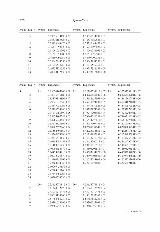
3 0.3905601419E�03 0.3905601419E�034 0.1653818952E�03 0.1653818952E�035 0.7533064367E�02 0.7533064367E�026 0.3623109802E�02 0.3623109802E�027 0.1806175106E�02 0.1806175106E�028 0.9161132870E�01 0.9161132870E�019 0.4640790035E�01 0.4640790035E�01
10 0.2304785435E�01 0.2304785435E�0111 0.1101557975E�01 0.1101557975E�0112 0.4973532155E�00 0.4973532155E�0013 0.2082311263E�00 0.2082311263E�00
Atom Exp. # Symm. Exponents Symm. Exponents Symm. Exponents
Sn 1 S� 0.1367616506E�09 P� 0.3279238911E�07 P� 0.3279238911E�072 0.3207567518E�08 0.6876544204E�06 0.6876544204E�063 0.8337631689E�07 0.1668262786E�06 0.1668262786E�064 0.2384191754E�07 0.4623102483E�05 0.4623102483E�055 0.7444703076E�06 0.1444957952E�05 0.1444957952E�056 0.2519633964E�06 0.5029297436E�04 0.5029297436E�047 0.9174608669E�05 0.1924720398E�04 0.1924720398E�048 0.3567580778E�05 0.7996758628E�03 0.7996758628E�039 0.1470524964E�05 0.3561427681E�03 0.3561427681E�03
10 0.6377632016E�04 0.1678710743E�03 0.1678710743E�0311 0.2888757796E�04 0.8268885924E�02 0.8268885924E�0212 0.1356449316E�04 0.4202573483E�02 0.4202573483E�0213 0.6554097939E�03 0.2175998589E�02 0.2175998589E�0214 0.3234561013E�03 0.1133325537E�02 0.1133325537E�0215 0.1618404145E�03 0.5862479071E�01 0.5862479071E�0116 0.8148993643E�02 0.2973831071E�01 0.2973831071E�0117 0.4098665607E�02 0.1460620651E�01 0.1460620651E�0118 0.2043989481E�02 0.6858395482E�00 0.6858395482E�0019 0.1003202567E�02 0.3039830388E�00 0.3039830388E�0020 0.4810038706E�01 0.1255728390E�00 0.1255728390E�0021 0.2236323434E�01 0.4773527188E�01 0.4773527188E�0122 0.1000743815E�0123 0.4278481114E�0024 0.1734646076E�0025 0.6620073933E�01
1 D� 0.3365477181E�04 D� 0.3365477181E�042 0.1134031272E�04 0.1134031272E�043 0.4301877047E�03 0.4301877047E�034 0.1801513356E�03 0.1801513356E�035 0.8166866523E�02 0.8166866523E�026 0.3930102306E�02 0.3930102306E�027 0.1968677733E�02 0.1968677733E�02
226 Appendix 5
Atom Exp. # Symm. Exponents Symm. Exponents Symm. Exponents
(continued )
Else_EAMC-TRSIC_appn5.qxd 5/19/2007 21:38 Page 226

8 0.1006606490E�02 0.1006606490E�029 0.5151706289E�01 0.5151706289E�01
10 0.2587859440E�01 0.2587859440E�0111 0.1251181866E�01 0.1251181866E�0112 0.5709292793E�00 0.5709292793E�0013 0.2411116835E�00 0.2411116835E�00
Atom Exp. # Symm. Exponents Symm. Exponents Symm. Exponents
Sb 1 S� 0.1286666567E�09 P� 0.3767144337E�07 P� 0.3767144337E�072 0.2892644943E�08 0.7660461482E�06 0.7660461482E�063 0.7292435698E�07 0.1810227108E�06 0.1810227108E�064 0.2044380799E�07 0.4907310156E�05 0.4907310156E�055 0.6320130199E�06 0.1506548501E�05 0.1506548501E�056 0.2136626666E�06 0.5170692952E�04 0.5170692952E�047 0.7833087738E�05 0.1958561693E�04 0.1958561693E�048 0.3088178581E�05 0.8082495901E�03 0.8082495901E�039 0.1298375258E�05 0.3587321615E�03 0.3587321615E�03
10 0.5772843776E�04 0.1690474307E�03 0.1690474307E�0311 0.2691748433E�04 0.8349435761E�02 0.8349435761E�0212 0.1305261607E�04 0.4266903573E�02 0.4266903573E�0213 0.6527433107E�03 0.2227268275E�02 0.2227268275E�0214 0.3338354157E�03 0.1172284682E�02 0.1172284682E�0215 0.1731533261E�03 0.6141739042E�01 0.6141739042E�0116 0.9032356318E�02 0.3161871342E�01 0.3161871342E�0117 0.4699010535E�02 0.1579022973E�01 0.1579022973E�0118 0.2417743642E�02 0.7551286997E�00 0.7551286997E�0019 0.1220045130E�02 0.3413804392E�00 0.3413804392E�0020 0.5987791878E�01 0.1440251286E�00 0.1440251286E�0021 0.2834301156E�01 0.5597791875E�01 0.5597791875E�0122 0.1283149111E�0123 0.5509642724E�0024 0.2225093503E�0025 0.8381368813E�01
1 D� 0.3620812446E�04 D� 0.3620812446E�042 0.1205684687E�04 0.1205684687E�043 0.4540956270E�03 0.4540956270E�034 0.1895993133E�03 0.1895993133E�035 0.8601854148E�02 0.8601854148E�026 0.4156265385E�02 0.4156265385E�027 0.2096333407E�02 0.2096333407E�028 0.1081815842E�02 0.1081815842E�029 0.5598506971E�01 0.5598506971E�01
10 0.2847783843E�01 0.2847783843E�0111 0.1395557516E�01 0.1395557516E�0112 0.6457796952E�00 0.6457796952E�0013 0.2765712079E�00 0.2765712079E�00
Appendix 5 227
Atom Exp. # Symm. Exponents Symm. Exponents Symm. Exponents
Else_EAMC-TRSIC_appn5.qxd 5/19/2007 21:38 Page 227
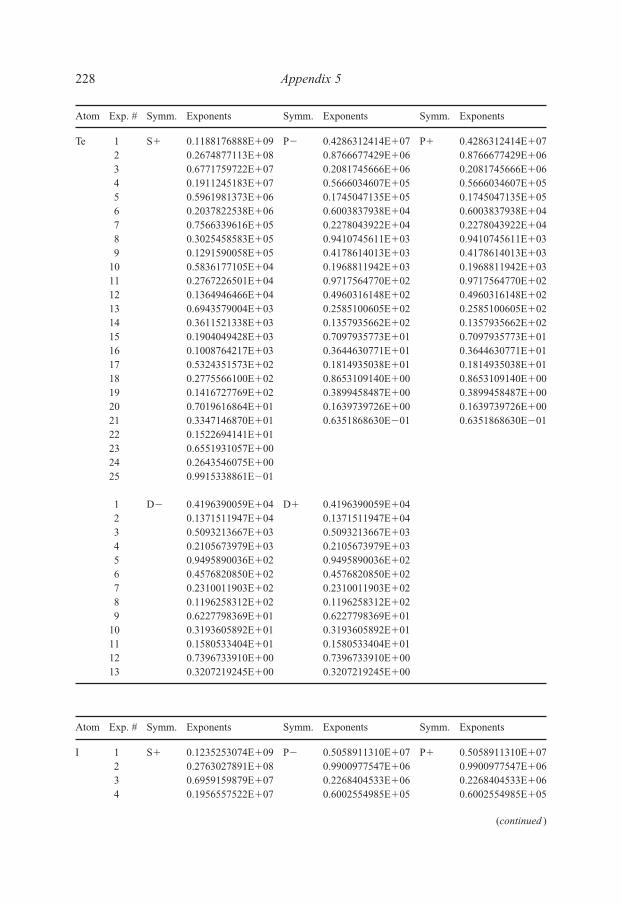
Atom Exp. # Symm. Exponents Symm. Exponents Symm. Exponents
Te 1 S� 0.1188176888E�09 P� 0.4286312414E�07 P� 0.4286312414E�072 0.2674877113E�08 0.8766677429E�06 0.8766677429E�063 0.6771759722E�07 0.2081745666E�06 0.2081745666E�064 0.1911245183E�07 0.5666034607E�05 0.5666034607E�055 0.5961981373E�06 0.1745047135E�05 0.1745047135E�056 0.2037822538E�06 0.6003837938E�04 0.6003837938E�047 0.7566339616E�05 0.2278043922E�04 0.2278043922E�048 0.3025458583E�05 0.9410745611E�03 0.9410745611E�039 0.1291590058E�05 0.4178614013E�03 0.4178614013E�03
10 0.5836177105E�04 0.1968811942E�03 0.1968811942E�0311 0.2767226501E�04 0.9717564770E�02 0.9717564770E�0212 0.1364946466E�04 0.4960316148E�02 0.4960316148E�0213 0.6943579004E�03 0.2585100605E�02 0.2585100605E�0214 0.3611521338E�03 0.1357935662E�02 0.1357935662E�0215 0.1904049428E�03 0.7097935773E�01 0.7097935773E�0116 0.1008764217E�03 0.3644630771E�01 0.3644630771E�0117 0.5324351573E�02 0.1814935038E�01 0.1814935038E�0118 0.2775566100E�02 0.8653109140E�00 0.8653109140E�0019 0.1416727769E�02 0.3899458487E�00 0.3899458487E�0020 0.7019616864E�01 0.1639739726E�00 0.1639739726E�0021 0.3347146870E�01 0.6351868630E�01 0.6351868630E�0122 0.1522694141E�0123 0.6551931057E�0024 0.2643546075E�0025 0.9915338861E�01
1 D� 0.4196390059E�04 D� 0.4196390059E�042 0.1371511947E�04 0.1371511947E�043 0.5093213667E�03 0.5093213667E�034 0.2105673979E�03 0.2105673979E�035 0.9495890036E�02 0.9495890036E�026 0.4576820850E�02 0.4576820850E�027 0.2310011903E�02 0.2310011903E�028 0.1196258312E�02 0.1196258312E�029 0.6227798369E�01 0.6227798369E�01
10 0.3193605892E�01 0.3193605892E�0111 0.1580533404E�01 0.1580533404E�0112 0.7396733910E�00 0.7396733910E�0013 0.3207219245E�00 0.3207219245E�00
Atom Exp. # Symm. Exponents Symm. Exponents Symm. Exponents
I 1 S� 0.1235253074E�09 P� 0.5058911310E�07 P� 0.5058911310E�072 0.2763027891E�08 0.9900977547E�06 0.9900977547E�063 0.6959159879E�07 0.2268404533E�06 0.2268404533E�064 0.1956557522E�07 0.6002554985E�05 0.6002554985E�05
228 Appendix 5
(continued )
Else_EAMC-TRSIC_appn5.qxd 5/19/2007 21:38 Page 228
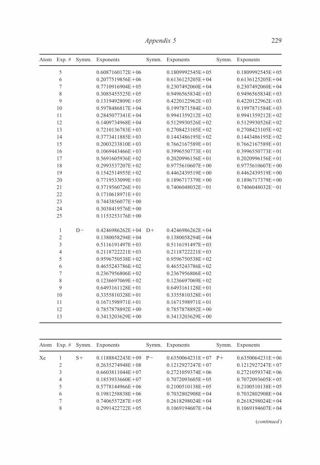
5 0.6087160172E�06 0.1809992545E�05 0.1809992545E�056 0.2077519856E�06 0.6136125205E�04 0.6136125205E�047 0.7710916904E�05 0.2307492060E�04 0.2307492060E�048 0.3085455525E�05 0.9496565834E�03 0.9496565834E�039 0.1319492809E�05 0.4220122962E�03 0.4220122962E�03
10 0.5978486817E�04 0.1997871584E�03 0.1997871584E�0311 0.2845077341E�04 0.9941359212E�02 0.9941359212E�0212 0.1409734968E�04 0.5129930526E�02 0.5129930526E�0213 0.7210136783E�03 0.2708423105E�02 0.2708423105E�0214 0.3773411885E�03 0.1443486195E�02 0.1443486195E�0215 0.2003233810E�03 0.7662167589E�01 0.7662167589E�0116 0.1069443466E�03 0.3996550773E�01 0.3996550773E�0117 0.5691605936E�02 0.2020996156E�01 0.2020996156E�0118 0.2993537207E�02 0.9775610607E�00 0.9775610607E�0019 0.1542514955E�02 0.4462439519E�00 0.4462439519E�0020 0.7719533099E�01 0.1896717379E�00 0.1896717379E�0021 0.3719560726E�01 0.7406048032E�01 0.7406048032E�0122 0.1710618971E�0123 0.7443856077E�0024 0.3038419576E�0025 0.1153253176E�00
1 D� 0.4246986262E�04 D� 0.4246986262E�042 0.1380058294E�04 0.1380058294E�043 0.5116191497E�03 0.5116191497E�034 0.2118722221E�03 0.2118722221E�035 0.9596750538E�02 0.9596750538E�026 0.4655243786E�02 0.4655243786E�027 0.2367956806E�02 0.2367956806E�028 0.1236697069E�02 0.1236697069E�029 0.6493161128E�01 0.6493161128E�01
10 0.3355810328E�01 0.3355810328E�0111 0.1671598971E�01 0.1671598971E�0112 0.7857878892E�00 0.7857878892E�0013 0.3413203629E�00 0.3413203629E�00
Atom Exp. # Symm. Exponents Symm. Exponents Symm. Exponents
Xe 1 S� 0.1188842243E�09 P� 0.6350064231E�07 P� 0.6350064231E�062 0.2635274948E�08 0.1212927247E�07 0.1212927247E�073 0.6603811044E�07 0.2721059374E�06 0.2721059374E�064 0.1853933660E�07 0.7072093605E�05 0.7072093605E�055 0.5778144966E�06 0.2100510138E�05 0.2100510138E�056 0.1981258838E�06 0.7032802908E�04 0.7032802908E�047 0.7406557287E�05 0.2618298024E�04 0.2618298024E�048 0.2991422722E�05 0.1069194607E�04 0.1069194607E�04
Appendix 5 229
(continued )
Atom Exp. # Symm. Exponents Symm. Exponents Symm. Exponents
Else_EAMC-TRSIC_appn5.qxd 5/19/2007 21:38 Page 229

9 0.1293568015E�05 0.4723909569E�03 0.4723909569E�0310 0.5934917342E�04 0.2227478948E�03 0.2227478948E�0311 0.2862976958E�04 0.1105739801E�03 0.1105739801E�0312 0.1439006147E�04 0.5700063067E�02 0.5700063067E�0213 0.7468147905E�03 0.3009912342E�02 0.3009912342E�0214 0.3965815294E�03 0.1605963189E�02 0.1605963189E�0215 0.2135429382E�03 0.8540532713E�01 0.8540532713E�0116 0.1155406880E�03 0.4465417330E�01 0.4465417330E�0117 0.6225088575E�02 0.2264263413E�01 0.2264263413E�0118 0.3309640473E�02 0.1098347412E�01 0.1098347412E�0119 0.1720697971E�02 0.5027597278E�00 0.5027597278E�0020 0.8669236774E�01 0.2142147085E�00 0.2142147085E�0021 0.4194433561E�01 0.8380428577E�01 0.8380428577E�0122 0.1931282736E�0123 0.8386144218E�0024 0.3403192942E�0025 0.1279035033E�00
1 D� 0.4354113781E�04 D� 0.4354113781E�042 0.1415449281E�04 0.1415449281E�043 0.5256557401E�03 0.5256557401E�034 0.2182902913E�03 0.2182902913E�035 0.9922170579E�02 0.9922170579E�026 0.4832051629E�02 0.4832051629E�027 0.2467870693E�02 0.2467870693E�028 0.1293875656E�02 0.1293875656E�029 0.6816404260E�01 0.6816404260E�01
10 0.3532028031E�01 0.3532028031E�0111 0.1762025943E�01 0.1762025943E�0112 0.8283867782E�00 0.8283867782E�0013 0.3592527253E�00 0.3592527253E�00
Atom Exp. # Symm. Exponents Symm. Exponents Symm. Exponents
Cs 1 S� 0.1532069592E�09 P� 0.6627847402E�07 P� 0.6627847402E�072 0.3868527134E�08 0.1317373589E�07 0.1317373589E�073 0.1082603162E�08 0.3041650948E�06 0.3041650948E�064 0.3335030815E�07 0.8057516929E�05 0.8057516929E�055 0.1123279296E�07 0.2418866898E�05 0.2418866898E�056 0.4108501282E�06 0.8127726277E�04 0.8127726277E�047 0.1620829365E�06 0.3019256302E�04 0.3019256302E�048 0.6850145392E�05 0.1224706913E�04 0.1224706913E�049 0.3080500847E�05 0.5357881369E�03 0.5357881369E�03
10 0.1464038012E�05 0.2496952125E�03 0.2496952125E�0311 0.7303705903E�04 0.1224365254E�03 0.1224365254E�0312 0.3798783406E�04 0.6239113661E�02 0.6239113661E�02
230 Appendix 5
Atom Exp. # Symm. Exponents Symm. Exponents Symm. Exponents
(continued )
Else_EAMC-TRSIC_appn5.qxd 5/19/2007 21:38 Page 230
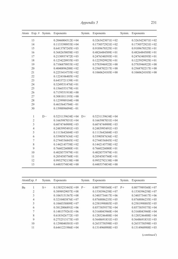
13 0.2046004312E�04 0.3263423071E�02 0.3263423071E�0214 0.1133390953E�04 0.1730572921E�02 0.1730572921E�0215 0.6413787245E�03 0.9189670325E�01 0.9189670325E�0116 0.3682658058E�03 0.4826484589E�01 0.4826484589E�0117 0.2130937472E�03 0.2476340393E�01 0.2476340393E�0118 0.1234220935E�03 0.1225929925E�01 0.1225929925E�0119 0.7106870953E�02 0.5783946922E�00 0.5783946922E�0020 0.4040896208E�02 0.2568702217E�00 0.2568702217E�0021 0.2253414755E�02 0.1060624103E�00 0.1060624103E�0022 0.1224106405E�0223 0.6433721139E�0124 0.3249531476E�0125 0.1566553179E�0126 0.7159551918E�0027 0.3081011193E�0028 0.1239989104E�0029 0.4635643704E�0130 0.1598896094E�01
1 D� 0.5231139634E�04 D� 0.5231139634E�042 0.1665987031E�04 0.1665987031E�043 0.6074744909E�03 0.6074744909E�034 0.2483995491E�03 0.2483995491E�035 0.1115642604E�03 0.1115642604E�036 0.5390587636E�02 0.5390587636E�027 0.2744536845E�02 0.2744536845E�028 0.1442145758E�02 0.1442145758E�029 0.7660226080E�01 0.7660226080E�01
10 0.4028575979E�01 0.4028575979E�0111 0.2054585760E�01 0.2054585760E�0112 0.9952792138E�00 0.9952792138E�0013 0.4485374834E�00 0.4485374834E�00
AtomExp. # Symm. Exponents Symm. Exponents Symm. Exponents
Ba 1 S� 0.1585253443E�09 P� 0.8077989360E�07 P� 0.8077989360E�072 0.3898929057E�08 0.1530396258E�07 0.1530396258E�073 0.1065151567E�08 0.3403734417E�06 0.3403734417E�064 0.3210403876E�07 0.8768886235E�05 0.8768886235E�055 0.1060358809E�07 0.2581998885E�05 0.2581998885E�056 0.3812006891E�06 0.8573859375E�04 0.8573859375E�047 0.1481579261E�06 0.3168043960E�04 0.3168043960E�048 0.6183426772E�05 0.1285246488E�04 0.1285246488E�049 0.2752513173E�05 0.5648691831E�03 0.5648691831E�03
10 0.1298040301E�05 0.2653758598E�03 0.2653758598E�0311 0.6441221986E�04 0.1314960988E�03 0.1314960988E�03
Appendix 5 231
(continued )
Atom Exp. # Symm. Exponents Symm. Exponents Symm. Exponents
Else_EAMC-TRSIC_appn5.qxd 5/19/2007 21:38 Page 231
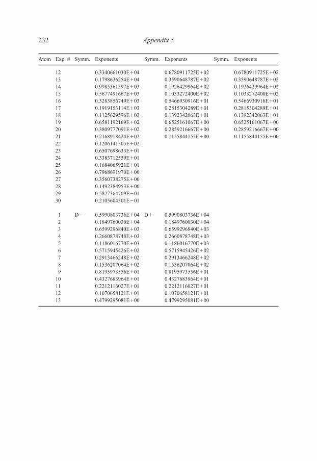
12 0.3340661030E�04 0.6780911725E�02 0.6780911725E�0213 0.1798636254E�04 0.3590648787E�02 0.3590648787E�0214 0.9985361597E�03 0.1926429964E�02 0.1926429964E�0215 0.5677491667E�03 0.1033272400E�02 0.1033272400E�0216 0.3283856749E�03 0.5466930916E�01 0.5466930916E�0117 0.1919153114E�03 0.2815304289E�01 0.2815304289E�0118 0.1125629596E�03 0.1392342063E�01 0.1392342063E�0119 0.6581192169E�02 0.6525161067E�00 0.6525161067E�0020 0.3809777091E�02 0.2859216667E�00 0.2859216667E�0021 0.2168918424E�02 0.1155844155E�00 0.1155844155E�0022 0.1206141505E�0223 0.6507698633E�0124 0.3383712559E�0125 0.1684065921E�0126 0.7968691970E�0027 0.3560738275E�0028 0.1492384953E�0029 0.5827364709E�0130 0.2105604501E�01
1 D� 0.5990803736E�04 D� 0.5990803736E�042 0.1849760030E�04 0.1849760030E�043 0.6599296840E�03 0.6599296840E�034 0.2660878748E�03 0.2660878748E�035 0.1186016770E�03 0.1186016770E�036 0.5715945426E�02 0.5715945426E�027 0.2913466248E�02 0.2913466248E�028 0.1536207064E�02 0.1536207064E�029 0.8195973556E�01 0.8195973556E�01
10 0.4327683964E�01 0.4327683964E�0111 0.2212116027E�01 0.2212116027E�0112 0.1070658121E�01 0.1070658121E�0113 0.4799295081E�00 0.4799295081E�00
232 Appendix 5
Atom Exp. # Symm. Exponents Symm. Exponents Symm. Exponents
Else_EAMC-TRSIC_appn5.qxd 5/19/2007 21:38 Page 232

Atom Exp. # Symm. Exponents Symm. Exponents Symm. Exponents Symm. Exponents
La 1 S� 0.1690768754E�09 P� 0.9519022377E�07 P� 0.9519022377E�07 D� 0.5658367057E�042 0.4063743075E�08 0.1815613495E�07 0.1815613495E�07 0.1859304540E�043 0.1088808219E�08 0.4058834142E�06 0.4058834142E�06 0.6958393192E�034 0.3229452276E�07 0.1049496330E�06 0.1049496330E�06 0.2906824142E�035 0.1052998849E�07 0.3097541458E�05 0.3097541458E�05 0.1328410331E�036 0.3748156190E�06 0.1029828208E�05 0.1029828208E�05 0.6508812458E�027 0.1446330134E�06 0.3806087412E�04 0.3806087412E�04 0.3351040178E�028 0.6008227561E�05 0.1543170529E�04 0.1543170529E�04 0.1776716805E�029 0.2668232738E�05 0.6773687208E�03 0.6773687208E�03 0.9507576281E�01
10 0.1257965277E�05 0.3176634721E�03 0.3176634721E�03 0.5032534902E�0111 0.6252452794E�04 0.1570707109E�03 0.1570707109E�03 0.2582387889E�0112 0.3253405714E�04 0.8080975660E�02 0.8080975660E�02 0.1259001350E�0113 0.1759953840E�04 0.4269017292E�02 0.4269017292E�02 0.5715487637E�0014 0.9828987685E�03 0.2285295808E�02 0.2285295808E�0215 0.5627687573E�03 0.1223382303E�02 0.1223382303E�0216 0.3280454774E�03 0.6463118127E�01 0.6463118127E�0117 0.1933259846E�03 0.3325347152E�01 0.3325347152E�0118 0.1143846427E�03 0.1644378358E�01 0.1644378358E�0119 0.6747388796E�02 0.7712430196E�00 0.7712430196E�0020 0.3940610321E�02 0.3385792516E�00 0.3385792516E�0021 0.2262664678E�02 0.1372979026E�00 0.1372979026E�0022 0.1268455013E�0223 0.6894413374E�0124 0.3607913860E�0125 0.1805181212E�0126 0.8575520045E�0027 0.3841000447E�0028 0.1610800263E�0029 0.6280897143E�0130 0.2261275824E�01
Appendix 5
233
(continued )
Else_EAMC-TRSIC_appn5.qxd 5/19/2007 21:38 Page 233

1 D� 0.5658367057E�04 F� 0.2092088640E�03 F� 0.2092088640E�032 0.1859304540E�04 0.8623295998E�02 0.8623295998E�023 0.6958393192E�03 0.3729218805E�02 0.3729218805E�024 0.2906824142E�03 0.1673248900E�02 0.1673248900E�025 0.1328410331E�03 0.7702790609E�01 0.7702790609E�016 0.6508812458E�02 0.3597719080E�01 0.3597719080E�017 0.3351040178E�02 0.1685950311E�01 0.1685950311E�018 0.1776716805E�02 0.7838760711E�00 0.7838760711E�009 0.9507576281E�01 0.3575871552E�00 0.3575871552E�00
10 0.5032534902E�01 0.1582686985E�00 0.1582686985E�0011 0.2582387889E�01 0.6720994200E�01 0.6720994200E�0112 0.1259001350E�0113 0.5715487637E�00
Atom Exp. # Symm. Exponents Symm. Exponents Symm. Exponents
La 1 S� 0.1693237518E�09 P� 0.1006323333E�08 P� 0.1006323333E�082 0.4026346052E�08 0.1896305287E�07 0.1896305287E�073 0.1068651416E�08 0.4193792744E�06 0.4193792744E�064 0.3143715721E�07 0.1074162164E�06 0.1074162164E�065 0.1017848604E�07 0.3144366069E�05 0.3144366069E�056 0.3601689774E�06 0.1038084959E�05 0.1038084959E�057 0.1383130323E�06 0.3814217268E�04 0.3814217268E�048 0.5724058554E�05 0.1539171004E�04 0.1539171004E�049 0.2535010020E�05 0.6731524308E�03 0.6731524308E�03
10 0.1192999944E�05 0.3148627237E�03 0.3148627237E�0311 0.5924296407E�04 0.1554341871E�03 0.1554341871E�0312 0.3082614600E�04 0.7991448358E�02 0.7991448358E�0213 0.1668930537E�04 0.4222739449E�02 0.4222739449E�02
234A
ppendix 5Atom Exp. # Symm. Exponents Symm. Exponents Symm. Exponents Symm. Exponents
Else_EAMC-TRSIC_appn5.qxd 5/19/2007 21:38 Page 234

14 0.9335645511E�03 0.2263023662E�02 0.2263023662E�0215 0.5357818380E�03 0.1213797140E�02 0.1213797140E�0216 0.3132706077E�03 0.6429859964E�01 0.6429859964E�0117 0.1853061447E�03 0.3319643854E�01 0.3319643854E�0118 0.1101156340E�03 0.1648360619E�01 0.1648360619E�0119 0.6527511134E�02 0.7768191256E�00 0.7768191256E�0020 0.3832977027E�02 0.3428709697E�00 0.3428709697E�0021 0.2213936965E�02 0.1398687948E�00 0.1398687948E�0022 0.1249065490E�0223 0.6835126755E�0124 0.3602465450E�0125 0.1815914711E�0126 0.8693285102E�0027 0.3924783772E�0028 0.1659362864E�0029 0.6523960148E�0130 0.2368514331E�01
1 D� 0.4775657703E�04 D� 0.4775657703E�042 0.1694015057E�04 0.1694015057E�043 0.6625280324E�03 0.6625280324E�034 0.2813420277E�03 0.2813420277E�035 0.1277464308E�03 0.1277464308E�036 0.6107833490E�02 0.6107833490E�027 0.3028240056E�02 0.3028240056E�028 0.1533199089E�02 0.1533199089E�029 0.7806428607E�01 0.7806428607E�01
10 0.3936336921E�01 0.3936336921E�0111 0.1935791648E�01 0.1935791648E�0112 0.9143066559E�00 0.9143066559E�0013 0.4084439970E�00 0.4084439970E�0014 0.1699499202E�00 0.1699499202E�0015 0.6486309520E�01 0.6486309520E�01
Appendix 5
235
Else_EAMC-TRSIC_appn5.qxd 5/19/2007 21:38 Page 235

236A
ppendix 5Atom Exp. # Symm. Exponents Symm. Exponents Symm. Exponents Symm. Exponents
Ce 1 S� 0.1694298758E�09 P� 0.7521231562E�07 P� 0.7521231562E�07 D� 0.6053135723E�042 0.4055344266E�08 0.1474930723E�07 0.1474930723E�07 0.2035709607E�043 0.1082496754E�08 0.3381958628E�06 0.3381958628E�06 0.7709593956E�034 0.3200030630E�07 0.8948671789E�05 0.8948671789E�05 0.3230595562E�035 0.1040346106E�07 0.2696634612E�05 0.2696634612E�05 0.1471716735E�036 0.3693730914E�06 0.9133526216E�04 0.9133526216E�04 0.7161624660E�027 0.1422275993E�06 0.3431526207E�04 0.3431526207E�04 0.3657629553E�028 0.5897952108E�05 0.1411393913E�04 0.1411393913E�04 0.1926388406E�029 0.2615681498E�05 0.6271924982E�03 0.6271924982E�03 0.1028014197E�02
10 0.1231976022E�05 0.2971835591E�03 0.2971835591E�03 0.5461609303E�0111 0.6119570545E�04 0.1481834249E�03 0.1481834249E�03 0.2838334329E�0112 0.3183526369E�04 0.7673703524E�02 0.7673703524E�02 0.1417695678E�0113 0.1722393160E�04 0.4073057655E�02 0.4073057655E�02 0.6687043810E�0014 0.9624096914E�03 0.2186884608E�02 0.2186884608E�0215 0.5515171951E�03 0.1172196881E�02 0.1172196881E�0216 0.3218822444E�03 0.6190478978E�01 0.6190478978E�0117 0.1899946614E�03 0.3178897742E�01 0.3178897742E�0118 0.1126314586E�03 0.1566524135E�01 0.1566524135E�0119 0.6659160329E�02 0.7311146142E�00 0.7311146142E�0020 0.3899313980E�02 0.3189343507E�00 0.3189343507E�0021 0.2245605350E�02 0.1283406402E�00 0.1283406402E�0022 0.1263056195E�0223 0.6890066982E�0124 0.3619955780E�0125 0.1818987261E�0126 0.8681007666E�0027 0.3907439225E�0028 0.1647264934E�0029 0.6458792379E�0130 0.2338963064E�01
Else_EAMC-TRSIC_appn5.qxd 5/19/2007 21:38 Page 236

1 D� 0.6053135723E�04 F� 0.2410059399E�03 F� 0.2410059399E�032 0.2035709607E�04 0.9641818099E�02 0.9641818099E�023 0.7709593956E�03 0.4071502271E�02 0.4071502271E�024 0.3230595562E�03 0.1793716347E�02 0.1793716347E�025 0.1471716735E�03 0.8148824502E�01 0.8148824502E�016 0.7161624660E�02 0.3773262804E�01 0.3773262804E�017 0.3657629553E�02 0.1760187013E�01 0.1760187013E�018 0.1926388406E�02 0.8176341370E�00 0.8176341370E�009 0.1028014197E�02 0.3738147558E�00 0.3738147558E�00
10 0.5461609303E�01 0.1662607996E�00 0.1662607996E�0011 0.2838334329E�01 0.7110466020E�01 0.7110466020E�0112 0.1417695678E�0113 0.6687043810E�00
Atom Exp. # Symm. Exponents Symm. Exponents Symm. Exponents Symm. Exponents
Ce 1 S� 0.1717256364E�09 P� 0.8604848729E�07 P� 0.8604848729E�07 D� 0.5159600038E�042 0.4172259351E�08 0.1654439451E�07 0.1654439451E�07 0.1782858144E�043 0.1128832905E�08 0.3728798994E�06 0.3728798994E�06 0.6845331933E�034 0.3377585130E�07 0.9721125997E�05 0.9721125997E�05 0.2873167449E�035 0.1109934383E�07 0.2892762121E�05 0.2892762121E�05 0.1296963628E�036 0.3978311103E�06 0.9695639708E�04 0.9695639708E�04 0.6194508062E�027 0.1544566788E�06 0.3611826321E�04 0.3611826321E�04 0.3079709449E�028 0.6450854322E�05 0.1475648559E�04 0.1475648559E�04 0.1568008086E�029 0.2878236301E�05 0.6524748159E�03 0.6524748159E�03 0.8043298959E�01
10 0.1362480847E�05 0.3080976256E�03 0.3080976256E�03 0.4089584792E�0111 0.6795559058E�04 0.1533118690E�03 0.1533118690E�03 0.2027659596E�0112 0.3546556477E�04 0.7933139290E�02 0.7933139290E�02 0.9644804606E�0013 0.1923408588E�04 0.4212261290E�02 0.4212261290E�02 0.4329982167E�0014 0.1076503092E�04 0.2264672957E�02 0.2264672957E�02 0.1805031566E�0015 0.6174960017E�03 0.1216563268E�02 0.1216563268E�02 0.6873868911E�0116 0.3605157428E�03 0.6443501969E�01 0.6443501969E�01
Appendix 5
237
(continued )
Else_EAMC-TRSIC_appn5.qxd 5/19/2007 21:38 Page 237
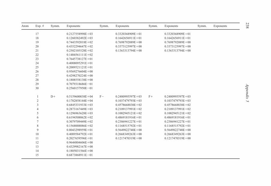
17 0.2127558998E�03 0.3320368909E�01 0.3320368909E�0118 0.1260382492E�03 0.1642656911E�01 0.1642656911E�0119 0.7443592018E�02 0.7698792089E�00 0.7698792089E�0020 0.4352294647E�02 0.3373125997E�00 0.3373125997E�0021 0.2502105528E�02 0.1363313794E�00 0.1363313794E�0022 0.1404561111E�0223 0.7645738127E�0124 0.4008095291E�0125 0.2009521121E�0126 0.9569276604E�0027 0.4298270224E�0028 0.1808558138E�0029 0.7079318686E�0130 0.2560157950E�01
1 D� 0.5159600038E�04 F� 0.2480995597E�03 F� 0.2480995597E�032 0.1782858144E�04 0.1037479793E�03 0.1037479793E�033 0.6845331933E�03 0.4578668838E�02 0.4578668838E�024 0.2873167449E�03 0.2109137991E�02 0.2109137991E�025 0.1296963628E�03 0.1002945121E�02 0.1002945121E�026 0.6194508062E�02 0.4869181916E�01 0.4869181916E�017 0.3079709449E�02 0.2386941227E�01 0.2386941227E�018 0.1568008086E�02 0.1168515792E�01 0.1168515792E�019 0.8043298959E�01 0.5649822740E�00 0.5649822740E�00
10 0.4089584792E�01 0.2668349263E�00 0.2668349263E�0011 0.2027659596E�01 0.1217470319E�00 0.1217470319E�0012 0.9644804606E�0013 0.4329982167E�0014 0.1805031566E�0015 0.6873868911E�01
238A
ppendix 5Atom Exp. # Symm. Exponents Symm. Exponents Symm. Exponents Symm. Exponents
Else_EAMC-TRSIC_appn5.qxd 5/19/2007 21:38 Page 238

Atom Exp. # Symm. Exponents Symm. Exponents Symm. Exponents Symm. Exponents
Pr 1 S� 0.1699651027E�09 P� 0.1095288748E�08 P� 0.1095288748E�08 D� 0.7298437961E�042 0.4107016606E�08 0.2076480462E�07 0.2076480462E�07 0.2377619340E�043 0.1106335377E�08 0.4614243269E�06 0.4614243269E�06 0.8745546960E�034 0.3299118982E�07 0.1186048606E�06 0.1186048606E�06 0.3568584343E�035 0.1081476755E�07 0.3480084549E�05 0.3480084549E�05 0.1587089376E�036 0.3869916790E�06 0.1150319171E�05 0.1150319171E�05 0.7558494880E�027 0.1501096063E�06 0.4227115566E�04 0.4227115566E�04 0.3787301441E�028 0.6267508919E�05 0.1704209697E�04 0.1704209697E�04 0.1961630137E�029 0.2797166032E�05 0.7438939671E�03 0.7438939671E�03 0.1031879941E�02
10 0.1325059974E�05 0.3469477549E�03 0.3469477549E�03 0.5416242480E�0111 0.6616129920E�04 0.1706232119E�03 0.1706232119E�03 0.2787122151E�0112 0.3457649030E�04 0.8731504408E�02 0.8731504408E�02 0.1381449370E�0113 0.1878120182E�04 0.4588523093E�02 0.4588523093E�02 0.6479882030E�0014 0.1052903657E�04 0.2443687075E�02 0.2443687075E�0215 0.6049700379E�03 0.1301556527E�02 0.1301556527E�0216 0.3537661458E�03 0.6841970473E�01 0.6841970473E�0117 0.2090706361E�03 0.3503128129E�01 0.3503128129E�0118 0.1239999107E�03 0.1724024608E�01 0.1724024608E�0119 0.7329231838E�02 0.8048212909E�00 0.8048212909E�0020 0.4287079102E�02 0.3517061461E�00 0.3517061461E�0021 0.2464266532E�02 0.1419844912E�00 0.1419844912E�0022 0.1382274193E�0223 0.7513430176E�0124 0.3929859627E�0125 0.1964118759E�0126 0.9314672003E�0027 0.4162303092E�0028 0.1740296885E�0029 0.6760731444E�0130 0.2423270650E�01
Appendix 5
239
(continued )
Else_EAMC-TRSIC_appn5.qxd 5/19/2007 21:38 Page 239

1 D� 0.7298437961E�04 F� 0.2575287643E�03 F� 0.2575287643E�032 0.2377619340E�04 0.1049843308E�03 0.1049843308E�033 0.8745546960E�03 0.4502499952E�02 0.4502499952E�024 0.3568584343E�03 0.2008110975E�02 0.2008110975E�025 0.1587089376E�03 0.9206630858E�01 0.9206630858E�016 0.7558494880E�02 0.4289108633E�01 0.4289108633E�017 0.3787301441E�02 0.2007062628E�01 0.2007062628E�018 0.1961630137E�02 0.9325167316E�00 0.9325167316E�009 0.1031879941E�02 0.4252344477E�00 0.4252344477E�00
10 0.5416242480E�01 0.1881267748E�00 0.1881267748E�0011 0.2787122151E�01 0.7981737008E�01 0.7981737008E�0112 0.1381449370E�0113 0.6479882030E�00
Atom Exp. # Symm. Exponents Symm. Exponents Symm. Exponents Symm. Exponents
Nd 1 S� 0.1691153375E�09 P� 0.9842830204E�07 P� 0.9842830204E�07 D� 0.7063732040E�042 0.4122575013E�08 0.1897373842E�07 0.1897373842E�07 0.2307956999E�043 0.1118983006E�08 0.4278989462E�06 0.4278989462E�06 0.8509658031E�034 0.3358376339E�07 0.1114286768E�06 0.1114286768E�06 0.3479136392E�035 0.1106796485E�07 0.3306985063E�05 0.3306985063E�05 0.1549850498E�036 0.3977592719E�06 0.1103974528E�05 0.1103974528E�05 0.7391817219E�027 0.1547991518E�06 0.4091565311E�04 0.4091565311E�04 0.3708854065E�028 0.6478793794E�05 0.1661634856E�04 0.1661634856E�04 0.1923709273E�029 0.2895867233E�05 0.7298093556E�03 0.7298093556E�03 0.1013524738E�02
10 0.1372788516E�05 0.3421551186E�03 0.3421551186E�03 0.5329770926E�0111 0.6854104494E�04 0.1690006965E�03 0.1690006965E�03 0.2748818486E�0112 0.3579327942E�04 0.8679962345E�02 0.8679962345E�02 0.1366252487E�0113 0.1941500643E�04 0.4575337522E�02 0.4575337522E�02 0.6430537944E�0014 0.1086276682E�04 0.2442960466E�02 0.2442960466E�02
240A
ppendix 5Atom Exp. # Symm. Exponents Symm. Exponents Symm. Exponents Symm. Exponents
Else_EAMC-TRSIC_appn5.qxd 5/19/2007 21:38 Page 240

15 0.6225752317E�03 0.1304096716E�02 0.1304096716E�0216 0.3629721267E�03 0.6869344233E�01 0.6869344233E�0117 0.2137796497E�03 0.3524073285E�01 0.3524073285E�0118 0.1263143485E�03 0.1737844086E�01 0.1737844086E�0119 0.7435562776E�02 0.8130644512E�00 0.8130644512E�0020 0.4330434039E�02 0.3562045605E�00 0.3562045605E�0021 0.2477918560E�02 0.1442269345E�00 0.1442269345E�0022 0.1383446088E�0223 0.7484083991E�0124 0.3895810832E�0125 0.1937855795E�0126 0.9147260158E�0027 0.4069004574E�0028 0.1693926217E�0029 0.6553775461E�0130 0.2340243112E�01
1 D� 0.7063732040E�04 F� 0.2566803987E�03 F� 0.2566803987E�022 0.2307956999E�04 0.1065449337E�03 0.1065449337E�033 0.8509658031E�03 0.4642639788E�02 0.4642639788E�024 0.3479136392E�03 0.2099296682E�02 0.2099296682E�025 0.1549850498E�03 0.9737418842E�01 0.9737418842E�016 0.7391817219E�02 0.4579938447E�01 0.4579938447E�017 0.3708854065E�02 0.2159264015E�01 0.2159264015E�018 0.1923709273E�02 0.1008710927E�01 0.1008710927E�019 0.1013524738E�02 0.4615589043E�00 0.4615589043E�00
10 0.5329770926E�01 0.2044897427E�00 0.2044897427E�0011 0.2748818486E�01 0.8671305100E�01 0.8671305100E�0112 0.1366252487E�0113 0.6430537944E�00
Appendix 5
241
Else_EAMC-TRSIC_appn5.qxd 5/19/2007 21:38 Page 241
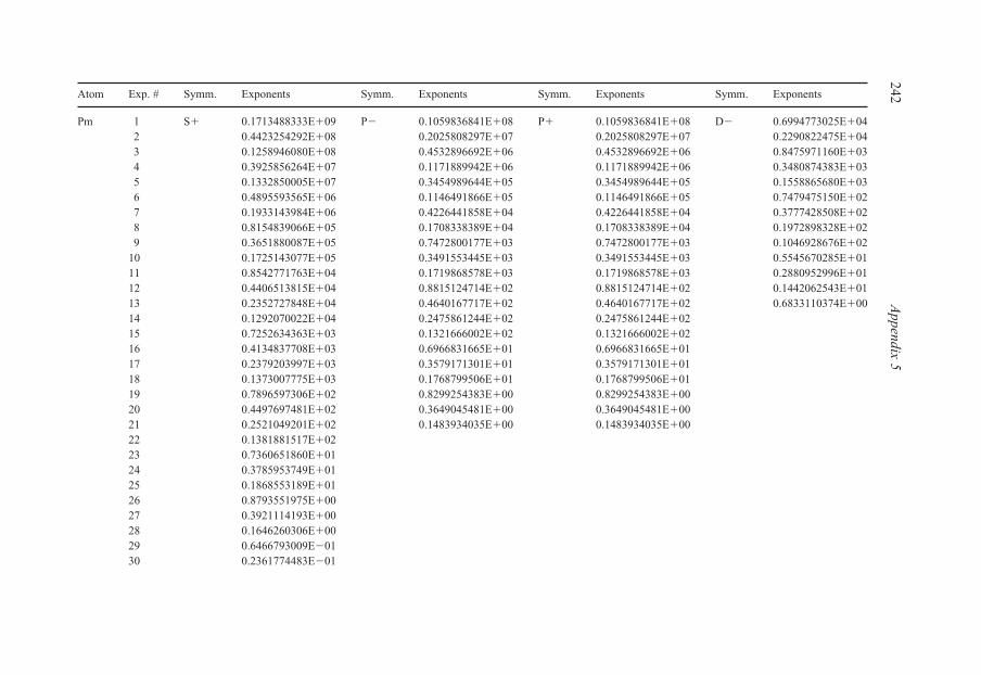
Atom Exp. # Symm. Exponents Symm. Exponents Symm. Exponents Symm. Exponents
Pm 1 S� 0.1713488333E�09 P� 0.1059836841E�08 P� 0.1059836841E�08 D� 0.6994773025E�042 0.4423254292E�08 0.2025808297E�07 0.2025808297E�07 0.2290822475E�043 0.1258946080E�08 0.4532896692E�06 0.4532896692E�06 0.8475971160E�034 0.3925856264E�07 0.1171889942E�06 0.1171889942E�06 0.3480874383E�035 0.1332850005E�07 0.3454989644E�05 0.3454989644E�05 0.1558865680E�036 0.4895593565E�06 0.1146491866E�05 0.1146491866E�05 0.7479475150E�027 0.1933143984E�06 0.4226441858E�04 0.4226441858E�04 0.3777428508E�028 0.8154839066E�05 0.1708338389E�04 0.1708338389E�04 0.1972898328E�029 0.3651880087E�05 0.7472800177E�03 0.7472800177E�03 0.1046928676E�02
10 0.1725143077E�05 0.3491553445E�03 0.3491553445E�03 0.5545670285E�0111 0.8542771763E�04 0.1719868578E�03 0.1719868578E�03 0.2880952996E�0112 0.4406513815E�04 0.8815124714E�02 0.8815124714E�02 0.1442062543E�0113 0.2352727848E�04 0.4640167717E�02 0.4640167717E�02 0.6833110374E�0014 0.1292070022E�04 0.2475861244E�02 0.2475861244E�0215 0.7252634363E�03 0.1321666002E�02 0.1321666002E�0216 0.4134837708E�03 0.6966831665E�01 0.6966831665E�0117 0.2379203997E�03 0.3579171301E�01 0.3579171301E�0118 0.1373007775E�03 0.1768799506E�01 0.1768799506E�0119 0.7896597306E�02 0.8299254383E�00 0.8299254383E�0020 0.4497697481E�02 0.3649045481E�00 0.3649045481E�0021 0.2521049201E�02 0.1483934035E�00 0.1483934035E�0022 0.1381881517E�0223 0.7360651860E�0124 0.3785953749E�0125 0.1868553189E�0126 0.8793551975E�0027 0.3921114193E�0028 0.1646260306E�0029 0.6466793009E�0130 0.2361774483E�01
242A
ppendix 5
Else_EAMC-TRSIC_appn5.qxd 5/19/2007 21:38 Page 242
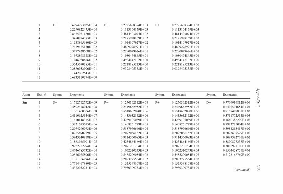
1 D� 0.6994773025E�04 F� 0.2725688394E�03 F� 0.2725688394E�032 0.2290822475E�04 0.1113164159E�03 0.1113164159E�033 0.8475971160E�03 0.4814403074E�02 0.4814403074E�024 0.3480874383E�03 0.2175928159E�02 0.2175928159E�025 0.1558865680E�03 0.1014107927E�02 0.1014107927E�026 0.7479475150E�02 0.4809278991E�01 0.4809278991E�017 0.3777428508E�02 0.2290079626E�01 0.2290079626E�018 0.1972898328E�02 0.1080474845E�01 0.1080474845E�019 0.1046928676E�02 0.4984147102E�00 0.4984147102E�00
10 0.5545670285E�01 0.2218185213E�00 0.2218185213E�0011 0.2880952996E�01 0.9398405338E�01 0.9398405338E�0112 0.1442062543E�0113 0.6833110374E�00
Atom Exp. # Symm. Exponents Symm. Exponents Symm. Exponents Symm. Exponents
Sm 1 S� 0.1712712792E�09 P� 0.1270362312E�08 P� 0.1270362312E�08 D� 0.7706916812E�042 0.4502418042E�08 0.2449662952E�07 0.2449662952E�07 0.2497594654E�043 0.1301400306E�08 0.5518602090E�06 0.5518602090E�06 0.9157489831E�034 0.4110625144E�07 0.1433632152E�06 0.1433632152E�06 0.3731772534E�035 0.1410148315E�07 0.4239105039E�05 0.4239105039E�05 0.1660386290E�036 0.5221673673E�06 0.1408251779E�05 0.1408251779E�05 0.7923725004E�027 0.2074296073E�06 0.5187976666E�04 0.5187976666E�04 0.3984253457E�028 0.8785690779E�05 0.2092036152E�04 0.2092036152E�04 0.2073637579E�029 0.3943240818E�05 0.9114560083E�03 0.9114560083E�03 0.1097382701E�02
10 0.1863935901E�05 0.4234864169E�03 0.4234864169E�03 0.5800878238E�0111 0.9222252294E�04 0.2071201704E�03 0.2071201704E�03 0.3008921100E�0112 0.4746783732E�04 0.1052510243E�03 0.1052510243E�03 0.1504458755E�0113 0.2526075806E�04 0.5485209054E�02 0.5485209054E�02 0.7123168769E�0014 0.1381356796E�04 0.2893775564E�02 0.2893775564E�0215 0.7714467980E�03 0.1525398108E�02 0.1525398108E�0216 0.4372952731E�03 0.7930309733E�01 0.7930309733E�01
Appendix 5
243
(continued )
Else_EAMC-TRSIC_appn5.qxd 5/19/2007 21:38 Page 243
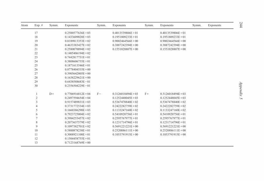
17 0.2500577636E�03 0.4013539806E�01 0.4013539806E�0118 0.1433609028E�03 0.1951809233E�01 0.1951809233E�0119 0.8189813353E�02 0.9002464566E�00 0.9002464566E�0020 0.4633383427E�02 0.3887242394E�00 0.3887242394E�0021 0.2580070094E�02 0.1551028807E�00 0.1551028807E�0022 0.1405406194E�0223 0.7442817731E�0124 0.3808606755E�0125 0.1871613546E�0126 0.8778404535E�0027 0.3905642005E�0028 0.1638229621E�0029 0.6438588683E�0130 0.2356504229E�01
1 D� 0.7706916812E�04 F� 0.3126018494E�03 F� 0.3126018494E�032 0.2497594654E�04 0.1252448045E�03 0.1252448045E�033 0.9157489831E�03 0.5367478840E�02 0.5367478840E�024 0.3731772534E�03 0.2422282759E�02 0.2422282759E�025 0.1660386290E�03 0.1133247160E�02 0.1133247160E�026 0.7923725004E�02 0.5410920756E�01 0.5410920756E�017 0.3984253457E�02 0.2595767977E�01 0.2595767977E�018 0.2073637579E�02 0.1231714796E�01 0.1231714796E�019 0.1097382701E�02 0.5691221221E�00 0.5691221221E�00
10 0.5800878238E�01 0.2520886111E�00 0.2520886111E�0011 0.3008921100E�01 0.1053791915E�00 0.1053791915E�0012 0.1504458755E�0113 0.7123168769E�00
244A
ppendix 5Atom Exp. # Symm. Exponents Symm. Exponents Symm. Exponents Symm. Exponents
Else_EAMC-TRSIC_appn5.qxd 5/19/2007 21:38 Page 244
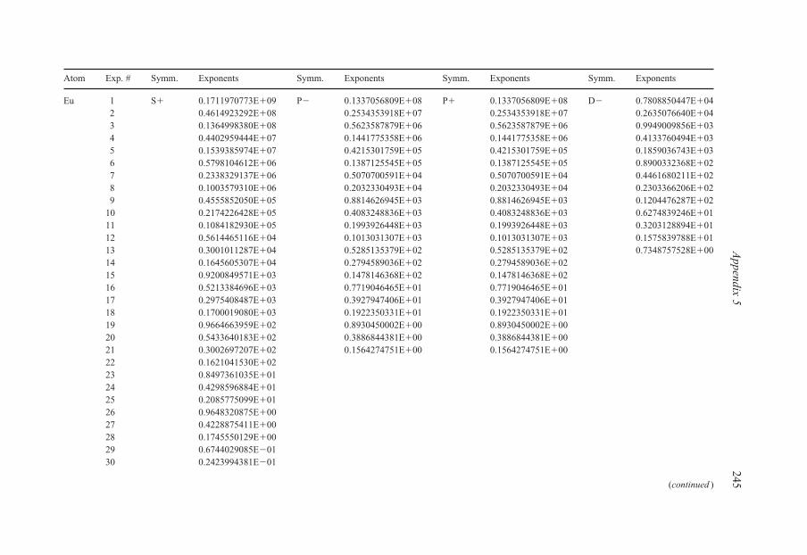
Atom Exp. # Symm. Exponents Symm. Exponents Symm. Exponents Symm. Exponents
Eu 1 S� 0.1711970773E�09 P� 0.1337056809E�08 P� 0.1337056809E�08 D� 0.7808850447E�042 0.4614923292E�08 0.2534353918E�07 0.2534353918E�07 0.2635076640E�043 0.1364998380E�08 0.5623587879E�06 0.5623587879E�06 0.9949009856E�034 0.4402959444E�07 0.1441775358E�06 0.1441775358E�06 0.4133760494E�035 0.1539385974E�07 0.4215301759E�05 0.4215301759E�05 0.1859036743E�036 0.5798104612E�06 0.1387125545E�05 0.1387125545E�05 0.8900332368E�027 0.2338329137E�06 0.5070700591E�04 0.5070700591E�04 0.4461680211E�028 0.1003579310E�06 0.2032330493E�04 0.2032330493E�04 0.2303366206E�029 0.4555852050E�05 0.8814626945E�03 0.8814626945E�03 0.1204476287E�02
10 0.2174226428E�05 0.4083248836E�03 0.4083248836E�03 0.6274839246E�0111 0.1084182930E�05 0.1993926448E�03 0.1993926448E�03 0.3203128894E�0112 0.5614465116E�04 0.1013031307E�03 0.1013031307E�03 0.1575839788E�0113 0.3001011287E�04 0.5285135379E�02 0.5285135379E�02 0.7348757528E�0014 0.1645605307E�04 0.2794589036E�02 0.2794589036E�0215 0.9200849571E�03 0.1478146368E�02 0.1478146368E�0216 0.5213384696E�03 0.7719046465E�01 0.7719046465E�0117 0.2975408487E�03 0.3927947406E�01 0.3927947406E�0118 0.1700019080E�03 0.1922350331E�01 0.1922350331E�0119 0.9664663959E�02 0.8930450002E�00 0.8930450002E�0020 0.5433640183E�02 0.3886844381E�00 0.3886844381E�0021 0.3002697207E�02 0.1564274751E�00 0.1564274751E�0022 0.1621041530E�0223 0.8497361035E�0124 0.4298596884E�0125 0.2085775099E�0126 0.9648320875E�0027 0.4228875411E�0028 0.1745550129E�0029 0.6744029085E�0130 0.2423994381E�01
Appendix 5
245(continued )
Else_EAMC-TRSIC_appn5.qxd 5/19/2007 21:38 Page 245

1 D� 0.7808850447E�04 F� 0.3141936420E�03 F� 0.3141936420E�032 0.2635076640E�04 0.1292530954E�03 0.1292530954E�033 0.9949009856E�03 0.5668323094E�02 0.5668323094E�024 0.4133760494E�03 0.2610001359E�02 0.2610001359E�025 0.1859036743E�03 0.1242801501E�02 0.1242801501E�026 0.8900332368E�02 0.6027540140E�01 0.6027540140E�017 0.4461680211E�02 0.2932636039E�01 0.2932636039E�018 0.2303366206E�02 0.1409802721E�01 0.1409802721E�019 0.1204476287E�02 0.6595429015E�00 0.6595429015E�00
10 0.6274839246E�01 0.2957431487E�00 0.2957431487E�0011 0.3203128894E�01 0.1251917406E�00 0.1251917406E�0012 0.1575839788E�0113 0.7348757528E�00
Atom Exp. # Symm. Exponents Symm. Exponents Symm. Exponents Symm. Exponents
Gd 1 S� 0.1691090010E�09 P� 0.1296942432E�08 P� 0.1296942432E�08 D� 0.8963245240E�042 0.4478131255E�08 0.2565070216E�07 0.2565070216E�07 0.2903473411E�043 0.1305765757E�08 0.5885442607E�06 0.5885442607E�06 0.1070051183E�044 0.4166019649E�07 0.1547472734E�06 0.1547472734E�06 0.4401302502E�035 0.1445154089E�07 0.4605678111E�05 0.4605678111E�05 0.1982000230E�036 0.5416179157E�06 0.1532687274E�05 0.1532687274E�05 0.9585788490E�027 0.2179250386E�06 0.5633335375E�04 0.5633335375E�04 0.4884380500E�028 0.9354179661E�05 0.2258876272E�04 0.2258876272E�04 0.2572198531E�029 0.4256356225E�05 0.9761054853E�03 0.9761054853E�03 0.1373310304E�02
10 0.2040107891E�05 0.4489947166E�03 0.4489947166E�03 0.7292188930E�0111 0.1023529656E�05 0.2171643682E�03 0.2171643682E�03 0.3777704920E�0112 0.5341079879E�04 0.1090941497E�03 0.1090941497E�03 0.1872987518E�0113 0.2880635340E�04 0.5622670093E�02 0.5622670093E�02 0.8718350225E�0014 0.1595611968E�04 0.2936802118E�02 0.2936802118E�02
246A
ppendix 5Atom Exp. # Symm. Exponents Symm. Exponents Symm. Exponents Symm. Exponents
Else_EAMC-TRSIC_appn5.qxd 5/19/2007 21:38 Page 246

15 0.9019766515E�03 0.1535537413E�02 0.1535537413E�0216 0.5170607083E�03 0.7938938707E�01 0.7938938707E�0117 0.2986862493E�03 0.4009068880E�01 0.4009068880E�0118 0.1727689103E�03 0.1953288094E�01 0.1953288094E�0119 0.9943558918E�02 0.9069712012E�00 0.9069712012E�0020 0.5658394490E�02 0.3964494273E�00 0.3964494273E�0021 0.3163507927E�02 0.1611431649E�00 0.1611431649E�0022 0.1726705160E�0223 0.9143031627E�0124 0.4666961879E�0125 0.2281915203E�0126 0.1062026094E�0127 0.4675095983E�0028 0.1934259572E�0029 0.7474068562E�0130 0.2680197023E�01
1 D� 0.8963245240E�04 F� 0.3870580284E�03 F� 0.3870580284E�032 0.2903473411E�04 0.1591000454E�03 0.1591000454E�033 0.1070051183E�04 0.7054733286E�02 0.7054733286E�024 0.4401302502E�03 0.3313412018E�02 0.3313412018E�025 0.1982000230E�03 0.1618539532E�02 0.1618539532E�026 0.9585788490E�02 0.8074073155E�01 0.8074073155E�017 0.4884380500E�02 0.4038797006E�01 0.4038797006E�018 0.2572198531E�02 0.1989160489E�01 0.1989160489E�019 0.1373310304E�02 0.9471408152E�00 0.9471408152E�00
10 0.7292188930E�01 0.4281093228E�00 0.4281093228E�0011 0.3777704920E�01 0.1803676722E�00 0.1803676722E�0012 0.1872987518E�0113 0.8718350225E�00
Appendix 5
247
Else_EAMC-TRSIC_appn5.qxd 5/19/2007 21:38 Page 247

Atom Exp. # Symm. Exponents Symm. Exponents Symm. Exponents Symm. Exponents
Gd 1 S� 0.1713671853E�09 P� 0.1385841396E�08 P� 0.1385841396E�08 D� 0.8163200583E�042 0.4630040864E�08 0.2757118722E�07 0.2757118722E�07 0.2559944230E�043 0.1374712740E�08 0.6358910174E�06 0.6358910174E�06 0.9221641680E�034 0.4457498385E�07 0.1679472284E�06 0.1679472284E�06 0.3732769757E�035 0.1568572747E�07 0.5017686950E�05 0.5017686950E�05 0.1660874821E�036 0.5952981043E�06 0.1675145354E�05 0.1675145354E�05 0.7946261555E�027 0.2421379317E�06 0.6173014364E�04 0.6173014364E�04 0.3998955628E�028 0.1048991048E�06 0.2480364896E�04 0.2480364896E�04 0.2070740162E�029 0.4809982435E�05 0.1073457874E�04 0.1073457874E�04 0.1079288224E�02
10 0.2319850960E�05 0.4942915874E�03 0.4942915874E�03 0.5538849927E�0111 0.1169509337E�05 0.2392146969E�03 0.2392146969E�03 0.2737849707E�0112 0.6124299892E�04 0.1201922780E�03 0.1201922780E�03 0.1275102137E�0113 0.3310552507E�04 0.6193369421E�02 0.6193369421E�02 0.5473476085E�0014 0.1835768521E�04 0.3233082289E�02 0.3233082289E�02 0.2118370285E�0015 0.1037745583E�04 0.1688976193E�02 0.1688976193E�02 0.7231001380E�0116 0.5942942603E�03 0.8722177822E�01 0.8722177822E�0117 0.3426351986E�03 0.4398439541E�01 0.4398439541E�0118 0.1976352208E�03 0.2139549019E�01 0.2139549019E�0119 0.1133393634E�03 0.9916842645E�00 0.9916842645E�0020 0.6421897707E�02 0.4326431308E�00 0.4326431308E�0021 0.3572681628E�02 0.1754967407E�00 0.1754967407E�0022 0.1939347787E�0223 0.1020774144E�0224 0.5177240412E�0125 0.2514454864E�0126 0.1162112912E�0127 0.5079183571E�0028 0.2086232580E�0029 0.8002706674E�0130 0.2849040127E�01
248A
ppendix 5
Else_EAMC-TRSIC_appn5.qxd 5/19/2007 21:38 Page 248

1 D� 0.8163200583E�04 F� 0.4313300740E�03 F� 0.4313300740E�032 0.2559944230E�04 0.1840308903E�03 0.1840308903E�033 0.9221641680E�03 0.8264134856E�02 0.8264134856E�024 0.3732769757E�03 0.3863836863E�02 0.3863836863E�025 0.1660874821E�03 0.1860561036E�02 0.1860561036E�026 0.7946261555E�02 0.9127710384E�01 0.9127710384E�017 0.3998955628E�02 0.4512961290E�01 0.4512961290E�018 0.2070740162E�02 0.2224499066E�01 0.2224499066E�019 0.1079288224E�02 0.1081341190E�01 0.1081341190E�01
10 0.5538849927E�01 0.5127931321E�00 0.5127931321E�0011 0.2737849707E�01 0.2346711088E�00 0.2346711088E�0012 0.1275102137E�0113 0.5473476085E�0014 0.2118370285E�0015 0.7231001380E�01
Atom Exp. # Symm. Exponents Symm. Exponents Symm. Exponents Symm. Exponents
Tb 1 S� 0.1690551753E�09 P� 0.1492826638E�08 P� 0.1492826638E�08 D� 0.9775593468E�042 0.4398733482E�08 0.2936009189E�07 0.2936009189E�07 0.3124141483E�043 0.1263577992E�08 0.6702983935E�06 0.6702983935E�06 0.1138852299E�044 0.3981411106E�07 0.1754670133E�06 0.1754670133E�06 0.4643215893E�035 0.1367155460E�07 0.5202272888E�05 0.5202272888E�05 0.2076111782E�036 0.5083116069E�06 0.1725499825E�05 0.1725499825E�05 0.9982253313E�027 0.2033100001E�06 0.6324331952E�04 0.6324331952E�04 0.5060786944E�028 0.8691392925E�05 0.2530149282E�04 0.2530149282E�04 0.2652679325E�029 0.3945547697E�05 0.1091347830E�04 0.1091347830E�04 0.1409594829E�02
10 0.1889721580E�05 0.5013252636E�03 0.5013252636E�03 0.7445816119E�0111 0.9487380070E�04 0.2422529945E�03 0.2422529945E�03 0.3833578807E�0112 0.4960644079E�04 0.1216369950E�03 0.1216369950E�03 0.1886410393E�0113 0.2683851426E�04 0.6268490611E�02 0.6268490611E�02 0.8699079071E�00
Appendix 5
249
(continued )
Else_EAMC-TRSIC_appn5.qxd 5/19/2007 21:38 Page 249

14 0.1492769821E�04 0.3275026731E�02 0.3275026731E�0215 0.8480599182E�03 0.1713464433E�02 0.1713464433E�0216 0.4889279721E�03 0.8867424887E�01 0.8867424887E�0117 0.2842059904E�03 0.4483693586E�01 0.4483693586E�0118 0.1654919632E�03 0.2187983883E�01 0.2187983883E�0119 0.9590942032E�02 0.1017831533E�01 0.1017831533E�0120 0.5496315359E�02 0.4458462087E�00 0.4458462087E�0021 0.3094520610E�02 0.1816458378E�00 0.1816458378E�0022 0.1700637754E�0223 0.9063841322E�0124 0.4654576295E�0125 0.2288235587E�0126 0.1069939894E�0127 0.4727607691E�0028 0.1961246696E�0029 0.7589568851E�0130 0.2721957950E�01
1 D� 0.9775593468E�04 F� 0.5092038278E�03 F� 0.5092038278E�032 0.3124141483E�04 0.2029714741E�03 0.2029714741E�033 0.1138852299E�04 0.8760969582E�02 0.8760969582E�024 0.4643215893E�03 0.4019878407E�02 0.4019878407E�025 0.2076111782E�03 0.1924806142E�02 0.1924806142E�026 0.9982253313E�02 0.9441568908E�01 0.9441568908E�017 0.5060786944E�02 0.4657514199E�01 0.4657514199E�018 0.2652679325E�02 0.2268228560E�01 0.2268228560E�019 0.1409594829E�02 0.1070561954E�01 0.1070561954E�01
10 0.7445816119E�01 0.4807274446E�00 0.4807274446E�0011 0.3833578807E�01 0.2016127094E�00 0.2016127094E�0012 0.1886410393E�0113 0.8699079071E�00
250A
ppendix 5Atom Exp. # Symm. Exponents Symm. Exponents Symm. Exponents Symm. Exponents
Else_EAMC-TRSIC_appn5.qxd 5/19/2007 21:38 Page 250

Atom Exp. # Symm. Exponents Symm. Exponents Symm. Exponents Symm. Exponents
Dy 1 S� 0.1701857069E�09 P� 0.1436689710E�08 P� 0.1436689710E�08 D� 0.1065705362E�052 0.4416412348E�08 0.2818594371E�07 0.2818594371E�07 0.3336605330E�043 0.1265715733E�08 0.6420070030E�06 0.6420070030E�06 0.1195738603E�044 0.3980159922E�07 0.1677015844E�06 0.1677015844E�06 0.4808082674E�035 0.1364395872E�07 0.4962235945E�05 0.4962235945E�05 0.2126436462E�036 0.5065631013E�06 0.1642907562E�05 0.1642907562E�05 0.1013953980E�037 0.2023754084E�06 0.6011695151E�04 0.6011695151E�04 0.5109871400E�028 0.8643521272E�05 0.2401493982E�04 0.2401493982E�04 0.2667891300E�029 0.3921120629E�05 0.1034473612E�04 0.1034473612E�04 0.1414598744E�02
10 0.1877128407E�05 0.4746388918E�03 0.4746388918E�03 0.7466996098E�0111 0.9421494349E�04 0.2291215008E�03 0.2291215008E�03 0.3846330884E�0112 0.4925670800E�04 0.1149422298E�03 0.1149422298E�03 0.1895291276E�0113 0.2665069292E�04 0.5919121688E�02 0.5919121688E�02 0.8757384756E�0014 0.1482609944E�04 0.3090661385E�02 0.3090661385E�0215 0.8425551609E�03 0.1616273006E�02 0.1616273006E�0216 0.4859600399E�03 0.8361800061E�01 0.8361800061E�0117 0.2826254756E�03 0.4227262652E�01 0.4227262652E�0118 0.1646676679E�03 0.2062745793E�01 0.2062745793E�0119 0.9549252891E�02 0.9596477302E�00 0.9596477302E�0020 0.5476110921E�02 0.4204460269E�00 0.4204460269E�0021 0.3085280181E�02 0.1713537356E�00 0.1713537356E�0022 0.1696735959E�0223 0.9049174234E�0124 0.4650037103E�0125 0.2287359451E�0126 0.1070090970E�0127 0.4730347137E�0028 0.1963039813E�0029 0.7598130263E�0130 0.2725233030E�01
Appendix 5
251
(continued )
Else_EAMC-TRSIC_appn5.qxd 5/19/2007 21:38 Page 251

1 D� 0.1065705362E�05 F� 0.4205025022E�03 F� 0.4205025022E�032 0.3336605330E�04 0.1706711037E�03 0.1706711037E�033 0.1195738603E�04 0.7476953295E�02 0.7476953295E�024 0.4808082674E�03 0.3471998835E�02 0.3471998835E�025 0.2126436462E�03 0.1678192126E�02 0.1678192126E�026 0.1013953980E�03 0.8291401888E�01 0.8291401888E�017 0.5109871400E�02 0.4112021771E�01 0.4112021771E�018 0.2667891300E�02 0.2010207876E�01 0.2010207876E�019 0.1414598744E�02 0.9512652543E�00 0.9512652543E�00
10 0.7466996098E�01 0.4279119062E�00 0.4279119062E�0011 0.3846330884E�01 0.1796867910E�00 0.1796867910E�0012 0.1895291276E�0113 0.8757384756E�00
Atom Exp. # Symm. Exponents Symm. Exponents Symm. Exponents Symm. Exponents
Ho 1 S� 0.1694621245E�09 P� 0.1367774085E�08 P� 0.1367774085E�08 D� 0.1076046342E�052 0.4340862049E�08 0.2718206220E�07 0.2718206220E�07 0.3416808552E�043 0.1230174031E�08 0.6263434920E�06 0.6263434920E�06 0.1236196284E�044 0.3831645861E�07 0.1653043868E�06 0.1653043868E�06 0.4998072270E�035 0.1303087002E�07 0.4936024839E�05 0.4936024839E�05 0.2214813339E�036 0.4806973301E�06 0.1647293359E�05 0.1647293359E�05 0.1055024201E�037 0.1910826514E�06 0.6069385437E�04 0.6069385437E�04 0.5298459232E�028 0.8131357664E�05 0.2438811049E�04 0.2438811049E�04 0.2751502095E�029 0.3679917912E�05 0.1055724889E�04 0.1055724889E�04 0.1449086683E�02
10 0.1759492677E�05 0.4863422990E�03 0.4863422990E�03 0.7590918723E�0111 0.8829824411E�04 0.2355220152E�03 0.2355220152E�03 0.3879189247E�0112 0.4620329479E�04 0.1184400718E�03 0.1184400718E�03 0.1896729655E�0113 0.2504327405E�04 0.6109743931E�02 0.6109743931E�02 0.8702798618E�0014 0.1396842855E�04 0.3193625997E�02 0.3193625997E�02
252A
ppendix 5Atom Exp. # Symm. Exponents Symm. Exponents Symm. Exponents Symm. Exponents
Else_EAMC-TRSIC_appn5.qxd 5/19/2007 21:38 Page 252
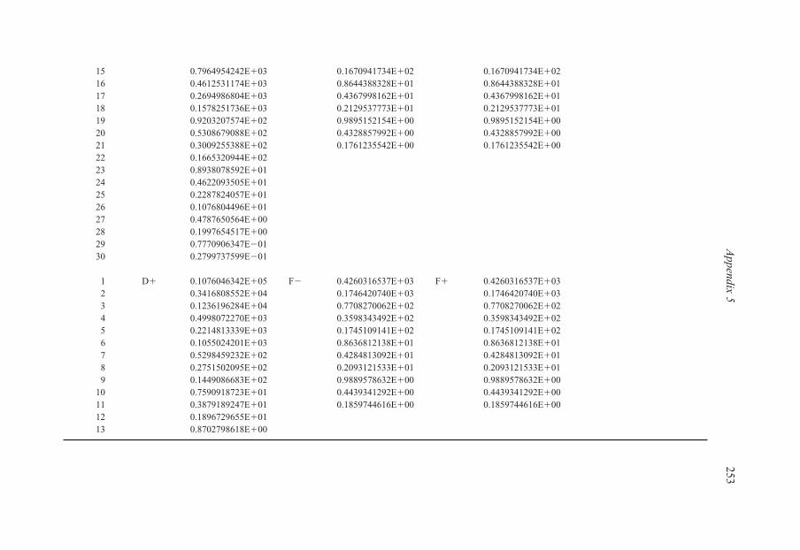
15 0.7964954242E�03 0.1670941734E�02 0.1670941734E�0216 0.4612531174E�03 0.8644388328E�01 0.8644388328E�0117 0.2694986804E�03 0.4367998162E�01 0.4367998162E�0118 0.1578251736E�03 0.2129537773E�01 0.2129537773E�0119 0.9203207574E�02 0.9895152154E�00 0.9895152154E�0020 0.5308679088E�02 0.4328857992E�00 0.4328857992E�0021 0.3009255388E�02 0.1761235542E�00 0.1761235542E�0022 0.1665320944E�0223 0.8938078592E�0124 0.4622093505E�0125 0.2287824057E�0126 0.1076804496E�0127 0.4787650564E�0028 0.1997654517E�0029 0.7770906347E�0130 0.2799737599E�01
1 D� 0.1076046342E�05 F� 0.4260316537E�03 F� 0.4260316537E�032 0.3416808552E�04 0.1746420740E�03 0.1746420740E�033 0.1236196284E�04 0.7708270062E�02 0.7708270062E�024 0.4998072270E�03 0.3598343492E�02 0.3598343492E�025 0.2214813339E�03 0.1745109141E�02 0.1745109141E�026 0.1055024201E�03 0.8636812138E�01 0.8636812138E�017 0.5298459232E�02 0.4284813092E�01 0.4284813092E�018 0.2751502095E�02 0.2093121533E�01 0.2093121533E�019 0.1449086683E�02 0.9889578632E�00 0.9889578632E�00
10 0.7590918723E�01 0.4439341292E�00 0.4439341292E�0011 0.3879189247E�01 0.1859744616E�00 0.1859744616E�0012 0.1896729655E�0113 0.8702798618E�00
Appendix 5
253
Else_EAMC-TRSIC_appn5.qxd 5/19/2007 21:38 Page 253

Atom Exp. # Symm. Exponents Symm. Exponents Symm. Exponents Symm. Exponents
Er 1 S� 0.1686601656E�09 P� 0.1519063382E�08 P� 0.1519063382E�08 D� 0.1022804216E�052 0.4286536604E�08 0.2995577566E�07 0.2995577566E�07 0.3251031433E�043 0.1206264733E�08 0.6852819950E�06 0.6852819950E�06 0.1180358384E�044 0.3733842594E�07 0.1796420859E�06 0.1796420859E�06 0.4798481771E�035 0.1262937511E�07 0.5330436955E�05 0.5330436955E�05 0.2141037275E�036 0.4637195473E�06 0.1768477039E�05 0.1768477039E�05 0.1027799033E�037 0.1836165522E�06 0.6480132276E�04 0.6480132276E�04 0.5203420901E�028 0.7789083140E�05 0.2590490987E�04 0.2590490987E�04 0.2723326200E�029 0.3516528469E�05 0.1115989241E�04 0.1115989241E�04 0.1444353522E�02
10 0.1678535089E�05 0.5117803130E�03 0.5117803130E�03 0.7609281614E�0111 0.8415315457E�04 0.2467849822E�03 0.2467849822E�03 0.3903402183E�0112 0.4402194915E�04 0.1236036804E�03 0.1236036804E�03 0.1911197698E�0113 0.2387053909E�04 0.6351664319E�02 0.6351664319E�02 0.8755153699E�0014 0.1332859832E�04 0.3307905336E�02 0.3307905336E�0215 0.7613269916E�03 0.1724622092E�02 0.1724622092E�0216 0.4419342599E�03 0.8891521707E�01 0.8891521707E�0117 0.2589876237E�03 0.4477807872E�01 0.4477807872E�0118 0.1522195556E�03 0.2175845080E�01 0.2175845080E�0119 0.8913888311E�02 0.1007696096E�01 0.1007696096E�0120 0.5166595097E�02 0.4393758791E�00 0.4393758791E�0021 0.2944539394E�02 0.1781614809E�00 0.1781614809E�0022 0.1639234983E�0223 0.8855460766E�0124 0.4611714556E�0125 0.2300012420E�0126 0.1091313812E�0127 0.4893910610E�0028 0.2060556484E�0029 0.8092269305E�0130 0.2944751449E�01
254A
ppendix 5
Else_EAMC-TRSIC_appn5.qxd 5/19/2007 21:38 Page 254

1 D� 0.1022804216E�05 F� 0.4810157991E�03 F� 0.4810157991E�032 0.3251031433E�04 0.1961000236E�03 0.1961000236E�033 0.1180358384E�04 0.8616533139E�02 0.8616533139E�024 0.4798481771E�03 0.4006951590E�02 0.4006951590E�025 0.2141037275E�03 0.1936476578E�02 0.1936476578E�026 0.1027799033E�03 0.9550300247E�01 0.9550300247E�017 0.5203420901E�02 0.4719743861E�01 0.4719743861E�018 0.2723326200E�02 0.2295125653E�01 0.2295125653E�019 0.1444353522E�02 0.1078378299E�01 0.1078378299E�01
10 0.7609281614E�01 0.4807313585E�00 0.4807313585E�0011 0.3903402183E�01 0.1996596975E�00 0.1996596975E�0012 0.1911197698E�0113 0.8755153699E�00
Atom Exp. # Symm. Exponents Symm. Exponents Symm. Exponents Symm. Exponents
Tm 1 S� 0.1690532079E�09 P� 0.1353755374E�08 P� 0.1353755374E�08 D� 0.1121380252E�052 0.4299514555E�08 0.2705319858E�07 0.2705319858E�07 0.3471149164E�043 0.1210227324E�08 0.6268269939E�06 0.6268269939E�06 0.1232828837E�044 0.3745561724E�07 0.1663397704E�06 0.1663397704E�06 0.4923200683E�035 0.1266252709E�07 0.4993815970E�05 0.4993815970E�05 0.2166275329E�036 0.4645454298E�06 0.1675427702E�05 0.1675427702E�05 0.1029217687E�037 0.1837347583E�06 0.6205035412E�04 0.6205035412E�04 0.5174095177E�028 0.7783245513E�05 0.2505860810E�04 0.2505860810E�04 0.2697126298E�029 0.3508224402E�05 0.1090014872E�04 0.1090014872E�04 0.1428610916E�02
10 0.1671560802E�05 0.5044747059E�03 0.5044747059E�03 0.7534918659E�0111 0.8364040382E�04 0.2453841761E�03 0.2453841761E�03 0.3877941098E�0112 0.4366366067E�04 0.1239146312E�03 0.1239146312E�03 0.1908481687E�0113 0.2362572780E�04 0.6417061398E�02 0.6417061398E�02 0.8801263971E�0014 0.1316322274E�04 0.3366325167E�02 0.3366325167E�0215 0.7502434218E�03 0.1767058345E�02 0.1767058345E�02
Appendix 5
255
(continued )
Else_EAMC-TRSIC_appn5.qxd 5/19/2007 21:38 Page 255

16 0.4345663006E�03 0.9168311562E�01 0.9168311562E�0117 0.2541409958E�03 0.4644512955E�01 0.4644512955E�0118 0.1490765020E�03 0.2269196098E�01 0.2269196098E�0119 0.8713856328E�02 0.1056218097E�01 0.1056218097E�0120 0.5042306978E�02 0.4626511008E�00 0.4626511008E�0021 0.2869569883E�02 0.1883825657E�00 0.1883825657E�0022 0.1595599591E�0223 0.8611951288E�0124 0.4482297742E�0125 0.2234972985E�0126 0.1060638151E�0127 0.4759228445E�0028 0.2006001024E�0029 0.7890453982E�0130 0.2877398583E�01
1 D� 0.1121380252E�05 F� 0.4933650201E�03 F� 0.4933650201E�032 0.3471149164E�04 0.2036727886E�03 0.2036727886E�033 0.1232828837E�04 0.9033005444E�02 0.9033005444E�024 0.4923200683E�03 0.4224827530E�02 0.4224827530E�025 0.2166275329E�03 0.2045530645E�02 0.2045530645E�026 0.1029217687E�03 0.1006389581E�02 0.1006389581E�027 0.5174095177E�02 0.4938922968E�01 0.4938922968E�018 0.2697126298E�02 0.2373270250E�01 0.2373270250E�019 0.1428610916E�02 0.1096109149E�01 0.1096109149E�01
10 0.7534918659E�01 0.4776336522E�00 0.4776336522E�0011 0.3877941098E�01 0.1927584316E�00 0.1927584316E�0012 0.1908481687E�0113 0.8801263971E�00
256A
ppendix 5Atom Exp. # Symm. Exponents Symm. Exponents Symm. Exponents Symm. Exponents
Else_EAMC-TRSIC_appn5.qxd 5/19/2007 21:38 Page 256

Atom Exp. # Symm. Exponents Symm. Exponents Symm. Exponents Symm. Exponents
Yb 1 S� 0.1684530008E�09 P� 0.1642668890E�08 P� 0.1642668890E�08 D� 0.1189615062E�052 0.4018834698E�08 0.3310566236E�07 0.3310566236E�07 0.3656012412E�043 0.1070110065E�08 0.7700728135E�06 0.7700728135E�06 0.1290997690E�044 0.3158141601E�07 0.2043103421E�06 0.2043103421E�06 0.5131039450E�035 0.1025835024E�07 0.6109838750E�05 0.6109838750E�05 0.2248499606E�036 0.3641951439E�06 0.2035175064E�05 0.2035175064E�05 0.1064224713E�037 0.1403361031E�06 0.7462050991E�04 0.7462050991E�04 0.5329327561E�028 0.5828425357E�05 0.2976122861E�04 0.2976122861E�04 0.2766021351E�029 0.2590881554E�05 0.1275943642E�04 0.1275943642E�04 0.1457565799E�02
10 0.1224126509E�05 0.5811013832E�03 0.5811013832E�03 0.7638987972E�0111 0.6104574535E�04 0.2778202489E�03 0.2778202489E�03 0.3900533280E�0112 0.3190823501E�04 0.1377904890E�03 0.1377904890E�03 0.1900807524E�0113 0.1735946662E�04 0.7005993558E�02 0.7005993558E�02 0.8660117377E�0014 0.9761669862E�03 0.3608836125E�02 0.3608836125E�0215 0.5634221648E�03 0.1861072593E�02 0.1861072593E�0216 0.3314619977E�03 0.9495328153E�01 0.9495328153E�0117 0.1973747043E�03 0.4736515300E�01 0.4736515300E�0118 0.1181340531E�03 0.2282769181E�01 0.2282769181E�0119 0.7057526381E�02 0.1050439237E�01 0.1050439237E�0120 0.4179185408E�02 0.4560763345E�00 0.4560763345E�0021 0.2435905414E�02 0.1846348150E�00 0.1846348150E�0022 0.1387799688E�0223 0.7674651491E�0124 0.4090948231E�0125 0.2087327896E�0126 0.1012340644E�0127 0.4634468155E�0028 0.1988741305E�0029 0.7943827007E�0130 0.2933069032E�01
Appendix 5
257
(continued )
Else_EAMC-TRSIC_appn5.qxd 5/19/2007 21:38 Page 257

1 D� 0.1189615062E�05 F� 0.4710253235E�03 F� 0.4710253235E�032 0.3656012412E�04 0.1929199564E�03 0.1929199564E�033 0.1290997690E�04 0.8455516396E�02 0.8455516396E�024 0.5131039450E�03 0.3898370751E�02 0.3898370751E�025 0.2248499606E�03 0.1858472365E�02 0.1858472365E�026 0.1064224713E�03 0.9005523830E�01 0.9005523830E�017 0.5329327561E�02 0.4360052285E�01 0.4360052285E�018 0.2766021351E�02 0.2073262062E�01 0.2073262062E�019 0.1457565799E�02 0.9518016014E�00 0.9518016014E�00
10 0.7638987972E�01 0.4146850026E�00 0.4146850026E�0011 0.3900533280E�01 0.1685465376E�00 0.1685465376E�0012 0.1900807524E�0113 0.8660117377E�00
Atom Exp. # Symm. Exponents Symm. Exponents Symm. Exponents Symm. Exponents
Lu 1 S� 0.4085370609E�09 P� 0.2029389073E�08 P� 0.2029389073E�08 D� 0.1464842357E�052 0.9995341697E�08 0.4122821908E�07 0.4122821908E�07 0.5343492749E�043 0.2715733446E�08 0.9668915279E�06 0.9668915279E�06 0.2130929377E�044 0.8138323089E�07 0.2588291998E�06 0.2588291998E�06 0.9175548485E�035 0.2671627988E�07 0.7819869987E�05 0.7819869987E�05 0.4213313805E�036 0.9542129206E�06 0.2636543593E�05 0.2636543593E�05 0.2037764634E�037 0.3682797442E�06 0.9808846862E�04 0.9808846862E�04 0.1025256015E�038 0.1525487258E�06 0.3981502008E�04 0.3981502008E�04 0.5299908481E�029 0.6735541682E�05 0.1743493464E�04 0.1743493464E�04 0.2780172878E�02
10 0.3148506861E�05 0.8143976677E�03 0.8143976677E�03 0.1461679885E�0211 0.1547532977E�05 0.4012305051E�03 0.4012305051E�03 0.7607105210E�0112 0.7943525860E�04 0.2061536396E�03 0.2061536396E�03 0.3870641138E�0113 0.4229215625E�04 0.1092260228E�03 0.1092260228E�03 0.1901745400E�0114 0.2319607133E�04 0.5900620702E�02 0.5900620702E�02 0.8911226256E�00
258A
ppendix 5Atom Exp. # Symm. Exponents Symm. Exponents Symm. Exponents Symm. Exponents
Else_EAMC-TRSIC_appn5.qxd 5/19/2007 21:38 Page 258

15 0.1301703633E�04 0.3213691282E�02 0.3213691282E�02 0.3933216429E�0016 0.7423143428E�03 0.1744792963E�02 0.1744792963E�02 0.1615076675E�0017 0.4272446382E�03 0.9337171830E�01 0.9337171830E�01 0.6093727369E�0118 0.2464980027E�03 0.4869864950E�01 0.4869864950E�0119 0.1415901960E�03 0.2447637022E�01 0.2447637022E�0120 0.8042127165E�02 0.1172206302E�01 0.1172206302E�0121 0.4486024534E�02 0.5289156840E�00 0.5289156840E�0022 0.2440845487E�02 0.2223272045E�00 0.2223272045E�0023 0.1286594965E�0224 0.6525312318E�0125 0.3162668220E�0126 0.1454902274E�0127 0.6309237089E�0028 0.2561637602E�0029 0.9671444162E�0130 0.3372350807E�01
1 D� 0.1464842357E�05 F� 0.6250352087E�03 F� 0.6250352087E�032 0.5343492749E�04 0.2477873290E�03 0.2477873290E�033 0.2130929377E�04 0.1069567716E�03 0.1069567716E�034 0.9175548485E�03 0.4936006082E�02 0.4936006082E�025 0.4213313805E�03 0.2391469939E�02 0.2391469939E�026 0.2037764634E�03 0.1194427065E�02 0.1194427065E�027 0.1025256015E�03 0.6038699865E�01 0.6038699865E�018 0.5299908481E�02 0.3034589732E�01 0.3034589732E�019 0.2780172878E�02 0.1488376770E�01 0.1488376770E�01
10 0.1461679885E�02 0.6996257291E�00 0.6996257291E�0011 0.7607105210E�01 0.3094869081E�00 0.3094869081E�0012 0.3870641138E�0113 0.1901745400E�0114 0.8911226256E�0015 0.3933216429E�0016 0.1615076675E�0017 0.6093727369E�01
Appendix 5
259
Else_EAMC-TRSIC_appn5.qxd 5/19/2007 21:38 Page 259

Atom Exp. # Symm. Exponents Symm. Exponents Symm. Exponents Symm. Exponents
Hf 1 S� 0.4035098028E�09 P� 0.2389384188E�08 P� 0.2389384188E�08 D� 0.1544031849E�052 0.1005172537E�09 0.4933321907E�07 0.4933321907E�07 0.5670906560E�043 0.2776336215E�08 0.1172481266E�07 0.1172481266E�07 0.2266611012E�044 0.8445229483E�07 0.3172067955E�06 0.3172067955E�06 0.9746514615E�035 0.2810100424E�07 0.9660648734E�05 0.9660648734E�05 0.4457476872E�036 0.1015935763E�07 0.3275325476E�05 0.3275325476E�05 0.2143462301E�037 0.3963763322E�06 0.1222486646E�05 0.1222486646E�05 0.1071393895E�038 0.1657712732E�06 0.4967437347E�04 0.4967437347E�04 0.5503115478E�029 0.7381318722E�05 0.2173083486E�04 0.2173083486E�04 0.2871532934E�02
10 0.3475720182E�05 0.1012122987E�04 0.1012122987E�04 0.1504819009E�0211 0.1719114682E�05 0.4963181475E�03 0.4963181475E�03 0.7829600488E�0112 0.8871092838E�04 0.2534043910E�03 0.2534043910E�03 0.3998520969E�0113 0.4743781370E�04 0.1332147630E�03 0.1332147630E�03 0.1981450240E�0114 0.2611021853E�04 0.7130696327E�02 0.7130696327E�02 0.9419124877E�0015 0.1469256713E�04 0.3843350715E�02 0.3843350715E�02 0.4246206456E�0016 0.8395551510E�03 0.2062736279E�02 0.2062736279E�02 0.1794627837E�0017 0.4838694269E�03 0.1090159735E�02 0.1090159735E�02 0.7029913983E�0118 0.2793814542E�03 0.5610562865E�01 0.5610562865E�0119 0.1605167799E�03 0.2780671715E�01 0.2780671715E�0120 0.9115065910E�02 0.1312432938E�01 0.1312432938E�0121 0.5081345571E�02 0.5833722465E�00 0.5833722465E�0022 0.2762105277E�02 0.2414975744E�00 0.2414975744E�0023 0.1454143737E�0224 0.7364497078E�0125 0.3563777108E�0126 0.1636713598E�0127 0.7085860520E�0028 0.2872323124E�0029 0.1082823846E�0030 0.3770762539E�01
260A
ppendix 5
Else_EAMC-TRSIC_appn5.qxd 5/19/2007 21:38 Page 260

1 D� 0.1544031849E�05 F� 0.8060066282E�03 F� 0.8060066282E�032 0.5670906560E�04 0.3095669662E�03 0.3095669662E�033 0.2266611012E�04 0.1325338695E�03 0.1325338695E�034 0.9746514615E�03 0.6171960444E�02 0.6171960444E�025 0.4457476872E�03 0.3050781470E�02 0.3050781470E�026 0.2143462301E�03 0.1561918956E�02 0.1561918956E�027 0.1071393895E�03 0.8082264177E�01 0.8082264177E�018 0.5503115478E�02 0.4124795846E�01 0.4124795846E�019 0.2871532934E�02 0.2025976790E�01 0.2025976790E�01
10 0.1504819009E�02 0.9345376106E�00 0.9345376106E�0011 0.7829600488E�01 0.3950546102E�00 0.3950546102E�0012 0.3998520969E�0113 0.1981450240E�0114 0.9419124877E�0015 0.4246206456E�0016 0.1794627837E�0017 0.7029913983E�01
Atom Exp. # Symm. Exponents Symm. Exponents Symm. Exponents Symm. Exponents
Hf 1 S� 0.4064202208E�09 P� 0.2220483811E�08 P� 0.2220483811E�08 D� 0.1321226722E�052 0.1060274894E�09 0.4548864585E�07 0.4548864585E�07 0.4610581956E�043 0.3049103105E�08 0.1074023790E�07 0.1074023790E�07 0.1770226707E�044 0.9603445484E�07 0.2890040097E�06 0.2890040097E�06 0.7382905562E�035 0.3291351349E�07 0.8763881315E�05 0.8763881315E�05 0.3302034130E�036 0.1219563707E�07 0.2961524552E�05 0.2961524552E�05 0.1563587393E�037 0.4854099632E�06 0.1102767596E�05 0.1102767596E�05 0.7738907525E�028 0.2061947960E�06 0.4474309711E�04 0.4474309711E�04 0.3952615659E�029 0.9287576540E�05 0.1955982904E�04 0.1955982904E�04 0.2056683608E�02
10 0.4407310767E�05 0.9110130761E�03 0.9110130761E�03 0.1076363332E�0211 0.2189184566E�05 0.4470213739E�03 0.4470213739E�03 0.5593573472E�01
Appendix 5
261
(continued )
Else_EAMC-TRSIC_appn5.qxd 5/19/2007 21:38 Page 261
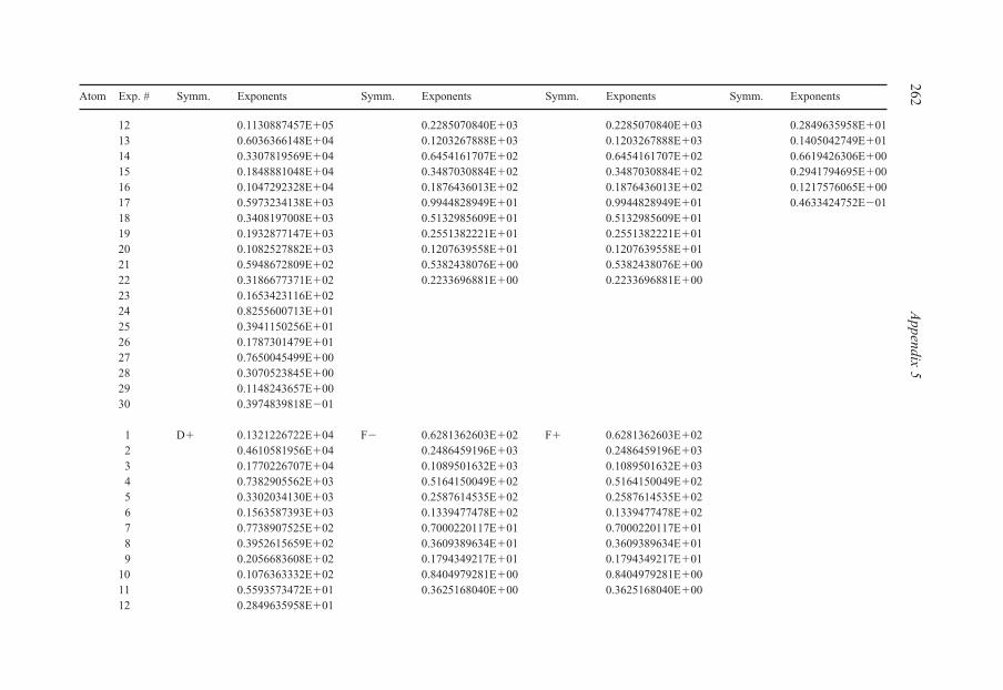
12 0.1130887457E�05 0.2285070840E�03 0.2285070840E�03 0.2849635958E�0113 0.6036366148E�04 0.1203267888E�03 0.1203267888E�03 0.1405042749E�0114 0.3307819569E�04 0.6454161707E�02 0.6454161707E�02 0.6619426306E�0015 0.1848881048E�04 0.3487030884E�02 0.3487030884E�02 0.2941794695E�0016 0.1047292328E�04 0.1876436013E�02 0.1876436013E�02 0.1217576065E�0017 0.5973234138E�03 0.9944828949E�01 0.9944828949E�01 0.4633424752E�0118 0.3408197008E�03 0.5132985609E�01 0.5132985609E�0119 0.1932877147E�03 0.2551382221E�01 0.2551382221E�0120 0.1082527882E�03 0.1207639558E�01 0.1207639558E�0121 0.5948672809E�02 0.5382438076E�00 0.5382438076E�0022 0.3186677371E�02 0.2233696881E�00 0.2233696881E�0023 0.1653423116E�0224 0.8255600713E�0125 0.3941150256E�0126 0.1787301479E�0127 0.7650045499E�0028 0.3070523845E�0029 0.1148243657E�0030 0.3974839818E�01
1 D� 0.1321226722E�04 F� 0.6281362603E�02 F� 0.6281362603E�022 0.4610581956E�04 0.2486459196E�03 0.2486459196E�033 0.1770226707E�04 0.1089501632E�03 0.1089501632E�034 0.7382905562E�03 0.5164150049E�02 0.5164150049E�025 0.3302034130E�03 0.2587614535E�02 0.2587614535E�026 0.1563587393E�03 0.1339477478E�02 0.1339477478E�027 0.7738907525E�02 0.7000220117E�01 0.7000220117E�018 0.3952615659E�02 0.3609389634E�01 0.3609389634E�019 0.2056683608E�02 0.1794349217E�01 0.1794349217E�01
10 0.1076363332E�02 0.8404979281E�00 0.8404979281E�0011 0.5593573472E�01 0.3625168040E�00 0.3625168040E�0012 0.2849635958E�01
262A
ppendix 5Atom Exp. # Symm. Exponents Symm. Exponents Symm. Exponents Symm. Exponents
Else_EAMC-TRSIC_appn5.qxd 5/19/2007 21:38 Page 262

13 0.1405042749E�0114 0.6619426306E�0015 0.2941794695E�0016 0.1217576065E�0017 0.4633424752E�01
Atom Exp. # Symm. Exponents Symm. Exponents Symm. Exponents Symm. Exponents
Ta 1 S� 0.4029653741E�09 P� 0.2543187682E�08 P� 0.2543187682E�08 D� 0.1976028565E�052 0.9938239359E�08 0.5384181130E�07 0.5384181130E�07 0.6791827243E�043 0.2719682560E�08 0.1307452284E�07 0.1307452284E�07 0.2577011130E�044 0.8202873159E�07 0.3601873342E�06 0.3601873342E�06 0.1065516102E�045 0.2708474590E�07 0.1113419683E�06 0.1113419683E�06 0.4739097095E�036 0.9724482495E�06 0.3819870912E�05 0.3819870912E�05 0.2238210202E�037 0.3771057637E�06 0.1438564305E�05 0.1438564305E�05 0.1108035354E�038 0.1568869260E�06 0.5882096434E�04 0.5882096434E�04 0.5675859739E�029 0.6955193604E�05 0.2582787845E�04 0.2582787845E�04 0.2969701441E�02
10 0.3263642301E�05 0.1204565796E�04 0.1204565796E�04 0.1566660272E�0211 0.1610047609E�05 0.5901861123E�03 0.5901861123E�03 0.8226130309E�0112 0.8294490067E�04 0.3004661668E�03 0.3004661668E�03 0.4243779988E�0113 0.4432282645E�04 0.1572105783E�03 0.1572105783E�03 0.2123364076E�0114 0.2440191782E�04 0.8361400346E�02 0.8361400346E�02 0.1017157503E�0115 0.1374836976E�04 0.4471145484E�02 0.4471145484E�02 0.4604917922E�0016 0.7873741509E�03 0.2377565998E�02 0.2377565998E�02 0.1944927122E�0017 0.4552875570E�03 0.1243517277E�02 0.1243517277E�02 0.7565024380E�0118 0.2640201435E�03 0.6327148027E�01 0.6327148027E�0119 0.1525130379E�03 0.3097651541E�01 0.3097651541E�0120 0.8717008760E�02 0.1443301256E�01 0.1443301256E�0121 0.4896554231E�02 0.6330131688E�00 0.6330131688E�0022 0.2685024205E�02 0.2584825883E�00 0.2584825883E�0023 0.1427619151E�0224 0.7310633692E�01
Appendix 5
263
(continued )
Else_EAMC-TRSIC_appn5.qxd 5/19/2007 21:38 Page 263

25 0.3581361447E�0126 0.1667107983E�0127 0.7324428239E�0028 0.3016825014E�0029 0.1157083981E�0030 0.4104780935E�01
1 D� 0.1976028565E�05 F� 0.9868407748E�03 F� 0.9868407748E�032 0.6791827243E�04 0.3859490338E�03 0.3859490338E�033 0.2577011130E�04 0.1662537720E�03 0.1662537720E�034 0.1065516102E�04 0.7718107692E�02 0.7718107692E�025 0.4739097095E�03 0.3778218218E�02 0.3778218218E�026 0.2238210202E�03 0.1908267347E�02 0.1908267347E�027 0.1108035354E�03 0.9729857447E�01 0.9729857447E�018 0.5675859739E�02 0.4900359179E�01 0.4900359179E�019 0.2969701441E�02 0.2385297907E�01 0.2385297907E�01
10 0.1566660272E�02 0.1097968090E�01 0.1097968090E�0111 0.8226130309E�01 0.4676363776E�00 0.4676363776E�0012 0.4243779988E�0113 0.2123364076E�0114 0.1017157503E�0115 0.4604917922E�0016 0.1944927122E�0017 0.7565024380E�01
Atom Exp. # Symm. Exponents Symm. Exponents Symm. Exponents Symm. Exponents
Ta 1 S� 0.4055824106E�09 P� 0.2257809132E�08 P� 0.2257809132E�08 D� 0.1587092359E�052 0.1007419648E�09 0.4780172024E�07 0.4780172024E�07 0.5671685668E�043 0.2774895370E�08 0.1161882792E�07 0.1161882792E�07 0.2222860718E�044 0.8418968500E�07 0.3206565157E�06 0.3206565157E�06 0.9434583323E�03
264A
ppendix 5Atom Exp. # Symm. Exponents Symm. Exponents Symm. Exponents Symm. Exponents
Else_EAMC-TRSIC_appn5.qxd 5/19/2007 21:38 Page 264

5 0.2794592056E�07 0.9937410617E�05 0.9937410617E�05 0.4282169015E�036 0.1008083266E�07 0.3420253378E�05 0.3420253378E�05 0.2052370309E�037 0.3925220217E�06 0.1292979580E�05 0.1292979580E�05 0.1025696116E�038 0.1638673653E�06 0.5309698411E�04 0.5309698411E�04 0.5278043921E�029 0.7285391988E�05 0.2342552356E�04 0.2342552356E�04 0.2761460405E�02
10 0.3426230461E�05 0.1098111612E�04 0.1098111612E�04 0.1450562361E�0211 0.1692990814E�05 0.5409259912E�03 0.5409259912E�03 0.7554156582E�0112 0.8730481565E�04 0.2769235336E�03 0.2769235336E�03 0.3851303874E�0113 0.4667008071E�04 0.1457165871E�03 0.1457165871E�03 0.1898112928E�0114 0.2568779609E�04 0.7794382063E�02 0.7794382063E�02 0.8929949360E�0015 0.1446019886E�04 0.4191547809E�02 0.4191547809E�02 0.3960124725E�0016 0.8268981104E�03 0.2241215692E�02 0.2241215692E�02 0.1634639101E�0017 0.4771239679E�03 0.1178435572E�02 0.1178435572E�02 0.6201664725E�0118 0.2759199826E�03 0.6026115515E�01 0.6026115515E�0119 0.1588469744E�03 0.2963977778E�01 0.2963977778E�0120 0.9042526695E�02 0.1386803017E�01 0.1386803017E�0121 0.5055765215E�02 0.6104546660E�00 0.6104546660E�0022 0.2757664494E�02 0.2500272388E�00 0.2500272388E�0023 0.1457553738E�0224 0.7414938079E�0125 0.3606296852E�0126 0.1665549692E�0127 0.7255495547E�0028 0.2961154828E�0029 0.1124633169E�0030 0.3948094905E�01
1 D� 0.1587092359E�05 F� 0.7007314780E�03 F� 0.7007314780E�032 0.5671685668E�04 0.2755704966E�03 0.2755704966E�033 0.2222860718E�04 0.1198161085E�03 0.1198161085E�034 0.9434583323E�03 0.5638900302E�02 0.5638900302E�025 0.4282169015E�03 0.2812325934E�02 0.2812325934E�026 0.2052370309E�03 0.1455205179E�02 0.1455205179E�02
Appendix 5
265
(continued )
Else_EAMC-TRSIC_appn5.qxd 5/19/2007 21:38 Page 265

7 0.1025696116E�03 0.7648309810E�01 0.7648309810E�018 0.5278043921E�02 0.3997465147E�01 0.3997465147E�019 0.2761460405E�02 0.2034122904E�01 0.2034122904E�01
10 0.1450562361E�02 0.9865936107E�00 0.9865936107E�0011 0.7554156582E�01 0.4465430423E�00 0.4465430423E�0012 0.3851303874E�0113 0.1898112928E�0114 0.8929949360E�0015 0.3960124725E�0016 0.1634639101E�0017 0.6201664725E�01
Atom Exp. # Symm. Exponents Symm. Exponents Symm. Exponents Symm. Exponents
W 1 S� 0.4030568474E�09 P� 0.2364696750E�07 P� 0.2364696750E�08 D� 0.2067899977E�052 0.1009191594E�09 0.4850572999E�07 0.4850572999E�07 0.7127031836E�043 0.2802465760E�08 0.1147948769E�07 0.1147948769E�07 0.2722426016E�044 0.8572617053E�07 0.3099260157E�06 0.3099260157E�06 0.1136755749E�045 0.2869062423E�07 0.9438300882E�05 0.9438300882E�05 0.5117258856E�036 0.1043439044E�07 0.3205708691E�05 0.3205708691E�05 0.2449414224E�037 0.4095828172E�06 0.1200723296E�05 0.1200723296E�05 0.1229524466E�038 0.1723498784E�06 0.4903934459E�04 0.4903934459E�04 0.6383482529E�029 0.7721859371E�05 0.2159351835E�04 0.2159351835E�04 0.3380797825E�02
10 0.3658655316E�05 0.1013615840E�04 0.1013615840E�04 0.1801429301E�0211 0.1820777397E�05 0.5015206119E�03 0.5015206119E�03 0.9524610147E�0112 0.9453116428E�04 0.2586210063E�03 0.2586210063E�03 0.4928385002E�0113 0.5085375235E�04 0.1374335023E�03 0.1374335023E�03 0.2461415589E�0114 0.2815450469E�04 0.7441653262E�02 0.7441653262E�02 0.1170263435E�0115 0.1593296922E�04 0.4059648573E�02 0.4059648573E�02 0.5223915727E�0016 0.9154118468E�03 0.2206194698E�02 0.2206194698E�02 0.2159324910E�00
266A
ppendix 5Atom Exp. # Symm. Exponents Symm. Exponents Symm. Exponents Symm. Exponents
Else_EAMC-TRSIC_appn5.qxd 5/19/2007 21:38 Page 266
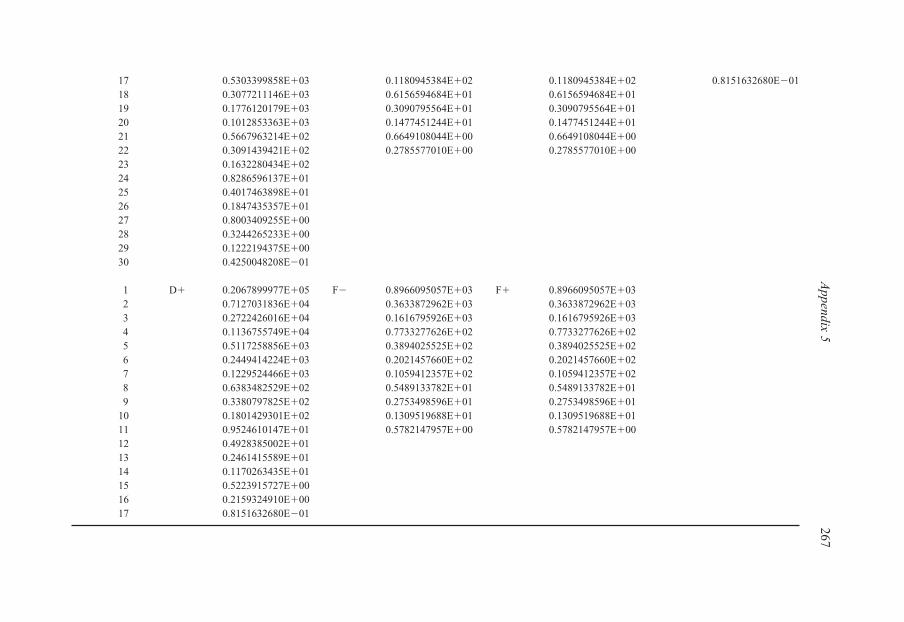
17 0.5303399858E�03 0.1180945384E�02 0.1180945384E�02 0.8151632680E�0118 0.3077211146E�03 0.6156594684E�01 0.6156594684E�0119 0.1776120179E�03 0.3090795564E�01 0.3090795564E�0120 0.1012853363E�03 0.1477451244E�01 0.1477451244E�0121 0.5667963214E�02 0.6649108044E�00 0.6649108044E�0022 0.3091439421E�02 0.2785577010E�00 0.2785577010E�0023 0.1632280434E�0224 0.8286596137E�0125 0.4017463898E�0126 0.1847435357E�0127 0.8003409255E�0028 0.3244265233E�0029 0.1222194375E�0030 0.4250048208E�01
1 D� 0.2067899977E�05 F� 0.8966095057E�03 F� 0.8966095057E�032 0.7127031836E�04 0.3633872962E�03 0.3633872962E�033 0.2722426016E�04 0.1616795926E�03 0.1616795926E�034 0.1136755749E�04 0.7733277626E�02 0.7733277626E�025 0.5117258856E�03 0.3894025525E�02 0.3894025525E�026 0.2449414224E�03 0.2021457660E�02 0.2021457660E�027 0.1229524466E�03 0.1059412357E�02 0.1059412357E�028 0.6383482529E�02 0.5489133782E�01 0.5489133782E�019 0.3380797825E�02 0.2753498596E�01 0.2753498596E�01
10 0.1801429301E�02 0.1309519688E�01 0.1309519688E�0111 0.9524610147E�01 0.5782147957E�00 0.5782147957E�0012 0.4928385002E�0113 0.2461415589E�0114 0.1170263435E�0115 0.5223915727E�0016 0.2159324910E�0017 0.8151632680E�01
Appendix 5
267
Else_EAMC-TRSIC_appn5.qxd 5/19/2007 21:38 Page 267
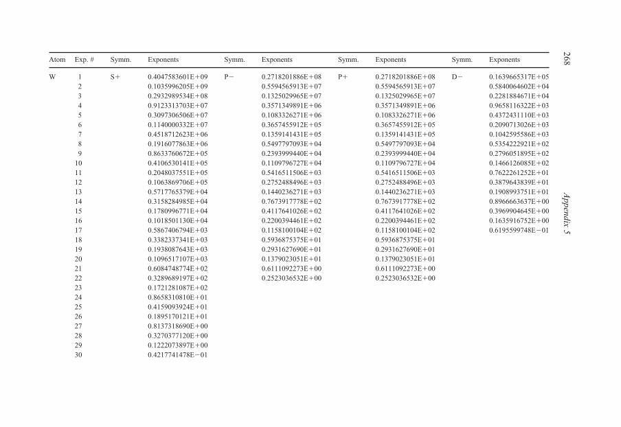
Atom Exp. # Symm. Exponents Symm. Exponents Symm. Exponents Symm. Exponents
W 1 S� 0.4047583601E�09 P� 0.2718201886E�08 P� 0.2718201886E�08 D� 0.1639665317E�052 0.1035996205E�09 0.5594565913E�07 0.5594565913E�07 0.5840064602E�043 0.2932989534E�08 0.1325029965E�07 0.1325029965E�07 0.2281884671E�044 0.9123313703E�07 0.3571349891E�06 0.3571349891E�06 0.9658116322E�035 0.3097306506E�07 0.1083326271E�06 0.1083326271E�06 0.4372431110E�036 0.1140000332E�07 0.3657455912E�05 0.3657455912E�05 0.2090713026E�037 0.4518712623E�06 0.1359141431E�05 0.1359141431E�05 0.1042595586E�038 0.1916077863E�06 0.5497797093E�04 0.5497797093E�04 0.5354222921E�029 0.8633760672E�05 0.2393999440E�04 0.2393999440E�04 0.2796051895E�02
10 0.4106530141E�05 0.1109796727E�04 0.1109796727E�04 0.1466126085E�0211 0.2048037551E�05 0.5416511506E�03 0.5416511506E�03 0.7622261252E�0112 0.1063869706E�05 0.2752488496E�03 0.2752488496E�03 0.3879643839E�0113 0.5717765379E�04 0.1440236271E�03 0.1440236271E�03 0.1908993751E�0114 0.3158284985E�04 0.7673917778E�02 0.7673917778E�02 0.8966663637E�0015 0.1780996771E�04 0.4117641026E�02 0.4117641026E�02 0.3969904645E�0016 0.1018501130E�04 0.2200394461E�02 0.2200394461E�02 0.1635916752E�0017 0.5867406794E�03 0.1158100104E�02 0.1158100104E�02 0.6195599748E�0118 0.3382337341E�03 0.5936875375E�01 0.5936875375E�0119 0.1938087643E�03 0.2931627690E�01 0.2931627690E�0120 0.1096517107E�03 0.1379023051E�01 0.1379023051E�0121 0.6084748774E�02 0.6111092273E�00 0.6111092273E�0022 0.3289689197E�02 0.2523036532E�00 0.2523036532E�0023 0.1721281087E�0224 0.8658310810E�0125 0.4159093924E�0126 0.1895170121E�0127 0.8137318690E�0028 0.3270377120E�0029 0.1222073897E�0030 0.4217741478E�01
268A
ppendix 5
Else_EAMC-TRSIC_appn5.qxd 5/19/2007 21:38 Page 268

1 D� 0.1639665317E�05 F� 0.7803787229E�03 F� 0.7803787229E�032 0.5840064602E�04 0.3016865533E�03 0.3016865533E�033 0.2281884671E�04 0.1292397088E�03 0.1292397088E�034 0.9658116322E�03 0.6004825531E�02 0.6004825531E�025 0.4372431110E�03 0.2961720982E�02 0.2961720982E�026 0.2090713026E�03 0.1517756626E�02 0.1517756626E�027 0.1042595586E�03 0.7909504920E�01 0.7909504920E�018 0.5354222921E�02 0.4102613005E�01 0.4102613005E�019 0.2796051895E�02 0.2073054949E�01 0.2073054949E�01
10 0.1466126085E�02 0.9987918860E�00 0.9987918860E�0011 0.7622261252E�01 0.4490844825E�00 0.4490844825E�0012 0.3879643839E�0113 0.1908993751E�0114 0.8966663637E�0015 0.3969904645E�0016 0.1635916752E�0017 0.6195599748E�01
AtomExp. # Symm. Exponents Symm. Exponents Symm. Exponents Symm. Exponents
Re 1 S� 0.4069415178E�09 P� 0.2512951096E�08 P� 0.2512951096E�08 D� 0.1907989292E�052 0.1043096748E�09 0.5195680795E�07 0.5195680795E�07 0.6303795739E�043 0.2958259343E�08 0.1237379184E�07 0.1237379184E�07 0.2342123823E�044 0.9220427258E�07 0.3356686553E�06 0.3356686553E�06 0.9636372504E�035 0.3137278546E�07 0.1025680576E�06 0.1025680576E�06 0.4323423773E�036 0.1157514475E�07 0.3491021737E�05 0.3491021737E�05 0.2082893287E�037 0.4599971955E�06 0.1308813524E�05 0.1308813524E�05 0.1061074093E�038 0.1955795417E�06 0.5344825296E�04 0.5344825296E�04 0.5628314635E�029 0.8837211241E�05 0.2351069642E�04 0.2351069642E�04 0.3061113828E�02
10 0.4215166220E�05 0.1101588599E�04 0.1101588599E�04 0.1680983828E�0211 0.2108171392E�05 0.5436771125E�03 0.5436771125E�03 0.9177936003E�0112 0.1098178539E�05 0.2794963032E�03 0.2794963032E�03 0.4906123063E�01
Appendix 5
269
(continued )
Else_EAMC-TRSIC_appn5.qxd 5/19/2007 21:38 Page 269
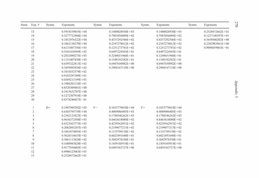
13 0.5918339855E�04 0.1480028930E�03 0.1480028930E�03 0.2528472662E�0114 0.3277712404E�04 0.7983056089E�02 0.7983056089E�02 0.1237140397E�0115 0.1852976322E�04 0.4337292546E�02 0.4337292546E�02 0.5658940202E�0016 0.1062138278E�04 0.2347278012E�02 0.2347278012E�02 0.2382983861E�0017 0.6131807356E�03 0.1251273781E�02 0.1251273781E�02 0.9096859063E�0118 0.3541410569E�03 0.6497224565E�01 0.6497224565E�0119 0.2032490275E�03 0.3249651960E�01 0.3249651960E�0120 0.1151407830E�03 0.1548192582E�01 0.1548192582E�0121 0.6395322813E�02 0.6947650982E�00 0.6947650982E�0022 0.3459492856E�02 0.2904167118E�00 0.2904167118E�0023 0.1810352579E�0224 0.9103297509E�0125 0.4369213199E�0126 0.1988203124E�0127 0.8520309401E�0028 0.3415632707E�0029 0.1272307918E�0030 0.4374240427E�01
1 D� 0.1907989292E�05 F� 0.1033779018E�04 F� 0.1033779018E�042 0.6303795739E�04 0.4089086405E�03 0.4089086405E�033 0.2342123823E�04 0.1788546262E�03 0.1788546262E�034 0.9636372504E�03 0.8463618080E�02 0.8463618080E�025 0.4323423773E�03 0.4239362951E�02 0.4239362951E�026 0.2082893287E�03 0.2199077213E�02 0.2199077213E�027 0.1061074093E�03 0.1155799138E�02 0.1155799138E�028 0.5628314635E�02 0.6021891640E�01 0.6021891640E�019 0.3061113828E�02 0.3042978350E�01 0.3042978350E�01
10 0.1680983828E�02 0.1459105914E�01 0.1459105914E�0111 0.9177936003E�01 0.6495363727E�00 0.6495363727E�0012 0.4906123063E�0113 0.2528472662E�01
270A
ppendix 5Atom Exp. # Symm. Exponents Symm. Exponents Symm. Exponents Symm. Exponents
Else_EAMC-TRSIC_appn5.qxd 5/19/2007 21:38 Page 270

14 0.1237140397E�0115 0.5658940202E�0016 0.2382983861E�0017 0.9096859063E�01
Atom Exp. # Symm. Exponents Symm. Exponents Symm. Exponents Symm. Exponents
Re 1 S� 0.4089684541E�09 P� 0.2596331943E�08 P� 0.2596331943E�08 D� 0.2017397237E�052 0.1020572413E�09 0.5398990794E�07 0.5398990794E�07 0.6599153746E�043 0.2825161456E�08 0.1291956836E�07 0.1291956836E�07 0.2424226036E�044 0.8616825148E�07 0.3518190647E�06 0.3518190647E�06 0.9849199852E�035 0.2876172803E�07 0.1078150987E�06 0.1078150987E�06 0.4358396098E�036 0.1043531310E�07 0.3676897732E�05 0.3676897732E�05 0.2068737024E�037 0.4087689825E�06 0.1379997085E�05 0.1379997085E�05 0.1037269610E�038 0.1717083645E�06 0.5636666509E�04 0.5636666509E�04 0.5410541505E�029 0.7682545911E�05 0.2477804102E�04 0.2477804102E�04 0.2891395212E�02
10 0.3636454840E�05 0.1159217558E�04 0.1159217558E�04 0.1559002323E�0211 0.1808713090E�05 0.5707805839E�03 0.5707805839E�03 0.8352444180E�0112 0.9389419446E�04 0.2925045266E�03 0.2925045266E�03 0.4378878050E�0113 0.5052944193E�04 0.1542794392E�03 0.1542794392E�03 0.2212327930E�0114 0.2799923030E�04 0.8282252629E�02 0.8282252629E�02 0.1060787691E�0115 0.1586728565E�04 0.4475141362E�02 0.4475141362E�02 0.4753950917E�0016 0.9134257937E�03 0.2406776753E�02 0.2406776753E�02 0.1961024870E�0017 0.5305387535E�03 0.1274056017E�02 0.1274056017E�02 0.7332779580E�0118 0.3088113768E�03 0.6564744162E�01 0.6564744162E�0119 0.1789208426E�03 0.3255941225E�01 0.3255941225E�0120 0.1024894516E�03 0.1537155054E�01 0.1537155054E�0121 0.5765103680E�02 0.6831153894E�00 0.6831153894E�0022 0.3163034436E�02 0.2825912002E�00 0.2825912002E�0023 0.1681236036E�0224 0.8598853690E�01
Appendix 5
271
(continued )
Else_EAMC-TRSIC_appn5.qxd 5/19/2007 21:38 Page 271
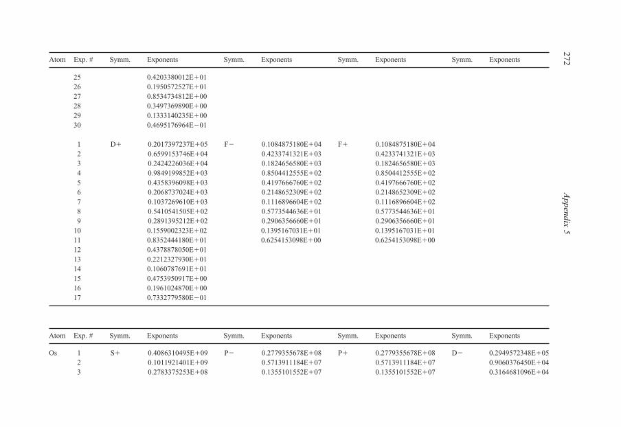
25 0.4203380012E�0126 0.1950572527E�0127 0.8534734812E�0028 0.3497369890E�0029 0.1333140235E�0030 0.4695176964E�01
1 D� 0.2017397237E�05 F� 0.1084875180E�04 F� 0.1084875180E�042 0.6599153746E�04 0.4233741321E�03 0.4233741321E�033 0.2424226036E�04 0.1824656580E�03 0.1824656580E�034 0.9849199852E�03 0.8504412555E�02 0.8504412555E�025 0.4358396098E�03 0.4197666760E�02 0.4197666760E�026 0.2068737024E�03 0.2148652309E�02 0.2148652309E�027 0.1037269610E�03 0.1116896604E�02 0.1116896604E�028 0.5410541505E�02 0.5773544636E�01 0.5773544636E�019 0.2891395212E�02 0.2906356660E�01 0.2906356660E�01
10 0.1559002323E�02 0.1395167031E�01 0.1395167031E�0111 0.8352444180E�01 0.6254153098E�00 0.6254153098E�0012 0.4378878050E�0113 0.2212327930E�0114 0.1060787691E�0115 0.4753950917E�0016 0.1961024870E�0017 0.7332779580E�01
Atom Exp. # Symm. Exponents Symm. Exponents Symm. Exponents Symm. Exponents
Os 1 S� 0.4086310495E�09 P� 0.2779355678E�08 P� 0.2779355678E�08 D� 0.2949572348E�052 0.1011921401E�09 0.5713911184E�07 0.5713911184E�07 0.9060376450E�043 0.2783375253E�08 0.1355101552E�07 0.1355101552E�07 0.3164681096E�04
272A
ppendix 5Atom Exp. # Symm. Exponents Symm. Exponents Symm. Exponents Symm. Exponents
Else_EAMC-TRSIC_appn5.qxd 5/19/2007 21:38 Page 272

4 0.8445672772E�07 0.3665684720E�06 0.3665684720E�06 0.1236689001E�045 0.2807774293E�07 0.1118353739E�06 0.1118353739E�06 0.5319712894E�036 0.1015742293E�07 0.3804871617E�05 0.3804871617E�05 0.2478354083E�037 0.3971240807E�06 0.1427359791E�05 0.1427359791E�05 0.1230371588E�038 0.1666549431E�06 0.5837883945E�04 0.5837883945E�04 0.6404088535E�029 0.7455682618E�05 0.2573960706E�04 0.2573960706E�04 0.3438561287E�02
10 0.3531521105E�05 0.1209675083E�04 0.1209675083E�04 0.1873893629E�0211 0.1759014123E�05 0.5991724462E�03 0.5991724462E�03 0.1019793261E�0212 0.9150354480E�04 0.3092766395E�03 0.3092766395E�03 0.5452914563E�0113 0.4937368348E�04 0.1644941652E�03 0.1644941652E�03 0.2818674430E�0114 0.2744543391E�04 0.8913697318E�02 0.8913697318E�02 0.1385833706E�0115 0.1560952123E�04 0.4865922440E�02 0.4865922440E�02 0.6376430357E�0016 0.9021565730E�03 0.2645868806E�02 0.2645868806E�02 0.2701436306E�0017 0.5262293321E�03 0.1416978184E�02 0.1416978184E�02 0.1036842450E�0018 0.3076783453E�03 0.7390020876E�01 0.7390020876E�0119 0.1790917172E�03 0.3711177441E�01 0.3711177441E�0120 0.1030715260E�03 0.1774423321E�01 0.1774423321E�0121 0.5825248974E�02 0.7986897779E�00 0.7986897779E�0022 0.3210929757E�02 0.3346341793E�00 0.3346341793E�0023 0.1714413548E�0224 0.8806367243E�0125 0.4322175109E�0126 0.2013076282E�0127 0.8836867838E�0028 0.3631154159E�0029 0.1387161923E�0030 0.4892983167E�01
1 D� 0.2949572348E�05 F� 0.1080012686E�04 F� 0.1080012686E�042 0.9060376450E�04 0.4039400774E�03 0.4039400774E�033 0.3164681096E�04 0.1702401381E�03 0.1702401381E�034 0.1236689001E�04 0.7888949721E�02 0.7888949721E�025 0.5319712894E�03 0.3922327892E�02 0.3922327892E�02
Appendix 5
273
(continued )
Else_EAMC-TRSIC_appn5.qxd 5/19/2007 21:38 Page 273

6 0.2478354083E�03 0.2041697340E�02 0.2041697340E�027 0.1230371588E�03 0.1085717565E�02 0.1085717565E�028 0.6404088535E�02 0.5755402161E�01 0.5755402161E�019 0.3438561287E�02 0.2967721023E�01 0.2967721023E�01
10 0.1873893629E�02 0.1452493953E�01 0.1452493953E�0111 0.1019793261E�02 0.6584226020E�00 0.6584226020E�0012 0.5452914563E�0113 0.2818674430E�0114 0.1385833706E�0115 0.6376430357E�0016 0.2701436306E�0017 0.1036842450E�00
Atom Exp. # Symm. Exponents Symm. Exponents Symm. Exponents Symm. Exponents
Os 1 S� 0.4031388801E�09 P� 0.2376389891E�08 P� 0.2376389891E�08 D� 0.2283588616E�052 0.1004703500E�09 0.4960325502E�07 0.4960325502E�07 0.7323833946E�043 0.2779230465E�08 0.1192761758E�07 0.1192761758E�07 0.2649987879E�044 0.8475391516E�07 0.3267151052E�06 0.3267151052E�06 0.1064948796E�045 0.2830014640E�07 0.1008039678E�06 0.1008039678E�06 0.4679373044E�036 0.1027676545E�07 0.3464175398E�05 0.3464175398E�05 0.2213173061E�037 0.4030957331E�06 0.1311163588E�05 0.1311163588E�05 0.1109191436E�038 0.1696247012E�06 0.5404674901E�04 0.5404674901E�04 0.5799034978E�029 0.7605788994E�05 0.2399158208E�04 0.2399158208E�04 0.3113563292E�02
10 0.3609265886E�05 0.1134085359E�04 0.1134085359E�04 0.1690079290E�0211 0.1800354597E�05 0.5644832658E�03 0.5644832658E�03 0.9130583552E�0112 0.9375769946E�04 0.2925471014E�03 0.2925471014E�03 0.4833110504E�0113 0.5063032241E�04 0.1560992636E�03 0.1560992636E�03 0.2467665627E�0114 0.2815881974E�04 0.8479830364E�02 0.8479830364E�02 0.1196387749E�0115 0.1602003094E�04 0.4637411743E�02 0.4637411743E�02 0.5422234836E�00
274A
ppendix 5Atom Exp. # Symm. Exponents Symm. Exponents Symm. Exponents Symm. Exponents
Else_EAMC-TRSIC_appn5.qxd 5/19/2007 21:38 Page 274

16 0.9259820040E�03 0.2524569093E�02 0.2524569093E�02 0.2261518115E�0017 0.5401037335E�03 0.1352828995E�02 0.1352828995E�02 0.8545389502E�0118 0.3157420277E�03 0.7056080244E�01 0.7056080244E�0119 0.1837440708E�03 0.3542174996E�01 0.3542174996E�0120 0.1057219449E�03 0.1692323311E�01 0.1692323311E�0121 0.5973556398E�02 0.7608944381E�00 0.7608944381E�0022 0.3292016107E�02 0.3183568212E�00 0.3183568212E�0023 0.1757507705E�0224 0.9027842444E�0125 0.4431668801E�0126 0.2064868301E�0127 0.9069937587E�0028 0.3730338688E�0029 0.1426820693E�0030 0.5040955311E�01
1 D� 0.2283588616E�05 F� 0.1116959292E�04 F� 0.1116959292E�042 0.7323833946E�04 0.4209006657E�03 0.4209006657E�033 0.2649987879E�04 0.1779745014E�03 0.1779745014E�034 0.1064948796E�04 0.8245508897E�02 0.8245508897E�025 0.4679373044E�03 0.4086996385E�02 0.4086996385E�026 0.2213173061E�03 0.2116234324E�02 0.2116234324E�027 0.1109191436E�03 0.1117741995E�02 0.1117741995E�028 0.5799034978E�02 0.5880080863E�01 0.5880080863E�019 0.3113563292E�02 0.3008392843E�01 0.3008392843E�01
10 0.1690079290E�02 0.1461641668E�01 0.1461641668E�0111 0.9130583552E�01 0.6584882141E�00 0.6584882141E�0012 0.4833110504E�0113 0.2467665627E�0114 0.1196387749E�0115 0.5422234836E�0016 0.2261518115E�0017 0.8545389502E�01
Appendix 5
275
Else_EAMC-TRSIC_appn5.qxd 5/19/2007 21:38 Page 275

AtomExp. # Symm. Exponents Symm. Exponents Symm. Exponents Symm. Exponents
Ir 1 S� 0.4073057026E�09 P� 0.2897100048E�08 P� 0.2897100048E�08 D� 0.2622620477E�052 0.1000535733E�09 0.5809391499E�07 0.5809391499E�07 0.8065785105E�043 0.2732287892E�08 0.1347405577E�07 0.1347405577E�07 0.2830235468E�044 0.8237862313E�07 0.3573677231E�06 0.3573677231E�06 0.1114478071E�045 0.2723386582E�07 0.1071594170E�06 0.1071594170E�06 0.4843974358E�036 0.9804449794E�06 0.3591634516E�05 0.3591634516E�05 0.2285713570E�037 0.3817409989E�06 0.1330299574E�05 0.1330299574E�05 0.1151701028E�038 0.1596461704E�06 0.5383330373E�04 0.5383330373E�04 0.6094863617E�029 0.7122046447E�05 0.2353128393E�04 0.2353128393E�04 0.3331983430E�02
10 0.3366046964E�05 0.1098454239E�04 0.1098454239E�04 0.1850821734E�0211 0.1673852130E�05 0.5413882335E�03 0.5413882335E�03 0.1027442624E�0212 0.8697772262E�04 0.2785318724E�03 0.2785318724E�03 0.5606477849E�0113 0.4690352422E�04 0.1478866502E�03 0.1478866502E�03 0.2957811543E�0114 0.2606885137E�04 0.8011609555E�02 0.8011609555E�02 0.1483908282E�0115 0.1483097726E�04 0.4378204625E�02 0.4378204625E�02 0.6963187698E�0016 0.8577516661E�03 0.2386198425E�02 0.2386198425E�02 0.3005951317E�0017 0.5008524196E�03 0.1282330636E�02 0.1282330636E�02 0.1174185990E�0018 0.2932424656E�03 0.6717770911E�01 0.6717770911E�0119 0.1709721233E�03 0.3391804511E�01 0.3391804511E�0120 0.9858652983E�02 0.1631795136E�01 0.1631795136E�0121 0.5583623974E�02 0.7395684842E�00 0.7395684842E�0022 0.3084846301E�02 0.3121891771E�00 0.3121891771E�0023 0.1651133383E�0224 0.8503045869E�0125 0.4184302727E�0126 0.1954071097E�0127 0.8600798808E�0028 0.3543487100E�0029 0.1357153713E�0030 0.4798945460E�01
276A
ppendix 5
Else_EAMC-TRSIC_appn5.qxd 5/19/2007 21:38 Page 276

1 D� 0.2622620477E�05 F� 0.9586109805E�03 F� 0.9586109805E�032 0.8065785105E�04 0.3683769739E�03 0.3683769739E�033 0.2830235468E�04 0.1591151033E�03 0.1591151033E�034 0.1114478071E�04 0.7535830800E�02 0.7535830800E�025 0.4843974358E�03 0.3817540295E�02 0.3817540295E�026 0.2285713570E�03 0.2017905530E�02 0.2017905530E�027 0.1151701028E�03 0.1085712138E�02 0.1085712138E�028 0.6094863617E�02 0.5800389666E�01 0.5800389666E�019 0.3331983430E�02 0.3001651125E�01 0.3001651125E�01
10 0.1850821734E�02 0.1467762463E�01 0.1467762463E�0111 0.1027442624E�02 0.6615700121E�00 0.6615700121E�0012 0.5606477849E�0113 0.2957811543E�0114 0.1483908282E�0115 0.6963187698E�0016 0.3005951317E�0017 0.1174185990E�00
Atom Exp. # Symm. Exponents Symm. Exponents Symm. Exponents Symm. Exponents
Ir 1 S� 0.4048743529E�09 P� 0.2420551978E�08 P� 0.2420551978E�08 D� 0.2353755986E�052 0.1003387811E�09 0.5052664329E�07 0.5052664329E�07 0.7622930683E�043 0.2761218824E�08 0.1213878071E�07 0.1213878071E�07 0.2787338430E�044 0.8380151754E�07 0.3319289005E�06 0.3319289005E�06 0.1132588257E�045 0.2785849158E�07 0.1021638496E�06 0.1021638496E�06 0.5033573880E�036 0.1007519757E�07 0.3500244719E�05 0.3500244719E�05 0.2408298429E�037 0.3937090588E�06 0.1320125879E�05 0.1320125879E�05 0.1220902662E�038 0.1651044236E�06 0.5420194294E�04 0.5420194294E�04 0.6454997574E�029 0.7379706329E�05 0.2395872684E�04 0.2395872684E�04 0.3503183217E�02
10 0.3491822199E�05 0.1127531768E�04 0.1127531768E�04 0.1920829277E�0211 0.1737134471E�05 0.5586975987E�03 0.5586975987E�03 0.1047324467E�0212 0.9024406146E�04 0.2882534990E�03 0.2882534990E�03 0.5589175167E�01
Appendix 5
277
(continued )
Else_EAMC-TRSIC_appn5.qxd 5/19/2007 21:38 Page 277

13 0.4862317429E�04 0.1531401026E�03 0.1531401026E�03 0.2873396792E�0114 0.2698628276E�04 0.8284887970E�02 0.8284887970E�02 0.1400658675E�0115 0.1532334262E�04 0.4513718859E�02 0.4513718859E�02 0.6371846141E�0016 0.8841180306E�03 0.2449059443E�02 0.2449059443E�02 0.2662575424E�0017 0.5148122542E�03 0.1308723503E�02 0.1308723503E�02 0.1005888058E�0018 0.3004726867E�03 0.6811566940E�01 0.6811566940E�0119 0.1745879331E�03 0.3414786108E�01 0.3414786108E�0120 0.1003025903E�03 0.1630662674E�01 0.1630662674E�0121 0.5658930744E�02 0.7335263175E�00 0.7335263175E�0022 0.3113985007E�02 0.3073866579E�00 0.3073866579E�0023 0.1659946789E�0224 0.8513397865E�0125 0.4172327698E�0126 0.1940690196E�0127 0.8508870932E�0028 0.3492699215E�0029 0.1333090294E�0030 0.4698970067E�01
1 D� 0.2353755986E�05 F� 0.1107522476E�04 F� 0.1107522476E�042 0.7622930683E�04 0.4132858342E�03 0.4132858342E�033 0.2787338430E�04 0.1734823240E�03 0.1734823240E�034 0.1132588257E�04 0.7999551998E�02 0.7999551998E�025 0.5033573880E�03 0.3957134435E�02 0.3957134435E�026 0.2408298429E�03 0.2050688191E�02 0.2050688191E�027 0.1220902662E�03 0.1087229243E�02 0.1087229243E�028 0.6454997574E�02 0.5758962760E�01 0.5758962760E�019 0.3503183217E�02 0.2976240679E�01 0.2976240679E�01
10 0.1920829277E�02 0.1465518960E�01 0.1465518960E�0111 0.1047324467E�02 0.6714496186E�00 0.6714496186E�0012 0.5589175167E�0113 0.2873396792E�01
278A
ppendix 5Atom Exp. # Symm. Exponents Symm. Exponents Symm. Exponents Symm. Exponents
Else_EAMC-TRSIC_appn5.qxd 5/19/2007 21:38 Page 278
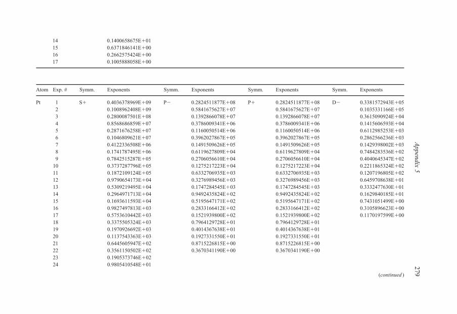
14 0.1400658675E�0115 0.6371846141E�0016 0.2662575424E�0017 0.1005888058E�00
Atom Exp. # Symm. Exponents Symm. Exponents Symm. Exponents Symm. Exponents
Pt 1 S� 0.4036378969E�09 P� 0.2824511877E�08 P� 0.2824511877E�08 D� 0.3381572943E�052 0.1008962408E�09 0.5841675627E�07 0.5841675627E�07 0.1035331166E�053 0.2800087501E�08 0.1392866078E�07 0.1392866078E�07 0.3615090924E�044 0.8568686859E�07 0.3786009341E�06 0.3786009341E�06 0.1415606593E�045 0.2871676258E�07 0.1160050514E�06 0.1160050514E�06 0.6112985253E�036 0.1046809621E�07 0.3962027867E�05 0.3962027867E�05 0.2862566236E�037 0.4122336508E�06 0.1491509626E�05 0.1491509626E�05 0.1429398002E�038 0.1741787495E�06 0.6119627809E�04 0.6119627809E�04 0.7484283536E�029 0.7842515287E�05 0.2706056610E�04 0.2706056610E�04 0.4040645347E�02
10 0.3737287796E�05 0.1275217223E�04 0.1275217223E�04 0.2211865324E�0211 0.1872109124E�05 0.6332706935E�03 0.6332706935E�03 0.1207196805E�0212 0.9790654173E�04 0.3276989456E�03 0.3276989456E�03 0.6459708638E�0113 0.5309219495E�04 0.1747284545E�03 0.1747284545E�03 0.3332477630E�0114 0.2964971713E�04 0.9492435824E�02 0.9492435824E�02 0.1629840185E�0115 0.1693611593E�04 0.5195647171E�02 0.5195647171E�02 0.7431051499E�0016 0.9827497813E�03 0.2833166412E�02 0.2833166412E�02 0.3105896623E�0017 0.5753610442E�03 0.1521939800E�02 0.1521939800E�02 0.1170197599E�0018 0.3375505324E�03 0.7964129728E�01 0.7964129728E�0119 0.1970926692E�03 0.4014367638E�01 0.4014367638E�0120 0.1137543363E�03 0.1927331550E�01 0.1927331550E�0121 0.6445605947E�02 0.8715226815E�00 0.8715226815E�0022 0.3561150502E�02 0.3670341190E�00 0.3670341190E�0023 0.1905373746E�0224 0.9805410548E�01
Appendix 5
279
(continued )
Else_EAMC-TRSIC_appn5.qxd 5/19/2007 21:38 Page 279

25 0.4820361727E�0126 0.2248299709E�0127 0.9881479901E�0028 0.4064578138E�0029 0.1554057721E�0030 0.5485414903E�01
1 D� 0.3381572943E�05 F� 0.1265788055E�04 F� 0.1265788055E�042 0.1035331166E�05 0.4549376132E�03 0.4549376132E�033 0.3615090924E�04 0.1863037997E�03 0.1863037997E�034 0.1415606593E�04 0.8466684842E�02 0.8466684842E�025 0.6112985253E�03 0.4158815825E�02 0.4158815825E�026 0.2862566236E�03 0.2150470015E�02 0.2150470015E�027 0.1429398002E�03 0.1140111439E�02 0.1140111439E�028 0.7484283536E�02 0.6036069343E�01 0.6036069343E�019 0.4040645347E�02 0.3108114015E�01 0.3108114015E�01
10 0.2211865324E�02 0.1516066547E�01 0.1516066547E�0111 0.1207196805E�02 0.6822774033E�00 0.6822774033E�0012 0.6459708638E�0113 0.3332477630E�0114 0.1629840185E�0115 0.7431051499E�0016 0.3105896623E�0017 0.1170197599E�00
Atom Exp. # Symm. Exponents Symm. Exponents Symm. Exponents Symm. Exponents
Pt 1 S� 0.4025108442E�09 P� 0.2521709505E�08 P� 0.2521709505E�08 D� 0.2983846478E�052 0.1003914263E�09 0.5257627178E�07 0.5257627178E�07 0.8927434537E�043 0.2778631465E�08 0.1261105378E�07 0.1261105378E�07 0.3061904062E�04
280A
ppendix 5Atom Exp. # Symm. Exponents Symm. Exponents Symm. Exponents Symm. Exponents
Else_EAMC-TRSIC_appn5.qxd 5/19/2007 21:38 Page 280
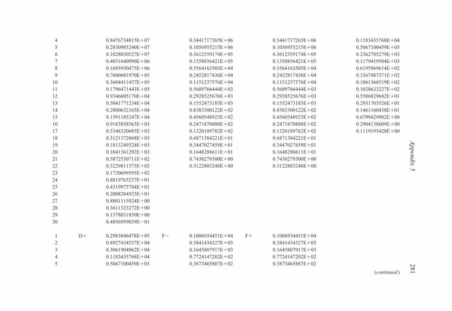
4 0.8476734815E�07 0.3441717265E�06 0.3441717265E�06 0.1183435768E�045 0.2830985240E�07 0.1056955215E�06 0.1056955215E�06 0.5067100459E�036 0.1028030527E�07 0.3612359174E�05 0.3612359174E�05 0.2362705279E�037 0.4031640990E�06 0.1358856421E�05 0.1358856421E�05 0.1179419504E�038 0.1695950475E�06 0.5564163505E�04 0.5564163505E�04 0.6195969614E�029 0.7600601970E�05 0.2452817436E�04 0.2452817436E�04 0.3367487371E�02
10 0.3604411457E�05 0.1151237576E�04 0.1151237576E�04 0.1861366519E�0211 0.1796471443E�05 0.5689766444E�03 0.5689766444E�03 0.1028633227E�0212 0.9346605170E�04 0.2928525676E�03 0.2928525676E�03 0.5586829682E�0113 0.5041771234E�04 0.1552473183E�03 0.1552473183E�03 0.2931703526E�0114 0.2800632165E�04 0.8383300122E�02 0.8383300122E�02 0.1461160438E�0115 0.1591185247E�04 0.4560548923E�02 0.4560548923E�02 0.6799429902E�0016 0.9183858563E�03 0.2471870888E�02 0.2471870888E�02 0.2904138609E�0017 0.5348320685E�03 0.1320189782E�02 0.1320189782E�02 0.1119195428E�0018 0.3121372068E�03 0.6871384221E�01 0.6871384221E�0119 0.1813249324E�03 0.3447027459E�01 0.3447027459E�0120 0.1041361292E�03 0.1648288611E�01 0.1648288611E�0121 0.5872530711E�02 0.7430279300E�00 0.7430279300E�0022 0.3229811373E�02 0.3122883248E�00 0.3122883248E�0023 0.1720699595E�0224 0.8819765237E�0125 0.4319973704E�0126 0.2008284923E�0127 0.8801115824E�0028 0.3611323272E�0029 0.1378031850E�0030 0.4856959039E�01
1 D� 0.2983846478E�05 F� 0.1006934451E�04 F� 0.1006934451E�042 0.8927434537E�04 0.3841434327E�03 0.3841434327E�033 0.3061904062E�04 0.1645807917E�03 0.1645807917E�034 0.1183435768E�04 0.7724147202E�02 0.7724147202E�025 0.5067100459E�03 0.3873465887E�02 0.3873465887E�02
Appendix 5
281
(continued )
Else_EAMC-TRSIC_appn5.qxd 5/19/2007 21:38 Page 281

6 0.2362705279E�03 0.2024505065E�02 0.2024505065E�027 0.1179419504E�03 0.1075722064E�02 0.1075722064E�028 0.6195969614E�02 0.5668073872E�01 0.5668073872E�019 0.3367487371E�02 0.2888798712E�01 0.2888798712E�01
10 0.1861366519E�02 0.1389112936E�01 0.1389112936E�0111 0.1028633227E�02 0.6147357389E�00 0.6147357389E�0012 0.5586829682E�0113 0.2931703526E�0114 0.1461160438E�0115 0.6799429902E�0016 0.2904138609E�0017 0.1119195428E�00
Atom Exp. # Symm. Exponents Symm. Exponents Symm. Exponents Symm. Exponents
Au 1 S� 0.4066823958E�09 P� 0.2785253005E�08 P� 0.2785253005E�08 D� 0.3948673620E�052 0.1021690667E�09 0.5682581802E�07 0.5682581802E�07 0.1159557137E�053 0.2848020759E�08 0.1339283582E�07 0.1339283582E�07 0.3916070420E�044 0.8749285699E�07 0.3605306047E�06 0.3605306047E�06 0.1494755394E�045 0.2942075545E�07 0.1096103112E�06 0.1096103112E�06 0.6337163824E�036 0.1075555604E�07 0.3721322475E�05 0.3721322475E�05 0.2932707705E�037 0.4245763424E�06 0.1395008201E�05 0.1395008201E�05 0.1455913385E�038 0.1797498940E�06 0.5709350619E�04 0.5709350619E�04 0.7619721221E�029 0.8106202961E�05 0.2522458942E�04 0.2522458942E�04 0.4131647697E�02
10 0.3867660398E�05 0.1189558691E�04 0.1189558691E�04 0.2281035327E�0211 0.1939131562E�05 0.5920644139E�03 0.5920644139E�03 0.1260111981E�0212 0.1014706281E�05 0.3075178271E�03 0.3075178271E�03 0.6845395473E�0113 0.5504192395E�04 0.1648112411E�03 0.1648112411E�03 0.3593718790E�0114 0.3074065363E�04 0.9011881968E�02 0.9011881968E�02 0.1791800503E�0115 0.1755678031E�04 0.4971108379E�02 0.4971108379E�02 0.8338330533E�00
282A
ppendix 5Atom Exp. # Symm. Exponents Symm. Exponents Symm. Exponents Symm. Exponents
Else_EAMC-TRSIC_appn5.qxd 5/19/2007 21:38 Page 282

16 0.1018438923E�04 0.2735249698E�02 0.2735249698E�02 0.3559232184E�0017 0.5959769882E�03 0.1484375151E�02 0.1484375151E�02 0.1369509868E�0018 0.3494414609E�03 0.7855797148E�01 0.7855797148E�0119 0.2038993605E�03 0.4008978001E�01 0.4008978001E�0120 0.1175979731E�03 0.1950611822E�01 0.1950611822E�0121 0.6658438638E�02 0.8947438792E�00 0.8947438792E�0022 0.3676034772E�02 0.3825729542E�00 0.3825729542E�0023 0.1965474956E�0224 0.1010839407E�0225 0.4966719243E�0126 0.2315665930E�0127 0.1017529714E�0128 0.4185325556E�0029 0.1600546853E�0030 0.5652109815E�01
1 D� 0.3948673620E�05 F� 0.9710235157E�03 F� 0.9710235157E�032 0.1159557137E�05 0.3731582036E�03 0.3731582036E�033 0.3916070420E�04 0.1612172712E�03 0.1612172712E�034 0.1494755394E�04 0.7636023630E�02 0.7636023630E�025 0.6337163824E�03 0.3866712529E�02 0.3866712529E�026 0.2932707705E�03 0.2041348862E�02 0.2041348862E�027 0.1455913385E�03 0.1095658214E�02 0.1095658214E�028 0.7619721221E�02 0.5830385732E�01 0.5830385732E�019 0.4131647697E�02 0.2999615562E�01 0.2999615562E�01
10 0.2281035327E�02 0.1454996094E�01 0.1454996094E�0111 0.1260111981E�02 0.6488850608E�00 0.6488850608E�0012 0.6845395473E�0113 0.3593718790E�0114 0.1791800503E�0115 0.8338330533E�0016 0.3559232184E�0017 0.1369509868E�00
Appendix 5
283
Else_EAMC-TRSIC_appn5.qxd 5/19/2007 21:38 Page 283

Atom Exp. # Symm. Exponents Symm. Exponents Symm. Exponents Symm. Exponents
Au 1 S� 0.4077830191E�09 P� 0.2655938944E�08 P� 0.2655938944E�08 D� 0.2945225745E�052 0.1010482232E�09 0.5538783723E�07 0.5538783723E�07 0.9011200977E�043 0.2781034561E�08 0.1328954856E�07 0.1328954856E�07 0.3152846805E�044 0.8442953849E�07 0.3628284947E�06 0.3628284947E�06 0.1240026481E�045 0.2808179948E�07 0.1114766015E�06 0.1114766015E�06 0.5389130971E�036 0.1016319144E�07 0.3812001514E�05 0.3812001514E�05 0.2544005214E�037 0.3975045430E�06 0.1434845885E�05 0.1434845885E�05 0.1282273087E�038 0.1668756881E�06 0.5879442313E�04 0.5879442313E�04 0.6783567019E�029 0.7468187101E�05 0.2593830137E�04 0.2593830137E�04 0.3702563940E�02
10 0.3538674543E�05 0.1218476867E�04 0.1218476867E�04 0.2049583707E�0211 0.1763199807E�05 0.6027805629E�03 0.6027805629E�03 0.1131095280E�0212 0.9175507159E�04 0.3105726607E�03 0.3105726607E�03 0.6117231963E�0113 0.4952887142E�04 0.1648257552E�03 0.1648257552E�03 0.3187019553E�0114 0.2754347650E�04 0.8911291103E�02 0.8911291103E�02 0.1572317754E�0115 0.1567267807E�04 0.4854066586E�02 0.4854066586E�02 0.7220603740E�0016 0.9062832823E�03 0.2634609216E�02 0.2634609216E�02 0.3034143382E�0017 0.5289482541E�03 0.1409184636E�02 0.1409184636E�02 0.1146779376E�0018 0.3094731921E�03 0.7346096758E�01 0.7346096758E�0119 0.1802709192E�03 0.3691290951E�01 0.3691290951E�0120 0.1038372716E�03 0.1768188809E�01 0.1768188809E�0121 0.5874054675E�02 0.7985526578E�00 0.7985526578E�0022 0.3241245944E�02 0.3362783289E�00 0.3362783289E�0023 0.1732636416E�0224 0.8911616811E�0125 0.4380173861E�0126 0.2043356472E�0127 0.8985599018E�0028 0.3699407760E�0029 0.1416223541E�0030 0.5007004900E�01
284A
ppendix 5
Else_EAMC-TRSIC_appn5.qxd 5/19/2007 21:38 Page 284

1 D� 0.2945225745E�05 F� 0.8572354967E�03 F� 0.8572354967E�032 0.9011200977E�04 0.3339664579E�03 0.3339664579E�033 0.3152846805E�04 0.1459968492E�03 0.1459968492E�034 0.1240026481E�04 0.6984674979E�02 0.6984674979E�025 0.5389130971E�03 0.3566441980E�02 0.3566441980E�026 0.2544005214E�03 0.1895546858E�02 0.1895546858E�027 0.1282273087E�03 0.1022747540E�02 0.1022747540E�028 0.6783567019E�02 0.5463375835E�01 0.5463375835E�019 0.3702563940E�02 0.2817971411E�01 0.2817971411E�01
10 0.2049583707E�02 0.1368734195E�01 0.1368734195E�0111 0.1131095280E�02 0.6105663114E�00 0.6105663114E�0012 0.6117231963E�0113 0.3187019553E�0114 0.1572317754E�0115 0.7220603740E�0016 0.3034143382E�0017 0.1146779376E�00
Atom Exp. # Symm. Exponents Symm. Exponents Symm. Exponents Symm. Exponents
Hg 1 S� 0.4082595892E�09 P� 0.2519545305E�08 P� 0.2519545305E�08 D� 0.3096414137E�052 0.1020218335E�09 0.5216082410E�07 0.5216082410E�07 0.9372516661E�043 0.2830329863E�08 0.1245938840E�07 0.1245938840E�07 0.3255952821E�044 0.8657800273E�07 0.3395209340E�06 0.3395209340E�06 0.1275788592E�045 0.2900307411E�07 0.1043617821E�06 0.1043617821E�06 0.5541305326E�036 0.1056783060E�07 0.3577742321E�05 0.3577742321E�05 0.2621997227E�037 0.4159799276E�06 0.1352560863E�05 0.1352560863E�05 0.1328290857E�038 0.1756883683E�06 0.5575352189E�04 0.5575352189E�04 0.7080256192E�029 0.7907462234E�05 0.2477667776E�04 0.2477667776E�04 0.3902596240E�02
10 0.3766986873E�05 0.1173698798E�04 0.1173698798E�04 0.2186055368E�0211 0.1886484891E�05 0.5860040434E�03 0.5860040434E�03 0.1222997603E�0212 0.9864025359E�04 0.3049035466E�03 0.3049035466E�03 0.6715850084E�01
Appendix 5
285
(continued )
Else_EAMC-TRSIC_appn5.qxd 5/19/2007 21:38 Page 285

13 0.5348549680E�04 0.1634668880E�03 0.1634668880E�03 0.3557470810E�0114 0.2987020986E�04 0.8928738704E�02 0.8928738704E�02 0.1786490409E�0115 0.1706476374E�04 0.4912821414E�02 0.4912821414E�02 0.8358590525E�0016 0.9905158581E�03 0.2692402162E�02 0.2692402162E�02 0.3580902163E�0017 0.5801778088E�03 0.1453130165E�02 0.1453130165E�02 0.1380488938E�0018 0.3405953403E�03 0.7636815263E�01 0.7636815263E�0119 0.1990368910E�03 0.3864121519E�01 0.3864121519E�0120 0.1149966333E�03 0.1861262104E�01 0.1861262104E�0121 0.6524281967E�02 0.8438594296E�00 0.8438594296E�0022 0.3610071047E�02 0.3560623375E�00 0.3560623375E�0023 0.1934967108E�0224 0.9978048635E�0125 0.4916671790E�0126 0.2299268941E�0127 0.1013539458E�0128 0.4182763049E�0029 0.1605081020E�0030 0.5688282163E�01
1 D� 0.3096414137E�05 F� 0.1206283892E�04 F� 0.1206283892E�042 0.9372516661E�04 0.4627868654E�03 0.4627868654E�033 0.3255952821E�04 0.1971486389E�03 0.1971486389E�034 0.1275788592E�04 0.9116005461E�02 0.9116005461E�025 0.5541305326E�03 0.4472292273E�02 0.4472292273E�026 0.2621997227E�03 0.2275555116E�02 0.2275555116E�027 0.1328290857E�03 0.1173796723E�02 0.1173796723E�028 0.7080256192E�02 0.6000169944E�01 0.6000169944E�019 0.3902596240E�02 0.2971092049E�01 0.2971092049E�01
10 0.2186055368E�02 0.1393052016E�01 0.1393052016E�0111 0.1222997603E�02 0.6045524717E�00 0.6045524717E�0012 0.6715850084E�0113 0.3557470810E�01
286A
ppendix 5Atom Exp. # Symm. Exponents Symm. Exponents Symm. Exponents Symm. Exponents
Else_EAMC-TRSIC_appn5.qxd 5/19/2007 21:38 Page 286
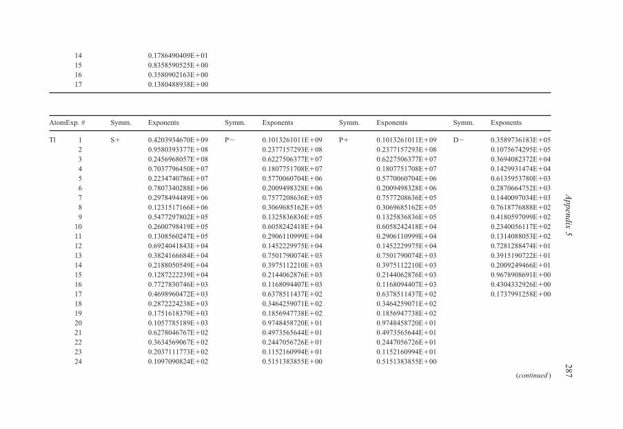
14 0.1786490409E�0115 0.8358590525E�0016 0.3580902163E�0017 0.1380488938E�00
AtomExp. # Symm. Exponents Symm. Exponents Symm. Exponents Symm. Exponents
Tl 1 S� 0.4203934670E�09 P� 0.1013261011E�09 P� 0.1013261011E�09 D� 0.3589736183E�052 0.9580393377E�08 0.2377157293E�08 0.2377157293E�08 0.1075674295E�053 0.2456968057E�08 0.6227506377E�07 0.6227506377E�07 0.3694082372E�044 0.7037796450E�07 0.1807751708E�07 0.1807751708E�07 0.1429931474E�045 0.2234740786E�07 0.5770060704E�06 0.5770060704E�06 0.6135953780E�036 0.7807340288E�06 0.2009498328E�06 0.2009498328E�06 0.2870664752E�037 0.2978494489E�06 0.7577208636E�05 0.7577208636E�05 0.1440097034E�038 0.1231517166E�06 0.3069685162E�05 0.3069685162E�05 0.7618776888E�029 0.5477297802E�05 0.1325836836E�05 0.1325836836E�05 0.4180597099E�02
10 0.2600798419E�05 0.6058242418E�04 0.6058242418E�04 0.2340056117E�0211 0.1308560247E�05 0.2906110999E�04 0.2906110999E�04 0.1314088053E�0212 0.6924041843E�04 0.1452229975E�04 0.1452229975E�04 0.7281288474E�0113 0.3824166684E�04 0.7501790074E�03 0.7501790074E�03 0.3915190722E�0114 0.2188050549E�04 0.3975112210E�03 0.3975112210E�03 0.2009249466E�0115 0.1287222239E�04 0.2144062876E�03 0.2144062876E�03 0.9678908691E�0016 0.7727830746E�03 0.1168094407E�03 0.1168094407E�03 0.4304332926E�0017 0.4698960472E�03 0.6378511437E�02 0.6378511437E�02 0.1737991258E�0018 0.2872224238E�03 0.3464259071E�02 0.3464259071E�0219 0.1751618379E�03 0.1856947738E�02 0.1856947738E�0220 0.1057785189E�03 0.9748458720E�01 0.9748458720E�0121 0.6278046767E�02 0.4973565644E�01 0.4973565644E�0122 0.3634569067E�02 0.2447056726E�01 0.2447056726E�0123 0.2037111773E�02 0.1152160994E�01 0.1152160994E�0124 0.1097090824E�02 0.5151383855E�00 0.5151383855E�00
Appendix 5
287
(continued )
Else_EAMC-TRSIC_appn5.qxd 5/19/2007 21:38 Page 287

25 0.5634668059E�01 0.2170325799E�00 0.2170325799E�0026 0.2739203885E�01 0.8549975957E�01 0.8549975957E�0127 0.1250958459E�01 0.3125305367E�01 0.3125305367E�0128 0.5326674541E�0029 0.2098922582E�0030 0.7596191414E�01
1 D� 0.3589736183E�05 F� 0.1317339294E�04 F� 0.1317339294E�042 0.1075674295E�05 0.5111787958E�03 0.5111787958E�033 0.3694082372E�04 0.2213273832E�03 0.2213273832E�034 0.1429931474E�04 0.1044616537E�03 0.1044616537E�035 0.6135953780E�03 0.5250617311E�02 0.5250617311E�026 0.2870664752E�03 0.2745793368E�02 0.2745793368E�027 0.1440097034E�03 0.1459491761E�02 0.1459491761E�028 0.7618776888E�02 0.7703428352E�01 0.7703428352E�019 0.4180597099E�02 0.3944458086E�01 0.3944458086E�01
10 0.2340056117E�02 0.1914184678E�01 0.1914184678E�0111 0.1314088053E�02 0.8600937886E�00 0.8600937886E�0012 0.7281288474E�0113 0.3915190722E�0114 0.2009249466E�0115 0.9678908691E�0016 0.4304332926E�0017 0.1737991258E�00
Atom Exp. # Symm. Exponents Symm. Exponents Symm. Exponents Symm. Exponents
Pb 1 S� 0.4397170675E�09 P� 0.1019329950E�09 P� 0.1019329950E�09 D� 0.3909520062E�052 0.9997473321E�08 0.2424307453E�08 0.2424307453E�08 0.1183891730E�053 0.2559639542E�08 0.6429845967E�07 0.6429845967E�07 0.4096297745E�04
288A
ppendix 5Atom Exp. # Symm. Exponents Symm. Exponents Symm. Exponents Symm. Exponents
Else_EAMC-TRSIC_appn5.qxd 5/19/2007 21:38 Page 288

4 0.7324217259E�07 0.1887308537E�07 0.1887308537E�07 0.1593069033E�045 0.2324661387E�07 0.6084210114E�06 0.6084210114E�06 0.6850366165E�036 0.8122626549E�06 0.2137833946E�06 0.2137833946E�06 0.3204067440E�037 0.3100943095E�06 0.8125342962E�05 0.8125342962E�05 0.1603506574E�038 0.1283730494E�06 0.3315102053E�05 0.3315102053E�05 0.8446827707E�029 0.5719510932E�05 0.1440884183E�05 0.1440884183E�05 0.4607261713E�02
10 0.2721893522E�05 0.6621062958E�04 0.6621062958E�04 0.2559711662E�0211 0.1373196840E�05 0.3192142972E�04 0.3192142972E�04 0.1424986303E�0212 0.7288969106E�04 0.1602442396E�04 0.1602442396E�04 0.7819416972E�0113 0.4040111018E�04 0.8312228924E�03 0.8312228924E�03 0.4160587464E�0114 0.2320793982E�04 0.4421575472E�03 0.4421575472E�03 0.2111660528E�0115 0.1371254942E�04 0.2393594449E�03 0.2393594449E�03 0.1005669482E�0116 0.8271044789E�03 0.1308662256E�03 0.1308662256E�03 0.4421002143E�0017 0.5054582798E�03 0.7171294663E�02 0.7171294663E�02 0.1764789964E�0018 0.3106098744E�03 0.3908859342E�02 0.3908859342E�0219 0.1904901074E�03 0.2103170609E�02 0.2103170609E�0220 0.1157121720E�03 0.1108563187E�02 0.1108563187E�0221 0.6909670543E�02 0.5680641606E�01 0.5680641606E�0122 0.4025589955E�02 0.2808502525E�01 0.2808502525E�0123 0.2271003776E�02 0.1329481319E�01 0.1329481319E�0124 0.1231245135E�02 0.5980109735E�00 0.5980109735E�0025 0.6366954910E�01 0.2536559552E�00 0.2536559552E�0026 0.3116748947E�01 0.1006884068E�00 0.1006884068E�0027 0.1433431335E�01 0.3711947918E�01 0.3711947918E�0128 0.6147226521E�0029 0.2439669603E�0030 0.8893127398E�01
1 D� 0.3909520062E�05 F� 0.1266249494E�04 F� 0.1266249494E�042 0.1183891730E�05 0.4951314662E�03 0.4951314662E�033 0.4096297745E�04 0.2162558019E�03 0.2162558019E�034 0.1593069033E�04 0.1030231291E�03 0.1030231291E�035 0.6850366165E�03 0.5227513482E�02 0.5227513482E�02
Appendix 5
289
(continued )
Else_EAMC-TRSIC_appn5.qxd 5/19/2007 21:38 Page 289

6 0.3204067440E�03 0.2758816231E�02 0.2758816231E�027 0.1603506574E�03 0.1478738220E�02 0.1478738220E�028 0.8446827707E�02 0.7860939748E�01 0.7860939748E�019 0.4607261713E�02 0.4047119330E�01 0.4047119330E�01
10 0.2559711662E�02 0.1970514586E�01 0.1970514586E�0111 0.1424986303E�02 0.8860314326E�00 0.8860314326E�0012 0.7819416972E�0113 0.4160587464E�0114 0.2111660528E�0115 0.1005669482E�0116 0.4421002143E�0017 0.1764789964E�00
Atom Exp. # Symm. Exponents Symm. Exponents Symm. Exponents Symm. Exponents
Bi 1 S� 0.4542592793E�09 P� 0.1013470007E�09 P� 0.1013470007E�09 D� 0.3945683354E�052 0.1041292784E�09 0.2418391061E�08 0.2418391061E�08 0.1183262191E�053 0.2686682302E�08 0.6441078405E�07 0.6441078405E�07 0.4062750518E�044 0.7743958349E�07 0.1900036971E�07 0.1900036971E�07 0.1570811529E�045 0.2474809506E�07 0.6160158785E�06 0.6160158785E�06 0.6726313670E�036 0.8703249831E�06 0.2178226976E�06 0.2178226976E�06 0.3137354635E�037 0.3342803647E�06 0.8335865683E�05 0.8335865683E�05 0.1567717911E�038 0.1391742409E�06 0.3426017803E�05 0.3426017803E�05 0.8254188635E�029 0.6233820123E�05 0.1500634181E�05 0.1500634181E�05 0.4503678412E�02
10 0.2981438929E�05 0.6951224996E�04 0.6951224996E�04 0.2504558714E�0211 0.1511132860E�05 0.3379124010E�04 0.3379124010E�04 0.1396208497E�0212 0.8055885715E�04 0.1710638208E�04 0.1710638208E�04 0.7673772158E�0113 0.4483185336E�04 0.8949081014E�03 0.8949081014E�03 0.4089699887E�0114 0.2584947184E�04 0.4800869778E�03 0.4800869778E�03 0.2078654188E�0115 0.1532629122E�04 0.2620822494E�03 0.2620822494E�03 0.9909817718E�00
290A
ppendix 5Atom Exp. # Symm. Exponents Symm. Exponents Symm. Exponents Symm. Exponents
Else_EAMC-TRSIC_appn5.qxd 5/19/2007 21:38 Page 290
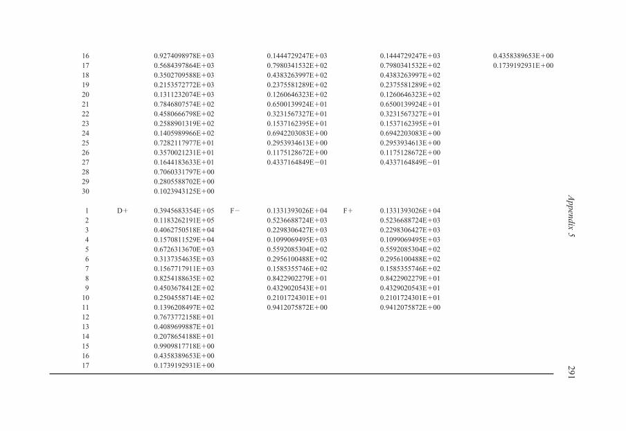
16 0.9274098978E�03 0.1444729247E�03 0.1444729247E�03 0.4358389653E�0017 0.5684397864E�03 0.7980341532E�02 0.7980341532E�02 0.1739192931E�0018 0.3502709588E�03 0.4383263997E�02 0.4383263997E�0219 0.2153572772E�03 0.2375581289E�02 0.2375581289E�0220 0.1311232074E�03 0.1260646323E�02 0.1260646323E�0221 0.7846807574E�02 0.6500139924E�01 0.6500139924E�0122 0.4580666798E�02 0.3231567327E�01 0.3231567327E�0123 0.2588901319E�02 0.1537162395E�01 0.1537162395E�0124 0.1405989966E�02 0.6942203083E�00 0.6942203083E�0025 0.7282117977E�01 0.2953934613E�00 0.2953934613E�0026 0.3570021231E�01 0.1175128672E�00 0.1175128672E�0027 0.1644183633E�01 0.4337164849E�01 0.4337164849E�0128 0.7060331797E�0029 0.2805588702E�0030 0.1023943125E�00
1 D� 0.3945683354E�05 F� 0.1331393026E�04 F� 0.1331393026E�042 0.1183262191E�05 0.5236688724E�03 0.5236688724E�033 0.4062750518E�04 0.2298306427E�03 0.2298306427E�034 0.1570811529E�04 0.1099069495E�03 0.1099069495E�035 0.6726313670E�03 0.5592085304E�02 0.5592085304E�026 0.3137354635E�03 0.2956100488E�02 0.2956100488E�027 0.1567717911E�03 0.1585355746E�02 0.1585355746E�028 0.8254188635E�02 0.8422902279E�01 0.8422902279E�019 0.4503678412E�02 0.4329020543E�01 0.4329020543E�01
10 0.2504558714E�02 0.2101724301E�01 0.2101724301E�0111 0.1396208497E�02 0.9412075872E�00 0.9412075872E�0012 0.7673772158E�0113 0.4089699887E�0114 0.2078654188E�0115 0.9909817718E�0016 0.4358389653E�0017 0.1739192931E�00
Appendix 5
291
Else_EAMC-TRSIC_appn5.qxd 5/19/2007 21:38 Page 291

Atom Exp. # Symm. Exponents Symm. Exponents Symm. Exponents Symm. Exponents
Po 1 S� 0.4793529497E�09 P� 0.1016177143E�09 P� 0.1016177143E�09 D� 0.4442663091E�052 0.1150969767E�09 0.2562843242E�08 0.2562843242E�08 0.1285917668E�053 0.3096165075E�08 0.7169640796E�07 0.7169640796E�07 0.4307518835E�044 0.9262636091E�07 0.2208390701E�07 0.2208390701E�07 0.1641049218E�045 0.3059102459E�07 0.7434264408E�06 0.7434264408E�06 0.6987673251E�036 0.1107136056E�07 0.2714964165E�06 0.2714964165E�06 0.3268107200E�037 0.4358671517E�06 0.1067664073E�06 0.1067664073E�06 0.1649866798E�038 0.1852900438E�06 0.4487763988E�05 0.4487763988E�05 0.8835406134E�029 0.8442935065E�05 0.2001385117E�05 0.2001385117E�05 0.4932480294E�02
10 0.4093330951E�05 0.9399765583E�04 0.9399765583E�04 0.2820990145E�0211 0.2096046622E�05 0.4614976612E�04 0.4614976612E�04 0.1624318942E�0212 0.1125289612E�05 0.2351086100E�04 0.2351086100E�04 0.9253600379E�0113 0.6287320476E�04 0.1233657306E�04 0.1233657306E�04 0.5125733528E�0114 0.3629137519E�04 0.6618017820E�03 0.6618017820E�03 0.2712959581E�0115 0.2148208430E�04 0.3602874619E�03 0.3602874619E�03 0.1348369121E�0116 0.1294443786E�04 0.1975780109E�03 0.1975780109E�03 0.6184272391E�0017 0.7881745077E�03 0.1083369827E�03 0.1083369827E�03 0.2572284028E�0018 0.4813850605E�03 0.5895816447E�02 0.5895816447E�0219 0.2927470249E�03 0.3160972281E�02 0.3160972281E�0220 0.1759627150E�03 0.1657247449E�02 0.1657247449E�0221 0.1037709336E�03 0.8433821279E�01 0.8433821279E�0122 0.5960138103E�02 0.4135349447E�01 0.4135349447E�0123 0.3309490013E�02 0.1939238592E�01 0.1939238592E�0124 0.1763553355E�02 0.8633003366E�00 0.8633003366E�0025 0.8952359884E�01 0.3621467842E�00 0.3621467842E�0026 0.4297406985E�01 0.1420953407E�00 0.1420953407E�0027 0.1936395595E�01 0.5176401418E�01 0.5176401418E�0128 0.8130157483E�0029 0.3157328175E�0030 0.1125783841E�00
292A
ppendix 5
Else_EAMC-TRSIC_appn5.qxd 5/19/2007 21:38 Page 292

1 D� 0.4442663091E�05 F� 0.1367160272E�04 F� 0.1367160272E�042 0.1285917668E�05 0.5474848526E�03 0.5474848526E�033 0.4307518835E�04 0.2428772741E�03 0.2428772741E�034 0.1641049218E�04 0.1166999165E�03 0.1166999165E�035 0.6987673251E�03 0.5937859308E�02 0.5937859308E�026 0.3268107200E�03 0.3128036071E�02 0.3128036071E�027 0.1649866798E�03 0.1668026294E�02 0.1668026294E�028 0.8835406134E�02 0.8802988249E�01 0.8802988249E�019 0.4932480294E�02 0.4495316152E�01 0.4495316152E�01
10 0.2820990145E�02 0.2171701080E�01 0.2171701080E�0111 0.1624318942E�02 0.9704124086E�00 0.9704124086E�0012 0.9253600379E�0113 0.5125733528E�0114 0.2712959581E�0115 0.1348369121E�0116 0.6184272391E�0017 0.2572284028E�00
Atom Exp. # Symm. Exponents Symm. Exponents Symm. Exponents Symm. Exponents
At 1 S� 0.4995639590E�09 P� 0.1024562876E�09 P� 0.1024562876E�09 D� 0.4736452685E�052 0.1214680951E�09 0.2560347544E�08 0.2560347544E�08 0.1360661431E�053 0.3304753792E�08 0.7111669722E�07 0.7111669722E�07 0.4527344172E�044 0.9987133025E�07 0.2179141879E�07 0.2179141879E�07 0.1714644286E�045 0.3328024118E�07 0.7310879445E�06 0.7310879445E�06 0.7264106021E�036 0.1213933985E�07 0.2665341384E�06 0.2665341384E�06 0.3383050242E�037 0.4811557931E�06 0.1048006761E�06 0.1048006761E�06 0.1702132563E�038 0.2057204576E�06 0.4410951325E�05 0.4410951325E�05 0.9092378277E�029 0.9418666659E�05 0.1972360530E�05 0.1972360530E�05 0.5067588213E�02
10 0.4583957940E�05 0.9299403976E�04 0.9299403976E�04 0.2896045419E�0211 0.2354236793E�05 0.4588467045E�04 0.4588467045E�04 0.1667747020E�0212 0.1266592909E�05 0.2351541934E�04 0.2351541934E�04 0.9510782598E�01
Appendix 5
293
(continued )
Else_EAMC-TRSIC_appn5.qxd 5/19/2007 21:38 Page 293

13 0.7086314477E�04 0.1242336842E�04 0.1242336842E�04 0.5278422335E�0114 0.4092788668E�04 0.6715161226E�03 0.6715161226E�03 0.2801782000E�0115 0.2422438822E�04 0.3685809494E�03 0.3685809494E�03 0.1397807586E�0116 0.1458612675E�04 0.2038907869E�03 0.2038907869E�03 0.6441452608E�0017 0.8869515277E�03 0.1128182905E�03 0.1128182905E�03 0.2694536884E�0018 0.5406940564E�03 0.6197371632E�02 0.6197371632E�0219 0.3280304661E�03 0.3354367136E�02 0.3354367136E�0220 0.1966105019E�03 0.1775487406E�02 0.1775487406E�0221 0.1155708367E�03 0.9121315159E�01 0.9121315159E�0122 0.6613903999E�02 0.4513974579E�01 0.4513974579E�0123 0.3658092387E�02 0.2135755114E�01 0.2135755114E�0124 0.1941143647E�02 0.9588781384E�00 0.9588781384E�0025 0.9810383217E�01 0.4054374977E�00 0.4054374977E�0026 0.4687687271E�01 0.1602366509E�00 0.1602366509E�0027 0.2102300145E�01 0.5874977040E�01 0.5874977040E�0128 0.8784424397E�0029 0.3394950668E�0030 0.1204687114E�00
1 D� 0.4736452685E�05 F� 0.1335057098E�04 F� 0.1335057098E�042 0.1360661431E�05 0.5475634642E�03 0.5475634642E�033 0.4527344172E�04 0.2473267456E�03 0.2473267456E�034 0.1714644286E�04 0.1203568356E�03 0.1203568356E�035 0.7264106021E�03 0.6172975537E�02 0.6172975537E�026 0.3383050242E�03 0.3264401190E�02 0.3264401190E�027 0.1702132563E�03 0.1741240401E�02 0.1741240401E�028 0.9092378277E�02 0.9164763005E�01 0.9164763005E�019 0.5067588213E�02 0.4656419483E�01 0.4656419483E�01
10 0.2896045419E�02 0.2234150222E�01 0.2234150222E�0111 0.1667747020E�02 0.9902916549E�00 0.9902916549E�0012 0.9510782598E�0113 0.5278422335E�01
294A
ppendix 5Atom Exp. # Symm. Exponents Symm. Exponents Symm. Exponents Symm. Exponents
Else_EAMC-TRSIC_appn5.qxd 5/19/2007 21:38 Page 294

14 0.2801782000E�0115 0.1397807586E�0116 0.6441452608E�0017 0.2694536884E�00
Atom Exp. # Symm. Exponents Symm. Exponents Symm. Exponents Symm. Exponents
Rn 1 S� 0.5121919362E�09 P� 0.1021095499E�09 P� 0.1021095499E�09 D� 0.4347487072E�052 0.1252581112E�09 0.2527747871E�08 0.2527747871E�08 0.1249139075E�053 0.3426720124E�08 0.6965741266E�07 0.6965741266E�07 0.4169838108E�044 0.1041051307E�08 0.2120662762E�07 0.2120662762E�07 0.1588467206E�045 0.3486642512E�07 0.7078660091E�06 0.7078660091E�06 0.6782701818E�036 0.1277925584E�07 0.2571047940E�06 0.2571047940E�06 0.3188653755E�037 0.5088474838E�06 0.1008447863E�06 0.1008447863E�06 0.1621089234E�038 0.2185116961E�06 0.4239214337E�05 0.4239214337E�05 0.8754193739E�029 0.1004587574E�06 0.1895441750E�05 0.1895441750E�05 0.4932303741E�02
10 0.4908491459E�05 0.8946087508E�04 0.8946087508E�04 0.2847886353E�0211 0.2530325945E�05 0.4423417844E�04 0.4423417844E�04 0.1655196008E�0212 0.1366136692E�05 0.2273994469E�04 0.2273994469E�04 0.9511409824E�0113 0.7668707409E�04 0.1206235064E�04 0.1206235064E�04 0.5307913069E�0114 0.4443053805E�04 0.6552244443E�03 0.6552244443E�03 0.2825536386E�0115 0.2637505879E�04 0.3617165017E�03 0.3617165017E�03 0.1409259454E�0116 0.1592497746E�04 0.2014054102E�03 0.2014054102E�03 0.6468576413E�0017 0.9708649210E�03 0.1122543073E�03 0.1122543073E�03 0.2683916040E�0018 0.5932728213E�03 0.6215391047E�02 0.6215391047E�0219 0.3607337895E�03 0.3392906993E�02 0.3392906993E�0220 0.2166591272E�03 0.1812249533E�02 0.1812249533E�0221 0.1275986313E�03 0.9399636817E�01 0.9399636817E�0122 0.7315010785E�02 0.4698461557E�01 0.4698461557E�0123 0.4052331086E�02 0.2246240741E�01 0.2246240741E�0124 0.2153460618E�02 0.1019336162E�01 0.1019336162E�01
Appendix 5
295
(continued )
Else_EAMC-TRSIC_appn5.qxd 5/19/2007 21:38 Page 295

25 0.1089763045E�02 0.4357561881E�00 0.4357561881E�0026 0.5213284369E�01 0.1741562989E�00 0.1741562989E�0027 0.2340431945E�01 0.6458159887E�01 0.6458159887E�0128 0.9788292754E�0029 0.3785866368E�0030 0.1344287237E�00
1 D� 0.4347487072E�05 F� 0.1329749051E�04 F� 0.1329749051E�042 0.1249139075E�05 0.5507367179E�03 0.5507367179E�033 0.4169838108E�04 0.2505258923E�03 0.2505258923E�034 0.1588467206E�04 0.1224792061E�03 0.1224792061E�035 0.6782701818E�03 0.6297094106E�02 0.6297094106E�026 0.3188653755E�03 0.3331601106E�02 0.3331601106E�027 0.1621089234E�03 0.1774874793E�02 0.1774874793E�028 0.8754193739E�02 0.9316467477E�01 0.9316467477E�019 0.4932303741E�02 0.4714879160E�01 0.4714879160E�01
10 0.2847886353E�02 0.2251088251E�01 0.2251088251E�0111 0.1655196008E�02 0.9921653440E�00 0.9921653440E�0012 0.9511409824E�0113 0.5307913069E�0114 0.2825536386E�0115 0.1409259454E�0116 0.6468576413E�0017 0.2683916040E�00
296A
ppendix 5Atom Exp. # Symm. Exponents Symm. Exponents Symm. Exponents Symm. Exponents
Else_EAMC-TRSIC_appn5.qxd 5/19/2007 21:38 Page 296

References
1. R. L. A. Haiduke, and A. B. F. da Silva, J. Comput. Chem., 2006, 27, 61.2. R. L. A. Haiduke, and A. B. F. da Silva, J. Comput. Chem., 2006, 27, 1970.
Appendix 5 297
Else_EAMC-TRSIC_appn5.qxd 5/19/2007 21:38 Page 297

This page intentionally left blank

Subject Index
1s and 2s orbital energies, 1141s generator functions, 622s HF weight function, 1564d weight function, 62, 65
ab initio calculations, 7accuracy, 1, 37, 50–52, 72–73, 75, 87,
89–90, 93–94, 110, 120, 131, 136accurate Adapted Gaussian Basis Sets, 119accurate basis set, 50, 94accurate GTF basis sets, 50, 52accurate numerical integration, 22accurate relativistic energy, 119adapted basis set, 67, 87, 135advanced numerical integration
techniques, 34algebraic approximation, 108algebraic structure, 20alkaline atoms, 73–74alternative paths, 14analytical formulas, 46analytical integration, 44analytical mathematical case, 11analytical solutions, 2, 5, 7, 9, 31angular functions, 81angular momentum, 81, 117anions, 67, 72antisymmetry, 20approximate eigenvalues, 16approximate linear dependence, 41approximate relativistic many-electron
Hamiltonian, 108approximate schemes, 2, 9arbitrary discretization parameters, 23atom-adapted basis sets, 67atom-adapted STF or GTF basis sets, 47,
49–52, 74
atomic and molecular relativisticcalculations, 2, 93
atomic GTF exponents, 49atomic mass number, 86–87, 93, 110,
114, 119atomic natural orbitals, 156atomic nuclear charge, 67atomic nucleus, 20, 89, 100–101, 117,
132–133, 148atomic number, 89, 94, 100, 115, 117,
120, 135–136, 146atomic orbital coefficients, 94atomic orbital symmetry, 48–51,
113–114, 119, 135atomic orbital, 48–51, 67, 73, 76, 93–94,
100, 107, 113–114, 119–120, 135atomic region, 132atomic relativistic energy, 87atomic symmetry, 76atomic system, 6, 20, 49, 72–73, 87, 89,
107, 110, 114, 117, 133, 148, 157atomic units, 9, 15, 27, 80atom-optimized results, 67atoms, 1, 3, 5, 12, 19, 23, 25, 46, 49–52,
55–58, 61, 63–65, 67–71, 73–75, 79,87–88, 93–94, 100–101, 107, 110,114, 117–120, 131–133, 135–136,145–146, 151–153
attractive interactions, 20augmentation, 145–148average energy, 93, 120
basis components, 155basis functions, 7, 27–28, 46, 56,
67, 72, 79, 83, 86–90, 111, 117
basis set design, 2, 26
Else_EAMC-TRSIC_index.qxd 6/6/2007 18:12 Page 299

basis set error, 93–95, 107, 120, 128,135–136, 143
basis set exponents, 50, 52, 56, 74, 83,108, 114
basis set functions, 55, 89, 94, 107, 117basis set segmentation, 52basis set selection, 156basis set size reduction, 117–118basis set size, 51–52, 67, 72, 75–76,
94–96, 98, 107, 113–114, 117–120,131, 135
basis set truncation process, 94basis set, 2, 23, 26, 46–47, 49–53,
55–57, 59, 61, 63–67, 69, 71–77, 79,83, 86–96, 98, 100–101, 107–108,110–120, 128, 130–132, 135–136,143–145, 147–148, 152–153,155–156
basis, 2, 7, 23, 26–28, 32, 35, 39, 46–47,49–53, 55–57, 59, 61, 63–67, 69,71–77, 79, 83, 86–96, 98, 100–101,107–108, 110–120, 128, 130–132,135–136, 143–145, 147–148,152–153, 155–156
Be-like species, 114, 117biorthogonal natural state expansion, 35block-diagonal form, 84Bohr model, 19bound state, 4–5boundary conditions, 33, 79, 85, 87,
90, 111Breit interaction matrices, 109Breit interaction, 108–113, 117Breit operator, 108brute force optimization, 44
Canonical orthonormalisation, 39cations, 67, 72central field potential, 81charge distribution, 87, 89, 93–94, 101,
110, 114, 119, 133, 145, 147–148charged fluorine atoms, 74CI calculation, 153, 158–159Clebsch-Gordon coefficients, 81closed-shell DF equations, 108
close-shell, 80collective aspects of nuclei, 3common ID interval, 94complete set, 46, 50completeness, 32computational cost of molecular
calculations, 50computational demanding process, 114computational effort, 3, 120computational time, 42, 45computer codes, 156configuration interaction, 1, 3, 151, 153continuous character, 83, 155–156continuous natural weight function, 153continuous representation, 22, 26, 39, 48continuous superpositions, 82continuous weight function, 158contracted basis, 155contraction, 67, 89convergence tests, 101, 107convergence, 22, 40–41, 44, 90,
100–107, 111–112, 132–134, 145–148coordinate space, 22, 48, 83, 88, 93correlated atomic and molecular
energies, 156correlated functions, 6Coulomb and Breit interactions, 108, 110Coulomb and exchange integrals, 85Coulomb and exchange kernels, 48Coulomb and exchange operators, 20Coulomb and exchange potentials, 26covariance, 108–109covariant contributions, 116cusp, 46cut-off value, 41
d orbital, 64, 72–73, 75, 77, 92, 116DC Hamiltonian, 108–109definite integral formulae, 13degree of the polynomial, 50–51, 114delta distribution, 42density functional theory, 1, 3, 151, 153,
155–157, 159density matrices, 85density of discretization points, 117
300 Subject Index
Else_EAMC-TRSIC_index.qxd 6/6/2007 18:12 Page 300

determinant, 20–21, 36, 47, 151determinants, 158DF environment, 80DF equations, 79–80, 82, 87, 90, 93, 108,
110, 114DF formalism, 80DF matrix, 84, 108DF orbital energies, 90DF theory, 119DFB calculations, 108, 110, 113, 116,
119, 148DFB energies, 110–111DFB equations, 108DFB matrix, 109DFB orbital energies, 112–113DFB-SCF calculations, 110DFC calculations, 87, 89, 93–94,
115, 119DFC energies, 87–89, 94–95, 111, 114,
128, 143DFC energy, 79, 87, 89–92, 100–101,
107, 114, 120, 131–132, 136, 145DFC matrix, 109DFC orbital energies, 90–92, 118–119DFC total energies, 94, 100–101, 107,
120, 135DFC total energy convergence, 148DFC total energy reduction, 133DFC total energy, 94, 101, 107, 132–133,
145, 148diagonal form, 84, 153diagonal matrix, 35diagonalization, 24, 35, 42, 45diatomic molecules, 46diffuse basis set function, 117, 120diffuse orbitals, 74–75, 154–155diffuseness, 94dimensionality, 36Dirac equation, 47Dirac Hamiltonian, 80Dirac matrices, 80–81Dirac � distribution, 76direct solution, 11discrete basis, 39discrete character, 19
discrete weight function, 41discretization parameters, 23, 25, 57,
65–67, 73, 76, 93, 100, 107, 114, 117,119, 135, 145
discretization, 2, 5, 7, 9, 11, 19, 22–23,25, 31, 33–35, 37–39, 41, 43–49, 51,56–57, 65–67, 73, 76, 82–83, 90, 93,100, 107–108, 110–111, 113–114,117, 119–120, 132, 135, 145, 152
discretized eigenvalue problem, 35discretized integration grid, 156discretized weight functions, 35, 46distribution, 6, 42, 75–76, 87, 89, 93–94,
101, 110, 114, 119, 133, 145, 147–148Dyall’s basis sets, 131
effective discretization process, 117Eigenfunction, 4eigenfunctions, 32, 35eigenvalue problem, 34–35, 37eigenvalues, 16, 21, 31, 35–37, 39,
41, 47eigenvector matrix, 35electron charge, 21electronic cloud, 94, 133, 136electronic configuration, 94, 120,
136, 145electronic structure, 46, 151, 158energy expectation value, 47, 82energy functional, 4equally spaced mesh, 23, 44even-tempered scheme, 114exact ground state energy, 156exact solution, 2, 4, 11–12, 15, 41exchange term, 157exchange-correlation term, 156–157excited state, 16, 42, 44–45, 56, 58–59,
61, 65, 67, 69, 71, 156, 158–159exclusion principle, 20expansion coefficients, 83
fine-structure constant, 108finite basis set expansion method, 46finite body, 89finite nuclear boundary conditions, 79
Subject Index 301
Else_EAMC-TRSIC_index.qxd 6/6/2007 18:12 Page 301

finite nuclear boundary results, 86finite nuclear model, 79, 85–87, 119finite nucleus approximation, 47finite nucleus model of uniform
proton-charge distribution, 87, 93, 110,114, 119
finite nucleus of Gaussian proton-chargedistribution, 94, 119
finite-difference procedure, 89first-order perturbative approach,
115–116first-order reduced density matrix, 152fission problem, 3Fock kernels, 21force constant, 33Fredhom equation, 34frontier atomic orbital, 67function exponents, 56, 79, 87, 90,
93–94, 110, 120, 132functional form, 3, 14
Gaussian 2p weight functions, 74Gaussian 2s weight functions, 73–74Gaussian basis functions, 87–89Gaussian distributions, 6Gaussian overlap approximation, 5, 9, 31Gaussian trial function, 11Gaussians weight functions, 73Gaussian-type functions, 1, 55, 79Gaussian-type orbitals, 44GC method, 52, 61, 67, 163, 164GCDF method, 80, 82–83, 87–90, 93–94,
100, 107–108, 110–111, 113–114,117–120, 132, 135–136, 148
GCDFB equations, 108GCDFB formalism, 108, 110GCDFC formalism, 85, 87, 108–110GCHF method, 38, 47–53, 55–56, 65,
73–77generating function, 38generator coordinate ansatz, 10, 32,
47, 82generator coordinate integral view, 158generator coordinate space, 22, 83,
88, 93
generator coordinate, 1–6, 9–10, 19,21–23, 25, 27, 31–34, 42, 47, 49, 55,75–76, 79–80, 82–88, 93, 100,108–109, 113, 119, 148, 151–152,154–155, 157–158
generator function, 25–27, 38, 42, 44, 47,62, 75, 82, 153, 155
geometrical Gaussian basis sets, 87GHW equation, 2, 5, 10–13, 15, 19, 27,
32, 34–35, 41, 44GHWHF equations, 21, 23, 47–49, 53, 82Gram determinant, 36Gram-matrix, 36ground-state hydrogen atom function, 11
Hamiltonian, 2, 4, 9–11, 33, 35, 80,108–109, 156–157
harmonic oscillator problem, 32, 34, 36,38, 43
Hartree-Fock theory, 2, 3He- and Be-like species, 114He atom, 20, 22, 25–26, 49–50, 52,
55–56, 58, 63, 65, 67–68, 74, 86–89,93–94, 100–101, 107, 110, 114–115,117, 119–120, 132–133, 135–136,146, 148, 151–153, 157–158
heavy atoms, 49, 52, 146Hermitian, 11, 14, 35HF energies, 51–52, 67, 72HF energy, 50–52, 73–74HF equations, 21, 23, 47–49, 53, 82HF limit, 25, 72HF orbitals, 152, 156HF weight function, 155–156HFS equations, 157Hohemberg and Kohn expansion, 156hydrogen atom, 11, 13, 15–16, 19, 44–45
ID technique, 56, 61, 65, 73, 83, 88, 90,93, 107–108, 110, 119
independent particle model, 47, 76, 82inner electrons, 80inner orbitals, 64, 100inner-core electronic penetration,
145–146
302 Subject Index
Else_EAMC-TRSIC_index.qxd 6/6/2007 18:12 Page 302

innermost atomic orbitals, 94instantaneous Coulomb operator, 108integral character, 48, 107–108, 111, 153integral Hellmann-Feynman
formulation, 11integral transform method, 6integration by parts, 14integration technique, 34, 44ions, 19, 55–56, 65–71, 73–74, 115–117isoelectronic species, 73iterative procedure, 22
kinetic balance condition, 87, 90, 93,110–111, 114, 117, 119
Koga’s basis set, 72Kohn and Sham scheme, 156Kohn-Sham orbitals, 156Kronecker delta, 81
Lagrange multipliers, 21Laplace transform, 6, 12large and small components, 81, 82, 84,
87, 117large and small exponents, 117large component, 117lighter atomic systems, 72, 107linear combination coefficients, 1linear dependence, 36, 41linear transformation, 156linearly independent variations, 5liner combination of functions, 15lowest positive parity solutions, 38low-lying excited states, 56, 58, 65, 67low-lying states, 37
many body perturbation theory, 1, 3many-electron system, 20, 156many-electron wave function, 20mass number, 86–87, 93, 110, 114, 119matrices of two-electron Coulomb and
exchange interactions, 84matrix DF equations, 87Matsuoka’s method, 93, 120mesh of ID points, 83model problems, 9, 31, 61
molecular nonrelativistic calculations, 55, 76
molecular nuclei, 20molecular relativistic calculations, 2, 93momentum operator, 81multicentre integrals, 46
natural orbital, 2, 151, 153, 155–157, 159natural weight function, 153–156negative ions, 55–56, 65–67, 70–71,
73–74negative parity solutions, 33negative parity states, 38neutral atoms, 55–57, 65, 67, 73, 117NHF energies, 51noble gases, 61–64nonlinear parameters, 22, 42, 44nonorhtogonal representation, 34nonrelativistic atomic and molecular
calculations, 77nonrelativistic limit, 82, 85, 87normalisation kernels, 33normalization constants, 86normalized spherical harmonics, 81normalized total wave function, 81nuclear charge density, 89nuclear charge, 9, 25–26, 67, 80, 89nuclear liquid drop model, 3nuclear models, 93–94, 101, 107,
119–120, 132–133Nuclear Physics, 1–5, 9, 19, 31nuclear proton-charge distribution, 145nuclear radius, 86–87, 93, 110, 114,
119, 148numerical accuracy, 89–90, 110numerical approach, 32, 34numerical approaches, 164numerical DFC calculations, 94numerical DFC energy results, 120numerical errors, 36, 41numerical HF functions, 65numerical integration procedure, 108, 110numerical techniques, 164numerical-finite-difference DF
calculations, 88, 90
Subject Index 303
Else_EAMC-TRSIC_index.qxd 6/6/2007 18:12 Page 303

one-electron density, 157one-electron eigenvalue, 20one-electron functions, 19–21, 47,
157–158one-electron Hamiltonian, 108, 156one-electron kernel, 48one-electron kinetic energy operator, 20one-electron matrix elements, 84one-electron spin-functions, 21optimized discretization parameters, 117optimized pGCDF parameters, 135orbital angular momentum, 81orbital energies, 90–92, 101, 107,
112–114, 116–119orbital exponents, 6, 57, 65, 79, 83, 108orbital reorganization, 110orbital symmetry, 48–51, 87, 113–114,
119–120, 132–133, 135orbital wave function, 62, 89orthogonal bases, 76orthogonality, 32, 76, 155orthonormal basis, 39orthonormality, 40, 81oscillator Hamiltonian, 33oscillator wave functions, 33outer shell electrons, 50overlap and two-electron integrals, 131overlap matrix, 31, 37, 84
parabolic-cylinder functions, 13para-helium independent particle case, 9Pauli matrices, 81pGCDF basis sets, 114–117pGCDF discretization parameters, 119,
135, 145pGCDF method, 113–114, 117, 119–120,
132, 135–136, 148point nucleus model, 46polyatomic calculations, 46polynomial degree, 114polynomial expansion, 49–53, 113, 120positive ions, 65–69post-HF calculations, 156potential energy, 81prolapse analysis, 100, 145, 148
prolapse problem, 100, 120, 132, 135prolapse-free RUGBS, 135, 146proton-charge density, 148proton-charge distribution, 87, 93–94,
101, 110, 114, 119, 133, 145, 147–148
quadrature method, 35quantum electrodynamics, 108quantum lattice dynamics, 7
radial large and small components, 82, 117radial large-component basis set, 86radial small-component basis set, 86radial wave functions, 81RAGBS augmented, 132, 145RAGBS error, 120, 130–131,
135–136, 144RAGBS exponents, 135Rayleigh-Ritz variational method, 1relativistic adapted Gaussian basis sets,
119, 135relativistic and nonrelativistic
calculations, 163, 164relativistic angular coefficients, 110relativistic atomic orbital symmetries, 93,
100, 107, 120relativistic atomic orbital symmetry, 135relativistic boundary conditions, 85relativistic calculation, 2, 47, 52, 55, 76,
79, 81, 83, 85, 87–91, 93, 95, 97, 99,101, 103, 105, 107, 109, 111, 113, 115,117, 119, 121, 123, 125, 127, 129, 131,133, 135, 137, 139, 141, 143, 145, 147
relativistic closed-shell atoms, 87, 110relativistic corrections, 108relativistic energies, 114relativistic Gaussian basis sets, 77,
113–114, 119, 148relativistic generator coordinate
formalism, 148relativistic GTF basis sets, 52relativistic Hartree-Fock limit, 79relativistic kinematics, 87, 89relativistic triple-zeta basis sets, 131
304 Subject Index
Else_EAMC-TRSIC_index.qxd 6/6/2007 18:12 Page 304

relativistic universal Gaussian basis set,87–88, 91–93, 100, 111
restricted kinetic balance condition, 87,93, 110, 114, 119
Roothaan equations, 22Roothaan expansions, 1RUGBS functions, 94
s, p and d orbitals, 72saddle critical point, 15saddle-like surface, 15scaling parameter, 48–49, 88, 110, 114scattering problem, 5SCF Breit energies, 115SCF energy, 110SCF equations, 93, 109, 120SCF procedure, 83, 108–110, 115Schrödinger equation, 4, 19, 156screened non interacting two-electron
system, 10secular equation, 15, 38segmentation, 50, 52segmentations, 50–51self-consistent random phase
approximation, 7shape parameter, 3SIMPLEX algorithm, 114, 120, 135Simpson rule, 41singularities, 31Slater- and Gaussian-function exponents,
163, 164Slater determinant, 21, 47Slater determinants, 163Slater orbitals, 163 Slater universal basis set, 55Slater’s rules, 163Slater’s transition state method, 156Slater’s X� potential, 157 small component, 117spatial one-electron functions, 21spectral problem, 37speed of light, 79, 85, 87, 93, 110,
114, 119square-integrable, 38–40square-well problem, 32, 38
square-well solutions, 32step function, 33STF and GTF HF energies, 67STF and GTF negative ions, 55, 65–67,
70, 73, 74 STF and GTF positive ions, 67STF weight functions, 62, 74symmetrical character, 42
test function, 76tight d or f functions, 101, 107, 148tight function, 100–101, 107, 119, 132,
145–147tight p function, 101, 132–133,
145–146tight s function, 101, 107, 133, 146total electronic energy, 55–56total wave function, 81translated Gaussian, 42trial function, 1–4, 6, 10–11, 21, 51, 157triangular inequality, 40truncation, 34, 37–38, 41, 51, 74, 94, 114two-body interactions, 108two-component Pauli spinors, 81two-electron interaction, 108two-electron kernels, 48two-electron matrices, 85two-parameter Hulthen function, 6
uncertainty principle, 20unequally spaced numerical mesh, 50uniform charge approximation, 85uniform density, 147uniform proton charge distribution, 89uniform sphere and Gaussian nucleus
models, 119, 133, 148unitary transformation, 153universal Gaussian basis set, 56–57, 79,
87–88, 91–94, 100, 111–112universal mesh, 56universal Slater basis set, 57unperturbed DC Hamiltonian, 80, 108–109
valence region, 94, 119variational approach, 10
Subject Index 305
Else_EAMC-TRSIC_index.qxd 6/6/2007 18:12 Page 305

variational Breit interaction energy, 110, 112
variational Breit interaction, 110–112variational discretization, 19, 38variational exponent optimization, 90, 93variational principle, 21, 47variational prolapse analysis, 100, 145variational prolapse problem, 120, 132
wave function, 5, 12, 20, 32–33, 42, 46,62–63, 65, 79, 81, 89, 152, 158
weight function behavior, 94weight function, 2, 4, 6–7, 9, 12,
15, 19, 21–23, 26–28, 31, 35, 41–42, 44–48, 55–57, 59, 61–65, 67, 69, 71–76, 82, 85, 94, 152–156, 158–159
well-tempered scheme, 79
X� method, 163
zero-order Hamiltonian, 108
306 Subject Index
Else_EAMC-TRSIC_index.qxd 6/6/2007 18:12 Page 306