International Journal Of Computational Engineering Research (ijceronline.com) Vol. 2 Issue. 5

Issn 2250-3005(on line) Sept em ber | 2012 Pa ge 1462

Numerical Analysis of Cavitating Flow over A2d Symmetrical Hydrofoil

1, Greeshma P Rao ,

2, Likith K,

3, Mohammed Naveed Akram,

4Adarsh

Hiriyannaiah 1,2,3,4

Department of Mechanical Engineering R V College of Engineering, Bangalore

Abstract

This report presents the numerical investigations of

cavitating flow over a 2D symmetrical hydrofoil. Turbulent

cavitating flow over a hydrofoil is simulated using a

transport equation based model with consideration of the

influence of non condensable gases. The results

presented in this report focuses on Cavitation inception,

shape and behaviour of sheet cavity, lift and drag forces

with cavitation and the pressure distribution around the

foil. Steady and unsteady simulations are carried out at

different cavitation numbers ranging from near inception

conditions to developed conditions and almost super

cavitating conditions. Standard k-ɛ model without any

modifications are used for simplicity. Effect of dissolved

gas content is also considered.

Index Terms— Cavitation, Hydrofoil, Standard k-ɛ

model.

I. INTRODUCTION Cavitation is defined as the process of formation of the

vapour phase of a liquid when it is subjected to reduced

pressures at constant ambient temperature. Thus, it is the

process of the boiling in a liquid as a result of pressure

reduction rather than heat addition. However, the basic

physical and1, 2 :UndergraduateStudents(UG)4Assistant

professor (RVCE)thermodynamic processes are the same

in both cases. A liquid is said to cavitate hen vapour

bubbles form and grow as a consequence of pressure

reduction.When the phase transition results from

hydrodynamic pressure changes, the two-phase flow

composed of a liquid and its vapour is called a ‗cavitating

flow‘. Cavitation flow may be seen (and heard) as water

flows through a glass venturi tube (fig 1), an experiment

first exhibited by Osborne Reynolds in 1894. According to

Bernoulli‘s equation, when the velocity increases, the

pressure decreases. At sufficiently high flow rates the

liquid in the throat begins to boil, because the velocity is

highest and the pressure is lowest at this section. The

small

bubbles formed there are filled with cold steam and other

gases diffused from the liquid. [1]

Hydrofoil

Hydrofoils are foils operating in liquid medium. They need

not be as large as an aerofoil due to higher density of

Liquid than air. They help in increasing the performance of

machines

Adverse Effects of Cavitation

The main effects of cavitation are adverse effects: noise,

erosion, vibrations and disruption of the flow, which

results in loss of lift and increase of drag. Cavitation is

known for its violent behaviour. That is caused by the fact

that vaporization of water and condensation of vapour are

very fast processes, much faster than the dynamics of a

vapour cavity. As a result the growth and collapse of a

cavity is not slowed down by these processes. Because

cavitation is part of the flow, it can move rapidly from

regions of low pressure into regions of a higher pressure.

This leads to a very rapid collapse. The collapse is so rapid

that the local speed of sound in the fluid is exceeded and

shock waves occur. The consequence is that cavitation

generates noise over a wide range of frequencies,

especially higher frequencies. Also the local pressure rises

very strongly at collapse, leading to damage of adjacent

surface. This effect is called erosion. When larger amounts

of vapour are involved the implosion of cavitation can

cause pressure variations in the fluid, which lead to

vibrations of the cavitating structure. Cavitation can also

alter the flow. This is the case on propellers when the

cavitation becomes extensive. In that case the flow over

the blades and the lift of the blades is altered by cavitation

and the thrust of the propeller is strongly reduced. This is

called ‗thrust breakdown‘. In valves cavitation can also

block or choke the flow. The volume of vapour in

cavitation is much larger than the volume of water that has

evaporated. In cases of extensive cavitation this leads to

large volume increases and decreases when cavitation

grows and collapses. The volume variations cause

pressure fluctuations in the surrounding fluid, resulting in

structural vibrations. The properties of cavitation and its

implosion can also be used, as mentioned below.

2. Cavitation number Generally tests are carried out in a cavitation tunnel. In this

case the easiest parameters to measure are:low velocity,

pressure upstream of hydrofoilIt is customary to define σ

by the following expression

Cp= (pv-pb )/ (0.5ρv

2 )

Figure 2.1

International Journal Of Computational Engineering Research (ijceronline.com) Vol. 2 Issue. 5

Issn 2250-3005(on line) Sept em ber | 2012 Pa ge 1463

The following figures (2.1, 2.2(a), 2.2(b), 2.2(c)) [3] show the

relation between pressure coefficient cp and cavitation

number σ for non cavitating, possible cavitation and

developed cavitating conditions

Figure 2.2(a)

Figure 2.2(b)

Figure 2.2(c)

3. Cavitation Simulation Cavitation is a two phase flow occurring in a liquid when

the local static pressure falls below the vapour pressure

corresponding to the liquid temperature. It affects the

performance of hydraulic machines. Need for

understanding cavitation in turbo machines is thus

apparent. Because of experimental difficulties, simulation

could be a useful tool to understand cavitation in such

applications Simulating the occurrence of cavitation in a

hydraulic machine is a challenging task because of the

complex flow phenomenon as well as the complicated

geometry of hydro turbo machines; usually new cavitation

models are tested against experimental data obtained from

much simpler geometry. One such flow simulation widely

used to validate numerical approach is the flow over a

hydrofoil. Hydrofoils form the basics of impeller blades of

axial flow machines. Thus information of cavitation on a

hydrofoil yields useful information about axial machine

performance under cavitation.

Simulation of cavitation requires a coupling between

Navier-stokes equation, physical model for cavitation and

closure model for turbulence. Moreover such flows are

systematically unsteady at some scale thus an effective

cavitation model is needed to correctly take into account

the different flow phenomenon Kubota et al[6] proposed a

new cavity model (bubble two-phase flow) that can

express well the interactions between vortices and

bubbles. Rebound et al [7] have investigated the ability of

two-equation turbulence models to reproduce the cavity

unsteadiness in the case of a venturi nozzle. They have

stated that the use of the k- ɛ turbulence model leads to

steady-state cavity because of the high turbulent

viscosity level induced by the turbulence model. Singhal et

al [8] developed the full cavitation model in which the

phase change expressions are derived from a reduced form

of a Rayleigh-Plesset equation. The numerical model has

been applied to the 2D configuration (fig 8.4).

The flows corresponding to different cavitation numbers

have been investigated, to obtain successively non

cavitating flow, steady and unsteady sheet cavitation

(cloud cavitation), finally supercavitation flow.

4. Mathematical Models Multi-Phase Model The multi-phase mixture model in FLUENT14.0 assumes

that the working medium is a single fluid with a

homogeneous mixture of two phases (liquid and vapour).

Therefore, only one set of RANS equations is solved for

the mixture fluid. Denoting the density of the mixture fluid

by ρm, the continuity equation for the mixture flow

becomes:

The momentum equation for the mixture reads:

The density constitution of each phase in a mixture-flow

cell is described by means of a scalar volume fraction. The

relation between different volume fractions is linked by:

Where αv and αl are the volume fraction of vapour and

liquid respectively. To close the equations an additional

transport equation is solved for αv. To account for the

mass transfer between phases a cavitation model is

needed, as discussed below.

Cavitation Model

Singhal et al cavitation model [8]This cavitation model is

based on the "full cavitation model", developed by Singhal

et al. It accounts for all first-order effects (i.e., phase

change, bubble dynamics, turbulent pressure fluctuations,

and non- condensable gases). It has the capability to

account for multiphase (N-phase) flows or flows with

multiphase species transport, the effects of slip velocities

between the liquid and gaseous phases, and the thermal

effects and compressibility of both liquid and gas phases.

The cavitation model can be used with the mixture

multiphase model, with or without slip velocities. However,

it is always preferable to solve for cavitation

using the mixture model without slip velocity; slip

velocities can be turned on if the problem suggests that

there is significant slip between phases.

To derive an expression of the net phase change rate,

Singhal et al uses the following two-phase continuity

equations

Liquid phase:

2

International Journal Of Computational Engineering Research (ijceronline.com) Vol. 2 Issue. 5

Issn 2250-3005(on line) Sept em ber | 2012 Pa ge 1464

Vapour phase:

Mixture:

The expression for the net phase change rate ( ) is

finally obtained as

Singhal et al. proposed a model where the vapour mass

fraction is the dependent variable in the transport

equation. This model accommodates also a single phase

formulation where the governing equations are given by:

Turbulence modelling [4]

In this simulation standard k ε model without any

modifications is tested and it q has been found that this

yields to inaccurate predictions especially in near wall

conditions. For this model the transport equation for k is

derived from the exact equation, but the transport for ε was

obtained using physical reasoning and is therefore similar

to the mathematically derived transport equation of k , but

is not exact. The turbulent kinetic energy k and its rate of

dissipation ε, for this model are obtained by the following

equations.

5. Procedure in ansys fluent

Geometry and Meshing

The shape of the hydrofoil is given by

Y/c=a0(x/c)1/2

+a1(x/c)+a2(x/c)2+a3(x/c)

3+a4(x/c)

4

Where a0=0.11858, a1=-0.02972, a2=0.00593,

a3=-0.07272,a4=-0.02207

The geometry is created by using the equation above. And

the surface is created from the curve obtained by the

coordinates satisfying the above equations.

Final surface is shown in fig (5.1.1)

Fig 5.1.1

The foil is 1m long in chord and maximum width 0.12m.The

dimensions of the arc of the c mesh is 12.5 m and length of

the rectangular part is 12.5m with the trailing edge of the

hydrofoil situated at the centre of the arc.

Once the c mesh outline is created a second surface (target

body) is generated from this a hydrofoil surface is

subtracted (tool body) shown in figure (5.1.2)

Figure 5.1.2

Then the obtained surface is spilt into 4 quadrants to

facilitate easy meshing.

The mesh is generated using mapped face meshing and

suitable edge sizing

Thus obtained mesh is as shown below

Figure 5.1.3

Computational domain

Fig 5.2

Solution set up- Grid and Boundary conditions

The foil has a 7° angle of attack (AoA) that is the flow is

inclined at 7° and is operated at and is operated at various

cavitation numbers. Table 1 gives the flow and boundary

conditions. The physical properties for the liquid and the

vapor in Table 1 correspond to a water temperature at 27°C

Table 1 – Boundary Conditions

2

2/1

2jjk

T

jj

iij

j

jx

k

x

k

xx

u

x

ku

2

2/1

2jjk

T

jj

iij

j

jx

k

x

k

xx

u

x

ku

2

2

2

22

21

2

x

u

kC

xxx

u

kC

xu T

j

T

jj

iij

j

j

International Journal Of Computational Engineering Research (ijceronline.com) Vol. 2 Issue. 5

Issn 2250-3005(on line) Sept em ber | 2012 Pa ge 1465

Table 2 Information on grids for hydrofoil

Table 3

6. Results and discussions For 7

o angle of attack after the numerical simulations for a

wide range of operating pressures the following five main

flow configurations have been observed in the system

Non cavitating flow(σ>4)

Near cavitation inception(σ=3)

Sheet cavitation(α from 2 to 3)

Sheet cavitation(σ=0.9)

Near super cavitation(σ=0.55)

The cpmin value is -2.375 for σ=4(figure 6.1)

Since the cp curve does not cross the –σ line the cavitation

does not happen. Hence σ=4 is for non cavitating

conditions.

The cavitation begins at about σ=3.5 but is prominently

noticed at σ=3 and this leads to developed cavitation at

σ=2.5 followed by σ=2.at lower cavitation numbers i.e...σ =

0.55, 0.9 etc the cavitation gets unsteady or cloud

cavitation. For σ=3 cp curve does crosses the –σ line the

cavitation happens. Hence σ=3cavitation begins.

(figure8.2) Cp v/s position for σ=2, that is developed

cavitation (figure 6.3)

However cavitation itself is an unsteady phenomenon

(transient flow) and hence we can speak only of degree of

unsteadiness in the flow.

Development of cavity

Sheet cavitation occurs when there is a strong low

pressure peak at the leading edge of the foil and sheet

cavitation therefore has its leading edge close to the

leading edge of the foil. The closure of the cavity is shown

in Fig6.7.At the beginning or leading edge of the cavity,

constant pressure means that the streamlines separate

tangentially from the surface of the foil at point A

(assuming that the foil is a smooth surface). Tangential

separation, however, means that there is a region just

downstream of the separation location where the cavity is

very thin, so thin that the surface tension becomes

recognizable and results in a curved surface, making the

leading edge of the cavity at point B instead of A.

Also point B experiences the lowest pressure marking the

beginning of the cavity. (Indicated by red regions) The

space around point A encounters flow separation leading

to reduced volume of vapour at that point, indicated by

yellow region ( also near the trailing edge), The phase

contours for σ=3 is plotted for different times. The fig (6.4,

6.5, 6.6), shows a few plots for 300,500,700ms are shown.

The vapour reaches a maximum volume fraction of

1.91x10^-2 in 500 ms.

Phase contours

For σ=2 the phase contours are plotted fig (6.8, 6.9,

6.10,6.11)And reaches a maximum vapour

volumefractionof2.03x10^-2 at 500ms which is greater than

that ofσ=3.Also the length of the cavity is increased .

For σ=0.9 the phase contours are plotted –fig( 6.12, 6.13,

6.14, 6.15) And reaches a maximum vapour volume fraction

of 2.18x10^-2 at 450 ms. The vapour content is greater and

reaches a maximum at a faster rate indicating that the

cavitation gets more unsteady. Also the length of the

cavity is increased.For the phase contour for σ=0.55 the

maximum vapour volume fraction is 2.21x10^-2

which is reached at 500ms which is greater than the

previous vapour factions. The fig (6.19) illustrates the

vapour shedding at 168.2ms The vapour shedding takes

place even before the full development of the cavity which

indicates that the shedding of the cavity takes place by

parts and not as a whole which is an example for unsteady

cloud cavitation.

Effect of cavitation on lift and drag

The drag coefficient is defined as:

Where:

Is the drag force, which is by definition the force

component in the direction of the flow velocity.

is the mass density of the fluid,

is the speed of the object relative to the fluid and

A is the reference area or projected area

The lift coefficient is equal to:

International Journal Of Computational Engineering Research (ijceronline.com) Vol. 2 Issue. 5

Issn 2250-3005(on line) Sept em ber | 2012 Pa ge 1466

Where

is the lift force, is fluid density, is true airspeed,

is dynamic pressure and is plan form area. Or

projected area

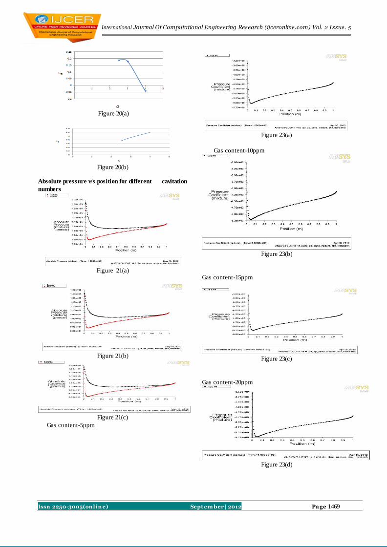
The plots (Figure 6.20 (a) & (b)) show the lift and drag

coefficient during the incipient flow for various cavitation

numbers.

We observe that the lift coefficient decreases and drag co

efficient increases with decrease in cavitation number

.indicating increase in drag force and decrease in lift force

with cavitation.

The Graphs figs (6.21 (a), (b), (c)) show the variation of

absolute pressure with respect to position on the hydro

foil, for cavitation numbers 0.9 We observe that the

absolute pressure distribution over lower surface remains

same however the pressure distribution over the upper

surface changes. It has observed that the area between the

two curves decreases as the cavitation number decreases

indicating decrease in lift force as

Effect of dissolved gas content For Cavitation number 0.9

and gas content 5, 10, 15 and 20ppm

Graphs 6.23(b),6.23(c),6.23(d) represents the variation of cp

with different dissolved gas contents. we observe that

with the incresing gas content(from 10ppm to 20ppm) the

value of cpmin falls, indicating that the conditions get more

favorable to cavitation. On the contrary the value of cpmin

for 5ppm(6.23 (a)) is lower than that of 10ppm. This is

probaly because very low gas content lead to lesser nuclei

in water which may lead to bubble cavitation which is a

stronger form of cavitation than sheet cavittion , justifying

the fall in cpmin.Hence high nuclei density is favorable for

sheet cavitation while low nuclei density l leads to bubble

cavitation

Conclusions Cavitation is a phenomenon that has adverse affects on

the performance and life of the hydraullic machines,

making it an inevitable subject of study.Analysis ng

cavitation can provide us information,about the sites

vulnerable to cavitation damage and therefore help us to

take suitable measures for its prevention.

The phenomenon is known to have a devastating effect

on the blades of the impellers used in various fluid

machinery. Therefore the investigation of the

phenomenon over different blade profiles is a cynosure of

cavitation studies.

Hydrofoil is one of the simplest and most widely used

profiles in impellers for axial flow machines. In the analysis

of a 2 D symetrical hydrofoil it is observed that by

decreasing cavitation number, different cavitation regimes

are formed.The near cavitation inception is obtained at 3 to

3.5 after which cavitation is developed and subsequently

becomes unsteady. Cloud cavitation occurs at a cavitation

number of 0.55. Further increase in cavitation number leads

to supercavitation conditions. It is also seen that the

regions close to leading edge are sites susceptible to this

phenomenon. It is observed from simulations that gas

content also has a major effect on the cavitation formation.

Lift decreases and drag increases with the increase in

cavitation.(which can thwart the performance of the

machinery).

Further the standard turbulence model k-ε used, without

any modification is not very accurate in predicting the

phase contours, vapour shedding and near wall

conditions.

In future the investigation can be extended to study the

phenomenon for various angles of attack with

modifications of models used to improve the accuracy and

reliability of the results.

Bibliography 1. Cavitation ―section 12, handbook of fluid

mechanics, McGraw-hill BookCo., Inc., 1961(section

12-I:‖mechanics of cavitation,‖ by Phillip Eisenberg;

section I2-II:‖supercavitating flows‖, by Marshall P

Tulin)

2. Bertin, John and Michael Smith; Aerodynamics for

Engineers, Third Edition. Prentice Hall: New Jersey,

1998.

3. Cavitation Bubble Trackers‖ BY Yves Lecoffre (2009)

4. Pope, S.B., 'Turbulent Flows', (2000)

References 1. Introduction to Cavitation and Supercavitation Paper

presented at the RTO AVT Lecture Series on

―Supercavitating Flows‖, held at the von Kármán

Institute (VKI) in Brussels, Belgium, 12-16 February

2001, and published in RTO EN-010.

2. Kubota a Kato, and Yamaguchi, H 1992, A new

modelling of cavitating flows; a numerical study of

unsteady cavitation on a hydrofoil section, J Fluid

mech.240, pp 59-96

3. Rebound J. L., Stutz B., and Coutier- Delgosha, o., 1998,

two phase flow structure of cavitation: experiment and

modelling of unsteady effects. Pre, oct 3rd

int.

4. Singhal A K Athavale M .M., Li ,H .Yi., and Jiang Y

2002, mathematical basis and validation of full

cavitation model J. Fluid Engg, 124, pp 617-624

5. ―Introduction to CFD Basics‖, Rajesh Bhaskaran , Lance

Collins (2010)

6. ranc J.P. and Michel J.M. (2004) "Fundamentals of

cavitation" Kluwer.

7. Kato H. (1984) "Thermodynamic effect on incipient and

developed sheet cavitation" Proc. Int. Symp. On

Cavitation inception, FED-Vol.16, New-Orleans

(USA), Dec. 9-14, 1984, 127-136.

8. A. Ducoin, J. A. Astolfi, F. Deniset, and J.-F. Sigrist,

―Computational and experimental investigation of

flow over a transient pitching hydrofoil,‖ European

Journal of Mechanics B, vol. 28, no. 6, pp. 728–743,

2009

International Journal Of Computational Engineering Research (ijceronline.com) Vol. 2 Issue. 5

Issn 2250-3005(on line) Sept em ber | 2012 Pa ge 1467

9. M. Morgut, E. Nobile, and I. Biluš, ―Comparison of

mass transfer models for the numerical prediction of

sheet cavitation around a hydrofoil,‖ International

Journal of Multiphase Flow, vol. 37, no. 6, pp.

620–626, 2011.

10. G.Kuiper, Cavitation in Ship Propulsion, January 15,

2010

11. Stepanoff A.J. (1964) "Cavitation properties of liquids"

J. of Eng. for Power, April 1964, 195-200.

12. Numerical and experimental study on unsteady

shedding of partial cavitation (2009)

BIN JIn XIANWU LUO† and YULIN WU

13. 5. J. Choi, C. T. Hsiao, G. Chahine and S. Ceccio, J.

Fluid Mech. 624 (2009) 255.

14. 8. B. Ji, F. W. Hong and X. X. Peng, Journal of

Hydrodynamics, Ser. A 23(04) (2009) 412.

15. De Lange D.F. & De Bruin G.J. (1998) "Sheet cavitation

and cloud cavitation, re-entrant jet and

threedimensionality"

Appl. Sci. Res. 58, 91-114.

16. MODELING OF CAVITATION FLOW

ON NACA 0015 HYDROFOIL(2009)

Jaroslav ˇStigler*, Jan Svozil*

Appendix A

Figure 1

Figure 2

Figure 3

Figure 8.4

Figure 5

Figure 6

Figure 7

Figure 8

International Journal Of Computational Engineering Research (ijceronline.com) Vol. 2 Issue. 5

Issn 2250-3005(on line) Sept em ber | 2012 Pa ge 1468

Figure 9

Figure 10

Figure 11

Figure 12

Figure 13

Figure 14

Figure 15

Figure15

Figure 16

Figure 17

Figure 18

Figure 19

International Journal Of Computational Engineering Research (ijceronline.com) Vol. 2 Issue. 5

Issn 2250-3005(on line) Sept em ber | 2012 Pa ge 1469

Figure 20(a)

Figure 20(b)

Absolute pressure v/s position for different cavitation

numbers

Figure 21(a)

Figure 21(b)

Figure 21(c)

Gas content-5ppm

Figure 23(a)

Gas content-10ppm

Figure 23(b)

Gas content-15ppm

Figure 23(c)

Gas content-20ppm

Figure 23(d)