notes on solving di⁄erence equationsyluo/teaching/6012_2017/notesdifferenceeqs.pdf ·...

Notes on Solving Difference Equations

Yulei Luo

SEF of HKU

September 13, 2012

Luo, Y. (SEF of HKU) Difference Equations September 13, 2012 1 / 36

Discrete-time, Differences, and Difference Equations

The note is largely based on Fundamental Methods of MathematicalEconomics (by Alpha C. Chiang and Kevin Wainwright, 4th edition, 2005).

When time is taken to be a discrete variable, so that the variable t isallowed to take integer values only, the concept of the derivative willno longer appropriate (it involves infinitesimal changes, dt) and thechange in variables must be described by so called differences (∆t).Accordingly, the techniques of difference equations need to bedeveloped.

We may describe the pattern of change of y by the followingdifference equations:

∆yt+1 = 2 (1)

or ∆yt+1 = −0.1yt (2)

where ∆yt+1 = yt+1 − yt .


Solving a FO Difference Equation

Iterative Method. For the FO case, the difference equation describesthe pattern of y between two consecutive periods only. Given aninitial value y0, a time path can be obtained by iteration.

Consider yt+1 − yt = 2 with y0 = 15,

y1 = y0 + 2

y2 = y1 + 2 = y0 + 2 (2)

· · ·

and in general, for any period t,

yt = y0 + t (2) = 15+ 2t. (3)


.

Consider yt+1 = 0.9yt with y0. By iteration,

y1 = 0.9y0, y2 = (0.9)2 y0

· · ·yt = (0.9)t y0 (4)

Consider the following homogeneous difference equation

myt+1 − nyt = 0 =⇒ yt+1 =( nm

)ty0, (5)

which can be written as a more general form

yt = Abt . (6)


General Method to Solve FO Difference Equation

Suppose that we are solving the FO DE:

yt+1 + ayt = c (7)

The general solution is the sum of the two components: a particularsolution yp (which is any solution of the above DE) and acomplementary function (CF) yc .Let’s first consider the CF. We try a solution of the form yt = Abt ,

Abt+1 + aAbt = 0 =⇒ b+ a = 0 or b = −a,which means that the CF should be

yc = A (−a)t (8)

Consider now the particular solution. We try the simplest formyt = k,

k + ak = c =⇒ k =c

1+ a=⇒ the PI is yp =

c1+ a

(a 6= −1) .(9)


(conti.) If it happens that a = −1, try another solution form yt = kt,

k (t + 1) + akt = c =⇒ k =c

t + 1+ at= c.

yp = ct (a = −1) . (10)

The general solution is then

yt = A (−a)t +c

1+ aor yt = A (−a)t + ct (a = −1) (11)

Using the initial condition yt = y0 when t = 0, we can easilydetermine the definite solution:

y0 = A+c

1+ a=⇒ A = y0 −

c1+ a

(a 6= −1) or

y0 = A+ c · 0 =⇒ A = y0 (a = −1)


The Dynamic Stability of Equilibrium

In the discrete-time case, the dynamic stability depends on the Abt

term. The dynamic stability of equilibrium depends on whether or notthe CF (Abt) will tend to zero as t → ∞. We can divide the range ofb into seven distinct regions: see Figure 17.1.{

Nonoscillatory if b > 0Oscillatory if b < 0

;

{Divergent if |b| > 1Convergent if |b| < 1

The role of A. First, it can produce a scale effect without changingthe basic configuration of the time path. Second, the sign of A canaffect the shape of the path: a negative A can produce a mirror effectas well as a scale effect.


The Cobweb Model

A variant of the market model: it treats Qs as a function not of thecurrent price but of the price of the preceding time period, that is, thesupply function is lagged or delayed.

Qs ,t = S (Pt−1) (12)

When this function interacts with a demand function of the formQd ,t = D (Pt ) ,interesting price dynamics will appear.

Assuming linear supply and demand functions, and the marketequilibrium implies

Qs ,t = Qd ,t (13)

Qd ,t = α− βPt (α, β > 0) (14)

Qs ,t = −γ+ δPt−1 (γ, δ > 0) . (15)


(conti.) In equilibrium, the model can be reduced to the following FODE

βPt + δPt−1 = α+ δ =⇒

Pt+1 +δ

βPt =

α+ δ

β(16)

Consequently, we have

Pt =(P0 −

α+ γ

β+ δ

)(− δ

β

)t+

α+ γ

β+ δ. (17)

The particular integral P = α+γβ+δ is the intertemporal equilibrium price

of the model. We can rewrite the price dynamics as follows

Pt =(P0 − P

) (− δ

β

)t+ P. (18)


(conti.) P0 − P can have both the scale effect and the mirror effecton the price dynamics. Given our model specification (δ, β > 0), wecan deduce an oscillatory time path because − δ

β < 0. That’s why wecall the model the Cobweb model. The model has three possibilitiesof oscillation patterns:

Explosive if δ > βUniform if δ = βDamped if δ < β

See Figure 17.2 in CW.


Nonlinear Difference Equations-The Qualitative-GraphicApproach

When nonlinearity occurs in the case of FO DE models, we can usethe graphic approach (Phase diagram) to analyze the properties ofthe DE. Consider the following nonlinear DEs

yt+1 + y3t = 5 or yt+1 + sin yt − ln yt = 3 =⇒yt+1 = f (yt )

when yt+1 and yt are plotted against each other, the resultingdiagram is a phase diagram and the curve corresponding to f is aphase line.See Figure 17.4. The first two phase lines, f1 and f2, are characterizedby positive slopes

f ′1 ∈ (0, 1) and f ′2 > 1and the remaining two, f3 and f4, are negatively sloped

f ′3 ∈ (−1, 0) and f ′4 < −1Luo, Y. (SEF of HKU) Difference Equations September 13, 2012 11 / 36

(conti.) For the phase line f1, the iterative process leads from y0 to yin a steady path, without oscillation.

For the phase line f2 (whose slope is greater than 1), a divergent pathappears.

For phase lines, f3 and f4, the slopes are negative. The oscillatorytime paths appear.

Summary: The algebraic sign of the slope of the phase linedetermines whether there will be oscillation, and the absolution valueof its slope governs the question of convergence.


Second Order Difference Equation

A second-order difference equation involves the second difference ofy :

∆2yt+2 = ∆ (∆yt+2) = ∆ (yt+2 − yt+1)= (yt+2 − yt+1)− (yt+1 − yt )= yt+2 − 2yt+1 + yt , (19)

where ∆ is the first difference.


SO Linear DEs with Constant Coeffi cients and ConstantTerm

A simple variety of SO equation takes the form

yt+2 + a1yt+1 + a2yt = c (20)

We first discuss particular solution. As usual, try the simplest solutionform yt = k, which means that

yp = k =c

1+ a1 + a2(1+ a1 + a2 6= 0) (21)

In case a1 + a2 = −1, try another solution form yt = kt, whichmeans that

yp = kt =c

a1 + 2t (22)


(conti.) We next discuss the complementary function which is thesolution of the reduced homogenous equation (c = 0). As in the FODE case, try the following solution form

yt = Abt =⇒ (23)

Abt+2 + a1Abt+1 + a2Abt = 0 =⇒ (24)

b2 + a1b+ a2 = 0 (25)

This quadratic characteristic equation have two roots:

b1, b2 =−a1 ±

√a21 − 4a22

(26)

and both should appear in the general solution of the reduced DE.There are three possibilities.


Case 1 (distinct real roots) When a21 − 4a2 > 0, the CF can bewritten as

yc = A1bt1 + A2bt2. (27)

Example: Consider

yt+2 + yt+1 − 2yt = 12, (28)

which means that b1 = 1, b2 = −2,

yt = A1 + A2 (−2)t + 4t (29)

where A1 and A2 can be determined by two initial conditions y0 = 4and y1 = 5 :

4 = A1 + A2 and 5 = A1 + A2 (−2) + 4 =⇒A1 = 3 and A2 = 1.


Case 2 (repeated real roots) When a21 − 4a2 = 0, the CF can bewritten as

yc = A3bt + A4tbt . (30)

Example: Consider

yt+2 + 6yt+1 + 9yt = 4, (31)

which means that b1 = b2 = −3,

yt = A3 (−3)t + A4t (−3)t +14

(32)

where A1 and A2 can be determined by two initial conditions y0 andy1.


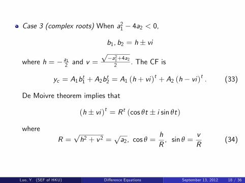
Case 3 (complex roots) When a21 − 4a2 < 0,

b1, b2 = h± vi

where h = − a12 and v =√−a21+4a22 . The CF is

yc = A1bt1 + A2bt2 = A1 (h+ vi)

t + A2 (h− vi)t . (33)

De Moivre theorem implies that

(h± vi)t = R t (cos θt ± i sin θt)

where

R =√h2 + v2 =

√a2, cos θ =

hR, sin θ =

vR

(34)


(conti.) The CF can be rewritten as

yc = A1R t (cos θt + i sin θt) + A2R t (cos θt − i sin θt) (35)

= R t [(A1 + A2) cos θt + (A1 − A2) i sin θt]

= R t (A5 cos θt + A6i sin θt) (36)

where R and θ can be determined once h and v become known.

Example: Consider yt+2 + 14yt = 5,which means that h = 0, v =

12 ,

R =

√0+

(12

)2=12, cos θ = 0, sin θ = 1, θ =

π

2=⇒ (37)

yc =

(12

)t (A5 cos

π

2t + A6i sin

π

2t). (38)


The Convergence of Time Path

The convergence of time path y is determined by the twocharacteristic roots of the SO DE.

In Case 1

if |b1 | > 1 and |b2 | > 1, then both components in the CF will beexplosive and yc must be divergent.if |b1 | < 1 and |b2 | < 1, then both components in the CF willconverge to 0 as t goes to infinity, as will yc also.if |b1 | > 1 and |b2 | < 1, then A2bt2 tend to converge to 0, while A1bt1tends to deviate further from 0 and will eventually render the pathdivergent.

Call the root with higher absolute value the dominant root since thisroot sets the tone of the time path. A time path will converge iff thedominant root is less than 1 in absolute value. The non-dominantroot also affects the time path, at least in the beginning periods.


In Case 2 (repeated roots), for the term A4tbt ,

if |b| > 1, the bt term will be explosive. and the multiplicative t termalso serves to intensify the explosiveness as t increases.if |b| < 1, the bt term will be converge. and the multiplicative t willoffset the convergence as t increases. It turns out the damping force bt

of will eventually dominant the exploding force t.Hence, the basic requirement for convergence is still that the root beless than 1 in absolution value.


In Case 3 (complex roots),

The term A5 cos θt + A6 i sin θt produces a fluctuation pattern of aperiodic nature. Since time is discrete, the resulting path displays asort of stepped fluctuation.The term Rt determines the convergence of y : determines whether thestepped fluctuation is to be intensified or mitigated as t increases.Hence, the basic requirement for convergence is still that the root beless than 1 in absolution value. The fluctuation can be graduallynarrowed down iff R < 1 (Note that R is just the absolute value of thecomplex roots h± vi).


Difference Equations System

So far our dynamic analysis has focused on a single differenceequation. However, some economic models may include a system ofsimultaneous dynamic equations in which several variables need to behandled. Hence, the solution method to solve such dynamic systemneed to be introduced.

The dynamic system with several dynamic equations and severalvariables can be equivalent with a single higher order equation with asingle variable. Hence, the solution of a dynamic system would stillinclude a set of PI and CF, and the dynamic stability of the systemwould still depend on the absolution values (for difference equationsystem) of the characteristic roots in the CF.


The Transformation of a Higher-order Dynamic Equation

In particular, a SO difference equation can be rewritten as twosimultaneous FOC equations in two variables. Consider the followingexample:

yt+2 + a1yt+1 + a2yt = c (39)

If we introduce an artificial new variable x , defined as xt = yt+1, wecan then express the original SO equation by the following two FO DE

xt+1 + a1xt + a2yt = c (40)

yt+1 − xt = 0 (41)


Solving Simultaneous Dynamic Equations

Suppose that we are given

xt+1 + 6xt + 9yt = 4 (42)

yt+1 − xt = 0 (43)

To solve this two-DE system, we still need to seek the PI and the CF,and sum them to obtain the desired time paths of the two variables xand y .

We first solve for the PI. As usual, try the constant solution:

yt+1 = yt = y and xt+1 = xt = x =⇒

x = y =14.


For the CF, try the following function forms

xt = mbt and yt = nbt

where m and n are arbitrary constants and b represents thecharacteristic root. Next, we need to find the values of m, n, and bthat satisfy the reduced version.Substituting these guessed solutions into the above dynamic systemand cancelling out the common term bt gives

(b+ 6)m+ 9n = 0 (44)

−m+ bn = 0 (45)

which is a linear homogeneous-equation system in m and n. We canrule out the uninteresting trivial solution (m = n = 0) by requiringthat ∣∣∣∣ b+ 6 9

−1 b

∣∣∣∣ = b2 + 6b+ 9 = 0 (46)

This characteristic equation have two roots b (= b1 = b2) = −3.Luo, Y. (SEF of HKU) Difference Equations September 13, 2012 26 / 36

(conti.) Given each bi (i = 1, 2), the above homogeneous equationimplies that there will have an infinite number of solutions for (m, n)

mi = kini (47)

For this repeated-root case, we have

xt = m1 (−3)t +m2t (−3)t , yt = n1 (−3)t + n2t (−3)t

which must satisfy yt+1 = xt :

n1 (−3)t+1 + n2 (t + 1) (−3)t+1 = m1 (−3)t +m2t (−3)t =⇒m1 = −3 (n1 + n2) ,m2 = −3n2

Setting n1 = A3 and n2 = A4 gives

xc = −3A3 (−3)t − 3A4 (t + 1) (−3)t (48)

yc = A3 (−3)t + A4t (−3)t (49)

Note that both time paths have the same (−3)t term, so they bothexplosive oscillation.


Matrix Notation

We can analyze the above dynamic system by using matrix. Theabove two-equation system can be written as[

1 00 1

]︸︷︷︸

I

[xt+1yt+1

]︸︷︷︸

u

+

[6 9−1 0

]︸︷︷︸

K

[xtyt

]︸︷︷︸

v

=

[40

]︸︷︷︸d

(50)

Try a constant PI first,

(I +K )[xy

]= d =⇒

[xy

]= (I +K )−1 d =

[1/41/4

].


(conti.) Next, try the CF

u =

[mbt+1

nbt+1

]=

[mn

]bt+1 and v =

[mn

]bt =⇒

(bI +K )[mn

]= 0

To avoid the trivial solution, we must have

|bI +K | = 0 =⇒ b = −3 =⇒mi = kini , where ni = Ai ,mi = kiAi

where Ai are arbitrary constants.


(conti.) With distinct real roots,[xcyc

]=

[m1bt1 +m2b

t2

n1bt1 + n2bt2

]=

[k1A1bt1 + k2A2b

t2

A1bt1 + A2bt2

]. (51)

With repeated roots,[xcyc

]=

[m1bt1 +m2tb

t2

n1bt1 + n2tbt2

](52)

The general solution can be written as[xtyt

]=

[xcyc

]+

[xy

]. (53)


Two-Variable Phase Diagram: Discrete-time Case

Now we shall discuss the qualitative-graphic (phase-diagram) analysisof a nonlinear difference equation system. Specifically, we focus onthe following two-equation system

xt+1 − xt = f (xt , yt ) (54)

yt+1 − yt = g (xt , yt ) (55)

which is called autonomous system (t is not an explicit argument in fand g).

The two-variable phase diagram (PD) can answer the qualitativequestions: the location and the dynamic stability of the intertemporalequilibrium.

The most crucial task of the PD is to determine the direction ofmovement of the two variables over time. In the two-variable case, wecan also draw the PD in the space of (x , y).


(Conti.) In this case, we have two demarcation lines:

∆xt+1 = xt+1 − xt = f (xt , yt ) = 0 (56)

∆yt+1 = yt+1 − yt = g (xt , yt ) = 0 (57)

which interact at point E representing the intertemporal equilibrium(∆xt+1 = 0 and ∆yt+1 = 0) and divide the space into 4 regions. (willbe specified later.)If the demarcation line can be solved for y in terms of x , we can plotthe line in the (x , y) space. Otherwise, we can use theimplicit-function theorem to derive:

slope of ∆xt+1 =dydx|∆xt+1=0 = −

∂f /∂x∂f /∂y

= − fxfy; (58)

slope of ∆yt+1 =dydx|∆yt+1=0 = −

∂g/∂x∂g/∂y

= −gxgy. (59)

Specifically, we assume that fx < 0, fy > 0, gx > 0, gy < 0,whichmeans that both slopes are positive. Further assume that − fxfy > −

gxgy.


(conti.) The two curves, at any other point, either x or y changesover time according to the signs of ∆xt+1 and ∆yt+1 at that point:

d (∆xt+1)dx

= fx < 0, (60)

which means that as we move from west to east in the space (as xincreases), ∆xt+1 decrease so that the sign of ∆xt+1 must passthrough three stages, in the order: +, 0,−. Similarly,

d (∆yt+1)dy

= gy < 0, (61)

which means that as we move from south to north in the space (as yincreases), ∆yt+1 decreases so that the sign of ∆yt+1 must passthrough three stages, in the order: +, 0,−.


Linearization of a Nonlinearization Difference-EquationSystem

Another qualitative technique of analyzing a nonlinear differenceequation system is to examine its linear approximation which isderived by using the Taylor expansion of the system around itsintertemporal equilibrium.

At the point of expansion (i.e., the IE), the linear approximation hasthe same equilibrium as the original nonlinear system. In a suffi cientlysmall neighborhood of E, the linear approximation should have thesame general streamline configuration as the original system.

As long as we confine our stability analysis to the immediateneighborhood of the IE, the approximated system can include enoughinformation from the original nonlinear system. This analysis is calledlocal stability analysis.


(Conti.) For the two difference equation system, we have

∆xt+1 = f (x0, y0) + fx (x0, y0) (x − x0) + fy (x0, y0) (y − y0)∆yt+1 = g (x0, y0) + gx (x0, y0) (x − x0) + gy (x0, y0) (y − y0)

For purpose of local stability analysis, the above linearization can beput a simpler form. First, the expansion point is the IE, (x , y) andf (x , y) = g (x , y) = 0. We then have another form of linearization

xt+1 − (1+ fx (x , y)) x − fy (x , y) y = −fx (x , y) x − fy (x , y) yyt+1 − gx (x , y) x − (1+ gy (x , y)) y = −gx (x , y) x − gy (x , y) y

which means that[xt+1 − xyt+1 − y

]−[1+ fx fygx 1+ gy

](x ,y )︸︷︷︸

JE

[xt − xyt − y

]=

[00

].


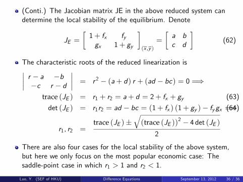
(Conti.) The Jacobian matrix JE in the above reduced system candetermine the local stability of the equilibrium. Denote

JE =[1+ fx fygx 1+ gy

](x ,y )

=

[a bc d

](62)

The characteristic roots of the reduced linearization is∣∣∣∣ r − a −b−c r − d

∣∣∣∣ = r2 − (a+ d) r + (ad − bc) = 0 =⇒

trace (JE ) = r1 + r2 = a+ d = 2+ fx + gy (63)

det (JE ) = r1r2 = ad − bc = (1+ fx ) (1+ gy )− fygx =⇒(64)

r1, r2 =trace (JE )±

√(trace (JE ))

2 − 4 det (JE )2

There are also four cases for the local stability of the above system,but here we only focus on the most popular economic case: Thesaddle-point case in which r1 > 1 and r2 < 1.


notes on solving di⁄erence equationsyluo/teaching/6012_2017/notesdifferenceeqs.pdf ·...

Documents