notes for math 230a, differential...
TRANSCRIPT

NOTES FOR MATH 230A, DIFFERENTIAL GEOMETRY
AARON LANDESMAN
CONTENTS
1. Introduction 42. 9/3/15 52.1. Logistics 52.2. Lecture begins 53. 9/8/15 73.1. Curvature of curves 83.2. Manifolds 83.3. Partitions of Unity 93.4. A is compact 103.5. A = ∪iAi with Ai compact and Ai ⊂ int(Ai+1) 103.6. A is open 113.7. A general 114. 9/10/15 114.1. Partitions of Unity, Hiro’s version 114.2. Submersions 135. 9/15/15 135.1. Tangent Spaces 135.2. Return to the submersion theorem 166. 9/17/15 166.1. Completing the submersion theorem 166.2. Lie Brackets 176.3. Constructing the Tangent bundle 187. 9/22/15 207.1. Constructing vector bundles 238. 9/24/15 258.1. Logistics 258.2. structure groups 258.3. Fiber bundles in general 268.4. Algebraic Prelude to differential forms 268.5. Differential Forms 279. 9/29/15 299.1. Integration 3310. 10/1/15 3410.1. Review 3410.2. Flows and Lie Groups 3410.3. Lie Derivatives 3611. 10/6/15 39
1
2 AARON LANDESMAN
11.1. Key theorems to remember from this class, not proven until latertoday 39
11.2. Class as usual 3912. 10/8/15 4312.1. Overview 4312.2. Today’s class 4412.3. Riemannian Geometry on vector bundles 4712.4. Connections 4813. 10/20/2015 4913.1. Key theorems for today 4913.2. Class time 4913.3. Connections 5114. 10/22/15 5414.1. Class time 5514.2. Connections and Riemannian Geometry 5615. 10/27/15 6015.1. Overview 6015.2. Parallel Transport 6016. 10/29/15 6516.1. Overview 6516.2. Connections 6616.3. The Fundamental Theorem of Riemannian Geometry 6716.4. Geodesics 7017. 11/2/15 7117.1. Geodesics and coming attractions 7117.2. Properties of the exponential map 7418. 11/5/15 7618.1. Review 7618.2. Geodesics and length 7719. 11/10/15 8119.1. Preliminary questions 8119.2. Hopf-Rinow 8219.3. Curvature 8319.4. Towards some properties and intuition on curvature tensors 8520. 11/12/15 8720.1. Types of curvatures 8720.2. Review of Linear Algebra 8820.3. Traces in Riemannian Geometry 8920.4. Back to linear algebra 9221. 11/17/15 9321.1. Plan and Review 9321.2. Scalar curvature 9321.3. Normal Coordinates 9721.4. Hodge Theory 9922. 11/19/15 10022.1. Questions and Overview 10022.2. Gauss’ Theorema Egregium 10022.3. Sectional Curvature and the Exp map 102

NOTES FOR MATH 230A, DIFFERENTIAL GEOMETRY 3
22.4. Hodge Theory 10323. 11/24/15 10523.1. Good covers, and finite dimensional cohomology 10523.2. Return to Hodge Theory 10723.3. Harmonic Forms and Poincare Duality 11024. 12/1/15 11324.1. Overview, with a twist on the lecturer 11324.2. Special Relativity 11324.3. The Differential Geometry Set Up 11424.4. Toward Maxwell’s equations 11525. 12/3/15 11825.1. Overview 11825.2. Principle G-bundles 11825.3. Connections and curvature on principle G-bundles 11925.4. An Algebraic characterization of connections on principleG-bundles12025.5. Curvature as Integrability 124
4 AARON LANDESMAN
1. INTRODUCTION
Hiro Tanaka taught a course (Math 230a) on Differential Geometry at Harvardin Fall 2015.
These are my “live-TEXed“ notes from the course. Conventions are as follows:Each lecture gets its own “chapter,” and appears in the table of contents with thedate.
Of course, these notes are not a faithful representation of the course, either in themathematics itself or in the quotes, jokes, and philosophical musings; in particular,the errors are my fault. By the same token, any virtues in the notes are to becredited to the lecturer and not the scribe. 1
Please email corrections to [email protected].
1This introduction has been adapted from Akhil Matthew’s introduction to his notes, with hispermission.

NOTES FOR MATH 230A, DIFFERENTIAL GEOMETRY 5
2. 9/3/15
2.1. Logistics.(1) Phil Tynan is the TF, who isn’t here(2) email: [email protected](3) Hiro’s office is 341, office hours are Tuesday 1:30 - 2:30pm, and Wednesday
2-3pm.(4) Phil will have office hours 2-3pm on Thursdays, in office 536 and 532.(5) There will be homeworks, once a week, the first homework is due Sept 17.(6) When homework is graded, we will get a remark from Phil to see Hiro and
Phil during office hours. You will not be numerically graded from week toweek, but you have to come to them in person, so that we know what isgoing on.
(7) There will be no midterm, but one take home final.
Remark 2.1. There are two words in the title of the course, Differential and Ge-ometry. This is not Riemannian geometry and we’ll discuss the difference later.“Differential” connotates calculus. You can ask how to do calculus on shapes likestriangles and cubes. To understand calculus, we will learn about manifolds, andcalculus on manifolds.
To understand geometry, we will think of a space together with some structure(possibly some type of metric).
Example 2.2. (1) Riemannian geometry(2) Symplectic geometry - use things like Hamiltonian to describe how vector
spaces evolve.(3) Complex geometry - generalize complex analysis to shapes you can build
with Cn or CW complex.(4) Kahler geometry(5) Calabi-Yau geometry - study supersymmetric string theory
2.2. Lecture begins. Consider a curve γ : R→ Rn, t 7→ γ(t).
Definition 2.3. For γ a curve, we define the length of γ to be∫R
|γ ′(t)| dt,
where
|γ ′(t)| =
√∑i
γ ′i(t)2 =
√〈γ ′,γ ′〉
.
Remark 2.4. The inner product from Definition 2.3 should really be thought ofas an inner product on Tγ(t)Rn and not on Rn. Even though these objects areisomorphic, they should not be thought of as “the same.”
Definition 2.5. Let U ⊂ Rn be an open set. A function f : U→ Rm is called
• C0 if it is continuous• C1 if it has partial derivatives ∂f
∂xifor i = 1, . . . ,nwhich are all C0
• Cr if it has all partial derivatives of order at most rwhich are all C0
• C∞ or smooth if f is Cr for all r.

6 AARON LANDESMAN
Definition 2.6. Let U ⊂ Rn be an open set. Then, a Riemannian metric on U is aC∞ function g : U→Mn×n(R) (where the matrix represents an inner product onthat space) such that
• g(x) is a symmetric nondegenerate matrix.• g(x) is positive definite
Example 2.7. (1) Set g(x) := In×n for all x. This is the standard Riemannianmetric on Rn.
(2) Fix a smooth map f : U→ Rm. Since f is C1, it induces a map dfx : TxU ∼=TxRn → Tf(x)Rm. In “standard basis” for TxRn, we can write
dfx :=
(∂fj
∂xi
)j=1,...,m,i=1,...,n
If there is a Riemannian metric h on Rm, this induces a bilinear product onU: Given u, v ∈ TxU, we send it to 〈u, v〉 := 〈dfx(u),dfx(v)〉. This definesa Riemannian metric on U precisely when dfx is an injection.
Definition 2.8. A C∞ map f : U → Rm is an immersion if dfx is injective for allx ∈ U. The induced Riemannian metric is denoted f∗h and is given by
f∗hx(u, v) := h(dfx(u),dfx(v))
Remark 2.9. Caution: Immersions need not be injective. For example, one cansend two points to the same point. Alternatively, one can take the universal coverR→ S1.
Definition 2.10. Let g be a Riemannian metric on U ⊂ Rn, the volume of (U,g) is
Vol(U,g) :=∫U
√deggdx1 · · ·dxn
Next, we describe when we should be able to think of two open sets with aRiemannian metric as equivalent.
Definition 2.11. A diffeomorphism if f is a bijection, f is C∞ and f−1 is C∞.
Definition 2.12. Fix (U,g) and (V ,h) to be two open sets each with a Riemannianmetric. An isometry from (U,g) to (V ,h) is a smooth diffeomorphism f : U → Vsuch that f∗h = g.
Remark 2.13. Why is there a square root in the volume function? When one triesto evaluate the volume function, we get two contributions from dfx, so we haveto take a square root.
Remark 2.14. What is the connection between giving a matrix and giving an innerproduct? If the function g, viewed as a matrix, defines an inner product gij :=
〈ei, ej〉, where ei is the ith standard basis vector. Then, g(u, v) := ut · g · v.
So far, there is an obvious constraint, that we’ve only been dealing with opensets in Rn. We would like the notion of manifolds, which are more general spacesin which one can do differential geometry. A manifold is a topological manifoldwith a smooth structure.
Definition 2.15. A topological space X is locally Euclidean if for all x ∈ X, thereexists d ≥ 0,d ∈ Z, an open set U ⊂ Rd, and a homeomorphism f : U→ X.

NOTES FOR MATH 230A, DIFFERENTIAL GEOMETRY 7
Remark 2.16. Caution: Locally Euclidean does not imply Hausdorff. As a coun-terexample, consider the affine line with a doubled origin.
Definition 2.17. A topological space X is second countable if X admits a countablebasis of open sets.
Definition 2.18. A basis for a topological space X is a collection of subsets Vα sothat
(1) x = ∪αVα(2) For every α,β, one can cover Vα ∩ Vβ = ∪γVγ
Warning 2.19. The above definition 2.18 determines a topology, where the opensets are given by arbitrary unions of elements in the basis. However, if we aregiven a topology on X to start with, we will also need to require that every openset U ⊂ X can be written as a union of basis elements.
Example 2.20. Euclidean space (Rn) is second countable. To see this, take a count-able basis given by balls around all rational points with rational radii. Any sub-space of a second countable space is also second countable, by restricting the basis.
Remark 2.21. If X is a topological manifold, every connected component is of Xwill be a locally Euclidean, Hausdorff, second countable space. So, one can definea topological manifold to be something satisfying these three properties.
Definition 2.22. An open cover Uα is locally finite if for every x ∈ X, there existsW ⊂ X an open subset containing x such that W ∩Uα 6= 0 for only finitely manyα.
Definition 2.23. A space X is paracompact if every open cover admits a locallyfinite refinement.
Definition 2.24. A topological manifold is a space X so that X is(1) locally Euclidean(2) Hausdorff(3) Paracompact
Paracompact allows you to turn local functions to global ones.
3. 9/8/15
Exercise 3.1. Let γ : R → Rn be an immersion. Show there exists a diffeomor-phism φ : R→ R such that γ φ is parameterized by arc length, i.e., |d(γφ)
dt | = 1.
Remark 3.2. If you’re given a smooth curve in Rn, we have an intuitive idea ofwhat it means, but we can choose various parameterizations. We can choose aparameterization by arc length so that the amount of time traveled is the amountof distance traveled.
This exercise looks a lot like a differential equation, which can be solved by thefundamental theorem of calculus.
Solution to exercise: take φ to be∫s0 |dγdt
−1dt By the chain rule,
d
dsγ φ =
dγ
dt
dφ
ds=dγ
dt
dγ
dt
−1
(3.1)
we use the fundamental theorem of calculus is employed to calculate the deriv-ative of φ.

8 AARON LANDESMAN
3.1. Curvature of curves.
Definition 3.3. Let γ : R→ Rn be an immersion. Define
~T : R→ Rnt 7→ γ
|γ|(3.2)
The curvature vector at γ(t) is defined to be
~κ :=d~T
ds=d~T/dtds/dt
(3.3)
Exercise 3.4. (1) Show ~κ ⊥ ~T .(2) If γ : R→ R2 has image a circle of radius R, show |~κ| = 1
R .(3) If φ : R→ R is a diffeomorphism, then the value of ~κ(γ(t)) = ~κ(γ φ(s)).
Solution to exercise:(1) Consider the function t 7→ 〈~T(t),~T(t)〉. This is a constant function. The de-
rivative ddt 〈~T(t),~T(t)〉 = 〈
ddt
~T(t),~T(t)〉+ 〈~T(t), ddt~T(t)〉 = 2〈ddt
~T(t),~T(t)〉.(2) Choose γ : R→ R2, t 7→ R · (cos t, sin t) So, ~T = (− sin t, cos t). Then
|d~T/dtds/dt
=1
ds/dt=1
R(3.4)
because we the circle is parameterized by t between 0 and 2π while thelength of the circle is 2πR.
(3) We use the chain rule. We write the circle in two ways.
Consider a hyperboloid in R3. Say we want to know the curvature of the sur-face at x. We can define a normal vector to a tangent plane at a point. Given twovectors, a normal vector and a point in the plane, we can intersect the plane with asurface and obtain a curve. Given this curve, we know how to compute the curva-ture. Then, there are two principal vectors in the tangent space, one with minimalcurvature and one with maximal curvature. The Gaussian curvature is then theproduct of the maximal and minimal curvature. This turns out to be independentof the embedding of the surface.
Remark 3.5. Curvature |κ(γ(t))| is the inverse radius of the best approximatingcircle at γ(t).
3.2. Manifolds. Recall the following definitions from the previous class:
Definition 3.6. An open cover Uα is locally finite if for every x ∈ X, there existsW ⊂ X an open subset containing x such that W ∩Uα 6= 0 for only finitely manyα.
Example 3.7. Say Uα = Bα(0),α ∈ Q, where Bα(0) is a ball about the origin ofradius α. Then, Uαα∈Q is not a locally finite cover about 0. Similarly, if we onlyindex over the integers, it is still not locally finite.
Definition 3.8. A space X is paracompact if every open cover admits a locallyfinite refinement, where a refinement is another cover so that each element of thenew cover is contained in some element of the original cover.
Definition 3.9. A topological manifold is a space X so that X is(1) locally Euclidean(2) Hausdorff

NOTES FOR MATH 230A, DIFFERENTIAL GEOMETRY 9
(3) Paracompact
Remark 3.10. We still can’t do calculus. On the overlap of two open sets, we willneed a compatibility condition. We have to check that the derivatives agree on theoverlaps. If φV φ−1
U , the composition of two chart functions isn’t smooth, there’sno way to compare calculus on φU(U) and φV (V).
Definition 3.11. Let X be a topological manifold. Then, a chart on X is a pair(U,φU) where U is open an φU is a homeomorphism onto some open set in Rn,for some n, possibly depending on U.
Definition 3.12. A Cr atlas is a collection of charts (Uα,φα) so that(1) Uα form a cover(2) for all α,β the function φβ φ−1
α where defined is C∞.
Definition 3.13. A Cr manifold is a pair (X,A) where X is a topological manifoldand A is a Cr atlas on X.
Definition 3.14. Let (X,AX), (Y,AY), be two Ct manifolds then a continuous func-tion f : X→ Y is Cr for r < t if it is locally Cr. That is, if for all x ∈ X, there is some(U,φ) ∈ AX, (V ,ψ) ∈ AY so that x ∈ U, f(x) ∈ V and the function ψV f φ−1
U isCr.
Remark 3.15. The existence of (U,φ), (V ,ψ) implies that ψβ f φ−1α is Cr for all
charts in AX,AY .
Definition 3.16. A function f(X,A)→ (Y,AY) is called a Cr diffeomorphism if(1) f is a bijection(2) f is Cr
(3) f−1 is Cr
Theorem 3.17. (Whitehead) Not every topological manifold admits a C∞ atlas.
Theorem 3.18. (Milnor) If X = S7, then X admits non diffeomorphic smooth structures.
Theorem 3.19. (Donaldson-Freedman) Say X = R4. Then, X admits uncountably manynon diffeomorphic smooth structures.
Remark 3.20. Define an equivalence relation on the set of possible C∞ atlases onX. Say A ∼ A ′ if A ∪ A ′ is also a C∞ atlas. It’s not hard to check this is equiv-alent to the existence of a diffeomorphism (given by the identity map) betweenthese two structures on A. Note that given an equivalence class of an atlas, thereexists a maximal representative, given by taking the union over all atlases in theequivalence class of A.
For this reason, one can also define a C∞ manifold to be a topological manifoldtogether with a maximal atlas A.
3.3. Partitions of Unity. Partitions of unity are devices that let us piece togetherfunctions on a manifold.
Definition 3.21. A partition of unity ofA subordinate to a coverUα is a collectionof functionsΦ, with U some open set containing A and φ : U→ [0, 1] so that
(1) For each x ∈ A there exists an open set V with x ∈ V so that only finitelymany φ ∈ Φ are nonzero on V .
10 AARON LANDESMAN
(2) We have∑φ∈Φφ(x) = 1, which makes sense as the sum is a finite sum,
by the previous point.(3) For each φ ∈ Φ, there exists α so that. we have Supp(φ) ⊂ Uα.
Theorem 3.22. Given any set A ⊂ Rn, and any open cover Uα, a partition of unity onA subordinate to Uα exists.
Proof. We prove this by breaking successively tackling more and more compli-cated types of sets A.
3.4. A is compact.
Lemma 3.23. For any open ball B(x, r) there exists a smaller open ball B(x, s) ⊂ B(x, r)and a smooth φ with φ|B(x,s) = 1 and φ|Rn\B(x,r) = 0.
Proof. We can replace B(x, r) and B(x, s) by cubes S =∏i(ai,bi) ⊂ R =
∏i(ci,di)
by choosing s so that B(x, s) ⊂ S ⊂ R ⊂ B(x, r). So, it suffices to prove the theoremfor cubes. Now, we have already shown this on problem set 5, problem 4c in thecase n = 1. Let fi : R→ R be a function which is 1 on on (ai,bi) and 0 outside of(ci,di). Then, f(x1, . . . , xn) =
∏i fi(xi) is the desired function.
In this case, for each x ∈ X, choose Bx to be an open ball so that there is someUα with Bx ⊂ Uα, and choose Cx to be a smaller open ball so that x ∈ Cx ⊂ Bx,so that there exists a function which takes the value 1 in Cx and 0 outside of Bx.Then, take a finite cover of A by such balls Cx. call the associated functions ψi,with 1 ≤ i ≤ n. Define
φk =ψk∑ni=1φn
.
Observe thatk∑i=1
φi = 1.
This shows the φi sum to 1 everywhere. Additionally, each φi has support con-tained in the same Uα that ψi does.
3.5. A = ∪iAi with Ai compact and Ai ⊂ int(Ai+1). t Take our given opencoverUα ofA. ConstructUiα an open cover of Bi = int(Ai+1) \Ai−2, by definingUiα = Uα ∩ Bi. Define Ci = Ai \
∫(Ai−1). Then, Ci ⊂ Bi. Therefore, we can
construct a partition of unity subordinate ofCi subordinate toUiα, Let the partitionof unity be denotedΦi. Define
σ(x) =∑
i∈N,φ∈φi
ψ(x).
Define φ(x) = ψ(x)/σ(x). Note that σ 6= 0 on some open set containing A, since ateach x ∈ A, some φ are strictly positive at x. Say x ∈ Ai, x /∈ Ai−1. Therefore, onthe domain where σ 6= 0, we obtain there are only finitely many φ with φ(x) 6= 0,since we must have φ ∈ Φk for k ≤ i+ 2, and there are only finitely many suchfunctions in each Φk. Additionally, the φi sum to 1 by construction, because wedivided by their sum, σ.

NOTES FOR MATH 230A, DIFFERENTIAL GEOMETRY 11
3.6. A is open. Construct
Ai = x ∈ A|d(x,∂A) ≥ 1
i, |x| ≤ i.
Observe this give a cover of A by sets as in the previous case.
3.7. A general. Say our open cover of A is Uα. Then, choose B = ∪αUα. Notethat there is a partition of unity for B, which is also a partition of unity for A.
4. 9/10/15
4.1. Partitions of Unity, Hiro’s version.
Exercise 4.1. (1) Consider j : R2 → R3, (x,y) 7→ (x, cosy, siny). Computej∗gstd.
(2) The arc length parameterization proof from last lecture is incorrect (some-thing about the chain rule being incorrectly applied) Why?
Solution:
(1) Recall j∗gstd : R2 → M2×2(R). Note the image j(R2) is a cylinder. To
compute the pullback of the inner product is given by dj(x,y) =
1 00 − siny0 cosy
Then, we compute g11 = 1,g12 = 0,g22 = 1, so it is the standard metric.We can see this also by computing j∗gstd = djt · dj
(2) Look at the errata. To correctly parameterize curves, given γ : R → Rn,consider the map ` : R → R, t 7→ ∫t0 |γ|dt. Since γ is an immersion, γ hasan inverse, so we see γ = γ `−1 and we can find the derivative of γ.
Remark 4.2. From now on, we write X for a smooth manifold, but remember thisalso comes with the datum of an atlas A.
Remark 4.3. In the previous day, I added some notes I had written for a previ-ous class on partitions of unity. Here, we repeat the same thing, but with Hiro’snotation.
Definition 4.4. Let X be a smooth manifold. Fix an open cover U = Uα. A parti-tion of unity subordinate to U is a collection of smooth functions
fβ : X→ R≥0
so that
(1)∑β∈B fβ(x) = 1
(2) For all β, Supp(fβ) =x : fβ(x) 6= 0
⊂ Uβ
(3)
Supp(fβ) is locally finite
That is, for every x there is an open x ∈ W sothatW ∩ Supp(fβ) 6= ∅ for only finitely many β ∈ B.
Theorem 4.5. (Existence of partitions of unity) Let X be a C∞ manifold. Then for allopen covers U =
Uβ
, there exists a C∞ partition of unity subordinate to U.
Remark 4.6. This is the way we’ll prove that any manifold admits a Riemannianmetric, and many other foundational results. It will let us patch things on Rn
together.

12 AARON LANDESMAN
Remark 4.7. Replace the words C∞ by Cr, and the theorem still holds. To provethis, we only need to show an analog of Lemma 4.8, and the rest goes throughautomatically.
Proof.
Lemma 4.8. Let U ⊂ Rn and K ⊂ U compact. Then, there exists a smooth functionf : U→ R≥0 so that
(1) f(int(K)) ⊂ R>0(2) Supp(f) ⊂ U.
Proof. Follows from homework.Cover K ⊂ U by open balls Wx : x ∈ K so thatWx ⊂ U. By compactness, choose a finite such collection. We can find Wx ⊂W ′x ⊂ U, and by the homework, there is a function fx : U→ R, with f > 0 on Wxand f ≥ 0 onWx.
Lemma 4.9. Let Cγ be a collection of closed subsets of X. If Cγ is locally finite, then∪γCγ is closed.
Proof. This is an easy topological lemma. By local finiteness, for all x ∈ X, there issome Wx so that Cγ ∩Wx 6= ∅ for only finitely many γ. So, this implies ∪γW ∩Cγ) is closed in Wx. This implies ∪γCγ is locally closed. Because X is locallyEuclidean and Hausdorff, then ∪γCγ is closed.
Using these lemmas, we now prove the theorem.
4.1.1. Step A. Let Wε be a refinement of Uβ. If there exists a partition of unitysubordinate toWε, then there exists a partition of unity subordinate to Uβ.
To see this, fix k : ε → β so that Wε ⊂ Uk(ε). Then, if fε is a partitionof unity, define fβ =
∑ε∈k−1(β) fε. The first two properties of partition of unity
hold because fε is. To verify Supp(fβ) ⊂ Uβ follows from. That is, we haveSupp(fβ) ⊂ Supp fε ⊂ ∪Wε ⊂ Uβ by Lemma 4.9.
4.1.2. Step B. We can always choose a refinementWε ofUβ so thatWε is compact.Proof: Homework
4.1.3. Step C. Fixing such aWε as in step B, we can find a locally finite refinementYε ofWε so that Yε ⊂Wε (with the same indexing set).
Proof: for each Wε, model it as a union of open balls in Rn, and then choosea refinement of Wε by very small open balls Zδ so that the closure of each Zδ iscontained in Wε, and we can assume by paracompactness that it is locally finite.Then, take the union of the Zδ in a given Wε to be Yε. This is implicitly assumingLemma 4.9.
4.1.4. Step D. We’re done!Let’s see why: By Lemma 4.8, we have smooth functions fε :Wε → R so that
(1) fε(Yε) ⊂ R≥0(2) Supp(fε) ⊂Wε.
Then, set
gε =fε∑ε fε
(4.1)
This assignment enforces that they sum to 1.

NOTES FOR MATH 230A, DIFFERENTIAL GEOMETRY 13
Remark 4.10. It is possible Hiro came up with this proof but the inspiration camefrom Collins’ textbook which mentioned that Lemma 4.9 as crucial.
4.2. Submersions. We will treat the submersion theorem just inside Rn. The prin-cipal for why we can do this is that anything you can do in Rn, you can do formanifolds in general by piecing together open sets.
Definition 4.11. Let f : U → V be a smooth map. Let U ⊂ Rn,V ⊂ Rm open.Then, f is called a submersion at x ∈ U if dfx : TxU→ Tf(x)V is a surjection.
Remark 4.12. (1) For f to be a submersion, n ≥ m.(2) if U→ V is an inclusion of open sets withm = n, then f is a submersion.(3) f : (x1, . . . , xn) 7→ (x1, . . . , xm) is a submersion, because dfx is (Im×m 0).
Definition 4.13. f is a submersion if f is a submersion at all x ∈ U.
Theorem 4.14. (Submersion Theorem) Let f : U → V be a submersion. Then, for ally ∈ V , f−1(y) ⊂ U is a smooth submanifold.
Remark 4.15. This theorem will readily generalize to arbitrary manifolds, once wedefine the relevant terms.
The following definition was stated in class, but isn’t relevant to the submersiontheorem
Definition 4.16. A continuous map f : X→ Y between topological spaces is properif for all K ⊂ Y compact, f−1(K) is compact.
Remark 4.17. The dimension of f−1(y) will be n−m if n = dimU,m = dimV .
Definition 4.18. A subset X ⊂ U ⊂ Rn with U open is a smooth submanifoldof U if for all x ∈ X there exists an open W ⊂ U and a smooth diffeomorphismφ : Rn →W so that φ(Ri) = X∩W with Ri ⊂ Rn some sub vector space.
Remark 4.19. A smooth submanifold of U is a smooth manifold.
Example 4.20. If f : Rn → R,~x 7→ |x|2.
5. 9/15/15
The course website is now on piazza.
5.1. Tangent Spaces.
Remark 5.1. A tangent vector gives me a way to take derivatives. Say we haveU ⊂ Rn, f : U → R. The derivative is a row vector with n entries. More ge-ometrically, we can discuss the derivative as follows: Given X ∈ TxU, we knowhow to compute the directional derivative of f at x in the direction of X, usingX(f),Xx(f),X(x)(f),X(f)(x) when X is a vector field.
Question 5.2. What algebraic properties does Xx : C∞(U)→ R satisfy?
Definition 5.3. Given a manifold X, we let C∞(X),C∞(X;R) denote the set ofsmooth functions X→ R.
What properties do tangent vectors satisfy?

14 AARON LANDESMAN
(1) Xx(af+ g) = aXx(f) +Xx(g) for a ∈ R, f,g ∈ C∞(M)(2) Leibniz rule, Xx(fg) = Xx(f) · e(g) + e(f) · Xx(g).
Definition 5.4. Let A,B be commutative algebras over R. Fix an R algebra homo-morphism e : A → B. A derivation is a function D : A → B satisfying linearityand the Leibniz rule.
Example 5.5. (1) Take A = C∞(M),B = R, and e = evx : C∞(M) → R, f 7→f(x).
(2) A = C∞(M),B = A, e = id.(3) A = C∞(M),B = C∞(N), j : N→M, e : A→ B, f 7→ f j.
Remark 5.6. In algebraic geometry, given a map of manifolds, we get a map ofrings, and this operation similarly encodes the relative geometry of the rings.
Definition 5.7. Let M be a smooth manifold. Then, the tangent space of M atx ∈M is denoted
TxM := D : C∞(M)→ R derivations with respect to evx .(5.1)
We should verify things like(1) T0Rn ∼= Rn as vector spaces(2) Chain rule
Proposition 5.8. Let x ∈ U ⊂ M. Then, if f|U = gU with f,g ∈ C∞(M), thenXx ∈ TxM implies Xx(f) = Xx(g).
Proof. Choose some compact ball Bwith int(B) 3 x so that B ⊂ U. Fix h :M→ R
so that h|B = 1 and Supph ⊂ U. Given a derivation Xx consider Xx(h · (f− g)) =0. By the Leibniz rule, we see
0 = Xx(h · (f− g))= Xx(h) · (f− g)(x) + h(x) · Xx(f− g)= h(x) · Xx(f− g)= Xx(f) −Xx(g).
Proposition 5.9. Let j : N → M. Then, there exists a R linear map notated by any ofdj|x,djx = dj(x) with x ∈M TxN→ Tj(x)M defined by
Xx 7→ (f 7→ Xx(f j))Proof. Exercise
Proposition 5.10. Let N j−→ Mh−→ L be C∞ functions. Then the chain rule holds. That
is,
d(h j)x = dhj(x) djxProof. Given f ∈ C∞(L), we have
d(h j)x(Xx)(f) = Xx(f (h j))= Xx((f h) j)= djx(Xx)(f h)= dhj(x)djx(Xx)(f)

NOTES FOR MATH 230A, DIFFERENTIAL GEOMETRY 15
Corollary 5.11. The natural map TxU→ TxM, induced by
C∞(M) C∞(U)
R
is an isomorphism.
This is supposed to be an algebraic incarnation of your intuition that tangentvectors depend only on germs around a point.
Proof. Immediate from Proposition 5.8.
Exercise 5.12. We have TxM is an R vector space.Solution: We have a 0 derivation, and derivations add and scale.
Remark 5.13. Why the Leibniz rule? This pops out of doing computations overSpec k[ε]/ε2, and maps of this into the manifold are the same as tangent vectors.
Proposition 5.14. T0Rn ∼= Rn as vector spaces, but not canonically.
Proof. Note that the assignment∂
∂xi|x : C∞(Rn)→ Rf 7→ ∂f
∂xi(0)
is a derivation. We claim ∂
∂xi|0, . . . ,
∂
∂xn|0
Form a basis for T0Rn. By Taylor’s theorem, any C∞ function Rn
f−→ R can bewritten as f(x) = f(0) +
∑i xigi(x) where gi : Rn → R is C∞ and gi(0) = ∂
∂xi|0.
Given a derivation X~0, because the derivation of a constant function is 9, we have
X~0 = X~0(f(0)) + sumiX~0(xigi(x))
= 0+∑i
X~0(xi)gi(~0) +
∑i
xi(~0) · X~0(gi(x))
=∑i
X~0(xi)∂
∂xi(0)
which is independent of f. That is, we have shown X~0(f) =∑
(ai∂∂xi
|0(f). This
shows ∂∂xi
span. They are also linearly independent since ∂∂xixj = δji.
Corollary 5.15. IfM is n dimensional at x then TxM ∼= Rn.
Proof. Follows from Proposition 5.14 and the above corollary stating that tangentspaces can be computed locally.
Remark 5.16. Let j : Rm → Rn be smooth. Then,
dj0
(∂
∂xi|0
)=∑j
(dj0)ij∂
∂xj
is the connection between Taylor’s definition and the matrix of partial functions.
16 AARON LANDESMAN
Remark 5.17. For all y ∈ Rn, there is a smooth diffeomorphism Ty : Rn →Rn, x 7→ x+ y. Then,
∂
∂xi|y = dTy
(∂
∂xi|0
)Exercise 5.18. By the chain rule, and diffeomorphism j : M → N induces linearisomorphism dxj : TxM ∼= Tj(x)N.
5.2. Return to the submersion theorem. Recall:
Definition 5.19. Let F :M → N be smooth. A point y ∈ N is a regular value of fif for all x ∈ f−1(y), dfx is a surjection.
Example 5.20. f : R→ R, t 7→ t2 is regular whenever y ∈ R is nonzero.
Definition 5.21. A subset Z ⊂ M is called a smooth submanifold if for all z ∈ Zthere is U ⊂M open and Z ⊂ U and a smooth diffeomorphism h : V → U so thath(Rm) = U∩ Z, with Rm ⊂ Rn.
Theorem 5.22. Let M,N be smooth manifolds and f : M → N be smooth. Then, for allregular values y ∈ N, we have f−1(y) ⊂M is a C∞ submanifold.
Proof. Go to local chartsM f−→ N ⊃ V 3 y. Then,
U V
φ(U) φ(V).
We now ask what f looks like in these coordinate charts. By definition of smooth-ness, ψ f φ−1 : U→ V is smooth. Since y is a regular value, d(ψ f φ−1)φ(x)
with x ∈ f−1(y) is a surjection. So, Tφ(x)U → Tφ(y)V is surjection. Without lossof generality, assume φ(x) = 0 ⊂ Rm and φ(y) = 0 ∈ Rn. By linear algebra,there is an invertible matrix A : Rn → Rn so that A d(ψ f φ−1 = (In 0).So, the C∞ function A ψ f φ−1 : Rm → Rn has the derivative (In 0) at 0.Now, define a function and expand the function so that the derivative matrix is theidentity matrix by the inverse function theorem, and make it the matrix mappingthe coordinate matrix to a hyperplane.
6. 9/17/15
6.1. Completing the submersion theorem. Hiro was up late last night, so hemight be a little less active and a little more sarcastic or dismissive, but he saidhe’ll try not to be.
The homework is due, emailed to Phil by 11:59pm tonight.Recall: Last time we defined TxM, tangent spaces, and started proving the sub-
mersion theorem:
Theorem 6.1. If f : X → Y smooth and y ∈ Y is a regular value, then f−1(y) ⊂ X is asmooth submanifold.
NOTES FOR MATH 230A, DIFFERENTIAL GEOMETRY 17
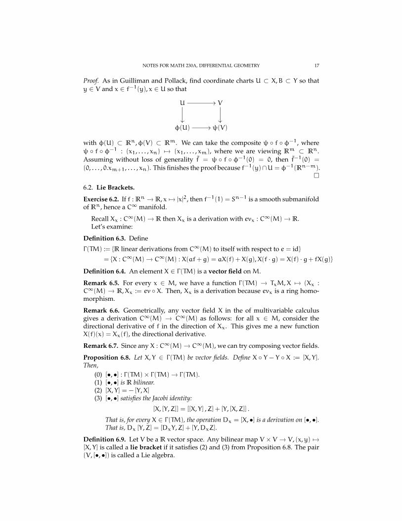
Proof. As in Guilliman and Pollack, find coordinate charts U ⊂ X,B ⊂ Y so thaty ∈ V and x ∈ f−1(y), x ∈ U so that
U V
φ(U) ψ(V)
with φ(U) ⊂ Rn,φ(V) ⊂ Rm. We can take the composite ψ f φ−1, whereψ f φ−1 : (x1, . . . , xn) 7→ (x1, . . . , xm), where we are viewing Rm ⊂ Rn.Assuming without loss of generality f = ψ f φ−1(0) = 0, then f−1(0) =
(0, . . . , 0.xm+1, . . . , xn). This finishes the proof because f−1(y)∩U = φ−1(Rn−m).
6.2. Lie Brackets.
Exercise 6.2. If f : Rn → R, x 7→ |x|2, then f−1(1) = Sn−1 is a smooth submanifoldof Rn, hence a C∞ manifold.
Recall Xx : C∞(M)→ R then Xx is a derivation with evx : C∞(M)→ R.Let’s examine:
Definition 6.3. Define
Γ(TM) := R linear derivations from C∞(M) to itself with respect to e = id
= X : C∞(M)→ C∞(M) : X(af+ g) = aX(f) +X(g),X(f · g) = X(f) · g+ fX(g)
Definition 6.4. An element X ∈ Γ(TM) is a vector field onM.
Remark 6.5. For every x ∈ M, we have a function Γ(TM) → TxM,X 7→ (Xx :C∞(M) → R,Xx := ev X. Then, Xx is a derivation because evx is a ring homo-morphism.
Remark 6.6. Geometrically, any vector field X in the of multivariable calculusgives a derivation C∞(M) → C∞(M) as follows: for all x ∈ M, consider thedirectional derivative of f in the direction of Xx. This gives me a new functionX(f)(x) = Xx(f), the directional derivative.
Remark 6.7. Since any X : C∞(M)→ C∞(M), we can try composing vector fields.
Proposition 6.8. Let X, Y ∈ Γ(TM) be vector fields. Define X Y − Y X := [X, Y].Then,
(0) [•, •] : Γ(TM)× Γ(TM)→ Γ(TM).(1) [•, •] is R bilinear.(2) [X, Y] = − [Y,X](3) [•, •] satisfies the Jacobi identity:
[X, [Y,Z]] = [[X, Y] ,Z] + [Y, [X,Z]] .
That is, for every X ∈ Γ(TM), the operation Dx = [X, •] is a derivation on [•, •].That is, Dx [Y,Z] = [DxY,Z] + [Y,DxZ].
Definition 6.9. Let V be a R vector space. Any bilinear map V × V → V , (x,y) 7→[X, Y] is called a lie bracket if it satisfies (2) and (3) from Proposition 6.8. The pair(V , [•, •]) is called a Lie algebra.

18 AARON LANDESMAN
Remark 6.10. The Proposition 6.8 is equivalent to Γ(TM) being a Lie algebra.
Proof of (0). We need to show X Y − Y X is a derivation. Pick f,g ∈ C∞(M). Wewant to show this satisfies the Leibniz rule.
X(Y(fg)) − Y(X(fg)) = X(Y(f)g+ fY(g)) − Y(X(f)g+ fX(g))
= X(Y(f))g+ Y(f)X(g) +X(f)Y(g) + fX(Y(g)) − Y(X(f))g−X(f)Y(g) − Y(f)X(g) − f(Y(X(g)))
= X(Y(f))g+ fX(Y)(g) − Y(X(f))g− f(Y(X(g))
= (X(Y(f)) − Y(X(f)))g+ f(X(Y(g)) − Y(X(g)))
Remark 6.11. For all commutative rings A, we have Der(A,A) is a Lie algebraunder [X, Y] = X Y − Y X, as follows from the proof of Proposition 6.8.
Exercise 6.12. IfM = Rn, any vector field X can be written as
X =
n∑i=1
Xi∂
∂xi
where the above derivation at x ∈ Rn satisfies ∂∂xi
(x) = ∂∂xi
|x. Then,
[X, Y] =[∑
Xi∂
∂xi,∑
Yj∂
∂xj
]=∑ij
Xi∂Yj
∂xi∂
∂xj− Yj
∂Xi
∂xj∂
∂xi
So X(Y) is “take the naive derivative of Xwith respect to Y.
Remark 6.13. A more geometric interpretation can be given as follows. Each vec-tor field X gives rise to a flow.’ If we have ΦX : M×R → M,ΦXt : M → M is adiffeomorphism for all t. Given X and Y, can we compare ΦYs −ΦXt and Φxt ΦYS .Then, [X, Y] measures noncommutativity of these vector fields near t = s = 0.
6.3. Constructing the Tangent bundle. We now embark on constructing the tan-gent bundle.
Definition 6.14. Given a smooth manifoldM, define
TM :=∐x∈X
TxM
We now want to topologize this tangent bundle and give it a smooth atlas. Ifwe manage to do this, we end up with the following structure:
(1) A smooth manifold TM together with
TMπ−→M
(x,y) 7→ x
(2) for all x, we have π−1(x) has the structure of a vector space over R
NOTES FOR MATH 230A, DIFFERENTIAL GEOMETRY 19
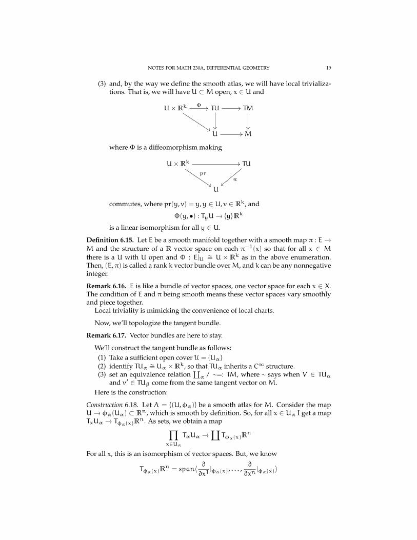
(3) and, by the way we define the smooth atlas, we will have local trivializa-tions. That is, we will have U ⊂M open, x ∈ U and
U×Rk TU TM
U M
Φ
whereΦ is a diffeomorphism making
U×Rk TU
U
prπ
commutes, where pr(y, v) = y,y ∈ U, v ∈ Rk, and
Φ(y, •) : TyU→ yRk
is a linear isomorphism for all y ∈ U.
Definition 6.15. Let E be a smooth manifold together with a smooth map π : E→M and the structure of a R vector space on each π−1(x) so that for all x ∈ M
there is a U with U open and Φ : E|U ∼= U × Rk as in the above enumeration.Then, (E,π) is called a rank k vector bundle overM, and k can be any nonnegativeinteger.
Remark 6.16. E is like a bundle of vector spaces, one vector space for each x ∈ X.The condition of E and π being smooth means these vector spaces vary smoothlyand piece together.
Local triviality is mimicking the convenience of local charts.
Now, we’ll topologize the tangent bundle.
Remark 6.17. Vector bundles are here to stay.
We’ll construct the tangent bundle as follows:(1) Take a sufficient open cover U = Uα
(2) identify TUα ∼= Uα ×Rk, so that TUα inherits a C∞ structure.(3) set an equivalence relation
∐α / ∼=: TM, where ∼ says when V ∈ TUα
and v ′ ∈ TUβ come from the same tangent vector onM.Here is the construction:
Construction 6.18. Let A = (U,φα) be a smooth atlas for M. Consider the mapU→ φα(Uα) ⊂ Rn, which is smooth by definition. So, for all x ∈ Uα I get a mapTxUα → Tφα(x)Rn. As sets, we obtain a map∏
x∈Uα
TαUα →∐ Tφα(x)Rn
For all x, this is an isomorphism of vector spaces. But, we know
Tφα(x)Rn = span〈 ∂∂x1
|φα(x), . . . ,∂
∂xn|φα(x)〉
20 AARON LANDESMAN
So, we have an isomorphism
Tφα(x)Rn ∼= φα(x)×Rn,
x 7→ (a1, . . . ,an)
where X =∑ai
∂∂xi
|φα(x). So, we obtain a map∐x∈Uα
TxUα → φα(Uα)×Rn
Let TUα =∐x∈Uα TxUα be given the unique smooth structure making this a
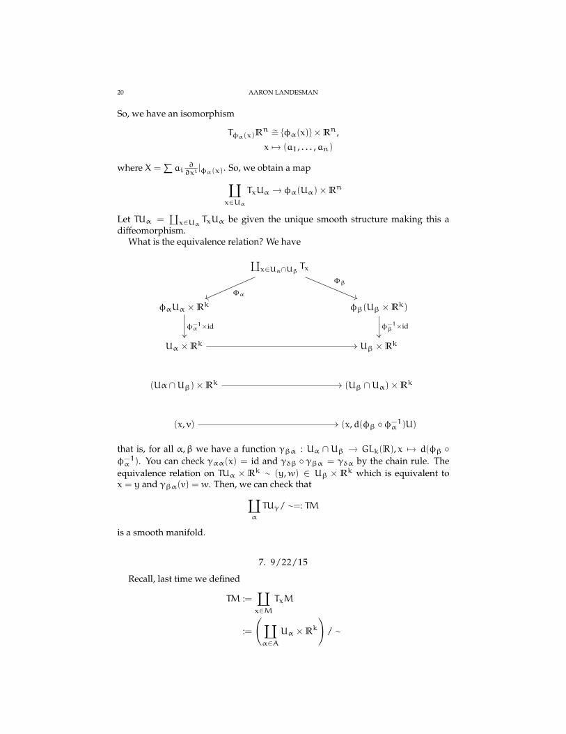
diffeomorphism.What is the equivalence relation? We have
∐x∈Uα∩Uβ Tx
φαUα ×Rk φβ(Uβ ×Rk)
Uα ×Rk Uβ ×Rk
(Uα∩Uβ)×Rk (Uβ ∩Uα)×Rk
(x, v) (x,d(φβ φ−1α )U)
Φα
Φβ
φ−1α ×id φ−1
β ×id
that is, for all α,β we have a function γβα : Uα ∩ Uβ → GLk(R), x 7→ d(φβ φ−1α ). You can check γαα(x) = id and γδβ γβα = γδα by the chain rule. The
equivalence relation on TUα × Rk ∼ (y,w) ∈ Uβ × Rk which is equivalent tox = y and γβα(v) = w. Then, we can check that∐
α
TUγ/ ∼=: TM
is a smooth manifold.
7. 9/22/15
Recall, last time we defined
TM :=∐x∈M
TxM
:=
(∐α∈A
Uα ×Rk
)/ ∼
NOTES FOR MATH 230A, DIFFERENTIAL GEOMETRY 21
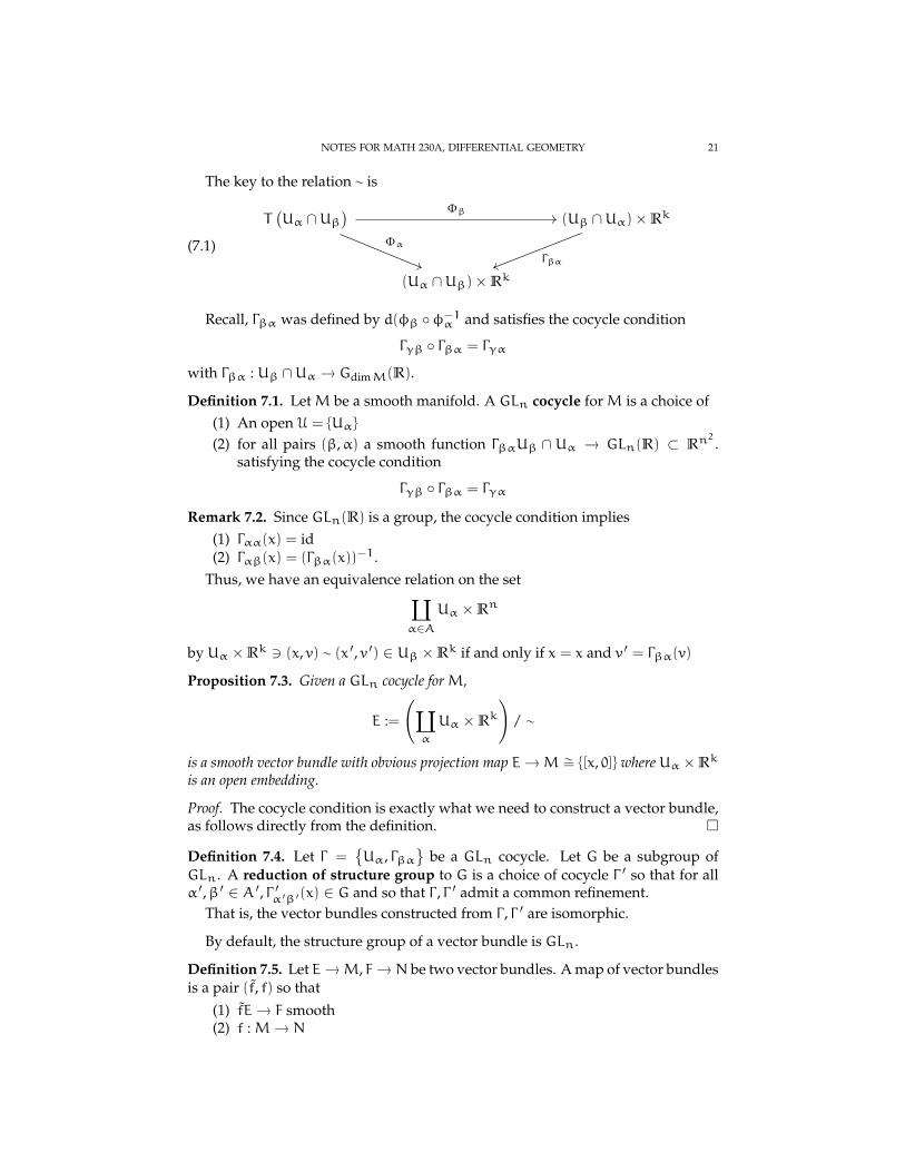
The key to the relation ∼ is
(7.1)
T(Uα ∩Uβ
)(Uβ ∩Uα)×Rk
(Uα ∩Uβ)×Rk
Φβ
Φα
Γβα
Recall, Γβα was defined by d(φβ φ−1α and satisfies the cocycle condition
Γγβ Γβα = Γγα
with Γβα : Uβ ∩Uα → GdimM(R).
Definition 7.1. LetM be a smooth manifold. A GLn cocycle forM is a choice of(1) An open U = Uα
(2) for all pairs (β,α) a smooth function ΓβαUβ ∩ Uα → GLn(R) ⊂ Rn2.
satisfying the cocycle condition
Γγβ Γβα = Γγα
Remark 7.2. Since GLn(R) is a group, the cocycle condition implies(1) Γαα(x) = id(2) Γαβ(x) = (Γβα(x))
−1.Thus, we have an equivalence relation on the set∐
α∈AUα ×Rn
by Uα ×Rk 3 (x, v) ∼ (x ′, v ′) ∈ Uβ ×Rk if and only if x = x and v ′ = Γβα(v)
Proposition 7.3. Given a GLn cocycle forM,
E :=
(∐α
Uα ×Rk
)/ ∼
is a smooth vector bundle with obvious projection map E→M ∼= [x, 0] where Uα ×Rk
is an open embedding.
Proof. The cocycle condition is exactly what we need to construct a vector bundle,as follows directly from the definition.
Definition 7.4. Let Γ =Uα, Γβα
be a GLn cocycle. Let G be a subgroup of
GLn. A reduction of structure group to G is a choice of cocycle Γ ′ so that for allα ′,β ′ ∈ A ′, Γ ′α ′β ′(x) ∈ G and so that Γ , Γ ′ admit a common refinement.
That is, the vector bundles constructed from Γ , Γ ′ are isomorphic.
By default, the structure group of a vector bundle is GLn.
Definition 7.5. Let E→M, F→ N be two vector bundles. A map of vector bundlesis a pair (f, f) so that
(1) fE→ F smooth(2) f :M→ N

22 AARON LANDESMAN
(3)
(7.2)E F
M N
(4) For all x ∈M we have a map f|x : Ex → Ff(x) is an R linear map of vectorspace.
Definition 7.6. An isomorphism of vector bundles is a bundle map (f, f) so that f(and hence f) are diffeomorphisms.
Definition 7.7. Let E → M be a smooth vector bundle. Then, a section of E is asmooth function s :M→ E so that
(7.3)M E
M
s
idπ
commutes, for all x ∈M, s(x) ∈ Ex.
Definition 7.8. We let Γ(E) denote the set of all sections of E
Note that the notation Γ has nothing to do with cocycles, it is just notation forglobal sections.
Example 7.9. An element X ∈ Γ(TM) is a vector field onM.
Proposition 7.10. DerR(C∞(M),C∞(M)) ∼= Γ(TM).
Proof. Exercise
Remark 7.11. Looking for sections is the first strategy for studying vector bundles,hence manifolds.
Example 7.12. Say a section s ∈ Γ(E) is nowhere vanishing if s(x) 6= 0 for allx ∈M.
The first question one might ask about a vector bundle is whether you can finda nowhere vanishing vector section (vector field).
Theorem 7.13. (Poincare-Hopf) TS2 does not admit a nowhere vanishing section.
Proof. Not given
Corollary 7.14. S2 6∼= S1 × S1
Proof. This follows from Theorem 7.13, though there are much easier ways toprove this.
Definition 7.15. A bundle E is orientable if it admits a reduction of structuregroup to
G = GL+n(R) = A ∈ GLn(R) : detA > 0

NOTES FOR MATH 230A, DIFFERENTIAL GEOMETRY 23
Intuitively, if we choose our transition functions, we want some sort of way toenforce that these transition functions preserve orientation, that is, preserve thesign of the determinant.
Remark 7.16. Studying whether TM can admit a G reduction yields informationaboutM
Definition 7.17. M is called orientable if TM is orientable.
Remark 7.18. This means you can choose coordinate charts (Uα,φα) so thatd(φβ φ−1
α ) always has positive determinant.
Definition 7.19. A bundle E is called trivial if E ∼= M×Rn as bundles and M isparallelizable if TM is trivial.
Remark 7.20. Poincare Hopf is a proof that TS2 is not trivial. A fancier form of thePoincare Hopf theorem says there is always a nonvanishing vector field on an odddimensional manifold.
Example 7.21. The number of linearly independent (nowhere vanishing) sectionsis a difficult, interesting, invariant of a vector bundle.
Proposition 7.22. E→M is trivial if and only if(1) E admits n linearly independent sections, with n = dimEx(2) E admits a reduction of structure group to id.
Proof. Omitted
7.1. Constructing vector bundles.
7.1.1. Pullbacks. First, we can pull back vector bundles.
Construction 7.23. Suppose F π−→M is a vector bundle. Fix a smooth map M→ N.Define
f∗F =(x, v) : x ∈M, v ∈ Ff(x)
It is not hard to check local triviality.
Remark 7.24. One way to see smoothness of f∗F is as follows:
(7.4)f∗F F
M N
π
f
then π is transverse (meaning that the direct sum of the derivatives span the tan-gent space) to f automatically. Now, the fiber product of these two smooth mapsis a smooth manifold, since the maps are transverse, their fiber product is smooth,as follows from the homework.
Example 7.25. Let Eπ1−−→M, F
π2−−→M. Then,
(7.5)• E
F M

24 AARON LANDESMAN
we have π∗1F = π∗2E and admits a projection map toM by
π∗F = (x, v,y,w)|(x, v) ∈ E, (y,w) ∈ F, x = y
In particular, π∗Fx = Fx ⊕ Ex. This is called the Whitney sum or direct sum of Eand F and is denoted E⊕ F→M.
Example 7.26. Consider j : Sn → Rn+1. We know TRn+1 is trivial so j∗(TRn+1)is trivial and TSn admits a fiberwise injective map of vector bundles
(7.6)TSn j∗TRn+1
Sn Sn
dj
Moreover, we can check that TSn⊕R ∼= j∗TRn+1, where by R we mean the trivialline bundle, which is the bundle of vectors perpendicular to TSn.
7.1.2. Functorial Methods. We often have ways of producing new vector spacesfrom old ones, such as dualizing and tensoring.
Definition 7.27. Given V we can send V 7→ ⊕n≥0 ⊗n V := T •(V), the tensoralgebra or free associative algebra on V , with Tk(V) = V⊗k.
Note that T •(V) is an associative algebra over primitives v1 ⊗ · · · ⊗ vk withmultiplication given by simple tensor and unit 1 ∈ T0(V) ∼= R.
Remark 7.28. This is a super useful algebra, it’s super fun!
Consider the two-sided ideal I ⊂ T •(V) generated by v⊗ v ∈ V⊗2
Definition 7.29. The exterior algebra ∧•(V) := T(V)/I.
Remark 7.30. Given V we can also construct also construct the exterior algebra by∧•V := ⊕n ∧n V .
Example 7.31. Given Tk → T •(V) → ∧•(V), we set ∧k(V) to be the image ofTk(V) and write [v1 ⊗ · · · ⊗ vk] := v1 ∧ · · ·∧ vk. Note that ∧0(V) ∼= T0(V) ∼= R
and ∧1(V) ∼= T1(V) ∼= V .Next, we want to understand ∧2(V). We demand that v⊗ v = 0, and so x⊗ y =
y ⊗ x, so we obtain anticommutativity, by expanding (x + y) ⊗ (x + y). Goingfurther, the product on T •(V) induces a product on ∧•(V)
∧k(V)×∧l(V)→ ∧l+k(V)
α,β 7→ α∧β
satisfying α∧β = (−1)klβ∧α.
Exercise 7.32. If dimV = 1 then T •(V) ∼= R[x].
All of these methods of making new vector spaces respects isomorphism smoothlyand composition of isomorphisms. That is, they determine functors on the groupoidof the category of vector spaces.
Then, given a cocycle, analogous constructions yield new vector bundles onM.

NOTES FOR MATH 230A, DIFFERENTIAL GEOMETRY 25
Example 7.33. (Dual Vector Bundles) Given E → M with cocycle Γ , we define anew cocycle as follows. We have We start with Γβα. Taking the dual construction,we consider the maps
(Γβα)∨ : Uβ ∩Uα × (Rk)∨ → Uα ∩Uβ × (Rk)∨
and note that Γ∨ determines a cocycle as well, hence a vector bundle. Then, thevector bundle constructed from Γ∨ is called the dual vector bundle to E.
Example 7.34. (Tensor Product) Let E, F be vector bundles. Assume we have co-cycles ΓE, ΓF over the same open cover U, possibly after taking refinements. Then,define ΓEαβ ⊗ ΓFαβ : Uα ∩ Uβ → GLnE·nF(R) where nE = dimEx,nF = dim Fx.This is a cocycle for E⊗ F called the tensor product for E⊗ F.Definition 7.35.
(TM)∨ =: T ∗M
is the cotangent bundle ofM.
8. 9/24/15
8.1. Logistics. Email Phil the homework by 11:59 tonight.Last time, we discussed:
(1) Reducing structure groups(2) E⊕ F,E⊗ F,∧•(E).
Today, we’ll discuss(1) Structure groups(2) Fiber bundles in general(3) Differential forms
8.2. structure groups.
Definition 8.1. For G a subgroup of automorphisms of the fibers, a G cocycle onM is the data of
(1) A set A(2) A function A→ Open(M),α 7→ Uα(3) For all α,β ∈ A×A a smooth function Γαβ : Uα ∩Uβ → G.
satisfying(1) Uα is an open cover(2) the cocycle condition
Definition 8.2. We’ll say a cocycle
Γ =A, Uα , Γαβ
is contained in another cocycle
Γ ′ =A ′,U ′α ′
, Γ ′α ′β ′
if there is an injection j : A→ A ′ so that(1) U ′
j(α) = Uα(2) Γj(α)j(β) = Γαβ
Alternatively, two cocycles have a common refinement if they are contained in acommon cocycle.
26 AARON LANDESMAN
8.3. Fiber bundles in general. We have now defined vector bundles, but it is nat-ural to ask if we can construct objects whose fibers are manifolds. These are calledfiber bundles.
Remark 8.3. More generally, consider a mathematical object F like a lie group,smooth manifold, a vector space with inner product then there is a groupAut(F) = smooth automorphisms of F. Then, we can define anAut(F) cocycle analogously.
Remark 8.4. We say Γαβ is smooth if(Uα ∩Uβ × F→ F
)is smooth, assuming F is a smooth manifold (assuming F has some smooth struc-ture).
Question 8.5. We can ask whether all bundles over the circle with fiber equal tothe circle are smooth
8.4. Algebraic Prelude to differential forms. Fix a field k. Recall:
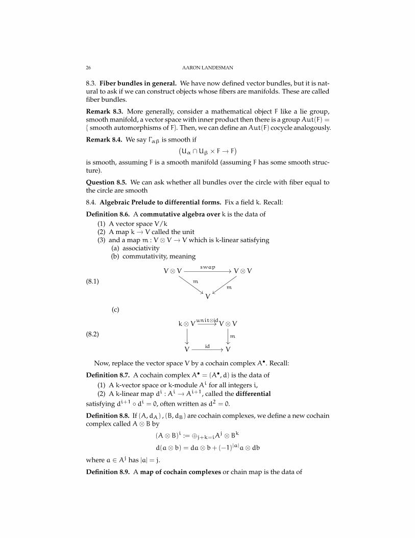
Definition 8.6. A commutative algebra over k is the data of(1) A vector space V/k(2) A map k→ V called the unit(3) and a mapm : V ⊗ V → V which is k-linear satisfying
(a) associativity(b) commutativity, meaning
(8.1)
V ⊗ V V ⊗ V
V
swap
mm
(c)
(8.2)
k⊗ V V ⊗ V
V V
unit⊗id
m
id
Now, replace the vector space V by a cochain complex A•. Recall:
Definition 8.7. A cochain complex A• = (A•,d) is the data of(1) A k-vector space or k-module Ai for all integers i,(2) A k-linear map di : Ai → Ai+1, called the differential
satisfying di+1 di = 0, often written as d2 = 0.
Definition 8.8. If (A,dA) , (B,dB) are cochain complexes, we define a new cochaincomplex called A⊗ B by
(A⊗ B)i := ⊕j+k=iAj ⊗ Bk
d(a⊗ b) = da⊗ b+ (−1)|a|a⊗ db
where a ∈ Aj has |a| = j.
Definition 8.9. A map of cochain complexes or chain map is the data of
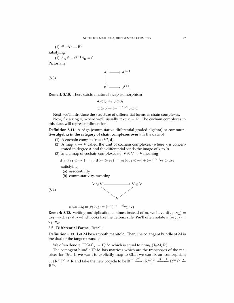
NOTES FOR MATH 230A, DIFFERENTIAL GEOMETRY 27
(1) fi : Ai → Bi
satisfying(1) dAfi − fi+1dB = 0.
Pictorially,
(8.3)Ai Ai+1
Bi Bi+1.
Remark 8.10. There exists a natural swap isomorphism
A⊗ B σ−→ B⊗A
a⊗ b 7→ (−1)|b||a|b⊗ aNext, we’ll introduce the structure of differential forms as chain complexes.Now, fix a ring k, where we’ll usually take k = R. The cochain complexes in
this class will represent dimension.
Definition 8.11. A cdga (commutative differential graded algebra) or commuta-tive algebra in the category of chain complexes over k is the data of
(1) A cochain complex V = (V•,d)(2) A map k → V called the unit of cochain complexes, (where k is concen-
trated in degree 0, and the differential sends the image of k to 0)(3) and a map of cochain complexesm : V ⊗ V → V meaning
d (m (v1 ⊗ v2)) = m (d (v1 ⊗ v2)) = m (dv1 ⊗ v2) + (−1)|v1|v1 ⊗ dv2satisfying(a) associativity(b) commutativity, meaning
(8.4)
V ⊗ V V ⊗ V
V
meaningm(v1, v2) = (−1)|v1||v2|v2 · v1.
Remark 8.12. writing multiplication as times instead of m, we have d(v1 · v2) =dv1 · v2± v1 · dv2 which looks like the Leibniz rule. We’ll often notatem(v1, v2) =v1 · v2.
8.5. Differential Forms. Recall:
Definition 8.13. LetM be a smooth manifold. Then, the cotangent bundle ofM isthe dual of the tangent bundle.
We often denote (T∨M)x := T∨x Mwhich is equal to homR(TxM, R).The cotangent bundle T∨M has matrices which are the transposes of the ma-
trices for TM. If we want to explicitly map to GLn, we can fix an isomorphism
ι : (Rm)∨ ∼= R and take the new cocycle to be Rmι−1−−→ (Rm)∨
df∨−−−→ (−→ Rm)∨ι−→
Rm.

28 AARON LANDESMAN
Definition 8.14. A differential k-form is a section of
∧k(T∨M)
Example 8.15. A differential 0-form is a section of R×M, i.e., a smooth functiononM. A differential one form is a section of T∨M. A k form is a smooth choice ofα(x) ∈ ∧k(T∨x M).
Recall
∧k(V) =∑
[v1 ⊗ · · · ⊗ vk
, vi ∈ V , v1,⊗ · · · ⊗ vk ∈ V⊗k, v1 ∧ v2 = −v2 ∧ v1
Remark 8.16. If you think of Vi ∈ V as being an element of degree 1, we obtaingraded commutativity
Lemma 8.17. If ei is a basis for V then ∧kV has a basis ei1 ∧ · · ·∧ eik , for i1 < · · · <ik.
Proof. Spanning is clear. Independence can be seen by relating it to independencein tensor products, I think.
The goal for the remainder is the prove the collection of differential forms, no-tated
Ω•deR(M) := Ω•(M) := A•(M)
is a cdga over R. That is, we’ll consider a cochain complex with the ith piecedefined to be Γ(∧i(T∨M)) and multiplication comes from that of concatenatingwedge products.
The work is in defining a differential which is a derivation
d = ddeR
the de Rham differential.
Definition 8.18. We define the 0th differential, d0 : Ω0(M) → Ω1(M) sendingC∞(M)→ Γ(T∨M), in which we want an assignment sending a function to a mapsending a point x to some dual vector to TxM.
We define d0 to be
f 7→ (TxM→ R,Xx 7→ Xx(f))
This map is indeed linear over R, meaning af+ g,a ∈ R, f,g ∈ C∞(M), because
Xx(af+ g) = aXx(f) +Xx(g)
and it is linear over TxM because
(Xx + Yx)(f) = Xx(f) + Yx(f).
We still need to check d0(f) is a smooth section, and notate d0(f) as df, which isannoying because df : TM→ TR, but instead df :M→ T∨M, which overloaded.Although, the composite
(8.5) TM TR RDf ∂t 7→1
has composite equal to df.Now, we’ll write df in local coordinates.

NOTES FOR MATH 230A, DIFFERENTIAL GEOMETRY 29
(1) Choose a consistent basis for T∨x U with U ⊂ Rn open. Consider the func-tion xi : U→ R, the ith coordinate function.
What does dxi do at a point x? We have dxi|x : TxM→ R as an elementof T∨x U. Let
v =
dimU∑i=1
vi∂
∂xi|x ∈ TxU
dxi|x(v) = v(xi) =
dimU∑j=1
vj∂
∂xj(xi) = vi
Proposition 8.19. Let f : U→ R be smooth. Then,
df|x =
dimU∑i=1
∂f
∂xi|xdx
i|x
so
df =
n∑i=1
∂f
∂xidxi
where n = dimU and ∂f∂xi∈ C∞(U) and dxi ∈ T∨U.
Proof. Not hard to prove
Proposition 8.20. Let g : U → V ,U ⊂ Rn,V ⊂ Rm be smooth. Defineg∗ : C∞(V)→ C∞(U), f 7→ f g. Then, d g∗ = g∗ d
(8.6)
Ω1(V) Ω1(U)
C∞(V) C∞(U(
Proof. Easy
Definition 8.21. Let g∗ : Ω1(V)→ Ω1(U),α 7→ α Dg.
Exercise 8.22. g∗α(Xx) = α|g(x)(Dg(Xx)) ∈ Tg(x)(V) where g∗(α)(Xx) ∈TxU.
9. 9/29/15
The goal for today is the following:(1) Prove (Ω•deR(M),ddR) is a cdga by class and homework(2) For all f : M → N smooth, there is an induced contravariant map f∗ :
Ω•(N)→ Ω•(M) as a map of cdga’s and cochain complexes.(3) Defining Hi(M) := kerdi/im di−1 and obtain an induced map on coho-
mology f∗ : H•(N) → H•(M). (This will be one of the easiest ways toprove(a) M 6∼= N(b) f 6' g.
(4) This defines a functorMfldop → grCommAlg/k sendingM 7→ H•deR(M).
30 AARON LANDESMAN
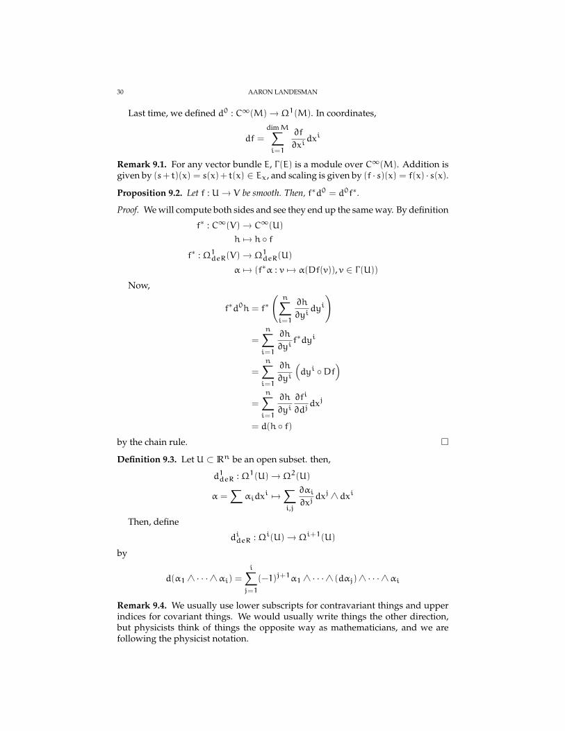
Last time, we defined d0 : C∞(M)→ Ω1(M). In coordinates,
df =
dimM∑i=1
∂f
∂xidxi
Remark 9.1. For any vector bundle E, Γ(E) is a module over C∞(M). Addition isgiven by (s+ t)(x) = s(x)+ t(x) ∈ Ex, and scaling is given by (f · s)(x) = f(x) · s(x).
Proposition 9.2. Let f : U→ V be smooth. Then, f∗d0 = d0f∗.
Proof. We will compute both sides and see they end up the same way. By definition
f∗ : C∞(V)→ C∞(U)
h 7→ h ff∗ : Ω1deR(V)→ Ω1deR(U)
α 7→ (f∗α : v 7→ α(Df(v)), v ∈ Γ(U))Now,
f∗d0h = f∗(n∑i=1
∂h
∂yidyi
)
=
n∑i=1
∂h
∂yif∗dyi
=
n∑i=1
∂h
∂yi
(dyi Df
)=
n∑i=1
∂h
∂yi∂fi
∂djdxj
= d(h f)by the chain rule.
Definition 9.3. Let U ⊂ Rn be an open subset. then,
d1deR : Ω1(U)→ Ω2(U)
α =∑
αidxi 7→∑
i,j
∂αi∂xj
dxj ∧ dxi
Then, define
dideR : Ωi(U)→ Ωi+1(U)
by
d(α1 ∧ · · ·∧αi) =i∑j=1
(−1)j+1α1 ∧ · · ·∧ (dαj)∧ · · ·∧αi
Remark 9.4. We usually use lower subscripts for contravariant things and upperindices for covariant things. We would usually write things the other direction,but physicists think of things the opposite way as mathematicians, and we arefollowing the physicist notation.
NOTES FOR MATH 230A, DIFFERENTIAL GEOMETRY 31
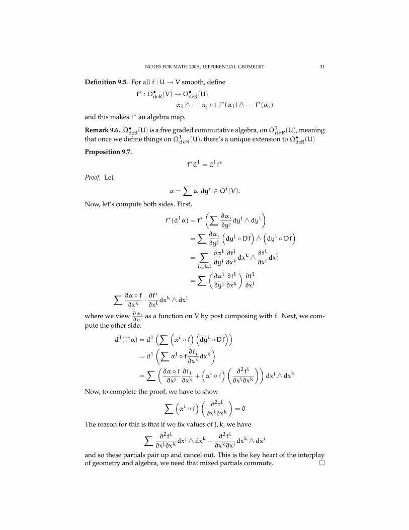
Definition 9.5. For all f : U→ V smooth, define
f∗ : Ω•deR(V)→ Ω•deR(U)
α1 ∧ · · ·αj 7→ f∗(α1)∧ · · · f∗(αi)
and this makes f∗ an algebra map.
Remark 9.6. Ω•deR(U) is a free graded commutative algebra, onΩ1deR(U), meaningthat once we define things onΩ1deR(U), there’s a unique extension toΩ•deR(U)
Proposition 9.7.
f∗d1 = d1f∗
Proof. Let
α =∑
αidyi ∈ Ωi(V).
Now, let’s compute both sides. First,
f∗(d1α) = f∗(∑ ∂αi
∂yjdyj ∧ dyi
)=∑ ∂αi
∂yj
(dyj Df
)∧(dyi Df
)=∑i,j,k,l
∂αi
∂yj∂fj
∂xkdxk ∧
∂fi
∂xldxl
=∑(
∂αi
∂yj∂fi
∂xk
)∂fi
∂xl∑ ∂α f∂xk
· ∂fi
∂xldxk ∧ dxl
where we view ∂αi∂yj
as a function on V by post composing with f. Next, we com-pute the other side:
d1(f∗α) = d1(∑(
αi f) (dyi Df
))= d1
(∑αi f ∂fi
∂xkdxk
)=∑(
∂α f∂xj
∂fi∂xk
+(αi f
)( ∂2fi
∂xi∂xk
))dxj ∧ dxk
Now, to complete the proof, we have to show∑ (αi f
)( ∂2fi
∂xi∂xk
)= 0
The reason for this is that if we fix values of j,k, we have∑ ∂2fi
∂xj∂xkdxj ∧ dxk +
∂2fi
∂xk∂xjdxk ∧ dxj
and so these partials pair up and cancel out. This is the key heart of the interplayof geometry and algebra, we need that mixed partials commute.

32 AARON LANDESMAN
Corollary 9.8. So, d1 defines a global assignment
d1 : Ω1(M)→ Ω2(M)
Proof. We have defined this map locally, and so if we write E =∐Uα ×Rk/ ∼, to
give a section of E, it is equivalent to give maps sα : Uα → Rk so that
Γαβ sα = sβ
This is what the proposition verifies. To complete the proof, we should really writedown what the induced overlap maps are, and check this is compatible with theoverlap maps, but this essentially follows because we have a two form and thederivatives of the two coordinates.
Proposition 9.9. d2deR = 0
Proof. It suffices to check this on an open set in Rn. We can further reduce tochecking d1 d0 = 0. (because d(α∧β) = dα∧β+ (−1)|α|α∧ dβ) and then
d1 d0(f) = d1(∑ ∂f
∂xjdxj)
=∑ ∂2f
∂xi∂xj
= 0
Corollary 9.10. The local definition of ddeR : Ω•deR(M)→ Ω•deR(M)
Proof. To show(Ω•deR(M),ddeR
)is a cdga, it remains to show It remains to show
d2 = 0. This follows from Proposition 9.9.
Remark 9.11. For any smooth f : U→ V , we showed
d0f∗ = f∗d0
d1f∗ = f∗d1
and so the analogous statement holds for 0, 1 replaced by i because we defined f∗
on i forms to define an algebra mapΩ•deR(V)→ Ω•deR(U).
Question 9.12. Here’s a slogan: k forms are things you can integrate over orientedkmanifolds. How do we integrate k forms?
We can answer the above question in two steps.(1) First, define an isomorphism ∧k(V∨) = (TxM)∨. Infinitesimally speak-
ing, we should get a map out of a collection of these k tangent vectors, andso we can think of ∧k(TxM) as an oriented collection of k tangent vectors.Getting a number from some vector is an element of a dual vector space.We then use the isomorphism ∧k(V∨) ∼= ∧k(V)∨.
(2) We then use partitions of unity.
Definition 9.13. (Definition of the isomorphism)(1) For k = 0, we want a map ∧0(R∨) ∼= R→ R∨ ∼= ∧0(V)∨, and since R is a
field we have a distinguished 1 ∈ R and we send 1 7→ (α : R→ R, 1 7→ 1).(2) When k = 1, we need a map R∨ → R∨, so take the identity map

NOTES FOR MATH 230A, DIFFERENTIAL GEOMETRY 33
(3) When k ≥ 2, We want
φ : ∧k(V∨)→ ∧k(V)∨
α1 ∧ · · ·∧αk 7→ (v1 ∧ · · ·∧ vk 7→ det
(αj(vk)
)ij
)Question 9.14. This induces a multiplication on⊕dimV
k=0 ∧k (V)∨ because⊕dimVk=1 ∧k
(V∨) has a multiplication, and we can then transfer the multiplication on the latteralgebra to the former algebra. But, what is the product?
Answer: Givenφ(α),φ(β) ∈ ∧k(V)∨,∧l(V)∨, we needφ(α)∧φ(β) ∈ ∧k+l(V)∨
is
φ(α)∧φ(β) (v1 ∧ · · ·∧ vk+l) =∑
π∈Shuffk,l
Sign(π)φα(vπ(1), . . . , vπ(k)) ·φβ(vπ(k+1), . . . , vπ(k+l)).
Where Shuffk,l ⊂ Sk+l is the set of k,l shuffles if π(1) < · · · < π(k) and π(k+1) <· · ·π(l).
9.1. Integration. Let U ⊂ M and φ : U → Rn be a chart. Let’s fix ω ∈ ΩndeR(M)so that Supp(ω) ⊂ U.
Then, φ−1 is a smooth map from φ(U) → M, so pulling back ω we get an nform on Rn or φ(U). But, any n form on Rn is of the form f · dx1 ∧ · · · ∧ dxn,and we know how to integrate a smooth function on Rn. We could try to define∫Mω :=
∫Rnf.
However, there is a problem with orientation, the integral∫Mω is only well
defined up to sign. Consider an orientation reversing diffeomorphism j : φ(U)→φ(U). This negates the value of the integral, by change of variables, if we denoteby f the function by pulling back along φ−1 j, we get∫
Mω =
∫Rnf =
∫Rn
−f
because the chain rule will have an absolute value around the determinant of theJacobian.
So, to make this well defined, we should demand that φ must satisfy somecompatibility condition with an orientation onM.
By definition of orientation, if φ is compatible with an orientation on M, thenj−1φ is not.
Definition 9.15. Let M be an oriented n manifold. Let U be a Euclidean open set,meaning that there exists a chart φ : U → Rn. Then, for any n form ω, withSuppω ⊂ U, ∫
Mω :=
∫Rnf
where f is obtained by pulling backω along a chartφ compatible with orientation.
Definition 9.16. Let M be oriented and ω any n form on M. Then, fix an atlasA = Uα,φα for M compatible with the orientation on M, fix a partition of unityhα subordinate to A, and define∫
Mω :=
∑α∈A
∫Mhαω

34 AARON LANDESMAN
Remark 9.17. Depending on the behavior ofω, this could be∞,−∞ or undefined.
Example 9.18. When a function is unbounded on R, you can define this by takingsome limit over extending open sets in R. Unless you choose such a conventionfor all manifolds, this integral might be undefined.
10. 10/1/15
10.1. Review. Last time, we showed the existence of a differential ddeR onΩ•deR(M).Locally,
Ωk(Rn) =∑
fIdxI
where I = (i1, . . . , ik), i1 < · · · < ik and dxI ∈ Γ(∧kT∨Rn). Then, d glues to aglobal mapΩk(M)→ Ωk+1(M).
Exercise 10.1. We have(1) Ω•deR(M) is a cdga over R for any smooth M(2) For all f :M→ Nwe have a map of cdga’s f∗Ω•deR(N)→ Ω•deR(M).(3) By the chain rule, (f g)∗ = g∗ f∗.
Remark 10.2. Using the isomorphism
∧k(V∨) ∼= ∧k(V)∨
α1 ∧ · · ·∧αk 7→ (v1 ∧ · · ·∧ vk 7→ det
(αi(vj)
))We can also write f∗ : Ωk(N)→ Ωk(M) as follows. Given α ∈ Ωk(N), we have
(f∗α)(x) ∈ ∧k(T∨x M) ∼=(∧k (TxM)
)∨defined by
(f∗α) (x) 7→ (v1 ∧ · · ·∧ vk 7→ α(f(x)) (Df(v1)∧ · · ·∧Df(vk)))
10.2. Flows and Lie Groups.
Remark 10.3. Here is some motivation. Fix a vector field X on M. Does it makesense to flow along X? That is, if we give our manifold some sort of fluid, does itmake sense for the fluid to move in the direction of the vector field?
Theorem 10.4. (Existence, Uniqueness, and smooth dependence of solutions to first orderODEs) Let U ⊂ Rn be open, and I ⊂ R open. Fix a smooth function
Y : I×U→ Rn
(t, x) 7→ Y(t, x)
Then, for every x ∈ U, there exists(1) tmin < 0 < tmax ∈ R.(2) A smooth function γ : (tmin, tmax)→ U
so that(1) γ(0) = x and(2)
∂γi
∂t= Yi(t,γ1(t), . . . ,γn(t))

NOTES FOR MATH 230A, DIFFERENTIAL GEOMETRY 35
In other words, γ = Y(t,γ(t)). (Existence)Furthermore, if γ : (t ′min, t ′max) → U also satisfies the above two conditions, then
γ = γ on the intersection of their domains of definition. (Uniqueness)Further,
(1) There existsW ⊃ U, x ∈W(2) ε > 0
so that the function
W × (−ε, ε)→ U
(x, t) 7→ γx(t)
is well defined and smooth (C∞ dependence).
Proof. Idea: Look at all smooth functions on U, pass to some vector space of mapsfrom R to U, and show that as you look for solutions, and create a contractionoperator, and the fixed point of this is the solution. This is just the contractionlemma. You have to show that the limit of these vector fields is a smooth vectorfield.
We won’t give a proof in class, though.
Remark 10.5. Theorem 10.4 is a consequence of the Picard Lindelof theorem.
Corollary 10.6. Fix X a vector field on M. Locally, this defines a function Y : U → Rn,where n = dimM,U ⊂M. For every x ∈M there isW ⊂M, ε > 0 x ∈W and smoothmap
Φx :W × (−ε, ε)→M
(x, t) 7→ Φ(x, t)
so that for all x, t, we have
DΦx|(x,t)
(∂
∂t|t
)= X(Φx(x,t))
and ΦX(x, 0) = x. That is,
(10.1)
T(W × (−ε, ε) TM
W × (−ε, ε) M
DΦx
Φx
(0, ∂∂t ) X
commutes.
Proof.
Corollary 10.7. By uniqueness we have
ΦXt ′ ΦXt = ΦXt ′+t
where defined. And, for all t,ΦXt is a diffeomorphism onto its image
Proof. Use thatΦXt ΦX−t = ΦX0 = id, and use uniqueness plus the fact that every-thing in sight is smooth.
Definition 10.8. A vector field X on M is complete if for all x ∈ M, the intervalIx ⊂ R on which the flow ΦX :W × Ix →M is defined can be taken to be R.

36 AARON LANDESMAN
Remark 10.9. Intuitively, completeness means that the flow exists for all time, forall x.
Definition 10.10. A manifold M is called complete if for every X ∈ Γ(TM), X iscomplete.
Example 10.11. Here are some examples why we need to be careful regardingcompleteness
(1) Let M = Rn \ 0 Take X = ∂∂xi
for some i be a constant vector field. Thisis not complete at points on the xi axis.
(2) Rn is note complete because we can choose an diffeomorphism betweenRn ∼= B(0, 1), an open ball, and take X = ∂
∂xiand then pull back along this
isomorphism, so that Rn is not complete.
Proposition 10.12. IfM is compact, any vector field on it is complete.
Proof. For every point there is some ε and W, choose a finite collection whichcovers. By uniqueness, we can patch together the flows. Then, the flows extendsas far as we want. So, we can flow for as long as you want.
Corollary 10.13. Any vector field X on M compact defines a family of diffeomorphismsΦXt :M→M called flowing for time t.
Proof. Immediate, note that the image is all of M because we have a two sidedinverse flowing by −t.
10.3. Lie Derivatives. Fix a vector field X and a section of(TM, T∨M,∧kT∨M
)called α.
How might we compute a derivative that measures how α changes along X?
Definition 10.14. A smooth curve γ : (−ε, ε) → M is called a flow line or anintegral curve for all X if γ(t) = X(γ(t)) where γ(t) ∈ Tγ(t)(M) where γ gives riseto a derivative
(10.2)
(−ε, ε) T(−ε, ε)
TM
∂∂t
γ
Dγ
Locally, ΦXt defines a diffeomorphism from Wx to WΦXt (x) so DΦXt admits aninverse, as does (Φxt )
∗. Call the isomorphism
(Φt)∗ : EΦxt (x) → Ex
or (Φ−t)∗. Then,
(Φt)∗ (α (Φt(x))) ∈ Ex
for all t small enough, t ∈ (−ε, ε) Then, we can take
limt→0 (Φt)
∗ (α (Φt(x))) −α(x)
t∈ Ex ∼= Rrk (E)
NOTES FOR MATH 230A, DIFFERENTIAL GEOMETRY 37
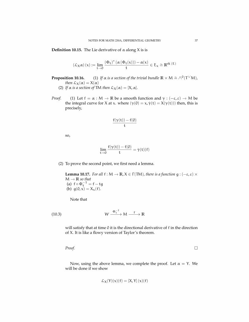
Definition 10.15. The Lie derivative of α along X is is
(LXα) (x) := limt→0 (Φt)
∗ (α (Φt(x))) −α(x)
t∈ Ex ∼= Rrk (E)
Proposition 10.16. (1) If α is a section of the trivial bundle R×M ∼= ∧0(T∨M),then LX(α) = X(α)
(2) If α is a section of TM then LX(α) = [X,α].
Proof. (1) Let f = α : M → R be a smooth function and γ : (−ε, ε) → M bethe integral curve for X at x. where (γ(0) = x, γ(t) = X(γ(t))) then, this isprecisely,
f(γ(t)) − f(0)
t
so,
limt→0 f(γ(t)) − f(0)t
= γ(t)(f)
(2) To prove the second point, we first need a lemma.
Lemma 10.17. For all f :M→ R,X ∈ Γ(TM), there is a function g : (−ε, ε)×M→ R so that(a) f Φ−1
t = f− tg(b) g(0, x) = Xx(f).
Note that
(10.3) W M RΦ−1t f
will satisfy that at time 0 it is the directional derivative of f in the directionof X. It is like a flowy version of Taylor’s theorem.
Proof.
Now, using the above lemma, we complete the proof. Let α = Y. Wewill be done if we show
LX(Y)(x)(f) = [X, Y] (x)(f)

38 AARON LANDESMAN
for all x, f :M→ R. We have, by Lemma 10.17
LX(Y)(x)(f) = limt→0 (Φt)
∗ (Y (Φt(x))) − Y(x)
t(f)
= limt→0 (Φ−t)∗ (Y (Φt(x))) (f) − Y(x)(f)
t
= limt→0 (Y (Φt(x))) (f Φ−t) − Y(x)(f)
t
= limt→0 (Y (Φt(x))) (f− tg) − Y(x)(f)t
= limt→0 (Y (Φt(x))) (f) − Y(x)(f)t
−tY(Φt(x))(g)
t
= limt→0 (Y (Φt(x))) (f) − Y(x)(f)t
− Y(Φ0(x))(g)
= X(Y(f))(x) − Y(Φ0(x))(g)
= X(Y(f))(x) − Y(x)(g)
= X(Y(f))(x) − Y(x)X(f)
= X(Y(f))(x) − Y(X(f))(x)
We still have to justify why Y(Φt(x))(f) = X(Y(f))(x), which follows fromthe fact that
Y(Φt(x))(f) = Y(f Φt(x))
= limt→0 Y(f(Φt(x)) − Y(f)(x)t
=Y(f)(Φt(x)) − Y(f)(Φ0(x))
t
= Φ0(x)(Y(f))
= X(Y(f))
Remark 10.18. Note if E = R×M, pulling back a section of E is just precomposing.That is, given a diffeomorphismM ′
g−→M, we have g∗(f) = f g.
Remark 10.19. How do we compute ∂∂dt (f γ). Then, ∂
∂dt ∈ Gamma(T (−ε, ε)).We have a map
γ : (−ε, ε)→M
DγT(−ε, ε)→ TM
By the derivation definition of Dγ, we have
X(γ(t))(f) = Dγ
(∂
∂t|t=0
)(f) =
∂
∂t|t=0(f γ)
where the first equality is the definition of an integral curve.
Remark 10.20. Note (Φ−t)∗ = DΦ−t.
The above remarks are key to understanding integral curves.
NOTES FOR MATH 230A, DIFFERENTIAL GEOMETRY 39
11. 10/6/15
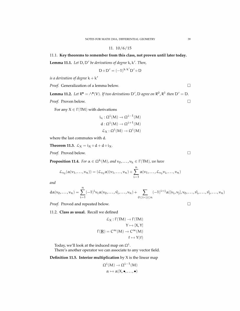
11.1. Key theorems to remember from this class, not proven until later today.
Lemma 11.1. Let D,D ′ be derivations of degree k,k ′. Then,
D D ′ = (−1)k·k′D ′ D
is a derivation of degree k+ k ′
Proof. Generalization of a lemma below.
Lemma 11.2. Let R• = ∧•(V). If two derivations D ′,D agree on R0,R1 then D ′ = D.
Proof. Proven below.
For any X ∈ Γ(TM) with derivations
ix : Ωi(M)→ Ωi−1(M)
d : Ωi(M)→ Ωi+1(M)
LX : Ωi(M)→ Ωi(M)
where the last commutes with d.
Theorem 11.3. LX = iX d+ d iX.
Proof. Proved below.
Proposition 11.4. For α ∈ Ωk(M), and v0, . . . , vk ∈ Γ(TM), we have
Lv0(α(v1, . . . , vn)) = (Lv0α)(v1, . . . , vn) +n∑i=1
α(v1, . . . ,Lv0vi, . . . , vn)
and
dα(v0, . . . , vn) =n∑i=1
(−1)iviα(v0, . . . , vi, . . . , vn) +∑
0≤i<j≤n(−1)i+jα([vi, vj], v0, . . . , vi, . . . , vj, . . . , vn)
Proof. Proved and repeated below.
11.2. Class as usual. Recall we defined
LX : Γ(TM)→ Γ(TM)
Y 7→ [X, Y]
Γ(R) = C∞(M)→ C∞(M)
f 7→ Y(f)
Today, we’ll look at the induced map onΩi.There’s another operator we can associate to any vector field.
Definition 11.5. Interior multiplication by X is the linear map
Ωi(M)→ Ωi−1(M)
α 7→ α(X, •, . . . , •)
40 AARON LANDESMAN
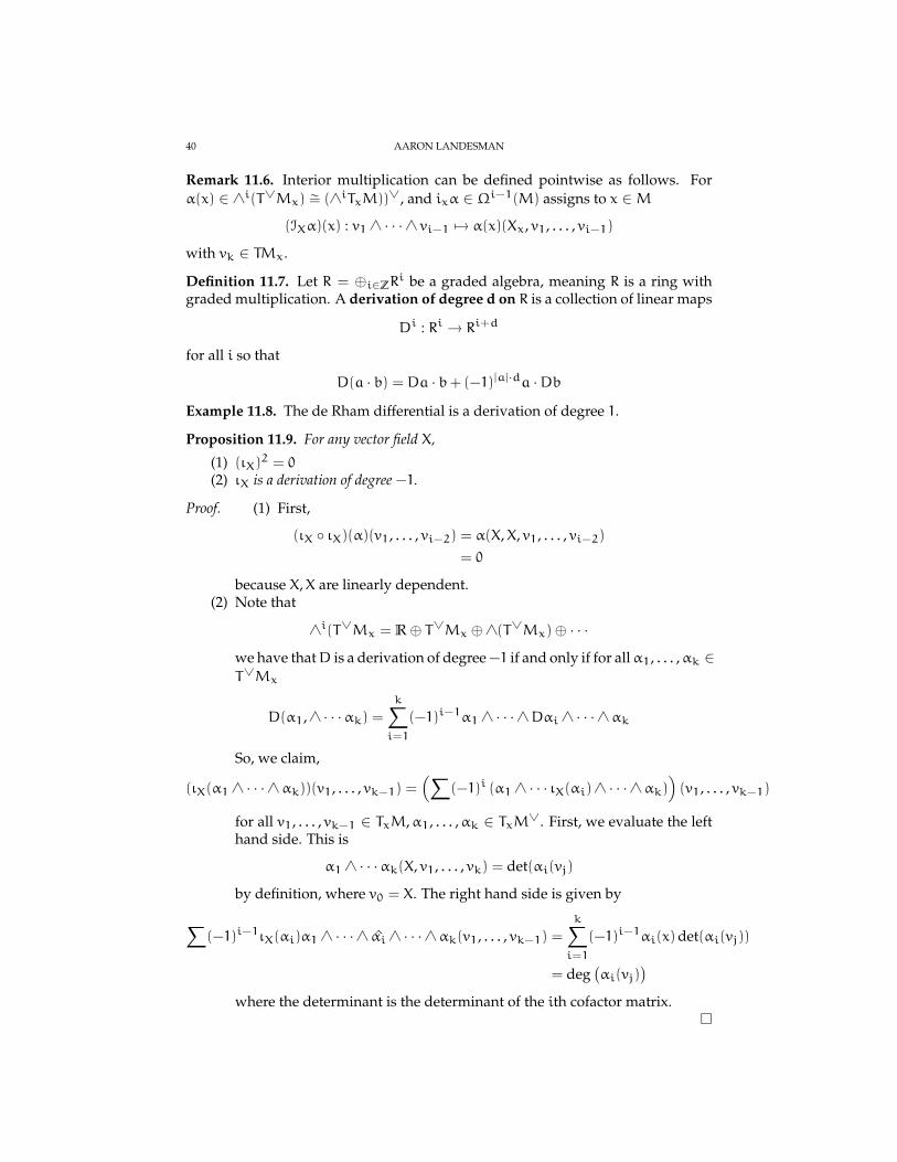
Remark 11.6. Interior multiplication can be defined pointwise as follows. Forα(x) ∈ ∧i(T∨Mx) ∼= (∧iTxM))∨, and ixα ∈ Ωi−1(M) assigns to x ∈M
(IXα)(x) : v1 ∧ · · ·∧ vi−1 7→ α(x)(Xx, v1, . . . , vi−1)
with vk ∈ TMx.
Definition 11.7. Let R = ⊕i∈ZRi be a graded algebra, meaning R is a ring with
graded multiplication. A derivation of degree d on R is a collection of linear maps
Di : Ri → Ri+d
for all i so that
D(a · b) = Da · b+ (−1)|a|·da ·Db
Example 11.8. The de Rham differential is a derivation of degree 1.
Proposition 11.9. For any vector field X,
(1) (ιX)2 = 0
(2) ιX is a derivation of degree −1.
Proof. (1) First,
(ιX ιX)(α)(v1, . . . , vi−2) = α(X,X, v1, . . . , vi−2)= 0
because X,X are linearly dependent.(2) Note that
∧i(T∨Mx = R⊕ T∨Mx ⊕∧(T∨Mx)⊕ · · ·
we have thatD is a derivation of degree −1 if and only if for allα1, . . . ,αk ∈T∨Mx
D(α1,∧ · · ·αk) =k∑i=1
(−1)i−1α1 ∧ · · ·∧Dαi ∧ · · ·∧αk
So, we claim,
(ιX(α1 ∧ · · ·∧αk))(v1, . . . , vk−1) =(∑
(−1)i (α1 ∧ · · · ιX(αi)∧ · · ·∧αk))(v1, . . . , vk−1)
for all v1, . . . , vk−1 ∈ TxM,α1, . . . ,αk ∈ TxM∨. First, we evaluate the lefthand side. This is
α1 ∧ · · ·αk(X, v1, . . . , vk) = det(αi(vj)
by definition, where v0 = X. The right hand side is given by
∑(−1)i−1ιX(αi)α1 ∧ · · ·∧ αi ∧ · · ·∧αk(v1, . . . , vk−1) =
k∑i=1
(−1)i−1αi(x)det(αi(vj))
= deg(αi(vj)
)where the determinant is the determinant of the ith cofactor matrix.

NOTES FOR MATH 230A, DIFFERENTIAL GEOMETRY 41
Remark 11.10. Recall the space of vector fields Γ(TM) forms a Lie algebra by notic-ing that X, Y ∈ Der(C∞(M)) implies
X Y − Y X ∈ Der(C∞(M))
Remark 11.11. Lemma 11.1 is just a generalization of the above proposition ??
We now have two derivations on Ω•(M). What derivation does [ιX d] corre-spond to?
Theorem 11.3 says this is precisely LX.The strategy of proof will be to show they agree on generating elements, and
this implies they agree everywhere, once we show they are derivations.
Proposition 11.12. For all X ∈ Γ(TM) we have LX : Ωi(M)→ Ωi(M) is a derivation.
Proof. The idea is to use the same proof as that of the proof of the product rulefrom one variable calculus.
Let’s fix α ∈ Ωk(M),β ∈ Ωl(M). Recall
LX(α∧β)(x) = limt→0 (Φ
Xt )∗α∧β(ΦXt (x)) −α∧β(x)
t
Now, expanding the above, we have
LX(α∧β)(x)
= limt→0 (Φ
Xt )∗α∧β(ΦXt (x)) −α∧β(x)
t
= limt→0 (Φ
Xt )∗(α(Φt(x)))∧ΦXt (β(Φ
Xt (x))) −α∧β(x)
t
= limt→0 (Φ
Xt )∗(α(Φt(x)))∧ΦXt (β(Φ
Xt (x))) − (ΦXt )
∗(α(Φt(x)))∧β(x) + (ΦXt )∗(α(Φt(x)))∧β(x) −α∧β(x)
t
= limt→0(ΦXt )∗(α(Φt(x)))∧ (
1
t(ΦXt (β(Φ
Xt (x)))β(x)) + (
1
t(ΦXt )
∗(α(Φt(x))) −α(x))
= α(x)∧ (LXβ)(x) + (LX(α))(x)∧β(x)
showing LX is a derivation.
Proposition 11.13. For all X, i ∈ Z we have LX commutes with d.
Proof. We’ll come back to this in a later class. The idea is that ∂∂t and derivatives
in theM component commute.
Remark 11.14. The name magic formula might have come from Raul Bott, whofound this formula very useful, and the name caught on.
Proof of Lemma 11.2. Any element of ∧i(V) can be written as a · v1∧ · · ·∧vk wherea ∈ R, vi ∈ V = ∧1(V). By definition of derivation,
D(a · v1 ∧ · · ·∧ vk) = Da · v1 ∧ · · ·∧ vk + ak∑i=1
(−1)(i−1)|D|v1 ∧ · · ·Dv1 ∧ · · ·∧ vk
so if D ′(a) = D(a) for all a and D ′(v) = D(v) for all v, then

42 AARON LANDESMAN
Proof of Theorem 11.3. Since LX, ιX d+ d ιX are derivations, by Lemma 11.2, weonly need check that both sides agree on C∞(M) and Ω1(M). For functions,LX(f) = X(f) = df(x) from last time and the definition of d0deR. From last time,(ιx d+ d ιX)(f) = ιX(df) + d(0) = df(X), and so the derivations agree on func-tions.
We next check they agree on 1 forms. Let α ∈ Ω1(U) so
α =
dimU∑i=1
fidxi
Then,
LX = L(dxi)
= LX(dxi)
= d(X(xi))
= d(Xi)
Where X =∑Xi ∂∂xi
. On the other hand, the right hand side is
(ιX d+ d ιX) (dxi) = d ιX(dxi)= d(dxi(X))
= d(Xi)
Remark 11.15. It’s only recently that we started paying attention to the geometryof Tm⊕ T∨M, but studying the geometry of this is a very useful tool into mirrorsymmetry. This is called generalized geometry, and is pioneered by Hitchin andGualtieri. This is an interesting example of something that is quite obvious tostudy but hasn’t been thought about until recently.
Proposition 11.16. For α ∈ Ωk(M), and v0, . . . , vk ∈ Γ(TM), we have
Lv0(α(v1, . . . , vn)) = (Lv0α)(v1, . . . , vn) +n∑i=1
α(v1, . . . ,Lv0vi, . . . , vn)(11.1)
and
dα(v0, . . . , vn) =n∑i=1
(−1)iviα(v0, . . . , vi, . . . , vn) +∑
0≤i<j≤n(−1)i+jα([vi, vj], v0, . . . , vi, . . . , vj, . . . , vn)
(11.2)
Remark 11.17. The first formula is just like the naive product rule. The secondformula is less geometric, and should just be thought of algebraically.
Proof. The proof of Equation 11.2, we induct on k. The base case of k = 0 is givenby α ∈ C∞(M), we have dα(v0) = v0(α) by definition.
When k = 1, we see, by 11.1
Lv0(α(v1)) = (Lv0(α))(v1) +α(Lv0v1)
= v0(α(v1)) = (d ιv0 + ιv0 d) (α)(v1) +α ([v0, v1])

NOTES FOR MATH 230A, DIFFERENTIAL GEOMETRY 43
Then,
d (α(v1)) (v0) = d (α(v0)) (v1) + dα (v0, v1) +α ([v0, v1])
implying
dα (v0, v1) = v0 (α(v1)) − v1 (α(v0)) −α ([v0, v1])
More generally, for higher k, we have
Lv0(α(v1, . . . , vk)) = Lv0(α))(v1) +∑
α(v1, . . . ,Lv0vi, . . . , vk)
= v0(α(v1, . . . , vk)) = (d ιv0 + ιv0 d) (α)(v1, . . . , vk) +α (v1, . . . , [v0, vi] , . . . , vk)
= d (ιv0α)(v1, . . . , vk)) + iv0(dα)(v1, . . . , vk) + · · ·= d (ιv0α)(v1, . . . , vk)) + dα(v0, v1, . . . , vk) + · · ·
By induction,
d(ιv0α(v1, . . . , vk) =∑
(−1)i+1viιv0α(v1, . . . , vi, . . . , vk) +∑i<j
(−1)i+1+j+1ιv0α([vi, vj
], v1, . . . , vi, . . . , vj, . . . , vk
)So, we have
v0(α(v0, . . . , vk)) =∑
(−1)i+1viα(v0, . . . , vi, . . . , vk)
+∑
(−1)i+jα(v0,[vi, vj
], . . . , vi, . . . , vj, . . . , vk
)+∑
α (v1, . . . , [v0, vi] , . . . , vk) + dα (v0, . . . , vk)
12. 10/8/15
12.1. Overview. First, LX commutes with d.
Definition 12.1. (1) f related vector field(2) Riemannian metrics on E(3) Connection on E
Results, without proof:
Theorem 12.2. [X, Y] = 0 if and only if
ΦXs ΦYt = ΦYt ΦXs
Theorem 12.3. (Frobenius) E ⊂ TM is involutive if and only if it is integrable
Proposition 12.4. Any E admits a Riemannian metric and connection.
Theorem 12.5. (Colloquially:) Γ takes ⊗ to ⊗C∞(M). More precisely, if E,E ′ are vectorbundles overM, there is a natural isomorphism
Γ(E⊗ E ′) ∼= Γ(E)⊗C∞(M) Γ(E′)
44 AARON LANDESMAN
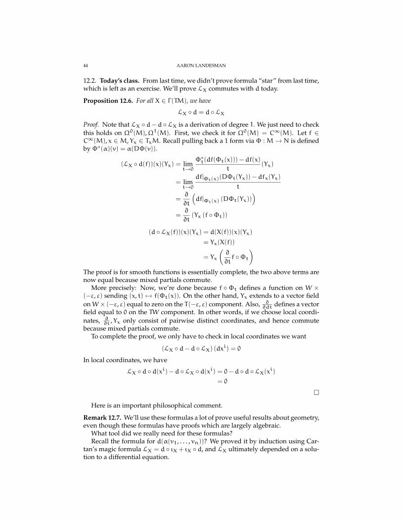
12.2. Today’s class. From last time, we didn’t prove formula “star” from last time,which is left as an exercise. We’ll prove LX commutes with d today.
Proposition 12.6. For all X ∈ Γ(TM), we have
LX d = d LXProof. Note that LX d− d LX is a derivation of degree 1. We just need to checkthis holds on Ω0(M),Ω1(M). First, we check it for Ω0(M) = C∞(M). Let f ∈C∞(M), x ∈M, Yx ∈ TxM. Recall pulling back a 1 form via Φ :M→ N is definedby Φ∗(α)(v) = α(DΦ(v)).
(LX d(f))(x)(Yx) = limt→0 Φ
∗t(df(Φt(x))) − df(x)
t(Yx)
= limt→0
df|Φt(x)(DΦt(Yx)) − dfx(Yx)
t
=∂
∂t
(df|Φt(x) (DΦt(Yx))
)=∂
∂t(Yx (f Φt))
(d LX(f))(x)(Yx) = d(X(f))(x)(Yx)= Yx(X(f))
= Yx
(∂
∂tf Φt
)The proof is for smooth functions is essentially complete, the two above terms arenow equal because mixed partials commute.
More precisely: Now, we’re done because f Φt defines a function on W ×(−ε, ε) sending (x, t) 7→ f(Φt(x)). On the other hand, Yx extends to a vector fieldonW× (−ε, ε) equal to zero on the T(−ε, ε) component. Also, ∂
∂dt defines a vectorfield equal to 0 on the TW component. In other words, if we choose local coordi-nates, ∂
∂t , Yx only consist of pairwise distinct coordinates, and hence commutebecause mixed partials commute.
To complete the proof, we only have to check in local coordinates we want
(LX d− d LX) (dxi) = 0In local coordinates, we have
LX d d(xi) − d LX d(xi) = 0− d d LX(xi)= 0
Here is an important philosophical comment.
Remark 12.7. We’ll use these formulas a lot of prove useful results about geometry,even though these formulas have proofs which are largely algebraic.
What tool did we really need for these formulas?Recall the formula for d(α(v1, . . . , vn))? We proved it by induction using Car-
tan’s magic formula LX = d ιX + ιX d, and LX ultimately depended on a solu-tion to a differential equation.

NOTES FOR MATH 230A, DIFFERENTIAL GEOMETRY 45
Here is the theme: We defined easy things where the de Rham derivative camefor free, and ιX is quite natural as well. But, however, we got the algebraic outputfrom an algebraic input by going through differential equations.
Much of the (algebraic) progress was due to Gromov who delved into differen-tial equations to prove something algebraic.
Definition 12.8. Let f : M → N be a smooth map and let X ∈ Γ(TM), X ∈ Γ(TN).Say (X, X) are f related if
(12.1)M N
TM TN
f
X X
Df
That is, for all x ∈M, we have Dfx(Xx) = Xf(x).
Remark 12.9. Note, vector fields don’t push forward, essentially because they cancome in conflict with themselves at nodes. even though tangent vectors do pushforward.
Proposition 12.10. Fix f :M→ N. Suppose(X, X
),(Y, Y
)are f related. Then,
[X, Y] ,[X, Y
]are f related.
Proof. We need to show that
Dfp
([X, Y]p
)=[X, Y
]p
We just need to show these are the same derivations. Let φ : N → R be a smoothfunction. We need to show the above evaluates to the same value on φ.[
X, Y]p(φ) = (X Y − Y X)pφ
= Xp(Y(φ)) − Yp(X(φ))
= Dfp(Xp)(Y(φ)) −Dfp(Yp)(X(φ))
= Xp(Y(φ) f) − Yp(X(φ) f)= Xp(Y(φ f)) − Yp(X(φ f))= [X, Y]p (φ f)
= Dfp
([X, Y]p
)(φ)
Note that above we used the following:
Y(φ) : N→ R
y 7→ Yy(φ)
Mf−→ N
Y(φ)−−−→ R
x 7→ f(x) 7→ Yf(x)(φ) = Dfx(Yx)(φ) = Yx(φ f)
Here is an interesting question:

46 AARON LANDESMAN
Question 12.11. Fix a subbundle E ⊂ TM and fix a bundle map
(12.2)E TM
M M
so that this map is an injection on the level of fibers. That is, the image is a subbun-dle To what extent does E look like the tangent bundle to a bunch of submanifolds?
To elaborate on the above question, we might try taking subspaces of the tan-gent bundle at each point For every x ∈M, we’re asking if there exists an immer-sion j : U→M so that Dj(TU) = E|j(U). We have
(12.3)TU TM
U M
and we’re asking if we can rig it so that the vector subbundle is the tangent bundleof the image of some immersion.
In fact, E is rarely such a subbundle
Question 12.12. What property does E have if it does come locally as the imagesof some immersions or embeddings?
Definition 12.13. If E satisfies the property that for all x ∈M, there exists a mani-fold jx : Nx →M an embedding, so that
Djx(TxN) = E|jx(Nx)
We then say that E is integrable.
Remark 12.14. You can image that if E is an integrable submanifold, then sectionsof E define flows, and we can find N along all of these flows.
It is called integrable, because Frobenius asked this question in terms of find-ing solution to differential equations, and finding such a solution is the same as“integrating” the differential equations to find a solution.
If E is integrable, consider
X, Y ∈ Γ(E) ⊂ Γ(TM)
Then, [X, Y] ∈ Γ(E) because locally X, Y are related to vector fields on Nx, and usethe Proposition 12.10. So, we see immediately that if E is integrable then Γ(E) mustbe a Lie subalgebra of Γ(TM). You can ask if this is enough.
Definition 12.15. A subbundle E ⊂ TM is involutive if X, Y ∈ Γ(E) then [X, Y] ∈Γ(E).
Theorem 12.16. E is involutive if and only if E is integrable.
In our homework, we’ll prove the Koszul dual version, which deals with differ-ential forms instead of subbundles.
Proof. Given in two weeks, when Hiro gets back.

NOTES FOR MATH 230A, DIFFERENTIAL GEOMETRY 47
Theorem 12.17. Let X, Y ∈ Γ(TM). Then, [X, Y] = 0 if and only if
ΦXs ΦYt = ΦYt ΦXswhere the flows are defined.
Proof. Given in two weeks, when Hiro gets back.
12.3. Riemannian Geometry on vector bundles.
Theorem 12.18. (Colloquially:) Γ takes⊗ to⊗C∞(M). More precisely, if E,E ′ are vectorbundles overM, there is a natural isomorphism
Γ(E⊗ E ′) ∼= Γ(E)⊗C∞(M) Γ(E′)
Remark 12.19. The proof is easy when M is compact. Try doing it at home. Thehard part is doing it for paracompact M. In this case, you need dimension theory(Lebesgue dimension theory).
Proof. Omitted, exercise in the compact case.
So, any s ∈ Γ(E⊗ E ′) can be written as a finite linear combination∑fijti ⊗ t ′j
where fij ∈ C∞(M), ti ∈ Γ(E), t ′i ∈ Γ(E ′).
Definition 12.20. Let E be a smooth vector bundle overM. A Riemannian metricon E is a section
g ∈ Γ((E⊗ E)∨)
so that(1) for all x ∈M, v,w,∈ Ex we have
g(x)(v⊗w) = g(x)(w⊗ v)(2)
g(x)(v⊗ v) ≥ 0and is equal to 0 if and only if v = 0.
Remark 12.21. A Riemannian metric is a smooth choice of positive definite innerproduct on each fiber.
Definition 12.22. A Riemannian metric onM is a Riemannian metric on TM.
Remark 12.23. All the definitions and results for whenM ⊂ Rn carry over to thismore general setting. For example:
(1) If j :M→ N is an immersion, and h is a Riemannian metric onN, then j∗hdefines a Riemannian metric onM.
Example 12.24. We have an inclusion of Sn → Rn+1 and this induces apullback of the standard Riemannian metric
We define
j∗h(v,w) := h(Djx(v),Djx(w)
)for all v,w ∈ TxM.

48 AARON LANDESMAN
(2) We say that f : (M,g)→ (N,h) is an isometry if f is a diffeomorphism andf∗h = g.
Question 12.25. Does any manifold admit a Riemannian metric?
One answer is given by the Whitney immersion theorem, since it embeds intoRn for some n.
However, we have something even stronger:
Proposition 12.26. Any vector bundle E onM admits a Riemannian metric.
Proof. The idea is to use partitions of unity.Let (Uα,φα) be local coordinates so that Uα is an open cover ofM.
Φα : E|Uα∼= Uα ×Rk
Now, U × Rk admits a Riemannian metric gα, take for example gij = δij andg = I, the identity matrix. Hence, we obtain an induced metric on E|Uα . Let Φαbe a partition of unity subordinate to Uα, and define
g =∑
φαgα
Explicitly, for all v,w ∈ Ex, we have
g(v,w) =∑
φα(x)gα(v,w)
Now, g(v,w) is symmetric. Further, it is positive definite because φα add up to 1and the gα are positive definite.
12.4. Connections. A connection will be a way to take directional derivatives ofsections of E.
Question 12.27. What could such a thing be?
Fix a v ∈ TxM. Fix s ∈ Γ(E). Intuitively, a directional derivative ∇ Fix s ∈ Γ(E).Intuitively, a directional derivative ∇ should produce
∇vs ∈ Ts(x)ExRemark 12.28. Intuitively, if we move along a tangent direction in M, this shouldinduce a movement along the tangent bundle to E to define a section of the tangentbundle to E
Proposition 12.29. Let V be a smooth vector space over R, and demand
R× V → V
V × V t−→ V
are smooth. Then, there exists a natural isomorphism T0V ∼= V .
Proof. Omitted.
Corollary 12.30. Since V is a lie group under addition, we have an isomorphism T0V ∼=TxV .
Proof. Omitted
Corollary 12.31. We have an isomorphism Ts(x)Ex∼= Ex.
Proof. Combine the above proposition and corollary.

NOTES FOR MATH 230A, DIFFERENTIAL GEOMETRY 49
So, a connection should take for all x ∈M,
TxM× Γ(E)→ Γ(E)
(v, s) 7→ (x 7→ ∇js(x)algebraically the directional derivative is linear in the Tx component. So taking allx at once, we get a map
Γ(TM)× Γ(E)→ Γ(E)
(X, s) 7→ ∇XsRemark 12.32. A connection is a way to take derivatives along a vector bundle.There are a lot of them, but only a few of them are special.
13. 10/20/2015
13.1. Key theorems for today.
Theorem 13.1.
[X, Y] = 0 ⇐⇒ ΦXs ΦYt = ΦYt ΦXs
wheneverΦXs ,ΦYt are defined.
Proof.
We’ll also learn about connections:
(1) locally(2) existence(3) convexity(4) curvature
13.2. Class time. Today, we’ll give a geometric interpretation of the Lie bracketvia Theorem 13.1.
Let’s recall what these symbols mean:Given X ∈ Γ(TM), for all x ∈ M, there is W ⊂ M, there is x ∈ W, (−ε, ε) ⊂ R
so that we have a mapΦX : (−ε, ε)×W →M is a diffeomorphism onto its image,satisfying a derivative condition.
Theorem 13.2.
[X, Y] = 0 ⇐⇒ ΦXs ΦYt = ΦYt ΦXs
whenever ΦXs ,ΦYt are defined.
Proof. First, we prove the reverse direction. This is mostly formal. We need toshow that for f :M→ R, we have
X(Y(f)) = Y(X(f))

50 AARON LANDESMAN
We have
X(Y(f))(x) = lims→0 Y(f)(Φ
Xs (x) − Y(f)(x)
s
= lims→0
YΦXs (x)(f)−Y(f)(x)
s
= lims→0 lim
t→0 f(ΦYt (Φ
Xs (x))) − f(Φ
Xs (x)
st−f(ΦYt (x) − f(x)
st
= lims→0 lim
t→0 f(ΦXs (Φ
Yt (x))) − f(Φ
Yt (x)
st−f(ΦXs (x) − f(x)
st
= Y(X(f))
For the reverse direction, we’ll need a clever little trick. Define a curve
~v : (−ε, ε)→ TΦYt (x)M
s 7→ (DΦXs )∨YΦXs ΦYt (x)
We a priori fix x ∈M and t ∈ R. We’ll show this curve is constant.We claim:
Lemma 13.3. ∂~v∂s = 0
We now show why the theorem follows from this lemma, and then come backto this lemma.
Now, we’re done: Set C : (−ε, ε) → M, t → ΦXs ΦYt (x) where s, x are fixed.Now, observe,
C(t) =∂
∂t
(ΦXs
(t 7→ ΦYt (x)
))= DΦXs (YΦYt
= DΦXs (~v(0))
= YΦXs ΦYt (x)
where the last step follows from Lemma 13.3 because
(DΦXs )∗(~v(0)) =(DΦXs
)∗(~v(s))
=(DΦXs
)∗
(DΦXs
)∗YΦXs ΦYt (x)
= YΦXs ΦYt (x)
So, C is a curve inM satisfying the condition
C(0) = ΦXs (x)
C(t) = YC(t)
However,ΦYt ΦXs also satisfies these derivative conditions, and so by uniqueness,
ΦYt ΦXs = C(t)
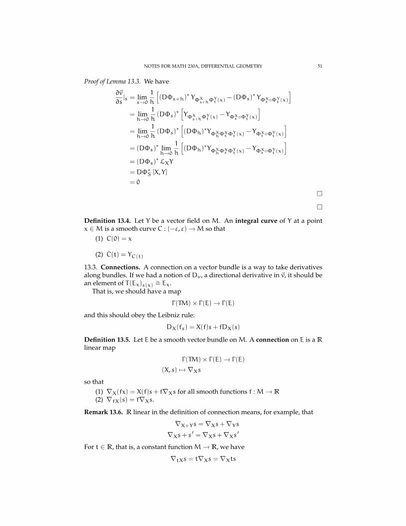
NOTES FOR MATH 230A, DIFFERENTIAL GEOMETRY 51
Proof of Lemma 13.3. We have
∂~v
∂s|s = lim
s→0 1h[(DΦs+h)
∗ YΦXs+hΦYt (x)− (DΦs)
∗ YΦXs ΦYt (x)
]= limh→0 1h (DΦs)
∗[YΦXs+hΦ
Yt (x)
− YΦXs ΦYt (x)
]= limh→0 1h (DΦs)
∗[(DΦh)
∗YΦXhΦXsΦYt (x)− YΦXs ΦYt (x)
]= (DΦs)
∗ limh→0 1h
[(DΦh)
∗YΦXhΦXsΦYt (x)− YΦXs ΦYt (x)
]= (DΦs)
∗ LXY
= DΦ∗S [X, Y]= 0
Definition 13.4. Let Y be a vector field on M. An integral curve of Y at a pointx ∈M is a smooth curve C : (−ε, ε)→M so that
(1) C(0) = x
(2) C(t) = YC(t)
13.3. Connections. A connection on a vector bundle is a way to take derivativesalong bundles. If we had a notion of Dv, a directional derivative in ~v, it should bean element of T(Ex)s(x) ∼= Ex.
That is, we should have a map
Γ(TM)× Γ(E)→ Γ(E)
and this should obey the Leibniz rule:
DX(fs) = X(f)s+ fDX(s)
Definition 13.5. Let E be a smooth vector bundle on M. A connection on E is a R
linear map
Γ(TM)× Γ(E)→ Γ(E)
(X, s) 7→ ∇Xsso that
(1) ∇X(fx) = X(f)s+ f∇Xs for all smooth functions f :M→ R
(2) ∇fX(s) = f∇Xs.
Remark 13.6. R linear in the definition of connection means, for example, that
∇X+Ys = ∇Xs+∇Ys∇Xs+ s ′ = ∇Xs+∇Xs ′
For t ∈ R, that is, a constant functionM→ R, we have
∇tXs = t∇Xs = ∇Xts

52 AARON LANDESMAN
The second property of connections gives us a dual interpretation
Γ(TM)× Γ(E) ∇−→ Γ(E)
is equivalent to the data of a map
Γ(E)Γ−→ (T∨M⊗ E)
s 7→ ∇swhere ∇s is waiting for a subscript vector field X to be plugged in.
Example 13.7. Let E = R :=M×R. Then, a connection is a map
Γ(TM)×C∞(M)→ C∞(M)
or equivalently, a map
C∞(M)→ Γ(T∨M⊗R) ∼= Γ(T∨M) =: Ω•deR(M)
and the de Rham derivative is a connection on R = E. What is the de Rhamderivative as a map
Γ(TM)×C∞(M)→ C∞(M)?
We know it should be X(s) =: ds(X) = ∇Xs That is,
∇ : (X, s) 7→ X(s)
Here X(s) is a function that at a point p is Xp(s), the derivative of s in the directionof Xp.
Proposition 13.8. Let E be a trivial vector bundle. Fix k = dimEx many linearlyindependent sections and an assignment
∇si ∈ Γ(T∨M⊗ E)
Then, there exists a unique connection on E so that ∇si are the prescribed sections.
Remark 13.9. A section of T∨M⊗ E is the same thing as an E valued 1 form. Thatis, any α ∈ Γ(T∨M⊗ E) is something that eats X ∈ TM and outputs a section of E.
Proof. Any section of E can be written as S =∑ki=1 f
isi where fi ∈ C∞(M). Wecan write ∇si =
∑kj=1 α
ji ⊗ sj where αji are one forms.
Then, set ∇(fsi) = df⊗ si + f∇si.
Example 13.10. Set E = R. Fix s a nowhere vanishing section. Declare ∇s = 0 ∈Ω•deR(M). Then, ∇(fs) = df⊗ s+ f∇s.
Locally df = ∂f∂xidxi and df⊗ s = s · ∂f
∂xidxi. If swere chosen to be the constant
function 1, then ∇ corresponds to the usual de Rham derivative.
Remark 13.11.
Question 13.12. In the dual picture, where ∇ : Γ(E) → Γ(T∨M⊗ E), what doesthe Leibniz rule become?
This becomes
∇(fs) = df⊗ s+ f∇s
where df ∈ Γ(T∨M) = Ω•deR(M) and s ∈ Γ(E) and so this tensor product df⊗ s ∈Γ(T∨M⊗ E).
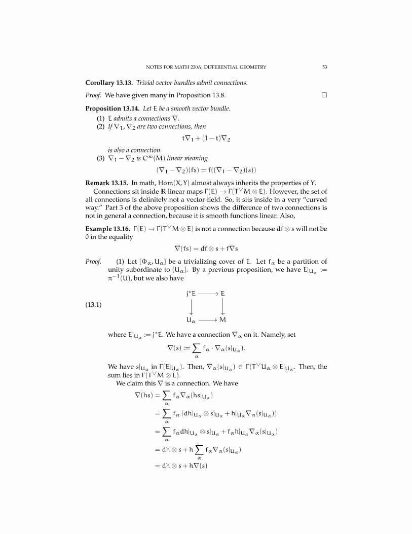
NOTES FOR MATH 230A, DIFFERENTIAL GEOMETRY 53
Corollary 13.13. Trivial vector bundles admit connections.
Proof. We have given many in Proposition 13.8.
Proposition 13.14. Let E be a smooth vector bundle.(1) E admits a connections ∇.(2) If ∇1,∇2 are two connections, then
t∇1 + (1− t)∇2is also a connection.
(3) ∇1 −∇2 is C∞(M) linear meaning
(∇1 −∇2)(fs) = f((∇1 −∇2)(s))
Remark 13.15. In math, Hom(X, Y) almost always inherits the properties of Y.Connections sit inside R linear maps Γ(E)→ Γ(T∨M⊗ E). However, the set of
all connections is definitely not a vector field. So, it sits inside in a very “curvedway.” Part 3 of the above proposition shows the difference of two connections isnot in general a connection, because it is smooth functions linear. Also,
Example 13.16. Γ(E)→ Γ(T∨M⊗ E) is not a connection because df⊗ swill not be0 in the equality
∇(fs) = df⊗ s+ f∇s
Proof. (1) Let Φα,Uα be a trivializing cover of E. Let fα be a partition ofunity subordinate to Uα. By a previous proposition, we have E|Uα :=
π−1(U), but we also have
(13.1)
j∗E E
Uα M
where E|Uα := j∗E. We have a connection ∇α on it. Namely, set
∇(s) :=∑α
fα · ∇α(s|Uα).
We have s|Uα in Γ(E|Uα). Then, ∇α(s|Uα) ∈ Γ(T∨Uα ⊗ E|Uα . Then, thesum lies in Γ(T∨M⊗ E).
We claim this ∇ is a connection. We have
∇(hs) =∑α
fα∇α(hs|Uα)
=∑α
fα (dh|Uα ⊗ s|Uα + h|Uα∇α(s|Uα))
=∑α
fαdh|Uα ⊗ s|Uα + fαh|Uα∇α(s|Uα)
= dh⊗ s+ h∑α
fα∇α(s|Uα)
= dh⊗ s+ h∇(s)

54 AARON LANDESMAN
(2) We need to show the Leibniz rule is satisfied. That is,
(t∇1 + (1− t)∇2)(fs) = df⊗ s+ f(t∇1 + (1− t)∇2)s
We have
(t∇1 + (1− t)∇2)(fs) = t (df⊗ s+ f∇1s) + (1− t) (df⊗ s+ f∇2s)= df⊗ s+ tf∇1s+ (1− t)f∇2s= df⊗ s+ f(t∇1 + (1− t)∇2)s
(3) Here we have
∇1 −∇2(fs) = df⊗ s+ f∇1s− df⊗ s− f∇2sf(∇1 −∇2)(s)
Remark 13.17. You can study the manifold of connections, but that’s not veryinteresting. More interesting is flat connections or Yang Mills theory.
Proposition 13.18. Given
Γ(E)∇−→ Γ(T∨M⊗ E)
there exists a unique operation
Γ(T∨M⊗ E) D−→ Γ(∧2T∨M⊗ E)
so that D(α⊗ s) = dα⊗ s+ (−1)|α| ∧∇s.
Proof. The proof is the same as before, where we extend by the Leibniz rule. Inlocal coordinates, the above is a definition for what D ought to be.
Remark 13.19. Given the de Rham derivative, we had a map Γ(R)→ Γ(T∨M) anda complex with d2 = 0.
Definition 13.20. A connection ∇ is called flat if D ∇ = 0.
14. 10/22/15
Theorem 14.1. Let E ⊂ TM be a subbundle. Then E is integrable if and only if E isinvolutive.
Proof.
Preview of Riemannian geometry:(1) fundamental theorem of Riemannian geometry(2) Parallel transport(3) geodesics
Principle G bundles We will see a correspondence between(1) ∇ flat on E(2) H involutive on P(3) a group homomorphism π1(M)→ G.

NOTES FOR MATH 230A, DIFFERENTIAL GEOMETRY 55
14.1. Class time.
Theorem 14.2. (Frobenius) Fix E ⊂ TM a subbundle. Then, E is integrable if and onlyif it is involutive.
Recall that E being integrable is a geometric condition: For all x ∈M there is animmersion j : Rk →M, 0 7→ x so that the im Dj = E|j(Rk).
Also, we have that E being involutive is an algebraic condition that Γ(E) ⊂Γ(TM) is a Lie subalgebra.
We’ll start with a lemma
Lemma 14.3. If E is involutive, then, for all x ∈M, there exist local sectionsX1, . . . ,Xk ∈Γ(E|U) where x ∈ U and U is open, k = rk E, so that[
Xi,Xj]= 0
Proof. Fix k linearly independent vector fields Yi with Yi ∈ Γ(EU) near x. In localcoordinates, choose
Yi =
n∑j=1
fji
∂
∂xj
By changing the order of j if necessary, we can assume
det(fji)i,j∈1,...,k
is nonzero. (The reason for reordering is that we are dealing with a k× n matrix,and we have to find the minor with nonvanishing determinant.)
Let g be the inverse and set
Xi = gjiYj
=∂
∂xi+∑j>k
cji
∂
∂xj
We claim that [Xi,Xj
]= 0
We now use that E is involutive Since E is involutive, we must have
[Xi,Xj
]=
k∑h=1
ahXh
=∑j≤k
ah∂
∂xh+∑l>k
bl∂
∂xl
= 0+∑l>k
bl∂
∂xl
The key insight is that when we are using h is involutive for the first sum to be upto k, and that we know the vector fields commute. We only had to show that ah
were 0.

56 AARON LANDESMAN
Proof of Theorem 14.2. Note, integral implies involutive. This is because if X ∈ Γ(E)is j related to X ∈ Γ(TRk), then [X,X ′] is j related to
[X, X ′
]. In other words,[
X, X ′]p= Dj
([X,X ′
])for p ∈ j(Rk).
Now, we prove the converse. Fix dx ∈M and vector fields Xi as in Lemma 14.3.Define a smooth map, for U ⊂ Rk as follows
Uj−→M
(t1, . . . , tk) 7→ ΦXk
tk · · ·ΦX1t1 (x)
Note that since[Xi,Xj
]= 0, the order of the ΦXiti is irrelevant, as we showed in
the previous class. We only need to show for all~t ∈ U that
Dj(T~tU) = Ej(~t)
Once we show equality, it will follow it is an immersion because the two vectorspaces have the same dimension.
Since X1, . . . ,Xk evaluated at j(~t) forms a basis for Ej(t), it suffices to show each
(Xi)j(~t) ∈ Dj(T~t(U))
But,
Dj∂
∂ti=
∂
∂ti|tiΦ
XitiΦXktk · · ·
^ΦXktk · · · ΦX1t1 (x) = (Xi)j(~t)
14.2. Connections and Riemannian Geometry.
Remark 14.4. Recall that a connection is a map
Γ(E)→ Γ(T∨M⊗ E)s 7→ ∇s
so that ∇fs = df⊗ s+ f∇s, with f a smooth function and s ∈ Γ(E).
Proposition 14.5. Fix a vector bundle E → M and a smooth map j : M → M. Fix aconnection ∇ on E. Then there exists a connection ∇ on j∗E such that the diagram
Γ(E)∇−→ Γ(T∨M⊗ E)
Note a section on E induces a section on the pullback.
(14.1)
E E
M Mj
s
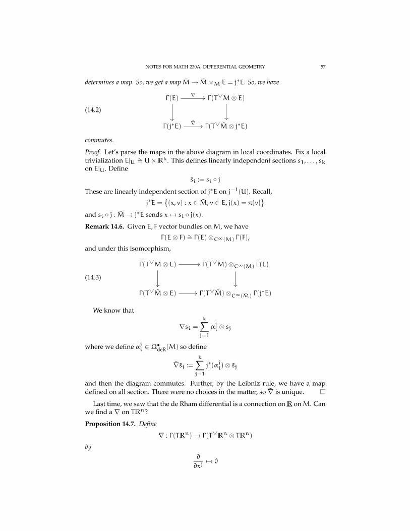
NOTES FOR MATH 230A, DIFFERENTIAL GEOMETRY 57
determines a map. So, we get a map M→ M×M E = j∗E. So, we have
(14.2)
Γ(E) Γ(T∨M⊗ E)
Γ(j∗E) Γ(T∨M⊗ j∗E)
∇
∇
commutes.
Proof. Let’s parse the maps in the above diagram in local coordinates. Fix a localtrivialization E|U ∼= U×Rk. This defines linearly independent sections s1, . . . , skon E|U. Define
si := si j
These are linearly independent section of j∗E on j−1(U). Recall,
j∗E =(x, v) : x ∈ M, v ∈ E, j(x) = π(v)
and si j : M→ j∗E sends x 7→ si j(x).
Remark 14.6. Given E, F vector bundles onM, we have
Γ(E⊗ F) ∼= Γ(E)⊗C∞(M) Γ(F),
and under this isomorphism,
(14.3)
Γ(T∨M⊗ E) Γ(T∨M)⊗C∞(M) Γ(E)
Γ(T∨M⊗ E) Γ(T∨M)⊗C∞(M) Γ(j∗E)
We know that
∇si =k∑j=1
αji ⊗ sj
where we define αji ∈ Ω•deR(M) so define
∇si :=k∑j=1
j∗(αji)⊗ sj
and then the diagram commutes. Further, by the Leibniz rule, we have a mapdefined on all section. There were no choices in the matter, so ∇ is unique.
Last time, we saw that the de Rham differential is a connection on R onM. Canwe find a ∇ on TRn?
Proposition 14.7. Define
∇ : Γ(TRn)→ Γ(T∨Rn ⊗ TRn)
by∂
∂xj7→ 0
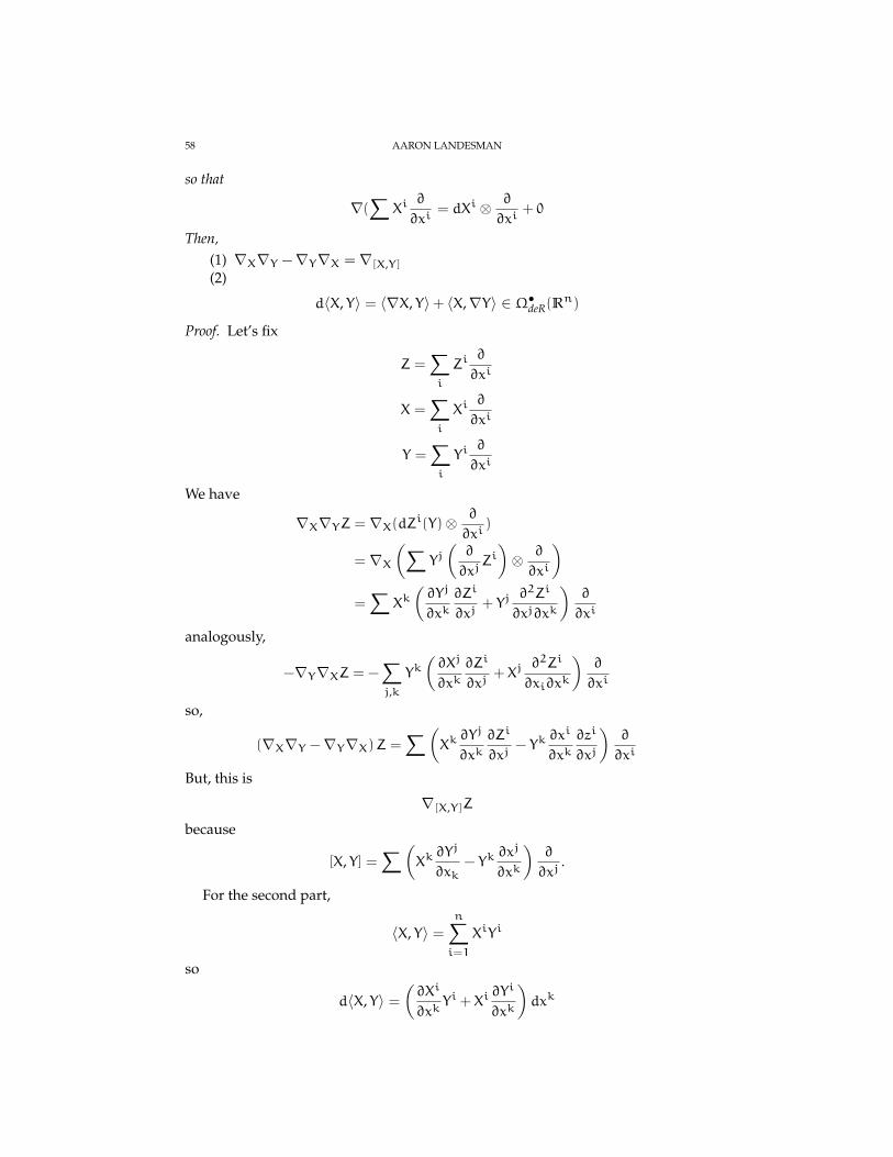
58 AARON LANDESMAN
so that
∇(∑
Xi∂
∂xi= dXi ⊗ ∂
∂xi+ 0
Then,(1) ∇X∇Y −∇Y∇X = ∇[X,Y](2)
d〈X, Y〉 = 〈∇X, Y〉+ 〈X,∇Y〉 ∈ Ω•deR(Rn)
Proof. Let’s fix
Z =∑i
Zi∂
∂xi
X =∑i
Xi∂
∂xi
Y =∑i
Yi∂
∂xi
We have
∇X∇YZ = ∇X(dZi(Y)⊗∂
∂xi)
= ∇X(∑
Yj(∂
∂xjZi)⊗ ∂
∂xi
)=∑
Xk(∂Yj
∂xk∂Zi
∂xj+ Yj
∂2Zi
∂xj∂xk
)∂
∂xi
analogously,
−∇Y∇XZ = −∑j,k
Yk(∂Xj
∂xk∂Zi
∂xj+Xj
∂2Zi
∂xi∂xk
)∂
∂xi
so,
(∇X∇Y −∇Y∇X)Z =∑(
Xk∂Yj
∂xk∂Zi
∂xj− Yk
∂xi
∂xk∂zi
∂xj
)∂
∂xi
But, this is
∇[X,Y]Z
because
[X, Y] =∑(
Xk∂Yj
∂xk− Yk
∂xj
∂xk
)∂
∂xj.
For the second part,
〈X, Y〉 =n∑i=1
XiYi
so
d〈X, Y〉 =(∂Xi
∂xkYi +Xi
∂Yi
∂xk
)dxk

NOTES FOR MATH 230A, DIFFERENTIAL GEOMETRY 59
while
〈∇zX, Y〉 = 〈Zk ∂Xi
∂xk∂
∂xi, Y〉
=∑i,k
Zk∂Xi
∂xkYi
and similarly,
〈X,∇ZY〉 =∑i,k
XiZk∂Yi
∂xk
and so the claimed equality holds.
Definition 14.8. Let ∇ be a connection on TM. Then, ∇ is called symmetric ortorsion free if ∇ satisfies ∇X∇Y −∇Y∇X = ∇[X,Y]
Definition 14.9. Fix a Riemannian metric on M. Then, ∇ is compatible with themetric if it satisfies
d〈X, Y〉 = 〈∇X, Y〉+ 〈X,∇Y〉 ∈ Ω•deR(Rn)
Now, we will ignore metrics altogether. Now, there’s a notion of constant sec-tion along curve, but not really along a manifold itself. That is, we realize a con-nection∇ is a way to take derivatives along tangent vectors. So, we have a notionof when a section is constant on a curve, where by curve, we mean a map fromR. However, we shouldn’t be able to do any better. But, we shouldn’t be able todefine constancy along higher dimensional objects.
Question 14.10. How do we make this notion of a section being constant along acurve concrete?
Definition 14.11. Fix a smooth map
γ : (−ε, ε)→M
By the previous proposition, if E is a vector bundle onMwith connection∇, thereis a unique connection ∇ on γ∗Ewhich makes the appropriate diagram commute.And, given s ∈ γ(E), s γ is a section of γ∗E.
On (−ε, ε) we have a vector field ∂∂t . We say
The section s is parallel along γ if
∇ ∂∂ts = 0
Exercise 14.12. We have
∇ ∂∂ts(t) = ∇cs(c(t))
You can show this immediately from the properties of the definition.
Definition 14.13. Fix γ : [a,b] →M. Fix va ∈ Eγ(a). Then, the parallel transportof va along γ is the point vb ∈ Eγ(b) obtained by evaluating a parallel section ofγ∗E starting with va at γ(b).
We’ll prove the following theorem later:
60 AARON LANDESMAN
Theorem 14.14. (Fundamental theorem of Riemannian geometry) Fix (M,g) on a Rie-mannian manifold. Then, there exists a unique connection on TM which are symmetric ancompatible with the metric.
Proof.
Remark 14.15. There are a large number of connections which are either sym-metric or compatible with the metric, but once you require both, there’s a uniqueconnection.
Corollary 14.16. ∇ ∂∂xi
= 0 is the unique connection on Rn compatible with gstd andsymmetric.
Proof.
15. 10/27/15
15.1. Overview. Today we’ll talk about(1) Parallel transport(2) Christoffel symbols(3) Connections and metrics
(a) torsion free(b) A theorem on Levi Civita Connections
15.2. Parallel Transport.
Definition 15.1. Fix ∇ a connection on E. Also fix s ∈ Γ(E),X ∈ Γ(TM) then∇Xs ∈ Γ(E) is called the covariant derivative of s in X.
Fix γ : R→M so we get
(15.1)
γ∗E E
R M
Then, recall,
Definition 15.2. A section s of γ∗E is called parallel along γ if ∇ ∂∂ts = 0.
Question 15.3. Fix γ : R → M and v0 ∈ Eγ(0). Can we find a parallel sections ∈ Γ(γ∗E) so that
∇ ∂∂ts
and
s(0) = v0?
If the answer is yes, then for all γ : R → M, we have a way of transportingelements of Eγ(0) to elements of Eγ(t) for all t ∈ R.
Remark 15.4. Caution! Looking flat depends on your choice of ∇

NOTES FOR MATH 230A, DIFFERENTIAL GEOMETRY 61
Proposition 15.5. For all v0 there exists a unique s of γ∗E so that
∇ ∂∂ts
and
s(0) = v0.
Moreover(1) For every γ we have a map
Eγ(0) → Γ(γ∗E)
which is R linear.(2) Further, we have a composition
Eγ(0) → Γ(γ∗E)evt−−→ Eγ(t)
is a linear isomorphism.
Definition 15.6. Fix ∇,E,γ. Then, the linear isomorphism
Eγ(0) → Eγ(t)
given by Proposition ??, called parallel transport along γ at time t.
Proof. Fix local linear independent sections s1, . . . , sk and let
∇si :=k∑j=1
αji ⊗ sj
for αji ∈ Ω•deR(M). Shrinking the trivializing neighborhood if necessary, we canwrite αji in local coordinates. We can write
∇si =k∑j=1
n∑q=1
αjiqdx
q ⊗ sj
Writing out the equation
∇si :=k∑j=1
αji ⊗ sj
we seek
s =
k∑i=1
fisi
so that ∑fiα
jiqdx
q(γ)⊗ sj +∑
dfi(∇)⊗ si = 0
where above we applied ∇ to s and got 0, since
∇s = ∇∑
fisi =∑
dfi ⊗ si + fi∇si
62 AARON LANDESMAN
That is, we’re looking for curve
~f : R→ Rk
t 7→ (f1(t), . . . , fk(t)
)satisfying the ordinary differential equation
∂fi
∂t
∂γi
∂t=∑i,q
−fiαjiq∂γj
∂t
and so for t ∈ (−ε, ε) there is a unique solution to this differential equation. Fur-ther, this ODE is linear. That is, it is of the form
f = Af
where A is some matrix of functions. Such ODE’s have solutions for all timest ∈ R.
So, by existence and uniqueness, the first part of the proposition is complete.Now, if f,g are two solutions to the ODE then so is f+ g. This proves part a
because if f(0) = v0,g(0) = w0 then f+ g is the unique solution so that (f+ g(0) =v0 +w0.
Additionally, part b follows from uniqueness as well. We can translate the ODEfrom time 0 to time t, and by uniqueness of solutions to ODE’s, the two solutionsagree, and the parallel transport backwards along the second curve is inverse tothe parallel transport forward along the first.
Remark 15.7. Here is a preview of coming attractions. Let E = TM. Then, anycurve γ : R→M defines a canonical section of γ∗TM called γ. So, given γ, we canask, does
∇ ∂∂tγ = 0?
Intuitively, this means γ has no acceleration. This will later be the definition ofbeing a geodesic, when we choose ∇ Levi-Civita with respect to some metric g.
Remark 15.8. When E = TM, then ∇ can be written in local coordinates
∇ ∂
∂xi=
n∑j=1
αji ⊗
∂
∂xj
=
n∑j,k
Γjikdx
k ⊗ ∂
∂xj=
These Γkij are a collection of n3 smooth functions. They are called the Christoffelsymbols.
Example 15.9. Caution ∇ ∂∂tγ 6= ˙γ. For example, take M = R2 \ 0. Let γ(t) =
(cos t, sin t). We then have ˙γ = −(cos t, sin t). Then, by reparameterizing R2 \ 0by r, θ, we have γ(t) = (1, t). We can pretty much take the connection on γ to bealmost anything.

NOTES FOR MATH 230A, DIFFERENTIAL GEOMETRY 63
Remark 15.10. When is γ : R→M a geodesic in this ∇ dependent sense? This iswhen γ satisfies the differential equation
∂2γk
∂t2+∂γi
∂t
∂γj
∂tΓkij = 0
if and only if ∇ ∂∂tγ = 0. We’re sloppily calling γ
(15.2)
M ⊃ U
R Rn
the bottom map.
Example 15.11. With the connections onM = Rn given by
∇ ∂
∂xi= 0
we have
Γkij = 0
so
γ is a geodesic ⇐⇒ ∂2γk
∂t2= 0
Remark 15.12. Some pros of the coordinate definition of the definition of geodesicis that
(1) it makes sense for any ∇(2) it has an interpretation as “no acceleration”(3) Obviously preserved by diffeomorphisms respecting ∇
while it has some cons in that(1) we don’t have an interpretation as distance minimizing.
Now it’s time to relate ∇ to g.
Remark 15.13. Fix a Riemannian metric onM. Then, g induces an isomorphism
TM→ T∨M
iv 7→ g(v, •)Fiber by fiber, a matrix is nondegenerate if and only if it defines an isomorphismbetween a vector space and its dual.
Recall from last time:
Definition 15.14. ∇ is compatible with g if and only if
dg(X, Y) = 〈∇X, Y〉+ 〈X,∇Y〉for all X, Y ∈ Γ(TM).
Definition 15.15. A connection ∇ is torsion free or symmetric if
∇XY −∇YX = [X, Y]

64 AARON LANDESMAN
Next, to lead up to our next lemma, note
(15.3)
Γ(TM) Γ(T∨M⊗ TM)
Γ(T∨M) Γ(T∨M⊗ T∨M)
∇
∇
where∇ is defined to make the above diagram commute. So,∇ induces a connec-tions ∇ on T∨M.
Lemma 15.16. Fix ∇ compatible with a metric g. Then, the following are equivalent:(1) For all X, Y ∈ Γ(TM), we have that ∇ is torsion free. That is,
∇XY −∇YX = [X, Y]
(This comes purely from derivatives, and was stated incorrectly last week)(2) The composition
(15.4)
Γ(T∨M) Γ(T∨M⊗ T∨M)
Ω2(M)
∇
ddeR∧
Fact 15.17. Here are some facts:(1) Fix a Riemannian metric g on E. Then, locally, there exist linear indepen-
dent sections s1, . . . , sk so that si are orthonormal. We have
g(si, sj) = δij
This can be proven by the Gram-Schmidt process. Namely, start with a vec-tor so that g(s1, s1) > 0. Set s1 := s1√
g(s1,s1). Then, set s2 :=
s2−〈s2,s1〉s1√s2−〈s1,s2〉s1
,
and proceed similarly. Caution if E = TM, then si are almost never ∂∂xi
.This will only happen if the metric g is locally isometric to Rn.
(2) Fixing such a local basis, ∇ is compatible with g if and only if αji = −αijwhere
∇si =∑j
αji ⊗ si
This is also not hard to check.
Proof. Start by reducing to the local case, since all formulas are local. Here aresome useful observations: If
∇si =∑j
αji ⊗ si
with si orthonormal local sections of TM. Then,
∇g(s, •) =∑j
αji ⊗ g(sj, •)
NOTES FOR MATH 230A, DIFFERENTIAL GEOMETRY 65
which holds by the commutative diagram
(15.5)
Γ(TM) Γ(T∨M⊗ TM)
Γ(T∨M) Γ(T∨M⊗ T∨M).
∇
∇
If the second property holds, then set θi := g(si, •). Then, observe dθi =∑j αji ∧
θj by condition 2. But,
dθj(sk, sl) = −θi([sk, sl]) + skθi(sl) − slθi(sk)
= −θi ([sk, sl])
by orthonormality. So, remember, dθi(sk, sl) = −θi ([sk, sl]).Meanwhile,
αji ∧ θj(sk, sl) = α
ji(sk)θj(sl) − θj(sk)α
ji(sl)
= αli(sk) −αki (sl)
Let’s study
∇sksl −∇slsk − [sk, sl]
well, we have
∇sksl = αil(sk)si
and
−∇slsk = −αki (sl)si
so the sith component of ∇sksl −∇slsk − [sk, sl] is, by compatibility
αil(sk) −αik(sl) − θi ([sk, sl]) = −αli(sk) +α
ki (sl) − θi ([sk, sl])
= −αji ∧ θj(sk, sl) + dθi(sk, sl)
and so the second and first statements are equivalent, by
¡++¿
16. 10/29/15
16.1. Overview.(1) More on compatibility of ∇ with g(2)
Example 16.1. Parallel transport is an isometry.(3)
Theorem 16.2. There exists a unique Levi Civita connection.
Proof.
(4) Geodesics(5) Exponential map

66 AARON LANDESMAN
16.2. Connections.
Proposition 16.3. (1) Fix ∇,∇ ′ on E,E ′. Then, there exists a natural connectionon E⊗ E ′ given by
Γ(E⊗ E ′)→ Γ(T∨M⊗ E⊗ E ′)s⊗ s ′ 7→ ∇s⊗ s ′ + s⊗∇ ′s ′
(2) Given ∇ on E there exists a connection ∇ on E∨ by, given s ∈ Γ(E∨), s ∈ Γ(E),
d(s(s)) =(∇s)(s) + s(∇s)
Proof. The proof is straightforward.(1) We send
fs⊗ s ′ 7→ (∇fs)⊗ s ′ + fs⊗∇ ′s ′
= df⊗ s⊗ s ′ + f(∇s)⊗ s ′ + fs⊗∇ ′s ′
= df⊗ (s⊗ s ′) + f(∇s⊗ s ′ + s⊗∇ ′s ′
)(2) Here, we check two things.(
∇s)(s) = d(s(s)) − s(∇s)
That is,(a) (
∇s)(fs) = f(∇s(s))
to check ∇s ∈ Γ(T∨M⊗ E∨))(b) The Leibniz rule
Checking these, we have(a)
∇s(fs) = d(s(fs)) − s (∇fs)= d (fs(s)) − s (df⊗ s+ f∇s)= dfs(s) + fd(s(s)) − dfs(s) − fs(∇s)= f∇s(s)
(b)
∇ (fs) (s) = d(fs(s)) − fs(∇s)= dfs(s) + fd(s(s)) − fs(∇s)= (df⊗ s) (s) + f (d (s(s)) − s (∇s))
Remark 16.4. Last time, we defined another connection on E∨ using a metric
(16.1)
Γ(E) Γ(T∨M⊗ E)
Γ(E∨) Γ(T∨M⊗ E∨)
NOTES FOR MATH 230A, DIFFERENTIAL GEOMETRY 67
Exercise 16.5. The two (this one from last time, and the one just defined) agreewhen ∇ is compatible with g, and don’t agree in some cases when ∇ is not com-patible with g.
Definition 16.6. We define 1-forms with values in E
Γ(∧•T∨M⊗ E) =: Ω•deR(E)
Definition 16.7. Fix a connection ∇ on E and γ : R→M. Then, for every section
s ∈ Γ(γ∗E)define
Dts := ∇ ∂∂ts
where ∇ is the the pullback connections.
Here is some more intuition for when ∇ is compatible with g
Proposition 16.8. Fix g on E The following are equivalent.(1) (∇ is compatible with the metric) d〈X, Y〉 = 〈∇X, Y〉+ 〈X,∇Y〉(2) Observe g ∈ Γ
((E⊗ E)∨
). Then, ∇g = 0. (The metric is constant from the
perspective of ∇.)(3) For all γ : R→M and all v,w ∈ Γ(γ∗E) we have
∂
∂t〈v,w〉 = 〈Dtv,w〉+ 〈v,Dtw〉
(4) If Dtv = Dtw = 0 then 〈v,w〉 is constant.(5) Parallel translation Eγ(t) → Eγ(t) defines an isometry of vector spaces with an
inner product.
Proof. For 1 and 2, just write out the definitions and they cancel out. 1 implies 3from the definition of the pullback connection. You have to write out the formulafor Dt. 3 implies 4 clearly. Then, 4 implies 5 because
Eγ(0) → Γ(γ∗E)→ Eγ(t)
sending v0,w0 to vt,wt, and∂
∂t〈vt,wt〉 = 0
if we chose v0,w0 = 0. For 5 implies 3, use
∇s(fs) = f∇s(s)So, to check 5 implies 3, if we choose a basis at γ(0), we get a basis for γ(t) andobtain 3. Finally, we can show 2 and 3 are equivalent.
16.3. The Fundamental Theorem of Riemannian Geometry.
Remark 16.9. Whenever we repeat two adjacent multiplied symbols with repeatedindices, there is an implied summation. For example,
Aijkθi ∧ θk =
∑j,k
Aijkθi ∧ θk
Theorem 16.10. (Fundamental Theorem (or Lemma) of Riemannian Geometry) Fix g onTM. Then, there exists a unique connection ∇ on TM so that
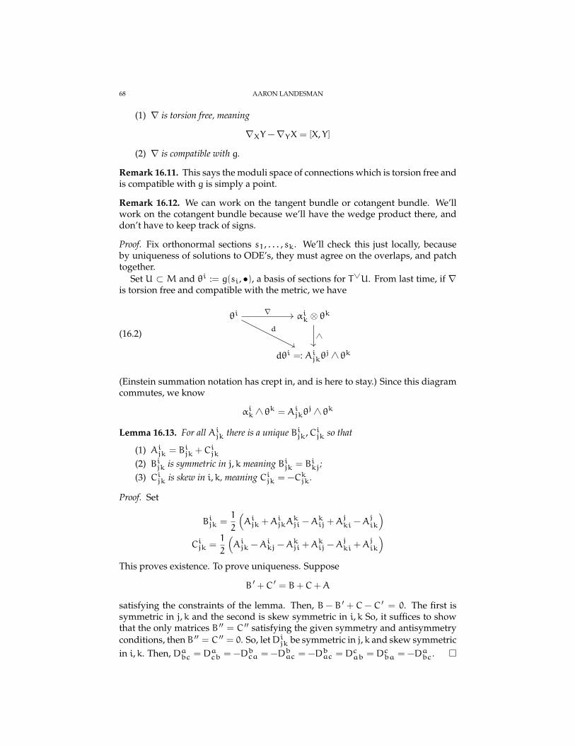
68 AARON LANDESMAN
(1) ∇ is torsion free, meaning
∇XY −∇YX = [X, Y]
(2) ∇ is compatible with g.
Remark 16.11. This says the moduli space of connections which is torsion free andis compatible with g is simply a point.
Remark 16.12. We can work on the tangent bundle or cotangent bundle. We’llwork on the cotangent bundle because we’ll have the wedge product there, anddon’t have to keep track of signs.
Proof. Fix orthonormal sections s1, . . . , sk. We’ll check this just locally, becauseby uniqueness of solutions to ODE’s, they must agree on the overlaps, and patchtogether.
Set U ⊂ M and θi := g(si, •), a basis of sections for T∨U. From last time, if ∇is torsion free and compatible with the metric, we have
(16.2)
θi αik ⊗ θk
dθi =: Aijkθj ∧ θk
∇
d∧
(Einstein summation notation has crept in, and is here to stay.) Since this diagramcommutes, we know
αik ∧ θk = Aijkθ
j ∧ θk
Lemma 16.13. For all Aijk there is a unique Bijk,Cijk so that
(1) Aijk = Bijk +Cijk
(2) Bijk is symmetric in j, k meaning Bijk = Bikj;(3) Cijk is skew in i,k, meaning Cijk = −Ckjk.
Proof. Set
Bijk =1
2
(Aijk +A
ijkA
kji −A
kij +A
jki −A
jik
)Cijk =
1
2
(Aijk −A
ikj −A
kji +A
kij −A
jki +A
jik
)This proves existence. To prove uniqueness. Suppose
B ′ +C ′ = B+C+A
satisfying the constraints of the lemma. Then, B− B ′ + C− C ′ = 0. The first issymmetric in j,k and the second is skew symmetric in i,k So, it suffices to showthat the only matrices B ′′ = C ′′ satisfying the given symmetry and antisymmetryconditions, thenB ′′ = C ′′ = 0. So, letDijk be symmetric in j,k and skew symmetricin i,k. Then, Dabc = D
acb = −Dbca = −Dbac = −Dbac = D
cab = Dcba = −Dabc.

NOTES FOR MATH 230A, DIFFERENTIAL GEOMETRY 69
Assuming this lemma, we have
dθi = Aijkθi ∧ θk
=(Bijk +C
ijk
)θj ∧ θk
= Cijkθj ∧ θk
This shows ∇θi must equal Cijkθj ⊗ θk. That is, αkj = Cijkθ
j. This proves unique-ness because for any choice of two Aijk, the Cijk is always determined. This showsuniqueness.
Remark 16.14. Given this theorem, how would we compute the Levi Civita con-nection? We take a dual basis, we compute the A’s and then the C’s. This proof isconstructive and nice if you have good candidates for si and can compute dθi.
Definition 16.15. This unique∇ from Theorem 16.10 is called the Levi-Civita con-nection or Riemannian connection of (M,g).
Theorem 16.16. In local coordinates, the Levi-Civita connection can be written
Γkij =1
2gkl ·
(∂gil∂xj
+∂gjl
∂xi−∂gij
∂xl
)where gab is the inverse of gab with
gij = 〈∂
∂xi,∂
∂xj〉
Proof. Not too hard, but very computational, and omitted. See any standard Rie-mannian geometry textbook.
Remark 16.17. In local coordinates, M ⊃ Mφ−→ Rn, we have a basis
∂∂xi
for
TM ∼= TRn ∼= Rn ×R6n then
gij = 〈∂
∂xi,∂
∂xj〉
and gab is the inverse matrix, so gabgbj = Iaj .Recall Γkij was defined
∇ ∂
∂xi
∂
∂xj= Γkij
∂
∂xk
Remark 16.18. This local coordinate version, we have that gij is hard to deal with,but [•, •] are easy to deal with in ∂
∂xi, the lie bracket is 0. In the si version, gij is
easy to deal with, but lie brackets are hard to deal with.
Example 16.19. TakeM = Rn and g = gstd. Then,
Γkij =1
2gkl = 0,
as they are derivatives of constants. This means,
∇ ∂
∂xi
∂
∂xj= Γkij
∂
∂xk= 0

70 AARON LANDESMAN
Example 16.20. take M = (~x,y) : y > 0 ∈ Rn+1. We have ~x ∈ Rn,y ∈ R>0.Define,
g =R2
y2gstd
for some R > 0. Let’s compute the Christoffel symbols. First,
∂gij
∂xl=
0 if l ≤ n−2R2
y3δij if l = n+ 1
Γkij =y2
2R2
(∂gik∂xj
+∂gik∂xi
−∂gij
∂xk
)Then,
−Γn+1ii = Γ j(n+1)j
= −1
y
and all other values are 0. So if ∇ is the Levi Civita connection, then
∇ ∂
∂xj
∂
∂xi=
1y∂∂y i = j
− 1y∂∂xi
j = n+ 1, i 6= j−1y
∂∂xj
i = n+ 1, i 6= j
Now we can’t really interpret these things very well, since we might not expectvertical vector fields to change when we move horizontally, but they do.
16.4. Geodesics. Let’s recall the definition.
Definition 16.21. Fix ∇ on TM. Then, a curve γ : (−ε, ε)→M is called a geodesicif
∇ ∂∂tγ = 0
That is, Dtγ = 0.
In local coordinates, we have
(16.3)
M ⊃ U
(−ε, ε) Rn
φγ
c

NOTES FOR MATH 230A, DIFFERENTIAL GEOMETRY 71
Let ci = vi, vi : R→ Rn. Then,
∇ ∂∂tγ = ∇ ∂
∂tvi∂
∂xi
= dvi(∂
∂t
)∂
∂xi+ vi∇ ∂
∂t
∂
∂xi
=
(∂vk
∂t+ viγ∗αki
)∂
∂xk
=
(∂vk
∂t+ viΓkijdx
j
(Dγ
(∂
∂t
)))∂
∂xk
=
(∂vk
∂t+ vivjΓkij
)∂
∂xk
We can solve when this equals 0.
17. 11/2/15
17.1. Geodesics and coming attractions. Today, we’ll show geodesics exist, theexp map is a diffeomorphism near the identity, define completeness, give exam-ples of the exp map. We’ll also give a preview of Hadammard’s theorem, theHopf-Rinow Theorem, and show that Geodesics locally minimize length.
Recall, last time, in local coordinates, a curve
γ : (ε, ε)→M
is a geodesic if, setting v = γ, we have
∂vk
∂t+ Γkijv
i · vj = 0
Recall
∇ ∂
∂xi
∂
∂xj= Γkij
∂
∂xk
Remark 17.1. We are thinking of this equation as lying in the tangent bundle asopposed to the trivial bundle because we’re using the coordinate ∂
∂t , written interms of ∂
∂xjwhich are thought of as a basis for the tangent bundle.
Question 17.2. Given x ∈M, v ∈ TxM, is there a geodesic γwith γ(0) = x, γ(0) =v?
This is now an ODE if we think of the geodesic equations as living in TM ratherthanM. In local coordinates, we look for a function
t 7→ (x(t), v(t)) ∈ Rn ×Rn
so that
·x = v∂vk
∂t+ Γkijv
i · vj = 0
So, by uniqueness of solutions to ODEs, there is a unique
(x(t), v(t)) : (−ε, ε)→ TM
so that x(t) is a geodesic.

72 AARON LANDESMAN
In fact, for all (x0, v0) ∈ TM there is an ε > 0 andW ⊂ TM, (x0, v0) ∈W so that
Φ : (−ε, ε)×W → TM
is defined as usual.
Example 17.3. Take M = (R,gstd) as our manifold In equations, v = γ, v =
Γijvivj = 0 defines a vector field on TM and Φ is the flow. This vector field only
has a horizontal component, and its value at a point v is v.
Remark 17.4. If you’re worried about transitioning from chart to chart, do home-work 9.
Intuitively, if γ : (−ε, ε)→M is a geodesic with initial vector γ(0) = v. Then, γwith initial vector ·(0) = av,a ∈ R should just be a reparameterization of γ.
Let’s now make this precise.
Definition 17.5. Given v ∈ TxM let
γv : (−ε, ε)→M
t 7→ γv(t)
be the geodesic with initial conditions
γv(0) = x
γv(0) = v
Proposition 17.6. γ satisfies the Rescaling property
γv(at) = γav(t)
Proof. Go into local coordinates and compute. We only need to show these twofunctions satisfy the same ODE’s.
Proposition 17.7. Let γ : (−ε, ε)→M be a geodesic. Then,
(−ε, ε)→ R≥0
t 7→ 〈·γ(t), ·γ(t)〉is constant.
Proof. Recall ∇ ∂∂t· γ = 0. Then, by compatibility of the metric
∂
∂t〈·γ(t),γ(t)〉 = 2〈∇ ∂
∂t· γ(t), ·γ(t)〉 = 0
So, at each x ∈M, we have an interesting map. Let
Wx ⊂ TxMbe
Wx = v ∈ TxM : γv is defined at least for time t = 1
Definition 17.8. The exponential map at x
expx :Wx →M
v 7→ γv(1).

NOTES FOR MATH 230A, DIFFERENTIAL GEOMETRY 73
Remark 17.9. This is highly dependent on the choice of metric g. If we havetwo different metrics, we can have two different exponential maps. We then useuniqueness of the Levi-Civita connection to define the exponential map as above.
Now, let’s see some examples.
Example 17.10. LetM = (Rn,gstd). Then,
expx :Wx → Rn
v 7→ γv(1)
If we have a point x ∈ Rn and a tangent vector v ∈ TxM. Recall γ is a geodesic in(Rn,gstd) if and only if ˙γ = 0. So, γv(t) = x+ tv.
Note expx is smooth, a surjection and an injection. Though, the injection is quitespecial to this case.
Example 17.11. LetM =(S1,g
)where g = j∗gstd where
j : S1 → R2
is the usual inclusion. Of course, in this case, the exponential map can’t be a dif-feomorphism because R is not compact and S1 is. So, expx is not an injection, butit is a covering map.
So, we can choose TxS1 ∼= R, we can show that exp(t) = eit ∈ S1.
Example 17.12. LetM = (Sn,g) with j∗gstd = g and
j : Sn → Rn+1
In our homework, we’ll show that geodesics of (Sn,g) in this metric are greatcircles with constant speed.
So, expx is an injection on the open ball TxSn of radius at most πR. It is asurjection but not a covering map.
Remark 17.13. Interesting theorems in differential geometry are often about thingswhere you ignore the differentiable structure, and just show something abouttopology, like the Gauss Bonnet theorem and Hadamard’s theorem.
Definition 17.14. (M,g) is complete if geodesics exist for all time. By rescaling,this is equivalent to expx is defined on all of TxM for all x.
Theorem 17.15. (Hadamaard) Let (M,g) be a connected complete Riemannian manifoldso that the sectional curvature is ≤ 0 everywhere.
Then, for all points x ∈M the exponential map
expx : TxM→M
is a covering map.
Proof. Not given now.
Question 17.16. How severe is the completeness condition?Answer: It always words for compact manifolds. However, even Rn isn’t nec-
essarily complete. For example, we can take a diffeomorphism between Rn ∼= U ⊂Rn, and if we take the induced metric on the first Rn coming from the second Rn,the metric won’t be complete.
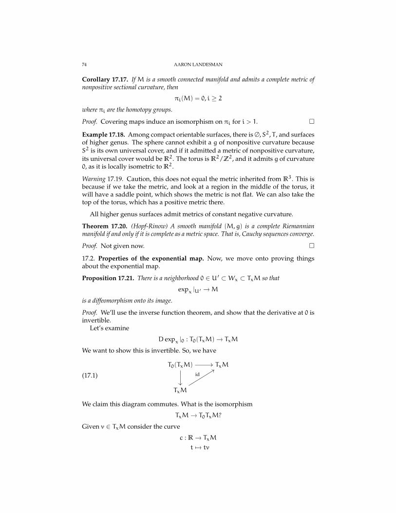
74 AARON LANDESMAN
Corollary 17.17. If M is a smooth connected manifold and admits a complete metric ofnonpositive sectional curvature, then
πi(M) = 0, i ≥ 2where πi are the homotopy groups.
Proof. Covering maps induce an isomorphism on πi for i > 1.
Example 17.18. Among compact orientable surfaces, there is ∅,S2, T , and surfacesof higher genus. The sphere cannot exhibit a g of nonpositive curvature becauseS2 is its own universal cover, and if it admitted a metric of nonpositive curvature,its universal cover would be R2. The torus is R2/Z2, and it admits g of curvature0, as it is locally isometric to R2.
Warning 17.19. Caution, this does not equal the metric inherited from R3. This isbecause if we take the metric, and look at a region in the middle of the torus, itwill have a saddle point, which shows the metric is not flat. We can also take thetop of the torus, which has a positive metric there.
All higher genus surfaces admit metrics of constant negative curvature.
Theorem 17.20. (Hopf-Rinow) A smooth manifold (M,g) is a complete Riemannianmanifold if and only if it is complete as a metric space. That is, Cauchy sequences converge.
Proof. Not given now.
17.2. Properties of the exponential map. Now, we move onto proving thingsabout the exponential map.
Proposition 17.21. There is a neighborhood 0 ∈ U ′ ⊂Wx ⊂ TxM so that
expx |U ′ →M
is a diffeomorphism onto its image.
Proof. We’ll use the inverse function theorem, and show that the derivative at 0 isinvertible.
Let’s examine
D expx |0 : T0(TxM)→ TxM
We want to show this is invertible. So, we have
(17.1)
T0(TxM) TxM
TxM
id
We claim this diagram commutes. What is the isomorphism
TxM→ T0TxM?
Given v ∈ TxM consider the curve
c : R→ TxM
t 7→ tv

NOTES FOR MATH 230A, DIFFERENTIAL GEOMETRY 75
Then, c(0) ∈ T0(TxM) and
v 7→ cv(0)
TxM→ T0TxM
is the isomorphism.
Question 17.22. What is the composite
TxM→ T0TxMD expx |0−−−−−−→ TxM?
We send
v 7→ (expx cv
)(0)
by the chain rule. Then,
expx cv : t 7→ expx(tv)
= γtv(1)
γv(t)
So, D(expx cv)∂∂t |t = 0. This is γv|t = 0. By definition of γv, we have γv(0) =
v.
Remark 17.23. By the rescaling property, Wx is a star-shaped neighborhood of0 ∈ TxM, meaning that for every v ∈ Wx, the segment from 0 to v is contained inWx.
Definition 17.24. An open neighborhood x ∈ U ⊂M is called a normal neighbor-hood if it is the image of
v : |v| < ε, ε > 0 ⊂ TxMunder expx.
We can do even better than the proposition.
Proposition 17.25. LetW ⊂ TM be
(x, v) ∈ TM : γv is defined for at least t = 1
Consider the map exp :W →M×M. sending (x, v) 7→ (γv(1), x) For all x ∈M, thereexists a neighborhood (x, 0) ∈ U ⊂W so that exp |U is a diffeomorphism onto its image.
Proof. Use the inverse function theorem. We have exp : TM → M×M. Locally,we have U × U ⊂ U × Rk ⊂ TU ⊂ TM. This locally defines a map U × U →M×M. This defines a map D exp |(x,0) is a matrix T(x,0)(U× U) = TxU⊕ T0Uand T(x,x)(M×M) = TxM⊕ TxM. So, we can write the map as a block matrix.What are the block components U×UT →M×M. We claim this matrix is of theform. (
I A0 I
)which would imply the matrix is invertible. The first component is the identity bydefinition. In the last component, we showed in the previous proposition is thatthis is the identity map. Finally, the first component of M doesn’t depend on thesecond component of U.
76 AARON LANDESMAN
Here are some corollaries.
Corollary 17.26. We can choose some Ux ⊂M open and some ε > 0 so that
Uε := (y, v) ∈ TM : y ∈ Ux, |v| < ε ⊂ Uwhere U is the neighborhood on which exp is a diffeomorphism from the proposition, and|v| =
√gy(v, v). Note that this is open because the Riemannian metric is continuous.
Then, we can chooseWx ⊂M so that x ∈Wx so thatWx ×Wx ⊂ expx(Uε).For all x, there exists ε > 0 andWx 3 x open, so that for any two points y0,y1 ∈Wx,
there exists a unique geodesic
γ : [0, 1]→M,γ(0) = y0,γ(1) = y1of length < ε from y0 to y1.
Proof. Given a point y0,y1 ∈ Wx ×Wx, we have a unique preimage (y0, v) inexp−1(Wx ×Wx). We know |v| < ε by construction. Therefore, the length of thegeodesic is |v|. This is unique because if we had any shorter length, it would haveto be given by a vector of length < ε, which means it has to be given by somevector in Uε, and then it is unique because the exp map is a diffeomorphism of Uonto its image.
Remark 17.27. This is better than expx being a diffeomorphism near 0. This isbecause we don’t know how points near x are related, but this stronger versionindeed tells us about the relation.
Remark 17.28. The geodesic γ need not be a map
γ : [0, 1]→Wx
It might escapeWx and pass to other parts ofM.
Remark 17.29. With work, you can chooseWx so γ is contained inWx.
18. 11/5/15
18.1. Review. Last time, we fixed g,∇,M and defined the exponential map by
exp :W →M
(x, v) 7→ γv(1)
Less generally, we defined
expx :Wx →M
by restriction of exp to x.We proved that expx is a diffeomorphism near the origin 0 ∈ TxM and also that
W →M×M(x, v) 7→ (
x, expx(v))
is a diffeomorphism near (x, 0).We obtained the corollary
Corollary 18.1. For all x ∈ M there is an ε > 0 with x ∈ Wx ⊂ M so that for ally0,y1 ∈Wx there is a unique geodesic from y0 to y1 of length < ε, where a geodesic is amap γ : [0, 1]→M
Proof. Done last time.

NOTES FOR MATH 230A, DIFFERENTIAL GEOMETRY 77
Today, we’ll show geodesics are locally length minimizing.
18.2. Geodesics and length.
Example 18.2. Geodesics are not length minimizing. For example, from the home-work, we know the geodesics are the great circle on the sphere. We can go the shortway or the long way around a great circle between two non antipodal points, oneof which has longer length than the other.
Our first goal for today is to prove
Proposition 18.3. For all x ∈M there is ε > 0 so that if(1) y ∈ expx(Bε(0)).(2) w : [0, 1]→M is a piecewise smooth curve from x to y
then len(w) ≥ len(γ) where γ is the unique geodesic of length< ε from x to y. Moreover,equality holds if and only if
im w = im γ.
and w is an immersion.
Remark 18.4. We will use U to distinguish between sets in the tangent space andtheir corresponding images U under the exponential map.
Proof. In order to prove the proposition, we give some Lemmas.
Lemma 18.5. (Geodesics are orthogonal to distance level sets) Let Ux ⊂ M be a normalneighborhood. Recall, this means Ux = exp(Ux). Let Sδ ⊂ Ux ⊂ TxM be a sphere ofradius δ. Then, for all geodesics γv from x, γv ⊥ Sδ = expx(Sδ).
Proof. It suffices to show this perpendicularity for each curve c on the surface Sδ.Fix a curve
c : [a,b]→ U
so that len(c) = 1. Consider the surface
R× [a,b]→ TxM
(t,φ) 7→ (tc(φ))
Consider the composition
R× [a,b]→ TxMexp−−→x M
and call the composition f.Note for φ0 fixed, f(•,φ0) is a geodesic. For t0 fixed, we have f(t0, •) is a curve
on St0 . We claim these two curves are orthogonal.It suffices to show
〈∂f∂t
,∂f
∂φ〉 = 0
by this, we mean
〈D exp(∂
∂t,D exp
∂
∂t
)〉
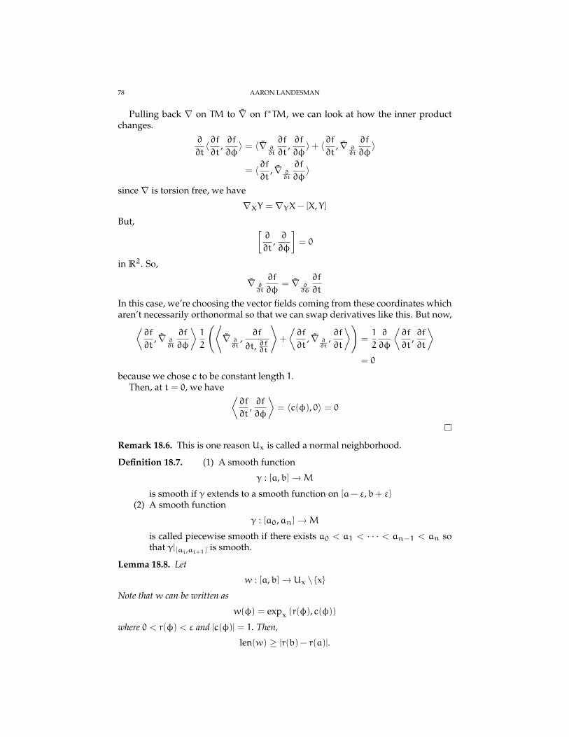
78 AARON LANDESMAN
Pulling back ∇ on TM to ∇ on f∗TM, we can look at how the inner productchanges.
∂
∂t〈∂f∂t
,∂f
∂φ〉 = 〈∇ ∂
∂t
∂f
∂t,∂f
∂φ〉+ 〈∂f
∂t, ∇ ∂
∂t
∂f
∂φ〉
= 〈∂f∂t
, ∇ ∂∂t
∂f
∂φ〉
since ∇ is torsion free, we have
∇XY = ∇YX− [X, Y]
But, [∂
∂t,∂
∂φ
]= 0
in R2. So,
∇ ∂∂t
∂f
∂φ= ∇ ∂
∂φ
∂f
∂t
In this case, we’re choosing the vector fields coming from these coordinates whicharen’t necessarily orthonormal so that we can swap derivatives like this. But now,⟨
∂f
∂t, ∇ ∂
∂t
∂f
∂φ
⟩1
2
(⟨∇ ∂∂t
,∂f
∂t, ∂f∂t
⟩+
⟨∂f
∂t, ∇ ∂
∂t,∂f
∂t
⟩)=1
2
∂
∂φ
⟨∂f
∂t,∂f
∂t
⟩= 0
because we chose c to be constant length 1.Then, at t = 0, we have ⟨
∂f
∂t,∂f
∂φ
⟩= 〈c(φ), 0〉 = 0
Remark 18.6. This is one reason Ux is called a normal neighborhood.
Definition 18.7. (1) A smooth function
γ : [a,b]→M
is smooth if γ extends to a smooth function on [a− ε,b+ ε](2) A smooth function
γ : [a0,an]→M
is called piecewise smooth if there exists a0 < a1 < · · · < an−1 < an sothat γ|[ai,ai+1] is smooth.
Lemma 18.8. Let
w : [a,b]→ Ux \ x
Note that w can be written as
w(φ) = expx (r(φ), c(φ))
where 0 < r(φ) < ε and |c(φ)| = 1. Then,
len(w) ≥ |r(b) − r(a)|.

NOTES FOR MATH 230A, DIFFERENTIAL GEOMETRY 79
Further, there is equality if and only if r is monotone (meaning the derivative of r alwayshas the same sign) and c is constant.
Proof. Again, set
f : R× [a,b]→M
(t,φ) 7→ expx(tc(φ))
so
w(φ) = f(r(φ)c(φ))
and
w = Dw
(∂
∂t
)= Df Dr
(∂
∂t
)+Df
(∂c
∂φ
)Now, because the two terms in the last equality above are orthogonal by Lemma ??,we have
〈w, w〉 = |∂d
∂r|2 +
⟨Df
(∂r
∂φ
),Df
(∂c
∂φ
)⟩≥ |∂r
∂t|2
So, equality is equivalent to
∂c
∂φ= 0
which is equivalent to c being constant.Then, integrating square roots, we have∫b
a|w|dφ ≥
∫ba|∂r
∂φ|dφ
≥ |r(b) − r(a)|
and further, we have equality if and only if r is monotone.
Finally, we are ready to prove the main proposition, which isn’t too difficultgiven our lemmas. Recall we’re trying to prove that geodesics locally give thepaths of shortest distance.
Given
w : [a,b]→M
a 7→ x
b 7→ y
is piecewise smooth and y ∈Wx. Let y = expx(r · c) where r ∈ R, c ∈ S1.Let Sr,Sδ be the images under the exponential map of spheres. w has to be
some curve going from x to y. For all real numbers δ > 0, there is some segment ofw going to and from the spheres Sr,Sδ. By Lemma 18.8, we have that the lengthof this segment is at least r− δ for all δ. Now, len(w) is at least the length of thissegment, and since inequality holds for all δ > 0, we have len(w) ≥ r.

80 AARON LANDESMAN
Now, suppose
im w 6= im γ
Then, there is some shell ∪δ<ε<rSε. on which the images of w,γ disagree. So, ifthe images disagree, then w couldn’t have been minimal by Lemma ??.
We now give some consequences of the above proposition.
Definition 18.9. Let
d(x,y) := infpiecewise smooth curves γ from x to y
lenγ
Lemma 18.10. This d(x,y) makesM into a metric space.
Proof. The only difficult part is that this is nondegenerate. This follows from theabove Proposition 18.3.
Remark 18.11. In fact (M,d) ∼=M is a homeomorphism via the identity map.
Here’s a fun side theorem.
Theorem 18.12. (Nash Embedding Theorem) For every second countable Riemannianmanifold (M,g) there is an embeddingM→ RN so that g is pulled back from RN.
Proof. Very difficult, we definitely won’t do this in class.
Corollary 18.13. Let w : [a,b]→M be piecewise smooth and assume
len(w) = d (w(a),w(b))
Then, w is a geodesic and can be reparameterized so w is smooth.
Proof. If we knew w is a geodesic, it would certainly be smooth after reparame-terization. If w minimizes length then it locally minimizes length. That is, if wehave two points w(a) and w(b) and a curve w between them. If we choose twoclose points on this curve, then wmust be the shortest path between those points,or else we could swap in this path for w and concatenate, and we would get ashorter path. So, by Proposition 18.3.
Remark 18.14. Since for any point x, the exponential map is a surjection, there isalways a geodesic which realizes a path between two points with respect to somemetric.
Our next goal is the following lemma. Recall a metric is complete if all geodesicsexist for all time.
Lemma 18.15. Suppose (M,g) is a complete Riemannian manifold. Then, for all x ∈M,
expx : TxM→M
is a surjection.
NOTES FOR MATH 230A, DIFFERENTIAL GEOMETRY 81
18.2.1. Idea of proof. The idea is the following. Pretend we are in kindergarten. Weknow the exponential map is locally a diffeomorphism. We take a small spherearound x, and the sphere is compact, there’s a path of minimum distance. We canthen flow along this geodesics. And we can keep doing this, and eventually endup at y.
Proof. Fix y ∈ M so that d(x,y) = r. We need to show y = expx(r · v) for some v.Fix δ small and consider Sδ = expx (Sδ). Since d(•,y) :M→ R is continuous, wehave
d(•,y) : Sδ → R
is continuous and attains a minimum at some x0 ∈ Sδ, where Sδ is compact. Then,set
x0 = expx(δv)
where |v| = 1, v ∈ TxM.The main claim is the following:
Lemma 18.16. Fro all t ∈ [δ, r] we have
d(γv(t),y) = r− t.
Proof. Note, this is true for t = δ because
d(x,y) = infx∈Sδ
(d(x, x) + d(x,y)
= infx∈Sδ
(δ+ d(x,y))
= δ+ infx∈Sδ
d(x,y)
= δ+ d(x0,y)
so d(x0,y) = d(x,y) − d = r− d. So, the claim is proven for t = δ. Now, let tmaxbe the supremum over all t so that the claim holds for t. Then, the claim holds fortmax by continuity. We need to show that tmax < r leads to a contradiction. Letx ′ = γv(tmax). Choose Sδ ′(x ′) and again minimize the function. Then,
d(x ′,y) = infx∈Sδ ′
(d(x ′, x
)+ d (x,y)
= δ ′ + d(x,y)
and so
d(x,y) = r− tmax − δ′
We are then done by the triangle inequality, because we got a further extension ofthe path.
This implies the Lemma 18.15 by taking r = t.
19. 11/10/15
19.1. Preliminary questions.
Question 19.1. What is the definition of integrable submanifold?
If E ⊂ TM and x ∈ M then an integrable submanifold is an immersion j : U →M, x ∈ j(U) and Dj(TU) = E|j(U).
Today, we’ll finish the proof of Hopf Rinow and curvature.
82 AARON LANDESMAN
19.2. Hopf-Rinow. Recall, we were proving the following proposition last time:
Proposition 19.2. If (M,g) is complete, then for all x ∈M, the map expx : TxM→Mis a surjection. In fact, for all y ∈M there is a geodesic of length d(x,y) from x to y.
Proof. Recall where we left off in the proof last Thursday: We fixed a small δ andlooked at the image of Sδ under the exponential map. We found and x0 whichminimizes d(•,y) : Sδ → R. Let r = d(x,y). We considered
t ∈ [δ, r] : d(γv(t),y) = r− t
We claimed that we were almost done by the triangle inequality.We now pick up where we left off. Consider tmax =
∑t < r so that t is in the
above set. Let’s find a contradiction.We take a point x ′ := γv(tmax). Then we repeat the above argument so that
d(•,y) : Sδ ′ → R and obtain a point x1 minimizing this function. Therefore, wehave a piecewise smooth curve from x to x1.
We claim:
Lemma 19.3. We have that the length of this piecewise smooth curve from x to x1 isd(x, x1).
Proof. Here, we’ll use the triangle inequality twice. We have
d(x, x1) ≤ d(x, x ′) + d(x ′, x)(19.1)
d(x,y) ≤ d(x, x1) + d(x1,y)(19.2)
So, we have
d(x,y) − d(x1,y) ≤ d(x, x1)
≤ d(x ′, x1) + d(x ′, x),since
d(x ′,y) = δ ′ + d(x1,y).
So,
r+ δ ′d(x ′,y) ≤ d(x, x1) ≤ δ ′ + d(x ′, x)r− d(x ′,y) ≤ d(x, x1) − δ ′ ≤ d(x ′, x)
tmax ≤ d(x, x ′) − δ ′
≤ tmax.
Finally, the claim holds because
d(x, x1 = tmax + δ′ = d(x, x ′) + d(x ′, x1).
By our lemma from last class, any piecewise smooth curve minimizing distanceis a geodesic, and, in particular, is smooth. Therefore, x1 = γv(tmax + δ
′). Thisfinishes the proof because
d(x1,y) + d(x ′, x1) = d(x ′,y)
d(γv(tmax + δ′),y) + δ ′ = r− tmax

NOTES FOR MATH 230A, DIFFERENTIAL GEOMETRY 83
But this concludes the proof because
d(γv(tmax + δ′),y) = r− (tmax + δ
′)
and so tmax was not maximal.
Now, let’s complete the proof of Hopf Rinow.
Theorem 19.4. The following are equivalent:(a) The Riemannian manifold (M,g) is complete.(b) Any bounded subset ofM has compact closure.(c) M is complete as a metric space.
Proof. First, we show a =⇒ b. Let A be bounded. Fix x ∈M and let
d :=∑y∈A
d(x,y) <∞.
Then, A lies in the image of expx(Bd(0)), by Proposition 19.2. Now, since theclosed ball is compact, the image under expx is also compact, and hence it containsthe closure of A. Therefore, the closure of A is also compact.
Next, we show b =⇒ c. Then, (x1) is Cauchy. Then, xi is compact, and soany sequence in xi has a convergent subsequence.
Finally, to show c =⇒ a, we only need to show any geodesic extends indefi-nitely.
So, fix x, v ∈ TxM. Let tmax be the supremum over all t for which γv(t) isdefined. This is open by the existence theorem for ODE’s. So, it suffices to showγv(t) is defined at tmax. Now, fix ti → tmax with ti < tmax. Then, γv(ti) is Cauchy.So, limti→tmax γ(ti) exists.
19.3. Curvature. Curvature is one of the most confusing concepts because thereare many types, but they are often all called curvature. Further, in many ways, thestudy of differential geometry is the study of curvature. Today, we’ll define somebasic types of curvature, and maybe talk about what flatness implies.
Recall the following:
Remark 19.5. Given a connection ∇ on E, there exists a unique map
D : Ω1(E)→ Ω2(E)
respecting the Leibniz rule
D(α⊗ s) = dα⊗ s−α∧∇s
where the minus sign is coming from +(−1)|α|. Here, D(α ⊗ s) ∈ Ω1(E) =
Γ(T∨M⊗E). In this case,D ∇ 6= 0 in general. So, recall∇ is flat whenD ∇ = 0.
If you’re algebraically minded, if we had a flat connection, we would get aninvariant of the cochain complex given by taking cohomology.
Proposition 19.6. We have
D ∇ : Γ(E)→ Ω2(E)
is C∞(M) linear.
84 AARON LANDESMAN
Proof. We check, working in local coordinates αj. Then,
(D ∇)(fs) = D (df⊗ s+ f∇s)
= D(df⊗ s+ fαj ⊗ sj
)= d2f⊗ s− df∧∇s+ d(fαj)⊗ sj − fαj ∧∇sj= 0− df∧αj ⊗ sj + (df∧αj + fdα
j)⊗ sj − fαj ∧∇sj= f
(dαj ⊗ sj −αj ∧∇sj
)= f (D ∇(s))
completing the proof.
Corollary 19.7. We can think of D ∇ as an End(E) valued 2-form.
Proof. Immediate from the above proposition.
Definition 19.8. By the above, we mean that given X, Y ∈ Γ(TM), we can take
(D ∇)X,Y : Γ(E)→ Γ(E)
by evaluating the mapD ∇ : Γ(E)→ Ω2(E) at X, Y, corresponding to composingit with the map Ω2(E) → Γ(E), which is evaluation at X, Y. Further, the map(D ∇)X,Y . Now, in generality, we know homC∞(M) (Γ(E), Γ(F)) ∼= hom(E, F) ∼=Γ(Hom(E, F)). Then, taking E = F, we know homC∞(M)(Γ(E), Γ(E)) ∼= Γ(End(E)).
Call this 2 form F ∈ Ω2(End(E)) by F∇. We call this the curvature tensor of ∇.
Proposition 19.9. For X, Y ∈ Γ(TM) we have
F∇(X, Y) = ∇X∇Y −∇Y∇X −N[X,Y]
Proof. Locally, choose a basis s1, . . . , xk of Γ(E|U). Set ∇si = αji ⊗ sj. Then,
F∇(X, Y)(si) = (D ∇si) (X, Y)
=(dαji ⊗ sj −α
ji ∧α
kj ⊗ sk
)(X, Y)
= X(αji(Y) − Y(αji(X)) −α
ji ([X, Y]) sj −α
ji(X)α
kj (Y) +α
ji(Y)α
kj (X)sk
Next, note
∇X∇Ysi = ∇X(αji(Y)⊗ sj
)=(dαji(Y)
)sj +α
ji(Y)∇sj(X)
= X(αji(Y))sj +αji(Y)α
ki (X)sk
This gives two terms of the left hand side. Similarly, switching X, Y we get twoother terms of the left hand side. So we obtain
X(αji(Y) − Y(αji(X)) −α
ji ([X, Y]) sj −α
ji(X)α
kj (Y) +α
ji(Y)α
kj (X)sk =
(∇X∇Y −∇Y∇X −∇[X,Y]
)si
Now, this identity is linear over R, and so it holds for all sections.
Remark 19.10. If we have a map Γ(E)→ Γ(E) given by
∇X∇Y −∇Y∇X −∇[X,Y]
which is C∞(M) linear.
NOTES FOR MATH 230A, DIFFERENTIAL GEOMETRY 85
Definition 19.11. If a map is C∞(M) linear it is often called a tensor or beingtensorial. This terminology is most commonly used when E = TM.
Remark 19.12. Being C∞(M) linear is super useful! This is because the values ofthe map at a point only depends on the values at that point, and not on the valuesin a neighborhood at that point. More precisely, if Xx = Xx, Yx = Yx, s(x) = s(x).Then,
F(X, Y)(s)(x) = F(X, Y)(s)(x)
Proposition 19.13. Let j : (M, g)→ (M,g) be an isometry. Then,(1) We have Dj : Γ(TM)→ Γ(TM) satisfies Dj(∇XY) = ∇Dj(X)Dj(Y).(2) We have
Dj(F(X, Y)Z
)= F
(DjX,DjY
)DjZ
where ∇, ∇ are Levi-Civita connections and F, F are their curvature tensors.
Proof. The first part follows from our homework problem, where we showed thatthe pullback of a Levi-Civita connection is the Levi-Civita connection.
The second part follows from plugging the first part into
∇X∇Y −∇Y∇X −∇[X,Y]
Definition 19.14. In this setting where (E,gE) is a vector bundle and a Riemannianmetric on the vector bundle, we have a function
Γ(TM)× Γ(TM)× Γ(E)× Γ(E)→ Γ(R)
(X, Y,Z,W) 7→ 〈F∇(X, Y)Z,W〉Note that∇ need not be related to g. However, because all parts of this expressionat C∞(M) linear, the map as a whole is.
And, when E = TM and∇ is the Levi-Civita connection, the above map is calledthe Riemann curvature tensor.
Remark 19.15. At the end of the day, we have
R : Γ(TM)× Γ(TM)× Γ(TM)× Γ(TM)→ C∞(M)
19.4. Towards some properties and intuition on curvature tensors.
Example 19.16. Consider M ⊃ U φ−→ Rn. Let ∂∂xi
be the coordinate vector fields.We know [
∂
∂xi,∂
∂xj
]= 0
So,
F
(∂
∂xi,∂
∂xj
)= ∇ ∂
∂xi
∇ ∂∂xj
−∇ ∂∂xj
∇ ∂∂xi
That is, Fmeasures the failure of ∇ to commute.
Recall, given ∇ : Γ(E) → Ω1(E) a connection, we obtain a covariant derivativealong X
∇X : Γ(E)→ Γ(E).
86 AARON LANDESMAN
Definition 19.17. We introduce the notation FX,YZ := F(X, Y)Z.
Proposition 19.18. We have for E = TM,∇ Levi-Civita
(1)
〈FX,YZ,W〉 = −〈FX,YW,Z〉
(2)
〈FX,YZ,W〉 = −〈FY,XZ,W〉
(3)
FX,YZ+ FY,ZX+ FZ,XY = 0
(4)
〈FX,YZ,W〉 = 〈FZ,WX, Y〉
Proof. First, we prove 1. Note
0 = (X Y − Y X− [X, Y]) 〈Z,W〉
by the definition of the Lie bracket. Let’s now write out the first term.
X Y (〈W,Z〉) = X (〈∇YW,Z〉+ 〈W,∇YZ〉)= 〈∇X (∇YW) ,Z〉+ 〈∇XW,∇YZ〉+ 〈∇YW,∇XZ〉+ 〈W,∇X∇YZ〉
By symmetry, we have
−Y X〈W,Z〉 = −〈∇Y∇XW,Z〉− 〈W,∇Y∇XZ〉− 〈∇XW,∇YZ〉− 〈∇YW,∇XZ〉
Then, substituting, we find
0 = (X Y − Y X− [X, Y]) 〈Z,W〉= 〈FX,YW,Z〉+ 〈W, FX,YZ〉
The proof of 2 is obvious, since F is a 2 form.To prove 3, note that since F is C∞(M) linear, it suffices to check this on local
linearly independent sections.Let’s choose X, Y,Z to be local vector fields so that their lie brackets are 0.Then, 3 becomes
FX,YZ = ∇X∇YZ−∇Y∇XZ− 0
FY,ZX = ∇Y∇ZX−∇Z∇YX− 0
FZ,XY = ∇Z∇XY −∇X∇ZY − 0
Then, we have
∇XY −∇YX = [X, Y]
because the connection is Levi-Civita, hence torsion free. Using this, the above 6terms all cancel outs.
The proof of 4 is omitted, because it is tedious.

NOTES FOR MATH 230A, DIFFERENTIAL GEOMETRY 87
Remark 19.19. Here is some geometric intuition. We have some algebraic defini-tion of ∇. We can view connections more geometrically. If we have some connec-tion on E, a vector bundle on a manifoldM. Say we have a point v ∈ Ex e can thenfind a parallel section γ. For every tangent vector formed by γ, we can look at thetangent vector formed by γ. Looking at lifts of γ from TM to ˜γin TvE. So, at everypoint x, we get a subspace Hv ⊂ TvE. This is a distribution H ⊂ TE. Moreover, ifwe project Dπ : Hv → TxM is an isomorphism.
So, every connection gives a distribution. We can ask whether this is integrableor involutive. If it is, we can find a manifold passing through this which is flat. So,∇ being flat turns out to H being integrable.
This is called a connection because it connects two different fibers.
20. 11/12/15
20.1. Types of curvatures. Today, we’ll discuss every type of curvature you mightsee in an introductory differential geometry textbook, which is a lot of types!
Recall from last time:
Definition 20.1. Given a map
R : Γ(TM⊗4)→ C∞(M)
X⊗ Y ⊗ Z⊗W 7→ 〈FX,YZ,W〉where we are given a curvature 2 form
F ∈ Ω2(End(TM))
and
FX,Y = ∇X∇Y −∇Y∇X −∇[X,Y]
Recall at the end of last class, we stated some properties of this tensor. Here is acorollary of those.
Corollary 20.2. We have
(20.1)
Γ(TM)⊗ Γ(TM)⊗ Γ(TM)⊗ Γ(TM) Γ(R)
Γ(∧2TM)⊗ Γ(∧2TM)
Sym2(∧2TM)
That is, R defines a symmetric bilinear map
∧2TM⊗∧2TM→ C∞(M).
In particular, for all x, a bilinear map
∧2TxM⊗∧2TxM→ R
Proof. Each of the two factorizations follow from different parts of the propositionfrom last time.
88 AARON LANDESMAN
Here is a summary of the types of curvature we’ll encounter:(1) Riemann curvature tensor: A map
Γ(TM)⊗4 → C∞(M)
or equivalently
Sym2(Γ(∧2TM))→ C∞(M)
(2) Ricci curvature tensor:
Ric : Γ(TM)⊗ Γ(TM)→ C∞(M)
(3) Scalar curvature: S :M→ R which is given by taking the trace of the Riccicurvature.
(4) Sectional curvature: A map
Gr2(TM)→ R
In fact the Riemann curvature tensor is equivalent to the sectional curva-ture.
20.2. Review of Linear Algebra.
Question 20.3. What is a trace?
Perhaps you usually think of trace as a function from matrices to R. Perhapsyou also think of this as summing the elements along a diagonal.
However, to define trace in this way, it is apparently basis dependant.It would be nice to have a basis free expression of trace. Here it is:
Definition 20.4. Let
φ : V ⊗ V∨ → End(V)
v⊗ ξ 7→ w 7→ v⊗ ξ(w).In the case V is finite dimensional, φ is invertible, by the following proposition:
Proposition 20.5. The following are equivalent:(1) The map φ : V ⊗ V∨ → End(V) is an isomorphism(2) idV is in the image of the map φ.(3) V is finite dimensional.
Proof. First, 1 =⇒ 2, is immediate, because isomorphisms are surjections.Second, 2 =⇒ 3. If A is in the image of φ, then dim im A <∞ because tensors
are finite sums. So, if A = idV then dimV <∞.Third, for 3 =⇒ 1, choose a basis and do a computation.
Also, define the evaluation map
ev : V ⊗ V∨ → k
v⊗ ξ 7→ ξ(v)
Then, we have a diagram
(20.2)V ⊗ V∨ End(V)
k
φ
ev

NOTES FOR MATH 230A, DIFFERENTIAL GEOMETRY 89
and we may define the trace map ev φ−1 : End(V)→ k.
Proposition 20.6. The trace as defined above agrees with the usual definition of trace.
Proof. This follows from a standard after choosing a basis. Essentially, it sends amatrix A to
∑iAv
i ⊗ ξi =∑iAii.
Remark 20.7. This is one of Hiro’s favorite propositions because it has to do with1 dimensional field theory.
20.3. Traces in Riemannian Geometry. If we’re given an isomorphism Vg−→ V∨,
then any element of V ⊗ V can be mapped to an element of V ⊗ Vid⊗g−−−→ V ⊗ V∨
Similarly, we can define a map
V∨ ⊗ V∨id⊗g−1−−−−−→ V∨ ⊗ V .
So, we can take the trace of any element of V ⊗ V or V∨ ⊗ V∨.
Warning 20.8. Caution, this depends on choice of g.
We have a map
(20.3)V ⊗ V V ⊗ V∨
R
id⊗g
ev
Given (M,g) we have an isomorphism
gx: TxM→ T∨x M
v 7→ 7→ g(v, •)
In local coordinates, fix
A ∈ Γ(T∨M⊗ T∨M)
A =∑
Aijdxi ⊗ dxj
Then,
id⊗ g−1(A) = Aijgjkdxi ⊗∂
∂xk
Proposition 20.9. We have gjk is a smooth function so that
(gik), (gab)
are inverse matrices.
Proof. We have
gx: TxM→ T∨x M
∂
∂xi7→ g
(∂
∂xi•)

90 AARON LANDESMAN
where the latter sends ∂∂xj7→ gij. Therefore,
g
(∂
∂xi
)=∑j
gijdxj
Therefore the inverse map is given by sending
dxjg−1x7→ (gij)
−1 ∂
∂xi
Remark 20.10. NoteAijgjk defines a new matrix of functions which we abbreviateas Aki .
Definition 20.11. Given
B ∈ Γ(TM)⊗ Γ(TM)
A ∈ Γ(T∨M)⊗ Γ(T∨M)
The trace is the smooth function
(20.4)
Γ(TM)⊗2 Γ(TM)⊗ Γ(T∨M)
C∞(M)
More generally, given
B ∈ Γ(TM)⊗ Γ(TM)
A ∈ Γ(T∨M)⊗ Γ(T∨M)
we locally obtain
tr(A) = Aijgji
tr(B) = BijgijSince g is symmetric, the choice of id⊗ g or g⊗ id yields the same result.
Definition 20.12. More generally yet, given
A ∈ Γ(T∨M⊗n)we can choose the ith and jth factor for i 6= j and take the trace along these.
That is, we can define a map
id⊗ · · · id⊗ g−1 ⊗ id⊗ · · · ⊗ id : Γ(T∨M)⊗n → Γ(T∨M)⊗(n−1) ⊗ Γ(TM)
And then compose this with the evaluation map
id⊗ · · · ⊗ idev : Γ(T∨M)⊗(n−1) ⊗ Γ(TM)→ Γ(T∨M⊗(n−2))
This is a section of T∨M⊗n−2 called the contraction (or trace) of A along the i, jfactors (or components) of A.
We can do this in the special case of the Riemannian curvature.
R : Γ(TM)⊗4 → Γ(R)
That is, R ∈ Γ(T∨M⊗4).

NOTES FOR MATH 230A, DIFFERENTIAL GEOMETRY 91
Question 20.13. Which factors can we take trace along?
Locally,
R = Rijkldxi ⊗ dxj ⊗ dxk ⊗ dxl
Since Rijlk is skew in i, j the trace along i, j is 0. Additionally, it is skew in k, l, sothe trace along k, l is 0.
So, it only remains to analyze the trace along(1) i, j(2) i,k(3) j, l(4) j,k
However, the trace along any one of these determines the three other ones since
Rijkl = Rklij
Definition 20.14. The Ricci curvature, denoted Ric is the trace of the Riemanncurvature tensor R along i and l (that is, X andW)
Remark 20.15. This convention is chosen so that the sphere has positive curvature.
Question 20.16. What does this trace encode?
Gregory Perelman allows us to motivate them.
Remark 20.17. There are two Hamiltons Hiro knows of. One is older and inventedthe quaternions. The other is younger and studies geometry. Aaron Slipper re-marks that there is yet another Hamilton who died in a duel!
The following is due to the second Hamilton. Consider the space of all possibleRiemannian metrics onM.
This set of Riemannian metrics lies inside the set of all sections Γ(T∨M⊗ T∨M).In fact, this set lies in Γ(Sym2(T∨M)), the symmetric bilinear forms. Further, Rie-mannian metrics are an open subset of this vector space, since being nondegener-ate is an open condition.
Question 20.18. What is Tg(Γ(Sym2(T∨M)))? As a vector space, abstractly, it isΓ(Sym2(T∨M)).
So, in other words, deformations of a metric g are given by flowing along a tan-gent vector. In other words, we only need to give an element of Γ(Sym2(T∨M)).
But, note Ric is a section of Sym2(T∨M). But, this Ricci curvature depended atthe beginning of time on g.
So, the assignment
g 7→ Ricgis a section of the tangent bundle on some co dimension manifold of the space ofall g.
Definition 20.19. The Ricci flow of a Riemannian metric g is a path
γ : (−ε, ε)→ g
so that∂γ
∂t= −2Ricγ(t)

92 AARON LANDESMAN
In local coordinate, we’re looking for functions
gij(t)
so that∂gij
∂t= −2Ricg(t)
Hamilton proved that these flows exist for small amounts of time.This flow was central in Perelman’s work on the Poincare conjecture, which was
about when you know when the Ricci flow exists.
Definition 20.20. The scalar contraction is the trace of Ric, the Ricci curvature,when Ric ∈ Γ(Sym2(T∨M)).
Remark 20.21. Hopefully the scalar curvature is memorable because it is a scalar.The only way to get a scalar from a 4 fold tensor is by taking traces twice.
Next, we will discuss sectional curvature
Remark 20.22. The most pedagogically sound way to describe the sectional cur-vature is to give a definition, and then say what it amounts to.
Definition 20.23. Let X, Y ∈ Γ(TM). The sectional curvature along the 2 planespanned by X and Y in the vector space Γ(TM) is defined to be
R(X, Y, Y,X|X|2|Y|2 − 〈X, Y〉2
where g(•, •) = 〈•, •〉.
20.4. Back to linear algebra. At the end of the day, all these curvatures comeabout from very good understanding of linear algebra.
We will say things for general vector spaces V , but for the application to differ-ential geometry, we should keep in mind
V = ∧2T∨x M
Consider a symmetric bilinear map
V ⊗ V A−→ R
Keep in mind the case that A = R at a point x ∈M.
Lemma 20.24. If V also has a separate nondegenerate inner product, we can recover Acompletely by the data of
(1) An orthonormal basis vi for V and(2) A(vi, vj) for all i, j.
Proof. This is a standard linear algebraic fact, purportedly, but Hiro didn’t knowhow to prove it in class.
Question 20.25. Can we put an inner product on V = ∧2TxM and understand theRiemann curvature R in an orthonormal basis?
First, let’s deal with an inner product on ∧kT∨x M.
Definition 20.26. Fix gx on V , thought of as TxM. Then,• gx induces an inner product on V∨, via g
x.
NOTES FOR MATH 230A, DIFFERENTIAL GEOMETRY 93
Proposition 20.27. Let
u1 ∧ · · ·∧ uk ∈ ∧kV∨
w1 ∧ · · ·∧wk ∈ ∧kV∨
Define
〈u1 ∧ · · ·∧ uk,w1 ∧ · · ·wk〉 := det(〈ui〉wj
)This is symmetric an nondegenerate.
Proof. This is symmetric because 〈•, •〉 is symmetric. We wish to see it is not non-degenerate. We can reduce to assuming ui,wi are orthonormal basis elements. Ife1, . . . , en is an orthonormal basis for V∨. Then,
ei1 ∧ · · ·∧ eik : i1 < · · · ik
is a basis for ∧kV∨. In fact, this determines an orthonormal basis for this innerproduct. This is normal because the matrix
(〈ui,wj〉
)becomes the identity matrix
because u = w is a basis vector. It’s orthonormal because the matrix(〈ui,wj〉
)will have a column which has all 0’s if u 6= w are two basis vectors.
21. 11/17/15
21.1. Plan and Review. Today, we’ll cover:(1) Sectional curvature determines a Riemannian metric R(2) Grassmannians(3) Normal coordinates(4) Toward Hodge Theory(5) Poincare Duality
Let’s recall where we were. We define
R : Γ(TM⊗4)→ C∞(M)
X⊗ Y ⊗ Z⊗W 7→ 〈(∇X∇Y −∇Y∇X −∇[X,Y]
)Z,W〉
the Riemannian curvatures and we define the Ricci curvature
Ric := gilRijkl : Γ(TM⊗2)→ C∞(M)
Today, we’ll talk more about the scalar curvature.
21.2. Scalar curvature.
Definition 21.1. Fix (M,g) let Xx, Yx ∈ TxM. Then, the sectional curvature of theplane σ spanned by Xx, Yx is defined as
K(σ) := K(Xx, Yx) :=R(Xx, Yx, Yx,Xx)
|Xx|2|Yx|2 − 〈Xx, Yx〉2
We’ll prove the following three propositions today.
Proposition 21.2. K really does depend only on σ, not on choice of basis Xx, Yx for σ.
Proof.
Proposition 21.3. The sectional curvature K determines R
Proof.
94 AARON LANDESMAN
Proposition 21.4. K is the curvature of the surface expx(σ) at x.
Proof.
Here is some linear algebra, which we’ll review from last time. Recall,
Proposition 21.5. If V has a nondegenerate inner product 〈•, •〉, then
∧k(V)×∧k(V)→ R
v1 ∧ · · ·∧ vk,w1 ∧ · · ·∧wk 7→ det(〈vi,wj〉
)is a nondegenerate inner product on ∧k(V).
Example 21.6. If k = 2, what is
〈v1 ∧ v2, v1 ∧ v2〉?It is
det(〈v1, v2〉 〈v1, v2〉〈v2, v1〉 〈v2, v2〉
)= |v1|
2|v2|2 − 〈v1, v2〉
which is denominator of the sectional curvature Kwhere X = v1, Y = v2.
Using notation from last time let
E := ∧2TxM
A := R : E⊗ E→ R
Then we have a well defined function
(21.1)
E \ 0 E⊗ E R
v 7→ v⊗−v
A
where the first map is not linear. Further, if E is equipped with an inner productwe obtain a map
(E \ 0)/R→ R
[v] 7→ A(v,−v)|v|2
.
Hence, by definition, K(σ) is the function
[v] 7→ A(v,−v)|v|2
.
applied to very particular elements v ∈ E = ∧2TxM. Namely, it is applied toindecomposable elements v = X∧ Y.
Definition 21.7. Define
Indecomp(∧kV) := v1 ∧ · · ·∧ vk ⊂ ∧kV
Let’s understand the function
K : Indecomp(∧2TxM) \ 0/R→ R
Proof of Proposition 21.3. Recall the symmetries of the Riemannian curvature R. Itis

NOTES FOR MATH 230A, DIFFERENTIAL GEOMETRY 95
(1) Skew in X, Y(2) Skew inW,Z(3) 0 = R(X, Y,Z, •) + R(Y,Z,X, •) + R(Z, Y,X, •)(4) R(X, Y,W,Z) = R(W,Z,X, Y).
Assume that r,R ′ are tensors satisfying the above four conditions and K = K ′ forall X, Y. Then,
R(X, Y, Y,X) = R ′(X, Y, Y,X)
for all X, Y. Then,
R(X+W, Y, Y,X+W) = R(X, Y, Y,X) + R(W, Y, Y,W) + 2R(X, Y, Y,W)
Now, because
R(X, Y, Y,W) = R(Y,X,W, Y)
= (R,W, Y, Y,X)
we obtain
R(X, Y, Y,W) = R ′(X, Y, Y,X)
Now,
R(X, Y +Z, Y +Z,W) = R ′(X, Y +Z, Y +Z,W)
implying
R(X, Y,Z,W) + R(X,Z, Y,W) = R ′(X, Y,Z,W) + R ′(X,Z, Y,W)
and so
R(X, Y,Z,W) − R ′(X, Y,Z,W) = R(Z,X, Y,W) − R ′(Z,X, Y,W)
Now, think of this as an operator. The only difference between the two sides is acyclic permutation.
So, the operator R− R ′ is invariant under cyclic permutation of X, Y,Z. So, thethird property from the beginning of the proof tells us
3(R(X, Y,Z,W) − R ′(X, Y,Z,W)
)= 0
Now, a fundamental definition:
Definition 21.8. The Grassmannian is the manifold whose points are all k planesin a vector space V , Gr(k,V). If dimV = n, we also write Gr(k,V) =: Gr(k,n).
If you really dislike exterior powers, hopefully this proposition will give yousome motivation to study them.
Proposition 21.9. Fix k ∈ Z>0 and V a vector space. Then, there exists a bijection
Indecomp(∧kV) \ 0/R ∼= Gr(k,V)
Proof. Note that v1∧ · · ·∧ vk 6= 0 if and only if the vi are all linearly independent.To see this, if vi =
∑i 6=j aivj when we expand v1∧ · · ·∧ vk we get that each term
is 0. Since V⊗k → ∧kV has kernel generated by k tuples of tensors.So, we have a function
v1 ∧ · · ·∧ vk 7→ v1, . . . , vk

96 AARON LANDESMAN
If the span Span vi = Span wi then wi =∑Aijvj where Aij is an invertible
k× kmatrix, and
w1 ∧ · · ·∧wk =(∑
A1jv1
)∧ · · ·∧
(∑Akjvk
)= detAv1 ∧ · · ·∧ vk
Hence, the map above is well defined, and determines an isomorphism.
Its worthwhile to study
Definition 21.10. The grassmannianGrk(Rn) := Gr(k,n). Let’s give it a topology.Consider
Inj(Rk, Rn) =f : Rk → Rn : f is a linear injection
⊂Mn×k(R)
f 7→ (f(Rk), f(ei)
)We have
Inj ∼= (W, v1 ∧ · · · vk) : W is a k dimensional linear subspace of Rn and vi is a basis forW .
So, we have to quotient by the right action of GLk(R)
Mn×k(R)← GLk(R)×Mn×k(R)
We obtain Grk(Rn) ∼= Inj/GLk(R). Give Grk(Rn) the induced topology. Wehave the following facts.
(1) Grk(Rn) is compact.(2) Grk(Rn) can be given the structure of a smooth manifold.(3) The smooth action GLn × Rn → Rn induces a smooth action GLn ×
Grk(Rn)→ Grk(R
n).
Example 21.11. Let k = 1 Then, an injective linear map
R→ Rn
1 7→ v 6= 0
is determined by V and GL1(R) ∼= R×. We then have
Gr1(Rn) ∼= R\ 0/R× ∼= RPn−1
Remark 21.12. By the third fact in the definition of the grassmannian, we have agroup homomorphisms
GLn → Diff(Grk(Rn))
In particular, ifM is a manifold with a GLn cocycle, one can construct the space∐Uα ×Grk(Rn)/gαβ →M
This is a fiber bundle with fibers diffeomorphic toGrk(Rn). This gives a construc-tion
E→M a vector bundle → Grk(E)→M a fiber bundle
Here 0 ≤ k ≤ n := rk E.
Here is a fascinating observation.

NOTES FOR MATH 230A, DIFFERENTIAL GEOMETRY 97
Remark 21.13. There exists a natural vector bundle γ on Grk(Rn) so that
(21.2)
W γ
W ⊂ Rn Grk(Rn)
This is called the tautological vector bundle on Grk(Rn).
Theorem 21.14. Let M be paracompact. Then, for all smooth vector bundles E on M ofrank k, there is a smooth map
Mf−→E Grk(RNE)
where NE is large enough so that E ∼= f∗Eγ.
Proof. We’ll see this on our final.
Remark 21.15. There is an even stronger version of the theorem. If we have
Grk(RN)→ Grk(R
N+1)
and this forms a sequence. Then,
(21.3)
M Grk(RN)
Grk(RN+1
fE
fE
commutes. That is, (f ′E)∗γ ∼= f∗Eγ. Then, if two maps fE are homotopic then the
cohomology classes are isomorphic. Being able to compute cohomology of thesegrassmannian spaces helps us understand vector bundles, and the classes we getare called the characteristic class of the vector bundle.
21.3. Normal Coordinates. Here is another digression. We’ll set up some tech-nology to prove Proposition 21.4.
Lemma 21.16. Fix (M,g) and x ∈M. Then, there exists a chart
φ : U→ Rn
x 7→ 0
so that the induced metric on φ(U) satisfies the following at the origin:
(1) g = In×n at 0(2) ∂
∂xkg = 0 at 0 for all k.
(3) Γkij = 0 at 0 for all i, j,k.
Proof. If we show property 2, we obtain property 3 because Γkij is defined in termsof the partial derivatives of g. So, it suffices to prove the first two parts. LetU ⊂ TxM be an open neighborhood of 0 on which expx is a diffeomorphism.

98 AARON LANDESMAN
Fix an orthonormal basis v1, . . . , vn for TxM. Then, let U = expx(U). We obtain acomposite
(21.4)
U U Rn
∑aivi (a1, . . . ,an)
Call the composite φ. Note
φ−1 : Rn → U
(a1, . . . ,an) 7→ expx(∑i
aivi)
T0Rn 3 ~eiD(φ−1)−−−−−→ vi ∈ TxM
In the past, we saw
D exp |0 = idTxMunder TxM ∼= T0(TxM). While
∂
∂xi|0Dφ−1
−−−−→ vi
so
gij(0) = gMx
(Dφ−1
(∂
∂xi
),Dφ−1
(∂
∂xj
))= gMx (vi, vj)
= (In×n)ij
This completes the first part.To prove the second part, fix
~U =∑
ui ~ei ∈ Rn
Then, the map
γ : t→ t~u
R 7→ Rn
is a geodesic. So, if ∇ is the Levi-Civita connection for (Rn,g), then setting X~Uto
be the constant vector field on Rn with value ~U, we have
∇X~UX~U
(0) = ∇ ∂∂t~γ(0)
= 0
In particular, if ~u = ei then
X~U=
∂
∂xi
and
∇ ∂
∂xi
∂
∂xi= 0

NOTES FOR MATH 230A, DIFFERENTIAL GEOMETRY 99
at 0. Since
∇ ∂
∂xi+ ∂
∂xj
∂
∂xi+
∂
∂xj(0) = 0
where ~u = ∂∂xi
+ ∂∂xj
. We have
∇ ∂
∂xi
∂
∂xj+∇ ∂
∂xj
∂
∂xi(0) = 0
Because ∇ is torsion free, we have
∇ ∂
∂xi
∂
∂xj = ∇ ∂
∂xj
∂∂xi
So,
2
(∇ ∂
∂xi
∂
∂xj
)(0) = 0
Then,
∂
∂xkgij :=
∂
∂xkg
(∂
∂xi,∂
∂xj
)= g
(∇ ∂
∂xk
∂
∂xi,∂
∂xj
)= g(
∂
∂xi,∇ ∂
∂xk
∂
∂xi
= 0
at 0.
21.4. Hodge Theory. Why are we doing some hodge theory? Because it will leadto a slick proof of Poincare duality.
Theorem 21.17. (Poincare Duality) Let M be a compact oriented smooth manifold ofdimension n. Then, there exists a nondegenerate pairing
HkdR(M)×Hn−kdR (M)→ R
([α] , [p]) 7→ ∫Mα∧β
There are at least two ingredients that go into this:(1) Is the above pairing well defined? This is Stokes’ theorem.(2) The harder part is nondegeneracy. This is where we will use Hodge The-
ory. The two ingredients for Hodge theory are an orientation and a Rie-mannian metric.
Let’s now review some basic linear algebra. Suppose we have V and a nonde-generate pairing 〈•, •〉. This gives a nondegenerate pairing on V∨ and hence alsoon ∧kV∨. Fix also an orientation on V . This induces an isomorphism
∧kV∨ → ∧n−kV∨
where dimV = n. This will induce an isomorphism
Ωk(M)→ Ωn−k(M)

100 AARON LANDESMAN
22. 11/19/15
22.1. Questions and Overview.
Question 22.1. Did we prove the proposition that sectional curvature was inde-pendent of basis?
Yes, we saw the Riemann Curvature tensor was
R : E⊗ E→ R
determined a map from primitives of E,
Prim(E) \ 0/R→ R
where Prim(E) means the pure tensors, i.e., the image of the plucker embedding.For today, fix j :M→ (
M, g)
an immersion. CompareR(X, Y,Z,W) to R(X, Y, Z, W). If V is a vector field, we use V to be an arbitrary
local extension of V to M. We’ll see
Definition 22.2. Recall from homework the second fundamental form is
II(X, Y) :=(∇XY
)⊥is a vector field in Γ(NM/M))
Remark 22.3. From homework, we saw
II(X, Y) = ∇XY −∇XY
22.2. Gauss’ Theorema Egregium. We’ll now develop a proposition, which willyield a slick proof of Gauss’ Theorema Egregium.
Proposition 22.4. (Gauss Equation) For all X, YZ,W ∈ Γ(TM) we have
R(X, Y,Z,W) = R(X, Y, Z, W) + 〈II(X,W), II(Y,Z)〉− 〈II(X,Z), II(W, Y)〉
Proof. We have
〈∇X∇YZ,W〉 = 〈∇X( ˜∇YZ
)− II (X,∇YZ) ,W〉
= ∇X( ˜∇YZ,W
)= 〈∇X
(∇YZ− II(Y,Z)
),W〉
= 〈∇X∇YZ,W〉− 〈∇X (II(Y,Z)) ,W〉
To compute this term, we need a lemma:
Lemma 22.5. (Weingarten Equation) For all X ∈ Γ(TM),N ∈ Γ(NM/M)) we have
〈∇XN,W〉 = −〈N, II(X,W)〉
Proof. The key idea is: the derivative of a constant function is 0. Observe
0 = X〈N, W〉= 〈∇XN, W〉+ 〈N,∇XW〉= 〈∇XN, W〉+ 〈N, II(X,W)〉
NOTES FOR MATH 230A, DIFFERENTIAL GEOMETRY 101
Now, we see, by using Lemma 22.5
〈∇X∇YZ,W〉 = 〈∇X∇YZ, W〉− 〈∇X (II(Y,Z)) ,W〉= 〈∇X∇YZ, W〉+ 〈II(Y,Z), II(X,W)〉
Likewise, we have
−〈∇Y∇XZ,W〉 = −〈∇Y∇XZ, W〉− 〈II(X,Z), II(Y,W)〉and
〈∇[X,Y]Z,W〉 = 〈∇ ˜[X,Y]Z, W〉− 〈II([X, Y]Z),W〉
= 〈∇ ˜[X,Y]Z, W〉
Then, adding the terms gives the proposition.
Remark 22.6. Recall, if dimM = dim M− 1, we can locally choose a normal vectorfield N toM so that
II(X, Y) = h(X, Y)N
for some h, as we saw in the homework. Here h is linear in X, Y.This induces the shape operator
S : TxM→ TxM
Where
hx : TxM⊗ TxM→ R
X⊗ Y 7→ h(X, Y)
and so we have the composition
(22.1) TxM (TxM)∨ TxMhx g
is the shape operator where g is the matrix.More explicitly, we can choose a orthonormal basis v1, . . . , vn for TxM. If we set
hij = h(vi, vj) then s = (hij). In this basis, the matrix of g is the identity matrix.
Remark 22.7. In homework, we defined the Gauss Curvature at x ∈ M to bedet(S). Some types of curvature are
(1) Gauss curvature(2) Ricci curvature(3) scalar curvature(4) sectional curvature(5) Riemann curvature
Warning 22.8. In general, the Gaussian curvature depends on j and not just j∗g.
Theorem 22.9. (Theorema Egregium) When dimM = 2 and (M, g) = (R3,gstd).Then,
GaussCurv(x) = K(x)
where K(x) is the sectional curvature at x.

102 AARON LANDESMAN
Remark 22.10. Here, since we’re in dimension 2, there is only a single two plane,so the sectional curvature doesn’t depend on any choice of vector fields.
Proof. First, s is a self adjoint operator (symmetric) because hij is. So, it has anorthonormal basis in which s is diagonal. We can choose coordinates around x sothat
gij = In×n
So, this orthonormal basis is orthonormal with respect to g. This uses a lemmafrom last time, that by taking normal coordinates, we can arrange that gij is theidentity at the origin.
Now, using dimM = 2, we can fix an orthonormal basis v1, v2 at TxM. Let’sfirst compute
K(v1, v2) =R(v1, v2, v2, v1)
|v1|2|v2|2 − 〈v1, v2〉2= R(v1, v2, v2, v1)
Now, when (M, g) = (Rn,gstd) we have R = 0. Also, observe
II(vi, vj) = hij · ~nwhere ~n is our choice of normal vector to the surface, so
〈II(vi, vj), II(va, vb)〉 = hijhabTherefore, using Proposition 22.4, we obtain
R(v1, v2, v2, v1) = 0+ h11h22 − h212= deth
= det s
Remark 22.11. Mean curvature measures whether an embedding is of minimalarea.
Remark 22.12. In higher dimensions, the Theorema Egregium is false.
22.3. Sectional Curvature and the Exp map.
Proposition 22.13. Let σ ⊂ TxM and
expx : σ→M.
Then,
KM(σ) = Kexpx(σ)(x)
Proof. As usual, fix some small open neighborhood U ⊂ σ on which expx is animmersion. Then, U inherits a metric fromM. Let R be the Riemann curvature forU and let R be the Riemann curvature forM.
Fix v1, v2 orthonormal vectors spanning σ. We need to show
R(v1, v2, v2, v1) = R(v1, v2, v2, v1)
because the left hand side is Kexpx(σ)(x) and the right hand side is KM(σ). Note,
we have an immersion j : U→M, also known as exp.

NOTES FOR MATH 230A, DIFFERENTIAL GEOMETRY 103
In light of the Gauss Equation, Proposition 22.4, it suffices to show II(v,w) = 0for all v,w at a point x. However, from the homework it suffices to show II(v, v) = 0for all v ∈ T0σ. This follows from the easy lemma:
Lemma 22.14. If T : V ⊗ V → R is symmetric, then T is determined by T(v, v).
This will again follow from our homework.Here expx sends t 7→ tv to a geodesic inM. In homework, we showed
∇ ˜γ ˜γ = ∇γγ+ II(γ, γ)
But, if γ = expx(tv), so the left hand side is 0, since γ is a geodesic. In the righthand side, the two terms are linearly independent. One is in TU and one is inNU/M. Therefore, since both terms on the right hand side are perpendicular, bothterms are 0.
Remark 22.15. In a coordinate chart given by the exponential map, the secondfundamental form always vanishes at the origin.
22.4. Hodge Theory. Here is a theme: Getting our heads around linear algebrahas really helped with geometry.
Here’s some more linear algebra!Here is the setup. Let V be an n dimensional vector space over R equipped
with the datum(1) A nondegenerate inner product 〈•, •〉(2) An orientation
Remark 22.16. These two choices induce an isomorphism
∧nV → R
as follows: Given an orthonormal basis v1, . . . , vn we declare
v1 ∧ · · ·∧ vn 7→1 if v1, . . . , vn is positive with respect to the orientation−1 else .
This is independent of the choice of orthonormal matrix. If we choose two differ-ent such bases, then they will differ by an element of O(n), and by an element ofSO(n) if they have the same orientation.
Now, by definition, there exists a map by wedging and then composing withthe above isomorphism.
∧kV ⊗∧n−kV → ∧nV ∼= R
So, by adjunction, we obtain a map
F : ∧kV → (∧n−kV
)∨ → g∧n−k V
Explicitly, given θ1, . . . , θn an orthonormal basis for V , we have
F(θ1 ∧ · · ·∧ θk
):= θk+1 ∧ · · ·∧ θn
and
F(θi1 ∧ · · ·∧ θik
)= θj1 ∧ · · ·∧ θjn−k

104 AARON LANDESMAN
where
θi1 ∧ · · ·∧ θik ∧ θj1 ∧ · · ·∧ θjn−k
is a positive n form under the orientation.Taking V = T∨x M and fixing
(1) g a metric onM and(2) an orientation onM
we obtain a map
F : ∧kT∨x M→ ∧n−kT∨x M
where n = dimM. Given
α ∈ Ωk(M)
define
(Fα) (x) :=F(α(x))
Lemma 22.17. Fα is a smooth form
Proof. Omitted due to ease.
Definition 22.18. The Hodge star operator is the map
Ωk(M)→ Ωn−k(M)
α 7→FαExercise 22.19. We knowF1 =: VolM ∈ Ωn(M). Locally, we can write
VolM =√
detgdx1 ∧ · · ·∧ dxn
= θ1 ∧ · · ·∧ θn
with the positive orientation for T∨M locally.
Proposition 22.20. Fix f ∈ C∞(M) and α,β ∈ Ωk(M). Then,(1)
F(fα+β) = fFα+Fβ
(2)
FFα = (−1)k(n−k)α
(3) We can define an inner product, not onM, but on the space of forms ofM because
α∧Fβ = β∧Fα
= 〈α,β〉VolM
This gives a top dimensional form. The top dimensional forms yield a line bundlewhich is trivial asM is orientable. Here,
〈α,β〉(x) := 〈α(x),β(x)〉= det (〈•, •〉)
(4)
F (α∧Fβ) = 〈α,β〉
NOTES FOR MATH 230A, DIFFERENTIAL GEOMETRY 105
(5) F is an isometry. That is,
〈Fα,Fβ〉 = 〈α,β〉
Proof. Assume α = θ1 ∧ · · ·∧ θk. are an orthonormal basis. Then, β = θj1 ∧ · · ·∧θjk . Then,
α∧Fβ =(θ1 ∧ · · · θk
)∧(θi1 ∧ · · ·∧ θin−k
)=
0 if ij ∈ 1, . . . ,kθ1 ∧ · · ·∧ θn else
23. 11/24/15
23.1. Good covers, and finite dimensional cohomology.
Definition 23.1. Let X be a topological space. An open cover Ui is called a goodcover if for all finite subsets i1, . . . , ik ∈ I then
Ui1,...,ii := Ui1 ∩ · · · ∩Uikis either empty or contractible.
Example 23.2. Take X = S1 and cover it with two connected open sets which arecontractible. Then, the intersection is a union of two disjoint open intervals, whichis not contractible as it is not connected.
Lemma 23.3. Any smooth manifoldM admits a good cover.
Proof. We will use Riemannian geometry. We will exhibit a good cover.Fix a Riemannian metric g on M. By (a souped-up version of) a lemma from
before, for all x ∈M there is an open subsetWx ⊂M so that for all pairs of pointsy,y ′ ∈Wx there is a unique geodesic passing through y and y ′ contained inWx.
Remark 23.4. Technically we didn’t prove that this path is contained in Wx. Es-sentially, we proved this by looking at a map
TM→M×M(x, v) 7→ (x, expx(v))
and we found an open subset of TMmapping diffeomorphically onto its image.
Now, take U = Wxx∈M. Note then, for every intersection Wi1,...,ik . Choosey ∈Wi1,...,ik and contract y ′ to y via the geodesic.
Here, the map is
W × [0, 1]→W
(y ′, t) 7→ γy ′(1− t)
This gives a strong deformation retraction ofW onto y ′.
Remark 23.5. Some authors require that a good cover satisfies that every inter-section is diffeomorphic to either the empty manifold or Rn. Note that beingdiffeomorphic to Rn, is quite a stronger condition. However, such a good coveralso exists.

106 AARON LANDESMAN
We might care about the Rn version because we might want to look at com-pactly supported cohomology, instead of de Rham cohomology, and then we wouldlike to know the diffeomorphism type of our manifold, and not just the homotopytype.
Our aim is to show cohomology is finite dimensional for a compact manifold.
Corollary 23.6. IfM is smooth and compact,M admits a finite good cover.
Proof. Just take a finite refinement of whatever cover constructed above.
Corollary 23.7. LetM be a smooth manifold which admit a finite good cover. Then,
⊕k≥0Hk(M)
is finite dimensional.
Proof. We will prove this by induction onN, which is the minimal number of opensets needed to form a good cover. The base cases are N = 0, 1, and clearly hold,as when N = 0, the manifold is empty. When N = 1, M is contractible and so thecohomology groups are concentrated in degree 0, and H0(M) ∼= R.
Now, we perform the induction, assuming it hold for N and showing it forN+ 1. Choose a good cover U1, . . . ,UN+1. Now, we use Mayer-Vietoris. Let
V0 = U1 ∪ · · · ∪UNV1 = U2 ∪ · · · ∪UN+1
Next, note that
V0 ∩ V1 = (U1 ∩UN+1)∪U2 ∪ · · ·UNThis intersection admits a good open cover
(U1 ∩UN+1) ,U2, . . . ,UN
So, all three of these admit a good open cover. Now, by Mayer-Vietoris, we obtaina long exact sequence associated to the short exact sequence.(23.1)
0 Ω•(M) Ω•(V0)⊕Ω•(V1) Ω•(V0 ∩ V1) 0.
Then, taking cohomology we obtain
dimH•(M) ≤ dimH•(V0 ∩ V1) + dimV•(V0) + dimH•(V1)
which is finite.
Remark 23.8. This same technique can be used to prove the Kunneth Theorem. Ifthere’s time at the end of class, we’ll prove it:
Theorem 23.9 (Kunneth Theorem). Let M be a smooth manifold. Suppose it admits afinite good cover. Then, say [α] ∈ H•(M). We then have two projection maps
(23.2)
M×N
M N
p1
p2
NOTES FOR MATH 230A, DIFFERENTIAL GEOMETRY 107
We also have a map
H•(M)⊗H•(N)→ H•(M×N)
[α]⊗ [β] 7→ p∗1 [α]∧ p∗2 [β]
Proof. With out loss of generality, assume M admits a finite good cover. This iseasy for base cases and then we perform the same induction trick. The only thingyou need to worry about is that everything is an algebra map.
Corollary 23.10. In particular
⊕i+j=kHi(M)⊗R Hj(N) ∼= Hk(M×N)
Proof. Use the isomorphism from the Kunneth Theorem.
23.2. Return to Hodge Theory. Now, fix (M,g). We defined a map
F : Ωk(M)→ Ωn−k(M)
where n = dimM. If θ1, . . . , θn is an orthonormal basis for T∨M, then
F (fθ1 ∧ · · ·∧ θk) = fθk+1 ∧ · · ·∧ θn
where f ∈ C∞(M).
Proposition 23.11. The following properties hold
(1) FF : Ωk(M)→ Ωk(M) is (−1)k(n−k) · id.(2) Suppose α,β ∈ Ωk(M). ;w We have
α∧Fβ = β∧Fα
= 〈α,β〉VolM
where VolM is the volume form.
Proof. (1) It suffice to prove this for
θi1 ∧ · · ·∧ θikAssume we’ve chosen ij so that
θi1 ∧ · · ·∧ θinis positive. Then,
F(θi1 ∧ · · ·∧ θik) = θik+1 ∧ · · ·∧ θinSo,
FF (· · · ) =F(θik+1 ∧ · · ·∧ θin
)= (−1)σθi1 ∧ · · · θik
where(θik+1 ∧ · · ·∧ θin
)∧(θi1 ∧ · · ·∧ θik
)= (−1)σθi1 ∧ · · ·∧ θin
and commuting a k form with a n− k form picks up a sign of (−1)k(n−k).
108 AARON LANDESMAN
(2) Set
α =∑I
fIθI
β =∑J
gJθJ
Then, note
〈α,β〉 =〈∑I
fIθI,∑J
gJθJ〉∑I,J
fIgJ〈θI, θJ〉
=∑I
fIgI
Therefore,
〈α,β〉VolM =
(∑I
fIgI
)VolM
On the other hand,
Fβ =∑I
gIθik+1 ∧ · · ·∧ θin
and so defining Jc to be the complement of J,
α∧Fβ =∑I
fIθI ∧ gJθJc
=∑I,J
fIgJθI ∧ θJc
=∑I
fIgIθ1 ∧ · · ·∧ θn
=∑I
fIgI VolM
Therefore the two are equal. The last equality holds because the innerproduct is symmetric in α,β.
Corollary 23.12. The map
Ω•(M)⊗R Ω•(M)→ R
α⊗ β 7→ ∫Mα∧Fβ
is an inner product. Here, if |α| 6= |β| we define∫Mα∧Fβ = 0.

NOTES FOR MATH 230A, DIFFERENTIAL GEOMETRY 109
Proof. Symmetry is clear by part 2 of the previous proposition. We only need tocheck positive definiteness. Note that∫
Mα∧Fα =
∫M〈α,α〉VolM
and note that
〈α,α〉(x) = 〈αx,αx〉 ≥ 0So, the form is positive. To see it is positive definite, note that if∫
Mα∧Fα = 0
then 〈α,α〉 = 0, meaning αx = 0 for all x, implying α = 0.
Remark 23.13. The weirdest thing may be that we not only needed an inner prod-uct on the tangent space, but also an orientation to get this map on cohomology ofthe manifold.
Remark 23.14. Note that Ω0 ⊕Ω1 ⊕ · · · is an orthogonal decomposition of Ω•.because the inner product of two forms of different degrees is 0.
Definition 23.15. We will write
〈α,β〉 :=∫Mα∧Fβ
Warning 23.16. This should not be confused with the inner product from the Rie-mannian metric, which spits out a function. This just spits out a number.
Proposition 23.17. We define the adjoint of ddeR to be δ with
δ : Ωk → Ωk−1
and
〈dα,β〉 = 〈α, δβ〉for all α,β. Explicitly,
δ = (−1)n(k+1)+1F d FProof. This follows from Stokes’ theorem. Note thatF is an invertible operation.We have∫dα∧Fβ =
∫d(α∧Fβ− (−1)|α|
∫α∧ dFβ
= 0+ (−1)|α|+1∫α∧ dFβ = (−1)|α|+1
∫α∧F(F−1dFβ)
Therefore,
δβ = (−1)|β|F−1 d FβExercise 23.18. Check the signs work out as claimed above.
Remark 23.19. I hope you get the feeling there is so much structure and you don’tknow what to do with it. Somehow, all we have is F, and everything falls outfrom F. Once you have operators, you should try to commute them past eachother, and see what happens.

110 AARON LANDESMAN
Definition 23.20. Define
∆ := [d, δ] := dδ− (−1)1·−1δ = dδ+ δd
to be the graded commutator a map
∆ : Ωk → Ωk
α 7→ dδα+ δdα
This is also called the Laplacian of (M,g).
Exercise 23.21. If (M,g) = (Rn,gstd) then for all f ∈ Ω0(M) then
∆f =
n∑i=1
± ∂2f
∂(xi)2
Remark 23.22. In terms of linear algebra, you should think of looking at the com-mutator of these two matrices. It makes sense to look at their simultaneous eigen-values.
23.3. Harmonic Forms and Poincare Duality.
Definition 23.23. A k-form ε is called harmonic if ∆ε = 0. Let Harmk be the set ofharmonic k forms.
Remark 23.24. We’ll see that a harmonic k form lives in the mutual null space ofd, δ.
Our next big goal is to show there is a natural map
Harmk → Hk(M)
which is an isomorphism, also known as the Hodge Theorem. This map comesfrom he second part of the following proposition.
Hodge theory is all about harmonic forms.
Proposition 23.25. We have(1)
∆F =F∆
(2)
∆α = 0 ⇐⇒ dα = 0, δα = 0
(3) ∆ is self adjoint, meaning
〈∆α,β〉 = 〈α,∆β〉
Proof. We will now ignore issues of signs.(1)
δFα = (dδ+ δd)Fα
= ±dFdFFα+±FdFdFα= ±FFdFdFFα±Fdδα= ±F (FdF)d± α±Fdδα=Fδdα+Fdδα
=F∆α

NOTES FOR MATH 230A, DIFFERENTIAL GEOMETRY 111
(2) Observing the above, we have
〈0,α〉 = 〈∆α,α〉= 〈dδα+ δdα,α〉= 〈dδα,α〉+ 〈δdα,α〉= 〈dα,dα〉+ 〈δα, δα〉= |δα|2 + |dα|2
so, δα = dα = 0.(3) This is a easy exercise.
Corollary 23.26. We have α is harmonic if and only ifFα is harmonic.
Remark 23.27. Consider the vector spaces
im d(Ωk−1) := dΩk−1 ⊂ Ωk
im δ(Ωk+1) := δΩk+1 ⊂ Ωk
These two spaces are mutually orthogonal. Therefore, we have an injection
dΩk−1 ⊕ δΩk+1 ⊕Harmk → Ωk
The Hodge decomposition theorem will state that this map is a surjection, hencean isomorphism.
Lemma 23.28. The spaces dΩk−1, δΩk+1, Harmk are orthogonal.
Proof. We have
〈dα, δβ〉 = 〈d2α,β〉= 〈0,β〉= 0
Similarly, if ∆ε = 0, then
〈ε, δβ〉 = 〈dε,β〉= 〈0,β〉= 0
and similarly
〈δ,dα〉 = 〈δε,α〉= 〈0,α〉= 0
Theorem 23.29 (Smooth solutions to elliptic PDEs). Let α0 ∈ (Harmk)⊥. Then,there exists α0 ∈ Ωk so that ∆α0 = α0.
Proof. We will omit the proof.

112 AARON LANDESMAN
Lemma 23.30. The map
Harmk → Hk(M)
is an injection. In particular, Harmk is finite dimensional because cohomology is.
Proof. We want to show that if ε, ε ′ ∈ Harmk and [ε] = [ε ′] then ε− ε ′ = dα. Wewill show its norm is 0 because
〈ε− ε ′, ε− ε ′〉 = 〈ε− ε ′,dα〉= 〈δε− εε ′,α〉= 〈0,α〉= 0
Corollary 23.31. The map
dΩk−1 ⊕ δΩk+1 ⊕Harmk → Ωk
is an isomorphism.
Proof. This is injective because it’s an inclusion of mutually orthogonal subspaces.Define
Pα :=∑〈α, εi〉εi
where εi is a basis for Harmk. By the theorem, choose α0 so that
α− Pα = ∆α0.
Then,
α = Pα+ dδα0 + δdα0
is harmonic.
Corollary 23.32. The map Harmk → Hk is a surjection.
Proof. Fix [α] ∈ Hk. By the corollary, we have
α = dα0 + δβ+ ε
but
〈α, δβ〉 = 〈dα,β〉= 0
So, α− ε = dα0, so α− ε are in the same cohomology class.
Corollary 23.33 (Poincare Duality). The map
Hk ⊗Hn−k → R
[α]⊗ [β] 7→ ∫Mα∧β
is nondegenerate.

NOTES FOR MATH 230A, DIFFERENTIAL GEOMETRY 113
Proof. Take β = Fα. Given any element α we can assume α is harmonic. Hence,β is also harmonic, so it represents a cohomology class. Therefore,
α∧β = α∧Fα
= 〈α,α〉> 0
if α 6= 0.
24. 12/1/15
24.1. Overview, with a twist on the lecturer. Today we have a special guest lec-turer: Tristan Collins.
Today, we’ll discuss how to recover Maxwell’s equations from Yang Mill’s The-ory.
In particular, we’ll take a detour into physics!
24.2. Special Relativity. Einstein Postulated two rules:(1) The laws of physics are the same in all inertial frames.(2) The speed of light, which we’ll notate c is finite and the same in all inertial
frames.
Question 24.1. What does this mean mathematically?If we have some metric which describes the laws of geometry, then that metric
has to be invariant under the group of Lorentzian isometries, where the Lorentziangroup is O(1, 3).
Consider M = R3 ×R with coordinates (x,y, z, t). Then axioms 1 and 2 abovehold for
ds2 = c2dt2 −(dx2 + dy2 + dz2
)and metric equal to
g =
c2 0 0 00 −1 0 00 0 −1 00 0 0 −1
.
Observe that(1) g is not positive definite, but(2) g is nondegenerate
Remark 24.2. We can still do Riemannian geometry when g is not positive defi-nite, but only nondegenerate. However, there will be some new strange featurescoming up.
The curve
γ(s) = (a · s,b · s,d · s, s) + ~p
is a geodesic and
|γ ′(s)| =√c2 −
(a2 + b2 + d2
)

114 AARON LANDESMAN
Remark 24.3. The statement that nothing can move faster than light implies
a2 + b2 + d2 ≤ c2
Light itself is characterized by equality.
Lemma 24.4. If γ(s) is a geodesic with length |γ ′(s)| = 0 or spatial speed a2+b2+d2 =
c2, then the length ∫τ0|γ ′(s)|ds = 0
Proof. Immediate because |γ ′(s)| = 0.
Remark 24.5. Spacetime has an interesting causal structure.We can make a picture which is a cone. Up is the future, down is the past and
the boundary of the cone is called the null cone, which is the cone generated bylight-like geodesics. That is, the only way to influence an event at the origin of thecone is to be inside the light cone in the past.
Now, consider the complex line bundle which is the trivial 1-complex dimen-sional bundle over R3,1 := (R3 ×R, c2dt2 − gR3).
Put a connection on this bundle. In this case,
∇ = d+Aαdxα
Definition 24.6. Here is our convention for Einstein summation notation on space-time: We let Greek indices run from 0, . . . , 3with x0 = t. We let roman indices runfrom 1, . . . , 3.
Example 24.7.
Aα = (A0,A1,A2,A3)
24.3. The Differential Geometry Set Up.
Definition 24.8. In general, if E→M is a vector bundle with a connection
∇ = d+Ajdxj
meaning
∇ ∂
∂xjσ = dσ+Ajσ
We define the curvature by
Fkj =[∇j,∇k
].
where F ∈ Γ(M,Ω2(End(E))). That is, if we plug in two vector fields, we get anendomorphism of the tangent bundle.
In terms of coordinates, we have
Fjkσ = ∇j∇kσ−∇k∇jσ
= (∂
∂xj+Aj)
(∂
∂xkσ+Akσ
)−
(∂
∂xk+Ak
)(∂
∂xjσ+Ajσ
)=
∂
∂xj∂
∂xkσ+
∂
∂xjAkσ+Ak
∂
∂xjσ+Aj
∂
∂xkσ+AjAkσ−
∂
∂xk∂
∂xjσ−
∂
∂xkAjσ−Aj
∂
∂xkσ−Ak
∂
∂xjσ−AkAjσ
=∂
∂xjAkσ+AjAkσ−
∂
∂xkAjσ−AkAjσ

NOTES FOR MATH 230A, DIFFERENTIAL GEOMETRY 115
So, invariantly, we can write
F = dA+A∧A
Using
A = Akdxk
dA =∑j,k
∂
∂xjAkdx
j ∧ dxk
Lemma 24.9 (Bianchi Identity). Then, ∇AF = 0.
Proof.
∇F = dF+A∧ F− F∧A
This is essentially by definition because F ∈ Ω2(End(E)). This is
∇F = d(dA+A∧A) +A∧ (dA+A∧A) − (dA+A∧A)∧A
= dA∧A−A∧ dA+A∧ dA+A∧A∧A− dA∧A−A∧A∧A
= 0
Here, writing A = Ajdxj then
A∧A =∑j,k
AjAkdxj ∧ dxk
Example 24.10. In the rank 1 case, we have F = dA because F = dA+A∧A = dA,as 1× 1matrices commute with each other so A∧A = 0.
Then, the curvature is
F =∑µ,α
∂
∂µAαdx
µ ∧ dxα
=1
2
∑µ,α
(∂
∂xµAα −
∂
∂xαAµ
)dxµ ∧ dxα.
24.4. Toward Maxwell’s equations.
Goal 24.11. Our goal for today is to recover Maxwell’s equations from Geometry.
Recall, in R3,1, we have
~E(x,y) = (E1(x, t),E2(x, t),E3(x, t))~B(x, t) = (B1(x, t),B2(x, t),B3(x, t))
where E is a electric field and B is a magnetic field. Then, maxwell’s equations are

116 AARON LANDESMAN
Theorem 24.12 (Maxwell’s Equations). Letting E be an electric field and B a magneticfield, we have
∇ · E = 0
∂
∂tE+∇× B = 0
∇B = 0
∂
∂t−∇× E = 0
Proof. Define Ea = F0a,Ba, Fbc where abc is a cyclic permutation of 123. We thenhave
F =
0 E1 E2 E3
−E1 0 B3 −B2−E2 −B3 0 B1−E3 B2 −B1 0
We want to check that this curvature will produce a solution of Maxwell’s equa-
tions.
Question 24.13. How does one derive physical laws?
One has the space of metrics on a Riemannian manifold, write down some ac-tion, and then study the critical points of that action. Here, we have a naturalaction on the space of connections.
Consider the action
A 7→ I(A) =−1
4
∫R3,1
gµβgναFβαFµνdx
This is just the L2 norm of the curvature. Here F = dA+A∧A. This is a map fromthe space of connections to R. We have F(A) = dA because A has rank 1.
Remark 24.14. A naive analogy is that we can consider the map
C∞(M)→ R
φ 7→ ∫ |∇φ|2and the critical points are Harmonic Functions.
Question 24.15. What are the critical points of I(A)?
That is, I can be thought of as a function from the infinite dimensional manifoldof connections to the reals, and we can ask where the derivative of this function is0.
Given A, consider At = A+ tτwhere τ ∈ Ω1(End(E)). Compute
∂
∂dtI(At)|t=0
and we find that the critical points satisfy
∂
∂xνFµν = 0
dF = 0
NOTES FOR MATH 230A, DIFFERENTIAL GEOMETRY 117
where the latter identity is the Bianchi identity. Let’s write out what this is. First,define
Fµν = gµβgναFαβ
We have
0 = dF
= dFµ,νdxµ ∧ dxν
=∂
∂ρFµνdx
ρ ∧ dxµ ∧ dxν
There are now several cases:(1) First, take the coefficient of dx1 ∧ dx2 ∧ dx3. This is
0 =∂
∂x1F23 +
∂
∂x2F31 +
∂
∂x3F12 = ∇ · ∇B
using the definition of divergence, and so we recover Maxwell’s third equa-tion.
(2) Second, let’s look at the coefficient of dx0∧dx1∧dx2. This gives the equa-tion
0 =∂
∂x0F12 +
∂
∂x1F20 +
∂
∂x2F01 =
∂
∂tB3 − (∇× E)3
Continuing in this way, we see that a critical point of the action of I(A)gives us a solution of Maxwell’s equations.
Warning 24.16. The following remark may use some terminology we have not yetseen.
Remark 24.17. It is an extremely interesting problem to study the critical points ofMaxwell’s equations. Somehow, in the simplest possible case, we already recov-ered Maxwell’s equations.
Other cases are also quite interesting. Another interesting case is when westudy critical points connections of a holomorphic vector bundle on a compactKahler manifold. In general, there turn out to be no critical points.
In fact, the existence of critical points is equivalent to some algebro geometriccondition. The algebro geometric conditions are Mumford-Takamoto stability.
That is, if E over (X,ω) is a holomorphic vector bundle over a compact Kahlermanifold, then the critical points of I over a suitable space are equivalent to Her-mitian metrics H on Ewhose curvature satisfies
∧ωFH = c · idcalled the Hermitian-Yang-Mills equation. where c is a topological constant. Theleft hand side is a contraction of a Kahler metric with the 2 form F.
Theorem 24.18 (Donaldson-Uhlenbeck-Yau). There exists a solution to the Hermitian-Yang-Mills equation if and only if for all S ⊂ E, where E is irreducible (not a direct sumof other vector bundles) and these are coherent torsion free subsheaves, we obtain
deg srk s
<degErk E
known as Mumford-Takemoto stability.
118 AARON LANDESMAN
In fact, every force other than gravity can be obtained from some such criticalpoint. This yields a beautiful relationship between algebraic geometry, differentialgeometry and physics.
25. 12/3/15
25.1. Overview. Today, we’ll talk about the “really smooth” version of RiemannHilbert.
Last week we finished the discussion of Hodge theory and Poincare duality.Today, we’ll build up some intuition for principle G-bundles.
25.2. Principle G-bundles. Recall, we can build bundles out of cocycles. If wewant to build a bundle E → M whose fiber is F over a point, we can choose acocycle
(1)
gαβ : Uαβ → Diff(f)
(2) gαβ gβγ = gαγ.Then, we can construct
∐αUα × F/ ∼, and we used this construction to construct
the tangent bundle early in class.In particular, if F = G is a Lie group, there is a natural map G→ Diff(G) given
by sending g to left multiplication by g.Consider a cocycle with values in G
gαβ : Uαβ → G
.
Givengαβ
, construct
P :=∐α
Uα ×G/ ∼
Remark 25.1. P has a right action of G
(25.1)
Uα ×G P
Uα M
Definition 25.2. A bundle Pwith fibersG and cocycle inG is a principleG-bundle
Example 25.3. (1) Take P = G×M. This is the trivial principle G-bundle.(2) Take P = S3
π−→ S2 the Hopf fibration. Here is how this is constructed:Recall S2 ∼= S3/S1 where
S3 ⊂ (z0, z1) ∈ C×C
and this has an action of eiθ. We saw in homework that this quotient wasdiffeomorphic to S2.
(3) Fix a vector bundle E→M. By definition, E is constructed from a cocyclegαβ : Uαβ → GLn(R)
.
In particular, this is enough to construct a GLn(R) principle bundle as fol-lows. Over each Uα we have a copy of GLn(R)×Uα. Then, the transition

NOTES FOR MATH 230A, DIFFERENTIAL GEOMETRY 119
function is given by left multiplication from the gαβ maps for E. Essen-tially, the relationship between this principle bundle and the original vec-tor bundle is that we can interpret an element of a fiber of the GLn(R)bundle as a choice of basis a fiber of E.
In other words, (PE)x ∼= GLn are identified with a choice of basis for Ex.
25.3. Connections and curvature on principle G-bundles.
Goal 25.4. Today, we want to
(1) Define connections and curvature for principle G-bundles.(2) Prove that if ω is a flat connection on P then ω defines a group homomor-
phism π1M→ G.
Question 25.5. What kind of geometry does a principle G-bundle P have?
Since P has a right action of P ← P×G, we have an induced map
Γ(TP)← g
which corresponds to a “rotation” of the lie group G on the fibers.Moreover, since we have a smooth map P π−→M.
Definition 25.6. We have a subspace
Vp ⊂ TpP p ∈ P
which we define to be the vertical tangent space given by
Vp := kerDπp
Remark 25.7. We have an isomorphism
Vp ∼= g
Why is this? Fixing p ∈ P we have a smooth map
jp : G→ P
g 7→ pg
and jp(G) = π−1(π(p)). Because right multiplication is transitive on a group, weobtain the whole fiber.
Definition 25.8. Let
Rg : P → P
denote the right action of G by g ∈ G.
Definition 25.9. A connection on P is a choice of a subbundle
H ⊂ TP
called a horizontal subbundle so that
(1) H⊕ V ∼= TP(2) DRg(H) = H.

120 AARON LANDESMAN
25.4. An Algebraic characterization of connections on principleG-bundles. Oneof the first theorems we want to prove is an algebraic characterization, since alge-braic characterizations usually let us do things with geometric objects.
Definition 25.10. Fix a Lie algebra V . Define
Ω•(M;V) := Ω•(M)⊗R V
Remark 25.11. Here is a general principle: If R is a commutative ring and A is analgebra, then R⊗A is an algebra.
This comes up because we should think of de Rham forms as a commutativealgebra. When we tensor with V , the resulting object should also be a Lie algebra.
So,Ω•(M)⊗ V is a graded Lie algebra.
Definition 25.12. Define the bracket onΩ•(M;V).
Ω•(M;V)×Ω•(M;V)→ Ω•(M;V)
(α⊗ u,β⊗w) 7→ α∧β⊗ [u,w]
where α ∈ Ω•(M),u ∈ V .For the remainder of this lecture, we’ll denote
w ∈ Ω•(M;V)
Lemma 25.13. We have [w, v] satisfies:(1) Define
d(α⊗ u) := (dα)⊗ uThen,
d [w,u] = [dw,u] + (−1)w [w,du]
(2)
[u, [v,w]] = [[u, v] ,w] + (−1)uv [v, [u,w]]
Proof. Omitted.
Example 25.14. Take M = G. There exists a g valued 1 form w so that if X ∈ g isleft invariant, we have
wx (Xx) = X
For shorthand we’ll write this as w(X) = X.Note, here
w : Γ(TM)→ C∞(M)⊗ Vso ifM = G,V = g then w defines a map
Γ(TG)→ C∞(M)⊗ g ∼= Γ(TG)
because the tangent bundle is a lie group, and this 1 form can be characterized byinducing the identity map.
Definition 25.15. The vector field satisfying w(X) = X is called the Mauer-Cartanform of G.
We will now denote w as the Mauer-Cartan form.

NOTES FOR MATH 230A, DIFFERENTIAL GEOMETRY 121
Proposition 25.16 (Mauer-Cartan Formula). We have
dw = −1
2[w,w]
Further w, the Mauer-Cartan form is a globally defined 1-form.
Proof. Choose a basis v1, . . . , vn ∈ g. Once we choose such a basis there is a canon-ical dual basisw1, . . . ,wn ∈ g∨. Note that g∨ is, as a set, the left invariant smooth1 forms. Then,
w =
n∑i=1
wi ⊗ vi
In particular, this shows that w defined fiber by fiber previously is a globallydefined 1 form.
Then, there exist unique constants cijk so that[vj, vk
]=∑
cijkvi
Let us now calculate this.Since left invariant vector fields span Γ(TG), it suffices to compute on left in-
variant vector fields X, Y. Further, let
X =∑
Xjvj
Y =∑
Ykvk.
Then,
dw =∑
dwi ⊗ vi
dw(X, Y) =∑
dwi(X, Y)⊗ vi
=∑ (
X(wi(Y)
)− Y
(wi(X)
)−wi ([X, Y])
)⊗ vi
= −∑
wi ([X, Y]) vi
=∑
−wi
(∑a
cajkXjYkva
)vi
= −∑
cijkXiYk ⊗ vi
= −1
2
∑i,j,k
wi(X)wk(Y) −wj(Y)wk(X)
= −1
2
∑i,j,k
cijkwj ∧wk (X, Y)⊗ vi
= dw (X, Y)
because wi(X),wi(Y) are constant functions so their directional derivatives are 0.Also, Xj = ωj(X). The factor of −1/2 is coming from pairing up the j,k terms,which are symmetric.

122 AARON LANDESMAN
Now, computing the right hand side, we have
[w,w] (X, Y) =∑
wi ∧wj ⊗[vi, vj
](X, Y)]
=∑ (
wi ∧wj)(X, Y)⊗
[vi, vj
]=∑
XiYj −XjYi ⊗(ckijvk
)and multiplying this by −1/2 gives us precisely the term above.
Remark 25.17. InΩ•(M;V), we have
[w,u] = (−1)1+uw [u,w]
So, if |w|, |v| are both odd, then
[w, v] = [v,w]
which is a bit strange to us, since it’s the opposite of the commutative world
α∧β = −β∧α
Here is one more tool:
Question 25.18. We have L∗gw = w. Can we compute R∗gw?
Proposition 25.19. We have
R∗gw = Ad(g−1)w
where
(25.2)
g g
TeG TeG
Ad(g−1)
DCg−1
where Cg is conjugation by g.
Proof. We need to compute
w (DRg(•)) = DR∗gw(•)But, note that if we plug in something left invariant for •, then DRg(•) is as well.
So, it suffices to check this at e ∈ G.So, computing
R∗gw(X) = w (DRg(X))
= w(DRg DLg−1(X)
)= w
(DCg−1(X)
)= DCg−1(X)
= DCg−1(w(X))
We want to next state the algebraic characterization of connections. Here is thepayoff:

NOTES FOR MATH 230A, DIFFERENTIAL GEOMETRY 123
Theorem 25.20. Fix a principle G-bundle P. Then, there is a bijection between
H ⊂ TP : H⊕ V ∼= TP,DRg(H) = H ∼=w ∈ Ω1(P; g) : w(X)p = X,R∗gw = Ad(g−1)w
where wp : TpP → g and in general
w : Γ(TP)→ C∞(P)⊗ g
Proof. Let’s construct the map from right to left. Map
w 7→ kerw = H
First, property 1 on the right hand side implies property 1 on the left hand sidebecause w, by definition, is non-singular along V. This is because on each fiber
wp : V → g
defines an isomorphism. Hence, this gives a splitting of the map
TpPw−→ g.
Call this splitting v. Note that the kernel of w is kerw.To show the second property, fix v ∈ kerwp. Then,
wpg (DRg(v)) = Rg∗w(v)
= Ad(g−1)(wp(v))
= 0
This means that if v ∈ kerwp then
DRg(v) ∈ ker(wpg
)Since Rg is invertible by Rg−1 , we have 2.
For each p ∈ P, if (vn,u) ∈ Hp ⊕ Vp, define
wp(vh + u) 7→ u 7→ wp(vh + u) ∈ TeGFor the inverse map from left to right, send
H 7→ wp.
This inverse map is essentially “project everything to the vertical tangent space.”The rest of the proof is left as an exercise.
Definition 25.21. Either H or w is called a connection on P.
Proposition 25.22. Any P admits a connection.
Proof. If P is trivial, P = G×M, then this is pretty obvious. Consider Ppr−−→ G and
set
w = pr∗wMC
whereMC is for Mauer-Cartan.IF P is not trivial, on a trivial cover Uα and set
wα = pr∗αwMC
with
prα : Uα ×G→ G
124 AARON LANDESMAN
Then, define π : P →M,
w =∑α
(fα π)wα
where fα is PαU for Uα.
Remark 25.23. So, essentially, the horizontal sections are members of this horizon-tal tangent space H.
25.5. Curvature as Integrability.
Definition 25.24. We saw
dw = −1
2[w,w]
on G = P → pt. In general, given a connection w, we have
dw 6= −1
2[w,w]
dw =−1
2[w,w] +Ω
whereΩ is some 2-form.The 2-formΩ is the curvature of w. We say w is flat ifΩ = 0.
Proposition 25.25. We have
(1)
Rg ∗Ω = Ad(g−1) Ω
(2) For all X, Y ∈ TpP, we have
Ω(X, Y) = dw (Xhoriz, Yhoriz)
(3) If X, Y ∈ H are horizontal, then
Ω(X, Y) = w ([X, Y])
(4) We have
dΩ = [Ω,w]
which is called the Bianchi identity.
Proof. Omitted
Remark 25.26. We will just prove 3. Observe that 2 tells us
Ω(X, Y) = 0 for all X, Y ∈ Γ(H) ⇐⇒ Ω(X, Y) = 0 for all X, Y
However, the former is equivalent to
Ω(X, Y) = 0 for all X, Y ∈ Γ(H) ⇐⇒ [X, Y] ∈ H for all X, Y ∈ Γ(H)
This tells us that a generalization of Frobenius’ theorem, that involutivity is thesame as integrability.

NOTES FOR MATH 230A, DIFFERENTIAL GEOMETRY 125
Let M be an integrable submanifold for H assuming w is flat. We have a com-muting diagram
(25.3)M P
M
η
We know under the projection map, the derivative of η is an isomorphism. More-over, this is a covering map. So, given a covering map, we can lift paths. If wehave a curve γ : [0, 1]→Mwe get a lift
γ : [0, 1]→ M
Let’s say γ(0) = p. We have a unique element with γ(1) = pg. This is an assign-ment
π1(M)→ G
γ 7→ g
Now,
Question 25.27. Is this a group homomorphism?
Not quite. By translating, we’ll realize this doesn’t satisfy the group homomor-phism, rather it satisfies the opposite. That is, we get a map
π1(M)→ Gop
γ 7→ g
Then, we get a map
(P, flat w)→ Rep(π1M,Gop
Theorem 25.28. If we mod out both sides of the above map by isomorphism, this is abijection.
Proof. Omitted.
Remark 25.29. If M is compact and has a fundamental group which is finitelygenerated, we can describe the space of representations in terms of polynomials.It’s very surprising that flat connections can be expressed in terms of polynomialexpressions.