course of differential geometry the...
TRANSCRIPT
RUSSIAN FEDERAL COMMITTEE
FOR HIGHER EDUCATION
BASHKIR STATE UNIVERSITY
SHARIPOV R.A.
COURSE OF DIFFERENTIAL GEOMETRY
The Textbook
Ufa 1996
2
MSC 97U20UDC 514.7
Sharipov R. A. Course of Differential Geometry: the textbook / Publ. ofBashkir State University — Ufa, 1996. — pp. 132. — ISBN 5-7477-0129-0.
This book is a textbook for the basic course of differential geometry. It isrecommended as an introductory material for this subject.
In preparing Russian edition of this book I used the computer typesetting onthe base of the AMS-TEX package and I used Cyrillic fonts of the Lh-familydistributed by the CyrTUG association of Cyrillic TEX users. English edition ofthis book is also typeset by means of the AMS-TEX package.
Referees: Mathematics group of Ufa State University for Aircraft andTechnology (UGATU);
Prof. V. V. Sokolov, Mathematical Institute of Ural Branch ofRussian Academy of Sciences (IM UrO RAN).
Contacts to author.
Office: Mathematics Department, Bashkir State University,32 Frunze street, 450074 Ufa, Russia
Phone: 7-(3472)-23-67-18Fax: 7-(3472)-23-67-74
Home: 5 Rabochaya street, 450003 Ufa, RussiaPhone: 7-(917)-75-55-786E-mails: R [email protected]
[email protected] [email protected] [email protected]
URL: http://www.geocities.com/r-sharipov
ISBN 5-7477-0129-0 c© Sharipov R.A., 1996English translation c© Sharipov R.A., 2004
CONTENTS.
CONTENTS. ............................................................................................... 3.
PREFACE. .................................................................................................. 5.
CHAPTER I. CURVES IN THREE-DIMENSIONAL SPACE. ....................... 6.
§ 1. Curves. Methods of defining a curve. Regular and singular pointsof a curve. ............................................................................................ 6.
§ 2. The length integral and the natural parametrization of a curve. ............. 10.§ 3. Frenet frame. The dynamics of Frenet frame. Curvature and torsion
of a spacial curve. ............................................................................... 12.§ 4. The curvature center and the curvature radius of a spacial curve.
The evolute and the evolvent of a curve. ............................................... 14.§ 5. Curves as trajectories of material points in mechanics. .......................... 16.
CHAPTER II. ELEMENTS OF VECTORIALAND TENSORIAL ANALYSIS. .......................................................... 18.
§ 1. Vectorial and tensorial fields in the space. ............................................. 18.§ 2. Tensor product and contraction. ........................................................... 20.§ 3. The algebra of tensor fields. ................................................................. 24.§ 4. Symmetrization and alternation. .......................................................... 26.§ 5. Differentiation of tensor fields. ............................................................. 28.§ 6. The metric tensor and the volume pseudotensor. ................................... 31.§ 7. The properties of pseudotensors. .......................................................... 34.§ 8. A note on the orientation. .................................................................... 35.§ 9. Raising and lowering indices. ............................................................... 36.§ 10. Gradient, divergency and rotor. Some identities
of the vectorial analysis. ................................................................... 38.§ 11. Potential and vorticular vector fields. .................................................. 41.
CHAPTER III. CURVILINEAR COORDINATES. ...................................... 45.
§ 1. Some examples of curvilinear coordinate systems. ................................. 45.§ 2. Moving frame of a curvilinear coordinate system. .................................. 48.§ 3. Change of curvilinear coordinates. ........................................................ 52.§ 4. Vectorial and tensorial fields in curvilinear coordinates. ......................... 55.§ 5. Differentiation of tensor fields in curvilinear coordinates. ....................... 57.§ 6. Transformation of the connection components
under a change of a coordinate system. ................................................. 62.§ 7. Concordance of metric and connection. Another formula
for Christoffel symbols. ........................................................................ 63.§ 8. Parallel translation. The equation of a straight line
in curvilinear coordinates. .................................................................... 65.§ 9. Some calculations in polar, cylindrical, and spherical coordinates. .......... 70.
4 CONTENTS.
CHAPTER IV. GEOMETRY OF SURFACES. ........................................... 74.
§ 1. Parametric surfaces. Curvilinear coordinates on a surface. ..................... 74.§ 2. Change of curvilinear coordinates on a surface. .................................... 78.§ 3. The metric tensor and the area tensor. ................................................. 80.§ 4. Moving frame of a surface. Veingarten’s derivational formulas. ............... 82.§ 5. Christoffel symbols and the second quadratic form. ............................... 84.§ 6. Covariant differentiation of inner tensorial fields of a surface. ................. 88.§ 7. Concordance of metric and connection on a surface. ............................. 94.§ 8. Curvature tensor. ................................................................................ 97.§ 9. Gauss equation and Peterson-Codazzi equation. .................................. 103.
CHAPTER V. CURVES ON SURFACES. ................................................. 106.
§ 1. Parametric equations of a curve on a surface. ...................................... 106.§ 2. Geodesic and normal curvatures of a curve. ........................................ 107.§ 3. Extremal property of geodesic lines. ................................................... 110.§ 4. Inner parallel translation on a surface. ................................................ 114.§ 5. Integration on surfaces. Green’s formula. .......................................... 120.§ 6. Gauss-Bonnet theorem. ..................................................................... 124.
REFERENCES. ....................................................................................... 132.
PREFACE.
This book was planned as the third book in the series of three textbooks forthree basic geometric disciplines of the university education. These are
– «Course of analytical geometry1»;– «Course of linear algebra and multidimensional geometry»;– «Course of differential geometry».
This book is devoted to the first acquaintance with the differential geometry.Therefore it begins with the theory of curves in three-dimensional Euclidean spaceE. Then the vectorial analysis in E is stated both in Cartesian and curvilinearcoordinates, afterward the theory of surfaces in the space E is considered.
The newly fashionable approach starting with the concept of a differentiablemanifold, to my opinion, is not suitable for the introduction to the subject. Inthis way too many efforts are spent for to assimilate this rather abstract notionand the rather special methods associated with it, while the the essential contentof the subject is postponed for a later time. I think it is more important to makefaster acquaintance with other elements of modern geometry such as the vectorialand tensorial analysis, covariant differentiation, and the theory of Riemanniancurvature. The restriction of the dimension to the cases n = 2 and n = 3 isnot an essential obstacle for this purpose. The further passage from surfaces tohigher-dimensional manifolds becomes more natural and simple.
I am grateful to D. N. Karbushev, R. R. Bakhitov, S. Yu. Ubiyko, D. I. Borisov(http://borisovdi.narod.ru), and Yu. N. Polyakov for reading and correcting themanuscript of the Russian edition of this book.
November, 1996;December, 2004. R. A. Sharipov.
1 Russian versions of the second and the third books were written in 1096, but the first book
is not yet written. I understand it as my duty to complete the series, but I had not enough timeall these years since 1996.
CHAPTER I
CURVES IN THREE-DIMENSIONAL SPACE.
§ 1. Curves. Methods of defining a curve.
Regular and singular points of a curve.
Let E be a three-dimensional Euclidean point space. The strict mathematicaldefinition of such a space can be found in [1]. However, knowing this definitionis not so urgent. The matter is that E can be understood as the regularthree-dimensional space (that in which we live). The properties of the space E
are studied in elementary mathematics and in analytical geometry on the baseintuitively clear visual forms. The concept of a line or a curve is also related tosome visual form. A curve in the space E is a spatially extended one-dimensionalgeometric form. The one-dimensionality of a curve reveals when we use thevectorial-parametric method of defining it:
r = r(t) =
∥
∥
∥
∥
∥
∥
x1(t)x2(t)x3(t)
∥
∥
∥
∥
∥
∥
. (1.1)
We have one degree of freedom when choosing a point on the curve (1.1), ourchoice is determined by the value of the numeric parameter t taken from someinterval, e. g. from the unit interval [0, 1] on the real axis R. Points of the curve(1.1) are given by their radius-vectors1 r = r(t) whose components x1(t), x2(t),x3(t) are functions of the parameter t.
The continuity of the curve (1.1) means that the functions x1(t), x2(t), x3(t)should be continuous. However, this condition is too weak. Among continuouscurves there are some instances which do not agree with our intuitive understand-ing of a curve. In the course of mathematical analysis the Peano curve is oftenconsidered as an example (see [2]). This is a continuous parametric curve on aplane such that it is enclosed within a unit square, has no self intersections, andpasses through each point of this square. In order to avoid such unusual curvesthe functions xi(t) in (1.1) are assumed to be continuously differentiable (C1 class)functions or, at least, piecewise continuously differentiable functions.
Now let’s consider another method of defining a curve. An arbitrary point ofthe space E is given by three arbitrary parameters x1, x2, x3 — its coordinates.We can restrict the degree of arbitrariness by considering a set of points whosecoordinates x1, x2, x3 satisfy an equation of the form
F (x1, x2, x3) = 0, (1.2)
1 Here we assume that some Cartesian coordinate system in E is taken.
§ 1. CURVES. METHODS OF DEFINING A CURVE . . . 7
where F is some continuously differentiable function of three variables. In atypical situation formula (1.2) still admits two-parametric arbitrariness: choosingarbitrarily two coordinates of a point, we can determine its third coordinate bysolving the equation (1.2). Therefore, (1.2) is an equation of a surface. Inthe intersection of two surfaces usually a curve arises. Hence, a system of twoequations of the form (1.2) defines a curve in E:
F (x1, x2, x3) = 0,
G(x1, x2, x3) = 0.(1.3)
If a curve lies on a plane, we say that it is a plane curve. For a planecurve one of the equations (1.3) can be replaced by the equation of a plane:Ax1 + B x2 + C x3 +D = 0.
Suppose that a curve is given by the equations (1.3). Let’s choose one of thevariables x1, x2, or x3 for a parameter, e. g. we can take x1 = t to make certain.Then, writing the system of the equations (1.3) as
F (t, x2, x3) = 0,
G(t, x2, x3) = 0,
and solving them with respect to x2 and x3, we get two functions x2(t) and x3(t).Hence, the same curve can be given in vectorial-parametric form:
r = r(t) =
∥
∥
∥
∥
∥
∥
tx2(t)x3(t)
∥
∥
∥
∥
∥
∥
.
Conversely, assume that a curve is initially given in vectorial-parametric formby means of vector-functions (1.1). Then, using the functions x1(t), x2(t), x3(t),we construct the following two systems of equations:
x1 − x1(t) = 0,
x2 − x2(t) = 0,
x1 − x1(t) = 0,
x3 − x3(t) = 0.(1.4)
Excluding the parameter t from the first system of equations (1.4), we obtain somefunctional relation for two variable x1 and x2. We can write it as F (x1, x2) = 0.Similarly, the second system reduces to the equation G(x1, x3) = 0. Both theseequations constitute a system, which is a special instance of (1.3):
F (x1, x2) = 0,
G(x1, x3) = 0.
This means that the vectorial-parametric representation of a curve can be trans-formed to the form of a system of equations (1.3).
None of the above two methods of defining a curve in E is absolutely preferable.In some cases the first method is better, in other cases the second one is used.However, for constructing the theory of curves the vectorial-parametric methodis more suitable. Suppose that we have a parametric curve γ of the smoothnessclass C1. This is a curve with the coordinate functions x1(t), x2(t), x3(t) being
CopyRight c© Sharipov R.A., 1996, 2004.
8 CHAPTER I. CURVES IN THREE-DIMENSIONAL SPACE.
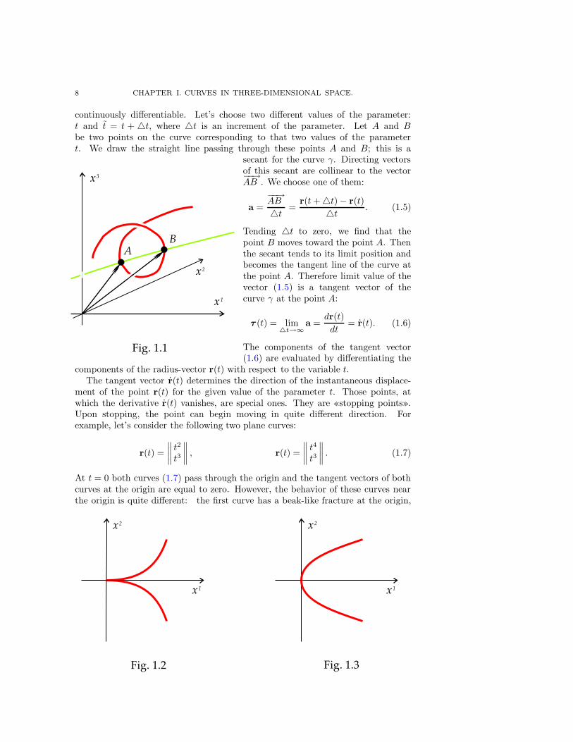
continuously differentiable. Let’s choose two different values of the parameter:t and t = t + 4t, where 4t is an increment of the parameter. Let A and Bbe two points on the curve corresponding to that two values of the parametert. We draw the straight line passing through these points A and B; this is a
secant for the curve γ. Directing vectorsof this secant are collinear to the vector−−→AB . We choose one of them:
a =
−−→AB
4t =r(t+ 4t) − r(t)
4t . (1.5)
Tending 4t to zero, we find that thepoint B moves toward the point A. Thenthe secant tends to its limit position andbecomes the tangent line of the curve atthe point A. Therefore limit value of thevector (1.5) is a tangent vector of thecurve γ at the point A:
τ (t) = lim4t→∞
a =dr(t)
dt= r(t). (1.6)
The components of the tangent vector(1.6) are evaluated by differentiating the
components of the radius-vector r(t) with respect to the variable t.The tangent vector r(t) determines the direction of the instantaneous displace-
ment of the point r(t) for the given value of the parameter t. Those points, atwhich the derivative r(t) vanishes, are special ones. They are «stopping points».Upon stopping, the point can begin moving in quite different direction. Forexample, let’s consider the following two plane curves:
r(t) =
∥
∥
∥
∥
t2
t3
∥
∥
∥
∥
, r(t) =
∥
∥
∥
∥
t4
t3
∥
∥
∥
∥
. (1.7)
At t = 0 both curves (1.7) pass through the origin and the tangent vectors of bothcurves at the origin are equal to zero. However, the behavior of these curves nearthe origin is quite different: the first curve has a beak-like fracture at the origin,
§ 1. CURVES. METHODS OF DEFINING A CURVE . . . 9
while the second one is smooth. Therefore, vanishing of the derivative
τ (t) = r(t) = 0 (1.8)
is only the necessary, but not sufficient condition for a parametric curve to have asingularity at the point r(t). The opposite condition
τ (t) = r(t) 6= 0 (1.9)
guaranties that the point r(t) is free of singularities. Therefore, those points of aparametric curve, where the condition (1.9) is fulfilled, are called regular points.
Let’s study the problem of separating regular and singular points on a curvegiven by a system of equations (1.3). Let A = (a1, a2, a3) be a point of such acurve. The functions F (x1, x2, x3) and G(x1, x2, x3) in (1.3) are assumed to becontinuously differentiable. The matrix
J =
∥
∥
∥
∥
∥
∥
∥
∥
∥
∂F
∂x1
∂F
∂x2
∂F
∂x3
∂G
∂x1
∂G
∂x2
∂G
∂x3
∥
∥
∥
∥
∥
∥
∥
∥
∥
(1.10)
composed of partial derivatives of F and G at the point A is called the Jacobimatrix or the Jacobian of the system of equations (1.3). If the minor
M1 = det
∣
∣
∣
∣
∣
∣
∣
∣
∣
∂F
∂x2
∂F
∂x3
∂G
∂x2
∂G
∂x3
∣
∣
∣
∣
∣
∣
∣
∣
∣
6= 0
in Jacobi matrix is nonzero, the equations (1.3) can be resolved with respect tox2 and x3 in some neighborhood of the point A. Then we have three functionsx1 = t, x2 = x2(t), x3 = x3(t) which determine the parametric representation ofour curve. This fact follows from the theorem on implicit functions (see [2]). Notethat the tangent vector of the curve in this parametrization
τ =
∥
∥
∥
∥
∥
∥
1x2
x3
∥
∥
∥
∥
∥
∥
6= 0
is nonzero because of its first component. This means that the condition M1 6= 0is sufficient for the point A to be a regular point of a curve given by the system ofequations (1.3). Remember that the Jacobi matrix (1.10) has two other minors:
M2 = det
∣
∣
∣
∣
∣
∣
∣
∣
∣
∂F
∂x3
∂F
∂x1
∂G
∂x3
∂G
∂x1
∣
∣
∣
∣
∣
∣
∣
∣
∣
, M3 = det
∣
∣
∣
∣
∣
∣
∣
∣
∣
∂F
∂x1
∂F
∂x2
∂G
∂x1
∂G
∂x2
∣
∣
∣
∣
∣
∣
∣
∣
∣
.
10 CHAPTER I. CURVES IN THREE-DIMENSIONAL SPACE.
For both of them the similar propositions are fulfilled. Therefore, we can formulatethe following theorem.
Theorem 1.1. A curve given by a system of equations (1.3) is regular at allpoints, where the rank of its Jacobi matrix (1.10) is equal to 2.
A plane curve lying on the plane x3 = 0 can be defined by one equationF (x1, x2) = 0. The second equation here reduces to x3 = 0. Therefore,G(x1, x2, x3) = x3. The Jacoby matrix for the system (1.3) in this case is
J =
∥
∥
∥
∥
∥
∥
∂F
∂x1
∂F
∂x20
0 0 1
∥
∥
∥
∥
∥
∥
. (1.11)
If rank J = 2, this means that at least one of two partial derivatives in the matrix(1.11) is nonzero. These derivatives form the gradient vector for the function F :
gradF =
(
∂F
∂x1,∂F
∂x2
)
.
Theorem 1.2. A plane curve given by an equation F (x1, x2) = 0 is regular atall points where gradF 6= 0.
This theorem 1.2 is a simple corollary from the theorem 1.1 and the relationship(1.11). Note that the theorems 1.1 and 1.2 yield only sufficient conditions forregularity of curve points. Therefore, some points where these theorems are notapplicable can also be regular points of a curve.
§ 2. The length integral
and the natural parametrization of a curve.
Let r = r(t) be a parametric curve of smoothness class C1, where the parametert runs over the interval [a, b]. Let’s consider a monotonic increasing continuously
differentiable function ϕ(t) on a segment [a, b] such that ϕ(a) = a and ϕ(b) = b.Then it takes each value from the segment [a, b] exactly once. Substitutingt = ϕ(t ) into r(t), we define the new vector-function r(t) = r(ϕ(t)), it describesthe same curve as the original vector-function r(t). This procedure is called thereparametrization of a curve. We can calculate the tangent vector in the newparametrization by means of the chain rule:
τ (t) = ϕ′(t) · τ (ϕ(t)). (2.1)
Here ϕ′(t) is the derivative of the function ϕ(t). The formula (2.1) is knownas the transformation rule for the tangent vector of a curve under a change ofparametrization.
A monotonic decreasing function ϕ(t ) can also be used for the reparametrization
of curves. In this case ϕ(a) = b and ϕ(b) = a, i. e. the beginning point and theending point of a curve are exchanged. Such reparametrizations are called changingthe orientation of a curve.
From the formula (2.1), we see that the tangent vector τ (t) can vanish at somepoints of the curve due to the derivative ϕ′(t ) even when τ (ϕ(t)) is nonzero.
§ 2. THE LENGTH INTEGRAL . . . 11
Certainly, such points are not actually the singular points of a curve. In orderto exclude such formal singularities, only those reparametrizations of a curveare admitted for which the function ϕ(t) is a strictly monotonic function, i. e.ϕ′(t) > 0 or ϕ′(t) < 0.
The formula (2.1) means that the tangent vector of a curve at its regular pointdepends not only on the geometry of the curve, but also on its parametrization.However, the effect of parametrization is not so big, it can yield a numeric factor tothe vector τ only. Therefore, the natural question arises: is there some preferableparametrization on a curve ? The answer to this question is given by the lengthintegral.
Let’s consider a segment of a parametric curve of the smoothness class C1 withthe parameter t running over the segment [a, b] of real numbers. Let
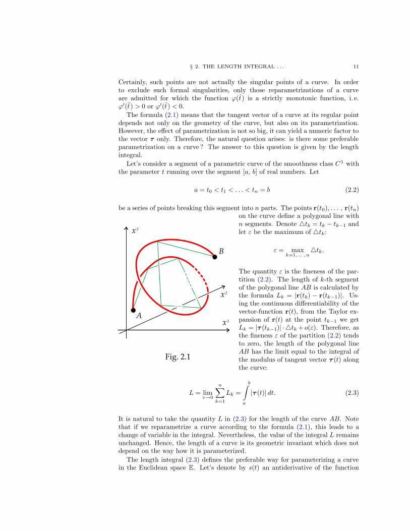
a = t0 < t1 < . . . < tn = b (2.2)
be a series of points breaking this segment into n parts. The points r(t0), . . . , r(tn)on the curve define a polygonal line withn segments. Denote 4tk = tk − tk−1 andlet ε be the maximum of 4tk:
ε = maxk=1, ... , n
4tk.
The quantity ε is the fineness of the par-tition (2.2). The length of k-th segmentof the polygonal line AB is calculated bythe formula Lk = |r(tk) − r(tk−1)|. Us-ing the continuous differentiability of thevector-function r(t), from the Taylor ex-pansion of r(t) at the point tk−1 we getLk = |τ (tk−1)| ·4tk + o(ε). Therefore, asthe fineness ε of the partition (2.2) tendsto zero, the length of the polygonal lineAB has the limit equal to the integral ofthe modulus of tangent vector τ (t) alongthe curve:
L = limε→0
n∑
k=1
Lk =
b∫
a
|τ (t)| dt. (2.3)
It is natural to take the quantity L in (2.3) for the length of the curve AB. Notethat if we reparametrize a curve according to the formula (2.1), this leads to achange of variable in the integral. Nevertheless, the value of the integral L remainsunchanged. Hence, the length of a curve is its geometric invariant which does notdepend on the way how it is parameterized.
The length integral (2.3) defines the preferable way for parameterizing a curvein the Euclidean space E. Let’s denote by s(t) an antiderivative of the function
12 CHAPTER I. CURVES IN THREE-DIMENSIONAL SPACE.
ψ(t) = |τ (t)| being under integration in the formula (2.3):
s(t) =
t∫
t0
|τ (t)| dt. (2.4)
Definition 2.1. The quantity s determined by the integral (2.4) is called thenatural parameter of a curve in the Euclidean space E.
Note that once the reference point r(t0) and some direction (orientation) on acurve have been chosen, the value of natural parameter depends on the point ofthe curve only. Then the change of s for −s means the change of orientation ofthe curve for the opposite one.
Let’s differentiate the integral (2.4) with respect to its upper limit t. As a resultwe obtain the following relationship:
ds
dt= |τ (t)|. (2.5)
Now, using the formula (2.5), we can calculate the tangent vector of a curve in itsnatural parametrization, i. e. when s is used instead of t as a parameter:
dr
ds=dr
dt· dtds
=dr
dt
/
ds
dt=
τ
|τ |. (2.6)
From the formula (2.6), we see that in the tangent vector of a curve in naturalparametrization is a unit vector at all regular points. In singular points this vectoris not defined at all.
§ 3. Frenet frame. The dynamics of Frenet
frame. Curvature and torsion of a spacial curve.
Let’s consider a smooth parametric curve r(s) in natural parametrization. Thecomponents of the radius-vector r(s) for such a curve are smooth functions ofs (smoothness class C∞). They are differentiable unlimitedly many times withrespect to s. The unit vector τ (s) is obtained as the derivative of r(s):
τ (s) =dr
ds. (3.1)
Let’s differentiate the vector τ (s) with respect to s and then apply the followinglemma to its derivative τ
′(s).
Lemma 3.1. The derivative of a vector of a constant length is a vector perpen-dicular to the original one.
Proof. In order to prove the lemma we choose some standard rectangularCartesian coordinate system in E. Then
|τ (s)|2 = (τ (s) | τ (s)) = (τ 1)2 + (τ2)2 + (τ3)2 = const .
§ 3. FRENET FRAME. THE DYNAMICS OF FRENET FRAME . . . 13
Let’s differentiate this expression with respect to s. As a result we get thefollowing relationship:
d
ds
(
|τ (s)|2)
=d
ds
(
(τ1)2 + (τ2)2 + (τ3)2)
=
= 2 τ1 (τ1)′ + 2 τ2 (τ2)′ + 2 τ3 (τ3)′ = 0.
One can easily see that this relationship is equivalent to (τ (s) | τ ′(s)) = 0. Hence,τ (s) ⊥ τ
′(s). The lemma is proved.
Due to the above lemma the vector τ′(s) is perpendicular to the unit vector
τ (s). If the length of τ′(s) is nonzero, one can represent it as
τ′(s) = k(s) · n(s), (3.2)
where k(s) = |τ ′(s)| and |n(s)| = 1. The scalar quantity k(s) = |τ ′(s)| in formula(3.2) is called the curvature of a curve, while the unit vector n(s) is called itsprimary normal vector or simply the normal vector of a curve at the point r(s).The unit vectors τ (s) and n(s) are orthogonal to each other. We can complementthem by the third unit vector b(s) so that τ , n, b become a right triple1:
b(s) = [τ (s), n(s)]. (3.3)
The vector b(s) defined by the formula (3.3) is called the secondary normalvector or the binormal vector of a curve. Vectors τ (s), n(s), b(s) compose anorthonormal right basis attached to the point r(s).
Bases, which are attached to some points, are usually called frames. One shoulddistinguish frames from coordinate systems. Cartesian coordinate systems are alsodefined by choosing some point (an origin) and some basis. However, coordinatesystems are used for describing the points of the space through their coordinates.The purpose of frames is different. They are used for to expand the vectors which,by their nature, are attached to the same points as the vectors of the frame.
The isolated frames are rarely considered, frames usually arise within familiesof frames: typically at each point of some set (a curve, a surface, or even the wholespace) there arises some frame attached to this point. The frame τ (s), n(s), b(s)is an example of such frame. It is called the Frenet frame of a curve. This is themoving frame: in typical situation the vectors of this frame change when we movethe attachment point along the curve.
Let’s consider the derivative n′(s). This vector attached to the point r(s) canbe expanded in the Frenet frame at that point. Due to the lemma 3.1 the vectorn′(s) is orthogonal to the vector n(s). Therefore its expansion has the form
n′(s) = α · τ (s) + κ · b(s). (3.4)
The quantity α in formula (3.4) can be expressed through the curvature of the
1 A non-coplanar ordered triple of vectors a1, a2, a3 is called a right triple if, upon moving
these vectors to a common origin, when looking from the end of the third vector a3, we see theshortest rotation from a1 to a2 as a counterclockwise rotation.
14 CHAPTER I. CURVES IN THREE-DIMENSIONAL SPACE.
curve. Indeed, as a result of the following calculations we derive
α(s) = (τ (s) |n′(s)) = (τ (s) |n(s))′−− (τ ′(s) |n(s)) = −(k(s) ·n(s) |n(s)) = −k(s). (3.5)
The quantity κ = κ(s) cannot be expressed through the curvature. This is anadditional parameter characterizing a curve in the space E. It is called the torsionof the curve at the point r = r(s). The above expansion (3.4) of the vector n′(s)now is written in the following form:
n′(s) = −k(s) · τ (s) + κ(s) ·b(s). (3.6)
Let’s consider the derivative of the binormal vector b′(s). It is perpendicularto b(s). This derivative can also be expanded in the Frenet frame. Due tob′(s) ⊥ b(s) we have b′(s) = β · n(s) + γ · τ (s). The coefficients β and γ in thisexpansion can be found by means of the calculations similar to (3.5):
β(s) = (n(s) |b′(s)) = (n(s) |b(s))′ − (n′(s) |b(s)) =
= −(−k(s) · τ (s) + κ(s) · b(s) |b(s)) = −κ(s).
γ(s) = (τ (s) |b′(s)) = (τ (s) |b(s))′ − (τ ′(s) |b(s)) =
= −(k(s) · n(s) |b(s)) = 0.
Hence, for the expansion of the vector b′(s) in the Frenet frame we get
b′(s) = −κ(s) ·n(s). (3.7)
Let’s gather the equations (3.2), (3.6), and (3.7) into a system:
τ′(s) = k(s) · n(s),
n′(s) = −k(s) · τ (s) + κ(s) ·b(s),
b′(s) = −κ(s) · n(s).
(3.8)
The equations (3.8) relate the vectors τ (s), n(s), b(s) and their derivatives withrespect to s. These differential equations describe the dynamics of the Frenetframe. They are called the Frenet equations. The equations (3.8) should becomplemented with the equation (3.1) which describes the dynamics of the pointr(s) (the point to which the vectors of the Frenet frame are attached).
§ 4. The curvature center and the curvature radius
of a spacial curve. The evolute and the evolvent of a curve.
In the case of a planar curve the vectors τ (s) and n(s) lie in the same plane asthe curve itself. Therefore, binormal vector (3.3) in this case coincides with theunit normal vector of the plane. Its derivative b′(s) is equal to zero. Hence, dueto the third Frenet equation (3.7) we find that for a planar curve κ(s) ≡ 0. TheFrenet equations (3.8) then are reduced to
τ′(s) = k(s) · n(s),
n′(s) = −k(s) · τ (s).(4.1)
CopyRight c© Sharipov R.A., 1996, 2004.
§ 4. THE CURVATURE CENTER AND THE CURVATURE RADIUS . . . 15
Let’s consider the circle of the radius R with the center at the origin lying in thecoordinate plane x3 = 0. It is convenient to define this circle as follows:
r(s) =
∥
∥
∥
∥
R cos(s/R)R sin(s/R)
∥
∥
∥
∥
, (4.2)
here s is the natural parameter. Substituting (4.2) into (3.1) and then into (3.2),we find the unit tangent vector τ (s) and the primary normal vector n(s):
τ (s) =
∥
∥
∥
∥
− sin(s/R)cos(s/R)
∥
∥
∥
∥
, n(s) =
∥
∥
∥
∥
− cos(s/R)− sin(s/R)
∥
∥
∥
∥
. (4.3)
Now, substituting (4.3) into the formula (4.1), we calculate the curvature of acircle k(s) = 1/R = const. The curvature k of a circle is constant, the inversecurvature 1/k coincides with its radius.
Let’s make a step from the point r(s) on a circle to the distance 1/k in thedirection of its primary normal vector n(s). It is easy to see that we come to thecenter of a circle. Let’s make the same step for an arbitrary spacial curve. As aresult of this step we come from the initial point r(s) on the curve to the pointwith the following radius-vector:
ρ(s) = r(s) +n(s)
k(s). (4.4)
Certainly, this can be done only for that points of a curve, where k(s) 6= 0. Theanalogy with a circle induces the following terminology: the quantity R(s) =1/k(s) is called the curvature radius, the point with the radius-vector (4.4) iscalled the curvature center of a curve at the point r(s).
In the case of an arbitrary curve its curvature center is not a fixed point. Whenparameter s is varied, the curvature center of the curve moves in the space drawinganother curve, which is called the evolute of the original curve. The formula (4.4)is a vectorial-parametric equation of the evolute. However, note that the naturalparameter s of the original curve is not a natural parameter for its evolute.
Suppose that some spacial curve r(t) is given. A curve r(s) whose evolute ρ(s)coincides with the curve r(t) is called an evolvent of the curve r(t). The problemof constructing the evolute of a given curve is solved by the formula (4.4). Theinverse problem of constructing an evolvent for a given curve appears to be morecomplicated. It is effectively solved only in the case of a planar curve.
Let r(s) be a vector-function defining some planar curve in natural parametri-zation and let r(s) be the evolvent in its own natural parametrization. Twonatural parameters s and s are related to each other by some function ϕ in formof the relationship s = ϕ(s). Let ψ = ϕ−1 be the inverse function for ϕ, thens = ψ(s). Using the formula (4.4), now we obtain
r(ψ(s)) = r(s) +n(s)
k(s). (4.5)
Let’s differentiate the relationship (4.5) with respect to s and then let’s apply theformula (3.1) and the Frenet equations written in form of (4.1):
ψ′(s) · τ (ψ(s)) =d
ds
(
1
k(s)
)
· n(s).
16 CHAPTER I. CURVES IN THREE-DIMENSIONAL SPACE.
Here τ (ψ(s)) and n(s) both are unit vectors which are collinear due to the aboverelationship. Hence, we have the following two equalities:
n(s) = ±τ (ψ(s)), ψ′(s) = ± d
ds
(
1
k(s)
)
. (4.6)
The second equality (4.6) can be integrated:
1
k(s)= ±(ψ(s) − C). (4.7)
Here C is a constant of integration. Let’s combine (4.7) with the first relationship(4.6) and substitute it into the formula (4.5):
r(s) = r(ψ(s)) + (C − ψ(s)) · τ (ψ(s)).
Then we substitute s = ϕ(s) into the above formula and denote ρ(s) = r(ϕ(s)).As a result we obtain the following equality:
ρ(s) = r(s) + (C − s) · τ (s). (4.8)
The formula (4.8) is a parametric equation for the evolvent of a planar curve r(s).The entry of an arbitrary constant in the equation (4.8) means the evolvent is notunique. Each curve has the family of evolvents. This fact is valid for non-planarcurves either. However, we should emphasize that the formula (4.8) cannot beapplied to general spacial curves.
§ 5. Curves as trajectories of material points in mechanics.
The presentation of classical mechanics traditionally begins with consideringthe motion of material points. Saying material point, we understand any materialobject whose sizes are much smaller than its displacement in the space. Theposition of such an object can be characterized by its radius-vector in someCartesian coordinate system, while its motion is described by a vector-functionr(t). The curve r(t) is called the trajectory of a material point. Unlike to purelygeometric curves, the trajectories of material points possess preferable parameter t,which is usually distinct from the natural parameter s. This preferable parameteris the time variable t.
The tangent vector of a trajectory, when computed in the time parametrization,is called the velocity of a material point:
v(t) =dr
dt= r(t) =
∥
∥
∥
∥
∥
∥
v1(t)v2(t)v3(t)
∥
∥
∥
∥
∥
∥
. (5.1)
The time derivative of the velocity vector is called the acceleration vector:
a(t) =dv
dt= v(t) =
∥
∥
∥
∥
∥
∥
a1(t)a2(t)a3(t)
∥
∥
∥
∥
∥
∥
. (5.2)
§ 5. CURVES AS TRAJECTORIES OF MATERIAL POINTS . . . 17
The motion of a material point in mechanics is described by Newton’s second law:
m a = F(r,v). (5.3)
Here m is the mass of a material point. This is a constant characterizing theamount of matter enclosed in this material object. The vector F is the forcevector. By means of the force vector in mechanics one describes the action ofambient objects (which are sometimes very far apart) upon the material pointunder consideration. The magnitude of this action usually depends on the positionof a point relative to the ambient objects, but sometimes it can also depend onthe velocity of the point itself. Newton’s second law in form of (5.3) shows thatthe external action immediately affects the acceleration of a material point, butneither the velocity nor the coordinates of a point.
Let s = s(t) be the natural parameter on the trajectory of a material pointexpressed through the time variable. Then the formula (2.5) yields
s(t) = |v(t)| = v(t). (5.4)
Through v(t) in (5.4) we denote the modulus of the velocity vector.Let’s consider a trajectory of a material point in natural parametrization:
r = r(s). Then for the velocity vector (5.1) and for the acceleration vector (5.2)we get the following expressions:
v(t) = s(t) · τ (s(t)),
a(t) = s(t) · τ (s(t)) + (s(t))2 · τ ′(s(t)).
Taking into account the formula (5.4) and the first Frenet equation, these expres-sions can be rewritten as
v(t) = v(t) · τ (s(t)),
a(t) = v(t) · τ (s(t)) +(
k(s(t)) v(t)2)
· n(s(t)).(5.5)
The second formula (5.5) determines the expansion of the acceleration vector intotwo components. The first component is tangent to the trajectory, it is called thetangential acceleration. The second component is perpendicular to the trajectoryand directed toward the curvature center. It is called the centripetal acceleration.It is important to note that the centripetal acceleration is determined by themodulus of the velocity and by the geometry of the trajectory (by its curvature).
CHAPTER II
ELEMENTS OF VECTORIAL AND TENSORIAL ANALYSIS.
§ 1. Vectorial and tensorial fields in the space.
Let again E be a three-dimensional Euclidean point space. We say that inE a vectorial field is given if at each point of the space E some vector attachedto this point is given. Let’s choose some Cartesian coordinate system in E; ingeneral, this system is skew-angular. Then we can define the points of the spaceby their coordinates x1, x2, x3, and, simultaneously, we get the basis e1, e2, e3 forexpanding the vectors attached to these points. In this case we can present anyvector field F by three numeric functions
F =
∥
∥
∥
∥
∥
∥
F 1(x)F 2(x)F 3(x)
∥
∥
∥
∥
∥
∥
, (1.1)
where x = (x1, x2, x3) are the components of the radius-vector of an arbitrarypoint of the space E. Writing F(x) instead of F(x1, x2, x3), we make all formulasmore compact.
The vectorial nature of the field F reveals when we replace one coordinatesystem by another. Let (1.1) be the coordinates of a vector field in some
coordinate system O, e1, e2, e3 and let O, e1, e2, e3 be some other coordinatesystem. The transformation rule for the components of a vectorial field under achange of a Cartesian coordinate system is written as follows:
F i(x) =
3∑
j=1
Sij F
j(x),
xi =
3∑
j=1
Sij x
j + ai.
(1.2)
Here Sij are the components of the transition matrix relating the basis e1, e2, e3
with the new basis e1, e2, e3, while a1, a2, a3 are the components of the vector−−→OO in the basis e1, e2, e3.
The formula (1.2) combines the transformation rule for the components of avector under a change of a basis and the transformation rule for the coordinates ofa point under a change of a Cartesian coordinate system (see [1]). The arguments
x and x beside the vector components F i and F i in (1.2) is an important noveltyas compared to [1]. It is due to the fact that here we deal with vector fields, notwith separate vectors.
Not only vectors can be associated with the points of the space E. In linearalgebra along with vectors one considers covectors, linear operators, bilinear forms
§ 1. VECTORIAL AND TENSORIAL FIELDS IN THE SPACE. 19
and quadratic forms. Associating some covector with each point of E, we get acovector field. If we associate some linear operator with each point of the space,we get an operator field. An finally, associating a bilinear (quadratic) form witheach point of E, we obtain a field of bilinear (quadratic) forms. Any choice of aCartesian coordinate system O, e1, e2, e3 assumes the choice of a basis e1, e2, e3,while the basis defines the numeric representations for all of the above objects:for a covector this is the list of its components, for linear operators, bilinearand quadratic forms these are their matrices. Therefore defining a covector fieldF is equivalent to defining three functions F1(x), F2(x), F3(x) that transformaccording to the following rule under a change of a coordinate system:
Fi(x) =
3∑
j=1
T ji Fj(x),
xi =
3∑
j=1
Sij x
j + ai.
(1.3)
In the case of operator field F the transformation formula for the components ofits matrix under a change of a coordinate system has the following form:
F ij (x) =
3∑
p=1
3∑
q=1
Sip T
qj F p
q (x),
xi =
3∑
p=1
Sip x
p + ai.
(1.4)
For a field of bilinear (quadratic) forms F the transformation rule for its compo-nents under a change of Cartesian coordinates looks like
Fij(x) =
3∑
p=1
3∑
q=1
T pi T
qj Fp q(x),
xi =
3∑
p=1
Sip x
p + ai.
(1.5)
Each of the relationships (1.2), (1.3), (1.4), and (1.5) consists of two formulas.The first formula relates the components of a field, which are the functions oftwo different sets of arguments x = (x1, x2, x3) and x = (x1, x2, x3). The secondformula establishes the functional dependence of these two sets of arguments.
The first formulas in (1.2), (1.3), and (1.4) are different. However, one can seesome regular pattern in them. The number of summation signs and the numberof summation indices in their right hand sides are determined by the number ofindices in the components of a field F. The total number of transition matricesused in the right hand sides of these formulas is also determined by the number ofindices in the components of F. Thus, each upper index of F implies the usage ofthe transition matrix S, while each lower index of F means that the inverse matrixT = S−1 is used.
20 CHAPTER II. ELEMENTS OF TENSORIAL ANALYSIS.
The number of indices of the field F in the above examples doesn’t exceedtwo. However, the regular pattern detected in the transformation rules for thecomponents of F can be generalized for the case of an arbitrary number of indices:
F i1...ir
j1...js=∑
p1...pr
q1...qs
Si1p1. . . Sir
prT q1
j1. . . T qs
jsF p1...pr
q1 ...qs(1.6)
The formula (1.6) comprises the multiple summation with respect to (r+s) indicesp1, . . . , pr and q1, . . . , qs each of which runs from 1 to 3.
Definition 1.1. A tensor of the type (r, s) is a geometric object F whosecomponents in each basis are enumerated by (r+ s) indices and obey the transfor-mation rule (1.6) under a change of basis.
Lower indices in the components of a tensor are called covariant indices, upperindices are called contravariant indices respectively. Generalizing the concept ofa vector field, we can attach some tensor of the type (r, s), to each point of thespace. As a result we get the concept of a tensor field. This concept is convenientbecause it describes in the unified way any vectorial and covectorial fields, operatorfields, and arbitrary fields of bilinear (quadratic) forms. Vectorial fields are fieldsof the type (1, 0), covectorial fields have the type (0, 1), operator fields are of thetype (1, 1), and finally, any field of bilinear (quadratic) forms are of the type (0, 2).Tensor fields of some other types are also meaningful. In Chapter IV we considerthe curvature field with four indices.
Passing from separate tensors to tensor fields, we acquire the arguments in for-mula (1.6). Now this formula should be written as the couple of two relationshipssimilar to (1.2), (1.3), (1.4), or (1.5):
F i1... ir
j1... js(x) =
∑
p1 ... pr
q1 ... qs
Si1p1. . . Sir
prT q1
j1. . . T qs
jsF p1... pr
q1... qs(x),
xi =3∑
j=1
Sij x
j + ai.
(1.7)
The formula (1.7) expresses the transformation rule for the components of atensorial field of the type (r, s) under a change of Cartesian coordinates.
The most simple type of tensorial fields is the type (0, 0). Such fields arecalled scalar fields. Their components have no indices at all, i. e. they are numericfunctions in the space E.
§ 2. Tensor product and contraction.
Let’s consider two covectorial fields a and b. In some Cartesian coordinatesystem they are given by their components ai(x) and bj(x). These are two sets offunctions with three functions in each set. Let’s form a new set of nine functionsby multiplying the functions of initial sets:
cij(x) = ai(x) bj(x). (2.1)
Applying the formula (1.3) we can express the right hand side of (2.1) through thecomponents of the fields a and b in the other coordinate system:
cij(x) =
(
3∑
p=1
T pi ap
)(
3∑
q=1
T qj bq
)
=
3∑
p=1
3∑
q=1
T pi T
qj (ap bq).
§ 2. TENSOR PRODUCT AND CONTRACTION. 21
If we denote by cpq(x) the product of ai(x) and bj(x), then we find that the quan-tities cij(x) and cpq(x) are related by the formula (1.5). This means that takingtwo covectorial fields one can compose a field of bilinear forms by multiplying thecomponents of these two covectorial fields in an arbitrary Cartesian coordinatesystem. This operation is called the tensor product of the fields a and b. Its resultis denoted as c = a⊗ b.
The above trick of multiplying components can be applied to an arbitrary pairof tensor fields. Suppose we have a tensorial field A of the type (r, s) and anothertensorial field B of the type (m,n). Denote
Ci1... irir+1... ir+m
j1... jsjs+1... js+n(x) = Ai1... ir
j1... js(x) B
ir+1 ... ir+m
js+1 ... js+n(x). (2.2)
Definition 2.1. The tensor field C of the type (r+m, s+n) whose componentsare determined by the formula (2.2) is called the tensor product of the fields A
and B. It is denoted C = A⊗ B.
This definition should be checked for correctness. We should make sure thatthe components of the field C are transformed according to the rule (1.7) when wepass from one Cartesian coordinate system to another. The transformation rule(1.7), when applied to the fields A and B, yields
Ai1... ir
j1... js=∑
p..q
Si1p1. . . Sir
prT q1
j1. . . T qs
jsAp1 ... pr
q1 ... qs,
Bir+1... ir+m
js+1... js+n=∑
p..q
Sir+1pr+1
. . . Sir+m
pr+mT
qs+1
js+1. . . T
qs+n
js+nBpr+1 ... pr+m
qs+1 ... qs+n.
The summation in right hand sides of this formulas is carried out with respectto each double index which enters the formula twice — once as an upper indexand once as a lower index. Multiplying these two formulas, we get exactly thetransformation rule (1.7) for the components of C.
Theorem 2.1. The operation of tensor product is associative, this means that(A⊗ B) ⊗ C = A ⊗ (B ⊗C).
Proof. Let A be a tensor of the type (r, s), let B be a tensor of the type(m,n), and let C be a tensor of the type (p, q). Then one can write the followingobvious numeric equality for their components:
(
Ai1... ir
j1... jsB
ir+1... ir+m
js+1... js+n
)
Cir+m+1... ir+m+p
js+n+1 ... js+n+q=
(2.3)
= Ai1... ir
j1... js
(
Bir+1... ir+m
js+1... js+nC
ir+m+1 ... ir+m+p
js+n+1... js+n+q
)
.
As we see in (2.3), the associativity of the tensor product follows from theassociativity of the multiplication of numbers.
The tensor product is not commutative. One can easily construct an exampleillustrating this fact. Let’s consider two covectorial fields a and b with thefollowing components in some coordinate system: a = (1, 0, 0) and b = (0, 1, 0).Denote c = a⊗b and d = b⊗ a. Then for c12 and d12 with the use of the formula(2.2) we derive: c12 = 1 and d12 = 0. Hence, c 6= d and a⊗ b 6= b⊗ a.
CopyRight c© Sharipov R.A., 1996, 2004.
22 CHAPTER II. ELEMENTS OF TENSORIAL ANALYSIS.
Let’s consider an operator field F. Its components F ij (x) are the components of
the operator F(x) in the basis e1, e2, e3. It is known that the trace of the matrixF i
j (x) is a scalar invariant of the operator F(x) (see [1]). Therefore, the formula
f(x) = tr F(x) =
3∑
i=1
F ii (x) (2.4)
determines a scalar field f(x) in the space E. The sum similar to (2.4) can bewritten for an arbitrary tensorial field F with at least one upper index and at leastone lower index in its components:
Hi1... ir−1
j1... js−1(x) =
3∑
k=1
Fi1... im−1 k im ... ir−1
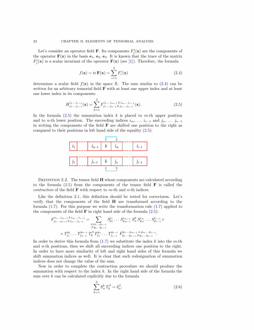
j1... jn−1 k jn... js−1(x). (2.5)
In the formula (2.5) the summation index k is placed to m-th upper positionand to n-th lower position. The succeeding indices im, . . . ir−1 and jn, . . . js−1
in writing the components of the field F are shifted one position to the right ascompared to their positions in left hand side of the equality (2.5):
Definition 2.2. The tensor field H whose components are calculated accordingto the formula (2.5) from the components of the tensor field F is called thecontraction of the field F with respect to m-th and n-th indices.
Like the definition 2.1, this definition should be tested for correctness. Let’sverify that the components of the field H are transformed according to theformula (1.7). For this purpose we write the transformation rule (1.7) applied tothe components of the field F in right hand side of the formula (2.5):
Fi1... im−1 k im... ir−1
j1... jn−1 k jn... js−1=
∑
α p1 ...pr−1
β q1...qs−1
Si1p1. . . Sim−1
pm−1Sk
α Sim
pm. . . Sir−1
pr−1×
× T q1
j1. . . T
qn−1
jn−1T β
k Tqn
jn. . . T
qs−1
js−1F
p1... pm−1 α pm... pr−1
q1... qn−1 β qn... qs−1.
In order to derive this formula from (1.7) we substitute the index k into the m-thand n-th positions, then we shift all succeeding indices one position to the right.In order to have more similarity of left and right hand sides of this formula weshift summation indices as well. It is clear that such redesignation of summationindices does not change the value of the sum.
Now in order to complete the contraction procedure we should produce thesummation with respect to the index k. In the right hand side of the formula thesum over k can be calculated explicitly due to the formula
3∑
k=1
Skα T
βk = δβ
α, (2.6)
§ 2. TENSOR PRODUCT AND CONTRACTION. 23
which means T = S−1. Due to (2.6) upon calculating the sum over k one cancalculate the sums over β and α. Therein we take into account that
3∑
α=1
F p1... pm−1 α pm... pr−1q1... qn−1 α qn ... qs−1
= Hp1... pr−1q1... qs−1
.
As a result we get the equality
Hi1... ir−1
j1... js−1=
∑
p1...pr−1q1...qs−1
Si1p1. . . Sir−1
pr−1T q1
j1. . . T
qs−1
js−1Hp1 ... pr−1
q1... qs−1,
which exactly coincides with the transformation rule (1.7) written with respect tocomponents of the field H. The correctness of the definition 2.2 is proved.
The operation of contraction introduced by the definition 2.2 implies that thepositions of two indices are specified. One of these indices should be an upperindex, the other index should be a lower index. The letter C is used as acontraction sign. The formula (2.5) then is abbreviated as follows:
H = Cm,n(F) = C(F).
The numbers m and n are often omitted since they are usually known from thecontext.
A tensorial field of the type (1, 1) can be contracted in the unique way. For atensorial field F of the type (2, 2) we have two ways of contracting. As a resultof these two contractions, in general, we obtain two different tensorial fields of thetype (1, 1). These tensorial fields can be contracted again. As a result we obtainthe complete contractions of the field F, they are scalar fields. A field of the type(2, 2) can have two complete contractions. In general case a field of the type (n, n)has n! complete contractions.
The operations of tensor product and contraction often arise in a natural waywithout any special intension. For example, suppose that we are given a vectorfield v and a covector field w in the space E. This means that at each point wehave a vector and a covector attached to this point. By calculating the scalarproducts of these vectors and covectors we get a scalar field f = 〈w |v〉. Incoordinate form such a scalar field is calculated by means of the formula
f =
3∑
k=1
wi vi. (2.7)
From the formula (2.7), it is clear that f = C(w ⊗ v). The scalar productf = 〈w |v〉 is the contraction of the tensor product of the fields w and v. In asimilar way, if an operator field F and a vector field v are given, then applying F
to v we get another vector field u = Fv, where
ui =
3∑
j=1
F ij v
j .
In this case we can write: u = C(F⊗ v); although this writing cannot be uniquelyinterpreted. Apart from u = Fv, it can mean the product of v by the trace of theoperator field F.
24 CHAPTER II. ELEMENTS OF TENSORIAL ANALYSIS.
§ 3. The algebra of tensor fields.
Let v and w be two vectorial fields. Then at each point of the space E we havetwo vectors v(x) and w(x). We can add them. As a result we get a new vectorfield u = v + w. In a similar way one can define the addition of tensor fields. LetA and B be two tensor fields of the type (r, s). Let’s consider the sum of theircomponents in some Cartesian coordinate system:
C i1... ir
j1... js= Ai1... ir
j1... js+Bi1 ... ir
j1... js. (3.1)
Definition 3.1. The tensor field C of the type (r, s) whose components arecalculated according to the formula (3.1) is called the sum of the fields A and B
of the type (r, s).
One can easily check up the transformation rule (1.7) for the components of thefield C. It is sufficient to write this rule (1.7) for the components of A and B thenadd these two formulas. Therefore, the definition 3.1 is consistent.
The sum of tensor fields is commutative and associative. This fact followsfrom the commutativity and associativity of the addition of numbers due to thefollowing obvious relationships:
Ai1... ir
j1... js+ Bi1... ir
j1... js= Bi1... ir
j1... js+ Ai1... ir
j1... js,
(
Ai1... ir
j1... js+ Bi1... ir
j1... js
)
+ C i1... ir
j1... js= Ai1... ir
j1... js+(
Bi1 ... ir
j1 ... js+ C i1... ir
j1... js
)
.
Let’s denote by T(r,s) the set of tensor fields of the type (r, s). The tensormultiplication introduced by the definition 2.1 is the following binary operation:
T(r, s) × T(m, n) → T(r+m, s+n). (3.2)
The operations of tensor addition and tensor multiplication (3.2) are related toeach other by the distributivity laws:
(A + B) ⊗ C = A⊗ C + B⊗ C,
C ⊗ (A + B) = C ⊗A + C ⊗B.(3.3)
The distributivity laws (3.3) follow from the distributivity of the multiplication ofnumbers. Their proof is given by the following obvious formulas:
(
Ai1 ... ir
j1... js+Bi1 ... ir
j1 ... js
)
Cir+1... ir+m
js+1... js+n=
= Ai1... ir
j1... jsC
ir+1... ir+m
js+1... js+n+Bi1 ... ir
j1 ... jsC
ir+1... ir+m
js+1... js+n,
C i1... ir
j1... js
(
Air+1... ir+m
js+1 ... js+n+ B
ir+1... ir+m
js+1... js+n
)
=
= C i1... ir
j1... jsA
ir+1... ir+m
js+1... js+n+ C i1... ir
j1... jsB
ir+1 ... ir+m
js+1 ... js+n.
Due to (3.2) the set of scalar fields K = T(0,0) (which is simply the setof numeric functions) is closed with respect to tensor multiplication ⊗, whichcoincides here with the regular multiplication of numeric functions. The set K is
§ 3. THE ALGEBRA OF TENSOR FIELDS. 25
a commutative ring (see [3]) with the unity. The constant function equal to 1 ateach point of the space E plays the role of the unit element in this ring.
Let’s set m = n = 0 in the formula (3.2). In this case it describes themultiplication of tensor fields from T(r,s) by numeric functions from the ringK. The tensor product of a field A and a scalar filed ξ ∈ K is commutative:A⊗ ξ = ξ ⊗A. Therefore, the multiplication of tensor fields by numeric functionsis denoted by standard sign of multiplication: ξ ⊗ A = ξ · A. The operation ofaddition and the operation of multiplication by scalar fields in the set T(r,s) possessthe following properties:
(1) A + B = B + A;(2) (A + B) + C = A + (B + C);(3) there exists a field 0 ∈ T(r,s) such that A + 0 = A for an arbitrary tensor
field A ∈ T(r,s);(4) for any tensor field A ∈ T(r,s) there exists an opposite field A′ such that
A + A′ = 0;(5) ξ · (A + B) = ξ ·A + ξ ·B for any function ξ from the ring K and for any
two fields A,B ∈ T(r,s);(6) (ξ + ζ) ·A = ξ · A + ζ ·A for any tensor field A ∈ T(r,s) and for any two
functions ξ, ζ ∈ K;(7) (ξ ζ) ·A = ξ ·(ζ ·A) for any tensor field A ∈ T(r,s) and for any two functions
ξ, ζ ∈ K;(8) 1 ·A = A for any field A ∈ T(r,s).
The tensor field with identically zero components plays the role of zero elementin the property (3). The field A′ in the property (4) is defined as a field whosecomponents are obtained from the components of A by changing the sign.
The properties (1)-(8) listed above almost literally coincide with the axioms ofa linear vector space (see [1]). The only discrepancy is that the set of functions Kis a ring, not a numeric field as it should be in the case of a linear vector space.The sets defined by the axioms (1)-(8) for some ring K are called modules overthe ring K or K-modules. Thus, each of the sets T(r,s) is a module over the ring ofscalar functions K = T(0,0).
The ring K = T(0,0) comprises the subset of constant functions which isnaturally identified with the set of real numbers R. Therefore the set of tensorfields T(r,s) in the space E is a linear vector space over the field of real numbers R.
If r > 1 and s > 1, then in the set T(r,s) the operation of contraction withrespect to various pairs of indices are defined. These operations are linear, i. e. thefollowing relationships are fulfilled:
C(A + B) = C(A) + C(B),
C(ξ ·A) = ξ · C(A).(3.4)
The relationships (3.4) are proved by direct calculations in coordinates. For thefield C = A + B from (2.5) we derive
Hi1... ir−1
j1... js−1=
3∑
k=1
Ci1... im−1 k im... ir−1
j1... jn−1 k jn... js−1=
=
3∑
k=1
Ai1... im−1 k im... ir−1
j1... jn−1 k jn ... js−1+
3∑
k=1
Bi1 ... im−1 k im... ir−1
j1 ... jn−1 k jn ... js−1.
26 CHAPTER II. ELEMENTS OF TENSORIAL ANALYSIS.
This equality proves the first relationship (3.4). In order to prove the second onewe take C = ξ ·A. Then the second relationship (3.4) is derived as a result of thefollowing calculations:
Hi1... ir−1
j1... js−1=
3∑
k=1
Ci1... im−1 k im... ir−1
j1... jn−1 k jn... js−1=
=
3∑
k=1
ξ Ai1... im−1 k im ... ir−1
j1... jn−1 k jn... js−1= ξ
3∑
k=1
Ai1... im−1 k im... ir−1
j1... jn−1 k jn ... js−1.
The tensor product of two tensors from T(r,s) belongs to T(r,s) only if r = s = 0(see formula (3.2)). In all other cases one cannot perform the tensor multiplicationstaying within one K-module T(r,s). In order to avoid this restriction the followingdirect sum is usually considered:
T =
∞⊕
r=0
∞⊕
s=0
T(r,s). (3.5)
The set (3.5) consists of finite formal sums A(1) + . . .+A(k), where each summandbelongs to some of the K-modules T(r,s). The operation of tensor product isextended to the K-module T by means of the formula:
(A(1) + . . .+ A(k)) ⊗ (A(1) + . . .+ A(q)) =
k∑
i=1
q∑
j=1
A(i) ⊗A(j).
This extension of the operation of tensor product is a bilinear binary operation inthe set T . It possesses the following additional properties:
(9) (A + B) ⊗ C = A⊗ C + B⊗ C;(10) (ξ ·A) ⊗C = ξ · (A ⊗C);(11) C ⊗ (A + B) = C ⊗A + C ⊗B;(12) C ⊗ (ξ ·B) = ξ · (C ⊗B).
These properties of the operation of tensor product in T are easily derived from(3.3). Note that a K-module equipped with an additional bilinear binary operationof multiplication is called an algebra over the ring K or a K-algebra. Thereforethe set T is called the algebra of tensor fields.
The algebra T is a direct sum of separate K-modules T(r,s) in (3.5). Theoperation of multiplication is concordant with this expansion into a direct sum;this fact is expressed by the relationship (3.2). Such structures in algebras arecalled gradings, while algebras with gradings are called graded algebras.
§ 4. Symmetrization and alternation.
Let A be a tensor filed of the type (r, s) and let r > 2. The number of upperindices in the components of the field A is greater than two. Therefore, we canperform the permutation of some pair of them. Let’s denote
Bi1 ... im... in... ir
j1 ..................js= Ai1 ... in... im ... ir
j1 ..................js. (4.1)
The quantities Bi1 ... ir
j1 ... jsin (4.1) are produced from the components of the tensor
field A by the transposition of the pair of upper indices im and in.
§ 4. SYMMETRIZATION AND ALTERNATION. 27
Theorem 4.1. The quantities B i1 ... ir
j1 ... jsproduced from the components of a ten-
sor field A by the transposition of any pair of upper indices define another tensorfield B of the same type as the original field A.
Proof. In order to prove the theorem let’s check up that the quantities (4.1)obey the transformation rule (1.7) under a change of a coordinate system:
Bi1 ... ir
j1 ... js=∑
p1...pr
q1 ...qs
Si1p1. . . Sin
pm. . . Sim
pn. . . Sir
prT q1
j1. . . T qs
jsAp1... pr
q1... qs.
Let’s rename the summation indices pm and pn in this formula: let’s denote pm
by pn and vice versa. As a result the S matrices will be arranged in the orderof increasing numbers of their upper and lower indices. However, the indices pm
and pn in Ap1... pr
q1... qswill exchange their positions. It is clear that the procedure of
renaming summation indices does not change the value of the sum:
Bi1... ir
j1... js=∑
p1...pr
q1...qs
Si1p1. . . Sir
prT q1
j1. . . T qs
jsAp1 ... pn ... pm ... pr
q1 ... qs.
Due to the equality Bp1 ... pr
q1 ... qs= Ap1 ... pn... pm... pr
q1 .................. qsthe above formula is exactly the
transformation rule (1.7) written for the quantities (4.1). Hence, they define atensor field B. The theorem is proved.
There is a similar theorem for transpositions of lower indices. Let again A be atensor field of the type (r, s) and let s > 2. Denote
Bi1 .................. ir
j1 ... jm... jn ... js= Ai1 .................. ir
j1 ... jn ... jm... js. (4.2)
Theorem 4.2. The quantities B i1 ... ir
j1 ... jsproduced from the components of a ten-
sor field A by the transposition of any pair of lower indices define another tensorfield B of the same type as the original field A.
The proof of the theorem 4.2 is completely analogous to the proof of thetheorem 4.1. Therefore we do not give it here. Note that one cannot transposean upper index and a lower index. The set of quantities obtained by such atransposition does not obey the transformation rule (1.7).
Combining various pairwise transpositions of indices (4.1) and (4.2) we canget any transposition from the symmetric group Sr in upper indices and anytransposition from the symmetric group Ss in lower indices. This is a well-knownfact from the algebra (see [3]). Thus the theorems 4.1 and 4.2 define the action ofthe groups Sr and Ss on the K-module T(r,s) composed of the tensor fields of thetype (r, s). This is the action by linear operators, i. e.
σ τ (A + B) = σ τ (A) + σ τ (B),
σ τ (ξ ·A) = ξ · (σ τ (A))(4.3)
for any two transpositions σ ∈ Sr and τ ∈ Ss. When written in coordinate form,the relationship B = σ τ (A) looks like
Bi1... ir
j1... js= A
iσ(1)... iσ(r)
jτ(1) ... jτ(s), (4.4)
where the umbers σ(1), . . . , σ(r) and τ (1), . . . , τ (s) are obtained by applying σand τ to the numbers 1, . . . , r and 1, . . . , s.
28 CHAPTER II. ELEMENTS OF TENSORIAL ANALYSIS.
Definition 4.1. A tensorial field A of the type (r, s) is said to be symmetricin m-th and n-th upper (or lower) indices if σ(A) = A, where σ is the permutationof the indices given by the formula (4.1) (or the formula (4.2)).
Definition 4.2. A tensorial field A of the type (r, s) is said to be skew-symmetric in m-th and n-th upper (or lower) indices if σ(A) = −A, where σ isthe permutation of the indices given by the formula (4.1) (or the formula (4.2)).
The concepts of symmetry and skew-symmetry can be extended to the caseof arbitrary (not necessarily pairwise) transpositions. Let ε = σ τ be sometransposition of upper and lower indices from (4.4). It is natural to treat it as anelement of direct product of two symmetric groups: ε ∈ Sr × Ss (see [3]).
Definition 4.3. A tensorial field A of the type (r, s) is symmetric or skew-symmetric with respect to the transposition ε ∈ Sr × Ss, if one of the followingrelationships is fulfilled: ε(A) = A or ε(A) = (−1)ε ·A.
If the field A is symmetric with respect to the transpositions ε1 and ε2, then itis symmetric with respect to the composite transposition ε1 ε2 and with respectto the inverse transpositions ε−1
1 and ε−12 . Therefore the symmetry always takes
place for some subgroup G ∈ Sr × Ss. The same is true for the skew-symmetry.Let G ⊂ Sr × Ss be a subgroup in the direct product of symmetric groups and
let A be a tensor field from T(r,s). The passage from A to the field
B =1
|G|∑
ε∈G
ε(A) (4.5)
is called the symmetrization of the tensor field A by the subgroup G ⊂ Sr × Ss.Similarly, the passage from A to the field
B =1
|G|∑
ε∈G
(−1)ε · ε(A) (4.6)
is called the alternation of the tensor field A by the subgroup G ⊂ Sr × Ss.The operations of symmetrization and alternation are linear operations, this
fact follows from (4.3). As a result of symmetrization (4.5) one gets a field B
symmetric with respect to G. As a result of alternation (4.6) one gets a field skew-symmetric with respect to G. If G = Sr × Ss then the operation (4.5) is calledthe complete symmetrization, while the (4.6) is called the complete alternation.
§ 5. Differentiation of tensor fields.
The smoothness class of a tensor field A in the space E is determined by thesmoothness of its components.
Definition 5.1. A tensor field A is called an m-times continuously differen-tiable field or a field of the class Cm if all its components in some Cartesian systemare m-times continuously differentiable functions.
Tensor fields of the class C1 are often called differentiable tensor fields, whilefields of the class C∞ are called smooth tensor fields. Due to the formula (1.7) thechoice of a Cartesian coordinate system does not affect the smoothness class of a
CopyRight c© Sharipov R.A., 1996, 2004.
§ 5. DIFFERENTIATION OF TENSOR FIELDS. 29
field A in the definition 5.1. The components of a field of the class Cm are thefunctions of the class Cm in any Cartesian coordinate system. This fact provesthat the definition 5.1 is consistent.
Let’s consider a differentiable tensor field of the type (r, s) and let’s consider allof the partial derivatives of its components:
Bi1 ... ir
j1 ... js js+1=∂Ai1... ir
j1... js
∂xjs+1. (5.1)
The number of such partial derivatives (5.1) is the same in all Cartesian coordinatesystems. This number coincides with the number of components of a tensor fieldof the type (r, s+ 1). This coincidence is not accidental.
Theorem 5.1. The partial derivatives of the components of a differentiabletensor field A of the type (r, s) calculated in an arbitrary Cartesian coordinatesystem according to the formula (5.1) are the components of another tensor filedB of the type (r, s+ 1).
Proof. The proof consists in checking up the transformation rule (1.7) for the
quantities B i1... ir
j1... js js+1in (5.1). Let O, e1, e2, e3 and O′, e1, e2, e3 be two Cartesian
coordinate systems. By tradition we denote by S and T the direct and inversetransition matrices. Let’s write the first relationship (1.7) for the field A and let’sdifferentiate both sides of it with respect to the variable xjs+1 :
∂Ai1... ir
j1... js(x)
∂xjs+1=∑
p1...pr
q1 ...qs
Si1p1. . . Sir
prT q1
j1. . . T qs
js
∂Ap1 ... pr
q1 ... qs(x)
∂xjs+1
In order to calculate the derivative in the right hand side we apply the chain rulethat determines the derivatives of a composite function:
∂Ap1 ... pr
q1 ... qs(x)
∂xjs+1=
3∑
qs+1=1
∂xqs+1
∂xjs+1
∂Ap1 ... pr
q1 ... qs(x)
∂xqs+1. (5.2)
The variables x = (x1, x2, x3) and x = (x1, x2, x3) are related as follows:
xi =3∑
j=1
Sij x
j + ai, xi =3∑
j=1
T ij x
j + ai.
One of these two relationships is included into (1.7), the second being the inversionof the first one. The components of the transition matrices S and T in theseformulas are constants, therefore, we have
∂xqs+1
∂xjs+1= T
qs+1
js+1. (5.3)
Let’s substitute (5.3) into (5.2), then substitute the result into the above expression
for the derivatives ∂Ai1... ir
j1... js/∂xjs+1 . This yields the equality
Bi1... ir
j1... js js+1=
∑
p1...pr
q1...qs+1
Si1p1. . . Sir
prT q1
j1. . . T
qs+1
js+1Bp1 ... pr
q1 ... js+1
30 CHAPTER II. ELEMENTS OF TENSORIAL ANALYSIS.
which coincides exactly with the transformation rule (1.7) applied to the quantities(5.1). The theorem is proved.
The passage from A to B in (5.1) adds one covariant index js+1. This is thereason why the tensor field B is called the covariant differential of the field A.The covariant differential is denoted as B = ∇A. The upside-down triangle ∇ isa special symbol, it is called nabla. In writing the components of B the additionalcovariant index is written beside the nabla sign:
Bi1 ... ir
j1 ... js k = ∇kAi1... ir
j1... js. (5.4)
Due to (5.1) the sign ∇k in the formula (5.4) replaces the differentiation operator:∇k = ∂/∂xk. However, for ∇k the special name is reserved, it is called the operatorof covariant differentiation or the covariant derivative. Below (in Chapter III) weshall see that the concept of covariant derivative can be extended so that it willnot coincide with the partial derivative any more.
Let A be a differentiable tensor field of the type (r, s) and let X be somearbitrary vector field. Let’s consider the tensor product ∇A ⊗ X. This is thetensor field of the type (r + 1, s + 1). The covariant differentiation adds onecovariant index, while the tensor multiplication add one contravariant index. Wedenote by ∇XA = C(∇A⊗ X) the contraction of the field ∇A⊗ X with respectto these two additional indices. The field B = ∇XA has the same type (r, s) asthe original field A. Upon choosing some Cartesian coordinate system we canwrite the relationship B = ∇XA in coordinate form:
Bi1... ir
j1... js=
3∑
q=1
Xq ∇qAi1... ir
j1... js. (5.5)
The tensor field B = ∇XA with components (5.5) is called the covariant derivativeof the field A along the vector field X.
Theorem 5.2. The operation of covariant differentiation of tensor fields posses-ses the following properties
(1) ∇X(A + B) = ∇XA + ∇XB;(2) ∇X+YA = ∇XA + ∇YA;(3) ∇ξ·XA = ξ · ∇XA;(4) ∇X(A⊗ B) = ∇XA ⊗B + A⊗∇XB;(5) ∇XC(A) = C(∇XA);
where A and B are arbitrary differentiable tensor fields, while X and Y are arbi-trary vector fields and ξ is an arbitrary scalar field.
Proof. It is convenient to carry out the proof of the theorem in some Cartesiancoordinate system. Let C = A+B. The property (1) follows from the relationship
3∑
q=1
Xq∂Ci1... ir
j1... js
∂xq=
3∑
q=1
Xq∂Ai1... ir
j1... js
∂xq+
3∑
q=1
Xq∂Bi1... ir
j1... js
∂xq.
Denote Z = X + Y and then we derive the property (2) from the relationship
3∑
q=1
Zq ∇qAi1... ir
j1... js=
3∑
q=1
Xq ∇qAi1... ir
j1... js+
3∑
q=1
Y q ∇qAi1 ... ir
j1 ... js.
§ 6. THE METRIC TENSOR AND THE VOLUME PSEUDOTENSOR. 31
In order to prove the property (3) we set Z = ξ ·X. Then
3∑
q=1
Zq ∇qAi1... ir
j1... js= ξ
3∑
q=1
Xq ∇qAi1 ... ir
j1 ... js.
This relationship is equivalent to the property (3) in the statement of the theorem.In order to prove the fourth property in the theorem one should carry out the
following calculations with the components of A, B and X:
3∑
q=1
Xq ∂/∂xq(
Ai1... ir
j1... jsB
ir+1... ir+m
js+1 ... js+n
)
=
(
3∑
q=1
Xq∂Ai1... ir
j1... js
∂xq
)
×
×Bir+1 ... ir+m
js+1 ... js+n+Ai1... ir
j1... js
(
3∑
q=1
Xq∂B
ir+1 ... ir+m
js+1 ... js+n
∂xq
)
.
And finally, the following series of calculations
3∑
q=1
Xq ∂
∂xq
(
3∑
k=1
Ai1... im−1 k im... ir−1
j1... jn−1 k jn... js−1
)
=
=
3∑
k=1
3∑
q=1
Xq∂A
i1 ... im−1 k im... ir−1
j1 ... jn−1 k jn... js−1
∂xq
proves the fifth property. This completes the proof of the theorem in whole.
§ 6. The metric tensor and the volume pseudotensor.
Let O, e1, e2, e3 be some Cartesian coordinate system in the space E. Thespace E is equipped with the scalar product. Therefore, the basis e1, e2, e3 of anyCartesian coordinate system has its Gram matrix
gij = (ei | ej). (6.1)
The gram matrix g is positive and non-degenerate:
det g > 0. (6.2)
The inequality (6.2) follows from the Silvester criterion (see [1]). Under a changeof a coordinate system the quantities (6.1) are transformed as the componentsof a tensor of the type (0, 2). Therefore, we can define the tensor field g
whose components in any Cartesian coordinate system are the constant functionscoinciding with the components of the Gram matrix:
gij(x) = gij = const .
The tensor field g with such components is called the metric tensor. The metrictensor is a special tensor field. One should not define it. Its existence isprovidentially built into the geometry of the space E.
Since the Gram matrix g is non-degenerate, one can determine the inversematrix g = g−1. The components of such matrix are denoted by gij, the indices iand j are written in the upper position. Then
3∑
j=1
gij gjk = δij . (6.3)
32 CHAPTER II. ELEMENTS OF TENSORIAL ANALYSIS.
Theorem 6.1. The components of the inverse Gram matrix g are transformedas the components of a tensor field of the type (2, 0) under a change of coordinates.
Proof. Let’s write the transformation rule (1.7) for the components of themetric tensor g:
gij =
3∑
p=1
3∑
q=1
T pi T
qj gpq.
In matrix form this relationship is written as
g = T tr gT. (6.4)
Since g, g, and T are non-degenerate, we can pass to the inverse matrices:
g−1 = (T tr gT )−1 = S g−1 Str. (6.5)
Now we can write (6.5) back in coordinate form. This yields
gij =
3∑
p=1
3∑
q=1
Sip S
jq g
pq . (6.6)
The relationship (6.6) is exactly the transformation rule (1.7) written for thecomponents of a tensor field of the type (2, 0). Thus, the theorem is proved.
The tensor field g = g−1 with the components gij is called the inverse metrictensor or the dual metric tensor. The existence of the inverse metric tensor alsofollows from the nature of the space E which has the pre-built scalar product.
Both tensor fields g and g are symmetric. The symmetruy of gij with respect tothe indices i and j follows from (6.1) and from the properties of a scalar product.The matrix inverse to the symmetric one is a symmetric matrix too. Therefore,the components of the inverse metric tensor gij are also symmetric with respect tothe indices i and j.
The components of the tensors g and g in any Cartesian coordinate system areconstants. Therefore, we have
∇g = 0, ∇g = 0. (6.7)
These relationships follow from the formula (5.1) for the components of thecovariant differential in Cartesian coordinates.
In the course of analytical geometry (see, for instance, [4]) the indexed objectεijk is usually considered, which is called the Levi-Civita symbol. Its nonzerocomponents are determined by the parity of the transposition of indices:
εijk = εijk =
0 if i = j, i = k, or j = k,
1 if (ijk) is even, i. e. sign(ijk) = 1,
−1 if (ijk) is odd, i. e. sign(ijk) = −1.
(6.8)
Recall that the Levi-Civita symbol (6.8) is used for calculating the vectorial prod-
§ 6. THE METRIC TENSOR AND THE VOLUME PSEUDOTENSOR. 33
uct1 and the mixed product2 through the coordinates of vectors in a rectangularCartesian coordinate system with a right orthonormal basis e1, e2, e3:
[X, Y] =
3∑
i=1
ei
(
3∑
j=1
3∑
k=1
εijkXj Y k
)
,
(X, Y, Z) =
3∑
i=1
3∑
j=1
3∑
k=1
εijkXi Y j Zk.
(6.9)
The usage of upper or lower indices in writing the components of the Levi-Civita symbol in (6.8) and (6.9) makes no difference since they do not definea tensor. However, there is a tensorial object associated with the Levi-Civitasymbol. In order to construct such an object we apply the relationship which isusually proved in analytical geometry:
3∑
p=1
3∑
q=1
3∑
l=1
εpql MipMjq Mkl = detM · εijk (6.10)
(see proof in [4]). Here M is some square 3 × 3 matrix. The matrix M can bethe matrix of the components for some tensorial field of the type (2, 0), (1, 1), or(0, 2). However, it can be a matrix without any tensorial interpretation as well.The relationship (6.10) is valid for any square 3 × 3 matrix.
Using the Levi-Civita symbol and the matrix of the metric tensor g in someCartesian coordinate system, we construct the following quantities:
ωijk =√
det g εijk. (6.11)
Then we study how the quantities ωijk and ωpql constructed in two differentCartesian coordinate systems O, e1, e2, e3 and O′, e1, e2, e3 are related to eachother. From the identity (6.10) we derive
3∑
p=1
3∑
q=1
3∑
l=1
T pi T
qj T
lk ωpql =
√
det g det T εijk. (6.12)
In order to transform further the sum (6.12) we use the relationship (6.4), asan immediate consequence of it we obtain the formula det g = (det T )2 det g.Applying this formula to (6.12), we derive
3∑
p=1
3∑
q=1
3∑
l=1
T pi T
qj T
lk ωpql = sign(det T )
√
det g εijk. (6.13)
Note that the right hand side of the relationship (6.13) differs from ωijk in (6.11)only by the sign of the determinant: sign(det T ) = sign(detS) = ±1. Therefore,we can write the relationship (6.13) as
ωijk = sign(det S)
3∑
p=1
3∑
q=1
3∑
l=1
T pi T
qj T
lk ωpql. (6.14)
1 It is also called the cross product of vectors.2 The mixed product is defined as (X, Y, Z) = (X | [Y, Z]).
34 CHAPTER II. ELEMENTS OF TENSORIAL ANALYSIS.
Though the difference is only in sign, the relationship (6.14) differs from thetransformation rule (1.6) for the components of a tensor of the type (0, 3). Theformula (6.14) gives the cause for modifying the transformation rule (1.6):
F i1... ir
j1... js=∑
p1... pr
q1 ... qs
(−1)S Si1p1. . . Sir
prT q1
j1. . . T qs
jsF p1... pr
q1... qs. (6.15)
Here (−1)S = sign(det S) = ±1. The corresponding modification for the conceptof a tensor is given by the following definition.
Definition 6.1. A pseudotensor F of the type (r, s) is a geometric objectwhose components in an arbitrary basis are enumerated by (r + s) indices andobey the transformation rule (6.15) under a change of basis.
Once some pseudotensor of the type (r, s) is given at each point of the space E,we have a pseudotensorial field of the type (r, s). Due to the above definition 6.1and due to (6.14) the quantities ωijk from (6.11) define a pseudotensorial field ω
of the type (0, 3). This field is called the volume pseudotensor. Like metric tensorsg and g, the volume pseudotensor is a special field pre-built into the space E. Itsexistence is due to the existence of the pre-built scalar product in E.
§ 7. The properties of pseudotensors.
Pseudotensors and pseudotensorial fields are closely relative objects for tensorsand tensorial fields. In this section we repeat most of the results of previoussections as applied to pseudotensors. The proofs of these results are practicallythe same as in purely tensorial case. Therefore, below we do not give the proofs.
Let A and B be two pseudotensorial fields of the type (r, s). Then the formula(3.1) determines a third field C = A + B which appears to be a pseudotensorialfield of the type (r, s). It is important to note that (3.1) is not a correct procedureif one tries to add a tensorial field A and a pseudotensorial field B. The sumA + B of such fields can be understood only as a formal sum like in (3.5).
The formula (2.2) for the tensor product appears to be more universal. Itdefines the product of a field A of the type (r, s) and a field B of the type (m,n).Therein each of the fields can be either a tensorial or a pseudotensorial field. Thetensor product possesses the following properties:
(1) the tensor product of two tensor fields is a tensor field;(2) the tensor product of two pseudotensorial fields is a tensor field;(3) the tensor product of a tensorial field and a pseudotensorial field is a
pseudotensorial field.
Let’s denote by P(r,s) the set of pseudotensorial fields of the type (r, s). Dueto the properties (1)-(3) and due to the distributivity relationships (3.3), whichremain valid for pseudotensorial fields too, the set P(r,s) is a module over the ringof scaral fields K = T(0,0). As for the properties (1)-(3), they can be expressed inform of the relationships
T(r,s) × T(m,n) → T(r+m,s+n),
P(r,s) × P(m,n) → T(r+m,s+n),
T(r,s) × P(m,n) → P(r+m,s+n),
P(r,s) × T(m,n) → P(r+m,s+n)(7.1)
that extend the relationship (3.2) from the section 3.
§ 8. A NOTE ON THE ORIENTATION. 35
The formula (2.5) defines the operation of contraction for a field F of the type(r, s), where r > 1 and s > 1. The operation of contraction (2.5) is applicable totensorial and pseudotensorial fields. It has the following properties:
(1) the contraction of a tensorial field is a tensorial field;(2) the contraction of a pseudotensorial field is a pseudotensorial field.
The operation of contraction extended to the case of pseudotensorial fields preserveits linearity given by the equalities (3.4).
The covariant differentiation of pseudotensorial fields in a Cartesian coordinatesystem is determined by the formula (5.1). The covariant differential ∇A of atensorial field is a tensorial field; the covariant differential of a pseudotensorialfield is a pseudotensorial field. It is convenient to express the properties of thecovariant differential through the properties of the covariant derivative ∇X in thedirection of a field X. Now X is either a vectorial or a pseudovectorial field. Allpropositions of the theorem 5.2 for ∇X remain valid.
§ 8. A note on the orientation.
Pseudoscalar fields form a particular case of pseudotensorial fields. Scalarfields can be interpreted as functions whose argument is a point of the spaceE. In this interpretation they do not depend on the choice of a coordinatesystem. Pseudoscalar fields even in such interpretation preserve some dependenceon a coordinate system, though this dependence is rather weak. Let ξ be apseudoscalar field. In a fixed Cartesian coordinate system the field ξ is representedby a scalar function ξ(P ), where P ∈ E. The value of this function ξ at a point Pdoes not change if we pass to another coordinate system of the same orientation,i. e. if the determinant of the transition matrix S is positive. When passing toa coordinate system of the opposite orientation the function ξ changes the sign:ξ(P ) → −ξ(P ). Let’s consider a nonzero constant pseudoscalar field ξ. In somecoordinate systems ξ = c = const, in others ξ = −c = const. Without loss ofgenerality we can take c = 1. Then such a pseudoscalar field ξ can be usedto distinguish the coordinate systems where ξ = 1 from those of the oppositeorientation where ξ = −1.
Proposition. Defining a unitary constant pseudoscalar field ξ is equivalent tochoosing some preferable orientation in the space E.
From purely mathematical point of view the space E, which is a three-dimensional Euclidean point space (see definition in [1]), has no preferableorientation. However, the real physical space E (where we all live) has suchan orientation. Therein we can distinguish the left hand from the right hand. Thisdifference in the nature is not formal and purely terminological: the left hemi-sphere of a human brain is somewhat different from the right hemisphere in itsfunctionality, in many substances of the organic origin some isomers prevail overthe mirror symmetric isomers. The number of left-handed people and the numberof right-handed people in the mankind is not fifty-fifty as well. The asymmetry ofthe left and right is observed even in basic forms of the matter: it is reflected inmodern theories of elementary particles. Thus, we can assume the space E to becanonically equipped with some pseudoscalar field ξE whose values are given by
CopyRight c© Sharipov R.A., 1996, 2004.
36 CHAPTER II. ELEMENTS OF TENSORIAL ANALYSIS.
the formula
ξE =
1 in right-oriented coordinate systems,
−1 in left-oriented coordinate systems.
Multiplying by ξE , we transform a tensorial field A into the pseudotensorialfield ξE ⊗A = ξE ·A. Multiplying by ξE once again, we transform ξE ·A back toA. Therefore, in the space E equipped with the preferable orientation in form ofthe field ξE one can not to consider pseudotensors at all, considering only tensorfields. The components of the volume tensor ω in this space should be defined as
ωijk = ξE√
detg εijk. (8.1)
Let X and Y be two vectorial fields. Then we can define the vectorial field Z
with the following components:
Zq =
3∑
i=1
3∑
j=1
3∑
k=1
gki ωijk Xj Y k. (8.2)
From (8.2), it is easy to see that Z is derived as the contraction of the fieldg ⊗ ω ⊗ a ⊗ b. In a rectangular Cartesian coordinate system with right-orientedorthonormal basis the formula (8.2) takes the form of the well-known formula forthe components of the vector product Z = [X, Y] (see [4] and the formula (6.9)above). In a space without preferable orientation, where ωijk is given by theformula (6.11), the vector product of two vectors is a pseudovector.
Now let’s consider three vectorial fields X, Y, and Z and let’s construct thescalar field u by means of the following formula:
u =
3∑
i=1
3∑
j=1
3∑
k=1
ωijk Xi Y j Zk. (8.3)
When (8.3) is written in a rectangular Cartesian coordinate system with right-oriented orthonormal basis, one easily sees that the field (8.3) coincides with themixed product (X, Y Z) of three vectors (see [4] and the formula (6.9) above).In a space without preferable orientation the mixed product of three vector fieldsdetermined by the volume pseudotensor (6.11) appears to be a pseudoscalar field.
§ 9. Raising and lowering indices.
Let A be a tensor field or a pseudotensor field of the type (r, s) in the space E
and let r > 1. Let’s construct the tensor product A ⊗ g of the field A and themetric tensor g, then define the field B of the type (r − 1, s+ 1) as follows:
Bi1 ... ir−1
j1 ... js+1=
3∑
k=1
Ai1... im−1 k im... ir−1
j1... jn−1 jn+1... js+1gkjn
. (9.1)
The passage from the field A to the field B according to the formula (9.1) is calledthe index lowering procedure of the m-th upper index to the n-th lower position.
§ 9. RAISING AND LOWERING INDICES. 37
Using the inverse metric tensor, one can invert the operation (9.1). Let B be atensorial or a pseudotensorial field of the type (r, s) and let s > 1. Then we definethe field A = C(B⊗ g) of the type (r + 1, s− 1) according to the formula:
Ai1... ir+1
j1... js−1=
3∑
q=1
Bi1 ... im−1 im+1... ir+1
j1 ... jn−1 q jn... js−1gqim . (9.2)
The passage from the field B to the field A according to the formula (9.2) is calledthe index raising procedure of the n-th lower index to the m-th upper position.
The operations of lowering and raising indices are inverse to each other. Indeed,we can perform the following calculations:
Ci1... ir
j1... js=
3∑
q=1
3∑
k=1
Ai1... im−1 k im+1 ... ir
j1... jn−1 jn... jsgkq g
qim =
=
3∑
k=1
Ai1... im−1 k im+1 ... ir
j1... jn−1 jn... jsδim
k = Ai1 ... ir
j1... js.
The above calculations show that applying the index lowering and the indexraising procedures successively A → B → C, we get the field C = A. Applyingthe same procedures in the reverse order yields the same result. This follows fromthe calculations just below:
Ci1... ir
j1... js=
3∑
k=1
3∑
q=1
Ai1... im−1 im... ir
j1... jn−1 q jn+1... jsgqk gkjn
=
=
3∑
q=1
Ai1... im−1 im... ir
j1... jn−1 q jn+1 ... jsδqin
= Ai1... ir
j1... js.
The existence of the index raising and index lowering procedures follows fromthe very nature of the space E which is equipped with the scalar product and,hence, with the metric tensors g and g. Therefore, any tensorial (or pseudotenso-rial) field of the type (r, s) in such a space can be understood as originated fromsome purely covariant field of the type (0, r + s) as a result of raising a part of itsindices. Therein a little bit different way of setting indices is used. Let’s considera field A of the type (0, 4) as an example. We denote by Ai1i2i3i4 its componentsin some Cartesian coordinate system. By raising one of the four indices in A onecan get the four fields of the type (1, 3). Their components are denoted as
Ai1i2i3i4
, A i2i1 i3i4
, A i3i1i2 i4
, A i4i1i2i3
. (9.3)
Raising one of the indices in (9.3), we get an empty place underneath it in thelist of lower indices, while the numbering of the indices at that place remainsunbroken. In this way of writing indices, each index has «its fixed position» nomatter what index it is — a lower or an upper index. Therefore, in the writingbelow we easily guess the way in which the components of tensors are derived:
Aijkq, A
ijkq, A
i kj q, A
jki q. (9.4)
38 CHAPTER II. ELEMENTS OF TENSORIAL ANALYSIS.
Despite to some advantages of the above form of index setting in (9.3) and (9.4),it is not commonly admitted. The matter is that it has a number of disadvantageseither. For example, the writing of general formulas (1.6), (2.2), (2.5), and someothers becomes huge and inconvenient for perception. In what follows we shall notchange the previous way of index setting.
§ 10. Gradient, divergency, and rotor.
Some identities of the vectorial analysis.
Let’s consider a scalar field or, in other words, a function f . Then apply theoperator of covariant differentiation ∇, as defined in § 5, to the field f . Thecovariant differential ∇f is a covectorial field (a field of the type (0, 1)). Applyingthe index raising procedure (9.2) to the covector field ∇f , we get the vector fieldF. Its components are given by the following formula:
F i =
3∑
k=1
gik ∂f
∂xk. (10.1)
Definition 10.1. The vector field F in the space E whose components arecalculated by the formula (10.1) is called the gradient of a function f . Thegradient is denoted as F = grad f .
Let X be a vectorial field in E. Let’s consider the scalar product of the vectorialfields X and grad f . Due to the formula (10.1) such scalar product of two vectorsis reduced to the scalar product of the vector X and the covector ∇f :
(X | grad f) =
3∑
k=1
Xk ∂f
∂xk= 〈∇f |X〉. (10.2)
The quantity (10.2) is a scalar quantity. It does not depend on the choice of acoordinate system where the components of X and ∇f are given. Another form ofwriting the formula (10.2) is due to the covariant differentiation along the vectorfield X, it was introduced by the formula (5.5) above:
(X | grad f) = ∇Xf. (10.3)
By analogy with the formula (10.3), the covariant differential ∇F of an arbitrarytensorial field F is sometimes called the covariant gradient of the field F.
Let F be a vector field. Then its covariant differential ∇F is an operator field,i. e. a field of the type (1, 1). Let’s denote by ϕ the contraction of the field ∇F:
ϕ = C(∇F) =
3∑
k=1
∂F k
∂xk. (10.4)
Definition 10.2. The scalar field ϕ in the space E determined by the formula(10.4) is called the divergency of a vector field F. It is denoted ϕ = divF.
Apart from the scalar field divF, one can use ∇F in order to build a vectorfield. Indeed, let’s consider the quantities
ρm =
3∑
i=1
3∑
j=1
3∑
k=1
3∑
q=1
gmi ωijk gjq ∇qF
k, (10.5)
§ 10. GRADIENT, DIVERGENCY AND ROTOR. 39
where ωijk are the components of the volume tensor given by the formula (8.1).
Definition 10.3. The vector field ρ in the space E determined by the formula(10.5) is called the rotor1 of a vector field F. It is denoted ρ = rotF.
Due to (10.5) the rotor or a vector field F is the contraction of the tensor fieldg⊗ ω ⊗ g⊗∇F with respect to four pairs of indices: rotF = C(g⊗ ω ⊗ g⊗∇F).
Remark. If ωijk in (10.5) are understood as components of the volume pseu-dotensor (6.11), then the rotor of a vector field should be understood as apseudovectorial field.
Suppose that O, e1, e2, e3 is a rectangular Cartesian coordinate system in E
with orthonormal right-oriented basis e1, e2, e3. The Gram matrix of the basise1, e2, e3 is the unit matrix. Therefore, we have
gij = gij = δij =
1 for i = j,
0 for i 6= j.
The pseudoscalar field ξE defining the orientation in E is equal to unity in a right-oriented coordinate system: ξE ≡ 1. Due to these circumstances the formulas(10.1) and (10.5) for the components of grad f and rotF simplifies substantially:
(grad f)i =∂f
∂xi, (10.6)
(rot F)i =
3∑
j=1
3∑
k=1
εijk
∂F k
∂xj. (10.7)
The formula (10.4) for the divergency remains unchanged:
divF =
3∑
k=1
∂F k
∂xk. (10.8)
The formula (10.7) for the rotor has an elegant representation in form of thedeterminant of a 3 × 3 matrix:
rotF =
∣
∣
∣
∣
∣
∣
∣
∣
e1 e2 e3
∂
∂x1
∂
∂x2
∂
∂x3
F 1 F 2 F 3
∣
∣
∣
∣
∣
∣
∣
∣
. (10.9)
The formula (8.2) for the vector product in right-oriented rectangular Cartesiancoordinate system takes the form of (6.9). It can also be represented in the formof the formal determinant of a 3 × 3 matrix:
[X, Y] =
∣
∣
∣
∣
∣
∣
∣
e1 e2 e3
X1 X2 X3
Y 1 Y 2 Y 3
∣
∣
∣
∣
∣
∣
∣
. (10.10)
1 The term «curl» is also used for the rotor.
40 CHAPTER II. ELEMENTS OF TENSORIAL ANALYSIS.
Due to the similarity of (10.9) and (10.10) one can formally represent the operatorof covariant differentiation ∇ as a vector with components ∂/∂x1, ∂/∂x2, ∂/∂x3.Then the divergency and rotor are represented as the scalar and vectorial products:
divF = (∇|F), rot F = [∇, F].
Theorem 10.1. For any scalar field ϕ of the smoothness class C2 the equalityrot gradϕ = 0 is identically fulfilled.
Proof. Let’s choose some right-oriented rectangular Cartesian coordinate sys-tem and then use the formulas (10.6) and(10.7). Let F = rot gradϕ. Then
F i =
3∑
j=1
3∑
k=1
εijk
∂2ϕ
∂xj ∂xk. (10.11)
Let’s rename the summation indices in (10.11). The index j is replaced by theindex k and vice versa. Such a swap of indices does not change the value of thesum in (10.11). Therefore, we have
F i =
3∑
j=1
3∑
k=1
εikj
∂2ϕ
∂xk ∂xj= −
3∑
j=1
3∑
k=1
εijk
∂2ϕ
∂xj ∂xk= −F i.
Here we used the skew-symmetry of the Levi-Civuta symbol with respect to thepair of indices j and k and the symmetry of the second order partial derivatives ofthe function ϕ with respect to the same pair of indices:
∂2ϕ
∂xj ∂xk=
∂2ϕ
∂xk ∂xj. (10.12)
For C2 class functions the value of second order partial derivatives (10.12) do notdepend on the order of differentiation. The equality F i = −F i now immediatelyyields F i = 0. The theorem is proved.
Theorem 10.2. For any vector field F of the smoothness class C2 the equalitydiv rotF = 0 is identically fulfilled.
Proof. Here, as in the case of the theorem 10.1, we choose a right-orientedrectangular Cartesian coordinate system, then we use the formulas (10.7) and(10.8). For the scalar field ϕ = div rotF from these formulas we derive
ϕ =
3∑
i=1
3∑
j=1
3∑
k=1
εijk
∂2F k
∂xj ∂xi. (10.13)
Using the relationship analogous to (10.12) for the partial derivatives
∂2F k
∂xj ∂xi=
∂2F k
∂xi ∂xj
and using the skew-symmetry of εijk with respect to indices i and j, from theformula (10.13) we easily derive ϕ = −ϕ. Hence, ϕ = 0.
§ 11. POTENTIAL AND VORTICULAR VECTOR FIELDS. 41
Let ϕ be a scalar field of the smoothness class C2. The quantity div gradϕ ingeneral case is nonzero. It is denoted 4ϕ = div gradϕ. The sign 4 denotes thedifferential operator of the second order that transforms a scalar field ϕ to anotherscalar field div gradϕ. It is called the Laplace operator or the laplacian. In arectangular Cartesian coordinate system it is given by the formula
4 =
(
∂
∂x1
)2
+
(
∂
∂x2
)2
+
(
∂
∂x3
)2
. (10.14)
Using the formulas (10.6) and (10.8) one can calculate the Laplace operator in askew-angular Cartesian coordinate system:
4 =
3∑
i=1
3∑
j=1
gij ∂2
∂xi ∂xj. (10.15)
Using the signs of covariant derivatives ∇i = ∂/∂xi we can write the Laplaceoperator (10.15) as follows:
4 =
3∑
i=1
3∑
j=1
gij ∇i∇j. (10.16)
The equality (10.16) differs from (10.15) not only in special notations for thederivatives. The Laplace operator defined as 4ϕ = div gradϕ can be applied onlyto a scalar field ϕ. The formula (10.16) extends it, and now we can apply theLaplace operator to any twice continuously differentiable tensor field F of anytype (r, s). Due to this formula 4F is the result of contracting the tensor productg ⊗∇∇F with respect to two pairs of indices: 4F = C(g ⊗∇∇F). The resultingfield 4F has the same type (r, s) as the original field F. The laplace operator inthe form of (10.16) is sometimes called the Laplace-Beltrami operator.
§ 11. Potential and vorticular vector fields.
Definition 11.1. A differentiable vector field F in the space E is called apotential field if rotF = 0.
Definition 11.2. A differentiable vector field F in the space E is called avorticular field if divF = 0.
The theorem 10.1 yields some examples of potential vector fields, while thetheorem 10.2 yields the examples of vorticular fields. Indeed, any field of the formgradϕ is a potential field, and any field of the form rotF is a vorticular one. As itappears, the theorems 10.1 and 10.2 can be strengthened.
Theorem 11.1. Any potential vector field F in the space E is a gradient ofsome scalar field ϕ, i. e. F = gradϕ.
Proof. Let’s choose a rectangular Cartesian coordinate system O, e1, e2, e3
with orthonormal right-oriented basis e1, e2, e3. In this coordinate system the

42 CHAPTER II. ELEMENTS OF TENSORIAL ANALYSIS.
potentiality condition rotF = 0 for the vector field F is equivalent tho the followingthree relationships for its components:
∂F 1(x1, x2, x3)
∂x2=∂F 2(x1, x2, x3)
∂x1, (11.1)
∂F 2(x1, x2, x3)
∂x3=∂F 3(x1, x2, x3)
∂x2, (11.2)
∂F 3(x1, x2, x3)
∂x1=∂F 1(x1, x2, x3)
∂x3. (11.3)
The relationships (11.1), (11.2), and (11.3) are easily derived from (10.7) or from(10.9). Let’s define the function ϕ(x1, x2, x3) as the sum of three integrals:
ϕ(x1, x2, x3) = c +
x1∫
0
F 1(x1, 0, 0) dx1+
+
x2∫
0
F 2(x1, x2, 0) dx2 +
x3∫
0
F 3(x1, x2, x3) dx3.
(11.4)
Here c is an arbitrary constant. Now we only have to check up that the function(11.4) is that very scalar field for which F = gradϕ.
Let’s differentiate the function ϕ with respect to the variable x3. The constantc and the first two integrals in (11.4) do not depend on x3. Therefore, we have
∂ϕ
∂x3=
∂
∂x3
x3∫
0
F 3(x1, x2, x3) dx3 = F 3(x1, x2, x3). (11.5)
In deriving the relationship (11.5) we used the rule of differentiation of an integralwith variable upper limit (see [2]).
Now let’s differentiate the function ϕ with respect to x2. The constant c andthe first integral in (11.4) does not depend on x2. Differentiating the rest twointegrals, we get the following expression:
∂ϕ
∂x2= F 2(x1, x2, 0) +
∂
∂x2
x3∫
0
F 3(x1, x2, x3) dx3.
The operations of differentiation with respect to x2 and integration with respectto x3 in the above formula are commutative (see [2]). Therefore, we have
∂ϕ
∂x2= F 2(x1, x2, 0) +
x3∫
0
∂F 3(x1, x2, x3)
∂x2dx3. (11.6)
In order to transform the expression being integrated in (11.6) we use the formula(11.2). This leads to the following result:
∂ϕ
∂x2= F 2(x1, x2, 0) +
x3∫
0
∂F 2(x1, x2, x3)
∂x3dx3 =
= F 2(x1, x2, 0) + F 2(x1, x2, x)x=x3
x=0= F 2(x1, x2, x3).
(11.7)
CopyRight c© Sharipov R.A., 1996, 2004.
§ 11. POTENTIAL AND VORTICULAR VECTOR FIELDS. 43
In calculating the derivative ∂ϕ/∂x1 we use that same tricks as in the case of theother two derivatives ∂ϕ/∂x3 and ∂ϕ/∂x2:
∂ϕ
∂x1=
∂
∂x1
x1∫
0
F 1(x1, 0, 0) dx1 +∂
∂x1
x2∫
0
F 2(x1, x2, 0) dx2+
+∂
∂x1
x3∫
0
F 3(x1, x2, x3) dx3 = F 1(x1, 0, 0)+
+
x2∫
0
∂F 2(x1, x2, 0)
∂x1dx2 +
x3∫
0
∂F 3(x1, x2, x3)
∂x1dx3.
To transform the last two integrals we use the relationships (11.1) and (11.3):
∂ϕ
∂x1= F 1(x1, 0, 0) + F 1(x1, x, 0)
x=x2
x=0+
+ F 1(x1, x2, x)x=x3
x=0= F 1(x1, x2, x3).
(11.8)
The relationships (11.5), (11.7), and (11.8) show that gradϕ = F for the functionϕ(x1, x2, x3) given by the formula (11.4). The theorem is proved.
Theorem 11.2. Any vorticular vector field F in the space E is the rotor ofsome other vector field A, i. e. F = rotA.
Proof. We perform the proof of this theorem in some rectangular Cartesiancoordinate system with the orthonormal basis e1, e2, e3. The condition of vorticityfor the field F in such a coordinate system is expressed by a single equation:
∂F 1(x)
∂x1+∂F 2(x)
∂x2+∂F 3(x)
∂x3= 0. (11.9)
Let’s construct the vector field A defining its components in the chosen coordinatesystem by the following three formulas:
A1 =
x3∫
0
F 2(x1, x2, x3) dx3 −x2∫
0
F 3(x1, x2, 0) dx2,
A2 = −x3∫
0
F 1(x1, x2, x3) dx3, (11.10)
A3 = 0.
Let’s show that the field A with components (11.10) is that very field for whichrotA = F. We shall do it calculating directly the components of the rotor in thechosen coordinate system. For the first component we have
∂A3
∂x2− ∂A2
∂x3=
∂
∂x3
x3∫
0
F 1(x1, x2, x3) dx3 = F 1(x1, x2, x3).
44 CHAPTER II. ELEMENTS OF TENSORIAL ANALYSIS.
Here we used the rule of differentiation of an integral with variable upper limit. Incalculating the second component we take into account that the second integral inthe expression for the component A1 in (11.10) does not depend on x3:
∂A1
∂x3− ∂A3
∂x1=
∂
∂x3
x3∫
0
F 2(x1, x2, x3) dx3 = F 2(x1, x2, x3).
And finally, for the third components of the rotor we derive
∂A2
∂x1− ∂A1
∂x2= −
x3∫
0
(
∂F 1(x1, x2, x3)
∂x1+∂F 2(x1, x2, x3)
∂x2
)
dx3+
+∂
∂x2
x2∫
0
F 3(x1, x2, 0) dx2 =
x3∫
0
∂F 3(x1, x2, x3)
∂x3dx3+
+F 3(x1, x2, 0) = F 3(x1, x2, x)x=x3
x=0+ F 3(x1, x2, 0) = F 3(x1, x2, x3).
In these calculations we used the relationship (11.9) in order to replace the sum oftwo partial derivatives ∂F 1/∂x1+∂F 2/∂x2 by −∂F 3/∂x3. Now, bringing togetherthe results of calculating all three components of the rotor, we see that rotA = F.Hence, the required field A can indeed be chosen in the form of (11.10).
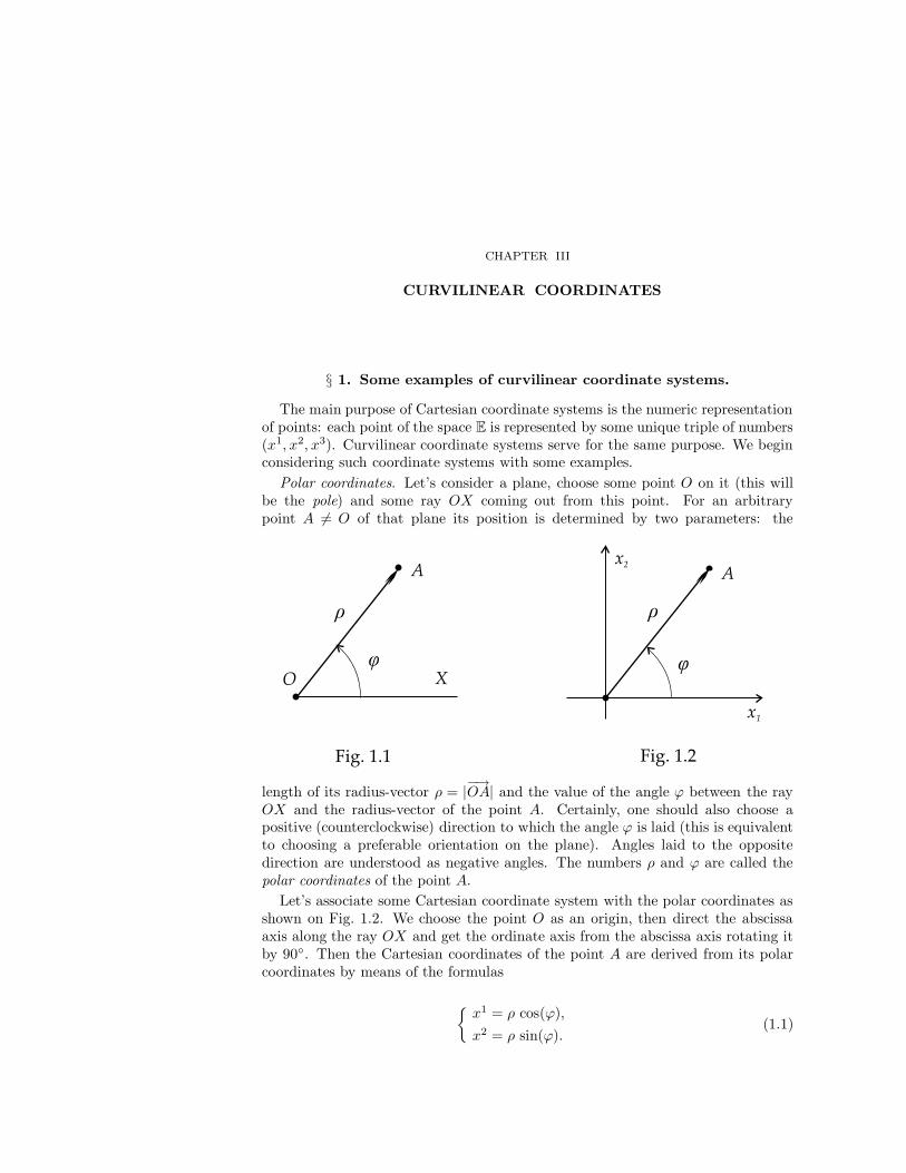
CHAPTER III
CURVILINEAR COORDINATES
§ 1. Some examples of curvilinear coordinate systems.
The main purpose of Cartesian coordinate systems is the numeric representationof points: each point of the space E is represented by some unique triple of numbers(x1, x2, x3). Curvilinear coordinate systems serve for the same purpose. We beginconsidering such coordinate systems with some examples.
Polar coordinates. Let’s consider a plane, choose some point O on it (this willbe the pole) and some ray OX coming out from this point. For an arbitrarypoint A 6= O of that plane its position is determined by two parameters: the
length of its radius-vector ρ = |−→OA| and the value of the angle ϕ between the rayOX and the radius-vector of the point A. Certainly, one should also choose apositive (counterclockwise) direction to which the angle ϕ is laid (this is equivalentto choosing a preferable orientation on the plane). Angles laid to the oppositedirection are understood as negative angles. The numbers ρ and ϕ are called thepolar coordinates of the point A.
Let’s associate some Cartesian coordinate system with the polar coordinates asshown on Fig. 1.2. We choose the point O as an origin, then direct the abscissaaxis along the ray OX and get the ordinate axis from the abscissa axis rotating itby 90. Then the Cartesian coordinates of the point A are derived from its polarcoordinates by means of the formulas
x1 = ρ cos(ϕ),
x2 = ρ sin(ϕ).(1.1)
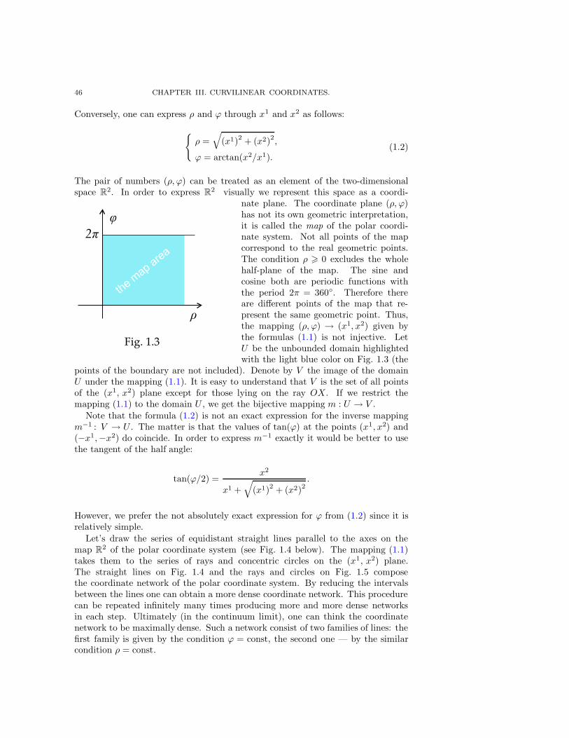
46 CHAPTER III. CURVILINEAR COORDINATES.
Conversely, one can express ρ and ϕ through x1 and x2 as follows:
ρ =√
(x1)2 + (x2)2,
ϕ = arctan(x2/x1).(1.2)
The pair of numbers (ρ, ϕ) can be treated as an element of the two-dimensionalspace R
2. In order to express R2 visually we represent this space as a coordi-
nate plane. The coordinate plane (ρ, ϕ)has not its own geometric interpretation,it is called the map of the polar coordi-nate system. Not all points of the mapcorrespond to the real geometric points.The condition ρ > 0 excludes the wholehalf-plane of the map. The sine andcosine both are periodic functions withthe period 2π = 360. Therefore thereare different points of the map that re-present the same geometric point. Thus,the mapping (ρ, ϕ) → (x1, x2) given bythe formulas (1.1) is not injective. LetU be the unbounded domain highlightedwith the light blue color on Fig. 1.3 (the
points of the boundary are not included). Denote by V the image of the domainU under the mapping (1.1). It is easy to understand that V is the set of all pointsof the (x1, x2) plane except for those lying on the ray OX. If we restrict themapping (1.1) to the domain U , we get the bijective mapping m : U → V .
Note that the formula (1.2) is not an exact expression for the inverse mappingm−1 : V → U . The matter is that the values of tan(ϕ) at the points (x1, x2) and(−x1,−x2) do coincide. In order to express m−1 exactly it would be better to usethe tangent of the half angle:
tan(ϕ/2) =x2
x1 +√
(x1)2 + (x2)2.
However, we prefer the not absolutely exact expression for ϕ from (1.2) since it isrelatively simple.
Let’s draw the series of equidistant straight lines parallel to the axes on themap R
2 of the polar coordinate system (see Fig. 1.4 below). The mapping (1.1)takes them to the series of rays and concentric circles on the (x1, x2) plane.The straight lines on Fig. 1.4 and the rays and circles on Fig. 1.5 composethe coordinate network of the polar coordinate system. By reducing the intervalsbetween the lines one can obtain a more dense coordinate network. This procedurecan be repeated infinitely many times producing more and more dense networksin each step. Ultimately (in the continuum limit), one can think the coordinatenetwork to be maximally dense. Such a network consist of two families of lines: thefirst family is given by the condition ϕ = const, the second one — by the similarcondition ρ = const.
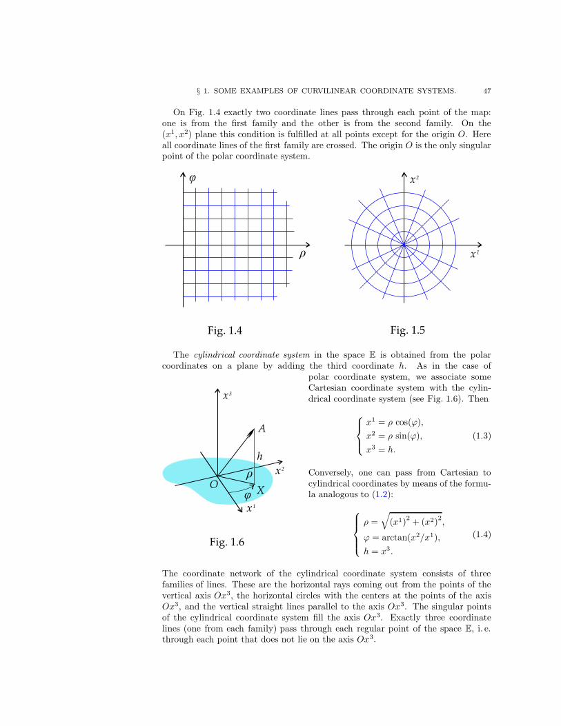
§ 1. SOME EXAMPLES OF CURVILINEAR COORDINATE SYSTEMS. 47
On Fig. 1.4 exactly two coordinate lines pass through each point of the map:one is from the first family and the other is from the second family. On the(x1, x2) plane this condition is fulfilled at all points except for the origin O. Hereall coordinate lines of the first family are crossed. The origin O is the only singularpoint of the polar coordinate system.
The cylindrical coordinate system in the space E is obtained from the polarcoordinates on a plane by adding the third coordinate h. As in the case of
polar coordinate system, we associate someCartesian coordinate system with the cylin-drical coordinate system (see Fig. 1.6). Then
x1 = ρ cos(ϕ),
x2 = ρ sin(ϕ),
x3 = h.
(1.3)
Conversely, one can pass from Cartesian tocylindrical coordinates by means of the formu-la analogous to (1.2):
ρ =
√
(x1)2
+ (x2)2,
ϕ = arctan(x2/x1),
h = x3.
(1.4)
The coordinate network of the cylindrical coordinate system consists of threefamilies of lines. These are the horizontal rays coming out from the points of thevertical axis Ox3, the horizontal circles with the centers at the points of the axisOx3, and the vertical straight lines parallel to the axis Ox3. The singular pointsof the cylindrical coordinate system fill the axis Ox3. Exactly three coordinatelines (one from each family) pass through each regular point of the space E, i. e.through each point that does not lie on the axis Ox3.
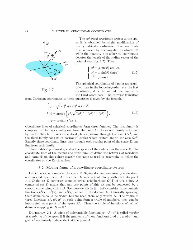
48 CHAPTER III. CURVILINEAR COORDINATES.
The spherical coordinate system in the spa-ce E is obtained by slight modification ofthe cylindrical coordinates. The coordinateh is replaced by the angular coordinate ϑ,while the quantity ρ in spherical coordinatesdenotes the length of the radius-vector of thepoint A (see Fig. 1.7). Then
x1 = ρ sin(ϑ) cos(ϕ),
x2 = ρ sin(ϑ) sin(ϕ),
x3 = ρ cos(ϑ).
(1.5)
The spherical coordinates of a point are usual-ly written in the following order: ρ is the firstcoordinate, ϑ is the second one, and ϕ isthe third coordinate. The converse transition
from Cartesian coordinates to these quantities is given by the formula:
ρ =
√
(x1)2 + (x2)2 + (x3)2,
ϑ = arccos
(
x3/
√
((x1)2 + (x2)2 + (x3)2)
,
ϕ = arctan(x2/x1).
(1.6)
Coordinate lines of spherical coordinates form three families. The first family iscomposed of the rays coming out from the point O; the second family is formedby circles that lie in various vertical planes passing through the axix Ox3; andthe third family consists of horizontal circles whose centers are on the axis Ox3.Exactly three coordinate lines pass through each regular point of the space E, oneline from each family.
The condition ρ = const specifies the sphere of the radius ρ in the space E. Thecoordinate lines of the second and third families define the network of meridiansand parallels on this sphere exactly the same as used in geography to define thecoordinates on the Earth surface.
§ 2. Moving frame of a curvilinear coordinate system.
Let D be some domain in the space E. Saying domain, one usually understanda connected open set. An open set D means that along with each its pointA ∈ D the set D comprises some spherical neighborhood O(A) of this point. Aconnected set D means that any two points of this set can be connected by asmooth curve lying within D. See more details in [2]. Let’s consider three numericfunctions u1(x), u2(x), and u3(x) defined in the domain D. Generally speaking,their domains could be wider, but we need them only within D. The values ofthree functions u1, u2, u3 at each point form a triple of numbers, they can beinterpreted as a point of the space R
3. Then the triple of functions u1, u2, u3
define a mapping u : D → R3.
Definition 2.1. A triple of differentiable functions u1, u2, u3 is called regularat a point A of the space E if the gradients of these functions gradu1, gradu2, andgradu3 are linearly independent at the point A.
§ 2. MOVING FRAME OF A CURVILINEAR COORDINATE SYSTEM. 49
Let’s choose some Cartesian coordinate system in E, in this coordinate systemthe above functions u1, u2, u3 are represented by the functions ui = ui(x1, x2, x3)of Cartesian coordinates of a point. The gradients of the differentiable functionsu1, u2, u3 form the triple of covectorial fields whose components are given by thepartial derivatives of u1, u2, u3 with respect to x1, x2, x3:
gradui =
(
∂ui
∂x1,∂ui
∂x2,∂ui
∂x3
)
. (2.1)
Let’s compose a matrix of the gradients (2.1):
J =
∥
∥
∥
∥
∥
∥
∥
∥
∥
∥
∥
∥
∥
∂u1
∂x1
∂u1
∂x2
∂u1
∂x3
∂u2
∂x1
∂u2
∂x2
∂u2
∂x3
∂u3
∂x1
∂u3
∂x2
∂u3
∂x3
∥
∥
∥
∥
∥
∥
∥
∥
∥
∥
∥
∥
∥
. (2.2)
The matrix J of the form (2.2) is called the Jacobi matrix of the mappingu : D → R3 given by the triple of the differentiable functions u1, u2, u3 in thedomain D. It is obvious that the regularity of the functions u1, u2, u3 at a pointis equivalent to the non-degeneracy of the Jacobi matrix at that point: det J 6= 0.
Theorem 2.1. If continuously differentiable functions u1, u2, u3 with the do-main D are regular at a point A, then there exists some neighborhood O(A) of thepoint A and some neighborhood O(u(A)) of the point u(A) in the space R
3 suchthat the following conditions are fulfilled:
(1) the mapping u : O(A) → O(u(A)) is bijective;(2) the inverse mapping u−1 : O(u(A)) → O(A) is continuously differentiable.
The theorem 2.1 or propositions equivalent to it are usually proved in the courseof mathematical analysis (see [2]). They are known as the theorems on implicitfunctions.
Definition 2.2. Say that an ordered triple of continuously differentiable func-tions u1, u2, u3 with the domain D ⊂ E define a curvilinear coordinate system inD if it is regular at all points of D and if the mapping u determined by them is abijective mapping from D to some domain U ⊂ R
3.
The cylindrical coordinate system is given by three functions u1 = ρ(x),u2 = ϕ(x), and u3 = h(x) from (1.4), while the spherical coordinate system isgiven by the functions (1.6). However, the triples of functions (1.4) and (1.6)satisfy the conditions from the definition 2.2 only after reducing somewhat theirdomains. Upon proper choice of a domain D for (1.4) and (1.6) the inversemappings u−1 are given by the formulas (1.3) and (1.5).
Suppose that in a domain D ⊂ E a curvilinear coordinate system u1, u2, u3 isgiven. Let’s choose an auxiliary Cartesian coordinate system in E. Then u1, u2, u3
is a triple of functions defining a map u from D onto some domain U ⊂ R3:
u1 = u1(x1, x2, x3),
u2 = u2(x1, x2, x3),
u3 = u3(x1, x2, x3).
(2.3)
CopyRight c© Sharipov R.A., 1996, 2004.
50 CHAPTER III. CURVILINEAR COORDINATES.
The domain D is called the domain being mapped, the domain U ⊂ R3 is called
the map or the chart, while u−1 : U → D is called the chart mapping. The chartmapping is given by the following three functions:
x1 = x1(u1, u2, u3),
x2 = x2(u1, u2, u3),
x3 = x3(u1, u2, u3).
(2.4)
Denote by r the radius-vector r of the point with Cartesian coordinates x1, x2, x3.Then instead of three scalar functions (2.4) we can use one vectorial function
r(u1, u2, u3) =
3∑
q=1
xq(u1, u2, u3) · eq . (2.5)
Let’s fix some two of three coordinates u1, u2, u3 and let’s vary the third of them.Thus we get three families of straight lines within the domain U ⊂ R
3:
u1 = t,
u2 = c2,
u3 = c3,
u1 = c1,
u2 = t,
u3 = c3,
u1 = c1,
u2 = c2,
u3 = t.
(2.6)
Here c1, c2, c3 are constants. The straight lines (2.6) form a rectangular coordinatenetwork within the chart U . Exactly one straight line from each of the families(2.6) passes through each point of the chart. Substituting (2.6) into (2.5) we mapthe rectangular network from U onto a curvilinear network in the domain D ⊂ E.Such a network is called the coordinate network of a curvilinear coordinate system.
The coordinate network of a curvilinear coordinate system on the domain Dconsists of three families of lines. Due to the bijectivity of the mapping u : D → Uexactly three coordinate lines pass through each point of the domain D — one linefrom each family. Each coordinate line has its canonical parametrization: t = u1
is the parameter for the lines of the first family, t = u2 is the parameter for thelines of the second family, and finally, t = u3 is the parameter for the lines ofthe third family. At each point of the domain D we have three tangent vectors,they are tangent to the coordinate lines of the three families passing through thatpoint. Let’s denote them E1, E2, E3. The vectors E1, E2, E3 are obtained bydifferentiating the radius-vector r(u1, u2, u3) with respect to the parameters u1,u2, u3 of coordinate lines. Therefore, we can write
Ej(u1, u2, u3) =
∂ r(u1, u2, u3)
∂uj. (2.7)
Let’s substitute (2.5) into (2.7). The basis vectors e1, e2, e3 do not depend on thevariables u1, u2, u3, hence, we get
Ej(u1, u2, u3) =
3∑
q=1
∂xq(u1, u2, u3)
∂uj· eq. (2.8)
§ 2. MOVING FRAME OF A CURVILINEAR COORDINATE SYSTEM. 51
The formula (2.8) determines the expansion of the vectors E1, E2, E3 in the basise1, e2, e3. The column-vectors of the coordinates of E1, E2, and E3 can beconcatenated into the following matrix:
I =
∥
∥
∥
∥
∥
∥
∥
∥
∥
∥
∥
∥
∥
∂x1
∂u1
∂x1
∂u2
∂x1
∂u3
∂x2
∂u1
∂x2
∂u2
∂x2
∂u3
∂x3
∂u1
∂x3
∂u2
∂x3
∂u3
∥
∥
∥
∥
∥
∥
∥
∥
∥
∥
∥
∥
∥
. (2.9)
Comparing (2.9) and (2.2), we see that (2.9) is the Jacobi matrix for the mappingu−1 : U → D given by the functions (2.4). Let’s substitute (2.4) into (2.3):
ui(x1(u1, u2, u3), x2(u1, u2, u3), x3(u1, u2, u3)) = ui. (2.10)
The identity (2.10) follows from the fact that the functions (2.3) and (2.4) definetwo mutually inverse mappings u and u−1. Let’s differentiate the identity (2.10)with respect to the variable uj:
3∑
q=1
∂ui(x1, x2, x3)
∂xq
∂xq(u1, u2, u3)
∂uj= δi
j . (2.11)
Here we used the chain rule for differentiating the composite function in (2.10).The relationship (2.11) shows that the matrices (2.2) and (2.9) are inverse to eachother. More precisely, we have the following relationship
I(u1, u2, u3) = J(x1, x2, x3)−1, (2.12)
where x1, x2, x3 should be expressed through u1, u2, u3 by means of (2.4), orconversely, u1, u2, u3 should be expressed through x1, x2, x3 by means of (2.3).The arguments shown in the relationship (2.12) are the natural arguments for thecomponents of the Jacobi matrices I and J . However, one can pass to any requiredset of variables by means of (2.3) or (2.4) whenever it is necessary.
The regularity of the triple of functions (2.3) defining a curvilinear coordinatesystem in the domain D means that the matrix (2.2) is non-degenerate. Then, dueto (2.12), the inverse matrix (2.9) is also non-degenerate. Therefore, the vectorsE1, E2, E3 given by the formula (2.8) are linearly independent at any point ofthe domain D. Due to the linear independence of the coordinate tangent vectorsE1, E2, E3 they form a moving frame which is usually called the coordinate frameof the curvilinear coordinate system. The formula (2.8) now can be interpretedas the transition formula for passing from the basis of the auxiliary Cartesiancoordinate system to the basis formed by the vectors of the frame E1, E2, E3:
Ej =
3∑
q=1
Sqj (u1, u2, u3) · eq . (2.13)
The transition matrix S in the formula (2.13) coincides with the Jacobi matrix(2.9), therefore its components depend on u1, u2, u3. These are the naturalvariables for the components of S.
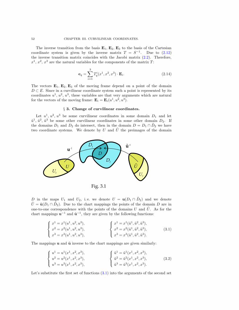
52 CHAPTER III. CURVILINEAR COORDINATES.
The inverse transition from the basis E1, E2, E3 to the basis of the Cartesiancoordinate system is given by the inverse matrix T = S−1. Due to (2.12)the inverse transition matrix coincides with the Jacobi matrix (2.2). Therefore,x1, x2, x3 are the natural variables for the components of the matrix T :
eq =3∑
i=1
T iq (x1, x2, x3) ·Ei. (2.14)
The vectors E1, E2, E3 of the moving frame depend on a point of the domainD ⊂ E. Since in a curvilinear coordinate system such a point is represented by itscoordinates u1, u2, u3, these variables are that very arguments which are naturalfor the vectors of the moving frame: Ei = Ei(u
1, u2, u3).
§ 3. Change of curvilinear coordinates.
Let u1, u2, u3 be some curvilinear coordinates in some domain D1 and letu1, u2, u3 be some other curvilinear coordinates in some other domain D2. Ifthe domains D1 and D2 do intersect, then in the domain D = D1 ∩ D2 we havetwo coordinate systems. We denote by U and U the preimages of the domain
D in the maps U1 and U2, i. e. we denote U = u(D1 ∩ D2) and we denote
U = u(D1 ∩ D2). Due to the chart mappings the points of the domain D are in
one-to-one correspondence with the points of the domains U and U . As for thechart mappings u−1 and u−1, they are given by the following functions:
x1 = x1(u1, u2, u3),
x2 = x2(u1, u2, u3),
x3 = x3(u1, u2, u3),
x1 = x1(u1, u2, u3),
x2 = x2(u1, u2, u3),
x3 = x3(u1, u2, u3).
(3.1)
The mappings u and u inverse to the chart mappings are given similarly:
u1 = u1(x1, x2, x3),
u2 = u2(x1, x2, x3),
u3 = u3(x1, x2, x3),
u1 = u1(x1, x2, x3),
u2 = u2(x1, x2, x3),
u3 = u3(x1, x2, x3).
(3.2)
Let’s substitute the first set of functions (3.1) into the arguments of the second set
§ 3. CHANGE OF CURVILINEAR COORDINATES. 53
of functions (3.2). Similarly, we substitute the second set of functions (3.1) intothe arguments of the first set of functions in (3.2). As a result we get the functions
u1(x1(u1, u2, u3), x2(u1, u2, u3), x3(u1, u2, u3)),
u2(x1(u1, u2, u3), x2(u1, u2, u3), x3(u1, u2, u3)),
u3(x1(u1, u2, u3), x2(u1, u2, u3), x3(u1, u2, u3)),
(3.3)
u1(x1(u1, u2, u3), x2(u1, u2, u3), x3(u1, u2, u3)),
u2(x1(u1, u2, u3), x2(u1, u2, u3), x3(u1, u2, u3)),
u3(x1(u1, u2, u3), x2(u1, u2, u3), x3(u1, u2, u3))
(3.4)
which define the pair of mutually inverse mappings u u−1 and u u−1. For thesake of brevity we write these sets of functions as follows:
u1 = u1(u1, u2, u3),
u2 = u2(u1, u2, u3),
u3 = u3(u1, u2, u3),
u1 = u1(u1, u2, u3),
u2 = u2(u1, u2, u3),
u3 = u3(u1, u2, u3).
(3.5)
The formulas (3.5) express the coordinates of a point from the domain D in somecurvilinear coordinate system through its coordinates in some other coordinatesystem. These formulas are called the transformation formulas or the formulas forchanging the curvilinear coordinates.
Each of the two curvilinear coordinate systems has its own moving frame withinthe domain D = D1∩D2. Let’s denote by S and T the transition matrices relatingthese two moving frames. Then we can write
Ej =
3∑
i=1
Sij ·Ei, Ei =
3∑
k=1
T ki · Ek. (3.6)
Theorem 3.1. The components of the transition matrices S and T for themoving frames of two curvilinear coordinate system in (3.6) are determined by thepartial derivatives of the functions (3.5):
Sij(u
1, u2, u3) =∂ui
∂uj, T k
i (u1, u2, u3) =∂uk
∂ui. (3.7)
Proof. We shall prove only the first formula in (3.7). The proof of the secondformula is absolutely analogous to the proof of the first one. Let’s choose someauxiliary Cartesian coordinate system and then write the formula (2.8) applied tothe frame vectors of the second curvilinear coordinate system:
Ej(u1, u2, u3) =
3∑
q=1
∂xq(u1, u2, u3)
∂uj· eq. (3.8)
Applying the formula (2.14), we express e1, e2, e3 through E1, E2, E3. Rememberthat the matrix T in (2.14) coincides with the Jacobi matrix J(x1, x2, x3) from
54 CHAPTER III. CURVILINEAR COORDINATES.
(2.2). Therefore, we can write the following formula:
eq =
3∑
i=1
∂ui(x1, x2, x3)
∂xq·Ei. (3.9)
Now let’s substitute (3.9) into (3.8). As a result we get the formula relating theframe vectors of two curvilinear coordinate systems:
Ej =
3∑
i=1
(
3∑
q=1
∂ui(x1, x2, x3)
∂xq
∂xq(u1, u2, u3)
∂uj
)
·Ei. (3.10)
Comparing (3.10) and (3.6), from this comparison for the components of S we get
Sij =
3∑
q=1
∂ui(x1, x2, x3)
∂xq
∂xq(u1, u2, u3)
∂uj. (3.11)
Remember that the Cartesian coordinates x1, x2, x3 in the above formula (3.11)are related to the curvilinear coordinates u1, u2, u3 by means of (3.1). Hence, thesum in right hand side of (3.11) can be transformed to the partial derivative of thecomposite function ui((x1(u1, u2, u3), x2(u1, u2, u3), x3(u1, u2, u3)) from (3.4):
Sij =
∂ui
∂uj.
Note that the functions (3.4) written in the form of (3.5) are that very functionsrelating u1, u2, u3 and u1, u2, u3, and their derivatives are in formula (3.7). Thetheorem is proved.
A remark on the orientation. From the definition 2.2 we derive that thefunctions (2.3) are continuously differentiable. Due to the theorem 2.1 the func-tions (2.4) representing the inverse mappings are also continuously differentiable.Then the components of the matrix S in the formula (2.13) coinciding with thecomponents of the Jacobi matrix (2.9) are continuous functions within the domainU . The same is true for the determinant of the matrix S: the determinantdet S(u1, u2, u3) is a continuous function in the domain U which is nonzero atall points of this domain. A nonzero continuous real function in a connected setU cannot take the values of different signs in U . This means that detS > 0 ordet S < 0. This means that the orientation of the triple of vectors forming themoving frame of a curvilinear coordinate system is the same for all points of adomain where it is defined. Since the space E is equipped with the preferableorientation, we can subdivide all curvilinear coordinates in E into right-orientedand left-oriented coordinate systems.
A remark on the smoothness. The definition 2.2 yields the concept of acontinuously differentiable curvilinear coordinate system. However, the functions(2.3) could belong to a higher smoothness class Cm. In this case we say that wehave a curvilinear coordinate system of the smoothness class Cm. The componentsof the Jacobi matrix (2.2) for such a coordinate system are the functions of theclass Cm−1. Due to the relationship (2.12) the components of the Jacobi matrix
§ 4. VECTORIAL AND TENSORIAL FIELDS . . . 55
(2.9) belong to the same smoothness class Cm−1. Hence, the functions (2.4)belong to the smoothness class Cm.
If we have two curvilinear coordinate systems of the smoothness class Cm, then,according to the above considerations, the transformation functions (3.5) belongto the class Cm, while the components of the transition matrices S and T givenby the formulas (3.7) belong to the smoothness class Cm−1.
§ 4. Vectorial and tensorial fields
in curvilinear coordinates.
Let u1, u2, u3 be some curvilinear coordinate system in some domain D ⊂ E
and let F be some vector field defined at the points of the domain D. Thenat a point with coordinates u1, u2, u3 we have the field vector F(u1, u2, u3) andthe triple of the frame vectors E1(u
1, u2, u3), E2(u1, u2, u3), E3(u
1, u2, u3). Let’sexpand the field vector F in the basis formed by the frame vectors:
F(u1, u2, u3) =
3∑
i=1
F i(u1, u2, u3) ·Ei(u1, u2, u3). (4.1)
The quantities F i(u1, u2, u3) in such expansion are naturally called the componentsof the vector field F in the curvilinear coordinates u1, u2, u3. If we have anothercurvilinear coordinate system u1, u2, u3 in the domain D, then we have the otherexpansion of the form (4.1):
F(u1, u2, u3) =
3∑
i=1
F i(u1, u2, u3) · Ei(u1, u2, u3). (4.2)
By means of the formulas (3.6) one can easily derive the relationships binding thecomponents of the field F in the expansions (4.1) and (4.2):
F i(u) =
3∑
j=1
Sij(u) F j(u),
ui = ui(u1, u2, u3).
(4.3)
The relationships (4.3) are naturally interpreted as the generalizations for therelationships (1.2) from Chapter II for the case of curvilinear coordinates.
Note that Cartesian coordinate systems can be treated as a special case ofcurvilinear coordinates. The transition functions ui = ui(u1, u2, u3) in the case ofa pair of Cartesian coordinate systems are linear, therefore the matrix S calculatedaccording to the theorem 3.1 in this case is a constant matrix.
Now let F be either a field of covectors, a field of linear operators, or a fieldof bilinear forms. In any case the components of the field F at some point aredetermined by fixing some basis attached to that point. The vectors of the movingframe of a curvilinear coordinate system at a point with coordinates u1, u2, u3
provide the required basis. The components of the field F determined by thisbasis are called the components of the field F in that curvilinear coordinates. Thetransformation rules for the components of the fields listed above under a changeof curvilinear coordinates generalize the formulas (1.3), (1.4), and (1.5) from
56 CHAPTER III. CURVILINEAR COORDINATES.
Chapter II. For a covectorial field F the transformation rule for its componentsunder a change of coordinates looks like
Fi(u) =
3∑
j=1
T ji (u) Fj(u),
ui = ui(u1, u2, u3).
(4.4)
The transformation rule for the components of an operator field F is written as
F ij (x) =
3∑
p=1
3∑
q=1
Sip(u)T q
j (u) F pq (x),
ui = ui(u1, u2, u3).
(4.5)
In the case of a field of bilinear (quadratic) forms the generalization of the formula(1.5) from Chapter II looks like
Fij(u) =
3∑
p=1
3∑
q=1
T pi (u)T q
j (u) Fpq(u),
ui = ui(u1, u2, u3).
(4.6)
Let F be a tensor field of the type (r, s). In contrast to a vectorial field,the value of such a tensorial field at a point have no visual embodiment inform of an arrowhead segment. Moreover, in general case there is no visuallyexplicit way of finding the numerical values for the components of such a fieldin a given basis. However, according to the definition 1.1 from Chapter II, atensor is a geometric object that for each basis has an array of componentsassociated with this basis. Let’s denote by F(u1, u2, u3) the value of the field F
at the point with coordinates u1, u2, u3. This is a tensor whose components inthe basis E1(u
1, u2, u3), E2(u1, u2, u3), E3(u
1, u2, u3) are called components of thefield F in a given curvilinear coordinate system. The transformation rules for thecomponents of a tensor field under a change of a coordinate system follow fromthe formula (1.6) in Chapter II. For a tensorial field of the type (r, s) it looks like
F i1... ir
j1... js(u) =
∑
p1 ... pr
q1 ... qs
Si1p1
(u) . . . Sir
pr(u)×
× T q1
j1(u) . . . T qs
js(u) F p1... pr
q1... qs(u),
ui = ui(u1, u2, u3).
(4.7)
The formula (4.7) has two important differences as compared to the correspondingformula (1.7) in Chapter II. In the case of curvilinear coordinates
(1) the transition functions ui(u1, u2, u3) should not be linear functions;(2) the transition matrices S(u) and T (u) are not necessarily constant matrices.
Note that these differences do not affect the algebraic operations with tensorialfields. The operations of addition, tensor product, contraction, index permutation,symmetrization, and alternation are implemented by the same formulas as in
CopyRight c© Sharipov R.A., 1996, 2004.
§ 5. DIFFERENTIATION OF TENSOR FIELDS . . . 57
Cartesian coordinates. The differences (1) and (2) reveal only in the operation ofcovariant differentiation of tensor fields.
Any curvilinear coordinate system is naturally equipped with the the metrictensor g. This is a tensor whose components are given by mutual scalar productsof the frame vectors for a given coordinate system:
gij = (Ei(u) |Ej(u)). (4.8)
The components of the inverse metric tensor g are obtained by inverting thematrix g. In a curvilinear coordinates the quantities gij and gij are not necessarilyconstants any more.
We already know that the metric tensor g defines the volume pseudotensorω. As before, in curvilinear coordinates its components are given by the formula(6.11) from Chapter II. Since the space E has the preferable orientation, thevolume pseudotensor can be transformed to the volume tensor ω. The formula(8.1) from Chapter II for the components of this tensor remains valid in acurvilinear coordinate system either.
§ 5. Differentiation of tensor fields
in curvilinear coordinates.
Let A be a differentiable tensor field of the type (r, s). In § 5 of Chapter II wehave defined the concept of covariant differential. The covariant differential ∇A
of a field A is a tensorial field of the type (r, s + 1). In an arbitrary Cartesiancoordinate system the components of the field ∇A are obtained by differentiatingthe components of the original field A with respect to x1, x2, and x3. The use ofcurvilinear coordinates does not annul the operation of covariant differentiation.However, the procedure of deriving the components of the field ∇A from thecomponents of A in curvilinear coordinates is more complicated.
Let u1, u2, u3 be some curvilinear coordinate system in a domain D ⊂ E.Let’s derive the rule for covariant differentiation of tensor fields in a curvilinearcoordinate system. We consider a vectorial field A to begin with. This is a fieldwhose components are specified by one upper index: Ai(u1, u2, u3). In order tocalculate the components of the field B = ∇A we choose some auxiliary Cartesiancoordinate system x1, x2, x3. Then we need to do the following maneuver: firstwe transform the components of A from curvilinear coordinates to Cartesian ones,then calculate the components of the field B = ∇A by means of the formula (5.1)from Chapter II, and finally, we transform the components of ∇A from Cartesiancoordinates back to the original curvilinear coordinates.
The Cartesian coordinates x1, x2, x3 and the curvilinear coordinates u1, u2, u3
are related by the following transition functions:
x1 = x1(u1, u2, u3),
x2 = x2(u1, u2, u3),
x3 = x3(u1, u2, u3),
u1 = u1(x1, x2, x3),
u2 = u2(x1, x2, x3),
u3 = u3(x1, x2, x3).
(5.1)
The components of the corresponding transition matrices are calculated accordingto the formula (3.7). When applied to (5.1), this formula yields
Sij(x) =
∂ui
∂xj, T k
i (u) =∂xk
∂ui. (5.2)
58 CHAPTER III. CURVILINEAR COORDINATES.
Denote by Ak(x1, x2, x3) the components of the vector field A in the Cartesiancoordinate system x1, x2, x3. Then we get
Ak =
3∑
p=1
T kp (u)Ap(u).
For the components of the field B = ∇A in these Cartesian coordinates, applyingthe formula (5.1) from Chapter II, we get
Bkq =
∂Ak
∂xq=
3∑
p=1
∂
∂xq
(
T kp (u)Ap(u)
)
. (5.3)
Now we perform the inverse transformation of the components of B from theCartesian coordinates x1, x2, x3 back to the curvilinear coordinates u1, u2, u3:
∇jAi = Bi
j(u) =
3∑
k=1
3∑
q=1
Sik(x)T q
j (u) Bkq . (5.4)
Let’s apply the Leibniz rule for calculating the partial derivative in (5.3). As aresult we get two sums. Then, substituting these sums into (5.4), we obtain
∇jAi =
3∑
q=1
3∑
p=1
(
3∑
k=1
Sik(x)T k
p (u)
)
T qj (u)
∂Ap(u)
∂xq+
+
3∑
p=1
(
3∑
q=1
3∑
p=1
Sik(x)T q
j (u)∂T k
p (u)
∂xq
)
Ap(u).
Note that the matrices S and T are inverse to each other. Therefore, we cancalculate the sums over k and p in the first summand. Moreover, we replace T q
j (u)
by the derivatives ∂xq/∂uj due to the formula (5.2), and we get
3∑
q=1
T qj (u)
∂
∂xq=
3∑
q=1
∂xq
∂uj
∂
∂xq=
∂
∂uj.
Taking into account all the above arguments, we transform the formula for thecovariant derivative ∇jA
i into the following one:
∇jAi(u) =
∂Ai(u)
∂uj+
3∑
p=1
(
3∑
k=1
Sik(x)
∂T kp (u)
∂uj
)
Ap(u).
We introduce the special notation for the sum enclosed into the round brackets inthe above formula, we denote it by Γi
jp:
Γijp(u) =
3∑
k=1
Sik(x)
∂T kp (u)
∂uj. (5.5)
§ 5. DIFFERENTIATION OF TENSOR FIELDS . . . 59
Taking into account the notations (5.5), now we can write the rule of covariantdifferentiation of a vector field in curvilinear coordinates as follows:
∇jAi =
∂Ai
∂uj+
3∑
p=1
ΓijpA
p. (5.6)
The quantities Γijp calculated according to (5.5) are called the connection compo-
nents or the Christoffel symbols. These quantities are some inner characteristics ofa curvilinear coordinate system. This fact is supported by the following lemma.
Lemma 5.1. The connection components Γijp of a curvilinear coordinate system
u1, u2, u3 given by the formula (5.5) do not depend on the choice of an auxiliaryCartesian coordinate system x1, x2, x3.
Proof. Let’s multiply both sides of the equality (5.5) by the frame vector Ei
and then sum over the index i:
3∑
i=1
Γijp(u)Ei(u) =
3∑
i=1
3∑
k=1
∂T kp (u)
∂ujSi
k(x)Ei(u). (5.7)
The sum over i in right hand side of the equality (5.7) can be calculated explicitlydue to the first of the following two formulas:
ek =
3∑
i=1
Sik Ei, Ep =
3∑
k=1
T kp ek. (5.8)
These formulas (5.8) relate the frame vectors E1, E2, E3 and the basis vectorse1, e2, e3 of the auxiliary Cartesian coordinate system. Now (5.7) is written as:
3∑
i=1
Γijp Ei =
3∑
k=1
∂T kp (u)
∂ujek =
3∑
k=1
∂
∂uj
(
T kp (u) ek
)
.
The basis vector ek does not depend on u1, u2, u3. Therefore, it is brought intothe brackets under the differentiation with respect to uj. The sum over k in righthand side of the above formula is calculated explicitly due to the second formula(5.8). As a result the relationship (5.7) is transformed to the following one:
∂Ep
∂uj=
3∑
i=1
Γijp ·Ei. (5.9)
The formula (5.9) expresses the partial derivatives of the frame vectors backthrough these vectors. It can be understood as another one way for calculatingthe connection components Γi
jp. This formula comprises nothing related to the
auxiliary Cartesian coordinates x1, x2, x3. The vector Ep(u1, u2, u3) is determinedby the choice of curvilinear coordinates u1, u2, u3 in the domain D. It is sufficientto differentiate this vector with respect to uj and expand the resulting vector inthe basis of the frame vectors E1, E2, E3. Then the coefficients of this expansion
60 CHAPTER III. CURVILINEAR COORDINATES.
yield the required values for Γijp. It is obvious that these values do not depend on
the choice of the auxiliary Cartesian coordinates x1, x2, x3 above.
Now let’s proceed with deriving the rule for covariant differentiation of anarbitrary tensor field A of the type (r, s) in curvilinear coordinates. For thispurpose we need another one expression for the connection components. It isderived from (5.5). Let’s transform the formula (5.5) as follows:
Γijp(u) =
3∑
k=1
∂
∂uj
(
Sik(x)T k
p (u))
−3∑
k=1
T kp (u)
∂Sik(x)
∂uj.
The matrices S and T are inverse to each other. Therefore, upon performing thesummation over k in the first term we find that it vanishes. Hence, we get
Γijp(u) = −
3∑
k=1
T kp (u)
∂Sik(x)
∂uj. (5.10)
Let Ai1... ir
j1... jsbe the components of a tensor field A of the type (r, s) in curvilinear
coordinates. In order to calculate the components of B = ∇A we do the samemaneuver as above. First of all we transform the components of A to someauxiliary Cartesian coordinate system:
Ap1... pr
q1... qs=
∑
v1... vr
w1... ws
T p1v1. . . T pr
vrSw1
q1. . . Sws
qsAv1... vr
w1... ws.
Then we calculate the components of the field B in this auxiliary Cartesiancoordinate system simply by differentiating:
Bp1 ... pr
q1 ... qs+1=
∑
v1... vr
w1... ws
∂(
T p1v1. . . T pr
vrSw1
q1. . . Sws
qsAv1... vr
w1... ws
)
∂xqs+1.
Then we perform the inverse transformations of the components of B from theCartesian coordinates back to the original curvilinear coordinate system:
Bi1... ir
j1... js+1=
∑
p1 ... pr
q1... qs+1
Si1p1. . . Sir
prT q1
j1. . . T
qs+1
js+1Bp1... pr
q1... qs+1=
=∑
p1 ... pr
q1... qs+1
∑
v1... vr
w1... ws
Si1p1. . . Sir
prT q1
j1. . . T
qs+1
js+1×
×∂(
T p1v1. . . T pr
vrSw1
q1. . . Sws
qsAv1... vr
w1 ... ws
)
∂xqs+1.
(5.11)
Applying the Leibniz rule for differentiating in (5.11), as a result we get threegroups of summands. The summands of the first group correspond to differenti-ating the components of the matrix T , the summands of the second group arisewhen we differentiate the components of the matrix S in (5.11), and finally, theunique summand in the third group is produced by differentiating Av1... vr
w1 ... ws. In
§ 5. DIFFERENTIATION OF TENSOR FIELDS . . . 61
any one of these summands if the term T pm
vmor the term Swn
qnis not differentiated,
then this term is built into a sum that can be evaluated explicitly:
3∑
pm=1
Sim
pmT pm
vm= δim
vm,
3∑
qn=1
T qn
jnSwn
qn= δwn
jn.
Therefore, one can evaluate explicitly the most part of the sums in the formula(5.11). Moreover, we have the following equality:
3∑
qs+1=1
Tqs+1
js+1
∂
∂xqs+1=
3∑
qs+1=1
∂xqs+1
∂ujs+1
∂
∂xqs+1=
∂
∂ujs+1.
Taking into account all the above facts, we can bring (5.11) to
∇js+1Ai1... ir
j1... js=
r∑
m=1
3∑
vm=1
(
3∑
pm=1
Sim
pm
∂T pm
vm
∂ujs+1
)
Ai1... vm ... ir
j1... js+
+
s∑
n=1
3∑
wn=1
(
3∑
qn=1
T qn
jn
∂Swn
qn
∂ujs+1
)
Ai1... ir
j1... wn ... js+∂Ai1 ... ir
j1 ... js
∂ujs+1.
Due to the formulas (5.5) and (5.10) one can express the sums enclosed into roundbrackets in the above equality through the Christoffel symbols. Ultimately, theformula (5.11) is brought to the following form:
∇js+1Ai1... ir
j1... js=∂Ai1... ir
j1... js
∂ujs+1+
+
r∑
m=1
3∑
vm=1
Γim
js+1 vmAi1... vm... ir
j1... js−
s∑
n=1
3∑
wn=1
Γwn
js+1 jnAi1... ir
j1... wn... js.
(5.12)
The formula (5.12) is the rule for covariant differentiation of a tensorial field A ofthe type (r, s) in an arbitrary curvilinear coordinate system. This formula can becommented as follows: the covariant derivative ∇js+1 is obtained from the partialderivative ∂/∂ujs+1 by adding r+s terms — one per each index in the componentsof the field A. The terms associated with the upper indices enter with the positivesign, the other terms associated with the lower indices enter with the negativesign. In such additional terms each of the upper indices im and each of the lowerindices jn are sequentially moved to the Christoffel symbol, while in its place wewrite the summation index vm or wn. The lower index js+1 added as a resultof covariant differentiation is always written as the first lower index in Christoffelsymbols. The position of the summation indices vm and wn in Christoffel symbolsis always complementary to their positions in the components of the field A sothat they always form a pair of upper and lower indices. Though the formula(5.12) is rather huge, we hope that due to the above comments one can easilyremember it and reproduce it in any particular case.
62 CHAPTER III. CURVILINEAR COORDINATES.
§ 6. Transformation of the connection components
under a change of a coordinate system.
In deriving the formula for covariant differentiation of tensorial fields in curvi-linear coordinates we discovered a new type of indexed objects — these areChristoffel symbols. The quantities Γk
ij are enumerated by one upper index andtwo lower indices, and their values are determined by the choice of a coordinatesystem. However, they are not the components of a tensorial fields of the type(1, 2). Indeed, the values of all Γk
ij in a Cartesian coordinate system are identically
zero (this follows from the comparison of (5.12) with the formula (5.1) in ChapterII). But a tensorial field with purely zero components in some coordinate systemcannot have nonzero components in any other coordinate system. Therefore,Christoffel symbols are the components of a non-tensorial geometric object whichis called a connection field or simply a connection.
Theorem 6.1. Let u1, u2, u3 and u1, u2, u3 be two coordinate systems in adomain D ⊂ E. Then the connection components in these two coordinate systemsare related to each other by means of the following equality:
Γkij =
3∑
m=1
3∑
p=1
3∑
q=1
Skm T p
i Tqj Γm
pq +
3∑
m=1
Skm
∂Tmi
∂uj. (6.1)
Here S and T are the transition matrices given by the formulas (3.7).
A remark on the smoothness. The derivatives of the components of T in(6.1) and the formulas (3.7), where the components of T are defined as the partialderivatives of the transition functions (3.5), show that the connection componentscan be correctly defined only for coordinate systems of the smoothness class notlower than C2. The same conclusion follows from the formula (5.5) for Γi
jp.
Proof. In order to prove the theorem 6.1 we apply the formula (5.9). Let’swrite it for the frame vectors E1, E2, E3, then apply the formula (3.6) for to
express Ej through the vectors E1, E2, and E3:
3∑
k=1
Γkij Ek =
∂Ej
∂ui=
3∑
m=1
∂
∂ui
(
Tmj Em
)
. (6.2)
Applying the Leibniz rule to the right hand side of (6.2), we get two terms:
3∑
k=1
Γkij Ek =
3∑
m=1
∂Tmj
∂uiEm +
3∑
q=1
T qj
∂Eq
∂ui. (6.3)
In the first term in the right hand side of (6.3) we express Em through the vectorsE1, E2, and E3. In the second term we apply the chain rule and express thederivative with respect to ui through the derivatives with respect to u1, u2, u3:
3∑
k=1
Γkij Ek =
3∑
k=1
3∑
m=1
Skm
∂Tmj
∂uiEk +
3∑
q=1
3∑
p=1
T qj
∂up
∂ui
∂Eq
∂up.
§ 7. CONCORDANCE OF METRIC AND CONNECTION. 63
Now let’s replace ∂up/∂ui by T pi relying upon the formulas (3.7) and then apply
the relationship (5.9) once more in the form of
∂Eq
∂up=
3∑
m=1
Γmpq Em.
As a result of the above transformations we can write the equality (6.3) as follows:
3∑
k=1
Γkij Ek =
3∑
k=1
3∑
m=1
Skm
∂Tmj
∂uiEk +
3∑
q=1
3∑
p=1
3∑
m=1
T pi T
qj Γm
pq Em.
Now we need only to express Em through the frame vectors E1, E2, E3 and collectthe similar terms in the above formula:
3∑
k=1
(
Γkij −
3∑
m=1
3∑
q=1
3∑
p=1
Skm T p
i Tqj Γm
pq −3∑
m=1
Skm
∂Tmj
∂ui
)
Ek = 0.
Since the frame vectors E1, E2, E3 are linearly independent, the expression en-closed into round brackets should vanish. As a result we get the equality exactlyequivalent to the relationship (6.1) that we needed to prove.
§ 7. Concordance of metric and connection.
Another formula for Christoffel symbols.
Let’s consider the metric tensor g. The covariant differential ∇g of the field g
is equal to zero (see formulas (6.7) in Chapter II). This is because in any Cartesiancoordinates x1, x2, x3 in E the components gij of the metric tensor do not dependon x1, x2, x3. In a curvilinear coordinate system the components of the metrictensor gij(u
1, u2, u3) usually are not constants. However, being equal to zero inCartesian coordinates, the tensor ∇g remains zero in any other coordinates:
∇kgij = 0. (7.1)
The relationship (7.1) is known as the concordance condition for a metric and aconnection. Taking into account (5.12), we can rewrite this condition as
gij
∂uk−
3∑
r=1
Γrki grj −
3∑
r=1
Γrkj gir = 0. (7.2)
The formula (7.2) relates the connection components Γkij and the components
of the metric tensor gij. Due to this relationship we can express Γkij through
the components of the metric tensor provided we remember the following veryimportant property of the connection components (5.5).
Theorem 7.1. The connection given by the formula (5.5) is a symmetric con-nection, i. e. Γk
ij = Γkj i.
Proof. From (5.2) and (5.5) for Γkij we derive the following expression:
Γkij(u) =
3∑
q=1
Skq
∂T qj (u)
∂ui=
3∑
q=1
Skq
∂2xq
∂uj ∂ui. (7.3)
CopyRight c© Sharipov R.A., 1996, 2004.
64 CHAPTER III. CURVILINEAR COORDINATES.
For the functions of the smoothness class C2 the mixed second order partialderivatives do not depend on the order of differentiation:
∂2xq
∂uj ∂ui=
∂2xq
∂ui ∂uj.
This fact immediately proves the symmetry of the Christoffel symbols given bythe formula (7.3). Thus, the proof is over.
Now, returning back to the formula (7.2) relating Γkij and gij, we introduce the
following notations that simplify the further calculations:
Γijk =
3∑
r=1
Γrij gkr. (7.4)
It is clear that the quantities Γijk in (7.4) are produced from Γkij by means of
index lowering procedure described in Chapter II. Therefore, conversely, Γkij are
obtained from Γijk according to the following formula:
Γkij =
3∑
r=1
gkr Γijr. (7.5)
From the symmetry of Γkij it follows that the quantities Γijk in (7.4) are also
symmetric with respect to the indices i and j, i. e. Γijk = Γjik. Using thenotations (7.4) and the symmetry of the metric tensor, the relationship (7.2) canbe rewritten in the following way:
∂gij
∂uk− Γkij − Γkji = 0. (7.6)
Let’s complete (7.6) with two similar relationships applying two cyclic transposi-tions of the indices i → j → k → i to the formula (7.6). As a result we obtain
∂gij
∂uk− Γkij − Γkji = 0,
∂gjk
∂ui− Γijk − Γikj = 0,
∂gki
∂uj− Γjki − Γjik = 0.
(7.7)
Let’s add the last two relationships (7.7) and subtract the first one from the sum.Taking into account the symmetry of Γijk with respect to i and j, we get
∂gjk
∂ui+∂gki
∂uj− ∂gij
∂uk− 2 Γijk = 0.
Using this equality, one can easily express Γijk through the components of themetric tensor. Then one can substitute this expression into (7.5) and derive
Γkij =
1
2
3∑
r=1
gkr
(
∂grj
∂ui+∂gir
∂uj− ∂gij
∂ur
)
. (7.8)
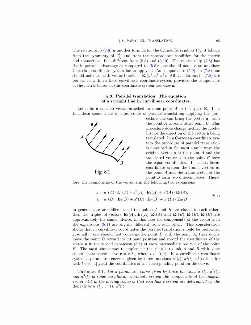
§ 8. PARALLEL TRANSLATION. 65
The relationship (7.8) is another formula for the Christoffel symbols Γkij, it follows
from the symmetry of Γkij and from the concordance condition for the metric
and connection. It is different from (5.5) and (5.10). The relationship (7.8) hasthe important advantage as compared to (5.5): one should not use an auxiliaryCartesian coordinate system for to apply it. As compared to (5.9), in (7.8) oneshould not deal with vector-functions Ei(u
1, u2, u3). All calculations in (7.8) areperformed within a fixed curvilinear coordinate system provided the componentsof the metric tensor in this coordinate system are known.
§ 8. Parallel translation. The equation
of a straight line in curvilinear coordinates.
Let a be a nonzero vector attached to some point A in the space E. In aEuclidean space there is a procedure of parallel translation; applying this pro-
cedure one can bring the vector a fromthe point A to some other point B. Thisprocedure does change neither the modu-lus nor the direction of the vector a beingtranslated. In a Cartesian coordinate sys-tem the procedure of parallel translationis described in the most simple way: theoriginal vector a at the point A and thetranslated vector a at the point B havethe equal coordinates. In a curvilinearcoordinate system the frame vectors atthe point A and the frame vector at thepoint B form two different bases. There-
fore, the components of the vector a in the following two expansions
a = a1(A) ·E1(A) + a2(A) ·E2(A) + a3(A) ·E3(A),
a = a1(B) ·E1(B) + a2(B) ·E2(B) + a3(B) ·E3(B)(8.1)
in general case are different. If the points A and B are closed to each other,then the triples of vectors E1(A), E2(A), E3(A) and E1(B), E2(B), E3(B) areapproximately the same. Hence, in this case the components of the vector a inthe expansions (8.1) are slightly different from each other. This considerationshows that in curvilinear coordinates the parallel translation should be performedgradually: one should first converge the point B with the point A, then slowlymove the point B toward its ultimate position and record the coordinates of thevector a in the second expansion (8.1) at each intermediate position of the pointB. The most simple way to implement this plan is to link A and B with somesmooth parametric curve r = r(t), where t ∈ [0, 1]. In a curvilinear coordinatesystem a parametric curve is given by three functions u1(t), u2(t), u3(t) that foreach t ∈ [0, 1] yield the coordinates of the corresponding point on the curve.
Theorem 8.1. For a parametric curve given by three functions u1(t), u2(t),and u3(t) in some curvilinear coordinate system the components of the tangentvector τ (t) in the moving frame of that coordinate system are determined by thederivatives u1(t), u2(t), u3(t).
66 CHAPTER III. CURVILINEAR COORDINATES.
Proof. Curvilinear coordinates u1, u2, u3 determine the position of a pointin the space by means of the vector-function r = r(u1, u2, u3), where r is theradius-vector of that point in some auxiliary Cartesian coordinate system (seeformulas (2.4) and (2.5)). Therefore, the vectorial-parametric equation of thecurve is represented in the following way:
r = r(u1(t), u2(t), u3(t)). (8.2)
Applying the chain rule to the function r(t) in (8.2), we get
τ (t) =dr
dt=
3∑
j=1
∂r
∂uj· uj(t). (8.3)
Remember that due to the formula (2.7) the partial derivatives in (8.3) coincidewith the frame vectors of the curvilinear coordinate system. Therefore the formula(8.3) itself can be rewritten as follows:
τ (t) =
3∑
j=1
uj(t) ·Ej(u1(t), u2(t), u3(t)). (8.4)
It is easy to see that (8.4) is the expansion of the tangent vector τ (t) in the basisformed by the frame vectors of the curvilinear coordinate system. The componentsof the vector τ (t) in the expansion (8.4) are the derivatives u1(t), u2(t), u3(t). Thetheorem is proved.
Let’s apply the procedure of parallel translation to the vector a and translatethis vector to all points of the curve linking the points A and B (see Fig. 8.1).Then we can write the following expansion for this vector
a =
3∑
i=1
ai(t) ·Ei(u1(t), u2(t), u3(t)). (8.5)
This expansion is analogous to (8.4). Let’s differentiate the relationship (8.5) withrespect to the parameter t and take into account that a = const:
0 =da
dt=
3∑
i=1
ai ·Ei +
3∑
i=1
3∑
j=1
ai ∂Ei
∂ujuj.
Now let’s use the formula (5.9) in order to differentiate the frame vectors of thecurvilinear coordinate system. As a result we derive
3∑
i=1
(
ai +
3∑
j=1
3∑
k=1
Γijk u
j ak
)
·Ei = 0.
Since the frame vectors E1, E2, E3 are linearly independent, we obtain
ai +
3∑
j=1
3∑
k=1
Γijk u
j ak = 0. (8.6)
§ 8. PARALLEL TRANSLATION. 67
The equation (8.6) is called the differential equation of the parallel translation ofa vector along a curve. This is the system of three linear differential equations ofthe first order with respect to the components of the vector a. Actually, in orderto perform the parallel translation of a vector a from the point A to the point Bin curvilinear coordinates one should set the initial data for the components of thevector a at the point A (i. e. for t = 0) and then solve the Cauchy problem for theequations (8.6).
The procedure of the parallel translation of vectors along curves leads us to thesituation where at each point of a curve in E we have some vector attached tothat point. The same situation arises in considering the vectors τ , n, and b thatform the Frenet frame of a curve in E (see Chapter I). Generalizing this situationone can consider the set of tensors of the type (r, s) attached to the points of somecurve. Defining such a set of tensors differs from defining a tensorial field in E
since in order to define a tensor field in E one should attach a tensor to each pointof the space, not only to the points of a curve. In the case, where the tensorsof the type (r, s) are defined only at the points of a curve, we say that a tensorfield of the type (r, s) on a curve is given. In order to write the components ofsuch a tensor field A we can use the moving frame E1, E2, E3 of some curvilinearcoordinate system in some neighborhood of the curve. These components form aset of functions of the scalar parameter t specifying the points of the curve:
Ai1... ir
j1... js= Ai1... ir
j1... js(t). (8.7)
Under a change of curvilinear coordinate system the quantities (8.7) are transfor-med according to the standard rule
Ai1... ir
j1... js(t) =
∑
p1 ... pr
q1... qs
Si1p1
(t) . . . Sir
pr(t)×
× T q1
j1(t) . . . T qs
js(t) Ap1... pr
q1... qs(t),
(8.8)
where S(t) and T (t) are the values of the transition matrices at the points of thecurve. They are given by the following formulas:
S(t) = S(u1(t), u2(t), u3(t)),
T (t) = T (u1(t), u2(t), u3(t)).(8.9)
We cannot use the formula (5.12) for differentiating the field A on the curvesince the only argument, which the functions (8.7) depend on, is the parameter t.Therefore, we need to modify the formula (5.12) as follows:
∇tAi1... ir
j1... js=dAi1... ir
j1... js
dt+
+
r∑
m=1
3∑
q=1
3∑
vm=1
Γim
q vmuq Ai1... vm... ir
j1... js−
s∑
n=1
3∑
q=1
3∑
wn=1
Γwn
q jnuq Ai1... ir
j1... wn... js.
(8.10)
The formula (8.10) expresses the rule for covariant differentiation of a tensorfield A with respect to the parameter t along a parametric curve in curvilinearcoordinates u1, u2, u3. Unlike (5.12), the index t beside the nabla sign is not an
68 CHAPTER III. CURVILINEAR COORDINATES.
additional index. It is set only for to denote the variable t with respect to whichthe differentiation in the formula (8.10) is performed.
Theorem 8.2. Under a change of coordinates u1, u2, u3 for other coordinatesu1, u2, u3 the quantities Bi1... ir
j1... js= ∇tA
i1... ir
j1... jscalculated by means of the formula
(8.10) are transformed according to the rule (8.8) and define a tensor field B = ∇tA
of the type (r, s) which is called the covariant derivative of the field A with respectto the parameter t along a curve.
Proof. The proof of this theorem is pure calculations. Let’s begin with thefirst term in (8.10). Let’s express Ai1... ir
j1... jsthrough the components of the field A
in the other coordinates u1, u2, u3 by means of (8.8). In calculating dAi1... ir
j1... js/dt
this is equivalent to differentiating both sides of (8.8) with respect to t:
dAi1... ir
j1... js
dt=∑
p1 ... pr
q1... qs
Si1p1. . . Sir
prT q1
j1. . . T qs
js
dAp1... pr
q1... qs
dt+
+
r∑
m=1
∑
p1... pr
q1... qs
Si1p1. . . Sim
pm. . . Sir
prT q1
j1. . . T qs
jsAp1 ... pr
q1 ... qs+
+
s∑
n=1
∑
p1... pr
q1... qs
Si1p1. . . Sir
prT q1
j1. . . T qn
jn. . . T qs
jsAp1... pr
q1 ... qs.
(8.11)
For to calculate the derivatives Sim
pmand T qn
jnin (8.11) we use the fact that the
transition matrices S and T are inverse to each other:
Sim
pm=
3∑
k=1
3∑
vm=1
Sim
k T kvmSvm
pm=
3∑
vm=1
3∑
k=1
d(
Sim
k T kvm
)
dtSvm
pm−
−3∑
vm=1
3∑
k=1
Sim
k
dT kvm
dtSvm
pm= −
3∑
vm=1
(
3∑
k=1
Sim
k
dT kvm
dt
)
Svm
pm,
T qn
jn=
3∑
k=1
3∑
wn=1
T kjnSwn
k T qn
wn=
3∑
wn=1
(
3∑
k=1
dT kjn
dtSwn
k
)
T qn
wn.
In order to transform further the above formulas for the derivatives Sim
pmand T qn
jn
we use the second formula in (8.9):
Sim
pm= −
3∑
vm=1
(
3∑
k=1
3∑
q=1
Sim
k
∂T kvm
∂uquq
)
Svm
pm, (8.12)
T qn
jn=
3∑
wn=1
(
3∑
k=1
3∑
q=1
Swn
k
∂T kjn
∂uquq
)
T qn
wn. (8.13)
Let’s substitute (8.12) and (8.13) into (8.11). Then, taking into account therelationship (8.8), we can perform the summation over p1, . . . , pr and q1, . . . , qs
§ 8. PARALLEL TRANSLATION. 69
in the second and the third terms in (8.11) thus transforming (8.11) to
dAi1... ir
j1... js
dt=∑
p1... pr
q1... qs
Si1p1. . . Sir
prT q1
j1. . . T qs
js
dAp1... pr
q1... qs
dt−
−r∑
m=1
3∑
q=1
3∑
vm=1
(
3∑
k=1
Sim
k
∂T kvm
∂uq
)
uq Ai1 ... vm... ir
j1... js+
+
s∑
n=1
3∑
q=1
3∑
wn=1
(
3∑
k=1
Swn
k
∂T kjn
∂uq
)
uq Ai1... ir
j1... wn... js.
(8.14)
The second and the third terms in (8.10) and (8.14) are similar in their structure.Therefore, one can collect the similar terms upon substituting (8.14) into (8.10).Collecting these similar terms, we get the following two expressions
Γim
q vm−
3∑
k=1
Sim
k
∂T kvm
∂uq, Γwn
q jn−
3∑
k=1
Swn
k
∂T kjn
∂uq
as the coefficients. Let’s apply (6.1) to these expressions:
Γim
q vm−
3∑
k=1
Sim
k
∂T kvm
∂uq=
3∑
r=1
3∑
p=1
3∑
k=1
Sim
r Γrpk T
pq T
kvm,
Γwn
q jn−
3∑
k=1
Swn
k
∂T kjn
∂uq=
3∑
r=1
3∑
p=1
3∑
k=1
Swn
r Γrpk T
pq T
kjn.
(8.15)
If we take into account (8.15) when substituting (8.14) into (8.10), then theequality (8.10) is written in the following form:
∇tAi1... ir
j1... js=∑
p1... pr
q1 ... qs
Si1p1. . . Sir
prT q1
j1. . . T qs
js
dAp1... pr
q1... qs
dt+
+
r∑
m=1
3∑
q=1
3∑
vm=1
3∑
pm=1
3∑
p=1
3∑
k=1
Sim
pmΓpm
pk T pq T
kvmuq Ai1... vm... ir
j1... js−
−s∑
n=1
3∑
q=1
3∑
wn=1
3∑
qn=1
3∑
p=1
3∑
k=1
Swn
k Γkp qn
T pq T
qn
jnuq Ai1 ... ir
j1 ... wn... js.
In order to transform it further we express Ai1... vm... ir
j1... jsand Ai1... ir
j1... wn... jsthrough
the components of the field A in the other coordinate system by means of theformula (8.8). Moreover, we take into account that T p
q uq upon summing up over
q yields ˙up. As a result we obtain:
∇tAi1... ir
j1... js=∑
p1... pr
q1... qs
Si1p1. . . Sir
prT q1
j1. . . T qs
js
(
dAp1... pr
q1... qs
dt+
+
r∑
m=1
3∑
p=1
3∑
vm=1
Γpm
p vm
˙up Ap1... vm... pr
q1 ... qs−
s∑
n=1
3∑
p=1
3∑
wn=1
Γwn
p qn
˙up Ap1... pr
q1... wn ... qs
)
.
(8.16)
70 CHAPTER III. CURVILINEAR COORDINATES.
Note that the expression enclosed into round brackets in (8.16) is ∇tAp1... pr
q1 ... qs
exactly. Therefore, the formula (8.16) means that the components of the field∇tA on a curve calculated according to the formula (8.10) obey the transformationrule (8.8). Thus, the theorem 8.2 is proved.
Now let’s return to the formula (8.6). The left hand side of this formulacoincides with the expression (8.10) for the covariant derivative of the vector fielda with respect to the parameter t. Therefore, the equation of parallel translationcan be written as ∇ta = 0. In this form, the equation of parallel translation canbe easily generalized for the case of an arbitrary tensor A:
∇tA = 0. (8.17)
The equation (8.17) cannot be derived directly since the procedure of paralleltranslation for arbitrary tensors has no visual representation like Fig. 8.1.
Let’s consider a segment of a straight line given parametrically by the functionsu1(t), u2(t), u3(t) in a curvilinear coordinates. Let t = s be the natural parameteron this straight line. Then the tangent vector τ (t) is a vector of the unit length atall points of the line. Its direction is also unchanged. Therefore, its components ui
satisfy the equation of parallel translation. Substituting ai = ui into (8.6), we get
ui +
3∑
j=1
3∑
k=1
Γijk u
j uk = 0. (8.18)
The equation (8.18) is the differential equation of a straight line in curvilinearcoordinates (written for the natural parametrization t = s).
§ 9. Some calculations in polar,
cylindrical, and spherical coordinates.
Let’s consider the polar coordinate system on a plane. It is given by formulas(1.1). Differentiating the expressions (1.1), we find the components of the framevectors for the polar coordinate system:
E1 =
∥
∥
∥
∥
cos(ϕ)
sin(ϕ)
∥
∥
∥
∥
, E2 =
∥
∥
∥
∥
−ρ sin(ϕ)
ρ cos(ϕ)
∥
∥
∥
∥
. (9.1)
The column-vectors (9.1) are composed by the coordinates of the vectors E1 andE2 in the orthonormal basis. Therefore, we can calculate their scalar products andthus find the components of direct and inverse metric tensors g and g:
gij =
∥
∥
∥
∥
1 0
0 ρ2
∥
∥
∥
∥
, gij =
∥
∥
∥
∥
1 0
0 ρ−2
∥
∥
∥
∥
. (9.2)
Once the components of g and g are known, we can calculate the Christoffelsymbols. For this purpose we apply the formula (7.8):
Γ111 = 0, Γ1
12 = Γ121 = 0, Γ1
22 = −ρ,(9.3)
Γ211 = 0, Γ2
12 = Γ221 = ρ−1, Γ2
22 = 0.
CopyRight c© Sharipov R.A., 1996, 2004.
§ 9. SOME CALCULATIONS . . . 71
Let’s apply the connection components (9.3) in order to calculate the Laplaceoperator 4 in polar coordinates. Let ψ be some scalar field: ψ = ψ(ρ, ϕ). Then
4ψ =
2∑
i=1
2∑
j=1
gij
(
∂2ψ
∂ui ∂uj−
2∑
k=1
Γkij
∂ψ
∂uk
)
. (9.4)
The formula (9.4) is a two-dimensional version of the formula (10.15) fromChapter II applied to a scalar field. Substituting (9.3) into (9.4), we get
4ψ =∂2ψ
∂ρ2+
1
ρ
∂ψ
∂ρ+
1
ρ2
∂2ψ
∂ϕ2. (9.5)
Now let’s consider the cylindrical coordinate system. For the components ofmetric tensors g and g in this case we have
gij =
∥
∥
∥
∥
∥
∥
∥
1 0 0
0 ρ2 0
0 0 1
∥
∥
∥
∥
∥
∥
∥
, gij =
∥
∥
∥
∥
∥
∥
∥
1 0 0
0 ρ−2 0
0 0 1
∥
∥
∥
∥
∥
∥
∥
. (9.6)
From (9.6) by means of (7.8) we derive the connection components:
Γ111 = 0, Γ1
12 = 0, Γ121 = 0,
Γ113 = 0, Γ1
31 = 0, Γ122 = −ρ, (9.7)
Γ123 = 0, Γ1
32 = 0, Γ133 = 0,
Γ211 = 0, Γ2
12 = ρ−1, Γ221 = ρ−1,
Γ213 = 0, Γ2
31 = 0, Γ222 = 0, (9.8)
Γ223 = 0, Γ2
32 = 0, Γ233 = 0,
Γ311 = 0, Γ3
12 = 0, Γ321 = 0,
Γ313 = 0, Γ3
31 = 0, Γ322 = 0, (9.9)
Γ323 = 0, Γ3
32 = 0, Γ333 = 0.
Let’s rewrite in the dimension 3 the relationship (9.4) for the Laplace operatorapplied to a scalar field ψ:
4ψ =
3∑
i=1
3∑
j=1
gij
(
∂2ψ
∂ui ∂uj−
3∑
k=1
Γkij
∂ψ
∂uk
)
. (9.10)
Substituting (9.7), (9.8), and (9.9) into the formula (9.10), we get
4ψ =∂2ψ
∂ρ2+
1
ρ
∂ψ
∂ρ+
1
ρ2
∂2ψ
∂ϕ2+∂2ψ
∂h2. (9.11)
72 CHAPTER III. CURVILINEAR COORDINATES.
Now we derive the formula for the components of rotor in cylindrical coordina-tes. Let A be a vector field and let A1, A2, A3 be its components in cylindricalcoordinates. In order to calculate the components of the field F = rotA we usethe formula (10.5) from Chapter II. This formula comprises the volume tensorwhose components are calculated by formula (8.1) from Chapter II. The signfactor ξE in this formula is determined by the orientation of a coordinate system.The cylindrical coordinate system can be either right-oriented or left-oriented. Itdepends on the orientation of the auxiliary Cartesian coordinate system x1, x2, x3
which is related to the cylindrical coordinates by means of the relationships (1.3).For the sake of certainty we assume that the right-oriented cylindrical coordinatesare chosen. Then ξE = 1 and for the components of the rotor F = rotA we derive
Fm =√
det g
3∑
i=1
3∑
j=1
3∑
k=1
3∑
q=1
gmi εijk gjq ∇qF
k. (9.12)
Taking into account (9.7), (9.8), (9.9), (9.6) and using (9.12), we get
F 1 =1
ρ
∂A3
∂ϕ− ρ
∂A2
∂h,
F 2 =1
ρ
∂A1
∂h− 1
ρ
∂A3
∂ρ,
F 3 = ρ∂A2
∂ρ− 1
ρ
∂A1
∂ϕ+ 2A2.
(9.13)
The relationships (9.13) can be written in form of the determinant:
rotA =1
ρ
∣
∣
∣
∣
∣
∣
∣
∣
∣
∣
E1 E2 E3
∂
∂ρ
∂
∂ϕ
∂
∂h
A1 ρ2A2 A3
∣
∣
∣
∣
∣
∣
∣
∣
∣
∣
, (9.14)
Here E1, E2, E3 are the frame vectors of the cylindrical coordinates.In the case of spherical coordinates, we begin the calculations by deriving the
formula for the components of the metric tensor g:
gij =
∥
∥
∥
∥
∥
∥
∥
∥
1 0 0
0 ρ2 0
0 0 ρ2 sin2(ϑ)
∥
∥
∥
∥
∥
∥
∥
∥
. (9.15)
Then we calculate the connection components and write then in form of the array:
Γ111 = 0, Γ1
12 = 0, Γ121 = 0,
Γ113 = 0, Γ1
31 = 0, Γ122 = −ρ, (9.16)
Γ123 = 0, Γ1
32 = 0, Γ133 = −ρ sin2(ϑ),
§ 9. SOME CALCULATIONS . . . 73
Γ211 = 0, Γ2
12 = ρ−1, Γ221 = ρ−1,
Γ213 = 0, Γ2
31 = 0, Γ222 = 0, (9.17)
Γ223 = 0, Γ2
32 = 0, Γ233 = − sin(2ϑ)
2,
Γ311 = 0, Γ3
12 = 0, Γ321 = 0,
Γ313 = ρ−1, Γ3
31 = ρ−1, Γ322 = 0, (9.18)
Γ323 = cot(ϑ), Γ3
32 = cot(ϑ), Γ333 = 0.
Substituting (9.16), (9.17), and (9.18) into the relationship (9.10), we get
4ψ =∂2ψ
∂ρ2+
2
ρ
∂ψ
∂ρ+
1
ρ2
∂2ψ
∂ϑ2+
cot(ϑ)
ρ2
∂ψ
∂ϑ+
1
ρ2 sin2(ϑ)
∂2ψ
∂ϕ2. (9.19)
Let A be a vector field with the components A1, A2, A3 in the right-orientedspherical coordinates. Denote F = rotA. Then for the components of F we get
F 1 = sin(ϑ)∂A3
∂ϑ− 1
sin(ϑ)
∂A2
∂ϕ+ 2 cos(ϑ)A3,
F 2 =1
ρ2 sin(ϑ)
∂A1
∂ϕ− sin(ϑ)
∂A3
∂ρ− 2 sin(ϑ)
ρA3,
F 3 =1
sin(ϑ)
∂A2
∂ρ− 1
ρ2 sin(ϑ)
∂A1
∂ϑ+
2
ρ sin(ϑ)A2.
(9.20)
Like (9.13), the formulas (9.20) can be written in form of the determinant:
rotA =ρ−2
sin(ϑ)
∣
∣
∣
∣
∣
∣
∣
∣
∣
∣
E1 E2 E3
∂
∂ρ
∂
∂ϑ
∂
∂ϕ
A1 ρ2A2 ρ2 sin2(ϑ)A3
∣
∣
∣
∣
∣
∣
∣
∣
∣
∣
. (9.21)
The formulas (9.5), (9.11), and (9.19) for the Laplace operator and the formulas(9.14) and (9.21) for the rotor is the main goal of the calculations performed justabove in this section. They are often used in applications and can be found insome reference books for engineering computations.
The matrices g in all of the above coordinate systems are diagonal. Suchcoordinate systems are called orthogonal, while the quantities Hi =
√gii are called
the Lame coefficients of orthogonal coordinates. Note that there is no orthonormalcurvilinear coordinate system. All such systems are necessarily Cartesian, this factfollows from (7.8) and (5.9).
CHAPTER IV
GEOMETRY OF SURFACES.
§ 1. Parametric surfaces.
Curvilinear coordinates on a surface.
A surface is a two-dimensional spatially extended geometric object. Thereare several ways for expressing quantitatively (mathematically) this fact of two-dimensionality of surfaces. In the three-dimensional Euclidean space E the choiceof an arbitrary point implies three degrees of freedom: a point is determined bythree coordinates. In order to decrease this extent of arbitrariness we can bindthree coordinates of a point by an equation:
F (x1, x2, x3) = 0. (1.1)
Then the choice of two coordinates determines the third coordinate of a point.This means that we can define a surface by means of an equation in somecoordinate system (for the sake of simplicity we can choose a Cartesian coordinatesystem). We have already used this method of defining surfaces (see formula (1.2)in Chapter I) when we defined a curve as an intersection of two surfaces.
Another way of defining a surface is the parametric method. Unlike curves,surfaces are parameterized by two parameters. Let’s denote them u1 and u2:
r = r(u1, u2) =
∥
∥
∥
∥
∥
∥
∥
∥
∥
x1(u1, u2)
x2(u1, u2)
x3(u1, u2)
∥
∥
∥
∥
∥
∥
∥
∥
∥
. (1.2)
The formula (1.2) expresses the radius-vector of the points of a surface in someCartesian coordinate system as a function of two parameters u1, u2. Usually, onlya part of a surface is represented in parametric form. Therefore, considering thepair of numbers (u1, u2) as a point of R
2, we can assume that the point (u1, u2)runs over some domain U ⊂ R
2. Let’s denote by D the image of the domain Uunder the mapping (1.2). Then D is the domain being mapped, U is the map orthe chart, and (1.2) is the chart mapping: it maps U onto D.
The smoothness class of the surface D is determined by the smoothness classof the functions x1(u1, u2), x2(u1, u2), and x3(u1, u2) in formula (1.2). In whatfallows we shall consider only those surfaces for which these functions are at leastcontinuously differentiable. Then, differentiating these functions, we can arrange
§ 1. PARAMETRIC SURFACES. 75
their derivatives into the Jacobi matrix:
I =
∥
∥
∥
∥
∥
∥
∥
∥
∥
∥
∥
∥
∥
∂x1
∂u1
∂x1
∂u2
∂x2
∂u1
∂x2
∂u2
∂x3
∂u1
∂x3
∂u2
∥
∥
∥
∥
∥
∥
∥
∥
∥
∥
∥
∥
∥
. (1.3)
Definition 1.1. A continuously differentiable mapping (1.2) is called regularat a point (u1, u2) if the rank of the Jacobi matrix (1.3) calculated at that pointis equal to 2.
Definition 1.2. A set D is called a regular fragment of a continuously differ-entiable surface if there is a mapping u : D → U from D to some domain U ⊂ R
2
and the following conditions are fulfilled:
(1) the mapping u : D → U is bijective;(2) the inverse mapping u−1 : U → D given by three continuously differentiable
functions (1.2) is regular at all points of the domain U .
The Jacobi matrix (1.3) has three minors of the order 2. These are thedeterminants of the following 2 × 2 matrices:
∣
∣
∣
∣
∣
∣
∣
∣
∂x1
∂u1
∂x1
∂u2
∂x2
∂u1
∂x2
∂u2
∣
∣
∣
∣
∣
∣
∣
∣
,
∣
∣
∣
∣
∣
∣
∣
∣
∂x2
∂u1
∂x2
∂u2
∂x3
∂u1
∂x3
∂u2
∣
∣
∣
∣
∣
∣
∣
∣
,
∣
∣
∣
∣
∣
∣
∣
∣
∂x3
∂u1
∂x3
∂u2
∂x1
∂u1
∂x1
∂u2
∣
∣
∣
∣
∣
∣
∣
∣
. (1.4)
In the case of regularity of the mapping (1.2) at least one of the determinants (1.4)is nonzero. At the expense of renaming the variables x1, x2, x3 we always can doso that the first determinant will be nonzero:
∣
∣
∣
∣
∣
∣
∣
∣
∂x1
∂u1
∂x1
∂u2
∂x2
∂u1
∂x2
∂u2
∣
∣
∣
∣
∣
∣
∣
∣
6= 0. (1.5)
In this case we consider the first two functions x1(u2, u2) and x2(u2, u2) in (1.2)as a mapping and write them as follows:
x1 = x1(u1, u2),
x2 = x2(u1, u2).(1.6)
Due to (1.5) the mapping (1.6) is locally invertible. Upon restricting (1.6) to somesufficiently small neighborhood of an arbitrary preliminarily chosen point one canconstruct two continuously differentiable functions
u1 = u1(x1, x2),
u2 = u2(x1, x2)(1.7)
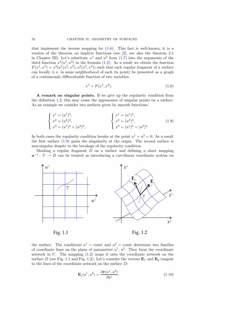
76 CHAPTER IV. GEOMETRY OF SURFACES.
that implement the inverse mapping for (1.6). This fact is well-known, it is aversion of the theorem on implicit functions (see [2], see also the theorem 2.1in Chapter III). Let’s substitute u1 and u2 from (1.7) into the arguments of thethird function x3(u1, u2) in the formula (1.2). As a result we obtain the functionF (x1, x2) = x3(u1(x2, x2), u2(x2, x2)) such that each regular fragment of a surfacecan locally (i. e. in some neighborhood of each its point) be presented as a graphof a continuously differentiable function of two variables:
x3 = F (x1, x2). (1.8)
A remark on singular points. If we give up the regularity condition fromthe definition 1.2, this may cause the appearance of singular points on a surface.As an example we consider two surfaces given by smooth functions:
x1 = (u1)3,
x2 = (u2)3,
x3 = (u1)2 + (u2)2,
x1 = (u1)3,
x2 = (u2)3,
x3 = (u1)4 + (u2)4.
(1.9)
In both cases the regularity condition breaks at the point u1 = u2 = 0. As a resultthe first surface (1.9) gains the singularity at the origin. The second surface isnon-singular despite to the breakage of the regularity condition.
Marking a regular fragment D on a surface and defining a chart mappingu−1 : U → D can be treated as introducing a curvilinear coordinate system on
the surface. The conditions u1 = const and u2 = const determine two familiesof coordinate lines on the plane of parameters u1, u2. They form the coordinatenetwork in U . The mapping (1.2) maps it onto the coordinate network on thesurface D (see Fig. 1.1 and Fig. 1.2). Let’s consider the vectors E1 and E2 tangentto the lines of the coordinate network on the surface D:
Ei(u1, u2) =
∂r(u1, u2)
∂ui. (1.10)
§ 1. PARAMETRIC SURFACES. 77
The formula (1.10) defines a pair of tangent vectors E1 and E2 attached to eachpoint of the surface D.
The vector-function r(u1, u2) which defines the mapping (1.2) can be written inform of the expansion in the basis of the auxiliary Cartesian coordinate system:
r(u1, u2) =
3∑
q=1
xq(u1, u2) · eq. (1.11)
Substituting the expansion (1.11) into (1.10) we can express the tangent vectorsE1 and E2 through the basis vectors e1, e2, e3:
Ei(u1, u2) =
3∑
q=1
∂xq(u1, u2)
∂ui· eq. (1.12)
Let’s consider the column-vectors composed by the Cartesian coordinates of thetangent vectors E1 and E2:
E1 =
∥
∥
∥
∥
∥
∥
∥
∥
∥
∥
∥
∥
∥
∂x1
∂u1
∂x2
∂u1
∂x3
∂u1
∥
∥
∥
∥
∥
∥
∥
∥
∥
∥
∥
∥
∥
, E2 =
∥
∥
∥
∥
∥
∥
∥
∥
∥
∥
∥
∥
∥
∂x1
∂u2
∂x2
∂u2
∂x3
∂u2
∥
∥
∥
∥
∥
∥
∥
∥
∥
∥
∥
∥
∥
. (1.13)
Note that the column-vectors (1.13) coincide with the columns in the Jacobimatrix (1.3). However, from the regularity condition (see the definition 1.1) itfollows that the column of the Jacobi matrix (1.3) are linearly independent. Thisconsideration proves the following proposition.
Theorem 1.1. The tangent vectors E1 and E2 are linearly independent at eachpoint of a surface. Therefore, they form the frame of the tangent vector fields in D.
The frame vectors E1 and E2 attached to some point of a surface D define thetangent plane at this point. Any vector tangent to the surface at this point liesin the tangent plane, it can be expanded in the basis formed by the vectors E1
and E2. Let’s consider some arbitrary curve γ lying completely on the surface (seeFig. 1.1 and Fig. 1.2). In parametric form such a curve is given by two functionsof a parameter t. They define the curve as follows:
u1 = u1(t),
u2 = u2(t).(1.14)
By substituting (1.14) into (1.11) or into (1.2) we find the radius-vector of a pointof the curve in the auxiliary Cartesian coordinate system r(t) = r(u1(t), u2(t)).Let’s differentiate r(t) with respect to t and find the tangent vector of the curvegiven by the above two functions (1.14):
τ (t) =dr
dt=
2∑
i=1
∂r
∂ui· du
i
dt.
CopyRight c© Sharipov R.A., 1996, 2004.
78 CHAPTER IV. GEOMETRY OF SURFACES.
Comparing this expression with (1.10), we find that τ is expressed as follows:
τ (t) =
2∑
i=1
ui ·Ei. (1.15)
Due to (1.15) the vector τ is a linear combination of the vectors E1 and E2
forming the tangent frame. Hence, if a curve γ lies completely on the surface, itstangent vector lies on the tangent plane to this surface, while the derivatives ofthe functions (1.14) are the components of the vector τ expanded in the basis ofthe frame vectors E1 and E2.
§ 2. Change of curvilinear coordinates on a surface.
Let’s consider two regular fragments D1 and D2 on some surface, each equippedwith with its own curvilinear coordinate system. Assume that their intersectionD = D1 ∩D2 is not empty. Then in D we have two curvilinear coordinate systemsu1, u2 and u1, u2. Denote by U and U the preimages of D under the correspondingchart mappings (see Fig. 3.1 in Chapter III). Due to the bijectivity of the chartmappings (see definition 1.2) we can construct two mappings
u u−1 : U → U , u u−1 : U → U. (2.1)
The mappings u u−1 and u u−1 in (2.1) are also bijective, they can be repre-sented by the following pairs of functions:
u1 = u1(u1, u2),
u2 = u2(u1, u2).
u1 = u1(u1, u2),
u2 = u2(u1, u2).(2.2)
Theorem 2.1. The functions (2.2) representing u u−1 and u u−1 are conti-nuously differentiable.
Proof. We shall prove the continuous differentiability of the second pair offunctions (2.2). For the first pair the proof is analogous. Let’s choose some pointon the chart U and map it to D. Then we choose a suitable Cartesian coordinatesystem in E such that the condition (1.5) is fulfilled and in some neighborhood ofthe mapped point there exists the mapping (1.7) inverse for (1.6). The mapping(1.7) is continuously differentiable.
The other curvilinear coordinate system in D induces the other pair of functionsthat plays the same role as the functions (1.6):
x1 = x1(u1, u2),
x2 = x2(u1, u2).(2.3)
These are two of three functions that determine the mapping u−1 in form of (1.2).The functions u1 = u1(u1, u2) and u2 = u2(u1, u2) that determine the mappingu u−1 in (2.2) are obtained by substituting (2.3) into the arguments of (1.7):
u1 = u1(x1(u1, u2), x2(u1, u2)),
u2 = u2(x1(u1, u2), x2(u1, u2)).(2.4)
§ 2. CHANGE OF CURVILINEAR COORDINATES ON A SURFACE. 79
The compositions of continuously differentiable functions in (2.4) are continuouslydifferentiable functions. This fact completes the proof of the theorem.
The functions (2.2), whose continuous differentiability was proved just above,perform the transformation or the change of curvilinear coordinates on a surface.They are analogous to the functions (3.5) in Chapter III.
A remark on the smoothness. If the functions (1.2) of both coordinatesystems u1, u2 and u1, u2 belong to the smoothness class Cm, then the transitionfunctions (2.2) also belong to the smoothness class Cm.
Let r(u1, u2) and r(u1, u2) be two vector-functions of the form (1.2) for twocurvilinear coordinate systems in D. They define the mappings u−1 and u−1
acting from the charts U and U to D. Due to the identity u−1 = u−1 (u u−1)
the function r(u1, u2) is obtained by substituting the corresponding transitionfunctions (2.2) into the arguments of r(u1, u2):
r(u1, u2) = r(u1(u1, u2), u2(u1, u2)). (2.5)
Let’s differentiate (2.5) with respect to uj and take into account the chain ruleand the formula (1.10) for the vectors of the tangent frame:
Ej =∂r
∂uj=
2∑
i=1
∂r
∂ui· ∂u
i
∂uj=
2∑
i=1
∂ui
∂uj·Ei.
Differentiating the identity r(u1, u2) = r(u1(u1, u2), u2(u1, u2)), we derive theanalogous relationship inverse to the previous one:
Ei =∂r
∂ui=
2∑
k=1
∂r
∂uk· ∂u
k
∂ui=
2∑
i=1
∂uk
∂ui· Ek.
It is clear that the above relationships describe the direct and inverse transitionsfrom some tangent frame to another. Let’s write them as
Ej =
2∑
i=1
Sij ·Ei, Ei =
2∑
k=1
T ki · Ek, (2.6)
where the components of the matrices S and T are given by the formulas
Sij(u
1, u2) =∂ui
∂uj, T k
i (u1, u2) =∂uk
∂ui. (2.7)
From (2.7), we see that the transition matrices S and T are the Jacobi matricesfor the mappings given by the transition functions (2.2). They are non-degenerateand are inverse to each other.
The transformations (2.2) and the transition matrices S and T related to themare used in order to construct the theory of tensors and tensor fields analogous tothat which we considered in Chapter II and Chapter III. Tensors and tensor fieldsdefined through the transformations (2.2) and transition matrices (2.7) are calledinner tensors and inner tensor fields on a surface:
F i1... ir
j1... js=∑
p1 ... pr
q1... qs
Si1p1. . . Sir
prT q1
j1. . . T qs
jsF p1... pr
q1... qs. (2.8)
80 CHAPTER IV. GEOMETRY OF SURFACES.
Definition 2.1. An inner tensor of the type (r, s) on a surface is a geometricobject F whose components in an arbitrary curvilinear coordinate system on thatsurface are enumerated by (r+ s) indices and under a change of coordinate systemare transformed according to the rule (2.8).
The formula (2.8) differs from the formula (1.6) in Chapter II only in the rangeof indices. Each index here runs over the range of two values 1 and 2. Bysetting the sign factor (−1)S = sign(det S) = ±1 into the formula (2.8) we get thedefinition of an inner pseudotensor
F i1... ir
j1... js=∑
p1... pr
q1 ... qs
(−1)S Si1p1. . . Sir
prT q1
j1. . . T qs
jsF p1... pr
q1... qs. (2.9)
Definition 2.3. An inner pseudotensor of the type (r, s) on a surface isa geometric object F whose components in an arbitrary curvilinear coordinatesystem on that surface are enumerated by (r + s) indices and under a change ofcoordinate system are transformed according to the rule (2.9).
Inner tensorial and pseudotensorial fields are obtained by defining an innertensor or pseudotensor at each point of a surface. The operations of addition,tensor product, contraction, transposition of indices, symmetrization and alter-nation for such fields are defined in a way similar to that of the case of the fieldsin the space E (see Chapter II). All properties of these operations are preserved.
A remark on the differentiation. The operation of covariant differentiationof tensor fields in the space E was first introduced for Cartesian coordinatesystems. Then it was extended to the case of curvilinear coordinates. On surfaces,as a rule, there is no Cartesian coordinate system at all. Therefore, the operationof covariant differentiation for inner tensor fields on a surface should be defined ina somewhat different way.
§ 3. The metric tensor and the area tensor.
The choice of parameters u1, u2 on a surface determines the tangent frameE1, E2 on that surface. Let’s consider the scalar products of the vectors E1, E2
forming the tangent frame of the surface:
gij = (Ei |Ej). (3.1)
They compose the 2 × 2 Gram matrix g which is symmetric, non-degenerate, andpositive. Therefore, we have the inequality
detg > 0. (3.2)
Substituting (2.6) into (3.1), we find that under a change of a coordinate systemthe quantities (3.1) are transformed as the components of an inner tensorial field ofthe type (0, 2). The tensor g with the components (3.1) is called the metric tensorof the surface. Note that the components of the metric tensor are determined bymeans of the scalar product in the outer space E. Therefore, we say that thetensor field g is induced by the outer scalar product. For this reason the tensor g
is called the metric tensor of the induced metric.
§ 3. THE METRIC TENSOR AND THE AREA TENSOR. 81
Symmetric tensors of the type (0, 2) are related to quadratic forms. This factyields another title for the tensor g. It is called the first quadratic form of asurface. Sometimes, for the components of the first quadratic form the specialnotations are used: g11 = E, g12 = g21 = F , g22 = G. These notations areespecially popular in the earlier publications on the differential geometry:
gij =
∥
∥
∥
∥
E FF G
∥
∥
∥
∥
(3.3)
Since the Gram matrix g is non-degenerate, we can define the inverse matrixg = g−1. The components of such inverse matrix are denoted by gij, setting theindices i and j to the upper position:
3∑
j=1
gij gjk = δij . (3.4)
For the matrix g the proposition analogous to the theorem 6.1 from Chapter IIis valid. The components of this matrix define an inner tensor field of the type(2, 0) on a surface, this field is called the inverse metric tensor or the dual metrictensor. The proof of this proposition is completely analogous to the proof of thetheorem 6.1 in Chapter II. Therefore, here we do not give this proof.
From the symmetry of the matrix g and from the relationships (3.4) it followsthat the components of the inverse matrix g are symmetric. The direct and inversemetric tensors are used in order to lower and raise indices of tensor fields. Theseoperations are defined by the formulas analogous to (9.1) and (9.2) in Chapter II:
Bi1 ... ir−1
j1... js+1=
2∑
k=1
Ai1... im−1 k im... ir−1
j1... jn−1 jn+1 ... js+1gkjn
,
Ai1... ir+1
j1... js−1=
2∑
k=1
Bi1 ... im−1 im+1... ir+1
j1 ... jn−1 q jn... js−1gqim .
(3.5)
The only difference of the formulas (3.5) here is that the summation index k runsover the range of two numbers 1 and 2. Due to (3.4) the operations of raising andlowering indices (3.5) are inverse to each other.
In order to define the area tensor (or the area pseudotensor) we need thefollowing skew-symmetric 2 × 2 matrix:
dij = d ij =
∥
∥
∥
∥
0 1−1 0
∥
∥
∥
∥
. (3.6)
The quantities (3.6) form the two-dimensional analog of the Levi-Civita symbol(see formula (6.8) in Chapter II). These quantities satisfy the relationship
2∑
p=1
2∑
q=1
dpq MipMjq = det M dij, (3.7)
where M is some arbitrary square 2 × 2 matrix. The formula (3.7) is an analog ofthe formula (6.10) from Chapter II (see proof in [4]).
82 CHAPTER IV. GEOMETRY OF SURFACES.
Using the quantities dij and the matrix of the metric tensor g in some curvilin-ear coordinate system, we construct the following quantities:
ωij =√
det g dij. (3.8)
From (3.7) one can derive the following relationship linking the quantities ωij andωpq defined according to the formula (3.8) in two different coordinate systems:
ωij = sign(det S)
3∑
p=1
3∑
q=1
T pi T
qj ωpq . (3.9)
Due to (3.9) the quantities (3.8) define a skew-symmetric inner pseudotensorialfield of the type (0, 2). It is called the area pseudotensor. If on a surface D one ofthe two possible orientations is marked, then the formula
ωij = ξD√
detg dij (3.10)
defines a tensorial field of the type (0, 2). It is called the area tensor. The formula(3.10) differs from (3.8) only in sign factor ξD which is the unitary pseudoscalarfield defining the orientation (compare with the formula (8.1) in Chapter II). Hereone should note that not any surface admits some preferable orientation globally.The Mobius strip is a well-known example of a non-orientable surface.
§ 4. Moving frame of a surface.
Veingarten’s derivational formulas.
Each choice of a curvilinear coordinate system on a surface determines someframe of two tangent vectorial fields E1, E2 on it. The vectors of such aframe define the tangent plane at each point of the surface. However, they areinsufficient for to expand an arbitrary vector of the space E at that point of thesurface. Therefore, they are usually completed by a vector that does not belong tothe tangent plane.
Definition 4.1. A unit normal vector n to a surface D at a point A is avector of the unit length attached to the point A and perpendicular to all vectorsof the tangent plane to D at that point.
The definition 4.1 fixes the unit normal vector n only up to the sign: at eachpoint there are two opposite unit vectors perpendicular to the tangent plane. Oneof the ways to fix n uniquely is due to the vector product:
n =[E1, E2]
|[E1, E2]|. (4.1)
The vector n determined by the formula (4.1) depends on the choice of a curvi-linear coordinate system. Therefore, under a change of coordinate system it canchange its direction. Indeed, the relation of the frame vectors E1,E2 and E1, E2
is given by the formula (2.6). Therefore, we write
E1 = T 11 · E1 + T 2
1 · E2, E2 = T 12 · E1 + T 2
2 · E2.
§ 4. VEINGARTEN’S DERIVATIONAL FORMULAS. 83
Substituting these expressions into the vector product [E1, E2], we obtain
[E1, E2] = (T 11 T
22 − T 2
1 T12 ) · [E1, E2] = det T · [E1, E2].
Now we easily derive the transformation rule for the normal vector n:
n = (−1)S · n. (4.2)
The sign factor (−1)S = sign(detS) = ±1 here is the same as in the formula (2.8).Another way of choosing the normal vector is possible if there is a preferable
orientation on a surface. Suppose that this orientation on D is given by theunitary pseudoscalar field ξD. Then n is given by the formula
n = ξD · [E1, E2]
|[E1, E2]|. (4.3)
In this case the transformation rule for the normal vector simplifies substantially:
n = n. (4.4)
Definition 4.2. The tangent frame E1, E2 of a curvilinear coordinate systemu1, u2 on a surface completed by the unit normal vector n is called the movingframe or the escort frame of this surface.
If the normal vector is chosen according to the formula (4.1), the escort frameE1, E2, n is always right-oriented. Therefore, in this case if we change theorientation of the tangent frame E1, E2, the direction of the normal vector n ischanged immediately. In the other case, if n is determined by the formula (4.3),then its direction does not depend on the choice of the tangent frame E1, E2. Thisfact means that the choice of the orientation on a surface is equivalent to choosingthe normal vector independent on the choice tangent vectors E1,E2.
There is a special case, when such an independent choice of the normal vectordoes exist. Let D be the boundary of a three-dimensional domain. Then one oftwo opposite normal vectors is the inner normal, the other is the outer normalvector. Thus, we conclude that the boundary of a three-dimensional domain inthe space E is always orientable.
Let D be some fragment of a surface of the smoothness class C2. The vectors ofthe escort frame of such a surface are continuously differentiable vector-functionsof curvilinear coordinates: E1(u
1, u2), E2(u1, u2), and n(u1, u2). The derivatives
of such vectors are associated with the same point on the surface. Hence, we canwrite the following expansions for them:
∂Ej
∂ui=
2∑
k=1
Γkij ·Ek + bij · n. (4.5)
The derivatives of the unit vector n are perpendicular to this vector (see lemma 3.1in Chapter I). Hence, we have the equality
∂n
∂ui=
2∑
k=1
cki ·Ek. (4.6)
84 CHAPTER IV. GEOMETRY OF SURFACES.
Let’s consider the scalar product of (4.5) and the vector n. We also consider thescalar product of (4.6) and the vector Ej . Due to (Ek|n) = 0 we get
(∂Ej/∂ui |n) = bij (n |n) = bij, (4.7)
(Ej | ∂n/∂ui) =
2∑
k=1
cki gkj. (4.8)
Let’s add the left hand sides of the above formulas (4.7) and (4.8). Upon rathereasy calculations we find that the sum is equal to zero:
(∂Ej/∂ui |n) + (Ej | ∂n/∂ui) = ∂(Ej |n)/∂ui = 0.
From this equality we derive the relations of bij and ckj in (4.5) and (4.6):
bij = −2∑
k=1
cki gkj.
By means of the matrix of the inverse metric tensor g we can invert this relation-ship. Let’s introduce the following quite natural notation:
bki =
2∑
j=1
bij gjk. (4.9)
Then the coefficients cki in (4.6) can be expressed through the coefficients bij in(4.5) by means of the following formula:
cki = −bki . (4.10)
Taking into account (4.10), we can rewrite (4.5) and (4.6) as follows:
∂Ej
∂ui=
2∑
k=1
Γkij ·Ek + bij · n,
∂n
∂ui= −
2∑
k=1
bki ·Ek.
(4.11)
The expansions (4.5) and (4.6) written in form of (4.11) are called the Veingarten’sderivational formulas. They determine the dynamics of the moving frame and playthe central role in the theory of surfaces.
§ 5. Christoffel symbols
and the second quadratic form.
Let’s study the first Veingarten’s derivational formula in two different coordinatesystems u1, u2 and u1, u2 on a surface. In the coordinates u1, u2 it is written as
∂Ej
∂ui=
2∑
k=1
Γkij ·Ek + bij · n. (5.1)
CopyRight c© Sharipov R.A., 1996, 2004.
§ 5. CHRISTOFFEL SYMBOLS AND THE SECOND QUADRATIC FORM. 85
In the other coordinates u1, u2 this formula is rewritten as
∂Eq
∂up=
2∑
m=1
Γmpq · Em + bpq · n. (5.2)
Let’s express the vector Ej in the left hand side of the formula (5.1) through theframe vectors of the second coordinate system. For this purpose we use (2.6):
∂Ej
∂ui=
2∑
q=1
∂(T qj · Eq)
∂ui=
2∑
q=1
∂T qj
∂ui· Eq +
2∑
q=1
T qj · ∂Eq
∂ui.
For the further transformation of the above expression we use the chain rule fordifferentiating the composite function:
∂Ej
∂ui=
2∑
m=1
∂Tmj
∂ui· Em +
2∑
q=1
2∑
p=1
(
T qj
∂up
∂ui
)
· ∂Eq
∂up.
The values of the partial derivatives ∂Eq/∂up are determined by the formula (5.2).
Moreover, we should take into account (2.7) in form of the equality ∂up/∂ui = T pi :
∂Ej
∂ui=
2∑
m=1
∂Tmj
∂ui· Em +
2∑
q=1
2∑
p=1
2∑
m=1
(T qj T
pi Γm
pq) · Em+
+
2∑
q=1
2∑
p=1
(T qj T
pi bpq) · n =
2∑
m=1
2∑
k=1
(
∂Tmj
∂uiSk
m
)
·Ek+
+
2∑
q=1
2∑
p=1
2∑
m=1
2∑
k=1
(T qj T
pi Γm
pq Skm) ·Ek +
2∑
q=1
2∑
p=1
(T qj T
pi bpq) · n.
The unit normal vectors n and n can differ only in sign: n = ±n. Hence, theabove expansion for ∂Ej/∂u
i and the expansion (5.1) both are the expansions inthe same basis E1, E2, n. Therefore, we have
Γkij =
2∑
m=1
Skm
∂Tmj
∂ui+
2∑
m=1
2∑
p=1
2∑
q=1
Skm T p
i Tqj Γm
pq, (5.3)
bij = ±2∑
p=1
2∑
q=1
T pi T
qj bpq. (5.4)
The formulas (5.3) and (5.4) express the transformation rules for the coefficientsΓk
ij and bij in Veingarten’s derivational formulas under a change of curvilinearcoordinates on a surface.
In order to make certain the choice of the sign in (5.4) one should fix some rulefor choosing the unit normal vector. If we choose n according to the formula (4.1),then under a change of coordinate system it obeys the transformation formula(4.2). In this case the equality (5.4) is written as
bij =
2∑
p=1
2∑
q=1
(−1)S T pi T
qj bpq. (5.5)
86 CHAPTER IV. GEOMETRY OF SURFACES.
It is easy to see that in this case bij are the components of an inner pseudotensorialfield of the type (0, 2) on a surface.
Otherwise, if we use the formula (4.3) for choosing the normal vector n, then n
does not depend on the choice of a curvilinear coordinate system on a surface (seeformula (4.4)). In this case bij are transformed as the components of a tensorialfield of the type (0, 2). The formula (5.4) then takes the form
bij =
2∑
p=1
2∑
q=1
T pi T
qj bpq. (5.6)
Tensors of the type (0, 2) correspond to bilinear and quadratic forms. Pseudo-tensors of the type (0, 2) have no such interpretation. Despite to this fact thequantities bij in Veingarten’s derivational formulas are called the components ofthe second quadratic form b of a surface. The following theorem supports thisinterpretation.
Theorem 5.1. The quantities Γkij and bij in Veingarten’s derivational formulas
(4.11) are symmetric with respect to the lower indices i and j.
Proof. In order to prove the theorem we apply the formula (1.10). Let’s writethis formula in the following way:
Ej(u1, u2) =
∂r(u1, u2)
∂uj. (5.7)
Then let’s substitute (5.7) into the first formula (4.11):
∂2r(u1, u2)
∂ui ∂uj=
2∑
k=1
Γkij ·Ek + bij · n. (5.8)
The values of the mixed partial derivatives do not depend on the order ofdifferentiation. Therefore, the left hand side of (5.8) is a vector that does notchange if we transpose indices i and j. Hence, the coefficients Γk
ij and bij of itsexpansion in the basis E1, E2, n do not change under the transposition of theindices i and j. The theorem is proved.
Sometimes, for the components of the matrix of the second quadratic form thenotations similar to (3.3) are used:
bij =
∥
∥
∥
∥
L MM N
∥
∥
∥
∥
. (5.9)
These notations are especially popular in the earlier publications.The tensor fields g and b define a pair of quadratic forms at each point of a
surface. This fact explains in part their titles — the first and the second quadraticforms. The first quadratic form is non-degenerate and positive. This situation iswell-known in linear algebra (see [1]). Two forms, one of which is positive, can bebrought to the diagonal form simultaneously, the matrix of the positive form beingbrought to the unit matrix. The diagonal elements of the second quadratic form
§ 5. CHRISTOFFEL SYMBOLS AND THE SECOND QUADRATIC FORM. 87
upon such diagonalization are called the invariants of a pair of forms. In order tocalculate these invariants we consider the following contraction:
bki =2∑
j=1
bij gjk. (5.10)
The quantities bki enter the second Veingarten’s derivational formula (4.11). Theydefine a tensor field (or a pseudotensorial field) of the type (1, 1), i. e. an operatorfield. The operator with the matrix (5.10) is called the Veingarten operator. Thematrix of this operator is diagonalized simultaneously with the matrices of thefirst and the second quadratic forms, and its eigenvalues are exactly the invariantsof that pair of forms. Let’s denote them by k1 and k2.
Definition 5.1. The eigenvalues k1(u1, u2) and k2(u
1, u2) for the matrix ofthe Veingarten operator are called the principal curvatures of a surface at its pointwith the coordinates u1, u2.
From the computational point of view the other two invariants are moreconvenient. These are the following ones:
H =k1 + k2
2, K = k1 k2. (5.11)
The invariants (5.11) can be calculated without knowing the eigenvalues of thematrix bki . It is sufficient to find the trace for the matrix of the Veingartenoperator and the determinant of this matrix:
H =1
2tr(bki ), K = det(bki ). (5.12)
The quantity H in the formulas (5.11) and (5.12) is called the mean curvature,while the quantity K is called the Gaussian curvature. There are formulas,expressing the invariants H and K through the components of the first and thesecond quadratic forms (3.3) and (5.9):
H =1
2
EN + GL− 2FM
EG− F 2, K =
LN −M 2
EG− F 2. (5.13)
Let v(u1, u2) and w(u1, u2) be the vectors of the basis in which the matrix ofthe first quadratic form is equal to the unit matrix, while the matrix of the secondquadratic form is a diagonal matrix:
v =
∥
∥
∥
∥
v1
v2
∥
∥
∥
∥
, w =
∥
∥
∥
∥
w2
w2
∥
∥
∥
∥
. (5.14)
Then v and w are the eigenvectors of the Veingarten operator. The vectors (5.14)have their three-dimensional realization in the space E:
v = v1 ·E1 + v2 ·E2, w = w1 ·E1 + w2 ·E2. (5.15)
This is the pair of the unit vectors lying on the tangent plane and being per-pendicular to each other. The directions given by the vectors (5.15) are called
88 CHAPTER IV. GEOMETRY OF SURFACES.
the principal directions on a surface at the point with coordinates u1, u2. If theprincipal curvatures at this point are not equal to each other: k1 6= k2, then theprincipal directions are determined uniquely. Otherwise, if k1 = k2, then anytwo mutually perpendicular directions on the tangent plane can be taken for theprincipal directions. A point of a surface where the principal curvatures are equalto each other (k1 = k2) is called an umbilical point.
A remark on the sign. Remember that depending on the way how we choosethe normal vector the second quadratic form is either a tensorial field or apseudotensorial field. The same is true for the Veingarten operator. Therefore,in general, the principal curvatures k1 and k2 are determined only up to the sign.The mean curvature H is also determined only up to the sign. As for the Gaussiancurvature, it has no uncertainty in sign. Moreover, the sign of the Gaussiancurvature divides the points of a surface into three subsets: for any point of asurface if K > 0, the point is called an elliptic point; if K < 0, the point is calleda hyperbolic point; and finally, if K = 0, the point is called a parabolic point.
§ 6. Covariant differentiation
of inner tensorial fields of a surface.
Let’s consider the formula (5.3) and compare it with the formula (6.1) inChapter III. These two formulas differ only in the ranges over which the indicesrun. Therefore the quantities Γk
ij, which appear as coefficients in the Veingarten’sderivational formula, define a geometric object on a surface that is called aconnection. The connection components Γk
ij are called the Christoffel symbols.
The main purpose of the Christoffel symbols Γkij is their usage for the covariant
differentiation of tensor fields. Let’s reproduce here the formula (5.12) fromChapter III for the covariant derivative modifying it for the two-dimensional case:
∇js+1Ai1... ir
j1... js=∂Ai1... ir
j1... js
∂ujs+1+
+
r∑
m=1
2∑
vm=1
Γim
js+1 vmAi1... vm... ir
j1... js−
s∑
n=1
2∑
wn=1
Γwn
js+1 jnAi1... ir
j1... wn ... js.
(6.1)
Theorem 6.1. The formula (6.1) correctly defines the covariant differentiationof inner tensor fields on a surface that transforms a field of the type (r, s) into afield of the type (r, s+ 1) if and only if the quantities Γk
ij obey the transformation
rule (5.3) under a change of curvilinear coordinates on a surface.
Proof. Let’s begin with proving the necessity. For this purpose we choosesome arbitrary vector field A and produce the tensor field B = ∇A of the type(1, 1) by means of the formula (6.1). The correctness of the formula (6.1) meansthat the components of the field B are transformed according to the formula (2.8).From this condition we should derive the transformation formula (5.3) for thequantities Γk
ij in (6.1). Let’s write the formula (2.8) for the field B = ∇A:
∂Ak
∂ui+
2∑
j=1
Γkij A
j =
2∑
m=1
2∑
p=1
Skm T p
i
(
∂Am
∂up+
2∑
q=1
Γmpq A
q
)
.
§ 6. COVARIANT DIFFERENTIATION . . . 89
Then we expand the brackets in the right hand side of this relationship. In thefirst summand we replace T p
i by ∂up/∂ui according to the formula (2.7) and we
express Am through Aj according to the transformation rule for a vector field:
2∑
p=1
T pi
∂Am
∂up=
2∑
p=1
∂up
∂ui
∂Am
∂up=∂Am
∂ui=
=∂
∂ui
(
2∑
k=1
Tmk Ak
)
=2∑
j=1
∂Tmj
∂uiAj +
2∑
j=1
Tmj
∂Aj
∂ui.
(6.2)
Taking into account (6.2), we can cancel the partial derivatives in the previousequality and bring it to the following form:
2∑
j=1
Γkij A
j =
2∑
j=1
2∑
m=1
Skm
∂Tmj
∂uiAj +
2∑
m=1
2∑
p=1
2∑
q=1
Skm T p
i Γmpq A
q.
Now we need only to express Aq through Aj applying the transformation rule forthe components of a vectorial field and then extract the common factor Aj:
2∑
j=1
(
Γkij −
2∑
m=1
Skm
∂Tmj
∂ui−
2∑
m=1
2∑
p=1
2∑
q=1
Skm T p
i Tqj Γm
pq
)
Aj = 0.
Since A is an arbitrary vector field, each coefficient enclosed into round bracketsin the above sum should vanish separately. This condition coincides exactly withthe transformation rule (5.3). Thus, the necessity is proved.
Let’s proceed with proving the sufficiency. Suppose that the condition (5.3)is fulfilled. Let’s choose some tensorial field A of the type (r, s) and prove that
the quantities ∇js+1Ai1... ir
j1... jsdetermined by the formula (6.1) are transformed as
the components of a tensorial field of the type (r, s+ 1). Looking at the formula
(6.1) we see that it contains the partial derivative ∂Ai1... ir
j1... js/∂ujs+1 and other r+ s
terms. Let’s denote these terms by Ai1... ir
j1... js+1
[
m0
]
and Ai1 ... ir
j1 ... js+1
[
0n
]
. Then
∇js+1Ai1... ir
j1... js= ∂Ai1... ir
j1... js/∂ujs+1 +
+
r∑
m=1
Ai1... ir
j1... js+1
[
m0
]
−s∑
n=1
Ai1... ir
j1... js+1
[
0n
]
.(6.3)
The tensorial nature of A means that its components are transformed accordingto the formula (2.8). Therefore, in the first term of (6.3) we get:
∂Ai1 ... ir
j1 ... js
∂ujs+1=
∂
∂ujs+1
∑
p1... pr
q1... qs
Si1p1. . . Sir
prT q1
j1. . . T qs
jsAp1... pr
q1 ... qs
=
=∑
p1 ... pr
q1 ... qs
2∑
qs+1=1
Si1p1. . . Sir
prT q1
j1. . . T qs
js
∂uqs+1
∂ujs+1
∂Ap1 ... pr
q1 ... qs
∂uqs+1+
90 CHAPTER IV. GEOMETRY OF SURFACES.
+
r∑
m=1
∑
p1 ... pr
q1... qs
Si1p1. . .
∂Sim
pm
∂ujs+1. . . Sir
prT q1
j1. . . T qs
jsAp1 ... pr
q1 ... qs+
+
s∑
n=1
∑
p1 ... pr
q1... qs
Si1p1. . . Sir
prT q1
j1. . .
∂T qn
jn
∂ujs+1. . . T qs
jsAp1 ... pr
q1 ... qs.
Here we used the Leibniz rule for differentiating the product of multiple functionsand the chain rule in order to express the derivatives with respect to ujs+1 throughthe derivatives with respect to uqs+1 . For the further transformation of the aboveformula we replace ∂uqs+1/∂ujs+1 by T
qs+1
js+1according to (2.7) and we use the
following identities based on the fact that S and T are mutually inverse matrices:
∂Sim
pm
∂ujs+1= −
2∑
vm=1
2∑
k=1
Sim
vm
∂T vm
k
∂ujs+1Sk
pm,
∂T qn
jn
∂ujs+1=
2∑
wn=1
2∑
k=1
Twn
jnSk
wn
∂T qn
k
∂ujs+1.
(6.4)
Upon substituting (6.4) into the preceding equality it is convenient to transposethe summation indices: pm with vm and qn with wn. Then we get
∂Ai1... ir
j1... js
∂ujs+1=∑
p1 ... pr
q1... qs
Si1p1. . . Sir
prT q1
j1. . . T qs
js×
×(
2∑
qs+1=1
Tqs+1
js+1
Ap1 ... pr
q1 ... qs
∂uqs+1−
r∑
m=1
V[
m0
]
+
s∑
n=1
W[
0n
]
)
,
(6.5)
where the following notations are used for the sake of simplicity:
V[
m0
]
=2∑
vm=1
2∑
k=1
Skvm
∂T pm
k
∂ujs+1Ap1... vm ... pr
q1... qs,
W[
0n
]
=
2∑
wn=1
2∑
k=1
Skqn
∂Twn
k
∂ujs+1Ap1... pr
q1... wn... qs.
(6.6)
No let’s consider Ai1... ir
j1... js+1
[
m0
]
in (6.3). They are obviously defined as follows:
Ai1 ... ir
j1 ... js+1
[
m0
]
=
2∑
vm=1
Γim
js+1 vmAi1... vm... ir
j1... js.
Applying the transformation rule (2.8) to the components of the field A, we get:
Ai1... ir
j1... js+1
[
m0
]
=∑
p1... pr
q1... qs
2∑
vm=1
Si1p1. . . Svm
pm. . . Sir
pr×
× T q1
j1. . . T qs
jsΓim
js+1 vmAp1... pr
q1... qs.
(6.7)
§ 6. COVARIANT DIFFERENTIATION . . . 91
For the further transformation of the above expression we use (5.3) written as
Γim
js+1 vm=
2∑
k=1
Sim
k
∂T kvm
∂ujs+1+
2∑
k=1
2∑
q=1
2∑
qs+1=1
Sim
k Tqs+1
js+1T q
vmΓk
qs+1 q .
Immediately after substituting this expression into (6.7) we perform the cyclictransposition of the summation indices: r → pm → vm → r. Some sums in theresulting expression are evaluated explicitly if we take into account the fact thatthe transition matrices S and T are inverse to each other:
Ai1... ir
j1... js+1
[
m0
]
=∑
p1 ... pr
q1... qs
Si1p1. . . Sir
prT q1
j1. . . T qs
js×
×(
2∑
qs+1=1
Tqs+1
js+1Ap1... pr
q1... qs+1
[
m0
]
+ V[
m0
]
)
.
(6.8)
By means of the analogous calculations one can derive the following formula:
Ai1 ... ir
j1 ... js+1
[
0n
]
=∑
p1 ... pr
q1... qs
Si1p1. . . Sir
prT q1
j1. . . T qs
js×
×(
2∑
qs+1=1
Tqs+1
js+1Ap1... pr
q1... qs+1
[
0n
]
+W[
0n
]
)
.
(6.9)
Now we substitute (6.5), (6.8), and (6.9) into the formula (6.3). Then the entries
of V[
m0
]
and W[
0n
]
do cancel each other. A a residue, upon collecting the similarterms and cancellations, we get the formula expressing the transformation rule(2.8) applied to the components of the field ∇A. The theorem 6.1 is proved.
The theorem 6.1 yields a universal mechanism for constructing the covari-ant differentiation. It is sufficient to have a connection whose components aretransformed according to the formula (5.3). We can compare two connections:the Euclidean connection in the space E constructed by means of the Cartesiancoordinates and a connection on a surface whose components are given by theVeingarten’s derivational formulas. Despite to the different origin of these twoconnections, the covariant derivatives defined by them have many common prop-erties. It is convenient to formulate these properties using covariant derivativesalong vector fields. Let X be a vector field on a surface. For any tensor field A ofthe type (r, s) we define the tensor field B = ∇XA of the same type (r, s) givenby the following formula:
Bi1 ... ir
j1 ... js=
2∑
q=1
Xq ∇qAi1... ir
j1... js. (6.10)
Theorem 6.2. The operation of covariant differentiation of tensor fields posses-ses the following properties:
(1) ∇X(A + B) = ∇XA + ∇XB;(2) ∇X+YA = ∇XA + ∇YA;(3) ∇ξ·XA = ξ · ∇XA;(4) ∇X(A⊗ B) = ∇XA⊗ B + A ⊗∇XB;(5) ∇XC(A) = C(∇XA);
CopyRight c© Sharipov R.A., 1996, 2004.
92 CHAPTER IV. GEOMETRY OF SURFACES.
where A and B are arbitrary differentiable tensor fields, while X and Y are arbi-trary vector fields and ξ is an arbitrary scalar field.
Looking attentively at the theorem 6.2 and at the formula (6.10), we see thatthe theorem 6.2 is a copy of the theorem 5.2 from Chapter II, while the formula(6.10) is a two-dimensional analog of the formula (5.5) from the same Chapter II.However, the proof there is for the case of the Euclidean connection in the spaceE. Therefore we need to give another proof.
Proof. Let’s choose some arbitrary curvilinear coordinate system on a surfaceand prove the theorem by means of direct calculations in coordinates. DenoteC = A + B, where A and B are two tensorial fields of the type (r, s). Then
C i1... ir
j1... js= Ai1... ir
j1... js+ Bi1... ir
j1... js.
Substituting C i1... ir
j1... jsinto (6.1), upon rather simple calculations we get
∇js+1Ci1... ir
j1... js= ∇js+1A
i1... ir
j1... js+ ∇js+1B
i1 ... ir
j1 ... js.
The rest is to multiply both sides of the above equality by Xjs+1 and performsummation over the index js+1. Applying (6.10), we derive the formula of theitem (1) in the theorem.
Note that the quantities Bi1 ... ir
j1 ... jsin the formula (6.10) are obtained as the linear
combinations of the components of X. The items (2) and (3) of the theorem followimmediately from this fact.
Let’s proceed with the item (4). Denote C = A ⊗B. Then for the componentsof the tensor field C we have the equality
Ci1... ir+p
j1... js+q= Ai1... ir
j1... jsB
ir+1 ... ir+p
js+1 ... js+q. (6.11)
Let’s substitute the quantities Ci1... ir+p
j1... js+qfrom (6.11) into the formula (6.1) defining
the covariant derivative. As a result for D = ∇C we derive
Di1... ir+p
j1... js+q+1=(
∂A i1... ir
j1... js/∂ujs+q+1
)
Bir+1... ir+p
js+1... js+q+
+A i1... ir
j1... js
(
∂Bir+1... ir+p
js+1 ... js+q/∂ujs+q+1
)
+
+
r∑
m=1
2∑
vm=1
Γim
js+q+1 vmAi1... vm... ir
j1... jsB
ir+1 ... ir+p
js+1 ... js+q+
+
r+p∑
m=r+1
2∑
vm=1
A i1... ir
j1... jsΓim
js+q+1 vmB
ir+1 ... vm... ir+p
js+1 ... js+q−
−s∑
n=1
2∑
wn=1
Γwn
js+q+1 jnAi1... ir
j1... wn ... jsB
ir+1... ir+p
js+1... js+q−
−s+q∑
n=s+1
2∑
wn=1
A i1... ir
j1... jsΓwn
js+q+1 jnB
ir+1... ir+p
js+1... wn... js+q.
§ 6. COVARIANT DIFFERENTIATION . . . 93
Note that upon collecting the similar terms the above huge formula can betransformed to the following shorter one:
∇js+q+1
(
Ai1... ir
j1... jsB
ir+1 ... ir+p
js+1 ... js+q
)
=(
∇js+q+1Ai1... ir
j1... js
)
×
× Bir+1... ir+p
js+1... js+q+Ai1 ... ir
j1 ... js
(
∇js+q+1Bir+1 ... ir+p
js+1 ... js+q
)
.
(6.12)
Now in order to prove the fourth item of the theorem it is sufficient to multiply(6.12) by Xjs+q+1 and sum up over the index js+q+1.
Proceeding with the last fifth item of the theorem, we consider two tensorialfields A and B one of which is the contraction of another:
Bi1 ... ir
j1 ... js=
2∑
k=1
Ai1... ip−1 k ip... ir
j1... jq−1 k jq... js. (6.13)
Substituting (6.13) into (6.1), for ∇js+1Bi1... ir
j1... jswe obtain
∇js+1Bi1 ... ir
j1 ... js=
2∑
k=1
∂Ai1 ... ip−1 k ip... ir
j1 ... jq−1 k jq... js
∂ujs+1+
+
r∑
m=1
2∑
k=1
2∑
vm=1
Γim
js+1 vmAi1... vm... k ... ir
j1... jq−1 k jq ... js
− (6.14)
−s∑
n=1
2∑
k=1
2∑
wn=1
Γwn
js+1 jnA
i1... ip−1 k ip... ir
j1... wn ... k ... js
.
The index vm in (6.14) can be either to the left of the index k or to the right of it.The same is true for the index wn. However, the formula (6.14) does not comprisethe terms where vm or wn replaces the index k. Such terms would have the form:
2∑
k=1
2∑
v=1
Γkjs+1 v A
i1... ip−1 v ip... ir
j1... jq−1 k jq... js
, (6.15)
−2∑
k=1
2∑
w=1
Γwjs+1 k A
i1... ip−1 k ip... ir
j1... jq−1 w jq ... js. (6.16)
It is easy to note that (6.15) and (6.16) differ only in sign. It is sufficient torename k to v and w to k in the formula (6.16). Adding both (6.15) and (6.16) to(6.14) would not break the equality. But upon adding them one can rewrite theequality (6.14) in the following form:
∇js+1Bi1 ... ir
j1 ... js=
2∑
k=1
∇js+1Ai1... ip−1 k ip... ir
j1... jq−1 k jq... js
. (6.17)
No in order to complete the proof of the item (5), and thus prove the theorem inwhole, it is sufficient to multiply the equality (6.17) by Xjs+1 and sum up over theindex js+1.
94 CHAPTER IV. GEOMETRY OF SURFACES.
Among the five properties of the covariant derivative listed in the theorem 6.2the fourth property written as (6.12) is most often used in calculations. Let’srewrite the equality (6.12) as follows:
∇k
(
Ai1... ir
j1... jsBv1 ... vp
w1 ... wq
)
=(
∇kAi1... ir
j1... js
)
Bv1... vp
w1... wq+ Ai1... ir
j1... js
(
∇kBv1 ... vp
w1 ... wq
)
. (6.18)
The formula (6.18) is produced from (6.12) simply by renaming the indices;however, it is more convenient for reception.
§ 7. Concordance of metric and connection on a surface.
Earlier we have noted that the covariant differential of the metric tensor g
in the Euclidean space E is equal to zero (see formula (6.7) in Chapter II).This property was called the concordance of the metric and connection. Uponpassing to curvilinear coordinates we used this property in order to express thecomponents of the Euclidean connection Γk
ij through the components of the metric
tensor (see formula (7.8) in Chapter III). Let’s study whether the metric and theconnection on surfaces are concordant or not. The answer here is also positive. Itis given by the following theorem.
Theorem 7.1. The components of the metric tensor gij and the connectioncomponents Γk
ij in arbitrary coordinates on a surface are related by the equality
∇kgij =∂gij
∂uk−
2∑
q=1
Γqki gqj −
2∑
q=1
Γqkj giq = 0 (7.1)
which expresses the concordance condition for the metric and connection.
Proof. Let’s consider the first Veingarten’s derivational formula in (4.11) andlet’s rewrite it renaming some indices:
∂Ei
∂uk=
2∑
q=1
Γqki ·Eq + bki · n. (7.2)
Let’s take the scalar products of both sides of (7.2) by Ej and remember that thevectors Ej and n are perpendicular. The scalar product of Eq and Ej in the righthand side yields the element gqj of the Gram matrix:
(∂Ei/∂uk |Ej) =
2∑
q=1
Γqki gqj. (7.3)
Now let’s transpose the indices i and j in (7.3) and take into account the symmetryof the Gram matrix. As a result we obtain
(Ei | ∂Ej/∂uk) =
2∑
q=1
Γqkj giq. (7.4)
§ 7. CONCORDANCE OF METRIC AND CONNECTION ON A SURFACE. 95
Then let’s add (7.3) with (7.4) and remember the Leibniz rule as applied to thedifferentiation of the scalar product in the space E:
(∂Ei/∂uk |Ej) + (Ei | ∂Ej/∂u
k) = ∂(Ei |Ej)/∂uk =
= ∂gij/∂uk =
2∑
q=1
Γqki gqj +
2∑
q=1
Γqkj giq.
Now it is easy to see that the equality just obtained coincides in essential with(7.1). The theorem is proved.
As an immediate consequence of the theorems 7.1 and 5.1 we get the followingformula for the connection components:
Γkij =
1
2
2∑
r=1
gkr( grj
∂ui+
gir
∂uj− gij
∂ur
)
. (7.5)
We do not give its prove here since, in essential, it is the same as in the case ofthe formula (7.8) in Chapter III.
From the condition ∇qgij = 0 one can easily derive that the covariant deriva-tives of the inverse metric tensor are also equal to zero. For this purpose oneshould apply the formula (3.4). The covariant derivatives of the identical operatorfield with the components δi
k are equal to zero. Indeed, we have
∇qδik =
∂(δik)
∂uq+
2∑
r=1
Γiqrδ
rk −
2∑
r=1
Γrqkδ
ir = 0. (7.6)
Let’s differentiate both sides of (3.4) and take into account (7.6):
∇q
(
2∑
j=1
gij gjk
)
=
2∑
j=1
(∇qgij gjk + gij ∇qgjk) =
=
2∑
j=1
∇qgij gjk = ∇qδ
ik = 0. (7.7)
In deriving (7.7) we used the items (4) and (5) from the theorem 6.2. Theprocedure of lowering j by means of the contraction with the metric tensor gjk isan invertible operation. Therefore, (7.7) yields ∇qg
ij = 0. Now the concordancecondition for the metric and connection is written as a pair of two relationships
∇g = 0, ∇g = 0, (7.8)
which look exactly like the relationships (6.7) in Chapter II for the case of metrictensors in the space E.
Another consequence of the theorem 7.1 is that the index raising and the indexlowering operations performed by means of contractions with the metric tensors
96 CHAPTER IV. GEOMETRY OF SURFACES.
g and g commute with the operations of covariant differentiations. This fact ispresented by the following two formulas:
∇q
(
2∑
k=1
gikA... k ...... ...
)
=
2∑
k=1
gik ∇qA... k ...... ...,
∇q
(
2∑
k=1
gikA... ...... k ...
)
=
2∑
k=1
gik ∇qA... ...... k ....
(7.9)
The relationship (7.9) is easily derived from (7.8) using the items (4) and (5) inthe theorem 6.2.
Theorem 7.2. The covariant differential of the area pseudotensor (3.8) on anysurface is equal to zero: ∇ω = 0.
In order to prove this theorem we need two auxiliary propositions which areformulated as the following lemmas.
Lemma 7.1. For any square matrix M whose components are differentiablefunctions of some parameter x the equality
d(lndetM )
dx= tr(M−1M ′) (7.10)
is fulfilled, where M ′ is the square matrix composed by the derivatives of thecorresponding components of the matrix M .
Lemma 7.2. For any square 2 × 2 matrix M the equality
2∑
q=1
(
Miq dqj +Mjq diq
)
= trM dij (7.11)
is fulfilled, where dij are the components of the skew-symmetric matrix determinedby the relationship (3.6).
The proof of these two lemmas 7.1 and 7.2 as well as the proof of the aboveformula (3.7) from § 3 can be found in [4].
Let’s apply the lemma 7.1 to the matrix of the metric tensor. Let x = uk. Thenwe rewrite the relationship (7.10) as follows:
1√det g
∂√
det g
∂uk=
1
2
2∑
q=1
2∑
p=1
gqp ∂gqp
∂uk. (7.12)
Note that in (7.11) any array of four numbers enumerated with two indices canplay the role of the matrix M . Having fixed the index k, one can use the
connection components Γjki as such an array. Then we obtain
2∑
q=1
(
Γqki dqj + Γq
kj diq
)
=
2∑
q=1
Γqkq dij. (7.13)

§ 8. CURVATURE TENSOR. 97
Proof for the theorem 7.2. The components of the area pseudotensor ω
are determined by the formula (3.8). In order to find the components of thepseudotensor ∇ω we apply the formula (6.1). It yields
∇kωij =∂√
det g
∂ukdij −
2∑
q=1
√
det g(
Γqki dqj + Γq
kj diq
)
=
=√
detg
(
1√det g
∂√
det g
∂ukdij −
2∑
q=1
(
Γqki dqj + Γq
kj diq
)
)
.
For the further transformation of this expression we apply (7.12) and (7.13):
∇kωij =√
detg
(
1
2
2∑
q=1
2∑
p=1
gqp ∂gqp
∂uk−
2∑
q=1
Γqkq
)
dij. (7.14)
Now let’s express Γqkq through the components of the metric tensor by means of
the formula (7.5). Taking into account the symmetry of gpq, we get
2∑
q=1
Γqkq =
1
2
2∑
q=1
2∑
p=1
gqp( gpq
∂uk+gkp
∂uq− gkq
∂up
)
=1
2
2∑
q=1
2∑
p=1
gqp gqp
∂uk.
Substituting this expression into the formula (7.14), we find that it vanishes.Hence, ∇kωij = 0. The theorem is proved.
A remark on the sign. The area tensor differs from the area pseudotensoronly by the scalar sign factor ξD . Therefore, the proposition of the theorem 7.2for the area tensor of an arbitrary surface is also valid.
A remark on the dimension. For the volume tensor (and for the volumepseudotensor) in the Euclidean space E we have the analogous proposition: itstates that ∇ω = 0. The proof of this proposition is even more simple thanthe proof of the theorem 7.2. The components of the field ω in any Cartesiancoordinate system in E are constants. Hence, their derivatives are zero.
§ 8. Curvature tensor.
The covariant derivatives in the Euclidean space E are reduced to the partialderivatives in any Cartesian coordinates. Is there such a coordinate system forcovariant derivatives on a surface ? The answer to this question is related to thecommutators. Let’s choose a vector field X and calculate the tensor field Y of thetype (1, 2) with the following components:
Y kij = ∇i∇jX
k −∇j∇iXk. (8.1)
In order to calculate the components of the field Y we apply the formula (6.1):
∇i∇jXk =
∂(∇jXk)
∂ui+
2∑
q=1
Γkiq∇jX
q −2∑
q=1
Γqij∇qX
k,
∇j∇iXk =
∂(∇iXk)
∂uj+
2∑
q=1
Γkjq∇iX
q −2∑
q=1
Γqji∇qX
k.
(8.2)
98 CHAPTER IV. GEOMETRY OF SURFACES.
Let’s subtract the second relationship (8.2) from the first one. Then the last termsin them do cancel each other due to the symmetry of Γk
ij:
Y kij =
∂
∂ui
(
∂Xk
∂uj+
2∑
r=1
Γkjr X
r
)
− ∂
∂uj
(
∂Xk
∂ui+
2∑
r=1
Γkir X
r
)
+
+2∑
q=1
Γkiq
(
∂Xq
∂uj+
2∑
r=1
ΓqjrX
r
)
−2∑
q=1
Γkjq
(
∂Xq
∂ui+
2∑
r=1
Γqir X
r
)
.
Upon expanding the brackets and some cancellations we get
Y kij =
2∑
r=1
(
∂Γkjr
∂ui− ∂Γk
ir
∂uj+
2∑
q=1
(
ΓkiqΓ
qjr − Γk
jqΓqir
)
)
Xr . (8.3)
It is important to note that the formula (8.3) does not contain the derivatives ofthe components of X — they are canceled. Let’s denote
Rkrij =
∂Γkjr
∂ui− ∂Γk
ir
∂uj+
2∑
q=1
ΓkiqΓ
qjr −
2∑
q=1
ΓkjqΓ
qir. (8.4)
The formula (8.3) for the components of the field (8.1) then can be written as
(∇i∇j −∇j∇i)Xk =
2∑
r=1
Rkrij X
r . (8.5)
Let’s replace the vector field X by a covector field. Performing the similarcalculations, in this case we obtain
(∇i∇j −∇j∇i)Xk = −2∑
r=1
RrkijXr . (8.6)
The formulas (8.5) and (8.6) can be generalized for the case of an arbitrary tensorfield X of the type (r, s):
(∇i∇j −∇j∇i)Xi1 ... ir
j1... js=
r∑
m=1
2∑
vm=1
Rim
vm ij Xi1... vm... ir
j1... js−
−s∑
n=1
2∑
wn=1
Rwn
jn ij Xi1... ir
j1... wn ... js.
(8.7)
Comparing (8.5), (8.6), and (8.7), we see that all of them contain the quantitiesRk
rij given by the formula (8.4).
Theorem 8.1. The quantities Rkrij introduced by the formula (8.4) define a
tensor field of the type (1, 3). This tensor field is called the curvature tensor or theRiemann tensor.
The theorem 8.1 can be proved directly on the base of the formula (5.3).However, we give another proof which is more simple.
CopyRight c© Sharipov R.A., 1996, 2004.
§ 8. CURVATURE TENSOR. 99
Lemma 8.1. Let R be a geometric object which is presented by a four-dimensio-nal array Rk
rij in coordinates. If the contraction of R with an arbitrary vector X
Y kij =
2∑
q=1
Rkqij X
q (8.8)
is a tensor of the type (1, 2), then the object R itself is a tensor of the type (1, 3).
Proof of the lemma. Let u1, u2 and u1, u2 be two curvilinear coordinatesystems on a surface. Let’s fix some numeric value of the index r (r = 1 or r = 2).Since X is an arbitrary vector, we choose this vector so that its r-th componentin the coordinate system u1, u2 is equal to unity, while all other components areequal to zero. Then for Y k
ij in this coordinate system we get
Y kij =
2∑
q=1
Rkqij X
q = Rkrij. (8.9)
For the components of the vector X in the other coordinate system we derive
Xm =
2∑
q=1
Tmq Xq = Tm
r ,
then we apply the formula (8.8) on order to calculate the components of the tensorY in the second coordinate system:
Y npq =
2∑
m=1
Rnmpq X
m =
2∑
m=1
Rnmpq T
mr . (8.10)
The rest is to relate the quantities Y kij from (8.9) and the quantities Y n
pq from(8.10). From the statement of the theorem we know that these quantities are thecomponents of the same tensor in two different coordinate systems. Hence, we get
Y kij =
2∑
n=1
2∑
p=1
2∑
q=1
Skn T
pi T
qj Y n
pq. (8.11)
Substituting (8.9) and (8.10) into the formula (8.11), we find
Rkrij =
2∑
n=1
2∑
m=1
2∑
p=1
2∑
q=1
Skn T
mr T p
i Tqj Rn
mpq.
This formula exactly coincides with the transformation rule for the components ofa tensorial field of the type (1, 3) under a change of coordinates. Thus, the lemmais proved.
The theorem 8.1 is an immediate consequence of the lemma 8.1. Indeed, theleft hand side of the formula (8.6) defines a tensor of the type (1, 2) for any choiceof the vector field X, while the right hand side is the contraction of R and X.
100 CHAPTER IV. GEOMETRY OF SURFACES.
The components of the curvature tensor given by the formula (8.4) are enumer-ated by three lower indices and one upper index. Upon lowering by means of themetric tensor the upper index is usually written in the first position:
Rqrij =
2∑
k=1
Rkrij gkq. (8.12)
The tensor of the type (0, 4) given by the formula (8.12) is denoted by the sameletter R. Another tensor is derived from (8.4) by raising the first lower index:
Rkqij =
2∑
r=1
Rkrij g
rq. (8.13)
The raised lower index is usually written as the second upper index. The tensorsof the type (0, 4) and (2, 2) with the components (8.12) and (8.13) are denoted bythe same letter R and called the curvature tensors.
Theorem 8.2. The components of the curvature tensor R determined by theconnection (7.5) according to the formula (8.4) satisfy the following relationships:
(1) Rkrij = −Rk
rji;
(2) Rqrij = −Rrqij;
(3) Rqrij = Rijqr;
(4) Rkrij + Rk
ijr + Rkjri = 0.
Proof. The first relationship is an immediate consequence of the formula (8.4)itself. When transposing the indices i and j the right hand side of (8.4) changesthe sign. Hence, we get the identity (1) which means that the curvature tensor isskew-symmetric with respect to the last pair of its lower indices.
In order to prove the identity in the item (2) we apply (8.7) to the metrictensor. As a result we get the following equality:
(∇i∇j −∇j∇i) gqr =
2∑
k=1
(
Rkqij gkr + Rk
rij gqk
)
.
Taking into account (8.12), this equality can be rewritten as
(∇i∇j −∇j∇i) gqr = Rrqij +Rqrij . (8.14)
Remember that due to the concordance of the metric and connection the covariantderivatives of the metric tensor are equal to zero (see formula (7.1)). Hence, theleft hand side of the equality (8.14) is equal to zero, and as a consequence we getthe identity from the item (2) of the theorem.
Let’s drop for a while the third item of the theorem and prove the fourth itemby means of the direct calculations on the base of the formula (8.4). Let’s writethe relationship (8.4) and perform twice the cyclic transposition of the indices in
§ 8. CURVATURE TENSOR. 101
it: i→ j → r → i. As a result we get the following three equalities:
Rkrij =
∂Γkjr
∂ui− ∂Γk
ir
∂uj+
2∑
q=1
ΓkiqΓ
qjr −
2∑
q=1
ΓkjqΓ
qir,
Rkijr =
∂Γkri
∂uj−∂Γk
ji
∂ur+
2∑
q=1
ΓkjqΓ
qri −
2∑
q=1
ΓkrqΓ
qji,
Rkjri =
∂Γkij
∂ui−∂Γk
rj
∂ui+
2∑
q=1
ΓkrqΓ
qij −
2∑
q=1
ΓkiqΓ
qrj .
Let’s add all the three above equalities and take into account the symmetry of theChristoffer symbols with respect to their lower indices. It is easy to see that thesum in the right hand side will be zero. This proves the item (4) of the theorem.
The third item of the theorem follows from the first, the second, and the thirditems. In the left hand side of the equality that we need to prove we have Rqrij .The simultaneous transposition of the indices q ↔ r and i ↔ j does not changethis quantity, i. e. we have the equality
Rqrij = Rrqji. (8.15)
This equality follows from the item (1) and the item (2). Let’s apply the item (4)to the quantities in both sides of the equality (8.15):
Rqrij = −Rqijr −Rqjri,
Rrqji = −Rrjiq −Rriqj.(8.16)
Now let’s perform the analogous manipulations with the quantity Rijqr:
Rijqr = Rjirq. (8.17)
To each quantity in (8.17) we apply the item (4) of the theorem:
Rijqr = −Riqrj −Rirjq,
Rjirq = −Rjrqi −Rjqir.(8.18)
Let’s add the equalities (8.16) and subtract from the sum the equalities (8.18). Itis easy to verify that due to the items (1) and (2) of the theorem the right handside of the resulting equality is zero. Then, using (8.15) and (8.17), we get
2Rqrij − 2Rijqr = 0.
Dividing by 2, now we get the identity that we needed to prove. Thus, the theoremis completely proved.
The curvature tensor R given by its components (8.4) has the indices on bothlevels. Therefore, we can consider the contraction:
Rrj =
2∑
k=1
Rkrkj. (8.19)
102 CHAPTER IV. GEOMETRY OF SURFACES.
The formula (8.19) for Rrj can be transformed as follows:
Rrj =2∑
i=1
2∑
k=1
gik Rirkj.
From this equality due to the symmetry gik and due to the item (4) of thetheorem 8.2 we derive the symmetry of the tensor Rrj :
Rrj = Rjr. (8.20)
The symmetric tensor of the type (0, 2) with the components (8.19) is called theRicci tensor. It is denoted by the same letter R as the curvature tensor.
Note that there are other two contractions of the curvature tensor. However,these contractions do not produce new tensors:
2∑
k=1
Rkkrj = 0,
2∑
k=1
Rkrik = −Rri.
Using the Ricci tensor, one can construct a scalar field R by means of the formula
R =
2∑
r=1
2∑
j=1
Rrj grj . (8.21)
The scalar R(u1, u2) defined by the formula (8.21) is called the scalar curvature ofa surface at the point with the coordinats u1, u2. The scalar curvature is a resultof total contraction of the curvature tensor R given by the formula (8.13):
R =2∑
i=1
2∑
j=1
Rijij. (8.22)
The formula (8.22) is easily derived from (8.21). Any other ways of contractingthe curvature tensor do not give other scalars essentially different from (8.21).
In general, passing from the components of the curvature tensor Rkrij to the
scalar curvature, we should lose a substantial part of the information contained inthe tensor R: this means that we replace 16 quantities by the only one. However,due to the theorem 8.2 in two-dimensional case we do not lose the information atall. Indeed, due to the theorem 8.2 the components of the curvature tensor Rkr
ij
are skew-symmetric both with respect to upper and lower indices. If k = r ori = j, they do vanish. Therefore, the only nonzero components are R12
12, R2112, R
1221,
R2121, and they satisfy the equalities R12
12 = R2121 = −R21
12 = −R1221. Hence, we get
R = R1212 + R21
21 = 2R1212.
Let’s consider the tensor D with the following components:
Dkrij =
R
2
(
δki δ
rj − δk
j δri
)
.
§ 9. GAUSS EQUATION AND PETERSON-CODAZZI EQUATION. 103
The tensor D is also skew-symmetric with respect to upper and lower indices andD12
12 = R1212. Hence, these tensors do coincide: D = R. In coordinates we have
Rkrij =
R
2
(
δki δ
rj − δk
j δri
)
. (8.23)
By lowering the upper index r, from (8.23) we derive
Rkrij =
R
2
(
δki grj − δk
j gri
)
. (8.24)
The formula (8.24) determines the components of the curvature tensor on anarbitrary surface. For the Ricci tensor this formula yields
Rij =R
2gij. (8.25)
The Ricci tensor of an arbitrary surface is proportional to the metric tensor.
A remark. The curvature tensor determined by the symmetric connection(7.5) possesses another one (fifth) property expressed by the identity
∇kRqrij + ∇iR
qrjk + ∇jR
qrki = 0. (8.26)
The relationship (8.23) is known as the Bianchi identity. However, in the case ofsurfaces (in the dimension 2) it appears to be a trivial consequence from the item(1) of the theorem 8.2. Therefore, we do not give it here.
§ 9. Gauss equation and Peterson-Codazzi equation.
Let’s consider the Veingarten’s derivational formulas (4.11). They can betreated as a system of nine vectorial equations with respect to three vector-functions E1(u
1, u2), E2(u1, u2), and n(u1, u2). So, the number of the equations is
greater than the number functions. Such systems are said to be overdetermined.Overdetermined systems are somewhat superfluous. One usually can derive newequations of the same or lower order from them. Such equations are calleddifferential consequences or compatibility conditions of the original equations.
As an example we consider the following system of two partial differentialequations with respect to the function f = f(x, y):
∂f
∂x= a(x, y),
∂f
∂y= b(x, y). (9.1)
Let’s differentiate the first equation (9.1) with respect to y and the second equationwith respect to x. Then we subtract one from another:
∂a
∂y− ∂b
∂x= 0. (9.2)
The equation (9.2) is a compatibility condition for the equations (9.1). It is anecessary condition for the existence of the function satisfying the equations (9.1).
104 CHAPTER IV. GEOMETRY OF SURFACES.
Similarly, one can derive the compatibility conditions for the system of Vein-garten’s derivational equations (4.11). Let’s write the first of them as
∂Ek
∂uj=
2∑
q=1
Γqjk ·Eq + bjk ·n. (9.3)
Then we differentiate (9.3) with respect to ui and express the derivatives ∂Ek/∂ui
and ∂n/∂ui arising therein by means of the derivational formulas (4.11):
∂Ek
∂ui ∂uj=
(
∂bjk
∂ui+
2∑
q=1
Γqjk biq
)
· n+
+
2∑
q=1
(
∂Γqjk
∂ui+
2∑
s=1
Γsjk Γq
is − bjk bqi
)
·Eq.
(9.4)
Let’s transpose indices i and j in the formula (9.4). The value of the second ordermixed partial derivative does not depend on the order of differentiation. Therefore,the value of the left hand side of (9.4) does not change under the transposition ofindices i and j. Let’s subtract from (9.4) the relationship obtained by transposingthe indices. As a result we get
2∑
q=1
(
∂Γqjk
∂ui− ∂Γq
ik
∂uj+
2∑
s=1
Γsjk Γq
is −2∑
s=1
Γsik Γq
js + bik bqj − bjk b
qi
)
·Eq+
+
(
∂bjk
∂ui+
2∑
q=1
Γqjk biq −
∂bik∂uj
−2∑
q=1
Γqik bjq
)
·n = 0.
The vectors E1, E2, and n composing the moving frame are linearly independent.Therefore the above equality can be broken into two separate equalities
∂Γqjk
∂ui− ∂Γq
ik
∂uj+
2∑
s=1
Γsjk Γq
is −2∑
s=1
Γsik Γq
js = bjk bqi − bik b
qj ,
∂bjk
∂ui−
2∑
q=1
Γqik bjq =
∂bik∂uj
−2∑
q=1
Γqjk biq.
Note that the left hand side of the first of these relationships coincides with theformula for the components of the curvature tensor (see (8.4)). Therefore, we canrewrite the first relationship as follows:
Rqkij = bjk b
qi − bik b
qj . (9.5)
The second relationship can also be simplified:
∇ibjk = ∇jbik. (9.6)
It is easy to verify this fact immediately by transforming (9.6) back to the initialform applying the formula (6.1).
§ 9. GAUSS EQUATION AND PETERSON-CODAZZI EQUATION. 105
The equations (9.5) and (9.6) are differential consequences of the Veingarten’sderivational formulas (4.11). The first of them is known as the Gauss equationand the second one is known as the Peterson-Codazzi equation.
The tensorial Gauss equation (9.5) contains 16 separate equalities. However,due to the relationship (8.24) not all of them are independent. In order to simplify(9.5) let’s raise the index k in it. As a result we get
R
2
(
δqi δ
kj − δq
j δki
)
= bqi bkj − bqj b
ki . (9.7)
The expression in right hand side of (9.7) is skew-symmetric both with respect toupper and lower pairs of indices and each index in (9.7) runs over only two values.Therefore the right hand side of the equation (9.7) can be transformed as
bqi bkj − bqj b
ki = B
(
δqi δ
kj − δq
j δki
)
. (9.8)
Substituting q = 1, k = 2, i = 1, j = 2 into (9.8), for B in (9.8) we get
B = b11 b22 − b12 b
21 = det(bki ) = K,
where K is the Gaussian curvature of a surface (see formula (5.12)). The aboveconsiderations show that the Gauss equation (9.5) is equivalent to exactly onescalar equation which is written as follows:
R = 2K. (9.9)
This equation relates the scalar and Gaussian curvatures of a surface. It is alsocalled the Gauss equation.
CopyRight c© Sharipov R.A., 1996, 2004.
CHAPTER V
CURVES ON SURFACES
§ 1. Parametric equations of a curve on a surface.
Let r(t) be the vectorial-parametric equation of a differentiable curve all pointsof which lie on some differentiable surface. Suppose that a fragment D containingthe points of the curve is charted, i. e. it is equipped with curvilinear coordinatesu1, u2. This means that there is a bijective mapping u : D → U that mapsthe points of the curve to some domain U ⊂ R
2. The curve in the chart U isrepresented not by three, but by two functions of the parameter t:
u1 = u1(t),
u2 = u2(t)(1.1)
(compare with the formulas (1.14) from Chapter IV). The inverse mapping u−1 isrepresented by the vector-function
r = r(u1, u2). (1.2)
It determines the radius-vectors of the points of the surface. Therefore, we have
r(t) = r(u1(t), u2(t)). (1.3)
Differentiating (1.3) with respect to t, we obtain the vector τ :
τ (t) =
2∑
i=1
ui ·Ei(u1(t), u2(t)). (1.4)
This is the tangent vector of the curve (compare with the formulas (1.15) inChapter IV). The formula (1.4) shows that the vector τ lies in the tangent planeof the surface. This is the consequence of the fact that the curve in whole lies onthe surface.
Under a change of curvilinear coordinates on the surface the derivatives ui aretransformed as the components of a tensor of the type (1, 0). They determine theinner (two-dimensional) representation of the vector τ in the chart. The formula(1.4) is used to pass from inner to outer (tree-dimensional) representation of thisvector. Our main goal in this chapter is to describe the geometry of curves lyingon a surface in terms of its two-dimensional representation in the chart.
The length integral is an important object in the theory of curves, see formula(2.3) in Chapter I. Substituting (1.4) into this formula, we get
L =
b∫
a
√
√
√
√
2∑
i=1
2∑
j=1
gij ui uj dt. (1.5)
§ 2. GEODESIC AND NORMAL CURVATURES OF A CURVE. 107
The expression under integration in (1.5) is the length of the vector τ in its innerrepresentation. If s = s(t) is the natural parameter of the curve, then, denotingdui = ui dt, we can write the following formula:
ds2 =
2∑
i=1
2∑
j=1
gij dui duj. (1.6)
The formula (1.6) approves the title «the first quadratic form» for the metrictensor. Indeed, the square of the length differential ds2 is a quadratic form ofdifferentials of the coordinate functions in the chart. If t = s is the naturalparameter of the curve, then there is the equality
2∑
i=1
2∑
j=1
gij ui uj = 1 (1.7)
that expresses the fact that the length of the tangent vector τ of a curve in thenatural parametrization is equal to unity (see § 2 in Chapter I).
§ 2. Geodesic and normal curvatures of a curve.
Let t = s be the natural parameter of a parametric curve given by the equations(1.1) in curvilinear coordinates on some surface. Let’s differentiate the tangentvector τ (s) of this curve (1.4) with respect to the parameter s. The derivative ofthe left hand side of (1.4) is given by the Frenet formulas (3.8) from Chapter I:
k · n curv =
2∑
k=1
uk ·Ek +
2∑
i=1
2∑
j=1
ui · ∂Ei
∂uj· uj. (2.1)
By n curv we denote the unit normal vector of the curve in order to distinguishit from the unit normal vector n of the surface. For to calculate the derivatives∂Ei/∂u
j we apply the Veingarten’s derivational formulas (4.11):
k ·n curv =
2∑
k=1
(
uk +
2∑
i=1
2∑
j=1
Γkji u
i uj
)
·Ek +
(
2∑
i=1
2∑
j=1
bij ui uj
)
· n. (2.2)
Let’s denote by k norm the coefficient of the vector n in the formula (2.2). Thisquantity is called the normal curvature of a curve:
k norm =
2∑
i=1
2∑
j=1
bij ui uj. (2.3)
In contrast to the curvature k, which is always a non-negative quantity, the normalcurvature of a curve (2.3) can be either positive, or zero, or negative. Taking intoaccount (2.3), we can rewrite the relationship (2.2) itself as follows:
k · n curv − k norm · n =
2∑
k=1
(
uk +
2∑
i=1
2∑
j=1
Γkji u
i uj
)
·Ek. (2.4)
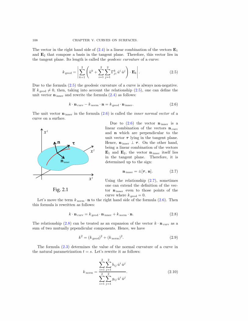
108 CHAPTER V. CURVES ON SURFACES.
The vector in the right hand side of (2.4) is a linear combination of the vectors E1
and E2 that compose a basis in the tangent plane. Therefore, this vector lies inthe tangent plane. Its length is called the geodesic curvature of a curve:
k geod =
∣
∣
∣
∣
∣
2∑
k=1
(
uk +
2∑
i=1
2∑
j=1
Γkji u
i uj
)
·Ek
∣
∣
∣
∣
∣
. (2.5)
Due to the formula (2.5) the geodesic curvature of a curve is always non-negative.If k geod 6= 0, then, taking into account the relationship (2.5), one can define theunit vector n inner and rewrite the formula (2.4) as follows:
k · n curv − k norm · n = k geod · n inner. (2.6)
The unit vector n inner in the formula (2.6) is called the inner normal vector of acurve on a surface.
Due to (2.6) the vector n inner is alinear combination of the vectors n curv
and n which are perpendicular to theunit vector τ lying in the tangent plane.Hence, n inner ⊥ τ . On the other hand,being a linear combination of the vectorsE1 and E2, the vector n inner itself liesin the tangent plane. Therefore, it isdetermined up to the sign:
n inner = ±[τ , n]. (2.7)
Using the relationship (2.7), sometimesone can extend the definition of the vec-tor n inner even to those points of thecurve where k geod = 0.
Let’s move the term k norm ·n to the right hand side of the formula (2.6). Thenthis formula is rewritten as follows:
k · n curv = k geod ·n inner + k norm · n. (2.8)
The relationship (2.8) can be treated as an expansion of the vector k · n curv as asum of two mutually prpendicular components. Hence, we have
k2 = (k geod)2 + (k norm)2. (2.9)
The formula (2.3) determines the value of the normal curvature of a curve inthe natural parametrization t = s. Let’s rewrite it as follows:
k norm =
2∑
i=1
2∑
j=1
bij ui uj
2∑
i=1
2∑
j=1
gij ui uj
. (2.10)
§ 2. GEODESIC AND NORMAL CURVATURES OF A CURVE. 109
In the natural parametrization the formula (2.10) coincides with (2.3) becauseof (1.7). When passing to an arbitrary parametrization all derivatives ui aremultiplied by the same factor. Indeed, we have
dui
dt=dui
ds
ds
dt. (2.11)
But the right hand side of (2.10) is insensitive to such a change of ui. Therefore,(2.10) is a valid formula for the normal curvature in any parametrization.
The formula (2.10) shows that the normal curvature is a very rough characte-ristic of a curve. It is determined only by the direction of its tangent vector τ inthe tangent plane. The components of the matrices gij and bij characterize notthe curve, but the point of the surface through which this curve passes.
Let a be some vector tangent to the surface. In curvilinear coordinates u1, u2
it is given by two numbers a1, a2 — they are the coefficients in its expansion inthe basis of two frame vectors E1 and E2. Let’s consider the value of the secondquadratic form of the surface on this vector:
b(a, a) =
2∑
i=1
2∑
j=1
bij ai aj. (2.12)
Definition 2.1. The direction given by a nonzero vector a in the tangentplane is called an asymptotic direction if the value of the second quadratic form(2.12) on such vector is equal to zero.
Note that asymptotic directions do exist only at those points of a surface wherethe second quadratic form is indefinite in sign or degenerate. In the first casethe Gaussian curvature is negative: K < 0, in the second case it is equal to zero:K = 0. At those points where K > 0 there are no asymptotic directions.
Definition 2.2. A curve on a surface whose tangent vector τ at all its pointslies in an asymptotic direction is called an asymptotic line.
Due to (2.12) the equation of an asymptotic line has the following form:
b(τ , τ ) =
2∑
i=1
2∑
j=1
bij ui uj = 0. (2.13)
Comparing (2.13) and (2.10), we see that asymptotic lines are the lines with zeronormal curvature: k norm = 0. On the surfaces with negative Gaussian curvatureK < 0 at each point there are two asymptotic directions. Therefore, on suchsurfaces always there are two families of asymptotic lines, they compose theasymptotic network of such a surface. On any surface of the negative Gaussiancurvature there exists a curvilinear coordinate system u1, u2 whose coordinatenetwork coincides with the asymptotic network of this surface. However, we shallnot prove this fact here.
The curvature lines are defined by analogy with the asymptotic lines. Theseare the curves on a surface whose tangent vector lies in a principal direction ateach point (see formulas (5.14) and (5.15) in § 5 of Chapter IV). The curvaturelines do exist on any surface, there are no restrictions for the Gaussian curvatureof a surface in this case.
110 CHAPTER V. CURVES ON SURFACES.
Definition 2.3. A geodesic line on a surface is a curve whose geodesic curva-ture is identically equal to zero: k geod = 0.
From the Frenet formula τ = k · n curv and from the relationship (2.8) for thegeodesic lines we derive the following equality:
dτ
ds= k norm · n. (2.14)
In the other words, the derivative of the unit normal vector on a geodesic line isdirected along the unit normal vector of a surface. This is the external descriptionof geodesic lines. The inner description is derived from the formula (2.5):
uk +
2∑
i=1
2∑
j=1
Γkji u
i uj = 0. (2.15)
The equations (2.15) are the differential equations of geodesic lines in naturalparametrization. One can pass from the natural parametrization to an arbitraryone by means of the formula (2.11).
§ 3. Extremal property of geodesic lines.
Let’s compare the equations of geodesic lines (2.15) with the equations ofstraight lines in curvilinear coordinates (8.18) which we have derived in Chap-ter III. These equations have the similar structure. They differ only in the rangesof indices: in the case of geodesic lines on a surface they run over two numbersinstead of three numbers in the case of straight lines. Therefore, geodesic linesare natural analogs of the straight lines in the inner geometry of surfaces. Thefollowing theorem strengthens this analogy.
Theorem 3.1. A geodesic line connecting two given points A andB on a surfacehas the extremal length in the class of curves connecting these two points.
It is known that in the Euclidean space E the shortest path from a point Ato another point B is the segment of straight line connecting these points. Thetheorem 3.1 proclaims a very similar proposition for geodesic lines on a surface.Remember that real functions can have local maxima and minima — they arecalled extrema. Apart from maxima and minima, there are also conditionalextrema (saddle points), for example, the point x = 0 for the function y = x3. Allthose points are united by the common property — the linear part of the functionincrement at any such point is equal to zero: f(x0 + h) = f(x0) + O(h2).
In the case of a geodesic line connecting the points A and B on a surface weshould slightly deform (variate) this line keeping it to be a line on the surfaceconnecting the same two points A and B. The deformed line is not a geodesic line.Its length differs from the length of the original line. The condition of the extremallength in the theorem 3.1 means that the linear part of the length increment isequal to zero.
Let’s specify the method of deforming the curve. For the sake of simplicityassume that the points A and B, and the geodesic line connecting these points inwhole lie within some charted fragment D of the surface. Then this geodesic line isgiven by two functions (1.1). Let’s increment by one the number of arguments in
§ 3. EXTREMAL PROPERTY OF GEODESIC LINES. 111
these functions. Then we shall assume that these functions are sufficiently manytimes differentiable with respect to all their arguments:
u1 = u1(t, h),
u2 = u2(t, h).(3.1)
For each fixed h in (3.1) we have the functions of the parameter t, they definea curve on the surface. Changing the parameter h, we deform the curve sothat in the process of this deformation its point are always on the surface. Thedifferentiability of the functions (3.1) guarantees that small deformations of thecurve correspond to small changes of the parameter h.
Let’s impose to the functions (3.1) a series of restrictions which are easy tosatisfy. Assume that the length of the initial geodesic line is equal to a and let theparameter t run over the segment [0, a]. Let
uk(0, h) = uk(0, 0), uk(a, h) = uk(a, 0). (3.2)
The condition (3.2) means that under a change of the parameter h the initial pointA and the ending point B of the curve do not move.
For the sake of brevity let’s denote the partial derivatives of the functionsui(t, h) with respect to t by setting the dot. Then the quantities ui = ∂ui/∂tdetermine the inner representation of the tangent vector to the curve.
Assume that the initial line correspond to the value h = 0 of the parameter h.Assume also that for h = 0 the parameter t coincides with the natural parameterof the geodesic line. Then for h = 0 the functions (3.1) satisfy the equations (1.7)and (2.15) simultaneously. For h 6= 0 the parameter t should not coincide with thenatural parameter on the deformed curve, and the deformed curve itself shouldnot be a geodesic line in this case.
Let’s calculate the lengths of the deformed curves. It is the function of theparameter h determined by the length integral of the form (1.5):
L(h) =
a∫
0
√
√
√
√
2∑
i=1
2∑
j=1
gij ui uj dt. (3.3)
For h = 0 we have L(0) = a. The proposition of the theorem 3.1 on the extremityof the length now is formulated as L(h) = a +O(h2) or, equivalently, as
dL(h)
dh h=0
= 0. (3.4)
Proof of the theorem 3.1. Let’s prove the equality (3.4) for the lengthintegral (3.3) under the deformations of the curve described just above. Denote byλ(t, h) the expression under the square root in the formula (3.3). Then by directdifferentiation of (3.3) we obtain
dL(h)
dh=
a∫
0
∂λ/∂h
2√λdt. (3.5)
112 CHAPTER V. CURVES ON SURFACES.
Let’s calculate the derivative in the numerator of the fraction (3.5):
∂λ
∂h=
∂
∂h
(
2∑
i=1
2∑
j=1
gij ui uj
)
=
2∑
i=1
2∑
j=1
2∑
k=1
∂gij
∂uk
∂uk
∂hui uj+
+
2∑
k=1
2∑
i=1
2∑
j=1
gij
∂(ui uj)
∂uk
∂uk
∂h=
2∑
i=1
2∑
j=1
2∑
k=1
∂gij
∂uk
∂uk
∂hui uj+
+
2∑
k=1
2∑
i=1
2∑
j=1
gij δik u
j ∂uk
∂h+
2∑
k=1
2∑
i=1
2∑
j=1
gij ui δj
k
∂uk
∂h.
Due to the Kronecker symbols δik and δj
k in the above expression we can performexplicitly the summation over k in the last two terms. Moreover, due to thesymmetry of gij they are equal to each other:
∂λ
∂h=
2∑
i=1
2∑
j=1
2∑
k=1
∂gij
∂uk
∂uk
∂hui uj + 2
2∑
i=1
2∑
j=1
gij ui ∂u
j
∂h.
Substituting this expression into (3.5), we get two integrals:
I1 =
2∑
i=1
2∑
j=1
2∑
k=1
a∫
0
∂gij
∂uk
ui uj
2√λ
∂uk
∂hdt, (3.6)
I2 =
2∑
i=1
2∑
j=1
a∫
0
gik ui
√λ
∂uk
∂hdt. (3.7)
The integral (3.7) contain the second order mixed partial derivatives of (3.1):
∂uk
∂h=∂2uk
∂t ∂h.
In order to exclude such derivatives we integrate (3.7) by parts:
a∫
0
gik ui
√λ
∂uk
∂hdt =
gik ui
√λ
∂uk
∂h
a
0
−a∫
0
∂
∂t
(
gik ui
√λ
)
∂uk
∂hdt.
Let’s differentiate the equalities (3.2) with respect to h. As a result we find thatthe derivatives ∂uk/∂h vanish at the ends of the integration segment over t. Thismeans that non-integral terms in the above formula do vanish. Hence, for theintegral I2 in (3.7) we obtain
I2 = −2∑
i=1
2∑
k=1
a∫
0
∂
∂t
(
gik ui
√λ
)
∂uk
∂hdt. (3.8)
CopyRight c© Sharipov R.A., 1996, 2004.
§ 3. EXTREMAL PROPERTY OF GEODESIC LINES. 113
Now let’s add the integrals I1 and I2 from (3.6) and (3.8). As a result for thederivative dL/dh in (3.5) we derive the following equality:
dL(h)
dh=
2∑
i=1
2∑
k=1
a∫
0
(
2∑
j=1
∂gij
∂uk
ui uj
2√λ− ∂
∂t
(
gik ui
√λ
)
)
∂uk
∂hdt.
In this equality the only derivatives with respect to the parameter h are ∂uk/∂h.For their values at h = 0 we introduce the following notations:
δuk =∂uk
∂h h=0
(3.9)
The quantities δuk = δuk(t) in (3.9) are called the variations of the coordinateson the initial curve. Note that under a change of curvilinear coordinates thesequantities are transformed as the components of a vector (although this fact doesnot matter for proving the theorem).
Let’s substitute h = 0 into the above formula for the derivative dL/dh. Whensubstituted, the quantity λ in the denominators of the fractions becomes equal tounity: λ(t, 0) = 1. This fact follows from (1.7) since t coincides with the naturalparameter on the initial geodesic line. Then
dL(h)
dh h=0
=2∑
i=1
2∑
k=1
a∫
0
(
2∑
j=1
∂gij
∂uk
ui uj
2− d(gik u
i)
dt
)
δuk dt.
Since the above equality does not depend on h any more, we replace the partialderivative with respect to t by d/dt. All of the further calculations in the righthand side are for the geodesic line where t is the natural parameter.
Let’s move the sums over i and k under the integration and let’s calculate thecoefficients of δuk denoting these coefficients by Uk:
Uk =2∑
i=1
(
2∑
j=1
∂gij
∂uk
ui uj
2− d(gik u
i)
dt
)
=
=2∑
i=1
2∑
j=1
(
1
2
∂gij
∂uk− ∂gik
∂uj
)
ui uj −2∑
i=1
gik ui.
(3.10)
Due to the symmetry of ui uj the second term within round brackets in theformula (3.10) can be broken into two terms. This yields
Uk =
2∑
i=1
2∑
j=1
1
2
(
∂gij
∂uk− ∂gik
∂uj− ∂gjk
∂ui
)
ui uj −2∑
i=1
gik ui.
Let’s raise the index k in Uk, i. e. consider the quantities U q given by the formula
U q =
2∑
k=1
gqk Uk.
114 CHAPTER V. CURVES ON SURFACES.
For these quantities from the previously derived formula we obtain
−U q = uq +
2∑
i=1
2∑
j=1
2∑
k=1
gqk
2
(
∂gkj
∂ui+∂gik
∂uj− ∂gij
∂uk
)
ui uj.
Let’s compare this formula with the formula (7.5) in Chapter IV that determinesthe connection components. As a result we get:
−U q = uq +
2∑
i=1
2∑
j=1
Γqij u
i uj. (3.11)
Now it is sufficient to compare (3.11) with the equation of geodesic lines (2.15)and derive U q = 0. The quantities Uk are obtained from U q by lowering the index:
Uk =
2∑
q=1
gkq Uq.
Therefore, the quantities Uk are also equal to zero. From this fact we immediatelyderive the equality (3.4) which means exactly that the extremity condition for thegeodesic lines is fulfilled. The theorem is proved.
§ 4. Inner parallel translation on a surface.
The equation of geodesic lines in the Euclidean space E in form of (8.18) wasderived in Chapter III when considering the parallel translation of vectors incurvilinear coordinates. The differential equation of the parallel translation (8.6)can be rewritten now in the two-dimensional case:
ai +
2∑
j=1
2∑
k=1
Γijk u
j ak = 0. (4.1)
The equation (4.1) is called the equation of the inner parallel translation of vectorsalong curves on a surface.
Suppose that we have a surface on some fragment of which the curvilinearcoordinates u1, u2 and a parametric curve (1.1) are given. Let’s consider sometangent vector a to the surface at the initial point of the curve, i. e. at t = 0.The vector a has the inner representation in form of two numbers a1, a2, they areits components. Let’s set the Cauchy problem for the differential equations (4.1)given by the following initial data at t = 0:
a1(t)t=0
= a1, a2(t)t=0
= a2. (4.2)
Solving the Cauchy problem (4.2), we get two functions a1(t) and a2(t) whichdetermine the vectors a(t) at all points of the curve. The procedure describedjust above is called the inner parallel translation of the vector a along a curve ona surface.
§ 4. INNER PARALLEL TRANSLATION ON A SURFACE. 115
Let’s consider the inner parallel translation of the vector a from the outer pointof view, i. e. as a process in outer (three-dimensional) geometry of the space E
where the surface under consideration is embedded. The relation of inner andouter representations of tangent vectors of the surface is given by the formula:
a =
2∑
i=1
ai ·Ei. (4.3)
Let’s differentiate the equality (4.3) with respect to t assuming that a1 and a2
depend on t as solutions of the differential equations (4.1):
da
dt=
2∑
i=1
ai ·Ei +
2∑
i=1
2∑
j=1
ai · ∂Ei
∂uj· uj. (4.4)
The derivatives ∂Ei/∂uj are calculated according to Veingarten’s derivational
formulas (see formulas (4.11) in Chapter IV). Then
da
dt=
2∑
i=1
(
ai +
2∑
j=1
2∑
k=1
Γijk u
j ak
)
·Ei +
(
2∑
j=1
2∑
k=1
bjk uj ak
)
· n.
Since the functions ai(t) satisfy the differential equations (4.1), the coefficients atthe vectors Ei in this formula do vanish:
da
dt=
(
2∑
j=1
2∑
k=1
bjk uj ak
)
· n. (4.5)
The coefficient at the normal vector n in the above formula (4.5) is determined bythe second quadratic form of the surface. This is the value of the correspondingsymmetric bilinear form on the pair of vectors a and τ . Therefore, the formula(4.5) is rewritten in a vectorial form as follows:
da
dt= b(τ , a) ·n. (4.6)
The vectorial equation (4.6) is called the outer equation of the inner paralleltranslation on surfaces.
The operation of parallel translation can be generalized to the case of innertensors of the arbitrary type (r, s). For this purpose we have introduced theoperation of covariant differentiation of tensorial function with respect to theparameter t on curves (see formula (8.10) in Chapter III). Here is the two-dimensional version of this formula:
∇tAi1... ir
j1... js=dAi1... ir
j1... js
dt+
+
r∑
m=1
2∑
q=1
2∑
vm=1
Γim
q vmuq Ai1... vm... ir
j1... js−
s∑
n=1
2∑
q=1
2∑
wn=1
Γwn
q jnuq Ai1... ir
j1... wn... js.
(4.7)
116 CHAPTER V. CURVES ON SURFACES.
In terms of the covariant derivative (4.7) the equation of the inner paralleltranslation for the tensorial field A is written as
∇tA = 0. (4.8)
The consistence of defining the inner parallel translation by means of the equation(4.8) follows from the two-dimensional analog of the theorem 8.2 from Chapter III.
Theorem 4.1. For any inner tensorial function A(t) determined at the points
of a parametric curve on some surface the quantities Bi1... ir
j1... js= ∇tA
i1... ir
j1... jscalculated
according to the formula (4.7) define a tensorial function B(t) = ∇tA of the sametype (r, s) as the original function A(t).
The proof of this theorem almost literally coincides with the proof of thetheorem 8.2 in Chapter III. Therefore, we do not give it here.
The covariant differentiation ∇t defined by the formula (4.7) possesses a seriesof properties similar to those of the covariant differentiation along a vector field∇X (see formula (6.10) and theorem 6.2 in Chapter IV).
Theorem 4.2. The operation of covariant differentiation of tensor-valued func-tions with respect to the parameter t along a curve on a surface possesses thefollowing properties:
(1) ∇t(A + B) = ∇tA + ∇tB;(2) ∇t(A⊗ B) = ∇tA⊗ B + A ⊗∇tB;(3) ∇tC(A) = C(∇tA).
Proof. Let’s choose some curvilinear coordinate system and prove the theoremby means of direct calculations in coordinates. Let C = A + B. Then for thecomponents of the tensor-valued function C(t) we have
C i1... ir
j1... js= Ai1... ir
j1... js+ Bi1... ir
j1... js.
Substituting C i1... ir
j1... jsinto (4.7), for the covariant derivative ∇tC we get
∇tCi1... ir
j1... js= ∇tA
i1 ... ir
j1 ... js+ ∇tB
i1... ir
j1... js.
This equality proves the first item of the theorem.Let’s proceed with the item (2). Denote C = A ⊗B. Then for the components
of the tensor-valued function C(t) we have
Ci1... ir+p
j1... js+q= Ai1... ir
j1... jsB
ir+1 ... ir+p
js+1 ... js+q. (4.9)
Let’s substitute the quantities Ci1... ir+p
j1... js+qfrom (4.9) into the formula (4.8) for the
covariant derivative. As a result for the components of ∇tC we derive
∇tCi1... ir+p
j1... js+q=(
dA i1... ir
j1... js/dt)
Bir+1 ... ir+p
js+1 ... js+q+
+A i1... ir
j1... js
(
dBir+1... ir+p
js+1... js+q/dt)
+
§ 4. INNER PARALLEL TRANSLATION ON A SURFACE. 117
+r∑
m=1
2∑
q=1
2∑
vm=1
Γim
vmuq Ai1... vm ... ir
j1... jsB
ir+1 ... ir+p
js+1 ... js+q+
+
r+p∑
m=r+1
2∑
q=1
2∑
vm=1
A i1... ir
j1... jsΓim
vmuq B
ir+1... vm... ir+p
js+1... js+q−
−s∑
n=1
2∑
q=1
2∑
wn=1
Γwn
jnuq Ai1... ir
j1... wn... jsB
ir+1... ir+p
js+1 ... js+q−
−s+q∑
n=s+1
2∑
q=1
2∑
wn=1
A i1... ir
j1... jsΓwn
jnuq B
ir+1... ir+p
js+1... wn... js+q.
Note that upon collecting the similar terms the above huge formula can betransformed to the following one:
∇t
(
Ai1... ir
j1... jsB
ir+1 ... ir+p
js+1 ... js+q
)
=(
∇tAi1... ir
j1... js
)
×
× Bir+1... ir+p
js+1... js+q+Ai1 ... ir
j1 ... js
(
∇tBir+1 ... ir+p
js+1 ... js+q
)
.
(4.10)
Now it is easy to see that the formula (4.10) proves the second item of the theorem.Let’s choose two tensor-valued functions A(t) and B(t) one of which is the
contraction of another. In coordinates this fact looks like
Bi1 ... ir
j1 ... js=
2∑
k=1
Ai1... ip−1 k ip... ir
j1... jq−1 k jq... js
. (4.11)
Let’s substitute (4.11) into the formula (4.7). For ∇tBi1... ir
j1... jswe derive
∇tBi1... ir
j1... js=
2∑
k=1
dAi1... ip−1 k ip... ir
j1... jq−1 k jq... js
dt+
+
r∑
m=1
2∑
k=1
2∑
q=1
2∑
vm=1
Γim
q vmuq Ai1... vm... k ... ir
j1... jq−1 k jq ... js− (4.12)
−s∑
n=1
2∑
k=1
2∑
q=1
2∑
wn=1
Γwn
q jnuq A
i1... ip−1 k ip... ir
j1... wn... k ... js
.
In the formula (4.12) the index vm sequentially occupies the positions to the leftof the index k and to the right of it. The same is true for the index wn. However,the formula (4.12) has no terms where vm or wn replaces the index k. Such terms,provided they would be present, according to (4.7), would have the form
2∑
k=1
2∑
q=1
2∑
v=1
Γkq v u
q Ai1 ... ip−1 v ip... ir
j1 ... jq−1 k jq ... js
, (4.13)
−2∑
k=1
2∑
q=1
2∑
w=1
Γwq k u
q Ai1... ip−1 k ip ... ir
j1... jq−1 w jq... js. (4.14)
118 CHAPTER V. CURVES ON SURFACES.
It is easy to note that (4.13) and (4.14) differ only in sign. Indeed, it is sufficientto rename k to v and w to k in the formula (4.14). If we add simultaneously(4.13) and (4.14) to (4.12), their contributions cancel each other thus keeping theequality valid. Therefore, (4.12) can be written as
∇js+1Bi1 ... ir
j1... js=
2∑
k=1
∇js+1Ai1... ip−1 k ip... ir
j1... jq−1 k jq... js. (4.15)
The relationship (4.15) proves the third item of the theorem and completes theproof in whole.
Under a reparametrization of a curve a new parameter t should be a strictlymonotonic function of the old parameter t (see details in § 2 of Chapter I). Undersuch a reparametrization ∇t and ∇t are related to each other by the formula
∇tA =dt(t)
dt· ∇tA (4.16)
for any tensor-valued function A on a curve. This relationship is a simpleconsequence from (4.7) and from the chain rule for differentiating a compositefunction. It is an analog of the item (3) in the theorem 6.2 of Chapter IV.
Let A be a tensor field of the type (r, s) on a surface. This means that at eachpoint of the surface some tensor of the type (r, s) is given. If we mark only thosepoints of the surface which belong to some curve, we get a tensor-valued functionA(t) on that curve. In coordinates this is written as
Ai1... ir
j1... js(t) = Ai1... ir
j1... js(u1(t), u2(t)). (4.17)
The function A(t) constructed in this way is called the restriction of a tensor fieldA to a curve. The specific feature of the restrictions of tensor fields on curvesexpressed by the formula (4.17) reveals in differentiating them:
dAi1... ir
j1... js
dt=
2∑
q=1
∂Ai1 ... ir
j1 ... js
∂uquq. (4.18)
Substituting (4.18) into the formula (4.7), we can extract the common factor uq inthe sum over q. Upon extracting this common factor we find
∇tAi1... ir
j1... js=
2∑
q=1
uq ∇qAi1... ir
j1... js. (4.19)
The formula (4.19) means that the covariant derivative of the restriction of atensor field A to a curve is the contraction of the covariant differential ∇A withthe tangent vector of the curve.
Assume that ∇A = 0. Then due to (4.19) the restriction of the field A to anycurve is a tensor-valued function satisfying the equation of the parallel translation(4.8). The values of such a field A at various points are related to each other byparallel translation along any curve connecting these points.
§ 4. INNER PARALLEL TRANSLATION ON A SURFACE. 119
Definition 4.1. A tensor field A is called an autoparallel field or a covariantlyconstant field if its covariant differential is equal to zero identically: ∇A = 0.
Some of the well-known tensor fields have identically zero covariant differentials:this is the metric tensor g, the inverse metric tensor g, and the area tensor(pseudotensor) τ . The autoparallelism of these fields plays the important role fordescribing the inner parallel translation.
Let a and b be two tangent vectors of the surface at the initial point of somecurve. Their scalar product is calculated through their components:
(a |b) =
2∑
i=1
2∑
j=1
gij ai bj .
Let’s perform the parallel translation of the vectors a and b along the curvesolving the equation (4.8) and using the components of a and b as initial data inCauchy problems. As a result we get two vector-valued functions a(t) and b(t) onthe curve. Let’s consider the function ψ(t) equal to their scalar product:
ψ(t) = (a(t) |b(t)) =
2∑
i=1
2∑
j=1
gij(t) ai(t) bj(t). (4.20)
According to the formula (4.7) the covariant derivative ∇tψ coincides with theregular derivative. Therefore, we have
dψ
dt= ∇tψ =
2∑
i=1
2∑
j=1
(
∇tgij ai bj + gij ∇ta
i bj + gij ai ∇tb
j)
.
Here we used the items (2) and (3) of the theorem 4.2. But ∇tai = 0 and
∇tbj = 0 since we a(t) and b(t) are obtained as a result of parallel translation of
the vectors a and b. Moreover, ∇tgij = 0 due to autoparallelism of the metrictensor. For the scalar function ψ(t) defined by (4.20) this yields dψ/dt = 0 andψ(t) = (a |b) = const. As a result of these considerations we have proved thefollowing theorem.
Theorem 4.3. The operation of inner parallel translation of vectors along cur-ves preserves the scalar product of vectors.
Preserving the scalar product, the operation of inner parallel translation pre-serves the length of vectors and the angles between them.
From the autoparallelism of metric tensors g and g we derive the followingformulas analogous to the formulas (7.9) in Chapter IV:
∇t
(
2∑
k=1
gikA... k ...... ...
)
=2∑
k=1
gik ∇tA... k ...... ...,
∇t
(
2∑
k=1
gikA... ...... k ...
)
=
2∑
k=1
gik ∇tA... ...... k ....
(4.21)
Then from the formulas (4.21) we derive the following fact.
Theorem 4.4. The operation of inner parallel translation of tensors commutatewith the operations of index raising and index lowering.
CopyRight c© Sharipov R.A., 1996, 2004.
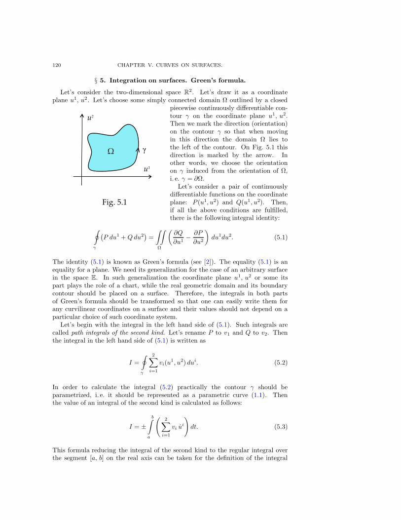
120 CHAPTER V. CURVES ON SURFACES.
§ 5. Integration on surfaces. Green’s formula.
Let’s consider the two-dimensional space R2. Let’s draw it as a coordinate
plane u1, u2. Let’s choose some simply connected domain Ω outlined by a closedpiecewise continuously differentiable con-tour γ on the coordinate plane u1, u2.Then we mark the direction (orientation)on the contour γ so that when movingin this direction the domain Ω lies tothe left of the contour. On Fig. 5.1 thisdirection is marked by the arrow. Inother words, we choose the orientationon γ induced from the orientation of Ω,i. e. γ = ∂Ω.
Let’s consider a pair of continuouslydifferentiable functions on the coordinateplane: P (u1, u2) and Q(u1, u2). Then,if all the above conditions are fulfilled,there is the following integral identity:
∮
γ
(
P du1 + Qdu2)
=
∫∫
Ω
(
∂Q
∂u1− ∂P
∂u2
)
du1du2. (5.1)
The identity (5.1) is known as Green’s formula (see [2]). The equality (5.1) is anequality for a plane. We need its generalization for the case of an arbitrary surfacein the space E. In such generalization the coordinate plane u1, u2 or some itspart plays the role of a chart, while the real geometric domain and its boundarycontour should be placed on a surface. Therefore, the integrals in both partsof Green’s formula should be transformed so that one can easily write them forany curvilinear coordinates on a surface and their values should not depend on aparticular choice of such coordinate system.
Let’s begin with the integral in the left hand side of (5.1). Such integrals arecalled path integrals of the second kind. Let’s rename P to v1 and Q to v2. Thenthe integral in the left hand side of (5.1) is written as
I =
∮
γ
2∑
i=1
vi(u1, u2) dui. (5.2)
In order to calculate the integral (5.2) practically the contour γ should beparametrized, i. e. it should be represented as a parametric curve (1.1). Thenthe value of an integral of the second kind is calculated as follows:
I = ±b∫
a
(
2∑
i=1
vi ui
)
dt. (5.3)
This formula reducing the integral of the second kind to the regular integral overthe segment [a, b] on the real axis can be taken for the definition of the integral
§ 5. INTEGRATION ON SURFACES. GREEN’S FORMULA. 121
(5.2). The sign is chosen regarding to the direction of the contour on Fig. 5.1. Ifa < b and if when t changes from a to b the corresponding point on the contourmoves along the arrow, we choose plus in (5.3). Otherwise, we choose minus.Changing the variable t = ϕ(t) in the integral (5.3) and choosing the propersign upon reparametrization of the contour, one can verify that the value of thisintegral does not depend on the choice of the parametrization on the contour.
Now let’s change the curvilinear coordinate system on the surface. Thederivatives ui in the integral (5.3) under a change of curvilinear coordinates on thesurface are transformed as follows:
ui =dui
dt=
2∑
j=1
∂ui
∂uj
duj
dt=
2∑
j=1
Sij
˙uj. (5.4)
Substituting (5.4) into the formula (5.3), for the integral I we derive:
I = ±b∫
a
(
2∑
j=1
(
2∑
i=1
Sij vi
)
˙uj
)
dt. (5.5)
Now let’s write the relationship (5.3) in coordinates u1, u2. For this purpose werename ui to ui and vi to vi in the formula (5.3):
I = ±b∫
a
(
2∑
i=1
vi˙ui
)
dt. (5.6)
Comparing the formulas (5.5) and (5.6), we see that these formulas are similarin their structure. For the numeric values of the integrals (5.3) and (5.6) to bealways equal (irrespective to the form of the contour γ and its parametrization)the quantities vi and vi should be related as follows:
vj =
2∑
i=1
Sij vi, vi =
2∑
i=1
T ji vj.
These formulas represent the transformation rule for the components of a covec-torial field. Thus, we conclude that any path integral of the second kind on asurface (5.2) is given by some inner covectorial field on this surface.
Now let’s proceed with the integral in the right hand side of the Green’s formula(5.1). Distracting for a while from the particular integral in this formula, let’sconsider the following double integral:
I =
∫∫
Ω
F du1du2. (5.7)
A change of curvilinear coordinates can be interpreted as a change of variables inthe integral (5.7). Remember that a change of variables in a multiple integral isperformed according to the following formula (see [2]):
∫∫
Ω
F du1du2 =
∫∫
Ω
F | det J | du1du2, (5.8)
122 CHAPTER V. CURVES ON SURFACES.
where J is the Jacobi matrix determined by the change of variables:
J =
∥
∥
∥
∥
∥
∥
∥
∥
∂u1
∂u1
∂u1
∂u2
∂u2
∂u1
∂u2
∂u2
∥
∥
∥
∥
∥
∥
∥
∥
. (5.9)
The Jacobi matrix (5.9) coincides with the transition matrix S (see formula (2.7)in Chapter IV). Therefore, the function F being integrated in the formula (5.7)should obey the transformation rule
F = | detS|F (5.10)
under a change of curvilinear coordinates on the surface. The quantity F hasno indices. However, due to (5.10), this quantity is neither a scalar nor apseudoscalar. In order to change this not very pleasant situation the integral (5.7)over a two-dimensional domain Ω on a surface is usually written as
I =
∫∫
Ω
√
detg f du1du2, (5.11)
where detg is the determinant of the first quadratic form. In this case thequantity f in the formula (5.11) is a scalar. This fact follows from the equalitydet g = (det T )2 det g that represent the transformation rule for the determinantof the metric tensor under a change of coordinate system.
Returning back to the integral in the right hand side of (5.1), we transform itto the form (5.11). For this purpose we use the above notations P = v1, Q = v2,and remember that v1 and v2 are the components of the covectorial field. Then
∂Q
∂u1− ∂P
∂u2=∂v2∂u1
− ∂v1∂u2
. (5.12)
The right hand side of (5.12) can be represented in form of the contraction withthe unit skew-symmetric matrix dij (see formula (3.6) in Chapter IV):
∂v2∂u1
− ∂v1∂u2
=
2∑
i=1
2∑
j=1
dij ∂vj
∂ui=
2∑
i=1
∂
∂ui
(
2∑
j=1
dij vj
)
. (5.13)
Note that the quantities dij with lower indices enter the formula for the areatensor ω (see (3.7) in Chapter IV). Let’s raise the indices of the area tensor bymeans of the inverse metric tensor:
ωij =2∑
p=1
2∑
q=1
gip gjq ωpq =2∑
p=1
2∑
q=1
ξD√
det g gip gjq dpq.
Applying the formula (3.7) from Chapter IV, we can calculate the components ofthe area tensor ωij in the explicit form:
ωij = ξD√
detg−1 dij. (5.14)
§ 5. INTEGRATION ON SURFACES. GREEN’S FORMULA. 123
The formula (5.14) expresses ωij through dij. Now we use (5.14) in order toexpress dij in the formula (5.13) back through the components of the area tensor:
∂v2∂u1
− ∂v1∂u2
=
2∑
i=1
∂
∂ui
(
2∑
j=1
ξD√
det g ωij vj
)
.
In order to simplify the further calculations we denote
yi =
2∑
j=1
ωij vj. (5.15)
Taking into account (5.15), the formula (5.13) can be written as follows:
∂v2∂u1
− ∂v1∂u2
=2∑
i=1
ξD∂(√
detg yi)
∂ui=
= ξD√
det g
2∑
i=1
(
∂yi
∂ui+
1
2
∂(
ln detg)
∂uiyi
)
.
(5.16)
The logarithmic derivative for the determinant of the metric tensor is calculatedby means of the lemma 7.1 from Chapter IV. However, we need not repeat thesecalculations here, since this derivative is already calculated (see (7.12) and theproof of the theorem 7.2 in Chapter IV):
∂(
lndet g)
∂ui=
2∑
p=1
2∑
q=1
gpq ∂gpq
∂ui=
2∑
q=1
2 Γqiq. (5.17)
With the use of (5.17) the formula (5.16) is transformed as follows:
∂v2∂u1
− ∂v1∂u2
= ξD√
det g
2∑
i=1
(
∂yi
∂ui+
2∑
q=1
Γqqi y
i
)
.
In this formula one easily recognizes the contraction of the covariant differential ofthe vector field y. Indeed, we have
∂v2∂u1
− ∂v1∂u2
= ξD√
detg
2∑
i=1
∇iyi. (5.18)
Using the formula (5.18), the notations (5.15), and the autoparallelism conditionfor the area tensor ∇qω
ij = 0, we can write the Green’s formula as
∮
γ
2∑
i=1
vi dui = ξD
∫∫
Ω
2∑
i=1
2∑
j=1
ωij∇ivj
√
det g du1du2. (5.19)
The sign factor ξD in (5.19) should be especially commented. The condition thatthe domain Ω should lie to the left of the contour γ when moving along the arrow
124 CHAPTER V. CURVES ON SURFACES.
is not invariant under an arbitrary change of coordinates u1, u2 by u1, u2. Indeed,if we set u1 = −u1 and u2 = u2, we would have the mirror image of the domainΩ and the contour γ shown on Fig. 5.1. This means that the direction should beassigned to the geometric contour γ lying on the surface, not to its image in achart. Then the sign factor ξD in (5.19) can be omitted.
The choice of the direction on a geometric contour outlining a domain on asurface is closely related to the choice of the normal vector on that surface. Thenormal vector n should be chosen so that when observing from the end of thevector n and moving in the direction of the arrow along the contour γ the domainΩ should lie to the left of the contour. The choice of the normal vector n definesthe orientation of the surface thus defining the unit pseudoscalar field ξD .
§ 6. Gauss-Bonnet theorem.
Let’s consider again the process of inner parallel translation of tangent vectorsalong curves on surfaces. The equation (4.6) shows that from the outer (three-dimensional) point of view this parallel translation differs substantially from theregular parallel translation: the vectors being translated do not remain parallelto the fixed direction in the space — they change. However, their lengths arepreserved, and, if we translate several vectors along the same curve, the anglesbetween vectors are preserved (see theorem 4.3).
From the above description, we see that in the process of parallel translation,apart from the motion of the attachment point along the curve, the rotation ofthe vectors about the normal vector n occurs. Therefore, we have the naturalproblem — how to measure the angle of this rotation? We consider this problemjust below.
Suppose that we have a surface equipped with the orientation. This meansthat the orientation field ξD and the area tensor ω are defined (see formula (3.10)in Chapter IV). We already know that ξD fixes one of the two possible normalvectors n at each point of the surface (see formula (4.3) in Chapter IV).
Theorem 6.1. The inner tensor field Θ of the type (1, 1) with the components
θij =
2∑
k=1
ωjk gki (6.1)
is an operator field describing the counterclockwise rotation in the tangent planeto the angle π/2 = 90 about the normal vector n.
Proof. Let a be a tangent vector to the surface and let n be the unit normalvector at the point where a is attached. Then, in order to construct the vectorb = Θ(a) obtained by rotating a counterclockwise to the angle π/2 = 90 aboutthe vector n one can use the following vector product:
b = Θ(a) = [n, a]. (6.2)
Let’s substitute the expression given by the formula (4.3) from Chapter IV for thevector n into (6.2). Then let’s expand the vector a in the basis E1, E2:
a = a1 ·E1 + a2 ·E2. (6.3)
§ 6. GAUSS-BONNET THEOREM. 125
As a result for the vector b in the formula (6.2) we derive
b =
2∑
j=1
ξD · [[E1, E2], Ej ]
|[E1, E2]|· aj . (6.4)
In order to calculate the denominator in the formula (6.4) we use the well-knownformula from the analytical geometry (see [4]):
|[E1, E2]|2 = det
∣
∣
∣
∣
(E1 |E1) (E1 |E2)(E2 |E1) (E2 |E2)
∣
∣
∣
∣
= detg.
As for the numerator in the formula (6.4), here we use the not less known formulafor the double vectorial product:
[[E1, E2], Ej ] = E2 · (E1 |Ej) −E1 · (Ej |E2).
Taking into account these two formulas, we can write (6.4) as follows:
b =
2∑
j=1
ξD · g1j ·E2 − g2j ·E1√det g
· aj. (6.5)
Using the components of the area tensor (5.14), no we can rewrite (6.5) in a morecompact and substantially more elegant form:
b =
2∑
i=1
(
2∑
j=1
2∑
k=1
ωki gkj aj
)
·Ei.
From this formula it is easy to extract the formula (6.1) for the components of thelinear operator Θ relating b and a. The theorem is proved.
The operator field Θ is the contraction of the tensor product of two fields ω
and g. The autoparallelism of the latter ones means that Θ is also an autoparallelfield, i. e. ∇Θ = 0.
We use the autoparallelism of Θ in the following way. Let’s choose someparametric curve γ on a surface and perform the parallel translation of some unitvector a along this curve. As a result we get the vector-valued function a(t) on thecurve satisfying the equation of parallel translation ∇ta = 0 (see formula (4.8)).Then we define the vector-function b(t) on the curve as follows:
b(t) = Θ(a(t)). (6.6)
From (6.6) we derive ∇t(b) = ∇tΘ(a) + Θ(∇ta) = 0. This means that thefunction (6.6) also satisfies the equation of parallel translation. It follows fromthe autoparallelism of Θ and from the items (2) and (3) in the theorem 4.2. Thevector-functions a(t) and b(t) determine two mutually perpendicular unit vectorsat each point of the curve. There are the following obvious relationships for them:
Θ(a) = b, Θ(b) = −a. (6.7)
126 CHAPTER V. CURVES ON SURFACES.
Let’s remember for the further use that a(t) and b(t) are obtained by paralleltranslation of the vectors a(0) and b(0) along the curve from its initial point.
Now let’s consider some inner vector field x on the surface (it is tangent to thesurface in the outer representation). If the field vectors x(u1, u2) are nonzero ateach point of the surface, they can be normalized to the unit length: x → x/|x|.Therefore, we shall assume x to be a field of unit vectors: |x| = 1. At the pointsof the curve γ this field can be expanded in the basis of the vectors a and b:
x = cos(ϕ) · a + sin(ϕ) · b. (6.8)
The function ϕ(t) determines the angle between the vector a and the field vector x
measured from a to x in the counterclockwise direction. The change of ϕ describesthe rotation of the vectors during their parallel translation along the curve.
Let’s apply the covariant differentiation ∇t to the relationship (6.8) and takeinto account that both vectors a and b satisfy the equation of parallel translation:
∇tx = (− sin(ϕ) · a + cos(ϕ) · b) · ϕ. (6.9)
Here we used the fact that the covariant derivative ∇t for the scalar coincides withthe regular derivative with respect to t. In particular, we have ∇tϕ = ϕ. Now weapply the operator Θ to both sides of (6.8) and take into account (6.7):
Θ(x) = cos(ϕ) · b− sin(ϕ) · a. (6.10)
Now we calculate the scalar product of Θ(x) from (6.10) and ∇tx from (6.9).Remembering that a and b are two mutually perpendicular unit vectors, we get
(Θ(x) |∇tx) = (cos2(ϕ) + sin2(ϕ)) ϕ = ϕ. (6.11)
Let’s write the equality (6.11) in coordinate form. The vector-function x(t) on thecurve is the restriction of the vector field x, therefore, the covariant derivative ∇tx
is the contraction of the covariant differential ∇x with the tangent vector of thecurve (see formula (4.19)). Hence, we have
ϕ =
2∑
q=1
2∑
i=1
2∑
j=1
(
xi ωij ∇qxj)
uq. (6.12)
Here in deriving (6.12) from (6.11) we used the formula (6.1) for the componentsof the operator field Θ.
Let’s discuss the role of the field x in the construction described just above.The vector field x is chosen as a reference mark relative to which the rotationangle of the vector a is measured. This way of measuring the angle is relative.Changing the field x, we would change the value of the angle ϕ. We have to admitthis inevitable fact since tangent planes to the surface at different points are notparallel to each other and we have no preferable direction relative to which wecould measure the angles on all of them.
There is a case where we can exclude the above uncertainty of the angle. Let’sconsider a closed parametric contour γ on the surface. Let [0, 1] be the range over
CopyRight c© Sharipov R.A., 1996, 2004.
§ 6. GAUSS-BONNET THEOREM. 127
which the parameter t runs on such contour. Then x(0) and x(1) do coincide.They represent the same field vector at the point with coordinates u1(0), u2(0):
x(0) = x(1) = x(u1(0), u2(0)).
Unlike x(t), the function a(t) is not the restriction of a vector field to a curve γ.Therefore, the vectors a(0) and a(1) can be different. This is an important featureof the inner parallel translation that differs it from the parallel translation in theEuclidean space E.
In the case of a closed contour γ the difference ϕ(1) − ϕ(0) characterizes theangle to which the vector a turns a as a result of parallel translation along thecontour. Note that measuring the angle from x to a is opposite to measuring itfrom a to x in the formula (6.8). Therefore, taking for positive the angle measuredfrom x in the counterclockwise direction, we should take for the increment of theangle gained during the parallel translation along γ the following quantity:
4ϕ = ϕ(0) − ϕ(1) = −1∫
0
ϕ dt.
Let’s substitute (6.12) for ϕ into this formula. As a result we get
4ϕ = −1∫
0
(
2∑
q=1
2∑
i=1
2∑
j=1
(
xi ωij ∇qxj)
uq
)
dt. (6.13)
Comparing (6.13) with (5.3), we see that (6.13) now can be written in the form ofa path integral of the second kind:
4ϕ = −∮
γ
2∑
q=1
2∑
i=1
2∑
j=1
(
xi ωij ∇qxj)
duq. (6.14)
Assume that the contour γ outlines some connected and simply connectedfragment Ω on the surface. Then for this fragment Ω we can apply to (6.14) theGreen’s formula written in the form of (5.19):
4ϕ = −ξD∫∫
Ω
2∑
i=1
2∑
j=1
2∑
p=1
2∑
q=1
ωij ∇i
(
xp ωpq ∇jxq)√
detg du1du2.
If the direction of the contour is in agreement with the orientation of the surface,then the sign factor ξD can be omitted:
4ϕ = −∫∫
Ω
2∑
i=1
2∑
j=1
2∑
p=1
2∑
q=1
(
xp ωijωpq ∇i∇jxq +
+ ∇ixp ωijωpq ∇jx
q)√
detg du1du2.
(6.15)
128 CHAPTER V. CURVES ON SURFACES.
Let’s show that the term ∇ixp ωijωpq ∇jx
q in (6.15) yields zero contribution tothe value of the integral. This feature is specific to the two-dimensional case wherewe have the following relationship:
ωijωpq = dij dpq = δip δ
jq − δi
q δjp. (6.16)
The proof of the formula (6.16) is analogous to the proof of the formula (8.23) inChapter IV. It is based on the skew-symmetry of dij and dpq.
Let’s complete the inner vector field x of the surface by the other inner vectorfield y = Θ(x). The vectors x and y form a pair of mutually perpendicular unitvectors in the tangents plane. For their components we have
2∑
q=1
xq xq = 1, xi =
2∑
k=1
gik xk, yi =
2∑
k=1
gik yk, (6.17)
2∑
q=1
∇kxq xq = 0, yq =
2∑
p=1
ωpq xp, yi =
2∑
j=1
ωji xj. (6.18)
The first relationship (6.17) expresses the fact that |x| = 1, other two relationships(6.17) determine the covariant components xi and yi of x and y. The firstrelationship (6.18) is obtained by differentiating (6.17), the second and the thirdrelationships (6.18) express the vectorial relationship y = Θ(x).
Let’s multiply (6.16) by ∇kxq xj x
p and then sum up over q, p, and j takinginto account the relationships (6.17) and (6.18):
∇kxi =
(
2∑
q=1
yq ∇kxq
)
yi = zk yi. (6.19)
Using (6.19), i. e. substituting ∇ixp = zi y
p and ∇jxq = zj y
q into (6.15), we seethat the contribution of the second term in this formula is zero. Then, applying(6.16) to (6.15), for the increment 4ϕ we derive
4ϕ = −∫∫
Ω
2∑
i=1
2∑
j=1
xi(
∇i∇jxj −∇j∇ix
j)√
det g du1du2.
Now we apply the relationship (8.5) from Chapter IV to the field x. Moreover, wetake into account the formulas (8.24) and (9.9) from Chapter IV:
4ϕ =
∫∫
Ω
2∑
i=1
2∑
j=1
(
K gij xi xj)√
detg du1du2.
Remember that the vector field x was chosen to be of the unit length from thevery beginning. Therefore, upon summing up over the indices i and j we shallhave only the Gaussian curvature under the integration:
4ϕ =
∫∫
Ω
K√
detg du1du2. (6.20)
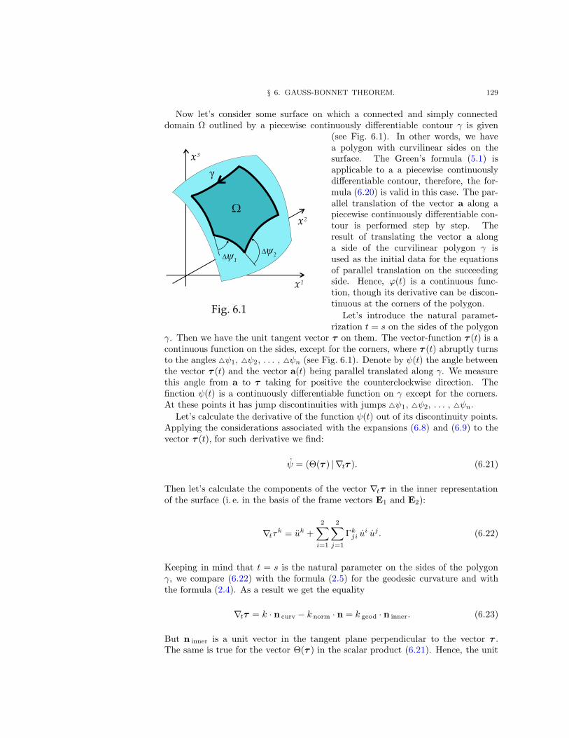
§ 6. GAUSS-BONNET THEOREM. 129
Now let’s consider some surface on which a connected and simply connecteddomain Ω outlined by a piecewise continuously differentiable contour γ is given
(see Fig. 6.1). In other words, we havea polygon with curvilinear sides on thesurface. The Green’s formula (5.1) isapplicable to a a piecewise continuouslydifferentiable contour, therefore, the for-mula (6.20) is valid in this case. The par-allel translation of the vector a along apiecewise continuously differentiable con-tour is performed step by step. Theresult of translating the vector a alonga side of the curvilinear polygon γ isused as the initial data for the equationsof parallel translation on the succeedingside. Hence, ϕ(t) is a continuous func-tion, though its derivative can be discon-tinuous at the corners of the polygon.
Let’s introduce the natural paramet-rization t = s on the sides of the polygon
γ. Then we have the unit tangent vector τ on them. The vector-function τ (t) is acontinuous function on the sides, except for the corners, where τ (t) abruptly turnsto the angles 4ψ1, 4ψ2, . . . , 4ψn (see Fig. 6.1). Denote by ψ(t) the angle betweenthe vector τ (t) and the vector a(t) being parallel translated along γ. We measurethis angle from a to τ taking for positive the counterclockwise direction. Thefinction ψ(t) is a continuously differentiable function on γ except for the corners.At these points it has jump discontinuities with jumps 4ψ1, 4ψ2, . . . , 4ψn.
Let’s calculate the derivative of the function ψ(t) out of its discontinuity points.Applying the considerations associated with the expansions (6.8) and (6.9) to thevector τ (t), for such derivative we find:
ψ = (Θ(τ ) |∇tτ ). (6.21)
Then let’s calculate the components of the vector ∇tτ in the inner representationof the surface (i. e. in the basis of the frame vectors E1 and E2):
∇tτk = uk +
2∑
i=1
2∑
j=1
Γkji u
i uj. (6.22)
Keeping in mind that t = s is the natural parameter on the sides of the polygonγ, we compare (6.22) with the formula (2.5) for the geodesic curvature and withthe formula (2.4). As a result we get the equality
∇tτ = k · n curv − k norm · n = k geod · n inner. (6.23)
But n inner is a unit vector in the tangent plane perpendicular to the vector τ .The same is true for the vector Θ(τ ) in the scalar product (6.21). Hence, the unit
130 CHAPTER V. CURVES ON SURFACES.
vectors n inner and Θ(τ ) are collinear. Let’s denote by ε(t) the sign factor equal tothe scalar product of these vectors:
ε = (Θ(τ ) |n inner) = ±1. (6.24)
Now from the formulas (6.23) and (6.24) we derive:
ψ = ε k geod. (6.25)
Let’s find the increment of the function ψ(t) gained as a result of round trip alongthe whole contour. It is composed by two parts: the integral of (6.25) and the sumjumps at the corners of the polygon γ:
4ψ =
∮
γ
ε k geod ds +
n∑
i=1
4ψi. (6.26)
The angle 4ϕ is measured from x to a in the counterclockwise direction, whilethe angle 4ψ is measured from a to τ in the same direction. Therefore, the sum4ϕ + 4ψ is the total increment of the angle between x and τ . It is importantto note that the initial value and the final value of the vector τ upon round tripalong the contour do coincide. The same is true for the vector x. Hence, the sumof increments 4ϕ+ 4ψ is an integer multiple of the angle 2π = 360:
4ϕ+ 4ψ = 2π r. (6.27)
Practically, the value of the number r in the formula (6.27) is equal to unity.Let’s prove this fact by means of the following considerations: we perform thecontinuous deformation of the surface on Fig. 6.1 flattening it to a plain, thenwe continuously deform the contour γ to a circle. During such a continuousdeformation the left hand side of the equality (6.27) changes continuously, whilethe right hand side can change only in discrete jumps. Therefore, under the abovecontinuous deformation of the surface and the contour both sides of (6.27) do notchange at all. On a circle the total angle of rotation of the unit tangent vector iscalculated explicitly, it is equal to 2π. Hence, r = 1. We take into account thiscircumstance when substituting (6.20) and (6.26) into the formula (6.27):
∫∫
Ω
K√
det g du1du2 +
∮
γ
ε k geod ds+
n∑
i=1
4ψi = 2π. (6.28)
The formula (6.28) is the content of the following theorem which is known as theGauss-Bonnet theorem.
Theorem 6.2. The sum of the external angles of a curvilinear polygon on asurface is equal to 2π minus two integrals: the area integral of the Gaussian cur-vature over the interior of the polygon and the integral of the geodesic curvature(taken with the sign factor ε) over its perimeter.
§ 6. GAUSS-BONNET THEOREM. 131
It is interesting to consider the case where the polygon is formed by geodesiclines on a surface of the constant Gaussian curvature. The second integral in(6.28) then is equal to zero, while the first integral is easily calculated. For thesum of internal angles of a geodesic triangle in this case we derive
α1 + α2 + α3 = π +K S,
where K S is the product of the Gaussian curvature of the surface and the area ofthe triangle.
A philosophic remark. By measuring the sum of angles of some sufficientlybig triangle we can decide whether our world is flat or it is equipped with thecurvature. This is not a joke. The idea of a curved space became generallyaccepted in the modern notions on the structure of the world.
REFERENCES.
1. Sharipov R. A. Course of linear algebra and multidimensional geometry, BashkirState University, Ufa, 1996; see on-line math.HO/0405323/ in Electronic Archivehttp://arXiv.org.
2. Kudryavtsev L. D. Course of mathematical analysis, Vol. I and II, «VisshayaShkola» publishers, Moscow, 1985.
3. Kostrikin A. I. Introduction to algebra, «Nauka» publishers, Moscow, 1977.
4. Beklemishev D. V. Course of analytical geometry and linear algebra, «Nauka»publishers, Moscow, 1985.
AUXILIARY REFERENCES 1.
5. Sharipov R. A. Quick introduction to tensor analysis, free on-line textbookmath.HO/0403252 in Electronic Archive http://arXiv.org.
6. Sharipov R. A. Classical electrodynamics and theory of relativity, BashkirState University, Ufa, 1997; see on-line physics/0311011 in Electronic Archivehttp://arXiv.org.
1 The references [5] and [6] are added in 2004.