north carolina department of transportation level iii ... · north carolina department of...
TRANSCRIPT

1
North Carolina Department of Transportation
Level III Design of Erosion & Sediment Control Plans
MODULE 1. Hydrology ……………………………………… page 7
MODULE 2. Soil Erosion …………………………………… page 12
MODULE 3. Regulatory Issues …………………………… page 20
MODULE 4. Open Channel Design……………………….. page 21
MODULE 5. Sediment Retention BMPs …………………… page 27
MODULE 6. Below Water Table Borrow Pits …………… page 30
CONVERSION FACTORS 1 acre = 43,560 ft2
1 mi2 = 640 acres 1 ft3 of water = 7.48 gallons = 62.4 pounds 1 ft3/sec = 1 cfs = 448.9 gallons per minute (gpm) 1,000,000 gallons per day (1 MGD) = 695 gpm = 1.56 cfs 1 m = 100 cm = 1000 mm

2
SYMBOLS MODULE 1. Hydrology A watershed drainage area in acres (ac) AJarrett Jarrett Maximum Area in acres (ac) C Rational Method runoff coefficient (decimal ranging from 0 to 1) H elevation change from most remote point to point of interest (ft) i rainfall intensity in inches per hour (in/hr) Lflow flow length from most remote point to point of interest (ft) P probability of a hydrologic event being exceeded in any year (decimal) Q peak runoff rate in cubic feet per second (cfs) S slope equal to elevation change over length (ft/ft) T return period for a specific hydrologic event (years) tc time of concentration in minutes (min) MODULE 2. Erosion Aerosion annual soil interrill + rill erosion in tons per acre per year (tons/ac-yr), Cditch regression constant for secondary roads dependent on ditch side slopes CP conservation practices factor (dimensionless) K soil erodibility factor (dimensionless) LS slope-length factor (dimensionless) R rainfall factor (dimensionless) Sditch slope of secondary road ditch (ft/ft) Vditch secondary road sediment volume expected in cubic feet per acre (ft3/ac) MODULE 4. Open Channel Design average tractive force acting on the channel lining (lbs/ft2), unit weight of water, assumed to be 62.4 lbs/ft3, dchan depth of flow in the channel (ft), Schan slope of the channel (ft/ft). MODULE 5. Sediment Retention BMPs Abasin surface area of a sediment retention basin in square feet (ft2) Dorifice diameter of the skimmer orifice in inches (in) Hskim driving head at the skimmer orifice from Table 5.1 in feet (ft) Qskim basin outflow rate in cubic feet per day (ft3/day) tdewater dewatering time for a BMP (days) Vbasin volume of a sediment retention basin in cubic feet (ft3) Vskim basin volume to be dewatered in cubic feet (ft3) MODULE 6. Below Water Table Borrow Pits Vstill volume of stilling basin in cubic feet (ft3) Qstill pumping rate entering the stilling basin in gallons per minute (gpm)

3
Soils Prone to Flooding in North Carolina Counties (Not for Infiltration Basins) Anson Chewacla (ChA) Chewacla and Chastain (CmA) Johnston (JoA) Beaufort Currituck (Cu) Dorovan (Do) Muckalee (Me) Bertie Bibb and Johnston (Bb) Chewacla (Ch) Dorovan (Dk) Roanoke (Ro) Wehadkee (WE) Bladen Congaree (Cn) Croatan (CT) Dorovan (DO) Johnston (JO) Pamlico (PC) Wilbanks (WN) Brunswick Bohicket (BO) Carteret (CA) Chowan (CH) Dorovan (DO) Longshoal (LA) Muckalee (Mk) Camden Chowan (CwA) Dorovan (DoA) Gertie (GtA) Carteret Carteret (CH, CL) Deloss (Dm) Dorovan (Do) Duckston (Du)
Lafitte (LF) Masontown (MA) Chowan Chowan (CO) Dorovan (DO) Columbus Brookman (Br) Dorovan (Do) Meggett (Me) Muckalee (Mk) Wilbanks (Wn) Craven Dorovan (Do) Lafitte (LF) Cumberland Chewacla (CH) Johnston (JT) Currituck Currituck (Cu) Dorovan (Do) Dare Carteret (CeA) Currituck (CuA) Hobonny (HoA) Duplin Bibb and Johnston (BbA) Muckalee (MkA) Edgecombe Chewacla (Cc) Johnston (JS) Meggett (Me) Wehadkee (Wh) Franklin Chewacla and Wehadkee (ChA)
Riverview and Buncombe (RmA) Wehadkee (WvA) Gates Chowan (ChA) Dorovan (DoA) Nawney (NaA) Greene Bibb (Bb) Johnston (JS) Kinston (KN) Halifax Chastain and Bibb (CbA) Chewacla and Wehadkee (CwA) Harnett Bibb (Bb) Polawana (Pn) Wehadkee (Wh0 Hertford Bibb and Johnston (BB) Dorovan (DO) Wehadkee (We) Wilbanks (WN) Hoke Chewacla (Ch) Johnston (JT) Hyde Backbay (BaA) Carteret (CaA) Delway (DeA) Dorovan (DoA) Engelhard (EnA) Longshoal (LfA) Newholland (NhA) Weeksville (WkA)

4
Jones Hobonny (Ho) Muckalee (Mk) Lee Chewacla (Ch) Congaree (Cp) Wehadkee (Wn) Lenoir Bibb (Bb) Chewacla (Ch) Johnston (JS) Kinston (Kn) Pamlico (Pc) Martin Bibb (Bb) Chastain (Ch) Dorovan (Do) Roanoke (Ro) Montgomery Bibb (BhA) Chastain (CkA) Chenneby (CnA) Johnston (JoA) Oakboro (OkA) Moore Bibb (Bb) Chewacla (Ch) Congaree (Co) Wehadkee (We) Nash Bibb (Bb) Congaree (Co) Meggett (Me) Wehadkee (Wh) New Hanover Dorovan (Do) Johnston (JO) Pamlico (Pm) Bohicket (TM)
Northampton Chastain and Bibb (CbA) Chewacla and Wehadkee (CwA) Onslow Bohicket (Bo) Carteret (Ca) Dorovan (Da) Masontown (Md) Muckalee (Mk) Pamlico Brookman (Bm) Hobucken (HN) Lafitte (LF) Masontown (MA) Stockade (Sm) Pasquotank Chowan (CwA) Dorovan (DoA) Hobonny (HoA) Pender Bohicket (Bo) Carteret (Ca) Chewacla (Ch) Meggett (Me) Muckalee (Mk) Perquimans Chowan (CO) Dorovan (DO) Pitt Bibb (Bb) Cape Fear (Ca) Leaf (Le) Pantego (Pg) Rains (Ra) Swamp (Sw) Richmond Chewacla (ChA)
Johnston (JmA) Robeson Bibb and Johnston (BB) Johnston (JT) Meggett (Me) Osier (Pm) Sampson Bibb and Johnston (BH) Johnston (JT) Pamlico (Pm) Scotland Bibb (BaA) Johnston (JmA) Tyrrell Chowan (Ch) Dorovan (Do) Wake Buncombe (BuB) Chewacla (CmA) Congaree (CoA) Wehadkee (WnA) Warren Chewacla and Wehadkee (ChA) Washington Dorovan (Do, Dr) Muckalee (Me) Wayne Chewacla (Ch) Johnston (Js) Kinston (Kn) Pamlico (Pa) Wilson Bibb (Bb) Wehadkee and Chewacla (Wh) Wilbanks (Wk)

5
Ta
ble
1. B
MP
Sel
ec
tio
n
BM
P
Lo
cati
on
C
atc
hm
en
t S
tru
ctu
re
Sed
. Ctl
. S
ton
e S
urf
ac
eA
rea
V
olu
me
F
un
ctio
n
T.
Ro
ck S
ed.
Dam
A
Sw
ale/
larg
e di
tch
< 1
ac.
C
lass
I
Yes
43
5Q1
0
3600
ft3
/ac
Rem
ove
sand
T
. R
ock
Sed
. D
am B
D
rain
age
outle
t <
1 a
c.
Cla
ss B
Y
es
435Q
10
3600
ft3
/ac
Rem
ove
sand
S
ilt
Bas
in B
D
rain
age
outle
t/ A
djac
ent t
o in
let
< 3
ac.
E
arth
N
o 43
5Q1
0
(325
Q1
0 @
in
lets
)
3600
ft3
/ac
(180
0 ft
3/a
c @
inle
ts)
Rem
ove
sand
Ski
mm
er B
asin
D
rain
age
outle
t <
10
ac.
Ear
th
No
325Q
10
1800
ft3
/ac
Rem
ove
sand
In
filt
rati
on
Bas
in
Dra
inag
e ou
tlet
< 1
0 ac
. E
arth
N
o 32
5Q1
0
1800
ft3
/ac
Rem
ove
sand
R
iser
Bas
in(n
on
-per
fora
ted
ri
ser
w/ s
kim
mer
) D
rain
age
outle
t <
100
ac.
E
arth
N
o
435Q
10
1800
ft3
/ac
Rem
ove
silt,
cla
y
Sti
llin
g B
asin
/Pu
mp
ed
Nea
r B
orro
w
Pit/
Cul
vert
N
/A
Ear
th a
nd
Sto
ne
No
2:1
L:W
ra
tio
Bas
ed o
n de
wat
erin
g R
emov
e si
lt, c
lay
Sp
. Sti
llin
g B
asin
(Sil
t B
ag)
Nea
r st
ream
N
/A
Filt
er F
abric
Y
es
N/A
V
aria
ble
Rem
ove
sand
R
ock
Pip
e In
let
Sed
. Tra
p A
P
ipe
inle
t <
1 a
c.
Cla
ss B
Y
es
N/A
36
00 f
t3/a
c R
emov
e sa
nd
Ro
ck P
ipe
Inle
t S
ed. T
rap
B
Pip
e in
let
< 1
ac.
C
lass
A
Yes
N
/A
3600
ft3
/ac
Rem
ove
sand
S
lop
e D
rain
w/
Ber
m
Fill
Slo
pes
< ½
ac.
12
-inc
h pi
pe
No
N/A
N
/A
Con
vey
conc
ent
rate
d ru
noff
R
ock
Inle
t S
ed. T
rap
A
Sto
rmw
ater
Inl
et
< 1
ac.
C
lass
B
Yes
N
/A
3600
ft3
/ac
Rem
ove
sand
R
ock
Inle
t S
ed. T
rap
B
Sto
rmw
ater
Inl
et
< 1
ac.
C
lass
A
Yes
N
/A
3600
ft3
/ac
Rem
ove
sand
R
ock
Inle
t S
ed. T
rap
C
Sto
rmw
ater
Inl
et
< 1
ac.
¼
” w
ire
mes
h Y
es
N/A
N
/A
Re
mov
e sa
nd
T.
Ro
ck S
ilt
Ch
eck
A
Dra
inag
e ou
tlet
< 1
ac.
C
lass
B
Yes
43
5Q1
0
3600
ft3
/ac
Rem
ove
sand
T
. R
ock
Sil
t C
hec
k B
C
hann
el
< ½
ac.
C
lass
B
No
N/A
N
/A
Red
uce
flow
vel
ocity
T
emp
ora
ry E
arth
Ber
m
Pro
ject
per
imet
er
< 5
ac.
E
arth
N
o N
/A
N/A
D
iver
t off
site
run
off
Tem
po
rary
Sil
t F
ence
B
otto
m o
f sl
ope
< ¼
acr
e pe
r 10
0 fe
et
Silt
fen
ce
No
N/A
N
/A
Cre
ate
smal
l bas
in;
Rem
ove
sand
, si
lt S
pec
ial S
edim
ent
Co
ntr
ol
Fen
ce
Bot
tom
of
slop
e <
½ a
c.
¼”
wir
e m
esh
Yes
N
/A
N/A
R
emo
ve s
and
Tem
po
rary
Sil
t D
itch
B
otto
m o
f sl
ope
< 5
ac.
E
arth
N
o N
/A
N/A
C
arry
sed
imen
t/w
ater
T
emp
ora
ry D
iver
sio
n
Pro
ject
& S
trea
m
perim
eter
<
5 a
c.
Ear
th
No
N/A
N
/A
Div
ert t
urbi
d w
ater
E
arth
Ber
m
< 5
ac.
E
arth
N
o N
/A
N/A
D
iver
t cle
an o
r tu
rbid
wat
er
Cle
an W
ater
Div
ersi
on
P
roje
ct p
erim
eter
<
5 ac
. E
arth
& F
abric
N
o N
/A
N/A
D
iver
t cle
an w
ater
C
on
stru
ctio
n E
ntr
ance
E
xit
to r
oad
N/A
C
lass
A
No
N/A
N
/A
Cle
an t
ruck
tire
s S
afet
y F
ence
P
erm
itted
Are
as
N/A
O
rang
e fe
nce
No
N/A
N
/A
Def
ine
perm
itted
bou
ndar
y B
orr
ow
Pit
Dew
ater
ing
B
asin
A
djac
ent t
o
Bor
row
Pits
N
/A
Ear
th
No
N/A
8.
02xQ
xT
Rem
ove
San
d an
d re
duce
tu
rbid
ity
Wat
tle/
Co
ir F
iber
Wat
tle
Cha
nnel
<
½ a
c.
Nat
ural
Fib
ers
No
N/A
N
/A
Inco
rpor
ate
PA
M
Sil
t C
hec
k A
wit
h M
atti
ng
an
d P
AM
C
hann
el
< ½
ac.
C
lass
B
Yes
N
/A
N/A
R
educ
e flo
w v
eloc
ity a
nd
inco
rpor
ate
PA
M
<2%
*
*Con
trib
utin
g la
nd s
lope
mus
t be
<2%

6
Locations of NC DOT Regional Offices.

7
MODULE 1. Hydrology
Hydrology is the study of water movement through the water cycle. The peak runoff/discharge rate in response to rainfall is required to design erosion and sediment control best management practices (BMPs). The rainfall-runoff relationship for a watershed is shown in Figure 1.1, including a hydrograph showing runoff rate in relation to time. During a rainfall event, the runoff rate increases as more land produces runoff water. As rainfall continues, more remote land areas contribute runoff, and eventually the entire watershed produces runoff at the time of concentration, tc, producing the peak runoff rate, Q.
Rational Method for Estimating Peak Runoff Rate The Rational Method (Water Pollution Control Federation, 1969) for predicting peak runoff rate is appropriate for designing small structures and channels in small watersheds: Q = (C) (i) (A) (Equation 1.1) where: Q = peak runoff rate for a given return period in cubic feet per second (cfs), C = Rational Method runoff coefficient (decimal ranging from 0 to 1), i = rainfall intensity for a given return period in inches per hour (in/hr), and A = watershed drainage area in acres (ac).
Figure 1.1. Conceptualization of hydrologic processes.

8
Long-term records of rainfall and runoff at a specific location can be used to estimate the probability of a certain hydrologic event being exceeded in any year and the return period for a specific hydrologic event: T = 1 / P (Equation 1.2) where: P = probability of a hydrologic event being exceeded in any year (decimal), and T = return period for a specific hydrologic event (years). Most erosion control structures are designed for 10-year or 25-year return periods, which have 0.1 and 0.04 probabilities of being exceeded each year, respectively.
Time of Concentration The time of concentration, tc, is defined by USDA-NRCS (1986), as the time required for runoff water to travel from the watershed's most remote point to the point-of-interest. Many methods can be used to estimate tc (Kirpich, 1940; USDA-SCS, 1972b; USDA-SCS, 1986). The most conservative design approach is to use the lowest predicted tc in sizing a basin since it will result in the highest design rainfall intensity and largest basin size. Jarrett Method for Small Drainage Areas Jarrett (2005) determined that time of concentration, tc, is approximated as 5 minutes for watersheds smaller than the Jarrett Maximum Area based on watershed slope: S = H / Lflow (Equation 1.3) where: S = average watershed slope (ft/ft), H = elevation change from most remote point to point of interest (ft), and Lflow = flow length from most remote point to point of interest (ft). AJarrett = 460 (S) (Equation 1.4) where: AJarrett = Jarrett Maximum Area in acres (ac), and S = average watershed slope (ft/ft). Example: For a watershed drainage area of 5 acres with an elevation drop of 10 ft over a
flow length of 500 ft, what is the average slope and the Jarrett Maximum Area? Slope, S = H / Lflow = 10 / 500 = 0.02 ft/ft
Jarrett Max Area, AJarrett = 460 (0.02) = 9.2 acres
Since the watershed drainage area of 5 acres < 9.2 acres, then use tc = 5 minutes.

9
NRCS Segmental Method For watersheds larger than the Jarrett Maximum Area, an appropriate method for estimating tc is the NRCS Segmental Method (USDA-SCS, 1986). This method is based on the premise that runoff from the most remote point will travel as sheet flow, then become shallow concentrated flow as it travels over the longest path, and finally enter a channel where Manning's equation describes flow hydraulics. Since most of a small watershed’s flow path is best classified as shallow concentrated flow, it is appropriate to use the following equations for estimating tc based on slope and flow length: Unpaved Areas: tc = 0.001 (Lflow ) / S0.53 (Equation 1.5) Paved Areas: tc = 0.0008 (Lflow ) / S0.53 (Equation 1.6) where: tc = time of concentration in minutes (min), Lflow = flow length from most remote point to point of interest (ft), S = average watershed slope (ft/ft). Example: For a construction site watershed drainage area of 10 acres with an elevation
drop of 14 ft over a flow length of 1000 ft, estimate time of concentration. Slope, S = H / Lflow = 14 / 1000 = 0.014 ft/ft Assume that the area is unpaved, therefore use Equation 1.5: tc = Lflow * 0.001/ (S0.53) = 1000* 0.001/ (0.0140.53) = 9.7 minutes Round to nearest whole number tc = 10 minutes. If the elevation drop for this site was 30 ft, the calculated value for tc would be 6.6
minutes. It that case, use a tc value of 5 minutes for determining rainfall intensity since the lower tc produces a higher rainfall intensity and a more conservative estimate of peak runoff rate and basin size.
Precipitation Data
The rainfall intensity data required to predict runoff rates using the Rational Method are available on the National Weather Service web site and summarized in Table 1.1: http://hdsc.nws.noaa.gov/hdsc/pfds/orb/nc_pfds.html

10
Table 1.1. Rainfall Intensity Data for North Carolina for the Rational Method. T (Yrs) 5 min 10 min 15 min 30 min 60 min Murphy
10 6.40 5.12 4.32 3.13 2.04 25 7.41 5.90 4.99 3.69 2.46
Asheville 10 6.96 5.57 4.70 3.40 2.22 25 8.03 6.40 5.41 4.00 2.67
Boone 10 7.34 5.87 4.95 3.59 2.34 25 8.43 6.72 5.68 4.20 2.80
Charlotte 10 7.19 5.74 4.85 3.51 2.29 25 8.00 6.37 5.38 3.99 2.65
Greensboro 10 6.80 5.44 4.59 3.32 2.16 25 7.46 5.94 5.02 3.72 2.48
Raleigh 10 6.97 5.58 4.70 3.41 2.22 25 7.72 6.16 5.20 3.85 2.56
Fayetteville 10 7.84 6.27 5.29 3.83 2.49 25 8.86 7.05 5.96 4.41 2.94
Wilmington 10 9.60 7.68 6.48 4.69 3.05 25 10.91 8.70 7.35 5.44 3.62
Washington 10 8.04 6.43 5.43 3.93 2.56 25 9.13 7.28 6.15 4.56 3.03
Manteo 10 8.23 6.59 5.55 4.02 2.62 25 9.35 7.45 6.29 4.66 3.10
Rational Method Runoff Coefficient, C The watershed characteristics affecting peak runoff rate are summarized in the runoff coefficient, C, a dimensionless parameter between 0.0 and 1.0. The value of C depends on soil infiltration rate, land use, and land slope. Sandy soils with rapid infiltration have low C values, while clay soils with slow infiltration have higher C values. Vegetation increases water infiltration, resulting in lower C values. For construction sites, land conditions are similar to disturbed agricultural watersheds. Table 1.4 summarizes typical C values based on soil texture, land use, and slope.
11
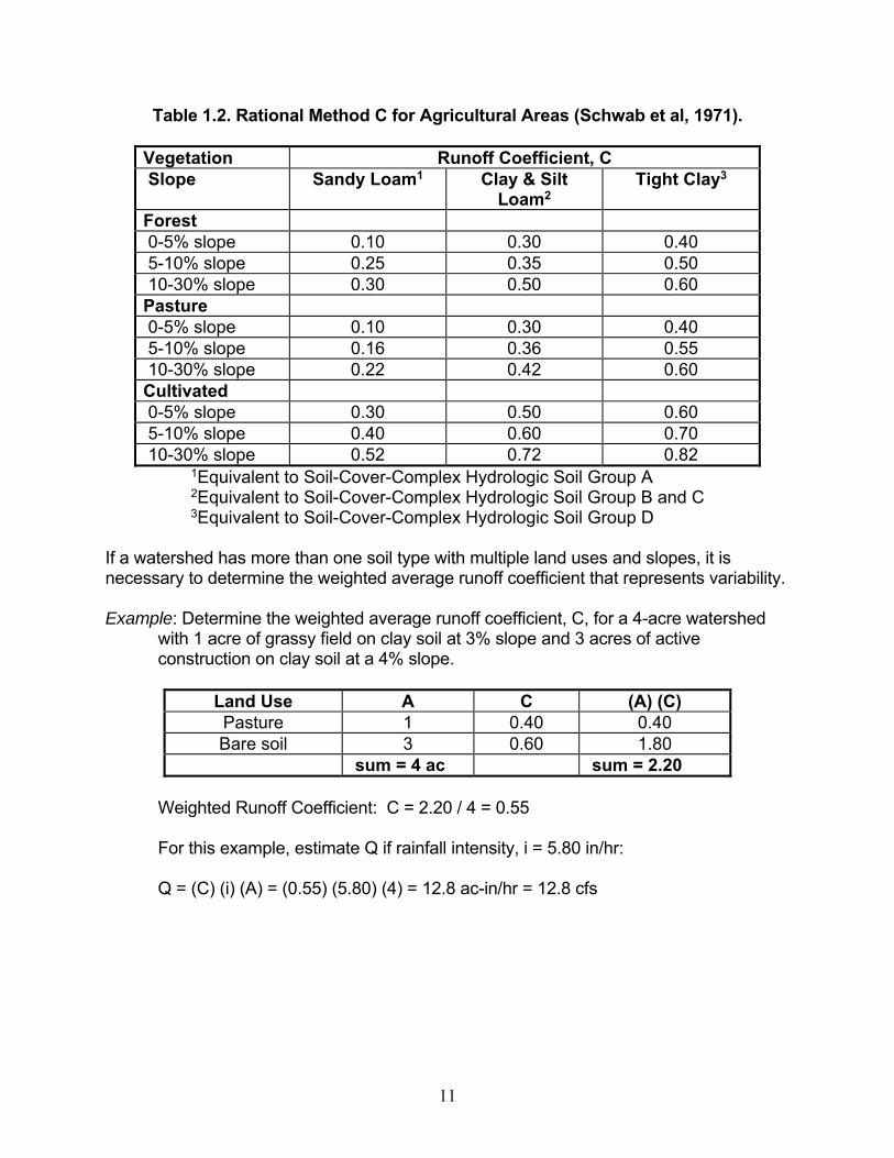
Table 1.2. Rational Method C for Agricultural Areas (Schwab et al, 1971).
Vegetation Runoff Coefficient, C Slope Sandy Loam1 Clay & Silt
Loam2 Tight Clay3
Forest 0-5% slope 0.10 0.30 0.40 5-10% slope 0.25 0.35 0.50 10-30% slope 0.30 0.50 0.60 Pasture 0-5% slope 0.10 0.30 0.40 5-10% slope 0.16 0.36 0.55 10-30% slope 0.22 0.42 0.60 Cultivated 0-5% slope 0.30 0.50 0.60 5-10% slope 0.40 0.60 0.70 10-30% slope 0.52 0.72 0.82
1Equivalent to Soil-Cover-Complex Hydrologic Soil Group A 2Equivalent to Soil-Cover-Complex Hydrologic Soil Group B and C 3Equivalent to Soil-Cover-Complex Hydrologic Soil Group D
If a watershed has more than one soil type with multiple land uses and slopes, it is necessary to determine the weighted average runoff coefficient that represents variability. Example: Determine the weighted average runoff coefficient, C, for a 4-acre watershed
with 1 acre of grassy field on clay soil at 3% slope and 3 acres of active construction on clay soil at a 4% slope.
Land Use A C (A) (C) Pasture 1 0.40 0.40 Bare soil 3 0.60 1.80
sum = 4 ac sum = 2.20 Weighted Runoff Coefficient: C = 2.20 / 4 = 0.55 For this example, estimate Q if rainfall intensity, i = 5.80 in/hr: Q = (C) (i) (A) = (0.55) (5.80) (4) = 12.8 ac-in/hr = 12.8 cfs

12
MODULE 2. Soil Erosion Erosion is defined as the process by which soil particles are detached and transported to a new location. Detachment is the breaking free of soil particles, caused by:
Raindrops hitting the soil surface, Flow of water over the soil surface that can lift and detach particles, Movement of wind over the soil surface, Breaking of rock and soil aggregates caused by freezing and thawing,
After soil particles have been detached, they may be transported by various methods:
Water flowing over the area where detached soil particles exist, Wind blowing over the area where detached particles exist, Raindrops impacting the surface and splashing detached soil to a new location, or
Splash erosion is the movement of soil that occurs when a raindrop impacts the exposed soil surface. The kinetic energy of a falling raindrop is dependent upon the drop's diameter and the velocity at which it impacts the soil. The greatest impact of splash erosion is its ability to detach soil particles. Interrill Erosion is the erosion that occurs as a result of raindrop energy and a thin sheet flow of runoff. As soon as the rainfall rate exceeds the soil’s infiltration rate, runoff begins flowing downslope as a thin sheet and carrying with it soil particles that have been dislodged. Rill Erosion occurs when the runoff water from interrill areas enters small channels called rills. Rills are usually linear and are oriented in a direction perpendicular to the contour (straight down the hill). As the flow moves down slope, rills tend to grow deeper and wider until small channels are visible. Typically, rills are small enough to be removed by tillage operations. Gully Erosion occurs in channels that cannot be eliminated by tillage operations. The erosion process in gullies or gully erosion is similar to rill erosion in that soil particles are detached by the shear forces of water flowing in the gully. Gully erosion is also often enhanced by sloughing and headcuts. Channel Erosion is the detachment and transport of soil particles from the walls and sides of a channel usually by the shearing force of water and sediment, generally on a larger scale than gully erosion. Sloughing of banks may also contribute to channel erosion. Factors Influencing Erosion The primary driving force of erosion on upland land areas is precipitation. Rainfall amount and intensity, both of which contribute to the energy of detachment, varies by location and

13
time of year. Soil characteristics affect soil erodibility. Clay particles are cohesive and difficult to detach, but are easily transported long distances. Silty soils are generally well-aggregated, but large aggregates often fall apart when wetted resulting in small aggregates and individual soil particles, which are more easily transported. Sand-sized soil particles, because of their relatively large size, are difficult to transport even though they are easily detached. Land shape affects erosion potential as typically the steeper the land slope and the loner the length-of-slope the greater is the erosion potential. Land use and conservation practices affect the potential for erosion.
Predicting Soil Erosion USDA-ARS developed the Revised Universal Soil Loss Equation (RUSLE) to estimate the long-term annual erosion potential on agricultural land. The equation is based on four factors affecting soil erosion potential: Aerosion = (R) (K) (LS) (CP) (Equation 2.1) where: Aerosion = annual soil interrill + rill erosion in tons per acre per year (tons/ac-yr), R = rainfall factor (dimensionless), K = soil erodibility factor (dimensionless), LS = slope-length factor (dimensionless), CP = conservation practices factor (dimensionless). Rainfall Factor, R is a measure of the erosive forces of rainfall for an area. It is based on a combination of rainfall intensity and accumulation. Annual R values for North Carolina are shown in Figure 2.1. However, because construction projects often do not last a year, it is necessary to compute partial-year R values. Partial-year R values area shown in Table 2.1. The partial-year R factor can be computed by summing the monthly values in Table 2.1
Table 2.1. Partial-Year Cumulative R Distributions (Renard et al, 1993). Geographic Region, Figure 2.2
Month 110 & 116 117 Jan 0.03 0.02 Feb 0.04 0.02 Mar 0.05 0.03 Apr 0.06 0.04 May 0.07 0.06 Jun 0.11 0.14 Jul 0.20 0.23 Aug 0.21 0.20 Sep 0.11 0.15 Oct 0.05 0.06 Nov 0.04 0.03 Dec 0.03 0.02

14
Figure 2.1. Annual Rainfall Factor, R, for North Carolina.
Figure 2.2. Regions for Determining Partial-Year R Values.
Soil Erodibility Factor, K is related to soil properties (Wischmeier et al, 1971):
Percent silt (MS; 0.002 to 0.05 mm) and very fine sand (VFS; 0.05 to 0.1 mm), Percent sand (SA; 0.1 to 2 mm), Percent organic matter (OM), Soil structure (S1), and Soil permeability (P1).
These soil parameters have been used to determine K values for most soils as listed in Table 2.2 and in other references such as Table 8.01d (NCDENR, 2006).

15
Table 2-2. Hydrologic Soil Group (HSG), Permeability, K and T values. B-Horizon
Soil Permeability RUSLE RUSLE RUSLE RUSLE Series HSG in/hr T K(A) K(B) K(C) Ailey B 0.6 to 2.0 2 0.15 0.24 0.24
Appling B 0.6 to 2.0 4 0.24 0.28 0.28 Autryville A 2.0 to 6.0 5 0.10 0.10 0.10
Badin B 0.6 to 2.0 3 0.15 0.24 0.15 Belhaven D 0.2 to 6.0 -- -- 0.24 0.24
Cecil B 0.6 to 2.0 4 0.24 0.28 -- Centenary A 6.0 to 20.0 5 0.10 0.10 0.10 Chastain D 0.06 to 0.2 4 0.28 0.37 -- Chewacla C 0.15 to 0.24 5 0.28 0.32 0.28
Cowee B 0.6 to 2.0 3 0.28 0.28 0.28 Creedmoor C 0.2 to 0.6 3 0.28 0.32 0.32
Emporia C 3.0 to 6.0 5 0.28 0.17 0.28 Evard B 0.6 to 2.0 5 0.24 0.24 0.24 Fannin B 0.6 to 2.0 3 0.32 0.32 0.32
Goldsboro B 0.6 to 2.0 3 0.20 0.24 0.24 Goldston C 2.0 to 6.0 2 0.15 0.05 -- Gritney C 0.06 to 0.2 3 0.32 0.32 0.20 Helena C 0.06 to 0.2 4 0.24 0.28
Hiwassee B 0.6 to 2.0 5 0.28 0.28 0.28 Hyde B/D 0.2 to 0.6 5 0.17 0.43 --
Johnston D 1.25 to 1.45 5 0.17 0.17 -- Lynn Haven B/D 1.35 to 1.6 5 0.10 0.15 --
Madison B 0.6 to 2.0 3 0.28 0.32 0.32 Mayodan B 0.6 to 2.0 4 0.24 0.32 0.28 Norfolk B 1.30 to 1.75 5 0.17 0.24 -- Pacolet B 0.12 to 0.16 3 0.15 0.28 0.28 Polkton D 1.15 to 1.60 2 0.37 0.37 0.37
Portsmouth B/D 0.6 to 2.0 5 0.24 0.28 0.17 Rains B/D 1.30 to 1.60 5 0.20 0.24 -- Rion B 0.6 to 2.0 3 0.24 0.24 0.24
Roanoke D < 0.02 4 0.37 0.24 0.24 Roper B/D 0.16 to 0.46 -- -- 0.43 0.43 State B 0.6 to 2.0 5 0.28 0.28 0.17 Tatum B 1.10 to 1.60 4 0.37 0.28 --
Tomotley A 0.6 to 2.0 5 0.20 0.20 0.20 Torhunta C 1.35 to 1.60 5 0.10 0.15 0.10
Vance C 0.06 to 0.2 3 0.24 0.28 -- Wakulla B/D 0.4 to 1.6 5 0.10 0.10 0.10
Wedowee B 0.6 to 2.0 3 0.24 0.28 0.28 Weeksville B/D 0.6 to 2.0 5 0.43 0.32 -- White Store D 0.06 to 0.6 3 0.37 0.37 0.32 Woodington A 0.6 to 2.0 5 0.10 0.20 0.10

16
Length-Slope Factor, LS is a single factor based on average land slope and the length of the uninterrupted slope over which water flows. The LS value is determined from Figure 2.3 for a known slope length and slope in %. For example, a slope length of 300 ft with slope of 0.05 ft/ft (5%) produces an LS value of 1.3.
Figure 2.3. LS factors for construction and mining site land uses that have a high
ratio of rill to interrill erosion. (Adapted from Renard et al., 1997). Conservation Practice Factor, CP accounts for the influences of protective vegetation and plant roots on erosion processes. The variations in earth-moving activities and their influence on erosion potential are shown in Table 2.3. Table 2.3 CP Values for Earth Disturbance Sites. Bare soil condition CP Fill Packed, smooth 1.00 a Fresh disked 0.95 a Rough (offset disk) 0.85 a Cut Loose to 12 inches, smooth 0.90 b Loose to 12 inches, rough 0.80 b Compacted by bulldozer 1.00 b Compacted by bulldozer and tracked parallel to the contour 0.50 c Rough, irregular tracked all directions 0.90 b

17
Surface Condition with No Cover Compact and smooth, scraped w/ bulldozer or scraper up / down hill 1.3 d Compact and smooth, raked w/ bulldozer root rake up and down hill 1.2 d Compact and smooth, scraped w/bulldozer or scraper across slope 1.2 d Compact and smooth, raked w/bulldozer root rake across slope 0.9 d Loose as a disked plow layer 1.0 d Ryegrass (perennial type) 0.05 d Small Grain 0.05 d Sod (freshly placed) 0.08 b Hay (1.0 tons/acre) 0.13 d Hay (2.0 tons/acre) 0.02 d Straw, 1 ton/acre, 69% cover when placed, 50% cover at 3 months 0.24 a Straw, 2 tons/acre, 91% cover when placed, 84% cover at 3 months 0.10 a Wood chips (2.0 tons/acre) 0.70 e Wood chips (4.0 tons/acre) 0.42 e Bark mulch (25 tons/acre of 2.5-in chips) 0.06 c Stone (200 tons/acre) 0.21 b Stone (400 tons/acre) 0.10 b
a. Adapted from Toy and Foster, 1998. b. Adapted from Israelson et al. (1980). c. Adapted from Jarrett et al. (1984). d. Adapted from USDA-NRCS, Connecticut Technical Guide e. Transportation Research Board (1980)
Example: Estimate erosion from a 5-acre site in Raleigh during March-May with R = 49.
The site is 600 ft long with elevation drop of 48 ft, and soil type is Creedmoor. Average slope = 48 / 600 = 0.08 ft/ft (8% slope) Table 2.2: K value is 0.32 (assume B Horizon – subsoil) Figure 2.3: LS value is 3.5 (slope length = 600 ft; slope = 8%) Table 2.3: CP value is 1.0 (assume loose surface with no cover) Erosion per acre = (49) (0.32) (3.5) (1.0) = 54.4 tons/acre (3 months, March-May) Total erosion for 5 acres = (54.4) (5) = 272 tons during the 3-month period If the construction period is July-September (partial-year R = 140): Erosion per acre = (140) (0.32) (3.5) (1.0) = 157 tons/acre (3 months, Jul-Sep) Total erosion for 5 acres = (157) (5) = 786 tons during the 3-month period

18
Erosion Volume Estimates from Secondary Roads
Based on the RUSLE2 analysis results, following is a shortcut equation that estimates the eroded sediment volume expected from secondary roads based on a 30-foot roadway including the road ditch: Vditch = (Cditch) (R) (K) (Sditch) (Equation 2.2) where: Vditch = secondary road sediment volume expected in cubic feet per acre (ft3/ac),
Cditch = regression constant for secondary roads dependent on ditch side slopes, R = Rainfall Factor for the duration of construction, K = Soil Erodibility Factor (B or C horizon, whichever his higher), Sditch = slope of secondary road ditch (ft/ft).
The values of CS are determined using Table 2.4 depending on road ditch side slope.
Table 2.4. Regression Constant, Cditch to be used in Equation 2.2. Ditch Side Slope Constant Cditch
4:1 291 3:1 399
2.5:1 467 2:1 549
1.5:1 659 1:1 808
Example: Estimate erosion volume from a 2-acre secondary roadway construction
during June-July in Carteret County with Goldsboro soil. The road ditch has a slope of 0.05 ft/ft and 2:1 side slopes.
Figures 2.1 and 2.2: Annual R = 340, and Carteret County is in Region 117. Table 2.1: During June-July, partial-year R = (0.14 + 0.23) (340) = 126 Table 2.2: K value is 0.24 (assume B Horizon – subsoil) Table 2.4: Cditch is 549 for 2:1 ditch side slopes Vditch = (549) (126) (0.24) (0.05) = 830 cubic ft per acre (Jun-Jul) Total erosion for 2 acres = (830) (2) = 1,660 cubic ft (Jun-Jul) To convert to cubic yards: Erosion = 1,660 / 27 = 61 cubic yards

19
MODULE 3. Regulatory Issues
The North Carolina Department of Transportation is regulated by many different environmental laws and regulations. Current requirements are posted on the NCDOT web site:
http://ncdot.gov/doh/operations/dp%5Fchief%5Feng/roadside/fieldops/ The current NC DENR Division of Water Quality General Permit NCG010000 to discharge stormwater under the NPDES for Construction Activities is effective August 3, 2011 to July 31, 2016. A critical part of this permit is the ground cover stabilization requirement as outlined in the table below.
Site Area Description Time Frame
Stabilization Time Frame Exceptions
Perimeter dikes, swales, ditches and slopes
7 days None
High Quality Water (HQW) Zones
7 days None
Slopes steeper than 3:1 7 days If slopes are 10 ft or less in height and are not steeper than 2:1, then 14 days are allowed
Slopes 3:1 or flatter 14 days 7-days for slopes greater than 50 feet in length
All other areas with slopes flatter than 4:1
14 days None (except for perimeters and HQW Zones)
20
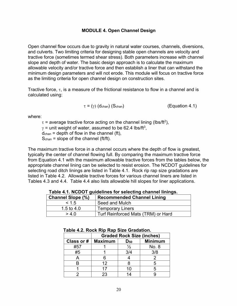
MODULE 4. Open Channel Design Open channel flow occurs due to gravity in natural water courses, channels, diversions, and culverts. Two limiting criteria for designing stable open channels are velocity and tractive force (sometimes termed shear stress). Both parameters increase with channel slope and depth of water. The basic design approach is to calculate the maximum allowable velocity and/or tractive force and then establish a liner that can withstand the minimum design parameters and will not erode. This module will focus on tractive force as the limiting criteria for open channel design on construction sites. Tractive force, , is a measure of the frictional resistance to flow in a channel and is calculated using:
= ( (dchan) (Schan) (Equation 4.1) where: = average tractive force acting on the channel lining (lbs/ft2), = unit weight of water, assumed to be 62.4 lbs/ft3, dchan = depth of flow in the channel (ft),
Schan = slope of the channel (ft/ft). The maximum tractive force in a channel occurs where the depth of flow is greatest, typically the center of channel flowing full. By comparing the maximum tractive force from Equation 4.1 with the maximum allowable tractive forces from the tables below, the appropriate channel lining can be selected to resist erosion. The NCDOT guidelines for selecting road ditch linings are listed in Table 4.1. Rock rip rap size gradations are listed in Table 4.2. Allowable tractive forces for various channel liners are listed in Tables 4.3 and 4.4. Table 4.4 also lists allowable hill slopes for liner applications.
Table 4.1. NCDOT guidelines for selecting channel linings. Channel Slope (%) Recommended Channel Lining
< 1.5 Seed and Mulch 1.5 to 4.0 Temporary Liners
> 4.0 Turf Reinforced Mats (TRM) or Hard
Table 4.2. Rock Rip Rap Size Gradation. Graded Rock Size (inches)
Class or # Maximum D50 Minimum #57 1 ½ No. 8 #5 1 3/4 3/8 A 6 4 2 B 12 8 5 1 17 10 5 2 23 14 9

21
Table 4.3. Allowable Tractive Forces for Channel Linings (PADEP, 2000).1 Channel Lining Category
Lining Type
Allowable Tractive Force, (lbs/ft2)
Unlined – Erodible Soils (K > 0.37)
Silts, Fine – Medium Sands 0.03
Coarse Sands 0.04 Very Coarse Sands 0.05 Fine Gravel 0.10 Erosion Resistant Soils (K < 0.37)
Sandy loam 0.02
Gravely, Stony, Channery loam 0.05 Stony or Channery silt loam 0.07 Loam 0.07 Sandy clay loam 0.10 Silt loam 0.12 Silty clay loam 0.18 Clay loam 0.25 Shale & Hardpan 1.00 Durable Bedrock 2.00 RECP Jute Netting 0.45 Geocoir/Dekowe; Straw; RS-1 0.83 Profile; Futerra 1.00 Am. Excelsior Co.; Curlex Net Free 1.00 Am. Excelsior Co.; Straw; 1 net 1.25 Geocoir/Dekowe; Straw; RS-2 1.25 E. Coast Ero. Blank.; Straw/Coir, 2 Jute nets 1.35 Am. Excelsior Co.; Straw; 2 nets 1.50 Am. Excelsior Co.; Curlex I.73; 1 net 1.55 E. Coast Ero. Blank.; Straw, 1 net 1.55 E. Coast Ero. Blank.; Coir, 2 Jute nets 1.63 Am. Excelsior Co.; Curlex I.98; 1 net 1.65 Am. Excelsior Co.; Curlex II.73; 2 nets 1.75 N. Am. Green; Straw; double net 1.75 E. Coast Ero. Blank.; Excelsior, 1 net 1.80 NAG; 70% straw: 30% Coconut; double net 2.00 NAG; Polypropylene; double net; Bare soil 2.00 Am. Excelsior Co.; Curlex II.98; 2 nets 2.00 Geocoir/Dekowe; Coconut, RSC-4 2.00 E. Coast Ero. Blank.; Excelsior, 2 nets 2.00 E. Coast Ero. Blank.; Straw, Jute net 2.10 E. Coast Ero. Blank.; Straw, 2 nets 2.10 N. Am. Green; Coconut; double net 2.25

22
Am. Excelsior Co.; Curlex III; 2 nets 2.30 Am. Excelsior Co.; Curlex Enforcer; 2 nets 2.30 E. Coast Ero. Blank.; Straw/Coir, 2 nets 2.60 Am. Excelsior Co.; Curlex High Velocity; 2 nets 3.00 Geocoir/Dekowe; 400 3.10 E. Coast Ero. Blank.; Coir, 2 nets 3.20 E. Coast Ero. Blank.; Polypropylene, 2 nets 3.21 Geocoir/Dekowe; 700 4.46 Geocoir/Dekowe; 900 4.63 NAG; Polypropylene; double net; Vegetated 8.00 Turf Reinforced Mats (TRM)
North Am. Green SC250; Bare soil 2.50
North Am. Green C350; Bare soil 3.00 North Am. Green P550; Bare soil 3.25 E. Coast Ero. Blank.; Coir, 3 nets 3.50 Profile/Enkamat; 7003 (BFM) 5.00 Profile/Enkamat; 7010, seed and hydromulch 6.00 Profile/Enkamat; 7010 – 7220, seed, BFM; Veg 6.0-8.0 Profile/Enkamat; 7010 - 7220, seed, BFM; Bare 6.7-11.2 Profile/Enkamat; 7018, seed and hydromulch 7.00 North Am. Green SC250; Vegetated 8.00 Profile/Enkamat; 7020, seed and hydromulch 8.00 Profile/Enkamat II; seed and BFM; Vege. 8.00 Profile/Enkamat; 7920, seed and BFM; Vege. 8.00 North Am. Green C350; Vegetated 10.0 Profile/Enkamat II; seed and BFM; Bare 10.0 Am. Excelsior Co.; Recyclex 10.0+ North Am. Green P550; Vegetated 12.5 Grass Liners Class D 0.60 Class C 1.00 Class B 2.10 Aggregate & Riprap #57 0.25 #5 0.50 Class A 1.00 Class B 2.00 Class 1 3.00 Class 2 4.00 Reno Mattress & Gabion
8.35
Concrete 100

23
Table 4.4. Allowable Tractive Force of RECPs. (Table 6.17a NCDENR (2006))1 Category
Product Type
Max. Permissible Shear Stress
(lbs/ft2)
SlopesUp to
RECP N. Am. Green; Straw; 1 net 1.55 3:1 Am. Excelsior Co.; Curlex Net Free 1.00 3:1 Am. Excelsior Co.; Straw; 1 net 1.25 3:1 Geocoir/Dekowe; Straw; RS-1 0.83 3:1 N. Am. Green; Straw; 2 nets 1.75 2:1 Am. Excelsior Co.; Curlex I.73; 1 net 1.55 2:1 Am. Excelsior Co.; Curlex I.98; 1 net 1.65 2:1 Am. Excelsior Co.; Straw; 2 nets 1.50 2:1 Geocoir/Dekowe; Straw; RS-2 1.25 2:1 Geocoir/Dekowe; 70% Straw 30%
Coconut; RSS/C-3 1.85 2:1
Geocoir/Dekowe; Poly/Fiber; RSP-5 2.00 2:1 Geocoir/Dekowe; Coconut, RSC-4 2.00 2:1 Am. Excelsior Co.; Curlex II.73; 2 nets 1.75 1.5:1 Am. Excelsior Co.; Curlex II.98; 2 nets 2.0 1.5:1 Am. Excelsior Co.; Straw/Coconut; 2 nets 1.5:1 NAG; 70% straw: 30% Coir; 2 nets 2.00 1:1 N. Am. Green; Coconut; 2 nets 2.25 1:1 Am. Excelsior Co.; Curlex III; 2 nets 2.3 1:1 NAG; Polypropylene; 2 nets; Bare soil 2.0 1:1 NAG; Polypropylene; 2 nets; Vegetated 8.0 1:1 Am. Excelsior Co.; Coconut; 2 nets 1:1 Am. Excelsior Co.; Curlex Enforcer; 2 nets 0.75:1 Am. Excelsior Co.; Curlex High Velocity; 2
nets 3.0 0.75:1
TRM Profile/Enka; 7003, Vege. 5.0 3.5:1 Profile/Enka; 7010, 7210, 7910, Vege. 6.0 2:1 Profile/Enka; 7220, 7020, Vege. 8.0 1.5:1 Profile/Enkamat II 8.0 1:1 Profile/Enka; 7520, Vege. 8.0 0.5:1 Am. Excelsior Co.; Recyclex 10.0+ 0.5:1 Degradable RECP’s
Nets and Mulch 0.1 – 0.2 20:1
(Unvegetated) Coir Mesh 0.4 – 3.0 3:1 Blanket – Single Net 1.55 – 2.0 2:1 Blanket – Double net 1.65 – 3.0 1:1 Nondegradable Unvegetated 2 – 4 1:1 Turf Reinforce Mats
Partially Vegetated 4 – 6 >1:1
Fully Vegetated 5 - 10 >1:1
24
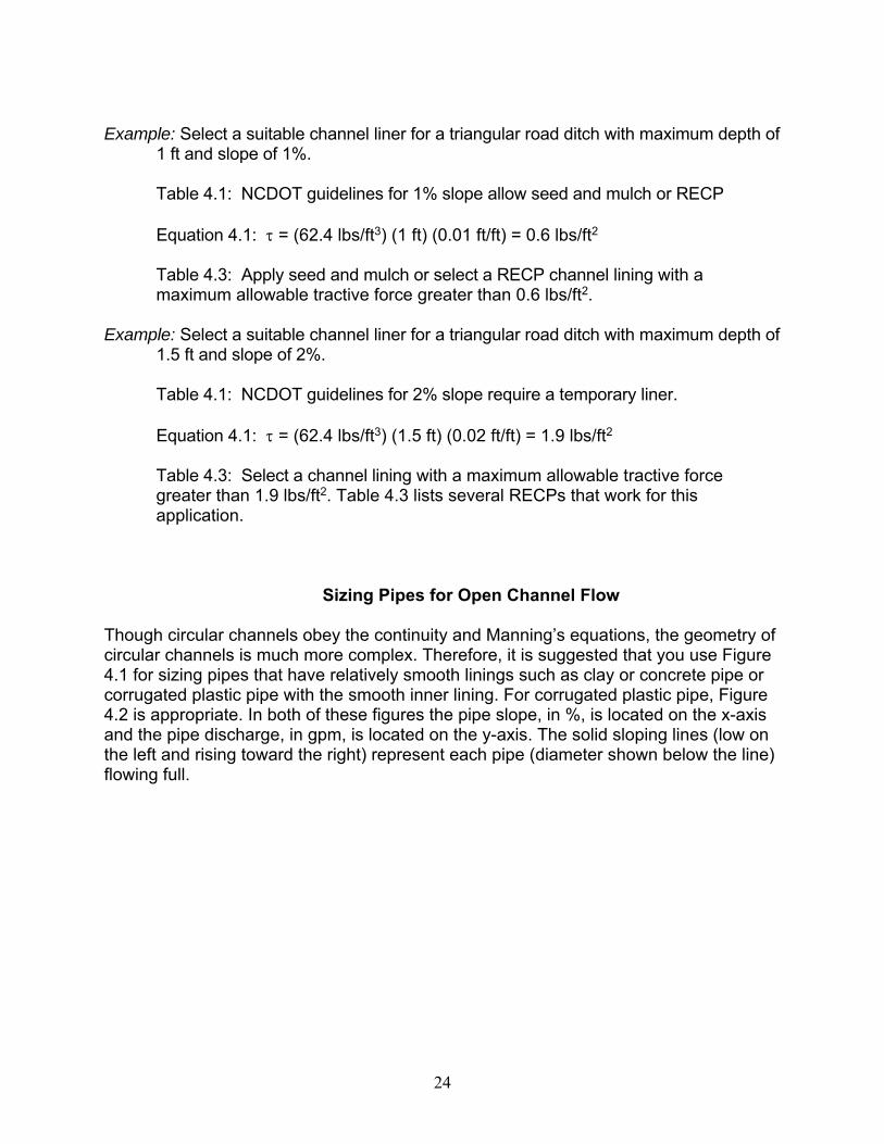
Example: Select a suitable channel liner for a triangular road ditch with maximum depth of
1 ft and slope of 1%. Table 4.1: NCDOT guidelines for 1% slope allow seed and mulch or RECP Equation 4.1: = (62.4 lbs/ft3) (1 ft) (0.01 ft/ft) = 0.6 lbs/ft2 Table 4.3: Apply seed and mulch or select a RECP channel lining with a
maximum allowable tractive force greater than 0.6 lbs/ft2. Example: Select a suitable channel liner for a triangular road ditch with maximum depth of
1.5 ft and slope of 2%. Table 4.1: NCDOT guidelines for 2% slope require a temporary liner. Equation 4.1: = (62.4 lbs/ft3) (1.5 ft) (0.02 ft/ft) = 1.9 lbs/ft2 Table 4.3: Select a channel lining with a maximum allowable tractive force
greater than 1.9 lbs/ft2. Table 4.3 lists several RECPs that work for this application.
Sizing Pipes for Open Channel Flow
Though circular channels obey the continuity and Manning’s equations, the geometry of circular channels is much more complex. Therefore, it is suggested that you use Figure 4.1 for sizing pipes that have relatively smooth linings such as clay or concrete pipe or corrugated plastic pipe with the smooth inner lining. For corrugated plastic pipe, Figure 4.2 is appropriate. In both of these figures the pipe slope, in %, is located on the x-axis and the pipe discharge, in gpm, is located on the y-axis. The solid sloping lines (low on the left and rising toward the right) represent each pipe (diameter shown below the line) flowing full.

25
Figure 4.1. Pipe sizing chart for clay, concrete and corrugated plastic pipe
with a smooth inner liner (Jarrett, 2000).
40,000
30,000
20,000
10,000
5,000
4,000
3,000
2,000
1,000
500
400
300
200
100
50
40
30
DIS
CH
AR
GE
(G
PM
)ACRES DRAINED
DRAINAGE COEFF..1 .2 .3 .4 .5 1.0 2.0 3.0 4.0 5.0 10 1/4 1/2 1 3/8 3/4
SLOPE IN FEET PER 100 FEET (%)
Based on Manning’s n=0.0108
8000
5000
4000
3000
2000
1000
500
400
300
200
100
50
40
30
20
10
4000
3000
2000
1000
500
400
300
200
100
50
40
30
20
10
5
4
3
2000
1000
500
400
300
200
100
50
40
30
20
10
5
4
3
2
1
5000
4000
3000
2000
1000
500
400
300
200
100
50
40
30
20
10
5
4
2000
1000
500
400
300
200
100
50
40
30
20
10
5
4
3
2
V=20
V=15
V=12
V=10V
=9
V=7
V=8
V=6
V=5
V=4
V=3
V=2
V=1
48”
42”
36”
30”
24”
18”
16”
14”
12”
10”
8”
6”
5”
4”

26
MODULE 5. Sediment Retention BMPs Sediment retention best management practices (BMPs) are treatment systems designed to remove suspended sediment from runoff water before discharging to a receiving stream or a neighboring property. BMPs are designed to maximize sediment retention based on (1) impoundment volume to store runoff water and collected sediment; (2) detention time to remove water by gravity; and (3) length of flow path within the structure to maximize settling. BMP characteristics that improve effectiveness include:
Stable interior sideslopes no steeper than 1.5:1, Plastic liner and/or vegetation established within the structure, Stable inlet(s) for water entering the structure to settle sediment, Baffles of porous jute or coir to divide the structure into 3 or more chambers, Surface dewatering device to remove cleaner water first, and Infiltration from the bottom of the basin if possible.
In North Carolina, sediment retention BMPs (basins or similar retention structures) are sized based on two criteria: 1. Volume, Vbasin, in cubic feet (ft3): Vbasin ≥ 3,600 ft3 per acre of disturbed land Vbasin ≥ 1,800 ft3 per acre of disturbed land (with a surface dewatering device) 2. Surface Area, Abasin, in square feet (ft2): Abasin ≥ 435 Q10 Abasin ≥ 325 Q10 (with a surface dewatering device) For environmentally sensitive areas, use the 25-year peak runoff rate, Q25. Example: Calculate minimum volume and surface area for a skimmer basin serving a 6-
acre construction site (all disturbed) with Q10 = 20 cfs.
Volume: Vbasin ≥ 1,800 ft3 per acre of disturbed land Vbasin ≥ 1,800 ft3/ac (6 ac) = 10,800 ft3 Surface Area: Abasin ≥ 325 Q10 (with a surface dewatering device) Abasin ≥ 325 (20) = 6,500 ft2
27
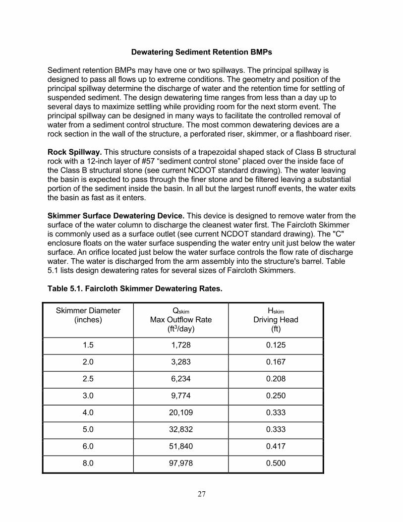
Dewatering Sediment Retention BMPs Sediment retention BMPs may have one or two spillways. The principal spillway is designed to pass all flows up to extreme conditions. The geometry and position of the principal spillway determine the discharge of water and the retention time for settling of suspended sediment. The design dewatering time ranges from less than a day up to several days to maximize settling while providing room for the next storm event. The principal spillway can be designed in many ways to facilitate the controlled removal of water from a sediment control structure. The most common dewatering devices are a rock section in the wall of the structure, a perforated riser, skimmer, or a flashboard riser. Rock Spillway. This structure consists of a trapezoidal shaped stack of Class B structural rock with a 12-inch layer of #57 “sediment control stone” placed over the inside face of the Class B structural stone (see current NCDOT standard drawing). The water leaving the basin is expected to pass through the finer stone and be filtered leaving a substantial portion of the sediment inside the basin. In all but the largest runoff events, the water exits the basin as fast as it enters. Skimmer Surface Dewatering Device. This device is designed to remove water from the surface of the water column to discharge the cleanest water first. The Faircloth Skimmer is commonly used as a surface outlet (see current NCDOT standard drawing). The "C" enclosure floats on the water surface suspending the water entry unit just below the water surface. An orifice located just below the water surface controls the flow rate of discharge water. The water is discharged from the arm assembly into the structure's barrel. Table 5.1 lists design dewatering rates for several sizes of Faircloth Skimmers. Table 5.1. Faircloth Skimmer Dewatering Rates.
Skimmer Diameter (inches)
Qskim Max Outflow Rate
(ft3/day)
Hskim Driving Head
(ft)
1.5 1,728 0.125
2.0 3,283 0.167
2.5 6,234 0.208
3.0 9,774 0.250
4.0 20,109 0.333
5.0 32,832 0.333
6.0 51,840 0.417
8.0 97,978 0.500

28
Table 5.1 is used to size the skimmer orifice located at the top of the water entry point. This orifice controls the basin outflow rate and must be sized carefully. The Faircloth skimmer is patented and is available from J. W. Faircloth and Sons, Inc at http://www.fairclothskimmer.com in specific sizes. The skimmer size refers to the diameter of the float and arm. The Faircloth Skimmer is sized by determining the required basin outflow rate as the water volume divided by the dewatering time:
Qskim = Vskim / tdewater (Equation 5.1) where: Qskim = basin outflow rate in cubic feet per day (ft3/day), Vskim = basin volume to be dewatered in cubic feet (ft3), tdewater = dewatering time (days). For NCDOT skimmer basins, the current design standard calls for dewatering the top 2 feet of volume in 3 days. For the design Qskim, select a skimmer and orifice from Table 5.1 which meets or exceeds this rate. The Faircloth Skimmer comes with a plastic plug that can be drilled to provide an orifice to limit outflow to the desired rate. The diameter of the orifice is calculated using the discharge rate and the driving head:
D
orifice
Qskim
2310 Hskim
(Equation 5.2)
where: Dorifice = diameter of the skimmer orifice in inches (in), Qskim = basin outflow rate in cubic feet per day (ft3/day), Hskim = driving head at the skimmer orifice from Table 5.1 in feet (ft). Example: Select a skimmer that will dewater 20,000 ft3 of water in 3 days.
Qskim = 20,000 ft3 / 3 days = 6,670 ft3/day From Table 5.1, select the 3-inch skimmer with an outflow rate of 9,774 ft3/day and a driving head of 0.25 ft. Since this outflow rate will dewater the basin in less than 3 days, an orifice smaller than 3 inches diameter can be drilled to slow the flow rate according to Equation 5.2.
D
orifice 6,670
2310 0.25 2.1 inches
If the plastic is drilled to a diameter of 2.1 inches and placed in the 3-inch skimmer, the dewatering rate is 6,670 ft3/d and 20,000 ft3 will dewater in 3 days.

29
Flashboard Riser. This device can be managed to maintain a minimum water depth and provide for surface dewatering, see Figure 5.1.
Figure 5.1. Flashboard Riser for Dewatering a Sediment Retention Basin.
Infiltration Basin. If soil conditions are conducive to high infiltration rates, most or all of the water entering a basin can be discharged through infiltration. The infiltration rate can be obtained from USDA-NRCS County Soil Surveys where the permeability (sometimes called saturated hydraulic conductivity) is typically listed as a range of values (e.g. 0.6 to 2.0 in/hr). For a conservative design, choose the lower permeability of the soil horizon with the slowest permeability. For example, if a soil has “A”, “B”, and “C” horizons with published permeabilities of 0.6-2.0, 0.2-0.8, and 6.0-20, respectively, the value to be used for the basin’s infiltration design would be 0.2 in/hr. For NCDOT projects, the soil permeability must be at least 0.5 in/hr to meet the design criteria of dewatering 3 ft of water in 3 days or less.
Emergency Spillway
The emergency spillway on a sediment retention BMP should be capable of passing large storm flows with a maximum depth of flow over the emergency spillway of 1 ft. For NCDOT skimmer basins and infiltration basins, the weir length (ft) is calculated by dividing the peak discharge (Qp in cfs) by 0.4, except for drainage areas <1 acre, which have a 4ft minimum weir length.

30
MODULE 6. Below Water Table Borrow Pits
Borrow pits are areas of suitable soil material excavated to provide necessary road building material. Between active borrow pit excavations, ground water may seep into the pit, and rainfall may produce runoff into the borrow pit, creating an impoundment that must be dewatered before additional borrow material can be removed. When a borrow pit is initially prepared to serve as a source of construction material, a rim ditch is dug around the perimeter, typically 10 to 25 ft wide at its bottom, dug to the lowest depth from which the borrow material will be removed. Because the rim ditch, and later all or part of the whole borrow pit area inside of the rim ditch, will fill with water at least to the depth of the regional water table, it is common practice for contractors to dewater rim ditches and borrow pits by placing a pump in the deepest rim ditch location. If the pumped water has a high turbidity level, the pumped borrow pit water must be treated. Stilling basin for Pumped Borrow Pit Water A common practice is to discharge the water pumped from the rim ditch into a stilling basin with a volume that provides sufficient time for settling. The required stilling basin volume can be calculated by multiplying the desired detention time by the pumping rate of water entering the basin. For NCDOT applications, the current design standard requires a detention time of at least 2 hours and a maximum pumping rate of 1,000 gpm. For a 2-hr detention time, the minimum stilling basin volume is:
Vstill = 16 (Qstill) (Equation 6.1) where:
Vstill = volume of stilling basin in cubic feet (ft3), and Qstill = pumping rate entering the stilling basin in gallons per minute (gpm).
At the maximum NCDOT pumping rate of 1,000 gpm, the required stilling basin volume is 16,000 ft3. If water pumped from the borrow pit has high turbidity, the water is most commonly discharged into a stilling basin located at the land surface. The stilling basin for pumped effluent is a rectangular-shaped basin with at least a 2:1 L:W shape, constructed from natural soil. The basin should receive sediment-laden water from a borrow pit excavation site where the water is pumped to the stilling basin for treatment. The maximum depth is 3 feet, and the embankment should have 1.5:1 interior and exterior side slopes. The basin is dewatered with a surface outlet device, most appropriately a 12-inch vertical riser pipe (with no perforations) set at the 3-ft water level. A flashboard riser system may also be used with the top flashboard set at 3 ft for normal operation. This system allows for dewatering by removing flashboards as necessary.

31
Polyacrylamide (PAM) For high-turbidity water, a polyacrylamide (PAM) may be added to the pumped water as a flocculant to help settle sediment in the stilling basin system. When PAM is properly injected into the pumped water, the stilling basin can be designed to detain the water for as little as 2 hours. PAM is available in powder form and can be mixed with water to form a liquid suspension of PAM. Normal mixing rates are one pound of PAM added to 100 gallons of water. This liquid PAM solution can be injected into the positive side of the pump using an injection pump unit to produce a PAM concentration of about 1 mg/L. The liquid PAM application or injection rates needed to create a 1 mg/L PAM concentration in the sediment-laden water are show in Figure 6.1.
Figure 6.1. PAM injection rate related to pump rate to create 1 mg/L of PAM.
Borrow pit pump water that has had PAM applied will quickly develop clay flocs (large aggregates of clay particles) that must be removed from the water. Normally this water should be pumped directly into the inlet chamber of a stilling basin. Applied Polymer Systems recommend discharging the flocculent-laden water into a level (perpendicular to flow direction) shallow (not more than 0.1 ft deep) channel lined with jute or coir erosion control blanket. The flocs tend to be captured in the jute/coir pores and removed from the gently flowing water. When the jute/coir layer becomes filled with settled/captured soil flocs, just add another layer of jute/coir. This stripping approach may work well for borrow pit dewatering systems where the pump rate is 350 gpm or less.
PAM Injection Rate
0.0
0.5
1.0
1.5
2.0
2.5
3.0
3.5
4.0
0 500 1000 1500 2000 2500 3000
Pump Rate (gpm)
PA
M In
jec
tio
n R
ate
(g
pm
)

32
Skaggs Method for Determining Wetlands Encroachment Where borrow pits are located near wetlands, it is critical that excavation be managed so that wetland hydrology is not altered. A site has wetland hydrology if, during the growing season, the water table is normally within 1 ft of the soil surface for a continuous critical duration, defined as 5 to 12.5% of the growing season (USACE, 1987). The lower limit of 5% of the growing season was used in the Skaggs Method to predict lateral effects of borrow pit excavation on the water table. The Skaggs Method is a procedure developed from simulating 50 years (1951-2000) of each county’s meteorological data on the flow cross-section shown in Figure 6.2 using a local hydric soil to determine the distance from the borrow pit where, once every 2 years, the water table will drop below the 0.83 ft depth; shown in Figure 6.2 as the “Lateral Effect.” During DRAINMOD simulations, a critical water table depth of 0.83 ft was used as a conservative approximation of the USACE (1987) 1-ft criterion. As boundary conditions for the DRAINMOD simulations, two additional parameters were used; (a) depth of water stored on the soil surface, either 1 or 2 inches; and (b) depth below surface where the borrow pit has ponded water, ranging from 1 to 6 ft. Other parameters for each county included depth from surface to impermeable layer, ho, soil drainable porosity, f, and soil effective hydraulic conductivity, Ke.
Figure 6.2. Borrow Pit with Lateral Effect on Wetland Hydrology.
The effective hydraulic conductivity is the weighted average of conductivities of each soil layer above the impermeable layer:
n
nne ddd
dKdKdKK
...
...
21
2211 (Equation 6.2)
where K1, K2, etc are the hydraulic conductivities and d1, d2, etc are the thicknesses of soil layers 1, 2, etc, respectively.
Lateral Effect
Wetland
Borrow Pit
Water Table
h
do=ho-d
d
0.83 ft @ T25
ho

33
The results of the county simulations are expressed in terms of T25, the time in days required for the water table to be drawn down from the soil surface to a depth of 0.83 ft. The results of these simulations are shown in Table 6.1 for areas with 1 and 2 inches of surface depressional strorage. The T25 value is used with other soil parameters to solve for the “Lateral Effect” distance, x:
1f
tKh
x
o
(Equation 6.3)
where:
Ke = effective hydraulic conductivity in feet per day (ft/d), ho = depth from soil surface to impermeable layer in feet (ft), t is T25 from Table 6.1 for appropriate depth of depressional storage (days), f = drainable porosity for the soil into which pit is excavated (decimal), 1/η = the value read from the x-axis of Figure 6.2 based on the parameters
H = h/ho and D = d/ho, where h is depth from critical water table depth (0.83 ft) to impermeable layer (ft) and d is depth from water surface in the borrow pit to impermeable layer.
Since critical water table depth is 0.83 ft, h is always h = ho – 0.83, so
o
o
h
hH
83.0 (Equation 6.4)
If do represents the “depth to water” in the borrow pit parameter, then d = ho - do and
o
oo
h
dhD
(Equation 6.5)
For NCDOT applications, the current design standard is to set the following parameters as constants:
f = 0.035 and do = 2 ft

34
Figure 6.3. Nondimensional solutions to the Boussinesq Equation for water table drawdown due to drainage to a single ditch or borrow pit (after Skaggs, 1976). Example: Determine the lateral effect of a borrow pit in Johnston County with Goldsboro soil, effective hydraulic conductivity of 4 ft/day, drainable porosity of 0.035, depth to impermeable layer of 15 ft, and surface depressional storage of 2 in. See schematic in Figure 6.4.

35
Figure 6.4. Example application of Skaggs Method. Given: f = 0.035
do = 2 ft Ke = 4.0 ft/day ho = 15 ft Table 6.1: t = T25 = 5.2 days
94.015
17.14
15
83.01525
o
o
h
hH
87.015
13
15
215
o
oo
h
dhD
From Figure 6.3, use interpolation to find the x-axis value, 1/η = 1.07 Solve Equation 6.3 for the “Lateral Effect”, x as:
ft
dftdftf
tKh
x
o
8807.1
42.94
07.1035.0
)2.5)(0.15(/0.4
1
The Lateral Effect is 88 ft. In other words the borrow pit can be placed 88 feet from the edge of the wetland area without causing drainage of the wetland and reducing its status as a wetland.
Lateral Effect
Wetland
Borrow Pit
Water Table
h
do=ho-d
d
0.83 ft @ T25
ho

36
Table 6.1. T25 (days) for 2-ft depth to water for 1 and 2 inch depressional storage.
County 1 inch storage 2 inches Alamance 9.0 4.6Alexander 5.6 3.5Alleghany 5.7 3.5Anson 8.5 4.6Ashe 2.9 1.9Avery 3.0 2.2Bertie 8.7 4.1Beaufort 6.2 3.7Bladen 10.3 4.8Brunswick 4.6 3.0Buncombe 4.0 2.8Burke 5.6 3.3Cabarrus 6.7 3.9Caldwell 5.1 2.9Camden 6.0 3.8Carteret 5.0 3.2Caswell 8.2 4.5Catawaba 5.6 3.5Chatham 5.4 3.6Cherokee 4.0 2.5Chowan 7.1 4.0Clay 2.8 1.7Cleveland 5.2 3.2Columbus 9.2 4.6Craven 5.2 3.2Cumberland 6.3 4.6Currituck 6.0 3.8Dare 5.7 3.2Davidson 8.6 4.8Davie 6.9 4.4Duplin 5.5 3.4Durham 7.1 4.0Edgecombe 9.5 4.7Forsyth 7.1 4.1Gaston 7.0 3.7Gates 6.2 3.7Graham 4.8 3.1Granville 9.7 4.6Greene 8.6 4.0Guilford 6.2 3.9Halifax 7.9 4.6Harnett 8.9 4.7Haywood 10.4 5.7Henderson 3.3 2.4Hertford 6.2 3.7Hoke 6.3 4.6Hyde 7.2 3.6Iredell 5.6 3.5