NONSMOOTH OPTIMIZATION VIA BFGS

ADRIAN S. LEWIS∗ AND MICHAEL L. OVERTON†

Abstract. We investigate the BFGS algorithm with an inexact line search when applied to non-smooth functions, not necessarily convex. We define a suitable line search and show that it generatesa sequence of nested intervals containing points satisfying the Armijo and weak Wolfe conditions, as-suming only absolute continuity. We also prove that the line search terminates for all semi-algebraicfunctions. The analysis of the convergence of BFGS using this line search seems very challenging;our theoretical results are limited to the univariate case. However, we systematically investigate thenumerical behavior of BFGS with the inexact line search on various classes of examples. The methodconsistently converges to local minimizers on all but the most difficult class of examples, and even inthat case, the method converges to points that are apparently Clarke stationary. Furthermore, theconvergence rate is observed to be linear with respect to the number of function evaluations, witha rate of convergence that varies in an unexpectedly consistent way with the problem parameters.When the problem is sufficiently difficult, convergence may not be observed, but this seems to bedue to rounding error caused by ill-conditioning. We try to give insight into why BFGS works aswell as it does, and we conclude with a bold conjecture.

Key words. BFGS, quasi-Newton, nonsmooth, nonconvex, line search, R-linear convergence

AMS subject classifications. 90C30, 65K05

1. Introduction. This paper is concerned with the behavior of the BFGS (Broy-den-Fletcher-Goldfarb-Shanno) variable metric (quasi-Newton) method with an inex-act line search applied to nonsmooth functions, convex or nonconvex. A companionpaper [LO08] analyzes BFGS with an exact line search on some specific nonsmoothexamples.

It was shown by Powell [Pow76] that, if f : Rn → R is convex and twice continu-ously differentiable, and the sublevel set {x : f(x) ≤ f(x0)} is bounded (x0 being thestarting point), then the sequence of function values generated by the BFGS methodwith a weak Wolfe inexact line search converges to or terminates at the minimal valueof f . This result does not follow directly from the standard Zoutendijk theorem as oneneeds to know that the eigenvalues of the inverse Hessian approximation Hk do notgrow too large or too small. The result has never been extended to the nonconvex case.Indeed, very little is known in theory about the convergence of the standard BFGSalgorithm when f is a nonconvex smooth function, although it is widely accepted thatthe method works well in practice [LF01].

There has been even less study of the behavior of BFGS on nonsmooth functions.While any locally Lipschitz nonsmooth function f can be viewed as a limit of increas-ingly ill-conditioned differentiable functions (see [RW98, Thm 9.67] for one theoreticalapproach, via “mollifiers”), such a view has no obvious consequence for the algorithm’sasymptotic convergence behavior when f is not differentiable at its minimizer. Yet,when applied to a wide variety of nonsmooth, locally Lipschitz functions, not nec-essarily convex, BFGS is very effective, automatically using the gradient differenceinformation to update an inverse Hessian approximation Hk that typically becomesextremely ill-conditioned. A key point is that, since locally Lipschitz functions are

∗School of Operations Research and Information Engineering, Cornell University, Ithaca, NY14853, U.S.A. aslewis@orie.cornell.edu. Research supported in part by National Science Founda-tion Grant DMS-0806057.

† Courant Institute of Mathematical Sciences, New York University, New York, NY 10012, U.S.A.overton@cs.nyu.edu. Research supported in part by National Science Foundation Grant DMS-0714321.

1

differentiable almost everywhere, as long as the method is initialized randomly and aninexact line search is used, it is very unlikely that an iterate will be generated at whichf is not differentiable. Under the assumption that such a point is never encountered,the method is well defined, and linear convergence of the function values to a locallyoptimal value is typical (not superlinear, as in the smooth case).

Although there has been little study of this phenomenon in the literature, thefrequent success of variable metric methods on nonsmooth functions was observed byLemarechal more than 25 years ago. His comments in [Lem82] include:

We have also exhibited the fact that it can be good practice to usea quasi-Newton method in nonsmooth optimization [as] convergenceis rather rapid, and often a reasonably good approximation of theoptimum is found; this, in our opinion, is essentially due to the factthat inaccurate line-searches are made. Of course, there is no the-oretical possibility to prove convergence to the right point (in factcounterexamples exist), neither are there any means to assess theresults....this raises the question: is there a well-defined frontier betweenquadratic and piecewise linear, or more generally, between smoothand nonsmooth functions?

Lemarechal’s observation was noted in several papers of Luksan and Vlcek [LV99,LV01, VL01]. They wrote in [VL01]: “standard variable metric methods are rela-tively robust and efficient even in the nonsmooth case. . . . On the other hand, noglobal convergence has been proved for standard variable metric methods appliedto nonsmooth problems, and possible failures or inaccurate results can sometimesappear in practical computations.” Motivated by the latter observation, combinedwith the attraction of the low overhead of variable metric methods, Luksan andVlcek proposed new methods intended to combine the global convergence propertiesof bundle methods [HUL93, Kiw85] with the efficiency of variable metric methods.Other papers that combine ideas from bundle and variable metric methods include[BGLS95, LS94, MSQ98, RF00].

Our interest is in the standard BFGS method [NW06, Chap. 6] applied directly tononsmooth functions without any modifications, except that care must be taken in theline search. Although we are motivated by the potential use of BFGS as a practicalmethod, primarily in the nonconvex case, this paper is focused on understanding itsbehavior on relatively simple examples, many of them convex. Our hope is that evenpartial success in this direction will lead the way toward a more complete picture ofhow BFGS behaves in general.

In Section 2 we give a detailed treatment of the line search. Standard line searchesfor smooth optimization impose an Armijo condition on reduction of the function valueand a Wolfe condition controlling the change in the directional derivative. For thelatter condition, often a “strong” version is imposed, requiring a reduction in the ab-solute value of the directional derivative, as opposed to a “weak” version that requiresonly an algebraic increase. The weak version is all that is required to ensure positivedefiniteness of the updated inverse Hessian approximation; nonetheless, it is popularboth in textbooks and software to require the strong condition, despite the substan-tial increase in implementation difficulty, perhaps because this is the traditional routeto proving convergence results for nonlinear conjugate gradient methods on smoothfunctions. For nonsmooth optimization, it is clear that enforcing the strong Wolfecondition is not possible in general, and it is essential to base the line search on the

2

simpler weak Wolfe condition. The line search we describe is close to earlier methodsin the literature, but our analysis differs. We prove that the line search generatesa sequence of nested intervals containing points that satisfy the Armijo and Wolfeconditions, assuming only that the function is absolutely continuous along the line.We also prove that the line search terminates under slightly stronger assumptions, inparticular covering all semi-algebraic functions (not necessarily locally Lipschitz).

The success of BFGS and most other variable metric methods in the smooth case isin large part because inexact line searches quickly find an acceptable step: eventuallythe method always accepts the unit initial step. The behavior of BFGS with aninexact line search on nonsmooth functions is complex: it is far from clear whetherthe unit step will be well scaled. As an initial analysis of this crucial but difficultquestion, we carefully consider the univariate case, which is surprisingly nontrivialand offers substantial insight. In Section 3 we prove that, for f(x) = |x|, the methodconverges with R-linear rate 1/2 with respect to the number of function evaluations.In Section 4, we argue that the rate for the function max{x,−ux} is, for large u,approximately 2−1/ log2 u.

In Section 5 we systematically investigate the numerical behavior of BFGS withthe inexact line search on various classes of examples. We find that the methodconsistently converges to local minimizers on all but the most difficult class of ex-amples, and even in that case, the method converges to points that are apparentlyClarke stationary. Furthermore, the convergence rate is observed to be linear withrespect to the number of function evaluations, with a rate of convergence that variesin an unexpectedly consistent way with the dimension and parameters defining theproblem in each class. When the problem is constructed to be sufficiently difficult,convergence may not be observed, but this seems to be due to rounding error causedby ill-conditioning, not a failure of the method to converge in exact arithmetic.

In Section 6 we briefly consider alternative methods that are applicable to non-smooth, nonconvex problems. We also mention our publicly available Matlab codehanso, addressing the issues of stopping criteria and how to assess the quality of theresult.

We conclude in Section 7 with a bold conjecture.An intuitive, although far from complete, argument for the success of BFGS

on nonsmooth problems goes as follows. Because the gradient differences may beenormous compared to the difference of the points where they are computed, the in-verse Hessian approximation typically becomes very ill-conditioned in the nonsmoothcase. Tiny eigenvalues of Hk correspond to directions along which, according to thequadratic model constructed by BFGS, the function has a huge second derivative. Infact, of course, f is not differentiable at the local optimizer being approximated, butcan be arbitrarily well approximated by a function with a sufficiently ill-conditionedHessian. As is familiar from interior point methods for constrained optimization, it isthis ill-conditioning of Hk that apparently enables the method to work so well. Re-markably, it often happens that the condition number of Hk approaches the inverseof the machine precision before rounding errors cause a breakdown in the method,usually failure to obtain a reduction of f in the inexact line search. The spectraldecomposition of the final Hk typically reveals two subspaces along which the behav-ior of f is very different: the eigenvalues that are not relatively tiny are associatedwith eigenvectors that identify directions from the final iterate along which f variessmoothly, while the tiny eigenvalues are associated with eigenvectors along whichf varies nonsmoothly. More specifically, when applied to partly smooth functions

3

[Lew03], it seems typical that BFGS automatically identifies the U and V-spaces as-sociated with f at the approximate minimizer. Furthermore, even when Hk is veryill-conditioned, the unit step is typically relatively well scaled, and this property doesnot deteriorate as the iteration count k increases (although, as noted in Section 5.4, itdoes seem to deteriorate as the dimension n increases). Mysteries that remain includethe mechanism that prevents the method from stagnating, the reason for the relativewell-scaledness of the unit step in the line search, and the condition measure of f thatdetermines the amazingly consistent linear rates of convergence that we observe.

A natural question is whether these observations extend to the well known limitedmemory variant of BFGS. Our experience with this is minimal and we do not addressthe issue here. However, we note that comments in the literature observing thatlimited memory BFGS sometimes works well in practice on nonsmooth problems haveappeared occasionally: see [Lee98, ZZA+00]. Negative comments have also appeared[Haa04, p.83],[YVGS08], leading the authors to propose modifications to the method.Although we do not consider limited memory variants in this paper, in our opinion akey change should be made to the widely used codes L-BFGS and L-BFGS-B [ZBN97]so that they are more generally applicable to nonsmooth problems: include the weakWolfe line search defined in Section 2 as an optional alternative to the strong Wolfeline search that is currently implemented.

2. The Line Search. We consider here an inexact line search for nonsmoothoptimization very close to one suggested by Lemarechal [Lem81], and similar to anal-ogous methods of Wolfe [Wol75] (for the convex case) and Mifflin [Mif77]. This linesearch imposes an Armijo condition on reduction of the function value and a weakWolfe condition imposing an algebraic increase in the directional derivative along theline. Our algorithm differs from theirs in one small respect: it only accepts pointsat which the function is differentiable along the search direction. Avoiding BFGSiterates at which the function f is nondifferentiable has some merits: in theory wethereby rule out examples of failure due to null steps along the lines discussed in[LO08, Section 3], and in practice, as implied by Lemarechal’s quote in the previoussection, the fact that an inexact line search generally avoids such points is crucial forthe success of BFGS in practice. For structured functions and initial conditions, theline search might indeed encounter nondifferentiable points. Our experiments, on theother hand, use random starting points and Hessian approximations, avoiding non-differentiable points almost surely. In any case, in the interests of broad practicality,our implementation does not check for differentiability.

Let x be an iterate of an optimization algorithm and p be a direction of search.Then the line search objective h is given by

h(t) = f(x + tp)− f(x).

We seek a method for selecting a step under the following assumption.Assumption 2.1. The function h : R+ → R is absolutely continuous on every

bounded interval, and bounded below. Furthermore, it satisfies

h(0) = 0 and s = lim supt↓0

h(t)t

< 0.

Absolutely continuous functions may be characterized as indefinite integrals of inte-grable functions [Roy63]. They are differentiable almost everywhere, and satisfy thefundamental theorem of calculus. Lipschitz functions are absolutely continuous, as

4

are semi-algebraic functions.1 Hence if the function f is locally Lipschitz or semi-algebraic, the line search objective h satisfies the absolute continuity assumption.

Given constants c1 < c2 in the interval (0, 1), we seek a weak Wolfe step, whichwe define to be a number t > 0 satisfying the Armijo and Wolfe conditions

S(t) : h(t) < c1st (2.2)C(t) : h is differentiable at t with h′(t) > c2s. (2.3)

Lemma 2.4. If the condition S holds at the number α > 0 but fails at the numberβ > α, then the set of weak Wolfe steps in the interval [α, β] has nonzero measure.Proof Define a number

t∗ = inf{t ∈ [α, β] : h′ ≤ c2s a.e. on [α, t]}.

Then h′ ≤ c2s a.e. on the interval [α, t∗], so

h(t∗)− h(α) =∫ t∗

α

h′ ≤ c2s(t∗ − α) ≤ c1s(t∗ − α).

Since the condition S(α) holds,

h(t∗)− c1st∗ ≤ h(α)− c1sα < 0,

so the condition S(t∗) holds. Since the condition S(β) fails, t∗ 6= β, so in fact t∗ < β.By the definition of t∗, for all small δ > 0, condition C must hold on a subset ofthe interval [t∗, t∗ + δ] of positive measure. But by continuity, the condition S holdsthroughout this interval for small δ. 2

Theorem 2.5 (existence of step). Under Assumption 2.1, the set of weak Wolfesteps has nonzero measure.Proof The “lim sup” assumption ensures that there exists α > 0 satisfying

h(α)α

< c1s

so condition S(α) holds. On the other hand, condition S(β) must fail for all largeβ > 0 because the function h is bounded below. Now apply the lemma. 2

In fact, for the purposes of the above result, the “lim sup” in Assumption 2.1 couldbe replaced by “lim inf”.

1The graph of a semi-algebraic function is a finite union of sets, each defined by a finite list ofpolynomial inequalities.

5

2.1. Definition of the inexact line search. We next describe the method.Algorithm 2.6 (line search).

α← 0β ← +∞t← 1repeat

if S(t) fails, β ← telse if C(t) fails, α← telse STOPif β < +∞, t← (α + β)/2else t← 2α

end(repeat)Each execution of the repeat loop involves trying one new choice of the step t. Wecall such an execution a trial.

Theorem 2.7 (convergence). Whenever the above line search iteration termi-nates, the final trial step t is a weak Wolfe step. In particular, it terminates underthe assumption

limt↑t

h′(t) exists in [−∞,+∞] for all t > 0. (2.8)

If, on the other hand, the iteration does not terminate, then it eventually generates anested sequence of finite intervals [α, β], halving in length at each iteration, and eachcontaining a set of nonzero measure of weak Wolfe steps. These intervals converge toa step t0 > 0 such that

h(t0) = c1st0 and lim supt↑t0

h′(t) ≥ c2s. (2.9)

Proof It is clear that if the line search terminates at t, both conditions S(t) andC(t) hold. Suppose the iteration does not terminate. Eventually, the upper boundβ becomes finite, since otherwise condition S(2k) must hold for all k = 1, 2, . . .,contradicting the boundedness assumption. Furthermore, from the update for β,once β is finite, condition S(β) always fails.

Next, notice that eventually the lower bound α > 0. Otherwise, α is always zero,and after the upper bound β becomes finite the trial step t keeps halving and thecondition S(t) keeps failing, contradicting the “lim sup” condition in Assumption 2.1.Notice also that after any update to the lower bound α, the condition S(α) must hold.

Let us denote by [αk, βk] the sequence of intervals generated by the iteration. Onceαk > 0 and βk < ∞, the intervals are positive, finite, and halve in length at eachiteration, and the sequences (αk) and (βk) are monotonic increasing and decreasingrespectively. Hence there must exist a point t0 > 0 such that αk ↑ t0 and βk ↓ t0.Furthermore, we know that the condition S(αk) holds and the condition S(βk) fails.

We deduce several consequences. First, by the continuity of the function h at thepoint t0, we must have h(t0) = c1st0, so the condition S(t0) fails. On the other hand,the condition S(αk) holds, so αk < t0 for all k. Now, Lemma 2.4 shows the existenceof a weak Wolfe step tk ∈ [αk, t0]. In particular, we know h′(tk) > c2s, so property(2.9) follows.

Now suppose assumption (2.8) holds, and yet, by way of contradiction, that theiteration does not terminate but instead generates an infinite sequence of intervals[αk, βk] as above, shrinking to a point t0 > 0. Every αk is a trial step at some

6

iteration j ≤ k, so the condition C(αk) fails. By our assumption, the function h isdifferentiable on some nonempty open interval (t′, t0), and hence in particular at αk

for all large k, and so must satisfy h′(αk) ≤ c2s. We deduce

limt↑t0

h′(t) ≤ c2s < c1s. (2.10)

On the other hand, h is continuous, so by the Mean Value Theorem there exists apoint γk in the interval (αk, t0) satisfying

h′(γk) =h(t0)− h(αk)

t0 − αk≥ c1st0 − c1sαk

t0 − αk= c1s.

Since γk converges to t0 from the left, this contradicts inequality (2.10). 2

The above convergence result is not restricted to Lipschitz functions. In partic-ular, assumption (2.8) holds for any semi-algebraic function h. By contrast with ourresult, [Lem81] considers locally Lipschitz functions and assumes a “semismoothness”property. As we now sketch, a very similar argument to the proof above covers thatcase too.

Suppose the function h weakly lower semismooth at every point t > 0: in otherwords, it is locally Lipschitz around t and satisfies

lim inft↓0

h(t + sd)− h(t)s

≥ lim supk

gkd

for d = ±1 and any sequence of Clarke subgradients gk of h at t + skd where sk ↓ 0.In the language of [?], this is equivalent to the function −h being “weakly uppersemismooth”. Suppose in addition that h is differentiable at every trial step. Wethen claim that the line search terminates.

To see this, assume as in the proof that the iteration does not terminate, so weobtain a sequence of points αk > 0 increasing to a point t0 > 0 such that h(t0) = c1st0,the condition S(αk) holds, the condition C(αk) fails, and h is differentiable at αk, foreach k = 1, 2, 3, . . .. We deduce the inequalities

lim infs↓0

h(t0 − s)− h(t0)s

≤ lim infk

h(αk)− h(t0)t0 − αk

≤ lim infk

c1sαk − c1st0t0 − αk

= −c1s

< −c2s

≤ lim supk

h′(αk)(−1),

which contradicts the definition of weak lower semismoothness.

2.2. The line search on a convex function. We now consider the complexityof the line search applied to a convex function h.

Unlike the method of [Lem81], due to our different approach to nondifferentiablepoints, our line search method may fail to terminate on some pathological functions,even assuming convexity. For example, consider the function h : R+ → R defined byh(t) = t2 − t for any number t of the form

tk =k∑

j=0

(−2)−j ,

7

and for t equal to 0 or 23 or larger than 1. On the closed intervals between neighboring

points of this form, define h by linear interpolation. Then h is convex (although notsemi-algebraic), and has a piecewise linear graph with corners (tk, h(tk)) accumulatingat the point ( 2

3 ,− 29 ). If c1 = 2

3 , then the points satisfying the Armijo conditionS(·) constitute the interval (0, 2

3 ). For any c2 ∈ (c1, 1), the sequence of trial pointsis then the sequence of partial sums t0, t1, t2, . . . above. The condition S(tk) failsfor even integers k and holds for odd k, and condition C(tk) always fails due tonondifferentiability. Hence the line search does not terminate.

However, in the convex case we can bound the number of function trials that areneeded to generate a point inside an interval in which almost every point satisfies theArmijo and Wolfe conditions.

Proposition 2.11 (complexity of line search). Consider a convex function hsatisfying Assumption 2.1. Then the set of weak Wolfe steps is an open intervalI ⊂ R+, with any points where h is nondifferentiable removed. Suppose I has left-hand endpoint b > 0 and length a ∈ (0,+∞]. Define

d = max{1 + blog2 bc, 0}.

Then after a number of trials between

d + 1 and d + 1 + max{

d +⌊

log2

1a

⌋, 0

}(interpreted in the natural way when a = +∞), the line search tries a step in I.Proof By convexity, it is easy to see that the interval of interest is given by

b = inf{t > 0 : C(t) holds}b + a = sup{t > 0 : S(t) holds}.

The line search behaves rather simply. It doubles the initial step until the trial satisfiest > b. Assuming this step does not lie in the interval I, the condition S(t) must fail,so the interval [α, β] used by the line search to bracket a weak Wolfe step is [0, t].After this “doubling” phase, the method moves to a “bisection” phase, repeatedlytrying a point t equal to the midpoint of the current bracketing interval. As long asthis point lies outside I, the trial t replaces either the left or right endpoint of thebracket, depending on whether t ≤ b or t ≥ b + a.

It is easy to see that the number of doubling steps is d, so the number of trialsneeded in this phase is d + 1. After this phase, the bracketing interval has length 2d.In fact, if the method continues, the interval I must be contained within the bracket[2d−1, 2d], and has length a. To find a point in I, the bisection phase repeatedly halvesthe length of the current bracket. Notice 2d−1 is a previous trial point. Hence weneed at most

h = max{

d +⌊

log2

1a

⌋, 0

}further trials before trying a point in I. The result follows. 2

In the above result, consider the special case where b is large but a = 1, so theinterval I is (b, b + 1). Then the line search will perform a large number,

d = 1 + blog2 bc,8

doubling steps, and then performs between zero and d additional bisection steps. Thepoint b lies in the interval [2d−1, 2d]. If b lies in the open unit interval 2d − (0, 1),no further trials will be needed. If, on the other hand, b lies in the interval 2d−2 +2d−1 − (0, 1), one further trial will be needed. Similarly, there exist two open unitintervals of possible values of b requiring two further trials, four requiring three, andmore generally, 2m−1 unit intervals requiring m further trials, for m = 1, 2, . . . , d− 1.If the point b was a random variable, uniformly distributed in the interval [2d−1, 2d],the expected number of trials until we try a point in I is then

21−d · 0 + 21−d · 1 + 22−d · 2 + 23−d · 3 + · · ·+ 2−1 · (d− 1)= 21−d(1 + 2 · 2 + 22 · 3 + · · ·+ 2d−2 · (d− 1))= d− 2 + 21−d.

Thus the expected number of trials in the bisection phase is roughly log2 b, so theexpected total number of trials is about 2 log2 b.

3. Analysis for the Absolute Value. We now consider the behavior of the linesearch given in Algorithm 2.6 when applied to the problem of minimizing the absolutevalue function. Given a current nonzero iterate xk ∈ R (where k = 0, 1, 2, . . . is theiteration counter), and a nonzero initial step γ ∈ R, we therefore apply the line searchto the function

h(t) = |xk + tγ|.

Assumption 2.1 becomes

γxk < 0 and s = −|γ|.

Since

h′(t) ={−|γ| (t < |xk|/|γ|)|γ| (t > |xk|/|γ|),

the value of the Wolfe parameter c2 ∈ (0, 1) is irrelevant to the algorithm. It simplifiesour analysis, and causes no difficulty for the absolute value function, if we set theArmijo parameter c1 = 0. The line search conditions then become

S(t) :|xk + tγ| < |xk|C(t) :xk(xk + tγ) < 0.

We make one last slight modification to the line search algorithm: we terminate itif we encounter the point zero (or in other words if t = −xk/γ). For the remainderof this section, when we refer to the inexact line search as applied to the absolutefunction x 7→ |x| we mean this version: 0 = c1 < c2 < 1 and terminating if weencounter x = 0.

Using this line search method, we now consider the behavior of the BFGS methodfor minimizing the absolute value. Clearly properties S and C guarantee

|xk+1| < |xk| and xkxk+1 < 0,

providing xk 6= 0 6= xk+1. The BFGS formula for the inverse Hessian approximationreduces to the secant equation

Hk+1 =2

|xk+1 − xk|9

and hence the initial step for the next line search is

γ = −|xk+1 − xk|2

sgn(xk+1).

To summarize, the iterates alternate signs, and the initial step in the line search hassize half the distance to the previous iterate.

The following very easy tool is basic in our analysis.Lemma 3.1. Consider any integer a, and any number x in the interval (2−a−1, 2−a).

Then the unique integer r satisfying both the properties(i) |x− 2−r| < x(ii) x < 2−r

is r = a. More precisely, if r < a, then inequality (i) fails (in fact strictly), and ifr > a, then inequality (i) holds but inequality (ii) fails (in fact strictly).

Using this tool, the first application of the line search is easy to analyze.Proposition 3.2 (first iteration). Consider the problem of minimizing the abso-

lute value function. Suppose that the initial point x0 lies in the interval (2−a−1, 2−a]for some integer a, and that the initial step in the inexact line search is −1. Then theline search terminates after 1 + |a| trials with the next iterate x1 = x0 − 2−a.Proof We distinguish two cases. If a ≥ 0, then the line search tries in turn thepoints

x0 − 2−r for r = 0, 1, 2, . . . .

Using Lemma 3.1, as long as r < a, the descent condition S fails, so the trial stephalves. Eventually r = a, and then Lemma 3.1 implies that both conditions S and Chold, so the line search terminates.

On the other hand, if a < 0, then the line search tries in turn the points

x0 − 2−r for r = 0,−1,−2, . . . .

Using Lemma 3.1, as long as r > a, the Wolfe condition C(t) fails, so the trial stepdoubles. Eventually r = a, and again the line search terminates. 2

An inductive argument now shows how the line search behaves on the subsequentiterations.

Proposition 3.3 (subsequent iterations). Consider the problem of minimizingthe absolute value function using BFGS with the inexact line search. Suppose twosuccessive iterates xk and xk+1 are both nonzero. Then the next iterate is

xk+2 = xk+1 +xk − xk+1

2r,

where the number r > 0 is the minimal strictly positive integer for which the right-hand side has absolute value strictly less than |xk+1|. The number of trials requiredby the line search is exactly r.Proof We can without loss of generality suppose xk < 0. Then, by our earlierobservations, we have 0 < xk+1 < −xk, and the initial trial step in the line searchtakes us from the point xk+1 to the point

xk + xk+1

2.

10

We now claim that the line search tries in turn the points

xk+1 −xk+1 − xk

2rfor r = 1, 2, 3, . . . ,

until the descent condition S is satisfied, or equivalently, until the displayed quantityhas absolute value strictly less than |xk+1|: our result then follows.

The claim follows by induction. The choice r = 1 gives the first trial point, as wehave already argued. As long as the descent condition S fails, the line search halvesthe trial step, thus incrementing the integer r by one. But as soon as we reach aninteger r such that the descent condition holds, then so does the Wolfe condition C,by Lemma 3.1, so the line search terminates. 2

Remarkably, minimizing the absolute value function in the above fashion, startingfrom the initial point x0, mimics exactly an algorithm for computing the alternatingbinary expansion of x0 that is described in Appendix A.

Theorem 3.4 (BFGS on the absolute value). Given any positive number x0,consider its alternating binary expansion

x0 =m∑

j=0

(−1)j2−aj ,

where m is either a nonnegative integer or ∞ and a0 < a1 < a2 < · · · . Then applyingBFGS to minimize the absolute value function, using the inexact line search, withinitial point x0 and initial Hessian approximation 1, generates the iterates

xk =m∑

j=k

(−1)j2−aj for all integers k ≤ m. (3.5)

Calculating the iterate x1 takes 1 + |a0| trials in the line search. For all k < m, giventhe iterate xk, calculating the subsequent iterate xk+1 takes ak − ak−1 trials. If thealternating binary expansion is finite (that is, m <∞), then BFGS terminates at zeroafter finitely many line search trials. Otherwise, with respect to the number of trials,the iterates xk converge to zero with R-linear rate 1

2 .Proof We prove the most interesting case: m = ∞. The argument when x has afinite alternating binary expansion is very similar.

We prove equation (3.5) by induction on k. The equation is trivially true whenk = 0. By Lemma A.1, we have 2−a0−1 < x < 2−a0 . The case k = 1 then followsby Proposition 3.2, and the number of trials the line search needs to compute x1 is1 + |a0|, as claimed.

Now suppose equation (3.5) holds for some given k, and also when k is replacedby k + 1. By Lemma A.1, we know

2−ak+1−1 < (−1)k+1xk+1 < 2−ak+1 .

Furthermore, by Proposition 3.3, the next iterate is

xk+2 = xk+1 +xk − xk+1

2r= xk+1 + (−1)k2−ak−r

where the number r > 0 is the minimal strictly positive integer for which the right-hand side has absolute value strictly less than |xk+1|. The number of trials required

11

by the line search is exactly r. Now Lemma 3.1 shows r = ak+1 − ak, and equation(3.5) with k replaced by k + 2 follows. This completes the induction.

To calculate the R-linear convergence rate, notice that if the total number of trialsin all the line searches so far is i, where

|a0|+ ak−1 − a0 < i ≤ |a0|+ ak − a0

for some index k = 1, 2, 3, . . ., then the current error is

|xk| ∈ (2−ak−1, 2−ak),

which is bounded above by 2|a0|−a0−i. Hence, with respect to trials in the line search,the convergence to zero in R-linear with rate at most 1

2 . Furthermore, since for all kthe error after |a0|+ ak − a0 trials is at least 2−ak−1, the rate 1

2 is exact. 2

As an example, consider the initial point

x0 =47

= 1− 12

+18− 1

16+ . . . =

∞∑r=0

(2−3r − 2−3r−1)

After one trial in the line search, we arrive at the point x1 = −3/7. One moretrial takes us to the point x2 = 1/14. The next line search takes two trials beforeterminating at the point x3 = −3/56. This pattern now repeats: the line searchbetween

x2j =4

7 · 8jand x2j+1 = − 3

7 · 8jfor j = 1, 2, 3, . . .

takes just one trial, but from x2j+1 to x2j+2 takes two trials. It is easy to confirmthat this is exactly the behavior predicted by Theorem 3.4.

Theorem 3.4 shows that, for any initial point x0 ∈ (1/2, 1), after ak trials BFGSguarantees an error less than 2−ak . Thus, the error is reduced to ε > 0 after aboutlog2(1/ε) trials. By contrast, it is easy to check that steepest descent on f(x) =|x|, starting with x0 = 2/3, needs k(k + 1)/2 trials to reduce the error to 21−k/3:consequently, reducing the error to ε requires about (log2(1/ε))2/2 trials.

4. A Conjecture for the Tilted Absolute Value. In the previous sectionwe saw that BFGS, when applied to the absolute value function, either terminates orconverges to zero with R-linear rate 1/2. We next consider the more general “tilted”case, where we add a linear function to the absolute value. Numerical experimentssuggest the following behavior.

Conjecture 4.1. Given any u > 0, consider the BFGS iteration for minimizingthe function

x 7→ max{x,−ux} (x ∈ R)

using the inexact line search, with any initial point and any strictly positive initialHessian approximation. The method either terminates at zero, or generates a sequenceof interates converging to zero, with R-linear rate r(u) (with respect to the number oftrials) depending only on the parameter u. Furthermore, this rate satisfies

log2 r(u) ∼ − 1log2 u

as u→ +∞.

12

We discuss this conjecture in some detail. First notice that, as in the case of theabsolute value function, the initial Hessian approximation is relevant only in the firstiteration. Indeed, the iterates xk alternate in sign, because of the Wolfe condition,and to calculate the next iterate xk+1 using the line search, we try adding to xk theinitial trial step

xk−1 − xk

u + 1if xk > 0

u(xk−1 − xk)u + 1

if xk < 0.

Our conjecture of an R-linear convergence rate independent of the initial point ismotivated by the case of the absolute value.

We motivate the conjectured asymptotic behavior of the rate for large values ofthe parameter u very loosely as follows. Consider a “typical” nonterminating instanceof the method. Given an iterate xk > 0 for some large iteration count k, the nextiterate xk+1 must lie in the interval (−xk/u, 0). Since u is large, this interval is smallrelative to its distance from the iterate xk, so we would expect the line search to requiremultiple trials before finding xk+1, thereby “randomizing” its position. (Indeed, anargument similar to the discussion after Proposition 2.11 suggests that, independentof the size of the initial trial step, we typically need at least log2 u bisection steps inthe line search.) It therefore seems reasonable to approximate the next iterate xk+1

by a random variable, uniformly distributed on (−xk/u, 0), an assumption supportedby numerical experiments.

As we have observed, the initial trial step at xk+1 is

u(xk − xk+1)u + 1

.

Throughout what follows, we loosely approximate expressions involving the large pa-rameter u by the leading term in a power series expansion. In particular, therefore,we approximate the above step simply by xk. The line search repeatedly bisects thistrial step until it finds an acceptable iterate xk+2. Thus we bisect the step m times,where m = 0, 1, 2, . . . is minimal such that

xk+2 ≈ xk+1 + 2−mxk < −uxk+1,

or in other words

12m

<−xk+1

xk/(u + 1)≈ −xk+1

xk/u.

Thus the line search terminates after m bisections (and hence m + 1 trials), for m =1, 2, 3, . . ., exactly when the iterate xk+1 lies in an interval approximating

xk

u

( −12m−1

,−12m

).

This event, which we denote Em, takes place with probability approximately 2−m,due to the uniform distribution of xk+1, and then

xk+2 ≈xk

2m.

13

Again, this approximation is supported by numerical evidence.Let us now restrict attention to event Em, for some fixed integer m = 1, 2, 3, . . ..

Since

xk+2 − xk+1 ≈xk

2m,

the initial trial step at xk+2 is approximately

− xk

2m(1 + u)≈ −xk+2

u.

The behavior of the algorithm is scale-invariant, in the following sense. Considertwo situations. In the first, the current iterate is x, and the initial trail step at thatiteration is z. In the second, the current iterate is γx, for some constant γ > 0, andthe initial trail step is γz. Then it is easy to see that the behavior of the algorithm inthe second situation is identical to that in the first, except that every trial is scaledby γ.

With this observation, we see that the algorithm, starting at the iterate xk+2 andwith initial trial step −xk+2/u, proceeds exactly as it would starting at the point u(resulting in the acceptable interval (−1, 0)), and with initial trial step approximately−1, except that all trials are scaled by the factor xk+2/u. The number of trialsnecessary will therefore equal the number of trials needed by our standard line searchwhen seeking a point in the interval (u, u + 1). The discussion after Proposition2.11 suggests that the line search therefore makes approximately 2 log2 u trials in thisiteration. Notice that this number is independent of m.

To summarize, in the course of a typical pair of iterations of the line search,event Em occurs with probability 2−m (for m = 1, 2, 3, . . .), and then approximatelym+2 log2 u trials results in a decrease in the value of the function by an approximatefactor 2−m. If the rate of linear convergence per trial, over this pair of iterations, isthe random variable R ∈ [0, 1), then

Rm+2 log2 u ≈ 12m

if Em occurs. Hence the expectation of log2 R is given approximately by

E(log2 R) ≈∞∑

m=1

12m

−m

m + 2 log2 u.

We expect this pattern to repeat in the long term, giving

log2 r(u) = E(log2 R),

Hence, as u→∞, we deduce

(log2 u)(log2 r(u)) ≈ −∞∑

m=1

12m

m log2 u

m + 2 log2 u→ −

∞∑m=1

12m

m

2= − 1,

using the fact that each term in the infinite sum is monotonic increasing in u. Hencewe estimate

log2 r(u) ≈ − 1log2 u

14

Fig. 4.1. BFGS with the inexact line search on the tilted absolute value function f(x) =max{x,−ux}. Top left: function trials when x0 = 4/7, for u = 1, 2, 4 and 8. Top right: same whenx0 = π/4. Bottom left: plots − log2(1 − r), where r is the average observed convergence rate withrespect to the number of function trials, against log2(u), where u takes values equal to powers of 2.Bottom right: same as a function of log2(u + 1), where u + 1 takes values equal to powers of 2.

for large u.Figure 4.1 shows numerical results obtained by applying BFGS with the inexact

line search to f(x) = max{x,−ux}. As in the theoretical analysis, we set the Armijoparameter c1 = 0; the Wolfe parameter c2 is not relevant for this function. Thetop left figure shows the function trials using x0 = 4/7 (to machine precision) foru = 1, 2, 4 and 8. In the case u = 1 we see the periodic behavior described at the

15

end of Section 3. In the top right, we see no such periodic behavior with the choicex0 = π/4, but the overall convergence rate remains about the same. The bottomleft plot shows − log2(1 − r) as a function of u = 2j , j = 0, . . . , 15, where r is anobserved convergence rate with respect to all function trials. Each dot in the plotrepresents a convergence rate computed by a least squares fit for a different randomstarting point. The least squares fits were made to the pairs (νk, fk), where fk is thefunction value f(xk) at the end of the kth line search and νk is the cumulative numberof function trials up to that point. Thus, each least squares fit takes account of thenumber of function trials in the line searches but not the function trial values. Eachleast squares fit uses 40% of the iterates, excluding the first half to avoid the transientinitial behavior, and excluding the final 10% to avoid contamination from roundingerrors. The asterisks show the mean of 100 such observations for each value of u. Thecircles plot − log2(1 − r) where r is the conjectured approximate convergence rate2−1/ log(u). The data roughly support the conjecture.

A startling observation results from comparing the plot on the lower left to the oneon the lower right, which is generated in the same way except that the experimentswere made for u = 2j − 1, j = 0, . . . , 15. The convergence rates are noticeablydifferent! We spent some time searching for an explanation until we realized that thisdiscrepancy reflects the special roles of powers of two in the line search. We mightthink of the results in the lower left as being better than we could expect because thevalues of u happen to be powers of two.

5. Experimental Results. We have found that the BFGS algorithm convergesconsistently at a linear rate on many different kinds of examples. The ones that wepresent here are chosen to gradually increase in complexity in order to illustrate anumber of interesting points. We first make some comments on practical aspects ofthe algorithm and then introduce some theoretical concepts that we will need.

5.1. Practical Aspects of the BFGS Algorithm. All the examples thatwe present below use the line search presented in Algorithm 2.6, with the Armijoand Wolfe conditions (2.2) and (2.3) modified as follows. For the Armijo condition,we set c1 = 0 (any reduction in f is acceptable). For theoretical reasons at leastin the smooth case, one normally uses a positive value for the Armijo parameter,but we have never encountered difficulties due to setting c1 = 0. For the Wolfecondition, we make no attempt to check the “differentiable” property. In the unlikelyevent that f is evaluated at a point where it is not differentiable, any “tie-breaking”rule is considered acceptable for the computed gradient; this generally produces asubgradient. In contrast with the situation for the Armijo parameter, it is importantfrom a practical point of view to set the Wolfe parameter c2 to a value in (0, 1).Setting c2 = 1 invites disaster in the BFGS update, since division by zero can occur.Setting c2 = 0 is not as bad, but this choice can destroy superlinear convergence whenf is smooth as steps of size 1 may never be allowed, and it can cause difficulties inthe nonsmooth case too. We therefore set c2 = 1/2 for all our experiments.

For the tests on functions for which the optimal value fopt is known (in most cases0 but in some cases 1) we terminate BFGS when f is reduced below fopt + 10−15.In all cases, we terminate the method when it breaks down: by this we mean thateither gT Hg ≤ 0, where g is the final gradient produced by a successful line searchand H is the updated Hessian, or the line search fails to satisfy the Armijo and Wolfeconditions: this is deemed to occur if a (large) limit on the number of doubling orbisection steps is exceeded. Normally, breakdown occurs because of rounding errors,although in principle it could also occur if a point where f is not differentiable is

16

reached. In all tests, x and H were initialized randomly except if explicitly notedotherwise. For this section only, we reserve subscripts for components of the vectorx ∈ Rn. The plots that follow require viewing in color to be fully appreciated. Allexperiments were conducted in Matlab, which uses IEEE double precision (about16 decimal digits).

5.2. Theoretical Nomenclature. Although we will not present any theoreticalresults in this section, we will need to refer to several standard concepts in nonsmoothanalysis. We use ∂f(x) to denote the Clarke subdifferential (generalized gradient)[Cla83, RW98] of f at x, which for locally Lipschitz f is simply the convex hull of thelimits of gradients of f evaluated at sequences converging to x. A key property, gen-eralizing both convexity and continuous differentiability, is regularity [Cla83, RW98]:a locally Lipschitz, directionally differentiable function f is Clarke regular at a pointwhen its directional derivative x 7→ f ′(x; d) is upper semicontinuous there for everyfixed direction d. A consequence of regularity of a function f at a point x is thatthe Clarke stationarity condition 0 ∈ ∂f(x) is equivalent to the first-order optimalitycondition f ′(x, d) ≥ 0 for all directions d. Another key property is partial smoothness[Lew03]. A regular function f is partly smooth at x relative to a manifold M con-taining x if (1) its restriction toM is twice continuously differentiable near x, (2) itssubdifferential ∂f is continuous onM near x, and (3) par ∂f(x), the subspace parallelto the affine hull of the subdifferential of f at x, is exactly the subspace normal toMat x. For convenience we refer to par ∂f(x) as the V-space for f at x (with respectto M), and to its orthogonal complement, the subspace tangent to M at x, as theU-space for f at x. When we refer to the V-space and U-space without referenceto a point x, we mean at a minimizer. For nonzero y in the V-space, the mappingt 7→ f(x + ty) is necessarily nonsmooth at t = 0, while for nonzero y in the U-space,t 7→ f(x + ty) is differentiable at t = 0 as long as f is locally Lipschitz.

For example, the norm function is partly smooth at 0 with respect to the trivialmanifold {0}, the V-space at 0 is Rn, and the U-space is {0}. When f is convex, thepartly smooth nomenclature is consistent with the usage of V-space and U-space in[LOS00]. Most of the functions that we have encountered in applications are partlysmooth at local optimizers with respect to some manifold, but many of them are notconvex.

5.3. Polyhedral Functions. It is shown in [LO08] that the BFGS algorithmwith an exact line search may fail on a polyhedral function. However, we have neverobserved BFGS with the inexact line search to fail in this manner when applied topolyhedral functions, including the counterexample given in [LO08] (which is un-bounded below). For polyhedral functions that are bounded below, BFGS with theinexact line search typically exhibits linear, although often slow, convergence of thefunction values to the optimal value. We omit details, as other examples are moreinteresting.

5.4. The Tilted Norm Function. Consider the Euclidean norm function onRn tilted by a linear term:

f(x) = w‖x‖+ (w − 1)eT1 x

where e1 is the first coordinate vector and w ≥ 1. The only minimizer is the origin,the V-space is Rn and the U-space is {0}. The case n = 1 is a variant of the tiltedabsolute value function discussed in Section 4.

17

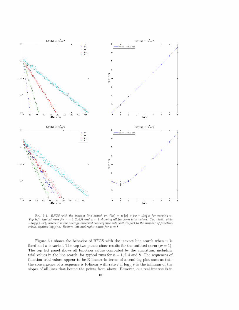
Fig. 5.1. BFGS with the inexact line search on f(x) = w‖x‖ + (w − 1)eT1 x for varying n.

Top left: typical runs for n = 1, 2, 4, 8 and w = 1 showing all function trial values. Top right: plots− log2(1−r), where r is the average observed convergence rate with respect to the number of functiontrials, against log2(n). Bottom left and right: same for w = 8.

Figure 5.1 shows the behavior of BFGS with the inexact line search when w isfixed and n is varied. The top two panels show results for the untilted norm (w = 1).The top left panel shows all function values computed by the algorithm, includingtrial values in the line search, for typical runs for n = 1, 2, 4 and 8. The sequences offunction trial values appear to be R-linear: in terms of a semi-log plot such as this,the convergence of a sequence is R-linear with rate r if log10 r is the infimum of theslopes of all lines that bound the points from above. However, our real interest is in

18

the rate of convergence of those function values that are accepted by the line search,taking into account nonetheless the number of function evaluations required by theline search: this rate is r if log10 r is the infimum of the slopes of all lines boundingthe points corresponding to accepted function values from above. We see from thefigure that, for these sequences, the rates r and r are approximately equal. For thisreason we choose to estimate the convergence rate of the function trial values as weexplained in Section 4, using a least squares fit to the pairs (νk, fk), where fk is thefunction value at the end of the kth line search and νk is the cumulative number offunction trials up to that point.

The top right panel of Figure 5.1 shows the estimated linear convergence ratesr computed in this way, averaged over 10 runs. As in the previous section, we plot− log2(1−r) against log2(n). The observed convergence rates are amazingly consistentand we see that r is well described by 1− 1/(2n). It is interesting to compare this tothe convergence rate with respect to the number of exact line searches for the sameproblem, which was observed in [LO08] to be somewhat greater than 1−1/

√2n. The

discrepancy between these rates is due to the fact that the average number of functiontrials needed in an inexact line search grows with n, as can be seen in the top leftpanel of Figure 5.1.

The bottom left and right panels of Figure 5.1 show the same information forw = 8. We observe that, as we saw in Section 4 for n = 1, the larger value of w causesdeterioration in the rate of convergence for small n, but this deterioration vanishesrapidly as n grows. This observation is confirmed by other experiments that are notshown here.

We also carried out a number of experiments minimizing f(Ax) where A is a non-singular matrix. Remarkably, we found that the results were essentially independentof A, for fixed n. One might suspect that this property extends to any positivelyhomogenous function, but experiments with polyhedral examples indicate that this isnot the case.

5.5. A Convex Partly Smooth Function. Consider the function

f(x) =√

xT Ax + xT Bx.

where A and B are positive semidefinite and at least one of them is positive definite,so the origin is the unique minimizer. If we take A = I and B = 0, f reduces to ‖x‖.Now let A = diag(1, 0, 1, 0, . . .) and choose B to be positive definite. Then f is partlysmooth at 0 with respect to the manifold

M = {x : x2j−1 = 0, j = 1, . . . ,n

2}.

This manifold is linear, so the U-space is M and the V-space is M⊥.Figure 5.2 shows the behavior of BFGS when B = I, the identity matrix. As pre-

viously, x and H were initialized randomly. In the top left panel, we see convergenceof the function trial values to zero for typical runs for n = 2, 4, 8. At the top right,we see the convergence of the iterate components xj , j = 1, . . . , n, for the case n = 8.Note that the odd components converge to zero in advance of the even components,reflecting the property that f grows away from the origin with the absolute value ofthe odd coordinates, as opposed to the square of the even coordinates. In the bottomleft panel, we see that four of the eigenvalues of H converge to zero, and the otherfour remain bounded away from zero. The eigenvectors of the final H correspondingto the tiny eigenvalues span the V-space M⊥ and the eigenvectors corresponding to

19

Fig. 5.2. BFGS with the inexact line search on f(x) =√

xT Ax + xT Bx, with A =diag(1, 0, 1, 0, . . .) and B = I. Top left: typical runs for n = 1, 2, 4, 8, showing all function trialvalues. Top right: |xj |, j = 1, . . . , n, after each line search, for n = 8. Bottom left: eigenvalues ofH after each line search, for the same run with n = 8. Bottom right: plots − log2(1− r), where r isthe average observed convergence rate with respect to the number of function trials, against log2(n).

the eigenvalues bounded away from zero span the U-space M (up to rounding error,not shown in the figures). The bottom right panel shows how the convergence ratewith respect to the number of function trials varies with n. This time we see thatthe rate r is approximately 1 − 1/n. This is consistent with the result for the normfunction in the sense that in both cases, the rate is approximately 1 − 1/(2d) whered is the dimension of the V-space.

20

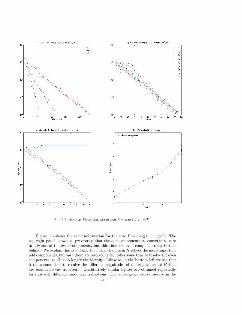
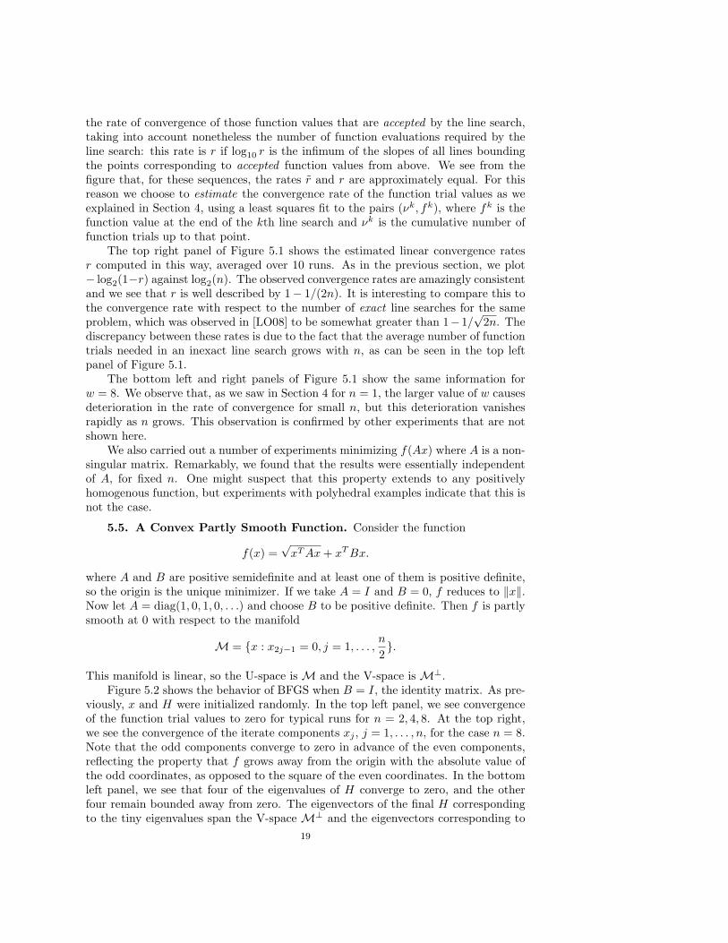
Fig. 5.3. Same as Figure 5.2, except that B = diag(1, . . . , 1/n2).

Figure 5.3 shows the same information for the case B = diag(1, . . . , 1/n2). Thetop right panel shows, as previously, that the odd components xj converge to zeroin advance of the even components, but this time the even components lag furtherbehind. We explain this as follows: the initial changes in H reflect the more importantodd components, but once these are resolved it still takes some time to resolve the evencomponents, as B is no longer the identity. Likewise, in the bottom left we see thatit takes some time to resolve the different magnitudes of the eigenvalues of H thatare bounded away from zero. Qualitatively similar figures are obtained repeatedlyfor runs with different random initializations. The convergence rates observed in the

21

Fig. 5.4. BFGS with the inexact line search on f(x) = (ε + (xT Ax)1/2 + xT Bx)1/2, withA = diag(1, 0, 1, 0, . . .) and B = diag(1, . . . , 1/n2). Left: typical runs for n = 4 with ε = 10k,k = −15,−12, . . . , 0, showing all function trial values. Top right: same for n = 8.

bottom right panel are not as consistent as they are for B = I, perhaps because ofrounding errors.

5.6. A Nonconvex Partly Smooth Function. Consider the function

f(x) =√

ε +√

xT Ax + xT Bx

where A = diag(1, 0, 1, 0, . . .), B = diag(1, . . . , 1/n2) and ε > 0. This function isnonconvex for ε < 1, and its Lipschitz constant is O(ε−1/2) as ε ↓ 0. It is partlysmooth with respect to the same manifold as in the previous example.

Figure 5.4 shows the behavior of BFGS with the inexact line search on this ex-ample for varying ε, with n = 4 on the left and n = 8 on the right. Remarkably,the convergence rates appear to be independent of ε, though for smaller values of ε,rounding errors limit the achievable accuracy. The value ε = 10−15 is near the ma-chine precision and hence the function is effectively non-Lipschitz; nonetheless, BFGSis able to reduce f to about 10−5.

5.7. A Nonsmooth Rosenbrock Function. Consider the following nonsmoothvariant of the well known Rosenbrock function in two variables:

f(x) = w|x2 − x21|+ (1− x2)2,

which is partly smooth with respect to the manifoldM = {x|x2 = x21}. This manifold

is not linear, as was the case in the previous example. The iterates rapidly approachM and then, much more slowly, “track” M, that is they follow a path close to butnot onM, converging to the minimizer [1, 1]T . This is clearly seen in the contour plotfor w = 8 at the top left of Figure 5.5. The different colored points and line segmentsindicate the path taken from 7 randomly generated initial points to the minimizer,

22

Fig. 5.5. BFGS with the inexact line search on the nonsmooth Rosenbrock function f(x) =w|x2−x2

1|+(1−x2)2. Top left: contour plot for w = 8, showing the iterates generated (colored pointsconnected by line segments) for 7 different starting points. Top right: typical runs for w = 1, 2, 4and 8 showing all function values. Bottom left: nonsmooth and smooth components of f after eachline search. Bottom right: plots − log2(1− r), where r is the average observed convergence rate withrespect to the number of function trials, against log2(w).

with H initialized to the identity matrix so that the first step is in the direction ofsteepest descent. Note that the colors plotted later (black being the latest) overwritepreviously plotted points. At the top right, we see linear convergence with respect tothe number of function trials for typical runs with w = 1, 2, 4 and 8. At the bottomleft, we see the evolution of the smooth and nonsmooth components of f after each

23

line search for w = 8. At the bottom right, observed convergence rates are shown as afunction of w. We see that the rate is approximately 1−1/(2w) for large w, and closeto 1/2 for small positive w. When w = 0, the convergence is superlinear, but this isnot the case for any positive value. Of course, if w is sufficiently small, superlinearconvergence is apparently observed due to limits of machine precision.

5.8. Nesterov’s Chebyshev-Rosenbrock Functions. Nesterov recently in-troduced the following smooth function:

f(x) =14(x1 − 1)2 +

n−1∑i=1

(xi+1 − 2x2i + 1)2.

A nonsmooth variation is

f(x) =14(x1 − 1)2 +

n−1∑i=1

|xi+1 − 2x2i + 1|.

In both cases the only minimizer is x = [1, 1, 1, . . . , 1]T . Consider the point x =[−1, 1, 1, . . . , 1]T and the manifold

M = {x : xi+1 = 2x2i − 1, i = 1, . . . , n− 1}

which contains both x and x. For x ∈M,

xi+1 = 2x2i − 1 = T2(xi) = T2i(x1) = cos(2i cos−1(x1)), i = 1, . . . , n− 1,

where Ti(x) denotes the ith Chebyshev polynomial.The functions f and f are both sums of a quadratic term and a nonnegative

sum whose zero set is the manifold M. Minimizing either function is equivalent tominimizing the first quadratic term on M. Typically, BFGS generates iterates that,as in the Rosenbrock example, approach M relatively rapidly and then track M toapproximate the minimizer. The iterates do not track M exactly, even if they areinitialized at x, but because they typically follow the highly oscillatory manifold Mfairly closely, particularly in the nonsmooth case, this tracking process requires manyiterations. To move from x to x alongM exactly would require xn to trace the graphof the 2n−1th Chebyshev polynomial, which has 2n−1 − 1 extrema in (−1, 1), as x1

increases from −1 to 1.Indeed, for n = 8, initializing x to x and H to the identity matrix, BFGS with

the inexact line search requires about 6700 iterations to reduce the smooth functionf below 10−15, and for n = 10, nearly 50,000 iterations are needed.

Minimizing the nonsmooth function f is, not surprisingly, much more difficult.This function is partly smooth with respect to M at all points in M. The codimen-sion of M is n − 1, so the dimension of the U and V-spaces at x are 1 and n − 1respectively. To run BFGS on f , we cannot use x for the initial point as the methodimmediately breaks down, f being nondifferentiable at x. Instead, we initialize x ran-domly, retaining the identity matrix for initializing H. We find that we can usuallysolve the problem reasonably accurately (reducing f to about 10−8 before breakdownoccurs) when n = 3, but not when n = 4, for which the method typically breaks downfar from x. We conjecture that the reason for this is rounding error, not a failure ofthe method to converge in theory. The final iterate x is very close toM, and the finalmatrix H has n − 1 tiny eigenvalues as expected, but the method is unable to trackM to minimize f .

24

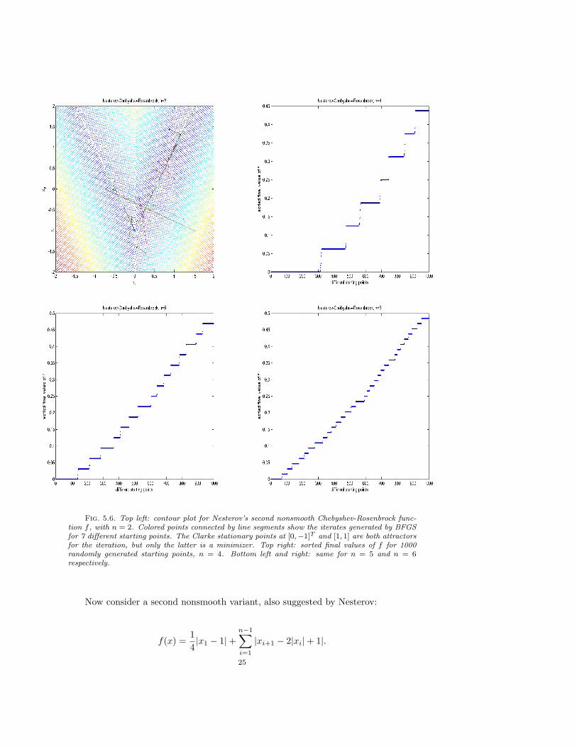
Fig. 5.6. Top left: contour plot for Nesterov’s second nonsmooth Chebyshev-Rosenbrock func-tion f , with n = 2. Colored points connected by line segments show the iterates generated by BFGSfor 7 different starting points. The Clarke stationary points at [0,−1]T and [1, 1] are both attractorsfor the iteration, but only the latter is a minimizer. Top right: sorted final values of f for 1000randomly generated starting points, n = 4. Bottom left and right: same for n = 5 and n = 6respectively.

Now consider a second nonsmooth variant, also suggested by Nesterov:

f(x) =14|x1 − 1|+

n−1∑i=1

|xi+1 − 2|xi|+ 1|.

25

Again, the only minimizer is x. Consider the set

S = {x : xi+1 = 2|xi| − 1, i = 1, . . . , n− 1}.

Minimizing f is equivalent to minimizing its first term on S, and BFGS typicallygenerates iterates that rapidly approach S and then need to track S to approximatex. Like M, the set S is highly oscillatory, but it has “corners”: it is not a manifoldaround any point x where any of the components x1, . . . , xn−1 vanishes. For example,consider the case n = 2, for which a contour plot is shown at the top left of Figure 5.6.It is easy to verify that the point [0,−1]T is Clarke stationary (zero is in the convexhull of gradient limits at the point), but not a local minimizer ([1, 2]T is a directionof linear descent from [0,−1]T ). Thus, f is not regular at [0,−1]T . The contour plotshows the path of the iterates generated by BFGS using 7 random starting points,plotted in 7 different colors (as previously, the points plotted later overwrite many ofthose plotted earlier near the attractors). Most of the runs converge to the minimizer[1, 1]T , but some converge to the Clarke stationary point [0,−1]T .

It is not hard to see that, in general, there are 2n−1 − 1 points in S where xj

vanishes for some j < n. For n ≤ 6, given enough randomly generated startingpoints, BFGS finds all these points, in addition to the minimizer. The top right,bottom left and bottom right panels plot final values of f found by 1000 runs ofBFGS starting with random x and H = I, sorted into increasing order, for the casesn = 4, 5 and 6 respectively. Most runs find either the minimizer or one of the 2n−1−1nonminimizing points described above, although a few runs break down earlier. Forn = 7, the method usually breaks down far away from these points, again presumablybecause of the limitations of machine precision. It seems likely that each of these2n−1 − 1 points is Clarke stationary and not Clarke regular, although we have notverified this algebraically.

Our work on this problem is in response to suggestions from both Y. Nesterovand K. Kiwiel. The latter informed us that this example is the only one he knowsfor which his bundle code converges to nonminimizing Clarke stationary points, thusraising our interest in this issue.

5.9. An Eigenvalue Product Application. All previous examples are con-trived, chosen to illustrate various points but for which the solution is known. Ourfinal example is a nonconvex relaxation of an entropy minimization problem arisingin an environmental application [AL04]. Let SN denote the space of real symmetricN by N matrices. The function f to be minimized is

f(X) = log EK (A ◦X) , (5.1)

where EK(X) denotes the product of the K largest eigenvalues of a matrix X in SN , Ais a fixed matrix in SN , and ◦ denotes the Hadamard (componentwise) matrix product,subject to the constraints that X is positive semidefinite and has diagonal entries equalto 1. If the requirement was to minimize the sum of the largest eigenvalues instead ofthe product, this would be equivalent to a semidefinite program, but the product of thelargest K eigenvalues is not convex. This problem was one of the examples in [BLO05];in the results reported there, the objective function was defined without the logarithmand we enforced the semidefinite constraint by an exact penalty function. It turnsout to be much more favorable for the convergence of BFGS to impose the constraintby the substitution X = V V T , where V is square. The constraint on the diagonal ofX then translates to a requirement that the rows of V have norm one, a constraint

26

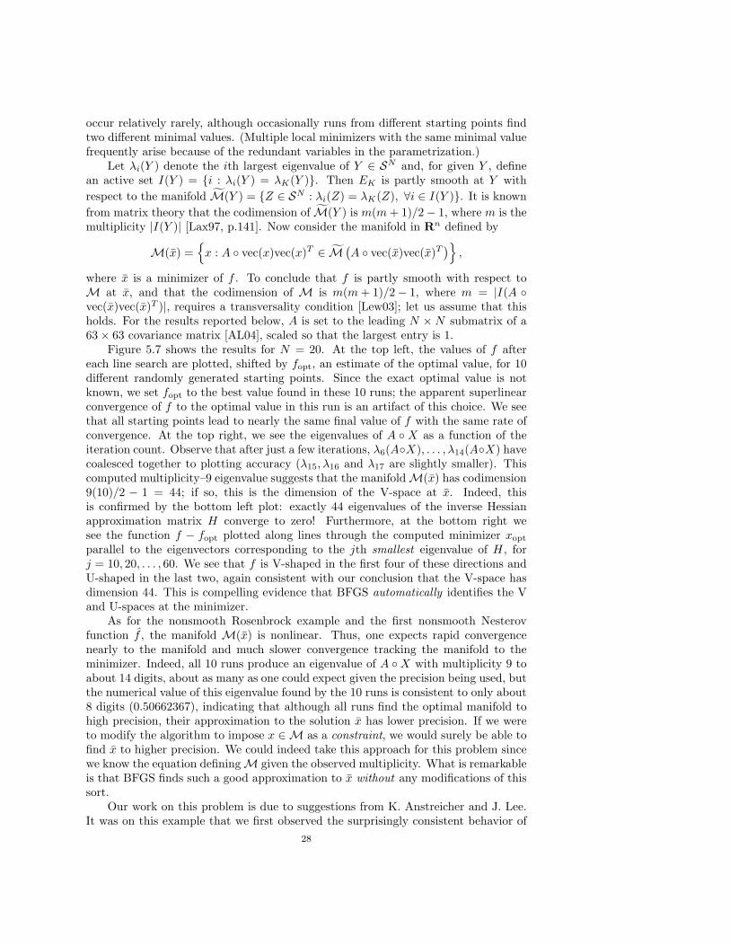
Fig. 5.7. . Results for minimizing the eigenvalue product, N = 20, n = 400. Top left: thefunction values after each line search for 10 randomly generated starting points, shifted by fopt, theminimal value found. Top right: eigenvalues of A ◦ X after each line search for one run. Bottomleft: eigenvalues of H for same run: 44 of these converge to zero. Bottom right: plots f −fopt alonga line xopt + tw, where xopt is the computed minimizer and w is the eigenvector of H associatedwith its jth smallest eigenvalue, for j = 10, 20, . . . , 60. The function f is “V-shaped” along theeigenvectors associated with tiny eigenvalues of H, and “U-shaped” along the others.

that can be easily removed from the problem, redefining f appropriately. Thus, theproblem is converted to the unconstrained minimization of a nonsmooth function fover Rn with n = N2 (the variable being x = vec(V ), the vector representation ofthe matrix V ). In principle, one might expect multiple local minimizers with differentminimal values, but at least with the data we have been using, this situation seems to

27

occur relatively rarely, although occasionally runs from different starting points findtwo different minimal values. (Multiple local minimizers with the same minimal valuefrequently arise because of the redundant variables in the parametrization.)

Let λi(Y ) denote the ith largest eigenvalue of Y ∈ SN and, for given Y , definean active set I(Y ) = {i : λi(Y ) = λK(Y )}. Then EK is partly smooth at Y withrespect to the manifold M(Y ) = {Z ∈ SN : λi(Z) = λK(Z), ∀i ∈ I(Y )}. It is knownfrom matrix theory that the codimension of M(Y ) is m(m + 1)/2− 1, where m is themultiplicity |I(Y )| [Lax97, p.141]. Now consider the manifold in Rn defined by

M(x) ={

x : A ◦ vec(x)vec(x)T ∈ M(A ◦ vec(x)vec(x)T

)},

where x is a minimizer of f . To conclude that f is partly smooth with respect toM at x, and that the codimension of M is m(m + 1)/2− 1, where m = |I(A ◦vec(x)vec(x)T )|, requires a transversality condition [Lew03]; let us assume that thisholds. For the results reported below, A is set to the leading N ×N submatrix of a63× 63 covariance matrix [AL04], scaled so that the largest entry is 1.

Figure 5.7 shows the results for N = 20. At the top left, the values of f aftereach line search are plotted, shifted by fopt, an estimate of the optimal value, for 10different randomly generated starting points. Since the exact optimal value is notknown, we set fopt to the best value found in these 10 runs; the apparent superlinearconvergence of f to the optimal value in this run is an artifact of this choice. We seethat all starting points lead to nearly the same final value of f with the same rate ofconvergence. At the top right, we see the eigenvalues of A ◦ X as a function of theiteration count. Observe that after just a few iterations, λ6(A◦X), . . . , λ14(A◦X) havecoalesced together to plotting accuracy (λ15, λ16 and λ17 are slightly smaller). Thiscomputed multiplicity–9 eigenvalue suggests that the manifoldM(x) has codimension9(10)/2 − 1 = 44; if so, this is the dimension of the V-space at x. Indeed, thisis confirmed by the bottom left plot: exactly 44 eigenvalues of the inverse Hessianapproximation matrix H converge to zero! Furthermore, at the bottom right wesee the function f − fopt plotted along lines through the computed minimizer xopt

parallel to the eigenvectors corresponding to the jth smallest eigenvalue of H, forj = 10, 20, . . . , 60. We see that f is V-shaped in the first four of these directions andU-shaped in the last two, again consistent with our conclusion that the V-space hasdimension 44. This is compelling evidence that BFGS automatically identifies the Vand U-spaces at the minimizer.

As for the nonsmooth Rosenbrock example and the first nonsmooth Nesterovfunction f , the manifold M(x) is nonlinear. Thus, one expects rapid convergencenearly to the manifold and much slower convergence tracking the manifold to theminimizer. Indeed, all 10 runs produce an eigenvalue of A ◦X with multiplicity 9 toabout 14 digits, about as many as one could expect given the precision being used, butthe numerical value of this eigenvalue found by the 10 runs is consistent to only about8 digits (0.50662367), indicating that although all runs find the optimal manifold tohigh precision, their approximation to the solution x has lower precision. If we wereto modify the algorithm to impose x ∈M as a constraint, we would surely be able tofind x to higher precision. We could indeed take this approach for this problem sincewe know the equation definingM given the observed multiplicity. What is remarkableis that BFGS finds such a good approximation to x without any modifications of thissort.

Our work on this problem is due to suggestions from K. Anstreicher and J. Lee.It was on this example that we first observed the surprisingly consistent behavior of

28

BFGS on nonsmooth problems.

6. Alternative Methods and Software. The purpose of this paper is to ex-plore the behavior of BFGS on nonsmooth functions, not to benchmark it againstother methods. Nonetheless, we make some brief comments in this direction. Westart by noting that huge nonsmooth convex problems are routinely solved in manyapplications by a variety of methods, notably bundle and interior point methods.While it is possible that a limited memory variant of BFGS might have a useful roleto play in the nonsmooth convex case, this has not been systematically investigated.We are therefore concerned here only with algorithms applicable to small to medium-sized, nonsmooth, nonconvex problems.

6.1. Shor’s R-Algorithm. Because of its simplicity, the easiest method to com-pare with BFGS is the Shor R-algorithm [Sho85]. Like BFGS, this can be viewed as avariable metric method, but one that does not satisfy the secant equation. In [BLO08],we presented the first proof that this algorithm is linearly convergent on some prob-lems; however, the proof is limited to quadratics (using an exact line search) whenn = 2. In contrast with the method of steepest descent, the rate of convergence isapparently independent of the conditioning of the quadratic. Not including the costof function and gradient evaluations, the overhead per iteration is the same as BFGS:O(n2), for matrix-vector products.

We carried out experiments with the Shor R-algorithm using the same inexactline search that has already been described. We found that it works poorly comparedto BFGS. One difficulty is that the algorithm requires the choice of a rather arbitraryparameter β [Sho85], equivalently 1− γ [BLO08], in (0, 1); convergence is slow if β isclose to 0 or 1 and it is not clear how to best choose its value. A second difficulty isthat if the Wolfe parameter c2 is set to a positive number, as we argued is favorablefor BFGS, the Shor algorithm often fails to converge even on simple examples. Thisis well known, as is the remedy: set c2 = 0 to ensure that the directional derivativealways changes sign in the line search, a property that BFGS does not require. Evenusing, say, β = 1/2 and c2 = 0, the Shor algorithm often requires significantly morefunction trials in the line search compared to BFGS. For the Shor algorithm, the unitstep is often not well scaled, as even the example f(x) = |x| shows, but no otherchoice is obviously better.

Figure 6.1 shows results for the Shor R-algorithm, with β = 1/2 and c2 = 0. Inthe top left and bottom left panels we show results for the tilted norm function ofSection 5.4, with A = I, and w set to 1 and 8 respectively. These may be comparedto the results for the same problem using BFGS shown in the top left and bottomleft panels of Figure 5.1. In several cases the number of line search trials made bythe Shor method increases steadily with the iteration number k. In such a case theconvergence rate for all function trial values is not the same as the convergence rate(still with respect to all function trials) for those function values that are accepted bythe line search.

The top right panel of the same figure shows results for the convex partly smoothproblem of Section 5.5, while the bottom right shows results for the nonsmooth Rosen-brock problem of Section 5.7. On these problems, the Shor algorithm does not takean excessive number of steps in the line search, but the convergence is slower thanBFGS nonetheless, and does not appear to be R-linear, especially for the Rosenbrockproblem. Compare with the results for BFGS in the top left panel of Figure 5.3 andthe top right panel of Figure 5.5 respectively.

29

Fig. 6.1. Results using the Shor R-Algorithm instead of BFGS, with c2 = 0 in the inexact linesearch. Top and bottom left: same problem as in Figure 5.1, top and bottom left. Top right: sameproblem as in Figure 5.3, top left. Bottom right: same problem as in Figure 5.5, top right.

We also experimented with a version of the Shor algorithm where we initializedthe line search by scaling the search direction by the step taken the previous iteration.This seems to improve the method, but not a great deal.

We emphasize that these results are for the basic version of the Shor R-algorithmas defined in [Sho85, BLO08]. It may be that some of the ideas developed, for example,in [KK00] would result in improved performance.

30

6.2. Gradient Sampling. The gradient sampling algorithm enjoys fairly strongconvergence results for locally Lipschitz functions [BLO05, Kiw07], although no rate ofconvergence has been established. Unfortunately, it becomes increasingly impracticalas n grows, both because of its computational requirements (multiple gradient eval-uations and the overhead of solving a convex quadratic program) and for theoreticalreasons [Sha05].

In practice we find that BFGS is generally superior, particularly as n increases,although for difficult functions with large Lipschitz constants or that are non-Lipschitzor even discontinuous, as can often happen in applications, gradient sampling seemsto have an advantage in robustness.

6.3. Bundle Methods. In Section 1, several references were given to bundlemethods, especially those that incorporate variable metric updates. In the nonconvexcase these methods are not easy to implement so we do not attempt to make com-parisons here. The overhead in most bundle methods is the cost of solving a convexquadratic program, but as noted in Section 1, methods with lower overhead have beendeveloped during the last decade; Haarala [Haa04] gives a good overview. We specu-late that on medium-sized partly smooth problems with relatively small-dimensionalV-spaces, there may be little to be gained by using the more complex bundle-variable-metric methods in preference to standard BFGS. At the opposite extreme, BFGSconverges very slowly on large polyhedral functions while bundle methods terminatefinitely. Thus, it does seem compelling that a method for general large-scale useshould incorporate key ingredients of bundle methods.

6.4. HANSO. In Section 1, the quote from Lemarechal alluded to the difficultyof assessing the result provided by BFGS. Our approach is simple: we run the methoduntil it breaks down because of rounding errors, or until a preset iteration or timelimit is exceeded, and view the resulting point as a candidate for a local minimizer.If the number of variables is not too large, one can then run a local bundle iterationto try to verify local optimality. If this fails, another possibility is to initiate gradientsampling, which, like ordinary bundle methods, returns information that can be usedto assess how well the final point may approximate a local minimizer. Our freelyavailable Matlab code hanso (Hybrid Algorithm for Non-Smooth Optimization)2 isbased on these ideas. hanso is used by our code hifoo (H-Infinity Fixed-Order Opti-mization)3 [BHLO06] to design low-order controllers for linear dynamical systems, animportant source of small-dimensional but difficult nonsmooth, nonconvex optimiza-tion problems. The BFGS code in hanso has been used to solve other nonsmoothoptimization problems as well, including the “condition geodesic” problem [BD08].

7. A Conjecture. This paper raises far more questions than it answers. Wehope that we have made a convincing case that BFGS is a practical and effectivemethod for nonsmooth optimization, and we have tried to give insight into why itworks as well as it does.

In practice, for functions with bounded level sets, when initialized randomly,BFGS always seems to generate function values converging linearly to a Clarke sta-tionary value. We speculate that, for some broad class of reasonably well-behavedfunctions, this behavior is almost sure. In framing a conjecture, let us first rule outthe worst kinds of pathology by considering objective functions whose graphs strat-ify into analytic manifolds. (A variety of dynamical systems associated with such

2http://www.cs.nyu.edu/overton/software/hanso/3http://www.cs.nyu.edu/overton/software/hifoo/

31

functions are known to behave well.) To be concrete, we consider the class of semi-algebraic functions, which includes all the examples given in this paper. Now let usconsider appropriately random initial data: the precise distributions are irrelevant,providing they are absolutely continuous with respect to Lebesgue measure. Again tobe concrete, let us assume a normally distributed intial point and an initial positivedefinite inverse Hessian approximation sampled from a Wishart distribution (that is,H = XXT where X is square with normally distributed entries.) In fact, this is howx and H were initialized in the experiments reported above. We now consider theBFGS method, in exact arithmetic, using the inexact line search defined in Section2, for any fixed Armijo and Wolfe parameters satisfying 0 < c1 < c2 < 1. Let usadopt the convention that if the algorithm generates a trial point at which f is notdifferentiable, then it terminates.

Conjecture 7.1. Consider any locally Lipschitz, semi-algebraic function f , andchoose x0 and H0 randomly. With probability one, the BFGS method generates aninfinite sequence of iterates. Furthermore, any cluster point x of this sequence isClarke stationary, that is 0 ∈ ∂f(x), and the sequence of all function trial valuesconverges to f(x) R-linearly.

Acknowledgment. Mille grazie a F. Facchinei e agli altri membri del Dipar-timento di Informatica e Sistemistica dell’ Universita di Roma “La Sapienza”, dovegran parte di questo lavoro e stato eseguito, per avermi fornito un ambiente piacevolee stimolante.

Appendix A. Alternating Series Representation. Section 3 studies thebehavior of the BFGS algorithm applied to the absolute value function, using the linesearch described in Section 2. This behavior turns out to depend on how the initialpoint can be represented as the sum of an alternating series of decreasing powers oftwo. We discuss this representation here, starting with a simple tool.

Lemma A.1. If

y =m∑

k=0

(−1)k2−bk ,

for some m = 2, 3, 4, . . . or ∞ and some strictly increasing sequence of integers (bj),then

2−b0−1 < y < 2−b0 .

Proof First notice that since y is the sum of an alternating series of strictly decreasingpositive terms, we have

2−b0 − 2−b1 < y < 2−b0 .

But b1 ≥ b0 + 1, so

2−b0 − 2−b1 ≥ 2−b0 − 2−b0−1 = 2−b0−1,

whence the result. 2

The following routine result describes the representation we use.Theorem A.2. Any number x ∈ R++ has a unique alternating binary rep-

resentation as the sum of a finite or infinite alternating series of strictly decreasing32

powers of two: that is, there is a unique number m = 0, 1, 2, . . . or ∞ and a uniquesequence of integers a0 < a1 < a2 < · · · (with m + 1 terms if m <∞) such that

x =m∑

k=0

(−1)k2−ak . (1.3)

Proof Consider the following iterative procedure.Algorithm A.4 (alternating binary representation).

s−1 ← 0m← +∞k ← 0repeat

ak ← b− log2[(−1)k(x− sk−1)]csk ← sk−1 + (−1)k2−ak

if sk = x, m = k, STOPk ← k + 1

end(repeat)We claim first that the algorithm is well-defined: that is, the partial sums

sk =k∑

j=0

(−1)j2−aj (1.5)

satisfy

(−1)k(x− sk−1) > 0 (1.6)

for all k < m. Notice that the sequence of integers (ak) is uniquely defined by theinequalities

2−ak−1 < (−1)k(x− sk−1) ≤ 2−ak , for all finite k ≤ m. (1.7)

To prove our claim (1.6), note that the case k = 0 follows immediately from theinequalities (1.7). On the other hand, if (1.6) holds for some k < m, then inequalities(1.7) hold, so

(−1)k+1(x− sk) = (−1)k+1(x− [sk−1 + (−1)k2−ak ])= − (−1)k(x− sk−1) + 2−ak ≥ 0,

and in fact the inequality is strict since k 6= m. Our claim (1.6) now follows byinduction.

We turn to proving the monotonicity of the sequence (ak). Assuming k < m, byapplying inequalities (1.7) once as they appear and once with k replaced by k +1, wededuce

2−ak+1−1 < (−1)k+1(x− sk) = (−1)k(sk − sk−1)− (−1)k(x− sk−1)< (−1)k(−1)k2−ak − 2−ak−1 = 2−ak−1.

Thus ak+1 > ak, as required. Finally, as a consequence, notice that the inequalities(1.7) imply sk → x as k →∞ if m =∞, so the representation (1.3) follows.

33

To prove uniqueness of the expression (1.3), suppose

x =∞∑

k=0

(−1)k2−bk , (1.8)

for some strictly increasing sequence of integers (bj). We then claim bk = ak for allindices k. (The proof for finite sums is similar.)

First notice that

2−b0−1 < x < 2−b0 ,

using Lemma A.1. Since inequalities (1.7) in the case k = 0 define ak uniquely, wededuce b0 = a0.

We now proceed by induction. Suppose bj = aj for all j = 0, 1, 2, . . . , k−1. Thenwe have

sk−1 =k−1∑j=0

(−1)j2−bj

and hence

x− sk−1 =∞∑

j=k

(−1)j2−bj .

Using Lemma A.1 again now shows

2−bk−1 < (−1)k(x− sk−1) < 2−bk .

Again, since inequalities (1.7) define ak uniquely, we deduce bk = ak. 2

REFERENCES

[AL04] K. Anstreicher and J. Lee. A masked spectral bound for maximum-entropy sampling.In A. di Bucchianico, H. Lauter, and H. P. Wynn, editors, MODA 7 - Advances inModel-Oriented Design and Analysis, pages 1–10. Springer, Berlin, 2004.

[BD08] P. Boito and J.-P. Dedieu. The condition metric in the space of rectangular full rankmatrices. 2008. Submitted to SIAM Journal on Matrix Analysis and Applications.

[BGLS95] J. Bonnans, J. Gilbert, C. Lemarechal, and C. Sagastizabal. A family of variable metricproximal methods. Mathematical Programming, 68:15–48, 1995.

[BHLO06] J.V. Burke, D. Henrion, A.S. Lewis, and M.L. Overton. HIFOO - a MATLAB packagefor fixed-order controller design and H∞ optimization. In Fifth IFAC Symposiumon Robust Control Design, Toulouse, 2006.

[BLO05] J.V. Burke, A.S. Lewis, and M.L. Overton. A robust gradient sampling algorithm fornonsmooth, nonconvex optimization. SIAM Journal on Optimization, 15:751–779,2005.

[BLO08] J.V. Burke, A.S. Lewis, and M.L. Overton. The speed of Shor’s R-algorithm. IMAJournal on Numerical Analysis, 28:711–720, 2008.

[Cla83] F. H. Clarke. Optimization and Nonsmooth Analysis. John Wiley, New York, 1983.Reprinted by SIAM, Philadelphia, 1990.

[Haa04] M. Haarala. Large-Scale Nonsmooth Optimization: Variable metric bundle method withlimited memory. PhD thesis, University of Jyvaskyla, Finland, 2004.

[HUL93] J.B. Hiriart-Urruty and C. Lemarechal. Convex Analysis and Minimization Algorithms.Springer-Verlag, New York, 1993. Two volumes.

[Kiw85] K.C. Kiwiel. Methods of Descent for Nondifferentiable Optimization. Lecture Notes inMathematics 1133. Springer-Verlag, Berlin and New York, 1985.

[Kiw07] K.C. Kiwiel. Convergence of the gradient sampling algorithm for nonsmooth nonconvexoptimization. SIAM Journal on Optimization, 18:379–388, 2007.

34

[KK00] F. Kappel and A. Kuntsevich. An implementation of Shor’s r-algorithm. ComputationalOptimization and Applications, 15:193–205, 2000.

[Lax97] P. D. Lax. Linear Algebra. John Wiley, New York, 1997.[Lee98] J. Lee. Constrained maximum-entropy sampling. Operations Research, 46:655–664,

1998.[Lem81] C. Lemarechal. A view of line searches. In Optimization and optimal control (Proc.

Conf. Math. Res. Inst., Oberwolfach, 1980), pages 59–78, Berlin and New York,1981. Springer. Lecture Notes in Control and Information Sciences, 30.

[Lem82] C. Lemarechal. Numerical experiments in nonsmooth optimization. In E.A. Nurmin-ski, editor, Progress in Nondifferentiable Optimization, pages 61–84, Laxenburg,Austria, 1982.

[Lew03] A.S. Lewis. Active sets, nonsmoothness and sensitivity. SIAM Journal on Optimization,13:702–725, 2003.

[LF01] D.-H. Li and M. Fukushima. On the global convergence of the BFGS method fornonconvex unconstrained optimization problems. SIAM Journal on Optimization,11:1054–1064, 2001.

[LO08] A.S. Lewis and M.L. Overton. Behavior of BFGS with an exact line search on non-smooth examples. 2008. Submitted to SIAM Journal on Optimization.

[LOS00] C. Lemarechal, F. Oustry, and C. Sagastizabal. The U-Lagrangian of a convex function.Trans. Amer. Math. Soc., 352:711729, 2000.

[LS94] C. Lemarechal and C. Sagastizabal. An approach to variable metric bundle methods.In IFIP Proceedings, Systems Modeling and Optimization, 1994.

[LV99] L. Luksan and J. Vlcek. Globally convergent variable metric method for convex nons-mooth unconstrained minimization. Journal of Optimization Theory and Applica-tions, 102:593–613, 1999.

[LV01] L. Luksan and J. Vlcek. Variable metric methods for nonsmooth optimization. TechnicalReport 837, Academy of Sciences of the Czech Republic, May 2001.

[Mif77] R. Mifflin. An algorithm for constrained optimization with semismooth functions. Math-ematics of Operations Research, 2:191–207, 1977.

[MSQ98] R. Mifflin, D. Sun, and L. Qi. Quasi-Newton bundle-type methods for nondifferentiableconvex optimization. SIAM Journal on Optimization, (2):583–603, 1998.

[NW06] J. Nocedal and S. Wright. Nonlinear Optimization. Springer, New York, second edition,2006.

[Pow76] M.J.D. Powell. Some global convergence properties of a variable metric algorithm forminimization without exact line searches. In Nonlinear Programming, pages 53–72,Providence, 1976. Amer. Math. Soc. SIAM-AMS Proc., Vol. IX.

[RF00] A.I. Rauf and M. Fukushima. Globally convergent BFGS method for nonsmooth con-vex optimization. Journal of Optimization Theory and Applications, 104:539–558,2000.

[Roy63] H.L. Royden. Real Analysis. Macmillan, New York, 1963.[RW98] R.T. Rockafellar and R.J.B. Wets. Variational Analysis. Springer, New York, 1998.[Sha05] A. Shapiro. Comments on “generalized derivatives and nonsmooth optimization, a finite

dimensional tour” by j. dutta. Sociedad de Estadustica e Investigacion Operativa,TOP, 13:302–306, 2005.

[Sho85] N.Z. Shor. Minimization Methods for Non-differentiable Functions. Springer-Verlag,New York, 1985.

[VL01] J. Vlcek and L. Luksan. Globally convergent variable metric method for nonconvexnondifferentiable unconstrained minimization. Journal of Optimization Theory andApplications, 111:407–430, 2001.

[Wol75] P. Wolfe. A method of conjugate subgradients for minimizing nondifferentiable func-tions. Math. Programming Stud., 3:145–173, 1975. In: Nondifferentiable Optimiza-tion, M.L. Balinski and P. Wolfe, eds.

[YVGS08] J. Yu, S.V.N. Vishwanathan, S. Gunther, and N. Schraudolph. A quasi-Newton ap-proach to non-smooth convex optimization. In Proceedings of the 25th InternationalConference on Machine Learning, 2008.

[ZBN97] C. Zhu, R.H. Byrd, and J. Nocedal. Algorithm 778, L-BFGS-B, FORTRAN routines forlarge scale bound constrained optimization. ACM Transactions on MathematicalSoftware, 23:550–560, 1997.

[ZZA+00] S. Zhang, X. Zou, J. Ahlquist, I. M. Navon, and J. G. Sela. Use of differentiableand nondifferentiable optimization algorithms for variational data assimilation withdiscontinuous cost functions. Monthly Weather Review, 128:4031–4044, 2000.

35