the nonsmooth landscape of phase retrieval
TRANSCRIPT
The nonsmooth landscape of phase retrieval
Damek Davis∗ Dmitriy Drusvyatskiy† Courtney Paquette‡
Abstract
We consider a popular nonsmooth formulation of the real phase retrieval problem.We show that under standard statistical assumptions, a simple subgradient methodconverges linearly when initialized within a constant relative distance of an optimalsolution. Seeking to understand the distribution of the stationary points of the problem,we complete the paper by proving that as the number of Gaussian measurementsincreases, the stationary points converge to a codimension two set, at a controlledrate. Experiments on image recovery problems illustrate the developed algorithm andtheory.
Keywords: Phase retrieval, stationary points, subdifferential, variational principle, sub-gradient method, spectral functions, eigenvalues
1 Introduction
Phase retrieval is a common task in computational science, with numerous applicationsincluding imaging, X-ray crystallography, and speech processing. In this work, we considera popular real counterpart of the problem. Given a set of tuples {(ai, bi)}mi=1 ⊂ Rd × R,the (real) phase retrieval problem seeks to determine a vector x ∈ Rd satisfying (aTx)2 = bifor each index i = 1, . . . ,m. Due to its combinatorial nature, this problem is known to beNP-hard [14]. One can model the real phase retrieval problem in a variety of ways. Here,we consider the following “robust formulation”:
minx
fS(x) :=1
m
m∑i=1
|(aTi x)2 − bi|.
This model of the problem has gained some attention recently with the work of Duchi-Ruan [10] and Eldar-Mendelson [12]. Indeed, this model exhibits a number of desirable
∗School of Operations Research and Information Engineering, Cornell University, Ithaca, NY 14850, USA;people.orie.cornell.edu/dsd95/.†Department of Mathematics, U. Washington, Seattle, WA 98195; www.math.washington.edu/∼ddrusv.
Research of Drusvyatskiy was supported by the AFOSR YIP award FA9550-15-1-0237 and by the NSF DMS1651851 and CCF 1740551 awards.‡Industrial and Systems Engineering Department, Lehigh University, Bethlehem, PA 18015;
sites.math.washington.edu/∼yumiko88/.
1

properties, making it amenable to numerical methods. Namely, in contrast to other possibleformulations, mild statistical assumptions imply that fS is both weakly convex [10, Corollary3.2] and sharp [12, Theorem 2.4], with high probability. That is, there exist numericalconstants ρ, κ > 0 such that
the assignment x 7→ fS(x) +η
2‖x‖2 is a convex function,
and the inequality
fS(x)− inf fS ≥ κ‖x− x‖‖x+ x‖ holds for all x ∈ Rd.
Here, ±x are the true signals and ‖ · ‖ denotes the `2-norm. Weak convexity is a well studiedconcept in optimization literature [5,13,23,25], while sharpness and the closely related notionof error bounds [2, 7, 21] classically underly rapid local convergence guarantees in nonlinearprogramming. Building on these observations, Duchi and Ruan [10] showed that with properinitialization, the so-called prox-linear algorithm [7,8,10,11,20] quadratically converges to ±x(even in presence of outliers). The only limitation of their approach is that the prox-linearmethod requires, at every iteration, invoking an iterative solver for a convex subproblem.For large-scale instances (m� 1, d� 1), the numerical resolution of such problems is non-trivial. In the current work, we analyze a lower-cost alternative when there are no errors inthe measurements.
We will show that the robust phase retrieval objective favorably lends itself to classicalsubgradient methods. This is somewhat surprising because, until recently, convergence ratesof subgradient methods in nonsmooth, nonconvex optimization have remained elusive; seethe discussion in [6]. We will prove that under mild statistical assumptions and properinitialization, the standard Polyak subgradient method
xk+1 = xk −(fS(xk)−min fS
‖gk‖2
)gk with gk ∈ ∂fS(xk),
linearly converges to ±x, with high probability. We note that high quality initialization,in turn, is straightforward to obtain; see e.g. [10, Section 3.3] and [29]. The argument wepresent is appealingly simple, relying only on weak convexity and sharpness of the function.
Aside from the current work and that of [10], we are not aware of other attemptsto optimize the robust phase retrieval objective directly. Other works focus on differ-ent problem formulations. Notably, Candes et al. [3] and Sun et al. [27] optimize thesmooth loss 1
m
∑mi=1(〈ai, x〉2 − bi)
2 using a second-order trust region method and a gradi-ent method, respectively. Wang et al. [29] instead minimize the highly nonsmooth function1m
∑mi=1(|〈ai, x〉| −
√bi)
2 by a gradient descent-like method. Another closely related recentwork is that of Tan and Vershynin [28]. One can interpret their scheme as a stochasticsubgradient method on the formulation 1
m
∑mi=1 ||〈ai, x〉| −
√bi|, though this is not explicitly
stated in the paper. Under proper initialization and assuming that ai are uniformly sam-pled from a sphere, they prove linear convergence. Their argument relies on sophisticatedprobabilistic tools. In contrast, we disentangle the probabilistic statements (weak convexityand sharpness) from the deterministic convergence of Algorithm 1. As a proof of concept,we illustrate the proposed subgradient method synthetic and large-scale real image recoveryproblems.
2

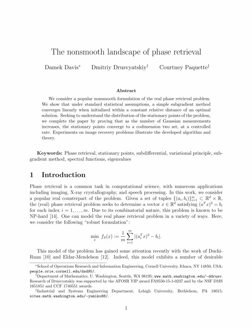
Figure 1: Depiction of the population objective fP with x = (1, 1): graph (left), contours(right).
Weak convexity and sharpness, taken together, imply existence of a small neighborhoodX of {±x} devoid of extraneous stationary points of fS (see Lemma 3.1). On the otherhand, it is intriguing to determine where the objective function fS may have stationarypoints outside of this neighborhood. We complete the paper by proving that as the numberof Gaussian measurements increases, the stationary points of the problem converge to acodimension two set, at a controlled rate. This suggests that there are much larger regionsthan the neighborhood X , where the objective function has benign geometry.
We follow an intuitive and transparent strategy. Setting the groundwork, assume thatai are i.i.d samples from a normal distribution N(0, Id×d). Hence the problem min fS is anempirical average approximation of the population objective
minx
fP (x) := Ea[|(aTx)2 − (aT x)2|].
Seeking to determine the location of stationary points of fS, we begin by first determiningthe stationary points of fP . We base our analysis on the elementary observation that fP (x)depends on x only through the eigenvalues of the rank two matrix X := xxT − xxT . Moreprecisely, equality holds:
fP (x) =4
π
[Tr(X) · arctan
(√∣∣∣∣λmax(X)
λmin(X)
∣∣∣∣)
+√|λmax(X)λmin(X)|
]− Tr(X).
See Figure 1 for a graphical illustration.Using basic perturbation properties of eigenvalues, we will show that the stationary points
of fP are precisely{0} ∪ {±x} ∪ {x ∈ x⊥ : ‖x‖ = c · ‖x‖}, (1.1)
where c ≈ 0.4416 is a numerical constant. Intuitively, this region, excluding {±x}, is wherenumerical methods may stagnate. In particular, fP has no extraneous stationary pointsoutside of the subspace x⊥. Along the way, we prove a number of results in matrix theory,
3

which may be of independent interest. For example, we show that all stationary points of acomposition of an orthogonally invariant gauge function with the map x 7→ xxT − xxT mustbe either perpendicular or collinear with x.
Having located the stationary points of the population objective fP , we turn to thestationary points of the subsampled function fS. This is where the techniques commonly usedfor smooth formulations of the problem, such as those in [27], are no longer applicable; indeed,the subdifferential ∂fP (x) is usually a very poor approximation of ∂fS(x). Nonetheless, weshow that the graphs of the subdifferentials ∂fP and ∂fS are close with high probability – aresult closely related to the celebrated Attouch’s convergence theorem [1]. The analysis ofthe stationary points of the subsampled objective flows from there. Namely, we show thatthere is a constant C such that whenever m ≥ Cd, all stationary points x of fS satisfy
‖x‖‖x− x‖‖x+ x‖‖x‖3
. 4
√d
mor
∣∣∣‖x‖‖x‖ − c∣∣∣ . 4
√dm·(
1 + ‖x‖‖x‖
)|〈x,x〉|‖x‖‖x‖ .
4
√dm· ‖x‖‖x‖
,
with high probability; compare with (1.1). The argument we present is very general, relyingonly on weak convexity and concentration of fS around its mean. Therefore, we believe thatthe technique may be of independent interest.
We comment in Section B.1 on the structure of stationary points for the variant of thephase retrieval problem, in which the measurements b are corrupted by gross outliers. It isstraightforward to obtain a full characterization of the stationary points of the populationobjective using the techniques developed in earlier sections.
The outline for the paper is as follows. Section 2 summarizes notation and basic results wewill need. In Section 3, we analyze the linear convergence of the Polyak subgradient methodfor a class of nonsmooth, nonconvex functions, which includes the subsampled objective fS.In Section 4, we perform a few proof-of-concept experiments, illustrating the performance ofthe Polyak subgradient method on synthetic and real large-scale image recovery problems.Section 5 is devoted to characterizing the nonsmooth landscape of the population objectivefP . In Section 6, we develop a concentration theorem for the subdifferential graphs of fSand fP , and briefly comment on robust extensions.
2 Notation
Throughout, we mostly follow standard notation. The symbol R will denote the real line,while R+ and R++ will denote nonnegative and strictly positive real numbers, respectively.We always endow Rd with the dot product 〈x, y〉 = xTy and the induced norm ‖x‖ :=√〈x, x〉. The symbol Sd−1 will denote the unit sphere in Rd, while B(x, r) := {y : ‖x− y‖ <
r} will stand for the open ball around x of radius r > 0. For any set Q ⊂ Rd, the distancefunction is defined by dist(x;Q) := infy∈Q ‖y−x‖. The adjoint of a linear map A : Rd → Rm
will be written as A∗ : Rm → Rd.Since the main optimization problem we consider is nonsmooth, we will use some basic
generalized derivative constructions. For a more detailed discussion, see for example themonographs of Mordukhovich [22] and Rockafellar-Wets [26].
4
Consider a function f : Rd → R and a point x. The Frechet subdifferential of f at x,denoted ∂f(x), is the set of all vectors v ∈ Rd satisfying
f(x) ≥ f(x) + 〈v, x− x〉+ o(‖x− x‖) as x→ x.
Thus v lies in ∂f(x) if and only if the affine function x 7→ f(x)+〈v, x− x〉 minorizes f near xup to first-order. Since the assignment x 7→ ∂f(x) may have poor continuity properties, it isuseful to extend the definition slightly. The limiting subdifferential of f at x, denoted ∂f(x),consists of all vectors v ∈ Rd such that there exist sequences xi and vi ∈ ∂f(xi) satisfying(xi, f(xi), vi) → (x, f(x), v). We say that x is stationary for f if the inclusion 0 ∈ ∂f(x)holds. The graph of ∂f is the set
gph ∂f := {(x, y) ∈ Rd × Rd : y ∈ ∂f(x)}.
For essentially all functions that we will encounter, the two subdifferentials, ∂f(x) and∂f(x), coincide. This is the case for C1-smooth functions f , where ∂f(x) and ∂f(x) consistonly of the gradient ∇f(x). Similarly for convex function f , both subdifferentials reduce tothe subdifferential in the sense of convex analysis:
v ∈ ∂f(x) ⇐⇒ f(x) ≥ f(x) + 〈v, x− x〉 for all x ∈ Rd.
Most of the nonsmooth functions we will encounter have a simple composite form:
F (x) := h(c(x)),
where h : Rm → R is a finite convex function and c : Rd → Rn is a C1-smooth map. Forsuch composite functions, the two subdifferentials coincide, and admit the intuitive chainrule [26, Theorem 10.6, Corollary 10.9]:
∂F (x) = ∇c(x)∗∂h(c(x)) for all x ∈ Rd.
A function f : Rd → R is called ρ-weakly convex if f + ρ2‖ · ‖2 is a convex function.
It follows immediately from [26, Theorem 12.17] that a lower-semicontinuous function f isρ-weakly convex if and only if the inequality
f(y) ≥ f(x) + 〈v, y − x〉 − ρ
2‖y − x‖2,
holds for all points x, y ∈ Rd and vectors v ∈ ∂f(x).Finally, we will often use implicitly the observation that the Lipschitz constant of any
lower-semicontinuous function f on a convex open set U coincides with sup{‖ζ‖ : x ∈ U, ζ ∈∂f(x)}; see e.g. [26, Theorem 9.13].
3 Subgradient method
In this work, we consider the robust formulation of the (real) phase retrieval problem. Settingthe stage, suppose we are given vectors {ai}mi=1 in Rd and measurements b := 〈ai, x〉2, for a
5

fixed but unknown vector x. The goal of the phase retrieval problem is to recover the vectorx ∈ Rd, up to a sign flip. The formulation of the problem we consider in this work is:
minx
fS(x) :=1
m
m∑i=1
|〈aTi , x〉2 − bi|.
The function fS (in contrast to other possible formulations) has a number of desirable prop-erties, which we will highlight as we continue.
In this section, we show that the landscape of the phase retrieval objective fS favorablylends itself to classical subgradient methods. Namely, with proper initialization and underappropriate statistical assumptions, the Polyak subgradient method [24] linearly convergesto ±x.
3.1 Subgradient method for weakly convex and sharp functions
The linear convergence guarantees that we present are mostly independent of the structureof fS and instead rely only on a few general regularity properties, which fS satisfies undermild statistical assumptions. Consequently, it will help the exposition in the current sectionto abstract away from fS.
Assumption A. Fix a function g : Rd → R such that there exist real ρ, µ > 0 satisfying thefollowing two properties.
1. Weak Convexity. The function g + ρ2‖ · ‖2 is convex;
2. Sharpness. The inequality holds:
g(x)−min g ≥ µ · dist(x;X ) for all x ∈ Rd,
where X 6= ∅ is the set of minimizers of g.
Duchi and Ruan [10], following the work of Eldar-Mendelson [12], showed that the robustphase retrieval loss fS(·) satisfies Assumption A, under reasonable statistical assumptions.We will discuss these guarantees in Section 3.2, where we will instantiate the subgradientmethod on the robust phase retrieval objective. Consider now the standard Polyak subgra-dient method applied to g (Algorithm 1).
Algorithm 1: Polyak Subgradient Method
Data: x0 ∈ Rd
Step k: (k ≥ 1)Choose ζk ∈ ∂g(xk).if ζk 6= 0 then
Set xk+1 = xk − g(xk)−min g‖ζk‖2
ζk.
elseExit algorithm.
end
As the fist step in the analysis of Algorithm 1, we must ensure that there are no extraneousstationary points of g near X . This is the content of the following lemma.
6

Lemma 3.1 (Neighborhood with no stationary points). Suppose Assumption A holds. Theng has no stationary points x satisfying
0 < dist(x;X ) <2µ
ρ. (3.1)
Proof. Consider a stationary point x of g, which is outside of X . Let x ∈ X be a pointsatisfying ‖x− x‖ = dist(x;X ). Properties 1 and 2 then imply
µ · dist(x;X ) ≤ g(x)− g(x) ≤ ρ
2‖x− x‖2 =
ρ
2· dist2(x;X ).
Dividing through by dist(x;X ), the result follows.
The following Theorem 3.2 – the main result of this subsection – shows that when Algo-rithm 1 is initialized within a certain tube T of X , the iterates xk stay within the tube andconverge linearly to X . It is interesting to note that the rate of local linear convergence doesnot depend on the weak convexity constant ρ; indeed, the value ρ only dictates the size ofthe tube T .
Theorem 3.2 (Linear rate). Suppose Assumption A holds. Fix a real γ ∈ (0, 1) and definethe tube
T :=
{x ∈ Rd : dist(x;X ) ≤ γ · µ
ρ
},
and the corresponding Lipschitz constant
Lg := supx∈T , ζ∈∂g(x)
‖ζ‖.
Then Algorithm 1 initialized at any point x0 ∈ T produces iterates that converge Q-linearlyto X at the rate:
dist2(xk+1;X ) ≤(
1− (1− γ)µ2
L2g
)dist2(xk;X ), (3.2)
Proof. We proceed by induction. Suppose that the theorem holds up to iteration k. We willprove the inequality (3.2). To this end, let x ∈ X be a point satisfying ‖xk−x‖ = dist(xk;X ).Note that if xk lies in X , there is nothing to prove. Thus we may suppose xk /∈ X . Notethat the inductive hypothesis implies dist(xk;S) ≤ dist(x0;S) and therefore xk lies in T .Lemma 3.2 therefore guarantees ζk 6= 0. Using Properties 1 and 2, we successively deduce
‖xk+1 − x‖2 = ‖xk − x‖2 + 2〈xk − x, xk+1 − xk〉+ ‖xk+1 − xk‖2
= ‖xk − x‖2 +2(g(xk)− g(x))
‖ζk‖2· 〈ζk, x− xk〉+
(g(xk)− g(x))2
‖ζk‖2
≤ ‖xk − x‖2 +2(g(xk)− g(x))
‖ζk‖2
(g(x)− g(xk) +
ρ
2‖xk − x‖2
)+
(g(xk)− g(x))2
‖ζk‖2
= ‖xk − x‖2 +(g(xk)− g(x))
‖ζk‖2
(ρ‖xk − x‖2 − (g(xk)− g(x))
)≤ ‖xk − x‖2 +
(g(xk)− g(x))
‖ζk‖2
(ρ‖xk − x‖2 − µ‖xk − x‖
)= ‖xk − x‖2 +
ρ(g(xk)− g(x))
‖ζk‖2
(‖xk − x‖ −
µ
ρ
)‖xk − x‖.
7
Combining the inclusion xk ∈ T with sharpness (Assumption 2), we therefore deduce
dist2(xk+1;X ) ≤ ‖xk+1 − x‖2 ≤(
1− (1− γ)µ2
‖ζk‖2
)‖xk − x‖2.
The result follows.
3.2 Convergence for the phase retrieval objective
We now turn to an application of Theorem 3.2 to the phase retrieval loss fS. In particular,to run the subgradient method, we must only compute a subgradient of fS, which can beeasily done using the chain rule:
1
m
m∑i=1
2〈ai, x〉 · sign(〈ai, x〉2 − bi)ai ∈ ∂fS(x).
Each iteration of Algorithm 1 thus requires a single pass through the set of measurementvectors. We will see momentarily that under mild statistical assumptions, {±x} are theunique minimizers of fS, as soon as m > 2d.
Thus for a successful application of Theorem 3.2, we must only address the followingquestions:
(i) Describe the statistical conditions on the data generating mechanism, which insure thatAssumption A holds with high probability.
(ii) Estimate the Lipschitz constant of fS on the union of balls T = B(x, γµρ
)∪B(−x, γµρ
).
(iii) Describe a good initialization procedure for producing x0 ∈ T .
Essentially all of these points follow from the work of Duchi and Ruan [10], Eldar-Mendelson[12], and Wang et al. [29]. We summarize them here for the sake of completeness. Henceforth,let us suppose that ai ∈ Rd (for i = 1, . . . ,m) are independent realizations of a random vectora ∈ Rd.
3.2.1 Sharpness
In order to ensure sharpness (or rather the stronger “stability” property [12]), we make thefollowing assumption on the distribution of a.
Assumption B. There exist constants κ∗st, p0 > 0 such that for all u, v ∈ Sd−1, we have
P (|〈a, v〉〈a, u〉| ≥ κ∗st) ≥ p0,
Roughly speaking, this mild assumption simply says that the random vector a has suf-ficient support in all directions. In particular, the standard Gaussian a ∼ N(0, Id) satisfiesAssumption B with κ∗st = 0.365 and p0 = 0.25; see [10, Example 1]. The following is provedin [10, Corollary 3.1].
8
Theorem 3.3 (Sharpness). Suppose that Assumption B holds. Then there exists a numericalconstant c <∞ such that if mp2
0 ≥ cd, we have
P(fS(x)− fS(x) ≥ 1
2κ∗stp0‖x− x‖‖x+ x‖ for all x ∈ Rd
)≥ 1− 2 exp
(−mp
20
32
).
To simplify notation, set dist(x; x) := min{‖x−x‖, ‖x+x‖}. Thus Assumption B implies,with high probability, that fS is sharp. Indeed, Theorem 3.3 directly implies that with highprobability we have
fS(x)− fS(x) ≥ 12κ∗stp0‖x− x‖‖x+ x‖
≥ 12κ∗stp0 ·min{‖x− x‖, ‖x+ x‖} ·max{‖x− x‖, ‖x+ x‖}
≥ 12κ∗stp0‖x‖ · dist(x; x).
Thus the sharpness condition in Assumption A holds for g = fS with µ = 12κ∗stp0‖x‖.
3.2.2 Weak convexity
We next look at weak convexity of the objective fS. We will need the following definition.
Definition 3.4. A random vector a ∈ Rd is σ2-sub-Gaussian if for all unit vectors v ∈ Sd−1,we have
E[exp
(〈a, v〉2
σ2
)]≤ e.
Assumption C. The random vector a is σ2-sub-Gaussian.
The following is a direct consequence of [10, Corollary 3.2].
Theorem 3.5 (Weak convexity). Suppose that Assumption C holds. Then there exists anumerical constant c <∞ such that whenever m ≥ cd, the function fS is 4σ2-weakly convex,with probability at least 1− exp
(−m
c
).
Proof. This follows almost immediately from [10, Corollary 3.2]. Define the separable func-tion h(z1, . . . , zm) := 1
m
∑mi=1 |zi| and the map F : Rd → Rm with the i’th coordinate given
by Fi(x) := (aTi x)2 − bi. Observe the equality fS(x) = h(F (x)). Corollary 3.2 in [10] showsthat there exists a numerical constant c <∞ such that whenever m ≥ cd, with probabilityat least 1− exp
(−m
c
), we have
fS(y) ≥ h(F (x) +∇F (x)(y − x))− 2σ2‖y − x‖2 for all x, y ∈ Rd.
Since h is convex, for any vector v ∈ ∂h(F (x)) we have
h(F (x) +∇F (x)(y − x)) ≥ h(F (x)) + 〈v,∇F (x)(y − x)〉 = fS(x) + 〈∇F (x)∗v, y − x〉.
Taking into account the equality ∂fS(x) = ∇F (x)∗∂h(F (x)), we conclude that fS is 4σ2-weakly convex.
9

3.2.3 Lipschitz constant on a ball
Let us next estimate the Lipschitz constant of fS on a ball of a fixed radius. To this end,observe the chain of inequalities
|fS(x)− fS(y)| ≤ 1
m
m∑i=1
∣∣|〈ai, x〉2 − 〈ai, x〉2| − |〈ai, y〉2 − 〈ai, x〉2|∣∣≤ 1
m
m∑i=1
|〈ai, x〉2 − 〈ai, y〉2|
= ‖x− y‖‖x+ y‖ · 1
m
m∑i=1
|〈ai, v〉〈ai, w〉|,
(3.3)
where we set v := x−y‖x−y‖ and w := x+y
‖x+y‖ . Thus we would like to upper-bound the term1m
∑mi=1 |〈ai, v〉〈ai, w〉| by a numerical constant, with high probability. Intuitively, there are
two key ingredients that would ensure this bound: the random vector a ∈ Rd should havelight tails (sub-Gaussian) and a should not concentrate too much along any single direction.A standard way to model the latter is through an isotropy assumption.
Definition 3.6 (Isotropy). A random vector a ∈ Rd is isotropic if E[aaT ] = Id.
Note that a ∈ Rd is isotropic if and only if E[〈a, v〉2] = 1 for all unit vectors v ∈ Sd−1.
Assumption D. The random vector a is isotropic.
Assumptions C and D imply that the term 1m
∑mi=1 |〈ai, v〉〈ai, w〉| cannot deviate too
much from its mean, uniformly over all unit vectors v, w ∈ Rd. Indeed, the following is aspecial case of [12, Theorem 2.8].
Theorem 3.7 (Concentration). Suppose that Assumptions C and D hold. Then there existconstants c1, c2, c3 depending only on σ so that with probability at least 1−2 exp(−c2c
21 min{m, d2}),
the inequality holds:
supv,w∈Sd−1
∣∣∣∣∣ 1
m
m∑i=1
|〈ai, v〉〈ai, w〉| − Ea[|〈a, v〉〈a, w〉|]
∣∣∣∣∣ ≤ c31c3
(√d
m+d
m
).
We can now establish Lipschitz behavior of fS on bounded sets.
Corollary 3.8 (Lipschitz constant on a ball). Suppose that Assumptions C and D hold.Then there exist constants c1, c2, c3 depending only on σ such that with probability at least
1− 2 exp(−c2c21 min{m, d2}),
we have
|fS(x)− fS(y)| ≤
(1 + c3
1c3
(√d
m+d
m
))‖x− y‖‖x+ y‖ for all x, y ∈ Rd, (3.4)
and consequently
maxζ∈∂fS(x)
‖ζ‖ ≤ 2
(1 + c3
1c3 ·
(√d
m+d
m
))‖x‖ for all x ∈ Rd. (3.5)
10

Proof. Combining inequalities (3.3) with Theorem 3.7, we deduce that there exist constantsc1, c2, c3 depending only on σ such that with probability
1− 2 exp(−c2c21 min{m, d2}),
all points x, y ∈ Rd satisfy
|fS(x)− fS(y)| ≤
(Ea[|〈a, v〉〈a, w〉|] + c3
1c3
(√d
m+d
m
))‖x− y‖‖x+ y‖,
where we set v := x−y‖x−y‖ and w := x+y
‖x+y‖ . Isotropy, in turn, implies
Ea[|〈a, v〉〈a, w〉|] ≤√Ea[|〈a, v〉|2] ·
√Ea[|〈a, w〉|2] = 1,
Equation (3.4) follows immediately. Consequently, notice
limsupx,y→z
|fS(x)− fS(y)|‖x− y‖
≤ 2
(1 + c3
1c3
(√d
m+d
m
))‖z‖.
Since the Lipschitz constant of fS at x coincides with the value maxζ∈∂f(x) ‖ζ‖ (see e.g. [26,Theorem 9.13]), the estimate (3.5) follows.
We now have all the ingredients in place to apply Theorem 3.2 to the robust phaseretrieval objective. Namely, under Assumptions B, C, and D, we may set1
ρ := 4σ2; µ := 12κ∗stp0‖x‖; Lg := 2
(1 + c3
1c3 ·
(√d
m+d
m
))(1 +
κ∗stp0
16σ2
)‖x‖. (3.6)
Thus, we have proved the following convergence guarantee – the main result of thissection. To simplify the formulas, we apply Theorem 3.2 only with γ := 1/2.
Corollary 3.9 (Linear convergence for phase retrieval). Suppose that Assumptions B, C,and D hold. Then there exists a numerical constant c < ∞ such that the following is true.Whenever we are in the regime, c
p20≤ m
d≤ d, and we initialize Algorithm 1 at x0 satisfying
min
{‖x0 − x‖‖x‖
,‖x0 + x‖‖x‖
}≤ κ∗stp0
16σ2, (3.7)
we can be sure with probability at least
1− 6 exp(−m ·min
{p2032, c−1, c
})that the produced iterates {xk} converge to {±x} at the linear rate:
dist2(xk+1; x) ≤
1−
p0κ∗st
√32
(1 + c ·
(√p20c
+p20c
))(1 +
κ∗stp016σ2
)
2 dist2(xk; x). (3.8)
Here, c and c are constants that depend only on σ. In particular, aside from numericalconstants, the linear rate depends only on κ∗st, p0, and σ.
1The definition of Lg uses that the norm of any point in the tube T = B(x, γµρ ) ∪ B(−x, γµρ ) is clearly
upper bounded by ‖x‖+ µ2ρ .
11

Thus under typical statistical assumptions, the subgradient method converges linearlyto {±x}, as long as one can initialize the method at a point x0 satisfying the relative errorcondition ‖x0 ± x‖ ≤ R‖x‖, where R is a constant. A number of authors have proposedinitialization strategies that can achieve this guarantee using only a constant multiple of dmeasurements [3, 10, 28–30]. For completeness, we record the strategy that was proposed in[29], and rigorously justified in [10]. To simplify the exposition, we only state the guaranteesof the initialization under Gaussian assumptions on the measurement vectors ai.
Theorem 3.10 ( [10, Equation (15)]). Assume that ai ∼ N(0, Id) are i.i.d. standard Gaus-sian. Define the value r2 := 1
m
∑mi=1 bi and the index set Isel := {i ∈ [m] | bi ≤ 1
2r2}.
Set
X init :=∑i∈Isel
aiaTi and w := argmin
w∈Sd−1
wTXinitw.
Then as soon as md& ε−2 the point x0 = rw satisfies
min
{‖x0 − x‖‖x‖
,‖x0 + x‖‖x‖
}. ε log
1
ε
with probability at least ≥ 1− 5 exp(−cmε2), where c is a numerical constant.
For more details and intuition underlying the initialization procedure, see [10, Section3.3].
4 Numerical Illustration
In this section, as a proof of concept, we apply the subgradient method to medium andlarge-scale phase retrieval problems. All of our experiments were performed on a standarddesktop: Intel(R) Core(TM) i7-4770 CPU3.40 GHz with 8.00 GB RAM.
We begin with simulated data. Set d = 5000. We generated a standard Gaussian randommatrix A ∈ Rm×d for each value m ∈ {11, 000, 12225, 13500, 14750, 16000, 17250, 18500};afterwards, we generated a Gaussian vector x ∼ N(0, Id) and set b = (Ax)2. We then appliedthe initialization procedure, detailed in Theorem 3.10, followed by the subgradient method.Figure 4 plots the progress of the iterates produced by the subgradient method in each of theseven experiments. The top curve corresponds to m = 11, 000, the bottom curve correspondsto m = 18500, while the curves for the other values of m interpolate in between. The iteratescorresponding to m = 11, 000 stagnate; evidently the number of measurements is too small.Indeed, the iterates do not even converge to a stationary point of the problem; this is incontrast to the prox-linear method in [10]. The iterates for the rest of the experimentsconverge to the true signal ±x at an impressive linear rate.
In out second experiment, we use digit images from the MNIST data set [17]; these arerelatively small so that the measurement matrices can be stored in memory. We illustratethe generic behavior of the algorithm on digit seven in Figure 2. The dimensions of the imagewe use are 32 × 32 (with 3 RGB channels). Hence, after vectorizing the dimension of thevariable is d = 3072, while the number of Gaussian measurements is m = 3d = 9216. The
12

initialization produced appears to be reasonable; the digit is visually discernible. The trueimage and the final image produced by the method are essentially identical. The convergenceplot appears in Figure 3.
Figure 2: Digit recovery; left is the true digit, middle is the initial, right is the digit producedby the subgradient method. Dimension of the problem: (n, d,m) = (32, 3072, 9216).
0 50 100 150 200 250 300Iteration k
10 7
10 5
10 3
10 1
101
|xk
x|/x
|
Figure 3: Convergence plot on MNIST digit (iterates vs. ‖xk − x‖/‖x‖).
We next apply the subgradient method for recovering large-scale real images. To allowan easy comparison with previous work, we generate the data using the same process asin [10, Section 6.3]. We first describe how we generate the operator A. To this end, let H ∈{−1, 1}l×l/
√l be a symmetric normalized Hadamard matrix. Consequently H satisfies the
equation H2 = Il. Note that by the virtue of being Hadamard, matrix vector multiplicationHv requires time l log(l). For some integer k, we then generate k i.i.d. diagonal sign matrices
13

Figure 4: Convergence plot for the experiment on simulated data (iteration vs. ‖xk−x‖/‖x‖).
S1, . . . , Sk ∈ diag({−1, 1}l) uniformly at random, and defineA =[HS1 HS2 . . . HSk
]T ∈Rkl×l.
We work with square colored images, represented as an array X ∈ Rn×n×3. The number3 appears because colored images have 3 RGB channels. We then stretch the matrix Xinto a 3n2-dimensional vector x and set the measurements bi := (A(i, ·)x)2, where A(i, ·)denotes the i’th row of A. Thus if the image is n×n, the number of variables in the problemformulation is d := 3n2 and the number of measurements is m := kd = 3kn2. We use theinitialization procedure proposed in Theorem 3.10, with a standard power method (with ashift) to find the minimal eigenvalue of X init. We complete the experiment by running thesubgradient method (Algorithm 1), which requires no parameter tunning.
We perform a large scale experiment on two pictures taken by the Hubble telescope.Figure 5 describes the results of the experiment, while Figure 6 plots the iterate progress.The image on the left is 1024 × 1024 and we use k = 3 Hadamard matrices. Hence thedimensions of the problem are d ≈ 222 and m = 3d ≈ 224. The image on the right is2048 × 2048 and we use k = 3 Hadamard matrices. Hence the dimensions of the problemare d ≈ 224 and m = 3d ≈ 225. For the image on the left, the entire experiment, includinginitialization and the subgradient method completed in 3 min. For the image on the right, itcompleted in 25.6 min. The vast majority of time was taken up by the initialization. Thus amore careful implementation and/or tunning of the initialization procedure could speed upthe experiment.
5 Nonsmooth landscape of the robust phase retrieval
In this section, we pursue a finer analysis of the stationary points of the robust phase retrievalobjective fS. To motivate the discussion, recall that under Assumptions B and C, Lemma 3.1
14

Figure 5: Image recovery; top row are the true images, bottom row are the images producedby the subgradient method. We do not record the images produced by the initialization asthey were both completely black. Dimensions of the problem: (n, k, d,m) ≈ (1024, 3, 222, 224)(left) and (n, k, d,m) ≈ (2048, 3, 224, 225) (right).
shows that there are no extraneous stationary points x satisfying
min
{‖x− x‖‖x‖
,‖x+ x‖‖x‖
}<κ∗stp0
4σ2.
This result is uninformative when x is far away from x or when x is close to the origin.Therefore, it is intriguing to determine the location of all the stationary points of fS. In
15

Figure 6: Convergence plot on the two Hubble images (iterates vs. ‖xk − x‖/‖x‖).
this section, we will see that under a Gaussian observation model, the stationary points offS cluster around the codimension two set, {0,±x} ∪ (x⊥ ∩ c · Sd−1), where c ≈ 0.4416 is anumerical constant.
5.1 A matrix analysis interlude
Before continuing, we introduce some basic matrix notation. We mostly follow [9, 18, 19].The symbol Sd will denote the Euclidean space of real symmetric d × d-matrices with thetrace inner product 〈X, Y 〉 := Tr(XY ). A function f : Rd → R is called symmetric ifequality, f(σx) = f(x), holds for all coordinate permutations σ. For any symmetric functionf : Rd → R, we define the induced function on the symmetric matrices fλ : Sd → R as thecomposition
fλ(X) := f(λ(X)),
where λ : Sd → Rd assigns to each matrix X ∈ Sd its eigenvalues in nonincreasing order
λ1(X) ≥ λ2(X) ≥ . . . ≥ λn(X).
Note that f coincides with the restriction of fλ to diagonal matrices, fλ(Diag(x)) = f(x).Any function on Sd that has the form fλ for some symmetric function f , is called spectral.Equivalently, spectral functions on Sd are precisely those that are invariant under conjugationby orthogonal matrices. Henceforth, let Od be the set of real d× d orthogonal matrices.
Recall that two matrices X, V ∈ Sd commute if and if they can be simultaneously di-agonalized. When describing variational properties of convex spectral functions, a strongernotion is needed. We say that X, V admit a simultaneous ordered spectral decomposition ifthere exists a matrix U ∈ Od satisfying
UV UT = Diag(λ(V )) and UXUT = Diag(λ(X)).
Thus the definition stipulates that X and V admit a simultaneous diagonalization, wherethe diagonals of the two diagonal matrices are simultaneously ordered.
16

The following is a foundational theorem in the convex analysis of spectral functions, dueto Lewis [18]. An extension to the nonconvex setting was proved in [19], while a muchsimplified argument was recently presented in [9].
Theorem 5.1 (Spectral convex analysis). Consider a symmetric function f : Rd → R ∪{+∞}. Then f is convex if and only if fλ is convex. Moreover, if f is convex, then thesubdifferential ∂fλ(X) consists of all matrices V ∈ Sd satisfying λ(V ) ∈ ∂f(λ(X)) and suchthat X and V admit a simultaneous ordered spectral decomposition.
5.2 Landscape of the population objective
Henceforth, we fix a point 0 6= x ∈ Rd and assume that a ∈ Rd is a normally distributedrandom vector a ∼ N(0, Id). In this section, we will investigate the population objective ofthe robust phase retrieval problem:
fP (x) := Ea[|〈a, x〉2 − 〈a, x〉2|
].
Our aim is to prove the following result; see Figure 7 for a graphical depiction.
Theorem 5.2 (Landscape of the population objective).The stationary points of the population objective fP are precisely
{0} ∪ {±x} ∪ {x ∈ x⊥ : ‖x‖ = c · ‖x‖}, (5.1)
where c > 0 (approx. c ≈ 0.4416) is the unique solution of the equation π4
= c1+c2
+arctan (c) .
Theorem 5.2 provides an exact characterization of the stationary points of the populationobjective fP . Looking ahead, when we will pass to the subsampled objective fS in Section 6,we will show that every stationary point of fS is close to an approximately stationary point offP . Therefore it will be useful to have an extension of Theorem 5.2 that locates approximatelystationary points of fP . This is the content of the following theorem.
Theorem 5.3 (Location of approximate stationary points). There exists a numerical con-stant γ > 0 such that the following holds. For any point x ∈ Rd with
ε := dist(0; ∂fP (x)) ≤ γ‖x‖,
it must be the case that ‖x‖ . ‖x‖ and x satisfies either
‖x‖‖x− x‖‖x+ x‖ . ε‖x‖2 or
|‖x‖ − c‖x‖| . ε‖x‖‖x‖
|〈x, x〉| . ε‖x‖
,
where c > 0 is the unique solution of the equation π4
= c1+c2
+ arctan (c) .
We present the proofs of Theorem 5.2 in Section 5.3, and defer the proof of Theorem 5.3to the Appendix (Section B), as the latter requires a much more delicate argument. At theircore, the arguments rely on the observation that the population objective fP (x) depends onthe input vector x only through the eigenvalues of the rank two matrix xxT − xxT . Thisobservation was already implicitly used by Candes et al. [4]. Since this matrix will appearoften in the arguments, we will use the symbol X := xxT − xxT throughout. For ease ofreference, we record the following simple observation: the matrix X is typically indefinite.
17

-1.0 -0.5 0.0 0.5 1.0
-1.0
-0.5
0.0
0.5
1.0
Figure 7: The contour plot of the function x 7→ ‖∇fP (x)‖, where x = (1, 1). The global min-imizers of fP are ±x, while the three extraneous stationary points are (0, 0) and ±c(−1, 1),where c ≈ 0.4416.
Lemma 5.4 (Eigenvalues of the rank two matrix). Suppose x and x are not collinear. ThenX has exactly one strictly positive and one strictly negative eigenvalue.
Proof. Suppose the claim is false. Then either X is positive semidefinite or negative semidef-inite. Let us dispense with the first case. Observe X � 0 if and only if (xTv)2 − (xTv)2 ≥ 0for all v. Hence if X were positive semidefinite, we would deduce x⊥ ⊂ x⊥; that is, x and xare collinear, a contradiction. The case X � 0 is analogous.
The following lemma, as we alluded to above, shows that fP (x) depends on x only throughthe eigenvalues of the rank two matrix X = xxT − xxT .
18

Lemma 5.5 (Spectral representation of the population objective).For all points x ∈ Rd, equality holds:
fP (x) = Ev[∣∣∣〈λ(X), v〉
∣∣∣] , (5.2)
where vi ∈ R are i.i.d. chi-squared random variables vi ∼ χ21.
Proof. Observe the equalities:
fP (x) = Ea[|〈a, x〉2 − 〈a, x〉2|
]= Ea[|〈a, x− x〉〈a, x+ x〉|]= Ea[|(x− x)TaaT (x+ x)|]= Ea
[|Tr(aT (x+ x)(x− x)Ta
)|].
Thus in terms of the matrix M := (x + x)(x − x)T , we have fP (x) = Ea[|Tr(aTMa
)|].
Taking into account the equalities aTMa = aT(M+MT
2
)a = aTXa, we deduce
fP (x) = Ea[|Tr(aTXa
)|].
Form now an eigenvalue decomposition X = UDiag(λ(X))UT , where U ∈ Rd×d is an orthog-onal matrix. Rotation invariance of the Gaussian distribution then implies
Ea[|Tr(aTXa)|
]= Ea
[|Tr((Ua)TX(Ua))|
]= Eu
[∣∣∣∣∣d∑i=1
λi(X)u2i
∣∣∣∣∣],
where ui are i.i.d standard normals. The result follows.
Thus Lemma 5.5 shows that the population objective fP is a spectral function of X.Combined with Lemma 5.4, we deduce that there are two ways to rewrite the populationobjective in composite form:
fP (x) = ϕλ(X) and fP (x) = ζ(λ1(X), λd(X)),
whereϕ(z) := Ev
[∣∣∣〈z, v〉∣∣∣] and ζ(y1, y2) := Ev1,v2 [|v1y1 + v2y2|] . (5.3)
Notice that ϕ and ζ are norms on Rd and R2, respectively. It is instructive to compute ζ inclosed form, yielding the following lemma. Since the proof is a straightforward computation,we have placed it in the appendix.
Lemma 5.6 (Explicit representation of the outer function).Let v1, v2 ∼ χ2
1 be i.i.d. chi-squared. Then for all real (y1, y2) ∈ R+ × R−, equality holds:
Ev1,v2 [|v1y1 + v2y2|] =4
π
[(y1 + y2) arctan
(√−y1
y2
)+√−y1y2
]− (y1 + y2).
Thus we have arrived at the following explicit representation of fP (x). Figure 1 in theintroduction depicts the graph and the contours of the population objective.
Corollary 5.7 (Explicit representation of the population objective).The explicit representation holds:
fP (x) =4
π
[Tr(X) · arctan
(√∣∣∣∣λmax(X)
λmin(X)
∣∣∣∣)
+√|λmax(X)λmin(X)|
]− Tr(X).
19

Figure 8: Contour plot of the function ζ(y1, y2) := Ev1,v2 [|v1y1 + v2y2|] on R+×R−. The blackline depicts all points (y1, y2) with ∇y1ζ(y1, y2) = 0; for the explanation of the significanceof this line, see Lemma 5.8.
5.3 Proof of Theorem 5.2
We next move on to the proof of Theorem 5.2. Let us first dispense with the easy implication,namely that every point in the set (5.1) is indeed stationary for fP ; in the process, we willsee how the slope c ≈ 0.4416 arises. Clearly ±x are minimizers of fP and are thereforestationary. The chain rule ∂fP (x) = ∂ϕλ(X)x implies that x = 0 is stationary as well. Fixnow a point x ∈ x⊥ \ {0}. Observe that the extremal eigenvalues of X are
λ1(X) = ‖x‖2 and λd(X) = −‖x‖2,
with corresponding eigenvectors
e1 :=x
‖x‖and ed :=
x
‖x‖.
Since λ1(X) and λd(X) each have multiplicity one, the individual eigenvalue functions λ1(·)and λd(·) are smooth at X with gradients
∇λ1(X) = e1eT1 and ∇λd(X) = ede
Td .
See for example [16, Theorem 5.11]. Setting (y1, y2) := (‖x‖2,−‖x‖2) and applying the chainrule to the decomposition fP (x) = ζ(λ1(X), λd(X)) shows
∇fP (x) =(∇y1ζ(y1, y2)e1e
T1 +∇y2ζ(y1, y2)ede
Td
)x = ∇y1ζ(y1, y2)x.
Thus a point x ∈ x⊥\{0} is stationary for fP if and only if the partial derivative ∇y1ζ(y1, y2)vanishes. The points (y1, y2) satisfying the equation 0 = ∇y1ζ(y1, y2) trace out exactly theline depicted in Figure 8.
20

Lemma 5.8. The solutions of the equation 0 = ∇y1ζ(y1, y2) on R++×R−− are precisely thetuples {(c2y,−y)}y>0, where c > 0 is the unique solution of the equation
π
4=
c
1 + c2+ arctan (c) .
Note c ≈ 0.4416.
Proof. Differentiating shows that ω(c) := c1+c2
+ arctan (c) is a continuous strictly increasingfunction on [0,+∞) with ω(0) = 0 and limc→+∞ ω(c) = π/2. Hence the equation π/4 = ω(c)has a unique solution in the set (0,∞). A short computation yields the expression
∇y1ζ(y1, y2) =4
π
(y1 + y2
2√−y1/y2(y1 − y2)
− y2
2√−y1y2
+ arctan
(√−y1
y2
))− 1.
Set y1 = −c2y2 for some c > 0 and y2 < 0. Then plugging in this value of y1, equality0 = ∇y1ζ(y1, y2) holds if and only if
π/4 =
(c
1 + c2+ arctan (c)
).
This equation is independent of y1 and its solution in c is exactly the value satisfying π/4 =ω(c).
Thus we have proved the following.
Proposition 5.9. Let c > 0 be the unique solution of the equation π4
= c1+c2
+ arctan (c).
Then a point x ∈ x⊥ \ {0} is stationary for fP if and only if equality ‖x‖ = c‖x‖ holds.
In particular, we have proved one implication in Theorem 5.2. To prove the converse,we must show that every stationary point of fP lies in the set (5.1). Various approachesare possible based either on the decomposition fP (x) = ϕλ(X) or fP (x) = ζ(λ1(X), λd(X)).We will focus on the former. We will prove a strong result about the location of stationarypoints of arbitrary convex spectral functions of X. Indeed, it will be more convenient toconsider the more abstract setting as follows.
Throughout, we fix a symmetric convex function f : Rd → R and a point 0 6= x ∈ Rd,and define the function
g(x) := fλ(xxT − xxT ).
Note, the population objective fP has this representation with f = ϕ. The chain rule directlyimplies
∂g(x) = ∂fλ(X)x.
Therefore, using Theorem 5.1 let us also fix a matrix V ∈ ∂fλ(X) and a matrix U ∈ Od
satisfying
λ(V ) ∈ ∂f(λ(X)), V = U(Diag(λ(V ))UT , and X = UDiag(λ(X))UT .
The following two elementary lemmas will form the core of the argument.
21

Lemma 5.10 (Eigenvalue correlation).The following are true.
1. Eigenvalues. We have λi(X) = 〈Ui, x〉2 − 〈Ui, x〉2 for i ∈ {1, d}, and consequently
0 ≤ λ1(X) ≤ 〈U1, x〉2 ≤ ‖x‖2
0 ≤ −λd(X) ≤ 〈Ud, x〉2 ≤ ‖x‖2.(5.4)
2. Anticorrelation. Equality holds:
〈U1, x〉〈Ud, x〉 = 〈U1, x〉〈Ud, x〉.
3. Correlation. Provided x /∈ {±x}, we have span{x, x} ⊂ span{U1, Ud} and
〈x, x〉 = 〈U1, x〉〈U1, x〉+ 〈Ud, x〉〈Ud, x〉.
Proof. From the eigenvalue decomposition, we obtain
λ1(X) = UT1 XU1 = 〈U1, x〉2 − 〈U1, x〉2
λd(X) = UTd XUd = 〈Ud, x〉2 − 〈Ud, x〉2.
Taking into account that always λ1(X) ≥ 0 and λ1(X) ≤ 0 (Lemma 5.4), we concludeλ1(X) ≤ 〈U1, x〉2 and λd(X) ≥ −〈Ud, x〉2. Claim 1 follows. For Claim 2, simply observe
0 = UTd XU1 = 〈U1, x〉〈Ud, x〉 − 〈U1, x〉〈Ud, x〉.
To see Claim 3, for each i ∈ {1, d} notice
〈Ui, x〉x− 〈Ui, x〉x = XUi = λi(X)Ui.
Suppose x /∈ {±x}. Then if x and x are not collinear, we may divide through by λi(X)and deduce, span{U1, Ud} = span{x, x}. On the other hand, if x and x are collinear, thenexactly one λ1 or λd is nonzero, and then x lies in the span of the corresponding column ofU . In either case, we may write x = 〈U1, x〉U1 + 〈Ud, x〉Ud and x = 〈U1, x〉U1 + 〈Ud, x〉Ud interms of their orthogonal expansions. We deduce
〈x, x〉 = 〈〈U1, x〉U1 + 〈Ud, x〉Ud, 〈U1, x〉U1 + 〈Ud, x〉Ud〉 = 〈U1, x〉〈U1, x〉+ 〈Ud, x〉〈Ud, x〉,
as claimed.
Lemma 5.11 (Spectral subdifferential). The following hold:
max {|λ1(V )〈U1, x〉|, |λd(V )〈Ud, x〉|} ≤ ‖V x‖, (5.5)
and
g(x)− g(x) ≤ λ1(V )λ1(X) + λd(V )λd(X). (5.6)
22

Proof. To see (5.5), observe that for all unit vectors z ∈ Sd−1, we have ‖V x‖ ≥ 〈z, V x〉.Thus, testing against all z ∈ {±U1,±Ud} yields the lower bounds (5.5). To prove the finalbound (5.6), we exploit the convexity of fλ. The subgradient inequality implies
fλ(X)− fλ(0) ≤ 〈V,X〉 = λ1(V )λ1(X) + λd(V )λd(X).
The result follows.
The following corollary follows quickly from the previous two lemmas.
Corollary 5.12 (Stationary point inclusion). Suppose that x is stationary for g, that isV x = 0. Then one of the following conditions holds:
1. g(x) ≤ g(x)
2. x = 0
3. 〈x, x〉 = 0, λ1(V ) = 0.
Moreover, if x minimizes g, then a point x is stationary for g if and only if x satisfies 1, 2,or 3.
Proof. Suppose V x = 0 and that the first two conditions fail, that is x 6= 0 and g(x) > g(x).We will show that the third condition holds. To this end, inequalities (5.5) and (5.6), alongwith Lemma 5.10, directly imply the following:
0 < g(x)− g(x) ≤ λ1(V )λ1(X) + λd(V )λd(X), (5.7)
λ1(V )〈U1, x〉 = λd(V )〈Ud, x〉 = 0, (5.8)
x = 〈U1, x〉U1 + 〈Ud, x〉Ud. (5.9)
Aiming towards a contradiction, suppose λ1(V ) 6= 0. Then (5.8) and (5.9) imply 〈U1, x〉 = 0and 〈Ud, x〉 6= 0. The second equation in (5.8), in turn, yields λd(V ) = 0. Appealing toLemma 5.10, we moreover deduce
0 ≤ λ1(X) = 〈U1, x〉2 − 〈U1, x〉2 ≤ 0.
Thus λ1(X) = 0 and therefore the right-hand-side of (5.7) is zero, a contradiction. We haveshown the equality λ1(V ) = 0, as claimed.
Inequality (5.7) implies λd(V ) 6= 0 and λd(X) 6= 0, and hence by Inequality (5.8),we have 〈Ud, x〉 = 0. Combining the latter equality with Lemma 5.10, we conclude 0 =〈U1, x〉〈Ud, x〉 = 〈U1, x〉〈Ud, x〉. Note 〈Ud, x〉 6= 0, since otherwise we would get λd(X) = 0by (5.4). We conclude 〈U1, x〉 = 0. Finally, Lemma 5.10 then yields
〈x, x〉 = 〈U1, x〉〈U1, x〉+ 〈Ud, x〉〈Ud, x〉 = 0,
thereby completing the proof.Now suppose that x minimizes g. Clearly ±x is a stationary point of g. In addition,
0 is a stationary point of g because V · 0 = 0. Thus, it remains to show that all pointssatisfying 3 are stationary. Thus suppose x satisfies 3 and x 6= 0. Then the eigenvalues ofX are precisely ‖x‖2 and −‖x‖2 with eigenvectors U1 = ± x
‖x‖ and Ud = ± x‖x‖ , respectively.
Thus, we have UTV x = Diag(λ(V ))UTx = (λ1(V )〈U1, x〉, 0, . . . , 0, λd(V )〈Ud, x〉)T = 0. Weconclude V x = 0, as required.
23

The proof of Theorem 5.2 is now immediate.
Proof of Theorem 5.2. We have already proved that every point in the set (5.1) is stationaryfor fP (Proposition 5.9). Thus we focus on the converse. In light of Proposition 5.9, it issufficient to show that every stationary point x of fP lies in the set {0,±x} ∪ x⊥. This isimmediate from Corollary 5.12 under the identification fP (x) = g(x) = ϕλ(X).
6 Concentration and stability
Having determined the stationary points of the population objective fP , we next turn to thestationary points of fS. Our strategy is to show that with high probability, every stationarypoint of fS is close to some stationary point of fP . The difficulty is that it is not truethat ∂fS(x) concentrates around ∂fP (x). Instead, we will see that the graphs of the twosubdifferentials ∂fS and ∂fP concentrate, which is sufficient for our purposes. Our argumentwill rely on two basic properties, namely (1) the subsampled objective fS concentrates wellaround fP , and (2) the function fS is weakly convex.
6.1 Concentration of subdifferential graphs
Armed with the concentration (Theorem 3.7) and the weak convexity (Theorem 3.5) guar-antees, we can show that the graphs of ∂fP and ∂fS are close. The following theorem willbe our main technical tool, and is of interest in its own right. In essence, the result is aquantitative extension of the celebrated Attouch’s convergence theorem [1] in convex analy-sis. Henceforth, for any function l : Rd → R and a point x ∈ Rd, with f(x) finite, we definethe local Lipschitz constant
lip(l; x) := limsupx→x
|l(x)− l(x)|‖x− x‖
.
Theorem 6.1 (Comparison). Consider four lsc functions f, g, l, u : Rd → R and a pair(x, v) ∈ gph ∂g. Suppose that l is locally Lipschitz continuous and that the following condi-tions l(y) ≤f(y)− g(y) ≤ u(y)
g(y) ≥ g(x) + 〈v, y − x〉 − ρ
2‖y − x‖2
hold for all points y ∈ Rd.
Then for any γ > 0, there exists a point x satisfying
‖x− x‖ ≤ 2γ and dist(v; ∂f(x)) ≤ 2ργ +u(x)− l(x)
γ+ lip(l; x).
In particular, if l(·) is constant, we have the estimate
dist(
(x, v), gph ∂f)≤√
4(ρ+√
2 + ρ2) ·√u(x)− l(x). (6.1)
24
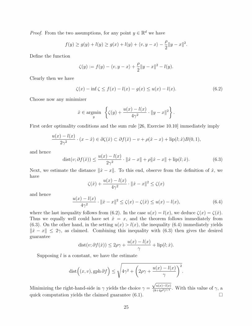
Proof. From the two assumptions, for any point y ∈ Rd we have
f(y) ≥ g(y) + l(y) ≥ g(x) + l(y) + 〈v, y − x〉 − ρ
2‖y − x‖2.
Define the function
ζ(y) := f(y)− 〈v, y − x〉+ρ
2‖y − x‖2 − l(y).
Clearly then we have
ζ(x)− inf ζ ≤ f(x)− l(x)− g(x) ≤ u(x)− l(x). (6.2)
Choose now any minimizer
x ∈ argminy
{ζ(y) +
u(x)− l(x)
4γ2· ‖y − x‖2
}.
First order optimality conditions and the sum rule [26, Exercise 10.10] immediately imply
u(x)− l(x)
2γ2· (x− x) ∈ ∂ζ(x) ⊂ ∂f(x)− v + ρ(x− x) + lip(l; x)B(0, 1),
and hence
dist(v; ∂f(x)) ≤ u(x)− l(x)
2γ2· ‖x− x‖+ ρ‖x− x‖+ lip(l; x). (6.3)
Next, we estimate the distance ‖x − x‖. To this end, observe from the definition of x, wehave
ζ(x) +u(x)− l(x)
4γ2· ‖x− x‖2 ≤ ζ(x)
and henceu(x)− l(x)
4γ2· ‖x− x‖2 ≤ ζ(x)− ζ(x) ≤ u(x)− l(x), (6.4)
where the last inequality follows from (6.2). In the case u(x) = l(x), we deduce ζ(x) = ζ(x).Thus we equally well could have set x = x, and the theorem follows immediately from(6.3). On the other hand, in the setting u(x) > l(x), the inequality (6.4) immediately yields‖x − x‖ ≤ 2γ, as claimed. Combining this inequality with (6.3) then gives the desiredguarantee
dist(v; ∂f(x)) ≤ 2ργ +u(x)− l(x)
γ+ lip(l; x).
Supposing l is a constant, we have the estimate
dist(
(x, v), gph ∂f)≤
√4γ2 +
(2ργ +
u(x)− l(x)
γ
)2
.
Minimizing the right-hand-side in γ yields the choice γ =
√u(x)−l(x)
(8+4ρ2)1/4. With this value of γ, a
quick computation yields the claimed guarantee (6.1).
25

Let us now specialize the theorem to the setting where the lower and upper boundsl(·), u(·) are functions of the product ‖x− x‖ · ‖x+ x‖, as in phase retrieval.
Corollary 6.2. Fix two functions f, g : Rd → R. Suppose that g is ρ-weakly convex and thatthere is a point x and a real δ > 0 such that the inequality
|f(x)− g(x)| ≤ δ‖x− x‖ · ‖x+ x‖ holds for all x ∈ Rd.
Then for any stationary point x of g, there exists a point x satisfying ‖x− x‖ ≤√
4δρ+2δ·√‖x− x‖‖x+ x‖,
dist(0; ∂f(x)) ≤ (δ + 2√δ(ρ+ 2δ)) · (‖x− x‖+ ‖x+ x‖)
.
Proof. Set u(x) := δ‖x− x‖ · ‖x− x‖ and l(x) := −δ‖x− x‖ · ‖x− x‖ and observe lip(l;x) ≤δ(‖x− x‖ + ‖x + x‖). Applying Theorem 6.1, we deduce that for any γ > 0, there exists apoint x satisfying
‖x−x‖ ≤ 2γ and dist(0; ∂f(x)) ≤ 2ργ+2δ‖x− x‖‖x+ x‖
γ+ δ(‖x− x‖+‖x+ x‖).
The triangle inequality implies
‖x− x‖ ≤ 2γ + ‖x− x‖ and ‖x+ x‖ ≤ 2γ + ‖x+ x‖,
and therefore
dist(0; ∂f(x)) ≤ 2(ρ+ 2δ)γ +2δ‖x− x‖‖x+ x‖
γ+ δ(‖x− x‖+ ‖x+ x‖)
Minimizing this expression in γ > 0 yields the choice γ :=√
δ‖x−x‖‖x+x‖ρ+2δ
. Plugging in this
value of γ and applying the AM-GM inequality then implies
dist(0; ∂f(x)) ≤ 4√δ(ρ+ 2δ)‖x− x‖‖x+ x‖+ δ(‖x− x‖+ ‖x+ x‖)
≤ (δ + 2√δ(ρ+ 2δ))(‖x− x‖+ ‖x+ x‖).
The result follows.
We now arrive at the main result of the section.
Corollary 6.3 (Subsampled stationary points). Consider the robust phase retrieval objectivefS(·) generated from i.i.d standard Gaussian vectors. There exist numerical constants c1, c2 >0 such that whenever m ≥ c1d, then with probability at least 1−2 exp(−min{m/c1, c2m, d
2}),every stationary point x of fS satisfies ‖x‖ . ‖x‖ and one of the two conditions:
‖x‖‖x− x‖‖x+ x‖‖x‖3
. 4
√d
mor
∣∣∣∣‖x‖‖x‖ − c
∣∣∣∣ . 4
√d
m·(
1 +‖x‖‖x‖
)|〈x, x〉|‖x‖‖x‖
. 4
√d
m· ‖x‖‖x‖
,
where c > 0 is the unique solution of the equation π4
= c1+c2
+ arctan (c) .
26

Proof. Theorem 3.7 shows that there exist constants c1, c2 > 0 such with probability at least1− 2 exp(−c1 min{m, d2}), we have
|fS(x)− fP (x)| ≤ c2
2
(√d
m+d
m
)‖x− x‖‖x+ x‖ for all x ∈ Rd. (6.5)
Lemma 3.5, in turn, shows that there exist numerical constants c3, ρ > 0 such that provided
m ≥ c3d, the function fS is ρ-weakly convex, with probability at least 1 − exp(−mc3
). Let
us now try to apply Corollary 6.2. To simplify notation, define ∆ :=√
dm
and set δ := c2∆.
Notice δ ≥ c22
(∆ + ∆2) and hence we may apply Corollary 6.2. We deduce that with highprobability, for any stationary point x of fS there exists a point x ∈ Rd satisfying ‖x− x‖ ≤
√4c2∆ρ+2c2∆
·√‖x− x‖‖x+ x‖,
dist(0; ∂fP (x)) ≤ (c2∆ + 2√c2∆(ρ+ 2c2∆)) · (‖x− x‖+ ‖x+ x‖)
. (6.6)
Notice√
4c2∆ρ+2c2∆
≤√
∆ ·√
4c2ρ≤ 2C ′
√∆ and (c2∆ + 2
√c2∆(ρ+ 2c2∆)) ≤ C ′
√∆ for some
numerical constant C ′. For notational convenience, set Dx := ‖x− x‖ + ‖x + x‖. Thus, bythe AM-GM inequality, the inclusion x ∈ B(x,C ′
√∆Dx) holds.
Claim 1. There exist constants C ′′, τ > 0 such that with high probability, for all ∆ < C ′′,the inequality ‖x‖ ≤ τ‖x‖ holds for any stationary point x of fS.
Proof. We may assume that ‖x‖ ≤ ‖x‖ since otherwise the result is trivial. Next, observethat ‖x‖ and ‖x‖ have comparable norms:
‖x‖ ≤ ‖x‖+ C ′√
∆Dx ≤ (1 + 4C ′√
∆)‖x‖,‖x‖ ≥ ‖x‖ − C ′
√∆Dx ≥ (1− 4C ′
√∆)‖x‖,
where we have used the bound Dx ≤ 4‖x‖ twice. To make the last bound meaningful, wemay set C ′′ < ( 1
8C′)2, thereby ensuring 1−4C ′
√∆ ≥ 1/2. Because the norms are comparable,
we deduce
dist(0; ∂fP (x)) ≤ C ′√
∆Dx ≤ 4C ′√
∆‖x‖ ≤ 4C ′√
∆
(1− 4C ′√
∆)‖x‖. (6.7)
Let us now decrease C ′′ if necessary to have C ′′ < min{(
18C′
)2,(γ
8C′
)2}, where γ is the
fixed constant from Theorem 5.3. Then for all ∆ < C ′′, we have 1 − 4C ′√
∆ ≥ 12
and4C′√
∆1−4C′
√∆≤ 8C ′
√∆ ≤ γ. Now we can apply Theorem 5.3 to x, which guarantees that
‖x‖ . ‖x‖. Thus because the norms of ‖x‖ and ‖x‖ are comparable, we obtain the desiredresult.
Provided ∆ ≤ min{(
18C′
)2,(γ
8C′
)2}, we obtain from (6.7) and Claim 1 the estimate
dist(0; ∂fP (x)) ≤ ε := C ′√
∆Dx ≤ 8C ′√
∆‖x‖ ≤ γ‖x‖.
27

Applying Theorem 5.3 we find that the point x ∈ B(x,C ′√
∆Dx) satisfies either
‖x‖‖x− x‖‖x+ x‖ .√
∆Dx‖x‖2 or
|‖x‖ − c‖x‖| .√
∆Dx‖x‖‖x‖
|〈x, x〉| .√
∆Dx‖x‖
. (6.8)
Applying the triangle inequality and the bound Dx ≤ (2 + 2τ)‖x‖, the claimed inequalitiesall follow (see Appendix A for a detailed explanation).
Acknowledgments We thank Peng Zheng (University of Washington, Seattle) for invalu-able help in developing the numerical illustrations.
References
[1] H. Attouch, J. L. Ndoutoume, and M. Thera. Epigraphical convergence of functionsand convergence of their derivatives in Banach spaces. Sem. Anal. Convexe, 20:Exp.No. 9, 45, 1990.
[2] J.V. Burke and M.C. Ferris. Weak sharp minima in mathematical programming. SIAMJ. Control Optim., 31(5):1340–1359, 1993.
[3] E.J. Candes, X. Li, and M. Soltanolkotabi. Phase retrieval via Wirtinger flow: theoryand algorithms. IEEE Trans. Inform. Theory, 61(4):1985–2007, 2015.
[4] E.J. Candes, T. Strohmer, and V. Voroninski. Phaselift: Exact and stable signal recov-ery from magnitude measurements via convex programming. Communications on Pureand Applied Mathematics, 66(8):1241–1274, 2013.
[5] F.H. Clarke, R.J. Stern, and P.R. Wolenski. Proximal smoothness and the lower-C2
property. J. Convex Anal., 2(1-2):117–144, 1995.
[6] D. Davis and B. Grimmer. Proximally guided stochastic method for nonsmooth, non-convex problems. Preprint arXiv:1707.03505, 2017.
[7] D. Drusvyatskiy and A.S. Lewis. Error bounds, quadratic growth, and linear conver-gence of proximal methods. To appear in Math. Oper. Res., arXiv:1602.06661, 2016.
[8] D. Drusvyatskiy and C. Paquette. Efficiency of minimizing compositions of convexfunctions and smooth maps. Preprint arXiv:1605.00125, 2016.
[9] D. Drusvyatskiy and C. Paquette. Variational analysis of spectral functions simplified.J. Convex Anal.,, 25(1), 2018.
[10] J.C. Duchi and F. Ruan. Solving (most) of a set of quadratic equalities: Compositeoptimization for robust phase retrieval. Preprint arXiv:1705.02356, 2017.
[11] J.C. Duchi and F. Ruan. Stochastic methods for composite optimization problems.Preprint arXiv:1703.08570, 2017.
28
[12] Y.C. Eldar and S. Mendelson. Phase retrieval: stability and recovery guarantees. Appl.Comput. Harmon. Anal., 36(3):473–494, 2014.
[13] H. Federer. Curvature measures. Trans. Amer. Math. Soc., 93(3):418–491, 1959.
[14] M. Fickus, D.G. Mixon, A.A. Nelson, and Y. Wang. Phase retrieval from very fewmeasurements. Linear Algebra Appl., 449:475–499, 2014.
[15] R.A. Horn and C.R. Johnson. Matrix analysis. Cambridge University Press, Cambridge,second edition, 2013.
[16] T. Kato. A short introduction to perturbation theory for linear operators. Springer-Verlag, New York-Berlin, 1982.
[17] Y. Lecun, L. Bottou, Y. Bengio, and P. Haffner. Gradient-based learning applied todocument recognition. Proceedings of the IEEE, 86(11):2278–2324, Nov 1998.
[18] A.S. Lewis. Convex analysis on the Hermitian matrices. SIAM J. Optim., 6(1):164–177,1996.
[19] A.S. Lewis. Nonsmooth analysis of eigenvalues. Math. Program., 84(1, Ser. A):1–24,1999.
[20] A.S. Lewis and S.J. Wright. A proximal method for composite minimization. Math.Program., pages 1–46, 2015.
[21] Z.-Q. Luo and P. Tseng. Error bounds and convergence analysis of feasible descentmethods: a general approach. Annals of Operations Research, 46(1):157–178, Mar 1993.
[22] B.S. Mordukhovich. Variational Analysis and Generalized Differentiation I: Basic The-ory. Grundlehren der mathematischen Wissenschaften, Vol 330, Springer, Berlin, 2006.
[23] R.A. Poliquin and R.T. Rockafellar. Prox-regular functions in variational analysis.Trans. Amer. Math. Soc., 348:1805–1838, 1996.
[24] B.T. Poljak. A general method for solving extremal problems. Dokl. Akad. Nauk SSSR,174:33–36, 1967.
[25] R.T. Rockafellar. Favorable classes of Lipschitz-continuous functions in subgradientoptimization. In Progress in nondifferentiable optimization, volume 8 of IIASA Collabo-rative Proc. Ser. CP-82, pages 125–143. Internat. Inst. Appl. Systems Anal., Laxenburg,1982.
[26] R.T. Rockafellar and R.J-B. Wets. Variational Analysis. Grundlehren der mathematis-chen Wissenschaften, Vol 317, Springer, Berlin, 1998.
[27] J. Sun, Q. Qu, and J. Wright. A geometric analysis of phase retrieval. To appear inFound. Comp. Math., arXiv:1602.06664, 2017.
29

[28] Y.S Tan and R. Vershynin. Phase retreival via randomized kaczmarz: Theoreticalguarantees. arXiv:1605.08285, 2017.
[29] G. Wang, G.B. Giannakis, and Y.C. Eldar. Solving systems of random quadratic equa-tions via a truncated amplitude flow. arXiv:1605.08285, 2016.
[30] H. Zhang, Y. Chi, and Y. Liang. Provable non-convex phase retrieval with outliers:Median truncated wirtinger flow. In Proceedings of the 33rd International Conferenceon International Conference on Machine Learning - Volume 48, ICML’16, pages 1022–1031. JMLR.org, 2016.
Appendices
A Auxiliary computations
Proof of Lemma 5.6. We let σ1 = y1 and σ2 = −y2. We may write
Ev[|σ1v
21 − σ2v
22|]
=1
2π
∫R2
|σ1v21 − σ2v
22| exp
(−(v2
1 + v22
2
))dv1dv2
=1
2π
∫R1
(σ1v
21 − σ2v
22
)exp
(−(v2
1 + v22
2
))dv1dv2
+1
2π
∫R2
(σ2v
22 − σ1v
21
)exp
(−(v2
1 + v22
2
))dv1dv2
where
R1 = {(v1, v2) :√σ1|v1| ≥
√σ2|v2|}
R2 = {(v1, v2) :√σ2|v2| ≥
√σ1|v1|} .
Using the convention arctan(θ) ∈[−π
2, π
2
], we define the angle θ1 := arctan
(√σ1σ2
). Passing
to the polar coordinates, we deduce
1
2π
∫R1
(σ1v21 − σ2v
22) exp
(−(v2
1 + v22
2
))dv1dv2
=1
2π
∫R1
r3(σ1 cos2(θ)− σ2 sin2(θ)) e−r2/2 drdθ.
We break up the region R1 into three wedges corresponding to the angles [0, θ1], [2π, 2π−θ1],and [π + θ1, π − θ1]. We will compute the integral over one of the regions. The rest will
30

follow analogously. To this end, we successively deduce
1
2π
∫ θ1
0
∫ ∞0
r3
(σ1 cos2(θ)− σ2 sin2(θ)
)e−r
2/2 drdθ
=1
2π
∫ θ1
0
σ1 (1 + cos(2θ))− σ2 (1− cos(2θ)) dθ
=1
2π
((σ1 − σ2)θ + (σ1 + σ2) sin(θ) cos(θ)
)∣∣∣∣θ10
=1
2π
((σ1 − σ2)θ1 + (σ1 + σ2) sin(θ1) cos(θ1)
)1
2π
∫ 2π
2π−θ1
∫ ∞0
r3
(σ1 cos2(θ)− σ2 sin2(θ)
)e−r
2/2 drdθ
=1
2π
((σ1 − σ2)θ1 + (σ1 + σ2) sin(θ1) cos(θ1)
)1
2π
∫ π+θ1
π−θ1
∫ ∞0
r3
(σ1 cos2(θ)− σ2 sin2(θ)
)e−r
2/2 drdθ
=1
2π
(2(σ1 − σ2)θ1 + 2(σ1 + σ2) sin(θ1) cos(θ1)
).
Similarly, we see that for the region R2, we have
1
2π
∫R2
(σ2v22 − σ1v
21) exp
(−(v2
1 + v22
2
))dv1dv2
=1
2π
∫R2
r3(σ2 sin2(θ)− σ1 cos2(θ)) e−r2/2 drdθ.
We break up the region R2 into two wedges where the angles range from [θ1, π − θ1] and[π + θ1, 2π − θ1] as we did in R1. We will show the explicit computation for one of theseterms and note the rest following using similar computations:
1
2π
∫ π−θ1
θ1
∫ ∞0
r3
(σ2 sin2(θ)−σ1 cos2(θ)
)e−r
2/2 drdθ
=1
2π
∫ π−θ1
θ1
σ2 (1− cos(2θ))− σ1 (1 + cos(2θ)) dθ
=1
2π
((σ2 − σ1)θ − (σ1 + σ2) sin(θ) cos(θ)
)∣∣∣∣π−θ1θ1
=1
2π
((σ2 − σ1)(π − 2θ1) + 2(σ1 + σ2) sin(θ1) cos(θ1)
)1
2π
∫ 2π−θ1
π+θ1
∫ ∞0
r3
(σ2 sin2(θ)−σ1 cos2(θ)
)e−r
2/2 drdθ
=1
2π
((σ2 − σ1)(π − 2θ1) + 2(σ1 + σ2) sin(θ1) cos(θ1)
).
31

By combining the computed integrals, we arrive at the full answer
Ev[|σ1v
21 − σ2v
22|]
=4
π
[(σ1 − σ2) arctan
(√σ1
σ2
)+√σ1σ2
]− (σ1 − σ2),
as claimed.
Proof showing Equation (6.8) implies Corollary 6.3. We observe that Dx ≤ 2‖x‖ + 2‖x‖,which by Claim 1 gives Dx ≤ (2τ + 2)‖x‖. First by applying the triangle inequality with‖x− x‖ ≤ C ′
√∆Dx and (6.8), we obtain
|‖x‖ − c‖x‖| ≤ |‖x− x‖+ ‖x‖ − c‖x‖| . C ′√
∆Dx +√
∆Dx‖x‖‖x‖
.
Using the bound on Dx gives the desired inequality. Next, we conclude
|〈x, x〉| ≤ ‖x‖‖x− x‖+ |〈x, x〉|. C ′
√∆Dx‖x‖+
√∆Dx‖x‖.
Applying the bound on Dx, the result is shown. Lastly, using ‖x‖ ≤ τ‖x‖ and ‖x‖ . ‖x‖,we conclude
‖x‖‖x− x‖‖x+ x‖ ≤ (‖x− x‖+ ‖x‖)(‖x− x‖‖x+ x‖)≤ D2
x‖x− x‖+ ‖x‖‖x− x‖‖x+ x‖. ‖x‖2Dx
√∆ + ‖x‖(‖x− x‖+ ‖x− x‖)‖x+ x‖
. ‖x‖3√
∆ + ‖x‖2√
∆Dx + ‖x‖‖x− x‖‖x+ x‖. ‖x‖3
√∆ + ‖x‖‖x− x‖(‖x− x‖+ ‖x+ x‖)
. ‖x‖3√
∆ + ‖x‖2Dx
√∆ + ‖x‖‖x− x‖‖x+ x‖
. ‖x‖3√
∆ +√
∆Dx‖x‖2.
Dividing through by ‖x‖3, finishes the proof.
B Proof of Theorem 5.3
In this section, we will prove Theorem 5.3. Contrasting with Theorem 5.2, the proof of The-orem 5.3 is much more delicate, in large part relying on perturbation bounds on eigenvalues;e.g. Gershgorin theorem [15, Corollary 6.1.3]. We continue using the notation of Section 5.3.Namely, fix a symmetric convex function f : Rd → R and a point x ∈ Rd \ {0}, and definethe function
g(x) := fλ(xxT − xxT ).
The chain rule directly implies∂g(x) = ∂fλ(X)x.
32

Therefore, using Theorem 5.1 let us also fix a matrix V ∈ ∂fλ(X) and a matrix U ∈ Od
satisfying
λ(V ) ∈ ∂f(λ(X)), V = U(Diag(λ(V ))UT , and X = UDiag(λ(X))UT .
We begin with two technical lemmas.
Lemma B.1. Suppose that there exists κ > 0 such that the inequality
g(x)− g(x) ≥ κ‖x− x‖‖x+ x‖ holds for all x ∈ Rd.
Then for any x /∈ {±x}, we have max{|λ1(V )|, |λd(V )|} ≥ κ/2.
Proof. Using Lemma 5.10, for i ∈ {1, d} we obtain
|λi(X)| = |〈Ui, x〉2 − 〈Ui, x〉2| = |〈Ui, x− x〉〈Ui, x+ x〉| ≤ ‖x− x‖‖x+ x‖.
Taking into account (5.6), yields
κ‖x− x‖‖x+ x‖ ≤ g(x)− g(x) ≤ λ1(V )λ1(X) + λd(V )λd(X)
≤ 2 max{|λ1(V )|, |λd(V )|}‖x− x‖‖x+ x‖,
as desired.
Lemma B.2. Suppose that there exists κ > 0 such that the inequality
g(x)− g(x) ≥ κ‖x− x‖‖x+ x‖ holds for all x ∈ Rd. (B.1)
Then any point x ∈ Rd \ {0} satisfies
κ‖x− x‖‖x+ x‖‖x‖
− (|λ1(V )|+ |λd(V )|)‖x‖2
‖x‖≤ dist(0; ∂g(x)).
Proof. First, note that for x ∈ {±x}, the result holds trivially, so we may assume x /∈{±x}. Recall the equality ∂g(x) = ∂fλ(X)x. Fix now a vector V ∈ ∂fλ(X) satisfyingdist(0; ∂g(x)) = ‖V x‖. Using convexity, we deduce
g(x)− g(x) = fλ(xxT − xxT )− fλ(0) ≤ 〈V, xxT − xxT 〉 ≤ ‖x‖dist(0, ∂g(x)) + |xTV x|.
(B.2)
We next upper bound the term |xTV x|. To this end, fix a matrix U ∈ Od satisfying V =UDiag(λ(V ))UT and X = UDiag(λ(X))UT , and such that the inclusion λ(V ) ∈ ∂f(λ(X))holds. Taking into account x ∈ span{U1, Ud} (Lemma 5.10), we deduce
|xTV x| = |λ1(V )〈U1, x〉2 + λd(V )〈Ud, x〉2| ≤ (|λ1(V )|+ |λd(V )|)‖x‖2.
Combining this estimate with (B.2) and (B.1) completes the proof.
We next prove a quantitative version of Corollary 5.12. The argument follows a similaroutline.
33

Theorem B.3 (Quantitative Version of Corollary 5.12). Suppose that there exists a constantκ > 0 such that the inequality
g(y)− g(x) ≥ κ‖y − x‖‖y + x‖ holds for all y ∈ Rd.
Suppose |λ1(V )|, |λd(V )| are both upper bounded by a numerical constant2 and set ε := ‖V x‖.Then there exists a numerical constant γ > 0, such that whenever ε ≤ γ · ‖x‖, we have that‖x‖ . ‖x‖ and x satisfies either
‖x‖‖x− x‖‖x+ x‖ . ε‖x‖2 or
{|λ1(V )| . ε/‖x‖|〈x, x〉| . ε‖x‖
}.
Proof. Clearly, we may suppose x /∈ {0,±x} and ε 6= 0, since otherwise the theorem wouldhold vacuously. We will prove the following precise bound, which immediately implies thestatement of the theorem: there exists a numerical constant γ > 0, such that wheneverε ≤ γ‖x‖, the inequalities ‖x‖ ≤ δ‖x‖ and
min
‖x− x‖‖x+ x‖2κ
max{(‖x‖√
2+√
2‖x‖2‖x‖
), ‖x‖(κ
√2+2|λd(V )|)κ
} ,max
{|λ1(V )|‖x‖√
2,
κ|〈x, x〉|2√
2δ‖x‖+ 2‖x‖
} ≤ ‖V x‖,(B.3)
hold, where we define the numerical constant
δ :=
√2(|λ1(V )|+ |λd(V )|)
κ+ 1.
As a first step, we show that ‖x‖ is within a numerical constant of ‖x‖.Claim 2. Provided γ < κ(1−1/δ)2
2, the inequality, ‖x‖ ≤ δ‖x‖, holds.
Proof. Assume for sake of contradiction ‖x‖‖x‖ > δ :=√
2(|λ1(V )|+|λd(V )|)κ
+ 1. Lemma B.1 shows
max{|λ1(V )|, |λd(V )|} ≥ κ2, and therefore δ > 1. Using the bound dist(0; ∂g(x)) ≤ ‖V x‖ = ε
and Lemma B.2, we deduce:
κ‖x− x‖‖x+ x‖‖x‖2
− ε
‖x‖≤ (|λ1(V )|+ |λd(V )|)‖x‖2
‖x‖2.
Clearly, we have
κ‖x− x‖‖x+ x‖‖x‖2
≥ κ(‖x‖ − ‖x‖)2
‖x‖2≥ κ(1− 1/δ)2.
Let us now choose γ < κ(1−1/δ)2
2, thereby guaranteeing ε
‖x‖ ≤κ(1−1/δ)2
2. Hence, we obtain
κ(1− 1/δ)2
2(|λ1(V )|+ |λd(V )|)≤ 1
|λ1(V )|+ |λd(V )|
(κ‖x− x‖‖x+ x‖
‖x‖2− ε
‖x‖
)≤ ‖x‖
2
‖x‖2<
1
δ2.
2This holds whenever (t, s) 7→ f(t, s, 0, . . . , 0) is Lipschitz continuous.
34

Rearranging yieldsκ
2(|λ1(V )|+ |λd(V )|)<
1
(δ − 1)2,
a contradiction.
Looking back at the expression, define the values:
ρ1 =‖x‖√
2and ρ3 =
2
κmax
{(‖x‖√
2+
√2‖x‖2
‖x‖
),‖x‖(κ
√2 + 2|λd(V )|)κ
}.
Notice that the inequality, ερ3 ≥ ‖x − x‖‖x + x‖, would immediately imply the validity ofthe theorem. Thus, we assume ερ3 < ‖x− x‖‖x+ x‖ throughout. It suffices now to show
|λ1(V )| ≤ ε/ρ1 and |〈x, x〉| ≤ ε
κ
(2√
2δ‖x‖+ ‖x‖).
We do so in order. We begin by observing that the inequality (5.5) guarantees
max{|λ1(V )〈U1, x〉|, |λd(V )〈Ud, x〉|} ≤ ε. (B.4)
Claim 3. The inequality |λ1(V )| < ε/ρ1 holds.
Proof. Let us assume the contrary, |λ1(V )| ≥ ε/ρ1. Inequality (B.4) then implies |〈U1, x〉| ≤ρ1, while Lemma 5.10 in turn guarantees
0 ≤ λ1(X) = 〈U1, x〉2 − 〈U1, x〉2 ≤ ρ21.
Taking into account 〈U1, x〉2+〈Ud, x〉2 = ‖x‖2 (Lemma 5.10, correlation), we deduce 〈Ud, x〉2 ≥‖x‖2 − ρ2
1. Combining this with (B.4), we deduce
|λd(V )| ≤ ε
|〈Ud, x〉|≤ ε√
‖x‖2 − ρ21
.
Therefore, using the correlation inequality (5.6), we find
ερ3κ < κ‖x− x‖‖x+ x‖ ≤ g(x)− g(x) ≤ λ1(V )λ1(X) + λd(V )λd(X)
≤ |λ1(V )|(〈U1, x〉2 − 〈U1, x〉2) +ε√
‖x‖2 − ρ21
(〈Ud, x〉2 − 〈Ud, x〉2
)≤ ε|〈U1, x〉|+
ε〈Ud, x〉2√‖x‖2 − ρ2
1
≤ ε
(ρ1 +
‖x‖2√‖x‖2 − ρ2
1
).
Dividing through by ε and plugging in the value of ρ1 yields
ρ3κ <‖x‖√
2+
√2‖x‖2
‖x‖,
which contradicts the definition of ρ3.
35

Let us now decrease γ > 0 further by ensuring γ < min{κ(1−1/δ)2
2, κ
2√
2}. Thus, from
Claim 3 and our standing assumption ‖V x‖ ≤ κ‖x‖2√
2, we conclude
|λ1(V )| <√
2ε
‖x‖<κ
2.
Lemma B.1 guarantees, max{|λ1(V )|, |λd(V )|} ≥ κ/2; thus, we deduce |λd(V )| ≥ κ/2. Ap-plying (B.4), we find that
|〈Ud, x〉| ≤ε
|λd(V )|≤ 2ε
κ. (B.5)
Thus, by Lemma 5.10, we have
|〈U1, x〉〈Ud, x〉| = |〈U1, x〉〈Ud, x〉| ≤2‖x‖εκ
. (B.6)
Claim 4. The inequality |〈Ud, x〉| > |〈U1, x〉| holds.
Proof. Let us assume the contrary |〈Ud, x〉| ≤ |〈U1, x〉|. Then from (B.6) we obtain3 〈Ud, x〉2 <2‖x‖εκ
. Hence from Lemma 5.10, we find that |λd(X)| ≤ 〈Ud, x〉2 ≤ 2‖x‖εκ
. Putting these factstogether with the correlation inequality (5.6), we successively deduce
ερ3κ < κ‖x− x‖‖x+ x‖ ≤ g(x)− g(x) ≤ λ1(V )λ1(X) + |λd(V )| · |λd(X)|
≤√
2ε
‖x‖· λ1(X) + |λd(V )| · 2‖x‖ε
κ
≤ κ√
2ε‖x‖κ
+2|λd(V )|ε‖x‖
κ,
where the last inequality uses the bound λ1(X) ≤ ‖x‖2. Therefore, we have reached acontradiction to the definition of ρ3.
Combining Claim 4 with the expression 〈U1, x〉2+〈Ud, x〉2 = ‖x‖2, we conclude 〈Ud, x〉2 ≥‖x‖2
2. Therefore, (B.6) and Claim 2 imply the strong result:
|〈U1, x〉| ≤2√
2ε‖x‖κ‖x‖
≤ 2√
2εδ
κ. (B.7)
Thus combining Claim 2, Lemma 5.10, and (B.5) we conclude
|〈x, x〉| = |〈U1, x〉〈U1, x〉+ 〈Ud, x〉〈Ud, x〉| ≤ |〈U1, x〉| · ‖x‖+ |〈Ud, x〉| · ‖x‖
≤ ε
κ
(2√
2δ‖x‖+ 2‖x‖).
The proof is complete.
3If ab < δ, then min{a, b}2 < δ.
36

In order to interpret the conclusion of Theorem B.3 on the phase retrieval objective fP ,we must show that the condition {
|λ1(V )| . ε/‖x‖|〈x, x〉| . ε‖x‖
}
guarantees that the equation ‖x‖ = c · ‖x‖ almost holds, where c is defined in Theorem 5.2.This is the content of the following two lemmas. Note that it is easy to verify the equalityλ1(V ) = ∇y1ζ(y1, y2), where we set (y1, y2) := (λ1(X), λd(X)).
Lemma B.4 (Extension of Lemma 5.8). Fix a real constant 0 ≤ ε < 1. The solutions ofthe inequality |∇y1ζ(y1, y2)| ≤ ε on R++ × R−− are precisely the elements of the open cone
{(c2y,−y) : 0 < y, 0 < c1 ≤ c ≤ c2},
where c1, c2 are the unique solutions of the equations
π
4(1 + ε) =
c2
1 + c22
+ arctan (c2) ,
andπ
4(1− ε) =
c1
1 + c21
+ arctan (c1) .
Moreover, considering c1 and c2 as functions of ε, we have c2(ε) − c1(ε) ≤ 5πε whenever0 < ε < 1/2.
Proof. The proof is completely analogous to that of Lemma 5.8. We leave the details to thereader. The only point worth commenting is the inequality c2(ε) − c1(ε) ≤ 5πε whenever0 < ε < 1/2. To get this bound, observe that 0 < c2(ε) ≤ c2(.5) ≤ .83 for all ε ≤ 1/2 as c2
is a increasing function of ε. Therefore,
π
2ε =
c2
1 + c22
− c1
1 + c21
+ arctan(c2)− arctan(c1) ≥ c2
1 + c22
− c1
1 + c21
=1− c1c2
(1 + c21)(1 + c2
2)(c2 − c1)
≥ 1− c22
(1 + c21)(1 + c2
2)(c2 − c1) ≥ 1− c2
2
(1 + c22)2
(c2 − c1).
(B.8)Thus, we have
c2(ε)− c1(ε) ≤ πε
2
(1 + c22(ε))2
1− c22(ε)
≤ πε
2
(1 + .832)2
1− .832≤ 5πε,
as claimed.
Lemma B.5. Fix a real constant 0 ≤ ε < 13
and vectors x, x ∈ Rd \ {0}. Suppose λ1(X) =−c2λd(X) for some real constant c > 0 and |〈x, x〉| ≤ ε‖x‖‖x‖. Then we have
1− (1 + c2)(ε+ ε2) ≤ c2‖x‖2
‖x‖2≤ 1 + (1 + c2)(ε+ ε2).
37
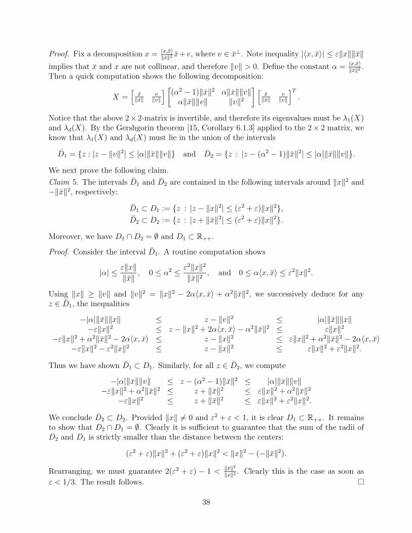
Proof. Fix a decomposition x = 〈x,x〉‖x‖2 x+v, where v ∈ x⊥. Note inequality |〈x, x〉| ≤ ε‖x‖‖x‖
implies that x and x are not collinear, and therefore ‖v‖ > 0. Define the constant α = 〈x,x〉‖x‖2 .
Then a quick computation shows the following decomposition:
X =[
x‖x‖
v‖v‖
] [(α2 − 1)‖x‖2 α‖x‖‖v‖α‖x‖‖v‖ ‖v‖2
] [x‖x‖
v‖v‖
]T.
Notice that the above 2× 2-matrix is invertible, and therefore its eigenvalues must be λ1(X)and λd(X). By the Gershgorin theorem [15, Corollary 6.1.3] applied to the 2× 2 matrix, weknow that λ1(X) and λd(X) must lie in the union of the intervals
D1 = {z : |z − ‖v‖2| ≤ |α|‖x‖‖v‖} and D2 = {z : |z − (α2 − 1)‖x‖2| ≤ |α|‖x‖‖v‖}.
We next prove the following claim.
Claim 5. The intervals D1 and D2 are contained in the following intervals around ‖x‖2 and−‖x‖2, respectively:
D1 ⊂ D1 := {z : |z − ‖x‖2| ≤ (ε2 + ε)‖x‖2},D2 ⊂ D2 := {z : |z + ‖x‖2| ≤ (ε2 + ε)‖x‖2}.
Moreover, we have D1 ∩D2 = ∅ and D1 ⊂ R++.
Proof. Consider the interval D1. A routine computation shows
|α| ≤ ε‖x‖‖x‖
, 0 ≤ α2 ≤ ε2‖x‖2
‖x‖2, and 0 ≤ α〈x, x〉 ≤ ε2‖x‖2.
Using ‖x‖ ≥ ‖v‖ and ‖v‖2 = ‖x‖2 − 2α〈x, x〉 + α2‖x‖2, we successively deduce for anyz ∈ D1, the inequalities
−|α|‖x‖‖x‖ ≤ z − ‖v‖2 ≤ |α|‖x‖‖x‖−ε‖x‖2 ≤ z − ‖x‖2 + 2α〈x, x〉 − α2‖x‖2 ≤ ε‖x‖2
−ε‖x‖2 + α2‖x‖2 − 2α〈x, x〉 ≤ z − ‖x‖2 ≤ ε‖x‖2 + α2‖x‖2 − 2α〈x, x〉−ε‖x‖2 − ε2‖x‖2 ≤ z − ‖x‖2 ≤ ε‖x‖2 + ε2‖x‖2.
Thus we have shown D1 ⊂ D1. Similarly, for all z ∈ D2, we compute
−|α|‖x‖‖v‖ ≤ z − (α2 − 1)‖x‖2 ≤ |α|‖x‖‖v‖−ε‖x‖2 + α2‖x‖2 ≤ z + ‖x‖2 ≤ ε‖x‖2 + α2‖x‖2
−ε‖x‖2 ≤ z + ‖x‖2 ≤ ε‖x‖2 + ε2‖x‖2.
We conclude D2 ⊂ D2. Provided ‖x‖ 6= 0 and ε2 + ε < 1, it is clear D1 ⊂ R++. It remainsto show that D2 ∩D1 = ∅. Clearly it is sufficient to guarantee that the sum of the radii ofD2 and D1 is strictly smaller than the distance between the centers:
(ε2 + ε)‖x‖2 + (ε2 + ε)‖x‖2 < ‖x‖2 − (−‖x‖2).
Rearranging, we must guarantee 2(ε2 + ε) − 1 < ‖x‖2‖x‖2 . Clearly this is the case as soon as
ε < 1/3. The result follows.
38

Thus we have proved D1 ∩ D2 = ∅ and D1 ⊂ R++. Since D1 and D2, each contains atleast one eigenvalue, it must be the case that λd(X) lies in D2 and λ1(X) lies in D1. Wethus conclude ∣∣λ1(X)− ‖x‖2
∣∣ ≤ (ε2 + ε)‖x‖2∣∣λd(X) + ‖x‖2∣∣ ≤ (ε2 + ε)‖x‖2.
Writing λ1(X) = −c2λd(X), we obtain∣∣−c2λd(X)− c2‖x‖2 + c2‖x‖2 − ‖x‖2∣∣ ≤ (ε2 + ε)‖x‖2,
and hence ∣∣‖x‖2 − c2‖x‖2∣∣ ≤ (1 + c2)(ε2 + ε)‖x‖2.
The result follows.
Combining Lemmas B.4 and B.5, we arrive at the following.
Corollary B.6 (Small λ1(V ) and near orthogonality). Fix a real constant 0 ≤ ε ≤ 18
andconsider a point x ∈ Rd \ {0} satisfying |∇y1ζ(λ1(X), λd(X))| ≤ ε and |〈x, x〉| ≤ ε‖x‖‖x‖.Then x satisfies ∣∣‖x‖ − c‖x‖∣∣ ≤ 26ε‖x‖,where c is the solution of the equation π
4= c
1+c2+ arctan(c).
Proof. Define the quantities c1(ε) and c2(ε) to be the solutions of the equations
π
4(1− ε) =
c1
1 + c21
+ arctan(c1),
π
4(1 + ε) =
c2
1 + c22
+ arctan(c2),
respectively. First, since c2(·) is an increasing function, it is easy to verify c2(ε) < 1 whenever0 < ε ≤ 1
8; thus we have 2ε(1 + c2
2(ε)) < 12. By Lemma B.4, we know that whenever
|∇y1ζ(λ1(X), λd(X))| ≤ ε, there exists c satisfying λ1(X) = −c2λd(X) and 0 < c1(ε) ≤ c ≤c2(ε). Lemma B.5, in turn, implies
(1− 2ε(1 + c2))‖x‖2 ≤ c2‖x‖2 ≤ (1 + 2ε(1 + c2))‖x‖2.
Looking at the right-hand-side, we deduce
c21(ε)‖x‖2 ≤ c2‖x‖2 ≤
(1 + 2ε(1 + c2
2(ε)))‖x‖2,
while looking at the left-hand-side yields
(1− 2ε(1 + c22(ε)))‖x‖2 ≤ c2‖x‖2 ≤ c2
2(ε)‖x‖2.
Isolating ‖x‖2 and taking square roots we obtain
c1(ε)√1 + 2ε(1 + c2
2(ε))‖x‖ ≤ ‖x‖ ≤ c2(ε)√
1− 2ε(1 + c22(ε))
‖x‖. (B.9)
39

Applying Lemma B.4 and the inequality c2(ε) < 1, we upper bound the right-hand-side:
c2(ε)√1− 2ε(1 + c2
2(ε))≤ 5πε+ c√
1− 4ε
= c
(1 +
5πε/c+ 1−√
1− 4ε√1− 4ε
)≤ c
(1 +
5πε/c+ 4ε√1/2
)≤ c(1 + 57ε).
Exactly the same reasoning shows
c1(ε)√1 + 2ε(1 + c2
2(ε))≥ c(1− 57ε).
Thus the inequality∣∣‖x‖ − c‖x‖∣∣ ≤ 57cε‖x‖ ≤ 26ε‖x‖ holds, as claimed.
We are now ready to prove the inexact extension of Theorem 5.3.
Proof of Theorem 5.3. We use the decomposition g = fP (X) and f = ϕ. Let us verify thatwe may apply Theorem B.3. To this end, observe that the population objective satisfies
fP (x)− fP (x) = Ea[⟨
a,x− x‖x− x‖
⟩⟨a,
x+ x
‖x+ x‖
⟩]‖x− x‖‖x+ x‖ ≥ κ‖x− x‖‖x+ x‖
for the numerical constant κ [12, Corollary 3.7]. Moreover, clearly ζ is globally Lipschitz(being a norm), and therefore |λ1(V )| and |λd(V )| are bounded by a numerical constant.Thus provided ε := ‖V x‖ satisfies ε ≤ γ · ‖x‖ for the numerical constant γ, we can be surethat x satisfies either
‖x‖‖x− x‖‖x+ x‖ . ε‖x‖2 or
{|λ1(V )| . ε/‖x‖|〈x, x〉| . ε‖x‖
}.
Now suppose the latter is the case, and let C be a numerical constant satisfying |λ1(V )| ≤Cε/‖x‖ and |〈x, x〉| ≤ Cε‖x‖. We aim to apply Corollary B.6. To do so, we must ensure
|λ1(V )| ≤ Cε
‖x‖≤ 1
8and
∣∣∣∣⟨ x
‖x‖,x
‖x‖
⟩∣∣∣∣ ≤ Cε · ‖x‖‖x‖‖x‖
=Cε
‖x‖≤ 1
8.
Adjusting γ if necessary, we can be sure that ε/‖x‖ is below 18C
. Applying Corollary B.6,
with Cε‖x‖ in place of ε, we conclude |‖x‖ − c‖x‖| . ε‖x‖‖x‖ , as claimed.
B.1 Comments on Robustness
We have thus far assumed that the measurement vector b = (Ax)2 has not been corruptedby errant noise. In this section, we record a few straightforward extensions of earlier results,which hold if the measurements b are noisy.
40

Assumption E. Let b1, . . . , bm be m i.i.d. copies of
b = (aTx)2 + δ · ξ,
where δ ∈ {0, 1}, ξ ∈ R, and a ∈ Rd are independent random variables satisfying (1)pfail := P (δ 6= 0) < 1, (2) E [|ξ|] <∞, and (3) a ∼ N(0, Id).
Under corruption by δ · ξ, we define new population and subsampled objectives
fP (x) := Ea,ξ,δ[|(aTx)2 − (aT x)2 − δ · ξ|];
fS(x) :=1
m
m∑i=1
|(aTi x)2 − bi|.
Then by following the outline of the proof of Lemma 5.5, we arrive at a similar characteri-zation of fP as a spectral function.
Lemma B.7 (Spectral representation of the population objective).For all points x ∈ Rd, equality holds:
fP (x) = Ev,ξ,δ[∣∣∣〈λ(X), v〉 − δ · ξi
∣∣∣] ,where vi ∈ R are i.i.d. chi-squared random variables vi ∼ χ2
1.
Thus, we may writefP (x) = ϕ(λ(X)),
where ϕ is the convex symmetric function
ϕ(z) := Ev,ξ,δ[∣∣∣〈z, v〉 − δ · ξi∣∣∣] .
Moreover, provided that x is a minimizer of fP , the complete set of stationary points of fpmay be determined from Corollary 5.12. We prove this now.
Lemma B.8. For all x ∈ Rd, the following inequality holds:
fP (x)− fP (±x) ≥ (1− 2pfail)fP (x).
Consequently, if pfail < 1/2, the points ±x are the only minimizers of fp, and there exists anumerical constant κ such that
fP (x)− fP (±x) ≥ κ(1− 2pfail)‖x− x‖‖x+ x‖.
Proof. By expanding the difference, we find that
fP (x)− fP (±x) = (1− pfail)(fP (x)− fP (x)) + pfailEa,ξ[|(aTx)2 − (aT x)2 − ξ| − |ξ|
]≥ (1− pfail)fP (x)− pfailEa
[|(aTx)2 − (aT x)2|
]≥ (1− 2pfail)fP (x).
Only the sharpness inequality is left to prove, but this is simply a consequence of the sharp-ness of fP , which was proved in [12, Corollary 3.7].
41

Therefore, by Corollary 5.12 we arrive at the complete characterization of the stationarypoints of fP .
Theorem B.9. The set of stationary points of fP are precisely
{±x} ∪ {0} ∪ {x | 〈x, x〉 = 0, and ∃ζ ∈ ∂ϕ(λ(X)),maxi{ζi} = 0}.
The exact location of those stationary points orthogonal to x depends on the structureof the convex function ϕ, which in turn depends the distribution of the noise δ · ξ. We willnot attempt to characterize such ϕ.
By the sharpness of fP , a quantitative version of Theorem B.9 immediately follows fromTheorem B.3. When coupled together with a concentration inequality like that in Theo-rem 3.7, such a theorem would imply concentration of the subdifferential graphs of fS andfP . We omit these straightforward details.
42