Nonsmooth Optimization for Multidisk H∞ Synthesis

Pierre Apkarian ∗ Dominikus Noll †

Abstract

We discuss output feedback control design with multiple performance specifications, each

measured in a weighted H∞-norm. The multidisk design problem consists in finding a sta-

bilizing output feedback controller which minimizes the different performance specifications

simultaneously using a worst case strategy. This is less conservative than existing approaches,

but difficult to solve algorithmically due to inherent nonsmoothness and nonconvexity. We

present a nonsmooth optimization method suited for the multidisk problem and more gener-

ally, for programs where the maximum of an infinite family of nonconvex maximum eigenvalue

functions is minimized. The method is shown to perform well on a control problem for a

helicopter at hover.

Keywords: H∞-synthesis, multi-channel design, multi-objective optimization, concurring per-formance specifications, static output feedback, reduced-order synthesis, decentralized control,PID, NP -hard problems, nonsmooth optimization, multidisk problems.

1 Introduction

Well designed feedback control systems are expected to respond favorably to an extended set ofdesign goals including robustness, good regulation against disturbances, desirable responses tocommands, and much else. Controller design therefore often involves a tradeoff between theseobjectives in order to achieve a suitable compromise. In this paper we discuss a class of multi-objective design problems, known as multidisk problems [11], where the performance channels areall measured in a weighted H∞-norm, and where these performances are optimized simultaneouslyusing a worst case strategy. Mathematically, the multidisk design problem may be regarded asminimizing the maximum of an infinite family of nonconvex maximum eigenvalue functions. Themultidisk problem is of great practical importance, but difficult to solve due to its semi-infinitemin-max structure. This explains why to date only a few heuristic approaches have been presented.Since our new approach is expected to reduce conservatism in existing multi-channel strategies,we comment on those subsequently.

∗ONERA-CERT, Centre d’etudes et de recherche de Toulouse, Control System Department, 2 av. Edouard

Belin, 31055 Toulouse, France - and - Universite Paul Sabatier, Institut de Mathematiques, Toulouse, France -

Email: apkarian@cert.fr - Tel: +33 5.62.25.27.84 - Fax: +33 5.62.25.27.64.†Universite Paul Sabatier, Institut de Mathematiques, 118, route de Narbonne, 31062 Toulouse, France - Email:

noll@mip.ups-tlse.fr - Tel: +33 5.61.55.86.22 - Fax: +33 5.61.55.83.85.

1

A first clearly conservative approach to multi-channel problems alleviates the difficulty bysetting up a single performance channel, using trade-offs between the conflicting performancespecifications. This may then be solved via traditional methods (LMIs and AREs) suited forsingle channel design.

A second more sophisticated strategy uses the Q-parametrization of all stabilizing controllersof a system. For the two-disk problem, this is elaborated in [21], the related strong stabilizationproblem is considered in [28, 7]. Unfortunately, these approaches use the Youla parametrization[29], which leads to feedback controllers with large state dimension, and moreover, makes itimpossible to add structural constraints, also known as control law specifications, on the controller.We refer the reader to the work of Scherer [25] for an analysis of structured design problems for aspecific class of plants, and for a Q-parametrization approach to multi-objective control problems.A thorough mathematical study of multidisk problems using tools from analytic function theoryis presented by Dym et al. in [11].

There exists yet another class of heuristic techniques for multidisk and multi-objective syn-thesis problems, which uses state-space LMI formulations. Unfortunately, these techniques relyon sufficient conditions, and are in general extremely conservative [18]. The reader is referred to[26, 16, 10] to list just a few of these approaches, and to [4] for an extension to Linear Parameter-Varying systems.

Here we attack the multi-objective design problem directly using techniques from nonsmoothoptimization. Such a strategy has already been proposed in [13], where the authors use the Q-parametrization, which allows them to treat the multi-disk problem via convex analysis. In orderto avoid the inconveniences of the Q-parametrization, we follow a different and more flexible linewhich allows us in particular to add structural constraints on the controller. The price to bepaid for this extension is that the optimization program is nonconvex and nonsmooth, so thatcomputed solutions are only locally optimal. Experiments nonetheless show that the advantage ofour local strategy is considerable. Note that a similar nonsmooth and nonconvex formulation ofH∞ synthesis is also investigated in [15]. There, the authors propose a global search strategy basedon a dynamical systems approach to determine solutions. In [1], we have combined direct searchtechniques, often referred to as derivative-free methods, with nonsmooth oracles to obtain a firstvalid approach to feedback control synthesis. These techniques have local convergence certificateseven in the presence of nonsmoothness, but are not efficient when the system order is large.

In this work we consider optimization of composite functions of the form

f(K) = maxi=1,...,N

‖Twi→zi(K)‖∞, (1)

where Twi→zi(K) are performance specifications used to probe the closed-loop system. Each Twi→zi

is a smooth operator defined on the open domain D of stabilizing feedback controllers K, withvalues in the infinite dimensional space RH∞ of rational stable transfer matrix functions. Inconsequence, the composite functions ‖ · ‖∞ Twi→zi are neither smooth nor convex, but theirstructure can be exploited algorithmically. One central contribution of this work is a spectralbundle algorithm suited for local optimization of functions of the form f , and more generally, forsemi-infinite nonconvex maximum eigenvalue functions with a related structure.

Notice that the max-H∞-function f(K) may be written as

f(K) = maxi=1,...,N

‖Twi→zi(K)‖∞ = maxω∈R

σ (T (K, jω)) = maxω∈R

λ1

(

T (K, jω)T (K, jω)H)1/2

(2)

2

where σ(M) and λ1(MMH) denote the maximum singular value respectively the maximum eigen-value, and where T (K, jω) has a block structure with N blocks regrouping the different perfor-mance channels:

T (K, jω) := diag(Tw1→z1(K, jω), . . . , TwN→zN (K, jω)) . (3)

In particular, T (K, jω)T (K, jω)H is then block diagonal with N blocks, so that f may be inter-preted as an infinite maximum of maximum eigenvalue functions. This structure will be exploitedfor the nonsmooth analysis of f . We mention that this particular structure of the objective falready occurs in the simpler H∞-synthesis discussed in [3]. It will again be exploited for themultidisk problem. In particular, computing subgradients in Section 3 will be based on the sameunderlying regularity result [8], where the composite structure of f is the crucial element.

The structure of the paper is as follows. In Section 4 we present a convergence result for ourmethod and discuss practical aspects. A related approach is developed in [3] and [20]. In Section2, we introduce the general setting of the multidisk H∞ synthesis problem and discuss a fewinstances of practical interest. Tools and ingredients from nonsmooth analysis that are introducedin Section 3. Nonsmooth descent techniques are developed in Section 4 and illustrated in Section5 for a helicopter control problem.

Notation

Let Rn×m be the space of n×mmatrices, equipped with the corresponding scalar product 〈X, Y 〉 =

Tr(XTY ), where XT is the transpose of the matrix X, TrX its trace. For complex matrices, XH

denotes the transconjugate. For Hermitian or symmetric matrices, X ≻ Y means that X − Yis positive definite, X Y that X − Y is positive semi-definite. We write λ1 for the maximumeigenvalue of a symmetric or Hermitian matrix and σ for the maximum singular value of a generalmatrix. The Frobenius norm of a matrix M is ‖M‖F =

√

Tr (MHM). The symbol ⊗ denotesthe usual Kronecker product of matrices. For a finite set I ⊂ N, diag

i∈IAi denotes a block diagonal

matrix with blocks Ai arranged on the main diagonal. We shall use notions from nonsmoothanalysis covered by [8]. In particular, for a locally Lipschitz function f : R

n → R, ∂f(x) denotesits Clarke subdifferential or generalized gradient at x, f ′(x; d) the Clarke directional derivative.The convex hull of vectors v1, . . . , vq is denoted co v1, . . . , vq.

2 Multidisk H∞ synthesis

We consider a plant P in state-space form

P (s) :

[

xy

]

=

[

A BC D

] [

xu

]

(4)

together with N concurring performance specifications, represented as a family of plants P i(s)described in state-space form as

P i(s) :

xi

zi

yi

=

Ai Bi1 Bi

2

Ci1 Di

11 Di12

Ci2 Di

21 Di22

xi

wi

ui

, i = 1, . . . , N, (5)

3

where xi ∈ Rni

is the state vector of P i, ui ∈ Rm2 the vector of control inputs, wi ∈ R

mi1 the

vector of exogenous inputs, yi ∈ Rp2 the vector of measurements and zi ∈ R

pi1 the controlled

or performance vector associated with the ith input wi. The performance channels typicallyincorporate frequency filters which create new states, so that the matrices Ai contain the originalsystem matrices A, etc. Without loss, it is assumed throughout that D = 0 and Di

22 = 0 for all i.The general multidisk synthesis problem consists in designing a dynamic output feedback

controller ui = K(s)yi for the plant family in (5) with the following properties:

• Internal stability: K(s) stabilizes the original plant P (s) in closed-loop.

• Performance: Among all stabilizing controllers, K minimizes the worst case performancefunction f(K) = max

i=1,...,N‖Twi→zi(K)‖∞.

We assume that the controller K has the following frequency domain representation:

K(s) = CK(sI −AK)−1BK +DK , AK ∈ Rk×k, (6)

where k is the order of the controller, and where the case k = 0 of a static controller K(s) = DK

is included.Often practical considerations impose additional structural constraints on the controller K.

For instance it may be desired to design low-order controllers (0 ≤ k ≪ n) or controllers withprescribed-pattern, sparse controllers, decentralized controllers, observed-based controllers, PIDcontrol structures, synthesis on a finite set of transfer functions, and much else. Formally, thesynthesis problem may then be represented as

minimize f(K) = maxi=1,...,N

‖Twi→zi(K)‖∞

subject to K stabilizes P (s)K ∈ K

(7)

where K ∈ K represents a structural constraint on the controller (6). In most cases, this takesthe more amenable form of an equality constraint g(K) = 0. A typical example will be given atthe end of section 3.

Remark. Our approach needs initial controllers K in the set D of closed-loop asymptoticallystabilizing controllers, because the different H∞-norm terms must be well-defined. The initial-ization problem is therefore of particular interest. It can be handled by solving a special H∞

synthesis problem, by selecting appropriate data in (5). The reader is referred to [1] for moredetails. There are numerous alternatives, see for instance [9] and references therein.

A related problem is to maintain stability K ∈ D in (7) during the optimization of K. As-suming K static for simplicity, this may be achieved indirectly by including a stabilizing channel‖TwN+1→zN+1(K)‖∞, where TwN+1→zN+1(K) := ρ(sI − (A + BKC))−1 for some small ρ > 0. In-cluded among the performance specifications i = 1, . . . , N , this new term guarantees closed-loopstabilization of P (s). Adding the stabilizing channel is convenient, because the constraint K ∈ Dis not a constraint in the usual sense of constrained optimization. This is because D is an open set,and the objective function is not defined outside D. This is why we prefer an indirect approachto this constraint via the stabilizing channel.

4

We are therefore led to replace problem (7) by the more amenable program

minimize f(K) = maxi=1,...,N

‖Twi→zi(K)‖∞

subject to K ∈ K(8)

where the stabilizing channel is included among the list. This problem becomes unconstrained assoon as the structural constraint can be eliminated.

3 Subdifferential of the max-H∞ mapping

The success of our algorithmic constructions hinges on the following central fact.

Proposition 3.1 Every closed-loop H∞-mapping of the form ‖ · ‖∞ Tw→z defined on the set Dof asymptotically stabilizing controllers K ∈ R

(m2+k)×(p2+k) is regular in the sense of Clarke [8].Consequently, the same is true for the function f(K) = maxi=1,...,N ‖Twi→zi(K)‖∞ defined on D.

Proof: Note that ‖ · ‖∞ is continuous and convex on the space H∞ of stable transfer functions.Since Tw→z is differentiable on the open subset D ⊂ R

(m2+k)×(p2+k), it follows from [8] that thecomposite function ‖ · ‖∞ Tw→z is regular. Finally, since f is a finite maximum of such functions,the same result is true for f .

This result has important consequences for control problems involving H∞ performances, be-cause calculus rules for generalized gradients simplify. As we shall see, it allows us to computethe Clarke subdifferential of the max-H∞ map f = max (‖ · ‖∞ Tw1→z1, . . . , ‖ · ‖∞ TwN→zN ).

In the sequel, the focus is on static feedback controllers, k = 0. Dynamic output feedbackdesign is easily converted into static output feedback design through prior dynamic augmentationof the plant:

K →

[

AK BK

CK DK

]

, Ai →

[

Ai 00 0k

]

Bi1 →

[

Bi1

0

]

, Ci1 → [Ci

1 0 ]

Bi2 →

[

0 Bi2

Ik 0

]

, Ci2 →

[

0 IkCi

2 0

]

, Di12 → [ 0 Di

12 ] , Di21 →

[

0Di

21

]

.

(9)

We refer the reader to [1] for further details. For static controllers, we will need the followingnotations:

Ai(K) := Ai +Bi2KC

i2, B

i(K) := Bi1 +Bi

2KDi21, C

i(K) := Ci1 +Di

12KCi2,

Di(K) := Di11 +Di

12KDi21 ,

(10)

for closed-loop data. The computation of generalized subgradients greatly simplifies if we introducethe following definitions:

[

Twi→zi(K, s) Gi12(K, s)

Gi21(K, s) ⋆

]

:=

[

Ci(K)Ci

2

]

(sI −Ai(K))−1

[Bi(K) Bi2 ] +

[

Di(K) Di12

Di21 ⋆

]

.

We are almost ready to characterize the Clarke subdifferential of the composite functionf(K) = maxi=1,...,N ‖Twi→zi(K)‖∞. Let us introduce two more notations. We let

I(K) = i ∈ 1, . . . , N : ‖Twi→zi(K)‖∞ = f(K), (11)

5

the set of active indices at a given K. Moreover, for each i ∈ I(K), we consider the set of activefrequencies

Ωi(K) = ω ∈ [0,+∞] : σ (Twi→zi(K, jω)) = f(K).

We assume throughout that Ωi(K) is a finite set, indexed as

Ωi(K) = ωiν : ν = 1, . . . , pi, i ∈ I(K). (12)

The set of all active frequencies is denotes as Ω(K).

Theorem 3.2 Assume that the controller K is static, k = 0, and stabilizes P (s) in (4), thatis, K ∈ D. With the notations introduced in (11) and (12), let Qi

ν be a matrix whose columnsform an orthonormal basis of the eigenspace of Twi→zi(K, jωi

ν)Twi→zi(K, jωiν)

H associated with thelargest eigenvalue λ1

(

Twi→zi(K, jωiν)Twi→zi(K, jωi

ν)H

)

= σ(Twi→zi(K, jωiν))

2. Then, the Clarkesubdifferential of the mapping f at K ∈ D is the compact and convex set ∂f(K) = ΦY : Y ∈S(K), where

ΦY = f(K)−1∑

i∈I(K)

∑

ν=1,...,pi

Re

Gi21(K, jω

iν)Twi→zi(K, jωi

ν)HQi

νYiν (Qi

ν)HGi

12(K, jωiν)

T, (13)

andS(K) = Y = (Y i

ν )i∈I(K),ν=1,...,pi : Y iν = (Y i

ν )H 0,∑

i∈I(K)

∑

ν=1,...,pi

Tr Y iν = 1. (14)

Proof: Let G ∈ H∞ be a nonzero stable transfer function. Suppose its H∞-norm is attained atthe finite set of frequencies ω1, . . . , ωp, possibly including ∞. Then the subgradients of ‖ · ‖∞ atG are linear functionals on H∞ of the form

φY (H) = ‖G‖−1∞

p∑

ν=1

Re Tr G(jων)HQνYνQ

Hν H(jων),

where the columns of the matrix Qν are an orthonormal basis of the eigenspace of G(jων)G(jων)H

associated with its largest eigenvalue ‖G‖2∞, and where Yν 0,

∑pν=1 Tr(Yν) = 1.

Next consider a composite function like ‖ · ‖∞ Tw→z. By Proposition 3.1, this functionsis regular, and the Clarke subdifferential is therefore obtained using the chain rule. In otherwords, ∂ (‖ · ‖∞ Tw→z) (K) = T ′

w→z(K)∗∂‖ · ‖∞ (Tw→z(K)). After computing the adjoint of thederivative of Tw→z atK, mapping the dual ofH∞ into R

(m2+k)×(p2+k), we find that the subgradientsof ‖ · ‖∞ Tw→z at K are precisely of the form

ΦY = ‖Tw→z(K)‖−1∞

p∑

ν=1

Re

G21(K, jων)Tw→z(K, jων)HQνYνQ

Hν G12(K, jων)

T,

indexed by Yν 0,∑p

ν=1 Tr(Yν) = 1. Notice that ΦY ∈ R(m2+k)×(p2+k) now acts on vectors K of

that space via the standard scalar product 〈K,ΦY 〉 = Tr(KT ΦY ).Next, according to Clarke [8, Proposition 2.3.12], the subdifferential of the finite maximum

f(K) = maxi∈I(K) ‖Twi→zi(K)‖∞ is obtained through

∂f(K) = co ∂(‖.‖∞ Twi→zi)(K) : i ∈ I(K) .

6

Combining with the above this leads to the set of subgradients

ΦY,τ = f(K)−1∑

i∈I(K)

τi∑

ν=1,...,pi

Re

Gi21(K, jω

iν)Twi→zi(K, jωi

ν)HQi

νYiν (Qi

ν)HGi

12(K, jωiν)

T,

(15)indexed by

∑

i∈I(K) τi = 1, τi ≥ 0 and∑

ν=1,...,pi Tr Y iν = 1, Y i

ν 0 . Note that (15) is equivalentto

ΦY,τ = f(K)−1∑

i∈I(K)

∑

ν=1,...,pi

Re

Gi21(K, jω

iν)Twi→zi(K, jωi

ν)HQi

ν τiYiν (Qi

ν)HGi

12(K, jωiν)

T.

(16)From the definitions of the τi and the Y i

ν , we have

Tr∑

i∈I(K)

∑

ν=1,...,pi

τiYiν =

∑

i∈I(K)

τi Tr∑

ν=1,...,pi

Y iν =

∑

i∈I(K)

τi = 1 .

Therefore, redefining τiYiν as Y i

ν , immediately gives (13) where the Y are as in (14), and where wemay now drop the reference to τ in the notation ΦY .

Remark. Under the assumption that the set Ω(K) of active frequencies is finite, a subset ofthe set ∂‖ · ‖∞(K) of all subgradients of the H∞-norm has first been presented in [24]. The fullcharacterization of ∂‖ · ‖∞(K), is given in [1, 3], and the formula for a composite function ∂f(K)with N = 1 follows by computing the adjoint T ′

w→z(K)∗. The extension to general finite N aboveuses the max formula and is therefore a straightforward extension of the case N = 1.

Example 1. Strongly structured controllers. We combine Theorem 3.2 with a chain rule toobtain the subdifferential of the max-H∞ operator for specially structured controllers, includingPID, lead-lag, fixed-pattern, decentralized, observer-based, companion form, and much else. Thiscan be formalized as follows.

Assume, an affine parametrization of the state-space data of the controller is known:

K = K0 + L diag(κ)R

where κ is a vector of free parameters to be designed. Then, using chain rules for subdif-ferentials of regular functions [8], the subdifferential ∂g(κ) of the max-H∞ function g(κ) :=f (K0 + L diag(κ)R) is obtained as the set of subgradients

ΨY = diag(LT ΦYRT ) , (17)

where ΦY is described in (13). In the notation above, we have used the convention that the diagoperation applied to a vector κ generates a diagonal matrix with κ on the main diagonal, whereasthe same operation applied to a matrix vectorizes the main diagonal.

Example 2. Decentralized PID controllers. We specialize to the case of decentralized PIDcontrollers, a structure often used in industrial applications. This class of structured controllersis well-defined for m×m square plants and can be described in the form:

K(s) = diag

(

K1P +

K1I

s+

sK1D

1 + τ 1s, . . . , Km

P +Km

I

s+

sKmD

1 + τms

)

.

7

Introduce parameter vectors

κτ := ( 1τ1, . . . , 1

τm),

κD := (−K1

D

τ1, . . . ,−

KmD

τm),

κI := (K1I , . . . , K

mI ),

κP := (K1P +

K1D

τ1, . . . , Km

P +Km

D

τm),

then an affine state-space parametrization of decentralized PID controllers can be written as:

[

AK BK

CK DK

]

:=

[

Im ⊗ 02,2 Im ⊗

[

10

]

Im ⊗ 02,1 Im ⊗ 0

]

+ L diag(κτ , κD, κI , κP ) R ,

where

L :=

[

Im ⊗

[

0−1

]

Im ⊗

[

01

]

0 0

Im 0 Im Im

]

, R :=

[

Im ⊗

[

01

]

0 Im ⊗

[

10

]

0

0 Im 0 Im

]T

, (18)

and where ⊗ denotes the standard Kronecker product of matrices. Then ∂g(κ) is obtained bycombining (17) and (18).

4 Nonsmooth descent techniques

With complete knowledge of the generalized subdifferential, several nonsmooth techniques canbe derived for the determination of local solutions to multidisk H∞ design problems. Differentvariants along with their convergence theory are discussed in [20, 1]. In the sequel, we brieflydiscuss two strategies. The second is supported by a sound convergence theory and has been usedin our numerical experiments of Section 5.

4.1 Steepest descent

A straightforward idea to compute locally optimal solutions to multidisk synthesis is the steepestdescent algorithm. Following Clarke [8, Theorem 6.2.2 p. 231], and leaving apart structuralconstraints on the controller, K is critical for problem (8) if and only if 0 ∈ ∂f(K), where ∂f(K)is described in (13). It therefore appears natural to consider the program

HK := −ΦY

‖ΦY ‖F

, ΦY := argmin‖ΦY ‖F : Y ∈ S(K) ,

which either shows that 0 ∈ ∂f(K) or produces the direction HK of steepest descent at K when0 /∈ ∂f(K). Clearly, the nature of the set S(K) in (14) entails that direction HK can be computedvia standard SDP codes or even using classical convex quadratic programming (QP) when singularvalues are simple, a fact that we discuss further in the sequel. The steepest descent algorithmrequires a line search along the direction of steepest descent computed by SDP, and these two stepsare repeated until 0 ∈ ∂f(K) is approximately satisfied. Unfortunately, this simple technique mayfail to converge to a critical point due to the nonsmoothness of f(K). Failure occurs because the

8

search direction HK at K does not depend continuously on K. This causes iterates to converge toso-called dead points [1], which are not critical and therefore no valid solution of the optimizationprogram (7) respectively (8). A more elaborate technique must therefore be found. This has beeninitiated in a general context in [1]. In the next section, we briefly discuss an attractive variantfor which convergence to local solutions can be established. The reader is referred to [20, 1] forrelated material.

4.2 Convergent nonsmooth descent method

Given a static controller K ∈ D, where D ⊂ Rm2×p2 is the set of closed-loop stabilizing controllers

for (4), introduce the function

f(K,ω) := σ (T (K, jω)) = maxi=1,...,N

σ(Twi→zi(K, jω)) ,

then f(K) = maxω∈R f(K,ω), and minimization of f may be interpreted as a semi-infinite min-imization problem involving the infinite family f(·, ω). At a given K, recall that Ω(K) is theset of active frequencies at K. Clearly, f(K,ω) ≤ f(K) for all ω ∈ R and f(K,ω) = f(K) forω ∈ Ω(K). As a consequence of Theorem 3.2, the subdifferential of the function f(K,ω) at K isdefined as the set of subgradients

ΦY,ω = f(K,ω)−1∑

i∈Iω(K)

Re

Gi21(K, jω)Twi→zi(K, jω)HQi

ωYiω(Qi

ω)HGi12(K, jω)

T,

where Iω(K) is the index set of active specifications at K and ω

Iω(K) := i ∈ 1, . . . , N : σ(Twi→zi(K, jω)) = f(K,ω) ,

and T (K, s) is defined in (3). As before we have∑

i∈Iω(K)

Tr Y iω = 1 , Y i

ω = (Y iω)H 0 .

For simplicity of the exposition we introduce the notation

Yω(K) :=

Yω := diagi∈Iω(K)

Y iω : Tr Yω = 1, Yω = (Yω)H 0

.

During the following, we consider finite extensions Ωe(K) of the set of active frequencies Ω(K).For any such set Ωe(K), and for some fixed δ > 0, we introduce the optimality function

θe(K) := infH∈Rm2×p2

supω∈Ωe(K)

supYω∈Yω(K)

−f(K) + f(K,ω) + 〈ΦY,ω, H〉 +1

2δ‖H‖2

F . (19)

Note that the optimality function θe is a first-order model for the original problem augmented bya second-order term 1

2δ‖H‖2

F . When Ωe(K) = Ω(K), we use the notation θ(K). Since Ω(K) ⊂Ωe(K) for any extension, we have θ(K) ≤ θe(K).

As we shall see, the name optimality function for θ(K) and θe(K) is justified by the fact thatθe(K) ≤ 0 for all K, while θe(K) = 0 implies that K is a critical point of f , independently of theextension used. Note that this type of optimality measure has first been introduced by E. Polak[23] for finite and infinite families of smooth functions.

9

Proposition 4.1 The following dual formula is valid:

θe(K) = supP

ω∈Ωe(K)

τω=1, τω≥0

supYω∈Yω(K)

∑

ω∈Ωe(K)

τω(f(K,ω) − f(K)) −1

2δ‖

∑

ω∈Ωe(K)

τωΦY,ω‖2F . (20)

A consequence is that θe(K) can be computed via SDP.

Proof. To begin with, we convert the inner double supremum in (19) into a supremum over thesimplex

∑

ω∈Ωe(K) τω = 1, τω ≥ 0. This operation leaves the function θe unchanged. We then havethat

θe(K) = infH∈Rm2×p2

supP

ω∈Ωe(K)

τω=1, τω≥0

supYω∈Yω(K)

−f(K)+

∑

ω∈Ωe(K)

τωf(K,ω) +∑

ω∈Ωe(K)

τω〈ΦY,ω, H〉 + δ2‖H‖2

F .

Next, invoking Fenchel duality, it is possible to interchange the inner double supremum with theouter infimum; (see also [23, Corollary 5.5.3], where this is called the discrete minimax theorem).The now inner infimum with respect to H becomes unconstrained and can be computed explicitly.We obtain the solution

H(K) := −1

δ

∑

ω∈Ωe(K)

τωΦY,ω . (21)

Substituting this expression back into (19) yields the desired dual expression for θe(K) given in(20).

Finally, using the change of variable Zω := τωYω, we readily get

Zω := diagi∈Iω(K)

Z iω with Tr (Zω) = τω, Zω = ZH

ω 0 . (22)

Defining

ΦZ,ω := f(K,ω)−1∑

i∈Iω(K)

Re

Gi21(K, jω)Twi→zi(K, jω)HQi

ωZiω(Qi

ω)HGi12(K, jω)

T,

and using (22) in the dual form (20) yields an SDP formulation for θe(K):

θe(K) := supP

ω∈Ωe(K)

Tr Zω=1, Zω0

∑

ω∈Ωe(K)

TrZω (f(K,ω) − f(K)) −1

2δ‖

∑

ω∈Ωe(K)

ΦZ,ω‖2F . (23)

Since f(K,ω) ≤ f(K) for all ω, we infer θe(K) ≤ 0. Using the dual formula (20), one cansee that equality θe(K) = 0 can only occur when τω = 0 for all ω ∈ Ωe(K) \ Ω(K). But thenθe(K) = 0 comes down to

0 = supYω∈Yω(K)

−1

2δ‖

∑

ω∈Ω(K)

τωΦY,ω‖2F (24)

10

for certain τω ≥ 0, ω ∈ Ω(K), summing up to one, independently of the extension Ωe(K) of Ω(K).By the definition of ΦY,ω, equality (24) is equivalent to

∑

ω∈Ω(K)

τωf(K)−1∑

i∈Iω(K)

Re

Gi21(K, jω)Twi→zi(K, jω)HQi

ωYiω(Qi

ω)HGi12(K, jω)

T= 0 ,

which by Theorem 3.2 is nothing else but the condition 0 ∈ ∂f(K) since Iω(K) coincides withI(K) in that case. To sum up our reasoning, we have the following

Theorem 4.2 A controller K ∈ D is critical for program (8) if and only if θe(K) = 0, whereθe(K) may be computed with respect to any finite extension Ωe(K) of the set of active frequenciesΩ(K). Whenever θe(K) < 0, direction (21), where τω, Yω are solutions to the dual program (20),is a descent direction of f(K) at K.

The statement about criticality follows from the previous arguments. The fact that H(K) isa descent direction as soon as θe(K) < 0 is a consequence of the following:

Lemma 4.3 When θe(K) < 0, then H(K) in (21) is a qualified descent direction of f at K inthe sense that

f ′ (K;H(K)) ≤ θe(K) −δ

2‖H(K)‖2 < 0, (25)

where f ′(K;H) denotes the Clarke directional derivative of f at K in direction H.

Proof. By the definition of H(K) we have

θe(K) = supP

ω∈Ωe(K)

τω=1, τω≥0

supYω∈Yω(K)

−f(K) +∑

ω∈Ωe(K)

τωf(K,ω) +∑

ω∈Ωe(K)

τω〈ΦY,ω, H(K)〉 +δ

2‖H(K)‖2

F

.

Since Ω(K) ⊂ Ωe(K), restricting the first supremum to the vertices of the simplex defined byΩ(K) yields

θe(K) −1

2δ‖H(K)‖2

F ≥ supω∈Ω(K)

supYω∈Yω(K)

〈ΦY,ω, H(K)〉

= sup〈ΦY , H(K)〉 : ΦY ∈ ∂f(K)

= f ′ (K;H(K)) .

Here we use the fact that for ω ∈ Ω(K), the terms −f(K) + f(K,ω) vanish.

The above analysis suggests the following nonsmooth descent algorithm for the minimizationof f(K), where 0 < α < 1, 0 < β < 1 and δ > 0 are fixed parameters.

11

Nonsmooth descent algorithm for multidisk H∞ synthesis

1. Initialization. Find a controller K which stabilizes the original plant P .2. Generate frequencies. Given the current K, compute f(K) and obtain

active frequencies Ω(K). Select a finite enriched set of frequencies Ωe(K)containing Ω(K), as outlined in Section 4.4.

3. Descent direction. Compute θe(K) and the solution (τ, Y ) of SDP (20).If θe(K) = 0, stop, because 0 ∈ ∂f(K). Otherwise compute descent directionH(K) given in (21).

4. Line search. Find largest t = βk such that f(K + tH(K)) ≤ f(K) + tαθe(K)and such that K + tH(K) remains stabilizing.

5. Step. Replace K by K + tH(K), increase iteration counter by one, and go backto step 2.

Remark. Notice here that the line search in step 4 is successful since by Lemma 4.3,

limt→0

1

t(f (K + tH(K)) − f(K)) = f ′ (K;H(K)) ≤ θe(K) −

1

2δ‖H(K)‖2

F < θe(K) < 0.

Given 0 < α < 1 and θe(K) < 0, we have θe(K) < αθe(K), and the set of admissible t in theline search of step 4 therefore contains a nonempty open interval (0, t). Locating the largestt = βk ∈ (0, t) is therefore a finite procedure.

Remark. A tractable SDP formulation for computing θe(K) is presented in (23). Whensingular values at selected frequencies are simple, i.e., σ (T (K, jω)) has multiplicity 1 for everyω ∈ Ωe(K), then each set Iω(K) must be singleton i(ω), and each basis Qi

ω reduces to a single

normalized vector qi(ω)ω . It follows that Zω is a (real) scalar zω, and the SDP (23) simplifies to a

convex QP:

θe(K) := supP

ω∈Ωe(K)

zω=1, zω0

∑

ω∈Ωe(K)

zω (f(K,ω)− f(K))

− 12δ‖

∑

ω∈Ωe(K)

zωf(K,ω)−1Re

Gi(ω)21 (K, jω)Twi(ω)→zi(ω)(K, jω)Hq

i(ω)ω (q

i(ω)ω )HG

i(ω)12 (ω)(K, jω)

T

‖2F .

(26)Because this situation appears to be the rule in practice, and because convex QP codes signifi-

cantly outperform SDP codes in terms of efficiency, this is very beneficial to our descent algorithmsfor solving multidisk H∞ problems.

4.3 Convergence

The question which remains to be resolved is how to choose the frequency set Ωe(K) in step 2of the algorithm in order to achieve convergence of the method. A crucial observation is thatthe optimality function θ(K) may fail to behave continuously, as the sequence of iterates Kn

approaches a limit point K∗. This is due to the fact that typically Ω(K∗) will contain frequencieswhich are not limit points of sequences of frequencies in Ω(Kn). This in turn is just another wayto express the fact that the steepest descent direction behaves discontinuously.

12

In order to force continuity of the optimality function, one has to use extended sets Ωe(Kn).The most general approach to assure convergence is to use a sequence of meshes Ωh ⊂ [0,∞] withmesh size h > 0, in order to approximate the infinite maximum. For instance, assure that Ωh isfinite, Ωh ⊂ Ωh′ for h > h′, and ∪h>0Ωh dense in [0,∞]. Assume that in step 2 of the algorithm,Ωe(K) = Ω(K) ∪ Ω1/n, where n is the actual value of the iteration counter. This simply ensuresthat as Kn → K∗, the set Ω(K∗) is contained in the set of accumulation points of the sequenceΩe(Kn) ⊃ Ω1/n.

Unfortunately, this is not a practically useful procedure, as we get subsets Ωe(K) of increasinglylarge size. Our experiments show that, on the contrary, it is possible to limit the size of the setsΩe(K) throughout the process. One naturally wonders how this may be justified theoretically. Weshow that this is indeed possible if some mild extra assumptions on the limit point K∗ are made.

Let us assume thatK∗ is a limit point of the sequence Kn of iterates generated by the algorithm.Assume as before that Ωi

ν is finite for every i ∈ I(K∗), so that the set of active frequenciesΩ(K∗) = ω∗

1, . . . , ω∗p is finite. Moreover, assume for the time being that the maximum eigenvalues

λ1

(

Twi→zi(K∗, jω)Twi→zi(K∗, jω)H)

at ω = ω∗ν have all multiplicity 1, so that the function f(K,ω)

is smooth in a neighborhood of each (K∗, ω∗ν) [22]. Now assume that

(H) fω(K∗, ω∗ν) = 0, and fωω(K∗, ω∗

ν) ≺ 0 for ν = 1, . . . , p.

Notice that the left hand condition is the first-order necessary optimality condition for a peakof the curve ω 7→ f(K∗, ω) at each ω∗

ν , while the second condition is the sufficient second orderoptimality condition, which is slightly conservative. Indeed, the necessary second order conditionwould only give fωω(K∗, ω∗

ν) 0, but this slight investment is certainly realistic. Now we mayinvoke the implicit function theorem and deduce that there exist p functions ων(K), ν = 1, . . . , p,of class C1 defined in a neighborhood of K∗ such that ων(K

∗) = ω∗ν and fω (K,ων(K)) = 0 in a

neighborhood of K∗. Since fωω(K,ων(K)) ≺ 0 for ν = 1, . . . , p in a neighborhood of K∗, and sincethe ω∗

1, . . . , ω∗p are the only frequencies where the maximum f(K∗) is attained, it follows that in

a neighborhood of K∗, the problem of minimizing f is equivalent to the program

minK∈D

maxν=1,...,p

f (K,ων(K)) .

In particular, Ω(K) ⊂ ω1(K), . . . , ωp(K) in a neighborhood of K∗, even though the inclu-sion may be strict at K 6= K∗. We refer to those local maxima ων(K) of f(K, ·) for whichf (K,ων(K)) < f(K) as secondary peaks, while those in Ω(K) are called peaks. Due to hypothe-sis (H), in a neighborhood of K∗, there can be at most p − 1 secondary peaks, because the onlylocal maxima are the ων(K), and at least one of them must be peak.

Now for a finite maximum of smooth functions, Fi(K) = f (K,ωi(K)), the optimality function(19) behaves continuously if defined as Ωe(K) = ω1(K), . . . , ωp(K) ⊇ Ω(K) in a neighborhoodof K∗. In conclusion, we have the following

Theorem 4.4 Let K∗ be an accumulation point of the sequence Kn generated by the nonsmoothalgorithm. Suppose that hypothesis (H) is satisfied at K∗. Suppose that θe(K) is computed usingthe p primary and secondary peaks, that is, Ωe(K) = ω1(K), . . . , ωp(K). Then K∗ is a criticalpoint of f .

Proof. As θe now varies continuously with K, so does the descent direction H(K) in (21). Sup-pose then we had θ(K∗) < 0. Then a descent step H(K∗) away from K∗ is possible, and descent

13

is at least f (K∗ + t(K∗)H(K∗)) ≤ f(K∗) +αt(K∗)θe(K∗), as shown by the line search procedure

and Lemma 4.3. Here t(K) is the step size function defined by the line search in step 4 of thealgorithm. We claim that the function K → t(K)θe(K) is semicontinuous at K∗ in the weaksense that there exists a neighborhood N∗ of K∗ such that t(K)θe(K) ≤ ρt(K∗)θ(K∗) for allK ∈ N∗ and some fixed 0 < ρ < 1. Accepting that this is the case, we argue as follows. Step 4 ofthe algorithm tells us that for Kn ∈ N∗, the value f(Kn+1) is below f(Kn) by a gap of at leastαt(Kn)θe(Kn) ≤ ραt(K∗)θ(K∗) < 0. Since this gap occurs infinitely often, f must be unboundedbelow, a contradiction. But notice that semicontinuity of t(K)θe(K) in the sense indicated is clearfrom the continuity of θe and from the definition of the stepsize rule.

Notice that hypothesis (H) is mild and sometimes referred to as the standard assumptions insemi-infinite optimization (see e.g. [12]).

4.4 Extended sets of frequencies

Multidisk H∞ synthesis requires repeated computations ofH∞ norms. This is done quite efficientlyusing the bisection algorithm [5, 6]. As a byproduct, this algorithm returns estimates of theprimary and secondary peak frequencies ω ∈ ω1(K), . . . , ωp(K). In our numerical experiments,we have observed that it is generally beneficial to consider an extended set of frequencies includingthe primary and secondary peak set Ωe(K) ⊇ Ω(K). This renders the algorithm less dependenton the accuracy to which peak frequencies are computed, and the resulting descent direction (21)often behaves more smoothly. Moreover, using a larger Ωe(K) allows to capture more informationon the frequency curve ω 7→ max

i=1,...,Nσ(Twi→zi(K, jω)), so that better steps are performed. In our

numerical testing, we have used the following simple scheme:

Selection of additional frequencies

1. Compute f(K) via the bisection algorithm and detect Ω(K).2. Guess the number p of active peaks in the limit K∗ and add

the p− |Ω(K)| largest secondary peaks.3. Define a cut-off level γc := β f(K) where β ∈ (0, 1).4. Determine nearly active models using γc. Model with index i

is retained for frequency gridding whenever ‖Twi→zi(K)‖∞ > γc.5. For each nearly active model i, grid those frequency intervals

where σ(Twi→zi(K, jω)) > γc. Keep track of the p largest(primary and secondary) peaks to assure that Ωe(K) containsω1(K), . . . , ωp(K) and depends continuously on this set.

Note that secondary peaks in step 2 as well as the intervals in step 5 can be located via thebisection algorithm in [5]. The accuracy of primary peaks is very high, while secondary peaks areusually obtained with slightly less precision. This does not present a serious problem in practice,because precision increases as soon as the ων(K) get closer to becoming active.

Both linearly or logarithmically spaced gridding may be used and we are not strict yet as towhat is a better choice in a given application. Typical values of β are β = 0.8; 0.9. In practice, ifΩe(K) happens to be too large a set, we truncate to retain the first 300 frequencies with leading

14

singular values. With this simple rule, the computational effort in generating descent directionsis kept under control and hardly exceeds a second in most applications.

To conclude this section, let us argue why the proposed method of selecting Ωe(K) does notput the convergence result Theorem 4.4 at stake, as long as the choice of the gridding in the zonewhere singular values exceed γc is continuous.

Theorem 4.5 Let the sequence Kn be generated by the nonsmooth algorithm, and suppose K∗

is one of its accumulation points for which the hypotheses of Theorem 4.4 are satisfied. Supposethe criticality measure θe(K) is computed on the basis of an extended set of frequencies Ωe(K)obtained via the above construction. Then K∗ is a critical point of f .

Proof. Consider a convergent subsequence Kn → K∗, n ∈ N . Since the number of models i isfinite, we may select a subsequence n ∈ N ′ such that the same i are nearly active in N ′. Since γc

depends continuously on K, the region of nearly active frequencies ω with σ (Twi→zi(K, jω)) > γc

also depends continuously on K. Since the gridding operator in step 5 depends continuouslyon the set ω1(K), . . . , ωp(K), we see that Ωe(K) also depends continuously on K. Then thestepsize t(K) has the same properties as in Theorem 4.4, that is, t(K)θe(K) is semi continuousin the weak sense of Theorem 4.4, and the convergence argument remains essentially the same.

Guessing the correct number of peaks p at K∗ may appear difficult in practice. However, theoutlined procedure is stable in the sense that if we overestimate p, the result remains correct. Anupper bound for p is also known, p ≤ dim vec (K) + 1, which may be proved rigorously usingHelly type theorems (see e.g. Hettich and Kortanek [12] and the references given there). A typicalbehavior of our selection strategy is depicted in Figure 2. These figures describe the evolution ofthe extended set Ωe(K) in a run of our nonsmooth technique for example AC8 from [14]. Notethat primary and secondary peaks remain in the extended set over the last 4 iterations.

To conclude this section, notice that one may go one step further in the analysis and dispensewith the hypothesis that maximum eigenvalues have multiplicity one at peak frequencies if asuitable hypothesis replacing (H) is made. We do not go into details here, as in our experiments,eigenvalues seem to have multiplicity one as a rule.

5 Applications

In this section, our nonsmooth method is used to design a variety of controllers for a helicopter athover. The model is presented in [27], where a comparative study of classical design techniques ispresented. Our tests use a slightly simplified model borrowed from [19]. The helicopter model isa 5th-order system. Control inputs are the main rotor collective pitch Am (rad) and the tail rotorcollective pitch At (rad). Performance outputs are the vertical position z (m) and the yaw angleψ (rad). In this application, vertical and yaw axis dynamics are strongly coupled and unstable.One must therefore stabilize the helicopter dynamics and achieve good decoupling between theaxes. Also, acceptable settling times must be obtained in response to step inputs. The synthesisinterconnection is a standard S/KS/T structure , see Figure 1.

The interconnection is complemented with an extra channel Td→zyto prevent inversion of the

helicopter dynamics by the controller. Signal d is an input disturbance. r is a reference inputdefined as r := [zref, ψref]. The outputs ze, zu and zy suitably weighted correspond to reference

15

K Gr

d

ze

zu

zy

Wd

Wu

We

Wy

+

−

+

+

Figure 1: synthesis interconnection

tracking, attenuation of high frequency gains and robustness to neglected high frequency dynamics,respectively.

The authors in [19] use SQP and the Nelder-Mead moving polytope method to computereduced-order and PID controllers. A difficulty with these techniques is that they do not offerany convergence certificate in the presence of nonsmoothness, a feature inherent to H∞ perfor-mance. The Nelder-Mead method may even fail to converge in the smooth case. Illustratingexamples of smooth and convex functions of two variables are discussed by McKinnon [17]. Notsurprisingly, for a highly nonsmooth problem like the present one, the authors report failure ofthe SQP method, whereas the Nelder-Mead method is still capable of making progress as it onlyemploys function values. However, solutions computed with such a strategy do not give any localconvergence certificate.

Subsequently we attack the helicopter problem using a multidisk H∞ strategy:

minimizeK(s)

f(K) := max

‖Td→zy(K)‖∞, ‖Tr→ze

(K)‖∞, ‖Tr→zu(K)‖∞,

‖Tr→zy(K)‖∞, 1e−7 ‖K‖∞, ρ‖T6(K)‖∞

.(27)

Note that the last channel in the definition of f(K) ensures closed-loop stabilization with theparameter ρ = 1e−6. See our discussion in section 2. The fifth channel enforces stability of thecontroller. The weighting filters in Figure 1 are the following [19]:

Wd := 1e−4 I, We :=600

100s+ 1I, Wu := 1e−4 I, Wy :=

0.1s

1e−4s+ 1.

Five different designs have been performed:

16

• Design of a full-order controller for the standard H∞ problem through conventional DGKFtechniques

minimizeK(s)

‖Tw→z‖∞

where w := [ d, r ]T , z := [ ze, zu, zy ]T . This controller is of order 9.

• Design of a 4th-order controller through balanced truncation of the full-order controller. Thisis a stable and stabilizing controller and can therefore be used to initialize our nonsmoothtechnique.

• Direct design of a stable 4th-order controller for the multichannel H∞ synthesis problem in(27) via our nonsmooth algorithm.

• Design of a decentralized PID controller for the multichannel H∞ synthesis problem in (27)via our nonsmooth algorithm.

• Design of a decentralized PID controller for the multichannel H∞ synthesis problem in (27),with prior pre-decoupling of the input matrix. Again, our nonsmooth algorithm is used.

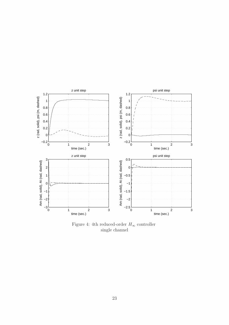
Time-domain simulations for each design are displayed in Figures 3-7. Plots on the left handcolumn show responses to a unit step in the vertical position z, while those on the right correspondto a unit step in the yaw angle ψ. The full-order H∞ controller of order 9 achieves perfectdecoupling of the vertical and yaw axes. Responses significantly deteriorate when this controlleris reduced to 4th order via balanced truncation, Figure 4. A 20% coupling appears on a z-step,while responses in ψ show unacceptable overshoot. In a next phase, we have therefore used this4th order controller to initialize our nonsmooth algorithm to compute a locally optimal solutionto (27). The associated simulations are shown in Figure 5. Responses of the optimal controllerare now satisfactory both in terms of coupling and overshoot.

Finally, we have attempted to compute decentralized PID controllers for the same problem(27) using our nonsmooth algorithm. An initial stabilizing PID controller is first computed usingthe hybrid MDS/nonsmooth technique developed in [1]. Since the controller now possesses pureintegral action, we have dispensed with the stability constraint on K in (27). In view of the sim-ulations in Figure 6, enforcing a pure PID structure seems a severe restriction in this application.Substantial coupling appears in response to z steps and responses show unacceptable overshoot.We have tried to improve these results by using a pre-decoupling H where the input matrix Bis replaced with BH as is done classically in helicopter applications. The new PID controller,however, can still not be considered a valid solution as compared to the stable 4th order controllerof Figure 5. If we insist on a decentralized PID structure, it appears difficult to satisfy all perfor-mance requirements by feedback alone. Open-loop compensation or feed-forward action might benecessary to achieve a desired input-output behavior.

For completeness, we provide values of the max-H∞ objective in (27) associated with eachcontroller in Table 1. Notice that the full-order H∞ controller has a slightly worse max-H∞

objective since channels are not separated in traditional H∞ synthesis. Put differently, the 4thorder controller computed by our method is even slightly better than the full-order controllerobtained via a single channel with weights. This shows that the multi-channel setting, if combinedwith our nonsmooth method, allows to address the different specifications much more favorably.Irrelevant cross channels, such as Td→ze

and Td→zuin this application, generally hinder proper

minimization of meaningful specifications.

17

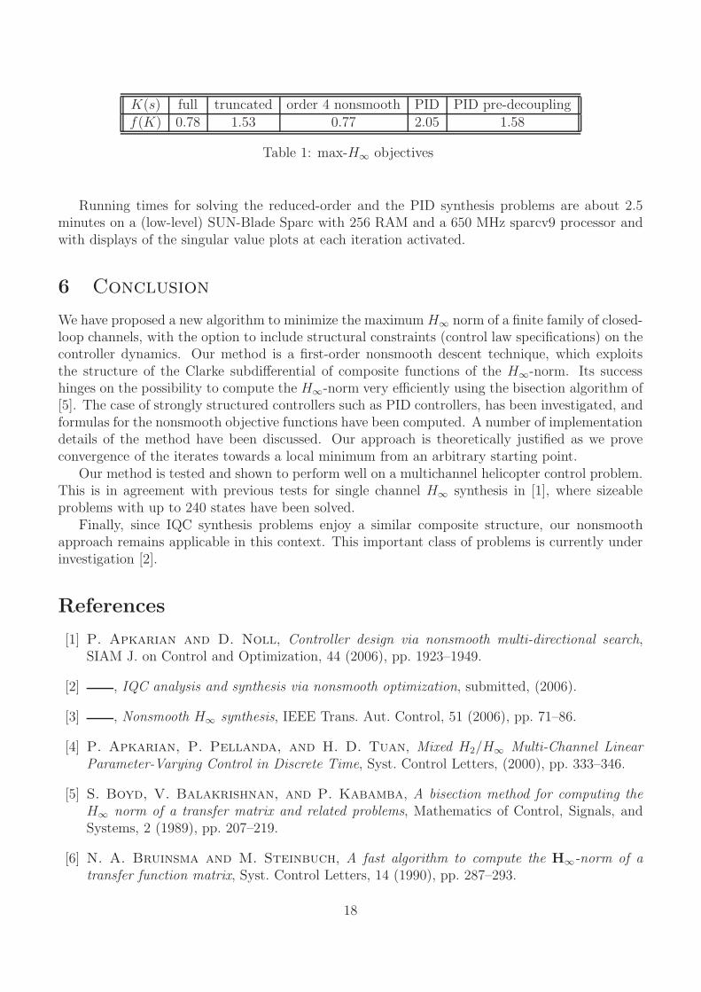
K(s) full truncated order 4 nonsmooth PID PID pre-decouplingf(K) 0.78 1.53 0.77 2.05 1.58

Table 1: max-H∞ objectives

Running times for solving the reduced-order and the PID synthesis problems are about 2.5minutes on a (low-level) SUN-Blade Sparc with 256 RAM and a 650 MHz sparcv9 processor andwith displays of the singular value plots at each iteration activated.

6 Conclusion

We have proposed a new algorithm to minimize the maximum H∞ norm of a finite family of closed-loop channels, with the option to include structural constraints (control law specifications) on thecontroller dynamics. Our method is a first-order nonsmooth descent technique, which exploitsthe structure of the Clarke subdifferential of composite functions of the H∞-norm. Its successhinges on the possibility to compute the H∞-norm very efficiently using the bisection algorithm of[5]. The case of strongly structured controllers such as PID controllers, has been investigated, andformulas for the nonsmooth objective functions have been computed. A number of implementationdetails of the method have been discussed. Our approach is theoretically justified as we proveconvergence of the iterates towards a local minimum from an arbitrary starting point.

Our method is tested and shown to perform well on a multichannel helicopter control problem.This is in agreement with previous tests for single channel H∞ synthesis in [1], where sizeableproblems with up to 240 states have been solved.

Finally, since IQC synthesis problems enjoy a similar composite structure, our nonsmoothapproach remains applicable in this context. This important class of problems is currently underinvestigation [2].

References

[1] P. Apkarian and D. Noll, Controller design via nonsmooth multi-directional search,SIAM J. on Control and Optimization, 44 (2006), pp. 1923–1949.

[2] , IQC analysis and synthesis via nonsmooth optimization, submitted, (2006).

[3] , Nonsmooth H∞ synthesis, IEEE Trans. Aut. Control, 51 (2006), pp. 71–86.

[4] P. Apkarian, P. Pellanda, and H. D. Tuan, Mixed H2/H∞ Multi-Channel LinearParameter-Varying Control in Discrete Time, Syst. Control Letters, (2000), pp. 333–346.

[5] S. Boyd, V. Balakrishnan, and P. Kabamba, A bisection method for computing theH∞ norm of a transfer matrix and related problems, Mathematics of Control, Signals, andSystems, 2 (1989), pp. 207–219.

[6] N. A. Bruinsma and M. Steinbuch, A fast algorithm to compute the H∞-norm of atransfer function matrix, Syst. Control Letters, 14 (1990), pp. 287–293.

18

[7] U. Campos-Delgado and K. Zhou, A parametric optimization approach to H∞ and H2

strong stabilization, Automatica, 39 (2003), pp. 1205–1211.

[8] F. H. Clarke, Optimization and Nonsmooth Analysis, Canadian Math. Soc. Series, JohnWiley & Sons, New York, 1983.

[9] M. C. de Oliveira and J. C. Geromel, Numerical comparison of output feedback designmethods, in Proc. American Control Conf., Albuquerque, NM, June 1997, pp. 72–76.

[10] M. C. de Oliveira, J. C. Geromel, and J. Bernussou, An LMI Optimization Ap-proach to Multiobjective Controller Design for Discrete-Time Systems, in Proc. IEEE Conf.on Decision and Control, Phoenix,AZ, 1999, pp. 3611–3616.

[11] H. Dym, J. W. Helton, and O. Merino, Multidisk problems in H∞ optimization: Amethod for analyzing numerical algorithms, Indiana Univ. Math. J., 51 (2002), pp. 1111–1160.

[12] R. Hettich and K. O. Kortanek, Semi-infinite programming: theory, methods, andapplications, SIAM Review, 35 (1993), pp. 380–429.

[13] Z. HU, S. E. Salcudean, and P. D. Loewen, Multiple objective control problems vianonsmooth analysis, in IFAC World Congress, San Fransisco, 1996, pp. 416–420.

[14] F. Leibfritz, COMPLeIB, COnstraint Matrix-optimization Problem LIbrary - a collection oftest examples for nonlinear semidefinite programs, control system design and related problems,tech. rep., Universitat Trier, 2003.

[15] M. Mammadov and R. Orsi, H∞ synthesis via a nonsmooth, nonconvex optimizationapproach, Pacific Journal of Optimization, 1 (2005), pp. 405–420.

[16] I. Masubuchi, A. Ohara, and N. Suda, LMI-based controller synthesis: a unified for-mulation and solution, Int. J. Robust and Nonlinear Control, 8 (1998), pp. 669–686.

[17] K. I. M. McKinnon, Convergence of the Nelder-Mead simplex method to a non-stationarypoint, SIAM J. on Optimization, 9 (1998), pp. 148–158.

[18] O. Merino, H. Dym, and J. W. Helton, Algorithms for solving multidisk problems inH∞ optimization, in Proc. IEEE Conf. on Decision and Control, 1999.

[19] H. E. Musch and M. Steiner, Tuning advanced pid controllers via direct H∞ minimiza-tion, in European Control Conference, Brussels, Belgium, July 1997.

[20] D. Noll and P. Apkarian, Spectral bundle methods for nonconvex maximum eigenvaluefunctions: first-order methods, Mathematical Programming Series B, (2005).

[21] S. Norman and S. Boyd, Numerical solution of a two-disk problem, in Proc. AmericanControl Conf., 1989, pp. 1745–1747. Reprinted in Recent Advances in Robust Control, pages285-287, edited by P. Dorato and R. K. Yedavalli, IEEE Press.

[22] M. Overton, On minimizing the maximum eigenvalue of a symmetric matrix, SIAM J. onMatrix Analysis and Applications, 9 (1988), pp. 256–268.

19

[23] E. Polak, Optimization : Algorithms and Consistent Approximations, Applied Mathemati-cal Sciences, 1997.

[24] E. Polak and Y. Wardi, A nondifferentiable optimization algorithm for the design ofcontrol systems subject to singular value inequalities over a frequency range, Automatica, 18(1982), pp. 267–283.

[25] C. Scherer, Structured finite-dimensional controller design by convex optimization, LinearAlgebra and Appl., (2002), pp. 639–669.

[26] C. Scherer, P. Gahinet, and M. Chilali, Multi-Objective Output-Feedback Control viaLMI Optimization, IEEE Trans. Aut. Control, 42 (1997), pp. 896–911.

[27] M. F. Weilenmann and H. P. Geering, A test bench for rotorcraft hover control, inAIAA Guid., Nav. and Control Conf., Monterey, CA, August 1993, pp. 1371–1382.

[28] M. Zeren and H. Ozbay, On the strong stabilization and stable H∞ controller designproblems for mimo systems, Automatica, (2000), pp. 1674–1684.

[29] K. Zhou, J. C. Doyle, and K. Glover, Robust and Optimal Control, Printice Hall, 1996.

Acknowledgements

Thanks to Dr. Martin Weilenmann, EMPA IC-Engines lab, Switzerland and Dr. Urs Christen,Ford Forschungszentrum, Germany, for providing models and details on the helicopter example.

20

10−5

10−4

10−3

10−2

10−1

100

101

102

103

104

1.7

1.8

1.9

2

2.1

2.2

2.3

2.4

2.5

10−5

10−4

10−3

10−2

10−1

100

101

102

103

104

1.3

1.4

1.5

1.6

1.7

1.8

1.9

2

2.1

10−5

10−4

10−3

10−2

10−1

100

101

102

103

104

1.5

1.6

1.7

1.8

1.9

2

2.1

2.2

10−5

10−4

10−3

10−2

10−1

100

101

102

103

104

1.5

1.6

1.7

1.8

1.9

2

2.1

2.2

Figure 2: Extended set over last 4 iterationssolid line: max singular value‘*’ frequencies in extended set

21

0 1 2 3−0.5

0

0.5

1

time (sec.)

z unit step

z (

rad,

sol

id),

psi

(m

, das

hed)

0 1 2 3−1

−0.5

0

0.5

1

1.5

time (sec.)

Am

(ra

d, s

olid

), A

t (ra

d, d

ashe

d)

z unit step

0 1 2 3−0.2

0

0.2

0.4

0.6

0.8

1

1.2

time (sec.)

psi unit step

z (r

ad, s

olid

), p

si (

m, d

ashe

d)

0 1 2 3−1

−0.8

−0.6

−0.4

−0.2

0

0.2

0.4

time (sec.)

Am

(ra

d, s

olid

), A

t (ra

d, d

ashe

d)

psi unit step

Figure 3: Full-order H∞ controllersingle channel

22

0 1 2 3−0.2

0

0.2

0.4

0.6

0.8

1

1.2

time (sec.)

z unit step

z (

rad,

sol

id),

psi

(m

, das

hed)

0 1 2 3−3

−2

−1

0

1

2

3

time (sec.)

Am

(ra

d, s

olid

), A

t (ra

d, d

ashe

d)

z unit step

0 1 2 3−0.2

0

0.2

0.4

0.6

0.8

1

1.2

time (sec.)

psi unit step

z (r

ad, s

olid

), p

si (

m, d

ashe

d)

0 1 2 3−2.5

−2

−1.5

−1

−0.5

0

0.5

time (sec.)

Am

(ra

d, s

olid

), A

t (ra

d, d

ashe

d)

psi unit step

Figure 4: 4th reduced-order H∞ controllersingle channel

23

0 1 2 3−0.2

0

0.2

0.4

0.6

0.8

1

1.2

time (sec.)

z unit step

z (

rad,

sol

id),

psi

(m

, das

hed)

0 1 2 3−1

−0.5

0

0.5

1

1.5

time (sec.)

Am

(ra

d, s

olid

), A

t (ra

d, d

ashe

d)

z unit step

0 1 2 3−0.2

0

0.2

0.4

0.6

0.8

1

1.2

time (sec.)

psi unit step

z (r

ad, s

olid

), p

si (

m, d

ashe

d)

0 1 2 3−1

−0.8

−0.6

−0.4

−0.2

0

0.2

0.4

time (sec.)

Am

(ra

d, s

olid

), A

t (ra

d, d

ashe

d)

psi unit step

Figure 5: 4th-order controller from nonsmooth techniquemultiple channels

24

0 1 2 3−1

−0.5

0

0.5

1

1.5

time (sec.)

z unit step

z (

rad,

sol

id),

psi

(m

, das

hed)

0 1 2 3−1

−0.5

0

0.5

1

1.5

time (sec.)

Am

(ra

d, s

olid

), A

t (ra

d, d

ashe

d)

z unit step

0 1 2 30

0.2

0.4

0.6

0.8

1

1.2

1.4

time (sec.)

psi unit step

z (r

ad, s

olid

), p

si (

m, d

ashe

d)

0 1 2 3−2

−1.5

−1

−0.5

0

0.5

1

time (sec.)

Am

(ra

d, s

olid

), A

t (ra

d, d

ashe

d)

psi unit step

Figure 6: 4th-order PID controller from nonsmooth techniquemultiple channels

25

0 1 2 3−0.2

0

0.2

0.4

0.6

0.8

1

1.2

time (sec.)

z unit step

z (

rad,

sol

id),

psi

(m

, das

hed)

0 1 2 3−0.4

−0.2

0

0.2

0.4

time (sec.)

Am

(ra

d, s

olid

), A

t (ra

d, d

ashe

d)

z unit step

0 1 2 3−0.2

0

0.2

0.4

0.6

0.8

1

1.2

time (sec.)

psi unit step

z (r

ad, s

olid

), p

si (

m, d

ashe

d)

0 1 2 3−0.5

−0.4

−0.3

−0.2

−0.1

0

0.1

0.2

time (sec.)

Am

(ra

d, s

olid

), A

t (ra

d, d

ashe

d)

psi unit step

Figure 7: 4th-order PID controller from nonsmooth techniquewith pre-decoupling and multiple channels

26