noise removal based on the variation of digitalized...

Noise Removal Based on the Variation of Digitalized

Energy ?

Qin Zhang1??, Jie Sun2, and Guoliang Xu3

1 Beijing Information Science and Technology University,Beijing 100085, China

2 Capital Normal University, Beijing 100037, China,3 Computational Mathematics Institute,

Chinese Academy of Sciences, Beijing 100080, China

Abstract. Image denoising, as a low-level step of image processing, is perhaps the oldest and still activeresearch topic. A general formulation based on the variation of digitalized energy to denoise image isproposed in this paper. This method is different from classical variational method employed in imageprocessing. For a digitalized energy functional, we first compute the variation, then design algorithmsleading to digital filters. Numerical experiments and comparative examples are thus carried out toverify the effectiveness of the proposed method, which is efficient, adaptive and easily implemented.Higher quality images can be obtained with characteristic singular features preserved. The method canbe easily expanded to color images.

Key words: Image denoising; Digitalized energy; Variation method; Graph.

1 Introduction

Image denoising is historically one of the oldest concerns in image processing and is still anecessary preprocessing step for many applications. What makes denoising so challenging isthat a successful approach also must preserve characteristic singular features of images suchas edges. Preservation of important singularities is absolutely necessary in image analysisand computer vision since digital ”objects” are very much defined (or detected) via edges(i. e. segmentation) and other singularities (e. g., the corners of eyes and lips). In the pastdecades, deterministic and stochastic models are proposed to solve this problem. The topicof image denoising has occupied a large part of many monographs on image processing andanalysis, such as [1, 2].

As two tightly linked methods, variational methods and Partial Differential Equations(PDEs) methods have been two successful tools in image processing in recent years. Beingan inverse problem, image denoising, according to the theory of Hadamard, is ill-posed.Suppose that u : Ω ⊂ R2 → R is an original image describing a real scene, and u0 is theobserved image of the same scene (i. e., a degradation of u). We always use u0 = Ru + n tomodel the process, where n stands for white additive Gauss noise and R is a linear operatorrepresenting the blur (usually a convolution). In this paper, R = I. The image denoisingproblem is to recover u from u0. A classical way to overcome this ill-posedness, based onthe theory of Tikhonov regularization, is to minimize the following regularized minimization

? Project supported in part by NSFC grant 60773165 and National Key Basic Research Project of China(2004CB318000).

?? Corresponding author, who is also supported by Beijing Educational Committee Foundation

2 Qin Zhang, Jie Sun, and Guoliang Xu

problem,

E(u) =

∫

Ω

φ(‖∇u‖)dx +λ

2

∫

Ω

(u− u0)2dx, (1.1)

where the first term is a regular term to describe the smoothness of the image and the secondterm measures the fidelity to the data. Parameter λ is a positive penalty constant to weighthese two parts. Function φ is chosen to depict the strength of the smoothness. The commonchoices for φ is φ(x) = x2 (the corresponding energy is Dirichlet energy) and φ(x) = x (thecorresponding energy is usually named as total variation).

Classical variational methods compute the Euler-Lagrange equation for (1.1) or constructan evolution equation by adding a temporal parameter. Then, the resulting differential equa-tions (either the evolution equation or the equilibrium equation) are discretized numericallyon a rectangular grid. The advantage of this method is that one can easily adapt many ex-isting numerical methods for PDEs to this problem and establish efficient algorithms. Largeamount of publications have appeared along this line (see e.g., [3–5]), and more papersutilized the variants of the PDEs obtained to denoising images. Since the Euler-Lagrangeequation associated with (1.1) is a nonlinear PDE, when applying it to a digital image, onehas to carefully choose numerical schemes to take care of the nonlinearity. Therefore, Osherand Shen [6] established a self-contained ”digital” theory for the PDE method, in whichknowledge of PDEs and numerical approximations is not required. Similar digitizing workon the evolution equation can also be found in Weickert [7]. However, the mathematicalfoundation of the latter is still the numerical discretization of PDEs on rectangular grids.

Motivated by the theory of [6], we propose to digitalize the energy (1.1) to obtain ageneral formulation for image denoising. Since this method avoids solving a continuous PDEon a rectangular grid, a linear system of equations is therefore unnecessarily solved. Thisformulation is yet implemented by a local iterative scheme which is more efficient than PDEmethod.

The method of computing the variation for discrete energy is also appeared in otherareas. For instance, in [8], discrete minimal surfaces and their conjugates are calculated bythe direct variation of discrete Dirichlet integral other than classical method of discretizingthe PDE obtained by the variation of continuous energy. In [9], discrete Willmore flow isconsidered from the variation of discrete Willmore energy.

The remainder of the paper is organized as follows. In Section 2, the graph model, energyfunctional and denoising equation are given. We provide the detailed algorithm in Section3. Numerical experiments and comparative examples are presented in Section 4. Section 5concludes the paper.

2 Graph, Energy Functional and Denoising Equation

2.1 Basic definitions for a graph

As per the nomenclature used in ([6]), let [Ω, G] denote an undirected graph with a finiteset Ω of vertices (or nodes) and a dictionary G of edges. The graph is assumed to have no

Noise Removal Based on the Variation of Digitalized Energy 3

self-loops and general vertices are denoted by α, β, . . .. If α and β are linked by an edge, thenwe write α ∼ β, and

Nα = β ∈ Ω; β ∼ α

denotes all the neighbors of α.A digital image u is a function u : Ω → R. The value at vertex α is denoted by uα. The

local variation or stength ‖∇guα‖ at any vertex α is defined by

‖∇guα‖ :=

√∑

β∼α

(uβ − uα)2.

For any positive number a, the regularized local variation is

‖∇guα‖a =√‖∇guα‖2 + a2.

According to the notation in [10], we define the edge derivative. Let e be the edge α ∼ β.Then the edge derivative of u along e is defined to be

∂u

∂e

∣∣∣α

:= uβ − uα.

Apparently,

∂u

∂e

∣∣∣α

= −∂u

∂e

∣∣∣β, and ‖∇guα‖ =

√∑

e`α

[∂u

∂e

∣∣∣α

]2

,

where e`α means that α is one node of e.

2.2 Digitalized energy and equations

For energy functional (1.1), the fitted digitalized version considered in this paper is as follows:

E(u) :=∑α∈Ω

φ(‖∇guα‖) +λ

2

∑α∈Ω

(uα − u0α)2, (2.1)

where function φ(x) is simply chosen as S. Kim in [11] as φ(x) = x2−q, 0 ≤ q < 2. Obviously,φ(x) can be selected as other forms, such as listed in ([1, p. 83]) φ(x) = x2

1+x2 , log(1 +

x2), 2√

1 + x2−2 etc. In practice, the penalty parameter (or Lagrange multiplier) λ is eitherchosen a priori([12]), or estimated using the projected gradient method ([4, 3]), and we willaddress this in later section.

Theorem 2.1. With respect to digitalized energy (2.1), the denoising equation is

0 =∑

β∈Nα

(uα − uβ)(φ′(‖∇guα‖)

‖∇guα‖ +φ′(‖∇guβ‖)‖∇guβ‖

)+ λ(uα − u0

α), α ∈ Ω. (2.2)


For the sake of saving space, we leave the proof in the appendix.

Corollary 2.1. If φ(x) = x2−q, 0 ≤ q < 2, then (2.2) turns out to be

0 = (2− q)∑

β∈Nα

(uα − uβ)(‖∇guα‖−q + ‖∇guβ‖−q) + λ(uα − u0α), α ∈ Ω. (2.3)

If we select q = 0, the energy is the fitted digitalized Dirichlet energy, and the correspondingequation is consistent with the result in [6]. If we select q = 1, the energy is the fitteddigitalized total variation, the obtained equation is the same as the outcome in [6] and [10].

If 0 ≤ q ≤ 1, as proved in [6], the minimizer of the fitted digitalized energy is existand unique since the energy functionals are strictly convex functionals of u. If 1 < q < 2,according to the theory of the calculus of variations, we could not expect the existence anduniqueness of minimizer. But in our numerical test, the results of this case are better thanthe former. This phenomenon is quiet similar to the results obtained in [13]. In that paper,an analogous PDE model has been utilized to perform simultaneous image denoising andedge enhancement and is called convex-concave anisotropic diffusion (CCAD) model. It hasbeen numerically verified that for 1 < q < 2, the CCAD model is superior to the ITV model([12]). In fact, this phenomenon also supports the result of Perona-Malik (PM) model ([14]),

∂u

∂t= div(c(‖∇u‖)∇u),

where c(x) = (1 + x2/K2)−1 for a threshold K. Note that if we select φ(x) = 12K2 ln(1 +

x2/K2), then c(x) = φ′(x)/x. The function φ(x) is strictly convex for x < K and strictlyconcave for x > K. PM model has been regarded as a revolution in the field of PDE modelsin image denoising.

Corollary 2.2. Equation (2.2) is the digital version of

div(φ′(‖∇u‖) ∇u

‖∇u‖)

+ λ(u0 − u) = 0,

which is the Euler-Lagrange equation of (1.1).

Proof. According to the definition of edge derivative, we can rewrite (2.2) as

∑

e`α

∂

∂e

[−φ′(‖∇gu‖)‖∇gu‖

∂u

∂e

]∣∣∣α

+ λ(u0α − uα) = 0.

Notice there is a sign difference between the the first term. If φ(x) = x, the result is consistentwith the result in [10].

3 Detailed Denoising Algorithm

We define weighted function

ωαβ(u) =φ′(‖∇guα‖)‖∇guα‖a

+φ′(‖∇guβ‖)‖∇guβ‖a

, (3.1)


where regularization has been performed in case of zero denominators. Then equation (2.2)becomes

(λ +

∑

β∈Nα

ωαβ(u))uα −

∑

β∈Nα

ωαβ(u)uβ = λu0α, (3.2)

for all α ∈ Ω. This is usually a system of nonlinear equations.To solve the system of equations (3.2), the simplest local iteration is the Gauss-Jacobi

method

uk+1α =

∑

β∈Nα

ωαβ(uk)

λ +∑

β∈Nα

ωαβ(uk)uk

β +λ

λ +∑

β∈Nα

ωαβ(uk)u0

α, (3.3)

for all α ∈ Ω, where k denotes the iteration step. This process can be independently explainedas a forced local low-pass digital filter. The update uα is a weighted average of the existinguβ on its direct neighbors and the raw data at α. The raw data serve as an attracting forcepreventing u from wandering far away.

If fact, image denoising is a process of weighted average. The key point is how to choosethe weight for each pixel. For classical linear filters, a solid template (e. g., 3 × 3 or 5 × 5)with fixed coefficients is used to scan the whole image, therefore it is difficult to distinguishbetween features and homogeneous regions. Although the weights vary with different pixelsin the nonlinear median filter, this filter is an exclusive filter in the sense that the filtercoefficients are 0 or 1. In most cases, features can be preserved while smoothness of imagescould not be expected unless large filter window. In general, large filter windows collide withthe local character of images.

For (3.3), the locality of images information can be preserved since the iteration is car-ried out merely in a neighborhood of each pixel. If suitable weighted functions ωαβ(u) canbe selected, to discern the features and homogeneous regions for images is automaticallyperformed. This adaptivity is easy to understand qualitatively. The key is the competitionbetween the Lagrange multiplier λ and the local weights ωαβ(u). The local weights dominateλ if the current data uk are very flat near a pixel α. Then the fitting term becomes less im-portant and the filter acts like low-pass filtering purely on uk, which makes the output uk+1

α

even flatter at the spot. On the other hand, if the current data uk undergo an abrupt changeof large amplitude at α, then the local weights ωαβ are insignificant compared with λ. If thisis the case, the filter intelligently sacrifices smoothness for faithfulness. This mechanism isobviously important for faithful denoising of edges in image processing.

Another possible scheme for (3.2) is Gauss-Seidel. We first label all vertices in a fixedlinear order · · · < γ < α < β < · · · . At each step, we compute

uk+1α =

∑

β∈Nα&β<α

ωαβ(uk+1)

λ +∑

β∈Nα

ωαβ(uk+1)uk+1

β +∑

β∈Nα&β>α

ωαβ(uk+1)

λ +∑

β∈Nα

ωαβ(uk+1)uk

β

+λ

λ +∑

β∈Nα

ωαβ(uk+1)u0

α,


here the weighted function ωαβ(uk+1) is real-timely calculated for each vertex α relying uponthe data of uk+1

β , β < α and ukβ, β > α in Nα. Gauss-Seidel is a local but sequential iterative

scheme. In this paper, we will not investigate this further.From the iterative scheme (3.3), the algorithm can be given as follows.

Filtering algorithm :

1) Assign a linear order to all pixels: α1 < α2 < · · · < α|Ω|. Set k=0.2) k=k+1. For each pixel α, calculate local variation ‖∇guα‖.3) For each pixel α and all its neighbors β, calculate weighted function ωαβ(uk) according

to (3.1).4) For each pixel α, compute uk+1

α according to (3.3).5) Go to 2).

4 Numerical Experiments and Comparative Results

Numerical experiments and comparative results are presented in this section. First, we ad-dress on some issues regarding implementation ([10]). All the results are carried out in alaptop (Intel( c©) Core(TM) 2 CPU T7200 2.00GHz, 1GB RAM) with Matlab( c©) software.

1) One attribute of this model is that it does not require any artificial ”boundary” con-dition. In the classical literature, the continuous diffusion equation is usually accomplishedby the adiabatic Newmann condition. In the digital model, the boundary condition has beenencoded into the structure of the graph and the definition of the local variation ‖∇guα‖.For instance, each of the four corner pixels has only two neighbors and a typical boundarypixel has three neighbors. A simple checking on the definition of the local variation ‖∇guα‖verifies that the above boundary structure of the graph indeed corresponds to a flat outwardextension of u, or the discrete outward Neumann condition.

2) The regularization constant a is purely for the purpose of avoiding a zero denominator.One can simply choose a small number such as 10−4.

3) The Lagrange multiplier λ is important for the denoising effect. Practical concernsand estimates are discussed in Rudin and Osher [3], Blomgren and Chan [15]. In terms ofthe digital model, an estimation of the optimal λ is by

λ ≈ 1

σ2

1

|Ω|∑α∈Ω

∑

β∼α

ωαβ(uβ − uα)(uα − u0α),

where σ2 is the variance of the noise, which is known or can be estimated form homogeneousregions in the image. The formula suggests that λ is comparable to 1/σ2.

4.1 The effect of the convex and concave properties of function φ

As we have narrated under Corollary 2.1, the convex and concave properties of function φinfluence the effect of denoising and features preservation. Since we merely select φ(x) = x2−q

in this paper, we select q = 0, 0.5, 1, 1.02, 1.2, 1.5 for testing. When 0 ≤ q ≤ 1, the density


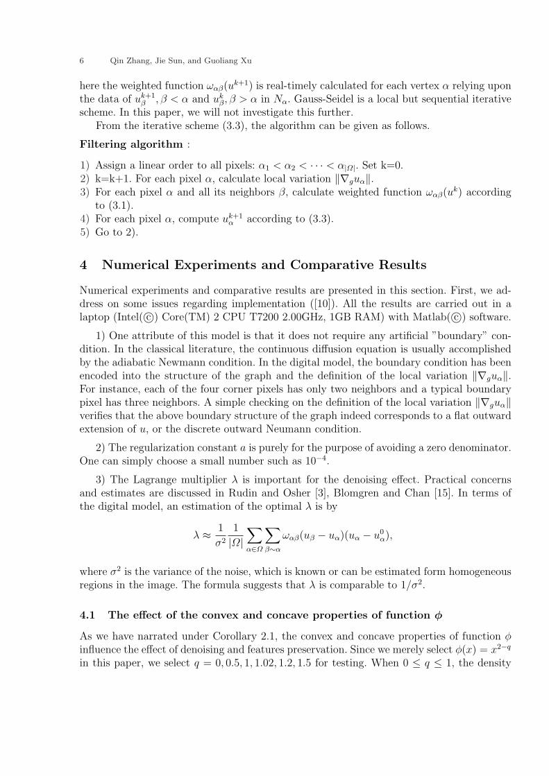
function is convex. If 1 < q < 2, the density function is concave, therefore the existenceand uniqueness of the minimizer for energy functional can not be guaranteed. Similarlyphenomena happened in PM model and in [13]. In Fig. 4.1, figure (a) is the original image.(b) is the contaminated image with Gauss noise σ = 1/7. (c)–(h) are the six cases for q,respectively. We can find that figure (g) is the best among all these figures. This fact isverified in Table 4.3. Thus we can draw a conclusion that the concave functions can preservemore features in some sense than convex functions.

(a) (b) (c) (d)

(e) (f) (g) (h)

Fig. 4.1. The effect of convex and concave properties of function φ. (a) is the original image. (b) is the contaminatedimage with Gauss noise σ = 0.1. (c) is the result of L2 energy, i. e., q = 0. (d) q = 0.5. (e) is the result of TV energy,i. e., q = 1. (f) q = 1.02. (g) q = 1.2. (h) q = 1.5.

4.2 Pepper & Salt noise removal

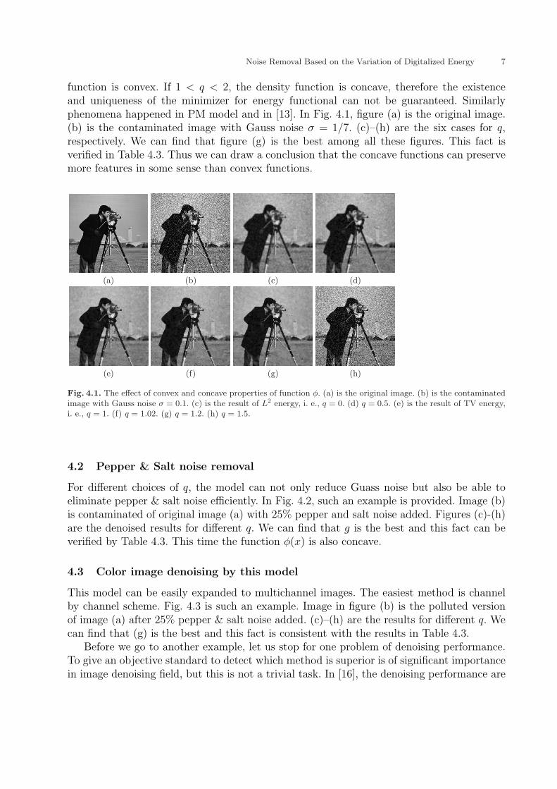
For different choices of q, the model can not only reduce Guass noise but also be able toeliminate pepper & salt noise efficiently. In Fig. 4.2, such an example is provided. Image (b)is contaminated of original image (a) with 25% pepper and salt noise added. Figures (c)-(h)are the denoised results for different q. We can find that g is the best and this fact can beverified by Table 4.3. This time the function φ(x) is also concave.

4.3 Color image denoising by this model

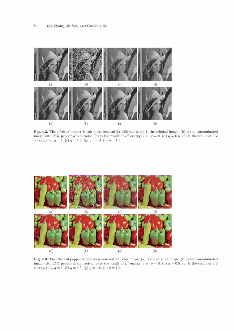
This model can be easily expanded to multichannel images. The easiest method is channelby channel scheme. Fig. 4.3 is such an example. Image in figure (b) is the polluted versionof image (a) after 25% pepper & salt noise added. (c)–(h) are the results for different q. Wecan find that (g) is the best and this fact is consistent with the results in Table 4.3.

Before we go to another example, let us stop for one problem of denoising performance.To give an objective standard to detect which method is superior is of significant importancein image denoising field, but this is not a trivial task. In [16], the denoising performance are


(a) (b) (c) (d)

(e) (f) (g) (h)

Fig. 4.2. The effect of pepper & salt noise removal for different q. (a) is the original image. (b) is the contaminatedimage with 25% pepper & slat noise. (c) is the result of L2 energy, i. e., q = 0. (d) q = 0.5. (e) is the result of TVenergy, i. e., q = 1. (f) q = 1.5. (g) q = 1.8. (h) q = 1.9.

(a) (b) (c) (d)

(e) (f) (g) (h)

Fig. 4.3. The effect of pepper & salt noise removal for color image. (a) is the original image. (b) is the contaminatedimage with 25% pepper & slat noise. (c) is the result of L2 energy, i. e., q = 0. (d) q = 0.5. (e) is the result of TVenergy, i. e., q = 1. (f) q = 1.5. (g) q = 1.8. (h) q = 1.9.


compared in four ways, that is: mathematical: asymptotic order of magnitude of the methodnoise under regularity assumptions; perceptual-mathematical:the algorithms artifacts andtheir explanation as a violation of the image model; quantitative experimental: by table ofL2 distances of the denoised version to the original image. The most powerful evaluationmethod seems, however, to be the visualization of the method noise on natural images. Inthe above figures, although we can discern which is the best, Table 4.3 is more persuasive.That is the L2 distance from the original image to its estimate, which can be calculated as

d(original, estimate) =( ∑

α∈Ω

(uorigα − uest

α )2)1/2

.

We also call it mean square error in this paper, noticing there is a square discrepancybetween this definition with the one in the paper [16]. Obviously, for the same originalimage, the smaller is mean square error, the more faithful of the estimated image is. Thetable corroborates our visualizing. Another frequently used criteria is the residue of theestimated image and original one (e. g., in [17]). Since it depends still upon the visualizing,we do not adapt this comparison method here.

Table 4.1. Mean square error

PPPPPPPFig.figure

(c) (d) (e) (f) (g) (h)

Fig. 4.1 135.54 124.48 113.95 115.77 109.62 156.10

Fig. 4.2 142.75 122.35 96.48 80.64 76.47 77.08

Fig. 4.3 557.65 453.67 345.13 276.41 270.77 272.76

4.4 Time consuming of this method compared with PDE methods

Since PDE methods always involve the solution of a linear system of equation, they mustconsume more than this method, which utilizes and explicitly iterate scheme. Fig. 4.4 is acomparative example of Gauss noise removal with this model and ROF model [4]. Figure(b) is the polluted image of figure (a) with σ = 1/7. Figure (c) is the result this model withq = 1.2 consuming 3.38 seconds. (d) is the result of ROF model consuming 26.80 seconds..

(a) (b) (c) (d)

Fig. 4.4. Time consuming of this model campared with ROF model. (a) is the original image. (b) is the contaminatedimage with σ = 1/7 Gauss noise added. (c) is the result of this model when q = 1.2. (d) is the result of ROF model.


5 Conclusion

A general formulation of image denoising method based on the variation of digitalized energyfunctional is presented. We investigate a special case of density function which can producehigher quality restored image when it is concave. An explicit iterative scheme is presentedto solve the system of equations. Large variety of numerical experiments are performed toverify the effectiveness of the proposed model and comparative experiments are also carriedout.

References

1. Aubert, G., Kornprobst, P.: Mathematical Problems in Image Processing: Partial Differential Equations and theCalculus of Variations. Second edn. Volume 147 of Applied Mathematical Sciences. Springer (2006)

2. Chan, T.F., Shen, J.H.: Image Processing and Analysis–Variational, PDE, Wavelet, and Stochastic Methods.SIAM, Philadelphia (2005)

3. Rudin, L., Osher, S.: Total variation based image restoration with free local constraints. In: Proceedings of theIEEE International Conference on Image Processing. Volume 1. (1994) 31–35

4. Rudin, L., Osher, S., Fatemi, E.: Nonlinear total variation based noise removal algorithms. Physica D 60 (1992)259–268

5. Lysaker, M., Lundervold, A., Tai, X.C.: Noise removal using fourth-order partial differential equation withapplications to magnetic resonance images in space and time. IEEE Trans. Image Processing 12(12) (2003)1579–1590

6. Osher, S., Shen, J.: Digitized PDE method for data restoration. In Anastassiou, G., ed.: Handbook of Analytic-Computational Methods in Applied Mathematics, Chapman & Hall/CRC (2000) 751–771

7. Weickert, J.: Anisotropic Diffusion in Image Processing. ECMI. Teubner-Verlag, Stuttgart, Germany (1998)

8. Pinkall, U., Polthier, K.: Computing discrete minimal surfaces and their conjugates. Experim. Math. 2(1) (1993)15–36

9. Bobenko, A.I., Schroder, P.: Discrete Willmore flow. In Desbrun, M., Pottmann, H., eds.: Eurographics Sympo-sium on Geometry Processing. (2005) 101–110

10. Chan, T.F., Osher, S., Shen, J.H.: The digital TV filter and nonlinear denoising. IEEE Trans. Image Processing10(2) (2001) 231–241

11. Kim, S., Lim, H.: A non-conver diffusion model for simultaneous image denoising and edge enhancement.Electronic Journal of Differential Equation (Conference 15) (2007) 175–192 Six Mississippi State Conference onDifferential Equations and Computational Simulations.

12. Marquina, A., Osher, S.: Explicit algorithms for a new time dependent model based on level set motion fornonlinear deblurring and noise removal. SIAM J. Sci. Comput. 22(2) (2000) 387–405

13. Kim, S.: Image denoising via diffusion modulation. International Journal of Pure and Applied Mathmatics 30(1)(2006) 72–91

14. Perona, P., Malik, J.: Scale-space and edge detection using anisotropic diffusion. IEEE Trans. Pattern Anal.Mach. Intell. 12(7) (1990) 629–639

15. Bloor, M.I.G., Wilson, M.J.: Modular solvers for image restoration problems using the discrepancy principle.Numerical Linear Algebra with Applications 9(5) (2002) 347–358

16. Buades, A., Coll, B., Morel, J.M.: On image denoising methods. Technical Report 2004-15, Centre deMathematiques et de Leurs Applications(CMLA) (2004)

17. Joo, K., Kim, S.: PDE-based image restoration I: Anti-staircasing and anti-diffusion. Technical Report 2003-07,Department of Mathematics, University of Kentucky (2003)

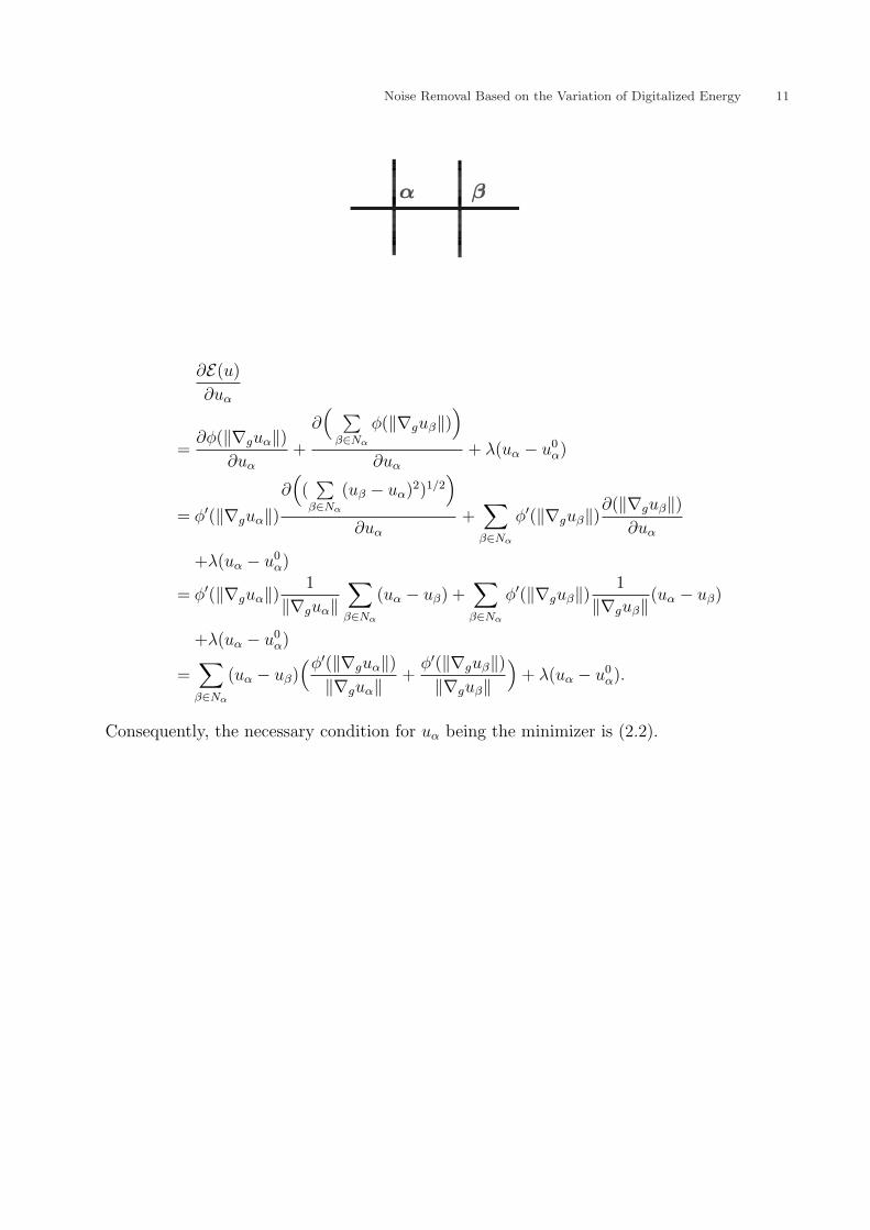
Appendix: Proof to Theorem 2.1

To compute the variation of digital energy (2.1), we take derivative for E(u) with respect touα. Since only Nα + 1 terms in E(u) contain uα, we thus compute the variation as


∂E(u)

∂uα

=∂φ(‖∇guα‖)

∂uα

+

∂( ∑

β∈Nα

φ(‖∇guβ‖))

∂uα

+ λ(uα − u0α)

= φ′(‖∇guα‖)∂((

∑β∈Nα

(uβ − uα)2)1/2)

∂uα

+∑

β∈Nα

φ′(‖∇guβ‖)∂(‖∇guβ‖)∂uα

+λ(uα − u0α)

= φ′(‖∇guα‖) 1

‖∇guα‖∑

β∈Nα

(uα − uβ) +∑

β∈Nα

φ′(‖∇guβ‖) 1

‖∇guβ‖(uα − uβ)

+λ(uα − u0α)

=∑

β∈Nα

(uα − uβ)(φ′(‖∇guα‖)

‖∇guα‖ +φ′(‖∇guβ‖)‖∇guβ‖

)+ λ(uα − u0

α).

Consequently, the necessary condition for uα being the minimizer is (2.2).

noise removal based on the variation of digitalized...

Documents