noaa special publication nos ngs 13 · 3/6/2018 · most of the documents consist of projection...
TRANSCRIPT

1
NOAA Special Publication NOS NGS 13
The State Plane Coordinate System History, Policy, and Future Directions
Michael L. Dennis
March 6, 2018

The State Plane Coordinate System: History, Policy, and Future Directions
i
Document Versions
Ver. Date Changes File name (at https://geodesy.noaa.gov/library/)
1 03/06/2018 Original release NOAA_SP_NOS_NGS_0013_v01_2018-03-06.pdf

The State Plane Coordinate System: History, Policy, and Future Directions
ii
Table of Contents Executive Summary ...................................................................................................................... 1
Introduction: Purpose and Scope ................................................................................................ 2
Before the North American Datum of 1927 ................................................................................ 3
Conformal Map Projections ........................................................................................................ 3
Non-Conformal Plane Rectangular Coordinates ......................................................................... 4
State Plane Coordinate System of 1927 ...................................................................................... 4
Timeline of SPCS 27 Development and Implementation ........................................................... 5
Status of State Plane in the 1970s ............................................................................................... 6
State Plane Coordinate System of 1983 .................................................................................... 13
Transition to a New Datum and Naming Conventions ............................................................. 13
Evaluation of State Plane and Changes from SPCS 27 to SPCS 83 ......................................... 13
Implementation and Documentation of SPCS 83 ..................................................................... 14
State Plane Coordinate System Policies .................................................................................... 15
Defining Policy on Projected Coordinates in the Federal Register ........................................... 15
Policies on Changes to State Plane ........................................................................................... 16
Other State Plane Policies ......................................................................................................... 16
The Role of Legislation in the State Plane Coordinate System ................................................ 17
Departures from Policy and Convention .................................................................................. 19
Recent Developments in Projected Coordinate Systems ......................................................... 25
Statewide Zones ........................................................................................................................ 27
Low Distortion Projections ....................................................................................................... 29
Projection Computations ........................................................................................................... 31
Summary and Conclusions ........................................................................................................ 32
Acknowledgments ....................................................................................................................... 33
References .................................................................................................................................... 34
Appendix A. SPCS 83 Defining Parameters (125 Zones) ........................................................ 40
Appendix B. SPCS 27 Defining Parameters (134 Zones) ........................................................ 48
Appendix C. SPCS 83 Legislation and Foot Version Adopted by States and Territories ... 56

The State Plane Coordinate System: History, Policy, and Future Directions
1
Executive Summary The State Plane Coordinate System (SPCS) is a system of conformal map projections created by
the National Geodetic Survey (NGS). SPCS was established to support surveying, engineering,
and mapping activities in the United States and its territories. The current version, SPCS 83, is
referenced to the North American Datum of 1983 (NAD 83) and consists of 125 zones based on
the Lambert Conformal Conic, Transverse Mercator, and Oblique Mercator projections. Because
NGS will replace NAD 83 with the 2022 Terrestrial Reference Frames (TRFs), SPCS 83 will
also be replaced by the State Plane Coordinate System of 2022 (SPCS2022). The main objective
of this publication is to provide the historical, practical, and philosophical context for initiating
development of SPCS2022. To achieve that objective, a review is conducted of NGS technical
documents and policy from the mid-1800s to the present. The historical review is augmented
with a brief assessment of current trends in usage of SPCS and other projected coordinate
systems. In addition, defining parameters are given for all zones since the inception of SPCS—
the first time all have been presented in a single NGS document. Also provided is the status of
SPCS 83 in state statute and regulations, including which jurisdictions adopted the U.S. survey
or international foot.
As first conceived in the 1930s, SPCS provided a way to perform “geodetic” surveys using plane
trigonometry, making it among the earliest practical means to access the National Spatial
Reference System (NSRS). Because of electronic computers, SPCS is no longer used for that
original purpose. Yet rather than decline, SPCS usage has grown due to widespread adoption of
technologies such as Computer Aided Drafting and Design (CADD), Geographic Information
Systems (GIS), and Global Navigation Satellite Systems (GNSS).
Over its long history, the characteristics and usage of SPCS have varied considerably. There
have been substantial departures from policies and conventions typically associated with SPCS;
for example: not always using aggregated counties for zone boundaries; greatly exceeding the
nominal criterion of 1:10,000 for maximum scale error; establishing “layered” zones that
completely overlap one another; modifying reference ellipsoid dimensions; scaling SPCS
coordinates to “ground”; and even using a non-conformal projection. In addition, there have been
recent developments in design and usage of projected coordinate systems outside of SPCS. These
developments include establishing statewide zones and small zones intended to minimize linear
distortion (scale error) at the topographic surface. Many such systems have been officially
adopted by states and local government agencies, and there is interest in having them become
part of SPCS.
The intent of this publication is two-fold. The first purpose is to give an historical overview
that consolidates complete definitions of every version of SPCS into a single document. The
second is to provide information useful for determining the appropriate bounds for design and
implementation of SPCS2022. The overall goal is that this publication will aid in defining a
projected coordinate system framework that serves as a technically sound and practical
foundation for building the SPCS of the future.

The State Plane Coordinate System: History, Policy, and Future Directions
2
Introduction: Purpose and Scope Two main objectives drove the development of this publication. The first was to give context for
development of a new State Plane Coordinate System (SPCS) referenced to the four Terrestrial
Reference Frames (TRFs) of 2022 (Smith, et al., 2017). That context is in terms of convention,
intent, and policy, as revealed through the entire SPCS history. A key part of this objective is to
provide the National Geodetic Survey (NGS) with the information and perspective to
appropriately and effectively move forward with an update of SPCS. Importantly, that includes
determining a balance between the desires of NGS customers and what can be achieved within
the technical, practical, and philosophical bounds of SPCS. This document serves as a basis and
reference for development of the State Plane Coordinate System of 2022 (SPCS2022).
The second objective was adopted during the preparation of this report. It was found that no
NGS document or webpage contained a complete definition of the current SPCS. Nor is there a
singular reference for the overall history of SPCS development, policy, and implementation that
had been carried through to the present day. This publication provides a summary of the entire
SPCS history. This document also serves as the only official NGS compendium containing
complete sets of defining parameters for all SPCS versions.
Research for this report was limited mostly to NGS publications or publications by NGS’
predecessors, the U.S. Coast & Geodetic Survey (C&GS) and the U.S. Coast Survey, although
other supporting and corroborating documents were referenced, as necessary. Perhaps most
striking is the extraordinary volume of work done by C&GS on map projections, extending back
to the mid-1800s; such publications number in the hundreds. Several dozen of these documents
provide the theoretical and practical basis for what ultimately became SPCS, including ground-
breaking work on conformal projections in the early 1900s. Most of the documents consist of
projection and intersection tables for computing coordinates and plotting maps. Such documents
may seem mundane, but the effort required to generate the tables is astounding; it required
computing projected coordinates (and related quantities) at 1 arc-minute and 2-1/2 arc-minute
intervals over the entire United States, with significant overlap between zones. Remarkably,
most of that work was done before electronic computing was available. After 1990, essentially
no documents were published by NGS on SPCS or map projections in general, other than
occasional policy statements.
A few NGS and C&GS documents stand out as particularly important. Perhaps most significant
is NOAA Manual NOS NGS 5 (Stem, 1990), the official defining document of SPCS 83. This
publication was intended to supplement (rather than replace) Special Publication 235 by Mitchell
and Simmons (1945 and 1977), which served a similar role for SPCS 27, but also for SPCS
overall. Special Publication 235 was the only SPCS document referenced in the SPCS policy
statement in the Federal Register (1977), published in preparation for the North America Datum
of 1983 (NAD 83). That Federal Registry entry was in turn cited in SPCS policy (NGS, 2001),
and again in the nearly identical, later superseding, SPCS policy (NGS, 2012).

The State Plane Coordinate System: History, Policy, and Future Directions
3
Although this report is intended to be comprehensive in breadth, there is too much material and
history for an in-depth treatment. Nonetheless, it should provide a fairly complete picture of
SPCS origin, evolution, and current status.
Before the North American Datum of 1927 The earliest found U.S. Coast Survey publication that provides a detailed treatment of map
projections was an annual report by Superintendent Alexander Bache (1853). This report focused
in particular on the Polyconic projection, which had been introduced approximately in 1820 by
Ferdinand Hassler, the first superintendent of the Survey of the Coast (Snyder, 1987). From 1853
through approximately 1920 (C&GS, 1898; Adams, 1919), most C&GS publications on
projections were on the Polyconic. By the 1880s it had become a standard in the United States
for maps and charts, and C&GS published several editions of Polyconic projection tables from
1884 to 1935 (e.g., C&GS 1900 and 1935). It was also adopted by the U.S. Geological Survey
(USGS) in the 1880s and used for nearly all large-scale USGS mapping into the 1950s (Snyder,
1987). The main advantage of the Polyconic is that it is easy to construct geometrically.
However, it is neither a conformal nor an equal-area projection.
A system of “progressive maps” for the entire United States based on Polyconic projections was
proposed by C&GS in 1919 (Bowie and Adams), both for civilian and military use. That system
was soon incorporated into the World Polyconic Grid (WPG) by the Army Map Service (Snyder,
1987). Although not adopted for civilian mapping, it demonstrated the usefulness of an
integrated system of map projections and ultimately led to development of both SPCS and the
Universal Transverse Mercator (UTM) system. The Department of Defense replaced WPG with
the conformal UTM system in the 1940s.
Conformal Map Projections Conformality was recognized as an important and desirable property for map projections used
for certain types of computations, such as those in engineering, surveying, and military
applications. Briefly, conformality enforces the condition that, at a point, angles are preserved
and scale error is the same in all directions. These qualities preserve shape locally, and it makes
them particularly useful for calculations involving directions, azimuths, and distances. They are,
however, much more difficult to compute and construct. Apart from the regular Mercator
projection used for nautical charts, conformal projections were not employed by official mapping
authorities anywhere in the world (with one exception noted below) until around 1920 (Eckman,
2015). Two now-familiar conformal projections were adopted at about that time. One was an
ellipsoidal form of the Lambert Conformal Conic (LCC) adopted by C&GS, as described and
developed by Deetz (1918) and Adams (1918). The other was the ellipsoidal Gauss-Krüger form
of the Transverse Mercator (TM) adopted by Prussia (Germany), as developed by Krüger in
1919. Interestingly, both the LCC and TM were originally derived nearly 150 years earlier, by
Lambert in 1772, although the TM was limited to its spherical form (Snyder, 1987). An
ellipsoidal form of the TM was developed by Gauss in 1825. The TM was further refined by
Schreiber in 1866 and 1897, and then by Krüger in 1912 and 1919 (Snyder 1987; Eckman,
2015). NGS used the Gauss-Schreiber form of the TM for SPCS 27 and the Gauss-Krüger form

The State Plane Coordinate System: History, Policy, and Future Directions
4
for SPCS 83 (Stem, 1990). These two forms of the TM yield slightly different coordinates,
particularly as distance from the central meridian increases.
To give credit where due, the earliest adoption of a conformal mapping projection by a national
mapping agency was indeed much earlier, by Sweden in 1817. It was essentially identical to the
LCC, but derived independently by Spens in 1817, without knowledge of Lambert’s work
(Eckman, 2015). The LCC as presented by Lambert was not used until C&GS re-derived its
ellipsoidal form (following the work of Gauss) and published projection tables in 1918.
Non-Conformal Plane Rectangular Coordinates Although development of map projections occurred at C&GS, beginning with the Polyconic and
later including the LCC (as well as other projections), additional work was done for computing
rectangular coordinates without a map projection. This included a method for computing local
rectangular coordinates published by Reynolds (1921). It is essentially a (non-conformal) local
geodetic horizon or “tangent plane” system of limited areal extent (e.g., three “zones” were used
for Greater New York City). The document by Reynolds was republished in 1936 and 1938 with
minor revision, shortly after the development of SPCS. No records were found of such non-
projected rectangular coordinate systems after this time, although it appears the 1938 document
served as the basis for the Guam Zone of SPCS 27, described as an “approximate” Azimuthal
Equidistant projection (not conformal); for details of its usage and implementation, see Claire
(1968, pp. 35-39 and 52-54) and Snyder (1987, pp. 194-201).
State Plane Coordinate System of 1927 In early 1933, the North Carolina State Highway and Public Works Commission contacted
C&GS concerning the creation of a system of plane coordinates for the state. The request was
described by Adams (1937) in the first known published use of the term “State Plane
Coordinates.” It was decided to use a conformal projection to preserve angles, and the C&GS-
developed LCC was used in a single zone for North Carolina, since it is longer in the east-west
direction. New Jersey was chosen as the test case for states long in the north-south direction,
using the Gauss-Schreiber form of the TM. Both projections worked well for the intended
purpose: to provide surveyors a means for using planar mathematics to perform “geodetic”
surveys based on the new North American Datum of 1927 (NAD 27). With the launch of the
Civil Works Administration, the need for such planar systems was apparent, and development
was expedited. In an example of remarkable diligence, design of the entire State Plane system
was completed within a year. By early 1934, a total of 110 projections were designed for all the
48 states of that time (66 LCC and 44 TM zones).
It is interesting to note that SPCS was originally considered a practical “engineering” solution
within C&GS. Adams (1937) described it as a “…State-wide systems of plane coordinates…
undertaken at the request of a practical engineer and surveyor… not as a result of a brainstorm of
some theoretical mathematician and geodesist.” This viewpoint persists throughout various
C&GS and NGS documents.

The State Plane Coordinate System: History, Policy, and Future Directions
5
Timeline of SPCS 27 Development and Implementation From the 1930s through the 1960s, significant effort was expended by C&GS to facilitate and
promote the use of SPCS 27. A majority of that work consisted of providing education and tools
to support customers. The activity in this time period is summarized in the following timeline.
1935. Manuals of traverse computations were published, one for the LCC and the other for the
TM projection (Adams and Claire, 1935a and 1935b, respectively). Much of this work was
greatly simplified by publication of SPCS 27 coordinates on control stations, and the later
publication of projection and intersection tables in the 1950s and 1960s.
1936. Federal Board of Surveys and Maps recommended that all federal agencies “adopt the
system of plane coordinates devised by… the Coast and Geodetic Survey…” (Mitchell and
Simmons, 1945 and 1977). It was also the first known use of the term “State plane-coordinate
systems.” This plural form of the name was used in C&GS and NGS publications until the
1990 manual by Stem for SPCS 83.
1945. “The State Coordinate Systems (A Manual for Surveyors)” was published by C&GS
(Mitchell and Simmons, 1945). This document provided a comprehensive description of
SPCS 27, including guidance on how to perform fieldwork and computations. It also provided
parameters for all 111 zones defined at that time (for the 48 states). This is the first known
C&GS documentation of California Zone 7 for Los Angeles County, which was not part of
the original 110 zones defined for SPCS 27. Zone 7 was not included in the projection tables
of the 1936 triangulation report for California (Mitchell, 1936), but it was included in later
projection tables (C&GS, 1951).
1947. U.S. Army replaced the World Polyconic Grid with UTM, expanding the role of conformal
projected coordinate systems (Snyder, 1987). UTM later also became the basis for the U.S.
National Grid (referenced to NAD 83).
1948. “Manual of Plane-Coordinate Computation” published by C&GS (Adams and Claire,
1948). This publication, along with the 1945 SPCS manual, served essentially the same role
Stem’s 1990 manual serves for SPCS 83. The combined 1945 and 1948 documents are
lengthier than Stem’s (348 pages vs. 130 pages); the 1948 manual required a great deal of
detail to demonstrate how to perform computations manually and necessitated lengthy tables.
1950. To encourage the use of SPCS by engineers, C&GS published a manual on its use in route
surveying (Mitchell, 1950).
1950 – 1969. Creation of projection tables (at 1 arc-minute intervals) for use in computing SPCS
coordinates for all states (except Alaska). These tables were accompanied by C&GS
publications of trigonometric and logarithmic tables, for use in slide rule and mechanical
machine computation. Intersection tables were also published for all states at 2-1/2 arc-minute
intervals, for use in plotting maps (and for interpolating coordinates in Alaska).
1950s. USGS began changing its topographic quadrangle maps from the Polyconic to the
projection used in the SPCS for the principal state on the map (Snyder, 1987).

The State Plane Coordinate System: History, Policy, and Future Directions
6
1952. In recognition of the importance of conformal projections for the C&GS and their
customers, “Conformal Projections in Geodesy and Cartography” was published (Thomas,
1952). This combined and expanded on previous C&GS publications on conformal
projections, putting all the existing C&GS computations into a single document.
1957. C&GS began using electronic computers for mass computation of SPCS 27 coordinates
(Claire, 1968). Prior to this, coordinates were computed from latitude and longitude rounded
to 0.001 arc-second (approximately 3 centimeters or 0.1 foot).
ca. 1960. C&GS defined ten SPCS 27 zones for Alaska and five for Hawaii. Zone 1 for the
Alaska panhandle was based on the Oblique Mercator (OM) projection, as developed by
Martin Hotine in 1947 (Snyder, 1987). Alaska Zone 1 added a third conformal projection type
to SPCS. Alaska Zone 1 is the only zone that uses this projection (for both SPCS 27 and 83),
possibly because it did not exist when SPCS was first created. However, it has also been used
for other government applications in the United States, such as the U.S. Lake Survey (Snyder,
1987).
1964. LCC projections referenced to a “scaled” Clarke 1866 ellipsoid were adopted for the three
zones in Michigan. The projections replaced the three previous TM zones that were based on
the unscaled 1866 ellipsoid (Burkholder, 1980; Lusch, 2005). This was done to reduce the
magnitude of map projection linear distortion (map scale error) throughout the state to within
1:10,000 at the topographic surface. A mean land elevation of 800 feet was used to compute a
factor of exactly 1.0000382 at 44° latitude, and the ellipsoid semi-major axis was scaled by
this value with its flattening held constant (C&GS, 1979). Such an approach to modifying the
reference ellipsoid has not been used for any other state in the SPCS, and it was not used for
the three SPCS 83 LCC zones in Michigan.
1968. Formulas for computing SPCS 27 coordinates by electronic means were published (Claire,
1968). Rather than strive for the most accurate coordinates, for the sake of consistency the
formulas were instead intended to replicate the approximate values in the previously
published projection and intersection tables. Although only accurate to about 3 centimeters
(0.1 foot) in an absolute sense, the coordinates had greater relative accuracy, making them
suitable for surveying and engineering work in areas of limited extent.
Status of State Plane in the 1970s With the creation of the National Oceanic and Atmospheric Administration (NOAA) in 1970,
C&GS was folded into the National Ocean Service (NOS), and NGS was created from the
geodesy portion of C&GS. Even by this time, SPCS was not used as widely within the surveying
and engineering community as NGS had hoped (Dracup, 1974 and 1977). The 1974 document by
Dracup provides the earliest explicit description of procedures for scaling State Plane coordinates
to “ground” (the topographic surface) and creating a “project datum.” This idea was apparently
first published by Pryor (1958), an engineer with the Bureau of Public Roads. But, the 1974
document is the first known occurrence of this scaling procedure in an NGS or C&GS
publication. The approach was widely taught in NGS workshops from the late 1960s into the
1990s (Zilkoski, 2017). It is often referred to as “modified State Plane,” although it appears NGS
The State Plane Coordinate System: History, Policy, and Future Directions
7
has not used that terminology. The 1974 document by Dracup is also the first known published
use of the abbreviation “SPCS.”
In 1974, a revised version of the 1945 State Plane “Manual for Surveyors” (Special Publication
235) was published, and it was soon followed by a 1977 revision (Mitchell and Simmons, 1977).
The 1977 version is apparently identical, with the exception of a 1977 Federal Register Notice
(FRN) that was inserted at the beginning of the document. The 1977 FRN was related to the new
1983 datum, as described in the next section. The 1974 and 1977 versions of Special Publication
235 included an additional 23 zones, for a total of 134 zone definitions. Three of the new zones
replaced three previous zones (in Michigan), so there was a net increase of 20 zones from the
111 defined in the 1945 edition of the manual, for a total set of 131 zones for the final SPCS 27
version. The 23 additional zones are listed below:
• Ten for Alaska (1 LCC, 8 TM, and 1 OM).
• Five for Hawaii (TM).
• Two for Puerto Rico and the U.S. Virgin Islands (LCC).
• One additional “offshore” zone for Louisiana, for the northern Gulf of Mexico (LCC).
• One for American Samoa (LCC).
• One for Guam (a non-conformal “approximate” Azimuthal Equidistant projection).
• Three new LCC zones for Michigan to replace the previous three TM zones, with the new
zones referenced to a “scaled” version of the Clarke 1866 ellipsoid (as discussed above).
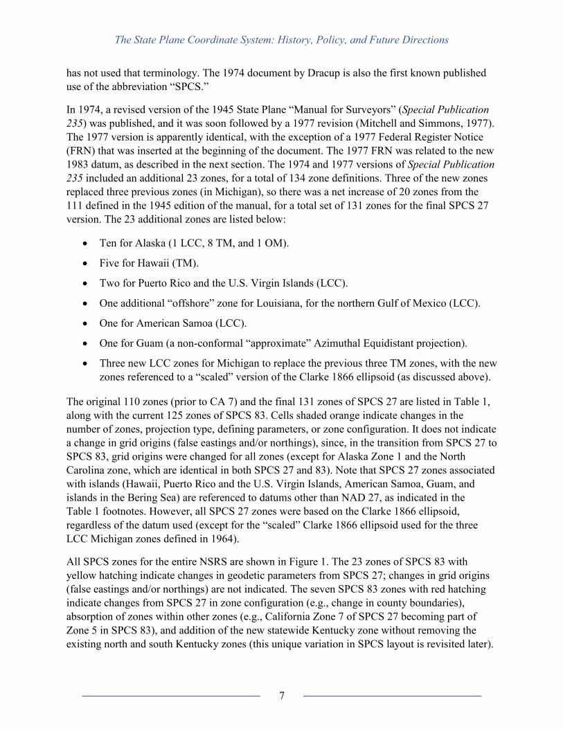
The original 110 zones (prior to CA 7) and the final 131 zones of SPCS 27 are listed in Table 1,
along with the current 125 zones of SPCS 83. Cells shaded orange indicate changes in the
number of zones, projection type, defining parameters, or zone configuration. It does not indicate
a change in grid origins (false eastings and/or northings), since, in the transition from SPCS 27 to
SPCS 83, grid origins were changed for all zones (except for Alaska Zone 1 and the North
Carolina zone, which are identical in both SPCS 27 and 83). Note that SPCS 27 zones associated
with islands (Hawaii, Puerto Rico and the U.S. Virgin Islands, American Samoa, Guam, and
islands in the Bering Sea) are referenced to datums other than NAD 27, as indicated in the
Table 1 footnotes. However, all SPCS 27 zones were based on the Clarke 1866 ellipsoid,
regardless of the datum used (except for the “scaled” Clarke 1866 ellipsoid used for the three
LCC Michigan zones defined in 1964).
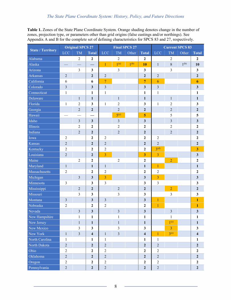
All SPCS zones for the entire NSRS are shown in Figure 1. The 23 zones of SPCS 83 with
yellow hatching indicate changes in geodetic parameters from SPCS 27; changes in grid origins
(false eastings and/or northings) are not indicated. The seven SPCS 83 zones with red hatching
indicate changes from SPCS 27 in zone configuration (e.g., change in county boundaries),
absorption of zones within other zones (e.g., California Zone 7 of SPCS 27 becoming part of
Zone 5 in SPCS 83), and addition of the new statewide Kentucky zone without removing the
existing north and south Kentucky zones (this unique variation in SPCS layout is revisited later).
The State Plane Coordinate System: History, Policy, and Future Directions
8
Table 1. Zones of the State Plane Coordinate System. Orange shading denotes change in the number of
zones, projection type, or parameters other than grid origins (false eastings and/or northings). See
Appendix A and B for the complete set of defining characteristics for SPCS 83 and 27, respectively.
State / Territory Original SPCS 27 Final SPCS 27 Current SPCS 83
LCC TM Total LCC TM Other Total LCC TM Other Total
Alabama 2 2 2 2 2 2
Alaska — — — 1 1(a) 1(b) 10 1 8 1(b) 10
Arizona 3 3 3 3 3 3
Arkansas 2 2 2 2 2 2
California 6 6 7 7 6 6
Colorado 3 3 3 3 3 3
Connecticut 1 1 1 1 1 1
Delaware 1 1 1 1 1 1
Florida 1 2 3 1 2 3 1 2 3
Georgia 2 2 2 2 2 2
Hawaii — — — 5(c) 5 5 5
Idaho 3 3 3 3 3 3
Illinois 2 2 2 2 2 2
Indiana 2 2 2 2 2 2
Iowa 2 2 2 2 2 2
Kansas 2 2 2 2 2 2
Kentucky 2 2 2 2 3(d) 3
Louisiana 2 2 3 3 3 3
Maine 2 2 2 2 2 2
Maryland 1 1 1 1 1 1
Massachusetts 2 2 2 2 2 2
Michigan 3 3 3 3 3 3
Minnesota 3 3 3 3 3 3
Mississippi 2 2 2 2 2 2
Missouri 3 3 3 3 3 3
Montana 3 3 3 3 1 1
Nebraska 2 2 2 2 1 1
Nevada 3 3 3 3 3 3
New Hampshire 1 1 1 1 1 1
New Jersey 1 1 1 1 1(e) 1
New Mexico 3 3 3 3 3 3
New York 1 3 4 1 3 4 1 3(e) 4
North Carolina 1 1 1 1 1 1
North Dakota 2 2 2 2 2 2
Ohio 2 2 2 2 2 2
Oklahoma 2 2 2 2 2 2
Oregon 2 2 2 2 2 2
Pennsylvania 2 2 2 2 2 2

The State Plane Coordinate System: History, Policy, and Future Directions
9
State / Territory Original SPCS 27 Final SPCS 27 Current SPCS 83
LCC TM Total LCC TM Other Total LCC TM Other Total
Rhode Island 1 1 1 1 1 1
South Carolina 2 2 2 2 1 1
South Dakota 2 2 2 2 2 2
Tennessee 1 1 1 1 1 1
Texas 5 5 5 5 5 5
Utah 3 3 3 3 3 3
Vermont 1 1 1 1 1 1
Virginia 2 2 2 2 2 2
Washington 2 2 2 2 2 2
West Virginia 2 2 2 2 2 2
Wisconsin 3 3 3 3 3 3
Wyoming 4 4 4 4 4 4
Puerto Rico &
U.S. Virgin Islands — — — 2(f) 2 1 1
American Samoa — — — 1(g) 1 — — — —
Guam — — — 1(h) 1 1 1
Totals 66 44 110 75 54 2 131 69 55 1 125
(a) Alaska Zone 9 consists of islands referenced to four local datums (the St. Lawrence, St. Matthew, St. Paul, and
St. George datums of 1952). (b) Oblique Mercator projection. (c) Referenced to Old Hawaiian Datum. (d) Additional statewide zone added to existing North and South zones for Kentucky in 2001. (e) New Jersey (2900) and New York East (3101) SPCS 83 zones have identical defining parameters. (f) Referenced to Puerto Rico 1940 Datum. (g) One-parallel (tangent) LCC projection referenced to the American Samoa 1962 Datum. (h) “Approximate” Azimuthal Equidistant projection (non-conformal) referenced to Guam 1963 Datum.
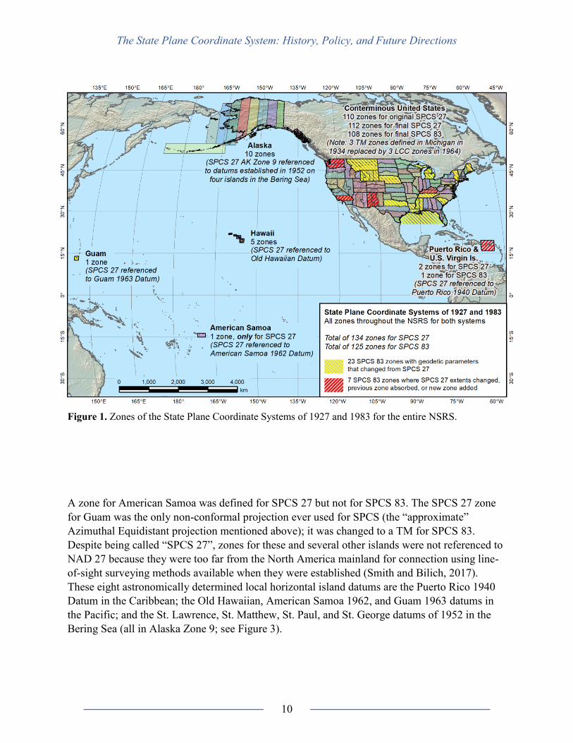
SPCS zones of the conterminous United States (CONUS) are shown in Figure 2. The top map
shows the final 112 CONUS zones of SPCS 27, and the bottom map shows the current 108
CONUS zones of SPCS 83. The same yellow and red hatching schemes are used to indicate
changes from SPCS 27 to 83.
Figure 3 shows SPCS 27 and 83 zones for Alaska (10 zones), Hawaii (5 zones), and Puerto Rico
and the U.S. Virgin Islands (PRVI). For SPCS 27, PRVI consisted of two zones, which were
consolidated into a single zone for SPCS 83. However, the two SPCS 27 and the one SPCS 83
zones all had identical geodetic parameters; the only difference between them is the grid origins
(false eastings and/or northings).
The State Plane Coordinate System: History, Policy, and Future Directions
10
Figure 1. Zones of the State Plane Coordinate Systems of 1927 and 1983 for the entire NSRS.
A zone for American Samoa was defined for SPCS 27 but not for SPCS 83. The SPCS 27 zone
for Guam was the only non-conformal projection ever used for SPCS (the “approximate”
Azimuthal Equidistant projection mentioned above); it was changed to a TM for SPCS 83.
Despite being called “SPCS 27”, zones for these and several other islands were not referenced to
NAD 27 because they were too far from the North America mainland for connection using line-
of-sight surveying methods available when they were established (Smith and Bilich, 2017).
These eight astronomically determined local horizontal island datums are the Puerto Rico 1940
Datum in the Caribbean; the Old Hawaiian, American Samoa 1962, and Guam 1963 datums in
the Pacific; and the St. Lawrence, St. Matthew, St. Paul, and St. George datums of 1952 in the
Bering Sea (all in Alaska Zone 9; see Figure 3).
The State Plane Coordinate System: History, Policy, and Future Directions
11
Figure 2. Zones of the State Plane Coordinate System of 1927 (top) and 1983 (bottom) in CONUS.

The State Plane Coordinate System: History, Policy, and Future Directions
12
Figure 3. Zones of the State Plane Coordinate Systems of 1927 and 1983 for Alaska, Hawaii, and Puerto
Rico and the U.S. Virgin Islands.
Appendices A and B give the defining parameters for all SPCS 83 and SPCS 27 zones,
respectively, In performing research for this report, finding a complete set of reliable (and
legible) defining constants for these three versions of SPCS proved difficult. Including that
information in this publication is the only known occurrence of a complete set of all SPCS zone
definitions in an official NGS document. It appears no NGS document—nor NGS webpage—has
a complete set of zone definitions for SPCS 83 (Stem’s 1990 manual does not include the more
recent Guam or statewide Kentucky zones).

The State Plane Coordinate System: History, Policy, and Future Directions
13
State Plane Coordinate System of 1983
Transition to a New Datum and Naming Conventions The 1977 revision of the 1974 SPCS 27 manual (Mitchell and Simmons, 1977) immediately
followed the publication of the Federal Register Notice (1977), “Policy on Publication of Plane
Coordinates.” As stated above, it appears the only difference between the 1974 and the 1977
versions of the manual is the addition of the 1977 FRN. This activity was in preparation for a
new SPCS that would reference the North American Datum of 1983 (NAD 83).
With regard to naming conventions, the 1977 Federal Register Notice (FRN) is the first known
use of the abbreviation “SPC” for “State Plane Coordinates” (without the “S” for “Systems” or
“System”). The abbreviation “SPCS” was employed earlier by Dracup (1974) for the plural
version of the name (“Systems”), as first used in the 1930s. A singular version of the name (and
abbreviation) was first published in the State Plane technical manual by Stem in 1989 (revised in
1990 with minor corrections), as the “State Plane Coordinate System of 1983.” It was in the
1989/1990 manual where the first known published use of the abbreviations “SPCS 27” and
“SPCS 83” was found to distinguish the two systems. That naming and abbreviation convention
is used in this publication.
Evaluation of State Plane and Changes from SPCS 27 to SPCS 83 According to Stem (1990), NGS performed studies in the mid-1970s to evaluate other NAD 83
projected coordinate systems as possible alternatives to the type of system used for SPCS 27.
Part of the motivation was concern over complexity of a system based on three projection types
(actually four, if Guam as defined at the time is included) and the large number of zones (131 at
the time). Among the alternatives considered were the existing UTM system and a UTM-like
system with narrower zones (to reduce scale error and arc-to-chord corrections). In the end, it
was decided to retain the fundamental SPCS 27 design for the following three reasons:
• SPCS had already been accepted as part of NAD 83 statute in 37 states (presently 48
states and two territories).
• Because SPCS had been in use for more than 40 years, there was widespread familiarity
with its definition and the procedures for using it.
• The availability of electronic computation made the advantages of reducing the number
of zones or projection types largely irrelevant.
With the decision to retain the overall structure of SPCS 27, NGS announced a policy for State
Plane (as well as UTM) referenced to NAD 83 in the Federal Register (1977). More details of the
Federal Register policy will be discussed in the next section. But it is worth noting at this point
that the 1977 announcement was used as an impetus for NGS to solicit comments from April
1978 through January 1979. Input was obtained from the land surveyor board members of the
National Council of Engineering Examiners (NCEES), officers and affiliates of the American
Congress on Surveying and Mapping (ACSM), and various state and local public agencies. This
effort produced committees or liaison contacts in 43 states. The resulting input, together with
The State Plane Coordinate System: History, Policy, and Future Directions
14
characteristics of NAD 83 itself, and existing NGS policy, resulted in several changes from
SPCS 27 to SPCS 83. The more important of these changes are listed below.
• Geodetic Reference System of 1980 (GRS 80) ellipsoid (Moritz, 2000) replaced the
Clarke 1866 ellipsoid.
• Gauss-Krüger form of the TM replaced the Gauss-Schreiber form (they do not yield the
same results, and the difference increases with distance from the central meridian).
• Grid origins (false eastings and northings) were defined in meters rather than U.S. survey
feet (although grid origins for three states are non-exact conversions to meters from U.S.
survey feet: Colorado, Connecticut, and North Carolina).
• Grid origins were changed by significant amounts for all zones to ensure projected
coordinates differed substantially from SPCS 27. Exceptions: they did not change at all
for Alaska Zone 1; changed false easting by less than 1 centimeter for North Carolina
(due to conversion of SPCS 27 grid origins to meters rounded to nearest centimeter);
decreased false easting by exactly 4 feet (1.219 meter) in South Carolina (due to treating
SPCS 27 grid origin value of 2,000,000 U.S. survey feet as international feet, and then
converting to meters).
• More accurate coordinates and related quantities were computed using new mapping
equations and high-precision electronic computers.
• Projection type or the defining parameters of several zones were changed, some zones
were eliminated, and a zone for one territory was removed (American Samoa). See Table
1 for a list of the states affected by these changes. These changes are also shown in the
maps of figures 1 and 2.
Implementation and Documentation of SPCS 83 NAD 83 was completed in 1986 and the SPCS 83 technical manual by Stem was published in
1989 (then slightly revised in 1990). This manual was intended to supplement (rather than
replace) the State Plane manual for surveyors (Mitchell and Simmons, 1977), and to replace the
“State Plane coordinates by automatic data processing” (Claire, 1968). Stem’s 1990 manual
includes all the equations necessary for performing forward and inverse electronic computer-
based coordinate computations to 1 millimeter (or better) accuracy within a zone, as well as for
computing point scale factors, line scale factors, convergence angles, and arc-to-chord
corrections. The manual also includes the parameters for 123 of the 125 current SPCS 83 zones
shown in Table 1 (the Guam TM and Kentucky single statewide LCC zones were created after
1990, and the manual was not updated with those zones). In addition, the 1990 manual contains
information on UTM, the status of NAD 83 legislation, formulas for approximate computations,
examples of using SPCs in traverses, and background information on SPCS and projections
in general.
Although intended to supplement the 1977 State Plane manual, Stem’s 1990 manual has become
the de facto sole defining document for SPCS 83, and it is widely referenced. It is interesting to
note that the 1990 manual is also the last official NGS technical publication on SPCS 83, or on
State Plane or map projections in general. This is in stark contrast to the half century from the

The State Plane Coordinate System: History, Policy, and Future Directions
15
1930s through the 1970s. During that period, NGS and (mainly) C&GS published well over a
hundred official documents on State Plane and map projections. Granted, most of those
documents were projection and intersection tables, but there were also a few dozen technical
publications that were not simply tabulated values. Given the changes in SPCS 83 and other
activities on projected coordinate systems, it is unclear why NGS stopped publishing on the
subject and why Stem’s 1990 manual was not updated. With the need to define and document
SPCS2022, NGS will produce new official reports on map projections within the next few years.
This publication is the first among those new NGS documents.
The only known NGS publications on map projections after Stem (1990) are related to policy,
specifically four official policy statements (from 1991 through 2012) and a dozen NGS Federal
Registry entries made in the mid-to-late 2000s regarding linear units of SPCS 83 coordinates as
adopted by various states. NGS policy on State Plane is the topic of the next section.
State Plane Coordinate System Policies
Defining Policy on Projected Coordinates in the Federal Register As previously mentioned, the earliest known published policy on State Plane was in 1977 in the
Federal Register (1977). This policy notice was made in preparation for the transition to
NAD 83, and it includes both SPCS and UTM (in the context of NAD 83). For SPCS, it
references a single document, Special Publication 235 (the 1974 version of the State Plane
“Manual for Surveyors”). Within three years, this 1974 version was revised (Mitchell and
Simmons, 1977) by incorporating the 1977 FRN in its first two pages. For all practical purposes,
Special Publication 235 has been superseded by Stem (1990).
For UTM, the 1977 Federal Register Notice (FRN) cites the 1958 Department of Army
Technical Manual TM 5-241-8. This manual has been superseded more than once; the current
UTM references are to the National Geospatial-Intelligence Agency (NGA 2014a and 2014b).
Since NGS will continue to publish UTM coordinates referenced to the four 2022 TRFs, the
most current NGA documentation should be referenced, as there have been changes, including
computation methods (discussed later in this publication).
The 1977 FRN on plane coordinates is short, as well as specific, with regard to SPCs. Most of
the items have been adopted for SPCS 83, but not all (those that have not are reviewed in the
next section). To summarize the main items, the policy note states that parameters will be
defined and coordinates published in meters, and that computed coordinate error will not exceed
0.1 millimeters within a zone. It includes amendments based on desires and needs within states,
such as elimination of negative coordinates within zones and changing grid origins. The two
more interesting entries are those of allowing part of a zone to not follow a county boundary
(Grant County in Washington state), and redefining or adding zones to avoid the splitting of
major metropolitan areas (such as Washington, D.C.) across zones. It also states that SPC
constants will not be published until 1982, to allow time for states to legislate their definitions—
one year prior to the planned release of NAD 83 (which was not finalized until 1986). That is the
same as if NGS would now say SPCS2022 parameters would not be published until 2021.

The State Plane Coordinate System: History, Policy, and Future Directions
16
Policies on Changes to State Plane The previous section mentioned that NGS solicited input on the 1977 Federal Register policy
notice. Yet there were no later entries in the Federal Register reflecting such input. This implies
that the 1977 FRN policy still stands. And indeed it has been referenced in two later NGS policy
statements: “Policy on Changes to Plane Coordinate Systems” (NGS, 2001), superseded by
“Policy on Changes to State Plane Coordinates” (NGS, 2012). The two policies are nearly
identical. Summarizing the current (2012) policy, all proposed SPCS 83 changes must satisfy the
following conditions:
1. Changes must be in writing to the NGS Director and be co-signed by the state
Department of Transportation (DOT), state office of Geographic Information Systems
(GIS), state land surveyor professional organization, and other organizations determined
by NGS on a state-by-state basis. A similar request must also be submitted to the USGS.
2. Limited to LCC, TM, and OM projections, defined with respect to the GRS 80 ellipsoid.
3. Changes must be adopted by state law (or regulations with no public opposition),
including all defining parameters and legislated units (meters, U.S. survey feet, or
international feet).
4. Zones must be defined only by international, state, or county boundaries. This item
references the 1977 FRN policy. But, the FRN does not explicitly include such a
requirement, and in fact includes exceptions for a specific county and for metropolitan
areas. (This will be revisited in the next section.)
5. Coordinates for new zones must differ by at least 10,000 meters from SPCS 27.
6. Must have a distinct naming convention.
7. May require state reimbursement for expenses incurred by NGS for changes to SPCS.
8. Requires that the state publish articles and provide education concerning any accepted
changes to SPCS, and those must be available on the internet. Travel expenses for NGS
personnel to provide technical support must be reimbursed by the state.
The main difference between the 2001 and 2012 policy statements is that the 2012 statement
includes an explanatory preamble. It provides context to the policy and recognizes that other
projected coordinate systems may be designed for specific local uses, but that coordinates from
such systems will not be published by NGS. For such cases, NGS recommended that the local
systems be designed and implemented within the state. This recommendation includes any
“layered” systems of zones that overlap one another or SPCS zones.
Other State Plane Policies The only other SPCS policies—whether published directly by NGS or posted in the Federal
Register—concern linear units. The earliest is “Policy of the National Geodetic Survey
Concerning Units of Measure for the State Plane Coordinate System of 1983” (NGS, 1991). This
policy was a change to the 1977 FRN policy that stated SPCS 83 coordinates would only be
published in meters. Its main requirement was that linear units of feet (U.S. survey or

The State Plane Coordinate System: History, Policy, and Future Directions
17
international) be specifically statute-defined for NGS to publish SPCS 83 coordinates in feet. It
was updated in “Policy of the National Geodetic Survey Concerning Units of Measure for the
State Plane Coordinate System of 1983” (NGS, 2006). Part of the update allowed for situations
where units of feet were not defined in statute, by publishing the change in the Federal Register
(among other requirements). That condition is why there are twelve Federal Register notices
concerning SPCS linear units from 2006 to 2009, as mentioned previously. Currently, 46 states
have specifically defined SPCS 83 linear units (40 in U.S. survey feet and six in international
feet); see NGS (2009). Table C1 in Appendix C lists the current linear unit adopted for each
state, along with associated legislation or FRN, and it gives the definition of each type of foot.
The Role of Legislation in the State Plane Coordinate System It is not the intent of this publication to provide a detailed discussion of legislation related to
SPCS. Yet legislation has played an integral role in the adoption and use of the SPCS since its
inception in the 1930s. To illustrate, consider the closing statement of the 1977 FRN: “The
National Geodetic Survey will not change projection defining parameters in states that have
legally adopted the SPC system until the state amends its legislation.”
Efforts to encourage adoption of SPCS in legislation played a prominent role in C&GS and NGS
publications throughout the history of the SPCS. It is mentioned by Adams (1937), and it was an
important part of Special Publication 235, the State Plane “Manual for Surveyors” (Mitchell and
Simmons, 1945 and 1977), which served as the defining document for SPCS 27. Special
Publication 235 contains extensive appendix entries on state legislation, including a model act
for SPCs. The model act has sections for specifying all defining parameters of the zones within a
state and specifically identifies the Clarke 1866 ellipsoid and NAD 27. For defining property
corners in the public record using SPCs, it specifies the accuracy of surveys and a maximum
distance of half a mile to geodetic control with published SPC values.
Stem’s SPCS manual (1990) effectively replaced Special Publication 235 and also contains an
extensive discussion of SPCS legislation, along with an updated version of the model act. It is
very similar to the previous model act, but with some differences. Both SPCS 27 and SPCS 83
are allowed and defined, although a section is included at the end of the model act where a date
can be specified for when SPCS 83 will replace SPCS 27. There are also SPCS 27 to SPCS 83
changes from U.S. survey feet to meters; from x, y coordinates to eastings and northings; and
from half a mile to 1 kilometer for maximum distance to geodetic control (2nd order or better).
Interestingly, a brief note at the end of the model act mentions that the 1 kilometer limitation
should be re-evaluated in light of emerging GPS technology.
Currently, 48 states and two territories have adopted SPCS 83 legislation, although it appears
few (if any) have amended their legislation to accommodate GPS or other improvements in
geodetic positioning. Table C1 in Appendix C lists citations (with embedded hyperlinks) for all
states and territories with SPCS 83 legislation. Figure 4 shows the states and territories that have
enacted SPCS 83 legislation, and the type of foot adopted (if any).

The State Plane Coordinate System: History, Policy, and Future Directions
18
Figure 4. States and territories with SPCS 83 legislation and the type of foot adopted.

The State Plane Coordinate System: History, Policy, and Future Directions
19
As part of the transition from NAD 83 (and SPCS 83) to the new 2022 TRFs, NGS is working
with the National Society of Professional Surveyors (NSPS) and the American Association for
Geodetic Surveying (AAGS) to draft a statute template that states may use in updating their
statutes. Part of this effort is to address the two main weaknesses in existing statute: 1) specific
reference to NAD 83 and 2) giving technical details of the defining parameters for each SPCS
zone. The approach for removing the first problem is to exclude specific names of datums and
adopt generic terminology, for example “the National Spatial Reference System or its
successor.” Because legislation can be difficult to change, another goal is to have states remove
the defining SPCS parameters from statute and place them where they are easy to modify, such
as in administrative rules. NSPS will work with states to adopt the new templates, and a draft
version has been developed (NSPS, 2016).
Departures from Policy and Convention As described in the previous two sections, there are three current NGS policies on projected
coordinates: “Policy on Changes to State Plane Coordinates” (NGS, 2012), “Policy of the
National Geodetic Survey Concerning Units of Measure for the State Plane Coordinate System
of 1983” (NGS, 2006), and “Policy on Publication of Plane Coordinates” (Federal Register,
1977). Both the 2012 and 2006 NGS policies cite the 1977 Federal Register policy notice. The
2012 policy cites it directly, and the 2006 indirectly as an explicit update to the 1991 policy,
which does directly reference it.
The NGS 2006 policy on linear units is in conformance with the 1977 FRN policy, even though
the notice specifies coordinates in meters. It is in conformance, because it is an update to the
NGS 1991 policy that explicitly identifies the portion of the 1977 FRN policy being amended,
and it specifies how such changes can be made.
In contrast, the NGS 2012 SPCS policy references the 1977 Federal Register notice without
modification. This implies that all parts of the 1977 FRN are still in effect (other than the
requirement for coordinates in meters, which was amended with the 2006 and 1991 policy
statements). Discrepancies between the 1977 FRN and NGS 2012 SPCS policies are listed
below. The distinction between “policy” and “convention” is not always clear, and actual
implementation can be a proxy for either one. Thus, both types are considered, with items
considered as departures from “policy” listed first, with prefix “P.”
P1. Zone boundaries must conform to county, state, or international boundaries. The obvious
and well-known exception to this policy is in Alaska, where the first nine zones are
bound by meridians, and Zone 10 is associated with the Aleutian Islands west of Unimak
Island (see Figure 3). A less well-known exception is in Hawaii, where Zone 4 and 5 are
both in Kauai County, but on separate islands (lower left map in Figure 3). Another
obscure exception is Grant County in Washington state, where the boundary between the
north and south Washington zones is along a parallel within the county (compare upper
and lower maps in Figure 2). Interestingly, this exception is specifically stated in the
1977 FRN as part of the transition from SPCS 27 to SPCS 83. Perhaps more importantly,
the restriction to political boundaries is not explicitly stated as a policy requirement. It

The State Plane Coordinate System: History, Policy, and Future Directions
20
may instead be a convention adopted from how the SPCS was originally created.
Although the distinction between policy and convention is not entirely clear for this case,
it could be argued that it is a policy, since an amendment in the 1977 FRN was used to
change the Grant County boundary. In any event, a simple amendment was all that was
required for the change. There is another entry in the 1977 FRN suggesting that zones
do not necessarily have to correspond to political boundaries. That is addressed in
the next item.
P2. Large urbanized areas located on or near zone boundaries. Perhaps the most interesting
entry in the 1977 FRN concerns metropolitan areas in multiple zones. It states that zone
parameters can be modified or new zones defined so that a large urban area that straddles
zones will be in a single zone. There are many urban areas in that situation (for example,
New York City, Los Angeles, Chicago, St. Louis), and it does present problems for users.
Had this been pursued for SPCS 83, such problems could possibly have been
ameliorated. It is worth noting that California Zone 7 of SPCS 27 effectively served that
purpose for the Los Angeles metro area (it consisted only of Los Angeles County). This
zone was created in 1938 based on consultation of local and state government officials
with then retired C&GS Division of Geodesy Chief Major William Bowie (Trimm and
Derby, 1966). Based on Major Bowie’s recommendation, an LCC projection was
designed that minimized scale error in the county. In addition, the grid origin of the
projection was selected, such that the coordinates differed as little as possible with those
of a previously defined Polyconic projection of the same area, also based on NAD 27
(that is why the false easting and northing for this zone are not “clean” values; see tables
B1 and B2 in Appendix B). By 1945, this zone was added to SPCS 27 by C&GS, and in
1947 it was adopted by state statute along with the other six original zones as part of the
California Coordinate System (Alexander, 1988). This is an early and noteworthy
example of mutually beneficial collaboration that served local needs while maintaining
consistency with the nationally defined system. When SPCS 83 was created, CA Zone 7
was eliminated and its area incorporated into CA Zone 5, perhaps because the metro area
had grown well beyond the boundaries of Los Angeles County by that time. In any case,
including the idea of metropolitan region zones in the 1977 FRN—and the earlier
cooperative development of CA Zone 7—shows flexibility in how zones could be defined
for special situations. Yet it was never pursued as part of SPCS 83.
P3. “Layered” zones. The preamble in the 2012 policy recommends against SPCS “zones in
various layering configurations” (although it does not go quite so far as to forbid it). Here
“layered” zones are taken as zones that are entirely within a larger zone (to distinguish
from previously mentioned metropolitan zones with partial overlap). Interestingly, a
layered system was created in Kentucky in 2001 (Kentucky Legislature, 2001; Kentucky
Geography Network, 2002). This statewide Kentucky “one zone” is now officially part of
SPCS 83 as KY1Z (code 1600), along with the previously existing north and south zones.
KY1Z coordinates are provided on NGS products and services, such as datasheets (along
with KY North and/or South coordinates), and on Online Positioning User Service
(OPUS) reports, where they are the only SPCS 83 coordinates for solutions in Kentucky.

The State Plane Coordinate System: History, Policy, and Future Directions
21
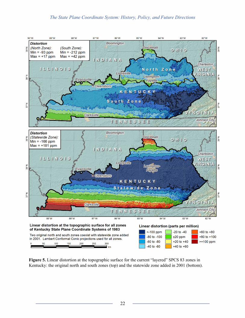
Figure 5 shows linear distortion at the topographic surface for all three current SPCS 83
zones in Kentucky. As expected, the range in distortion for the statewide zone is greater
for the statewide zone, but the positive and negative values are better balanced around
zero, indicating there was an attempt to minimize distortion at the topographic surface.
Table A1 in Appendix A gives defining parameters for all three zones. Statewide zones
are discussed in greater detail later in this publication.
P4. Restriction of projected coordinates to SPCS only. The 2012 NGS policy states that NGS
will only publish SPCS projected coordinates. However, NGS also publishes UTM
coordinates (as well as closely related U.S. National Grid coordinates). It is explicitly
stated in the 1977 FRN that NGS will publish and support UTM as defined by the
Department of Defense (but referenced to NAD 83).
P5. Computational accuracy. The 1977 FRN states that the error of computed SPCS 83
coordinates will never exceed 0.1 millimeter within a zone. It is not clear whether this
objective was achieved in all areas of all zones. Stem (1990) states that computations
using the SPCS 83 formulas are accurate to 1 millimeter within a zone, if at least 12
digits of numerical precision are used. Other than this statement by Stem, there is no
known documentation of SPCS 83 computational accuracy. The accuracy of calculations
is also affected by distance from the projection axis (central parallel for the LCC, central
meridian for the TM, and skew axis for the OM projections). Creation of a single large
zone for entire states in SPCS 83 (such as Montana) could degrade computational
accuracy, as well as increase maximum scale error (as discussed in the next item).
P6. Maximum scale error limitation. A limit on maximum scale error (linear distortion) is not
explicitly stated in the 1977 FRN or other policy statements. However, many other
C&GS and NGS documents (including Special Publication 235 referenced in the 1977
FRN) state that SPCS zone design is based on a maximum scale error criterion of
1:10,000 with respect to the ellipsoid (not the topographic surface); this value can also be
expressed as ±100 parts per million (ppm). In some sense, this is a convention that has
taken on the color of policy, similar to the “convention” of using aggregated counties to
define zone extents. And, similar to the county boundary convention/policy, there are
exceptions. As shown in the 1977 edition of Special Publication 235, the maximum scale
error criterion was exceeded in only 11 of the 131 zones. The largest was 1:7300
(±137 ppm) for the Texas South Central Zone and 1:6600 (±152 ppm) for Alaska Zone
10. Both of these are nonetheless substantially less than the maximum scale error of
1:2500 (±400 ppm) for UTM, which was considered too large (Stem, 1990). Yet for
SPCS 83, three states were changed from multiple to single zone systems, with a
corresponding increase in scale error. Most significant among these was Montana, which
went from three LLC zones to one. This change caused an increase in maximum linear
distortion to 1:1600 (±625 ppm), which is substantially greater than that of UTM.
Moreover, for nearly all areas in all zones, distortion is greater at the topographic surface
than on the ellipsoid.
The State Plane Coordinate System: History, Policy, and Future Directions
22
Figure 5. Linear distortion at the topographic surface for the current “layered” SPCS 83 zones in
Kentucky: the original north and south zones (top) and the statewide zone added in 2001 (bottom).
The State Plane Coordinate System: History, Policy, and Future Directions
23
In addition to the above issues that could be considered implicit policy, other “irregularities” in
SPCS design and implementation can be construed as departures from convention. These have
occurred over the history of SPCS, and several are listed below, with prefix “C.”
C1. Projection type and implementation. The 2012 NGS policy explicitly limits SPCS to the
three conformal projections LCC, TM, and OM. Yet mathematical variants of these
projections exist, most notably the Gauss-Schreiber (used for SPCS 27) and Gauss-
Krüger (used for SPCS 83) versions. The difference in coordinates for these two versions
of the TM projection (as implemented by C&GS/NGS) increases with distance from the
central meridian, reaching about 10 centimeters at a distance of 150 kilometers (mostly in
northing). The American Samoa zone (which exists only for SPCS 27) was based on a
one-parallel (tangent) version of the LCC. This is a perfectly valid form of the LCC, but
the algorithm currently used by NGS will fail with a division-by-zero error for a one-
parallel LCC. These two cases show the importance of not just naming the projection
type, but also clearly specifying its mathematical implementation. And finally, the
SPCS 27 zone for Guam used an “approximate” Azimuthal Equidistant projection. It is
not conformal, and it is probably better described as a tangent plane coordinate system.
This approach was selected despite the stated importance of conformality from the very
beginning of SPCS in the 1930s, and it is the only zone in the SPCS that is not an LCC,
TM, or OM projection (the SPCS 83 zone for Guam is a TM projection). It is not known
why such a system was used for Guam in SPCS 27, but it does illustrate the variability of
approaches used for SPCS.
C2. Reference ellipsoid. The 2012 NGS policy explicitly states SPCS should be “…defined at
the surface of the ellipsoid of the current Datum.” It is not entirely clear what is meant by
“surface,” since only three zones in the entire history of SPCS are tangent; all others are
“secant” (i.e., the developable surface of the projection is “below” the ellipsoid surface
for most of a zone’s area). This requirement is thus taken to mean that the mapping
equations refer directly to the unmodified reference ellipsoid (Clarke 1866 for SPCS 27
and GRS 80 for SPCS 83). An exception to this was created in 1964 for three SPCS 27
zones in Michigan, which were based on a “scaled” version of the Clarke 1866 ellipsoid
(as described earlier). As with projection types, this shows how SPCS varied over time.
C3. Datums and reference frames. Policies and model laws state that SPCS 27 should be
referenced to NAD 27, and SPCS 83 to NAD 83. However, nine SPCS 27 zones refer to
other datums (as listed in the notes at the bottom of Table 1), although all were based on
the Clarke 1866 ellipsoid. This was out of necessity, since in all cases these were islands
that could not at the time be accurately connected to the NAD 27 geodetic network in
North America. Nonetheless, it represents a (slight) inconsistency that can cause
confusion. All SPCS 83 zones are referenced to NAD 83, but there is a complication here
as well: there are three NAD 83 frames, nominally referenced to the North America,
Pacific, and Mariana tectonic plates, although SPCS 83 uses the GRS 80 ellipsoid in all
cases. Using these three frames is an unavoidable characteristic of the modern GNSS-
based realizations of NAD 83, but it can still be a source of confusion.
The State Plane Coordinate System: History, Policy, and Future Directions
24
C4. Scaling of SPCS coordinates to “ground.” The SPCS grid distance between a pair of
points is almost always different (usually shorter) than the actual horizontal distance on
the topographic surface, which is often called the “grid to ground” problem by surveyors
and engineers. In high-elevation areas, this difference can greatly exceed the nominal
maximum 1:10,000 scale error. The problem can be dealt with in a number of different
ways. One method has been taught by NGS and is presented in at least one technical
document (Dracup, 1974). Without going into detail, it consists of dividing the SPCS
coordinates by the “combined factor” for an area of interest. This factor is a function of
both location and (ellipsoid) height, and it is usually less than 1. The purpose is to “scale”
the coordinates such that the distance between points is approximately equal to the actual
horizontal ground distance. It works because SPCS uses conformal projections, so the
scale error (linear distortion) is the same in all directions from a point. Dracup called
these scaled coordinates “project datum coordinates.” They have often gone by other
names, such as “modified” State Plane or State Plane “at ground,” but these names are
misleading, since the coordinates are no longer State Plane once they have been scaled. In
any event, this approach has become very common. It is the approach used by many
DOTs, and it has been incorporated into various commercial geospatial software
packages. Although NGS taught this process in the past, it appears NGS no longer
teaches this method, and (apart from the 1974 Dracup document) it seems it is not
included in any NGS technical manuals, memoranda, reports, or policy. This has created
something of a vacuum within the geospatial community and a consequent lack of a
standard approach: there is no universally accepted way to perform the scaling; projects
based on scaled coordinates lack sufficient metadata; and it has caused a proliferation of
local coordinate systems that can easily be confused with “true” State Plane (typically
every project has its own scaled coordinate system). The problem is actually larger than
scaling SPCS coordinates; it also applies to other methods used for minimizing linear
distortion. An example is the previously mentioned three Michigan SPCS 27 zones based
on a “scaled” Clarke 1866 ellipsoid (which, similar to the creation of CA Zone 7
discussed earlier, is a notable instance of cooperation between C&GS and the local
surveying community). Other methods for reducing linear distortion exist—as discussed
below in the section on low distortion projections—but there is a lack of uniformity in the
approaches used.
C5. Zone uniqueness. None of the SPCS policies explicitly state that the parameters for each
zone must be unique. Yet such a convention could be inferred from other requirements
for changes to SPCS as stated in the 2012 NGS policy. Despite such an inference, every
defining parameter for the New Jersey and New York East TM zones are completely
identical in SPCS 83, so they are effectively a single zone (their SPCS 27 parameters
were different). This may have been done to achieve consistency in coordinates in the
two zones, in a manner similar to defining zones for metropolitan areas as proposed in the
1977 FRN policy statement. But that reason seems unlikely, since these zones share
major urbanization with the adjoining and completely distinct New York Long Island
LCC (NY L) zone. Regardless of the reason, as part of documenting apparent
irregularities in SPCS, it is worthwhile to point out that two SPCS 83 zones are identical.

The State Plane Coordinate System: History, Policy, and Future Directions
25
C6. Ambiguous SPCS 83 Guam zone definitions. Similar to the Kentucky statewide “one
zone,” the SPCS 83 zone for Guam is not defined in any official NGS publication or
webpage. Yet SPCS 83 coordinates are computed for Guam on NGS datasheets and
OPUS solution reports. Compounding this problem is the NGS computer program used
for SPCS 83 computations (NGS, 2002a). Its Fortran source code has three TM
definitions for the Guam zone. The first is commented out, and it has the same ID number
(133) as the second one, which is not commented out. The third has a different ID
number (135), and it is identical to the second, with the exception that its false easting
and northing values are swapped. This is a confusing situation for determining which
definition is used by NGS. For this publication, it was determined that the second
definition is used by NGS (the version of ID 133 that is not commented out, with zone
code 5400) by duplicating datasheet and OPUS SPCS 83 coordinates for Guam. This was
further confirmed by comparison to the Guam Annotated Code (Guam Compiler of Laws,
2017), a geodetic network report (Dyson, 1995), and the European Petroleum Survey
Group (EPSG) Geodetic Registry (EPSG, 2017). The third Guam definition (ID 135) in
the NGS SPCS 83 Fortran program was apparently never implemented. Why it exists in
the program is unknown, but it was assigned an NGS zone code of 5401. These NGS
zone (or “FIPS”) codes are discussed in the next item.
C7. NGS SPCS “FIPS” codes. SPCS zones are identified by a four-digit NGS code in Stem’s
1990 manual and the SPCS 83 computer program. The first two digits identify the state,
and the last two identify the zone. These codes are often referred to as “FIPS” (Federal
Information Processing Standard) codes, particularly outside of NGS. However, the state
part of the code does not match the official FIPS codes used for states and territories by
the U.S. federal government (U.S. Census Bureau, 2015). Documentation on the source
of this discrepancy has proven difficult to find. According to Esri (2017), the NGS SPCS
codes were part of a proposed FIPS that was withdrawn. Because of that, NGS zones are
often identified (incorrectly) as FIPS zones by many organizations, individuals, and
software vendors. In the case of Esri, this is done intentionally to maintain continuity
with historic zone identifiers.
The above items are not intended to indicate that SPCS is somehow deficient. Rather, the intent
is to identify inconsistencies and the importance of documentation, particularly in the context of
updating the NSRS for 2022. Any of the above discrepancies can be remedied through
appropriate updates of policy and through additional documentation (such as this publication).
But policy updates for SPCS 83 are likely unnecessary at this time, since it will soon be replaced
by SPCS2022. Preparation for SPCS2022 will afford NGS the opportunity to completely and
consistently define SPCS policy.
Recent Developments in Projected Coordinate Systems Although NGS has not published an official technical document on SPCS since Stem’s 1990
manual, that is not to say there has been no activity on projected coordinate systems in the
United States. A subtle but important change that has occurred since Stem’s manual is how
SPCS is used. The original reason for creating SPCS was to give surveyors and engineers a

The State Plane Coordinate System: History, Policy, and Future Directions
26
mathematically sound way to using simple plane trigonometry for performing “geodetic” surveys
referenced to the NSRS. An essential part of making that possible was to provide a means for
converting between geodetic and projected coordinates and azimuths. These were important
considerations prior to electronic computers. Massive effort was dedicated to developing
instructions, performing computations, and publishing the necessary information in numerous
manuals and tables. Even as late as 1990, Stem’s manual devotes eight pages to a detailed
example on performing a traverse in SPCS using plane trigonometry. Another 44 pages of that
manual are used to provide an approximate polynomial method for manually computing
coordinates in the 68 LCC zones of SPCS 83 (excluding the Kentucky single statewide zone).
Yet by that time it was already evident such methods were becoming obsolete with the rise of
inexpensive electronic hand calculators and personal computers. This change is foreshadowed
in the 1990 manual by the absence of an approximate coordinate computation method for
the 55 TM zones. According to Stem, it had not yet been fully developed “…pending the
demonstrated requirement for such a method.” That comment was prescient; the requirement
would never arise.
By the mid to late 1990s the situation had changed completely. Powerful hand-held field
computers (“data collectors”) were becoming common. These devices had sufficient power and
numerical precision to reliably perform complex geodetic reductions and map projection
computations essentially instantaneously. The days of tedious manual computations were over. A
parallel change was occurring in the office with the adoption of Computer Aided Drafting and
Design (CADD) and Geographic Information Systems (GIS). Projected coordinates were
becoming the dominant currency for representing geospatial information, and the use of
coordinate geometry was particularly important in CADD. For both surveying and engineering,
CADD implementations worked in 3D topocentric Cartesian space. The horizontal plane is
defined, more often than not, using conformal projected coordinates. The vertical component is
simply “height” or “elevation” perpendicular to the mapping plane. GNSS accelerated the use of
projected coordinates, especially SPCS, because some type of projection was needed to convert
the geodetic output of GNSS to a useful, local, topocentric Cartesian system. SPCS was
increasingly used, because it was easy for manufacturers to preload all SPCS zones into field and
office software, and users could simply pick their zone from a list. SPCS (and UTM) were
embraced in GIS for largely the same reason—the coordinate systems were preloaded in the
software, and standard implementations simply used the zone corresponding to their location.
Surveying, engineering, CADD, and GIS all use essentially such an approach to this day. Even
sophisticated modern 3D applications in CADD and GIS are usually more “2.5D” than true
3D—they are typically implemented as projected coordinate systems, with the third dimension
“extruded” perpendicular to the mapping plane.
Two changes in the “traditional” definition and usage of SPCS (and similar conformal projected
coordinate systems) warrant further discussion. One is the establishment of single statewide
zones, even for states much too large to achieve the nominal SPCS maximum scale error (linear
distortion) of 1:10,000 (±100 ppm) on the ellipsoid. The other is the creation of small zones that
minimize linear distortion at the topographic surface (rather than at the ellipsoid), for example to
1:50,000 (±20 ppm), or even less. These two apparently opposing approaches have their origins

The State Plane Coordinate System: History, Policy, and Future Directions
27
several decades in the past. But, both have seen a recent resurgence in interest due in no small
part to the ubiquity of electronic computers. Each is discussed in the following two sections.
Statewide Zones Montana’s move from three LCC zones in SPCS 27 to a single LCC zone in SPCS 83 represents
the most extreme existing example of exceeding the nominal maximum SPCS scale error of
1:10,000. The maximum scale error for the SPCS 83 Montana zone is 1:1646 (-607 ppm) with
respect to the ellipsoid, which is significantly greater than even the UTM limit of 1:2500
(±400 ppm). And, because of the overall high elevations in Montana, the scale error (linear
distortion) at the topographic surface is greater yet. In the city of Missoula, located near the
central parallel, the linear distortion with respect to the ellipsoid is about 1:1650 (-606 ppm), as
expected. But, since the topographic height of Missoula is approximately 1000 meters, the total
linear distortion at the ground surface is about 1:1310 (-764 ppm). That means a horizontal
distance of 100 meters on the ground is 7.6 centimeters shorter when represented using SPCS 83
coordinates. For engineering plans and survey plats, such a difference could easily be detected
even with a tape measure used for construction layout or boundary measurements. But does it
matter? As long as all users of the geospatial data understand the situation, and the appropriate
scale factors are used, then this does not necessarily represent a problem. Clearly, the state of
Montana did not consider it a problem when they elected to use a single zone, and many within
the state continue to use it to this day (including the Montana Department of Transportation,
although they use SPCS scaled “to ground” to minimize linear distortion for projects with tight
tolerances, such as bridges).
Figure 6 shows linear distortion at the topographic surface in Montana, based on the three zones
of the SPCS 27 definition (top), and for the single SPCS 83 zone definition (bottom). Note the
very large increase in (negative) distortion for the statewide SPCS 83 version: minimum of
-1045 ppm, versus -655 ppm for SPCS 27 (in the south zone). The minimum and maximum
distortion occurs in the south SPCS 27 zone, due to its greater north-south width, and thus its
more widely spaced standard parallels (see Table B1 in Appendix B for the full set of defining
SPCS 27 parameters).
For the single SPCS 83 Montana zone shown in Figure 6, it is interesting to note that the south
and north standard parallels (45°N and 49°N; see Table A1 in Appendix A) are further apart than
necessary to provide balanced positive and negative distortion coverage for Montana (with
respect to the ellipsoid). It is not known why these standard parallels were used, as balanced
distortion of lower magnitude (on par with UTM) could have been achieved through selection of
more closely spaced parallels.
In the context of planning for SPCS2022, the use of such a large SPCS zone in Montana raises
some questions. Does it render the 1:10,000 maximum scale error design criterion of SPCS
obsolete or irrelevant? Should SPCS2022 switch to a system where every state has a single zone?
If this works in Montana, then it would certainly work in all or most other states. Only Texas and
Alaska have their shortest dimension larger (California has greater area than Montana, but it is
narrower perpendicular to its long axis).
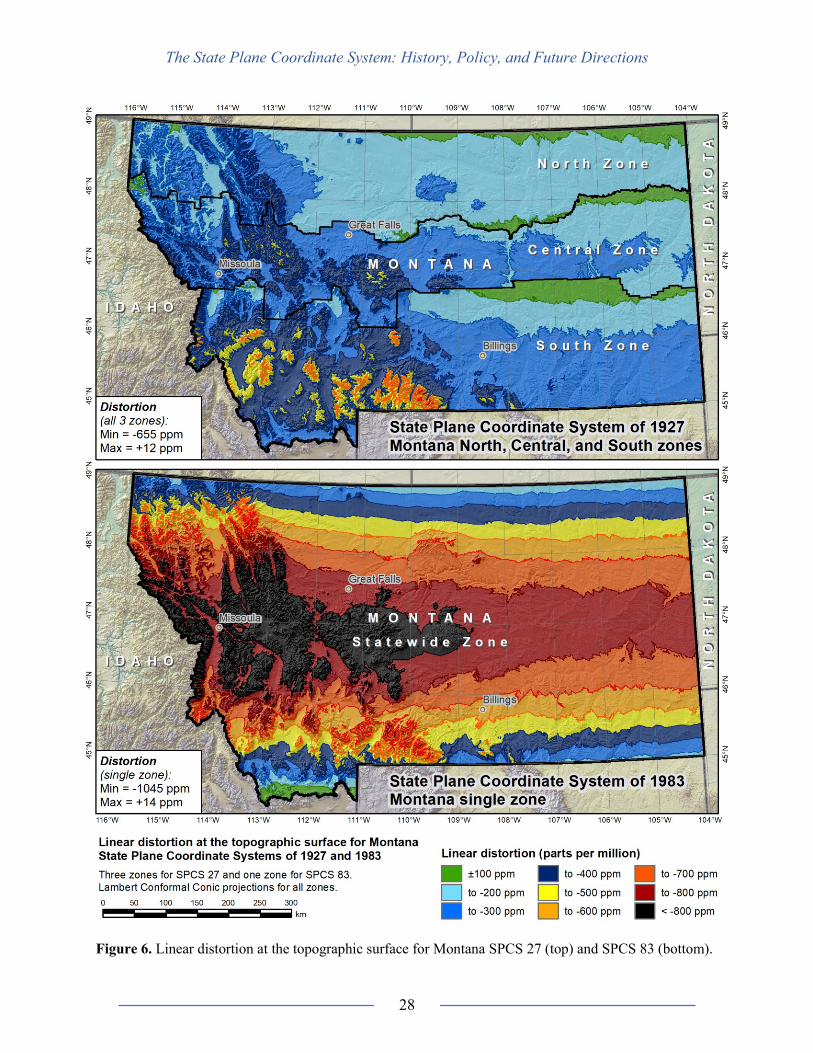
The State Plane Coordinate System: History, Policy, and Future Directions
28
Figure 6. Linear distortion at the topographic surface for Montana SPCS 27 (top) and SPCS 83 (bottom).

The State Plane Coordinate System: History, Policy, and Future Directions
29
Many states have designed their own statewide projections. One for Kentucky was discussed
earlier in this report, and it was incorporated into SPCS 83 (without replacing its previously
existing north and south zones). Many other states have also designed statewide zones, although
they have not become part of SPCS 83. The main motivation for these statewide zones is that
they are especially useful for a statewide GIS. Many analytical operations in GIS require a single
geometry (such as linear referencing and network analysis), and a conformal projected
coordinate system is particularly useful for such operations.
Low Distortion Projections At the opposite extreme from that of Montana, other states have designed multiple-zone
projected coordinate systems, where each zone covers a relatively small area, such as a county or
specific topographically-defined region. The objective for such systems is to reduce linear
distortion at the topographic surface such that it is negligible for most practical applications.
Such systems are not new; both Wisconsin and Minnesota have had statewide county coordinate
systems since the 1980s (Wisconsin State Cartographer’s Office, 2012; Minnesota Department of
Transportation, 2009), and these have long been incorporated in commercial software packages.
In recent years there has been an increase in interest and implementation of such systems, which
are often called “low distortion projections” (LDPs). Examples include Oregon (Armstrong et
al., 2017), Kansas (Dennis, 2017), and Indiana (Badger, 2016).
The motivation for LDPs is to have a consistent set of projected coordinates that yield distances
so close to horizontal ground distances that no additional scale factor is required. This desire
had been met for many years using the “project datum” approach of scaling SPCs, as described
earlier in this report. Reasons for moving away from the scaled SPC approach are that it:
1) creates systems that can easily be confused with “true” SPCS; 2) is not readily transferrable
across platforms, especially GIS; and 3) does not optimally minimize distortion. Coupled with
this is: 1) the growing capabilities of modern geospatial software, such as the ability to design
custom projections without having to use existing projected coordinates; 2) standardization of
machine-readable projection definitions; 3) “projection-on-the-fly” capabilities that allow data
with different projections to coexist; and 4) improvement in the ability to optimally minimize
linear distortion over large areas (Dennis, 2016).
To provide an indication of the number of LDP systems in the United States, examples of those
that are government sanctioned are listed in Table 2 and shown in Figure 7. Note the wide
variety of zone types. Included are those in the eastern and central United States that consist of a
single county or group of counties, metropolitan areas (Washington, D.C. and Las Vegas), single
cities (San Francisco), and topographically defined regions (Oregon and Alaska). The one in
northwestern Arizona is for an Indian reservation (Navajo Nation) that is too large to achieve
what most would consider “low distortion” (within about ±25 ppm). Nonetheless, it was
designed to minimize linear distortion at the topographic surface (at a mean ellipsoid height of
1800 meters), making it more akin to LDPs than traditional SPCS.

The State Plane Coordinate System: History, Policy, and Future Directions
30
Table 2. Examples of U.S. LDP coordinate systems. (see Figure 7 for locations and zones).
Multiple-zone LDP systems Single-zone LDP systems
1. Oregon Coordinate Reference System,
OCRS (39 zones)
11. City of Flagstaff Low Distortion Grid Coordinate System
2. Rocky Mountain Tribal Coordinate
Reference System, RMTCRS (10 zones)
12. Maricopa County Low Distortion Projection
3. Minnesota County Coordinate System,
MCCS (97 zones)
13. Gila Valley Low Distortion Projection, GVLDP
4. Wisconsin Coordinate Reference
Systems, WISCRS (72 zones)
14. Cochise County Low Distortion Projection
5. Iowa Regional Coordinate System,
IaRCS (14 zones)
15. Navajo Nation Coordinate System
6. Indiana Geospatial Coordinate System,
IGCS (92 zones)
16. Lancaster County Grid Low Distortion Projection
7. Kansas Regional Coordinate System,
KRCS (20 zones)
17. Craighead County Low Distortion Projection Coordinate
System
8. Nevada Coordinate Reference System,
NCRS (2 zones)
18. Washington Metropolitan Area Transit Authority (WMATA)
Low Distortion Projection Coordinate System
9. Pima County Coordinate System, PCCS
(4 zones)
19. Southeast High-Speed Rail - Richmond Area to Potomac
Segment (SEHSR-RAPS) Low Distortion Coordinate System
10. Alaska Low Distortion Projection
Coordinate System (47 zones)
20. City & County of San Francisco 2013 Coordinate System,
SFCS13
Figure 7. Examples of U.S. LDP coordinate systems (see Table 2 for additional information).

The State Plane Coordinate System: History, Policy, and Future Directions
31
Clearly, there is significant and growing use of LDPs. But, like single statewide zones, this raises
questions about how or whether LDPs should be implemented in SPCS2022, as well as what
NGS’ role should be. How do LDPs fit into SPCS, if at all? If LDPs are incorporated into
SPCS2022, how will that be accomplished? Would it be an “either/or” situation, where a state
must use LDPs or larger (even single statewide) zones, but not both? Or will “layered” systems
be permitted? A layered system already exists in SPCS 83 for Kentucky—should this be
perpetuated for Kentucky or elsewhere?
Even if LDPs are allowed in SPCS2022, it is highly unlikely NGS will have the resources to
design them. Instead, NGS could provide standards, guidelines, and criteria for designing
appropriate LDPs for inclusion in SPCS2022. Yet questions remain over how NGS would
manage and deliver coordinates for such a large number of zones (e.g., by OPUS and on
datasheets), particularly if layered systems are used. Alternatively, for the case where LDPs do
not become part of SPCS2022, NGS may need to consider providing other mechanisms that
allow users to reference the NSRS when using LDPs.
Whether or not NGS decides to support statewide projections or LDPs (or both) as part of
SPCS2022 (or by other means), it is worth noting that detailed and standardized information on
coordinate systems is readily available from other sources. One of the best known is the
European Petroleum Survey Group (EPSG) Geodetic Parameter Registry (2017). The registry is
a freely available database of various geodetic parameters used worldwide, including projected
coordinate reference systems. Importantly, it provides machine-readable definitions in both
Well-Known Text (WKT) and Geography Markup Language (GML) formats, and it is widely
used by commercial and government organizations. The parameters for zones of the statewide
and LDP projected coordinate systems mentioned above are available through EPSG. Such a
resource would likely make implementation of these various projected systems much simpler
for NGS.
Projection Computations Methods for performing projection computations have also evolved since Stem’s 1990 manual.
Dramatic improvements in computer power have made it possible to compute more accurate
coordinates. One way to accomplish this is simply by including additional terms from the
traditional series expansions used for the ellipsoidal mapping equations. Another way is to use
more complex algorithms or derivations that were too computationally expensive in the past.
Although a fairly extensive review of NGS and C&GS documents was performed for this report,
no technical documents were found regarding the sources of the SPCS 83 map projection
algorithms. Stem (1990) provides the formulas, but only includes references for a few specific
computations. Checking comments in the SPCS 83 Fortran source code (NGS, 2002a) showed
that all three projections were written, or last revised, by Thaddeus Vincenty in 1984 and 1985.
The lack of documentation is in contrast to the many technical documents published for
SPCS 27. But, the SPCS 27 formulas will not give the same results as the Vincenty algorithms,
particularly for the TM projections, as different derivations were used (Gauss-Schreiber for
SPCS 27 and Gauss-Krüger for SPCS 83).

The State Plane Coordinate System: History, Policy, and Future Directions
32
It is not clear whether the SPCS 83 algorithms meet the 1977 FRN objective of 0.1 millimeter
coordinate accuracy throughout every zone (especially large zones such as Montana). No
documents quantifying accuracy were found, apart from the statement of 1 millimeter within a
zone in Stem (1990). The only other information found was a comment by Vincenty in the TM
source code stating that calculations provide “geodetic accuracy” within ±3.5° longitude of the
central meridian (NGS, 2002a).
Since NGS also publishes UTM coordinates (and will continue to do so for the 2022 TRFs),
those algorithms were also checked (NGS, 2002b). They are identical to the 1984 and 1985
algorithms used for TM zones of SPCS 83. NGA (2014a) has published new, highly accurate
formulas for the TM projection, which are now used by the DoD for performing UTM
computations. If all terms are used, both the forward and inverse mapping equations are accurate
to 0.01 millimeter within ±60° longitude of the central meridian, and to 0.00001 millimeter
within ±40° (these accuracies are generalizations of the information given in NGA, 2014a,
p. 19). Based on the information available, it appears these computations are more accurate than
the current NGS TM algorithm. Because NGS produces UTM coordinates for NSRS stations,
consistency with NGA algorithms is desirable, at least within well-defined bounds.
Summary and Conclusions Since its inception in 1933, SPCS has become a well-established system that has enjoyed
widespread use in the U.S. surveying, engineering, and mapping professions. Its history and
usage are more complex and nuanced than might be expected. Characteristics of SPCS that are
often assumed fixed have varied considerably, and some depart substantially from NGS policies
and conventions, both today and in the past. These variations show that rather than being static,
NGS has allowed for considerable flexibility over the long history of SPCS. The more important
of these variants are summarized below:
• Not using aggregated counties for zone boundaries in all cases (Alaska and Washington)
or having more than one zone per county (Hawaii).
• Establishing “layered” zones that completely overlap one another (the Kentucky north
and south zones, with overlying statewide zone for SPCS 83).
• Greatly exceeding the nominal 1:10,000 maximum scale error for some zones (most
notably the Montana statewide SPCS 83 zone).
• Modifying reference ellipsoid dimensions (scaling of the Clarke 1866 ellipsoid for the
SPCS 27 Michigan LCC zones to reduce linear distortion at the topographic surface).
• Providing training on scaling of SPCS coordinates to “ground” to reduce linear distortion
(which has been widely adopted, including by many DOTs and software vendors).
• Proposing in the 1977 FRN that additional zones be created for metropolitan areas that
straddle two or more existing zones (e.g., Washington, D.C., New York City, Chicago).
• Usage of a non-conformal projection (for the Guam zone referenced to its 1963 datum).

The State Plane Coordinate System: History, Policy, and Future Directions
33
There have also been recent developments in design and usage of projected coordinate systems
outside of SPCS:
• Establishing statewide zones in states that do not have one defined in SPCS 83.
• Creation of “low distortion projection” (LDP) zones to minimize linear distortion (scale
error) at the topographic surface (often coexisting with a statewide zone).
• Improvements in computational accuracy (e.g., the latest version of UTM developed
by NGA).
Many statewide and LDP systems have been officially adopted by states and local governments,
and there is interest in having them become part of SPCS. Whether or how NGS allows for such
systems is not yet known, but these are issues that should be addressed in some manner as part of
developing SPCS2022.
SPCS began at the request of NGS customers, and its role as a product for NGS customers
continues to this day. NGS does not use SPCS for internal operations. Ideally, then, the
characteristics of SPCS should conform to the needs of NGS customers. Yet SPCS must also be
a technically correct and robust system that can be efficiently and effectively implemented
nationwide, not just at the local level. Fortunately, modern databases and recent standardization
of coordinate system definitions (such as the WKT and GMT formats) greatly simplify the task
of managing large coordinate system datasets. The EPSG Geodetic Parameter Registry is an
example of one that is not only freely available but also covers the entire world—including all
versions of SPCS and many of the U.S. state, county, and city systems.
In designing SPCS2022, NGS must balance the desires of customers at the local level with the
mission to support the NSRS at the national level. This publication is intended to help with that
process, by providing context to SPCS through its history and recent trends in the use of
projected coordinate systems. The goal is to provide information that helps in making informed
decisions. That will ensure SPCS2022 is a technically sound, consistent, and practical product
that meets the needs of NGS customers.
Acknowledgments The initial inspiration for this publication came from NGS’ NSRS Modernization Manager
Dru Smith, as part of the SPCS2022 Project. His idea was to prepare a document that defined the
history and bounds of SPCS, a document that would serve as a guide in developing SPCS2022.
This publication grew from that idea, into something more substantial than either of us
anticipated. While it was more work than originally expected, it puts the SPCS2022 Project on a
better footing, and this document stands on its own as a much-needed supplement to existing
NGS SPCS literature.
Others also provided important contributions to this publication. First among those was the
NGS Executive Steering Committee in their review of the first draft. Their direction changed
(and improved) its trajectory, from a somewhat awkward policy and procedures document to
a solid report on the history and status of SPCS. This was followed by helpful input from
The State Plane Coordinate System: History, Policy, and Future Directions
34
many others, mostly on matters of SPCS history and documentation. Those whose generous
assistance affected the content of this publication are listed alphabetically, first from NGS:
Dana Caccamise, Ed Carlson, Joe Evjen, David Grosh, Ross Mackay, Dan Martin,
Mark Schenewerk, Bruce Tran, and Dave Zilkoski; and from California (regarding the
mysterious history of SPCS 27 CA Zone 7): Cesar Bregaudit, Scott Martin, Steven Martin,
and Jay Satalich.
I am also indebted to the NGS technical reviewers John Ellingson and Dave Zenk for their
detailed assessments and insightful comments. And lastly, I must thank the people who took the
time to perform the final NGS reviews for approval: the NGS Writer/Editor, Bobbi Simmons; the
NGS Observation and Analysis Division Chief (and my supervisor), Vicki Childers; the NGS
Chief Geodesist, Dan Roman; the NGS Director, Juliana Blackwell; and the members of the
NGS Products and Services Committee.
References Adams, O.S. and Claire, C.N., 1935a. “Manual of traverse computation on the Lambert grid”, Special
Publication 194, U.S. Department of Commerce, Coast and Geodetic Survey. <ftp://ftp.library.noaa.
gov/docs.lib/htdocs/rescue/cgs_specpubs/QB275U35no1941935.pdf> (Dec 26, 2017)
Adams, O.S. and Claire, C.N., 1935b (revised 1944). “Manual of traverse computation on the Transverse
Mercator grid”, Special Publication 195, U.S. Department of Commerce, Coast and Geodetic Survey.
<ftp://ftp.library.noaa.gov/docs.lib/htdocs/rescue/cgs_specpubs/QB275U35no1951935.pdf> (Dec 26,
2017)
Adams, O.S. and Claire, C.N., 1948. “Manual of plane-coordinate computation”, Special Publication 193,
U.S. Department of Commerce, Coast and Geodetic Survey. <ftp://ftp.library.noaa.gov/
docs.lib/htdocs/rescue/cgs_specpubs/QB275U35no1931948.pdf> (Dec 26, 2017)
Adams, O.S., 1918. “General theory of the Lambert Conformal Conic projection”, Special Publication 53,
Department of Commerce, U.S. Coast and Geodetic Survey <ftp://ftp.library.noaa.gov/
docs.lib/htdocs/rescue/cgs_specpubs/QB275U35no531918.pdf> (Dec 26, 2017)
Adams, O.S., 1919. “General theory of polyconic projections”, Special Publication 57, Department of
Commerce, U.S. Coast and Geodetic Survey. <ftp://ftp.library.noaa.gov/docs.lib/htdocs/rescue/
cgs_specpubs/QB275U35no571934.pdf> (Dec 26, 2017)
Adams, O.S., 1937 (revised; original 1935). “State Plane Coordinates”, Geodetic Letter, No. 1, Vol. 4,
U.S. Department of Commerce, Coast and Geodetic Survey. Presented as “State-wide systems of
plane coordinates” to the Surveying and Mapping Division of the American Society of Engineers in
Pittsburgh, Pennsylvania, October 1935.
<https://geodesy.noaa.gov/PUBS_LIB/StatePlaneCoordinates1937.pdf> (Dec 26, 2017)
Alexander, I.H., 1988. “Some Comments on Projection Tables”, The California Surveyor, No. 87, Spring
1988, The California Land Surveyors Association, Inc.
<https://www.californiasurveyors.org/calsurveyor/CALSURV87.pdf> (Jan 3, 2018)
Armstrong, M.L., Thomas, J., Bays, K., and Dennis, M.L., 2017. Oregon Coordinate Reference System
Handbook and Map Set, version 3.01, Oregon Department of Transportation, Geometronics Unit,
Salem, Oregon, <ftp://ftp.odot.state.or.us/ORGN/Documents/ocrs_handbook_user_guide.pdf> (Dec
26, 2017)
The State Plane Coordinate System: History, Policy, and Future Directions
35
Bache, A.D., 1853. Report of the Superintendent of the Coast Survey Showing the Progress of the Survey
During the Year 1853, Treasury Department, U.S. Coast Survey.
<ftp://ftp.library.noaa.gov/docs.lib/htdocs/rescue/cgs/001_pdf/CSC-0002.PDF> (Dec 26, 2017)
Badger, M.G. (lead author), 2016. Indiana Geospatial Coordinate System Handbook and User Guide,
version 1.05, Indiana Department of Transportation and Land & Aerial Survey Office, Indianapolis,
Indiana <http://www.in.gov/indot/files/InGCS_HandbookUserGuide_20160901.pdf> (Dec 26, 2017)
Bowie, W. and Adams, O.S., 1919. “Grid systems for progressive maps in the United States”, Special
Publication 59, Department of Commerce, U.S. Coast and Geodetic Survey. <ftp://ftp.library.noaa.
gov/docs.lib/htdocs/rescue/cgs_specpubs/QB275U35no591919.pdf> (Dec 26, 2017)
Burkholder, E.F., 1980. “The Michigan Scale Factor”, technical paper presented at 40th Annual Meeting
of the American Congress on Surveying and Mapping, St. Louis, Missouri, March 1980.
<http://www.globalcogo.com/MichGSF80.pdf> (Dec 26, 2017)
C&GS (Coast & Geodetic Survey), 1898. “Descriptive catalogue of publications relating to the U.S.
Coast and Geodetic Survey, 1807-1896, and to U.S. Standard Weights and Measures, 1790-1896”,
Special Publication 2, Treasury Department, U.S. Coast and Geodetic Survey.
<ftp://ftp.library.noaa.gov/docs.lib/htdocs/rescue/cgs_specpubs/QB275U35no2.pdf> (Dec 26, 2017)
C&GS (Coast & Geodetic Survey), 1900. “Tables for a polyconic projection of maps, based upon
Clarke’s reference spheroid of 1866”, Special Publication 5, 2nd Edition, Treasury Department, U.S.
Coast and Geodetic Survey. <ftp://ftp.library.noaa.gov/docs.lib/htdocs/rescue/cgs_specpubs/
QB275U35no52nded1900.pdf> (Dec 26, 2017)
C&GS (Coast & Geodetic Survey), 1935. “Tables for a Polyconic Projection of Maps and Lengths of
Terrestrial Arcs of Meridians and Parallels, Based upon Clarke’s Reference Spheroid of 1866”,
Special Publication 5, 6th Edition, U.S. Department of Commerce, Coast and Geodetic Survey.
<ftp://ftp.library.noaa.gov/docs.lib/htdocs/rescue/cgs_specpubs/QB275U35no56thed1935repr1946.pdf
> (Dec 26, 2017)
C&GS (Coast & Geodetic Survey), 1951. “Plane Coordinate Projection Tables: California”, Special
Publication 253, U.S. Department of Commerce, Coast and Geodetic Survey.
<ftp://ftp.library.noaa.gov/docs.lib/htdocs/rescue/cgs_specpubs/QB275U35no2531951.pdf> (Jan 3,
2018)
C&GS (Coast & Geodetic Survey), 1979 (revised; original 1965). “Plane Coordinate Projection Tables:
Michigan (Lambert)”, Publication 65-3, U.S. Department of Commerce, Coast and Geodetic Survey.
<https://www.ngs.noaa.gov/library/pdfs/Special_Publication_No_65_3.pdf> (Jan 19, 2018)
Claire, C.N., 1968 (revised 1973?). “State Plane coordinates by automatic data processing”, Publication
62-4, U.S. Department of Commerce, Coast and Geodetic Survey. [Records indicate there is a 1973
revision with corrections, but that is not clear for the document found. However, the document states
that it was republished in 1986 so it presumably includes the 1973 corrections]
<https://geodesy.noaa.gov/library/pdfs/Special_Publication_62_4.pdf> (Dec 26, 2017)
Deetz, C.H., 1918. “The Lambert conformal conic projection with two standard parallels, including a
comparison of the Lambert projection with the Bonne and polyconic projections”, Special Publication
47, Department of Commerce, U.S. Coast and Geodetic Survey.
<ftp://ftp.library.noaa.gov/docs.lib/htdocs/rescue/cgs_specpubs/QB275U35no47.pdf> (Dec 26, 2017)

The State Plane Coordinate System: History, Policy, and Future Directions
36
Dennis, M.L., 2016. “Ground Truth: Low Distortion Map Projections for Engineering, Surveying, and
GIS”, Proceedings of the Pipelines 2016 Conference, Utility Engineering and Surveying Institute of
the American Society of Civil Engineers, July 17–20, 2016 Kansas City, Missouri, U.S.A.
Dennis, M.L., 2017. The Kansas Regional Coordinate System: A Statewide Multiple-Zone Low-Distortion
Projection Coordinate System for the State of Kansas, Kansas Department of Transportation.
<http://data.kansasgis.org/catalog/other/KS_LDP/KRCS_report_2017-11-01.pdf> (Dec 30, 2017)
Dracup, J.F., 1974. “Fundamentals of the State Plane Coordinate Systems”, preprint, National Oceanic
and Atmospheric Administration, National Geodetic Survey.
<http://geodesy.noaa.gov/PUBS_LIB/FundSPCSys.pdf> (Dec 26, 2017)
Dracup, J.F., 1977. “Understanding the State Plane Coordinate Systems”, preprint, National Oceanic and
Atmospheric Administration, National Geodetic Survey.
<https://geodesy.noaa.gov/PUBS_LIB/UnderstandingSPC.pdf> (Dec 26, 2017)
Dyson, A., 1995. 1993 Guam Geodetic Network Project: Final Report, South Australian Department of
Environmental and Natural Resources for Department of Land Management, Government of Guam.
Eckman, M., 2015. “On the First Conformal Projection in Official Topographic Mapping”, Small
Publications in Historical Geophysics No. 28, Summer Institute for Historical Geophysics, Åland
Islands. <http://www.historicalgeophysics.ax/sp/28.pdf> (Dec 26, 2017)
Esri, 2017. “State Plane Coordinate System”, ArcMap, Esri, Redlands, California.
<http://desktop.arcgis.com/en/arcmap/10.5/guide-books/map-projections/state-plane-coordinate-
system.htm> (Dec 26, 2017)
European Petroleum Survey Group, 2017. “EPSG Geodetic Parameter Dataset”, EPSG Geodetic
Parameter Registry, version 9.1.1, Geodesy Subcommittee of the IOGP Geomatics Committee,
International Association of Oil & Gas Producers. <http://www.epsg-registry.org> (Dec 26, 2017)
Federal Register., 1977. “Policy on Publication of Plane Coordinates”, Federal Register, Vol. 42, No. 57,
pp. 15943-15944, National Oceanic and Atmospheric Administration, National Ocean Survey,
National Geodetic Survey, Silver Spring, Maryland.
<https://geodesy.noaa.gov/PUBS_LIB/FedRegister/FRdoc77-8947.pdf> (Aug 10, 2017)
Guam Compiler of Laws, 2017. Guam Code Annotated, Title 21, Division 2, Chapter 60, Article 5,
60501-60519 (added to code in 1995), Supreme Court of Guam, Territory of Guam.
<http://www.guamcourts.org/CompilerofLaws/GCA/21gca/21gc060.PDF> (Dec 16, 2017)
Kentucky Geography Network, 2002. Kentucky State Plane Coordinate System, Division of Geographic
Information, Frankfort, Kentucky <ftp://kygeonet.ky.gov/kygeodata/standards/Ky_StatePlane.pdf>
(Dec 15, 2017)
Kentucky Legislature, 2001. “The Kentucky Single Zone Coordinate System of 1983”, Kentucky
Administrative Regulation 10 KAR 5:010, Frankfort, Kentucky
<http://www.lrc.ky.gov/kar/010/005/010.htm> (Dec 15, 2017)
Lusch, D.P., 2005. A Primer on Coordinate Systems Commonly Used in Michigan, Dept. Geography,
Remote Sensing & GIS Research and Outreach Services Group, Michigan State University.
<http://www.rsgis.msu.edu/pdf/mi_coordinate_systems.pdf> (Dec 26, 2017)

The State Plane Coordinate System: History, Policy, and Future Directions
37
Minnesota Department of Transportation, 2009. Map Projections and Parameters, Minnesota Department
of Transportation and Office of Land Management.
<http://www.dot.state.mn.us/surveying/pdf/projections.pdf> (Dec 26, 2017)
Mitchell, H.C. and Simmons, L.G., 1945 (revised 1974 and 1977) “The State Coordinate Systems (A
Manual for Surveyors)”, Special Publication 235, U.S. Department of Commerce, Coast and Geodetic
Survey. <ftp://ftp.library.noaa.gov/docs.lib/htdocs/rescue/cgs_specpubs/QB275U35no2351945.pdf>
(Dec 26, 2017)
Mitchell, H.C. and Simmons, L.G., 1977 (previous 1974; original 1945). “The State Coordinate Systems
(A Manual for Surveyors)”, Special Publication 235, National Oceanic and Atmospheric
Administration, National Geodetic Survey, Silver Spring, Maryland. [this is a revision of the 1974
version, apparently with the only difference being the insertion of the Federal Register Notice (1977)
at the beginning of the document; a copy of the 1974 version was not found]
<https://geodesy.noaa.gov/library/pdfs/Special_Publication_No_235.pdf> (Dec 26, 2017)
Mitchell, H.C., 1936. “First and Second Order Triangulation in California (1927 Datum)”, Special
Publication 202, U.S. Department of Commerce, Coast and Geodetic Survey.
<ftp://ftp.library.noaa.gov/docs.lib/htdocs/rescue/cgs_specpubs/QB275U35no2021936.pdf> (Jan 3,
2018)
Mitchell, H.C., 1950. Use of State Plane Coordinates in Route Surveying, U.S. Department of Commerce,
Coast and Geodetic Survey. <https://geodesy.noaa.gov/PUBS_LIB/
StatePlaneCoordinatesInRouteSurveying_CGS.pdf> (Dec 26, 2017)
Moritz, H., 2000. “Geodetic Reference System 1980,” J. Geod., 74(1), pp. 128– 162,
doi:10.1007/S001900050278. <ftp://athena.fsv.cvut.cz/ZFG/grs80-Moritz.pdf> (Dec 30, 2017)
NGA (National Geospatial-Intelligence Agency), 2014a. The Universal Grids and the Transverse
Mercator and Polar Stereographic Map Projections, version 2.0.0, NGA.SIG.0012_2.0.0_UTMUPS
(National Geospatial-Intelligence Agency Standardization Document). <earth-info.nga.mil/GandG/
publications/NGA_SIG_0012_2_0_0_UTMUPS/NGA.SIG.0012_2.0.0_UTMUPS.pdf> (Dec 26,
2017)
NGA (National Geospatial-Intelligence Agency), 2014b. Universal Grids and Grid Reference Systems,
version 2.0.0, NGA.STND.0037_2.0.0_GRIDS (National Geospatial-Intelligence Agency
Standardization Document). <earth-info.nga.mil/GandG/publications/
NGA_STND_0037_2_0_0_GRIDS/NGA.STND.0037_2.0.0_GRIDS.pdf> (Dec 26, 2017)
NGS (National Geodetic Survey), 1986. Geodetic Glossary, National Oceanic and Atmospheric
Administration, National Geodetic Survey, Silver Spring, Maryland
<https://www.ngs.noaa.gov/CORS-Proxy/Glossary/xml/NGS_Glossary.xml> (Jan 19, 2018)
NGS (National Geodetic Survey), 1991. “Policy of the National Geodetic Survey Concerning Units of
Measure for the State Plane Coordinate System of 1983”, National Oceanic and Atmospheric
Administration, National Geodetic Survey, Silver Spring, Maryland [superseded by 2006 policy].
<https://www.ngs.noaa.gov/INFO/Policy/files/superseded/011991_Units_of_Measure_83.pdf> (Dec
28, 2017)
NGS (National Geodetic Survey), 2001. “Policy on Changes to the Plane Coordinate Systems”, National
Oceanic and Atmospheric Administration, National Geodetic Survey, Silver Spring, Maryland
[superseded by 2012 policy]. < https://geodesy.noaa.gov/INFO/Policy/SPCS4.html > (Dec 26, 2017)

The State Plane Coordinate System: History, Policy, and Future Directions
38
NGS (National Geodetic Survey), 2002a. “State Plane Coordinates”, SPCS83, version 2.1 (computer
program), National Oceanic and Atmospheric Administration, National Geodetic Survey, Silver
Spring, Maryland. <https://geodesy.noaa.gov/TOOLS/spc.shtml> (Dec 26, 2017)
NGS (National Geodetic Survey), 2002b. “Universal Transverse Mercator Coordinates”, UTMS, version
2.1 (computer program), National Oceanic and Atmospheric Administration, National Geodetic
Survey, Silver Spring, Maryland. <https://geodesy.noaa.gov/TOOLS/utm.shtml> (Dec 26, 2017)
NGS (National Geodetic Survey), 2003 (revised; original 1986). “Geodetic Position to Plane Coordinate
to Geodetic Position”, GPPCGP, version 2.1 (computer program), National Oceanic and Atmospheric
Administration, National Geodetic Survey, Silver Spring, Maryland.
<ftp://ftp.ngs.noaa.gov/pub/pcsoft/gppcgp/> (Dec 16, 2017)
NGS (National Geodetic Survey), 2006. “Policy of the National Geodetic Survey Concerning Units of
Measure for the State Plane Coordinate System of 1983”, NGS Policy 02-2006, National Oceanic and
Atmospheric Administration, National Geodetic Survey, Silver Spring, Maryland <https://geodesy.
noaa.gov/INFO/Policy/files/022006_Policy_on_Units_of_Measure_83.pdf> (Dec 26, 2017)
NGS (National Geodetic Survey), 2009. “Status of SPC83 Legislation”, National Oceanic and
Atmospheric Administration, National Geodetic Survey, Silver Spring, Maryland.
<https://geodesy.noaa.gov/datums/newdatums/SPC83_Legislation.pdf> (Dec 26, 2017)
NGS (National Geodetic Survey), 2012. “Policy on Changes to State Plane Coordinates”, NGS Policy 08-
2012, National Oceanic and Atmospheric Administration, National Geodetic Survey, Silver Spring,
Maryland. <https://geodesy.noaa.gov/INFO/Policy/files/082012_State_Plane_Coordinate_Policy.pdf>
(Dec 26, 2017)
NSPS (National Society of Professional Surveyors), 2016. Template Draft NSRS Legislation,
NSPS/AAGS/NGS Advisory Committee on National Spatial Reference System Legislation.
<http://c.ymcdn.com/sites/www.nsps.us.com/resource/resmgr/govt_affairs/NSR_Model_LegistationTe
mplat.pdf> (Dec 26, 2017)
Pryor, W.T., 1958. “Bureau of Public Roads Experiences in Highway Surveys”, Transactions of the
American Society of Civil Engineers, Vol. 123, Issue 1, pp. 1026-1038. [document not found;
reference inferred from Dracup, 1974]
Reynolds, W.F., 1921 (revised 1936 and 1938). “Relation between plane rectangular coordinates and
geographic positions”, Special Publication 71, U.S. Department of Commerce, Coast and Geodetic
Survey. <ftp://ftp.library.noaa.gov/docs.lib/htdocs/rescue/cgs_specpubs/QB275U35no71rev1938.pdf>
(Dec 26, 2017)
Smith, D.A., and Bilich, A., 2017. “NADCON 5.0: Geometric Transformation Tool for points in the
National Spatial Reference System”, NOAA Technical Report NOS NGS 63, National Oceanic and
Atmospheric Administration, National Geodetic Survey, Silver Spring, Maryland.
<https://geodesy.noaa.gov/library/pdfs/NOAA_TR_NOS_NGS_0063.pdf> (Feb 24, 2017)
Smith, D.A., Roman, D.R., and Hilla, S.A., 2017. “Blueprint for 2022, Part 1: Geometric Coordinates”,
NOAA Technical Report NOS NGS 62, National Oceanic and Atmospheric Administration, National
Geodetic Survey, Silver Spring, Maryland.
<https://geodesy.noaa.gov/library/pdfs/NOAA_TR_NOS_NGS_0062.pdf> (Dec 26, 2017)
Snyder, J.P., 1987. “Map Projections ─ A Working Manual”, U.S. Geological Survey Professional Paper
1395, Washington, D.C. <pubs.er.usgs.gov/djvu/PP/PP_1395.pdf> (Dec 26, 2017)

The State Plane Coordinate System: History, Policy, and Future Directions
39
Stem, J.E., 1990 (revised; original 1989). “State Plane Coordinate System of 1983”, NOAA Manual NOS
NGS 5, National Oceanic and Atmospheric Administration, National Geodetic Survey, Silver Spring,
Maryland. <http://geodesy.noaa.gov/library/pdfs/NOAA_Manual_NOS_NGS_0005.pdf> (Dec 16,
2017)
Thomas, P.D., 1952. “Conformal projections in geodesy and cartography”, Special Publication 251, U.S.
Department of Commerce, Coast and Geodetic Survey. <ftp://ftp.library.noaa.gov/docs.lib/htdocs/
rescue/cgs_specpubs/QB275U35no2511952.pdf> (Dec 26, 2017)
Trimm, L. and Derby, J.B., 1966. “The California Coordinate System: Its Growth and Application”,
California Transportation Agency, Department of Public Works, Division of Highways.
U.S. Census Bureau, 2015. “American National Standards Institute (ANSI) Codes for States, the District
of Columbia, Puerto Rico, and the Insular Areas of the United States”, U.S. Department of Commerce.
<https://www.census.gov/geo/reference/ansi_statetables.html> (Dec 16, 2017)
Wisconsin State Cartographer’s Office, 2012. Wisconsin Coordinate Reference Systems, 2nd Edition, State
Cartographer’s Office, Madison, Wisconsin. <https://www.sco.wisc.edu/pubs/wisconsin-coordinate-
reference-systems-second-edition/> (Dec 26, 2017)
Zilkoski, D.B., 2017. Personal communication, National Geodetic Survey Director (retired).

Appendix A. SPCS 83 Defining Parameters (125 Zones)
40
Appendix A. SPCS 83 Defining Parameters (125 Zones)
Table A1. Complete defining parameters for the 125 zones of the State Plane Coordinate System of 1983 (SPCS 83). All projections are defined with
respect to the Geodetic Reference System of 1980 (GRS 80) ellipsoid, with semi-major axis a = 6,378,137 meters (exact) and inverse geometric flattening
1/f = 298.257222101 (derived). Information in this table is available in digital format on the NGS website (geodesy.noaa.gov), including geodetic origins
in decimal degrees. Table A2 gives additional information for the “Comments” column of this table. Note the following:
• Changes from SPCS 27. Denoted by entries in italics. No parameters changed for zones Alaska 1 or North Carolina.
• Projection axis scale. Ratio values for LCC zones were computed and rounded to nearest whole number. Decimal values that are not infinitely
repeating are shown as exact; repeating values are rounded to nine decimal places with ellipses indicating they are not exact.
• Origin longitude. Central meridian for LCC and TM projections. A central meridian is not defined for the OM projection (the convergence angle is
zero at the local origin but does not remain zero along that meridian).
• Grid origin (false eastings and northings). Given as the exact metric values used to define a zone, including the three states where the origins are not
whole numbers (Colorado, Connecticut, and North Carolina), even though the metric conversion is not exact.
• Abbreviations.
o Projections: LCC = Lambert Conformal Conic; TM = Transverse Mercator; OM = Oblique Mercator.
o Standard parallels (applies only to LCC projections): S std = South standard; N std = North standard
o Linear units of grid origins: sft = U.S. survey feet; ift = international feet
Zone
abrev
Zone
code
Zone
designation Type
Projection axis scale Origin
longitude
Origin
latitude
S std
parallel
N std
parallel
Grid origin (meters) Comments (see Table A2 for
additional information) (ratio) (decimal) Easting Northing
Alabama (AL): SPCS 83
AL E 0101 East TM 1:25,000 0.999 96 85°50'W 30°30'N — — 200,000 0
AL W 0102 West TM 1:15,000 0.999 933 333... 87°30'W 30°00'N — — 600,000 0
Alaska (AK): SPCS 83
AK 1 5001 1 OM 1:10,000 0.999 9 133°40'W 57°00'N — — 5,000,000 -5,000,000 Skew axis azimuth = tan−1 (-¾)
AK 2 5002 2 TM 1:10,000 0.999 9 142°00'W 54°00'N — — 500,000 0
AK 3 5003 3 TM 1:10,000 0.999 9 146°00'W 54°00'N — — 500,000 0
AK 4 5004 4 TM 1:10,000 0.999 9 150°00'W 54°00'N — — 500,000 0
AK 5 5005 5 TM 1:10,000 0.999 9 154°00'W 54°00'N — — 500,000 0
AK 6 5006 6 TM 1:10,000 0.999 9 158°00'W 54°00'N — — 500,000 0
AK 7 5007 7 TM 1:10,000 0.999 9 162°00'W 54°00'N — — 500,000 0
AK 8 5008 8 TM 1:10,000 0.999 9 166°00'W 54°00'N — — 500,000 0
AK 9 5009 9 TM 1:10,000 0.999 9 170°00'W 54°00'N — — 500,000 0
AK10 5010 10 LCC 1:6,582 0.999 848 060... 176°00'W 51°00'N 51°50'N 53°50'N 1,000,000 0
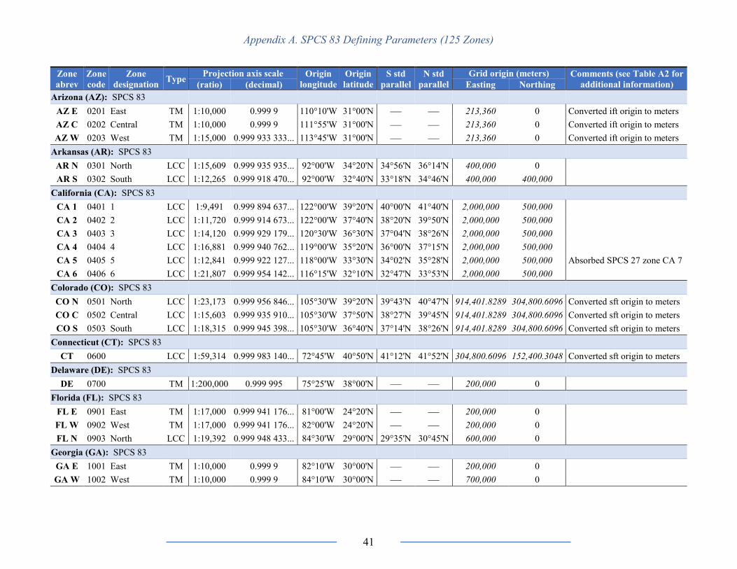
Appendix A. SPCS 83 Defining Parameters (125 Zones)
41
Zone
abrev
Zone
code
Zone
designation Type
Projection axis scale Origin
longitude
Origin
latitude
S std
parallel
N std
parallel
Grid origin (meters) Comments (see Table A2 for
additional information) (ratio) (decimal) Easting Northing
Arizona (AZ): SPCS 83
AZ E 0201 East TM 1:10,000 0.999 9 110°10'W 31°00'N — — 213,360 0 Converted ift origin to meters
AZ C 0202 Central TM 1:10,000 0.999 9 111°55'W 31°00'N — — 213,360 0 Converted ift origin to meters
AZ W 0203 West TM 1:15,000 0.999 933 333... 113°45'W 31°00'N — — 213,360 0 Converted ift origin to meters
Arkansas (AR): SPCS 83
AR N 0301 North LCC 1:15,609 0.999 935 935... 92°00'W 34°20'N 34°56'N 36°14'N 400,000 0
AR S 0302 South LCC 1:12,265 0.999 918 470... 92°00'W 32°40'N 33°18'N 34°46'N 400,000 400,000
California (CA): SPCS 83
CA 1 0401 1 LCC 1:9,491 0.999 894 637... 122°00'W 39°20'N 40°00'N 41°40'N 2,000,000 500,000
CA 2 0402 2 LCC 1:11,720 0.999 914 673... 122°00'W 37°40'N 38°20'N 39°50'N 2,000,000 500,000
CA 3 0403 3 LCC 1:14,120 0.999 929 179... 120°30'W 36°30'N 37°04'N 38°26'N 2,000,000 500,000
CA 4 0404 4 LCC 1:16,881 0.999 940 762... 119°00'W 35°20'N 36°00'N 37°15'N 2,000,000 500,000
CA 5 0405 5 LCC 1:12,841 0.999 922 127... 118°00'W 33°30'N 34°02'N 35°28'N 2,000,000 500,000 Absorbed SPCS 27 zone CA 7
CA 6 0406 6 LCC 1:21,807 0.999 954 142... 116°15'W 32°10'N 32°47'N 33°53'N 2,000,000 500,000
Colorado (CO): SPCS 83
CO N 0501 North LCC 1:23,173 0.999 956 846... 105°30'W 39°20'N 39°43'N 40°47'N 914,401.8289 304,800.6096 Converted sft origin to meters
CO C 0502 Central LCC 1:15,603 0.999 935 910... 105°30'W 37°50'N 38°27'N 39°45'N 914,401.8289 304,800.6096 Converted sft origin to meters
CO S 0503 South LCC 1:18,315 0.999 945 398... 105°30'W 36°40'N 37°14'N 38°26'N 914,401.8289 304,800.6096 Converted sft origin to meters
Connecticut (CT): SPCS 83
CT 0600 LCC 1:59,314 0.999 983 140... 72°45'W 40°50'N 41°12'N 41°52'N 304,800.6096 152,400.3048 Converted sft origin to meters
Delaware (DE): SPCS 83
DE 0700 TM 1:200,000 0.999 995 75°25'W 38°00'N — — 200,000 0
Florida (FL): SPCS 83
FL E 0901 East TM 1:17,000 0.999 941 176... 81°00'W 24°20'N — — 200,000 0
FL W 0902 West TM 1:17,000 0.999 941 176... 82°00'W 24°20'N — — 200,000 0
FL N 0903 North LCC 1:19,392 0.999 948 433... 84°30'W 29°00'N 29°35'N 30°45'N 600,000 0
Georgia (GA): SPCS 83
GA E 1001 East TM 1:10,000 0.999 9 82°10'W 30°00'N — — 200,000 0
GA W 1002 West TM 1:10,000 0.999 9 84°10'W 30°00'N — — 700,000 0

Appendix A. SPCS 83 Defining Parameters (125 Zones)
42
Zone
abrev
Zone
code
Zone
designation Type
Projection axis scale Origin
longitude
Origin
latitude
S std
parallel
N std
parallel
Grid origin (meters) Comments (see Table A2 for
additional information) (ratio) (decimal) Easting Northing
Hawaii (HI): SPCS 83
HI 1 5101 1 TM 1:30,000 0.999 966 667... 155°30'W 18°50'N — — 500,000 0
HI 2 5102 2 TM 1:30,000 0.999 966 667... 156°40'W 20°20'N — — 500,000 0
HI 3 5103 3 TM 1:100,000 0.999 99 158°00'W 21°10'N — — 500,000 0
HI 4 5104 4 TM 1:100,000 0.999 99 159°30'W 21°50'N — — 500,000 0
HI 5 5105 5 TM Exact 1 160°10'W 21°40'N — — 500,000 0
Idaho (ID): SPCS 83
ID E 1101 East TM 1:19,000 0.999 947 368... 112°10'W 41°40'N — — 200,000 0
ID C 1102 Central TM 1:19,000 0.999 947 368... 114°00'W 41°40'N — — 500,000 0
ID W 1103 West TM 1:15,000 0.999 933 333... 115°45'W 41°40'N — — 800,000 0
Illinois (IL): SPCS 83
IL E 1201 East TM 1:40,000 0.999 975 88°20'W 36°40'N — — 300,000 0
IL W 1202 West TM 1:17,000 0.999 941 176... 90°10'W 36°40'N — — 700,000 0
Indiana (IN): SPCS 83
IN E 1301 East TM 1:30,000 0.999 966 667... 85°40'W 37°30'N — — 100,000 250,000
IN W 1302 West TM 1:30,000 0.999 966 667... 87°05'W 37°30'N — — 900,000 250,000
Iowa (IA): SPCS 83
IA N 1401 North LCC 1:18,304 0.999 945 368... 93°30'W 41°30'N 42°04'N 43°16'N 1,500,000 1,000,000
IA S 1402 South LCC 1:19,368 0.999 948 370... 93°30'W 40°00'N 40°37'N 41°47'N 500,000 0
Kansas (KS): SPCS 83
KS N 1501 North LCC 1:23,176 0.999 956 851... 98°00'W 38°20'N 38°43'N 39°47'N 400,000 0
KS S 1502 South LCC 1:15,605 0.999 935 918... 98°30'W 36°40'N 37°16'N 38°34'N 400,000 400,000
Kentucky (KY): SPCS 83
KY1Z 1600 One LCC 1:10,520 0.999 904 942... 85°45'W 36°20'N 37°05'N 38°40'N 1,500,000 1,000,000 Statewide zone added in 2001
KY N 1601 North LCC 1:26,371 0.999 962 080... 84°15'W 37°30'N 37°58'N 38°58'N 500,000 0
KY S 1602 South LCC 1:18,316 0.999 945 402... 85°45'W 36°20'N 36°44'N 37°56'N 500,000 500,000
Louisiana (LA): SPCS 83
LA N 1701 North LCC 1:11,729 0.999 914 741... 92°30'W 30°30'N 31°10'N 32°40'N 1,000,000 0
LA S 1702 South LCC 1:13,467 0.999 925 745... 91°20'W 28°30'N 29°18'N 30°42'N 1,000,000 0
LASH 1703 Offshore LCC 1:9,505 0.999 894 794... 91°20'W 25°30'N 26°10'N 27°50'N 1,000,000 0
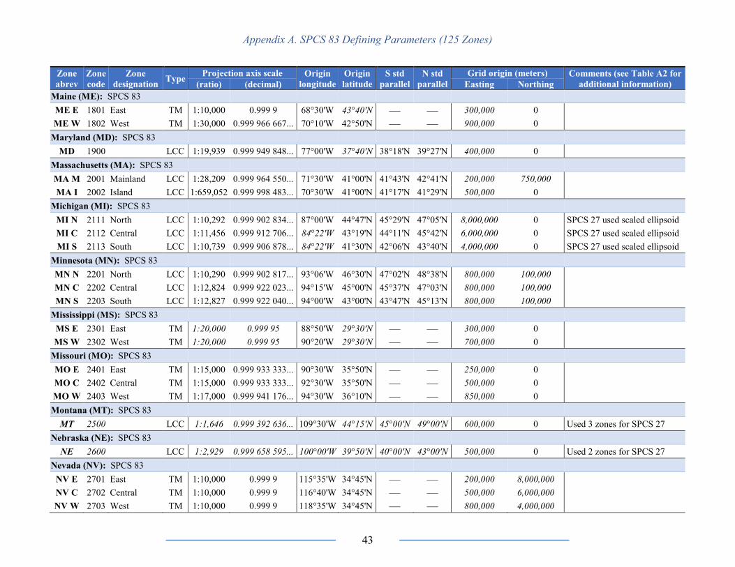
Appendix A. SPCS 83 Defining Parameters (125 Zones)
43
Zone
abrev
Zone
code
Zone
designation Type
Projection axis scale Origin
longitude
Origin
latitude
S std
parallel
N std
parallel
Grid origin (meters) Comments (see Table A2 for
additional information) (ratio) (decimal) Easting Northing
Maine (ME): SPCS 83
ME E 1801 East TM 1:10,000 0.999 9 68°30'W 43°40'N — — 300,000 0
ME W 1802 West TM 1:30,000 0.999 966 667... 70°10'W 42°50'N — — 900,000 0
Maryland (MD): SPCS 83
MD 1900 LCC 1:19,939 0.999 949 848... 77°00'W 37°40'N 38°18'N 39°27'N 400,000 0
Massachusetts (MA): SPCS 83
MA M 2001 Mainland LCC 1:28,209 0.999 964 550... 71°30'W 41°00'N 41°43'N 42°41'N 200,000 750,000
MA I 2002 Island LCC 1:659,052 0.999 998 483... 70°30'W 41°00'N 41°17'N 41°29'N 500,000 0
Michigan (MI): SPCS 83
MI N 2111 North LCC 1:10,292 0.999 902 834... 87°00'W 44°47'N 45°29'N 47°05'N 8,000,000 0 SPCS 27 used scaled ellipsoid
MI C 2112 Central LCC 1:11,456 0.999 912 706... 84°22'W 43°19'N 44°11'N 45°42'N 6,000,000 0 SPCS 27 used scaled ellipsoid
MI S 2113 South LCC 1:10,739 0.999 906 878... 84°22'W 41°30'N 42°06'N 43°40'N 4,000,000 0 SPCS 27 used scaled ellipsoid
Minnesota (MN): SPCS 83
MN N 2201 North LCC 1:10,290 0.999 902 817... 93°06'W 46°30'N 47°02'N 48°38'N 800,000 100,000
MN C 2202 Central LCC 1:12,824 0.999 922 023... 94°15'W 45°00'N 45°37'N 47°03'N 800,000 100,000
MN S 2203 South LCC 1:12,827 0.999 922 040... 94°00'W 43°00'N 43°47'N 45°13'N 800,000 100,000
Mississippi (MS): SPCS 83
MS E 2301 East TM 1:20,000 0.999 95 88°50'W 29°30'N — — 300,000 0
MS W 2302 West TM 1:20,000 0.999 95 90°20'W 29°30'N — — 700,000 0
Missouri (MO): SPCS 83
MO E 2401 East TM 1:15,000 0.999 933 333... 90°30'W 35°50'N — — 250,000 0
MO C 2402 Central TM 1:15,000 0.999 933 333... 92°30'W 35°50'N — — 500,000 0
MO W 2403 West TM 1:17,000 0.999 941 176... 94°30'W 36°10'N — — 850,000 0
Montana (MT): SPCS 83
MT 2500 LCC 1:1,646 0.999 392 636... 109°30'W 44°15'N 45°00'N 49°00'N 600,000 0 Used 3 zones for SPCS 27
Nebraska (NE): SPCS 83
NE 2600 LCC 1:2,929 0.999 658 595... 100°00'W 39°50'N 40°00'N 43°00'N 500,000 0 Used 2 zones for SPCS 27
Nevada (NV): SPCS 83
NV E 2701 East TM 1:10,000 0.999 9 115°35'W 34°45'N — — 200,000 8,000,000
NV C 2702 Central TM 1:10,000 0.999 9 116°40'W 34°45'N — — 500,000 6,000,000
NV W 2703 West TM 1:10,000 0.999 9 118°35'W 34°45'N — — 800,000 4,000,000

Appendix A. SPCS 83 Defining Parameters (125 Zones)
44
Zone
abrev
Zone
code
Zone
designation Type
Projection axis scale Origin
longitude
Origin
latitude
S std
parallel
N std
parallel
Grid origin (meters) Comments (see Table A2 for
additional information) (ratio) (decimal) Easting Northing
New Hampshire (NH): SPCS 83
NH 2800 TM 1:30,000 0.999 966 667... 71°40'W 42°30'N — — 300,000 0
New Jersey (NJ): SPCS 83
NJ 2900 TM 1:10,000 0.999 9 74°30'W 38°50'N — — 150,000 0 Identical to NY E zone (3101)
New Mexico (NM): SPCS 83
NM E 3001 East TM 1:11,000 0.999 909 091... 104°20'W 31°00'N — — 165,000 0
NM C 3002 Central TM 1:10,000 0.999 9 106°15'W 31°00'N — — 500,000 0 Changed SPCS 27 zone
boundary (Cibola County) NM W 3003 West TM 1:12,000 0.999 916 667... 107°50'W 31°00'N — — 830,000 0
New York (NY): SPCS 83
NY E 3101 East TM 1:10,000 0.999 9 74°30'W 38°50'N — — 150,000 0 Identical to NJ zone (2900)
NY C 3102 Central TM 1:16,000 0.999 937 5 76°35'W 40°00'N — — 250,000 0
NY W 3103 West TM 1:16,000 0.999 937 5 78°35'W 40°00'N — — 350,000 0
NY L 3104 Long Island LCC 1:196,094 0.999 994 900... 74°00'W 40°10'N 40°40'N 41°02'N 300,000 0
North Carolina (NC): SPCS 83
NC 3200 LCC 1:7,849 0.999 872 592... 79°00'W 33°45'N 34°20'N 36°10'N 609,601.22 0 Converted sft origin to meters
North Dakota (ND): SPCS 83
ND N 3301 North LCC 1:15,587 0.999 935 842... 100°30'W 47°00'N 47°26'N 48°44'N 600,000 0
ND S 3302 South LCC 1:15,589 0.999 935 852... 100°30'W 45°40'N 46°11'N 47°29'N 600,000 0
Ohio (OH): SPCS 83
OH N 3401 North LCC 1:16,431 0.999 939 140... 82°30'W 39°40'N 40°26'N 41°42'N 600,000 0
OH S 3402 South LCC 1:15,602 0.999 935 908... 82°30'W 38°00'N 38°44'N 40°02'N 600,000 0
Oklahoma (OK): SPCS 83
OK N 3501 North LCC 1:18,318 0.999 945 409... 98°00'W 35°00'N 35°34'N 36°46'N 600,000 0
OK S 3502 South LCC 1:15,611 0.999 935 942... 98°00'W 33°20'N 33°56'N 35°14'N 600,000 0
Oregon (OR): SPCS 83
OR N 3601 North LCC 1:9,486 0.999 894 583... 120°30'W 43°40'N 44°20'N 46°00'N 2,500,000 0
OR S 3602 South LCC 1:9,488 0.999 894 608... 120°30'W 41°40'N 42°20'N 44°00'N 1,500,000 0
Pennsylvania (PA): SPCS 83
PA N 3701 North LCC 1:23,170 0.999 956 840... 77°45'W 40°10'N 40°53'N 41°57'N 600,000 0
PA S 3702 South LCC 1:24,691 0.999 959 500... 77°45'W 39°20'N 39°56'N 40°58'N 600,000 0

Appendix A. SPCS 83 Defining Parameters (125 Zones)
45
Zone
abrev
Zone
code
Zone
designation Type
Projection axis scale Origin
longitude
Origin
latitude
S std
parallel
N std
parallel
Grid origin (meters) Comments (see Table A2 for
additional information) (ratio) (decimal) Easting Northing
Rhode Island (RI): SPCS 83
RI 3800 TM 1:160,000 0.999 993 75 71°30'W 41°05'N — — 100,000 0
South Carolina (SC): SPCS 83
SC 3900 LCC 1:4,846 0.999 793 657... 81°00'W 31°50'N 32°30'N 34°50'N 609,600 0 Used 2 zones for SPCS 27
South Dakota (SD): SPCS 83
SD N 4001 North LCC 1:16,424 0.999 939 112... 100°00'W 43°50'N 44°25'N 45°41'N 600,000 0
SD S 4002 South LCC 1:10,738 0.999 906 870... 100°20'W 42°20'N 42°50'N 44°24'N 600,000 0
Tennessee (TN): SPCS 83
TN 4100 LCC 1:19,380 0.999 948 401... 86°00'W 34°20'N 35°15'N 36°25'N 600,000 0
Texas (TX): SPCS 83
TX N 4201 North LCC 1:11,220 0.999 910 876... 101°30'W 34°00'N 34°39'N 36°11'N 200,000 1,000,000
TXNC 4202 North Central LCC 1:7,851 0.999 872 623... 98°30'W 31°40'N 32°08'N 33°58'N 600,000 2,000,000
TX C 4203 Central LCC 1:8,456 0.999 881 744... 100°20'W 29°40'N 30°07'N 31°53'N 700,000 3,000,000
TXSC 4204 South Central LCC 1:7,312 0.999 863 244... 99°00'W 27°50'N 28°23'N 30°17'N 600,000 4,000,000
TX S 4205 South LCC 1:9,505 0.999 894 794... 98°30'W 25°40'N 26°10'N 27°50'N 300,000 5,000,000
Utah (UT): SPCS 83
UT N 4301 North LCC 1:23,170 0.999 956 841... 111°30'W 40°20'N 40°43'N 41°47'N 500,000 1,000,000
UT C 4302 Central LCC 1:9,883 0.999 898 821... 111°30'W 38°20'N 39°01'N 40°39'N 500,000 2,000,000
UT S 4303 South LCC 1:20,533 0.999 951 297... 111°30'W 36°40'N 37°13'N 38°21'N 500,000 3,000,000
Vermont (VT): SPCS 83
VT 4400 TM 1:28,000 0.999 964 286... 72°30'W 42°30'N — — 500,000 0
Virginia (VA): SPCS 83
VA N 4501 North LCC 1:19,374 0.999 948 385... 78°30'W 37°40'N 38°02'N 39°12'N 3,500,000 2,000,000
VA S 4502 South LCC 1:18,315 0.999 945 401... 78°30'W 36°20'N 36°46'N 37°58'N 3,500,000 1,000,000
Washington (WA): SPCS 83
WA N 4601 North LCC 1:17,317 0.999 942 253... 120°50'W 47°00'N 47°30'N 48°44'N 500,000 0 Changed SPCS 27 zone
boundary (Grant County) WA S 4602 South LCC 1:11,709 0.999 914 598... 120°30'W 45°20'N 45°50'N 47°20'N 500,000 0
West Virginia (WV): SPCS 83
WV N 4701 North LCC 1:16,875 0.999 940 741... 79°30'W 38°30'N 39°00'N 40°15'N 600,000 0
WV S 4702 South LCC 1:13,455 0.999 925 678... 81°00'W 37°00'N 37°29'N 38°53'N 600,000 0

Appendix A. SPCS 83 Defining Parameters (125 Zones)
46
Zone
abrev
Zone
code
Zone
designation Type
Projection axis scale Origin
longitude
Origin
latitude
S std
parallel
N std
parallel
Grid origin (meters) Comments (see Table A2 for
additional information) (ratio) (decimal) Easting Northing
Wisconsin (WI): SPCS 83
WI N 4801 North LCC 1:18,297 0.999 945 345... 90°00'W 45°10'N 45°34'N 46°46'N 600,000 0
WI C 4802 Central LCC 1:16,865 0.999 940 705... 90°00'W 43°50'N 44°15'N 45°30'N 600,000 0
WI S 4803 South LCC 1:14,825 0.999 932 547... 90°00'W 42°00'N 42°44'N 44°04'N 600,000 0
Wyoming (WY): SPCS 83
WY E 4901 East TM 1:16,000 0.999 937 5 105°10'W 40°30'N — — 200,000 0
WYEC 4902 East Central TM 1:16,000 0.999 937 5 107°20'W 40°30'N — — 400,000 100,000
WYWC 4903 West Central TM 1:16,000 0.999 937 5 108°45'W 40°30'N — — 600,000 0
WY W 4904 West TM 1:16,000 0.999 937 5 110°05'W 40°30'N — — 800,000 100,000
United States Territories
Puerto Rico and U.S. Virgin Islands (PR and VI): SPCS 83
PRVI 5200 LCC 1:165,138 0.999 993 944... 66°26'W 17°50'N 18°02'N 18°26'N 200,000 200,000 Used 2 zones for SPCS 27
Guam (GU): SPCS 83
GU 5400 TM Exact 1 215°15'W
(144°45'E) 13°30'N — — 100,000 200,000 Zone added in 1995

Appendix A. SPCS 83 Defining Parameters (125 Zones)
47
Table A2. Additional information for “Comments” column of Table A1 for SPCS 83 zones.
State or Territory Zones Additional information
Alaska AK 1
Skew axis azimuth = tan−1 (-¾) = -36°52'11.6315250385". The grid origin is defined at the “natural” origin on the equator of
the “aposphere”, an intermediate surface of rotation with constant total curvature derived from the ellipsoid at the central point
(local origin) of the projection. The ellipsoid is conformally projected onto the aposphere before final projection onto the plane.
See NGS (1986) and Snyder (1987).
Arizona (all zones) AZ E, C, W False easting is exact metric conversion of 700,000 international feet, as defined by Arizona state law.
California CA 5 Includes Los Angeles County, which was zone CA Zone 7 in SPCS 27 (see tables B1 and B2).
Colorado (all zones) CO N, C, S Grid origin is non-exact conversion of U.S. survey feet to meters: false easting = 3,000,000.000 316 sft and false northing =
999,999.999 996 sft (note discrepancy for false easting at fourth decimal place).
Connecticut CT Grid origin is non-exact conversion of U.S. survey feet to meters: false easting = 999,999.999 996 sft and false northing =
499,999.999 998 sft (note coordinate discrepancy at sixth decimal place).
Kentucky KY1Z Statewide zone added in 2001, after publication of SPCS 83 manual (Stem, 1990). Coexists with KY North and South zones.
Michigan (all zones) MI N, C, S
Final version of SPCS 27 used LCC zones created in 1964 by scaling Clarke 1866 ellipsoid semi-major axis by a factor of
exactly 1.0000382 with its flattening held constant (see tables B1 and B2). The SPCS 83 version of these zones are based on
the GRS 80 ellipsoid without any modification.
Montana MT Three zones used for SPCS 27 combined into a single zone for SPCS 83.
Nebraska NE Two zones used for SPCS 27 combined into a single zone for SPCS 83.
New Jersey NJ All projection parameters are identical to NY E zone.
New Mexico (two zones) NM C, W Changed SPCS 27 zone boundary because Cibola County created from westernmost four-fifths of the formerly much larger
Valencia in 1981, with Cibola County in West zone and Valencia County in Central zone.
New York NY E All projection parameters are identical to NJ zone.
North Carolina NC False easting is non-exact conversion of U.S. survey feet to meters: false easting = 2,000,000.0026 sft (note coordinate
discrepancy is at third decimal place).
South Carolina SC Two zones used for SPCS 27 combined into single zone for SPCS 83. False easting is exact metric conversion from 2,000,000
international feet = 1,999,996 sft (exact), which differs from SPCS 27 false easting of 2,000,000 sft by only 4 feet (exact).
Washington (both zones) WA N, S Changed SPCS 27 zone boundary in Grant County by having it follow latitude 47°30'N rather than the county boundary.
Puerto Rico & Virgin Is. PRVI Two zones used for SPCS 27 combined into a single zone for SPCS 83 (SPCS 27 zones identical except for false northing).
Guam GU Zone added in 1995, after publication of SPCS 83 manual (Stem, 1990), per Guam Annotated Code (Guam Compiler of Laws,
2017).
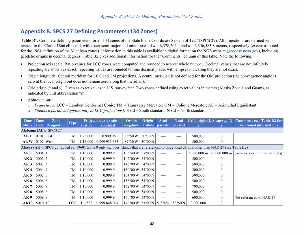
Appendix B. SPCS 27 Defining Parameters (134 Zones)
48
Appendix B. SPCS 27 Defining Parameters (134 Zones)
Table B1. Complete defining parameters for all 134 zones of the State Plane Coordinate System of 1927 (SPCS 27). All projections are defined with
respect to the Clarke 1866 ellipsoid, with exact semi-major and minor axes of a = 6,378,206.4 and b = 6,356,583.8 meters, respectively (except as noted
for the 1964 definition of the Michigan zones). Information in this table is available in digital format on the NGS website (geodesy.noaa.gov), including
geodetic origins in decimal degrees. Table B2 gives additional information for the “Comments” column of this table. Note the following:
• Projection axis scale. Ratio values for LCC zones were computed and rounded to nearest whole number. Decimal values that are not infinitely
repeating are shown as exact; repeating values are rounded to nine decimal places with ellipses indicating they are not exact.
• Origin longitude. Central meridian for LCC and TM projections. A central meridian is not defined for the OM projection (the convergence angle is
zero at the local origin but does not remain zero along that meridian).
• Grid origin (x and y). Given as exact values in U.S. survey feet. Two zones defined using exact values in meters (Alaska Zone 1 and Guam), as
indicated by unit abbreviation “m.”
• Abbreviations.
o Projections: LCC = Lambert Conformal Conic; TM = Transverse Mercator; OM = Oblique Mercator; AE = Azimuthal Equidistant.
o Standard parallels (applies only to LCC projections): S std = South standard; N std = North standard
Zone
abrev
Zone
code
Zone
designation Type
Projection axis scale Origin
longitude
Origin
latitude
S std
parallel
N std
parallel
Grid origin (U.S. survey ft) Comments (see Table B2 for
additional information) (ratio) (decimal) x y
Alabama (AL): SPCS 27
AL E 0101 East TM 1:25,000 0.999 96 85°50'W 30°30'N — — 500,000 0
AL W 0102 West TM 1:15,000 0.999 933 333... 87°30'W 30°00'N — — 500,000 0
Alaska (AK): SPCS 27 (added ca. 1960); Zone 9 only includes islands that are referenced to three local datums other than NAD 27 (see Table B2)
AK 1 5001 1 OM 1:10,000 0.999 9 133°40'W 57°00'N — — 5,000,000 m -5,000,000 m Skew axis azimuth = tan−1 (-¾)
AK 2 5002 2 TM 1:10,000 0.999 9 142°00'W 54°00'N — — 500,000 0
AK 3 5003 3 TM 1:10,000 0.999 9 146°00'W 54°00'N — — 500,000 0
AK 4 5004 4 TM 1:10,000 0.999 9 150°00'W 54°00'N — — 500,000 0
AK 5 5005 5 TM 1:10,000 0.999 9 154°00'W 54°00'N — — 500,000 0
AK 6 5006 6 TM 1:10,000 0.999 9 158°00'W 54°00'N — — 500,000 0
AK 7 5007 7 TM 1:10,000 0.999 9 162°00'W 54°00'N — — 700,000 0
AK 8 5008 8 TM 1:10,000 0.999 9 166°00'W 54°00'N — — 500,000 0
AK 9 5009 9 TM 1:10,000 0.999 9 170°00'W 54°00'N — — 600,000 0 Not referenced to NAD 27
AK10 5010 10 LCC 1:6,582 0.999 848 064... 176°00'W 51°00'N 51°50'N 53°50'N 3,000,000 0

Appendix B. SPCS 27 Defining Parameters (134 Zones)
49
Zone
abrev
Zone
code
Zone
designation Type
Projection axis scale Origin
longitude
Origin
latitude
S std
parallel
N std
parallel
Grid origin (U.S. survey ft) Comments (see Table B2 for
additional information) (ratio) (decimal) x y
Arizona (AZ) ): SPCS 27
AZ E 0201 East TM 1:10,000 0.999 9 110°10'W 31°00'N — — 500,000 0
AZ C 0202 Central TM 1:10,000 0.999 9 111°55'W 31°00'N — — 500,000 0
AZ W 0203 West TM 1:15,000 0.999 933 333... 113°45'W 31°00'N — — 500,000 0
Arkansas (AR): SPCS 27
AR N 0301 North LCC 1:15,610 0.999 935 939... 92°00'W 34°20'N 34°56'N 36°14'N 2,000,000 0
AR S 0302 South LCC 1:12,266 0.999 918 474... 92°00'W 32°40'N 33°18'N 34°46'N 2,000,000 0
California (CA): SPCS 27
CA 1 0401 1 LCC 1:9,491 0.999 894 641... 122°00'W 39°20'N 40°00'N 41°40'N 2,000,000 0
CA 2 0402 2 LCC 1:11,720 0.999 914 677... 122°00'W 37°40'N 38°20'N 39°50'N 2,000,000 0
CA 3 0403 3 LCC 1:14,121 0.999 929 182... 120°30'W 36°30'N 37°04'N 38°26'N 2,000,000 0
CA 4 0404 4 LCC 1:16,882 0.999 940 765... 119°00'W 35°20'N 36°00'N 37°15'N 2,000,000 0
CA 5 0405 5 LCC 1:12,842 0.999 922 131... 118°00'W 33°30'N 34°02'N 35°28'N 2,000,000 0
CA 6 0406 6 LCC 1:21,808 0.999 954 145... 116°15'W 32°10'N 32°47'N 33°53'N 2,000,000 0
CA 7 0407 7 LCC 1:87,223 0.999 988 535... 118°20'W 34°08'N 33°52'N 34°25'N 4,186,692.58 4,160,926.74 LA County (added by 1945)
Colorado (CO): SPCS 27
CO N 0501 North LCC 1:23,174 0.999 956 848... 105°30'W 39°20'N 39°43'N 40°47'N 2,000,000 0
CO C 0502 Central LCC 1:15,604 0.999 935 913... 105°30'W 37°50'N 38°27'N 39°45'N 2,000,000 0
CO S 0503 South LCC 1:18,315 0.999 945 401... 105°30'W 36°40'N 37°14'N 38°26'N 2,000,000 0
Connecticut (CT): SPCS 27
CT 0600 LCC 1:59,316 0.999 983 141... 72°45'W 40°50'N 41°12'N 41°52'N 600,000 0
Delaware (DE): SPCS 27
DE 0700 TM 1:200,000 0.999 995 75°25'W 38°00'N — — 500,000 0
Florida (FL): SPCS 27
FL E 0901 East TM 1:17,000 0.999 941 176... 81°00'W 24°20'N — — 500,000 0
FL W 0902 West TM 1:17,000 0.999 941 176... 82°00'W 24°20'N — — 500,000 0
FL N 0903 North LCC 1:19,393 0.999 948 436... 84°30'W 29°00'N 29°35'N 30°45'N 2,000,000 0
Georgia (GA): SPCS 27
GA E 1001 East TM 1:10,000 0.999 9 82°10'W 30°00'N — — 500,000 0
GA W 1002 West TM 1:10,000 0.999 9 84°10'W 30°00'N — — 500,000 0

Appendix B. SPCS 27 Defining Parameters (134 Zones)
50
Zone
abrev
Zone
code
Zone
designation Type
Projection axis scale Origin
longitude
Origin
latitude
S std
parallel
N std
parallel
Grid origin (U.S. survey ft) Comments (see Table B2 for
additional information) (ratio) (decimal) x y
Hawaii (HI): SPCS 27 (added ca. 1960; referenced to Old Hawaiian Datum)
HI 1 5101 1 TM 1:30,000 0.999 966 667... 155°30'W 18°50'N — — 500,000 0
HI 2 5102 2 TM 1:30,000 0.999 966 667... 156°40'W 20°20'N — — 500,000 0
HI 3 5103 3 TM 1:100,000 0.999 99 158°00'W 21°10'N — — 500,000 0
HI 4 5104 4 TM 1:100,000 0.999 99 159°30'W 21°50'N — — 500,000 0
HI 5 5105 5 TM Exact 1 160°10'W 21°40'N — — 500,000 0
Idaho (ID): SPCS 27
ID E 1101 East TM 1:19,000 0.999 947 368... 112°10'W 41°40'N — — 500,000 0
ID C 1102 Central TM 1:19,000 0.999 947 368... 114°00'W 41°40'N — — 500,000 0
ID W 1103 West TM 1:15,000 0.999 933 333... 115°45'W 41°40'N — — 500,000 0
Illinois (IL): SPCS 27
IL E 1201 East TM 1:40,000 0.999 975 88°20'W 36°40'N — — 500,000 0
IL W 1202 West TM 1:17,000 0.999 941 176... 90°10'W 36°40'N — — 500,000 0
Indiana (IN): SPCS 27
IN E 1301 East TM 1:30,000 0.999 966 667... 85°40'W 37°30'N — — 500,000 0
IN W 1302 West TM 1:30,000 0.999 966 667... 87°05'W 37°30'N — — 500,000 0
Iowa (IA): SPCS 27
IA N 1401 North LCC 1:18,305 0.999 945 370... 93°30'W 41°30'N 42°04'N 43°16'N 2,000,000 0
IA S 1402 South LCC 1:19,369 0.999 948 372... 93°30'W 40°00'N 40°37'N 41°47'N 2,000,000 0
Kansas (KS): SPCS 27
KS N 1501 North LCC 1:23,177 0.999 956 853... 98°00'W 38°20'N 38°43'N 39°47'N 2,000,000 0
KS S 1502 South LCC 1:15,606 0.999 935 921... 98°30'W 36°40'N 37°16'N 38°34'N 2,000,000 0
Kentucky (KY): SPCS 27
KY N 1601 North LCC 1:26,372 0.999 962 081... 84°15'W 37°30'N 37°58'N 38°58'N 2,000,000 0
KY S 1602 South LCC 1:18,316 0.999 945 404... 85°45'W 36°20'N 36°44'N 37°56'N 2,000,000 0
Louisiana (LA): SPCS 27
LA N 1701 North LCC 1:11,730 0.999 914 746... 92°30'W 30°40'N 31°10'N 32°40'N 2,000,000 0
LA S 1702 South LCC 1:13,468 0.999 925 749... 91°20'W 28°40'N 29°18'N 30°42'N 2,000,000 0
LASH 1703 Offshore LCC 1:9,506 0.999 894 800... 91°20'W 25°40'N 26°10'N 27°50'N 2,000,000 0 Established in 1968
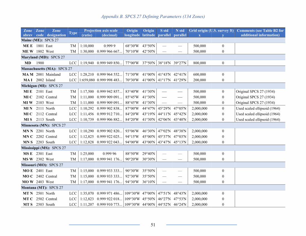
Appendix B. SPCS 27 Defining Parameters (134 Zones)
51
Zone
abrev
Zone
code
Zone
designation Type
Projection axis scale Origin
longitude
Origin
latitude
S std
parallel
N std
parallel
Grid origin (U.S. survey ft) Comments (see Table B2 for
additional information) (ratio) (decimal) x y
Maine (ME): SPCS 27
ME E 1801 East TM 1:10,000 0.999 9 68°30'W 43°50'N — — 500,000 0
ME W 1802 West TM 1:30,000 0.999 966 667... 70°10'W 42°50'N — — 500,000 0
Maryland (MD): SPCS 27
MD 1900 LCC 1:19,940 0.999 949 850... 77°00'W 37°50'N 38°18'N 39°27'N 800,000 0
Massachusetts (MA): SPCS 27
MA M 2001 Mainland LCC 1:28,210 0.999 964 552... 71°30'W 41°00'N 41°43'N 42°41'N 600,000 0
MA I 2002 Island LCC 1:659,080 0.999 998 483... 70°30'W 41°00'N 41°17'N 41°29'N 200,000 0
Michigan (MI): SPCS 27
MI E 2101 East TM 1:17,500 0.999 942 857... 83°40'W 41°30'N — — 500,000 0 Original SPCS 27 (1934)
MI C 2102 Central TM 1:11,000 0.999 909 091... 85°45'W 41°30'N — — 500,000 0 Original SPCS 27 (1934)
MI W 2103 West TM 1:11,000 0.999 909 091... 88°45'W 41°30'N — — 500,000 0 Original SPCS 27 (1934)
MI N 2111 North LCC 1:10,292 0.999 902 838... 87°00'W 44°47'N 45°29'N 47°05'N 2,000,000 0 Used scaled ellipsoid (1964)
MI C 2112 Central LCC 1:11,456 0.999 912 710... 84°20'W 43°19'N 44°11'N 45°42'N 2,000,000 0 Used scaled ellipsoid (1964)
MI S 2113 South LCC 1:10,739 0.999 906 882... 84°20'W 41°30'N 42°06'N 43°40'N 2,000,000 0 Used scaled ellipsoid (1964)
Minnesota (MN): SPCS 27
MN N 2201 North LCC 1:10,290 0.999 902 820... 93°06'W 46°30'N 47°02'N 48°38'N 2,000,000 0
MN C 2202 Central LCC 1:12,825 0.999 922 025... 94°15'W 45°00'N 45°37'N 47°03'N 2,000,000 0
MN S 2203 South LCC 1:12,828 0.999 922 043... 94°00'W 43°00'N 43°47'N 45°13'N 2,000,000 0
Mississippi (MS): SPCS 27
MS E 2301 East TM 1:25,000 0.999 96 88°50'W 29°40'N — — 500,000 0
MS W 2302 West TM 1:17,000 0.999 941 176... 90°20'W 30°30'N — — 500,000 0
Missouri (MO): SPCS 27
MO E 2401 East TM 1:15,000 0.999 933 333... 90°30'W 35°50'N — — 500,000 0
MO C 2402 Central TM 1:15,000 0.999 933 333... 92°30'W 35°50'N — — 500,000 0
MO W 2403 West TM 1:17,000 0.999 941 176... 94°30'W 36°10'N — — 500,000 0
Montana (MT): SPCS 27
MT N 2501 North LCC 1:35,070 0.999 971 486... 109°30'W 47°00'N 47°51'N 48°43'N 2,000,000 0
MT C 2502 Central LCC 1:12,823 0.999 922 018... 109°30'W 45°50'N 46°27'N 47°53'N 2,000,000 0
MT S 2503 South LCC 1:11,207 0.999 910 773... 109°30'W 44°00'N 44°52'N 46°24'N 2,000,000 0

Appendix B. SPCS 27 Defining Parameters (134 Zones)
52
Zone
abrev
Zone
code
Zone
designation Type
Projection axis scale Origin
longitude
Origin
latitude
S std
parallel
N std
parallel
Grid origin (U.S. survey ft) Comments (see Table B2 for
additional information) (ratio) (decimal) x y
Nebraska (NE): SPCS 27
NE N 2601 North LCC 1:28,210 0.999 964 551... 100°00'W 41°20'N 41°51'N 42°49'N 2,000,000 0
NE S 2602 South LCC 1:12,833 0.999 922 075... 99°30'W 39°40'N 40°17'N 41°43'N 2,000,000 0
Nevada (NV): SPCS 27
NV E 2701 East TM 1:10,000 0.999 9 115°35'W 34°45'N — — 500,000 0
NV C 2702 Central TM 1:10,000 0.999 9 116°40'W 34°45'N — — 500,000 0
NV W 2703 West TM 1:10,000 0.999 9 118°35'W 34°45'N — — 500,000 0
New Hampshire (NH): SPCS 27
NH 2800 TM 1:30,000 0.999 966 667... 71°40'W 42°30'N — — 500,000 0
New Jersey (NJ): SPCS 27
NJ 2900 TM 1:40,000 0.999 975 74°40'W 38°50'N — — 2,000,000 0
New Mexico (NM): SPCS 27
NM E 3001 East TM 1:11,000 0.999 909 091... 104°20'W 31°00'N — — 500,000 0
NM C 3002 Central TM 1:10,000 0.999 9 106°15'W 31°00'N — — 500,000 0
NM W 3003 West TM 1:12,000 0.999 916 667... 107°50'W 31°00'N — — 500,000 0
New York (NY): SPCS 27
NY E 3101 East TM 1:30,000 0.999 966 667... 74°20'W 40°00'N — — 500,000 0
NY C 3102 Central TM 1:16,000 0.999 937 5 76°35'W 40°00'N — — 500,000 0
NY W 3103 West TM 1:16,000 0.999 937 5 78°35'W 40°00'N — — 500,000 0
NY L 3104 Long Island LCC 1:196,102 0.999 994 901... 74°00'W 40°30'N 40°40'N 41°02'N 2,000,000 100,000
North Carolina (NC): SPCS 27
NC 3200 LCC 1:7,849 0.999 872 598... 79°00'W 33°45'N 34°20'N 36°10'N 2,000,000 0
North Dakota (ND): SPCS 27
ND N 3301 North LCC 1:15,587 0.999 935 844... 100°30'W 47°00'N 47°26'N 48°44'N 2,000,000 0
ND S 3302 South LCC 1:15,589 0.999 935 854... 100°30'W 45°40'N 46°11'N 47°29'N 2,000,000 0
Ohio (OH): SPCS 27
OH N 3401 North LCC 1:16,432 0.999 939 143... 82°30'W 39°40'N 40°26'N 41°42'N 2,000,000 0
OH S 3402 South LCC 1:15,603 0.999 935 911... 82°30'W 38°00'N 38°44'N 40°02'N 2,000,000 0
Oklahoma (OK): SPCS 27
OK N 3501 North LCC 1:18,319 0.999 945 411... 98°00'W 35°00'N 35°34'N 36°46'N 2,000,000 0
OK S 3502 South LCC 1:15,612 0.999 935 946... 98°00'W 33°20'N 33°56'N 35°14'N 2,000,000 0
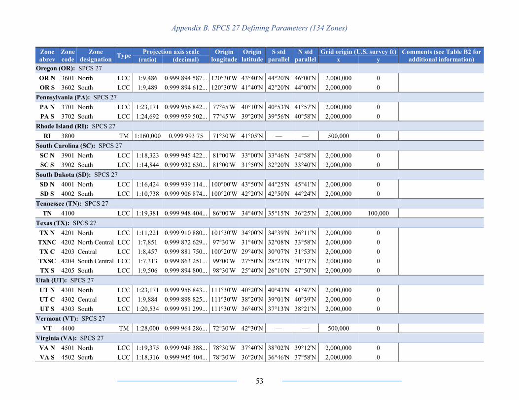
Appendix B. SPCS 27 Defining Parameters (134 Zones)
53
Zone
abrev
Zone
code
Zone
designation Type
Projection axis scale Origin
longitude
Origin
latitude
S std
parallel
N std
parallel
Grid origin (U.S. survey ft) Comments (see Table B2 for
additional information) (ratio) (decimal) x y
Oregon (OR): SPCS 27
OR N 3601 North LCC 1:9,486 0.999 894 587... 120°30'W 43°40'N 44°20'N 46°00'N 2,000,000 0
OR S 3602 South LCC 1:9,489 0.999 894 612... 120°30'W 41°40'N 42°20'N 44°00'N 2,000,000 0
Pennsylvania (PA): SPCS 27
PA N 3701 North LCC 1:23,171 0.999 956 842... 77°45'W 40°10'N 40°53'N 41°57'N 2,000,000 0
PA S 3702 South LCC 1:24,692 0.999 959 502... 77°45'W 39°20'N 39°56'N 40°58'N 2,000,000 0
Rhode Island (RI): SPCS 27
RI 3800 TM 1:160,000 0.999 993 75 71°30'W 41°05'N — — 500,000 0
South Carolina (SC): SPCS 27
SC N 3901 North LCC 1:18,323 0.999 945 422... 81°00'W 33°00'N 33°46'N 34°58'N 2,000,000 0
SC S 3902 South LCC 1:14,844 0.999 932 630... 81°00'W 31°50'N 32°20'N 33°40'N 2,000,000 0
South Dakota (SD): SPCS 27
SD N 4001 North LCC 1:16,424 0.999 939 114... 100°00'W 43°50'N 44°25'N 45°41'N 2,000,000 0
SD S 4002 South LCC 1:10,738 0.999 906 874... 100°20'W 42°20'N 42°50'N 44°24'N 2,000,000 0
Tennessee (TN): SPCS 27
TN 4100 LCC 1:19,381 0.999 948 404... 86°00'W 34°40'N 35°15'N 36°25'N 2,000,000 100,000
Texas (TX): SPCS 27
TX N 4201 North LCC 1:11,221 0.999 910 880... 101°30'W 34°00'N 34°39'N 36°11'N 2,000,000 0
TXNC 4202 North Central LCC 1:7,851 0.999 872 629... 97°30'W 31°40'N 32°08'N 33°58'N 2,000,000 0
TX C 4203 Central LCC 1:8,457 0.999 881 750... 100°20'W 29°40'N 30°07'N 31°53'N 2,000,000 0
TXSC 4204 South Central LCC 1:7,313 0.999 863 251... 99°00'W 27°50'N 28°23'N 30°17'N 2,000,000 0
TX S 4205 South LCC 1:9,506 0.999 894 800... 98°30'W 25°40'N 26°10'N 27°50'N 2,000,000 0
Utah (UT): SPCS 27
UT N 4301 North LCC 1:23,171 0.999 956 843... 111°30'W 40°20'N 40°43'N 41°47'N 2,000,000 0
UT C 4302 Central LCC 1:9,884 0.999 898 825... 111°30'W 38°20'N 39°01'N 40°39'N 2,000,000 0
UT S 4303 South LCC 1:20,534 0.999 951 299... 111°30'W 36°40'N 37°13'N 38°21'N 2,000,000 0
Vermont (VT): SPCS 27
VT 4400 TM 1:28,000 0.999 964 286... 72°30'W 42°30'N — — 500,000 0
Virginia (VA): SPCS 27
VA N 4501 North LCC 1:19,375 0.999 948 388... 78°30'W 37°40'N 38°02'N 39°12'N 2,000,000 0
VA S 4502 South LCC 1:18,316 0.999 945 404... 78°30'W 36°20'N 36°46'N 37°58'N 2,000,000 0

Appendix B. SPCS 27 Defining Parameters (134 Zones)
54
Zone
abrev
Zone
code
Zone
designation Type
Projection axis scale Origin
longitude
Origin
latitude
S std
parallel
N std
parallel
Grid origin (U.S. survey ft) Comments (see Table B2 for
additional information) (ratio) (decimal) x y
Washington (WA): SPCS 27
WA N 4601 North LCC 1:17,318 0.999 942 255... 120°50'W 47°00'N 47°30'N 48°44'N 2,000,000 0 WA S 4602 South LCC 1:11,710 0.999 914 601... 120°30'W 45°20'N 45°50'N 47°20'N 2,000,000 0
West Virginia (WV): SPCS 27
WV N 4701 North LCC 1:16,876 0.999 940 744... 79°30'W 38°30'N 39°00'N 40°15'N 2,000,000 0
WV S 4702 South LCC 1:13,456 0.999 925 682... 81°00'W 37°00'N 37°29'N 38°53'N 2,000,000 0
Wisconsin (WI): SPCS 27
WI N 4801 North LCC 1:18,297 0.999 945 347... 90°00'W 45°10'N 45°34'N 46°46'N 2,000,000 0
WI C 4802 Central LCC 1:16,865 0.999 940 707... 90°00'W 43°50'N 44°15'N 45°30'N 2,000,000 0
WI S 4803 South LCC 1:14,826 0.999 932 550... 90°00'W 42°00'N 42°44'N 44°04'N 2,000,000 0
Wyoming (WY): SPCS 27
WY E 4901 I TM 1:17,000 0.999 941 176... 105°10'W 40°40'N — — 500,000 0
WYEC 4902 II TM 1:17,000 0.999 941 176... 107°20'W 40°40'N — — 500,000 0
WYWC 4903 III TM 1:17,000 0.999 941 176... 108°45'W 40°40'N — — 500,000 0
WY W 4904 IV TM 1:17,000 0.999 941 176... 110°05'W 40°40'N — — 500,000 0
United States Territories
Puerto Rico and U.S. Virgin Islands (PR and VI): SPCS 27 (added between 1945 and 1974; referenced to Puerto Rico Datum of 1940)
PRZ1 5201 Zone 1 LCC 1:165,150 0.999 993 945... 66°26'W 17°50'N 18°02'N 18°26'N 500,000 0
VISX 5202 St. Croix LCC 1:165,150 0.999 993 945... 66°26'W 17°50'N 18°02'N 18°26'N 500,000 100,000
American Samoa (AS): SPCS 27 (added between 1945 and 1974; referenced to American Samoa Datum of 1962)
AS 5300 LCC Exact 1 170°00'W 14°16'S 14°16'S 500,000 312,234.65 One parallel LCC
Guam (GU): SPCS 27 (referenced to 1963 Guam Datum)
GU 5400 AE Not
applicable
Not
applicable
144°44'55.50254"E — — 50,000 m 50,000 m
“Approximate” Azimuthal
Equidistant projection (meters) 13°28'20.87887"N

Appendix B. SPCS 27 Defining Parameters (134 Zones)
55
Table B2. Additional information for “Comments” column of Table B1 for SPCS 27 zones.
State or Territory Zones Additional information
Alaska AK 1
Skew axis azimuth = tan−1 (-¾) = -36°52'11.6315250385". SPCS 27 Fortran code in subroutine “akspec.f” (NGS, 2003) defines
grid origin as exactly 3.28083333333 × (±5,000,000) = ±16,404,166.66665 sft. The grid origin is defined at the “natural” origin on
the equator of the “aposphere”, an intermediate surface of rotation with constant total curvature derived from the ellipsoid at the
central point (local origin) of the projection. The ellipsoid is conformally projected onto the aposphere before final projection onto
the plane. See NGS (1986) and Snyder (1987).
Alaska AK 9
Entire zone consists of islands in the Bering Sea too far from the mainland for connection to the NAD 27 datum. Four islands each
have their own astronomically determined local horizontal datums: the St. Lawrence, St. Matthew, St. Paul, and St. George datums
of 1952 (see Figure 3).
California CA 7
Initially developed in 1938 and added to SPCS 27 by 1945. Grid origin selected such that coordinates were as close as possible to
those of a Polyconic projection referenced to NAD 27 that had been previously defined for part of Los Angeles County. For
SPCS 83, this zone was eliminated and its area included in CA Zone 5.
Louisiana (offshore) LASH
The included area of the Gulf of Mexico was defined as being within 200 miles of the state of Louisiana by state law. The extents
of the zone by positive grid coordinates covers all of the Gulf of Mexico north of 25°40'N latitude, with its south margin
approximately 220 miles (350 kilometers) south of the southernmost part of the Louisiana coast. For SPCS 83, the south edge of
the zone was moved to 25°30'N latitude, approximately 230 miles (370 kilometers) south of the Louisiana coast.
Michigan (all zones) MI E, C, W TM zones created in original 1934 definition, superseded by three LCC zones in 1964.
Michigan (all zones) MI N, C, S
LCC zones created in 1964 by scaling Clarke 1866 ellipsoid semi-major axis by a factor of exactly 1.0000382 with its flattening
held constant (yields scaled ellipsoid axes of a = 6,378,450.047484 meters and b = 6,356,826.621501 meters). The scale factor was
based on a height of 800 feet at 44° latitude to create a reference ellipsoid surface near the topographic surface for Michigan. The
objective was to keep linear distortion at ground within ±100 parts per million (1:10,000) over the entire state.
American Samoa AS One-parallel LCC with false northing of 312,234.65 corresponds to single standard parallel (where scale is exactly 1).
Guam GU Non-conformal “approximate” Azimuthal Equidistant projection. Origin coordinates of latitude 13°28'20.87887"N and longitude
144°44'55.50254"E are for station Agana Monument 1945 based on Guam Datum of 1963 (Claire 1968, p. 35).
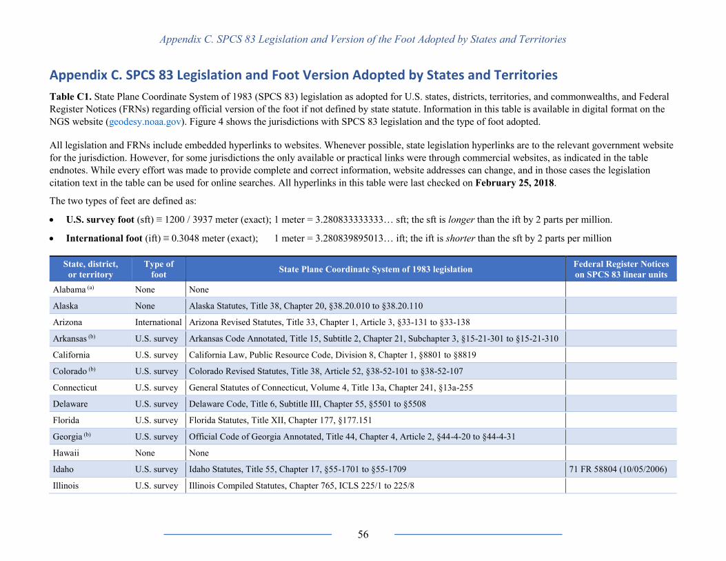
Appendix C. SPCS 83 Legislation and Version of the Foot Adopted by States and Territories
56
Appendix C. SPCS 83 Legislation and Foot Version Adopted by States and Territories
Table C1. State Plane Coordinate System of 1983 (SPCS 83) legislation as adopted for U.S. states, districts, territories, and commonwealths, and Federal
Register Notices (FRNs) regarding official version of the foot if not defined by state statute. Information in this table is available in digital format on the
NGS website (geodesy.noaa.gov). Figure 4 shows the jurisdictions with SPCS 83 legislation and the type of foot adopted.
All legislation and FRNs include embedded hyperlinks to websites. Whenever possible, state legislation hyperlinks are to the relevant government website
for the jurisdiction. However, for some jurisdictions the only available or practical links were through commercial websites, as indicated in the table
endnotes. While every effort was made to provide complete and correct information, website addresses can change, and in those cases the legislation
citation text in the table can be used for online searches. All hyperlinks in this table were last checked on February 25, 2018.
The two types of feet are defined as:
• U.S. survey foot (sft) ≡ 1200 / 3937 meter (exact); 1 meter = 3.280833333333… sft; the sft is longer than the ift by 2 parts per million.
• International foot (ift) ≡ 0.3048 meter (exact); 1 meter = 3.280839895013… ift; the ift is shorter than the sft by 2 parts per million
State, district,
or territory
Type of
foot State Plane Coordinate System of 1983 legislation
Federal Register Notices
on SPCS 83 linear units
Alabama (a) None None
Alaska None Alaska Statutes, Title 38, Chapter 20, §38.20.010 to §38.20.110
Arizona International Arizona Revised Statutes, Title 33, Chapter 1, Article 3, §33-131 to §33-138
Arkansas (b) U.S. survey Arkansas Code Annotated, Title 15, Subtitle 2, Chapter 21, Subchapter 3, §15-21-301 to §15-21-310
California U.S. survey California Law, Public Resource Code, Division 8, Chapter 1, §8801 to §8819
Colorado (b) U.S. survey Colorado Revised Statutes, Title 38, Article 52, §38-52-101 to §38-52-107
Connecticut U.S. survey General Statutes of Connecticut, Volume 4, Title 13a, Chapter 241, §13a-255
Delaware U.S. survey Delaware Code, Title 6, Subtitle III, Chapter 55, §5501 to §5508
Florida U.S. survey Florida Statutes, Title XII, Chapter 177, §177.151
Georgia (b) U.S. survey Official Code of Georgia Annotated, Title 44, Chapter 4, Article 2, §44-4-20 to §44-4-31
Hawaii None None
Idaho U.S. survey Idaho Statutes, Title 55, Chapter 17, §55-1701 to §55-1709 71 FR 58804 (10/05/2006)
Illinois U.S. survey Illinois Compiled Statutes, Chapter 765, ICLS 225/1 to 225/8

Appendix C. SPCS 83 Legislation and Version of the Foot Adopted by States and Territories
57
State, district,
or territory
Type of
foot State Plane Coordinate System of 1983 legislation
Federal Register Notices
on SPCS 83 linear units
Indiana U.S. survey Indiana Code, Title 32, Article 19, Chapters 1 to 4 (IC 32-19-1 to IC 32-19-4)
Iowa U.S. survey Iowa Code, Chapter 355, §355.16 to §355.19 71 FR 58805 (10/05/2006)
Kansas U.S. survey Kansas Statutes, Chapter 58, Article 20a, §58-20a01 to §58-20a07 71 FR 67857 (11/24/2006)
Kentucky U.S. survey Kentucky Revised Statutes, Chapter 1.020
Louisiana U.S. survey Louisiana Revised Statutes, Title 50, Chapter 1
Maine U.S. survey Maine Revised Statutes, Title 33, Chapter 13, §801 to §807 72 FR 70575 (12/12/2007)
Maryland U.S. survey Annotated Code of Maryland, Article - Real Property, Title 14, Subtitle 4, §14-401 to §14-407
Massachusetts U.S. survey General Laws of Massachusetts, Part 1, Title XV, Chapter 97, §8 to §17
Michigan International Michigan Complied Laws, Public Act 9 of 1964, §54.231 to §54.239
Minnesota U.S. survey Minnesota Statutes, Chapter 505, §505.18 to §505.28 72 FR 32287 (06/12/2007)
Mississippi (b) U.S. survey Mississippi Code of 1972 Annotated, Title 89, Chapter 6, §89-6-1 to §89-6-19
Missouri None Revised Statutes of Missouri, Title VI, Chapter 60, §60.401 to §60.491
Montana International Montana Code Annotated, Title 70, Chapter 22, Part 2, §70-22-201 to §70-22-210
Nebraska U.S. survey Nebraska Revised Statutes, Chapter 76, §76-2501 to §76-2506 72 FR 73771 (12/28/2007)
Nevada U.S. survey Nevada Revised Statutes, Chapter 327, §327.005 to §327.090 71 FR 42817 (07/28/2006)
New Hampshire U.S. survey New Hampshire Statutes, Title 1, Chapter 1-A, §1-A:1 to §1-A:5
New Jersey (c) U.S. survey New Jersey General and Permanent Statutes, Title 51, §51:3-7 to §51:3-10 71 FR 42816 (07/28/2006)
New Mexico (c) U.S. survey New Mexico Statutes Annotated, Chapter 47, Article 1, §47-1-49 to §47-1-56
New York (c) U.S. survey Laws of New York, 1995, Chapter 605 [link is to 1995 act showing edits from previous 1938 law]
North Carolina U.S. survey North Carolina General Statutes, Chapter 102, §102-1 to §102-17
North Dakota International North Dakota Century Code, Title 47, Chapter 20.2, §47-20.2-01 to §47-20.2-09
Ohio U.S. survey Ohio Revised Code, Title 1, Chapter 157, §157.01 to §157.11 72 FR 9737 (03/05/2007)
Oklahoma U.S. survey Oklahoma Statutes, Title 60, §60-1001 to §60-1008
Oregon (d) International Oregon Revised Statutes, Volume 3, Chapter 93, §93.320 to §93.380
Pennsylvania U.S. survey Pennsylvania Coordinate System Law - Omnibus Amendment, P.L. 1224, No. 161, Cl. 76

Appendix C. SPCS 83 Legislation and Version of the Foot Adopted by States and Territories
58
State, district,
or territory
Type of
foot State Plane Coordinate System of 1983 legislation
Federal Register Notices
on SPCS 83 linear units
Rhode Island U.S. survey State of Rhode Island General Laws, Title 34, Chapter 8, §34-8-1 to §34-8-10
South Carolina International South Carolina Code of Laws, Title 27, Chapter 2, §27-2-10 to §27-2-110
South Dakota U.S. survey South Dakota Codified Laws Title 43, Chapter 22, §43-22-1 to §43-22-14
Tennessee U.S. survey Tennessee Code Annotated, Title 66, Chapter 6, §66-6-101 to §66-6-106
Texas U.S. survey Texas Statutes, Natural Resources Code, Title 2, Chapter 21, Subchapter D, §21.071 to §21.079
Utah U.S. survey Utah Code, Title 57, Chapter 10, §57-10-1 to §57-10-11 74 FR 34557 (07/16/2009)
Vermont U.S. survey Vermont Statutes, Title 1, Chapter 17, §671 to §679
Virginia U.S. survey Code of Virginia, Title 55, Chapter 17, §55-287 to §55-297
Washington U.S. survey Revised Code of Washington, Title 58, Chapter 20, §58.20.110 to §58.20.901
West Virginia U.S. survey West Virginia Code, Chapter 1, Article 1, §1-1-5 72 FR 46214 (08/17/2007)
Wisconsin U.S. survey Wisconsin Statutes, Chapter 236, Subchapter III, §236.18
Wyoming U.S. survey Wyoming Statutes, Title 34, Chapter 25, §34-25-101 to §34-25-108 72 FR 9737 (03/05/2007)
United States Districts, Territories, and Commonwealths
Washington D.C. (e) None None
Puerto Rico (b) None Laws of Puerto Rico Unannotated, Title 23, Part VII, Chapter 203, Subchapter V, §7722 to §7722c
U.S. Virgin Islands None None
American Samoa None None
Guam None Guam Code Annotated, Title 21, Division 2, Chapter 60, Article 5, §60516
Northern Marianas None None
(a) No SPCS 83 legislation, but SPCS 27 legislation exists (see Code of Alabama, Title 35, Chapter 2, Article 1, §35-2-1 to §35-2-9).
(b) Government website for statute redirects to LexisNexis portal. If difficult to access, select jurisdiction from list at http://www.lexisnexis.com/hottopics/michie/.
(c) Hyperlink is to commercial website; no direct access via hyperlink to statute through government website.
(d) Coordinate systems also defined in Oregon Administrative Rules, Chapter 734, Division 5, §734-005-0005 to §734-005-0015.
(e) State Plane Coordinate System of 1927 or 1983 never defined for Washington D.C.; intent was that Maryland or Virginia North zones be used.