nn modelling of physical properties - university of ottawapetriu/nn_modeling-tutorial.pdf · nn...
TRANSCRIPT

NN Modelling of
Physical Properties
Emil M. PetriuEmil M. PetriuEmil M. PetriuEmil M. Petriu, Professor School of Electrical Engineering and Computer Science
University of Ottawahttp://www.site.uottawa.ca/~petriu/
Modelling allows to simulate the behavior of a system for a variety
of initial conditions,excitations and systems configurations
- often in a much shorter time than would be required to
physically build and test a prototype experimentally
The quality and the degree of the approximation of the model can be
determined only by a validation against experimental measurements.
The convenience of the model means that it is capable of performing
extensive parametric studies, in which independent parameters
describing the model can be varied over a specified range in order to gain
a global understanding of the response.
A more relevant model might be one which provides results more
rapidly - even if a degradation in a solution accuracy results.
NEURAL NETWORK MODELS OF PHYSICAL PROCESSES
Analog Computer vs. Neural Network Toolsfor Physical Processes Modelling
� Both the Analog Computers and the Neural Networks are continuous
modelling devices.
� The Analog Computer (AC) allows to solve the linear or nonlinear differential
and/or integral equations representing mathematical model of a given physical
process. The coefficients of these equations must be exactly known as they are
used to program/adjust the coefficient-potentiometers of the AC’s computing
-elements (OpAmps). The AC doesn’t follow a sequential computation, all its
computing elements perform simultaneously and continuously.
As an interesting note, “because of the difficulties inherent in
analog differentiation the [differential] equation is rearranged so that it can be
solved by integration rather than differentiation.” [A.S. Jackson, Analog
Computation, McGraw-Hill Book Co., 1960].
� The Neural Network (NN) doesn’t require a prior mathematical model.
A learning algorithm is used to adjust, sequentially by trail and error
during the learning phase, the synaptic-weights/ coefficient-potentiometers
of the neurons/computing-elements. As the AC, the NN don’t follow a
sequential computation, all its neuron performing simultaneously and
continuously. The neurons are also integrative-type computing/processing
elements.
>> Analog Computer vs. Neural Network Tools for Physical Processes Modelling
University of Ottawa
School of Information Technology - SITE
Prof. Emil M. Petriu
http://www.site.uottawa.ca/~petriu/
NN Modelling of
3D Electromagnetic Fields for a
Virtual Prototyping Environment
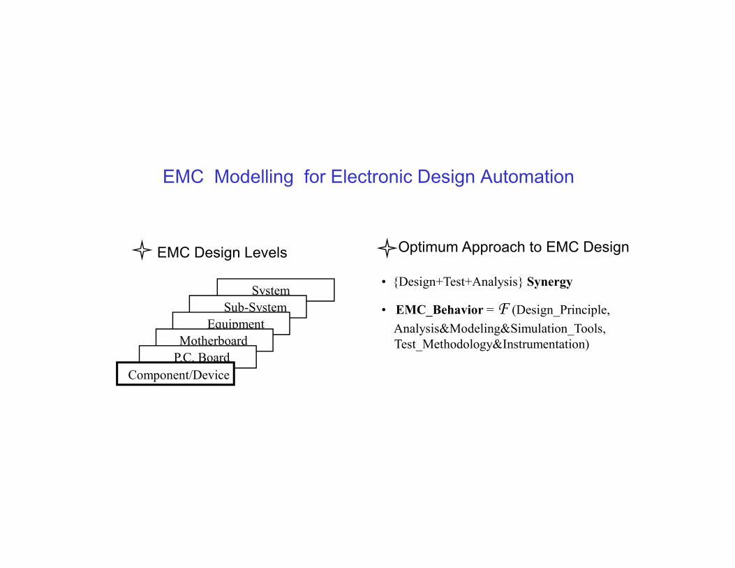
EMC Modelling for Electronic Design Automation
Optimum Approach to EMC Design
• {Design+Test+Analysis} Synergy
• EMC_Behavior = F (Design_Principle,
Analysis&Modeling&Simulation_Tools,
Test_Methodology&Instrumentation)
System
Sub-System
Equipment
Motherboard
P.C. Board
Component/Device
EMC Design Levels
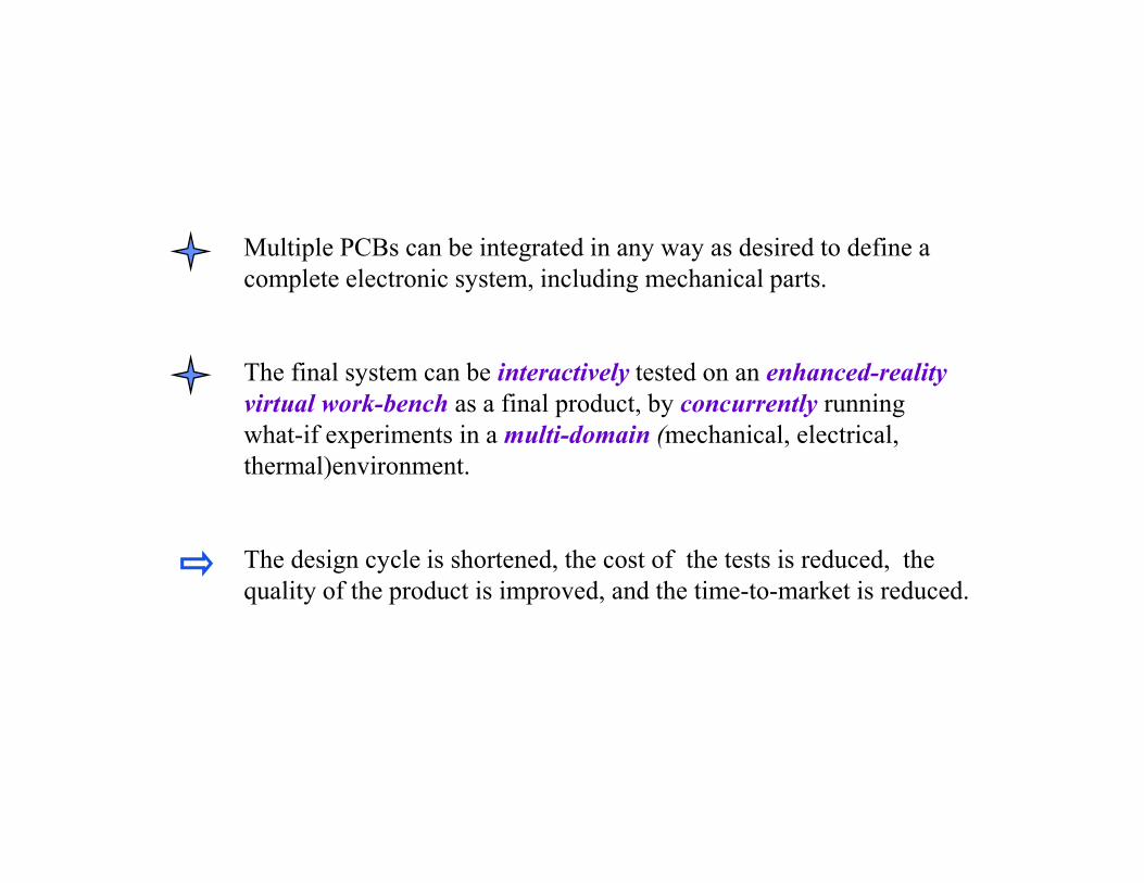
Multiple PCBs can be integrated in any way as desired to define a
complete electronic system, including mechanical parts.
The final system can be interactively tested on an enhanced-reality
virtual work-bench as a final product, by concurrently running
what-if experiments in a multi-domain (mechanical, electrical,
thermal)environment.
The design cycle is shortened, the cost of the tests is reduced, the
quality of the product is improved, and the time-to-market is reduced.
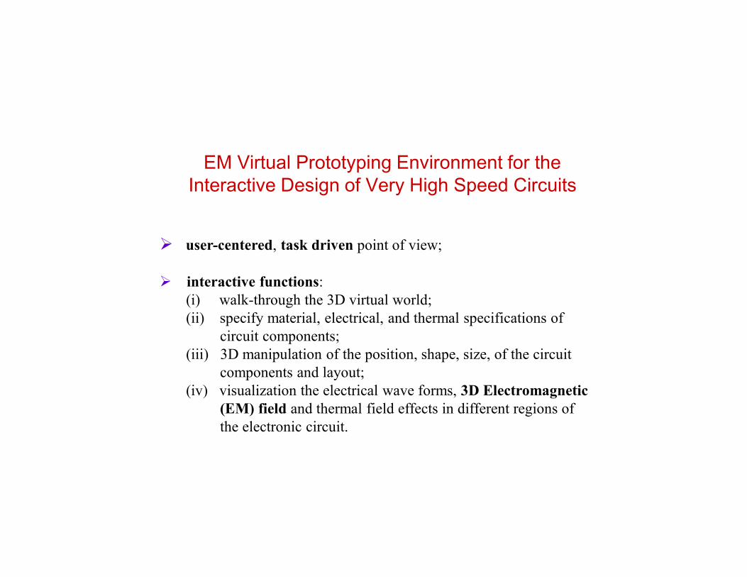
EM Virtual Prototyping Environment for the Interactive Design of Very High Speed Circuits
� user-centered, task driven point of view;
� interactive functions:
(i) walk-through the 3D virtual world;
(ii) specify material, electrical, and thermal specifications of
circuit components;
(iii) 3D manipulation of the position, shape, size, of the circuit
components and layout;
(iv) visualization the electrical wave forms, 3D Electromagnetic
(EM) field and thermal field effects in different regions of
the electronic circuit.
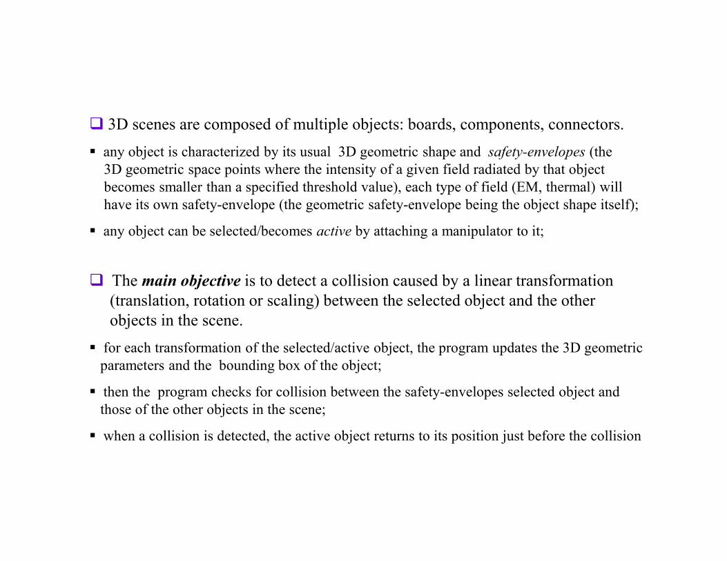
� 3D scenes are composed of multiple objects: boards, components, connectors.
� any object is characterized by its usual 3D geometric shape and safety-envelopes (the
3D geometric space points where the intensity of a given field radiated by that object
becomes smaller than a specified threshold value), each type of field (EM, thermal) will
have its own safety-envelope (the geometric safety-envelope being the object shape itself);
� any object can be selected/becomes active by attaching a manipulator to it;
� The main objective is to detect a collision caused by a linear transformation
(translation, rotation or scaling) between the selected object and the other
objects in the scene.
� for each transformation of the selected/active object, the program updates the 3D geometric
parameters and the bounding box of the object;
� then the program checks for collision between the safety-envelopes selected object and
those of the other objects in the scene;
� when a collision is detected, the active object returns to its position just before the collision
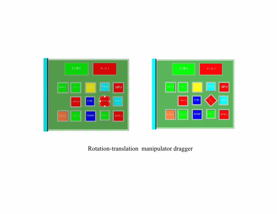
Rotation-translation manipulator dragger
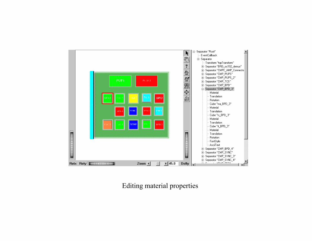
Editing material properties

Assembling multiple PCBs
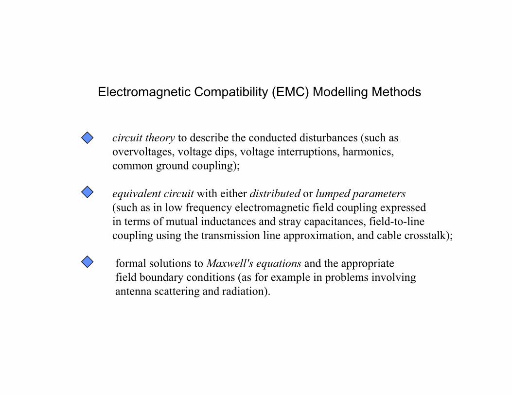
circuit theory to describe the conducted disturbances (such as
overvoltages, voltage dips, voltage interruptions, harmonics,
common ground coupling);
equivalent circuit with either distributed or lumped parameters
(such as in low frequency electromagnetic field coupling expressed
in terms of mutual inductances and stray capacitances, field-to-line
coupling using the transmission line approximation, and cable crosstalk);
formal solutions to Maxwell's equations and the appropriate
field boundary conditions (as for example in problems involving
antenna scattering and radiation).
Electromagnetic Compatibility (EMC) Modelling Methods
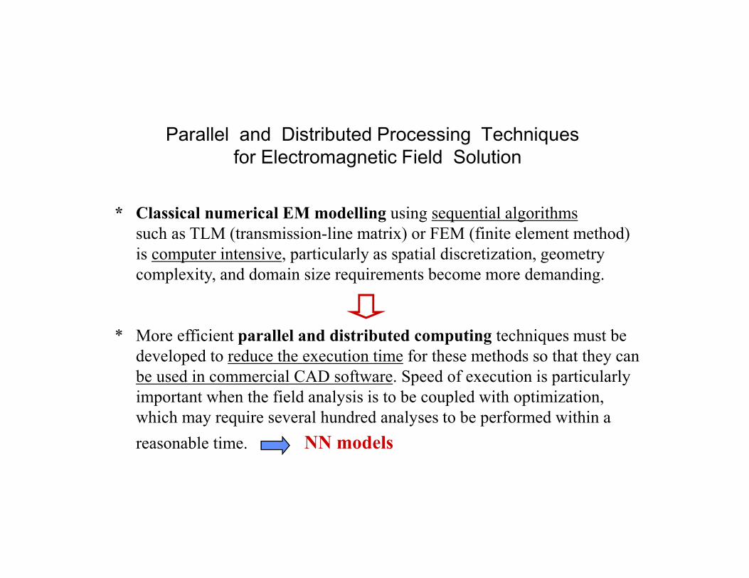
* Classical numerical EM modelling using sequential algorithms
such as TLM (transmission-line matrix) or FEM (finite element method)
is computer intensive, particularly as spatial discretization, geometry
complexity, and domain size requirements become more demanding.
* More efficient parallel and distributed computing techniques must be
developed to reduce the execution time for these methods so that they can
be used in commercial CAD software. Speed of execution is particularly
important when the field analysis is to be coupled with optimization,
which may require several hundred analyses to be performed within a
reasonable time. NN models
Parallel and Distributed Processing Techniques for Electromagnetic Field Solution
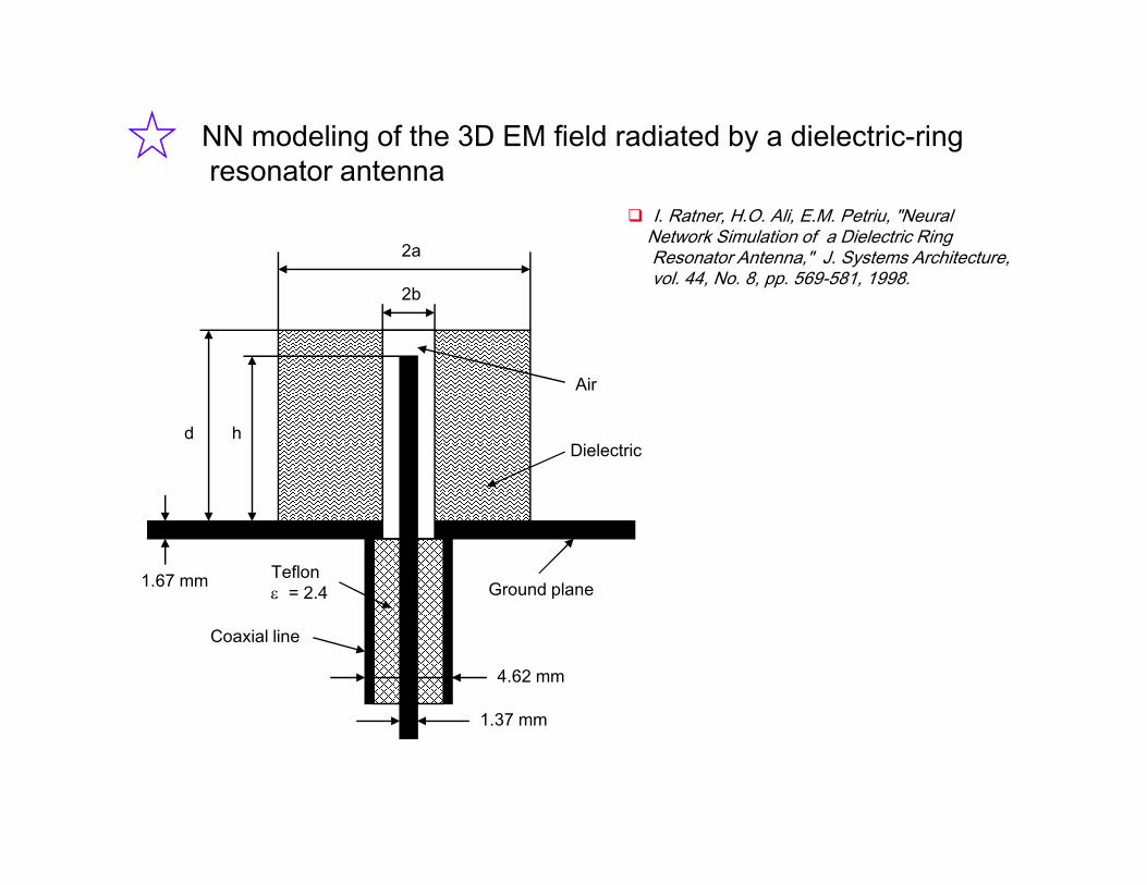
NN modeling of the 3D EM field radiated by a dielectric-ringresonator antenna
� I. Ratner, H.O. Ali, E.M. Petriu, "Neural Network Simulation of a Dielectric Ring Resonator Antenna," J. Systems Architecture, vol. 44, No. 8, pp. 569-581, 1998.
Dielectric
Air
Coaxial line
Teflonε = 2.4
d h
2b
2a
1.37 mm
4.62 mm
1.67 mm Ground plane
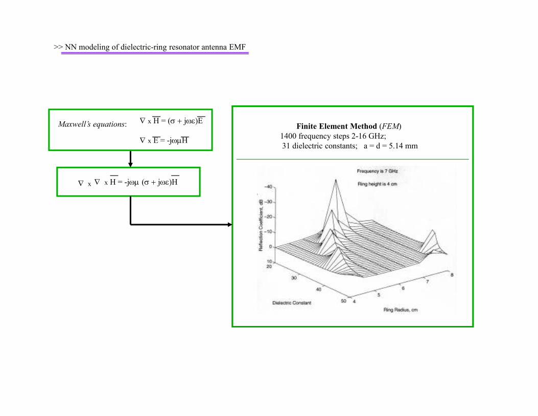
Finite Element Method (FEM)
1400 frequency steps 2-16 GHz;
31 dielectric constants; a = d = 5.14 mm
∇ x H = (σ + jωε)E
∇ x E = -jωµH
Maxwell’s equations:
∇ x H = -jωµ (σ + jωε)H∇ x
>> NN modeling of dielectric-ring resonator antenna EMF
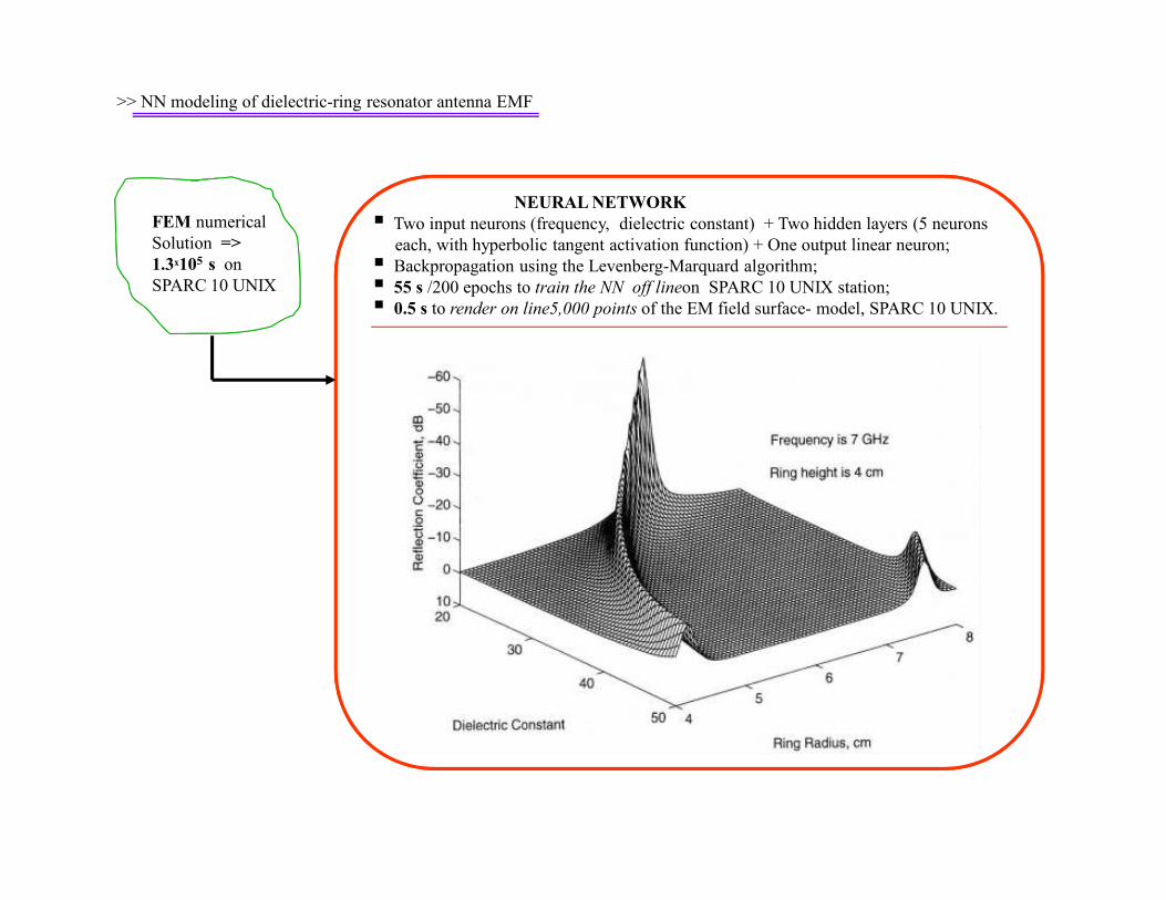
NEURAL NETWORK
� Two input neurons (frequency, dielectric constant) + Two hidden layers (5 neurons
each, with hyperbolic tangent activation function) + One output linear neuron;
� Backpropagation using the Levenberg-Marquard algorithm;
� 55 s /200 epochs to train the NN off lineon SPARC 10 UNIX station;
� 0.5 s to render on line5,000 points of the EM field surface- model, SPARC 10 UNIX.
FEM numerical
Solution =>
1.3x10⁵ s on
SPARC 10 UNIX
>> NN modeling of dielectric-ring resonator antenna EMF

MODEL CALIBRATION
The whole idea of virtual prototyping relies on the ability
to develop models conformable to the physical objects and
phenomena which represent reality very closely.
There is a need for calibration techniques able to validate
the conformance with the physical reality of the models
incorporated in the new prototyping tools.
Experimental Measurements
� The EM field training data are conveniently obtained as analytical
estimations of far-field values in 3D space and frequency from near-field
data using the finite element method combined with method of integral
absorbing boundary conditions.
� The near field data could be obtained analytically and/or by physically
measuring EM field values at for given frequency values and 3D space locations.
� This approach allows to replace the usual cumbersome open site far-field
measurement technique by anechoic chamber measurements.
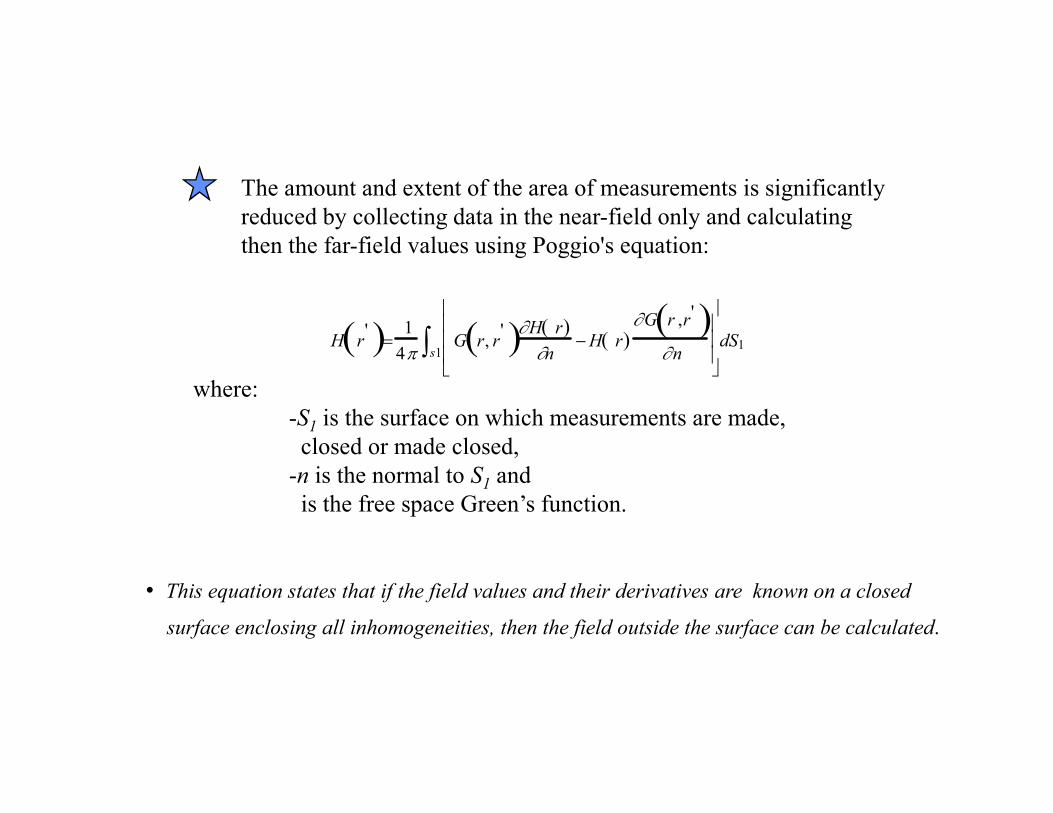
The amount and extent of the area of measurements is significantly
reduced by collecting data in the near-field only and calculating
then the far-field values using Poggio's equation:
where:
-S1 is the surface on which measurements are made,
closed or made closed,
-n is the normal to S1 and
is the free space Green’s function.
H r'( )=
1
4πG r, r
'( )∂H r( )∂n
− H r( )∂G r ,r'( )
∂n
dS1
s1∫
• This equation states that if the field values and their derivatives are known on a closed
surface enclosing all inhomogeneities, then the field outside the surface can be calculated.
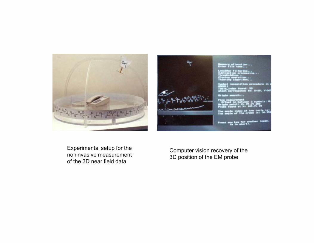
Experimental setup for the noninvasive measurement of the 3D near field data
Computer vision recovery of the 3D position of the EM probe
Neural Network Modeling of
3D Objects
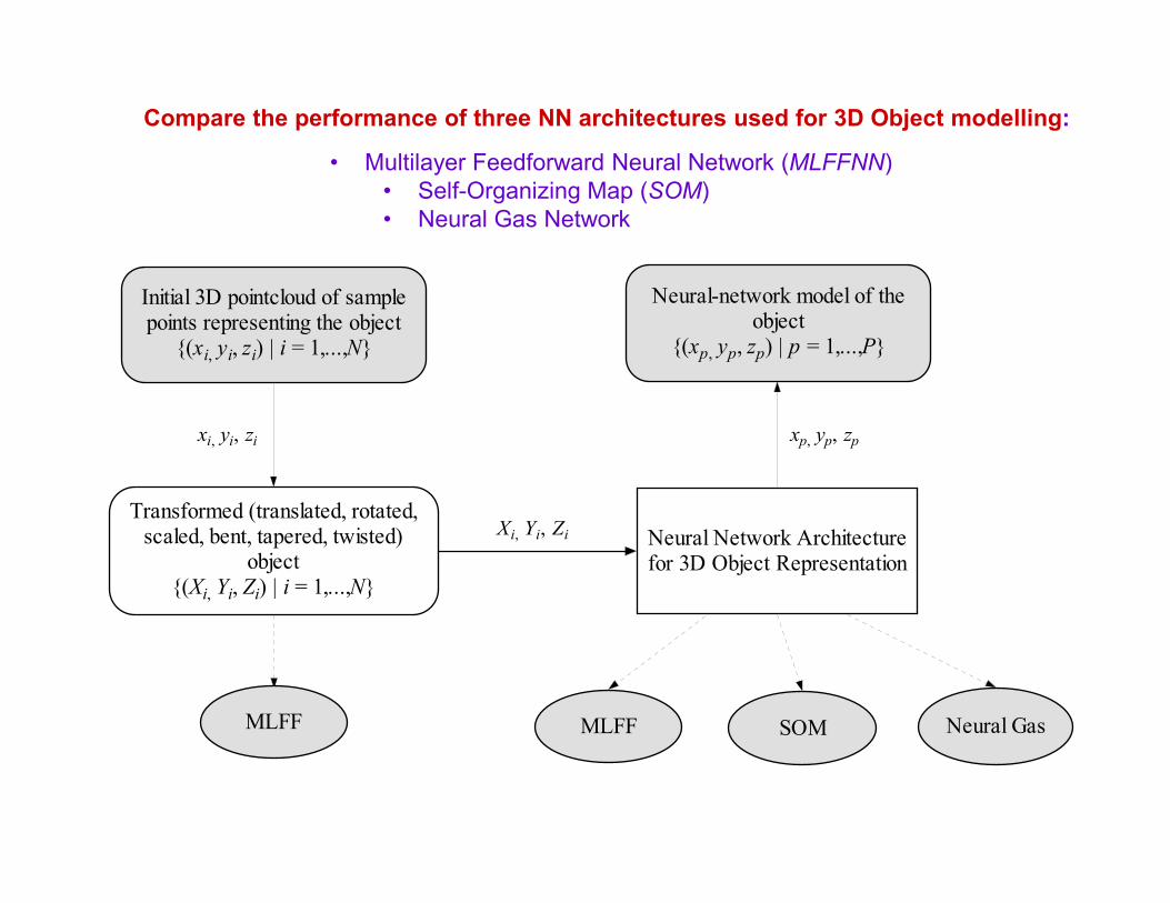
Initial 3D pointcloud of samplepoints representing the object
{(xi, yi, zi) | i = 1,...,N}
Neural-network model of theobject
{(xp, yp, zp) | p = 1,...,P}
xi, yi, zi xp, yp, zp
Transformed (translated, rotated,scaled, bent, tapered, twisted)
object{(Xi, Yi, Zi) | i = 1,...,N}
Neural Network Architecturefor 3D Object Representation
MLFF SOM Neural Gas
Xi, Yi, Zi
MLFF
Compare the performance of three NN architectures used for 3D Object modelling:
• Multilayer Feedforward Neural Network (MLFFNN)
• Self-Organizing Map (SOM)
• Neural Gas Network
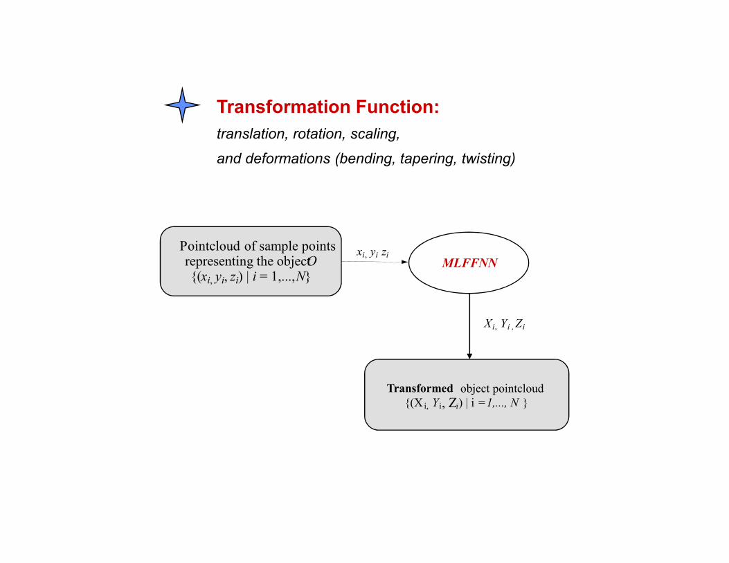
MLFFNN
Pointcloud of sample pointsrepresenting the objectO{(xi, yi, zi) | i = 1,...,N}
xi, yi zi
Transformed object pointcloud
{(X i, Yi, Zi) | i =1,..., N }
X i, Yi , Zi
Transformation Function:
translation, rotation, scaling,
and deformations (bending, tapering, twisting)

Transformation Function – NN Architecture
ψϕ
ψϕ
ϕ
ψθψϕθ
ψθψϕθ
ϕθ
ψθψϕθ
ψθψϕθ
ϕθ
coscos
sincos
sin
)sincoscossin(sin
)coscossinsin(sin
cossin
)sinsincossin(cos
)cossinsinsin(cos
coscos
33
32
31
23
22
21
13
12
11
aq
aq
aq
an
an
an
am
am
am
=
=
−=
−=
−=
=
+=
−=
=X
Z
Y
x
y
z
m1
m2
m3
n1
n2
n3
q1
q2
q3
a
b
c
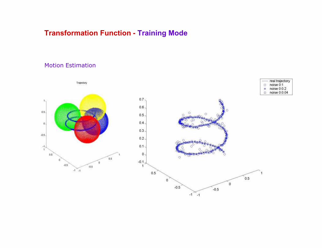
Transformation Function - Training Mode
Motion Estimation
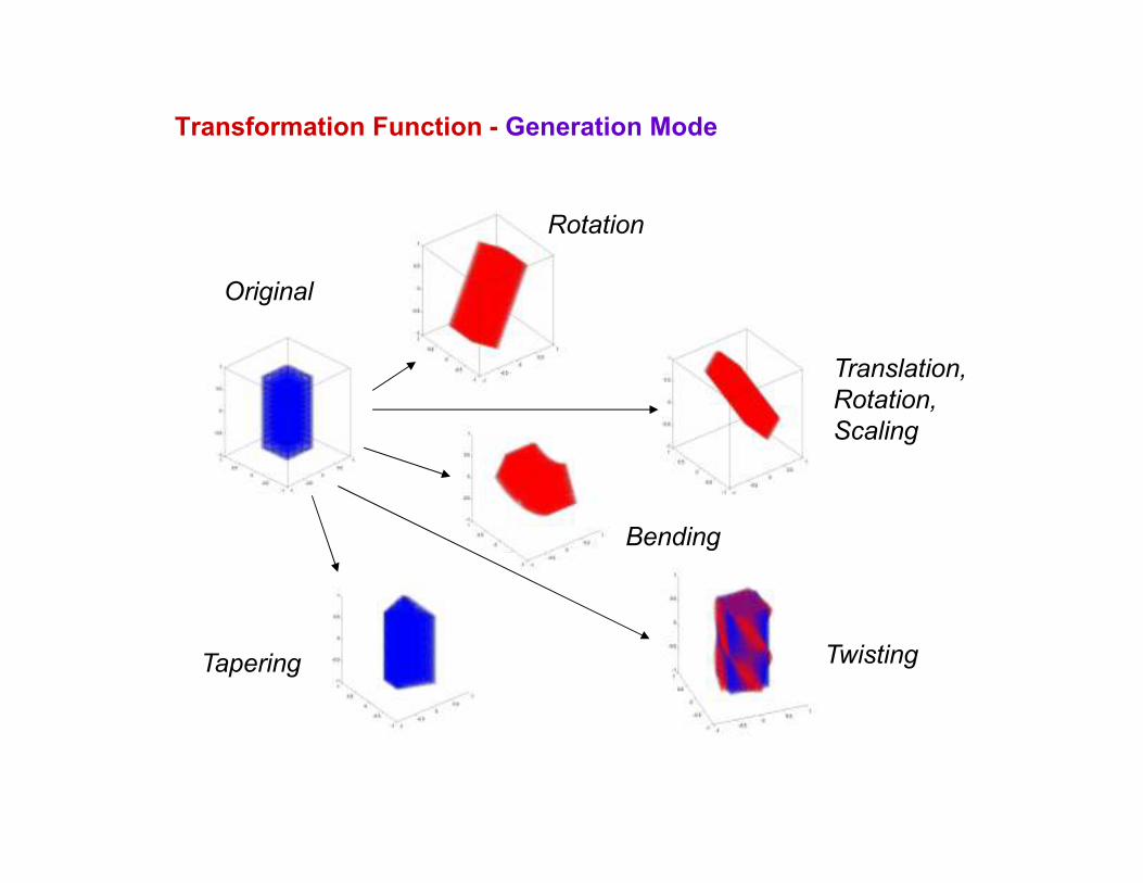
Transformation Function - Generation Mode
Original
Tapering
Rotation
Translation,
Rotation,
Scaling
Twisting
Bending
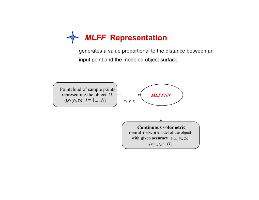
MLFF Representation
generates a value proportional to the distance between an
input point and the modeled object surface
Pointcloud of sample pointsrepresenting the object O{(xi, yi, zi) | i = 1,...,N}
MLFFNN
xi, yi zi
Continuous volumetricneural-networkmodel of the object
with given accuracy {(xi, yi, zi) |
(xi,yi,zi)∈ O}
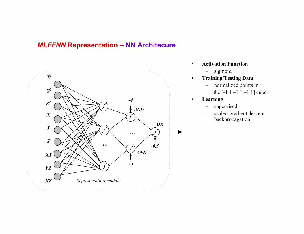
MLFFNN Representation – NN Architecure
• Activation Function
– sigmoid
• Training/Testing Data
– normalized points in
the [-1 1 –1 1 –1 1] cube
• Learning
– supervised
– scaled-gradient descent backpropagation
Representation module
...
OR
X2
Z2
Y2
X
Y
Z
XY
YZ
XZ
...
-4
-4
-0.5
AND
AND
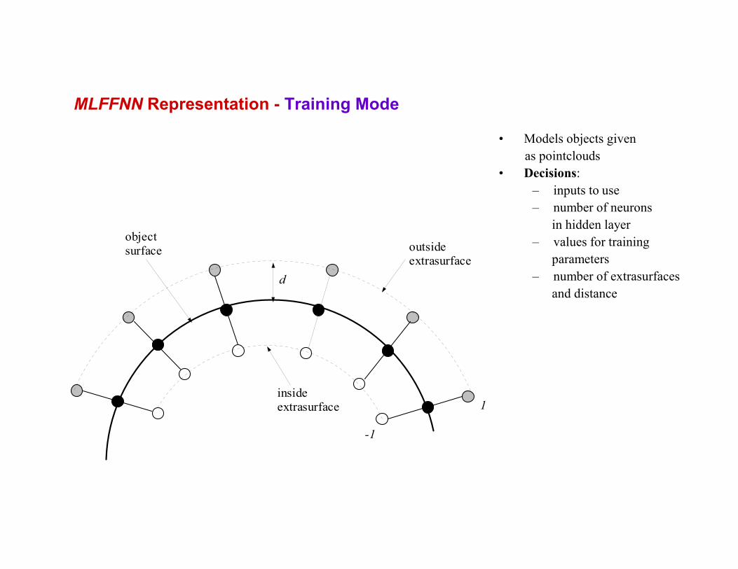
MLFFNN Representation - Training Mode
• Models objects given
as pointclouds
• Decisions:
– inputs to use
– number of neurons
in hidden layer
– values for training
parameters
– number of extrasurfaces
and distance
outsideextrasurface
insideextrasurface
object
surface
d
-1
1

250 points, 6-3-1, 1
extrasurface, d=0.055, 550
epochs, mse: 0.14, 7 min.
19000 points, 14-7-1, 4
extrasurfaces, d=0.055, 1100
epochs, mse: 0.4, 3.3 hrs51096 points, 20-10-1, 5
extrasurfaces, d=0.055, 2000
epochs, mse: 0.67, 5.2 hrs.
19080 points, 10-5-1, 5
extrasurfaces, d=0.055, 1200
epochs, mse: 0.35, 2.8 hrs.
7440 points, 8-4-1, 5
extrasurfaces, d=0.055,
1100 epochs, mse: 0.24,
1 hr
2500 points, 12-6-1, 2
extrasurfaces, d=0.06, 1020
epochs, mse: 0.39, 45 min.
MLFFNN Modelling - Results
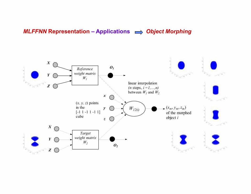
W12(i)
(x, y, z) points
in the
[-1 1 -1 1 -1 1]
cube
X
Z
Y
Reference
weight matrix
W1
linear interpolation
(n steps, i =1,...,n)
between W1 and W2
X
Z
Y
Target
weight matrix
W2
O1
O2
(xm, ym, zm)
of the morphedobject i
x
z
y
MLFFNN Representation – Applications Object Morphing
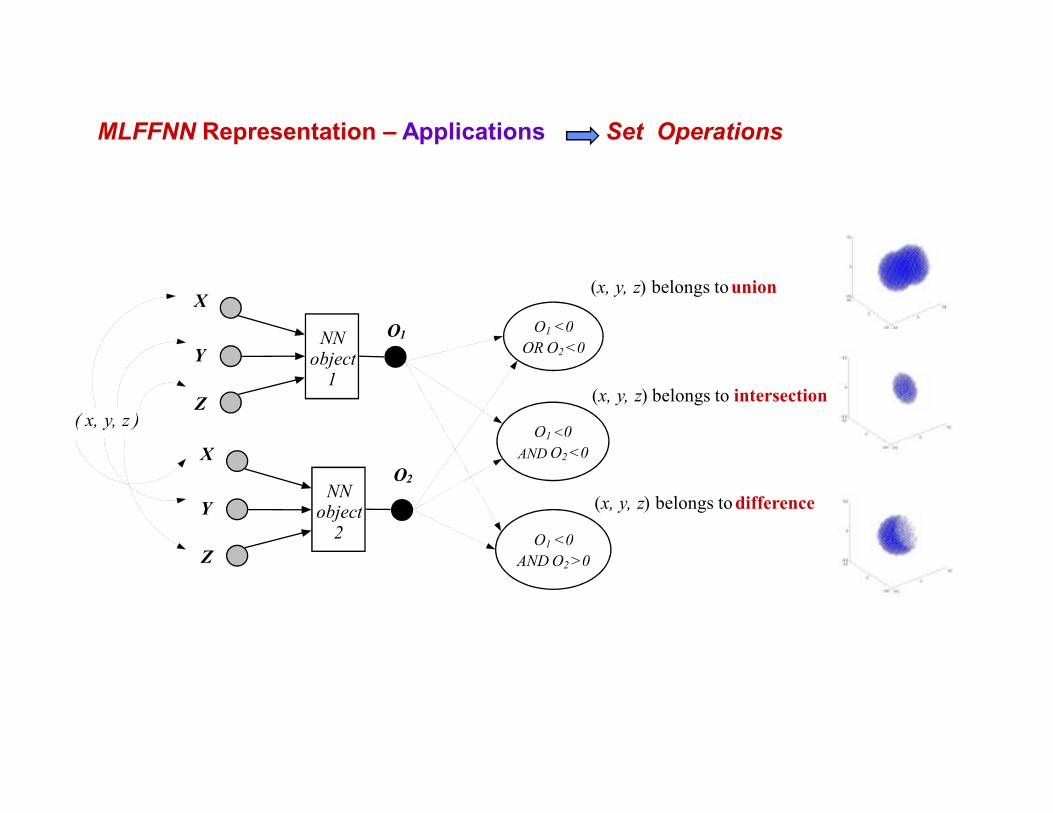
MLFFNN Representation – Applications Set Operations
X
Z
YNN
object1
O1
X
Z
YNN
object2
O2
( x, y, z )
O1 <0
OR O2 <0
O1 <0
AND O2 <0
(x, y, z) belongs tounion
(x, y, z) belongs to intersection
O1 <0
AND O2 >0
(x, y, z) belongs to difference
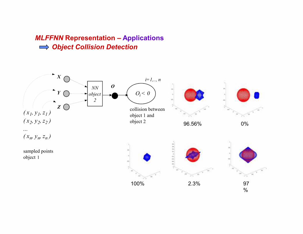
96.56%
97
%
0%
2.3%100%
X
Z
YNN
object
2
O
( x1, y1, z1 )
( x2, y2, z2 )
...
( xn, yn, zn )
sampled points
object 1
Oi < 0
collision between
object 1 and
object 2
i=1,.., n
MLFFNN Representation – Applications
Object Collision Detection
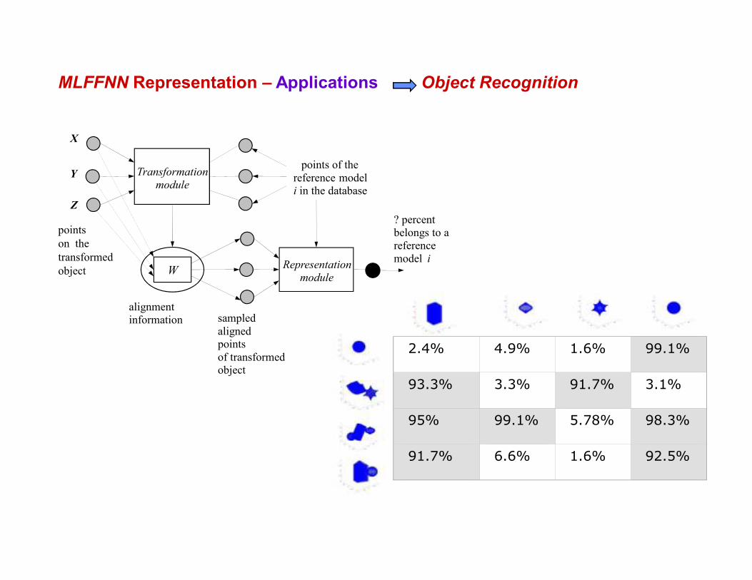
2.4% 4.9% 1.6% 99.1%
93.3% 3.3% 91.7% 3.1%
95% 99.1% 5.78% 98.3%
91.7% 6.6% 1.6% 92.5%
MLFFNN Representation – Applications Object Recognition
W
alignment
information
Representation
module
X
Z
Y Transformation
module
points of the
reference modeli in the database
sampled
alignedpoints
of transformedobject
? percent
belongs to a
reference
model i
points
on the
transformed
object
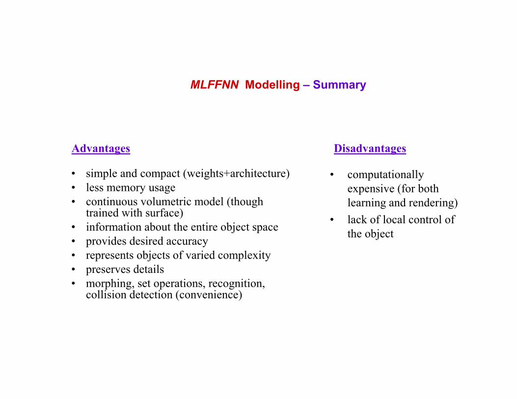
• simple and compact (weights+architecture)
• less memory usage
• continuous volumetric model (though trained with surface)
• information about the entire object space
• provides desired accuracy
• represents objects of varied complexity
• preserves details
• morphing, set operations, recognition, collision detection (convenience)
• computationally
expensive (for both
learning and rendering)
• lack of local control of
the object
MLFFNN Modelling – Summary
Advantages Disadvantages
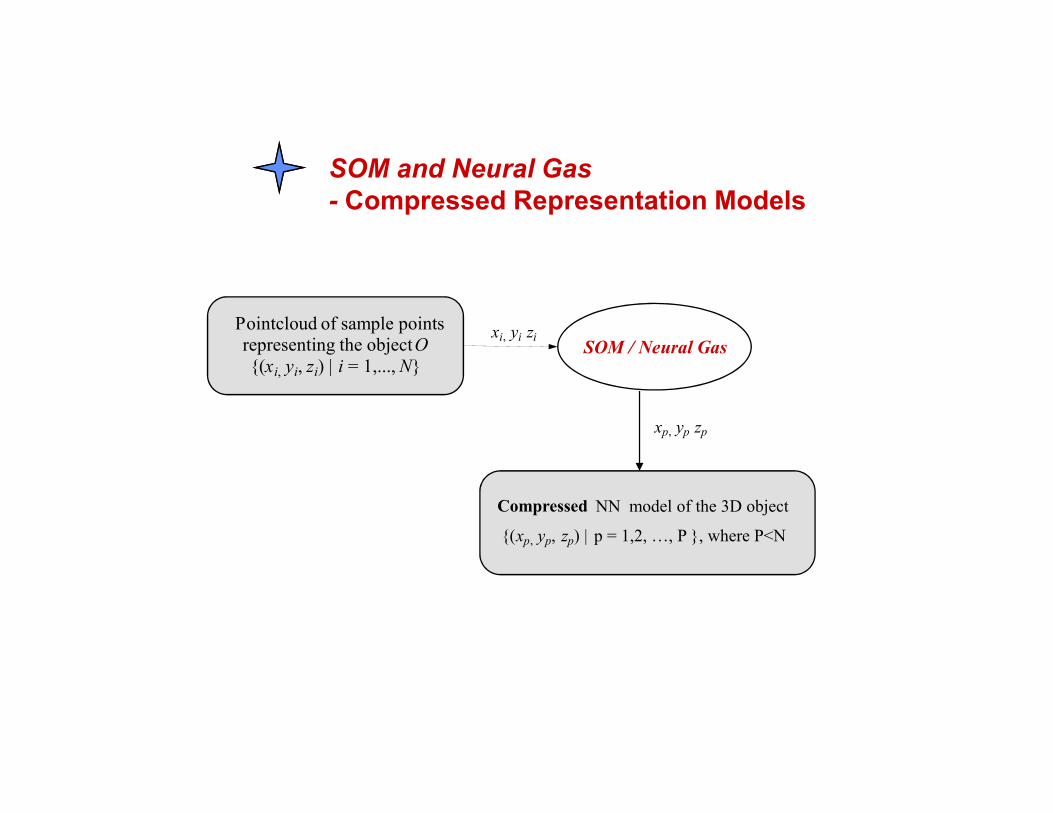
SOM and Neural Gas
- Compressed Representation Models
Compressed NN model of the 3D object
{(xp, yp, zp) | p = 1,2, …, P }, where P<N
SOM / Neural Gas
Pointcloud of sample points
representing the objectO
{(xi, yi, zi) | i = 1,..., N}
xi, yi zi
xp, yp zp
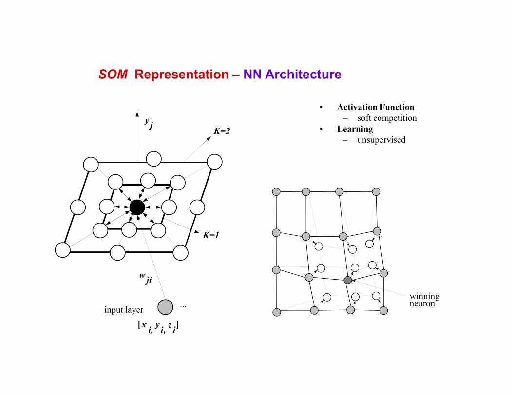
SOM Representation – NN Architecture
• Activation Function
– soft competition
• Learning
– unsupervised
input layer...
[ xi,
yi,
zi]
wji
yj
K=2
K=1
winningneuron
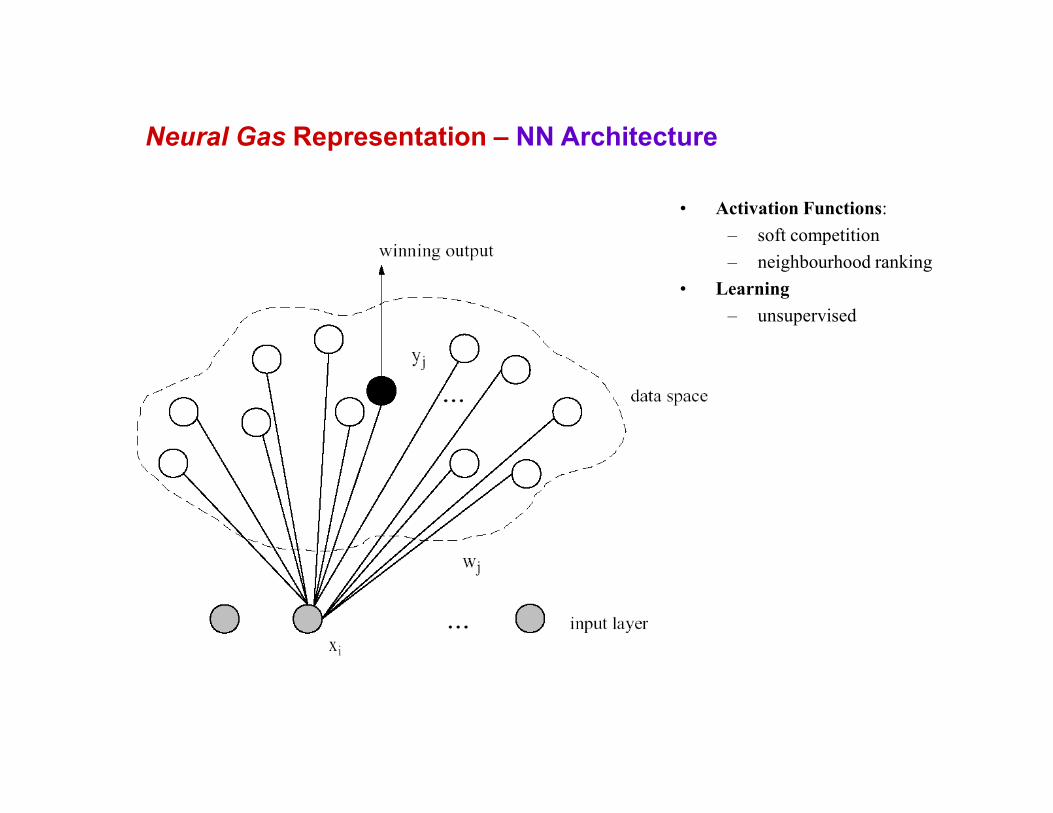
• Activation Functions:
– soft competition
– neighbourhood ranking
• Learning
– unsupervised
Neural Gas Representation – NN Architecture

Initial
pointcloud
Neural Gas
SOM
19080 points 14914 points 13759 points
1125 points,
42 min.
1125 points,
26 min.
875 points,
11 min.
875 points,
24.5 min.
875 points
22 min.
875 points,
10 min.
er= 0.0098
er= 0.0125
SOM and Neural Gas Modelling - Results
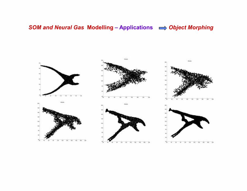
SOM and Neural Gas Modelling – Applications Object Morphing
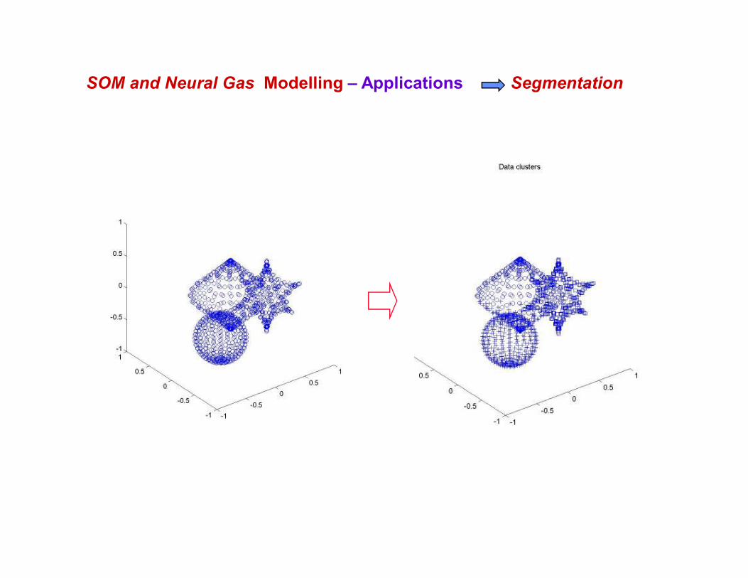
SOM and Neural Gas Modelling – Applications Segmentation
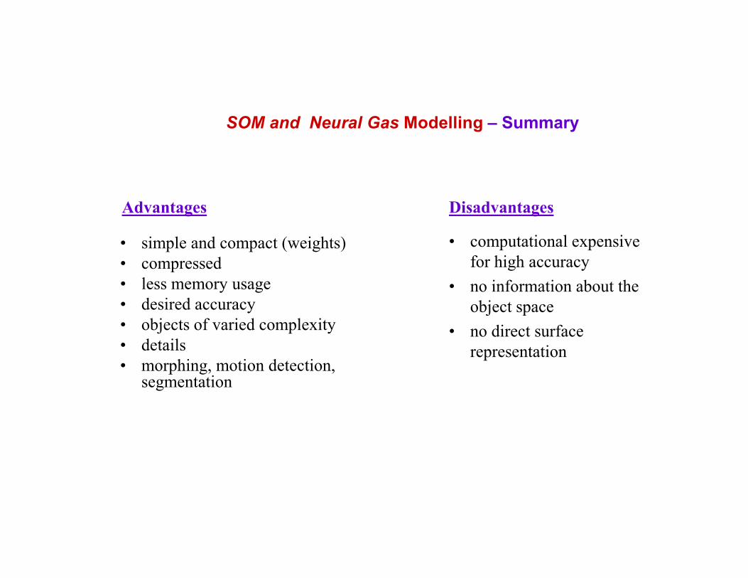
• simple and compact (weights)
• compressed
• less memory usage
• desired accuracy
• objects of varied complexity
• details
• morphing, motion detection, segmentation
• computational expensive
for high accuracy
• no information about the
object space
• no direct surface
representation
SOM and Neural Gas Modelling – Summary
Advantages Disadvantages
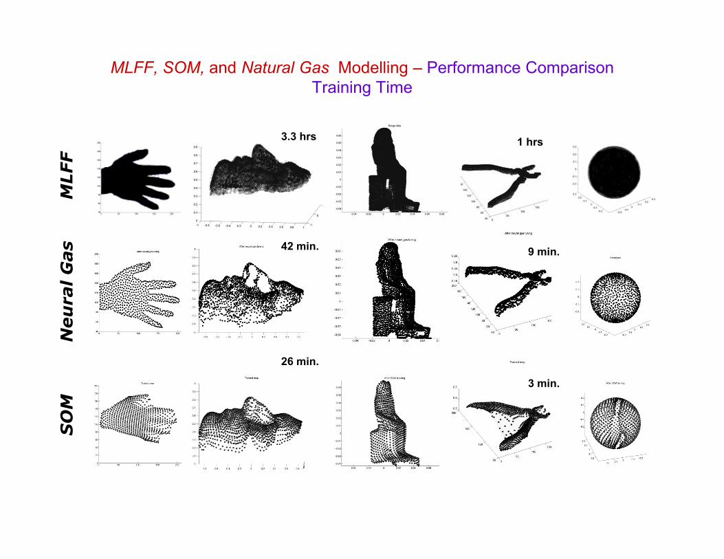
MLFF
Neu
ral G
as
SO
M
3.3 hrs1 hrs
42 min.
26 min.
9 min.
3 min.
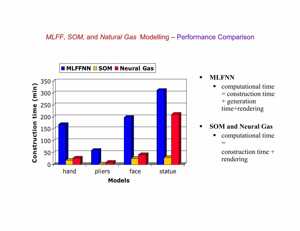
MLFF, SOM, and Natural Gas Modelling – Performance Comparison
Training Time
0
50
100
150
200
250
300
350
Co
nstr
ucti
on
tim
e (
min
)
hand pliers face statue
Models
MLFFNN SOM Neural Gas
� MLFNN
� computational time = construction time + generation time+rendering
� SOM and Neural Gas
� computational time =
construction time + rendering
MLFF, SOM, and Natural Gas Modelling – Performance Comparison
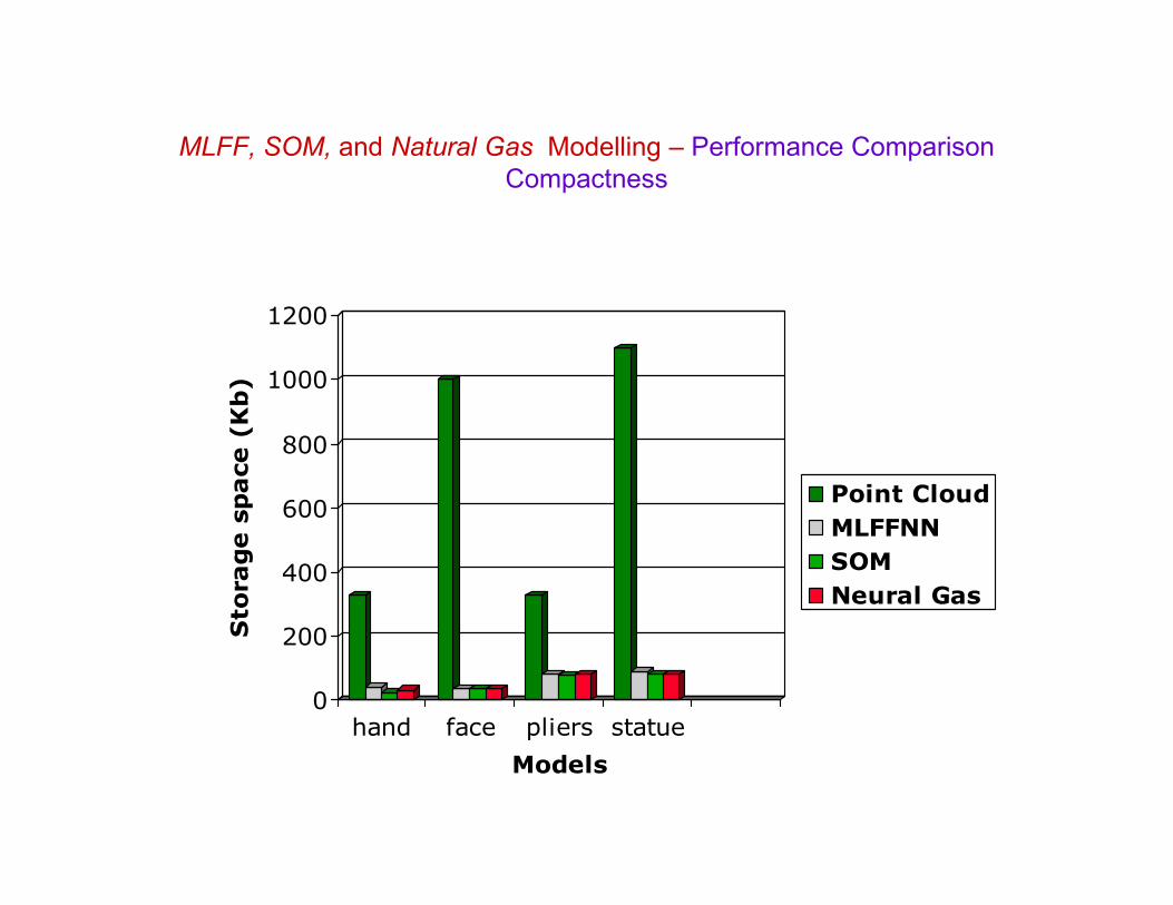
0
200
400
600
800
1000
1200
Sto
rage s
pace (
Kb)
hand face pliers statue
Models
Point Cloud
MLFFNN
SOM
Neural Gas
MLFF, SOM, and Natural Gas Modelling – Performance Comparison
Compactness
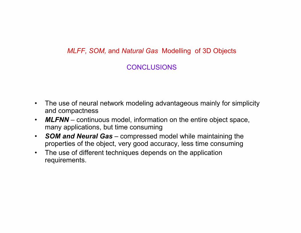
• The use of neural network modeling advantageous mainly for simplicity and compactness
• MLFNN – continuous model, information on the entire object space, many applications, but time consuming
• SOM and Neural Gas – compressed model while maintaining the properties of the object, very good accuracy, less time consuming
• The use of different techniques depends on the application requirements.
MLFF, SOM, and Natural Gas Modelling of 3D Objects
CONCLUSIONS
Neural Network Adaptive Sampling
of 3D Surface Elastic Properties
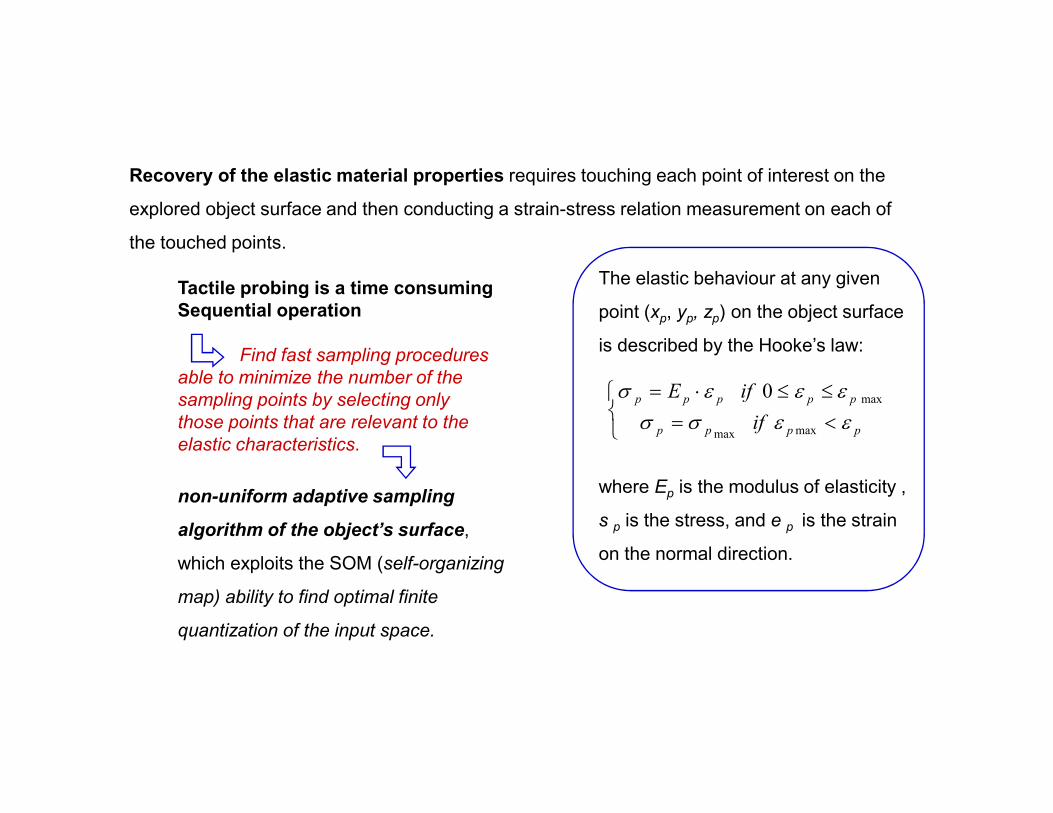
Recovery of the elastic material properties requires touching each point of interest on the
explored object surface and then conducting a strain-stress relation measurement on each of
the touched points.
< =
≤≤ ⋅=
0
maxmax
max
pppp
ppppp
if
ifE
εεσσεεεσ
The elastic behaviour at any given
point (xp, yp, zp) on the object surface
is described by the Hooke’s law:
where Ep is the modulus of elasticity ,
s p is the stress, and e p is the strain
on the normal direction.
Tactile probing is a time consuming
Sequential operation
Find fast sampling procedures
able to minimize the number of the
sampling points by selecting only
those points that are relevant to the
elastic characteristics.
non-uniform adaptive sampling
algorithm of the object’s surface,
which exploits the SOM (self-organizing
map) ability to find optimal finite
quantization of the input space.
Initial3D geometric
model of the object's surface
{(xi, yi, zi) | i = 1,...,N}SOM / Neural Gas
Adaptive-sampled3D geometric
model of the object surface
{(xp, yp, zp) | p = 1,...,P}
RoboticTactile
Probing
Adaptive-sampled3D geometric
&
elastic composite model
of object's surface
{(xp, yp, zp, Ep) | p = 1,...,P}
xi, yi, zi
xp, yp, zp
Ep
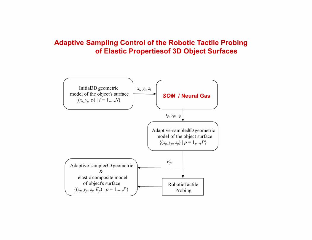
Adaptive Sampling Control of the Robotic Tactile Probing
of Elastic Propertiesof 3D Object Surfaces

Starting from a 3D point-cloud, a neural gas NN yields a reduced set of points on the 3D
object’s surface which are relevant for the tactile probing. The density of these tactile
probing points is higher in the regions with more pronounced variations in the geometric
shape. A feedforward NN is then employed to model the force/displacement behavior of
selected sampled points that are probed simultaneously by a force/torque sensor and the
active range finder.
3D pointcloud
of data
Sample
points
Deformation
profiles
Force
Measurements
Feedforward
Neural Network
F
profile(f0)
profile(f1)
profile(f2)
profile(f3)
f0
f1
f2
f3
Neural gas
network
Range
finder
Force/Torque
sensor
Neural Network Mapping an Clustering of Elastic Behavior from
Tactile and Range Imaging
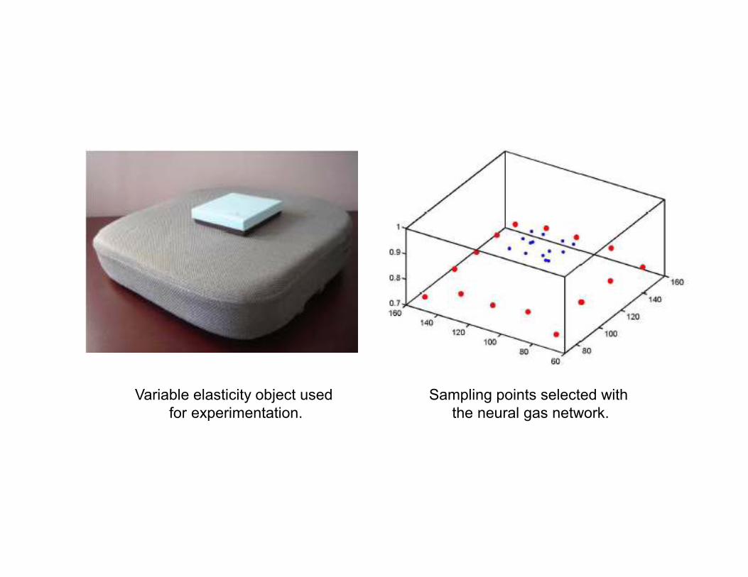
Sampling points selected with
the neural gas network.
Variable elasticity object used
for experimentation.
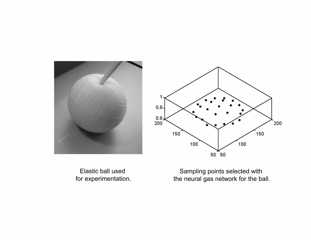
Sampling points selected with
the neural gas network for the ball.
Elastic ball used
for experimentation.
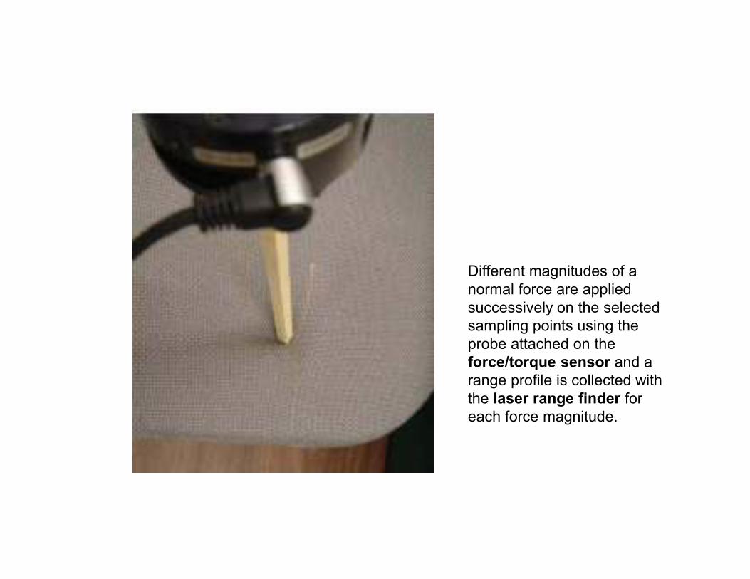
Different magnitudes of a
normal force are applied
successively on the selected
sampling points using the
probe attached on the
force/torque sensor and a
range profile is collected with
the laser range finder for
each force magnitude.
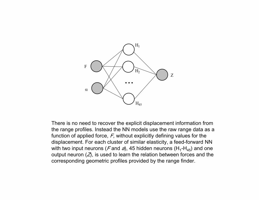
There is no need to recover the explicit displacement information from the range profiles. Instead the NN models use the raw range data as a function of applied force, F, without explicitly defining values for the displacement. For each cluster of similar elasticity, a feed-forward NN with two input neurons (F and a), 45 hidden neurons (H1-H45) and one output neuron (Z), is used to learn the relation between forces and the corresponding geometric profiles provided by the range finder.
F
Z
...
H1
H45
H2
α
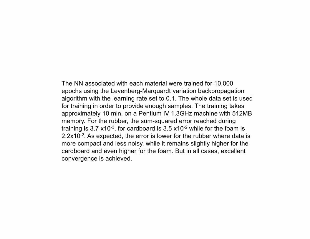
The NN associated with each material were trained for 10,000
epochs using the Levenberg-Marquardt variation backpropagation
algorithm with the learning rate set to 0.1. The whole data set is used
for training in order to provide enough samples. The training takes
approximately 10 min. on a Pentium IV 1.3GHz machine with 512MB
memory. For the rubber, the sum-squared error reached during
training is 3.7 x10⁻³, for cardboard is 3.5 x10⁻² while for the foam is
2.2x10⁻². As expected, the error is lower for the rubber where data is
more compact and less noisy, while it remains slightly higher for the
cardboard and even higher for the foam. But in all cases, excellent
convergence is achieved.

Deformation profiles for semi-stiff material (cardboard).

Deformation profiles for smooth material (foam).
Real and modeled deformation curves using neural network for semi-stiff material (cardboard) under a normal force of: a) F=0.1N, b) F=0.37N, and c) F=2.65N.
(a) (b) (c)
Real and modeled deformation curves using neural network for smooth material
(foam) under a normal force of: a) F=0N, b) F=0.93N, and c) F=3.37N.
(a) (b) (c)
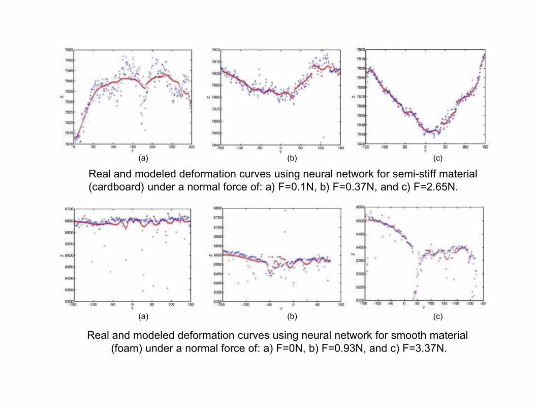
Real and modeled deformation
curves using neural network for
rubber under a normal force of:
a) F=0N, b) F=65.52N, and
c) F=80.5N.
(a) (b)
(c)
(a) (b)
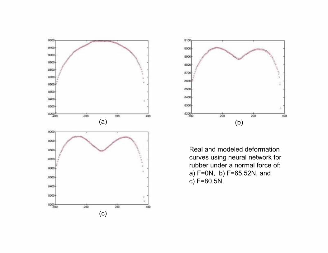
Real and modeled deformation curves using neural network for rubber under
forces applied at different angles:
a) F=65N, a1=10° and F=65N, a2=170°,b) F=36N, a1=25°, and F=36N, a2=155
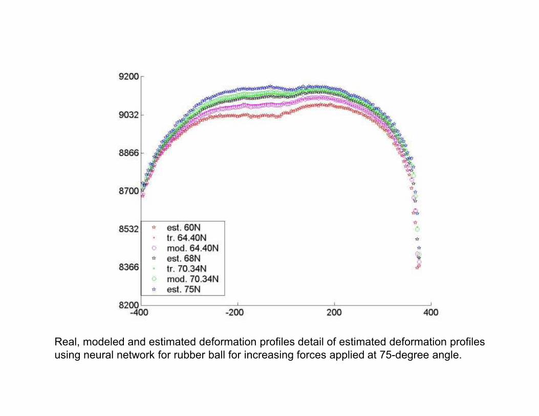
Real, modeled and estimated deformation profiles detail of estimated deformation profiles
using neural network for rubber ball for increasing forces applied at 75-degree angle.

Modelling Avatar Behaviours in
Interactive Virtual Environments.
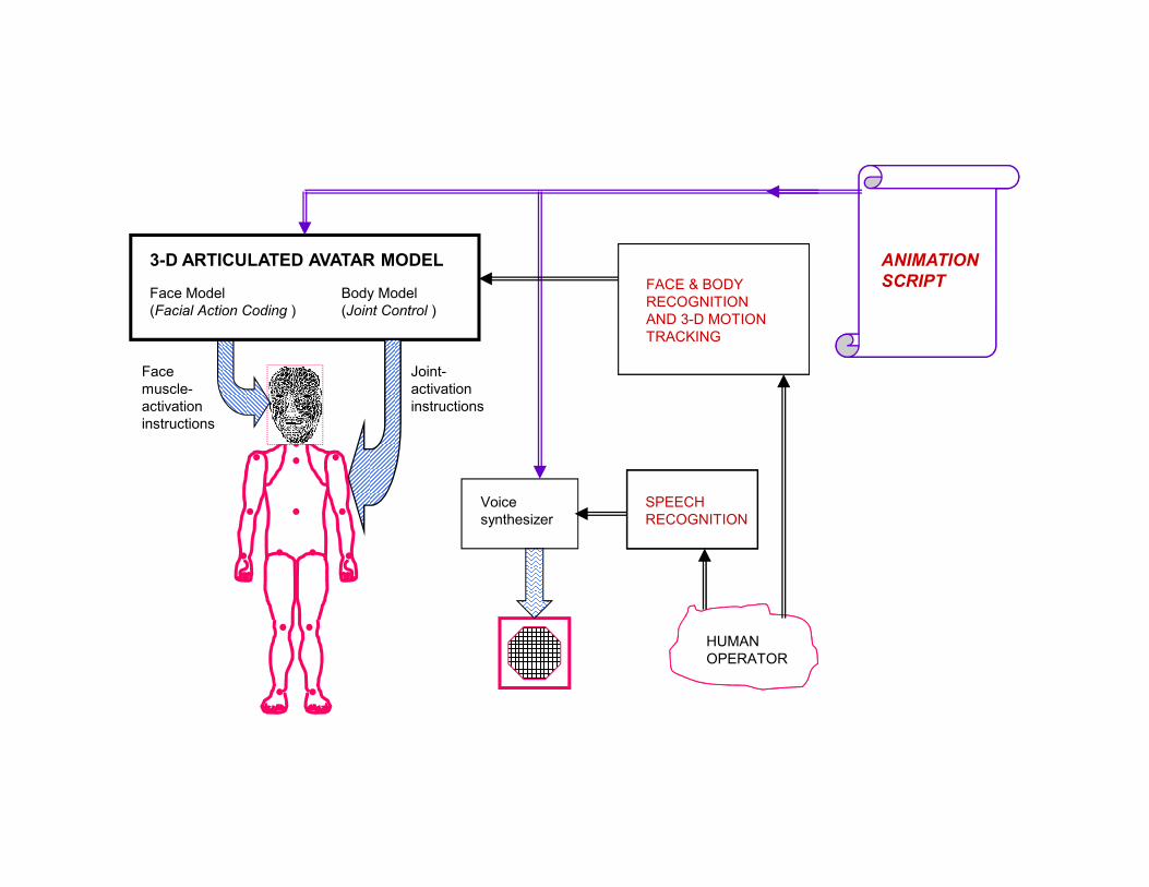
Face
muscle-
activation
instructions
Joint-
activation
instructions
Voice
synthesizer
Face Model
(Facial Action Coding )
Body Model
(Joint Control )
FACE & BODY
RECOGNITION
AND 3-D MOTION
TRACKING
HUMAN
OPERATOR
SPEECH
RECOGNITION
ANIMATION
SCRIPT
3-D ARTICULATED AVATAR MODEL

ANIMATION
SCRIPT
Voice
synthesizer
Face
muscle-
activation
instructions
Joint-
activation
instructions
Face Modell
(Facial Action Coding )
Body Model
(Joint Control )
3-D ARTICULATED AVATAR
Avatar Machine-level Instructions
Story-level
Instructions
� COMPILER
� INVERSE KINEMATIC CONTROL
� SCHEDULER
� CONCURRENCY MANAGER
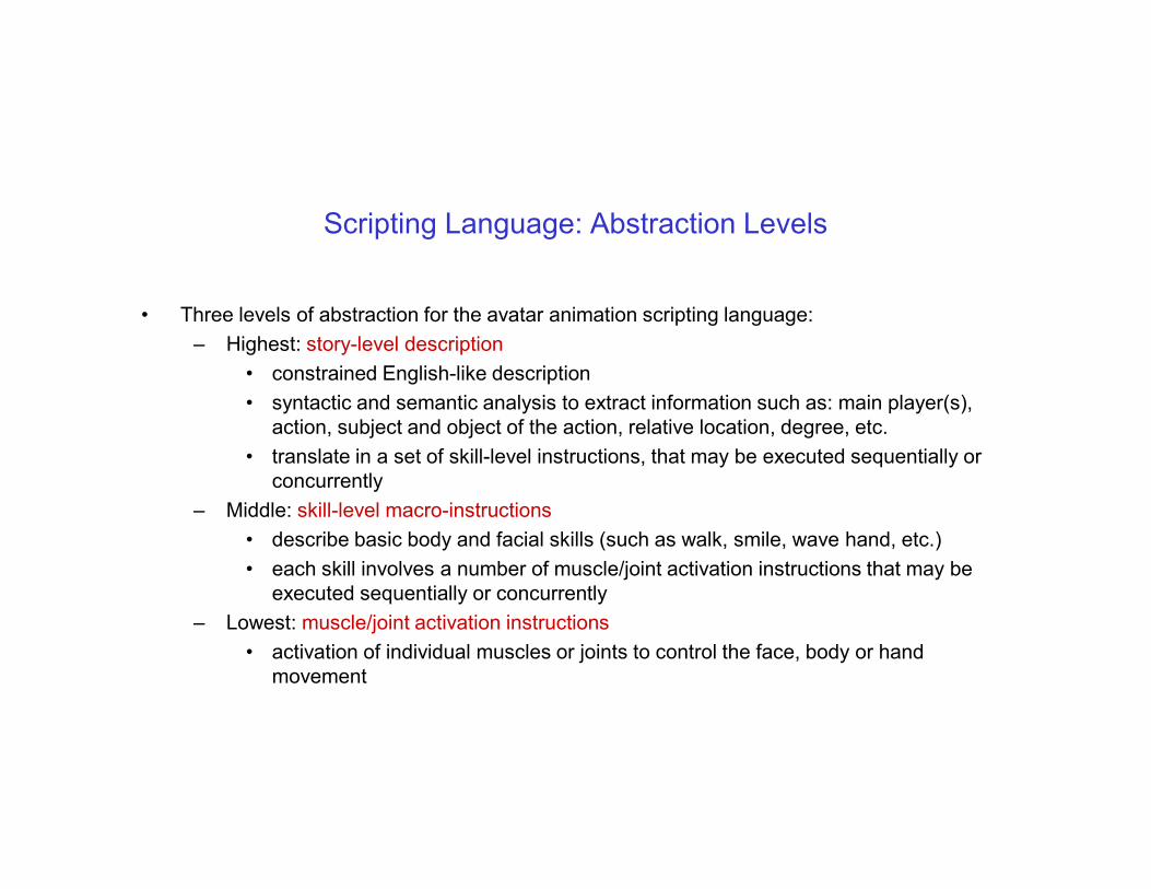
Scripting Language: Abstraction Levels
• Three levels of abstraction for the avatar animation scripting language:
– Highest: story-level description
• constrained English-like description
• syntactic and semantic analysis to extract information such as: main player(s),
action, subject and object of the action, relative location, degree, etc.
• translate in a set of skill-level instructions, that may be executed sequentially or
concurrently
– Middle: skill-level macro-instructions
• describe basic body and facial skills (such as walk, smile, wave hand, etc.)
• each skill involves a number of muscle/joint activation instructions that may be
executed sequentially or concurrently
– Lowest: muscle/joint activation instructions
• activation of individual muscles or joints to control the face, body or hand
movement
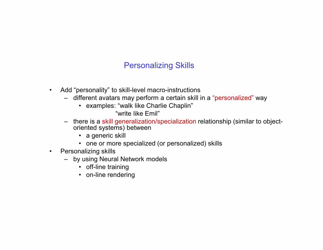
Personalizing Skills
• Add “personality” to skill-level macro-instructions
– different avatars may perform a certain skill in a “personalized” way
• examples: “walk like Charlie Chaplin”
“write like Emil”
– there is a skill generalization/specialization relationship (similar to object-oriented systems) between
• a generic skill
• one or more specialized (or personalized) skills
• Personalizing skills
– by using Neural Network models
• off-line training
• on-line rendering

STORY-LEVEL DESCRIPTION
…..
DanielA sits on the red chair.
DanielA writes “Hello” on stationary.
DanielA sees HappyCat under the white
table and starts smiling.
HappyCat grins back.
……
SKILL-LEVEL (“MACRO”) INSTRUCTIONS
…..
DanielA’s right hand moves the pen to follow the trace representing “H”.
DanielA’s right hand moves the pen to follow the trace representing “e”.
DanielA’s right hand moves the pen to follow the trace representing “l”.
DanielA’s right hand moves the pen to follow the trace representing “l”.
DanielA’s right hand moves the pen to follow the trace representing “o”.
……
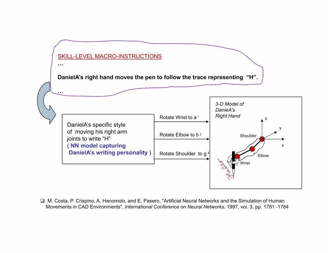
DanielA’s specific style
of moving his right arm
joints to write “H”
( NN model capturing
DanielA’s writing personality )
Rotate Wrist to a i
Rotate Elbow to b j
Rotate Shoulder to g k
Wrist
Elbow
Shoulder
x
y
z
3-D Model of
DanieA’s
Right Hand
SKILL-LEVEL MACRO-INSTRUCTIONS
…
DanielA’s right hand moves the pen to follow the trace representing “H”.
…
� M. Costa, P. Crispino, A. Hanomolo, and E. Pasero, "Artificial Neural Networks and the Simulation of Human
Movements in CAD Environments", International Conference on Neural Networks, 1997, vol. 3, pp. 1781 -1784

Thank You!