trip distribution modelling using neural network · various studies in transportation modelling...

Australasian Transport Research Forum 2013 Proceedings

2 - 4 October 2013, Brisbane, Australia

Trip Distribution Modelling Using Neural Network

Mohammad Rasouli 1, Hamid Nikraz

2

1 PhD Student, Curtin University, Senior Transport Modeller, Transcore Pty Ltd

([email protected])

2 Head of the Department of Civil Engineering, Curtin University

ABSTRACT

Trip distribution is the second important stage in the 4-step travel demand forecasting. The

purpose of the trip distribution forecasting is to estimates the trip linkages or interactions

between traffic zones for trip makers. The problem of trip distribution is of non-linear nature and

Neural Networks (NN) are well suited for addressing the non-linear problems. This fact supports

the use of artificial neural networks for trip distribution problem. In this study a new approach

based on the Generalised Regression Neural Network (GRNN) has been researched to estimate

the distribution of the journey to work trips. The advantage of GRNN models among other feed-

forward or feedback neural network techniques is the simplicity and practicality of these models.

As a case study the model was applied to the journey to work trips in City of Mandurah in WA.

Keeping in view the gravity model, the GRNN model structure has been developed. The inputs

for the GRNN model are kept same as that of the gravity model. Accordingly the inputs to the

GRNN model is in the form of a vector consist of land use data for the origin and destination

zones and the corresponding distance between the zones. The previous studies generally used trip

generations and attractions as the inputs to the NN model while this study tried to estimate the

trip distribution based on the land uses. For the purpose of comparison, gravity model was used

as the traditional method of trip distribution. The modelling analysis indicated that the GRNN

modelling could provide slightly better results than the Gravity model with higher correlation

coefficient and less root mean square error and could be improved if the size of the training data

set is increased.

Keywords:

Trip Distribution, Neural Network, Generalised Regression Neural Network, Gravity Model.



1 INTRODUCTION

Conventional transport modelling, known as 4-step modelling is highly depending on the input

data used in different modelling steps. The trip distribution process is relatively complex in

nature and difficult to model without adequate amounts of data. Errors that are generated during

the trip distribution stage, distribute through the other stages of modelling which in turn affects

the reliability of the modelling results. Therefore it is important to ensure that the trip distribution

techniques are able to estimate accurate results.

A robust and efficient technique to estimate the trip distribution is always an essential part of the

modelling process. There is no technique in trip distribution that is universally applicable, so

attempts to develop alternative techniques are always needed. This includes the utilisation of

approaches from other disciplines. Neural Networks are one of them and are proposed as an

alternative method in this study. The problem of trip distribution is of non-linear nature and

complex. Neural networks have been used successfully for solving the non-linear problems. This

fact supports the use of artificial neural networks for trip distribution problem.

Since the beginning of nineties, neural network models were introduced as alternatives for

traditional modelling approaches. The previous studies suggest that the NN approach is able to

model the commodity, migration and work trip flows. However, its performance is not as good

as the well-known gravity model. According to the literature review, the majority of the previous

studies utilised the standard Back Propagation (BP) algorithm and there have not been enough

attempts to utilise the GRNN approach. The knowledge required to develop the GRNN structure

is relatively small and can be done without additional input by the user. This makes GRNN a

very powerful tool in practice. This research aims to apply the GRNN model to test the ability of

the neural network in prediction of the trip distribution problem. One of the differences in this

approach with the previous studies is the use of land use data as an input to the NN model

instead of using the trip generation and attraction. There is direct relation between the land use

data and trip distribution between different land uses in a modeled area. Sometimes estimation of

trip productions and attractions from the land use data involves simplistic assumptions that

generate errors in the trip production and attraction stage. This error would distribute to the other

stages of the modeling process including trip distribution stage which in turn affects the



reliability of the modeling results. Therefore estimation of the trip distribution directly from the

land use data would remove the errors related to the trip production and attraction stage. This

study also compares the GRNN approach with the gravity model and documents the outcomes of

this comparison.

2 BACKGROUND

The use of NN is growing fast and covers many disciplines, including transport modelling. The

literature indicates that NN were used in some 13 areas of transport modelling studies up to year

1990 where driver behaviour simulation models had the highest usage of NN applications

(Dougherty, 1995). However, more recent research indicates a growing application of NN in

travel demand modelling, mostly by Mode Choice and Trip Distribution problems.

It must be noted that the NN approach must be followed by logic and sensible theory, otherwise

NN is just a naive tool. According to Black (1995), NN is an intelligent computer system that

simulates the processing capabilities of the human brain. It is a forecasting method that generates

output by minimizing an error calculated by the deviation between input and output through the

use of a complex training process (Black, 1995; Zhang et al, 1998).

Various studies in transportation modelling prove the advantages and disadvantages of using

NN. It is usually compared with the existing methods in relevant studies. For example, the neural

network has been compared with the Discrete Choice Model as reported by Cantarella & de Luca

(2005), Hensher & Ton (2000), Carvalho et al. (1998), and Subba Rao et al. (1998). Reviewing

the literature indicates that there is less application of NN in trip distribution problem compared

to mode choice studies. Black (1995) investigated the spatial interaction modelling using NN

focusing on commodity flows. This model was structured similarly to the gravity model.

Mozolin et al. (2000) utilised NN to model trip distribution for passenger flow modelling. The

studies by Black and Mozolin et al. were based on multilayer perceptron neural networks.

NN is recognised by its important characters, such as learning algorithm, activation function,

number of layers (input, hidden and output), number of nodes inside each layer, and learning rate

(Teodorovic and Vukadinovic, 1998, Dougherty, 1995). The amount of data and the split of the



data which is used for training, validating and testing purpose are also essential for NN

performance (Carvalho et al., 1998). Zhang et al. (1998) suggested that if there is not any

appropriate guideline then NN model can only be developed through trial and error procedures.

There is also a lack of reported researches on the behaviour of NN with respect to these

properties. Lack of knowledge in structuring the main properties of NN could lead to

disadvantages in using NN models, for example if the modeller is not able to enforce the network

to simulate according to the existing constraints. This problem has happened in the study by

Mozolin et al (2000). They reported that NN was not able to meet the double constraints and they

provided adjustment factors for the output of the NN model so that the model satisfied the

Production and Attraction constraints. They also reported that NN had slightly poor

generalization capability. Although this was not comprehensively reported, Black (1995)

provided a small report about this issue in commodity flow estimation using NN. It was not

clearly reported if the model can properly satisfy the constraints.

Accordingly a number of different studies were undertaken to improve the ability of the NN to

satisfy the production and attraction constrains. Gusri Yaldi, M A P Taylor and Wen Long Yue

(2009) reported that a NN with simple data normalization and a linear activation function

(Purelin) in the output layer could satisfy the two constraints, with average correlation

coefficients (r) of 0.958 and 0.997 for Production and Attraction respectively. The test results of

their research also proved that a validated NN could generate a similar goodness of fit as a

doubly-constrained gravity model. However, the error level is still more than the gravity model

as indicated by the average Root Mean Square Error (RMSE), where the RMSE for the NN and

gravity model are reported 181 and 174 respectively.

In another research they tried to fix the testing performance of NN by training the models with

the Levenberg-Marquardt (LM) algorithm, while the previous studies used standard Back

propagation (BP), Quickprop and Variable Learning Rate (VLR) algorithms. The main

difference between those algorithms is the method used in defining the optimum connection

weights. The research results suggest that the RMSE are 168, 152 and 125 for model trained with

BP, VLR and LM respectively, while the R2 values are 0.194 0.315, 0.505. The models trained

by BP and VLR have underestimated the forecasted total trip numbers, while the LM algorithm



has slightly higher numbers. The research concluded that the testing performance of NN

approach can be improved to the same level as doubly constrained gravity model when the

model is trained by LM algorithm.

Fischer and Leung (1998) developed different models of NN by the use of different learning

algorithms, and in conjunction with Genetic Algorithm (GA), to forecast traffic flows in a region

in Australia. They found that GA can improve the NN modelling results.

3 A BRIEF DESCRIBTION OF NEURAL NETWORK

Neural Network is an artificial intelligence method that simulate the operation of the human

brain (nerves and neurons), and consist of number of interconnected computer processors that

perform simultaneously in parallel. NN was founded by McCulloch and co-workers in the early

1940s (Haque ME, Sudhakar KV, 2002). They developed simple neural networks to model

simple logic functions.

Nowadays, neural networks are used for problems that do not have algorithmic solutions or

problems that algorithmic solutions are too complex to be developed. In other words, it is not

easy to establish a mathematical model for problems that with no clear relationship between

inputs and outputs. To solve this sort of problems, NN uses the samples and will be trained to

learn the relationship of such systems. The ability of NN to learn by samples makes them very

flexible and powerful. Therefore, neural networks have been largely used for mapping regression

and classification problems in many disciplines. In short, neural networks are nonlinear

algorithms that perform learning and classification.

In general, neural networks are adjusted/ trained to reach from a particular input to a desired

output. Therefore the neural network can learn the system. This type of learning is called

supervised learning. The learning ability of a neural network depends on its structure and the

training algorithm. Training algorithm can be stopped if the difference between the network

output and actual output is less than a certain tolerance value. When the NN was learned, the

network is then ready to estimate outputs based on the new inputs that are not used in the training

data set. A neural network is usually consisting of three parts: the input layer, the hidden layer



and the output layer. The information saved in the input layer is transferred to the output layers

through the hidden layers. Each unit can transfer its output to the units on the higher layer only

and receive its input from the lower layer.

3. 1 Generalised Regression Neural network

The Generalised Regression Neural Network (GRNN) is a feed-forward network. The use of a

GRNN is especially helpful because it has the ability to converge to the desired outcome with

only few training data available. The additional knowledge required to train the network and

develop the NN structure is relatively small and can be done without additional input by the user.

This makes GRNN a very powerful tool in practice.

The fundamentals of the GRNN can be found from Specht, (1991); Nadaraya–Watson kernel

regression (1964), Tsoukalas and Uhrig (1997), also Schioler and Hartmann (1999). A schematic

structure of the GRNN is illustrated in figure 1. A GRNN does not require an iterative training

procedure. It can estimate any non-linear function between input and output vectors, learning the

relationship between the input and output data directly from the training data. Furthermore, it is

found that if the training set size becomes large, the estimation error approaches zero, with

minimum restrictions on the function. The GRNN is used to predict the continuous variables as

in standard regression methods.

Figure 1: Schematic structure of GRNN



The GRNN consist of four layers: Input layer, pattern layer, summation layer, and output layer.

The total number of parameters is identical to the number of input units in the input layer. The

first layer is connected to the second, pattern layer. In pattern layer, each unit represents a

training pattern, and its output calculates the distance between the input and the stored patterns.

Each pattern layer unit is joined to the two neurons in the summation layer: S- summation neuron

and D- summation neuron. Here, the sum of the weighted outputs of the pattern layer is

measured by the summation and the un-weighted output of the pattern neurons is calculated by

the D-summation. The linkage weight between the S-summation neuron and the ith neuron in the

pattern layer is called yi ; the target output value joint to the ith input pattern. The output layer

just splits the output of each S-summation neuron by the output of each D-summation neuron,

providing the predicted value to an unknown input vector x as:

��(�) = ∑ ��[− (�, ��)]��∑ �[− (�, ��)]��

In which the number of training patterns is specified by n and the Gaussian D function is

calculated as:

(�, ��) = �(�� − ��

�

��)�

In which p represents the number of element of an input vector. The xj and xij show the jth

element of x and xi, respectively. The � is generally known as the spread factor, whose optimal

value is often calculated experimentally for the problems. If the spread factor becomes larger, the

function approximation will be smoother. If spread factor is too large, then a lot of neurons will

involve fitting a fast changing function. If the spread factor is small then many neurons will be

required to fit a smooth function, and the network may not generalize well.



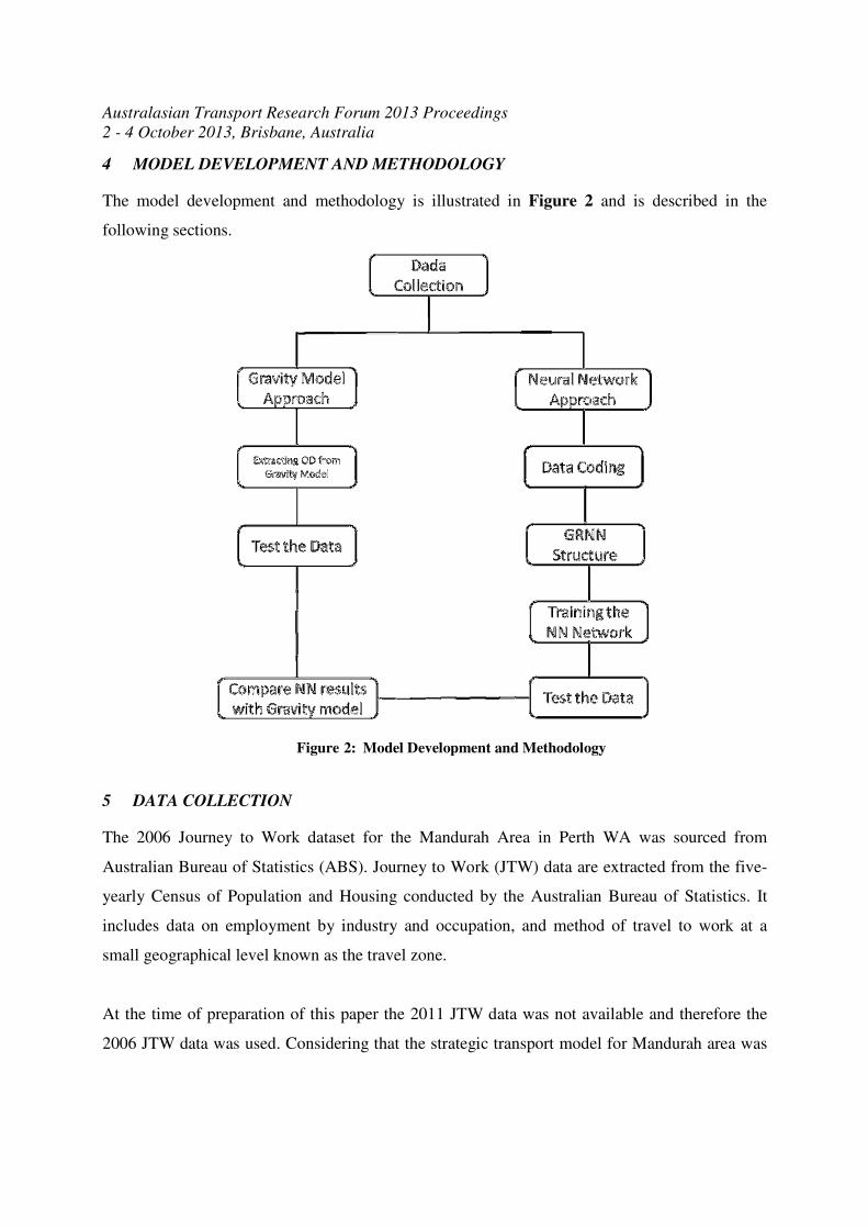
4 MODEL DEVELOPMENT AND METHODOLOGY

The model development and methodology is illustrated in Figure 2 and is described in the

following sections.

Figure 2: Model Development and Methodology

5 DATA COLLECTION

The 2006 Journey to Work dataset for the Mandurah Area in Perth WA was sourced from

Australian Bureau of Statistics (ABS). Journey to Work (JTW) data are extracted from the five-

yearly Census of Population and Housing conducted by the Australian Bureau of Statistics. It

includes data on employment by industry and occupation, and method of travel to work at a

small geographical level known as the travel zone.

At the time of preparation of this paper the 2011 JTW data was not available and therefore the

2006 JTW data was used. Considering that the strategic transport model for Mandurah area was



developed and calibrated for year 2011, then the 2011 JTW data was estimated from the 2006

data assuming the same travel pattern for the JTW in 2006.

6 O-D MATRIX ESTIMATION USING GRAVITY MODEL

6. 1 Mandurah strategic transport model

Due to significant growth in recent years and anticipated future growth the City of Mandurah is

faced with a number of challenges with planning and managing its movement network and

transport system particularly within the City Centre. The City has ambitious plans for the future

to deliver an attractive, dynamic and vibrant City. These plans will generate significant transport

demand which will put pressure on the existing transport infrastructure and systems, particularly

the road network within the City Centre.

In order to assist with its decision-making process, the City has engaged Transcore Pty Ltd to

develop a strategic transport model for the greater Mandurah area. The strategic transport model

will assist the City in establishing the future transport demand and test the impact of land use

growth, major developments and road network options.

The modelled study area entails the Inner Peel Region including Mandurah, Pinjarra and

Yunderup. The number of residential dwellings for the City of Mandurah was calculated for the

38 individual modelling zones as per Figure 3. According to the Australian Bureau of Statistics

census results for 2011 the total number of dwellings in Mandurah is estimated to be about

35,372 with about 69,903 people residing in the municipality.



Figure 3: Mandurah Model Area and Zoning System

6. 2 Model Structure

The traffic model is based on the traditional four-stage model process (trip generation, trip

distribution, mode split and traffic assignment) however, the trip generation within this model

considered only private vehicle trips and therefore the mode split stage was not adopted. The

mode split was taken into consideration when generating the trip production rates for the trip

generation stage. For the purpose of this study the trips were divided into 5 different categories

based on the trip purposes: Work, Education, Social, Other and Non Home Based (NHB) trips.



Trips internal to the modelling area have been distributed based on the following gamma

function:

�� = � ∗ ��∗� !("#∗$��) where:

wij : weight between zone i and zone j

dij : distance between zone i and zone j

Parameters a, b and c were calibrated for each trip purpose so that the model reflects the

proportion of trips for each length as observed in the travel surveys. Assignment of the trips was

based on the fixed demand traffic assignment module in EMME software.

Calibration of the model was based on the existing traffic volumes on the road links. The actual

traffic data was provided by City of Mandurah. Figure 4 shows the modelled traffic volumes

against the actual traffic counts. The linear regression analysis for the 107 traffic count locations

indicates that R2 of the regression plot is 0.985 which shows how well the model is calibrated.

Figure 4: Regression Plot, Calibration of the Base Case (2011)



6. 3 Extracting and comparing the journey to work OD matrix from Gravity Model

The journey to work OD matrix was extracted from the Mandurah strategic transport model and

compared with the 2011 JTW OD matrix obtained from the ABS data. The R2 for the trend line

in Figure 5 is 0.59. According to the analysis undertaken the average Root Mean Square Error

(RMSE) of the modelled trips were estimated to be 51.

Figure 5: Observed and Modelled work Trips Base on Gravity Model

7 O-D MATRIX ESTIMATION USING NEURAL NETWORK

7. 1 Neural Network Model Architecture

People’s activities can be represented by land uses scattered on different zones that are separated

by distance in an area. Therefore, trip distribution relates to the land use patterns in different

zones inside that area. For instance, one zone which is typically occupied by residential land use

patterns generates trips that are attracted to another zone which is formed by retail, industrial,

commercial, etc.

On this basis the input layer of the neural network is represented by land use data in each zone,

which is assigned to RD (Residential Dwellings), RE (Retails), CO (Commercial Land use), SH



(showroom) and SC (Schools). In order to represent the spatial distribution of a pair of zones, the

distance Dij (meters) between zones i and j is defined. Accordingly the input vector (X) is

defined as:

Xij=(RDi, REi, COi, SHi, SCi,,RDj, REj, COj, SHj, SCj, Dij)

Where i and j shows the origin and destination, respectively.

Trips (Tij) between a pair of zones are considered as the output layer of the neural network. The

GRNN has to be able to model the relation between trips Tij and input vector X ij. The model is

developed to forecast the work trip. MATLAB R2011a is used to develop the network where the

optimum spread factor was selected through try and error process. The model structure used in

MATLAB software is illustrated by Figure 6. It has 11 input nodes representing the land uses

for zone i and zone j, and distance between zone i and j (as defined in the above Xij input

vector). There is one node in the output layer which represents the estimated trip number (Tij).

Figure 6: GRNN Model Structure Used in MATLAB Software

Simple data normalization method is used in this study for the input vectors. Simple

normalization will convert the input data to the range [0,1].

There are usually two kinds of input data sets in neural networks, namely training and testing

data sets. The training data set is used in estimating the model parameters/variables while the

testing data set is for evaluating the forecasting ability of the model. For the purpose of this study

90% of the data (400 input vectors) were used for training and 10% were used for testing.



7. 2 GRNN modelling results

The training data set (400 vectors selected randomly) were trained using the GRNN model and

with different spread factors. The optimum spread factor of 1 was selected through try and error

process. Figure 7 illustrates the goodness of fit for the trained GRNN model; R2 of 0.984 was

obtained from the training process which shows how well the network is trained.

Figure 7, Modeled Tij through the Training Process against the Observed Ones

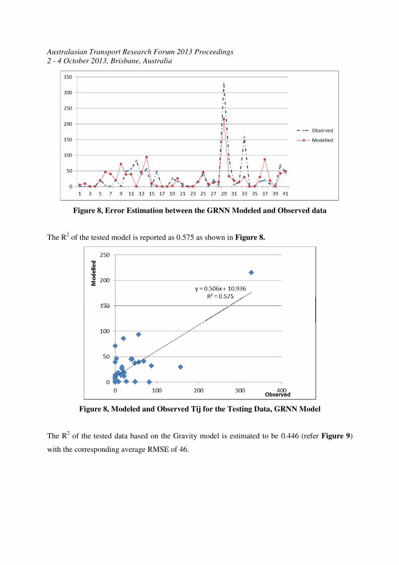
The trained GRNN model was then used to test the 41 unused vectors. Figure 8 illustrates the

modeled trip distribution against the observed data. The absolute difference (error) is also shown

in this figure. The average RMSE for the tested data recorded as 38.



Figure 8, Error Estimation between the GRNN Modeled and Observed data

The R2 of the tested model is reported as 0.575 as shown in Figure 8.

Figure 8, Modeled and Observed Tij for the Testing Data, GRNN Model

The R2 of the tested data based on the Gravity model is estimated to be 0.446 (refer Figure 9)

with the corresponding average RMSE of 46.



Figure 9, Modeled and Observed Tij for the Testing Data, Gravity Model

8 CONCLUSION AND RECOMMENDATION

Based on the results of the analysis undertaken, it can be concluded that the Neural Network

model can be used to forecast trip distribution, especially for work trips. GRNN model could

forecast the work trip distribution based on the land use data for each pair of traffic zones and the

corresponding distance between the two zones.

The modeling results have also provided evidence that a validated GRNN could provide slightly

better goodness of fit than a gravity model with the error level less than the gravity model as

indicated by the average Root Mean Square Error (RMSE), where the RMSE for the NN and

Gravity Model are 38 and 45 respectively. The estimated R2 for the GRNN model and gravity

model is reported 0.557 and 0.446 respectively.

The GRNN outputs highly rely on the amount of data available and the variety of the training

data set vectors. The more the number of input vectors in the training data set the more accurate

results in the output vector. Therefore it is recommended that the efficiency of the GRNN model

be tested and improved with a bigger data set if available.

y = 0.6321x + 7.4264

R² = 0.446

0

50

100

150

200

250

300

350

0 100 200 300 400

Modelled

Observed



References

BLACK, W. R. (1995) Spatial interaction modelling using artificial neural networks. Journal of

Transport Geography, 3, 159-166.

CANTARELLA, G. E. & DE LUCA, S. (2005) Multilayer feed forward networks for

transportation mode choice analysis: An analysis and a comparison with random utility

models. Transportation Research Part C: Emerging Technologies, 13, 121-155.

CARVALHO, M. C. M., DOUGHERTY, M. S., FOWKES, A. S. & WARDMAN, M. R. (1998)

Forecasting travel demand: a comparison of logit and artificial neural network methods.

The Journal of the Operational Research Society, 49, 711-722.

DOUGHERTY, M. (1995) A review of neural networks applied to transport. Transportation

Research Part C: Emerging Technologies, 3, 247-260.

HAGAN, M. T. & MENHAJ, M. B. (1994) Training feed forward networks with the Marquardt

algorithm. Neural Networks, IEEE Transactions on, 5, 989-993.

HENSHER, D. A. & TON, T. T. (2000) A comparison of the predictive potential of artificial

neural networks and nested logit models for commuter mode choice. Transportation

Research Part E: Logistics and Transportation Review, 36, 155-172.

HYMAN, G. M. (1969) The Calibration of Trip Distribution Models. Environment and Planning,

1, 105-112.

MOZOLIN, M., THILL, J. C. & LYNN, U. E. (2000) Trip distribution forecasting with

multilayer perceptron neural networks: A critical evaluation. Transportation Research

Part B: Methodological, 34, 53-73.

SUBBA RAO, P. V., SIKDAR, P. K., KRISHNA RAO, K. V. & DHINGRA, S. L. (1998)

Another insight into artificial neural networks through behavioural analysis of access

mode choice. Computers, Environment and Urban Systems, 22, 485-496.

TEODOROVIC, D. & VUKADINOVIC, K. (1998) Traffic Control and Transport Planning: A

Fuzzy Sets and Neural Networks Approach, Massachusetts, USA, Kluwer Academic

Publisher.

ZHANG, G., PATUWO, B. E. & HU, M. Y. (1998) Forecasting with artificial neural networks:

The state of the art. International Journal of Forecasting, 14, 35-62.

GUSRI, Y., TAYLOR, M.A.P. and YUE, W.L. (2011) Forecasting origin-destination matrices

by using neural network approach: A comparison of testing performance between back

propagation, variable learning rate and levenberg-marquardt algorithm. The 34th

Australian Transport Research Forum, Adelaide, Australia.

GUSRI, Y., TAYLOR, M.A.P. and YUE, W.L. (2009). Improving artificial neural network

performance in calibration doubly-constrained work trip distribution by using a simple

data normalisation and linear activation function. Proceedings of the 32nd

Australian

Transport Research Forum. Auckland, New Zealand.

FISCHWR MM, LUNGE Y. A (1998) Genetic-algorithms Based Evolutionary Computational

Neural Network for Modelling Spatial Interaction Data, Vol. 32, Regional Science:

Springer-Verlag 437–458.

CELIKOGLUE HB. (2007) Public transportation trip flow modelling with generalized

regression neural networks. Advances in Engineering Software; 38:71–79.

HAQUE ME, SUDHAKAR KV. ANN back propagation prediction model for fracture toughness

in microalloy steel. Int J Fatique 2002; 24:1003–10.

D. F. SPECHT, “A general regression neural network,” IEEE Trans. Neural Netw. 2 (6) (1991)

568–576.



E.A. NADARAYA, “On estimating regression,” Theory Probab. Appl. 10 (1964) 186–190.

G.S. WATSON, Smooth regression analysis, Sankhya, Ser. A 26 (4)

TSOUKALAS, L. H., and R. E., Uhrig, 1997. Fuzzy and Neural Approache in Engineering: New

York, John Wiley and Sons, Inc., 87p.

H. SCHIOLER, U. Hartmann, “Mapping neural network derived from the Parzen window

estimator”, Neural Netw. 5 (6) (1992) 903–909.1964) 359–372

trip distribution modelling using neural network · various studies in transportation modelling...

Documents