new technology demonstration program, kennedy … technology demonstration program, kennedy space...
TRANSCRIPT

New TechnologyDemonstration Program,Kennedy Space Center,Hangar L Heat Pipe Project:Performance Evaluation Report
Period of PerformanceJune 1996 to February 1998
C.E. HancockPaul ReevesMountain Energy PartnershipBoulder, Colorado
March 1999 • NREL/SR-710-24738

March 1999 • NREL/SR-710-24738
New TechnologyDemonstration Program,Kennedy Space Center,Hangar L Heat Pipe Project:Performance Evaluation Report
Period of PerformanceJune 1996 to February 1998
C.E. HancockPaul ReevesMountain Energy PartnershipBoulder, Colorado
NREL technical monitor: Richard Parish
National Renewable Energy Laboratory1617 Cole BoulevardGolden, Colorado 80401-3393
NREL is a U.S. Department of Energy LaboratoryOperated by Midwest Research Institute • Battelle • Bechtel
Contract No. DE-AC36-98-GO10337

NOTICE
This report was prepared as an account of work sponsored by an agency of the United States government.Neither the United States government nor any agency thereof, nor any of their employees, makes anywarranty, express or implied, or assumes any legal liability or responsibility for the accuracy, completeness,or usefulness of any information, apparatus, product, or process disclosed, or represents that its use wouldnot infringe privately owned rights. Reference herein to any specific commercial product, process, or serviceby trade name, trademark, manufacturer, or otherwise does not necessarily constitute or imply itsendorsement, recommendation, or favoring by the United States government or any agency thereof. Theviews and opinions of authors expressed herein do not necessarily state or reflect those of the United Statesgovernment or any agency thereof.
Available to DOE and DOE contractors from:Office of Scientific and Technical Information (OSTI)P.O. Box 62Oak Ridge, TN 37831
Prices available by calling (423) 576-8401
Available to the public from:National Technical Information Service (NTIS)U.S. Department of Commerce5285 Port Royal RoadSpringfield, VA 22161(703) 605-6000 or (800) 553-6847orDOE Information Bridgehttp://www.doe.gov/bridge/home.html
This publication received minimal editorial review at NREL
Printed on paper containing at least 50% wastepaper, including 20% postconsumer waste

iii
Preface
This work was funded by the DOE/NREL FEMP program under NREL Subcontract No. KAP-6-16318-08. Weappreciate the support and encouragement of Karen Thomas as the NREL project manager. We thank Will Minerand his staff (Dynamac Corp.) and Bill Ruppert and Dave Koval (EG&G) for their substantial assistance in ourwork on-site at the Kennedy Space Center.

iv
Executive Summary
In December of 1996, heat pipe heat exchangers were installed on three air handlers at Hangar L at theCape Canaveral Air Station, Kennedy Space Center, Cape Canaveral, Florida. These retrofits wereimplemented with the intent to improve the dehumidification performance of the cooling systems,reduce the electric and steam energy required for reheating air, and reduce electric energy used by thechillers.
Audits were conducted before and after the heat pipes were installed and a detailed monitoring systemwas set up to record hourly operating conditions of each of the three air-handling units. The auditinformation and monitored data were used to create a simulation model of the three air-handlingsystems and annual energy savings were predicted.
Energy savings for air handling unit 1 (AHU-1) were found to be negligible. Heat pipe installation inAHU-1 may have been inappropriate because of the design of the original cooling coils. Annualsavings for AHU-2 are small, primarily because the required reheat for the system was already small.AHU-3 was the best application for the heat pipes and showed savings of 70,000 kWh per year.Interior humidity conditions improved after installation of the heat pipes for AHU-2 and AHU-3.
Summary of Heat Pipe Installation Savings
Savings Component AHU-1 AHU-2 AHU-3
Reheat Savings (kWh*) 0 3,000 51,600
Cooling Coil Load Reduction (ton-hours) 0 -880 11,000
Total Energy Savings (kWh) 0 1,600 69,600
Humidity Control Improvement None 5-10% 5-10%
*kilowatt-hours

v
ContentsPage
Preface .................................................................................................................................................. iii
Executive Summary.............................................................................................................................. iv
Contents ..................................................................................................................................................v
Introduction.............................................................................................................................................1
System Description .................................................................................................................................3
Evaluation Approach ..............................................................................................................................6
Direct Comparison of Measured Performance Data ...............................................................................7
Direct Comparison of Reheat Energy Use ..........................................................................................7Direct Comparison of Chiller Energy Use ..........................................................................................9Direct Comparison of Space Conditions...........................................................................................10Known Differences Between the Preretrofit and Postretrofit Periods...............................................12Observations on Direct Comparison of Data ....................................................................................14
System Performance Modeling and Annual Energy Prediction ...........................................................15
Modeling Approach ..........................................................................................................................15Annual Energy Prediction for AHU-1...............................................................................................16Annual Energy Prediction for AHU-2...............................................................................................19Annual Energy Prediction for AHU-3...............................................................................................24
Conclusions...........................................................................................................................................30
References.............................................................................................................................................31
Appendix A -- Pre-Retrofit Evaluation Report
Appendix B -- Post-Retrofit Evaluation Report
Appendix C -- Detailed Measured Performance Graphs

vi
List of Tables
Summary of Heat Pipe Installation Savings.......................................................................................................... ivTable 1. Supply Air Flow Rates.......................................................................................................................... 13Table 2. Summary of Heat Pipe Savings ............................................................................................................ 30
List of Figures
Figure 1. The heat pipe precool and reheat principle ............................................................................................ 1Figure 2. Heat pipe dehumidification process....................................................................................................... 1Figure 3. Schematic of AHU-1 with heat pipe installed ....................................................................................... 3Figure 4. Schematic of AHU-2 and AHU-3 with heat pipe installed.................................................................... 4Figure 5. Photo of AHU-3 .................................................................................................................................... 5Figure 6. Photo of Hangar L chillers..................................................................................................................... 5Figure 7. Direct comparison of electric reheat energy, AHU-2. ........................................................................... 7Figure 8. Direct comparison of electric reheat energy, AHU-3. ........................................................................... 8Figure 9. Fuel oil purchases. ................................................................................................................................. 8Figure 10. Direct comparison of electric chiller energy, chiller 1......................................................................... 9Figure 11. Direct comparison of electric chiller energy, chiller 2....................................................................... 10Figure 12. Direct comparison of space conditions, AHU-1. ............................................................................... 11Figure 13. Direct comparison of space conditions, AHU-2. ............................................................................... 11Figure 14. Direct comparison of space conditions, AHU-3. ............................................................................... 12Figure 15. Total heat removed, AHU-3, showing increased cooling capacity in the postretrofit period. ........... 13Figure 16. Chilled water supply temperatures during preretrofit and postretrofit periods. ................................. 14Figure 17. Average delivered air temperatures for AHU-1................................................................................. 17Figure 18. SHR for precool and main cooling coils, AHU-1, preretrofit and postretrofit periods...................... 18Figure 19. SHR for combined precool + main cooling coils, AHU-1, preretrofit and postretrofit periods......... 18Figure 20. Average space sensible load used for simulation, AHU-2................................................................. 20Figure 21. Average space latent load used for simulation, AHU-2..................................................................... 20Figure 22. Predicted vs. measured SHR for AHU-2, preretrofit period.............................................................. 21Figure 23. Predicted vs. measured SHR for AHU-2, postretrofit period ............................................................ 22Figure 24. Daily average predicted SHR, with and without the heat pipe retrofit .............................................. 22Figure 25. Predicted daily reheat, with and without the heat pipe, AHU-2 ........................................................ 23Figure 26. Average space sensible load used for simulation, AHU-3................................................................. 25Figure 27. Average space latent load used for simulation, AHU-3..................................................................... 25Figure 28. Predicted vs. measured SHR for AHU-3, preretrofit period.............................................................. 26Figure 29. Predicted vs. measured SHR for AHU-3, postretrofit period ............................................................ 27Figure 30. Daily average predicted SHR, with and without the heat pipe retrofit .............................................. 27Figure 31. Predicted daily reheat, with and without the heat pipe, AHU-3 ........................................................ 28Figure 32. Reheat energy savings due to the heat pipe installation, AHU-3....................................................... 29
1
Introduction
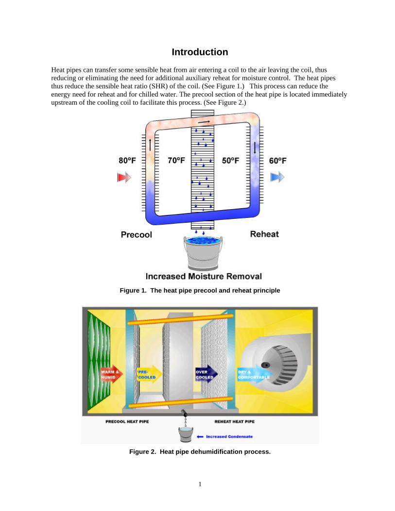
Heat pipes can transfer some sensible heat from air entering a coil to the air leaving the coil, thusreducing or eliminating the need for additional auxiliary reheat for moisture control. The heat pipesthus reduce the sensible heat ratio (SHR) of the coil. (See Figure 1.) This process can reduce theenergy need for reheat and for chilled water. The precool section of the heat pipe is located immediatelyupstream of the cooling coil to facilitate this process. (See Figure 2.)
Figure 1. The heat pipe precool and reheat principle
Figure 2. Heat pipe dehumidification process.

2
Heat pipe heat exchangers were installed on three air handlers at Hangar L at the Cape Canaveral AirStation, Kennedy Space Center, Cape Canaveral, Florida, in December of 1996. The intent of theseretrofits was to improve the dehumidification performance of the cooling systems, reduce the electricand steam energy required for reheating air, and reduce electric energy used by the chillers.
Direct measurements of the primary energy quantities have been made over an extended period, bothbefore and after the retrofit. The instrumentation and the measured preretrofit and postretrofitperformance were described in previous reports (January 1997 and October 1997). This reportdescribes the annual energy savings attributed to the heat pipe installation.
Direct comparisons have been made between the measured performances of the three systems for thesame months before and after the retrofit. Changes in reheat and chiller electric power were observed,as well as changes in interior space temperature and relative humidity (RH). Because other systemoperating parameters changed between 1996 and 1997, this direct comparison is not a complete andaccurate quantitative representation of savings attributable to the heat pipes. Significant changes thataffected the performance of the air-handling systems that are not attributable to the heat pipeinstallations include: a new condenser and a new compressor for the chiller serving two of the retrofittedair handlers, changes in supply air flow rates, and possible changes to the cooling coil controlmechanism.
The measured data were used to develop thermal performance models of each system. These modelswere used to calculate the annual savings from the heat pipes for a consistent set of operatingconditions. Results of the simulation analysis provide significant insight regarding the appropriateapplication of heat pipes in existing HVAC systems.
3
System Description
The NASA Life Sciences Support Facility is located in Hangar L at the Cape Canaveral Air Station,Cape Canaveral, Florida. Laboratory and office areas have been constructed inside the original hangarstructure. The hangar is approximately 175 feet wide, 150 feet long, and 30 feet high, covering aground floor area of about 26,000 square feet. There are approximately 20,000 square feet of air-conditioned space inside the hangar, including offices, labs, and clean rooms. There are very fewwindows and essentially no direct solar gains on conditioned spaces. Most of the cooling load is causedby internal gains from operating lights and equipment and from conditioning outside air for ventilation.Normal operating hours for personnel at the building are 0700 through 1700. Much of the equipmentand interior lighting operates 24 hours per day.
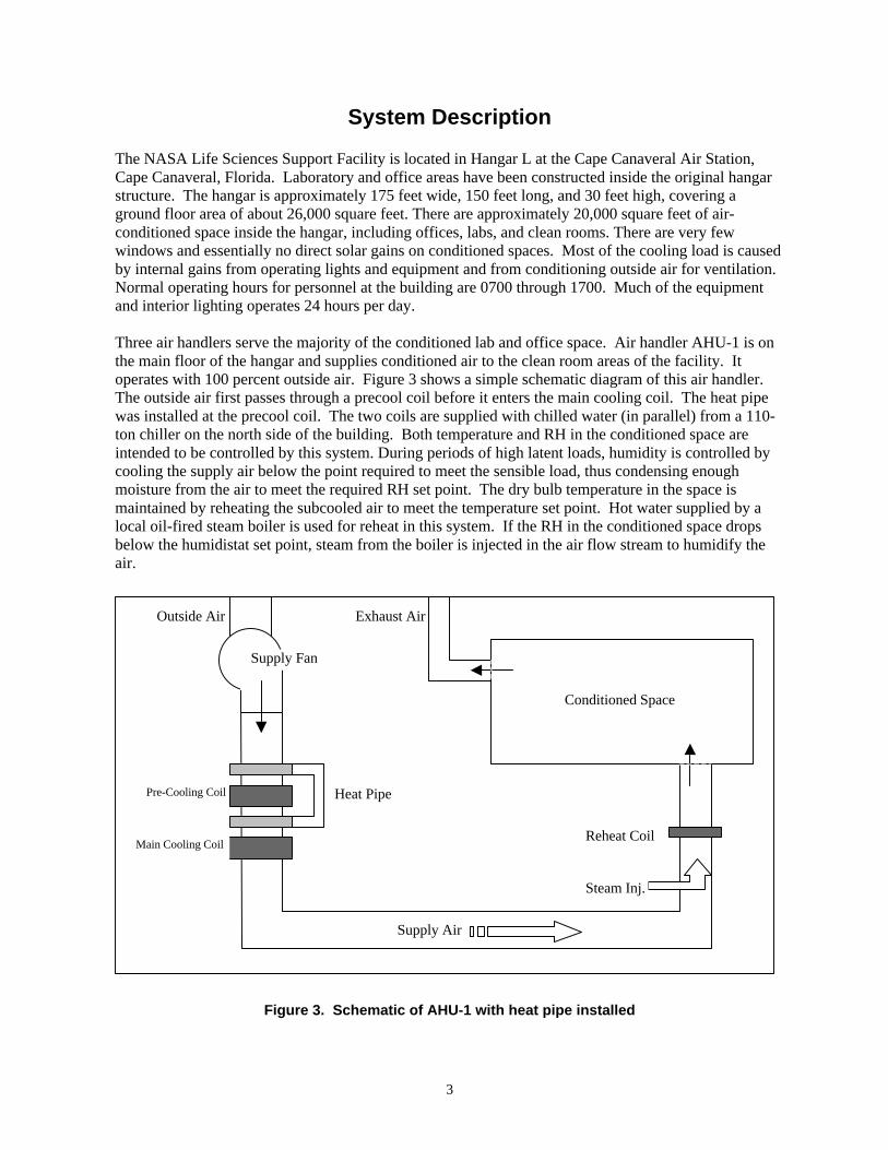
Three air handlers serve the majority of the conditioned lab and office space. Air handler AHU-1 is onthe main floor of the hangar and supplies conditioned air to the clean room areas of the facility. Itoperates with 100 percent outside air. Figure 3 shows a simple schematic diagram of this air handler.The outside air first passes through a precool coil before it enters the main cooling coil. The heat pipewas installed at the precool coil. The two coils are supplied with chilled water (in parallel) from a 110-ton chiller on the north side of the building. Both temperature and RH in the conditioned space areintended to be controlled by this system. During periods of high latent loads, humidity is controlled bycooling the supply air below the point required to meet the sensible load, thus condensing enoughmoisture from the air to meet the required RH set point. The dry bulb temperature in the space ismaintained by reheating the subcooled air to meet the temperature set point. Hot water supplied by alocal oil-fired steam boiler is used for reheat in this system. If the RH in the conditioned space dropsbelow the humidistat set point, steam from the boiler is injected in the air flow stream to humidify theair.
Figure 3. Schematic of AHU-1 with heat pipe installed
Pre-Cooling Coil Heat Pipe
Conditioned Space
Exhaust Air
Supply Air
Outside Air
Reheat Coil
Supply Fan
Main Cooling Coil
Steam Inj.

4
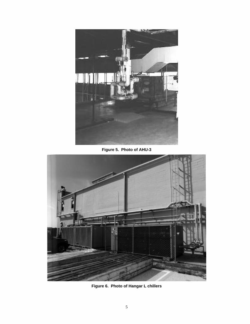
Figure 4 shows a simple schematic diagram typical of AHU-2 and AHU-3. These air handlers are onthe mezzanine level above the office spaces on the south side of the building. (Note that our AHU-3 isdesignated AHU-1 [Mezzanine] in the original mechanical plans.) These AHUs serve a combination ofoffices and lab space. Chilled water is supplied (in parallel) by a 55-ton air-cooled chiller on the northside of the building. Figure 5 shows a photograph of AHU-3. The chillers on the north side of thehangar are pictured in Figure 6. Humidity is controlled by subcooling the air flow to condensesufficient moisture from the air, and then reheating to maintain the dry bulb temperature set point.Reheating is accomplished by electric heaters in the supply ducts to each zone. Steam can be injected inthe supply ducts to humidify the air during rare periods of low humidity in cool weather.
Figure 4. Schematic of AHU-2 and AHU-3 with heat pipe installed
The heat pipes are intended to transfer some of the sensible heat from the air entering the coil to the airleaving the coil, thus reducing or eliminating the need for additional auxiliary reheat for moisturecontrol (assuming that the supply air was indeed already cooler than was required to meet the sensiblespace load). The heat pipes essentially reduce the SHR of the coil. The purpose of the heat pipe retrofitwas to use less energy for reheat and for chilled water. It was recognized that the heat pipe installationcould cause a large drop in pressure, and thus could slightly increase fan power.
Cooling Coil Heat Pipe
Conditioned Space
Return Air
Supply Air
Outside Air
Reheat CoilSupply Fan
Exhaust Air
Steam Inj.
5
Figure 5. Photo of AHU-3
Figure 6. Photo of Hangar L chillers

6
Evaluation Approach
Direct measurements of the primary energy quantities have been made over an extended period bothbefore and after the retrofit. The instrumentation and the measured preretrofit and postretrofitperformance were described in previous reports (Pre-Retrofit Evaluation Report, January 1997[Appendix A] and Post-Retrofit Monitoring and Evaluation Report, October 1997 [Appendix B]). Thisreport describes the annual energy savings attributed to the heat pipe installation.
Direct comparisons were made between the measured performance of the three systems for the samemonths before and after the retrofit. Because other system operating parameters changed between 1996and 1997, this direct comparison is not an accurate quantitative representation of savings attributable tothe heat pipes. The measured data were used to develop thermal performance models of each system.These models were used to calculate the savings from the heat pipes for a consistent set of operatingconditions.
The energy savings attributed to the heat pipes were expected to be derived from:
Reduced reheat power —during periods when either electric or steam reheat would be used to raise themain supply air to the minimum temperature required by the space loads.
Reduced chiller power —during periods when main supply air reheat is required and the chiller isrunning at less than full load.
In addition, interior space conditions may be improved by the heat pipes.
Direct comparisons of daily total electric reheat power for AHU-2 and AHU-3 are made for thecomparable periods before and after the retrofit (August through November). Direct comparisons ofdaily total electric power for both chillers are also made for the period of overlapping data. Interior drybulb temperature and RH are compared for typical summer periods before and after the retrofit.
Measured data were used to characterize the individual components and a simulation model of eachHVAC system was developed. These model components were used to simulate the energy use of eachHVAC system on an hourly basis, using a consistent set of driving functions and operating conditions.Changes caused by the heat pipes were accounted for in the preretrofit and postretrofit simulations,while changes caused by other factors were adjusted for and eliminated from the analysis. Details of themodel development and the predicted annual energy savings are presented.

7
Direct Comparison of Measured Performance Data
Having collected long-term data, it is compelling to directly compare the monitored energy use of thevarious systems before and after the heat pipe retrofits to assess the energy savings. Though thisapproach does offer valuable insight into the system operation, there are a number of reasons whysavings are not accurately represented in such a direct comparison. These reasons will be enumeratedafter presenting a direct comparison of the monitored data. More sophisticated techniques are needed todetermine the actual energy savings.
Direct Comparison of Reheat Energy Use
Electric reheat energy was measured for AHUs 2 and 3 and is presented in the following two figures(hot water reheat for AHU-1 was not measured). The preretrofit period extends from mid-August 1996to mid-November 1996. The postretrofit period includes all of 1997. For the preretrofit period, the x-axis of Figure 7 is the Julian day number in 1996; for the postretrofit period, the x-axis is the Julian daynumber in 1997.
Figure 7. Direct comparison of electric reheat energy, AHU-2.
As shown in Figure 7, there is minimal reheat for AHU-2 during the hot summer days with increasingreheat as the daily average outdoor temperature begins to cool down. For the postretrofit period, there isno reheat energy during summer months (June through September) and significant reheat energy usedduring the winter, spring, and late fall. Note that there is no reheat data for this air handler during partsof February and March 1997 because of equipment problems. This data set shows that there was muchless reheat energy used after the heat pipe was installed for the period August through November. It isnot possible to quantify the amount of annual savings attributed to the heat pipe from this data, partlybecause of the wide variation in reheat energy required for any given period. The figure also shows thatthe average daily outdoor temperature (Tave) was not significantly different from year to year.
AHU System 2Preretrofit & Postretrofit Reheat Power, 1996 & 1997
0
100
200
300
400
500
600
700
800
1 15 29 43 57 71 85 99 113
127
141
155
169
183
197
211
225
239
253
267
281
295
309
323
337
351
365
day
dai
ly R
ehea
t (k
Wh
)
0
5
10
15
20
25
30
35
Averag
e Daily
Tem
peratu
re (C)
Reheat, Preretrofit
Reheat, Postretrofit
Tave, Preretrofit
Tave, Postretrofit
8
Figure 8. Direct comparison of electric reheat energy, AHU-3.
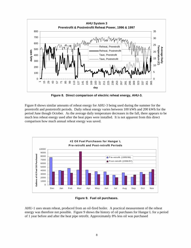
Figure 8 shows similar amounts of reheat energy for AHU-3 being used during the summer for thepreretrofit and postretrofit periods. Daily reheat energy varies between 100 kWh and 200 kWh for theperiod June though October. As the average daily temperature decreases in the fall, there appears to bemuch less reheat energy used after the heat pipes were installed. It is not apparent from this directcomparison how much annual reheat energy was saved.
Figure 9. Fuel oil purchases.
AHU-1 uses steam reheat, produced from an oil-fired boiler. A practical measurement of the reheatenergy was therefore not possible. Figure 9 shows the history of oil purchases for Hangar L for a periodof 1 year before and after the heat pipe retrofit. Approximately 8% less oil was purchased
#2 Oil Fuel Purchases for Hangar L
Pre-retrofit and Post-retrofit Periods
0
1000
2000
3000
4000
5000
6000
7000
8000
9000
10000
Dec Jan Feb M a r Apr M a y Jun Jul Aug Sep Oct Nov
Gal
lon
s o
f #2
Fu
el O
il P
urc
has
ed
P re-retrofit (1995/96)
Pos t-retrofit (1996/97)
AHU System 3Preretrofit & Postretrofit Reheat Power, 1996 & 1997
0
100
200
300
400
500
600
700
800
1 15 29 43 57 71 85 99 113
127
141
155
169
183
197
211
225
239
253
267
281
295
309
323
337
351
365
day
dai
ly k
Wh
0
5
10
15
20
25
30
35A
verage D
aily T
emp
erature (C
)
Reheat, Preretrofit
Reheat, Postretrofit
Tave, Preretrofit
Tave, Postretrofit

9
during the year following the heat pipe retrofit. It is not apparent that this usage difference can beattributed to changes in reheat energy, as opposed to other factors, such as maintenance, purchase dates,and changes in other end uses.
Direct Comparison of Chiller Energy Use
One possible effect of the heat pipes is to lower cooling coil loads, assuming that the coils are beingcontrolled based upon dehumidification requirements. As noted in the previous two reports however,the chillers appeared to run at maximum capacity during the summer months, with or without the heatpipes. It is only during off-peak periods, then, that some chiller energy might be saved.
Figure 10. Direct comparison of electric chiller energy, chiller 1.
Figure 10 shows comparable chiller energy use for the 110-ton chiller (chiller 1) for the preretrofit andpostretrofit periods. It is not apparent that there is a difference in chiller energy use during theoverlapping summer and fall periods, leading to the conclusion that chiller energy use was notsignificantly influenced by the heat-pipe retrofit.
AHU System 1Preretrofit & Postretrofit Chiller Power, 1996 & 1997
0
500
1000
1500
2000
2500
3000
1 15 29 43 57 71 85 99 113
127
141
155
169
183
197
211
225
239
253
267
281
295
309
323
337
351
365
day
dai
ly k
Wh
Preretrofit, 1996
Postretrofit, 1997
10
Figure 11. Direct comparison of electric chiller energy, chiller 2.
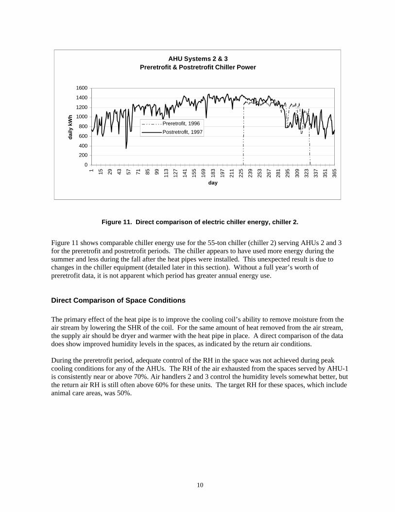
Figure 11 shows comparable chiller energy use for the 55-ton chiller (chiller 2) serving AHUs 2 and 3for the preretrofit and postretrofit periods. The chiller appears to have used more energy during thesummer and less during the fall after the heat pipes were installed. This unexpected result is due tochanges in the chiller equipment (detailed later in this section). Without a full year’s worth ofpreretrofit data, it is not apparent which period has greater annual energy use.
Direct Comparison of Space Conditions
The primary effect of the heat pipe is to improve the cooling coil’s ability to remove moisture from theair stream by lowering the SHR of the coil. For the same amount of heat removed from the air stream,the supply air should be dryer and warmer with the heat pipe in place. A direct comparison of the datadoes show improved humidity levels in the spaces, as indicated by the return air conditions.
During the preretrofit period, adequate control of the RH in the space was not achieved during peakcooling conditions for any of the AHUs. The RH of the air exhausted from the spaces served by AHU-1is consistently near or above 70%. Air handlers 2 and 3 control the humidity levels somewhat better, butthe return air RH is still often above 60% for these units. The target RH for these spaces, which includeanimal care areas, was 50%.
AHU Systems 2 & 3Preretrofit & Postretrofit Chiller Power
0
200
400
600
800
1000
1200
1400
16001 15 29 43 57 71 85 99 113
127
141
155
169
183
197
211
225
239
253
267
281
295
309
323
337
351
365
day
dai
ly k
Wh
Preretrofit, 1996
Postretrofit, 1997
11
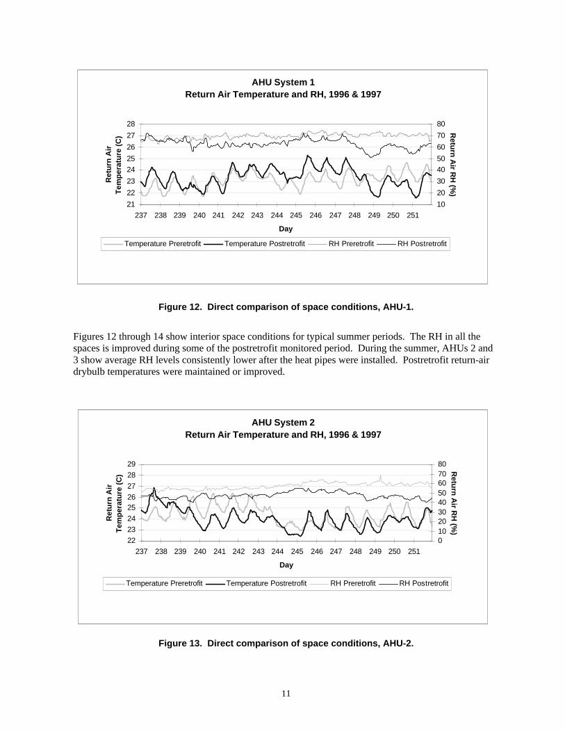
Figure 12. Direct comparison of space conditions, AHU-1.
Figures 12 through 14 show interior space conditions for typical summer periods. The RH in all thespaces is improved during some of the postretrofit monitored period. During the summer, AHUs 2 and3 show average RH levels consistently lower after the heat pipes were installed. Postretrofit return-airdrybulb temperatures were maintained or improved.
Figure 13. Direct comparison of space conditions, AHU-2.
AHU System 1Return Air Temperature and RH, 1996 & 1997
21
22
23
24
25
26
27
28
237 238 239 240 241 242 243 244 245 246 247 248 249 250 251
Day
Ret
urn
Air
T
emp
erat
ure
(C
)
10
20
30
40
50
60
70
80
Retu
rn A
ir RH
(%)
Temperature Preretrofit Temperature Postretrofit RH Preretrofit RH Postretrofit
AHU System 2Return Air Temperature and RH, 1996 & 1997
22
23
24
2526
27
28
29
237 238 239 240 241 242 243 244 245 246 247 248 249 250 251
Day
Ret
urn
Air
T
emp
erat
ure
(C
)
01020304050607080
Retu
rn A
ir RH
(%)
Temperature Preretrofit Temperature Postretrofit RH Preretrofit RH Postretrofit
12
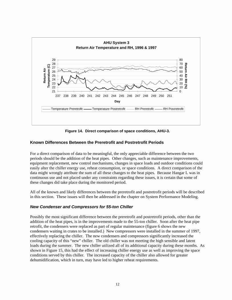
Figure 14. Direct comparison of space conditions, AHU-3.
Known Differences Between the Preretrofit and Postretrofit Periods
For a direct comparison of data to be meaningful, the only appreciable difference between the twoperiods should be the addition of the heat pipes. Other changes, such as maintenance improvements,equipment replacement, new control mechanisms, changes in space loads and outdoor conditions couldeasily alter the chiller energy use, reheat consumption, or space conditions. A direct comparison of thedata might wrongly attribute the sum of all these changes to the heat pipes. Because Hangar L was incontinuous use and not placed under any constraints regarding these issues, it is certain that some ofthese changes did take place during the monitored period.
All of the known and likely differences between the preretrofit and postretrofit periods will be describedin this section. These issues will then be addressed in the chapter on System Performance Modeling.
New Condenser and Compressors for 55-ton Chiller
Possibly the most significant difference between the preretrofit and postretrofit periods, other than theaddition of the heat pipes, is in the improvements made to the 55-ton chiller. Soon after the heat piperetrofit, the condensers were replaced as part of regular maintenance (figure 6 shows the newcondensers waiting in crates to be installed.) New compressors were installed in the summer of 1997,effectively replacing the chiller. The new condensers and compressors significantly increased thecooling capacity of this “new” chiller. The old chiller was not meeting the high sensible and latentloads during the summer. The new chiller utilized all of its additional capacity during these months. Asshown in Figure 15, this had the effect of increasing chiller energy use as well as improving the spaceconditions served by this chiller. The increased capacity of the chiller also allowed for greaterdehumidification, which in turn, may have led to higher reheat requirements.
AHU System 3Return Air Temperature and RH, 1996 & 1997
212223242526272829
237 238 239 240 241 242 243 244 245 246 247 248 249 250 251
Day
Ret
urn
Air
T
emp
erat
ure
(C
)
01020304050607080
Retu
rn A
ir RH
(%)
Temperature Preretrofit Temperature Postretrofit RH Preretrofit RH Postretrofit
13
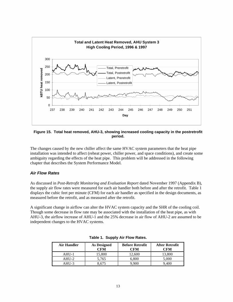
Figure 15. Total heat removed, AHU-3, showing increased cooling capacity in the postretrofitperiod.
The changes caused by the new chiller affect the same HVAC system parameters that the heat pipeinstallation was intended to affect (reheat power, chiller power, and space conditions), and create someambiguity regarding the effects of the heat pipe. This problem will be addressed in the followingchapter that describes the System Performance Model.
Air Flow Rates
As discussed in Post-Retrofit Monitoring and Evaluation Report dated November 1997 (Appendix B),the supply air flow rates were measured for each air handler both before and after the retrofit. Table 1displays the cubic feet per minute (CFM) for each air handler as specified in the design documents, asmeasured before the retrofit, and as measured after the retrofit.
A significant change in airflow can alter the HVAC system capacity and the SHR of the cooling coil.Though some decrease in flow rate may be associated with the installation of the heat pipe, as withAHU-3, the airflow increase of AHU-1 and the 25% decrease in air flow of AHU-2 are assumed to beindependent changes to the HVAC systems.
Table 1. Supply Air Flow Rates.
Air Handler As DesignedCFM
Before RetrofitCFM
After RetrofitCFM
AHU-1 15,800 12,600 13,800AHU-2 5,765 6,800 5,000AHU-3 8,675 9,900 9,400
Total and Latent Heat Removed, AHU System 3High Cooling Period, 1996 & 1997
0
50
100
150
200
250
300
237 238 239 240 241 242 243 244 245 246 247 248 249 250 251
Day
kBT
U h
eat
rem
ove
d Total, Preretrofit
Total, Postretrofit
Latent, Preretrofit
Latent, Postretrofit
14
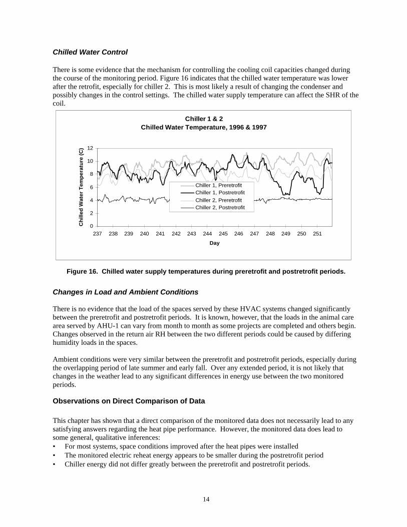
Chilled Water Control
There is some evidence that the mechanism for controlling the cooling coil capacities changed duringthe course of the monitoring period. Figure 16 indicates that the chilled water temperature was lowerafter the retrofit, especially for chiller 2. This is most likely a result of changing the condenser andpossibly changes in the control settings. The chilled water supply temperature can affect the SHR of thecoil.
Figure 16. Chilled water supply temperatures during preretrofit and postretrofit periods.
Changes in Load and Ambient Conditions
There is no evidence that the load of the spaces served by these HVAC systems changed significantlybetween the preretrofit and postretrofit periods. It is known, however, that the loads in the animal carearea served by AHU-1 can vary from month to month as some projects are completed and others begin.Changes observed in the return air RH between the two different periods could be caused by differinghumidity loads in the spaces.
Ambient conditions were very similar between the preretrofit and postretrofit periods, especially duringthe overlapping period of late summer and early fall. Over any extended period, it is not likely thatchanges in the weather lead to any significant differences in energy use between the two monitoredperiods.
Observations on Direct Comparison of Data
This chapter has shown that a direct comparison of the monitored data does not necessarily lead to anysatisfying answers regarding the heat pipe performance. However, the monitored data does lead tosome general, qualitative inferences:• For most systems, space conditions improved after the heat pipes were installed• The monitored electric reheat energy appears to be smaller during the postretrofit period• Chiller energy did not differ greatly between the preretrofit and postretrofit periods.
Chiller 1 & 2Chilled Water Temperature, 1996 & 1997
0
2
4
6
8
10
12
237 238 239 240 241 242 243 244 245 246 247 248 249 250 251
Day
Ch
illed
Wat
er T
emp
erat
ure
(C
)
Chiller 1, PreretrofitChiller 1, Postretrofit
Chiller 2, PreretrofitChiller 2, Postretrofit

15
System Performance Modeling and Annual Energy Prediction
In order to predict the annual energy savings of the heat pipe retrofit, it is necessary to distinguishbetween the influence of the heat pipes and the influence of other factors on the annual energy use of theHVAC systems under analysis. The previous section points to a number of other known differencesbetween the preretrofit and postretrofit periods that might affect the HVAC energy use. In this chapter,the analysis will attempt to isolate the changes due to the heat pipes and then apply these changes to anannual simulation of the HVAC systems. The simulation will predict the annual energy use of eachHVAC system with and without the changes attributed to the heat pipes, leading to an annual energysavings prediction.
Modeling Approach
The modeling approach utilizes the monitored data to characterize individual components of each HVACsystem. These components are then used to simulate the energy use of each HVAC system on an hourlybasis. Changes caused by the heat pipe are accounted for in the preretrofit and postretrofit annualsimulations, while changes due to other influences can be adjusted for and eliminated from the analysis.The individual components are described below, with a description of how each component ischaracterized and used. Details of the actual calculation are presented in subsequent sections of thereport.
• Space sensible heat load:The space sensible heat load is determined from the monitored data, based on the temperature of theair delivered to the spaces (after any reheat), the return air temperature and the supply air flow rate.By applying regression analysis to a year’s worth of calculated space sensible heat load and ambientconditions, the sensible heat load can be predicted based on ambient conditions of drybulbtemperature and relative humidity. During the annual simulation, the estimated space sensible heatload is used to calculate the required supply air temperature as well as the return air temperature.
• Space latent heat load:The space latent heat load is determined from the monitored supply and return air relative humidity.Regression analysis applied to the calculated latent heat load and ambient conditions yields aprediction of the latent load based on ambient conditions of drybulb temperature and relativehumidity. The space latent heat load is used to determine the conditions of the return air for each hourof the annual simulation.
• Mixed air fractions of return and outdoor air:The fraction of outdoor air added to the return air was measured during the system audits, and is usedto calculate the mixed air temperature (return air plus mixed air).
• Cooling coil capacity:The maximum cooling coil capacity, as observed from the monitored data, is used as a limit on thehourly heat extraction.
• Chilled water temperature:It was observed from the monitored data that the chilled water temperature to the coil could bepredicted based on the space sensible and latent load. The chilled water temperature is used as anindependent variable in predicting the cooling coil SHR.
• Cooling coil SHR:The cooling coil sensible-heat-ratio is predicted for each cooling coil based on separate regressionanalyses for the preretrofit and postretrofit periods. The independent variables for the regressionanalyses are the drybulb temperature of the air entering the coil, the relative humidity of the airentering the coil, and the temperature of the chilled water entering the coil. The SHR is used todetermine the conditions of the air leaving the cooling coil.

16
• Supply air temperature and RH control:The supply air temperature used for the simulation is based on the minimum supply air temperaturemeasured in the conditioned spaces. The maximum allowed moisture content of the supply air,expressed as the humidity ratio, is controlled based upon average measured data for each system.
• Ambient conditions:Ambient conditions of drybulb temperature and relative humidity were measured during the entire 14-month monitoring period. A 1-year period of data is used for the simulation model.
The model created for this analysis is fairly simple and is not intended to accurately predict the totalenergy use of the HVAC system. Instead, it focuses on predicting the change in cooling energy andreheat energy as a direct result of changes in the cooling coil characteristics, as influenced by the heatpipes. Where changes occurred to other aspects of the HVAC system, the conditions that existed after theretrofit are used for the simulation. These changes (supply flow rate and chiller components, forexample) would have occurred regardless of the heat pipe installation and actual savings are, therefore,better characterized by the conditions that existed soon after the heat pipe was installed.
There are two components of the reheat energy used in these HVAC systems. One component is reheatenergy used as a control mechanism to supply air of the proper temperature to each space. Eachmultizone, constant volume system must supply air cold enough to cool the zone with the greatest coolingload relative to supply volume that it serves. All other spaces not requiring supply air at this lowtemperature must reheat the supply air to prevent over-cooling. The heat pipes are not intended norexpected to reduce this type of reheat energy requirement.
The second component of reheat energy is the energy required to reheat the supply air that was cooled(for dehumidification purposes) below the minimum temperature required by the space cooling loads.The heat pipes are intended to reduce or eliminate this reheat requirement by allowing the cooling coils toremove more moisture from the air for the same amount of cooling coil load (i.e. by lowering the coolingcoil SHR). The model is intended to predict the cooling coil load and the amount of reheat needed tobring the supply air up to the minimum temperature required by the space loads.
The essential comparison regarding the heat pipe installation is how much energy the HVAC systemswould use in a typical year with the heat pipes versus how much energy the systems would use in atypical year without the heat pipes. The simulation model will use the current conditions, including thenew air flow rates and increased chiller capacity, to model the systems with and without the heat pipes.
Annual Energy Prediction for AHU-1
AHU-1 uses chilled water from the 110-ton chiller, has two cooling coils in series and utilizes 100%outdoor air taken from inside the hangar. Because it uses 100% outside air, the system has a very largelatent load. Figure 12 shows that the system does not adequately regulate humidity levels in the space.Even after the heat pipes were installed, humidity levels have sometimes reached 70% in the spaces.
Calculating the Space Sensible and Latent Loads
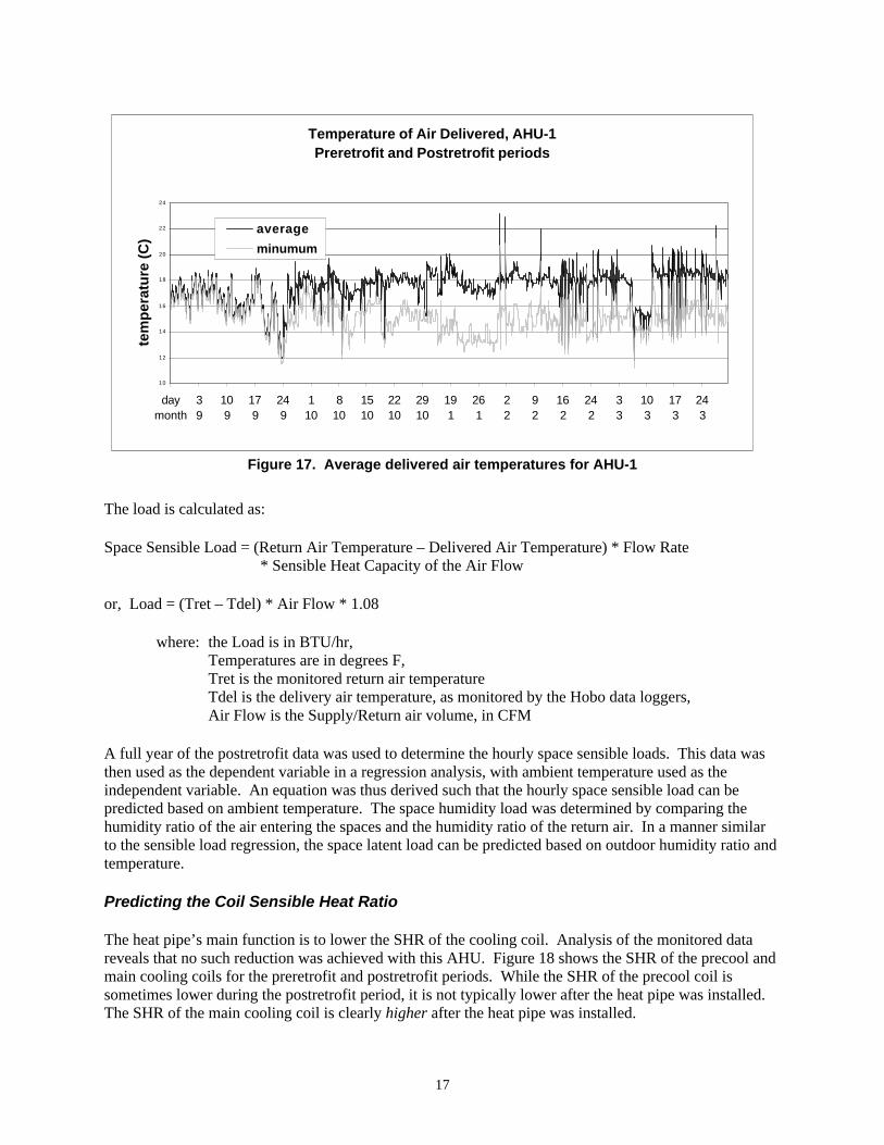
The Hobo data loggers recorded supply air temperatures delivered to the areas served by this HVACsystem. These temperatures are monitored after any reheat energy is added to the supply air stream. Theaverage sensible load of the spaces is determined by observing the difference in the average return airtemperature (return air from all spaces mixed together) and the average delivery air temperature, asrecorded by the Hobo data loggers, Figure 17.
17
Figure 17. Average delivered air temperatures for AHU-1
The load is calculated as:
Space Sensible Load = (Return Air Temperature – Delivered Air Temperature) * Flow Rate* Sensible Heat Capacity of the Air Flow
or, Load = (Tret – Tdel) * Air Flow * 1.08
where: the Load is in BTU/hr,Temperatures are in degrees F,Tret is the monitored return air temperatureTdel is the delivery air temperature, as monitored by the Hobo data loggers,Air Flow is the Supply/Return air volume, in CFM
A full year of the postretrofit data was used to determine the hourly space sensible loads. This data wasthen used as the dependent variable in a regression analysis, with ambient temperature used as theindependent variable. An equation was thus derived such that the hourly space sensible load can bepredicted based on ambient temperature. The space humidity load was determined by comparing thehumidity ratio of the air entering the spaces and the humidity ratio of the return air. In a manner similarto the sensible load regression, the space latent load can be predicted based on outdoor humidity ratio andtemperature.
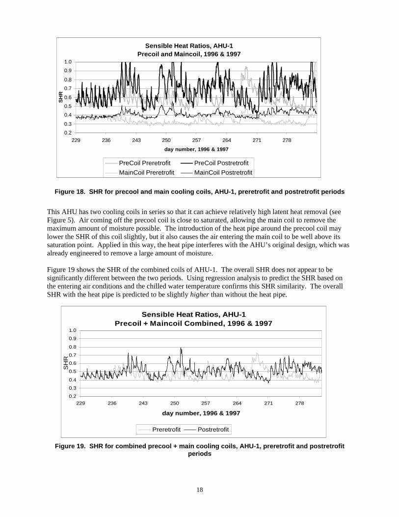
Predicting the Coil Sensible Heat Ratio
The heat pipe’s main function is to lower the SHR of the cooling coil. Analysis of the monitored datareveals that no such reduction was achieved with this AHU. Figure 18 shows the SHR of the precool andmain cooling coils for the preretrofit and postretrofit periods. While the SHR of the precool coil issometimes lower during the postretrofit period, it is not typically lower after the heat pipe was installed.The SHR of the main cooling coil is clearly higher after the heat pipe was installed.
Temperature of Air Delivered, AHU-1Preretrofit and Postretrofit periods
10
12
14
16
18
20
22
24
daymonth
39
109
179
249
110
810
1510
2210
2910
191
261
22
92
162
242
33
103
173
243
tem
per
atu
re (
C)
average
minumum
18
Figure 18. SHR for precool and main cooling coils, AHU-1, preretrofit and postretrofit periods
This AHU has two cooling coils in series so that it can achieve relatively high latent heat removal (seeFigure 5). Air coming off the precool coil is close to saturated, allowing the main coil to remove themaximum amount of moisture possible. The introduction of the heat pipe around the precool coil maylower the SHR of this coil slightly, but it also causes the air entering the main coil to be well above itssaturation point. Applied in this way, the heat pipe interferes with the AHU’s original design, which wasalready engineered to remove a large amount of moisture.
Figure 19 shows the SHR of the combined coils of AHU-1. The overall SHR does not appear to besignificantly different between the two periods. Using regression analysis to predict the SHR based onthe entering air conditions and the chilled water temperature confirms this SHR similarity. The overallSHR with the heat pipe is predicted to be slightly higher than without the heat pipe.
Figure 19. SHR for combined precool + main cooling coils, AHU-1, preretrofit and postretrofitperiods
Sensible Heat Ratios, AHU-1Precoil and Maincoil, 1996 & 1997
0.2
0.3
0.4
0.5
0.6
0.7
0.8
0.9
1.0
229 236 243 250 257 264 271 278
day number, 1996 & 1997
SH
R
PreCoil Preretrofit PreCoil Postretrofit
MainCoil Preretrofit MainCoil Postretrofit
Sensible Heat Ratios, AHU-1Precoil + Maincoil Combined, 1996 & 1997
0.2
0.3
0.4
0.5
0.6
0.7
0.8
0.9
1.0
229 236 243 250 257 264 271 278
day number, 1996 & 1997
SH
R
Preretrofit Postretrofit

19
Because this result has such an important and unexpected impact on the results of this retrofit analysis, efforts weremade to verify the accuracy of the monitored data regarding the calculation of the SHRs. The overall SHR wascalculated from the monitored data in two ways. Air conditions were monitored before the precool coil, between thetwo coils, and after the main cooling coil. The first two data points were used to calculate the sensible and latentheat removed by the precool coil. Likewise, the second two data points were used to calculate the sensible andlatent heat removed by the main coil. The overall SHR was then calculated by adding the heat removed from eachcoil. Alternatively, the air conditions entering the precool coil and the air conditions leaving the main coil were usedto determine the overall SHR. Both methods led to the same result, lending confidence to the monitored data.
Annual Energy Savings
The annual energy prediction is based on all conditions being the same, except for the heat pipe’s effectof the SHR. For this system, the heat pipe did not have a positive effect on the SHR, and no energysavings are predicted.
Discussion and Conclusions
The heat pipe had no positive effect on lowering the overall SHR of the two cooling coils. As originallydesigned, this combination of cooling coils was able to achieve SHRs at, and even below, 0.4. Applyingthe heat pipe to the precool coil defeated the original design of having saturated air entering the maincooling coil and did not lead to a lower SHR, nor any reheat or chiller energy savings.
Annual Energy Prediction for AHU-2
AHU-2 uses chilled water from the 55-ton chiller, has a single cooling coil and has a fresh-air ratio of13% ducted from outside the hangar. Figure 13 shows that this system achieved very good RH controlafter the retrofit, but with little change in the space drybulb temperatures.
Calculating the Space Sensible and Latent Loads
The actual space sensible load can be calculated based on the monitored data for supply air conditions,return air conditions and the amount of reheat used. The sensible load is calculated as:
Space Sensible Load = (Return Air Temperature – Delivered Air Temperature) * Flow Rate* Sensible Heat Capacity of the Air Flow
or, LOADsens = (Tret – Tdel) * Air Flow * 1.08In this case, the delivered air temperature is calculated based on the monitored supply air temperature andthe amount of reheat energy used:
Tdel = Tsup + Reheat Energy / (Air Flow * 1.08)
where: LOADsens is the sensible load, in Btu/hr,Temperatures are in degrees F,Tret is the monitored return air temperature (F),Tsup is the monitored supply air temperature (F),Tdel is the delivery air temperature (F),Reheat Energy is the monitored reheat energy (Btu/hr),Air Flow is the Supply/Return air volume, in CFM

20
The space sensible load is calculated for each hour of the 1997 postretrofit monitored data and used for the modelsimulation. Since this load is assumed to be independent of the HVAC performance, the values determined for the1997 period are used for both the preretrofit and postretrofit simulations. The daily average sensible loads areshown in Figure 20.
Figure 20. Average space sensible load used for simulation, AHU-2
The space latent load was determined by comparing the humidity ratio of the air entering the spaces andthe humidity ratio of the return air. As with the sensible loads, the latent load is determined for each hourof the 1997 period and used for both the preretrofit and postretrofit simulations. The daily average latentloads are shown in Figure 21.
Figure 21. Average space latent load used for simulation, AHU-2
Average Daily Space Sensible Load, AHU-2based on 1997 monitored data
0
20000
40000
60000
80000
100000
120000
1 15
29
43
57
71
85
99
113
127
141
155
169
183
197
211
225
239
253
267
281
295
309
323
337
351
365
day
BT
U/h
r
Average Daily Space Latent Load, AHU-2based on 1997 monitored data
0
0.0005
0.001
0.0015
0.002
0.0025
1 15 29 43 57 71 85 99 113
127
141
155
169
183
197
211
225
239
253
267
281
295
309
323
337
351
365
day
lbm
w/lb
ma
21
Predicting the Coil Sensible Heat Ratio
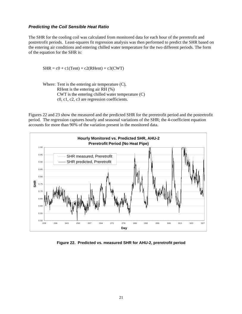
The SHR for the cooling coil was calculated from monitored data for each hour of the preretrofit andpostretrofit periods. Least-squares fit regression analysis was then performed to predict the SHR based onthe entering air conditions and entering chilled water temperature for the two different periods. The formof the equation for the SHR is:
SHR = c0 + c1(Tent) + c2(RHent) + c3(CWT)
Where: Tent is the entering air temperature (C),RHent is the entering air RH (%)CWT is the entering chilled water temperature (C)c0, c1, c2, c3 are regression coefficients.
Figures 22 and 23 show the measured and the predicted SHR for the preretrofit period and the postretrofitperiod. The regression captures hourly and seasonal variations of the SHR; the 4-coefficient equationaccounts for more than 90% of the variation present in the monitored data.
Figure 22. Predicted vs. measured SHR for AHU-2, preretrofit period
Hourly Monitored vs. Predicted SHR, AHU-2Preretrofit Period (No Heat Pipe)
0.50
0.55
0.60
0.65
0.70
0.75
0.80
0.85
0.90
0.95
1.00
229 236 243 250 257 264 271 278 285 292 299 306 313 320 327
Day
SH
R
SHR measured, PreretrofitSHR predicted, Preretrofit

22
Figure 23. Predicted vs. measured SHR for AHU-2, postretrofit period
Figure 24 shows the daily average predicted SHR for a 1-year period with and without the heat piperetrofit. The heat pipe clearly lowers the SHR by a significant amount, as much as 5 to 8% during thesummer months.
Figure 24. Daily average predicted SHR, with and without the heat pipe retrofit
Hourly Monitored vs. Predicted SHR, AHU-2Postretrofit Period (With Heat Pipe)
0.50
0.55
0.60
0.65
0.70
0.75
0.80
0.85
0.90
0.95
1.001
318
635
952
1269
1586
1903
2220
2537
2854
3171
3488
3805
4122
4439
4756
5073
5390
5707
6024
6341
6658
6975
7292
7609
7926
8243
8560
Hour
SH
R
SHR measured, Postretrofit
SHR predicted, Postretrofit
Daily Average Predicted SHR, AHU-2Preretrofit vs. Postretrofit Periods
0.50
0.55
0.60
0.65
0.70
0.75
0.80
0.85
0.90
0.95
1.00
1 15 29 43 57 71 85 99 113
127
141
155
169
183
197
211
225
239
253
267
281
295
309
323
337
351
365
Day
SH
R
SHR predicted, Preretrofit
SHR predicted, Postretrofit

23
Annual Energy Savings
The HVAC system model predicts energy use based on attempting to meet both the sensible and latentspace comfort conditions. The space temperature is controlled to 24° C, and the supply air humidity ratiois maintained at or below 0.010 pounds mass of water per pound mass of air (lbmw/lbma). The coolingcoil and reheat capacities are accounted for, as are the supply flow rate and the variable chilled watertemperature. Reheat energy required to raise the supply air temperature above the minimum temperaturerequired by any space is not accounted for, but, as discussed above, is not affected by the heat pipeinstallation.
Figure 25. Predicted daily reheat, with and without the heat pipe, AHU-2
The simulation indicates that almost no reheat is required due to dehumidification requirements and thatslightly more cooling coil load is needed because of the heat pipe. The reheat requirements are reducedby approximately 3000 kWh, while the cooling coil load increases by 880 ton-hours. The net energysavings are approximately 1600 kWh.
Discussion and Conclusions
The monitored data (Figure 7) indicate that this system might have saved a significant amount of reheatenergy during the shoulder seasons before and after the summer months. The simulation, however,indicates that dehumidification requirements caused very little reheat energy use, either with or withoutthe heat pipe (Figure 25).
The main cause for this phenomenon is the decrease in the supply air flow rate that coincided with theheat pipe installation. Also, the cooling coil for this HVAC system has a relatively low SHR, evenwithout the addition of the heat pipe. During periods of high latent load, the coil had an SHR between0.60 and 0.65 (compare this with AHU-3, Figure 30).
Predicted Daily Reheat Energy, AHU-2Preretrofit & Postretrofit Periods
0
50
100
150
200
250
300
1 15 29 43 57 71 85 99 113
127
141
155
169
183
197
211
225
239
253
267
281
295
309
323
337
351
365
day
Dai
ly R
ehea
t E
ner
gy
(kW
h)
Preretrofit
Posetretrofit
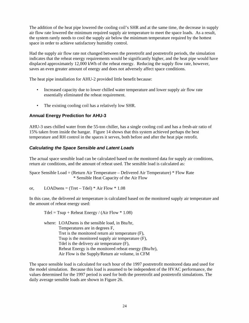
24
The addition of the heat pipe lowered the cooling coil’s SHR and at the same time, the decrease in supplyair flow rate lowered the minimum required supply air temperature to meet the space loads. As a result,the system rarely needs to cool the supply air below the minimum temperature required by the hottestspace in order to achieve satisfactory humidity control.
Had the supply air flow rate not changed between the preretrofit and postretrofit periods, the simulationindicates that the reheat energy requirements would be significantly higher, and the heat pipe would havedisplaced approximately 12,000 kWh of the reheat energy. Reducing the supply flow rate, however,saves an even greater amount of energy and does not adversely affect space conditions.
The heat pipe installation for AHU-2 provided little benefit because:
• Increased capacity due to lower chilled water temperature and lower supply air flow rateessentially eliminated the reheat requirement.
• The existing cooling coil has a relatively low SHR.
Annual Energy Prediction for AHU-3
AHU-3 uses chilled water from the 55-ton chiller, has a single cooling coil and has a fresh-air ratio of15% taken from inside the hangar. Figure 14 shows that this system achieved perhaps the besttemperature and RH control in the spaces it serves, both before and after the heat pipe retrofit.
Calculating the Space Sensible and Latent Loads
The actual space sensible load can be calculated based on the monitored data for supply air conditions,return air conditions, and the amount of reheat used. The sensible load is calculated as:
Space Sensible Load = (Return Air Temperature – Delivered Air Temperature) * Flow Rate* Sensible Heat Capacity of the Air Flow
or, LOADsens = (Tret – Tdel) * Air Flow * 1.08
In this case, the delivered air temperature is calculated based on the monitored supply air temperature andthe amount of reheat energy used:
Tdel = Tsup + Reheat Energy / (Air Flow * 1.08)
where: LOADsens is the sensible load, in Btu/hr,Temperatures are in degrees F,Tret is the monitored return air temperature (F),Tsup is the monitored supply air temperature (F),Tdel is the delivery air temperature (F),Reheat Energy is the monitored reheat energy (Btu/hr),Air Flow is the Supply/Return air volume, in CFM
The space sensible load is calculated for each hour of the 1997 postretrofit monitored data and used forthe model simulation. Because this load is assumed to be independent of the HVAC performance, thevalues determined for the 1997 period is used for both the preretrofit and postretrofit simulations. Thedaily average sensible loads are shown in Figure 26.

25
Figure 26. Average space sensible load used for simulation, AHU-3
The space latent load was determined by comparing the humidity ratio of the air entering the spaces andthe humidity ratio of the return air. As with the sensible loads, the latent load is determined for each hourof the 1997 period and used for both the preretrofit and postretrofit simulations. The daily average latentloads are shown in Figure 27.
Figure 27. Average space latent load used for simulation, AHU-3
Average Daily Space Sensible Load, AHU-3based on 1997 monitored data
0
20000
40000
60000
80000
100000
120000
140000
1600001 15 29 43 57 71 85 99 113
127
141
155
169
183
197
211
225
239
253
267
281
295
309
323
337
351
365
day
BT
U/h
r
Average Daily Space Latent Load, AHU-3based on 1997 monitored data
0
0.0005
0.001
0.0015
0.002
0.0025
0.003
0.0035
0.004
0.0045
1 15 29 43 57 71 85 99 113
127
141
155
169
183
197
211
225
239
253
267
281
295
309
323
337
351
365
day
late
nt
load
(lb
mw
/lbm
a)

26
Predicting the Coil Sensible Heat Ratio
The SHR for the cooling coil was calculated from monitored data for each hour of the preretrofit andpostretrofit periods. Least-squares fit regression analysis was then performed to predict the SHR based onthe entering air conditions and entering chilled water temperature for the two different periods. The formof the equation for the SHR is:
SHR = c0 + c1(Tent) + c2(RHent) + c3(CWT)
Where: Tent is the entering air temperature (C),RHent is the entering air RH (%)CWT is the entering chilled water temperature (C)c0, c1, c2, c3 are regression coefficients.
Figures 28 and 30 show the measured and the predicted SHR for the preretrofit period and the postretrofitperiod. The regression captures hourly and seasonal variations of the SHR; the 4-coefficient equationaccounts for approximately 90% of the variation present in the monitored data.
Figure 28. Predicted vs. measured SHR for AHU-3, preretrofit period
Hourly Monitored vs. Predicted SHR, AHU-3Preretrofit Period (No Heat Pipe)
0.50
0.55
0.60
0.65
0.70
0.75
0.80
0.85
0.90
0.95
1.00
229 236 243 250 257 264 271 278 285 292 299 306 313 320 327
Day
SH
R
SHR measured, PreretrofitSHR predicted, Preretrofit

27
Figure 29. Predicted vs. measured SHR for AHU-3, postretrofit period
Figure 30 shows the daily average predicted SHR for a 1-year period with and without the heat piperetrofit. The heat pipe clearly lowers the SHR by a significant amount, as much as 10 – 15% during thesummer months.
Figure 30. Daily average predicted SHR, with and without the heat pipe retrofit
Hourly Monitored vs. Predicted SHR, AHU-3Postretrofit Period (With Heat Pipe)
0.50
0.55
0.60
0.65
0.70
0.75
0.80
0.85
0.90
0.95
1.001
325
649
973
1297
1621
1945
2269
2593
2917
3241
3565
3889
4213
4537
4861
5185
5509
5833
6157
6481
6805
7129
7453
7777
8101
8425
8749
Hour
SH
R
SHR predicted, Postretrofit
SHR measured, Postretrofit
Daily Average Predicted SHR, AHU-3Preretrofit vs. Postretrofit Periods
0.50
0.55
0.60
0.65
0.70
0.75
0.80
0.85
0.90
0.95
1.00
1 15 29 43 57 71 85 99 113
127
141
155
169
183
197
211
225
239
253
267
281
295
309
323
337
351
365
Day
SH
R
SHR predicted, Preretrofit
SHR predicted, Postretrofit

28
Annual Energy Savings
The HVAC system model predicts energy use based on attempting to meet both the sensible and latentspace comfort conditions. The space temperature is controlled to 24° C, and the supply air humidity ratiois maintained at or below 0.010 lbmw/lbma. The cooling coil and reheat capacities are accounted for, asare the supply air flow rate and the variable chilled water temperature. Reheat energy required to raisethe supply air temperature above the minimum temperature required by any space is not accounted for,but, as discussed above, is not affected by the heat pipe installation.
If the heat pipe were not installed, but all other changes discussed in the previous chapter wereimplemented, the annual reheat energy would be predicted as 62,500 kWh. With the heat pipe installed,the annual reheat energy would be predicted as 10,900 kWh, representing an annual savings of 51,600kWh. In addition, the chiller can expect a reduced load of approximately 11,000 ton-hours per year. Thereduced chiller load translates to electric savings of approximately 18,000 kWh per year.
Figure 31. Predicted daily reheat, with and without the heat pipe, AHU-3
It is worth comparing Figures 8 and 31, which show the reheat as monitored during the preretrofit andpostretrofit periods, and the reheat as predicted by the simulation. The simulation predicts the mostamount of reheat occurring in the summer months, while the monitored data demonstrate just theopposite. This implies that much of the reheat used during the off-peak months is required because of thespace load diversity, and not because of dehumidification requirements. Also, the simulation indicates fargreater reheat requirements for the preretrofit condition than was measured during the preretrofit period.This large amount of summer reheat in the preretrofit period is a result of the increased cooling coilcapacity that occurred after the preretrofit period. The analysis predicts that increasing the coolingcapacity to the postretrofit level without installing the heat pipe would have nearly doubled the amount ofreheat required to maintain space conditions.
Predicted Daily Reheat Energy, AHU-3Preretrofit & Postretrofit Periods
0
100
200
300
400
500
600
700
1 15 29 43 57 71 85 99 113
127
141
155
169
183
197
211
225
239
253
267
281
295
309
323
337
351
365
day
Dai
ly R
ehea
t E
ner
gy
(kW
h)
Preretrofit
Postretrofit
29
Discussion and Conclusions
The monitored data does not indicate that this system saved a large amount of reheat energy during thesummer months. The simulation, however, indicates that the increased cooling capacity, due to a newcondenser and compressor, would have provided better comfort control at the expense of greatlyincreased reheat requirements. Had only the chiller improvements been applied, energy use would haveincreased by approximately 50,000 kWh. Applying both the heat pipe retrofit and chiller improvements tothis system reduced energy use by nearly 20,000 kWh.
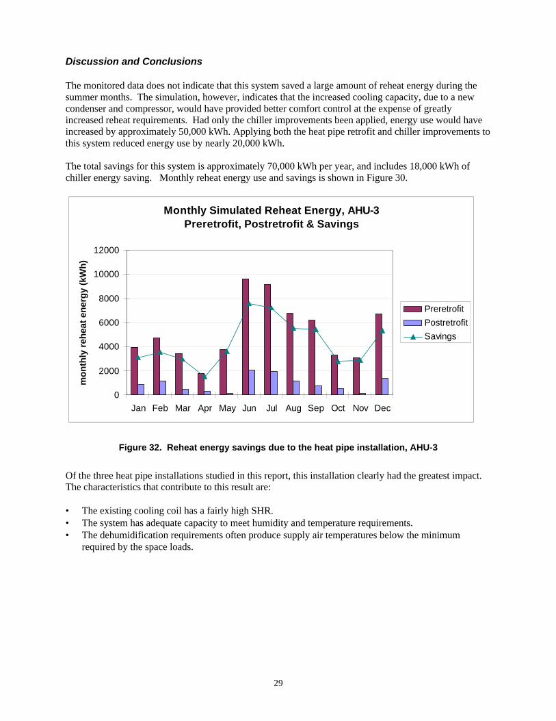
The total savings for this system is approximately 70,000 kWh per year, and includes 18,000 kWh ofchiller energy saving. Monthly reheat energy use and savings is shown in Figure 30.
Figure 32. Reheat energy savings due to the heat pipe installation, AHU-3
Of the three heat pipe installations studied in this report, this installation clearly had the greatest impact.The characteristics that contribute to this result are:
• The existing cooling coil has a fairly high SHR.• The system has adequate capacity to meet humidity and temperature requirements.• The dehumidification requirements often produce supply air temperatures below the minimum
required by the space loads.
Monthly Simulated Reheat Energy, AHU-3Preretrofit, Postretrofit & Savings
0
2000
4000
6000
8000
10000
12000
Jan Feb Mar Apr May Jun Jul Aug Sep Oct Nov Dec
mo
nth
ly r
ehea
t en
erg
y (k
Wh
)
Preretrofit
Postretrofit
Savings
30
Conclusions
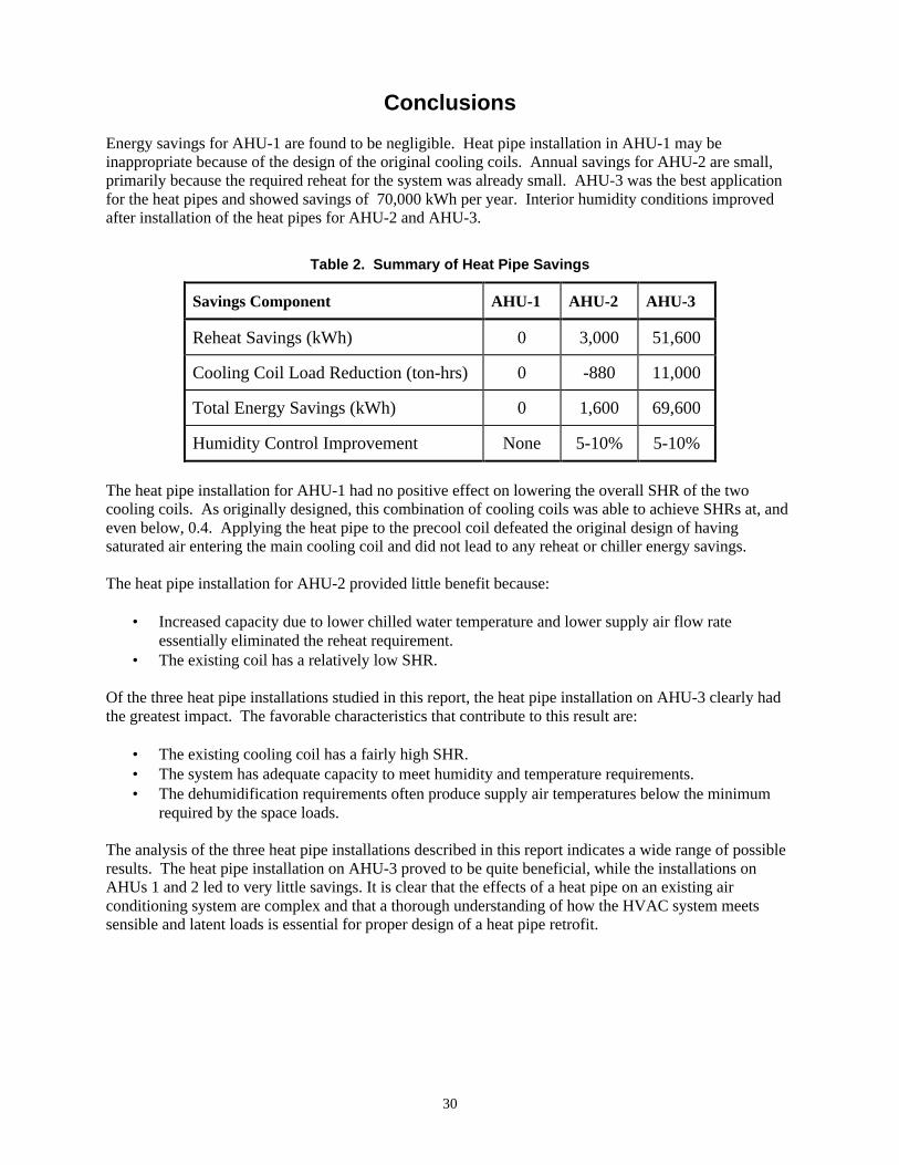
Energy savings for AHU-1 are found to be negligible. Heat pipe installation in AHU-1 may beinappropriate because of the design of the original cooling coils. Annual savings for AHU-2 are small,primarily because the required reheat for the system was already small. AHU-3 was the best applicationfor the heat pipes and showed savings of 70,000 kWh per year. Interior humidity conditions improvedafter installation of the heat pipes for AHU-2 and AHU-3.
Table 2. Summary of Heat Pipe Savings
Savings Component AHU-1 AHU-2 AHU-3
Reheat Savings (kWh) 0 3,000 51,600
Cooling Coil Load Reduction (ton-hrs) 0 -880 11,000
Total Energy Savings (kWh) 0 1,600 69,600
Humidity Control Improvement None 5-10% 5-10%
The heat pipe installation for AHU-1 had no positive effect on lowering the overall SHR of the twocooling coils. As originally designed, this combination of cooling coils was able to achieve SHRs at, andeven below, 0.4. Applying the heat pipe to the precool coil defeated the original design of havingsaturated air entering the main cooling coil and did not lead to any reheat or chiller energy savings.
The heat pipe installation for AHU-2 provided little benefit because:
• Increased capacity due to lower chilled water temperature and lower supply air flow rateessentially eliminated the reheat requirement.
• The existing coil has a relatively low SHR.
Of the three heat pipe installations studied in this report, the heat pipe installation on AHU-3 clearly hadthe greatest impact. The favorable characteristics that contribute to this result are:
• The existing cooling coil has a fairly high SHR.• The system has adequate capacity to meet humidity and temperature requirements.• The dehumidification requirements often produce supply air temperatures below the minimum
required by the space loads.
The analysis of the three heat pipe installations described in this report indicates a wide range of possibleresults. The heat pipe installation on AHU-3 proved to be quite beneficial, while the installations onAHUs 1 and 2 led to very little savings. It is clear that the effects of a heat pipe on an existing airconditioning system are complex and that a thorough understanding of how the HVAC system meetssensible and latent loads is essential for proper design of a heat pipe retrofit.

31
References
Shirey, D.B. (1999) “Demonstration of Efficient Humidity Control Techniques at an Art Museum”, ASHRAETransactions. Vol. 99; p. 694.
ASHRAE Handbook 1993 Fundamentals, published by American Society of Heating, Refrigerating and Air-Conditioning Engineers, Inc.

Appendix A Pre-Retrofit Evaluation Report

Appendix A-1
New Technology Demonstration ProgramKennedy Space Center Hangar L Heat Pipe Project:
Pre-Retrofit Evaluation Report
January, 1997
National Renewable Energy LaboratorySubcontract No. AAR-6-16320-01
C. E. HancockPaul Reeves
815 Alpine #6Boulder, CO 80304(303) 447-8458

Appendix A-2
New Technology Demonstration Program
Kennedy Space Center Hangar L Heat Pipe Project:
Pre-Retrofit Evaluation Report
January, 1997
Summary
Heat pipe heat exchangers will be installed on three air handlers at Hangar L at the CapeCanaveral Air Station, Cape Canaveral, Florida in the Fall of 1996. The intent of theseretrofits is to significantly improve the dehumidification performance of the cooling systems,reduce the electric and steam energy required for re-heating air and reduce electric energyused by the chillers. The energy savings from these retrofits will be evaluated by comparingthe energy used before the retrofit and after the retrofit. Direct measurements of the primaryenergy quantities will be made over an extended period of time. Direct comparisons ofbefore-and-after energy will be shown for periods with comparable cooling loads. Empiricalmodels of the system performance will be derived from the measured data and simulationmodels will be used to calculate annual energy savings. This report describes the results ofpre-retrofit performance monitoring.
Monitoring equipment was initially installed in May 1996 and additional sensors wereinstalled in August 1996. Complete, continuous data have been recorded since August 15,1996. The retrofit is currently scheduled to be completed by December 15, 1996. The dataacquisition system will remain in place during the retrofit and post-retrofit monitoring willbegin immediately following the retrofit. Post-retrofit data collection is expected to continuethrough August 1997. With the retrofit occurring in December, system performance over anappropriate range of weather conditions will be measured both before and after the retrofit.

Appendix A-3
System Description
The NASA Life Sciences Support Facility is located in Hangar L at the Cape Canaveral AirStation, Cape Canaveral, Florida. Laboratory and office areas have been constructed insidethe original hangar structure. The hangar is approximately 175 feet wide, 150 feet long, and30 feet high, yielding a foot print area of about 26,000 square feet. There are approximately20,000 square feet of conditioned space inside the hangar including offices, labs, and cleanrooms. There are very few windows and essentially no direct solar gains on conditionedspaces. Most of the cooling load is due to internal gains from operation of lights andequipment and from conditioning of outside air for ventilation. Normal operating hours forpersonnel at the building are 0700 through 1700. Much of the equipment and interiorlighting remains in operation 24 hours per day. Three air handlers serve the majority of theconditioned lab and office space. Smaller air handlers provide air conditioning for smallportions of the building. The nominal air flow rates, water flow rates and cooling capacitiesfor each air handler are listed in Table 1.
Table 1. Nominal flow rates and cooling capacitiesAir Handler Cooling Cap.,
Btu/hrChilled waterflow, GPM
Supply airflow, CFM
Outside airflow, CFM
AHU-1 697,000 68 15,800 15,800AHU-2 314,000 64 5,765 1,970AHU-3 297,000 60 8,675 1,100
Air handler AHU-1 is located on the main floor of the hangar and supplies conditioned air tothe clean room areas of the facility. It operates with 100 percent outside air. The outside airfirst passes through a pre-cool coil before it enters the main cooling coil. The two coils aresupplied with chilled water (in parallel) from a 110 ton chiller located on the north side of thebuilding. Two coils are used to meet the large latent load imposed by the large flow rate ofoutside air. Both temperature and relative humidity in the conditioned space are intended tobe controlled by this system. Humidity control is accomplished during periods of high latentloads by cooling the supply air below the point required to meet the sensible load, thuscondensing enough moisture from the air to meet the required RH set point. The dry bulbtemperature in the space is maintained by re-heating the sub-cooled air to meet thetemperature set point. Hot water supplied by a local oil-fired steam boiler is used for re-heaton this system. If the RH in the conditioned space drops below the humidistat set point,steam from the boiler is injected in the air flow stream to humidify the air.
Air handlers AHU-2 and AHU-3 are located on the mezzanine level above the office spaceson the south side of the building. (Note that our AHU-3 is designated AHU-1(Mezzanine) inthe original mechanical plans) Chilled water is supplied (in parallel) by a 55 ton air-cooledchiller located on the north side of the building. Figure 1 shows a photograph of AHU-3.
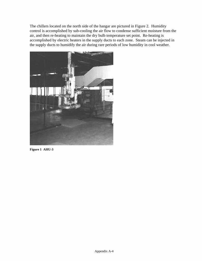
Appendix A-4
The chillers located on the north side of the hangar are pictured in Figure 2. Humiditycontrol is accomplished by sub-cooling the air flow to condense sufficient moisture from theair, and then re-heating to maintain the dry bulb temperature set point. Re-heating isaccomplished by electric heaters in the supply ducts to each zone. Steam can be injected inthe supply ducts to humidify the air during rare periods of low humidity in cool weather.
Figure 1 AHU-3
Appendix A-5
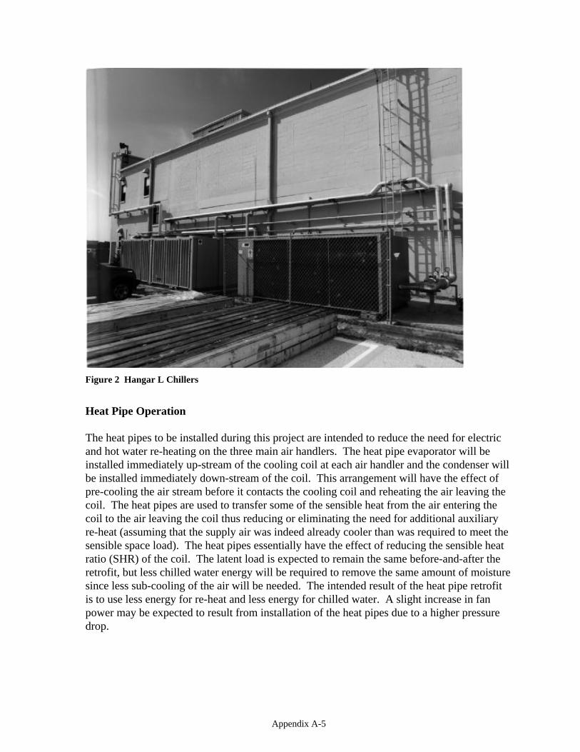
Figure 2 Hangar L Chillers
Heat Pipe Operation
The heat pipes to be installed during this project are intended to reduce the need for electricand hot water re-heating on the three main air handlers. The heat pipe evaporator will beinstalled immediately up-stream of the cooling coil at each air handler and the condenser willbe installed immediately down-stream of the coil. This arrangement will have the effect ofpre-cooling the air stream before it contacts the cooling coil and reheating the air leaving thecoil. The heat pipes are used to transfer some of the sensible heat from the air entering thecoil to the air leaving the coil thus reducing or eliminating the need for additional auxiliaryre-heat (assuming that the supply air was indeed already cooler than was required to meet thesensible space load). The heat pipes essentially have the effect of reducing the sensible heatratio (SHR) of the coil. The latent load is expected to remain the same before-and-after theretrofit, but less chilled water energy will be required to remove the same amount of moisturesince less sub-cooling of the air will be needed. The intended result of the heat pipe retrofitis to use less energy for re-heat and less energy for chilled water. A slight increase in fanpower may be expected to result from installation of the heat pipes due to a higher pressuredrop.

Appendix A-6
Evaluation Approach
The energy savings from these retrofits will be evaluated by comparing the energy usedbefore the retrofit and after the retrofit. Direct measurements of the primary energy quantitieswill be made over an extended period of time. Direct comparisons of before-and-after energyuse will be shown for periods with comparable cooling loads. Empirical models of thesystem performance will be derived from the measured data and simulation models will beused to calculate annual energy savings.
The energy savings attributed to the heat pipes are expected to be derived from:
1. reduced reheat power 2. reduced chiller power
The electricity used for re-heat and for the chiller will be measured directly as part of theevaluation. Typical hourly load shapes for mid-summer and cooler season months will bereported. We expect to report annual kWh and peak kilowatts for the re-heat and chillers, forthe system with and without heat pipes. The sensible and latent energy removed from the airflow at each air handler will also be carefully measured. These quantities provide the basisfor comparing the system performance in the before and after retrofit periods, and alsoprovide inputs for developing functional models of the reheat and chillers.
In addition to energy savings, interior humidity conditions may be improved after the retrofit.The present system appears to allow the inside RH to float above the set point during thesummer. The chillers presently appear to be operating at maximum capacity during thesummer months, and still the cooling loads are not met. To the extent that new technologyprovides improved interior temperature and RH conditions, we plan to use the functionalmodels to:
1. calculate how much less energy the New system would use to achieve the Oldconditions, or:
2. calculate how much more energy the Old system would use to achieve the Newconditions
The heat pipe project should be able to take credit for improved conditions that wereachieved without buying a new chiller.
We will also observe the data carefully to try to identify possible problems in systemoperating performance that could develop because of the retrofit. In particular, it is possiblethat the system with heat pipes may experience an inability to meet sensible loads duringpeak summer cooling season. This possibility is indicated in the pre-retrofit data as periodsduring which no reheat is required during the summer and neither the sensible nor latent loadis presently met. The heat pipes will provide reheat during these periods. It is also possiblethat the systems with heat pipes could use more steam for humidification in winter when theheat pipes provide dehumidification when it is not needed.

Appendix A-7
Instrumentation Plan
The evaluation plan requires that the thermal performance of the existing HVAC system bemeasured over an extended period. Instruments have been installed to measure the heatremoved at the cooling coil for each air handler, the re-heat energy for each air handler, andthe total electric power for the two chillers.
Data Logger
A Campbell Scientific CR10X data logger system was installed to record the signals from thesensors measuring thermal performance. The sensors are sampled once every 30 seconds.Data are averaged over a period of one hour and stored in the CR10X memory. Forty twovariables are presently stored on an hourly basis. At this rate, the CR10X memory canaccommodate approximately three months of stored data. Stored data are transferred viamodem approximately once each week to our computers for analysis and archiving. The datalogger is located in the mezzanine electrical room, reasonably near all three air handlers.
Energy Flow Measurements at Each Air Handler
The total heat removed at the cooling coil of each air handler is measured on the air side andon the water side. These two heat flow quantities should be equal and are compared in ouranalysis to assure good quality in the measured data. The latent and sensible heat removed ismeasured only on the air side. Measurement of entering and leaving temperature, relativehumidity, and mass flow rate are required on the air side. On the water side, entering andleaving chilled water fluid temperature and flow rate are measured.
The temperature and relative humidity (RH) of the air is measured in four locations at eachair handler. The supply, return, outside and mixed (outside and return) conditions aremeasured. The sensor used for these measurements is a CS500 temperature and relativehumidity probe supplied by Campbell Scientific. The nominal accuracy for these sensors is0.4 C for temperature and 3% or better for RH. Each sensor is located at the center of ductsections at locations where the flow is expected to be well mixed. An array of points wassampled at each sensor location to verify that the flow was well mixed with respect totemperature and RH. The ducts happen to be appropriately configured to facilitate thismeasurement. The sensor location for the supply air sampling point was limited due to thelocation of HEPA filters. Sensors could not be located down stream of the filters.
The supply and return air flow rate for each air handler was measured in a short term testusing the NREL tracer gas monitoring system. The tracer gas Sulfur hexafluoride (SF6) isinjected into a duct at a known, constant rate. The concentration of the SF6 is measured at adown stream point where the tracer gas is well mixed with the air stream. The total air flowrate is equal to the dosing rate divided by the concentration. The air flow rates are reasonablyassumed to be constant over long periods of time.

Appendix A-8
The entering and leaving chilled water temperatures for each cooling coil are measured withType T multi-junction thermopiles and reference thermocouples. The thermocouplejunctions are installed on the exterior surface of the steel chilled water pipes. The accuracyof the temperature difference measurement is typically 0.1C or better. The standard pipeinsulation is replaced after installation of the thermocouples and extra insulation is added toassure reasonably accurate indication of fluid temperature difference.
The chilled water flow rate for each cooling coil was measured in a short term test using aControlotron model 1010 ultrasonic flow meter. This meter is temporarily mounted on theexterior surface of the steel chilled water pipes. The nominal accuracy of this flowmeasurement is 2 percent. Measurements were taken over a period of at least 24 hours andwere found to be constant during this period of operation. We understand that the fluid is asolution of water with approximately 10 percent propylene glycol.
Electric Power Measurements
Electric power used by the chillers and re-heat elements is measured directly using HallEffect watthour transducers, Ohio Semitronics model WL40R. The nominal accuracy ofthese transducers is 0.5 percent. One transducer is used for each chiller and one for the totalre-heat power for each air handler with electric re-heat, AHU-2 and AHU-3. The chiller watttransducers are located in the chiller electrical enclosures and are connected to a separateCR10 data logger outside the building.
The re-heat energy for air handler AHU-1 is supplied via a heat exchanger by steam from aboiler located near the hangar. The re-heat energy for this system is determined by measuringthe rise in temperature in the supply air at the air handler and the supply air at diffusers in thezones. The diffuser supply air temperature is measured with single-channel temperaturelogger made by Onset Computer Corporation. This air handler supplies conditioned air to theclean room areas. We were not allowed to enter this area, but Life Science Support Facilitypersonnel placed these sensors for us. The sensors record data for a period of 75 days.EG&G maintains records of monthly oil use by the boiler.
Measured Data
Air Flow Rates and Chilled Water Flow Rates
The measured flow rates shown in Table 2 can be compared to the nominal values listed inTable 1, above. The measured air flow rate in AHU-1 is about 20 percent lower thannominal, and the chilled water flow rate is somewhat higher than design values. Themeasured air flow rates in AHU-2 and AHU-3 are 18 percent higher and 14 percent higher,respectively. These measured air flow rates will be compared to the measured flow ratesafter the retrofit to determine any change in air flow due to the heat pipe installation.
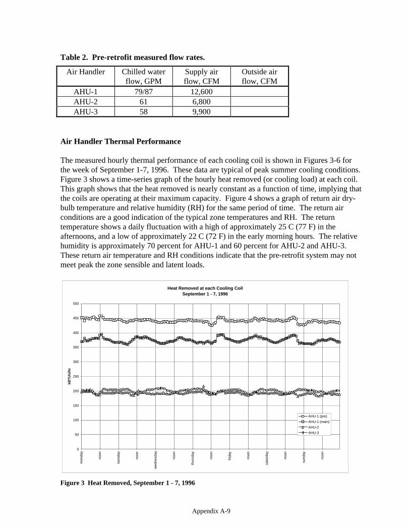
Appendix A-9
Table 2. Pre-retrofit measured flow rates.
Air Handler Chilled waterflow, GPM
Supply airflow, CFM
Outside airflow, CFM
AHU-1 79/87 12,600AHU-2 61 6,800AHU-3 58 9,900
Air Handler Thermal Performance
The measured hourly thermal performance of each cooling coil is shown in Figures 3-6 forthe week of September 1-7, 1996. These data are typical of peak summer cooling conditions.Figure 3 shows a time-series graph of the hourly heat removed (or cooling load) at each coil.This graph shows that the heat removed is nearly constant as a function of time, implying thatthe coils are operating at their maximum capacity. Figure 4 shows a graph of return air dry-bulb temperature and relative humidity (RH) for the same period of time. The return airconditions are a good indication of the typical zone temperatures and RH. The returntemperature shows a daily fluctuation with a high of approximately 25 C (77 F) in theafternoons, and a low of approximately 22 C (72 F) in the early morning hours. The relativehumidity is approximately 70 percent for AHU-1 and 60 percent for AHU-2 and AHU-3.These return air temperature and RH conditions indicate that the pre-retrofit system may notmeet peak the zone sensible and latent loads.
Heat Removed at each Cooling CoilSeptember 1 - 7, 1996
0
50
100
150
200
250
300
350
400
450
500
mon
day
noon
tues
day
noon
wed
nesd
ay
noon
thur
sday
noon
frid
ay
noon
satu
rday
noon
sund
ay
noon
kBT
UU
/hr
AHU-1 (pre)
AHU-1 (main)
AHU-2
AHU-3
Figure 3 Heat Removed, September 1 - 7, 1996
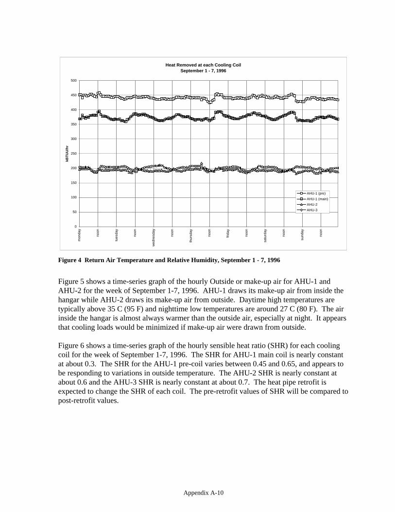
Appendix A-10
Heat Removed at each Cooling CoilSeptember 1 - 7, 1996
0
50
100
150
200
250
300
350
400
450
500m
onda
y
noon
tues
day
noon
wed
nesd
ay
noon
thur
sday
noon
frid
ay
noon
satu
rday
noon
sund
ay
noon
kBT
UU
/hr
AHU-1 (pre)
AHU-1 (main)
AHU-2
AHU-3
Figure 4 Return Air Temperature and Relative Humidity, September 1 - 7, 1996
Figure 5 shows a time-series graph of the hourly Outside or make-up air for AHU-1 andAHU-2 for the week of September 1-7, 1996. AHU-1 draws its make-up air from inside thehangar while AHU-2 draws its make-up air from outside. Daytime high temperatures aretypically above 35 C (95 F) and nighttime low temperatures are around 27 C (80 F). The airinside the hangar is almost always warmer than the outside air, especially at night. It appearsthat cooling loads would be minimized if make-up air were drawn from outside.
Figure 6 shows a time-series graph of the hourly sensible heat ratio (SHR) for each coolingcoil for the week of September 1-7, 1996. The SHR for AHU-1 main coil is nearly constantat about 0.3. The SHR for the AHU-1 pre-coil varies between 0.45 and 0.65, and appears tobe responding to variations in outside temperature. The AHU-2 SHR is nearly constant atabout 0.6 and the AHU-3 SHR is nearly constant at about 0.7. The heat pipe retrofit isexpected to change the SHR of each coil. The pre-retrofit values of SHR will be compared topost-retrofit values.
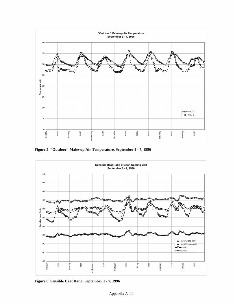
Appendix A-11
"Outdoor" Make-up Air TemperatureSeptember 1 - 7, 1996
0
5
10
15
20
25
30
35
40
mon
day
noon
tues
day
noon
wed
nesd
ay
noon
thur
sday
noon
frid
ay
noon
satu
rday
noon
sund
ay
noon
Tem
per
atu
re (
C)
AHU-1
AHU-2
Figure 5 "Outdoor" Make-up Air Temperature, September 1 - 7, 1996
Sensible Heat Ratio of each Cooling CoilSeptember 1 - 7, 1996
0.0
0.1
0.2
0.3
0.4
0.5
0.6
0.7
0.8
0.9
1.0
mon
day
noon
tues
day
noon
wed
nesd
ay
noon
thur
sday
noon
frid
ay
noon
satu
rday
noon
sund
ay
noon
Sen
sib
le H
eat
Rat
io
AHU-1(pre-coil)
AHU-1(main-coil)
AHU-2
AHU-3
Figure 6 Sensible Heat Ratio, September 1 - 7, 1996
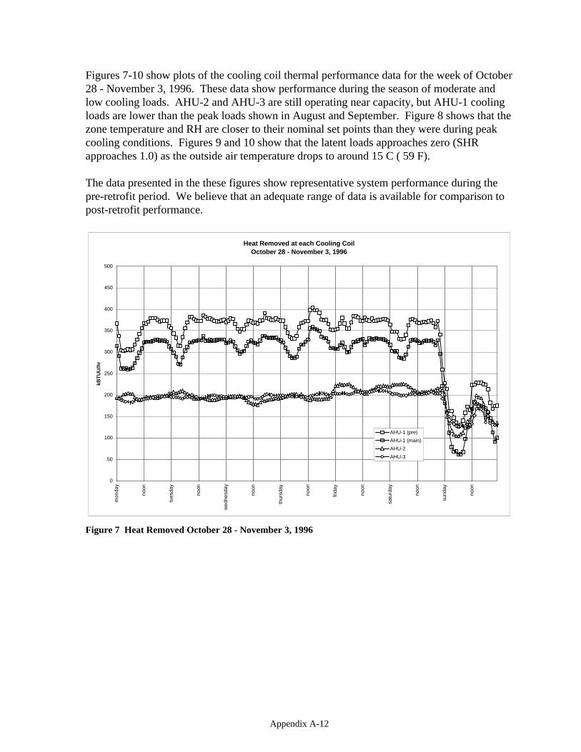
Appendix A-12
Figures 7-10 show plots of the cooling coil thermal performance data for the week of October28 - November 3, 1996. These data show performance during the season of moderate andlow cooling loads. AHU-2 and AHU-3 are still operating near capacity, but AHU-1 coolingloads are lower than the peak loads shown in August and September. Figure 8 shows that thezone temperature and RH are closer to their nominal set points than they were during peakcooling conditions. Figures 9 and 10 show that the latent loads approaches zero (SHRapproaches 1.0) as the outside air temperature drops to around 15 C ( 59 F).
The data presented in the these figures show representative system performance during thepre-retrofit period. We believe that an adequate range of data is available for comparison topost-retrofit performance.
Heat Removed at each Cooling CoilOctober 28 - November 3, 1996
0
50
100
150
200
250
300
350
400
450
500
mon
day
noon
tues
day
noon
wed
nesd
ay
noon
thur
sday
noon
frid
ay
noon
satu
rday
noon
sund
ay
noon
kBT
UU
/hr
AHU-1 (pre)
AHU-1 (main)
AHU-2
AHU-3
Figure 7 Heat Removed October 28 - November 3, 1996
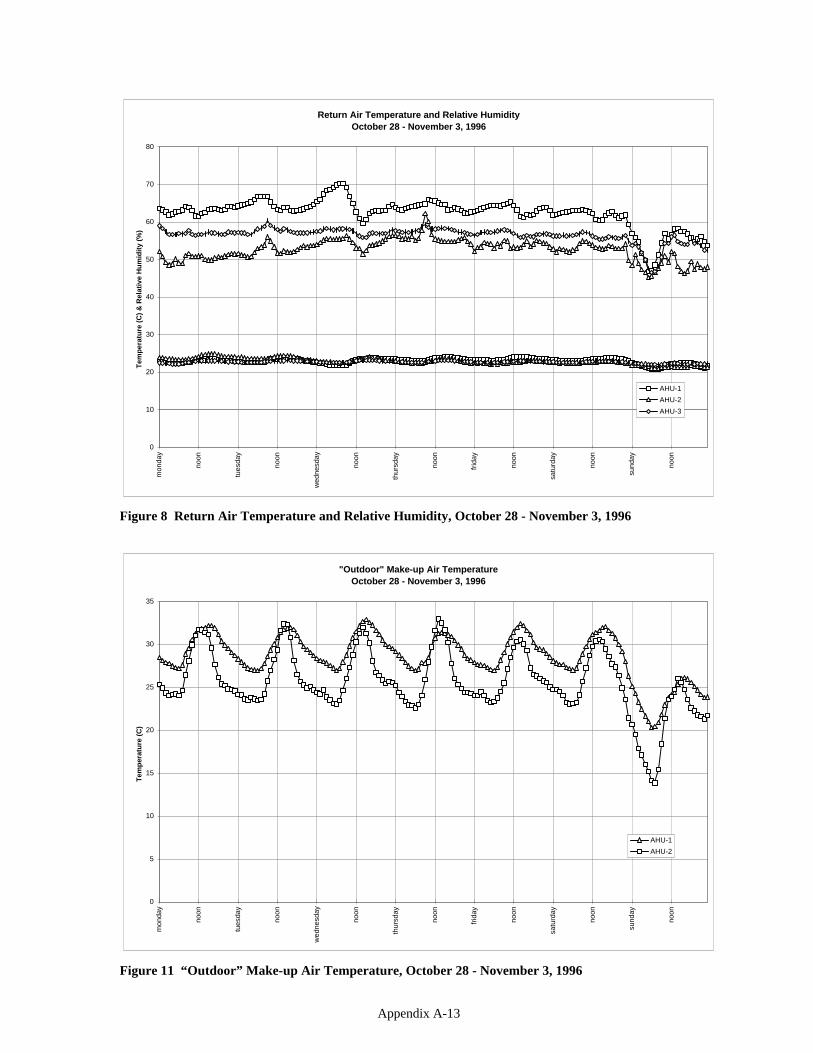
Appendix A-13
Return Air Temperature and Relative HumidityOctober 28 - November 3, 1996
0
10
20
30
40
50
60
70
80
mon
day
noon
tues
day
noon
wed
nesd
ay
noon
thur
sday
noon
frid
ay
noon
satu
rday
noon
sund
ay
noon
Tem
per
atu
re (
C)
& R
elat
ive
Hu
mid
ity
(%)
AHU-1
AHU-2
AHU-3
Figure 8 Return Air Temperature and Relative Humidity, October 28 - November 3, 1996
"Outdoor" Make-up Air TemperatureOctober 28 - November 3, 1996
0
5
10
15
20
25
30
35
mon
day
noon
tues
day
noon
wed
nesd
ay
noon
thur
sday
noon
frid
ay
noon
satu
rday
noon
sund
ay
noon
Tem
per
atu
re (
C)
AHU-1
AHU-2
Figure 11 “Outdoor” Make-up Air Temperature, October 28 - November 3, 1996
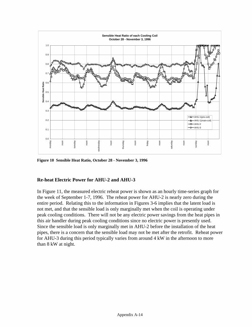
Appendix A-14
Sensible Heat Ratio of each Cooling CoilOctober 28 - November 3, 1996
0.0
0.1
0.2
0.3
0.4
0.5
0.6
0.7
0.8
0.9
1.0
mon
day
noon
tues
day
noon
wed
nesd
ay
noon
thur
sday
noon
frid
ay
noon
satu
rday
noon
sund
ay
noon
Sen
sib
le H
eat
Rat
io
AHU-1(pre-coil)
AHU-1(main-coil)
AHU-2
AHU-3
Figure 10 Sensible Heat Ratio, October 28 - November 3, 1996
Re-heat Electric Power for AHU-2 and AHU-3
In Figure 11, the measured electric reheat power is shown as an hourly time-series graph forthe week of September 1-7, 1996. The reheat power for AHU-2 is nearly zero during theentire period. Relating this to the information in Figures 3-6 implies that the latent load isnot met, and that the sensible load is only marginally met when the coil is operating underpeak cooling conditions. There will not be any electric power savings from the heat pipes inthis air handler during peak cooling conditions since no electric power is presently used.Since the sensible load is only marginally met in AHU-2 before the installation of the heatpipes, there is a concern that the sensible load may not be met after the retrofit. Reheat powerfor AHU-3 during this period typically varies from around 4 kW in the afternoon to morethan 8 kW at night.

Appendix A-15
Electric Reheat PowerSeptember 1 - 7, 1996
0
5
10
15
20
25
mon
day
noon
tues
day
noon
wed
nesd
ay
noon
thur
sday
noon
frid
ay
noon
satu
rday
noon
sund
ay
noon
kW
AHU-2
AHU-3
Figure 11 Electric Reheat Power, September 1 - 7, 1996
Similar data for reheat power for the week of October 28 - November 3, 1996 are shown inFigure 12. Both air handlers require substantial reheating, with power increasing as theoutside air temperature decreases later in the week. Note that the reheat power is highestwhen the SHR (from Figure 10) is highest. That is, the reheat power is greatest when thelatent load is small. This may indicate incorrect operation of the cooling coil control systemrather than an optimum opportunity for heat pipe savings.

Appendix A-16
Electric Reheat PowerOctober 28 - November 3, 1996
0
5
10
15
20
25
mon
day
noon
tues
day
noon
wed
nesd
ay
noon
thur
sday
noon
frid
ay
noon
satu
rday
noon
sund
ay
noon
kW
AHU-2
AHU-3
Figure 12 Electric Reheat Power, October 28 - November 3, 1996
Figure 13 shows the AHU-2 average hourly profile for reheat power for typical weeks inAugust, September, October, and November. Figure 14 shows similar information for AHU-3. Reheat power is lowest in August and September, and highest in November. Each curveexhibits a daily variation with minimum reheat required in the afternoon, and maximumreheat required in the early morning hours. This performance is consistent with theobservation that the maximum sensible cooling loads are during daytime hours.
Weekly total reheat power for AHU-2 and AHU-3 is shown in the bar chart in Figure 15.
The data presented in the these figures show representative system performance during thepre-retrofit period. We believe that an adequate range of reheat power data is available forcomparison to post-retrofit performance.

Appendix A-17
AHU-2 Reheat Average Hourly Profilefor typical weeks in August, September, October and November
0
2
4
6
8
10
12
14
16
18
1 2 3 4 5 6 7 8 9 10 11 12 13 14 15 16 17 18 19 20 21 22 23 24
hour
kW
August
September
October
November
Figure 13 AHU-2 Reheat, Average Hourly Profiles, August - November, 1996
AHU-3 Reheat Average Hourly Profilefor typical weeks in August, September, October and November
0
2
4
6
8
10
12
14
16
18
1 2 3 4 5 6 7 8 9 10 11 12 13 14 15 16 17 18 19 20 21 22 23 24
hour
kW
August
September
October
November
Figure 14 AHU-3 Reheat, Average Hourly Profiles, August - November, 1996
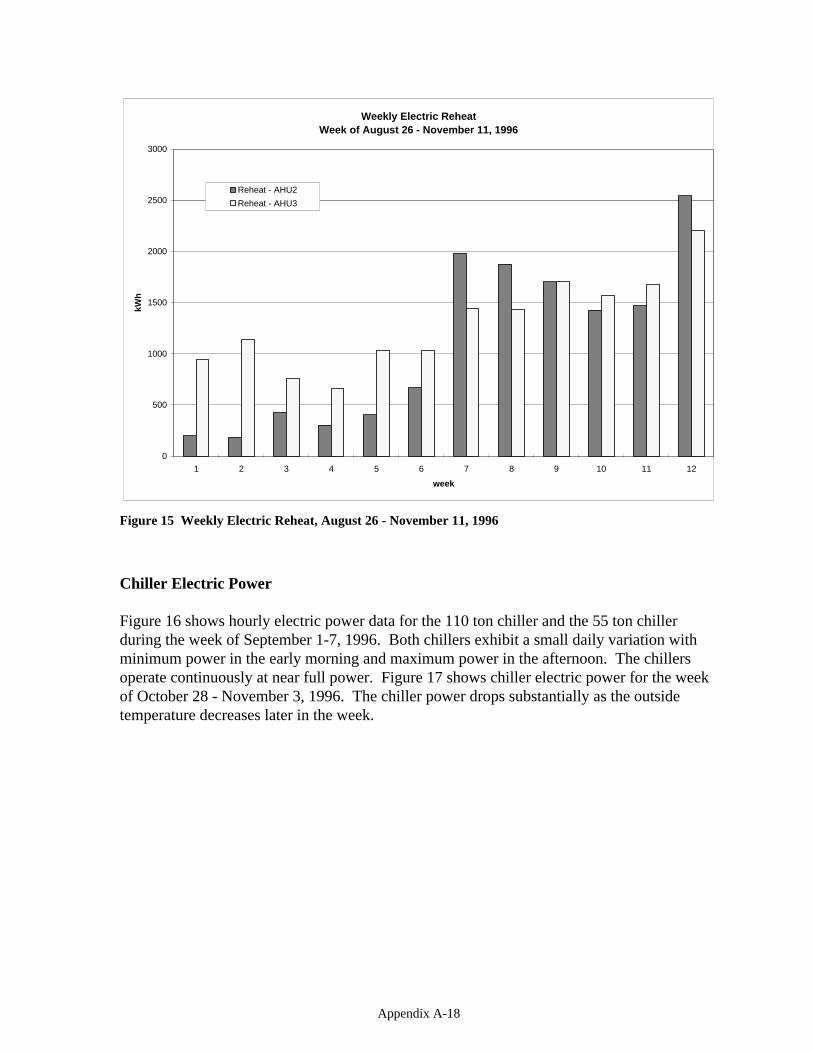
Appendix A-18
Weekly Electric ReheatWeek of August 26 - November 11, 1996
0
500
1000
1500
2000
2500
3000
1 2 3 4 5 6 7 8 9 10 11 12
week
kWh
Reheat - AHU2
Reheat - AHU3
Figure 15 Weekly Electric Reheat, August 26 - November 11, 1996
Chiller Electric Power
Figure 16 shows hourly electric power data for the 110 ton chiller and the 55 ton chillerduring the week of September 1-7, 1996. Both chillers exhibit a small daily variation withminimum power in the early morning and maximum power in the afternoon. The chillersoperate continuously at near full power. Figure 17 shows chiller electric power for the weekof October 28 - November 3, 1996. The chiller power drops substantially as the outsidetemperature decreases later in the week.

Appendix A-19
Chiller PowerSeptember 1 - 7, 1996
0
20
40
60
80
100
120m
onda
y
noon
tues
day
noon
wed
nesd
ay
noon
thur
sday
noon
frid
ay
noon
satu
rday
noon
sund
ay
noon
kW
110 ton Chiller
55 ton Chiller
Figure 16 Chiller Power, September 1 - 7, 1996
Chiller PowerOctober 28 - November 3, 1996
0
20
40
60
80
100
120
mon
day
noon
tues
day
noon
wed
nesd
ay
noon
thur
sday
noon
frid
ay
noon
satu
rday
noon
sund
ay
noon
kW
110 ton Chiller
55 ton Chiller
Figure 17 Chiller Power, October 28 - November 3, 1996
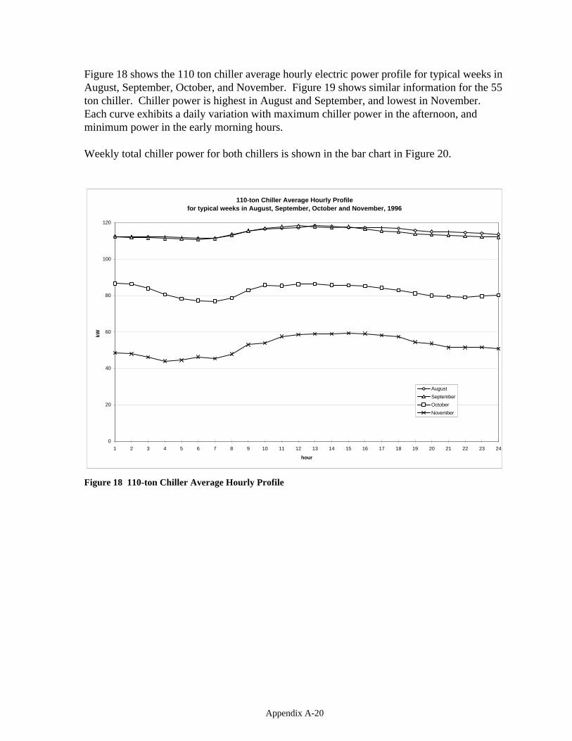
Appendix A-20
Figure 18 shows the 110 ton chiller average hourly electric power profile for typical weeks inAugust, September, October, and November. Figure 19 shows similar information for the 55ton chiller. Chiller power is highest in August and September, and lowest in November.Each curve exhibits a daily variation with maximum chiller power in the afternoon, andminimum power in the early morning hours.
Weekly total chiller power for both chillers is shown in the bar chart in Figure 20.
110-ton Chiller Average Hourly Profilefor typical weeks in August, September, October and November, 1996
0
20
40
60
80
100
120
1 2 3 4 5 6 7 8 9 10 11 12 13 14 15 16 17 18 19 20 21 22 23 24
hour
kW
August
September
October
November
Figure 18 110-ton Chiller Average Hourly Profile

Appendix A-21
55-ton Chiller Average Hourly Profilefor typical weeks in August, September, October and November, 1996
0
10
20
30
40
50
60
1 2 3 4 5 6 7 8 9 10 11 12 13 14 15 16 17 18 19 20 21 22 23 24
hour
kW
August
September
October
November
Figure 19 55-ton Chiller Average Hourly Profile
Weekly Chiller ElectricWeek of August 26 - November 11, 1996
0
2000
4000
6000
8000
10000
12000
14000
16000
18000
20000
1 2 3 4 5 6 7 8 9 10 11 12
week
kWh
Chiller - 110 ton
Chiller - 55 ton
Figure 20 Weekly Chiller Electric Use, August 26 - November 11, 1996
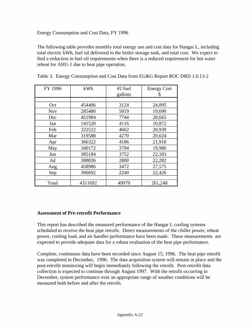
Appendix A-22
Energy Consumption and Cost Data, FY 1996
The following table provides monthly total energy use and cost data for Hangar L, includingtotal electric kWh, fuel oil delivered to the boiler storage tank, and total cost. We expect tofind a reduction in fuel oil requirements when there is a reduced requirement for hot waterreheat for AHU-1 due to heat pipe operation.
Table 3. Energy Consumption and Cost Data from EG&G Report BOC DRD 1.0.13-2
FY 1996 kWh #2 fuelgallons
Energy Cost$
Oct 454406 3124 24,095Nov 285480 5819 19,690Dec 451984 7744 28,665Jan 141520 4116 10,872Feb 322522 4662 20,939Mar 319588 4270 20,624Apr 366322 4186 21,918May 340172 3794 19,980Jun 385184 3752 22,183Jul 388836 2800 22,282
Aug 458986 3472 27,575Sep 396692 2240 22,426
Total 4311692 49979 261,248
Assessment of Pre-retrofit Performance
This report has described the measured performance of the Hangar L cooling systemsscheduled to receive the heat pipe retrofit. Direct measurements of the chiller power, reheatpower, cooling load, and air handler performance have been made. These measurements areexpected to provide adequate data for a robust evaluation of the heat pipe performance.
Complete, continuous data have been recorded since August 15, 1996. The heat pipe retrofitwas completed in December, 1996. The data acquisition system will remain in place and thepost-retrofit monitoring will begin immediately following the retrofit. Post-retrofit datacollection is expected to continue through August 1997. With the retrofit occurring inDecember, system performance over an appropriate range of weather conditions will bemeasured both before and after the retrofit.

Appendix A-23
Acknowledgments:
This work was funded by the DOE/NREL FEMP program under NREL Subcontract No.AAR-6-16320-01. We appreciate the support and encouragement of Karen Thomas as theNREL project manager. We thank Will Miner and his staff (Dynamac Corp) and BillRuppert and Mike Mann (EG&G) for their substantial assistance in our work on-site at KSC.

Appendix B Post-Retrofit Evaluation Report
Appendix B-1
New Technology Demonstration ProgramKennedy Space Center Hangar L Heat Pipe Project:
Post-Retrofit Monitoring and Evaluation Report
November, 1997
National Renewable Energy LaboratorySubcontract No. AAR-6-16320-01
C. E. HancockPaul Reeves
815 Alpine #6Boulder, CO 80304(303) 447-8458

Appendix B-2
New Technology Demonstration ProgramKennedy Space Center Hangar L Heat Pipe Project:Post-Retrofit Monitoring and Evaluation Report
November, 1997
Summary
Heat pipe heat exchangers were installed on three air handlers at Hangar L at the CapeCanaveral Air Station, Cape Canaveral, Florida in December of 1996. These retrofits areintended to improve the dehumidification performance of the cooling systems, reduce theelectric and steam energy required for re-heating air and reduce electric energy used by thechillers.
The energy savings from these retrofits will be evaluated by comparing the energy usedbefore the retrofit and after the retrofit. Complete, continuous system performance data havebeen recorded since August 15, 1996. This report describes the results of post-retrofitperformance monitoring. A previous report (January, 1997) described the systemperformance for the pre-retrofit period. A subsequent report (December, 1997) will provide adetailed evaluation of the effects of the heat pipe retrofit. In that report, direct comparisonsof before-and-after energy use will be made for periods with comparable cooling loads.Empirical models of the system performance will be derived from the measured data andsimulation models will be used to calculate annual energy savings.

Appendix B-3
System Description
The NASA Life Sciences Support Facility is located in Hangar L at the Cape Canaveral AirStation, Cape Canaveral, Florida. Laboratory and office areas have been constructed insidethe original hangar structure. The hangar is approximately 175 feet wide, 150 feet long, and30 feet high, yielding a foot print area of about 26,000 square feet. There are approximately20,000 square feet of conditioned space inside the hangar including offices, labs, and cleanrooms. There are very few windows and essentially no direct solar gains on conditionedspaces. Most of the cooling load is due to internal gains from operation of lights andequipment and from conditioning of outside air for ventilation. Normal operating hours forpersonnel at the building are 0700 through 1700. Much of the equipment and interiorlighting remains in operation 24 hours per day.
Three air handlers serve the majority of the conditioned lab and office space. Air handlerAHU-1 is located on the main floor of the hangar and supplies conditioned air to the cleanroom areas of the facility. It operates with 100 percent outside air. The outside air firstpasses through a pre-cool coil before it enters the main cooling coil. The heat pipe wasinstalled at the pre-cool coil. The two coils are supplied with chilled water (in parallel) froma 110 ton chiller located on the north side of the building. Both temperature and relativehumidity in the conditioned space are intended to be controlled by this system. Humiditycontrol is accomplished during periods of high latent loads by cooling the supply air belowthe point required to meet the sensible load, thus condensing enough moisture from the air tomeet the required RH set point. The dry bulb temperature in the space is maintained by re-heating the sub-cooled air to meet the temperature set point. Hot water supplied by a localoil-fired steam boiler is used for re-heat on this system. If the RH in the conditioned spacedrops below the humidistat set point, steam from the boiler is injected in the air flow streamto humidify the air.
Air handlers AHU-2 and AHU-3 are located on the mezzanine level above the office spaceson the south side of the building. (Note that our AHU-3 is designated AHU-1(Mezzanine) inthe original mechanical plans) Chilled water is supplied (in parallel) by a 55 ton air-cooledchiller located on the north side of the building. Figure 1. shows a photograph of AHU-3.The chillers located on the north side of the hangar are pictured in Figure 2. Humiditycontrol is accomplished by sub-cooling the air flow to condense sufficient moisture from theair, and then re-heating to maintain the dry bulb temperature set point. Re-heating isaccomplished by electric heaters in the supply ducts to each zone. Steam can be injected inthe supply ducts to humidify the air during rare periods of low humidity in cool weather.
The heat pipes are intended to transfer some of the sensible heat from the air entering the coilto the air leaving the coil thus reducing or eliminating the need for additional auxiliary re-heat for moisture control (assuming that the supply air was indeed already cooler than wasrequired to meet the sensible space load). The heat pipes essentially have the effect ofreducing the sensible heat ratio (SHR) of the coil. The intended result of the heat pipe retrofitis to use less energy for re-heat and less energy for chilled water. A slight increase in fanpower may be expected to result from installation of the heat pipes due to a higher pressuredrop.

Appendix B-4
Figure 1 AHU-3
Figure 2 Hangar L Chillers

Appendix B-5
Evaluation Approach
The energy savings from the heat pipe retrofits will be evaluated by comparing the energyused before the retrofit and after the retrofit. Direct measurements of the primary energyquantities have been made over an extended period of time. The pre-retrofit performancewas described in a previous report (January, 1997). This present report describes the post-retrofit system performance. Some preliminary observations of before-and-after energy useare made in this report. A subsequent report will make detailed comparisons of before-and-after energy use, and use empirical models of the system performance and simulation modelsto calculate annual energy savings.
The energy savings attributed to the heat pipes are expected to be derived from:
1. reduced reheat powerduring periods when either electric or steam re-heat would be used to raise the mainsupply air to the minimum temperature required by the space loads
2. reduced chiller powerduring periods when main supply air reheat is required and the chiller is running atless than full load
The data collected during the post-retrofit period, as well as values calculated from monitoreddata, are presented in this report in a number of different formats. Typical weeks, averageprofiles and weekly sums are used to present the data in a meaningful way.
Week long periods during January, March and August were chosen to represent “low-cooling”, “moderate cooling”, and “high cooling” periods, respectively. These weeks werechosen based on the weather conditions, the amount of continuous data collected and theuninterrupted operation of the cooling equipment. Daily profiles were created by averagingthe data for typical weeks in each month of the post retrofit period. Weekly totals werecalculated for select data and presented for each week of the post-retrofit period.
Average hourly profiles for reheat and chiller power are created by averaging the dailyprofiles of a typical week in each month of post-retrofit data. Total weekly reheat and chillerpower are shown for the entire post-retrofit period
The sensible and latent energy removed from the air flow at each air handler is reported forthe three weekly periods along with the sensible heat ratio (SHR) is reported for each coil.These quantities provide the basis for comparing the system performance in the before andafter retrofit periods, and also provide inputs for developing functional models of the reheatand chillers.
In addition to energy savings, interior temperature and humidity conditions may be modifiedby the heat pipe retrofit. Return air temperature and relative humidity are reported for each ofthe air handlers during typical period of operation.

Appendix B-6
Post Retrofit Measured Performance Data
Air Flow Rates
The supply air flow rates were measured for each air handler both before and after theretrofit. Table 1. displays the CFM for each air handler as specified in the design documents,as measured before the retrofit, and as measured after the retrofit. The installation of the heatpipes adds resistance to the air flow, which could result in lower flow rate, higher fan power,or both. The air flow measurements indicate that the flow rate increased by about 10 percentfor AHU-1 and decreased by about 5 percent for AHU-3 after the installation of the heatpipes. These changes are not considered significant. The air flow for AHU-2 appeared todrop by about 25 percent after the retrofit, from 6,800 CFM to 5,000 CFM. This may notconstitute a serious problem since the design flow rate was originally 5,765 CFM. Theresulting measured flow rate after the retrofit is about 13 percent below nominal.
Table 2. Supply air flow rates.
Air Handler As DesignedCFM
Before RetrofitCFM
After RetrofitCFM
AHU-1 15,800 12,600 13,800AHU-2 5,765 6,800 5,000AHU-3 8,675 9,900 9,400
Air Handler Thermal Performance
The measured hourly thermal performance of each cooling coil is shown in Figures 3-6 forthe week of August 11-17, 1997. These data are typical of peak summer cooling conditions.Figure 3 shows a time-series graph of the hourly heat removed (or cooling load) at each coil.This graph shows that the heat removed is nearly constant as a function of time, implying thatthe coils are operating near their maximum capacity. Compared to a similar period before theretrofit, AHU-2 and AHU-3 show heat removed to be about 10 percent higher in the post-retrofit period. For AHU-1, the post retrofit heat removal is lower for the pre-cool coil andhigher for the main coil. These observations are consistent with expected operation of theheat pipes.
Figure 4 shows a graph of return air dry-bulb temperature and relative humidity (RH) for thesame period of time. The return air conditions are a good indication of the typical zonetemperatures and RH. The return dry bulb temperature from each AHU shows a dailyfluctuation with a high in the afternoons, and a low in the early morning hours. The averagetemperature for AHU-1 is approximately 25C (77F) and the relative humidity isapproximately 70 percent. These conditions are similar to the pre-retrofit conditions. (Notethat for AHU-1 this is the exhaust air condition, not return.) The daily average returntemperature for AHU-2 is typically 26C (79F) and the RH is between 45 percent and 50percent. AHU-2 may not be adequately meeting the sensible cooling load as evidenced by
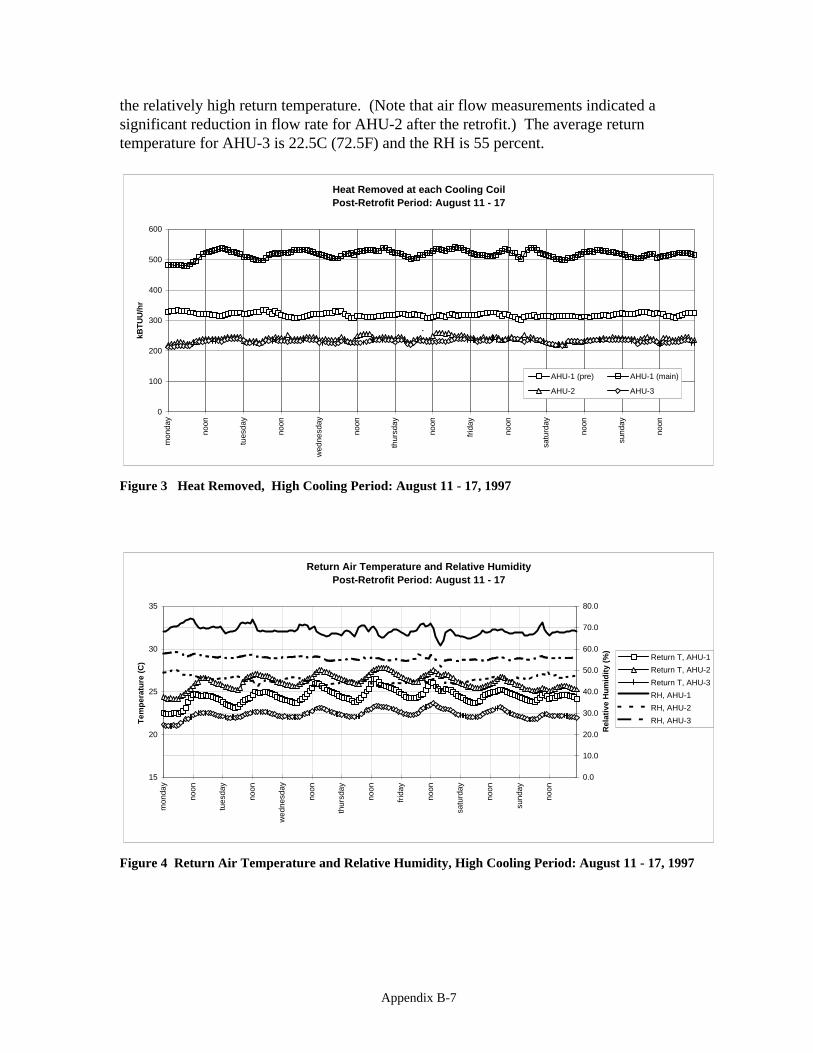
Appendix B-7
the relatively high return temperature. (Note that air flow measurements indicated asignificant reduction in flow rate for AHU-2 after the retrofit.) The average returntemperature for AHU-3 is 22.5C (72.5F) and the RH is 55 percent.
Heat Removed at each Cooling CoilPost-Retrofit Period: August 11 - 17
0
100
200
300
400
500
600
mon
day
noon
tues
day
noon
wed
nesd
ay
noon
thur
sday
noon
frid
ay
noon
satu
rday
noon
sund
ay
noon
kBT
UU
/hr
AHU-1 (pre) AHU-1 (main)
AHU-2 AHU-3
.
Figure 3 Heat Removed, High Cooling Period: August 11 - 17, 1997
Return Air Temperature and Relative HumidityPost-Retrofit Period: August 11 - 17
15
20
25
30
35
mon
day
noon
tues
day
noon
wed
nesd
ay
noon
thur
sday
noon
frid
ay
noon
satu
rday
noon
sund
ay
noon
Tem
per
atu
re (
C)
0.0
10.0
20.0
30.0
40.0
50.0
60.0
70.0
80.0R
elat
ive
Hu
mid
ity
(%)
Return T, AHU-1
Return T, AHU-2
Return T, AHU-3
RH, AHU-1
RH, AHU-2
RH, AHU-3
Figure 4 Return Air Temperature and Relative Humidity, High Cooling Period: August 11 - 17, 1997

Appendix B-8
Figure 5 shows a time-series graph of the hourly Outside or make-up air for AHU-1 andAHU-2 for the week of August 11-17, 1997. AHU-1 (and AHU-3) draws its make-up airfrom inside the hangar while AHU-2 draws its make-up air from outside. Daytime hightemperatures are typically above 35 C (95 F) and nighttime low temperatures are around 27 C(80 F). The air inside the hangar is almost always warmer than the outside air, especially atnight. It appears that cooling loads would be minimized if make-up air were drawn fromoutside. This condition has not changed since pre-retrofit monitoring started.
Figure 6 shows a time-series graph of the hourly sensible heat ratio (SHR) for each coolingcoil for the week of August 11-17, 1997. The SHR for AHU-1 main coil is nearly constant atabout 0.38. This value is somewhat higher than during the pre-retrofit period and is a resultof the heat pipe installed on the pre-cooling coil. The SHR for the AHU-1 pre-coil variesbetween 0.50 and 0.75. The AHU-2 SHR varies between 0.55 and 0.60 and the AHU-3 SHRvaries between 0.65 and 0.70. It appears that AHU-2 and AHU-3 have slightly lower SHR inthe post-retrofit period. This is the expected effect of the heat pipes.
"Outdoor" Make-up Air TemperaturePost-Retrofit Period: August 11 - 17
0
5
10
15
20
25
30
35
40
mon
day
noon
tues
day
noon
wed
nesd
ay
noon
thur
sday
noon
frid
ay
noon
satu
rday
noon
sund
ay
noon
Tem
per
atu
re (
C)
AHU-1
AHU-2
Figure 5 "Outdoor" Make-up Air Temperature, High Cooling Period: August 11 - 17, 1997
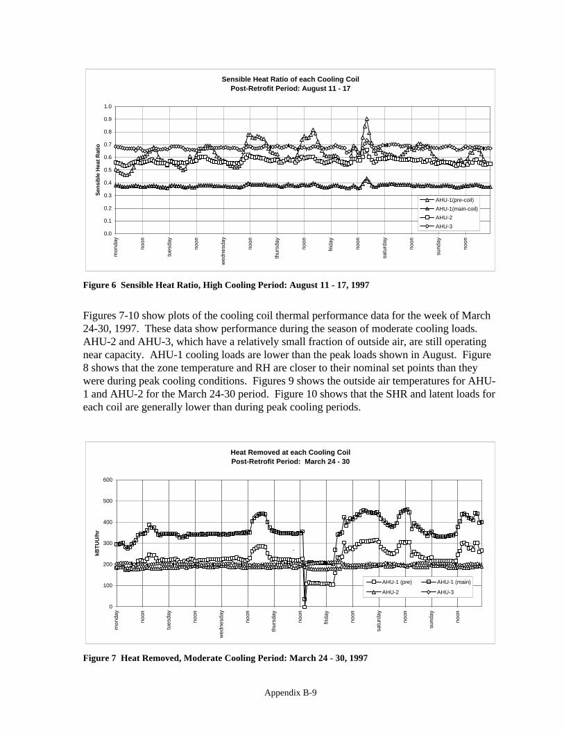
Appendix B-9
Sensible Heat Ratio of each Cooling CoilPost-Retrofit Period: August 11 - 17
0.0
0.1
0.2
0.3
0.4
0.5
0.6
0.7
0.8
0.9
1.0
mon
day
noon
tues
day
noon
wed
nesd
ay
noon
thur
sday
noon
frid
ay
noon
satu
rday
noon
sund
ay
noon
Sen
sib
le H
eat
Rat
io
AHU-1(pre-coil)
AHU-1(main-coil)
AHU-2
AHU-3
Figure 6 Sensible Heat Ratio, High Cooling Period: August 11 - 17, 1997
Figures 7-10 show plots of the cooling coil thermal performance data for the week of March24-30, 1997. These data show performance during the season of moderate cooling loads.AHU-2 and AHU-3, which have a relatively small fraction of outside air, are still operatingnear capacity. AHU-1 cooling loads are lower than the peak loads shown in August. Figure8 shows that the zone temperature and RH are closer to their nominal set points than theywere during peak cooling conditions. Figures 9 shows the outside air temperatures for AHU-1 and AHU-2 for the March 24-30 period. Figure 10 shows that the SHR and latent loads foreach coil are generally lower than during peak cooling periods.
Heat Removed at each Cooling CoilPost-Retrofit Period: March 24 - 30
0
100
200
300
400
500
600
mon
day
noon
tues
day
noon
wed
nesd
ay
noon
thur
sday
noon
frid
ay
noon
satu
rday
noon
sund
ay
noon
kBT
UU
/hr
AHU-1 (pre) AHU-1 (main)
AHU-2 AHU-3
.
Figure 7 Heat Removed, Moderate Cooling Period: March 24 - 30, 1997

Appendix B-10
Return Air Temperature and Relative HumidityPost-Retrofit Period: March 24 - 30
15
20
25
30
35m
onda
y
noon
tues
day
noon
wed
nesd
ay
noon
thur
sday
noon
frid
ay
noon
satu
rday
noon
sund
ay
noon
Tem
per
atu
re (
C)
0.0
10.0
20.0
30.0
40.0
50.0
60.0
70.0
80.0
Rel
ativ
e H
um
idit
y (%
)
Return T, AHU-1
Return T, AHU-2
Return T, AHU-3
RH, AHU-1
RH, AHU-2
RH, AHU-3
Figure 8 Return Air Temp. and Relative Humidity, Moderate Cooling Period: March 24 - 30, 1997
"Outdoor" Make-up Air TemperaturePost-Retrofit Period: March 24 - 30
0
5
10
15
20
25
30
35
40
mon
day
noon
tues
day
noon
wed
nesd
ay
noon
thur
sday
noon
frid
ay
noon
satu
rday
noon
sund
ay
noon
Tem
per
atu
re (
C)
AHU-1
AHU-2
Figure 9 “Outdoor” Make-up Air Temperature, Moderate Cooling Period: March 24 - 30, 1997
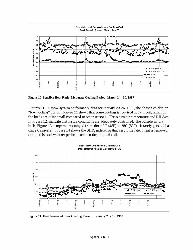
Appendix B-11
Sensible Heat Ratio of each Cooling CoilPost-Retrofit Period: March 24 - 30
0.0
0.1
0.2
0.3
0.4
0.5
0.6
0.7
0.8
0.9
1.0
mon
day
noon
tues
day
noon
wed
nesd
ay
noon
thur
sday
noon
frid
ay
noon
satu
rday
noon
sund
ay
noon
Sen
sib
le H
eat
Rat
io
AHU-1(pre-coil)
AHU-1(main-coil)
AHU-2
AHU-3
Figure 10 Sensible Heat Ratio, Moderate Cooling Period: March 24 - 30, 1997
Figures 11-14 show system performance data for January 20-26, 1997, the chosen colder, or“low cooling” period. Figure 11 shows that some cooling is required at each coil, althoughthe loads are quite small compared to other seasons. The return air temperature and RH datain Figure 12. indicate that inside conditions are adequately controlled. The outside air drybulb, Figure 13, temperatures ranged from about 9C (48F) to 28C (82F). It rarely gets cold atCape Canaveral. Figure 14 shows the SHR, indicating that very little latent heat is removedduring this cool weather period, except at the pre-cool coil.
Heat Removed at each Cooling CoilPost-Retrofit Period: January 20 - 26
0
100
200
300
400
500
600
mon
day
noon
tues
day
noon
wed
nesd
ay
noon
thur
sday
noon
frid
ay
noon
satu
rday
noon
sund
ay
noon
kBT
UU
/hr
AHU-1 (pre) AHU-1 (main)
AHU-2 AHU-3
.
Figure 11 Heat Removed, Low Cooling Period: January 20 - 26, 1997

Appendix B-12
Return Air Temperature and Relative HumidityPost-Retrofit Period: January 20 - 26
15
20
25
30
35m
onda
y
noon
tues
day
noon
wed
nesd
ay
noon
thur
sday
noon
frid
ay
noon
satu
rday
noon
sund
ay
noon
Tem
per
atu
re (
C)
0.0
10.0
20.0
30.0
40.0
50.0
60.0
70.0
80.0
Rel
ativ
e H
um
idit
y (%
)
Return T, AHU-1
Return T, AHU-2
Return T, AHU-3
RH, AHU-1
RH, AHU-2
RH, AHU-3
Figure 12 Return Air Temp. and Relative Humidity, Low Cooling Period: January 20 - 26, 1997
"Outdoor" Make-up Air TemperaturePost-Retrofit Period: January 20 - 26
0
5
10
15
20
25
30
35
40
mon
day
noon
tues
day
noon
wed
nesd
ay
noon
thur
sday
noon
frid
ay
noon
satu
rday
noon
sund
ay
noon
Tem
per
atu
re (
C)
AHU-1
AHU-2
Figure 13 “Outdoor” Make-up Air Temperature, Low Cooling Period: January 20 - 26, 1997

Appendix B-13
Sensible Heat Ratio of each Cooling CoilPost-Retrofit Period: January 20 - 26
0.0
0.1
0.2
0.3
0.4
0.5
0.6
0.7
0.8
0.9
1.0
mon
day
noon
tues
day
noon
wed
nesd
ay
noon
thur
sday
noon
frid
ay
noon
satu
rday
noon
sund
ay
noon
Sen
sib
le H
eat
Rat
io
AHU-1(pre-coil)
AHU-1(main-coil)
AHU-2
AHU-3
Figure 14 Sensible Heat Ratio, Low Cooling Period: January 20 - 26, 1997
Re-heat Electric Power for AHU-2 and AHU-3
In Figure 15, the measured electric reheat power for AHU-2 and AHU-3 is shown as anhourly time-series graph for the week of August 11-17, 1997, the “high cooling” period. Thereheat power for AHU-2 is zero during the entire period. The reheat power for AHU-2 wasnear zero during the pre-retrofit period so there is not much opportunity for savings duringpeak cooling conditions. Figure 8. showed that the return temperature for AHU-2 wassometimes above 27C (80F) indicating that the sensible cooling loads may not be met duringthis period. Reheat from the heat pipes may cause sensible overheating in this zone whichwas not meeting the cooling loads before the retrofit.
Reheat power for AHU-3 during this period typically varies from about 3 kW to nearly 5 kWwith small daily variations. This is 2 to 3 kW lower than for a comparable period before theretrofit, an expected effect of the retrofit.
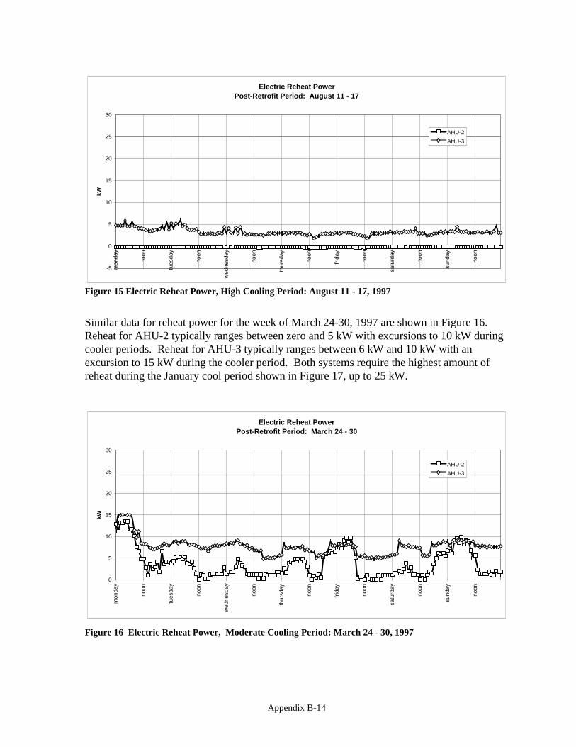
Appendix B-14
Electric Reheat PowerPost-Retrofit Period: August 11 - 17
-5
0
5
10
15
20
25
30m
onda
y
noon
tues
day
noon
wed
nesd
ay
noon
thur
sday
noon
frid
ay
noon
satu
rday
noon
sund
ay
noon
kW
AHU-2
AHU-3
Figure 15 Electric Reheat Power, High Cooling Period: August 11 - 17, 1997
Similar data for reheat power for the week of March 24-30, 1997 are shown in Figure 16.Reheat for AHU-2 typically ranges between zero and 5 kW with excursions to 10 kW duringcooler periods. Reheat for AHU-3 typically ranges between 6 kW and 10 kW with anexcursion to 15 kW during the cooler period. Both systems require the highest amount ofreheat during the January cool period shown in Figure 17, up to 25 kW.
Electric Reheat PowerPost-Retrofit Period: March 24 - 30
0
5
10
15
20
25
30
mon
day
noon
tues
day
noon
wed
nesd
ay
noon
thur
sday
noon
frid
ay
noon
satu
rday
noon
sund
ay
noon
kW
AHU-2
AHU-3
Figure 16 Electric Reheat Power, Moderate Cooling Period: March 24 - 30, 1997
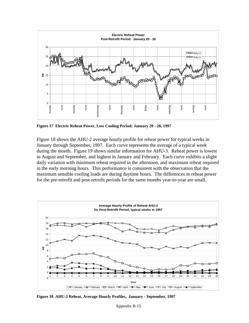
Appendix B-15
Electric Reheat PowerPost-Retrofit Period: January 20 - 26
0
5
10
15
20
25
30m
onda
y
noon
tues
day
noon
wed
nesd
ay
noon
thur
sday
noon
frid
ay
noon
satu
rday
noon
sund
ay
noon
kW
AHU-2
AHU-3
Figure 17 Electric Reheat Power, Low Cooling Period: January 20 - 26, 1997
Figure 18 shows the AHU-2 average hourly profile for reheat power for typical weeks inJanuary through September, 1997. Each curve represents the average of a typical weekduring the month. Figure 19 shows similar information for AHU-3. Reheat power is lowestin August and September, and highest in January and February. Each curve exhibits a slightdaily variation with minimum reheat required in the afternoon, and maximum reheat requiredin the early morning hours. This performance is consistent with the observation that themaximum sensible cooling loads are during daytime hours. The differences in reheat powerfor the pre-retrofit and post-retrofit periods for the same months year-to-year are small.
Average Hourly Profile of Reheat AHU-2for Post-Retrofit Period, typical weeks in 1997
-2
0
2
4
6
8
10
12
14
16
18
20
1 2 3 4 5 6 7 8 9 10 11 12 13 14 15 16 17 18 19 20 21 22 23 24
hour
kW
January February March April May June July August September
Figure 18 AHU-2 Reheat, Average Hourly Profiles, January - September, 1997
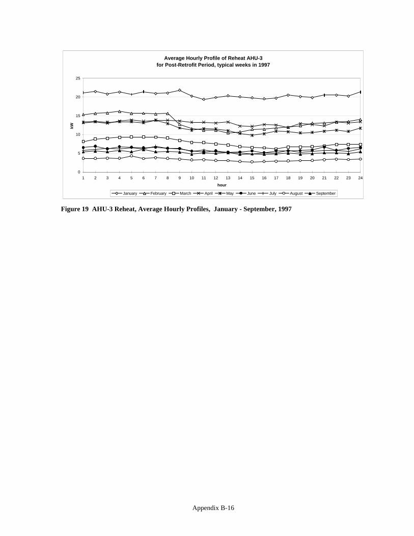
Appendix B-16
Average Hourly Profile of Reheat AHU-3for Post-Retrofit Period, typical weeks in 1997
0
5
10
15
20
25
1 2 3 4 5 6 7 8 9 10 11 12 13 14 15 16 17 18 19 20 21 22 23 24
hour
kW
January February March April May June July August September
Figure 19 AHU-3 Reheat, Average Hourly Profiles, January - September, 1997
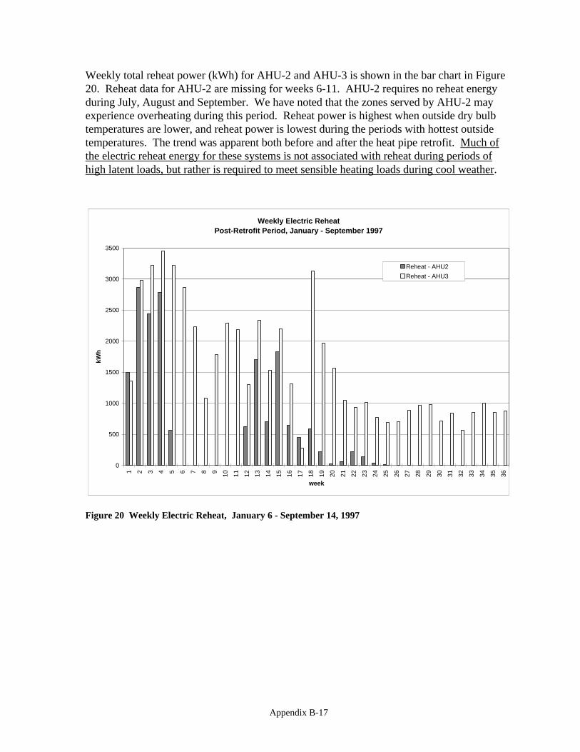
Appendix B-17
Weekly total reheat power (kWh) for AHU-2 and AHU-3 is shown in the bar chart in Figure20. Reheat data for AHU-2 are missing for weeks 6-11. AHU-2 requires no reheat energyduring July, August and September. We have noted that the zones served by AHU-2 mayexperience overheating during this period. Reheat power is highest when outside dry bulbtemperatures are lower, and reheat power is lowest during the periods with hottest outsidetemperatures. The trend was apparent both before and after the heat pipe retrofit. Much ofthe electric reheat energy for these systems is not associated with reheat during periods ofhigh latent loads, but rather is required to meet sensible heating loads during cool weather.
Weekly Electric ReheatPost-Retrofit Period, January - September 1997
0
500
1000
1500
2000
2500
3000
3500
1 2 3 4 5 6 7 8 9 10 11 12 13 14 15 16 17 18 19 20 21 22 23 24 25 26 27 28 29 30 31 32 33 34 35 36
week
kWh
Reheat - AHU2
Reheat - AHU3
Figure 20 Weekly Electric Reheat, January 6 - September 14, 1997

Appendix B-18
Chiller Electric Power
Figure 21 shows hourly electric power data for the 110 ton chiller and the 55 ton chillerduring the week of August 11-17, 1997. The 110 ton chiller has a peak demand ofapproximately 120 kW, and the 55 ton chiller has a peak of approximately 62 kW. Bothchillers exhibit a small daily variation with minimum power in the early morning andmaximum power in the afternoon. The chillers operate continuously at near full power.Figures 22 and 23 show chiller electric power for the weeks of March 24-30, and January 20-26, 1997, respectively. The larger chiller in particular experiences substantially reducedpower during cooler periods.
Chiller PowerPost-Retrofit Period: August 10 - 17
0
20
40
60
80
100
120
mon
day
noon
tues
day
noon
wed
nesd
ay
noon
thur
sday
noon
frid
ay
noon
satu
rday
noon
sund
ay
noon
kW
110 ton Chiller
55 ton Chiller
Figure 21 Chiller Power, High Cooling Period: August 11 - 17, 1997
Chiller PowerPost-Retrofit Period: March 24 - 30
0
20
40
60
80
100
120
mon
day
noon
tues
day
noon
wed
nesd
ay
noon
thur
sday
noon
frid
ay
noon
satu
rday
noon
sund
ay
noon
kW
110 ton Chiller
55 ton Chiller
Figure 22 Chiller Power, Moderate Cooling Period: March 24 - 30, 1997
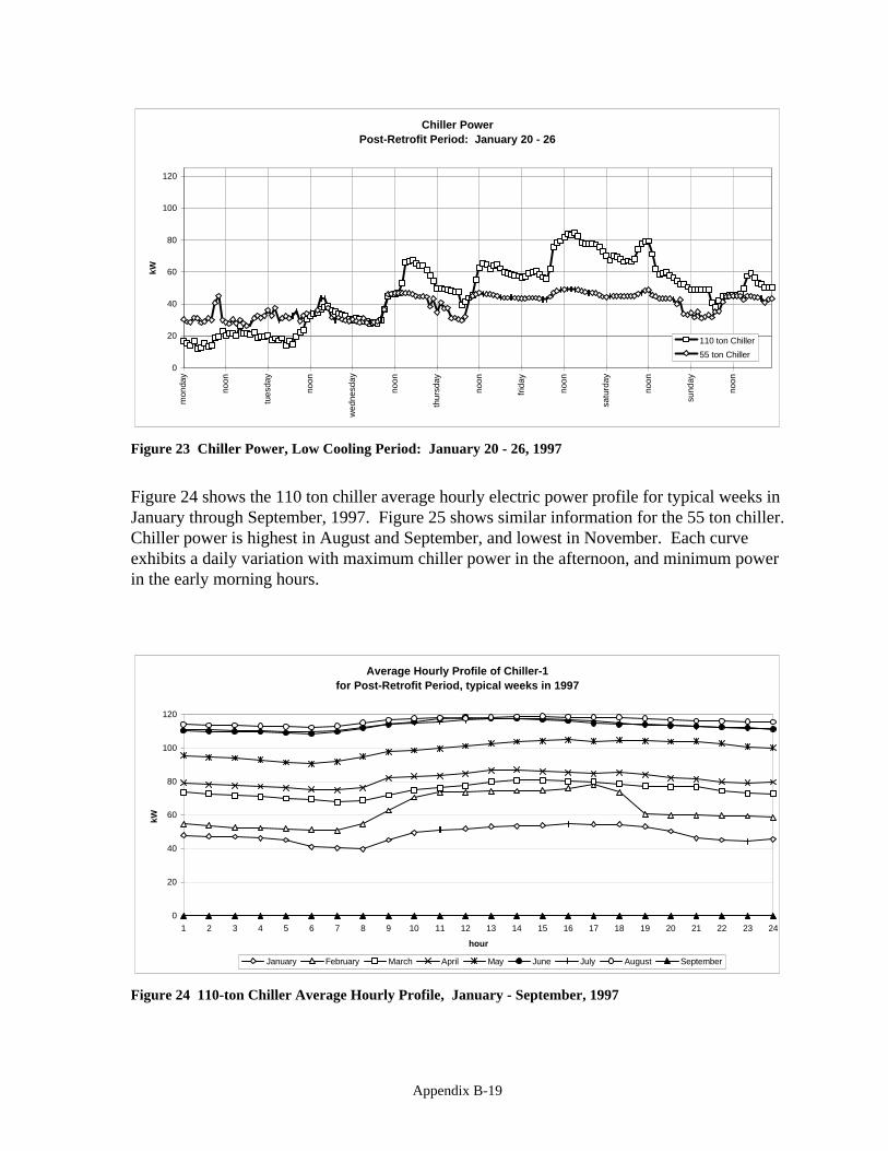
Appendix B-19
Chiller PowerPost-Retrofit Period: January 20 - 26
0
20
40
60
80
100
120m
onda
y
noon
tues
day
noon
wed
nesd
ay
noon
thur
sday
noon
frid
ay
noon
satu
rday
noon
sund
ay
noon
kW
110 ton Chiller
55 ton Chiller
Figure 23 Chiller Power, Low Cooling Period: January 20 - 26, 1997
Figure 24 shows the 110 ton chiller average hourly electric power profile for typical weeks inJanuary through September, 1997. Figure 25 shows similar information for the 55 ton chiller.Chiller power is highest in August and September, and lowest in November. Each curveexhibits a daily variation with maximum chiller power in the afternoon, and minimum powerin the early morning hours.
Average Hourly Profile of Chiller-1for Post-Retrofit Period, typical weeks in 1997
0
20
40
60
80
100
120
1 2 3 4 5 6 7 8 9 10 11 12 13 14 15 16 17 18 19 20 21 22 23 24
hour
kW
January February March April May June July August September
Figure 24 110-ton Chiller Average Hourly Profile, January - September, 1997
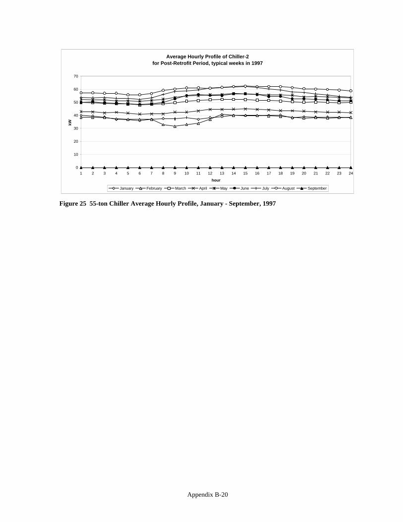
Appendix B-20
Average Hourly Profile of Chiller-2for Post-Retrofit Period, typical weeks in 1997
0
10
20
30
40
50
60
70
1 2 3 4 5 6 7 8 9 10 11 12 13 14 15 16 17 18 19 20 21 22 23 24
hour
kW
January February March April May June July August September
Figure 25 55-ton Chiller Average Hourly Profile, January - September, 1997
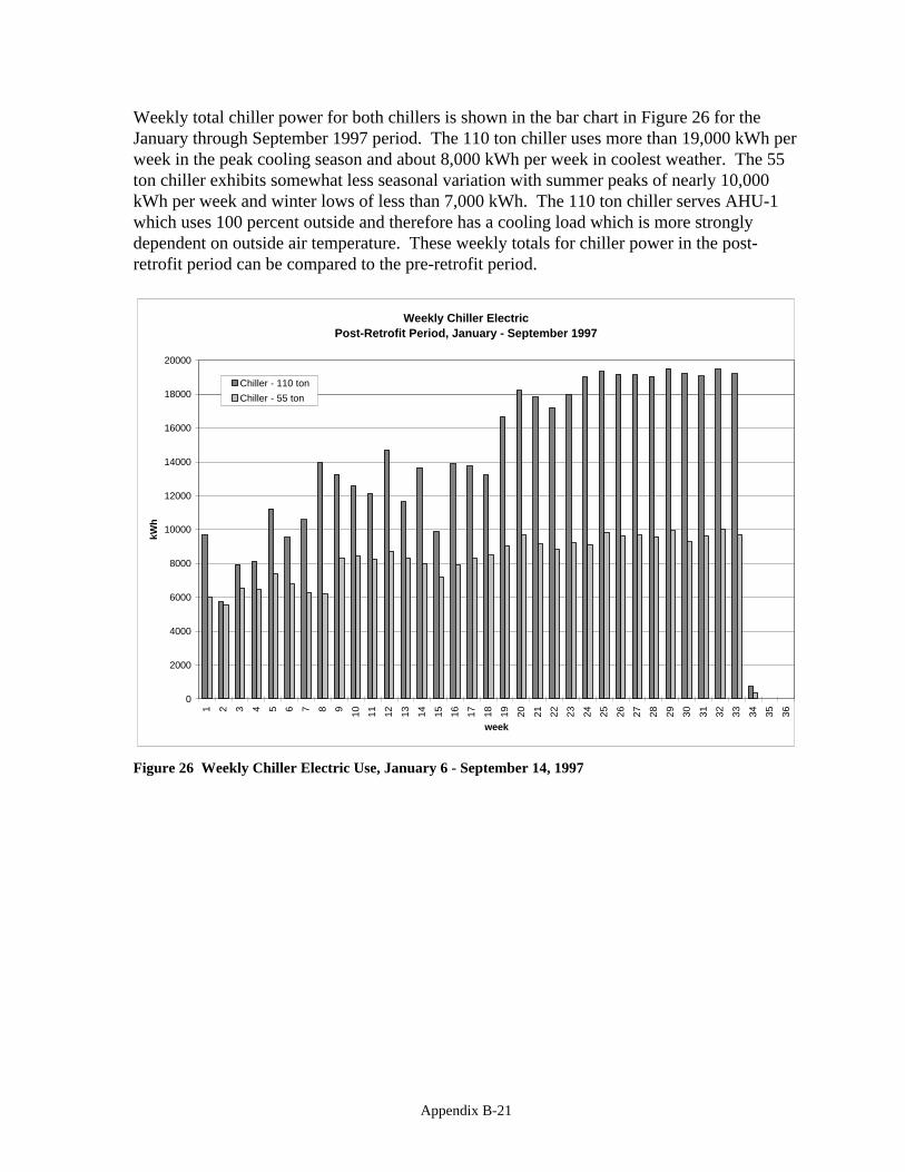
Appendix B-21
Weekly total chiller power for both chillers is shown in the bar chart in Figure 26 for theJanuary through September 1997 period. The 110 ton chiller uses more than 19,000 kWh perweek in the peak cooling season and about 8,000 kWh per week in coolest weather. The 55ton chiller exhibits somewhat less seasonal variation with summer peaks of nearly 10,000kWh per week and winter lows of less than 7,000 kWh. The 110 ton chiller serves AHU-1which uses 100 percent outside and therefore has a cooling load which is more stronglydependent on outside air temperature. These weekly totals for chiller power in the post-retrofit period can be compared to the pre-retrofit period.
Weekly Chiller ElectricPost-Retrofit Period, January - September 1997
0
2000
4000
6000
8000
10000
12000
14000
16000
18000
20000
1 2 3 4 5 6 7 8 9 10 11 12 13 14 15 16 17 18 19 20 21 22 23 24 25 26 27 28 29 30 31 32 33 34 35 36
week
kWh
Chiller - 110 ton
Chiller - 55 ton
Figure 26 Weekly Chiller Electric Use, January 6 - September 14, 1997

Appendix B-22
Assessment of Post-retrofit Monitoring
Complete, continuous data have been recorded since August 15, 1996. The retrofit wascompleted in December, 1996. Following the retrofit, data have been recorded from Januarythrough September, 1997 to characterize post-retrofit performance. Initial observations havebeen made to directly compare similar periods before-and-after the retrofit. A subsequentreport in December, 1997 is intended to provide a detailed evaluation of the heat pipeperformance in these systems.
Acknowledgments
This work was funded by the DOE/NREL FEMP program under NREL Subcontract No.AAR-6-16320-01. We appreciate the support and encouragement of Karen Thomas as theNREL project manager. We thank Will Miner and his staff (Dynamac Corp.) and BillRuppert (EG&G) for their substantial assistance in our work on-site at KSC.

Appendix C Detailed Measured Performance Graphs

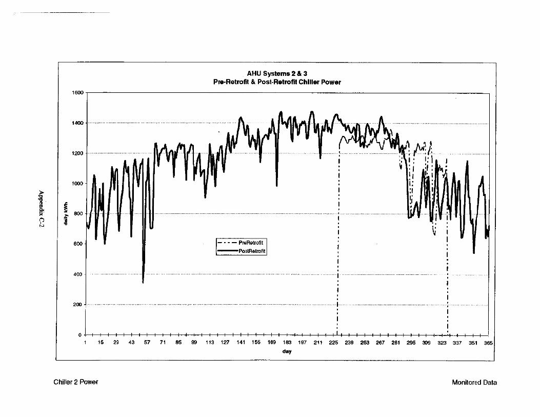
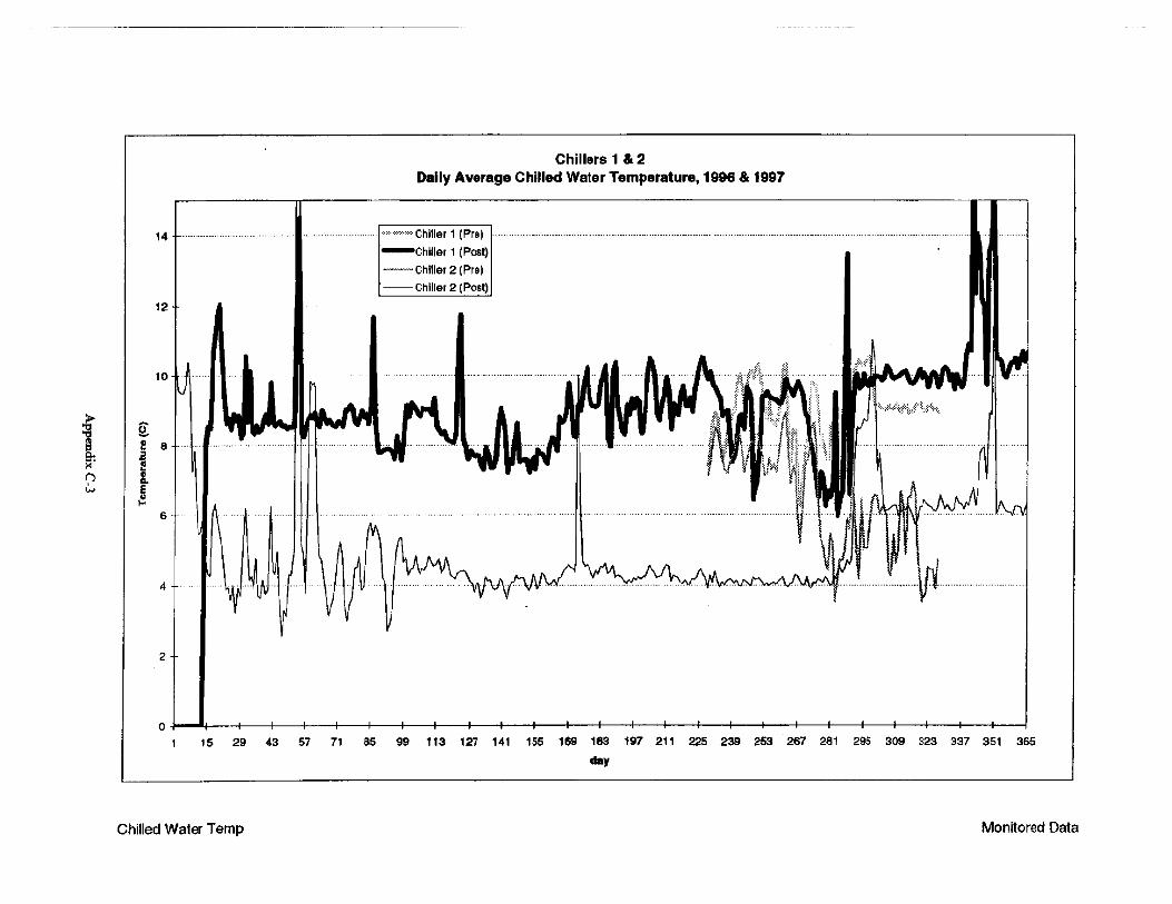
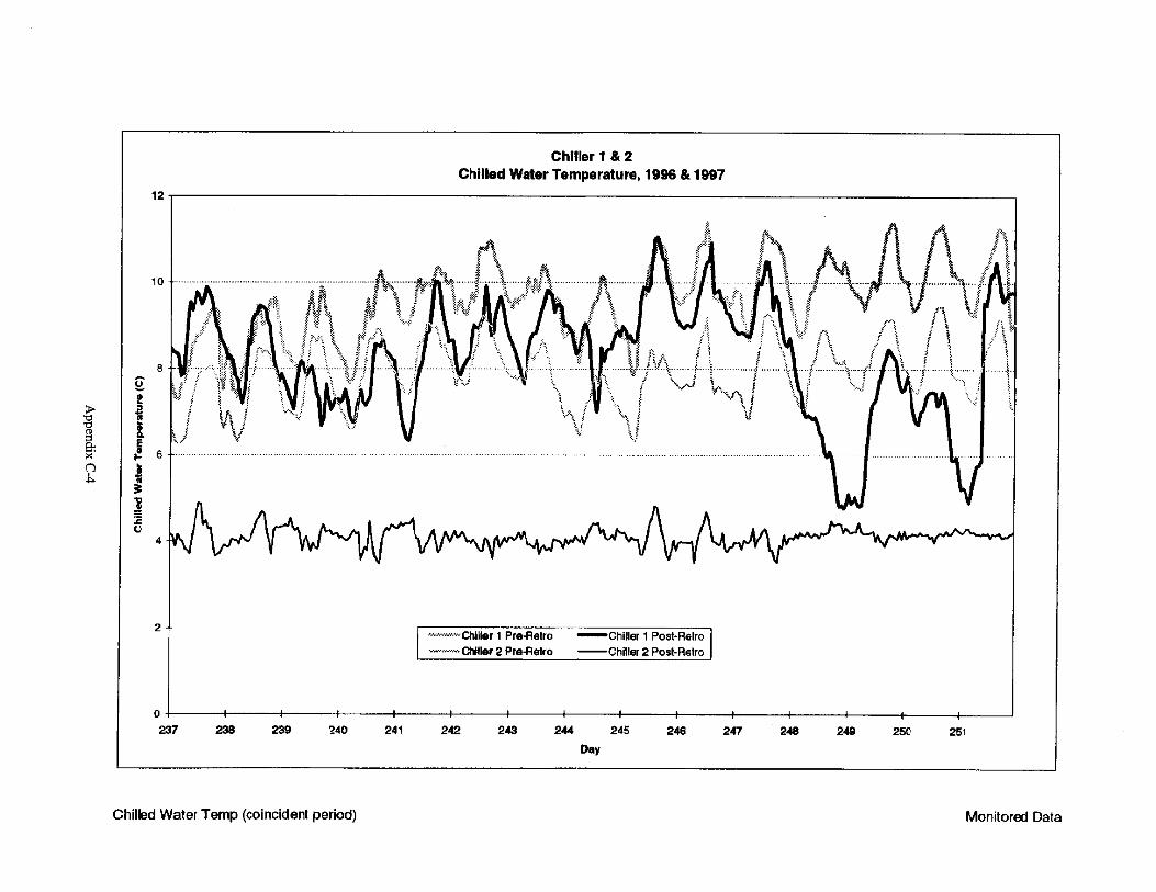


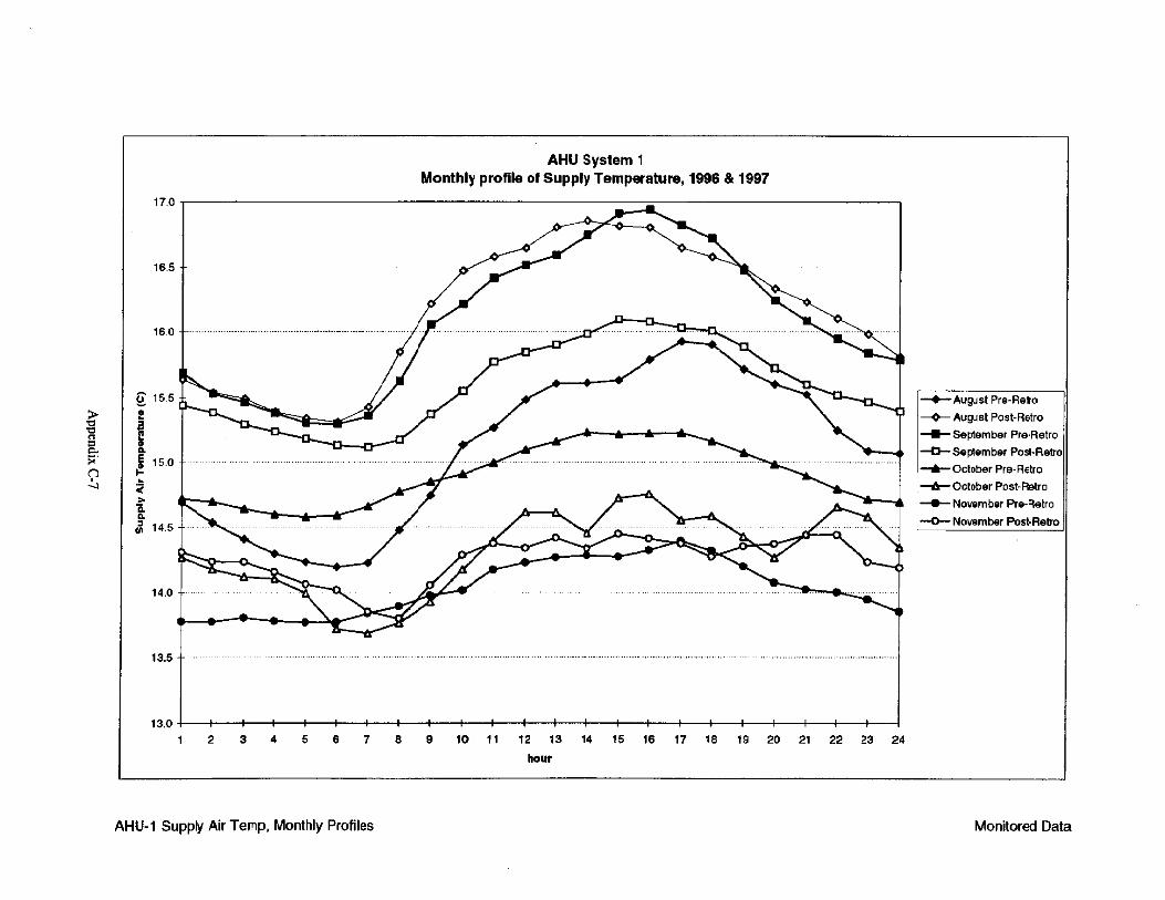
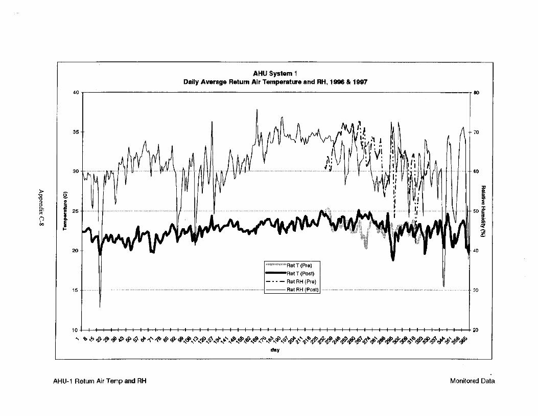


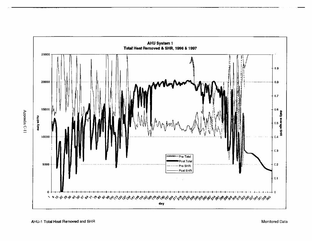
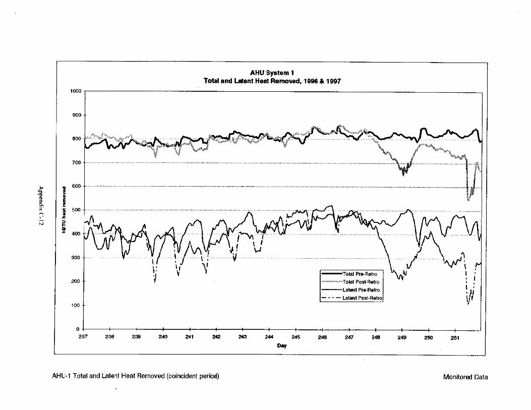

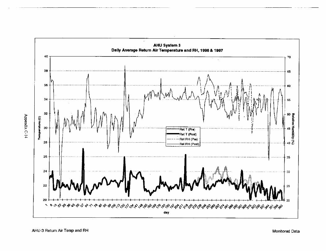
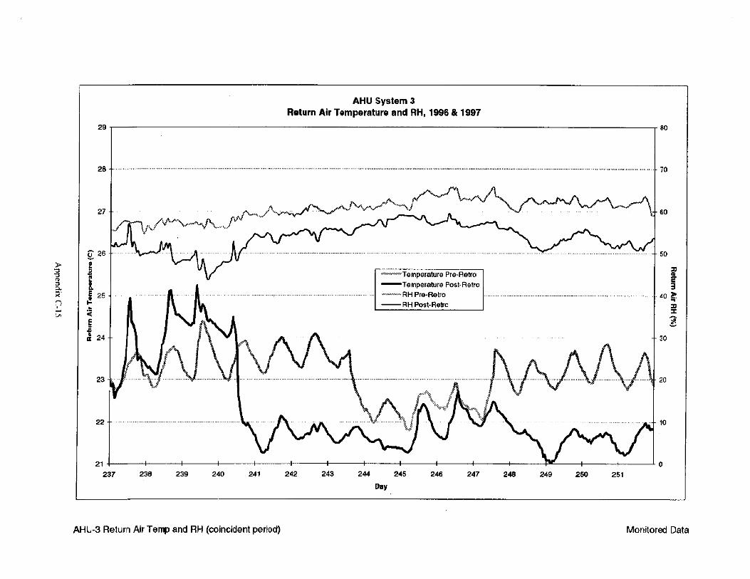
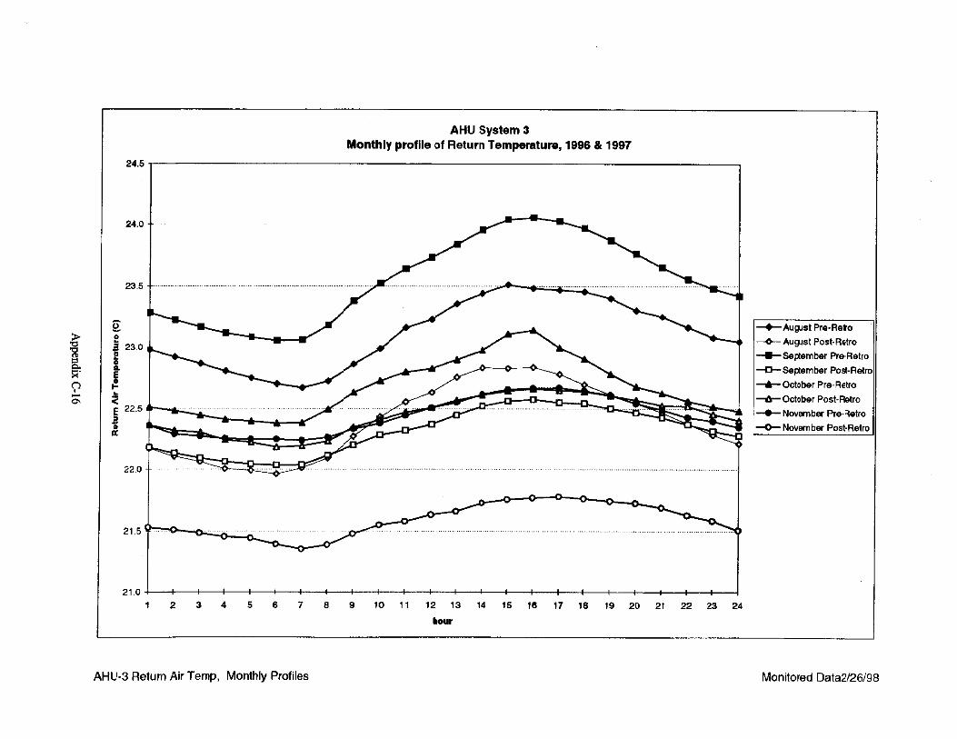


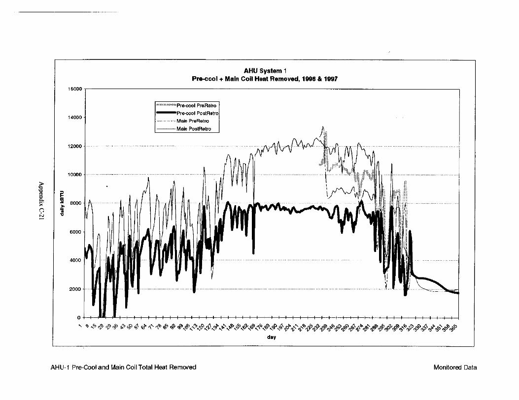

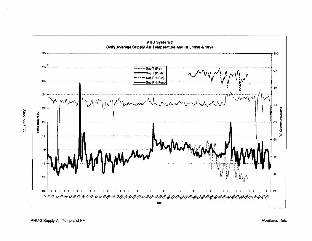
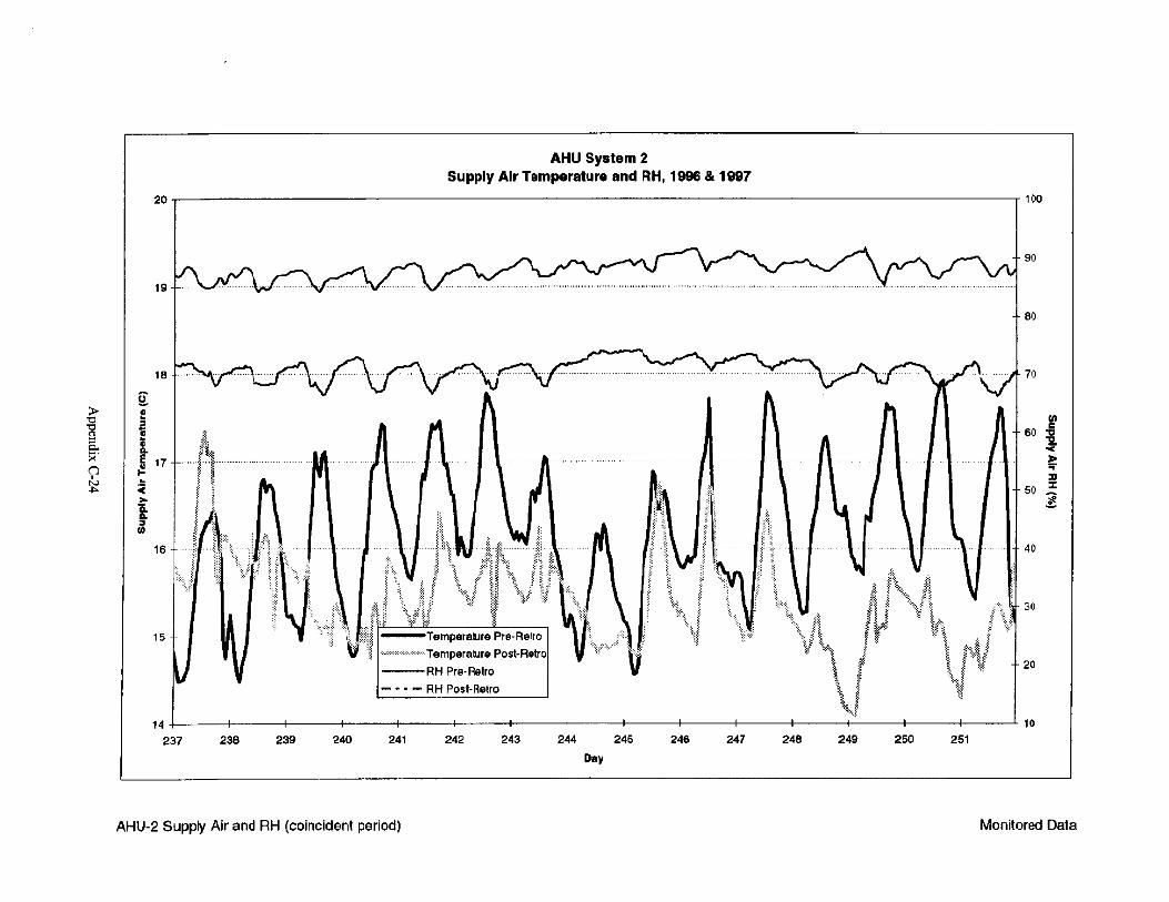
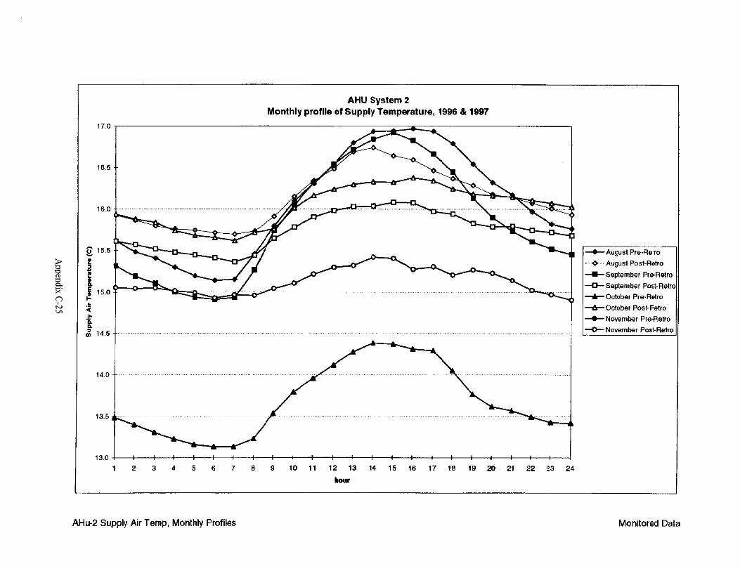
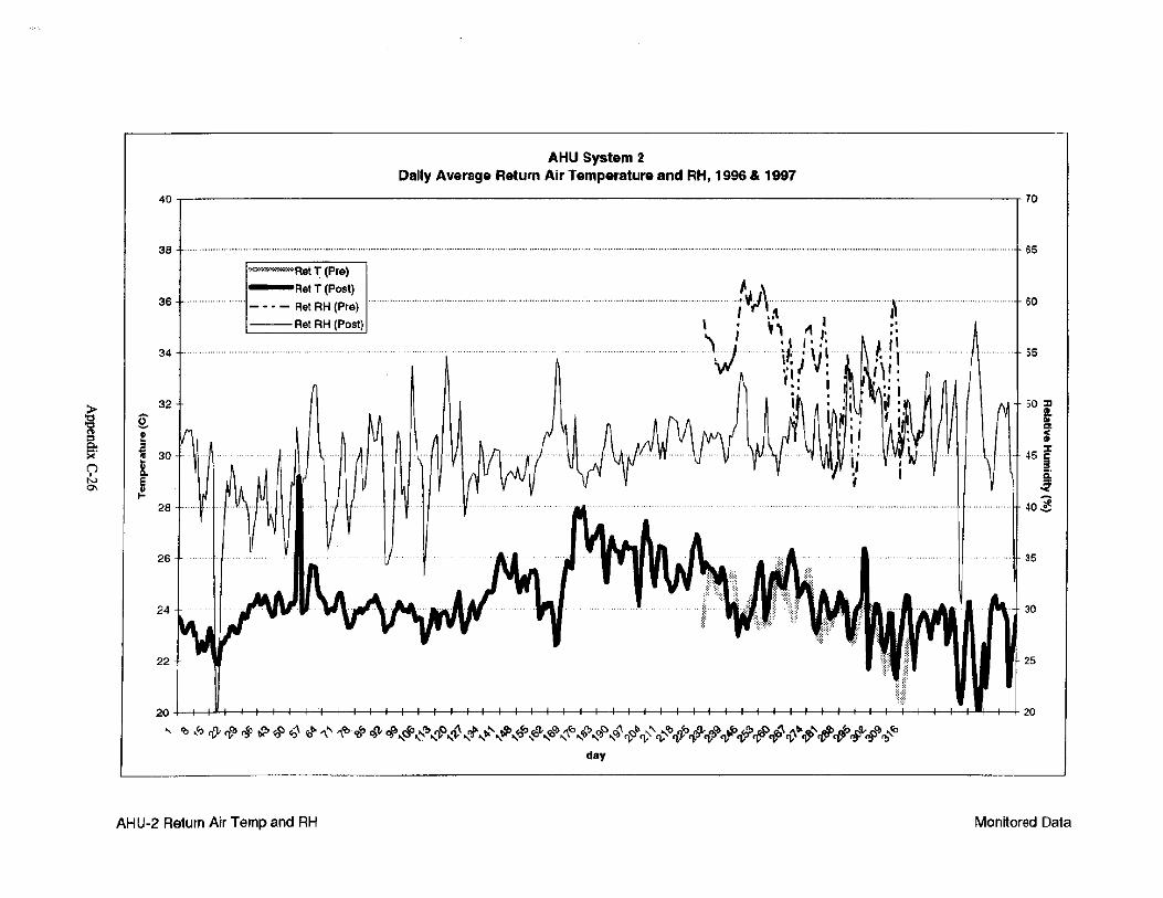
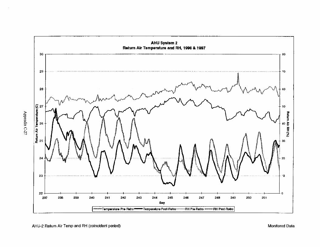

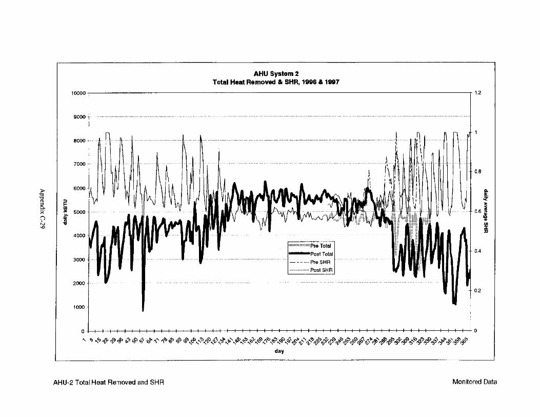
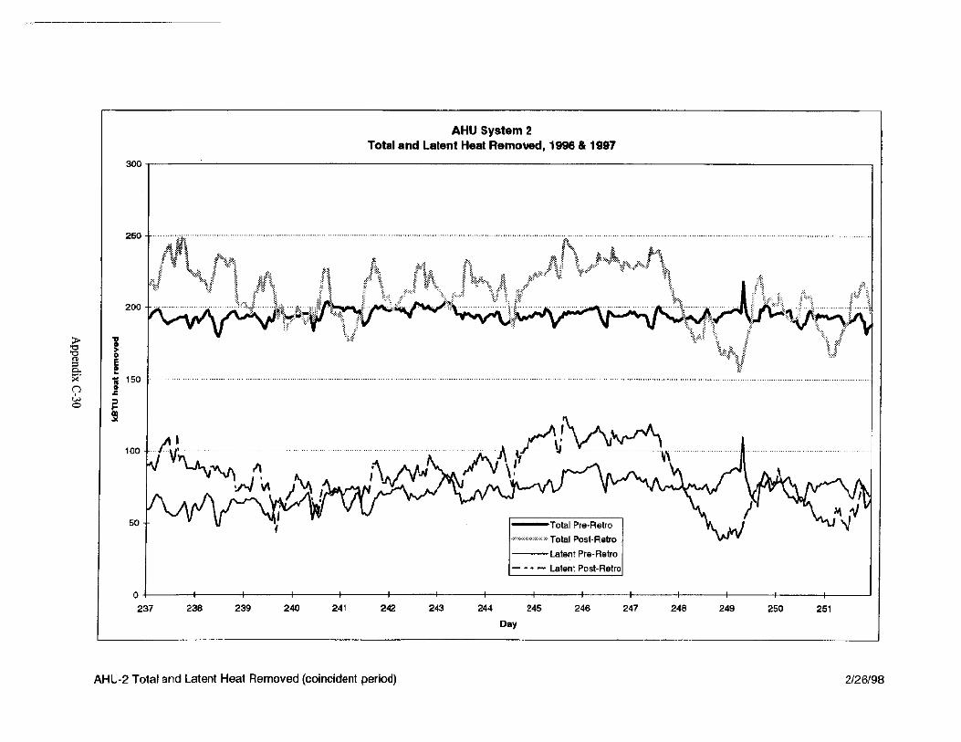

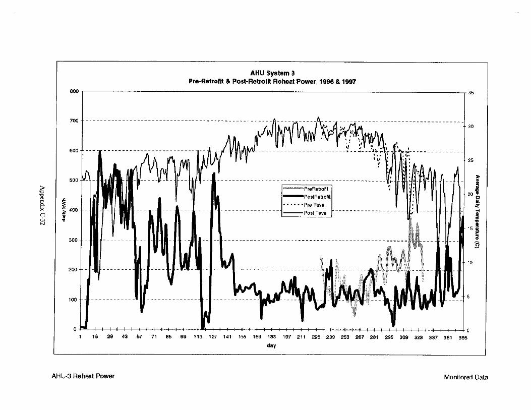
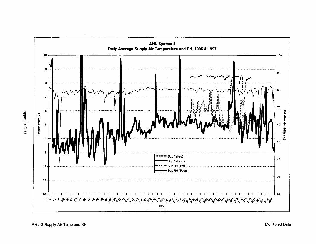
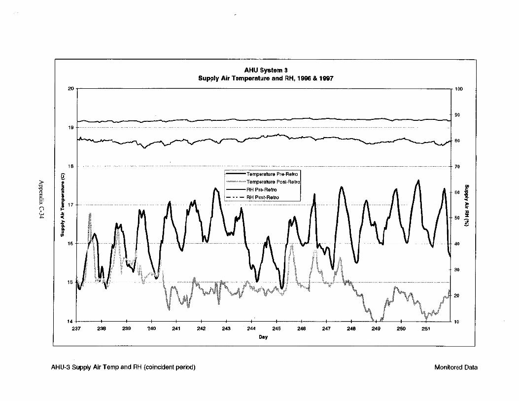

REPORT DOCUMENTATION PAGE Form ApprovedOMB NO. 0704-0188
Public reporting burden for this collection of information is estimated to average 1 hour per response, including the time for reviewing instructions, searching existing data sources,gathering and maintaining the data needed, and completing and reviewing the collection of information. Send comments regarding this burden estimate or any other aspect of thiscollection of information, including suggestions for reducing this burden, to Washington Headquarters Services, Directorate for Information Operations and Reports, 1215 JeffersonDavis Highway, Suite 1204, Arlington, VA 22202-4302, and to the Office of Management and Budget, Paperwork Reduction Project (0704-0188), Washington, DC 20503.
1. AGENCY USE ONLY (Leave blank) 2. REPORT DATEMarch 1999
3. REPORT TYPE AND DATES COVEREDTechnical Report
4. TITLE AND SUBTITLENew Technology Demonstration Program Kennedy Space Center Hangar L Heat Pipe Project: Performance Evaluation Report
6. AUTHOR(S)
Ed Hancock, Paul Reeves (Mountain Energy Partnership)
5. FUNDING NUMBERS
AS02.2010.
7. PERFORMING ORGANIZATION NAME(S) AND ADDRESS(ES)
Mountain Energy Partnership815 Alpine #6Boulder, CO 80304
8. PERFORMING ORGANIZATIONREPORT NUMBER
9. SPONSORING/MONITORING AGENCY NAME(S) AND ADDRESS(ES)
National Renewable Energy Laboratory1617 Cole BoulevardGolden, Colorado 80401-3393
10. SPONSORING/MONITORINGAGENCY REPORT NUMBER
TP-710-24738
11. SUPPLEMENTARY NOTES
12a. DISTRIBUTION/AVAILABILITY STATEMENT National Technical Information Service U.S. Department of Commerce 5285 Port Royal Road Springfield, VA 22161
12b. DISTRIBUTION CODE
13. ABSTRACT (Maximum 200 words)
In December of 1996, heat pipe heat exchangers were installed on three air handlers at Hangar L at the Cape Canaveral Air Station,Kennedy Space Center, Cape Canaveral, Florida. These retrofits were implemented with the intent to improve the dehumidificationperformance of the cooling systems, reduce the electric and steam energy required for reheating air, and reduce electric energy used bythe chillers.
Audits were conducted before and after the heat pipes were installed and a detailed monitoring system was set up to record hourlyoperating conditions of each of the three air-handling units. The audit information and monitored data were used to create a simulationmodel of the three air-handling systems and annual energy savings were predicted.
Energy savings for air handling unit 1 (AHU-1) were found to be negligible. Heat pipe installation in AHU-1 may have been inappropriatebecause of the design of the original cooling coils. Annual savings for AHU-2 are small, primarily because the required reheat for thesystem was already small. AHU-3 was the best application for the heat pipes and showed savings of 70,000 kWh per year. Interiorhumidity conditions improved after installation of the heat pipes for AHU-2 and AHU-3.
15. NUMBER OF PAGES14. SUBJECT TERMS
heat pipes, heat exchangers, air handlers, humidity, dehumidification, reheating, chillers, energysavings, cooling coils, 16. PRICE CODE
17. SECURITY CLASSIFICATIONOF REPORTunclassified
18. SECURITY CLASSIFICATIONOF THIS PAGEunclassified
19. SECURITY CLASSIFICATIONOF ABSTRACTunclassified
20. LIMITATION OF ABSTRACTUL
NSN 7540-01-280-5500 Standard Form 298 (Rev. 2-89)Prescribed by ANSI Std. Z39-18
298-102