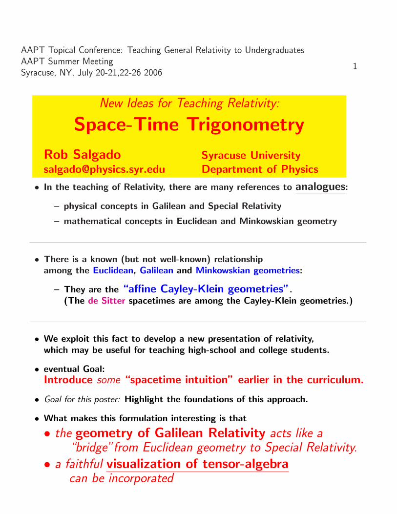
new ideas for teaching relativity: space-time trigonometry · new ideas for teaching relativity:...
TRANSCRIPT
1
AAPT Topical Conference: Teaching General Relativity to UndergraduatesAAPT Summer MeetingSyracuse, NY, July 20-21,22-26 2006
New Ideas for Teaching Relativity:
Space-Time Trigonometry
Syracuse University
Department of Physics
• In the teaching of Relativity, there are many references to analogues:
– physical concepts in Galilean and Special Relativity
– mathematical concepts in Euclidean and Minkowskian geometry
• There is a known (but not well-known) relationshipamong the Euclidean, Galilean and Minkowskian geometries:
– They are the “affine Cayley-Klein geometries”.(The de Sitter spacetimes are among the Cayley-Klein geometries.)
• We exploit this fact to develop a new presentation of relativity,which may be useful for teaching high-school and college students.
• eventual Goal:Introduce some “spacetime intuition” earlier in the curriculum.
• Goal for this poster: Highlight the foundations of this approach.
• What makes this formulation interesting is that
• the geometry of Galilean Relativity acts like a“bridge”from Euclidean geometry to Special Relativity.
• a faithful visualization of tensor-algebracan be incorporated

2A trigonometric analogy (Yaglom)a
aI.M. Yaglom, A Simple Non-Euclidean Geometry and Its Physical Basis (1979).
Euclidean rotation
t′ = ( cos θ)t + (− sin θ)y t′ =
1√1+v2
t +
−v√1+v2
y
y′ = ( sin θ)t + ( cos θ)y y′ =
v√1+v2
t +
1√1+v2
y
where v = tan θ.
Galilean boost transformation
t′ = (cosg θ)t + (0sing θ)y t′ =
1
t
y′ = (sing θ)t + ( cosg θ)y y′ =
v
t +
1
y
where v = tang θ.
Yaglom defines cosg θ ≡ 1, sing θ ≡ θ so that tang θ ≡ sing θ
cosg θ≡ θ.
Lorentz boost transformation
t′ = ( cosh θ)t + (+ sinh θ)y t′ =
1√1 − v2
t +
+v√1 − v2
y
y′ = ( sinh θ)t + ( cosh θ)y y′ =
v√1 − v2
t +
1√1 − v2
y
where v = tanh θ.

3The Cayley-Klein Geometries
measure of length between two points
measure ofangle betweentwo lines
elliptic(η2 = −1)
parabolic(η2 = 0)
hyperbolic(η2 = +1)
elliptic(ǫ2 = −1) Elliptic Euclidean Hyperbolic
parabolic(ǫ2 = 0)
co-Euclidean“anti-Newton-Hooke”
Galilean co-Minkowskian“Newton-Hooke”
hyperbolic(ǫ2 = +1) anti-De-Sitter Minkowski De-Sitter
2-dimensional manifolds with
metric signature (+1,−ǫ2) and constant curvature κ = −η2
ds2 = gab dxadxb
=(1 + η2ǫ2y2)dt2 − (1 − η2t2)ǫ2dy2 − 2η2ǫ2ty dt dy
(1 − η2(t2 − ǫ2y2))2
Column η2 = 0 are the affine Cayley-Klein geometries.
Row ǫ2 = −1 includes the classical non-Euclidean geometries.
Row ǫ2 = +1 are the constant curvature Lorentzian spacetimes.

4
The Metric(Proper Time)
We will be concerned with the “η2 = 0” (or “affine”) geometries.[Observe that Euclid V, the Parallel Postulate, is valid for these geometries.]In this case, the line-element reduces to
dS2 = (dt)2 − ǫ2(dy)2
which is a unified (meta-)expression for
(ds2)Euc = (dt)2 + (dy)2 if ǫ2 = −1(ds2)Gal = (dt)2 if ǫ2 = 0(ds2)Min = (dt)2 − (dy)2 if ǫ2 = +1
.
Upon introducing the metric tensor, the line-element can be written
dS2 =
(
dtdy
)T (
1 00 −ǫ2
)(
dtdy
)
.
Since the Galilean metric is degenerate, one needs to provide an additional metric in orderto measure spacelike separations:
dL2 =
− 1
ǫ2dS2 if ǫ2 6= 0
(dy)2 if ǫ2 = 0.
The Circle
Define the “CIRCLE of radius R” to be the locus of points (t, y) that is a constantpositive square-interval R2 from a common point (t0, y0).
R2 = (t − t0)2
− ǫ2(y − y0)2
In fact, the unit-circle [generally, unit-sphere] provides afaithful visualization of a symmetric metric tensor.

5
The Pole and the Polar(Visualizing Tensor-Index raising and lowering)
A metric tensor is a symmetric tensor that can be used to assign magnitudes to vectors.A metric tensor can also provide a rule to identify a vector with a unique covector.
The vector and its covector are [metric-]duals of each other with this metric. Given avector V a, in the presence of a metric gab, we can form the combination gabV
a, whichis a covector denoted by Vb. This is known as “index lowering”, a particular move whenperforming “index gymnastics”.
gabmetric tensor
y
t
Va
“the pole”
gabVa = Vb
“the polar [hyperplane]”
through the pole, drawthe tangents to the conic
This constructionis due to W. Burke,Applied Differential Geometry
–1
–0.5
0
0.5
1
1.5
2
y
–1 –0.5 0.5 1t
the number of polar hyperplanes of Vb
pierced by the vector V a
(number of “bongs of bell”)
=
(
square-norm of the vector V a
gabVaV b
)
In Minkowski spacetime: a timelike vector and a lightlike vector and their metric-duals.

6
The Trilogy of the Surveyorsa draft ofthe Trilogyis available
Euclidean
y
t
y
t
–2
–1
1
2
–2 –1 1 2
–2
–1
1
2
–2 –1 1 2
Galilean
y
t
y
t
Here, wherethe tangentscoincide,“simultaneity”is absolute.
–2
–1
1
2
–2 –1 1 2
–2
–1
1
2
–2 –1 1 2
Minkowskian
y
t
y
t
–2
–1
1
2
–2 –1 1 2
–2
–1
1
2
–2 –1 1 2
Family of surveyors of a two-dimensional plane:From this point, travel in all possible directions. Stop when your odometer reads 1 mi.This “calibration curve” defines a circle, with perpendicular as “tangent to the circle”.Family of observers of a two-dimensional spacetime:From this event, travel with all possible velocities. Stop when your wristwatch reads 1 s.This “calibration curve” defines a “circle”, with simultaneous as “tangent to the circle”.

7The Angle(Rapidity)
Define the “ANGLE-measure between two future-timelike lines ℓ1 and ℓ2”:
Θ =CIRCULAR arc-LENGTH L intercepted by ℓ1 and ℓ2
radius R of the CIRCLE centered at o
Θ = TANH−1v
θe = tan−1 vPPPPPq
θg = tang−1v
AAAAU
θm = tanh−1 v
t
ℓ1
ℓ2
0
0.2
0.4
0.6
0.8
1
1.2
1.4
1.6
1.8
2
0.2 0.4 0.6 0.8 1 1.2 1.4 1.6 1.8 2
Use the [spacelike] square-interval to measure the spacelike arc-length alongthe circle t2 − ǫ2y2 = R2:
Θ =1
R
∫
dL

8
For ǫ2 6= 0 cases,
Θ =1
R
∫
√
dy2 − 1
ǫ2dt2 =
∫ dy√R2 + ǫ2y2
=1
ǫsinh−1(ǫy/R)
Thus,ǫy = R sinh(ǫΘ)
t = R cosh(ǫΘ).
Euclidean case (ǫ2 = −1) Minkowskian case (ǫ2 = +1)
y = R sin(θe) y = R sinh(θm)
t = R cos(θe) t = R cosh(θm)
For the Galilean case (ǫ2 = 0),
θg =1
R
∫
dL =1
R
∫
dy =y
R.
Thus,y = Rθg = R sing(θg)
t = R = R cosg(θg)
where cosg(θg) = 1 and sing(θg) = θg
We can write the results for the three cases as
y = R SINHΘ
t = R COSHΘ
the connecting relation (“velocity = tangent(rapidity)”)
v =y
t= tan θe = tang θg = tanh θm
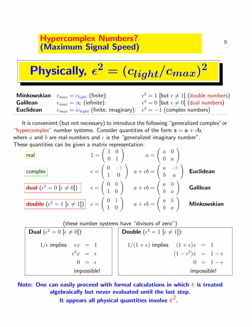
9Hypercomplex Numbers?(Maximum Signal Speed)
Physically, ǫ2 = (clight/cmax)2
Minkowskian cmax = clight (finite): ǫ2 = 1 [but ǫ 6= 1] (double numbers)Galilean cmax = ∞ (infinite): ǫ2 = 0 [but ǫ 6= 0] (dual numbers)Euclidean cmax = iclight (finite, imaginary): ǫ2 = −1 (complex numbers)
It is convenient (but not necessary) to introduce the following “generalized complex”or“hypercomplex” number systems. Consider quantities of the form z = a + ǫb,where a and b are real-numbers and ǫ is the “generalized imaginary number”.These quantities can be given a matrix representation:
real 1 =
(
1 00 1
)
a =
(
a 00 a
)
complex ǫ =
(
0 −11 0
)
a + ǫb =
(
a −bb a
)
Euclidean
dual (ǫ2 = 0 [ǫ 6= 0]) ǫ =
(
0 01 0
)
a + ǫb =
(
a 0b a
)
Galilean
double (ǫ2 = 1 [ǫ 6= 1]) ǫ =
(
0 11 0
)
a + ǫb =
(
a bb a
)
Minkowskian
(these number systems have “divisors of zero”)
Dual (ǫ2 = 0 [ǫ 6= 0]):
1/ǫ implies ǫx = 1
ǫ2x = ǫ
0 = ǫ
impossible!
Double (ǫ2 = 1 [ǫ 6= 1]):
1/(1 + ǫ) implies (1 + ǫ)x = 1
(1 − ǫ2)x = 1 − ǫ
0 = 1 − ǫ
impossible!
Note: One can easily proceed with formal calculations in which ǫ is treatedalgebraically but never evaluated until the last step.
It appears all physical quantities involve ǫ2.

10The Circular Functions(The Relativistic “Factors”)
Let Θ be a real number.
EXP Θ ≡ exp(ǫΘ)
= 1 + (ǫΘ) +(ǫΘ)2
2!+
(ǫΘ)3
3!+
(ǫΘ)4
4!+ · · ·
=
[
1 +(ǫΘ)2
2!+
(ǫΘ)4
4!+ · · ·
]
+
[
(ǫΘ) +(ǫΘ)3
3!+
(ǫΘ)5
5!+ · · ·
]
= cosh (ǫΘ) + sinh (ǫΘ)
=
[
1 + ǫ2Θ2
2!+ ǫ4
Θ4
4!+ · · ·
]
+ǫ
[
Θ + ǫ2Θ3
3!+ ǫ4
Θ5
5!+ · · ·
]
= COSH Θ + ǫ SINH Θ
ǫ TANH Θ ≡ tanh(ǫΘ) =sinh(ǫΘ)
cosh(ǫΘ)=
ǫ SINH Θ
COSH Θ
Algebraic Identities1 = COSH2Θ − ǫ
2SINH2Θ
TANH (Θ1 + Θ2) =TANH Θ1 + TANH Θ2
1 + ǫ2 TANH Θ1 TANH Θ2
COSH Θ = (1 − ǫ2 TANH2Θ)−1/2
Differential Identitiesd
dΘEXP Θ = ǫ EXP Θ
d
dΘCOSH Θ = ǫ2 SINH Θ
d
dΘSINH Θ = COSH Θ
d
dΘTANH Θ = 1 − ǫ2 TANH 2Θ

11
Every vector can be thought of
as the HYPOTENUSE
of some RIGHT triangle.
u
u
0
1
2
1 2
Euclidean decomposition of a vector.
u
u
0
1
2
1 2
Galilean decomposition of a vector.
u
u
0
1
2
1 2
Minkowskian decomposition of a vector.
Project the vector into components parallel and perpendicular to a given direction.“Drop the perpendicular” by constructing parallels to the tangent of the circle.

12
The Rotation(Boost Transformation)
Consider a linear transformation ~V ′ = R(Θ)~V , where R satisfies:
det R = 1 R(0) = I
RT GR = G R(Θ)R(Φ) = R(Θ + Φ)
In terms of an orthogonal basis {t, y} with metric G =
(
1 00 −ǫ2
)
, we find the lineartransformation
R(Θ) =
COSH Θ ǫ2SINH Θ
SINH Θ COSH Θ
is a “rotation” for that metric.
–2
–1
1
2
–2 –1 1 2
t
Euclidean–2
–1
1
2
–2 –1 1 2
t
Galilean–2
–1
1
2
–2 –1 1 2
t
Minkowskian
Eigenvectors of the Rotations(“Absolutes”)
eigenvalue eigenvectors
EUC cos θ ± i sin θ (actually, complex) ~0 =
(
00
)
(better: invariant vector)
GAL 1 “absolute length” y =
(
01
)
“absolute time”
MIN cosh θ ± sinh θ = exp(±θ) k =1√2
(
11
)
=
√
1 ± v
1 ∓ vDoppler-Bondi factor and l =
1√2
(
1−1
)
“absolutespeed of light”

13
Projection onto a LineProper-Time (and “Time-Dilation”)
t
y
cos θe cosg θg cosh θm
sin θe
sing θg
sinh θm
Θ
The “proper time”is the hypotenusealong the radius.
The “apparent time”is the projection ontoour observer’s t-axis.
0
1
1
The arrow along the t-axis is a unit-vector in each geometry. Follow the arc along each“circle” to a line with slope v. Note that the corresponding unit vectors generally havedifferent projections onto the t-axis.
The Distance between ParallelsProper-Length (and “Length Contraction”)
t
t t
y = b2
y = b1
ℓ1
ℓ2ℓM⊥
ℓG⊥
ℓE⊥
ΘΘ Θ
M
G
E
L = (b2 − b1)COSHΘO
The “apparent length”is the hypotenuse OG,perpendicular toour observer’s t-axis.
The “proper length”is the perpendicular distance(either OE, OG, OM)between the parallel lines
Note that E, G, and M are “right angles” in their respective geometries. So, OG (beingthe side of the triangle opposite to the “right angle”) is the hypotenuse in each geometry.(In Galilean relativity, the triangle is degenerate.)
(In special relativity, one sees the above relation in the formL
COSH Θ= (b2 − b1). )

14The Law of Cosines(“The Clock Effect”)
A
BC
S
~b
~a
~c
~c = ~b + ~a
~c · ~c = ~b ·~b + ~a · ~a + 2~b · ~ac2 = b2 + a2 + 2ba COSH (m 6 BCS)
In terms of the proper-time elapsed,
(tAB)2 = (tAC)2 + (tCB)2 + 2tACtCB COSH (m 6 BCS)
Comparing this with the identity
(tAC + tCB)2 = (tAC)2 + (tCB)2 + 2tACtCB
and using the facts that cos θe ≤ 1, cosg θg = 1, and cosh θm ≥ 1,the Law of Cosines implies the following relations:
tAB <tAC + tCB for ǫ2 = −1 “triangle inequality”
tAB =tAC + tCB for ǫ2 = 0 non-“clock effect”
tAB >tAC + tCB for ǫ2 = +1 “clock effect”

15“The Doppler Effect”a unified trigonometric derivation
0 TS
y = vRt@
@R
TR
T′R
y = ct@@R
y = c(t − TS)@@R
TRSINH Θ
� TRCOSH Θ -
TRSINH ΘΘ
Moving [Receding] Receiver
TS = TR(COSH Θ − SINH Θ)
νR =
νS(1 − vc) Gal
νS
√
1 − vc
1 + vc
Min
0 TR
y = vSt@@I
TS
T′S
y = ct@@R
y = −c(t − T ′S) + vST ′
S
��
TSCOSH Θ
TSSINH Θ
TSSINH ΘΘ
Moving [Receding] Source
TR = TS(COSH Θ + SINH Θ)
TS = TR1
(COSH Θ + SINH Θ)
νR =
νS1
(1 + vc)
Gal
νS
√
1 − vc
1 + vc
Min
Note: In Minkowskian geometry (ǫ2 = +1),
1
(COSH Θ + SINH Θ)= (COSH Θ − SINH Θ).

16The Curve of Constant CurvatureThe Uniformly Accelerating Observer
Euc
Gal
Miny
t
–1
1
2
–2 –1 1 2
The curvature ρ of a plane curve is a measure of how the angle φ of thetangent vector y changes with arc-length s along the curve. We will consider a timelikeplane curve y(t), i.e., a curve whose tangent is everywhere timelike.
The acceleration ρ of a worldline is a measure of how the rapidity φ of thevelocity vector y changes with proper-time s along the curve.
ρ ≡
dφ
ds=
dφ
dt
dt
ds
=y
[1 − ǫ2(y)2]3/2
We seek the curve of constant curvature: ρ = a0:If ǫ2 6= 0,
(y − y0)2 − 1
ǫ2(t − t0)
2 =1
ǫ4a0
−2
{
if ǫ2 = −1 circleif ǫ2 = +1 hyperbola
If ǫ2 = 0,y − y0 =
1
2a0(t − t0)
2{
parabola
“uniform acceleration” is an “invariant state of motion”

17Trigonometric IdentitiesTransformations of spatial-velocityand spatial-acceleration
Consider an object whose spacetime position is specified by ~y(s), where s is the arc-length (proper time). Let an inertial-observer O1 study this object and assign it coordinatesy1(t1). Similarly, assign y2(t2) for an inertial-observer O2. Let v21 be the invariant relativevelocity of O2 with respect to O1:
v21 = TANH (Θ20 − Θ10),
where the rapidities are measured with respect to some fiducial timelike axis (a thirdobserver). It will be convenient to use the abbreviation
Θ21 = Θ20 − Θ10.
First, suppose that ~y is inertial.If O1 says that ~y moves with spatial velocity dy1
dt1= vy1 = TANH Θy1,
what does O2 say? That is, express dy2
dt2= vy2 = TANH Θy2 in terms of Θy1 and Θ21.
vy2 = TANH Θy2
= TANH (Θy1 − Θ21)
=TANH Θy1 − TANH Θ21
1 − ǫ2TANH Θy1TANH Θ21
=vy1 − v21
1 − ǫ2vy1v21
Suppose now that ~y is uniformly accelerated.If O1 says that ~y moves with spatial acceleration d2y1
dt12 = ay1 = ρy1
COSH3
Θy1
,
what does O2 say? That is, express d2y2
dt22 = ay2 = ρy1
COSH3
Θy2
in terms of Θy1 and Θ21.
ay2 =ρy
COSH3Θy2
=ρy
COSH3(Θy1 − Θ21)
=ρy
(COSH Θy1COSH Θ21 − ǫ2SINH Θy1SINH Θ21)3
=ρy
COSH3Θy1
1
COSH3Θ21 (1 − ǫ2TANH Θy1TANH Θ21)3
= ay1
(√1 − ǫ2v21
2
1 − ǫ2vy1v21
)3

18Euclidean Postulate ISimultaneity
Euclid I : “To draw a unique straight “line” from any point toany point.”
Euclid V (Playfair) : “Given a line, and a point not on thatline, there exists only one line through that point whichis parallel to (i.e., does not “intersect”) the given line.[This asserts the existence and uniqueness of a parallel to agiven line through a given point.]
“duality” in projective geometry exchanges points with lines, and so forth...
Euclid I (dual-Playfair) : “Given a point, and a line not throughthat point, there exists no point on that line which cannotbe joined (by an “ordinary” line) to the given point.[This asserts the nonexistence of a non-ordinary line from agiven point.]
Euclid I (spacetime) : “Given an event, and a worldline not ex-periencing that event, there exists no event on that world-line which is not “timelike-related” to the given event.[This asserts the nonexistence of non-timelike-related eventsfrom a given event.]
Loosely speaking, regard
(the spacetime interpretation of) Euclid Ias a statement concerning
“simultaneity with distant events”
spacetime geometryan event (on a given distant worldline)that is simultaneous with our given event
Euclidean does not existGalilean exists and is uniqueMinkowskian exists and is not unique

19Spacetime Geometry is non-Euclidean
Consider a given point [event],and a straight line [inertial worldline]not through [experiencing] that point [event].
Euclidean
y
t
y
t
no pointson this line
are inaccessible to or from O
–2
–1
1
2
–2 –1 1 2
–2
–1
1
2
–2 –1 1 2
Galilean
y
t
y
t
exactly one eventon this worldline
is inaccessible to or from O
–2
–1
1
2
–2 –1 1 2
–2
–1
1
2
–2 –1 1 2
Minkowskian
y
t
y
t
infinitely many eventson this worldline
are inaccessible to or from O
–2
–1
1
2
–2 –1 1 2
–2
–1
1
2
–2 –1 1 2

Salgado Spacetime Trigonometry DRAFT Version: 7/21/2006 1
AAPT Topical Conference: Teaching General Relativity to Undergraduates
AAPT Summer Meeting
Syracuse, NY, July 20-21,22-26 2006
Spacetime Trigonometry and Analytic Geometry I:The Trilogy of the Surveyors
Roberto B. SalgadoDepartment of Physics, Syracuse University, Syracuse, NY [email protected]
I. INTRODUCTION
This is the first of a series of articles in which we expound a unified formalism for two-dimensional Euclideanspace, Galilean spacetime,1 2 and Minkowski spacetime rooted in the geometrical studies of Arthur Cayley andFelix Klein. Using techniques familiar from the analytic geometry and trigonometry of Euclidean space, we developthe corresponding analogues for Galilean and Minkowskian spacetimes and provide them with physical interpretations.This provides a new approach for teaching relativity and allows us to clarify many terms used in relativity.
Our presentation is primarily inspired by two works:
• I.M. Yaglom’s A Simple Non-Euclidean Geometry and Its Physical Basis,3
which is an insightful study of the geometry associated with the Galilean transformations,
• E.F. Taylor and J.A. Wheeler’s Spacetime Physics,4
which presents Special Relativity from a geometrical viewpoint.
II. THE TRILOGY OF THE SURVEYORS
(These passages were inspired by “The Parable of the Surveyors” in E.F. Taylor and J.A. Wheeler’s SpacetimePhysics.5 )
A. The Euclidean Surveyors
Once upon a time, a student of Euclid was asked to devise a method to survey an unexplored territory of thekingdom, a featureless plane stretching as far as the eye can see. So, he organized a team of surveyors and equippedeach surveyor with a pair of ideal measuring tools. The first tool is an “odometer,” or “rolling tape-measure,” whichmeasures the distance a surveyor has traveled along his path, in units of miles. The second tool is a very long ruler,calibrated in feet, which measures the perpendicular distance from his path to a distant point not his path.
He instructed the surveyors to begin at a common origin, O, then to travel in a straight line in all possible spatialdirections in the plane. Each is instructed to mark the point with a flag when his tape-measure reads “t=1 mi.”What is the locus of these points? Of course, the result of the experiment is that these points lie on a “circle withradius R = 1 mi.” This circle, the Euclidean student declared, provides the basic calibration curve for measuring theseparation between points on this plane. Indeed, later surveys of this territory would show that such a circle couldbe constructed from any origin and be extended to any radius.
In order to complete the survey of the plane, each surveyor is told to assign to each point a pair of coordinates(t, y), where t represents the displacement “along his path” (as measured by his tape-measure) and y represents thedisplacement “perpendicular to his path” (as measured by his ruler). What does “perpendicular to his path” mean?Geometrically, it means “along the tangent-line to the circle of radius t” at his point on that circle. Operationally,this means “along a line of points that he regards as having the same value of t.”
When the radial surveyors’ data were collected, it was noticed that for any given point P on the circle, there wasgeneral disagreement on its assigned t-displacements and on its assigned y-displacements from the origin O. That is,comparing the measurements from two radial surveyors U and U
′, we have
(tP − tO) 6= (t′P − t′
O) and (yP − yO) 6= (y′
P − y′
O).

Salgado Spacetime Trigonometry DRAFT Version: 7/21/2006 2
y
k(mi)
t (mi)
y
k(mi)
t (mi)
–2
–1
0
1
2
–2 –1 1 2
–2
–1
0
1
2
–2 –1 1 2
FIG. 1: The Euclidean surveyors define a unit circle, the basic calibration curve for measuring separations in space. Eachsurveyor operationally defines “perpendicular to his radial path” as “along his tangent-line to the circle.”
However, there was unanimous agreement on the quadratic quantity (tP − tO)2 + ((yP − yO)/k)2:
(tP − tO)2 +
(
yP − yO
k
)2
= (t′P − t′
O)2 +
(
y′
P − y′
O
k
)2
,
where k is a unit-conversion constant,6 which simplifies the arithmetic. The Euclideans called this quadratic quantitythe “square-distance” from point O, which provides an invariant measure of the separation between points P and O.(See Fig. 1) Indeed, each radial surveyor used the same equation to describe the circle:
(t − tO)2 +
(
y − yO
k
)2
= R2.
In fact, by comparing the unlabeled plots from each radial surveyor, the Euclidean student could not distinguishamong these radial surveyors. So, no radial surveyor is preferred over any other. However, when the labeling isaccounted for, there is a way to relate the measurements of one radial surveyor with those of another.7
Having been successful at defining an invariant measure of separation between pairs of points, the Euclidean studentnow wished to define an invariant measure of separation between pairs of radial surveyor-paths through O. It seemedreasonable to define this measure using the signed arc-length Se of the circle cut by those paths. However, thismeasure was deemed to be somewhat limited because the arc-length Se depends on the radius R of the circle used todetermine it. After a little analysis, it was observed that for a given pair of surveyor-paths, the corresponding valuesof Se and R are in constant proportion. So, in order for the measure of separation to be independent of the size ofthe circle used, the Euclidean student defined a quantity called the signed “angle” by
θe ≡(
Se/k
R
)
,
where the unit-conversion constant k is used to make this angle dimensionless.The Euclidean student observed that, since the arc-length Se is bounded, the range of the angle θe is bounded:
−π < θe ≤ π, where π is a numerical constant that was determined to be approximately 3.14159. Since the arc-lengthis additive, the angle measure is also an additive quantity. That is, for radial surveyor-paths OA, OB, and OC fromO through the respective points A, B, and C on the circle, we have
θe,AB + θe,BC = θe,AC ,
where, for example, θe,AB is the signed-angle from OA to OB.Many years later, another student of Euclid defined another invariant measure of separation between pairs of radial
surveyor-paths in terms of the parallel and perpendicular projections, (t − tO) and (y − yO), respectively, of one

Salgado Spacetime Trigonometry DRAFT Version: 7/21/2006 3
surveyor path onto another surveyor path. This quantity, called the “slope,” is defined by ve ≡ (y − yO)/(t − tO),which is expressed in units of miles/ft. This can be expressed in terms of the angle θe using
ve
k≡ (y − yO)/k
(t − tO)= tan
(
Se/k
R
)
= tan(θe),
where we have used the unit-conversion constant k since the trigonometric tangent function and its argument aredimensionless. Observe that the range of the slope is unbounded: −∞ < ve < ∞ [in units of ft/mile]. Furthermore,unlike the angle measure, the slope is not an additive quantity:
ve,AB + ve,BC 6= ve,AC .
Instead,
ve,AB + ve,BC
1 − ve,ABve,BC/k2= ve,AC .
As a postscript to this story, the use of the unit-conversion constant k was eventually seen as an unnecessary nuisancein the arithmetic. By expressing “ruler measurements” for “y” (traditionally in units of feet) in the “odometer units”used by “t” (traditionally in units of miles), the need to use k was eliminated. With this advancement, the Euclideanresults can be written more simply as:
(t − tO)2 + (y − yO)2
= R2
θe ≡ Se/R θe,AB + θe,BC = θe,AC
ve ≡ (y − yO)
(t − tO)= tan(Se/R) = tan θe
ve,AB + ve,BC
1 − ve,ABve,BC
= ve,AC
B. The Galilean Surveyors
In the study of kinematics, one naturally draws “distance vs. time” graphs. This is a different kind of space, called“spacetime,” whose points are called “events.” Thus, a “distance vs. time” graph is sometimes called a “spacetimediagram.” How might a student of Galileo proceed to survey spacetime? He decided to follow an analogue of theEuclidean procedure used in the preceding section.
He organized a team of “spacetime surveyors,” henceforth, called “observers”. As time elapses, each observer willtrace out a path in spacetime called his “worldline.” Those observers who travel inertially will trace out straightworldlines in spacetime.
Each observer is equipped with a pair of ideal measuring tools. The first tool is a “chronometer,” or “wristwatch,”which measures the interval of time that has elapsed along his worldline, in units of seconds. The second tool is avery long ruler, calibrated in meters, which measures the “[Galilean-]perpendicular” distance from his worldline to adistant event not on his worldline. [We will more fully define this notion of perpendicularity shortly.]
He instructed the observers to begin at a common event, O, then to travel inertially with all possible velocitiesalong a common straight line in space. Each is instructed to mark the event with a firecracker explosion when hiswristwatch reads “t = 1 second”. What is the locus of these events on a spacetime diagram?
Due to the technological limitations of their day, the maximum speed attempted by the Galilean observers wasa small fraction of the speed of light, clight, which they knew to be finite. Nevertheless, they boldly extrapolatedtheir experimental observations and reached the conclusion that these events lie on a vertical line in our spacetimediagram, which they might have called a “[future Galilean] circle with radius R = 1 second.” This [Galilean] circle,the Galilean student declared, provides the basic calibration curve for measuring the separation between events inspacetime. Note that this declaration implicitly asserts that all finite speeds (including those faster than the speed oflight, clight) are theoretically attainable by observers!
In order to complete the survey of the spacetime, each observer is told to assign to each event a pair of coordinates(t, y), where t represents the temporal displacement “along his worldline” (as measured by his wristwatch) and y
represents the spatial-displacement “perpendicular to his worldline” (as measured by his ruler). But what does“perpendicular to his worldline” mean here? Geometrically, following the Euclidean procedure, this means “along thetangent-line to the [Galilean] circle.” (See Fig. 2.) Operationally, this means “along a line of events that he regardsas having the same value of t.” Physically, this means “along a line of events that he regards as simultaneous.”

Salgado Spacetime Trigonometry DRAFT Version: 7/21/2006 4
y (m)
t (sec)
y (m)
t (sec)
–2
–1
0
1
2
–2 –1 1 2
–2
–1
0
1
2
–2 –1 1 2
FIG. 2: The Galilean observers define a “[Galilean] unit circle,” the basic calibration curve for measuring intervals in spacetime.Each inertial observer operationally defines “perpendicular to his worldline” as “along his tangent-line to the [Galilean] circle.”Physically, the events that lie on a given line perpendicular to his worldline are simultaneous according to this observer.
When the observers’ data were collected, it was noticed that for any given event P on the Galilean circle, there wasgeneral disagreement on its assigned y-displacements from the origin O. That is, comparing the measurements fromtwo inertial observers U and U
′, we have
(yP − yO) 6= (y′
P − y′
O).
However, there was unanimous agreement on its assigned t-displacements,
(tP − tO) = (t′P − t′
O),
and, therefore, on the quadratic quantity (tP − tO)2:
(tP − tO)2 = (t′P − t′
O)2.
Inspired by the Euclidean observers, the Galileans decided to call this quadratic quantity the “[Galilean] square-interval,” which provides an invariant measure of the separation between events P and O. (See Fig. 2) Indeed, eachinertial observer used the same equation to describe the [Galilean] circle:
(t − tO)2 = R2.
In fact, by comparing the unlabeled plots from each inertial observer, the Galilean student could not distinguishamong these inertial observers. So, no inertial observer is preferred over any other. However, when the labeling isaccounted for, there is a way to relate the measurements of one inertial observer with those of another.8
The Galilean observers noted several geometrical features not seen by the Euclidean surveyors. First, about half ofthe spacetime could not be surveyed by the inertial observers starting at event O. Even if the experiment had beenexpanded to include inertial observers that would end up meeting at event O, the key feature noted was that therewas an inaccessible radial direction to or from event O on their spacetime diagrams. This corresponds to a speedthat was unattainable by the observers through event O. Moreover, all of these observers determine the same valuefor this unattainable speed: the universal constant cmax,g whose value was experimentally extrapolated to be infinite.Second, for any given Galilean circle, the tangent-lines corresponding to different radii coincided. Physically, this wasinterpreted by saying that “simultaneity is absolute.” Moreover, for a given pair of events on a given tangent-line tothe Galilean circle, all observers determine the same value for the spatial separation between that pair. Physically,this was interpreted by saying that “the measured length of an object [whose bounding worldlines pass through thoseevents] is absolute.”
Following the Euclideans, the Galileans also wished to define an invariant measure of separation between pairs ofinertial observer-worldlines through O. They defined that separation in terms of the [Galilean] arc-length Sg of a[Galilean] circle of radius R cut by those worldlines. They defined a quantity analogous to the Euclidean angle,
θg ≡(
Sg/kg
R
)
,

Salgado Spacetime Trigonometry DRAFT Version: 7/21/2006 5
called the “Galilean-angle,” or, more physically, the “Galilean rapidity.” Note that, in order for this angle to bedimensionless, one must introduce a unit-conversion constant kg with units of meters/second. For ease of comparisonwith the Minkowskian case later, we will choose kg = clight. Since the arc-length Sg is unbounded, the rapidity θg isunbounded: −∞ < θg < ∞. Since the [Galilean] arc-length is additive, the [Galilean] rapidity measure is an additivequantity. That is, for inertial observer-paths from O through events A, B, and C on the [Galilean] circle:
θg,AB + θg,BC = θg,AC .
where, for example, θg,AB is the signed Galilean-rapidity from OA to OB.They also defined another measure of separation between pairs of observer worldlines analogous to the slope, called
the “velocity,” by vg ≡ (y − yO)/(t − tO), where (t− tO) is the elapsed-time and (y − yO) is the spatial-displacementfrom event O. The velocity is expressed in units of meters/second. The Galilean observers were pleasantly surprisedto find that the Galilean-rapidity is directly-proportional to the velocity
vg
kg
≡ (y − yO)/kg
(t − tO)=
(
Sg/kg
R
)
= θg,
differing only by a unit-conversion constant. Thus, the velocity is also unbounded: −∞ < vg < ∞ [in units ofmeters/second], as well as additive
vg,AB + vg,BC = vg,AC .
This can be a great convenience for doing calculations in Galilean relativity. In particular, with the emphasis onvelocity, there is little need to be concerned with [Galilean] rapidity and the unit-conversion constant kg. However,the failure to recognize the distinction between [Galilean] rapidity and velocity will become one source of confusionfor Galileans who will try to understand more modern models of spacetime.
C. The Minkowskian Surveyors
Consider now a technologically-advanced team of inertial observers, who can now attempt speeds comparable toclight. If the same experiment were repeated, what is the locus of these events on a spacetime diagram?
Surprisingly [to the Galileans], the result of such an experiment9 is that these events lie not on a straight line,but on a hyperbola in spacetime, which we call a “[future Minkowskian] circle with radius R = 1 second.” This, ofcourse, is consistent with the experimental results obtained by the Galilean observers since, for the small range ofslow velocities that they attempted, the line is a good approximation to the hyperbola.
In the assignment of coordinates (t, y), what does “perpendicular to his worldline” mean here? Geometrically, thisstill means “along the tangent-line to the [Minkowskian] circle.” Operationally, this still means “along a line of eventsthat he regards as having the same value of t.” Physically, this still means “along a line of events that he regards assimultaneous.”
When the observers’ data were collected, it was noticed that for any given event P on the Minkowskian circle, therewas general disagreement on its assigned t-displacements and on its assigned y-displacements. That is, comparing themeasurements from two inertial observers U and U
′, we have
(tP − tO) 6= (t′P − t′
O) and (yP − yO) 6= (y′
P − y′
O).
However, there was unanimous agreement on the quadratic quantity (tP − tO)2 − ((yP − yO)/clight)2, i.e.,
(
tP − tO
)2
−(
yP − yO
clight
)2
= (t′P − t′
O)2 −(
y′
P − y′
O
clight
)2
,
where, at this stage, clight is a unit-conversion constant10 that we will call km. The Minkowskians decided to callthis quadratic quantity the “[Minkowskian] square-interval,” which provides an invariant measure of the separationbetween events P and O. Indeed, when the surveyors’ plots were compared, it was also realized that all surveyorsdescribe the same set of events on their Minkowskian circles
(t − tO)2 −(
y − yO
clight
)2
= R2.

Salgado Spacetime Trigonometry DRAFT Version: 7/21/2006 6
y (light-sec)
t (sec)
y (light-sec)
t (sec)
–2
–1
0
1
2
–2 –1 1 2
–2
–1
0
1
2
–2 –1 1 2
FIG. 3: The Minkowskian observers define a “[Minkowskian] unit circle,” the basic calibration curve for measuring intervals inspacetime. (For comparison, we have included the efforts of the Galilean observers for their range of velocities. Note the unitson the spatial axis.) Each inertial observer operationally defines “perpendicular to his worldline” as “along his tangent-lineto the [Minkowskian] circle.” Physically, the events that lie on a given line perpendicular to his worldline are simultaneousaccording to this observer.
In fact, by comparing the unlabeled plots from each inertial observer, the Minkowskian student could not distinguishamong these inertial observers. So, no inertial observer is preferred over any other. However, when the labeling isaccounted for, there is a way to relate the measurements of one inertial observer with those of another.11
The Minkowskian observers noted several geometrical features in conflict with those seen by the Galilean observers.First, there were infinitely many inaccessible radial directions to or from event O on their spacetime diagrams, whichcorrespond to infinitely many speeds unattainable by the observers through event O. Moreover, all observers determinethe same value for the least upper bound of the attainable speeds: the universal constant cmax,m whose numericalvalue is measured to be equal to the speed of light clight. (Note that the speed of light clight plays two roles, oneas a unit-conversion constant and the other as a maximum signal speed. We will emphasize this point in the nextsection.) Second, for a given Minkowskian circle, the tangent-lines corresponding to different radii of the same circledid not coincide. Physically, this was interpreted to mean that “simultaneity is, in fact, not absolute.” Furthermore,the measured length of an object is not absolute.
The Minkowskian observers also wished to define a measure of separation between pairs of concurrent inertialobserver-worldlines. Following the Euclidean and Galilean procedure, they defined the separation in terms of thearc-length Sm of a [Minkowskian] circle of radius R cut by those worldlines. The “Minkowski-angle”, also known asthe “rapidity,” was defined by
θm ≡(
Sm/km
R
)
,
and the velocity by vm ≡ (y − yO)/(t − tO). In this case, however, the velocity and the rapidity are related by
vm
km
≡ (y − yO)/km
(t − tO)= tanh
(
Sm/km
R
)
= tanh (θm) ,
Observe that the range of the rapidity is unbounded: −∞ < θm < ∞, whereas the velocity is bounded: −cmax,m <
vm < cmax,m. Furthermore, unlike the rapidity measure, the velocity is not an additive quantity:
vm,AB + vm,BC 6= vm,AC .
Instead,
vm,AB + vm,BC
1 + vm,ABvm,BC/k2m
= vm,AC .
These results are also in conflict with the results obtained by the Galilean observers.

Salgado Spacetime Trigonometry DRAFT Version: 7/21/2006 7
D. An observation about clight
This trilogy suggests a similarity among these three geometries, which we will develop more fully in a subsequentarticle. Here, we begin to make precise those analogies by focusing on the line-elements of the three geometries.
Consider two infinitesimally-close points12 O and P in each of two-dimensional Euclidean space, Galilean spacetime,and Minkowski spacetime. Let us write down the line-elements13 or “infinitesimal square-intervals” for the threegeometries:
(ds2)Euc = (dt)2 +
(
dy
k
)2
(1a)
(ds2)Gal = (dt)2 (1b)
(ds2)Min = (dt)2 −
(
dy
clight
)2
, (1c)
where, in our spacetime diagram, dt is the displacement from O to P along the horizontal axis and dy is the displace-ment from O to P along with the vertical axis. In order to facilitate the comparison of the three geometries, let usexpress the Euclidean measure of distance between two points in terms of the time it takes light to travel betweenthem. Thus,
(ds2)Euc = (dt)2 +
(
dy
clight
)2
,
where (ds2)Euc is in units of square-seconds, (dt) is in units of seconds and (dy) is in distance units of light-seconds.
We emphasize that, here, clight plays the role of a convenient unit-conversion constant between the coordinates t andy. In this role, it has no physical significance.
Now, let us write
(ds2)Euc = (dt)2 − (−1)
(
dy
clight
)2
(2a)
(ds2)Gal = (dt)2 − (0)
(
dy
clight
)2
(2b)
(ds2)Min = (dt)2 − (+1)
(
dy
clight
)2
, (2c)
or in a unified way as
dS2 = (ds
2)ǫ = (dt)2 − ǫ2
(
dy
clight
)2
, (3)
where ǫ2 is a dimensionless quantity we will call the “indicator,” which can take the value −1, 0, or 1, corresponding
to the Euclidean, Galilean, and Minkowskian cases, respectively. [We will defer the discussion of the indeterminate ǫ
for a later section.] Physically, the indicator can be interpreted as
ǫ2 ≡
(
clight
cmax
)2
(4)
where cmax is the maximum signal speed of the particular spacetime theory. For the Minkowskian case, we havecmax = clight, which can be inferred from Einstein’s second postulate. For the Galilean case, we have cmax = ∞since there is no upper bound on the speed of signal transmission in Galilean relativity. For consistency, if we wereto interpret the Euclidean case as a spacetime theory, we would say cmax = iclight, where i is the complex number√−1.14
Recognizing the role of clight as merely a conversion factor in these equations, it is now convenient to redefine“y/clight” as “y” (which is now measured in seconds) so that we can write
dS2 = (ds
2)ǫ = dt2 − ǫ
2dy
2, (5)
where t and y are real-valued. Henceforth, we will use words and symbols in UPPER-CASE letters to indicate thatthe represented quantity has a dependence on the indicator ǫ
2. We will do this when emphasis is required. Thisformalism will allow us to discuss aspects of the three geometries and their physical interpretations in a unified way.

Salgado Spacetime Trigonometry DRAFT Version: 7/21/2006 8
E. Postulates for Relativity
Consider the following formulation of the two postulates1516171819 for “relativity”:
1. The laws of physics are the same for all inertial observers.
2. There is a real-valued maximum signal speed, cmax, and it is the same for all observers.
Special relativity declares the maximum signal speed to be the speed of light clight = 2.99792458× 10⁸ m/s. In termsof the indicator (4), special relativity corresponds to ǫ
2 = 1. Galilean relativity, however, implicitly declares themaximum signal speed to be infinite. Thus, Galilean relativity corresponds to ǫ
2 = 0.
In a subsequent article, we will more fully develop a unified presentation for Euclidean space, Galilean spacetime,and Minkowskian spacetime.
1 I.M. Yaglom, A Simple Non-Euclidean Geometry and Its Physical Basis (Springer-Verlag, New York, 1979). This is an Englishtranslation of the original: I.M. Yaglom, Printsipi otnositelnosti Galileya i Neevklidova Geometriya (Nauka, Moscow, 1969).
2 R. Geroch, General Relativity from A to B (The University of Chicago Press, Chicago, 1978); J. Ehlers, “The Nature andStructure of Spacetime,” and A. Trautman, “Theory of Gravitation” in The Physicist’s Conception of Nature, edited by J.Mehra (D. Reidel Publ, Dordrecht, Holland, 1973); R. Penrose, “Structure of Space-Time,” in Battelle Rencontres: 1967
Lectures in Mathematics and Physics, edited by C.M. DeWitt and J.A. Wheeler (Benjamin, New York, 1967); M. Heller andD.J. Raine, The Science of Space-Time (Pachart Publishing House, Tucson, Arizona, 1981).
3 I.M. Yaglom, Ibid.4 E.F. Taylor and J.A. Wheeler, Spacetime Physics (W.H. Freeman, New York, 1966).5 Ibid.6 Since t is measured in miles and y is measured in feet, the constant k = 5280 ft/mi.7 These are called rotations, which comprise a particular type of Euclidean transformation.8 These are called Galilean boosts, which comprise a particular type of Galilean transformation.9 D. Frisch and J. Smith, “Measurement of the Relativistic Time Dilation Using Mesons,” Am. J. Phy. 31 342 (1963).
10 Since t is measured in seconds and y is measured in meters, the constant clight = 2.99792458× 10⁸ m/s.11 These are called Lorentzian boosts, which comprise a particular type of Lorentz transformation.12 We use “point” and “event” interchangeably.13 Note our signature conventions. Note also that, in most of the literature, the Galilean line-element is taken to be the spatial
line-element (ds2)Gal = (dy)2.14 H. Minkowski, “Space and Time” (1909) in The Principle of Relativity by H.A. Lorentz, A. Einstein, H. Minkowski, and
H. Weyl, (Dover Publications, New York, 1923).This interpretation could be seen as an attempt to confront the issues in Box 2.1 “Farewell to ‘ict”’, p. 51 in C.W. Misner,K.S. Thorne, and J.A. Wheeler, Gravitation (W.H. Freeman, New York, 1973).
15 V. Mitvalsky, “Special Relativity without the Postulate of the Constancy of Light,” Am. J. Phy. 34 825 (1966).16 A.R. Lee and T.M. Kalotas, “Lorentz transformations from the first postulate,” Am. J. Phy. 43 434-437 (1975);
A.R. Lee and T.M. Kalotas, “Response to ‘Comments on ‘Lorentz transformations from the first postulate’ ’ ,” Am. J. Phy.44 1000 (1976)A.R. Lee and T.M. Kalotas, “Causality and the Lorentz transformation,” Am. J. Phy. 45 870 (1977).
17 J.-M. Levy-Leblond, “One more derivation of the Lorentz transformation,” Am. J. Phy. 44 271-277 (1976).J.-M. Levy-Leblond and Jean-Pierre Provost, “Additivity, rapidity, relativity,” Am. J. Phy. 47 1045 (1979).
18 D.A. Sardelis, “Unified derivation of the Galileo and the Lorentz Transformations,” Eur. J. Phy. 3 96-99 (1982).19 N.D. Mermin, “Relativity without light,” Am. J. Phy. 52 119-124 (1984).