1

NEURAL COMPUTING (COMP3058/GC26)

• Studies the information processing capabilities of networks

('neural networks') of simple processors that are in some ways like the neurons of the brain.

• Uses a distributed representation for the information in the network -- this makes such networks robust and fault-tolerant like their biological counterparts.

• Uses training (application of a weight-modifying algorithm during exposure to an appropriate environment) as opposed to programming to develop the required response -- this means that neural networks can be used in situations (eg image processing applications) where rules describing the desired behaviour are hard to come by.

The weights are numerical parameters that determine how strongly, and in what way, the processors (often referred to as 'neurons', though they are much simpler than real biological neurons) affect each other.

2

BOOK LIST There are no books which are essential for this course; the suggestions below are for background reading. NEURAL COMPUTING: An Introduction -- Russell Beale and Tom Jackson (IOP Publishing) This is excellent supplementary reading for this course and is at the right mathematical level. THE ESSENCE OF NEURAL NETWORKS -- Robert Callan (Prentice-Hall) This is another relatively inexpensive book which is at the right level. However though it’s well-written and well-explained, the index convention for weights is the opposite way round the usual one (which is the one adopted in this course); this could be confusing to someone new to the subject. NEURAL NETWORKS. A Comprehensive Foundation -- Simon Haykin (Macmillan) This one is just as the title suggests. It is very comprehensive and detailed, and goes well beyond the content of this course both in scope of material and technical level. Recommended though if you want to pursue this subject further.

3

Three classes of learning: 1. SUPERVISED Information from a 'teacher' is provided which tells the net the output required for a given input. Weights are adjusted so as to minimise the difference between the desired and actual outputs for each input pattern. 2. REINFORCED In contrast to supervised learning in reinforcement learning the network receives only a global reward/penalty signal. The weights are changed so as to develop an I/O behaviour that maximises the probability of receiving a reward and minimises that of receiving a penalty. If supervised training is 'learning with a teacher', reinforcement training is 'learning with a critic'. 3. UNSUPERVISED The network is able to discover statistical regularities in its input data space and automatically develops different modes of behaviour to represent different classes of inputs. (No user intervention? So it’s easy? No! Clusterings need to be validated and interpreted before they are useful.) The course will give an introduction to all three of these forms of learning, though with the strongest emphasis on supervised learning, reflecting the predominance of this style in applications.

4

A net’s architecture is the basic way that neurons are connected (without considering the strengths and signs of such connections). The architecture strongly determines what kinds of functions can be carried out, as weight-modifying algorithms normally only adjust the effects of connections, they do not usually add or subtract neurons, or create/delete connections. FEEDFORWARD NETS Most neural networks currently used are of this type. These are arranged in layers such that information flows in a single direction, usually only from layer n to layer n+1 (ie can’t skip over layers such as connection layer 1 directly to layer 3). (Note the convention that an 'N-layer net' is one in which there are N layers of processing units, and an initial layer 0 which is a buffer to store the currently-seen pattern and which serves only to distribute inputs, not to carry out any computation; hence the above is, indeed, a '2-layer net'.) The input to the net in layer 0 is passed forward layer by layer, each layer’s neuron units performing some computation before handing information on the to next layer. By the use of adaptive interconnects ('weights') the net learns to perform a set of mappings from input vectors x to output vectors y.

5

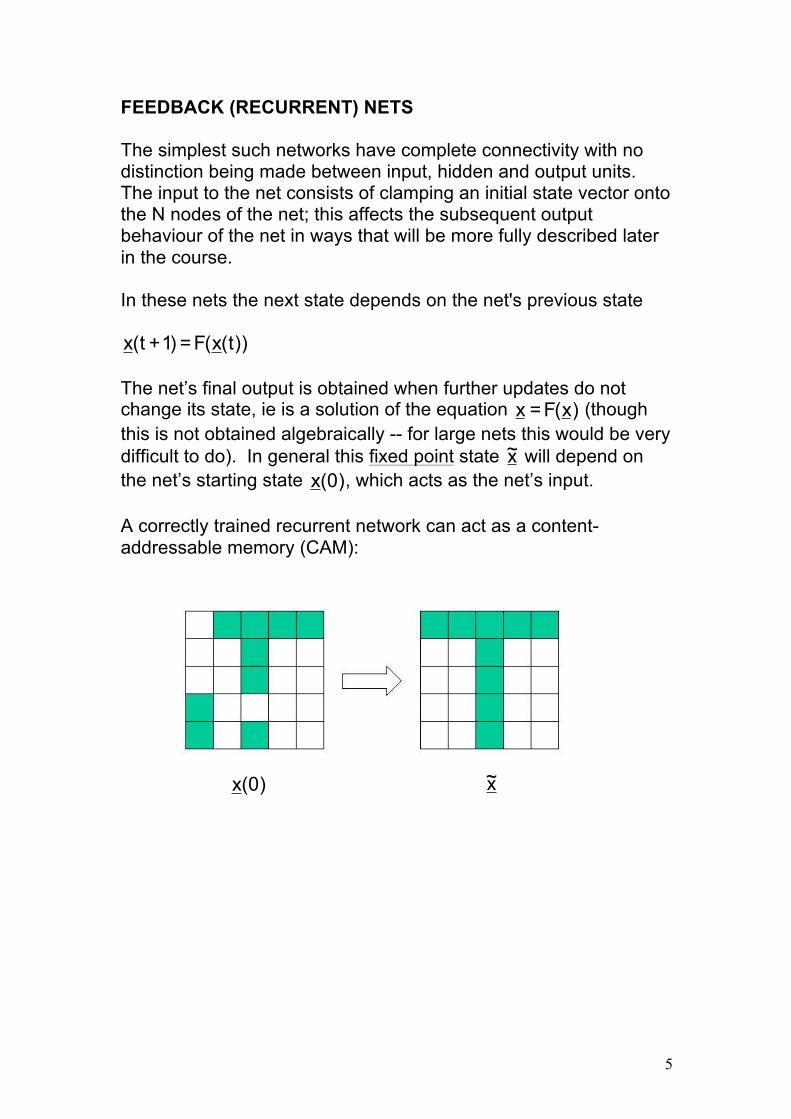
FEEDBACK (RECURRENT) NETS The simplest such networks have complete connectivity with no distinction being made between input, hidden and output units. The input to the net consists of clamping an initial state vector onto the N nodes of the net; this affects the subsequent output behaviour of the net in ways that will be more fully described later in the course. In these nets the next state depends on the net's previous state

))t(x(F=)1+t(x The net’s final output is obtained when further updates do not change its state, ie is a solution of the equation )x(F=x (though this is not obtained algebraically -- for large nets this would be very difficult to do). In general this fixed point state x~ will depend on the net’s starting state )0(x , which acts as the net’s input. A correctly trained recurrent network can act as a content-addressable memory (CAM): )0(x x~

6

A correctly trained net can generalise. For example in the context of a classification problem The net is trained to associate 'perfect' examples of the letters T and C to target vectors that indicate the letter type; here a target of (1,0) is used for the letter T, (0,1) for the letter C (the first neuron is therefore being required to be a 'T-detector', the second a 'C-detector'). After training, the net should be able to recognise that the pattern below is more T-like than C-like, in other words, neuron 1’s output should be significantly greater than neuron 2’s: Generalisation is fundamental to learning. A net that cannot generalise from its training set to a similar but distinct testing set is of no real use. If a net can generalise, then in some sense it has learned a rule to associate inputs to desired outputs; this 'rule', however, cannot be expressed verbally, and may be hard to deduce from the trained net’s behaviour.

7

APPLICATIONS OF NEUROCOMPUTING Finance: Credit application scoring; financial time series prediction; stock and commodity trading advisory systems; portfolio management. Health care: Medical image interpretation; cell sample classification; prediction of treatment outcomes. Bioinformatics: Prediction of protein structure and function; interpretation of microarray data. Communications: Optimal routing in communications networks; speech and speaker recognition; 'intelligent agents' for information gathering. Security: Face/voice/fingerprint etc ('biometric') recognition; detection of credit card fraud; airport baggage scanner. Robotics: Vision systems; appendage and motion controllers; autonomous guidance systems.

8

The most successful current applications of neural computing generally satisfy the criteria:

• The task is well-defined -- we know precisely what we want (eg to classify on-camera images of faces into 'employee' or 'intruder'; to predict future values of exchange rates based on past values).

• There is a sufficient amount of data available to train the net

to acquire a useful function based on what it should have done in these past examples.

• The problem is not of the type for which a rule base could be

constructed, and which therefore could more easily be solved using a symbolic AI approach.

There are many situations in business and finance which satisfy these criteria, and this area is probably the one in which neural networks have been used most widely so far, and with a great deal of success.

9

Example: Detecting credit card fraud Neural networks have been used for a number of years to identify spending patterns that might indicate a stolen credit card, both here and in the US. The network scans for patterns of card usage that differ in a significant way from what might have been expected for that customer based on their past use of their card -- someone who had only used their card rarely who then appeared to be on a day’s spending spree of £1000s would trigger an alert in the system leading to the de-authorisation of that card. (Obviously this could sometimes happen to an innocent customer too. The system needs to be set up in such a way as to minimise such false positives, but these can never be totally avoided.) The neural network system used at Mellon Bank, Delaware had paid for itself within 6 months of installation, and in 2003 was daily monitoring 1.2 million accounts. The report quoted here from Barclays Bank states that after the installation of their Falcon Fraud Manager neural network system in 1997, credit card frauds fell by 30% between then and 2003; the bank attributed this fall mainly to the new system.

10

Example: Predicting cash machine usage Banks want to keep cash machines filled, to keep their customers happy, but not to overfill them. Different cash machines will get different amounts of use, and a neural network can look at patterns of past withdrawals in order to decide how often, and with how much cash, a given machine should be refilled. Siemens developed a very successful neural network system for this task; in benchmark tests in 2004 it easily outperformed all its rival (including non-neural) predictor systems, and, as reported below, could gain a bank very significant additional profit from funds that would otherwise be tied up in cash machines.

11

THE BIOLOGICAL PROTOTYPE

The effects of presynaptic ('input') neurons are summed at the axon hillock. Some of these effects are excitatory (making the neuron more likely to become active itself), some are inhibitory (making the neuron receiving the signal less likely to be active).

12

A neuron is a decision unit. It fires (transmits an electrical signal down its axon which travels without decrement to the dentritic trees of other neurons) if the electrical potential V at the axon hillock exceeds a threshold value Vcrit of about 15mV.

MCCULLOUGH-PITTS MODEL (binary decision neuron (BDN)) This early neural model (dating back in its original form to 1943) has been extremely influential both in biological neural modelling and in artifical neural networks. Although nowadays neurologists work with much more elaborate neural models, most artificial neural network processing units are still very strongly based on the McCullough-Pitts BDN. The neuron has n binary inputs }1,0{xj∈ and a binary output y:

'ON' 1= 'OFF ' 0=y ,x j

↔↔

13

Each input signal jx is multiplied by a weight jw which is effectively the synaptic strength in this model.

0<w j ↔ input j has an inhibitory effect ↔ 0>w j input j has an excitatory effect

The weighted signals are summed, and this sum is then compared to a threshold s:

!

y = 0 if w jx jj=1

n

" # s

!

y = 1 if w jx jj=1

n

" > s

This can equivalently be written as

!

y = " wjx jj=1

n

# - s$

% & &

'

( ) )

where ( ) xθ is the step (or Heaviside) function It can also be useful to write this as ( ) aθ=y with the activation a defined as

!

a = wjx jj=1

n

" - s

as this separates the roles of the BDN activation function (whose linear form is still shared by almost all common neural network models) and the firing function θ(a), the step form of which has since been replaced by an alternative, smoother form in more computationally powerful modern neural network models.

14

If the weights and thresholds are set appropriately BDNs can be made to perform logical functions Example: AND function 21 xx ∧ A possible choice of parameters is 1.0 = s 1.0, = w= w 21 x1 x2 a y=θ(a) 0 0 -1.0 0 0 1 0.0 0 1 0 0.0 0 1 1 1.0 1 Example: OR function 21 xx ∨ A possible choice of parameters is 0.0 = s 1.0, = w= w 21 x1 x2 a y=θ(a) 0 0 0.0 0 0 1 1.0 1 1 0 1.0 1 1 1 2.0 1 A NET OF BDNs CAN PERFORM ANY LOGICAL FUNCTION (McCullough and Pitts, 1943)

15

In fact it can be shown that a 2-layer feedforward BDN net can do this, based on results you will be familiar with from digital circuit theory (the use of first canonical, or 'sum of products' form). A Boolean function of n variables n1 x...x can be specified by a truth table with 2n entries eg XOR (n=2)

x1 x2 y 0 0 0 0 1 1 1 0 1 1 1 0

To obtain a circuit to implement this function, for each entry

)x,...,x,x( n21 in the truth table that has a '1' as its desired output, form the product expression

)x(f...)x(f)x(f n21 ∧∧∧ where

f(x)=x if x=1, f(x)=1-x (written here as x ) if x=0 In the XOR example, the lines for which a '1' output is required are the 2nd (input (0,1)) and 3rd (input 1,0)), and these respectively contribute 21 xx ∧ , 21 xx ∧ . Then for each such entry, construct a BDN node that implements this product function, combining the output of these via an OR gate BDN in layer 2.

16

The only possible difficulty here is working out weights that will allow the relevant n-input product functions and m-input (assuming there are m lines of the truth table for which a '1' is required) OR function to be performed by a BDN. There is an easy prescription for the weights and thresholds that can be used to replace a time-consuming 'trial-and-error' method, though it’s important to realise that this provides a solution to the problem, not the solution (as in, say, solving a quadratic equation) -- because of the use of the θ-function as output function there are in fact an infinite number of equivalent solutions, weight/threshold sets that would allow a net to carry out a given Boolean function. Layer 1 Suppose as above that there are m lines of the function truth table for which a '1' is required, for which the jth needs to implement the product function )x(f...)x(f)x(f n21 ∧∧∧ . A weight setting that will work is

kk

kkjk x=)f(x if 1-

x=)f(x if 1{ = w , k=1..n

A suitable threshold setting can be given by

}x=)f(x whichfor j unit to k inputs of {number - ½- n = s kkj

17

For example in the XOR case, for the first of the two layer 1 units, which is required to carry out the function 21 xx ∧ , this gives w11 = -1 (because input 1 is complemented) w12 = 1 (because input 2 is not complemented) s1 = 2 – ½ – 1 = ½ (because there is just one complemented input to this unit) Check:

x1 x2 w11x1 + w12x2 – s1 output y2 0 0 -½ 0 0 1 ½ 1 1 0 2

3- 0 1 1 -½ 0

The function correctly only gives output 1 when x1=0 and x2=1.

18

Layer 2 Supposing again that there are m lines in the function truth table for which a '1' output is required, an m-input OR function is needed in this 2nd layer so that the overall output will be '1' if any one of the input product conditions is satisfied. A weight and threshold choice which will achieve this is

1..mi ,1wi == ½s =

Checking that this works in the XOR case for the output neuron (m=2):

x1 x2 y1 y2 w1y1 + w2y2 – s final output y 0 1

0 1

0 0 -½ 0

1 0 0 1 ½ 1 0 1 1 0 ½ 1 - - 1 1 2

3 1

The output layer function is 2-input OR, as required.

(Note that the condition y1= y2 = 1 is never in fact encountered as the first layer construction ensures that no more than one neuron in Layer 1 can have a '1' as output.)

19

So what’s wrong with this as a solution for the problem of how to fix the variable parameters in a neural net?

• Not all problems are binary! Classification problems can be assigned binary targets, but what about problems in financial time series prediction, for example?

• The procedure for constructing nets according to the rules

above is potentially very costly -- it only gives a solution, not necessarily the most efficient solution. (You will be familiar with this from digital circuit theory, where circuits derived from a first canonical form construction usually have to be simplied by the use of techniques like Karnaugh maps to reduce the number of gates used.)

For a Boolean function of n variables the average number of BDNs required by the above prescription is given by <# BDNs> = <# layer 1 nodes> + 1 ½ x 2n (assuming (OR gate in layer 2) half the lines of the function-defining truth table require a ‘1’ as output) eg if n=100 (10x10 binary image) <#BDNs> > 1030 >> total world computer memory!

Thus this 'universal architecture' is not of much practical use, even for binary problems. Few neural nets rely on this kind of direct, calculation-based, setting of weights and thresholds (the Hopfield net, which will be discussed later in the course, is one of the few that does). Most require the net to learn the parameters necessary to implement a particular mapping.

20

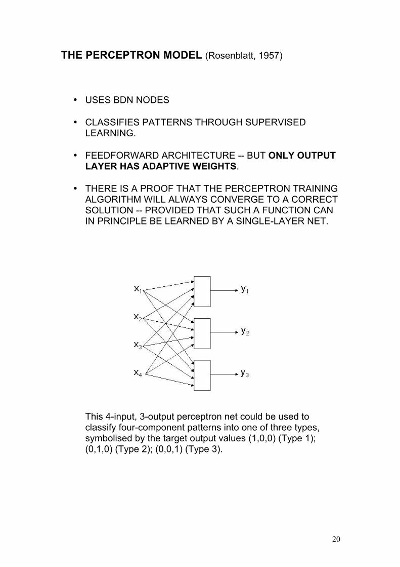
THE PERCEPTRON MODEL (Rosenblatt, 1957)

• USES BDN NODES • CLASSIFIES PATTERNS THROUGH SUPERVISED

LEARNING. • FEEDFORWARD ARCHITECTURE -- BUT ONLY OUTPUT

LAYER HAS ADAPTIVE WEIGHTS. • THERE IS A PROOF THAT THE PERCEPTRON TRAINING

ALGORITHM WILL ALWAYS CONVERGE TO A CORRECT SOLUTION -- PROVIDED THAT SUCH A FUNCTION CAN IN PRINCIPLE BE LEARNED BY A SINGLE-LAYER NET.

This 4-input, 3-output perceptron net could be used to classify four-component patterns into one of three types, symbolised by the target output values (1,0,0) (Type 1); (0,1,0) (Type 2); (0,0,1) (Type 3).

21

Perceptron processing unit This is essentially a binary decision neuron (BDN), in which the threshold for each neuron is treated as an extra weight w0 from an imagined unit, the bias unit, that is always 'on' (x0=1):

!

y = " w jx jj=1

n

# - s$

% & &

'

( ) ) = " wjx j

j=0

n

#$

% & &

'

( ) ) if w0 = -s

This notational change from the McCullough-Pitts BDN formulation was made for two reasons:

1. To emphasise that in the perceptron, threshold values are adaptive, unlike those of biological neurons, which correspond to a fixed voltage level that has to be exceeded before a neuron can fire. Using a notation that represents the effect of the threshold as that of another weight highlights this difference.

2. For compactness of expression in the learning rules -- we do

not now need two separate rules, one for the weights 1..nj ,wΔ j = and one for the adaptive threshold sΔ , just one

for this extended set of weights 0..nj ,wΔ j = .

Perceptron learning algorithm Each of the i=1..N n-input (in the example on the previous page N=3, n=4) BDNs in the net is required to map one set of input vectors n}1,0{∈ (CLASS A) to 1, and another set (CLASS B) to 0:

Bx if 0Ax if 1

{=tp

pp,i ∈

∈

p,it is the desired response for neuron i to input pattern px .

The learning rule is supervised because p,it is known for all patterns p = 1..P (where P is the total number of patterns in the training set).

22

Outline of the algorithm:

• initialise: for each node i in the net, set ijw , j=0..n to their initial values.

• repeat

for p =1 to P

o load pattern px , and note desired outputs p,it .

o calculate node outputs for this pattern according to

!

yi,p = " wijx j,pj=0

n

#$

% & &

'

( ) )

o adapt weights

p,jp,ip,iijij x)y-t(ηww +→ until (error = 0) or (max epochs reached) Notes

• Using this procedure, any ijw can change its value from positive (excitatory) to negative (inhibitory), regardless of the origin of the input signal with which this weight is associated. This cannot happen in biological neural nets, where a neuron’s chemical signal (neurotransmitter) is either of an excitatory or inhibitory type, so that, say, if j is an excitatory neuron, all ijw must be 'excitatory synaptic weights' (in the BDN formulation, greater than 0). However this restriction, known as Dale’s Law, is an instance where it would not be desirable to follow the guidelines of biology too closely -- the restriction has no innate value, it is just an artifact of how real neurons work and its introduction would only reduce the flexibility of artifical neural networks.

23

• Small initial values for the weights, both positive and negative -- for example in the interval ]1.0,1.0[ +− -- give the smoothest convergence to a solution, but in fact for this type of net any initial set will eventually reach a solution -- if one is possible.

• The weight-change rule ijijij wΔww +→ , where

p,jp,ip,iij x)y-t(η=wΔ is known as the Widrow-Hoff delta rule (Bernard Widrow was another early pioneer of neural computing, marketing a rival system to Rosenblatt’s perceptron known as the 'Adeline' or 'Madeline'.)

• A single epoch is a complete presentation of all P patterns,

together with any weight updates necessary (ie everything between 'repeat' and 'until').

• η (always positive) is the training rate. The original

perceptron algorithm used η=1. Smaller values make for smoother convergence, but as with the case of starting weight values above, no choice will actually cause the net to fail unless the problem is fundamentally insoluble by a perceptron net. (This kind of robustness is NOT typical of neural network training algorithms in general!)

Error function This is usually defined by the mean squared error

!

E =1

PN (ti,p - yi,p )2

i=1

N

"p=1

P

"

(where P is the number of training patterns, N the number of output nodes) or the root mean squared (rms) error E=Erms Of these the rms error is the one most frequently used as it gives some feel for the 'average difference' between desired and actual outputs. The mean squared error itself can be rather deceiving as this sum of squared-fractional values can appear to have fallen very significantly with epoch even though the net has some substantial amount of learning still to do.

24

Training curve This is a very useful visual aid to gauging the progress of the learning process. It shows the variation of error E with epoch t: A smaller value of η gives slower but smoother convergence of E; a larger training rate give a faster but more erratic (ie not reducing E at each epoch) convergence. (Though this last doesn’t -- for this model -- affect the ability of the net to find a solution if one exists, it is good practice to avoid erratic training behaviour even here, as for other neural network models such behaviour is usually damaging.) A simple task for a single-layer perceptron might be to distinguish those 3-bit input vectors with a majority of 0’s from those with a majority of 1’s: input desired pattern output

CLASS A (majority 0, target 1) CLASS B (majority 1, target 0)

1x 2x 3x y 0 0 0 1 0 0 1 1 0 1 0 1 0 1 1 0 1 0 0 1 1 0 1 0 1 1 0 0 1 1 1 0

25

Error 0.30

training curve with η=0.01 0.20 0.10 0.00 0 5 10 Epoch Perceptron architectures A variety of network topologies were used in perceptron studies in the 1950s and 1960s. Not all of these were of the simple single-layer type -- there could be one or more preprocessing layers, usually randomly connected to the input grid, though the perceptron learning algorithm was only able to adapt the weights of the neurons in the output layer, the neurons in the added preprocessing layers having their weights as well as their connections chosen randomly. These extra layers were added because it was observed that quite frequently a single-layer net just couldn’t learn to solve a problem, even after many thousands of epochs had elapsed, but that adding a randomly connected 'hidden' layer sometimes allowed a solution to be found.

26

2-layer perceptron character classifier However it wasn’t fully appreciated that it was the restriction to a single learning layer that was the fundamental reason for the failures, or that the trial-and-error connection of a preprocessing layer, reconnecting if learning still failed, was in effect a primitive form of training for this hidden layer (a random search in connection and weight space).

27

GEOMETRY OF PERCEPTRON CLASSIFICATION For a general 2-input BDN

!

y = "( wjx jj=0

2

# )

though for this analysis it’s convenient to go back to the use of a threshold rather than a bias weight, and write the expression for the output in ‘McCullough-Pitts’ style as

( ) 02211 w- = s ,s - xw + xwθ = y There are four possible input patterns: (0 0), (0 1), (1 0), (1 1). These can be represented as the vertices of a unit square: Suppose the patterns are to be divided into two classes: CLASS A: s > xw+xw 1=y 2211⇒ CLASS B:

!

y = 0 " w1x1 + w2x2 # s

28

Consider the example 21 x OR x=y for which the two pattern classes are A = { (0,1), (1,0), (1,1) } B = { (0,0) } The line s = xw+xw 2211 or equivalently

121

22 x

ww

- ws

= x

divides the plane into two regions, one of which contains the 'class A' vertices, one the 'class B' vertices.

29

The classification of higher-dimensional vectors can be visualised by analogy to the 2-dimensional case. For an n-input perceptron unit the input patterns occupy the vertices of the n-dimensional hypercube [0,1]n. Pattern separation is achieved by means of an (n-1)-dimensional hyperplane w1x1+...+wnxn = s. Example: for the 3-bit classifier of p.24 A = { (0,0,0), (0,0,1), (0,1,0), (1,0,0) } B = { (1,1,1), (1,1,0), (1,0,1), (0,1,1) } and the pattern separation after training, with the weights then acquired, looks in 3D like

30

The general geometrical picture of perceptron training (for 2-component input patterns) is that the initial weights define a line positioned at random in the 2D pattern space, and then the position of this class-separating line is gradually adjusted as training changes w1, w2 and s: (In this OR-function example, correct classification would have been achieved in four epochs.) The Perceptron Convergence Theorem (see for example the discussion in Beale and Jackson) states that the above process will always eventually converge to a solution which correctly partitions the pattern space, but only if such a partition is theoretically possible -- which unfortunately isn’t always true.

31

LIMITATIONS OF PERCEPTRONS (Minsky and Papert, 1969) There are some desired pattern classifications for which the perceptron training algorithm fails to converge to zero error. The root of the problem can be seen in the simplest such example, the XOR problem (2-bit 'not-parity'), defined by the truth table The desired pattern separation is thus It is clear no line can be drawn on the plane that will achieve this. LINEAR SEPARABILITY The only functions that can be represented by a single layer net (and thus learned by a perceptron) are those for which the 'A' and 'B' class input vectors can be separated by a line (more generally a hyperplane in the n-dimensional input space). Such functions are referred to as linearly separable. But is this a real problem? What proportion of functions are not linearly separable? If that number is small, we are OK...

1x 2x y 0 0 0 0 1 1 1 0 1 1 1 0

32

A processing unit with n binary inputs can have n2 different input patterns. Because each such pattern can independently be assigned the output value 0 or 1 there are thus

n22 distinct Boolean functions of n variables. For example, if n=2 there are

222 =16 different functions, of which only two (XOR and XNOR) are not linearly separable. This looks OK; it’s only just over 10%. However, as n increases the proportion of linearly separable functions (ie those which could be learned by an n-input perceptron) becomes vanishingly small:

n n22 Number of linearly separable functions

Proportion of linearly separable functions

1 4 4 1 2 16 14 0.88 3 256 104 0.41 4 65,336 1,882 0.03 5 ~4.3x109 94,572 ~2.2x10-5 6 ~1.8x1019 5,028,134 ~2.8x10-13

So there is a problem; for even modest values of n only a vanishingly small number of Boolean functions can be learned by a perceptron. It’s not surprising therefore that Rosenblatt’s group frequently encountered difficulties when using their perceptron nets for image recognition problems. However, remember that they were able to partly overcome these difficulties with a trial-and-error training method that involved a 'preprocessing layer'. It’s the use of such an additional layer -- but with weights acquired by something more efficient than random search -- that underpins modern 'multilayer perceptron' nets, which are not subject to the learning restrictions of Rosenblatt’s day.

33

Overcoming the linear separability restriction using multiple layers You have already seen a proof that all Boolean functions can be performed by a 2-layer BDN net. For example, XOR can be realised by the net below where the required functions 21 xx ∧ , 21 xx ∧ , and 21 yy ∧ can all be performed by BDNs. ( Using the weight-setting rule of pp.16-18: ( ) -x+x- θ=y 2

1211

( ) -x- xθ=y 21

212 y3 = ! y1 + y2- 1

2 ( ) )

Geometrically this corresponds to the 'OR'ing of two separate regions, each of which can be isolated by a single line, to form a new region for which y=1:

34

Any n-input boolean function can be realised in a similar way, by 'OR'ing disjoint regions in the space [0,1]n for which the desired output is 1, and for each of which there exists some BDN function

of the general form

!

y = "( wijx j )j=0

n

# .

However, it was made clear in the earlier discussion that although this is a proof-of-concept that 2-layer nets have the power to represent non-linearly separable functions, it does not constitute a viable method of generating such nets for applications, as the architectures resulting from the application of the weight-setting rule of pp.16-18 are frequently unrealistically over-sized. (Also, of course, the construction works only for problems which have binary target values -- and self-evidently not all problems are of this type.)

35

We need multilayer nets that can

• learn appropriate weight values in an efficient way • produce non-binary outputs (for applications such as time

series prediction which do not naturally fall into the class of Boolean problems)

MULTILAYER PERCEPTRON (MLP) The MLP, trained usually using the method of error backpropagation (to be discussed in detail later), was independently introduced in the mid-1980s by a number of workers (Werbos (1974); Parker (1982); Rumelhart and Hinton (1986)) and is still by far the most widely used of all neural network types for applications in classification, prediction and control. In the MLP network the BDN’s step function output is 'softened':

!

yi = f( wijx j )j=0

n

" where ]1,0[→R:f n not into {0,1}

This modified output function must:

• be continuous • be differentiable • be non-decreasing • have bounded range (normally the interval [0,1])

36

The most commonly used such function is the sigmoid

x-e+11

=)x(f

The sigmoid is the 'squashing' function that is most often chosen because

• its output range [0,1] can be interpreted as a neural firing probability or firing rate, should that in certain applications be required

• it has an especially simple derivative

which is useful as this quantity needs to be calculated often during the error backpropagation training process.

) f(x)-1 )(x(f = )e+1(

e =))x(f(

dxd

)x(f ′ 2x-

x-≡

37

Backpropagation training process for MLPs With a continuous and differentiable output function like the sigmoid above, it is possible to discover how small changes to the weights in the hidden layer(s) affect the behaviour of the units in the output layer, and to update the weights of all neurons so as to improve performance. The error backpropagation process is based on the concept of gradient descent of the error-weight surface. The error-weight surface can be imagined as a highly complex landscape with hills, valleys etc, but with as many dimensions as there are free parameters (weights) in the network. The height of the surface is the error at that point, for that particular set of weight values. Obviously, the objective is to move around on this surface (ie change the weights) so as to reach its overall lowest point, where the error is a minimum. This idea of moving around on the error-weight surface, according to some algorithmic procedure which moves one -- hopefully -- in the direction of lower errors, is intrinsic to the geometrical view of training a neural network. Gradient descent is the process whereby each step of training is chosen so as to take the steepest downhill direction in the (mean squared) error.

38

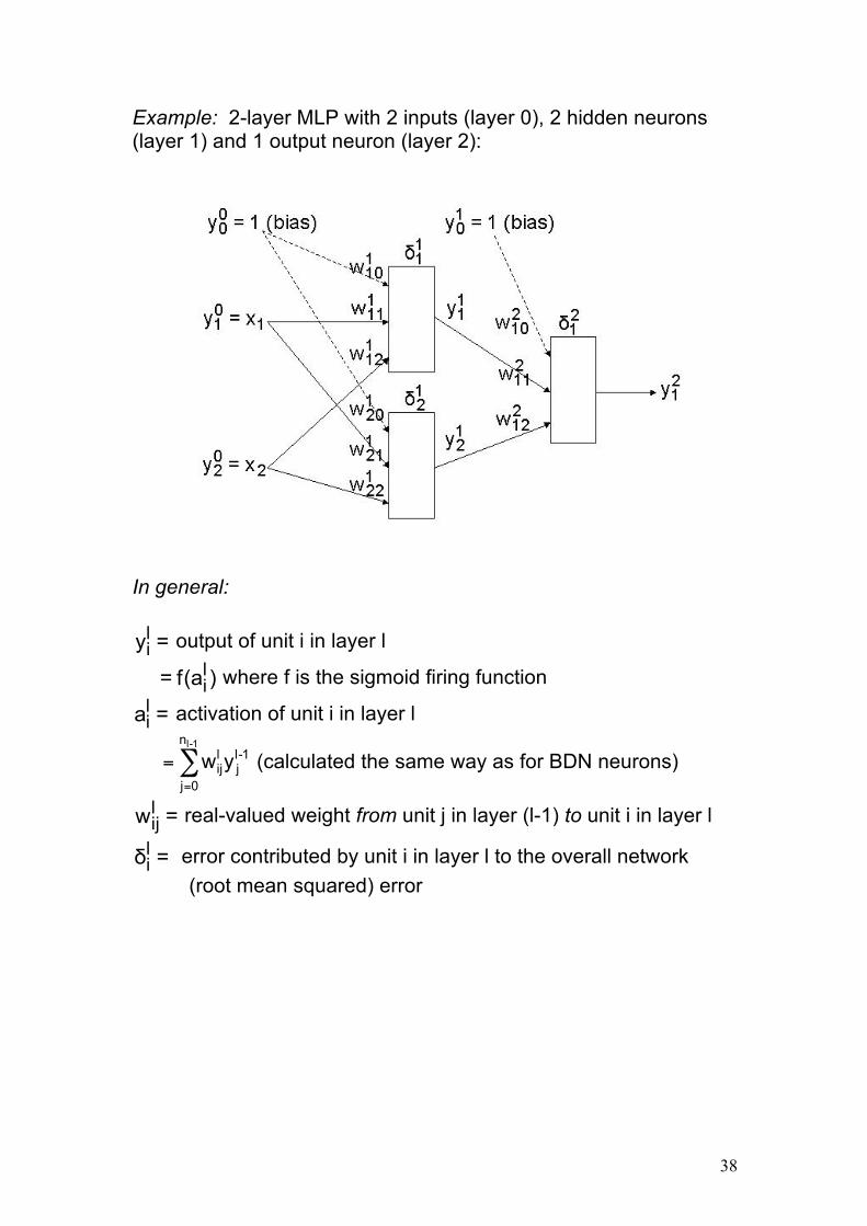
Example: 2-layer MLP with 2 inputs (layer 0), 2 hidden neurons (layer 1) and 1 output neuron (layer 2): In general: =yli output of unit i in layer l

)a(f= li where f is the sigmoid firing function

=ali activation of unit i in layer l

!

= wijl y j

l-1

j=0

nl-1

" (calculated the same way as for BDN neurons)

=wlij real-valued weight from unit j in layer (l-1) to unit i in layer l

=δli error contributed by unit i in layer l to the overall network (root mean squared) error

39

The weight-change rule for multilayer networks, considering the change to the jth input weight of the ith neuron in layer l, takes the form

1-lj

li

lij yηδ=wΔ

The above rule for multilayer nets is sometimes known as the generalised delta rule, because of the formal similarity between it and the Widrow-Hoff delta rule used for the single-layer perceptron. The essential difference, however, is how the error contribution for neuron i, l

iδ , is now calculated. It can be proved that using the principle of gradient descent that the forms this takes for the output layer (layer l=L) and hidden layers (layers l<L) are Layer l=L (where target values it for the outputs are known):

)a(f ′)y-t(=δ Li

Lii

Li

Hidden layers l<L:

!

" jl = [ "i

l+1wijl+1

i=1

nl+1

# ] $ f (ajl )

(In this case the error contributed by neuron j in layer l is proportional to the sum of the errors associated with the units in layer l+1 above that j feeds its outputs into, which seems intuitively reasonable.)

40

Outline of error backpropagation algorithm

• initialise: for each node in the net, set lijw , j=0..nl-1 to small

random values. • repeat

for p =1 to P

o load pattern px into layer 0 ( p0 x=y )

o forward pass -- calculate node outputs

for l=1 to L for i=1 to nl

!

yil = f( wij

l y jl-1)

j=0

nl-1

"

o backward pass -- adapt weights

for l=L down to 1 for i=1 to nl for j=0 to nl-1

1-lj

li

lij

lij yηδ+w=w

until (Erms < ε ) or (max epochs reached)

41

Notes

• Setting initial weights to small random values is important for MLP learning: large and/or very similar starting values impede learning. The MLP, although it is more powerful than the single layer perceptron, does not come with a guarantee of success; although it’s theoretically possible that a given net can learn to perform a particular function, in practice this may be prevented by a number of factors such as starting weight values or an over-large training rate (which causes the net not to even approximately follow the desired gradient descent path, theoretically only followed when η is infinitesimally small).

• How many layers and/or units do you use? It’s not

normally necessary to use more than one hidden layer, because there is a universal approximation theorem that says that any reasonable function can be learned by a two-layer net. But note the phase 'a two-layer net' -- this does not tell the user how many hidden neurons are needed for a given problem! Despite a lot of theoretical work, trial and error (with some consideration given to the 'overtraining' problem to be discussed later) is actually still the best way to determine this.

• Use of 'target error' ε: With MLP learning, unlike the case

of the single layer perceptron, it is not reasonable to expect the error to drop to exactly zero, partly because the use of the sigmoid function prevents output neurons (for any finite weight values) ever exactly reaching binary targets 0,1, and partly because problems to which the MLP is applied are usually intrinsically difficult. Also, it may not be desirable in any case to continue training until the training data error is as low as possible -- overtraining may well be a problem, and early stopping of the training process therefore advisable.

• Use of 'max epochs': If a problem’s level of difficulty is not

at first appreciated, it is easy to give the net a too-simple architecture (not enough hidden units) so that the anticipated target error cannot ever be reached; the 'max epochs' limit stops the training carrying on for an unreasonable length of time in this case.

42

PROBLEMS THAT CAN OCCUR WHEN TRAINING A MULTILAYER PERCEPTRON 1. Trapping in local minima Sometimes when training an MLP the final error reached is considerably higher than one might have expected. This can either be because the difficulty of the problem had been underestimated, or possibly be because the net had become trapped in a less-than-optimal solution known as a local minimum of the error function. The error-weight surface is usually very high-dimensional, potentially very complex, and can contain 'traps' for a net whose learning is based on gradient descent. The basic principle of gradient descent is to continue to go downhill until the surface seems flat -- but although this would be true at the lowest overall error position, the global minimum, it might also be true at some higher error positions, as illustrated schematically below: Where the net ends up is unavoidably a function of what part of the error-weight surface it starts off in; the set of initial positions leading to a particular final set of weights is referred to as the basin of attraction of that final position. There is no known way of ensuring that the net starts in the basin of attraction of the global minimum, it really is all down to chance! If a local minimum is suspected the best policy is to re-start the net with a different set of weights -- if it was a local minimum the first time, chances are that the net will do better, but if the problem is simply unexpectedly hard, the final error this second time will be very similar to the first.

43

2. Overtraining Realistic problems contain 'noise', which is variation in the input values that is not in any way related to the solution of the problem the net is being applied to. An example might be the background lighting level in photographs of individuals used as a face recognition training data set. In particular all applications to financial data can be expected to contain a lot of noise, so much so that in the past some theoreticians believed that the movements of the financial markets were, despite the apparently law-like behaviour that can be seen over short time scales, fundamentally unpredictable (this is known as ‘the strong form of the Efficient Markets Hypothesis’). When a problem contains a lot of noise there is a risk that if the net has sufficient spare weight parameters (typically, if it contains more hidden units than the problem really needs), that these unnecessary weights will 'memorise' the noise in the training data. Since this noise is by definition something random, not something related in a law-like way to the training targets, its form will not be shared by any future data the net is exposed to, and in the absence of the noise features that it now, wrongly, ‘expects’, the net will perform badly, leading to a loss of generalisation ability. As previously emphasised generalisation is fundamental to true learning; without it we have only created a look-up table of values, which could be done more easily (though still pointlessly) by storing the input-output training pairs in a file or database.

Overtraining may most easily be avoided by the use of a training test set (sometimes also known as a verification set). This is a subset of the available training data (about 20% of it is a good proportion to pick) which can be used during the training process for continuous testing.

44

At the end of each epoch of training the net is shown the training test set data and a forward pass only done on this, to evaluate, for that epoch, the rms error for this data set as well as for the training set. The shapes of the error curves for both the training and training test set data are monitored; when that for the training test set begins to rise (even though the error for the training set itself may still be decreasing) it is time to stop training as it is likely now that the net is improving on the training set by memorising the noise features it contains. One thing to note is that a strict approach to neural network training -- not always followed -- would also demand a third set of data, a true test set, to be used only when the net has been trained to completion (with possible ‘early stopping’ when the training test set error starts to rise). The argument is that the training test set, although it wasn’t used in an obvious way to guide the weight changes, was used in a subtle way because it determined when the training process should end. A true test set should ideally not be used in any way whatsoever to affect the training process. Which is more important in practice, trapping in local minima or overtraining? In most applications -- as mentioned above, especially in the noise-riddled area of finance -- I would say almost always overtraining. (In one example a financial problem allowed training only for 2 or 3 epochs before overtraining set in -- clearly in a case like this there is little chance of reaching any error minimum, either global or local!)

45

THE HOPFIELD NETWORK Recurrent networks Feedforward nets, such as the MLP, are always stable; they never enter a mode in which the output is continuously, unusably changing. However their range of behaviours is limited. The output of a recurrent N-node net at time t,

))t(x),...,t(x),t(x(=)t(x N21 is not only a function of any external inputs (in fact in most cases there are no external inputs in the usual sense), but of its own state at the previous time, )1-t(x . The input is continuously modified by the previous output

) )t(x (F = )1+t(x A stable network will eventually reach a condition in which the recirculated output no longer changes the network state. Such a system is said to have reached a fixed point x~ , given as an implicit function of the network parameters by the equation

) x~ (F =x~ It’s important to note that x~ will in general be also a function of the initial state )0(x -- in fact it is this initial state alone which in these nets usually plays the role of an 'input.' There are other possible limiting behaviours for recurrent nets, such as cyclic behaviour, for example the 2-cycle

,...x=)1+t(x ,x=)t(x ,x=)1-t(x... )1()2()1( Recurrent nets whose neurons have continuous, as opposed to discrete-valued, outputs may also display chaotic behaviour, where the net moves essentially unpredictably from state to state. Predicting which networks would be stable was difficult, and so for a long time researchers ignored recurrent nets in favour of feedforward ones.

46

However in 1982 John Hopfield, a statistical physicist, showed that symmetrically connected BDN-type nets

1..N=ji, ,w=w jiij with no self-feedback

1..N=i ,0=wii were indeed stable in the sense of reaching only fixed points ('1-cycles'). In fact such nets could have many such (locally) stable fixed points, each of which might be considered to be a stored pattern. In order that these nets could be useful in practical applications it was necessary to be able to choose which points would be stable, and Hopfield also succeeded in providing a storage prescription which would allow the fixed points to correspond to a particular set of stored patterns )P()2()1( x..., ,x ,x . Content-addressable memory (CAM) The Hopfield net additionally has the property that if the system is started in a statex sufficiently close to one of these locally stable fixed points, say )p(x (such that δ+x=x )p( ), it will evolve in time until )p(x ≈ x .

The initial state is the input, the final (fixed point) state is the output.

The following quotation from Hopfield’s 1982 paper gives an idea of what he wanted to achieve:

Suppose that an item stored in memory is "H.A. Kramers & G.H. Wannier, Phys. Rev. 60, 252 (1941)." A general content-addressable memory would be capable of retrieving this entire memory on the basis of sufficient partial information. The input "& Wannier, (1941)" might suffice. An ideal memory could deal with errors and retrieve this reference even from the input "Vannier, (1941)."

47

In conventional computer technology error correction is usually introduced as software. In neural networks the line between hardware and software disappears. In the Hopfield net content-addressability is an emergent property of the system. The Hopfield energy function The existence of locally stable fixed points in the Hopfield net can be related to the presence of local minima in a so-called (by analogy to similar measures in statistical physics) energy function, H. Like the error surface in the case of the MLP backpropagation algorithm, the Hopfield energy surface is a complicated high-dimensional structure with hills, valleys, etc. This energy function is given by

∑ ∑j < ij ,i i

iijiij xs + xxw- = H

where the first summation is over all pairs (i, j) in the N-node net

such that j<i , a total of )1-N(2N

terms.

Example: N=2

221121 xs + xs + xxw- = H For an N-node net possessing particular values of the iij s ,w there will be an associated complex energy surface whose many local minima ...x ,x )2()1( have positions determined by these weight and threshold values.

48

These local minima correspond to the stable states of the system. Each minimum has its own basin of attraction, a range of input states that will ultimately iterate to that minimum; this defines the CAM property of the system. In order to set up a CAM structure using this type of network we need

1. An update rule ) )t(x (F = )1+t(x that reduces the energy H at each time step (so the 'nearest' local minimum can be reliably entered).

2. A way of ensuring that the local minima of H correspond to

the patterns )P()2()1( x..., ,x ,x we want to store. The update rule Suppose we split the energy function into two parts: iH is the contribution made by the ith node, H′ is the rest:

H′ + H = H i where

!

Hi = -xi wijx j - sij<i"#

$ % %

&

' ( (

49

Now suppose that the ith node changes state from 1ix to 2ix , ie there is a change in state value 1})+ 0, {-1, ( x-x=xΔ 1i2ii ∈ . There is a corresponding change in iH , )x(H-)x(H=HΔ 1ii2iii , given by

!

"Hi = -"xi wijx j - sij<i#$

% & &

'

( ) )

If

!

wijx j - sij<i" = 0 there is no change in iH no matter what new

value 2ix neuron i has chosen. The interesting cases, which allow us to define a useful update rule, are when this quantity is non-zero. There are two such cases to consider

1. If

!

wijx j - sij<i" > 0,

!

"Hi # 0 if "xi $ 0

-- "switch on (go from state 0 to 1) or leave on (stay in state 1)" 2. If

!

wijx j - sij<i" < 0,

!

"Hi # 0 if "xi # 0

-- "switch off (go from state 1 to 0) or leave off (stay in state 0)" Note that in either case the recommended action at least ensures H is not increased by the change to neuron i's state (it can't always decrease, because the aim is to reach local minima which are defined precisely by the fact that the energy can't at these points be any further decreased). So to reduce iH , define a Hopfield firing function h by

!

xi(t + 1) = h( wijx j(t)j<i" # si,xi(t) )

where 0<a ,00=a ,x0>a ,1

=)x,a(h = otherwise ]rule BDN[ )a(θ

0=a if x

50

Note that this is almost the same as the BDN firing function, differing only when the activation a is exactly zero. Because when this is the case iHΔ is always zero no matter what the neuron does, it is a matter of convention what should happen here -- Hopfield chose to say the neuron should stay in its previous state, whatever that was, and this convention will also be used here also. (It's because of this decision about what to do when a=0 that neuron's previous state always has to be recorded, so 'h' is therefore a function of two variables, as given above.) Thus we now have a firing rule that will go downhill in energy wherever possible, and is guaranteed never to increase the total energy H. But note that this construction depended on the assumption that only one neuron had its firing state changed at any time; this is referred to as asynchronous update. Asynchronous update is essential to ensure the downhill-gradient following property of the network update rule, since if more than one neuron was updated at any time this would lead to extra terms in iHΔ of the form

!

- wij"xij<i# "x j

which would not be guaranteed

!

" 0 by any simple firing rule. It is additionally important that the connection matrix is symmetric, since if this isn't true there will be two separate and distinct contributions to iHΔ

!

"Hi = - 12"xi wijx j - si

j<i#$

% & &

'

( ) ) - 1

2"xi wjix j - sij<i#$

% & &

'

( ) )

only the first of which can be guaranteed

!

" 0 by the Hopfield firing rule. The second sum is not over inputs to neuron i but over the destinations of i's output signal; a sum like this can't be linked to a BDN-type rule (or given any sensible neurobiologically-inspired interpretation -- neurons don't 'know' in any direct way where their output signals go to).

51

Given then that it's important to have synchronous update, there is a question as to how the next neuron to have its state updated should be chosen. For example, should the neurons be updated in a fixed pattern (x1 at t, x2 at t+1, x3 at (t+2)...)? It turns out the net has the widest and more flexible range of behaviours if the firing neuron is chosen randomly, with a probability of 1/N for each of the N neurons. So even though the firing rule itself is deterministic, the way the next neuron to fire is chosen introduces an element of indeterminacy into the time-evolution of the Hopfield net. (There are some Hopfield variations where the output of the updated neuron, once picked, is then also generated in a probabilistic way; these types of net -- generally used in optimisation applications, not as CAM memory -- aren't now covered in the course, but you may like to look up 'stochastic Hopfield nets' and 'simulated annealing' if this interests you.) Example: 2-node Hopfield net In this case the energy function is given by

2121 x+x-xx = H Later we will consider ways to set weights and thresholds so that particular states are stored as stable states, but for now will just look at the questions

• How does the energy surface look as a function of the firing states x1, x2?

• What are the fixed points of the system?

52

The shape of the energy surface of any Hopfield net is determined by the values of its weight and threshold parameters. For the current example the (2-dimensional) surface looks like This has roughly the shape of a funnel with the state (1,0) at its lowest point. Going downhill from any of the other three points will ultimately end up in this lowest-energy state (1,0), and since from this point there is no way to further reduce the energy, it will be a stable state (fixed point). The lowest-energy state of a Hopfield net is always a fixed point (but may not be the only such stable state). (Pictures can be helpful in visualisation, but it should be remembered that Hopfield network outputs are actually binary, and thus most of the surface drawn is just an interpolation between the energies of the binary states -- mathematically correct, since the function H can be defined for non-binary values of the xi's, but not corresponding to possible real-life conditions of the network.) Are there any other fixed points? In this case not, but to really understand the dynamics of the network -- which states are stable, which are reachable ('downhill') from others -- it's necessary to draw a state transition diagram rather than attempt a picture of the energy surface (which would be unfeasible anyhow for N>2).

53

State transition diagrams The process of construction starts by writing down the detailed form of the firing rule for each of the neurons of the network, given the you have been supplied with (or -- see later -- have calculated to make a particular state or states stable). In the current 2-node example

) )t(x ,1+)t(x- (h = ) )t(x ,s-)t(wx (h = )1+t(x 121121

) )t(x ,1-)t(x- (h = ) )t(x ,s-)t(wx (h = )1+t(x 212212 Then one works through each of the 2N states of the net, considering for each state what would happen if each of the N neurons were allowed (independently, using asynchronous update) to change its state according to the firing function for that node. Start here, for example, with the state (1,1). The energy of this state is

1=)1(+)1(-)1)(1(=]x+x-xx[ = H 1=x,1=x2121 21

Either neuron 1 or neuron 2 may update its state, with probability ½ in each case. If neuron 1 updates: x1(t+1) = h(-1+1,1) = h(0,1) = 1 )1 ,1(=)1+t(x ⇒ Since the state of neuron 1 is unchanged in this case there is no decrease in energy. If neuron 2 updates: x2(t+1) = h(-1-1,1) = h(-2,1) = 0 )0 ,1(=)1+t(x ⇒ Since neuron 2's new firing state is now 0, and H(1,0) = -1 there is in this case a decrease of 2 energy units.

54

The first part of the state transition diagram -- possible transitions out of (1,1) -- can now be drawn: The arrows from a state point to a possible next state, labelled by the probability of that transition. (By convention if more than one transition from a given start point ends up in the same new state there is just one arrow connecting the states, with a probability label that is the sum of the probabilities of the various ways that one can make the transition.) Doing the same thing for starting states (0,0), (0,1), (1,0) -- recommended as an exercise -- the complete state transition diagram for this 2-node example becomes Notice that the stable state (1,0) is re-entrant with probability 1. Choosing either neuron 1 or neuron 2 to fire (both with probability ½ ) leads back into the same firing state (1,0). In this case there are no other stable states -- all states are in the basin of attraction of (1,0).

55

So far we have seen how to define and visualise an energy surface whose shape depends on the weight and threshold parameters, and how to determine, for a given set of parameters, what the stable states of the system are and which other states are in their basins of attraction. However Hopfield nets would not be useful in CAM applications if there was no way to ensure a particular set of states -- equivalent to the set of prototype patterns to be stored -- was stable. For this we need a method of training the network, or other way to assign appropriate values to the net's parameters. Although there are ways of obtaining parameters for a Hopfield net that are closer to traditional neural network training (ie an iterative, multi-epoch process, with some kind of error measure to be reduced), the simplest and most often used method to determine parameters for a Hopfield net is calculational. The weight setting rule The storage prescription below is the one that was given by Hopfield in his original 1982 paper. It states that to store a set of p=1..P patterns, the weights should be chosen according to

!

wij = (2xi(p) - 1)

p=1

P

" (2x j(p) - 1) i # j

0=wii with -- in this simplest case -- the thresholds si set to zero. Later it will be shown that this latter choice has some disadvantages, and a way to assign useful non-zero values to thresholds will be introduced, but the simple rule above is workable for many applications and allows an easier analysis of the net's properties.

56

Stability of stored patterns The activation of node i in some given state s is given by

!

ai(s) = wijx j

(s)

j<i"

If the above weight-setting rule (with zero thresholds) is used, this can be written as

The right hand side of this can then be split into two parts: a 'signal' part that contains all the references to state s, and a 'noise' part arising from all the other stored patterns. In the 'signal' case (p=s), when 0=x )s(

j ,

0 = )0)(1-( = x)1-x2( )s(j

)s(j

and conversely when 1=x )s(

j

1 = )1)(1+( = x)1-x2( )s(j

)s(j

Since this latter condition occurs roughly half the time this gives rise to a non-zero mean value of around N/2 in this case. In the 'noise' case (p≠s), when 0=x )s(

j ,

!

(2x j(p) - 1)x j

(s) = (+1 or -1)"(0) = 0 for any x j(p)

and when 1=x )s(

j

0=x if 1- = )1(×)-1( = x)1-x2( )p(j

)s(j

)p(j

1=x if 1+ = )1(×)1+( = x)1-x2( )p(j

)s(j

)p(j

and since these two latter situations are equally likely, overall the average contribution from this 'noise' term is zero.

!

ai(s) = (2xi

(p) "1)(2x j(p) "1)x j

(s)

j#

p#

57

Considering these average conditions allows us to define an 'effective field' on neuron i in state s

2N×)1-x2( = >a< )s(

i)s(

i

where it is clear that

if 1=x )s(i , since the RHS is positive, 'i stays on'

and

if 0=x )s(i , since the RHS is negative, 'i stays off'

In other words, provided that the contribution from the noise term can indeed be neglected, the state s is stable. Storage capacity of the Hopfield net The above analysis depended on the assumption that state s could be considered independently of other stable states. However as the number of stored patterns increases interference effects between the patterns begin to affect the network's capacity.

About 0.15N patterns can be stored before error in recall is severe. (Hopfield, 1982)

As more fixed points are added, how quickly do errors become noticeable? Hopfield carried out computer simulations to investigate storage limitations, using sets of randomly chosen patterns. For N=100 he found that with P=5 the stored patterns could almost always be recalled exactly, but with P=15 significant errors were already creeping in -- in this case only about half of the patterns evolved to stable states with less than 5/100 incorrect bits.

58

Given that the total number of binary patterns that can be represented by an N-node binary network is 2N, the value 0.15N -- indeed, any linear function of N -- is disappointingly low. Various ways were tried to squeeze more patterns in as stable fixed points but none did significantly better (in the 'O'-notation sense) than the very simple weight-setting rule above. Although the Hopfield net has been very important in the history of neural computing because it demonstrated that at least some types of network were amenable to rigorous mathematical analysis, it hasn't for this reason been widely used in the type of CAM applications that Hopfield had originally envisaged. There is however a small modification that can be made to the above parameter-setting rule which, though it does not have a major effect on storage capacity for large N, does improve CAM properties for smaller scale problems where a Hopfield net is a workable data storage solution. Using non-zero threshold values The Hopfield storage algorithm has the property that if

)x,...,x,x( N21 is an assigned stable state then its complement )x-1,...,x-1,x-1( N21 is also a fixed point.

For example if (1,0) is a desired stable state, leading to the weight setting 1-=)1-)(1(=)1-0×2)(1-1×2(=w=w 12 , then it can be seen that (0,1) is stable also:

(h(-1×1, 0), 1) = (0,1) updating neuron 1

(0,1)

updating neuron 2 (0, h(-1×0, 1)) = (0,1)

This symmetry is usually undesirable as it wastes the net's limited storage capacity.

59

Automatic storage of complement states can be prevented by the use of bias units and the allocation of non-zero threshold weights. In this case the non-bias weight setting rule is as before but an analogous rule is now also applied to thresholds:

!

si = -wi0 = - (2xi(p) - 1)(2x0

(p) - 1)p=1

P

" = - (2xi(p) - 1)

p=1

P

"

(since the bias unit output )p(0x

is equal to 1 for all patterns p) If the state (1,0) is now stored using this extended rule the weight between neurons 1 and 2 has the same value as before (-1) but now the thresholds are set to

1+=)1-0×2(-=s ,1-=)1-1×2(-=s 21 These settings for the weight and thresholds are the same as were used in the earlier 2-node example, where the resulting net was seen to have only the single stable fixed point (1,0). A last example: store (1,1) in a 2-node net using non-zero thresholds The weight joining neurons 1 and 2 has the assigned value w = (2×1-1)(2×1-1) = 1 and the thresholds are given by s1 = -(2×1-1) = -1, s2 = -(2×1-1) = -1 The Hopfield energy function in this case is H = -x1x2 - x1 - x2 giving energies for the four possible binary states H(0,0) = 0 H(0,1) = H(1,0) = -1 H(1,1) = -3

60

The neuron state update rules are x1(t+1) = h( x2(t)+1, x1(t) ) x2(t+1) = h( x1(t)+1, x2(t) ) giving state transitions ( h(0+1,0), 0 ) = (1,0) (0,0) ( 0, h(0+1,0) ) = (0,1) ( h(1+1,0), 0 ) = (1,1) ( h(0+1,1), 0 ) = (1,0) (0,1) (1,0) ( 0, h(0+1,1) ) = (0,1) ( 1, h(1+1,0) ) = (1,1) ( h(1+1,1), 1 ) = (1,1) (1,1) (stable, as expected & required) ( 1, h(1+1,1) ) = (1,1) and resulting state transition diagram

61

REINFORCEMENT LEARNING In contrast to supervised learning the network receives only a global reward/penalty signal. The weights are changed so as to develop an I/O behaviour that maximises the probability of receiving a reward and minimises that of receiving a penalty. If supervised training is 'learning with a teacher', reinforcement training is 'learning with a critic'. Reinforcement learning acts on the simple principle

If an action gets a good result become more likely to choose the same action under such circumstances. If it gets a bad result become more likely to try an alternative (random) action.

Why use reinforcement as opposed to supervised learning?

• Can be used

o when only a 'quality level' of feedback is available

o where it’s undesirable to be too restrictive as to how the system solves the problem.

• Approximates gradient descent but has stochastic features

that can allow escape from local minima. Reinforcement is currently the least frequently used method of neural network learning. But this reflects its use in much more ambitious AI scenarios, especially in control and robotics, where fully satisfactory solutions are likely waiting on a much better understanding of how the brain handles such tasks.

62

Control and identification Suppose you have two coins and are faced with the problem of maximising the number of heads obtained when tossing the coins over some time interval, given that the coins are not fair. However you don't know which of the coins is more likely to turn up heads. There is a conflict between the need to maximise short-term returns (the number of heads) and to discover, by experimentation, the nature of the bias so as to ultimately do better. This conflict between short-term and long-term gains, or between control of the environment and identification of the problem, is one faced by all systems in interaction with an uncertain environment. The above coin-tossing problem is known as the two-armed bandit problem and is the simplest example of a class of problems involving the sequential allocation of experiments that have both theoretical and practical importance (in the two-armed bandit problem the coins may be replaced by two clinical treatments, the coin tosses by the allocation of these to patients, and 'heads/tails' by their recovery or otherwise). STOCHASTIC LEARNING AUTOMATA These adaptive systems, of which reinforcement-trained neural networks are an instance, represent one approach to the problem of the sequential allocation of experiments, providing rules whereby a system can learn to maximise the reward it receives from an initially unknown and unpredictable environment. The simplest such system consists of a single automaton in interaction with its environment:

63

There are usually just two possibilities for the reinforcement signal r=1 (success), r=0 (failure) This is referred to as the 'P-model'. One can also have graded reinforcement ]1,0[ r∈ ('S-model') but the behaviour of this system is harder to analyse. At each time step the automaton selects one of N actions io with probability ip and (assuming the P-model) is rewarded with a 'success' reinforcement signal r=1 with probability iq , otherwise receiving a 'failure' signal r=0. If the reinforcement }1,0{ r∈ is allocated according to a time-independent rule the environment is said to be stationary, otherwise it is non-stationary. The action probabilities ip must sum to 1

!

pi = 1i=1

N

"

but the environmental reward probabilities iq are not so restricted because they are conditional on the action taken (if the iq do sum to 1 then the problem becomes much easier -- in the two-action case an optimal solution can be discovered without ever taking one of the actions). If the iq are all small failure usually occurs, and strategies learned tend to oscillate between bad solutions. Conversely if the iq are all large it is hard for the system to find the best solution. Learning is easiest when the environment provides feedback that distinguishes clearly between more and less preferred actions.

64

Measuring success for stochastic learning automata The expected probability of success at time t (assuming one trial takes place every discrete timestep, and the environment is stationary so the reward probabilities iq do not depend on time) is given by

!

Mt = qi pi(t)i=1

N

"

where )t(pi is the probability of the automaton choosing action i at time t (clearly unlike the iq these probabilities must depend on time as it is the change in the ip , using some appropriate method, that constitutes learning). A learning automaton is expedient if in the limit ∞→t the average expected reward is greater than that which could be obtained by choosing one of the N actions randomly

!

limt "#

< Mt > > 1N

qii=1

N

$

and optimal if in the limit it always chooses the action with the greatest probability of reward

} q { i

max = >M<

tlim

it∞→

65

Collective behaviour of learning automata A learning automaton faces a more difficult task if in addition to the exogenous uncertainty provided by its environment it also has to deal with endogenous uncertainty associated with the actions of other automata, all of which are also trying to maximise the profit derived from their actions. In a team situation all the automata receive the same reinforcement and have to learn to cooperate to maximise their reward; in a game the reinforcements are different for each automaton and an automaton can increase the reward it receives only by decreasing that given to its neighbours. Neural networks trained by reinforcement learning can be considered as a team as each neuron receives the same reinforcement, that given to the network as a whole as a result of some action. However neural nets do not operate in a void in which their only contact with the outside world is a reinforcement signal for some randomly triggered action -- actions are instead taken in response to an input signal that gives a context for an action.

66

Associative learning automata This is an extension of the basic learning automaton model in which systems are able to 'sense' their environment via an n-component context vector signal x : Associative automata must discover not a single optimal action but a (non-verbal) rule associating context input with optimal actions. Suppose there are K distinct contexts )k(x , k=1..K, each occurring

with probability )k(ξ such that

!

"(k ) = 1k=1

K

# . The earlier performance

measure may in this case be extended to

!

Mt = "(k )

k=1

K

# qi(x(k)

) pi(x(k)

,t)i=1

N

#

where )x(q )k(

i is the (time-independent, since we are still assuming a stationary environment) probability of receiving a reward for action io in context )k(x and )t,x(p )k(

i is the probability of performing that action in context )k(x at time t.

67

The ideal situation would be where in all contexts )k(x the automaton chose with probability 1 the action that maximised the reward probability in that context, ie the action co such that

!

qc(x(k)

) = imax { qi(x

(k)) }

In this case the performance measure would also be maximised and given by

!

Mmax = "(k )

k=1

K

# imax { qi(x

(k)) }

ASSOCIATIVE REWARD-PENALTY (ARP) ALGORITHM This is the simplest and best-known reinforcement learning procedure, developed in the 1980s by Andrew Barto and co-workers. The ARP unit is essentially an MLP neuron with a probabilistic interpretation of its output function:

ia-iii e+1

1=)a(f≡)a|1=y(obPr

where as usual, for an n-input unit with input x , the neuron activation is given by

!

ai = wijx jj=0

n

"

Note that ]1,0[ a(f i ∈) but }1,0{ yi∈ : the probability is real-valued but the neuron output is binary. In the learning theory language used earlier the ARP unit is a two-action (firing/not firing), associative (because the output is dependent on a 'context' signal x ) stochastic (because the output is produced with a specified probability) learning automaton. Behaviour is modified, through the application of a weight-changing rule, upon the receipt of a reinforcement input r. This is

68

usually drawn from the set {0,1} (failure, success) though it is also possible to use real-valued reinforcement ]1,0[ r∈ . It is desired to change the weights so that if r=1 (success) the unit is more likely to do whatever led to the positive reinforcement, whereas if r=0 (failure) the unit becomes more likely to try the other action under the same circumstances (input context x ). This principle may be implemented by the rule jiiiiij x] )r-1))(a(f-y-1(λ + r))a(f-y( [η=wΔ where ]1,0[ λ∈ is an 'exploration' parameter that determines the degree to which the opposite action is encouraged when the system receives a penalty. The rule may be written in the form jiij xηδ=wΔ so that for active pathways )1=x( j the change to ijw is just proportional to

!

-1" #i " +1. How it works There are four situations to consider:

iy r iδ future action in context x

action is...

0 1 )a(f- i more likely to be 0 same 1 1 )a(f-1 i " " " " 1 same 0 0 ))a(f-(1λ i " " " " 1 opposite 1 0 )a(fλ- i " " " " 0 opposite

It can be clearly seen that λ determines the degree to which opposite actions are tried.

69

If λ is too small the system can converge on a solution that seems good but which is not optimal (in effect a local minimum). If λ is too large the system can't home in on any solution unless for this behaviour a reward is always obtained. This situation is unlikely since even a system behaving perfectly may receive penalties due to reinforcement feedback errors. λ implements the trade-off between control (small λ) and identification (large λ) discussed earlier in the more general context of learning automata. The effect of λ on learning performance can be seen in the following example. Example: a single ARP unit (adapted from Barto (1985) to use binary {0,1} rather than bipolar {-1,+1} output values) The environmental reward probabilities iq are tabulated below, for i = 0,1 (actions not firing or firing) and the equiprobable ( )0(ξ = )1(ξ = ½ ) input patterns x1 = 0,1:

x1 )x(q 10 )x(q 11 0 0.6 0.9 1 0.4 0.2

It can be seen that the optimal actions are to fire when x1 = 0 and not fire when x1 = 1. In the former case the unit would then receive a reward with probability 0.9, the latter with probability 0.4. Therefore the maximal performance measure in this task is Mmax = ½ (0.6×0 + 0.9×1) + ½ (0.4×1 + 0.2×0) = 0.65 This is quite low due to the fact that even optimal behaviour in the presence of pattern x1 = 1 is not likely to result in a reward.

70

Barto began the simulation with (w0, w1) = (0, 0). In this case both actions (y=0, y=1) are equiprobable and the initial performance measure is Minit = ½ (0.6×0.5 + 0.9×0.5) `+ ½ (0.4×0.5 + 0.2×0.5) = 0.525 The first figure below shows the results of simulations with learning rate η=0.5 and three values of the penalty parameter λ=0.01, λ=0.05, and λ=0.25. Each point represents the average value of the performance measure Mt for trial t, taken over 100 runs (each run a sequence of 1000 trials). The dashed lines are the theoretical asymptotic performance levels for each value of λ. The second figure shows the way Mt evolves for a single run, with λ=0.05. This curve is much more erratic than the average for the same λ value; it will be discussed later how to try to ensure that weights converge smoothly not just on average but in a given run, which is clearly of practical importance.

From p.237 of A G Barto, "Learning by statistical co-operation of self-interested neuron-like computing elements," Human Neurobiology, 4, 229-256 (1985).

71

It is possible to work out theoretical values for the converged ( ∞→t ) values of w0 and w1 as a function of λ, by setting <Δw0>=<Δw1>=0 (convergence implies no further weight changes are expected) and solving the resulting equations for the final weight values. These converged weight values can then be used to work out the expected limiting value of the performance measure Mt as a function of λ. These curves clearly show the role of λ as an 'exploration parameter' that given too large a value prevents a decisive solution being achieved -- for λ=1 it can be seen that the weights are close to zero, implying not much more than a random choice of action is being made, which is in turn reflected in an Mt value not much greater than the initial value of 0.525.

72

Convergence of the ARP algorithm As was seen in the one-unit example given earlier, the value of Mt for a single run is not very smooth; the weights appear unable to settle down to fixed values even when a good solution has been obtained. To some extent this is a function of , but the effect is present for any 0≠λ : without some adaptation of the basic ARP learning algorithm single runs show only convergence in the mean, as illustrated in the run-averaged figure for the one-unit example. The convergence of the ARP algorithm was investigated by Barto and Anandan in 1985. They showed that in order for the weights to settle down to steady values it is necessary for the training rate η to be decreased in a certain way as training progresses. The full set of conditions that must be satisfied is

1. The context vectors }x,..,x,x{ )K()2()1( form a linearly independent set.

2. Each context vector occurs with non-zero probability

0>ξ )k( for k=1..K

3. The training rate decreases with time in such a way that

(i)

!

"t # 0 for all trials t (ii)

!

"tt# = $

(iii)

!

"t2

t# < $

(the function 55.00

t tη

=η is often used).

4. The penalty probability is non-zero

!

0 < " # 1

Of these conditions the most restrictive, and problematical, is the first, the requirement for a linearly independent set of input vectors.

73

In realistic neural network training situations this is hard to achieve. The compromise is usually to set λ to a small value such as 0.01 -- in that case learning behaviour is fairly smooth even though in theory it is still not convergent. Example: two cooperating ARP units This example from (Barto, 1985) shows how neurons can operate as a 'team' to solve a problem even though the reinforcement given to them is a global signal rather than the more informative individual neuron errors of the error backpropagation method. Only the first unit here receives input from the environment, whilst only the second communicates the output to it, ie the first of the units is acting as a hidden unit. As in the single-unit example the two input patterns x1=0, x1=1 are equiprobable ( )0(ξ = )1(ξ = ½ ) . The environmental reward probabilities iq for i = 0,1 (actions not firing or firing) are in this case given by:

x1 )x(q 10 )x(q 11 0 0.9 0.1 1 0.1 0.9

The system is thus being encouraged to learn the identity function, with the optimal actions being to not fire when x1 = 0 and to fire when x1 = 1.

74

The maximal performance measure is thus in this case Mmax = ½ (0.9×1 + 0.1×0) `+ ½ (0.1×0 + 0.9×1) = 0.90 and the initial value of this measure is given by Minit = ½ (0.9×0.5 + 0.1×0.5) `+ ½ (0.1×0.5 + 0.9×0.5) = 0.50 There are two ways the net can learn to solve the problem: (i) Both units perform the identity function (ii) Both units perform the inverse function The first two pairs of the figures to follow show a network that is learning to develop a solution of type (i) over 500 trials, with

5.1=η and 04.0=λ . The four figures show learning curves for the firing probabilities of each of the units in the presence of each of the input patterns. (Note the erratic behaviour during the first 200 trials -- this is because the figures show only a single run, and the learning rate η is not here being decremented.) The fifth figure from the top shows how the overall performance measure Mt develops, starting from the value Minit = 0.5 and reaching a level (since λ is relatively small) to the theoretical maximum of Mmax = 0.9. The sixth and final figure is a histogram showing how the number of trials taken to reach a level of 98% of Mmax is distributed, for 100 runs. In 45% of the runs the network reached a type (i) solution within a maximum of 1500 trials; in the remaining 55% of cases it reached a solution of type (ii).

75

From p.237 of A G Barto, "Learning by statistical co-operation of self-interested neuron-like computing elements," Human Neurobiology, 4, 229-256 (1985).

76

Relationship between supervised and reinforcement learning Any supervised learning task can be rephrased as a reinforcement learning problem by relating the reward signal to an available error function. Williams (1987) showed that in a P-model ( }1,0{ r∈ ) feedforward ARP net with 0=λ the expected change to a weight is such as to increase the chance of a reward:

lij

lij w∂

>r<∂η>=wΔ<

The expectation of an increase in reward can then be related to the decrease of an estimated error value

!

0 " <E>

!

" 1, for example a mean squared error averaged over a suitable number of output opportunities

!

< E >=1

PnL (ti,p - yi,p

L )2

i=1

nL

"p=1

P

"

(The outputs L

iy of the ARP neurons in the final layer are samples produced with a probability )a(f L

i . In establishing a performance measure the aim is to estimate this probability for each pattern over a number of output opportunities and compare these quantities, >y< L

p,i , to the targets p,it .) The reward given at each epoch can be defined by >E<- 1 = >r< ≡ )1=r(obPr and with this definition

lij

lij w

>E<η->=wΔ<∂∂

so that on average the network's trajectory is down the gradient of the expected error.

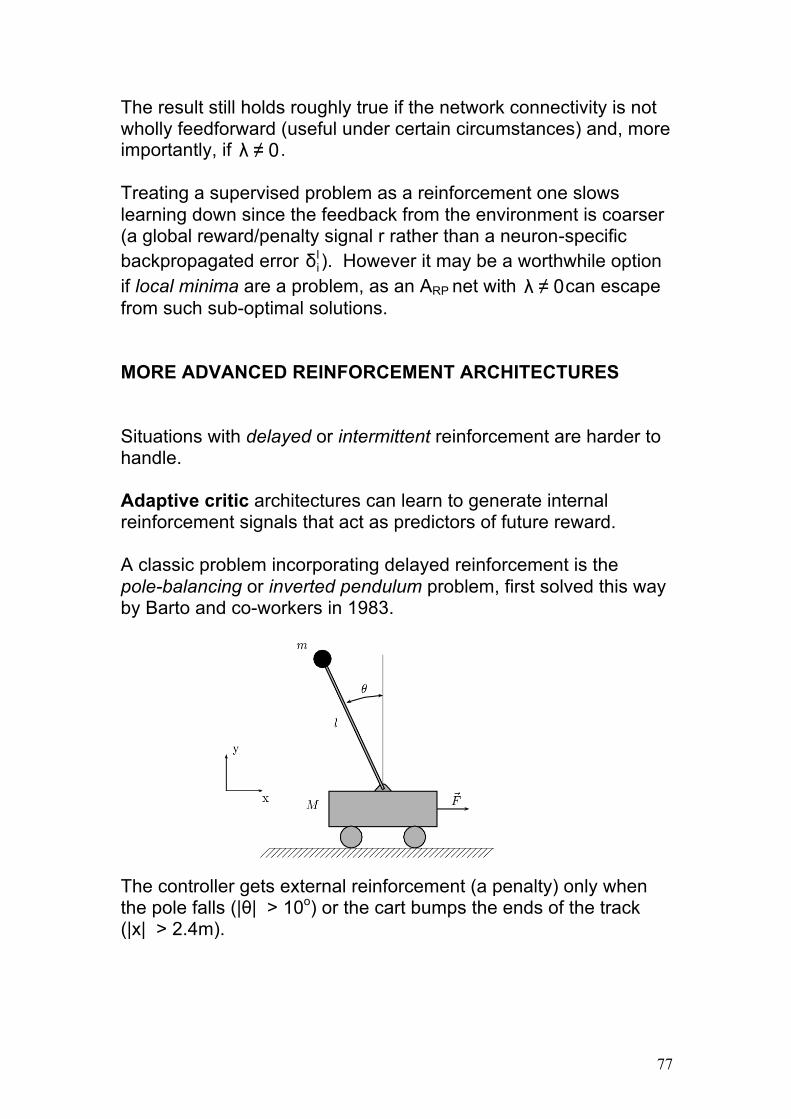
77

The result still holds roughly true if the network connectivity is not wholly feedforward (useful under certain circumstances) and, more importantly, if 0≠λ . Treating a supervised problem as a reinforcement one slows learning down since the feedback from the environment is coarser (a global reward/penalty signal r rather than a neuron-specific backpropagated error l

iδ ). However it may be a worthwhile option if local minima are a problem, as an ARP net with 0≠λ can escape from such sub-optimal solutions. MORE ADVANCED REINFORCEMENT ARCHITECTURES Situations with delayed or intermittent reinforcement are harder to handle. Adaptive critic architectures can learn to generate internal reinforcement signals that act as predictors of future reward. A classic problem incorporating delayed reinforcement is the pole-balancing or inverted pendulum problem, first solved this way by Barto and co-workers in 1983. The controller gets external reinforcement (a penalty) only when the pole falls (|θ| > 10o) or the cart bumps the ends of the track (|x| > 2.4m).

78

Outline of the network used, from p.842 of A G Barto, R S Sutton & C W Anderson, "Neuronlike adaptive elements that can solve difficult learning control problems," IEEE Trans. SMC, 13, 834-846. The ACE ("adaptive critic element") learns to associate degrees of safety (distance from failure) with dynamical states. Internally generated reinforcements are sent to the ASE ("associative search element", the part of the net that generates actions) when the system moves from a more to less safe state, or vice-versa. Cases with 2 & 3 jointed poles have also been balanced using the adaptive critic method.

79

However more complex control problems have been beyond this method's current capabilities and have required resorting to 'apprenticeship learning '. This is a form of reinforcement learning in which the controller net learns to copy a recognised control strategy or the actions of an expert human. A reinforcement signal is provided every time the net takes an action (a reward if it chooses the (known) 'right' action, a penalty otherwise). This is in fact the way the cart-pole control problem was first solved by reinforcement (by Bernard Widrow, the inventor of the perceptron-like learning machines the Adeline & Madeline). Done this way it's easy, as at least for the single-pole problem there is a well-recognised control strategy the net can learn to emulate. However systems trained this way are far from autonomous and are unable to learn to do things that we cannot. Another example of apprenticeship learning is the control of a (model) helicopter in aerobatic flight (Abbeel, Coates, Quigley & Ng, NIPS 2006): The authors noted that attacking the problem without this trainer feedback “would inevitably lead to crashes”...

80

The current situation, then, is somewhat disappointing. We would very much like to build control systems that could learn to function in regimes that are unfamiliar or difficult for humans. For example the US government funded a number of studies in the 1990s as to the possibility of using adaptive critic type reinforcement-trained neural network architectures for hypersonic flight control but the work didn’t get anywhere near as far as had been hoped. Why is it so difficult? Control problems are solved in the brain by complex modular networks. These are less well understood than, say, object recognition in the visual cortex. Problems requiring forward planning, especially if this requires the establishment and attainment of sub-goals, are especially hard.

81

SELF-ORGANISATION AND COMPETITIVE LEARNING The object of any self-organising or unsupervised learning system is to discover statistical structure or classes in the input data, in a way that does not require the intervention of either a 'teacher' (supervised learning) or 'critic' (reinforcement learning). Suppose the input space is 2-dimensional, with 2)p( ]1,0[∈x , p=1..P, and that when the P different patterns are plotted out as functions of (x1,x2) It is clear to the eye that the patterns fall into two distinct clusters. In problems where the input space is high-dimensional it is much harder to detect statistical structure of this kind. There are many well-known non-neural techniques (K-means clustering, spectral clustering) to tackle the problem but these can be computationally expensive. A self-organising neural network algorithm should be able to detect the existence of such clusters in its feature space.

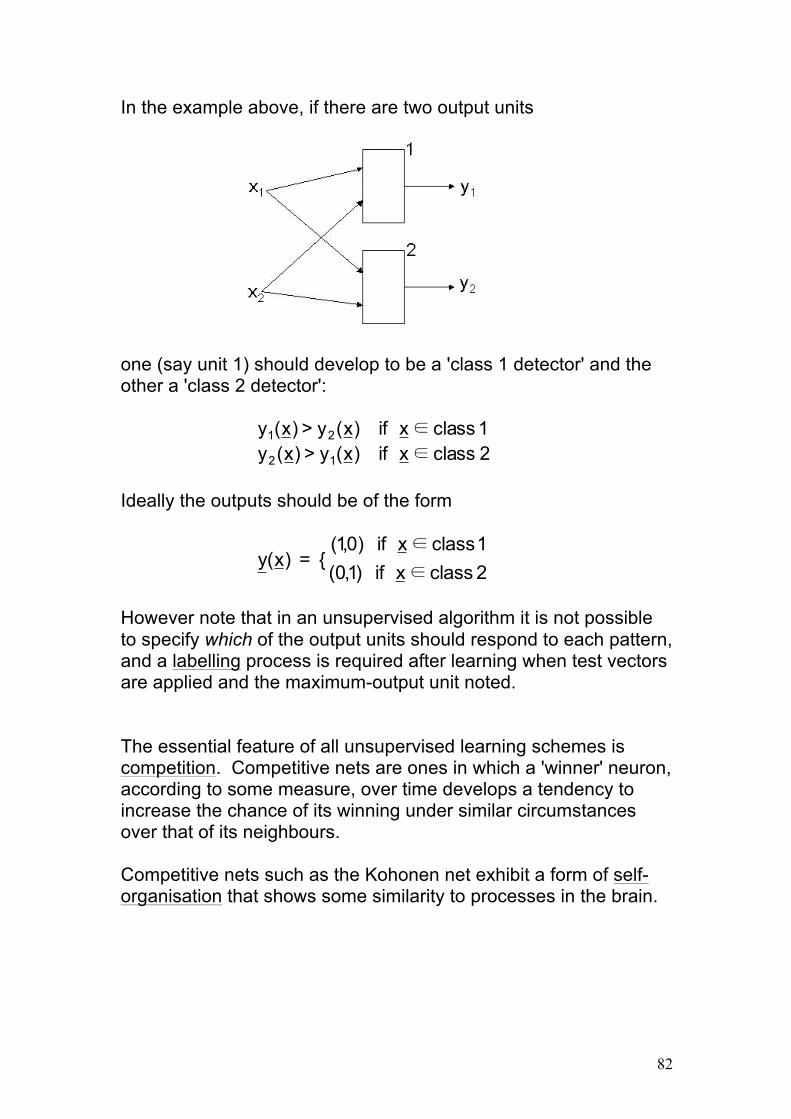
82

In the example above, if there are two output units one (say unit 1) should develop to be a 'class 1 detector' and the other a 'class 2 detector': 1 class x if )x(y>)x(y 21 ∈ 2 class x if )x(y>)x(y 12 ∈ Ideally the outputs should be of the form

2 class x if )1,0(1 class x if )0,1(

{ = )x(y∈

∈

However note that in an unsupervised algorithm it is not possible to specify which of the output units should respond to each pattern, and a labelling process is required after learning when test vectors are applied and the maximum-output unit noted. The essential feature of all unsupervised learning schemes is competition. Competitive nets are ones in which a 'winner' neuron, according to some measure, over time develops a tendency to increase the chance of its winning under similar circumstances over that of its neighbours. Competitive nets such as the Kohonen net exhibit a form of self-organisation that shows some similarity to processes in the brain.

83

TOPOGRAPHIC MAPS If the weights to the neighbours (with respect to some spatial distance measure) of the winning unit are adjusted in a similar way to the winner itself a topographic map may be formed in which class-detector nodes that are spatially close in the output grid. Suppose that in the 2-class example above a line of n output nodes was used: A topographic map would have developed if the 'winner' units were organised so that (or vice-versa). (Note that this regular arrangement would not occur if neighbour units were not updated in a similar way to the winner itself.) If there are roughly as many patterns in class 1 as in class 2 one would expect that m ≈ n/2. However one very useful feature of a topographic mapping is that if a sufficient number of output units are present the number of them more sensitive to a pattern of one class than any other reflects the number of patterns of that type which were seen. In the above example if there were twice as many patterns of class 1 as class 2 one might expect that around 2/3 of the units would become 'class 1 specialists' and 1/3 would be more sensitive to patterns of class 2.

84

In the this example a 2-dimensional feature space was mapped to a 1-dimensional output space. This process of making statistical structure in a higher dimensional feature space apparent by the spatial organisation of 'detector' or 'winner' units in a lower dimensional output space is one that is used in biological systems and which results in maps of the surface of the body or of sensory feature spaces. THE KOHONEN SELF-ORGANISING MAP (SOM) The Kohonen network is a single-layer competitive net in which patterns are classified by the units they activate in the output layer. Similar input vectors activate groups of units that are spatially close in the output layer (topographic map). Vectors of high dimension may be classified by a (usually) 2-dimensional spatial pattern (data compression), provided a sufficient number of output units are available, thus providing a graphical representation of complex statistical relationships in a multidimensional feature space. The network consists of an mxm neural grid, each neuron connected to all n data vector components The weight wij connects the jth input line to neuron i (i=1..m2) to the jth data vector component. Connectivity is usually complete -- every output unit has connections to all n input units.

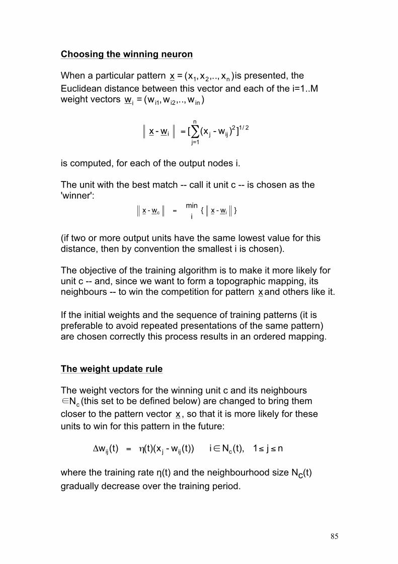
85

Choosing the winning neuron When a particular pattern )x,..,x,x(=x n21 is presented, the Euclidean distance between this vector and each of the i=1..M weight vectors )w,..,w,w(=w in2i1ii

!

x - wi = [ (x j - wij )2

j=1

n

" ]1/ 2

is computed, for each of the output nodes i. The unit with the best match -- call it unit c -- is chosen as the 'winner':

!

x - wc = min

i { x - wi }

(if two or more output units have the same lowest value for this distance, then by convention the smallest i is chosen). The objective of the training algorithm is to make it more likely for unit c -- and, since we want to form a topographic mapping, its neighbours -- to win the competition for pattern xand others like it. If the initial weights and the sequence of training patterns (it is preferable to avoid repeated presentations of the same pattern) are chosen correctly this process results in an ordered mapping. The weight update rule The weight vectors for the winning unit c and its neighbours

cN∈ (this set to be defined below) are changed to bring them closer to the pattern vector x , so that it is more likely for these units to win for this pattern in the future:

!

"wij(t) = #(t)(x j - wij(t)) i$Nc(t), 1% j % n where the training rate η(t) and the neighbourhood size Nc(t) gradually decrease over the training period.

86

Note that the variable t indexes the training iteration, or pattern presented, not the epoch. Patterns are usually presented in random order, and can be drawn from either a finite (eg {0,1}2) or infinite (eg [0,1]2) pattern set X. Both the width, d, of the neighbourhood of the winning node, and the training rate η must be decremented appropriately with t. Unlike the case of reinforcement learning, where difficulties in convergence could be got around by using a small training rate, here there is no choice but to decrement these parameters. For a 2-dimensional mxm output grid (the most common situation), with neurons indexed by their 2-dimensional 'coordinates' 2}m,..,2,1{ ∈)j,i( the neighbourhood Nc(t) of unit c (located at (ic, jc)) can be defined by the set of (i, j) such that

!

ic - d(t) " i " ic + d(t),

!

jc - d(t) " j " jc + d(t) This defines a square neighbourhood centred on (ic, jc): (if a calculated neighbourhood goes off the edge of the output grid it is clipped appropriately).

87

There are no well-defined rules for deciding the shape of the neighbourhood, or how quickly its size should be shrunk and to what final value. Kohonen suggested a linear decrease, ie that the size of the neighbourhood at training interation t should be the integer part of

d(t) = d0 +tT(dT-d0)

where d0 = initial neighbourhood size (~m/2, m/3 for an mxm output grid) dT = final neighbourhood size ((typically 1 unit, ie 8 nodes for a square neighbourhood T = total number of training steps In choosing a rate of decrease for the training rate there are somewhat firmer guidelines. Ritter and Schulten (1988) showed for a net mapping an n-dimensional input onto an n-dimensional grid (note though this is not the usual situation, where dimensional reduction is being performed) the most stable convergence to a final set of weights is obtained when the function obeys certain mathematical restrictions, one appropriate function being !(t)" t#r , 0 < r $1 However in practice one can obtain good convergence from a linear function analogous to the form for the neighbourhood function

!(t) = !0(1-tT)

where !0 = initial training rate (0.2-0.5 is usual) T = total number of training steps The total number of training steps is an important parameter. It is better to choose this too large than too small as not allowing enough time for meaningful weight changes before the training rate and neighbourhood size are too-far decremented can result in a distorted mapping in which some patterns that are close together in the data space are represented by winner neurons that are far apart on the neural grid. This kind of unfaithful topographic mapping is the equivalent of a local error minimum in supervised learning. T-values of the order of 10,000s are usually used.

88

Example: An mxm square-grid Kohonen network is to be uses to cluster the speech signatures of a number of individuals. Each speaker in this set is equally likely to be male or female, and equally likely to be from London or from Melbourne, Australia. With equiprobable origins and genders one might expect a map like the one below (where 'M,L' = male from London, etc) -- here vertical groups segregate origin, horizontal ones gender (note the the orientation of the map is a matter of chance and not significant).

The square regions delimit areas in which the neurons are more sensitive (have better matched weight-to-pattern vectors) to patterns of a given type than any of the others. The overall winner for that class will be found among these neurons, but the size (and sometimes shape) of the 'specialist region' is also informative about the nature of the data. Suppose the probability of a speaker being male increased to 0.75, and the probability of a speaker being a Londoner independently decreased to 0.25. The net will change to reflect the new data distribution along the lines below. Now around 9/16 of the nodes represent males from Melbourne where previously only 1/4 of them did.

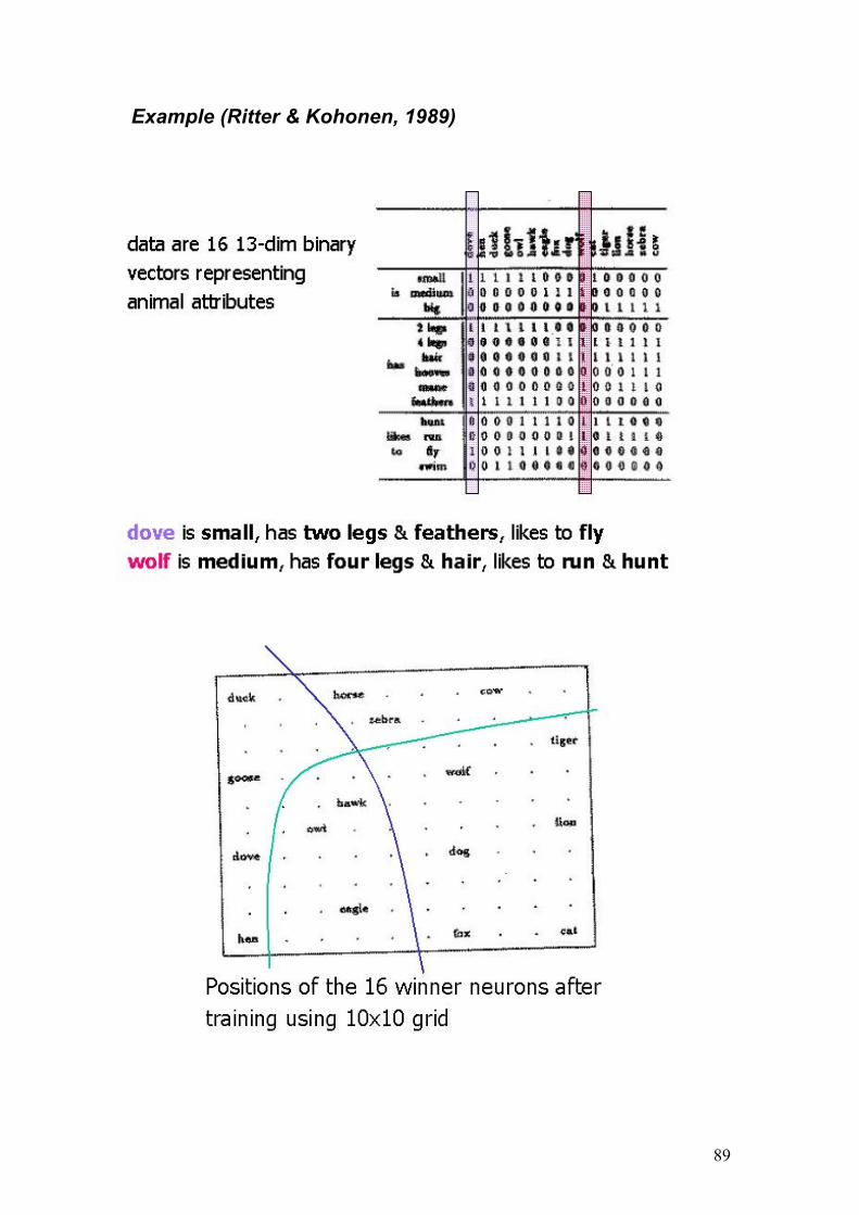
89

Example (Ritter & Kohonen, 1989)

90

The net has grouped the animals by 'type' in a way that confirms our intuitions. But what exactly has it discovered? • The difference between birds & animals (two clusters)?

• Between predators & prey (two clusters)?

• Both (four clusters)?

• Something else?

Too many applications of the Kohonen map have in the past relied on hand labelling of the data clusters on the 2D neural grid. But this process only confirms the experimenter’s prior beliefs, which may in any case be erroneous. It requires a post-processing phase using a method such as k-means clustering on the set of weights and the use of one or more cluster validation measures (Dunn, Davies-Bouldin, Silhouette indices...) to decide on the number of clusters that best describes the data. While self-organising maps are intuitive, give visually appealing results, and reflect something of the way the brain forms internal maps, they are not quite as simple to apply as is often believed, not if a predictive as opposed to a descriptive result is wanted: "Tell me something I don’t know!" The bottom line: Neural networks (specifically MLPs) have been very successful in many classification and prediction tasks that do not suit symbolic, rule-based approaches to AI. Control applications (ARP and related algorithms) are likely waiting on a much better understanding of the brain -- but it will come. Data mining (Kohonen's SOM) needs appropriate thought given to post-processing and the analysis of results -- but that can be done and there are good mathematical tools out there.