financial informatics –xiii: neural computing systems

1

Financial Informatics –XIII:Neural Computing Systems

1

Khurshid Ahmad, Professor of Computer Science,

Department of Computer Science

Trinity College,Dublin-2, IRELAND

November 19th, 2008.https://www.cs.tcd.ie/Khurshid.Ahmad/Teaching.html

2

Neural Networks:Real Networks

London, Michael and Michael Häusser (2005). Dendritic Computation. Annual Review of Neuroscience. Vol. 28, pp 503–32

3

Real Neural Networks:Cells and Processes

AXONCELL BODY

NUCLEUS

DENDRITES

A neuron is a cell with appendages; every cell has a nucleus and the one set of appendages brings in inputs – the dendrites – and another set helps to output signals generated by the cell

4


The human brain is mainly composed of neurons: specialised cells that exist to transfer information rapidly from one part of an animal's body to another.

This communication is achieved by the transmission (and reception) of electrical impulses (and chemicals) from neurons and other cells of the animal. Like other cells, neurons have a cell body that contains a nucleus enshrouded in a membrane which has double-layered ultrastructure with numerous pores.

SOURCE: http://en.wikipedia.org/wiki/Neurons

Nucleus

Dendrite

Soma

AxonTerminals

5

Real Neural NetworksAll the neurons of an organism, together with their supporting cells, constitute a nervous system. The estimates vary, but it is often reported that there are as many as 100 billion neurons in a human brain. Neurobiologist and neuroethologists have argued that intelligence is roughly proportional to the number of neurons when different species of animals compared. Typically the nervous system includes a :

Spinal Cord is the least differentiated component of the central nervous system and includes neuronal connections that provide for spinal reflexes. There are also pathways conveying sensory data to the brain and pathways conducting impulses, mainly of motor significance, from the brain to the spinal cord; and,

Medulla Oblongata: The fibre tracts of the spinal cord are continued in the

medulla, which also contains of clusters of nerve cells called nuclei.

6

Real Neural NetworksInputs to and outputs from an animal

nervous system

Cerebellum receives data from most sensory systems and the cerebral cortex, the cerebellum eventually influences motor neurons supplying the skeletal musculature. It produces muscle tonus in relation to equilibrium, locomotion and posture, as well as non-stereotyped movements based on individual experiences.

7

Real Neural NetworksProcessing of some information in the nervous system takes place in Diencephalon. This forms the central core of the cerebrum and has influence over a number of brain functions including complex mental processes, vision, and the synthesis of hormones reaching the blood stream.

Diencephalon comprises thalamus, epithalmus, hypothalmus, and subthalmus. The retina is a derivative of diencephalon; the optic nerve and the visual system are therefore intimately related to this part of the brain.

8

Real Neural NetworksInputs to the nervous system are relayed

thtough the Telencephalon (Cereberal

Hemispheres) which includes the cerebral cortex, corpus striatum, and medullary center. Nine-tenths of the human cerebral cortex is neocortex, a possible result of evolution, and contains areas for all modalities of sensation (except smell), motor areas, and large expanses of association cortex in which presumably intellectual activity takes place. Corpus striatum, large mass of gray matter, deals with motor functions and the medullary center contains fibres to connect cortical areas of two hemispheres.

9

Real Neural NetworksInputs to the nervous system are relayed

thtough the Telencephalon (Cereberal

Hemispheres) which includes the cerebral cortex, corpus striatum, and medullary center. Nine-tenths of the human cerebral cortex is neocortex, a possible result of evolution, and contains areas for all modalities of sensation (except smell), motor areas, and large expanses of association cortex in which presumably intellectual activity takes place. Corpus striatum, large mass of gray matter, deals with motor functions and the medullary center contains fibres to connect cortical areas of two hemispheres.

10


Neurons have a variety of appendages, referred to as 'cytoplasmic processes known as neurites which end in close apposition to other cells. In higher animals, neurites are of two varieties: Axons are processes of generally of uniform diameter and conduct impulses away from the cell body; dendrites are short-branched processes and are used to conduct impulses towards the cell body.The ends of the neurites, i.e. axons and dendrites are called synaptic terminals, and the cell-to-cell contacts they make are known as synapses.

SOURCE: http://en.wikipedia.org/wiki/Neurons

Nucleus

Dendrite

Soma

AxonTerminals

11


–

– +

summation

10 fan-in4

1 - 100 meters per sec.

Asynchronousfiring rate, c. 200 per sec.

10 fan-out4

1010 neurons with 104 connections and an average of 10 spikes per second = 1015 adds/sec. This is a lower bound on the equivalent computational power of the brain.

12


Henry Markram (2006). The Blue Brain Project. Nature Reviews Neuroscience Vol. 7, 153-160

13http://en.wikipedia.org/wiki/Neural_network#Neural_networks_and_neuroscience

Neural Networks &Neurosciences

Observed Biological Processes (Data)

Biologically PlausibleMechanisms for Neural Processing & Learning

(Biological Neural Network Models)

Theory(Statistical Learning Theory &

Information Theory)

Neural Networks: Real and Artificial






Information Theory)

Neural Networks & Neuro-economics

The behaviour of economic actors: pattern recognition, risk-averse/prone activities; risk/reward

15

Neural Networks

Artificial Neural Networks The study of the behaviour of neurons, either as 'single' neurons or as cluster of neurons controlling aspects of perception, cognition or motor behaviour, in animal nervous systems is currently being used to build information systems that are capable of autonomous and intelligent behaviour.

16

Neural NetworksArtificial Neural Networks, the uses

of

Application

Artificial Neural Networks

Classification: Given the knowledge of classes amongst objects, train a network to recognise the different classes using examples of idiosyncratic features of each of the classes

Categorisation

No class information is available. The network trains itself by assigning ‘similar’ objects to proximate neurons

Pattern Association

Auto- and hetero associations between input and generated output patterns

Forecasting Training neurons with time serial data with one- or two step forecasting; Networks that learn to remove noise from a time serial data.

17

Neural NetworksArtificial Neural Networks

Artificial neural networks emulate threshold behaviour, simulate co-operative phenomenon by a network of 'simple' switches and are used in a variety of applications, like banking, currency trading, robotics, and experimental and animal psychology studies.

These information systems, neural networks or neuro-computing systems as they are popularly known, can be simulated by solving first-order difference or differential equations.

18

Neural Networks

Artificial Neural Networks The basic premise of the course, Neural Networks, is to introduce our students to an alternative paradigm of building information systems.

19


• Statisticians generally have good mathematical backgrounds with which to analyse decision-making algorithms theoretically. […] However, they often pay little or no attention to the applicability of their own theoretical results’ (Raudys 2001:xi).

• Neural network researchers ‘advocate that one should not make assumptions concerning the multivariate densities assumed for pattern classes’ . Rather, they argue that ‘one should assume only the structure of decision making rules’ and hence there is the emphasis in the minimization of classification errors for instance.

• In neural networks there are algorithms that have a theoretical justification and some have no theoretical elucidation’.

•Given that there are strengths and weaknesses of both statistical and other soft computing algorithms (e.g. neural nets, fuzzy logic), one should integrate the two classifier design strategies (ibid)

Raudys, Šarûunas. (2001). Statistical and Neural Classifiers: An integrated approach to design. London: Springer-Verlag

20


• Artificial Neural Networks are extensively used in dealing with problems of classification and pattern recognition. The complementary methods, albeit of a much older discipline, are based in statistical learning theory

•Many problems in finance, for example, bankruptcy prediction, equity return forecasts, have been studied using methods developed in statistical learning theory:

21


Many problems in finance, for example, bankruptcy prediction, equity return forecasts, have been studied using methods developed in statistical learning theory:

“The main goal of statistical learning theory is to provide a framework for studying the problem of inference, that is of gaining knowledge, making predictions, making decisions or constructing models from a set of data. This is studied in a statistical framework, that is there are assumptions of statistical nature about the underlying phenomena (in the way the data is generated).” (Bousquet, Boucheron, Lugosi)

Statistical learning theory can be viewed as the study of algorithms that are designed to learn from observations, instructions, examples and so on.

Olivier Bousquet, Stephane Boucheron, and Gabor Lugosi. Introduction to Statistical Learning Theory (http://www.econ.upf.edu/~lugosi/mlss_slt.pdf)

22


“Bankruptcy prediction models have used a variety of statistical methodologies, resulting in varying outcomes. These methodologies include linear discriminant analysis regression analysis, logit regression, and weighted average maximum likelihood estimation, and more recently by using neural networks.”

The five ratios are net cash flow to total assets, total debt to total assets, exploration expenses to total reserves, current liabilities to total debt, and the trend in total reserves (over a three year period, in a ratio of change in reserves in computed as changes in Yrs 1 & 2 and changes in Yrs 2 &3). Zhang et al (1999) found that (a variant of) ‘neural network and Fischer Discriminant Analysis ‘achieve the best overall estimation’, although discriminant analysis gave superior results.

Z. R. Yang, Marjorie B. Platt and Harlan D. Platt (1999)Probabilistic Neural Networks in Bankruptcy Prediction. Journal of Business Research, Vol 44, pp 67–74

23


A neural network can be described as a type of multiple regression in that it accepts inputs and processes them to predict some output. Like a multiple regression, it is a data modeling technique.

Neural networks have been found particularly suitable in complex pattern recognition compared to statistical multiple discriminant analysis (MDA) since the networks are not subject to restrictive assumptions of MDA models

Shaikh A. Hamid and Zahid Iqbal (2004). (1999) Using neural networks for forecasting volatility of S&P 500 Index futures prices. Journal of Business Research, Vol 57, pp 1116-1125.

24


Neural Networks for forecasting volatility of S&P 500 Index: A neural network was trained to learn to generate volatility forecasts for the S&P 500 Index over different time horizons. The results were compared with pricing option models used to compute implied volatility from S&P 500 Index futures options (the Barone-Adesi and Whaley American futures options pricing model)

Forecasts from neural networks outperform implied volatility forecasts and are not found to be significantly different from realized volatility.

Implied volatility forecasts are found to be significantly different from realized volatility in two of three forecast horizons.

Shaikh A. Hamid and Zahid Iqbal (2004). (1999) Using neural networks for forecasting volatility of S&P 500 Index futures prices. Journal of Business Research, Vol 57, pp 1116-1125.

25


The ‘remarkable qualities’ of neural networks: the dynamics of a single layer perceptron progresses from the simplest algorithms to the most complex algorithms:

• Initial Training each pattern class characterized by sample mean vector neuron behaves like E[uclidean] D[istance] C[lassifier] ;• Further Training neuron begins to evaluate correlations and variances of features neuron behaves like standard linear Fischer classifier• More training neuron minimizes number of incorrectly identified training patterns neuron behaves like a support vector classifier.

Statisticians and engineers usually design decision-making algorithms from experimental data by progressing from simple algorithms to more complex ones.

Raudys, Šarûunas. (2001). Statistical and Neural Classifiers: An integrated approach to design. London: Springer-Verlag







Information Theory)







Information Theory)

Neural Networks & Neuro-economics

The behaviour of economic actors: pattern recognition, risk-averse/prone activities; risk/reward

28Camelia M. Kuhnen and Brian Knutson (2005). “Neural Antecedents of Financial Decisions.” Neuron, Vol. 47, pp 763–770


Neural Networks: Neuro-economics

Investors systematically deviate from rationality when making financial decisions, yet the mechanisms responsible for these deviations have not been identified. Using event-related fMRI, we examined whether anticipatory neural activity would predict optimal and suboptimal choices in a financial decision-making task. [] Two types of deviations from the optimal investment strategy of a rational risk-neutral agent as risk-seeking mistakes and risk-aversion mistakes.



Nucleus accumbens [NAcc] activation preceded risky choices as well as risk-seeking

mistakes, while anterior insula activation preceded riskless choices as well as risk-aversion mistakes. These findings suggest that distinct neural circuits linked to anticipatory affect promote different types of

financial choices and indicate that excessive activation of these circuits may lead to investing mistakes.




Association of Anticipatory Neural Activation with Subsequent ChoiceThe left panel indicates a significant effect of anterior insula activation on the odds of making riskless (bond) choices and risk-aversion mistakes (RAM) after a stock choice (Stockt-1). The right panel indicates a significant effect of NAcc activation on the odds of making risk-aversion mistakes, risky choices, and risk-seeking mistakes (RSM) after a bond choice (Bondt-1). The odds ratio for a given choice is defined as the ratio of the probability of making that choice divided by the probability of not making that choice. Percent change in odds ratio results from a 0.1% increase in NAcc or anterior insula activation. Error bars indicate the standard errors of the estimated effect. *coefficient significant at p < 0.05.

Obs

erve

d B

iolo

gica

l P

roce

sses

(D

ata)



Nucleus accumbens [NAcc] activation preceded risky choices as well as risk-seeking mistakes, while anterior insula activation preceded riskless choices as well as risk-aversion mistakes. These findings suggest that distinct neural circuits linked to anticipatory affect promote different types of financial choices and indicate that excessive activation of these circuits may lead to investing mistakes.

Obs

erve

d B

iolo

gica

l P

roce

sses

(D

ata)

32Brian Knutson and Peter Bossaerts (2007). “Neural Antecedents of Financial Decisions.” The Journal of Neuroscience, (August 1, 2007), Vol. 27 (No. 31), pp 8174–8177



To explain investing decisions, financial theorists invoke two opposing metrics: expected reward and risk. Recent advances in the spatial and temporal resolution of brain imaging techniques enable investigators to visualize changes in neural activation before financial decisions. Research using these methods indicates that although the ventral striatum plays a role in representation of expected reward, the insula may play a more prominent role in the representation of expected risk. Accumulating evidence also suggests that antecedent neural activation in these regions can be used to predict upcoming financial decisions. These findings have implications for predicting choices and for building a physiologically constrained theory of decision-making.

33

Organising Principles and Common Themes:

Association between neurons and competition amongst the neurons

Two examples: Categorisation and attentional modulation of conditioning


Levine, Daniel S. (1991). Introduction to Neural and Cognitive Modeling. Hillsdale, NJ & London: Lawrence Erlbaum Associates, Publishers (See Chapter 1)

34

Organising Principles and Common Themes:Association between neurons and competition amongst the neurons

A network for identifying handwritten letters of the alphabet.


Category Nodes

Feature Nodes

Feature nodes respond to the presence or absence of marks at particular locations.

Category nodes respond to the patterns of activation in the feature nodes.

Weighted sum of inputs


35


Artificial Neural Networks (ANN) are computational systems, either hardware or software, which mimic animate neural systems comprising biological (real) neurons. An ANN is architecturally similar to a biological system in that the ANN also uses a number of simple, interconnected artificial neurons.

36

Artificial Neural NetworksIn a restricted sense artificial neurons are simple emulations of biological neurons: the artificial neuron can, in principle, receive its input from all other artificial neurons in the ANN; simple operations are performed on the input data; and, the recipient neuron can, in principle, pass its output onto all other neurons.

Intelligent behaviour can be simulated through computation in massively parallel networks of simple processors that store all their long-term knowledge in the connection strengths.

37

Artificial Neural NetworksAccording to Igor Aleksander, Neural Computing is the study of cellular networks that have a natural propensity for storing experiential knowledge.

Neural Computing Systems bear a resemblance to the brain in the sense that knowledge is acquired through training rather than programming and is retained due to changes in node functions.

Functionally, the knowledge takes the form of stable states or cycles of states in the operation of the net. A central property of such states is to recall these states or cycles in response to the presentation of cues.

38


A network for identifying handwritten letters of the alphabet: e.g. 25 patterns for representing 32 letters.


The line patterns (vertical, horizontal, short. Long strokes) and circular patterns in Roman alphabet can be represented in a binary system.

10 1 0U

00 0 0A 1

10 0 0E 1

00 1 0I 1

10 0 0O 11


39


The transformation of linear and circular patterns into binary patterns requires a degree of pre-processing and judicious guesswork!

Neural Networks:Real and Artificial


The line patterns (vertical, horizontal, short. Long strokes) and circular patterns in Roman alphabet can be represented in a binary system.

10 1 0U

00 0 0A 1

10 0 0E 1

00 1 0I 1

10 0 0O 11M

A

P

P

I

N

G

40

00 0 01




Category Nodes

Association between feature nodes and category nodes should be allowed to change over time (during training), more specifically as a result of repeated activation of the connection

-


A


41




Category Nodes


-


A

10 0 0

E

1


42




Category Nodes

Feature Nodes

Competition amongst to win over an individual letter shape and then to inhibit other neurons to respond to that shape. Especially helpful when there is noise in the signal, e.g. sloppy writing

-



43


A network for identifying handwritten letters of the alphabet: e.g. 25 patterns for representing 32 letters.


The line patterns (vertical, horizontal, short. Long strokes) and circular patterns in Greek alphabet can be represented in a binary system.

10 1 0υ

00 0 0α 1

10 0 0ε 1

00 1 0ι 1

10 0 0θ 11


44

00 0 01




Category Nodes

Since the weights change due to repeated presentation our system will learn to ‘identify’ Greek letters of the alphabet

-


α


45




Category Nodes


-


α

10 0 0

ε

1


46

Artificial Neural Networks and Learning

Artificial Neural Networks 'learn' by adapting in accordance with a training regimen: The network is subjected to particular information environments on a particular schedule to achieve the desired end-result.

There are three major types of training regimens or learning paradigms:

SUPERVISED;UN-SUPERVISED;

REINFORCEMENT or GRADED.

47

Biological and Artificial NN’s

Entity Biological Neural Networks


Processing Units Neurons Network Nodes

Input Dendrites(Dendrites may form synapses

onto other dendrites)

Network Arcs(No interconnection

between arcs)

Output Axons or Processes(Axons may form synapses onto

other axons)


between arcs)

Inter-linkage Synaptic Contact (Chemical and Electrical)

Node to Node via Arcs

Plastic Connections Weighted Connections Matrix

48




Processing Units Neurons Network Nodes

Input Dendrites(Dendrites may form synapses

onto other dendrites)


between arcs)

Output Axons or Processes(Axons may form synapses onto

other axons)


between arcs)

Inter-linkage Synaptic Contact (Chemical and Electrical)

Node to Node via Arcs

Plastic Connections Weighted Connections Matrix

49




Inter-linkage Excitatory –with asymmetrical

membrane specialisation, thicker on the post-synaptic

side and presynaptic side containing round vesicles

Positive connection weights between nodes

Inter-linkage Inhibitory–with symmetrical

membrane specialisation, with ellipsoidal vesicles

Negative connection weights between nodes

50




Output Dendrites bring inputs from different locations: so does the brain wait for

all the inputs and then start up the summing

exercise or does it perform many different intermediate

computations?

All inputs arrive instantaneously and are summed up in the same

computational cycle: distance (or location)

between neuronal nodes is not an issue.

51




Output The threshold: the neurons, being in a noisy environment, tend not to

abide by a fixed, discontinuous threshold and there is a degree of tolerance of the input.

The threshold is usually a discontinuous (step) function and after the

threshold is ‘crossed’ the amount of input is

immaterial

52


An ANN system can be characterised by

•its ability to learn;•its dynamic capability;

and • its interconnectivity

53

Artificial Neural Networks:

An Operational View

Input S

ignals yk

Output

Signal

wk3

wk1

wk2

wk4

Neuron xk

x1

x2

x3

x4

bk

Summing Junction

Activation Function

)(

)(0

****

:

1

1

1

44332211

THRESHOLDnetifnety

THRESHOLDnetify

functionidentitynegativenon

netyfunctionidentity

outputNeuronal

xwxwxwxwnet

sumweightedorinputNet

54


An Operational View A neuron is an information processing unit forming the key ingredient of a

neural network: The diagram above is a model of a biological neuron. There are three key ingredients of this neuron labelled xk which is connected to the (rest of the) neurons in the network labelled

x1, x2, x3,…xj.

A set of links, the biological equivalent of synapses, which the kth neuron has with the (rest of the) neurons in the network. Note that each link has a WEIGHT denoted by labelled

wk1, wk2,…wkj, where the first subscript (k in this case) denotes the recipient neurons and

the second subscript (1,2,3…..j) denotes the neurons transmitting to the recipient neurons. The synaptic weight wkj may lie in a range that includes negative (inhibitory) values and positive (excitatory) values.

(From Haykin 1999:10-12)

55


An Operational View

The kth neuron adds up the inputs of all the transmitting neurons at the summing junction or the adder, denoted by S. The adder acts as a linear combiner and generates a weighted average usually denoted by uk:

uk = wk1i*x1 + wk2*x2 + wk3*x3 + ………. + wkj*xj;

the bias (bk )has the effect of increasing or decreasing the net input to the activation function depending on the value of the bias.(From Haykin 1999:10-12)


56

ANN’s: an Operational View

Finally, the linear combination, denoted as vk = uk + bk, is passed through the activation function which engenders the non-linear behaviour seen in the behaviour of the biological neurons: the inputs to and outputs from a given neuron show a complex, often non-linear behaviour. For example, if the output from the adder was positive or zero then the neuron will emit a signal,

yk = 1 if (vk)0 , however if the output from the adder was negative then there will be no output,

yk = 0 if (vk)< 0 .

There are other models of the activiation function as we will see later.


57


Input S

ignals yk

Output

Signal

wk3

wk1

wk2

wk4

Neuron xk

x1

x2

x3

x4

bk

Summing Junction

Activation Function

)(

)(0

tan

****

:

1

1

1

44332211

THRESHOLDnetifCy

THRESHOLDnetify

netytcons

outputNeuronal

xwxwxwxwnet


58


Input S

ignals yk

Output

Signal

wk3

wk1

wk2

wk4

Neuron xk

x1

x2

x3

x4

bk

Summing Junction

Activation Function

)(1

)(0

****

:

1

1

44332211

THRESHOLDnetify

THRESHOLDnetify

outputSaturated

outputNeuronal

xwxwxwxwnet


59


Discontinuous Output

Input S

ignals yk

Output

Signal

wk3

wk1

wk2

wk4

Neuron xk

x1

x2

x3

x4

bk

Summing Junction

Activation Function

)(1

)(0

****

:

1

1

44332211

THRESHOLDnetify

THRESHOLDnetify

outputSaturated

outputNeuronal

xwxwxwxwnet


f(

net)

net

No output

Output

Threshold (θ)

(Normalised) output (eg. 1)

60


Input S

ignals yk

Output

Signal

wk3

wk1

wk2

wk4

Neuron xk

x1

x2

x3

x4

bk

Summing Junction

Activation Function

The notion of a discontinuous function simulates the fundamental notion that biological neurons usually fire if there is ‘enough’ stimulus available in the environment.

But discontinuous is biologically implausible, so there must be some degree of continuity in the output such that an artificial neuron has a degree of biological plausibility.

61


Pseudo-Continuous Output

Input S

ignals yk

Output

Signal

wk3

wk1

wk2

wk4

Neuron xk

x1

x2

x3

x4

bk

Summing Junction

Activation Function

),,,(

)(

)(

****

:

'1

'1

1

44332211

fy

THRESHOLDSaturationnetify

THRESHOLDnetify

outputSaturated

outputNeuronal

xwxwxwxwnet


f(

net)

net

Output=α

Output βThreshold (θ)

Saturation Threshold (θ’)

62

ANN’s: an Operational

View

A schematic for an 'electronic' neuron

ykwk3

wk1

wk2

wk4

Neuron xkx1

x2

x3

x4bk

Input Signals

Output

Signal

Summing Junction

Activation Function

63


Neural Nets as directed graphsA directed graph is a geometrical object consisting of a set of points (called nodes) along with a set of directed line segments (called links) between them. A neural network is a parallel distributed information processing structure in the form of a directed graph.

64


View

Input Connections

Processing Unit

Output Connection

Fan Out

65


View

A neural network comprisesA set of processing unitsA state of activationAn output function for each unitA pattern of connectivity among unitsA propagation rule for propagating patterns of activities through the network An activation rule for combining the inputs impinging on a unit with the current state of that unit to produce a new level of activation for the unitA learning rule whereby patterns of connectivity are modified by experienceAn environment within which the system must operate

66

The McCulloch-Pitts Network

. McCulloch and Pitts demonstrated that any logical function can be duplicated by some network of all-or-none neurons referred to as an artificial neural network (ANN).

Thus, an artificial neuron can be embedded into a network in such a manner as to fire selectively in response to any given spatial temporal array of firings of other neurons in the ANN.

Artificial Neural Networks for Real Neuroscientists: Khurshid Ahmad, Trinity College, 28 Nov 2006

67

The McCulloch-Pitts

Network

Demonstrates that any logical function can be implemented by some network of neurons.

•There are rules governing the excitatory and inhibitory pathways.•All computations are carried out in discrete time intervals.•Each neuron obeys a simple form of a linear threshold law: Neuron fires whenever at least a given (threshold) number of excitatory pathways, and no inhibitory pathways, impinging on it are active from the previous time period.•If a neuron receives a single inhibitory signal from an active neuron, it does not fire.•The connections do not change as a function of experience. Thus the network deals with performance but not learning.

68

The McCulloch-Pitts

Network

Computations in a McCulloch-Pitts Network

‘Each cell is a finite-state machine and accordingly operates in discrete time instants, which are assumed synchronous among all cells. At each moment, a cell is either firing or quiet, the two possible states of the cell’ – firing state produces a pulse and quiet state has no pulse. (Bose and Liang 1996:21)

‘Each neural network built from McCulloch-Pitts cells is a finite-state machine is equivalent to and can be simulated by some neural network.’ (ibid 1996:23)

‘The importance of the McCulloch-Pitts model is its applicability in the construction of sequential machines to perform logical operations of any degree of complexity. The model focused on logical and macroscopic cognitive operations, not detailed physiological modelling of the electrical activity of the nervous system. In fact, this deterministic model with its discretization of time and summation rules does not reveal the manner in which biological neurons integrate their inputs.’ (ibid 1996:25)

69

The McCulloch-Pitts

Network

Consider a McCulloch-Pitts network which can act as a minimal model of the sensation of heat from holding a cold object to the skin and then removing it or leaving it on permanently.

Each cell has a threshold of TWO, hence fires whenever it receives two excitatory (+) and no inhibitory (-) signals from other cells at a previous time.


70

The McCulloch-Pitts

Network

1

3

A

B

42

-

+

+

+ +

++

+ +

+

+

Heat

Receptors Cold

Hot

Cold

Heat Sensing Network

71

The McCulloch-Pitts

Network

1

3

A

B

42

-

+

+

+ +

++

+ +

+

+

Heat

Receptors Cold

Hot

Cold


Time Cell 1 Cell 2 Cell a Cell b Cell 3 Cell 4

INPUT INPUT HIDDEN HIDDEN OUTPUT OUTPUT

1 No Yes No No No No

2 No No Yes No No No

3 No No No Yes No No

4 No No No No Yes No

Truth tables of the firing neurons when the cold object contacts the skin and is then removed

72

The McCulloch-Pitts

Network


‘Feel hot’/’Feel cold’ neurons show how to create OUTPUT UNIT RESPONSE to given INPUTS that depend ONLY on the previous values. This is known as a TEMPORAL CONTRAST ENHANCEMENT.

The absence or presence of a stimulus in the PREVIOUS time cycle plays a major role here.

The McCulloch-Pitts Network demonstrates how this ENHANCEMENT can be simulated using an ALL-OR-NONE Network.

73

The McCulloch-Pitts

NetworkHeat Sensing Network


INPUT INPUT HIDDEN HIDDEN OUTPUT OUTPUT

1

2

3

Truth tables of the firing neurons for the case when the cold object is left in contact with the skin – a simulation of temporal contrast enhancement

74

The McCulloch-Pitts

NetworkHeat Sensing Network


INPUT INPUT HIDDEN

HIDDEN

OUTPUT

OUTPUT

1 No Yes No No No No

2 No Yes Yes No No No

3 No Yes Yes No No Yes

Truth tables of the firing neurons for the case when the cold object is left in contact with the skin – a simulation of temporal contrast enhancement

1

3

A

B

42

-

+

+

+ +

++

+ +

+

+

Heat

Receptors Cold

Hot

Cold

75

The McCulloch-Pitts

Network

+

++

+

+ + +

+

1 2

A

B

1 2+

+

Memory Models

Three stimulus model

Permanent Memory model

+

+

76

The McCulloch-Pitts

Network

In the permanent memory model, the output neuron has threshold ‘1’; neuron 2 fires if the light has ever been on anytime in the past.Levine, D. S. (1991:16)

1 2+

+

Memory Models

Permanent Memory model

77

The McCulloch-Pitts

NetworkMemory Models

1 2

A

B

Three stimulus model

Time Cell 1 Cell A Cell B Cell 2

1 Yes No No No

2 Yes No Yes No

3 Yes Yes Yes No

4 No Yes Yes Yes

Consider, the three stimulus all-or-none neural network. In this network, neuron 1 responds to a light being on. Each of the neurons has threshold ‘3’.

In the three stimulus model neuron 2 fires after the light has been on three time units in a row.

All connections are unit positive

78

The McCulloch-Pitts

Network

Why is a McCulloch-Pitts a FSM?

A finite state machine (FSM)is an AUTOMATON.An input string is read from left to right; the machine looks at each symbol in turn. At any time the FSM is in one of many finitely interval states.The state changes after each input symbol is read.The NEW STATE depends (only) on the symbol just read and on the current state.

79



‘The McCulloch-Pitts model, though it uses an oversimplified formulation of neural activity patterns, presages some issues that are still important in current cognitive models. [..][Some] Modern connectionist networks contain three types of units or nodes – input units, output units, and hidden units. The input units react to particular data features from the environment […]. The output units generate particular organismic responses […]. The hidden units are neither input nor output units themselves but, via network connections, influence output units to respond to prescribed patterns of input unit firings or activities. [..] [This] input-output-hidden trilogy can be seen as analogous to the distinction between sensory neurons, motor neurons, and all other (interneurons) in the brain’

Levine, Daniel S. (1991: 14-15)

80


Linear Neuron: Output is the weighted sum of all the inputs;McCulloch-Pitts Neuron: Output is the thresholded value of the weighted sumInput Vector? X = X (1,-20,4,-2); Weight vector? wji=w(wj1,wj2,wj3,wj4)

=[0.8,0.2,-1,-0.9]

0th input

x1

x2

x3

x4

yjj

wj1

wj2

wj3

wj4

81


vj=wjixi; y=f(v); y=0 if v<=0 or y=1 if v>0Input Vector? X = X (1,-20,4,-2); Weight vector? wji=w(wj1,wj2,wj3,wj4)

=[0.8,0.2,-1,-0.9]wj0=0, x0=0

0th input

x1

x2

x3

x4

yjj

wj1

wj2

wj3

wj4

82


Input Vector? X = X (1,-20,4,-2); Weight vector? w=w(wj1,wj2,wj3,wj4)

=[0.8,0.2,-1,-0.9]wj0=0, x0=0

vj=wjixi; y=f(v); f activation functionLinear Neuron: y=vMcCulloch Pitts: y=0 if v<=0 or y=1 if v>0Sigmoid activation function: f(v)=1 /(1+exp(-v))

83


What are the circumstance in a neuron with a sigmoidal activation function will act like a McCulloch Pitts network?

Large synaptic weights

What are the circumstance in a neuron with a sigmoidal activation function will act like a linear neuron?

Small synaptic weights

84

Widrow-Hoff Networks:Error-correction or Performance Learning

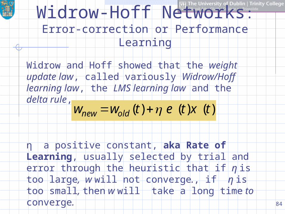
Widrow and Hoff showed that the weight update law, called variously Widrow/Hoff learning law, the LMS learning law and the delta rule,

η a positive constant, aka Rate of Learning, usually selected by trial and error through the heuristic that if η is too large, w will not converge., if η is too small, then w will take a long time to converge.

Typically, 0.01≤ η ≤ 10, with η=0.1 as a usual starting point.

)()()( txtetww oldnew

85

Widrow-Hoff Networks:

Error-correction or Performance Learning

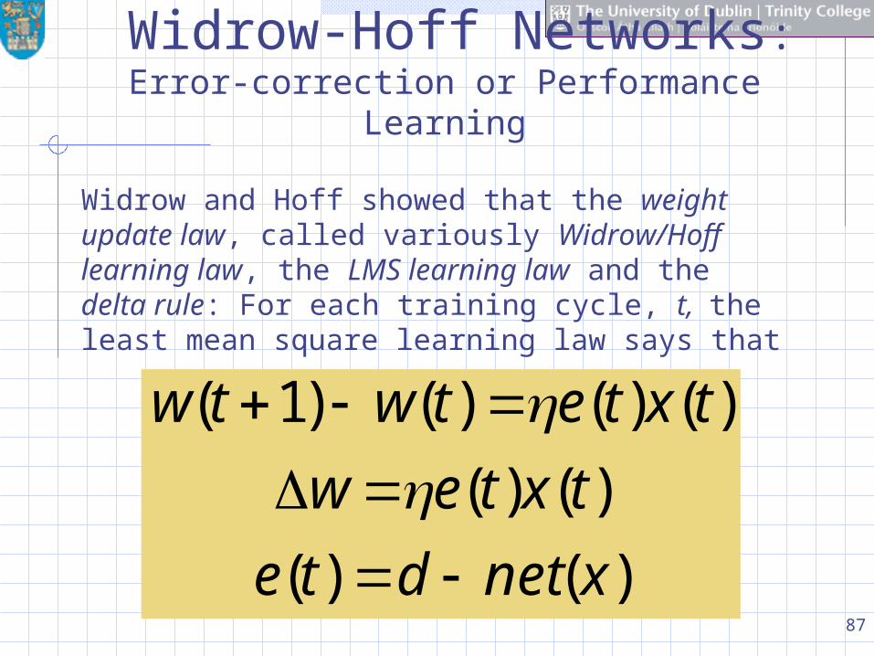
Widrow and Hoff showed that the weight update law, called variously Widrow/Hoff learning law, the LMS learning law and the delta rule: For each training cycle, t, the least mean square learning law says that

)()(

)()(

)()()()1(

xnetdte

txtew

txtetwtw

86



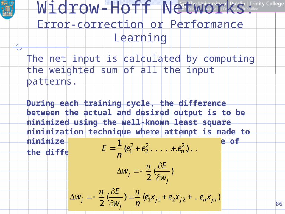
The net input is calculated by computing the weighted sum of all the input patterns.

During each training cycle, the difference between the actual and desired output is to be minimized using the well-known least square minimization technique where attempt is made to minimize the error-energy, E, or the square of the difference of the errors:

)...()(2

)(2

)..........(1

2211

222

21

jnnjjj

j

jj

n

xexexenw

Ew

w

Ew

eeen

E

87



Widrow and Hoff showed that the weight update law, called variously Widrow/Hoff learning law, the LMS learning law and the delta rule: For each training cycle, t, the least mean square learning law says that

)()(

)()(

)()()()1(

xnetdte

txtew

txtetwtw

88



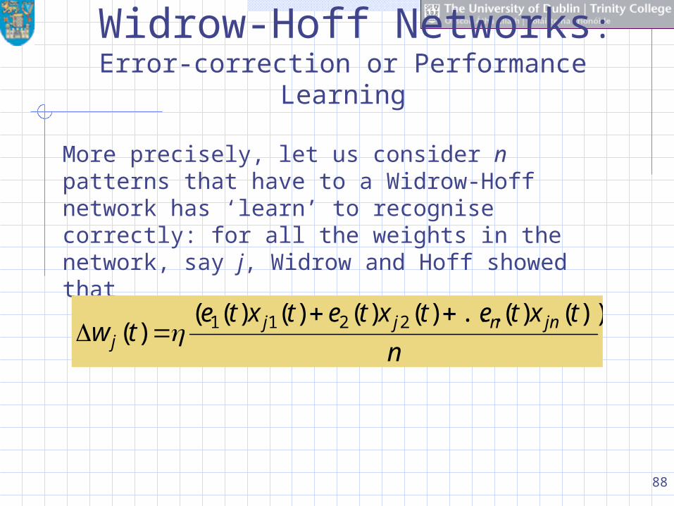
More precisely, let us consider n patterns that have to a Widrow-Hoff network has ‘learn’ to recognise correctly: for all the weights in the network, say j, Widrow and Hoff showed that

n

txtetxtetxtetw jnnjj

j

))()(...)()()()(()( 2211

89

Rosenblatt’s Perceptron

Rosenblatt, Selfridge and others generalised McCulloch-Pitts form of the linear threshold law was generalised to laws such that activities of all pathways (cf. dendrites) impinging on a neuron are computed, and the neuron fires whenever some weighted sum of those activities is above a given amount.

90


In the early days of neural network modelling, considerable attention was paid to McCulloch and Pitts who essentially incorporated the behaviouristic learning approach, that of interrelating stimuli and responses as a mechanism for learning, due originally to Donald Hebb, for learning into a network of all-or-none neurons. This led a number of other workers to adapt this approach during the late 1940's. Prominent among these workers were

Rosenblatt (1962): PERCEPTRONS

Selfridge (1959): PANDEMONIUM

The modellers called these networks, adaptive networks in that the network adapted to its environment quite autonomously. Rosenblatt developed a network architecture, and successfully implemented aspects of his architecture, which could make and learn choices between different patterns of sensory stimuli.

91


Rosenblatt's Perceptron has the following 'properties':

(1) It can receive inputs from other neurons(2) The 'recipient' neuron can integrate the input(3) The connection weights are modelled as follows:

If the presence of features xi stimulates the perceptron to firethen wi will be positive;If the presence of features xi inhibits the perceptron

then wi will be negative.

(4) The output function of the neuron is all-or-none(5) Learning is a process of modifying the weights

Whatever a neuron can compute, it can learn to compute!

92


Rosenblatt's Perceptron is an early example of the so-called electronic neurons. The electronic neuron, a simulation of the biological neuron, had the following properties:

(1)It can receive inputs from a number of sources (~dendrites inputting onto a neuron) e.g. other neurons (e.g. sensory input to an inter-neuron). Typically the inputs are vector-like - i.e. a magnitude and a sign; x = {x1, x2,....xn}

(2) The 'recipient' electronic neuron can integrate the input - either by simply summing up the individual inputs or by weighing the individual inputs in proportion to their 'strength of connection' (wi) with the recipient (a biological neuron can filter, add, subtract and amplify the input) and then summing up the weighted input as g(x).

Usually the summation function g(x) has an additional weight w0 - the threshold weight which incorporates the propensity of the electronic neuron to fire irrespective of the input (the depolarisation of the biological neuron's membrane induced by an external stimuli, results in the neuron responding with an action potential or impulse. The critical value of this depolarisation is called the threshold value).

93


(3) The connection weights are modelled as follows:

(3a) If the presence of some features xi tends the perceptron to fire then wi will be positive;

(3b) If the presence of some features xi inhibits the perceptron then wi will be negative.

(4) The output function of the electronic neuron (the impulse output along the axon terminals of biological neurons) is all-or-none output in that the output function:

ouptut(x) = 1 if g(x) > 0= 0 if g(x) < 0

(5) Learning, in electronic neurons, is a process of modifying the values of the weights (plasticity of synaptic connections) and the threshold.

94


Rosenblatt was serious about using his perceptrons to build a computer system. Rosenblatt demonstrated that his perceptrons can LEARN to build four logic gates.

A combination of these gates, in turn, comprise the central processing unit of a computer (and othe parts): Ergo, perceptrons can learn to build themselves into computer systems!!

Rosenblatt became very famous for suggesting that one can design a computer based on neuro-scientific evidence


The XOR ‘problem’ The simple perceptron cannot learn a linear decision

surface to separate the different outputs, because no such decision surface exists.

Such a non-linear relationship between inputs and outputs as that of an XOR-gate are used to simulate vision systems that can tell whether a line drawing is connected or not, and in separating figure from ground in a picture.

96


Rosenblatt was serious about using his perceptrons to build a computer system. Rosenblatt demonstrated that his perceptrons can LEARN to build four logic gates. A combination of these gates, in turn, comprise the central processing unit of a computer: Ergo, perceptrons can learn to build themselves into computer systems!!

The logic gates can be traced back to Albert Boole (1815-1864), Professor of Mathematics at Queens College, Cork (now University of Cork). Boole has developed an algebra for analysing logic and published the algebra in his famous book:

‘An investigation into the Laws of Thought, on Which are founded the Mathematical Theories of Logic and Probabilities’.

97


The logic gates can be traced back to Albert Boole (1815-1864), Professor of Mathematics at Queens College, Cork (now University of Cork). Boole has developed an algebra for analysing logic and published the algebra in his famous book:

‘An investigation into the Laws of Thought, on Which are founded the Mathematical Theories of Logic and Probabilities’.

Boole’s algebra of logic forms the basis of (computer) hardware design and includes the various processing units within.

Boolean logic is used to specify how key operations on a computer system, like addition, subtraction, comparison of two values and so on, are to be excuted.

Boolean logic is an integral part of hardware design and hardware circuits are usually referred to as logic circuits.

98


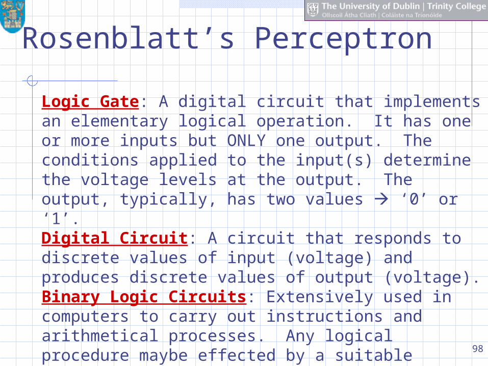
Logic Gate: A digital circuit that implements an elementary logical operation. It has one or more inputs but ONLY one output. The conditions applied to the input(s) determine the voltage levels at the output. The output, typically, has two values ‘0’ or ‘1’.Digital Circuit: A circuit that responds to discrete values of input (voltage) and produces discrete values of output (voltage).Binary Logic Circuits: Extensively used in computers to carry out instructions and arithmetical processes. Any logical procedure maybe effected by a suitable combinations of the gates. Binary circuits are typically formed from discrete components like the integrated circuits.

99


Logic Circuits: Designed to perform a particular logical function based on AND, OR (either), and NOR (neither). Those circuits that operate between two discrete (input) voltage levels, high & low, are described as binary logic circuits.

Logic element: Small part of a logic circuit, typically, a logic gate, that may be represented by the mathematical operators in symbolic logic.

100


Gate Input(s) Output

AND Two

(or more)

High if and only if both (or all) inputs are high.

NOT One High if input low and vice versa

OR Two

(or more)

High if any one (or more) inputs are high

101


Input 1 Input 2 Output0 0 0

0 1 0

1 0 0

1 1 1

The operation of an AND gate

AND (x,y)= minimum_value(x,y);AND (1,0)=minimum_value(1,0)=0;AND (1,1)=minimum_value(1,1)=1

102


A single layer perceptron can carry out a number can perform a number of logical operations which are performed by a number of computational devices.

x 1

x 2

w=+1 1

w=+1 2

w1x1+w2x2+

= 1.5

y=1 if y=0 if

A hard-wired perceptron below performs the AND operation.This is hard-wired because the weights are predetermined and not learnt

103



A learning perceptron below performs the AND operation.

An algorithm: Train the network for a number of epochs(1) Set initial weights w1 and w2 and the threshold θ to set of random numbers; (2) Compute the weighted sum:

x1*w1+x2*w2+ θ (3) Calculate the output using a delta function

y(i)= delta(x1*w1+x2*w2+ θ ); delta(x)=1, if x is greater than zero, delta(x)=0,if x is less than equal to zero

(4) compute the difference between the actual output and desired output:

e(i)= y(i)-ydesired

(5) If the errors during a training epoch are all zero then stop otherwise update

wj(i+1)=wj(i)+ *xj*e(i) , j=1,2

104


A single layer perceptron can carry out a number can perform a number of logical operations which are performed by a number of computational devices:

=0.1Θ=0.2

Epoch

X1

X2

Y desired

InitialW1

Weights

W2

Actual Outpu

t

Error Final W1

Weights

W2

1 0 0 0 0.3 -0.1 0 0 0.3

-0.1

0 1 0 0.3 -0.1 0 0 0.3

-0.1

1 0 0 0.3 -0.1 1 -1 0.2

-0.1

1 1 1 0.2 -0.1 0 1 0.3

0.0

105



Epoch

X1

X2

Ydesired InitialW1

Weights

W2

Actual Outpu

t

Error Final W1

Weights

W2

2 0 0 0 0.3 0.0 0 0 0.3

0.0

0 1 0 0.3 0.0 0 0 0.3

0.0

1 0 0 0.3 0.0 1 -1 0.2

0.0

1 1 1 0.2 0.0 1 0 0.2

0.0

106



Epoch

X1

X2

Ydesired InitialW1

Weights

W2

Actual Outpu

t

Error Final W1

Weights

W2

3 0 0 0 0.2 0.0 0 0 0.2

0.0

0 1 0 0.2 0.0 0 0 0.2

0.0

1 0 0 0.2 0.0 1 -1 0.1

0.0

1 1 1 0.1 0.0 1 1 0.2

0.1

107



Epoch

X1

X2

Ydesired InitialW1

Weights

W2

Actual Outpu

t

Error Final W1

Weights

W2

4 0 0 0 0.2 0.1 0 0 0.2

0.1

0 1 0 0.2 0.1 0 0 0.2

0.1

1 0 0 0.2 0.1 1 -1 0.1

0.1

1 1 1 0.1 0.1 1 0 0.1

0.1

108



Epoch

X1

X2

Ydesired InitialW1

Weights

W2

Actual Outpu

t

Error Final W1

Weights

W2

5 0 0 0 0.1 0.1 0 0 0.1

0.1

0 1 0 0.1 0.1 0 0 0.1

0.1

1 0 0 0.1 0.1 0 0 0.1

0.1

1 1 1 0.1 0.1 1 0 0.1

0.1

109

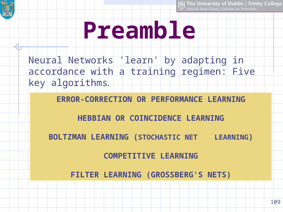
PreambleNeural Networks 'learn' by adapting in accordance with a training regimen: Five key algorithms.

ERROR-CORRECTION OR PERFORMANCE LEARNING

HEBBIAN OR COINCIDENCE LEARNING

BOLTZMAN LEARNING (STOCHASTIC NET LEARNING)

COMPETITIVE LEARNING

FILTER LEARNING (GROSSBERG'S NETS)

110

PreambleNeural Networks 'learn' by adapting in accordance with a training regimen: Five key algorithms.

California sought to have thelicense of one of the largest auditing firms(Ernst & Young) removed because of their rolein the well-publicized collapse of Lincoln Savings& Loan Association. Further, regulatorscould use a bankruptcy

111



However, the single layer perceptron cannot perform the exclusive-OR or XOR operation. The reason is that a single layer perceptron can only classify two classes, say C1 and C2, should be sufficiently separated from each other to ensure the decision surface consists of a hyperplane.

Linearly separable classes

C1C2

C1 C2

Linearly non-separable classes

112


An informal perceptron learning algorithm:•If the perceptron fires when it should not, make each wi smaller by an amount proportional to xi.

•If the perceptron fails to fire when it should fire, make each wi larger by a similar amount.

113

Rosenblatt’s Perceptrons

A neuron learns because it is adaptive: • SUPERVISED LEARNING: The connection strengths of a neuron are modifiable depending on the input signal received, its output value and a pre-determined or desired response. The desired response is sometimes called teacher response. The difference between the desired response and the actual output is called the error signal. • UNSUPERVISED LEARNING: In some cases the teacher’s response is not available and no error signal is available to guide the learning. When no teacher’s response is available the neuron, if properly configured, will modify its weight based only on the input and/or output. Zurada (1992:59-63)

114


jiij

ii

i

ii

xxwdcw

xxwdcw

andxwy

ydr

)]sgn([

)]sgn([

);sgn(

;

t

i

t

i

t

i

Rosenblatt’s perceptrons learn in presence of a teacher. The

desired signal is denoted as di and the output as yi. The error

signal is denoted as ei . The weights are modified in

accordance with the perceptron learning rule; the weight

change is denoted as w which is proportional to the error

signal; c is a proportionality constant:

115


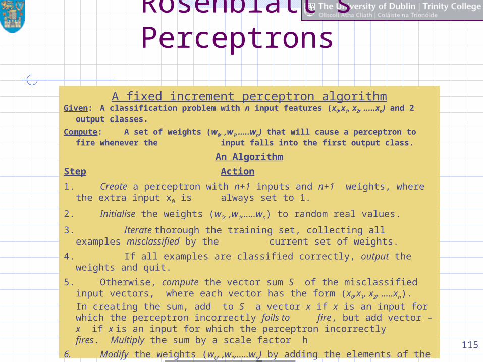
A fixed increment perceptron algorithmGiven: A classification problem with n input features (x0,x1, x2, .....xn) and 2

output classes.

Compute: A set of weights (w0, ,w1,.....wn) that will cause a perceptron to fire whenever the input falls into the first output class.

An Algorithm

Step Action

1. Create a perceptron with n+1 inputs and n+1 weights, where the extra input x0 is always set to 1.

2. Initialise the weights (w0, ,w1,.....wn) to random real values.

3. Iterate thorough the training set, collecting all examples misclassified by the current set of weights.

4. If all examples are classified correctly, output the weights and quit.

5. Otherwise, compute the vector sum S of the misclassified input vectors, where each vector has the form (x0,x1, x2, .....xn). In creating the sum, add to S a vector x if x is an input for which the perceptron incorrectly fails to fire, but add vector -x if x is an input for which the perceptron incorrectly fires. Multiply the sum by a scale factor h

6. Modify the weights (w0, ,w1,.....wn) by adding the elements of the vector S to them. GO TO STEP 3.

116


yj

j

wj1

wj2

wj3

Consider the following set of training vectors x1, x2, and x3, which are to be used in training a Rosenblatt's perceptron, labelled j with the desired responses d1, d2, and d3, and initial weights wj1, wj2, and wj3,

3

2

1

d

d

d

3

2

1

x

x

x

117


The Method:

The Perceptron j has to learn all the three patterns x1, x2, and x3, such that when we show patterns as same as the three or similar patterns the perceptron recognises them.

How will the perceptron indicate that it has recognised the patterns? By responding as d1, d2, and d3, respectively when shown x1, x2, and x3.

We have to show the patterns repeatedly to the perceptron. At each showing (training cycle) the weights change in an attempt to produce the correct desired response.

118


Input Output

X1 X2 Y

0 0 0

0 1 1

1 0 1

1 1 1

Decision line

Denotes 1 Denotes 0

(0,1)

(0,0)

(1,1)

(1,0)

x

x1

Definition of OR

119


Input Output

X1 X2 Y

0 0 0

0 1 0

1 0 0

Decision line

Denotes 1 Denotes 0

(0,1)

(0,0)

(1,1)

(1,0)

x2

x1

Definition of AND

120


Input Output

X1 X2 Y

0 0 0

0 1 1

1 0 1

1 1 0

Decision line #2

Denotes 1 Denotes 0

(0,1)

(0,0)

(1,1)

(1,0)

x2

x1

Decision line #1

Definition of XOR


The XOR ‘problem’ The simple perceptron cannot learn a linear decision

surface to separate the different outputs, because no such decision surface exists.

Such a non-linear relationship between inputs and outputs as that of an XOR-gate are used to simulate vision systems that can tell whether a line drawing is connected or not, and in separating figure from ground in a picture.


The XOR ‘problem’ For simulating the behaviour of an

XOR-gate we need to draw elliptical decision surfaces that would encircle two ‘1’ outputs: A simple perceptron is unable to do so.

Solution? Employ two separate line-drawing stages.


The XOR ‘problem’One line drawing to separate the pattern

where both the inputs are ‘0’ leading to an output ‘0’

and another line drawing to separate the remaining three I/O patternswhere either of the inputs is ‘0’ leading to an output

‘1’where both the inputs are ‘0’ leading to an output ‘0’


The XOR ‘solution’In effect we use two perceptrons to solve the XOR problem: The output of the first perceptron becomes the input of the second.If the first perceptron sees both inputs as ‘1’. it sends a massive inhibitory signal to the second perceptron causing it to output ‘0’.If either of the inputs is ‘0’ the second perceptron gets no inhibition from the first perceptron and outputs 1, and outputs ‘1’ if either of the inputs is ‘1’.


The XOR ‘solution’The multilayer perceptron designed to solve the XOR problem has a serious problem.The perceptron convergence theorem does not extend to multilayer perceptrons. The perceptron learning algorithm can adjust the weights between the inputs and

outputs, but it cannot adjust weights between perceptrons.

For this we have to wait for the back-propagation learning algorithms.

126


•A perceptron computes a binary function of its input. A group of perceptrons can be trained on sample input-output pairs until it learns to compute the correct function.

•Each perceptron, in some models, can function independently of others in the group, they can be separately trained – linearly separable.

•Thresholds can be varied together with weights.

•Given values of x1 and x2 to train such that the perceptron outputs 1 for white dots and 0 for black dots.

127


Rosenblatt’s contribution•What Rosenblatt proved was that if the patterns were drawn from two linearly separable classes, then the perceptron algorithm converges and positions the decision surface in the form of a hyperplane between the two classes the perceptron convergence theorem (Haykin 117).

128


011

101

110

000

2XORX1X2X1X

X1

X2

1

x1

x2

-1.5

1

1

1

x1

x2

-9.0

J(w) = x

xw

If is misclassified as a negative example

xxx

x

If –x is misclassified as a positive example

11

-0.5

J(w) is Called the PerceptronCriterion Function

129

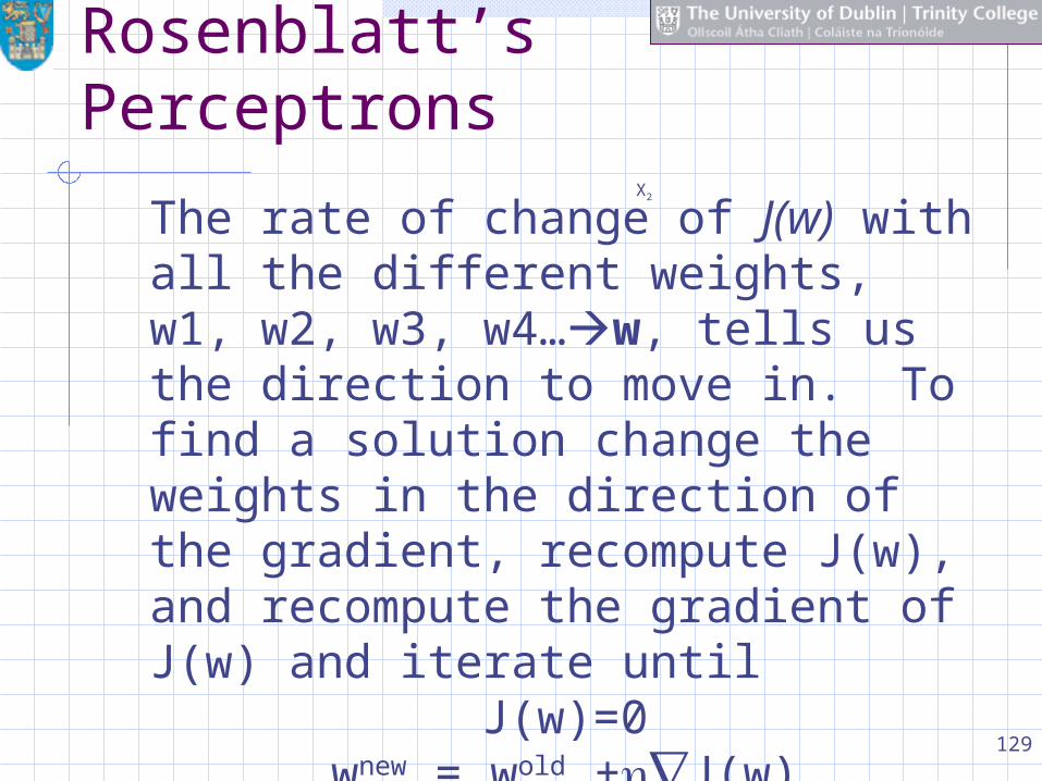
Rosenblatt’s PerceptronsX2

The rate of change of J(w) with all the different weights, w1, w2, w3, w4…w, tells us the direction to move in. To find a solution change the weights in the direction of the gradient, recompute J(w), and recompute the gradient of J(w) and iterate until

J(w)=0wnew = wold +J(w)

130


Multilayer PerceptronThe perceptron built around a single neuron is limited to performing pattern classification with only two classes (hypotheses). By expanding the output (computation) layer of perceptron to include more than one neuron, it is possible to perform classification with more than two classes- but the classes have to be seperable.

131

ANN Learning Algorithms

ENVIRONMENT

LEARNING SYSTEM

Error Signal

Vector describing the environment

Desired response

Actual

Response

- +

TEACHER

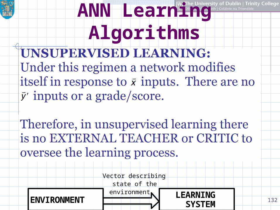
132ENVIRONMENTLEARNING SYSTEM

Vector describing state of the

environment


133


ENVIRONMENT CRITIC

LEARNING SYSTEMActions

State-vector input

Primary Reinforcement

Heuristic Reinforcement

134

Hebbian Learning

DONALD HEBB, a Canadian psychologist, was interested in investigating PLAUSIBLE MECHANISMS FOR LEARNING AT THE CELLULAR LEVELS IN THE BRAIN. (see for example, Donald Hebb's (1949) The Organisation of Behaviour. New York: Wiley)

135

Hebbian Learning

HEBB’s POSTULATE: When an axon of cell A is near enough to excite a cell B and repeatedly or persistently takes part in firing it, some growth process or metabolic changes take place in one or both cells such that A's efficiency as one of the cells firing B, is increased.

136

Hebbian Learning

Hebbian Learning laws CAUSE WEIGHT CHANGES IN RESPONSE TO EVENTS WITHIN A PROCESSING ELEMENT THAT HAPPEN SIMULTANEOUSLY. THE LEARNING LAWS IN THIS CATEGORY ARE CHARACTERIZED BY THEIR COMPLETELY LOCAL - BOTH IN SPACE AND IN TIME-CHARACTER.

137

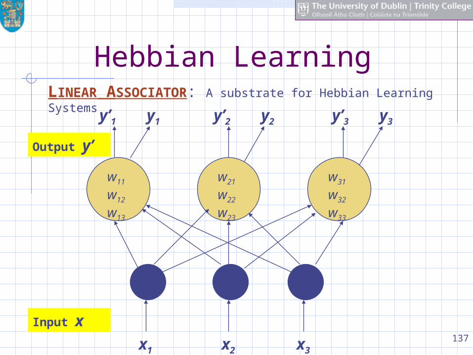
Hebbian Learning

LINEAR ASSOCIATOR: A substrate for Hebbian Learning Systems

x1

Output y’

x2 x3

y1y’1 y2y’2 y3y’3

Input x

w11

w12

w13

w21

w22

w23

w31

w32

w33

138

Hebbian Learning

A simple form of Hebbian Learning Rule

,jkold

jknew

jk xyww

where h is the so-called rate of learning and x and y are the input and output respectively.

This rule is also called the activity product rule.

139

Hebbian Learning

A simple form of Hebbian Learning Rule

x 1,

y 1

x m ,y m

w y 1

x 1

T y 2 x 2

Ty nxnT

If there are "m" pairs of vectors,

to be stored in a network ,then the training sequence will change the weight-matrix, w, from its initial value of ZERO to its final state by simply adding together all of the incremental weight change caused by the "m" applications of Hebb's law:

140

Hebbian Learning

A worked example: Consider the Hebbian learning of three input vectors:

5.1

1

1

0

;

5.1

2

5.0

1

;

0

5.1

2

1

)3()2()1( xxx

in a network with the following initial weight vector:

5.0

0

1

1

w

141

Hebbian Learning


5.1

1

1

0

;

5.1

2

5.0

1

;

0

5.1

2

1

)3()2()1( xxx


5.0

0

1

1

w

142

Hebbian Learning


5.1

1

1

0

;

5.1

2

5.0

1

;

0

5.1

2

1

)3()2()1( xxx


5.0

0

1

1

w

143

Hebbian Learning


5.1

1

1

0

;

5.1

2

5.0

1

;

0

5.1

2

1

)3()2()1( xxx


5.0

0

1

1

w

144

Hebbian Learning

The worked example shows that with discrete f(net) and =1, the weight change involves ADDING or SUBTRACTING the entire input pattern vectors to and from the weight vectors respectively.

Consider the case when the activation function is a continuous one. For example, take the bipolar continuous activation function:

.0

;1)( )*(exp12

where

netf net

145

Hebbian Learning

The worked example shows that with bipolar continuous activation function indicates that the weight adjustments are tapered for the continuous function but are generally in the same direction:

Vector Discrete Bipolar f(net)

Continuous Bipolar f(net)

x(1) 1 0.905

x(2) -1 -0.077

x(3) -1 -0.932

146

Hebbian LearningThe details of the computation for the three steps with a discrete bipolar activation function are presented below in the notes pages. The input vectors and the initial weight vector are:

5.1

1

1

0

;

5.1

2

5.0

1

;

0

5.1

2

1

)3()2()1( xxx

5.0

0

1

1

w

147

Hebbian LearningThe details of the computation for the three steps with a continuous bipolar activation function are presented below in the notes pages. The input vectors and the initial weight vector are:

5.1

1

1

0

;

5.1

2

5.0

1

;

0

5.1

2

1

)3()2()1( xxx

5.0

0

1

1

w

148

Hebbian Learning

Recall that the simple form of Hebbian learning law suggests that the repeated application of the presynaptic signal xj leads to an increase in yk and therefore exponential growth that finally drives the synaptic connection into saturation.

jkjkold

jknew

jk xywww A number of researchers have proposed ways in which such saturation can be avoided. Sejnowski has suggested that

.

&;

),()(

k

j

jkjk

yofvalueaveragedtimethey

xofvalueaveragedtimethex

wherexxyyw

149

Hebbian Learning

The Hebbian synapse described below is said to involve the use of POSITIVE FEEDBACK.

jkjkold

jknew

jk xywww

150

Hebbian Learning

What is the principal limitation of this simplest form of learning?

The above equation suggests that the repeated application of the input signal leads to an increase in , and therefore exponential growth that finally drives the synaptic connection into saturation. At that point of saturation no information cannot be stored in the synapse and selectivity will be lost. Graphically the relationship with the postsynaptic activityis a simple one: it is linear with a slope .

jkjkold

jknew

jk xywww

151

Hebbian Learning

The so-called covariance hypothesis was introduced to deal with the principal limitation of the simplest form of Hebbian learning and is given as

where and denote the time-averaged values of the pre-synaptic and postsynaptic signals.

))(())(()( xnxynynw jkkj

152

Hebbian Learning

If we expand the above equation:

the last term in the above equation is a constant and the first term is what we have for the simplest Hebbian learning rule:

))()()()()( xyxnynxynxnynw kjjkkj

xy

xny

nxy

nwnw

k

j

kjkj SimpleModified

)(

)(

)()(

))(())(()( xnxynynw jkkj

153

Hebbian Learning

Graphically the relationship ∆wij with the postsynaptic activity yk is still linear but with a slope

and the assurance that the straight line curve changes its rate of change at

and the minimum value of the weight change ∆wij is

))(( xnx j

))(( xnx j

y

financial informatics –xiii: neural computing systems

Documents