Neural NetworksMachine Learning and Pattern Recognition

Chris Williams

School of Informatics, University of Edinburgh

October 2014

(These slides have been adapted from previous versions by Charles Sutton, Amos

Storkey and David Barber

1 / 33

Classification Methods So Far

I So far, our classification methods have been linear in theparameters.

I If you want nonlinearity, you have to add it in yourself byadding new features

I Wouldn’t it be nice to learn the features from data?

I One method: artificial neural networks (ANNs)

I We will consider only a particular kind of artificial neuralnetwork, called a feedforward network

2 / 33

Overview

I An artificial neuron

I Multilayer neural networks

I Representation Power of NNs

I Training NNs: Backpropagation

I Applications of Neural Networks

I Reading: Murphy sec 16.5 up to end of 16.5.4

3 / 33

An artificial neuron

x

x

1

D

.

.

.Σ

f(x)

I Take an input vector x = (x1, . . . , xD)T

I Compute the neuron’s activation a = x>w =∑D

d=1 xdwd

(As in linear and logistic regression, we need a bias weight. Soassume xD is always set to 1.)

I Set the neuron output f(x) as a function of its activationf(x) = g(a). For now let’s say

g(a) = σ(a) =1

1 + e−ai.e., logistic sigmoid

I A highly simplified picture of synaptic integration

4 / 33

Why we need multilayer networks

I We haven’t done anything new yet.

I This is just an odd way of presenting logistic regression

I Idea: Use recursion. Use the output of some neurons as inputto another neuron that actually makes the prediction

I Builds an artificial neural network (ANN)

5 / 33

A Slightly More Complex NN: The Units

x

x

1

D

.

.

.Σ

f(x)Σ

Σ

z

z2

1

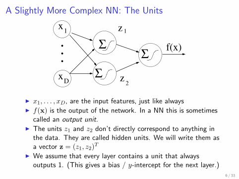
I x1, . . . , xD, are the input features, just like alwaysI f(x) is the output of the network. In a NN this is sometimes

called an output unit.I The units z1 and z2 don’t directly correspond to anything in

the data. They are called hidden units. We will write them asa vector z = (z1, z2)T

I We assume that every layer contains a unit that alwaysoutputs 1. (This gives a bias / y-intercept for the next layer.)

6 / 33

A Slightly More Complex NN: The Weights

x

x

1

D

.

.

.Σ

f(x)Σ

Σ

z

z2

1

I Each unit gets its own weight vector.

I v1 = (v11, . . . , v1D) are the weights for z1.

I v2 = (v21, . . . , v2D) are the weights for z2.

I w = (w1, w2) are the weights for the output unit.

I Use θ = (v1,v2,w) to refer to all of the weights stacked intoone vector.

7 / 33

A Slightly More Complex NN: Prediction

x

x

1

D

.

.

.Σ

f(x)Σ

Σ

z

z2

1

Here is how to compute a class label in this network:

1. z1 ← g(vT1 x) = g(

∑Dd=1 v1dxd)

2. z2 ← g(vT2 x) = g(

∑Dd=1 v2dxd)

3. f(x)← g(wT z) = g(w1z1 + w2z2)4. If f(x) > 0.5, assign to class 1, otherwise assign to class 0.

8 / 33

NN for Regression

x

x

1

D

.

.

.Σ

f(x)Σ

z

z2

1

Σ

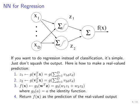
If you want to do regression instead of classification, it’s simple.Just don’t squash the output. Here is how to make a real-valuedprediction:

1. z1 ← g(vT1 x) = g(

∑Dd=1 v1dxd)

2. z2 ← g(vT2 x) = g(

∑Dd=1 v2dxd)

3. f(x)← g3(wT z) = g3(w1z1 + w2z2)where g3(a) = a the identity function.

4. Return f(x) as the prediction of the real-valued output9 / 33

x

x

1

D

.

.

.Σ

f(x)Σ

Σ

z

z2

1

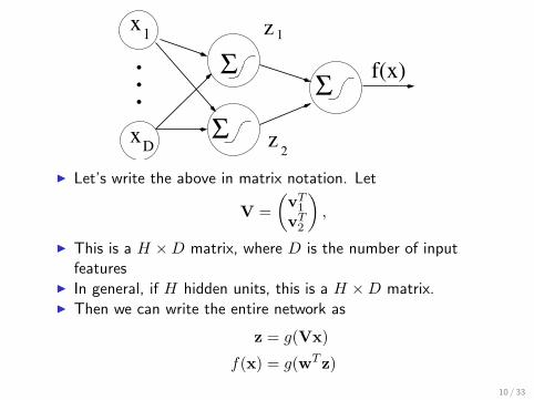
I Let’s write the above in matrix notation. Let

V =(vT

1

vT2

),

I This is a H ×D matrix, where D is the number of inputfeatures

I In general, if H hidden units, this is a H ×D matrix.I Then we can write the entire network as

z = g(Vx)

f(x) = g(wT z)

10 / 33

You can have more hidden layers and more units. An examplenetwork with 2 hidden layers

. . .

. . .

. . .

hidden layer 1

hidden layer 2

output layer

input layer (x)

11 / 33

I There can be an arbitrary number of hidden layers

I The networks that we have seen are called feedforwardbecause the structure is a directed acyclic graph (DAG).

I Each unit in the first hidden layer computes a non-linearfunction of the input x

I Each unit in a higher hidden layer computes a non-linearfunction of the outputs of the layer below

12 / 33

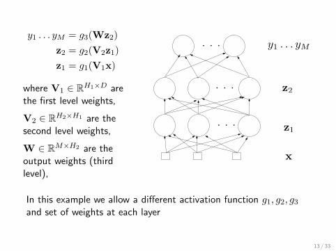
y1 . . . yM = g3(Wz2)z2 = g2(V2z1)z1 = g1(V1x)

where V1 ∈ RH1×D arethe first level weights,

V2 ∈ RH2×H1 are thesecond level weights,

W ∈ RM×H2 are theoutput weights (thirdlevel),

. . .

. . .

. . .

hidden layer 1

hidden layer 2

output layer

input layer (x)x

z1

z2

y1 . . . yM

In this example we allow a different activation function g1, g2, g3and set of weights at each layer

13 / 33

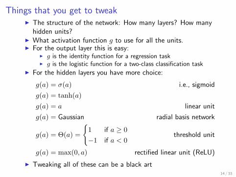
Things that you get to tweakI The structure of the network: How many layers? How many

hidden units?I What activation function g to use for all the units.I For the output layer this is easy:

I g is the identity function for a regression taskI g is the logistic function for a two-class classification task

I For the hidden layers you have more choice:

g(a) = σ(a) i.e., sigmoid

g(a) = tanh(a)g(a) = a linear unit

g(a) = Gaussian radial basis network

g(a) = Θ(a) =

{1 if a ≥ 0−1 if a < 0

threshold unit

g(a) = max(0, a) rectified linear unit (ReLU)

I Tweaking all of these can be a black art14 / 33

Representation Power of NNs

For Boolean functions, i.e., x’s and y always binary:

I Every boolean function can be represented by network withsingle hidden layer

I but might require exponentially many (in number of inputs)hidden units

I To see why, consider the truth table representation of theboolean function

15 / 33

Representation Power of NNs

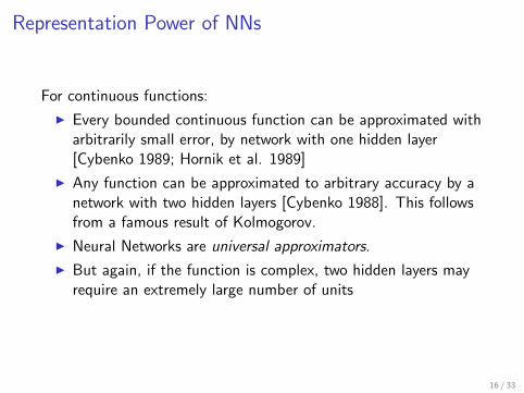
For continuous functions:

I Every bounded continuous function can be approximated witharbitrarily small error, by network with one hidden layer[Cybenko 1989; Hornik et al. 1989]

I Any function can be approximated to arbitrary accuracy by anetwork with two hidden layers [Cybenko 1988]. This followsfrom a famous result of Kolmogorov.

I Neural Networks are universal approximators.

I But again, if the function is complex, two hidden layers mayrequire an extremely large number of units

16 / 33

ANN predicting 1 of 10 vowel sounds based on formats F1 andF2Figure from Mitchell (1997)

9 / 26

Limitations of Representation Power Results

� The fact that a function is representable does not tell ushow many hidden units would be required for itsapproximation

� Nor does it tell us if it is learnable (a search problem)� Nor does it say anything about how much training data

would be needed to learn the function� In fact universal approximation has only a limited benefit:

need bias

10 / 26

Training ANNs

� As in linear and logistic regression, we create an errorfunction that measures the agreement of the target y(x)and the prediction f (x)

� Linear regression, squared error: E =�n

i=1(yi − f (xi))2

� Logistic regression (0/1 labels):E =

�ni=1 yi log f (xi) + (1− yi) log(1− f (xi))

� These are both related to the log likelihood of the dataunder the relevant model

� For linear and logistic regression the optimization problemfor w had a unique optimum; this is no longer the case forANNs (e.g. hidden layer neurons can be permuted)

11 / 26

Backpropagation

� As discussed for logistic regression, we need the gradientof E wrt all the parameters w, i.e. g(w) = ∂E

∂w� This is in fact an exercise in using the chain rule to

compute derivatives; for ANNs this is given the namebackpropagation

� We make use of the layered structure of the net tocompute the derivatives, heading backwards from theoutput layer to the inputs

� Once you have g(w), you can use your favouriteoptimization routines to minimize E ; see discussion ofgradient descent and other methods in Logistic Regressionslides

� It can make sense to use a regularization penalty (e.g.λ|w|2) to help control overfitting

12 / 26

NN predicting 1 of 10 vowel sounds based on formats F1 and F2Figure from Mitchell (1997)

17 / 33

Training NNs

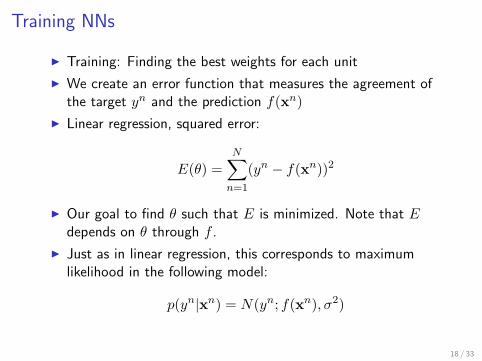
I Training: Finding the best weights for each unit

I We create an error function that measures the agreement ofthe target yn and the prediction f(xn)

I Linear regression, squared error:

E(θ) =N∑

n=1

(yn − f(xn))2

I Our goal to find θ such that E is minimized. Note that Edepends on θ through f .

I Just as in linear regression, this corresponds to maximumlikelihood in the following model:

p(yn|xn) = N(yn; f(xn), σ2)

18 / 33

Training for Classification

I Logistic regression (0/1 labels): minimize a different errorfunction:

E(θ) = −N∑

n=1

yn log f(xn)− (1− yn) log(1− f(xn))

I Again minimize with respect to θ

I If more than two classes, use softmax

19 / 33

Local Minima

I For linear and logistic regression the optimization problem forw had a unique optimum; this is no longer the case for NNs(e.g. hidden layer neurons can be permuted).

I Example: Take a one-layer network for regression

f(x) = Wz

z = g1(Vx)

with g1(x) = σ(x) the sigmoid function. Rememberσ(−x) = 1− σ(x).

I Set V′ = −V and W′ so that W′z = (1−Wz)I Then using W′,V′ yields the same predictions as W, V. If

one is a local minimum, so is the other.

20 / 33

Local Minima (Example 2)

I Example two: Permute the meanings of the hidden units, i.e.,permute the rows of V while permuting the rows of W tomatch.

I These local minima all make the same predictions.

I There are other local minima that do worse than the optimalvalue of θ.

I And there is not really any way of telling one kind ofminimum from the other.

21 / 33

Backpropagation

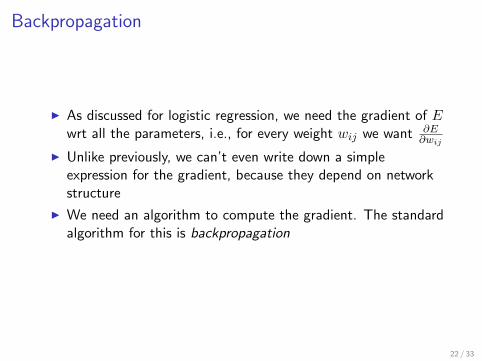
I As discussed for logistic regression, we need the gradient of Ewrt all the parameters, i.e., for every weight wij we want ∂E

∂wij

I Unlike previously, we can’t even write down a simpleexpression for the gradient, because they depend on networkstructure

I We need an algorithm to compute the gradient. The standardalgorithm for this is backpropagation

22 / 33

Backpropagation

I There is a clever recursive algorithm for computing thederivatives. It uses the chain rule, but stores someintermediate terms. This is called backpropagation.

I We make use of the layered structure of the net to computethe derivatives, heading backwards from the output layer tothe inputs

I Once you have g(θ), you can use your favourite optimizationroutines to minimize E.

23 / 33

Backpropagation. It’s the Chain Rule.I Consider the simple network

f(x) = wT z

z = g1(Vx)

with g1(a) = σ(a) the sigmoid and the error function(negative log likelihood)

E =N∑

n=1

(yn − f(xn))2

Let’s compute the derivative ∂E∂wj

.

∂E

∂wj= −2

N∑n=1

(yn − f(xn))∂f(xn)∂wj︸ ︷︷ ︸

This is the chain rule.

= −2N∑

n=1

(yn − f(xn)) zj

24 / 33

Backpropagation. It’s the Chain Rule.

f(x) = wT z

z = g1(Vx)

I with g1(a) = σ(a) the sigmoidI To get the vjk derivatives, we propagate twice:

∂E

∂vjk= −2

N∑n=1

(yn − f(xn))∂f(xn)∂vjk

I For this one we need

∂f(xn)∂vjk

=∂f(xn)∂zj

∂zj∂vjk

= wj∂

∂vjk

[σ(vT

j x)]

= wjσ(vTj x)(1− σ(vT

j x))xk

= wjzj(1− zj)xk25 / 33

Backpropagation. It’s the Chain Rule.

I The full derivative

∂E

∂wj= −2

N∑n=1

(yn − f(xn)) zj

∂E

∂vjk= −2

N∑n=1

(yn − f(xn))wjzj(1− zj)xk

I If we had three layers, the derivatives would get longer. Wecould work backward through the network, cachingintermediate results. Hence the name.

I To compute these, we run the network “forward” to get f(x)and z, then run a “backward pass” where we compute all ofthe gradients

I If there are multiple output notes the notation gets slightlymore complicated (see the book) but it’s the same idea.

26 / 33

Why is backpropagation clever?

I What’s so special about this algorithm? It’s just the chainrule of derivatives.

I Well, here’s a generic way to compute ∂E∂wjk

for every weight.

Just use the definition from calculus:

∂E

∂wjk≈ 1ε

(E(θ + ε∆jk)− E(θ)),

where ∆jk is a weight vector that has a weight of 1 inposition jk and 0 everywhere else.

I This is called numerical differentiation.

I Each time we call E, we need to compute the output of thenetwork f(xn). So this naive algorithm calls f many times: 2times the number of weights, just to get one gradient.

I The backpropagation algorithm gets the whole gradient atonce, using roughly the same amount of time as 2 calls to f .

27 / 33

Dealing with Local Minima in Training

I Neural network training finds only a local minimum, asdescribed before.

I Common solution: Train multiple nets from different startingplaces, and then choose best (or combine in some way)

I Initialize weights near zero; therefore, initial networks arenear-linear

I Increasingly non-linear functions possible as training progresses

28 / 33

Bayesian training of Neural Networks

0 0.5 1

−2

−1

0

1

2

input, xf(x

)

I Prior p(θ)I Can understand the effect of p(θ) by looking at sample

functions from the prior

I Approximations for the posterior and making predictions, e.g.Gaussian approximation, Markov chain Monte Carlo (see later)

I p(w|D) ∝ exp(−βE(w)), so local minima in error functionare local maxima in the posterior

29 / 33

Training NNs: Summary

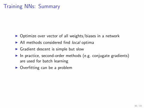
I Optimize over vector of all weights/biases in a network

I All methods considered find local optima

I Gradient descent is simple but slow

I In practice, second-order methods (e.g. conjugate gradients)are used for batch learning

I Overfitting can be a problem

30 / 33

Applications of Neural Networks

In general, neural networks are most commonly used for domainswhere we really need to do feature construction, because theoriginal features are not directly informative about y.

I Recognizing handwritten digits on cheques and post codes(LeCun and Bengio, 1995)

I Used by the US Postal Service to process handwritten letters

I Visual object classification (Krizhevsky et al, 2012; “deep”neural network)

I Financial forecasting

I Speech recognition

I Language modelling: Given a partial sentence “Neuralnetworks are”, predict the next word (Bengio et al, 2003)

They are less common for domains like text because word identityis already a really good feature. There are exceptions.

31 / 33

Convolutional NNs

Convolutional neural nets: apply same filters at different locations;later subsample responses over some region

INPUT 32x32

Convolutions SubsamplingConvolutions

C1: feature maps 6@28x28

Subsampling

S2: f. maps6@14x14

S4: f. maps 16@5x5

C5: layer120

C3: f. maps 16@10x10

F6: layer 84

Full connectionFull connection

Gaussian connections

OUTPUT 10

Figure credit: Murphy Fig 16.14

32 / 33

NNs: Summary

I Artificial neural networks are a powerful nonlinear modellingtool for classification and regression

I These were never very good models of the brain. But aspredictors they work.

I The hidden units are new representation of the original input.Think of this as learning the features

I Trained by optimization methods making use of thebackpropagation algorithm to compute derivatives

I Local optima in optimization are present, cf linear and logisticregression.

I Ability to automatically discover useful hidden-layerrepresentations

33 / 33