neural coding of leg proprioception in...

Article

Neural Coding of Leg Prop
rioception in Drosophila
Graphical Abstract

Highlights

d Proprioceptors in the fly leg encode tibia position,movement,

and vibration

d Proprioceptor axons are organized topographically in the fly

ventral nerve cord

d Genetic tools subdivide proprioceptors that encode distinct

kinematic features

d Single proprioceptors are tuned to specific joint angles and

vibration frequencies

Mamiya et al., 2018, Neuron 100, 1–15November 7, 2018 ª 2018 Elsevier Inc.https://doi.org/10.1016/j.neuron.2018.09.009

Authors

Akira Mamiya, Pralaksha Gurung,

John C. Tuthill

[email protected]

In Brief

Proprioception, the internal sense of

body position and movement, is essential

for adaptive motor control. Mamiya et al.

use in vivo calcium imaging to reveal the

functional tuning and spatial organization

of proprioceptors that monitor the femur-

tibia joint of the Drosophila leg.

mailto:tuthill@uw.�edu

https://doi.org/10.1016/j.neuron.2018.09.009

Please cite this article in press as: Mamiya et al., Neural Coding of Leg Proprioception in Drosophila, Neuron (2018), https://doi.org/10.1016/j.neuron.2018.09.009

Neuron

Article

Neural Coding of Leg Proprioception in DrosophilaAkira Mamiya,1 Pralaksha Gurung,1 and John C. Tuthill1,2,*1Department of Physiology and Biophysics, University of Washington, Seattle, WA 98195, USA2Lead Contact

*Correspondence: [email protected]://doi.org/10.1016/j.neuron.2018.09.009

SUMMARY

Animals rely on an internal sense of body positionand movement to effectively control motor behavior.This sense of proprioception is mediated by diversepopulations of mechanosensory neurons distributedthroughout the body. Here, we investigate neuralcoding of leg proprioception in Drosophila, usingin vivo two-photon calcium imaging of propriocep-tive sensory neurons during controlled movementsof the fly tibia. We found that the axons of leg propri-oceptors are organized into distinct functional pro-jections that contain topographic representations ofspecific kinematic features. Using subclass-specificgenetic driver lines, we show that one group of axonsencodes tibia position (flexion/extension), anotherencodes movement direction, and a third encodesbidirectional movement and vibration frequency.Overall, our findings reveal how proprioceptive stim-uli from a single leg joint are encoded by a diversepopulation of sensory neurons, and provide a frame-work for understanding how proprioceptive feed-back signals are used bymotor circuits to coordinatethe body.

INTRODUCTION

Proprioception, the internal sense of body position and move-

ment (Sherrington, 1906), is essential for the neural control of

motor behavior. Sensory feedback from proprioceptive sen-

sory neurons (i.e., proprioceptors) contributes to a wide range

of behaviors, from regulation of body posture (Hasan and

Stuart, 1988; Zill et al., 2004) to locomotor adaptation (Bidaye

et al., 2018; Lam and Pearson, 2002) and motor learning

(Isakov et al., 2016; Takeoka et al., 2014). But despite the

fundamental importance of proprioception to our daily experi-

ence, it is perhaps the most poorly understood of the primary

senses.

Proprioceptors are found in nearly all motile animals, from pu-

bic lice (Graber, 1882) to sperm whales (Sierra et al., 2015). Sin-

gle-unit electrophysiological recordings have revealed that pro-

prioceptors can vary widely in their mechanical sensitivity and

stimulus tuning, even within a single limb segment or muscle.

For example, most vertebrate muscles contain two distinct clas-

ses of proprioceptive organs that are innervated by specialized

sensory neurons: muscle spindles detect muscle length and

contraction velocity, while Golgi tendon organs detect mechan-

ical load (Proske and Gandevia, 2012; Windhorst, 2007). Insects

also possess proprioceptor subclasses that encode joint posi-

tion, velocity, and load (Burrows, 1996; Tuthill and Wilson,

2016a), suggesting that the nervous systems of invertebrates

and vertebrates may have arrived at similar evolutionary solu-

tions to a set of common sensorimotor constraints (Tuthill and

Azim, 2018).

Although individual proprioceptors may be narrowly tuned,

most body movements are likely to drive activity in large

numbers of proprioceptors (Proske and Gandevia, 2012; Zill

et al., 2004). Characterizing the population-level structure of pro-

prioceptive encoding has been challenging, due to the technical

difficulty of recording from multiple neurons simultaneously, or

identifying the same neurons across individuals. It has also

been difficult to identify spatial structure or topography within

proprioceptive populations from recordings of single neurons.

However, a detailed understanding of proprioceptive population

coding is important for understanding the function of down-

stream circuits and identifying the role of proprioceptive feed-

back in the neural control of movement.

Here, we combine genetic tools, two-photon calcium imag-

ing, and a magnetic leg control system to study the anatomy

and function of a proprioceptor population from the leg of

the fruit fly, Drosophila. Embedded within the femur of the in-

sect leg is a cluster of proprioceptor cell bodies known collec-

tively as the femoral chordotonal organ (FeCO; Field and Math-

eson, 1998). Experimental manipulation of the FeCO in locusts

and stick insects has revealed a critical role for these proprio-

ceptors during behaviors that require precise control of leg

position, such as walking (B€assler, 1988) and targeted reach-

ing (Page and Matheson, 2009). Single-unit electrophysiolog-

ical recordings in these larger insect species have found that

FeCO neurons monitor the position and movement of the fe-

mur-tibia joint, and that FeCO neurons may be narrowly tuned

to specific kinematic features (Field and Pfl€uger, 1989; Hof-

mann et al., 1985; Kondoh et al., 1995; Matheson, 1990,

1992; Stein and Sauer, 1999; Zill, 1985). However, it has

been challenging to integrate data from single neurons to un-

derstand the population-level structure and function of the

leg proprioceptive system. In Drosophila, where genetic tools

enable systematic dissection of neuronal populations, the

anatomy and physiology of FeCO neurons have not previously

been investigated.

Using in vivo population-level calcium imaging of FeCO axons

during controlled leg manipulations, we first mapped the spatial

organization of proprioceptive signals in the fly ventral nerve

Neuron 100, 1–15, November 7, 2018 ª 2018 Elsevier Inc. 1

mailto:[email protected]


500 μm

insectpin

femur

tibia

tarsus

magnet

0°0°

180°180°

90°

flexionextension

extension

flexion

pixel correlations after clustering

corr

elat

ion

0

180

femoral chordotonal

organ (FeCO)

femur

tibia

20 μm

10 μm

90

300 %200 %200 %200 %

fem

ur-ti

bia

angl

e (°

)

3 sec

A

D

F G

HE

C

1.0

0

-1.0

100 μm

iav-Gal4(GGaMP6f)

iav-Gal4(GFP)

FeCO axonsin VNC

T1

T2

T3

ΔF/F

magnet

servo motor

two-photonmicroscope

camera

fly holder

pin

prismpiezo

B

brainprothoracic

leg (T1)

VNC

iav-Gal4(GFP)

Figure 1. Investigating Proprioceptive Tuning of the Drosophila FeCO

(A) A confocal image of the front (T1) leg of Drosophila melanogaster, showing the location of the FeCO cell bodies and dendrites (green). Magenta is auto-

fluorescence from the cuticle.

(B) An experimental setup for two-photon calcium imaging from the axons of FeCO neurons while controlling and tracking the femur-tibia joint. To control joint

angle, we glued a pin to the tibia and positioned it using a magnet mounted on a servo motor. In vibration trials, we vibrated the tibia with a piezoelectric crystal

fixed to the magnet. We backlit the tibia with an IR LED and recorded the tibia position from below using a prism and high-speed video camera.

(C) An example frame from a video used to track joint angle. The pin is painted black to enhance the contrast against the background.

(D) FeCO axon terminals (green) in the fly ventral nerve cord (VNC). Magenta is a neuropil stain (nc82). Teal box indicates region imaged by the two-photon

microscope.

(E) Two-photon image of FeCO axon terminals expressing GCaMP6f driven by iav-Gal4. The teal box indicates the region imaged in the example recording shown

in (G) and (H).

(F) A cross-correlation matrix showing pixel-to-pixel correlations of the changes in GCaMP6f fluorescence (DF/F) during the example trial shown in (G) and (H).

Left: the cross-correlation matrix before correlation-based clustering. Right: the matrix after clustering. The colors on the right of the correlation matrix corre-

spond to the cluster colors used in (G) and (H).

(G) Image of GCaMP6f fluorescence showing the recording region for the example trial shown in (F) and (H). Each group of pixels is shaded according to its cluster

identity. The colors correspond to the DF/F traces shown in (H).

(H) Calcium signals from different clusters of pixels during an example trial. Each trace shows the changes in GCaMP6f fluorescence (DF/F) for the groups of

pixels shaded with the same color in the (G).

See also Figure S1.


cord (VNC). We then identified genetically and anatomically

distinct FeCO subclasses that encode specific kinematic fea-

tures, including position, movement direction, and vibration fre-

quency. Overall, our results reveal the basic architecture and

neural code for a key leg proprioceptive system in Drosophila.

These findings provide a foundation for understanding how

specialized proprioceptive feedback signals enable robust and

accurate motor control.

2 Neuron 100, 1–15, November 7, 2018

RESULTS

Methods to Record and Map Proprioceptive Signals inDrosophila

Positioned in the proximal femur of each Drosophila leg is a

femoral chordotonal organ (FeCO) that contains �135 cell

bodies (Figure 1A). The dendrites of the FeCO neurons are con-

nected to the cuticle and surrounding muscles by attachment


cells and tendons (Shanbhag et al., 1992), and the axons of

FeCO neurons project through the leg nerve into the VNC (Phillis

et al., 1996; Smith and Shepherd, 1996). Most FeCO axons

arborize within the VNC neuropil, with only 3–4 cells from each

leg projecting directly to the brain (Figures 1A and 1D) (Tsubou-

chi et al., 2017).

To investigate proprioceptive signal encoding of the FeCO

population, we recorded the activity of proprioceptor axons

while manipulating the joint angle between the femur and tibia

of the fly’s right front leg (Figures 1B and 1C; Video S1). We

chose to control leg kinematics, rather than force, because

biomechanical studies have found that chordotonal neurons

directly monitor joint displacement (Field and Matheson, 1998).

For fast and accurate positioning of the leg, we designed a mag-

netic control system that allowed us to manipulate a pin glued to

the fly’s tibia using a servo-actuated magnet (Figure 1B). This

system allowed us to reproduce the range of tibia positions

and speeds observed in walking flies (see STAR Methods for

details). The femur and proximal leg joints were fixed to the fly

holder with UV-cured glue. We continuously recorded the posi-

tion of the tibia using an IR-sensitive video camera (Figure 1C)

and automatically tracked its orientation to calculate the

femur-tibia joint angle. We used the Gal4-UAS system (Brand

and Perrimon, 1993) to express a genetically encoded calcium

indicator, GCaMP6f (Chen et al., 2013), in the majority of FeCO

neurons (iav-Gal4; Kwon et al., 2010) and recorded their calcium

activity in vivo with two-photon calcium imaging (Figure 1B).

To identify proprioceptor projections with shared functional

tuning, we first recorded calcium activity of FeCO axons as we

swung the tibia from flexion to extension at 360�/s (Figures

1F–1H). To categorize calcium activity in an unbiased manner,

we then calculated pairwise correlations between the calcium

signal (DF/F) in each pixel and performed k-means clustering

on the resulting correlation matrix. Figure 1F shows an example

of a pixel correlation matrix before and after clustering. In this

trial, we identified four groups of pixels whose activity was highly

correlated (for details about how the number of clusters was

selected, see Figure S1A). Although this correlation-based clus-

tering does not impose any spatial restrictions, we found that the

pixels that clustered together based on their activity were also

grouped together spatially (Figures 1G and 1H). This example

illustrates that clustering of pixel correlations is sufficient to iden-

tify groups of FeCO axons that encode distinct proprioceptive

stimulus features.

Functional Organization of FeCO Axons in the Fly VNCTo identify functional subclasses within the FeCO population,

we recorded calcium signals from four regions of interest that

encompassed the different axon projections in the VNC (Figure 2;

Video S2). For these experiments, we first clustered similarly

responding pixels within each trial to identify the different

response classes. Then, we combined the responses recorded

from the same region in different flies and again grouped them

using correlation-based k-means clustering (Figures 2A–2D,

middle columns).

We identified five basic subclasses of responses within the

FeCOaxons: two tonic (non-adapting)and threephasic (adapting).

Pixels that responded tonically increased their activity when the

tibia was either flexed (red) or extended (blue). Phasic pixels

increased their activity transiently during the movement phase of

the swing stimulus; one group responded with relatively similar

amplitudes to movements in either direction (green, direction

selectivity index [DSI] = 0.222 ± 0.027; mean ± SEM; n = 29

clusters from 22 flies), while the two other groups responded in a

more directionally selective manner to either flexion (orange,

DSI=0.494±0.039; n=19clusters from17flies) or extension (pur-

ple, DSI =�0.493 ± 0.036; n = 29 clusters from 22 flies). We found

the same basic response subclasseswhenwe repeated this anal-

ysis on swing movements in the opposite direction (compare Fig-

ures2andS1B).Each responsesubclasswasconsistently located

in similar positions across multiple flies (Figures 2A–2D, right col-

umns, and Figures S2B and S2C). The time courses of FeCO cal-

cium signals were also more similar within a response subclass

than across subclasses (Figure S2A). Overall, these results indi-

cate that FeCO neurons that encode distinct kinematic features

(i.e., tibia position, movement, and direction) are grouped into

functional projections within the VNC.

Specific Genetic Driver Lines Delineate Club, Claw, andHook ProprioceptorsPopulation-level imaging from FeCO neurons with a broad driver

line (iav-Gal4) revealed that different axon projections have

distinct proprioceptive tuning and are systemically organized

across flies (Figure 2). We next sought to identify more specific

Gal4 driver lines that would provide a genetic handle for these

functional subclasses and enable more fine-grained analysis of

proprioceptor anatomy and function. We screened through

Gal4 lines in the Janelia FlyLight collection (Jenett et al., 2012)

for lines that drove expression in each axon projection. From

this screen, we identified three Gal4 lines that labeled the cardi-

nal FeCO axon projections (Figure 3). Although we will focus on

the front legs in this study, each driver line labels similar axons in

all three VNC segments (Figure S3).

The first driver line (R64C04-Gal4) labels axons that run later-

ally through the center of the leg neuropil and form an arboriza-

tion in the shape of a club (Figure 3A, 2nd column). Themajority of

the club axons terminate near the midline, although some also

project toward the brain or other VNC segments. The second

line (R73D10-Gal4) labels a group of axons shaped like a claw

(club/claw nomenclature from Phillis et al., 1996). Upon entering

the VNC from the leg nerve, this projection splits into three

smaller branches (Figure 3A, 3rd column). We refer to these as

the X, Y, and Z branches: the X branch of the claw continues

to run parallel to the club, while the Y branch projects anteriorly,

and the Z branch projects dorsally. The third line (R21D12-Gal4)

labels axons that project along the Z branch of the claw, with only

a small protuberance along the Y branch, and extend a longer

arborization toward the midline, just anterior to the club (Fig-

ure 3A, 4th column). We call this projection the hook due to its

resemblance to a lumberjack’s peavey hook.

To characterize the anatomy of single neurons within each

driver line, we used the multicolor FlpOut technique (Nern

et al., 2015) to stochastically label single cells, and manually

traced their morphology (Figure 3B). Every neuron we traced

from the claw Gal4 line (n = 3 cells from 3 flies) had a similar

morphology, including projections to all three branches (X, Y,

Neuron 100, 1–15, November 7, 2018 3

180

3 secMLA

P

600 %400 %300 %300 %200 %

BA

C D

femur-tibia angle (°)

180

0

0

ΔF/F180

0

representative ROIs calcium signals spatial layout

180

0

5-5

5

-5 μm

10 μm

iav-Gal4(GGaMP6f)

5-5

5

5-5

5

5-5

5

-5 μm

-5 μm-5 μm

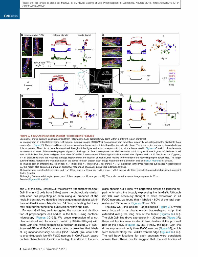
Figure 2. FeCO Axons Encode Distinct Proprioceptive Features

Each panel shows calcium signals recorded from FeCO axons (UAS-GCamp6f; iav-Gal4) within a different region of interest.

(A) Imaging from an anterolateral region. Left column: example images of GCaMP6f fluorescence from three flies. In each fly, we categorized the pixels into three

clusters (as in Figure 1F). The red and blue regions are tonically active when the tibia is flexed (red) or extended (blue). The green region responds phasically during

tibia movement. The color scheme is maintained throughout the figure and also corresponds to the color scheme used in Figures 1G and 1H. A white cross

represents the center of the recording region, aligned to the long axis of each axon projection. Middle column: calcium signals for each group of pixels recorded

from multiple flies. Red, blue, and green lines show GCaMP6f fluorescence (DF/F) during the trial for each cluster of pixels (red, n = 10 flies; blue, n = 10; green,

n = 9). Black lines show the response average. Right column: the location of each cluster relative to the center of the recording region across flies. The larger

outlined circles represent the mean location of the center for each cluster. Each image was rotated to a common axis (see STAR Methods for details).

(B) Imaging from an anteromedial region (red, n = 11 flies; blue, n = 11; green, n = 10; orange, n = 10). In addition to the three response subclasses we identified in

(A), this region also contained a group of pixels that responded phasically during tibia extension (orange).

(C) Imaging from a posterolateral region (red, n = 10 flies; blue, n = 10; purple, n = 8; orange, n = 9). Here, we identified pixels that responded phasically during joint

flexion (purple).

(D) Imaging from a medial region (green, n = 10 flies; purple, n = 11; orange, n = 10). The scale bar in the center image represents 20 mm.

See also Figures S1 and S2.


and Z) of the claw. Similarly, all the cells we traced from the hook

Gal4 line (n = 2 cells from 2 flies) were morphologically similar,

with each cell projecting an axon along all branches of the

hook. In contrast, we identified three uniquemorphologies within

the club Gal4 line (n = 14 cells from 14 flies), indicating that there

may exist further functional subdivisions within the club.

For each Gal4 line, we investigated the number and distribu-

tion of proprioceptor cell bodies in the femur using confocal

microscopy (Figures 3C–3E). We drove expression of a nu-

clear-localized red fluorescent protein (UAS-RedStinger) with

each Gal4 line, while expressing a nuclear-localized GFP (Lex-

Aop-nlsGFP) in all FeCO neurons using a LexA line that labels

all leg mechanosensory neurons (ChAT-LexA). (We were able

to unambiguously identify FeCO neurons in ChAT-LexA based

on their characteristic location in the leg.) In addition to the sub-

4 Neuron 100, 1–15, November 7, 2018

class-specific Gal4 lines, we performed similar co-labeling ex-

periments using the broadly expressing line iav-Gal4. Although

iav-Gal4 was previously thought to drive expression in all

FeCO neurons, we found that it labeled �80% of the total pop-

ulation (�135 neurons; Figures 3F and 3G).

The claw Gal4 line labeled �20 cell bodies (Figure 3F), which

were located in a characteristic blade-shaped strip that

extended along the long axis of the femur (Figures 3C–3E).

The club Gal4 line drove expression in �30 neurons (Figure 3F);

these cell bodies were located in two clusters at the proximal

part of the FeCO (Figures 3C–3E). Finally, the hook Gal4 line

drove expression in only three FeCO neurons (Figure 3F), which

were located along the FeCO’s ventral edge (Figures 3C–3E).

The cell body locations for each subclass were consistent

across flies. These results suggest that the cell bodies of

0

40

80

120

# of

cel

ls c

ount

ed in

leg

broad (iav-Gal4) hook (R21D12-Gal4)A

B

C

D

E

F

iavcla

wclu

bhook

all (ChAT)

G

axon

s of

all

neur

ons

in V

NC

axon

s of

si

ngle

neu

rons

cell

bodi

es

in fe

mur

ChA

Tco

-labe

ling

rota

ted

view

H

10 μm

0

0.5

1

# of

cel

ls c

ount

ed fr

om

Gal

4 dr

iver

/ C

hAT-

LexA

iavcla

wclu

bhook

claw (R73D10-Gal4)club (R64C04-Gal4)

50 μm

clubclawhook

50 μm

peripheralFeCO

organization

I

clubclawhook

Figure 3. Organization of Genetically Defined FeCO Neuron Subclasses in the VNC and Leg

(A) Four Gal4 lines label subsets of FeCO axons in the VNC. Green, GFP driven by each Gal4 line; magenta, nc82 neuropil staining. Scale bar, 50 mm.

(B) Example morphologies of single FeCO neurons driven by each Gal4 line, traced from images obtained by stochastic labeling with the multi-color FlpOut

technique. Dotted lines indicate severed axons.

(C) FeCO cell bodies are clustered in characteristic locations in the fly leg. Cell bodies were labeled with UAS-Redstinger driven by each Gal4 line. Scale

bars, 10 mm.

(D) Co-labeling of FeCO cell bodies from each Gal4 line (as in C), with a green reference marker that labels all FeCO neurons (ChAT-Lexa; LexAop-nlsGFP).

(E) Same as (D) but viewed from the dorsal side.

(F) Number of neurons labeled by each Gal4 line shown in (A). Circles are individual flies; lines indicate the mean (iav, n = 6 flies; club, n = 5; claw, n = 4; hook, n = 2;

ChAT, n = 19).

(G) Ratio of neurons labeled by each Gal4 line to those labeled by ChAT-LexA in the same leg.

(H) In silico overlay of the axon projections of the club, claw, and hook neurons in the VNC.

(I) A schematic of the FeCO in the femur, showing the location of cell bodies labeled by each Gal4 line.

See also Figure S3.


FeCO neurons with distinct central projections are grouped in

specific locations in the FeCO (Figure 3I). Although these three

Gal4 lines label less than half of the total FeCO neuron popula-

tion, computational registration to a standard VNC confirmed

that these three subclasses span the cardinal FeCO projections

labeled by iav-Gal4 (Figure 3H).

Calcium Imaging from Specific Gal4 Lines Shows thatPosition, Movement, and Direction Are Encoded bySeparate Proprioceptor SubclassesWe next performed calcium imaging from the claw, club, and

hook neurons (Figures 4 and S4; Video S3). Claw neurons

increased their activity tonically in response to either flexion or

Neuron 100, 1–15, November 7, 2018 5

tip middle

claw(R73D10-Gal4)

club(R64C04-Gal4)

hook(R21D12-Gal4)

X

Y

Z

tip

middle

tipY

Z

20 μm

1800

1800

ΔF/F300 %300 %300 %600 %3 sec

A

B

C

Z

1800

tip

1800

Y

1800

Z

1800

X

1800

10 μm

1800

Y


Figure 4. Three Gal4 Lines Delineate FeCO Functional Subclasses(A) Claw neurons encode tibia position, with distinct pixels responding to either flexion (red) or extension (blue). Left: the claw axon projection in the VNC

visualized with GCaMP6f fluorescence driven by R73D10-Gal4. White rectangles represent the imaging locations for the X, Y, and Z branches shown in the right

three columns. In each column, the top image shows a representative region of interest, with flexion-encoding pixels shaded in red, extension encoding pixels

in blue. The Y branch is rotated 90� clockwise. The bottom rows show changes in GCaMP6f fluorescence relative to the baseline (DF/F) recorded from each

sub-region in different flies (n = 10 flies for each region). Thick black lines represent average responses.

(B) Same as (A), but for movement-sensitive club neurons (R64C04-Gal4). The club neurons respond phasically to both flexion and extension of the joint (n = 14

flies for tip, 11 flies for middle).

(C) Same as (A) and (B), but for directionally tuned hook neurons (R21D12-Gal4). The hook neurons respond phasically to flexion of the joint, but not extension

(n = 14 flies for tip and Z, 9 flies for Y).

See also Figures S4 and S5.


extension of the tibia (Figure 4A). Each branch of the claw axon

projection had two sub-branches that responded either to

flexion or extension, which we identified with the clustering

methods described above (Figure 4A). The time courses of these

responses were similar across the X, Y, and Z branches of the

claw (Figures 4A and S5A). Given that single claw neurons inner-

vate all three branches (Figure 3B), these data suggest that the

6 Neuron 100, 1–15, November 7, 2018

claw subclass can be further subdivided into separate groups

of cells that encode either tibia flexion or extension. The spatial

organization and functional tuning of claw neurons were also

consistent with the position-tuned tonic responses recorded

from population imaging (Figure 2).

Calcium signals in club axons increased phasically during both

flexion and the extension of the tibia (Figure 4B). The amplitude


and time course of these calcium signals were similar during

extension and flexion (DSI = 0.117 ± 0.022; mean ± SEM;

n = 25 regions from 15 flies), and across different regions of

the club (Figures 4B and S5A). These results are consistent

with population imaging data (Figure 2), although the weaker di-

rection selectivity of the club neurons labeled by a specific driver

line (Figure 4B) suggests that the bidirectional clusters identified

from population imaging may have been partly contaminated by

axons from directionally selective (e.g., hook) neurons.

The axons of hook neurons increased their activity phasically

during tibia flexion, but responded only weakly during extension

(DSI = 0.811 ± 0.028; mean ± SEM; n = 37 regions from 23 flies;

Figure 4C). We recorded from three different locations along the

hook axon projection and found that the responses were similar

in all three locations (Figures 4C and S5A). The time courses of

these responseswere similar to those of the flexion-tuned phasic

responses we observed in population-imaging experiments (Fig-

ure 2). Again, the greater direction selectivity of neurons labeled

with a specific driver line (Figure 4C) suggests that the cluster

identified from population imaging (Figure 2) may have been

partly contaminated by nearby axons from non-directionally se-

lective or weakly directionally selective (e.g., club) neurons.

Together, our experiments imaging from claw-, club-, and

hook-specific Gal4 drivers reveal that these lines label distinct

proprioceptor subclasses that encode different stimulus fea-

tures. The response tuning of each subclass was similar for

swing stimuli in the opposite direction (extension followed by

flexion; Figure S4). These resultsmatch the functional and spatial

organization we observed in population imaging experiments

with a broad driver line (Figure 2), indicating that they represent

major FeCO subclasses. The only response subclass that we

failed to identify with a specificGal4 linewas the extension-tuned

complement of the hook neurons (orange traces in Figure 2).

Based on the location of extension-tuned pixels in population im-

aging experiments, we expect these neurons to have similar

morphology and projections to the flexion-tuned hook neurons.

Next, we will use a broader range of proprioceptive stimuli to

characterize the encoding properties of each proprioceptor sub-

class in more detail.

Claw Neurons Encode Tibia Position, Club NeuronsEncode Bidirectional Tibia Movement, and HookNeurons Encode Directional Tibia MovementWe used ramp-and-hold stimuli to more comprehensively

explore the position-dependent tuning of each proprioceptor

subclass (Figure 5). The tibia started at either a flexed (�18�) orextended (�180�) position, then moved in 18� steps to the oppo-

site position. Claw neurons responded to these stimuli with tonic

increases in calcium during either flexion (red) or extension (blue)

of the tibia (Figure 5A). We identified flexion- and extension-

tuned pixels using the same clustering methods that we used

for population imaging (Figures 1 and 2). The responses within

these two regions were highly position-dependent: the activity

of extension-tuned pixels increased when the tibia was between

90� and 180�, while the activity of flexion-tuned pixels increased

when the tibia was between �90� and 18�. Neither group was

active in the middle of the joint range, close to 90�. Overall, the

activity of claw neurons increased as a relatively linear function

of the femur-tibia joint angle, although we observed some direc-

tional hysteresis (see below).

Club neurons responded phasically to each tibia movement,

regardless of movement direction (Figure 5B). Movement re-

sponses occurred across the joint angle range but were slightly

larger around 90� and smaller at full extension (180�). In addition

to these bidirectional responses to movement steps, we occa-

sionally observed tonic responses during the hold period,

possibly due to low-amplitude vibrations of the tibia (Figure 6).

These results confirm that club neurons respond to bidirectional

tibia movement.

Hook neurons phasically increased their activity during tibia

flexion, but not extension (Figure 5C). Similar to the club neurons,

hook responses were slightly weaker at fully extended positions.

Phasic responses to tibia movement decayed rapidly, and we

never observed tonic activity during the hold period. Overall,

we found that hook neurons are directionally selective and

encode flexion movements of the tibia.

To analyze the position dependence of claw neurons in more

detail, we measured steady-state calcium activity at the end of

each hold period (Figure 5D, inset) as a function of the femur-tibia

angle (Figure 5D). To compare activity across flies, we normal-

ized the response amplitudes from each fly with the largest

steady-state response recorded in that fly. The position tuning

of claw neurons was relatively consistent across flies (Figure 5D)

and branches of the claw. However, we did observe differences

in claw position tuning across stimuli. For the flexion-activated

branch, steady-state activity at each position (0�–90�) was larger

when the tibia was flexed compared to when it was extended.

On the other hand, extension-activated branch showed larger

steady-state activity (at 90�–180� range) during extension

compared to flexion. (Figures 5D and 5E). This phenomenon,

commonly referred to as hysteresis, would introduce ambiguity

for downstream neurons trying to decode absolute leg angle.

We did not observe directional hysteresis in the movement-

tuned claw or hook neurons.

For movement-sensitive club and hook neurons, we also

examined velocity tuning using swing stimuli across a range of

speeds (100–800�/s). Because the amplitude of calcium signals

reflects the integration of electrical activity over time, we

compared the maximum slope of the calcium signals at different

tibia movement speeds (Figure S5B). For club neurons, the slope

of the calcium signal peaked around 400�/s and decayed slightly

at higher speeds (Figure S5B). In contrast, the slope of the cal-

cium signal in hook neurons was similar across the entire speed

range we tested (Figure S5B). These results suggest that in addi-

tion to their direction selectivity, club and hook neuronsmay also

differ in their velocity sensitivity.

Club Axons Respond to Low-Amplitude Vibrations of theTibia and Contain a Spatial Map of FrequencyWhile imaging from club neurons, we occasionally observed sus-

tained bursts of axonal calcium following a ramp movement of

the tibia. We hypothesized that these variable signals were

caused by spontaneous leg movements below the spatial reso-

lution of our leg imaging system (3.85 mm/pixel). Indeed, previous

recordings in other insects have shown that FeCO neurons can

be sensitive to low-amplitude vibrations (Field and Pfl€uger,

Neuron 100, 1–15, November 7, 2018 7

claw: X branch

club: tip

hook: Y branch ΔF/F400 %400 %200 %300 %10 sec

10 μm

A

B

C


norm

aliz

ed s

tead

y st

ate

ampl

itude

D E

180

0

0.5

1

0 90 180

0

0.5

1

0 90

0

180

flexion extension flexion

flexion

extension

0

180

0

180

flexion

extension

50°

200%ΔF/F

steadystate

hyst

eres

is

0 90 180

0.2

0

-0.2

-0.4

extension

femur-tibiaangle (°)

Figure 5. Claw Neurons Encode Joint Position, Club Neurons Encode Bidirectional Movements, and Hook Neurons Encode Movement Di-

rection

(A) Responses of position-encoding claw neurons (R73D10-Gal4) to ramp-and-hold stimuli. Left column: averageGCaMP6f fluorescence from the X branch of the

claw projection where the example recordings were made (red, flexion encoding; blue, extension encoding). Middle column: responses from the two regions to a

ramp-and-hold stimulus that starts with the joint extended (n = 10 flies). Right column: same as above but starting with the joint flexed. The gray rectangle in-

dicates the location of the trace shown in the top inset in (D).

(B) Same as (A), but for club neurons (R64C04-Gal4), which increase their activity phasically in response to each step (n = 14 flies).

(C) Same as (A) and (B), but for hook neurons (driven by R21D12-Gal4), which only respond during flexion (n = 9 flies).

(D) Calcium signals of claw neurons depend on movement history. Left column: steady-state DF/F at different joint angles for the flexion activated (red, during

flexion; black, during extension; thick lines, average response) sub-branches of the claw, normalized by the maximum peak response recorded in each fly (n = 10

flies). Steady-state responses were measured at the end of the hold step (top inset at right). In these recordings, flexion preceded extension. Right column: same

as the left column but for the extension activated (blue, during extension; black, during flexion; thick lines, average response) sub-branches of the claw (n = 10

flies). In these recordings, extension preceded flexion.

(E) Hysteresis (difference between the response to the activating direction and the non-activating direction) of the steady-state response for flexion (red) and

extension (blue) activated sub-branches of the claw (thick lines, average response; shading, SEM).

8 Neuron 100, 1–15, November 7, 2018


300

0 ΔF/F

(%)

0.9 μmmagnet piezoelectric

crystal

200 Hz 400 Hz 800 Hz 1600 Hz100 Hz 2000 Hz

0.9 μmamplitude

0.054 μmamplitude

5 s

200%

ΔF/

F

100 200 400 800 1600 2000

club:tip claw: X branch hook: Y branch

150

100 200 400 800 1600 2000 100 200 400 800 1600 2000

aver

age ΔF

/F (%

)

100 Hz200 Hz400 Hz800 Hz1600 Hz2000 Hz

X

10 μm

club: tip

300

200

100

0

piezo vibration frequency (Hz)

0.9 μm amplitude0.054 μm amplitude

0 ΔF/F

(%)

10 μm

10 μm

A

B

C D

E

FG

0

0.2

0.4

0.6

0.8

1

200 Hz

400 Hz

800 Hz

1600 Hz

2000 Hz

norm

aliz

ed Δ

F/F

0 5-5distance from center (μm)

anteromedial posterolateral

0 0

2.5 μm

400 Hz

0.9 μmamplitude

0.054 μmamplitude

0.054 μm amplitude

post

piezovibrationfrequency

Figure 6. A Map of Vibration Frequency in the Axons of Club Neurons

(A) To vibrate the fly’s tibia, we attached one side of a piezoelectric crystal to a magnet and the other to a post fixed to a servo motor. The magnet was placed

directly onto a pin glued to the tibia (see Figure S6 for details).

(B) Average GCaMP6f fluorescence from an example recording location, at the tip of the club axons (R64C04-Gal4).

(C) An example time course of the club’s response (DF/F) to a 400 Hz, 0.9 mm vibration of the magnet. We averaged the activity level in a 1.25 s window (indicated

by a darker gray shading) starting from 1.25 s after the stimulation onset, and used it as a measure of response amplitude in (D) and as activity maps in (E).

(D) Only club neurons respond reliably to the vibration stimulus. Plots show the activity of different subsets of FeCO axons in response to tibia vibrations at

different frequencies and amplitudes. Each line represents an average response from one fly.

(E) Example DF/F maps of GCaMP6f fluorescence at the tip of the club in response to tibia vibration at different frequencies and amplitudes. For both amplitudes,

the responding regions shifted from the anterolateral side to the posteromedial side of the axon projection as stimulation frequency increased.

(F) A map of vibration frequency in club axon terminals. Smaller empty circles with different shades of red (0.9 mm amplitude) or gray (0.054 mm amplitude)

represent the location of the weighted center of the responding region in different flies (n = 14 flies for both amplitudes). Larger outlined circles represent the

average location. The blue line represents the best fit line to the average locations across frequencies. We rotated the images from each fly to match the

orientation of the example images shown in (E).

(G) Distribution of activity (DF/F) along the anterolateral to posteromedial axis (blue lines in F) of the club axons during tibia vibration. Signals were normalized by

the maximum average activity during each stimulus in that fly. Responses shifted from the anterolateral to posteromedial side as vibration frequency increased.

See also Figure S6


1989; Stein and Sauer, 1999). To test this hypothesis, we used a

piezoelectric chip to vibrate the magnet in a sinusoidal pattern

(peak-to-peak amplitude 0.9 or 0.054 mm) at different fre-

quencies (100–2,000 Hz) (Figure 6A) and recorded calcium sig-

nals from club, claw, and hook neurons (see Figure S6 for piezo

calibration details).

Club neurons exhibited large, sustained calcium signals to

tibia vibration (Figure 6). An example trace in Figure 6C shows

the response of club axons to 4 s of a 400 Hz vibration stimulus.

Claw and hook neurons did not respond to these stimuli (Fig-

ure 6D). To examine frequency tuning of club neurons, we aver-

aged the calcium signal across the stimulus period (darkly

Neuron 100, 1–15, November 7, 2018 9


shaded region in Figure 6C) and compared responses across

different frequencies and amplitudes formultiple flies (Figure 6D).

For the larger amplitude stimulus (0.9 mm), the club neurons

showed significant responses at all frequencies, peaking at

400 Hz (Figure 6D, red). The responses to the smaller amplitude

vibration stimulus (0.054 mm) were slightly weaker and peaked at

800 Hz (Figure 6D, black).

When we examined the distribution of calcium signals during

tibia vibration, we noticed a consistent spatial shift in activity

as a function of vibration frequency (Figure 6E). Specifically,

the center of the calcium response moved from anterolateral to

the posteromedial side of the club axon projection as frequency

increased (Figure 6F). This shift was clearly visible in DF/F maps

of the club axons for both large- (0.9 mm) and small- (0.054 mm)

amplitude vibrations (Figure 6E). The frequency map was also

consistent across flies (Figure 6F).

The spatial maps in Figure 6F are not merely due to additional

axons being recruited at higher frequencies. When we plotted

the average activity along the anterolateral to posteromedial

axis of the club axon projection for each fly, we found a signifi-

cant shift in the entire response distribution as vibration fre-

quency increased (Figure 6G). This effect was larger for smaller

vibrations (0.054 mm), perhaps due to the saturation of calcium

signals during higher amplitude vibrations (0.9 mm). Overall, our

imaging data reveal the existence of a frequency map within

the axon terminals of club proprioceptors.

Frequency and Position Tuning of Single Club and ClawNeuronsUsing driver lines that label subsets of FeCO neurons, we iden-

tified three proprioceptor subclasses that encode distinct kine-

matic features: tibia position (claw), directional movement

(hook), and bidirectional movement/vibration (club). However,

two of these subclasses, the club and claw, are each composed

of more than 20 neurons. Are cells within each subclass tuned to

detect the same stimulus features, or do different cells detect

different features? Imaging from 20–30 overlapping axons is

likely to obscure fine-scale differences in stimulus tuning across

neurons. Therefore, we sought to characterize the responses of

individual club and claw neurons.

We used a FlpOut approach to stochastically express

GCamp6f in single club and claw axons, and imaged their re-

sponses to swing, ramp-and-hold, and vibration stimuli (Fig-

ures 7 and S7). As we observed when imaging from the entire

subclass (Figures 4 and 5), single club neurons responded to

tibia movement in a bidirectional manner (Figure 7B; DSI =

0.179 ± 0.042; n = 13 cells from 9 flies) and increased their ac-

tivity in response to tibia vibration (Figures 7C and 7D). In addi-

tion, we found that single club neurons were tuned to different

vibration frequencies—for example, one cell’s peak response

(DF/F) occurred at 200 Hz, while another cell responded maxi-

mally at 1,600 Hz (Figure 7D). In cases in which two club neu-

rons were labeled from the same leg, the more posterior axon

was tuned to a lower frequency than the anterior axon (Fig-

ure S7A). This suggests that the axonal map of vibration fre-

quency we describe above (Figures 6E–6G) is comprised of

anatomically and functionally distinct club neurons tuned to

specific frequency bands.

10 Neuron 100, 1–15, November 7, 2018

We also recorded calcium activity from single claw neurons

(Figures 7E–7G). Each cell responded to either flexion or exten-

sion, but not both, consistent with the results we obtained by

clustering across multiple claw neurons (Figures 4 and 5). How-

ever, single claw neurons were tuned to more specific femur-

tibia angles—for example, one cell’s response peaked at 70�

and decreased at more flexed angles, while a second cell re-

sponded maximally at the most flexed position (20�) (Figure 7H).

These results indicate that different claw neurons encode

different tibia positions. Thus, calcium signals recorded from

the entire claw subclass (Figure 5) likely reflect the sum of activity

across FeCO neurons tuned to a narrower range of tibia

positions.

DISCUSSION

In this study, we used in vivo calcium imaging to investigate

the population coding of leg proprioception in the FeCO of

Drosophila. Our results reveal a basic logic for proprioceptive

sensory coding: genetically distinct proprioceptor subclasses

detect and encode distinct kinematic features, including tibia po-

sition, directional movement, and vibration. The cell bodies of

each proprioceptor subclass reside in separate parts of the

FeCO in the leg, and their axons project to distinct regions of

the fly VNC. This organization suggests that different kinematic

features may be processed by separate downstream circuits,

and function as parallel feedback channels for the neural control

of leg movement and behavior.

Neural Representation of Tibia PositionClaw neurons encode the position of the tibia relative to the fe-

mur. Specifically, each branch consists of two sub-branches,

whose calcium signals increase when the tibia is flexed or

extended (Figure 5). Imaging from single claw neurons revealed

that individual cells can be narrowly tuned to even more specific

tibia angles (Figure 7). These data are consistent with previous

reports of angular range fractionation in the locust FeCO (Math-

eson, 1992). Interestingly, we observed minimal activity in claw

axons when the tibia was close to 90� (Figure 5), and we did

not find any single claw neurons tuned to this range in our limited

sample (Figure 7). Similar tuning distributions have been

observed in multiunit recordings from the FeCO of locusts and

stick insects (Burns, 1974; Usherwood et al., 1968). However,

single-unit recordings from these species also revealed the exis-

tence of a small number of position-tuned cells with peak activity

in this middle range (Hofmann et al., 1985; Matheson, 1990,

1992). It is possible that the driver lines we used did not label

the FeCO neurons tuned to this range. It is also possible that

this represents a real difference between Drosophila and other

insects. The fly FeCO has about half as many neurons as that

of the stick insect and locust, and the biomechanics of the

organ may also differ between species (Field, 1991; Shanbhag

et al., 1992).

How does the position tuning of claw neurons relate to natural

leg kinematics? When a fly is standing still, the tibia of the front

leg rests �90� relative to the femur; during straight walking, the

tibia flexes to �40� and extends to 120� (unpublished data).

Thus, we predict that claw neurons are largely silent in a

100 200 400 800 1600 2000

aver

age ΔF

/F (%

)

piezo vibration frequency (Hz)

A B C D

0

200

400

600

20 μmclub: FLP out

claw: FLP out 20 μm

femur-tibia angle (°)180

0

180

0

180

0

ΔF/F200 %

3 sec

ΔF/F200 %200 %

3 sec

ΔF/F300 %300 %

10 sec


norm

aliz

ed s

tead

y s

tate

am

plitu

de

180

0

0.5

1

0 90flexion

extension

0.9 μm

3 s

300%

ΔF/

F

400 Hz

E F G H

Figure 7. Calcium Imaging from Single FeCO Axons Reveals Narrow Tuning of Club and Claw Neurons

(A) GCamp6f fluorescence in a single club neuron (R64C04-Gal4), imaged with a two-photon microscope.

(B) Single club neurons respond to swing movements of the tibia in both directions (flexion and extension). Each trace indicates the average response of one club

axon (n = 13 cells from 9 flies).

(C) Single club neurons respond to tibia vibration. Each trace is the average response of one axon (n = 12 cells from 7 flies). The stimulus duration is indicated by

light gray shading.

(D) Frequency tuning of club neurons is diverse. Each line represents an average response from one neuron. We averaged the activity level in a 1.25 s window

(indicated by the darker gray shading in C) starting from 1.25 s after the stimulation onset.

(E) GCamp6f fluorescence in a single claw axon (R73D10-Gal4).

(F) Single claw neurons encode either flexion or extension. Each trace shows the average calcium signal from a single claw axon (n = 5 cells from 5 flies, indicated

by different colors).

(G) Position tuning of single claw neurons. Each trace shows average calcium responses to ramp-and-hold movement of the tibia.

(H) Single claw neurons encode different tibia angles. Each line indicates steady-state activity at different joint angles for the claw neurons shown in (F) and (G),

normalized by the maximum response of each cell. Steady-state responses were measured at the end of the hold step, as in Figure 5D. To remove the effect of

hysteresis, we plotted the responses during flexion for the flexion-activated neurons (red) and during extension for the extension activated neurons (blue).

See also Figure S7.


stationary fly, while extension- and flexion-tuned neurons are

rhythmically active during walking. Encoding deviations from

the natural resting position may reflect an adaptive strategy to

minimize metabolic cost.

Position-encoding claw neurons exhibit response hysteresis:

both flexion- and extension-tuned sub-branches of the claw

showed larger steady-state activity when the tibia is moved in

a direction that increases their activity (Figure 5). This response

asymmetry is notable because it presents a problem for down-

stream circuits and computations that rely on a stable readout

of tibia angle. Proprioceptive hysteresis has also been described

in vertebrate muscle spindles (Wei et al., 1986) and FeCO neu-

rons of other insects (Matheson, 1992). One possible solution

for solving the ambiguities created by hysteresis would be to

combine the tonic activity of claw neurons with signals from di-

rectionally selective hook neurons (Figures 4 and 5). This could

allow a neuron to decode tibia position based on past history

of tibia movement. However, it is also possible that tibia angle

hysteresis is a useful feature of the proprioceptive system, rather

than a bug. For example, it has been proposed that hysteresis

could compensate for the nonlinear properties of muscle activa-

tion in short sensorimotor loops (Zill and Jepson-Innes, 1988).

Neural Representation of Tibia Movement/VibrationWe identified two functional subclasses of FeCO neurons that

respond phasically to tibia movement. Club neurons respond

to both flexion and the extension of the tibia, while hook neurons

respond only to flexion (Figures 4 and 5). In both population (Fig-

ure 2) and single neuron (Figure S7) imaging experiments, we

also observed directionally selective responses to tibia exten-

sion, although we were unable to identify a specific Gal4 line

for this response subclass. The movement sensitivity of the

club and hook neurons resembles that of other phasic proprio-

ceptors, including primary muscle spindle afferents (Jones

et al., 2001), and movement-tuned FeCO neurons recorded in

the locust and stick insect (Hofmann et al., 1985; Matheson,

1990, 1992). Although the slow temporal dynamics of GCaMP6f

did not permit a detailed analysis of velocity tuning, our results

indicate that FeCO neurons respond to the natural range of

leg speeds encountered during walking (Mendes et al., 2013;

Neuron 100, 1–15, November 7, 2018 11


Pereira et al., 2018; Wosnitza et al., 2013). In the future, it will be

interesting to investigate how FeCO neurons encode leg move-

ments during walking, and how active movements may be en-

coded differently from passive movements, for example through

presynaptic inhibition of FeCO axon terminals (Wolf and Bur-

rows, 1995).

In addition to their directional tuning, we found that club and

hook neurons differ in their sensitivity to fast (100–2,000 Hz),

low-amplitude (0.9–0.054 mm) tibia vibration. Club neurons are

strongly activated by vibration stimuli, but hook neurons are not

(Figure 6). This difference in vibration sensitivity is not likely to

be caused by a difference in velocity tuning because these differ-

ences are relatively small at the range of the speeds experienced

during tibia vibration (Figure S5B). Rather, it seems that the club

neurons have a lower mechanical threshold and/or may be more

sensitive to the constant acceleration produced by vibration.

The functional role of vibration-sensitive FeCO neurons is not

entirely clear. Previous studies in stick insects and locusts have

found that vibration-tuned FeCO neurons do not contribute to

postural reflexes in the same manner as FeCO neurons tuned

to joint position and directional movement (Field and Pfl€uger,

1989; Kittmann and Schmitz, 1992; Stein and Sauer, 1999).

This raises the possibility that vibration-tuned chordotonal neu-

rons sense external mechanosensory stimuli. For example,

club neurons could monitor substrate vibrations in the environ-

ment, which serve as an important communication signal for

many insect species (Hill and Wessel, 2016). Abdominal vibra-

tions produced during courtship by male Drosophila coincide

with pausing behavior in females, and hence increased recep-

tivity to copulation (Fabre et al., 2012). These vibrations occur

at frequencies that match the sensitivity of club neurons

(200–2,000 Hz; C. Fabre, personal communication). Therefore,

club neurons are well-positioned to mediate intraspecific vibra-

tory communication during courtship or other behaviors.

Stereotypic Spatial Organization of Leg ProprioceptorsUsing genetic driver lines for specific FeCO neuron subclasses,

we provide the first detailed anatomical characterization of

Drosophila leg proprioceptors. Our anatomy and imaging exper-

iments revealed a systematic relationship between the functional

tuning of proprioceptor subclasses and their anatomical struc-

ture. The cell bodies of the three proprioceptor subclasses are

clustered in different regions of the femur, an organization that

may reflect biomechanical specialization for detecting position,

movement, and vibration. Proprioceptor axons then converge

within the leg nerve, before branching within the VNC to form

subclass-specific projections that we call the club, claw, and

hook (Figures 2, 3, and 4). We found that this organization is

highly stereotyped across flies.

The axons of claw neurons split into three symmetric

branches, resembling a claw. This unique arborization pattern

is suggestive of a Cartesian coordinate system; for example,

each branch could represent a different spatial axis. However,

we found that each claw neuron innervates all three branches,

and that the X, Y, and Z branches all encode the same stimuli.

Specifically, our calcium imaging experiments revealed that

each claw branch is divided into two sub-branches that

are specialized for encoding flexion or extension of the tibia (Fig-

12 Neuron 100, 1–15, November 7, 2018

ures 2 and 4). If each claw branch is functionally similar, what is

the purpose of this tri-partite structure? Each branch may target

different downstream neurons, or could be independently modu-

lated by presynaptic inhibition. Interestingly, the axons of direc-

tionally tuned hook neurons arborized alongside the claw but did

not innervate all three of the claw branches. Thus, the X, Y, and Z

branches may facilitate integration of positional information with

directionally tuned movement signals.

We were surprised to discover a topographic map of leg vibra-

tion frequency within the axon terminals of club neurons. This

structure has not previously been described in flies, but resem-

bles the tonotopic map of sensory afferents in the cricket audi-

tory system (Oldfield, 1983; Romer, 1983) or the cochlear nu-

cleus in vertebrates (Cohen and Knudsen, 1999). Interestingly,

the spatial layout of the frequencymap in club axons was consis-

tent across different vibration amplitudes, despite a shift in the

peak frequency tuning curve (Figure 6). Recordings from single

club neurons suggest that this frequency map is comprised of

individual axons that are each tuned to a narrow frequency

band (Figures 7 and S7). An orderly map of vibration frequency

could facilitate feature identification in downstream circuits, for

example through lateral inhibition between neighboring axons

with shared tuning (Suga, 1989).

Comparison with Other Sensory SystemsNeurons in the FeCO population can be generally classified as

either tonic (position-encoding) or phasic (movement-encoding).

This division has been observed among proprioceptors of many

animals, including other insects (Hofmann et al., 1985;Matheson,

1990; Zill, 1985), crustaceans (Burke, 1954), and mammals

(Proske and Gandevia, 2012). For example, mammalian muscle

spindles are innervated by both phasic (Group 1a) and tonic

(Group II) afferents (Boyd, 1980). The same has been found in

other primarymechanosensory neurons, including touch (Abraira

and Ginty, 2013; Burrows and Newland, 1997; Juusola and

French, 1998), hearing (Kamikouchi et al., 2009;Kiang, 1965;Yor-

ozu et al., 2009), and vestibular (Cullen, 2011; Fox et al., 2010) af-

ferents. The ubiquity of tonic and phasic neurons suggests that

these two parallel information channels are essential building

blocks of sensory circuits. Now that we have identified genetic

tools thatdelineate tonicandphasicneurons in theproprioceptive

system of Drosophila, these circuits have the potential to provide

general insights into the utility of this sensory coding strategy.

Flies possess other chordotonal organs: themost well-studied

is the Johnston’s organ (JO), which detects antennal movements

produced by near-field sound, wind, gravity, and touch (Albert

and Gopfert, 2015; Matsuo and Kamikouchi, 2013). Unlike the

FeCO, the JO monitors rotation of a body segment that is not

actively controlled by muscles or coupled to the substrate. The

JO is also much larger (�500 versus �135 neurons). Despite

these differences, the coding schemes of the two mechanosen-

sory organs share some key similarities. JO neurons can be clas-

sified into tonic and phasic classes (Kamikouchi et al., 2009; Yor-

ozu et al., 2009), some exhibit direction selectivity (Patella and

Wilson, 2018), and their axon terminals form a rough tonotopic

map of frequency (Patella and Wilson, 2018). The FeCO and

JO share genetic and developmental homology (Eberl and

Boekhoff-Falk, 2007), which suggests that mechanosensory


specialization in these organs could arise through similar molec-

ular or biomechanical mechanisms.

SummaryWith the advent of new methods for simultaneously monitoring

the activity of hundreds or thousands of neurons (Ahrens et al.,

2013; Mann et al., 2017; Sofroniew et al., 2016), a critical chal-

lenge has been to link the activity of large neuronal populations

to the underlying diversity of specific cell types (Alivisatos

et al., 2013). Previous efforts have used statistical methods to

compare the responses of single neurons to simultaneous opti-

cal (Tsodyks et al., 1999) or electrophysiological (Okun et al.,

2015) population recordings. Here, we took a different approach,

which took advantage of the fact that neurons in the fly can be

reliably identified across individuals. We first used two-photon

imaging to monitor activity across a population of proprioceptive

sensory neurons during controlled leg movements. From this

population data, we identified spatially distinct axon branches

that encode specific proprioceptive stimulus features. We then

searched for genetic driver lines that specifically labeled each

axon branch and further characterized their functional tuning

with targeted calcium imaging. With this approach, we were

able to identify and characterize the major neuronal subclasses

in a key proprioceptive organ.

With a genetic handle on position, movement, and direction

pathways, it should now be possible to trace the flow of proprio-

ceptive signals into downstream circuits and to identify the func-

tional role of specific proprioceptor subclasses within the broader

context of motor control and behavior. We anticipate that

Drosophilawill provide a useful complement toothermodel organ-

isms indissecting fundamentalmechanismsofproprioceptionand

deepening our understanding of this mysterious ‘‘sixth sense.’’

STAR+METHODS

Detailed methods are provided in the online version of this paper

and include the following:

d KEY RESOURCES TABLE

d CONTACT FOR REAGENT AND RESOURCE SHARING

d EXPERIMENTAL MODEL AND SUBJECT DETAILS

d METHOD DETAILS

B Fly preparation for in vivo two-photon calcium imaging

of FeCO axons

B Image acquisition using a two-photon excitation mi-

croscope

B Moving the tibia/pin using a magnetic control system

B Tracking the femur-tibia joint angle

B Vibrating the tibia using a piezoelectric crystal

B Immunohistochemistry and anatomy

d QUANTIFICATION AND STATISTICAL ANALYSIS

B Image processing, K-means clustering of the re-

sponses, and analyses of clustered responses

B Analysis of the spatial organization of each

response class

B Analyzing frequency tuning within the club axon pro-

jection

d DATA AND SOFTWARE AVAILABILITY

SUPPLEMENTAL INFORMATION

Supplemental Information includes seven figures, one table, and three videos

and can be found with this article online at https://doi.org/10.1016/j.neuron.

2018.09.009.

ACKNOWLEDGMENTS

We thank Eiman Azim, Richard Mann, Jim Truman, Julijana Gjorgjieva, Caro-

line Fabre, and members of the Tuthill laboratory for helpful discussions and

comments on the manuscript. We thank Sophia Tintori for making the sche-

matic in Figure 1B; Peter Detwiler, Fred Rieke, and Rachel Wong for generous

sharing of equipment; Shellee Cunnington for preparation of solutions; Aljo-

scha Nern for advice on multicolor FlpOut; Ed Rogers for advice on GCamp

FlpOut; Greg Jefferis for assistance with VNC anatomy registration; and Barret

Pfeiffer, Michael Reiser, Peter Weir, and Michael Dickinson for sharing fly

stocks. We acknowledge support from the NIH (S10 OD016240) to the Keck

Imaging Center at UW, and the assistance of its manager, Nathaniel Peters.

This work was funded by a Searle Scholar Award, a UW Innovation Award, a

Klingenstein-Simons Fellowship, and NIH grant R01NS102333 to J.C.T.

AUTHOR CONTRIBUTIONS

A.M. and P.G. performed the experiments. A.M., P.G., and J.C.T. analyzed the

data. A.M. and J.C.T. designed the experiments and wrote the manuscript.

DECLARATION OF INTERESTS

The authors declare no competing interests.

Received: March 23, 2018

Revised: July 1, 2018

Accepted: September 5, 2018

Published: October 4, 2018

REFERENCES

Abraira, V.E., andGinty, D.D. (2013). The sensory neurons of touch. Neuron 79,

618–639.

Ahrens, M.B., Orger, M.B., Robson, D.N., Li, J.M., and Keller, P.J. (2013).

Whole-brain functional imaging at cellular resolution using light-sheet micro-

scopy. Nat. Methods 10, 413–420.

Albert, J.T., and Gopfert, M.C. (2015). Hearing in Drosophila. Curr. Opin.

Neurobiol. 34, 79–85.

Alivisatos, A.P., Chun, M., Church, G.M., Deisseroth, K., Donoghue, J.P.,

Greenspan, R.J., McEuen, P.L., Roukes, M.L., Sejnowski, T.J., Weiss, P.S.,

and Yuste, R. (2013). Neuroscience. The brain activity map. Science 339,

1284–1285.

B€assler, U. (1988). Functional principles of pattern generation for walking

movements of stick insect forelegs: the role of the femoral chordotonal organ

afferences. J. Exp. Biol. 136, 125–147.

Bidaye, S.S., Bockem€uhl, T., and B€uschges, A. (2018). Six-legged walking in

insects: how CPGs, peripheral feedback, and descending signals generate

coordinated and adaptive motor rhythms. J. Neurophysiol. 119, 459–475.

Boyd, I.A. (1980). The isolatedmammalianmuscle spindle. Trends Neurosci. 3,

258–265.

Brand, A.H., and Perrimon, N. (1993). Targeted gene expression as ameans of

altering cell fates and generating dominant phenotypes. Development 118,

401–415.

Burke, W. (1954). An organ for proprioception and vibration sense in Carcinus

Maenas. J. Exp. Biol. 31, 127–138.

Burns, M.D. (1974). Structure and physiology of the locust femoral chordotonal

organ. J. Insect Physiol. 20, 1319–1339.

Burrows, M. (1996). Neurobiology of an Insect Brain (Oxford: Oxford

University Press).

Neuron 100, 1–15, November 7, 2018 13



http://refhub.elsevier.com/S0896-6273(18)30782-7/sref1
































Burrows, M., and Newland, P.L. (1997). Processing of tactile information in

neuronal networks controlling leg movements of the Locust. J. Insect

Physiol. 43, 107–123.

Chen, T.W., Wardill, T.J., Sun, Y., Pulver, S.R., Renninger, S.L., Baohan, A.,

Schreiter, E.R., Kerr, R.A., Orger, M.B., Jayaraman, V., et al. (2013).

Ultrasensitive fluorescent proteins for imaging neuronal activity. Nature 499,

295–300.

Cohen, Y.E., and Knudsen, E.I. (1999). Maps versus clusters: different repre-

sentations of auditory space in the midbrain and forebrain. Trends Neurosci.

22, 128–135.

Cullen, K.E. (2011). The neural encoding of self-motion. Curr. Opin. Neurobiol.

21, 587–595.

Eberl, D.F., and Boekhoff-Falk, G. (2007). Development of Johnston’s organ in

Drosophila. Int. J. Dev. Biol. 51, 679–687.

Euler, T., Hausselt, S.E., Margolis, D.J., Breuninger, T., Castell, X., Detwiler,

P.B., and Denk, W. (2009). Eyecup scope–optical recordings of light stim-

ulus-evoked fluorescence signals in the retina. Pflugers Arch. 457, 1393–1414.

Fabre, C.C., Hedwig, B., Conduit, G., Lawrence, P.A., Goodwin, S.F., and

Casal, J. (2012). Substrate-borne vibratory communication during courtship

in Drosophila melanogaster. Curr. Biol. 22, 2180–2185.

Field, L.H. (1991). Mechanism for range fractionation in chordotonal organs of

Locusta migratoria (L) and Valanga sp. (Orthoptera: Acrididae). Int. J. Insect

Morphol. Embryol. 20, 25–39.

Field, L.H., and Matheson, T. (1998). Chordotonal organs of insects. In

Advances in Insect Physiology, P.D. Evans, ed. (San Diego: Academic Press

Inc.), pp. 1–228.

Field, L.H., and Pfl€uger, H.J. (1989). The femoral chordotonal organ: a bifunc-

tional orthopteran (Locustamigratoria) sense organ? Comp. Biochem. Physiol.

A Comp. Physiol. 93, 729–743.

Fox, J.L., Fairhall, A.L., and Daniel, T.L. (2010). Encoding properties of haltere

neurons enable motion feature detection in a biological gyroscope. Proc. Natl.

Acad. Sci. USA 107, 3840–3845.

Graber, V. (1882). Die chordotonalen Sinnesorgane und das Gehor der

Insecten. Archiv f€ur mikroskopische Anatomie 20, 506–640.

Guizar-Sicairos, M., Thurman, S.T., and Fienup, J.R. (2008). Efficient subpixel

image registration algorithms. Opt. Lett. 33, 156–158.

Haralick, R.M., and Shapiro, L.G. (1992). Computer and Robot Vision

(Reading, Mass: Addison-Wesley Pub. Co.).

Hasan, Z., and Stuart, D.G. (1988). Animal solutions to problems of movement

control: the role of proprioceptors. Annu. Rev. Neurosci. 11, 199–223.

Hill, P.S.M., and Wessel, A. (2016). Biotremology. Curr. Biol. 26, R187–R191.

Hofmann, T., Koch, U.T., and B€assler, U. (1985). Physiology of the femoral

chordotonal organ in the stick insect, Cuniculina impigra. J. Exp. Biol. 114,

207–223.

Isakov, A., Buchanan, S.M., Sullivan, B., Ramachandran, A., Chapman, J.K.,

Lu, E.S., Mahadevan, L., and de Bivort, B. (2016). Recovery of locomotion after

injury in Drosophila melanogaster depends on proprioception. J. Exp. Biol.

219, 1760–1771.

Jefferis, G.S., Potter, C.J., Chan, A.M., Marin, E.C., Rohlfing, T., Maurer, C.R.,

Jr., and Luo, L. (2007). Comprehensive maps of Drosophila higher olfactory

centers: spatially segregated fruit and pheromone representation. Cell 128,

1187–1203.

Jenett, A., Rubin, G.M., Ngo, T.T., Shepherd, D., Murphy, C., Dionne, H.,

Pfeiffer, B.D., Cavallaro, A., Hall, D., Jeter, J., et al. (2012). A GAL4-driver

line resource for Drosophila neurobiology. Cell Rep. 2, 991–1001.

Jones, K.E., Wessberg, J., and Vallbo, A.B. (2001). Directional tuning of human

forearm muscle afferents during voluntary wrist movements. J. Physiol. 536,

635–647.

Juusola, M., and French, A.S. (1998). Adaptation properties of two types of

sensory neurons in a spider mechanoreceptor organ. J. Neurophysiol. 80,

2781–2784.

14 Neuron 100, 1–15, November 7, 2018

Kamikouchi, A., Inagaki, H.K., Effertz, T., Hendrich, O., Fiala, A., Gopfert, M.C.,

and Ito, K. (2009). The neural basis of Drosophila gravity-sensing and hearing.

Nature 458, 165–171.

Kiang, N.Y.-S. (1965). Stimulus coding in the auditory nerve and cochlear nu-

cleus. Acta Otolaryngol. 59, 186–200.

Kittmann, R., and Schmitz, J. (1992). Functional specialization of the scolopa-

ria of the femoral chordotonal organ in stick insects. J. Exp. Biol. 173, 91–108.

Kondoh, Y., Okuma, J., and Newland, P.L. (1995). Dynamics of neurons con-

trolling movements of a locust hind leg: Wiener kernel analysis of the re-

sponses of proprioceptive afferents. J. Neurophysiol. 73, 1829–1842.

Kwon, Y., Shen, W.L., Shim, H.S., and Montell, C. (2010). Fine thermotactic

discrimination between the optimal and slightly cooler temperatures via a

TRPV channel in chordotonal neurons. J. Neurosci. 30, 10465–10471.

Lam, T., and Pearson, K.G. (2002). The role of proprioceptive feedback in the

regulation and adaptation of locomotor activity. Adv. Exp. Med. Biol. 508,

343–355.

Longair, M.H., Baker, D.A., and Armstrong, J.D. (2011). Simple Neurite Tracer:

open source software for reconstruction, visualization and analysis of neuronal

processes. Bioinformatics 27, 2453–2454.

Mann, K., Gallen, C.L., and Clandinin, T.R. (2017). Whole-brain calcium imag-

ing reveals an intrinsic functional network in Drosophila. Curr. Biol. 27, 2389–

2396.e4.

Matheson, T. (1990). Responses and locations of neurones in the locust meta-

thoracic femoral chordotonal organ. J. Comp. Physiol. A Neuroethol. Sens.

Neural Behav. Physiol. 166, 915–927.

Matheson, T. (1992). Range fractionation in the locust metathoracic femoral

chordotonal organ. J. Comp. Physiol. A Sen. Neural Behav. Physiol. 170,

509–520.

Matsuo, E., and Kamikouchi, A. (2013). Neuronal encoding of sound, gravity,

and wind in the fruit fly. J. Comp. Physiol. A Neuroethol. Sens. Neural

Behav. Physiol. 199, 253–262.

Mendes, C.S., Bartos, I., Akay, T., Marka, S., and Mann, R.S. (2013).

Quantification of gait parameters in freely walking wild type and sensory

deprived Drosophila melanogaster. eLife 2, e00231.

Nern, A., Pfeiffer, B.D., and Rubin, G.M. (2015). Optimized tools for multicolor

stochastic labeling reveal diverse stereotyped cell arrangements in the fly vi-

sual system. Proc. Natl. Acad. Sci. USA 112, E2967–E2976.

Okun, M., Steinmetz, N., Cossell, L., Iacaruso, M.F., Ko, H., Bartho, P., Moore,

T., Hofer, S.B., Mrsic-Flogel, T.D., Carandini, M., and Harris, K.D. (2015).

Diverse coupling of neurons to populations in sensory cortex. Nature 521,

511–515.

Oldfield, B.P. (1983). Central projections of primary auditory fibres in

Tettigoniidae (Orthoptera: Ensifera). J. Comp. Physiol. A Neuroethol. Sens.

Neural Behav. Physiol. 151, 389–395.

Page, K.L., and Matheson, T. (2009). Functional recovery of aimed scratching

movements after a graded proprioceptive manipulation. J. Neurosci. 29,

3897–3907.

Patella, P., and Wilson, R.I. (2018). Functional maps of mechanosensory fea-

tures in the Drosophila brain. Curr. Biol. 28, 1189–1203.e5.

Pereira, T.D., Aldarondo, D.E., Willmore, L., Kislin, M., Wang, S.S.-H., Murthy,

M., and Shaevitz, J.W. (2018). Fast animal pose estimation using deep neural

networks. bioRxiv. https://doi.org/10.1101/331181.

Phillis, R., Statton, D., Caruccio, P., andMurphey, R.K. (1996). Mutations in the

8 kDa dynein light chain gene disrupt sensory axon projections in the

Drosophila imaginal CNS. Development 122, 2955–2963.

Preibisch, S., Saalfeld, S., and Tomancak, P. (2009). Globally optimal stitching

of tiled 3D microscopic image acquisitions. Bioinformatics 25, 1463–1465.

Proske, U., and Gandevia, S.C. (2012). The proprioceptive senses: their roles

in signaling body shape, body position and movement, and muscle force.

Physiol. Rev. 92, 1651–1697.

Romer, H. (1983). Tonotopic organization of the auditory neuropile in the bush-

cricket Tettigonia viridissima. Nature 306, 60–62.


















































































































https://doi.org/10.1101/331181












Schindelin, J., Arganda-Carreras, I., Frise, E., Kaynig, V., Longair, M., Pietzsch,

T., Preibisch, S., Rueden, C., Saalfeld, S., Schmid, B., et al. (2012). Fiji: an

open-source platform for biological-image analysis. Nat. Methods 9, 676–682.

Shanbhag, S.R., Singh, K., and Naresh Singh, R. (1992). Ultrastructure of the

femoral chordotonal organs and their novel synaptic organization in the legs

of Drosophila melanogaster Meigen (Diptera: Drosophilidae). Int. J. Insect

Morphol. Embryol. 21, 311–322.

Sherrington, C.S. (1906). The Integrative Action of the Nervous System (New

Haven, CT: Yale University Press).

Sierra, E., Fernandez, A., Espinosa de los Monteros, A., Dıaz-Delgado, J.,

Bernaldo de Quiros, Y., Garcıa-Alvarez, N., Arbelo, M., and Herraez, P.

(2015). Comparative histology of muscle in free ranging cetaceans: shallow

versus deep diving species. Sci. Rep. 5, 15909.

Smith, S.A., and Shepherd, D. (1996). Central afferent projections of proprio-

ceptive sensory neurons in Drosophila revealed with the enhancer-trap tech-

nique. J. Comp. Neurol. 364, 311–323.

Sofroniew, N.J., Flickinger, D., King, J., and Svoboda, K. (2016). A large field of

view two-photon mesoscope with subcellular resolution for in vivo imaging.

eLife 5, https://doi.org/10.7554/eLife.14472.

Stein, W., and Sauer, A.E. (1999). Physiology of vibration-sensitive afferents

in the femoral chordotonal organ of the stick insect. J. Comp. Physiol.

A Neuroethol. Sens. Neural Behav. Physiol. 184, 253–263.

Suga, N. (1989). Principles of auditory information-processing derived from

neuroethology. J. Exp. Biol. 146, 277–286.

Takeoka, A., Vollenweider, I., Courtine, G., and Arber, S. (2014). Muscle spin-

dle feedback directs locomotor recovery and circuit reorganization after spinal

cord injury. Cell 159, 1626–1639.

Tsodyks, M., Kenet, T., Grinvald, A., and Arieli, A. (1999). Linking spontaneous

activity of single cortical neurons and the underlying functional architecture.

Science 286, 1943–1946.

Tsubouchi, A., Yano, T., Yokoyama, T.K., Murtin, C., Otsuna, H., and Ito, K.

(2017). Topological andmodality-specific representation of somatosensory in-

formation in the fly brain. Science 358, 615–623.

Tuthill, J.C., and Azim, E. (2018). Proprioception. Curr. Biol. 28, R194–R203.

Tuthill, J.C., and Wilson, R.I. (2016a). Mechanosensation and adaptive motor

control in insects. Curr. Biol. 26, R1022–R1038.

Tuthill, J.C., and Wilson, R.I. (2016b). Parallel transformation of tactile signals

in central circuits of Drosophila. Cell 164, 1046–1059.

Usherwood, P.N., Runion, H.I., and Campbell, J.I. (1968). Structure and phys-

iology of a chordotonal organ in locust leg. J. Exp. Biol. 48, 305–323.

Watson, J.T., and Ritzmann, R.E. (1998). Leg kinematics and muscle activity

during treadmill running in the cockroach, Blaberus discoidalis: II. Fast

running. J. Comp. Physiol. A Neuroethol. Sens. Neural Behav. Physiol.

182, 23–33.

Wei, J.Y., Simon, J., Randi�c, M., and Burgess, P.R. (1986). Joint angle

signaling by muscle spindle receptors. Brain Res. 370, 108–118.

Windhorst, U. (2007). Muscle proprioceptive feedback and spinal networks.

Brain Res. Bull. 73, 155–202.

Wolf, H., and Burrows, M. (1995). Proprioceptive sensory neurons of a locust

leg receive rhythmic presynpatic inhibition during walking. J. Neurosci. 15,

5623–5636.

Wosnitza, A., Bockem€uhl, T., D€ubbert, M., Scholz, H., and B€uschges, A.

(2013). Inter-leg coordination in the control of walking speed in Drosophila.

J. Exp. Biol. 216, 480–491.

Yorozu, S., Wong, A., Fischer, B.J., Dankert, H., Kernan, M.J., Kamikouchi, A.,

Ito, K., and Anderson, D.J. (2009). Distinct sensory representations of wind and

near-field sound in the Drosophila brain. Nature 458, 201–205.

Zill, S.N. (1985). Plasticity and proprioception in insects. I. Responses and

cellular properties of individual receptors of the locust metathoracic femoral

chordotonal organ. J. Exp. Biol. 116, 435–461.

Zill, S.N., and Jepson-Innes, K. (1988). Evolutionary adaptation of a reflex

system: sensory hysteresis counters muscle ‘catch’ tension. J. Comp.

Physiol. A Neuroethol. Sens. Neural Behav. Physiol. 164, 43–48.

Zill, S., Schmitz, J., and B€uschges, A. (2004). Load sensing and control of

posture and locomotion. Arthropod Struct. Dev. 33, 273–286.

Neuron 100, 1–15, November 7, 2018 15

















https://doi.org/10.7554/eLife.14472





















































STAR+METHODS

KEY RESOURCES TABLE

REAGENT or RESOURCE SOURCE IDENTIFIER

Antibodies

mouse anti-Bruchpilot antibody Developmental Studies Hybridoma Ban RRID: AB_2314866

rat, anti-CD8 monoclonal antibody Thermo Fisher Scientific RRID: AB_10392843

goat anti-mouse secondary antibody, Alexa Fluor 633 conjugate Invitrogen RRID: AB_141431

goat anti-rat secondary antibody, Alexa Fluor 488 conjugate Thermo Fisher Scientific RRID: AB_2534074

mouse polyclonal anti-V5:DyLight 550 AbD Serotec RRID: AB_2687576

rabbit polyclonal anti-HA Cell Signaling Technologies RRID: AB_1549585

rat monoclonal anti-FLAG Novus Bio RRID: AB_1625982

donkey anti-rat Alexa 647 Jackson ImmunoResearch RRID: AB_2340694

donkey anti-rabbit Alexa 594 Jackson ImmunoResearch RRID: AB_2340621

donkey anti-mouse Alexa 488 Jackson ImmunoResearch RRID: AB_2341099

Experimental Models: Organisms/Strains

P{iav-Gal4.K}3 Bloomington RRID: BDSC_52273

P{JFRC7-20XUAS-IVS-mCD8::GFP} attp40 Bloomington RRID: BDSC_32194

P{20xUAS-IVS-GCaMP6f} attP40; P{w[+mC] = UAS-tdTom.S}3 Gift from Peter Weir and Michael Dickinson N/A

P{GMR73D10-GAL4}attP2 Bloomington RRID: BDSC_39819

P{GMR64C04-GAL4}attP2 Bloomington RRID: BDSC_39296

P{GMR21D12-GAL4}attP2 Bloomington RRID: BDSC_48946

w[1118] P{y[+t7.7] w[+mC] = hs-FLPG5.PEST}attP3;

PBac{y[+mDint2] w[+mC] = 10xUAS(FRT.stop)myr::smGdP-

HA}VK00005 P{y[+t7.7] w[+mC] = 10xUAS(FRT.stop)myr::smGdP-

V5-THS-10xUAS(FRT.stop)myr::smGdP-FLAG}su(Hw)attP1

Bloomington RRID: BDSC_64085

P{UAS-RedStinger}3 Bloomington RRID: BDSC_8545

P{lexAop-2xhrGFP.nls}2b Bloomington RRID: BDSC_29966

Mi{Trojan-lexA:QFAD.0}ChAT[MI04508-TlexA:QFAD.0] Bloomington RRID: BDSC_60319

20XUAS > myrTopHat2 > Syn21-OpGCamp6F-p10 su(Hw)attP8 Gift from Barrett Pfeiffer, David Anderson,

and Michael Reiser

N/A

pBPhsFlpPESTOpt attp3; sp/CyO; MKRS/TM6B Gift from Barrett Pfeiffer, David Anderson,

and Michael Reiser

N/A

Software and Algorithms

Computational Morphometry Toolkit Neuroimaging Informatics Tools and

Resources Clearinghouse

https://www.nitrc.org/

projects/cmtk/

MATLAB MathWorks RRID: SCR_001622

ScanImage 5.2 Vidrio Technologies RRID: SCR_014307

Fiji Open-source RRID: SCR_002285

CONTACT FOR REAGENT AND RESOURCE SHARING

Further information and requests for resources and reagents should be directed to and will be fulfilled by the Lead Contact, John

Tuthill ([email protected]).

EXPERIMENTAL MODEL AND SUBJECT DETAILS

Drosophila melanogaster were raised on a standard cornmeal and molasses medium and kept at 25�C in a 14:10 h light dark cycle.

We used female flies 1 to 5 days post-eclosion for all experiments, except for FlpOut functional imaging experiments. In the FlpOut

imaging experiments, we heatshocked the flies (genotype shown in Table S1) 1-3 days post eclosion for 16 to 25 min at 37�C and

imaged the flies 5 to 7 days after the heat shock. The genotypes used for each experiment are included in Table S1.

e1 Neuron 100, 1–15.e1–e6, November 7, 2018

mailto:[email protected]

https://www.nitrc.org/projects/cmtk/

https://www.nitrc.org/projects/cmtk/


METHOD DETAILS

Fly preparation for in vivo two-photon calcium imaging of FeCO axonsTo gain optical access to the VNC while moving the tibia, we used a previously described fly holder (Tuthill and Wilson, 2016b; Fig-

ure 1B), but replaced the metal sheet that holds the fly’s thorax with thin, translucent plastic. The plastic sheet served as a light

diffuser and provided a bright background during the automated tracking of the tibia. To place the fly into the holder, we first anes-

thetized the fly by cooling in a plastic tube on ice, then put the fly’s head through the hole in the holder and glued the ventral side of the

thorax onto the hole using UV-cured glue (Bondic). We glued the head to the upper side of the fly holder. On the bottom side of the

holder, we glued down the femur of the right prothoracic leg so that we could control the femur-tibia joint angle by moving the tibia.

When gluing the femur, we held it at a position where the movement of the tibia during the rotation of the femur-tibia joint was parallel

to the plane of the fly holder. To eliminate mechanical interference, we glued down all other legs. We also pushed the abdomen to the

left side and glued it at that position, so that the abdomen did not block tibia movement during flexion. To position the tibia with the

magnetic control system described below, we cut a small piece of insect pin (length �1.0 mm, 0.1 mm diameter; Living Systems

Instrumentation) and glued it onto the tibia and the tarsus of the right prothoracic leg. We painted the pin with black India ink (Super

Black, Speedball Art Products) to enhance contrast and improve tracking of the tibia/pin position. After immersing the preparation in

Drosophila saline, we removed the cuticle above the prothoracic segment of the VNCwith fine forceps and took out the digestive tract

to reduce the movements of the VNC. We also removed fat bodies and larger trachea to improve optical access to the leg neuropil.

The fly remained alert throughout the experiment, as indicated by the presence of spontaneous legmovements when themagnet was

removed. Fly saline contained: 103 mM NaCl, 3 mM KCl, 5 mM TES, 8 mM trehalose, 10 mM glucose, 26 mM NaHCO3, 1 mM

NaH2PO4, 1.5 mM CaCl2, and 4 mM MgCl2 (pH 7.1, osmolality adjusted to 270-275 mOsm). Recordings were performed at

room temperature.

Image acquisition using a two-photon excitation microscopeWe used a modified version of a custom two-photon microscope previously described in detail (Euler et al., 2009). For the excitation

source, we used a mode-locked Ti/sapphire laser (Mira 900-F, Coherent) set at 930 nm and adjusted the laser power using a neutral

density filter to keep the power at the back aperture of the objective (40x, 0.8 NA, 2.0 mm wd; Nikon Instruments) below �25 mW

during the experiment. We controlled the galvo laser scanning mirrors and the image acquisition using ScanImage software

(version 5.2) within MATLAB (MathWorks). To detect GCaMP6f and tdTomato fluorescence, we used an ET510/80M (Chroma

Technology Corporation) emission filter (GCaMP6f) and a 630 AF50/25R (Omega optical) emission filter (tdTomato) and GaAsP pho-

tomultiplier tubes (H7422P-40 modified version without cooling; Hamamatsu Photonics). We acquired images (256 3 120 pixels or

128 3 240 pixels) at 8.01 Hz. At the end of the experiment, we acquired a z stack of the FeCO axons in the right hemisphere

of the prothoracic leg neuropil to confirm the recording location. In initial pilot experiments, we sampled different imaging regions

in the VNC, and selected 4 ROIs that captured all of the major response classes (shown in Figure 2). We used these 4 ROIs for all

the experiments reported in this paper. These ROIs corresponded to the axon terminals of major axon bundles of the FeCO.

Moving the tibia/pin using a magnetic control systemWe designed the magnetic control system to manipulate the variable most relevant for chordotonal neurons, namely joint displace-

ment (Field and Matheson, 1998). To move the tibia/pin to different positions, we attached a rare earth magnet (1 cm height x 5 mm

diameter column) to a steel post (M3x20mm flat head machine screw) and controlled its position using a programmable servo motor

(SilverMax QCI-X23C-1; Max speed 24,000 �/s, Position resolution 0.045�; QuickSilver Controls). We placed a piezoelectric crystal

(PA3JEW; ThorLabs) between the post and the magnet in order to vibrate the tibia as described below. To move the magnet in a

circular trajectory centered at the femur-tibia joint, we placed the motor on a micromanipulator (MP-285, Sutter Instruments) and

adjusted its position while visually inspecting the movement of the magnet and the tibia using the tibia tracking camera described

below. This brought the top edge of the magnet to the same height as the tibia/pin, and the inner edge of the magnet to be

1.5 mm from the center of the femur-tibia joint (Figure 1C). Because the pin was glued slightly off the center of the joint, the distance

between the pin and the magnet was approximately 300 mm. For each trial, we controlled the speed and the position of the servo

motor using QuickControl software (QuickSilver Controls). During all trials, we tracked the tibia position (as described below) to

confirm the tibia movement during each trial.

Because it was difficult to fully flex the femur-tibia joint without the tibia/pin and the magnet colliding with the abdomen, we only

flexed the joint up to �18�. During swing motion trials (Figures 2 and 4), we commanded the motor to move from a fully extended

position (180�) to a fully flexed position (18�) at 360 �/s andmove back to the original position with the same speed. (For velocity sensi-

tivity experiments in Figure S5, we also used 180, 720, and 1440 �/s movements.) We chose these range of speeds based on the

available data on the kinematics of the leg movements in walking Drosophila and other insects. Although the exact kinematics of

the femur-tibia joint during walking in Drosophila has not been described, quantification of gait parameters in freely walking flies

show that the swing duration of the forelegs ranges from approximately 25 to 45 ms, while the stance duration ranges from 30 to

140 ms (Mendes et al., 2013; Wosnitza et al., 2013). Data from other insects suggest that the femur-tibia joint does not move through

the entire range of motion (0� to 180�) during walking. For example, for the mesothoracic leg of the fast walking cockroach, the

maximum femur-tibia joint excursion is approximately 60� (Watson and Ritzmann, 1998) and our unpublished observations of

Neuron 100, 1–15.e1–e6, November 7, 2018 e2


tethered, walking Drosophila have found a maximum excursion of �80�. These ranges would correspond to the maximum average

speed of 2400-3200 �/s for the swing phase and approximately 2000-2670 �/s for the stance phase. This is comparable to the mean

joint angular velocity reported for the mesothoracic leg of the cockroach during walking, which ranges from 0 to 800 �/s (Watson and

Ritzmann, 1998).

For the data in Figure 2, there was a 5 s interval between the flexion and the extension movement. We repeated this swing motion

3 times with a 5 s inter-trial interval. Responses to each repetition of the swing motion were similar, and thus we averaged the re-

sponses within each fly prior to averaging across flies. In the experiments using iav-Gal4, the mean ratio of the amplitude of the

response to the 2nd stimulus compared to the 1st, and 3rd stimulus compared to the 2nd, was 0.953 ± 0.035 (mean ± SEM) and

0.9748 ± 0.034, respectively, for bidirectional phasic neurons responding to flexion, 0.907 ± 0.033 and 0.998 ± 0.023, respectively,

for bidirectional phasic neurons responding to extension, 0.987 ± 0.023 and 1.001 ± 0.025, respectively, for flexion selective phasic

neurons, 0.984 ± 0.025 and 1.024 ± 0.039, respectively, for extension selective phasic neurons, 0.927 ± 0.043 and 1.016 ± 0.118,

respectively, for flexion selective tonic neurons, and 1.099 ± 0.036 and 1.176 ± 0.054, respectively, for extension selective tonic neu-

rons. For the experiments using R73D10-Gal4, they were 0.894 ± 0.029 and 0.969 ± 0.026, respectively, for flexion selective tonic

neurons, and 1.179 ± 0.036 and 1.061 ± 0.031, respectively, for extension selective tonic neurons. For the club neurons (expressed

usingR64C04-Gal4), theywere 1.058 ± 0.038 and 0.997 ± 0.021, respectively, for responses to flexion, and 1.015 ± 0.036 and 0.975 ±

0.046, respectively, for responses to extension. For the hook neurons (expressed using R21D12-Gal4), they were 0.971 ± 0.017 and

0.984 ± 0.019, respectively, for responses to flexion.

For ramp-and-hold motion trials (Figures 5 and 7), we programmed the motor to move in 18� steps between full extension and

flexion at 240 �/s. There was a 3 s hold step between each ramp movement. We used two types of movements for ramp-and-

hold motion: one that started with flexion of the joint and extended back to the original position and another that started with exten-

sion of the joint and flexed back to the original position. We repeated each type of trial twice and averaged the responses within each

fly before averaging across flies. We set the acceleration of the motor to 72000 �/s2 for all movements. Movements of the tibia during

each trial varied slightly due to several factors, including a small offset between the center of the motor rotation and the femur-tibia

joint, and the acceleration and deceleration of the tibia movement in response to the magnet motion. Because these variations were

relatively small (judging from how the responses changed with speed in Figure S5B), we did not consider these differences in the

initial summary of the responses to swing motion and ramp-and-hold motion (Figures 2, 4, and 5A–5C). However, for quantifying

the positional dependence of the responses, we plotted the response against the actual position of the tibia during each trial (Fig-

ure 5D). Because the actual position of the tibia differed slightly between preparations, we interpolated the data at 5� intervals

when averaging position dependent responses across preparations.

Tracking the femur-tibia joint angleTo track the position of the tibia, we backlit the tibia/pin with an 850 nm IR LED (M850F2, ThorLabs) and recorded video using an IR

sensitive high speed video camera (Basler Ace A800-510um, Basler AG) with a 1.0x InfiniStix lens (94 mmwd, Infinity) equipped with

900 nm short pass filter (Edmund optics) to filter out the two-photon laser light (Figure 1B). Because the servo motor was directly

underneath the fly, we placed the camera to the side and used a prism to capture the view from below. We recorded the images

at 180 Hz for the ramp-and-hold motion, and at 200 Hz for the swing motion (exposure time 2.5 ms for both types of motion). To syn-

chronize the images taken by the camera with those taken by the two-photon microscope, we acquired both the camera exposure

signal and the position of the galvo scanning mirrors at 20 kHz. After acquiring the images (Figure 1C), we identified the position of

the dark tibia/pin against the bright background by thresholding the image. We then approximated the orientation of the leg as the

long axis of an ellipse with the same normalized second central moments as the thresholded image (Haralick and Shapiro, 1992). The

spatial resolution of the image was 3.85 mmper pixel and assuming circular movement of the tibia/pin, 1-pixel movement at the edge

of the tibia/pin (�1.2 mm from the center of the rotation) corresponded to 0.18�.

Vibrating the tibia using a piezoelectric crystalTo vibrate the tibia at high frequencies, we moved the magnet using a piezoelectric crystal (PA3JEW, Max displacement 1.8 mm;

ThorLabs) (Figure 6A). For controlling the movement of the piezo, we generated sine waves of different frequencies in MATLAB

(sampling frequency 10 kHz) and sent them to the piezo through a single channel open-loop piezo controller (Thorlabs). Because tibia

movements induced by the piezo electric crystal were below the resolution of our tibia tracking system (3.85 mm/pixel), we first cali-

brated the piezo induced tibia movements using a separate tracking system equipped with a long working distance high magnifica-

tion objective (50x, 0.45 NA, Nikon) connected to a high speed video camera (A800-510um, Basler) via an InfiniTube FM-100 micro-

scope (Infinity) (Figure S6). In this setup, we were able to record images at 4000 Hz (exposure 190 ms) with a spatial resolution of

0.106 mm/pixel. For better control of the tibia position during high-frequency vibration, we attached the magnet to the pin for all vi-

bration experiments (magnet overlapped with the pin for�200 mm). For each vibration frequency, we measured the amplitude of the

tibia oscillation envelope (Figures S6B and S6D) and power spectrum of the tibia movement (Figures S6C and S6E; Thomson’s multi-

taper power spectral density estimate with time-half bandwidth product = 4). The power spectrum of tibia movement showed a large

peak at the command frequency of the piezo electric crystal, suggesting that most of the vibrations were indeed at the target fre-

quency (Figure S6C). Both the amplitude of the oscillation envelope and the power of the oscillation at the target frequency decreased

greatly at around 2000 Hz (Figures S6D and S6E). Thus, we decided to use vibration stimuli up to 2000 Hz.



For each stimulus, we presented 4 s of vibration twice with an inter-stimulus interval of 8 s. We averaged the responses within each

fly before averaging across flies. For calculating DF/F maps and average response amplitudes, we used the activity level in a 1.25 s

window starting 1.25 s after the vibration onset.

Immunohistochemistry and anatomyFor confocal imaging of the FeCO neuron axons driven by each Gal4 line in the VNC (Figure 3A), we crossed flies carrying the Gal4

driver to flies carrying pJFRC7-20XUAS-IVS-mCD8::GFP and dissected the VNC out of the thorax in Drosophila saline. We first

fixed the VNC in a 4% paraformaldehyde PBS solution for 15 min. After rinsing the VNC in PBS three times, we put it in blocking so-

lution (5%normal goat serum in PBSwith 0.2%Triton-X) for 20min, then incubated it with a solution of primary antibody (anti-CD8 rat

antibody 1:50 concentration; anti-brp mouse for neuropil staining; 1:50 concentration) in blocking solution for 24 hours at room tem-

perature. At the end of the first incubation, wewashed the VNC in PBSwith 0.2%Triton-X (PBST) three times, then incubated the VNC

in a solution of secondary antibody (anti-rat-Alexa 488 1:250 concentration; anti-mouse-Alexa 633 1:250 concentration) dissolved in

blocking solution for 24 hours at room temperature. Finally, we washed the VNC in PBST three times and then mounted it on a slide

with Vectashield (Vector Laboratories). We acquired a z stack image of the slides on a confocal microscope (FV1000; Olympus) to

capture the axonal projection pattern relative to the neuropil.

For multicolor FlpOut experiments (Figure 3B), we crossed flies carrying the multicolor FlpOut cassettes and Flp recombinase

drivers (Nern et al., 2015) to flies carrying different Gal4 drivers, and dissected out the VNCs of resulting progeny. For temperature

induced expression of Flp, we placed adult flies in a plastic tube and incubated them in a 37�Cwater bath for 13 to 15min (up to 1 hour

for the R21D12-Gal4 flies). We dissected the VNC three days after the Flp induction and followed the procedure described in

Nern et al. (2015) to detect HA (using anti-HA-rabbit antibody and anti-Rabbit-Alexa 594 secondary antibody), V5 (using DyLight

549-conjugated anti-V5), and FLAG (using anti-FLAG-rat antibody and anti-Rat-Alexa 647 secondary antibody) labels expressed

due to Flp induction in individual neurons. VNCs were mounted in Vectashield and imaged on a confocal microscope (Leica SP8).

Single neurons were manually traced using the Simple Neurite Tracer in Fiji (Longair et al., 2011).

For co-labeling of FeCO cell bodies (Figures 3C–3F), we crossed flies carrying UAS-RedStinger, LexAop-nlsGFP, and ChAT-LexA

to all four FeCO Gal4 lines. Legs from the resulting flies were removed with forceps, mounted in Vectashield, and imaged on a

confocal microscope (FV 1000; Olympus). To improve image quality, we imaged each leg from both the dorsal and ventral sides

and stitched the resulting images together using the pairwise stitching function in Fiji (Preibisch et al., 2009). Cell bodies were

then counted manually with Fiji (Schindelin et al., 2012).

For in silico overlay of the expression patterns of specific Gal4 lines (Figure 3G), we used confocal stacks of each Gal4 line with

neuropil counterstaining (from the Janelia FlyLight database; Jenett et al., 2012) and used the neuropil staining to align the expression

pattern in the VNC using the Computational Morphometry Toolkit (CMTK; Jefferis et al., 2007).

QUANTIFICATION AND STATISTICAL ANALYSIS

Image processing, K-means clustering of the responses, and analyses of clustered responsesWe performed all image processing and analyses using scripts written in MATLAB (MathWorks). After acquiring the images for a trial,

we first applied a Gaussian filter (size 5x5 pixel, s = 3) and aligned each frame to a mean image of the trial using a sub-pixel regis-

tration algorithm (registered to ¼ pixel; Guizar-Sicairos et al., 2008). For alignment of images, we used the red channel tdTomato

fluorescence, which should not change as a function of calcium. TdTomato fluorescence remained stable over the course of each

experiment (data not shown), indicating that movement artifacts were absent or small. For detecting calcium signals, we chose pixels

whosemeanGCaMP6f fluorescencewas above a set threshold. Based on the level of GCaMP expression in eachGal4 line, aswell as

the background fluorescence level in our recordings, we used a uniform threshold of 150 (fluorescence intensity, arbitrary unit) for all

recordings except for the hook neurons (R21D12-Gal4 x UAS-GCaMP6f; threshold set to 100) and FlpOut experiments (threshold set

to 60), which had a lower expression level. For all experiments except for FlpOut experiments, we used correlation based k-means

clustering to group pixels based on the similarity of their intensity change during the trial (Figure 1F). We initially chose the number of

clusters based on visual inspection of the response patterns during individual trials. After this initial clustering, we manually adjusted

the number of clusters to verify response separability.When the cluster number was too small, clustering failed to capture some of the

response features (Figure S1A, 1-3 clusters). On the other hand, when we increased the number of clusters above a certain number,

we started to see clusters with similar response features (Figure S1A, 5-6 clusters). We chose the minimal number of clusters that

captured all themain features of the response. For FlpOut experiments, wemanually selected pixels that belonged to an axon branch

of a single cell.

For calculating the GCaMP6f fluorescence change relative to the baseline (DF/F), we used the lowest average fluorescence level in

a 10-frame window as the baseline fluorescence during that trial. To group similarly-responding clusters across flies in an unbiased

fashion, we collected the DF/F traces recorded from each region in all flies and performed another correlation based k-means clus-

tering. As in the clustering for each trial, we initially chose the number of groups based on visual inspection of the responses recorded

from that region.We varied the group numbers for each region and selected the number of groups that best categorized the response

patterns we observed. The results of this second clustering exercise are indicated by the red, blue, green, purple, and orange

response classes in Figure 2. In the anterolateral region, we found red, blue, and green response classes in n = 10, 10, and 9 flies,



respectively. In the anteromedial region, we found red, blue, green, and orange response classes in n = 11, 11, 10, and 10 flies,

respectively. In the posterolateral region, we found red, blue, purple, and orange response classes in n = 10, 10, 8, and 9 flies, respec-

tively. In the medial region, we found green, purple, and orange response classes in n = 10, 11, and 10 flies, respectively.

When comparing the time course of the same class of responses recorded from different axonal regions during swing motion, we

first normalized each response time course (74 frames starting from 10 frames before the onset of the flexion) with the maximum

amplitude for that response. After the normalization, we calculated the root mean square error for each response time course against

the average response time course for that region, or for all the recording regions (Figures S2A and S5A). If the root mean square errors

in both cases were not statistically different (two-tailed t-test; p > 0.05), we considered that the time course of the same response

class recorded from different regions were not statistically different. As a reference, we also calculated the root mean square error

against the overall average response time course of different response classes (Figures S2A and S5A). For Figure S2A, extension

selective tonic responses in anteromedial, anterolateral, and posterolateral regions were recorded from 11, 10, and 10 flies, respec-

tively. Flexion selective tonic responses in anteromedial, anterolateral, and posterolateral regions were recorded from 11, 10, and 10

flies, respectively. Bi-directional phasic responses in medial, anteromedial, and anterolateral regions were recorded from 10, 10, and

9 flies, respectively. Extension selective phasic responses in medial, anteromedial, and posterolateral regions were recorded

from 10, 10, and 9 flies, respectively. Flexion selective phasic responses in medial and posterolateral regions were recorded

from 11 and 8 flies, respectively. For Figure S5A, flexion and extension selective claw responses in X, Y, and Z branches were all

recorded from 10 flies. In hook neurons, n = 14 flies for tip and Z, and 9 flies for Y. In club neurons, n = 14 flies for tip and 11 flies

for middle.

To investigate the velocity sensitivity of the club and hook neurons, we first calculated the maximum slope of the DF/F curves for

these neurons during swing motion (both flexion and extension for club neurons, flexion only for hook neurons) based on the frame-

by-frame change in the DF/F value. We reasoned that the maximum slope of the DF/F curves more accurately represents the

maximum activity level of these neurons than the maximum amplitude of the DF/F curves, because the calcium signal integrates

the activity of the neuron over time. For each response, we calculated the average tibia speed during the inter-frame interval that

showed the maximum slope, and plotted the maximum slope against this speed (Figures S5D and S5E). In a minority of cases,

the maximum slope of the DF/F curve occurred very early in the stimulus, when the angular velocity of the tibia had not yet reached

the target velocity. This resulted in multiple angular velocities for each stimulus speed. We recorded flexion and extension responses

of the club neurons from 14 flies for all speeds. For hook neurons, we recorded from 9 flies for all speeds.

Tomore quantitatively evaluate directional tuning of phasic responses to swingmotion of the tibia, we calculated a direction selec-

tivity index (DSI = ðflexion response� extension responseÞ=ðflexion response + extension responseÞ) for each response cluster (Fig-

ure 2), or for club and hook neurons (Figure 4). DSI ranges from 1 for a purely flexion selective response to �1 for a purely extension

selective response. We used the maximum response amplitude during a 6-frame period after the onset of the tibia movement as a

measure of the response amplitude to the flexion and the extension of the tibia. In Figure 2, for green clusters, we calculated DSI

using 29 clusters recorded from 22 flies. For orange clusters, we used 19 clusters recorded from 19 flies. For purple clusters, we

used 29 clusters recorded from 22 flies. In Figure 4, for club neurons, we calculated DSI using recordings from 25 regions in 15 flies.

For hook neurons, we used recordings from 37 regions in 23 flies.

Analysis of the spatial organization of each response classAfter identifying different response classes for each trial, we inspected the spatial organization of pixels that belonged to each

response class. Because these pixels were grouped together in space, we used the center of mass of these pixels as a measure

of their location and calculated their position relative to the center of mass of all the GCaMP6f positive pixels in the image. We

used the characteristic shapes of the axon projections as landmarks and recorded from similar locations in different flies, but the

anterior-posterior axis of the VNC in the image slightly differed across flies (Figures 2A–2D, left columns). Before analyzing the spatial

organization of each response classes, we compensated for these differences by rotating the images. For each recording region, we

rotated the images from different flies to align the orientation of the claw axon projection (for recordings near the X and Y branches),

the anterior edge of the club axon projection (for recordings near the tip of the club), or the axis connecting the Z branch and the

directionally selective branch (for recordings near the Z branch) in the images (Figures 2A–2D, right columns). Figure S2A shows out-

lines of the GCaMP6f positive pixels from different iav-Gal4 x UAS-GCaMP6f flies for each recording location after these compen-

sations (anterolateral, n = 10 flies; anteromedial, n = 11 flies; posterolateral, n = 10 flies; medial, n = 11 flies). As can be seen from

the figure, these rotations were able to account for most of the differences in the recording region orientations. For a statistical com-

parison of the locations of the different response classes in iav-Gal4 x UAS-GCamp6f flies, we calculated the relative orientation and

distance between each cluster’s center ofmass and constructed a vector plot (Figure S2C). For each cluster pair, we first calculated a

mean vector and took each vector’s component along themean vector orientation. Then, we ran one-tailedWilcoxon signed rank test

on those components. If they were significantly positive, we considered the centers of mass for these two clusters to be statistically

different. For Figure S2C anteromedial region, we recorded red, blue, green, and orange response clusters from n = 11, 11, 10, and

10 flies, respectively. For medial region, we recorded green, purple, and orange response clusters from n = 10, 11, and 10 flies,

respectively. For anterolateral region, we recorded red, blue, and green response clusters from n = 10, 10, and 9 flies, respectively.

For posterolateral region, we recorded red, blue, purple, and orange response clusters from n = 10, 10, 8, and 9 flies, respectively.



Analyzing frequency tuning within the club axon projectionBecause the orientation of the club axon projection in the recorded image differed slightly between preparations, we first rotated the

images so that the orientation of the anterior edge of the club axon projection matched the example images in Figure 6E. In each fly,

we defined the center of the response for each vibration frequency as the weighted center of mass of the average DF/F map for each

stimulus. To see how the location of the response centers changed with the vibration frequency, we plotted the response centers

relative to the center of mass for all the GCaMP6f positive pixels in the image (Figure 6F). After calculating the location of the average

response centers for each vibration frequency, we fit a line through them by taking the first principal component of the x, y coordi-

nates of the average response centers as the slope of the line. This line minimizes the total distance between the line and average

response centers. To calculate the response distribution along this line (Figure 6G), we binned (5 pixels/bin) the pixels based on the

distance along this line and averaged their DF/F values. For each vibration frequency in each fly, we normalized the response distri-

bution by the maximum response. For both the 0.9 mm and 0.054 mm amplitude vibrations, we recorded responses from 14 flies for

each frequency.

DATA AND SOFTWARE AVAILABILITY

All calcium imaging data is available for download from our lab website.


http://faculty.washington.edu/tuthill/publications.html

neural coding of leg proprioception in...

Documents