network meta-analysis of diagnostic accuracy studies

Network Meta-Analysis of Diagnostic Accuracy Studies

by

Wei Cheng

B.S., Beijing Normal University, 2008

A Dissertation Submitted in Partial Fulfillment of the Requirements for

the Degree of Doctor of Philosophy

in Biostatistics at Brown University

Providence, Rhode Island

May 2016

c© Copyright March 2016

by Wei Cheng

This dissertation by Wei Cheng is accepted in its present form

by the Department of Biostatistics as satisfying the

dissertation requirement for the degree of Doctor of Philosophy

Date . . . . . . . . . . . . . . . . . . . . . . . . . . . . . . . . . . . . . . . . . . . . . . . . . . . . . . . . . . . . . . . . . . . . . . . . . . . . . .

Constantine A. Gatsonis, Advisor

Recommended to the Graduate Council

Date . . . . . . . . . . . . . . . . . . . . . . . . . . . . . . . . . . . . . . . . . . . . . . . . . . . . . . . . . . . . . . . . . . . . . . . . . . . . . .

Christopher H. Schmid, Co-advisor and Reader

Date . . . . . . . . . . . . . . . . . . . . . . . . . . . . . . . . . . . . . . . . . . . . . . . . . . . . . . . . . . . . . . . . . . . . . . . . . . . . . .

Thomas A. Trikalinos, Co-advisor and Reader

Approved by the Graduate Council

Date . . . . . . . . . . . . . . . . . . . . . . . . . . . . . . . . . . . . . . . . . . . . . . . . . . . . . . . . . . . . . . . . . . . . . . . . . . . . . .

Peter M. Weber , Dean of the Graduate School

iii

The Vita of Wei Cheng

Birthdate: May 30, 1986

Birthplace: Quzhou, Zhejiang Province, China

Education:

2016 Doctor of Philosophy (Ph.D.), Biostatistics,

School of Public Health, Brown University, Providence, RI, United States

2008 Bachelor of Science (B.S.), Mathematics and Applied Mathematics,

School of Mathematical Sciences, Beijing Normal University, Beijing, China

Areas of Interest:

Evidence synthesis methodology, especially network meta-analysis (NMA) of treatments

and diagnostic accuracy studies; Bayesian inference and computation; statistical meth-

ods for the evaluation of diagnostic tests; health technology assessment (HTA) and

health economic evaluations; health services, policy and practices; comparative effec-

tiveness research; clinical and patient-reported outcomes, among other topics.

Research Papers:

Guyot P, Cheng W, Tremblay G, Copher R, Burnett H, Li X, Makin C. Number needed

to treat in indirect treatment comparison. To be submitted to Pharmacoeconomics,

2016.

Cope S, Burnett H, Cheng W, Earley A, Dias S. Comparative effectiveness of alter-

native pharmacological treatment classes and combinations for chronic heart failure:

Choice of network meta-analysis model for overall mortality. To be submitted to BMC

Medicine, 2016.

Cope S, Zhang J, Hurry M, Sasane M, Cheng W, Bending M, Karabis A, Taylor

R, Dahabreh I, Hoaglin DC. Methods for assessing the comparative effectiveness of

iv

oncology treatments based on single-arm studies from a health technology assessment

decision-making perspective. To be submitted, 2016.

Professional Experience:

05/2012-04/2016 Dissertation research with Professor Constantine Gatsonis,

Professor Christopher Schmid, and Professor Thomas Trikalinos

08/2014-08/2015 Research Consultant, Mapi Group

Evidence synthesis (especially the network meta-analysis of

competing treatments) followed by health economic evaluations

06/2011-05/2012 The randomized test design for the assessment of test

performance, Supervisor: Professor Constantine Gatsonis

01/2011-05/2011 Graduate Teaching Assistant, Brown University

Teaching lab sessions for Applied Regression Analysis (PHP2511)

Course Instructor: Crystal Linkletter, Ph.D.

09/2008-12/2010 Graduate Research Assistant, Brown University

- Programming the Bootstrap confidence region for METADAS,

a SAS macro for meta-analysis of diagnostic accuracy studies

Supervisor: Professor Constantine Gatsonis

- Data cleaning and SAS programming

American College of Radiology Imaging Network (ACRIN),

Providence, RI. Supervisor: Mr. Benjamin Herman

07/2007-06/2008 Internship with Professor Chen Yao

Biostatistics Unit, Peking University First Hospital, Beijing, China

v

Acknowledgments

I owe a debt of gratitude to my advisor and mentor, Professor Constantine A. Gatsonis, who

has offered me the opportunity to pursue my doctoral studies at Brown University, taught

me the statistical methods for the evaluation of diagnostic test, and introduced me to other

members of my dissertation committee in 2012. I am also deeply grateful to my co-advisors

and mentors, Professor Thomas A. Trikalinos, director of the Center for Evidence-based

Medicine (CEBM) at Brown University, and Professor Christopher H. Schmid, faculty mem-

ber of the Department of Biostatistics and a core member of the CEBM. All three professors

have motivated my exploration of the network meta-analysis of diagnostic accuracy studies

and witnessed my endeavor, guided and supported me throughout my research with their

patience and knowledge whilst allowing me the room to work in my own way. Without their

advice and persistent help on the subject matter of network meta-analysis (and evidence

synthesis in general), this dissertation would not have been possible.

vi

Table of Contents

Table of Contents vii

List of Tables xi

List of Figures xii

1 Introduction and overview 1

1.1 Introduction to meta-analysis of diagnostic accuracy studies . . . . . . . . . 1

1.2 Network meta-analysis for competing treatments . . . . . . . . . . . . . . . 6

1.3 Considerations for the network meta-analysis of diagnostic accuracy studies 7

1.4 An illustrative example . . . . . . . . . . . . . . . . . . . . . . . . . . . . . 10

1.5 Outline of this thesis . . . . . . . . . . . . . . . . . . . . . . . . . . . . . . . 10

2 Network meta-analysis shared-parameter modeling framework for diag-

nostic accuracy studies with mixed study-types 14

2.1 Outline of this chapter . . . . . . . . . . . . . . . . . . . . . . . . . . . . . . 15

2.2 The shared-parameter modeling framework . . . . . . . . . . . . . . . . . . 16

2.2.1 The full model for all tests and their complete cross-tables . . . . . . 17

2.2.2 Model for studies without cross-tables . . . . . . . . . . . . . . . . . 20

2.2.3 Rationale of the shared-parameter modeling framework . . . . . . . 23

vii

2.2.4 Identifiability constraints and prior specifications . . . . . . . . . . . 25

2.2.5 Construction of HSROC curves and other summary measures . . . 27

2.3 Defining Inconsistency Factors . . . . . . . . . . . . . . . . . . . . . . . . . 29

2.4 Network Meta-Analysis of the Prenatal Ultrasound Example . . . . . . . . 32

2.4.1 Assessment of consistency between different sources of evidence . . . 33

2.4.2 Estimation of summary measures assuming strict consistency equa-

tions . . . . . . . . . . . . . . . . . . . . . . . . . . . . . . . . . . . 36

3 The network meta-analysis extension of the HSROC model 44

3.1 Outline of this chapter . . . . . . . . . . . . . . . . . . . . . . . . . . . . . . 45

3.2 Extension of the HSROC model . . . . . . . . . . . . . . . . . . . . . . . . . 46

3.2.1 Model for studies with complete cross-tables . . . . . . . . . . . . . 46


3.2.3 Construction of HSROC curves and other summary measures . . . . 56

3.3 Application to the Prenatal Ultrasound Example . . . . . . . . . . . . . . . 57



tions . . . . . . . . . . . . . . . . . . . . . . . . . . . . . . . . . . . 60

4 Network meta-analysis of diagnostic accuracy studies using beta-binomial

marginals and multivariate Gaussian copulas 67

4.1 Background and introduction . . . . . . . . . . . . . . . . . . . . . . . . . . 68

4.1.1 Dependence modeling with copulas . . . . . . . . . . . . . . . . . . . 69

4.1.2 Model using beta-binomial distributions and bivariate copulas . . . . 70

4.1.3 Outline of this chapter . . . . . . . . . . . . . . . . . . . . . . . . . . 71

viii

4.2 Shared-parameter models for mixed study-types . . . . . . . . . . . . . . . . 71

4.2.1 Use of the beta-binomial distribution for margins . . . . . . . . . . . 72

4.2.2 Use of the multivariate Gaussian copula . . . . . . . . . . . . . . . . 73


4.2.4 Modeling to accommodate available cross-tables . . . . . . . . . . . 78

4.2.5 Consideration of common parameters; Identifiability constraints . . . 80

4.2.6 The Poisson-Zeros approach for MCMC computation . . . . . . . . 82

4.3 Summary Measures of Diagnostic Performance . . . . . . . . . . . . . . . . 83

4.3.1 Posterior mean summary points, and contours for summary points . 83

4.3.2 Summary ROC curves . . . . . . . . . . . . . . . . . . . . . . . . . . 83

4.4 Application to the Prenatal Ultrasound Example . . . . . . . . . . . . . . . 84



tions . . . . . . . . . . . . . . . . . . . . . . . . . . . . . . . . . . . 86

5 Discussion 91

5.1 Exchangeability . . . . . . . . . . . . . . . . . . . . . . . . . . . . . . . . . . 92

5.2 About missingness . . . . . . . . . . . . . . . . . . . . . . . . . . . . . . . . 93

5.3 Choosing among the three approaches . . . . . . . . . . . . . . . . . . . . . 94

5.3.1 Strength and limitations of the beta-binomial marginals and multi-

variate Gaussian copulas model . . . . . . . . . . . . . . . . . . . . . 94

5.3.2 Advantages of the NMA extension of the HSROC model over the

NMA extension of the bivariate normal model . . . . . . . . . . . . . 96

A Data used in the example 99

ix

A.1 Aggregated study-level data Smith-Bindman et al. (2001) has extracted . . 99

A.2 Available or partially available cross-tables . . . . . . . . . . . . . . . . . . 102

B Appendices for Chapter 2 109

B.1 The covariance matrix to accommodate available cross-tables in the prenatal

ultrasound example . . . . . . . . . . . . . . . . . . . . . . . . . . . . . . . . 109

B.2 Extra constraints for the estimation purpose . . . . . . . . . . . . . . . . . . 110

B.3 Assessing consistency between different sources of evidence . . . . . . . . . 112

B.3.1 The direct and indirect sources of evidence between HS and NFT . . 112

B.3.2 Two sources of direct evidence between FS and HS . . . . . . . . . . 113

B.4 Sensitivity analysis: model with all but single-test studies . . . . . . . . . . 114

C Appendices for Chapter 3 120

C.1 Extra conditions for the NMA extension of bivariate normal model to be

completely equivalent to the NMA extension of HSROC model . . . . . . . 120

C.2 Assessing consistency between different sources of evidence . . . . . . . . . 121

C.2.1 The direct and indirect sources of evidence between HS and NFT . . 122

C.2.2 Two sources of direct evidence between FS and HS . . . . . . . . . . 122

D Appendices for Chapter 4 125

D.1 The ranges for the study-type specific effects . . . . . . . . . . . . . . . . . 125

D.2 Constraints under consistency assumptions for estimation . . . . . . . . . . 126

D.3 Assessing consistency between different sources of evidence . . . . . . . . . 128

D.3.1 The direct and indirect sources of evidence between HS and NFT . . 129

D.3.2 Two sources of direct evidence between FS and HS . . . . . . . . . . 129

x

List of Tables

1.1 Contingency table classifying binary test results versus disease status . . . . 1

2.1 Fully available cross-table for a triplet-test study . . . . . . . . . . . . . . . 17

2.2 Notation of counts in the cross-tables for paired-test studies . . . . . . . . . 21

2.3 Sources of direct and indirect evidence if the collection of studies consists of

single-, paired- or triplet-test studies only . . . . . . . . . . . . . . . . . . . 30

5.1 Comparison of the posterior summary points from Chapters 1-3 . . . . . . . 95

A.1 The list of all single-test studies, and the list of paired- or triplet-test studies

without cross-tables available . . . . . . . . . . . . . . . . . . . . . . . . . . 100

A.2 Available or partially available FS-HS cross-tables for Biagiotti et al. (2005),

Nyberg et al. (1993) and Vintzileos et al. (1996) . . . . . . . . . . . . . . . 104

A.3 Available or partially available FS-NFT cross-tables for Benacerraf et al.

(1989), Ginsberg et al. (1990) and Lynch et al. (1989) . . . . . . . . . . . . 105

A.4 Cross-tables for Benacerraf et al. (1991) . . . . . . . . . . . . . . . . . . . . 106

A.5 Partially available cross-tables for Benacerraf et al. (1992) . . . . . . . . . . 106

xi

List of Figures

1.1 The linkage between FPF and TPF via the threshold for test positivity . . 3

1.2 Navigating diagram: square boxes indicate the methodologic contributions

in this thesis . . . . . . . . . . . . . . . . . . . . . . . . . . . . . . . . . . . 13

2.1 Graphical depiction of the prenatal ultrasound example (after simplification) 33

2.2 The accuracy measures (FPF,TPF) in the original scale for all single-, paired-

, and triplet-test studies . . . . . . . . . . . . . . . . . . . . . . . . . . . . . 34

2.3 Posterior contours of the kernel smoothed density of the difference between

FS-NFT direct evidence (left: from paired-test studies, right: from triplet-

test studies) and FS-NFT indirect evidence (from single-test studies) . . . . 36

2.4 The fitted HSROC curve for each ultrasound marker using the posterior

estimates βt, Λt only, t ∈ 1, 2, 3 . . . . . . . . . . . . . . . . . . . . . . . . 38

2.5 The 5% and 95% posterior quantiles of TPF at pointwise FPF, and the

posterior mean or median summary points for each ultrasound marker . . . 39

2.6 Posterior contours of the summary point for each ultrasound marker . . . . 40

2.7 Posterior contours of the pairwise contrasts of summary points . . . . . . . 41

2.8 Probability superior at pointwise FPF (left) and pointwise TPF (right) . . 42

2.9 The distribution of the study-level residual terms . . . . . . . . . . . . . . . 43

xii




3.2 The fitted HSROC curve for each ultrasound marker using the posterior

estimates βt, Λt only, t ∈ 1, 2, 3 . . . . . . . . . . . . . . . . . . . . . . . . 62

3.3 The posterior 5%, 50% and 95% quantiles of TPF at pointwise FPF, and the



3.5 Posterior contours of the pairwise contrasts of summary points . . . . . . . 65

3.6 Probability superior at pointwise FPF (left) and pointwise TPF (right) . . 66




4.2 The posterior 5%, 50% and 95% quantiles of TPF at pointwise FPF, and the



A.1 Graphical depiction of the prenatal ultrasound example (before & after sim-

plification) . . . . . . . . . . . . . . . . . . . . . . . . . . . . . . . . . . . . . 102

B.1 The posterior contours of the kernel smoothed density of the difference be-

tween HS-NFT direct evidence (from triplet-test studies) and HS-NFT indi-

rect evidence (from FS-HS and FS-NFT paired-test studies) . . . . . . . . . 116

B.2 The posterior contours of the kernel smoothed density of the design incon-

sistency factor between FS and HS . . . . . . . . . . . . . . . . . . . . . . . 117

xiii

B.3 Sensitivity analysis with all but single-test studies: the fitted HSROC curve

for each ultrasound marker using the posterior estimates βt, Λt only . . . . 118

B.4 Sensitivity analysis with all but single-test studies: the 5% and 95% poste-

rior quantiles of TPF at pointwise FPF, and the posterior mean or median

summary points for each ultrasound marker . . . . . . . . . . . . . . . . . . 119

C.1 The posterior contours of the kernel smoothed density of the difference be-



C.2 The posterior contours of the kernel smoothed density of the design incon-


D.1 The posterior contours of the kernel smoothed density of the difference be-



D.2 The posterior contours of the kernel smoothed density of the design incon-


xiv

Abstract of Network Meta-Analysis of Diagnostic Accuracy Studies,

by Wei Cheng, Ph.D., Brown University, May 2016

Three categories of meta-analysis methods can be used to summarize diagnostic accuracy

measures (FPF, TPF) of a single test across studies: the bivariate normal model, the

hierarchical summary ROC (HSROC) model, and the beta-binomial model with bivariate

copulas. This thesis generalizes these methods to network meta-analysis (NMA), in which

the evidence network of multiple tests consists of single test and comparative studies of two

or more tests performed on the same subjects, with complete cross-tables or only marginal

counts. We review concepts and models that motivate our approaches to NMA of diagnostic

accuracy studies in Chapter 1.

In Chapter 2, we propose a shared-parameter modeling framework for incorporating

all available information in the networks of diagnostic accuracy studies with mixed study-

types (single-, paired-, and triplet-test studies), with and without complete cross-tables.

We then extend the bivariate normal model and decompose the underlying true and false

positive fractions for each test on the logit scale into components that represent their overall

average across study-types for each test, study-type specific effects to reflect inconsistency,

and within-study-type random effects.

In Chapter 3, we extend the HSROC model and decompose the study-level positivity

and accuracy parameters into test-specific effects representing overall mean positivity and

accuracy parameters for each test across study-types, study-type specific effects to reflect

inconsistency, and within-study-type random effects to adjust for residual randomness.

In Chapter 4, we model the observed number of subjects with true and false positive

results of a test using beta-binomial marginal distributions, decompose the underlying FPFs

and TPFs similar to Chapter 2 but on their original scale, and account for the dependence

structure using multivariate Gaussian copulas.

We test the consistency among different direct and indirect sources of evidence in the

network, estimate the summary points and summary ROC curves and compare tests, using

the example of a network of studies of three prenatal ultrasounds markers for detecting

Down syndrome.

We summarize conclusions in Chapter 5 and compare the three approaches discussed in

this thesis.

Chapter 1

Introduction and overview

1.1 Introduction to meta-analysis of diagnostic accuracy studies

The field of research synthesis of studies reporting on the diagnostic accuracy of tests has

experienced major growth in recent decades. A substantial body of methodologic literature

has been accumulated, a large number of empirical studies has been published, and diag-

nostic accuracy reviews are now included in major databases such as the Cochrane Library

(http://www.cochranelibrary.com/topic/Diagnosis/).

The majority of the development in both methodologic and empirical studies has been

in research synthesis of studies evaluating a single test. However, many studies evaluate and

compare two or more tests. To fix ideas, consider a study evaluating T tests of the presence

Table 1.1: Contingency table classifying binary test results versus disease status

Test result Non-diseased (d = 0) Diseased (d = 1)

Negative true negative (TN) false negative (FN)

Positive false positive (FP) true positive (TP)

1

2

or absence of a target condition and that each test has a binary outcome. The results of the

study can be displayed in a cross-table with 2× 2T entries, in which the number of subjects

are cross-classified according to the results of T tests and the true target condition status.

For a study of a single test, the columns of the 2× 2 table classify subjects by true target

condition status, and the rows summarize test results (Table 1.1).

In biomedical literature, the most commonly reported measures of diagnostic perfor-

mance for binary tests are the sensitivity and the specificity of the test. The analogous

measures of predictive performance are the positive and negative predictive value of the

test. Test sensitivity and 1−specificity are estimated, respectively, by the true positive

fraction (TPF for short), the fraction of diseased subjects correctly classified with a pos-

itive test result among the total number of diseased, and false positive fraction (FPF for

short), the fraction of non-diseased subjects incorrectly classified with a positive test result

among the total number of non-diseased. For simplicity, we use the (FPF, TPF) notation

and parameter space instead of (sensitivity, specificity) by default hereafter in this thesis

unless otherwise noted (when we cite previous research which has handled differently). The

various classification decisions depend on the choice of positivity threshold, that is, the

threshold for declaring a test result as “positive”. If the underlying positivity threshold

increases, which means that the clinicians must exercise more discretion or require more

confidence to call a test result “positive” (Metz 1978), both false and true positive fractions

will decrease (and vise versa), as is displayed in Figure 1.1.

A collection of eligible studies may typically have different underlying positivity thresh-

olds, determined by differences in study-level factors, such as patient selection, study design,

disease spectrum and prevalence, etc. The purpose of meta-analysis methods for diagnostic

accuracy studies is to summarize the performance of tests across varying positivity thresh-

3

Figure 1.1: The linkage between FPF and TPF via the threshold for test positivity. With its

prototype dating back to as early as Metz (1978), this figure is adapted and modified from

Figure 1.4, Zou et al. (2011).

olds. The majority of available methods for meta-analysis of diagnostic test accuracy work

with the estimates of test sensitivity and specificity.

For a single test and a single study the ROC curve shows all pairs of sensitivity and

1−specificity that can be achieved as the threshold moves. Summaries of the ROC curve in-

clude the area under the curve and the partial area under the curve. Now, for meta-analysis

of studies reporting estimates of test sensitivity and specificity, the summary receiver op-

erating characteristic (SROC) curve has been proposed and used as a summary of the

4

diagnostic accuracy of the tests (Moses et al. 1993). The SROC curve is plotted on the

usual ROC coordinates and can be used to derive summaries similar to those for an ROC

curve.

Among the existing meta-analysis methods for diagnostic accuracy studies that can

provide us with both SROC curves and mean/median summary points, the hierarchical

summary ROC (HSROC) model proposed by Rutter and Gatsonis (2001), and the bivariate

normal model proposed by Reitsma et al. (2005) and Chu and Cole (2006) represent the

general framework for the meta-analysis of studies reporting estimates of test sensitivity

and specificity.

The HSROC model explains the factors that drive the mechanism between the true and

false positive fractions, which are the probability p `d that a subject in study ` with disease

status d has a positive test result (d = 0 for non-diseased and d = 1 for diseased). The

model can be specified as follows:

Level I (within-study variation):

y `d ∼ Binom(n `d , p

`d

), d = 0, 1, (1.1)

logit(p `d

)=(γ` + λ`X`

d

)exp

(−βX`

d

)(1.2)

where n `d is the number of non-diseased (d = 0) or diseased (d = 1) subjects, among which

y `d is the number of subjects with positive test result, X`d is a dummy variable coded as −1

2

for d = 0 and1

2for d = 1. The parameter γ` is referred to as a “positivity parameter” (since

both TPF and FPF increase with increasing γ`), λ` as an “accuracy parameter” (since it

models the difference between true positive and false positive subjects), and β as a “scale

parameter” (since it allows differences in the variance of outcomes in disease negative and

disease positive populations).

Level II (between-study variation) models the variation of the study level parameters

5

γ` and λ` as conditionally independent normal distributed:

γ` ∼ N(Γ, σ2γ

)λ` ∼ N

(Λ, σ2λ

)(1.3)

Level III model completes the hierarchical model by the prior specification on the hyper-

parameters.

The bivariate normal model assumes the logit-transformed true sensitivity and true

specificity in each study have a bivariate normal distribution across studies, logit(p `1)

logit(1− p `0

) ∼ N

µ1

µ0

,

σ21 σ10

σ10 σ20

(1.4)

The positivity threshold is modeled implicitly in the bivariate normal model in the sense

that a transformation from the bivariate normal model to the HSROC model exists under

certain conditions (Harbord et al. 2007).

Elaborations of the bivariate model were proposed by Chu et al. (2009) and Doebler

et al. (2012) using generalized linear mixed models (GLMM).

Instead of modeling in the logit-transformed accuracy scale as in the bivariate normal

model and the HSROC model, some alternative meta-analysis methods keep the diagnostic

accuracy measures in their original scale by using beta-binomial marginal distributions and

bivariate copulas (Kuss et al. 2014; Hoyer and Kuss 2015; Chen et al. 2016). These methods

produce can be used to generate summary points, but no summary ROC curves.

While many primary studies have evaluated a single test, an increasing number of more

recent primary studies evaluate two or more tests for comparative accuracy. Application

of different tests to the same subjects is used to control for confounding but also induces

correlation in the test results. When a duo or a trio of tests are performed on the same

6

subjects in some studies, conducting meta-analysis separately by each test ends up ignoring

information on their correlation. Thus, modeling the accuracy measures of each test sep-

arately is suboptimal, if they are reported from a mixture of study-types (single-, paired-

and triplet-test studies, and so on).

1.2 Network meta-analysis for competing treatments

The recent development of NMA methods for multiple treatments has inspired our methods

for the NMA of diagnostic accuracy studies.

A randomized controlled trial (RCT) generates direct evidence about the comparison

between its treatments. Among all treatments for a certain target condition, in a collection

of eligible studies, head-to-head trials may be absent for some pairwise comparisons. For

two treatments that do not have a direct pairwise comparison, indirect evidence about

them can be derived from the contrast with a common comparator or a pathway including

several comparisons. In a network of randomized controlled trials, each trial compares

different subsets of all treatments and could vary in the numbers of arms (two or more). If

both direct and indirect sources of evidence are available, the analysis is called a network

meta-analysis (NMA), alternatively termed as mixed treatment comparisons (MTC) meta-

analysis. Dias et al. (2013) provide a comprehensive overview of network meta-analysis for

comparing treatments.

Network meta-analysis for multiple competing treatments addresses how to combine

direct and indirect evidence to obtain a better estimate of the difference in treatment

outcomes, and evaluates the inconsistencies between direct and indirect sources of evidence.

In Higgins et al. (2012), the relative effect of treatment J compared with reference treatment

A (J 6= A) in a study is decomposed into a fixed effect to reflect treatment contrast, a

7

study-by-treatment random effect to reflect heterogeneity, and a design-by-treatment term

to reflect inconsistency. The idea of decomposition provide intuition to our work.

In this thesis, we aim to generalize network meta-analysis methods to diagnostic accu-

racy studies, accounting for the bivariate nature of FPF and TPF as well as the tradeoffs

imposed by test thresholds.

1.3 Considerations for the network meta-analysis of diagnostic accuracy

studies

Like the network meta-analysis of treatments in which the evidence network has RCTs

with two or more arms of competing treatments, evidence synthesis of diagnostic accuracy

measures become network meta-analysis when a collection of eligible studies have mixed

study-types (single-, paired- and triplet-test studies, and so on) and thus comprise an evi-

dence network.

In related work, Chu et al. (2010) presented two models, a bivariate generalized linear

mixed effects model and a bivariate beta-binomial model, for meta-analysis of comparative

studies with binary outcomes. Trikalinos et al. (2012, 2014) proposed a method to jointly

model the sensitivity and specificity of two or more tests, which incorporated the correlation

between the sensitivity and specificity of each test as well as the correlation between tests

when measured on the same subjects. The approaches by Chu et al. (2010) and Trikalinos

et al. (2012, 2014) can be useful in some NMA settings but do not accommodate aggregated

data with a mixture of study-types as is often the case in NMA of diagnostic test accuracy.

Parallel to the mixed-treatment comparisons meta-analysis, Menten and Lesaffre (2015)

developed a Bayesian model that allows for direct (head-to-head) comparisons of diagnostic

tests as well as indirect comparisons through a third test, and expanded it to a hierarchical

8

latent class model when no perfect reference standard is available. Their approach models

directly the differences in the logit sensitivities and specificities among competing tests, and

can be applied to a collection of studies, each with a subset of three or more index tests and

two reference tests. By fitting the model, it is natural to obtain summary measures such as

posterior summary points, but not summary ROC curves.

A network meta-analysis methodology of diagnostic accuracy studies needs to address

a number of issues that are specific to the intrinsic logic of diagnostic tests. We cannot

simply utilize the existing methods originally proposed for mixed treatment comparisons

for several reasons.

First, in paired- and triplet-test studies, there are two kinds of dependence among the

diagnostic accuracies of multiple tests: the dependence between false and true positive

fractions (FPF, TPF) of each test, and the dependence among the measures of diagnostic

accuracy of different tests. These dependencies require a multivariate extension of methods

for meta-analysis of diagnostic accuracy studies. Moreover, the dependence mechanism

between grand mean FPF and TPF across all studies, induced by a moving positivity

threshold, can be represented by a summary ROC curve. However, neither the HSROC

model (Rutter and Gatsonis 2001) nor other methods for deriving summary ROC curves

have been generalized to network meta-analysis.

Second, the rate at which (FPF, TPF) decrease as the positivity threshold increas-

es typically varies across tests, and so does the degree of asymmetry with respect to the

counter-diagonal line in the SROC plane. The accuracy measures rather than their dif-

ferences between tests define the summary ROC curves, hence, it is more intuitive and

convenient to begin with modeling the accuracy parameters themselves rather than their

differences in each study. This is the dominant concern that outweighs the arguments in

9

favor of the contrast-based models. The discussion about contrast-based models (relative

effect) versus arm-based models (absolute effect) in NMA of therapy studies (as in Hong

et al. 2015a; Dias and Ades 2015; Hong et al. 2015b) does not carry directly to diagnostic

test context. Moreover, the majority of publications answering clinical questions about

several competing treatments are more concerned with the relative effects, while studies of

diagnostic tests are interested in both the comparison of tests and in the evaluation of each

test separately.

Third, for the evidence synthesis of interventions, researchers usually consider incorpo-

rating single-arm studies in their modeling only when there are very few or no head-to-head

clinical trials for reliable inference. In the literature, Begg and Pilote (1991), Li and Begg

(1994), Stram (1996), Brumback et al. (1999), Sutton et al. (2000), etc., discussed meta-

analysis modeling with incorporation of single-arm and comparative studies / controlled

and uncontrolled studies / studies of disparate designs while some of them do not include

concurrent controls.

For diagnostic tests, a substantial number of studies still evaluate a single test. Studies

comparing two or more tests are recently growing in numbers. Such comparative studies

offer distinct advantages because they avoid the type of confounding that arises from having

tests evaluated in different populations, and also lead to efficient designs if two or more tests

can be performed in each individual. Data from single-test studies are often informative

for estimating the summary measures of each test and should be considered in evidence

synthesis.

Finally, some eligible studies provide us the necessary information to restore the joint

layout of counts across all tests and true target condition status, while others report no more

details than marginal counts or the (TPF, FPF) for each test. Modeling the cross-tables

10

for paired-test studies can provide more precision in estimating the correlation structure

(Trikalinos et al. 2012, 2014). Network meta-analysis for a mixture of study-types should

account for the extra information from these cross-tables (as in Menten and Lesaffre 2015)

and partially available cross-tables extracted from the original articles.

1.4 An illustrative example

We use data from 45 studies reporting 3 of the 8 biomarkers for detecting trisomy 21

(Down syndrome) with ultrasound in the second trimester, included and reviewed by Smith-

Bindman et al. (2001). These 3 ultrasound markers are femoral shortening (abbreviated

as FS), humeral shortening (abbreviated as HS) and nuchal fold thickening (abbreviated

as NFT). Appendix A.1 presents the counts of true positive, false negative, false positive

and true negative results for each ultrasound marker in each study. Smith-Bindman et al.

(2001) only provide marginal counts by test and study.

In addition, we extract the joint layout of counts across all tests and true target condition

status (see cross-tables or partially available cross-tables in Appendix A.2 from the original

articles, if they have provided us with the necessary information to restore these cross-tables.

1.5 Outline of this thesis

A shared-parameter modeling framework for diagnostic accuracy studies with mixed study-

types is introduced and illustrated first with the network meta-analysis extension of the

bivariate normal model in Chapter 2. We extend the HSROC model and the beta-binomial

model with bivariate copulas to multiple tests, and integrate with same shared-parameter

modeling framework to address the network meta-analysis question in Chapter 3 and Chap-

ter 4, respectively. All three chapters highlight our efforts in achieving the goals:

11

1) Each chapter features the network meta-analysis (NMA) extension of an existing

meta-analytic method of diagnostic accuracy measures for a single test.

2) Each chapter begins with modeling the accuracy measures themselves rather than their

differences. The method presented in each chapter is capable of synthesizing evidence

from a mixture of study-types, and accommodating cross-tables (joint layout of counts

across all tests and target condition status) and partially available cross-tables.

3) The method in each chapter utilizes generalized linear mixed models (with Bayesian

implementation) and decomposes either logit-transformed accuracy measures (Chap-

ter 1), or accuracy measures in their original scale (Chapter 3), or the intermediate

parameters that model the positivity threshold and the difference between true and

false positive subjects (Chapter 2) into test and study-type specific effects along with

within-study-type random effects, and naturally allows inconsistencies across study-

types.

4) The method in each chapter can address both the testing of consistency and the

estimation of summary measures mentioned in Section 1.2.

All chapters discuss network meta-analysis methodology of diagnostic accuracy studies

with known reference standard, and do not cover the NMA methods that “allow and correct

for imperfect reference tests” as Menten and Lesaffre (2015) did. The readers can also refer

to Chu et al. (2009) for an approach to meta-analysis of diagnostic accuracy measures of

two tests without a gold standard.

The navigation diagram (Figure 1.2) displays three existing approaches to meta-analysis

for a single test (the HSROC model, the bivariate normal model, and the beta-binomial

model with bivariate copulas), each with our extension for the network meta-analysis of

12

three or more tests in a mixture of study-types, and where our contributions are positioned.

13

Meta-analysis ofdiagnostic accuracy

studies

not explicitmodeling of the

positivity threshold

explicitmodeling of the

positivity threshold

positivitythreshold not

considered in modeling

1. Synthesize evidence from amixture of study-types withtest & study-type specific

effects to allow inconsistency

Bivariate normal modelReitsma et al 2005/Chu & Cole 2006

conditions // HSROC modelRutter & Gatsonis 2001

Harbord et aloo Beta-binomial and bivariate copulas

Kuss et al 2014/Hoyer & Kuss 2015/Chen et al 2016

2. Accommodate complete &partially available cross-tables

(joint layout of counts across alltests & target condition status)

Multivariate normal modelwith decomp. of test andstudy-type specific effects

extra

conditions//

Multivariateextension of

HSROC model

ooBeta-binomial marginals

and multivariateGaussian copulas

Figure 1.2: Navigating diagram: rounded boxes are existing methods on the meta-analysis of diagnostic accuracy for a single test; square

boxes indicate the methodologic contributions in this thesis

Chapter 2

Network meta-analysis shared-parameter modeling

framework for diagnostic accuracy studies with mixed

study-types

Abstract

Modeling and analysis for the network meta-analysis of diagnostic test accuracy studies

in order to compare multiple tests is more complex than doing so for studies of treatment

efficacy. Synthesizing diagnostic accuracy studies may focus on summarizing the diagnostic

performance of each test as well as the pairwise contrast. The approach in this chapter in-

cludes information from eligible subjects with single-, paired- and triplet-test studies for each

test, and accounts for the correlated TPF (true positive fraction, which equals the estimat-

ed sensitivity) and FPF (false positive fraction, which equals the estimated 1−specificity)

within each test and across tests in a diagnostic accuracy study are correlated. We pro-

pose a shared-parameter modeling framework for all available information in the network of

diagnostic accuracy studies with mixed study-types (single-, paired-, and triplet-test stud-

ies), with or without cross-tables. The model assumes that true and false positive counts

14

15

follow binomial distributions independently among diseased and non-diseased individuals.

The underlying true and false positive fractions for each test are decomposed on the logit

scale into components that represent their overall average across study-types for each test,

study-type specific effects to reflect inconsistency, and within-study-type random effects.

We assess heterogeneity and consistency, as adapted to the diagnostic accuracy context.

The method is applied to a network of studies testing the utility of multiple biomarkers

obtained by second-trimester prenatal ultrasounds for the detection of trisomy 21 (Down

syndrome) in fetuses.

2.1 Outline of this chapter

In section 2.2, we propose a Bayesian hierarchical shared-parameter modeling framework

in which a network of diagnostic accuracy studies with mixed study-types (single test and

comparative) can be meta-analyzed with common test-specific parameters. Our shared-

parameter modeling framework is used in combination with, but is not limited to, multi-

variate normal models of the accuracy measures in the logit scale, which is an extension of

the bivariate normal model (Reitsma et al. 2005; Chu and Cole 2006). In section 2.3, we

define different sources of direct and indirect effects, and the various types of inconsistency

factors among them. In section 2.4, we test the consistency between the direct and indirect

sources of evidence in the network, and then estimate the overall mean accuracy of each test

in the network. Diagnostic performance of tests is summarized with the posterior mean or

median summary points and the corresponding density contours for each test, the summary

ROC curves, and also measures of pairwise contrast among tests.

16

2.2 The shared-parameter modeling framework

Within a study, tests may be conducted on the same subjects or on different subjects.

Hereafter, we assume that subjects in the paired- or triplet-test studies receive all tests in

accordance with the study-type as defined in the protocol of the study, and the test results

are all observed. Multiple-test studies on different set of subjects can be divided into

separate single-test studies, but one would still need to account for potential within-study

correlation across tests.

Without loss of generality, we assume three tests in total and each subject evaluated on

one, or two, or three of them. We also note that our method can be easily extended to more

than three tests. Suppose we have a collection of L eligible single-, paired-, and triplet-test

studies. Let Y `d, ijk be the number of individuals with condition status d in study ` who

have test result i in test 1, j in test 2 and k in test 3. We only consider the case of binary

target condition status, namely diseased (d = 0) and non-diseased (d = 1). Although the

test result may be an ordinal or continuous value, it is common for them to be reported

with a threshold dividing the results into positive and negative values so that i, j, k can

take values 0 (negative) and 1 (positive). A missing test result is labeled with a ‘ ∗ ’. For

instance, Y `1, 01∗ represents the number of diseased individuals with a negative result for test

1, a positive result for test 2 and no result for test 3. Corresponding to these counts are

probabilities p `d, ijk of each test result combination. Table 2.1 arrays these counts for a study

with three tests given to each individual in the study.

17

Table 2.1: Fully available cross-table for a triplet-test study

Test 1 Test 2 Test 3Diseased Non-diseased

counts prob counts prob

0 0 0 Y `1, 000 p `1, 000 Y `

0, 000 p `0, 000

1 0 0 Y `1, 100 p `1, 100 Y `

0, 100 p `0, 100

0 1 0 Y `1, 010 p `1, 010 Y `

0, 010 p `0, 010

0 0 1 Y `1, 001 p `1, 001 Y `

0, 001 p `0, 001

1 1 0 Y `1, 110 p `1, 110 Y `

0, 110 p `0, 110

0 1 1 Y `1, 011 p `1, 011 Y `

0, 011 p `0, 011

1 0 1 Y `1, 101 p `1, 101 Y `

0, 101 p `0, 101

1 1 1 Y `1, 111 p `1, 111 Y `

0, 111 p `0, 111

Total Y `1,+++ 1 Y `

0,+++ 1

2.2.1 The full model for all tests and their complete cross-tables

It is natural to assume a multinomial distribution for the counts across all tests and true

target condition status such that with complete data for fully available cross-tables

Y `d ∼ Multinom

(Y `d,+++ , p

`d

), d = 0, 1, (2.1)

where Y `d =

(Y `d, 000 , Y

`d, 100 , . . . , Y

`d, 111

)is the vector of 8 counts corresponding to all

possible combinations of the test results for subjects with target condition status d, Y `d,+++ =

1∑i=0

1∑j=0

1∑k=0

Y `d, ijk is the total number of individuals with condition state d, and p `d =(

p `d, 000 , p`d, 100 , . . . , p

`d, 111

)is the vector of 8 probabilities corresponding to the counts

with constraint

1∑i=0

1∑j=0

1∑k=0

p `d, ijk = 1. Note that each disease state invokes a separate

18

multinomial distribution.

Interest often focuses on the true positive fraction (TPF), or sensitivity, and false positive

fraction (FPF), or 1−specificity, of each test. For test 1 the TPF is p `1,1++, i.e., the marginal

probability of a positive test 1 where the ‘ + ’ indicates summation over the other tests.

Similarly the marginal TPF is p `1,+1+ for test 2 and p `1,++1 for test 3. The corresponding

FPFs are p `0, 1++, p `0,+1+, and p `0,++1.

When full cross-tables are available for paired- or triplet-test studies, one may also be

interested in the joint probability of two or more positive tests. The joint probability of

positive test results on tests 1 and 2 among diseased subjects is p `1, 11+. Similarly, p `1, 00+ is

the joint probability of 2 negative test results; p `1, 10+ and p `1, 01+ are the joint probabilities

of one positive and one negative test. Analogous notation applies to the probabilities of

test results on other pairs of tests and on non-diseased subjects. The joint probability for

all 3 tests with results i, j, k ∈ 0, 1 among subjects with target condition status d may be

expressed as p `d,ijk.

It will be more convenient to work with the 7-element vector of marginal and joint

probabilities p `d =(p `d, 1++ , p

`d,+1+ , p

`d,++1 , p

`d, 11+ , p

`d, 1+1 , p

`d,+11 , p

`d, 111

), which, when

combined with the constraint that the multinomial probabilities sum to one, is a set with

1-1 mapping to p `d .

For later notational simplicity, we define θ ` = f(p `0, 1++ , p

`1, 1++ , p

`0,+1+ , p

`1,+1+ , . . . ,

p `1, 111 , p`0, 111

), i.e. stacking p `0 and p `1 with individual elements interspaced, for some link

function f , say logit. Denote study-type as S and the complete set of study-types as

S = 1, 2, 3, 12, 23, 13, 123. The transformed marginal and joint probabilities are θ `1 =

f(p `0, 1++ , p

`1, 1++

)for test 1 positive, θ `2 = f

(p `0,+1+ , p

`1,+1+

)for test 2 positive, θ `3 =

f(p `0,++1 , p

`1,++1

)for test 3 positive, θ `12 = f

(p `1, 11+ , p

`0, 11+

)for both tests 1 and 2

19

positive, θ `23 = f(p `1,+11 , p

`0,+11

)for both tests 2 and 3 positive, θ `13 = f

(p `1, 1+1 , p

`0, 1+1

)for both tests 1 and 3 positive, θ `123 = f

(p `1, 111 , p

`0, 111

)for all three tests positive.

The full model for the triplet-test studies with complete cross-tables can be written as

θ ` =(θ `1 ,θ

`2 ,θ

`3 ,θ

`12,θ

`23,θ

`13,θ

`123

)′∼ N14 (µ+ ξ, Ω) (2.2)

where µ = (µ′1,µ′2,µ

′3,µ

′12,µ

′13,µ

′23,µ

′123)

′ and ξ =(ξ′1|123, ξ

′2|123, ξ

′3|123, ξ

′12|123, ξ

′23|123,

ξ′13|123, 0′)′

are the grand mean and the study-type specific effects corresponding to the

appropriate elements of θ where each term has two elements, one for the non-diseased

(FPF) and one for the diseased (TPF). The decomposition of study-level accuracy measures

is motivated by Higgins et al. (2012). If the evidence network only includes three tests,

ξ123|123 = 0 because θ123 is only informed by triplet test studies so θ123 = µ123.

In Equation (2.2), the 14× 14 variance-covariance matrix

Ω14×14

=

Σ1,1 Σ1,2 Σ1,3 Σ1,12 Σ1,23 Σ1,13 Σ1,123

Σ2,1 Σ2,2 Σ2,3 Σ2,12 Σ2,23 Σ2,13 Σ2,123

Σ3,1 Σ3,2 Σ3,3 Σ3,12 Σ3,23 Σ3,13 Σ3,123

......

......

......

...

Σ123,1 Σ123,2 Σ123,3 Σ123,12 Σ123,23 Σ123,13 Σ123,123

(2.3)

is a block matrix with each 2× 2 elements ΣS1, S2 representing the covariance between θ `S1

and θ `S2. For instance, Σ1,2 is the covariance between the logit FPF and TPF of test 1 and

the logit FPF and TPF of test 2, Σ123,23 is the covariance of the logit-transformed joint

probabilities of positive results in both tests 2 and 3 with positive results in tests 1, 2 and

3. The variance-covariance matrix in the full model for all three tests and their cross-tables

could be simplified if we assume equality of some correlations. The result of the derivation

in Appendix C.1 gives an example of such a matrix structure.

20

We can decompose Ω into a vector of standard deviations σ = (σ1,σ2,σ3,σ12,σ23,σ13,

σ123) and a correlation matrix R, where σS includes the 2 standard deviations of θ `S ,

S ∈ S = 1, 2, 3, 12, 23, 13, 123. In particular, for t ∈ 1, 2, 3, µt = (µt,0, µt,1) and

σt = (σt,0, σt,1) are the overall means and variances of the logit FPF and TPF for test t.

The joint layout of FP or TP counts across all tests is often incomplete in at least one

of two ways:

a) Studies contain fewer than the full set of tests, i.e., a test may not be applicable due

to the clinical context in a specific study;

b) Studies report only marginal counts for some combinations of tests.

The notation for the counts in the available cross-tables for all combinations of paired-test

studies is given in Table 2.2 (the asterisk ‘ * ’ which appears in each study-type means that

the corresponding test is not performed).

One could assume the marginal probabilities that correspond to scenarios a) and b) are

equivalent, i.e., p `d, 1++ = p `d, 1 ∗ ∗ , p `d, 11+ = p `d, 11 ∗ , etc. However, we do not make this

assumption since our model allows study-type specific effects. For paired-test studies with

fully available cross-tables, an analogous model holds as in Equation (2.2) with appropriate

changes in the design matrices and the dimensions of vectors and matrices.

2.2.2 Model for studies without cross-tables

Ideally, when only the marginal total FP and TP counts are available for the tests in

some paired- or triplet-test studies, one can start from modeling FP (or TP) counts across

tests as bivariate / multivariate binomials when extending the bivariate normal model. We

proceed here with the simplifying assumptions that FP (or TP) counts across tests are

independent binomial distributed variables, conditioning on the total of non-diseased (or

21

Table 2.2: Notations of counts in the cross-tables for paired-test studies of tests 1 and 2, tests

2 and 3, and tests 1 and 3 (d = 1: diseased, d = 0: non-diseased)

d = 1 Test 2 d = 0 Test 2

0 1 Total 0 1 Total

Test 10 Y `1, 00∗ Y `1, 01∗ Y `1, 0+∗

Test 10 Y `0, 00∗ Y `0, 01∗ Y `0, 0+∗

1 Y `1, 10∗ Y `1, 11∗ Y `1, 1+∗ 1 Y `0, 10∗ Y `0, 11∗ Y `0, 1+∗

Total Y `1,+0∗ Y `1,+1∗ Y `1,++∗ Total Y `0,+0∗ Y `0,+1∗ Y `0,++∗


0 1 Total 0 1 Total

Test 20 Y `1, ∗00 Y `1, ∗01 Y `1, ∗0+

Test 20 Y `0, ∗00 Y `0, ∗01 Y `0, ∗0+

1 Y `1, ∗10 Y `1, ∗11 Y `1, ∗1+ 1 Y `0, ∗10 Y `0, ∗11 Y `0, ∗1+

Total Y `1, ∗+0 Y `1, ∗+1 Y `1, ∗++ Total Y `0, ∗+0 Y `0, ∗+1 Y `0, ∗++


0 1 Total 0 1 Total

Test 10 Y `1, 0∗0 Y `1, 0∗1 Y `1, 0∗+

Test 10 Y `0, 0∗0 Y `0, 0∗1 Y `0, 0∗+

1 Y `1, 1∗0 Y `1, 1∗1 Y `1, 1∗+ 1 Y `0, 1∗0 Y `0, 1∗1 Y `0, 1∗+

Total Y `1,+∗0 Y `1,+∗1 Y `1,+∗+ Total Y `0,+∗0 Y `0,+∗1 Y `0,+∗+

22

diseased) subjects. Accordingly, we reduce the vector of data and parameters from the full

model. For instance, if the cross-table for tests 2 and 3 is unavailable in a paired-test study

`, then Y `d,∗11 and θ`23 are unobservable, and this study does not contribute to the estimation

of µ23, Σ23, S and ΣS, 23, S ∈ 1, 2, 3, 12, 23, 13, 123.

The model specification for triplet-test studies without cross-tables is as follows:

Level 1 (within-study variation): In the ` th triplet-test study, the true positive, false

negative, false positive and true negative counts of subjects are denoted as(Y `1, 1++ , Y

`1, 0++ ,

Y `0, 1++ , Y

`0, 0++

)for test 1,

(Y `1,+1+ , Y

`1,+0+ , Y

`0,+1+ , Y

`0,+0+

)for test 2 and

(Y `1,++1 , Y

`1,++0 ,

Y `0,++1 , Y

`0,++0

)for test 3,

Y `d, 1++ ∼ Binom

(Y `d,0++ + Y `

d,1++ , p`d,1++

),

Y `d,+1+ ∼ Binom

(Y `d,+0+ + Y `

d,+1+ , p`d,+1+

),

Y `d,++1 ∼ Binom

(Y `d,++0 + Y `

d,++1 , p`d,++1

), d = 0, 1, (2.4)

(p `0, 1++, p

`1, 1++

),(p `0, 1++, p

`1, 1++

),(p `0, 1++, p

`1, 1++

)are the study-specific accuracy (FPF,

TPF) of test 1, 2 and 3, respectively.

In a triplet-test study without cross-tables, if the total numbers of the diseased or non-

diseased subjects are the same across tests, Y `d,+++ = Y `

d,0++ + Y `d,1++ = Y `

d,+0+ + Y `d,+1+ =

Y `d,++0 + Y `

d,++1. If the result of a test is missing completely at random for some subjects,

Equation (2.4) can still adjust for the unequal total number of subjects across tests in a

study. We will revisit the missingness topic in the discussion section.

Level 2 (between-study variation): The multivariate normal model can be written as

(θ `1 ,θ

`2 ,θ

`3

)′∼ N6

(X123 (µ+ ξ) , X123 ΣX

′123

)(2.5)

where the mean vector is decomposed into the grand mean logit-transformed FPF and TPF

of the three tests marginally across study-types X123µ and the study-type specific effect

23

X123 ξ, the elements of µ are unchanged from the full model, and the 6× 14 design matrix

X123 has I6 in its left corner and 0 elsewhere.

Models for single- and paired-test studies without cross-tables are similar in shape:

the 2 × 14 design matrices X1, X2, and X3 have

(I2 O O

),

(O I2 O

), and(

O O I2

)in their left corner but 0 elsewhere, while the 4× 14 design matrices X12,

X23, and X13 have

I2 O O

O I2 O

,

O I2 O

O O2 I2

, and

I2 O O

O O I2

in their left

corner but 0 elsewhere, correspondingly, where I2 is a two-dimensional identity matrix.

We denote the correlation matrix of the 6× 6 covariance matrix X123 ΣX′123 =

X123 diag(σ)R diag(σ)X′123 in Equation (2.5) as

1 ρ11,01 ρ12,00 ρ12,01 ρ13,00 ρ13,01

ρ11,01 1 ρ12,10 ρ12,11 ρ13,10 ρ13,11

ρ12,00 ρ12,10 1 ρ22,01 ρ23,00 ρ23,01

ρ12,01 ρ12,11 ρ22,01 1 ρ23,10 ρ23,11

ρ13,00 ρ13,10 ρ23,00 ρ23,10 1 ρ33,01

ρ13,01 ρ13,11 ρ23,01 ρ23,11 ρ33,01 1

(2.6)

where ρt1t2, d1d2 is the correlation between the logit FPF or TPF of test t1 and the logit

FPF or TPF of test t2 for t1, t2 ∈ 1, 2, 3, and d1, d2 ∈ 0, 1 each denotes whether the

corresponding accuracy is FPF (dt = 0) or TPF (dt = 1). It is the upper-left 6× 6 block of

R for the full model.

2.2.3 Rationale of the shared-parameter modeling framework

In this subsection, we elucidate the rationale for the decomposition of effects in Equation

(2.2) and for the shared-parameter modeling framework. The elements of µ and Σ serve

24

as common parameters across models for single-, paired-, and triplet-test studies, with and

without cross-tables. The first 6 elements of µ are the grand mean estimates of logit FPF

and TPF for the three tests, pooled over all observable study-types for each test.

The FPF or TPF of the same test in studies of different types may vary around the

overall mean; the inconsistency between study-types may be attributed to the differences

in study populations. Consider, for example, the diagnostic accuracy of test 1. Four study-

types contribute to the synthesis of its overall mean logit FPF and TPF: single-test studies

of test 1, paired-test studies of tests 1 and 2, paired-test studies of tests 1 and 3, as well

as triplet-test studies. One test might be inappropriate or impractical for some subgroups

of subjects, leading to the disparity between the target population for the study-types with

and without this test, and also impact the overall mean accuracy estimates of the tests.

The study-type specific effects are devised to adjust for inconsistency. In a paired-test

study of tests 1 and 2 without cross-tables, if we only consider the marginal FPF and TPF

of the two tests, (θ `1 ,θ

`2

)′∼ N4

(X12 (µ+ ξ) , X12 ΣX

′12

)Similarly, in a paired-test study of test 1 and 3, we have

(θ `′

1 ,θ`′3

)′∼ N4

(X13 (µ+ ξ) , X13 ΣX

′13

)These imply that the logit-transformed accuracy for test 1 in the two types of paired-test

studies have bivariate normal distributions with mean µ1 +ξ1|12 and µ1 +ξ1|13 respectively,

but with the same covariance matrix. In addition, the corresponding summary ROC curves

of test 1 in the two types of paired-test studies will have the same degree of asymmetry

with respect to the counter-diagonal, but with a shift due to the study-type. The proof of

this is straightforward using the transformation in Harbord et al. (2007).

25

2.2.4 Identifiability constraints and prior specifications

The four possible study-type specific effects for test 1 are: ξ1|1 for single-test studies of test

1, ξ1|12 for paired-test studies of test 1 and 2, ξ1|13 for paired-test studies of test 1 and 3,

and ξ1|123 for triplet-test studies. By restricting the sum of the four 2× 1 vectors to equal

0, and doing the same to the study-type specific effects for test 2 and test 3, i.e.,

ξ1|1 + ξ1|12 + ξ1|13 + ξ1|123 = 0 for test 1, (2.7)

ξ2|2 + ξ2|12 + ξ2|23 + ξ2|123 = 0 for test 2, (2.8)

ξ3|3 + ξ3|23 + ξ3|13 + ξ3|123 = 0 for test 3, (2.9)

the grand mean logit-transformed accuracy parameters and the study-type specific effects

become identifiable. If studies of a certain study-type are not observed, the corresponding

study-type specific effect can be set to 0.

For triplet-test studies, rather than specifying a diffuse six-dimensional normal prior on

the study-type specific effects, we set ξ1|123 = −ξ1|1 − ξ1|12 − ξ1|13, ξ2|123 = −ξ2|2 − ξ2|12 −

ξ2|23 , and ξ3|123 = −ξ3|3 − ξ3|23 − ξ3|13 (if all study-types are present) according to the

identifiability constraints in equations (2.16)-(2.9).

The grand mean logit-transformed accuracy parameters are given the priors µt ∼

N2

(0,Sµt

), with hyper-priors S−1µt

∼ Wishart (κ · I2, ν = 2), E(S−1µt

)= 2κ · I2 for t ∈

1, 2, 3, 12, 23, 13, 123. Hyper-priors placed on the common parameters in Ω as well as the

corresponding computational issues will also be discussed at the end of this subsection.

For single-test studies without cross-tables, the study-type specific effects have the pri-

ors ξ1|1, ξ2|2, ξ3|3 ∼ N2 (0,Sξ1), with S−1ξ1 ∼ Wishart (κ · I2, ν = 2), E(S−1ξ1

)= 2κ · I2.

For paired-test studies without cross-tables, the study-type specific effects have the priors(ξ′1|12, ξ

′2|12

)′,(ξ′1|13, ξ

′3|13

)′,(ξ′2|23, ξ

′3|23

)′∼ N4 (0,Sξ2), with S−1ξ2 ∼Wishart (κ · I4, ν = 4),

26

E(S−1ξ2

)= 4κ · I4.

For paired-test studies with complete cross-tables, the study-type specific effects have

the priors(ξ′1|12, ξ

′2|12, ξ

′12|12

)′,(ξ′1|13, ξ

′3|13, ξ

′13|13

)′,(ξ′2|23, ξ

′3|23, , ξ

′23|23

)′∼ N6

(0,Sξ2′

),

with S−1ξ2′ ∼Wishart (κ · I6, ν = 6), E(S−1ξ2′

)= 6κ · I6.

One can try different settings of κ such as 0.1, 0.01, 0.001 for the priors and see whether

the parameter estimates are affected by the choices of κ.

Additional identifiability constraints that correspond to two or more tests being positive,

such as ξ12|12 + ξ12|123 = 0, ξ13|13 + ξ13|123 = 0, and ξ23|23 + ξ23|123 = 0, can be applied

similarly, if there are enough complete cross-tables available for both paired- and triplet-test

studies to estimate such parameters. The parameters ξ12|12, ξ13|13, ξ23|23 could also be given

multivariate normal priors centered at zero with covariance matrices taking noninformative

Wishart priors.

To guarantee that the covariance matrices are always positive definite when updated in

MCMC simulations, we apply the Cholesky decomposition to Ω,

Ω = U ′ΩUΩ, UΩ = diag (σ) UR (2.10)

where UR is upper-diagonal matrix called the “Cholesky factor” for the correlation matrix

of Ω. Let Uν = (U1ν , . . . , Uνν , 0, · · · , 0)′ represent the νth column of UR, given by the

triangular representation as follows (Pinheiro and Bates 1996):

U1ν = cos(ϕ1,ν)

Uν′ν = cos(ϕν′,ν)ν′−1∏u=1

sin(ϕu,ν), for 2 ≤ ν ′ ≤ ν − 1

Uνν =

ν−1∏u=1

sin(ϕu,ν) (2.11)

with U11 = 1. We let all the angles (ϕ’s) in Equation (2.11) have prior Unif (0, π), and

let the elements in the vector of standard deviations σ (of the within-study-type random

27

effects) have the vague prior Unif (0, 3), which allows the logit-transformed accuracy mea-

sures specific to every study-type span from a very small negative number to a very large

positive number.

Appendix B.1 details the triangular representation of the Cholesky factors for the covari-

ance matrix in the model which accommodates the available cross-tables from paired-test

studies of tests 1 and 2.

2.2.5 Construction of HSROC curves and other summary measures

In this subsection, we describe several ways of presenting the summary measures, including

the summary ROC curves and the summary points for each test, and the comparative

measures between every two tests.

In Chapter 3, we propose the multivariate extension of the HSROC model and show the

relationship of its parameters to our modeling. The parameters required for the construction

of the HSROC curve can be converted from parameters in our shared-parameter hierarchical

models, using the transformations derived by Harbord et al. (2007):

βt = log (σt,0/σt,1) , (2.12)

Γt =1

2

exp

(βt/2

)µt,1 + exp

(−βt/2

)µt,0

, (2.13)

Λt = exp(βt/2

)µt,1 − exp

(−βt/2

)µt,0, t ∈ 1, 2, 3, (2.14)

where βt, Γt and Λt are the posterior mean of the scale parameter, cutpoint parameter,

and accuracy parameter for the HSROC curve of test t, t ∈ 1, 2, 3. We can construct

the HSROC curve for test t by replacing E(βt) and E(Λt) with βt and Λt, respectively, in

Equation (2.15):

ROCt(FPF) = logit−1(

logit(FPF)e−E(βt) + E(Λt)e−E(βt)/2

)(2.15)

28

For the graphical display of the HSROC curve, we have several options. A simple option

is the “fitted HSROC curve”, for which we only use posterior mean estimates βt and Λt,

t ∈ 1, 2, 3 to plug into Equation (2.15) to get a smooth HSROC curve for each test.

Another option is to connect the medians of posterior TPF at pointwise FPF calculated

from Equation (2.16),

TPFt(FPF) = logit−1(

logit(FPF)e−βt + Λt e−βt/2

)(2.16)

which does not result in a true summary ROC curve by definition but still provide a graph-

ical representation of the tradeoff between FPF and TPF. The credible region consisting of

the posterior 100 · (α/2)% and 100 · (1 − α/2)% quantiles at pointwise FPF value can be

constructed similarly. Extrapolation beyond the range of FPF in available data is not rec-

ommended by some authors, so usually the HSROC curve is plotted only over the observed

range of FPF.

In addition to the summary ROC curve and its functionals, the posterior median or mean

summary points, defined as posterior median or mean of logit−1 (µt) for t ∈ 1, 2, 3, could

be helpful though they are not as informative as the summary ROC curves. The posterior

100 · (1 − α)% contour for a bivariate summary point, which means 100 · (1 − α)% of the

kernel smoothed density of the summary point falls within the boundary of the contour,

can be obtained from the numerical volume under the kernel smoothed density over a grid.

In order to compare tests, plots of the probability that one test is superior than the

other can also be used. This probability is estimated as the proportion of iterations in

which a test has higher TPF at pointwise FPF values, and also in the other direction, the

proportion of iterations in which a test has lower FPF at pointwise TPF values. In addition,

posterior contours for the pairwise contrast of summary points can be plotted and used to

check how tests compare in FPF and TPF.

29

2.3 Defining Inconsistency Factors

By modeling the study-level point estimates of (FPF, TPF) rather than comparative accu-

racy, our shared-parameter modeling framework not only makes it possible to incorporate

single-test studies into the evidence network, but also allows us to assess whether indirect

evidence coming from various study-types differs significantly from the direct sources of

evidence.

In a full evidence network of three tests, direct sources of evidence come from paired-

test studies or triplet-test studies, whereas indirect sources of evidence exists between two

paired-test study-types or between two single-test study-types. The various types of direct

and indirect effects between tests 1 and 3 are defined for each of the following scenarios:

Definition (types of direct and indirect effects):

Type 2 direct effect (from paired-test studies):

µ1 − µ3 + ξ1|13 − ξ3|13 (2.17)

Type 3 direct effect (from triplet-test studies):

µ1 − µ3 + ξ1|123 − ξ3|123 (2.18)

Type 1 indirect effect (from single-test studies):

µ1 − µ3 + ξ1|1 − ξ3|3 (2.19)

Type 2 indirect effect (from paired-test studies):

(µ1 − µ2 + ξ1|12 − ξ2|12

)−(µ3 − µ2 + ξ3|23 − ξ2|23

)= µ1 − µ3 + ξ1|12 − ξ2|12 + ξ2|23 − ξ3|23 (2.20)

Table 2.3 lists the direct and indirect sources of evidence, if the collection of eligible studies

consists of single-, paired- or triplet-test studies only.

30

Table 2.3: Sources of direct and indirect evidence if the collection of studies consists of single-,

paired- or triplet-test studies only

Contrast Sources of direct evidence Sources of indirect evidence

of tests Type 2 Type 3 Type 1 Type 2

1 vs. 2 paired-test studies

of tests 1 and 2

triplet-test

studies

single-test studies

of tests 1 and 2

paired-test studies

of tests 1 and 3, and

of tests 2 and 3


of tests 2 and 3

triplet-test

studies

single-test studies

of tests 2 and 3

paired-test studies


of tests 1 and 3


of tests 1 and 3

triplet-test

studies

single-test studies

of tests 1 and 3

paired-test studies


of tests 2 and 3

Lu and Ades (2006) proposed the consistency factor (ICF) as a measure of the incon-

sistency between direct and indirect evidence of each pairwise comparison, also known as

“loop inconsistency”. One can also synthesize direct and indirect evidence into an overall

estimate, using the same hierarchical model but assuming the consistency equation(s) with

the ICF(s) restricted to 0. Higgins et al. (2012) extend the Lu-Ades model to a more general

design-by-treatment interaction model for assessing inconsistency, identified and named the

“design inconsistency factor” as the difference between direct effects from two-arm trials

and multi-arm trials, and in addition, the “loop inconsistency factor” as the difference be-

tween direct and indirect effects among the two-arm trials. We borrow their nomenclature

and define three basic types of inconsistency factors (ICFs) as follows:

Definition (Types of Inconsistency Factors):

The design inconsistency factor, which captures the inconsistency between the type 2

31

direct effect and the type 3 direct effect, can be quantified as

ψdsgn13 =

(µ1 + ξ1|13 − µ3 − ξ3|13

)−(µ1 + ξ1|123 − µ3 − ξ3|123

)(2.21)

The edge inconsistency factor, which captures the inconsistency between the type 2

direct effect and the type 1 indirect effect, can be quantified as

ψedge13 =

(µ1 + ξ1|13 − µ3 − ξ3|13

)−(µ1 + ξ1|1 − µ3 − ξ3|3

)(2.22)

The loop inconsistency factor, which captures the inconsistency between the type 2


ψloop13 =

(µ1 + ξ1|13 − µ3 − ξ3|13

)−(µ1 − µ3 + ξ1|12 − ξ2|12 + ξ2|23 − ξ3|23

)(2.23)

Other inconsistencies can be derived algebraically from the design, edge and loop incon-

sistency factors. The inconsistency between the type 3 direct effect and the type 1 indirect

effect is ψedge13 −ψdsgn

13 , and the inconsistency between the type 3 direct effect and the type

2 effect comparison is ψloop13 −ψ

dsgn13 .

For the assessment of inconsistency among different sources of direct and indirect evi-

dence, we incorporate eligible studies of all study-types in the shared-parameter modeling

and check the distribution of the various types of inconsistency factors after model fitting.

For estimation purposes, we exclude sources of evidence that are inconsistent with the direct

evidence from paired-test studies, fit the model again assuming strict consistency equations

(by forcing all inconsistency factors to equal 0) to get the summary measures (summary

points with corresponding contours, fitted HSROC curves, and the posterior median TPF

at pointwsie FPF).

32

2.4 Network Meta-Analysis of the Prenatal Ultrasound Example

For either one or both of the following reasons, we simplified some studies from the prenatal

ultrasound data in Smith-Bindman et al. (2001):

a) insufficient number of the studies with complete cross-tables which pertain to a specific

study-type for parameter estimation in the corresponding model; or

b) incomplete cross-tables for paired- or triplet-test studies, but margins for at least two

tests are available.

Figure 2.1 shows the number of studies in each study-type after simplification. The

details about each study with available or partially available cross-tables that we have

simplified, as well as the four studies used for the model accommodating FS-HS cross-tables,

are given in Appendix A.2.

First, we checked the distribution of the pairs of accuracy (TPF,FPF) on the original

scale for all single-, paired- and triplet-test studies, as in Figure 2.2. No obvious patterns

of each ultrasound marker across different study-types have been observed, except for the

extraordinarily large FPF of femoral shortening in one FS-NFT paired-test study (Lynch

et al. 1989), which is a potential outlier.

Before estimating the overall mean accuracy parameters of each ultrasound marker, we

checked whether the different types of direct and indirect effects defined earlier were equal.

Data from single-test studies may be combined with data from paired- and triplet-test

studies, if the type 1 indirect evidence (from single-test studies) does not contradict that of

the type 2 and type 3 direct evidence (from paired- and triplet-test studies).

We implement the shared-parameter Bayesian hierarchical models by calling JAGS

(Plummer 2014) from R through package R2jags (Su and Yajima 2014), then used the

33

Figure 2.1: Graphical depiction of the prenatal ultrasound example (after simplification). The

dashed-dotted represents FS-HS paired-test studies, the dashed line represents FS-NFT paired-

test studies, the closed circles represents FS or NFT single-test studies and the closed triangle

with solid line represents triplet-test studies. The number of studies is also labeled for each

study-type.

returned posterior samples for further analysis and visualization. For the model fitting in

subsections 2.4.1 and 2.4.2, we used 2 chains, each with 500,000 iterations (first half dis-

carded) and a thinning rate of 25, and record posterior samples of 10,000 iterations from

each chain. The Gelman-Rubin convergence diagnostics for all parameters and quantities

of interest (including the TPF at pointwise FPF) are between 1.00 and 1.05, which suggest

that convergence is good.

2.4.1 Assessment of consistency between different sources of evidence

The feasibility to examine direct and indirect effects in the evidence network of the prenatal

ultrasound example is limited by the availability of studies. In particular, regarding the

direct and indirect sources of evidence for each pairwise comparison:

• For the FS-HS comparison: there are two direct sources of evidence but no indirect

34

Figure 2.2: The accuracy measures (FPF,TPF) in the original scale for all single-, paired-, and

triplet-test studies; FS, HS, and NFT stand for Femoral Shortening, Humeral Shortening, and

Nuchal Fold Thickening.

0.0 0.2 0.4 0.6 0.8 1.0

0.0

0.2

0.4

0.6

0.8

1.0

FPF

TP

F

FS in single−test studiesHS in single−test studiesNFT in single−test studiesFS in paired−test studiesHS in paired−test studiesNFT in paired−test studiesFS in triplet−test studiesHS in triplet−test studiesNFT in triplet−test studies

evidence. Thus the only possibility is to derive the design inconsistency factor ψdsgn12 .

• For the HS-NFT comparison, we can check the difference between the HS-NFT direct

evidence (from triplet-test studies) and the HS-NFT indirect evidence (from FS-HS,

FS-NFT paired-test studies), which happens to equal ψloop23 −ψ

dsgn23 by simple algebraic

reduction.

35

• For the FS-NFT comparison, we can check the difference between the FS-NFT direct

evidence from paired-test studies and the FS-NFT indirect evidence from single-test

studies, ψedge13 , as well as the difference between the FS-NFT direct evidence from

triplet-test studies and the FS-NFT indirect evidence from single-test studies, ψedge13 −

ψdsgn13 .

Consider the assessment of direct and indirect sources of evidence between FS and

NFT as an example. The posterior estimates of type 2 direct evidence from paired-test

studies is ξ1|13 − ξ3|13=(0.059, 0.083), the type 3 direct evidence from triplet-test studies is

ξ1|123 − ξ3|123=(−0.123,−0.167) and the type 1 indirect evidence from single-test studies

is ξ1|1 − ξ3|3 = (0.132,−0.037). In each pair, the first number is in the logit FPF axis

and the second number is in the logit TPF axis. The difference between the FS-NFT

type 2 direct evidence and the type 1 indirect evidence is (−0.073, 0.119); the posterior

probabilities that its kernel smoothed density, falls in each of the four quadrants in the

Cartesian plane are (0.25, 0.37, 0.24, 0.14). The difference between the FS-NFT type 3 direct

evidence and the type 1 indirect evidence is (−0.357,−0.284); the posterior probabilities

that its kernel smoothed density falls in each of the four quadrants in the Cartesian plane are

(0.07, 0.20, 0.58, 0.15). The kernel smoothed densities are obtained by using default settings

of the KernSur() subroutine in the R package GenKern (Lucy and Aykroyd 2013). From

the bivariate posterior contours of the kernel smoothed density of the difference between

FS-NFT type 2 direct evidence versus type 1 indirect evidence (left panel in Figure 2.3),

and that of the difference between FS-NFT type 3 direct evidence versus type 1 indirect

evidence (right panel), we can see that the point (0, 0) is inside the innermost posterior 50%

contour of the kernel smoothed density. The evidence supports the conclusion that there

is no significant difference between the direct and indirect sources of evidence in FS-NFT

36

comparison (albeit low power due to the small number of comparative studies).

Figure 2.3: Posterior contours of the kernel smoothed density of the difference between FS-

NFT direct evidence (left: from paired-test studies, right: from triplet-test studies) and FS-NFT

indirect evidence (from single-test studies)

−1.0 −0.5 0.0 0.5

−0.

50.

00.

51.

0

logit FPF axis

logi

t TP

F a

xis

0.5

0.75

0.9

−2.0 −1.5 −1.0 −0.5 0.0 0.5 1.0

−1.

5−

1.0

−0.

50.

00.

51.

0

logit FPF axis

logi

t TP

F a

xis

0.5

0.75

0.9

We show in supplementary material that there is no significant difference between the

type 3 direct and type 2 indirect evidence of the HS-NFT comparison (Appendix B.3.1).

Also, there is no significant difference between the two direct sources of evidence (from

paired- and triplet-test studies) of the FS-HS comparison (Appendix B.3.2).


tions

In order to estimate the overall mean accuracy parameters of each ultrasound marker as well

as comparative accuracy in the network, we assume that the different sources of evidence

informing the comparison of every pair of tests are equal, i.e., the design, edge and loop

inconsistency factor in equations (2.21)-(2.23) are all equal to zero, ψdsgn13 = ψedge

13 = ψloop13 =

37

0. As a result, we only need to assign priors to eight (8) of the study-type specific parameters

(Appendix B.2). Additional consistency equations would be needed if the complete cross-

tables for enough more paired- and triplet-test studies were available. In particular, such

consistency equations would apply to the probabilities of two or more tests positive among

the diseased or the non-diseased. In the prenatal ultrasound example, four FS-HS paired-

test studies and only one triplet-test study have complete cross-tables, so we cannot apply

the extra consistency equation ξ12|12 + ξ12|123 = 0.

By substituting the posterior mean estimates βt and Λt, t ∈ 1, 2, 3 into Equation

(2.15), smooth fitted HSROC curves for each marker were obtained (Figure 2.4). Posterior

quartiles (5%, median, and 95%) of TPF for each FPF value using Equation (2.16) are

presented in Figure 2.5. As shown in Figure 2.5, the pointwise HSROC curve of NFT is

closer to the upper-left corner than that of FS and HS, and its 90% credible region does not

overlap much with those of FS and HS, suggesting that NFT have superior test accuracy.

As shown in Figures 2.4, 2.5, the curves of FS and HS do not differ markedly in the

common observed range of FPF, since their 90% credible regions are very wide and overlap.

The posterior mean summary points for (FPF, TPF) are (0.072, 0.312) for femoral short-

ening, (0.039, 0.299) for humeral shortening, and (0.006, 0.315) for nuchal fold thickening.

With a thinning rate of 25, we collected 10,000 iterations from each chain (total 20,000)

to estimate the kernel smoothed density of summary points. Posterior 50%, 75%, and 90%

contours of the summary point for each ultrasound marker are presented in Figure 2.6.

Figure 2.6 suggests that nuchal fold thickening has the lowest summary FPF (highest

specificity) as well as the lowest variability in both the posterior estimates of TPF and FPF.

Femoral shortening has the largest summary FPF, and humeral shortening has the largest

variability in both the posterior estimates of TPF and FPF. Nevertheless, the posterior

38

Figure 2.4: The fitted HSROC curve for each ultrasound marker using the posterior estimates

βt, Λt only, t ∈ 1, 2, 3

0.0 0.2 0.4 0.6 0.8 1.0

0.0

0.2

0.4

0.6

0.8

1.0

FPF

TP

F

Fitted HSROC curves

Femoral ShorteningHumeral ShorteningNuchal Fold Thickening

contours of all pairwise contrasts of summary points cross the horizontal axis, and confirms

that the three markers perform very much alike if we look at the TPF scale alone (Figure

2.7).

The left panel of Figure 2.8 shows the probability that one test has higher TPF compared

to another when the FPF is fixed. In the other direction, right panel of Figure 2.8 shows

the probability that one test has lower FPF compared to another when TPF is fixed.

39

Figure 2.5: The 5% and 95% posterior quantiles of TPF at pointwise FPF, and the posterior

mean or median summary points for each ultrasound marker

0.0 0.2 0.4 0.6 0.8 1.0

0.0

0.2

0.4

0.6

0.8

1.0

FPF

TP

F

TPF at pointwise FPF

FS post. median5% & 95% quantilesHS post. median5% & 95% quantilesNFT post. median5% & 95% quantiles

Summary Points

FS post. meanHS post. meanNFT post. meanFS post. medianHS post. medianNFT post. median

The residual terms of study-level logit FPF and TPF, formed from the study-level ran-

dom effects after taking out the test specific effect and study-type specific effect, displayed

no evidence of non-normality (Figure B.1).

As a sensitivity analysis, we also fit the model with all but single-test studies (results

detailed in Appendix B.4). The posterior mean summary points, overall mean accuracy

measures and fitted HSROC curve of each ultrasound marker do not contradict those ob-

40

Figure

2.6:

Pos

teri

orco

nto

urs

ofth

esu

mm

ary

poi

nts

:th

ep

oste

rior

50%

,75

%,

and

90%

con

tou

rsar

eth

ein

ner

mos

t,th

em

idd

lean

dth

e

oute

rmos

t,re

spec

tive

ly.

0.00

0.02

0.04

0.06

0.08

0.10

0.12

0.14

0.00.20.40.60.81.0

Fem

oral

Shor

tenin

g

FPF

TPF

0.5

0.7

5 0

.9

0.00

0.02

0.04

0.06

0.08

0.10

0.12

0.14

0.00.20.40.60.81.0

Hum

eral

Shor

tenin

g

FPF

TPF

0.5

0.7

5

0.9

0.00

0.02

0.04

0.06

0.08

0.10

0.12

0.14

0.00.20.40.60.81.0

Nuch

al Fo

ld Th

icken

ing

FPF

TPF

0.5

0.9

41

Figure 2.7: Posterior contours of the pairwise contrasts of summary points

FPF axis

TP

F a

xis

0.5

0.9

−0.10 −0.05 0.00 0.05

−0.

2−

0.1

0.0

0.1

0.2

0.3

FS − HS

0.5

0.9

NFT − FS

NFT − HS

0.5

0.9

NFT − HS

tained from fitting the model in the main text with inclusion of all study-types, although

slight shifts of the summary points have been observed.

42

Figure 2.8: Probability superior at pointwise FPF (left) and pointwise TPF (right)

0.00 0.05 0.10 0.15 0.20

0.75

0.80

0.85

0.90

0.95

1.00

FPF

Pro

babi

lity

Prob. superior at pointwise FPF

P(HS has higher TPF than FS)P(NFT has higher TPF than FS)P(NFT has higher TPF than HS)

0.0 0.2 0.4 0.6 0.8 1.0

0.75

0.80

0.85

0.90

0.95

1.00

TPF

Pro

babi

lity

Prob. superior at pointwise TPF

P(HS has lower FPF than FS)P(NFT has lower FPF than FS)P(NFT has lower FPF than HS)

43

Figure 2.9: The distribution of the study-level residual terms

−3 −2 −1 0 1 2 3

−4

−3

−2

−1

01

2

residual term in the logit FPF axis

resi

dual

term

in th

e lo

git T

PF

axi

s

FS in single−test studiesNFT in single−test studiesFS in paired−test studiesHS in paired−test studiesNFT in paired−test studiesFS in triplet−test studiesHS in triplet−test studiesNFT in triplet−test studies

Chapter 3

The network meta-analysis extension of the HSROC

model

Abstract

We extend the hierarchical summary ROC (Rutter and Gatsonis 2001, HSROC for short)

model in a shared-parameter modeling framework to incorporate all available information

in the networks of diagnostic accuracy studies with mixed study-types (single-, paired-,

and triplet-test studies), with and without full cross-tables. The study-level positivity and

accuracy parameters are decomposed into test specific effects that represent overall mean

positivity and accuracy parameters for each test across study-types, study-type specific

effects to reflect inconsistency, and within-study-type random effects to adjust for the resid-

ual randomness. The method is applied to a network of studies of the accuracy of multiple

biomarkers obtained by second-trimester prenatal ultrasounds for the detection of trisomy

21 (Down’s syndrome) in fetuses. The NMA extension of the HSROC approach appears

to have conceptual and computational advantages when compared with the multivariate

extension of the bivariate method in the same shared-parameter modeling framework.

44

45

3.1 Outline of this chapter

Observed TPF and FPF in each study are conditionally uncorrelated because they are es-

timated on the basis of separate sets of subjects (with and without the condition). TPF

and FPF for a test are correlated across studies with varying positivity threshold in the

meta-analysis context. The underlying parameters of sensitivity and specificity are linked

via the underlying positivity threshold. This tradeoff is reflected in the hierarchical sum-

mary ROC (Rutter and Gatsonis 2001) model and, with appropriate one-to-one mapping

of parameters, the bivariate normal model (Reitsma et al. 2005; Chu and Cole 2006).

The HSROC method summarizes the diagnostic performance of one test in a collec-

tion of studies by a summary ROC curve, and summary measures derived from the curve.

The model describes the true test FPF and TPF as a function of a positivity parameter,

an accuracy parameter, and a scale parameter, and allows for the inclusion of additional

covariates at the individual case and study level.

The bivariate normal model assumes the pair of the logit TPF and 1−FPF (specificity)

within studies are correlated and follow a bivariate normal distribution. It explains the

correlation between the logit accuracy parameters but does not explicitly account for their

mechanism driven by the positivity criteria. Harbord et al. (2007) showed that the bivariate

normal model is equivalent to the HSROC model and that their model parameters are

related by a one-to-one transformation.

These methods were originally proposed for meta-analysis of studies of a single test and

did not account for the correlation induced by different tests applied to the same subjects.

However, as we show in this thesis they can be extended to the context of network meta-

analysis, in which studies of multiple tests with a mixture of study-types (single-, paired-,

46

and triplet-test studies, etc.), with or without complete cross-tables, are typically available.

In Chapter 2, we have extended the bivariate normal model for one test to multivariate

normal models in a shared-parameter modeling framework for the network meta-analysis of

three tests. In this chapter, we extend the HSROC model to the setting of network meta-

analysis of accuracy measures of multiple tests. We use the shared-parameter modeling

of Chapter 2 and apply the extended HSROC method to the same case study of prenatal

ultrasound markers to detect Down syndrome. In parallel to Chapter 2, the primary purpose

is to estimate and compare summary measures of the accuracy of the tests in the network

of evidence after having accounted for study-type specific effects and within study-type

random effects. In order to combine the information from the network, we also assess

different sources of direct and indirect evidence and test whether they are consistent with

each other and thus can be combined.

3.2 Extension of the HSROC model

3.2.1 Model for studies with complete cross-tables

Level 1 (within-study variation): As in Chapter 2, we begin with the full model for the

counts across all tests and true target condition status such that with complete data for

fully available cross-tables

Y `d ∼ Multinom

(Y `d,+++ , p

`d

), d = 0, 1, (3.1)

where Y `d =

(Y `d, 000 , Y

`d, 100 , Y

`d, 010 , . . . , Y

`d, 111

)is the vector of 8 counts corresponding to

all possible combinations of the test results for subjects with target condition status d,

Y `d,+++ =

1∑i=0

1∑j=0

1∑k=0

Y `d, ijk is the total number of individuals with condition state d, and

p `d =(p `d, 000 , p

`d, 100 , p

`d, 010 , . . . , p

`d, 111

)is the vector of 8 probabilities corresponding to

47

the counts with the constraint

1∑i=0

1∑j=0

1∑k=0

p `d, ijk = 1. Note that each disease state invokes a

separate multinomial distribution.

The marginal true FPF and TPF for each test, together with the joint probabilities

of every possible combination of two or more positive tests among the diseased and non-

diseased population, can be modeled as

logit(p `0, 1++

)=

(γ`1|123 −

1

2λ`1|123

)exp

(1

2β1

)(3.2)

logit(p `1, 1++

)=

(γ`1|123 +

1

2λ`1|123

)exp

(−1

2β1

)(3.3)

logit(p `0,+1+

)=

(γ`2|123 −

1

2λ`2|123

)exp

(1

2β2

)(3.4)

logit(p `1,+1+

)=

(γ`2|123 +

1

2λ`2|123

)exp

(−1

2β2

)(3.5)

logit(p `0,++1

)=

(γ`3|123 −

1

2λ`3|123

)exp

(1

2β3

)(3.6)

logit(p `1,++1

)=

(γ`3|123 +

1

2λ`3|123

)exp

(−1

2β3

)(3.7)

logit(p `0, 11+

)=

(γ`12|123 −

1

2λ`12|123

)exp

(1

2β12

)(3.8)

logit(p `1, 11+

)=

(γ`12|123 +

1

2λ`12|123

)exp

(−1

2β12

)(3.9)

logit(p `0,+11

)=

(γ`23|123 −

1

2λ`23|123

)exp

(1

2β23

)(3.10)

logit(p `1,+11

)=

(γ`23|123 +

1

2λ`23|123

)exp

(−1

2β23

)(3.11)

logit(p `0, 1+1

)=

(γ`13|123 −

1

2λ`13|123

)exp

(1

2β13

)(3.12)

logit(p `1, 1+1

)=

(γ`13|123 +

1

2λ`13|123

)exp

(−1

2β13

)(3.13)

logit(p `0, 111

)=

(γ`123|123 −

1

2λ`123|123

)exp

(1

2β123

)(3.14)

logit(p `1, 111

)=

(γ`123|123 +

1

2λ`123|123

)exp

(−1

2β123

)(3.15)

Level 2 (between-study variation): For t ∈ 1, 2, 3, 12, 23, 13, 123, the study-level positiv-

ity parameter or accuracy parameter can be decomposed into a test-specific effect which

stands for the overall mean positivity or accuracy parameter, a study-type specific parame-

48

ter to reflect inconsistency, and a within-study-type random effects to adjust for the residual

randomness:

γ`t|123 = Γt + ξγt|123 + εγ`,t (3.16)

λ`t|123 = Λt + ξλt|123 + ελ`,t. (3.17)

where Γ12, Λ12, β12, εγ`,12, and ελ`,12 correspond to joint probabilities of positive results in

both tests 1 and 2, and similarly for other parameters corresponding to combinations of

tests in paired- and triplet-test studies.

The HSROC model, compared with the bivariate normal model of Reitsma et al. (2005)

and Chu and Cole (2006), emphasizes the dependence mechanism between FPF and TPF

which operates through a moving positivity threshold (Figure 1.1). As in the case of the

HSROC model for a single test, the test-specific parameters Γt are referred to as the “pos-

itivity parameters” (note that both FPF and TPF increase as Γt increases) for test t if

t ∈ 1, 2, 3. Similar interpretation can be made for the parameters referring to the com-

bination of two tests or more if t ∈ 12, 23, 13, 123. The test-specific parameters Λt are

referred to as the “accuracy parameters” (since Λt models the difference between true and

false positive subjects), and the test-specific parameters βt are referred to as the “scale

parameters” (since βt allows the degree of asymmetry with respect to the counter-diagonal

line and also differences in the variance of outcomes in disease negative and disease positive

populations). Also ξγt|123 and ξλt|123 are the study-type specific effects for the positivity and

accuracy parameters of each test or combination of tests, respectively.

We note that for t ∈ 12, 23, 13, 123, the positivity parameter Γt, the accuracy parameterΛt,

and scale parameters βt define a summary ROC curve that corresponds to a “combined”

test, which has a positive test result if all tests involved show positive results.

The parameters Γt, Λt, βt, εγ`,t, and ελ`,t (t = 1, 2, 3, 12, 23, 13, 123) are elements of the

49

vectors Γ, Λ, β, εγ` , and ελ` correspondingly, and

Γ7×1

= (Γ1,Γ2,Γ3,Γ12,Γ23,Γ13,Γ123)′ ∼ N7 (0, ΣΓ) , (3.18)

Λ7×1

= (Λ1,Λ2,Λ3,Λ12,Λ23,Λ13,Λ123)′ ∼ N7 (0, ΣΛ) , (3.19)

β7×1

= (β1, β2, β3, β12, β23, β13, β123)′ ∼ N7 (0, Σβ) , (3.20)

εγ`7×1

=(εγ`,1, ε

γ`,2, ε

γ`,3, ε

γ`,12, ε

γ`,23, ε

γ`,13, ε

γ`,123

)′∼ N7(0, Ωγ

7×7), (3.21)

ελ`7×1

=(ελ`,1, ε

λ`,2, ε

λ`,3, ε

λ`,12, ε

λ`,23, ε

λ`,13, ε

λ`,123

)′∼ N7(0 ,Ωλ

7×7), (3.22)

and Σ−1Γ ∼Wishart(κ · I7, 7), Σ−1Λ ∼Wishart(κ · I7, 7), Σ−1β ∼Wishart(κ · I7, 7).

One can try different settings of κ such as 0.1, 0.01, 0.001 for the priors and see whether

the parameter estimates are affected by the choices of κ.

In Equation (3.21) the 7× 7 variance-covariance matrix

Ωγ = σγ

1 ργ1,2 ργ1,3 ργ1,12 ργ1,23 ργ1,13 ργ1,123

ργ1,2 1 ργ2,3 ργ2,12 ργ2,23 ργ2,13 ργ2,123

ργ1,3 ργ2,3 1 ργ3,12 ργ3,23 ργ3,13 ργ3,123

......

......

......

...

ργ1,123 ργ2,123 ργ3,123 ργ12,123 ργ23,123 ργ13,123 1

σγ′

where σγ is the vector of standard deviations for the study-level positivity parameters, σγ =

(σγ1 , σγ2 , σ

γ3 , σ

γ12, σ

γ23, σ

γ13, σ

γ123), and each element of the correlation matrix ργt1,t2 represents

the correlation between the study-level positivity parameters γ`t1|123 and γ`t2|123, t1, t2 ∈

1, 2, 3, 12, 23, 13, 123.

50

In Equation (3.22) the 7× 7 variance-covariance matrix

Ωλ = σλ

1 ρλ1,2 ρλ1,3 ρλ1,12 ρλ1,23 ρλ1,13 ρλ1,123

ρλ1,2 1 ρλ2,3 ρλ2,12 ρλ2,23 ρλ2,13 ρλ2,123

ρλ1,3 ρλ2,3 1 ρλ3,12 ρλ3,23 ρλ3,13 ρλ3,123

......

......

......

...

ρλ1,123 ρλ2,123 ρλ3,123 ρλ12,123 ρλ23,123 ρλ13,123 1

σλ′

where σλ is the vector of standard deviations for the study-level accuracy parameters, σλ =(σλ1 , σ

λ2 , σ

λ3 , σ

λ12, σ

λ23, σ

λ13, σ

λ123

), and each element of the correlation matrix ρλt1,t2 represents

the correlation between the study-level accuracy parameters γ`t1|123 and γ`t2|123, t1, t2 ∈

1, 2, 3, 12, 23, 13, 123.

For paired-test studies with fully available cross-tables, analogous model holds as in

Equation (3.1)-(3.22) with appropriate changes in the design matrices and the dimensions

of vectors and matrices.

In order to guarantee the positive-definiteness of the covariance matrices during every

iteration of Bayesian computation, we apply the triangular decomposition of Cholesky fac-

tors (Pinheiro and Bates 1996) to the variance-covariance matrices Ωγ and Ωλ similar to

that of Chapter 2.

The probabilities for possible combinations of positive/negative results other than the

combinations of tests all positive, for example in the paired-test studies of tests 1 and 2,

can be calculated as follows:

p `d, 01 ∗ = p `d,+1 ∗ − p `d, 11 ∗

p `d, 10 ∗ = p `d, 1+ ∗ − p `d, 11 ∗

p `d, 00 ∗ = 1− p `d, 1+ ∗ − p `d,+1 ∗ + p `d, 11 ∗ , d = 0, 1.

Their values, which depend on posterior draws of p `d,+1 ∗ , p `d, 1+ ∗ , p `d, 11 ∗ , are not guaranteed

51

to be bounded by [0, 1], and require special attention on enforcing the lower and upper limits

for all probabilities in order to avoid numerical breakdown.


The HSROC model of the previous section is simpler when cross-tables are not available.

Ideally, when only the marginal total FP and TP counts are available for the tests in some

paired- or triplet-test studies, one can start from modeling FP (or TP) counts across tests as

bivariate / multivariate binomials when extending the bivariate normal model. In practice,

exactly the same as in the model for studies without cross-tables in Chapter 2,

Level 1 (within-study variation): the hierarchical model starts with the simplifying assump-

tions that FP (or TP) counts across tests are independent binomial distributed conditioning

on the total of non-diseased (or diseased) subjects. For example, in paired-test studies of

tests 1 and 2, the study-specific FPF and TPF for test 1 and test 2 are modeled as

logit(p `0, 1+∗

)=

(γ`1|12 −

1

2λ`1|12

)exp

(1

2β1

)logit

(p `1, 1+∗

)=

(γ`1|12 +

1

2λ`1|12

)exp

(−1

2β1

)logit

(p `0,+1∗

)=

(γ`2|12 −

1

2λ`2|12

)exp

(1

2β2

)logit

(p `1,+1∗

)=

(γ`2|12 +

1

2λ`2|12

)exp

(−1

2β2

)(3.23)

For single- and triplet-test studies without cross-tables, the logit transformed FPF and TPF

can be modeled similarly with corresponding changes in notation.

Level 2 (between-study variation): For single-test studies, the study-level positivity param-

eter γ`t or accuracy parameter λ`t can be decomposed into a test-specific effect which stands

for the overall mean positivity parameter Γt or accuracy parameter Λt, a study-type specific

parameter ξγt|S or ξλt|S to reflect inconsistency, and a within-study-type random effects to

52

adjust for the residual randomness:

γ`t = Γt + ξγt|S + εγ`,t εγ`,t ∼ N(0,Xt ΩγX

′t

)(3.24)

λ`t = Λt + ξλt|S + ελ`,t ελ`,t ∼ N (0,Xt ΩλX′t) (3.25)

where t ∈ 1, 2, 3, S = t, the design matrices X11×7

, X21×7

and X31×7

have

(1 0 0

),(

0 1 0

)and

(0 0 1

)in their left corner but 0 elsewhere, correspondingly.

For paired-test studies of tests 1 and 2 without cross-tables, γ`1|12

γ`2|12

=

Γ1

Γ2

+

ξγ1|12

ξγ2|12

+ εγ`,122×1

, εγ`,12 ∼ N2

(0,X12 ΩγX

′12

)(3.26)

λ`1|12

λ`2|12

=

Λ1

Λ2

+

ξλ1|12

ξλ2|12

+ ελ`,122×1

, ελ`,12 ∼ N2(0,X12 ΩλX′12) (3.27)

where the design matrices X122×7

, X232×7

and X132×7

have

1 0 0

0 1 0

,

0 1 0

0 0 1

and

1 0 0

0 0 1

in their left corner and 0 elsewhere.

For triplet-test studies without cross-tables,γ `1|123

γ `2|123

γ `3|123

=

Γ1

Γ2

Γ3

+

ξγ1|123

ξγ2|123

ξγ3|123

+ εγ`,1233×1

, εγ`,123 ∼ N3

(0,X123 ΩγX

′123

)(3.28)

λ`1|123

λ`2|123

λ`3|123

=

Λ1

Λ2

Λ3

+

ξλ1|123

ξλ2|123

ξλ3|123

+ ελ`,1233×1

, ελ`,123 ∼ N3

(0,X123 ΩλX

′123

)(3.29)

where X1233×7

has an identity matrix of rank 3 in its left corner and 0 elsewhere.

53

The study-type specific effects for single-test studies ξγ1|1, ξγ2|2, ξ

γ3|3, ξ

λ1|1, ξ

λ2|2, ξ

λ3|3 take

diffuse univariate normal priors, such as N (0, 100). The study-type specific effects for

paired-test studies without cross-tables, e.g., ξγ12 =(ξγ1|12, ξ

γ2|12

), ξλ12 =

(ξλ1|12, ξ

λ2|12

)take

diffuse bivariate normal priors, such as N2 (0, 100 · I2). For triplet-test studies, rather than

specifying a diffuse prior on the study-type specific effects, we calculated them from the

identifiability constraints

ξγ1|1 + ξγ1|12 + ξγ1|13 + ξγ1|123 = 0

ξγ2|2 + ξγ2|12 + ξγ2|23 + ξγ2|123 = 0

ξγ3|3 + ξγ3|23 + ξγ3|13 + ξγ3|123 = 0

ξλ1|1 + ξλ1|12 + ξλ1|13 + ξλ1|123 = 0

ξλ2|2 + ξλ2|12 + ξλ2|23 + ξλ2|123 = 0

ξλ3|3 + ξλ3|23 + ξλ3|13 + ξλ3|123 = 0

(3.30)

which make the overall mean positivity and accuracy parameters for each test and the

study-type specific effects identifiable. Additional identifiability constraints can be applied

similarly to the study-type specific effects that correspond to two or more tests positive,

if there are enough full cross-tables available for both paired- and triplet-test studies to

estimate such parameters.

Level 3 completes the Bayesian hierarchical modeling by the hyper-prior specification

on the parameters Γt, Λt, βt, t ∈ 1, 2, 3.

Next, we prove that the multivariate extensions of the HSROC model and the bivariate

normal model for each study-type can be transformed from one to the other. For instance,

taking the expectation of(logit

(p `0, 1+∗

), logit

(p `1, 1+∗

), logit

(p `0,+1∗

), logit

(p `1,+1∗

))′over

all paired-test studies of tests 1 and 2 with cross-tables, we get the left side of the equation

54

below from subsection 2.2, and the right side from the extension of the HSROC model:

µ12×1

+ ξ1|122×1

µ22×1

+ ξ2|122×1

=

(Γ1 + ξγ1|12 −

1

2Λ1 −

1

2ξλ1|12

)exp

(1

2β1

)(

Γ1 + ξγ1|12 +1

2Λ1 +

1

2ξλ1|12

)exp

(−1

2β1

)(

Γ2 + ξγ2|12 −1

2Λ2 −

1

2ξλ2|12

)exp

(1

2β2

)(

Γ2 + ξγ2|12 +1

2Λ2 +

1

2ξλ2|12

)exp

(−1

2β2

)

(3.31)

Note that on both sides of the equations above, the study-type specific effects sum to 0 and

µ1,0

µ1,1

µ2,0

µ2,1

= C12

Γ1

Λ1

Γ2

Λ2

, where C12 =

b1 −1

2b1 0 0

b−11

1

2b−11 0 0

0 0 b2 −1

2b2

0 0 b−12

1

2b−12

, (3.32)

bt = exp

(1

2βt

), t ∈ 1, 2. Likewise, the variance of

(θ `0, 1+∗, θ

`1, 1+∗, θ

`0,+1∗, θ

`1,+1∗

)over all

paired-test studies of tests 1 and 2 with cross-tables is

(σ1,0)2 ρ11,01 σ1,0 σ1,1 ρ12,00 σ1,0 σ2,0 ρ12,01 σ1,0 σ2,1

ρ11,01 σ1,0 σ1,1 (σ1,1)2 ρ12,10 σ1,1 σ2,0 ρ12,11 σ1,1 σ2,1

ρ12,00 σ1,0 σ2,0 ρ12,10 σ1,1 σ2,0 (σ2,0)2 ρ22,01 σ2,0 σ2,1

ρ12,01 σ1,0 σ2,1 ρ12,11 σ1,1 σ2,1 ρ22,01 σ2,0 σ2,1 (σ2,1)2

= C12

(σγ1 )2

0 ργ12σγ1σ

γ2 0

0(σλ1)2

0 ρλ12σλ1σ

λ2

ργ12σγ1σ

γ2 0 (σγ2 )

20

0 ρλ12σλ1σ

λ2 0

(σλ2)2

C′12 (3.33)

The number of parameters stays the same during the mapping. By solving equations

(3.32-3.33), the parameters in the extension of the HSROC model can be expressed by

55

parameters in the model of section 2:

βt = log (σt,0/σt,1) , (3.34)

Γt =1

2

(σt,0/σt,1)

1/2 µt,1 + (σt,1/σt,0)1/2 µt,0

, (3.35)

Λt = (σt,0/σt,1)1/2 µt,1 − (σt,1/σt,0)

1/2 µt,0, (3.36)

(σγt )2 =1

2σt,1 σt,0 (1 + ρtt, 01) , (3.37)

(σλt )2 = 2σt,1 σt,0 (1− ρtt, 01) , t = 1, 2, 3, (3.38)

ργ12 =(ρ12,11 + ρ12,01)σ1,0 σ2,1 + (ρ12,10 + ρ12,00)σ1,1 σ2,0

2√

(σ1,1 σ1,0 + ρ11,10 σ1,1 σ1,0) (σ2,1 σ2,0 + ρ22,10 σ2,1 σ2,0)(3.39)

ρλ12 =(ρ12,11 − ρ12,01)σ1,0 σ2,1 − (ρ12,10 − ρ12,00)σ1,1 σ2,0

2√

(σ1,1 σ1,0 − ρ11,10 σ1,1 σ1,0) (σ2,1 σ2,0 − ρ22,10 σ2,1 σ2,0)(3.40)

and ργ23, ρλ23, ρ

γ13, ρ

λ13 can be derived similarly. This proof of equivalence remains valid when

cross-tables for paired- and triplet-test studies are available. Notice that these transforma-

tions, starting from modeling true FPF and TPF of each study, look slightly different from

Harbord et al. (2007) since the latter starts with modeling sensitivity and specificity.

Level 2 (between-study variation) of our shared-parameter hierarchical models allows

us to adjust for study-level covariates affecting both FPF and TPF. Harbord et al. (2007)

has proved that a bivariate model with covariates affecting both sensitivity and specificity

is equivalent to an HSROC model in which the same covariates are allowed to affect both

the accuracy and positivity parameters. The same conclusion applies to the link between

the NMA extension of the bivariate normal model and of the HSROC model.

The differences between the NMA extension of the bivariate normal model and the

HSROC model are embodied in Equations (3.28)-(3.29) and (3.32)-(3.33). In paired-test

studies with complete cross-tables, the NMA extension of the bivariate model includes a

six-dimensional normal distribution for the residual term of the logit-transformed accura-

cies. However, the NMA extension of the HSROC model uses a three-dimensional normal

56

distribution for both the residual terms of the positivity and accuracy parameters. By as-

suming that the residual terms of the positivity and accuracy parameters are independent,

the grand variance-covariance matrix acquires a structured form includes reduced number

of parameters, namely T 2 + T instead of 2T 2 + T , where T is the total number of tests.

Models for single- and triplet-test studies without cross-tables take analogous forms, with

appropriate changes in the design matrices and the dimensions of vectors and matrices.

3.2.3 Construction of HSROC curves and other summary measures

We can construct a HSROC curve for test t by replacing E(βt) and E(Λt) with βt and Λt,

respectively, in Equation (3.41):

ROCt(FPF) = logit−1(

logit(FPF)e−E(βt) + E(Λt)e−E(βt)/2

)(3.41)

For the graphical display of the reconstructed HSROC curve, we have several options. A

simple option is the “fitted HSROC curve”, for which we only use posterior mean estimates

βt and Λt, t ∈ 1, 2, 3 to plug into Equation (3.41) and obtain a smooth HSROC curve for

each test. Another option is to connect the medians of posterior TPF at pointwise FPF

calculated from Equation (3.42),

TPFt(FPF) = logit−1(

logit(FPF)e−βt + Λt e−βt/2

). (3.42)

Note that this approach does not necessarily result in an ROC curve. The coverage band

consisting of the posterior 100 · (α/2)% and 100 · (1 − α)% quantiles at pointwise FPF

value can also be constructed. Extrapolation beyond the range of FPF in available data is

not recommended by some authors, so usually the HSROC curve is plotted only over the

observed range of FPF.

Summary points can also be constructed in this context. For example, the posterior

57

median or mean of logit−1 (µt) for t ∈ 1, 2, 3, represents a condensed version of the

information encompassed by the HSROC curves. As in the case of meta-analysis for a

single test, summary points would be informative if the range in the observed TPF, FPF

estimates is narrow. The posterior 100 · (1 − α)% contour for a bivariate summary point,

estimated as the contour which covers 100 · (1− α)% mass of the kernel smoothed density,

can be derived from the computation of volume under the kernel smoothed density over a

grid.

For the contrast between two tests, one can obtain and plot the probability that one

test is superior than the other, measured by the proportion of iterations in which a test has

higher TPF at pointwise FPF values. A similar plot can be derived for the other dimension

and is estimated by the proportion of iterations in which the same test has lower FPF at

pointwise TPF values. One can also plot the posterior contours of the pairwise contrast of

summary points.

3.3 Application to the Prenatal Ultrasound Example

We implemented the shared-parameter Bayesian hierarchical models by calling JAGS (Plum-

mer 2014) from R through package R2jags (Su and Yajima 2014), and used the posterior

samples for further analysis and visualization. For the model fitting in subsections 2.3.1

and 2.3.2, we used 2 chains, each with 500,000 iterations (first half discarded) and a thin-

ning rate of 25, and record posterior samples of 10,000 iterations from each chain. The

Gelman-Rubin convergence diagnostics for all parameters and quantities of interest we have

monitored (including the TPF at pointwise FPF) are between 1.00 and 1.05, which suggest

that convergence is good.

58


We transformed the study-type specific positivity and accuracy parameters back to the

study-type specific effects in the logit FPF and TPF scale using Equations (3.23). The

feasibility to examine direct and indirect effects in the evidence network of the prenatal









reduction.



studies, ψedge13 , as well as the difference between the FS-NFT direct evidence from


ψdsgn13 .

Consider the assessment of direct and indirect sources of evidence between FS and NFT

as an example. The posterior estimates of type 2 direct effect from paired-test studies

is ξ1|13 − ξ3|13 = (0.195, 1.185), type 3 direct effect from triplet-test studies is ξ1|123 −

ξ3|123 = (−0.666,−1.070), and type 1 indirect effect from single-test studies is ξ1|1− ξ3|3 =

(0.613,−0.126). In each tuple, the first number is in the logit FPF axis and the second

number is in the logit TPF axis. The difference between FS-NFT type 2 direct evidence

59

and type 1 indirect evidence is (−0.418, 1.311); its kernel smoothed density falls in each of

the four quadrants in the Cartesian plane with posterior probabilities (0.26, 0.58, 0.13, 0.04).

The difference between FS-NFT type 3 direct evidence and type 1 indirect evidence is

(−1.279,−0.945); its kernel smoothed density falls in each of the four quadrants in the

Cartesian plane with posterior probabilities (0.03, 0.12, 0.80, 0.06). The kernel smoothed

densities are obtained by using default settings of the KernSur() subroutine in the R package

GenKern (Lucy and Aykroyd 2013). From the bivariate posterior contours of the kernel

smoothed density of the difference between FS-NFT type 2 direct evidence versus type 1

indirect evidence (left panel in Figure 3.1), and that of the difference between FS-NFT type

3 direct evidence versus type 1 indirect evidence (right panel), we can see that the point

(0, 0) is inside the posterior 75% contour of the kernel smoothed density: based on available

data, we cannot reject the null hypothesis that the indirect source of evidence are consistent

with the direct sources. The evidence supports the conclusion that there is no significant

difference between the direct and indirect sources of evidence in the FS-NFT comparison

(albeit low power due to the small number of comparative studies).

We show in supplementary material that there is no significant difference between the

type 3 direct and type 2 indirect evidence of the HS-NFT comparison. Also there is no

significant difference between the two direct sources of evidence (from paired- and triplet-

test studies) of the FS-HS comparison (Appendix C.2).

60




−4 −2 0 2 4

−2

02

46

log FPF axis

log

TP

F a

xis

0.5

0.75

0.9

−4 −3 −2 −1 0 1−

4−

3−

2−

10

12

log FPF axis

log

TP

F a

xis

0.5

0.75

0.9


tions



ψdsgn13 =

(µ1 + ξ1|13 − µ3 − ξ3|13

)−(µ1 + ξ1|123 − µ3 − ξ3|123

)(3.43)



ψedge13 =

(µ1 + ξ1|13 − µ3 − ξ3|13

)−(µ1 + ξ1|1 − µ3 − ξ3|3

)(3.44)

61



ψloop13 =

(µ1 + ξ1|13 − µ3 − ξ3|13

)−(µ1 − µ3 + ξ1|12 − ξ2|12 + ξ2|23 − ξ3|23

)(3.45)

In order to estimate the overall pairwise comparative accuracy, we assume that the different

sources of evidence between every two tests are equal, which is equivalent to the assumption

that the design, edge and loop inconsistency factors (3.43)-(3.45) are all equal to zero,

ψdsgn13 = ψedge

13 = ψloop13 = 0. As a result, we only need to assign priors to eight (8) of the

study-type specific parameters. Additional consistency equations would be needed if the full

cross-tables for enough many paired- and triplet-test studies were available. In particular

such consistency equations would apply to the probabilities of two or more tests positive

among the diseased or the non-diseased.

By substituting the posterior mean estimates βt and Λt, t ∈ 1, 2, 3 into Equation

(3.41), smooth fitted HSROC curves for each marker were obtained (Figure 3.2). Addition-

ally, posterior quantiles (5%, 50%, and 95%) of TPF for each FPF value using Equation

(3.41) are presented in Figure 3.3. As shown in Figure 3.3, FS and HS are close in perfor-

mance since their 90% credible regions are very wide and overlap with each other, and NFT

is significantly superior than both HS and FS since its pointwise HSROC curve is closer to

the upper-left corner and its 90% credible region does not overlap with those of FS and HS.

As the estimated posterior median and mean summary points do not differ by much

(almost overlap in Figure 3.3), we report the posterior mean summary points, which are

(0.071, 0.311) for femoral shortening, (0.044, 0.311) for humeral shortening, and (0.007, 0.305)

for nuchal fold thickening. With a thinning rate of 25, we used 10,000 iterations from each

chain (total 20,000) to estimate the kernel smoothed density of summary points. Poste-

rior 50%, 75%, and 90% contours of the summary point for each ultrasound marker are

62

Figure 3.2: The fitted HSROC curve for each ultrasound marker using the posterior estimates

βt, Λt only, t ∈ 1, 2, 3

0.0 0.2 0.4 0.6 0.8 1.0

0.0

0.2

0.4

0.6

0.8

1.0

FPF

TP

F

Fitted HSROC curves


presented in Figure 3.4.

Figure 3.4 suggests that nuchal fold thickening has the lowest summary FPF (highest

specificity) as well as the lowest variability in both the posterior estimates of TPF and FPF.

Femoral shortening has the largest summary FPF, and humeral shortening has the largest

variability in both the posterior estimates of TPF and FPF. Nevertheless, the 50% posterior

contours of all pairwise contrasts of summary points cross the horizontal axis, and confirm

63

Figure 3.3: The posterior 5%, 50% and 95% quantiles of TPF at pointwise FPF, and the

posterior mean or median summary points for each ultrasound marker

0.0 0.2 0.4 0.6 0.8 1.0

0.0

0.2

0.4

0.6

0.8

1.0

FPF

TP

F



Summary Points


that the three markers perform very much alike if we look at the TPF scale alone (Figure

3.5).

Regarding the pairwise contrasts of the three ultrasound markers, the reader can see

from the left panel of Figure 3.6 the probability of a test superior than the another, P(NFT

has higher TPF than FS), P(NFT has higher TPF than HS), and P(HS has higher TPF

than FS) at pointwise FPF values. In the other direction, you can also read from the right

64

Figure

3.4:

Pos

teri

orco

nto

urs

ofth

esu

mm

ary

poi

nts

:th

ep

oste

rior

50%

,75

%,

and

90%

con

tou

rsar

eth

ein

ner

mos

t,th

em

idd

lean

dth

e

oute

rmos

t,re

spec

tive

ly.

0.00

0.02

0.04

0.06

0.08

0.10

0.12

0.14

0.00.20.40.60.81.0

Fem

oral

Shor

tenin

g

FPF

TPF

0.5

0

.75

0.9

0.00

0.02

0.04

0.06

0.08

0.10

0.12

0.14

0.00.20.40.60.81.0

Hum

eral

Shor

tenin

g

FPF

TPF

0.5

0.7

5 0

.9

0.00

0.02

0.04

0.06

0.08

0.10

0.12

0.14

0.00.20.40.60.81.0

Nuch

al Fo

ld Th

icken

ing

FPF

TPF

0.5

0.7

5 0.9

65

Figure 3.5: Posterior contours of the pairwise contrasts of summary points

FPF axis

TP

F a

xis

0.5

0.9

−0.10 −0.05 0.00 0.05

−0.

2−

0.1

0.0

0.1

0.2

0.3

FS minus HS

0.5

0.9

NFT minus FS

0.5

0.9

NFT minus HS

panel of Figure 3.6 the probability of a test superior than the another at pointwise TPF

values, P(NFT has lower FPF than FS), P(NFT has lower FPF than HS), and P(HS has

lower FPF than FS) at pointwise TPF values.

The readers may have noticed that the summary measures and their visualization in this

chapter are somewhat different from that of the previous chapter. Especially, the pointwise

HSROC curves by connecting the posterior median quantiles of the TPF at pointwise values

of FPF, has a narrower 90% credible region in Fugure 3.3 compared with Figure 2.5. These

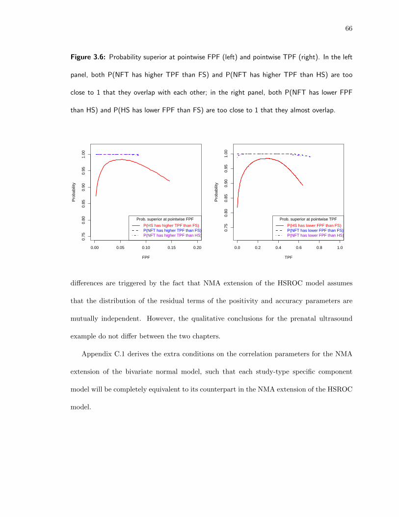
66

Figure 3.6: Probability superior at pointwise FPF (left) and pointwise TPF (right). In the left

panel, both P(NFT has higher TPF than FS) and P(NFT has higher TPF than HS) are too

close to 1 that they overlap with each other; in the right panel, both P(NFT has lower FPF

than HS) and P(HS has lower FPF than FS) are too close to 1 that they almost overlap.

0.00 0.05 0.10 0.15 0.20

0.75

0.80

0.85

0.90

0.95

1.00

FPF

Pro

babi

lity

Prob. superior at pointwise FPF

P(HS has higher TPF than FS)P(NFT has higher TPF than FS)P(NFT has higher TPF than HS)

0.0 0.2 0.4 0.6 0.8 1.0

0.75

0.80

0.85

0.90

0.95

1.00

TPF

Pro

babi

lity

Prob. superior at pointwise TPF

P(HS has lower FPF than FS)P(NFT has lower FPF than FS)P(NFT has lower FPF than HS)

differences are triggered by the fact that NMA extension of the HSROC model assumes

that the distribution of the residual terms of the positivity and accuracy parameters are

mutually independent. However, the qualitative conclusions for the prenatal ultrasound

example do not differ between the two chapters.

Appendix C.1 derives the extra conditions on the correlation parameters for the NMA

extension of the bivariate normal model, such that each study-type specific component

model will be completely equivalent to its counterpart in the NMA extension of the HSROC

model.

Chapter 4

Network meta-analysis of diagnostic accuracy stud-

ies using beta-binomial marginals and multivariate

Gaussian copulas

Abstract

Bivariate beta-binomial distributions have been used to model two-dimensional bino-

mial data in settings including meta-analysis of studies reporting pairs of estimated TPF

(true positive fraction, which equals sensitivity) and FPF (false positive fraction, which

equals 1-specificity) of tests. In particular, Kuss et al. (2014) and Chen et al. (2016) model

the observed number of subjects with true and false positive results of a test using beta-

binomial marginal distributions, and account for the dependence structure using several

bivariate copulas of the Archimedean family. In this chapter, we first generalize this ap-

proach from a single test to the duo/trio of tests performed on the same subjects by using

the multivariate Gaussian copulas. We integrate the new model with the shared-parameter

modeling framework and thus extend our network meta-analysis method to the evidence

network with a mixture of study-types, and account for different types of inconsistencies.

67

68

We apply this approach to the network meta-analysis of three second-trimester prenatal

ultrasound markers detecting trisomy 21 (Down’s syndrome) as an example. We also com-

pare the approach with the methods discussed in Chapter 2 and 3, which use models based

on logit-transformed FPF and TPF. Summary measures of diagnostic performance include

the posterior mean summary points and the corresponding contours, and summary ROC

curve for each test.

4.1 Background and introduction

TPF and FPF for a test are correlated across studies with varying positivity threshold in

the meta-analysis context. This correlation is accommodated by methods for meta-analysis

of studies reporting estimates of sensitivity and specificity. For example, the hierarchical

summary ROC approach (Rutter and Gatsonis 2001) models the relationship between logit

TPF and FPF. The two accuracy measures can be expressed as functions of a positivity

parameter, an accuracy parameter and a scale parameter. The bivariate method (Reitsma

et al. 2005; Chu and Cole 2006; Harbord et al. 2007) models the logit TPF and 1−FPF

(specificity) within studies as having a bivariate normal distribution. The linkage of TPF

and FPF via a moving positivity threshold is emphasized in the former approach, but this

mechanism is not modeled explicitly in the latter; instead, dependence is induced by the

correlation matrix in the bivariate normal model.

Both the bivariate normal method and the HSROC method model FPF and TPF in

the logit scale, which may lead to systematic bias in the summary points due to the shape

of the logit function. Alternative methods that model the FPF and TPF in their original

proportion scale and the dependence structure with copulas have been proposed (Kuss et al.

2014; Hoyer and Kuss 2015; Chen et al. 2016).

69

4.1.1 Dependence modeling with copulas

Consider two random variables X1 and X2 with distribution functions F1(·) and F2(·). If

we can represent their joint distribution as

H (x1, x2) = C (F1(x1), F2(x2)) = C(u1, u2) (4.1)

where ui = Fi(xi), and H(X1 = x1, X2 = x2) is a distribution function for the original

variables X1 and X2, The distribution function C(·, ·) is called a “copula” for a bivariate

pair of uniform random variables. The exclusive role of C(·, ·) is to determine the dependence

between F1(x1) and F2(x2) and thus between x1 and x2.

In Equation (4.1), the marginal distributions F1 and F2 are independent from the de-

pendence parameter of the copula. The families of bivariate distributions that separate the

bivariate dependence structure from the marginal distributions include, but are not limited

to, the Farlie-Gumbel-Morgenstern (FGM), Mardia, Sarmanov and Archimedean families

(Olkin and Trikalinos 2015).

To model the joint density of (FPF,TPF), a bivariate distribution with beta marginals

and a dependence structure that can accommodate the full range of correlation between

FPF and TPF is desired. Chu et al. (2010) used beta-binomial marginal distributions for

the meta-analysis of bivariate response data and modeled the dependence structure with

the Sarmanov family of bivariate distributions, proposed by Sarmanov (1966). Chen et al.

(2011) used the same approach in a Bayesian analysis for meta-analysis of case-control

studies. The use of the Sarmanov family of distributions has the disadvantage that only a

restricted range of values is allowed for the correlation parameters (Lee 1996). Analogously,

bivariate densities obtained with the FGM and Mardia families also restrict correlations

to a narrow range. This limitation is discussed by several authors, including Danaher and

70

Smith (2011), Kuss et al. (2014), and Chen et al. (2016).

4.1.2 Model using beta-binomial distributions and bivariate copulas

Recent work on meta-analysis of diagnostic accuracy studies for a single test models the

dependence structure with the Archimedean family of bivariate copulas. In particular, Kuss

et al. (2014) model the two accuracy measures using beta-binomial marginal distributions

and the Clayton, or the Gaussian, or the Plackett copula, while Chen et al. (2016) use the

marginal beta-binomial model with bivariate distributions induced by the Clayton or the

Frank copula (both radially symmetric) instead of the Sarmanov beta-binomial model.

Here, we briefly mention some copulas that could be applied to one test without re-

stricting correlations to a narrow range, and check their eligibility to be extended to two

or more tests. The multivariate extension of any one-parameter copula of the Archimedean

family (Nelsen 2007, subsection 4.2 and table 4.1), such as the quad-variate Clayton or the

Frank copula density, assumes the same correlation across the marginals, which is inap-

propriate for modeling (FPF, TPF) from paired-test studies. The Plackett copula, which

also belongs to the Archimedean family of copulas, allows multiple dependence parameter-

s. Although the Plackett copula has an explicit analytic expression for its bivariate form,

it requires the user to either solve a fourth order polynomial in order to model trivariate

responses (Kao and Govindaraju 2008), or to resort to pair-copula constructions (PCCs in

short, also known as vines) that allow the construction of copulas of arbitrary dimension

with only bivariate copulas as building blocks (Hoyer and Kuss 2015). We will be using

the multivariate Gaussian copulas in this chapter, as they do not imply restricted range

of correlations, have explicit analytic expression for arbitrary multi-dimensional form, and

allow as many dependence parameters as modeling all pairs of dimensions may need. We

71

note that none of the above methods has ever been used to jointly meta-analyze single-,

paired- and triplet-test studies.

The readers can also refer to Joe (2014) for comprehensive and up-to-date details about

dependence modeling with copulas, including multivariate copulas and their construction

methods.

4.1.3 Outline of this chapter

In this chapter, we use beta-binomial marginal distributions to model the observed number

of subjects with true and false positive test results, and use multivariate Gaussian copulas

to model the dependence between pairs of marginals. Our approach does not restrict the de-

pendence parameters between FPF and TPF to be the same for different tests. Alternative

approaches based on vine copulas construction will not be discussed.

Through integration with the shared-parameter modeling framework introduced in pre-

vious chapters, our network meta-analysis method can be used to analyze an evidence net-

work with a mixture of study-types. The meta-analysis of data on the accuracy measures

of three biomarkers from prenatal ultrasound in detecting trisomy 21 in fetuses (Smith-

Bindman et al. 2001) serves as an example.

4.2 Shared-parameter models for mixed study-types

As in Chapters 2 and 3, we assume that there are three tests t ∈ 1, 2, 3, and the collection

of studies consists of single-, paired- and triplet-test studies only. We denote study-type as

S and the complete set of study-types as S = 1, 2, 3, 12, 23, 13, 123.

Let Y `d, ijk be the number of individuals with target condition status d who have test

result i in test 1, j in test 2 and k in test 3. Usually, target condition status takes two

72

values: non-diseased with d = 0 and diseased with d = 1. Although the test result may be

a continuous value, it is common to set a threshold dividing the results into positive and

negative values so that i, j, k can take values 0 (negative) and 1 (positive). A missing test

result is labelled with a ‘ ∗ ’. For example, Y1, 01∗ would represent the number of diseased

individuals with a negative result for test 1, a positive result for test 2 and no result for

test 3. Corresponding to these counts are probabilities π`d, ijk that represent the chance of

each test result in the study, with values of ` label studies in the same study-type.

4.2.1 Use of the beta-binomial distribution for margins

First, we illustrate the use of bivariate distributions in summarizing single-test studies of

test 1 as a motivating example. For studies ` = 1, . . . , N1, d = 0, 1, the number of false and

true positive subjects Y `0, 1 ∗ ∗ , Y `

1, 1 ∗ ∗ are distributed as binomial

P(Y `d, 1 ∗ ∗ | Y `

d,+∗ ∗, p`d, 1 ∗ ∗

)=

Y `d,+∗ ∗

Y `d, 1 ∗ ∗

(p `d, 1 ∗ ∗)Y `d, 1∗∗

(1− p `d, 1 ∗ ∗

)Y `d,+∗∗−Y

`d, 1∗∗

(4.2)

where(p `0, 1∗∗, p

`1, 1∗∗

)are the (FPF, TPF) in the single-test study of test 1. The priors for

the FPF and TPF can be specified via the beta distribution:

f d1|1

(p `d, 1∗∗ | αd1|1, β

d1|1

)=

(p `d, 1∗∗

)αd1|1−1

(1− p `d, 1∗∗

)β d1|1−1

B(αd1|1, β

d1|1

) (4.3)

where ` = 1, . . . , N1, d = 0, 1, B(αd1|1, β

d1|1

)= Γ

(αd1|1

)Γ(β d1|1

)/Γ(αd1|1 + β d1|1

)is the

beta function.

Next, we generalize the specification for the beta-binomial marginals to paired- and

triplet-test studies without cross-tables. Ideally, when only the marginal total FP and TP

counts are available for the tests in some paired- or triplet-test studies, one can start from

modeling FP (or TP) counts across tests as bivariate / multivariate binomials when extend-

ing the bivariate normal model. We proceed here with the simplifying assumptions that

73

FP (or TP) counts across tests are independent binomial distributed variables, conditioning

on the total of non-diseased (or diseased) subjects. As an example, for the ` th paired-test

study of tests 1 and 2, suppose we have the positive counts Y `d, 1+∗ for test 1 and Y `

d,+1∗ for

test 2 (d = 0, 1) distributed as binomial in the first level:

P(Y `d,1+∗ | Y `

d,++∗, p`d,1+∗

)=

Y `d,++∗

Y `d,1+∗

(p `d,1+∗)Y `d,1+∗

(1− p `d,1+∗

)Y `d,++∗−Y

`d,1+∗

P(Y `d,+1∗ | Y `

d,++∗, p`d,+1∗

)=

Y `d,++∗

Y `d,+1∗

(p `d,+1∗

)Y `d,+1∗

(1− p `d,+1∗

)Y `d,++∗−Y

`d,+1∗

(4.4)

where(p `0, 1+∗, p

`1, 1+∗

),(p `0,+1∗, p

`1,+1∗

)are the (FPF, TPF) for test 1 and test 2 in the

paired-test study. The priors for the FPF and TPF can be specified via the beta distribution:

f d1|12

(p `d, 1+∗

∣∣∣α d1|12, β d1|12) =

(p `d, 1+∗

)α d1|12−1

(1− p `d, 1+∗

)β d1|12−1

B(α d1|12, β

d1|12

)f d2|12

(p `d,+1∗

∣∣∣α d2|12, β d2|12) =

(p `d,+1∗

)α d2|12−1

(1− p `d,+1∗

)β d2|12−1

B(α d2|12, β

d2|12

) (4.5)

where ` = N12, d = 0, 1.

We will discuss the model for paired-test studies with complete cross-tables later in sub-

section 4.2.4, including the specification of the beta-binomial marginals for the probabilities

that both tests are positive.

4.2.2 Use of the multivariate Gaussian copula

For any multivariate absolutely continuous distribution with CDF H and marginal CDFs

Fi, i = 1, . . . , p, a p-dimensional copula CG is a distribution function on (0, 1) p (with

uniform univariate marginals) such that the equation

H (x1, . . . , xp) = CG (F1(x1), . . . , Fp(xp)) = CG(u1, . . . , up) (4.6)

74

holds, where u = (u1, . . . , up), ui = Fi(xi) with Fi the marginal CDF’s. In our context,

Fi’s are the beta-binomial marginal CDFs of the positive counts given the total number

of diseased or non-diseased subjects. Let h be the corresponding joint density and fi, i =

1, . . . , p, the marginal densities. The copula density cG is defined by

cG =∂ pCG

∂u1 . . . ∂up(4.7)

and the joint density can be expressed as

h (x) = cG (F1(x1), . . . , Fp(xp))

p∏i=1

fi(xi) (4.8)

The p-dimensional Gaussian copula is defined by

CG(u,Ω) = Φp

(Φ−1(u1), . . . ,Φ

−1(up) | Ω), (4.9)

where Φp (·, · · · | Ω) is the CDF of the p-dimensional normal distribution Np(0,Ω). The

density of the corresponding p-dimensional Gaussian copula is

cG(u,Ω) = |Ω|−1/2 exp

−1

2v′(Ω−1 − Ip

)v

(4.10)

where v = (v1, . . . , vp)′, vi = Φ−1 (ui) = Φ−1 (Fi(xi)).

If CG is an n-dimensional Gaussian copula, then for any k, 2 ≤ k < n, all k-dimensional

subcopulas of CG are k-dimensional Gaussian copulas.

The Gaussian copulas in our model describe the dependence between the marginal cu-

mulative distributions in the diseased (d = 1) and the non-diseased (d = 0) population. For

example, the CDF of Y `d, 1∗∗ conditioning on the binomial total is

P(Y `d, 1∗∗ ≤ y | Y `

d,+∗∗

)

=

y∑Y `d, 1∗∗=0

Y `d,+∗∗

Y `d, 1∗∗

B(αd1|1 + Y `

d,+∗∗ , βd1|1 + Y `

d,+∗∗ − Y `d, 1∗∗

)B(αd1|1, β

d1|1

)

76

of accuracy measures σdt ∼ Unif

(0,√µdt (1− µdt )

). The multipliers Mt|S signify how much

the study-type specific variance parameters are inflated or deflated compared to the overall

variance parameters of a test across study-types. The multipliers M1|1, M2|2, M3|3 have

prior Gamma(κ, κ) with mean 1 and variance 1/κ. One can try different settings of κ such

as 0.1, 0.01, 0.001 for the priors and see whether the parameter estimates are affected by the

choices of κ.

For single-test studies, the study-type specific effects ξt =(ξ 0t|S , ξ

1t|S

)′are assumed to

have priors ξ dt|S | µdt ∼ Unif

(−µdt , 1− µdt

), d = 0, 1, t ∈ 1, 2, 3, S = t, to guarantee that

the right side of Equation (4.14) is bounded by [0, 1].

For paired-test studies without cross-tables, the study-type specific effects ξ12 =(ξ′1|12 ,

ξ′2|12

)′=(ξ 01|12, ξ

11|12, ξ

02|12, ξ

12|12

), ξ13 =

(ξ′1|13 , ξ

′3|13

)′=(ξ 01|13, ξ

11|13, ξ

03|13, ξ

13|13

)are as-

sumed to have uniform priors with their upper and lower bounds not only contained by(−µdt , 1− µdt

), d = 0, 1, t ∈ 1, 2, but subject to further constraints (see Appendix D.1 for

details), in order to guarantee that the right side of Equation (4.14) is bounded by [0, 1]. In

addition, by assuming the consistency equations for the estimation of the summary mea-

sures, we require a more stringent approach to sample the study-type specific effects in

order to avoid numerical breakdown (see Appendix D.2).

Notice that Ω6×6

is the overall variance-covariance matrix for the 6-dimensional Gaussian

copula, which does not have the same standard deviation parameters as those standard

deviations of the accuracy measures σdt , d = 0, 1, t ∈ 1, 2, 3. The variance-covariance

matrix in the 2-dimensional Gaussian subcopula for single-test studies of test t is

Xt ΩX′t , t ∈ 1, 2, 3 (4.16)

where the design matrices X12×6

=

(I2 O O

), X2

2×6=

(O I2 O

), and X3

2×6=

77

(O O I2

)are for the single-test studies of test 1, test 2 or test 3, respectively.

Model specification for paired- or triplet-test studies without cross-tables is analogous

to that of the single-test studies, with appropriate changes in the design matrices and

the dimensions of vectors and matrices. For instance, the variance-covariance matrix in

the 4-dimensional subcopula is Xt ΩX′t for the paired-test studies of the combination

t ∈ 12, 23, 13, where the design matrices

X124×6

=

I2 O O

O I2 O

, X234×6

=

O I2 O

O O I2

, X134×6

=

I2 O O

O O I2

are for the paired-test studies of tests 1 and 3, of tests 2 and 3, and of tests 1 and 3,

respectively.

We note that dimensions that a multivariate copula models are on the marginal CDFs

whereas the dependence is induced by the copula. The marginal CDFs of the beta-binomial

distribution of the ` th paired-test study of tests 1 and 2 can be derived as follows by

integrating out p `d, 1+∗ and p `d,+1∗:

P(Y `d, 1+∗ ≤ y | Y `

d,++∗

)=

y∑Y `d, 1+∗=0

∫g(Y `d, 1+∗

∣∣∣Y `d,++∗ , p

`d, 1+∗

)f d1|12

(p `d, 1+∗

∣∣∣α d1|12, β d1|12) d p `d, 1+∗=

y∑Y `d, 1+∗=0

Y `d,++∗

Y `d, 1+∗

B(α d1|12 + Y `

d, 1+∗, βd1|12 + Y `

d,++∗ − Y `d, 1+∗

)B(α d1|12, β

d1|12

) (4.17)

P(Y `d,+1∗ ≤ y | Y `

d,++∗

)=

y∑Y `d,+1∗=0

∫g(Y `d,+1∗

∣∣∣Y `d,++∗ , p

`d,+1∗

)f d2|12

(p `d,+1∗

∣∣∣α d2|12, β d2|12) d p `d,+1∗

=

y∑Y `d,+1∗=0

Y `d,++∗

Y `d,+1∗

B(α d2|12 + Y `

d,+1∗, βd2|12 + Y `

d,++∗ − Y `d,+1∗

)B(α d2|12, β

d2|12

) (4.18)

78

where g(· | ·) stands for binomial density function, f dt|S(·) stands for the beta density function

for the FPF (d = 0) or TPF (d = 1) of test t ∈ 1, 2 in the paired-test studies of tests 1

and 2 (S = 12).

The Gaussian copulas in our model describe the dependence between the marginal cumu-

lative distributions of the number of patients with positive test results in the non-diseased

(d = 0) and the diseased (d = 1) population, for example P(Y `1, 1+∗ ≤ y | Y `

1,++∗)

for TPF

and P(Y `0, 1+∗ ≤ y | Y `

0,++∗)

for FPF of test 1 in paired-test studies of tests 1 and 2.

By using the “Poisson-zeros approach” for arbitrary log-likelihood (Ntzoufras 2009), we

can base MCMC computation on the likelihood contributions.

4.2.4 Modeling to accommodate available cross-tables

In this subsection, we discuss modeling to accommodate complete cross-tables from some

paired-test studies. Inclusion of the cross-tables can provide more precision in estimating

the correlation structure, according to Trikalinos et al. (2012, 2014).

The notation of the counts in the available cross-tables for different types of paired-test

studies is described in Chapter 2, Table 2.2. The asterisk ‘ * ’ means that the corresponding

test is not performed and corresponds to the study-type). For paired-test studies of tests 1

and 2 with available cross-tables:

(Y `d, 00∗, Y

`d, 01∗, Y

`d, 10∗, Y

`d, 11∗

)∼ Multinom

(Y `d,++∗ , p

`d, 01∗ , p

`d, 10∗ , p

`d, 11∗

)(4.19)(

p `d, 00∗, p`d, 01∗, p

`d, 10∗, p

`d, 11∗

)∼ Dirichlet

(κ∗ · π `

d

), d = 0, 1, (4.20)

where κ∗ · π `d is the vector of parameters for the Dirichlet distribution, the normalizing

constant κ∗ has an arbitrary choice of diffuse Gamma prior κ∗ ∼ Gamma(2, 0.5) with mean

4 and variance 8, and the elements of π `d sum up to 1.

In addition to marginal CDFs of subjects with positive results on one test by Equations

79

(4.17-4.18), we also need the marginal CDFs of subjects with positive results on both

tests among the diseased and non-diseased. Multivariate copulas model marginal CDFs

in each dimension, and since beta and binomial are the marginal distributions of Dirichlet

and multinomial, respectively, we can interchange the integration step (to obtain marginal

CDFs) and the multiplication step. In particular, we can model the probabilities of both

tests being positive as beta-distributed variables again:

f d12|12

(p `d, 11 ∗

∣∣∣α d12|12, β d12|12) =

(p `d, 11 ∗

)α d12|12−1

(1− p `d, 11 ∗

)β d12|12−1

B(α d12|12, β

d12|12

) (4.21)

d = 0, 1. The CDFs of the number of subjects with both tests 1 and 2 positive can be

derived by integrating the beta-binomial density in Equation (4.21) over p `d, 11 ∗ and then

summing over possible values of Y `d, 11 ∗:

P(Y `d, 11 ∗ ≤ y | Y `

d, 1+∗, Y`d,+1 ∗, Y

`d,++∗

)

=

min(y, Y `d, 1+∗, Y

`d,+1∗)∑

Y `d, 11 ∗=max(0, Y `

d, 1+∗+Y`d,+1∗−Y

`d,++ ∗)

Y `d,++∗

Y `d, 11 ∗

·B(α d12|12 + Y `

d, 11 ∗ , βd12|12 + Y `

d,++∗ − Y `d, 11 ∗

)B(α d12|12, β

d12|12

) (4.22)

where the lower and upper bounds of the sum over Y `d, 11 ∗ attribute to the its range in the

corresponding non-central hypergeometric distribution.

The covariance matrix to accommodate complete cross-tables for paired-test studies is

given in Appendix B.1. In the prenatal ultrasound example, we can use just a few extra

correlation parameters in addition to the correlation matrix of the model for studies without

cross-tables, in order to account for the cross-tables of the 4 FS-HS paired-test studies.

Model specification for triplet-test studies with complete cross-tables is analogous with

appropriate changes in the design matrices and the dimensions of vectors and matrices.

80

4.2.5 Consideration of common parameters; Identifiability constraints

As we have discussed in the subsection 2.2.3, the shared-parameter modeling framework

enables us to jointly model diagnostic accuracy studies with mixed study-types, and de-

compose the study-level accuracy measures (in their original scale in this chapter) into

test-specific overall mean accuracy and study-type specific effects.

Using Sklar’s Theorem (Sklar 1959; Schweizer and Sklar 1983), we can show that any

subset of the vector of proportions in Equation (4.9) is distributed as a subfamily of Gaussian

copula with beta-binomial marginals and a subset of parameters correspond to the subset

of proportions. The rationale of sharing the same set of dependence parameters is based on

this property of the multivariate Gaussian copulas.

From the common parameters µdt and σdt , d = 0, 1, t ∈ 1, 2, 3, we can summarize the

overall accuracy of tests across study-types. Meanwhile, for those cross-test dependence

parameters, such as the dependence parameters in Ω, the convergence (judged by Gelman-

Rubin diagnostics) and the precision (judged by posterior s.d.) depend on the number

of paired-test studies corresponding to the particular cross-test dependence parameter. In

situations that there are too few studies to estimate all dependence parameters in Ω, we

may want to reduce the number of dependence parameters by assuming equality among

certain dependence parameters.

Consider the 4 possible study-type specific effects for test 1: ξ1|1 for single-test studies

of test 1, ξ1|12 for paired-test studies of tests 1 and 2, ξ1|13 for paired-test studies of tests

1 and 3, and ξ1|123 from triplet-test studies. By restricting the sum of the four parameters

81

to equal 0, and doing the same to the study-type specific effects for test 2 and test 3, i.e.,

ξ1|1 + ξ1|12 + ξ1|13 + ξ1|123 = 0 for test 1, (4.23)

ξ2|2 + ξ2|12 + ξ2|23 + ξ2|123 = 0 for test 2, (4.24)

ξ3|3 + ξ3|23 + ξ3|13 + ξ3|123 = 0 for test 3, (4.25)

we can reduce the number of parameters from the 3 two-dimensional constraints by 6, say,

ξ1|123, ξ2|123, ξ3|123 are calculated from Equations (4.23-4.25), while the remaining study-

type specific effects are sampled from priors. Additional identifiability constraints and prior

settings can be applied similarly to the study-type specific effects that correspond to two

or more tests positive among the non-diseased or diseased subjects, if there are enough full

cross-tables available for both paired- and triplet-test studies to estimate such parameters.

Similarly, by putting a restriction on the product of the study-type specific multipliers

which pertain to the variance of each test, we have the identifiability constraints

M1|1 ·M1|12 ·M1|13 ·M1|123 = 1 for test 1, (4.26)

M2|2 ·M2|12 ·M2|23 ·M2|123 = 1 for test 2, (4.27)

M3|3 ·M3|23 ·M3|13 ·M3|123 = 1 for test 3. (4.28)

M1|123, M2|123, M3|123 are calculated from Equations (4.26-4.28), while other study-type

specific multipliers are sampled from priors. If studies of a certain study-type are not

observed, the identifiability constraints stay the same with the corresponding study-type

specific effect replaced by 0 and the corresponding study-type specific multiplier replaced

by 1.

To guarantee that the unstructured covariance matrices are always positive definite when

updated in MCMC simulations, we apply the Cholesky decomposition to the correlation

82

matrix of Ω,

Ω = L′ΩLΩ, LΩ = diag (σ∗) LR (4.29)

where σ∗ is the vector of standard deviation parameters in variance-covariance matrix for

the Gaussian copula, LR is upper-diagonal matrix called the “Cholesky factor” for the

correlation matrix of Ω. Let Lk = (L1k, . . . , Lkk, 0, · · · , 0)′ represent the kth column of LR,

given by the triangular representation as follows (Pinheiro and Bates 1996):

L1k = cos(ϕ1,k)

Lk′k = cos(ϕk′,k)

k′−1∏l=1

sin(ϕl,k), for 2 ≤ k′ ≤ k − 1

Lkk =k−1∏l=1

sin(ϕl,k) (4.30)

with L11 = 1. All the angles (ϕ’s) have uniform prior Unif (0, π). We let the elements in

the vector of standard deviations σ∗ for the multivariate Gaussian copulas have the vague

prior Unif(0, 3), d = 0, 1, t ∈ 1, 2, 3.

4.2.6 The Poisson-Zeros approach for MCMC computation

The hierarchical models in this article involve multivariate Gaussian copulas, and, to the

best of our knowledge, cannot be handled directly by available MCMC calculation packages

such as OpenBUGS and JAGS. Even when we cannot write the codes in a hierarchical style

specified by built-in statistical distributions, the computational trick called the “Poisson-

zeros approach” in Ntzoufras (2009, subsection 8.1.1) or “zeros trick” in Lunn et al. (2012,

subsection 9.5.1) for an arbitrary log-likelihood allows us to utilize OpenBUGS / JAGS for

the likelihood contribution. The model likelihood can be re-written as the product of the

densities of new pseudo-random variables which follow the Poisson distribution with mean

83

equal to minus the log-likelihood, and all observed values set equal to 0:

∏S ∈S

NS∏`=1

elogL`S ∝

∏S ∈S

NS∏`=1

e−(− logL`S+C0)(− logL`S + C0)0

0 !, (4.31)

where logL`S is the log likelihood contribution for the ` th study of the study-type S ∈ S =

1, 2, 3, 12, 23, 13, 123. A positive constant term C0 can be added to the Poisson mean

in order to ensure the positivity. C0 must satisfy − logL`S +C0 > 0 for all ` = 1, . . . , NS in

all study-types (in practice C0 = 1000 suffices).

4.3 Summary Measures of Diagnostic Performance

4.3.1 Posterior mean summary points, and contours for summary points

We use the posterior mean summary point µt =(µt0, µ

t1

)as a summary measure of (FPF,TPF)

for each test, t ∈ 1, 2, 3. The posterior 100(1−α)% contour for a bivariate summary point,

which means 100(1−α)% of the kernel smoothed density of the summary point falls within

the boundary of the contour, can also be very useful.

4.3.2 Summary ROC curves

By applying the delta method, we can approximate the grand mean vector and variance-

covariance matrix of the logit accuracy measures, logit(µtd)

and(σdt)2/µtd(1 − µtd), from

the posterior distribution of µtd and(σdt)2

, d = 0, 1, t ∈ 1, 2, 3, if and only if they can be

considered as asymptotic means and variances.

Analogous to the transformation between the bivariate normal model and the HSROC

model Harbord et al. (2007), we can solve the parameters used to plot the summary ROC

84

curve for each test:

βt = log(σt0/σ

t1

)− 1

2

(log(µt0) + log(1− µt0)

)+

1

2

(log(µt1) + log(1− µt1)

)(4.32)

Λt = exp(βt/2

)logit

(µt1)− exp

(−βt/2

)logit

(µt0), t ∈ 1, 2, 3, (4.33)

The summary ROC curve we are proposing in this article is neither naturally derived

from a proof of equivalence to the HSROC model, nor like the HSROC parameter space

(Rutter and Gatsonis 2001) in which the mechanism between TPF and FPF is driven by a

moving positivity threshold. As such, we call it the “pseudo” summary ROC curve to make

a distinction.

As in the previous chapters, plots of the probability that one test is superior than the

other can be used in order to compare tests. This probability is estimated as the proportion

of iterations in which a test has higher TPF at pointwise FPF values, and also in the other

direction, the proportion of iterations in which a test has lower FPF at pointwise TPF

values. In addition, posterior contours for the pairwise contrast of summary points can be

plotted and used to check how tests compare in FPF and TPF.

4.4 Application to the Prenatal Ultrasound Example

We implemented the shared-parameter Bayesian hierarchical models by calling JAGS (Plum-

mer 2014) from R through package R2jags (Su and Yajima 2014), then use the returned

posterior samples for further analysis and visualization. We used 2 chains, each with 20,000

iterations (first half discarded) and a thinning rate of 5, and record posterior samples of

2,000 iterations from each chain. The Gelman-Rubin convergence diagnostics for all param-

eters and quantities of interest we have monitored (including the TPF at pointwise FPF)

are between 1.00 and 1.05, which suggest that convergence is good.

85


The feasibility to examine direct and indirect effects in the evidence network of the prenatal









reduction.



studies, ψedgeAC , as well as the difference between the FS-NFT direct evidence from


ψdsgn13 .

Here we take the assessment of direct and indirect sources of evidence between FS and

NFT as an example. The posterior estimates of type 2 direct evidence from paired-test

studies is ξ1|13− ξ3|13 = (−0.008, 0.097), the type 3 direct evidence from triplet-test studies

is ξ1|123− ξ3|123 = (−0.013,−0.171), and the type 1 indirect evidence from single-test stud-

ies is ξ1|1 − ξ3|3 = (−0.008, 0.055). The first and second numbers of each tuple are in the

FPF and TPF axes, respectively. The difference between FS-NFT type 2 direct evidence

and type 1 indirect evidence is (0.0003, 0.041); its kernel smoothed density falls in each

of the four quadrants with posterior probability (0.304, 0.273, 0.213, 0.210). The difference

86

between FS-NFT type 3 direct evidence and type 1 indirect evidence is (−0.005,−0.226);

the posterior probability that the kernel smoothed density falls in each of the four quad-

rants are (0.024, 0.008, 0.557, 0.410). The kernel smoothed densities are obtained by using

default settings of the KernSur() subroutine in the R package GenKern (Lucy and Aykroyd

2013). From the bivariate posterior contours of the kernel smoothed density of the differ-

ence between FS-NFT type 2 direct evidence versus type 1 indirect evidence (left panel in

Figure 4.1), and that of the difference between FS-NFT type 3 direct evidence versus type

1 indirect evidence (right panel), we can see that the point (0, 0) is inside the posterior 90%

contour of the kernel smoothed density: based on available data, we cannot reject the null

hypothesis that the indirect source of evidence are consistent with the direct sources. The

evidence supports the conclusion that there is no significant difference between the direct

and indirect sources of evidence in the FS-NFT comparison (albeit low power due to the

small number of comparative studies).

We show in the supplementary material that there is no significant difference between

the type 3 direct and type 2 indirect evidence of the HS-NFT comparison. Also there

is no significant difference between the two direct sources of evidence (from paired- and

triplet-test studies) of the FS-HS comparison (Appendix D.3).


tions



ψdsgn13 =

(µ1 + ξ1|13 − µ3 − ξ3|13

)−(µ1 + ξ1|123 − µ3 − ξ3|123

)(4.34)

87




−0.4 −0.2 0.0 0.2 0.4

−0.

4−

0.2

0.0

0.2

0.4

FPF axis

TP

F a

xis

0.5

0.75

0.9

−0.4 −0.2 0.0 0.2 0.4−

0.6

−0.

4−

0.2

0.0

FPF axis

TP

F a

xis

0.5

0.75

0.9



ψedge13 =

(µ1 + ξ1|13 − µ3 − ξ3|13

)−(µ1 + ξ1|1 − µ3 − ξ3|3

)(4.35)



ψloop13 =

(µ1 + ξ1|13 − µ3 − ξ3|13

)−(µ1 − µ3 + ξ1|12 − ξ2|12 + ξ2|23 − ξ3|23

)(4.36)

In order to estimate the overall pairwise comparative accuracy, we make the assumption

that the different sources of evidence between every two tests are equal, which is equivalent

to the assumption that the design, edge and loop inconsistency factors (4.34)-(4.36) are all

equal to zero, ψdsgn13 = ψedge

13 = ψloop13 = 0. As a result, we only need to assign priors to eight

(8) of the study-type specific parameters. Additional consistency equations would be needed

88

if the full cross-tables for enough many paired- and triplet-test studies were available. In

particular such consistency equations would apply to the probabilities of two or more tests

positive among the diseased or the non-diseased.

We connect posterior quantiles (5%, median, and 95%) of posterior TPF calculated by

the HSROC formula at pointwise FPF (Figure 4.2). From the pointwise curve consisted

of the posterior median (the 5% and 95% quartiles as well for pointwise credible interval),

we can see that HS performs slightly but not significantly better than FS, and NFT is

significantly superior than both HS and FS.

As the estimated posterior median and mean summary points do not differ much (al-

most overlap in Figure 4.2), we report the posterior mean summary points, which are

(0.102, 0.323) for femoral shortening, (0.080, 0.341) for humeral shortening, and (0.019, 0.393)

for nuchal fold thickening. With a thinning rate of 5, we obtain 2,000 iterations from each

chain (total 4,000) to estimate the kernel smoothed density of summary points.

The posterior mean summary points as well as the corresponding posterior contours

suggest that nuchal fold thickening has slightly higher specificity than the other two markers,

as well as the lowest variability in both the posterior estimates of TPF and FPF. Femoral

shortening has the largest variability in the posterior estimates of FPF. Nevertheless, if we

look at the posterior median summary points of sensitivity alone, the three markers perform

very much alike.

89

Figure 4.2: The posterior 5%, 50% and 95% quantiles of TPF at pointwise FPF, and the

posterior mean or median summary points for each ultrasound marker

0.0 0.2 0.4 0.6 0.8 1.0

0.0

0.2

0.4

0.6

0.8

1.0

FPF

TP

F



Summary Points


90

Figure

4.3:

Pos

teri

orco

nto

urs

ofth

esu

mm

ary

poi

nts

:th

ep

oste

rior

50%

,75

%,

and

90%

con

tou

rsof

the

sum

mar

yp

oin

tfo

rea

chu

ltra

sou

nd

mar

ker

isth

ein

ner

mos

t,th

em

idd

lean

dth

eou

term

ost,

resp

ecti

vely

.

0.00

0.05

0.10

0.15

0.20

0.00.20.40.60.81.0

Fem

ur S

horte

ning

FPF

TPF

0.5

0.7

5 0

.9

0.00

0.05

0.10

0.15

0.20

0.00.20.40.60.81.0

Hum

erus

Sho

rtenin

g

FPF

TPF

0.5

0.7

5 0

.9

0.00

0.05

0.10

0.15

0.20

0.00.20.40.60.81.0

Nuch

al Fo

ld Th

icken

ing

FPF

TPF

0.5

0.7

5

0.9

Chapter 5

Discussion

In our framework of shared-parameter modeling, inference for common mean and covariance

parameters borrows strength from various study-types, i.e. single-, paired- and triplet-test

studies in the example, and can accommodate data in the available cross-tables for two or

more tests, leading to refined dependence structure among tests. MCMC simulations on

the set of shared mean and covariance parameters across mixed study-types can lead to

slow convergence, especially when the accuracy of the same test in different study-types is

too heterogeneous. Computational challenges arise from the additional modeling needed

to accommodate available cross-tables. For example, extension of the model in subsection

2.2.4 to accommodate triplet-test studies with cross-tables requires the use of a fourteen-

dimensional normal distribution and results in a large number of extra mean and covariance

parameters. Nevertheless, the use of the more complex model may be warranted if there is

a sufficient number of studies with available or partially available cross-tables.

When testing whether indirect sources of evidence (e.g. from single-test studies) differ

from direct sources of evidence, the question of statistical power arises. Low statistical

power is a consequence of too few comparative studies. As direct evidence accumulates

with the number of multiple test studies increasing over time, researchers on a specific

91

92

research question may eventually find they are ready to abandon the indirect evidence at

some point.

Evaluation of the diagnostic accuracy measures usually addresses several questions of

interest, rather than a simple comparison between FPF or TPF of two tests. Different

metrics of diagnostic accuracy may be relevant in different decision making settings, for

example:

1. If the summary ROC curves of two tests do not cross each other, the test with higher

posterior median TPF at pointwise values of FPF is better. That is to say, a test is

better if its pointwise HSROC curve is closer to the upper-left corner than other tests

at all values over the range of FPF.

2. If the summary ROC curve of two tests cross at a certain point, one could narrow

down the range of FPF or TPF that is meaningful to the clinical context and compare

the partial area under the curve.

3. One could consider the test with higher overall mean TPF or lower overall mean FPF

or with both criteria as the better test, if it is appropriate in the clinical context.

If the performance of one test is superior to other tests in aspects of greatest interest, we

can choose the unequivocal best option if such an option arises from the data; otherwise,

we need to weigh the advantages and disadvantages of one test over another.

5.1 Exchangeability

NMA of interventions takes two different approaches: modeling treatment means or relative

treatment effects (difference between means). Each approach relies on different exchange-

ability assumptions. Since our modeling is arm-based rather than contrast-based, the ex-

93

changeability assumption in this thesis is similar to that of the arm-based NMA models for

competing interventions.

The rate at which (FPF, TPF) decrease as the positivity threshold increases varies across

tests, and so does the degree of asymmetry with respect to the counter-diagonal line in the

SROC plane. Both of these features of the summary ROC curve cannot be conveniently

represented if we begin with modeling the comparative accuracy measures, because the

accuracy measures rather than their differences between tests define the summary ROC

curve.

Our network meta-analysis of diagnostic accuracy studies starts with modeling the

study-level point estimates of (FPF, TPF) rather than comparative accuracy that Menten

and Lesaffre (2015) did. We are essentially assuming that the logit-transformed FPF and

TPF (Chapters 2 and 3) or FPF and TPF in their original scale (Chapter 4) are exchange-

able across studies within each study-type.

5.2 About missingness

In a paired- or triplet-test study, for the duo/trio of tests performed on the same subjects

without missingness in the results for each test, the total numbers of the diseased or the

non-diseased should be consistent across tests. If test results for some subjects in a study

are missing completely at random (MCAR), the models for studies without cross-tables

can still accommodate the unequal total number of diseased and non-diseased across tests.

However, if the missing data mechanism are MAR or MNAR, an analytic strategy using

the subset of subjects with complete data may yield biased parameter estimates and would

need adjustments. One common scenario would include a selection process of test results

missingness dependent on covariates that might affect the probability of a positive test

94

result. The use of imputation-based method is not likely to be applicable due to lack of

individual level data (comprehensive confounders and effect-modifiers required to adjust for

in the missing data mechanism).

5.3 Choosing among the three approaches

We first discuss the beta-binomial marginals and multivariate Gaussian copulas model

(Chapter 4), because this method shall be excluded first if the reader is interested in the

summary ROC curves but not the summary points of tests.

5.3.1 Strength and limitations of the beta-binomial marginals and mul-

tivariate Gaussian copulas model

Network meta-analysis using multivariate copulas is computationally expensive due to the

repetitive calculations of the CDFs. The multivariate Gaussian copulas model with beta-

binomial marginals (Chapter 4) takes longer time to converge than methods in Chapters

2 and 3, but requires fewer MCMC iterations. Future development should focus on more

efficient computational algorithms.

Compared with the results obtained in Chapters 2 and 3, in which we inversely transform

the estimated overall mean logit accuracy from a multivariate normal model or the HSROC

model back into the original scale, the posterior mean/median summary points in the beta-

binomial marginals and multivariate Gaussian copulas model are larger (Table 5.1) and

further away from 0 in both the FPF and the TPF axes. This phenomenon can be explained

as follows. Due to concavity of the logit function on the interval (0, 0.5], logit(E(FPF)) >

E(logit(FPF)) holds for tests with overall mean FPF less than 0.5, and the same inequality

95

Table 5.1: Comparison of the posterior mean/median summary points from Chapters 1-3

(accurate to the second decimal place; posterior mean and median summary points almost

overlap with each other)

Chapter 2: NMA extension of the bivariate normal model

Chapter 3: NMA extension of the HSROC model

Chapter 4: Beta-binomial marginals and multivariate Gaussian copulas model

Ultrasound Posterior Chapter 2 Chapter 3 Chapter 4

Markers Summary Points FPF TPF FPF TPF FPF TPF

FSmean 0.072 0.312 0.071 0.311 0.102 0.323

median 0.071 0.309 0.070 0.310 0.102 0.323

HSmean 0.039 0.299 0.044 0.311 0.080 0.341

median 0.037 0.293 0.043 0.308 0.080 0.341

NFTmean 0.006 0.315 0.007 0.305 0.019 0.393

median 0.006 0.313 0.007 0.303 0.019 0.393

also holds for tests with overall mean TPF less than 0.5. Thus,

Ech4(FPF) > logit−1(Ech2/ch3(logit(FPF))

).

The left side is the expected FPF under the model in Chapter 4; the right side is the inverse

logit of the expected logit(FPF) under the model in Chapter 2 or Chapter 3. Similar

phenomenon appears on TPF in the prenatal ultrasound example. The bias caused by logit

transformation is more obvious if the overall FPF or TPF is close to 0 or 1.

The beta-binomial marginals and multivariate Gaussian copulas model provide a less

biased estimate of the posterior median (or mean) summary points, compared with the

96

other two approaches. The readers may prefer it if the summary points of multiple tests

for a specific condition are of interest in the clinical context.

The summary ROC curves based on the beta-binomial marginals and multivariate Gaus-

sian copulas model rely on the approximate grand mean vector and variance-covariance ma-

trix of the logit accuracy measures, which are derived from the posterior overall mean and

variance estimates of accuracy measures by applying the delta method. The precision of the

delta method approximation depends on large sample properties of the estimators before

transformation. The summary ROC curves in Chapter 4 are not reliable summary mea-

sures, unless a sufficiently large number of studies can guarantee the asymptotic properties

of the overall mean and variance estimates of accuracy measures.

We have only considered the Archimedean copulas families and found the multivariate

Gaussian copulas suitable for our purpose; one can construct certain vine copulas with no

restricted range of correlation as well, and apply the remaining parts of our model.

5.3.2 Advantages of the NMA extension of the HSROC model over the

NMA extension of the bivariate normal model

To obtain the fitted HSROC curve and the pointwise HSROC curve (with credible region)

for each test, the NMA extension of the HSROC model should be used. The correspondence

between the HSROC model and the bivariate normal model for the meta-analysis of single

test diagnostic accuracy studies has been shown by Harbord et al. (2007). The comparison

of the two approaches is more involved in the context of NMA: while this is true for evidence

synthesis of one test’s performance across studies, the network meta-analysis extension of

these two methods differ in several aspects:

• The NMA extension of the HSROC model assumes that the distribution of the resid-

97

ual terms of the positivity and accuracy parameters are mutually independent. Com-

pare the full model of Chapter 3 to that of Chapter 2, Equations (3.2)-(3.15) have

two independent 7-dimensional normal residual terms of the positivity and accuracy

parameters, whereas the NMA extension of the bivariate normal model has one 14-

dimensional normal within-study-type random effect in Equation (2.2). This leads to

differences between the pointwise HSROC curves as well as the plot of the probability

superior at pointwise FPF or TPF from Chapter 2 and 3.

• Though the total number of parameters does not change, the NMA extension of the

HSROC model has the number of scale parameters βt (t = 1, 2, 3, 12, 23, 13, 123) to

compensate for the same amount of reduction in parameters for the the variance-

covariance matrices (see the structured matrix on the right side of Equation (3.42) as

an example). Correlation parameters are fewer in the NMA extension of the HSROC

model compared with that of the bivariate normal model, consequently, the correlation

matrices (actually, the parameters of the triangular representation for their Cholesky

factors) also converge faster, and computation takes much less time with the same

sufficient number of iterations.

• The transformation of parameters in Equations (3.32-3.33) shows extra conditions

on the correlation parameters for the NMA extension of the bivariate normal model,

such that each study-type specific component model will be completely equivalent

to its counterpart in the NMA extension of the HSROC model. The derivations are

described in Appendix C.1.

• The identifiability constraints in the NMA extension of the HSROC model are on the

positivity and accuracy parameters in Equation (3.30), while the consistency equations

98

are still in the logit accuracy scale and in conformity with the NMA extension of the

bivariate normal model.

The summary point of each test is pooled over all studies with a plethora of study-types,

and is influenced by how the prevalence of the condition is distributed across the studies

included.

All three methods in this thesis can accommodate study-level covariates (e.g., the preva-

lence) the same way as the bivariate normal model and HSROC model do in Harbord et al.

(2007) for a single test. For instance, the study-level covariates can serve as additional

explanatory variables for the study-level threshold and accuracy parameters in Chapter 3.

In conclusion, we suggest that one could prefer NMA extension of the HSROC model

due to its conceptual advantage as well as computational efficiency over the other two

models, or the beta-binomial marginals and multivariate Gaussian copulas model if less

biased summary points are of interest.

Appendix A

Data used in the example

A.1 Aggregated study-level data Smith-Bindman et al. (2001) has ex-

tracted

For at least one of the following two reasons, we simplified some studies from prenatal

ultrasound data in Smith-Bindman et al. (2001):

a) insufficient number of the studies with complete cross-tables which pertain to a specific

study-type for parameter estimation in the corresponding model; or

b) incomplete cross-tables for paired- or triplet-test studies, but margins for at least two

tests are available.

Figure A.1 shows the number of studies for each study-type before and after simplification.

99

100

Table

A.1:

Th

elis

tof

all

sin

gle-

test

stu

die

s,an

dth

elis

tof

pai

red

-or

trip

let-

test

stu

die

sw

ith

out

cros

s-ta

ble

sav

aila

ble

Cou

nts

Stu

dy

IDIn

dex

Des

ign

Fem

ora

lS

hort

enin

gH

um

eral

Sh

ort

enin

gN

uch

al

Fold

Th

icke

nin

g

TP

FN

FP

TN

TP

FN

FP

TN

TP

FN

FP

TN

Bru

mfi

eld

etal

.(1

989)

`=

1ca

se-c

ontr

ol

69

144

Cam

pb

ell

etal

.(1

994)

`=

2p

rosp

ecti

ve2

320

244

Cu

ckle

etal

.(1

989)

`=

3ca

se-c

ontr

ol

20

63

84

1276

Dic

keet

al.

(198

9)`

=4

case

-contr

ol

528

18

159

Gra

ngje

anan

dS

arra

mon

(199

5a)

`=

5p

rosp

ecti

ve15

19

495

2268

Gri

stet

al.

(199

0)`

=6

pro

spec

tive

33

25

403

Hil

let

al.

(198

9)`

=7

case

-contr

ol

418

6280

Joh

nso

net

al.

(199

3)`

=8

pro

spec

tive

10

431

300

LaF

olle

tte

etal

.(1

989)

`=

9ca

se-c

ontr

ol

426

27

202

Lock

wood

etal

.(1

987)

`=

10ca

se-c

ontr

ol

18

17

24

325

Mar

qu

ette

etal

.(1

990)

`=

11ca

se-c

ontr

ol

328

14

141

Nyb

erg

etal

.(1

990)

`=

12ca

se-c

ontr

ol

742

35

537

Sh

ahet

al.

(199

0)`

=13

case

-contr

ol

314

116

Ver

din

and

Eco

nom

ides

(199

8)

`=

14ca

se-c

ontr

ol

65

5444

Bah

ado-

Sin

ghet

al.

(199

5)`

=1

pro

spec

tive

34

9638

Ben

acer

raf

etal

.(1

985)

`=

2p

rosp

ecti

ve2

41

897

Ben

acer

raf

etal

.(1

987)

`=

3p

rosp

ecti

ve2

63

2108

Ben

acer

raf

etal

.(1

987)

`=

4ca

se-c

ontr

ol

21

74

188

Bor

rell

etal

.(1

998)

`=

5p

rosp

ecti

ve10

14

21363

Boy

det

al.

(199

8)`

=6

pro

spec

tive

565

105

33201

Cra

ne

and

Gra

y(1

991)

`=

7p

rosp

ecti

ve12

435

3287

Der

enet

al.

(199

8)`

=8

pro

spec

tive

539

22

3652

DeV

ore

and

Alfi

(199

5)`

=9

pro

spec

tive

428

13

1987

Don

nen

feld

etal

.(1

994)

`=

10p

rosp

ecti

ve1

12

16

1330

101

Tab

le1:

Th

elis

tof

all

sin

gle-

test

stu

die

s,an

dth

elis

tof

pai

red

-or

trip

let-

test

stu

die

sw

ith

out

cros

s-ta

ble

sav

aila

ble

(con

t.)

Cou

nts

Stu

dy

IDIn

dex

Des

ign

Fem

ora

lS

hort

enin

gH

um

eral

Sh

ort

enin

gN

uch

al

Fold

Th

icke

nin

g

TP

FN

FP

TN

TP

FN

FP

TN

TP

FN

FP

TN

D’O

ttav

ioet

al.

(199

7)`

=11

pro

spec

tive

19

83496

Gra

ngje

anan

dS

arra

mon

(199

5b)

`=

12p

rosp

ecti

ve17

27

273

2932

Gra

yan

dC

ran

e(1

994)

`=

13p

rosp

ecti

ve14

18

81

8025

Nic

olai

des

etal

.(1

992)

`=

14p

rosp

ecti

ve53

248

91

1694

Nyb

erg

etal

.(1

990)

`=

15p

rosp

ecti

ve4

21

10

3490

Wat

son

etal

.(1

994)

`=

16p

rosp

ecti

ve7

727

1426

Bia

giot

tiet

al.

(200

5)∗

`=

1ca

se-c

ontr

ol

13

14

60

440

15

12

73

427

Joh

nso

net

al.

(199

5)†

`=

2ca

se-c

ontr

ol

15

21

127

667

8‖13

25‖4

024‖3

8462‖7

39

Nyb

erg

etal

.(1

993)∗

`=

3ca

se-c

ontr

ol

11

34

44

898

11

34

42

900

Rod

iset

al.

(199

1)`

=4

case

-contr

ol

29

95

1795

74

95

1795

Vin

tzil

eos

etal

.(1

996)∗

`=

5p

rosp

ecti

ve5

17

50

443

10

12

49

444

Ben

acer

raf

etal

.(1

989)∗ †

`=

1ca

se-c

ontr

ol

713

28‖

139

681‖

3341

812

10

3470

Gin

sber

get

al.

(199

0)∗

`=

2ca

se-c

ontr

ol

56

14

198

57

0212

Lyn

chet

al.

(198

9)∗

`=

3ca

se-c

ontr

ol

54

54

54

54

Nyb

erg

etal

.(1

995)

`=

4p

rosp

ecti

ve5

13

14

218

315

1231

Ben

acer

raf

etal

.(1

991)∗

`=

1ca

se-c

ontr

ol

10

14

40

360

12

12

25

375

12

12

0400

Ben

acer

raf

etal

.(1

992)∗

`=

2ca

se-c

ontr

ol

23

963

525

17

15

34

554

22

10

2586

Ben

acer

raf

etal

.(1

994)†

`=

3ca

se-c

ontr

ol

20

25

4102

20‖

25

17‖2

13‖4

81‖1

01

19

26

0106

Bro

mle

yet

al.

(199

7)†

`=

4ca

se-c

ontr

ol

25

28

14

163

19‖

22

27‖3

25‖6

144‖1

70

27

26

1176

Lock

wood

etal

.(1

993)

`=

5p

rosp

ecti

ve6

36

163

4786

12

30

198

4751

21

21

242

4707

Nyb

erg

etal

.(1

998)

`=

6ca

se-c

ontr

ol

7135

33

897

4138

2928

33

109

4926

*:S

ixp

aire

d-t

est

stu

die

san

dtw

otr

iple

t-te

stst

ud

ies

hav

eav

ail

able

or

part

iall

yav

ail

ab

lecr

oss

-tab

les,

wh

ich

are

det

ail

edin

Ap

pen

dix

B.

†:B

oth

the

tota

lnu

mb

erof

case

san

dco

ntr

olsu

bje

cts

are

not

equ

al

acr

oss

bio

mark

ers

inB

enace

rraf

etal.

(1994),

Bro

mle

yet

al.

(1997),

an

d

Joh

nso

net

al.

(199

5);

for

the

HS

ofea

chst

ud

y,th

eta

ble

ab

ove

hav

eli

sted

TP

,F

N,

FP

,T

Nco

unts

rep

ort

edin

ori

gin

al

art

icle

foll

owed

by

the

cou

nts

inflat

edp

rop

orti

onal

lyin

ord

erto

hav

eth

esa

me

tota

las

oth

erb

iom

ark

ers.

Ben

ace

rraf

etal.

(1989)

on

lyh

as

the

tota

lnum

ber

of

contr

ol

sub

ject

sfo

rF

Snot

equ

alto

that

ofN

FT

,an

dw

ein

flate

its

FP

an

dT

Nco

unts

inp

rop

ort

ion

tore

ach

the

sam

eto

tal

nu

mb

eras

that

of

NF

T.

102

Figure A.1: Graphical depiction of the prenatal ultrasound example (before & after simplifica-

tion). The dashed-dotted line represents FS-HS paired-test studies, the dashed line represents

FS-NFT paired-test studies, the closed circles represents FS or NFT single-test studies and the

closed triangle represents triplet-test studies. The number of studies is also labeled for each

study-type.

A.2 Available or partially available cross-tables

We use only the fully available FS-HS cross-tables from Biagiotti et al. (2005), Nyberg et al.

(1993), Benacerraf et al. (1991), and Benacerraf et al. (1992). The latter two are triplet-test

studies collapsed over the NFT margin and used as FS-HS paired-test studies with cross-

tables, since there are too few of them to estimate the extra parameters in a model which

accommodate available cross-tables from triplet-test studies (14-dimensional Normal).

The available or partially available cross-tables for the FS-HS paired-test studies Bia-

giotti et al. (2005), Nyberg et al. (1993) and Vintzileos et al. (1996) are displayed in table

A.2 (` = 1, 3 and 5, respectively). To begin with Vintzileos et al. (1996), the counts in its

2 × 2 table for trisomy 21 fetuses are known, however, only the two margins of the 2 × 2

table are available and the exact number of the four counts are incomplete for normal fe-

103

tuses. The Data Augmentation (Tanner and Wong 1987) algorithm can be applied to the

partially available cross-tables. Although we did not take the data augmentation approach

for simplicity, we would like to describe the details.

In the main text of this article, we only use the margins of Vintzileos et al. (1996). One

could draw the count of normal fetuses showing both femur and humerus lengths short from

the conditional distribution

[Y `=50, 11∗

∣∣∣Y `=50, 1+∗ = 50, Y `=5

0, 0+∗ = 443, Y `=50,+1∗ = 49, p `=5

0, 00∗, p`=50, 01∗, p

`=50, 10∗, p

`=50, 11∗

]∼ Noncentral-Hypergeometric

(50, 443, 49,OR`=5

0, AB

)(A.1)

in the imputation step, where OR`=50, AB = p `=5

0, 11∗ p`=50, 00∗/

(p `=50, 10∗ p

`=50, 01∗

)is calculated from the

previous iteration.

The available or partially available cross-tables for the FS-NFT paired-test studies Be-

nacerraf et al. (1989), Ginsberg et al. (1990) and Lynch et al. (1989) are displayed in table

A.3 (` = 1, 2 and 3, respectively). For Benacerraf et al. (1989), one can draw the count of

normal fetuses showing both FS and NFT from the conditional distribution

[Y `=10, 1∗1

∣∣∣Y `=10, 1∗+ = 139, Y `=1

0, 0∗+ = 3341, Y `=10,+∗1 = 10, p `=1

0, 0∗0, p`=10, 0∗1, p

`=10, 1∗0, p

`=10, 1∗1


(139, 3341, 10,OR`=1

0, AC

)(A.2)

in the imputation step, where OR`=10, AC = p `=1

0, 11∗ p`=10, 00∗/

(p `=10, 10∗ p

`=10, 01∗


previous iteration.

For Ginsberg et al. (1990), we assume that the FS diagnosis for this case is distributed

as(Y `=21, 1∗1 − 3

)∼ Bernoulli

(p `=21, 1∗1|∗∗1

)such that the total numbers of trisomy 21 fetuses

for both markers reach 12, where p `=21, 1∗1|∗∗1 = p `=2

1, 1∗1/p`=21, ∗∗1.

104

Table A.2: Available or partially available FS-HS cross-tables for Biagiotti et al. (2005), Nyberg

et al. (1993) and Vintzileos et al. (1996)

Trisomy 21 HS Normal HS

− + − +

BiagiottiFS

− 11 3 14FS

− 405 35 440

` = 1 + 1 12 13 + 22 38 60

12 15 27 427 73 500


− + − +

NybergFS

− 31 3 34FS

− 871 27 898

` = 3 + 3 8 11 + 29 15 44

34 11 45 900 42 942


− + − +

VintzileosFS

− 11 6 17FS

− Y `=50, 11∗+394 49− Y `=5

0, 11∗ 443

` = 5 + 1 4 5 + 50− Y `=50, 11∗ Y `=5

0, 11∗ 50

12 10 22 444 49 493

105

Table A.3: Available or partially available FS-NFT cross-tables for Benacerraf et al. (1989),

Ginsberg et al. (1990) and Lynch et al. (1989).

†: In Benacerraf et al. (1989), the FS vs. NFT cross-table is available for trisomy 21 fetuses.

Nuchal fold is evaluated in the total 3480 normal fetuses by genetic amniocentesis, yielding a

FPF of 0.29%, while a subgroup of consecutive 709 normal fetuses 15-20 menstrual weeks of

age were used as control group for femur length, yielding a FPF of 4%. We inflate proportionally

the FP and the TN counts in the FS margin to be 3341 and 139 such that the total number of

control subjects agrees across biomarkers.

‡: In Ginsberg et al. (1990), all 12 cases of trisomy 21 are included in the analysis of nuchal

thickness, among which femur lengths were measured for 11 cases. The context of the article

implies that the trisomy 21 case, whose femur length was not measured, had thickened (> 6

mm) nuchal folds.

Diseased NFT Normal NFT

0 1 0 1

BenacerrafFS

0 11 2 13FS

0 Y `=10, 1∗1+3331 10−Y `=1

0, 1∗1 3341†

` = 1 1 1 6 7 1 139− Y `=10, 1∗1 Y `=1

0, 1∗1 139 †

12 8 20 3470 10 3480


0 1 0 1

GinsbergFS

0 3 5− Y `=21, 1∗1

FS0 198 0 198

` = 2 1 4 Y `=21, 1∗1

=(1 or 2)‡

1 14 0 14

7 5 12 212 0 212


0 1 0 1

LynchFS

0 3 1 4FS

0 2 2 4

` = 3 1 1 4 5 1 2 3 5

4 5 9 4 5 9

106

Table A.4: Cross-tables for Benacerraf et al. (1991), ` = 1.

Trisomy 21

HS: 0 NFT HS: 1 NFT

0 1 0 1

FS0 5 6 11

FS0 3 0 3

1 1 0 1 1 3 6 9

6 6 12 6 6 12

Normal

HS: 0 NFT HS: 1 NFT

0 1 0 1

FS0 354 0 354

FS− 6 0 6

1 21 0 21 + 19 0 19

375 0 375 25 0 25

Table A.5: Partially available cross-tables for Benacerraf et al. (1992), ` = 2.

§: We only know the marginal counts of FS but not NFT, and cases with nuchal fold thickening

detected in normal fetuses sum up to two.

Trisomy 21

HS: 0 NFT HS: 1 NFT

0 1 0 1

FS0 Y `=2

1, 101 + 1 8− Y `=21, 101 9

FS0 0 0 0

1 6− Y `=21, 101 Y `=2

1, 101 6 1 3 14 17

7 8 15 3 14 17

Normal

HS: 0 NFT HS: 1 NFT

0 1 0 1

FS

0 514 −

Y `=20, 001

Y `=20, 001

= 0 or 1

514

FS

0 9+Y `=20, 001+

Y `=20, 101

2−Y `=20, 001−

Y `=20, 101

§

11

1 40−Y `=20, 101 Y `=2

0, 101

= 0 or 1

40 1 23 0 23

≤ 2 § 554 34

107

Among all FS-NFT paired-test studies, only Lynch et al. (1989) has complete cross-

tables. Thus it is insufficient for parameter estimation in the model accommodating FS-

NFT cross-table. In this article, we only use its margins.

There are only two triplet-test studies from which detailed information in the cross-tables

can be extracted. The cross-tables for Benacerraf et al. (1991) and the partially available

cross-tables for Benacerraf et al. (1992) are displayed in tables A.4 and A.5 (` = 1, 2).

Notice that from Benacerraf et al. (1992), we only have the counts in the cross-table for

trisomy 21 fetuses with abnormal humerus lengths and the counts for normal fetuses with

abnormal femur and humerus lengths. In the main text, we degenerate both of them and

use them as FS-HS paired-test studies with cross-tables.

Assuming the four counts in the cross-table for trisomy 21 fetuses with normal humerus

lengths(Y `=21, 000, Y

`=21, 001, Y

`=21, 100, Y

`=21, 101

)are distributed as noncentral-hypergeometric since

the two margins of the 2× 2 table are known to be (9, 6) and (7, 8), one can draw the count

of trisomy 21 fetuses with normal humerus lengths but showing both FS and NFT from the

conditional distribution

[Y `=21, 101

∣∣∣Y `=21, 10∗ = 6, Y `=2

1, 00∗ = 9, Y `=21, ∗01 = 8, p `=2

1, 101, p`=21, 001, p

`=21, 100, p

`=21, 000


(6, 9, 8,OR`=2

1, ∗0∗

)(A.3)

in the imputation step, where OR`=21, ∗0∗ = p `=2

1, 101 p`=21, 000/

(p `=21, 100 p

`=21, 001


previous iteration.

Among the non-diseased fetuses with normal humerus length but abnormal nuchal fold

thickness, we know that both the count Y `=20, 101 with abnormal femur lengths and the count

Y `=20, 001 with normal femur lengths are only possible to rest on 0 or 1, so one can draw the

108

counts from

[Y `=20, 101

∣∣∣Y `=20, 10∗ = 40, p `=2

0, 101, p`=20, 100

]∼ Bernoulli

(p `=20, 101|10∗

)(A.4)[

Y `=20, 001

∣∣∣Y `=20, 00∗ = 40, p `=2

0, 001, p`=20, 000

]∼ Bernoulli

(p `=20, 001|00∗

)(A.5)

where p `=20, 101|10∗ = p `=2

0, 101/(p `=20, 101 + p `=2

0, 100

)and p `=2

0, 001|00∗ = p `=20, 001/

(p `=20, 001 + p `=2

0, 000

)are cal-

culated from the previous iteration. The rest of the counts in the cross-table can be ex-

pressed in Y `=20, 001 and Y `=2

0, 101 algebraically.

Appendix B

Appendices for Chapter 2

B.1 The covariance matrix to accommodate available cross-tables in the

prenatal ultrasound example

The main text has specified the full model for all three tests and their complete cross-tables.

It is common that not all study-types with two tests or more have fully available cross-tables.

This appendix describes the covariance matrix to accommodate available cross-tables in the

prenatal ultrasound example, in which only 4 FS-HS paired-test studies have reported the

layout of the cross-tables for the results from the two tests and the true condition status.

Instead of modeling the 14×14 correlation matrix in the full model, we can use just a few

extra correlation parameters in addition to the correlation matrix of the model for studies

without cross-tables, in order to account for the cross-tables of the 4 FS-HS paired-test

studies.

The Cholesky factor for the covariance matrix in the model which accommodates the

fully available cross-tables from paired-test studies of tests 1 and 2 is

UΩ12

6×6= diag (σ1,0, σ1,1, σ2,0, σ2,1, s1, s2)U R12

6×6, where

109

110

U R12[1 : 4, 1 : 4] = UR[1 : 4, 1 : 4]

=

1 cos(ϕ12) cos(ϕ13) cos(ϕ14)

0 sin(ϕ12) sin(ϕ13) cos(ϕ23) sin(ϕ14) cos(ϕ24)

0 0 sin(ϕ13) sin(ϕ23) sin(ϕ14) sin(ϕ24) cos(ϕ34)

0 0 0 sin(ϕ14) sin(ϕ24) sin(ϕ34)

U R12[1 : 6, 5 : 6] =

cos(φ′1) cos(φ′5)

sin(φ′1) cosφ′2 sin(φ′5) cosφ′6

sin(φ′1) sin(φ′2) cosφ′3 sin(φ′5) sin(φ′6) cosφ′7

sin(φ′1) sin(φ′2) sinφ′3 cos(φ′4) sin(φ′5) sin(φ′6) sinφ′7 cos(φ′8)

sin(φ′1) sin(φ′2) sinφ′3 sin(φ′4) sin(φ′5) sin(φ′6) sinφ′7 sin(φ′8) cos(φ′9)

0 sin(φ′5) sin(φ′6) sin(φ′7) sin(φ′8) sin(φ′9)

and all the lower-triangular elements of U

R12are 0. All the extra angles that have not

been used previously in the models without cross-tables (φ′1, . . . , φ′9) have the uniform prior

Unif (0, π).

B.2 Extra constraints for the estimation purpose

Regardless of whether our real evidence network has missing study-types, the constraints

used for answering the estimation question shall be discussed under the full evidence net-

work. For three tests 1, 2 and 3, if we force all direct and indirect sources of evidence to be

111

equal:

ξ1|123 − ξ2|123 = ξ1|12 − ξ2|12 (B.1)

ξ1|123 − ξ2|123 = ξ1|1 − ξ2|2 (B.2)

ξ1|123 − ξ2|123 =(ξ1|13 − ξ3|13

)−(ξ2|23 − ξ3|23

)(B.3)

ξ2|123 − ξ3|123 = ξ2|23 − ξ3|23 (B.4)

ξ2|123 − ξ3|123 = ξ2|2 − ξ3|3 (B.5)

ξ2|123 − ξ3|123 =(ξ2|12 − ξ1|12

)−(ξ3|13 − ξ1|13

)(B.6)

ξ1|123 − ξ3|123 = ξ1|13 − ξ3|13 (B.7)

ξ1|123 − ξ3|123 = ξ1|1 − ξ3|3 (B.8)

ξ1|123 − ξ3|123 =(ξ1|12 − ξ2|12

)−(ξ3|23 − ξ2|23

)(B.9)

After substitution of ξ1|123 = −(ξ1|1 + ξ1|12 + ξ1|13), ξ2|123 = −(ξ2|2 + ξ2|12 + ξ2|23) and

ξ3|123 = −(ξ3|3 + ξ3|23 + ξ3|13) in equations (B.1)-(B.9) according to the identifiability

constraints, we get the matrix form of equations as:

1 −1 0 2 −2 −1 0 1 0

2 −2 0 1 −1 −1 0 1 0

1 −1 0 1 −1 −2 1 2 −1

0 1 −1 0 1 2 −2 0 −1

0 2 −2 0 1 1 −1 0 −1

0 1 −1 −1 2 1 −1 1 −2

1 0 −1 1 0 0 −1 2 −2

2 0 −2 1 0 0 −1 1 −1

1 0 −1 2 −1 1 −2 1 −1

ξ1|1

ξ2|2

ξ3|3

ξ1|12

ξ2|12

ξ2|23

ξ3|23

ξ1|13

ξ3|13

= 0 (B.10)

112

Since the rank of the matrix on the left is 5, we can put priors on the parameters ξ1|1,

ξ2|2, ξ3|3, ξ1|12 ∼ N2 (0,Sξ1), with S−1ξ1 ∼ Wishart (κ · I2, ν = 2), E(S−1ξ1

)= 2κ · I2 , and

let the rest to be expressed algebraically as:

ξ2|12 = ξ1|12 − ξ1|1 + ξ2|2 (B.11)

ξ2|23 = ξ1|12 + 3 ξ1|1 + ξ2|2 − 4 ξ3|3 (B.12)

ξ3|23 = ξ1|12 + 3 ξ1|1 − 3 ξ3|3 (B.13)

ξ1|13 = ξ1|12 + 4 ξ2|2 − 4 ξ3|3 (B.14)

ξ3|13 = ξ1|12 − ξ1|1 + 4 ξ2|2 − 3 ξ3|3 (B.15)

As single-test studies of test 2 and paired-test studies of tests 2 and 3 are absent in the

prenatal ultrasound example, we set ξ2|2 to be 0, and no longer need the equations for ξ2|23

and ξ3|23.

B.3 Assessing consistency between different sources of evidence

In this appendix, we report the assessment of consistency between direct and indirect sources

of evidence for the HS-NFT comparison, and between two sources of direct evidence for the

FS-HS comparison, which are not detailed in the main text.

B.3.1 The direct and indirect sources of evidence between HS and NFT

In the prenatal ultrasound example, there exist no HS single-test studies and HS-NFT

paired-test studies. Let us take the comparison between HS and NFT as an example.

Type 2 direct evidence which requires HS-NFT paired-test and type 3 indirect evidence

which requires HS single-test studies do not exist. We can only estimate the type 3

direct evidence from triplet-test studies and the type 2 indirect evidence from FS-HS

113

and FS-NFT paired-test studies. We obtain the posterior estimate of type 3 direct evi-

dence as ξ2|123 − ξ3|123=(−0.123,−0.167) and type 2 indirect evidence as(ξ2|12 − ξ1|12

)−(

ξ3|13 − ξ1|13)

=(−0.005,−0.054). As for the difference of type 3 direct evidence versus type

2 indirect evidence between HS and NFT, the posterior estimate is (−0.119,−0.113); the

posterior probability that the kernel smoothed density falls in each of the four quadrants

are (0.18, 0.21, 0.41, 0.20), among which the largest is 0.41 for the 3rd quadrant. From the

posterior contours of the kernel smoothed density of the difference of type 2 indirect evi-

dence versus type 3 direct evidence between HS and NFT (Figure B.1), we can see that the

point (0, 0) is inside the innermost posterior 50% contour of the kernel smoothed density.

The outermost posterior 90% contour of the kernel smoothed density is bound by the box

(−1.5, 1.2) × (−1.6, 1.2) (under the logit scale). From the analysis above, we can see that

there is no significant difference between the type 3 direct and type 2 indirect evidence for

HS and NFT.

B.3.2 Two sources of direct evidence between FS and HS

For the comparison between FS and HS, we check the difference between direct effects from

paired- and triplet-test studies, which is the design inconsistency factor between FS and

HS. The posterior estimate of the difference between type 2 and type 3 direct evidence is

(0.165, 0.290); the posterior probability that the kernel smoothed density falls in each of the

four quadrants are (0.48, 0.25, 0.15, 0.13). From Figure B.2, we can see that the point (0, 0)

is inside the innermost posterior 50% contour of the kernel smoothed density. There is no

significant difference between the two direct sources of evidence in FS-HS comparison.

114

B.4 Sensitivity analysis: model with all but single-test studies

In this section we describe the sensitivity analysis of the model with all but single-arm

studies, and report the findings. The constraints used for answering the estimation question

shall be discussed under the evidence network that all paired- and triplet-test study-types

are present. By forcing all direct and indirect sources of evidence to be equal, we have

the Equations (B.1)(B.3)(B.4)(B.6)(B.7)(B.9). After substitution of ξ1|123 = −(ξ1|12 +

ξ1|13), ξ2|123 = −(ξ2|12 + ξ2|23) and ξ3|123 = −(ξ3|23 + ξ3|13) according to the identifiability

constraints, we get the matrix form of equations as:

2 −2 −1 0 1 0

1 −1 −2 1 2 −1

0 1 2 −2 0 −1

−1 2 1 −1 1 −2

1 0 0 −1 2 −2

2 −1 1 −2 1 −1

ξ1|12

ξ2|12

ξ2|23

ξ3|23

ξ1|13

ξ3|13

= 0 (B.16)

Since the rank of the matrix on the left is 3, we can put priors on the 3 parameters ξ1|12,

ξ2|23, ξ3|13 ∼ N2 (0,Sξ1), with S−1ξ1 ∼ Wishart (κ · I2, ν = 2), E(S−1ξ1

)= 2κ · I2 , and let

the rest to be expressed algebraically:

ξ1|13 =(−2 ξ1|12 + 3 ξ2|23 + 6 ξ3|13

)/7 (B.17)

ξ2|12 =(

6 ξ1|12 − 2 ξ2|23 + 3 ξ3|13

)/7 (B.18)

ξ3|23 =(

3 ξ1|12 + 6 ξ2|23 − 2 ξ3|13

)/7 (B.19)

As paired-test studies for tests 2 and 3 and single-test studies for test 2 are absent in the

prenatal ultrasound example, we do not need ξ3|23, and ξ2|23 is set to be 0.

115

We run the sensitivity analysis of the model with all but single-arm studies under strict

consistency equation with 500,000 iterations and 2 chains. Based on the last 1,000 iterations

for each node with 2 chains (total 2,000), we obtain the posterior mean summary points,

which are (0.085, 0.409) for FS, (0.061, 0.399) for HS, and (0.006, 0.427) for NFT. The

Gelman-Rubin convergence diagnostics for most parameters we have monitored are between

1.0 and 1.1, which suggest that convergence is reasonably well. Compared to the posterior

mean summary points of FS, HS and NFT of (0.072, 0.314), (0.038, 0.298) and (0.006, 0.320)

in the main text, the posterior mean summary points for all three tests shift larger in the

TPF direction.

We also use the posterior mean estimates Bt and Λt, t ∈ 1, 2, 3 to plug into (2.15)

to get a smooth HSROC curve for each ultrasound marker (Figure B.3). Additionally, we

connect posterior quantiles (5%, 50%, and 95%) of posterior TPF calculated by equation

(2.15) at pointwise FPF (Figure B.4). From the pointwise curve consisted of the posterior

median (the 5% and 95% quantiles as well for pointwise credible interval), we can reach at

the same conclusion as in the main text: FS and HS are close in performance since their

90% credible interval overlap with each other, and NFT is significantly more advantageous

than both HS and FS since its pointwise HSROC is closer to the upper-left corner and its

90% credible interval does not overlap with those of FS and HS.

116

Figure B.1: The posterior contours of the kernel smoothed density of the difference between

HS-NFT direct evidence (from triplet-test studies) and HS-NFT indirect evidence (from FS-HS

and FS-NFT paired-test studies)

−1.5 −1.0 −0.5 0.0 0.5 1.0 1.5

−2.

0−

1.5

−1.

0−

0.5

0.0

0.5

1.0

1.5

logit FPF axis

logi

t TP

F a

xis

0.5

0.75

0.9

117

Figure B.2: The posterior contours of the kernel smoothed density of the design inconsistency

factor between FS and HS

−1.0 −0.5 0.0 0.5 1.0 1.5

−1.

0−

0.5

0.0

0.5

1.0

1.5

logit FPF axis

logi

t TP

F a

xis

0.5

0.75

0.9

118

Figure B.3: Sensitivity analysis with all but single-test studies: the fitted HSROC curve for

each ultrasound marker using the posterior estimates βt, Λt only, t ∈ 1, 2, 3

0.0 0.2 0.4 0.6 0.8 1.0

0.0

0.2

0.4

0.6

0.8

1.0

FPF

TP

F

Fitted HSROC curves


119

Figure B.4: Sensitivity analysis with all but single-test studies: the 5% and 95% posterior

quantiles of TPF at pointwise FPF, and the posterior mean or median summary points for each

ultrasound marker

0.0 0.2 0.4 0.6 0.8 1.0

0.0

0.2

0.4

0.6

0.8

1.0

FPF

TP

F



Summary Points


Appendix C


C.1 Extra conditions for the NMA extension of bivariate normal model

to be completely equivalent to the NMA extension of HSROC model

By matrix multiplication, the upper-right 2 × 2 block matrix on both sides of Equation

(3.33) are ρ12,00 σ1,0 σ2,0 ρ12,01 σ1,0 σ2,1

ρ12,10 σ1,1 σ2,0 ρ12,11 σ1,1 σ2,1

=

b1 b2 (ργ12σγ1σ

γ2 + 1

4ργ12σ

λ1σ

λ2 ) b1b

−12 (ργ12σ

γ1σ

γ2 − 1

4ργ12σ

λ1σ

λ2 )

b−11 b2(ργ12σ

γ1σ

γ2 − 1

4ργ12σ

λ1σ

λ2 ) b−11 b−12 (ργ12σ

γ1σ

γ2 + 1

4ργ12σ

λ1σ

λ2 )

(C.1)

ρ12,10 σ1,1 σ2,0 =

(b2b1

)2

· ρ12,01 σ1,0 σ2,1

=

(σ2,0σ2,1

)(σ1,1σ1,0

)· ρ12,01 σ1,0 σ2,1

= ρ12,01 σ1,1 σ2,0 (C.2)

120

121

Analogously,

ρ12,00 σ1,0 σ2,0 = (b1 b2)2 · ρ12,11 σ1,1 σ2,1

=

(σ2,0σ2,1

)(σ1,0σ1,1

)· ρ12,11 σ1,1 σ2,1

= ρ12,11 σ1,0 σ2,0 (C.3)

These derivations end up with

ρ12,10 = ρ12,01 and ρ12,00 = ρ12,11. (C.4)

In other words, the primary diagonal elements of each off-diagonal 2 × 2 block within the

grand correlation matrix are equal (as are the counter-diagonal elements of each off-diagonal

2×2 block). Therefore, the grand correlation matrix in Chapter 1 must follow this distinctive

pattern, in order for our NMA extension of the bivariate normal model (Chapter 2) to be

completely equivalent to our NMA extension of the HSROC model (Chapter 3).

One would have to first solve the symbolic equation systems to enforce the required

structure while guarantee the positive definiteness of the correlation matrix during MCMC

simulations. Unfortunately, even the software for symbolic computation (such as Matlab

and Mathematica) cannot return solution(s) to such symbolic equation systems when there

are more than two tests.

C.2 Assessing consistency between different sources of evidence




122

C.2.1 The direct and indirect sources of evidence between HS and NFT



Type 2 direct evidence which requires HS-NFT paired-test and type 3 indirect compar-

ison which requires HS single-test studies do not exist. We can only estimate the type

3 direct evidence from triplet-test studies and the type 2 indirect evidence from FS-HS

and FS-NFT paired-test studies. We obtain the posterior estimates of type 3 direct evi-

dence as ξ2|123 − ξ3|123=(−0.517,−1.212) and type 2 indirect evidence as(ξ2|12 − ξ1|12

)−(

ξ3|13 − ξ1|13)

= (0.211, 1.383). As for the difference of type 3 direct evidence versus type

2 indirect evidence between HS and NFT, the posterior estimate is (−0.728,−2.595); the

posterior probability that the kernel smoothed density falls in each of the four quadrants are

(0.05, 0.03, 0.73, 0.19). From the posterior contours of the kernel smoothed density of the

difference of type 2 indirect evidence versus type 3 direct evidence between HS and NFT

(Figure C.1), we can see that the point (0, 0) is inside the posterior 75% contour of the

kernel smoothed density. From the analysis above, we can see that there is no significant

evidence to reject the null hypothesis that there is no difference between the type 3 direct

and type 2 indirect evidence for the HS-NFT comparison.

C.2.2 Two sources of direct evidence between FS and HS



HS. From Figure C.2, we can see that the point (0, 0) is inside the innermost posterior 50%

contour of the kernel smoothed density; the posterior probability that the kernel smoothed

density falls in each of the four quadrants are (0.22, 0.06, 0.38, 0.35), among which the largest

123

is 0.38 for the 3rd quadrant. The outermost posterior 50% contour of the kernel smoothed

density is bound by the box (−1.4, 1.6) × (−1.9, 1.1) (under the logit scale). There is no

significant difference between the two direct sources of evidence in FS-HS comparison.

Figure C.1: The posterior contours of the kernel smoothed density of the difference between



−4 −2 0 2 4

−6

−4

−2

02

log FPF axis

log

TP

F a

xis

0.5

0.75

0.9

124

Figure C.2: The posterior contours of the kernel smoothed density of the design inconsistency


−2 −1 0 1 2

−2

−1

01

log FPF axis

log

TP

F a

xis

0.5

0.75

0.9

126

Third, based on the values of µd1, ξd1|1, and in ξd1|12 addition, we sample ξd1|13:

ξd1|13 ∼ Unif(

max(−µd1, µd1 − 1− ξd1|1 − ξd1|12), min(1− µd1, µd1 − ξd1|1 − ξ

d1|12)

)(D.3)

Last, obtain ξd1|123 = −(ξd1|1 + ξd1|12 + ξd1|13

).

Proof of the ranges in Equation (D.3):

0 ≤ µd1 + ξd1|13 ≤ 1 ⇐⇒ −µd1 ≤ ξd1|13 ≤ 1− µd1 (D.4)

0 ≤ µd1 + ξd1|123 ≤ 1 and ξd1|123 = −ξd1|1 − ξd1|12 − ξ

d1|13

⇐⇒ 0 ≤ µd1 + ξd1|123 = µd1 − ξd1|1 − ξd1|12 − ξ

d1|13 ≤ 1

⇐⇒ µd1 − 1− ξd1|1 − ξd1|12 ≤ ξ

d1|13 ≤ µ

d1 − ξd1|1 − ξ

d1|12 (D.5)

The union of the intervals (D.4) and (D.5) yields

max(−µd1, µd1 − 1− ξd1|1 − ξ

d1|12

)≤ ξd1|13 ≤ min

(1− µd1, µd1 − ξd1|1 − ξ

d1|12

),

which validates the prior in Equation (D.3).

In the prenatal ultrasound example, since there are no single-test studies of test 2 or

paired-test studies of tests 2 and 3, the terms ξd2|2, ξd2|23, and ξd3|23 equal 0 and drop from

the upper and lower boundaries of the sampling distributions.

D.2 Constraints under consistency assumptions for estimation

Please be aware that the consistency equations, when applied to the model on diagnostic

accuracy measures without transformation in this chapter, can cause a lot of numerical

problems. In this appendix, we describe the details to sample the study-type specific effects

under consistency assumptions.

127

Analogous to the constraints used for the estimation purpose in Chapter 1, we can

put priors on the parameters ξd1|1 ∼ Unif(−µd1, 1− µd1

), ξd2|2 ∼ Unif (−µd2, 1 − µd2 ), ξd3|3 ∼

Unif (−µd3, 1 − µd3 ), ξd1|12 ∼ Unif (1 − µd1, µd1 − ξd1|1 ), and let the rest to be expressed alge-

braically as:

ξd2|12 = ξd1|12 − ξd1|1 + ξd2|2 (D.6)

ξd2|23 = ξd1|12 + 3 ξd1|1 + ξd2|2 − 4 ξd3|3 (D.7)

ξd3|23 = ξd1|12 + 3 ξd1|1 − 3 ξd3|3 (D.8)

ξd1|13 = ξd1|12 + 4 ξd2|2 − 4 ξd3|3 (D.9)

ξd3|13 = ξd1|12 − ξd1|1 + 4 ξd2|2 − 3 ξd3|3 (D.10)

For the example of prenatal ultrasound markers to detect Down syndrome, as single-

test studies of test 2 and paired-test studies of tests 2 and 3 are absent in the prenatal

ultrasound example, we set ξd2|2 to be 0 and no longer need the equations for ξd2|23 and ξd3|23.

After simplification, we get

ξd2|12 = ξd1|12 − ξd1|1 (D.11)

ξd1|13 = ξd1|12 − 4 ξd3|3 (D.12)

ξd3|13 = ξd1|12 − ξd1|1 − 3 ξd3|3 (D.13)

As the accuracy measures are modeled in the original scale bounded by [0, 1] in this

chapter, we need to pay additional attention to avoid numerical breakdown during Bayesian

computation, specifically, the following relationships should always hold during the posterior

128

updating:

µd2 + ξd2|12 = µd2 + ξd1|12 − ξd1|1 ∈ (0, 1) (D.14)

µd1 + ξd1|13 = µd1 + ξd1|12 − 4 ξd3|3 ∈ (0, 1) (D.15)

µd3 + ξd3|13 = µd3 + ξd1|12 − ξd1|1 − 3 ξd3|3 ∈ (0, 1) (D.16)

For d = 0, 1, we sample the following candidates

ξ d2|12 ∼ Unif(−µd2, 1− µd2

)(D.17)

ξ d1|13 ∼ Unif(

max(−µd1, µd1 − 1− ξd1|1 − ξd1|12),min(1− µd1, µd1 − ξd1|1 − ξ

d1|12)

)(D.18)

ξ d3|13 ∼ Unif(

max(−µd3, µd3 − 1− ξd3|3),min(1− µd3, µd3 − ξd3|3))

(D.19)

and let the study-type specific effects be

ξd2|12 =

ξd1|12 − ξ

d1|1 , if ξd1|12 − ξ

d1|1 ∈

(−µd2, 1− µd2

)ξ d2|12 , otherwise;

(D.20)

ξd1|13 =

ξd1|12 − 4 ξd3|3 , if ξd1|12 − 4 ξd3|3 ∈

(Lξd

1|13, Uξd

1|13

)ξ d1|13 , otherwise; Lξd

1|13= max

(−µd1, µd1 − 1− ξd1|1 − ξ

d1|12

)Uξd

1|12= min

(1− µd1, µd1 − ξd1|1 − ξ

d1|12

) (D.21)

ξd3|13 =

ξd1|12 − ξ

d1|1 − 3 ξd3|3 , if ξd1|12 − ξ

d1|1 − 3 ξd3|3 ∈

(Lξ3|13d

, Uξ3|13d

)ξ d3|13 , otherwise; Lξd

3|13= max

(−µd3, µd3 − 1− ξd3|3

)Uξd

3|13= min

(1− µd3, µd3 − ξd3|3

).

(D.22)

D.3 Assessing consistency between different sources of evidence




129

D.3.1 The direct and indirect sources of evidence between HS and NFT



Type 2 direct evidence which requires HS-NFT paired-test and type 3 indirect evidence

which requires HS single-test studies do not exist. We can only estimate the type 3 di-

rect evidence from triplet-test studies and the type 2 indirect evidence from FS-HS and

FS-NFT paired-test studies. We obtain the posterior estimates of type 3 direct evidence

as ξ2|123 − ξ3|123=(−0.0273,−0.1118) and type 2 indirect evidence as(ξ2|12 − ξ1|12

)−(

ξ3|13 − ξ1|13)

= (−0.0110, 0.0858). As for the difference of type 3 direct evidence versus

type 2 indirect evidence between HS and NFT, the posterior estimate is (−0.0163,−0.1976);

the posterior probability that the kernel smoothed density falls in each of the four quadrants

are (0.035, 0.085, 0.621, 0.259). From the posterior contours of the kernel smoothed density

of the difference of type 2 indirect evidence versus type 3 direct evidence between HS and

NFT (Figure D.1), we can see that the point (0, 0) is inside the posterior 75% contour of the

kernel smoothed density. From the analysis above, we can see that there is no significant

evidence to reject the null hypothesis that there is no difference between the type 3 direct

and type 2 indirect evidence of the HS-NFT comparison.

D.3.2 Two sources of direct evidence between FS and HS



HS. From Figure D.2, we can see that the point (0, 0) is inside the innermost posterior 50%

contour of the kernel smoothed density; the posterior probability that the kernel smoothed

density falls in each of the four quadrants are (0.328, 0.428, 0.195, 0.049), among which the

130

largest is 0.428 for the 4th quadrant. The outermost posterior 50% contour of the kernel

smoothed density is bound by the box (−0.10, 0.08)× (−0.18, 0.30) (under the logit scale).

There is no significant difference between the two direct sources of evidence of the FS-HS

comparison.

Figure D.1: The posterior contours of the kernel smoothed density of the difference between



−0.4 −0.2 0.0 0.2 0.4

−0.

6−

0.4

−0.

20.

00.

2

FPF axis

TP

F a

xis

0.5

0.75

0.9

131

Figure D.2: The posterior contours of the kernel smoothed density of the design inconsistency


−0.3 −0.2 −0.1 0.0 0.1 0.2 0.3

−0.

2−

0.1

0.0

0.1

0.2

0.3

FPF axis

TP

F a

xis

0.5

0.75

0.9

Bibliography

Bahado-Singh, R. O., Goldstein, I., Uerpairojkit, B., Copel, J. A., Mahoney, M. J., and

Baumgarten, A. (1995). Normal nuchal thickness in the midtrimester indicates reduced

risk of Down syndrome in pregnancies with abnormal triple-screen results. American

Journal of Obstetrics and Gynecology 173, 1106–1110.

Begg, C. B. and Pilote, L. (1991). A model for incorporating historical controls into a

meta-analysis. Biometrics 47, 899–906.

Benacerraf, B. R., Barss, V. A., and Laboda, L. A. (1985). A sonographic sign for the

detection in the second trimester of the fetus with Down’s syndrome. American Journal

of Obstetrics and Gynecology 151, 1078–1079.

Benacerraf, B. R., Cnann, A., Gelman, R., Laboda, L. A., and Frigoletto, Jr., F. D. (1989).

Can sonographers reliably identify anatomic features associated with Down syndrome in

fetuses? Radiology 173, 377–380.

Benacerraf, B. R., Frigoletto, Jr., F. D., and Cramer, D. W. (1987). Down syndrome:

Sonographic sign for diagnosis in the second-trimester fetus. Radiology 163, 811–813.

Benacerraf, B. R., Gelman, R., and Frigoletto, Jr., F. D. (1987). Sonographic identification

of second-trimester fetuses with Down’s syndrome. New England Journal of Medicine

317, 1371–1376.

132

133

Benacerraf, B. R., Nadel, A., and Bromley, B. (1994). Identification of second-trimester

fetuses with autosomal trisomy by use of a sonographic scoring index. Radiology 193,

135–140.

Benacerraf, B. R., Neuberg, D., Bromley, B., and Frigoletto, Jr., F. D. (1992). Sonographic

scoring index for prenatal detection of chromosomal abnormalities. Journal of Ultrasound

in Medicine 11, 449–458.

Benacerraf, B. R., Neuberg, D., and Frigoletto, Jr., F. D. (1991). Humeral shortening in

second-trimester fetuses with Down syndrome. Obstetrics and Gynecology 77, 223–227.

Biagiotti, R., Periti, E., and Cariati, E. (2005). Humerus and femur length in fetuses with

Down syndrome. Prenatal Diagnosis 14, 429–434.

Borrell, A., Costa, D., Martinez, J., Delgado, R., Farguell, T., and Fortuny, A. (1998).

Criteria for fetal nuchal thickness cut-off: A re-evaluation. Prenatal Diagnosis 17, 23–29.

Boyd, P., Chamberlain, P., and Hicks, N. (1998). 6-year experience of prenatal diagnosis in

an unselected population in Oxford, UK. The Lancet 352, 1577–1582.

Bromley, B., Lieberman, E., and Benacerraf, B. (1997). The incorporation of maternal age

into the sonographic scoring index for the detection at 14-20 weeks of fetuses with Down’s

syndrome. Ultrasound in Obstetrics and Gynecology 10, 321–324.

Brumback, B. A., Holmes, L. B., and Ryan, L. M. (1999). Adverse effects of chorionic villus

sampling: a meta-analysis. Statistics in Medicine 18, 2163–2175.

Brumfield, C. G., Hauth, J. C., Cloud, G. A., Davis, R. O., Henson, B. V., and Cosper, P.

(1989). Sonographic measurements and ratios in fetuses with Down syndrome. Obstetrics

and Gynecology 73, 644–646.

134

Campbell, W. A., Vintzileos, A. M., Rodis, J. F., Ciarleglio, L., and Craffey, A. (1994). Ef-

ficacy of the biparietal diameter/femur length ratio to detect Down syndrome in patients

with an abnormal biochemical screen. Fetal Diagnosis and Therapy 9, 175–182.

Chen, Y., Chu, H., Luo, S., Nie, L., and Chen, S. (2011). Bayesian analysis on meta-analysis

of case-control studies accounting for within-study correlation. Statistical methods in

medical research .

Chen, Y., Hong, C., Ning, Y., and Su, X. (2016). Meta-analysis of studies with bivariate

binary outcomes: a marginal beta-binomial model approach. Statistics in medicine 35,

21–40.

Chu, H., Chen, S., and Louis, T. A. (2009). Random effects models in a meta-analysis of

the accuracy of two diagnostic tests without a gold standard. Journal of the American

Statistical Association 104, 512–523.

Chu, H. and Cole, S. R. (2006). Bivariate meta-analysis of sensitivity and specificity with

sparse data: A generalized linear mixed model approach. Journal of Clinical Epidemiology

59, 1044–1055.

Chu, H., Guo, H., and Zhou, Y. (2009). Bivariate random effects meta-analysis of diagnostic

studies using generalized linear mixed models. Medical Decision Making .

Chu, H., Nie, L., Chen, Y., Huang, Y., and Sun, W. (2010). Bivariate random effects models

for meta-analysis of comparative studies with binary outcomes: Methods for the absolute

risk difference and relative risk. Statistical Methods in Medical Research 21, 621–633.

Crane, J. P. and Gray, D. L. (1991). Sonographically measured nuchal skinfold thickness

135

as a screening tool for Down syndrome: Results of a prospective clinical trial. Obstetrics


Cuckle, H., Wald, N., Quinn, J., Royston, P., and Butler, L. (1989). Ultrasound fetal femur

length measurement in the screening for Down’s syndrome. British Journal of Obstetrics

and Gynaecology 96, 1373–1378.

Danaher, P. J. and Smith, M. S. (2011). Modeling multivariate distributions using copulas:

Applications in marketing. Marketing Science 30, 4–21.

Deren, O., Mahoney, M. J., Copel, J. A., and Bahado-Singh, R. O. (1998). Subtle ultra-

sonographic anomalies: Do they improve the Down syndrome detection rate? American


DeVore, G. R. and Alfi, O. (1995). The use of color Doppler ultrasound to identify fetuses

at increased risk for trisomy 21: An alternative for high-risk patients who decline genetic

amniocentesis. Obstetrics and Gynecology 85, 378–386.

Dias, S. and Ades, A. (2015). Absolute or relative effects? arm-based synthesis of trial

data. Research Synthesis Methods .

Dias, S., Welton, N. J., Sutton, A. J., Caldwell, D. M., Lu, G., and Ades, A. (2013).

Evidence synthesis for decision making 4 inconsistency in networks of evidence based on

randomized controlled trials. Medical Decision Making 33, 641–656.

Dicke, J. M., Gray, D. L., Songster, G. S., and Crane, J. P. (1989). Fetal biometry as a

screening tool for the detection of chromosomally abnormal pregnancies. Obstetrics and

Gynecology 74, 726–729.

136

Doebler, P., Holling, H., and Bohning, D. (2012). A mixed model approach to meta-analysis

of diagnostic studies with binary test outcome. Psychological Methods 17, 418.

Donnenfeld, A. E., Carlson, D. E., Palomaki, G. E., Librizzi, R. J., Weiner, S., and Platt,

L. D. (1994). Prospective multicenter study of second-trimester nuchal skinfold thickness

in unaffected and Down syndrome pregnancies. Obstetrics and Gynecology 84, 844–847.

D’Ottavio, G., Meir, Y., Rustico, M., Pecile, V., Fischer-Tamaro, L., Conoscenti, G., Natale,

R., and Mandruzzato, G. (1997). Screening for fetal anomalies by ultrasound at 14 and

21 weeks. Ultrasound in Obstetrics and Gynecology 10, 375–380.

Ginsberg, N., Cadkin, A., Pergament, E., and Verlinsky, Y. (1990). Ultrasonographic

detection of the second-trimester fetus with trisomy 18 and trisomy 21. American Journal

of Obstetrics and Gynecology 163, 1186–1190.

Grangjean, H. and Sarramon, M.-F. (1995a). Femur/foot length ratio for detection of Down

syndrome: Results of a multicenter prospective study. American Journal of Obstetrics


Grangjean, H. and Sarramon, M.-F. (1995b). Sonographic measurement of nuchal skinfold

thickness for detection of Down syndrome in the second-trimester fetus: A multicenter

prospective study. Obstetrics and Gynecology 85, 103–106.

Gray, D. L. and Crane, J. P. (1994). Optimal nuchal skin-fold thresholds based on gesta-

tional age for prenatal detection of Down syndrome. American Journal of Obstetrics and

Gynecology 171, 1282–1286.

Grist, T. M., Fuller, R. W., Albiez, K. L., and Bowie, J. D. (1990). Femur length in the US

prediction of trisomy 21 and other chromosomal abnormalities. Radiology 174, 837–839.

137

Harbord, R. M., Deeks, J. J., Egger, M., Whiting, P., and Sterne, J. A. (2007). A unification

of models for meta-analysis of diagnostic accuracy studies. Biostatistics 8, 239–251.

Higgins, J. P. T., Jackson, D., Barrett, J., Lu, G., Ades, A. E., and White, I. R. (2012).

Consistency and inconsistency in network meta-analysis: Concepts and models for multi-

arm studies. Research Synthesis Methods 3, 98–110.

Hill, L. M., Guzick, D., Belfar, H. L., Hixson, J., Rivello, D., and Rusnak, J. (1989). The

current role of sonography in the detection of Down syndrome. Obstetrics and Gynecology

74, 620–623.

Hong, H., Chu, H., Zhang, J., and Carlin, B. P. (2015a). A bayesian missing data frame-

work for generalized multiple outcome mixed treatment comparisons. Research Synthesis

Methods .

Hong, H., Chu, H., Zhang, J., and Carlin, B. P. (2015b). Rejoinder to the discussion of

a bayesian missing data framework for generalized multiple outcome mixed treatment

comparisons, by s. dias and ae ades. Research Synthesis Methods .

Hoyer, A. and Kuss, O. (2015). Meta-analysis of diagnostic tests accounting for disease

prevalence: A new model using trivariate copulas. Statistics in Medicine .

Joe, H. (2014). Dependence Modeling with Copulas. CRC Press.

Johnson, M. P., Barr, Jr., M., Treadwell, M. C., Michaelson, J., Isada, N. B., Pryde, P. G.,

Dombrowski, M. P., Cotton, D. B., and Evans, M. I. (1993). Fetal leg and femur/foot

length ratio: A marker for trisomy 21. American Journal of Obstetrics and Gynecology

169, 557–563.

138

Johnson, M. P., Michaelson, J. E., Barr, M., Treadwell, M. C., Hume, R. F., Dombrowski,

M. P., and Evans, M. I. (1995). Combining humerus and femur length for improved

ultrasonographic identification of pregnancies at increased risk for trisomy 21. American


Kao, S.-C. and Govindaraju, R. S. (2008). Trivariate statistical analysis of extreme rainfall

events via the plackett family of copulas. Water Resources Research 44,.

Kuss, O., Hoyer, A., and Solms, A. (2014). Meta-analysis for diagnostic accuracy studies: A

new statistical model using beta-binomial distributions and bivariate copulas. Statistics

in Medicine 33, 17–30.

LaFollette, L., Filly, R. A., Anderson, R., and Golbus, M. S. (1989). Fetal femur length to

detect trisomy 21: A reappraisal. Journal of Ultrasound in Medicine 8, 657–660.

Lee, M.-L. T. (1996). Properties and applications of the Sarmanov family of bivariate

distributions. Communications in Statistics: Theory and Methods 25, 1207–1222.

Li, Z. and Begg, C. B. (1994). Random effects models for combining results from con-

trolled and uncontrolled studies in a meta-analysis. Journal of the American Statistical

Association 89, 1523–1527.

Lockwood, C., Benacerraf, B., Krinsky, A., Blakemore, K., Belanger, K., Mahoney, M.,

and Hobbins, J. (1987). A sonographic screening method for Down syndrome. American


Lockwood, C. J., Lynch, L., Ghidini, A., Lapinski, R., Berkowitz, G., Thayer, B., Miller,

W. A., et al. (1993). The effect of fetal gender on the prediction of Down syndrome by

139

means of maternal serum alpha-fetoprotein and ultrasonographic parameters. American


Lu, G. and Ades, A. E. (2006). Assessing evidence inconsistency in mixed treatment com-

parisons. Journal of the American Statistical Association 101, 447–459.

Lucy, D. and Aykroyd, R. (2013). Genkern: Functions for generating and manipulating

binned kernel density estimates, version 1.2-60. CRAN: The Comprehensive R Archive

Network. http://cran.r-project.org/web/packages/GenKern/ .

Lunn, D., Jackson, C., Best, N., Thomas, A., and Spiegelhalter, D. (2012). The BUGS

Book: A Practical Introduction to Bayesian Analysis. CRC Press.

Lynch, L., Berkowitz, G. S., Chitkara, U., Wilkins, I. A., Mehalek, K. E., and Berkowitz,

R. L. (1989). Ultrasound detection of Down syndrome: Is it really possible? Obstetrics


Marquette, G. P., Boucher, M., Desrochers, M., and Dallaire, L. (1990). Screening for

trisomy 21 with ultrasonographic determination of biparietal diameter/femur length ratio.

American Journal of Obstetrics and Gynecology 163, 1604–1605.

Menten, J. and Lesaffre, E. (2015). A general framework for comparative bayesian meta-

analysis of diagnostic studies. BMC medical research methodology 15, 1.

Metz, C. E. (1978). Basic principles of roc analysis. In Seminars in nuclear medicine,

volume 8, pages 283–298. Elsevier.

Moses, L. E., Shapiro, D., and Littenberg, B. (1993). Combining independent studies of a

diagnostic test into a summary roc curve: data-analytic approaches and some additional

considerations. Statistics in medicine 12, 1293–1316.

140

Nelsen, R. B. (2007). An Introduction to Copulas, 2nd Edition. Springer.

Nicolaides, K., Snijders, R., Gosden, C., Berry, C., and Campbell, S. (1992). Ultrasono-

graphically detectable markers of fetal chromosomal abnormalities. The Lancet 340,

704–707.

Ntzoufras, I. (2009). Bayesian Modeling Using WinBUGS. John Wiley & Sons, Inc.

Nyberg, D. A., Luthy, D. A., Cheng, E. Y., Sheley, R. C., Resta, R. G., and Williams,

M. A. (1995). Role of prenatal ultrasonography in women with positive screen for Down

syndrome on the basis of maternal serum markers. American Journal of Obstetrics and

Gynecology 173, 1030–1035.

Nyberg, D. A., Luthy, D. A., Resta, R. G., Nyberg, B. C., and Williams, M. A. (1998).

Age-adjusted ultrasound risk assessment for fetal Down’s syndrome during the second

trimester: Description of the method and analysis of 142 cases. Ultrasound in Obstetrics


Nyberg, D. A., Resta, R. G., Hickok, D. E., Hollenbach, K. A., Luthy, D. A., and Mahony,

B. S. (1990). Femur length shortening in the detection of Down syndrome: Is prenatal

screening feasible? American Journal of Obstetrics and Gynecology 162, 1247–1252.

Nyberg, D. A., Resta, R. G., Luthy, D. A., Hickok, D. E., Mahony, B. S., and Hirsch, J. H.

(1990). Prenatal sonographic findings of Down syndrome: Review of 94 cases. Obstetrics


Nyberg, D. A., Resta, R. G., Luthy, D. A., Hickok, D. E., and Williams, M. A. (1993).

Humerus and femur length shortening in the detection of Down’s syndrome. American


141

Olkin, I. and Trikalinos, T. A. (2015). Constructions for a bivariate beta distribution.

Statistics & Probability Letters 96, 54–60.

Pinheiro, J. C. and Bates, D. M. (1996). Unconstrained parameterizations for variance-

covariance matrices. Statistics and Computing 6, 289–296.

Plummer, M. (2014). JAGS: Just Another Gibbs Sampler, version 3.4.0.

Reitsma, J. B., Glas, A. S., Rutjes, A. W., Scholten, R. J., Bossuyt, P. M., and Zwinder-

man, A. H. (2005). Bivariate analysis of sensitivity and specificity produces informative

summary measures in diagnostic reviews. Journal of Clinical Epidemiology 58, 982–990.

Rodis, J. F., Vintzileos, A. M., Fleming, A. D., Ciarleglio, L., Nardi, D. A., Feeney, L.,

Scorza, W. E., Campbell, W. A., and Ingardia, C. (1991). Comparison of humerus length

with femur length in fetuses with Down syndrome. American Journal of Obstetrics and

Gynecology 165, 1051–1056.

Rutter, C. M. and Gatsonis, C. A. (2001). A hierarchical regression approach to meta-

analysis of diagnostic test accuracy evaluations. Statistics in Medicine 20, 2865–2884.

Sarmanov, O. V. (1966). Generalized normal correlation and two-dimensional frechet class-

es. Doklady (Soviet Mathematics) 168, 596–599.

Schweizer, B. and Sklar, A. (1983). Probabilistic Metric Spaces. North Holland.

Shah, Y. G., Eckl, C. J., Stinson, S. K., and Woods, Jr., J. R. (1990). Biparietal diam-

eter/femur length ratio, cephalic index, and femur length measurements: Not reliable

screening techniques for Down syndrome. Obstetrics and Gynecology 75, 186–188.

Sklar, A. (1959). Fonctions de repartition a n dimensions et leurs marges. Universite Paris

8.

142

Smith-Bindman, R., Hosmer, W., Feldstein, V. A., Deeks, J. J., and Goldberg, J. D. (2001).

Second-trimester ultrasound to detect fetuses with Down syndrome: A meta-analysis.

JAMA 285, 1096–1101.

Stram, D. O. (1996). Meta-analysis of published data using a linear mixed-effects model.

Biometrics 52, 536–544.

Su, Y.-S. and Yajima, M. (2014). R2jags: A package for running JAGS from R,

version 0.04-03. CRAN: The Comprehensive R Archive Network. http://cran.r-

project.org/web/packages/R2jags/ .

Sutton, A. J., Abrams, K. R., Jones, D. R., Jones, D. R., Sheldon, T. A., and Song, F.

(2000). Methods for meta-analysis in medical research.

Tanner, M. A. and Wong, W. H. (1987). The calculation of posterior distributions by

data augmentation (C/R: P541-550). Journal of the American Statistical Association

82, 528–540.

Trikalinos, T. A., Hoaglin, D. C., Small, K. M., and Schmid, C. H. (2012). Methods for the

joint meta-analysis of multiple tests (AHRQ methods report).

Trikalinos, T. A., Hoaglin, D. C., Small, K. M., Terrin, N., and Schmid, C. H. (2014).

Methods for the joint meta-analysis of multiple tests. Research Synthesis Methods 5,

294–312.

Verdin, S. M. and Economides, D. L. (1998). The role of ultrasonographic markers for

trisomy 21 in women with positive serum biochemistry. British Journal of Obstetrics and

Gynaecology 105, 63–67.

143

Vintzileos, A. M., Egan, J. F., Smulian, J. C., Campbell, W. A., Guzman, E. R., and Rodis,

J. F. (1996). Adjusting the risk for trisomy 21 by a simple ultrasound method using fetal

long-bone biometry. Obstetrics and Gynecology 87, 953–958.

Watson, W. J., Miller, R. C., Menard, M. K., Chescheir, N. C., Katz, V. L., Hansen, W. F.,

and Wolf, E. J. (1994). Ultrasonographic measurement of fetal nuchal skin to screen

for chromosomal abnormalities. American Journal of Obstetrics and Gynecology 170,

583–586.

Zou, K. H., Liu, A., Bandos, A. I., Ohno-Machado, L., and Rockette, H. E. (2011). Statistical

evaluation of diagnostic performance: topics in ROC analysis. CRC Press.

network meta-analysis of diagnostic accuracy studies

Documents