ners 312 elements of nuclear engineering and radiological
TRANSCRIPT

NERS 312
Elements of Nuclear Engineering and Radiological Sciences II
aka Nuclear Physics for Nuclear Engineers
Lecture Notes for Chapter 14: α decay
Supplement to (Krane II: Chapter 8)
The lecture number corresponds directly to the chapter number in the online book.The section numbers, and equation numbers correspond directly to those in the online book.
c©Alex F Bielajew 2012, Nuclear Engineering and Radiological Sciences, The University of Michigan
How α decay works
Nuclear Engineering and Radiological Sciences NERS 312: Lecture 14, Slide # 2:14.0
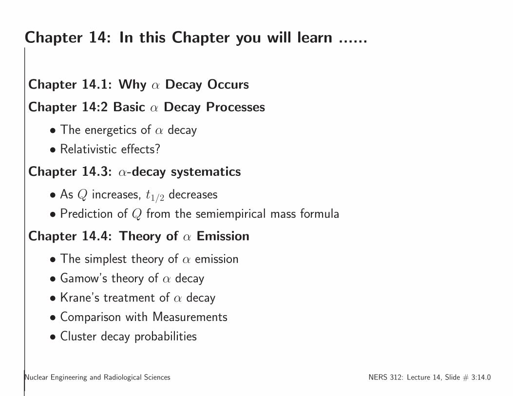
Chapter 14: In this Chapter you will learn ......
Chapter 14.1: Why α Decay Occurs
Chapter 14:2 Basic α Decay Processes
• The energetics of α decay
• Relativistic effects?
Chapter 14.3: α-decay systematics
• As Q increases, t1/2 decreases
• Prediction of Q from the semiempirical mass formula
Chapter 14.4: Theory of α Emission
• The simplest theory of α emission
• Gamow’s theory of α decay
• Krane’s treatment of α decay
• Comparison with Measurements
• Cluster decay probabilities
Nuclear Engineering and Radiological Sciences NERS 312: Lecture 14, Slide # 3:14.0

Chapter 14.5: Angular momentum and parity in α decay
• Angular momentum
• Conservation of angular momentum and parity
• Angular intensity of α decays for elliptic nuclei
Chapter 14.5: α-decay spectroscopy
Nuclear Engineering and Radiological Sciences NERS 312: Lecture 14, Slide # 4:14.1

14.1—Why α decay occurs
The mass excess (in MeV) of 4He and its near neighbors, is shown below.
⇓ N\Z ⇒ 0 1 2 30 - 7.2889705(1) - -1 8.0713171(5) 13.1357216(3) 14.9312148(24) 25.32(21)2 - 14.9498060(23) 2.4249156(1) 11.680(50)3 - 25.90(10) 11.390(50) 14.086793(15)
Thus, we see that, compared to its low-A neighbors in the periodic table, it is bound verystrongly.
We know, from the shell model of the nucleus, that 4He is a doubly-magic nucleus, andthis is what we may have expected.
So, thinking classically, occasionally 2 protons and 2 neutrons appear together at the edgeof a nucleus, with outward pointing momentum, and bang against the Coulomb barrier.
Every once in a while, it can tunnel through, as we saw in 311.
Nuclear Engineering and Radiological Sciences NERS 312: Lecture 14, Slide # 5:14.1

Nuclear Engineering and Radiological Sciences NERS 312: Lecture 14, Slide # 6:14.1

So compelling is this concept, that the α particles can stay intact in the nucleus, promptedtwo-time Nobel Laureate, Linus Pauling (the only person two have won two Nobel Prizes,awarded to a single person): http://en.wikipedia.org/wiki/Linus_Pauling
to invent a “spheron model” of the nucleus.
Nuclear Engineering and Radiological Sciences NERS 312: Lecture 14, Slide # 7:14.1

Quoting from the SOAK-TN (Source Of All Knowledge, True or Not)On September 16, 1952, Pauling opened a new research notebook with the words ”I have decided to at-
tack the problem of the structure of nuclei.”[86] On October 15, 1965, Pauling published his Close-Packed
Spheron Model of the atomic nucleus in two well respected journals, Science and the Proceedings of the
National Academy of Sciences.For nearly three decades, until his death in 1994, Pauling published numerous
papers on his spheron cluster model.
The basic idea behind Pauling’s spheron model is that a nucleus can be viewed as a set of “clusters of
nucleons”. The basic nucleon clusters include the deuteron [np], helion [pnp], and triton [npn]. Even-even
nuclei are described as being composed of clusters of alpha particles, as has often been done for light nuclei.
Pauling attempted to derive the shell structure of nuclei from pure geometrical considerations related to
Platonic solids rather than starting from an independent particle model as in the usual shell model. In an
interview given in 1990 Pauling commented on his model:
“Now recently, I have been trying to determine detailed structures of atomic nuclei by analyzing the ground
state and excited state vibrational bends, as observed experimentally. From reading the physics literature,
Physical Review Letters and other journals, I know that many physicists are interested in atomic nuclei, but
none of them, so far as I have been able to discover, has been attacking the problem in the same way that
I attack it. So I just move along at my own speed, making calculations...”
Nuclear Engineering and Radiological Sciences NERS 312: Lecture 14, Slide # 8:14.1
Who is this person?
http://en.wikipedia.org/wiki/Lenny_Susskind
Nuclear Engineering and Radiological Sciences NERS 312: Lecture 14, Slide # 9:14.2

14.2—Basic α-decay processes
An α decay is a nuclear transformation in which a nucleus reduces its energy by emittingan α-particle.
AZXN −→A−4
Z−2X′N−2 +4
2He2 ,
or, more compactly :
AX −→ X ′ + α .
The resultant nucleus, X ′ is usually left in an excited state, followed, possibly, by anotherα decay, or by any other form of radiation, eventually returning the system to the groundstate.
Nuclear Engineering and Radiological Sciences NERS 312: Lecture 14, Slide # 10:14.2

The energetics of α decay
The α-decay process is “fueled” by the rest mass energy difference of the initial state andfinal state. That is, using a relativistic formalism:
Ei = Ef
mXc2 = m
X′c2 + TX ′ + mαc
2 + Tα
Q = TX ′ + Tα where
Q ≡ mXc2 − m
X′c2 − mαc
2
Q/c2 ≈ m(AX) − m(A−4X ′) − m(4He) , (1)
TX ′ and Tα are the kinetic energies of the nucleus and the α-particle following the decay
The atomic masses may be substituted for the nuclear masses, as shown in the last lineabove.
The electron masses balance in the equations, and there is negligible error in ignoring thesmall differences in electron binding energies.
Nuclear Engineering and Radiological Sciences NERS 312: Lecture 14, Slide # 11:14.2

The line of flight of the decay products are in equal and opposite directions, assumingthat X was at rest. Conservation of energy and momentum apply. Thus we may solvefor Tα in terms of Q (usually known). X ′ is usually not observed directly. Solving for Tα
by eliminating X ′:
Q = Tα + TX ′ (2)
|~pα| = |~pX′|
p2α = p2
X′2mαTα = 2m
X′TX ′
(mα/mX′)Tα = TX ′ . (3)
Using (3) and (2) to eliminate TX ′ results in:
Q = Tα(1 + mα/mX′) or (4)
Tα =Q
(1 + mα/mX′)(5)
Nuclear Engineering and Radiological Sciences NERS 312: Lecture 14, Slide # 12:14.2

Tα ≈ Q
(1 + 4/A′)or (6)
Tα ≈ Q
(1 + 4/A)or (7)
Tα ≈ Q(1 − 4/A) (8)
Equations (4) and (5) are exact within a non-relativistic formalism.
Equation (6) is an approximation, but a good one that is suitable for all α-decay’s, in-cluding 8Be→ 2α.
Equation (7) is suitable for all the other α-emitters, while (8) is only suitable for the heavyemitters, since it assumes A ≫ 4.
We see from (8) that the typical recoil energy, for heavy emitters is:
TX ′ = Q − Tα ≈ (4/A)Q . (9)
Nuclear Engineering and Radiological Sciences NERS 312: Lecture 14, Slide # 13:14.2

For a typical α-emitter, this recoil energy (Q = 5 MeV, A = 200) is 100 keV.
This is not insignificant. α-emitters are usually found in crystalline form, and that recoilenergy is more than sufficient to break atomic bonds, and cause a microfracture along thetrack of the recoil nucleus.
Nuclear Engineering and Radiological Sciences NERS 312: Lecture 14, Slide # 14:14.2

Relativistic effects?
One may do a fully relativistic calculation, from which it is found that:
Tα =
Q
(
1 + 12
Qm
X′c2
)
(
1 + mαm
X′+ Q
mX′c2
) , (10)
TX ′ =
(
mαm
X′
)
Q(
1 + 12
Qmαc2
)
(
1 + mαm
X′+ Q
mX′c2
) . (11)
Even in the worst-case scenario (low-A) this relativistic correction is about 2.5 × 10⁻⁴.Thus the non-relativistic approximation is adequate for determining Tα or TX ′.
Nuclear Engineering and Radiological Sciences NERS 312: Lecture 14, Slide # 15:14.3

14.3—α Decay Systematics
As Q increases, t1/2 decreases
This is, more or less, self-evident. More “fuel” implies faster decay.
The “smoothest” example of this “law” is seen in the α decay of the even-even nuclei
Shell model variation is minimized in this case, since no pair bonds are being broken.
See Figure 1, where log10(t1/2) is plotted vs. Q.
Geiger and Nuttal proposed the following phenomenological fit for log10(t1/2(Q)):
log10 λ = C − DQ−1/2 or (12)
log10 t1/2 = −C ′ + DQ−1/2 , (13)
where C and D are fitting constants, and C ′ = C − log10(ln 2).
Odd-odd, even-odd and odd-even nuclei follow the same general systematic trend, but thedata are much more scattered, and their half-lives are 2–1000 times that of their even-evencounterparts.
Nuclear Engineering and Radiological Sciences NERS 312: Lecture 14, Slide # 16:14.3
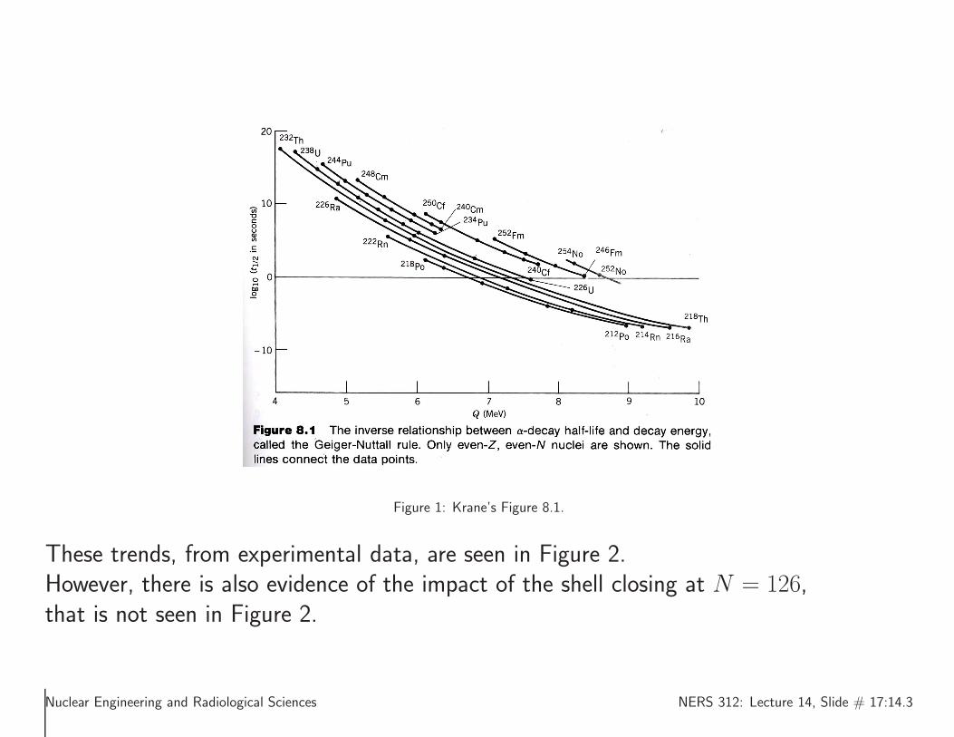
Figure 1: Krane’s Figure 8.1.
These trends, from experimental data, are seen in Figure 2.However, there is also evidence of the impact of the shell closing at N = 126,that is not seen in Figure 2.
Nuclear Engineering and Radiological Sciences NERS 312: Lecture 14, Slide # 17:14.3
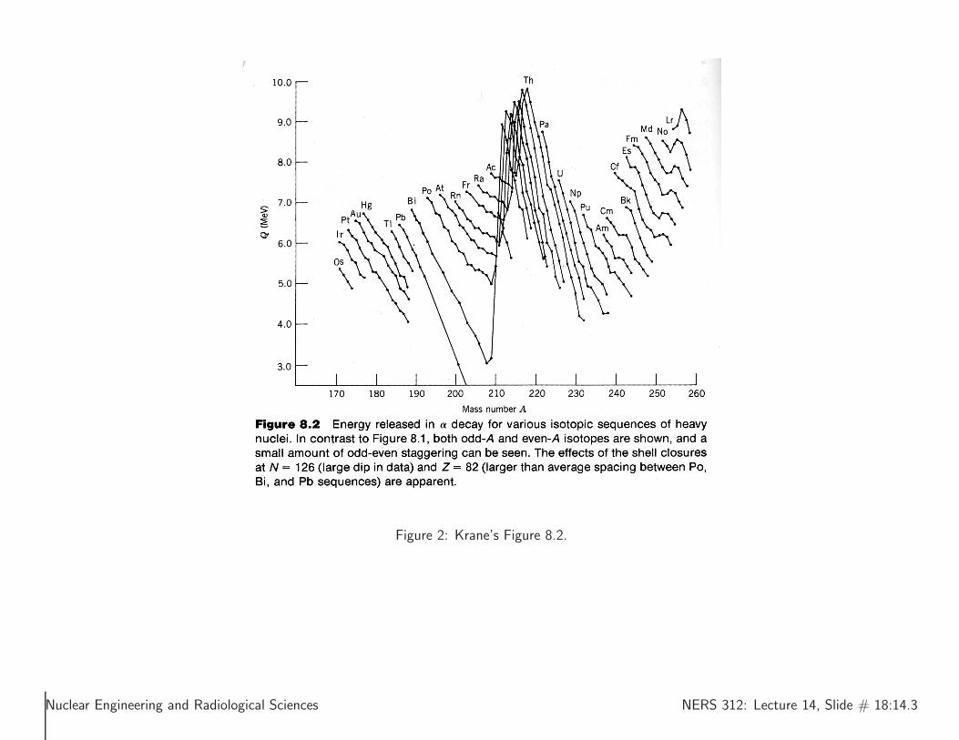
Figure 2: Krane’s Figure 8.2.
Nuclear Engineering and Radiological Sciences NERS 312: Lecture 14, Slide # 18:14.3

Prediction of Q from the semiempirical mass formula
The semiempirical mass formula can be employed to estimate Qα,as a function of Z and A.
Q = B(Z − 2, A − 4) + B(eHe) − B(Z, A)
≈ 28.3 − 4aV
+8
3a
SA−1/3 + 4a
CZA−1/3(1 − Z/3A) − 4asym(1 − 2Z/A)2 + 3apA
−7/4 .
(14)
A plot of Q(Z,A) using (14) is given in Figure 3.
Nuclear Engineering and Radiological Sciences NERS 312: Lecture 14, Slide # 19:14.3

160 170 180 190 200 210 220 230 240 250 260
3
4
5
6
7
8
9
10Q vs. A
A
Q (
MeV
)
Figure 3: Q(Z, A) using (14). The dashed line is for Pb (Z = 82), while the lower dotted is for Os (Z = 76). The upper dotted line is for Lr(Z = 103). Each separate Z has its own line with higher Z’s oriented to the right.
Nuclear Engineering and Radiological Sciences NERS 312: Lecture 14, Slide # 20:14.4
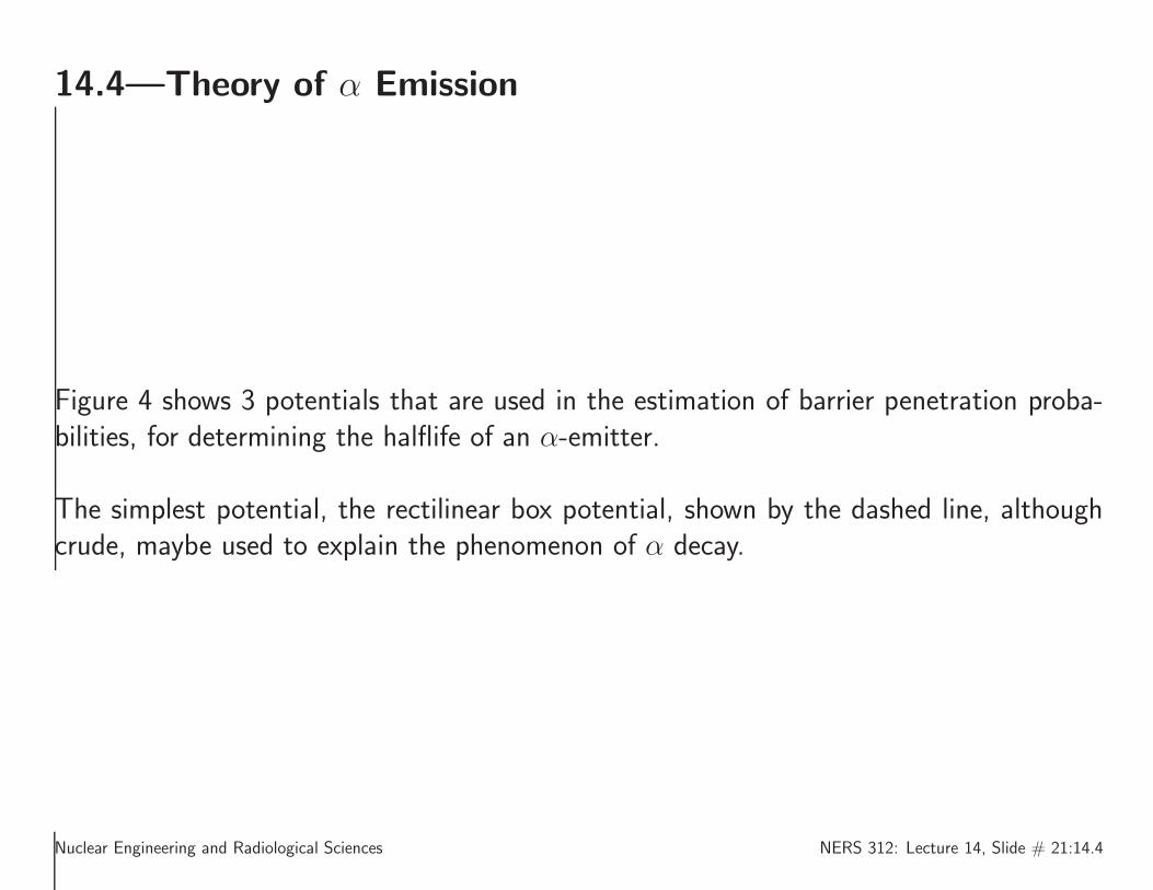
14.4—Theory of α Emission
Figure 4 shows 3 potentials that are used in the estimation of barrier penetration proba-bilities, for determining the halflife of an α-emitter.
The simplest potential, the rectilinear box potential, shown by the dashed line, althoughcrude, maybe used to explain the phenomenon of α decay.
Nuclear Engineering and Radiological Sciences NERS 312: Lecture 14, Slide # 21:14.4

0 10 20 30 40 50 60 70−40
−30
−20
−10
0
10
20
30
40
r (fm)
V (
MeV
)
Potentials for α−barrier penetration, 190Pb
V
simple
Vcoulomb
Vigo
Q
Figure 4: Potentials for α decay.
Nuclear Engineering and Radiological Sciences NERS 312: Lecture 14, Slide # 22:14.4

The simplest theory of α emission
In this section we solve for the decay probability using the simplest rectilinear box potential.
This potential is characterized by:
V1(r < RN) = −V0
V2(RN < r < b) = VC
V3(r > b) = 0 , (15)
where V0 and VC are constants.
The 3-D radial wavefunctions (assuming that the α is in an s-state), are of the form,Ri(r) = ui(r)/r take the form:
u1(r) = Aeik1r + Be−ik1r
u2(r) = Cek2r + De−k2r
u3(r) = Feik3r , (16)
where
k1 =√
2m(V0 + Q)/~
k2 =√
2m(VC − Q)/~
k3 =√
2mQ/~ . (17)
Nuclear Engineering and Radiological Sciences NERS 312: Lecture 14, Slide # 23:14.4

Turning the mathematical crank, we arrive at the transmission coefficient:
T =
[
1
4
(
2 +k1
k3+
k3
k1
)
+sinh2[2k2(b − RN)]
4
(
k1k3
k22
+k2
2
k1k3+
k1
k3+
k3
k1
)]−1
(18)
Note: We solved a similar problem in NERS 311, but with V0 = 0, that is, k1 = k3.
The factor k2(b − RN) ≈ 35 for typical α emitters. Thus, we can simplify to:
T =16e−2k2(b−RN)
(
k1k3
k22
+k22
k1k3+ k1
k3+ k3
k1
) (19)
Nuclear Engineering and Radiological Sciences NERS 312: Lecture 14, Slide # 24:14.4
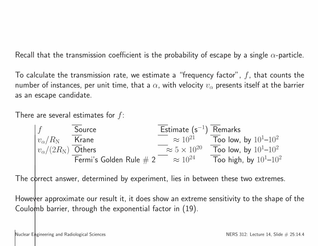
Recall that the transmission coefficient is the probability of escape by a single α-particle.
To calculate the transmission rate, we estimate a “frequency factor”, f , that counts thenumber of instances, per unit time, that a α, with velocity vα presents itself at the barrieras an escape candidate.
There are several estimates for f :
f Source Estimate (s−1) Remarksvα/RN Krane ≈ 1021 Too low, by 101–102
vα/(2RN) Others ≈ 5 × 10²⁰ Too low, by 101–102
Fermi’s Golden Rule # 2 ≈ 1024 Too high, by 101–102
The correct answer, determined by experiment, lies in between these two extremes.
However approximate our result it, it does show an extreme sensitivity to the shape of theCoulomb barrier, through the exponential factor in (19).
Nuclear Engineering and Radiological Sciences NERS 312: Lecture 14, Slide # 25:14.4
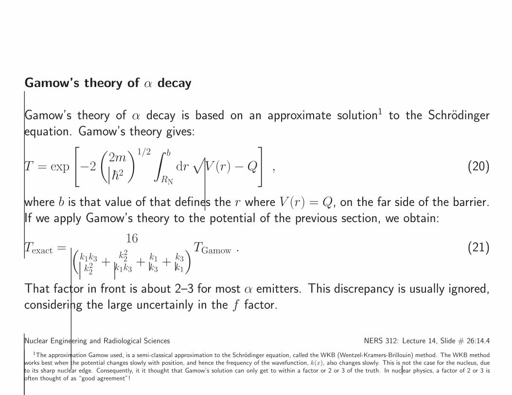
Gamow’s theory of α decay
Gamow’s theory of α decay is based on an approximate solution1 to the Schrodingerequation. Gamow’s theory gives:
T = exp
[
−2
(
2m
~2
)1/2 ∫ b
RN
dr√
V (r) − Q
]
, (20)
where b is that value of that defines the r where V (r) = Q, on the far side of the barrier.If we apply Gamow’s theory to the potential of the previous section, we obtain:
Texact =16
(
k1k3
k22
+k22
k1k3+ k1
k3+ k3
k1
)TGamow . (21)
That factor in front is about 2–3 for most α emitters. This discrepancy is usually ignored,considering the large uncertainly in the f factor.
Nuclear Engineering and Radiological Sciences NERS 312: Lecture 14, Slide # 26:14.4
1The approximation Gamow used, is a semi-classical approximation to the Schrodinger equation, called the WKB (Wentzel-Kramers-Brillouin) method. The WKB methodworks best when the potential changes slowly with position, and hence the frequency of the wavefunction, k(x), also changes slowly. This is not the case for the nucleus, dueto its sharp nuclear edge. Consequently, it it thought that Gamow’s solution can only get to within a factor or 2 or 3 of the truth. In nuclear physics, a factor of 2 or 3 isoften thought of as “good agreement”!

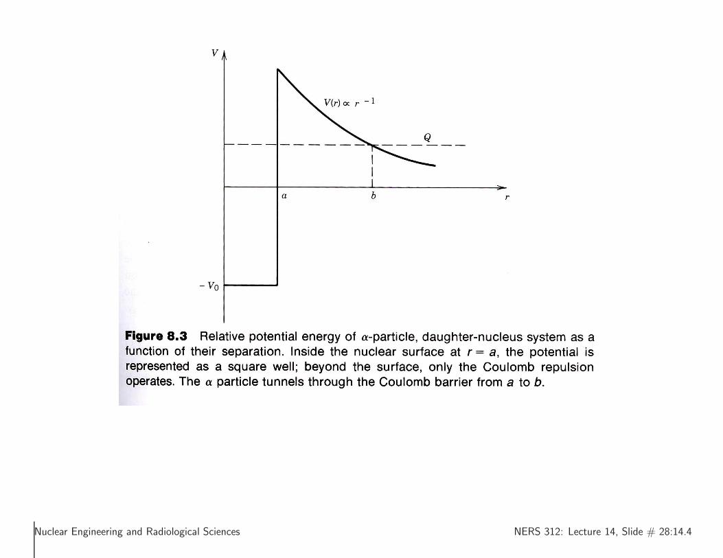
Krane’s treatment of α-decay
Krane starts out with (20), namely:
T = exp
[
−2
(
2m
~2
)1/2 ∫ b
a
dr√
V (r) − Q
]
,
where
V (x) =2(Z − 2)e2
4πǫ0x
V (a) ≡ B =2(Z − 2)e2
4πǫ0a
a = R0(A − 4)1/3
V (b) ≡ Q =2(Z − 2)e2
4πǫ0b. (22)
That is, the α moves in the potential of the daughter nucleus, B is the height of thepotential at the radius of the daughter nucleus, and b is the radius where that potentialis equal to Q. Therefore, Q = B.
Nuclear Engineering and Radiological Sciences NERS 312: Lecture 14, Slide # 27:14.4
Nuclear Engineering and Radiological Sciences NERS 312: Lecture 14, Slide # 28:14.4

Substituting the potential in (22) into (20) results in:
T = exp
{
−2
(
2m′αc
2
Q(~c)2
)1/2zZ ′e2
4πǫ0
[
arccos(√
x) −√
x(1 − x)]
}
, (23)
where x ≡ a/b = Q/B. Note that the reduced mass,
m′α =
mαmX ′
mα + mX ′≈ mα(1 − 4/A) . (24)
has been used.
This “small” difference can result in a change in T by a factor of 2–3, even for heavy nuclei!
Krane also discusses the approximation to (23) that results in his equation (8.18). Thiscomes from the Taylor expansion:
arccos(√
x) −√
x(1 − x) −→ π
2− 2
√x + O(x3/2) .
This is only valid for small x. Typically x ≈ 0.3, and use of Krane’s (8.18) involves toomuch error. So, stick with the equation given on the next page, instead.
Nuclear Engineering and Radiological Sciences NERS 312: Lecture 14, Slide # 29:14.4

Factoring in the frequency factor, one can show that:
t1/2 = ln(2)a
c
√
mαc2
2(V0 + Q)×
exp
{
2
(
2m′αc
2
Q(~c)2
)1/2zZ ′e2
4πǫ0
[
arccos(√
x) −√
x(1 − x)]
}
. (25)
Nuclear Engineering and Radiological Sciences NERS 312: Lecture 14, Slide # 30:14.4

14.4.1—Comparison with Measurements
In this section we employ the simplest form of f and compute the half-life for α-decay asfollows:
t1/2 = ln(2)a
c
√
mαc2
2(V0 + Q)exp
{
2
(
2m′αc
2
Q(~c)2
)1/2zZ ′e2
4πǫ0
[
arccos(√
x) −√
x(1 − x)]
}
(26)
The data are shown in the following table, where the half-lives of the even-even isotopesof Th (Z = 90) are shown.
A Q (MeV) t1/2 (s) t1/2 (s) t1/2 (s) t1/2 (s)
abs. meas. abs. calc. rel. meas. rel. calc.
220 8.95 10−5 10−3 5.4 × 10⁻⁹ 3.6 × 10⁻⁹
222 8.13 2.8 × 10⁻³ 2.1 × 10⁻¹ 1.5 × 10⁻⁶ 7.3 × 10⁻⁷
224 7.31 1.04 1.1 × 10² 5.6 × 10⁻⁴ 3.8 × 10⁻⁴
226 6.45 1854 2.9 × 10⁵ ≡ 1 ≡ 1
228 5.52 6.0 × 10⁷ 1.2 × 10¹⁰ 3.2 × 10⁴ 4.2 × 10⁴
230 4.77 2.5 × 10¹² 6.0 × 10¹⁴ 1.3 × 10⁹ 2.1 × 10⁹
232 4.08 4.4 × 10¹⁷ 1.8 × 10²⁰ 2.4 × 10¹⁴ 6.2 × 10¹⁴
Table 1: Half-lives of Th isotopes, absolute and relative comparisons of measurement and theory.
Nuclear Engineering and Radiological Sciences NERS 312: Lecture 14, Slide # 31:14.4

The calculations were performed using a nuclear radius of a = 1.25A1/3 (fm),and V0 = 35 (MeV).
The absolute comparison exhibits the same trends for both experiment and calculations,with the calculations being overestimated by 2–3 orders of magnitude.
This is most likely due to a gross underestimate of f . The relative comparisons are inmuch better shape, showing discrepancies of about a factor of 2–3, quite a success forsuch a crude theory.
We note that small changes in Q result in enormous differences in the results.
In this table Q changes by about a factor of 2, while the half-lives span about 23 ordersof magnitude.
The probability of escape is greatly influenced by the height and width of the Coulombbarrier.
Nuclear Engineering and Radiological Sciences NERS 312: Lecture 14, Slide # 32:14.4

Besides this dependence, the only other variation in the comparison relates to the nuclearradius.
This also affects the barrier since the nuclear radius is proportional to A1/3. This hintsthat the remaining discrepancy, at least for the relative comparison, is related to the finedetails of the shape of the barrier, perhaps mostly in the vicinity of the inner turning point.
A more refined shape of the Coulomb barrier would likely yield better results, as well woulda higher-order WKB analysis that would account more precisely, for that shape variation.
Additionally, the α-particle was treated as if it were a point charge in this analysis. Arefined calculation should certainly take this effect into account.
Nuclear Engineering and Radiological Sciences NERS 312: Lecture 14, Slide # 33:14.4

Cluster decay probabilities
If α decay can occur, surely 8Be and 12C decay can occur as well. It is just a matter ofrelative probability. For these decays, the escape probabilities are given approximately by:
T8Be = T 2α
T12C = T 3α
TAX = TZ/2α . (27)
The last estimate is for a A X cluster, with Z protons and an atomic mass of A.
Nuclear Engineering and Radiological Sciences NERS 312: Lecture 14, Slide # 34:14.5

14.5—Angular momentum and parity in α decay
Angular momentum
If the α-particle carries off angular momentum, we must add the repulsive potential asso-ciated with the centrifugal barrier to the Coulomb potential, VC(r):
V (r) = VC(r) +l(l + 1)~2
2m′αr
2, (28)
represented by the second term on the right-hand side of (28).The effect on 90Th, with Q = 4.5 MeV is:
l 0 1 2 3 4 5 6Tl/T0 1 0.84 0.60 0.36 0.18 0.078 0.028
So, as l ↑, T ↓.
Nuclear Engineering and Radiological Sciences NERS 312: Lecture 14, Slide # 35:14.5

Conservation of angular momentum and parity
α decay’s must satisfy the constraints given by theconservation of total angular momentum:
~Ii = ~If + ~Iα
Πi = Πf × Πα , (29)
where i represents the parent nucleus, and f represents the daughter nucleus. Since theα-particle is a 0+ nucleus, (29) simplifies to:
~Ii = ~If +~lαΠi = Πf × (−1)lα , (30)
where lα is the orbital angular momentum carried off by the α-particle.
If Ii is non-zero, the α decay is able to populate any excited state of the daughter, or godirectly to the ground state.
Nuclear Engineering and Radiological Sciences NERS 312: Lecture 14, Slide # 36:14.5

If the initial state has total spin 0, with few exceptions it is a 0+. In this case, (30)becomes.
~0 = ~If +~lα+1 = Πf × (−1)lα , (31)
or,
~If = ~lαΠf+ = (−1)lα , (32)
Thus the only allowed daughter configurations are: 0+, 1−, 2+, 3−, 4+, 5−, 6+, 7−, 8+, 9− · · ·All other combinations are absolutely disallowed.
The α decay can show these allowed transitions quite nicely. A particularly nice exampleis the case where the transition is 0+ −→ 0+, where the low-lying rotational band, andhigher energy phonon structure are explicitly revealed through α decay.
Nuclear Engineering and Radiological Sciences NERS 312: Lecture 14, Slide # 37:14.5
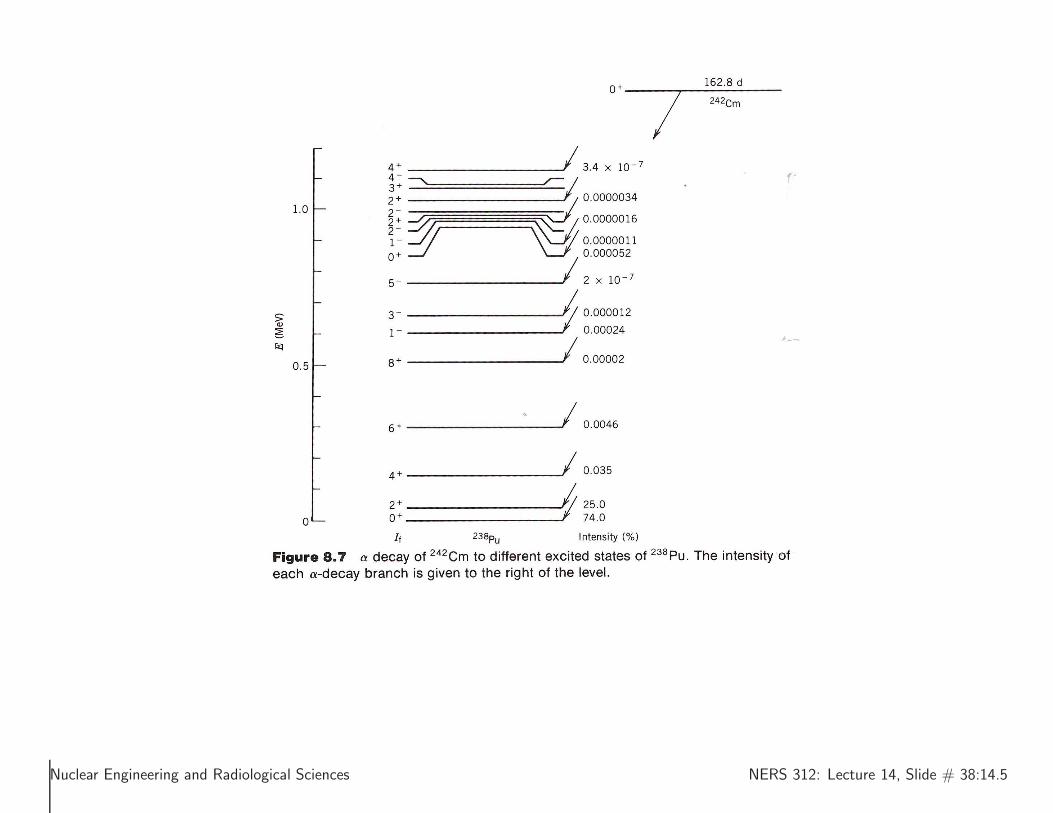
Nuclear Engineering and Radiological Sciences NERS 312: Lecture 14, Slide # 38:14.5

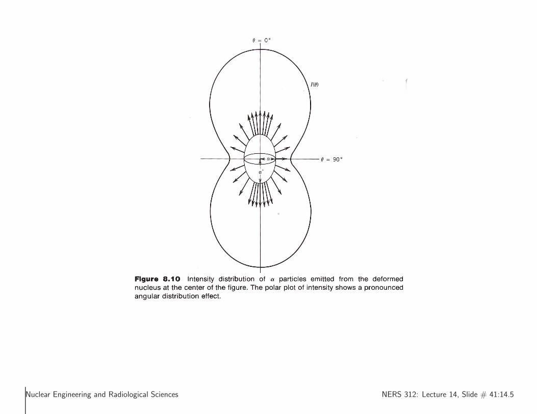
Angular intensity of α decays for elliptic nuclei
Nuclei in the mass range 150 < A < 190 and A > 200 have permanent non-sphericaldeformations.
These deformations can be modeled as prolate (elongated, cigar-shaped) or oblate (flat,pancake) on the azimuthal symmetry axis.
It follows that the α-decay angular distributions are anisotropic.
The α emission from the longer axes is enhanced, as seen in the following two figures.
Clearly, a more sophisticated approach is required to describe this mathematically.This is a well-defined, do-able, but tough 499 project!
Nuclear Engineering and Radiological Sciences NERS 312: Lecture 14, Slide # 39:14.5

Nuclear Engineering and Radiological Sciences NERS 312: Lecture 14, Slide # 40:14.5
Nuclear Engineering and Radiological Sciences NERS 312: Lecture 14, Slide # 41:14.5