ners 312 elements of nuclear engineering and …ners311/courselibrary/lecture13.pdf · ners 312...

NERS 312

Elements of Nuclear Engineering and Radiological Sciences II

aka Nuclear Physics for Nuclear Engineers

Lecture Notes for Chapter 13: Radioactive decay

Supplement to (Krane II: Chapter 6)

Note: The lecture number corresponds directly to the chapter number in the online book.The section numbers, and equation numbers correspond directly to those in the online book.

c©Alex F Bielajew 2016, Nuclear Engineering and Radiological Sciences, The University of Michigan

Chapter 13: In this Chapter you will learn ......

Chapter 13.1: The Radioactive Decay Law ...

1. The reason for exponential decay

2. What half-life is

3. Lifetime, or mean lifetime

4. Activity

5. Decay from one isotope, with two decay channels

6. Decay from one “parent”, to many stable “daughters”

7. Decay from two isotopes, to independent decay channels

Chapter 13.2: Quantum Theory of Radioactive Decay

1. Application to nuclear γ decay

2. The Lorentz distribution

3. Density of final states...

4. Density of final states for γ-decay

5. Derivation of Fermi’s Golden Rule #2

6. The small perturbation approximation

Nuclear Engineering and Radiological Sciences NERS 312: Lecture 13, Slide # 2:13.0

Chapter 13.3: Production and Decay of Radioactivity

1. Secular equilibrium

2. Application to a real-life engineering application

Chapter 13.4: Growth of Daughter Activities

1. Parent ⇒ Daughter ⇒ Granddaughter

2. Very long-lived parent: λ1 ≪ λ2 decays

3. Long-lived parent: λ1 ≪ λ2 decays

4. Series of Decays — The Bateman equations


Chapter 13.5: Types of Decays

1. α decay

2. β decay

3. γ decay

4. Internal conversion

5. Nucleon emission

6. Spontaneous fission

7. Cluster decay

Chapter 13.8: Units for Measuring Radiation

1. Activity

2. Exposure

3. Absorbed Dose

4. Dose Equivalent


13.1—The Radioactive Decay Law

Exponential decay law

• Consider a system of particles, N0 in number at time, t = 0.

• Each particle has an independent, = probability of decay per unit time, λ.

• How many particles are observed at a later time?

• Assume that N is large enough, use calculus.

• Particles are integral quantities, so this is really an approximation!

Thus, the change in N us given by:

dN = −λNdt; N(0) = N0

dN

N= −λdt

d[logN ] = −λdt

logN − logN0 = −λt

logN = logN0 − λt

N = N0 exp(−λt) (13.1)

Voila, the well-known exponential decay law, N(t) = N0e−λt.


Half-life

The half-life, t1/2, is defined as follows:

N(t + t1/2)

N(t)≡

1

2=N0 exp(−λt− λt1/2)

N0 exp(−λt)= exp(−λt1/2) ,

or,

t1/2 =log 2

λ≈

0.693

λ. (13.2)

Thus we see, a population of N radioactive particles at t would be reduced by half (onaverage) at time t + t1/2.


Lifetime, or mean lifetime

The exponential law can also be interpreted as the decay probability for a single radioactiveparticle to decay in the interval dt, about t.. This probability, p(t), properly normalized,is given by:

p(t)dt = λe−λtdt ;

∫ ∞

0

p(t)dt = 1 . (13.3)

The we see that the probability a particle decays within time t, P (t) is given by,

P (t) =

∫ t

0

p(t′)dt′ = 1− e−λt. (13.4)

The mean lifetime or lifetime of a particle, τ , is evaluated by calculating 〈t〉, using theprobability distribution (13.3),

τ = λ

∫ ∞

0

te−λtdt =1

λ. (13.5)


Activity

The number of decays, ∆N , observed from t and t +∆t, obtained from (13.1)

N(t) = N0e−λt

is:

∆N = N(t)−N(t +∆t) = N0e−λt(1− e−λ∆t) .

If ∆t≪ τ , then, in the limit as ∆t→ 0, we may rewrite the above as:

lim∆t→0

∣

∣

∣

∣

∆N

∆t

∣

∣

∣

∣

≡

∣

∣

∣

∣

dN

dt

∣

∣

∣

∣

= λN0e−λt = λN(t) ≡ A(t) = A0e

−λt , (13.6)

defining the activity, A(t), and its initial value, A0. Activity is usually what is measured,sinceN0 andN(t) are usually unknown, and not of particular interest in many applications.

What is generally of real interest is the actual activity of a real source, or the actual valueof λ.


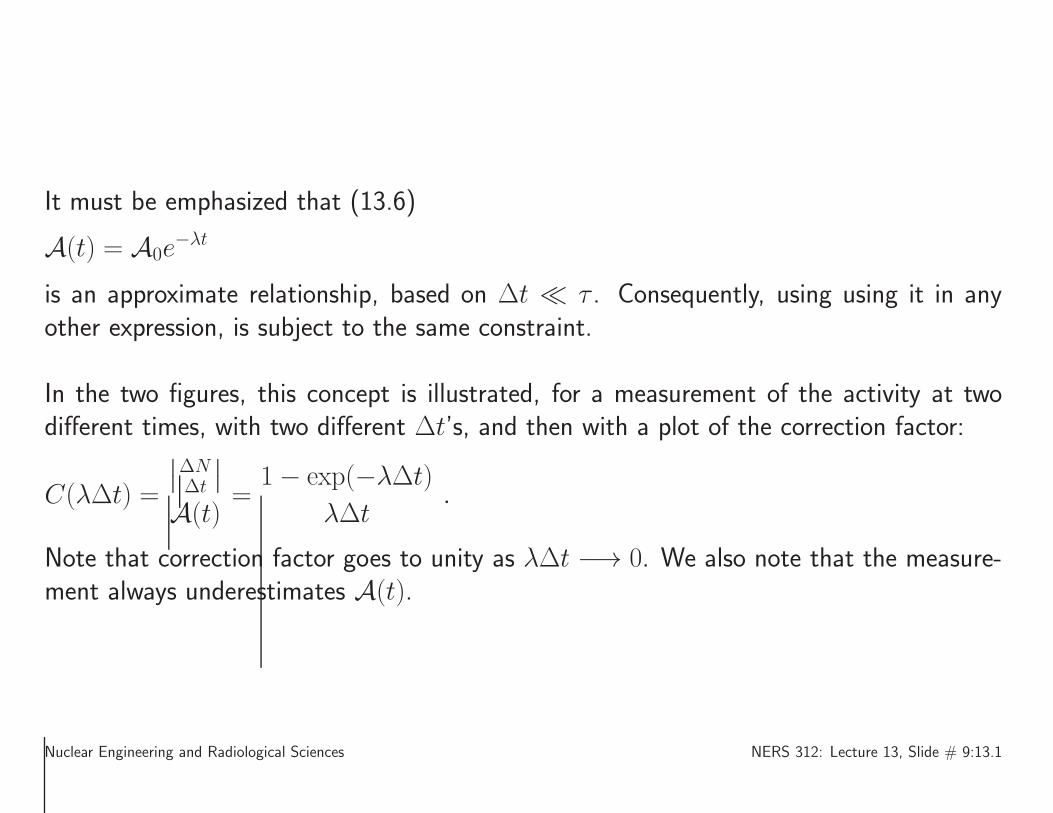
It must be emphasized that (13.6)

A(t) = A0e−λt

is an approximate relationship, based on ∆t ≪ τ . Consequently, using using it in anyother expression, is subject to the same constraint.

In the two figures, this concept is illustrated, for a measurement of the activity at twodifferent times, with two different ∆t’s, and then with a plot of the correction factor:

C(λ∆t) =

∣

∣

∆N∆t

∣

∣

A(t)=

1− exp(−λ∆t)

λ∆t.

Note that correction factor goes to unity as λ∆t −→ 0. We also note that the measure-ment always underestimates A(t).


λt0 0.5 1 1.5 2 2.5 3

A(t)A

/A(0)

0

0.1

0.2

0.3

0.4

0.5

0.6

0.7

0.8

0.9

1Activity measurements over finite time spans


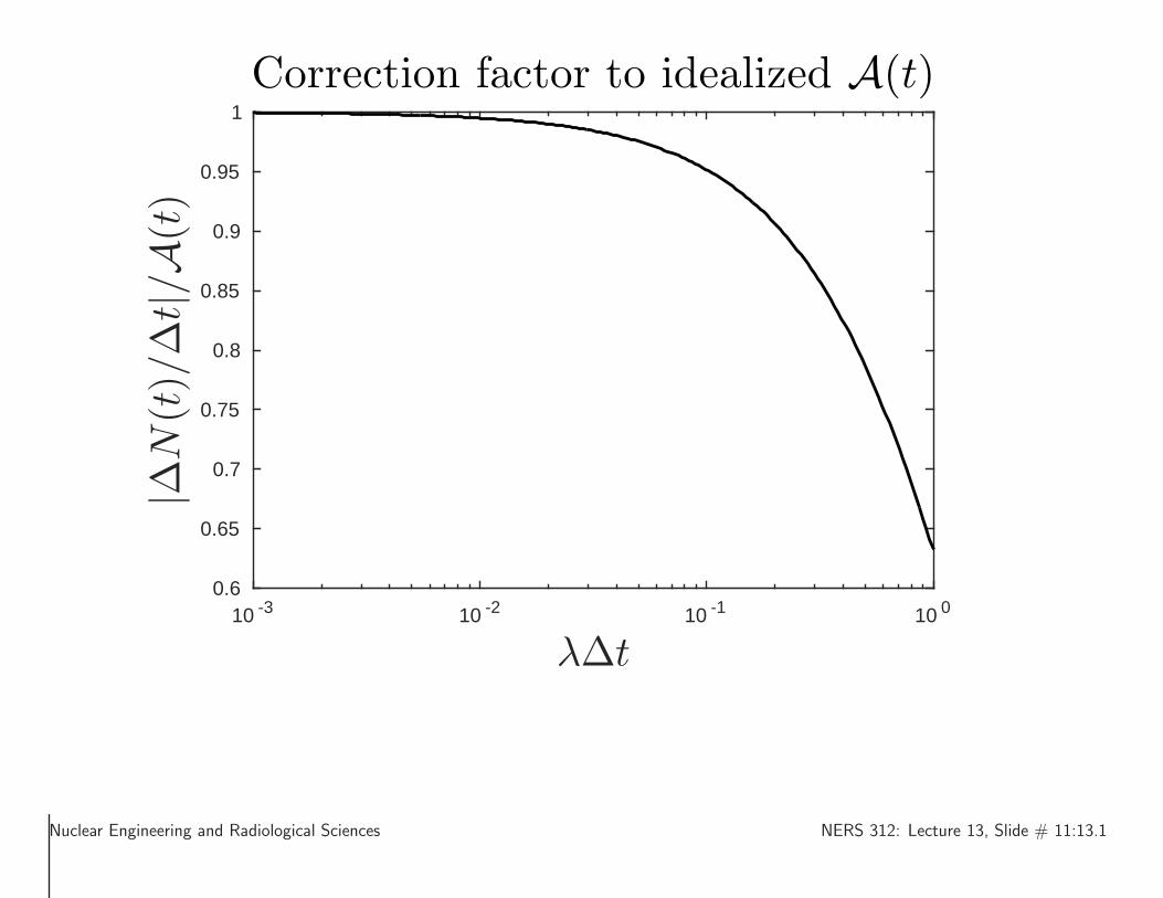
λ∆t10 -3 10 -2 10 -1 10 0

|∆N(t)/∆t|/A

(t)

0.6

0.65

0.7

0.75

0.8

0.85

0.9

0.95

1

Correction factor to idealized A(t)


If it is the measured value of λ that is desired, we have a uniform expression:

λ =log[A(t1)/A(t2)]

t2 − t1=

log[N (t1)/N (t2)]

t2 − t1

Finally, this discussion only applies for the decay of a single isotope, N0, to another(presumably stable) nucleus, N1. Any measurement involving very short measurementtimes, must be analyzed carefully.


Growth and decline of radioactivity generations

General considerationsThe most general form for describing the growth and decline of the generations of ra-dioisotopes is with the general differential form that described the growth and/or declineof isotope Ni:

dNi =

Npi∑

j=1

Njλjidt−Ni

Ndi∑

j=1

λijdt ,

where,Npi = Number of parents of isotope Ni

Ndi = Number of daughters of isotope Ni

λji = Rate of growth of isotope Ni from parent Nj

λij = Rate of decay of isotope Ni into daughter Nj

If there are two subscripts on λ, the left one refers to that parent, and the right one refersto the daughter.

If there is only one subscript, it means that there is only one parent. That subscript refersto the daughter only. Most of the examples that follow fall into this category.


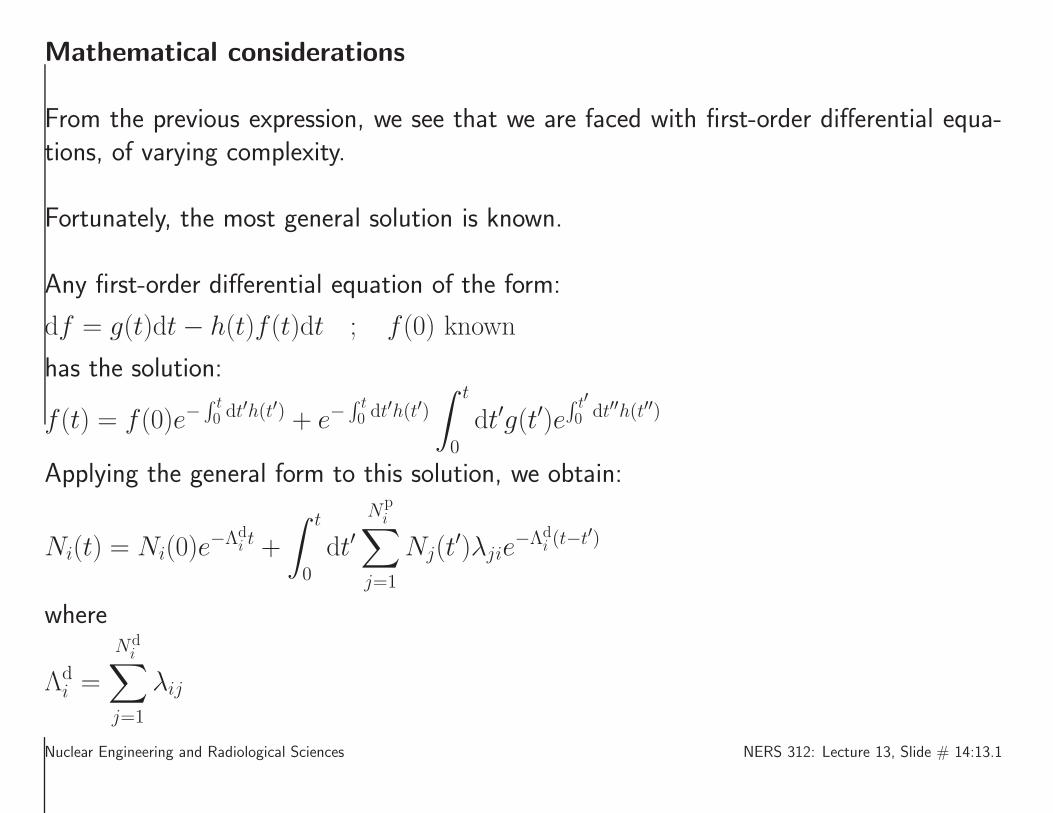
Mathematical considerations

From the previous expression, we see that we are faced with first-order differential equa-tions, of varying complexity.

Fortunately, the most general solution is known.

Any first-order differential equation of the form:

df = g(t)dt− h(t)f(t)dt ; f(0) known

has the solution:

f(t) = f(0)e−∫ t0 dt

′h(t′) + e−∫ t0 dt

′h(t′)

∫ t

0

dt′g(t′)e∫ t′

0 dt′′h(t′′)

Applying the general form to this solution, we obtain:

Ni(t) = Ni(0)e−Λd

i t +

∫ t

0

dt′N

pi∑

j=1

Nj(t′)λjie

−Λdi (t−t

′)

where

Λdi =

Ndi∑

j=1

λij


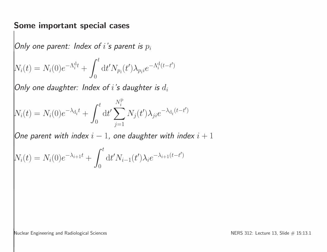
Some important special cases

Only one parent: Index of i’s parent is pi

Ni(t) = Ni(0)e−Λd

i t +

∫ t

0

dt′Npi(t′)λpiie

−Λdi (t−t

′)

Only one daughter: Index of i’s daughter is di

Ni(t) = Ni(0)e−λdit +

∫ t

0

dt′N

pi∑

j=1

Nj(t′)λjie

−λdi(t−t′)

One parent with index i− 1, one daughter with index i + 1

Ni(t) = Ni(0)e−λi+1t +

∫ t

0

dt′Ni−1(t′)λie

−λi+1(t−t′)


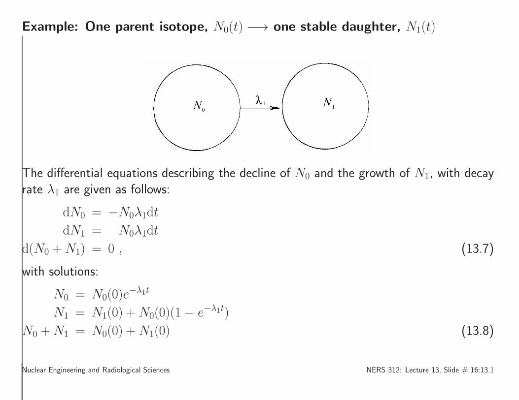
Example: One parent isotope, N0(t) −→ one stable daughter, N1(t)

The differential equations describing the decline of N0 and the growth of N1, with decayrate λ1 are given as follows:

dN0 = −N0λ1dt

dN1 = N0λ1dt

d(N0 +N1) = 0 , (13.7)

with solutions:

N0 = N0(0)e−λ1t

N1 = N1(0) +N0(0)(1− e−λ1t)

N0 +N1 = N0(0) +N1(0) (13.8)


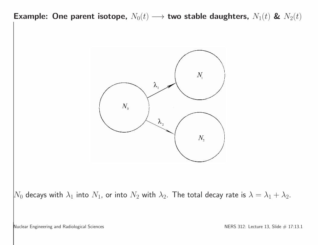
Example: One parent isotope, N0(t) −→ two stable daughters, N1(t) & N2(t)

N0 decays with λ1 into N1, or into N2 with λ2. The total decay rate is λ = λ1 + λ2.


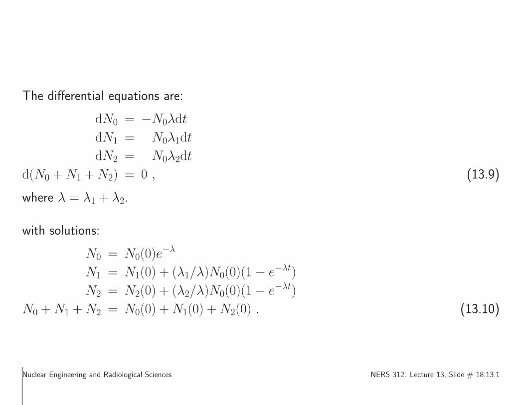
The differential equations are:

dN0 = −N0λdt

dN1 = N0λ1dt

dN2 = N0λ2dt

d(N0 +N1 +N2) = 0 , (13.9)

where λ = λ1 + λ2.

with solutions:

N0 = N0(0)e−λ

N1 = N1(0) + (λ1/λ)N0(0)(1− e−λt)

N2 = N2(0) + (λ2/λ)N0(0)(1− e−λt)

N0 +N1 +N2 = N0(0) +N1(0) +N2(0) . (13.10)


Example: One parent isotope, N0(t) −→ many stable daughters

The results of the one parent (nuclear isotope) −→ 2 stable daughters),can easily be generalized to many daughters.


The differential equations are:

dN0 = −N0λdt

dN1 = N0λ1dt

dN2 = N0λ2dt... = ...

dNn = N0λndt

d

(

N0 +

n∑

i=1

Ni

)

= 0 , (13.11)

where λ =∑n

i=1 λ0i, or,∑

i=1 λ0i/λ = 1.

The solutions are given by:

N0 = N(0)e−λt

Ni = Ni(0) + (λ0i/λ)N0(1− e−λ)

N +

n∑

i=1

Ni = N(0) +

n∑

i=1

Ni(0) . (13.12)

The quantity λ0i/λ is called the branching ratio for decay into channel i.


Example: One parent isotope, two-generation decay chain

In this example, N1(0) = N2(0) = 0.By definition, decays chains end in a stable nucleus.The differential equations are:

dN0 = −N0λ1dt

dN1 = N0λ1dt−N1λ2dt

dN2 = N1λ2dt

d(N0 +N1 +N2) = 0 .


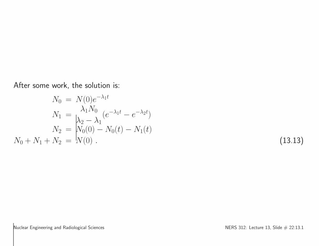
After some work, the solution is:

N0 = N(0)e−λ1t

N1 =λ1N0

λ2 − λ1(e−λ1t − e−λ2t)

N2 = N0(0)−N0(t)−N1(t)

N0 +N1 +N2 = N(0) . (13.13)


Example: One parent isotope, n-generation decay chainIn this example, Ni(0) = 0 for i ≥ 1.By definition, decays chains end in a stable nucleus.

These result in the Bateman equations, a special case of our general considerations...

An = N0(0)n−1∑

i=0

cie−λi+1t

cm =

∏n−1i=0 λi

∏n−1i=0;i 6=m(λi+1 − λm+1)

Please note that Krane’s equations single-index λ’s differ in that his λ refers to the parent,not the daughter.


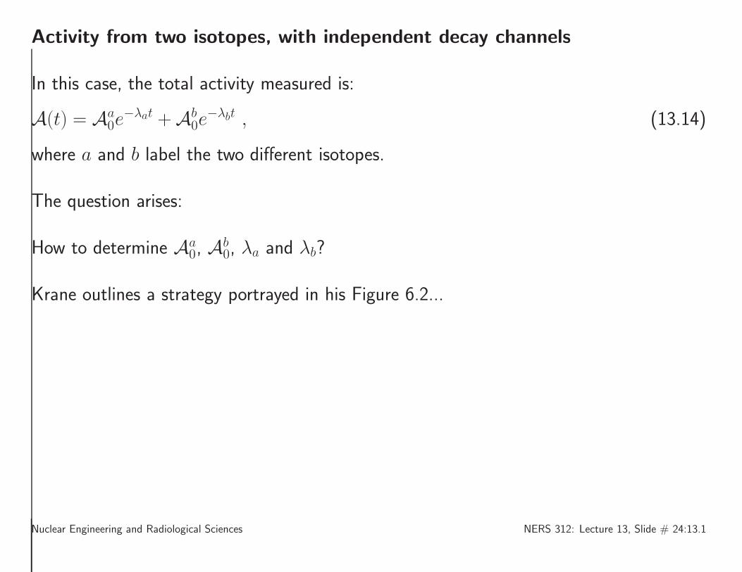
Activity from two isotopes, with independent decay channels

In this case, the total activity measured is:

A(t) = Aa0e

−λat +Ab0e

−λbt , (13.14)

where a and b label the two different isotopes.

The question arises:

How to determine Aa0, A

b0, λa and λb?

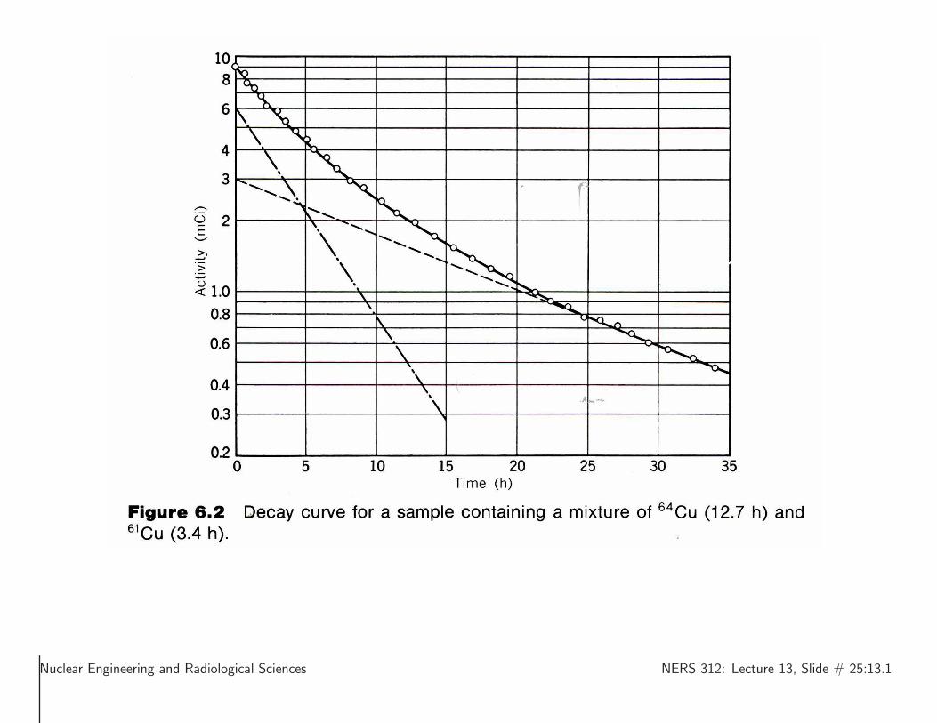
Krane outlines a strategy portrayed in his Figure 6.2...


If, for example, isotope a has a considerably longer half-life, the linear tail of the log-linearplot of A can be extrapolated backward to isolate Aa

0.

The slope of this line also yields λa. The one plots log(A(t)−Aa0e

−λat) that should givea straight line log-linear plot.

The values of Ab0 and λb can then be determined.


13.2—Quantum Theory of Radioactive Decay

The Quantum Theory of Radioactive Decay starts with a statement of Fermi’s GoldenRule #2, the equation from which decays rates, and cross sections are obtained.

It is one of the central equations in Quantum Mechanics. Fermi’s Golden Rule #2 for thetransition rate (probability of transition per unit time), λ, is given by:

λ =2π

~|〈ψf |Vp|ψi〉|

2 dnfdEf

, (13.15)

where ψi is the initial quantum state, operated on by a perturbation (transition) potential,Vp, resulting in the final quantum state, ψf .

The factor dnf/dEf is called the density of final states [sometimes given the notationρ(Ef)].

The density of final states factor enumerates the number of possible final states (degen-eracy) that can acquire the final energy Ef .


It is not possible to express a less generic form of this factor, without a specific applicationin mind.

It must be derived on a case-by-case basis, for a given application. We shall have oppor-tunity to do for several examples before the conclusion of lecture.


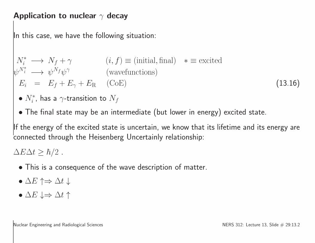
Application to nuclear γ decay

In this case, we have the following situation:

N ∗i −→ Nf + γ (i, f) ≡ (initial, final) ∗ ≡ excited

ψN∗i −→ ψNfψγ (wavefunctions)

Ei = Ef + Eγ + ER (CoE) (13.16)

• N ∗i , has a γ-transition to Nf

• The final state may be an intermediate (but lower in energy) excited state.

If the energy of the excited state is uncertain, we know that its lifetime and its energy areconnected through the Heisenberg Uncertainly relationship:

∆E∆t ≥ ~/2 .

• This is a consequence of the wave description of matter.

• ∆E ↑⇒ ∆t ↓

• ∆E ↓⇒ ∆t ↑


What is the exact relationship between a state’s lifetime,and the distribution of energies that are observed????

• The derivation is sketched in the following and the results presented.

• The details of the derivation are left to the optional section at the end of this section.


Derivation of the Lorentzian distribution

We start by assuming that the final nuclear state is given by:

ψNf (~x, t) = ψNf(~x)eiEf t/~e−t/(2τ)

|ψNf(~x, t)|2 = |ψNf(~x)|2e−t/τ , (13.17)

to agree with our discussion, in the last section, of the probability of decay of a singleparticle. Recall that τ is the “lifetime”.

The derivation in the next section reveals that the probability of observing decay energyE, p(E), is given by:

p(E) =Γ

2π

1

(E − Ef)2 + (Γ/2)2, (13.18)

where Γ ≡ ~/τ . This probability distribution is normalized:∫ ∞

−∞

dE p(E) = 1 .


• The peak of this distribution is p(Ef)

• Γ width of the distribution at half-maximumThat is, p(Ef ± Γ/2) = 1

2p(Ef)

• 〈E〉 = Ef .

• This distribution is called the Lorentz distribution, or simply, the Lorentzian function.a.k.a. the Cauchy-Lorentz, Cauchy, or Breit-Wigner distribution

• Wikipedia has a useful page on this topic.

• The unnormalized Lorentzian is plotted in Figure 13.1

• The normalized Lorentzian is plotted in Figure 13.2.

• We note that this spread of energies is intrinsicIt has nothing to do with measurement uncertaintiesEven with a perfect detector, we would observe this spread of detected energies

• It is a result of the finite lifetime, and Heisenberg Uncertainty


E/Ef

0 0.5 1 1.5 2

p(E/E

f)

0

0.1

0.2

0.3

0.4

0.5

0.6

0.7

0.8

0.9

1

Lorentz distribution (unnormalized)

Γ/(2Ef ) = 0.05

Γ/(2Ef ) = 0.10

Γ/(2Ef ) = 0.20

Figure 13.1: The unnormalized Lorentzian.


E/Ef

0 0.5 1 1.5 2

p(E/E

f)

0

1

2

3

4

5

6

7

8

Lorentz distribution (normalized)

Γ/(2Ef ) = 0.05

Γ/(2Ef ) = 0.10

Γ/(2Ef ) = 0.20

Figure 13.2: The normalized Lorentzian.


Consequences?

• For typical γ-transition lifetimes, 10−12 s < τ <∞, 0.00066 eV > Γ > 0

• γ spectroscopy can exquisitely isolate the individual energy levels

• This is drastically difference for high-energy physics, where intrinsic widths can be ofthe order of 1 GeV or so. Nearby excitation can overlap with each other, and theidentification of excited states (of hadrons) can be very difficult.


Density of final states

Finally, we calculate the density of states, after talking about it for so long!

• Given a final energy of a quantum system, how many states, dnf enumerates thenumber of quantum states that fall in the range, Ef −→ Ef + dEf?

• From this, we form the ratio dnf/dEf , a.k.a. the density of final states.

• This version assumes that there is just one free particle in the final state.

• This will cover most (but not all!) of the physics of interest in this course.


• Expressing the free particle wave function, as it would exist in a cubical L3 box, withV = 0 inside, V → ∞ outside, and one corner at the origin of the coordinate system

• As we discovered in NERS311, the wavefunction is given by:

ψnx,ny,nz(x, y, z) =

(

2

L

)3/2

sin(nxπx

L

)

sin(nyπy

L

)

sin(nzπz

L

)

(13.19)

where 1 ≤ ni <∞ are the 3 quantum numbers (i = 1, 2, 3) in the 3D system.

• The 3 momentum components are given by:

pi =niπ~

L(13.20)


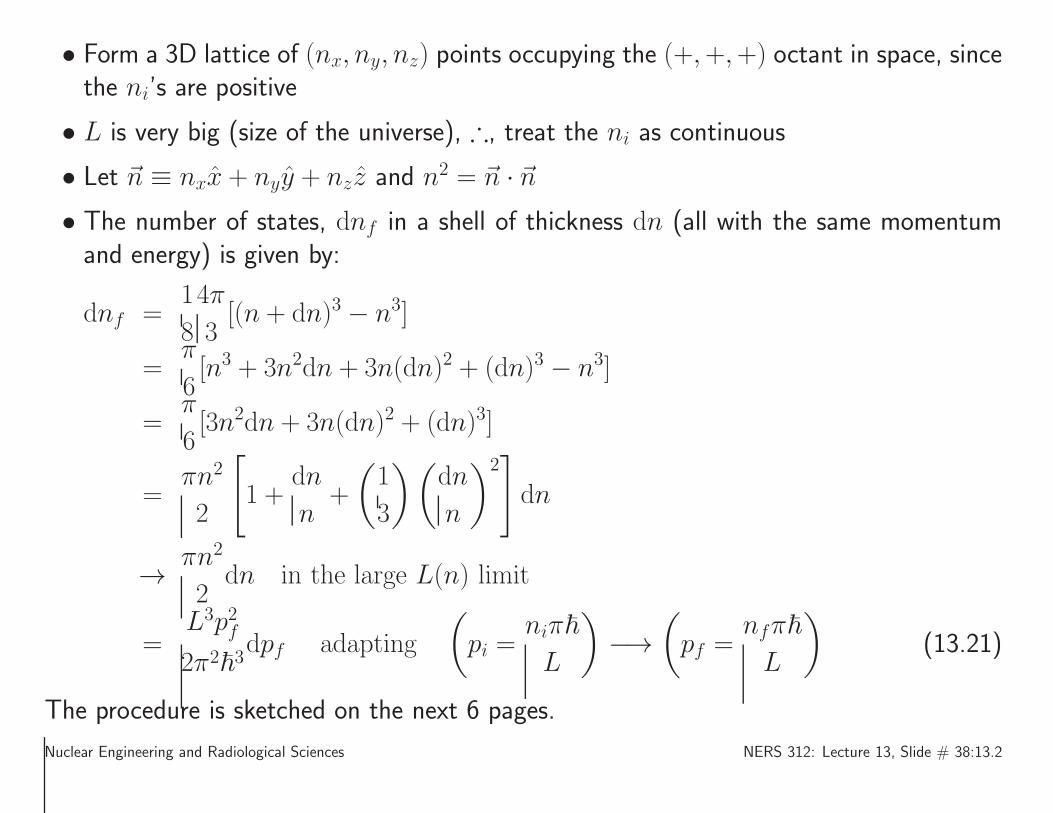
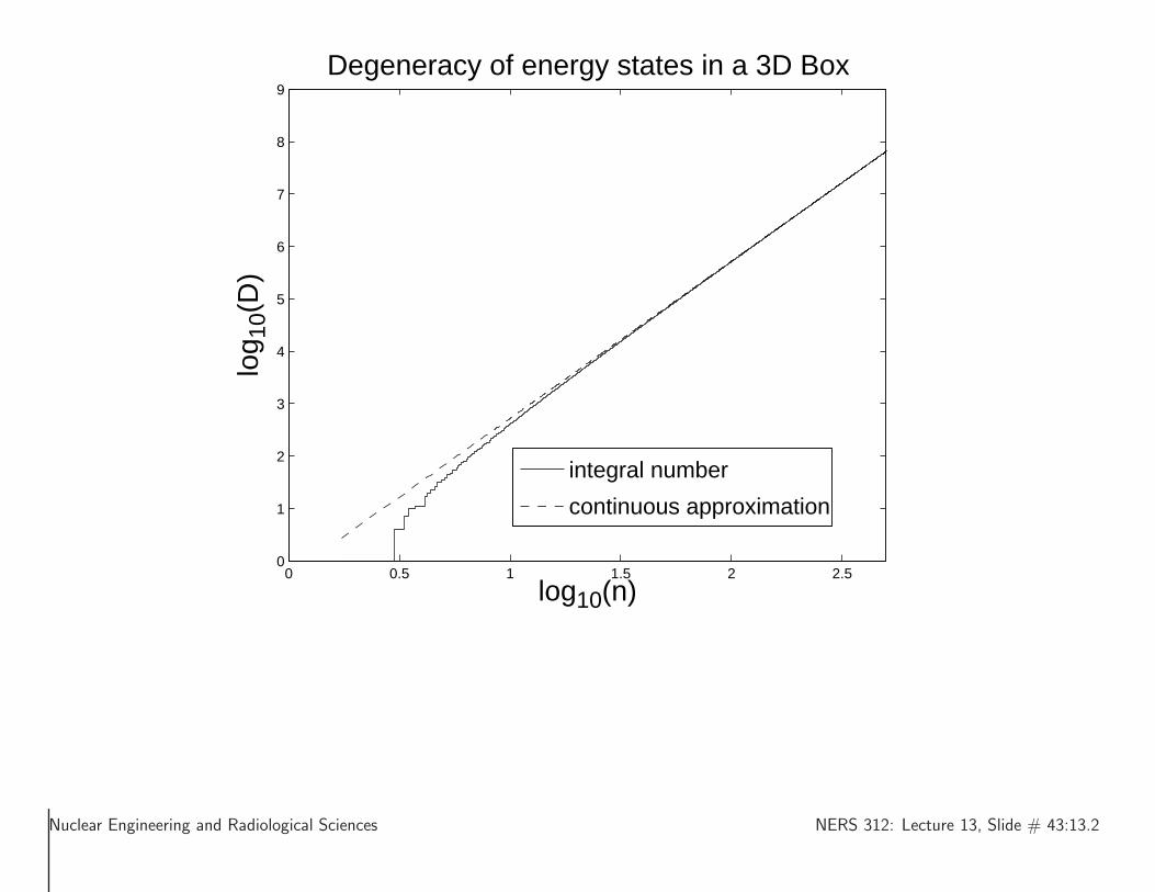
• Form a 3D lattice of (nx, ny, nz) points occupying the (+,+,+) octant in space, sincethe ni’s are positive

• L is very big (size of the universe), ∴, treat the ni as continuous

• Let ~n ≡ nxx + nyy + nzz and n2 = ~n · ~n

• The number of states, dnf in a shell of thickness dn (all with the same momentumand energy) is given by:

dnf =1

8

4π

3[(n + dn)3 − n3]

=π

6[n3 + 3n2dn + 3n(dn)2 + (dn)3 − n3]

=π

6[3n2dn + 3n(dn)2 + (dn)3]

=πn2

2

[

1 +dn

n+

(

1

3

)(

dn

n

)2]

dn

→πn2

2dn in the large L(n) limit

=L3p2f2π2~3

dpf adapting

(

pi =niπ~

L

)

−→

(

pf =nfπ~

L

)

(13.21)

The procedure is sketched on the next 6 pages.


0 10 20 30 40 50 60 70 80 90 1000

10

20

30

40

50

60

70

80

90

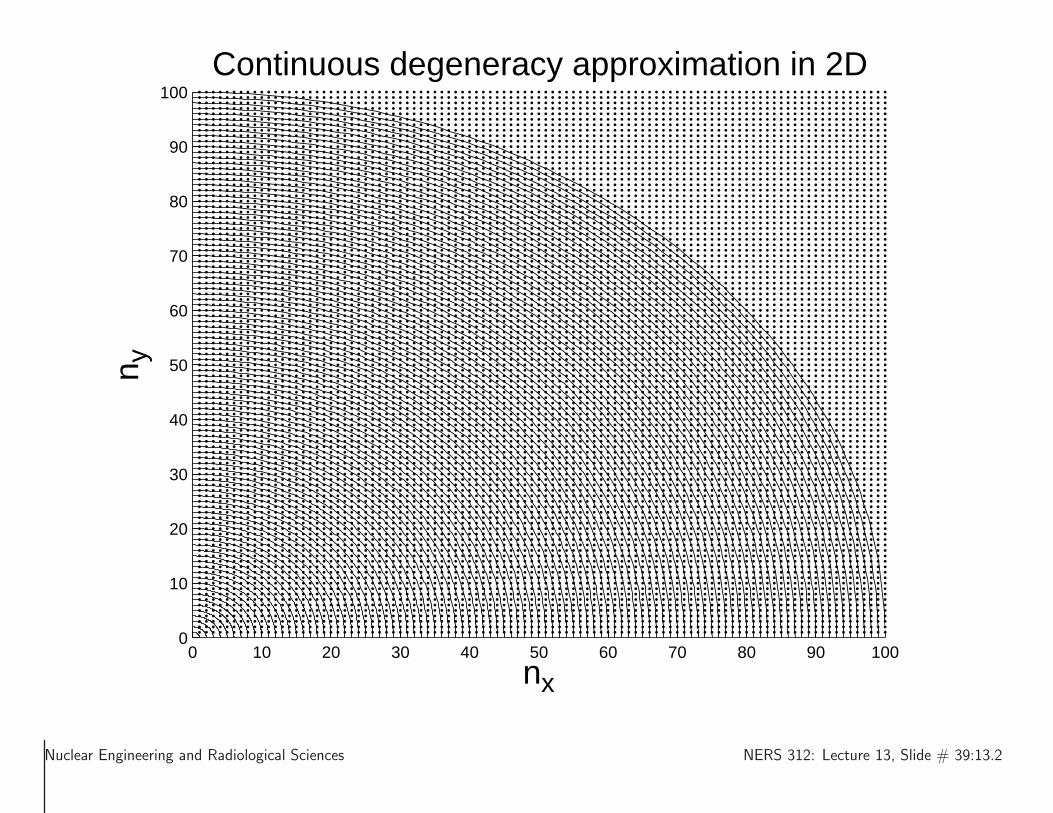
100Continuous degeneracy approximation in 2D

nx

n y


• n is a ginormous! number, of the order of 1015 if L is macroscopic

• n is as large as 1040, if we use an L that is the size of the known universe (about 92billion light years across)

• (Aside) The age of the universe is known to be 13.772(59) billion years, how did theymeasure that distance? [Wiki: “Universe”]

Regarding the plot on the previous page ...


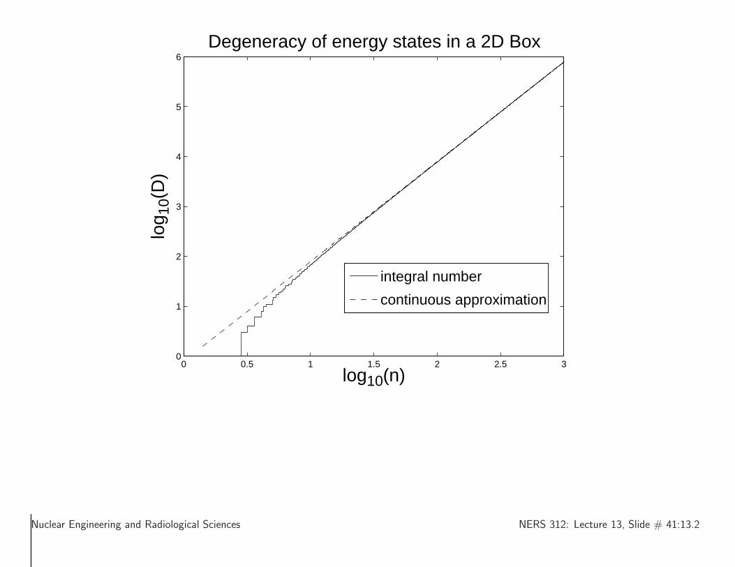
0 0.5 1 1.5 2 2.5 30

1

2

3

4

5

6Degeneracy of energy states in a 2D Box

log10(n)

log 1

0(D

)

integral number

continuous approximation


0 0.5 1 1.5 2 2.5 30

0.001

0.002

0.003

0.004

0.005

0.006

0.007

0.008

0.009

0.01Error in the 2D continuous approximation

log10(n)

log 1

0(co

ntin

uous

/inte

gral

)


0 0.5 1 1.5 2 2.50

1

2

3

4

5

6

7

8

9Degeneracy of energy states in a 3D Box

log10(n)

log 1

0(D

)

integral number

continuous approximation


0 0.5 1 1.5 2 2.50

0.001

0.002

0.003

0.004

0.005

0.006

0.007

0.008

0.009

0.01Error in the 3D continuous approximation

log10(n)

log 1

0(co

ntin

uous

/inte

gral

)


From (13.21)

dnf =L3p2f2π2~3

dpf

• This nf is the degeneracy of pf .

• The above expression is valid for quantum particles with or without mass, relativisticor not!

Finally, we write the density of states, as:

∴dnfdEf

=

(

dnfdpf

)(

dpfdEf

)

=L3p2f2π2~3

(

dpfdEf

)

Using the familiar kinematic expressions,

Ef =p2f2m

; Ef = pfc ; Ef =√

(pfc)2 + (mc2)2

for particles that are non-relativistic, massless, and relativistic with mass


Thus

dnfdEf

=L3

2π2~3

√

2m3Ef

=L3

2π2~3E2f

c3

=L3

2π2~3

Ef

√

E2f − (mc2)

c3(13.22)

for particles that are non-relativistic, massless, and relativistic with mass


γ-decay

For one photon in the final state, from (13.20)

Eγ = cpγ = nπ~c/L . (13.23)

Thus,

n =EγL

π~cdn

dEγ=

L

π~c. (13.24)

Recognizing that Ef = Eγ, the results of (13.24) used in (13.22) gives:

dnfdEγ

=1

2π2L3

(~c)3E2γ . (13.25)


Specializing to γ decay, we adapt (13.15)

λ =2π

~|〈ψf |Vp|ψi〉|

2 dnfdEf

,

using the notation of (13.16)

N ∗i −→ Nf + γ

ψN∗i −→ ψNfψγ

Ei = Ef + Eγ + ER ,

along with result of (13.25):

dnfdEγ

=1

2π2L3

(~c)3E2γ .

to get:

λγ =L3

π~(~c)3∣

∣〈ψNfψγ|Vp|ψN i〉∣

∣

2E2γ .


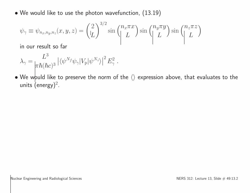
• We would like to use the photon wavefunction, (13.19)

ψγ ≡ ψnx,ny,nz(x, y, z) =

(

2

L

)3/2

sin(nxπx

L

)

sin(nyπy

L

)

sin(nzπz

L

)

in our result so far

λγ =L3

π~(~c)3∣

∣〈ψNfψγ|Vp|ψN i〉∣

∣

2E2γ .

• We would like to preserve the norm of the 〈〉 expression above, that evaluates to theunits (energy)2.


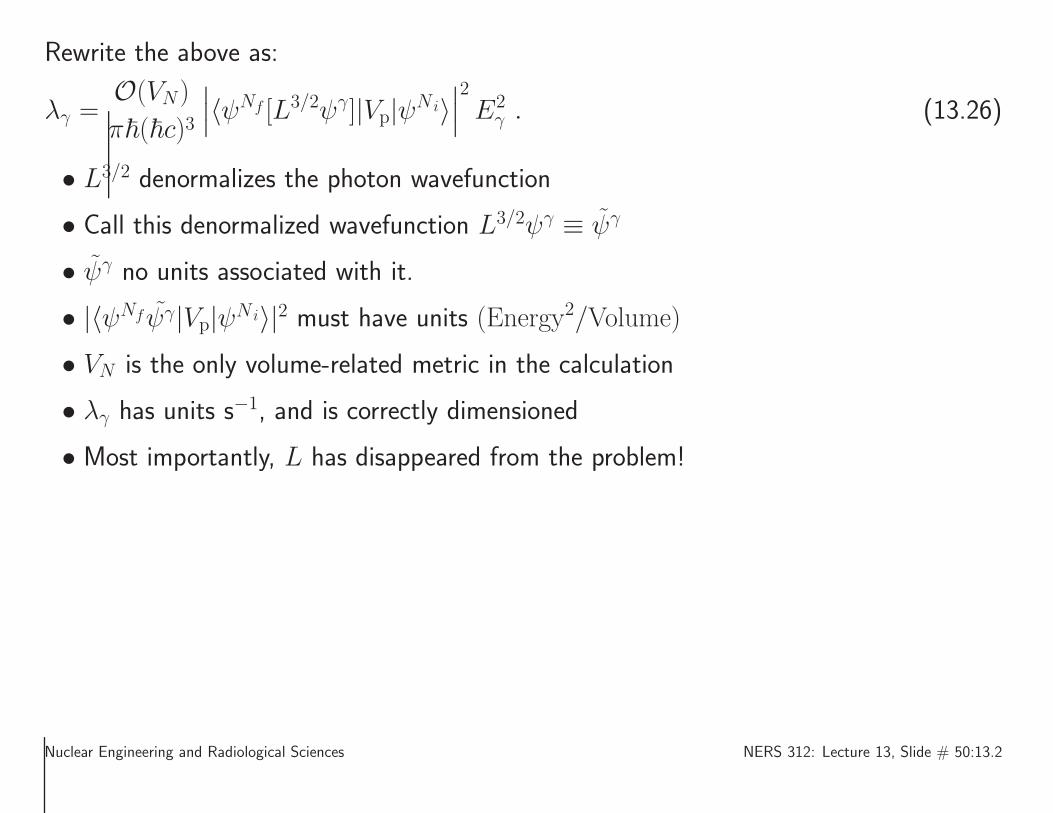
Rewrite the above as:

λγ =O(VN)

π~(~c)3

∣

∣

∣〈ψNf [L3/2ψγ]|Vp|ψ

N i〉∣

∣

∣

2

E2γ . (13.26)

• L3/2 denormalizes the photon wavefunction

• Call this denormalized wavefunction L3/2ψγ ≡ ψγ

• ψγ no units associated with it.

• |〈ψNf ψγ|Vp|ψN i〉|2 must have units (Energy2/Volume)

• VN is the only volume-related metric in the calculation

• λγ has units s−1, and is correctly dimensioned

• Most importantly, L has disappeared from the problem!


Interested students, please see the book for these advanced topics...

Derivation of Fermi’s Golden Rule #2

Discussion of the “small perturbation” approximation

Derivation of the Lorentz distribution


13.3—Production and Decay of Radioactivity

Secular equilibrium

Consider a beam of radiation, with intensity I , that impinges upon a block of materialcontaining nuclei of type “0”. There are N0 nuclei in the target to start, and the externalradiation activates the material, producing nuclear species “1”. We make two assumptions:

1. The target is “thin enough”, so that the external radiation is not attenuated.

2. The irradiation is weak enough so that N0 does not decline.

With these assumptions, R, the rate of production of N1 is given by:

R = IσN0 , (13.55)

where σ is the radioactivity production cross section.


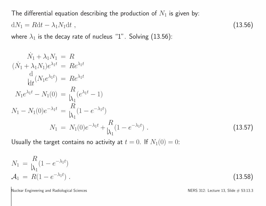
The differential equation describing the production of N1 is given by:

dN1 = Rdt− λ1N1dt , (13.56)

where λ1 is the decay rate of nucleus “1”. Solving (13.56):

N1 + λ1N1 = R

(N1 + λ1N1)eλ1t = Reλ1t

d

dt(N1e

λ1t) = Reλ1t

N1eλ1t −N1(0) =

R

λ1(eλ1t − 1)

N1 −N1(0)e−λ1t =

R

λ1(1− e−λ1t)

N1 = N1(0)e−λ1t +

R

λ1(1− e−λ1t) . (13.57)

Usually the target contains no activity at t = 0. If N1(0) = 0:

N1 =R

λ1(1− e−λ1t)

A1 = R(1− e−λ1t) . (13.58)


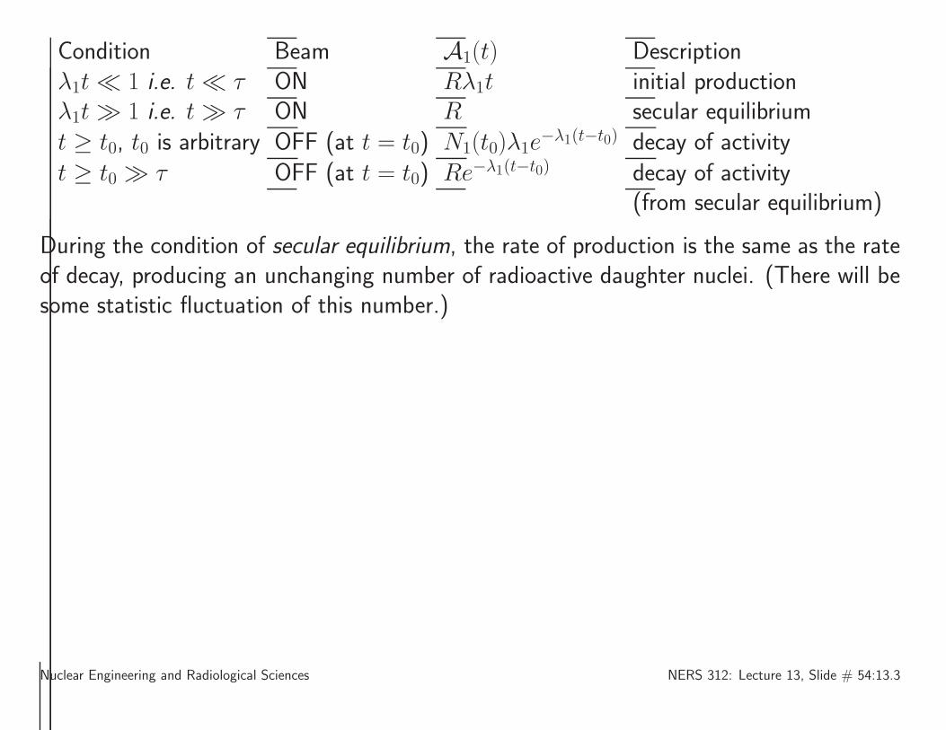
Condition Beam A1(t) Descriptionλ1t≪ 1 i.e. t≪ τ ON Rλ1t initial productionλ1t≫ 1 i.e. t≫ τ ON R secular equilibriumt ≥ t0, t0 is arbitrary OFF (at t = t0) N1(t0)λ1e

−λ1(t−t0) decay of activityt ≥ t0 ≫ τ OFF (at t = t0) Re−λ1(t−t0) decay of activity

(from secular equilibrium)

During the condition of secular equilibrium, the rate of production is the same as the rateof decay, producing an unchanging number of radioactive daughter nuclei. (There will besome statistic fluctuation of this number.)


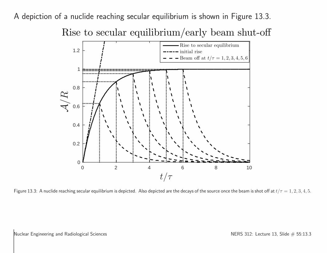
A depiction of a nuclide reaching secular equilibrium is shown in Figure 13.3.

t/τ0 2 4 6 8 10

A/R

0

0.2

0.4

0.6

0.8

1

1.2

Rise to secular equilibrium/early beam shut-offRise to secular equilibrium

initial rise

Beam off at t/τ = 1, 2, 3, 4, 5, 6

Figure 13.3: A nuclide reaching secular equilibrium is depicted. Also depicted are the decays of the source once the beam is shot off at t/τ = 1, 2, 3, 4, 5.


A real-life engineering application

A typical engineering challenge, in the area of creating radioactive sources, is to minimizethe cost of producing a given amount of activity. We model this as follows:

The cost, C, per unit activity, factoring start-up costs, S0, (manufacture of the inactivesource, delivery costs, operator start-up and take-down), and the cost of running the ac-celerator or reactor, per unit meanlife, R0, is given as follows:

C =S0 +R0x01− e−x0

, (13.59)

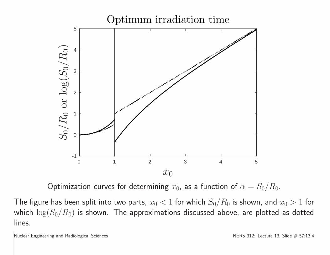
where x0 is the number of meanlives that the target is irradiated.The optimization condition is given by:

S0/R0 = ex0 − (1 + x0) . (13.60)

For small S0/R0, the optimum x0 ≈√

2S0/R0. For large S0/R0, the optimum x0 ≈log(S0/R0).

The solutions for the optimum value of x0 can be obtained from the figure shown on thenext page.


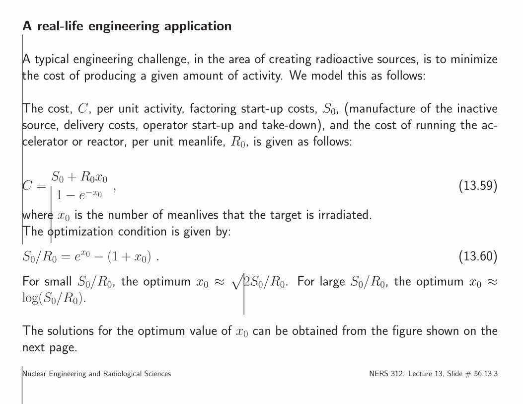
x00 1 2 3 4 5

S0/R

0or

log(S

0/R

0)

-1

0

1

2

3

4

5

Optimum irradiation time

Optimization curves for determining x0, as a function of α = S0/R0.

The figure has been split into two parts, x0 < 1 for which S0/R0 is shown, and x0 > 1 forwhich log(S0/R0) is shown. The approximations discussed above, are plotted as dottedlines.


13.4—Growth of Daughter Activities

Parent ⇒ Daughter ⇒ Granddaughter (stable)

We now describe the simplest decay chain, whereby a parent decays to an unstable daugh-ter, that decay to a stable granddaughter. We’ll use Krane’s notation:

Differential equation At t = 0 Description

N1 = −λ1N1 N1(0) = N0 N1: Parent–rate constant λ1 (decay only)

N2 = λ1N1 − λ2N2 N2(0) = 0 N2: Daughter–growth, decay rate constant λ2N3 = λ2N2 N3(0) = 0 N3: Granddaughter–growth only

N1 + N1 + N3 = 0 “Conservation of particles”

The integrals are elementary, giving, for the Ni’s:

N1 = N0e−λ1t

N2 = N0λ1

λ2 − λ1(e−λ1t − e−λ2t)

N3 = N0 −N1 −N2 (13.61)


In this discussion, we concern ourselves mostly with the activity of the daughter, in relationto the parent, namely:

A2 = A1λ2

λ2 − λ1(1− e−(λ2−λ1)t) , (13.62)

and consider some special cases.Very long-lived parent: λ1 ≪ λ2

In this case, the parent’s meanlife is considered to be much longer than that of thedaughter, essentially infinite within the time span of any measurement of interest. Inother words, the activity of the parent is constant. In this case, (13.62) becomes:

A2 = A1(0)(1− e−λ2t) . (13.63)

Comparing with (13.58), we see that (13.63) describes A2’s rise to secular equilibrium,with effective rate constant, A1(0).


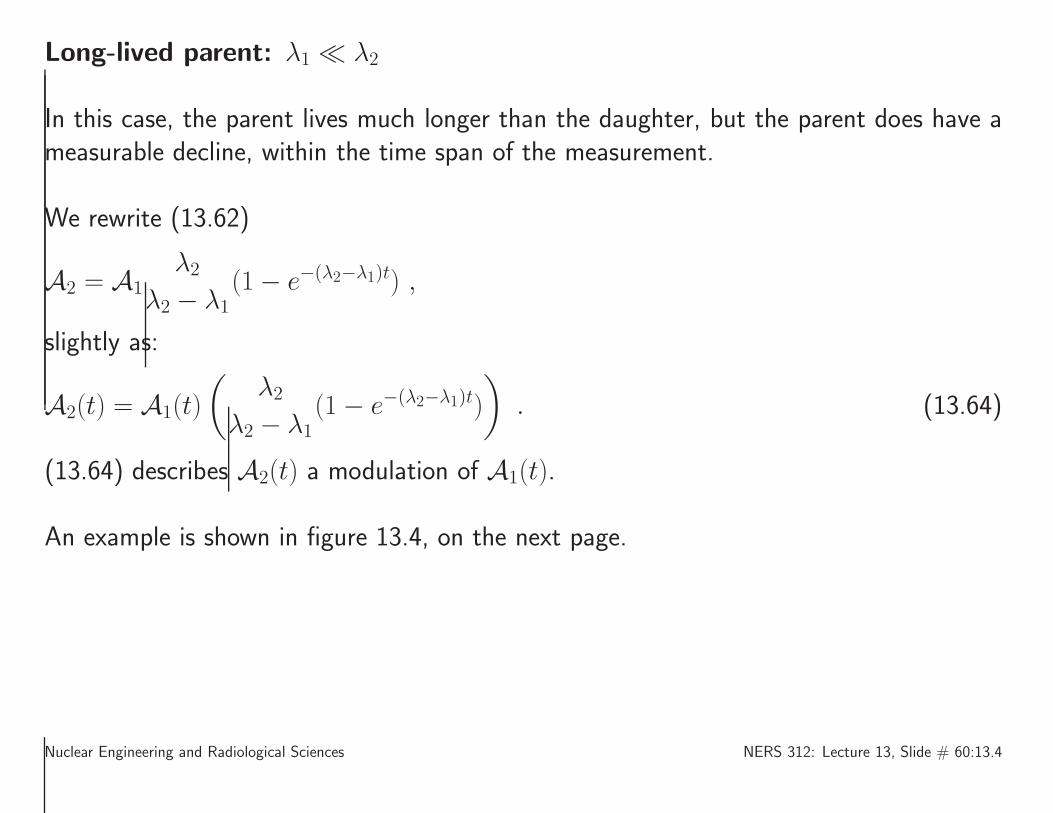
Long-lived parent: λ1 ≪ λ2

In this case, the parent lives much longer than the daughter, but the parent does have ameasurable decline, within the time span of the measurement.

We rewrite (13.62)

A2 = A1λ2

λ2 − λ1(1− e−(λ2−λ1)t) ,

slightly as:

A2(t) = A1(t)

(

λ2λ2 − λ1

(1− e−(λ2−λ1)t)

)

. (13.64)

(13.64) describes A2(t) a modulation of A1(t).

An example is shown in figure 13.4, on the next page.


t/τ10 0.5 1 1.5 2

Relativeactivity,

A/A

1(0)

0

0.1

0.2

0.3

0.4

0.5

0.6

0.7

0.8

0.9

1

Transient equilibrium λ1/λ2 = 0.1

A1/A1(0)

A2/A1(0)

Figure 13.4: The relative activity of the daughter, A2 and the parent, A2, for λ2 = 10λ1.


We see, from the figure, that the activity of the daughter, A2, rises quickly to match theparent, and then follows the parent activity closely.

This latter condition, beyond a few meanlives of the daughter, is called the region oftransient secular equilibrium, or more commonly, transient equilibrium.

In the region of transient equilibrium, the activity of the daughter is always slightly greaterthan that of the parent, with a temporal offset of about τ2.


Special case: λ = λ1 = λ2

In this case, parent and daughter decay with the same meanlife. This is more of amathematical curiosity, but should it occur, the result can be derived from (13.64) byassuming λ1 = λ, λ1 = λ + ǫ, performing a series expansion in ǫ, and taking the ǫ → 0at the end. The result is:

A2(t) = A1(t)λt . (13.65)


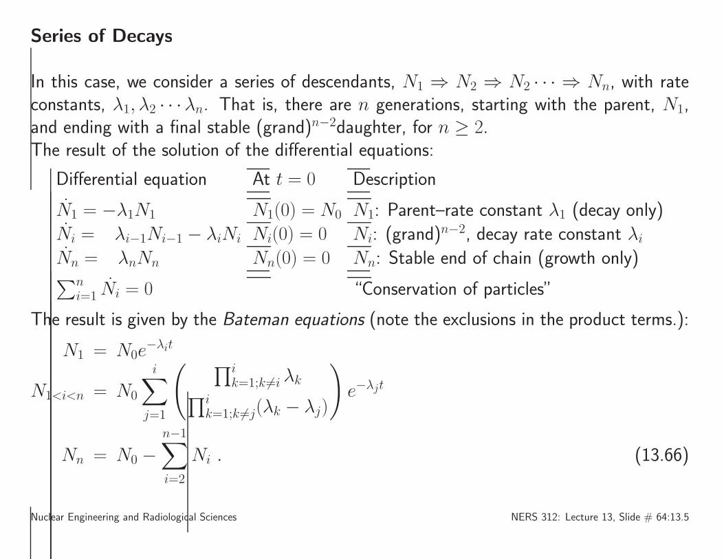
Series of Decays

In this case, we consider a series of descendants, N1 ⇒ N2 ⇒ N2 · · · ⇒ Nn, with rateconstants, λ1, λ2 · · ·λn. That is, there are n generations, starting with the parent, N1,and ending with a final stable (grand)n−2daughter, for n ≥ 2.The result of the solution of the differential equations:

Differential equation At t = 0 Description

N1 = −λ1N1 N1(0) = N0 N1: Parent–rate constant λ1 (decay only)

Ni = λi−1Ni−1 − λiNi Ni(0) = 0 Ni: (grand)n−2, decay rate constant λi

Nn = λnNn Nn(0) = 0 Nn: Stable end of chain (growth only)∑n

i=1 Ni = 0 “Conservation of particles”

The result is given by the Bateman equations (note the exclusions in the product terms.):

N1 = N0e−λit

N1<i<n = N0

i∑

j=1

(

∏ik=1;k 6=i λk

∏ik=1;k 6=j(λk − λj)

)

e−λjt

Nn = N0 −n−1∑

i=2

Ni . (13.66)


13.5—Types of Decays

Details are covered elsewhere in this course. Here we just give a list of relevant decays forNuclear Engineering and Radiological Sciences.


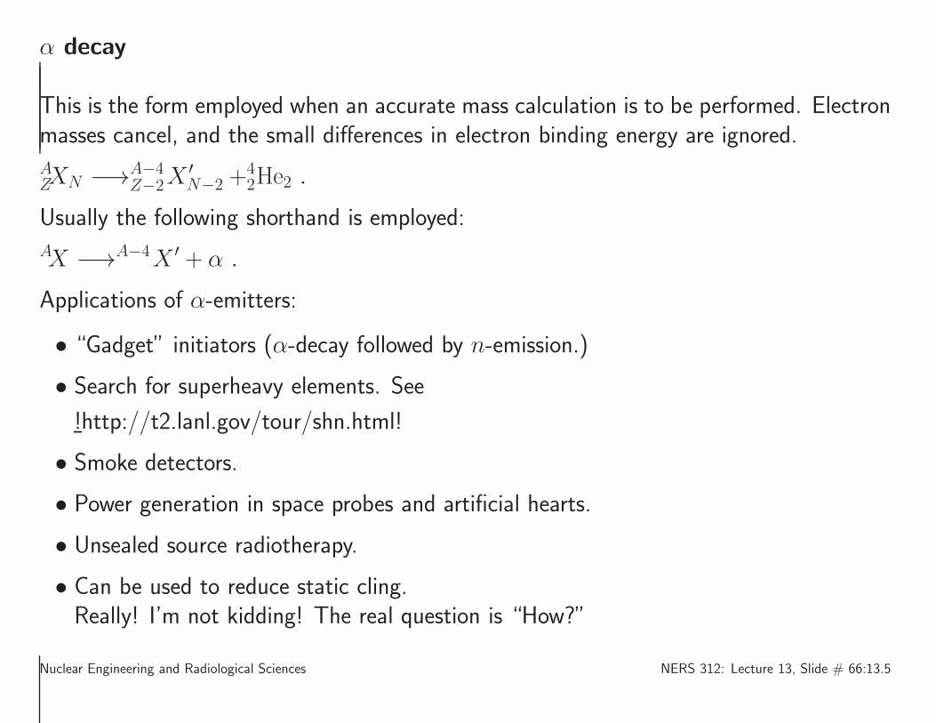
α decay

This is the form employed when an accurate mass calculation is to be performed. Electronmasses cancel, and the small differences in electron binding energy are ignored.

AZXN −→A−4

Z−2X′N−2 +

42He2 .

Usually the following shorthand is employed:

AX −→A−4X ′ + α .

Applications of α-emitters:

• “Gadget” initiators (α-decay followed by n-emission.)

• Search for superheavy elements. See

!¯http://t2.lanl.gov/tour/shn.html!

• Smoke detectors.

• Power generation in space probes and artificial hearts.

• Unsealed source radiotherapy.

• Can be used to reduce static cling.Really! I’m not kidding! The real question is “How?”


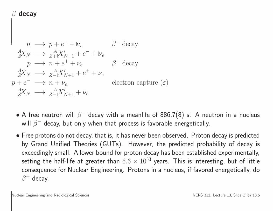
β decay

n −→ p + e− + νe β− decayAZXN −→ A

Z+1X′N−1 + e− + νe

p −→ n + e+ + νe β+ decayAZXN −→ A

Z−1X′N+1 + e+ + νe

p + e− −→ n + νe electron capture (ε)AZXN −→ A

Z−1X′N+1 + νe

• A free neutron will β− decay with a meanlife of 886.7(8) s. A neutron in a nucleuswill β− decay, but only when that process is favorable energetically.

• Free protons do not decay, that is, it has never been observed. Proton decay is predictedby Grand Unified Theories (GUTs). However, the predicted probability of decay isexceedingly small. A lower bound for proton decay has been established experimentally,setting the half-life at greater than 6.6 × 1033 years. This is interesting, but of littleconsequence for Nuclear Engineering. Protons in a nucleus, if favored energetically, doβ+ decay.


• Finally, there is a process called electron capture, (ε), or K-capture, whereby a protonin a nucleus captures an orbital electron (usually from a 1s atomic orbital, and convertsitself to a neutron.

• All these process result in a electron neutrino, νe, or an electron antineutrino, νe. Byconvention, antiparticles, like the antiproton, p, and the antineutron, n, are writtenwith an overline or an “overtilde” ˜. There are exceptions to this rule. The positron,e+ is the e−’s antiparticle. However, it is never written as e−.

Some applications of β-emitters:

• Betavoltaics (non-thermal) (long-life, low-power batteries).

• Radiotherapy (brachytherapy).

• PET (Positron Emission Tomography.)

• Radiopharmaceuticals.

• Quality assurance in large-scale paper production.

• Irradiation of domestic ruminant (cattle, goats, sheep, bison, deer, camels, alpacas,llamas) behinds to cure the effects of “fly strike”. (I’m not kidding about this oneeither.) (And I’d really rather not delve into the details of “fly strike”. Kindly googlethis one on your own.)


γ decay

AX∗ −→ AX + γ

Here, a nucleus in an excited state, denoted by the asterisk, decays via the γ process, toa lower excited state, or the ground state. All nuclei that are observed to have excitedstates, (A > 5), have γ transitions.Applications of γ-emitters:

• Basic physics: Nuclear structure, astrophysics.

• Radiotherapy, 60Co, 137Cs, brachytherapy..

• Sterilization of pharmaceutical products, food.

• Imaging vehicles for National Security Administration purposes.

• Industrial quality assurance.

• Discovery of oil. (Oil-well logging.)


Internal conversion

AZX

∗N −→ A

ZX+

N + e−

Here, a nucleus in an excited state (denoted by the ∗, de-excites by exchanging a virtualphoton with a K-shell electron in a “close encounter” with the nucleus. The electron ac-quires the de-excitation energy and exits the nucleus, leaving the atom in a singly-chargedstate.

Since it is usually a K-shell electron that is usually ejected, the atom is also in an excitedstate, followed by fluorescence and Auger electron emission, to de-excite the atom.


Nucleon emission

AZXN −→ A−1

Z−1XN + pAZXN −→ A−1

Z XN−1 + n

Applications of nucleon emitters:

• Fission.


Spontaneous fission

AZXN −→

∑

i,j

ci,j[i+ji Xj +

A−i−jZ−i XN−j]

Here a nucleus fractures into 2 (equation shown) or more (equation not shown) nuclei.This is similar to “normal” fission, except that it occurs spontaneously. Generally aspectrum of nuclei result, with the probabilities given by the c coefficients.


Cluster decay

AZXN −→ i+j

i Xj +A−i−jZ−i XN−j

where i, j > 2.From:http://en.wikipedia.org/wiki/Cluster_decay!...Cluster decay is a type of nuclear decay in which a radioactive atom emits a cluster of

neutrons and protons heavier than an alpha particle. This type of decay happens only in

nuclides which decay predominantly by alpha decay, and occurs only a small percentage of

the time in all cases. Cluster decay is limited to heavy atoms which have enough nuclear

energy to expel a portion of its nucleus.


13.8—Units for Measuring Radiation

Some useful radiometric quantities are listed in Table 13.1, along their traditional (out-dated but still in some use), along with their new, almost universally adopted, SI.

Quantity Measures... Old Units New (SI) UnitsActivity (A) decay rate curie (Ci) bequerel (Bq)Exposure (X) ionization in air rontgen (R) C/kgAbsorbed Dose (D) Energy absorption rad gray (Gy = J/kg)Dose Equivalent (DE) Radiological effectiveness rem sievert (Sv = J/kg)

Table 13.1: Units for the measurement of radiation


SI units Definition Notes:Bq 1 “decay”/s derivedGy 1 J/kg derivedSv 1 J/kg derived

Traditional units Conversion Notes:Ci 3.7× 1010 Bq (exactly)R 1 esu/(0.001293 g) = 2.58× 10−4 C/kg Charge/(1g) of dry, STP airrad 1 ergs/g = 10−2 Gyrem 1 rem = 10−2 Sv

Table 13.2: Conversion factors

A derived unit is one that is based upon the several base units in SI, namely:length ([m], meter), mass ([kg], kilogram), time([s], seconds) current([A], ampere),temperature ([K], degrees in Kelvin), amount of substance ([mol],mole),luminosity ([cd], candela).


Activity

Activity (A) has been covered already. However, the units of measurement were notdiscussed. The traditional unit, the curie, (Ci),was named in honor of Marie Curie, andthe modern unit in honor of Henri Bequerel.


Exposure

Exposure, given the symbol X , is defined as

X = lim∆m→0

∆Q

∆m, (13.67)

where ∆Q is the amount of charge of one sign produced in, dry, STP air. (NIST definition:STP at STP: 20◦C (293.15 K, 68◦F, and an absolute pressure of 101.325 kPa (14.696 psi,1 atm).) There are no accepted derived SI unit for exposure. Exposure measurements areprobably the most accurately measured radiometric quantity.


Absorbed Dose

Absorbed dose measures the energy absorbed in matter, due to radiation. The traditionalunit, the rad, has been supplanted by the Gy.


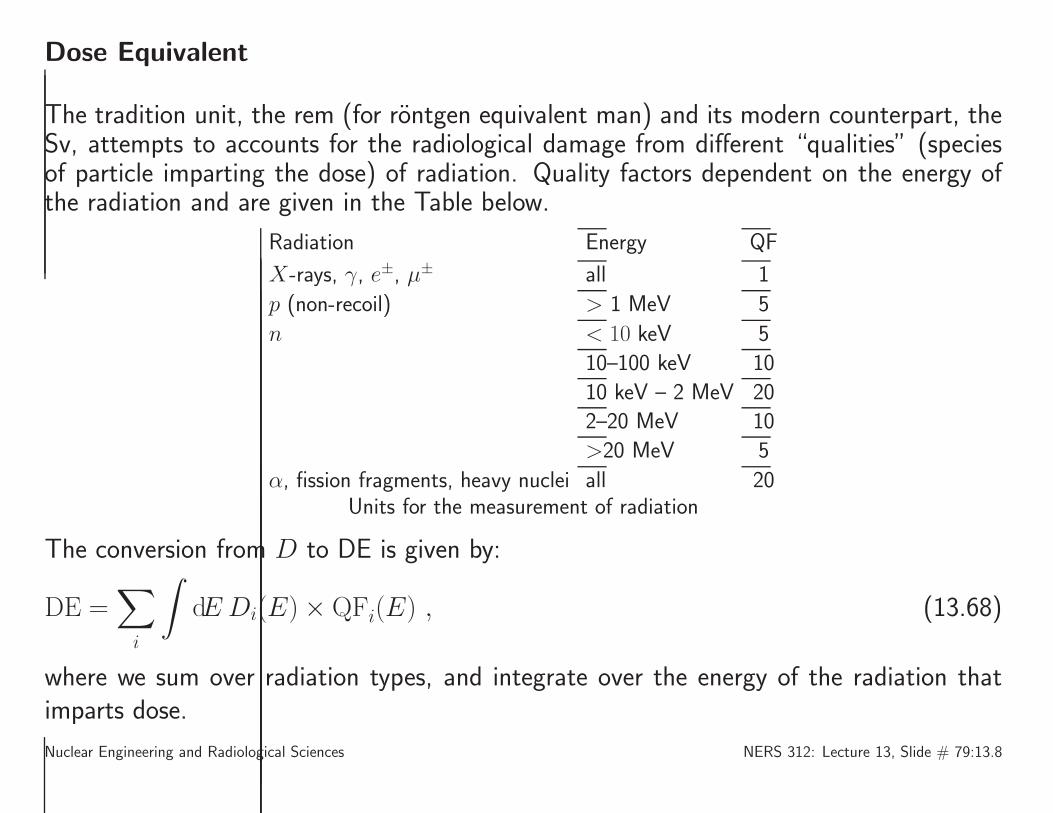
Dose Equivalent

The tradition unit, the rem (for rontgen equivalent man) and its modern counterpart, theSv, attempts to accounts for the radiological damage from different “qualities” (speciesof particle imparting the dose) of radiation. Quality factors dependent on the energy ofthe radiation and are given in the Table below.

Radiation Energy QF

X-rays, γ, e±, µ± all 1

p (non-recoil) > 1 MeV 5

n < 10 keV 5

10–100 keV 10

10 keV – 2 MeV 20

2–20 MeV 10

>20 MeV 5

α, fission fragments, heavy nuclei all 20Units for the measurement of radiation

The conversion from D to DE is given by:

DE =∑

i

∫

dEDi(E)× QFi(E) , (13.68)

where we sum over radiation types, and integrate over the energy of the radiation thatimparts dose.


Things to think about ...

1. Radioactive Decay

(a) Given a decay rate λ, derive the “exponential decay law”.(b) What is “lifetime”, or “mean lifetime”? Derive an expression for it.(c) What is “Activity”?

(a) Show diagrams and differential equations for:

i. Decay from one isotope, with two decay channels with stable daughters.ii. Decay from two isotopes, to independent decay channels

2. What is secular equilibrium? Derive the relation the describes it.3. What do the the Bateman equations describe?4. Consider the case of a radioactive parent, decay rate λ1 that decays to a radioactive

daughter, decay rate λ2.

(a) Solve the differential equation.(b) Discuss the limit for a very long-lived parent: λ1 ≪ λ2 and show that it contains

the secular equilibrium condition.(c) Discuss the limit for a long-lived parent: λ1 ≪ λ2 and plot the activity of the

parent and the daughter.


...Things to think about

5. Quantum decay theory

(a) What is the Lorentz distribution? What does it mean?(b) State Fermi’s Golden Rule #2(c) What does the density of final states describe?(d) extra credit Derive the density of final states for relativistic particles with and

without mass, and non-relativistic particles.

6. Types of decays ... Describe and give at least one application of:

(a) α decay(b) β decay(c) γ decay(d) Internal conversion(e) Nucleon emission(f) Spontaneous fission(g) Cluster decay

7. Radiological physics. What is:

(a) Exposure(b) Absorbed Dose(c) Dose Equivalent

ners 312 elements of nuclear engineering and …ners311/courselibrary/lecture13.pdf · ners 312...

Documents