nazrul hizam yusoff, bsc
TRANSCRIPT

Yusoff, Nazrul Hizam (2012) Stratifying of liquid-liquid two phase flows through sudden expansion. PhD thesis, University of Nottingham.
Access from the University of Nottingham repository: http://eprints.nottingham.ac.uk/12939/1/PhD_Thesis_N.H_YUSOFF.pdf
Copyright and reuse:
The Nottingham ePrints service makes this work by researchers of the University of Nottingham available open access under the following conditions.
This article is made available under the University of Nottingham End User licence and may be reused according to the conditions of the licence. For more details see: http://eprints.nottingham.ac.uk/end_user_agreement.pdf
For more information, please contact [email protected]

STRATIFYING OF LIQUID-LIQUID TWO PHASE FLOWS THROUGH SUDDEN
EXPANSION
NAZRUL HIZAM YUSOFF, BSc.
Thesis submitted to the University of Nottingham for the degree of Doctor of Philosophy
December 2012
Abstract
ii
ABSTRACT
The transport and separation of oil and water is an essential process to the oil and
chemical industries. Although transporting the mixtures is often necessary due to few
reasons, it is generally beneficial to separate out the phases in order to reduce
installation and maintenance costs, at the same time, avoiding safety problems. Thus,
separation of liquid-liquid flows is a necessary part of many industrial processes.
Hence, knowledge of two-phase flow dynamics is important for the design
optimisation of separators. Therefore, the aim of this research is to investigate the
feasibility of a sudden pipe expansion to be used as phase separator because it
compact in design and capable for converting dispersed flow to stratified flow.
In the test section, spatial distribution of the liquid-liquid phases in a dynamics flow
system was visualised for the first time for by means of capacitance Wire Mesh
Sensor (CapWMS), providing instantaneous information about the interface shapes,
waves and phase layer evolution of oil-water flow. Visual assessment and analysis of
the WMS data showed three distinct layers: an oil layer at the pipe top; a water layer
at the pipe bottom and a mixed layer between them. The interfaces that form between
the separated phases (oil or water) and the mixed layer were classified as oil interface
or water interface. Results showed interface shapes were initially concave or convex
near to the inlet of the test section and became flat further downstream the expansion,
especially for water interfaces. There were no waves observed for horizontal and
downward pipe orientations at all flow conditions and axial position downstream of
the expansion. As for the upward inclined pipe orientation, waves were found, and
they formed at position close to the inlet at all input oil volume fraction except at 0.2

Abstract
iii
OVF. The amplitude of the waves was: ~ 0.29D for 0.8 OVF; ~ 0.22D for 0.6 OVF
and ~ 0.26D for 0.4 OVF. The higher the input oil volume fraction, the larger the
waves become. In conclusion, the WMS results demonstrated that spatial
distributions are strongly dependent on the mixture velocity, input oil fraction and
inclination angles for the far position.
In this present work, droplets were found to be larger near the interface. Drops were
large nearer to the interface at the near position (10D) for all pipe orientations and
throughout the test section for horizontal flow. The drops size decreased when the
distance from the interface increased for these pipe configurations. As for the furthest
position from the expansion for upward and downward inclined pipe orientation,
larger droplets could also be seen at distance away from the interface and vice versa.
The gravity or buoyant force is one of the contributing factors to the settling of the
droplets. These forces are acting simultaneously on the droplets i.e. if the buoyant
force which tends to spread the droplets throughout the pipe cross-section, is not
large enough to overcome the settling tendency of gravity settling of the droplets
occurs. Hence, the droplets that are non-uniformly scattered within the continuous
phase begin to coalesce as they flow further downstream the pipe, producing larger
drops. In addition, as the distance from expansion increased, the mixed layer
becomes narrow and more drops begin to coalescence to form large drop due to
increased droplet-droplet collision. Owing to these factors, results indicate that the
mechanisms of coalescence occurred faster at the bottom, for water droplets and at
the top, for oil droplets than the other locations in a pipe cross-section. For a better
separation design, the coalescence process should occur at the aforementioned
(bottom for water and top for oil) locations within the expansion pipe. However, at
Abstract
iv
higher mixture velocities the mixed layer would be responsible for the smaller
droplet size for horizontal and both inclinations of pipe orientation. The mixed layer
dominated almost entirely in the pipe cross-section.

Acknowledgements
v
ACKNOWLEDGEMENTS
It has been a pleasure and a privilege to work with both my supervisors Prof. Barry
Azzopardi and Dr Buddhika Hewakandamby, and to study at the Nottingham
University. It has been a great learning and enjoyable experience. I am extremely
grateful to Prof. Azzopardi for his informality, patience, and above all guidance in
every stage of this thesis. My upmost gratitude also to Dr Buddhi for his unfailing
help, support and encouragement, that keep me striving towards this success. It was a
great honour to work with them.
There are many other people whom I can‟t thank them enough for their help and
support: Bayou, Mohammed, Lokman, Safa, Peter, Mukhtar, Mayowa, Abolore and
Aime who have rendered their expertise to ensure that every task is within reach.
They have always been very supportive throughout the good and hard times.
Apologies to anyone unintentionally not mentioned here.
In addition, I wish to express my gratitude to the technical staffs, in particular Phill
Bennett, Mick Fletcher, Reg, Terry, Paul, Jim, Marion Bryce, Fred Anderson, Sue
Richard and Phill Perry for their invaluable technical contribution. Special thanks to
Mel. We achieved a great deal when we put our efforts together.
The biggest thanks I reserved to my wife, Siti Nadira; my two lovely daughters,
Nurin and Nissa who have given me constant love, support and patience throughout
my time here in Nottingham. My Mum for the never ending prays. Words cannot
express my gratitude for their encouragement. Above all, I thank God for granting
me the will to achieve this accomplishment. All the glory belongs to Him.

Acknowledgements
vi
I wish to dedicate this thesis to my late Father...
3 Jamadilakhir 1429H
7th June 2008
Al-Fatihah
Table of contents
vii
TABLE OF CONTENTS
ABSTRACT ............................................................................................................. i
ACKNOWLEGEMENT ........................................................................................ iv
TABLE OF CONTENTS ....................................................................................... vi
LIST OF FIGURES ............................................................................................... xi
LIST OF TABLES ............................................................................................. xxiv
NOMENCLATURE............................................................................................ xxv
CHAPTER 1: INTRODUCTION .......................................................................... 1
1.1 Background......................................................................................................... 2
1.2 Motivations ......................................................................................................... 5
1.3 Research aims and objectives .............................................................................. 6
1.4 Structure of the thesis .......................................................................................... 7
CHAPTER 2: LITERATURE REVIEW ............................................................... 9
2.1 Background....................................................................................................... 10
2.2 Flow pattern and Flow pattern maps .................................................................. 13
2.2.1 Flow patterns for liquid-liquid flows ........................................................ 14
2.2.1.1 Flow pattern in horizontal pipes .................................................... 16
2.2.1.2 Flow pattern in inclined pipes ....................................................... 25
2.2.2 Flow pattern maps .................................................................................... 31
2.3 Liquid-liquid dispersion .................................................................................... 35
2.3.1 Drop breakage and coalescence in dispersion ........................................... 36
2.3.2 Models for drop breakage and coalescence ............................................... 38
Table of contents
viii
2.4 Drop size distribution ........................................................................................ 43
2.4.1 Measurement techniques for drop size distribution ................................... 49
2.4.1.1 Laser backscatter technique .......................................................... 49
2.4.2 Estimating particle size............................................................................. 50
2.5 Oil volume fraction ........................................................................................... 54
CHAPTER 3:INSTRUMENTS AND EXPERIMENTAL METHODS .............. 62
3.1 The liquid-liquid flow facility ........................................................................... 63
3.2 Test section ....................................................................................................... 64
3.3 The separator and liquid storage tanks ............................................................... 67
3.4 Metering and control system ............................................................................. 68
3.5 Properties of fluids ............................................................................................ 70
3.6 Experimental approaches .................................................................................. 70
3.7 Instrumentation ................................................................................................. 74
3.7.1 Rotameter ................................................................................................. 74
3.7.2 Differential pressure flow meter ............................................................... 75
3.7.3 Laser backscatter equipment ..................................................................... 76
3.7.3.1 Principle of Lasentec FBRM M500P ............................................ 77
3.7.3.2 Verification of Lasentec FBRM M500P ........................................ 78
3.7.3.3 Measurement of drop size ............................................................. 81
3.7.4 Capacitance wire mesh sensor (CapWMS) ............................................... 82
3.7.4.1 Design of capacitance wire mesh sensor (CapWMS)..................... 85
3.7.4.2 Principle of capacitance wire mesh sensor (CapWMS) .................. 86
3.7.4.3 Calibration and validation of CapWMS ........................................ 87
3.7.4.4 Determination of oil volume fraction ............................................ 88
Table of contents
ix
CHAPTER 4: WMS RESULTS AND FIRST INTERPRETATIONS ............... 89
4.1 Wire mesh sensor results ................................................................................... 91
4.2 Experimental design .......................................................................................... 91
4.3 Experiment results and discussions ................................................................... 95
4.3.1 WMS results for horizontal pipe expansion .............................................. 96
4.3.1.1 Interface Shapes and Waves – Horizontal pipe orientation .......... 100
4.3.2 WMS results for an upward inclined pipe expansion .............................. 104
4.3.2.1 Interface Shapes and Waves – Upward pipe orientation .............. 108
4.3.3 WMS results for an downward inclined pipe expansion .......................... 111
4.3.3.1 Interface Shapes and Waves – Downward pipe orientation.......... 115
4.3.4 Comparison between different angles of inclination................................ 117
CHAPTER 5: EVOLUTION OF INTERFACE ................................................ 122
5.1 Flow pattern evolution .................................................................................... 123
5.2 Experimental design ........................................................................................ 124
5.3 Experimental results and discussions ............................................................... 124
5.3.1 Flow pattern evolution in horizontal pipe expansion ............................... 125
5.3.2 Flow pattern evolution in an upward inclined pipe expansion ................. 128
5.3.3 Flow pattern evolution in downward inclined pipe expansion ................. 132
5.4 Comparison between different angles of inclination ........................................ 135
Table of contents
x
CHAPTER 6: DROP SIZES DOWNSTREAM OF PIPE EXPANSION ......... 139
6.1 Drop size distribution ...................................................................................... 139
6.2 Experimental design ........................................................................................ 141
6.3 Results and discussions ................................................................................... 143
6.3.1 SMD of drop size distribution in mixed and interface layer .................... 144
6.3.2 SMD of drop size distribution in horizontal expansion ........................... 146
6.3.2.1 SMD of drop size distribution - Effect of the volume fraction ..... 147
6.3.2.2 SMD of drop size distribution - Effect of the mixture velocity .... 150
6.3.2.3 SMD of drop size distribution - Probe position ........................... 155
6.3.2.4 Development of drops size - Cross sectional of horizontally
pipe expansion ........................................................................... 158
6.3.3 SMD of drop size distribution in an upward inclined expansion .............. 160
6.3.3.1 SMD of drop size distribution - Effect of the volume fraction ..... 161
6.3.3.2 SMD of drop size distribution - Effect of the mixture velocity .... 165
6.3.3.3 SMD of drop size distribution - Probe position ........................... 170
6.3.3.4 Development of drops size - Cross sectional of upward inclined
pipe expansion ........................................................................... 175
6.3.4 SMD of drop size distribution in downward inclined expansion ............ 179
6.3.4.1 SMD of drop size distribution - Effect of the volume fraction .... 180
6.3.4.2 SMD of drop size distribution - Effect of the mixture velocity ... 183
6.3.4.3 SMD of drop size distribution - Probe position........................... 187
6.3.4.4 Development of drops size - Cross sectional of downward
inclined pipe expansion ............................................................. 192
6.3.5 Comparison between different angles of inclination............................... 195
Table of contents
xi
CHAPTER 7: PRELIMINARY INVESTIGATION ON INFLUENCE OF
SURFACETENSION ON DROP SIZE ............................................................. 199
7.1 Influence of interfacial tension on drop size .................................................... 200
7.1.1 Interfacial tension – static flow ............................................................... 200
7.1.1.1 Drop weight method ................................................................... 201
7.1.1.2 High speed camera (CCD) .......................................................... 203
7.1.1.3 Interfacial tension results - Static flow results ............................. 204
7.1.2 Interfacial tension – mixing flow ............................................................ 205
7.1.2.1 Experimental conditions ............................................................. 206
7.1.2.2 Interfacial tension results - Mixing flow results ........................... 207
CHAPTER 8: CONCLUSIONS AND RECOMMENDATIONS ..................... 216
8.1 Contributions to knowledge ............................................................................ 217
8.2 Evolution of interface...................................................................................... 217
8.3 Flow patterns .................................................................................................. 219
8.4 Drop size distributions .................................................................................... 220
8.5 Recommendations for future work .................................................................. 222
BIBLIOGRAPHY ................................................................................................ 226
APPENDIX 2A .................................................................................................... 244
APPENDIX 2B ..................................................................................................... 249
APPENDIX 3A .................................................................................................... 253
APPENDIX 7A .................................................................................................... 254
List of figures
xii
LIST OF FIGURES
CHAPTER 2
Figure 2.1: Pipe configurations .............................................................................. 11
Figure 2.2: Pipe fittings .......................................................................................... 12
Figure 2.3: Conical diffuser ................................................................................... 12
Figure 2.4: Drawing prepared from photographs showing transition from mixed
flow, through stratified flow, to bubble flow for fixed water
superficial velocity 1.07 m/s and varying oil input fraction, Rv
(Russell et al., 1959) ............................................................................ 18
Figure 2.5: Flow patterns defined by Arirachakaran et al., (1989) .......................... 20
Figure 2.6: Horizontal oil-water flow pattern sketches (Trallero et al., 1997) ......... 21
Figure 2.7: Flow patterns for oil-water system in a horizontal pipe (Nädler and
Mewes, 1997) ...................................................................................... 24
Figure 2.8: Flow regimes in 15o upward inclined pipes (Scott, 1985)
(a) Rolling wavy counter current flow (b) Rolling wavy co-current
flow (c) Bubble flow stratified (d) Bubble flow massive ................... 26
Figure 2.9: Schematic representations of vertical oil-water flow patterns by
Flores et al., (1997). ............................................................................ 30
Figure 2.10: Schematic representation of upward inclined oil-water flow patterns
by Flores et al., (1997) ......................................................................... 31
Figure 2.11: A typical flow pattern map for oil-water horizontal flow (Trallero,
1996) ................................................................................................... 32
Figure 2.12: The Sauter mean diameter (D32) measured by the backscatter
technique for horizontal flow in Simmons and Azzopardi (2001) ........ 47
Figure 2.13: Measurement principle and schematic drawing of the FBRM probe .... 50
CHAPTER 3
Figure 3.1: Schematic diagram B09/ R123 Multiphase flow inclined liquid-
liquid test facility (68mm) ................................................................... 63
Figure 3.2: Photograph, B09/ R123 Multiphase flow inclined liquid-liquid test
facility (68mm)..................................................................................... 64
List of figures
xiii
Figure 3.3: Cross-section and photograph of sudden pipe expansion ...................... 65
Figure 3.4: Test section mounted on a tubular steel frame hinged at one end,
which permitted the small angle of inclination by 7 to the
horizontal ............................................................................................. 65
Figure 3.5: Plan view of multi-holes orifice plate {18 holes (5 mm) = 32%
orifice open area} ................................................................................. 65
Figure 3.6: Cross-section of Lasentec FBRM pipe test section ............................... 66
Figure 3.7: The capacitance wire mesh sensor (CapWMS) unit on experimental
rig ........................................................................................................ 67
Figure 3.8: Diagram of separator vessel ................................................................. 68
Figure 3.9: Components of the control system........................................................ 69
Figure 3.10: The calibration of water and silicone oil flowrates. ............................. 74
Figure 3.11: Schematic of differential pressure (Dp) flow meters engaged on the
flow facility ......................................................................................... 75
Figure 3.12: Calibration of mixtures flow rates with differential pressure flow
meter ................................................................................................... 76
Figure 3.13: Typical diagram of laser backscatter system (Mettler Toledo) ............. 77
Figure 3.14: Focused Beam Reflectance Measurement, FBRM (Lasentec, 2007) .... 78
Figure 3.15: PVC Reference procedure set up (Lasentec, 2007) .............................. 80
Figure 3.16: PVC reference calibration ................................................................... 81
Figure 3.17: Example of the (a) CLD and (b) DDD graphs ..................................... 82
Figure 3.18: Electrical schematic of capacitance WMS (Da Silva et al., 2007) ........ 85
Figure 3.19: Capacitance wire mesh sensor 24 x 24 (Left) Sketch of wire mesh
sensor (Right) ...................................................................................... 86
Figure 3.20: Tomographic images of water-oil in horizontal pipe. (a) water only,
(b) silicone oil only and (c) oil volume fraction 0.4 (d) oil volume
fraction 0.6 .......................................................................................... 88
CHAPTER 4
Figure 4.1: Mixture velocities after orifice (Usmo) and mixture velocities
downstream (Usme) of flow pattern encountered within the rig and
possible operational limits plotted on flow pattern map of Trallero et
al., (1997) ............................................................................................ 92
List of figures
xiv
Figure 4.2: Usmo and Usme of flow pattern transition through the sudden
expansion and WMS images plotted on horizontal liquid-liquid
flow pattern map of Trallero et al., (1997) ........................................... 92
Figure 4.3: The capacitance wire mesh sensor (CapWMS) system on
experimental rig................................................................................... 94
Figure 4.4: Oil volume fraction and phase distributions in a pipe cross section
for distance from expansion 10D, mixture velocity 0.20 m/s and
horizontal flow, at different input oil fractions ..................................... 96
Figure 4.5: Oil volume fraction and phase distribution in a pipe cross section for
distance from expansion 34D, mixture velocity 0.20 m/s and
horizontal flow, at different input oil fractions ..................................... 97
Figure 4.6: Oil volume fraction in a pipe cross section for distance from
expansion 34D, input oil fraction 0.2 and horizontal flow, at
different mixture velocities. ................................................................. 98
Figure 4.7: Oil volume fraction in a pipe cross section for distance from
expansion 34D, input oil fraction 0.4 and horizontal flow, at
different mixture velocities .................................................................. 98
Figure 4.8: Oil volume fraction in a pipe cross section for distance from
expansion 34D, input oil fraction 0.6 and horizontal flow, at
different mixture velocities .................................................................. 99
Figure 4.9: Oil volume fraction in a pipe cross section for distance from
expansion 34D, input oil fraction 0.8 and horizontal flow, at
different mixture velocities.. ................................................................ 99
Figure 4.10: Oil volume fraction in a pipe cross section for mixture velocity 0.20
m/s, input oil fraction 0.2 and horizontal flow, at different distances
from expansion. ................................................................................. 100
Figure 4.11: Interface shape for distance from expansion 10D, mixture velocity
0.2 m/s and horizontal flow, at different input oil fractions ................ 101
Figure 4.12: Interface shape for distance from expansion 20D, mixture velocity
0.2 m/s and horizontal flow, at different input oil fractions ................ 102
Figure 4.13: Interface shape for distance from expansion 34D, mixture velocity
0.2 m/s and horizontal flow, at different input oil fractions ................ 102
List of figures
xv
Figure 4.14: Spatial distribution for distance from expansion 10D, mixture
velocity 0.2 m/s and horizontal flow: (a) 0.2 OVF (b) 0.4 OVF (c)
0.6 OVF (d) 0.8 OVF........................................................................ 103
Figure 4.15: Spatial distribution for distance from expansion 34D, mixture
velocity 0.2 m/s and horizontal flow: (a) 0.2 OVF (b) 0.4 OVF (c)
0.6 OVF (d) 0.8 OVF........................................................................ 104
Figure 4.16: Oil volume fraction in a pipe cross section for distance from
expansion 34D, mixture velocity 0.2 m/s and +6 degree flow, at
different input oil fractions ............................................................... 105
Figure 4.17: Oil volume fraction in a pipe cross section for distance from
expansion 34D, input oil fraction 0.2 and +6 degree flow, at
different mixture velocities ............................................................... 105
Figure 4.18: Oil volume fraction in a pipe cross section for distance from
expansion 34D, input oil fraction 0.8 and +6 degree flow, at
different mixture velocities ............................................................... 106
Figure 4.19: Oil volume fraction and phase distribution in a pipe cross section
for mixture velocity 0.20 m/s, input oil fraction 0.2 and +6 degree
flow, at different distances from expansion ....................................... 107
Figure 4.20: Oil volume fraction and phase distribution in a pipe cross section
for mixture velocity 0.20 m/s, input oil fraction 0.8 and +6 degree
flow, at different distances from expansion ....................................... 107
Figure 4.21: Interface shape for distance from expansion 10D, mixture velocity
0.2 m/s and +6o upward flow, at different input oil fractions .............. 108
Figure 4.22: Interface shape for distance from expansion 20D, mixture velocity
0.2 m/s and +6o upward flow, at different input oil fractions .............. 109
Figure 4.23: Interface shape for distance from expansion 34D, mixture velocity
0.2 m/s and +6o upward flow, at different input oil fractions .............. 109
Figure 4.24: Spatial distribution for distance from expansion 10D, mixture
velocity 0.2 m/s and +6o upward flow: (a) 0.2 OVF (b) 0.4 OVF (c)
0.6 OVF (d) 0.8 OVF........................................................................ 110
Figure 4.25: Spatial distribution for distance from expansion 34D, mixture
velocity 0.2 m/s and +6o upward flow, (a) 0.2 OVF (b) 0.4 OVF (c)
0.6 OVF (d) 0.8 OVF........................................................................ 110
List of figures
xvi
Figure 4.26: Oil volume fraction in a pipe cross section for distance from
expansion 34D, mixture velocity 0.2 m/s and -6 degree flow, at
different input oil fractions. .............................................................. 111
Figure 4.27: Oil volume fraction in a pipe cross section for distance from
expansion 34D, mixture velocity 0.20 m/s and -3 degree flow, at
different input oil fractions ............................................................... 112
Figure 4.28: Oil volume fraction in a pipe cross section for distance from
expansion 34D, input oil fraction 0.2 and -6 degree flow, at
different mixture velocities ............................................................... 113
Figure 4.29: Oil volume fraction in a pipe cross section for distance from
expansion 34D, input oil fraction 0.8 and -6 degree flow, at
different mixture velocities ............................................................... 114
Figure 4.30: Oil volume fraction in a pipe cross section for mixture velocity 0.20
m/s, input oil fraction 0.2 and -6 degree flow, at different distances
from expansion ................................................................................. 114
Figure 4.31: Oil volume fraction in a pipe cross section for mixture velocity 0.20
m/s, input oil fraction 0.8 and -6 degree flow, at different distances
from expansion ................................................................................. 115
Figure 4.32: Interface shape for distance from expansion 10D, mixture velocity
0.2 m/s and -6o downward flow, at different input oil fractions .......... 115
Figure 4.33: Interface shape for distance from expansion 20D, mixture velocity
0.2 m/s and -6o downward flow, at different input oil fractions .......... 116
Figure 4.34: Interface shape for distance from expansion 34D, mixture velocity
0.2 m/s and -6o downward flow, at different input oil fractions .......... 116
Figure 4.35: Spatial distribution for distance from expansion 34D, mixture
velocity 0.2 m/s and -6o downward flow: (a) 0.2 OVF (b) 0.4 OVF
(c) 0.6 OVF (d) 0.8 OVF .................................................................. 117
Figure 4.36: Phase distribution in a pipe cross-section for distance from
expansion 10D, mixture velocity 0.20 m/s, input oil fraction 0.2 at
different angles of inclination ........................................................... 118
Figure 4.37: Phase distribution in a pipe cross-section for distance from
expansion 34D, mixture velocity 0.20 m/s, input oil fraction 0.2 at
different angles of inclination ........................................................... 118
List of figures
xvii
Figure 4.38: Phase distribution in a pipe cross-section for distance from
expansion 10D, mixture velocity 0.20 m/s, input oil fraction 0.8 at
different angles of inclination ........................................................... 119
Figure 4.39: Phase distribution in a pipe cross-section for distance from
expansion 34D, mixture velocity 0.20 m/s, input oil fraction 0.8 at
different angles of inclination ........................................................... 119
Figure 4.40: Phase distribution in a pipe cross-section for distance from
expansion 24D, mixture velocity 0.2 m/s and horizontal flow, at
different input oil fractions (Hasan, 2006)......................................... 120
Figure 4.41: Phase distribution in a pipe cross-section for distance from
expansion 24D, mixture velocity 0.2 m/s and -4 degree flow, at
different input oil fractions (Hasan, 2006)......................................... 120
Figure 4.42: Spatial distribution for distance from expansion 10D, mixture
velocity 0.2 m/s and 0.8 input oil volume fractions at different
angles of inclination ......................................................................... 121
CHAPTER 5
Figure 5.1: Phase layer evolution downstream of the pipe expansion at Usme 0.20
m/s, oil volume fraction 0.5 for horizontal pipe orientation plotted
with Yang (2003)................................................................................ 125
Figure 5.2: Analysis of the cross section for the three flow pattern observed by
Vedapuri (1999). ................................................................................ 125
Figure 5.3: Effect of the oil volume fraction on the phase layer evolution
downstream of the horizontally pipe expansion at Usme 0.20 m/s. ....... 126
Figure 5.4: Effect of the oil volume fraction on the phase layer evolution
downstream of the horizontally pipe expansion at Usme 0.30 m/s. ....... 127
Figure 5.5: Effect of the oil volume fraction on the phase layer evolution
downstream of the horizontally pipe expansion at Umse 0.35 m/s. ..... 128
Figure 5.6: Prediction of interfacial level for stratified flow with the model of
Taitel and Dukler, 1976 by Yang (2003). ........................................... 129
Figure 5.7: Effect of the oil volume fraction on the phase layer evolution
downstream of the +3o upward inclined pipe expansion at Umse
0.20 m/s. ............................................................................................ 130
List of figures
xviii
Figure 5.8: Effect of the oil volume fraction on the phase layer evolution
downstream of the +6o upward inclined pipe expansion at Umse
0.20 m/s. ............................................................................................ 131
Figure 5.9: Effect of the oil volume fraction on the phase layer evolution
downstream of the +3o upward inclined pipe expansion at Umse
0.35 m/s. ............................................................................................ 131
Figure 5.10: Effect of the oil volume fraction on the phase layer evolution
downstream of the +6o upward inclined pipe expansion at Usme
0.35 m/s. ........................................................................................... 132
Figure 5.11: Effect of the oil volume fraction on the phase layer evolution
downstream of the -3o downward inclined pipe expansion at Usme
0.20 m/s. ........................................................................................... 133
Figure 5.12: Effect of the oil volume fraction on the phase layer evolution
downstream of the -6o downward inclined pipe expansion at Usme
0.20 m/s. ........................................................................................... 133
Figure 5.13: Effect of the oil volume fraction on the phase layer evolution
downstream of the -3o downward inclined pipe expansion at Usme
0.35 m/s. ........................................................................................... 134
Figure 5.14: Effect of the oil volume fraction on the phase layer evolution
downstream of the -6o downward inclined pipe expansion at Usme
0.35 m/s. ........................................................................................... 135
Figure 5.15: Effect of the angles inclination on the phase layer evolution
downstream of the pipe expansion for 0.2 OVF at downstream
mixture velocity, Usme = 0.20 m/s. .................................................... 136
Figure 5.16: Effect of the angles inclination on the phase layer evolution
downstream of the pipe expansion for 0.8 OVF at downstream
mixture velocity, Usme = 0.20 m/s. .................................................... 137
Figure 5.17: Effect of the angles inclination on the phase layer evolution
downstream of the pipe expansion for 0.8 OVF at downstream
mixture velocity, Usme = 0.30 m/s. .................................................... 138

List of figures
xix
CHAPTER 6
Figure 6.1: Locations of probe positions downstream of the expansion and in a
pipe cross-section with height from the bottom of the pipe. ................ 141
Figure 6.2: D32 of water droplets for downstream mixture velocity, Umse =
0.20 m/s, within test distance in horizontally pipe orientation at oil
volume fraction system, OVF = 0.8, at different probe position. ......... 146
Figure 6.3: Interface mapping along the axial length of the pipe. The lower line
indicates the interface between water and the mixture whilst the
upper line shows the interface between oil and the mixture at
downstream of the horizontal pipe expansion at Usme 0.20 m/s, OVF
= 0.8. .................................................................................................. 146
Figure 6.4: Orifice and downstream mixture velocities of flow pattern transition
through the sudden expansion plotted on the flow pattern maps of
Trallero et al., (1997). ......................................................................... 147
Figure 6.5: Sauter mean diameter for downstream mixture velocity, Usme 0.20
m/s, within test distance in horizontally pipe orientation, probe
position 17 mm from bottom at different oil volume fraction, OVF. ... 148
Figure 6.6: Sauter mean diameter for downstream mixture velocity, Usme 0.20
m/s, within test distance in horizontally pipe orientation, probe
position 34 mm from bottom at different oil volume fraction, OVF. ... 149
Figure 6.7: Sauter mean diameter for downstream mixture velocity, Usme 0.20
m/s, within test distance in horizontally pipe orientation, probe
position 51 mm from bottom at different oil volume fraction, OVF. .. 150
Figure 6.8: D32 of oil droplets for 0.2 oil volume fraction system, within test
distance in horizontally pipe orientation, probe position 51 mm from
bottom at different downstream mixture velocity, Usme. ..................... 151
Figure 6.9: D32 of oil droplets for 0.4 oil volume fraction system, within test
distance in horizontally pipe orientation, probe position 34 mm from
bottom at different downstream mixture velocity, Usme. ...................... 152
Figure 6.10: D32 of water droplets for 0.6 oil volume fraction system, within
test distance in horizontally pipe orientation, probe position 34 mm
from bottom at different downstream mixture velocity, Usme. ............ 153
List of figures
xx
Figure 6.11: D32 of water droplets for 0.8 oil volume fraction system, within test
distance in horizontally pipe orientation, probe position 17 mm from
bottom at different downstream mixture velocity, Usme ...................... 153
Figure 6.12: D32 of oil droplets for downstream mixture velocity, Umse =
0.20 m/s, within test distance in horizontally pipe orientation at oil
volume fraction system, OVF = 0.2, at different probe position ........ 155
Figure 6.13: D32 of oil droplets for downstream mixture velocity, Usme = 0.20
m/s, within test distance in horizontally pipe orientation at oil
volume fraction system, OVF = 0.4, at different probe position ........ 156
Figure 6.14: D32 of water droplets for downstream mixture velocity, Usme = 0.20
m/s, within test distance in horizontally pipe orientation at oil
volume fraction system, OVF = 0.6, at different probe position. ........ 157
Figure 6.15: D32 of water droplets for downstream mixture velocity, Usme = 0.20
m/s, within test distance in horizontally pipe orientation at oil
volume fraction system, OVF = 0.8, at different probe position ......... 158
Figure 6.16: Sauter mean diameter as a function of the distance from |Z| at Usme
0.20 m/s of horizontal pipe orientation flow, 10D downstream the
expansion .......................................................................................... 159
Figure 6.17: Sauter mean diameter as a function of the distance from |Z| at Usme
0.20 m/s of horizontal pipe orientation flow, 34D downstream the
expansion. ......................................................................................... 160
Figure 6.18: Sauter mean diameter for downstream mixture velocity, Usme 0.20
m/s, within test distance in upward 6o pipe orientation, probe
position 17 mm from bottom at different oil volume fraction, OVF ... 163
Figure 6.19: Sauter mean diameter for downstream mixture velocity, Usme 0.20
m/s, within test distance in upward 6o pipe orientation, probe
position 34 mm from bottom at different oil volume fraction, OVF ... 164
Figure 6.20: Sauter mean diameter for downstream mixture velocity, Usme 0.20
m/s, within test distance in upward 6o pipe orientation, probe
position 51 mm from bottom at different oil volume fraction, OVF. .. 165
Figure 6.21: D32 of water droplets for 0.8 oil volume fraction system, within test
distance in upward 6o pipe orientation, probe position 17 mm from
bottom at different downstream mixture velocity, Usme. ..................... 166
List of figures
xxi
Figure 6.22: D32 of water droplets for 0.8 oil volume fraction system, within test
distance in upward 6o pipe orientation, probe position 34 mm from
bottom at different downstream mixture velocity, Usme. .................... 167
Figure 6.23: D32 of water droplets for 0.8 oil volume fraction system, within test
distance in upward 3o pipe orientation, probe position 17 mm from
bottom at different downstream mixture velocity, Usme.. ................... 169
Figure 6.24: D32 of water droplets for 0.8 oil volume fraction system, within test
distance in upward 3o pipe orientation, probe position 34 mm from
bottom at different downstream mixture velocity, Usme. .................... 169
Figure 6.25: D32 of oil droplets for downstream mixture velocity, Umse =
0.20 m/s, within test distance in upward 6o pipe orientation at oil
volume fraction system, OVF = 0.2, at different probe position ........ 171
Figure 6.26: D32 of water droplets for downstream mixture velocity, Usme = 0.20
m/s, within test distance in upward 6o pipe orientation at oil volume
fraction system, OVF = 0.8, at different probe position. .................... 172
Figure 6.27: D32 of water droplets for downstream mixture velocity, Usme = 0.35
m/s, within test distance in upward 6o pipe orientation at oil volume
fraction system, OVF = 0.8, at different probe position. .................... 173
Figure 6.28: D32 of water droplets for downstream mixture velocity, Usme = 0.20
m/s, within test distance in upward 3o pipe orientation at oil volume
fraction system, OVF = 0.8, at different probe position. .................... 174
Figure 6.29: D32 of water droplets for downstream mixture velocity, Usme = 0.35
m/s, within test distance in upward 3o pipe orientation at oil volume
fraction system, OVF = 0.8, at different probe position ..................... 175
Figure 6.30: Sauter mean diameter as a function of the distance from |Z| at Usme
0.20 m/s of +6o upward inclined pipe orientation flow, 10D
downstream the expansion ................................................................ 176
Figure 6.31: Sauter mean diameter as a function of the distance from |Z| at Usme
0.20 m/s of +6o upward inclined pipe orientation flow, 34D
downstream the expansion. ............................................................... 177
Figure 6.32: Sauter mean diameter as a function of the distance from |Z| at Usme
0.20 m/s of +3o upward inclined pipe orientation flow, 10D
downstream the expansion. ............................................................... 178
List of figures
xxii
Figure 6.33: Sauter mean diameter as a function of the distance from |Z| at Usme
0.20 m/s of +3o upward inclined pipe orientation flow, 34D
downstream the expansion ................................................................ 179
Figure 6.34: Sauter mean diameter for downstream mixture velocity, Usme 0.20
m/s, within test distance in downward 6o pipe orientation, probe
position 17 mm from bottom at different oil volume fraction, OVF... 181
Figure 6.35: Sauter mean diameter for downstream mixture velocity, Usme 0.20
m/s, within test distance in downward 6o pipe orientation, probe
position 34 mm from bottom at different oil volume fraction, OVF... 182
Figure 6.36: Sauter mean diameter for downstream mixture velocity, Usme 0.20
m/s, within test distance in downward 3o pipe orientation, probe
position 17 mm from bottom at different oil volume fraction, OVF... 183
Figure 6.37: Sauter mean diameter for downstream mixture velocity, Usme 0.20
m/s, within test distance in downward 3o pipe orientation, probe
position 34 mm from bottom at different oil volume fraction, OVF... 183
Figure 6.38: D32 of oil droplets for 0.2 oil volume fraction system, within test
distance in downward 6o pipe orientation, probe position 17 mm
from bottom at different downstream mixture velocity, Usme ............. 184
Figure 6.39: D32 of water droplets for 0.8 oil volume fraction system, within test
distance in downward 6o pipe orientation, probe position 17 mm
from bottom at different downstream mixture velocity, Usme.. ........... 185
Figure 6.40: D32 of water droplets for 0.8 oil volume fraction system, within test
distance in downward 6o pipe orientation, probe position 34 mm
from bottom at different downstream mixture velocity, Usme. ............ 186
Figure 6.41: D32 of water droplets for 0.8 oil volume fraction system, within test
distance in downward 6o pipe orientation, probe position 51 mm
from bottom at different downstream mixture velocity, Usme.. ........... 187
Figure 6.42: D32 of oil droplets for downstream mixture velocity, Usme = 0.20
m/s, within test distance in downward 6o pipe orientation at oil
volume fraction system, OVF = 0.2, at different probe position. ....... 188
Figure 6.43: D32 of water droplets for downstream mixture velocity, Usme = 0.20
m/s, within test distance in downward 6o pipe orientation at oil
volume fraction system, OVF = 0.8, at different probe position ........ 188

List of figures
xxiii
Figure 6.44: D32 of oil droplets for downstream mixture velocity, Usme = 0.35
m/s, within test distance in downward 6o pipe orientation at oil
volume fraction system, OVF = 0.2, at different probe position ........ 189
Figure 6.45: D32 of water droplets for downstream mixture velocity, Usme = 0.35
m/s, within test distance in downward 6o pipe orientation at oil
volume fraction system, OVF = 0.8, at different probe position. ....... 190
Figure 6.46: D32 of water droplets for downstream mixture velocity, Usme = 0.20
m/s, within test distance in downward 3o pipe orientation at oil
volume fraction system, OVF = 0.8, at different probe position... ..... 191
Figure 6.47: D32 of water droplets for downstream mixture velocity, Usme = 0.35
m/s, within test distance in downward 3o pipe orientation at oil
volume fraction system, OVF = 0.8, at different probe position. ....... 192
Figure 6.48: Sauter mean diameter as a function of the distance from |Z| at Usme
0.20 m/s of -6o downward inclined pipe orientation flow, 10D
downstream the expansion. ............................................................... 193
Figure 6.49: Sauter mean diameter as a function of the distance from |Z| at Usme
0.20 m/s of -6o downward inclined pipe orientation flow, 34D
downstream the expansion. ............................................................... 194
Figure 6.50: D32 of oil droplets for downstream mixture velocity, Usme = 0.20
m/s, oil volume fraction system, OVF = 0.2, at 17 mm probe
position from bottom, along test section distance for different pipe
orientation. ....................................................................................... 195
Figure 6.51: D32 of oil droplets for downstream mixture velocity, Usme = 0.35
m/s, oil volume fraction system, OVF = 0.2, at 17 mm probe
position from bottom, along test section distance for different pipe
orientation. ....................................................................................... 196
Figure 6.52: D32 of oil droplets for downstream mixture velocity, Usme = 0.35
m/s, oil volume fraction system, OVF = 0.2, at 51 mm probe
position from bottom, along test section distance for different pipe
orientation ........................................................................................ 196
Figure 6.53: D32 of water droplets for downstream mixture velocity, Usme = 0.20
m/s, oil volume fraction system, OVF = 0.8, at 17 mm probe
position from bottom, along test section distance for different pipe
orientation. ....................................................................................... 197
List of figures
xxiv
Figure 6.54: D32 of water droplets for downstream mixture velocity, Usme = 0.35
m/s, oil volume fraction system, OVF = 0.8, at 17 mm probe
position from bottom, along test section distance for different pipe
orientation. ....................................................................................... 198
CHAPTER 7
Figure 7.1: Correction factors (F) for the drop weight method (Harkins and
Brown, 1919) .................................................................................... 203
Figure 7.2: Effect of surfactant on interfacial tension ........................................... 204
Figure 7.3: Interfacial tension for different surfactant CMC ................................. 205
Figure 7.4: Effect of surfactant CMC concentration on droplet size ...................... 205
Figure 7.5: The effect of mixing time for 0.5 OVF at NRe=10000 ......................... 207
Figure 7.6: The effect of IFT on drop size distribution for 0.8 OVF at
NRe=10000 ........................................................................................ 208
Figure 7.7: The effect of IFT on drop size distribution for 0.6 OVF at
NRe= 10000 ....................................................................................... 209
Figure 7.8: The effect of IFT on drop size distribution for 0.5 OVF at
NRe= 10000 ....................................................................................... 209
Figure 7.9: The effect of IFT on drop size distribution for 0.4 OVF at
NRe= 10000 ....................................................................................... 210
Figure 7.10: The effect of IFT on drop size distribution for 0.15 OVF at
NRe= 10000....................................................................................... 201
Figure 7.11: The effect of the impeller Reynolds number (impeller speed) on
drop size distribution for Ø = 0.8 system with IFT 44mN/m ............. 211
Figure 7.12: The effect of the impeller Reynolds number (impeller speed) on
drop size distribution for Ø = 0.8 systems with IFT 17mN/m ............ 212
Figure 7.13: The effect of the impeller Reynolds number (impeller speed) on
drop size distribution for 0.15 OVF systems with IFT 44mN/m. ....... 213
Figure 7.14: The effect of the impeller Reynolds number (impeller speed) on
drop size distribution for 15 OVF systems with IFT 17mN/m ........... 213
Figure 7.15: The effect of the impeller Reynolds number (impeller speed) on
drop size distribution for 0.8 OVF systems with IFT 6mN/m ............ 214
Figure 7.16: The effect of the impeller Reynolds number (impeller speed) on
drop size distribution for 0.15 OVF systems with IFT ....................... 214
List of tables
xxv
LIST OF TABLES
Table 2.1: Pertinent experimental flow pattern maps for oil-water flow in
horizontal pipelines .............................................................................. 17
Table 2.2: Summary of some studies on liquid-liquid dispersion in mechanically
agitated contractors. .............................................................................. 41
Table 3.1: Physical properties of fluids at 25oC. ..................................................... 70
Table 4.1: Summary of experimental conditions .................................................... 94
Nomenclature
xxvi
NOMENCLATURE
Symbol Description Dimension
Roman letters
A(ho) Function in Table 2.2 (-)
a interfacial area per unit volume (-)
C Capacitance (F)
CD Drag coefficient (-)
D pipe diameter (m)
Di diameter of impeller (m)
d drop diameter ( m)
di the drop i in a drop distribution (-)
D32 Sauter mean drop diameter (mm)
dmax maximum drop diameter (mm)
dmin minimum drop diameter (mm)
Ea energy of adhesion between two drops (Joule)
f Friction factor (-)
F turbulent force (N/m3)
fcol frequency of collision (-)
f(h) Attraction forces per unit area between
two finite parallel surfaces separated by
distance h (N/m2)
g gravitational acceleration (m/s2)
h distance (m)
H distance from bottom of the pipe
cross-section (mm)
Nvi viscosity group (-)
Nd number of drops (-)
N impeller speed (m/s)
ni drop number in the ith size range (-)
OVF input oil volume fraction (m3)
Pi probability of obtaining ith chord size (-)
NRe Reynolds number (-)
Nomenclature
xxvii
uo oil average in-situ velocity (m/s)
uw water average in-situ velocity (m/s)
U velocity (m/s)
Um Mixture velocity (m/s)
Uc velocity of continuous phase (m/s)
Uos oil superficial velocity (m/s)
Uws water superficial velocity (m/s)
Usmo superficial mixture velocity at orifice (m/s)
Usme superficial mixture velocity after expansion (m/s)
Vcum cumulative volume fraction (-)
vcoal frequency of coalescence (-)
V volume (m3/s)
We Weber Number (-)
We’crit Critical Weber Number (-)
NRe Reynolds number (-)
Wcut water cut (-)
Greek symbols
Volume fraction of dispersed phase (-)
d concentration of dispersed phase (-)
µw Water viscosity (cP or mPa.s)
µo Oil viscosity (cP or mPa.s)
Interfacial tension (dyne/cm or N/m)
Energy dissipation (m2/s
2)
r relative permittivity (F/m)
mat permittivity of material (F/m)
o average in-situ volume fraction of oil (-)
w average in-situ volume fraction of water (-)
Viscosity (cP or mPa s)
Density (kg/m3)
Water density (kg/m3)
o oil density (kg/m3)

Nomenclature
xxviii
c density of continuous phases (kg/m3)
Inclination angle from horizontal (degree)
Subscripts
c Continuous
cut Cut
coal coalescence
col collision
cum cumulative
d dispersed
drain drainage
e expansion
m mixture
M mean
max maximum
min minimum
o oil
s superficial
t total
w water
Chapter 1: Introduction
1
CHAPTER 1
INTRODUCTION
Multiphase flow involves in a wide range of applications and widely encountered in
the chemical and petroleum industries. In the latter, it is important in both the
upstream and downstream. An examination of the flows in many pieces of equipment
from these industries would reveal that many flows involve more than one phases. It
occurs in as relatively simple equipment as pipelines to as complex geometries such
as heat exchangers, reactors and separators.
The term multiphase flow can be defined as a simultaneous fluid flow which contains
of two or more phases. In many cases, the two phases are gas and liquid. There are,
however, other possible combinations - two immiscible liquids (oil/water), solid/gas
(fluidized beds, pneumatic conveying), solid/liquid (hydraulic conveying), and
occasionally more than two phases (gas/oil/water). This thesis concentrates on two
immiscible liquids systems (oil/water).
In oil fields producing hydrocarbon (upstream industry), multiphase flows can
consist of water, gas, hydrocarbon liquids and solids (sands). They are lifted to the
surface through a drilled well connected to a reservoir. As there is no gain in
transporting water and sands, these phases then need to be separated for further
downstream processing. Conventionally, a separator such as a vessel or cyclone is
Chapter 1: Introduction
2
employed to accomplish this. However, such separators involve high capital and
installation costs and at the same time, safety measures are extremely restricted. One
way to remove this economic and safety problem is to use smaller but more efficient
process vessels or to invent novel techniques (separation in pipe) to separate
components of the mixture while still being transported within the pipes. Thus, by
introducing the use of an expansion pipe as an alternative method for efficient
separation of the mixture is the subject of this thesis. This chapter serves as an
introduction to the scope of this thesis; that is, the subject of stratification of liquid-
liquid two phase flows through sudden pipe expansion with respect to
hydrodynamics properties is presented. Motivations that have led to select those
areas within the research field are included. It also reviews the aims of this study and
outlines the details of the structure of this thesis.
1.1 Background
The multiphase flow of two immiscible liquids is encountered in a variety of
industrial processes such as liquid-liquid extraction and most importantly petroleum
transportation. The flow characteristics of the immiscible liquids and their
configuration in the pipe are of fundamental as well as of practical interest. In
contrast, gas-liquid flows have received more attention than the other forms of two-
phase flow. This includes massive of experimental data and has resulted in many
predictive models being developed. However, for liquid-liquid flow there is much
less experimental data despite the importance in the hydrodynamic process.
Particularly, there is still a lack of understanding on how drop size distributions and
interaction of droplets within the phases affect the phase separation in liquid-liquid
two-phase flow. These phases need to be transported to the downstream processing

Chapter 1: Introduction
3
plant and therefore, one possible solution is through pipelines. The uses of pipelines
have become more prevalent in recent years due to the exploitation of marginal fields
some of which are in deep water. Generally, multiphase flowing through pipelines
involves dynamic flow characteristics which are important in applications such as the
designing of downstream equipment. The standard separator is a large cylindrical
vessel with axis horizontal. These are expensive, particularly for high pressure
operation. There are of very significant weight which is unwelcome for platform
applications. Most recently, high aspect ratio liquid-liquid separators have been
investigated as possible replacements. These are essentially pipes which are
employed for converting dispersed flow to stratified flow. To understand how this
occurs is a challenge.
Hence, research in the field of liquid-liquid multiphase flow is of high importance
from engineering and economical point of view, to improve safety, reliability,
sustainability, efficiency and a significant decreasing maintenance frequency of
multiphase flow applications. The present project has been planned to gather
information in a particular geometry. But the understanding gained will be useful for
the understanding of pipeline flows. The information obtained from the experiment
of separation process of oil-water in a pipe expansion will give confidence to the
potential users of the novel technique to separate components of the mixture while
still being transported within a pipe work system and would meet the essential
requirements which are economic, safe to use, smaller than standard process vessel
separator.

Chapter 1: Introduction
4
Furthermore, oil-water flow behaviour is also important in arriving at the correct
interpretation of the response of production logging instruments. The performances
of separation facilities and multiphase pumps are all a strong function of upstream
flow pattern and droplet size. The developments of the pipeline separator for gas-
liquid flow have been successfully demonstrated by many researchers (e.g. Wren,
2001 and Baker, 2003) and have now been extended to liquid-liquid flow (Yang et
al., 2001, 2003; Liu, 2005 and Hasan, 2006).
Research at Nottingham has indicated that a cheaper and safer alternative for the
gas/liquid separation process may be pipe junctions as investigated by Roberts
(1994), Wren (2001) and Baker (2003). However, the introduction of a T-junction is
quite successful only for gas-liquid flow, leaving liquid-liquid flow inexplicable.
There is therefore a need to develop a new approach for liquid-liquid separation
which could overcome the problems that troubled the industries, and one possibility
is by using an expansion pipe. Accordingly, results showed that an expansion pipe
can reduce the mixture velocity of two-phase flow and hence can convert the
dispersed flows to the stratified flow patterns which can be easily separated later
(Yang et al., 2003 and Liu, 2005). Yang et al. (2003) showed that, if the flow
approaching the T-junction with a horizontal pipe and a vertical side arm was
stratified, good separation of liquids could be obtained.
Chapter 1: Introduction
5
1.2 Motivations
Research into multiphase flow has been prompted by industrial problems. Among the
critical problems are high construction costs and safety measures are extremely
restricted. For example, current separators used on offshore platforms are large and
the bulk of these separators means that they are costly, both to manufacture and to
install. Moreover, they contain a large flammable inventory and as safety is a major
concern on offshore platforms this is not good news. Furthermore, evidence has
indicated that incidents which occur on oil production platforms are caused by
human factors associated with large equipment size (separator vessels) which contain
this flammable inventory.
On 6 July 1988, the disaster on the Piper Alpha, the worst offshore oil disaster in
terms of lives lost and industry impact, killing 167 men, with only 61 survivors. The
disaster on this oil production platform at the UK North Sea continental shelf became
a turning point as Cullen (1990) recommended that inventories of flammable fluid on
the platforms should be minimised to curtail hazards. It is therefore essential to find
possible ways to improve the design and performance of separation processes, with
the ultimate goal of saving capital costs at a time of ever tightening environmental
regulations and to enhance the safety of the working environment. Thus the
motivation of this project is to examine more closely the relationships between the
properties of liquids and an expansion pipe designed to produce stratified flow upon
the performance of the separator.
Chapter 1: Introduction
6
1.3 Research aims and objectives
The information available for the phase separation of liquid-liquid two-phase flow in
an expansion pipe is limited. This research program was, therefore undertaken to
study the stratification process of two immiscible liquid-liquid flows in such
geometry. The purpose to monitor the effects of flow conditions approaching sudden
expansion in terms of microscopic level and phase distributions resulting.
This program of research global objective is to provide data of two immiscible
liquids‟ flow in an expansion pipe to optimise the operational conditions for the
phase separation. Due to the importance of liquid-liquid flows in the petroleum
industry, resemblance of the industry liquids which are silicone oil and deionised
water were chosen as test fluids. The main objectives of this research programme
are:
To investigate the effect of different input oil volume fractions, downstream
mixture velocity and inclination angle on drop size distributions at downstream
expansion.
To investigate the drop size evolution, vertically in the pipe cross section and
axially downstream of the pipe expansion for different experimental conditions.
To visualise the liquid-liquid two phase flow pattern boundaries of transition and
to determine the phase distributions for different operating conditions with the use of
capacitance Wire Mesh Sensor (CapWMS).
To investigate the phase evolution and identify the flow pattern development
downstream expansion pipe for different experiment conditions.
Chapter 1: Introduction
7
To carry out preliminary investigations into the effect of impurities on drop size
distributions in a liquid/liquid flow containing a surfactant in a stirred vessel and to
examine the rate of separation when the stirring speed is decreased.
1.4 Structure of the thesis
The project is primarily experimental in nature. Henceforth, a comprehensive series
of literature reviews were conducted to provide supportive background and a
foundation on which to base resultant research study. The following gives a concise
breakdown of the major conclusions drawn from the research investigations
identified by these literature surveys and contents of chapter in this thesis.
A brief background and the rationale for carrying out this work were discussed in
Chapter 1. Chapter 2 gives a brief review of published work on two-phase flows in
industrial pipelines. Particular attention is focused on physical configurations and
operational conditions of the system. Chapter 3 describes the apparatus and
methodology used to performed experiments on liquid-liquid flow through the
sudden pipe expansion, as well as the instruments calibration and validations of the
experimental measurements. The results obtained from the Wire Mesh Sensor
instrumentation downstream of an expansion pipe are presented and discussed in
Chapter 4. Subsequently, in Chapter 5, further analysis on WMS data was made and
discussion on evolution and stratification that results when dispersed flow passes
through a sudden expansion is illustrated. Findings on mean drop size and drop size
distribution over the cross section of the pipe downstream of an expansion are
presented in Chapter 6. Chapter 7 discussed the results of preliminary investigations
on effect of impurities (surfactant) on drop size distributions and characterise the

Chapter 1: Introduction
8
drop size distribution of the dispersed mixed flows. Finally, summary of the main
findings drawn from this research project and recommendations for further work are
presented in the final chapter, Chapter 8.
Chapter 2: Literature review
9
CHAPTER 2
LITERATURE REVIEW
In reality most of the practical oil-water flows in the petroleum and chemical
industries are to some extent dispersed. The flow characteristics of the immiscible
liquids and their configuration in the pipe are of the fundamental as well as of
practical interest. An extensive literature of published research related to liquid-
liquid flow was conducted with the most relevant results demonstrated in this
chapter. However, the flow pattern, drop size distribution and oil volume fraction
have been addressed in a number of the articles but these are mainly for stirred
vessels and mixing tanks only. These studies related to pipes were limited to liquid-
liquid flow in either horizontal or vertical straight pipes. Less than a handful of
papers have had significant data pertinent to the current work.
Knowledge on transformation processes of the dispersed flow to the segregated flow
is crucial to the use of pipe expansion as phase separators. There is a need to examine
more closely the relationships between the flow and drop characteristics on liquid-
liquid flow, together with pipe configurations upon the possibilities of uses the
sudden expansion as separator. Once a greater understanding of the processes taking
place is found, then it will be possible to suggest ways to improving design and
performance, at the same time eliminating the economic and safety problems. The
Chapter 2: Literature review
10
reviews are intended to provide background and context to the results presented later
in the thesis.
2.1 Background
Of the work on multiphase flows, studies on gas-liquid flows have the most attention
than other forms of two phase flows. Investigations on gas-liquid flows have and still
increase in volume, generating a large amount of data. Hence, many predictive
models being developed, improving the understanding of the physical phenomena
involved. In contrary, investigations on liquid-liquid two phase flows are much less
compared to gas-liquid. Despite of their importance in many engineering
applications, liquid-liquid two phase flows have not been explored to the same extent
as gas-liquid flows i.e. study of two immiscible liquids flowing in a pipeline.
While many forms of transportation are used to move products from production field
to marketplace, pipelines remain the safest, most efficient and economical way to
move this natural resource. However, in many applications, pumping of dispersions
or emulsions through pipelines and pipe fittings is required. Consequently, some of
the parameters are changed, especially when the liquids flow through pipe
configurations and fittings. Furthermore, despite their widespread use, there is at
present, a severe lack of information concerning liquid-liquid flow behaviour through
these pipe configurations and fittings.
In practice, most of the pipes are mounted horizontally or vertically but there are
some cases where the pipeline is slightly inclined. The angle of inclination from
horizontal can be divided into two types, positive values of indicate upward flow
Chapter 2: Literature review
11
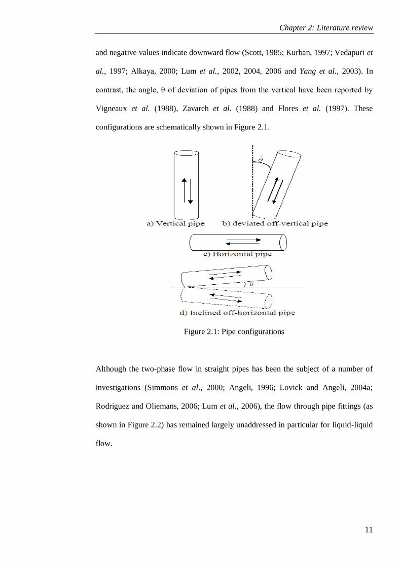
and negative values indicate downward flow (Scott, 1985; Kurban, 1997; Vedapuri et
al., 1997; Alkaya, 2000; Lum et al., 2002, 2004, 2006 and Yang et al., 2003). In
contrast, the angle, θ of deviation of pipes from the vertical have been reported by
Vigneaux et al. (1988), Zavareh et al. (1988) and Flores et al. (1997). These
configurations are schematically shown in Figure 2.1.
Figure 2.1: Pipe configurations
Although the two-phase flow in straight pipes has been the subject of a number of
investigations (Simmons et al., 2000; Angeli, 1996; Lovick and Angeli, 2004a;
Rodriguez and Oliemans, 2006; Lum et al., 2006), the flow through pipe fittings (as
shown in Figure 2.2) has remained largely unaddressed in particular for liquid-liquid
flow.
Chapter 2: Literature review
12
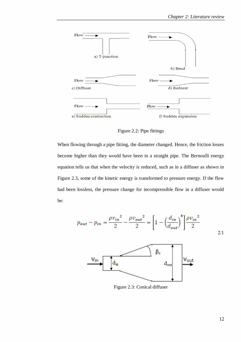
Figure 2.2: Pipe fittings
When flowing through a pipe fitting, the diameter changed. Hence, the friction losses
become higher than they would have been in a straight pipe. The Bernoulli energy
equation tells us that when the velocity is reduced, such as in a diffuser as shown in
Figure 2.3, some of the kinetic energy is transformed to pressure energy. If the flow
had been lossless, the pressure change for incompressible flow in a diffuser would
be:
2.1
Figure 2.3: Conical diffuser
Chapter 2: Literature review
13
Since dout > din, clearly pout > pin, as expected. Furthermore, in general, very small
angles βc lead to a smooth flow with relatively small losses, and the flow follows the
conical geometry without separating from the wall. Increasing β beyond a certain
point leads to separation, and the losses increase. At exactly which angle separation
starts depends on both Re, din/dout and any upstream disturbances. Measurements
carried out by Idelchik (1992) indicate that if βc ≤ 2o, no separation occurs under any
circumstances, and losses are kept to a minimum. For relatively large βc, separation
becomes so dominant that the conical section has no effect, and one may as well use
an abrupt diameter step (βc = 90o).
It is noticeably demonstrated that the pipe configuration and fittings play an
important role in determining the pattern of liquid-liquid flow, as reported by Nädler
and Mewes (1997), Flores et al. (1997) and Yang et al. (2001; 2003).
Hence, having the fundamental knowledge of flow patterns and flow pattern maps is
certainly a great advantage in understanding the separation process of liquid-liquid
two-phase flow.
2.2 Flow pattern and flow pattern maps
In the pipe flow of two fluids with different properties flowing simultaneously, the
interface between the phases can appear in quite different topological or
morphological configurations. The flows with similar interfacial shapes and spatial
distributions can be classified as being one flow regime or flow pattern. Each
individual flow pattern refers to its unique hydrodynamics properties. In two-phase
flow, the fluid phases within the pipe is distributed in several fundamentally different

Chapter 2: Literature review
14
flow patterns or flow regimes, depending primarily on these properties, e.g. mixture
velocity, input phase ratio, pipe orientation, pipe geometry and other interfacial
properties. All flow patterns are usually delineated in terms of areas on a graph with
two independent axes, giving the flow pattern maps. Many different names have
been given to these various patterns, with as many as 84 having been reported in the
literature (Rouhani et al, 1983). Nevertheless, the interest on the flow pattern maps
lies on the fact that in each regime, the flow has certain hydrodynamic
characteristics. When flow patterns are taken into account, not only can a better
model be developed but also the operational conditions can be optimised (Yang,
2003).
2.2.1 Flow patterns for liquid-liquid flows
In liquid-liquid flows, a flow pattern is defined as a characteristic geometrical flow
configuration or physical geometry exhibited by a multiphase flow in a conduit. Each
individual flow pattern has its unique hydrodynamics properties.
However, as in gas/liquid flow a number of names have been put forward for flow
pattern for liquid-liquid flows. Each paper have classified oil-water flow patterns
based on their own investigations, e.g., Guzhov (1973), Laflin (1976), Oglesby
(1979), Cox (1985), Scott (1985), Arirachakaran et al. (1989), Nadler and Mewes
(1995), Trallero (1996), Angeli (1996), Simmons (1998), Fairuzov et al. (2000) and
Munaweera et al. (2002). In general, these variations pattern names is due to the
subjective nature of flow pattern definitions and others are the variety of names given
to what are essentially the same geometric flow patterns. However, for the oil-water
flow in the petroleum industry, these classifications can be reduced to four main flow

Chapter 2: Literature review
15
patterns. These flow patterns that have been observed can be classified as dispersed
flow, annular flow, stratified flow and stratified flow with mixed layer at the
interface.
Segregated flow is defined as the flow pattern where there is continuity of both
phases (liquids) in the axial direction. The two liquids flow tends to stratify when
flowing together in a pipe due to their different densities. These separate layers
which are segregated flows can be classified as stratified flow (ST) and stratified
flow with mixed layer at the interface (ST&MI). Details of SI and SI & MI flow
patterns are discussed in the following sub-section.
In general, dispersed flow is characterized by the flow where one phase is dispersed
in the other continuous phase. The dispersed phase often present in the form of small
droplets that are non-uniformly scattered within the continuous phase in two
immiscible liquids. According to the size of the drops and their distribution in the
continuous medium, several subdivisions of this flow pattern can be observed. The
dispersed flow can either be water dominated or oil dominated. Further detail will be
presented later on in this thesis.
Furthermore, annular flow is characterized by the presence of a liquid film flowing
on the channel wall (in a round channel this film is annulus-shaped which gives the
name to this type of flow). In liquid-liquid flows, the lighter fluid flows in the centre
of the pipe, and the heavier fluid is contained in a thin film on the pipe wall. The
lighter fluid may be a mist or an emulsion. Annular flow occurs at high velocities of
the lighter fluid, and is observed in both vertical and horizontal wells. As the velocity
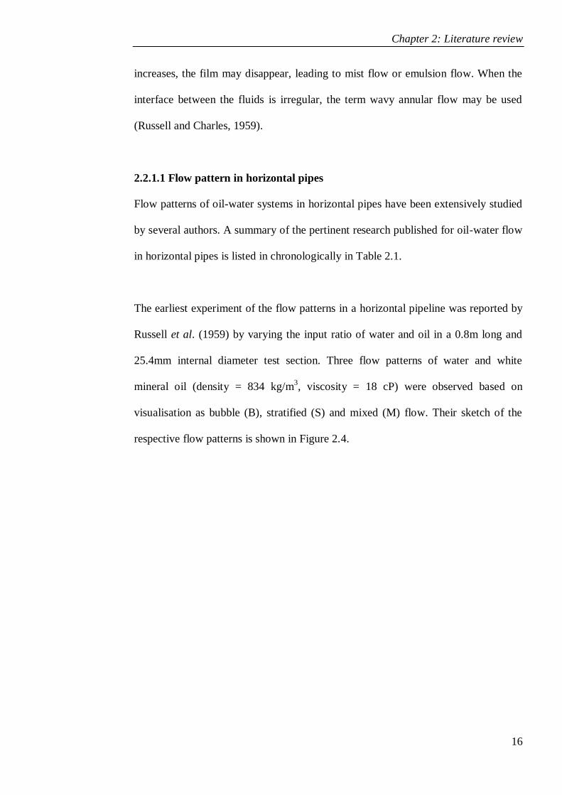
Chapter 2: Literature review
16
increases, the film may disappear, leading to mist flow or emulsion flow. When the
interface between the fluids is irregular, the term wavy annular flow may be used
(Russell and Charles, 1959).
2.2.1.1 Flow pattern in horizontal pipes
Flow patterns of oil-water systems in horizontal pipes have been extensively studied
by several authors. A summary of the pertinent research published for oil-water flow
in horizontal pipes is listed in chronologically in Table 2.1.
The earliest experiment of the flow patterns in a horizontal pipeline was reported by
Russell et al. (1959) by varying the input ratio of water and oil in a 0.8m long and
25.4mm internal diameter test section. Three flow patterns of water and white
mineral oil (density = 834 kg/m3, viscosity = 18 cP) were observed based on
visualisation as bubble (B), stratified (S) and mixed (M) flow. Their sketch of the
respective flow patterns is shown in Figure 2.4.
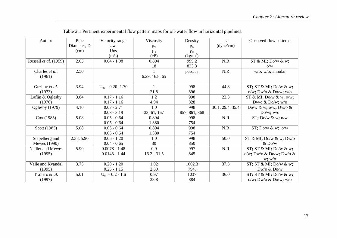
Chapter 2: Literature review
17
Table 2.1 Pertinent experimental flow pattern maps for oil-water flow in horizontal pipelines.
Author Pipe Diameter, D
(cm)
Velocity range Uws
Uos
(m/s)
Viscosity µw
µo
(cP)
Density ρw
ρo
(kg/m3)
σ (dyne/cm)
Observed flow patterns
Russell et al. (1959) 2.03 0.04 - 1.08 0.894 18
999.2 833.3
N.R ST & MI; Do/w & w; o/w
Charles et al.
(1961)
2.50 1
6.29, 16.8, 65
ρo/ρw = 1
N.R w/o; w/o; annular
Guzhov et al.
(1973)
3.94 Um = 0.20-.1.70 1
21.8
998
896
44.8 ST; ST & MI; Do/w & w;
o/w; Dw/o & Do/w; w/o
Laflin & Oglesby (1976)
3.84 0.17 - 1.16 0.17 - 1.16
1.2 4.94
998 828
22.3 ST & MI; Do/w & w; o/w; Dw/o & Do/w; w/o
Oglesby (1979) 4.10 0.07 - 2.71
0.03 - 3.19
1.0
33, 61, 167
998
857, 861, 868
30.1, 29.4, 35.4 Do/w & w; o/w; Dw/o &
Do/w; w/o
Cox (1985) 5.08 0.05 - 0.64 0.05 - 0.64
0.894 1.380
998 754
N.R ST; Do/w & w; o/w
Scott (1985) 5.08 0.05 - 0.64
0.05 - 0.64
0.894
1.380
998
754
N.R ST; Do/w & w; o/w
Stapelberg and Mewes (1990)
2.38, 5.90 0.06 - 1.20 0.04 - 0.65
1.0 30
998 850
50.0 ST & MI; Do/w & w; Dw/o & Do/w
Nadler and Mewes
(1995)
5.90 0.0078 - 1.48
0.0143 - 1.44
0.9
16.2 - 31.5
997
845
N.R ST; ST & MI; Do/w & w;
o/w; Dw/o & Do/w; Dw/o &
w; w/o
Valle and Kvandal
(1995)
3.75 0.20 - 1.20
0.25 - 1.15
1.02
2.30
1002.3
794.
37.3 ST; ST & MI; Do/w & w;
Dw/o & Do/w
Trallero et al.
(1997)
5.01 Um = 0.2 - 1.6 0.97
28.8
1037
884
36.0 ST; ST & MI; Do/w & w;
o/w; Dw/o & Do/w; w/o
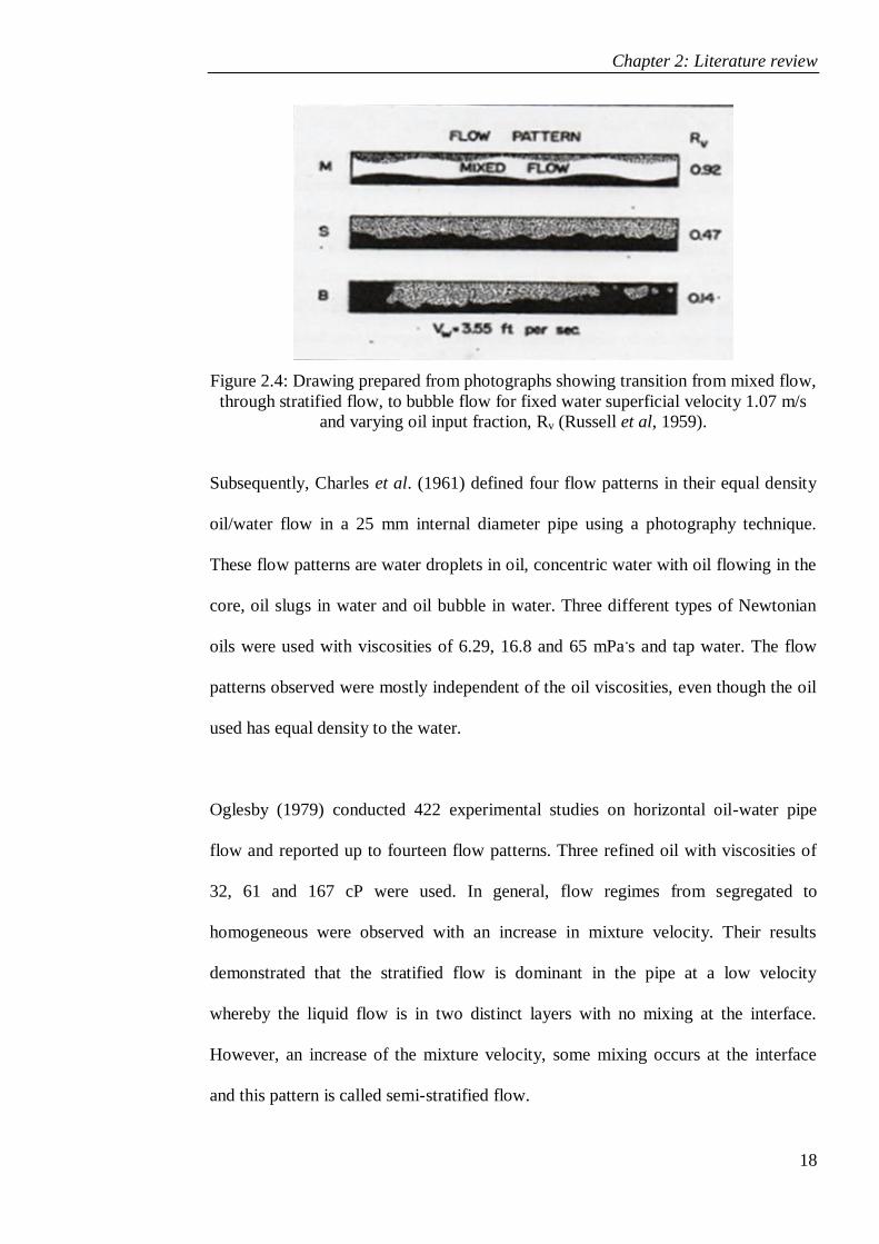
Chapter 2: Literature review
18
Figure 2.4: Drawing prepared from photographs showing transition from mixed flow,
through stratified flow, to bubble flow for fixed water superficial velocity 1.07 m/s
and varying oil input fraction, Rv (Russell et al, 1959).
Subsequently, Charles et al. (1961) defined four flow patterns in their equal density
oil/water flow in a 25 mm internal diameter pipe using a photography technique.
These flow patterns are water droplets in oil, concentric water with oil flowing in the
core, oil slugs in water and oil bubble in water. Three different types of Newtonian
oils were used with viscosities of 6.29, 16.8 and 65 mPa.s and tap water. The flow
patterns observed were mostly independent of the oil viscosities, even though the oil
used has equal density to the water.
Oglesby (1979) conducted 422 experimental studies on horizontal oil-water pipe
flow and reported up to fourteen flow patterns. Three refined oil with viscosities of
32, 61 and 167 cP were used. In general, flow regimes from segregated to
homogeneous were observed with an increase in mixture velocity. Their results
demonstrated that the stratified flow is dominant in the pipe at a low velocity
whereby the liquid flow is in two distinct layers with no mixing at the interface.
However, an increase of the mixture velocity, some mixing occurs at the interface
and this pattern is called semi-stratified flow.
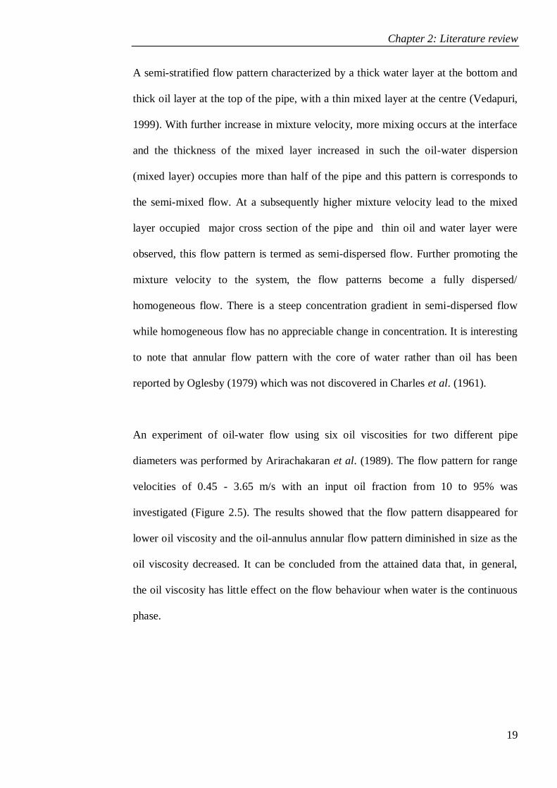
Chapter 2: Literature review
19
A semi-stratified flow pattern characterized by a thick water layer at the bottom and
thick oil layer at the top of the pipe, with a thin mixed layer at the centre (Vedapuri,
1999). With further increase in mixture velocity, more mixing occurs at the interface
and the thickness of the mixed layer increased in such the oil-water dispersion
(mixed layer) occupies more than half of the pipe and this pattern is corresponds to
the semi-mixed flow. At a subsequently higher mixture velocity lead to the mixed
layer occupied major cross section of the pipe and thin oil and water layer were
observed, this flow pattern is termed as semi-dispersed flow. Further promoting the
mixture velocity to the system, the flow patterns become a fully dispersed/
homogeneous flow. There is a steep concentration gradient in semi-dispersed flow
while homogeneous flow has no appreciable change in concentration. It is interesting
to note that annular flow pattern with the core of water rather than oil has been
reported by Oglesby (1979) which was not discovered in Charles et al. (1961).
An experiment of oil-water flow using six oil viscosities for two different pipe
diameters was performed by Arirachakaran et al. (1989). The flow pattern for range
velocities of 0.45 - 3.65 m/s with an input oil fraction from 10 to 95% was
investigated (Figure 2.5). The results showed that the flow pattern disappeared for
lower oil viscosity and the oil-annulus annular flow pattern diminished in size as the
oil viscosity decreased. It can be concluded from the attained data that, in general,
the oil viscosity has little effect on the flow behaviour when water is the continuous
phase.

Chapter 2: Literature review
20
Figure 2.5: Flow patterns defined by Arirachakaran et al. (1989)
Trallero (1996) has divided the oil-water flow pattern into two major categories:
Segregated Flow and Dispersed Flow. As for these two categories, six different flow
patterns for oil-water flow in pipes have been characterised. A sketch of the flow
patterns and abbreviated names are shown in Figure 2.6 (Trallero et al., 1997). Based
on his own experiments and the results of previous investigators for horizontal flow,
Trallero (1996) identified and reclassified the flow pattern nomenclature and defined
the six flow patterns as the following:
Segregated flows:
Stratified flow (ST)
Stratified flow with mixed layer at the interface (ST & MI)
Dispersed flows:
Water dominated
Dispersion of oil in water and water (Do/w & w)
Oil in water emulsion (o/w)
Oil dominated
Dispersion of water in oil and oil in water (Dw/o & Do/w)
Water in oil emulsion (w/o)
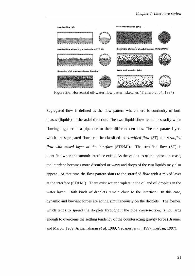
Chapter 2: Literature review
21
Figure 2.6: Horizontal oil-water flow pattern sketches (Trallero et al., 1997)
Segregated flow is defined as the flow pattern where there is continuity of both
phases (liquids) in the axial direction. The two liquids flow tends to stratify when
flowing together in a pipe due to their different densities. These separate layers
which are segregated flows can be classified as stratified flow (ST) and stratified
flow with mixed layer at the interface (ST&MI). The stratified flow (ST) is
identified when the smooth interface exists. As the velocities of the phases increase,
the interface becomes more disturbed or wavy and drops of the two liquids may also
appear. At that time the flow pattern shifts to the stratified flow with a mixed layer
at the interface (ST&MI). There exist water droplets in the oil and oil droplets in the
water layer. Both kinds of droplets remain close to the interface. In this case,
dynamic and buoyant forces are acting simultaneously on the droplets. The former,
which tends to spread the droplets throughout the pipe cross-section, is not large
enough to overcome the settling tendency of the counteracting gravity force (Brauner
and Maron, 1989; Arirachakaran et al. 1989; Vedapuri et al., 1997; Kurban, 1997).

Chapter 2: Literature review
22
As continuity of both phases (liquids) in the axial direction defined segregated flow,
dispersed flow on the other hand is identified when the continuity is lost in either or
both phases. In general, dispersed flow is characterized by the flow where one phase
is dispersed in the other continuous phase. The dispersed phase often present in the
form of small droplets that are non-uniformly scattered within the continuous phase
in two immiscible liquids. According to the size of the drops and their distribution in
the continuous medium, several subdivisions of this flow pattern can be observed.
The dispersed flow can either be water dominated or oil dominated. As for water-
dominated flows, the water is always the continuous (dominant) phase and vice
versa. A dispersion of oil in water over a water layer (Do/w & w) and emulsion of oil
in water (o/w) are dispersed flow patterns where water is the dominant phase. On the
other hand, an emulsion of water in oil (w/o) and the coexistence of both type of
dispersions (Dw/o & Do/w) are oil dominated flow patterns (Hinze, 1955; Karabelas,
1978; Trallero, 1996: Angeli and Hewitt, 2000b). Interestingly, dual continuous
dispersed flow namely oil continuous and water continuous, have been
experimentally identified by Jayawardena et al., 2000 and Lovick and Angeli 2003,
2004a.
Beretta et al. (1997) studied the flow patterns of oil-water flow in a 3 mm small
diameter tube for three oil viscosities using a stroboscope and a photography
technique. They found that most flow patterns for gas-liquid also occur in liquid-
liquid horizontal flow in a small diameter tube.
In general, two immiscible liquids of different densities tend to stratify when flowing
together in a pipe. The greater the density difference, the more nearly complete is the
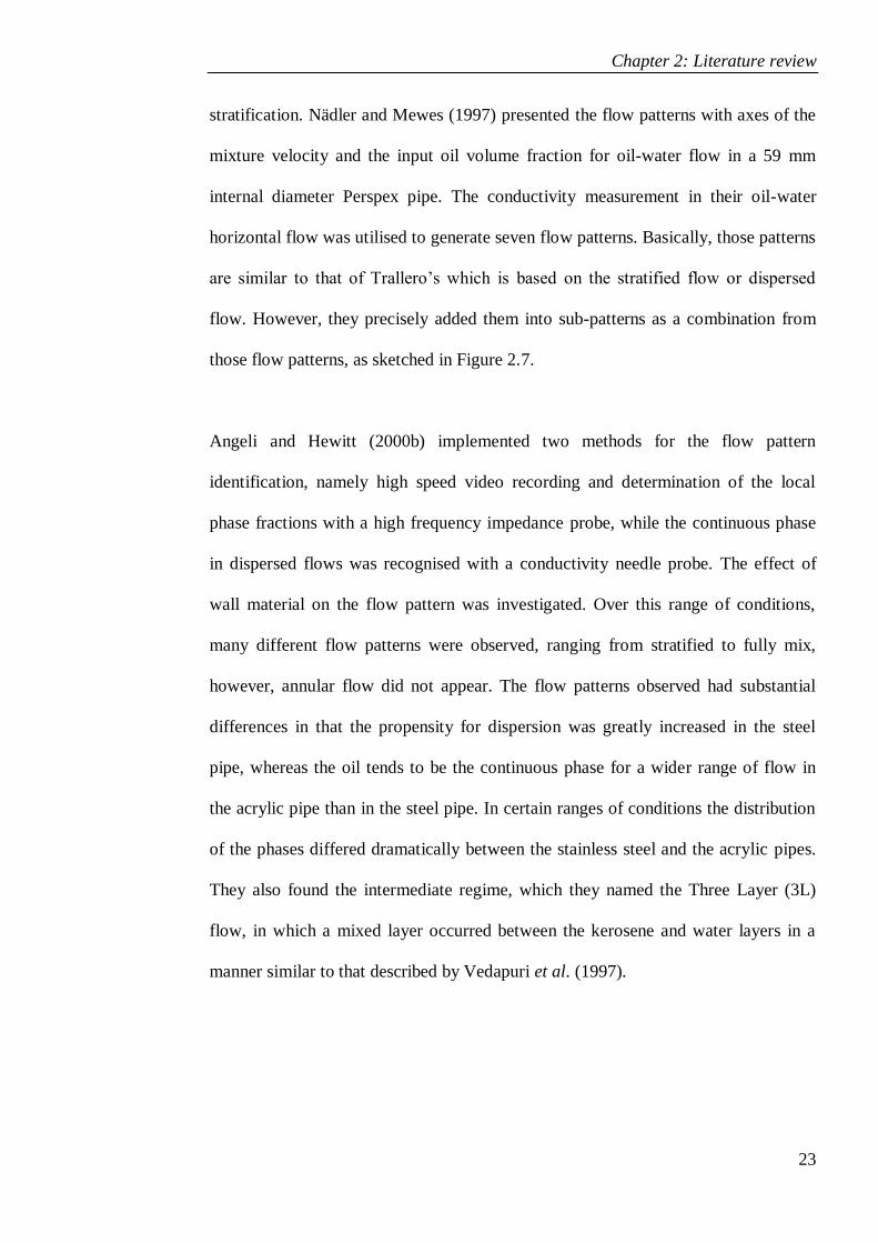
Chapter 2: Literature review
23
stratification. Nädler and Mewes (1997) presented the flow patterns with axes of the
mixture velocity and the input oil volume fraction for oil-water flow in a 59 mm
internal diameter Perspex pipe. The conductivity measurement in their oil-water
horizontal flow was utilised to generate seven flow patterns. Basically, those patterns
are similar to that of Trallero‟s which is based on the stratified flow or dispersed
flow. However, they precisely added them into sub-patterns as a combination from
those flow patterns, as sketched in Figure 2.7.
Angeli and Hewitt (2000b) implemented two methods for the flow pattern
identification, namely high speed video recording and determination of the local
phase fractions with a high frequency impedance probe, while the continuous phase
in dispersed flows was recognised with a conductivity needle probe. The effect of
wall material on the flow pattern was investigated. Over this range of conditions,
many different flow patterns were observed, ranging from stratified to fully mix,
however, annular flow did not appear. The flow patterns observed had substantial
differences in that the propensity for dispersion was greatly increased in the steel
pipe, whereas the oil tends to be the continuous phase for a wider range of flow in
the acrylic pipe than in the steel pipe. In certain ranges of conditions the distribution
of the phases differed dramatically between the stainless steel and the acrylic pipes.
They also found the intermediate regime, which they named the Three Layer (3L)
flow, in which a mixed layer occurred between the kerosene and water layers in a
manner similar to that described by Vedapuri et al. (1997).
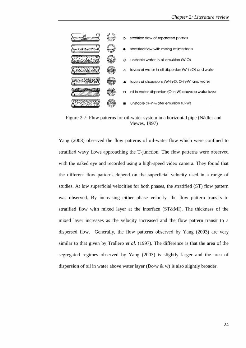
Chapter 2: Literature review
24
Figure 2.7: Flow patterns for oil-water system in a horizontal pipe (Nädler and
Mewes, 1997)
Yang (2003) observed the flow patterns of oil-water flow which were confined to
stratified wavy flows approaching the T-junction. The flow patterns were observed
with the naked eye and recorded using a high-speed video camera. They found that
the different flow patterns depend on the superficial velocity used in a range of
studies. At low superficial velocities for both phases, the stratified (ST) flow pattern
was observed. By increasing either phase velocity, the flow pattern transits to
stratified flow with mixed layer at the interface (ST&MI). The thickness of the
mixed layer increases as the velocity increased and the flow pattern transit to a
dispersed flow. Generally, the flow patterns observed by Yang (2003) are very
similar to that given by Trallero et al. (1997). The difference is that the area of the
segregated regimes observed by Yang (2003) is slightly larger and the area of
dispersion of oil in water above water layer (Do/w & w) is also slightly broader.
Chapter 2: Literature review
25
2.2.1.2 Flow pattern in inclined pipes
Two phase flow occurrences in industry are ubiquitous, whether it was in horizontal,
vertical or inclined pipelines. Even though it occurs in all of the pipe orientations,
horizontal and vertical pipe orientations received the most attention. Therefore, there
is little flow patterns data of the oil-water system available for inclined pipe
orientation. Nevertheless, researchers have reported flow patterns for inclinations
from the horizontal, such as Scott (1985), Cox (1985), Vigneaux et al. (1988);
Kurban (1997), Vedapuri et al. (1997), Alkaya (2000), Lum et al. (2002; 2004;
2006), Yang et al. (2003) and Rodriguez and Oliemans (2006).
Scott (1985) studied the flow of a mixture water and mineral oil in upward inclined
pipes. The physical phenomenon studied were flow regime occurrence and hold-up,
as a function of flow rate and pipe inclination. Interestingly, the effect of the flow
patterns on the inclination angle was first investigated by him. He applied the upward
angle from +5o to + 30
o and concluded that the effect of inclination on the transition
to dispersed flow was influenced by the mixture composition. In addition, the
appearance of local backflow or recirculation cells within the angles studied was also
observed. Figure 2.8 shows the flow pattern observed by Scott (1985) in inclined
pipes.
At the same time, Cox (1985) has conducted experiments of horizontal and downhill
two-phase oil-water flow. He concludes that at low oil-water flow rate ratios,
stratified flow is naturally unstable. The parallel gravity component drives the
instability, causing a wavy interface. An increase in the oil superficial velocity
stabilizes the oil, and both phases flow as continuous layer even though the interface
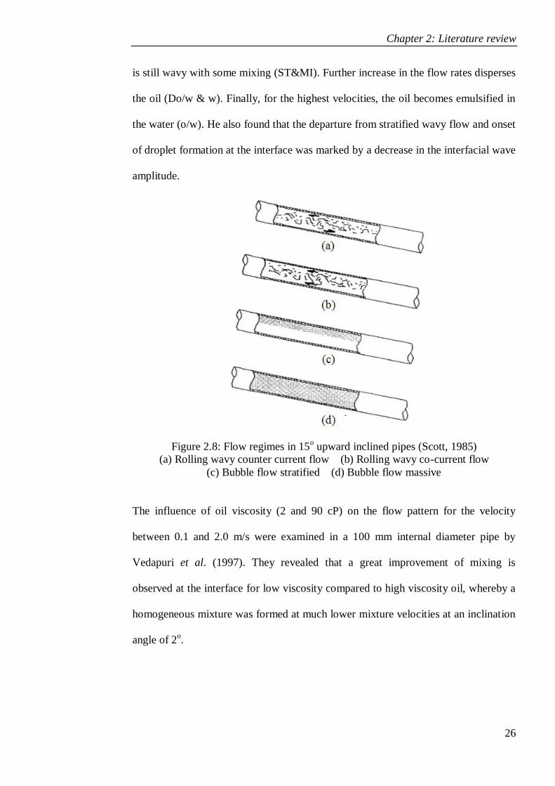
Chapter 2: Literature review
26
is still wavy with some mixing (ST&MI). Further increase in the flow rates disperses
the oil (Do/w & w). Finally, for the highest velocities, the oil becomes emulsified in
the water (o/w). He also found that the departure from stratified wavy flow and onset
of droplet formation at the interface was marked by a decrease in the interfacial wave
amplitude.
Figure 2.8: Flow regimes in 15o upward inclined pipes (Scott, 1985)
(a) Rolling wavy counter current flow (b) Rolling wavy co-current flow
(c) Bubble flow stratified (d) Bubble flow massive
The influence of oil viscosity (2 and 90 cP) on the flow pattern for the velocity
between 0.1 and 2.0 m/s were examined in a 100 mm internal diameter pipe by
Vedapuri et al. (1997). They revealed that a great improvement of mixing is
observed at the interface for low viscosity compared to high viscosity oil, whereby a
homogeneous mixture was formed at much lower mixture velocities at an inclination
angle of 2o.
Chapter 2: Literature review
27
Meanwhile, Alkaya (2000) who applied horizontal and four inclination angles of ±5o,
and found that the inclination did not have a significant effect on the transition
boundaries of dispersed regimes as compared to a horizontal position, except for the
appearance of a dispersion of water-in-oil under an oil layer (Dw/o and o)at the
highest oil fraction. Alkaya (2000) also reported that the velocity ratio at low mixture
velocities increased with increasing upward inclination, indicating that the water
tended to stay back.
Lum et al. (2002; 2004) investigated the effect of a small inclination angle (0o& +5
o)
on flow patterns using a visual identification and an impedance probe. They used an
experimental set-up as described in detail by Lovick and Angeli (2001). They
exhibited that three flow patterns as follows: stratified wavy flow, Three-Layer (3L)
flow and fully dispersed, which is similar to those seen in the horizontal flows.
However, the three-layer pattern predominated in flows at small inclination, lower
mixture velocity and at an intermediate oil fraction. Besides, three-layers were also
reported to have appeared at lower mixture velocity for the oil-in-water dispersions
and at high mixture velocity for the water-in-oil dispersions, due to the increase of
dispersion present that favours drag reduction in inclined flow.
In addition, Lum et al. (2006) who initially used the same experimental facility as
reported in Lum et al. (2002; 2004) but added two other inclination angles (-5o&
+10o) in his studies found a new flow pattern called oil plug flow at both +5
o and
+10o of inclination angles. This was not reported by Scott (1985) and Alkaya (2000).
However, this pattern was not seen in downward flow but is in accordance with other
investigators (Vedapuri et al., 1997 and Alkaya, 2000). The stratified wavy flow was
Chapter 2: Literature review
28
observed to become wavier as the upward inclination angle is increased but
disappeared completely in downward flow. In general, four flow patterns in upward
flow and two flow patterns in downward flow were recorded by Lum et al. (2006).
Furthermore, Yang (2003) studied the small inclination angle between -7o and +6
o
from the horizontal downstream of a pipe expansion. For upward inclination, he
found that large waves occur at the interface between the water and mixed layer. The
larger the upward inclined angle, the larger the waves become and the shorter the
distance downstream of the singularity at which the waves occur. Conversely, for
downward inclinations, as the angle of inclinations increased, the amplitude of the
waves severely decreases. The waves dissipated quickly with very thin water layer
and at -7o the waves and the thin water layer also dissipated.
Recently, Rodriguez and Oliemans (2006) conducted an experimental study on oil-
water flow in horizontal and slightly inclined pipes in a 82.8 mm internal diameter
steel pipe at the inclination angles of -5o, -2
o, -1.5
o, +1
o, +2
o, +5
o and horizontal flow.
Basically, seven flow patterns were observed for horizontal, upward and downward
inclined flow, and are reasonably well described by the Trallero‟s flow pattern map.
They observed a stratified smooth flow pattern appears in most horizontal flow;
however, this pattern disappeared with inclination and is replaced by the stratified
wavy (SW) flow pattern in downward and upward flow.
Most recently, Hasan (2006) performed experiment on phase separation of the oil-
water flows downstream of sudden expansion with an internal diameter of 63 mm
inlet and 100 mm outlet, which can be inclined. The test fluids used were oil and
Chapter 2: Literature review
29
purified water at operating conditions for mixture velocities 0.2, 0.3 and 0.4 m/s,
input oil fraction from 20 to 70% and pipe orientations at angles of +6 , +3 , 0 , -4
and -7 to the horizontal. He concludes that the mechanisms of coalescence occurred
faster at the top than the other locations in a pipe cross-section. Furthermore, Hasan
(2006) also observed 3 different interface shapes for the stratified oil-water flow;
plane horizontal interface, concave interface and convex interface. The concave
interfaces were observed for horizontal and downward flow, and the convex
interfaces were identified only for an upward inclination.
Moreover, the experiments at an upward deviation angle off vertical were conducted
by Vigneaux et al. (1988), Zavareh et al. (1988) and Flores et al. (1997). Vigneaux et
al. (1988) have conducted experiments on kerosene-water for inclinations between 5o
and 65o from the vertical in 100 mm and 200 mm ID pipes for a mixture velocity
ranges from 0.1 to 0.5 m/s. Most of the studies concentrated on the effect of
inclination and mixture velocity on the slip velocity (oil-water) and on water volume
fraction radial gradient. They found that in inclined pipes, the gradient of the water
volume fraction is very large in the centre part of the pipe. Whereas the upper part of
the pipe section is almost occupied only by oil and the lower section by water. They
also observed that the fast-moving droplet swarms occurred at the deviation angle
above 10o and the concentration of oil remains very small outside the swarms.
Oil-water flow behaviour in vertical and large deviated incline pipe to characterize
flow pattern flow in a transparent pipe of 50 mm internal diameter was investigated
by Flores et al. (1997). The conductance probes were employed at various points in a
pipe cross-section and the oil-water flow patterns in vertical and large deviated
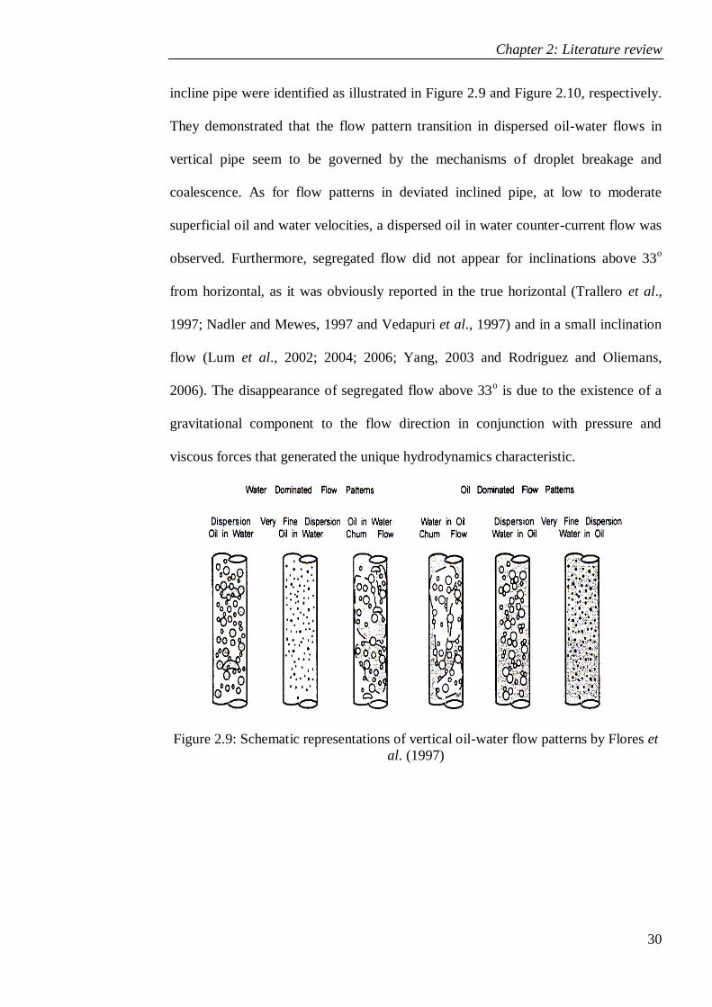
Chapter 2: Literature review
30
incline pipe were identified as illustrated in Figure 2.9 and Figure 2.10, respectively.
They demonstrated that the flow pattern transition in dispersed oil-water flows in
vertical pipe seem to be governed by the mechanisms of droplet breakage and
coalescence. As for flow patterns in deviated inclined pipe, at low to moderate
superficial oil and water velocities, a dispersed oil in water counter-current flow was
observed. Furthermore, segregated flow did not appear for inclinations above 33o
from horizontal, as it was obviously reported in the true horizontal (Trallero et al.,
1997; Nadler and Mewes, 1997 and Vedapuri et al., 1997) and in a small inclination
flow (Lum et al., 2002; 2004; 2006; Yang, 2003 and Rodriguez and Oliemans,
2006). The disappearance of segregated flow above 33o is due to the existence of a
gravitational component to the flow direction in conjunction with pressure and
viscous forces that generated the unique hydrodynamics characteristic.
Figure 2.9: Schematic representations of vertical oil-water flow patterns by Flores et
al. (1997)
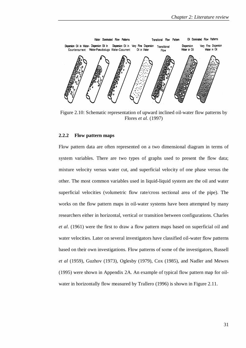
Chapter 2: Literature review
31
Figure 2.10: Schematic representation of upward inclined oil-water flow patterns by
Flores et al. (1997)
2.2.2 Flow pattern maps
Flow pattern data are often represented on a two dimensional diagram in terms of
system variables. There are two types of graphs used to present the flow data;
mixture velocity versus water cut, and superficial velocity of one phase versus the
other. The most common variables used in liquid-liquid system are the oil and water
superficial velocities (volumetric flow rate/cross sectional area of the pipe). The
works on the flow pattern maps in oil-water systems have been attempted by many
researchers either in horizontal, vertical or transition between configurations. Charles
et al. (1961) were the first to draw a flow pattern maps based on superficial oil and
water velocities. Later on several investigators have classified oil-water flow patterns
based on their own investigations. Flow patterns of some of the investigators, Russell
et al (1959), Guzhov (1973), Oglesby (1979), Cox (1985), and Nadler and Mewes
(1995) were shown in Appendix 2A. An example of typical flow pattern map for oil-
water in horizontally flow measured by Trallero (1996) is shown in Figure 2.11.
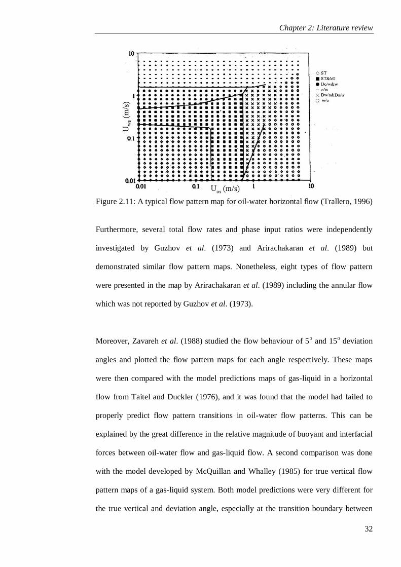
Chapter 2: Literature review
32
Figure 2.11: A typical flow pattern map for oil-water horizontal flow (Trallero, 1996)
Furthermore, several total flow rates and phase input ratios were independently
investigated by Guzhov et al. (1973) and Arirachakaran et al. (1989) but
demonstrated similar flow pattern maps. Nonetheless, eight types of flow pattern
were presented in the map by Arirachakaran et al. (1989) including the annular flow
which was not reported by Guzhov et al. (1973).
Moreover, Zavareh et al. (1988) studied the flow behaviour of 5o and 15
o deviation
angles and plotted the flow pattern maps for each angle respectively. These maps
were then compared with the model predictions maps of gas-liquid in a horizontal
flow from Taitel and Duckler (1976), and it was found that the model had failed to
properly predict flow pattern transitions in oil-water flow patterns. This can be
explained by the great difference in the relative magnitude of buoyant and interfacial
forces between oil-water flow and gas-liquid flow. A second comparison was done
with the model developed by McQuillan and Whalley (1985) for true vertical flow
pattern maps of a gas-liquid system. Both model predictions were very different for
the true vertical and deviation angle, especially at the transition boundary between
Chapter 2: Literature review
33
bubbly flow and dispersed flow. Nevertheless, it did come closer than the gas-liquid
flow maps in predicting the correct boundary.
Meanwhile, an experiment of stratified flow oil-water had been undertaken by Valle
and Kvandal (1995). The dispersed region was found at the bottom when oil
superficial velocity is greater than water superficial velocity, in contrast the opposite
true for water dispersed oil zone in the upper region of pipe. On the other hand, a
major conclusion cannot be done due to the fact that the experiment range was too
small compared to predicted results. As a consequence, most of the flow patterns that
appeared were stratified flows with negligible droplet entrainment and dispersed
flow regions.
On the other hand, the flow pattern map of a Newtonian and low-viscosity oil-water
system in a horizontal pipe was developed by Trallero (1996), as shown in Figure
2.11. A video camera coupled with a still camera was used to record the flow
patterns and their structure. Consequently, the map showed that the segregated flow
region was dominant at low and intermediate superficial velocities while the water or
oil could be the dominant phase at a high superficial velocity and was not previously
mentioned by Charles et al. (1961).
Additionally, the effect of the mixture velocity and phase input ratio on the flow
pattern map was explored by Nadler and Mewes (1997) and the conductivity
technique was used to distinguish different flow patterns. The continuous layers of
both phases occurred simultaneously in the water-in-oil and oil-in-water dispersion
Chapter 2: Literature review
34
zones. A drag reduction was also observed in these zones appearing between the
water continuous dispersed flow and the oil continuous dispersed flow.
In the same year, Flores et al. (1997) developed four flow pattern maps for upward
inclination flows of 45o, 60
o and 75
o from horizontal and vertical upward flow
respectively. The flow pattern map for vertical flow was completely different to that
of horizontal flow, as described elsewhere (Trallero, 1996; 1997). They argued that
the dispersed oil-in-water was the most predominant area wherein a slightly churning
flow occurred at high oil velocity. Nevertheless, the dispersed areas were divided
into oil-in-water-Pseudo slugs and oil-in-water counter current as the deviation angle
was increased (45o). They established that stratified flow and stratified flow with
some mixing at the interface, which were previously reported in horizontal and near
horizontal flows no longer exists for inclination above 33o from horizontal. This
revealed that the inclination angle significantly affected the flow pattern map.
Simmons (1998) developed a flow pattern map from the experiment of oil-water
mixed aqueous in a 63 mm horizontal pipe and used video footage for the flow
pattern determination. The boundaries of the flow pattern map obtained from that
study showed an excellent agreement with the theoretical flow boundaries predicted
by Brauner and Moalem Maron (1992a).
Undoubtedly, the deviation or inclination angles have maximal effect to the flow
pattern maps produced and this is possibly due to the presence of droplet sizes in oil-
water flowing at appropriated pipe configurations. Thus further investigation on

Chapter 2: Literature review
35
droplet size distributions would be valuable in order to understand the behaviour of
the flow present in the pipeline.
2.3 Liquid-liquid dispersion
Outside the ST and ST&MI regions, the liquids are dispersed in different ways,
contingent upon which one is dominant. A dispersion of two immiscible liquids,
where one of the liquids forms a continuous phase and the other is dispersed in it, is a
flow pattern often observed in liquid-liquid systems. In some conditions, each phase
can be dispersed as drops into the other phase in different layers, e.g., dual
dispersions. Dispersions will always form in motions of two immiscible liquids
which are sufficiently intense, where the disperse forces are due to the turbulent
energy dissipation. The formation of dispersions is generally governed by two
competing processes; drop break-up and drop coalescence (Sajjadi et al, 2001). The
drop breakage rate dominates the drop coalescence rate in the initial stage, which
causes the drop sizes to decrease with time (Narishman, Ramkrihna, & Gupta, 1980).
However with time, the drop breakage rate decreases while drop coalescence rate
increases. Ultimately, a steady state is reached where the rate of both processes
become equal, and a steady-state drop size distribution is established.
Therefore, without a shred of doubt, behaviour of the dispersion depends strongly on
hydrodynamic interaction of drops which includes drop breakage, drop coalescence
and drop sedimentation or settling. These events results in changes in the drop sizes,
drop size distribution and drop size distribution profile across the pipe section, as
well as layer separation of the two phases.
Chapter 2: Literature review
36
2.3.1 Drop breakage and coalescence in dispersion.
There are three factors that acting on drops in dispersion; turbulences, coagulating
and gravity/buoyancy. The first is the factor of turbulences of the continuous phase
which arise to breaks the drops or to prevent the coalescence of the drops. The
turbulence of the continuous phase can be considered to be the inertial force and
viscous shear force analysed by Kolmogoroff (1949), Hinze (1955), Taylor (1934)
and Shinnar (1961). The second factor is the coagulating of the dispersed phased
which make the drops coalesce or prevents the drops from breaking up. The
coagulating of the dispersed phase are the forces of interfacial tension, viscous
friction and inner agglutination of the drops (Shinnar, 1961 and Thomas, 1981). The
third is the gravity or buoyant force which is the main contribution to the settling of
the drops.
In dispersion, the drop size and drop size distribution mainly depend on the
equilibrium balance between the turbulence forces and the coagulating forces. Size
distribution of the disperse phase affects the overall performance efficiency. Smaller
droplets provide larger interfacial area per unit volume and contrariwise. The sizes
distribution of the drops depend on several factors as mentioned earlier. In order to
understand the dispersive process better, it is important that drop break-up and
coalescence be investigated.
In dispersed flow, drop break-up usually occurs when large droplets break into
smaller ones. For a dispersed phase with low viscosity, the viscous friction forces can
be neglected. Therefore, interfacial tension and agglutination of the drops are the two
main coagulating forces. If the turbulence forces overcome the interfacial tension, the
Chapter 2: Literature review
37
drops deformed and break up, by turbulence inertial force and turbulence shear force.
If the turbulence forces overcome the agglutination of the drops and then prevent
coalescence of drops, coalescence blocked by turbulence inertial force and by
turbulence shear force.
According to the observation of Ali et al (1981), the breakage processes of the drops
for the two breaks up mechanisms are different. For the drop break up by turbulence
inertial force, the drop is lashed by inertial force and smashed into a cloud of smaller
drops and then these smaller drops separate. For the drop break up by viscous shear
force, the drop firstly deforms and prolongs and the ruptures to form smaller drops.
There is other mechanism for drop breakage, i.e., accelerated drops (Cohen, 1991;
Brauner, 2002). For accelerated drops, drops deform and break due to rapid
acceleration of drops bursting into a stream of a second fluid, which is the main
mechanism for pneumatic atomisation.
Hence, a wide range of concepts has been developed from the studies of drop
breakage by many investigators (Kolmogoroff, 1949; Hinze, 1955; Taylor, 1934;
Shinnar, 1961; Sleicher, 1962; Sprow, 1967; Hughmark, 1971; Kubie and Gradner,
1977; Karabelas, 1978 and Noik et al., 2002).
In most cases, investigators have not reported on drop coalescence probably because
they were observing single drops in a turbulent flow field or working with dilute
dispersions. Whereas, in dense dispersions, droplets coalescence and additional
factors introduced when a swarm of droplets interact must be taken into account
(Jeelani, 1993 and Wagner, 1997).
Chapter 2: Literature review
38
In turbulent dispersion, coalescence results when smaller droplets tend to form large
ones. Coalescence phenomenon is more complex since it involves the approach of
two drops collides, trapping a small amount of liquid between them. Then the
drainage of the liquid film separating the drops until it reaches a critical values and
eventual rupture of the intervening liquid film resulting in coalescence. Therefore the
physical properties of the fluids and interfaces play an important role in drops
coalescence. For example, coalescence in dispersion is usually reduced considerably
by the combined action of a protective colloid and turbulent agitation. Hence, there is
not as many concepts have been developed as for drop breakage. Among the few that
involved in studies of drop coalescence are Sleicher (1961), Levich (1962), Howarth
(1964), Coulaloglou and Tavlarides (1977) and Thomas (1981).
What's more, sedimentation or settling in liquid-liquid system has scarcely been
studied. Mostly, the sedimentation has been studied in liquid-solids systems
(Coulson and Richardson, 1991).
2.3.2 Models for drop breakage and coalescence
The possibility of predicting fluid particle (drops or bubbles) size distributions is
very important for determining interfacial areas and heat- and mass-transfer rates
when designing and scaling up equipment such as chemical reactors and separators.
Population balances can be used to describe changes in the fluid particle size
distributions and other dispersion properties, and are usually the result of dynamic
fluid particle breakage and coalescence processes.
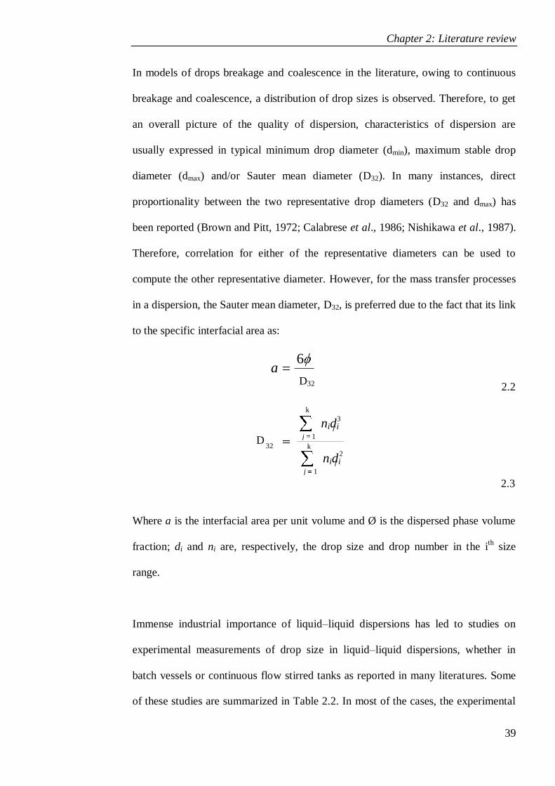
Chapter 2: Literature review
39
In models of drops breakage and coalescence in the literature, owing to continuous
breakage and coalescence, a distribution of drop sizes is observed. Therefore, to get
an overall picture of the quality of dispersion, characteristics of dispersion are
usually expressed in typical minimum drop diameter (dmin), maximum stable drop
diameter (dmax) and/or Sauter mean diameter (D32). In many instances, direct
proportionality between the two representative drop diameters (D32 and dmax) has
been reported (Brown and Pitt, 1972; Calabrese et al., 1986; Nishikawa et al., 1987).
Therefore, correlation for either of the representative diameters can be used to
compute the other representative diameter. However, for the mass transfer processes
in a dispersion, the Sauter mean diameter, D32, is preferred due to the fact that its link
to the specific interfacial area as:
2.2
2.3
Where a is the interfacial area per unit volume and Ø is the dispersed phase volume
fraction; di and ni are, respectively, the drop size and drop number in the ith
size
range.
Immense industrial importance of liquid–liquid dispersions has led to studies on
experimental measurements of drop size in liquid–liquid dispersions, whether in
batch vessels or continuous flow stirred tanks as reported in many literatures. Some
of these studies are summarized in Table 2.2. In most of the cases, the experimental
32
6
da
k
j j
k
j j
nidi
nidi
D
1
2
1
3
32
D32

Chapter 2: Literature review
40
data have been correlated using the functional form developed by Hinze (1955) and
modified by subsequent researchers (Shinnar and Church, 1960; Doulah, 1975). In
some cases, altogether different functional forms are reported (Wienstein and
Treybal, 1973; Quadros and Baptista, 2003).
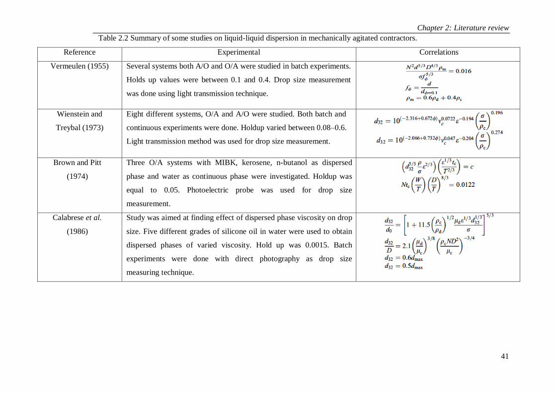
Chapter 2: Literature review
41
Table 2.2 Summary of some studies on liquid-liquid dispersion in mechanically agitated contractors.
Reference Experimental Correlations
Vermeulen (1955) Several systems both A/O and O/A were studied in batch experiments.
Holds up values were between 0.1 and 0.4. Drop size measurement
was done using light transmission technique.
Wienstein and
Treybal (1973)
Eight different systems, O/A and A/O were studied. Both batch and
continuous experiments were done. Holdup varied between 0.08–0.6.
Light transmission method was used for drop size measurement.
Brown and Pitt
(1974)
Three O/A systems with MIBK, kerosene, n-butanol as dispersed
phase and water as continuous phase were investigated. Holdup was
equal to 0.05. Photoelectric probe was used for drop size
measurement.
Calabrese et al.
(1986)
Study was aimed at finding effect of dispersed phase viscosity on drop
size. Five different grades of silicone oil in water were used to obtain
dispersed phases of varied viscosity. Hold up was 0.0015. Batch
experiments were done with direct photography as drop size
measuring technique.
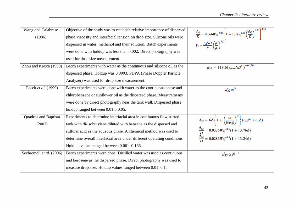
Chapter 2: Literature review
42
Wang and Calabrese
(1986)
Objective of the study was to establish relative importance of dispersed
phase viscosity and interfacial tension on drop size. Silicone oils were
dispersed in water, methanol and their solution. Batch experiments
were done with holdup was less than 0.002. Direct photography was
used for drop size measurement.
Zhou and Kresta (1998) Batch experiments with water as the continuous and silicone oil as the
dispersed phase. Holdup was 0.0003. PDPA (Phase Doppler Particle
Analyzer) was used for drop size measurement.
Pacek et al. (1999) Batch experiments were done with water as the continuous phase and
chlorobenzene or sunflower oil as the dispersed phase. Measurements
were done by direct photography near the tank wall. Dispersed phase
holdup ranged between 0.01to 0.05.
Quadros and Baptista
(2003)
Experiments to determine interfacial area in continuous flow stirred
tank with di-isobutylene diluted with benzene as the dispersed and
sulfuric acid as the aqueous phase. A chemical method was used to
determine overall interfacial area under different operating conditions.
Hold up values ranged between 0.061–0.166.
Sechremeli et al. (2006) Batch experiments were done. Distilled water was used as continuous
and kerosene as the dispersed phase. Direct photography was used to
measure drop size. Holdup values ranged between 0.01–0.1.

Chapter 2: Literature review
43
2.4 Drop size distribution
Knowledge of drop size and distribution would improve understanding of dispersed
system and contribute to better design and modelling of many industrial processes as
well as oil production and transportation. The size of the dispersed phase is important
when interfacial mass and/or heat transfer involved, while it will affect phase
separation at the end of the process. Drop size, drop size distribution and dynamics
of their evolution are significant factors that determine the rheology and stability of
dispersions. Hence, knowledge of the parameters would enhance and optimised the
energy consumption and pumping requirements of the system.
Experimental studies of drop sizes in liquid-liquid flow have mainly been carried out
in stirred tanks or agitated vessels. While information on the drop size during pipe
flow is almost entirely limited to low dispersed phase concentrations (Sleicher, 1962;
Ward and Knudsen, 1967; Collins and Knudsen, 1970; Kubie and Gardner, 1976;
Karabelas, 1978; El-Hamouz and Stewart, 1996; Simmons and Azzopardi, 2001 and
Hasan, 2006). In addition, most models are based on the fundamental theory
developed by Kolmogorov (1949) and/or Hinze (1955) for drop break-up in isotropic
turbulence with improvements to account for increasing dispersed phase fraction.
Drop size distributions during the pipe flow of two immiscible liquids have been
given by a few researchers. Among early studies, Ward and Knudsen (1967) present
an investigation to obtain information on drop size and drop size distribution of
liquid-liquids dispersions in turbulent flow. They investigated the distribution of oil
drops in water fraction up to 47% for downward vertical flow in dispersions formed
in stirred vessels before entering the test section. The photography technique was
Chapter 2: Literature review
44
used to capture photos of droplets in the dispersions. Over 1000 photographs of
dispersions were obtained and from these photos, the Sauter mean diameters (D32) of
the well-defined droplets were measured. The Sauter mean drop diameter, D32 was
found to augment when dispersed phase fraction increases. Interestingly, it was
observed that D32 initially increases and then decreases with increasing velocity. The
decrease in size at high velocities agreed with the model suggested by Sleicher
(1962) while the initial increase confirmed the theory proposed by Howarth (1964)
whereby an increase in velocity causes an increase in coalescence frequency.
Collins and Knudsen (1970) conducted an experimental program to characterise the
drop size distributions formed when liquid-liquid dispersion was exposed to
turbulent pipe flow. They used photography technique to study the effect of pipe
turbulence on drops formed by injecting an organic phase at low concentrations (0.6
– 10%) into the vertical downward flowing aqueous. The observed distributions are
two superimposed distributions; the initial distribution formed at the injecting nozzle
and the distribution produced by the turbulence of the flowing stream. Increasing the
dispersed phase viscosity seemed to delay drop deformation and break-up, while
drop break-up appeared to be much more probable near the pipe wall rather than in
the turbulent core. The authors presented a model for the evolution of drop size
distribution along the pipe, which its experimental data is in agreement with the
maximum stable drop size (dmax) as predicted by Sleicher‟s correlation.
Kubie and Gardner (1977) conducted experiments in a 4m long, 17.2 mm diameter
horizontal glass tube and in helical coils to get information on the equilibrium drop
size distribution, especially on the dmax occurring in the flow of two liquids. They

Chapter 2: Literature review
45
used four different injectors for the disperse phase and found that the various
methods of disperse phase injection had little effect on the drop size distributions. In
fact, suggesting that the steady-state distribution was probably independent of the
initial distribution. The droplet size distribution obtained by photography through the
pipe wall became narrower with increasing continuous phase velocity as maximum
drop size (dmax) decreased at a greater rate than minimum drop size (dmin). For drops
smaller than the size of the energy-containing eddies, the model suggested by Hinze
(1955) predicted satisfactorily maximum drop size (dmax) but for larger drops an
alternative model was suggested.
Karabelas (1978) performed an experiment using an encapsulation technique
concurrently with photography technique to study drop size distributions formed by
turbulence when oil was injected at low concentrations (0.2%) into flowing water in
horizontal pipes. The resulting distribution can be well represented by either Rosin-
Rammler or the upper limit log-normal function, while maximum drop diameter
(dmax) was found to satisfy Kolmogorov/Hinze model.
Kurban et al. (1995) used photography and needle conductivity probe to measure
local droplet size of oil-water flow in a horizontal acrylic pipe and have attained
significant differences between the two results. Their results showed that Sauter
mean diameters of 678 µm for the photographic technique and 206 µm for the
conductivity techniques were reported at the same flow conditions. However, the
conductance technique did have some disadvantages, like the fact that it is only
suitable for water volume fractions below 4%due to the conductive properties of
water.
Chapter 2: Literature review
46
Furthermore, El-Hamouz and Stewart (1996) utilised a laser back-scatter technique
to measure chord length distributions formed downstream of a static mixer in
horizontal flow system. The droplets were formed in the static mixer before entering
the 25.4 mm internal diameter pipe test section. The mean chord length increased
with the distance from the mixer, suggesting that the distributions were influenced by
drop coalescence in the test section rather than turbulent drop break-up.
Subsequently, the laser backscattering technique was employed, together with laser
diffraction technique by Simmons and Azzopardi (2001) to examine drop size
distribution in a dispersed vertically and horizontally pipe flow. Both measurement
techniques have been found to be limited to different concentration ranges. The laser
diffraction technique was suitable at dispersed phase concentrations less than 3%,
while the backscatter technique was suitable at concentrations greater than 5% by
volume. The Sauter means diameter (D32) measured by the backscatter technique for
horizontal flow in Simmons and Azzopardi (2001) was shown in Figure 2.12. The
D32 detected were small at higher measurement positions at low velocities,
conversely at higher velocities, the value converge at around 350 µm. Stratification
of droplets was observed at low mixtures velocities for horizontal flow. This showed
that D32 decreased with increasing mixture velocity until it reached certain value.
However, for vertical up-flow, homogeneous dispersions were obtained and no
stratification was observed. The drop sizes for dispersed phase volume fraction up to
42.3%, acquired by the laser backscatter technique were generally fitted by an upper
limit log-normal distribution (ULLN). Although the authors demonstrated that the
maximum drop size, dmax, at low concentration of the dispersed phase could be
described by the Hinze (1955) model. Nevertheless, for the minimum drop size, dmin,
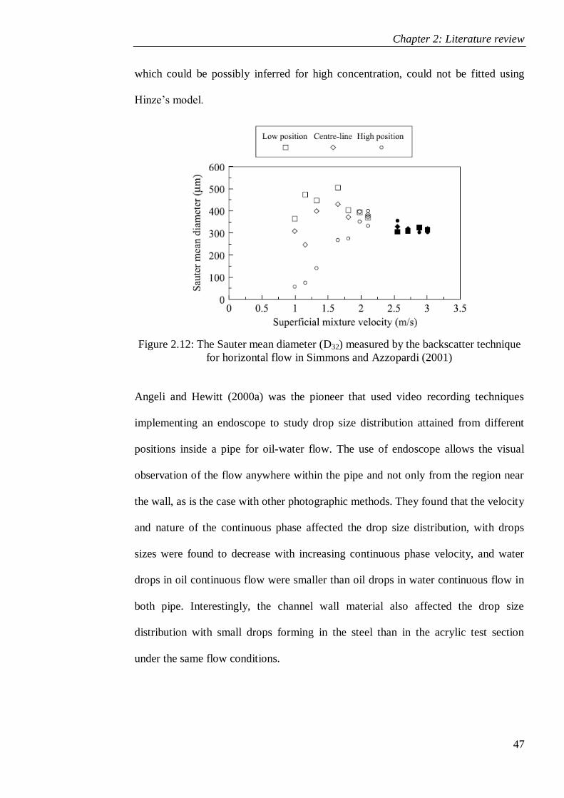
Chapter 2: Literature review
47
which could be possibly inferred for high concentration, could not be fitted using
Hinze‟s model.
Figure 2.12: The Sauter mean diameter (D32) measured by the backscatter technique
for horizontal flow in Simmons and Azzopardi (2001)
Angeli and Hewitt (2000a) was the pioneer that used video recording techniques
implementing an endoscope to study drop size distribution attained from different
positions inside a pipe for oil-water flow. The use of endoscope allows the visual
observation of the flow anywhere within the pipe and not only from the region near
the wall, as is the case with other photographic methods. They found that the velocity
and nature of the continuous phase affected the drop size distribution, with drops
sizes were found to decrease with increasing continuous phase velocity, and water
drops in oil continuous flow were smaller than oil drops in water continuous flow in
both pipe. Interestingly, the channel wall material also affected the drop size
distribution with small drops forming in the steel than in the acrylic test section
under the same flow conditions.

Chapter 2: Literature review
48
The droplet size and vertical distribution of drops of dual continuous flow in a
stainless steel pipe were investigated by Lovick and Angeli (2004b).A dual sensor
impedance probe was used in the investigation to allowed drop chord length
measurement at different location vertically of the pipe cross section. The size and
number of drops dispersed in the respective continuous phases was found to decrease
as the distance from the interface increased. They asserted that in dual continuous
flow mixture velocity does not have a clear effect on the drop size. Instead,
proclaimed that a decrease in mixture velocity decreases the number of drops
entrained from one phase into the opposite and causes greater vertical concentration
gradient, vice versa for increasing mixture velocity. Moreover, Rosin-Rammler
distribution was used to describe their experimental data and they found Rosin-
Rammler‟s model fit satisfactorily the chord length distribution.
Hasan (2006) performed an investigation on the feasibility of a sudden pipe
expansion towards stratification of liquid-liquid dispersion in horizontal and inclined
horizontal pipe flow. Drop size distributions were measured using a laser back-
scatter technique, which measured chord length distributions at several locations
vertically and axially of the test section. According to Hasan (2006), at the same
axial position of the test section, large drops were initially detected at the top of the
pipe cross-section. Therefore assumption were made that the mechanisms of
coalescence occurred faster at the top than the other locations in a pipe cross-section.
Furthermore, log-normal distribution and Rosin-Rammler function were found to fit
satisfactorily the experiment on chord length distributions at all regions except in the
interface between mixed and kerosene regions.
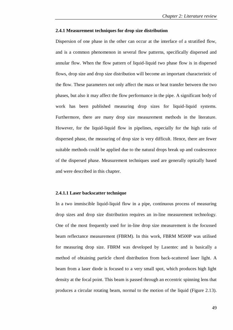
Chapter 2: Literature review
49
2.4.1 Measurement techniques for drop size distribution
Dispersion of one phase in the other can occur at the interface of a stratified flow,
and is a common phenomenon in several flow patterns, specifically dispersed and
annular flow. When the flow pattern of liquid-liquid two phase flow is in dispersed
flows, drop size and drop size distribution will become an important characteristic of
the flow. These parameters not only affect the mass or heat transfer between the two
phases, but also it may affect the flow performance in the pipe. A significant body of
work has been published measuring drop sizes for liquid-liquid systems.
Furthermore, there are many drop size measurement methods in the literature.
However, for the liquid-liquid flow in pipelines, especially for the high ratio of
dispersed phase, the measuring of drop size is very difficult. Hence, there are fewer
suitable methods could be applied due to the natural drops break up and coalescence
of the dispersed phase. Measurement techniques used are generally optically based
and were described in this chapter.
2.4.1.1 Laser backscatter technique
In a two immiscible liquid-liquid flow in a pipe, continuous process of measuring
drop sizes and drop size distribution requires an in-line measurement technology.
One of the most frequently used for in-line drop size measurement is the focussed
beam reflectance measurement (FBRM). In this work, FBRM M500P was utilised
for measuring drop size. FBRM was developed by Lasentec and is basically a
method of obtaining particle chord distribution from back-scattered laser light. A
beam from a laser diode is focused to a very small spot, which produces high light
density at the focal point. This beam is passed through an eccentric spinning lens that
produces a circular rotating beam, normal to the motion of the liquid (Figure 2.13).
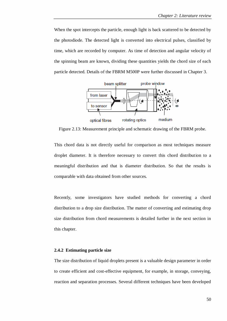
Chapter 2: Literature review
50
When the spot intercepts the particle, enough light is back scattered to be detected by
the photodiode. The detected light is converted into electrical pulses, classified by
time, which are recorded by computer. As time of detection and angular velocity of
the spinning beam are known, dividing these quantities yields the chord size of each
particle detected. Details of the FBRM M500P were further discussed in Chapter 3.
Figure 2.13: Measurement principle and schematic drawing of the FBRM probe.
This chord data is not directly useful for comparison as most techniques measure
droplet diameter. It is therefore necessary to convert this chord distribution to a
meaningful distribution and that is diameter distribution. So that the results is
comparable with data obtained from other sources.
Recently, some investigators have studied methods for converting a chord
distribution to a drop size distribution. The matter of converting and estimating drop
size distribution from chord measurements is detailed further in the next section in
this chapter.
2.4.2 Estimating particle size
The size distribution of liquid droplets present is a valuable design parameter in order
to create efficient and cost-effective equipment, for example, in storage, conveying,
reaction and separation processes. Several different techniques have been developed

Chapter 2: Literature review
51
by many researchers to obtain such particle size data. Examples of methods, which
have been applied to gas–liquid and liquid–liquid systems, are photography,
conductivity probes and droplet encapsulation. An advantage of the majority of the
techniques that have been employed is that the droplet diameter distribution is
measured directly or can be obtained by simple analysis. However, these methods
can only obtain useful data from dilute systems whereas within the oil industry,
concentrated oil–water dispersions frequently occur. Hence, it is necessary to
measure drop sizes for such systems. Therefore, FBRM M500P instrument,
developed by Lasentec, is one of very few techniques suitable for this task. However,
the FBRM produces distributions of droplet chord lengths (CLD) whereas most other
techniques produce diameter distributions directly. It is therefore necessary to
process the CLD to give diameter distributions so that the present data could be
compared with data obtained from other sources. The process of transformation from
CLD to diameter distribution is known as estimating particle size.
As chord length is neither directly useful nor unique even for a perfectly spherical
particle, though spheres can be uniquely defined by the diameter. Herringe and Davis
(1976) and Clark and Turton (1988) presented probabilistic techniques to solve this
problem. However, the output is very dependent upon the shape of the particles and
can suffer problems with very irregular distributions.
Consequently, Liu and Clark (1995) further revised the works by Clark and Turton
(1988) and considered that the bubble sizes are represented in two geometric shapes,
i.e. an ellipsoidal shape and a truncated ellipsoidal shape. In these cases, they found
Chapter 2: Literature review
52
that the means and standard deviations of chord lengths and bubble sizes are related
but are not dependent on the nature of their distributions.
In 1991 Hobbel et al., described a method of calculating diameter distribution from
chord measurements assuming random sphere cuts. In this circumstance, the largest
chord size is assumed to be the largest diameter and the chord distribution from this
diameter is subtracted from the total chord size distribution. This is basically a
„peeling method‟ and it should be noted that this method was successively only for
smaller diameters. Conversely, this method is too sensitive to “noise” in the
population of the largest sizes.
Meanwhile, Liu et al. (1998) have considered the probability relationships in
obtaining representative overall bubble size distribution by inferring the bubble size
density from local chord measurements in a heterogeneous bubbling system. They
showed that the accuracy of information transformed by a numerical approach using
Monte-Carlo simulation was increased as the number of partitions in the bubble size
range increased.
In order to create an ideal chord size distribution from a known particle diameter
distribution, Simmons et al. (1999) emphasized that it is necessary to make some
assumptions. For spherical particle in dilute systems, where there are no interactions
between particles, the probability of the beam taking a cut through any part of the
projected area of the sphere is equal. Thus, probability apportioning method (PAM)
described a method of calculating diameter distribution from chord randomly sphere
cuts measurements using equation 2.4. This method assumes the diameter bands are

Chapter 2: Literature review
53
known, where P{x1, x2} is the probability of obtaining a chord size between x1 and x2
for a sphere of diameter D.
D
xDxDxxP
2
2
22
1
2
21, 2.4
Hence for a known diameter distribution, range of chord lengths for each diameter
band can be calculated using equation 2.4. Full details of the derivation of equation
2.4 are shown in Simmons et al (1999) and Langston et al. (2001).
Unfortunately, PAM was inaccurate and has shown poor results for unknown
diameters distributions because it did not use the collective information from the data
set. Therefore, Langston et al. (2001) revised this method; which they incorporated
the Bayes‟ theorem (Equation 2.5) for combining conditional probabilities and
included an iterative procedure that can approach the true diameter distribution. This
revised method was named probability apportioning method version 2.0 (PAM2).
N
k
kk
iii
APABP
APABPBAP
1
)()/(
)()/()/( Ni ,...,2,1 2.5
Even though, Hasan (2006) found that the results of the transformation of chord
lengths using PAM2 were shown unsatisfactorily. In this present work the
computational coding for the PAM2 has been updated and upgraded (see Appendix
2B), allowing the measured chord length distribution to be transformed into a drop
size distribution successively. Since PAM2 (newer version – version 2.1) methods
were found to successfully convert a chord length distribution to a drop diameter
distribution, the latter were then analysed further to obtain Sauter mean diameter
(SMD). This SMD of the drop diameter distribution were then used in the results,
discussion and comparisons between different conditions.
Chapter 2: Literature review
54
2.5 Oil volume fraction
In most of process and industrial plants, pipeline is universally used as transportation
of their raw material and products from one place to the other. Pipelines are generally
the safest, most efficient and most economical way to transport large quantities of
these material or products. In petroleum industry for instance, increased of offshore
oil and gas exploration have resulted in transportation of well fluids in pipelines over
relatively long distances. Often the fluid delivered by the wells contains water, which
is already present within the stratum. Over period of time, maturing oil wells produce
more and more amount of free water, due to naturally presence of water in the old
wells or injection of water into the wells for a better oil exploration. The presence
and amount of free water phase in contact with pipe wall could cause corrosion and
in some cases, blockage in the pipe. Wicks et al (1975) found that corrosion in
pipelines was usually dominant in areas where the possible accumulation of water in
the pipe.
Recently, researchers have come up with an important method to curb this corrosion
problem, by introducing corrosion inhibitors. However, the effectiveness of the
inhibitors depends on the pipeline material, the inhibitor composition and the type of
flow (Vedapuri, 1999). Therefore, it is necessary to introduce the inhibitor into the
appropriate phase that in contact with the pipe wall. This can be accomplished only if
the flow pattern and the phase distributions under different conditions are known.
Therefore, optimisation of pipeline operations for transport of these fluids requires
the knowledge of the several parameters. One of the major parameters is the
knowledge of the volume ratio of each phase over the total volume also known as
volume fraction.
Chapter 2: Literature review
55
Oil volume fraction (OVF) is a dimensionless quantity that varies from 0 to 1, or is
sometimes expressed as a percentage between 0 - 100%, which indicates of a
geometry or temporal domain occupied by the oil in a two-phase oil-water flow.
There are many typical methods of measurement for oil volume fraction, including
irradiation methods (x-ray and γ-ray), quick-closing valve (QCV) method, ultrasonic
method and electrical methods (electrical tomography and conductance probe).
Besides, there are some other methods, such as optical probe method, observation
method, etc.
In industrial applications, the studies that include imaging of phase distribution in
process pipelines have becoming important. Process imaging techniques allow us to
investigate inside complex structures such as the oil volume fraction of liquid-liquid
mixtures. Today, a number of techniques to measure the dispersed phase volume
fraction or hold-up have been attempted. These techniques employed non-intrusive
or intrusive measurement sensors. Examples of some non-intrusive techniques are x-
ray tomography, gamma-densitometry tomography, ultrasonic system, electrical
capacitance tomography, electrical resistance tomography and impedance
tomography. While, for intrusive measurement sensors such as needle-contact probe
and parallel wire probe, are also popular. However, in the recent years, much
attention has been focused to a newly developed intrusive method namely the wire-
mesh sensor (WMS) method.
Vigneaux et al. (1988) reported results of systematic volume fraction profile
measurements obtained using a local high-frequency probe in vertically inclined pipe
orientation (0o to 65
o) of a liquid-liquid flow. High frequency impedance probe was
Chapter 2: Literature review
56
used to measure mean water volume fraction because of large dielectric constant
contras between the two liquids used. The effect of pipe orientation with water flow
rate fraction ranging from 30 to 100% and mean velocity between 0.027 and 0.35
m/s was investigated. They demonstrated that the input oil fraction was dependent on
the mean volume composition of mixture and the deviation angle but was minimally
affected by the total flow rate (in the range studied).
Two different measurement techniques, a high frequency probe (impedance probe)
and a gamma densitometer system were applied by Soleimani et al. (1999a) for
measuring volume fraction distribution across the tube. Interestingly, the results of
the oil volume fraction from the two systems showed an agreement for all mixture
velocities used in the range studied. The results exhibited that oil encapsulation by
water, especially at low mixture velocity. This phenomenon could probably be
explained the wetting of the surface, viscous instability and waves spreading in the
water layer due to a high shear stress from the oil layer. In the meantime, in the
dispersed flow regime (high mixture velocity) oil droplets were concentrated at the
centre of the tube. Thus, they suggested that three mechanisms are responsible for
droplet rearrangement in the turbulent dispersed flow regime; the droplets had the
same diffusivity as the continuous phase, the lift force in the boundary layer pushed
the droplets towards the core region and the distribution of droplets was influenced
by gravity.
Oddie et al (2003) measured water holdup in two- and three-phase flows using 3
different methods which were quick-closing valve (QCV), electrical conductivity
probe and gamma densitometer. The effects of the flow rates of the different phases
Chapter 2: Literature review
57
and pipe deviation on holdup were evaluated. They concluded that deviation angle
had minimum effect to the hold-up at higher oil-water flow rates and the opposite
was true for the very flow rates. They also found that steady-state holdups from
nuclear measurements were in reasonably close agreement with QCV‟s
measurements. However as for probe data, even though can provide transient and
steady-state holdup profiles along the length of the pipe, the accuracy of the probes
was not as high as that of the nuclear densitometer or QCV measurements (Oddie et
al., 2003).Further, they concluded that deviation angle had minimum effect to the
hold-up at higher oil-water flow rates and the opposite was true for the very flow
rates.
In the meantime, Yang (2003) used a direct observation method to study the spatial
distribution of oil-water flow in a downstream expansion pipe for mixture velocities
of 0.2, 0.3 & 0.4 m/s for water cut of 30, 50 & 80%, and horizontal and small
inclination angles of 7o. The results demonstrated that the stratifying liquid-liquid
flow is most rapidly obtained for a horizontal pipe, lower downstream velocities and
higher water cuts. However, the water phase is entirely dominating at downstream
expansion for the same configurations but with high mixture velocities. In general,
Yang (2003) concludes that horizontal is the best pipe position for a dispersed flow
to evolve quickly to a segregated flow through the sudden expansion within a short
distance. Both, upward and downward inclinations tend to increase the mixed layer
and slow down the evolution process.
A spatial distribution of dual continuous liquid-liquid flow has been studied by
Lovick and Angeli (2004a) using an impedance probe. The comparison of average
Chapter 2: Literature review
58
oil volume fraction between the impedance probe and the use of quick closing valves
(QCVs) was obtained at less than 5.8% for all conditions. Moreover, the velocity
ratio increased during dual continuous flow to above 1 as the oil input fraction
increased. At high input oil fractions, however, the velocity ratio decreased again to
values below 1 as the mixture velocity increased. These could possibly be explained
by the change of interface shape and thus interestingly if the cross section of this
shape can be real-time imaged.
Subsequently, Liu (2005) used the same pipe test section as initially described by
Yang et al. (2003), but employed the sampling method to measure the oil volume
fraction across the section of pipe at middle expansion. The mixture velocities and
input oil fractions are also the same as the ones applied by Yang‟s. Liu‟s results
confirmed the phase profiles by Yang‟s at downstream expansion. Furthermore, the
dispersed flow actually dominated over a pipe cross-section at downstream
expansion for low input oil fractions and high mixture velocities which was not been
mentioned by Yang et al. (2003).
Meanwhile, Lum et al. (2006) investigated the phase distribution of oil-water flow at
±5o (from horizontal) and horizontal flow using similar liquid-liquid flow rig,
mixture velocities and oil volume fractions to Lovick and Angeli (2004a). The results
of phase distribution in a pipe cross-section showed that the convex interface shapes
were obtained in downward flow at a high input oil fraction and high mixture
velocity, whereas the shape of interface is replaced by concave interface shape at low
mixture velocity even though high input oil fraction is applied. It is clearly showed
that the mixture velocity plays a major role in determining the shape of interface in a
Chapter 2: Literature review
59
pipe cross-section for downward flow. Meanwhile, the shape obtained in an upward
flow is similar to those in a horizontal flow as concluded by other investigators
(Soleimani et al., 1999a; Angeli and Hewitt, 2000b; Lovick and Angeli, 2004a).
In 2006, Hasan used electrical capacitance tomography (ECT) method to study the
spatial distribution of oil-water flow, downstream of an expansion pipe. In this
technique, the continuous measurement of dispersed phase volume fraction exploits
the differences in electrical permittivity of the two liquid phases to obtain images
(Xie et al., 1995; Williams and Beck, 1995; Reinecke and Mewes, 1996; Dyakowski,
1996 and Isaksen, 1996). The effect of pipe orientation (horizontal and small
inclination angles of 7o) with input oil fraction of 20, 50, & 70% and mixture
velocities 0.2, 0.3 and 0.4 m/s was investigated. Hasan (2006) proclaimed that the
obtained results clearly indicate the images are satisfactorily agreed well with two
methods (Yang, 2003 and Liu, 2005) and could then be used to substantiate the flow
patterns as predicted in the Trallero map. The results of phase distribution in the pipe
cross-section showed that the concave interfaces were present for horizontal and
downward flow, whereas convex interfaces were observed only for upward
inclination flow at high input oil fraction and mixture velocity.
Most recently, new technology to generate images of the phase fraction distribution
and investigate the flow of fluids in a pipe called Wire Mesh Sensor (WMS) has been
developed. The wire-mesh sensor is an intrusive imaging device which provides flow
images at high spatial and temporal resolutions (Da Silva et al., 2010) and it has been
accepted as an alternative technique for multiphase flow tomographic imaging. The
use of tomographic imaging for the investigation of two-phase flows has been

Chapter 2: Literature review
60
reported in a few review papers (Chaouki et al., 1997, Prasser, 2008, Mudde, 2010)
and a book (Williams and Beck, 1995).There are two variants of the WMS, which
are conductance and capacitance WMS, often abbreviated in this thesis as
CondWMS/ CapWMS.
A wire-mesh sensor for measuring the volumetric fraction of water in crude oil was
first described by Johnson (1987). This consisted of a crude device that had two
planes of wire grids are placed into the flow in a short distance from each other.
However, sensor developed by Johnson (1987) contained no imaging capability.
A wire-mesh device that performs tomographic imaging was presented by Reinecke
et al. (1996), who proposed a three plane sensor of 29 thin wires each of 0.1 mm
diameter. However, the sensor had several limitations and the main disadvantage is
that the transformation into the image has to be performed by applying tomographic
image reconstruction algorithms (Prasser et al, 1988).
Further development of the WMS was made by Prasser et al. (1988). He developed a
two plane conductivity (conductance) wire mesh sensor which is a fast tomographic
imaging without the need of time consuming and inaccurate image reconstruction
procedures. Further, special emphasis was given to a stable sensor design for hostile
conditions in industrial facilities.
Up till now, conductance wire-mesh sensors have been applied in many gas-liquid
flows (Prasser 2008, Da Silva et al., 2010, Szalinski et al., 2010). However, with
increased of interest in two-phase liquid–liquid flows, mostly from the petroleum

Chapter 2: Literature review
61
industry where, for instance, oil (non-conducting) and water are often produced and
transported together. The conductive WMS could not be used in such applications.
Therefore, a new WMS was developed by Da Silva et al. (2007) based on the
measurement of the electrical permittivity (capacitance), to extend the sensor‟s
capabilities to the detection of the non-conducting fluids.
In this thesis focused are on CapWMS since working fluids are oil and water. Great
details of the principle and application of CapWMS in determine the volume fraction
of multiphase system of two immiscible liquids is discussed in Chapter 3.

Chapter 3: Instruments and experimental methods
62
CHAPTER 3
INSTRUMENTS AND EXPERIMENTAL METHODS
The literature review in the previous chapter gave an overview of published research
related to liquid-liquid flow. The focus of most studies were on drop size
distribution, oil volume fraction and flow pattern, especially studies or research
conducted in stirred vessels, mixing tanks and pipes. Furthermore, most of these
studies were limited to liquid-liquid flow in either horizontal or vertical straight pipe.
Up to date, there is no previous studies have had significant data pertinent to the
current work which concentrates on sudden expansions.
This chapter discusses the apparatus and methodology used to perform experiments
on liquid-liquid flow through a sudden expansion in a pipe. A liquid-liquid flow
facility has been built for the purpose of these studies. The physical properties of the
system, the criteria of experimental design and the operational principle of each
instrument are explained. The experimental processes of drop size measurements and
determination of phase layer evolution completed on the flow facility were discussed
briefly in Chapter 2.
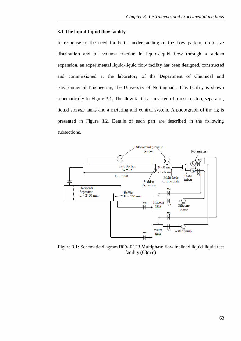
Chapter 3: Instruments and experimental methods
63
3.1 The liquid-liquid flow facility
In response to the need for better understanding of the flow pattern, drop size
distribution and oil volume fraction in liquid-liquid flow through a sudden
expansion, an experimental liquid-liquid flow facility has been designed, constructed
and commissioned at the laboratory of the Department of Chemical and
Environmental Engineering, the University of Nottingham. This facility is shown
schematically in Figure 3.1. The flow facility consisted of a test section, separator,
liquid storage tanks and a metering and control system. A photograph of the rig is
presented in Figure 3.2. Details of each part are described in the following
subsections.
Figure 3.1: Schematic diagram B09/ R123 Multiphase flow inclined liquid-liquid test
facility (68mm)
Rotameters
Dp Dp
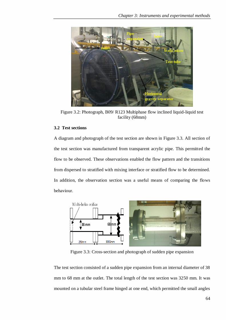
Chapter 3: Instruments and experimental methods
64
Figure 3.2: Photograph, B09/ R123 Multiphase flow inclined liquid-liquid test
facility (68mm)
3.2 Test sections
A diagram and photograph of the test section are shown in Figure 3.3. All section of
the test section was manufactured from transparent acrylic pipe. This permitted the
flow to be observed. These observations enabled the flow pattern and the transitions
from dispersed to stratified with mixing interface or stratified flow to be determined.
In addition, the observation section was a useful means of comparing the flows
behaviour.
Figure 3.3: Cross-section and photograph of sudden pipe expansion
The test section consisted of a sudden pipe expansion from an internal diameter of 38
mm to 68 mm at the outlet. The total length of the test section was 3250 mm. It was
mounted on a tubular steel frame hinged at one end, which permitted the small angles
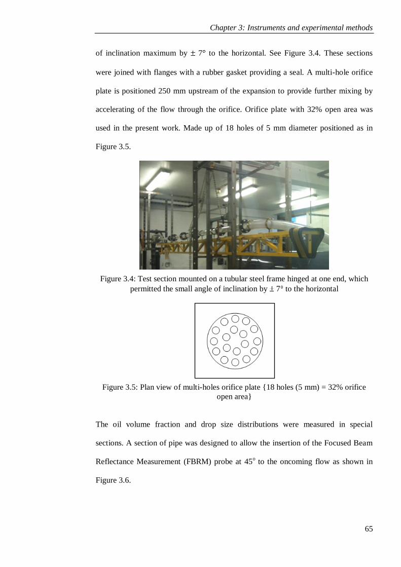
Chapter 3: Instruments and experimental methods
65
of inclination maximum by 7 to the horizontal. See Figure 3.4. These sections
were joined with flanges with a rubber gasket providing a seal. A multi-hole orifice
plate is positioned 250 mm upstream of the expansion to provide further mixing by
accelerating of the flow through the orifice. Orifice plate with 32% open area was
used in the present work. Made up of 18 holes of 5 mm diameter positioned as in
Figure 3.5.
Figure 3.4: Test section mounted on a tubular steel frame hinged at one end, which
permitted the small angle of inclination by 7 to the horizontal
Figure 3.5: Plan view of multi-holes orifice plate {18 holes (5 mm) = 32% orifice
open area}
The oil volume fraction and drop size distributions were measured in special
sections. A section of pipe was designed to allow the insertion of the Focused Beam
Reflectance Measurement (FBRM) probe at 45o to the oncoming flow as shown in
Figure 3.6.
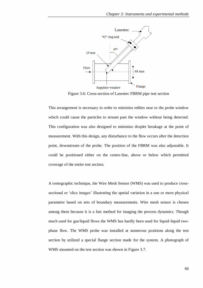
Chapter 3: Instruments and experimental methods
66
Figure 3.6: Cross-section of Lasentec FBRM pipe test section
This arrangement is necessary in order to minimise eddies near to the probe window
which could cause the particles to stream past the window without being detected.
This configuration was also designed to minimise droplet breakage at the point of
measurement. With this design, any disturbance to the flow occurs after the detection
point, downstream of the probe. The position of the FBRM was also adjustable. It
could be positioned either on the centre-line, above or below which permitted
coverage of the entire test section.
A tomographic technique, the Wire Mesh Sensor (WMS) was used to produce cross-
sectional or „slice images‟ illustrating the spatial variation in a one or more physical
parameter based on sets of boundary measurements. Wire mesh sensor is chosen
among them because it is a fast method for imaging the process dynamics. Though
much used for gas/liquid flows the WMS has hardly been used for liquid-liquid two-
phase flow. The WMS probe was installed at numerous positions along the test
section by utilized a special flange section made for the system. A photograph of
WMS mounted on the test section was shown in Figure 3.7.
Lasentec
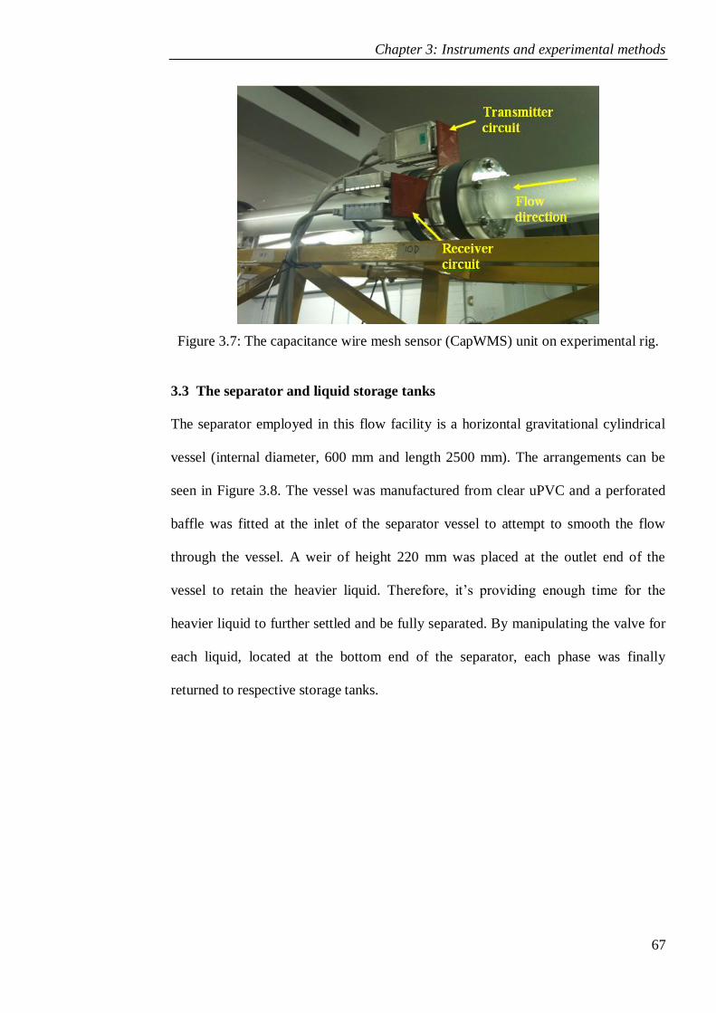
Chapter 3: Instruments and experimental methods
67
Figure 3.7: The capacitance wire mesh sensor (CapWMS) unit on experimental rig.
3.3 The separator and liquid storage tanks
The separator employed in this flow facility is a horizontal gravitational cylindrical
vessel (internal diameter, 600 mm and length 2500 mm). The arrangements can be
seen in Figure 3.8. The vessel was manufactured from clear uPVC and a perforated
baffle was fitted at the inlet of the separator vessel to attempt to smooth the flow
through the vessel. A weir of height 220 mm was placed at the outlet end of the
vessel to retain the heavier liquid. Therefore, it‟s providing enough time for the
heavier liquid to further settled and be fully separated. By manipulating the valve for
each liquid, located at the bottom end of the separator, each phase was finally
returned to respective storage tanks.
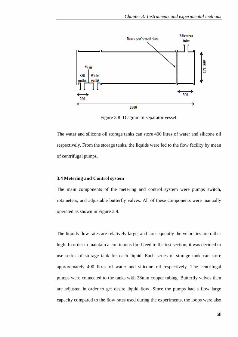
Chapter 3: Instruments and experimental methods
68
Figure 3.8: Diagram of separator vessel.
The water and silicone oil storage tanks can store 400 litres of water and silicone oil
respectively. From the storage tanks, the liquids were fed to the flow facility by mean
of centrifugal pumps.
3.4 Metering and Control system
The main components of the metering and control system were pumps switch,
rotameters, and adjustable butterfly valves. All of these components were manually
operated as shown in Figure 3.9.
The liquids flow rates are relatively large, and consequently the velocities are rather
high. In order to maintain a continuous fluid feed to the test section, it was decided to
use series of storage tank for each liquid. Each series of storage tank can store
approximately 400 litres of water and silicone oil respectively. The centrifugal
pumps were connected to the tanks with 28mm copper tubing. Butterfly valves then
are adjusted in order to get desire liquid flow. Since the pumps had a flow large
capacity compared to the flow rates used during the experiments, the loops were also
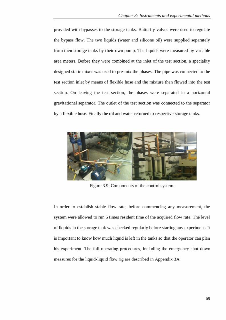
Chapter 3: Instruments and experimental methods
69
provided with bypasses to the storage tanks. Butterfly valves were used to regulate
the bypass flow. The two liquids (water and silicone oil) were supplied separately
from then storage tanks by their own pump. The liquids were measured by variable
area meters. Before they were combined at the inlet of the test section, a speciality
designed static mixer was used to pre-mix the phases. The pipe was connected to the
test section inlet by means of flexible hose and the mixture then flowed into the test
section. On leaving the test section, the phases were separated in a horizontal
gravitational separator. The outlet of the test section was connected to the separator
by a flexible hose. Finally the oil and water returned to respective storage tanks.
Figure 3.9: Components of the control system.
In order to establish stable flow rate, before commencing any measurement, the
system were allowed to run 5 times resident time of the acquired flow rate. The level
of liquids in the storage tank was checked regularly before starting any experiment. It
is important to know how much liquid is left in the tanks so that the operator can plan
his experiment. The full operating procedures, including the emergency shut-down
measures for the liquid-liquid flow rig are described in Appendix 3A.
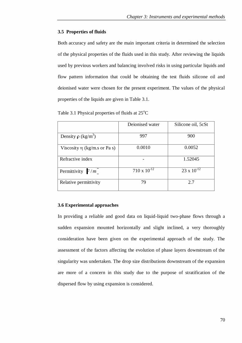
Chapter 3: Instruments and experimental methods
70
3.5 Properties of fluids
Both accuracy and safety are the main important criteria in determined the selection
of the physical properties of the fluids used in this study. After reviewing the liquids
used by previous workers and balancing involved risks in using particular liquids and
flow pattern information that could be obtaining the test fluids silicone oil and
deionised water were chosen for the present experiment. The values of the physical
properties of the liquids are given in Table 3.1.
Table 3.1 Physical properties of fluids at 25oC
Deionised water Silicone oil, 5cSt
Density (kg/m3) 997 900
Viscosity (kg/m.s or Pa s) 0.0010 0.0052
Refractive index - 1.52045
Permittivity mF / 710 x 10-12
23 x 10-12
Relative permittivity 79 2.7
3.6 Experimental approaches
In providing a reliable and good data on liquid-liquid two-phase flows through a
sudden expansion mounted horizontally and slight inclined, a very thoroughly
consideration have been given on the experimental approach of the study. The
assessment of the factors affecting the evolution of phase layers downstream of the
singularity was undertaken. The drop size distributions downstream of the expansion
are more of a concern in this study due to the purpose of stratification of the
dispersed flow by using expansion is considered.
Chapter 3: Instruments and experimental methods
71
There are two categories of factors affecting the evolution of drop size distribution
through a sudden expansion, these which are linked to the rig configuration and
others which are limited to the operational conditions.
Factors that are related to the rig configuration could be divided into three areas,
which are the pipe orientation, the expansion ratio (the ratio of downstream to
upstream pipe cross-sectional area) and the pipe lengths of both the upstream and
downstream sections. Studies of the drop size distribution in horizontal pipes have
been published by many researchers (Sleicher 1962; Ward and Knudsen, 1967;
Collins and Knudsen, 1970; Swartz and Kessler, 1970; Kubie and Gardner, 1977;
Karabelas, 1978; Simmons et al., 1998; Angeli and Hewitt, 2000a; Angeli, 2001;
Lovick and Angeli, 2004b). Almost all of these were for horizontal pipe. Only Lum
et al. (2002; 2004; 2006) has reported the effect of upward or downward pipe
inclination. Today, there has not many reports on the literature about the drop size
distribution evolution through a sudden expansion for liquid-liquid flow and it is still
left unsolved.
As for the operational conditions criteria, two factors have been identified. These are
input oil fraction and mixture velocity for a given working system. In order to
explore the transition of drop size distribution from the dispersed to the segregated
flow through the expansion, the experiments were designed to distribute the
dispersed regimes in the inlet of test section and expected stratified flow or stratified
flow with mixing at the interface after expansion.
Chapter 3: Instruments and experimental methods
72
The mixture orifice velocity (Usmo) is a mixture velocity in the small diameter pipe
(38 mm) after the perforated orifice. The downstream velocity is a mixture velocity
based on the cross-sectional area of the larger diameter pipe (68 mm). The angle of
inclination is the angle between the flow direction and the horizontal. A positive
angle is an upward inclination and a negative angle a downward inclination. The
range of the inclinations that are worth studying has been determined from
calculations of the fully developed stratified flow using the model Taitel and Dukler
(1976). The same prediction model was applied in Yang (2003) and Hasan (2006),
and it gave a prediction of the position of the aqueous/ oil interface and has been
shown to give an accurate prediction for horizontal flows. The result showed the
effect of the angle of inclination which had a significant change over 2o from
horizontal and become quite small beyond 6o (Taitel and Dukler, 1976).
A multi-hole orifice plate was used in order to produce the dispersed flow in the
upstream pipe. The results of El-Hamouz et al. (1995) were used to estimate the
drops expected. Their results showed that drop sizes increased by 20% when
measured at 7 pipe diameters downstream and 40% at 38 pipe diameters downstream
of a needle valve. The current study of sudden expansion was 7 pipe diameters
downstream of a multi-hole perforated plate; therefore, it was expected that the drop
sizes arriving at the sudden expansion would be those created by the perforated plate.
The choice of input oil fraction had been considered in a work by Shi et al. (2001)
who studied the distribution of phases and velocity profile at the end of a 100 mm
internal diameter pipe, 18 m long. They found that separation of oil/water flow was
only possible for mixture velocities below 0.75 m/s and for input oil fraction between

Chapter 3: Instruments and experimental methods
73
20 to 80%. Furthermore, an input oil fraction of 60 to 70% was considered as water
dispersed in an oil regime and below 50% was described as oil dispersed in a water
regime. According to the flow pattern maps of Trallero et al. (1997), stratified flow
occurs at velocities in which the order of magnitude is higher than those at the upper
limit laminar flow. The limit of stratified flow was then considered as mixture
velocity wherein this velocity is 0.2 m/s, and x1.5 and x2 higher. Their results had a
good agreement with Shi et al. (2001). Based on these facts, the downstream mixture
velocities chosen were 0.20 m/s, 0.30 m/s and 0.35 m/s which are x1, x1.5 and x1.75
higher.
In order to understand drop size evolution downstream of a sudden expansion, three
positions of drop size measurement in a pipe cross-section were selected and images
of phase distributions from WMS measurements were captured at number of
downstream location. Details were discussed in subsection 4.2 and 6.2 (Experimental
design) of chapters 4 and 6. A similar position of drop size measurement was also
used by Simmons (1998) in dispersed flow and his results indicated that there was
little effect in the size measured at these positions. Another reason for choosing these
measurement positions relates to the interface profiles observed by Yang et al.
(2003) in which they suggested making investigations between 2 and 35 pipe
diameter downstream of the expansion, particularly at the interface between the
mixed region and the oil or water region.
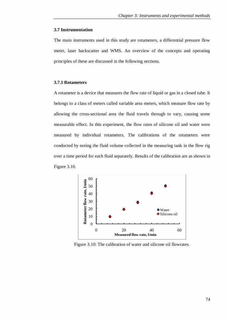
Chapter 3: Instruments and experimental methods
74
3.7 Instrumentation
The main instruments used in this study are rotameters, a differential pressure flow
meter, laser backscatter and WMS. An overview of the concepts and operating
principles of these are discussed in the following sections.
3.7.1 Rotameters
A rotameter is a device that measures the flow rate of liquid or gas in a closed tube. It
belongs to a class of meters called variable area meters, which measure flow rate by
allowing the cross-sectional area the fluid travels through to vary, causing some
measurable effect. In this experiment, the flow rates of silicone oil and water were
measured by individual rotameters. The calibrations of the rotameters were
conducted by noting the fluid volume collected in the measuring tank in the flow rig
over a time period for each fluid separately. Results of the calibration are as shown in
Figure 3.10.
Figure 3.10: The calibration of water and silicone oil flowrates.
0
10
20
30
40
50
60
0 20 40 60
Rota
mete
r flo
w r
ate
, l/
min
Measured flow rate, l/min
WaterSilicone oil
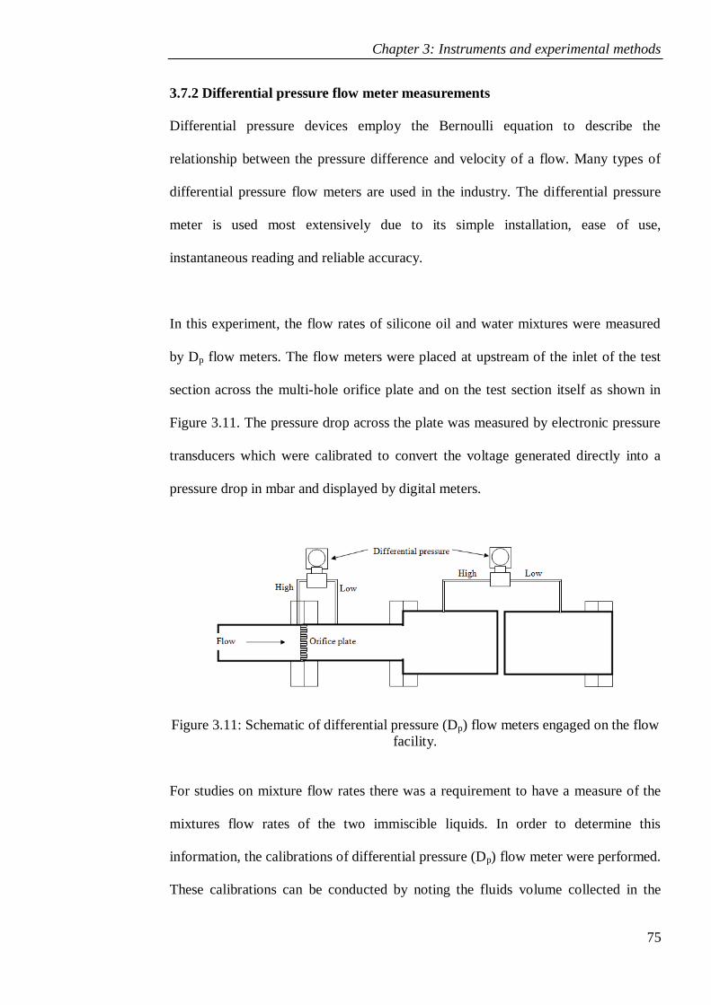
Chapter 3: Instruments and experimental methods
75
3.7.2 Differential pressure flow meter measurements
Differential pressure devices employ the Bernoulli equation to describe the
relationship between the pressure difference and velocity of a flow. Many types of
differential pressure flow meters are used in the industry. The differential pressure
meter is used most extensively due to its simple installation, ease of use,
instantaneous reading and reliable accuracy.
In this experiment, the flow rates of silicone oil and water mixtures were measured
by Dp flow meters. The flow meters were placed at upstream of the inlet of the test
section across the multi-hole orifice plate and on the test section itself as shown in
Figure 3.11. The pressure drop across the plate was measured by electronic pressure
transducers which were calibrated to convert the voltage generated directly into a
pressure drop in mbar and displayed by digital meters.
Figure 3.11: Schematic of differential pressure (Dp) flow meters engaged on the flow
facility.
For studies on mixture flow rates there was a requirement to have a measure of the
mixtures flow rates of the two immiscible liquids. In order to determine this
information, the calibrations of differential pressure (Dp) flow meter were performed.
These calibrations can be conducted by noting the fluids volume collected in the
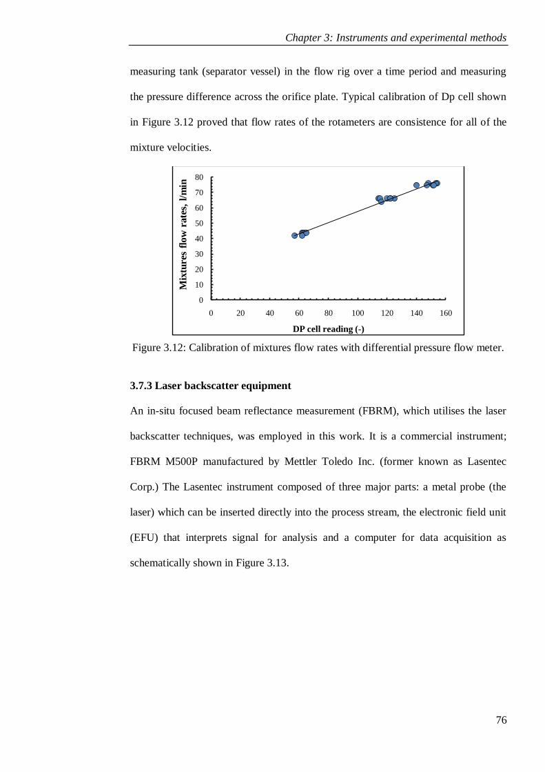
Chapter 3: Instruments and experimental methods
76
measuring tank (separator vessel) in the flow rig over a time period and measuring
the pressure difference across the orifice plate. Typical calibration of Dp cell shown
in Figure 3.12 proved that flow rates of the rotameters are consistence for all of the
mixture velocities.
Figure 3.12: Calibration of mixtures flow rates with differential pressure flow meter.
3.7.3 Laser backscatter equipment
An in-situ focused beam reflectance measurement (FBRM), which utilises the laser
backscatter techniques, was employed in this work. It is a commercial instrument;
FBRM M500P manufactured by Mettler Toledo Inc. (former known as Lasentec
Corp.) The Lasentec instrument composed of three major parts: a metal probe (the
laser) which can be inserted directly into the process stream, the electronic field unit
(EFU) that interprets signal for analysis and a computer for data acquisition as
schematically shown in Figure 3.13.
0
10
20
30
40
50
60
70
80
0 20 40 60 80 100 120 140 160
Mix
ture
s fl
ow
rate
s, l
/min
DP cell reading (-)
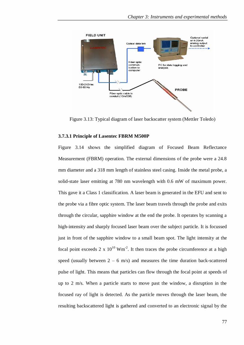
Chapter 3: Instruments and experimental methods
77
Figure 3.13: Typical diagram of laser backscatter system (Mettler Toledo)
3.7.3.1 Principle of Lasentec FBRM M500P
Figure 3.14 shows the simplified diagram of Focused Beam Reflectance
Measurement (FBRM) operation. The external dimensions of the probe were a 24.8
mm diameter and a 318 mm length of stainless steel casing. Inside the metal probe, a
solid-state laser emitting at 780 nm wavelength with 0.6 mW of maximum power.
This gave it a Class 1 classification. A laser beam is generated in the EFU and sent to
the probe via a fibre optic system. The laser beam travels through the probe and exits
through the circular, sapphire window at the end the probe. It operates by scanning a
high-intensity and sharply focused laser beam over the subject particle. It is focussed
just in front of the sapphire window to a small beam spot. The light intensity at the
focal point exceeds 2 x 10¹⁰
Wm-2
. It then traces the probe circumference at a high
speed (usually between 2 – 6 m/s) and measures the time duration back-scattered
pulse of light. This means that particles can flow through the focal point at speeds of
up to 2 m/s. When a particle starts to move past the window, a disruption in the
focused ray of light is detected. As the particle moves through the laser beam, the
resulting backscattered light is gathered and converted to an electronic signal by the

Chapter 3: Instruments and experimental methods
78
EFU using a photo-detector which converts the light energy into an electric signal.
Right after the opposite edge of the particle is reached, the backscatter of light
ceases. A unique discrimination circuit is used to isolate the time period of the
backscatter from one edge of an individual particle to its opposite edge. The period
over which the backscatter signal was recorded is then multiplied by the scan speed.
The result is then converted as distance, hence giving the chord length (Lasentec,
2007). The duration and frequency of signals are indications of particle chord length
and counts, respectively. The chord length is defined as “a straight line between any
two points on the edge of a particle or particle structure” (Lasentec, 2007).
Figure 3.14: Focused Beam Reflectance Measurement, FBRM (Lasentec, 2007)
3.7.3.2 Verification of Lasentec FBRM M500P
As this study was confined to non-aggregated systems, only the F (fine) electronics
data were presented. The focal point at the time of purchase was set to few microns
(external face of the window) as calibrated by the manufacturer (Lasentec). As the
instrument was last used 2 years ago, it needs to be re-calibrated to maintain the
integrity of the FBRM. The focal point position of the FBRM device was re-
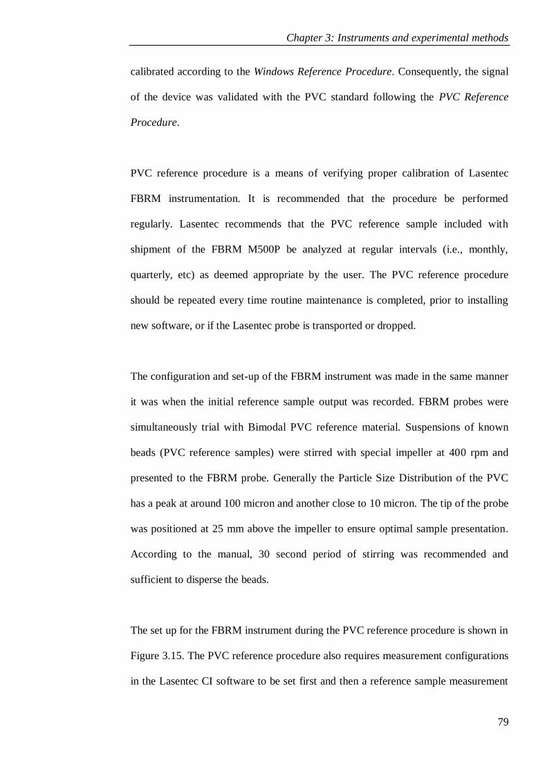
Chapter 3: Instruments and experimental methods
79
calibrated according to the Windows Reference Procedure. Consequently, the signal
of the device was validated with the PVC standard following the PVC Reference
Procedure.
PVC reference procedure is a means of verifying proper calibration of Lasentec
FBRM instrumentation. It is recommended that the procedure be performed
regularly. Lasentec recommends that the PVC reference sample included with
shipment of the FBRM M500P be analyzed at regular intervals (i.e., monthly,
quarterly, etc) as deemed appropriate by the user. The PVC reference procedure
should be repeated every time routine maintenance is completed, prior to installing
new software, or if the Lasentec probe is transported or dropped.
The configuration and set-up of the FBRM instrument was made in the same manner
it was when the initial reference sample output was recorded. FBRM probes were
simultaneously trial with Bimodal PVC reference material. Suspensions of known
beads (PVC reference samples) were stirred with special impeller at 400 rpm and
presented to the FBRM probe. Generally the Particle Size Distribution of the PVC
has a peak at around 100 micron and another close to 10 micron. The tip of the probe
was positioned at 25 mm above the impeller to ensure optimal sample presentation.
According to the manual, 30 second period of stirring was recommended and
sufficient to disperse the beads.
The set up for the FBRM instrument during the PVC reference procedure is shown in
Figure 3.15. The PVC reference procedure also requires measurement configurations
in the Lasentec CI software to be set first and then a reference sample measurement
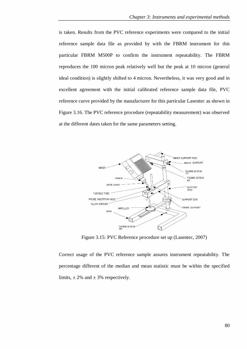
Chapter 3: Instruments and experimental methods
80
is taken. Results from the PVC reference experiments were compared to the initial
reference sample data file as provided by with the FBRM instrument for this
particular FBRM M500P to confirm the instrument repeatability. The FBRM
reproduces the 100 micron peak relatively well but the peak at 10 micron (general
ideal condition) is slightly shifted to 4 micron. Nevertheless, it was very good and in
excellent agreement with the initial calibrated reference sample data file, PVC
reference curve provided by the manafacturer for this particular Lasentec as shown in
Figure 3.16. The PVC reference procedure (repeatability measurement) was observed
at the different dates taken for the same parameters setting.
Figure 3.15: PVC Reference procedure set up (Lasentec, 2007)
Correct usage of the PVC reference sample assures instrument repeatability. The
percentage different of the median and mean statistic must be within the specified
limits, ± 2% and ± 3% respectively.
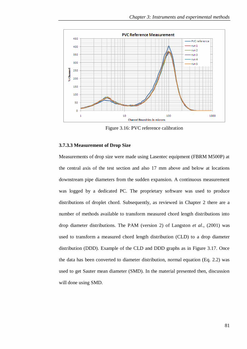
Chapter 3: Instruments and experimental methods
81
Figure 3.16: PVC reference calibration
3.7.3.3 Measurement of Drop Size
Measurements of drop size were made using Lasentec equipment (FBRM M500P) at
the central axis of the test section and also 17 mm above and below at locations
downstream pipe diameters from the sudden expansion. A continuous measurement
was logged by a dedicated PC. The proprietary software was used to produce
distributions of droplet chord. Subsequently, as reviewed in Chapter 2 there are a
number of methods available to transform measured chord length distributions into
drop diameter distributions. The PAM (version 2) of Langston et al., (2001) was
used to transform a measured chord length distribution (CLD) to a drop diameter
distribution (DDD). Example of the CLD and DDD graphs as in Figure 3.17. Once
the data has been converted to diameter distribution, normal equation (Eq. 2.2) was
used to get Sauter mean diameter (SMD). In the material presented then, discussion
will done using SMD.
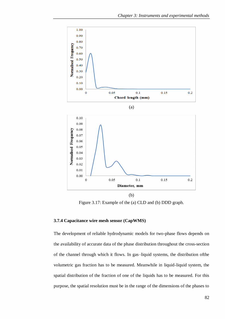
Chapter 3: Instruments and experimental methods
82
(a)
(b)
Figure 3.17: Example of the (a) CLD and (b) DDD graph.
3.7.4 Capacitance wire mesh sensor (CapWMS)
The development of reliable hydrodynamic models for two-phase flows depends on
the availability of accurate data of the phase distribution throughout the cross-section
of the channel through which it flows. In gas–liquid systems, the distribution ofthe
volumetric gas fraction has to be measured. Meanwhile in liquid-liquid system, the
spatial distribution of the fraction of one of the liquids has to be measured. For this
purpose, the spatial resolution must be in the range of the dimensions of the phases to

Chapter 3: Instruments and experimental methods
83
be detected. Further, the measuring volume must be well defined. Ideally, the
extension of a tomographic sensor in the direction perpendicular to the measuring
plane should be in the range of the spatial resolution. Last but not least, the
measuring time for one complete image must be very short, in order to make it
possible to measure instantaneous phase distributions.
Today gamma ray and X-ray computerized tomography were the widely used non-
intrusive methods. The spatial resolution achieved is in the range of millimetres. The
γ-ray tomograph developed by Kumar et al.(1995) and applied to a 260 mm diameter
bubble column provides a resolution of 5 mm. A good example of X-ray tomography
is given by Schmitz et al.(1997), who used a 360 kV X-ray source and 15 detectors
to achieve a resolution of 0.4 mm. In both cases, the projections needed for the image
reconstruction were produced by rotating either the sourcedetector assembly or the
object. The scanning time is in the range of several minutes and it is not possible to
measure instantaneous phase distributions.
An attempt to increase time resolution was carried out by Frøystein (1997), who uses
a non-rotating configuration with 5 sources and 5 arrays with 17 individual detectors
each. In this way, 5 projections are recorded simultaneously. The main factor
limiting the resolution of such a configuration is the low number of projections
available for the image reconstruction. This problem was solved by Hori et al. (1997)
by applying 66 X-ray tubes, the electron beam of which is controlled by grids. The
projections are produced in a successive order bygenerating short X-ray flashes. The
entire measuring procedure for one frame takes 0.5 ms, i.e. all X-ray tubes flash
within this period. The detector array consists of 584 CdTe crystals. Consequently,
Chapter 3: Instruments and experimental methods
84
66 independent projections are recorded within the measuring period of 0.5 ms. After
the image reconstruction, this results in 2000 frames per second with a resolution of
about 2 mm. These are by far the best results published up to now.
The main disadvantage of high-speed X-ray tomography is its high costs and also the
requirement for shielding. Unfortunately, the much less expensive methods of
electrical impedance tomography are not able to provide a comparable spatial
resolution for some of the principal reasons. This motivated Prasser et al.(1998) to
start the development of the electrode-mesh tomograph. The goal was to achieve a
similar high-speed visualisation of transient gas fraction distributions in pipelines
with a comparatively cheap device. The principle is based on the measurement of the
local instantaneous conductivity of the two-phase mixture. The time resolution is
1024 frames per second. The developed signal acquisition circuitry guarantees the
suppression of crosstalk between selected and non-selected electrodes. In this way
the highest possible spatial resolution is achieved,which is given by the pitch of the
electrodes. The sensor is available in two designs: (1) wire-mesh sensor for lab
applications and (2) sensor with enforced electrode rods for high mechanical loads.
The electrode rods of the second design are manufactured with a lentil shaped cross-
section in order to reduce pressure drop over the sensor.
Local time varying void fractions were obtained by using the WMS (conductivity)
measurement transducer. It is suitable for studies of transient two-phase flows, as
well as for the instrumentation of industrial plants. In those cases, when an intrusive
sensor is acceptable, the electrode-mesh sensor is an economic alternative to
expensive X-ray or γ-ray tomographs. The design of this sensor formed the basis for
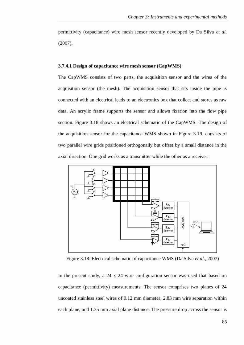
Chapter 3: Instruments and experimental methods
85
permittivity (capacitance) wire mesh sensor recently developed by Da Silva et al.
(2007).
3.7.4.1 Design of capacitance wire mesh sensor (CapWMS)
The CapWMS consists of two parts, the acquisition sensor and the wires of the
acquisition sensor (the mesh). The acquisition sensor that sits inside the pipe is
connected with an electrical leads to an electronics box that collect and stores as raw
data. An acrylic frame supports the sensor and allows fixation into the flow pipe
section. Figure 3.18 shows an electrical schematic of the CapWMS. The design of
the acquisition sensor for the capacitance WMS shown in Figure 3.19, consists of
two parallel wire grids positioned orthogonally but offset by a small distance in the
axial direction. One grid works as a transmitter while the other as a receiver.
Figure 3.18: Electrical schematic of capacitance WMS (Da Silva et al., 2007)
In the present study, a 24 x 24 wire configuration sensor was used that based on
capacitance (permittivity) measurements. The sensor comprises two planes of 24
uncoated stainless steel wires of 0.12 mm diameter, 2.83 mm wire separation within
each plane, and 1.35 mm axial plane distance. The pressure drop across the sensor is

Chapter 3: Instruments and experimental methods
86
small (approximately 3%), because the wires are evenly distributed over the circular
pipe cross-section and are widely spreads and only occupy 2-3% of the pipe cross-
section. Therefore, they will not obstruct or stop the flow. Since the square sensor is
installed in a circular pipe, only 440 of the total 576 wire crossing points are within
the radius of the pipe. The spatial resolution of the images generated by the sensor is
2.83 mm, which corresponds to the wire separation within a single plane. Though the
instrument can sample the entire cross-section at up to 5 kHz, data was acquired at a
frequency of 1 kHz as this gave sufficient temporal resolution.Trials showed that a
10 second sampling period gave sufficient data for temporal resolution.
Figure 3.19: Capacitance wire mesh sensor 24 x 24 (Left) Sketch of wire mesh
sensor (Right)
3.7.4.2 Principle of capacitance wire mesh sensor (CapWMS)
The principle of the sensor is based on two planes of wires, where one grid works as
a transmitter while the other as a receiver. By activating each wire successively, the
current at each crossing point is detected. During the measuring cycle, the transmitter
wires are activated in a successive order while all other wires are kept at the ground
potential. For each time frame, a transmitter wire is activated and all the receiver
Chapter 3: Instruments and experimental methods
87
wires are sampled in parallel (Da Silva et al, 2007a-c). Each crossing point of the
transmitter and receiver electrodes is scanned individually, generating a matrix in the
x-y plane depending on the size of the sensor. The local instantaneous void fractions
are calculated from the measured capacitance between crossing points, a series of 2
dimensional data sets can be obtained. By reconstructing these sets in time sequence,
a high speed visualization may be achieved.
3.7.4.3 Calibration and validation of CapWMS
As mentioned earlier in this chapter, this present work is the first attempt to adapt the
usage of CapWMS to study two immiscible liquid flowing through pipe expansion in
horizontal and inclined horizontal. Therefore, all the necessary precaution needs to
be taken in account. Routine calibrations of the system is requires and it is conducted
twice daily i.e. in the morning (before start any experimental measurement) and in
the evening (after finishing the experimental measurement). In this work, routine
calibration of the CapWMS was made on bench due to the difficulty in getting the
test section fully occupied by the liquid. Especially, calibration for silicone oil which
need to be done without any residual of air or water in the test section. The CapWMS
sensor was submerged in one of the liquids i.e. water or silicone oil in a piece of the
test section. The liquid was left for appropriate period to settle down before starting
to take calibration measurement. A 30-second period of measurement was found to
be sufficient for the calibration for each liquid. After each calibration runs, the
CapWMS was rinsed with deionised water a few times, generally to ensures the
meshes is kept clean before commence calibrations of the other liquid. However, fine
droplet/droplets are sometimes remained to adhere to the wires. These droplets will
influenced and affect the CapWMS calibration. Wire mesh cleaning was therefore
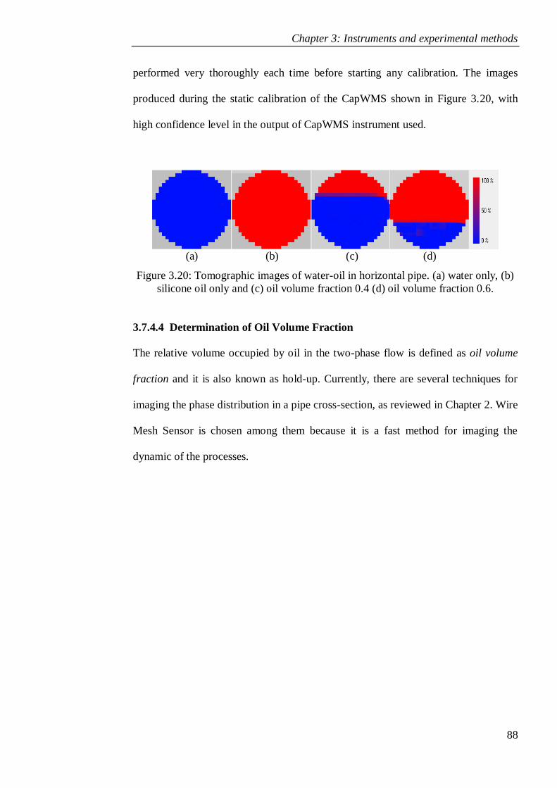
Chapter 3: Instruments and experimental methods
88
performed very thoroughly each time before starting any calibration. The images
produced during the static calibration of the CapWMS shown in Figure 3.20, with
high confidence level in the output of CapWMS instrument used.
(a) (b) (c) (d)
Figure 3.20: Tomographic images of water-oil in horizontal pipe. (a) water only, (b)
silicone oil only and (c) oil volume fraction 0.4 (d) oil volume fraction 0.6.
3.7.4.4 Determination of Oil Volume Fraction
The relative volume occupied by oil in the two-phase flow is defined as oil volume
fraction and it is also known as hold-up. Currently, there are several techniques for
imaging the phase distribution in a pipe cross-section, as reviewed in Chapter 2. Wire
Mesh Sensor is chosen among them because it is a fast method for imaging the
dynamic of the processes.

Chapter 4: Wire mesh sensor and analysis
89
CHAPTER 4
WIRE MESH SENSOR AND ANALYSIS
When two immiscible liquids flow together through a pipe, then they can distribute
themselves in a variety of flow configurations. Therefore, prediction of oil-water
flow characteristics such as spatial distribution and interface shapes are of significant
importance.
The possibilities of using of Wire Mesh Sensor as a tool to imaging the spatial
distribution across the pipe cross-section in liquid-liquid two-phase flows have been
reviewed extensively in the previous chapters. Thus in that chapters, the fundamental
concept of wire mesh sensor is briefly described. This included the design of sensor
and calibration of sensor system for oil-water system.
A new 24 x 24 capacitance sensor has been developed. With this, cross section oil-
water distribution images of the spatial distribution and interfaces curve were
obtained at the various flow conditions for horizontal and small inclination angles. In
addition, this is the simplest and fastest procedure capable of real-time operation in
dynamic two-phase flows.
Chapter 4: Wire mesh sensor and analysis
90
The prescription of the free interface configuration in gas-liquid and liquid-liquid
systems is of importance in a variety of equipment and processes. Of particular
importance is the interface curvature in two-phase flow systems. In stratified flow
pattern, particularly when the viscosity ratio is high, the interface curvature and its
influence on wetted areas may be of crucial effect on the flow pressure drop; for
example, the performance of crude-oil/water transportation lines (Russell & Charles
1959; Charles 1960; Charles & Redberger 1962).
So far, stratified two-phase flow studies have assumed plane interface between the
phases, which may be reasonable in gas-liquid (air-water) systems (Gemmell &
Epstein, 1962; Wallis, 1969; Taitel & Dukler, 1976; Brauner & Moalem Maron,
1989; Hall & Hewitt, 1993). Previous studies, focusing on liquid-liquid two-phase
systems, point out the need to account for phases wet ability properties and of the
interface curvature in solving for the two-phase pressure-drop, in-situ holdup and the
stability of the free interface (Russell et al., 1959; Bentwich, 1964, 1976; Yu &
Sparrow, 1969; Hasson et al., 1970; Brauner & Moalem Maron, 1992(a), 1992(b);
Barajas & Panton, 1993).
It is therefore, the objective of the present study to provide a predictive tool for
determining the spatial distribution and characteristic interface curvature in two
phase liquid-liquid systems. The prescription of the interface configuration is a basic
input which is needed to further the modelling of two-phase flow problems in a
variety of two-fluid systems (Brauner, 1996)
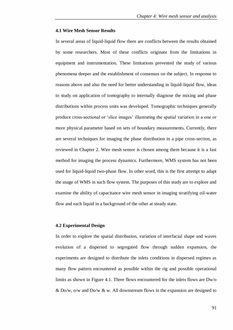
Chapter 4: Wire mesh sensor and analysis
91
4.1 Wire Mesh Sensor Results
In several areas of liquid-liquid flow there are conflicts between the results obtained
by some researchers. Most of these conflicts originate from the limitations in
equipment and instrumentation. These limitations prevented the study of various
phenomena deeper and the establishment of consensus on the subject. In response to
reasons above and also the need for better understanding in liquid-liquid flow, ideas
to study on application of tomography to internally diagnose the mixing and phase
distributions within process units was developed. Tomographic techniques generally
produce cross-sectional or „slice images‟ illustrating the spatial variation in a one or
more physical parameter based on sets of boundary measurements. Currently, there
are several techniques for imaging the phase distribution in a pipe cross-section, as
reviewed in Chapter 2. Wire mesh sensor is chosen among them because it is a fast
method for imaging the process dynamics. Furthermore, WMS system has not been
used for liquid-liquid two-phase flow. In other word, this is the first attempt to adapt
the usage of WMS in such flow system. The purposes of this study are to explore and
examine the ability of capacitance wire mesh sensor in imaging stratifying oil-water
flow and each liquid in a background of the other at steady state.
4.2 Experimental Design
In order to explore the spatial distribution, variation of interfacial shape and waves
evolution of a dispersed to segregated flow through sudden expansion, the
experiments are designed to distribute the inlets conditions in dispersed regimes as
many flow pattern encountered as possible within the rig and possible operational
limits as shown in Figure 4.1. Three flows encountered for the inlets flows are Dw/o
& Do/w, o/w and Do/w & w. All downstream flows in the expansion are designed to
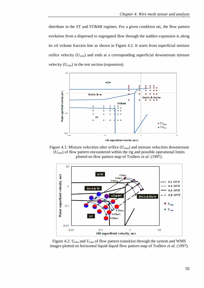
Chapter 4: Wire mesh sensor and analysis
92
distribute in the ST and ST&MI regimes. For a given condition set, the flow pattern
evolution from a dispersed to segregated flow through the sudden expansion is along
its oil volume fraction line as shown in Figure 4.2. It starts from superficial mixture
orifice velocity (Usmo) and ends at a corresponding superficial downstream mixture
velocity (Usme) in the test section (expansion).
Figure 4.1: Mixture velocities after orifice (Usmo) and mixture velocities downstream
(Usme) of flow pattern encountered within the rig and possible operational limits
plotted on flow pattern map of Trallero et al. (1997).
Figure 4.2: Usmo and Usme of flow pattern transition through the system and WMS
images plotted on horizontal liquid-liquid flow pattern map of Trallero et al. (1997).
Chapter 4: Wire mesh sensor and analysis
93
All the experiments were carried out using CapWMS. Such experiments using
CapWMS were the first time to be carried out in the oil-water flow system.
Measurements were performed at three distances downstream of the expansion of
10D (near), 20D (middle) and34D (far), where D is the internal diameter of the pipe
(68 mm). Experiments were conducted for input oil fractions ranging from 0.2 to 0.8
OVF, orifice open area 32%, downstream expansion mixture velocities (Usme) of
0.20, 0.30, & 0.35 m/s with a horizontal pipe or inclined at angles of +6, +3, -3 & -6
degrees. The CapWMS calibration method is applied in all experiments. The
summary of the experimental conditions is given in Table 4.1.
A continuous measurement was then logged by a computer and allowed the
proprietary software to produce volume fraction as shown in Figure 4.3.The data
collection was carried out using a PC associated with data acquisition system and
WMS equipment wherein the CapWMS was employed at locations along the test
section (expansion pipe). This PC was utilised as a tool for data collecting and
storage only. The raw data then analysed using copyrighted software supplied by the
manufacturer to produce images of spatial volume fraction results. These data then
was used for further data processing.
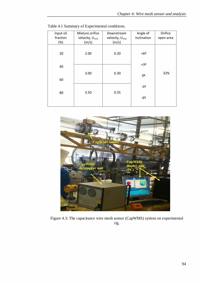
Chapter 4: Wire mesh sensor and analysis
94
Table 4.1 Summary of Experimental conditions.
Input oil fraction
(%)
Mixture orifice velocity, Usmo
(m/s)
Downstream velocity, Usme
(m/s)
Angle of inclination
Orifice open area
20
40
60
80
2.00
0.20
+6º
+3º
0º
-3º
-6º
32%
3.00
0.30
3.50
0.35
Figure 4.3: The capacitance wire mesh sensor (CapWMS) system on experimental
rig.
Chapter 4: Wire mesh sensor and analysis
95
4.3 Experiment results and discussion
According to the flow pattern map of Trallero et al (1997), all the downstream flow
patterns in the expansion in the present study are in the segregated flow regimes, if
they were fully developed horizontal flows. However, in real situation there are other
factors assisting the flow segregation as discussed in details in Chapter 3. Input oil
volume fraction (OVF) and the downstream superficial mixture velocity (Usme) are
among the factors that affect the phase layer evolution. In this section the flow
development along expansion pipe and interface shapes of the singularity are to be
recognised by data and images obtained from the CapWMS. Furthermore, the effect
of the mixture velocity, oil volume fraction and distance from expansion are explored
for the different pipe orientations. As well as explaining the relationship between the
data and images captured with phase volume fraction distributions of oil-water flow
established by previous researchers.
Many analysis of stratified flow assume that the interface between the phases is flat
(Agrawal et al, 1973; Taitel and Dukler, 1976 and Hall, 1992). However actual
interface may not be flat; there are, of course, interfacial waves in many cases, but
even in time averaged sense, the interface may be curved. Interface curvature
introduced by interfacial tension may occur in all two phase flow but it is likely to be
most severe in case of liquid-liquid flow.
In this chapter, discussions were made based on the first interpretation of the
CapWMS results to demonstrate the advantages of Wire Mesh Sensor, i.e., good in-
line visualization capabilities due to its high resolution, providing reliable
information across the full cross section of a pipe.
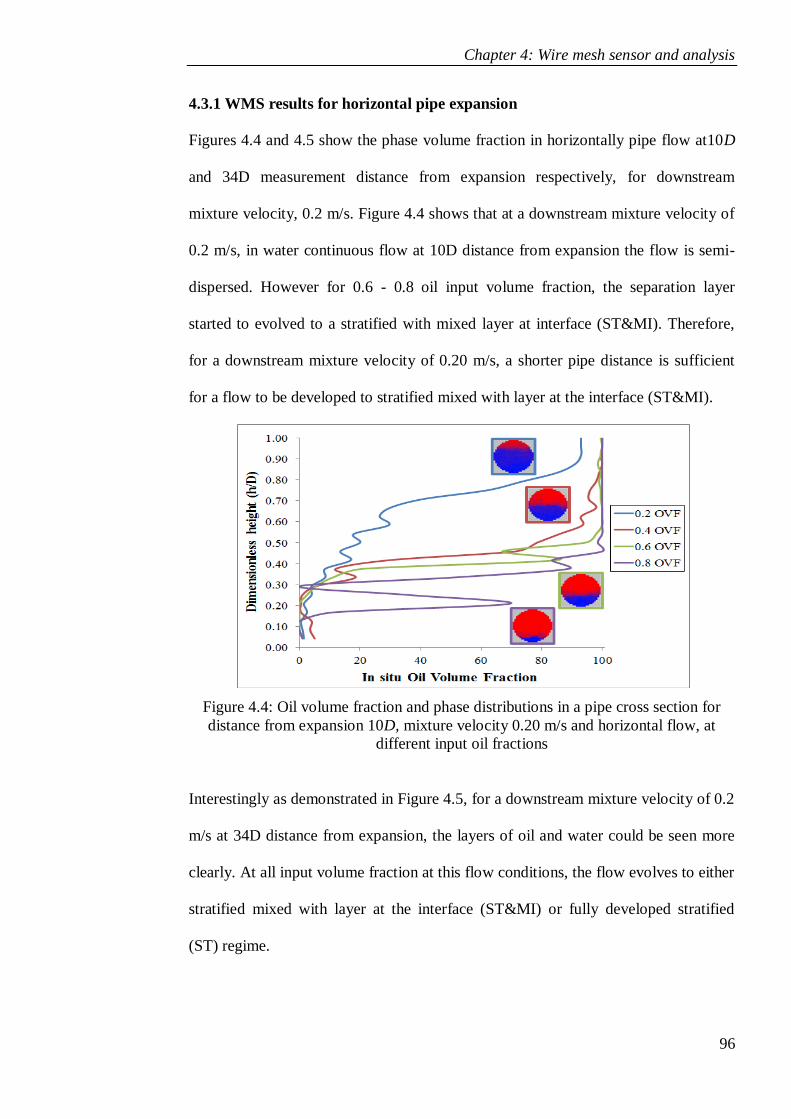
Chapter 4: Wire mesh sensor and analysis
96
4.3.1 WMS results for horizontal pipe expansion
Figures 4.4 and 4.5 show the phase volume fraction in horizontally pipe flow at10D
and 34D measurement distance from expansion respectively, for downstream
mixture velocity, 0.2 m/s. Figure 4.4 shows that at a downstream mixture velocity of
0.2 m/s, in water continuous flow at 10D distance from expansion the flow is semi-
dispersed. However for 0.6 - 0.8 oil input volume fraction, the separation layer
started to evolved to a stratified with mixed layer at interface (ST&MI). Therefore,
for a downstream mixture velocity of 0.20 m/s, a shorter pipe distance is sufficient
for a flow to be developed to stratified mixed with layer at the interface (ST&MI).
Figure 4.4: Oil volume fraction and phase distributions in a pipe cross section for
distance from expansion 10D, mixture velocity 0.20 m/s and horizontal flow, at
different input oil fractions
Interestingly as demonstrated in Figure 4.5, for a downstream mixture velocity of 0.2
m/s at 34D distance from expansion, the layers of oil and water could be seen more
clearly. At all input volume fraction at this flow conditions, the flow evolves to either
stratified mixed with layer at the interface (ST&MI) or fully developed stratified
(ST) regime.
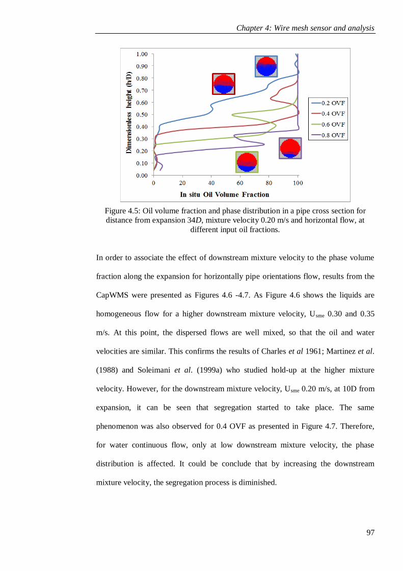
Chapter 4: Wire mesh sensor and analysis
97
Figure 4.5: Oil volume fraction and phase distribution in a pipe cross section for
distance from expansion 34D, mixture velocity 0.20 m/s and horizontal flow, at
different input oil fractions.
In order to associate the effect of downstream mixture velocity to the phase volume
fraction along the expansion for horizontally pipe orientations flow, results from the
CapWMS were presented as Figures 4.6 -4.7. As Figure 4.6 shows the liquids are
homogeneous flow for a higher downstream mixture velocity, Usme 0.30 and 0.35
m/s. At this point, the dispersed flows are well mixed, so that the oil and water
velocities are similar. This confirms the results of Charles et al 1961; Martinez et al.
(1988) and Soleimani et al. (1999a) who studied hold-up at the higher mixture
velocity. However, for the downstream mixture velocity, Usme 0.20 m/s, at 10D from
expansion, it can be seen that segregation started to take place. The same
phenomenon was also observed for 0.4 OVF as presented in Figure 4.7. Therefore,
for water continuous flow, only at low downstream mixture velocity, the phase
distribution is affected. It could be conclude that by increasing the downstream
mixture velocity, the segregation process is diminished.

Chapter 4: Wire mesh sensor and analysis
98
Figure 4.6: Oil volume fraction in a pipe cross section for distance from expansion
34D, input oil fraction 0.2 and horizontal flow, at different mixture velocities.
Figure 4.7: Oil volume fraction in a pipe cross section for distance from expansion
34D, input oil fraction 0.4 and horizontal flow, at different mixture velocities.
As exemplified in Figures 4.8 and 4.9, at higher input oil volume fraction,
downstream mixture velocity has minimal effect on the phase separation.
Segregation of phases occurs at all Usme. At higher downstream mixture velocities,
Usme 0.30 and 0.35 m/s, the flow is stratified with mixed layer at the interface. As for
Usme 0.20 m/s, stratified flow had been achieved.
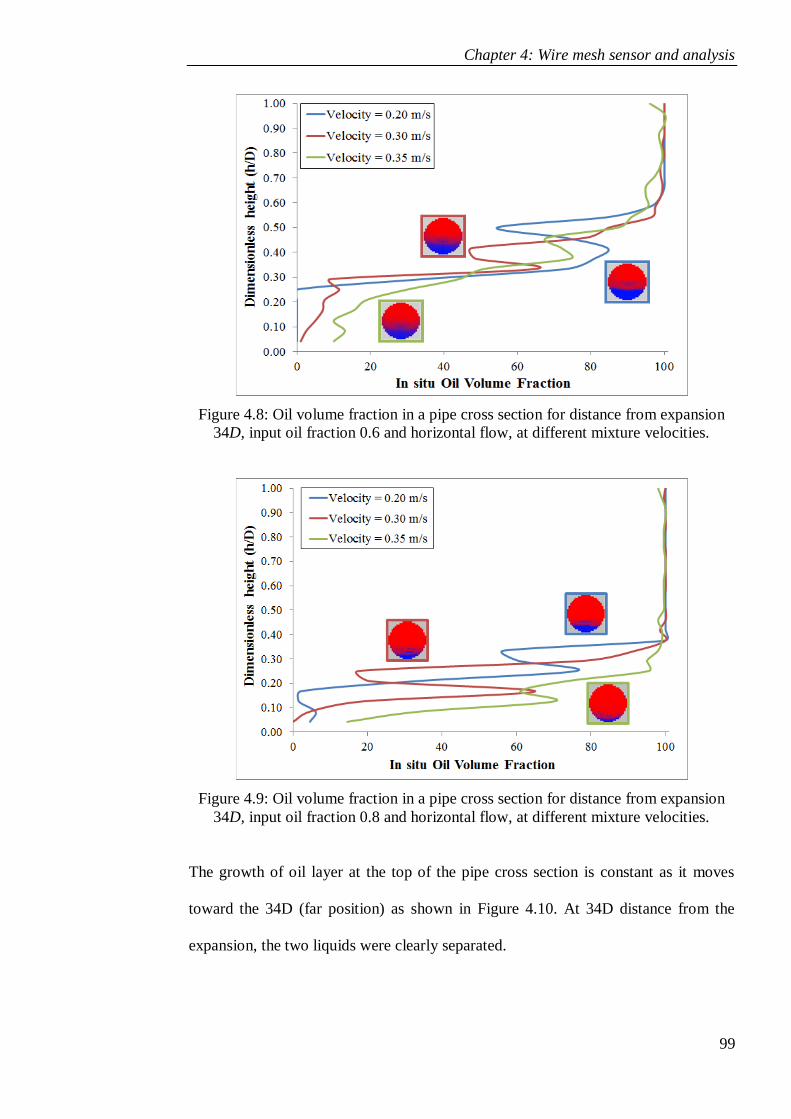
Chapter 4: Wire mesh sensor and analysis
99
Figure 4.8: Oil volume fraction in a pipe cross section for distance from expansion
34D, input oil fraction 0.6 and horizontal flow, at different mixture velocities.
Figure 4.9: Oil volume fraction in a pipe cross section for distance from expansion
34D, input oil fraction 0.8 and horizontal flow, at different mixture velocities.
The growth of oil layer at the top of the pipe cross section is constant as it moves
toward the 34D (far position) as shown in Figure 4.10. At 34D distance from the
expansion, the two liquids were clearly separated.
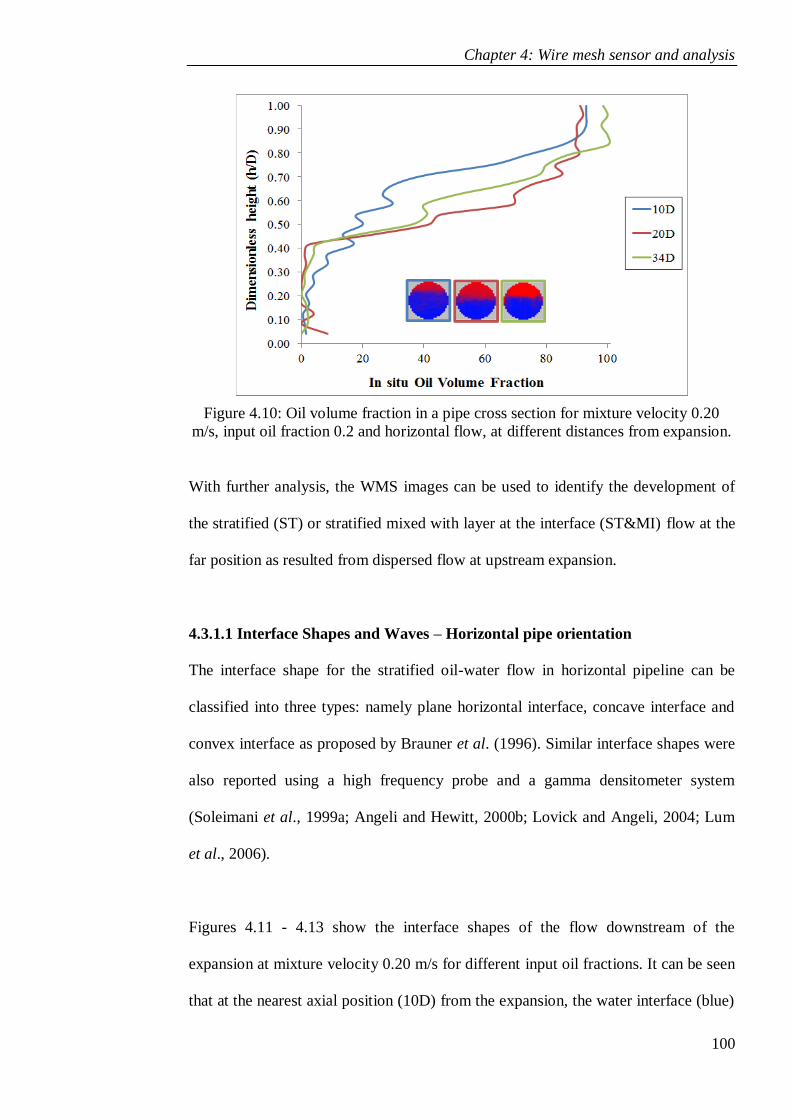
Chapter 4: Wire mesh sensor and analysis
100
Figure 4.10: Oil volume fraction in a pipe cross section for mixture velocity 0.20
m/s, input oil fraction 0.2 and horizontal flow, at different distances from expansion.
With further analysis, the WMS images can be used to identify the development of
the stratified (ST) or stratified mixed with layer at the interface (ST&MI) flow at the
far position as resulted from dispersed flow at upstream expansion.
4.3.1.1 Interface Shapes and Waves – Horizontal pipe orientation
The interface shape for the stratified oil-water flow in horizontal pipeline can be
classified into three types: namely plane horizontal interface, concave interface and
convex interface as proposed by Brauner et al. (1996). Similar interface shapes were
also reported using a high frequency probe and a gamma densitometer system
(Soleimani et al., 1999a; Angeli and Hewitt, 2000b; Lovick and Angeli, 2004; Lum
et al., 2006).
Figures 4.11 - 4.13 show the interface shapes of the flow downstream of the
expansion at mixture velocity 0.20 m/s for different input oil fractions. It can be seen
that at the nearest axial position (10D) from the expansion, the water interface (blue)
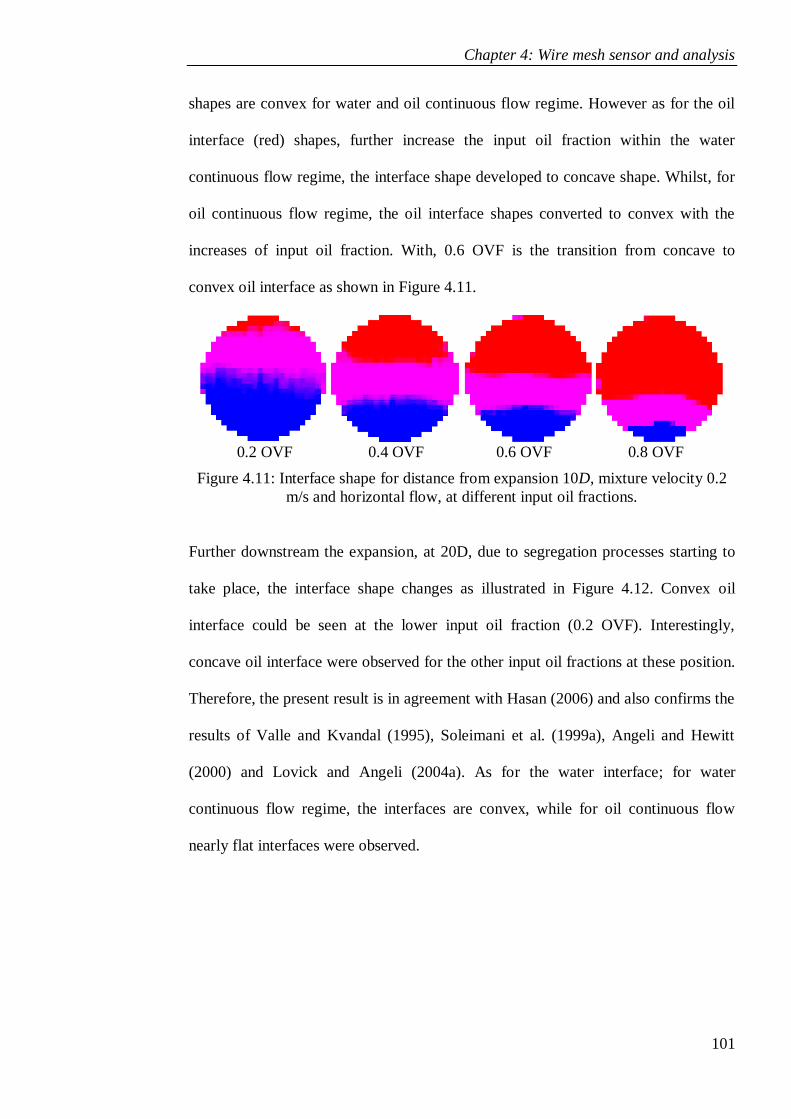
Chapter 4: Wire mesh sensor and analysis
101
shapes are convex for water and oil continuous flow regime. However as for the oil
interface (red) shapes, further increase the input oil fraction within the water
continuous flow regime, the interface shape developed to concave shape. Whilst, for
oil continuous flow regime, the oil interface shapes converted to convex with the
increases of input oil fraction. With, 0.6 OVF is the transition from concave to
convex oil interface as shown in Figure 4.11.
0.2 OVF 0.4 OVF 0.6 OVF 0.8 OVF
Figure 4.11: Interface shape for distance from expansion 10D, mixture velocity 0.2
m/s and horizontal flow, at different input oil fractions.
Further downstream the expansion, at 20D, due to segregation processes starting to
take place, the interface shape changes as illustrated in Figure 4.12. Convex oil
interface could be seen at the lower input oil fraction (0.2 OVF). Interestingly,
concave oil interface were observed for the other input oil fractions at these position.
Therefore, the present result is in agreement with Hasan (2006) and also confirms the
results of Valle and Kvandal (1995), Soleimani et al. (1999a), Angeli and Hewitt
(2000) and Lovick and Angeli (2004a). As for the water interface; for water
continuous flow regime, the interfaces are convex, while for oil continuous flow
nearly flat interfaces were observed.
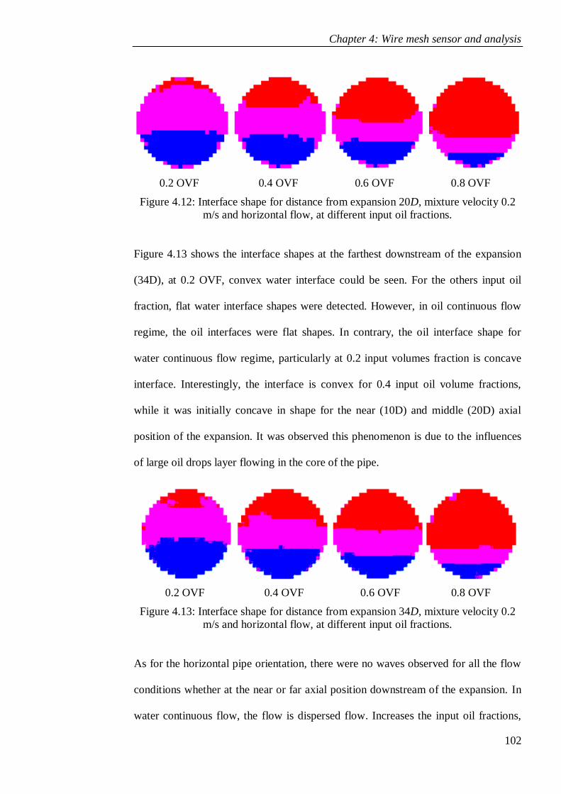
Chapter 4: Wire mesh sensor and analysis
102
0.2 OVF 0.4 OVF 0.6 OVF 0.8 OVF
Figure 4.12: Interface shape for distance from expansion 20D, mixture velocity 0.2
m/s and horizontal flow, at different input oil fractions.
Figure 4.13 shows the interface shapes at the farthest downstream of the expansion
(34D), at 0.2 OVF, convex water interface could be seen. For the others input oil
fraction, flat water interface shapes were detected. However, in oil continuous flow
regime, the oil interfaces were flat shapes. In contrary, the oil interface shape for
water continuous flow regime, particularly at 0.2 input volumes fraction is concave
interface. Interestingly, the interface is convex for 0.4 input oil volume fractions,
while it was initially concave in shape for the near (10D) and middle (20D) axial
position of the expansion. It was observed this phenomenon is due to the influences
of large oil drops layer flowing in the core of the pipe.
0.2 OVF 0.4 OVF 0.6 OVF 0.8 OVF
Figure 4.13: Interface shape for distance from expansion 34D, mixture velocity 0.2
m/s and horizontal flow, at different input oil fractions.
As for the horizontal pipe orientation, there were no waves observed for all the flow
conditions whether at the near or far axial position downstream of the expansion. In
water continuous flow, the flow is dispersed flow. Increases the input oil fractions,
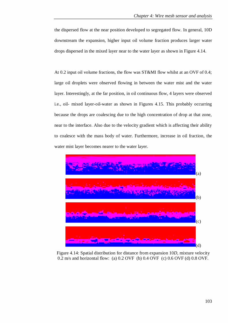
Chapter 4: Wire mesh sensor and analysis
103
the dispersed flow at the near position developed to segregated flow. In general, 10D
downstream the expansion, higher input oil volume fraction produces larger water
drops dispersed in the mixed layer near to the water layer as shown in Figure 4.14.
At 0.2 input oil volume fractions, the flow was ST&MI flow whilst at an OVF of 0.4;
large oil droplets were observed flowing in between the water mist and the water
layer. Interestingly, at the far position, in oil continuous flow, 4 layers were observed
i.e., oil- mixed layer-oil-water as shown in Figures 4.15. This probably occurring
because the drops are coalescing due to the high concentration of drop at that zone,
near to the interface. Also due to the velocity gradient which is affecting their ability
to coalesce with the mass body of water. Furthermore, increase in oil fraction, the
water mist layer becomes nearer to the water layer.
(a)
(b)
(c)
(d)
Figure 4.14: Spatial distribution for distance from expansion 10D, mixture velocity
0.2 m/s and horizontal flow: (a) 0.2 OVF (b) 0.4 OVF (c) 0.6 OVF (d) 0.8 OVF.
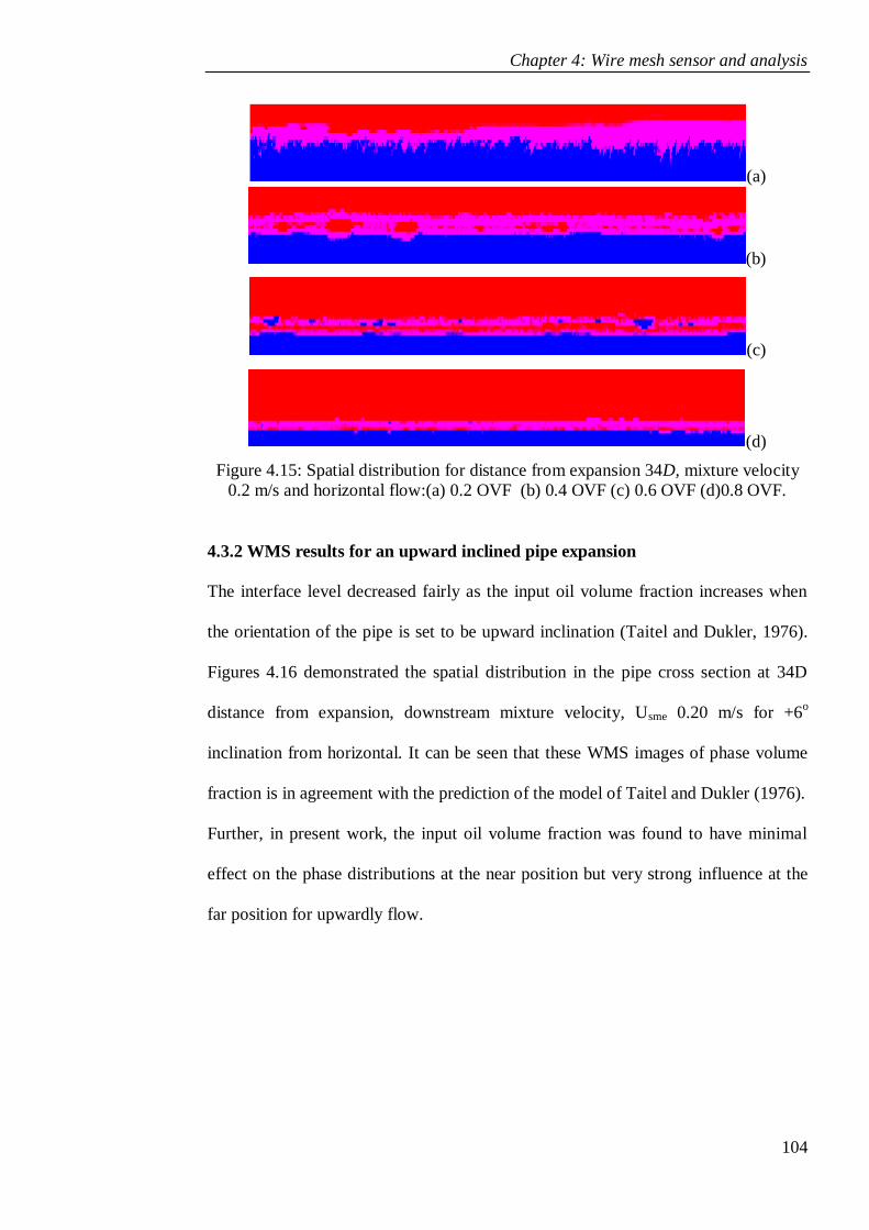
Chapter 4: Wire mesh sensor and analysis
104
(a)
(b)
(c)
(d)
Figure 4.15: Spatial distribution for distance from expansion 34D, mixture velocity
0.2 m/s and horizontal flow:(a) 0.2 OVF (b) 0.4 OVF (c) 0.6 OVF (d)0.8 OVF.
4.3.2 WMS results for an upward inclined pipe expansion
The interface level decreased fairly as the input oil volume fraction increases when
the orientation of the pipe is set to be upward inclination (Taitel and Dukler, 1976).
Figures 4.16 demonstrated the spatial distribution in the pipe cross section at 34D
distance from expansion, downstream mixture velocity, Usme 0.20 m/s for +6o
inclination from horizontal. It can be seen that these WMS images of phase volume
fraction is in agreement with the prediction of the model of Taitel and Dukler (1976).
Further, in present work, the input oil volume fraction was found to have minimal
effect on the phase distributions at the near position but very strong influence at the
far position for upwardly flow.

Chapter 4: Wire mesh sensor and analysis
105
Figure 4.16: Oil volume fraction in a pipe cross section for distance from expansion
34D, mixture velocity 0.2 m/s and +6 degree flow, at different input oil fractions.
The influences of downstream mixture velocities on the in-situ oil volume fraction
downstream of the expansion for upward flow are presented in Figures 4.17 and
4.18. In water continuous flow, increases of the downstream mixture velocity, the oil
phase layer that can be seen at lower Usme gradually diminished. The transition of the
flow is as shown in Figure 4.17. At higher Usme, a fully dispersed flow was recorded.
Figure 4.17: Oil volume fraction in a pipe cross section for distance from expansion
34D, input oil fraction 0.2 and +6 degree flow, at different mixture velocities.
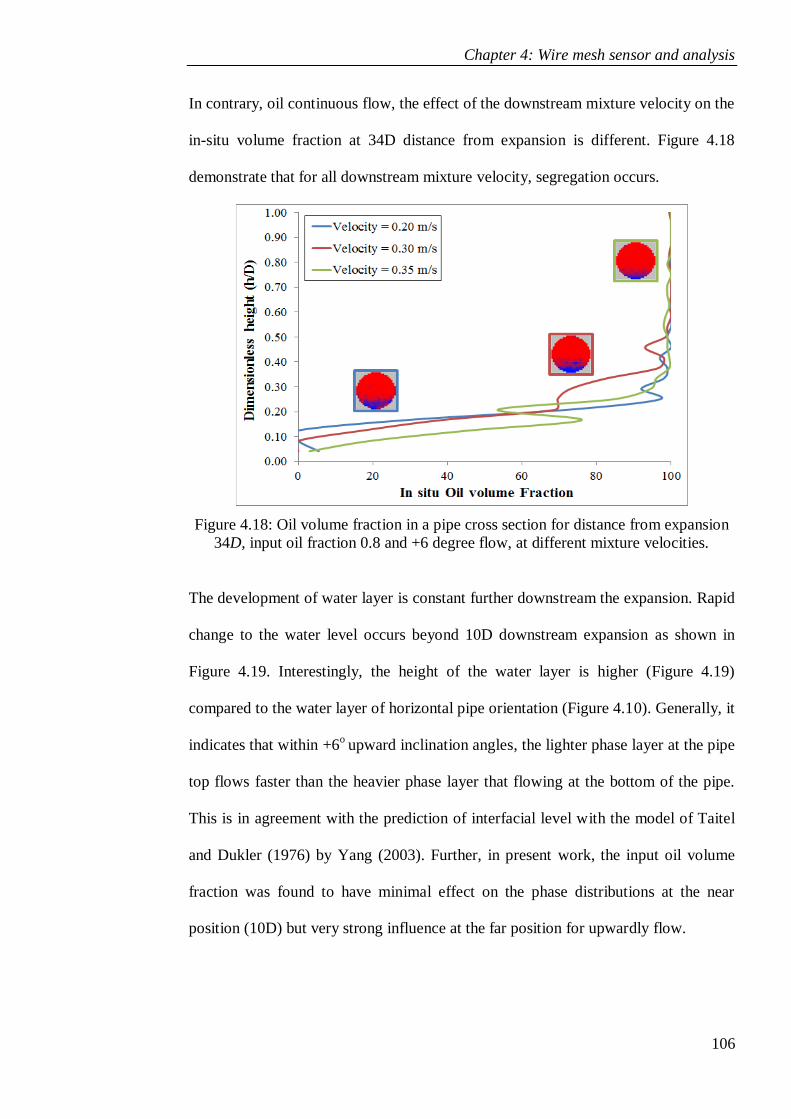
Chapter 4: Wire mesh sensor and analysis
106
In contrary, oil continuous flow, the effect of the downstream mixture velocity on the
in-situ volume fraction at 34D distance from expansion is different. Figure 4.18
demonstrate that for all downstream mixture velocity, segregation occurs.
Figure 4.18: Oil volume fraction in a pipe cross section for distance from expansion
34D, input oil fraction 0.8 and +6 degree flow, at different mixture velocities.
The development of water layer is constant further downstream the expansion. Rapid
change to the water level occurs beyond 10D downstream expansion as shown in
Figure 4.19. Interestingly, the height of the water layer is higher (Figure 4.19)
compared to the water layer of horizontal pipe orientation (Figure 4.10). Generally, it
indicates that within +6o
upward inclination angles, the lighter phase layer at the pipe
top flows faster than the heavier phase layer that flowing at the bottom of the pipe.
This is in agreement with the prediction of interfacial level with the model of Taitel
and Dukler (1976) by Yang (2003). Further, in present work, the input oil volume
fraction was found to have minimal effect on the phase distributions at the near
position (10D) but very strong influence at the far position for upwardly flow.
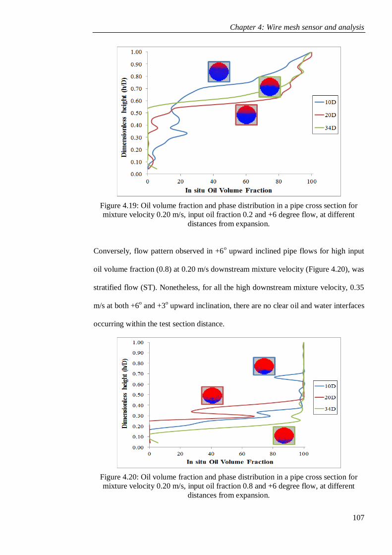
Chapter 4: Wire mesh sensor and analysis
107
Figure 4.19: Oil volume fraction and phase distribution in a pipe cross section for
mixture velocity 0.20 m/s, input oil fraction 0.2 and +6 degree flow, at different
distances from expansion.
Conversely, flow pattern observed in +6o upward inclined pipe flows for high input
oil volume fraction (0.8) at 0.20 m/s downstream mixture velocity (Figure 4.20), was
stratified flow (ST). Nonetheless, for all the high downstream mixture velocity, 0.35
m/s at both +6o and +3
o upward inclination, there are no clear oil and water interfaces
occurring within the test section distance.
Figure 4.20: Oil volume fraction and phase distribution in a pipe cross section for
mixture velocity 0.20 m/s, input oil fraction 0.8 and +6 degree flow, at different
distances from expansion.
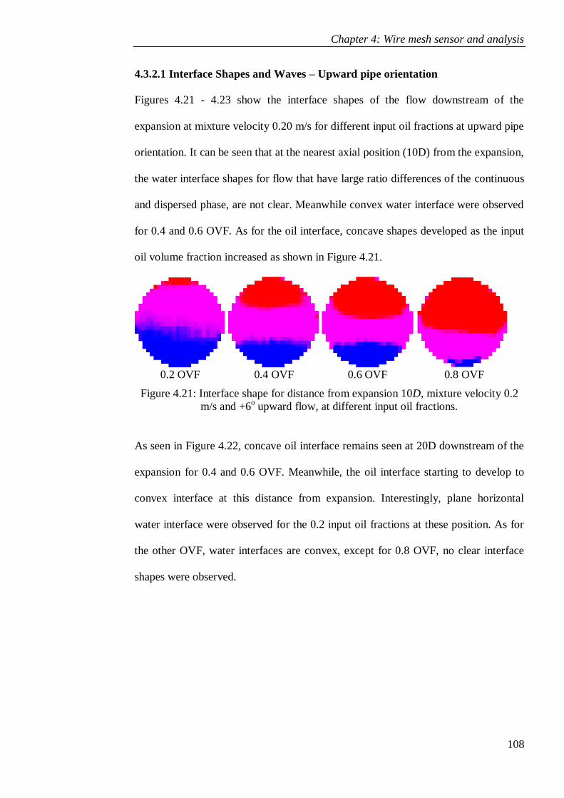
Chapter 4: Wire mesh sensor and analysis
108
4.3.2.1 Interface Shapes and Waves – Upward pipe orientation
Figures 4.21 - 4.23 show the interface shapes of the flow downstream of the
expansion at mixture velocity 0.20 m/s for different input oil fractions at upward pipe
orientation. It can be seen that at the nearest axial position (10D) from the expansion,
the water interface shapes for flow that have large ratio differences of the continuous
and dispersed phase, are not clear. Meanwhile convex water interface were observed
for 0.4 and 0.6 OVF. As for the oil interface, concave shapes developed as the input
oil volume fraction increased as shown in Figure 4.21.
0.2 OVF 0.4 OVF 0.6 OVF 0.8 OVF
Figure 4.21: Interface shape for distance from expansion 10D, mixture velocity 0.2
m/s and +6o upward flow, at different input oil fractions.
As seen in Figure 4.22, concave oil interface remains seen at 20D downstream of the
expansion for 0.4 and 0.6 OVF. Meanwhile, the oil interface starting to develop to
convex interface at this distance from expansion. Interestingly, plane horizontal
water interface were observed for the 0.2 input oil fractions at these position. As for
the other OVF, water interfaces are convex, except for 0.8 OVF, no clear interface
shapes were observed.
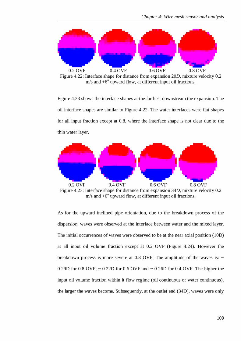
Chapter 4: Wire mesh sensor and analysis
109
0.2 OVF 0.4 OVF 0.6 OVF 0.8 OVF
Figure 4.22: Interface shape for distance from expansion 20D, mixture velocity 0.2
m/s and +6o upward flow, at different input oil fractions.
Figure 4.23 shows the interface shapes at the farthest downstream the expansion. The
oil interface shapes are similar to Figure 4.22. The water interfaces were flat shapes
for all input fraction except at 0.8, where the interface shape is not clear due to the
thin water layer.
0.2 OVF 0.4 OVF 0.6 OVF 0.8 OVF
Figure 4.23: Interface shape for distance from expansion 34D, mixture velocity 0.2
m/s and +6o upward flow, at different input oil fractions.
As for the upward inclined pipe orientation, due to the breakdown process of the
dispersion, waves were observed at the interface between water and the mixed layer.
The initial occurrences of waves were observed to be at the near axial position (10D)
at all input oil volume fraction except at 0.2 OVF (Figure 4.24). However the
breakdown process is more severe at 0.8 OVF. The amplitude of the waves is: ~
0.29D for 0.8 OVF; ~ 0.22D for 0.6 OVF and ~ 0.26D for 0.4 OVF. The higher the
input oil volume fraction within it flow regime (oil continuous or water continuous),
the larger the waves become. Subsequently, at the outlet end (34D), waves were only
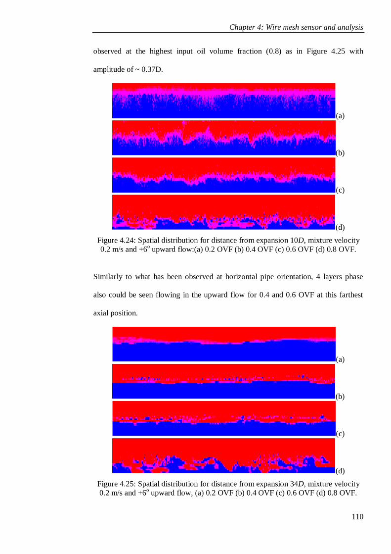
Chapter 4: Wire mesh sensor and analysis
110
observed at the highest input oil volume fraction (0.8) as in Figure 4.25 with
amplitude of ~ 0.37D.
(a)
(b)
(c)
(d)
Figure 4.24: Spatial distribution for distance from expansion 10D, mixture velocity
0.2 m/s and +6o upward flow:(a) 0.2 OVF (b) 0.4 OVF (c) 0.6 OVF (d) 0.8 OVF.
Similarly to what has been observed at horizontal pipe orientation, 4 layers phase
also could be seen flowing in the upward flow for 0.4 and 0.6 OVF at this farthest
axial position.
(a)
(b)
(c)
(d)
Figure 4.25: Spatial distribution for distance from expansion 34D, mixture velocity
0.2 m/s and +6o upward flow, (a) 0.2 OVF (b) 0.4 OVF (c) 0.6 OVF (d) 0.8 OVF.
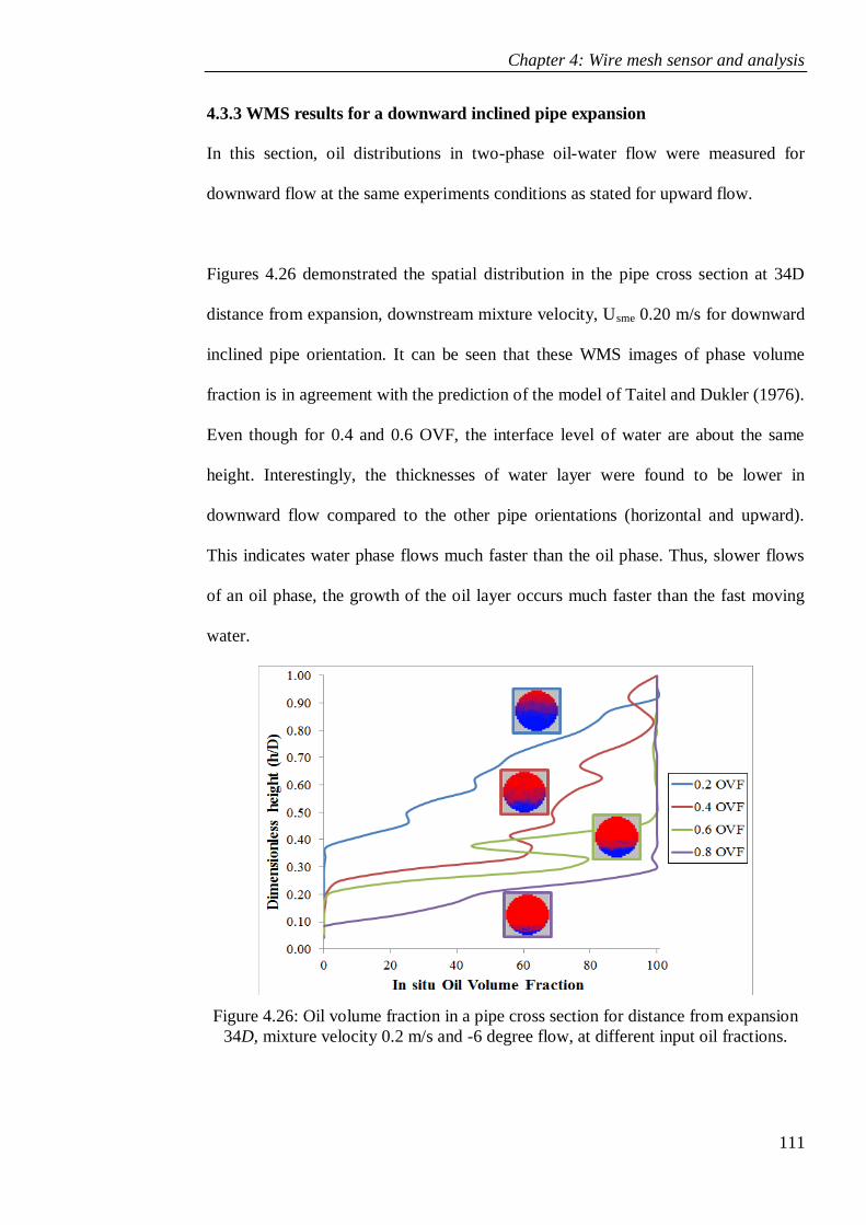
Chapter 4: Wire mesh sensor and analysis
111
4.3.3 WMS results for a downward inclined pipe expansion
In this section, oil distributions in two-phase oil-water flow were measured for
downward flow at the same experiments conditions as stated for upward flow.
Figures 4.26 demonstrated the spatial distribution in the pipe cross section at 34D
distance from expansion, downstream mixture velocity, Usme 0.20 m/s for downward
inclined pipe orientation. It can be seen that these WMS images of phase volume
fraction is in agreement with the prediction of the model of Taitel and Dukler (1976).
Even though for 0.4 and 0.6 OVF, the interface level of water are about the same
height. Interestingly, the thicknesses of water layer were found to be lower in
downward flow compared to the other pipe orientations (horizontal and upward).
This indicates water phase flows much faster than the oil phase. Thus, slower flows
of an oil phase, the growth of the oil layer occurs much faster than the fast moving
water.
Figure 4.26: Oil volume fraction in a pipe cross section for distance from expansion
34D, mixture velocity 0.2 m/s and -6 degree flow, at different input oil fractions.
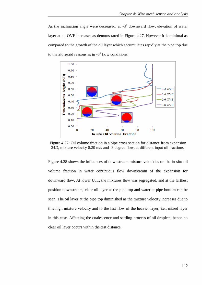
Chapter 4: Wire mesh sensor and analysis
112
As the inclination angle were decreased, at -3o downward flow, elevation of water
layer at all OVF increases as demonstrated in Figure 4.27. However it is minimal as
compared to the growth of the oil layer which accumulates rapidly at the pipe top due
to the aforesaid reasons as in -6o flow conditions.
Figure 4.27: Oil volume fraction in a pipe cross section for distance from expansion
34D, mixture velocity 0.20 m/s and -3 degree flow, at different input oil fractions.
Figure 4.28 shows the influences of downstream mixture velocities on the in-situ oil
volume fraction in water continuous flow downstream of the expansion for
downward flow. At lower Usme, the mixtures flow was segregated, and at the farthest
position downstream, clear oil layer at the pipe top and water at pipe bottom can be
seen. The oil layer at the pipe top diminished as the mixture velocity increases due to
this high mixture velocity and to the fast flow of the heavier layer, i.e., mixed layer
in this case. Affecting the coalescence and settling process of oil droplets, hence no
clear oil layer occurs within the test distance.
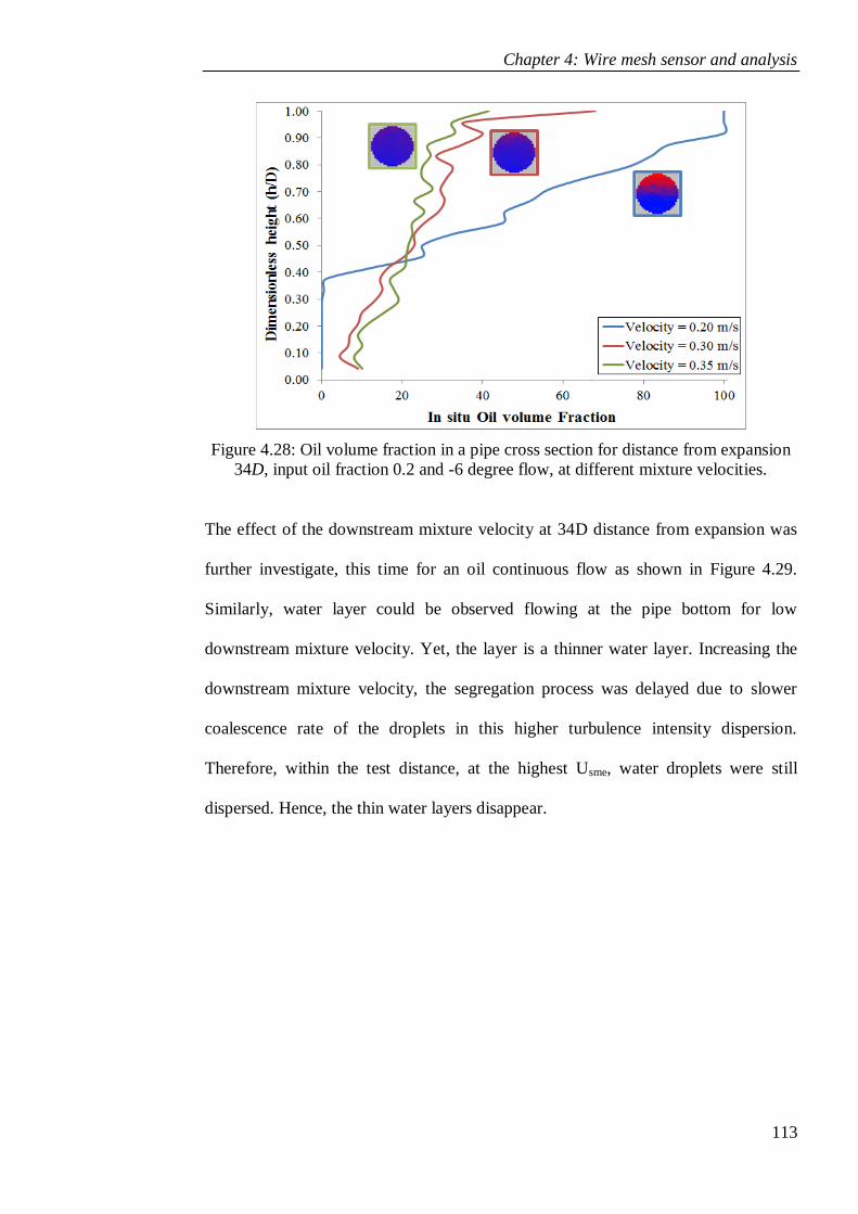
Chapter 4: Wire mesh sensor and analysis
113
Figure 4.28: Oil volume fraction in a pipe cross section for distance from expansion
34D, input oil fraction 0.2 and -6 degree flow, at different mixture velocities.
The effect of the downstream mixture velocity at 34D distance from expansion was
further investigate, this time for an oil continuous flow as shown in Figure 4.29.
Similarly, water layer could be observed flowing at the pipe bottom for low
downstream mixture velocity. Yet, the layer is a thinner water layer. Increasing the
downstream mixture velocity, the segregation process was delayed due to slower
coalescence rate of the droplets in this higher turbulence intensity dispersion.
Therefore, within the test distance, at the highest Usme, water droplets were still
dispersed. Hence, the thin water layers disappear.
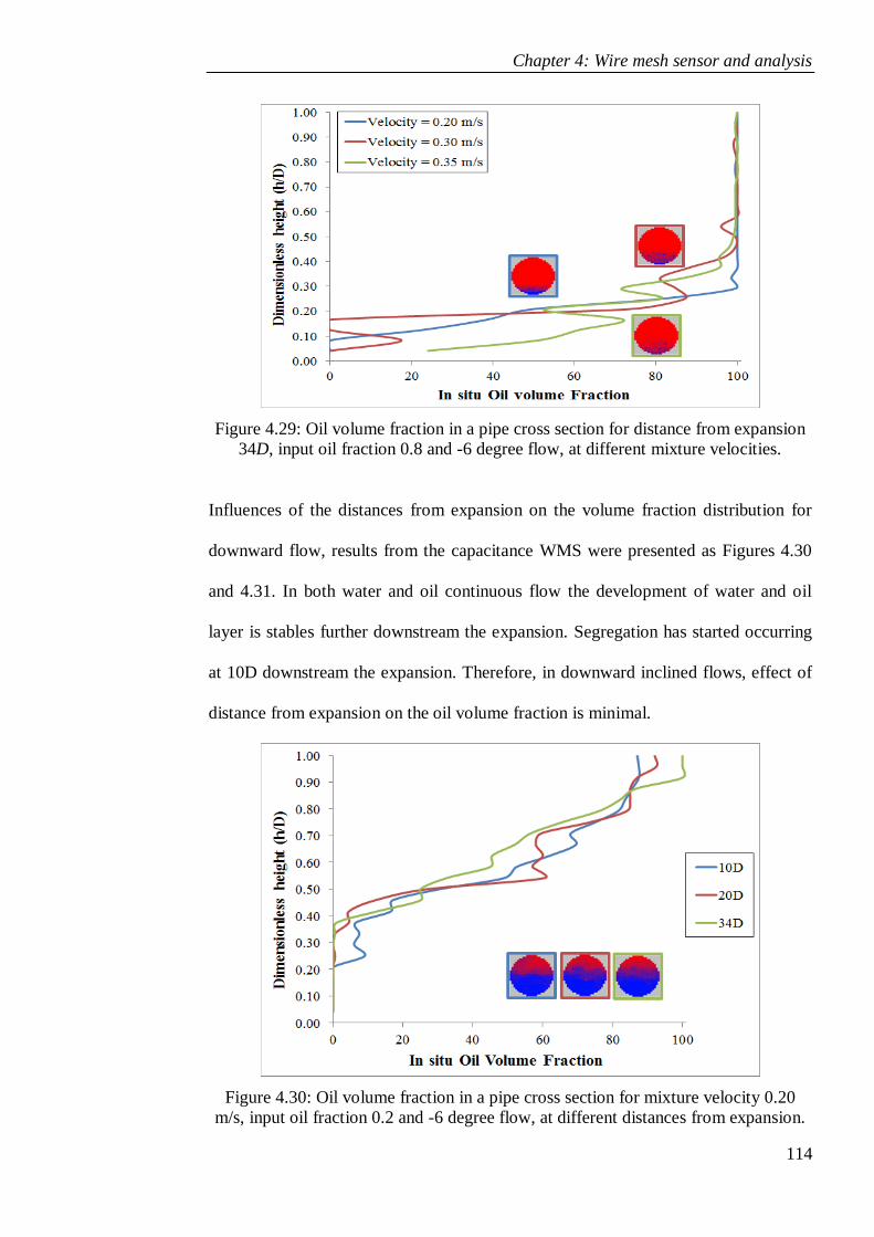
Chapter 4: Wire mesh sensor and analysis
114
Figure 4.29: Oil volume fraction in a pipe cross section for distance from expansion
34D, input oil fraction 0.8 and -6 degree flow, at different mixture velocities.
Influences of the distances from expansion on the volume fraction distribution for
downward flow, results from the capacitance WMS were presented as Figures 4.30
and 4.31. In both water and oil continuous flow the development of water and oil
layer is stables further downstream the expansion. Segregation has started occurring
at 10D downstream the expansion. Therefore, in downward inclined flows, effect of
distance from expansion on the oil volume fraction is minimal.
Figure 4.30: Oil volume fraction in a pipe cross section for mixture velocity 0.20
m/s, input oil fraction 0.2 and -6 degree flow, at different distances from expansion.

Chapter 4: Wire mesh sensor and analysis
115
Figure 4.31: Oil volume fraction in a pipe cross section for mixture velocity 0.20
m/s, input oil fraction 0.8 and -6 degree flow, at different distances from expansion.
4.3.3.1 Interface Shapes and Waves –Downward pipe orientation
Figures 4.32 - 4.34 show the interface shapes of the flow downstream of the
expansion at mixture velocity 0.20 m/s for different input oil fractions in a downward
pipe orientation. At the near position, the water interface shapes are convex in both
oil and water continuous flow regime as shown in Figure 4.32. However for mixture
with lower ratio differences of the dispersed and continuous phase, i.e., 0.4 and 0.6
OVF, concave oil interfaces could be seen. In contrary, at 0.8 OVF, nearly horizontal
shapes of oil interface appear at these near position whilst no clear interface layer
could be seen at 0.2 OVF.
0.2 OVF 0.4 OVF 0.6 OVF 0.8 OVF
Figure 4.32: Interface shape for distance from expansion 10D, mixture velocity 0.2
m/s and -6o downward flow, at different input oil fractions.

Chapter 4: Wire mesh sensor and analysis
116
At the middle position of the test distance, 20D, similar oil interface shapes as at 10D
occurs for 0.4, 0.6 and 0.8 OVF. This concave interface shape was also observed by
Hasan (2006). Meanwhile, at lowest input oil volume fraction (0.2), due to
segregation processes starting to take place, the oil interface shape evolves to convex
shapes as illustrated in Figure 4.33. Interestingly, convex water interface seen earlier
at 10D evolves to plane horizontal interfaces at these axial positions for all input oil
volume fraction.
0.2 OVF 0.4 OVF 0.6 OVF 0.8 OVF
Figure 4.33: Interface shape for distance from expansion 20D, mixture velocity 0.2
m/s and -6o downward flow, at different input oil fractions.
Figure 4.34 show the interface shapes at 34D downstream the pipe expansion. At this
position, segregation is clearly observed as the layer of oil and water are well
distinguished. Besides, the water interface shape is plane horizontal at this position
except at 0.8 OVF which is concave, due to the thin layer of water being pushed to
the wall by the oil. Whilst, the oil interface shapes remains convex for 0.2 OVF and
concave for 0.4 and 0.6 OVF. The oil interface evolves to plane horizontal for 0.8
input oil volume fraction.
0.2 OVF 0.4 OVF 0.6 OVF 0.8 OVF
Figure 4.34: Interface shape for distance from expansion 34D, mixture velocity 0.2
m/s and -6o downward flow, at different input oil fractions.
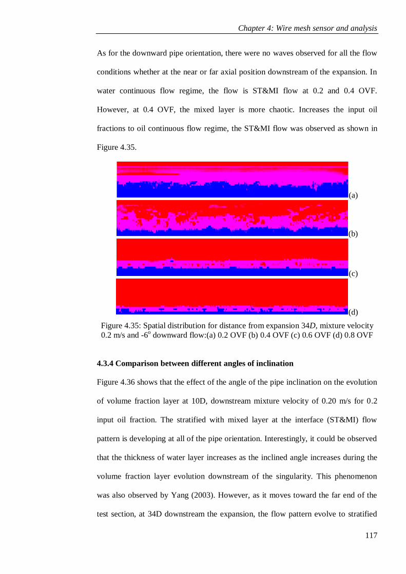
Chapter 4: Wire mesh sensor and analysis
117
As for the downward pipe orientation, there were no waves observed for all the flow
conditions whether at the near or far axial position downstream of the expansion. In
water continuous flow regime, the flow is ST&MI flow at 0.2 and 0.4 OVF.
However, at 0.4 OVF, the mixed layer is more chaotic. Increases the input oil
fractions to oil continuous flow regime, the ST&MI flow was observed as shown in
Figure 4.35.
(a)
(b)
(c)
(d)
Figure 4.35: Spatial distribution for distance from expansion 34D, mixture velocity
0.2 m/s and -6o downward flow:(a) 0.2 OVF (b) 0.4 OVF (c) 0.6 OVF (d) 0.8 OVF
4.3.4 Comparison between different angles of inclination
Figure 4.36 shows that the effect of the angle of the pipe inclination on the evolution
of volume fraction layer at 10D, downstream mixture velocity of 0.20 m/s for 0.2
input oil fraction. The stratified with mixed layer at the interface (ST&MI) flow
pattern is developing at all of the pipe orientation. Interestingly, it could be observed
that the thickness of water layer increases as the inclined angle increases during the
volume fraction layer evolution downstream of the singularity. This phenomenon
was also observed by Yang (2003). However, as it moves toward the far end of the
test section, at 34D downstream the expansion, the flow pattern evolve to stratified
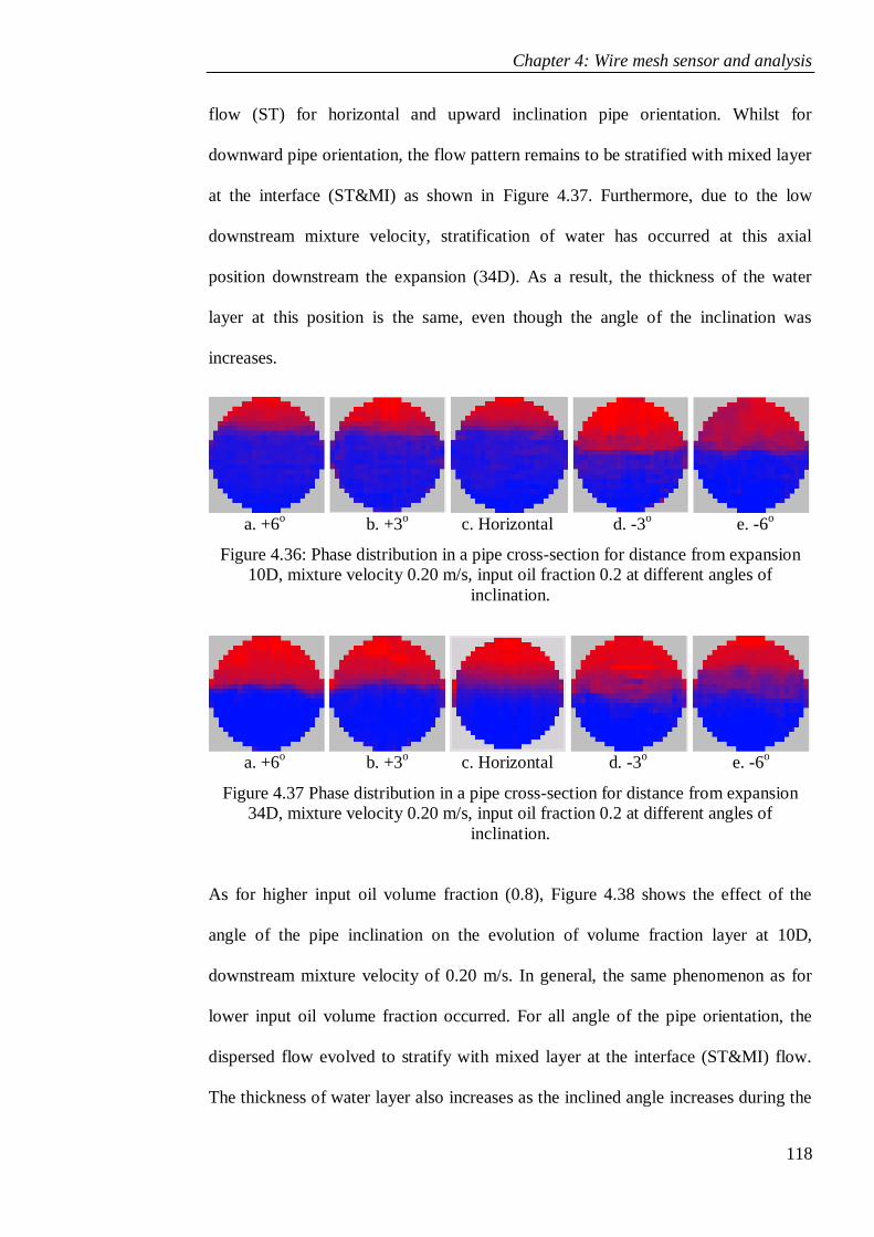
Chapter 4: Wire mesh sensor and analysis
118
flow (ST) for horizontal and upward inclination pipe orientation. Whilst for
downward pipe orientation, the flow pattern remains to be stratified with mixed layer
at the interface (ST&MI) as shown in Figure 4.37. Furthermore, due to the low
downstream mixture velocity, stratification of water has occurred at this axial
position downstream the expansion (34D). As a result, the thickness of the water
layer at this position is the same, even though the angle of the inclination was
increases.
a. +6
o b. +3
o c. Horizontal d. -3
o e. -6
o
Figure 4.36: Phase distribution in a pipe cross-section for distance from expansion
10D, mixture velocity 0.20 m/s, input oil fraction 0.2 at different angles of
inclination.
a. +6
o b. +3
o c. Horizontal d. -3
o e. -6
o
Figure 4.37 Phase distribution in a pipe cross-section for distance from expansion
34D, mixture velocity 0.20 m/s, input oil fraction 0.2 at different angles of
inclination.
As for higher input oil volume fraction (0.8), Figure 4.38 shows the effect of the
angle of the pipe inclination on the evolution of volume fraction layer at 10D,
downstream mixture velocity of 0.20 m/s. In general, the same phenomenon as for
lower input oil volume fraction occurred. For all angle of the pipe orientation, the
dispersed flow evolved to stratify with mixed layer at the interface (ST&MI) flow.
The thickness of water layer also increases as the inclined angle increases during the
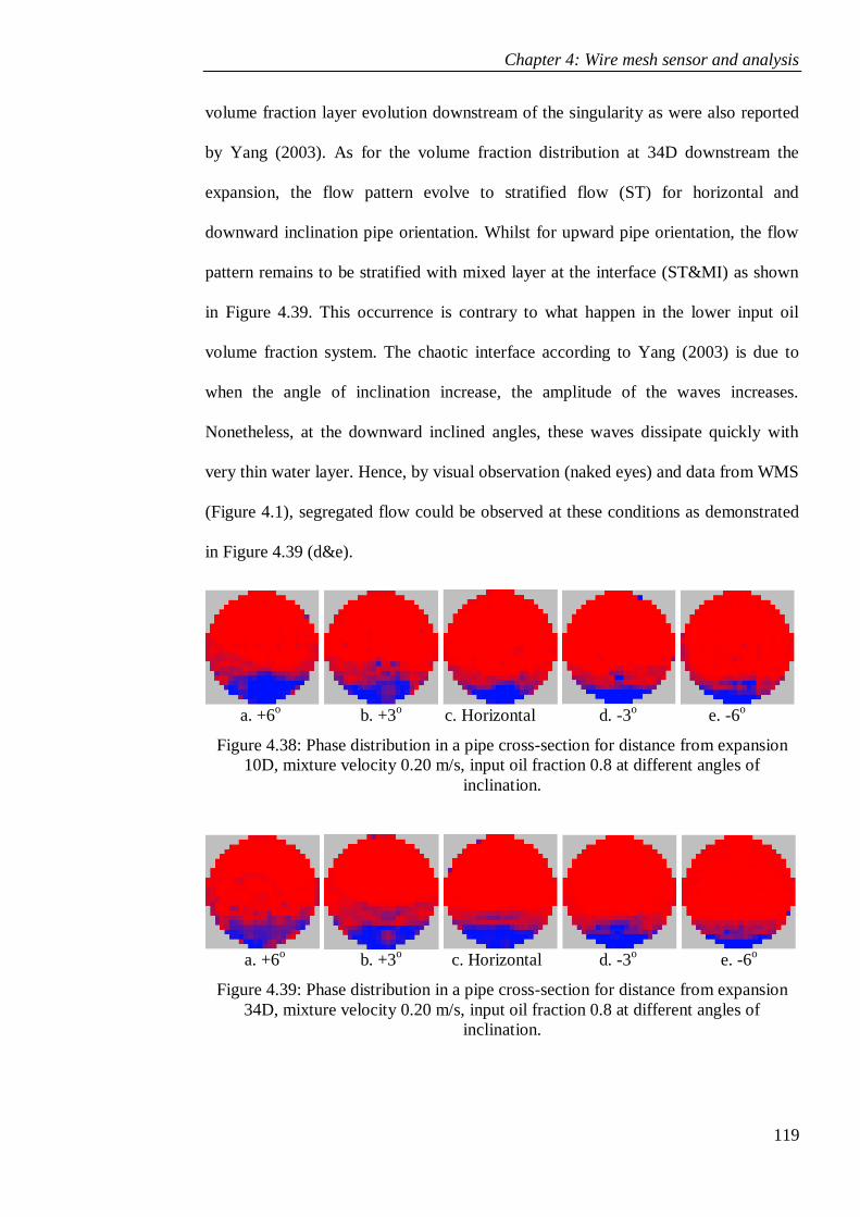
Chapter 4: Wire mesh sensor and analysis
119
volume fraction layer evolution downstream of the singularity as were also reported
by Yang (2003). As for the volume fraction distribution at 34D downstream the
expansion, the flow pattern evolve to stratified flow (ST) for horizontal and
downward inclination pipe orientation. Whilst for upward pipe orientation, the flow
pattern remains to be stratified with mixed layer at the interface (ST&MI) as shown
in Figure 4.39. This occurrence is contrary to what happen in the lower input oil
volume fraction system. The chaotic interface according to Yang (2003) is due to
when the angle of inclination increase, the amplitude of the waves increases.
Nonetheless, at the downward inclined angles, these waves dissipate quickly with
very thin water layer. Hence, by visual observation (naked eyes) and data from WMS
(Figure 4.1), segregated flow could be observed at these conditions as demonstrated
in Figure 4.39 (d&e).
a. +6
o b. +3
o c. Horizontal d. -3
o e. -6
o
Figure 4.38: Phase distribution in a pipe cross-section for distance from expansion
10D, mixture velocity 0.20 m/s, input oil fraction 0.8 at different angles of
inclination.
a. +6
o b. +3
o c. Horizontal d. -3
o e. -6
o
Figure 4.39: Phase distribution in a pipe cross-section for distance from expansion
34D, mixture velocity 0.20 m/s, input oil fraction 0.8 at different angles of
inclination.

Chapter 4: Wire mesh sensor and analysis
120
Results of the interface shapes for the stratified oil-water flow of Hasan (2006) at
24D were compared with present data at 20D. Hasan (2006) observed a concave
interface shape at this position for horizontal and downward pipe orientation as
shown in Figure 4.40 and 4.41. Interestingly, in the present work this was confirmed
(refer to Figure 4.12 and 4.33), the same interface shapes was also identified. Even
though the spatial accuracy of the WMS better than the spatial accuracy of ECT. The
fact that both techniques giving the same trend, basically give confirmation of the
results presented above.
0.2 OVF 0.5 OVF 0.7 OVF
Figure 4.40: Phase distribution in a pipe cross-section for distance from expansion
24D, mixture velocity 0.2 m/s and horizontal flow, at different input oil fractions
(Hasan, 2006).
0.2 OVF 0.5 OVF 0.7 OVF
Figure 4.41: Phase distribution in a pipe cross-section for distance from expansion
24D, mixture velocity 0.2 m/s and -4 degree flow, at different input oil fractions
(Hasan, 2006).
Furthermore, WMS image of the spatial distribution time average were shown in
Figure 4.42 to visualize the phenomenon of waves in the pipe expansion to show the
effect of pipe inclination. It was observed that with decrease in the inclined angle, the
waves gradually dissipate. The highest waves amplitude for +6o orientation is ~
0.29D whereas for +3o the waves amplitude is ~ 0.23D. Furthermore, it is noticeable
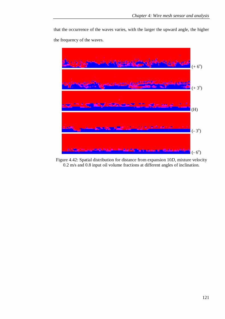
Chapter 4: Wire mesh sensor and analysis
121
that the occurrence of the waves varies, with the larger the upward angle, the higher
the frequency of the waves.
(+ 6o)
(+ 3o)
(H)
(- 3o)
(- 6o)
Figure 4.42: Spatial distribution for distance from expansion 10D, mixture velocity
0.2 m/s and 0.8 input oil volume fractions at different angles of inclination.
Chapter 5: Evolution of interface
122
CHAPTER 5
EVOLUTION OF INTERFACE
Separation of two immiscible liquids is important in the petroleum and chemical
industries. As many liquid-liquid systems travel as one phase dispersed in another.
To achieve separation these dispersion have to be converted into stratified flow. In
the previous chapter, application of the latest tomography techniques; capacitance
wire mesh sensor (CapWMS), tomography techniques to internally diagnose the
mixing and phase distributions within process units was implemented of the test
section. The purposes of this study are to explore the factors (rig configuration and
operational conditions) affecting the evolution of phase layers downstream of the
pipe expansion.
In designing such simple phase separator, as high a velocity as possible is sought so
as to minimize the size of equipment. Extensive studies have been reported on the
liquid-liquid two-phase flow in pipes (Valle, 1998; Azzopardi, 2001; Brauner, 2002).
When the flow is stratified, the position of the interface can be reasonably predicted
using the model of Taitel and Dukler (1976), originally developed for gas-liquid
glow. Kurban et al. (1995) and Simmons et al. (1998) have shown the method to be
accurate for the horizontal flows. The effect of upward pipe inclination on flow
pattern in liquid-liquid flows has been the subject of study by Vedapuri et al. (1997
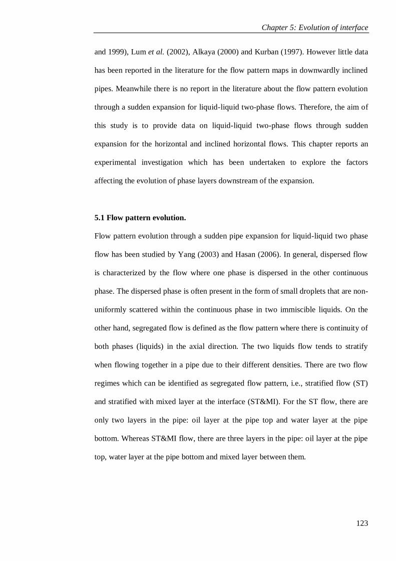
Chapter 5: Evolution of interface
123
and 1999), Lum et al. (2002), Alkaya (2000) and Kurban (1997). However little data
has been reported in the literature for the flow pattern maps in downwardly inclined
pipes. Meanwhile there is no report in the literature about the flow pattern evolution
through a sudden expansion for liquid-liquid two-phase flows. Therefore, the aim of
this study is to provide data on liquid-liquid two-phase flows through sudden
expansion for the horizontal and inclined horizontal flows. This chapter reports an
experimental investigation which has been undertaken to explore the factors
affecting the evolution of phase layers downstream of the expansion.
5.1 Flow pattern evolution.
Flow pattern evolution through a sudden pipe expansion for liquid-liquid two phase
flow has been studied by Yang (2003) and Hasan (2006). In general, dispersed flow
is characterized by the flow where one phase is dispersed in the other continuous
phase. The dispersed phase is often present in the form of small droplets that are non-
uniformly scattered within the continuous phase in two immiscible liquids. On the
other hand, segregated flow is defined as the flow pattern where there is continuity of
both phases (liquids) in the axial direction. The two liquids flow tends to stratify
when flowing together in a pipe due to their different densities. There are two flow
regimes which can be identified as segregated flow pattern, i.e., stratified flow (ST)
and stratified with mixed layer at the interface (ST&MI). For the ST flow, there are
only two layers in the pipe: oil layer at the pipe top and water layer at the pipe
bottom. Whereas ST&MI flow, there are three layers in the pipe: oil layer at the pipe
top, water layer at the pipe bottom and mixed layer between them.
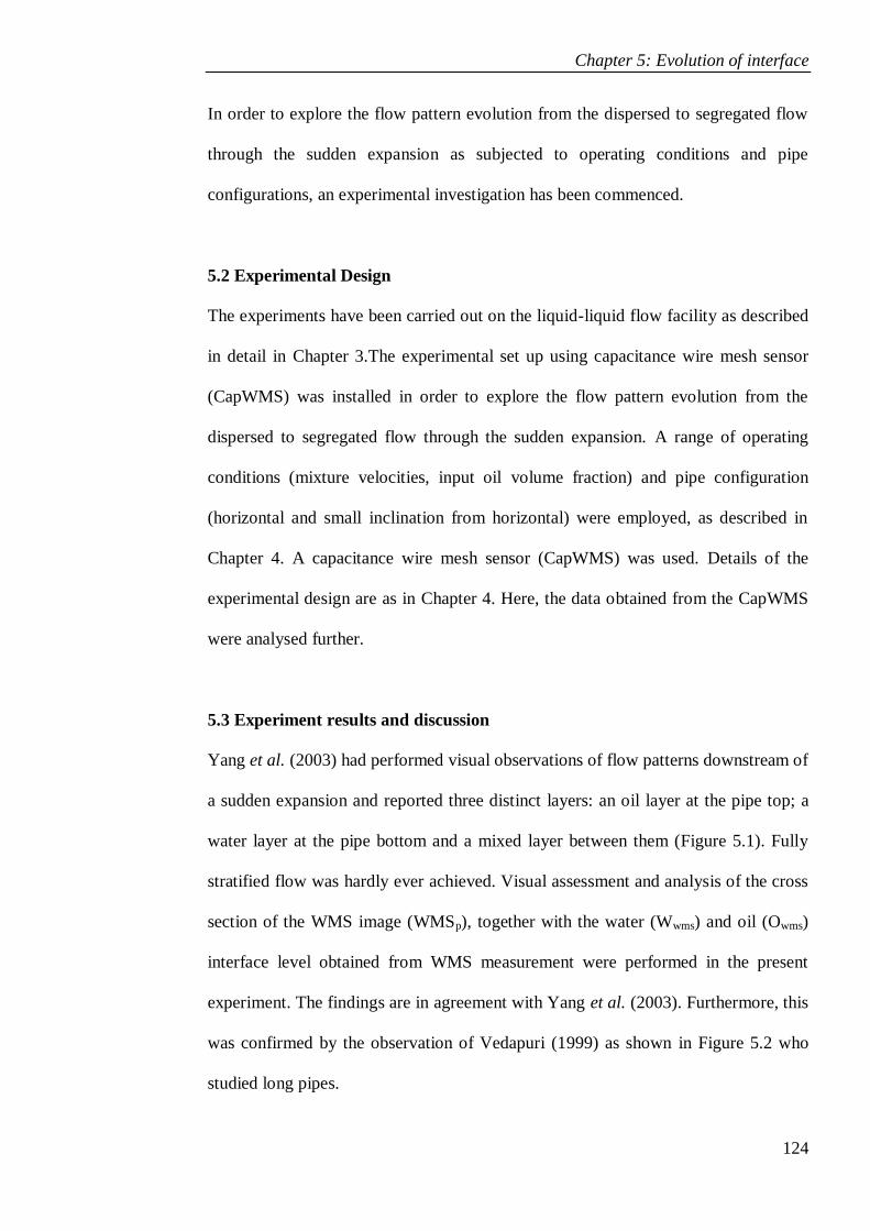
Chapter 5: Evolution of interface
124
In order to explore the flow pattern evolution from the dispersed to segregated flow
through the sudden expansion as subjected to operating conditions and pipe
configurations, an experimental investigation has been commenced.
5.2 Experimental Design
The experiments have been carried out on the liquid-liquid flow facility as described
in detail in Chapter 3.The experimental set up using capacitance wire mesh sensor
(CapWMS) was installed in order to explore the flow pattern evolution from the
dispersed to segregated flow through the sudden expansion. A range of operating
conditions (mixture velocities, input oil volume fraction) and pipe configuration
(horizontal and small inclination from horizontal) were employed, as described in
Chapter 4. A capacitance wire mesh sensor (CapWMS) was used. Details of the
experimental design are as in Chapter 4. Here, the data obtained from the CapWMS
were analysed further.
5.3 Experiment results and discussion
Yang et al. (2003) had performed visual observations of flow patterns downstream of
a sudden expansion and reported three distinct layers: an oil layer at the pipe top; a
water layer at the pipe bottom and a mixed layer between them (Figure 5.1). Fully
stratified flow was hardly ever achieved. Visual assessment and analysis of the cross
section of the WMS image (WMSp), together with the water (Wwms) and oil (Owms)
interface level obtained from WMS measurement were performed in the present
experiment. The findings are in agreement with Yang et al. (2003). Furthermore, this
was confirmed by the observation of Vedapuri (1999) as shown in Figure 5.2 who
studied long pipes.
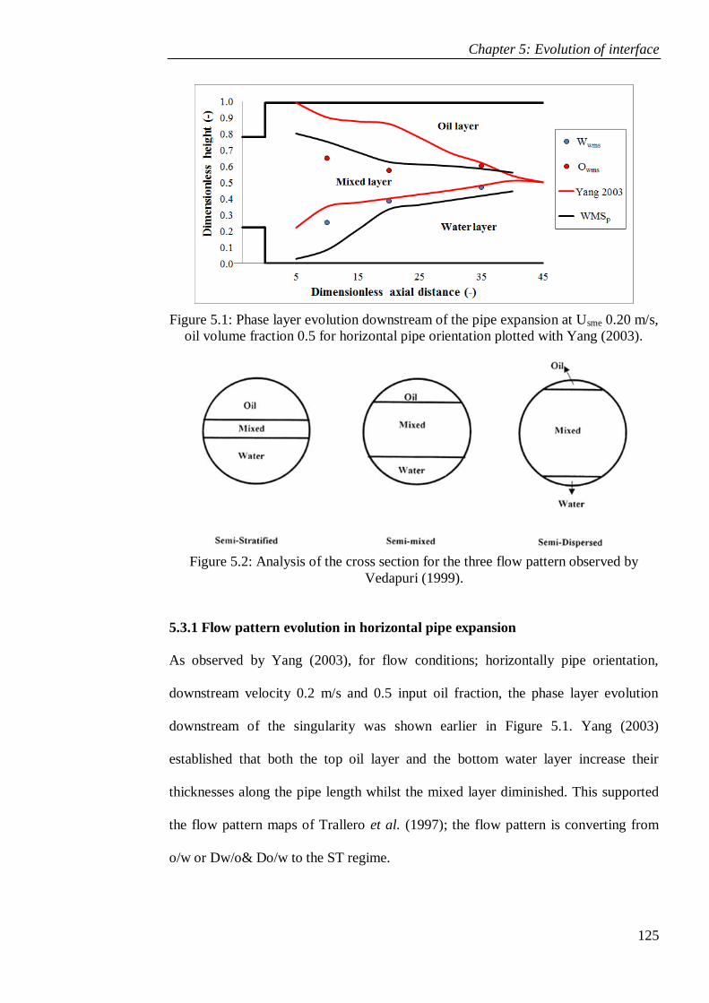
Chapter 5: Evolution of interface
125
Figure 5.1: Phase layer evolution downstream of the pipe expansion at Usme 0.20 m/s,
oil volume fraction 0.5 for horizontal pipe orientation plotted with Yang (2003).
Figure 5.2: Analysis of the cross section for the three flow pattern observed by
Vedapuri (1999).
5.3.1 Flow pattern evolution in horizontal pipe expansion
As observed by Yang (2003), for flow conditions; horizontally pipe orientation,
downstream velocity 0.2 m/s and 0.5 input oil fraction, the phase layer evolution
downstream of the singularity was shown earlier in Figure 5.1. Yang (2003)
established that both the top oil layer and the bottom water layer increase their
thicknesses along the pipe length whilst the mixed layer diminished. This supported
the flow pattern maps of Trallero et al. (1997); the flow pattern is converting from
o/w or Dw/o& Do/w to the ST regime.
Chapter 5: Evolution of interface
126
The physical properties of the phases, the flow pattern and drop sizes present in the
inlet of the pipe are parameters which are likely to affect the separation. It is
therefore of interest to examine the effect of input oil volume fraction, the mixture
velocity and the distance from expansion, for horizontally piping orientations. In this
chapter, the purpose of these studies is to investigate the effects of the experimental
conditions on the phase volume fraction distribution and the flow development in
horizontal pipe.
Figure 5.3 shows the effect of the input oil volume fraction on the phase layer
evolution downstream of the horizontally pipe expansion at a downstream mixture
velocity (Usme) 0.20 m/s. The phase layer evolution could be clearly distinguished
with oil flowing on the pipe top and water on the pipe bottom while mixed layer
were in flowing in between them. For all input oil volume fractions employed, the
flows were not fully developed to ST regime within the length of the test pipe. The
nearest approach was oil volume fraction of 0.2 and 0.8.
Figure 5.3: Effect of the oil volume fraction on the phase layer evolution downstream
of the horizontally pipe expansion at Usme 0.20 m/s
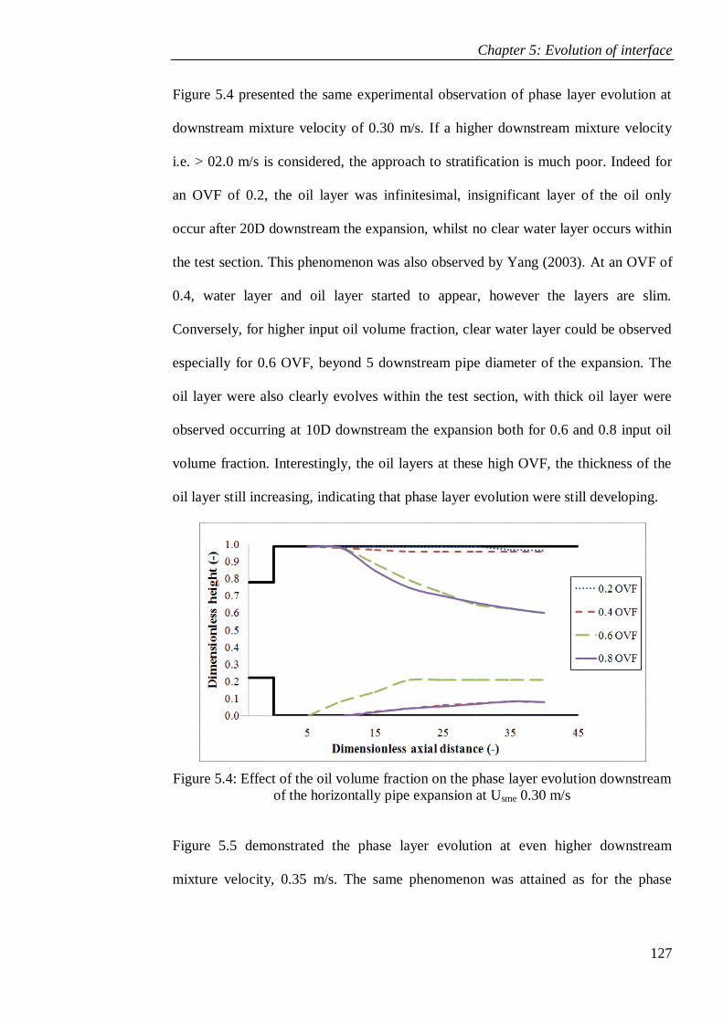
Chapter 5: Evolution of interface
127
Figure 5.4 presented the same experimental observation of phase layer evolution at
downstream mixture velocity of 0.30 m/s. If a higher downstream mixture velocity
i.e. > 02.0 m/s is considered, the approach to stratification is much poor. Indeed for
an OVF of 0.2, the oil layer was infinitesimal, insignificant layer of the oil only
occur after 20D downstream the expansion, whilst no clear water layer occurs within
the test section. This phenomenon was also observed by Yang (2003). At an OVF of
0.4, water layer and oil layer started to appear, however the layers are slim.
Conversely, for higher input oil volume fraction, clear water layer could be observed
especially for 0.6 OVF, beyond 5 downstream pipe diameter of the expansion. The
oil layer were also clearly evolves within the test section, with thick oil layer were
observed occurring at 10D downstream the expansion both for 0.6 and 0.8 input oil
volume fraction. Interestingly, the oil layers at these high OVF, the thickness of the
oil layer still increasing, indicating that phase layer evolution were still developing.
Figure 5.4: Effect of the oil volume fraction on the phase layer evolution downstream
of the horizontally pipe expansion at Usme 0.30 m/s
Figure 5.5 demonstrated the phase layer evolution at even higher downstream
mixture velocity, 0.35 m/s. The same phenomenon was attained as for the phase
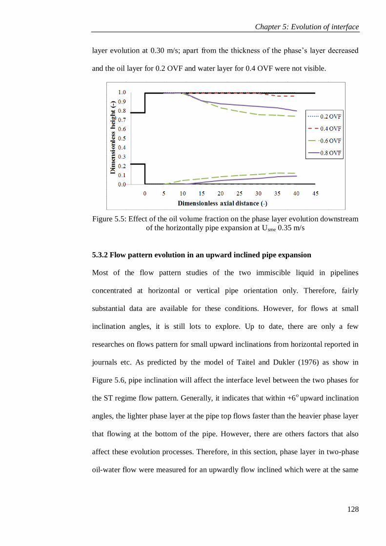
Chapter 5: Evolution of interface
128
layer evolution at 0.30 m/s; apart from the thickness of the phase‟s layer decreased
and the oil layer for 0.2 OVF and water layer for 0.4 OVF were not visible.
Figure 5.5: Effect of the oil volume fraction on the phase layer evolution downstream
of the horizontally pipe expansion at Usme 0.35 m/s
5.3.2 Flow pattern evolution in an upward inclined pipe expansion
Most of the flow pattern studies of the two immiscible liquid in pipelines
concentrated at horizontal or vertical pipe orientation only. Therefore, fairly
substantial data are available for these conditions. However, for flows at small
inclination angles, it is still lots to explore. Up to date, there are only a few
researches on flows pattern for small upward inclinations from horizontal reported in
journals etc. As predicted by the model of Taitel and Dukler (1976) as show in
Figure 5.6, pipe inclination will affect the interface level between the two phases for
the ST regime flow pattern. Generally, it indicates that within +6o upward inclination
angles, the lighter phase layer at the pipe top flows faster than the heavier phase layer
that flowing at the bottom of the pipe. However, there are others factors that also
affect these evolution processes. Therefore, in this section, phase layer in two-phase
oil-water flow were measured for an upwardly flow inclined which were at the same

Chapter 5: Evolution of interface
129
experiments conditions used in horizontal flow. Analysis of results and discussion
are presented below.
Figure 5.6: Prediction of interfacial level for stratified flow with the model of Taitel
and Dukler, 1976 by Yang (2003)
Figure 5.7 shows the trend of the interface between the water layer and oil layer at a
lower downstream velocity of 0.20 m/s for +3o upward inclined pipe orientation. It
can be seen that within the test distance, the data from this present work as shown in
Figure 5.7 are in agreement with Taitel and Dukler (1976) predictions. Phase layer of
oil and water layer of those flow conditions could be distinct clearly; the oil layer
was visibly flow at the pipe top and the water layer at the pipe bottom. Nevertheless,
the flow could not develop to ST regime within the test distance. Instead, the mixed
layer thicknesses growth to thicker layer compared to the horizontal counterpart.
0.1 0.2
0.5 0.7
0.9
Input oil volume fraction
0.9 0.7 0.5 0.2 0.1
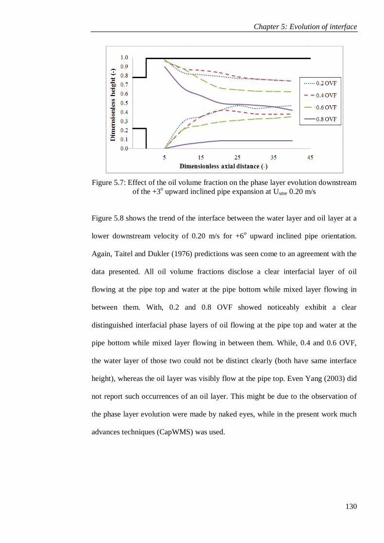
Chapter 5: Evolution of interface
130
Figure 5.7: Effect of the oil volume fraction on the phase layer evolution downstream
of the +3o upward inclined pipe expansion at Usme 0.20 m/s
Figure 5.8 shows the trend of the interface between the water layer and oil layer at a
lower downstream velocity of 0.20 m/s for +6o upward inclined pipe orientation.
Again, Taitel and Dukler (1976) predictions was seen come to an agreement with the
data presented. All oil volume fractions disclose a clear interfacial layer of oil
flowing at the pipe top and water at the pipe bottom while mixed layer flowing in
between them. With, 0.2 and 0.8 OVF showed noticeably exhibit a clear
distinguished interfacial phase layers of oil flowing at the pipe top and water at the
pipe bottom while mixed layer flowing in between them. While, 0.4 and 0.6 OVF,
the water layer of those two could not be distinct clearly (both have same interface
height), whereas the oil layer was visibly flow at the pipe top. Even Yang (2003) did
not report such occurrences of an oil layer. This might be due to the observation of
the phase layer evolution were made by naked eyes, while in the present work much
advances techniques (CapWMS) was used.
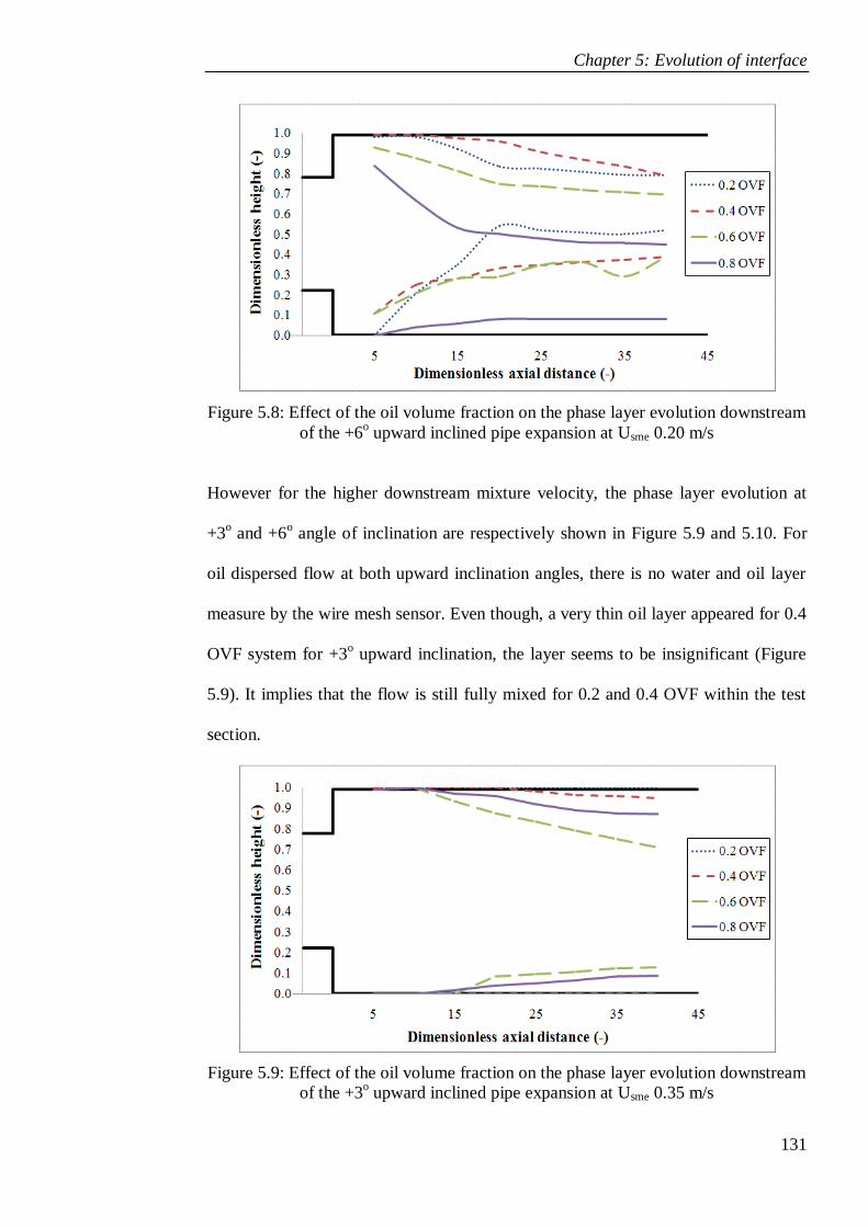
Chapter 5: Evolution of interface
131
Figure 5.8: Effect of the oil volume fraction on the phase layer evolution downstream
of the +6o upward inclined pipe expansion at Usme 0.20 m/s
However for the higher downstream mixture velocity, the phase layer evolution at
+3o and +6
o angle of inclination are respectively shown in Figure 5.9 and 5.10. For
oil dispersed flow at both upward inclination angles, there is no water and oil layer
measure by the wire mesh sensor. Even though, a very thin oil layer appeared for 0.4
OVF system for +3o upward inclination, the layer seems to be insignificant (Figure
5.9). It implies that the flow is still fully mixed for 0.2 and 0.4 OVF within the test
section.
Figure 5.9: Effect of the oil volume fraction on the phase layer evolution downstream
of the +3o upward inclined pipe expansion at Usme 0.35 m/s
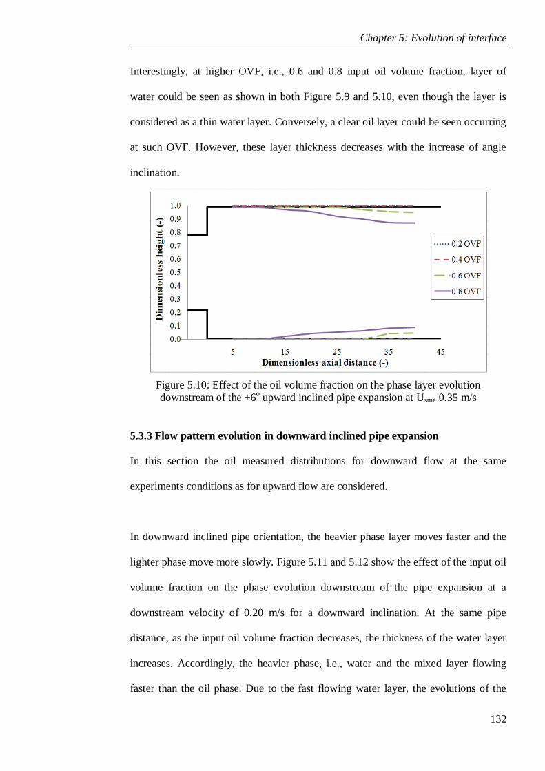
Chapter 5: Evolution of interface
132
Interestingly, at higher OVF, i.e., 0.6 and 0.8 input oil volume fraction, layer of
water could be seen as shown in both Figure 5.9 and 5.10, even though the layer is
considered as a thin water layer. Conversely, a clear oil layer could be seen occurring
at such OVF. However, these layer thickness decreases with the increase of angle
inclination.
Figure 5.10: Effect of the oil volume fraction on the phase layer evolution
downstream of the +6o upward inclined pipe expansion at Usme 0.35 m/s
5.3.3 Flow pattern evolution in downward inclined pipe expansion
In this section the oil measured distributions for downward flow at the same
experiments conditions as for upward flow are considered.
In downward inclined pipe orientation, the heavier phase layer moves faster and the
lighter phase move more slowly. Figure 5.11 and 5.12 show the effect of the input oil
volume fraction on the phase evolution downstream of the pipe expansion at a
downstream velocity of 0.20 m/s for a downward inclination. At the same pipe
distance, as the input oil volume fraction decreases, the thickness of the water layer
increases. Accordingly, the heavier phase, i.e., water and the mixed layer flowing
faster than the oil phase. Due to the fast flowing water layer, the evolutions of the
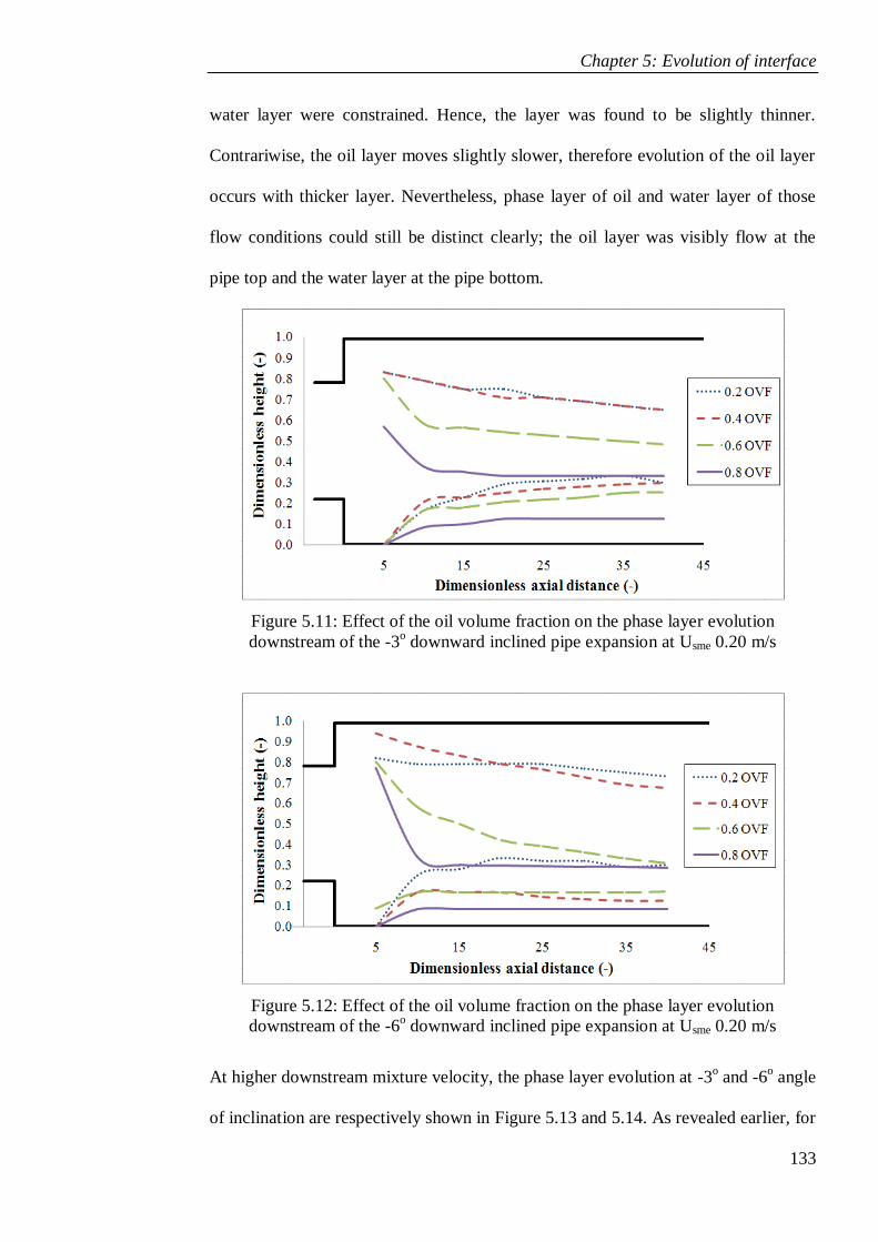
Chapter 5: Evolution of interface
133
water layer were constrained. Hence, the layer was found to be slightly thinner.
Contrariwise, the oil layer moves slightly slower, therefore evolution of the oil layer
occurs with thicker layer. Nevertheless, phase layer of oil and water layer of those
flow conditions could still be distinct clearly; the oil layer was visibly flow at the
pipe top and the water layer at the pipe bottom.
Figure 5.11: Effect of the oil volume fraction on the phase layer evolution
downstream of the -3o downward inclined pipe expansion at Usme 0.20 m/s
Figure 5.12: Effect of the oil volume fraction on the phase layer evolution
downstream of the -6o downward inclined pipe expansion at Usme 0.20 m/s
At higher downstream mixture velocity, the phase layer evolution at -3o and -6
o angle
of inclination are respectively shown in Figure 5.13 and 5.14. As revealed earlier, for
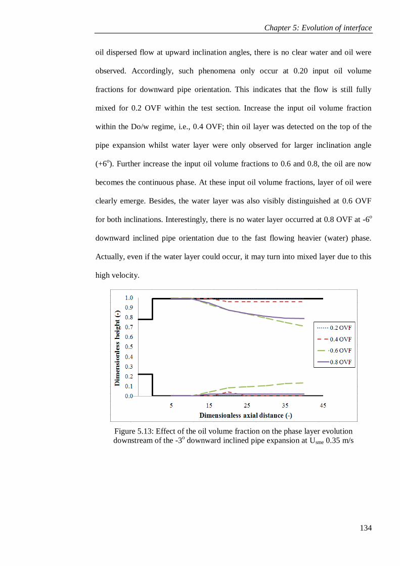
Chapter 5: Evolution of interface
134
oil dispersed flow at upward inclination angles, there is no clear water and oil were
observed. Accordingly, such phenomena only occur at 0.20 input oil volume
fractions for downward pipe orientation. This indicates that the flow is still fully
mixed for 0.2 OVF within the test section. Increase the input oil volume fraction
within the Do/w regime, i.e., 0.4 OVF; thin oil layer was detected on the top of the
pipe expansion whilst water layer were only observed for larger inclination angle
(+6o). Further increase the input oil volume fractions to 0.6 and 0.8, the oil are now
becomes the continuous phase. At these input oil volume fractions, layer of oil were
clearly emerge. Besides, the water layer was also visibly distinguished at 0.6 OVF
for both inclinations. Interestingly, there is no water layer occurred at 0.8 OVF at -6o
downward inclined pipe orientation due to the fast flowing heavier (water) phase.
Actually, even if the water layer could occur, it may turn into mixed layer due to this
high velocity.
Figure 5.13: Effect of the oil volume fraction on the phase layer evolution
downstream of the -3o downward inclined pipe expansion at Usme 0.35 m/s
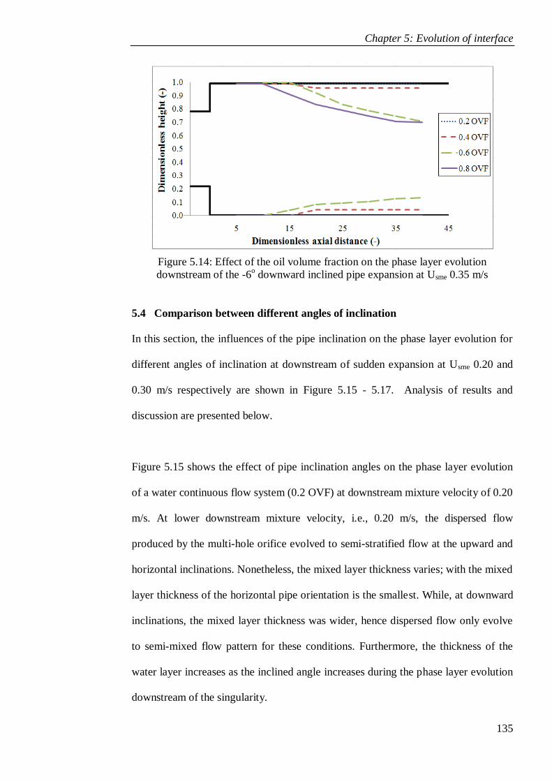
Chapter 5: Evolution of interface
135
Figure 5.14: Effect of the oil volume fraction on the phase layer evolution
downstream of the -6o downward inclined pipe expansion at Usme 0.35 m/s
5.4 Comparison between different angles of inclination
In this section, the influences of the pipe inclination on the phase layer evolution for
different angles of inclination at downstream of sudden expansion at Usme 0.20 and
0.30 m/s respectively are shown in Figure 5.15 - 5.17. Analysis of results and
discussion are presented below.
Figure 5.15 shows the effect of pipe inclination angles on the phase layer evolution
of a water continuous flow system (0.2 OVF) at downstream mixture velocity of 0.20
m/s. At lower downstream mixture velocity, i.e., 0.20 m/s, the dispersed flow
produced by the multi-hole orifice evolved to semi-stratified flow at the upward and
horizontal inclinations. Nonetheless, the mixed layer thickness varies; with the mixed
layer thickness of the horizontal pipe orientation is the smallest. While, at downward
inclinations, the mixed layer thickness was wider, hence dispersed flow only evolve
to semi-mixed flow pattern for these conditions. Furthermore, the thickness of the
water layer increases as the inclined angle increases during the phase layer evolution
downstream of the singularity.
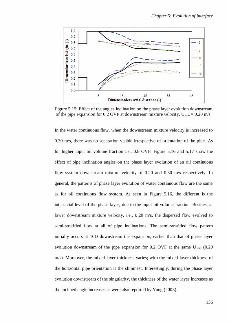
Chapter 5: Evolution of interface
136
Figure 5.15: Effect of the angles inclination on the phase layer evolution downstream
of the pipe expansion for 0.2 OVF at downstream mixture velocity, Usme = 0.20 m/s.
In the water continuous flow, when the downstream mixture velocity is increased to
0.30 m/s, there was no separation visible irrespective of orientation of the pipe. As
for higher input oil volume fraction i.e., 0.8 OVF, Figure 5.16 and 5.17 show the
effect of pipe inclination angles on the phase layer evolution of an oil continuous
flow system downstream mixture velocity of 0.20 and 0.30 m/s respectively. In
general, the patterns of phase layer evolution of water continuous flow are the same
as for oil continuous flow system. As seen in Figure 5.16, the different is the
interfacial level of the phase layer, due to the input oil volume fraction. Besides, at
lower downstream mixture velocity, i.e., 0.20 m/s, the dispersed flow evolved to
semi-stratified flow at all of pipe inclinations. The semi-stratified flow pattern
initially occurs at 10D downstream the expansion, earlier than that of phase layer
evolution downstream of the pipe expansion for 0.2 OVF at the same Usme (0.20
m/s). Moreover, the mixed layer thickness varies; with the mixed layer thickness of
the horizontal pipe orientation is the slimmest. Interestingly, during the phase layer
evolution downstream of the singularity, the thickness of the water layer increases as
the inclined angle increases as were also reported by Yang (2003).
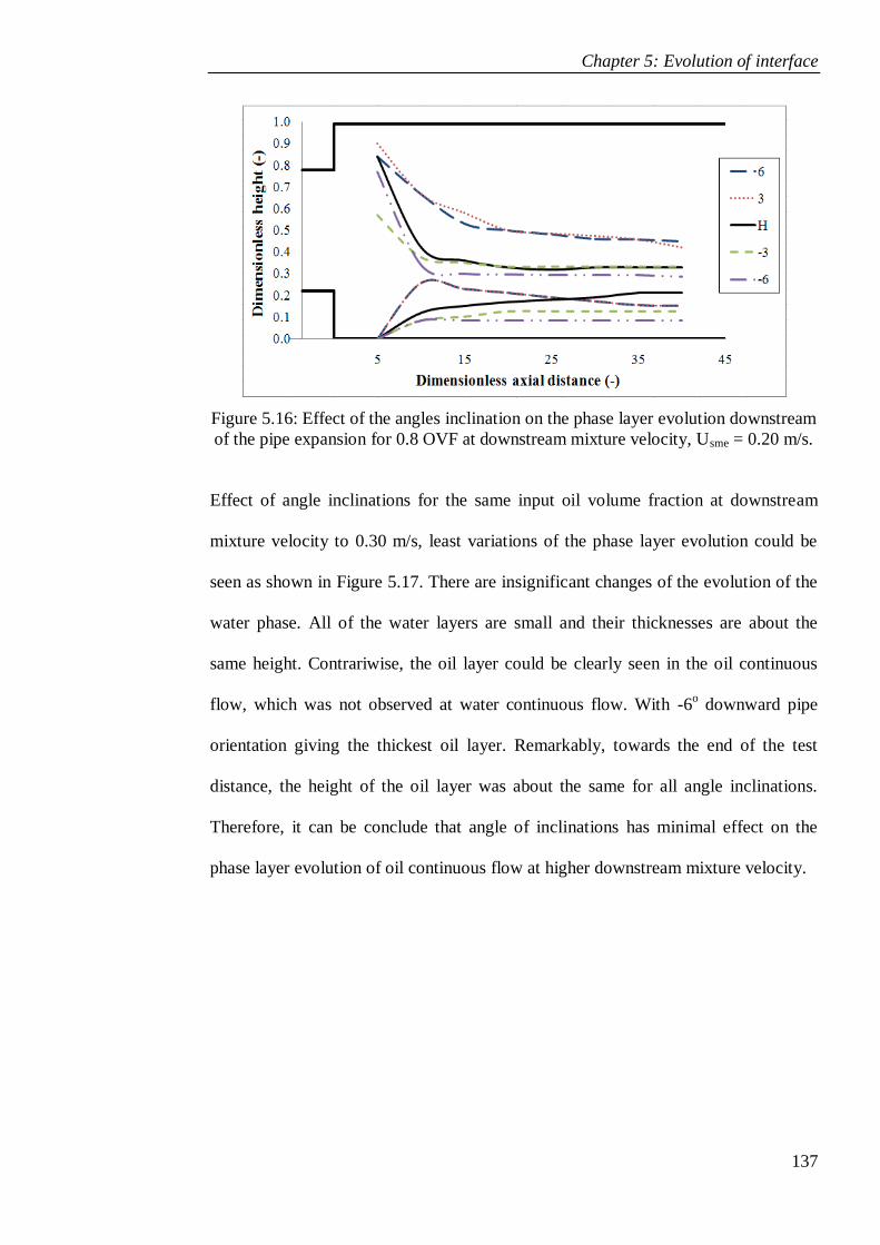
Chapter 5: Evolution of interface
137
Figure 5.16: Effect of the angles inclination on the phase layer evolution downstream
of the pipe expansion for 0.8 OVF at downstream mixture velocity, Usme = 0.20 m/s.
Effect of angle inclinations for the same input oil volume fraction at downstream
mixture velocity to 0.30 m/s, least variations of the phase layer evolution could be
seen as shown in Figure 5.17. There are insignificant changes of the evolution of the
water phase. All of the water layers are small and their thicknesses are about the
same height. Contrariwise, the oil layer could be clearly seen in the oil continuous
flow, which was not observed at water continuous flow. With -6o downward pipe
orientation giving the thickest oil layer. Remarkably, towards the end of the test
distance, the height of the oil layer was about the same for all angle inclinations.
Therefore, it can be conclude that angle of inclinations has minimal effect on the
phase layer evolution of oil continuous flow at higher downstream mixture velocity.
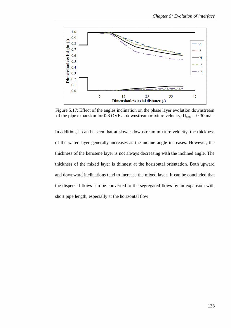
Chapter 5: Evolution of interface
138
Figure 5.17: Effect of the angles inclination on the phase layer evolution downstream
of the pipe expansion for 0.8 OVF at downstream mixture velocity, Usme = 0.30 m/s.
In addition, it can be seen that at slower downstream mixture velocity, the thickness
of the water layer generally increases as the incline angle increases. However, the
thickness of the kerosene layer is not always decreasing with the inclined angle. The
thickness of the mixed layer is thinnest at the horizontal orientation. Both upward
and downward inclinations tend to increase the mixed layer. It can be concluded that
the dispersed flows can be converted to the segregated flows by an expansion with
short pipe length, especially at the horizontal flow.
Chapter 6: Drop sizes downstream of pipe expansion
139
CHAPTER 6
DROP SIZES DOWNSTREAM OF PIPE EXPANSION
In most of industrial processes, knowledge of the nature of multiphase flow is
important. For example, in chemical, petrochemical and food industries, liquid-liquid
dispersions appear in processes such as emulsification and two-phase reactions.
Therefore, knowledge of drop formation and the nature of dispersions mechanisms
involve in their formation, as well as the size distribution of any particles or liquids
droplets existent are important. This information is important for analysing the
hydrodynamic and transport phenomena in the flow of liquid-liquid dispersions and
also a valuable design parameter in order to design efficient and cost effective
equipment. Hence, information of the drop size and drop size distribution over the
cross section of the pipe downstream of an expansion is presented in this chapter.
6.1 Drop size distribution
Knowledge and evidence of the drop size distribution is necessary when subsequent
separation of two phases of liquids is considered. Most of the experimental works on
drop break-up and coalescence has mainly been conducted in stirred tanks. As a
result, several models for the relationships between drop size, physical properties and
operating conditions have been proposed for predicting the maximum drop diameter
and minimum drop diameter during turbulent dispersion flow that can then be
correlated with drop break-up and drop coalescence. Conversely, due to the nature of
Chapter 6: Drop sizes downstream of pipe expansion
140
the experiments involved, in-situ and on-line (during pipe flow) drop size
distributions data conducted in pipelines are very much inadequate compared to the
ones conducted in stirred vessels or tanks.
Number of studies that address the drop size distribution in pipe flow of two
immiscible fluids is few. Evolution of drops emerging from homogenise system into
a pipe flow merely exist. The inclination of the piping can also have a significant
effect on drop size distribution. Up to date, there have only been a small number of
studies on the effect of expansions and inclinations on the drop size distribution of
oil-water dispersions. Even though, the effect of inclination on momentum transport
is readily estimated but the effect of pipe expansion with a small inclination is again
unknown. In other words, these sections of research area are remains unstudied.
Pipe expansion and inclination have been considered as the imposition on the flow of
an external field that affects momentum. Total pressure gradient for two-phase flow
has three components; frictional, acceleration and gravitational pressure gradients.
For horizontal oil-water flow, acceleration and gravitational components can be
neglected. For steady flows in inclined pipe the acceleration component can still be
neglected but the gravitational component becomes very significant. An expansion
provides an unfavourable pressure gradient in multiphase flow, whereas inclination is
a skewing of the buoyant body force to the stream wise pressure gradient. Therefore,
particular attention in this research has been applied to the drop size measurements of
two immiscible liquids downstream of an expansion in a pipe with small inclination
angles. The size of the dispersed phase is important when interfacial mass and/or
heat transfer are involved and will affect phase separation at the end of the process.

Chapter 6: Drop sizes downstream of pipe expansion
141
6.2 Experimental Design
Here, an experimental study of drops downstream of a pipe expansion using a laser
backscatter technique is presented. Measurements were taken downstream of the
expansion both for horizontal and small positive or negative inclinations for a range
of flow rates.
Measurements of drop size were made using Lasentec equipment (FBRM M500P) at
the central axis of the pipe and also 17 mm either side (top or bottom) of the central
axis of the test section. The probe positions in a pipe cross-section were then labelled
as Top, Middle and Bottom. As for the axial positions, the terms used are defined as
near, for the distance from expansion of 10D; middle, for the distance from
expansion of 20D; and far, for the distance from expansion of 34D, where D is the
internal diameter of the pipe (68 mm) as shown in Figure 6.1.
Figure 6.1: Locations of probe positions downstream of the expansion and in a pipe
cross-section with height from the bottom of the pipe.
In order to explore the flow pattern from the dispersed to the segregated flow through
the expansion, the experiments are designed to distribute the inlet conditions in
dispersed regimes (Dw/o & Do/w, o/w and Do/w&w), and downstream mixtures
velocities (0.20, 0.30 and 0.35 m/s) in the expansion are in the segregated flow (ST
and ST&MI). Furthermore, the experiments were executed for input oil volume
Chapter 6: Drop sizes downstream of pipe expansion
142
fractions ranging from 0.2 - 0.8 for horizontal and inclined pipe orientations of -6, -3,
+3, +6 degrees. The positive and negative degrees indicated upward flow and
downward flow from horizontal, respectively.
By means of the FBRM M500P, a continuous measurement was then logged by a
computer and allowed the copyrighted software to produce distributions of droplet
chord as reviewed in Chapter 2. Diagram of the Lasentec FBRM M500P settings are
as shown in Figure 3.13.
The FBRM control software allows the acquired chord length data to be discretesed
into a series of user-defined intervals that is 100 linear-channels over the range of 1
to 1,000 microns. Six consecutive measurements were averaged to produce each
distribution, which one measurement duration was ten seconds. Furthermore,
measurements were made after 5 residence times of the system. Both, measurement
duration and 5 times residence time were to ensure the flow is in stable state and
sufficiently robust sample numbers for all condition that being investigated. In this
measurement campaign, FBRM software had been used to record the data before it
was transferred to Excel data format. These chord data were then converted to
diameter distribution using PAM2 and used for further statistical data processing.
Chapter 6: Drop sizes downstream of pipe expansion
143
6.3 Results and discussions
Previous researchers have made several important investigations of the simultaneous
flow of two immiscible liquids through sudden expansion in a pipe. Thus from their
preliminary investigations they have established three flow patterns which involved
in the flow of two immiscible liquids through sudden pipe expansion. These patterns
were dispersed flow, which appeared at the near position, followed by stratified flow
with mixing at the interface (ST&MI) at the middle position and stratified flow (ST)
at the far position (Yang et al., 2003).According to Yang et al. (2003), there are
clearly three regions of phase profile downstream of a pipe expansion. The regions
were classified as; oil region, at the top of the pipe cross section; mixed region, in
between lighter and heavier phase and; water region, at the bottom of the pipe cross
section (Yang et al., 2003). Yang et al. also reported that the mixed region was
dominating at the near position and diminished downstream in the pipe length whilst
the top oil region and bottom water region increased their layer until they achieved
fully stratified flow. In terms of the microscopic level, the mixed region is actually
occupied by different sizes of drops. These sizes, in principle, are then determined by
a balance between the overall rates of drop break-up and coalescence.
As mentioned earlier, phase profiles development downstream of a pipe expansion
was recorded by Yang et al. (2003). Later on, based on the profiles of Yang‟s, Hasan
(2006) performed experiments on the drops size distribution (chord length).A laser
backscatter technique was employed to measure the drop size distributions
downstream of the expansion. The Probability Apportioning Method (version 2) of
Langston et al. (2001) was used to transform a measured chord length distribution
into a drop size distribution. However, according to Hasan (2006) the results of the
Chapter 6: Drop sizes downstream of pipe expansion
144
transformation of chord lengths were shown unsatisfactorily. On the other hand, in
this present work the computational coding for the PAM2 has been updated and
upgraded as shown in Appendix 2B. This allowed the measured chord length
distribution to be transformed into a drop size distribution successfully. Since PAM2
(newer version) methods were found to successfully convert a chord length
distribution to a drop diameter distribution, the latter were then analysed further to
obtain Sauter mean diameter (SMD). This SMD of the drop diameter distribution
were then used in the results, discussion and comparisons between different
conditions.
6.3.1 SMD of drop size distribution in mixed and interface layer
With the intention of exploring the flow pattern evolution from the dispersed to the
segregated flow, factors affecting the flow pattern evolution through the sudden
expansion as mentioned earlier (Chapter 3) were studied. The flow patterns
downstream of the system are more concerned in this study due to the purpose of
stratification of the dispersed flow by using the expansion.
For the better understanding of the stratifications of the dispersed flow based on the
phase profile observations of Yang et al. (2003), the location at 34D was selected as
the main position to be measured. According to the flow pattern map of Trallero et
al. (1997), for the downstream mixture velocity of 0.20 m/s, its predicted flow
pattern might develop to the stratified flow (ST) or stratified mixed with layer at the
interface (ST&MI). Hence, SMD of drops diameter for several axial measurement
point (10D, 20D and 34D) from expansion within the test section at downstream
mixture velocity, Usme = 0.20 m/s and 0.8 input oil fraction at various probe positions
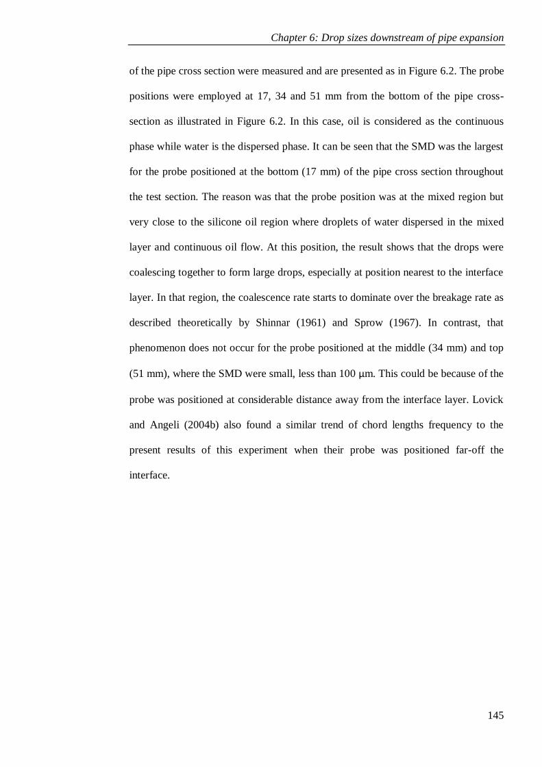
Chapter 6: Drop sizes downstream of pipe expansion
145
of the pipe cross section were measured and are presented as in Figure 6.2. The probe
positions were employed at 17, 34 and 51 mm from the bottom of the pipe cross-
section as illustrated in Figure 6.2. In this case, oil is considered as the continuous
phase while water is the dispersed phase. It can be seen that the SMD was the largest
for the probe positioned at the bottom (17 mm) of the pipe cross section throughout
the test section. The reason was that the probe position was at the mixed region but
very close to the silicone oil region where droplets of water dispersed in the mixed
layer and continuous oil flow. At this position, the result shows that the drops were
coalescing together to form large drops, especially at position nearest to the interface
layer. In that region, the coalescence rate starts to dominate over the breakage rate as
described theoretically by Shinnar (1961) and Sprow (1967). In contrast, that
phenomenon does not occur for the probe positioned at the middle (34 mm) and top
(51 mm), where the SMD were small, less than 100 µm. This could be because of the
probe was positioned at considerable distance away from the interface layer. Lovick
and Angeli (2004b) also found a similar trend of chord lengths frequency to the
present results of this experiment when their probe was positioned far-off the
interface.
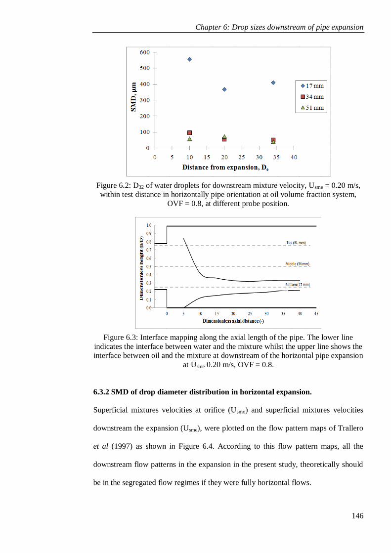
Chapter 6: Drop sizes downstream of pipe expansion
146
Figure 6.2: D32 of water droplets for downstream mixture velocity, Usme = 0.20 m/s,
within test distance in horizontally pipe orientation at oil volume fraction system,
OVF = 0.8, at different probe position.
Figure 6.3: Interface mapping along the axial length of the pipe. The lower line
indicates the interface between water and the mixture whilst the upper line shows the
interface between oil and the mixture at downstream of the horizontal pipe expansion
at Usme 0.20 m/s, OVF = 0.8.
6.3.2 SMD of drop diameter distribution in horizontal expansion.
Superficial mixtures velocities at orifice (Usmo) and superficial mixtures velocities
downstream the expansion (Usme), were plotted on the flow pattern maps of Trallero
et al (1997) as shown in Figure 6.4. According to this flow pattern maps, all the
downstream flow patterns in the expansion in the present study, theoretically should
be in the segregated flow regimes if they were fully horizontal flows.

Chapter 6: Drop sizes downstream of pipe expansion
147
Figure 6.4: Orifice and downstream mixture velocities of flow pattern transition
through the sudden expansion plotted on the flow pattern maps of Trallero et al.
(1997).
It is therefore of interest to examine the effect of input oil volume fraction, the
mixture velocity and the distance from expansion, for horizontally piping
orientations. Hence, one of the main parts of these studies is to investigate and relate
the effects of the experimental conditions and axial tabular positions with the drop
size distribution and the flow development in horizontal pipe.
6.3.2.1 SMD of drops distribution - Effect of the oil volume fraction
Generally the flow patterns seem to be rapidly stratifying for low downstream
mixture velocities (Usme). Trallero (1997), affirmed the phenomenon and produce a
well-known flow pattern maps that been used by many of liquid-liquid multiphase
researchers (Figure 6.4).
SMD of drop diameter distributions for downstream mixture velocity, Usme 0.20 m/s,
at several axial positions after expansion within test distance in horizontally pipe
orientation for probe position 17, 34 and 51 mm from bottom at different oil volume
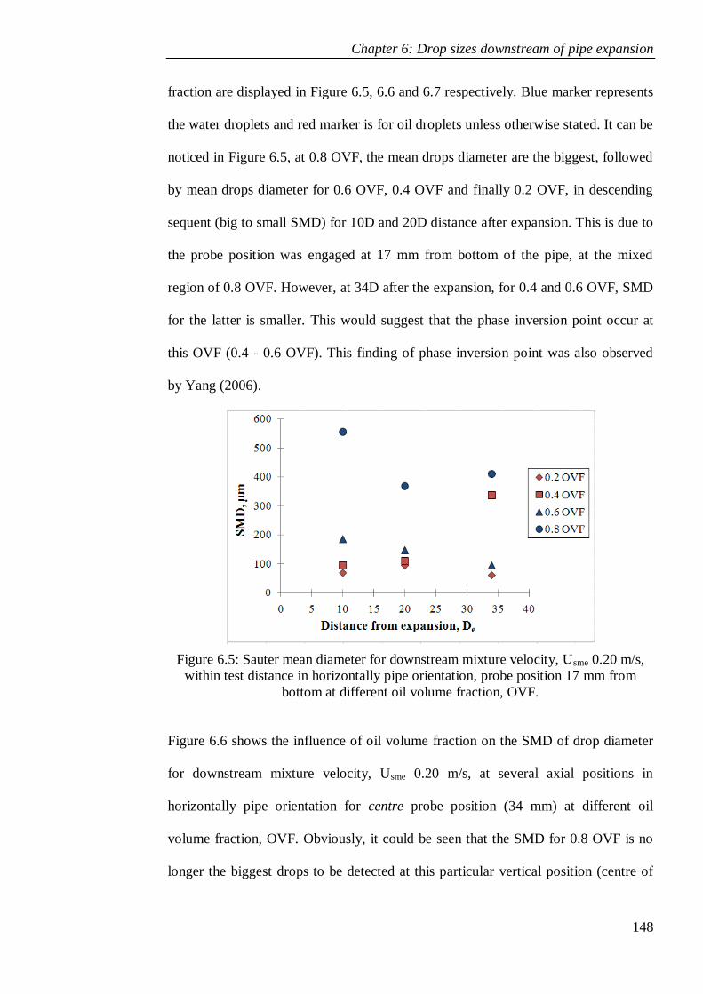
Chapter 6: Drop sizes downstream of pipe expansion
148
fraction are displayed in Figure 6.5, 6.6 and 6.7 respectively. Blue marker represents
the water droplets and red marker is for oil droplets unless otherwise stated. It can be
noticed in Figure 6.5, at 0.8 OVF, the mean drops diameter are the biggest, followed
by mean drops diameter for 0.6 OVF, 0.4 OVF and finally 0.2 OVF, in descending
sequent (big to small SMD) for 10D and 20D distance after expansion. This is due to
the probe position was engaged at 17 mm from bottom of the pipe, at the mixed
region of 0.8 OVF. However, at 34D after the expansion, for 0.4 and 0.6 OVF, SMD
for the latter is smaller. This would suggest that the phase inversion point occur at
this OVF (0.4 - 0.6 OVF). This finding of phase inversion point was also observed
by Yang (2006).
Figure 6.5: Sauter mean diameter for downstream mixture velocity, Usme 0.20 m/s,
within test distance in horizontally pipe orientation, probe position 17 mm from
bottom at different oil volume fraction, OVF.
Figure 6.6 shows the influence of oil volume fraction on the SMD of drop diameter
for downstream mixture velocity, Usme 0.20 m/s, at several axial positions in
horizontally pipe orientation for centre probe position (34 mm) at different oil
volume fraction, OVF. Obviously, it could be seen that the SMD for 0.8 OVF is no
longer the biggest drops to be detected at this particular vertical position (centre of
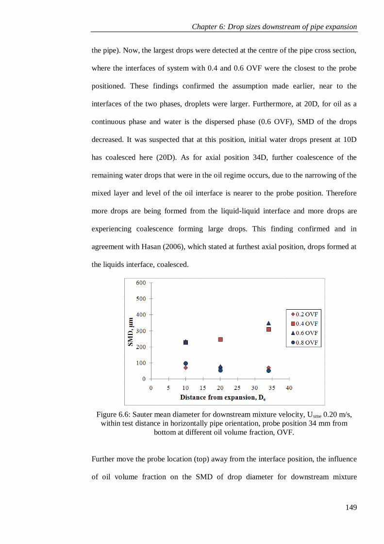
Chapter 6: Drop sizes downstream of pipe expansion
149
the pipe). Now, the largest drops were detected at the centre of the pipe cross section,
where the interfaces of system with 0.4 and 0.6 OVF were the closest to the probe
positioned. These findings confirmed the assumption made earlier, near to the
interfaces of the two phases, droplets were larger. Furthermore, at 20D, for oil as a
continuous phase and water is the dispersed phase (0.6 OVF), SMD of the drops
decreased. It was suspected that at this position, initial water drops present at 10D
has coalesced here (20D). As for axial position 34D, further coalescence of the
remaining water drops that were in the oil regime occurs, due to the narrowing of the
mixed layer and level of the oil interface is nearer to the probe position. Therefore
more drops are being formed from the liquid-liquid interface and more drops are
experiencing coalescence forming large drops. This finding confirmed and in
agreement with Hasan (2006), which stated at furthest axial position, drops formed at
the liquids interface, coalesced.
Figure 6.6: Sauter mean diameter for downstream mixture velocity, Usme 0.20 m/s,
within test distance in horizontally pipe orientation, probe position 34 mm from
bottom at different oil volume fraction, OVF.
Further move the probe location (top) away from the interface position, the influence
of oil volume fraction on the SMD of drop diameter for downstream mixture
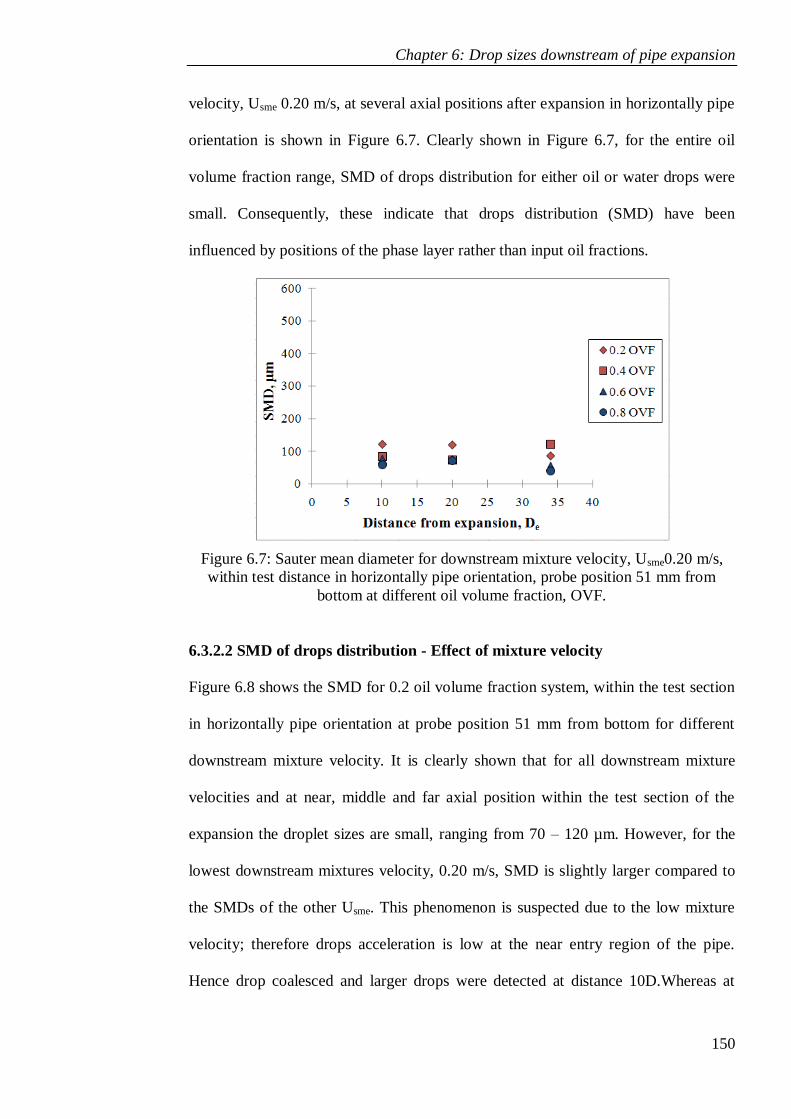
Chapter 6: Drop sizes downstream of pipe expansion
150
velocity, Usme 0.20 m/s, at several axial positions after expansion in horizontally pipe
orientation is shown in Figure 6.7. Clearly shown in Figure 6.7, for the entire oil
volume fraction range, SMD of drops distribution for either oil or water drops were
small. Consequently, these indicate that drops distribution (SMD) have been
influenced by positions of the phase layer rather than input oil fractions.
Figure 6.7: Sauter mean diameter for downstream mixture velocity, Usme0.20 m/s,
within test distance in horizontally pipe orientation, probe position 51 mm from
bottom at different oil volume fraction, OVF.
6.3.2.2 SMD of drops distribution - Effect of mixture velocity
Figure 6.8 shows the SMD for 0.2 oil volume fraction system, within the test section
in horizontally pipe orientation at probe position 51 mm from bottom for different
downstream mixture velocity. It is clearly shown that for all downstream mixture
velocities and at near, middle and far axial position within the test section of the
expansion the droplet sizes are small, ranging from 70 – 120 µm. However, for the
lowest downstream mixtures velocity, 0.20 m/s, SMD is slightly larger compared to
the SMDs of the other Usme. This phenomenon is suspected due to the low mixture
velocity; therefore drops acceleration is low at the near entry region of the pipe.
Hence drop coalesced and larger drops were detected at distance 10D.Whereas at
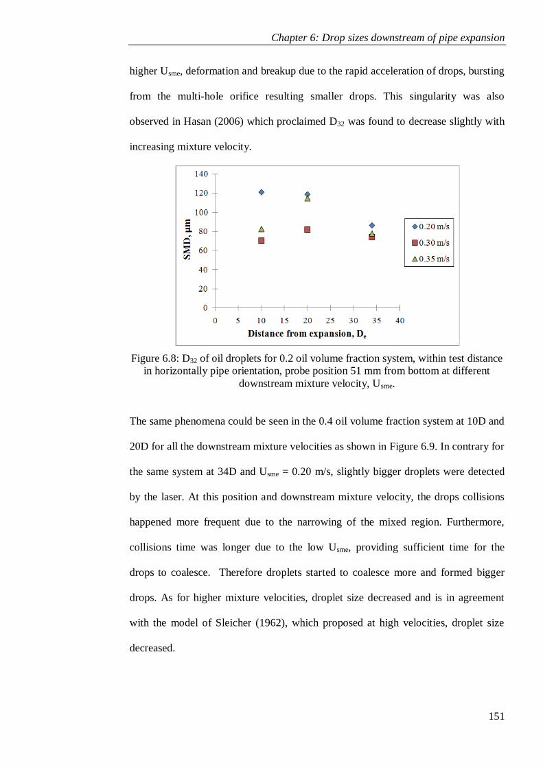
Chapter 6: Drop sizes downstream of pipe expansion
151
higher Usme, deformation and breakup due to the rapid acceleration of drops, bursting
from the multi-hole orifice resulting smaller drops. This singularity was also
observed in Hasan (2006) which proclaimed D32 was found to decrease slightly with
increasing mixture velocity.
Figure 6.8: D32 of oil droplets for 0.2 oil volume fraction system, within test distance
in horizontally pipe orientation, probe position 51 mm from bottom at different
downstream mixture velocity, Usme.
The same phenomena could be seen in the 0.4 oil volume fraction system at 10D and
20D for all the downstream mixture velocities as shown in Figure 6.9. In contrary for
the same system at 34D and Usme = 0.20 m/s, slightly bigger droplets were detected
by the laser. At this position and downstream mixture velocity, the drops collisions
happened more frequent due to the narrowing of the mixed region. Furthermore,
collisions time was longer due to the low Usme, providing sufficient time for the
drops to coalesce. Therefore droplets started to coalesce more and formed bigger
drops. As for higher mixture velocities, droplet size decreased and is in agreement
with the model of Sleicher (1962), which proposed at high velocities, droplet size
decreased.

Chapter 6: Drop sizes downstream of pipe expansion
152
Figure 6.9: D32 of oil droplets for 0.4 oil volume fraction system, within test distance
in horizontally pipe orientation, probe position 34 mm from bottom at different
downstream mixture velocity, Usme.
Further increased the oil volume fraction to 0.6, the dispersed phase is now water and
the oil become continuous phase. Figure 6.10 illustrated the SMD for 0.6 oil volume
fraction system for various Usme. As demonstrated in that figure, at 10D downstream
the expansion at Usme 0.30 and 0.35 m/s, the drop size was medium size drops.
Nevertheless, at Usme 0.20 m/s for the same position downstream the expansion
(10D) the drop size was slightly larger. While at 20D downstream the pipe
expansion, water droplet become smaller for Usme0.20 and 0.30 m/s. This was not
observed for system of 0.4 OVF earlier. In contrary, at Usme 0.35 m/s, the drop sizes
remain the same throughout the whole test section. Further downstream the test
section, SMD for Usme 0.20 m/s increased from 70 µm at 20D to about 350 µm at
34D. This is due to coalescence of the dispersed water drop from the oil layer with
the drops in the mixed layer due to the narrowing of the mixed region. Stratification
is predicted to start beyond this position; if longer test section were to be used
probably this could be confirmed.
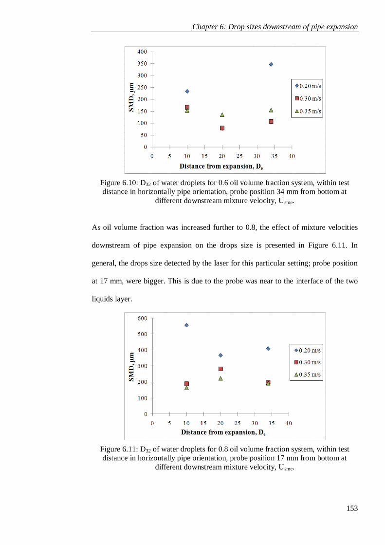
Chapter 6: Drop sizes downstream of pipe expansion
153
Figure 6.10: D32 of water droplets for 0.6 oil volume fraction system, within test
distance in horizontally pipe orientation, probe position 34 mm from bottom at
different downstream mixture velocity, Usme.
As oil volume fraction was increased further to 0.8, the effect of mixture velocities
downstream of pipe expansion on the drops size is presented in Figure 6.11. In
general, the drops size detected by the laser for this particular setting; probe position
at 17 mm, were bigger. This is due to the probe was near to the interface of the two
liquids layer.
Figure 6.11: D32 of water droplets for 0.8 oil volume fraction system, within test
distance in horizontally pipe orientation, probe position 17 mm from bottom at
different downstream mixture velocity, Usme.

Chapter 6: Drop sizes downstream of pipe expansion
154
Downstream of the pipe expansion 10D, the biggest water drops were detected by the
laser for Usme 0.20 m/s. For this flow conditions, the interface is a bit chaotic and
produced bigger droplets near to the interface of these two liquids. Furthermore, the
probe was slightly above this interface, in the mixed layer where these big droplets
occurred. However as for higher downstream mixture velocities, coalescence did not
happened due to time of collision is not enough for the droplets to coalesce.
Therefore, droplets with medium size were obtained at these velocities. As for 20D
downstream the pipe expansion, size of the water droplets at Usme 0.20 m/s
decreased, owing to the stratification process that started to happen which make the
interface less disturbed. Hence, the bigger water droplets start to merge with the
water layer and left only medium droplet that burst into the mixed layer and detected
by the laser. Promoting higher downstream mixture velocity to 0.30 or 0.35 m/s,
resulted contrary finding with Usme 0.20 m/s. Instead of decreasing in size, it
increased to some extent. The drop size increased as the chaotic interface of the
system created by higher mixture velocities causing bigger droplet to be produced
then burst into the mixed layer and be detected by the laser. Even though Sleicher
(1962) mentioned about decrease in size at high velocities, Howarth (1964) did also
mentioned about an increase in velocity causes an increase in coalescence frequency.
It is suspected that at 0.30 m/s of these particular conditions and axial position, the
velocity of the mixture is optimal for collision of the droplets to happen. Hence
increases the coalescence frequency and produced larger droplet. As for axial
position 34D downstream the pipe expansion, at Usme 0.20 m/s, the drop size is about
the same as at 20D. For higher Usme i.e. 0.30 m/s, the drops size decreased back to
medium droplet size as at 10D, because the larger droplet has coalesce at 20D, and
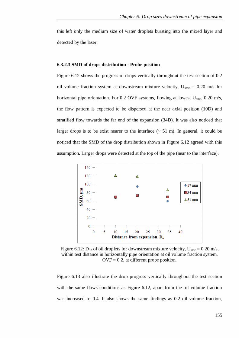
Chapter 6: Drop sizes downstream of pipe expansion
155
this left only the medium size of water droplets bursting into the mixed layer and
detected by the laser.
6.3.2.3 SMD of drops distribution - Probe position
Figure 6.12 shows the progress of drops vertically throughout the test section of 0.2
oil volume fraction system at downstream mixture velocity, Usme = 0.20 m/s for
horizontal pipe orientation. For 0.2 OVF systems, flowing at lowest Usme, 0.20 m/s,
the flow pattern is expected to be dispersed at the near axial position (10D) and
stratified flow towards the far end of the expansion (34D). It was also noticed that
larger drops is to be exist nearer to the interface (~ 51 m). In general, it could be
noticed that the SMD of the drop distribution shown in Figure 6.12 agreed with this
assumption. Larger drops were detected at the top of the pipe (near to the interface).
Figure 6.12: D32 of oil droplets for downstream mixture velocity, Usme = 0.20 m/s,
within test distance in horizontally pipe orientation at oil volume fraction system,
OVF = 0.2, at different probe position.
Figure 6.13 also illustrate the drop progress vertically throughout the test section
with the same flows conditions as Figure 6.12, apart from the oil volume fraction
was increased to 0.4. It also shows the same findings as 0.2 oil volume fraction,
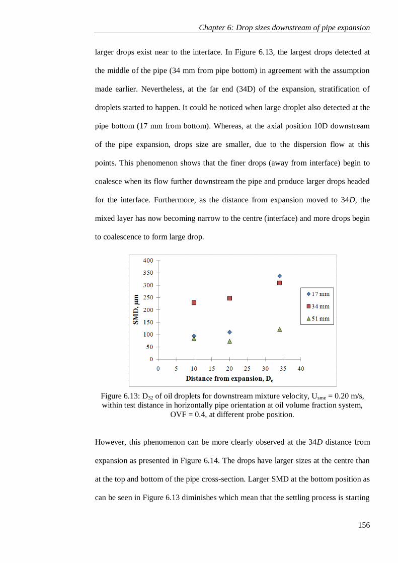
Chapter 6: Drop sizes downstream of pipe expansion
156
larger drops exist near to the interface. In Figure 6.13, the largest drops detected at
the middle of the pipe (34 mm from pipe bottom) in agreement with the assumption
made earlier. Nevertheless, at the far end (34D) of the expansion, stratification of
droplets started to happen. It could be noticed when large droplet also detected at the
pipe bottom (17 mm from bottom). Whereas, at the axial position 10D downstream
of the pipe expansion, drops size are smaller, due to the dispersion flow at this
points. This phenomenon shows that the finer drops (away from interface) begin to
coalesce when its flow further downstream the pipe and produce larger drops headed
for the interface. Furthermore, as the distance from expansion moved to 34D, the
mixed layer has now becoming narrow to the centre (interface) and more drops begin
to coalescence to form large drop.
Figure 6.13: D32 of oil droplets for downstream mixture velocity, Usme = 0.20 m/s,
within test distance in horizontally pipe orientation at oil volume fraction system,
OVF = 0.4, at different probe position.
However, this phenomenon can be more clearly observed at the 34D distance from
expansion as presented in Figure 6.14. The drops have larger sizes at the centre than
at the top and bottom of the pipe cross-section. Larger SMD at the bottom position as
can be seen in Figure 6.13 diminishes which mean that the settling process is starting
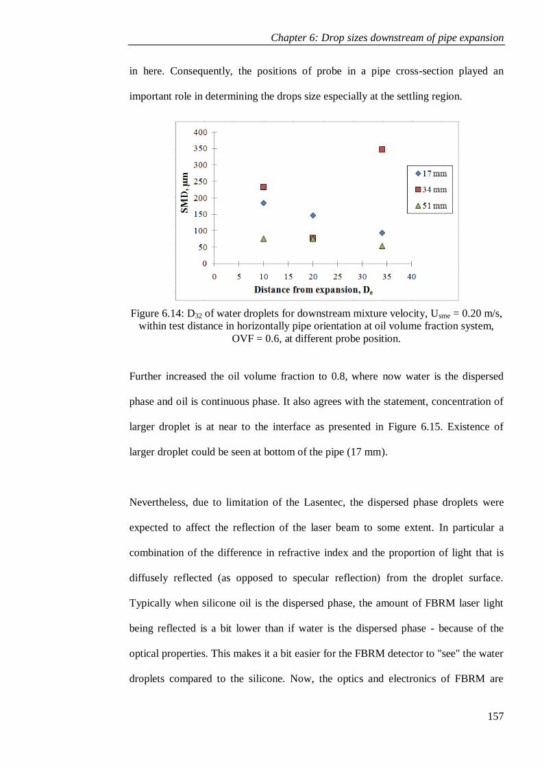
Chapter 6: Drop sizes downstream of pipe expansion
157
in here. Consequently, the positions of probe in a pipe cross-section played an
important role in determining the drops size especially at the settling region.
Figure 6.14: D32 of water droplets for downstream mixture velocity, Usme = 0.20 m/s,
within test distance in horizontally pipe orientation at oil volume fraction system,
OVF = 0.6, at different probe position.
Further increased the oil volume fraction to 0.8, where now water is the dispersed
phase and oil is continuous phase. It also agrees with the statement, concentration of
larger droplet is at near to the interface as presented in Figure 6.15. Existence of
larger droplet could be seen at bottom of the pipe (17 mm).
Nevertheless, due to limitation of the Lasentec, the dispersed phase droplets were
expected to affect the reflection of the laser beam to some extent. In particular a
combination of the difference in refractive index and the proportion of light that is
diffusely reflected (as opposed to specular reflection) from the droplet surface.
Typically when silicone oil is the dispersed phase, the amount of FBRM laser light
being reflected is a bit lower than if water is the dispersed phase - because of the
optical properties. This makes it a bit easier for the FBRM detector to "see" the water
droplets compared to the silicone. Now, the optics and electronics of FBRM are

Chapter 6: Drop sizes downstream of pipe expansion
158
designed in such a way that some degree of variability in the amount of reflected
light should not affect the size of the chord length being measured. However in the
older models of FBRM such as FBRM M500P that degree of variability is quite
modest - thus it is quite likely droplets detected will yield slightly smaller chord
lengths in the system of oil dispersed compared to water dispersed.
Figure 6.15: D32 of water droplets for downstream mixture velocity, Usme = 0.20 m/s,
within test distance in horizontally pipe orientation at oil volume fraction system,
OVF = 0.8, at different probe position.
6.3.2.4 Development of drops size - Cross-sectional of horizontally pipe
expansion
SMD for drops distribution of two immiscible liquids flowing at various downstream
mixture velocities after pipe expansion in horizontal with effect of vertically cross
section of the pipe will be presented in this sub-section. Measurement of the drops
distribution were made at 3 vertically position from pipe bottom, namely bottom (17
mm), middle (34 mm) and top (51 mm).
In the two-phase flow pattern there is a mixed layer of oil/water flow along the larger
pipe downstream of the expansion. However, in this case, the centre of mixed region

Chapter 6: Drop sizes downstream of pipe expansion
159
is considered as the centre of the interface (Z), while the distances above and below
from the centre of interface are measured and identified as a function of distance
from centre of the interface, |Z|. Figure 6.16 below demonstrated the mean drops
diameter of oil-water two phase flow in a horizontally pipe orientation, 10D
downstream the expansion for mixture velocity 0.20 m/s, as a function of distance
from centre of the interface, |Z|. Overall it is clearly shown that larger drops were
dispersed nearer to the interface. Nevertheless, there are also smaller drops near to
the interface, due to the dispersion of droplets in the entry region of the pipe
(adjacent to sudden expansion).
Figure 6.16: Sauter mean diameter as a function of the distance from |Z| at Usme 0.20
m/s of horizontal pipe orientation flow, 10D downstream the expansion.
Figure 6.17 revealed the mean drops diameter of oil-water two phase flow in a
horizontally pipe orientation, 34D downstream the expansion for mixture velocity
0.20 m/s, as a function of distance from centre of the interface, |Z|. Clearly shown
drops were large nearer to the interface. Thus, from the present data, it is established
that drops size decreased when the distance from the interface increased (further
away).
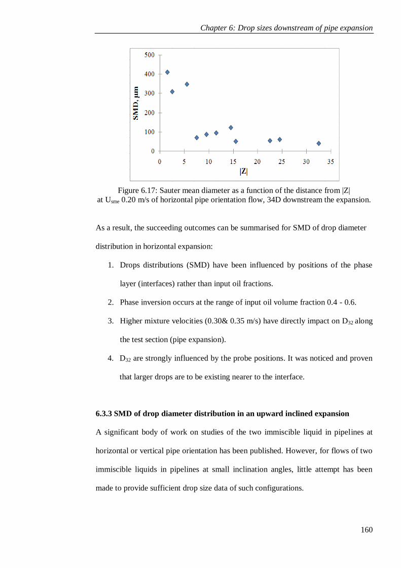
Chapter 6: Drop sizes downstream of pipe expansion
160
Figure 6.17: Sauter mean diameter as a function of the distance from |Z|
at Usme 0.20 m/s of horizontal pipe orientation flow, 34D downstream the expansion.
As a result, the succeeding outcomes can be summarised for SMD of drop diameter
distribution in horizontal expansion:
1. Drops distributions (SMD) have been influenced by positions of the phase
layer (interfaces) rather than input oil fractions.
2. Phase inversion occurs at the range of input oil volume fraction 0.4 - 0.6.
3. Higher mixture velocities (0.30& 0.35 m/s) have directly impact on D32 along
the test section (pipe expansion).
4. D32 are strongly influenced by the probe positions. It was noticed and proven
that larger drops are to be existing nearer to the interface.
6.3.3 SMD of drop diameter distribution in an upward inclined expansion
A significant body of work on studies of the two immiscible liquid in pipelines at
horizontal or vertical pipe orientation has been published. However, for flows of two
immiscible liquids in pipelines at small inclination angles, little attempt has been
made to provide sufficient drop size data of such configurations.
Chapter 6: Drop sizes downstream of pipe expansion
161
Dispersion of one phase in the other can occur at the interface in stratified flow and
is a common phenomenon in several flow patterns. When the flow pattern of two
immiscible liquids is in a dispersed flow, the drop size and drop size distribution will
become an important characteristic of the flow. Up to date, there are only a few
researches on flows pattern for small upward inclinations from horizontal reported in
journals etc.
As predicted by the model of Taitel and Dukler (1976), pipe inclination will affect
the interface level between the two phases for the ST regime flow pattern. Generally,
it indicates that the lighter phase layer at the pipe top flows faster than the heavier
phase layer that flowing at the bottom of the pipe for upward pipe orientations.
However, there are others factors that also affect these evolution processes.
Therefore, in this section, SMD of drop diameter distribution in two-phase oil-water
flow were measured for an upwardly flow inclined which were at the same
experiments conditions used in horizontal flow. The angles of an upward inclination
flow are +3 and +6 degrees respectively. Analysis of results and discussion are
presented below.
6.3.3.1 SMD of drops distribution - Effect of input oil volume fraction
In order to investigate the relation of upward pipe orientation and drop diameter
distributions with effect of oil volume fraction (OVF), a few experimental conditions
and setting were set up. Result of the experiments were presented and discussed in
the following sub-paragraph.

Chapter 6: Drop sizes downstream of pipe expansion
162
SMD of drop diameter distributions for downstream mixture velocity, Usme 0.20 m/s,
at several axial position after expansion in upward pipe orientation (+6o) for probe
position 17, 34 and 51 mm from bottom at different oil volume fraction are displayed
in Figure 6.18 - 6.20 respectively. In general, SMD of the drop diameter distributions
for 0.8 OVF was found to be larger than 0.2 OVF systems for the same probe
position (17 and 34 mm from pipe bottom) except for top position (51 mm). In
Figure 6.18, at 0.2 OVF, throughout the test section the oil droplets are very fine
droplets which concentrating at bottom of the pipe throughout the test section. In
contrary, at 0.8 OVF, due to the probe position engaged at 17 mm from bottom of the
pipe, at the mixed region of 0.8 OVF, larger droplets were detected. The highest
SMD of the distribution for this system is about 350µm at 10D downstream from
expansion. Towards the end (downstream) of the pipe expansion, SMD of drop
diameter distribution become smaller, at 20D SMD is about 290µm and at 34D is
240µm. The reason being is that, the flow entered the pipe expansion as dispersed
flow and coalescence has already happen by the time the drops reached 10D.
Moreover, beyond 10D the process of stratification is starting to begin. Therefore at
10D for probe position 17 mm from bottom, larger droplets were detected by the
laser. Whereas at 20D and 34D downstream of the expansion, the flow near the
interface becoming less wavy and stratified, respectively. Hence, fewer bigger water
droplets were detected in the mixed layer. In other words, settling has happened.
Therefore, smaller droplets compared to droplets produced at 10D were detected by
the laser at 20D and 34D.

Chapter 6: Drop sizes downstream of pipe expansion
163
Figure 6.18: Sauter mean diameter for downstream mixture velocity, Usme 0.20 m/s,
within test distance in upward 6o pipe orientation, probe position 17 mm from bottom
at different oil volume fraction, OVF.
Figure 6.19 shows the influence of oil volume fraction on the SMD of drop diameter
for downstream mixture velocity, Usme 0.20 m/s, at several axial positions after
expansion in +6o upward pipe orientation for probe position 34 mm from bottom at
different oil volume fraction, OVF. Throughout the test section there are only small
sizes of oil droplet detected at middle of the pipe cross section for 0.2 OVF systems.
Interestingly, at 10D from expansion the SMD of the distribution is as small as SMD
for 0.2 OVF. It is suspected that at 34 mm vertically from pipe bottom, for 10D axial
distance downstream from expansion, the position of the laser probe are in the
dispersed flow with the probe position located in the mid position for both systems
(0.2 and 0.8 OVF). Hence, smaller SMD of water drops was observed at this
location. Conversely, for 0.8 OVF at probe position 34 mm from bottom of the pipe,
medium/ large water droplets were detected at 20D and 34D downstream expansion.
Nevertheless, the SMD of the drops diameter distribution were comparatively
slightly smaller than SMD at probe position 17 mm from pipe bottom of the same
flow condition, about 180 and 240µm at 20D and 34D downstream of the pipe

Chapter 6: Drop sizes downstream of pipe expansion
164
expansion respectively. At 20D position, coalescence of smaller droplets started to
materialize. Further coalescence of the drops take place at the farthest position within
the test section (34D). Therefore size of drops increased towards the end of the pipe
expansion as can be seen in Figure 6.19.
Figure 6.19: Sauter mean diameter for downstream mixture velocity, Usme 0.20 m/s,
within test distance in upward 6o pipe orientation, probe position 34 mm from bottom
at different oil volume fraction, OVF.
Figure 6.20 demonstrated the effect of oil volume fraction on SMD for drop diameter
distributions at top (51 mm from pipe bottom) of the pipe expansion for +6o pipe
orientation at Usme 0.20 m/s. It is clearly seen that SMD of the distributions were
small for both volume fraction. The water droplets in the 0.8 OVF systems,
throughout the test section are very fine droplets. This is due to the interface of the
two fluids are relatively far down from the detection point. Hence, only small
droplets were burst to the top of the pipe and be detected by the laser. Contrariwise,
for 0.2 OVF system, the oil drops detected at 10D were slightly bigger compared to
oil drops detected at other vertically position (17 and 34 mm) at the same distance
downstream of the expansion. Further downstream of the expansion, at 20D, SMD of
the oil drop distributions are the biggest. It is assumed that at 20D, coalescence of the
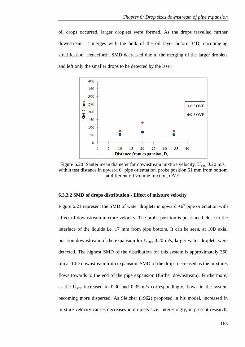
Chapter 6: Drop sizes downstream of pipe expansion
165
oil drops occurred, larger droplets were formed. As the drops travelled further
downstream, it merges with the bulk of the oil layer before 34D, encouraging
stratification. Henceforth, SMD decreased due to the merging of the larger droplets
and left only the smaller drops to be detected by the laser.
Figure 6.20: Sauter mean diameter for downstream mixture velocity, Usme 0.20 m/s,
within test distance in upward 6o pipe orientation, probe position 51 mm from bottom
at different oil volume fraction, OVF.
6.3.3.2 SMD of drops distribution - Effect of mixture velocity
Figure 6.21 represent the SMD of water droplets in upward +6o pipe orientation with
effect of downstream mixture velocity. The probe position is positioned close to the
interface of the liquids i.e. 17 mm from pipe bottom. It can be seen, at 10D axial
position downstream of the expansion for Usme 0.20 m/s, larger water droplets were
detected. The highest SMD of the distribution for this system is approximately 350
µm at 10D downstream from expansion. SMD of the drops decreased as the mixtures
flows towards to the end of the pipe expansion (further downstream). Furthermore,
as the Usme increased to 0.30 and 0.35 m/s correspondingly, flows in the system
becoming more dispersed. As Sleicher (1962) proposed in his model, increased in
mixture velocity causes decreases in droplets size. Interestingly, in present research,
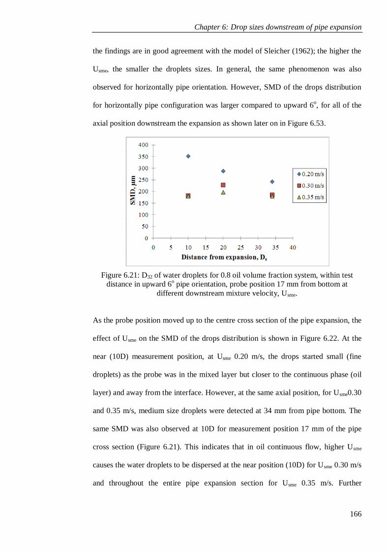
Chapter 6: Drop sizes downstream of pipe expansion
166
the findings are in good agreement with the model of Sleicher (1962); the higher the
Usme, the smaller the droplets sizes. In general, the same phenomenon was also
observed for horizontally pipe orientation. However, SMD of the drops distribution
for horizontally pipe configuration was larger compared to upward 6o, for all of the
axial position downstream the expansion as shown later on in Figure 6.53.
Figure 6.21: D32 of water droplets for 0.8 oil volume fraction system, within test
distance in upward 6o pipe orientation, probe position 17 mm from bottom at
different downstream mixture velocity, Usme.
As the probe position moved up to the centre cross section of the pipe expansion, the
effect of Usme on the SMD of the drops distribution is shown in Figure 6.22. At the
near (10D) measurement position, at Usme 0.20 m/s, the drops started small (fine
droplets) as the probe was in the mixed layer but closer to the continuous phase (oil
layer) and away from the interface. However, at the same axial position, for Usme0.30
and 0.35 m/s, medium size droplets were detected at 34 mm from pipe bottom. The
same SMD was also observed at 10D for measurement position 17 mm of the pipe
cross section (Figure 6.21). This indicates that in oil continuous flow, higher Usme
causes the water droplets to be dispersed at the near position (10D) for Usme 0.30 m/s
and throughout the entire pipe expansion section for Usme 0.35 m/s. Further
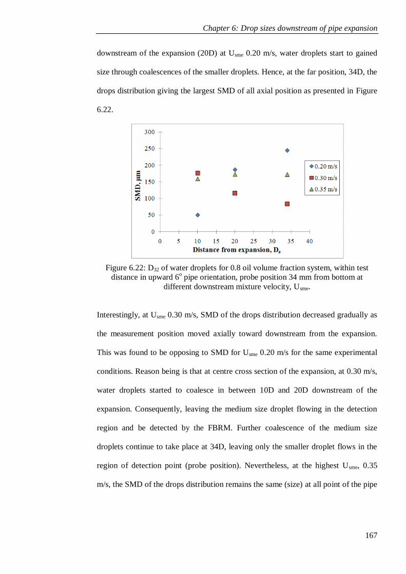
Chapter 6: Drop sizes downstream of pipe expansion
167
downstream of the expansion (20D) at Usme 0.20 m/s, water droplets start to gained
size through coalescences of the smaller droplets. Hence, at the far position, 34D, the
drops distribution giving the largest SMD of all axial position as presented in Figure
6.22.
Figure 6.22: D32 of water droplets for 0.8 oil volume fraction system, within test
distance in upward 6o pipe orientation, probe position 34 mm from bottom at
different downstream mixture velocity, Usme.
Interestingly, at Usme 0.30 m/s, SMD of the drops distribution decreased gradually as
the measurement position moved axially toward downstream from the expansion.
This was found to be opposing to SMD for Usme 0.20 m/s for the same experimental
conditions. Reason being is that at centre cross section of the expansion, at 0.30 m/s,
water droplets started to coalesce in between 10D and 20D downstream of the
expansion. Consequently, leaving the medium size droplet flowing in the detection
region and be detected by the FBRM. Further coalescence of the medium size
droplets continue to take place at 34D, leaving only the smaller droplet flows in the
region of detection point (probe position). Nevertheless, at the highest Usme, 0.35
m/s, the SMD of the drops distribution remains the same (size) at all point of the pipe
Chapter 6: Drop sizes downstream of pipe expansion
168
cross section throughout the test section (pipe expansion), indicated that water
droplets were fully dispersed along the expansion.
Figure 6.23 denoted the SMD of water droplets in upward +3o pipe orientation with
effect of downstream mixture velocity, Usme. Oil volume fraction for the system is
0.8 with the probe positioned 17 mm from the pipe bottom. As the probe was close to
the interface, the drops were found to be as large as for the other pipe orientations i.e.
horizontal and +6o upward inclination, for Usme 0.20 m/s. Furthermore, at higher
Usme, the drops size decreased, with Usme = 0.35 m/s giving the smallest SMD of drop
distribution. Interestingly, for such flow system (oil continuous flow), the drops size
were about the same size throughout the test section. Additionally, the drops size
were nearly the same for all pipe orientation; horizontal, +6o and +3
o. This points out
that the drops sizes were measured in the mixed layer of the flow system.
Figure 6.24 shows the influence of downstream mixture velocity (Usme) on drop size
distribution for oil continuous flow system (0.8 OVF) at several axial position
downstream expansion and probe position at centre of the pipe cross section (34 mm)
in +3o upward pipe orientation. The highest SMD of the drops distribution were
found to be at the near (10D) position of detection for Usme 0.20 m/s. For the same
mixture velocity, it can be seen that SMD of the drops decreased as the mixtures
flows towards to the end of the pipe expansion (further downstream).

Chapter 6: Drop sizes downstream of pipe expansion
169
Figure 6.23: D32 of water droplets for 0.8 oil volume fraction system, within test
distance in upward 3o pipe orientation, probe position 17 mm from bottom at
different downstream mixture velocity, Usme.
It is observed that at 34D downstream of the expansion, the flow was ST&MI and
the probe was in the oil layer. Hence, only smaller droplets or less large water
droplets were detected by the probe at this position as presented in Figure 6.24.
Figure 6.24: D32 of water droplets for 0.8 oil volume fraction system, within test
distance in upward 3o pipe orientation, probe position 34 mm from bottom at
different downstream mixture velocity, Usme.
Increased the Usme to 0.30 and 0.35 m/s correspondingly, flows in the system
becoming more dispersed, particularly at the near (10D) position downstream the
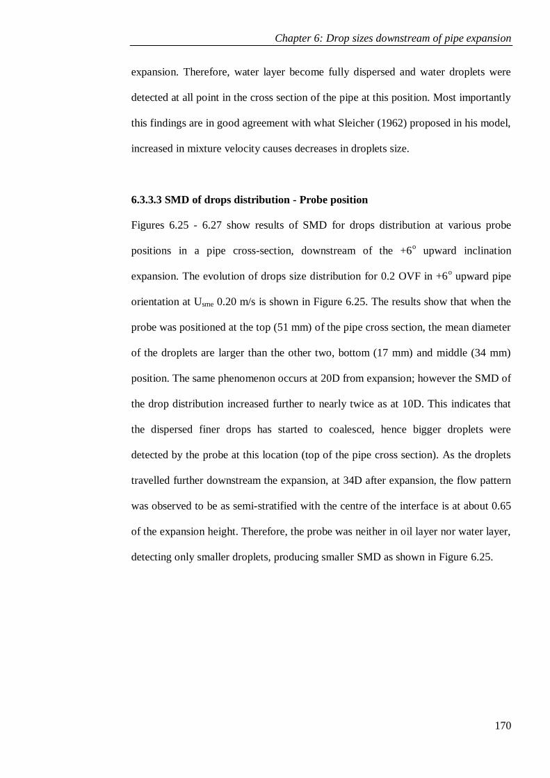
Chapter 6: Drop sizes downstream of pipe expansion
170
expansion. Therefore, water layer become fully dispersed and water droplets were
detected at all point in the cross section of the pipe at this position. Most importantly
this findings are in good agreement with what Sleicher (1962) proposed in his model,
increased in mixture velocity causes decreases in droplets size.
6.3.3.3 SMD of drops distribution - Probe position
Figures 6.25 - 6.27 show results of SMD for drops distribution at various probe
positions in a pipe cross-section, downstream of the +6o upward inclination
expansion. The evolution of drops size distribution for 0.2 OVF in +6o upward pipe
orientation at Usme 0.20 m/s is shown in Figure 6.25. The results show that when the
probe was positioned at the top (51 mm) of the pipe cross section, the mean diameter
of the droplets are larger than the other two, bottom (17 mm) and middle (34 mm)
position. The same phenomenon occurs at 20D from expansion; however the SMD of
the drop distribution increased further to nearly twice as at 10D. This indicates that
the dispersed finer drops has started to coalesced, hence bigger droplets were
detected by the probe at this location (top of the pipe cross section). As the droplets
travelled further downstream the expansion, at 34D after expansion, the flow pattern
was observed to be as semi-stratified with the centre of the interface is at about 0.65
of the expansion height. Therefore, the probe was neither in oil layer nor water layer,
detecting only smaller droplets, producing smaller SMD as shown in Figure 6.25.
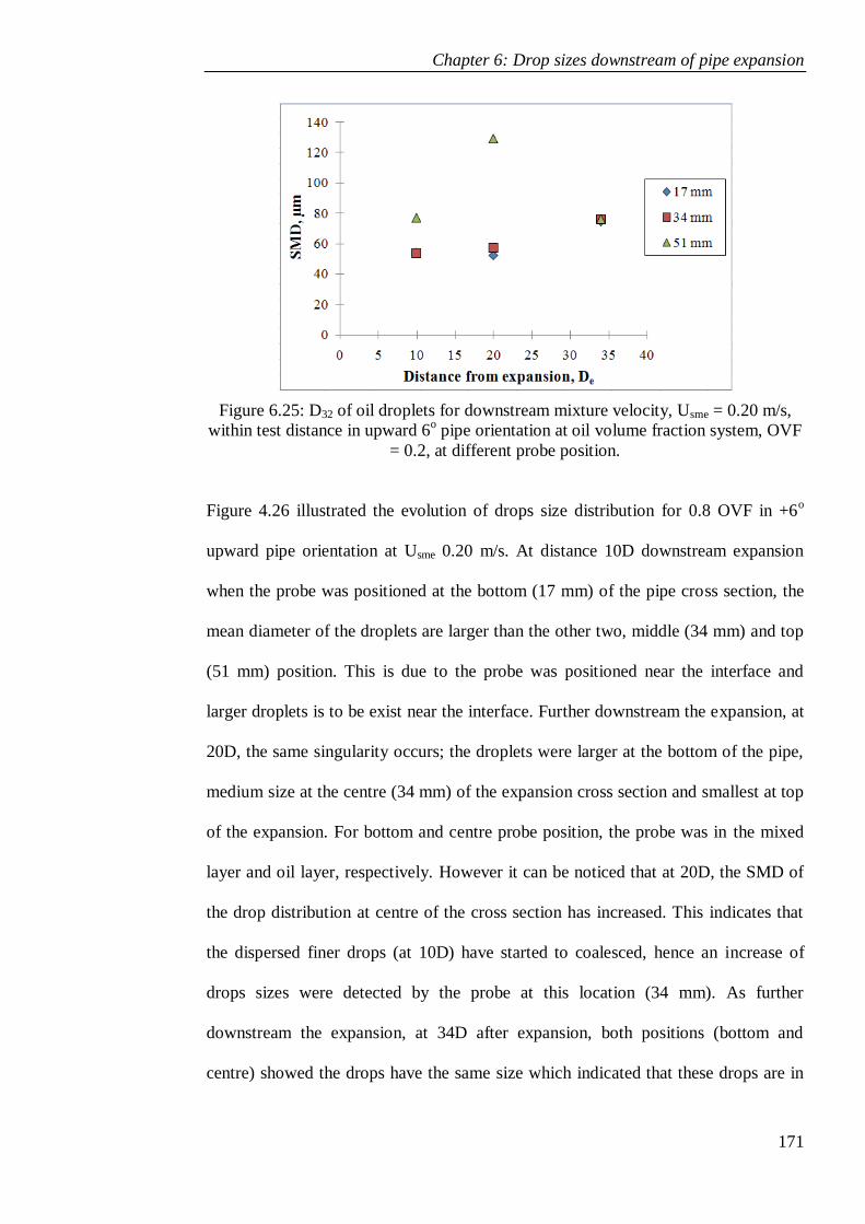
Chapter 6: Drop sizes downstream of pipe expansion
171
Figure 6.25: D32 of oil droplets for downstream mixture velocity, Usme = 0.20 m/s,
within test distance in upward 6o pipe orientation at oil volume fraction system, OVF
= 0.2, at different probe position.
Figure 4.26 illustrated the evolution of drops size distribution for 0.8 OVF in +6o
upward pipe orientation at Usme 0.20 m/s. At distance 10D downstream expansion
when the probe was positioned at the bottom (17 mm) of the pipe cross section, the
mean diameter of the droplets are larger than the other two, middle (34 mm) and top
(51 mm) position. This is due to the probe was positioned near the interface and
larger droplets is to be exist near the interface. Further downstream the expansion, at
20D, the same singularity occurs; the droplets were larger at the bottom of the pipe,
medium size at the centre (34 mm) of the expansion cross section and smallest at top
of the expansion. For bottom and centre probe position, the probe was in the mixed
layer and oil layer, respectively. However it can be noticed that at 20D, the SMD of
the drop distribution at centre of the cross section has increased. This indicates that
the dispersed finer drops (at 10D) have started to coalesced, hence an increase of
drops sizes were detected by the probe at this location (34 mm). As further
downstream the expansion, at 34D after expansion, both positions (bottom and
centre) showed the drops have the same size which indicated that these drops are in

Chapter 6: Drop sizes downstream of pipe expansion
172
the mixed layer. Therefore, the height of the mixed layer has increased toward the
downstream of the expansion.
Figure 6.26: D32 of water droplets for downstream mixture velocity, Usme = 0.20 m/s,
within test distance in upward 6o pipe orientation at oil volume fraction system, OVF
= 0.8, at different probe position.
Figures 6.27 show the results of SMD for drops distribution in a pipe cross-section,
downstream of the +6o upward inclination expansion for higher Usme (0.35 m/s). As
the oil volume fraction is 0.8, the continuous flow is oil and dispersed flow is water.
The results show that at 10D downstream the expansion, the mean diameter of the
water droplets is the same at any point in the pipe cross-sectional area. This indicates
that at 10D the two liquids are nearly homogeneous flow. At this point, the dispersed
flows are well mixed, so that the oil and water velocities are similar. The same mean
diameters were also detected, further downstream at 20D and 34D of the expansion
for bottom and centre of the expansion cross section. In contrary, mean diameter at
the pipe top (51 mm from bottom) decreased, due to the droplet (at 10D) has settle
due to gravity forces. However as for bottom and centre of the pipe cross section, the
mixed layer hardly decays. Owing to higher Usme, the turbulence intensity also
increase, hence coalescence of the droplets in the dispersion were delayed.

Chapter 6: Drop sizes downstream of pipe expansion
173
Figure 6.27: D32 of water droplets for downstream mixture velocity, Usme = 0.35 m/s,
within test distance in upward 6o pipe orientation at oil volume fraction system, OVF
= 0.8, at different probe position.
In the studies of the development of drops size in the entire pipe cross-sectional area
downstream of an expansion, measurement of drops size distribution were made at
the same conditions as in the previous measurement except that now the inclined
angle are +3o upward. Figure 6.28 - 6.29 show results of SMD for drops distribution
at various probe positions in a pipe cross-section, downstream of the +3o upward
inclination expansion. The evolution of drops size distribution for 0.8 OVF in +3o
upward pipe orientation at Usme 0.20 m/s is shown in Figure 6.28. The results
demonstrate that at 10D, largest droplets were detected when the probe was
positioned at centre (34 mm) of the pipe cross section followed by medium size at
pipe bottom and the smallest at 51 mm (pipe top). The reason is because at this
position the mixed layer was slightly below to centre of the pipe cross section, even
though the oil volume fraction is 0.8. As observed by Hasan (2006), drops size tend
to increase above and below the centre of the mixed layer. At the middle of the pipe
expansion (axially), the mixed layer become narrow and the level of the water/mixed
layer interface increased. This indicates that coalescence and settling at the centre
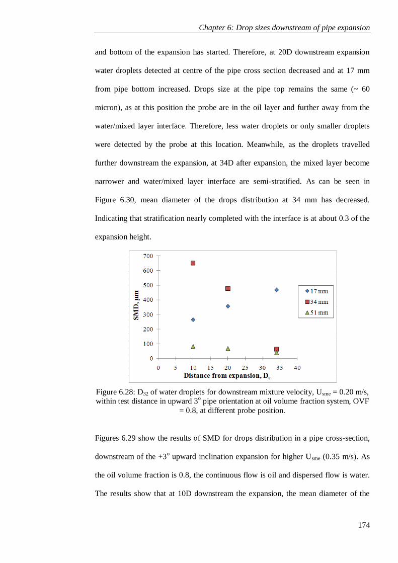
Chapter 6: Drop sizes downstream of pipe expansion
174
and bottom of the expansion has started. Therefore, at 20D downstream expansion
water droplets detected at centre of the pipe cross section decreased and at 17 mm
from pipe bottom increased. Drops size at the pipe top remains the same (~ 60
micron), as at this position the probe are in the oil layer and further away from the
water/mixed layer interface. Therefore, less water droplets or only smaller droplets
were detected by the probe at this location. Meanwhile, as the droplets travelled
further downstream the expansion, at 34D after expansion, the mixed layer become
narrower and water/mixed layer interface are semi-stratified. As can be seen in
Figure 6.30, mean diameter of the drops distribution at 34 mm has decreased.
Indicating that stratification nearly completed with the interface is at about 0.3 of the
expansion height.
Figure 6.28: D32 of water droplets for downstream mixture velocity, Usme = 0.20 m/s,
within test distance in upward 3o pipe orientation at oil volume fraction system, OVF
= 0.8, at different probe position.
Figures 6.29 show the results of SMD for drops distribution in a pipe cross-section,
downstream of the +3o upward inclination expansion for higher Usme (0.35 m/s). As
the oil volume fraction is 0.8, the continuous flow is oil and dispersed flow is water.
The results show that at 10D downstream the expansion, the mean diameter of the

Chapter 6: Drop sizes downstream of pipe expansion
175
water droplets is the same at any point in the pipe cross-sectional area. This indicates
that at 10D the two liquids are nearly homogeneous flow. At this point, the dispersed
flows are well mixed, so that the oil and water velocities are similar. In contrary, at
20D, mean diameter for middle (34 mm) and top (51 mm) decreased steeply and
remain about the same size throughout the test section (34D). Furthermore, mean
diameter at the pipe bottom (17 mm from bottom) slightly increase, perhaps due to
collisions frequency increased. However, there are no further coalescence happened
at 34D, as for higher Usme, collision time is not sufficient enough for drop-drop
coalescence to materialise. Owing to higher Usme, the turbulence intensity also
increase, hence coalescence of the droplets in the dispersion were delayed. Hence,
the mixed layer hardly decays within the test section.
Figure 6.29: D32 of water droplets for downstream mixture velocity, Usme = 0.35 m/s,
within test distance in upward 3o pipe orientation at oil volume fraction system, OVF
= 0.8, at different probe position.
6.3.3.4 Development of drops size - Cross-sectional of the upward pipe
expansion
As mentioned earlier in this chapter, in order to studies the development of drops size
in the entire pipe cross-sectional area downstream of an expansion, measurement of
drops size distribution were made at several position of the pipe expansion for
Chapter 6: Drop sizes downstream of pipe expansion
176
various downstream mixture velocities. In this sub-section though, the test section
were set to be upward inclination.
Figure 6.30 below demonstrated the mean drops diameter of oil-water two phase
flow in +6o upward pipe orientation, 10D downstream the expansion for mixture
velocity 0.20 m/s, as a function of distance from the interface, |Z|. Clearly shown
drops were large nearer to the interface at axial position 10D downstream the
expansion.
Figure 6.30: Sauter means diameter as a function of the distance from |Z| at Usme 0.20
m/s of +6o upward inclined pipe orientation flow, 10D downstream the expansion.
However, for the mean drops diameter as a function of distance from the interface,
|Z| at Usme 0.20 m/s of +6o upward inclined pipe orientation at 34D from expansion
as shown in Figure 4.31, different phenomena arises. The assumption made for
horizontal flow is no longer valid for +6o upward inclined flow. This is in line for the
force equilibrium conditions were modifies when the pipe orientation was changed
from horizontal to +6o upward inclined. The flow gravity force is now divided into
two components, normal and parallel to the pipe axis. The normal gravity component
enhances the segregation of the fluids, similar to the horizontal case. However the
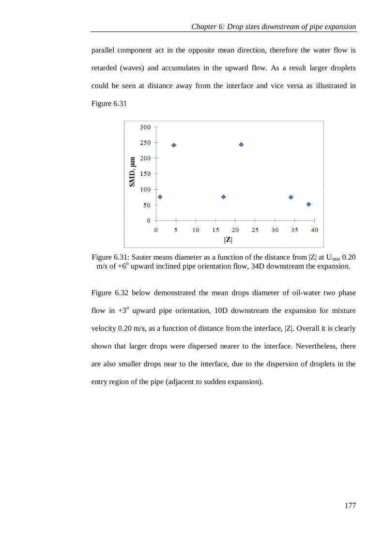
Chapter 6: Drop sizes downstream of pipe expansion
177
parallel component act in the opposite mean direction, therefore the water flow is
retarded (waves) and accumulates in the upward flow. As a result larger droplets
could be seen at distance away from the interface and vice versa as illustrated in
Figure 6.31
Figure 6.31: Sauter means diameter as a function of the distance from |Z| at Usme 0.20
m/s of +6o upward inclined pipe orientation flow, 34D downstream the expansion.
Figure 6.32 below demonstrated the mean drops diameter of oil-water two phase
flow in +3o upward pipe orientation, 10D downstream the expansion for mixture
velocity 0.20 m/s, as a function of distance from the interface, |Z|. Overall it is clearly
shown that larger drops were dispersed nearer to the interface. Nevertheless, there
are also smaller drops near to the interface, due to the dispersion of droplets in the
entry region of the pipe (adjacent to sudden expansion).
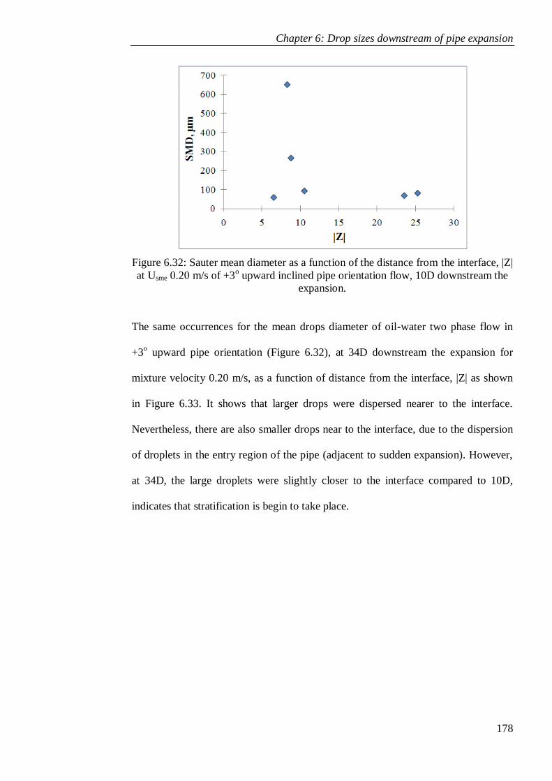
Chapter 6: Drop sizes downstream of pipe expansion
178
Figure 6.32: Sauter mean diameter as a function of the distance from the interface, |Z|
at Usme 0.20 m/s of +3o upward inclined pipe orientation flow, 10D downstream the
expansion.
The same occurrences for the mean drops diameter of oil-water two phase flow in
+3o upward pipe orientation (Figure 6.32), at 34D downstream the expansion for
mixture velocity 0.20 m/s, as a function of distance from the interface, |Z| as shown
in Figure 6.33. It shows that larger drops were dispersed nearer to the interface.
Nevertheless, there are also smaller drops near to the interface, due to the dispersion
of droplets in the entry region of the pipe (adjacent to sudden expansion). However,
at 34D, the large droplets were slightly closer to the interface compared to 10D,
indicates that stratification is begin to take place.

Chapter 6: Drop sizes downstream of pipe expansion
179
Figure 6.33: Sauter means diameter as a function of the distance from |Z| at Usme 0.20
m/s of +3o upward inclined pipe orientation flow, 34D downstream the expansion.
The following points can be concluded for the D32 in the upward inclination:
1. Droplets in oil continuous flow, settle down (stratified) slightly quicker than
droplets in water continuous flow.
2. In higher input oil volume fractions, waves could be observed especially at
10D and then become weaker further downstream.
3. Distance from the interface |Z| increase, mean drops diameter decreased only
true for upward inclination angle ≤ +3o.
6.3.4 SMD of drop size distribution in a downward inclined flow
As predicted by the model of Taitel and Dukler (1976), pipe inclination will affect
the interface level between the two phases for the ST regime flow pattern. Therefore,
in this section, SMD of drop diameter distribution in two-phase oil-water flow were
measured for downward flow inclined which were carried out in the same conditions
as in the previous section but in the opposite direction. The angles of downward
inclination flow are -3 and -6 degrees respectively. The effect of downward
Chapter 6: Drop sizes downstream of pipe expansion
180
inclination flow on development of drop size distributions is again investigated and
demonstrated.
6.3.4.1 SMD of drops distribution - Effect of input oil volume fraction
Earlier in this chapter, the relation of upward pipe (expansion) orientation and drop
diameter distributions with effect of oil volume fraction (OVF) has been
investigated. In this subsection, the same parameter was also being investigate,
however this time the orientation of the pipe expansion was downward angle
inclination. Result of the experiments were presented and discussed in the following
sub-paragraph.
Figures 6.34- 6.35 represented the results for SMD of drop diameter distributions for
downstream mixture velocity, Usme 0.20 m/s, at several axial position after expansion
in downward pipe orientation (-6o) for probe position 17 and 34 mm from bottom at
different oil volume fraction, OVF. As presented in Figure 6.34, two significant that
are clearly showed by the figure; (a) oil droplets started small (D32= 50 µm) at 10D
and 20D indicating that it is still in dispersed regime, thereafter, the droplets gained
size (coalescence) when flowing further downstream to D32= 300 µm at 34D .(b)
water droplets started big (D32 = 200 µm) at 10D, drop size decreased at 20D due to
coalescence of the bigger droplet leaving the medium drops (D32=116 µm) dispersed
in the detection region and further towards the end of the test section, coalescence
and stratification of droplets occurs here at 34D, D32 decreased to 80µm.
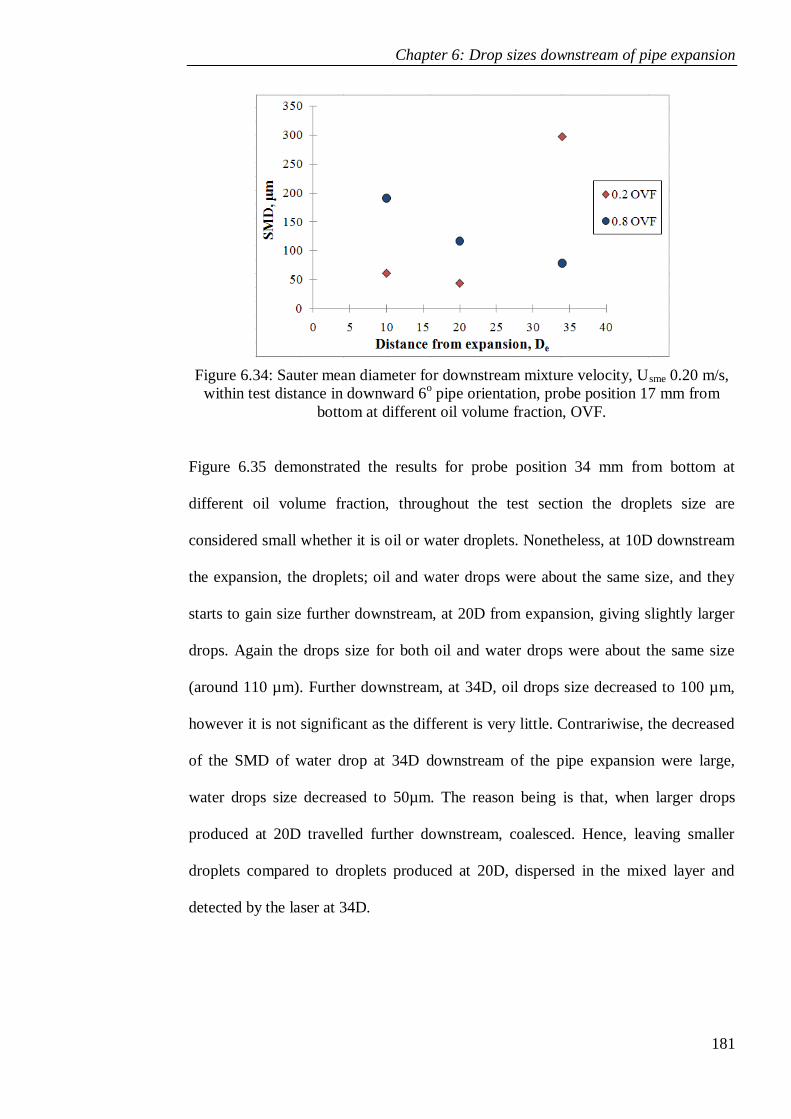
Chapter 6: Drop sizes downstream of pipe expansion
181
Figure 6.34: Sauter mean diameter for downstream mixture velocity, Usme 0.20 m/s,
within test distance in downward 6o pipe orientation, probe position 17 mm from
bottom at different oil volume fraction, OVF.
Figure 6.35 demonstrated the results for probe position 34 mm from bottom at
different oil volume fraction, throughout the test section the droplets size are
considered small whether it is oil or water droplets. Nonetheless, at 10D downstream
the expansion, the droplets; oil and water drops were about the same size, and they
starts to gain size further downstream, at 20D from expansion, giving slightly larger
drops. Again the drops size for both oil and water drops were about the same size
(around 110 µm). Further downstream, at 34D, oil drops size decreased to 100 µm,
however it is not significant as the different is very little. Contrariwise, the decreased
of the SMD of water drop at 34D downstream of the pipe expansion were large,
water drops size decreased to 50µm. The reason being is that, when larger drops
produced at 20D travelled further downstream, coalesced. Hence, leaving smaller
droplets compared to droplets produced at 20D, dispersed in the mixed layer and
detected by the laser at 34D.

Chapter 6: Drop sizes downstream of pipe expansion
182
Figure 6.35: Sauter mean diameter for downstream mixture velocity, Usme 0.20 m/s,
within test distance in downward 6o pipe orientation, probe position 34 mm from
bottom at different oil volume fraction, OVF.
As for -3o downward pipe orientation, Figure 6.36 - 6.37 respectively representing
the results for SMD of drop diameter distributions for downstream mixture velocity,
Usme 0.20 m/s, at probe position 17 and 34 mm from bottom for different oil volume
fraction. Figure 6.36 and 6.38 show the same pattern, especially for water drops of
the drops evolution throughout the test section, water droplets started big (D32 = 300
µm) at 10D, drop size decreased sharply at 20D due to stratification and coalescence
of the bigger droplet leaving only the drops of mean size around 70 µm dispersed in
the detection region. Further towards the end of the test section, at 34D, D32 remain
the same as at 20D.
Interestingly, the same occurrences as Figure 6.34 and 6.36 could be seen for mean
diameter at Usme 0.20 m/s, in downward 3o pipe orientation for probe position 34 mm
from bottom as shown in Figure 6.37. However the D32 decreased gradually rather
than sharply decreased for D32 measured at bottom of the pipe cross section (17 mm).
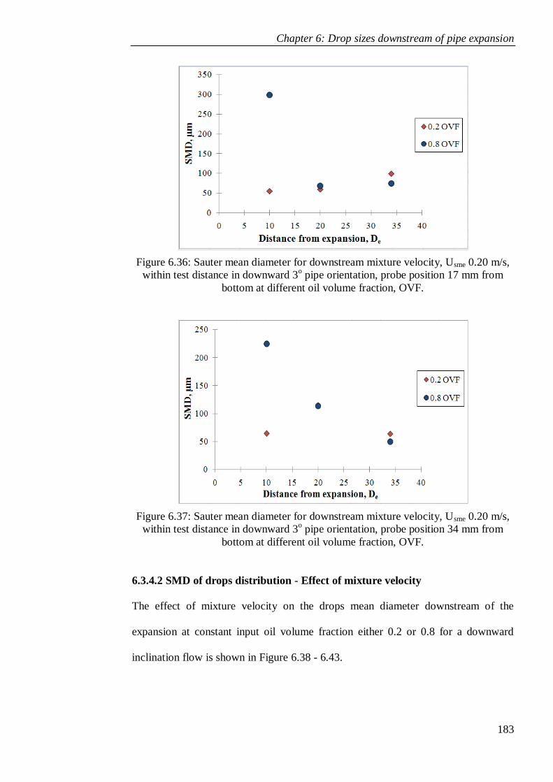
Chapter 6: Drop sizes downstream of pipe expansion
183
Figure 6.36: Sauter mean diameter for downstream mixture velocity, Usme 0.20 m/s,
within test distance in downward 3o pipe orientation, probe position 17 mm from
bottom at different oil volume fraction, OVF.
Figure 6.37: Sauter mean diameter for downstream mixture velocity, Usme 0.20 m/s,
within test distance in downward 3o pipe orientation, probe position 34 mm from
bottom at different oil volume fraction, OVF.
6.3.4.2 SMD of drops distribution - Effect of mixture velocity
The effect of mixture velocity on the drops mean diameter downstream of the
expansion at constant input oil volume fraction either 0.2 or 0.8 for a downward
inclination flow is shown in Figure 6.38 - 6.43.
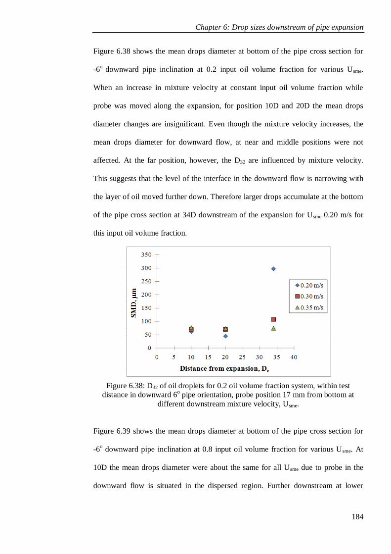
Chapter 6: Drop sizes downstream of pipe expansion
184
Figure 6.38 shows the mean drops diameter at bottom of the pipe cross section for
-6o
downward pipe inclination at 0.2 input oil volume fraction for various Usme.
When an increase in mixture velocity at constant input oil volume fraction while
probe was moved along the expansion, for position 10D and 20D the mean drops
diameter changes are insignificant. Even though the mixture velocity increases, the
mean drops diameter for downward flow, at near and middle positions were not
affected. At the far position, however, the D32 are influenced by mixture velocity.
This suggests that the level of the interface in the downward flow is narrowing with
the layer of oil moved further down. Therefore larger drops accumulate at the bottom
of the pipe cross section at 34D downstream of the expansion for Usme 0.20 m/s for
this input oil volume fraction.
Figure 6.38: D32 of oil droplets for 0.2 oil volume fraction system, within test
distance in downward 6o pipe orientation, probe position 17 mm from bottom at
different downstream mixture velocity, Usme.
Figure 6.39 shows the mean drops diameter at bottom of the pipe cross section for
-6o downward pipe inclination at 0.8 input oil volume fraction for various Usme. At
10D the mean drops diameter were about the same for all Usme due to probe in the
downward flow is situated in the dispersed region. Further downstream at lower

Chapter 6: Drop sizes downstream of pipe expansion
185
downstream mixtures velocity, D32 measured gradually becomes smaller, owing to
the coalescence has occurred, leaving medium drops dispersed in the detection
region. Followed by semi-stratification of water droplets at 34D, where only small
water drops left in the mixed layer. At 20D downstream the expansion, for 0.30 and
0.35 m/s, seems like coalescence beginning to happen. This could be noticed as the
mean drops size start to become slightly larger than that of 10D.Nevertheless, at
higher Usme, coalescence was minimal due to the collisions time were not sufficient
enough, even though it is expected that more droplets are created as the mixture
velocity increases. Interestingly, at 34D, D32 turn out to be smaller, in fact smaller
than the initial drops size (10D). Beyond this distance from expansion further
coalescence of the medium size drops is predicted to take place, if looking and based
on the progress of the drops size. However how much further downstream, that is
something needs to be determined further by future researcher.
Figure 6.39: D32 of water droplets for 0.8 oil volume fraction system, within test
distance in downward 6o pipe orientation, probe position 17 mm from bottom at
different downstream mixture velocity, Usme.
Figure 6.40 shows the mean drops diameter at the centre of the pipe cross section for
the same experimental conditions as demonstrated in Figure 6.39.The mean drops
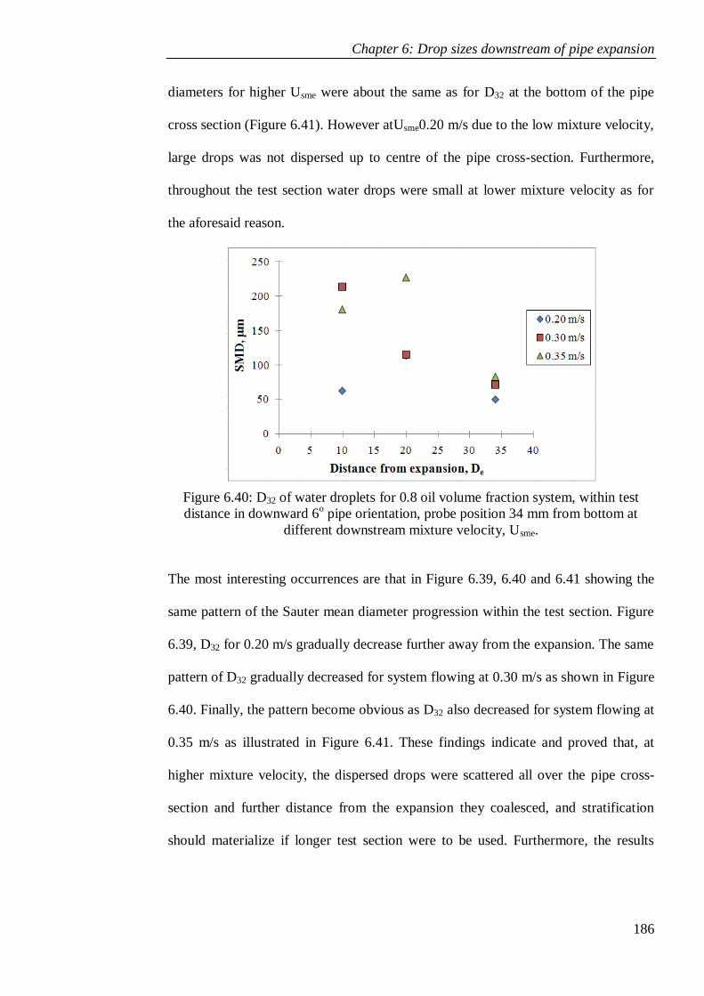
Chapter 6: Drop sizes downstream of pipe expansion
186
diameters for higher Usme were about the same as for D32 at the bottom of the pipe
cross section (Figure 6.41). However atUsme0.20 m/s due to the low mixture velocity,
large drops was not dispersed up to centre of the pipe cross-section. Furthermore,
throughout the test section water drops were small at lower mixture velocity as for
the aforesaid reason.
Figure 6.40: D32 of water droplets for 0.8 oil volume fraction system, within test
distance in downward 6o pipe orientation, probe position 34 mm from bottom at
different downstream mixture velocity, Usme.
The most interesting occurrences are that in Figure 6.39, 6.40 and 6.41 showing the
same pattern of the Sauter mean diameter progression within the test section. Figure
6.39, D32 for 0.20 m/s gradually decrease further away from the expansion. The same
pattern of D32 gradually decreased for system flowing at 0.30 m/s as shown in Figure
6.40. Finally, the pattern become obvious as D32 also decreased for system flowing at
0.35 m/s as illustrated in Figure 6.41. These findings indicate and proved that, at
higher mixture velocity, the dispersed drops were scattered all over the pipe cross-
section and further distance from the expansion they coalesced, and stratification
should materialize if longer test section were to be used. Furthermore, the results

Chapter 6: Drop sizes downstream of pipe expansion
187
showed that coalescence process initially occur at the bottom of the pipe cross
section within the pipe expansion (test section).
Figure 6.41: D32 of water droplets for 0.8 oil volume fraction system, within test
distance in downward 6o pipe orientation, probe position 51 mm from bottom at
different downstream mixture velocity, Usme.
6.3.4.3 SMD of drops distribution - Probe position
Variations of probe positions in a pipe cross-section downstream of the -6o
downward expansion are presented in Figure 6.42 and 6.45. The results generally
show that when the probe is positioned at the bottom of the pipe cross-section, the
mean drops diameters are strongly affected whereas when the probe is positioned at
the centre and top of the pipe, D32 are less influenced either in oil or water
continuous downwardly flow.
As for water continuous flow of the -6o downward orientation, this phenomenon
suggesting that the drops at the bottom position are experiencing a more rapid
coalescence process to form larger drops compared to those at the top position, in
particular at the furthest distance from the expansion (Figure 6.42).

Chapter 6: Drop sizes downstream of pipe expansion
188
Figure 6.42: D32 of oil droplets for downstream mixture velocity, Usme = 0.20 m/s,
within test distance in downward 6o pipe orientation at oil volume fraction system,
OVF = 0.2, at different probe position.
Inversely, for oil continuous downwardly flow of the same pipe orientation, drops at
the bottom position are experiencing a steadily stratification process, initially started
at bottom position at 10D downstream pipe expansion. Hence, beyond this distance
(10D), smaller droplets were measured, producing smaller D32 as shown in Figure
6.43.
Figure 6.43: D32 of water droplets for downstream mixture velocity, Usme = 0.20 m/s,
within test distance in downward 6o pipe orientation at oil volume fraction system,
OVF = 0.8, at different probe position.
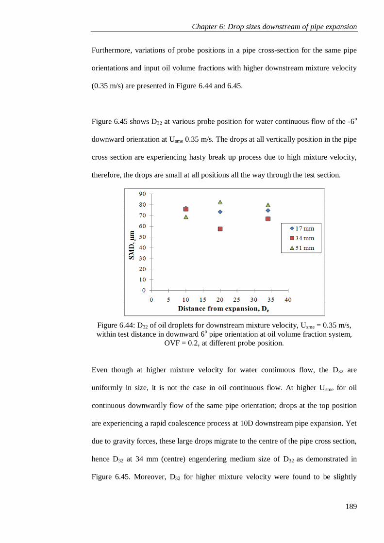
Chapter 6: Drop sizes downstream of pipe expansion
189
Furthermore, variations of probe positions in a pipe cross-section for the same pipe
orientations and input oil volume fractions with higher downstream mixture velocity
(0.35 m/s) are presented in Figure 6.44 and 6.45.
Figure 6.45 shows D32 at various probe position for water continuous flow of the -6o
downward orientation at Usme 0.35 m/s. The drops at all vertically position in the pipe
cross section are experiencing hasty break up process due to high mixture velocity,
therefore, the drops are small at all positions all the way through the test section.
Figure 6.44: D32 of oil droplets for downstream mixture velocity, Usme = 0.35 m/s,
within test distance in downward 6o pipe orientation at oil volume fraction system,
OVF = 0.2, at different probe position.
Even though at higher mixture velocity for water continuous flow, the D32 are
uniformly in size, it is not the case in oil continuous flow. At higher Usme for oil
continuous downwardly flow of the same pipe orientation; drops at the top position
are experiencing a rapid coalescence process at 10D downstream pipe expansion. Yet
due to gravity forces, these large drops migrate to the centre of the pipe cross section,
hence D32 at 34 mm (centre) engendering medium size of D32 as demonstrated in
Figure 6.45. Moreover, D32 for higher mixture velocity were found to be slightly

Chapter 6: Drop sizes downstream of pipe expansion
190
bigger than of for 0.20 m/s at all vertically position along the test section. This is
expected to be the influences of collisions frequency and time as alleged by Howarth
(1964).
Figure 6.45: D32 of water droplets for downstream mixture velocity, Usme = 0.35 m/s,
within test distance in downward 6o pipe orientation at oil volume fraction system,
OVF = 0.8, at different probe position.
Subsequently when the inclination angle were reduced to -3o downward orientation,
for water continuous flow as presented in Figure 6.46, the same phenomenon as
Figure 6.43 occurs. However for -3o downwardly flow, due to slower in-situ water
velocity compared to -6o, at 10D downstream of the expansion, D32 were found to be
larger at probe position centre of the pipe cross section which was not observed in -6o
downwardly flow. Suggesting that the drops at the centre position too are
experiencing coalescence process to form larger drops owing to slower in-situ water
velocity which allowed sufficient time for oil drops to coalesce.

Chapter 6: Drop sizes downstream of pipe expansion
191
Figure 6.46: D32 of water droplets for downstream mixture velocity, Usme = 0.20 m/s,
within test distance in downward 3o pipe orientation at oil volume fraction system,
OVF = 0.8, at different probe position.
Figure 6.47 shows D32 at various probe position for water continuous flow of the -3o
downward orientation at Usme 0.35 m/s. The mean drops pattern was found to be
about the same as for -6o downward flow, except that at position 10D of -3
o pipe
orientation, the mean drops size is smaller. This is due to the turbulent forces at a
lower in-situ water velocity may not be large enough to overcome the frictional drags
on the drops. Hence, larger drops were less dispersed to the top of the pipe cross
section, thus producing smaller value of D32 at this position.

Chapter 6: Drop sizes downstream of pipe expansion
192
Figure 6.47: D32 of water droplets for downstream mixture velocity, Usme = 0.35 m/s,
within test distance in downward 3o pipe orientation at oil volume fraction system,
OVF = 0.8, at different probe position.
6.3.4.4 Development of drops size - Cross-sectional of downward pipe
expansion
Figure 6.48 below demonstrated the mean drops diameter of oil-water two phase
flow in -6o downward pipe orientation, 10D downstream the expansion for mixture
velocity 0.20 m/s, as a function of distance from the interface, |Z|. Remarkably, the
pattern of droplets dispersion is similar to the droplets dispersion at the other pipe
orientations (Figure 6.16, 6.30 and 6.32); larger drops were dispersed closer to the
interface. However, the largest mean drops diameter for this condition (-3o
downward) were slightly smaller compared to the D32 at the other orientations.
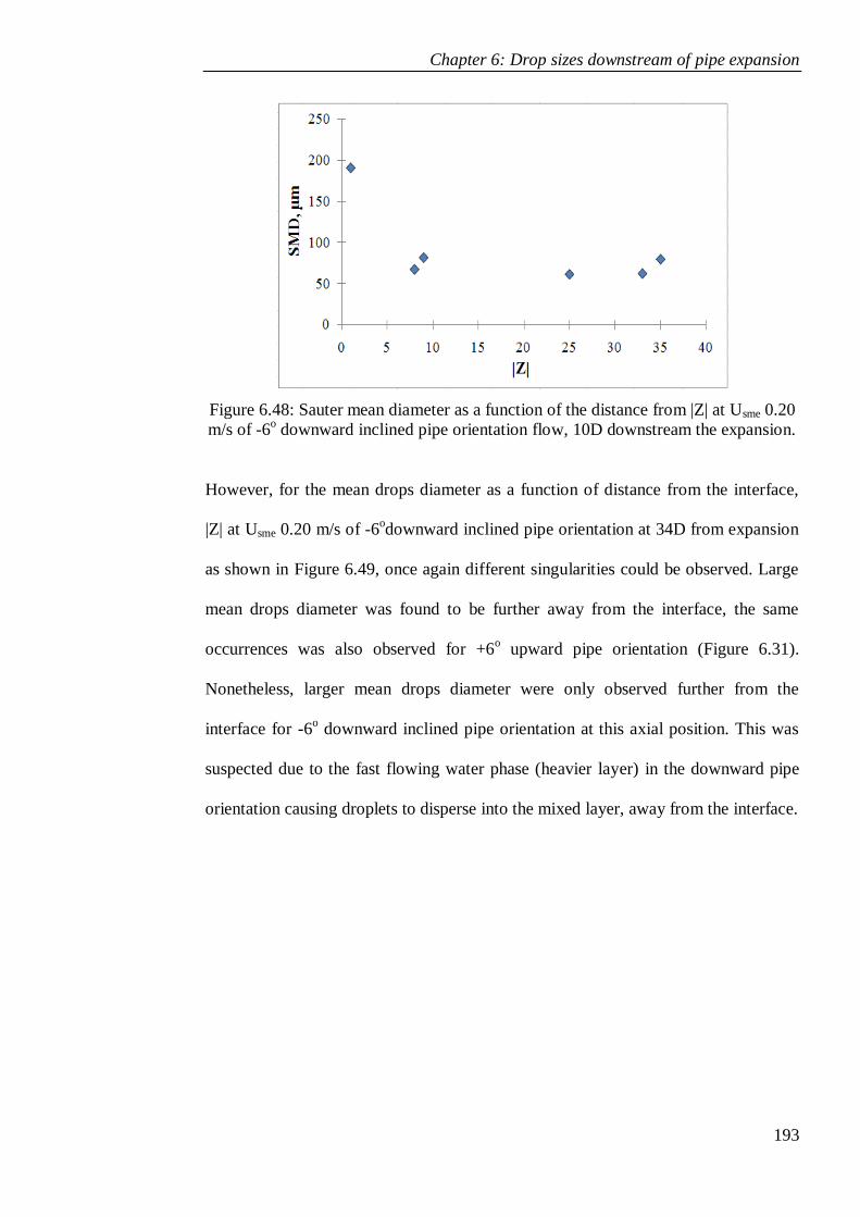
Chapter 6: Drop sizes downstream of pipe expansion
193
Figure 6.48: Sauter mean diameter as a function of the distance from |Z| at Usme 0.20
m/s of -6o downward inclined pipe orientation flow, 10D downstream the expansion.
However, for the mean drops diameter as a function of distance from the interface,
|Z| at Usme 0.20 m/s of -6odownward inclined pipe orientation at 34D from expansion
as shown in Figure 6.49, once again different singularities could be observed. Large
mean drops diameter was found to be further away from the interface, the same
occurrences was also observed for +6o upward pipe orientation (Figure 6.31).
Nonetheless, larger mean drops diameter were only observed further from the
interface for -6o downward inclined pipe orientation at this axial position. This was
suspected due to the fast flowing water phase (heavier layer) in the downward pipe
orientation causing droplets to disperse into the mixed layer, away from the interface.
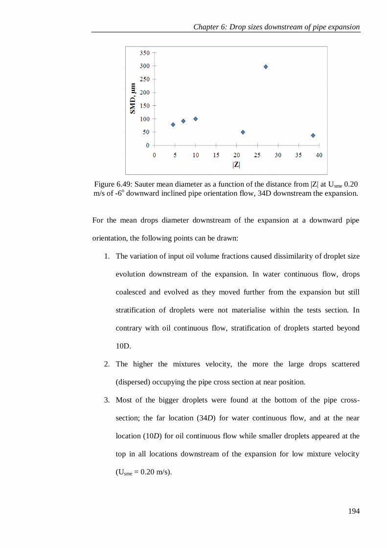
Chapter 6: Drop sizes downstream of pipe expansion
194
Figure 6.49: Sauter mean diameter as a function of the distance from |Z| at Usme 0.20
m/s of -6o downward inclined pipe orientation flow, 34D downstream the expansion.
For the mean drops diameter downstream of the expansion at a downward pipe
orientation, the following points can be drawn:
1. The variation of input oil volume fractions caused dissimilarity of droplet size
evolution downstream of the expansion. In water continuous flow, drops
coalesced and evolved as they moved further from the expansion but still
stratification of droplets were not materialise within the tests section. In
contrary with oil continuous flow, stratification of droplets started beyond
10D.
2. The higher the mixtures velocity, the more the large drops scattered
(dispersed) occupying the pipe cross section at near position.
3. Most of the bigger droplets were found at the bottom of the pipe cross-
section; the far location (34D) for water continuous flow, and at the near
location (10D) for oil continuous flow while smaller droplets appeared at the
top in all locations downstream of the expansion for low mixture velocity
(Usme = 0.20 m/s).

Chapter 6: Drop sizes downstream of pipe expansion
195
6.3.5 Comparison between different angles of inclination
The effect of angles of inclination for 0.20 and 0.35 m/s with 0.2 input oil volume
fractions downstream of the expansion is shown in Figure 6.50, 6.51 and 6.52.
Results of the drop size measurements of water continuous flow in a sudden
expansion at Usme0.20 m/s downward inclination flow show only minimal effect of
the inclination angle. The noticeable effect of the inclination angle of this flow
conditions are at axial position 34D for -6o
downward inclination flow, where large
droplet were detected as shown in Figure 6.50.
Figure 6.50: D32 of oil droplets for downstream mixture velocity, Usme = 0.20 m/s, oil
volume fraction system, OVF = 0.2, at 17 mm probe position from bottom, along test
section distance for different pipe orientation.
Furthermore, the angle of inclination has negligible effect on drop size distributions
when the downstream mixture velocity is increased to 0.35 m/s (Figure 6.51 and
6.52). In this condition, the mixed layer would be responsible for the droplet size for
horizontal and both inclination of pipe orientation, whether it is upward or
downward. It should be noted that the mixed layer almost entirely dominated in a
pipe cross-section even with the probe positioned at the top (Figure 6.52), and this is
clearly supported by the results of Hasan (2006) and Yang et al. (2003).
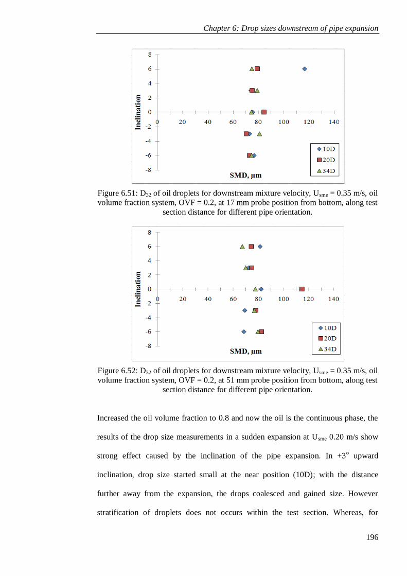
Chapter 6: Drop sizes downstream of pipe expansion
196
Figure 6.51: D32 of oil droplets for downstream mixture velocity, Usme = 0.35 m/s, oil
volume fraction system, OVF = 0.2, at 17 mm probe position from bottom, along test
section distance for different pipe orientation.
Figure 6.52: D32 of oil droplets for downstream mixture velocity, Usme = 0.35 m/s, oil
volume fraction system, OVF = 0.2, at 51 mm probe position from bottom, along test
section distance for different pipe orientation.
Increased the oil volume fraction to 0.8 and now the oil is the continuous phase, the
results of the drop size measurements in a sudden expansion at Usme 0.20 m/s show
strong effect caused by the inclination of the pipe expansion. In +3o upward
inclination, drop size started small at the near position (10D); with the distance
further away from the expansion, the drops coalesced and gained size. However
stratification of droplets does not occurs within the test section. Whereas, for

Chapter 6: Drop sizes downstream of pipe expansion
197
downward flow, droplets detected were small, indicated that stratification of droplets
has occurred beyond 10D for downward pipe orientation as shown in Figure 6.53.
Figure 6.53: D32 of water droplets for downstream mixture velocity, Usme = 0.20 m/s,
oil volume fraction system, OVF = 0.8, at 17 mm probe position from bottom, along
test section distance for different pipe orientation.
As the downstream mixture velocity is increased to 0.35 m/s, the angle of inclination
has insignificant effect on drop size distributions. This was demonstrated in the
Figure 6.54. Similar to the phenomena in water continuous flow (0.2 OVF), the
mixed layer would be responsible for the droplet size for horizontal and both
inclination of pipe orientation, whether it is upward or downward. The mixed layer
dominated almost entirely in the pipe cross-section.
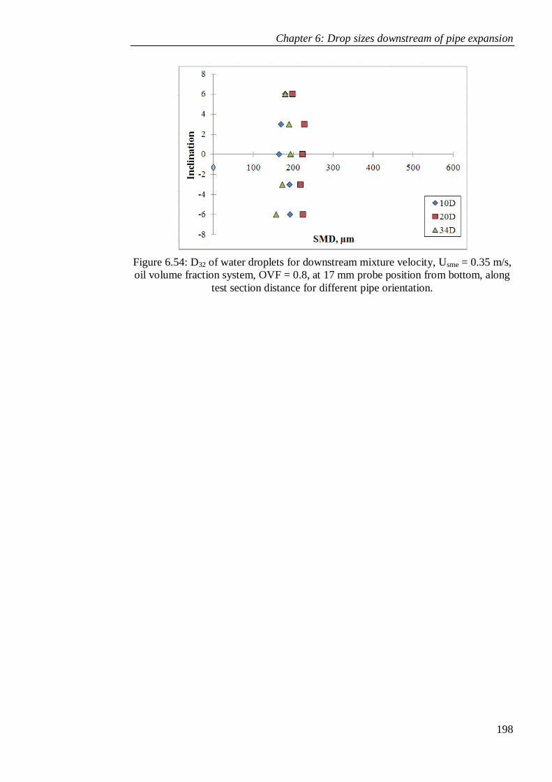
Chapter 6: Drop sizes downstream of pipe expansion
198
Figure 6.54: D32 of water droplets for downstream mixture velocity, Usme = 0.35 m/s,
oil volume fraction system, OVF = 0.8, at 17 mm probe position from bottom, along
test section distance for different pipe orientation.

Chapter 7: Preliminary investigation on influence of surface tension on drop size
199
CHAPTER 7
PRELIMINARY INVESTIGATION ON INFLUENCE OF
SURFACE TENSION ON DROP SIZE
Many researchers have reported experimental works on measurement of average
droplet size used light transmittance techniques or chemical methods. Size
distributions were also studied by measurements with photography, encapsulation,
sedimentation and electro-resistivity measurements. Concurrently, droplet mixing
measurements were made by various indirect methods such as following a chemical
reaction or dispersion of a non-transferring dye in the dispersed phase. A number of
investigators reported experimental data on interfacial areas (Mok and Treybal, 1971;
Schindler and R. E., 1968; Weinstein and Treybal, 1973) and drop distributions
(Bouyatiotis and Thornton, 1967) in flow systems.
In certain industrial flows or experimental facility, the presence or usage of
surfactants is reported. In the process industry, surfactants are added to process
liquids to prevent unwanted deposits by keeping them finely dispersed. These agents
influence the interfacial tension interaction in liquid-liquid multiphase system.
Therefore, as a starting point the droplet generation under controlled conditions and
the impact of surfactants are investigated.
Chapter 7: Preliminary investigation on influence of surface tension on drop size
200
This chapter presents briefly the apparatus, methodology and results of interfacial
tension experiments of two liquids and liquid-liquid mixing in fully baffle mixing
vessel. The criteria of experimental design and the principle work of each instrument
are explained. The experiment procedures for the measurement of interfacial tension,
drop size and drop size distribution performed on the rig are briefly covered.
7.1 Influence of interfacial tension on drop size
Interfacial tension plays a greater role in homogenization. In order to investigate the
impact of interfacial tension on breakage and coalescence behaviour, dynamics of
droplet clusters needs to be investigated under controlled environment. The
experiment on effect of interfacial tension on drop size and drop size distribution in a
static flow and dynamic liquid-liquid flow (mixing vessel), two measurement
methods were used. In static flow, interfacial tensions were measured by mean of
drop weight method and high speed camera. Whereas in mixing vessel, the laser
backscattered technique (Lasentec FBRM M500P) was used to determine the drop
size and drop size distribution of the system. However, to understand what really
happened to the droplet clusters in homogenisation and coalescence process,
measurement for a single droplet under controlled environment must first be studied.
7.1.1 Interfacial tension – static flow
One of most frequently used method to measure interfacial tension involves the
formation of a drop of one liquid in the bulk of the other. Either the drop is allowed
to fall when fully grown (Harkins and Humphery, 1916) or the contours of the partly
grown pendent drop are measured (Andreas et al., 1938).In static flow, interfacial
tensions were measured by mean of drop weight method and high speed camera. The
Chapter 7: Preliminary investigation on influence of surface tension on drop size
201
criteria of experimental design and the principle work of each instrument are
explained.
7.1.1.1 Drop weight method
The drop-weight method is a known method for measuring surface tension and is one
of the simplest and reasonably acceptable methods which have been used for
interfacial tension. Interfacial tension was measured by mean of drop weight method
as proposed in the Practical Physical Chemistry (James, 1967) as shown in Appendix
7A. Interfacial tension measurement of water-kerosene oil with surfactant added was
performed. The accuracy of a drop-weight method is improved by increasing the
number of drops.
The methods depend on the equilibrium of the two forces; the weight of a drop of
liquid (m) just about to fall from a vertical tube with an external radius, r and the
force due to the surface or interfacial tension (γ) acting around the periphery of the
needle holding the drop. The weight of a drop that falls should be given by:
mg = 2π.r.γ 7.1
In actual fact, only a portion of the drop falls; Harkins and Brown proposed that the
drop of weight (mg) given by the equation 7.1 be called the „ideal drop‟. The fraction
of the ideal drop which falls was determined by these workers in an extensive series
of experiments. The form of the maximum stable hanging drop is a function of r/v1/3,
where r is the outer radius of the tube and v the volume of the drop (determined from
the mass of the drop and the density of the liquid). This determines the fraction
f(r/v1/3
) of the drop which falls. The actual weight of the drop which falls is thus:
mg = 2.π.r.γ. f(r/v1/3
) 7.2
Chapter 7: Preliminary investigation on influence of surface tension on drop size
202
Hence γ= (m.g) /{ 2.π.r. f(r/v1/3
)}
= (F.m.g)/r 7.3
Thus, to determine the surface tension of a liquid it is only necessary to determine
the mass of 1 drop of the liquid, calculate its volume v from a rough density
determination, multiply this by 1/r3, look up the value of F (Figure 7.1) and finally
multiply by mg/r. The density of the liquid is involved only in determining the value
of the correction which is not sensitive to density differences.
As for measuring interfacial tension of two immiscible liquids, the mass (m) in the
equation 7.3 is replaced by υ(ρ1 – ρ2), where υ is the recorded volume and ρ1 and ρ2
the densities of water and kerosene respectively. Thus
σ = {F.υ.g(ρ1 – ρ2)}/r 7.4
The Antonoff‟s rule was used to get an approximation values for water – kerosene
interfacial tension. Antonoff‟s rule says that the interfacial tension between two
liquids is approximately equal to the difference between the surface tensions of the
two liquids:
σ ≈ γ1 –γ2 7.5
The experimental results may then be compared with Antonoff‟s rule to make sure
the result obtained is reasonable and acceptable.
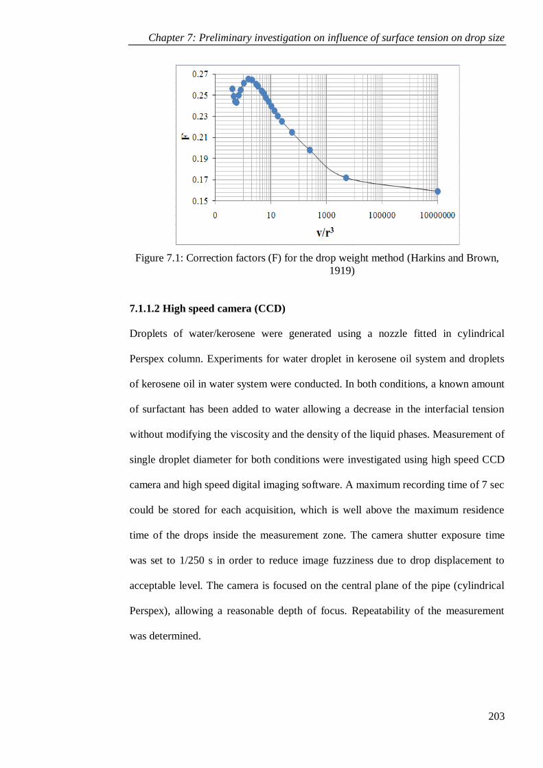
Chapter 7: Preliminary investigation on influence of surface tension on drop size
203
Figure 7.1: Correction factors (F) for the drop weight method (Harkins and Brown,
1919)
7.1.1.2 High speed camera (CCD)
Droplets of water/kerosene were generated using a nozzle fitted in cylindrical
Perspex column. Experiments for water droplet in kerosene oil system and droplets
of kerosene oil in water system were conducted. In both conditions, a known amount
of surfactant has been added to water allowing a decrease in the interfacial tension
without modifying the viscosity and the density of the liquid phases. Measurement of
single droplet diameter for both conditions were investigated using high speed CCD
camera and high speed digital imaging software. A maximum recording time of 7 sec
could be stored for each acquisition, which is well above the maximum residence
time of the drops inside the measurement zone. The camera shutter exposure time
was set to 1/250 s in order to reduce image fuzziness due to drop displacement to
acceptable level. The camera is focused on the central plane of the pipe (cylindrical
Perspex), allowing a reasonable depth of focus. Repeatability of the measurement
was determined.

Chapter 7: Preliminary investigation on influence of surface tension on drop size
204
Droplet images data were taken using the high speed CCD camera for sets of
mixtures conditions. Droplet images from the high speed CCD camera were analysed
using high speed digital imaging software (PFV Ver. 318). Then digitize using the
software to get the diameter of the drops.
7.1.1.3 Interfacial tension results - Static flow results
Drop weight results:
The mean value of interfacial tension obtained from the experiments is 0.0437 N/m.
In literature we found the value of 0.0728 N/m for water surface tension and 0.024
N/m for kerosene surface tension. Using these values, the Antonoff‟s rule predicts
that the water-kerosene interfacial tension has to be 0.0488 N/m which is 10.4%
greater than measured interfacial tension value. The result of the mean value for the
measured interfacial tension is shown in Figure 7.2.
Figure 7.2: Effect of surfactant on interfacial tension.

Chapter 7: Preliminary investigation on influence of surface tension on drop size
205
High speed camera results:
Figure 7.3 shows the IFT for different surfactant CMC obtained from drop weight
method. In correspondence to the result shown in Figure 7.3, series of droplet image
with effect of the same surfactant CMC concentration used is shown in Figure 7.4. It
clearly shows that, for different surfactant concentration, diameter of drops at the
same position taken (height) varies.
Figure 7.3: Interfacial tension for different surfactant CMC.
Figure 7.4: Effect of surfactant CMC concentration on droplet size
7.1.2 Interfacial tension – mixing flow
An experimental liquid-liquid dispersions facility has been constructed and
measurements of mean drop and drop size distribution using Laser focused beam
reflectance measurement technique are reported. Lasentec M500P FBRM
manufactured by Mettler-Toledo Ltd has been employed on a vessel 125 mm

Chapter 7: Preliminary investigation on influence of surface tension on drop size
206
diameter. An experimental investigation has been carried out to characterise the
influences of impurities on the drop size distributions of liquid–liquid dispersion in a
stirred vessel. Water/kerosene oil system in the 125 mm vessel was agitated using 38
mm diameter radial impeller (6 paddles). Each experiment was performed by pouring
the kerosene oil and water into the mixing vessel, let it settle and then agitation was
commenced. Dispersion was produced in the mixing vessel. Drop size measurements
were taken when the process reached steady-state conditions.
7.1.2.1 Experimental conditions
In order to study the effect of the surfactant presence on drop size distributions,
series of experiments were performed. At the first series, the drop size distributions
were investigated for pure system, IFT 44 mN/m (kerosene/water) at various oil
volume fractions (0.8, 0.6, 0.5, 0.4 and 0.15) with different impeller Reynolds
number, NRe 10000 and 15000 respectively. At the second series, drop size
distributions have been investigated at the same oil volume fractions and impeller
Reynolds numbers as the first series. However, this time with addition of surfactant
at different concentrations, ranges from 0.005% - 0.5 % SDScmc. With these additions
of surfactant concentrations, interfacial tensions of the system ranges are 37- 6mN/m
(kerosene/water).
In all of the experiments, the probe was placed at the liquids interface and the system
was then agitated for 5 minutes using radial 6 paddle impeller (RP 6) for NRe 10000
and 15000 respectively before commence measurements. This procedure is
performed to make sure that the system break up and coalescence is well balance as
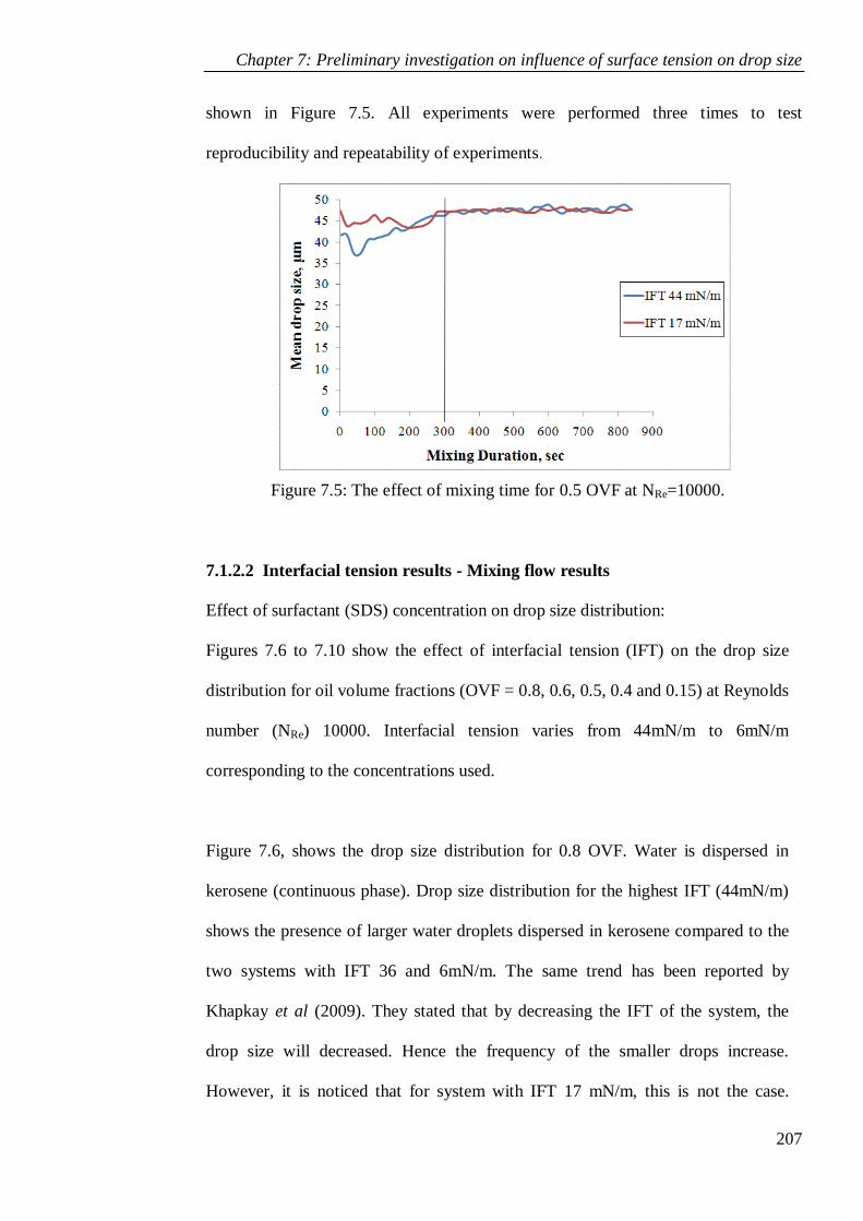
Chapter 7: Preliminary investigation on influence of surface tension on drop size
207
shown in Figure 7.5. All experiments were performed three times to test
reproducibility and repeatability of experiments.
Figure 7.5: The effect of mixing time for 0.5 OVF at NRe=10000.
7.1.2.2 Interfacial tension results - Mixing flow results
Effect of surfactant (SDS) concentration on drop size distribution:
Figures 7.6 to 7.10 show the effect of interfacial tension (IFT) on the drop size
distribution for oil volume fractions (OVF = 0.8, 0.6, 0.5, 0.4 and 0.15) at Reynolds
number (NRe) 10000. Interfacial tension varies from 44mN/m to 6mN/m
corresponding to the concentrations used.
Figure 7.6, shows the drop size distribution for 0.8 OVF. Water is dispersed in
kerosene (continuous phase). Drop size distribution for the highest IFT (44mN/m)
shows the presence of larger water droplets dispersed in kerosene compared to the
two systems with IFT 36 and 6mN/m. The same trend has been reported by
Khapkay et al (2009). They stated that by decreasing the IFT of the system, the
drop size will decreased. Hence the frequency of the smaller drops increase.
However, it is noticed that for system with IFT 17 mN/m, this is not the case.
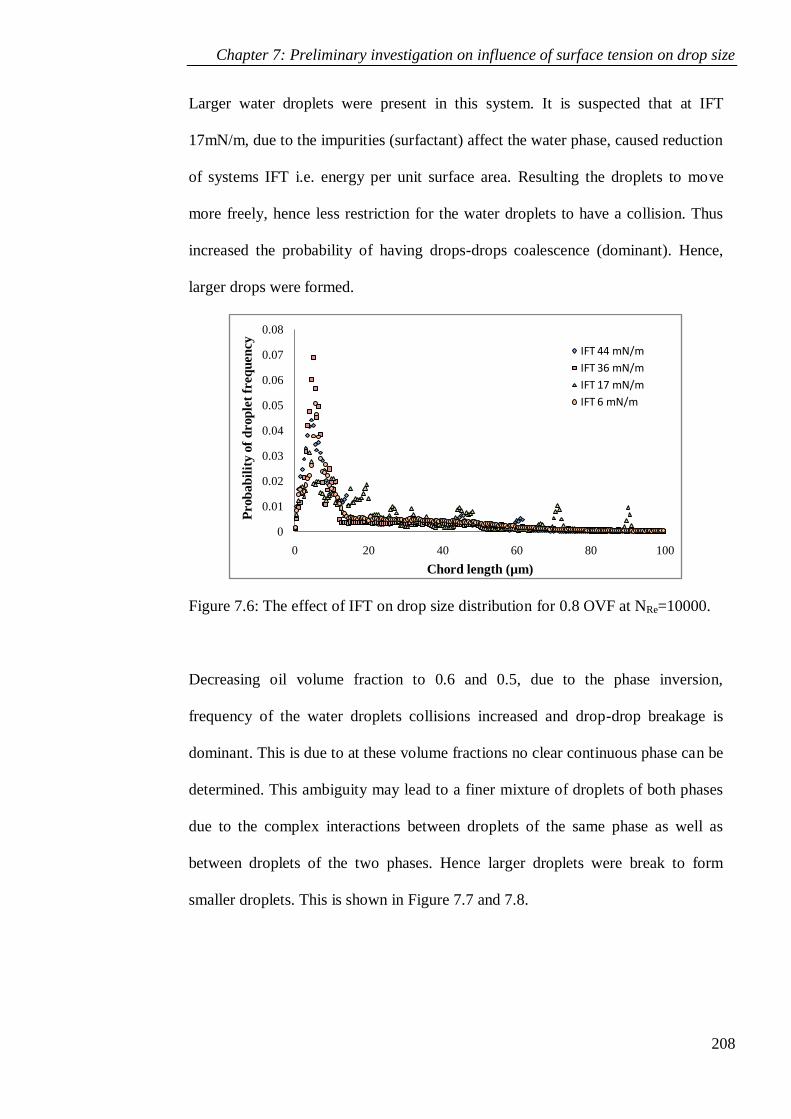
Chapter 7: Preliminary investigation on influence of surface tension on drop size
208
Larger water droplets were present in this system. It is suspected that at IFT
17mN/m, due to the impurities (surfactant) affect the water phase, caused reduction
of systems IFT i.e. energy per unit surface area. Resulting the droplets to move
more freely, hence less restriction for the water droplets to have a collision. Thus
increased the probability of having drops-drops coalescence (dominant). Hence,
larger drops were formed.
Figure 7.6: The effect of IFT on drop size distribution for 0.8 OVF at NRe=10000.
Decreasing oil volume fraction to 0.6 and 0.5, due to the phase inversion,
frequency of the water droplets collisions increased and drop-drop breakage is
dominant. This is due to at these volume fractions no clear continuous phase can be
determined. This ambiguity may lead to a finer mixture of droplets of both phases
due to the complex interactions between droplets of the same phase as well as
between droplets of the two phases. Hence larger droplets were break to form
smaller droplets. This is shown in Figure 7.7 and 7.8.
0
0.01
0.02
0.03
0.04
0.05
0.06
0.07
0.08
0 20 40 60 80 100
Prob
ab
ilit
y o
f d
rop
let
freq
uen
cy
Chord length (µm)
IFT 44 mN/m
IFT 36 mN/m
IFT 17 mN/m
IFT 6 mN/m
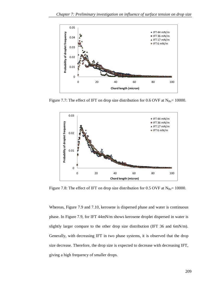
Chapter 7: Preliminary investigation on influence of surface tension on drop size
209
Figure 7.7: The effect of IFT on drop size distribution for 0.6 OVF at NRe= 10000.
Figure 7.8: The effect of IFT on drop size distribution for 0.5 OVF at NRe= 10000.
Whereas, Figure 7.9 and 7.10, kerosene is dispersed phase and water is continuous
phase. In Figure 7.9, for IFT 44mN/m shows kerosene droplet dispersed in water is
slightly larger compare to the other drop size distribution (IFT 36 and 6mN/m).
Generally, with decreasing IFT in two phase systems, it is observed that the drop
size decrease. Therefore, the drop size is expected to decrease with decreasing IFT,
giving a high frequency of smaller drops.
0
0.01
0.02
0.03
0.04
0.05
0 20 40 60 80 100
Pro
bab
ility
of
dro
ple
t fr
equ
ency
Chord length (micron)
IFT 44 mN/mIFT 36 mN/mIFT 17 mN/mIFT 6 mN/m
0
0.01
0.02
0.03
0 20 40 60 80 100
Pro
bab
ility
of
dro
ple
t fr
equ
ency
Chord length (micron)
IFT 44 mN/mIFT 36 mN/mIFT 17 mN/mIFT 6 mN/m

Chapter 7: Preliminary investigation on influence of surface tension on drop size
210
Conversely, this is not the case when oil volume fraction decrease from Ø = 0.4 to
0.15. Larger kerosene droplets were observed for 0.15 OVF at lower IFTs (see
Figure 7.10). This is due to collisions of kerosene droplets; drop-drop coalescence
is dominant. Due to the impurities (surfactant) affect the water phase, caused
reduction of systems IFT.
Figure 7.9: The effect of IFT on drop size distribution for 0.4 OVF at NRe= 10000.
Figure 7.10: The effect of IFT on drop size distribution for 0.15 OVF at NRe=
10000.
0
0.01
0.02
0.03
0 20 40 60 80 100
Pro
bab
ility
of
dro
ple
t fr
equ
ency
Chord length (micron)
IFT 44 mN/m
IFT 36 mN/m
IFT 17 mN/m
IFT 6 mN/m
0
0.01
0.02
0.03
0.04
0 20 40 60 80 100
Pro
bab
ility
of
dro
ple
t fr
eq
uen
cy
Chord length (micron)
IFT 44 mN/mIFT 36 mN/mIFT 17 mN/mIFT 6 mN/m
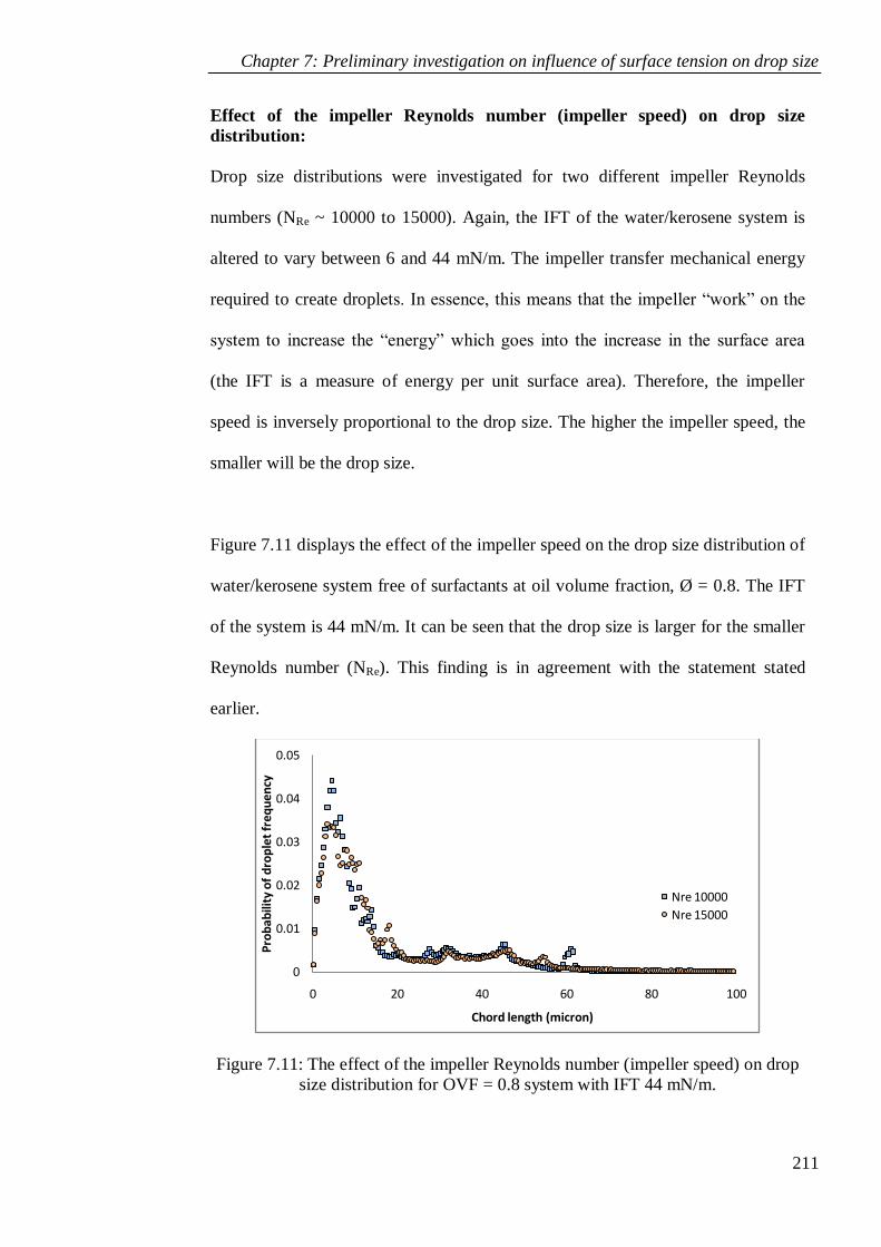
Chapter 7: Preliminary investigation on influence of surface tension on drop size
211
Effect of the impeller Reynolds number (impeller speed) on drop size
distribution:
Drop size distributions were investigated for two different impeller Reynolds
numbers (NRe ~ 10000 to 15000). Again, the IFT of the water/kerosene system is
altered to vary between 6 and 44 mN/m. The impeller transfer mechanical energy
required to create droplets. In essence, this means that the impeller “work” on the
system to increase the “energy” which goes into the increase in the surface area
(the IFT is a measure of energy per unit surface area). Therefore, the impeller
speed is inversely proportional to the drop size. The higher the impeller speed, the
smaller will be the drop size.
Figure 7.11 displays the effect of the impeller speed on the drop size distribution of
water/kerosene system free of surfactants at oil volume fraction, Ø = 0.8. The IFT
of the system is 44 mN/m. It can be seen that the drop size is larger for the smaller
Reynolds number (NRe). This finding is in agreement with the statement stated
earlier.
Figure 7.11: The effect of the impeller Reynolds number (impeller speed) on drop
size distribution for OVF = 0.8 system with IFT 44 mN/m.
0
0.01
0.02
0.03
0.04
0.05
0 20 40 60 80 100
Pro
bab
ility
of
dro
ple
t fr
eq
uen
cy
Chord length (micron)
Nre 10000
Nre 15000
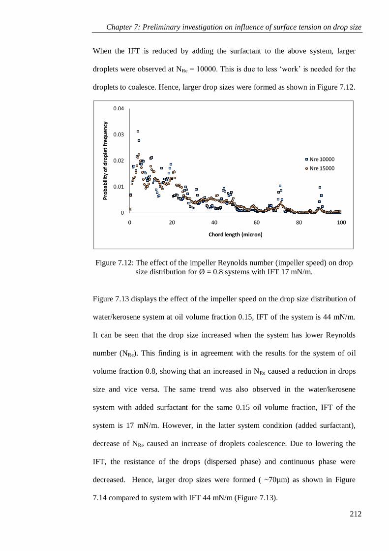
Chapter 7: Preliminary investigation on influence of surface tension on drop size
212
When the IFT is reduced by adding the surfactant to the above system, larger
droplets were observed at NRe = 10000. This is due to less „work‟ is needed for the
droplets to coalesce. Hence, larger drop sizes were formed as shown in Figure 7.12.
Figure 7.12: The effect of the impeller Reynolds number (impeller speed) on drop
size distribution for Ø = 0.8 systems with IFT 17 mN/m.
Figure 7.13 displays the effect of the impeller speed on the drop size distribution of
water/kerosene system at oil volume fraction 0.15, IFT of the system is 44 mN/m.
It can be seen that the drop size increased when the system has lower Reynolds
number (NRe). This finding is in agreement with the results for the system of oil
volume fraction 0.8, showing that an increased in NRe caused a reduction in drops
size and vice versa. The same trend was also observed in the water/kerosene
system with added surfactant for the same 0.15 oil volume fraction, IFT of the
system is 17 mN/m. However, in the latter system condition (added surfactant),
decrease of NRe caused an increase of droplets coalescence. Due to lowering the
IFT, the resistance of the drops (dispersed phase) and continuous phase were
decreased. Hence, larger drop sizes were formed ( ~70µm) as shown in Figure
7.14 compared to system with IFT 44 mN/m (Figure 7.13).
0
0.01
0.02
0.03
0.04
0 20 40 60 80 100
Pro
bab
ility
of
dro
ple
t fr
equ
ency
Chord length (micron)
Nre 10000
Nre 15000
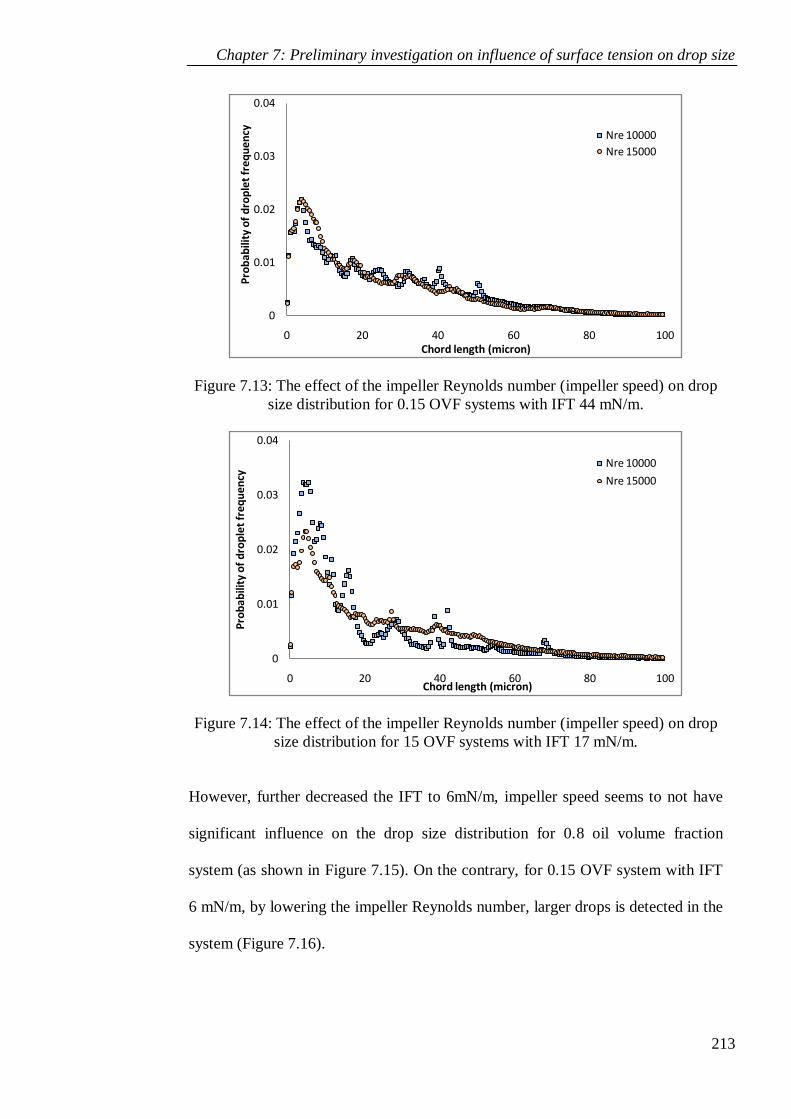
Chapter 7: Preliminary investigation on influence of surface tension on drop size
213
Figure 7.13: The effect of the impeller Reynolds number (impeller speed) on drop
size distribution for 0.15 OVF systems with IFT 44 mN/m.
Figure 7.14: The effect of the impeller Reynolds number (impeller speed) on drop
size distribution for 15 OVF systems with IFT 17 mN/m.
However, further decreased the IFT to 6mN/m, impeller speed seems to not have
significant influence on the drop size distribution for 0.8 oil volume fraction
system (as shown in Figure 7.15). On the contrary, for 0.15 OVF system with IFT
6 mN/m, by lowering the impeller Reynolds number, larger drops is detected in the
system (Figure 7.16).
0
0.01
0.02
0.03
0.04
0 20 40 60 80 100
Pro
bab
ility
of
dro
ple
t fr
equ
ency
Chord length (micron)
Nre 10000
Nre 15000
0
0.01
0.02
0.03
0.04
0 20 40 60 80 100
Pro
bab
ility
of
dro
ple
t fr
equ
ency
Chord length (micron)
Nre 10000
Nre 15000
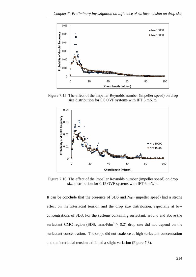
Chapter 7: Preliminary investigation on influence of surface tension on drop size
214
Figure 7.15: The effect of the impeller Reynolds number (impeller speed) on drop
size distribution for 0.8 OVF systems with IFT 6 mN/m.
Figure 7.16: The effect of the impeller Reynolds number (impeller speed) on drop
size distribution for 0.15 OVF systems with IFT 6 mN/m.
It can be conclude that the presence of SDS and NRe (impeller speed) had a strong
effect on the interfacial tension and the drop size distribution, especially at low
concentrations of SDS. For the systems containing surfactant, around and above the
surfactant CMC region (SDS, mmol/dm3 ≥ 8.2) drop size did not depend on the
surfactant concentration. The drops did not coalesce at high surfactant concentration
and the interfacial tension exhibited a slight variation (Figure 7.3).
0
0.01
0.02
0.03
0.04
0.05
0.06
0 20 40 60 80 100
Pro
bab
ility
of
dro
ple
t fr
equ
ency
Chord length (micron)
Nre 10000
Nre 15000
0
0.01
0.02
0.03
0.04
0 20 40 60 80 100
Pro
bab
ility
of
dro
ple
t fr
equ
ency
Chord length (micron)
Nre 10000
Nre 15000
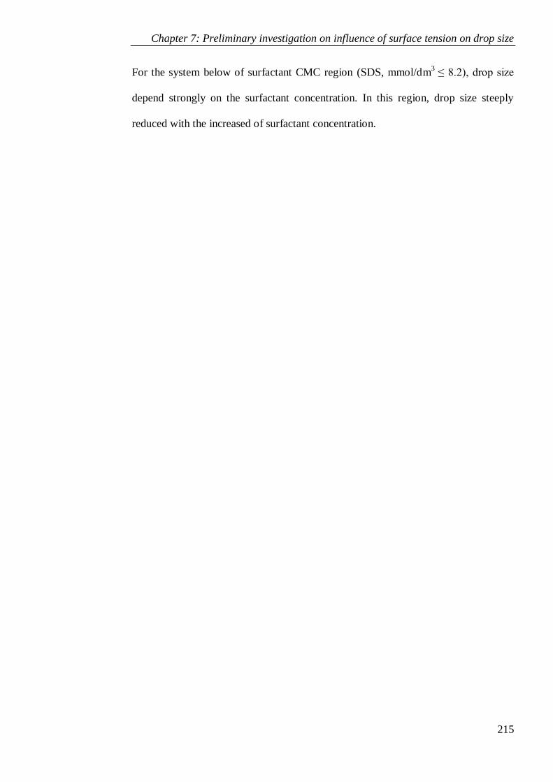
Chapter 7: Preliminary investigation on influence of surface tension on drop size
215
For the system below of surfactant CMC region (SDS, mmol/dm3
≤ 8.2), drop size
depend strongly on the surfactant concentration. In this region, drop size steeply
reduced with the increased of surfactant concentration.

Chapter 8: Conclusions and recommendations
216
CHAPTER 8
CONCLUSIONS AND RECOMMENDATIONS
Primary separators perform a vital role in providing the initial separation of
hydrocarbon production (upstream industry) that consist water, gas, hydrocarbon
liquids and solids (sands), obtained from oil wells. The solid and water loading add
to the production cost as they needed to be pump and separated. If removed at an
early stage, the pumping cost and further downstream cost can be deducted. For this
purpose, separation of solids and water from the crude coming out from the well is
an important step in oil and gas industry. Conventionally, a separator such as a vessel
or cyclone is employed to accomplish this task. However, the production rates
demands large vessels that lead to high capital cost. At the same time, safety
measures are extremely restrictive, particularly on offshore platforms. Therefore,
there has been a considerable industrial motivation to remove this economic and
safety problem by reducing size and improved the efficiency of the process vessels or
by introducing alternative method (expansion pipe) for efficient separation of the
phases. Compared to conventional separators, a pipe expansion can be considered to
be a continuous, compact, economical and safer phase separator (Yang, 2003).
This demand on continuous separation methods was at the core of the work carried
out in this research project. Quantitative and qualitative studies of separation of one
liquid phase from another after an expansion in pipe diameter have been carried out.
Chapter 8: Conclusions and recommendations
217
The findings were presented in detail in preceding chapters of this thesis and also
summaries of the investigations main findings are presented. The main conclusions
are presented below and followed by some future works related and recommended to
the present study.
8.1 Contributions to knowledge
The present work is the first that explored the application of capacitance wire mesh
sensor (CapWMS) in liquid-liquid flow system to define stratification of liquid-
liquid two phase flow through sudden pipe expansion. The results show that it can be
used to achieve information here to deem not possible. This has lead to the
reconstruction of cross-sectional plots which provide information on the phase
distribution at any given point in the pipe. Therefore, a significant amount of data has
been collected and analysed in attempt to understand the two-phase flow behaviour
downstream of the expansion.
8.2 Evolution of Interface
New experimental data of spatial distributions have been generated for a two-phase
oil-water flow. The capacitance wire mesh sensor used in this study proves to be an
appropriate tool for an on-line visualisation of spatial distribution in a pipe cross-
section. The data gathered using the WMS show instantaneous information about the
interface shapes, waves and phase layer evolution of oil-water flow. The WMS
images demonstrated that the spatial distributions are strongly dependent on the
mixture velocity, input oil fraction and inclination angles for the far position.
Chapter 8: Conclusions and recommendations
218
In the present study, the location of the two interfaces that form between the
separated phases and the oil-water mixture were obtained. In water continuous flow,
convex and concave of oil-mixed layer interfaces were observed for all pipe
orientation. However, in oil continuous flows, concave interfaces of the oil-mixed
later were observed only at upward and downward flow at the far position, except for
high input oil fractions where horizontal plane interface were detected. Meanwhile,
plane horizontal interfaces were identified for horizontal pipe orientation.
Subsequently, for water-mixed layer interfaces in water continuous flow, convex and
horizontal interfaces were observed for upward and horizontal pipe orientation whilst
only convex interfaces at downward orientation. In oil continuous flows, convex
interfaces of the water-mixed layer were observed only at upward flow at low input
oil volume fraction within the oil continuous flow regime (0.4 OVF). Meanwhile,
plane horizontal interfaces were identified for horizontal and downward pipe
orientation.
There are no waves at the interface between the water and the mixed layers for oil
continuous flow at downward flow as they are dissipated due to the thinner water
layer. As for upward inclined orientation, waves were observed at near axial position
(10D) for all input oil volume fractions except for 0.2 OVF. The amplitude of the
waves is: ~ 0.29D for 0.8 OVF; ~ 0.22D for 0.6 OVF and ~ 0.26D for 0.4 OVF. The
larger the upward inclined angle, the shorter the distance downstream of the
expansion at which the waves occur. Furthermore, the higher the input oil volume
fraction within it flow regime (oil continuous or water continuous), the larger the

Chapter 8: Conclusions and recommendations
219
waves become. Subsequently, at the outlet end (34D), waves were only observed at
the highest input oil volume fraction (0.8) with wave‟s amplitude of ~ 0.37D.
8.3 Flow patterns
Liquid-liquid two phase flows through a sudden expansion evolve from a dispersed
flow to a segregated flow. The flow patterns were observed along the test section.
The flow pattern for Usme ≤ 0.20 m/s is semi-stratified flow. By increasing the
mixture velocity, the flow pattern change to semi-mixed flow with wider mixture
layer between the two separated phases. Further increase of the mixture velocity
changes the flow pattern into a dispersed flow especially for water continuous flows.
Generally, the flow patterns presented in this work are similar to that given by
Vedapuri (1999). The difference is that the 4 layers observed in the present work
which has not been reported in the previous studied. At a fixed inlet mixture velocity
within the ST&MI regime, increase of the input oil volume fraction, the 4 layers
thickness decreased. Layers of oil/water mist/oil/water were observed at high input
oil volume fraction for horizontal and downward pipe orientation.
Horizontal orientation is the best pipe position for a dispersed flow to evolve quickly
to a segregated flow through the expansion within a relatively short test distance.
However, for upward and downward inclinations the mixed layer tends to increase
and slow down the evolution process.
Chapter 8: Conclusions and recommendations
220
8.4 Drop size distributions
Drop size distributions in liquid-liquid system as a subjected to operating conditions
(mixture velocities and input oil volume fractions) and pipe configurations
(inclination angles) were obtained using a laser backscatter technique. Positioning of
the probe at various axial locations of the test section and at various depths in the
pipe has provided excellent drop size distributions without causing appreciable flow
disturbance. These results are unique and comprehensive as they are not only
represent the evolution of drop size distribution along the pipe expansion but also
show the evolution of drops size distributions from the top to the bottom of the pipe
cross-section. This technique measured the chord length distributions rather than
drop diameter distributions. The chord length data was then converted to diameter
distribution using a statistical technique reviewed in the literature. The drop diameter
distributions obtained were then characterised by use of the Sauter Mean Diameter
(SMD) and used in the discussion of the experimental data.
The evolution of drops size distributions at various depths of the pipe cross-section
was measured. It was discovered that the drops were large nearer the interface at the
near position (10D) for all pipe orientations and throughout the test section for
horizontal flow. Thus, from the present data, it is concluded that drop size decreased
when the distance from the interface increased (further away) for these pipe
configurations. Contrarily, at the furthest position from the expansion for upward and
downward inclined pipe orientation, larger droplets could also be seen at distance
away from the interface and vice versa.
Chapter 8: Conclusions and recommendations
221
Furthermore, the experimental results show that large drops were primarily found to
be at the bottom of the pipe cross-section for high input oil volume fraction at low
mixture velocity. This indicates that the mechanisms of coalescence occurred faster
at the bottom than the other locations in a pipe cross-section. For a better separation
design, the coalescence process should occur at the bottom within the length of then
pipe. However, at higher mixture velocity the mixed layer would be responsible for
the smaller droplet size for horizontal and both inclination of pipe orientation,
whether it is upward or downward. The mixed layer dominated almost entirely in the
pipe cross-section.
The experiment results show a significant influence of both operating conditions and
inclination angles on the drop size distributions. The results presented in this study
can be used to optimise the separation processes involving liquid-liquid two-phase
flow.
Consequently, the understanding of characterisation of liquid-liquid flow through
expansion is important for a successful development of the separator performances.
Within the present work, knowledge of the stratifying of two immiscible liquids has
been extended in several areas. Special consideration was given to the operational
flow conditions and geometry of the pipe with the aim of enhancing the phase
separation qualities of the phases. The evolution of drop size distribution axially and
vertically of the pipe expansion were prudently observed. Hence, the experiments
reported in this work certainly represent the most comprehensive study of the drop
size distributions of the expansion.
Chapter 8: Conclusions and recommendations
222
8.5 Recommendations for future work
In this work, the use of the wire mesh sensor on liquid-liquid system has been
explored. It has been shown that it can be used to collect substantial amounts of
novel and useful information in the present study. Even though the method is
intrusive, the information it gives is valuable. Without such a technique, mapping the
phase evolution across the cross-sectional area would be a difficult task to achieve.
Furthermore, this technique captured the waves at the interface. The formation and
subsequent evolution of interfacial waves in stratified system is an important
phenomenon that needs further attention.
The system used has not addressed the presence of any surface active materials. The
presence of such substances has a bigger influence on coalescence. Even though a
little attempt has been made here, this has to be investigated in greater detail in order
to have a better understanding that requires for the design of inline phase separators.
Even though the industry does not encourage the installation of internal structures
such as honeycomb packing or plates could improve the phase separation. The
influence of such modification could be attempted a modest effort to investigate the
separation efficiencies. Detail investigation should include installing such internals
after an expansion and monitoring the effect of the drop size distribution at
downstream of the expansion.
In the present work, only semi-stratified was achieved within the test section due to
the length of the expansion part is not is enough for the fully stratification process to

Chapter 8: Conclusions and recommendations
223
happens. Therefore, it is suggested to use longer test section together with the
aforesaid internal structures to accomplished fully stratified (ST) flow.
Though numerous attempts have been made to predict the stratifying water-oil flow
downstream of the expansion, there are still some issues that need further
investigation. In order to better understanding these issues, i.e., the phase evolution
of two phase liquid-liquid flows, more thorough full parameter space has to be
investigated. There may be regions where the flow becomes unstable hindering the
separation process. Even though it has not been observed in this work, the formation
of interfacial tension waves has been observed.
Pressure drop measurements along the axial distance should be carried out to
complement the present data. These would be of interest for the phase separation
predictions and in determining the nature of the pressure reversal phenomena
occurred during the experimentation.
Although an adequate effort has been taken to quantify the wave‟s amplitude that
occurs at the interface between the water and mixed layer, further experimental study
using WMS is recommended to be undertaken to produce and establish more
concrete argument on the occurrences and properties of these waves.
Though the existing database has been expanded by considering industrially relevant
fluids, consideration should also be paid to investigate the effect of fluid properties
(viscosity, density and interfacial tension) and temperature on the phase separation
downstream of the expansion. For instance, altering the interfacial tension of the
Chapter 8: Conclusions and recommendations
224
liquids by addition of surfactant to the liquid-liquid dispersed flow to investigate the
effect of coalescence and break up on pressure drop and its influence on the
stratification downstream of an expansion. Such information would be useful in
order to build on the preliminary investigation work completed and extend the work
presented in Chapter 7 onto pipe flow.
The current technique for converting chord length distribution to diameter
distribution was found to be successful in the present work. In some cases it still
need to be improved further to make sure the results obtained is beyond reasonable
doubt. This could be achieved by improving the PAM2 by validating its data with
other instrumentation data.
The evolution of the mixed layer downstream of the expansion, presents the macro-
scale of the interaction of drops in dispersion. Therefore, to rectify this shortcoming,
micro-scale information, i.e., drop size distribution profiles along the expansion and
across the pipe cross section were attained from the Lasentec FBRM. However, it
would be of great advantage if the size distribution data was also obtained from the
WMS. It is therefore encouraging if the instruments could have directly or indirectly
validated each other by producing drop size distribution results. Nevertheless, further
improvisation of WMS, especially on the spatial resolution is needed. As up to date,
the WMS manufacturers is in the final stage of the development of drop size
distribution software, and soon the software will be launch and available to be
applied in the future research. Furthermore, drops size could also be measured with
more sophisticated instrumentation which is now available at the University of
Nottingham, such as Super High Speed Camera and Boroscopic camera.
Chapter 8: Conclusions and recommendations
225
Last but not least, it would be a useful aid to the understanding of flow development
if more drop size distribution profiles along the expansion and across the pipe cross
section at different distances from the expansion, and for different expansion ratios
could be established. Furthermore, a systematic study of flow development in
different diameter pipes would add greatly to the current knowledge.
Bibliography
226
BIBLIOGRAPHY
Allen, T., (1990), “Particle Size Measurement 4th Edition”, Chapman and Hall,
London.
Alkaya, B., (2000), “Oil-water flow pattern and pressure gradients in slightly
inclined pipes”, M.S Thesis, The University of Tulsa.
Andreas, J.M., Hauser, E.A. and Tucker, W.B., (1938), “Boundary tension by
pendant drops”, The Journal of Physical Chemistry”, Vol. 42, pp. 1001-1019.
Angeli, P., (2001), “Droplet size in two-phase liquid dispersed pipeline flows”,
Chemical Engineering Technology, Vol. 24, pp. 431-434.
Angeli, P. and Hewitt, G. F., (1998), “Pressure gradient in horizontal liquid-liquid
flows”, International Journal of Multiphase flow, Vol. 24, pp. 1183-1203.
Angeli, P. and Hewitt, G. F., (2000a), “Drop size distributions in horizontal oil-water
dispersed flows”, Chemical Engineering Science, Vol. 55, pp. 3133-3143.
Angeli, P. and Hewitt, G. F., (2000b), “Flow structure in horizontal oil-water flow”,
International Journal of Multiphase Flow, Vol. 26, pp. 1117-1140.
Angeli, P., Lovick, J., and Lum, J. Y.-L., (2002), “Investigations on the three-layer
pattern during liquid-liquid flows”, 40th European Two-Phase Flow Group Meeting,
Stockholm.
Arirachakaran, S., Oglesby, K. D., Malinovsky, M. S., Shoham, O., and Brill, J. P.,
(1989), “An analysis of oil-water flow phenomena in horizontal pipes”, SPE
Professional product operating symposium, SPE paper 18836, Oklahoma, US.
Baker, G., (2003), “Separation and control of gas-liquid flows at T-junction”, Ph.D.
Thesis, The University of Nottingham, United Kingdom.
Barrett, P. and Glennon, B., (1999), “In-line FBRM monitoring of particle size in
dilute agitated suspensions”, Part. Part. Syst. Charact., Vol. 16, pp. 207-211.
Bibliography
227
Beretta, A., Ferrari, P., Galbiati, L. and Andreini, P.A., (1997), “Horizontal oil-water
flow in small diameter tubes: Flow patterns”, Int. Comm. Heat Mass Transfer, Vol.
24, No. 2, pp. 223-229.
Beck, M. S., Green, R. G., and Thorn, R., (1987), “Non-intrusive measurement of
solids mass flow in pneumatic conveying”, J. Phys. E: Sci. Instrum., Vol. 20, pp.
835-840.
Beggs, H. D. and Brill, J. P., (1973), “A study of two-phase flow in inclined pipes”,
Journal of Petroleum Technology, Vol. 25, pp. 607-617.
Bolton, G. T., Korchinsky, W. J., and Waterfall, R. C., (1998), “Calibration of
capacitance tomography system for liquid-liquid dispersions”, Measurement Science
Technology, Vol. 9, pp. 1797-1800.
Bolton, G. T., Bolton, G. T., Korchinsky, W. J. and Waterfall, R. C. (1999),
“Imaging Immiscible Liquid-Liquid Systems By Capacitance Tomography”, Trans
IChemE 77A, pp. 699-707.
Bouyatiotis, B.S. and Thornton, J.D., (1967), “Liquid-liquid extraction studies in
stirred tanks, Part 1, Droplet Size and Hold-up”, Inst. Chem. Engrs. (London) Symp.
Ser., Vol. 26, pp. 43.
Brauner, N., Rovinsky, J. and MoalemMaron, D., (1996), “Determination of the
interface curvature in stratified two-phase systems by energy considerations”,
International Journal of Multiphase Flow, Vol. 22, No. 6, pp. 1167-1185.
Brauner, N. and MoalemMaron, D., (1998), “The effect of surface forces on flow
pattern and flow characteristics in two-phase system”, International Symposium on
Liquid-liquid Transport Phenomena, International Centre for Heat and Mass
Transfer, Antalya, Turkey.
Brauner, N., (1998b), “Liquid-liquid two phase flow”, Heat exchanger design
update, Vol. 5, pp. 1-40.
Brauner, N., (2001), “The prediction of dispersed flows boundaries in liquid-liquid
and gas-liquid system”, International Journal of Multiphase Flow, Vol. 27, pp. 885-
910.
Bibliography
228
Brauner, N., (2002), “Liquid-liquid two-phase flow systems”, Modelling and control
of two-phase phenomena, Udine.
Brauner, N. and MoalemMaron, D., (1992a), “Flow pattern transitions in two-phase
liquid-liquid flow in horizontal tubes”, International Journal of Multiphase Flow,
Vol. 18, No. 1, pp. 123-140.
Brauner, N. and MoalemMaron, D., (1992b), “Stability analysis of stratified liquid-
liquid flow”, International Journal of Multiphase Flow, Vol. 18, No. 1, pp. 103-121.
Brauner, N. and MoalemMaron, D., (1989), “Two phase liquid-liquid stratified
flow”, PhysicoChemical Hydrodynamics, Vol. 11, No. 4, pp. 487-506.
Brauner, N. and Ullmann, A., (2002), “Modelling of phase inversion phenomenon in
two-phase pipe flows”, International Journal of Multiphase Flow, Vol. 28, pp. 117-
1204.
Charles, M.E., Govier, G.W. and Hodgson, G.W., (1961), “The horizontal pipe flow
of equal density oil-water mixtures”, Can. J. Chem. Eng., Vol. 39, pp. 27-36.
Clark, N. N., Liu, W., and Turton, R., (1996), “Data interpretation techniques for
inferring bubble size distribution from probe signals in fluidized systems”, Powder
Technology, Vol. 88, No. 2, pp. 179-188.
Clark, N. N. and Turton, R., (1988), “Chord length distributions related to bubble
size distributions in multiphase flows”, International Journal of Multiphase Flow,
Vol. 14, No. 4, pp. 413-424.
Clay, P. H., (1940), “The mechanism of emulsion formation in turbulent flow”,
Proceedings, Akademie van Wetenschappen, (Amsterdam), Vol. 43, pp. 852-965.
Collins, S. B. and Knudsen, J. G., (1970), “Drop size distributions produced by
turbulent pipe flow of immiscible liquids”, AIChE Journal, Vol. 16, No. 6, pp. 1072-
1080.
Coulaloglou, C.A. and Tavlarides, L.L., (1977), “Description of interaction processes
in agitated liquid-liquid dispersions”, Chemical Engineering Science, Vol. 32, pp.
1289-1297.
Cox, A. L., (1985), “A study of horizontal and downhill two-phase oil-water flow”,
M.S. Thesis, The University of Texas, US.
Bibliography
229
Cullen, L., (1990), “The public inquiry into the Piper Alpha disaster”, London: His
Majesty‟s Stationery Office (HMSO).
CVCP, (1992), “Safety in Universities: Notes of Guidance part 2:1 Laser”,
Committee of Vice Chancellors and Principals (CVCP), U.K.
Da Silva M.J., Schleicher E. and Hampel U., (2007a), “Capacitance wire-mesh
sensor for fast measurement of phase fraction distributions”, Meas. Sci. Technol.,
Vol. 18, pp. 2245–2251.
Da Silva M.J., Schleicher E. and Hampel U., (2007b), “Capacitance wire-mesh
tomography for multiphase flow applications”, 5th World Congress on Industrial
Process Tomography., Norway, pp. 624–629.
Da Silva M.J., Schleicher E. and Hampel U., (2007c), “Novel wire mesh sensor for
the investigation of non-conducting fluids”, 6th International Conference on
Multiphase flow, ICMF 2007, S7_Thu_B_51.
Desnoyer, C., Masbernat, O. and Gourdon, C., (2002), “Experimental study of drop
size distributions at high phase ratio in liquid-liquid dispersions”, Chemical
Engineering Science, Vol 58, pp. 1353-1363.
Dong, F., Liu, X., Deng, X., Xu, L.J. and Xu, L.A., (2001), “Identification of two-
phase flow regimes in horizontal, inclined and vertical pipes”, Measurement Science
Technology, Vol. 12, pp. 1069-1075.
Dyakowski, T., (1996), “Process tomography applied to multi-phase flow
measurement”, Measurement Science Technology, Vol. 7, pp. 343-353.
Dyakowski, T., Edwards, R. B., Xie, C. G., and Williams, R. A., (1997),
“Application of capacitance tomography to gas-solid flows”, Chemical Engineering
Science, Vol. 52, No. 13, pp. 2099-2110.
Dyakowski, T., Jeanmeure, L.F.C. and Jaworski, A.J., (2000), “Applications of
electrical tomography for gas-solids and liquid-solids flows - a review”, Powder
Technology, Vol. 112, No.3, pp. 174-192.
El-Hamouz, A. M., Stewart, A. C., and Davies, G. A., (1995), “A study of kerosene-
water dispersion in shear flow through pipes and fittings”, Proc. of the 1st Int. Symp.
on Two-Phase Modelling and Experimentation, Rome, Italy.
Bibliography
230
El-Hamouz, A. M. and Stewart A. C., (1996), “On-line drop size distribution
measurement of oil-water dispersion using a Par-Tec M300 laser back-scatter
instrument”, SPE International, SPE 36672, pp. 1-14.
Elseth, G., Kvandal, H. K. and Melaaen, M. C., (2000), “Measurement of velocity
and phase fraction in stratified oil-water flow”, International Symposium on
Multiphase Flow and Transport Phenomena, Antalya, Turkey, pp. 206-210.
Fairuzov, Y.V., Arenas-Medina, P., Verdejo-Fierro, J. and Gonzales-Islas, R.,
(2000), “Flow pattern transitions in horizontal pipeline carrying oil-water mixtures:
Full-scale experiments”, J. Energy Resources Technology, Vol. 122, pp. 169-176.
Flores, J. G., Chen, X. T., Sarica, C. and Brill, J. P., (1997), “Characterization of oil-
water flow pattern in vertical and deviated wells”, SPE Annual Technical Conference
and Exhibition, San Antonio, Texas, SPE paper 38810, pp. 1-10.
Frøystein T., (1997), “Flow imaging by gamma-ray tomography: data processing and
reconstruction techniques”, In Proceedings of Frontiers in Industrial Process
Tomography II, Delft, pp. 185–187.
Gao, H., Gu, H.-Y. and Guo, L.-J., (2003), “Numerical study of stratified oil-water
two-phase turbulent flow in a horizontal tube”, Int. J. Heat and Mass Transfer, Vol.
46, pp. 749-754.
Gomez, S., Ono, M., Gamio, C., and Fraguela, A., (2003), “Reconstruction of
capacitance tomography images of simulated two-phase flow regimes”, Applied
Numerical Mathematics, Vol. 46, pp. 197-208.
Govier, G. W., Sullivan, G. A., and Wood, R. K., (1961), “The upward vertical flow
of oil-water mixtures”, Canadian Journal of Chemical Engineering, Vol. 39, pp. 27-
36.
Guzhov, A., Grishin, A.D., Medredev, V.F. and Medredeva, O.P., (1973), “Emulsion
formation during the flow of two immiscible liquids”, Neft.Khoz.,No. 8, pp. 58-61 (in
Russian).
Han, J. H. and Kim S. D., (1993), “Bubble chord length distribution in three-phase
fluidized beds”, Chemical Engineering Science, Vol. 48, No. 6, pp. 1033-1039.
Bibliography
231
Hanzevack, E.L. and Demetriou, G.D., (1989), “Effect of velocity and pipeline
configuration on dispersion in turbulent hydrocarbon-water flow using laser image
processing”, International Journal of Multiphase Flow, Vol. 15, pp. 985-996.
Hapanowicz, J. and Troniewski L., (2002), “Two-phase flow of liquid-liquid mixture
in the range of the water droplet pattern”, Chemical engineering and processing, Vol.
41, pp. 165-172.
Harkins, W.D. and Humphery, E.C., (1916), “Apparatus for the determination of the
surface tension at the interface between two liquids (Surface tension II)”, Journal of
the American Chemical Society, Vol. 38, pp. 236-241.
Harkins, W.D. and Brown, F.E., (1919), “The determination of surface tension (free
surface energy), and the weights of falling drops: The surface tension of water and
benzene by capillary height method”, Journal of the American Chemical Society,
Vol. 41, pp. 499-524.
Hasan, N.M., (2006), “Stratifying liquid-liquid flows”, Ph.D. Thesis, University of
Nottingham, United Kingdom.
Hasson, D., Mann, U. and Nir, A., (1970), “Annular flow of two immiscible liquids I
- Mechanisms”, The Canadian Journal of Chemical Engineering, Vol. 48, pp. 514-
520.
Herringe, R.A. and Davis M. R., (1976), “Structural development of gas - liquid
mixture flow”, Journal of Fluid Mechanics, Vol. 73, No. 1, pp. 97-123.
Hinze, J.O., (1955), “Fundamentals of the hydrodynamic mechanism of splitting
dispersion processes”, AIChE Journal, Vol. 1, pp. 289-295.
Hobbel, E.F., Davies, R., Rennie, F. W., Allen, T., Butler, L. E., Waters, E. R.,
Smith, J. T., and Sylvester, R. W., (1991), “Modern Methods of On-line Size
Analysis for Particulate Process Streams”, Part. Part. Syst. Charact., Vol. 8, pp. 29-
34.
Hori K., Fujimoto T., Kawanishi K. and Nishikawa H., (1997), “Advanced high
speed X-ray CT scanner for measurement and visualisation of multi-phase flow”, In:
OECD/CSNI Specialist Meeting on Advanced Instrumentation and Measurement
Techniques, Santa Barbara, USA.
Bibliography
232
Howarth, W.J., (1964), “Coalescence of drops in a turbulent flow field”, Chemical
Engineering Science, Vol. 19, pp. 33-38.
Huang, S.M., Plaskowski, A.B., Xie, C.G. and Beck, M.S., (1989), “Tomography
imaging of two-component flow using capacitance sensors”, J. Phys. E: Science
Instrum., Vol. 22, pp. 173-177.
Hughmark, G.A., (1971), “Drop break-up in turbulent pipe flow”, AIChE Journal,
Vol. 17, No. 4, p. 1000.
Hwang, C. J. and Pal, R., (1998), “Performance characteristics of pipe bends as
metering devices for oil/water mixtures”, Chemical Engineer Communications, Vol.
169, pp. 185-195.
Isaksen, O., (1996), “A review of reconstruction techniques for capacitance
tomography”, Measurement Science Technology, Vol. 7, pp. 325-337.
Ishii, M and Zuber, N., (1979), “Drag coefficient and relative velocity in bubbly,
droplet or particulate flows”, AIChE Journal, Vol. 25, pp. 843-855.
Issa, R.I., (1988), “Prediction of turbulent, stratified, two-phase flow in inclined
pipes and channels”, International Journal of Multiphase Flow, Vol. 14, pp. 141-
154.
James, A.M., (1967), “Practical physical chemistry”, J&A Churchill Ltd, London
James, P. W., Azzopardi, B. J., Graham, D. I., and Sudlow, C. A., (2000), “The
effect of a bend on droplet size distribution in two-phase flow”, 7th International
Conference on Multiphase Flow in Industrial Plants, Bologna, Italy, 19-23
September, pp. 211-222.
Jaworski, A.J. and Bolton, G.T., (2000), “The design of an electrical capacitance
tomography sensors for use with media of high dielectric permittivity”, Measurement
Science Technology, Vol. 11, pp. 743-757.
Jaworski, A.J. and Dyakowski, T., (2001), “Application of electrical capacitance
tomography for measurement of gas-solid flow characteristics in a pneumatic
conveying system”, Measurement Science and Technology, Vol. 12, pp. 1109-1119.

Bibliography
233
Jeanmeure, L. F. C., Dyakowski, T., Zimmermen, W. B. J., and Clark, W., (2002),
“Direct flow pattern identification using electrical capacitance tomography”,
Experimental Thermal and Fluid Science, Vol. 26, pp. 763-773.
Jayawardena, S.S., Alkaya, B., Redus, C.L. and Brill, J.P., (2000), “A new model for
dispersed multi-layer oil-water flow”, Proceedings of BHR 2000 Multiphase
Technology, Banff, Canada, pp.77-89.
Johansen, G. A., Froystein, T., Hjertaker, B. T., and Olsen, O., (1996), “A dual
sensor flow imaging tomographic system”, Measurement Science and Technology,
Vol. 7, pp. 297-307.
Karabelas, A. J., (1978), “Droplet size spectra generated in turbulent pipe flow of
dilute liquid-liquid dispersions”, AIChE Journal, Vol. 24, No. 2, pp. 170-180.
Karabelas, A. J., (1996), “Droplet size spectral generated in turbulent pipe flow of
dilute liquid-liquid dispersion”, AIChE Journal, Vol. 24, pp. 170-180.
Khapkay, A., Abolghasemi, H. and Khorsidi, A.S., (2009), “The effect of a
surfactant on mean drop size in mixer-settler extractor”, Chemical Engineering and
Processing”, Vol. 48, pp. 1105-1111.
Kolmogorov, A.N., (1949), “On the breaking of drops in turbulent flow”,
DokladyakadNauk (USSR), Vol. 66, pp. 825-828.
Kostoglou, M. and Karabelas A. J., (2001), “A contribution towards predicting the
evaluation of droplet size distribution in flowing dilute liquid/liquid dispersions”,
Chemical Engineering Science, Vol. 56, pp. 4283-4292.
Kostoglou, M. Dovas S. and Karabelas A. J., (1997), “On the steady state size
distribution of dispersions in breakage processes”, Chemical Engineering Science,
Vol. 52, No. 8, pp. 1285-1299.
Kostoglou, M and Karabelas, A. J., (1998), “On the attainment of steady state in
turbulent pipe flow of dilute dispersions”, Chem. Eng. Sci., Vol. 53, No. 3, pp. 505-
513.
Krepper, E., Lucas, D. and Prasser, H-M., (2005), “On the modeling of bubbly flow
in vertical pipes”, Nuclear Engineering and Design, Vol. 235, pp. 597-611.
Bibliography
234
Kubie, J. and Gardner, G. C., (1977), “Drop sizes and drop dispersion in straight
horizontal tubes and in helical coils”, Chemical Engineering Science, Vol. 32, No. 2,
pp. 195-202.
Kumar, S., Kumar, R. and Gandhi, K.S., (1993), “A new model for coalescence
efficiency of drops in stirred dispersions”, Chemical Engineering Science, Vol. 48,
No. 11, pp. 2025-2038.
Kumar SB., Moslemian D. and Dudukovic´ M., (1995), “A g-ray tomographic
scanner for imaging voidage distribution in two-phase flow systems”, Flow Meas.
Instrum. Vol. 6, No. 1, pp. 61–73.
Kurban, A. P. A., Angeli, P. A., Mendes-Tatsis, M. A., and Hewitt, G. F., (1995),
“Stratified and dispersed oil-water flows in horizontal pipes”, Proceedings of the 7th
International Conference on Multiphase Flow Production, Cannes, France, pp. 277-
291.
Kurban, A. P. A., (1997), “Stratified liquid-liquid flow”, Ph.D. Thesis, Imperial
College of Science, Technology and Medicine, The University of London.
Langston, P. A., Burbidge, T. F., Jones, T. F., and Simmons, M. J. H., (2001),
“Particle and droplet size analysis from chord measurement using Bayes' theorem”,
Powder Technology, Vol. 116, pp. 33-42.
Langston, P. A. and Jones, T. F., (2001), “Non-spherical 2-Dimonsional particle size
analysis from chord measurements using Bayes' theorem”, Part. Part. Syst. Charact.,
Vol. 18, pp. 12-21.
Lasentec, (2007), “Lasentec M-Series hardware manual”, Mettler-Toledo, Rev 1.
Launder, B. E., Reece, G. J. and Rodi, W., (1975), “Progress in the developments of
a Reynolds-stress turbulence closure”, J. Fluid Mechanics, Vol. 68, pp. 537-566.
Launder, B. E. and Spalding, D. B., (1974), “The numerical computation of turbulent
flows”, Comp. Meth. Appl. Mech. Eng., Vol. 3, pp. 269-289.
Levick, V. G., (1962), “Physcochemical hydrodynamics”, Prentice Hall, Englewood
Clifls, New York, USA.
Li, D., (1994), “Coalescence between two small bubbles or drops”, Journal of
Colloid and Interface Science, Vol. 163, pp. 108-119.
Bibliography
235
Li, D., (1996a), “Coalescence between small bubbles: Effects of bulk and surface
diffusion”, Chemical Engineering Science, Vol. 51, No. 14, pp. 3623-3630.
Li, D., (1996b), “Coalescence between small bubbles: Effects of surface tension
gradient and surface viscosities”, Journal of Colloid and Interface Science, Vol. 181,
pp. 34-44.
Lim, K.S. and Agarwal, P.K., (1990), “Conversion of pierced lengths measured at a
probe to bubble size measures: an assessment of the geometrical probability
approach and bubble shape models”, Powder Technology, Vol. 63, pp. 205-219.
Liu, S. and Li, D., (1999), “Drop coalescence in turbulent dispersions”, Chemical
Engineering Science, Vol. 54, pp. 5667-5675.
Liu, S., (2005), “Novel separator for liquid-liquid flow”, M.Sc. Thesis, The
University of Nottingham, UK.
Liu, W. and Clark, N. N., (1995), “Relationships between distributions of chord
lengths and distributions of bubble sizes including theory statistical parameters”,
International Journal of Multiphase Flow, Vol. 21, No. 6, pp. 1073-1089.
Liu, W., Clark, N. N., and Karamavruc, A. I., (1996), “General method for the
transformation of chord-length data to a local bubble-size distribution”, AIChE
Journal, Vol. 42, No. 10, pp. 2713-2719.
Liu, W., lark, N. N., and Karamavruc, A. I., (1998), “Relationship Between Bubble
Size Distribution and Chord Length Distribution in Heterogeneously Bubbling
System”, Chemical Engineering Science, Vol. 53, No. 3, pp. 1267-1276.
Lucas, D., Krepper, E. and Prasser, H.-M., (2005), “Development of co-current air-
water flow in a vertical pipe”, International Journal of Multiphase Flow, Vol. 31, pp.
1304-1328.
Lum, J. Y.-L., Lovick, J., and Angeli, P., (2002), “Two-phase flows in inclined
pipelines”, 3rd
North American Conference on Multiphase Technology, 6-7 June,
Banff, Canada, pp.219-231.
Lum, J. Y.-L., Lovick, J., and Angeli, P., (2004), “Low inclination oil-water flows”,
The Canadian Journal of Chemical Engineering, Vol. 82, pp. 303-315.
Bibliography
236
Lum, J. Y.-L., Al-Wahaibi, T., and Angeli, P., (2006), “Upward and downward
inclination oil-water flows”, International Journal of Multiphase Flow, Vol. 32, pp.
413-435.
Luo, S. M. and Svendsen, H., (1996), “Theoretical model for drop and bubble
breakup in turbulent dispersion”, AIChE Journal, Vol. 42, pp. 1225-1233.
Lovick, J. and Angeli, P., (2001), “Impedance probe for phase distribution
measurements and flow pattern identification in oil-water flows”, In: Proceedings of
5th
International Conference on Experimental Heat Transfer, Fluid Mechanics and
Thermodynamics, Thessaloniki, Greece.
Lovick, J. and Angeli, P., (2003), “Drop size during dual continuous, oil-water
flows”, 41st European Two-phase Flow Group Meeting, Trondheim, Norway, 12-13
May.
Lovick, J. and Angeli, P., (2004a), “Experimental studies on the dual continuous
flow pattern in oil-water flows”, International Journal of Multiphase Flow, Vol. 30,
No. 2, pp. 139-157.
Lovick, J. and Angeli, P., (2004b), “Droplet size and velocity profiles in liquid-liquid
horizontal flows”, Chemical Engineering Science, Vol. 59, pp. 3015-3115.
McQuillan, K.W. and Whalley, P.B., (1985), “Flow patterns in vertical two-phase
flow”, International Journal of Multiphase Flow, Vol. 11, pp. 161-175.
Mok, Y.I. and Treybal, R.E., (1971), “Continuous phase mass transfer coefficient for
liquid extraction in agitated vessels II”, AIChe Journal, Vol. 17, pp. 916-920.
Mukherjee, H., Brill, J.P. and Beggs, H.D., (1981), “Experimental study of oil-water
flow in inclined pipes”, Journal of Energy Resources Technology, Vol. 103, pp. 56-
63.
Mwanbela, A. J. and Johansen, G. A., (2001), “Multiphase flow component volume
fraction measurement: experimental evaluation of entropic thresholding methods
using an electrical capacitance tomography system”, Measurement Science
Technology, Vol. 12, pp. 1092-1101.
Noik, C., Dalmazzone, C., Rambeau, O. and Simonet, C., (2002), “Formation of
dispersions or emulsions under controlled flow conditions”, 3rd
North America
Conference on Multiphase Technology, Banff, Canada, June 6-7.
Bibliography
237
Nädler, M. and Mewes, D., (1997), “Flow induced emulsification in the flow of two
immiscible liquids in horizontal pipes”, International Journal of Multiphase Flow,
Vol. 23, No. 1, pp. 55-68.
Oakley, J.P. and Bair, M.S., (1995), “A mathematical model for the multi-electrode
capacitance sensor”, Measurement Science Technology, Vol. 6, pp. 1617-1630.
Oglesby, K.D., (1979), “An experimental study on the effects of oil viscosity,
mixture velocity and water fraction on horizontal oil-water flow”, M.S Thesis, the
University of Tulsa.
Oddie, G., Shi, H., Durlofsky, L.J., Aziz, K., Pfeffer, B. and Holmes, J.A., (2003),
“Experimental study of two and three phase flows in large diameter inclined pipes”,
International Journal of Multiphase Flow, Vol. 29, pp. 527-558.
Olmos, E., Gentric, C., Vial, Ch., Wild, G. and Midoux, N., (2001), “Numerical
simulation of multiphase flow in bubble column reactors: Influence of bubble
coalescence and break-up”, Chemical Engineering Science, Vol. 56, No. 21-22, pp.
6359-6365.
Ottino, J.M., DeRoussel, P., Hansen, S. and Khakhar, D.V., (1999), “Mixing and
dispersion of viscous liquids and powdered solids”, Adv. Chem. Eng., v.25, pp.105-
204.
Pacek, A.W., Nienow, A.W. and Moore, I.P.T., (1994), “On the structure of turbulent
liquid--liquid dispersed flows in an agitated vessel”, Chemical Engineering Science,
Vol. 49, pp. 3485-3498.
Pacek, A. W. Man C. C. and Nienow A. W., (1998), “On the Sauter mean diameter
and size distributions in turbulent liquid-liquid dispersions in stirred vessel”,
Chemical Engineering Science, Vol. 53, No. 11, pp. 2005-2011.
Paras, S. V. Vlachos, N. A., and Karabelas, A. J., (1994), “Liquid layer
characteristics in stratified - atomization flow”, International Journal of Multiphase
Flow, Vol. 20, pp. 939-956.
Park, J.Y. and Blair, L.M., (1975), “The effect of coalescence on drop size
distribution in an agitated liquid-liquid dispersion”, Chemical Engineering Science,
Vol.30, pp. 1057-1064.
Bibliography
238
Parzen, E., (1962), “On estimation of a probability density function and mode”, Ann.
Math. Stat., Vol. 33, pp. 1065- .
Prasser H.M., Bottger A. and Zschau J., (1988), “A new electrode-mesh tomograph
for gas–liquid flows”, Flow Measurement and Instrumentation, Vol. 9, pp. 111–119.
Prasser H.M., Scholz D. and Zippe C., (2001), “Bubble size measurement using
wire-mesh sensors”, Flow Measurement and Instrumentation, Vol. 12, pp. 299–312.
Ramkrishna, D., (1974), “Drop-breakage in agitated liquid--liquid dispersions”,
Chemical Engineering Science, Vol.29, pp. 987-992.
Reinecke, N. and Mewes, D., (1996), “Recent developments and industrial/research
applications of capacitance tomography”, Measurement Science Technology, Vol. 7,
pp. 233-246.
Reinecke, N. and Mewes, D., (1997), “Multi-electrode capacitance sensors for the
visualisation of transient two-phase flow”, Experimental Thermodynamics and Fluid
Science, Vol. 15, pp. 253-266.
Reinecke, N., Petritsch, G., Boddem, M., and Mewes, D., (1998), “Tomographic
imaging of the phase distribution in two-phase slug flow”, International Journal of
Multiphase Flow, Vol. 24, No. 4, pp. 617-634.
Roberts, P. A., (1994), “Two-phase flow at T-junction”, Ph. D. Thesis, The
University of Nottingham, U.K.,
Rodriquez, O. M. H. and Oliemans, R. V. A., (2006), “Experimental study on oil-
water flow in horizontal and slightly inclined pipes”, International Journal of
Multiphase Flow, Vol. 32, pp. 323-343.
Rosin, P. and Rammler, E., (1933), “Laws governing the fineness of powered coal”,
J. Inst. Fuel, Vol. 7, pp. 29-36.
Russell, T. W. F. and Charles, M. E., (1959), “The effect of the less viscous liquid in
laminar flow of two immiscible liquids”, The Canadian Journal of Chemical
Engineering, Vol. 37, pp. 18-24.
Bibliography
239
Russell, T. W. F., Hodgson, G. W., and Govier, G. W., (1959), “Horizontal pipeline
flow of mixtures of oil and water”, The Canadian Journal of Chemical Engineering,
Vol. 37, pp. 9-17.
Santana, D. and Macias-Machin, A., (2000), “Local bubble-size distribution in
fluidized beds”, AIChE Journal, Vol. 46, No. 7, pp. 1340-1347.
Sato, Y. and Sekoguchi, K., (1975), “Liquid velocity distribution in two-phase
bubbly flow”, International Journal of Multiphase Flow, Vol. 2, pp. 79-95.
Schindler, H.D. and Treybal, R.E., (1968), “Continuous phase mass transfer
coefficient for liquid extraction in agitated vessels”, AIChe Journal, Vol. 15, pp.790-
798.
Schmitz D., Reinecke N., Petritsch G. and Mewes D.,(1997), “X-Ray computed
tomography for stationary multiphase flow in random and structured packings”, In:
Proceedings of Frontiers in Industrial Process Tomography II, Delft, pp. 103–108.
Scott, G. M., (1985), “A study of two-phase liquid-liquid flow at variable
inclinations”, M.S. Thesis, The University of Texas, US.
Shi, H., Cai, J.Y. and Jepson, W.P., (1999), “oil-water distributions in large diameter
horizontal pipelines”, Proc. Of the 4th
International Symposium Multiphase flow and
heat transfer, Xi‟an, China, 22-24 August.
Shi, H., Cai, J., and Jepson, W. P., (2001), “Oil-water two-phase flows in large-
diameter pipeline”, Trans of ASME: Journal of Energy Resources Technology, Vol.
123, pp. 270-276.
Shoham, O. and Taitel, T., (1984), “Stratified turbulent-turbulent gas-liquid flow in
horizontal and inclined pipes”, AIChE J., Vol. 30, pp. 377-385.
Shinnar, R., (1961), “On the behaviour of liquid dispersions in mixing vessels.”,
Journal of Fluid Mechanics, Vol. 10, pp. 259-275.
Simmons, M. J. H., (1998), “Liquid-liquid flow and separation”, Ph. D. Thesis, The
University of Nottingham, U.K.,
Simmons, M. J. H., Azzopardi, B. J., and Zaidi, S. H., (1998), “Measurement of drop
sizes and flow patterns in liquid-liquid pipe flow”, 3rd International Conference on
Multiphase Flow, Lyon, France.
Bibliography
240
Simmons, M. J. H., Langston, P. A., and Burbidge, A. S., (1999), “Particle and
droplet size analysis from chord distribution”, Powder Technology, Vol. 102, pp. 75-
83.
Simmons, M. J. H. Zaidi S. H. and Azzopardi B. J., (2000), “Comparison of laser
based drop size measurement techniques and their application to dispersed liquid-
liquid pipe flow”, Optical Eng., Vol. 32, No. 2, pp. 505-509.
Simmons, M. J. H. and Azzopardi, B. J., (2001), “Drop size distribution in dispersed
liquid-liquid pipe flow”, International Journal of Multiphase Flow, Vol. 27, pp. 843-
859.
Sleicher Jr., C. A., (1962), “Maximum stable drop size in turbulent flow”, AIChE
Journal, Vol. 8, No. 4, pp. 471-477.
Soleimani, A., Lawrence. C.J. and Hewitt, G.F., (1999a), “Spatial distribution of oil
and water in horizontal pipe flow”, SPE International, SPE paper 56524.
Soleimani, A., (1999b), “Phase distribution and associated phenomena in oil-water
flows in horizontal tubes”, Ph. D. Thesis, Imperial College of Science, Technology
and Medicine, The University of London.
Speziale, C. G., Sarkar, S. and Gatski, T. B., (1991), “Modelling the pressure-strain
correlation of turbulence: an invariant dynamical systems approach”, J. Fluid
Mechanics, Vol. 277, pp. 245-272.
Sprow, F.B., (1967), “Distribution of drop sizes produced in turbulent liquid--liquid
dispersion”, Chemical Engineering Science, Vol. 22, pp. 435-442.
Su, H. and Hanzevack E. L., (1988), “A model for drop size distribution and
maximum drop size in two-phase liquid-liquid flow”, AIChE Annual Meeting,
Washington, DC.
Swartz, J. E. and Kessler, D. P., (1970), “Single drop breakup in developing
turbulent pipe flows”, AIChE Journal, Vol. 16, pp. 256-260.
Tadyyon, A. and Rohani, S., (1998), “Determination of particle size distribution by
Par-Tec 100: Modelling and Experimental results”, Part. Part. Syst. Charact., Vol.
15, pp. 127-135.
Bibliography
241
Taitel, Y. and Barnea, D., (1997), “Simplified transient simulation of two phase flow
using quasi-equilibrium momentum balances”, International Journal of Multiphase
Flow, Vol. 23, No. 3, pp. 493-501.
Taitel, Y., and Dukler, A. E., (1976), “A model for predicting flow regime transitions
in horizontal and near horizontal gas-liquid flow”, AIChE Journal, Vol. 22, pp. 47-
55.
Taitel, Y., Lee, N., and Dukler, A. E., (1978), “Transient gas-liquid flow in
horizontal pipes: Modelling the flow pattern transitions”, AIChE Journal, Vol. 24,
No. 5, pp. 920-933.
Tavlarides, L. L. and Stamataudis, M., (1981), “The analysis of interface reactions
and mass transfer in liquid-liquid dispersions”, Advances in Chemical Engineering,
Vol. 11, pp. 199-213.
Taylor, J. R., (1982), “An introduction to error analysis, 2nd ed.”, University Science
Books, California. U.S.
Taylor, G.I., (1934), “The formation of emulsions in definable fields of flow”, Proc.
Royal Society London A146, pp.501-523.
Thomas, R. M., (1981), “Bubbles coalescence in turbulent flows”, International
Journal of Multiphase Flow, Vol. 7, No. 6, pp. 709-717.
Trallero, J. L., (1996), “Oil-water flow patterns in horizontal pipes”, Ph. D. Thesis,
The University of Tulsa.
Trallero, J. L., Sarica, C., and Brill, J. P., (1997), “A study of oil/water flow patterns
in horizontal pipes”, SPE Production and Facilities, SPE paper 36609.
Tsouris, C. and Tavlarides, L. L., (1994), “Breakage and coalescence models for
drops in turbulent dispersion”, AIChE Journal, Vol. 40, No. 3, pp. 395-406.
Valentas, K. J and Amundson, N. R., (1966), “Breakage and coalescence in dispersed
phase system”, Industrial Engineering Chemical Fundamental, Vol. 5, No. 4, pp.
533-542.
Valle, A and Kvandal H. K., (1995), “Pressure drop and dispersion characteristics of
separated oil-water flow”, In proceedings of the international symposium on two-
phase flow modelling and experiment, Rome, Italy, 9 - 11 Oct., pp. 583-591.

Bibliography
242
Vedapuri, D., Bessette, D. and Jepson, W.P., (1997), “A segregated flow model to
predict water layer thickness in oil-water flows in horizontal and slightly inclined
pipelines”, Proc. 8th
international Conference on Multiphase Flow 97, pp. 75-105.
Vedapuri, D., 1999. Study on oil–water flows in inclined pipelines. MS. Thesis, Ohio
University, OH.
Vigneaux, P., Chenais, P., and Hulin, J. P., (1988), “Liquid-liquid flows in an
inclined pipe”, AIChE Journal, Vol. 34, No. 5, pp. 781-789.
Ward, J. P. and Knudsen, J. G., (1967), “Turbulent flow of unstable liquid-liquid
dispersions: Drop sizes and velocity distributions”, AIChE Journal, Vol. 13, No. 2,
pp. 356-365.
Weimer, A. W. Gyure D. D. and Clough D. E., (1985), “Application of a gamma-
radiation density gauge for determining hydrodynamic properties of fluidized beds”,
Powder Technology, Vol. 44, pp. 179-194.
Weisman, J., Duncan, D., Gibson, J., and Crawford, T., (1979), “Effects of fluid
properties and pipe diameter on two-phase flow patterns in horizontal lines”,
International Journal of Multiphase Flow, Vol. 5, pp. 437-462.
Williams, R. A. and Beck, M. S., (1995), “Process Tomography - principles,
technique and application”, Butterworth-Heinemann, Oxford.
Wren, E., (2001), “Geometric effects on phase split at a T-junction”, PhD Thesis,
The University of Nottingham, UK.
Wynn, E. J. W., (2003), “Relationship between particle-size and chord-length
distributions in focused beam reflectance measurement: stability of direct inversion
and weighting”, Powder Technology, Vol. 133, No. 1-3, pp. 125-133.
Xie, C. G., Reinecke, N., Beck, M. S., Mewes, D., and Williams, R. A., (1995),
“Electrical tomography techniques for process engineering applications”, Chemical
Engineering Journal, Vol. 56, pp. 127-133.
Yang, L., Weng, Z., Huang, Z. and Pan, Z., (1990), “Mechanism and models for non-
surfactant liquid-liquid turbulent dispersion in agitated vessels”, Chemical
Engineering (in Chinese), Vol. 18, N0. 2. pp.24-30.
Bibliography
243
Yang, L., Azzopardi, B. J., and Belghazi, A., (2001), “Application of T-junction as a
partial separator for liquid/liquid flows”, Proc. 5th Int. Conf. on Experimental Heat
Transfer, Fluid Mechanics and Thermodynamics, Thessaloniki.
Yang, L., (2003), “Liquid-liquid two-phase flows at T-junction and through
expansion”, PhD Thesis, The University of Nottingham, UK.
Yang, L., Azzopardi, B. J., Baker, G., Belghazi, A., and Giddings, D., (2003), “The
approach to stratification of a dispersed liquid-liquid flow at a sudden expansion”,
41st European Two-phase Flow Group Meeting, Trondheim, Norway, 12-13 May.
Zhou, G. and Kresta S. M., (1998a), “Correlation of mean drop size and minimum
drop size with the turbulence energy dissipation and the flow in a agitated tank”,
Chemical Engineering Science, Vol. 53, No. 11, pp. 2063-2079.
Zhou, G. and Kresta S. M., (1998b), “Evolution of drop size distribution in liquid-
liquid dispersions for various impellers”, Chemical Engineering Science, Vol. 53,
No. 11, pp. 2099-2113.
Zavareh, F., Hill, A.D. and Podio, A.L., (1988), “Flow regime in vertical and
inclined oil-water flow in pipes”, SPE 63rd
Annual Technical Conference and
Exhibition, Houston, October 2-5, SPE paper 18215.
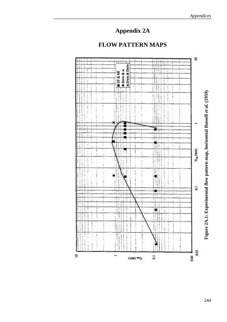
Appendices
244
Appendix 2A
FLOW PATTERN MAPS
Fig
ure
2A
.1:
Exp
erim
enta
l fl
ow
patt
ern
map
, h
ori
zon
tal
Ru
ssel
l et
al.
(1959)
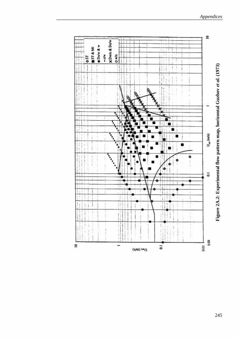
Appendices
245
Fig
ure
2A
.2:
Exp
erim
enta
l fl
ow
patt
ern
map
, h
ori
zon
tal
Gu
zhov
et
al.
(1973)

Appendices
246
Fig
ure
2A
.3:
Exp
erim
enta
l fl
ow
patt
ern
map
, h
ori
zon
tal
Ogle
sby (
1979)
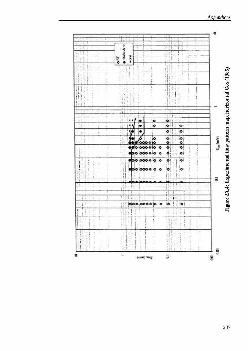
Appendices
247
Fig
ure
2A
.4:
Exp
erim
enta
l fl
ow
patt
ern
map
, h
ori
zon
tal
Cox (
1985)
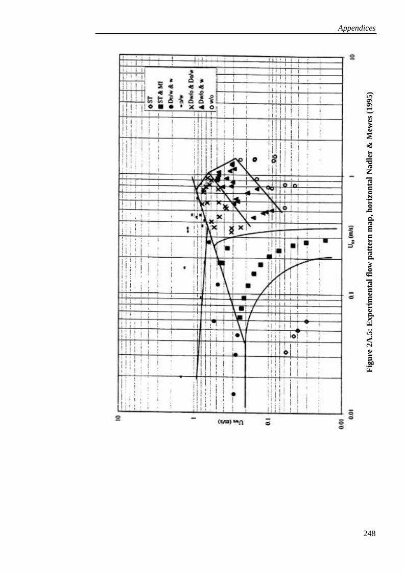
Appendices
248
Fig
ure
2A
.5:
Exp
erim
enta
l fl
ow
patt
ern
map
, h
ori
zon
tal
Nad
ler
& M
ewes
(1995)
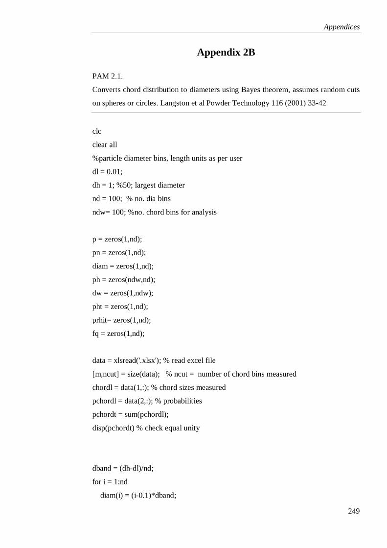
Appendices
249
Appendix 2B
PAM 2.1.
Converts chord distribution to diameters using Bayes theorem, assumes random cuts
on spheres or circles. Langston et al Powder Technology 116 (2001) 33-42
clc
clear all
%particle diameter bins, length units as per user
dl = 0.01;
dh = 1; %50; largest diameter
nd = 100; % no. dia bins
ndw= 100; %no. chord bins for analysis
p = zeros(1,nd);
pn = zeros(1,nd);
diam = zeros(1,nd);
ph = zeros(ndw,nd);
dw = zeros(1,ndw);
pht = zeros(1,nd);
prhit= zeros(1,nd);
fq = zeros(1,nd);
data = xlsread('.xlsx'); % read excel file
[m,ncut] = size(data); % ncut = number of chord bins measured
chordl = data(1,:); % chord sizes measured
pchordl = data(2,:); % probabilities
pchordt = sum(pchordl);
disp(pchordt) % check equal unity
dband = (dh-dl)/nd;
for i = 1:nd
diam(i) = (i-0.1)*dband;
Appendices
250
pn(i) = 0;
fq(i) = 1/nd; % initialise frequency
end
dwidth=dh/ndw; % width of analysis chord bins
for j = 1:ndw
dw(j) = (j-0.1)*dwidth; % analysis chord bin sizes
end
for i = 1:nd
d = diam(i);
pht(i) = 0;
for j = 1:ndw
d1 = dw(j) - 0.1*dwidth;
d2 = d1 + dwidth;
if (d2 <= d)
ph(j,i) = (sqrt(d*d - d1*d1) - sqrt(d*d - d2*d2))/d;
else
ph(j,i) = 0; % probability hit chord j given particle i
end
pht(i) = pht(i) + ph(j,i); % check should sum to unity
end
end
disp(pht) % check output
disp(diam)
iter = 0;
n_iter=10; % no. iterations between output
igo = input('Start iteration type 1: ');
while (igo == 1) % could use a for loop if many iterations required
for iter=1:n_iter
prhitt = 0; % step 2
Appendices
251
for i = 1:nd
prhit(i) = fq(i)*diam(i);
prhitt = prhitt + prhit(i);
end
for i = 1:nd
prhit(i) = prhit(i)/prhitt;
pn(i) = 0;
end
for k = 1:ncut % step 3
cl = chordl(k);
j = round(cl/dwidth + 0.5); % identify analysis chord bin
pt = 0;
for i = 1:nd
p(i) = ph(j,i)*prhit(i);
pt = pt + p(i);
end
if (pt ~= 0) % step 4
for i = 1:nd
p(i) = p(i)/pt;
pn(i) = pn(i) + p(i)*pchordl(k);
end
end
end
fqtot = 0; % step 5
for i = 1:nd
prhit(i) = pn(i);
fq(i) = prhit(i)/diam(i);
fqtot = fqtot + fq(i);
end
for i = 1:nd
fq(i) = fq(i)/fqtot;
end
Appendices
252
end
disp(fq) % step 6
% hold on
%plot (diam,fq,'b')
%xlabel ('Diameter')
%ylabel ('Fq')
%plot (diam,pht,'r')
%xlabel ('Diameter')
%ylabel ('pht')
%hold off
igo = input('Continue?: ');
end
disp (diam)
disp (fq)
disp (pht)
xlswrite('filename.xlsx',diam,'B1:CV1');
xlswrite('filename.xlsx',fq,'B2:CV2');
xlswrite('filename.xlsx',pht,'B3:CV3');
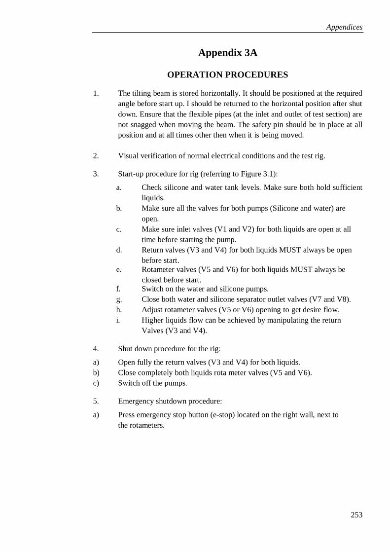
Appendices
253
Appendix 3A
OPERATION PROCEDURES
1. The tilting beam is stored horizontally. It should be positioned at the required
angle before start up. I should be returned to the horizontal position after shut
down. Ensure that the flexible pipes (at the inlet and outlet of test section) are
not snagged when moving the beam. The safety pin should be in place at all
position and at all times other then when it is being moved.
2. Visual verification of normal electrical conditions and the test rig.
3. Start-up procedure for rig (referring to Figure 3.1):
a. Check silicone and water tank levels. Make sure both hold sufficient
liquids.
b. Make sure all the valves for both pumps (Silicone and water) are
open.
c. Make sure inlet valves (V1 and V2) for both liquids are open at all
time before starting the pump.
d. Return valves (V3 and V4) for both liquids MUST always be open
before start.
e. Rotameter valves (V5 and V6) for both liquids MUST always be
closed before start.
f. Switch on the water and silicone pumps.
g. Close both water and silicone separator outlet valves (V7 and V8).
h. Adjust rotameter valves (V5 or V6) opening to get desire flow.
i. Higher liquids flow can be achieved by manipulating the return
Valves (V3 and V4).
4. Shut down procedure for the rig:
a) Open fully the return valves (V3 and V4) for both liquids.
b) Close completely both liquids rota meter valves (V5 and V6).
c) Switch off the pumps.
5. Emergency shutdown procedure:
a) Press emergency stop button (e-stop) located on the right wall, next to
the rotameters.
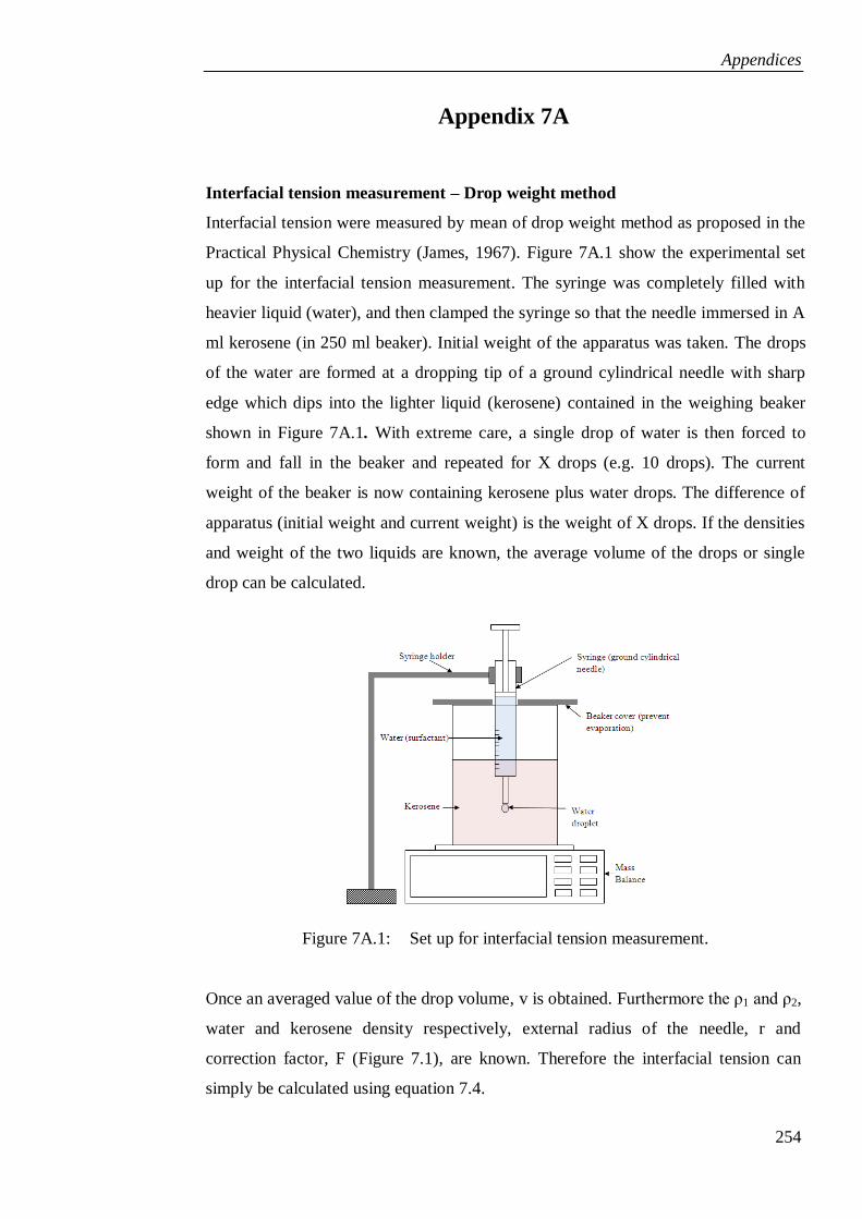
Appendices
254
Appendix 7A
Interfacial tension measurement – Drop weight method
Interfacial tension were measured by mean of drop weight method as proposed in the
Practical Physical Chemistry (James, 1967). Figure 7A.1 show the experimental set
up for the interfacial tension measurement. The syringe was completely filled with
heavier liquid (water), and then clamped the syringe so that the needle immersed in A
ml kerosene (in 250 ml beaker). Initial weight of the apparatus was taken. The drops
of the water are formed at a dropping tip of a ground cylindrical needle with sharp
edge which dips into the lighter liquid (kerosene) contained in the weighing beaker
shown in Figure 7A.1. With extreme care, a single drop of water is then forced to
form and fall in the beaker and repeated for X drops (e.g. 10 drops). The current
weight of the beaker is now containing kerosene plus water drops. The difference of
apparatus (initial weight and current weight) is the weight of X drops. If the densities
and weight of the two liquids are known, the average volume of the drops or single
drop can be calculated.
Figure 7A.1: Set up for interfacial tension measurement.
Once an averaged value of the drop volume, v is obtained. Furthermore the ρ1 and ρ2,
water and kerosene density respectively, external radius of the needle, r and
correction factor, F (Figure 7.1), are known. Therefore the interfacial tension can
simply be calculated using equation 7.4.
Appendices
255
Interfacial tension measurement of water-kerosene with surfactant added was
performed. The experimental results then be compared with Antonoff‟s rule (eq. 7.5)
to make sure the result obtained is reasonable and acceptable. Antonoff‟s rule says
that the interfacial tension between two liquids is approximately equal to the
difference between the surface tensions of the two liquids.