NAVAL POSTGRADUATE SCHOOLMONTEREY, CALIFORNIA

CLn

(n -oSTA I #-,.00

uADg OTICC•ADECTE

JS 2 2 1994GTHESISI DTIC QUALTTY TTISPECTED

SUBMARINE MACHINERY CRADLE:STRUCTURAL DYNAMIC DESIGN AND ANALYSIS TECHNIQUES

USING FREQUENCY DOMAIN STRUCWURAL SYNTHESIS

by

Ronald E. Cook

March, 1994

Thesis Advisor: Joshua H. Gordis

Approved for public release, distribution is unlimited.

94-19089o 620II I~lllllllll94 6 22 021

UnclassifiedsECUtI`IY CI.ASSilIC(ATION (* TWS ~fI

REPORT DOCUMENTATION PAGEIs. RI-YOH. Sb(TRrrY CLASSUI-I( AAIN *h RLS I RICI 1V %I ARIN 0

Unclassified________________ _____

2a. ,Et1'RrTY CL'_ýSSEFICAT10N AUTHURITY D1SIRIBI flo\,A%-&4JLA-BU.JFN *l RkF-HT______________________________________ Approved for public release; distribution is unlimited

'b. Dr.(-LASSIflCATI()NiI)OW'.(;iRADIN(G SCHEDUIX

I'l.RIO(RŽ.IIN(, 0RGANI7ArION REPORT MIFS .ONITORING R;N7TO REPORT NIUMBER(S

he NAME (* PERoI~)NOi 0R6AN\ZLArIIN JAb 0)lFICE SYIB4)L 'a. NAE 4*F MIOTORIX(i ()RGAN1ZATI0N(ICappliwable,

Naval Postgraduate School ME Naval Postgraduate School6c ADDRESS tCity. State. and ZIP (Code) 'b ADDRESS (City. State. and ZIP Code)

Monterey. CA 93943-5000 Monterey. CA 93943-5000fla. NAME OF FILNSDING/SPONSORING 'tb, oFFICE SYMBOL 9 PRO(CURBES(E. INSTRtMENT [DENTIFICAT10\ NINIBER

O)RGANIZATION (if applitable)

Si.. ADDRESN (City. State. and LIP Code) It0. SOURCE OF FUNDING NLTMBLRSPROGRAMt PROJECT TASK WOK UI Tr

-rFMN No No. NO ACSSIO No

11. TITLE fInclude Security (7laisuificatiool

SUBMARINE MACHINERY CRADLE: STRUCTURAL DYNAMIC DESIGN AND ANALYSISTECHNIQUES USING FREQUENCY DOMAIN STRUCTrURAL SYNTHESIS

12. PERSONAL AUTHOR(S)Ronald Edward Cook

13a. TYPE OF REPORT 13b. TIME COVERED 14 DATE OF REPORT (Year.MontliDay) IS. PAGE COUN-17Master's Thesis IFROM _ TO March 1994 8R

16. SUP)PLEMENTARY NOTATION

The views expressed in this thesis are those of the author and do not reflect the official policy or position ofthe Deauent of Defense or the U.S. Government. __________

17. COSATI CODES IS. SUBJECT TERIMS (Continue an revene if necessary and identify by block nuimber)FIELD GROUP SUB-GROUP

Frequency Domfain Structural Synthesis

19. ABSTRACT (Continue on ,mverse if necessary and identify by block number)The tactical implications of submarine acoustic radiation and UNDEX-survivability have

motivated the development of an advanced machinery cradle which will provide shock andvibration isolation of the submarine internals, thereby minimizing the resulting acousticradiation. The cradle space frame must be designed and optimized for both minimumshock/vibration bi-directional transmissibility and minimum total cradle weight. Frequencydomain structural synthesis (structural modification and substructure coupling), is applied tothe cradle design. The method addresses static and complex dynamic problems in structuraldesign analysis, and allows the direct analytic treatment of specialized equipment. such asfrequency -dependent visco-elastic isolators.

20. DISTRXDL7ION/AVAIJABMITY OF ABSTRACT I21. ABSTRACT SECURITY CLASSIFICATION

19UNCIAssmED/tUNLuhCT 5 SAME As UFT. 5 DTIC USER Unclassified22s. SAME OF RESPONSIBLE INDWVIUAL 22b. TELEPHONE (include Ame Code) 22c. OFFICE SYIMBO

Joshua H. Gordis (408) 656 - 2866 1 ME/GoDD Form 1473. J04N 84 Previous aditions are obsolete. SECURITY CLASSO.CATION OF THIS PAGF

S/N 0102-LF-014-6603 Unclassified

Approved for public release: distribution is unlimited

Submarine Machinery Cradle:Structural Dynamic Design and Analysis Techniques

Using Frequency Domain Structural Synthesis

by

Ronald E. Cook

Lieutenant, United States Navy

B.S.P.E., University of Wyoming, 1985

Submitted in partial fulfillment ofrequirements for the degree of

MASTER OF SCIENCE IN MECHANICAL ENGINEERING

from the

NAVAL POSTGRADUATE SCHOOL

March 1994

Author_ _ _ _ _ _ _ _

Ronald E. Cook

Appovdby:

Jsua H. Gordis, hsfAio

/11224he rD.3 Kefleher, Ch"r-man,Deprtment of Mechanical Engineering

ii

ABSTRACT

The tactical implications of submarine acoustic radiation and UNDEX-survivability

have motivated the development of an advanced machinery cradle which will provide shock

and vibration isolation of the submarine internals, thereby minimizing the resulting acoustic

radiation. The cradle space frame must be designed and optimized for both minimum

shock/vibration bi-directional transmissibility and minimum total cradle weight. Frequency

domain structural synthesis (structural modification and substructure coupling), is applied

to the cradle design. The method addresses static and complex dynamic problems in

structural design analysis, and allows the direct analytic treatment of specialized equipment.

such as frequency-dependent visco-elastic isolators.

Accesion ForNTIS CRA&I

DTIC TABUnannounced 0Justification

ByDistribution .

Availability Codes

Avail and orDist Special

ulILI

TABLE OF CONTENTS

I. INTRO D UCT IO N .............................................................................. 1

II. FINITE ELEMENT FORMULATION ....................................................... 3

I1. FREQUENCY DOMAIN STRUCTURAL SYNTHESIS ............................ 16

A. GENERALIZED FREQUENCY RESPONSE .................................... 18

B. MATRIX PARTITIONING ........................................................ 23

C. STRUCTURAL MODIFICATION AND INDIRECT SUBSTRUCTURE

COUPLING ........................................................................... .26

D SUBSTRUCTURE COUPLING AND CONSTRAINT IMPOSITION ..... 31

E. DIRECTED GRAPHS AND MAPPING MATRICES .............................. 36

F. MODIFICATION AND INDIRECT COUPLING USING MAPPING

M ATRICES ........................................................................... 39

IV. NUMERICAL EXAMPLES .............................................................. 44

A. EXAMPLE (1): DYNAMIC INDIRECT COUPLING .......................... 45

B. EXAMPLE (2): DYNAMIC DIRECT COUPLING .............................. 49

C. EXAMPLE (3): STRUCTURAL MODIFICATION

(REMOVAL OF A BEAM ELEMENT) .......................................... 54

D. EXAMPLE (4): STRUCTURAL MODIFICATION

(ADDITION OF A BEAM ) ...........................).............................. 59

E. EXAMPLE (5): INDIRECT COUPLING WITH ISOLATORS ............... 62

iv

F. EXAMPLE (6): INDIRECT COUPLING WITH FREQUENCY

DEPENDENT ISOLATORS ........................................................... 68

G. EXAMPLE (7): STRESS CALCUATION BY DYNAMIC

INDIRECT COUPLING ............................................................. 72

H. EXAMPLE (8): DYNAMIC DIRECT COUPLING USING MODAL

REPRESENTATION OF FRF ...................................................... 80

V. CONCLUSIONS / RECOMMENDATIONS .............................................. 90

APPENDIX A MATLAB CODE FOR EXAMPLE ONE ..................... 92

APPENDIX B MATLAB CODE FOR EXAMPLE TWO ................................... 100

APPENDIX C MATLAB CODE FOR EXAMPLE THREE .............................. III

APPENDIX D MATLAB CODE FOR EXAMPLE FOUR .................................. 121

APPENDIX E MATLAB CODE FOR EXAMPLE FIVE. ................................... 130

APPENDIX F MATLAB CODE FOR EXAMPLE SIX ..................................... 141

APPENDIX G MATLAB CODE FOR EXAMPLE SEVEN ................................ 151

APPENDIX H MATLAB CODE FOR EXAMPLE EIGHT ................................ 158

APPENDIX I GENERAL MATLAB FUNCTIONS ......................................... 174

LIST OF REFERENCES ......................................................................... 180

INITIAL DISTRIBUTION LIST ................................................................ 181

V

1. INTRODUCTION

The design of complex structural dynamic systems requires the building of detailed

mathematical models with which to predict static and dynamic response. Most commonly.

the finite element (FE) method is used to generate structure system matrices with which

dynamic response can be calculated. While the FE method currently provides the best

means of predicting response for complex structural systems, the time required to assemble

the system matrices and to process them for the calculation of dynamic response can be

prohibitive. Therefore, the use of the FE method for performing design analyses often

precludes the performance of numerous design analyses in the search for an optimal

design. This is especially true when a FE based analysis is to be used in conjunction with

advanced design techniques such as optimization. The iterative process of modeling the

system and analyzing the model to determine the system performance is the design-analysis

cycle.

The traditional design-analysis cycle consists of the following process. A designer

builds a FE model which best represents the system. The system model is the complete

system structure, for example, a submarine hull and an internal machinery support cradle is

modeled as one structure. The definition of the FE model yields system matrices, which

include stiffness, mass, and less commonly damping. The numerical generation of the

system matrices is referred to as the assembly phase. At this point, loads are applied and

responses, static and/or dynamic, are calculated. The calculation of system response is

referred to as the solution phase. The responses are then used to calculate stresses and

strains in the model. These calculations are referred to as the post-processing phase. The

solution phase is the most costly in terms of time and computing resources.

Based on the acceptability of the displacements. stresses, and strains calculated, the

design or system model may have to be changed in the interest of improving the response

characteristics of the initial or follow on design. For example, a high stress which is

unacceptable may exist at a certain location in the design. The designer decides that if a

particular alteration is made to the design, the stress response will become within tolerable

levels. Traditionally. this alteration requires a repeat of the assembly, solution, and post-

processing phase of the analysis, a cost and time intensive procedure which limits the

number of design re-analyses that can be accomplished. Since the re-analysis is time

consuming, the optimal design is abandoned for a final design which is less than optimal.

Therefore, with the intent of accelerating the design process and lowering the attendant

costs, new methodologies for assembling and modifying system models is presented. The

new method replaces all three of the FE analysis phases with a single computationally

efficient calculation. The method to be described herein, generally referred to as frequency

domain structural synthesis (Refs. 1,2,31, is directed specifically at drasticaUy reducing the

time required to perform a design analysis cycle. This capability for rapid re-analysis makes

structural synthesis ideal for use in advanced automated design environments, such as in

conjunction with optimization codes.

2

!1. FINITE EI.EMENT FORMUIATION

The finite element method used for comparison with the solution obtained from

frequency domain structural synthesis is based on Lagrange's equation of motion I Ref. 41.

Various types of elements are used in modeling of structural systems, including for

example, plate. shell, and beam elements. Our discussion will be limited to beam elements

experiencing combined bending and axial deformations. We are using beam elements to

demonstrate the methodology because the beam element allows for a manageable system of

equations and matrices that are easily handled by a personal computer. The theory remains

valid for all types of elements and is unaffected by the complexity of shell or plate

elements. Beam elements that are subject to bending and axial deformation have three joint

displacements at each end of the beam element The beam element has six generalized

coordinates and six degrees of freedom (DOF), which yields a mass, stiffness, and

damping matrix for the beam element of size (6 x 6). The beam element is shown in

Figure 1.

1 2

Figure 1. Beam Element with Coordinate and Nodal Orientation

Each node has a set of coordinates, axial (x), lateral (y), and rotational (0), however

elements are not limited to three DOF. Elements can be modeled with six DOF per node.

3

The derivation presented in referencel4j assumes that the axial forces associated with the

axial joint displacements (x) have only a negligible effect on the shape functions associated

with the joint displacements (y) and (0). With this assumption the mass and stiffness

matrices are derived.

The elemental stiffness and mass matrices are

r 0 ( 0 0 F140 0 0 70 ) 0'

0 12 61 0 -12 61 1 1 2 0 54 -11

El 0 61 412 0 -61 2 20 221 412 1) 13 -A/'

41N 70 0 0 1400 ').1)2 0 0 54 1! 0 156 o-2I1

r 0 -131 -V2 O -222 412-12- -61 0 12 -61

0 61 2 2 0 -61 4Q2

where the terms E is Young's Modulus, I is the area moment of inertia, I is the elemental

beam length in inches, y is the weight density, and r is the radius of gyration. The

elemental matrices are partitioned in the following way:

Al 3A ý -t 3202:[

The damping matrix is usually impossible to determine analytically and is typically

determined experimentally. Here damping is applied to the system model by one of three

ways. The three methods generally used are:

Type (1): Proportional structural damping of the form:

[C]- a(Kl + [M()

4

Type (2): Proportional viscous damping of the form:

ICI =ulKI

Type (3): Frequency-dependent viscous damping of the form:

[C]-- [C,,e-J(1 131

Type (1) damping is used in adding damping to structural elements, and Types (2) and (3)

are used in adding damping to vibration isolators which are a combination of springs and

dampers; adding proportional damping to just the isolators constitutes non-proportional

damping for the whole structure.

The equation of motion of these finite elements can be written in terms of their joint

displacements as

[ml,{iI. +cKe{(, 1 + [kLfui 1, VifL (4)

where {u1L = axial, lateral, or angular joint displacements

[ml, = mass matrix of element

[c), = damping matrix of element

[k], = stiffness matrix of element

If I, = joint forces and moments

Since the elements vary in orientation with respect to the system axis, the elemental

mass and stiffness matrices must be transformed into global coordinates. The

transformation of the damping matrix is neglected, since the elemental damping matrix is

modeled as a function of the transformed elemental mass and stiffness matrix. A method

for relating local joint displacements of each element to the global system displacements

5

must be incorporated. This method is referred to as a coordinate transformation. The

elemental mass and stiffness matrices after transformation are in the following form

(Ref. 41.

"140C2 + 156S2 -16CS -221S 70C2 +54S2 16CS 131S

-16CS 140S 2 + 156C 2 22/C 16CS 70S 2 + 54C2 -131C

yl -221S 221C 41- - 131S 13/C -31-

[ 42]01j- 70C2 +54S2 16CS -13/S 140(2 +156S2 -16CS 221S16CS 70S2 5 54C2 131C - 16CS 140S 2 + 156C 2 -21C'

L 131S -131C -312 221S -221C 41- '

C-+.12S - ( C, s -,12Cs -61S -(j) 2C- -1s-I ,2 S -,S,2rL•cS- 12CS lS + 12C 6C (/L 2 61C

I -i5CS + 12CS S2 - 12C26/krr) k, r)r}

El -61S 6/C 4/2 61/ - 61C 21-

[ 2 12S2 -)CS+12CS 61S ( 1C12 S2 lCS- 12CS 61S_(j)2 (1) Sý -12C2 _o,2"S+12CS + 12- 2 C "61C CS12CS -j6C12c' C

-61S 61C 212 6/S -61C 4/?

Noting that:

I = elemental beam length in inches

E = Young's modules in psi

I = Area Moment of Inertia in in4

r = radius of gyration in inches

y = mass density per unit length in 1b s2 in2

C=cos a

S = sin a

6

Once the finite elements are transformed to global coordinates, the elements are

assembled to generate the giobal mass, stiffness, and damping matrices. The equation of

motion for the modeled system in global coordinates is

IMJiUI +[CJfiu +!KJlul IF- F5)

where Iul = axial, lateral, or angular global joint displacements

[MI = global mass matrix

[Ci = global damping matrix

[KI = global stiffness matrix

I F1 global joint forces and moments

The following example will demonstrate how the global mass and stiffness matrices are

generated. Consider the structural system modeled with two beam elements and having no

boundary conditions shown in Figure 2.

1,2,3 1 4,5,6 1 7,8,9

2 3

Figure 2. A Beam Modeled Using Two Elements

FxthseEmleY =10 lb/n .! 10 1b -s', I = 1.0 in and r-- .0 in.. S ince theE1 420For this example 7- =-1.0 lbstin, 49-2 10 l'2 . nadrlOi. ic h

beam elements lie horizontally along the x axis, the angle a = 0. The global mass and

stiffness matrices are generated from the assembly of the elemental matrices. The elemental

matrices are:

7

iI - " Id I I

1 0 0 -I 0 0 140 0 0 70 0 0

0 12 6 0 -12 6 0 156 22 0 54 -13,

0 6 4 0 -6 2 0 22 4 0 13 -3(kl 1 01kj=I-l 0 0 1 0 0 70 0 0 140 0 0

i 0 -12 -6 0 12 -6: 0 54 13 0 156 -22

,0 6 2 0 -6 4 i_ 0 -13 -3 0 -22 4

Referring to Figure 2. the lower bold type numerals represent the node numbering and the

upper numbers represent the beam nodal coordinates. Coordinates 1. 2, 3. 4. 5, 6. 7, 8.

and 9 are respectively x1 . e, . x,., y,.0,. x,, y3, and 0,. Remembering how the matrices are

partitioned and noting that coordinates 4, 5 and 6 of beam element I are the same

coordinates of beam element 2 and thus are shared. The two elemental matrices are

assembled together through the shared coordinates. Figure 3 shows the beam element

arrangements.

1,2,3 1 4,5,6 4,5,6 1 7L8,9

2 2 3

Figure 3. Beam Elements with Node and Global Nodal Coordinate Numbering

For discussion purposes only, the stiffness matrices will be demonstrated, since the

mass and damping matrices are generated in the same manner. The elemental stiffness

matrices are in the following form.

123456 456789

1 4

2 5[k .,., ] 34 [k , ,2 6 7

tki 4 7

5 8

6 9

8

The two matrices are combined by adding shared nodal coordinates, this process is

determined by the element connectivity. Figure 3 shows that element 1 is coupled to

element 2 through global nodal coordinates 4. 5 and 6. These global coordinates are the

combination of local coordinates x., y,. 0, of element I and x,. y,- 0, of element 2. The

resulting matrix is a (9x9) global matrix represented by I KJ. The size of the global matrix

is the number of nodes times the DOF. The global stiffness matrix [KJ is shown below

with the numbers installed, take special note to the shared coordinates which are additive.

F1 0 0 -1 0 0 0 0 00 12 6 0 -12 6 0 0 010 6 4 0 -6 2 0 0 0

-1 0 0 2 0 0 -1 0 0

[K]= 0 -12 -6 0 24 0 0 -12 60 6 2 0 0 8 0 -6 2

0 0 -1 0 0 1 0 00 0 0 0 -12 -6 0 12 -6

0 0 0 0 6 2 0 -6 4J

The shared coordinates are demonstrated by looking at the 3x3 partition, rows 4 through 6

and columns 4 through 6. After the global matrix is generated, the boundary conditions are

applied. Boundary conditions are determined by coordinate restraints. If a coordinate is

restrained then the row and column corresponding to that coordinate are deleted. For

example, if in Figure 2, the left end had been fixed, displacements for global coordinates 1,

2, and the slope of coordinate 3 are zero, and therefore the rows and columns

corresponding to these coordinates would be deleted resulting in a (6x6) [ K1 matrix.

The derivation of the equation for a second order linear structural system described in

the frequency domain is presented below. The differential equation of motion for a second

order linear structural system is written as

9

m.i + ckk + ,•= = Fsin iOt. 0)

The solution to equation (6). which is the total system response is

X =X +X (7)

where Xk is the real or homogeneous solution and X, is the particular solution. We

consider only steady state harmonic excitation, therefore the particular solution is used as

the total solution. The solution is assumed to have the form

X - X, - Xe-4'. (8)

Taking the first and second derivatives of X and substituting into equation (y I . 'ds

(-nlmX + jX + kX)e - Fel. (9)

Dividing both sides by e" and rearranging equation (9) gives the equation of motion as

(k-_m2 + jc)X - F. (10)

Writing equation (10) in matrix form gives the equation for second order linear

structural systems described in the frequency domain.

[[K]-] 2 [M, AC(O)DfXl -(Fl (11)

to

where the vector IxJ is the set of generalized responses in the global coordinate system.

The vector {FJ contains generalized global forces and moments. fKI and [MI are

symmetric. real valued and of order n. The damping matrix ICI) )] is in general. frequency

dependent. but here is modeled as a linear proportional combination of the mass and

stiffness matrices. Equation (6) is generally written in compact form as

[Z(f,)Jlxl = (Fl (12)

where the matrix [Z(01) is called the system impedance matrix. Equation (12) is the system

impedance relationship and represents the dynamic response of the system. The impedance

matrix is the dynamic stiffness of the system. The static case is when fQ - 0 and then the

system impedance matrix is just the stiffness matrix [KI.

The impedance matrix for the assembled beam (Figure 2) is

[zJ - IK] - lV[MJ (13)

Equation (13) is reduced because damping [C(L)J is neglected in this example. [Z(Q)J is

calculated over the frequency band of interest, where 0 is the frequency band of interest in

rad/sec.

The frequency response function (FRF) matrix for the assembled beam is

H1)]- [z(r)f]. (14)

11

The FRF matrix allows the calculation of the steady state harmonic response amplitude I Xf

resulting from a harmonic force amplitude {Fl. The frequency response relation is

determined by matrix inversion of equation (12), which yields

lxi - IH(O)]IF. F15.

Any element /4. of the frequency response matrix is defined as the dynamic response of

motion coordinate i due to a unit harmonic generalized force acting on motion coordinate j.

The FRF matrix can be used to represent information about displacements, velocities.

accelerations, stress, or strains. For example, if a structure is excited at nodal coordinate 5,

then H,, is the complex amplitude of the response at nodal coordinate I due to a unit

harmonic excitation at nodal coordinate 5 at some frequency 0 of interest.

A typical frequency response function plot is shown in Figure 4. The peaks shown in

Figure 4 occur at the frequency of peak response. The relationship between the natural

undamped frequency, the damped natural frequency, and the frequency of peak response is

shown on the following page. The plot shows at what frequencies the structure will have

maximum responses and enables the designer to redesign the structure so that the system

will have small responses in the frequency bandwidth of interest

12

50--, o ,50 -... .. ... ... ..I-,o

. .-150"•... .-15 0 ............. ............. i!............. j. ........... !...... ....... .... .L 200

0 t0 20 30 40 50 60

Frequency Hz

Figure 4. Typical Frequency Response Function Plot

Generally there are three distinct frequencies of interest, the undamped natural

frequency, the damped natural frequency, and the frequency of peak response. These

frequencies are related by the modal damping factor. The amplitude of the response of a

forced vibration can become very large when the frequency of the excitation approaches

one of the natural frequencies of the system . This condition where the excitation frequency

is the same as one of the natural frequencies is referred to as resonance. When a system

vibrates at resonance, the attendant stresses and strains have the potential of causing

structural failure. A structal system will have a maximum response when the frequency

of excitation is near the undamped natural frequency. If the system has no damping, then

the maximum response will occur at the undamped natural frequency. The undamped

natural frequency is a function of the system mass and stiffness and is analytically

expressed as the solution to the eigensystemn

[K- w 2M](j - (01 (16)

13

Every real structural system has an infinite number of natural frequencies and mode shapes.

The finite modeling of the structural system yields a finite number of eigensolutions or

mode shapes and eigenvalues or natural frequencies depending on how many degrees of

freedom the structural system is modeled with. Each eigenvector has a corresponding

eigenvalue or natural frequency. However. all systems inherently have some degree of

damping and the relationship that relates the damped natural frequency to the undamped

natural frequency is

W 44 (17)

where • is the modal damping factor for mode i. The damped natural frequency is slightly

lower than the undamped natural frequency and a typical damping factor for structural

systems is 0.2. The frequency of peak response is the frequency of excitation where the

response of the system is maximum. The analytical relation that relates the frequency of

peak response to the undamped natural frequency is determined by taking the derivative

with respect to (.-)of equation (18) and setting it equal to zero.

Fo/ki (18)

+ [zi(:

14

and substituting back into equation ( 18) yields

Now performing 0

i[(,_@2)2 +( 2(@). V] (-_4d(1 -&) +8:i V @=0 (20)

and knowing for equation (20) to equal zero, the numerator must equal zero. Setting the

numerator equal to zero

2@(l- CO2 )- 4g i 0 (21)

and simplifying

@2 . 1 -_2 (22)

and solving for w , which is the frequency of peak response yields

= ,, - .(23)

It is important when designing a structural system that the excitation frequency is not close

to these frequencies or failure of the structural system is likely to occur.

15

!11. FREQUENCY DOMALN STRUCTURAL SYNTHESIS

The theory presented herein is taken directly and exclusively from references 11. 2. and

31. The purpose of this thesis is to explore the application of this previously developed

theory to the analysis of a submarine cradle structure.

Frequency domain structural synthesis was first presented in 1939 and has evolved to

the latest formulation, which was published in Journal of Sound and Vibration (1991)

[Ref. 11. The most recent formulation of the theory is a new method for analyzing

structural systems [Ref. 31. This method handles all types of structural models and is more

efficient and cost effective compared with traditional finite element solution procedures.

Frequency domain structural synthesis refers to substructure coupling and structural

modification using frequency response function data. The previously developed

formulation for structural synthesis, Ref. [31, is applicable to the static and dynamic

structural analysis of direct coupling of substructures, indirect coupling of substructures,

modification of substructures, and constraint application. The theory allows the synthesis

of displacements, velocities, accelerations, stresses, and strains.

An intportant feature of the frequency domain formulation is the arbitrary and exact

model order reduction possible when performing a synthesis. A finite element method

(FEW when applied to practical problems typically generates between 102 to I05 degrees-

of-freedom (DOF). The frequency domain formulation allows, as a minimum, only those

DOF of interest to be included in the analysis. This feature is in fact the reason for the high

computational efficiency of the method. Using one of the numerical examples presented in

the section "Nunmic Examples, " the computing time required for a frequency domain

synthesis can be compared with the same analysis using traditional finite element (FE)

16

procedure. Referring to Example (6) the following count of floating point operations

(FLOPS) shows the efficiency of the frequency domain method:

FEM direct assembly: Time - 25876 sec or 431.3 mins

FLOPS - 1.49 x 109

FRF synthesis: Time - 1167 sec or 19.45 mins

FLOPS- 517.2 x 106

This clearly demonstrates that synthesis by FRF is more efficient and better suited for the

re-analysis of complex structures with large numbers of DOF. Moreover. the savings in

time grows with increasing model size.

There are two major classifications of stuctural synthesis. These classifications are

coupling and modification and each classification can be viewed as direct or indirect.

Coupling is defined as the joining of two separate substructures to form one structure and

modification is defined as the creation of a new load path in an existing structure. An

example of coupling is the coupling of a submarine hull and the machinery support cradle.

The hull is modeled as one substructure and the cradle is modeled as another substructure.

We want to join these two substructures together to create one complete structural system.

This process is known as stutural coupling. As an example of the use of structural

modification, an analysis of the complete cradle structural system shows that a certain

element has unacceptable stresses. By installing an additional support, the stresses become

acceptable. This process of changing the structure is known as structural modification.

Indirect coupling is the joining of structures with the introduction of an intermediate or

intonnecting stuctural element, referred to as an interconnection impedance element or

impedance patch [Ref. 1]. Direct modification can be viewed as the application of a

constwint equation to a given structural model; direct coupling is simple substructure

synthesis [Ref. 11. The theory is unique in that it allows any linear structural element to be

17

used as an interconnection impedance. for example a spring and viscous damper may be

installed between two elements of a structure. The synthesis is performed at each frequency

of interest, which makes possible the efficient treatment of frequency dependent properties.

like the properties in the spring and viscous damper. Frequency domain structural synthesis

allows changes to a finite element model without reassembly of the mass. stiffness, or

damping matrices.

A. GENERALIZED FREQUENCY RESPONSE

The derivations presented here are taken exclusively from References 1, 2, and 3. The

derivations are reproduced with more intermediate steps leading to the fmnal operative

equations. We begin the development with the previously derived formulation for a second

order linear structural system described in the frequency domain.

The differential equation of motion for a second order linear structural system is

written as

+&+ cx + - Fsin ft. (6)

The solution to equation (6), which is the total system response is

X= XA +X (7)

where Jl is the real or homogeneous solution and XP is the particular solution. We

consider only steady state harmonic excitation, therefore the particular solution is used as

the total solution. The solution is assumed to have the form

Sx - xP M xe1 . (8)

S~18

Taking the first and second derivatives of X and substituting into equation (6) yields

(-0'mX + j•'cX+kX ,+U = FeA4. (9)

Dividing both sides by e"# and rearranging equation (9) gives the equation of motion as

(k- 0m + jffC)X = F. (10)

The dynamic stiffness of the structural system is known as the system impedance which is

written as

Z(O) = k -_ 2m + j0C. (24)

The static system stiffness k is determined by the case where Ql = 0 and the system

impedance is

zA() -k. (25)

The matrix notation for the structural system impedance is

[Z(oL)j{xJ - ff1. (26)

The system impedance matrix [Z(fQ)j is both complex valued and frequency dependent.

The general equation for the frequency response structural model is found by taking the

matrix inversion of equation (26) and is indicated as

19

1x) and If I are vectors of complex valued generalized response and excitation coordinates

at a specific frequency fl. and I H] is the frequency response function (FRF) matrix

evaluated at the frequency 0. In general an element of the FRF matrix is defined by taking

the partial derivative of Ixl with respect to If I. Referring to equation (24) and writing the

equation for x, we get

x, =•HIIf + H,,+.Af + ""+ H,..f (28)

and taking the partial derivative of equation (28), the general form for an element of the

FRF matrix is

•i = a (29)

and is defined as the partial derivative of the ith generalized response coordinate with

respect to the jth generalized excitation coordinate.

There are other types of frequency response which are classified by the type of

coordinates involved. For example, strain-force and stress-force frequency response are

defined as

SIo)-[ °lI:).30,31)

The difference between equation (27) and the two equations (30.31) is the FRF matrix [HI

contains displacement-force information in equation (27) and strain/stress-force information

20

in equations (30.31). The general element of the strain and stress FRF is determined in the

same manner as the displacement-force FRF. The general elements are defined as

/-,' = Lc' F /r, = '=a' (32.33)

where E, and a, are complex valued strains and stresses at coordinates i at a specific

frequency L

Here we will show the development of the frequency response function in the modal

coordinate system. We start with the differential equation of motion for a second order

linear structural system in physical coordinates.

m~i + cx + /cr = F(t) (34)

where we assume F(t) is of the form {PIe,' and the vector {IT is the set of force

amplitudes. Now we apply the linear transformnation

{xI [4)1 qI (35)

to equation (34) where the vector {xI is the set of physical coordinates to be transformed,

the vector {qj is the set of modal coordinates, and the matrix [D] is the set of mass

normalized normal mode shapes. Pre multiplying the transformed equation by 4)1] and

using the relation [ 4ý1 1 M[i@] - [11 yields

[1l1 + t;,to, 141+ * l t,- Iqj - ['T IF - 111. (36)

21

Rewriting equation (36). the differential equation of motion in the modal coordinate system

is

iji + 24,q+t = W2 t). (37)

Since we assumed steady state harmonic forces, equation (34). the modal forces are also of

the form fI [ {e'Ie•1' and the solution is assumed as a steady state harmonic modal

response of the form {qj - IY¢e•'. Taking the first and second derivative of fqj and

substituting back into equat- ;7) and simplifying yields

J" 2 02l1 + j 2A(, ,' (38)

Rewriting equation (38)

2o _ 0 2 + j Q24 o •'-{ ' (39)

and solving equation (39) in terms of the modal response yields

" 2 Qj 1l- (40)

22

To transform equaton (40) back to the physical coordinate system, we use the

transformation of modal force. [¢] flF1= IYI. and the transformation of modal

coordinates. Ixl = [tII! to substitute back into equation (40) and simplify. The

resulting equation in physical coordinates is

IxI = [4][ u)-W +J'22 .,1 }]r1v1. (41)

Remembering the general form of the frequency response, equation (27). the frequency

response function [H(])J in terms of the system modal information is

[H(Q)] = [({ -]-f2 + (2t,(42)

and any specific element of H is given by

IA. =•smd (43)•J = o ", 2 + jinx;trw

B. MATRIX PARTITIONING

First we will define the classification of coordinates. Figure 5 represents two

substructures A and B that will be joined together by merging coordinates 2 with 3 and 6

with 7. These coordinates are referred to as connection coordinates and are denoted by the

subscript "c". By the definition just stated, the connection coordinates for substructure A is

2 and 6, likewise the connection coordinates for substructure B are 3 and 7. Internal

23

coordinates, denoted by the subscript "i." are all the remaining coordinates not directly

involved in the substructure coupling. In Figure 5. the internal coordinates for substructure

A are I and 5 and the internal coordinates for substructure B are 4 and 8. The set of all the

physical coordinates are denoted as coordinate set "e". if one structure is involved, then the

coordinate set "e" contains only the connection and internal coordinates for that structure. If

two or more substructures are involved, then the coordinate set "e" contains all the

coordinates for all the substructures. The mathematical representation is e = i U c.

1 " 3 4

5 6 7 8

A B

Figure 5. Structural Model with Internal and Connection Coordinates

Referring to the general equation for frequency response, equation (27), and writing it

in matix form with coordinate partitioning as

Ix}j I[H Hj}j (44)

where xi and f, are a set of generalized responses and excitations at the internal coordinates

and XC and fc are a set of generalized response and excitation at the connection coordinates.

One of the special features about the frequency response is that in addition to response

information, we can also determine other information at the same time, for example,

stresses. We can append a set of stress coordinates and then equation (44) becomes

24

r H7, H,,x, H,, H,,. (45)

The stress coordinates will allow the direct calculation of synthesized system stress.

The generalized excitations are partitioned into internal and external excitations.

Referring to Figure 5, and looking at the internal coordinates, for example coordinate 1. it

is obvious that the only force possible on this coordinate is an externally applied force.

Since the internal coordinates do not participate in synthesis, there are no coupling forces

present on internal coordinates. The connection coordinates, for example, coordinate 2 in

Figure 5, may experience both externally applied forces and coupling forces which are

established through synthesis. Therefore

f ,,+", (46)

and by definition of the interna coordinates

f xf" (47)

Introducing equatim (46 and 47) into equation (45) allows for the expansion of equation

(45) as

H. H, (48)

25

where the asterisk superscript denotes a synthesized quantity due to the fact that we have

introduced the forces of synthesis, fCPI. Note that with the introduction of equations (46

and 47). a redundant equation, the fourth row of equation (48), has been appended. Using

the definition of the set "e", equation (48) is written in the new condensed form

x, - H,, H,, (49)x, _ H, o ,

where The vector fe is externally applied forces which may exist at

all physical coordinates, and the vector fc is the coupling forces present only at the

connection coordinates.

C. STRUCTURAL MODIFICATION AND INDIRECT SUBSTRUCTURE

COUPLING

In this section we will develop the governing equation for structural modification and

indirect substructure coupling. As previously defined, structural modification is the creation

of redundant load paths within a structure, and indirect coupling is the creation of new load

path with a structural element between uncoupled substructures Indirect coupling and

sructual modification are confined to connection coordinates. There is only one restriction

enforced for these processes. The structural change used for modification or

interconnection impedance used for indirect coupling must be described by the following

equation

IfI - jK(O) - 2 M() + jC( 11 x: (50)

or

26

If, I = -(zl} X51)

where the negative sign shows that the reaction is on the structure to be modified or

substructures to be coupled. Equation (50) defines the transformation of forces which is

used to transform equation (49). The transformation which operates on equation (49) is

{ 0=[ Z]} (52)

Substituting equation (52) into equation (49) yields

x, H, H• (531x,. H,.H, 1H -lll-

then performing matrix multiplication and simplifying equation (53), the resulting form is

given by the relationship

Ut. [SE f~iZ{t}(54)

Extracting the third row of equation (54)

I1x1 - [H,.l fj - [IH.lZ~lzl (55)

and rean~ging equation (55)

27

H Zlfx} I = I H, iI 56

and solving equation (56) in terms of IX]i yields

[I.: = [j ÷ [Hj]- jfo. (57)

Extracting the second row of equation (54)

IxjI - [HoflfjI - [Ho.,zJ{•,x:l (58)

and substituting equation (57) into equation (58)

{x,*- [H,,JIfl - [H,,, z([ + H.I-'[H ff.. I ) (59)

now, using the known relation that

Ix,1 - ](60)

and substituting equation (60) into equation (59) gives the following relation

[H.el'1 HI- [H]] f, I -[I zH,.IZlHI + H cefZ" ] (61)

and remranging equation (61) and setting it equal to zero

[H. I-[H..]I + [HIzXI + H,]"f'[H.jfjI "8101 (62)

28

and rewriting equation (62) as

j[." - I H, j+IHj,.I Z1 + H,,Z]- [H,,oIJl{.. = 0. (63)

Since by definition If1* 01, then

IIH,,l I'- .I +I H IZ11 + Hca.Z'l[H,,l]-[o01 (64)

and solving equation (64) in terms of IH,]" yields

Now we will simplify the third term of equation (65). Extracting the following portion

zI I+ AzA-'

factoring the inverse term

[zJ(z-, + H4)zJ-'

and applying the identity (abY' - a-tb"

Z -1 W, + -,,)'

29

and then simplifying yields

Substituting the above simplified portion back into equation (65) and performing the same

process on the first row of equation (54) yields the final operative equation for structural

modification and indirect coupling

[_,. [,L,[L.]z- +.-'I.. (66)

Note for the static case when Q1 - 0. the impedance matrix [ZI = [KI and [KI is a singular

matrix which is not invertible, therefore equation (66) is not valid and a form of the

equation which does not require the matrix inversion of [Z] must be used. The following

equation is for the static case when fQ -0.

[H.,. j _[H_ Ha.) II+H -[

[ J .[j]_[,],z ,,, (67)

Terms on the right side of equations (66 and 67) are pre-synthesized values and the left

hand side is the synthesized values. The matrix [ZI describes the modification to be made

for structural modification and can be negative if the modification to be made is the removal

of a structural modification, or it describes the new load path between two structures for

indirect coupling. The quantity [ HaI allows for the direct calculation of stress due to

externally applied loads in the synthesized structure. Stress frequency response could be

replaced with strain or other structural frequency response.

30

1). SUBSTRUCTURE COUPLING AND CONSTRAINT IMPOSITION

In this section. the development of the theory of direct substructure coupling using

boolean mapping matrices is shown. A formal discussion of the mapping matrix is

presented in the next section. The development of this theory also applies to constraint

imposition. Substructure coupling involves the joining of two or more separate

substructures where constraint imposition involves one structure, the coupled structure.

Constraint imposition is the application of two conditions on the synthesized connection

coordinates. The first condition being force equilibrium where the summation of forces on

a coordinate are equal to zero and the second condition being compatibility where the

displacement of the synthesized coordinates are equal to zero. Compatibility is interpreted

as the connection coordinate from the first substructure most have the same displacement as

the connection coordinate from the second substructure in order for them to be merged as a

single coordinate.

We extract the third row from equation (49) which is shown here again for reader

convenience.

Xe H" H"(49)

The third row of equation (49) is

Ix "I [HJlf,1 + [HJIJfj. (68)

We construct the conditions for equilibrium and compatibility to be imposed on the

connection coordinates. Figure 6 shows two connection coordinates from two

31

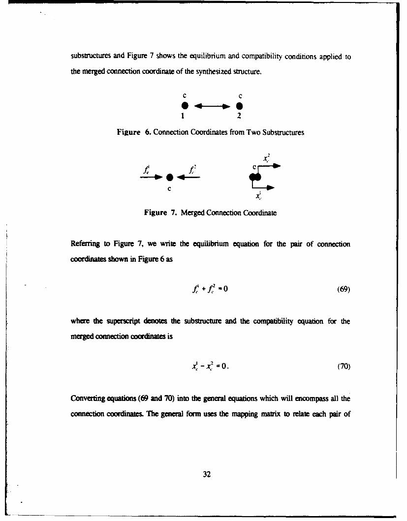
substructures and Figure 7 shows the equilibrium and compatibility conditions applied to

the merged connection coordinate of the synthesized structure.

c c

Figure 6. Connection Coordinates from Two Substructures

f f2

c

Figure 7. Merged Connection Coordinate

Referring to Figure 7, we write the equilibrium equation for the pair of connection

coordinates shown in Figure 6 as

fl +f2 _0 (69)

where the superscript denotes the substructure and the compatibility equation for the

merged connection coordinates is

- - 02 (70)

Converting equations (69 and 70) into the general equations which will encompass all the

connection coordinates. The general form uses the mapping matrix to relate each pair of

32

coordinates. Noting that f -7t" and r, - x,. we can write the general equations. The

general equation for the force equilibrium is

It. I -= L , :} (71)

where the vector if represents the arbitrarily selected independent subset of the

connection coordinates. Noting that the mapping matrix I MI must remain constant for the

constraint imposition to hold, the general form of the compatibility equation is

.1i.. = [Afl*(.,ll = {fo (72)

where the vector [.. } represents the compatibility for the pairs of connection coordinates.

This vector is the zero vector.

The transformation equations that operate on equation (49) are derived from the general

equilibrium and compatibility equations and are of the form

Ijl0 (73)

f~l [I 01I

xl -L. X, (74)

Substituting equation (73 and 74) into equation (49)

{;IX 4[ °TI. [T TM (75)

33

noting that we are using the displacement frequency response only for derivation purposes.

and then performing matrix multiplication and simplifying equation (75). The resulting

form is given by equation (76).

:. = [H > M r H. M .if . (76)

Extracting the second row of equation (76)

IM 'I = [I..M.§I + [MTF(.C.MJ{f 1 (77)

and rewriting the second term of the left hand side

[MT Hý.MJ = ["ccI

and enforcing compatibility between pairs of connection coordinates,

[1i= 01 (72)

equation (70) becomes

101 _ [HeM T]{ffj+[kio (78)

Rearranging equation (78)

[k.:1f1 = -[H,•Mr{ffj (79)

34

and pre multiplying both sides of equation (79) by [h.,.j- yields

Extracting the first row of equation (76)

Ix, * [Hee1fj + [FiAf 1ff 1 (81)

and substituting equation (80) into equation (81)

Ix, " = [H,(1f ol.I, , - [,M•I Ml•c L f I f.I (82)

and substituting the known relation

for the right hand side of equation (82)

H. _[-H

[HJ]If,}f=[H'J]Ifj }-HeM][HcMTI,,,] jfI (83)

and dividing both sides by if,) yields the operative equation for direct substructure

coupling

[H•]' - [to- [H.][Mji,] 3[M5jH] (84)

35

where the terms on the right hand side are frequency response values calculated from the

uncoupled structures and the left hand side is the frequency response values for the coupled

system.

Performing the same derivation presented above on the first row of equation (49),

yields the operative equation for direct substructure coupling with coupled system stress

response.

[H_, JH,.]M H[,, 1-[,[~~ MT~H (85)

E. DIRECTED GRAPHS AND MAPPING MATRICES

The theory of direct substructure coupling requires mapping matrices to invoke the

constraints of equilibrium and compatibility. The theory developed in the preceding section

demonstrated how the mapping matrix represented the conditions of equilibrium and

compatibility on the synthesized connection coordinates. The mapping matrix can be

constructed from a graph which represents the connectivity that is established when

substructures are coupled through synthesis. The general formulation of the mapping

matrices using directed graphs presented below is taken directly from reference [31.

The use of equation (85) to perform substructure coupling requires the constructionof the mapping matrices, (M]. As was developed in the preceding section, each columnof [Ml represents a statement of the equilibrium and compatibility which is enforced foreach pair of connection coordinates being coupled. We will now -nonstrate that [M]can be constructed from a graph which is drawn to represent the connectivity to beestablished through the synthesis.

36

A A

I I Ai-I -I -!

B B C

Figure 8. Substructure Couplings and Directed Graphs

Consider the coupling depicted on the left in Figure 8. Substructure "A" is beingcoupled to substructure "B," through, say, a single pair of connection coordinates, xand x. The coupling of this pair of coordinates creates load path "'." To construct themapping matrix for this connection -I," we arbitrarily assign a value of -l" to theconnection coordinate of substructure "A" and a value "- 1" to the connection coordinateof substructure "B." The mapping matrix for this connection is

I "B[MJ =[ B"~

Considering now the more complicated coupling on the right of Figure 8, and alsoacknowledging that in general two substructures are coupled using more than one pairof connection coordinates, we may construct the mapping matrix. Here, theconnections 1I", "J", and "K" consist of more than one pair of connection coordinateseach; these are, in general, sets of connection coordinate pairs. The mapping matrix is

"I" %J" "K"

1 0 1~ A"[M= I J "B"

-0 1 1 "C"

where each column contains plus/minus identity matrices whose elements correspond tothe coupling to be established between each pair of connection coordinates. Forexample, in column 2 of the above mapping matrix, all connection coordinatesassociated with substructure "A" are assigned a "I" (i.e. [I]) and they are to be coupledto their count in substructure "C" which have been assigned a "-I" (i.e. -[I1).The coupling of these coordinates constitutes the set of load paths denoted as "J".

The directed graphs and their boolean mapping matrices provide a means oforganizing complex couplings, and also provide a framework for the comptationlimplementation of the synthesis, i.e. equation (85). Of course, care must be exercisedto insure that all matrices in equation (85) are appropriately prtitioned.

37

An example of using directed graphs to generate the mapping matrix is presented here.

Figure 9 shows substructure coupling and the associated directed graph for the load paths

created when connection coordinates are coupled through synthesis

1 2

A

2 ---w.S20--- @ 2O3 ._C -, 3 O ,A-'"

Figure 9. Substructure Coupling Using Directed Graphs

The upper portion of Figure 9 shows two nodes from two substructures that are to be

coupled and the lower portion of Figure 9 shows that each node has three degrees of

freedom which correlates to three coordinates. Each coordinate of node I is synthesized to

its corresponding coordinate of node 2. The synthesis of the these coordinates creates load

paths "A", "B", and "C". Invoking the constraints of equilibrium and compatibility, the

mapping matrix is constructed. Using the equilibrium equation presented earlier

where the vector {f) is the complete set of connection coordinates from both substructures

and the vector ftI is the ariitaiy selected subse of connection coordinates to be retained

pertaining to the selected substructure. From the equilibrium equation, we get the

relationship between the two subsets of connection coordinates, f,2 - -f,. If we arbitrarily

select the connection coordinates from substructure I as our set to retain, then we assign a

38

1 to those coordinates and from the relationship shown above, we assign a -1 to the

connection coordinates of substructure 2. The mapping matrix for the system in Figure 9 is

determined using equation (71)

"A' 'B' "C'

f1V Fl 0 0"

21 0 1 0

N 00 1 (86)

L 0 0 -1

wherer1 0 0

0 1 0

0 0 1IM ] ... ....- ,.....

0 -1 0

-0 0 -1-

The upper partition of equation (86) corresponds to arbitrarily selected coordinates of

substructure 1 and the lower partition corresponds to connection coordinates of

substructure 2. The mapping matrix relates how theses coordinates are connected.

F. MODIFICATION AND INDIRECT COUPLING USING MAPPINC

MATRICES

This section will show the development of the operative equation of synthesis for

indirect substructure coupling and structural modification. There are two classes of

synthesis for which mapping matrices are used. The first class is direct substructure

coupling which was discussed in Section C and the second class is for indirect substructure

39

coupling and structural modification. This class of synthesis again uses interconnection

impedance to synthesize two substructures or modify an existing structure. The mapping

matrix contains the connectivity information corresponding to the equilibrium of the

interconnection impedance and the equilibrium of the modification. The interconnection

impedance for this method of synthesis has the requirement that the structural element used

as an interconnection impedance must be described without mass terms. The

interconnection impedance is a function of stiffness and damping. This method is well

suited for the synthesis of visco-elastic isolators between substructures.

Visco-elastic isolators are modeled as a combination of a spring and dash pot damper.

The isolators are treated as having proportional viscous dampers or as having frequency

dependent viscous dampers. A special note here is that adding proportional damping to just

the isolators constitutes non-proportional damping for the complete synthesized structure.

We begin the derivation with the description of the structural system, equation (49).

x, =H,, H.• (49)xo Ho, H,.,.•

The transformation matrices which operate on equation (49) and lead to the operative

equation for indiec coupling and modification using mapping matrices are

-! sJ{tE} j(87)

and

,0 100 X,(

40

The impedance introduced in equation (87) is a reduced system impedance that is massless

and is of the form

[ M']= [M]I[ZX[MAr). f(89)

Using the displacement frequency response of equation (49) and substituting the

transformation equations, equation (87 and 88) into equation (49)

Ixj[I 7.H., H,,0 JfJ (90)

.iJh 0 iTIf H 1, H 0 (90)1ý

and simplifying equation (90) yields

H,: r -.. - - 1f=MTH•, -Mrugr& t-.) (911)

Extracting the second row of equation (91)

Il = [MT HCIJlI _[MT HcMijZ1i;I (92)

and rewriting equation (92) yields

IAo1" + [MTH-M•jlioH -[ . (93)

Equation (93) is rewritten so that the left hand side is a product of sums

41

Pre multiplying both sides of equation (94) by [i+ MrH,,Af ] and simplifying yields

Ix, 1 =[/+ MT H,. MZ-1[MrH,,J]f,j. (95)

Extracting the first row of equation (91)

Ix,. "-H,.f , -[HeI.'[ M=V[H, (96)

and substituting equation (95) into equation (96)

eI,. '-[H.lf+ ,-[MjiI. Mrý.MiZ[MrI., I1ffJ (97)

and using the definition of the frequency response

I.1 = [H'oIILI (60)

to substitute into the left hand side of equation (97) yields

IHe," ,.- [HJ - M4ZtI + MTI,,P]i"[MTIHjI. (98)

Noting that

[ MT M] _ -[1

42

we will simplify the third term of equation (94). Extracting the following portion

+

factoring the inverse term

and then simplifying yields

+

Substituting the above simplified portion back into equation (98) yields the final operative

equation, equation (99), for indirect synthesis and modification using mapping matrices

[H.,] - [H, - [HjM][JZ' + H.1]-[MTIHJ,] (99)

where the terms on the right hand side are fiequency response values calculated from the

uncoupled structures and the left hand side is the frequency response values for the coupled

system.

Performing the same derivation presented above on the first row of equation (49),

yields the opmzive equation for indirect substructre coupling and modification using

mapping matrices with coupled system stress response.

[H_ [H_.]H[(M 11"<.,! ,]-'.0oI. H.J (100)

43

IV. NUMERICAL EXAMPLES

The following numerical examples are provided to give a detailed explanation for each

type of synthesis. The results of each example are presented graphically and are compared

with the traditional finite element method (FEM) solution.

Three types of damping that are addressed in the numerical examples are:

Type (1): Proportional structural damping of the form:

[Cl- a[K] + 1P[ul (1)

Type (2): Proportional viscous damping of the form:

C]-c4[KI (2)

Type (3): Frequency-dependent viscous damping of the form:

[ C] - [ Coe -d1 (3)

Type (1) damping is used in adding damping to a substructure, and Types (2) and (3) are

used in adding damping to the isolators which are a combination of spring and dampers.

The system impedance matrix Z for these damping types are:

Type (1): 1Z(Q)J - [K] -fV2[M] + A/C), where[C]-a[KJ+ 0[MJ. (100)

Type (2): [Z(.I)] _ [K] - fl 2[M] + A jC, where [C] - a[K]. (101)

Type (3): [Z(a)] - [K]- _n2 [M+] + AC(n)], where [C] _ [Coe-OI. (102)

44

A. EXAMPLE (1): DYNAMIC INDIRECT COUPLING

Consider the structures shown in the following figures. The structure shown in Figure

1.1 will be directly assembled by the finite element method in order to compare a traditional

calculation of the frequency response with that synthesized from the substructures shown

in Figure 1.2.

j.23 4-.6 '.8.9 10,11.12

I !

3

3 element beam

Figure 1.I. Structure Analyzed Using Traditional FE Procedures.

4.2 4.56 1.2.3 4.5.6 " ..345.

smuacu I Zacclsoe iwpcdm z

Figure 1.2. Synthesis of Structure

The total structure shown in Figure 1.1 is synthesized from Structure I and Structure 2

through the inrcotnnection impedance Z or "new load path." For this example, the

following beam parameters will be used:

Young's Modulus E - 30.0 x 106 psi

Area moment of inertia I - 0.1666W x 1V in4

Cross-sectional area A - 0.2 in2

Weight density WTD - 0.2832 lbf/in3

2 percent proportional strucual damping a = 0.02

Beam element lengths = 24 in

Proportional structural damping is applied only to structures I and 2, and the

in mconnection impedance Z is undamped. The damping applied in this example was

45

arbitrarily selected. The synthesis method is not limited to proportional structural damping.

any arbitrary linear frequency dependent damping can be used. Referring to Figure 1.2, the

system of structures I and 2 and the interconnection impedance z are synthesized in the

frequency domain to yield exact results as the FEM direct assembly method. The general

synthesis equation for dynamic indirect coupling is

[Hoe] = [H,,] - [HC[Z" + Hc [H,,] (66)

Note again that structures I and 2 have proportional structural damping and the

interconnection impedance Z is undamped. The general procedure for performing the

synthesis is as follows.

The mass and stiffness matrices [KI and [M] for the three substructures (including the

middle beam analytically treated as an interconnection impedance) are generated using

traditional FEM. Since each structure is comprised of only one beam element, the elemental

matrices with boundary conditions applied are the substructure global matrices. The

impedance matrix is calculated for each structure as

[1] -[KJ]-Q'jMj

[4 2 -[K2-Q 2 [M2 1 (103)[z.Jl- (KZJ- n(~

Note that [ K1 I and [ K21 are complex-valued and [ K1 is real-valued. The FRF matrix [ HI

for structures I and 2 is calculated by inverting the impedance matrix IZ]. We now have

[Hj, [H,] and [ZK-. Refering to the general synthesis equation provided above, the

matrices [H.], [H,,], [H.J], and [Hj] are generated by assembling [H1J and [H.] by

appropriate partitioning. [H.] is the combination of [H,] and [H21 and is partitioned by

46

internal and connection coordinates. Referring to Figure 1.2. after the boundary conditions

are applied. coordinates 4. 5. and 6 are renumbered 1. 2, and 3 respectively for structure 1.

Structure 2 is unaffected since the boundary conditions remove coordinates 4. 5, and 6 and

coordinates 1. 2. and 3 remain the same. The impedance z is unchanged. IHA is

partitioned in the following manner

= H(c,i) H(c,c)]

where the subscript "'i" represents the set of internal coordinates and -c" represents the set

of connection coordinates. A more detailed representation is

C1 C,

H )1(i1,.i) 0 HI(i.,C.) 0[H.]-lc'2 0 H.(o:"i) 0 H,(i,,c,)

C, I(C,4) 0 H I(c. cj)- 0

C2 0 0,(c,,) 0,c,)

In this representation "il" denotes the internal coordinates of structure I and "cl" denotes

the connection coordinates of structure 1. The same principle follows for "2" and "c2"

relating to structure 2. The partitioning for Hec, Hcc, and Hce are

C, C

[I4,, 0 1iC'2 0 4202, C) [Hj ,(q, C) 0

[ ql H,(cq,q )=°0=C2 0 H,.c ,,C2C2 0 H(,c),(c,,c,)J

47

ii, c,

I c[H ,(c .1) 0 Hý(c a. :) 0)[ IC2L 0') H,. ,) o Ht,.)

In this example there are no internal coordinates. The connection coordinates for structure I

are (1, 2, 3) and for structure 2 are (1. 2. 3). With the appropriate partitioning complete,

the synthesis can now be performed. Using the indirect coupling relation

[H."= [Hje - H,]-LZ + , (66)

structure 1 is synthesized to structure 2 through the "new load path" Z. [H,,]" is the

synthesized FRF relation representing the exact dynamics of the total structure. Finally the

FRF relation is calculated over the frequency range 0.1 - 65 Hz and plotted in the figures

which follow.

50

o -50

"• -150

.- 2000 10 20 30 40 50 60

Frequency Hz

Figure 1.3. Plot of H. (2,2) from Synthesis

48

50

0 - --1 5 . . ........ . ............. : ............. :............. .......... ... ...........

'5 -200

0 10 20 30 40 50 60

Frequency Hz

Figure 1.4. Plot H (2,2) from Traditional FE Calculation

Figures 1.3 is a plot of the synthesized [Hee" matrix, element (2,2), and Figure 1.4 is

the same FRF element calculated using the traditional FE procedure. The FRF element

plotted in both figures corresponds to coordinate 5 of Figure 1.1, a lateral motion

coordinate. Notice both plots are identical, demonstrating that the synthesis procedure

provides an exact solution for the synthesized system dynamics. The figures show the first

four damped natural frequencies. The FRF plots show the magnitude of the response at

coordinate 5 due to a unit excitation of varying frequency at coordinate 5.

B. EXAMPLE (2): DYNAMIC DIRECT COUPLING

Consider the following figures. The structure shown in Figure 2.1 will be directly

assembled using FEM for the purpose of comparing with the results obtained by

synthesizing structures I and 2 of Figure 2.2.

49

Zq2162- 2 2 n 24 4• r". 21

2389 30 I 4 43

31 32 33 '3 .*'

34 1339 '0 '2

i23 456 7 89

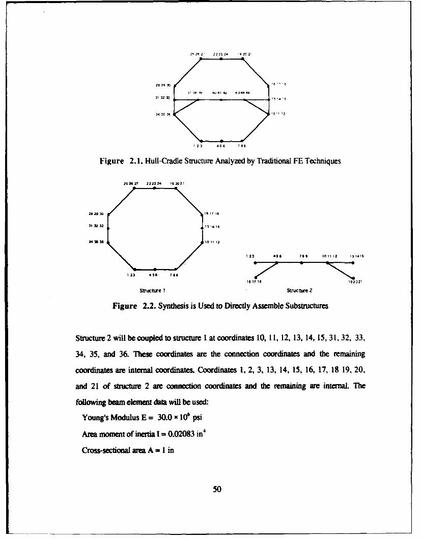
Figure 2.1. Hull-Cradle Structure Analyzed by Traditional FE Techniques

2S 26 V7 222324 19 2021

26 a930 1 7

31 3232 13 1415

343636 11312

1 23 456 769 1011 13 13 1415

123 456 169

'17 17 8 192021

Strture I Sructxure 2

Figure 2.2. Synthesis is Used to Directly Assemble Substructures

Structure 2 will b coupled to structure I at coordinates 10, 11, 12, 13, 14, 15, 31, 32, 33,

34, 35, and 36. These coordinates are the connection coordinates and the remaining

coordinates are internal coordinates. Coordinates 1, 2, 3, 13, 14, 15, 16, 17, 18 19, 20,

and 21 of structure 2 are connection coordinates and the remaining are internal. The

following beam element data will be used:

Young's Modulus E = 30.0 x 106 psi

Area moment of inertia I = 0.02083 in4

Cross-sectional area A = I in

50

Weight density WTD = 0.2832 lbf/in'

Proportional structural damping ( %) a = 0.01

The proportional structural damping was arbitrarily selected and is applied to both

structures. The general equation for dynamic direct coupling is

[.,j] = [Hj - [H,[Ml[h,]-'[Mr[1H.1. (84)

In this equation, M is the boolean mapping matrix which is used to establish the

connectivity between the two substructures for synthesis. The mapping matrix is

determined by the connectivity i.e. what is connected to what and by imposing the

equilibrium and compatibility relations associated with each pair of coordinates. We can

define the mapping matrix by {ffi [M1J1f". Where iff4 is a vector of all the connection

coordinates of both structures and ijf I is the arbitrarily selected independent subset of the

connection coordinates relating to one of the substructures. We have selected the

connection coordinates of structure I as the arbitrary subset of connection coordinates. The

mapping matrix [MI is a matrix of size (24 x 12) and is depicted as:

51

We will calculate the FRF matrix [H) for both substructures. First the I K I and M)

matrices are generated for each substructure. [K, ] and [K_, I are both complex since

proportional structural damping was applied to both structures; again this damping is

arbitrary. [K,1 and [K]1 are of the form IKI-[K +jaoKI. We next form the impedance

matrix for each substructure. The impedance matrix is of the form IZI = [K] - 0:2[MI. With

the impedance matrix generated for each substructure, the FRF matrix H can be calculated

by inverting the impedance matrix. This process is done at each frequency of interest.

These FRF matrices are required in order to couple the two structures together to form the

structure in figure 2.1. Referring to the synthesis equation above, the matrices [H.,1,

[H.4, [JH,.J, and [114 are formed by combining [Hj and [11] by appropriate

partitioning. The partitioning is shown below.

i 2 C, C2

[HI(i,,i) [01 H1 (ic,cj) 101]I •_I1 [01 101 to]k1, 10(12C,)c, [01 4(c,,) [0 1 01 H1(c2,c2 )J

C) CC

[H , ' ,(c,,i) [01 [,( H,,c,) 101o1[']C2i [01 H2(c•,2) J2 01 kn(C12,IC2

H,(,r-,,,<) to0 c, [H,(c,,C) 1o0 ,•2I 101 (," I I0

c2L [01 H2(c2,c2)J

52

Referring to Figure,2.2. i•"• i denotes the set of internal coordinates of structure I which are

1. 2, 3. 4. 5. 6. 7. 8,9, 16. 17. 18. 19. 20. 21. 22. 23. 24. 25. 26. 27. 28. 29. and 30.

"-cI denotes the set of connection coordinates of structure 1 which are 10, 11, 12. 13. 14.

15. 31. 32. 33. 34, 35. and 36. "i2" denotes the set of internal coordinates of structure 2

which are 4. 5, 6, 7, 8, 9, 10, 11. and 12. -c2" denotes the set of connection coordinates

of structure 2 which are 1. 2, 3. 13, 14. 15. 16. 17. 18. 19. 20. and 21. With the

appropriate partitioning complete, the synthesis of structure 1 to structure 2 can be

performed using the direct coupling relation

[-H-" (fleo - I[H,, I[I -. ]I Mf[,o (84)

[H4.] is the synthesized FRF relation which is the combination of both structures. The

synthesis is done over the frequency range of interest and plotted in Figure 2.3. The

frequency range for this example was 0.1 to 10.0 Hz. Figure 2.4 is the solution from

traditional FE calculations included for direct comparison. Both plots are identical.

200

S1 0 0 ............... ................ ............... ............... ..................

0,. . . . . . . . . . . . . . . .. . . . . . . . .. . . . . . . .. . . . . . . .o .... ..... . ... ........S0

• .S-2001

0 2 4 6 8 10Frequency Hz

Figure 2.3. Plot of Synthesized He-(8,8)

53

200

I-.

cL,

• " -2 0 0 1,0 . 4 6 8 10

Frequency Hz

Figure 2.4. Plot of H (8,8) from Traditional FE Calculations.

Figures 2.3 and 2.4 are the plots of the FRF at element (8,8) from the synthesized and FE

[ HI matrices. This element corresponds to the lateral motion coordinate 8 of Figure 2.1.

Notice both plots are identical and both show the first seven damped natural frequencies.

The plots show the magnitude of the response of unit amplitude at coordinate 8 due to a

unit excitation at varying frequency at coordinate 8. As the frequency of excitation

approaches the damped natural frequency, the response approaches infinity.

C. EXAMPLE (3): STRUCTURAL MODIFICATION (REMOVAL OF A

BEAM ELEMENT)

Consider the following figurs Figure 3.1 depicts a combined hull-cradle suctu

which will be directly assembled by traditional FE procedures. Note that the structure in

Figure 3.1 has asymmetric reintforcing trusses. The synthesis methodology will be used to

arrive at the strctuml configuration shown on the left of Figure 3.1 by removing the beam

54

shown on the right of Figure 3.2. The FRF calculated from the FE model (Figure 3.1) will

be compared with that calculated using synthesis.

2S 6 ? 22 2"324 '9 20 21

2 29 30D

31 32 33 '34 '

34 15'1 '0"'' 2

' 23 4S6 789

Figure 3.1. Final Hull-Cradle Configuration

•S252627 2223 24 19 20 21

S28930 t ?1

as 30 V 3.8 9 4.0 41 42 434"11?t

31 3233 131415

341011 1224

4SG

1 23 4S6 769 1 23

Structure 1 Sbucture 2

Figure 3.2. Synthesis Used to Remove a Beam Element

Referring to Figure 3.2, saucture 1 will be modified by removing the beam, structure 2.

located between nodal coordinates 10, 11, 12, 43, 44, and 45. The following beam element

data will be used.

Young's Modulus E = 30.0 x 106 psi

Area moment of inertia I = 0.02083 in4

Cross-sectional ama A = 1 in

55

Weight density WTD = 0.2,832. lbf/in

1 percent proportional structural damping a = 0.01

The proportional structural damping was arbitrarily selected and is applied to both

structures. The general equation for dynamic indirect coupling/modification is

[Hoor = [i-, .- [H, - z--[H,.I. (66)

Note that the sign in the term [H,, -Z-']-' is opposite from that in the original indirect

coupling equation. This is because we are removing the beam element from the structure

instead of synthesizing it to the structure. The first step is to generate the (K] and [MI

matrices for structure 1 and structure 2. The [KI matrices for both structures are complex

since proportional damping was applied. They are of the form [KI - [K + jaK]. Next we

form the impedance matrices for each structure. [ZJ = [K] - fl 2[MI. This method requires

the calculation of the FRF matrix [ HI only for the structmue to be modified. structure 1 of

Figure 3.2. The impedance and the FRF matrices are calculated at the frequency of interest.

Once the FRF and impedance matrices are generated, we are ready to partition the FRF

matrix. The matrices [H,.], [ Hj], [H,.l, and IHcj are formed by partitioning (HI] . The

partitioning is shown below.

[H4]" <,([H 1 -,, 4) .Ht(i,c,)J[

l-,,- AL ,,c,)] Hlj - c4l[,(•,c,)J

56

The connection coordinates for structure I are 10, 11. 12. 43. L and 45. The rest are all

teated as internal coordinates. With the appropriate partitioning of [HI completed, the

removal of the beam from the structure can now be completed by using the correct form of

the indirect coupling relation mentioned above. [He,] is the synthesized FRF relation

which reflects the removal of structure 2 from of structure 1. This modification is

calculated over the frequency range of interest and plotted in Figure 3.3. The frequency

range for this example was 0.1 to 7.0 Hz. Figure 3.4 is the solution from the traditional

FE procedure and is provided to allow direct comparison of the two solutions. Both plots

are identical.

200

-.,o ...........

u-2000 1 2 3 4 5 6 7

Frequency Hz

Figure 3.3. Plot of H.( 11,11) as Calculated Using Synthesis

57

200"I.-

........... .. ... . . . . . . . . . . . . .... .... .. .........

-100 . . .. ...... . ...

S-2000 1 2 3 4 5 6 7

Frequency Hz

Figure 3.4. Plot of H(14.14) Calculated Using Traditional FE Procedures

Figures 3.3 and 3.4 are the plots of the FRF corresponding to the lateral motion coordinate

14 of Figure 3.1. A special note here is that the element (14,14) of the FRF generated by

FEM is the coordinate 14, which corresponds to the element (11,1 1) of the FRF generated

by the indirect coupling relation. The reason for this is because of the partitioning. [ H, ]" is

partitioned with intal coordinates first followed by the connection coordinates. Care is

required here to ensure the coordinate of interest is actually being used. Notice both plots

are identical and show the first six damped natural frequencies. The plots show the

magnitude of the response at coordinate 14 due to a unit excitation at varying frequency at

coorinate 14. As the fiequercy of excitation approaches the damped natural frequency, the

response approaches infinity.

58

D. EXAMPLE (4): STRUCTURAL M(ODIFICATION (ADI)ITION tWt A

BEAM)

Consider the following figures. The FRF for the structure shown in Figure 4.1 will be

calculated by traditional FE procedures to compare with that calculated using the synthesis

procedure to add the beam element, as shown in Figure 4.2.

2S 25 27 2221 24 1 20 21

2829304041 4 4344 1

31 3233 6 114¶5

363536 6 1011 12

123 4S6 78a

Figure 4.1. Hull-Cradle Structure Analyzed by Traditional FE Techniques.

2S a • 2223 24 19 20 21

282930 1

31 3233 31 5

38 35 36 101112

4S8

1 23 456 789 123

Sructure 1 Structure 2

Figure 4.2. Synthesis is Used to Add the Beam Element

Referring to Figure 4.2, cture I will be modified by adding the beam, structure 2, at the

nodal coordinates 10, 11, 12, 43, 44, and 45. The following beam element data was used:

Young's Modulus E = 30.0 x 106 psi

Area moment of inertia I = 0.02083 in4

59

Cross-sectional area A = 1 in

Weight density WD = 0.2832 lbf/in'

Proportional structural damping (1%) a = 0.01

The proportional structural damping was arbitrarily selected and is applied to both

structures. The general equation for dynamic indirect coupling/modification is

[ Hj- ]'- - [H, .[Z- + Hc I[H,., (66)

The first step is to generate the [ K] and [ MI matrices for structure I and structure 2. The

[KI matrices for both structures are complex since proportional damping was applied.

They are of the form I K -[K + jaKI. Next, impedance matrices are formed for each

structure as [Z] = [K] - WT2[M]. This method requires the calculation of the FRF matrix

[ HI only for the structure to be modified, structure I of Figure 4.2. The impedance and the

FRF matrices are calculated at the frequency of interest. Once the FRF and impedance

matrices are generated, partition of the FRF matrix is required. The matrices I[4, [H, ],

[ H,.], and [ Hj are formed by partitioning [ H,]. The partitioning is shown below.

4 c, 4 C

[H1,]= c [ H,,(4,c,)J [., - c,[H,(4,4) I H,J(c,,c,)]

C,

[H.:', L.,(c,,c,). H-..,..1 -' [ H, (<:,, ,j

The connection coordinates for structure I are 10, 11, 12, 43, 44, and 45. The rest are all

treated as internal coordinates. With the appropriate partitioning of [IHI completed, the

synthesis of the beam to the structure can now be completed by using the correct form of

60

the indirect coupling relation mentioned above. [H-/. is the modified FRF relation which

is the combination of structure I and the added element. structure 2. The synthesis is

performed over the frequency range of interest and plotted in Figure 4.3. The frequency

range for this example is 0.1 to 8.5 Hz. Figure 4.4 is the solution from a traditional FE

calculation for direct comparison of the two solutions. Both plots are identical.

m 200

-200

• .0 .

0 1 2 3 4 5 6 7 8 9Frequency Hz

Figure 4.3. Plot of Synthesized FRF Element Hee(8.8)

~200-

.9100-

0-

S •0

~-100.-200

Um 0 1 2 3 4 5 6 7 8 9

Frequency Hz

Figure 4.4. Plot of H (8,8) Calculated Using Traditional FE Procedures.

61

Figures 4.3 and 4.4 are the plots of the FRF corresponding to the lateral motion coordinate

8 of Figure 4.1. A special note here is that the element (8.8) of the FRF generated by FEM

corresponds to the coordinate 8, as does the element (8.8) of the FRF generated by the

indirect coupling relation. This is different from the previous example. The reason for this

is because of the partitioning. [ H,, " is partitioned with internal coordinates first followed

by the connection coordinates. Care is required here to ensure the coordinate of interest is

actually being used. Notice both plots are identical and show the first six damped natural

frequencies. The plots show the magnitude of the response at coordinate 8 due to a unit

excitation at varying frequency at coordinate 8. As the frequency of excitation approaches

the damped natural frequency, the response approaches infinity.

E. EXAMPLE (5): INDIRECT COUPLING WITH ISOLATORS

Consider the following figures. The FRF for the structure shown in Figure 5.1 will be

calculated using traditional FE procedures to compare with the FRF calculated using the

synthesis method. The synthesis will combine the various components shown in Figure

5.2. In this figure, the hull model (structure 1) will be coupled to the cradle model

(structure 2). Note that this example demonstrates that the synthesis procedure easily and

exactly reats problems with non-proportional damping, a truly unique feature of the

methodology.

62

zs2 E2- 22 23 24 i2C

28 2930 16 1 - 183' 31A 39 43 4,44 49 50 51

3' 32 32 - 1314 '

5253 503 545565

-3 4,

34 35 36 4 ' '2

23 .1 6 '89

Figure 5.1. Traditional FE Procedures are Used to Calculate FRF for the Combined

Hull-Isolator-Cradle Structural System.

2526 27 22 2324 19 2021

2630 30 14'? 'a

3132 32 131413

34353 lo 10 2

S223 456 789 1011 12 131415

1 23 456 709

1617 161 19 212

Structure I Structure 2

Spring and DMnr Isohltor

Figure 5.2. Total Hull-Isolator-Cradle System is Synthesized from Components.

Referring to Figure 5.2, structure 1, structure 2, and four spring-damper isolator sets will

be synthesized together to form the system in Figure 5.1. Each isolator set consists of three

spring-damper isolators, are for each connection coordinate. The connection coordinates

for structure 1 are 10, II, 12, 13, 14, 15, 31, 32, 33, 34, 35, and 36. The remaining

63

coordinates are internal coordinates. Coordinates 1. 2, 3. 13, 14. 15, 16. 17, 18 19. 20.

and 21 of structure 2 are connection coordinates and the remaining are internal. For this

structural synthesis method, the spring-damper isolators are treated as a lumped system

(with no physical dimensions) installed at the connection coordinates. The connection

coordinates do not merge into one but are joined by way of the isolators. The following

beam element data will be used:

Young's Modulus E = 30.0 - 106 psi

Area moment of inertia I = 0.02083 in'

Cross-sectional area A = I in

Weight density WIT) = 0.2832 lbf/in 3

Proportional structural damping (2%) a = 0.02

Proportional viscous damping (2%) 0 = 0.02

Isolator spring constant k = 25 lbs/in

The proportional structural damping was arbitrarily selected and is applied to both

structure I and 2 of Figure 5.2. The proportional viscous damping used for the damper in

the isolator is arbitrary and is not limited to being proportional but could be any frequency

dependent function. For our example the isolator is of the analytic form [ k + j 00k] where

j=.,7T. Recalling the impedance relation [Z(0)]-[KI_-02[M]+ j C] , [CI is the

proportional viscous damping, [I k}. The operative equation for indirect coupling with

mapping matrices is

[H',," -[Hel - [H-JMfk-÷ + hJ1'[Mft[HJ], (99)

where [[M [ ZIMfr and M] = HIMI.

64

Note that [21 reduces to [IJXk + jf)ok) and its size is ( 12 x 12 ). The boolean mapping

matrix I MI is determined the same way as explained in example two. The connection

coordinates for structure 1 and structure 2 are listed above. We can deftie the mapping

matrix by If} = [ M]ff .I Where if[I is a vector of all the connection coordinates of both

structures and {if. I is the arbitrarily selected independent subset of the connection

coordinates relating to one of the substructures. We have selected structure I as the

arbitrary subset of connection coordinates. The mapping matrix [MI is a matrix of size (24

x 12) and is

The FRF matrix [HI for both substructures is required. First the [ K] and [MI matrices are

generated for each substructure. 1K,] and [K, I are both complex since proportional

structural damping was applied to both structures, again this damping is arbitrary. [ K, ] and

[ K,] are of the form [KJ- [K + jaKJ. We next form the impedance matrix for each

substructure. The impedance matrix is of the form [ZI = [K] - 01[MI. With the impedance

matix generated for each substructure, the FRF matrix H can be calculated by inverting the

impedance matrix. This process is done at each frequency of interesL Now with the FRF

matrix for each substructure calculated, we are ready to synthesize the two structures and

isolators together to form the structure in Figure 5.1. Referring to the synthesis equation

65

above, the matrices[ H]. [H,. [H.,.. and [H.,,] are formed by combining H/, and [Hj

by appropriate partitioning. The partitioning is shown below.

C, C,

i, [01 H(,.i,) [01 H,(i,.c,)

[0 1() [01 HHc( a ) [0cL (01 H,_(cI,) [01 H0(1, .. ,)J

[He=' H(c1,i) [0 1 c, 1) 01 1

",L [01 H(c.i) [01 H(c-,.c,)J

C1 C2,

[H, [01 H,0(0,c 2 [H= Hl(c,,c, ) [0 ) 1C, 11 kC- 1- 11 4--c)

H1(c,/ 1c,c,) [01 C 101 (2 I-,(c,,,)j

c, [01 H2(c2,c)J

Referring to Figure 5.2, "il" denotes the set of internal coordinates of structure I which

include 1, 2, 3, 4, 5, 6, 7, 8, 9, 16, 17, 18, 19, 20, 21, 22, 23, 24, 25, 26, 27, 28 ,29,

and 30, "ci" denotes the set of connection coordinates of structure 1 which include 10, 11,

12, 13, 14, 15, 31, 32, 33, 34, 35, and 36, "i2" denotes the set of internal coordinates of

structure 2 which include 4, 5, 6, 7, 8, 9, 10, 11, and 12, "c2" denotes the set of

connection coordinates of structure 2 which are 1, 2, 3, 13, 14, 15, 16, 17, 18, 19, 20,

and 21. With the appropriate partitioning complete, the synthesis of structure 1 to structure

2 can be performed using the indirect coupling relation

66

[ H..I" = tHI!- [HjFI Mh + "', Mjt H!,. 9

Structure I is synthesized to structure 2 by the isolators or load paths described by [z1.

(H," is the synthesized FRF relation which is the combination of both structures and

isolators. The synthesis is done over the frequency range of interest and the response is

plotted in Figure 5.3. The frequency range for this example was 0. 1 to 8.0 Hz. Figure 5.4

is the solution from traditional FE calculations for direct comparison. Both plots are

identical.

S1 0 .. .. .. .. .. .. .. .. ............ ........................... .. .....................

• 150S-100 .... : .

........... ..............

-150 ..... . .

-150 0 I 2 3 4 5 6 7 8

Frequency Hz

Figure 5.3. Plot of H,48,8) for Synthesized System.

67

150

S 100 ..... .......... ..... ...... .............. . . . ... .. . . . .

• = 50

.- 150 "'0 1 3 4 5 6 7 8

Frequency Hz

Figure 5.4. Plot of H(8.8) from Traditional FE Calculations.

Figures 5.3 and 5.4 are the plots of the FRF at element (8,8) of the synthesized [(H,, and

traditional FE [H] matrices, respectively. This element (8.8) correspo-nds to the lateral

motion coordinate 8 of Figure 5.1. Notice both plots are identical and show the first five

damped natural frequencies. The plots show the magnitude of the response at coordinate 8

due to a unit excitation at varying frequency at coordinate 8. As the frequency of excitation

approaches the damped natural frequency, the response approaches infinity.

F. EXAMPLE (6): INDIRECT COUPLING WITH FREQUENCY

DEPENDENT ISOLATORS

In this example, we demonstrate the capability of synthesizing components with

frequency dependent propties. Specifically, we will repeat the preceding example using

isolators that have frequency dependent damping. Consider the following figures. The FRF

for the structure shown in Figure 6.1 will be calculated using traditional FE procedures to

68

compare with the FRF calculated using the synthesize method. The components to be

synthesized are shown in Figure 6.2.

252627 Z2 Z3 24 l33021

282930 37 $ 9 48

3i 32 3Z 3 4 t3 4 15S•2 53 54 SS $e $7

343536 0 / 011 12

123 4S6 769

Figure 6.1. Traditional FE Procedures are Used to Calculate FRF for the Combined

Hull-Isolator-Cradle Structural System

25 2S V7 1222 19 201)ZZ

3929 30 1417 i

3132 32 1314 1s

""2 I 4 6 789 101112 '314 15

28 4S6 7663

ý7 11 192021

Strucure 1 Structure 2

Spring aWd Diaper IM~atOr

Figure 6.2. Total Hull-Isolator-Cradle System is Synthesized from Components.

In Example (5), the isolators were treated as having proportional viscous damping. This

example will use viscous damping which is frequency dependent. The methodology is the

69

same as in the previous example and will not be repeated here. The disxussiov, here will

focus on the only difference which is the damping applied to the isolator. Referring to the

general impedance relation [Z(I)I - [ K] - 02[M] + jC] . [C] is now a function of f).

The equation is now of the form

[Z(n)]=[Kl- n2[M! + 4CIl)]. (104)

The damping applied to the isolator was arbitrarily selected as an exponential decay

dependent on frequency. The form of the function used is

C = C~e-' (3)

where C. - k = 25 lb- s/in and a = 0.1.

The damping function is plotted in Figure 6.3.

S10.

0 5 10 15 20 25

Frquency rad/sec

Figure 6.3. Plot of Isolator Damping Versus Frequency

The reduced impedance in this example is now of the form [ZJIi(k + jnke-") and the

size of the matrix is (12 x 12).

70

Structure I is coupled to structure 2 with isolators described by [2]. [H,,' is the

synthesized FRF relation which is the combination of both structures and isolators. The

synthesis is done over the frequency range of interest and plotted. Figure 6.4. The

frequency range for this example was 0.1 to 8.0 Hz. Figure 6.5 is the solution from

traditional FE calculations provided for direct comparison. Both plots are identical.

W .. . . . . .

0 . .. .. .......... • .......... .. .. .......... . ° ........... ......... ..........

-100 ..........

S-2000 1 2 3 4 5 6 7• 8Frequency Hz

Figure 6.4. Plot of Hee(8,8) Calculated Using the Synthesis Method.

S200

S100O

0-

-100 " -... . . .. .. .

U. -200

0 1 2 3 4 5 6 7 8

Frequency Hz

Figure 6.5. Plot of H(8,8) Calculated Using Traditional FE Procedures.

71

Figures 6.4 and 6.5 are the plots of the FRF at element (8.8) calculated using the

synthesized [H,,J'and FE [H] matrices, respectively The FRF element (8.8) corresponds

to the lateral motion coordinate 8 of Figure 6.1. Notice both plots are identical and show

the first five damped natural frequencies. The plots show the magnitude of the response at

coordinate 8 due to a unit excitation at varying frequency at coordinate 8. As the frequency

of excitation approaches the damped natural frequency, the response approaches infinity.

A comparison of the compute time required for the synthesis versus traditional FE

calculation. The actual computing time and the number of floating point operations (flops)

for each method is provided:

FEM direct assembly: time - 25876 sec or 431.3 mins

FLOPS - 1.49 x 109

FRF synthesis: time - 1167 sec or 19.45 mins

FLOPS - 517.2 x 106

This clearly demonstrates that synthesis by FRF is more efficient and well suited for design

analysis.

G. EXAMPLE (7): STRESS CALCULATION BY DYNAMIC INDIRECT

COUPLING

Consider the structures shown in the following figures. The structure shown in Figure

7.1 will be directly assembled by the finite element method and the peak bending stress

frequency response will be calculated in beam element #4 whose location is shown by the

dashed line A--A. The same structure will be synthesized using the frequency domain

method and the same stress frequency response will be calculated. The FRF results

calculated by the synthesis methodology, shown in Figure 7.5, will be compared with that

calculated by traditional FEM, Figure 7.6. Again, the structure (specifically, its FRF) as

shown in Figure 7.1 will be obtained by synthesizing strucre I and the modification,

72

structure 2, as shown in Figure 7.2. Note that a stress frequency response allows the direct

calculation of stress due to the application of a force or moment. The equation for

determining synthesized stress is shown as equation (105).

(i-) = (H)o,()l"I tiQ)l . (105)

where the synthesized stress FRF matrix [H,(fl )]* reflects the total structure, including

any modifications or couplings.

783

10111 456

AA9

//

^//

123

Figure 7.1. SCmture Analyzed for Peak Bending Stress

189

10111! 456

A,

<A>

123456 121

Stnwture I 5Unjumu 21

Figure 7.2. Components of Synthesized Structure

73

Referring to Figure 7.2, structure I will be modified by adding the beam. structure 2 at the

nodal coordinates 4, 5, 6, 10, 11, and 12. The following beam element data will be used:

Young's Modulus E = 30.0 x 106 psi

Area moment of inertia I = 0.02083 in4

Cross-sectional area A = I in

Weight density WTD = 0.2832 lbf/in'

Distance from beam center to outer most fiber c = 0.05 in

For this example, damping was not used, but the methodology is able to handle all

forms of linear damping as described earlier. The general equation for synthesizing stress

information by dynamic indirect coupling/modification is

[Ho.l" = [H,,.]- [o H.IZ-' + Fý-[ , 66)

This equation is the first row extracted from the relationship shown as equation (12). Note

that the synthesis of stresses can be done at the same time as the synthesis of

displacements. We are here demonsrating just the synthesis of stress information.

The first step is to generate the [KJ and [MI matrices for structure I and the beam

element shown in Figure 7.2. Next the impedance matrices are generated for each structure

as [Z(fl)J - [K] - W2[M]. Since we are modifying structure 1, the FRF matrix [ H] is only

calculated for structure 1 of Figure 7.2. The complete process as described here is

performed over the frequency range of interest. There is basically two sections to this

pocess: (1) the partitioning of the [ HI matrix into its required sub matrices for the general

synthesis process and (2) the extraction of the information from the [HI matrix and the

processing of that information to calculate the stress frequency response.

74

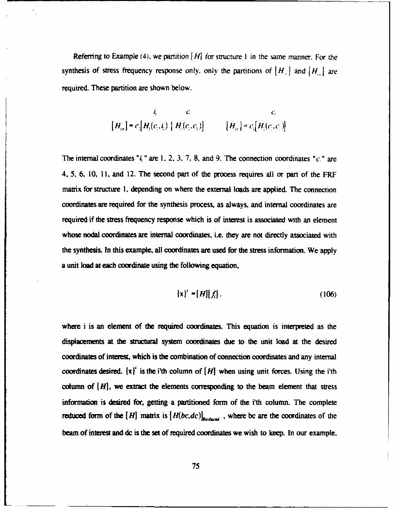
Referring to Example (4). we partition [ HI for structure I in the same manner. For the

synthesis of stress frequency response only. only the partitions of [H J and[H j are

required. These partition are shown below.

I Ck[He] = cIj H(,L. Hi CC 14j [H el [H. (c. .c,

The internal coordinates "/ Hare 1, 2, 3, 7. 8, and 9. The connection coordinates "c," are

4, 5, 6, 10, 11, and 12. The second part of the process requires all or part of the FRF

matrix for structure 1, depending on where the external loads are applied. The connection

coordinates are required for the synthesis process, as always, and internal coordinates are

required if the stress frequency response which is of interest is associated with an element

whose nodal coordinates are internal coordinates, i.e. they are not directly associated with

the synthesis. In this example, all coordinates are used for the stress information. We apply

a unit load at each coordinate using the following equation,

jx)' =[HJjff}. (106)

where i is an element of the required coordinates. This equation is interpreted as the

displacements at the structural system coordinates due to the unit load at the desired

coordinates of interest, which is the combination of connection coordinates and any internal

coordinates desired. Ix I' is the i'th column of [ HI when using unit forces. Using the i'th

column of [ HI, we extract the elements corresponding to the beam element that stress

information is desired for, getting a partitioned form of the ith column. The complete

reduced form of the [HI matrix is [H(bcdc)L, , where bc are the coordinates of the

beam of interest and dc is the set of required coordinates we wish to keep. In our example,

75

the set of beam coordinates, "bc" is 1. 2, 3. 10. 11. and 12 and the set of required

coordinates. "dc" is 1. 2. 3, 4, 5. 6, 7. 8. 9. 10. 11. and 12. [HIRoJý-.,d is a matrix of size

(6 x 12). Each column of IHIR.d.,.o is in the global coordinate system and needs to be

transformed to local coordinates by using the following relation

1Y 1 edswed4,w [TI IH' IRied(ed" (107)

where the transformation matrix [T] is

cosa sina 0 0 0 0-s- a cosa 0 0 0 0

0 0 1 0 0 0

[T]= 0 0 0 cosa sina 0

0 0 0 -sina cosa 0

0 0 0 0 0 1

Now with the H transformed to the local coordinate system, we can get the nodal forces by

the following relation

(PI -[klfH'I (108)

where [kj I is the elemental stiffness matrix in the local coordinates system. We are ready to

solve for the FRF stress, first combining all the column vectors {ff into a nodal force

matrix [F] and then multiplying it by the moment equation to solve for the FRF peak

internal bending stress of the beam element.

76

The FRF stress equation is

IH, HIM 7 [FI . (109)

The IH, I is a row vector size (1 x 12). since we used all the coordinates as our set of

desired coordinates. Noting that I M, I is determined from equilibrium for the element in

question. and here we provide the internal bending moment. The derivation is shown using

Figures 7.3 and 7.4.

Beam Element

Figure 7.3. Beam Element for Stress Calculation

Sectioned Beam Element

Figure 7.4. Beam Section Cut at the Midpoint

Consider the beam element in Figure 7.3, The moment is to be calculated at the midpoint of

the beam. First the beam is cut, Figure 7.4 and the moment at A is solved for:

1MA =M- + _• (110)

The moment equation in vector form is shown as equation (111).

77

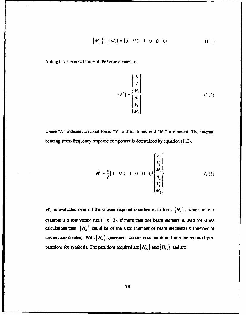
Mj=-IM )-IO 1//2 1 0 0 0) (111)

Noting that the nodal force of the beam element is

A,

V

jF' =(112)

M,

where "A" indicates an axial force, -V" a shear force, and "M." a moment. The internal

bending stress frequency response component is determined by equation (113).

AV,

R,--0o //2 1 0 0 o M' (113)A2

V2

/i. is evaluated over all the chosen required coordinates to form H, I, which in our

example is a row vector size (1 x 12). If more then one beam element is used for stress

calculations then IH, ] could be of the size: (number of beam elements) x (number of

desired coordinates). With [ H, I generated, we can now partition it into the required sub-

partitions for synthesis. The partitions required are [I H,] and [ H,,} and are

78

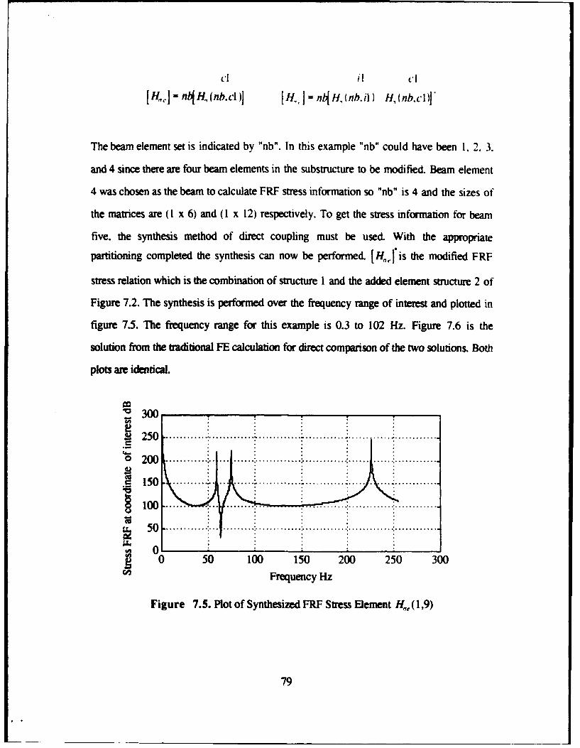
Hcl il c'l

The beam element set is indicated by "nb". In this example "nb" could have been 1. 2. 3.

and 4 since there are four beam elements in the substructure to be modified. Beam element

4 was chosen as the beam to calculate FRF stress information so "nb" is 4 and the sizes of

the matrices are (I x 6) and (I x 12) respectively. To get the stress information for beam

five, the synthesis method of direct coupling must be used. With the appropriate

partitioning completed the synthesis can now be performed. [H,,]is the modified FRF

stress relation which is the combination of structure 1 and the added element structure 2 of

Figure 7.2. The synthesis is performed over the frequency range of interest and plotted in

figure 7.5. The frequency range for this example is 0.3 to 102 Hz. Figure 7.6 is the

solution from the traditional FE calculation for direct comparison of the two solutions. Both

plots are identical.

v3002 2 5 0 .......... . .. ............. ............ ........... ............ .............

15 0 ... . . . . .: ... .. ...... ! . ............. ........... ..... . .... .............~1500..... ...... ... .......................

5 0 .. _ _ _ _ _ _ _ _ _ _ _

0 50 100 150 200 250 300S2Frequency Hz

Figure 7.5. Plot of Synthesized FRF Stress Element Ho,(1,9)

79

S300

-250 . . . -

* 150~1 0 0 ... .... ...... ...

i 10 0 .. ..... .... ............. .. ............ : ............. • ... ........

S50 " ". .0~~~~~~~ .. ... .. .... ......

S 0

S0 50 100 150 200 250 300Frequency Hz

Figure 7.6. Plot of H, (1.6) Calculated Using Traditional FE Procedures.

Figures 7.5 and 7.6 are the plots of the FRF stress corresponding to beam element four of

Figure 7.1. These plots represent the stress amplitude in beam element four due to a unit

force applied at coordinate 6. Both plots are identical. Note that the frequency of peak

response is slightly lower than the'undamped natural frequency.

H. EXAMPLE (8): DYNAMIC DIRECT COUPLING USING MODAL

REPRESENTATION OF FRF

Consider the stuctres shown in the following figures. The structure shown in Figure

8.1 will be directly assembled by the finite element method in order to compare the

frequency response calculated by traditional FE methods and the solution obtained by

synthesizing structure 1 and structure 2 as shown in Figure 8.2. This example will show

three results, the first being the solution from synthesis using the modal representation of

the frequency response, the second being direct assembly using FE and the modal

representation and thirdly, direct assembly using FE where frequency response is

calculated by the inverse of the impedance matrix.

80

123 456 789

Figure 8.1. Structure Analyzed Using Traditional FE

123 456 123 456

Structure I Structure 2

Figure 8.2. Structures to be Synthesized Using Modal Representation

Referring to Figure 8.2, structures 1 and 2 will be synthesized by direct coupling using

connection coordinates 4, 5, and 6 of structure I and connection coordinates 1, 2. and 3 of

structure 2. One internal coordinate will be kept in this synthesis process to show that the

frequency response for a specific coordinate can be synthesized using just the connection

coordinates and any internal coordinates that might be of interest. This example will use the

internal coordinate "2" of structure I as the coordinate of interest. The information desired

in this example is the frequency response at coordinate 2 due to a unit harmonic load at

coordinate 6. Note that when structure 1 and structure 2 are synthesized, the coordinate

numbering becomes the same as depicted in Figure 8.1. The following beam element data

was used:

Young's Modulus E = 30.0 x 106 psi

Area moment of inertia I = 0.02083 in'

Cross-sectional area A = I in

Weight density WTD = 0.2832 lbf/in3

Structural proportional damping - us not used, but the methodology will handle all

forms of damping discussed earlier. The frequency response matrix [ HI can be generated

by two methods. The first is by the relationship

81

where [z((Q)I= [KI-02[MI+ jfXC

The second method is by matrix modal representation. The relationship is

[H(I(~I[j 2 jn2 (421)

where I P] is the set of eigenvectors or mode shapes, and the middle term is the diagonal

matrix of the natural frequencies or eigenvalues less the frequency of interest. This

relationship can also be expressed in terms of individual elements of the frequency

response function by equation (114)

H~j - Y(114)Wr

which allows the calculation of specific frequency response of interest without having to

generate the complete FRF.

The general synthesis equation for dynamic direct coupling is

[HIS - [HJ - (HjM[h,- I•[Mf[HC]. (84)

82

This equation is written in terms of all the coordinates. This example concerns the synthesis

of a single FRF matrix element involving one coordinate. In general, the synthesis process

requires FRF information for all connection coordinates, and FRF information for any

internal coordinates of interest. Rewriting the general equation for this specific example. the

equation becomes

[H--,] -[Hjf.ji[MT[H( (115)

where the subscript "2" signifies the internal coordinate "2" of structure I and the subscript

"c" signifies the set of connection coordinates of both structures. In this equation, [Ml is

the boolean mapping matrix which is used to establish the connectivity between the two

substructures for synthesis. The mapping matrix is determined by the connectivity i.e. what

is connected to what and by imposing the equil'iium and compatibility relations associated

with each pair of coordinates. We can define the mapping matrix by JfJ =IM)I)f.

Where If- isa vector ofall the connection coordinaes of both structures and isthe

arbitrarily selected independent subset of the connection coordinates relating to one of the

substructures. We have selected the connection coordinates of structure I as the arbitrary

subset of connection coordinates. The mapping matrix [M] is a matrix of size (6 x 3) and is

depicted as:

1

[1[MI- .

-1-1

83

The FRF matrix I HI for both substructures 1 and 2 is calculated using the matrix modal

representation relation discussed earlier. The important point here is that we are not using

all the coordinates. The coordinates used from substructure I are 2. 4, 5, and 6. the first

coordinate is the coordinate of interest and the rest are connection coordinates which must

be used. The coordinates used from substructure 2 are just the required connection

coordinates 1, 2, and 3. All six mode shapes for each coordinate are kept for the calculation

of the FRF matrix. The FRF matrix [H: is calculated by using the appropriate

partitioning of the modal matrix [b I. The diagram of the relation on the next page is

showing the coordinates kept and the number of modes.

6 6 2456

The size of [ HJ ] is now a (4 x 4) matrix which contains all the necessary information. This

also shows a significant computational advantage because the size has been reduced from a

(6 x 6) to a (4 x 4) matrix which requires less computational time to manipulate the matrix.

I H21 is generated in the same manner. We will use all six mode shapes for each coordinate

kept of substructure 2. The required coordinates are the connection coordinates 1, 2, and

3. The diagram of the relation is given on the next page showing the coordinates kept and

the number of modes.

84

6 6 123

Now with h I and h2 generated, the two substructures can be synthesized. Referring to the

example-specific synthesis equation above, the matrices [H,, I and [H,, are formed by

combining h I and h2 by appropriate partitioning. The partitioning is shown on the next

page.

H2,1h4H,(4,c,) [01] [H] 4 [ H c1, C ( 01

Referring to Figure 8.2, "it" is the set of internal coordinates for substructure 1. Since

coordinate 2 is the only coordinate of interest, the set of internal coordinates is just

coordinate 2. The set of connection coordinates "c1" consists of 3. 4, and 5 and "c2"

consists of 1, 2, and 3. With the apprpriate partitioning complete, the two structures are

synthesized together, to form the structure in Figure 8.1, using the case specific form of the

direct coupling relation

[H2 "f _ [H2,1 -[H,,IMtl -'[MIMT[H,.. (115)

[H2+• is the synthesized FRF by modal representation relation which is the combination of

both structures. The synthesis is done over the frequency range of interest and plotted in

Figure 8.3. The frequency range for this example was 0.1 to 80.0 Hz. Figure 8.4 is the

85

solution from traditional FE calculations using the inverse of the impedance matrix to

calculate the FRF and Figure 8.5 is the solution from traditional FE calculations using the

modal representation to calculate the FRF. Figures 8.4 and 8.5 are included for direct

comparison. All three plots are identical.

0

S-5 0 ... .. ................... ............................................. . . .

-350 , , ,,0 10 20 30 40 50 60 70 80

Frequency Hz

Figure 8.3. Plot of Synthesized H,, (1,3)

86

0

S-50 o

S ° ..........i.. ........ ....................... 12 5 0 I ......... .......... .......... ........ ... ..... .......... ............ i .........

-3500 10 20 30 40 50 60 70 80

Frequency Hz

Figure 8.4. Plot of H(2,6) from Traditional FE Calculations

01

-5o0

o-150- ý -'

_150• ,

-200k L

I-. I§-250;1-300k

-350 .0 10 20 30 40 50 60 70 80

Frequency Hz

Figure 8.5. Plot of H(1,4) from Traditional FE Calculations Using Modal Representation

Figures 8.3, 8.4 and 8.5 are the plots of the FRF at element (1,3), (2,6), and (1,4)

respectively. These elennts corresponds to the lateral motion coordinate 2 of Figure 8.1.

87

A special note here is that the element (2.6) of the FRF generated by FEM is the response at

coordinate 2. which corresponds to the element (1,3) of the synthesized FRF generated by

the direct coupling relation using modal representation, and element (1.4) of the FRF

generated by traditional FE using modal representation. The reason for this is because of

the partitioning and the coordinates used in the calculation. Care is required here to ensure

the coordinate of interest is actually being used. The plots show the magnitude of the

response at coordinate 2 due to a unit excitation at varying frequency at coordinate 6. As the

frequency of excitation approaches the natural frequency of response, the response

approaches infinity.

Figure 8.6 is the plot of the determinant of H, which shows the natural frequencies of

the synthesized structure. The frequencies where the plot crosses the axis or equivalently,the frequencies for which the det[ fi] -0 correspond to the natural frequencies of the

synthesized structure. This information is important because it gives the designer a starting

point on deciding how many modes to keep in the modeling of the system and the

frequency bandwidth over which to perform the synthesis. Reducing the number of

retained modes will decrease the computational cost and the computer time required to

analyze a given design. The number of modes required to accurately model a given

structure is case specific.

88

xlO-12

.. 5....

.. ... .... U................

S -5 "'. ... ........... .................................... .................

0 i20 40 60 80Frequency Hz

Figure 8.6. Plot of the Determinant of Hc (Plotted over Reduced Bandwidth)

89

II - U.II I II

V. CONCLUSIONS AND RECOMMENDATIONS

The most important conclusion from this study is that the analysis and re-analysis of

structural systems is performed most efficiently by working in the frequency domain. It

was shown in example (6) that synthesis of complex structures was approximately 22

times faster than the traditional FE methods. The large increase in efficiency means that

rapid analysis and re analysis of structures can be performed. Large scale structural

analysis can now be looked at in man hours where analysis by traditional FE methods is in

man days.

Structural synthesis in the frequency domain provides for an arbitrary order model

reduction that requires only the coordinates involved in the synthesis and any other

coordinates that might be of interest. The solution to the reduced model is exact. This is a

significant point because a 10,000 degree of freedom model can be reduced to a system of

tens or hundreds of degrees of freedom, significantly improving the computational

efficiency.

The frequency response theory allows for the direct synthesis of response information

of any kind. Using a generalized definition of frequency response, displacement, velocity,

acceleration, stress, and strain information may be directly synthesized. based on this

generalization, the theory is an ideal means for doing static and dynamic design re-analysis.

Static problems are treated as the zero frequency case.

The frequency domain structural synthesis theory allows for any combination of

substructure coupling and structural modification to be performed, either simultaneously or

sequentially.

90

Recommendations to further utilize and demonstrate the theory of frequency domain

structural synthesis is first, to write computer code that will interface with existing finite

element codes, for example NASTRANS (MSC. Corp.) or IDEAS (SDRC, Corp.) to

synthesize substructures in three dimensions using plate. shell, and beam elements with six

degrees of freedom per node which allows for out of plane analysis. Using the combination

of plate, shell, and beam elements will more closely approximate actual structures. Second.

build a scaled prototype of a submarine and equipment cradle and compare the theoretical

results with experimental results.

91

APPENDIX A MATLAB CODE FOR EXAMPLE ONE

clgclear

unif ineel

% This program will calculate the eigenvalues,eigenvectors% natural frequencies, and frequency response function matrix% for a three degree of freedom at each node element.% The system is modeled with beam elements that are% aligned in the same plane but at any angle (2-D).

%I I

% This program works for a beam element modeled with six general% coordinates and thus six DOF.

% the user must enter the following data to meet the beam configuration% (E) youngs modulus psi% (1) area moment of inertia in^4% (WrD) weight density lbf/in^3% (A) cross sectional area in^2.% conductivity [ the node connection mapping ]% node coordinates [ cartesian coordinates for each node ]% (bb) proportional damping constantclear;% call the data filebeam2

% start the program clock and flops to determine program running% time and floating point calculationsto-clock;flops(O);

% calculate the number of beam elementsa-size (con)numel-a(l);

% calculate the number of beam elements proportionally dampedaa-size(dcon);

92

numel-damp-aa(l);

%calculate the number z~f nodes.b-size(coord);nodes=b'(1);

%convert the coordinates in to the correct units (in.)coord=ccocrd*!Z;

% calculate the beam element lengths and beam angles% in radiansfor i=.L:numelIC-con i, 1);ID-con(i,2);

DX(ii)=coord((IDc)ord(IDCoodI,)^2(orl);()cociI,)^)DY(i)=coord(ID,1)-coord(IC,I);

if DX(i)>-O & DY(i)>0O;t (I, i)-acos(DX(i) /1 (1,i) )

elseif DX(i) <0 & DY(i)>0O;t (I,i)-acos(DY(i) /1(1,1)) +pi/2;

elseif DX(iK<O & DY(i)<0O;t(i,i)=acos(abs(DX(i))/1(l..i))+pi;

elset(l,i)=acos(abs(DY(i))/1(l,i))+(3*pi/2);

end;end;

%call trig function(c,s]-ftrig(t,nuxnel);

%calculate radius of gyrationfor i'.l:numel

end;

% create the global matrix which is all zeroes.

kg-Ezeros(nodes*3,nodes*3)];

mg-(zeros(nodes*3,nodes*3) 1;

%assemble the elemental matrices to the global matrix.

for i-l:numelt[cel,mel]-felernent6(1(i) ,WTD(i) ,I(i) ,E(i) ,A(i) ,r(i) ,c(i) ,s(i));

v-con (i,i) ;w-cnCf(i,2);

kg(3*v-2:3*v,3*v-2:3*v) - kg(3*V-2:3*V,3*V-2:3*v) + kel(l:3,I:3);kg(3*v-2:3*v,3*w-2t3*w) - kg(3*v-2:3*v,3*w-2:3*w) +kel(1:3,4:6);

93

kg,3*w-2:3*w,3*v-2:3*v, = kg3*w-Z:3*w,3*v-2:3*v. - iei:4:6,-':3,;kg(3*w-d:3*w,3*w-2:3*w) - kg(3*w-4':3*w,3*w-.'i3*w) e',:64r

mg(3*v-d':3*v,3*v-2:3*v) = mgý3*v-2:3*v,3*v-2:3*v: + mell!:3,1.:3);mg(3*v-d2:3*v,3*w-.24:3*w) = mgt3*v-2:3*v,3*w-2:3*w- + melý1:3,4:6);mg(3*w-2:3*w,3*V-2:3*v) -=mgt3*W-4':3*w,3*v-2:3*v) mfeiA:6,1:3;;mg(3*w-2:3*w,3*w-2:3*w) -mg(3*w-2:3*w,3*w-2:3*w) *Mei(4:6,4:6);end

% apply structural prop. damping to the k matrix and set% global k matrix to equal damped matrix

kgd-kg;for i-l:numel dampu-dcon (i,.1) ;

v=dcon (1, 1);w-dcon(i,2);

icgd(3*v-2:3*v,3*v-2:3*v) - kgd(3*v-2:3*v,3*v-2:3*v) + j*bb*kel(l:3,l:3);kgd(3*v-2:3*v,3*w-2:3*w) = kgd(3*V-2:3*V,3*w-2:3*w) + j*bb*kel(i:3,4:6);kgd(3*V-2:3*w,3*v-2:3*v) -icgd(3*W-2:3*w,3*v-2:3*v) + j*bb*Jcel(4:6,i:3);kgd(3*w-2:3*w,3*w-2:3*w) - kgd(3*w-2:3*w,3*w-2:3*w) + j*bb*kel(4:6.,4:6);

end

% apply the boundary conditions% the user must adjust the global matrix to meet the boundary conditions

%to delete rowskg([BC],:) - 1;kgd([BC],:) - E ;mg( (BC]I :) = [ ;% to delete columnskg(:..IBCJ) - ( 1;kgd (: ,(BC) I ]mg(:,CBC]) = 1;

% call the function and calculate eigenvectors and the eigenvalues% which are the mode shapes and undamped natural frequency in(rad/sec)*2

(lambda,phi]-fgmodes(kg,mg);% this now converts the eigenvalues to nat frequency in (rad/sec) and% and hertz(l/sec)

omega sqrt(laxnbda);freq -omega/(2*pi);

94

% construct the frequency response -L2:1 :ver :he frecruencies% of interestcount=O;for Comega=2:.5:375ccuflt-cou:nt l;Z-kgd- Comega' 2*mg;H-ilv ZI;

% this determines the coordinate of interest to plotHH(count)-H(5,5 ;end;% end the program clock and flopsetime(clock,to) ,flopsComega=2:.5 :375;Freq=Comega/ (2*pi);plot(Freq,20*log(HH)), gridxlabel(' Frequency Hz ')ylabel('FRF at coordinate of interest dB')

% END

beam2% This is the data for the full structure I-------I

% The data will be in the form of- (E) youngs modulus psi- (I) area moment of inertia in^4- (WTD) weight density lbf/in°3- (A) cross sectional area in^2- conductivity C the node connection mapping I- node coordinates ( cartesian coords for each node in ft.

the main program will convert to in..- (bb) structural proportional damping constant

E-[30 30 30 ]*le6;I-[.1666 .1666 .1666 ]*le-3;A-[.2 .2 .2 1;WrD-(.2832 .2832 .2832 1;bb-.02;% nodal connectivitycon- [1,2;

2,3;3,4];

% nodal damping connectivitydcon- (1,2;

3,4];% nodal cartesian coordinatescoord-[ 0,0;

2,0;

95

4,,0;

6,0];% boundary conditionsBC[(l 2 3 10 11 121;

beamI% This data handles all three substructures for synthesis

% I- ... , ----

% The data will be in the form of- (E) youngs modulus psi- (I1 area moment of inertia in^4- (WTD) weight density lbf/in*3- (A) cross sectional area in°2- conductivity [ the node connection mapping- node coordinates [ cartesian coords for each node in ft. ]

the main program will convert to in..- (bb) structural proportional damping constant

E-[30 ]*le6;1-[. 1666 ]*le-3;

A-(.2 1;WTD-[.2832 1;bb-.02;% nodal connectivitycon- [1, 2];% nodal damping connectivitydcon-([,2];% nodal cartesian coordinatescoord- [O, 0;

2,0] ;

% Boundary conditions% structure I%BC-(I 2 31;% structure 2BC-[4 5 61;% impedence z%BC-[ ];

clear;cig;% This is example I which demonstrates dynamic indirect coupling.% Two structures will be synthesized together by way of the new load% path z to form one structure that is restrained at both ends

% . . . . . . . .-- -I- -

% z 2

% Hee - Hee* - Hec * inv( inv(z) + Hcc) * Hce

96

% Lcad data from running r 0unqflneel pr2gram" fcr each sstructure,W the K and M matrix for each structure is savedIoad cl.mat % kl,mi is stored hereload c2.mat I k2,m2 is stored hereload c3.mat % kz,mz is stored here%

* we need ': create a single FRF matrix representing% both subsr-ructures in the form:%

% [hee] = [ h(i,i) h~i,c)% [h(c,i) h(c,cf ]%

W So we create arrays containing the DOF numbers of our original% mcdels which correspond to the 6cm and Him coordinates for% each substructure.%

% call the synthesis data file in now which contains the% internal coordinates and connection coordinates for each sub% structure.% il= internal coords of sub structure i% i2- internal coords of sub structure 2% cl- connection coords of sub structure II c2- connection coords of sub structure 2%

FRF INDIRDATAI

t 0=c lock;flops(O);count-•O;for Comega-2:.5:375count-count÷1;%% Form Frequency Response Models for Each SubstructureIzl=k1-Comega^2*ml;z2-k2 -Comega^2*m2;z-k3-Comega^2*m3;hl-inv(zl);h2-inv(z2);a-size(il);b-size(cl);c-size(i2);d-size(c2);%

aa-a(2);bb-b(2);cc-c (2);dd-d(2);

% Remember, we are trying to calculate the following:9

97

% hee* = hee - hec * :rv;;nv~z -ce

%So we need to assemble heel, ýhecl , [hýce! and ~hcc", using tne%the coordinate sets we just defined.%These matrices contain "t!he FRF data for both substructures%prior to coupling, i.e the pre-synthesis FRF data.

Coord-inate Partitioning

%Build up uncoupled FRF mnatrix arnd sub-partitions:

hee = hi(il,i1) zeros(aa~cc' hl~il,c.', zeros(aa,dd);zeros(cc,aa) h2(i2,i2) zeros(cc,bb) h2(i2,c2);hl(cl,il) zeros(bb,ccý hil.cl,ci) zeros(bb,dd);zeros(dd,aa) h2(c2,i2) zeros~dd,bb) h2(c2,c2)1;

hec =[hl(-il,cl) zeros(aa,dd);zeros(cc,bb) h2(i2,c2);hi(cl,cl) zeros (bb,dd);zeros(dd,bb) h2(c2,c2)1;

hcc -(hI(cl,,cl) zeros(bb,dd);zeros(dd,bb) h2(c2,c2)];

hce - (hl(cl,il) zeros(bb,cc) hl(cl,c.l) zeros(bb,dd);zeros(dd,aa) h2(c2,i2) zeros(dd,bb) h2(c2,c2)I;

%We can now perform the synthesis:

heestar - hee - hec * inv(inv(z) + hcc) *hce;

%remove the redundant informationheestar - heestar(l:nodes*3. i:nodes*3);

%look at the coordinate of interestHH (count) -heestar(C5, 5) ;end;etime(clock,tO) ,flopsComega-2: .5:375;Freq=-Comega/ (2*pi);plot (F'req,20*log(HH)) ,gridxlabel(' Frequ.ency Hz ')ylabel(' FR? at coordinate of interest db '

% FR?_INDIRDATA

% The following data will be provided by this file% for the synthesis program.

98

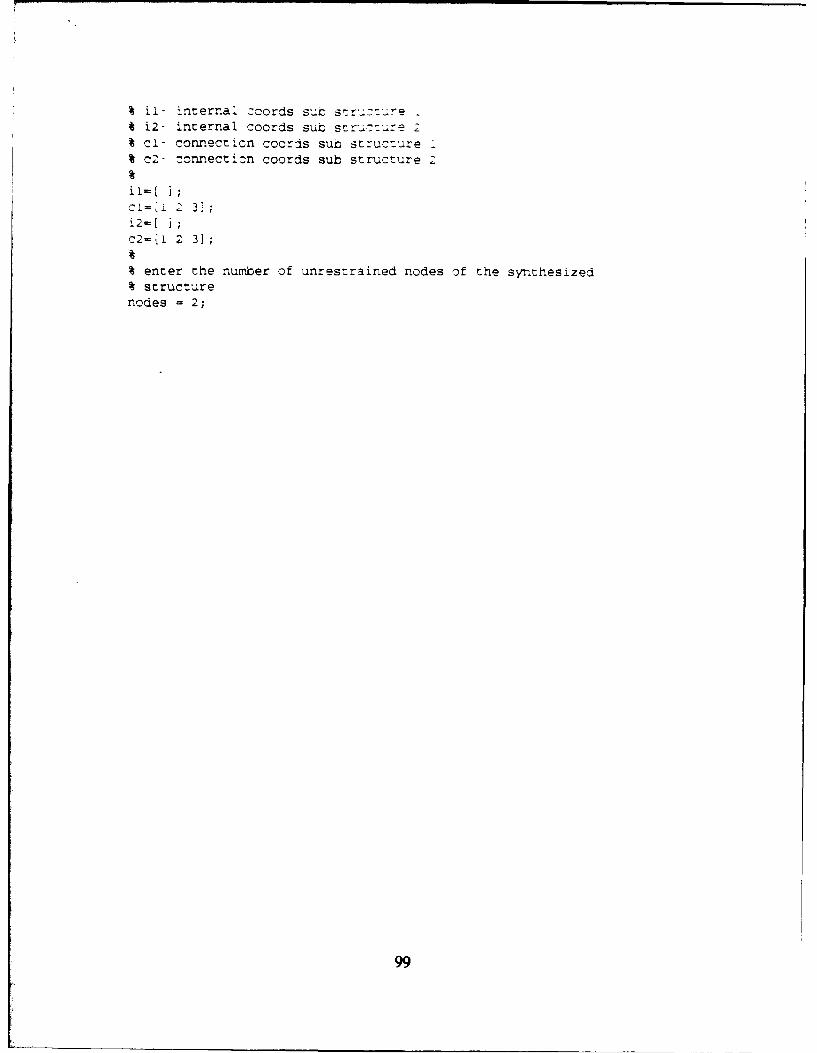
% ii- internal coords sur str-z--re* i2- internal coords sub struc-ure 2% ci- connecticn coords sub structure I% c2- 7onnecticn coords sub structure 2

cI-.i 2 3i2=[ i;

c2-t'i 2 3];

% enter the number of unrestrained nodes of the synthesized% structurenodes = 2;

99

APPENDIX B MATLAB CODE FOR EXAMPLE TWO

clear;cig;

unif ineell

% This program will calculate the eigenvalues, eigenveccors% natural frequencies, and frequency response function matrix% for a three degree of freedom at each node element.% The system is modeled with beam elements that are% aligned in the same plane but at any angle (2-D)

% This program works for a beam element modeled with six general% coordinates and thus six DOF.

% The user must enter the following data to meet the beam configuration.% (E) youngs modulus psi% (I) area moment of inertia in^4% (WTD) weight density lbf/in'3% (A) cross sectional area in^2% conductivity ( the node connection mapping% node coordinates [ cartesian coordinates for each node ]% (bb) proportional damping constant% call the data fileminihull data2AI

% Start the program clock and flops to determine program running% time and floating point calculations.tO-clock;flops(O);I

I calculate the number of beam elementsa-size (con);numel-a(l);I

% calculate the number of beam elements porportionally dampedaa-size(dcon);numel_damp-aa(l);

100

% alculate the number :ýf nodesb-size kcoord);rnodes-t~l);

%convert the coordinates in to the zorrect 1r.-:-:s 4r.

coord=ccord*L72;

% calculate the beam element lengths and beam angles in radiansfor i=!:numel

ID-conti, 2);Pii,i)=sqrt((coord)ID,Jj-coord(IC,I)12'+(coordý'ID,2)-coord(ICý,2.,' ,DX(i)=coord(ID,I)-coord(IC,I);DY(i)=coord)ID,2)-coord&IC,2);

if DX(i)>=O & DY(i)>-O;

elseif DX(iY(O & DY(il>=O;t(1,i)=acos(DY(i,/1(1,i))+pi/2;

elseif DX(i)<O & DY(i)(=O;t(I,i,=acos(abs(DX(i))/l(l,i) )*pi;

elset(l,i)=acos(abs(DY(i))/l(1,i))+(3*pi/2);

end;end;

t call trig function[c,s]=ftrig(t,numel);

%calculate radius of gyrationfor il1:nunmelr(l,i)=sqrt(I(i)/A(i));end;

% create the global matrix which is all zeroes

kg=fzeros(nodes*3,nodes*3)];

mg-[zeros(nodes*3,nodes*3)];

%assembel the elemental matricies to the global matrix

for i-1:numel[kel.,mel]-felement6(l(i) ,WTD(i) ,I(i) ,E(i) ,A(i) ,r(i) ,c(i) ,s(i))

v-con(i,l);w-con(i,2);

kg(3*v-2:3*v,3*v-2:3*v) - kg(3*v-2:3*v,3*v-2:3*v) +kel(l:3,l:3);kg(3*v-2:3*v,3*w-2:3*w) - kg(3*v-2:3*v,3*w-2:3*w) + kel(l:3,4:6);kg(3*w-2:3*w,3*v-2:3*v) -kg(3*w-2:3*w,3*v-2:3*v) +kel(4:6,l:3);kg(3*w-2:3*w,3*W-2:3*w) - kg(3*W-2:3*w,3*w-2:3*w) + kel(4:6,4:6);

101

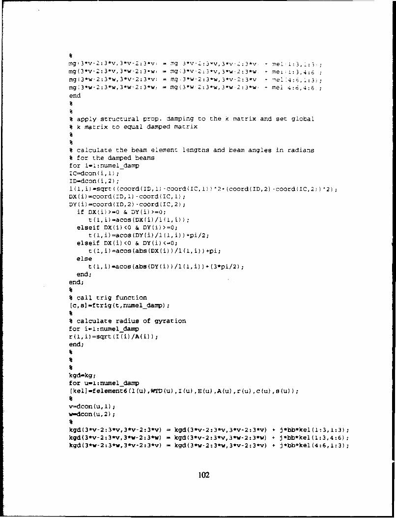
mg '3*v-2:3 v, 3*v- 2: 3*v; = T' 3 *v-2:3 71v, 3*v- 3 *v - mell:3,::3,mg(3*v-Z:3*v,3*w-2:3-w) = m9g3*v-2:3*v,3*w-2:3*w, - mei i:3,4:6;mg(3*w-2:3*w,3*v-2:3*v; = mg.3*w-2:3*w,3*v-2:3*v,-Ml:613ýmgA3*W-Z:3*w,3*w-2:3*w, = mgk3*w-Z:3*w,3*w-2:3*w,, mel 4:6,4:6,;end

% app:ly structural prop. damping to the k matrix and set globalt k matrix to equal damped matrix

% calculate the beam element lengths and beam angles in radians% for the damped beamsfor i=!:numei dampIC=dcon( i, 1) 1ID=dcon(i,2);l(l,i)=sqrt((coord(ID,l)-coord(IC,l)V^2+(coord(ID,2)-coord(IC,2,))2);DX(i)=coord(ID, I) -coord(IC, I);DY(i)=coord(ID,2)-coord(IC,2);

if DX(i)>=O & DY(i))=O;t(1,i)=acos(DX(i)/l(l,i));

elseif DX(i)(O & DY(i)>=O;t(l,i)=acos(DY(i)/l(i,i))+Pi/2;

elseif DX(i)<O & DY(i)<=O;t(l,i)=acos(abs(DX(i))/l(l,i))+pi;

elset(l,i)=acos(abs(DY(i))/1(i,i))+(3*pi/2);

end;end;

% call trig function[c,s]-ftrig(t,numel-damp);

% calculate radius of gyrationfor i-i:nuxnel_dampr(l, i)=sqrt (I(i) /A(i))end;

kgd-kg;for u-l:numel-damp(kel]=felement6(l(u) ,WTD(u) ,I(u) ,E(u) ,A(u) ,r(u) ,c(u) ,s(u))

v-dcon (u,1);w-dcon (u, 2);

kgd(3*v-2:3*v,3*v-2:3*v) - kgd(3*v-2:3*v,3*v-2:3*v) + j*bb*kel(l:3,.1:3);Jcgd(3*v-2:3*v,3*w-2:3*w) - kgd(3*v-2:3*v,3*w-2:3*w) + j*bb*kel(l:3,4:6);kgd(3*w-2:3*w,3*v-2:3*v) - kgd(3*w-2:3*W,3*V-2:3*v) + j*bb*kel(4:6,1:3);

102

kgcd3*w-2:3*w,3*w-2:3*w. = kgd 3*w-2:3*w, 3*w-2:3*w; ÷ bz*<ei 4:.,): ;Wend

% apply the boundary zcnditions% the user must adjust the global matrix to meet the boundary conditions

% to delete r~wskg([BCI,:) = H;kgdiiBC ,:) [;mg( (BCI , :) = "I% to delete columnskg(:,[BC] • =kgd(:,[BC]) I[;mg(:, [BCI) = ;

% call the function and calculate eigenvectors and the eigenvalues% which are the mode shapes and undamped natural frequency in%(rad/sec) 2

ilambda,phi]-fgmodes(kg,mg);% convert the eigenvalues to nat frequency in (rad/sec) and% and hertz(i/sec)

omega = sqrt(lambda);freq = omega/(2*pi);

% construct the frequency response plot over the frequencies% of interestcouxit=0;for Comega-.l:.1:22count-count+ 1;Z-kgd-Comega 2*mg;H=inv(Z);

% determines the coordinate of intrest to plotHH (count) -H (8,8) ;end;% end the program clock and flopsetime(clock,tO),flopsComega-.l: .1:22;Freq=Comega/(2*pi);plot(Freq,20*log(HH)) ,gridxlabel( Frequency Hz ')ylabel('FRF at coordinate of interest dB ,)

%END

minihull data2A

103

% This is the data for :he finite element program w,;nr -- ree% degrees of freedom at a node.

% The data wi2.1 be in the form ofS(E, youngs modulus psi

(- I) area moment of inertia inf4- (WTD) weight density lbf/in^3- (A) cross sectional area in^2- conductivity [ the node connection mapping- node coordinates [ cartesian coords for each node in ft. ]

the main program will convert to in..- (bb) structural proportional damping constant

E=[30 30 30 30 30 30 30 30 30 30 30 30 30 30 30 30 30 301*Ie6;I=[.02083 .02083 .02083 .02083 .02083 .02083 .02083 .02083 .02083 .02083.02083 .02083 .02083 .02083 .02083 .02083 .02083 .020831 ;%1/i2bh'3 b=2,h=. 5A=[I I I I I I 1 I 1 I i I 1 1 1 1 1 ];WTD=[.2832 .2832 .2832 .2832 .2832 .2832 .2832 .2832 .2832 .2832 .2832.2832 .2832 .2832 .2832 .2832 .2832 .2832];bbO0.01;con= [1,2;

2,3;3,4;4,5;5,6;6,7;7,8;8,9;9, 10;10,11;11,12;12, 1;11,13;13,14;14, 15;15,5;13,12;15,4];

% this determines what elements have dampingdcon= [1,2;

2,3;3,4;4,5;5,6;6,7;7,8;8,9;

104

9, 10;10, 11;1!, 12;12, 1;11, 13;13, 14;!4, 15;

15,5;13, 12;

15,4i

coord= [4, 0;8,0;12, 0;16,4;16,8;16, 12;12, 16;8, 16;4, 16;0,12;0,8;0,4;4,8;8,8;12,8];

BC=[ ];

inner struc2A

% This is the data for the finite element program with three% degrees of freedom at a node.

-(I.----------I)

% The data will be in the form oft - (E) youngs modulus psi% - (I) area moment of inertia in^4

- (WTD) weight density lbf/in'3- (A) cross sectional area in^2- conductivity [ the node connection mapping- node coordinates [ cartesian coords for each node in ft. I

the main program will convert to in..- (bb) structural proportional damping constant

E-,[30 30 30 30 30 30]*1e6;I-( .02083 .02083 .02083 .02083 .02083 .02083] ;%1/12bh^3 b-2, h=.5A-( 1 1 1 1 1 1];

WTD-f .2832 .2832 .2832 .2832 .2832 .2832] ;

105

bb=0.0 1;con- 1 1, 2;

2,3;3,4;4,5;2,6;4,7]

% this determines what elements have dampingdcon= [1, 2;

2,3;

3,4;4,5;2,6;4,7];

coord= [0,4;4,4;8,4;12,4;16,4;0,0;16,01;

BC=( 1;

out struc2A%%% This is the data for the finite element program with three% degrees of freedom at a node.%

S (I----------I)

I the data will be in the form of- (E) youngs modulus psi- (I) area moment of inertia in^4

I - (WTD) weight density lbf/in'3I - (A) cross sectional area in^2

- conductivity ( the node connection mapping- node coordinates ( cartesian coords for each node in ft. I

% the main program will convert to in..- (bb) structural proportional damping constant

E-(30 30 30 30 30 30 30 30 30 30 30 301*1e6;I-[ .02083 .02083 .02083 .02083 .02083 .02083 .02083 .02083 .02083.02083 .02083 .02083] ;%1/12bh*3 b-2, h=.5A-[ 1 1 1 1 1 1 1 1 1 1 1 1];WTD-[.2832 .2832 .2832 .2832 .2832 .2832 .2832 .2832 .2832 .2832 .2832.2832] ;

bb-0.o1;

106

I

2,3;3,4;4.5;5,6;-. 7;7,

8,9;9, 10;

j12, I: ;

% this determines what elements have dampingdcon= ! -, 2;

,2.,3;

3,4;4,5;5,6;

6,7;8,9;9,10;10, It;11,12;12,1];

coord=[4, 0;8,0;12,0;16,4;16,8;16,12;12,16;8,16;4,16;0,12;0,8;0,4];

BC=[ ];

clearclg

FRFSynth2A

% This is example 2, dynamic direct coupling using the boolean% mapping matrix to synthesize two structures together.

% Load data from running unifineel program for each substructure% where the K and M matrix for each structure is saved

107

load ex2Aa.mat % kI mi is storedeload ex2Ab.mat % k2 m2 is stored here

% we need to create a single FRF matrix representing% both substructures in the form:

%heel = h(i,i) h(i,ch~c,i) h~c,c) I

% So we create arrays containing the DOF numbers of our original% models which correspond the the Oc" and OiO coordinates for% each substructure.

% Call the synthesis data file which contains the% internal coordinates and connection coordinates for each substructure.

%i= internal coords of sub structure I% i2- internal coords of sub structure 2% cl= connection coords of sub structure i% c2= connection coords of sub structure 2

FRFSynth_data2A

to=clock;flops(O);counts0;for Comega=.I:.3:60count couflt + 1;

Form Frequency Response Models for Each Substructure

zi-ki -Comega^2*ml;z2-k2-Comega^2*m2;hl-inv(zl);h2-inv(z2);

a=size(il);b-size (cl);c-size(i2);d-size(c2);

aa-a(2);bb-b(2);cc-c(2);dd-d(2);

% Remember, we are trying to calculate the following:

% hee* - hee hec* M * inv( hccr) *M' *hce% hccr M' *hcc* M

108

% So we need to assemble knfee:ý , '.Hecý I~ an'd -r:. s r~e% the coordinate sets we just defined.% These matrices contain the FIRF data for both substructures% prior to coupling, i.e the pre-synthesis FFRF data.

I 'ooriinate Partitioni~ng-- - - - - - - - - - -

% Build up uncoupled FRF matrix and sub-partitions:

hee = hi~il,il) zeros~aa,cc! hl~il,cl) zeros(aa,dd);zeros(oc,aa) h2(i2,i2) zeros~cc,bbi h2(i2,c2,;

hL~l~l) zeros(bb,cc) hl(cl,cij zeros~bb,ddj;zeros(dd,aa) h2(c2,i2) zeros(dd,bb) h2I(c2,c2)J;

hoc = hl(4il,cl) zeros(aa,dd);zeros~cc,bb) h2(i2,c2l;hli~c,cfl zeros(bb,dd);zeros(dd,bb) h2(c2,c2)];

hcc = hl(cl,cl) zeros(bb,dd);zeros(dd,bb) h2(c2,c2)];

hce = hl(cl..il) zeros(bb,cc) hi(cl~cl) zeros(bb,dd);zeros(dd,aa) h2(c2,i2) zeros(dd,bb) h2(c2,c2)];

W we can nov perform the synthesis:hccr-M' hcc *M;

heestar -hoe hoc * M * inv( hccr ) M* hce;

Iremove the redundent informationheestar =heestar(l:nodes*3,l:nodes*3);Ilook at the coordinate of interest

HH (count) -heestar (8, 8) ;end;etime(clock~tO) ,flopsComega-.l: .3:60;Freg-Comega! (2*pi);plot (Freq,20*logCHH)) ,gridxlabel(, Frequency Hz 1)ylabel('FRF at coordinate of interest dB')

I FRFSynth-data2AIThis is the data file for the synthesis program.

109

W The following data will be provided Cy -his fi'e.

% il- internal coords sub structure I% i2- internal coords sub structure 2% ci- connection coords sub structure 2% c2- connection coords sub structure 2

iI=ri 2 3 4 5 6 7 8 9 16 17 18 19 20 21 22 23 24 25 26 27 28 29 30!;

C-1(10 11 12 13 14 15 31 32 33 34 35 36];i2=[4 5 6 7 8 9 10 11 12];c2-(1 2 3 13 14 15 16 17 18 19 20 21];

% The following is the mapping matrix.% The mapping matrix is not general and is% case specific.

M=[eye(12);0 0 0 0 0 0 -1 0 0 0 0 0;0 0 0 0 0 0 0 -1 0 0 0 0;0 0 0 0 0 0 0 0 -1 0 0 0;0 0 0 -1 0 0 0 0 0 0 0 0;0 0 0 0 -1 0 0 0 0 0 0 0;0 0 0 0 0 -1 0 0 0 0 0 0;0 0 0 0 0 0 0 0 0 -1 0 0;0 0 0 0 0 0 0 0 0 0 -1 0;o 0 0 0 0 0 0 0 0 0 0 -1;-1 0 0 0 0 0 0 0 0 0 0 0;0 -1 0 0 0 0 0 0 0 0 0 0;0 0 -1 0 0 0 0 0 0 0 0 0];

% Enter the number of unrestrained nodes of the synthesized% structure.nodes - 15;

110

APPENDIX C MATI.AB CODE FOR EXAMPLE THREE

clearclg

unifineei

% This program will calculate the eigenvalues,eigenvectors% natural frequencies, and frequency response function matrix% for a three degree of freedom at each node element.% The system is modeled with beam elements that are% aligned in the same plane but at any angle (2-D).

%I I

% This program works for a beam element modeled with six general% coordinates and thus six DOF.

% the user must enter the following data to meet the beam configurationI (E) youngs modulus psi

M (I) area moment of inertia in^4I (WTD) weight density lbf/in^3I (A) cross sectional area in^2% conductivity [ the node ccnnection mapping ]% node coordinates [ cartesian coordinates for each node I% (bb) proportional damping constantalear;% call the data fileminihull data31% start the program clock and flops to determine program running% time and floating point calculationsto-clock;flops(O);I% calculate the number of beam elementsa-size(con);numel-a(l);II calculate the number of beam elements porportionally dampedaa-size(dcon);

ill

riumel_damp=aaKI

%calculate the number of ncies.b-size (coord);nodes-b~ I ;

W ccnvert rtoe coordinates in to the correct uni-s ýin.ýcoord-ccoord*-';

% calculate the beam element lengths and beam angl.es in radiansfor i-i:numelIC-con(i,l);ID-Con'i.2);l(l,i,=-sqrt((coord(ID,l)-coord(IC,I)V24ý-(coord(ID,2)-coord('ICý,2ý))v);DX(i)-coord(ID,l)-coord(IC,l);DY~i)-coord(ID,2V-coord(IC,2);

if DX(i)>0O & DY(i)>s0;t(1,i4)=acos(DX(i)/l(1,i));

elseif DX(i)<O & DY(i)>0O;t(l,i)=acos(DY(i)/l(1,i) )+pi/2ý;

elseif DX(i)<Q & DY(i)<u'O;t(l,i)=acos(abs(DX(i))/l(l,i))+pi;

elset(1,i)=acos(abs(DY(i))/l(l,i))+(3*pi/2);

end;end;

% call trig function[c,s]-ftrig(t,numel);

%calculate radius of gyrationfor i-1:nuxnelr(I,i)=sQrt(I(i)/A(i));end;

%create the global matrix which is all zeroes.

kg=(zeros(nodes*3,nodes*3)];

mg- (zeros (nodes*3,nodes*3) 1;

%assembel the elemental matricaies to the global matrix.

f or iml:numel[kel~melI-felement6(l(i) ,WrD(i),I(i) ,E(i) ,A(i) ,r(i) ,c(i) ,s(i))

v-con (i,.1);wm-con(i,2);

kg(3*v-2:3*v,3*v-2:3*v) - kg(3*v-2:3*v,3*v-2:3*v) + kel(1:3,l:3);kg(3*v.2:3*v,3*w-2:3*w) - kg(3*v-2:3*v,3*w-2:3*w) +kel(1:3,4:6);kg(3*v-2:3*w,3*v-2:3*v) - kg(3*w-2:3*w,3*v-2:3*v) + kel(4:6,1:3);

112

k9;3*w-2:3*W,3*w-2:3*w) -kg 3*w-2:3*w,3*w-Z:3*w -ke! 4:6,4:6

mg13*v-2:3*V,3*V-2:3*v = rngý3*v-2:3*v,3*v-Z:3*v ml-:,:mg,,3*v-.':3*V,3*W-2:3*w) -=mg(3*v-2:3*v,3*w-2:3*w rne~l1:3,4:6,;mg:3*w-2:3*w,3*v-2.:3*v.- mg(3*w-2:3*w,3*v-2:3*vý mel,4:6,i:3!;mgt3*W-Z:3*W,3*W-2:3*wJ -=mg(3*w-2:3*w,3*w-2:3*w) meik4:6,4:6);end

% apply structural prop. damping to the k matrix and set global-% matrix to equal damped matrix

% calculate the beam element lengths and beam angles in radians% for the damped beamsfor i-l:nuxnel-damp

DCdcon(i,2);

DXki)coord(ID,1)-coord(IC,I);DY~i)=coord(ID,2) -coord(IC,2);

if DX(i)>0O & DY(i)>0O;t(1,i)-acos(DX(i)/l(1,i));

elseif DX(i)<O & DY(i)>0O;

elseif DX(i) <0 & DY(i)<=0;

elset(i.,i)-acos(abs(DY(i))/1(1,i))+(3*pi/2);

end;end;

% call trig function[c,s]-ftrig(t,nuxnel_damp);

%calculate radius of gyrationfor P.'l:numel_dampr(l,i)=sqrt(I(i)/A(i))end;

kgd-kg;for u-l:numel_damp[kel]=felement6(l(u) ,WTD(u) ,I(u) ,E(u) ,A(u) ,r(u) ,c(u) ,s(u))

v-dcon(u,l);w-dcon(u,2);

kgd(3*v-2:3*v,3*v-2:3*v) - kgd(3*v-2:3*V,.3*V-2:3*v) +j*bb*kel(1:3,i:3);Jcgd(3*v-2:3*v,3*w-2:3*w) - kgd(3*v-2:3*v,3*w-2:3*w) + J*bb*kel(l:3,4:6);

113

kgd(3*W-2:3*w,3*v-2;3*v, = kg,-*-:*w *-:*kgd(3-w-2:3*w,3*w-2:3*w; kgQ.3*w-2:3*w, 3*w-2:3*w - 4*bzwkel41,:

end

% apply the initial conditions% the user must adjust --he global matrix to meet the iri.itai zcnditic.4ns

%to delete rowskg( [BC],:) - [ 1;kgd ( BCJ., = 2mg( LBCJ , :) ;% to delete columnskg(:, (BC]) 1

kgd (:, ¶BC]) I ;mg(:,EBC]) = 1;

% call the function and calculate eigenvectors and the eigenvalluesW which are the mode shapes and u~ndamnped natural freq'.xency in(rad/sec)^2

(larnbda,phi]=fgmodes(kg,mg);%this now converts the eigenvalues to nat frequency in (rad/sec) and%hertz(i/sec)

omega - scqrt(lambda);freq - omega/(2*pi);

% constuct the frequency response plot over the frequencies% of interestcount =0;for Comega-.l:.3:40count-count '1.;Z-kgd -Comega 2 *mg;H-inv(Z);

%this determines the coordinate of intrest to plotHH (count)-H (14, 14);end;% end the program clock and flopsetime(clock,tO) ,flopsComega=.l: .3:40;Freq=pComega/(2*pi);plot (Freq,20*log(HH)) ,gridxlabel(' Frequency Hz ')ylabel('FRF at coordinate of interest dB')% EN

minihull-data3

114

% This is the data file for example 3

% The data will be in the fzrm Af- (E) youngs modulus psi

n,- area moment of inertia in*4- (WTD) weight density lbf/inO2- A cross sectional area in'2- conductivity j the node connection mapping% node coordinates : cartesian coords for each node in ft.

the main program will convert :c in..% bb) structural proportional damping constant

E=1 30 30 30 30 30 30 30 30 30 30 30 30 30 30 30 30 30]*.e6;I=( .02083 .02083 .02083 .02083 .02083 .02083 .02083 .A2083 .02083.02083 .02083 .02083 .02083 .02083 .02083 .02083 .02083] ;%1/12bh^3 b=2,h=.5A=( I I i I 1 1 1 1 1 1 1 1 1 1 1 1 11;WTD-( .2832 .2832 .2832 .2832 .2832 .2832 .2832 .2832 .2832 .2832 .2832.2832 .2832 .2832 .2832 .2832 .2832];bb-0.01;con=[i,2;

2,3;3,4;4,5;5,6;6,7;7,8;8,9;9,10;10,11;11,12;12,1;11,13;13,14;14,15;15,5;13,121;

% this deteremines what elements have dampingdcon [1,2;

2,3;3,4;4,5;5,6;6,7;7,8;8,9;9,10;10,11;11,12;12,1;11,13;

115

13, 14;14, 15;15, 5;I-- , 12]

coord= [4, 0;6,0;

16,4;16, 8;16, 12;12,1.6;8, 16;4, 16;0, 12;0,8;0,4;4,8;8,8;12,8];

BC=[];

hull mod3

% This is the data file for the beam modification.

% The data will be in the form of- (E) youngs modulus psi- (I) area moment of inertia in'4- (WrD) weight density lbf/in^3- (A) cross sectional area in^2- conductivity [ the node connection mapping I- node coordinates [ cartesian coords for each node in ft.

the main program will convert to in..- (bb) structural proportional damping constant

E-[30 ] *le6;

I--.02083 1;A--l ];WTID-[.2832]bb-0.01;con- (1, 2] ;% this determines what elements have dampingdcon-[, 2];

coord-[4,0;0,41;

116

BC=['

red mod3

% This is :he data file for the main sutscructure.

W The data will be in the form of% - (E) youngs modulus psi% - (I) area moment of inertia in^4% - (WTD) weight density lbf/in'3W - W cross sectional area in^2% conductivity [ the node connection mapping% - node coordinates [ cartesian coords for each node in ft.% the main program will convert to in..% - (bb) structural proportional damping constant%

E=[30 30 30 30 30 30 30 30 30 30 30 30 30 30 30 30 30 30]*1e6;I=[.02083 .02083 .02083 .02083 .02083 .02083 .02083 .02083 .02083 .02083.02083 .02083 .02083 .02083 .02083 .02083 .02083 .020831 ;%1/12bh°3 b=2,h-.5

A=[ I I 1 1 11 i 1 I I i 1 I I 1 11 1];WTD-I.2832 .2832 .2832 .2832 .2832 .2832 .2832 .2832 .2832 .2832 .2832.2832 .2832 .2832 .2832 .2832 .2832 .28321;bbO. 01;

con- [1,2;2,3;3,4;4,5;5,6;6,7;7,8;8,9;9,10;10,11;11,12;12,1;11,13;13,14;14,15;15,5;13,12;15,41;

% this determines what elements have dampingdcon [1,2;

2,3;3,4;4,5;5,6;

117

L --.- ....- - ~ mm m m l nnm mm s

6,7;7,8;

8,9;9, !0;10 U1;11, 12;

U, .3;

13, 14;14, 15;15, 5;13, 12;15,4];

coord= [4, 0;8,0;12, 0;16, 4;16,8;16, 12;12, 16;8,16;4, 16;0,12;0,8;0,4;

4,8;8,8;12, 81;

BC=[];

% This program will modify a substructure by removing a beam% element from the structure.

% program FRFMOD3clear;clg;load ex3a.mat % kl, ml are stored hereload ex3b.mat % k2, m2 are stored here% call the data fileMOD DAT3

% we need to partion the H matrix of the structure to be* modified in the following way*

L [ii I ic]

* [ci Icc]

118

r-tee' = ic

7hel= icccl

to=ciock;f lops ý3

for Comega=.!:.3:40count =ccun~t~zi-ki -Comega^2*Ml;z-k2-Comega^2*m2';h=inv~zi);

hee = [h(ic,ic) hiic,cc);bicc,ic) hicc,cc)j;

hec - [h(ic,cc);

h (cc, cc)];

hcc - [h(cc.~cc)];

hce = [h~cc,ic) h(cc,cc)];

%this is for adding a component

%heestar -hee - hec * inv(inv(z) + hcc) *hce;

% this is for removing a componentheestar - hee - hec * inv(hcc - inv(z)) *hce;

HH(count)-heestar(ll,ll);end;etime(clock,tO) ,flopsComega=.l: .3:40;Freq=-Comega/ (2*pi);plot(Freq,20*log(HH)) ,gridxlabel(' Frequency Hz ')

ylabel(IFRF at coordinate of interest dB 1)

MODDAT3

%This is the data file for the modification program,%the following data will be provided by this file

%ic- internal coords of synthesized structuret cc- connection coords of synthesized structure

119

ic=L[1 2 3 4 5 6 7 8 9 13 14 15 L6 17 i6 19 20 21 22 23 24 25 2E 27 2Z 8.30 31 32 33 34 35 36 37 38 39 40 41 42

ccf[10 11 12 43 44 45];

120

APPENI)IX D MATLAB CODE FOR EXAMPLE FOUR

clearclg

unif ineell

% This program will calcuiate the eigenvalues, eigenvectors% natural frequencies, and frequency response function matrix% for a three degree of freedom at each node element.% The system is modeled with beam elements that are% aligned in the same plane but at any angle (2-D).

%I I

% This program works for a beam element modeled with six general% coordinates and thus six DOF.

(I------- 0-I)

% the user must enter the following data to meet the beam configuration% (E) youngs modulus psi% (M) area moment of inertia in^4% (WrD) weight density lbf/in^3% (A) cross sectional area in^2% conductivity [ the node connection mapping ]% node coordinates ( cartesian coordinates for each node ]% (bb) proportional damping constantclear;% call the data fileminihull data4

% start the program clock and flops to determine program running% time and floating point calculationsto-clock;flops(0);

% calculate the number of beam elementsa-size (con);numel-a(l);

% calculate the number of beam elements porportionally dampedaa-size(dcon);

121

numel!-damp-aaý;

% calculate the number of nodes.b-size (coord);nodes-b (1);

W convert ::he ::zýrdinates in to the correct units 'in.,coord=czord*!12;

%now calculate the beam element lengths and beam angles in radiansfor il1:numelIC-con (i, 1);ID-con(i,2);l(l,i)=sqrt((coord(ID,l)-coord(IC,l))'2+(coord(lD,2)-coord(IC,2,j2);DX(i)=coord(ID,l)-coord(IC,1);DY(i)-cz_-ord(ID,2)-coord(IC,2);

ifsJ~ DXi>=O & DY(i)>0O;

c(l,i)-acos(DY(i)/1(l,i))+pi/2;elseif Dx(i)<O & DY(i)<0O;

t(l,i)-acos(abs(DX(i))/1(1,i))+pi;else

end; aosasD~))11i)+3p/)end;

%call trig function(c,s]-ftrig(t,numel);

%calculate radius of gyrationfor i-l:nuxnel

end;

%create the global matrix which is all zeroes.

kg=(zeros(nodes*3,nodes*3) j;mgmCzeros(nodes*3,nodes*3)];

%assenibel the elemental matricies to the global matrix.

f or i-'l:numel[kel,mel]-felement6(l(i) ,WI'(i) 1(i) ,E(i) ,A(i) ,r(i) ,c(i) ,s(i))

v-con (i, 1);v-con (i, 2);

kg(3*v-2:3*v,3*v-2:3*v) = kg(3*v-2:3*v,3*v-2:3*v) + kel(l:3,l:3);Icg(3*v-2:3*v,3*w-2:3*w) - kg(3*v-2:3*v,3*w-2:3*w) + Jcel(l:3,4:6);kgC3*w-2:3*v,3*v-2:3*v) - kg(3*w-2:3*v,3*v-2:3*v) + kel(4:6,I:3);

122

kg3*-&:3w,*wZ:*w =kg,3*w2:3*w,3-*w-2:3*w ~i4~ :

,,,gýý3*V-2:3*v,3*v-2:3*v- mgk3*v-2:3*v, 3*vlZ:3*v, ~melý1:3i:3);mg13*v-2~:3*v,3*w-2:3*w) -rngt3*v-2:3*v,3*w-Z:3*w) meliJ:3,4:E';mg,3*w-2:3*w,3*v-2:3*vI - mg(3*w-Z:3*W,3*v-2:3*v me'L(4:6,1:3u;mgt3*w-2:3*w,3*w-2:3*w) - mg(3*w-&':3*w,3*w-&2:3*w; +melA4:6,4:6);end

% apply structural prop. damping to the k matri4x and set global-% k matrix to equal damped matr-ix

% calculate the beam element lengths and beam angles in radians% for the damped beamsfor i'i:numel dampIC-dcon~i,U;;ID-dcofl(i,2);l(l,i)-sqrt((coord(ID,l)-coordC4I-,.V2^&+'coord(ID,2ý)-coord(IC,21;'*2);DX(i)-coord(ID,i)-cocrd(IC,l);DY(i)-coord(ID,2)-coord(IC-,2ý);

if DX(i)>-O & DY(i)>=O;

elsif Xi)<ao & DY(i)/l-Oi);

elseif DX(i)<O & DY(i)<..O;

elset(l,i)-acos(abs(DY(i))/l(1,i))+(3*pi/2);

end;end;

% call trig function[c,s1-ftrig(t,nuniel_damp);

% calculate radius of gyrationfor i-i:nurnel dampr(l, i)-sqrt (I(i) /A(i))end;

kgd-kg;for u'-I:numel damp[kell-feiement6(l(u) ,WrD(u) ,I(u) ,E(u) ,A(u) ,r(u) ,c(u) ,s(u))

v-dcon(u,L);w-dcon(u,2);

1cgd(3*v-2:3*v,3*v-2:3*v) -kgd(3*v-2:3*v,3*v-2:3*v) + j*bb*kel(i:3,i:3);kgd(3*v-2:3*v,3*w-2:3*w) kgd(3*v-2:3*V,3*w-2:3*w) +j*bb*kel(1:3,4:6);Jcgd(3*w-2:3*w,3*v-2:3*v) kgd(3*w-2:3*w,3*v-2:3*v) + j*bb*kel(4:6,i:3);kgd(3*w-2:3*w,3*w-2:3*w) -kgd(3*w-2:3*w,3*w-2:3*w) + j*bb*kel(4:6,4:6);

end

123

% apply the boundary conditizns% the user must adjust the global matrix to meet the boundary conrditiJons

% to delete rowskg([ BC],:) = ;kgdF %BC , :=mgt[BCi ,:% to delete columnskg(:,[BCI' - ();kgd(:,(BC]) = H;Mg(:, (BC] ) - ];

% call the function and calculate eigenvectors and the eigenvalues% which are the mode shapes and undamped natural frequency in% (rad/sec)^2

[lambda,phi]-fgmodes(kg,mg);% this now converts the eigenvalues to nat frequency in (rad/sec) and% hertz(l/sec)

omega = sqrt(lambda);freq : omega/(2*pi);

% constuct the frequency response plot over the frequencies% of interestcount-0;for Comega-.l:.3:53count-count. ÷1;Z-kgd- Comega 2*mg;H-inv(Z);

% this determines the coordinate of intrest to plotHH (count)-H (8,8);end;% end the program clock and flopsetime(clock,tO),flopsComega=.l:.3:53;Freq-Comeqa/(2*pi);plot(Freq,20*log(HH)) ,gridxlabel(' Frequency Hz ')

ylabel('FRF at coordinate of interest dR')% end

minihull data4

% This is the data file for the finite element program.

% the data will be in the form of

124

% (E) youngs modulus psi% (I) area moment of inertia in^4% WA) cross sectional area in^2% conductivity [ the node connection mapping I% node coordinates [ cartesian coordinates for each node% (bb) proportional damping constant

E=f30 30 30 30 30 30 30 30 30 30 30 30 30 30 30 30 30 301*Ie6;I-[.02083 .02083 .02083 .02083 .02083 .02083 .02083 .02083 .02083 .02083.02083 .02083 .02083 .02083 .02083 .02083 .02083 .020831 ;%1/!2bh^3 b=2,h-. 5A-[I 1i 1 1 1 1 1 1 1 1 1 1 i 1 1 1 1 1;WTD-[.2832 .2832 .2832 .2832 .2832 .2832 .2832 .2832 .2832 .2832 .2832.2832 .2832 .2832 .2832 .2832 .2832 .2832];bb-0.01;con- [1,2;

2,3;3,4;4,5;5,6;6,7;7,8;8,9;9,10;10,11;11,12;12,1;11, 13;13,14;14,15;15,5;13, 12;15,4] ;

% this determines what elements have dampingdcon- [1,2;

2,3;3,4;4,5;5,6;6,7;7,8;8,9;9,10;10,11;11,12;12,1;11,13;13,14;14,15;15,5;13,12;

125

15,4] ;

coord- [4,0;8,0;12,0;16,4;16, 8;12, 16;12,16;8,16;

4, 16;0,12;0,8;0,4;4,8;8,8;12,8];

BC=]

hul l-mod4

% This is the data file for the finite element program.% This is the data for the modification

% the data will be in the form of% (E) youngs modulus psi% (I) area moment of inertia in'4% (A) cross sectional area in*2% conductivity [ the node connection mapping% node coordinates [ cartesian coordinates for each node I% (bb) proportional damping constantE-[30 ]*le6;I-[.02083 ];A--[I 1;WTD-[.2832];bb-O.01;con- [ 1, 2] ;% this determines what elements have dampingdcon- [1,21;

coord- [4,0;0,4];

BC- (1;

redmod4

% This is the data file for the main structure to be modified.

126

% the data will be in the form of% (E) youngs modulus psi% W area moment of inertia in^4% (A) cross sectional area in^2% conductivity [ the node connection mapping I% ncde coordinates[ cartesian coordinates for each node% pbb rporticnal damping constant

E-! 30 30 30 30 30 30 30 30 30 30 30 30 30 30 30 30 30j*le6;I1- .02083 .02083 .02083 .02083 .02083 .02083 .02083 .02083 .02083.02083 .02083 .02083 .02083 .02083 .02083 .02083 .02083] ;%1/Q2bn'3 b=2,h-. 5A-! I I i 1! 1 1 1i i I I 1 1 1];

WTD-[ .2832 .2832 .2832 .2832 .2832 .2832 .2832 .2832 .2832 .2832 .2832.2832 .2832 .2832 .2832 .2832 .2832];bb-0.01;

con= [1, 2;2,3;

3,4;4,5;5,6;6,7;7,8;8,9;9,10;10,11;II, 12;12,1;11,13;13,14;14, 15;15,5;13, 12] ;

% this determines what elements have dampingdcon- [1,2;

2,3;3,4;4,5;5,6;6,7;7,8;8,9;9,10;10,11;11,12;12,1;11,13;13,14;14,15;

127

15,5;

13, 121

ccord= -4, 0;8,0;12, 0;'_6, 4;

16, 12;12, 16;8, 16;4, 16;0, 12;0,8;0,4;4,8;8,8;12,8];

BC=[;

clear;clg;

program FRFMOD4

% This program will modify a structure by adding a beam element.

load ex4a.mat % ki, ml are stored hereload ex4b.mat % k2, m2 are stored hereMODDAT4

% we need to partion the H matrix of the structure to be% modified in the following way

% [ ii I ic ]

% [ci I cc]

% (hee]= [ ii icci cc I

[hecl= (iccc]

[hcc] - [cc ]

to-clock;flops(O);count-O;

128

for Comega=.!:.3:53coulnt=count- i;zi-k1 - Comega 2*ml;z-k2-Comega'2*-m2;h-inv (zl)

hee = ihic,iz h~ic,=cz);

hec = (h~ic,cc ;h(cc,cc ];

hec = [h(cccc ];

hce = [h(cc,ic) h(cc,cc)];

% this is for adding a componentheestar = hee - hec * inv(inv(z) ÷ hcc) *hce;

% this is for removing a component%heestar = hee - hec * inv(hcc - inv(z)) * hce;

HH (count) =heestar (8,8);end;etime(clock,tO),flopsComega-. 1:.3:53;Freq=Comega/(2*pi);plot (Freq,20*log(HH)) ,gridxlabel (' Frequency Hz ')ylabel('FRF at coordinate of interest dB ')

% MODDAT4

% This is the data file for the synthesis program% the following data will be provided by this file

% ic- internal coords of synthesized structure

% cc- connection coords of synthesized structure

ic-[l 2 3 4 5 6 7 8 9 13 14 15 16 17 18 19 20 21 22 23 24 25 26 27 28 2930 31 32 33 34 35 36 37 38 39 40 41 42 1;cc[10 11 12 43 44 45];

% enter the number of unrestrained nodes of the synthesized% structurenodes - 15;

129

APPENDIX E MATLAB CODE FOR EXAMPLE FIVE

cLear;clg;

unif ineelsprdam

% This program will calculate the eigenvalues, eigenvectors% nAtural frequencies, and frequency response function matrix% for a three degree of freedom at each node element.% The system is modeled with beam elements that are% aligned in the same plane but at any angle (2-D).

% --- --% I I

%% I I

% This program works for a beam element modeled with six general% coordinates and thus six DOF.% H-.-------I)%% the user must enter the following data to meet the beam configuration% (E) youngs modulus psi% (I) area moment of inertia in*4% (WTD) weight density lbf/in^3% (A) cross sectional area in'2% conductivity [ the node connection mapping I% node coordinates ( cartesian coordinates for each node I% spring-damper conductivity% (bb) proportional damping constantI (B) viscous proportional damping constant% (k) spring constant%I call the data fileminihullsprdamda5

% start the program clock and flops to determine program running% time and floating point calculationst0-click;flops (0);

% calculate the number of beam elementsa-size (con) ;numel-a(l);

130

%cal~culate the number of bear, elements porportizrnaIl'y damped

aa-size(dcon);numel-damp=aa(l);

%calculate the number of nodes.b=size~lcoord)nodes-b(.w

%convert the coordinates in to the correct units :n.rcoord-coord* 12;

%calculate the beam element lengths and beam angles in radiansfor i1l:nuxnelIC=con(i,l);ID=con(i,2);1(1, i)=sqrt ((coord(ID, I) -coord(IC, I)) ý+ (coord(ID,2ý -coord(IC,2 ) '2);DX(i)=coord(ID,1) -coord(IC, I);DY(i)=coord(ID),2)-coord(IC,2ý);if DX(i)>=O & DY(i)>=O;

elsifDXi)<ao & DY(i)/l10);

els.if DX(i)<o & DY(i)<=O;

t(l,i')=-aczos(abs(DX(i))/l(l,i) )*pi;else

end; Ia,.,.)sasD~) 11i -3p/)end;

% call trig function[c,s]-ftrig(t,numel);

% calculate radius of gyrationfor i=i:numelr(l,i)-sqrt(I(i)/A(i));end;

% create the global matrix which is all zeroes.

kg-(zeros(nodes*3,nodes*3)];mg-E[zeros (nodes*3,nodes*3) 1;

%assemble the elemental matricies to the global matrix.

for i-1:nuznel[kel,mel]=felement6(l(i) ,WTD(i) ,I(i) ,E(i) ,A(i) ,r(i) ,c(i) ,s(i));

v-con (i,1);w-conl( i, 2);

131

kg,3*V-2:3*v,3*v-2:3*v = kg:3*v-Z:3*v,3*v-2:3*v.-'(? 3e,:I.: 3kg(3*v-2:3*v,3*w-4':3*w) = kgý3*V-2:3*v,3*w-Z:3*w) - e,:46kg(3*w-2:3*w,3*v-2:3*vi = kg,3*w-2:3*w,3*v-2:3*v' ke-A:6,i:3,;kg(3*w-2:3*w,3*w-2:3*wj = kg3W23w3w.13w kelA:6,4:6);

mg(3*v-2:3*v,3*v-2:3*v) = mg(3*v-2:3*v,3*v-2:3*v) -mel(L:3,I:3);mg(3*v-.2:3*v,3*w-2:3*w) = mg(3*v-2:3*v.J*w-2:3*w, + nel,1:3,4:6);mgk3*w-Z:3*w,3*v-Z:3*vý = rng!3*w-d:3*w,3*v-,:3*v) +melk4:6,1:3);mg(3*w-2:3*W,3*w-2:3*w) = mg(3*w-2:3*w,3*w-2:3*w) + mel(4:6,4:6);end

%This section will apply structural prop. damping to the k%matrix and set global k matrix to equal damped matrix

%calculate the beam element lengths and beam angles in radians%for the damped beams

for i=l:nuxnel-dampIC-dconu.. I);ID=dcon(i,2);

DX(ii)=sr(coord(ID,l)-coord(IC,i);-cod(D2-ordl,)^)DY(i)=coord(ID,2) -coord(IC,2);

if DX(i)>0O & DY(i)>0O;t(l,i)=acos(DX(i)/l(l,i));

elseif DX(i)<O & DY(i)>0O;

elseif DX(ii<Q & DY~i)<=O;t(l,i)=acos(abs(DX(i))/l(l,i))+pi;

elset (1,i)-acos(abs(DY(i) )/1 (l,i)) (3*pii2) ;

end;end;

% call trig function(c, s]-f trig (t, nuxnel__damp);

%calculate radius of gyrationfor i-si:numel_dampr(l,i)=sqrt(I(i)/A(i));end;

kgd-kg;for u-1:numel_damp[kel]=felement6(l(u) ,WTD(u) ,I(u) ,E(u) ,A(u) ,r(u) ,C(u) ,s(u);

v-dcon(u,l);w-dcon (u, 2);

kgd(3*V.2:3-v,3*v-2:3*v) -kgd(3*v-2:3*v,3*v-2:3*v) +j*bb*kel(1:3,l:3);Jcgd(3*v-2:3*v,3*w-2:3*w) -kgd(3*v-2:3*v,3*w-2:3*w) +j*bb*kel(1:3,4:6);kgd(3*w-2:3*v,3*v-2:3*v) - kgd(3*w-2:3*w,3*v-2:3*v) + j*bb*kel(4:6,l:3);

132

kgd(3*w-Z:3*w, 3*w-Z:3*wý = kgd,3*w2:3*W,3*w-2:3*w; - *bb*ke'iA:64:,D-

end

W this section will connect a spring-damper system -to the global% stiffness matrix, the spring-damper system is made up of a set ofthree springs and dampers that correspond to the degrees of freedom.% at a ncde. :z attaches to the global stiffness matrix based on the% spring damper connectivity.

kgds=kgd;d = size(sdcon);nuxnspg = dWl;count =0;for Comega=.I:.2:50count-count~i;for j=l:numspg;[kdsprgj=fsprngdamp(k(j) ,Comega,B(j));

x=sdcon (j,;1y=sdcon (j ,2)

kgds(3*x-2:3*x,3*x-2:3*x) = kgd(3*x-2:3*x,3*x-2:3*x) + kdsprg(l:3,l:3);kgds(3*x-2:3*x,3*y-2:3*y) -kgd(3*x-2:3*x,3*y-2:3*y) + kdsprg(I:3,4:6);kgds(3*y-2:3*y,3*x-2:3*x) -kgd(3*y-2:3*y,3*x-2:3*x) + kdsprg(4:6,1:3);kgds(3*y-2:3*y,3*y-2:3*y) - kgd(3*y-2:3*y,3*y-2:3*y) + kdsprg(4:6,4:6);end

% apply the boundary conditions% the user must adjust the global matrix to meet the boundary conditions

%to delete rowskgds( (BC] ,:mgU[BCI,:)= ;% to delete columnskgds (: ,[BCJ) Img(:, (BC])=[;

Z=kgdls-Comega'2*mg;H-inv(Z);

HH (count) -H ( 8, 8);end;

(lambda,phi1-fginodes(kgds,mg);% this now converts the eigenvalues to nat frequency in (rad/sec) and% hertz(l/sec)

omega -sqrt(lambda);

f req =omega/ (2 *pi);

133

etime(clock,cO0 ,flopsComega=.I:.2:50;

Freq=Comega/(2*pi);plot(Freq,20*log(HH)) ,gridxlabel(' Frequency Hz ')

ylabel('FRF at coordinate of interest dB% end

% minihullsprdam_data5

% This is the data for the finite element program.

% the data will be in the form of- (E) youngs modulus psi% (I) area moment of inertia in°4% (A) cross sectional area in^2- conductivity [ the node connection mapping I- node coordinates ( cartesian coordinates for each node ]- (bb) proportional damping constant

% - (k) spring constant lbs/in% - (B) proportional viscous damping constant

E=(30 30 30 30 30 30 30 30 30 30 30 30 30 30 30 30 30 30]*1e6;I=.02083 .02083 .02083 .02083 .02083 .02083 .02083 .02083 .02083 .02083.02083 .02083 .02083 .02083 .02083 .02083 .02083 .02083] ;%1/12bh'3 b=2,h-.5

A=(I 1 1 I 1 1 1 1 1 1 1 1 1 1 1 1 1 1];WTD-[.2832 .2832 .2832 .2832 .2832 .2832 .2832 .2832 .2832 .2832 .2832.2832 .2832 .2832 .2832 .2832 .2832 .28321;B-(.01 .01 .01 .01]; % porp damp 2%k=[25 25 25 25] ; % lbs/inbb-0.02; % structural porp damp 2%con-[1,2;

2,3;3,4;4,5;5,6;6,7;7,8;8,9;9,10;10,11;11, 12;12,1;13, 14;14,15;15,16;16,17;

134

14, 18;16, 19]

% this determines what elements have damping

dcon- [1, 2;2,3;3,4;4,5;5,6;6,7;7,8;8,9;9,10;10,11;11,12;12, 1;13,14;14,15;15,16;16,17;14, 18;16,19];

% this is the isolator connectivitysdcon=[11, 13;

17,5;12,18;19,4];

coord= [4, 0;8,0;12,0;16,4;16,8;16,12;12,16;8,16;4,16;0,12;0,8;0,4;0,8;4,8;8,8;12,8;16,8;0,4;16,4];

BC-[]];

outstruc5

135

% This is the data file for :he :iter structure :o be synr--esized.

% the data will be in the form of- (E) youngs modulus psi- (I) area moment of inertia in'4- (A) cross sectional area in^2- conductivity ( the node connection mapping- node coordinates [ cartesian coordinates for each node- (bb) proportional damping constant

E=(30 30 30 30 30 30 30 30 30 30 30 30]*1e6;I-[ .02083 .02083 .02083 .02083 .02083 .02083 .02083 .02083 .02083

.02083 .02083 .02083] ;%1/12bh^3 b-2, h=.5A-[ 1 1 1 1 1 1 1 1 1 1 1 i1;WTD=[.2832 .2832 .2832 .2832 .2832 .2832 .2832 .2832 .2832 .2832 .2832.2832];bb=0.02;

con- [1,2;2,3;3,4;4,5;5,6;6,7;7,8;8,9;9,10;10,11;11, 12;12,1)];

% this determines what elements have dampingdcon- [1,2;

2,3;3,4;4,5;5,6;6,7;7,8;8,9;9,10;10,11;11,12;12,1];

coord- [4,0;8,0;12,0;16,4;16,8;16,12;

136

• 2, 16;

8, 16;4, 16;

0, 12;0,8;0, 41

Bc=i ;

inner struc5

% This is the data file for the inner structure to be synthesized

% the data will be in the form of- (E) youngs modulus psi- (1) area moment of inertia in'4- (WTD) weight density lbf/in'3- (A) cross sectional area in12- conductivity [ the node connection mapping I- node coordinates [ cartesian coords for each node in ft. I

the main program will convert to in..- (bb) structural proportional damping constant

E-[30 30 30 30 30 30]*1e6;1-[ .02083 .02083 .02083 .02083 .02083 .020831;%1/12bh'3 b-2, h=.5A-[ 1 1 1 1 1 1];WTD-[ .2832 .2832 .2832 .2832 .2832 .2832];bb-0.02;con=[1,2;

2,3;3,4;4,5;2,6;4,7];

% this determines what elements have dampingdcon-[1,2;

2,3;3,4;4,5;2,6;4,7];

coord-[0,4;4,4;8,4;12,4;16,4;0,0;16,0];

137

BC-];

c'ear;K-c;cig;1

% FR 17 *MSP:-.AM1

% Load data from running urn-firneel program for each substructure.% The K and M matrix for eaz-h structure is saved.load ex5a.mat % kI m! are stored hereload ex5b.mat % k2 m2 are stored here%% we need to create a single FRF matrix representing% both substructures in the form:%

( [heel = h(i,i) h(i,c' I% [ h(c,i, h c,c ]%

% So we create arrays containing the DOF numbers of our origiralI models which correspond the the 'co and oil coordinates forI each substructure.%

% call the synthesis data file in now which contains the% internal coordinates and connection coordinates for each sub% structure.%i% i- internal coords of sub structure I% i2- internal coords of sub structure 2% c2- connection coords of sub structure 2% c2- connection coords of sub structure 2I

FRFIndsprdamdata5ItO - clock;flops(O);count-0;for Comega-.i:.2:50count-count+ 1;

% Form Frequency Response Models for Each Substructure

I

z-klI-Comega2 ml ;z2-k2 -Comega^2*m2;hl-inv(zl);h2-inv(z2);I

a-size(iI);b-size (cl);

138

cu-size(i2);d-size(c2);

aa-a (2);bb-b(2)cc-.c (2);dd-d (2

%Remember, we are trying to calculate the following:

% hee* = hee -hec * M * inv~zr + hccr M * * hceW hccr =M' hcc *M

%zr - pinv(M) * z * pinv(M') which is just identity matrix size3 times the number of spring-damp systems

%So we need to assemble [heel, [hec], (hce] and Ehcc] using the%the coordinate sets we just defined.%These matrices contain the FRF data for both substructures

% prior to coupling, i.e the pre-synthesis FRF data.

% Coordinate Partitioning

%Build up uncoupled FRF matrix and sub-partitions:

hee =[hi(il,ii) zeros(aa,cc) hl(il,cl) zeros(aa,dd);zeros(cc,aa) h2(i2,i2) zeros(cc,bb) h2(i2,c2);hl(cl,ii) zeros(bb,cc) hl(cl,cl) zeros(bb,dd);zeros(dd,aa) h2(c2,i2) zeros(dd,bb) h2(C2,c2)];

hec C hl(ii,ci~) zeros(aa,dd);zeros(cc,bb) h2(i2,c2);hi(cl,cl) zeros (bb,dd);zeros(dd,bb) h2(c2,c2)];

hcc C hl(cl,cl) zeros(bb,dd);zeros(dd,bb) h2(c2,c2)];

hce- [hi(cl,il) zeros(bb,cc) hi(cl,cl) zeros(bb,dd);zeros(dd,aa) h2(c2,i2) zeros~dd,bb) h2(c2,c2)];

%we can now perform the synthesis:zr - (k +J*Comega*B*k) * eye(12);hccr - M4' * hcc * M;lieestar - hee - hoc * 14 * inv(inv(zr) + hccr M 1' hce;HH(countI-heestar(8,S);end;etime(clocic,tO) ,flope

Comega-.l: .2:50;Frq(-Comeqa/ (2*pi);

139

plot(Freq,20*log(HH; ,gridxlabel(' Frequency Hz '2ylabel('FRF at coordinate of interest dB

FRF_Indsprdam-dataS

% This is the data file for the synthesis program.% The folizwing data will be provided by this file

%ii- internal coords sub structure I% i2- internal coords sub structure 2%c- connection coords sub structure I% c2- connection coords sub structure 2

i=[11 2 3 4 5 6 7 8 9 16 17 18 19 20 21 22 23 24 25 26 27 28 29 301;cl-(10 11 12 13 14 15 31 32 33 34 35 361;i2-(4 5 6 7 8 9 10 11 12];c2-(1 2 3 13 14 15 16 17 18 19 20 21]

% The following is the mapping matrix.% The mapping matrix is not general and is case specific

M=[eye(12);0 0 0 0 0 0 -1 0 0 0 0 0;0 0 0 0 0 0 0 -1 0 0 0 0;0 0 0 0 0 0 0 0 -l 0 0 0;0 0 0 -l 0 0 0 0 0 0 0 0;0 0 0 0 -1 0 0 0 0 0 0 0;0 0 0 0 0 -1 0 0 0 0 0 0;o 0 0 0 0 0 0 0 0 -1 0 0;0 0 0 0 0 0 0 0 0 0 -1 0;00000000000 -1;-1 0 0 0 0 0 0 0 0 0 0 0;0 -1 0 0 0 0 0 0 0 0 0 0;0 0 -1 0 0 0 0 0 0 0 0 0];

k- 25; % spring constantB-.02; % viscous damping constant

140

APPENDIX F MATLAB CODE FOR EXAMPLE SIX

clear;clg;% f inesprdamp7

% This program will calculate the eigenvalues, eigenvectors% natural frequencies, and frequency response function matrix% for a three degree of freedom at each node element.% The system is modeled with beam elements that are% aligned in the same plane but at any angle (2-D).

%I I

%I I

% This program works for a beam element modeled with six general% coordinates and thus six DOF.

% ~(I-.-----.....I)

% the user must enter the following data to meet the beam configuration% (E) youngs modulus psi% (I) area moment of inertia in'4% (WMD) weight density lbf/in^3% (A) cross sectional area in^2% conductivity [ the node connection mapping% node coordinates ( cartesian coordinates for each node I% spring-damper conductivity% (k) spring constant% (q) viscous frequency dependent damping coefficient

% call the data fileminihullsprdamd7

% calculate the number of beam elementsto-clock;flops (0) ;a-size (con);numel-a(l);

% calculate the number of nodes.b-size(coord);nodes-b(i);

141

%convert th"e coordinazes :- -re:-.ni-s ir'.ý

coord=coord*! 2;

% calculate the beam element lengths and beam angles in radians

for i=l:nurnelIC=con(i,i);ID=conki,2;

DX~i)=coord(ID,l)-coord(IC,1);DY(W-=coord(ID,2)-coord(TC,2¼,

if DX(i)>0O & DY(iV"=O;

elsif Xi)(O & (DY(i)/l=Oi);

elseif DX(i)<O & DY(i)>O;

else

end; acsasDYi)l(li)(3p/)end;

% call trig function(c~s]=ftrig(t~nurnel);

%calculate radius of gyrationfor i'..:nuxnel

end;

% create the global matrix which is all zeroes.

kg=tzeros(nodes*3,nodes*3)];

mg=[zeros(nodes*3,nodes*3)];

%assemble the elemental matricies to the global matrix.

for i-l:numel(kel,mel]=felement6(l(i) ,WPD(i) ,I(i) ,E(i) ,A(i) ,r(i) ,c(i) ,s(i) )

v'-con(i,i);w-con(i,2);

kg(3*v-2:3*v,3*v-2:3*v) - kg(3*v-2:3*v,3*v-2:3*v) + kel(l:3,l:3);kg(3*v-2:3*v,3*w-2:3*w) - kg(3*v-2:3*v,3*w-2:3*w) +kel(l:3,4:6);kg(3*w-2:3*w,3*v-2:3*v) - kg(3*w-2:3*w,3*v-2:3*v) +kel(4:6,l:3);kg(3*w-2:3*w,3*w-2:3*w) - kg(3*w.2:3*w,3*w-2:3*w) + kel(4:6,4:6);

tg3v23v3v23v g3v23v3v23v e~:,:)mg(3*v-2:3*v,3*v-2:3*v) - mg(3*v.2:3*V,3*w-2:3*w) + mel(i:3,1:6);mg(3*w-2:3*w,3*v-2:3*v') - mg(3*v-2:3*v,3*v-2:3*v) + mel(4:6,l:3);mg(3*w-2:3*w,3*w-2:3*v) - mg(3*w-2:3*w,3*w-2:3*w) + mel(4:6,4:6);

142

end

% This section will connect a spring-damper system to the global% stiffness matrix. The spring-damper system is made up of a set of% three springs and dampers that correspond to the degrees of freedom% at node. It attaches to the global stiffness matrix based on the% the spring-damper connectivity.

kgds=kg;d - size(scon);numspg = d(i);count =0;for Comega=.I:.1:25count=count- 1;for j=l:numspg;[kdsprg]-fsprngdampC(k(j),Comega,q(j );

x=scon(j,I);y=scon(j,2);

kgds(3*x-2:3*x,3*x-2:3*x = kg(3*x-2:3*x,3*x-2:3*x) + kdsprg(1:3,l:3j;kgds(3*x-2:3*x,3*y-2:3*y) = kg(3*x-2:3*x,3*y-2:3*y) + kdsprg(l:3,4:63;kgds(3*y-2:3*y,3*x-2:3*x) = kg(3*y-2:3*y,3*x-2:3*x) + kdsprg(4:6,4:36;kgds(3*y-2:3*y,3*y-2:3*y) = kg(3*y-2:3*y,3*y-2:3*y) + kdsprg(4:6,4:63;end

% apply the boundary conditions% the user must adjust the global matrix to meet the boundary conditions

t to delete rowskgds([BC], :) = [

mg([BC],:) - (]% to delete columnskgds(:,[BC]) - H;mg(:,[BCI) =

% call the function and calculate eigenvectors and the eigenvalues% which are the mode shapes and natural frequency in (rad/sec)^2

[lambda,phi]-fgmodes(kgds,mg);% now convert the eigenvalues to nat frequency in (rad/sec) and% hertz(l/sec)

omega - sqrt(lambda);freq - omega/(2*pi);

Z-kgds - Comega 2*mg;H-invv(Z);

HH(count)-H(8,8);end;

143

.. ._._._....._........_........

etime zlock,tO! ,flopsComega-. I: 1 :25;Freq=Comega/(2*pi:;plot Freq,20*log(HH) ),gridxlabelt'Frequency Hz')ylabelUIFRF at coordinate of interest dB',

% END

minihuilsprdamd7

% This is the data for the finite element program with three% degrees of freedom at a node.

% i-• -I)

% the data will be in the form of- (E) youngs modulus psiS(1) area moment of inertia in^4- (WTD) weight density lbf/in'3% (A) cross sectional area in^2% conductivity [ the node connection mapping% node coordinates [ cartesian coords for each node in ft.

the main program will convert to in..- (q) frequency dependent viscous damping coefficient- (k) spring constant

E=[30 30 30 30 30 30 30 30 30 30 30 30 30 30 30 30 30 301*le6;I=[.02083 .02083 .02083 .02083 .02083 .02083 .02083 .02083 .02083 .02083.02083 .02083 .02083 .02083 .02083 .02083 .02083 .02083] ;%1/12bh^3 b=2,h-. 5A=[1I I I 1 1 I I I i I I I i I I I] ;WTD-=.2832 .2832 .2832 .2832 .2832 .2832 .2832 .2832 .2832 .2832 .2832.2832 .2832 .2832 .2832 .2832 .2832 .2832];q_[.1 .1 .1 .11 ; % damping coefficientk=[25 25 25 25]; % lbs/in

con= [ 1,2 ;2,3;3,4;4,5;5,6;6,7;7,8;8,9;9,10;10,11;II, 12;12,1;13,14;

144

14, 15;15, 16;16, 17;

14, 18;"6, .9] ;

% sprirnq zormnec!ivicyscon=[iI, i3;,

17,5;12, 18;19,4] ;

coord= [4,0;8,0;12,0;16,4;16,8;16,12;12,16;8,16;4,16;0,12;0,8;0,4;0,8;4,8;8,8;12,8;16,8;0,4;16,4];

BC=(];

out struc7

% This is the data for the finite element program with three* degrees of freedom at a node.

S (I----------I)

* the data will be in the form of* - (E) youngs modulus psi

- (I) area moment of inertia in°4% - (WTD) weight density lbf/in'3t - (A) cross sectional area in'2% - conductivity [ the node connection mapping I% - node coordinates ( cartesian coords for each node in ft. ]% the main program will convert to in..

145

E=[30 30 30 30 3J 30 30 30 30 30 30 3•'*Ie6;r=[ .02083 .02083 .02083 .02083 .02083 .22083 .02083 .02083 .02083.02083 .02083 .02083] ;%!/i2bh'3 b-2, h=.5A=! rI I 1 1 1 1 1 1 1 1 1 11 ;

WTD=[.2832 .2832 .2832 .2832 .2832 .2832 .2832 .2832 .2832 .2832 .2832.2832! ;

con= [1, 2;2,3;3,4;4,5;5,6;6,7;7,8;8,9;9,10;10,1i;11,12;12,1];

coord= [4, 0;8,0;12,0;16,4;16,8;16, 12;12,16;8,16;4,16;0,12;0,8;0,4];

BC=] (;

!W inner struc7

% This is the data for the finite element program with three% degrees of freedom at a node.

(I---------I)

% the data will be in the form of- (E) youngs modulus psi

- (I) area moment of inertia in^4- (WTD) weight density lbf/in^3- (A) cross sectional area in^2- conductivity [ the node connection mapping ]

146

- node coordinates , -artesian czocrds for each node . .-he main crogram will conver!: in..

E=,30 30 30 30 30 30]*-e6;i=r .02083 .02083 .02083 .02083 .02083 .02083] ;%I/12bh^3 b=2, h=.EA=[ I I I I 1 1];WTD=ý .2832 .2832 .2832 .2832 .2832 .28321,;

con= 1, 2;2,3;3,4;4,5;2,6;4,7];

coord= [0, 4;4,4;8,4;12,4;16,4;0,0;16,0];

BC=[] ;

clear;

clg;

FRFINDSPRDlAM 7

% Load data from running unifineel program for each substructure.% The K and M matrix for each substructure is saved.

load ex7a.mat % ki m% are stored hereload ex7b.mat % k2 m2 are stored here

% we need to create a single FRF matrix representing% both substructures in the form:

% [hee] = [ h(i,i) h(i,c)h(c,i) h(c,c)

% So we create arrays containing the DOF numbers of our original% models which correspond the the mc" and ai" coordinates for% each substructure.

% call the synthesis data file in now which contains the% internal coordinates and connection coordinates for each sub% structure.

147

%i- internal coords of sub stru:ure% i2- internal coords of sub structure 2% cl= connection coords of sub structure 1% c2= connection coords of sub structure 2

FRF :ndsprdamdata7

tO = clock;flops O) ;count=O;for Comega=.l:.1:50count=count +l ;

Form Frequency Response Models for Each Substructure

zl=kl-Comega^2*ml;z2-k2 -Comega 2*m2;hl=inv(zl);h2=inv(z2);

a=size(il);b-size(cl);c=size(i2);d-size(c2);Waa=a(2);bb-b(2);cc=c(2);dd=d(2);

% Remember, we are trying to calculate the following:

% hee* = hee hec * M * inv(zr + hccr ) M * hce% hccr M' *hcc* M% zr = pinv(M) * z * pinv(M') which is just the identity matrix size

3 times the number of spring-damp systems

% So we need to assemble [heel, [hec], [hce] and [hcc] using theW the coordinate sets we just defined.% These matrices contain the FRF data for both substructures% prior to coupling, i.e the pre-synthesis FRF data.

Coordinate Partitioning

% Build up uncoupled FRF matrix and sub-partitions:

hee - [hl(il,il) zeros(aa,cc) hl(ilcl) zeros(aa,dd);zeros(cc,aa) h2(i2,i2) zeros(cc,bb) h2(i2,c2);

148

zeros(dd,aa) h2'c2,i2; zeros'dd,bb, , );

hec =h..Li,cI zeros(aa,dd.;zerosccbb. h2(i2,c2:;hi'I,cl' zeros'bb,ddý;zerzs:ad,bb; h2IcZ,c2!:;

hcc= .•.c.,c-- zeros bb,d)J;zeros~dd,bb) h2(c2,c21i;

hce= - h1c.,iI zerosibb,cc) hi c1,c1) zeros'bb,dd);zerosidd,aa) h2(c2,i2) zeros(dd,bb) h2tc2,c2K;

% We can now perform the synthesis:zr = (k + j*Comega*k*exp(-q*Comega)) * eye(12);hccr = M' * hcc * M;heestar = hee - hec * M * inv(inv(zr) + hcCr * ' hce;HH(count)=heestar(8,8);end;etime(clock,tO),flops

Comega=.i:.1:50;Freq=Comega/(2*pi);plot(Freq,20*log(HH)),gridxlabel(' Frequency Hz ')ylabel('FRF at coordinate of interest dB ,)

FRF_Indsprdamdata7

% This is the data file for the synthesis program.% The following data will be provided by this file.

%il internal coords sub structure 1% i2- internal coords sub structure 2% ci- connection coords sub structure I% c2- connection coords sub structure 2

il=[1 2 3 4 5 6 7 8 9 16 17 18 19 20 21 22 23 24 25 26 27 28 29 30];Cl[10 11 12 13 14 15 31 32 33 34 35 36];i2=[4 5 6 7 8 9 10 11 12];C2- (1 2 3 13 14 15 16 17 18 19 20 21];

% the following is the mapping matrix% the mapping matrix is not general and is% case specific

M-feye(12);0 0 0 0 0 0 -1 0 0 0 0 0;0 0 0 0 0 0 0 -1 0 0 0 0;

149

o 3 0 0 0 0 3 0 -1 0 0 0;o 0 0 K.1 0 0 0 0 0 0 0 0;o 0 0 0 -1 0 C 0 0 0 0 0;o 0 0 0 0 -1 0 0 0 0 0 0;0 0 C 0 0 0 0 0 0 -1 0 0;0 0 0 0 0 0 0 0 0 0 -1 0;030,00030000-1;-1 -3 " , 3 0 0 0 0 0o;0K - 0 0 0 0 00 0 0;0 1 01 0 0 0 0 C 0 0 0 0;00 -1000000000];

% spring constant and damping coefficientk- 25;q~=.1;

150

APPENDIX G MATLAB CODE FOR EXAMPLE SEVEN

z!ear

unif ineelstress

% This program will calculate the eigenvaiues, eigenvectors% natural frequencies, and stress frequency response function rnatrix% for a three degree of freedom at each node element.% The system is modeled with beam elements that are% aligned in the same plane but at any angle (2-D;.

%I I

%I I

% This program works for a beam element modeled with six general% coordinates and thus six DOF.

(I-------- . I)

% the user must enter the following data to meet the beam configuration% (E) youngs modulus psi% (I) area moment of inertia in*4% (WTD) weight density lbf/in^3% (A) cross sectional area in^2% conductivity [ the node connection mapping ]% node coordinates [ cartesian coordinates for each node I% (beam)the beam element of interest% (cc) structure connection coordinates% (bcoord) beam element coordinates% (cd) distance from beam center to outer most fiberclear;% call the data filehullstressdata

% calculate the number of beam elementsa-size (con);numel-a(I);

% calculate the number of nodes.b-size(coord);nodes-b(I);

% convert the coordinates in to the correct units (in.)

151

Wccord-coord* 12;

% calculate the beam element lengtts and beam an~gles in radiansfor i-i:nuinel

ID-corP i,2);

D)Y(i)-coord(ID,2)-coord(IC-,'2;if DX(i)>0O & DY(i)>0O;

t(l,i)-acos(DX(i./l(i,iJ):;elseif DX(i)<O & DY(i)>=O;

elseif DX~i)<O & DY(i)<0O;t-t.,iP-acos(abs(DX(i))/lU',iP,+pi;

else

e n d ;- c s ~ b ( Y i ) / ( ~ ' ) .( * i " )end;

% call trig function(c,s]=ftrig(t,numel);

W calculate radius of gyrationfor i.'l:nuwfel

end;

%create the global matrix which is all zeroes.

1cg-wzeroo(nodes*3,nodeu*3)];mglmfzero8(node9*3,nodes9*3)];

%assemble the elemental matricies to the global matrix.

f or i-l:numel

[kel,mel]=felement6(l(i) ,WPD(i) ,I (i) ,E(i) ,A(i) ,r(i) ,c(i) .9(i));

v-con(i,l);w-con(i,2);

kg(3*v-2:3*v.3*v-2:3*v) - kg(3*v-2:3*v,3*v-2:3*v) + kel(l:3,l:3);kg(3*v-2:3*v,3*W-2:3*w) - kg(3*v-2:3*v,3*w-2:3*w) + kel(l:3,4:6);kg(3*w-2:3*w,3*v-2:3*v) - kg(3*W-2:3*W,3*V-2:3*v) + kel(4:6.,l:3);kg(3*w-2:3*w,3*v-2:3*w) - kg(3*w-2:3*w,3*w-2:3*w) + kel(4:6,4:6);

mg(3*v-2:3*v,3*v-2:3*v) - mg(3*v-2:3*V,3*V-2:3*v) + mel(l:3,1:3);mg(3*V-2:3*V,3tW-2:3*w) - mg(3*V-2:3*v,3*w-2:3*w) +mel(1:3,4:6);mg(3*w-2:3*w.3*v-2:3*v) - mg(3*W-2:3*w,3*v-2:3*v) + mel(4:6,l:3);mg(3*W-2:3*W,3*W.2:3*w) - mg(3*w-2:3*w,3*w-2:3*w) + mel(4:6,4:6);end

152

% apply the bourndary condition~s%the user must adjust the global matrix to meet the bcu~ndary tzonditiorns

to delete rowskgk[BCI,:) D;

%to de-'ete zrskgi :, [BCj ) img( :, BCI: ~

% call the function and calculate eigenvectors and the eigenvalues

% which are the mode shapes and natural frequency in (rad/sec; *2

Ilambda,phi]=fgmodes(kg,mg);

%this converts the eigenvalues to nat frequency in (rad/sec) and%and hertz(l/sec)

omega -sqrt(Iambda);freq -omega/(2*pi);

%calculate the FRF over the f req. of interest

count-a;for Comega=2:l:I600count-count +1;Z-kg-Comega^2*mg;Hininv(Z);% save the coordinate of interest to plotHH(count)-H(1,l);

Ithis portion calculates the stress FRF in a given element

HCOL-size(cc);NHCOL-HCOL(2);MEQ-( [l 1(beam) /2 1 0 0 01;[Trmatrix]-ftrans(c,s,beam);(Icel]=fkelement6(l(beam) ,WPD(bean) ,I(beam) ,E(beam) ,A(beam) ,r(beam));for i-l:NHCOLHEL-H(:;,Ccc(i))HELR-HEL(bcoord,:);HLOCAL-Trmatr ix*HELR;NODEF-Icel*HLOCAL;stress (I,i) -cd/I (beam) *MQ*NODEF;end;Stress (count) -stress (1,3);% this is the end of the stress F'RF calculationend;CoMega-2:1:1600;FreqI-Comeqa/ (2*pi);

153

plot(Freq,20*logtHH) ,grid,pauseplot(Freq, 20*log(Stress, ,grid

% end

hullstressdata

% This is the data for the finite element program.

% the data will be in the form of% (E) youngs modulus psi- (I) area moment of inertia in^4- (WTD) weight density ibf/in^3- (A) cross sectional area in^2- conductivity [ the node connection mapping I- node coordinates [ cartesian coords for each node in ft. ]

the main program will convert to in..- (beam) the beam element of interest- (bcoord) the beam element coordinates- (cc) structure connection coordinates- (cd) distance from beam center to outer most fiber in

E-[30 30 30 30 30 ]*1e6;1-(.1666 .1666 .1666 .1666 .1666]*le-3;%1/12bh-3 b-2, h-0.1A-[.2 .2 .2 .2 .2];WTD-[.2832 .2832 .2832 .2832 .2832];beam-4;cc-[4 5 6 10 11 12];bcoord-[I 2 3 10 11 12];cd-.05;

con-[1,2;2,3;3,4;

4,1;4,2];

coord-10, 0;20,10;10,20;0,10]; % this is in (in.)

BC-H;

% hullstressdatal

% This is the data for the finite element program.

154

% This is the outer structure.

% the data will be in :he form of- (E) youngs modulus psi- !i area moment of inertia in 4- (WTD weight density lbf/in^3- A' cross sectional area in°2- conduc-ivi-y ( the node connection mapping I- node coordinates ( cartesian coords for each node in ft.

the main program will convert to in..

E=(30 30 30 30]*ie6;1=(.1666 .1666 .1666 .1666]*ie-3;%i/12bh^3 b=2, h=0.1A=[.2 .2 .2 .2];WTD=(.2832 .2832 .2832 .2832];

con=11,2;2,3;3,4;4,1];

coord- [10,0;20,10;10,20;0,10]; % this is in (in.)

hullstressdata2

% This is the data for the finite element program.% This is the inner structure.

% the data will be in the form of- (E) youngs modulus psi- (I) area moment of inertia in^4- (WTD) weight density lbf/in^3- (A) cross sectional area in^2- conductivity C the node connection mapping I- node coordinates f cartesian coords for each node in ft. I

the main program will convert to in..

E=[30] *le6;I-.1666 ]*Ie-3;%I/12bh^3 b-2, h-0.1A--[.21 ;

WTD-[.2832];

con--[,21;

155

coorn- (20,0;0,01; % this is in in..

BC-L]

program FRF stress8

% this program will calculate stress FRF by the indirect% coupling method

clear;clg;%load ex8a.mat % ki, ml are stored here%load ex8b.mat % k2, m2 are stored here

stressdata8

% we need to partion the H matrix of the structure to% be modified in the following way.

% [ii I ic]

% [ci I cc]

% [heel = [ ii ic% ci cc ]

% [hec]= ic% cc ]

% [hcc] - ( cc ]

% define the variables% internal moment equation in vector formMEQ-[O 11/2 1 0 0 0] ;% number of columns in the frf matrixnhcol-nodes*3;% calling functions[kell=frfkelement6(ll,WTD,I,E,A,rr);[Trmatrix]-frftrans(ccc,ss)% set the clock and flopstO-clock;flops(0);count-0;for Comega-2:l:1600count-count+l;

% Form Frequency Response Models for Each Substructure

156

. ... ..

zI-ki-Ccmfega^Z*mj;z-k2 -Corega^2*rn2;

Coordinate Partitiornin'g

- - - - - - - - - - - - -

rice = h(cc,ic) h(cc,cc)ý;

% calculate the stress of desired beamfor i1l:nhcolhel=h(:,i);helr-hel (bcoord,:,;hlocai=Trmatrix*helr;nodalF-kel*hlocal;Sf1, i)=cd/I*MEQ*nodalF;end;hse=[S(i,ic) s(l,cc)];hsc- [S (1, cc)I;% now we will synthesize the stresseshsestar-hse - hsc * inv(inv(z) *hoc) *hce;

HS(count) - hsestar(l,9); %this is for coord 6endetime(clock,to) ,flopsCoinega-'2: 1:1600;Freq=Comega/ (2*pi);plot(Freq,20*log(HS)) ,gridxlabel(' Frequency HZ ')ylabel('Stress FRF at coordinate of interest dB 1)

stressdata8

%This is the data file for the stress synthesis program.%The following data will be provided by this file.

%ic- internal coords of synthesized structure%cc- connection coords of synthesized structure

ic-El 2 3 7 8 9];cc-(4 5 6 10 11 12];bcoord-f1 2 3 10 11 12];

E- [30] *1e6;

Aam(.2];WTD-[.2832]cdn. 05;nodes-4;

157

APPENDIX iH MATLAB CODE FOR EXAMPLE EIGHT

clear;cig;

unifineelL

% This program will calculate the eigenvalues, eigenvectors% natural frequencies, and frequency response function matrix% for a three degree of freedom at each node element.% The system is modeled with beam elements that are% aligned in the same plane but at any angle (2-D).

% I I

% This program works for a beam element modeled with six general% coordinates and thus six DOF.% (1-.-----.-o )

% the user must enter the following data to meet the beam configuration% (E) youngs modulus psi* (V) area moment of inertia in^4% (WMD) weight density lbf/in^3% (A) cross sectional area in'2% conductivity ( the node connection mapping I% node coordinates [ cartesian coordinates for each node ]% (bb) structural proportional damping constant%

% call the data filefxbeam data9%

% start the program clock and flops to determine program running% time and floating point calculationstO-clock;flops(o);

% calculate the number of beam elementsa-size (con);numel-a(l);

% calculate the number of beam elements proportionally dampedaa-size(dcon);

158

numel _damp=aa.;1,

%calculate the number of nodes.b--size~coord;nodes=b ±'

t converz tz-e coordinates in to the correct urics -4n.,coord~c:zrci*L2;

%calculate the beam element lengths and beam angles in radiansfor i4=i:numelIC=con'i,i);ID=con~i,2)l~~'=qt(or(I,)codC,~^+codI,)codIi^,DX(i)=coordjID,Il-coord(IC,i),;DY'i)=coord(ID,2) -coord(IC,'G1

if DX(i)>=O & DY(i)>0O;t(l',i)=acos(DX(i)/14I,i,',;

elseif Dx(i)<o & DY(i)>=O;

elseif DX(i)<O & DY(i)<0O;t(l,i)=acos(abs(Dx(i))/l(1,i))+pi;

else

end; acsasDYi)1(,)-3*iý)end;

end

Icall trig function[c, s]-f trig (t, numel);

Icalculate radius of gyrationfor i1I:numelr(l,i)-sqrt(I(i)/A(i));end;

Icreate the global matrix which is all zeroes.

kgI eo~oes3nds31kg=(~zeros(nodes*3,nodes*3)];

Iassemble the elemental matricies to the global matrix.

for i=l:nurnel[kel,mel]=felement6(l(i),WTD(i),I(i),E(i),A(i),r(i),c-(i),s(i));

v-con (i, 1);w-con(i,2);

kg(3*v-2:3*v,j*v-2:3*v) - kg(3*v-2:3*v,3*v-2:3*v) +kel(l:3,1:3);kg(3*v-2:3*v,3*w-2:3*w) -kg(3*v-2:3*v,3*w-2:3*w) +kel(l:3,4:6);kg(3*w-2:3*w,3*v-2:3*v) = kg(3*w-2:3*w,3*v-2:3*v) + kel(4:6,!:3);

159

kg(3*w-2:3*w,3*w-2:.3*w = K9g3*w-2:3*w,3*w-2:3*w *kel'4:6,4:.6

mg(3*v-2:3*v,3*V-2:3*v) = mng.3*v-2:3*v,3*v-2:3*vI * rneIK1:3,1:3,;mg(3*v-2:3*v,3*w-2:3*wi = mg(3*v-2:3*v,3*w-2:3*wi meld1:3,4:6);mg(3*w-4':3*W,3*v-2:3*v) = mg(3*w-4:3*w,3*v-2:3*v) + mei(4:6,l:3);mg(3*w-2:3*w,3*w-2:3*w) - mg(3*w-2:3*w,3*W-2:3*w) + mel(4:6,4:6);end

% apply structural prop. damping to the k matrix and set globa'l% k matrix to equal damped matrix

% calculate the beam element lengths and beam angles in radians% for the damped beamsfor i-1:numel dampIC-dcon(i,l);-ID-dcon(i,2);

DX(ii)-sr=codI,)codI,)^+coord(ID,2)-coord(IC,2));)DY(i)=coord(ID,1)-coord(IC,1);

if DX(i)>0O & DY(i)>=O;t(iI,i)-acos(DX(i)/l(1,i));

elseif DX(i)<O & DY(i)>0O;t (1,i)-acos (DY(i) /1 (1, i) )+pi/2;

elseif DX(i)<O & DY(i)<0O;t(1,i)=acos(abs(DX(i))/1(1,i))+pi;

elset (I,i)=acos(abs(DY(i) )/1(1, i) ) (3*pi/2);

end;end;

% call trig functionfc,s]=ftrig(t,numel_damp);

% calculate radius of gyrationfor i-l:numel_dIamp

end;

kgd-kg;for u-l:numel_damp[Icel] -felement6 (1(u) ,WTn(u) ,I(u) ,E (u) ,A(u) ,r (u) ,c (u) ,su)

v-dcon(u,l);w-dcon (u, 2);

kgd(3*v-2:3*v,3*v-~2:3*v) =kgd(3*v-2:3*v,3*v-2:3*v) +j*bb*kel(1:3,i:3);kgd(3*v-2:3*v,3*w-2:3*w) - kgd(3*v-2:3*v,3*w-2:3*w) + j*bb*kel(1:3,4:6);kgd(3*w-2:3*w,3*v-2:3*v) -kgd(3*w-2:3*w,3*v-2:3*v) + j*bb*kel(4:6,1:3);kgd(3*w-2:3*w,3*w-2:3*w) - kgd(3*w-2:3*w,3*w-2:3*w) + j~bb~kel(4:6,4:6);

end

160

% now apply the boundary condzo.Lns% the user must adjust the global matrix zo meet the boundary conditions

% to delete rowskg([BC,:, = [;kgd. B -' [mgKB .,: = ;

% to delete columnskg(:,BCI) = i;kgd(:, [BC]) = [1;mg(:, [BC])= []

% call the function and calculate eigenvectors and the eigenvalues% which are the mode shapes and undamped natural frequency in(rad/sec) 2

[lambda,phi]-fgmodes(kg,mg);% this now converts the eigenvalues to nat frequency in (rad/sec) and% hertz(l/sec)

omega = sqrt(lambda);freq = omega/(2*pi);

% constuct the frequency response plot over the frequencies% of interestcount=O;for Comega-.l:.5:500count=count÷ 1;Z-kgd- Comega 2*mg;H=inv(Z);

% this determines the coordinate of intrest to plotHi (count) =H (2, 6)end;% end the program clock and flopsetime(clock,tO),flopsComega=.l:.5:500;Freq-Comega/(2*pi);plot (Freq,20*log(HH)) ,gridxlabel(' Frequency Hz ')ylabel('FRF at coordinate of interest dB ')

% end

clear;

clg;

unif ineel imode

% This program will calculate the eigenvalues, eigenvectors

16i

% natural frequencies, and fre.T:ency respcrnse funz:i:n ratr~x% for a three degree of freedom at each node element using modal% representation. The system is modeled with beam eements -'at are% aligned in the same plane but at any angle (2-0D.

%I I

% This program works for a beam element modeled with six general% coordinates and thus six DOF.

% the user must enter the following data to meet the beam configuration% (E) youngs modulus psi% (I) area moment of inertia in^4% (WTD) weight density lbf/in*3% (A) cross sectional area in'2% conductivity [ the node connection mapping ]% node coordinates [ cartesian coordinates for each node% (bb) structural proportional damping constant

% call the data filefxbeam data9

% start the program clock and flops to determine program running% time and floating point calculationst0-clock;flops(0);%% calculate the number of beam elementsa-size(con);numel-a(l);

% calculate the number of hiam elements proportionally dampedaa-size(dcon);numeldamp-aa(1);

% calculate the number of nodes.b-size(coord);nodes-b(l);

% convert the coordinates in to the correct units (in.)coord-coord*12;

% calculate the beam element lengths and beam angles in radiansfor i-1:numelIC-con(i,l);ID-con(i,2);

162

DX(i)=coord(ID,i.-coordff-ITC;cyWi=coord(ID,2G)-coordiiC,2i;

if DX(i)>=O & DY(i)>=~O;t(I, i)=acos(DX(i )Il(I,'>)ý

elseif DX(i)<O &DY(i)>0O;

elseif DXý':. 0 DYý;i(=0;

else

end; aosasr(-,/~,-i-3p/)end;

%call trig function[c,s]=ftrig(t,nuxnel);

%calculate radius of gyrationfor i=l:nuxnel

end;

W create the global matrix which is all zeroes.

kg-[zeros(nodes*3,nodes*3)];mg=(zeros(nodes*3,nodes*3)];

% assemble the elemental matricies to the global matrix.

for i-i:nuniel

(kel,melJ-felement6 (1(i) ,WI'(i) , I(i) ,E(i) ,A(i) ,r(i) ,c(i) ,s(i)) ;

v-con(i,l);w-con(i,2);

kg(3*v-2:3*v,3*v-2:3*v) - kg(3*v-2:3*v,3*v-2:3*v) + kel(l:3,l:3);kg(3*v-2:3*v,.3*v-2:3*w) = kg(3*v-2:3*v,3*w-2:3*w) + kel(l:3,4:6);kg(3*w-2:3*w,3*v-2:3*v) - kg(3*w-2:3*w,3*v-2:3*v) + kel(4:6,l:3);kg(3*w-2:3*w,3*w-2:3*w) - kg(3*w-2:3*w,3*w-2:3*w) + kel(4:6,4:6);

mg(3*v-2:3*v,3*v-2:3*v) - mg(3*v-2:3*V,23*V-2:3*v) + mel(l:3,l:3);mg(3*v-2:3*v,3*w-2:3*w) - mg(3*v-2:3*v,3*w-2:3*w) + mel(l:3,4:6);mg(3*w-2:3*w,3*v-2:3*v) - mg(3*w-2:3*w,3*v-2:3*v) + mel(4:6,1:.3);mg(3*w-2:3*w,3*w-2:3*w) = mg(3*w-2:3*w,3*w-2:3*w) + mel(4:6,4:6);end

% apply structural prop. damping to the k matrix and set global% k matrix to equal damped matrix

163

% calct-,ate the beam element l'engths and beam angles in rad~ansW f or the damped beamsfor i4-1:numel-damp

IC dconli~i);IDO~dcon(i,2);l(l,i,=sqrt((coord(ID,l)-coord(IC,l-)''-coord(ID,2)-cocrd(IC,2)h2);DX(i;=ccord=:,I)-coord(IC,1);-Y~i)-ez:r~iDI,2~-coord(TC,2ý;if DX(i))-O & DY(i)>-O;

elseif DX(i)<O & DY(i)>=O;

elseif DX(i.)<Q & DY(i)<=0;

else

end;end;

% call trig function[c,s]-ftrig(t,nurnel-damp);

%calculate radius of gyrationfor i=1:numel dampr(l,i)=sqrt(I(i)/A(i));end;

kgd-kg;for u-i:numel damp[kel]=felement6(l(u) ,WTD(u) ,I(u) ,E(u) ,A(u) ,r(u) ,c(u) .s(u));

v-dcon(u, i);w-dcon(u,2);

kgd(3*v-2:3*v,3*v-2:3*v) -kgd(3*V-2:3*v,3*v-2:3*v) +j*bb*kel(1:3,1:3);kgd(3*v-2:3*v,3*w-2:3*w) - kgd(3*v-2:3*v,3*w-2:3*w) +j*bb*kel(1:3,4:6);kgd(3*w-2:3*w,3*v-2:3*v) - kgd(3*w-2:3*w,3*v-2:3*v) +j*bb*kel(4:6,1:3);kgd(3*w-2:3*w,3*w-2:3*'w) = kgd(3*w-2:3*w,3*w-2:3*w) + j*bb*kel(4:6..4:6);

end

% apply the boundary conditions% the user must adjust the global matrix to meet the boundary conditions

%to delete rowskg((BCI,:) -Ikgd( [BC],:) =U

mg((BC],:) (I% to delete columnskg(:,CBCI) = H;kgd(:, (BC]) [I(

164

mg(:, [BC]I =

% call the function and calculate eigenvectors and the eigenvazles% which are the mode shapes and undamped natural frequency in(rad/sec) 2

[lambda,phij=fqmodes kg,mgi;% this ncw converts the eigenvaiues to nat frequency in (rad/sec, and% hertz(I/sec)

omega = sqrt(lambda);freq = omega/(2*pi;

% constuct the frequency response plot over the frequencies% of interestcount=0;fs-size(freq);nmnfs(l);% extract the mode shapes for the coordinates of interestphired=phi(ci,:);for Comega=.1:.5:500count-count+l;% generate the diagonal frequency matrixfor iil:nmnomega(i)-lI/(omega(i) 2-Comega°2);end;% generate the FRF matrixH-phired*diag(nomega)*phired,;

% this determines the coordinate of intrest to plotHH(count)-H(l,3); % this refers to (2,6)end;% end the program clock and flopsetime(clock, tO),flopsComega-.l:.5:500;Freq-Comega/(2*pi);plot(Freq, 20*log(HH)),gridxlabel(' Frequency Hz ')ylabel('FRF at coordinate of interest dB ,)% end

fxbeam data9

% This is the data for the finite element program and the finite% element program using modal representation.

% the data will be in the form of- (E) youngs modulus psi- (I) area moment of inertia in^4

165

- %WTD) weight density lbf/inr3- (A) cross sectional area in 2- conductivity [ the node cornection mapping- node coordinates " cartesian coords for each node in ft. ]

the main program will convert to in..- bb) structural proportional damping constant- -i. coordinates of interest

E= 30 3%3,, 3 ;*Ie6;

I=[.02083 .02083 .02083 .02083] ;%l/12bh^3 b-2, h=.5A-I I i] ;WTD-t.2832 .2832 .2832 .2832];bb-0;% coordinates of interest (any internal and all connection)ci-[2 4 5 61;con= [1, 2;

2,3;3,4;4,5];

dcon= [1,2;2,3;3,4;4,5];

coord= [0, 0;4,0;8,0;12,0;16,01;

BC-[I 2 3 13 14 15];

% right_struc9

% This is the data for the finite element program.%% the data will be in the form of% (E) youngs modulus psi% (M) area moment of inertia in'4% (WrD) weight density lbf/in^3% (A) cross sectional area in^2%- conductivity [ the node connection mapping ]%- node coordinates [ cartesian coords for each node in ft.

the main program will convert to in..- (bb) structural proportional damping constant

E=[30 30]*1e6;I=( .02083 .02083j;%l/12bh^3 b-2, h-.5A-[ I I];

166

WTD-[.2832 .2832];bb-O;Wcon= 1, 2;

2,3];

dcon= [H, 2;2,3';

coord- [O 0,;4,0;8,0];

BC=[7 8 9];

left struc9

% This is the data for the finite element program.

% the data will be in the form of- (E) youngs modulus psi- (I) area moment of inertia in-4- (WrD) weight density lbf/in*3- (A) cross sectional area in^2- conductivity ( the node connection mapping I- node coordinates [ cartesian coords for each node in ft. I

the main program will convert to in..- (bb) structural proportional damping constant

E-[30 30]*Le6;I- .02083 .02083] ;%1/12bhh3 b-2, h-.5A-[I 11;WTD-'.2832 .2832];bb-0;con- [1,2;

2,3];

dcon- (1,2;2,3] ;

coord- [,O 0;4,0;8,0] ;

BC-[l 2 3];

clearclg

FRFSynth9

167

% This program synthesizes by jynamic direc-t zcuP ong using t*e bozlean% mapping matrix to syntnesize two structures together.

% Load data from running unifineel program for each substructure.% The K and M matrix for each structure is savedload ex9a.mat % ki ml is stored hereload exgh.mat % k2 m2 is stored here% calculate the eigenvectors and eigenvalues for each structure(lambda,phi] fgmodestkI,mlI;lambda i-lambda;% calculate nat freq in rad/secomegal-sqrt (lambdal );phil-phi;[lambda,phi]-fgmodes(k2,m2);lambda2-lambda;% calculate nat freq in rad/secomega2-sqrt lambda2);phi2-phi;

% We need to create a single FRF matrix representing% both substructures in the form:

% [heel - [ h(i,i) h(i,c)h(c,i) h(c,c) ]

% So we create arrays containing the DOF numbers of our original% models which correspond the the ac" and "i" coordinates for% each substructure.

% call the synthesis data file in now which contains the% internal coordinates and connection coordinates for each sub% structure.% il- internal coords of sub structure 1% i2- internal coords of sub structure 2% cl- connection coords of sub structure I% c2- connection coords of sub structure 2% cil- coordinates of interest of sub structure 1% ci2- coordinates of interest of sub structure 2% nil- redefined internal coords of sub structure I% ncl- redefined connection coords of sub structure I% ni2- redefined internal coords of sub structure 2% nc2- redefined connection coords of sub structure 2

FRFSynthdata9

to-clock;flops(O);count-0;% extract the rows of phi relating to the coordinates of interestphiredl-phil(cil,:);

168

phired2-phi2ýci2,:ý;for Comega-.i:.5:500count-count i;

Form Frequency Response Models for Each Substructure

for i4=:6nomega" i =_/' megaI(i^i 2-Cmega^2 ;end;hlphiredl*diag(nomegal)*phiredi';for i-1:6nomega2(i)-l/(omega2(i)'2-Come-a"2);end;h2=phired2*diag(nomega2)*phired2U;

a=size(il);b-size(cl);c=size(i2);d-size(c2);

aa-a(2);bb-b(2);cc-c(2);dd-d(2);

% Remember, we are trying to calculate the following:

% hic* = hic - hic* M * inv( hccr ) *M' *1hcc% hccr - M' *hcc* M

% So we need to assemble [hic] and [hcc] using the% the coordinate sets we just defined.% These matrices contain the FRF data for both substructures% prior to coupling, i.e the pre-synthesis FRF data.

Coordinate Partitioning

% Build up uncoupled FRF matrix and sub-partitions:

hic - (hl(nil,ncl) zeros(aa,dd)];

hcc = [hl(ncl,ncl) zeros(bb,dd);zeros(dd,bb) h2(nc2,nc2)];

% We can now perform the synthesis:hccr-M' * hcc *M;

hicstar = hic - hic * M * inv( hccr ) * M* hcc;

Slook at the coordinate of interestHH(count)-hicstar(l,3);

169

end;etimelclock,tO) ,flopsComega=. !:.5:500;Freq=Comega/(2*pi);plot (Freq,20*log(HH)),gridxlabel(' Frequency Hz ')ylabelt'FRF at coordinate of interest dB'

Called FRFSynth data9

% This is the data file for the synthesis program using modal% representation.

% the following data will be provided by this file

% ii- internal coords sub structure I% i2- internal coords sub structure 2% cl- connection coords sub structure 1% c2- connection coords sub structure 2

% These are the coordinates of interest and are not the complete set.% The connection coordinates are complete.% The internal are the coordinates we wish to keep.% This is used for defining the zeros partitionil-[2];CI=[4 5 61;i2=[];c2-[l 2 31;

% The coordinates of interst are internal and connection and the set% is redefined. This is used for defining the reduced phi matrixcil=f2 4 5 61;ci2-[l 2 3];

% the following is the mapping matrix% the mapping matrix is not general and is% case specific

M-[eye(3);-I*eye(3)];

% HI and H2 are in the form of the coordinates kept for each structure.% These reduced H matrices are (cilxcil) and (ci2xci2). The internal% and connection positions of hl and h2 are redefined by there position% in HI and H2 (example internal coord 2 is now position I and% connection coordinate 4 is position 2 etc)

* new coordinatesnil-Ei];ncl-[2 3 4];

170

nc2=(l 2 31;

clearclg

FRFSynth9 hcc reduced

% This ;rogram is used to determine the natural frequencies of% the synthesized structure. We are interested in plotting the% determenent of hcc reduced

% Load data from running unifineel program for each substructure.% The K and M matrix for each structure is savedload ex9a.mat % ki ml is stored hereload ex9b.mat % k2 m2 is stored here% calculate the eigenvectors and eigenvalues for each structure[lambda,phi]-fgmodes(kl,mi);lambdal-lambda;% calculate nat freq in rad/secomegal-sqrt (lambdal);phil-phi;[lambda,phi]-fgmodes(k2,m2);lambda2-Iambda;% calculate nat freq in rad/secomega2-sqrt (lambda2);phi2-phi;

% We need to create a single FRF matrix representing% both substructures in the form:

% (heel - [ h(i,i) h(i,c) Ih(c,i) h(c,c) ]

% So we create arrays containing the DOF numbers of our original% models which correspond the the "c" and wim coordinates for% each substructure.

% call the synthesis data file in now which contains the% internal coordinates and connection coordinates for each sub% structure.% il' internal coords of sub structure 11 12- internal coords of sub structure 2

% cl- connection coords of sub structure 1* c2- connection coords of sub structure 2* cil- coordinates of interest of sub structure I* ci2= coordinates of interest of sub structure 2% nil- redefined internal coords of sub structure I* ncl- redefined connection coords of sub structure I* ni2- redefined internal coords of sub structure 2% nc2- redefined connection coords of sub structure 2

171

FRFSynth data9

t3=c2.ozk;f lops ;

count=O;% ex-racn the rows of phi relating to the coordinates cf rinterestphired=phi, > !, :) ;phired2=phi2 (ci2, :);for Comega=.l,:.5:500count-count + I;

Form Frequency Response Models for Each Substructure

for 1-'1:6nomegai (i)=I/ (omegal (i) '2-Comega^ 2 );end;hl=phiredl*diag (nomegal) *phiredl ';for i=1:6nomega2(i)=i/(omega2(i) 2-Comega 2);end;h2=phired2*diag (nomega2) *phired2';

a=size(ii);b-size (cl);c-size(i2);d=size(c2);

aa-a (2);bb-b(2)',cc-c(2);dd-d(2);

% Remember, we are trying to calculate the following:

% hccr - M' * hcc * M

% So we need to assemble [hcc] using the% the coordinate sets we just defined.% These matrices contain the FRF data for both substructures% prior to coupling, i.e the pre-synthesis FRF data.

% Coordinate Partitioning

% Build up uncoupled FRF matrix and sub-partitions:

hcc - [hl(ncl,ncl) zeros(bb,dd);zeros(dd,bb) h2(nc2,nc2)];

% We can now perform the synthesis:

172

hccr-M' * hcc~ * M!;% determine the nat freq cftihe synthesized s'-ruct,-redhccr=det (hccr);dh (Count) =dhccr;end;etime~clock,tO) ,flopsComega=.!:L:500;Freq=Comega/ '2*p.,axis([0 80 -Ie-12 le-12V)plot(Freq,dh) ,gridxlabel (I Frequency Hz 1

ylabe1ý'Determinent of Hcc reduced')

173

APPENDIX I GENERAl. MATLAB FUNCTIONS

functior., ,f=ftrig(t,nume!l% This function is used to calculate the values of% cos and sin. The input to the function is the beam% element angle

for i=I:numelif t(l,i)<.02 & t(l,i)>6.25c( 1•--)=1;s(l,i)=0;elseif t(i,i)<1.58 & t(i,i)>1.56c (I,i) =0;s(1, i)l;

elseif t(l,i)>3.11 & t(l,i)<3.17c(l,i)=-l;s(l,i)=0;elseif t(l,i)>4.68 & t(l,i)<4.74c(l,i)=0;s(l,i)=-l;else

endend

function [kel,mel] = felement6(l,WTD,I,E,A,rc,s)

% This function is generating the elemental mass and% stiffness matrix. Input is element length, weight density,% area moment of inertia, young modulus, radius of gyration% and the angel of the element with respect to horizontal x% axis. Counter clock is positive angle and clock is negative % angle.

% element mass matrix

gray = 386.4;

mel(l,l) - 140-c^2 + 156*s^2;mel(1,2) = -16*c*s;mel(1,3) - -22*i*s;mel(1,4) = 70*c^2 + 54*s^2;

mel(1,5) = 16*c-s;mel(1,6) = 13*l*s;mel(2,1) = mel(l,2);

174

mel(2.2) - 140*s^4 + 56*C'2;mel(2,3) = 22*1*c;mel(2,4) = 16*c*s;mel(2,5) = 70*s^2 * 54*C^2;mel('2,6) = .13*l*c;mel(3,l) - mel(1,3);mel(3,2) = mel(2,3);mel(3,3', = 4* , -.̂Z;

mel(3,4) - -13*l*s;

mel(3,5) = 13*l*c;mel(3,6) = -3*l^2;

mel(4,I) = nel(1,4);mel(4,2) = mel(2,4);mel(4,3) = mel(3,4);mel(4,4) - mel(L,I);mel(4,5) - mel(2,l);mel(4,6) - 22*1*s;mel(5,I) =mel(1,S);mel(5,2) =mel(2,5);mel(S,3) =mel(3,5);

mel(5,4) =mel(4,S);

mel(5,5) =mel(2,2);

mel(5,6) - 22*l*C;mel(6,l) = mel(l,6);mel(6,2) - mel(2,6);mel(6,3) - mel(3..6);mel(6,4) - mel(4,6);mel(6,5) - mel(5,6) ;

% nov calculate gamma.% gamma is mass density per unit length and gray is the% gravitational constant in in/seCA2.

gamma - WrD*A/grav;

%now apply the mass constant to the elemental matrix

mel - mel*(gamma*l/420);

%now make the element stiffness matrix

kel(,l) - (l/r)*2*c^2 + 12*s^2;kel(l,2) - (l/r)^2*c*s - 12*c*s;kel(i,3) - -6*l*s;

kel(1,4) - -(l/r)^2*c*2 - 12*s^2;kel(l,5) - -(l/r)*2*c*s + 12*c*s;kel(1,6) - -6l1*s;

kel(2,l) - kel(1,2);kel(2,2) - (l/r)^2*s^2 + 12*c^2;kel(2,3) - 6*1c;

175

keJ''2,4)- -dir. ̂Z*c*S -7*CS

kel(2,5) = -dl/r ^2*s2Z -2c2

kel(42,6) = 61c

kelk3,I', = kel(1,3;ke1'L3,d' = kel12,3);keik3,3) = 4*1^2;kel%.3,4: E1Skelý3,~ -5 - - * I .!

ke!13,6 = 2*1'2;kel (4,1) =kel (i,4);ke'-h4,2) =kel(2,4);

kel)4,3) =kel(3,4);kel(4,4) =keldl,ij;kel(4,5) =keld..2);kel(4,6) =kel(4,3);

kel(5,1) =kel(1,5);

keliS,2) =kel(2..5);

kel(5,3) =kel(3,5);

kel(5,4) =kel(4,5) ;kel(5,5) =kel(2,2);

kel(5,S) =kel(3,5);

kel(6,1) =kel(1,6);

kel(6,2) = kel(2,6);kel(6,3) = kel(3,6);kel(6,4) = kel(4,6);kel(6,5) = kel(5,6);kel(6,6) = kel(3,3);

%now apply the stiffness constant to the elemental matrix

kel-kel*(E*I/(1D3));

function[lambda,phi]-fgmodes (kg,mg)

% This function calculates the natural frequencies and% the mode shapes. Theses are the eigenvalues and% eigenvectors

a=length(mg);

[omga,index]-sort(diag(D));lambda-zeros (a, a);for i'.i:a;lambda(i, i)-omga(i);end;for i'=l:a;phitemp(:,i)=V(:,index(i));end;lambda-diag (lambda);(phi,orth] -fgmassnorm(phitemp,mg);

176

function [phin'-rm. orth] =Egmassncrrn phi.,mass,

%This function mass normalizes the eigenvectors

a~size (phi);ninodes-a(i,21;phinorm=zeros phi);for iiI!:nmodes;

if modalmass(ii)-=0phinorm(:,ii)=(I/sqrt(modalmass(4i)))*phi,(:,ii4);elsephinorm(:,ii)=phi(:,ii),;end;end;% now check orthoganalityorth-phinorm' *mass*phinorm* 100;

function[kdsprg] ~fsprngdamp(k,Comega,B);

% This function will generate a spring and damper system k% matrix of size [6 x 6] which correlates with the 3 dof ofW the beam element kx, ky, k(the~.a), cx, cy, c(theta).% Remember that for a spring of stiffness k and a damper% with damping Sk, the matrix looks like

% tkx +j~ik -kx - jfl~k%- kx - j C~k kx +jC~k]I.

W k has the units of lbs/in

kdsprg - zeros(6);kdsprg(I,1) - k + j*Comega*B*k;kdsprg(l,4) - -k - j*Comega*B*k;kdsprg(2,2) - k + j*Comega*B*k;kdsprg(2,5) - -k - j*Comega*B*k;kdsprg(3,3) - k + j*Comega*B*k;kdsprg(3,6) - -k - j*Comega*B*k;kdsprg(4,l) - -k - J*Comega*B*k;kdoprg(4,4) - k + J*Comega*B*k;kduprg(5,2) - -k - J*Comeqa*B*k;kdsprg(5,5) - k + J*Comega*B*k;kdsprg(6,3) - -k - i*Comega*B*k;kdsprg(6,6) - k + j*Comega*B~k;

function (kdsprg] -fsprnqdampC (k, Comega, q);

% This function will generate a spring and damper system k% matrix of size (6 x 6] which correlates with the 3 dof of%the beam element icc, ky, k(theta), cx, cy, c(theta).%Remember that for a spring of stiffness k and a damper with*damping (Co e^-qOD), the matrix looks like

177

~kx * QC (Q) -kx -fLC L-1-kx j(C (0) kx lcO'Q

%k has the units of o1sl/in

fe=exp( cq*CcDmega);kdsprg = zeros(6)kdsprg'!,! = k + j*Cornega*k*fe;kdsprgkwl4 = -k J*Comega*k*f-e;kdsprg(2,2) = k + j*Comega*k*fe;kdsprg(2,5) = -k -j*Comega*k*fe;kdsprg(3,3) = k +j*Comega*k*fe;kdsprg(3,6) = -k -j*Comega*k*fe;kdsprg(4,I) = -k -j*Comega*k*fe;kdsprg(4,4) = k + j*Comega*k*fe;kdsprg(5,2) = -k -j*Comega*k*fe;kdsprg(5,5) = k + j*Comega*k*fe;kdsprg(6,3) = -k -j*Comega*k*fe;kdsprg(6,6) = k + j*Comega*k*fe;

function (TrmatrixI =ftrans (c,s, beam)

% This function generates the transformation matrix% used in the finite element program

Trmatrix-zeros (6,6);Trmatrix(l,.1)-c(beam);Trmatrix (1, 2)=s (beam) ;Trmatrix(2,1])=-s(beam);Trmatrix(2,2)=c (beam);Trmatrix(3, 3)1l;Trmatrix(4,4)-c(beam);Trmatrix(4,5)-s(beam);Trmatrix(5,4)--s(beam);Trrnatrix(5,5)-c(beam);Trmatrix(6,6)=l;

function fTrmatrix] -frftrans (ccc, as)

% This function generates the transformation matrix% used in the synthesis program

Trmatrix-zeros(6,6);TrMatrix(l, l)-ccc;Trmatrix(1,2)-Bs;Trmatrix(2,l)=-sas;Trmatrix(2, 2)-ccc;Trmatrix(3, 3VI;Trmatrix(4, 4)-CCc;Trrnatrix(4, 5)-as;

178

Trmatrixý 5,41 =-ss;

Trmatrix 5,5 ) ccc;Trrnatrix •6,16) =7;

179

LIST OF REFERENCES

1. Gordis. J.H..Bielawa. R.L., Flannelly, W.G.. "A General Theory for FrequencyDomain Structural Synthesis," Journal of Sound and Vibration, Vol. 150 No. 1. pp.139-158, 1989.

2. Gordis, J. H., Flannelly. W.G. Analysis of Stress Due to Fastener Tolerance inAssembled Components. Proceedings of the 34th AIAA/ASMEIASCE/AHS/ACSStructures, Structural Dynamics, and Materials Conference. La Jolla. CA.. 1993.

3. Gordis, J. H. Structural Synthesis in the Frequency Domain: A GeneralFormulation. To appear, Proceedings of the 12th International Modal AnalysisConference, Honolulu, HI., 1993.

4. James, M.L., Smith, G.M., Wolford, J.C., Whaley, P.W., Vibration of Mechanicaland Structural Systems, Harper and Row, Publishers, Inc., New York. NY. pp.482-572, 1989.

180

INITIAL I)ISTRIBUTION LIST

No. Copies

1. Defense Technical Information Center 2Cameron StationAlexandria. Virginia 22304-6145

2. Library. Code 52Naval Postgraduate SchoolMonterey. California 93943-5002

3. Professor J. H. Gordis. Code ME/Go 3Department of Mechanical EngineeringNaval Postgraduate SchoolMonterey. California 93943

4. Professor A. Healey, Code ME/HeDepartment of Mechanical EngineeringNaval Postgraduate SchoolMonterey, California 93943

5. Departmnt Chairmn. Code MEDepmarment of Mechanical EngineeringNaval Potrgaduate SchoolMonterey, California 93943

6. Naval Engineering Curricular Office (Code 34)Naval Postgraduate SchoolMonterey, California 93943

7. LT. Ronald E. Cook1090 Derby StreetCasper, Wyoming 82609

181