national aeronautics and space administration (nasa ... · the 1989 johnson space center (jsc)...
TRANSCRIPT

NASA Contractor Report 185601
National Aeronautics and Space Administration(NASA)/American Society for EngineeringEducation (ASEE) Summer Faculty FellowshipProgram-1989
Volume 1
William B. Jones, Jr., Editor
Texas A&M University
College Station, Texas
Stanley H. Goldstein, Editor
University Programs Office
Lyndon B. Johnson Space Center
Houston, Texas
=!
Grant NGT 44-001-800
December 1989
(_ASA-CR-]8560I-VoI-I) NATIdNAL AERONAUTICSA_O _PACE An_INI_T&ATTi]N (NASA)/AHERICAN
SOCIETY FnR ENGIi_FERI_JG _UCATION (A_Fc)
StJHM_R FACULTY FtLLOWSH!P PROGRAM-198_,
V_LH_ ] (Texds A&M Univ.) 163 p CSCL 051 G_/_O
N_0-24972
--THRU--
NQ0-2498_
Uncl as
027191o
https://ntrs.nasa.gov/search.jsp?R=19900015656 2020-07-15T10:09:35+00:00Z


PREFACE
The 1989 Johnson Space Center (JSC) National Aeronautics and Space Administration (NASA)/
American Society for Engineering Education (ASEE) Summer Faculty Fellowship Program was
conducted by Texas A&M University and JSC. The 10-week program was operated under the auspices
of the ASEE. The program at JSC, as well as the programs at other NASA Centers, was funded by the
Office of University Affairs, NASA Headquarters, Washington, D.C. The objectives of the program,
which began nationally in 1964 and at JSC in 1965, are
1. To further the professional knowledge of qualified engineering and science faculty members
2. To stimulate an exchange of ideas between participants and NASA
3. To enrich and refresh the research and teaching activities of participants' institutions
4. To contribute to the research objective of the NASA Centers
Each faculty fellow spent at least 10 weeks at JSC engaged in a research project commensurate with
his/her interests and background and worked in collaboration with a NASA/JSC colleague. This
document is a compilation of the final reports on the research projects performed by the faculty fellows
during the summer of 1989. Volume 1 contains reports 1 through 11, and Volume 2 contains reports
12 through 26.


.
.
3.
.
.
,
,
,
10.
11.
CONTENTS
Volume I
Akundi, Murty A. "Temperature Determination of Shock LayerUsing Spectroscopic Techniques" . ........................................... 1-1
Barnes, Ron. "A Bayesian Approach to Reliability and Confidence" . ............... 2-1
Beumer, Ronald J. "Effect of Low Air Velocities on Thermal Homeostasisand Comfort During Exercise at Space Station Operational
Temperature and Humidity" . ............................................... 3-1
Bishop, Phillip A. "Noninvasive Estimation of Fluid Shifts BetweenBody Compartments by Measurement of Bioelectric Characteristics" . ........... 4-1
Casserly, Dennis M. "Identifying Atmospheric Monitoring Needsfor Space Station Freedom" . ................................................ 5-1
Davis, John E. "Effect of Fluid Countermeasures of VaryingOsmolarity on Cardiovascular Responses to Orthostatic Stress" . ................ 6-1
de Korvin, Andre. "Solving Problems by Interrogating Sets of Knowledge
Systems: Toward a Theory of Multiple Knowledge Systems" . .................. 7-1
Dottery, Edwin L. "Utilization of Moir_ Patterns as an OrbitalDocking Aid to Space Shuttle/Space Station Freedom" . ........................ 8-1
Geer, Richard D. "Electrochemical Control of Iodine Disinfectant for Space
Transportation System and Space Station Potable Water" . .................... 9-1
Hackney, Anthony C. "Overtraining and Exercise Motivation:A Research Prospectus" . ................................................... 10-1
Hasson, Scott M. "Research in Human Performance Related to Space:A Compilation of Three Projects/Proposals" . ................................ 11-1
12.
13."
14.
15.
16.
Volume 2
Johnson, Debra S. "The Development of Expertise on an Intelligent
Tutoring System" . ........................................................ 12-1
Knopp, Jerome. "Optical Calculation of Correlation Filters for aRobotic Vision System" . ................................................... 13-1
Lachman, Roy. "Knowledge-Based Control of an Adaptive Interface" . ............. 14-1
Lacovara, Robert C. "Some Issues Related to Simulation of theTracking and Communications Computer Network" . ......................... 15-1
Lawless, DeSales. "The Effects of Simulated Hypogravity onMurine Bone Marrow Cells" . ............................................... 16-1
iiiPRECEDING PAGE BLANK NOT FILMED


17.
18.
19.
20.
21.
22.
23.
24.
25.
26.
Leslie, Ian H. "Thermodynamic and Fluid Mechanic Analysis of RapidPressurization in a Dead-end Tube" . ........................................
Munro, Paul W. "A Comparison of Two Neural Network Schemesfor Navigation" . ..........................................................
Navard, Sharon E. "Evaluating SPC Techniques and Computingthe Uncertainty of Force Calibrations" . .....................................
Nechay, Bohdan R. "Conservation of Body Calcium by Increased DietaryIntake of Potassium: A Potential Measure to Reduce the
Osteoporosis Process During Prolonged Exposure to Microgravity" . ............
Nerheim, Rosalee. "A Comparison of Select Image-Compression
Algorithms for an Electronic Still Camera" . .................................
Squires, W. G. "The Use of Underwater Dynamometry to EvaluateTwo Space Suits" . .........................................................
Tezduyar, Tayfun E. "Finite Element Formulations for Compressible Flows" . ......
Uhde-Lacovara, Jo A. "Optical Rate Sensor Algorithms" . ........................
Williams, Raymond. "Weight and Cost Forecasting for AdvancedManned Space Vehicles" . ..................................................
Yin, Paul K. "A Preliminary Design of Interior Structure and Foundationof an Inflatable Lunar Habitat" . ............................................
17-1
18-1
19-1
20-1
21-1
22-1
23-1
24-1
25-1
26-1
V PRECEDING PAGE BLANK NOT FILMED


N90-24973
TEMPERATURE DETERMINATION OF SHOCK LAYER
USING
SPECTROSCOPIC TECHNIQUES
Final Report
NASA/ASEE Summer Faculty Fellowship Program -- 1989
Johnson Space Center
Prepared BY:
Academic Rank:
University & Department:
NASA/JSC
Directorate:
Division:
Branch:
JSC Colleague:
Date Submitted:
Contract Number:
Murty A. Akundi, Ph.D.
Associate Professor
Xavier University
Physics/Engineering Department
New Orleans, Louisiana 71245
Engineering
Structure and Mechanics Division
Thermal
John E. Grimaud
August ii, 1989
NGT 44-001-800
i-i

ABSTRACT
Shock layer temperature profiles are obtained
through analysis of radiation from shock layers produced by a
blunt body inserted in an arc jet flow. Spectral measurements
of N2 + have been made at 0.5", 1.0" and 1.4" from the bluntbody. A technique is developed to measure the vibrational
and rotational temperatures of N2 +. Temperature profilesfrom the radiation layers show a high temperature near the
shock front and decreasing temperature near the boundary
layer. Precise temperature measurements could not be made
using this technique due to the limited resolution. Use of a
high resolution grating will help to make a more accurate
temperature determination. Laser induced fluorescence
technique is much better since it gives the scope for
selective excitation and a better spacial resolution.
1-2

INTRODUCTION
Temperature determination of the shock layer duringthe space vehicle reentry conditions is of utmost importancefor thermal protection system (TPS). The identification,characterization and temperature determination of differentatomic,molecular and ionic species in the shock layer andboundary layers form the basis of the plasma diagnosticsprogram in the atmospheric reentry materials and structuresevaluation facility (ARMSEF). Vibrational and rotationaltemperature determinations were made for N2 and N2+ byBlackwell et. al. (I). Their technique involves calculatingthe spectrum for a number of cases and obtain integrals overthe wavelength regions of the spectrum as functions oftemperature. Ratios of these integrals were then related tothe temperatures used to generate the spectra. Spectralintegrals from measured spectra were then compared with thecalculated values to determine the temperature. Thistechnique has some limitations and needs lot of parameters toproduce the calculated spectra. In this report I will presenta simple technique to find the vibrational and rotationaltemperatures of molecules in the shock layer which inturn canbe related to the temperature of the shock layer.
MEASUREMENTS
Facility:
A lay out of the experimental set up is shown infig. I. Mixture of N2 and 02 are heated in an arc powered bya variable direct current power supply. The hot dischargeproducts (Plasma) are then expanded through a conical nozzlewhich gives hypersonic speeds to the plasma. A shock layeris formed when a thermal protection system (TPS), forexample a tile, is introduced in this flow. One of the majorcriteria at the NASA/JSC arc jet facility is to understandthe heat transfer process to TPS. Rotational temperaturedetermination of molecular species is one of the majorparameters , since this temperature is close to the shocklayer temperature. This is achieved by spectroscopictechniques which are non intrusive in nature.
Spectral system:
Light emitted from the shock layer of a blunt bodyis focused on to an entrance slit of 0.6m SPEX triplematespectrometer having 1024 linear diode array detector. A 600lines/mm and 1800 lines/mm gratings were used, yielding apixel resolution of 0.069nm and 0.023nm respectively.
1-3

The spectral data were recorded using an optical multichannelanalyzer (OMA) system, on which the wavelength and intensitycalibrations are performed and integrations may be made.
N2+ spectra between 340 nm and 480 nm at 0.5" fromthe blunt body using 600 lines/mm grating is shown in fig. 2.This low resolution spectra was used to find the vibrationaltemperature. Rotation structure of 0-I band taken on1800 lines/mm grating at various distances from the bluntbody are used for rotational temperature determinations.
RESULTS AND ANALYSIS
Vibrational temperature of a given vibrationalstate can be obtained theoretically (2) using
In [ I v',v"/ _4 ] =
where
c I = a constant
we' (v'+ .5)
c I - G' (v') hc/kT (I)
- We,Xe, (v'+.5) 2G'(v') =We'and we 'x e'values are taken from Huber and Herzberg (3)
= Planck's constant
= Speed of light
= Boltzmann's constant
= the temperature to be determined_, ....... _ _
h
c
k
T
By plotting a graph of logarithm of the intensities of the
progressions against the vibrational term (G(v) ), a
straight line is obtained. The slope of the line gives hc/kT
from which the vibrational temperature of a given electronic
state can be determined. This method is used for the spectra
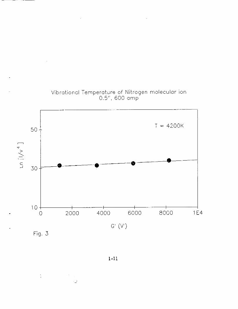
taken at 0.5" from the blunt body and is shown in fig.2. The
areas under the curves of 0-i, i-I, 2-1, and 3-1 bands of theN +T_e were used for vibrational temperature determinations.
graph along with the calculated temperature is shown in
fig.3. The temperature determined using this technique is
close to the one determined earlier by Blackwell et.al(1) at
this distance. Vibrational temperature determinations usingother progressions could not be made as sufficient data is
not available. This procedure seems to be simple and
1-4

comparable to the methods used by earlier workers (i).
During my stay here, more empahasis is given forrotational temperature determinations of N_+. The necessaryequations for determining the rotational llne intensities areshown in Appendix I. When a graph is plotted using equation(4) between in [I/(k'+k"+l)] against k'(k'+l), a straightline is obtained. The slope of the line gives B0hc/kT fromwhich the rotational temperature can be determined.
+ isThe rotational structure of the 0-i band of N2shown in fig.4. Due to the limited resolution the spectrum isnot well resolved and we could not resolve P and R branches.AS a first order approximation, we tried to treat theobserved peak intensity as purely due to the P branch onlyand rotational temperature determinations are made as perequation (4) shown in Appendix I. Similarly considering theobserved intensity as purely due to the R branch, rotationaltemperature is determined. As shown in fig.5, thetemperatures obtained are not the same and not close to therotational temperatures determined by earlier methods(4).this is expected because the experimental spectra containsthe intensity contributions of both P and R branches. Onetherefore can not use equation (4) for cases where thespectra are not well resolved.
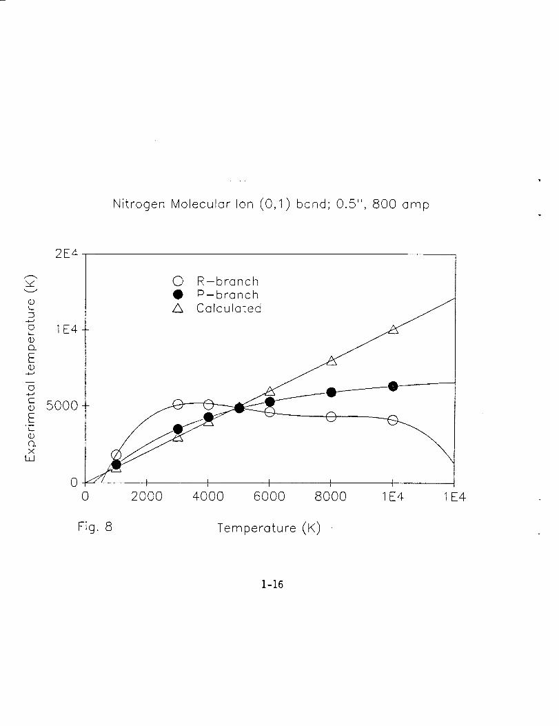
We have developed a method to determine therotational temperatures in cases where the P and R branchesare not well resolved. The necessary equations have beenderived and shown in Appendix 2. Using equations (7) and
(8) the observed intensity is corrected for P and R branchesat various temperatures(T). Graphs are now plotted;
in[Ipc/(K'+K"+l)] against K'(K'+I) for P- branch and
In[IRc/(K'+K"+I) against K'(K'+I) for R-branch. The
temperatures (Tp and TR) are now calculated using the slopesof the straight lines obtained from the graphs for both P and
R branches. The particular set for which the temperature
Tp = TR = T is considered as the temperature of the shocklayer.
Using this method, spectra taken at 0.5", 1.0" and
1.4" from the blunt body on October '88 are analyzed for
rotational temperature determination. Figs. 6 and 7 show the
graphs plotted for the corrected P and R branches at various
temperatures for the spectra taken at 0.5" from the body.
Temperatures are calculated using the slopes of the lines and
are tabulated in Table I. The best agreement is obtained at5000 K as can be seen from the % errors shown in Table i.
Fig. 8 is a graph showing the agreement between P and Rbranches. Similar calculations are carried out for spectra
1-5

taken at 1.0" and 1.4" and the corresponding temperatures arefound to be 6000 K and 5000 K respectively.
CONCLUSIONS
We have developed a procedure to calculate thevibrational and rotational temperatures of simple molecules.These methods have been tested to determine the shock layertemperatures of N2+ and it could be extended to othermolecular species present in the shock layer. We encounteredsome problems of convergence when the rotational temperatureprocedure was tested on a different data set. This thereforeneeds further testing with bigger data base. The accuracy ofrotational temperature determination could be improvedfurther if the P and R branches could be resolved.
Recommendations: In order to obtain a more accuratetemperature determination and to resolve P and R branches thefollowing Suggestions are made.
, A bigger spectrometer of at least one meter in length
with !800 lines/mm will be able to resolve the spectra.
• A photodiode array with five times the present photodiode
density will basically also resolve the spectra.
. Laser Induced fluorescence on the other hand will provide
selective excitation, spatial as well as high resolution.
Therefore this seems to be the ideal approach for the
present problem.
1-6

ACKNOWLEDGMENTS
I wish to take this opportunity to thank NASA/ASEEsummer faculty fellowship program for giving me anopportunity to work at NASA, Johnson Space center. My sincerethanks are to John Grimaud, my NASA colleague, for providingthe facilities and for his complete cooperation. My specialthanks are to Dr. Sivaram Arepalli of Lockheed with out whosehelp I might not have been able to complete this work. Lastbut not the least, I wish to thank all NASA and the Lockheedpersonnel of the arc jet facility who made my stay here verypleasant and rewarding.
1-7

REFERENCES
ii Blackwell, H.E., Wierum, F.A., Arepalli, S.and Scott,
C.d., " vibrational measurements of N 2 and N2 + shock
layer radiation." 27th Aerospace Sciences Meeting,
AIAA-89-0248, (1989).
. Herzberg, G., " Molecular Spectra and Molecular
structure, Vol 1 Spectra of Diatomic Molecules"
D. Van Nostrand Co., Inc., New York, N.Y. (1950).
•
.
Huber, K.P., and Herzberg, G.," Molecular spectra and
Molecular structure Vol. IV, Constants of Diatomic
Molecules.", D. Van Nostrand Co., Inc., New York, N.Y
(1979).
Blackwell, H.E., Yuen E., Arepalli, S., and Scott,
C.D., " Nonequilibrium shock layer temperature profiles
from arc jet radiation measurements." 24th
Thermophysics conference, AIAA-89-1679, (1989).
1-8

vml
ii

0
.=
Nirogen Molecular lon, V_rational Sp_trum
mo
,.340,0 360.0 38D.0 400.0 420.O 4-40.0 4E;Q.O 480.0
WAV___-'TH(NM)
Fig. 2. 1-10
Vibrotionol Temperoture of Nitrogen moleculor ion0.5", 600 omp
>
i i
C_J
5O
5O
10
T = 4200K
1 i i I0 2000 4000 6000 8000 1E4
c' (v')
1-11

i
C'-
iiI
°
il
_') I-- ,'
- !
i
II,:
Nitrogen Molecular lon
l
I
I!
I
I_-'
Ii
(0,1) band, Rotational structure
J"0
d)
q
0
i
_ 144 14_ f_ l_; 1_ I_,,_ .....i t,'"I , -- i l , P"I _ ,_ _t_", i
,t , tl l: li I, r ,, '
_', i :' ]_ !,.-,",_, _ _ll,,'. , !'.:',_ ,.,!- _.,':_'i i i , ,,, _ _ ! ' '_ _ I '," I: I ,/_! ,;', '" ' _
/_/ .,,_:'__,._._ i I,, v' t!( _,. _' L..
J| I ;
...- - _ ,-. , , , :
.... '- ":-':C_ 4-_ C " '- -I_-:EC
I
i
I
I
i
Fig. 4. 1-12
. t
;i
ORIGINAL PAGE
OF POOR (_UALIT¥

Nitrogen Molecular Ion (0,1) band, 0.5", 800omp
6
5 0
branch{860 K)branch(15,500 K)
÷
Y÷
m
C
4
5
2
0-200
Fig.
0
I
5O0
1-13
ORIGINAL PAGE IS
OF POOR QUALITY

Nitrogen Molecular Ion (0,1) bond, 0.5", 800 ampP-branch
+
+
mi i
C
2
I
0
-1
-2
-55OO
oo o "__
o 1000 K• 3000 K" 4000 K• 5OOO KD 6000 K• 8000 K
,710000 K
1000 1500 2000 2500
Fig 6
K'(K'+I)lo/2¢/ss
1-14

Nitrogen Molecular Ion (0,1) band, 0.5",800 amp
R-branch
+
+
i i
C
4
5
2
o t000 K• 3000 K
4000 K-__ • 5000 K
°o [] 6000 K- -_ • 8000 K
o _0000 K
AZ_ • •
0 I 1 I 1 1 I t
--200 --100 0 100 200 500 400 500 600
Fig. 7 k'(k'+l)
10/24/88
1-15
Nitrogen Molecular Ion (0,1) band; 0.5", 800 amp
2E4
2d
@
©Q.
E@
(-@
E°__
®Q_X
Ill
1E4
5O0O
0
0 R-branch• P-branch
_'/_ 1 I I I f
0 2000 4000 6000 8000 1 E4 1E4
Fig. 8 Temperature (K)
1-16

O
Z,<
O_-_oo
,<=:)z
Uu_
f._•
_-JoOZ
Z
C9_
OI--I_.
Zo
_..c=
E_
(D
L_
OL_
Av.O.,!
E_
0or'---
_oo
00c'_
_
c,4,.-.t
i._•
cx]_o
o_
!
A(DO.,
r_C)
OO
OO
OO
OO
OO
OO
OO
OO
OO
OO
O

APPENDIX - 1
ROTATIONAL TEMPERATURE EQUATIONS
BoJ(J- l)hc
I(P- Branch )= A- 2 Je- kT (1)
l(R-branch)=A-2(J+ 1)e
Bo(J + l)(J + 2)hc
kT (2)
Rearranging equations (I) and (2)
=In A-B'0J( J - I )hc
kT
l°I ]--A'-B 'oJ(J- 1)hc
kT(3)
Similarly for R Branch
IR I= B'o(J+ l)(J+2)hcIn 2 (J+ I)] A'- kT(4)
Equation (3) and (4) can general be written for
either case as
In[k, + kI,,+ i =A-B' K'(k'+ l)hc
kT
where k'- upper rotational state quantum number
k" = lower rotational state quantum number
I=18

APPENDIX- 2
CORRECTED INTENSITIES
I EXp = Ip + I R (5)
I IEXP
I IR R
P+I (6)
ILet ----P=P= B where I and I are
I p RR
the
intensities calculated for any temperature
using equations (1) and (2)
I =I IRc EXP I + B (7)
I Pc = I EXP (8)
IRc and I Pc are the intensity contributions
of P and R branches in the observed spectra
i=19


N90-24974
A BAYESIAN APPROACH TO RELIABILITY AND CONFIDENCE
Final Report
NASA/ASEE Summer Faculty Fellowship Program 1989
Johnson Space Center
Prepared By:
Academic Rank:
University & Department:
Ron Barnes, Ph.D.
Associate Professor
University of Houston-DowntownDepartment of AppliedMathematical SciencesOne Main StreetHouston, Texas 77002
NASA/JSCDirectorate:
Division:
JSC Colleague:
Date Submitted:
Contract Number:
Safety, Reliability, andQuality AssuranceReliability andMaintainability
Richard Heydorn
August 4, 1989
NGT 44-001-800
2-1

ABSTRACT
tn response to the Challenger accident, NASA has expanded its risk assessmentstudies from a completely qualitative Failure Modes and Effects Analysis�CriticalItems Lists (FMEA/CIL) to include some quantitative investigations like ProbabilityRisk Assessment (PRA).
Dr. Richard Heydorn (Reliability) presented lectures on quantitative methods to theVehicle Reliability Branch at the request of branch chief, Malcolm Himel. As anoutgrowth, the Extended Duration Orbiter- Weakest Link study is being developed.Three avionics subsystems and one with mechanical components, the freon coolantloop, have been identified as posing potential problems to keeping the Orbiter inspace for long periods of time. The intent of the study is to devise a standardmethodology for constructing system reliability diagrams and identifying what datais needed and/or potentially available. The data will then be utilized in Bayesianprobability models to estimate reliabilities and consequently identify any significantproblem subsystems.
Classical statistical methods are not suitable for many NASA problems. At NASA,data records are often sparse, incomplete or in a form not amenable to classicalconfidence estimates. Also, since problem-identification-problem-correction isemployed throughout the operating lifetime of many NASA systems, the usefulnessof failure history data is greatly compromised. Bayesian analysis addresses suchconcerns since it allows for the insertion of informed opinions instead of/or inaddition to observational data on failures.
=
Our summer work generalized some of Dr. Heydorn's results for systems with aconstant failure rate (exponential model) that is generally applicable to avionicsystems, to the case of a variable failure rate (Weibull model) which contains theexponential as a special case. TheWeibull model applies to reliability systems withburn in and/or wear out stages including most mechanical systems.
In the exponential case a closed form was obtained for the Bayesian estimate of thereliability function of a single component. The reliability of a system can then beevaluated using the rules of probability. With these estimators it is also possible tocalculate the probability that the true reliability of a component lies within a certaininterval and estimate the probability that the reliability of a system lies in a certaininterval.
Using Bayesian ideas it now becomes possible to handle situations which the classicalanalysis could not, namely: (1) how to handle problems where no failure data hasbeen observed over a period of time and (2) how to incorporate expert opinions intothe probability calculations along with the data on failures.
In the more general Weibull (variable failure rate) model we have obtained aBayesian estimator for the reliability which reduces to a closed form for special cases.In these cases the rest of the Bayesian analysis can be pursued.
Further investigations will consider the numerical evaluation of the Weibull Bayesianestimator for reliability in the general case. Bayesian estimates for the reliability ofsingle components and systems, and probability statements similar to thosedescribed for the exponential model may then be pursued. The results can then beapplied to the freon coolant subsystem of the Extended Duration Orbiter - WeakestLink study.
2-2

INTRODUCTION
In response to the Challenger accident and subsequent reports bygovernmental commissions [NRC, House Report], NASA has expanded its riskassessment studies from a completely qualitative Failure Modes and EffectsAnalysis/Critical Items List (FMEA/CIL) to some quantitative investigationsincluding Probability Risk Assessment (PRA).
FMEA/ClL is basically a bottom-up approach. Individual components of asystem are analyzed. Their individual failure modes are determined and theeffects of each type of failure are investigated. On the basis of this analysis,various critical categories are assigned to each failure mode of eachcomponent. One shortcoming of the FMEAlClLapproach is that it does notassign priorities. As Charles Harlan, director of the Safety, Reliability, andQuality Assurance Directorate at NASA/JSC has noted, "There are manycriticality I items in a system like the Shuttle, or in your car for that matter,...How do you distinguish the very unlikely failure you can live with from thelikely ones you have to fix?" He further stated that "Our present systemdoesn't assess priorities, and we're going to modify that. We need a relativeranking of the risk associated with each failure mode."[SPECTRUM]
Probability Risk Assessment addresses this shortcoming. In contradistinctionto FMEA/ClL, PRA is a top-down method in which possible failure modes ofthe entire system are first identified. The possible ways this could occur areenumerated and for each fault, chains of faults are traced out until eventuallyone arrives at the failure of a single component or a human error. Adownward branching fault tree is constructed in which probabilities areassigned to the basic faults and then the total probability of various failurepaths can be computed. In this way their relative contributions to the totalrisk are assessed.
NASA's historical preference for a qualitative approach to reliability andshunning of quantitative procedures is documented in the June 1989 specialissue on risk analysis in SPECTRUM. As noted by the SPECTRUM editors:
During the Apollo days NASA contracted with GeneralElectric to do a PRA to determine the chances of landinga man on the moon and safely returning him to earth.When the study indicated the probability of success wasless than five percent, NASA decided the studywould do "irreparable harm..." and they "studiously stayedaway from [numerical risk assessment] as a result.
Will Willoughby, NASA head of Reliability and Safety at the time, added
"That's when we threw all that garbage out and got down towork... Statistics don't count for anything. They have no place inengineering anywhere."[SPECTRU M]
As a result, NASA adapted qualitative failure modes and effects analysis(FMEA).
2-3

The SPECTRUMarticle further pointed out that in the 1970's and early 1980's,because of political realities it became necessary for NASA to show that theShuttle would be "cheap and routine, rather than expensive and risky." Suchpressures led to examples where data was disregarded and arbitraryassignments of risk levels were made.
The deliberate decision by NASA to forgo quantitative (probabilistic) riskanalyses determined the type of data NASA decided to collect. For exampleno elapsed times were originally recorded for components on the shuttle. Thefailure to record various kinds of data, which was recoverable, precludedmany forms of statistical analyses from even being considered.
After the Challenger accident the National Research Council (NRC) and theHouse of Representative committee on Science and Technology issuedreports, in addition to the Presidential Commission [Roger's Report]. TheCongressional report noted that:
Without some means of estimating theprobability of failure of the variouselements, it is not clear how NASA canfocus its attention and resources aseffectively as possible on the mostcritical systems.
In a similar vein the NRC noted
The Committee views the NASA/CIL
waiver decision making process as beingsubjective with little in the way offormal and consistent criteria for
approval or rejection of waivers.Waiver decisions appear to be drivenalmost exclusively by the design basedFMEA/CIL retention rationale rather
than being based on an integratedassessment of all inputs to riskmanagement.
In response to the Challenger accident and these reports, NASA is nowchanging in favor of a "willingness to explore other things" [SPECTRUM].NASA has contracted two PRA pilot projects and has developed workshops totrain engineers and others in quantitative risk assessment techniques.
One Approach
In this spirit, Dr. Richard Heydorn presented lectures on quantitative methodsto the Vehicle Reliability Branch at the request of branch chief, MalcolmHimel. As an outgrowth, the Extended Duration Orbiter- Weakest Link studyis being developed. Three avionics subsystems and one with mechanicalcomponents, the freon coolant loop, have been identified as posing potentialproblems to keeping the Orbiter in space for long periods of time. The intentof the study is to devise a standard methodology for constructing
2-4

system reliability diagrams and identifying what data is needed and/orpotentially available. The data will then be utilized in Bayesian probabilitymodels to estimate reliabilities and consequently identify any significant
problem subsystems.
Classical statistical methods are not suitable for many NASA problems. AtNASA, data records are often sparse, incomplete or in a form not amenable toclassical confidence estimates. Also, since problem-identification-problem-correction is employed throughout the operating lifetime of many NASAsystems, the usefulness of failure history data is greatly compromised.Bayesian analysis addresses such concerns since it allows for the insertion ofinformed opinions instead of/or in addition to observational data on failures.
PRELIMINARY WORK ON A BAYESIAN APPROACH TO RELIABILITY ANDCONFIDENCE
Prior to my arrival to take part in the NASA Summer Faculty Fellow program,Dr. Heydorn had begun Bayesian investigations into reliability by modelingthe reliability of a single component (e.g. valve, piston, computer chip,etc...)assuming a constant rate of failurel The reliability of a system ofcomponents can then be modeled using the laws of probability.
The Bayesian approach was selected because of the shortcomings of classicalstatistical analysis with NASA data as pointed out earlier. In particular, incases with very few data values on failures, classical confidence intervals forthe reliability may be larger than the unit interval [0,1] and hence quitemeaningless. Similarly since classical estimates of reliability depend on thefailure history sample, an extreme but not uncommon situation in which nofailures are recorded can lead one to blindly believe that we can conclude a
high confidence in high reliability. The Bayesian approach appears to bemuch more fruitful in that it can address such data difficulties.
In the case where the failure rate x is constant, under the fairly general
assumptions that (a) the number of failures in any two disjoint time intervalsare independent and (b) the distribution of the number of failures in any timeinterval depends only on the interval length, it follows that for t>O, N(t) thenumber of failures from time 0 to t is a random variable defined on a
probability spaceOs, N(_o,t) has a Poisson probability distribution with
Pr(N(t) = n) : ((xt)n/n!)e-_t (i)
Forthisprocessletx(co,t) = t if N(_,t) = 0 and letx(_,t) = 0 ifN(_0,t)>O.The reliability function is then defined as:
R(t) = Pr(x(t) : i) = P(N(t) : O) = e-Xt (2)
2-5
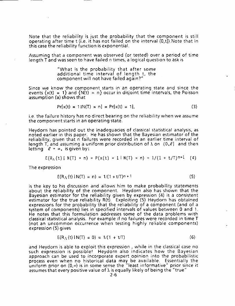
Note that the reliability is just the probability that the component is stilloperating after time t (i.e. it has not failed on the interval (0,t]).Note that inthis case the reliability function is exponential.
Assuming that a component was observed (or tested) over a period of timelength T and was seen to have failed n times, a logical question to ask is
"What is the probability that after someadditional time interval of length t, thecomponent will not have failed again?"
Since we know the component starts in an operating state and since theevents{x(t) = 1} and {N(t) = n}occurin disjoint time intervals, the Poissonassumption Ca) shows that
Pr[x(t) = l IN(T) = n] = Pr[x(t) = 1], (3)
i.e. the failure history has no direct bearing on the reliability when we assumethe component starts in an operating state.
Heydorn has pointed out the inadequacies of classical statistical analysis, asnoted earlier in this paper. He has shown that the Bayesian estimator of thereliability, given that n failures were recorded in an earlier time interval oflengthT, and assuming a uniform prior distribution of,\on (0,¢] and thenletting _ ÷ ,_, is given by:
E(RA(t) I N(T) : n) : P(x(t) : 11N(T) : n) = i/(l + t/T)n+l (4)
The expression
E(RA(t) IN(T) = n) = 1/(1 +t/T)n+ 1 is)
is the key to his discussion and allows him to make probability statementsabout the reliability of the component. Heydorn also has shown that theBayesian estimator for the reliability given by expression (4) is a consistentestimator for the true reliability R(t). Exploiting (5) Heydorn has obtainedexpressions for the probability that the reliability of a component (and of asystem of components) lies in specified intervals of values between 0 and 1.He notes that this formulation addresses some of the data problems withclassical statistical analysis. For example if no failures were recorded in timeT(not an uncommon occurrence when testing highly reliable components)expression (5) gives
E(RA(t) IN(T) = 0) = 1/(1 + t/T) (6)
and Heydorn is able to exploit this expression , while in the classical case nosuch expression is possible! Heydorn also indicates how the Bayesianapproach can be used to incorporate expert opinion into the probabilisticprocess even when no historical data may be available. Essentially theuniform prior on (0,,_) is in some sense the "least informative" prior since itassumes that every positive value of._ is equally likely of being the "true"
2-6

value of the constant rate _. Given additional expert opinion, it is oftenpossible to incorporate that opinion into the choice of an alternate priordistribution for,\. Heydorn illustrates this with an example and shows howasystem containing a mixture of components, some with failure data andothers will only expert opinions on the failure mechanisms, can beprobabilistically analyzed.
DISCUSSION
For these summer investigations, the first objective was to extend the resultsto the more general case where the failure rate (hazard function) is non-constant. A good model for a non-constant hazard function is theWeibulldistribution, W(.\,[3), which can model both "break in" and "wear out"failure conditions in a system and contains the constant failure rate model as aspecial case. The discussion that follows considers the following formulationof the Weibull distribution.
13t
R(t,k,_) : e -,_t13
h(t,x,[3) : , 13t -i
,\,I3,t > o
(7)
Note that in the special case when [3 = l the hazard function reduces to theconstant.\ and the reliability function isthe exponential function, i.e. one hasthe constant failure rate model considered earlier.
In Weibull reliability analysis it is often the case that the value of the shapeparameter [3 is known. In fact the literature sharply divides into the casewhere [3 is known and only the scale parameterS_ is unknown and the moregeneral case where both parameters are unknown. In the case where [3 isknown considerable analysis has occurred [Martz].
If one assumes a non-constant intensity function h(t,2t,[3) = k ./3 t !3-1, it iseasy to show under assumptions similar to (a) and (b) given earlier that theprobability of n failures occurring by time T is given by
P[N(T) : n] = (e-,\T[3(kT_)n)/n! (8)
This is usually referred to as the nonhomogeneous Poisson process.
SPECIAL CASE
Now for the Weibull model with [3 known, the Bayesian estimate for thereliability can be calculated (assuming _ has a uniform prior and the limitingprocess is carried out as before) and one sees that
E(R\(t) I N(T):n) : P[x(t) : I IN(T):n] : i/(i + (t/T)_) _t (9)
2-7

In this special casethe Bayesian estimate isseen to be a consistent estimator ofthe reliability function (7). With expression (8) one is able to make probabilitystatements about the reliability of a component (and system) as Heydorn didfor the exponential case for situations that classical reliability theory can notaddress. The inclusion of expert opinion into the process can also proceed aswas indicated earlier.
GENERALCASE
In the more general case where both _ and .\ are unknown, we assume theyare unknown values of random variables that must be estimated. We assume
prior uniform distribution on (0,4.\] and (0,_13] and eventually take thelimiting values so that k and [3 may take on any nonnegativevatues. In asense, these are the least informative priors since they assume that everypossible value for ,\ (and 13) is equally likely of occurring i.e. we have noadditional information on the true values of _\ and _.
Preliminary investigations indicated that N(T), the number of failuresrecorded in time T, is not sufficient to ensure that the corresponding Bayesianestimate of reliability is a consistent estimator of the true reliability.
It is well known [Bain, Finklestein, et al.] that if T1,...,Tn denote the first nsuccessive times of failure of a Weibull process (TI<_ T2 . . . <_< Tn) then thelikelihood function is given by:
f(tl,...tn,_\,13) : ;tn_3n( FI ti)P-le-.k(t,)P (io)
The Bayesian Estimator of reliability is this case (for uniform priors on (O,_a\](O,_?[3]and taking limits) reduces to:
E[R,\(t) I TI : tl, ....Tn=tn]
= [In[tnTI(tn/ti)]]n+l
n]
While expression (11) does notobservations are in order'
= P[x(t) .] 11 T1 : tl,...Tn:tn]
limit e__o (_13 ln[t nlI (tnitii] d_:
J [i + (D'tn)[3]n+I (ii)0
have a closed form in general, a few
(a) The form of (11) indicates thattn and It ti together carry all theinformation necessary to obtain the Bayesian estimate of reliability. We notethat in the classical analysis tnand II ti are joint sufficient statistics[Bain].
(b) The Bayesian estimate (1 1) is a consistent estimator for R(t), the truereliability. In fact, we conjecture that an even more general result holds.
Namely, under some rather general conditions we believe it is possible toshow that for any estimator 0 of O,
E[®lxl...Xn] -_O (as n -_ _) (12)
2-8

(c) In the special case that t = tn, i.e. one wants to estimate the reliabilityafter time t in the future that is equal to the total elapsed time for the first npast failures, expression (11) reduces to
E[R\(t) I TI = ti ..... Tn : tn] : (I/2)n+l (13)
With this closed form one can again make probability statements about thereliability of a component, conditioned on the failure times tt...tn. Inparticular the probability that this system has not failed after t units of timegiven that it failed n times over a period of time t in the past is (1/2)n ÷ 1. Forexample if one had data on 1 failure after 10,000 hours of operation then theprobability that the component (starting from an operating state) will not failduring the next 10,000 hours is (1/2)2 = 1/4 = .25. Expression (13) suggeststhat if no failures were encountered in t units of time then the probabilitythat there will be no failures in a future time interval of t units (starting froman operating state) would be 1/2 = .50. In some sense there is a 50/50 chanceof the component failing in the next t units of time if it has not failed in aprior t units of time.
Again with expression (13), using the laws of probability it is possible toobtain expressions for the probability that the reliability of a component (or asystem of components) lies in a specified range of values between 0 and 1.
CONCLUSION
This report outlined the historical evolution of NASA's interest is quantitativemeasures of reliability assessment. The introduction of some quantitativemethodologies into the Vehicle Reliability Branch of the SR&OA Division atJSC was noted along with the development of the Extended Orbiter Duration- Weakest Link study which will utilize quantitative tools for a Bayesianstatistical analysis.
Extending the earlier work of my NASA sponsor, Richard Heydorn, we havebeen able to produce a consistent Bayesian estimate for the reliability of acomponent and hence by a simple extension for a system of components insome cases where the rate of failure is not constant but varies over time.
Mechanical systems in 9eneral have this property since the reliability usuallydecreases markedly as the parts degrade over time. While we have been ableto reduce the Bayesian estimator to a simple closed form for a large class ofsuch systems, the form for the most general case needs to be attacked by thecomputer. Onceatable is generated for this form, we will have a numericalform for the general solution. With this, the corresponding probabilitystatements about the reliability of a system can be made in the most generalsetting. Note that the utilization of uniform Bayesian priors represent a"worst case" scenario in the sense that as we incorporate more expert opinioninto the model we will be able to improve the strength of the probabilitycalculations.
2-9

REFERENCES
1. National Research Council, Aeronautics and Space Engineering Board,Committee on Shuttle Criticality Review and Hazard Analysis audit, "Post-Challenger Evaluation of Space Shuttle Risk Assessment and Management,"January 1988.
2. Committee on Science and Technology, U.S. House of Representatives,"Investigation of the Challenger Accident , Ninety - Ninth Congress, October29, 1986.
3. BelI,TrudyE. and Karl Esch,"SpeciaIReport: the Space Shuttle ACaseofSubjective Engineering,' IEEESPECTRUM,42-46,June 1989.
4. Presidential Commission on the Space Shuttle Challenger Accident, "Reportto the President", June 6, 1986.
5. Heydorn, Richard, unpublished lecture notes on quantitative methods forreliability, NASA/JSC,Reliability and Maintainability Division, Spring 1989.
6. Martz, Harry F. and RayA.Waller, Bayesian Reliability Analyses, John Wileyand Sons, New York, 1982.
7. Bain, Lee J. Statistical Analysis of Reliability and Life-Testinq Models,Marcel Dekker Inc., New York, 1978.
8. Finkelstein, J. M., "Confidence Bands on the Parameters of the WeibullProcess,'Technometrics, Vol. 18, No. 1,115-117, February1976.
2-10

APPENDIX
E[R_t_(t) I TI : tl, .... Tn:tnJ : P[x(t) : I ITI : tl ...Tn:tn]
¢j3 ¢_ _3n X n ( ll ti)P-le-2_(tn)13e-XtPd2_d_
-- limit _..= c o
limit ex_,_ i i /-'"F"]#_(_"
Q o
2-11


N90-24975
EFFECT OF LOW AIR VELOCITIES ON THERMAL HOMEOSTASIS
AND COMFORT DURING EXERCISE AT SPACE STATION
OPERATIONAL TEMPERATURE AND HUMIDITY
Final Report
NASA/ASEE Summer Faculty Fellowship Program--1989
Johnson Space Center
Prepared By:
Academic Rank:
University & Department:
Ronald J. Beumer, Ph.D.
Associate Professor
Armstrong State College
Department of Biology
Savannah, Georgia 31419
NASA/JSC
Directorate:
Division:
Branch:
JSC Colleague:
Date Submitted:
Contract Number:
Space and Life Sciences
Medical Sciences
Space Biomedical ResearchInstitute
James M. Waligora
August 14, 1989
NGT44-O01-800
3-I

ABSTRACT
This study investigated the effectiveness of different lowair velocities in maintaining thermal comfort andhomeostasis during exercise at space station operationaltemperature and humidity. Five male subjects exercised ona treadmill for successive ten minute periods at 60, 71 and83% of maximum oxygen consumption at each of four airvelocities, 30, 50, 80 and 120 ft/min, at 22°C and 62%relative humidity. No consistent trends or statisticallysignificant differences between air velocities were foundin body weight loss, sweat accumulation, or changes inrectal, skin and body temperatures. Occurrence of thesmallest body weight loss at 120 ft/min, the largest sweataccumulation at 30 ft/min, and the smallest rise in rectaltemperature and the greatest drop in skin temperature at120 ft/min all suggested more efficient evaporative coolingat the highest velocity. Heat storage at all velocitieswas evidenced by increased rectal and body temperatures;skin temperatures declined or increased only slightly.Body and rectal temperature increases corresponded withincreased perception of warmth and slight thermaldiscomfort as exercise progressed. At all air velocities,mean thermal perception never exceeded "warm" and meandiscomfort, greatest at 30 ft/min, was categorized at worstas "uncomfortable"; sensation of thermal neutrality andcomfort returned rapidly aft@r cessation of exercise.Suggestions for further elucidation of the effects of lowair velocities on thermal comfort and homeostasis includelarger numbers of subjects, more extensive skin temperaturemeasurements and more rigorous analysis of the data fromthis study.
3-2
INTRODUCTION
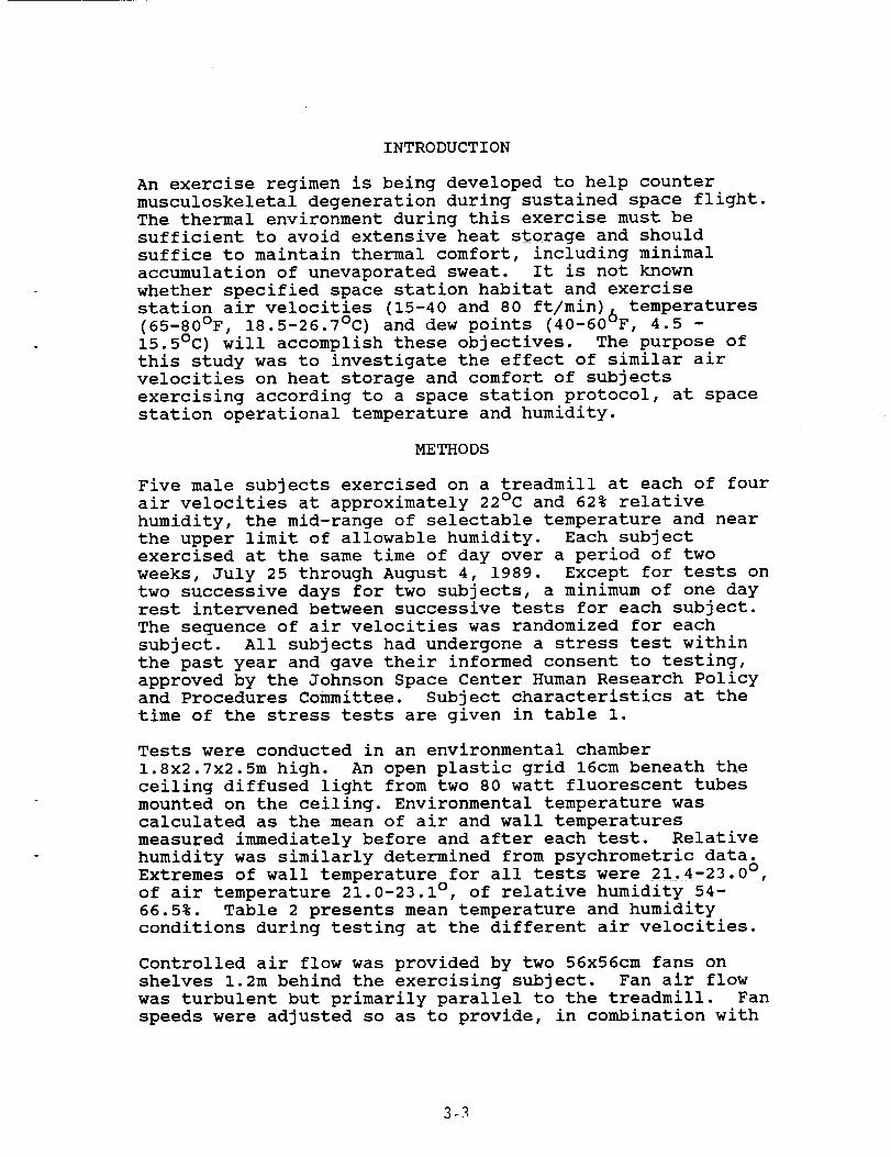
An exercise regimen is being developed to help countermusculoskeletal degeneration during sustained space flight.The thermal environment during this exercise must besufficient to avoid extensive heat storage and shouldsuffice to maintain thermal comfort, including minimalaccumulation of unevaporated sweat• It is not knownwhether specified space station habitat and exercisestation air velocities (15-40 and 80 ft/min) 6 temperatures(65-80°F, 18.5-26.7°C) and dew points (40-60 F, 4.5 -15.5°C) will accomplish these objectives. The purpose ofthis study was to investigate the effect of similar airvelocities on heat storage and comfort of subjectsexercising according to a space station protocol, at spacestation operational temperature and humidity.
METHODS
Five male subjects exercised on a treadmill at each of fourair velocities at approximately 22°C and 62% relativehumidity, the mid-range of selectable temperature and nearthe upper limit of allowable humidity. Each subjectexercised at the same time of day over a period of twoweeks, July 25 through August 4, 1989. Except for tests ontwo successive days for two subjects, a minimum of one dayrest intervened between successive tests for each subject.The sequence of air velocities was randomized for eachsubject. All subjects had undergone a stress test withinthe past year and gave their informed consent to testing,approved by the Johnson Space Center Human Research Policy
and Procedures Committee. Subject characteristics at the
time of the stress tests are given in table i.
Tests were conducted in an environmental chamber
1.8x2.7x2.5m high. An open plastic grid 16cm beneath the
ceiling diffused light from two 80 watt fluorescent tubes
mounted on the ceiling• Environmental temperature was
calculated as the mean of air and wall temperatures
measured immediately before and after each test. Relative
humidity was similarly determined from psychrometric data.
Extremes of wall temperature for all tests were 21 4-23 0°
of air temperature 21•0-23.1 °, of relative humidity 54-
66.5%• Table 2 presents mean temperature and humidity
conditions during testing at the different air velocities.
Controlled air flow was provided by two 56x56cm fans on
shelves 1.2m behind the exercising subject. Fan air flow
was turbulent but primarily parallel to the treadmill. Fan
speeds were adjusted so as to provide, in combination with
3-3
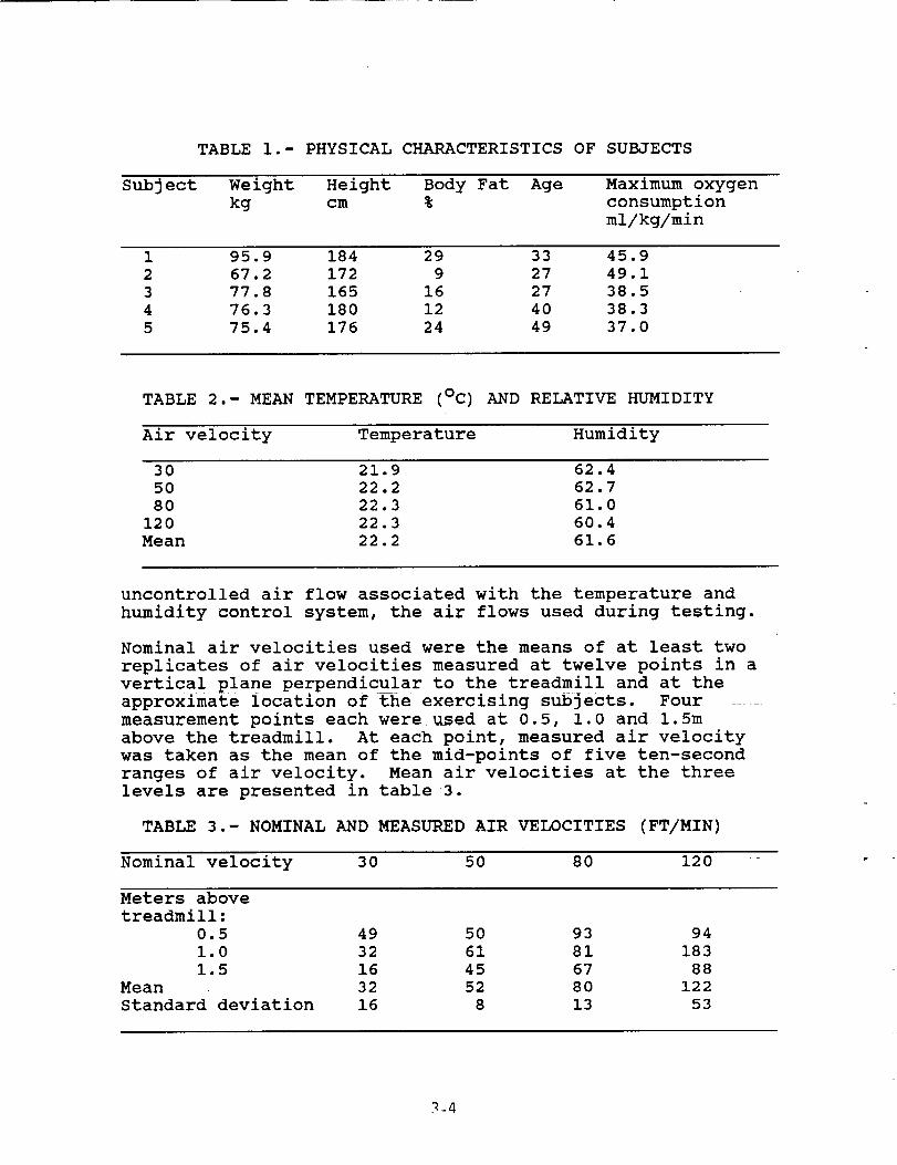
TABLE i.- PHYSICAL CHARACTERISTICS OF SUBJECTS
Subject Weight Height Body Fat Age
kg cm %
Maximum oxygen
consumption
ml/kg/min
1 95.9 184 29 33 45.9
2 67.2 172 9 27 49.1
3 77.8 165 16 27 38.5
4 76.3 180 12 40 38.3
5 75.4 176 24 49 37.0
TABLE 2.- MEAN TEMPERATURE (°C) AND RELATIVE HUMIDITY
Air velocity Temperature Humidity
30 21.9 62.4
50 22.2 62.7
80 22.3 61.0
120 22.3 60.4
Mean 22.2 61.6
uncontrolled air flow associated with the temperature and
humidity control system, the air flows used during testing.
Nominal air velocities used were the means of at least two
replicates of air velocities measured at twelve points in a
vertical plane perpendicular to the treadmill and at the
approximate location of the exercising subjects. Four
measurement points each were used at 0.5, 1.0 and 1.5m
above the treadmill. At each point, measured air velocity
was taken as the mean of the mid-points of five ten-second
ranges of air velocity. Mean air velocities at the three
levels are presented in table 3.
TABLE 3.- NOMINAL AND MEASURED AIR VELOCITIES (FT/MIN)
Nominal velocity 30 50 80 120
Meters above
treadmill:
0.5 49 50 93 94
1.0 32 61 81 183
1.5 16 45 67 88
Mean 32 52 80 122
Standard deviation 16 8 13 53

The suggested space station exercise schedule specifies
successive ten minute periods at 65, 75 and 85% maximum
oxygen consumption. Treadmill speeds and grades needed toachieve these oxygen consumptions for each subject were
estimated using the chart and formula of Givoni and Goldman
(1971). Small adjustments were made after each subject's
first test to more closely approximate targeted values.
The range of speeds and grades used was 5.6-6.6km/hr and 5-15%.
Before each test, thermistor probes were attached with
porous paper tape to the mid-sternum, anterior left thigh
and dorsal left hand of the subject, a rectal thermistor
was inserted to 10cm, and EKG electrodes and transmitter
were attached; total mass of this apparatus was
approximately 430gm. The nude subject was then weighed to
the nearest 5gm on an electronic platform balance before
donning preweighed shorts, socks and shoes. Within five
minutes after completing exercise, clothing and a towel
used to remove perspiration after exercise were placed in a
plastic bag and nude weight was again determined. Body
weight loss was determined as the difference of these two
weights; unevaporated sweat accumulation was estimated as
the difference in garment and towel weight before and afterexercise.
After the first weighing, fans were turned on and the
subject stood at rest on the treadmill for 15 minutes inorder to establish thermal equilibrium. At the beginning
of this period, the beginning of exercise, and at each five
minute interval thereafter during exercise and a subsequent
15 minute recovery period, rectal and the three skin
temperatures were recorded. Mean skin and bodytemperatures were computed according to equations modified
from Berenson and Robertson (1973):
Tskin=0.53Tthigh+0-33Tchest+0-14Thand;
Tbody=0.67Trectal+0-33Tskin •
At the same time intervals, subjects categorized perception
of temperature and thermal comfort according to temperatureand discomfort scales described by Gagge et al. (1967) and
illustrated in table 4. Scales were posted in front of the
treadmill to facilitate subject response.
During the initial equilibrium period and at the mid-point
of each exercise level, oxygen consumption and carbon
dioxide production were measured by timed collection of
3-5

TABLE 4.- TEMPERATURESENSATION AND THERMAL COMFORT SCALES
Temperature: Comfort:-3 cold 0
-2 cool 1
-I slightly cool 20 neutral 3
+I slightly warm 4+2 warm
+3 hot
comfortable
slightly uncomfortableuncomfortable
very uncomfortableintolerable
expired gas samples and analysis of gas composition by a
mass spectrometer.
RESULTS
Table 5 presents mean percentages of maximum oxygen
consumption during the three ten minute periods of exercise
at each air velocity. The percentage in each case was
lower than the targeted values of 65, 75 and 85%. Analysis
of variance (ANOVA) within exercise periods revealed no
significant differences between the different air velocities.
TABLE 5.- MEAN PERCENTAGE OF MAXIMUM OXYGEN CONSUMPTION
DURING SUCCESSIVE EXERCISE PERIODS ( )=S.D.
Air velocity Period
ft/min First Second Third
30 59 (6) 73 (6) 81 (ii)
50 60 (6) 71 (6) 82 (i0)
80 62 (7) 72 (9) 81 (7)
120 60 (6) 71 (I0) 83 (ii)- u
Body weight loss was least at 120 ft/min and sweatrecovered was greatest at 30 ft/min (table 6), ANOVA
indicated no significant differences between air velocities
for any of these parameters.
Figures 1 and 2 show that rectal and body temperatures both
rose gradually through the exercise period and declined
during the recovery period. The decline in rectal
temperature was more gradual than its rise and more
immediate and consistent than the decline in body
temperature. Air velocity had little effect on the change
in rectal temperature at 30 minutes, nor any consistent
effect on body temperature. ANOVA indicated no significant
differences between air velocities in mean body or rectal
3-6

TABLE 6.- MEAN ABSOLUTE AND PERCENTAGEBODY WEIGHT LOSSES,ABSOLUTE WEIGHT OF RECOVEREDSWEATAND WEIGHT OF RECOVERED
SWEATAS PERCENTAGEOF BODY WEIGHT LOSS ( )=S.D.
Air velocity Weight lossft/min gm percent
Sweat recoveredgm percent
30 425 (213) 0.5 (0.2) 85 (95) 16.2 (10.5)
50 421 (174) 0.5 (0.2) 68 (75) 13.5 (9.5)
80 442 (158) 0.6 (0.I) 63 (69) 12.1 (9.6)
120 356 (229) 0.4 (0.2) 64 (72) 14.8 (7.9)
temperature changes at 30 minutes.
All skin temperatures dropped initially and then rose
slightly (figure 3). At 80 and 50 ft/min, skin temperaturecontinued to rise through the exercise period, at 30 ft/min
it oscillated, and at 120 ft/min it declined until the endof the exercise. At the end of the exercise period, the
skin temperatures at 50 and 80 ft/min were approximately
the same as at the beginning of the period; the greatest
change was at 120 ft/min, slightly greater than that at 30ft/min. Differences at 30 minutes were not statistically
significant.
During recovery, skin temperatures first rose then declined
precipitously at all air velocities except 80 ft/min, in
which case the opposite occurred. At the end of the
recovery period, the greatest change from the start of the
exercise was at 120 ft/min and the least at 80 ft/min.
Figure 4 indicates that mean temperature perception at the
start of exercise was slightly cool at 80 and 120 ft/min
and near neutral at 30 and 50 ft/min. Ranking of perceived
temperature rose until the end of exercise, when subjects
felt warm at 80 ft/min and between slightly warm and warm
at other velocities. Feeling of warmth decreased rapidly
at the beginning of the recovery period and thereafter
approximated starting values.
Subjects at 120 ft/min were slightly less comfortable than
at other velocities at the beginning of exercise (figure
5). Mean discomfort level at 30 ft/min was almost a whole
category above that at other velocities at 25 minutes. At
30 minutes, subjects at 30 ft/min gave the highest
discomfort ranking, and subjects at 120 ft/min were the
most comfortable. After exercise, comfort level at all
velocities rapidly returned to "comfortable".
3-7

I
a6ueq=aJn:;eJadule.L
3-8

%
_%
%%
\
I!
II
II
I
aOc5c5
U')
_I"I_
C41
.-0
.="c5
c5c5
c5c_
c5,:5I
aOueqo
aJn:_eJadWal
0mQ0I$clP
_:I::
Ul
o,..,me
-,,9=m_
4.-
0Cm
-CO
•"'
l"J
LC
-_'-e
o_,,I
=&
EeI
0
3-g

_.,o,m
_,$•
°'_l'
,.imi,p,j"
_t'
%%
%%
%%
,Ib%
//##%
%,%'l
%
%
%%
coo
I,,It=
0
I¢%i
o
Jt
o
m,
lllli
,,I
7"t
"-,i
//
"-i-/
j_,oo
_7
_i
t
I_'_
7,/
II4'i
%\°;i
I',,,,
11\/.i
'll=.
_
oo
Iri(%
1,,lu-I
+1o.,-.tJ
O3Olilo
II
II
II
I
(%1
_I"tO
IX3
._ii'i.l
$.
•_
|•
i
00
0_
_-i_-o
II
II
II
aOu
eq0
aJn_eJadla¢
!
!_,m.,
_o
LX_
®i
_EC
O
f..o¢3
I=C
O
=._
¢Z=l
x_
_oEei¢:
mm
C_
C0UI
to=
•_
I
3-10

uo
T_d
eoJed
eJn_eJed
e8_
3-11

!
3-12

DISCUSSION
These results suggest little difference in the contributionof the studied air velocities to thermal homeostasis and
comfort. No statistically significant effects of air
velocity were observed, nor were there consistent trends in
the observed parameters.
That mean energy expenditures were less than planned
suggests the desirability of further study using exercise
levels more closely resembling the space station protocol.
Nevertheless, their similarity at the four velocities
studied validates comparisons of other measured parameters.
That the smallest body weight loss occurred at 120 ft/min
might be due to this highest velocity fostering more
efficient evaporative cooling. This suggestion is
strengthened by the greatest accumulation of sweat at the
lowest velocity. More thorough analysis of these weights
relative to factors such as surface area, energy
expenditure and insensible evaporation may be useful.
Increases in rectal and body temperatures indicated heat
storage at all air velocities. That increase in body
temperature in all cases was smaller than rectal
increase is explained by smaller increases or declines in
skin temperature, probably the effect of evaporative
cooling. That the greatest increase in rectal temperature
occurred at the lowest air velocity is a reasonable
corollary of reduced evaporative cooling, but a further,
unfulfilled corollary would be a smaller decline in skin
temperature and larger increase in body temperature than atthe intermediate velocities.
Greater evaporative cooling similarly would explain the
smallest rise in body temperature and greatest drop in skin
temperature occurring at 120 ft/min. This conclusion is
weakened by the second greatest drop in skin temperature
occurring at the lowest air velocity and by only small
changes at intermediate velocities.
During the post-exercise period, rectal temperatures
declined more consistently than body temperatures and skin
temperatures were erratic. This may reflect rectal
temperature being affected more by activity and skin
temperature by environment. The primary purpose of this
period was to assure recovery of homeostasis; no effort was
made to control the posture or location of subjects in
relation to air flow. Environmental variability during
this period might have contributed to variable skin
3-13

temperatures. Temperature changes might have been moreinformative if this variability had been reduced.
Subjective sensation of being cooler before and afterexercise at the higher velocities than at the lowervelocities can be explained by greater convective coolingand post-exercise evaporative cooling. Lower comfort atthe highest velocity than at lower velocities at thebeginning of exercise probably was associated with thisperception of coolness.
During the later part of the exercise period, greaterdiscomfort was perceived at 30 ft/min than at highervelocities. A possible explanation of lesser convectiveand evaporative cooling is not supported by changes inmeasured temperatures. Greater skin wettedness as apossible explanation is corroborated by the greatestaccumulation of sweat at this velocity. Decreasedsensation of air movement is another possible cause.
Increased perception of warmth and slightly decreasedcomfort with increasing activity at all air velocitiescorresponds with increases in body and rectal temperatures.It is notable that at all these velocities the mean thermalsensation never exceeded warm, mean discomfort at worst wascategorized between uncomfortable and slightly so, and thatpost-exposure perception rapidly returned to near thermalneutrality and comfort.
Although this study has revealed little difference in theeffectiveness of different low air velocities under theconditions of the study, these data should be analyzed morerigorously. Perhaps also the study should be repeatedunder more precisely controlled conditions and using morepowerful measures to either validate its results orotherwise elucidate the effects of different airvelocities. In addition to suggestions made above, airflow should be more uniformly controlled or at least morecompletely characterized. Temperature data might be moreinformative if skin temperatures were measured at a largernumber of sites, especially on the dorsal surface mostdirectly affected by airflow in this study. The use oflarger numbers of subjects might also help to overcome theeffects of large individual differences in response to thetest protocol_ _ - .... _.....
3-14

REFERENCES
Berenson, P.J.; and Robertson, W.G.: Temperature. In
Parker, J.F., Jr.; and West, V.R. (Eds.):
Bioastronautics Data Book, second edition, NASA
SP-3006, 1973, pp 65-148.
Gagge, A.P.; Stolwijk, J.A.J.; and Hardy, J.D.: Comfortand thermal sensations and associated physiological
responses at various ambient temperatures. Environ.
Res., vol. i(i), 1967, pp 1-20.
Givoni, B.; and Goldman, R.F.: Predicting metabolic energy
cost. J. Appl. Physiol., vol. 30(3), 1971, pp 429-
433.
3-15


N90-24976
NONINVASIVE ESTIMATION OF FLUID SHIFTS BETWEEN
BODY COMPARTMENTS BY MEASUREMENT OF
BIOELECTRIC CHARACTERISTICS
Final Report
NASA/ASEE Summer Faculty Fellowship Program--1989
Johnson Space Center
Prepared by:
Academic Rank:
University Department:
Performance
Phillip A. Bishop, Ed.D.
Assistant Professor
Area of Health and Human
University of Alabama
Tuscaloosa, AL 35487
NASA/JSC
Directorate:
Division:
Branch:
JSC Colleague:
Date Submitted:
Contract Number:
Space and Life Sciences
Medical Sciences
Cardiovascular Laboratories
Suzanne Fortney, Ph.D.
August 17, 1989
NGT44001800
4-1
ABSTRACT
Previous research has established that bioelectrical
characteristics of the human body reflect fluid status to some
extent. It has been previously assumed that changes in
electrical resistance (R) and reactance (X) are associated
with changes in total body Water (TBW). The purpose of the
present pilot investigation was to assess the correspondence
between body R and X and changes in estimated TBW and plasma
volume during a period of bedrest (simulated weightlessness).
R and X were measured pre-, during, and post- a 13 day bedrest
interspersed with treatments designed to alter body fluid
status. Although a clear relationship was not elucidated,
evidence was found suggesting that R and X reflect plasma
volume rather than TBW. Indirect evidence provided by
previous studies which investigated other aspects of theelectrical/fluid relationship, also suggests the independence
of TBW and electrical properties. With further research, a
bioelectrical technique for noninvasively tracking fluid
changes consequent to space flight may be developed.
4-2

INTRODUCTION
That body fluid volumes are altered as a consequence ofsimulated or actual space flight is well established (7).It is generally believed that the loss of intravascular fluid(blood plasma) contributes significantly to the observeddecline in orthostatic tolerance subsequent to microgravityexposure. Body fluid compartments have been studied insimulated weightlessness studies (bedrest, and waterimmersion) by invasive means, but the time requirements andthe necessity of blood withdrawal and isotope injectionrequired by these measurements, have generally precluded theiruse _uring space flight. The development of an accuratenoninvasive technique for estimating the shift in body fluidsthroughout the course of an extended duration space flightwould provide considerable information useful in understandingand protecting against the adverse effects of prolongedmicrogravity exposure.
The work of Nyboer (18) and others has shown thatbioelectrical characteristics respond to changes in bodyfluids. This technique involves introduction of 0.8-4milliamps of high frequency (50-I00 kHz) current into the bodyvia surface electrodes. These current levels at thesefrequencies are safe and painless. Tetrapolar electrodesare employed with two electrodes used for current injectionand two used for voltage pickup, which obviates skin-electrodeimpedance complications (14,18). Knowledge of the injectedcurrent and frequency and the voltage drop and phase shiftacross a body part can be used to calculate resistance andreactance which can be combined to yield impedance. Basicelectrical theory can be used to derive an equation forvolume:
volume=resistivity*length2/resistance. (Eq. i)
Since within a given subject, under certain conditions, shortterm resistivity and length (distance between electrodes)remain constant, resistance and volume are inversely related.
Previous cross-sectional research (4,5,10,13,14,23,24,27)has demonstrated strong relationships between impedance andTBW or fat free mass (which is correlated to TBW). Numerousinvestigators have observed high test-retest reliability andalso good correspondence between separate laboratories (12).
Studies by Nyboer, (18), Spence et al. (25) andPatterson (19) have demonstrated strong correlations betweenimpedance and acute weight changes (i.e. fluid volume changes)in hemodialysis patients, and studies by Carlson et al. (2),and Mayfield and Uauy (15), have demonstrated strong
4-3
correlations between impedance and hydration status of burn
victims, and infantile diarrhea patients, respectively. It has
been demonstrated that bioelectrical properties can be used
to estimate cardiac output (9), total body water (23), and
limb blood flow (ii).
Recently, Patterson (19) has argued that measures of
impedance of individual limbs and the trunk (segmental
measures) should be better predictors of TBW or fat free mass
than the right side whole body measurements. Right side
whole body measurement is the most common technique used
currently. He bases his argument on the observation that the
small bony cross-sections of the wrist and ankle contribute
to produce limb impedances which are much higher than trunk
impedance. Consequently, when these impedances are summed,
the trunk, where most of the resting blood volume is located,
has a disproportionately small contribution to the overall
measured impedance value. Conversely, the wrist and ankle,
which are not much influenced by fluid shifts, strongly
influence the total impedance. Patterson presented data from
duplicate measurements on patients before and after
hemodialysis and found that combined segmental measures
yielded a higher correlation coefficient, (r=.87) than whole
body measures (r=.64), in predicting weight changes subsequent
to dialysis. However, Patterson's report did not include a
rigorous statistical analysis of all the data.
All the bioelectrical/hydration relationship studies,
have been cross-sectional or acute treatments without
consideration of fluid shifts or of specific resistivity
changes. A comprehensive longitudinal (i.e. pre-post
systematic fluid manipulation) study of the relationship
between hydration status and segmental and whole body
resistance and reactance in healthy humans has not been
reported. The purpose of the present pilot investigation was
to determine the correspondence between changes in segmental
limb R and X and estimated changes in body fluid compartments.
Because fluid Shifts and losses have been implicated in
orthostatic intolerance, decreased cardiovascular function,
and space adaptation syndrome, the ability to continuously
monitor fluid levels would contribute greatly to our
understanding of the physiological responses to acute and
chronic exposures to microgravity. The use of reactance
measurements as well as resistance measurements may permit
discrimination between extra- and intra- cellular water
compartments (15,16,17).
4-4

METHODS
Subjects
Subjects were two volunteers for a previously approved
13 day bedrest study at Johnson Space Center. Subjects had
given prior informed consent for measurement of bioelectrical
properties. Subjects were fully advised of the nature of this
specific aspect of the bedrest study, and gave permission
prior to each measurement.
Conditions
These measurements were made during the course of a 13
day six degree head down tilt bedrest (-6HDT) which wasintended to determine the effectiveness of lower body negative
pressure (LBNP) and fluid loading in ameliorating loss oforthostatic tolerance consequent to fluid shifts associated
with -6HDT and similar to those observed in microgravity.
After a two day ambulatory hospitalization, subjects underwent
a 13 day bedrest interrupted by LBNP response tests and LBNPand fluid treatments. Subjects were kept on a 2476 Kcal diet
with 2500 ml of additional daily fluid intake. This food and
fluid level replicates the average intake of the astronauts
during Shuttle flights. Body weights were determined with
a portable bed scale (Techtronix) just after the noon mealeach day. Blood samples were collected prior to breakfast
each day. Blood volumes were determined from red blood cellslabeled with 51Cr. Plasma volumes were determined from blood
volumes corrected for blood removal and hematocrits.
Bioelectrical MeasurementsResistance and reactance were measured at three sites
with a RJL analyzer at 50 Khz with 0.8 mA induced current.
Prejelled double electrodes (BOMED) were located at theantecubital fossa, just anterior and centered on the acromium
process, just distal to the inguinal fold on the anteriorsurface, and on the anterior surface superior to the patella.
In each case, except the inguinal, the electrode was locatedwith the distal border located at the landmark. Injection and
current pick-up electrodes were 5cm apart. Inter-electrodedistances and limb circumferences at the midpoint between
electrodes were measured with a cloth tape. This electrode
arrangement permitted determination of three separate
electrical measurements designated arm, trunk, and leg.
Segmental measurements were used rather than whole-bodymeasurements in keeping with Patterson's (19) observations
regarding joint-induced alterations in electrical resistivity.
For simplicity, segmental R's were summed to represent anestimator of total body R and designated "combined R". For
ease of comparison, resistances and reactances values were
also converted to their inverse, conductance.4-5

RESULTS
Figures la and ib, and 2a and 2b, are illustrations of
alterations in segmental resistance and reactance throughout
the time course of bed rest for subjects A and B,
respectively. Subject B underwent two LBNP treatments with
saline ingestion and a presyncopal LBNP (labeled PSL) which
are shown in the figures.
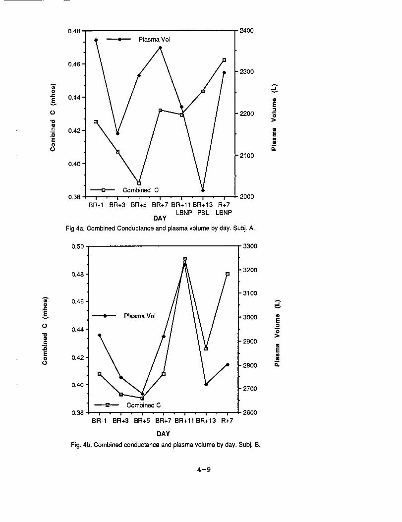
Figures 3a and 3b portray combined conductance (inverse
resistance) and body weight changes (which approximate TBW
changes) by day for each subject. Figures 4a and 4b portray
combined conductance and plasma volume for each test day of
the experiment. Figures 5a and 5b portray combined reactive
conductance and plasma volume by day for each subject.
4-6

120 30
110
"_'IO0E
Ov
90
U
-_ 80
0
70
6O
5O I ' I ' I ' I ' I ' I ' I
BR-1 BR+3 BR+5 BR+7BR+11BR+13 R+7
LBNP PSL LBNPDAY
FIG.la. Segmental resistances by day. Subj A.
Am
E 20,.CO
v
QOr"
ID
re
10
•----e--- TRUNK X
I ' I ' I ' I ' I ' I ' I
BR-1 BR+3 BR+5 BR+7BR+11BR+13 R+7LBNP PSL LBNP
DAY
Fig lb. Segmental Reactances by day. Subj. A.
110
100
E 90l-O
v
ul© 800C(Q
_, 7o&lg
6O
5O
ARM R
BR-1 BR+3 BR+5 BR+7 BR+11BR+13 R+7DAY
Fig 2a. Segmental resistances by day. Subj. B.
20 , _ TRUNKX
'°18 i
4-7
I " I " I " I ' I " i
BR-1 BR+3 BR+5 BR+7 BR+11BR+13 R+7DAY
Fig. 2b. Segmental reactances by day. Subj B.

161 0.48
.,Q
r"
m
@
160
15g
158
Fig 3a.
• Combined C
Weight LBNP PSL LBNP
BR-1 BR+3 BR+5 BR+7 BR+11BR+13 R+7
0.46
0.44
0.42
0.40
0.38
DAY
Combined conductance and body weight by day. Subj A.
O,,c
E
@
"0
O0
"13Q
J=
EO(J
A
J=n
3=
188 0.50
186
184
182
180
178
Combined C
BR-1 BR+3 BR+5 BR+7 BR+11BR+13 R+7
0.48
0.46
0.44
0.42
0.40
0.38
DAY
Fig 3b. Combined conductance and body weight by day. Subj B.
A
O,.c
E
@uc
-l"Ct-Oo
oc
.oEOo
4-8
0.48 2400
o
E
_o
"oq)c
_oE0ro
0.46
0.44
0.42
0.40
0.38
• Plasma Vol
Combined C
I " I ' I " I " i " I " I
BR-1 BR+3 BR+5 BR+7 BR+11BR+13 R+7
LBNP PSL LBNPDAY
'2300
22O0
' 2100
2OOO
Fig 4a. Combined Conductance and plasma volume by day. Subj. A.
0.50 3300
A
,..,I
oE
O
Ew¢=
O.
or-
E
t_
"o@e..
,,DEO
0.48
0.46
0.44
0.42
0.40
0.38
Plasma Vol
Combined C
l " l ' I " I " l " l "
BR-1 BR+3 BR+5 BR+7 BR+llBR+13
DAY
I
R+7
32OO
3100
3000
290O
2800
27OO
26O0
Fig. 4b. Combined conductance and plasma volume by day. Subj. B.
-I
QE
-6
E
4-9

2400 2.0
A
.J
@E=I
u
O
=lE
m
a.
2300
2200
2100
2000
; Combined 1IX
I I I "
BR-1 BR+3 BR+5
Plasma Volume (L)
I • I I I
BR+7 BR+11 BR+13 R+7
LBNP PSL LBNPDAY
1.9
1.8
1.7
1.6
Fig. 5a. Combined reactive conductance and plasma volume by day. Subj. A.
Ol-E
(DOCm
O
"10COo
@
m
o
ort
c
,.DEOo
3300 2.6
A
-Iv
oE=i
0
EwIQ
32OO
3100
3OOO
2900
28OO
27OO
Plasma Vol
02.5 .,=
E
2600 ' 2.0
BR-1 BR+3 BR+5 BR+7 BR+11 BR+13 R+7
ot=1,
o.-I
"ocoo
@
(g@,,w
"UQ¢=
,.oEOo
DAY
FIG. 5b. Combined reactive conductance and plasma volume by day. Subj. B.
4-i0
DISCUSSION
Previously cited works suggest that total body water is
strongly related to electrical resistance. The findings in
the present investigation suggests that human bioelectrical
properties may be related to fluid levels in various
compartments rather than total body water. For both
subjects, individual segmental R's and X's roughly paralleledeach other, except arm R and X in Subject B showed an
exaggerated drop on bedrest day 5 (BR+5). The segmental
approach resulted in arm, trunk, and leg R's which were
similar in magnitude. This approach appeared to alleviate
previously discussed joint interference problems. In both
subjects, body weight loss, which should reflect TBW, appearsto be disassociated from conductance (inverse resistance).
If TBW and resistance were inversely related, as has been
generally believed, good correspondence should have beenobserved. Since TBW is not altered during LBNP, if R and TBW
were related, this relationship should remain robust. In
Subject B, rapid weight loss, which should reflect TBW loss,
was not closely paralleled by any bioelectrical measurement
(Fig.3b). In subject A, combined R roughly tracked plasma
volume, but LBNP apparently changed somewhat the relationship
between plasma volume and resistance. But, for subject B,
combined resistance was closely linked to plasma volume
changes (Fig.4b). Combined X appeared to track changes in
plasma volume better than R in subject A, but less well than
R in subject B (Figs. 5a and 5b).
Interpretation of these data is complicated by theobservation that changes in resistance measurements do not
consistently relate to changes in fluid levels in a simple
way. In the case of dehydration by heating, Hutcheson et al.
(6) report a decrease in body weight accompanied by a decrease
in impedance (which would be interpreted as an increase in TBW
by equation i). Likewise, Caton et al.'s (3) observationsthat resistance decreases as skin temperature increases,
suggests that the distribution of blood (i.e. into the skinin the case of heating) influences electrical properties.
The authors speculate that the shift of fluid between
plasma and interstitium may also be involved. This isfurther substantiated by the observation that impedance
changes with changes in posture (20). Obviously, temperature
changes and postural changes reflect fluid redistribution
rather than changes in total body fluid volume. Changes in
specific resistivity are too small and in some cases in thewrong direction to account for these observations.
Many previous investigators have assumed that specific
resistivity was unchanged throughout the course of theirmeasurements of bioelectrical properties. Bonnardeaux (i)
and Salansky and Utrata (21) reported data from animal studies4-11
which suggest that blood osmolality and impedance are
inversely related. Likewise Kobayashi et al. (8) reports on
a paper written in Japanese by Tanaka et al. (26) which
observed that specific resistivity of blood in humans was
related to hematocrit. Kobayashi et al. (8) found that
adjustment of specific resistivity for hematocrit resulted in
much improved impedance cardiography. Postural changes,
changes resulting from dehydration due to unreplaced sweat
loss, and metabolic activity can all influence the electrical
characteristics of blood which would likely result in
alterations of electrical properties independent of changes
in fluid volumes. In the present study, plasma osmolality
was frequently measured and changed only slightly during the
measurement period. For Subject A, however, a lower body
negative pressure treatment preceded three of the
bioelectrical measurements and caused among other things,
hemoconcentration. Despite the lack of fluid loss
consequent to LBNP, the resistance measurements were
influenced (Fig 4a.).
In view of this somewhat cloudy picture, a number of
questions remain unanswered. Among these are:
i) How does specific resistivity vary among individuals?
2) Within individuals, how does specific resistivity vary
as intravascular, interstitial, and intracellular fluid levels
change?
3) Why do segmental resistances and reactances vary in
response to the same general body fluid alteration? (i.e. Why
did the resistance and reactance values for the segments fail
to unanimously track each other in a parallel fashion?)
,4) Which fluid compartment(s) exert the greatest influenceon electrical resistance and reactance?
CONCLUS IONS ....
A large body of literature exists which suggests that
alterations in body electrical pr0perties are related to
alterations in fluid levels. Among these are studies which
demonstrate good correspondence between impedance and cardiac
output (8,9), impedance and limb volume (ii), and impedance
and weight changes consequent to dialysis (19). The present
data, although i imited to two subjects, suggests that
electrical changes may be more closely linked to blood volume
rather than TBW. This does not directly contradict previous
studies, in that TBW and blood volume are probably closely
related. Undoubtedly some of the relationships between
electrical characteristics and fluid volumes and distributions
are causal. The exact nature of these relationships awaits
further research.
4-12

REFERENCES
i. Bonnardeaux, J.L. The behavior of blood plasma duringasphyxia and water deprivation. Arch. Int. Physiol. Biochem.
80:749-760, 1972.
2. Carlson R., E. Fegelman, R.K. Finley, S.F. Miller, L.M.
Jones, R. Richards, and S. Alkire. Assessment of fluid
retention in burn patients by using bioelectrical impedance
analysis. (Abstract) Am. Burn Assn, spring, 1986.
3. Caton, J.R., P.A. Mole, W.C. Adams, and D.S. Heustis. Body
composition analysis by bioelectrical impedance: effect of
skin temperature. Med. Sci. Spo_ts Exerc. 20(5), 489-491,
1988.
4. Hoffer E.C., C.K. Meador, D.C. Simpson. Correlation of
whole-body impedance with total body water volume. J. Appl.
Physiol. 27(4):531-534, 1969.
5. Hoffer E.C., C.K. Meador, and D.C. Simpson. A relationship
between whole body impedance and total body water volume.
Annals NY Acad. Sci. 197:452-469, 1970.
6. Hutcheson, L., R.W. Latin, and K.E. Berg. Body impedance
analysis and body water loss. Res. Q. Exerc. Sport 59 (4):359-
362, 1988.
7. Johnson, P.C. Fluid volume changes induced by spaceflight.
Acta Astro. 6:1335-1341, 1977.
8. Kobayashi, Y., T. Andoh, T. Fujinami, K. Nakayama, K.
Takada, T. Takeuchi, and M. Okamoto. Impedance cardiography
for estimating cardiac output during submaximal and maximal
work. J. Appl. Physiol.:Respirat. Environ. Exercise Physiol.
45(3):459-462, 1978.
9. Kubichek, W.G., R.P. Patterson, and D.A. Witsoe. Impedance
cardiography as a noninvasive method of monitoring cardiac
function and other parameters of the cardiovascular system.
Ann. NY Acad. Sci. 170:724-732, 1970_
i0. Kushner R.F., and D.A.Schoeller. Estimation of total body
water by bioelectrical impedance analysis. Am J. Clin. Nutri.
44:417-424, 1986.
4-13

ii. Levithan, B.M., L.D. Montgomery, P.K.Bagat, and J.F.Zieglschmid. A comparison of limb plethysmograph systemsproposed for use on the space shuttle. Aviat. Space Eviron.
Med. 54(1):6-10, 1983.
12. Lohman T.G., S.B. Going, L. Golding, J.H. Wilmore, W.
Sinning, R.A. Boileau, and M. Van Loan. Interlaboratory
bioelectrical resistance comparisons. _Abstract) Med. Sci.
Sports Exerc. 19(2): Suppl., S40, 1987.
13. Lukaski H.C., P.E. Johnson, W.W. Bolonchuk, and G.I.
Lykken. Assessment of fat-free mass using bioelectrical
impedance measurements of the human body. Am. J. Clin Nutri.
41:810-817, 1985.
14. Lukaski H.C., W.W. Bolonchuk, C.B. Hall, and W. A. Siders.
Validation of tetrapolar bioelectrical impedance method to
assess human body composition. J. Appl. Physiol. 60(4):1327-
1332, 1986.
15. Mayfield S.R., and R. Uauy. Measurement of extracellular
water (ECW) in low birth weight (LBW) infants using
bioelectrical reactance. Am. Ped. Soc., 1987.
16. McDougall D., and H.M. Shizgal. Body composition
measurements from whole body resistance and reactance. Surq_.
Forum 37:42-44, 1986.
17. Molina S., T. Arango, O. Pineda, and N.W. Solomons.
Response of bioelectrical impedance analysis (BIA) indices to
rehydration therapy in severe infantile diarrhea. (Abstract)
Am. J. Clin Nutri. 45(4):837, 1987.
18. Nyboer J. Workable volume and flow c0ncepts of bio"
segments by electrical impedance plethysmography_ T.-I_-T. J.
Li_e Sc_. _2_-_137 _ 197_i_i __ _ .....
19. Patterson R. Body fluid determinations using multiple
impedance measurements. IEEE Eng. Med. Biol. March, 16-18,
1989.
20. Quigley, M., S. Siconolfi, J. Agnew, and T. Rehbein. Fluid
volume shifts during supine rest: effect on estimated total
body water, lean body mass adn percent body fat from total
body electrical impedance. Med. Sci Sports Exerc. 21(2):S99,
1989.
4-14

21. Salansky, I., And F. Utrata. Electrical tissue impedanceof the organism and its relation to body fluids. Physiol
Bohem. 21:295-304, 1972.
22. Schloerb P.R., J.H. Gurian, L.M. Lord, E.A. Winiarski, and
C.M. Casey. Bioimpendance as a measure of total body water and
body cell mass in surgical nutrition. (Abstract) Eur. Surg.
Rsch. 18(si):3, 1986.
23. Schoeller D.A., and R.F. Kushner. Determination of body
fluids by the impedance technique. IE_E Eng. Med. Biol. March,
19-21, 1989.
24. Segal K.R., J.G. Kral, J. Wang, R.N. Pierson, T.B. van
Itallie. Estimation of body water distribution by
bioelectrical impedance. (Abstract) Fed. Proc. 46(4), 1987.
25. Spence J.A., R. Baliga, J. Nyboer, J. Seftick, and L.
Fleischman. Changes during hemodialysis in total body water,
cardiac output and chest fluid as detected by bioelectrical
impedance analysis. Trans. Am. Soc. Artif. Intern. Organs
25:51-55, 1979.
26. Tanaka, K., H. Kanai, K. Nakayama, and N. Ono. The
impedance of blood: the effects of red cell orientation and
its application. Japan. J. Med. Eng.8:436-443, 1970.(In
Japanese).
27. Zabetakis P.M., G.W. Gleim, K.E. Vitting, M.H.
Gadensworty, M. Agrawal, M.F. Micheklis, and J.A. Nicholas.
Volume changes effect electrical impedance measurement of body
composition. (Abstract) Med. Sci. Sports Exerc. 19(2): Suppl.,
$40, 1987.
4-15


N90-24977
IDENTIFYING ATMOSPHERIC MONITORING NEEDS
FOR SPACE STATION FREEDOM
Final Report
NASA/ASEE Summer Faculty Fellowship Program--1989
Johnson Space Center
Prepared By:
Academic Rank:
University & Department:
Dennis M. Casserly, Ph.D.,CIH
Assistant Professor
University of Houston - Clear LakeSchool of Natural and Applied Sciences
Division of Life Sciences
Houston, Texas 77058
NASA/JSC
Directorate:
Division:
Branch:
JSC Colleague:
Date Submitted:
Contract Number:
Space and Life Sciences
Medical Sciences
Biomedical Laboratories
Dane M. Russo, Ph.D.
August ii, 1989
NGT 44-001-800
5-1

ABSTRACT
The atmospheric monitoring needs for Space Station Freedomwere identified by examining from an industrial hygieneperspective: the experiences of past missions; ground based testsof proposed life support systems; the unique experimental andmanufacturing facilities; the contaminant load model; metabolicproduction; and a fire. A target list of compounds to bemonitored is presented and information is provided relative tothe frequency of analysis, concentration ranges, and locationsfor monitoring probes.
5-2

INTRODUCTION
The Space Station Freedom is designed to operate for
extended periods, up to 180 days, without resupply by utilizing a
regenerative, nearly closed loop life support system. Under
normal operating procedures, overboard disposal of wastes and
venting of gases to space will not be allowed. All wastematerials will be treated and recycled. Concentrated wastes will
be stabilized and stored for ground disposal. The thirty year
life of the station and the diversity of materials brought aboard
for experimental or manufacturing purposes increases thelikelihood of cabin contamination. Sources of contamination
include: biological waste production, material off-gassing,
process leakage, accidental containment breach, and accumulation
due to poor removal efficiencies of the purification units.
An industrial hygiene approach was used to identify
monitoring needs for Freedom. Included was a preliminary review
of monitoring requirements for analogous ground based situations
when breathing air is supplied, in confined spaces and on nuclearsubmarines. It was clear that continuous monitoring should be
provided for components critical for life support, and that
intermittent analysis be provided for all agents that may exceed
the Space Maximum Allowable Concentration (SMAC). The minimum
monitoring effort should include continuous monitoring for:
nitrogen (N2), oxygen (02), carbon dioxide (C02), carbon monoxide
(CO), water (H20), hydrogen (H2), methane (CH4), hydrocarbons,refrigerants, and halons. _
In this paper the monitoring needs are identified by
examining: the experiences of past missions; ground based tests;
the station configuration; the life support system; the metabolicload from an 8-man crew; the contaminant load model; and a fire
scenario.
SPACE STATION
The Space Station Freedom will have four modules: the U.S.
Laboratory (USL); the U.S. Habitation module (USHAB); the
Japanese Experimental Module (JEM); and the European Space Agency
(ESA) module, Columbus. The modules are connected by four
resource nodes. An airlock and a logistics module are connected
to the resource nodes.
Air Revitalization System
Each module will have an independent Air Revitalization
System (ARS) with an Environmental Control Life Support System
(ECLSS) and a Trace Contaminant Control System (TCCS). The U.S.modules will have four ARS units, two in each module. Each ARS
is designed to support four crew members. One ARS at a time will
operate in each module.
5-3

The ARS will provide ventilation to each module and node butnot to the airlock. Intramodule circulation will approximate nearperfect mixing with an intermodule air exchange of 140 cubic feetper minute (CFM). 2 The ventilation design is based: on heattransfer and humidity control to maintain crew comfort; and on 02supply and CO 2 removal based on metabolic requirements. 3 The air
exchange rate will be 1-2 years, achieved through air loss from
leakage and airlock extra vehicular activity (EVA).
The technology base for the TCCS is good and system tests
have worked as predicted. The TCCS will consist of fixed bed
charcoal filters, high efficiency particulate filters, and a high
temperature (680 °C) catalytic oxidizer (palladium/aluminum) with
pre and post sorbent beds of lithium hydroxide (LiOH). There will
be four units, two in each module. The air flow through each
catalytic oxidizer is 2.5 CFM, or 5 CFM for the two U.S.
modules.4 Assuming a station volume of 900 M 3, this is only 0.22
air changes per day of what should be considered as fresh air.
This flow rate is low as, the indoor air quality ventilation
guideline for fresh air intake is 15 CFM per person. 5 This
guideline is intended to keep odors to an acceptable level to 80%
of the visitors entering the space and it assumes that one third
of the occupants are smoking at the rate of 2.2 cigarettes perhour. The TCCS will receive cabin air from the temperature and
humidity control system. It must handle purge gases that will be
routed to the TCCS for contaminant removal from the ARS, waste
water recovery, urine processing, waste reduction, storage
systems, and lab racks.
U.S. Modules
The U.S modules will provide facilities for on-orbit
repair, health maintenance, and a number of material processing
and biological experiments intended to lead to manufacturing in
space.
A maintenance work station will allow on-orbit repair of
defective or damaged hardware. Processes likely to be required
are drilling, sawing, welding, soldering, and epoxy gluing. A
work bench/contaminant control console is envisioned that will
collect the particulate and gaseous emissions generated in the
repair process near their source. 6 The rack would be equipped
with filters and the air recirculated with some venting to the
TCCS. The work station would be a source of particulates, metal
fumes, and gases not encountered on prior missions.
The health maintenance facility will provide critical care
for one individual for 28 days and outpatient care for the crew
complement for the mission duration. The equipment and supplylist for this facility will be lengthy. 7 It may be an additional
source of trace contaminants, mainly sterilants.
5-4

The U.S. Labo_gtory will provide facilities for experimentsand manufacturing. _ The candidate facilities, experimentalprocesses, and materials are being baselined. These processeswill generate biologicals, combustion and oxidation products,acid gases, metal and crystal fumes, and assorted lab wastes.Approximately 300 chemicals and mixtures have been identified foruse in USL experiments. An evaluation should be made to determine
the probability of these agents to approach harmfulconcentrations. Also, many of these materials are capable of
adversely affecting the ECLSS subsystems by poisoning the
catalyst or absorption beds, or they could appear in the humidity
condensate, the potable water supply. These materials will have
to be stored, transported to the point of use, and the waste
products handled. The lab racks will be contained with at least atwo failure tolerant design. That is, there will be three levels
of containment by procedure or seal. Each rack will be equipped
with some type of contaminant control equipment and vented to the
TCCS. The lab racks should be equipped with monitors, specific
for the process they contain to detect internal leaks. The
chemical storage area should be monitored, and the cabin
atmosphere must be routinely sampled to alert the crew of anyleak.
MONITORING NEEDS
Past Experiences
Experiences of past missions and ground based systems testshave identified a number of health concerns that should be
addressed in a monitoring plan for Space Station Freedom.
Paramount is the flight and post flight health complaints of the
crews: headache; irritation of the eyes and upper res2iratorytract; and odor complaints, symptomatic of noxious air. = Early
missions had insufficient monitoring data for evaluation, which
indicated a need for a more comprehensive monitoring system.
Analyses of activated carbon and LiOH filters of the atmospheric
revitalization systems, and the active sampling and analysis forair contaminants of later missions have identified over 250
contaminants in spacecraft air. I0 Most were observed at trace
levels, well below the SMAC. Others may have been present in
sufficient concentrations to elicit symptoms among crew members,
may accumulate to harmful levels during extended missions, or may
have potential to poison the spacecraft's life support system.
Nitrogen tetroxide (N204), hydrazine, and monomethyl
hydrazine are the main liquid propellants to be used on Freedom.
Because of the quantities involved and the frequency of EVA, someinternal contamination will occur. The airlock will likely serve
as a decontamination station and will contain a propellant
monitor or probe. If elevated propellant concentrations are
detected in the airlock, then that atmosphere will be dumped to
space to prevent contamination of the cabin atmosphere. The air
5-5
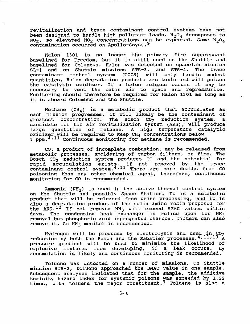
revitalization and trace contaminant control systems have notbeen designed to handle high pollutant loads. N204 decomposes toNO2, so elevated NO2 concentrations can be expected. Some N204contamination occurred on Apollo-Soyuz. 9
Halon 1301 is no longer the primary fire suppressantbaselined for Freedom, but it is still used on the Shuttle andbaselined for Columbus. Halon was detected on spacelab mission
SL-I and on Shuttle missions STS-3, and STS-4. The trace
contaminant control system (TCCS) will only handle modest
quantities. Halon degradation products are toxic and will poison
the catalytic oxidizer. If a halon release occurs it may be
necessary to vent the cabin air to space and repressurize.
Monitoring should therefore be required for Halon 1301 as long asit is aboard Columbus and the Shuttle.
Methane (CH4) is a metabolic product that accumulates aseach mission progresses. It will likely be the contaminant of
greatest concentration. The Bosch CO 2 reduction system, acandidate for the air revitalization system (ARS), will produce
large quantities of methane. A high temperature catalytic
oxidizer will be required to keep CH 4 concentrations below1 ppm. 4,11 Continuous monitoring for methane is recommended.
CO, a product of incomplete combustion, may be released from
metabolic processes, smoldering of carbon filters, or fire. The
Bosch CO 2 reduction system produces CO and the potential forrapid accumulation exists, if not removed by the tracecontaminant control system. 4,11 There are more deaths from CO
poisoning than any other chemical agent, therefore, continuous
monitoring for CO is recommended.
Ammonia (NH3) is used in the active thermal control system
on the Shuttle and possibly Space Station. It is a metabolic
product that will be released from urine processing, and it is
also a deqradation product of the solid amine resin proposed for
the ARS. 12 If not removed NH 3 will exceed SMAC values within
days. The condensing heat exchanger is relied upon for NH 3removal but phosphoric acid impregnated charcoal filters can also
remove it. An NH 3 monitor is recommended.
Hydrogen will be produced by electrolysis and used in CO 2
reduction by both the Bosch and the Sabatier processes. 4,11,13 A
pressure gradient will be used to minimize the likelihood of
explosive mixtures from developing, if a leak occurs. H 2
accumulation is likely and continuous monitoring is recommended.
Toluene was detected on a number of missions. On Shuttle
mission STS-2, toluene approached the SMAC value in one sample.
Subsequent analyses indicated that for the sample, the additive
toxicity hazard index for systemic poisons was exceeded by 1.22times, with toluene the major constituent. 9 Toluene is also a
5-6

contaminant which off-gases from the solid amine resin of theARS. 12
Trimethylamine is a principal breakdown product of the solid
amine resin of the ARS. The trimethylamine concentration hasexceeded safe limits in tests of the ARS. 12 Because of the
numerous trace organics off-gassing from solid amine process a
post sorbent bed such as phosphoric acid impregnated charcoalwill be used.
Glutaraldehyde escaped containment on Spacelab mission SL-
DI. Glutaraldehyde is a preservative and disinfectant with
irritating properties. It may also be used in electrophoresisexperiments on Space Station.
Silicon oil was released on mission 61A, wetting surfaces
and making decontamination difficult. Silicon compounds are
catalyst poisons and will occur on Space Station.
Freons have been detected on all Shuttle missions. 14 The
degradation products are corrosive, irritating, toxic, and
catalyst poisons. Freon 12 will be on Freedom and continuous
monitoring is recommended.
A computer model developed from Shuttle activated charcoal
canister analysis for TCCS contaminant removal studies indicated
that five contaminants may exceed SMAC values: propenal
Cacrolein), an irritant; benzene, a systemic poison and
carcinogen; o-diethylphthalate, an irritant; propylfluorosilane,
an irritant and catalyst poison; and 2-methylhexane, a central
nervous system depressant. 15 Benzene has also temporarilyexceeded SMAC values during preflight off-gassing tests. 1
Ethanal (acetaldehyde), ethanol, dichloromethane, and
acetone have a high frequency of occurrence on shuttle missionsand are likely to be present on Freedom. 14
Oxidation products will be produced in the catalytic
oxidizer. Post sorbent beds are necessary to prevent the releaseof oxidants and free radicals to the cabin air from the TCCS.
Also, it has been hypothesized that secondary pollutants are
important in cabin atmospheres. Trial simulations have indicated
that spacecraft cabins may develop elevated NO 2 concentrations
and 03 concentrations exceeding SMAC values. 16 Oxidation
products, NO2, 03, and formaldehyde, were among the contaminants
suspected of causing irritation on Shuttle flights, although
particulates from biological sources were an undisputed cause ofcrew discomfort. 17 Intermittent monitoring is recommended forthese contaminants.
5-7

Contaminant Load Model
The Space Station trace contaminant load model is being used
to design the ECLSS such that no substance will exceed theSMAC. 18 In the model the generation rates in mg/day for 214
contaminants were estimated for the Space Station, consisting of
two habitation modules, two laboratory modules and a logistics
module. That configuration is slightly larger than the
configuration presently baselined. The generation rates, thecorresponding SMACs, and the Space Station volume (900 M 3) were
used to estimate the time required to reach _ SMAC, provided no
removal mechanisms were operating. Those agents without a SMAC
were assigned a conservative value of 0.I mg/M 3. The time in days
is given by:
T½SMA C = SMAC (mg/M 3) ISS Volume (900 M3)] (0.5)Generation rate (mg/day)
Contaminants not reaching ½ SMAC within 365 days would be
controlled by leakage alone, provided all contaminant sources
were considered by the model. In such a case, monitoring would
not be necessary. Any contaminant which would not reach ½ SMAC
within 90 days could be excluded from monitoring requirements
(provided all contaminant sources were considered by the model),
since the SMAC would not be reached for 180 days. Presumably,
samples will be returned for exhaustive ground based analysis atleast every 180 days, thus providing adequate time for
identifying any etiological agent and remedial action.
From the trace contaminant load model analysis, 34contaminants were identified and listed below as candidates for
onboard monitoring:
methanol
isopropyl alcohol
isobutyl alcohol
n-butyl alcohol
cyclohexanol
n-butylaldehydehexanal
heptanal
m-xyleneindene
propylbenzene
p-cymene
ethyl cellosolve
butylacetatefuran
sylvan
ethylacetoxyacetate
vinyl chloride
allyl chloridechlorobenzene
isobutylene chloride
trichloroethylene
tetrachloroethylene
methyl ethyl ketone
methyl isobutyl ketone
cyclopentanone
methylheptanoneisobutyl ketoneacetonitrile
nitromethane
mercury
trimethylsilanol
p-dioxane
tetramethyl-l,2-epoxyethane
5-8
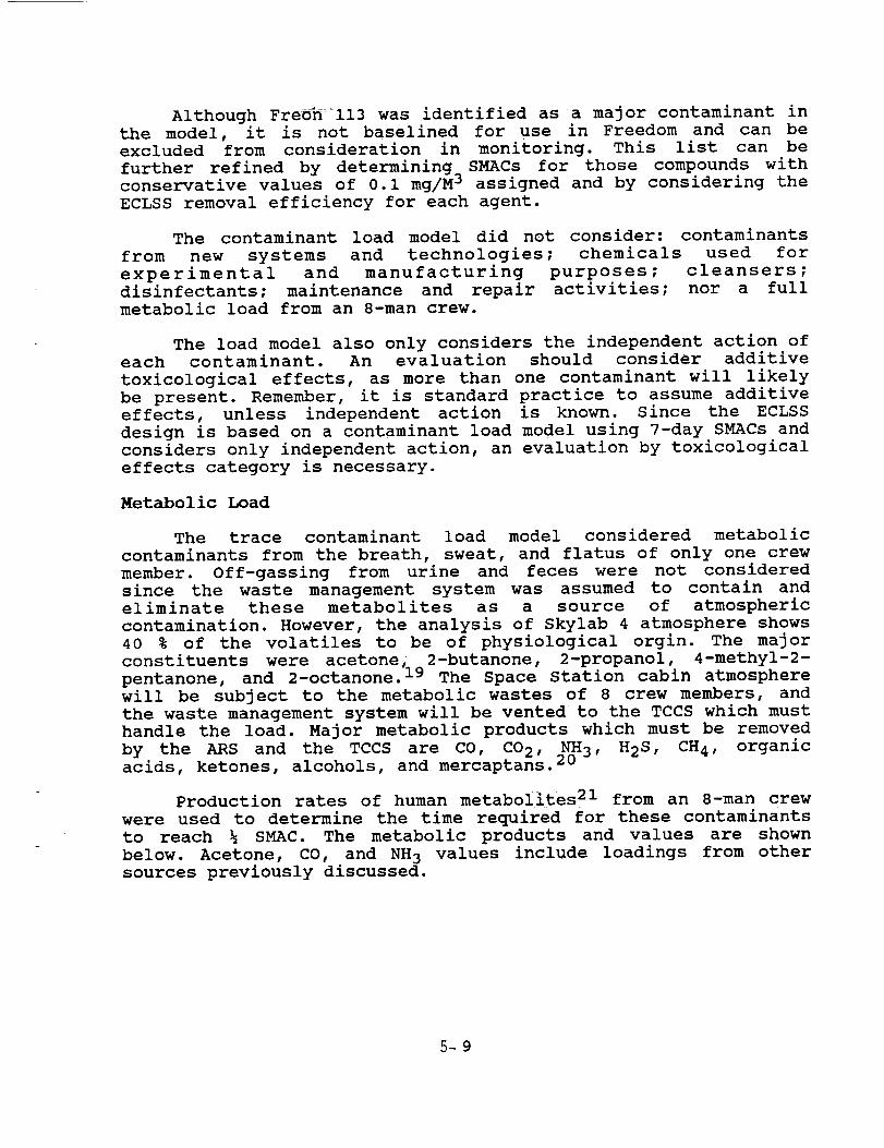
Although FreSh _ 113 was identified as a major contaminant inthe model, it is not baselined for use in Freedom and can beexcluded from consideration in monitoring. This list can befurther refined by determining_ SMACs for those compounds withconservative values of 0.i mg/M3 assigned and by considering the
ECLSS removal efficiency for each agent.
The contaminant load model did not consider: contaminants
from new systems and technologies ; chemicals used for
experimental and manufacturing purposes ; cleansers ;disinfectants; maintenance and repair activities; nor a full
metabolic load from an 8-man crew.
The load model also only considers the independent action of
each contaminant. An evaluation should consider additive
toxicological effects, as more than one contaminant will likely
be present. Remember, it is standard practice to assume additive
effects, unless independent action is known. Since the ECLSS
design is based on a contaminant load model using 7-day SMACs andconsiders only independent action, an evaluation by toxicological
effects category is necessary.
Metabolic Load
The trace contaminant load model considered metabolic
contaminants from the breath, sweat, and flatus of only one crew
member. Off-gassing from urine and feces were not considered
since the waste management system was assumed to contain and
eliminate these metabolites as a source of atmospheric
contamination. However, the analysis of Skylab 4 atmosphere shows40 % of the volatiles to be of physiological orgin. The major
constituents were acetone, 2-butanone, 2-propanol, 4"methyl-2-
pentanone, and 2-octanone. 19 The Space Station cabin atmosphere
will be subject to the metabolic wastes of 8 crew members, and
the waste management system will be vented to the TCCS which must
handle the load. Major metabolic products which must be removed
by the ARS and the TCCS are CO, CO2, _3, H2S, CH4, organicacids, ketones, alcohols, and mercaptans.
Production rates of human metaboiites 21 from an 8-man crew
were used to determine the time required for these contaminants
to reach ½ SMAC. The metabolic products and values are shown
below. Acetone, CO, and NH 3 values include loadings from other
sources previously discussed.
5-9

METABOLIC PRODUCTS(8-MAN CREW)
Contaminant TIME to ½ SMAC
(Days)CO 6.9
NH 3 2.1Acetone 76
Ethanol 8.1
Methyl Mercaptan 14
Ethyl Mercaptan 14
Propyl Mercaptan 14
Pyruvic Acid 1.0Indole 0.7
Skatole 1.2
Fire
An unusual odor and crew headaches occurred on Shuttle
flight STS-6. Burnt wire insulation from an electrical short was
the suspected causal agent. 9 Electrical fire can produce a number
of noxious agents including halogenated organics, benzene
derivatives, nitriles, and cyanates. 22 Space Station design must
be able to handle such contingencies either through the TCCS or asmoke removal unit, 23 without having to rely on venting the cabin
air to space and repressurizing. The trace gas monitoring system
should be able to detect and quantify contaminants representative
of those generated by an electrical short or fire.
To ascertain monitoring needs following a combustion
incident, the hypothesized concentrations of pyrolysis products
after a fire and their corresponding SMACs were used to estimate
a factor proportional to monitoring importance _ ........
Contaminant Concentration 23 SMAC Concentration/SMAC
(PPS) (PPM)
CO2 i0,000-i00,000 5,000 2-20
CO 3,000-30,000 25 120-1200HCN 5-100 1 5-100
HCI 5-100 1 5-100
NO2 i-I00 0.5 2-200
H2S 1 2 0.5
S02 i00 1 i00
Although the concentration of pyrolysis products vary widely
from fire to fire, smoke detectors provide adequate warning of
toxic products, since smoke is generally produced in copious
amounts. Analysis of fire reports involving death or serious
injury where smoke detectors have been installed show that thedetector was inoperative or evacuation was not possible.
5-10

Investigation of fire fatalities have shown CO to be the primarytoxicant with HCN often present in toxic quantities. However,documented cases of HCN being the primary toxicant are rare. 24
Of the toxic gaseous products presented above, CO isexpected to exist in highest concentration relative to its SMAC,therefore, if CO is below its SMAC value then the other toxicproducts would likely be also. Because of the uncertainty ofpredicting the concentration of pyrolysis products after a fire,monitoring should be considered for other toxic products as well:HCN, NO2, HCI, and SO2. Although no specific data could be foundon the production of COC12, HF, COF2, and short chain aldehydes,contingency monitoring should be considered because of theirtoxic and corrosive action.
For fire safety concerns, CO2 will be used for firesuppression, followed by venting cabin air to space andrepressurizing. Smoke detectors are an integral part of the firedetection and suppression system. To protect from toxiccombustion products, infrared monitors have been previouslyrecommended for CO, hydrogen fluoride (HF), and hydrogen cyanide(HCN). 25
Volatiles will be released to the atmosphere fromelectrolysis and from phase change urine processinq. Carboxylicacids and phenols will be major contaminants. 26,27 Iodinationproducts from the water disinfection process may cross theair/water interface and permeate the life support environment.The identity of these products, their expected concentrations,and their medical effects are largely unknown. 28 However, thebyproduct concentrations and effects of iodination are probablyless than those resulting from chlorination.
CONCLUSIONS
The monitoring system for Space Station Freedom must beadaptable to accommodate new parameters and concentration ranges.All agents should be monitored that have a reasonable probabilityof occurrence at or above some action level, such as ½ SMAC. Thiswould include the capability to monitor for toxics after a fireor spill so a pressurized element could be declared safe forentry or for removing protective gear donned during an incident.The analytical method relied upon must be able to quantify ataction level concentrations. The basis for monitoring should bethe contaminants: toxicity, quantities or production rates,removal efficiencies of the ECLSS system, and capacity to poisonthe ECLSS system. The importance for monitoring is increased bythe relatively low air flow rate through the TCCS and highreliance on the TCCS for contaminant removal.
Continuous monitoring of cabin return air is required for
major components and those critical for life support. The minimum
5-11

monitoring effort should include continuous monitoring for: N2,02, CO2, CO, H20, H2, CH4, non-methane hydrocarbons, aromatics,and halocarbons. There should be a sample line to each moduleroutine comparison of atmospheres from remote sections of thespacecraft.
A monitor or probe will be needed in the EVA airlock foranalysis of propellants: N204, hydrazine, and monomethylhydrazine.
Other chemicals targeted for routine monitoring include:Freon 12, HCI, HCN, NH3, 03, NO2, H2S, HF, formaldehyde, Halon1301, toluene, acetaldehyde, ethanol, acetone, dichloromethane,glutaral dehyde, t rimethylamine, benzene, o-diethylphthalate,propyl fluorosil ane, 2-methylhexane, acrol ein, methanol, vinylchloride, isopropyl alcohol, allyl chloride, isobutyl alcohol,chlorobenzene, n-butyl alcohol, isobutylene chloride,cyclohexanol , trichloroethylene, n-butylaldehyde,tetrachloroethylene, hexanal, methyl ethyl ketone, heptanal,methyl isobutyl ketone, m-xylene, cyclopentanone, indene,methy i hept anone, propyl ben zene, isobutyl ketone, p-cymene,acetonitrile, ethyl cellosolve, nitromethane, butylacetate,mercury, furan, trimethylsilanol, sylvan, p-dioxane,ethylacetoxyacetate, tetramethyl-l, 2-epoxyethane, methylmercaptan, ethyl mercapt an, propyl mercaptan, pyruv ic acid,indole, and skatole.
The chemical list can be refined by considering the removalefficiencies of the ECLSS and by assigning SMAC v_alues _to thosecompounds for which a value of 0.I mg/M3-was_assumed. Also, anevaluation by .............. effects category should be done toaddress additive effects. The above list was determined byconsidering independent action only, and more than onecontaminant wiil 5e present_ ..........
Each experiment and manufacturing process must be evaluatedin great detail for possible sources of cabin contamination. Labfacilities will be sources of biologicals, combustion andoxidation products, acid gases, metal and crystal fumes, andassorted lab wastes. The lab racks should be equipped withmonitoring devices specific to the process being contained. Thechemical storage area should also be equipped with a monitoringprobe.
Finally, sample collection and preservation will have to becontinued for ground based analyses, to confirm the accuracy andreliability of the onboard monitoring system.
5-12

REFERENCES
i. Casserly, D. M. and D. M. Russo: "A Rationale for Atmospheric
Monitoring on Space Station Freedom." Proceedings of the 19th
Intersociety Conference on Environmental Systems, San Diego, CA,
July 1989. Paper No. 89154.
2. Davis, R. G. and J. L. Reuter: "Intermodule Ventilation
Studies for the Space Station." Proceedings of the 17th
Intersociety Conference on Environmental Systems, Seattle, WA,
July 1987. Paper No. 871428.
3. Reuter, J. L., L. D. Turner, and W. R. Humphries: "Preliminary
Design of the Space Station Environmental Control and Life
Support System." Proceedings of the 18th Intersociety Conferenceon Environmental Systems, San Francisco, CA, July 1988. Paper No.
881031.
4. Ray, C. D., K. Y. Ogle, R. W. Tipps, R. L. Carrasquillo and P.
Wieland: "The Space Station Air Revitalization Subsystem Design
Concept." Proceedings of the 17th Intersociety Conference on
Environmental Systems, Seattle, WA, July 1987. Paper No. 871448.
5. Janssen, J. E. and D. T. Grimsrud: "Ventilation Standard DraftOut for Review." ASHRAE Journal. pp. 43-45. November 1986.
6. Junge, J.: "A Maintenance Work Station for Space Station."
Proceedings of the 16th Intersociety Conference on Environmental
Systems, San Diego, CA, July 1986. Paper No. 860933.
7. Harvey, W. T., S. M. Farrell, J. A. Howard Jr., and F.
Pearlman: "Space Station Health Maintenance Facility."
Proceedings of the 16th Intersociety Conference on Environmental
Systems, San Diego, CA, July 1986. Paper No. 860922.
8. Perry, J. P. and W. R. Humphries: "Process Material Management
in the Space Station Environment." Proceedings of the 18thIntersociety Conference on Environmental Systems, San Francisco,
CA, July 1988. Paper No. 880996.
9. Rockoff, L. A.: "Internal Contamination Issues." Proceedings
of the Seminar on Space Station Human Productivity, NASA, Ames
Research Center, Moffett Field, CA, March 1985. Paper N85-29543.
i0. Buoni, C., R. Coutant, R. Barnes, and L. Slivon: "Space
Station Atmospheric Monitoring Systems." Proceedings of the 37thInternational Astronautical Congress, Innsbruck, Austria, October
1986. Paper A87-15845.
5- 13

ii. Wagner, R. C., R. Carrasquillo, J. Edwards, and R. Holmes:
"Maturity of the Bosch CO 2 Reduction Technology for Space Station
Application." Proceedings of the 18th Intersociety Conference on
Environmental Systems, San Francisco, CA, July 1988. Paper No.880995.
12. Wood, P. C. and T. Wydeven: "Stability of IRA-45 Solid Amine
Resin as a Function of Carbon Dioxide Absorption and Steam
Desorption Cycling." Proceedings of the 17th IntersocietyConference on Environmental Systems, Seattle, WA, July 1987.
Paper No. 871452.
13. Boehm, A. M., C. K. Boynton, and R. K. Mason: "Regenerative
Life Support Program Equipment Testing." Proceedings of the 18th
Intersociety Conference on Environmental Systems, San Francisco,
CA, July 1988. Paper No. 881126.
14. Coleman, M. E.: "Summary Report of Post Flight Atmospheric
Analysis for STS-I to STS 41C." NASA-JSC Memorandum SD4-84-351,
January 1985.
15. Schwartz, M. R. and S. I. Oldmark: "Analysis and Composition
of a Model Trace Gaseous Mixture for a Spacecraft." Proceedings
of the 16th Intersociety Conference on Environmental Systems, San
Diego, CA, July 1986. Paper No. 860917.
16. Brewer, D. A. and J. B. Hall Jr.: "A Simulation Model for the
Analysis of Space Station Gas-Phase Trace Contaminants." Acta
Astronautica. Vol. 15, No. 8, pp. 527-543, 1987.
17. Brewer, D. A. and J. B. Hall Jr.: "Effects of VaryingEnvironmental Parameters on Trace Contaminant Concentrations in
the NASA Space Station Reference Configuration." Proceedings of
the 16th Intersociety Conference on Environmental Systems, San
Diego, CA, July 1986. Paper No. 860916.
18. Leban, M. I. and P. A. Wagner: "Space Station Freedom Gaseous
Trace Contaminant Load Model Development." Proceedings of the
19th Intersociety Conference on Environmental Systems, San Diego,
CA, 1989. Paper No. 891513.
19. Liebich, H. M., W. Bertch, A. Zlatkis, and H. J. Schneider:
"Volatile Organic Components in the Skylab 4 Spacecraft
Atmosphere." Aviation, Space. and Environmental Medicine. Vol.
46, No 8, 1975.
20. Poythress, C.: "Internal Contamination in the Space Station."
Proceedings of the Seminar on Space Station Human Productivity,NASA, Ames Research Center, Moffett Field, CA, March 1985. Paper
N85-29549.
5- 14

21. Coleman, M. E., D. L. Pierson and N. M. Cintron:
"Toxicological Requirements and Support Plan for the SpaceStation." JSC 32016, NASA-JSC, Houston, TX, June 1988.
22. Nulton, C. P. and H. S. Silvus: "Ambient Air Contamination-
Characterization and Detection Techniques." Proceedings of the
Seminar on Space Station Human Productivity. NASA, Ames Research
Center, Moffett Field, CA, March 1985. Paper No. N85-29546.
23. Birbara, P. J. and J. T. Leonard: "A Smoke Removal Unit."
Proceedings of the 17th Intersociety Conference on Environmental
Systems, Seattle, WA, July 1987. Paper No. 871449.
24. National Fire Protection Association:
Handbook." 15th Ed. Quincy, MA, NFPA, 1981.
"Fire Protection
25. Cole, M. B.: "Space Station Internal Environmental and Safety
Concerns." In Spacecraft _ire Safety. NTIS HC A07/MF A01. NASA,1987.
26. Dehner, G. F. and D. F. Price: "Thermoelectric IntegratedMembrane Evaporation Subsystem Testing." Proceedings of the 17th
Intersociety Conference on Environmental Systems, Seattle, WA,July 1987. Paper No. 871446.
27. Fortunato, F. A. and K. A. Burke: "Static Feed Electrolyzer
Technology Advancement for Space Application." Proceedings of the
17th Intersociety Conference on Environmental Systems, Seattle,WA, July 1987. Paper No. 871450.
28. Sauer, R. L., D. S. Janik, and ¥. R. Thorstenson: "Medical
Effects of Iodine Disinfection Products in Spacecraft Water."Proceedings of the 17th Intersociety Conference on Environmental
Systems, Seattle, WA, July 1987. Paper No. 871490.
5-15


N90-24978
EFFECT OF FLUID COUNTERMEASURES OF VARYING OSMOLARITY ON
CARDIOVASCULAR RESPONSES TO ORTHOSTATIC STRESS
Final Report
NASA/ASEE Summer Faculty Fellowship Program--1989
Johnson Space Center
Prepared By:
Academic Rank:
University & Department:
NASA/JSC
Directorate:
Division:
Branch:
JSC Colleague:
Date Submitted
Contract Number:
John E. Davis
Assistant Professor
Alma College
Department of Exercise andHealth Science
Alma, Michigan 48801
Space and Life Sciences
Medical Sciences
Space BiomedicalResearch Institute
John B. Charles
August ii, 1989
NGT 44-001-800
6-I
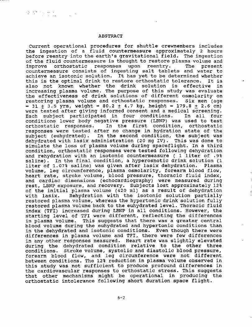
=
ABSTRACT
Current operational procedures for shuttle crewmembers includes
the ingestion of a fluid countermeasure approximately 2 hours
before reentry into the earth's gravitational field. The ingestion
of the fluid countermeasure is thought to restore plasma volume and
improve orthostatic responses upon reentry. The present
countermeasure consists of ingesting salt tablets and water to
achieve an isotonic solution. It has yet to be determined whether
this is the optimal drink to restore orthostatic tolerance. It isalso not known whether the drink solution is effective in
increasing plasma volume. The purpose of this study was evaluate
the effectiveness of drink solutions of different osmolarity on
restoring plasma volume and orthostatic responses. Six men (age
= 31 ± 3.5 yrs, weight = 80.2 ± 4.7 kg, height = 179.8 _ 2.6 cm)
were tested after giving informed consent and a medical screening.
Each subject participated in four conditions. In all fourconditions lower body negative pressure (LBNP) was used to test
orthostatic responses. In the first condition, orthostatic
responses were tested after no change in hydration state of the
subject (euhydrated). In the second condition, the subject was
dehydrated with lasix administration (20 mg IV). This was done to
simulate the loss of plasma volume during spaceflight. In a third
condition, orthostatic responses were tested following dehydration
and rehydration with an isotonic countermeasure ( 1 liter of .9%
saline). In the final condition, a hyperosmotic drink solution (i
liter of 1.07% saline) was given after lasix dehydration. Plasma
volume, leg circumference, plasma osmolarity, forearm blood flow,
heart rate, stroke volume, blood pressure, thoracic fluid index,
and cardiac dimensions (echocardiography) were measured during
rest, LBNP exposure, and recovery. Subjects lost approximately 12%
of the initial plasma volume (420 mi) as a result of dehydration
with lasix. Rehydration with the isotonic solution partially
restored plasma volume, whereas the hypertonic drink solution fully
restored plasma volume back to the euhydrated level. Thoracic fluid
index (TFI) increased during LBNP in all conditions. However, the
starting level of TFI were different, reflecting the differences
in plasma volume. This suggests that there was a greater centralblood volume during the euhydrated and hypertonic conditions than
in the dehydrated and isotonic conditions. Even though there were
differences in plasma volume and TFI, there were few differences
in any other responses measured. Heart rate was slightly elevated
during the dehydrated condition relative to the other three
conditions. Stroke volume, systolic and diastolic blood pressure,
forearm blood flow, and leg circumference were not different
between conditions. The 12% reduction in plasma volume observed in
this study was not sufficient to produce profound differences in
the cardiovascular responses to orthostatic stress. This suggests
that other mechanisms might be operational in producing the
orthostatic intolerance following short duration space flight.
6-2

INTRODUCTION
Orthostatic hypotension has been commonly reported after spaceflight by crewmembers both during reentry and upon egress from aspacecraft. The decrease in blood pressure could have severeramifications on the ability of the crew to control the spacecraftduring reentry and any emergency egress that might occur.Orthostatic intolerance after short duration space flight (5-14days) is thought to be a result of a reduction in plasma volume.
Plasma volume decreases during spaceflight as a result of anegative water balance. The decrease in plasma volume has beenreported to be between 8 and 15% (8). In microgravity, there is aredistribution of fluids from the lower body to the head and upperbody. Originally this was thought to result in a suppression ofantidiuretic hormone and a potentiated diuresis (7). Recentstudies have suggested that atrial natriuretic factor (ANF) isinvolved in the control of plasma volume during volume expansion(9,10). It is possible that ANF is involved in plasma volumeregulation during space flight.
Crew members are well suited to a microgravity environment.
However, upon return to a gravitational environment they are
hypovolemic relative to preflight and thus more prone toorthostatic intolerance. A study by Bungo and Charles(l) has
indicated that fluid ingestion prior to reentry minimizes the
impairment of orthostatic responses following spaceflight. Theyattribute the improvement in orthostatic responses in those
crewmembers that ingested a fluid countermeasure to a restoration
of plasma volume as a direct result of the ingestion of thesolution. No controlled measurements of plasma volume with and
without the countermeasure have ever been made.
The present countermeasure consists of ingesting salt tabletsand eight ounces of water approximately 2 hours before reentry.
This is thought to result in an isotonic solution (.9% saline).
A recent study by Bungo et al. (2) has looked at the ingestion of
drinks of varying osmolarity and composition on plasma volume.
They found that a hypertonic drink solution was more effective in
increasing and maintaining plasma volume (4 hours).
To date, no studies have looked at the relationship between
plasma volume and LBNP tolerance in a controlled study. Thepurpose of this study was to evaluate the effectiveness of drink
solutions of varying osmolarity on restoring plasma volume and
orthostatic responses.
HISTORICAL BACKGROUND
For a detailed historical background, please see 1988 Summer
Faculty Fellowship Report (4).
6-3

METHODS
Six volunteers were recruited for the study by KrugInternational. All subjects were medically screened and given adetailed explanation of the study. Informed consent was obtainedfrom all subjects before participating in the study. The studywas approved by the JSC IRB. Each subject participated in fourconditions: i) LBNP control - euhydrated (EUH), 2) LBNP followinglasix dehydration (DEH), 3) LBNP following lasix dehydration (20mg IV) and rehydration (ISO) with an isotonic drink solution (Iliter of a .9% saline solution), and 4) LBNP following dehydrationwith lasix and rehydration (HYPER) with a hypertonic drink (I literof a 1.07% saline solution). Control LBNP tests were administeredto each subject until a consistent pattern of responses wasproduced. Lasix was used to simulate the decrease in plasma volumeobserved during spaceflight. This dosage of lasix producedapproximately a 12% reduction in plasma volume from the euhydratedlevel as has been reported previously (4). We randomized the orderof treatments to eliminate any effects of one LBNP test on asubsequent test. All experiments began at the same time of day foreach individual subject to eliminate any circadian effects on ourfindings. Testing began 2 hours after the ingestion of a smallmeal. Lower body negative pressure was performed approximately 3hours and 30 minutes after ingestion of fluids. At least 72 hourswas allowed between testing sessions.
Lower body negative pressure was applied using a chamber sealedat the waist with a rubber gasket. A vacuum pump was then used towithdraw air out of the chamber. The LBNP protocol is displayed inTable i. The test was terminated if the subject's systolic bloodpressure dropped suddenly (greater than 25 mmHg in 1 minute),systolic pressure reached 80 mmHg, bradycardia occurred (drop inHR greater than 15 BPM), subject distress, or subject request.Before, during, and immediately after LBNP a series ofphysiological measures described below were determined everyminute. Only the results from the last 3 minutes from each stagewere analyzed as the first 2 minutes at each stage representtransition responses.
Table i. LBNP protocol
Time at Stage (min) Pressure (mmHg)
20 05 -55 -i05 -205 -305 -405 -505 0
6-4

Blood samples were taken from an antecubital vein before lasixinjection (baseline) after lasix injection, after drink ingestion,2 and 1/2 hours after drink ingestion, 90 minutes before, andimmediately after LBNP. Changes in plasma volume were calculated
from hematocrit (microhematocrit technique) and hemoglobin (Coulter
Counter) ratios using the formula of Dill and Costill (5). A
direct measurement of plasma volume was performed once (human serum
labeled 125-I) in each subject before the first experimental
testing. This value was used as the absolute plasma volume and
changes were expressed relative to that value. Plasma osmolalitywas determined using freezing point depression on all blood
samples. A 5 ml sample was required to do all of the hematological
analysis. Plasma levels of antidiuretic hormone, atrialnatriuretic factor, aldosterone, and catecholamines (epinephrine,
norepinephrine) were measured for certain blood samples.
Leg circumference measurements were made every minute with a
mercury-in-silastic strain gauge. The changes in leg circumference
during LBNP exposure were used to approximate the amount of venous
pooling in the legs.
Venous occlusion plethysmography with a mercury-in-silastic
strain gauge was used to measure forearm blood flow. The forearmvasoconstrictor response as indicated by this technique was
measured at each step of LBNP. Heart rate was determined using a
three lead EKG. Blood pressure was measured once a minute using
a standard auscultatory technique. 2-D and M-Mode echocardiography
(ATL 4000 S/LC ultrasound system, ATL, Botheli, WA.) was performedat each stage of LBNP in order to assess relative changes in leftventricular dimensions with LBNP. Thoracic fluid index and stroke
volume were measured with bioelectrical impedance (BOMED).
Thoracic fluid index represents the impedance to current flow and
thus is inversely related to the amount of fluid in the chest.
EMG was used to assess abdominal and leg muscle tension in order
to monitor for muscle tensing. The subject was asked to maintain
a resting EMG level throughout all LBNP tests.
RESULTS
Plasma Volume and Plasma Osmolarity.
Plasma volume decreased by approximately 12% as a result of lasix
injection (Figure I). Drink ingestion with the isotonic drink
solution partially restored plasma volume to euhydrated levels.
Ingestion of the hypertonic drink solution (HYPER) fully restored
plasma volume to euhydrated levels. Plasma osmolarity did not
change through any of the dehydration or rehydration procedures
(Figure 2). This indicates the fluid losses and gains wereisotonic relative to the plasma. There was a slight increase in
plasma volume in all four conditions from the post drink to the pre
6-5

LBNP sample. This was probably a result of a change in posture(sitting to supine). During LBNP there was a decrease in plasmavolume in all four conditions. This hemoconcentration has beencommonly observed in the literature.
Thoracic Fluid Index.
Thoracic fluid index (TFI) increased in all four conditions withincreasing levels of LBNP (Figure 3). This represents an increasein blood pooling in the legs and less in the thorax. The startingTFI was also different between condition, reflecting the differentplasma volumes at the start of LBNP.
Heart Rate and Stroke Volume.
Heart rate increased in all conditions with increasing levels ofLBNP (Figure 4). Heart rates tended to be higher at the higherlevels of LBNP in the dehydrated condition than in the euhydrated,isotonic, or hypertonic conditions. Stroke volume decreased withincreasing LBNP (Figure 5). Even though plasma volume and TFI weredifferent between the conditions, stroke volumes were similar inthe four conditions.
Blood Pressure.
Systolic blood pressure decreased with increasing levels of LBNP(Figure 6). However, there were no differences in systolic bloodpressure between conditions. Diastolic pressure tended to increaseat the higher levels of LBNP in the dehydrated, isotonic, andhyperhydrated conditions (Figure 7). There were no differences inmean arterial blood pressure with increasing LBNP stage or betweenconditions.
Forearm Blood Flow and Leg Circumference.
Forearm blood flow decreased in all conditions with increasing
levels of LBNP (Figure 8). This was a reflex response to maintain
blood pressure in the face of falling venous return. There were no
differences between conditions. Leg circumference increased with
increasing levels of LBNP (Figure 9). As LBNP level increases,
venous pooling in the legs increase. There were no differences
in leg circumference with differing hydration states.
6-6

DISCUSSION
Lasix reduced plasma volume by 12% in the present study. Thiswas similar to the reduction observed in our previous study (4).Rehydration with an isotonic solution (present operationalcountermeasure) partially restored plasma volume to the euhydratedlevel. When subjects ingested the hypertonic solution, plasmavolume was fully restored to the euhydrated level. These datasupport a recent study (2) which demonstrated that plasma volumeincreased following ingestion of both an isotonic and hypertonicdrink solution, but the plasma volume was maintained longer withthe hypertonic solution.
Bungo and Charles (I) found that ingestion of a drink solution
improved orthostatic tolerance after spaceflight. They attributedthe decrease in orthostatic tolerance (higher heart rates, lower
blood pressures) to the decrease in plasma volume that has been
observed after space flight (8). We expected to see improved
orthostatic responses after rehydration with both the isotonic and
hypertonic drink solutions in comparison to the dehydratedcondition, our model for space flight. However, there were only
minor differences between conditions in heart rate, stroke
volume,blood pressure (systolic and diastolic), forearm blood flow,
and leg circumference.
It is possible that the differences in plasma volume produced in
this study were not great enough to produce marked differences in
cardiovascular responses. Other studies using exercise as a
stressor have shown that plasma volume differences of the magnitude
observed in this study produce significant differences in
cardiovascular responses (6).
It is also possible that the reduction in plasma volume produced
by lasix administration does not truly model spaceflight. Lasix
did produce a 12% reduction in plasma volume which is consistent
with space flight reductions in plasma volume. Our model might not
have produce some of the other physiological alterations that have
been observed with space flight. However, most of the alterations
that would influence orthostatic responses are thought to occur in
response to longer duration space flight (greater than 14 days).
Although a recent study by Convertino et al. (3) has demonstrated
changes in venous compliance with 4 days of 6 ° head down bed rest.
This reduction in venous compliance was inversely related to the
loss of the size of the leg muscle compartment. This might be a
contributing factor to the orthostatic intolerance that occurs
after short duration spaceflight and might be more important than
plasma volume alterations.
6-7

Another explanation could be the difference in the composition ofthe countermeasure. The present countermeasure consists ofingesting 2 salt tablets and 8 ounces of water every 30 minutesfor 2 hours prior to reentry. In the present study, subjectsingested a solution of .9% saline. Perhaps there are differencesin the physiological effects of ingesting a solution verses salttablets and water.
CONCLUSIONS
A hypertonic drink solution was more effective in restoringplasma volume after dehydration than an isotonic solution. However,there were no differences in their effects on an orthostaticchallenge. These data suggest that the plasma volume differencesproduced in this study were not sufficient to produce differencesin the cardiovascular responses to an orthostatic challenge, orthere are other changes that occur during space flight that aremore important in determining orthostatic intolerance.
6-8

REFERENCES
i. Bungo, M. W., J.B. Charles, and P.C. Johnson. Cardiovascular
deconditioning during space flight and the use of saline as a
countermeasure to orthostatic tolerance. AerosDace Med. 56: 985-
990, 1985.
2. Bungo, M.W., M.A.B. Frey, J.M. Riddle, and J.B. Charles. Effect
of hyperosmotic saline ingestion on plasma volume and urine flow.
Aerospace Med. 60: 499, 1989.
3. Convertino, V.A., D.F. Doerr, K.L. Mathes, S.S. Stein, and P.B.
Buchanan. Changes in volume, muscle compartment, and compliance
of the lower extremities in man following 30 days of exposure to
simulated microgravity. Aerospace Med. 60: 653-658, 1989.
4. Davis, J.E. A model for plasma volume changes during short
duration space flight. In Summer Faculty Fellowship Report, eds.
R. Bannerot and S. Goldstein, NASA Report # NGT 44-005-803, 1988.
5. Dill, D.B., and D.L. Costill. Calculation of percentage changes
in volumes of blood, plasma, and red cells in dehydration. J. Appl.
__hysiol. 37:247-248, 1974.
6. Fortney, S.M., C.B. Wenger, J.R. Bove, and E.R. Nadel. Effect
of blood volume on forearm venous and cardiac stroke volume during
exercise. J. ApDI. Physiol. 55: 884-890, 1983.
7. Gauer, O.H., and J.P. Henry. Neurohumoral control of plasma
volume. Int Rev. Physiol. 9:145 -190, 1976.
8. Johnson, P.C. Fluid volume changes induced by spaceflight. Acta
Astro. 6:1335-1341, 1977.
9. Lang, R.E., H. Tholken, D. Ganten, F.C. Luft, H. Rushoka, and
T.H. Urger. Atrial natriuretic factor: a circulating hormone
stimulated by volume loading. Nature 314: 264-266, 1985.
I0. Sakamoto, H., and F. Marumo. Atrial natriuretic peptide
secretion in response to volume expansion and contraction in normal
man. Acta End. 118:260-268, 1988.
6-9

Figure 1. Plasma volume plotted as a function of sample number. Mean ÷ SE
m
E
EB
O_>
E(o
n
4000
38OO
3600
3400
3200
3OOO
28OO
Pre LBNP
Baseline
T!
Post Drink
_, Post LBNP
// ,!
LPost Lasix
1I ' I |
1 2 3' I ' i I
4 5 6
Sample Number
.... _ : : - 7
Figure 2__piasma 0smoiariiy plotted as a functi°n0f sample number. Mean + SE
295
E
(}E
v
>,
m
OEu_o
E1/)
m
n_
290
285
280
275 I ' I " I
1 2 3
I " !
5 6 7
----,Im-.-
..----IP--
#
E_DehIso
Hyper
EUHCB-IISOHYPER
!
Sample Number
6-10

Figure 3. Thoracic fluid index plotted as a function of LBNP stage. Mean + SE.
X¢D
"O¢..
m
"10ii
m
I1_
O
¢J
O¢,-
I--
32O
3O0
28O
26O
240
220
200-10 0 10 20 30 40 50 60
LBNP (mmHg)
G
EUH
ISOHYPER
6-11

Figure 4. Heart rate plotted as a function of LBNP stage• Mean + SE•
EQ.
J_v
Q)
n"
-r
100
80
60
4O • I • I " I I " I " ! '
0 0 10 20 30 40 50 60
LBNP (mmHg)
,0
BJ-i
iSO
t-WPF_R
Figure 5. Stroke volume plotted as a function of LBNP stage. Mean + SE.
Am
E
Q)E
m
O_>
Q)J¢OL-
140
120
100
8O
6O
4O • I " I I " I " I I
0 0 10 20 30 40 50 60
LBNP (mmHg)
EU-t
D_
IS(?HYPER
6-12
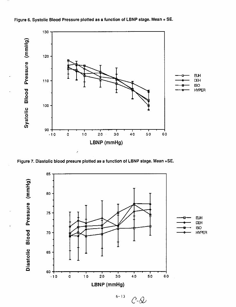
Figure 6. Systolic Blood Pressure plotted as a function of LBNP stage. Mean + SE.
A
EE
v
m
!.--
"IDOO
i
t_.ii
O
¢n
03
130
120
110
100
90
-10 0 10 20 30 40 50 60
LBNP (mmHg)
Figure 7. Diastolic blood presure plotted as a function of LBNP stage. Mean +SE.
l
i
EUHDEHISOHYPER
A
O).I-EE
t._
t_
O..
"IDOO
i
.ii
O
=i
¢3
85
80
75
7O
65
60
0
i
i
, l
, |
I • I
0 10
• I " I " I " I
20 30 40 50
LBNP (mmHg)
60
B.JHEEHISOHYPER
6,3

Figure 8. Forearm blood flow plotted as a function of LBNP stage. Mean + SE.
A
p.,m
E
tJ
OO
m
E
Om
I,I.
"OOO
m
EL_
4)
OIJ.
0
i
n
I I " I " I " I " I
0 0 10 20 30 40 50 60
LBNP (mmHg)
B.H
ISOHYPER
Figure 9. Change in leg circumference plotted as a function of LBNP stage. Mean + SE.
A
O1
EE
t-
¢_
ill==
E
!.--.!
qm!
¢0
p.,m
O_C
J=ro
8
6
4
2
-2 I ' I ' I I ' I I
0 10 20 30 40 50 60
LBNP (mmHg)
ELHCEH
ISOHYPER
6-14

N90-24979
SOLVING PROBLEMS BY INTERROGATING SETS OF KNOWLEDGE SYSTEMS:
TOWARD A THEORY OF MULTIPLE KNOWLEDGE SYSTEMS
FINAL REPORT
NASA/ASEE Summer Faculty Fellowship Program--1989
Johnson Space Center
Prepared By:
Academic Rank:
University & Department:
Andre de Korvin, Ph. D.
Professor
University of Houston - Downtown
Applied Mathematical Sciences
Houston, Tx. 77002
NASA / JSC
Directorate:
Division:
Branch:
JSC Colleague:
Date Submitted:
Contract Number:
Mission Support
Mission Planning and Analysis
Technology Development and Applications
Robert Lea, Ph.D.
August 11, 1989
NGT 44-001-800
7-1

ABSTRACT
The main purpose of the present work is to develop a theory for multiple knowledge systems. A
knowledge system could be a sensor or an expert system, but it must specialize in one feature. The
problem is that we have an exhaustive list of possible answers to some query (such as "What object is
it?"). By collecting different feature values, we should, in principle, be able to give an answer to the
query, or at least narrow down the list.
Since a sensor, or for that matter an expert system, do not in most cases yield a precise value for
the feature, uncertainty must be built into the model. Also, we must have a formal mechanism to be
able to put the information together. We chose to use the Dempster - Sharer approach to handle the
problems mentioned above.
We introduce the concept of a state of recognition and point out that there is a relation between
receiving updates and defining a set valued Markov Chain. Also, deciding what the value of the next
set valued variable is can be phrased in terms of classical decision making theory such as minimizing
the maximum regret. Other related problems are looked at.
7-2

INTRODUCTION
The purpose of the present work is to show how taking independent and very diverse evidence,
we can piece things together to arrive at an answer to the question: "What object is it?". We will take
the Dempster - Sharer approach to put the evidence together. Such an approach has recently been
taken in expert systems, see [2], [3], and [4]. However, to the best of this writer's knowledge, the
results shown here are original. We start out with a simple example.
Consider the following data which assigns masses to subsets o£ {Bird, Plane, & Superman}
according to the velocity observed:
VELOCITY B P S {BP} {BS} {PS} {BPS}
0- 100 .5 .1 .'1 .2 .04 .04 .02101 - 200 0 .4 .1 0 0 .5 0201 - 500 0 .5 .1 0 0 .4 0
0 .1> 500 .7 0 0 .2 0
NOTE:
• Birds don't fly with velocity :> 100.
• Superman likes to fly at over 500 but he can fly at any speed he wants to.
It should be noted that the sum across each row is 1. The interpretation of the results says, for
example, that at velocities exceeding 500 mph, the expert believes that the object is Superman. That
expert doesn't totally rule out the possibility of plane as he assigns a mass of. 1 to that event, and also
that expert is somewhat unsure if the object is Plane or Superman and therefore, he assigns a mass of
.2 to that aggregate. Note that we do not have Probability o£ {PS} be the sum of the Probability of P
and orS. Masses assigned to sets that are not singletons denote the uncertainty of the expert. For
example, .02 assigned to {BPS} reflects the degree of total ignorance that the expert has regarding
what the object is when the object travels at less than 100 mph. Such a mass assigned is typical of the
Dempster - Sharer approach to handle uncertainty in expert systems. See [10].
We now write down the data relative to observed color:
COLOR B P S {BP}
SILVER .05 .6 .05 .IWHITE .1 .1 .05 .5
RED .1 .1 .1 .2BLUE .1 .1 .1 .2
RED-BLUE .04 .04 .8 0
OTHER .6 I, .1 0 .3NOTE:
• Red and blue generate the same (conditional) mass
• A gray bird may appear silver
{BS} {PS} {BPS}
0 .15 .05.05 .15 .05.2 .2 .1.2 .2 .1
.05 .05 .020 0 0
• Superman wears red and blue but from some angles he may appear all red or all blue
• When flying at certain speeds, Superman may appear as a white or silver streak
• Color other than red, blue, white, silver rules out Superman
These two tables sum up the information collected from the experts. What we would like to do,
of course, is to put these two pieces of evidence together.
7-3

CONCEPTS AND NOTATIONS
We now will formally define the concept of a mass function. A mass function is a function from
subsets of the frame of discernment O into [0, 1] satisfying the following conditions:
(i) ra (_) = 0
2 m(A) = 1(ii)
If ml & rn2 are two mass functions, we define
(ml_m2)(C)= 2AAB=C
Where k is the conflict
where the sum is over all subsets of O
rnl(A)me(B) (l-k)
k = 2 ml(A)ra2(B)AAB=(_
The operation defined above defines how to put information together. If two knowledge systems
generate mI & m2, rnl _ m2 is the mass generated by combining the two knowledge systems, see
[10]. For a very readable interpretation of the combination rule in the setting of databases, see [12].
The belief generated by m is defined by
Bel(A) = 2 rn(B) overallsetsBsuchthat BCA. Alsowedefinetheplausabilityby
Pls(A) = 2 re(B) overallsetsBsuchthat BAA _
Now if the l th sighting takes place at time t z , set dt t = tt - tt_1
Obviously, dt t denotes the elapsed time between sightings. Assume that we have a weight
function 3, (.) satisfying
(i)O<_ (dtt)<-l, dt t >0
( ii ) ,k ( dt t ) non decreasing as a function of dt t
We use weight to adjust masses. There are two ways to adjust
ml(,)= mi(-)
a) mt(.)=k (dt t)m (o)+(l-_, (dt t))m t 1(.)l
b) rat(*) =3' (dt t)rn (-)+(1,t (dt l))m t l(*)l
If _ is high i.e., dt t high, go with the current observation
If ]k is low i.e., dt t low, go with the accumulated data.
Note that the first update is Markov - like as it only uses the mass collected on the previous sighting.
7-4

Forourexample,wecoulddefinetheweightfunctionby:
_tl / aooif dtl <_aoo1X ( dt t ) = t othervAse J
That is, after 5 minutes, forget the previous observations and assume that a new object is being
observed. The rationale for this is that the data has become too old to be reliable.
Going back to our example of bird, plane, and Superman, assume we have three sightings:
SIGHTING TIME
1:00 p.m.
1:01 p.m.
1:29 p.m.
dr,
6O
1740
VELOCITY
101-200
201-500
O- 100
COLOR
WHITE
WHITE
OTHER
The combined masses, not time adjusted are given below:
SIGHTING
1 m t (')
2 rn_ (.)
3 m_(.)
B
.811
p
.7750
.8101
.1024
S
.1
.0886
[BP}
0
.0866
{BS} {ps}
.125
.1013
{BPS}
0
0
0
The combined masses, time adjusted are given below:
SIGHTING B P S [BP} {BS} {PS} {BPS}
0 .775 .1 0 0 .125 01 m, (')
2 ms(-)
3 rn3(o)
NOTE:
0
.811
.78202
.1024
.09772 0 0 .12026 0
0 .0866 0 0 0
m 3 is not really time adjusted as sightings are more than 5 minutes apart.
7-5

Computing the belief, at each sighting, with respect to the time adjusted mass we have:
SIGHTING OBJECT Bel (')
0
.775
.I
0
.78202
.09772
Bel (-_ -)
1
.1
.775
I
.09772
.782O2
Bel (-) - Bel (-_ .)
-1
.675
-.675
.6843
-6843
.811
.1024
0
.1024
B11
I
.7086
-.7086
-1
CLASSIFICATION
The rationale for the table above is that Bel (.)- Bel (-"I .) measures how much a specific object
exceeds, belief- wise, its competition. This criterion was already used in [8]. Thus the conclusion is
that a plane was observed on the first and second sighting and a bird was observed on the last sighting.
This example shows that there will be a payoffin studying a multi-knowledge systems setting. We
also remark that a similar, but somewhat more complex approach could be used to obtain classification
sequences.
MESHING THE INFORMATION COLLECTED FROM MULTIPLE KNOWLEDGE SYSTEMS
In this section, we consider the composition rule to be defined by the numerator only of
(m I 0 m 2) (C). (Thus the empty set may pick up mass).
We now shift somewhat our perspective. Consider Knowledge Systems KS z, KS 2, ... KS n
i with a probability aKSj reads the J th feature and interprets its value to be fj J
It is important to keep in mind that in this setting, each knowledge system specializes in recognizing a
specific feature.
Thus, KS i defines the mass mj on O by
mj (Aj i ) - aj i where
iA . denotes all objects of O whose jth feature has value fjJ_
After we have interrogated KS I, KS2, ..., KSq possible answers are in sets
Air I A A 2t 2 A ... A Aqt q . Let Xq be set-valued variables whose values are A1t I A ... A Aqt q
(tp ..., tq range over all possible values of the corresponding features). Xq indicates the current state
of recognition. Xq may be viewed as a random set [9].
We have shown that X forms a (non-stationary) Markov chain. In fact, the transitionq
probabilities are given by
Pr(Xq+l:Altl A'''AAqtqAAq+Itq+ 1 X :Aq t, l A...AAqtq)= _" mq+l(Bq+l,i)
7-6

Where the sum is over sets Bq÷1, i
If
such that
AltlA...AA A =A 1 A...A A Aq tq Bq+ l, i t 1 q tq Aq+ 1tq+ t
Pr(Xq=AltlA...AA )=laq(A 1 A...AA ) thenq tq t 1 q tq
tlq+l(A)= _'Pr(Xq+l=Al Xq=B) pq(B ) whereB
A is of the form Altl A ... A Aqtq A Aq ÷ ltq÷l and B is of the form Alul A ... A Aquq
with B A Aq÷ Itq÷1 -- A
Since Xq forms a Markov Chain, a study of absorbing sets as well as entry and exit times could
be made. We choose not to deal with these rather general questions but rather to pause some specific
problems such as: what is the probability of realizing for the first time, as we interrogate KSq ÷ 1,
that the answer is not in the frame of discernment. What is the probability of getting no information
from KSq ÷ 1? (Of course we assume that KS I, KS2o .... KSq were already interrogated). The
answer to such questions has been derived and is given below.
Pr (Realizing for the I st time at time q ÷ I that answer not in frame of discernment)
q tq
where the sum is over all local elements Bq ÷ I, i of mq 4-1 such that
Altl A...A AqtqBq+l,i= _ yet Altl A...A Aqtq _: _
That is, the averaged BeIq ÷ 1 of being outside the range of Xq when KSq ÷ 1 is interrogated.
Pr(NoInfo. fromKSq÷l) :_ mq+l(Bq+l,i)laq(A )
where the sum is over Bq ÷ I, i superset of A, and A is of the form AIQ A... A Aqtq
Using the transition probabilities we have
A...A APr Xq+ 1 -- Aq+ l tq+ 1
itl...X l : Altl)
where the first sum is over all BA Altl = A2t2 A A1Q, and the last sum is over all B such that
BAAqtqA...AAItl =Aq÷ltq÷l A...AAltl
All of this points out that it is very important to carefully evaluate Xq
7-7

TRUNCATING THE INFORMATION
Let {A1, A2, ... } be distinct focal elements of ml, m2, ... We can view KSt as confirming
Ai to the degree ati Let ati* be the largest ati for t fixed (i* depends on t).
Now view KZt as confirming Ai* to the degree ati* and ignore the rest of the information
yielded by KSt (i.e., take only the highest confirmation ofKSt). Ifsl, s2, ... Sk supported Ai*,
Ai* is supported to the degree 1- (1 -Sl) (1 -s2) ... (1 -Sk)
If the resulting mass on Ai is
Evil (Ai) = Pi' weset Evi i {A1 .... An} = ri, where Pi + r_= 1
The rationale for doing this is to trust our estimate of the mass on each Ai, which came from the
highest degrees of confirmation, and to ignore the rest, i.e., spread the rest of the mass on all the
possibilities.
It can be shown, see [1] that
Bel(Aj) = Kpj [] r i Where_j
K=ll [ [] rj(l+_- Pi] ri)]
j i
At stage q + l, we then pick Aj maximizing Bel coming from mI, m2, ... mq + 1. In this way,
prior information given by ml, ... mq, as well as the current information yielded by rnq + I, is taken
into account.
We can extend this to keeping the two highest confirmations KSt, as mentioned ealier, assigns
ati* to Ai* and if the second highest clti, call it _3tj*, is assigned to
(Ai / i=/=i*} (spread around the 2nd highest)
The rest ] - ati* - [Jtj* is assigned to {At, ... An}
It can be shown, see [1], that
j_i j_t
Where Pi -f- ci -¢- di = I.
j i j
7-8

APPLYING CLASSICAL DECISION THEORY TO SELECT VALUES FOR Xq 4-7
If KS1, ... KSq yield enough information so that
Pr(Xq AIqA...AA )=laq(AltlA...AA )q tq q tq
can be trusted then, maximize over Bq+i, i the following expression:
Belief q + l isgeneratedby ml _ "'" _ mq+ l
We view this as making a decision in the environment A 1Q A ... A Aqtq assuming the
probabilities are known. Picking the alternative Bq + 1, i yields a payoff of
Belief q + I (A I tl A ... A Aqtq A Bq + I, i ) and we maximize the averaged payoff. What if
KS1,...KSq are not too reliable? We know the patterns but we are not sure about their probabilities.
Pick the alternative Bq + I, i so as to maximize the minimum of
( AAqtqAB )-BeIq+l( A...AAqtq A v )Belq+l Altl A''" q+l,i Altl j _e _ Bq+l,i
Here the minimum is taken over all environments A IQ A ... A Aqta . Bel q + 1 is generated
by mq + I. The motivation is that picking the minimum represents the worst environment for payoff
of alternative Bq+l, i over competing alternatives. Picking the maximum represents then the
maximum gain. This approach is pessimistic in nature (going to the worst environment and then
making the best of a bad situation). At the other end of the spectrum, the maximum of the maximum
represents the optimistic attitude.
Picking a convex combination of the two represents a compromise.
Another approach yet is to minimize the largest regret. Let
T(AltlA"'AAqtq):Di(Altl A'''AAqtq)- MaxD (AltlA'''AAii qtq)
Where Di denotes the above difference of beliefs. T measures the regret of picking the
alternative Bq +I, i over the best alternative (T__ 0) Picking the minimum over the environment,
produces the largest regret. Picking then the maximum, minimizes that largest regret.
7-9

DECISION MAKING AND TRUNCATING THE INFORMATION
Here, we believe that some patterns are a definite possibility. We also want to ignore the rest of
the patterns, also we do not trust any probabilities functions associated with KSI .... KZq. Going
back to the previous section, we see that the four previous algorithms are well defined if we restrict the
environments AIQ/k ... A Aqtq to a fixed set P. We now refine this by allowing P to be a fuzzy set.
Thus
P = __ aq(tl.., tk) I Altl A'''A Aqtq
Here aq(t 1 - th) denotes the degree of membership of
A ItlA,..AAqt in P.q
We now must define an appropriate fuzzy set of payoffs. In the case of an optimistic or
pesimistic or a somewhere in between attitude, we consider
We need to be able to take the minimum or maximum element of a fuzzy set.
If A = __ nit a_ Set
The minimum of A is defined as
ty(h)=Min[a i ai>-h }
This coincides with minimum in the crisp case and is defined in [11] Again the 4 algorithms
defined earlier nowmake sense.
THE GENERAL CASE
We interrogate KS1, ... KSq and split the corresponding patterns into disjoint blocks Pk.
The blocks could correspond to classifications such as highly likely, likely, somewhat likely patterns,
etc .... We also assume Pk are fuzzy sets (is AIQ A ... A Aqtq highly likely?). We set
Pj= _" aq¢tl th),j [ AltlA'"AA... qtq
7-10

Also we assign masses to each block, reflecting the weight put on the blocks (this reflects the
trust put on the corresponding patterns in the class). Let
m(Pj)=a..1
The first criteria, for example, would maximize over the alternatives B q+l,i
k
X_a Belq+ 1 AltlA..-A ABq+I, i -Belq+ 1 Attt A...A Ai;_jBq+l,jz-- q( t I.'' tk),_
It is clear that the other three algorithms generalize to this situation. The sets are replaced by
"averages" and the minimum and maximum need to be taken over fuzzy sets, as explained earlier. For
other methods available in the setting of decision making, the reader is referred to [5], [6], and [7].
TOWARD A GENERAL THEORY OF MULTIPLE KNOWLEDGE SYSTEMS
The previous discussion points out the importance of building a formal theory for the multiple
knowledge systems setting. Our present work generalizes the situation described in [8] and
constitutes the first steps toward such a theory. Our basic assumptions are:
(i) Our knowledge systems are independent
(ii) Each knowledge system specializes in one feature
(iii) Each feature may have several knowledge systems assigned to it.
We may not want to access all KS's and therefore, we have to solve the following problem:
The access problem: Which sets of KS's does one access? (some KS may run in parallel)
In what order does one access these sets?
We have performance parameters such as reliability, expense, response time, etc... Information
regarding these parameters are contained in special KS's called CKS's (Control Knowledge Systems).
Each CKS specializes in one performance parameter
One performance parameter may correspond to several CKS's.
Each KS has two components:
a) The observational component which reports on the value of a specific feature. It may
return a value or a probability distribution over the set of possible feature values (e.g.,
red or .8/red + .2/blue).
b) The judgemental component which reports on how likely it is that the true answer lies in
some set of possible answers given that a specific value of a feature has been observed.
7-11

We define a control strategy to be a sequence of performance parameters specifications. This
generates an access to a set of KS's. After these KS's have been used, the belief structure of the
frame of discernment is updated. Then stopping rules are looked at. If stopping criterias are not met,
we go to the next control strategy.
If all control strategies have been exhausted, a decision is made as to what the probable answer is.
Access Policy
Each control strategy is a list of performance objectives. On the I th control strategy, let Ol
denote all available KS's 01 _ 02 _ ... _ Ol ... as we don't want to reuse the same KS's (we
want to have independent sources of information). The decision as to what KS's to use is made on
information contained in the CKS's.
Each CKS has two components:
a) Component- A which decides on what are the best subsets of Ol to consider when the
value of performance objective Pj p_
i.e., If CKS! CKS rj specialize on performancejj,"" jComponent A computes all
u(k)" 20/"_ [ 0' 1 1jtrepresent
We define
Thus
b)
Let B COl
which
1 <_t<_r.J
u(jkt)(B) = 0 ifBcontainsanypairofKS'swhichcan'truninparallel
ck) is non-zero only on sets of KS's that run in parallelUjt
Component - B which makes a probabilisticjudgement of what is the best value of
performance Pj. i.e., for CKSt,
_"jka(¢) = Pr P j = P1
(set of available KS's) Define
j _'jk jt :k
Here u(k)(B)jt isgivenbyc°mp°nentA°fCKStj for each value p_ and [3_ ) is given by component - B
t for each value p_. In other words, the above expression represents how good, on the average,of CKS j
the set B is as determined by CKS tJ
We now want to mesh all the CKS for a fixed performance.
F
n.(B] CKS _ CKSy) $I ( CKS_)j . '"" =t=l nj B
7-12

Now to mesh all the performance parametersr.
= B CKS I ,...CKSn B all the CKS involved tt I nit . Jt Jt
Now look at all B C ®l made up of KS's that can be accessed in parallel For such B's maximize
Bel (B) - Bel ( "-,B)
At this point, we have picked a set of KS's to run in parallel.
We now have to interrogate the KS's that are in B and update our belief structure on the frame of
discernment (and go from Ol tO Gl-1 )
Now we have KS ! Recall it has an observational and ajudgemental component
The judgemental component is represented by
°II(k).2 Q--* 0,1vii
This represents
A
the degree of belief that A is the smallest set containing the right answer, _ven feature value fik
The observational component returns either a single value but in more complex case, a probability
distribution. The notation:
1 i ...KSKS t i '
means that KS's on the Ith strategy that are in the selected set B report on features ii, i2, ... isl
The observational components report
a_(it,t):Pr[fiktl KSi(it)]
(the I index refers to the l th control strategy)
Thus, we define masses (over fixed features)
A
(the averaged mass assigned by the judgemental component)
We now mesh over all features (determined by B, the selected set)
( .,, (m l A KS l, t = I rnlt A KS i t
At the end of the L control strategy, our total information is summed by
rn L • all KS'sinvolved = l = I ml • KSI '
We now must deal with the decision rule of what object must be selected as a plausible answer.
7-13

Step 1:
Let a in E)Q be the element maximizing
BelL (a) - BelL (--,a)
IfL denotes last control strategy, pick 'a'
else go to Step 2
Step 2:
a) If 8 i >0 denotes some fixed threshold
Pick 'a' if Bel(a) > 81
b) If 82>0 denotes some fixed number
Pick 'a' if PIs L (a) - Bel (a) < 82
c) Combined 'a' and 'b'
Ifa doesn't satisfy the criterion, go to the next control strategy. The rationale for the stopping rule is
'c' is that we would like the belief in 'a' to exceed some threshold and have uncertainty relative to a
drop below some predefined level.
It is clear that much research remains to be done. For example, degradation of the information
contained in the KS's has not been considered in the last part of this report. This and additional
problems will be addressed in future work. Finally, for applications of the Dempster-Shafer approach
to artificial intelligence, the reader is referred to [3] and [4].
7-14

REFERENCES
1. J.A. Barnett (1981), "Computational methods for a Mathematical Theory of Evidence"
Proceedings IJCAI-81 Vancouver, B.C. pp 868-875.
2. Davis, L.S., Rosenfeld, A. "Computer Vision Systems". Hanson, A.R., and Riseman, E.M.
eds,. 101, Academic Press, New York (1978).
3. Garvey, T.D., (1976) "Perceptual Strategies For Purposive Vision" SRI International Tech. Note
No. 117, Artificial Intelligence, Ctr, Menlo Park, California.
4. J. Gordon and E. H. Shortliffe (1984), "The Dempster-Shafer Theory of Evidence Rule-based
Expert Systems: The MYCIN experiments of the Stanford heuristic programming project" Eds B. G.
Buchanan and E. H. Shortliffe. pp 272-292. Addison - Wesley.
5. Kleyle, R.M. and de Korvin, A. (1984), "Switching Mechanisms in a Generalized Information
System", Cybernetics and Systems, Vol. 15, pp. 145-167.
6. Kleyle, R.M. and de Korvin, A. (1986), "A Two Phase Approach to Making Decisions Involving
Goal Uncertainty", Journal of Information Science, Vol. 12, pp. 161-171.
7. K]eyle, R.M., de Korvin, A. "A Belief Function Approach To Information Utilization In Decision
Making". Accepted for publication in the Journal of the American Association for Information
Science.
8. A. de Korvin, R. Kleyle and R. Lea, "An Evidential Approach to Problem Solving When a Large
Number of Knowledge Systems are Available", submitted.
9. H.T. Nguyen (1978), "On random Sets and Belief Functions", J. of Math Analysis and Appl. 65,
pp 531-542.
Schafer, G. (1976), A Mathematical Theory of Evidence. Princeton, NJ, Princeton University10.
Press.
11. R.R. Yager (1986), "A General Approach to Decision Making With Evidential Knowledge",
Uncertainty in Artificial Intelligence. Eds L. N. Kanac and J. F. Lemmer, North Holland, pp 317-327.
12. Zadeh, L.A. (1986), "A Simple View of the Dempster-Shafer Theory of Evidence and its
Implication for the Rule of Combination", The AI Magazine, pp. 85-90.
7-15


N90-24980o o . _ °
UTILIZATION OF MOIRE PATTERNS
AS AN ORBITAL DOCKING AID TO
SPACE SHUTTLE/SPACE STATION FREEDOM
Final Report
NASA/ASEE Summer Faculty Fellowship Program--1989
Johnson Space Center
Prepared By:
Academic Rank:
University and department:
NASA/JSC
Directorate:
Division:
Branch:
JSC Colleague:
Date Submitted:
Contract Number:
Edwin L. Dottery
Assistant Professor
United States Military Academy
Department of Physics
West Point, NY 10996
Engineering
Communications & Tracking
Tracking Techniques
Richard D. Juday, Ph.D.
August 12, 1989
NGT 44-0010800
8-1

ABSTRACT
Moir6 patterns are investigated as possible docking aids for use between
the National Space Transportations System (Space Shuttle Orbiter) and the
Space Station Freedom. A sight reticle placed in optical conjunction with a
docking target can generate moir6 fringes from which position and
alignment can be inferred. Design specifications and a mathematical
development to meet those specifications are discussed. A motion based
simulator and experimental hardware have been constructed.
INTRODUCTION
Space operations in the mid to late 1990's will require frequent
rendezvous and docking missions between the Space Shuttle and
numerous on orbit spacecraft, especially construction and servicing
of the Space Station Freedom (SSF). At costs on the order of $3,000 a
pound for carrying Shuttle payloads to low earth orbit, any hardware
or protocol which can be developed to reduce the amount of
contingency fuel required to be carried aloft, at the expense of
payload, will quickly pay for itself. To ensure a successful docking
between Shuttle and SSF, current scenarios and simulations dictate a
large, heavy capture mechanism with a large capture cross section.
Alternatively, a smaller mechanism with a correspondingly smaller
capture cross section requires a greater quantity of reaction control
system (RCS) propellant and exacerbates the problem of Shuttle
plume impingement on SSF. Either solution reduces the Shuttle
payload on every docking mission to SSF.
Improved pilot sighting and sensing systems are an alternative
to the "brute force" solutions mentioned above. One of several
techniques proposed to alleviate the docking scenario is the
utilization of moir6 patterns generated between a sight and a docking
target. Moir6 patterns are the fringes generated between two
approximately equally spaced grids 1. They can be designed to have
the property of being quite sensitive to their relative translation and
rotation, and their basic properties have been commented on since
the 1800's. x Contemporary applications are numerous and include
1The French word "moirC' and its English translation "water" may both mean awavy pattern imprinted on fabric, as in "watered silk". The term moir6 hasnow come to represent many families of interference fringes.
2Lord Rayleigh (J.W. Strutt), Phil. Mag. 47, 81, 193 (1894).
8-2
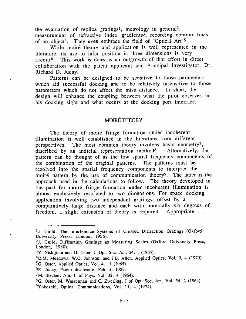
the evaluation of replica gratings 1, metrology in general 2,
measurement of refractive index gradients 3, recording contour lines
of an object 4. They even embrace the field of "Optical Art ''5.
While moir6 theory and application is well represented in the
literature, its use to infer position in three dimensions is very
recent 6. This work is done as an outgrowth of that effort in direct
collaboration with the patent applicant and Principal Investigator, Dr.
Richard D. Juday.
Patterns can be designed to be sensitive to those parameters
which aid successful docking and to be relatively insensitive to those
parameters which do not affect the miss distance. In short, the
design will enhance the coupling between what the pilot observes in
his docking sight and what occurs at the docking port interface.
MOIRI_ THEORY
The theory of moir6 fringe formation under incoherent
illumination is well established in the literature from different
perspectives. The most common theory involves basic geometry 7,
discribed by an indicial representation method 8. Alternatively, the
pattern can be thought of as the low spatial frequency components of
the combination of the original patterns. The patterns must be
resolved into the spatial frequency components to interpret the
moir6 pattern by the use of communication theory 9. The latter is the
approach used in the calculations to follow. The theory developed in
the past for moir6 fringe formation under incoherent illumination is
almost exclusively restricted to two dimensions. For space docking
application involving two independent gratings, offset by a
comparatively large distance and each with nominally six degrees of
freedom, a slight extension of theory is required. Appropriate
1j. Guild, The Interference Systems of Crossed Diffraction Gratings (Oxford
University Press, London, 1956).
2j. Guild, Diffraction Gratings as Measuring Scales (Oxford University Press,London, 1960).
3y. Nishijima and G. Oster, J. Opt. Soc. Am. 54, 1 (1964).
4D.M. Meadows, W.O. Johnson, and J.B. Allen, Applied Optics, Vol. 9, 4 (1970).
5G. Oster, Applied Optics, Vol. 4, 11 (1965).
6R. Juday, Patent disclosure, Feb. 5, 1989.
7M. Stecher, Am. J. of Phys. Vol. 32, 4 (1964).
8G. Oster, M. Wasserman and C. Zwerling, J of Opt. Soc. Am, Vol. 54, 2 (1964).
9yokozeki, Optical Communications, Vol. 11, 4 (1974).
8-3

simulations will also have to be made before final flight hardwarecan be designed.
The moire pattern itself, a periodic spatial function, can beformed optically by addition, subtraction, and multiplication of two(or more) spatially varying structures (gratings or filters). The mostcommon way to combine the two original structures is by theirtransmittance or reflectance functions. The illuminating light isaffected by the product of their transmittances and/or reflectances.We say then that when the same light field has impinged on each ofthe original structures in turn, a multiplicative pattern has emerged.This can be illustrated by the following two periodic structures andtheir product
1A (x) = _. (1 + cos2 rcfl x)
(1)
1B (x) = _-(1 + cos 2 n f2 x)
(2)
1A (x) B (x) = _- (cos _ ( fl + f2 ) x'cos _ (fl- f2) x )
(3)
Being a low pass filter, the eye will pass the low frequency
component, which will be manifested by readily resolvable fringes.
A multiplicative moire fringe is used in our design.
An additive type pattern, in contrast, occurs when two separate
light fields impinge on the two separate structures, and are then
superposed to form
A (x) + B (x) = 1 + cos rc (t'1 + f2 ) x'cos rc ( fl- f2 ) x(4)
which yields a modulated sinusoid that is far more difficult to
resolve. This effect would be important if an attempt were made to
modify the existing Crew Optical Alignment Sight (COAS) to accept a
moire reticle. The COAS works on a projected backlit reticle imaged
at infinity. Thus, a moirE-generating reticle inserted in the COAS
would yield an additive moire pattern when placed in conjunction
with a moirE-generating docking target placed on SSF. For a more
8-4

thorough treatment of types of superposed patterns in optics, seeBryngdahl. 1
DOCKING ENVIRONMENT AND GEOMETRY
The current Shuttle to SSF docking scenario involves a series ofprimary, secondary, and emergency sensors. These include groundtracking, rendezvous radar, the star tracker, and visual acquisition tobring the Shuttle to the vicinity of SSF. The docking scenario isspecified for a totally passive SSF, although it is assumed that SSFAttitude Control System (ACS) is operational. At approximately 50feet out, the pilot, flying from the aft bay, observing through theoverhead window, will attempt to keep the Shuttle within anacceptance cone with a full width vertex angle of 6-10 degrees.From here until docking, the pilot will probably have range andrange rate data fed to him via a laser sensor. At from 10-20 feetfrom docking, the pilot will attempt to hold his lateral misalignmentto less than a six inch radius circle. He makes closing velocity ( z-direction) and lateral alignment corrections (x-y) by pulsing ReactionControl System (RCS) thrusters. The other three degrees of freedom,roll, pitch and yaw, are held steady within one-degree accuracy bythe Shuttle Attitude Control System (ACS). Roll, pitch and yaw arealso held steady within one-degree accuracy by the ACS on the SSF.These attitude uncertainties are known as the deadbands of theShuttle ACS and SSF ACS, respectively. The anticipated closingvelocity is on the order of one-tenth of a foot per second.
This final closing range, from 10-20 feet to dock, is whereaccuracy must be improved to less than approximately six inches.Current contingency docking scenarios for the Shuttle to the dockingmast of SSF utilizing the COAS do not provide adequate accuracies(close to twelve inches) for a single docking attempt. Shuttle ClosedCircuit Television (CCTV), placed at the docking port, does meet therequisite accuracy (approximately three inches), but is objectionablefrom a reliability standpoint 2. Though the COAS is a reasonablyprecise instrument for the applications it was originally designed for,its difficulty with Space Shuttle/Space Station Freedom docking is theoffset distance from the sight to the docking port adapter. Figure 1shows how this offset acts as a lever arm, converting acceptable roll,
10. Bryngdahl, Opt. Soc. of Am., Vol. 66, 2, (1976).
2Miss distances were provided based on simulations run by Brian Rochon, aspresented in Analytical Docking Contact Conditions, April 13, 1989.
8-5

Roll Induced System Error
Pitch Induced System Error
7
Yaw Induced S.qstem Error
figure i.
8-6

pitch and yaw deadband error of the shuttle at the sight-docking
target point of reference, into an unacceptable miss distance at the
docking port. The same lever arm also affects instrument error and
pilot error. Our design, essentially replacing the COAS with a robust,
simple, small telescope must negate this effect to achieve missdistances less than six inches.
Referring to figure 2, note where and how our COAS-
replacement system will be mounted. It will be mounted in
approximately the same location as the COAS in the aft bay overhead
window. This figure shows the baseline SSF docking scenario, using a
docking mast which will retract to mate airlocks after hard dock is
achieved. Figure 3 shows the docking mast retracted. The standoff
distance from the COAS or COAS-replacement to the SSF docking
target is approximately 18 feet, if a non-retractable target is used.
DESIGN CRITERIA AND THE FIRST GENERATION DESIGN
Our design criteria, which should serve to minimize miss
distances, are:
1. Maximal sensitivity to x-y translation as
measured at the docking port location.
2. No yaw sensitivity about the docking port.
3. Acceptable sensitivity to roll and pitch.
4. Simple to interpret patterns.
The first criterion underscores that it is how far off you miss the
docking port--not how close your sight is to its target's bullseye--
that is critical (and is presently a problem with the COAS). Second,
some yaw is acceptable about the docking port (not the center of
mass). Sensitivity to yaw about the docking port should be removed,
so a pilot will not inadvertently correct for a perceived (but not
actual) misalignment. Third, some roll and pitch will be present due
to the deadbands of the ACS. Our design must be able to accept this.
Finally (and on occasion, neglected), the design must give completely
unambiguous cues to the pilot during those critical last seconds of
docking, both in terms of how far and in which direction from the
optimum docking position he is, and in his ability to sense hisdirection of motion.
Even a casual examination of commercially produced moir6
patterns indicates that a variable frequency, ("chirped") pattern can
give excellent sensitivity. Yaw insensitivity can be readily included
8-7

o
0

x=-
00i
oU9C0c"t-O.-_
>u
:Ecui-,-
>-i-Zmot_
figure
3.
8-9

by making our patterns radially symmetric about the docking
adapter axis. Combining these two properties yields an off-axis
Fresnel zone plate as an excellent candidate pattern. A zone plate
(figure 4) is a series of bright and dark rings about a central circle,
and is notable in that each ring and the circle ("zone") has the same
area. The equation of the radii that would draw such a figure is
rm = B _'m(5)
where r m is the ruth radii, B is some constant to be determined, and
m is an integer.
When two identical zone plates are overlapped with an offset
less than the radius of the inner circle, a series of bars results
perpendicular to the direction of the offset. Figure 5 demonstrates
this fringe pattern, while the mathematics of this using the indicial
equation method is shown by Oster et al 1.
SIGHT RETICLE AND DOCKING TARGET DESIGN
While an off axis zone plate will generate a series of equally
spaced, equal thickness bars, for alignment purposes it is better to
vary the frequency function of at least one zone plate to permit
centering of the sight. Our first "centering chirp" is of quadratic
form.
First, we must select a phase function _)(r) whose zeros of
sint)(r) will correspond to an arc with radius rm to construct the zone
plate. This condition is met by the function
(r) =n (r/B )2 (6)
where B has yet to be specified. We next need to determine the
spatial frequency f(r). It relates to phase _(r) by
f(r) = 1/2r _ d_(r)/dr=l/2_ x d/dr [ r_ (r/B)2 ] -- r/B 2 (7)
f(r) -- r/B 2 (8)
1G. Oster, M. Wasserman and C. Zwerling, J. Opt. Soc. Am, Vol. 54, 2 (1964).
8-10

ou
_z
c_OzZ
figure 4.
Z
z_u
6_2
_o
ZZ
figure 5.
8-Ii

We now subscript T for target and R for reticle, and introduce a
quadratic chirp into fT- This quadratic chirp in fT is symmetric about
the center of the target, w_iich in turn is I I_ qnches from the docking
port (the origin of our pattern). Our target frequency is thus
f'r =fR +D(r- 114) 2+E (9)
which can be interpreted by the following figure
f(r)fT=fR+D (r-l14)2+E
r
114 inches
figure 6.
Noting that our target frequency fT will correspond to the
inverse of our chosen arc width, d, constraints may now be imposed
to solve for the constants D, E and B. The constraints are:
,
2.
Choose a differential frequency ratio of
say, two times, edge to center.
Design to give 5 fringes (thus easy to
observe) in moir6 pattern between
r = 102 and r = 126 inches for a 2 foot by
two foot target.
From the first constraint, we see that
E= 144D. (10)
8-12

Next, the number of fringes must equal the number of arcs in thetarget less the number of bars in the reticle, edge to edge; thus
N fringes = (q_r- q_R)/2n. (11)
The phase difference from center to edge has half the fringes, andrecallingN=5,
5 n =A q_C-E. (12)
This is also equal to the integrated phase from the center to edge
12
2nf (E +D _2) d_
(13)yielding
5/2 = 12E +576 D (14)
Rewriting equation (9) at its maximum value at r = 126,
1 _ 126
[YT]MAX = dr= 126 B 2+144D +E
(15)
and selection of an appropriate cut width d yields suitable solutionsfor the constants.
To cut the sight reticle recall that a zero occurs (and hence.a cut
in our pattern) for the sine of the phase function every rc radians, so
2r
rnm
_R(rm)-mn=n B 2(16)
which leads immediately to equation (5) to control our cuts.
To find where to make the cuts in the target, its phase function
is found as a function of r. This equals the integrated frequency,
r
_T(r) =2gffT (_) d_
o(17)
8-13

resulting in the following cubic equation for the target phasefunction,
2_T (r) r
2re 2B 2
D+rE+-_- [ (r-114) 3 + 114 3 ] .
(18)
As with the phase function of the reticle,
_v (rm) = m r_ (19)
will lead directly to a cubic equation in terms of m and r m. An
algorithm using Newton's method then solves the cubic and control
the cutting of our target pattern.
Finally, our reticle pattern is photo reduced to place it in the
focal plane of our telescope.
PHYSICAL IMPLEMENTATION
The objective of the experiment was not only to generate the
functions of a suitable moirr-generating telescope reticle and docking
target reticle, but also to translate them into laboratory hardware.
The patterns were created by cutting a membrane of red plastic
layered on a transparent substrate, then peeled to create alternating
red and clear arcs. This process is known as "ruby-lithography" or
"ruby-lith", and is traditionally used in miniaturized electronic circuit
fabrication. Arcs can be cut as close as every 15 mils without undue
tearing, but to ease the burden of iterative fabrication, an arc widthof about 50-60 mils was selected.
The ruby-lith software had no trouble with either of the
equations used to generate the two templates, not even the routine
to solve the above mentioned cubic equation using Newton's method,
though it was painfully slow and required frequent human-
intervention due to memory limitations.
The target pattern eventually used for flight hardware will
need to be made of high contrast alternating reflective and
absorptive bands, as the shuttle floodlights will be the only lighting
we can confidently depend on under our "passive SSF" criteria. For
our first generation tests using off-the-shelf ruby lith, a light box or
simple lamp will provide high contrast rear illumination.
8- 14

A target just under two feet square was initially used to ensurethe field of view of our test telescope would be filled by the target atthe initial test ranges of between 18 and 28 feet.
An inexpensive four power rifle telescopic sight wasdisassembled to gain access to the focal plane. The eyepiece, photoreduced reticle and telescope were placed in optical mounts, and thephoto reduced reticle was placed at the focal plane.
The telescope assembly was mounted on a three degree offreedom motion based, full scale simulator. The "Shuttle" could thentranslate (z-direction) toward "SSF" at a realistic one-tenth of a footper second, while simultaneously translating laterally (x & ydirections), as illustrated in figure 7. Near term simulatorimprovements will allow all six degrees of freedom, incorporatingroll, pitch and yaw.
Of particular note in the figure is the offset "docking port"marker on the boom of the simulator. This demonstrates in full scalethe relation between how close the pilot has in fact docked comparedto what he observed in his docking sight.
LABORATORY RESULTS
Laboratory runs are now begining to evaluate the first
generation docking targets and reticles. The data will published in a
future publication by Juday and Dottery, et. ah
8-15


N90-24981
ELECTROCHEMICAL CONTROL OF IODINE DISINFECTANT FOR
SPACE TRANSPORTATION SYSTEM AND
SPACE STATION POTABLE WATER
Final Report
NASA/ASEE Summer Faculty Fellowship Program--1989
Johnson Space Center
Prepared By:
Academic Rank:
University & Department:
Richard D. Geer, Ph.D.
Associate Professor
Montana State University
Department of Chemistry
Bozeman, Montana 59717
NASA/JSC
Directorate:
Division:
Branch:
JSC Colleague:
Date Submitted:
Contract Number:
Space and Life Sciences
Medical Sciences
Biomedical Laboratories
Richard L. Sauer, P.E.
September i, 1989
NGT 44-001-800
9-1

ABSTRACT
The National Aeronautics and Space Administration willcontinue to use iodine as the microbial disinfectant forpotable waker (PW) on manned space operations. The currentmethod for adding iodine is the "Microbial Check Valve", apassive ion exchange device whose output is temperaturedependent and also adds excess iodide to the water. An"active" electrochemical technique, using silver and inertelectrodes, is proposed to allow controlled addition andremoval of the iodine from the PW by cycling a silver iodidelayer. The units can be physically recycled between the twolocations for these modes.
The design is based upon the constrains set by the PWsystem, including conductivity, expected flow rates, andiodine treatment levels. The units require a minimumelectrode area of 300 cm2 and fits into a space of 3x3x5 cm.The efficiency of iodine and iodide removal will depend uponthe thickness of silver iodide on the silver electrode, whichunder nominal conditions could approach 40 Nm in 90 days ofoperation. The time between recycling the units will alsodepend upon the iodine removal efficiency.
The equilibria for iodine species in the water wereevaluated. Graphs for the iodine species, carbonate speciesand hydrogen ion are presented, based upon levels of iodineadded and total inorganic carbon present. The effect oftemperature on the residual level of iodine (iodide) andsilver in the waker is graphically presented. The oxidation
and reduction reactions were also examined at the expected
concentrations of reactive species in the PW to test the
feasibility of the iodine removal and generation processes.
The major difficulty encountered was due to the presents of
oxygen in the waker. While oxygen could possibly help in
removing excess iodide, it would cause a problem in the
controlled generation of iodine due to its preferentialreduction relative to that of silver iodide.
The analytical chemistry required to monitor the
performance of the PW system was reviewed. It is clear that
potentiometric measurements (like pH) are inaccurate in pure
water, but ik is possible for conductivity techniques with ion
selective electrodes can make accurate measurements. Methods
based upon conductivity were used to calculate pH and the
concentrations of iodine species in treated water. These
methods allowed a check upon the accuracy of the total trace
ion analysis of the PW. The report makes a final point that
oxygen should be routinely monitored in the PW system.
9-2

INTRODUCTION
The National Aeronautics and Space Administration (NASA)plans on using iodine for microbial control in the recycledpotable water (PW) system on its Space Station. Iodine iscurrently used on the Space Transportation System (STS)missions where the water is not recycled but is obtained asa byproduct from the fuel cells. Because of its convenient
method of addition and its adequate disinfectant properties,
iodine will probably be used in future long duration spaceventures like missions to Mars and Lunar base facilities.
There is limited experience with the long term use of iodine
disinfectant in water and it could present scme potential
health problems. These include possible formation of toxic
compounds from the reaction of iodine with organic material
(residual or in the stomach) and increased iodide levels
effecting the thyroid f_inction. Iodine levels some what above
nominal will give water a noticeable and objectionable taste
(however even pure water is noted for its objectionable "flat"
taste.) Thus, it would be desireable and perhaps necessary
to remove nearly all of the iodine species before the water
is consumed. In some situations it may be important to
recycle the iodine.
Currently NASA is adding iodine to PW systems by means of
a "microbial check valve" (MCV), an effective PASSIVE DEVICE.
The MCV consist of a chamber containing a anion exchange resin
loaded with iodine (mainly as the triiodide ion, I3-) which
delivers low levels of iodine (I2), iodide (I-) and hydrogen
ion (H +) to the water. The behavior of iodine in this system
is characterized by a set of chemical equilibria involving
both the ion exchange material and reactions of water. During
use the 12 level slowly drops as the resin iodine load
decreases a. The equilibrium constants for these processes are
temperature dependent and high temperature water can produce
iodine levels above the acceptable limits. The MCV also
produces H + and excess I-, even when operating at normal
temperatures, and the pH of the treated water can fall
significantly below the pH 6 limit for the Space Station PW I.
These problems could be overcome by removing the excess iodine
and related ions just before the water is used.
At present NASA has no device for this end-use treatment
but they are considering using a high capacity ion exchange
unit, working in the reverse mode of the MCV. However the
end-use position of the unit requires it to treat hot water
where the chemical equilibria are not favorable. Vapor,
a. Unpublished results from Water and Food Analysis Lab,
NASA, Johnson Space Center, Houston TX.
9-3

liquid or chemical extraction of i 2 from the water isconceivable, but most methods appear bulky and not suitablefor microgravity conditions.
As an alternative to the MCV system, I have studied thepossibility of an ACTIVE electrochemical technique forgenerating, recycling and removing 12 and its associated ionsin PW. In this report the device will be called the EC-MCV(electrochemical microbial check valve), though based upon itsconstruction it is often referred to as the "silver bullet"This report discusses a design based upon the limitingrequirements for PW treatment in both the Space Station andSTS environments. The advantages of the EC-MCV will bepresented along with some possible limiting complications thatneed to be investigated.
OVERVIEWOF THE EC-MCV
In principle the operation of the EC-I_CV is simple and canbe followed on the schematic diagram in Figure i:
o In the Iodine Removal Mode (IRN) the silver electrodereacts spontaneously with any iodine (I2) or other activeiodine species in solution to form a very insolublecoating of silver iodide (Agl). Excess iodide (I-) canbe removed by oxidizing the silver electrode under acontrolled potential to form more AgI.
o In the Iodine Generation Mode (IGM) a controlled currentis past through %he device and the Agl on the silverelectrode is reduced to silver and iodide (I-) isreleased into the water. Upon reaching the counterelectrode the I- is oxidized to 12. The iodine level inthe water is controlled by the electrode current relativeto the water flow rate.
CONSTRAINTSON THE EC-MCV DESIGN
The nature of the PW system puts severe constraints onpractical designs of the EC-MCV and some basic research willbe needed to prove this a viable concept.
Conductivity
A major design limitation is the low conductivity of thePW which is measured in units of Siemens/cm (S/cm) for a onecm_ area. Its reciprocal (resistivity) is often used and isgiven in ohm cm. Completely pure water has a value of 0.056
NS/cm or 18.3 M_ cm. Water samples from the Biofilm Test Bed
(BTB), a system designed to simulate aspects of the PW system
for the Space Station, have values of 0.2 to 0.5 NS/cm a.
These low values limit the current densities that the water
9-4

can carry with reasonable applied voltages. For an electricfield of i V/cm the PWwill only support current densities of0.2 to 0.5 vA/cm 2. Water from the STS fuel cells may be more
pure and have lower conductivity. For wi£er with 2 ppm of ! 2
added the conductivity increase to about 2 NS/cm.
:<..... :
I
I
I I
I I
I PW
i>i- .... !_>N
I
V- >--I I PW
I I +
SILVER SCR]_EN ELECTRODE(l)
with Agl coating. _ .... >:......... : Nembrane
!/SeparatorI
2C;ODE I PW + 12
PORCUS I)___NT ELECTIIODE(2) ; ....... >
: I & trace I
V+ >--I
A. Arrangement for adding 12 to PW at a set rate by
controlled current electrolysis.
:<..... I
I I
I V+ >--I I
I ANODE I
: PW + I_ k \ SIL_m sC_Z_ _ECTRODEI >..... I'-'-,>\ being coated with Agl. ->I
: ...........................,,
.....5_q, ..........\I POROUS INE_T ELECTRODEN ....... I
V- >--I
PW
_embrane
Separator
I PW
1............. >
I
B. Arrangement for removing 12 and I- from PW
under controlled potential.
Figure i.- Schematic drawing of the proposed recyclable EC-NCV.
(i) The cell consists of a stacked array of alternating thin (<i mm)
electrodes and separators. (2) Possible inert electrode materials are:
platinum, titanium, tin, reticulated vitreous carbon, or carbon cloth.
9-5

Water Flow Rates
The inflow of PW is one factor determining the rate of
iodine addition to the water. The anticipated Space Station
flow is Z5 I/day (0.3 ml/sec) of humidity condensate from the
cabin. The system residence time for the treated water is
expected to be about I00 hours, with most of the time in
storage tanks. The demand of water at the output will be
intermittent, with flows of I0 to 30 ml/sec of either hot or
cold water being requlred b,
Iodine Treatment Levels
Currently the planned iodine treatment level is 2 to 3 ppm,
but a standard MCV using hot water from the STS fuel cells has
produced levels above i0 ppm a. For the purpose of more
complete disinfection even higher levels could be allowed if
the total iodine level was reduced before consumption.
Electrode Area
The above requirements set the typical rate of 12 addition
for an EC-MCV at 2 to 3 nanomol/sec, requiring a total current
up to 0.6 mA. To handle this current at a current density of
0.2 _A/cm 2 will require a minimum effective surface area forthe electrochemical cell of 300 cm 2. Since the area on each
side of the electrode is counted, this is equivalent to a
stack of i0 pairs of 3 x 5 cm electrodes. (From here on, this
report will deal with a nominal 3 ppm level of added iodine,
if higher levels are under consideration the units can be
scaled accordingly.)
The iodine removal mode could present some design problems
if most of the added iodine ends up in the form of I- and has
to be removed electrochemically. At a projected flow rate of
ii ml/sec this would require a reaction rate of 26 @mol/secor 25 mA which translates into a maximum electrode area of
13000 cm _. This may not be a real constraint, as a EC-MCV
unit should produce little or no excess I-. However, the
excess I- output of a conventional MCV on the BTB is about 0.7
ppm a and would require a 3000 cm 2 surface area. The reduction
of 12 in the system is another source of I-, but these
problems may be irrelevant if oxygen is present, see thesection on Redox Reactions.
Electrode Construction
A practical design for the electrodes should approach I00
b. Private communication from Richard L. Sauer, PE, NASA
SD4, Johnson Space Center, Houston TX.
9-6

% efficiency for the electrode reactions producing 12 from I-
and forming AgI. To keep the voltage drop low and to maximize
the water contact time, the water flow must parallel the
electrodes while the charge migration is at right angle
through a membrane separator. This requires thin (<Imm)
porous electrodes that produce turbulent flow and narrow
stagnant diffusion layers at the surface. The typical
diffusion distance for an ion is about 40 _m in 1.6 sec and
200 _m in 60 sec 2. Tending to counter these requirements is
the need for the electrodes to have good electrical
conductivity, low flow resistance and to be readily
fabricated. While one electrode must be made of silver, or
silver plated, the choice of material for the counter
electrode is only limited by the need for inertness and
conductivity. Finely woven metal gauzes have an adequate
structure. Titanium, tantalum, or tin might be good choices
and are not considered toxic metals. Platinum, palladium and
gold are rather expensive and may react with iodide under
oxidative potentials 3. Also to be considered are flexible
carbon cloth and reticulated vitreous carbon, which has an
excellent pore structure but is brittle.
The calculated EC-MCV performance in Table 1 is based upon
a conservative design using 15 pairs of electrodes (each pair
being 2 mm thick including membrane separator) with a total
area of 450 cm 2 in a 3x3x5 cm space. Research is needed on
how the AgI film thickness effects the efficiency of the
silver/iodine reaction, as this will determine how often the
electrodes need to be recycled. As the silver surface is
recycled it should become rough (possibly with dendritic
growth) causing the surface to volume ratio to increase
substantially, extending the recycle time. Now the questions
are how many times can an electrode can be recycled and what
limits electrode life.
TABLE I.- EXPECTED CHANGES IN SILVER ELECTRODE WITH TIME IN
THE IODINE REMOVAL MODE AT 3 PPM 12.
Time 0 7 30 90 days
Ag weight a 37.7 37.3 35.8 32.0 g
AgI weight 0 0.97 4.16 12.5 g
AgI thickness b 0 3.1 13. 39 _m
Residence time c 1.66 1.65 1.61 1.52 sec
a Based upon 15 layers of 3 x 5 cm electrodes of 40
mesh I0 mil smooth Ag wire gauze.
b. Calculated for a total Ag surface area of 565 cm 2.
c. For a 11 ml/sec flow; the IGM time is about 60 sec.
9-7

Other EC-MCV Components
The membrane separators are another critical part of theEC-MCV. They need to be thin and have high conductivity toions, have limited water passage and be nonreactive to iodine.Nafion by Dupont, a Teflon base cation exchange resin may work
well, but bipolar membranes would be preferred. The
literature of battery technology may show how this problem was
solved some time ago.
The best material for cell body construction is also an
open question. Plastic materials like polypropylene, Teflon,
epoxy, polycarbonate, and polymethylmethacrylate come to mind.
The body design should allow for simple construction and
repair. Some potential problems to investigate are: the
degree of 12 adsorption by the body material, is it areservoir for active iodine, and does it limit bacterial
growth on the cell body?
The electronic control for the EC-MCV will not be covered
here as the circuits are very simply implemented at these low
currents and modest voltages.
CONSTRAINTS ON WATER CHEMISTRY
While source water for the PW system may be fairly pure,
its trace constituents and temperature can affect the function
of the EC-MCV (as well as the MCV) and the 1 2 water chemistry.
Fuel Cell Water
STS fuel cell water entering the MCV is quite warm. The
water should be very pure except for the possibility of
entrainment of small amounts of potassium hydroxide
electrolyte and residual hydrogen gas. However no excessive
amounts of K + or OH- have shown up in analys@s of PW from this
source a. I£ shouid C6n-£i_n no oxygen or carbon _i0xide,
Information on its pH and conductivity would be desirable.
This water source would be a prime candidate for the EC-MCV
because the regular MCV has problems treating hot water.
Humidity Condensate
The Space Station will use humidity condensate from the
cabin atmosphere as its source of potable water. This source
will have low levels of a number of inorganic ions and a
large variety of organic chemicals, mostly in trace amounts 4.
The water should be saturated with 0 2 , N 2 and CO 2 at their
partial cabin pressures. After polishing the water with
delonlzing resins and activated charcoal filters the water
should be at ambient temperature and its composition similar
to that observed in the Biofilm Test Bed studies a.
9-8

Chemical Reactions and Equilibria
The addition of 12 to water sets up several equilibria that
are sensitive to the existing pH and the I- level. These are
given in Table 2 along with several other important reactions.
TABLE 2.- CHEMICAL EQUILIBRIA NEEDED TO UNDERSTAND THE
CHEMISTRY OF 12 IN WATER 5,6.
Reaction Xeq at 25 °C
1 12a q + H20 .... > HOI + I- + H +
2 13 .... > 12a q + I-
3 12a q + H20 .... > H2OI + + I-4 AgI .... > Ag + + I-
5 ResI 3 .... > ResI + I2a q
6 ResI + H20 .... > ResOH + H ÷ + I-
7 H20 .... > H + + OH-
8 CO 2 + H20 .... > H2C03_9 H2CO 3 .... > HC03 + H +i0
5.40E-13
1.38E-03
1.20E-If
8.51E-17
N/A a
N/A
1.00E-14
N/A
4.30E-7
HCO 3 ..... > CO 3- + H + 5.60E-IIa These constants are not available, the ones with ResI
represent the ion exchange equilibria of the MCV resin.
Reactions 2 and 3 are not important as the concentrations
of 13- and H2OI + are normally insignificant in PW. However,reaction i produces HOI, H +, and I- in amounts sufficient to
give PW a 5.75 pH and provide equivalent amounts of I- and
HOI. Figure 2 shows the relationship of these species to the
amount of 12 added to pure water. If the incoming water is
much above pH 7 it can divert a large portion of 12 to HOI and
I-. In pure water the amount of dissolved CO 2 will determine
the pH by reactions 8 and 9, Table 2 and Figure 3. However,
in treated water the usual levels of CO 2 are I00 fold below
that of 12 and the H2CO3/HCO 3- ratio is controlled by the 12reactions.
Excess I-
If I- is present in the water in concentrations greater
than available from the above reactions, the solution is
considered to have "excess I-". A major portion of the I- in
water treated with the regular MCV is "excess I-"j released
from the resin by ion exchange reaction 7, Table 2. It is
accompanied by equivalent amounts of H +, which lowers the pH
to about 5.3. Other sources of excess I- are reactions which
reduce 12 to I- and usually produce H + at the same time.
Two reactions that may be important in the PW systems are:
I) Microbial reduction of 12 by iodine resistant bacteria,
(perhaps they are using it as an energy source?). 2) Theoxidation of reactive chromium or other atoms of stainless
9-9

-11I I I I I I
-1.5 -1 -0.5 0 0.5 1 1,5 2
LOG ( IOOINE AOOED_ PPW
Figure 2.- Concentrations of ions from 12 added to pure
water. Legend: I2added; --X-- I2; --[]-- -pH; --A-- HOI
and I-; --+-- I3-.
steel in the PW system. Th%s reaction, if it occurs, must be
slow at room _empera_ure, but possibly becomes Impor£in_ at
higher temperatures. However no unusual amounts of crate
seen in 12 treated water, even though Fe, Ni, and Cr have beenobserved in untreated water in the BTB a. This might imply
that an 12 oxidation could be part of a metal passivatlon
process leading to thicker oxide coatings, but also producingmore H + and I-
Silver Iodide
The formation and stability of silver iodide (AgI) plays a
key role in the operation of the EC-MCV for removal of iodine
species. As mentioned earlier, the effect of the AgI
thickness on the rate 12 reacts with the underlying silver
needs investigation, for the thickness can approach 40 _m in
90 days. Also important is the durability of the surface, as
flaking of the AgI would interfere with recycling electrodes
and could contaminate the PW. Finally, the increased
solubility of the AgI with temperature may be important as the
output water will often be heated prior to iodine removal.
9-10

However, Figure 4 shows that even at I00 C the Ag is stillbelow the 50 ppb limit.
-5
f-%
-5
X
k2
-8I I I
13 0_5 1 I ,5 2
LOG ([ T I C_ PPB _)
Figure 3.- Concentration of chemical species in pure waker
from dissolved CO 2 (reported as TIC). Legend: H+; --*--
HCO3-; --x-- H2CO 3.
Redox Reactions and Electrode Potentials
Reduction and oxidation chemistry is at the heart of the
generation and removal of 12 by the EC-MCV and the significant
reaction are given in Table 3. A negative cell potential
indicates an electrolysis reaction controlled by an applied
current or voltage. The more positive a value is the more
"spontaneous" the reaction.
Included in the table are several reactions involving
oxygen that may be important to the EC-MCV operation. In the
iodine removal mode, without oxygen, the values for reactions
2 and 4 show that Ag reacts very vigorously with I 2, while it
requires electrolysis condition with a voltage greater than
0.31 volts to remove I-. Note, while Ag has only the
slightest tendency to react with 02 alone, in the presence of
I- it has a very positive potential to form AgI_ This could
solve all the problems of "excess I-" removal without
9-11

50
m 40ci&
I
o 3OZ
÷
__ 20ZD0
10
/
0_ _ -_ i_ I 1 1 ..........
0 2D 40 60 80 "1O0
TEMPERATURE, C
Figure 4.- The effect of temperature on the amounts of A_ +
and I-released by silver iodide surfaces. Legend: --*-- AgT;----+----I--.
electrolysis, Just add oxygen. BUT, this idea must be tested
experimentally, for 02 reactions are notorious for having veryslow kinetics even when the thermodynamics are very favorable.
On the other hand, silver and iodine reactions have catalytic
activity, so hopefully the reaction will proceed. Reaction
5 also indicates that oxygen in solution would be helpful in
reforming 12 from I-, but this reaction is knOWn to be slow
unless catalyzed by near ultraviolet light.
Oxygen Problem
In the iodine addition mode, reactions 6 and 7 indicate
that the controlled current generation of 12 occurs before 02
and the process may require less than I volt applied to the
cell. However, reaction 8 presents another problem, any
oxygen dissolved in the input water will be reduced very
easily and the applied current will not reduce AgI to Ag and
I- until all the oxygen is reduced. Thus, for the EC-MCV to
work as planned, the source of water must be free of oxygen,
like that from the STS rue!cells. However_ In this situation
oxygen is not available to help remove excess I-. One
9-12
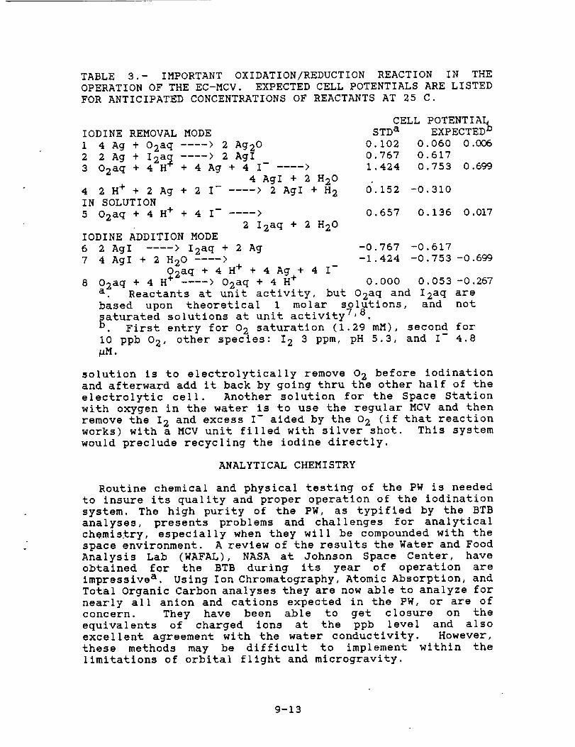
TABLE 3.- IMPORTANT OXIDATION/REDUCTION REACTION IN THE
OPERATION OF THE EC-MCV. EXPECTED CELL POTENTIALS ARE LISTED
FOR ANTICIPATED CONCENTRATIONS OF REACTANTS AT 25 C.
IODINE REMOVAL MODE
1 4 Ag + 02aq .... > 2 Ag20
2 2 Ag + I2a_ .... > 2 AgI3 O2a q + 4 H + 4 Ag + 4 I- ---->
4 AgI + 9. H20
4 2 H + + 2 Ag + 9. I- ----> 2 AgI + H 2
IN SOLUTION
5 O2a q + 4 H + + 4 I- ---->
2 I2a q + 2 H20
IODINE ADDITION MODE
6 2 AgI .... > I2a q + 2 Ag
CELL POTENTIA_STD a EXPECTED _
0.102 0.060 0.006
0.767 0.617
1.424 0.753 0.699
6.152 -0.310
0. 657 0. 136 0.017
-0.767 -0.617
-1.424 -0.753 -0.6997 4 AgI + 2 H20 .... >
HO2aq+ + 4 H + + 4 Ag + 4 I-> O2a q + 4 H + 0.000 0.053 -0.2678 + 4
Reactants at unit activity, but 02a q and I2a q are
based upon theoretical 1 molar solutions, and not
aturated solutions at unit activity 7'8.
• First entry for 02 saturation (1.29 mM), second for
i0 ppb 02 , other species: 12 3 ppm, pH 5.3, and I- 4.8
_M.
solution is to electrolytically remove 02 before iodination
and afterward add it back by going thru the other half of the
electrolytic cell. Another solution for the Space Station
with oxygen in the water is to use the regular MCV and then
remove the 12 and excess I- aided by the 02 (if that reaction
works) with a MCV unit filled with silver shot. This system
would preclude recycling the iodine directly.
ANALYTICAL CHEMISTRY
Routine chemical and physical testing of the PW is needed
to insure its quality and proper operation of the iodination
system• The high purity of the PW, as typified by the BTB
analyses, presents problems and challenges for analytical
chemistry, especially when they will be compounded with the
space environment. A review of the results the Water and Food
Analysis Lab (WAFAL), NASA at Johnson Space Center, have
obtained for the BTB during its year of operation are
impressive a. Using Ion Chromatography, Atomic Absorption, and
Total Organic Carbon analyses they are now able to analyze for
nearly all anion and cations expected in the PW, or are of
concern. They have been able to get closure on the
equivalents of charged ions at the ppb level and also
excellent agreement with the water conductivity. However,
these methods may be difficult to implement within the
limitations of orbital flight and mlcrogravity.
9-13

To monitor the performance of the iodination of PW one
needs to know the total amount of iodine added, and the
amounts of 12, I-, CO 2 and H +. As found from the BTB results,
the common potentlometric technique for pH is not accurate in
low conductivity water a. However, in fairly pure systems
conductivity gives a very good measure of pH as the H +
contributes 82 % to the conductivity below pH 7 and the otherions all have similar equivalent conductances 9. Ion Selective
Electrodes (ISE) in general will have the same problems as pH
electrodes unless buffers are added to increase conductivity.
Conductance techniques should be adaptable to ISE I0 for ion
measurements in these "pure" water systems and development of
these methods should be supported.
The determination of i- has been a problem for WAFAL as the
photometric method depends on the H T and 13- measurements,
both of which where inaccurate. A technique that removes the
active iodine species with metallic silver after measuring Iphotometrically is being developed to measure the residual I_
without interference a. From these data all the iodine species
can be calculated accurately. It also appears feasible to
carry out these same iodine measurements automatically using
cathodic stripping voltammetry II
Oxygen is one important component of the PW system that is
not currently being measured. It should be measured at
several locations in the system, as its concentrations may
reflect the degree of microbial growth. The oxygen data would
also be important for the proper operation of a EC-HCV and if
excess oxygen or one of its reactive derivatives (ozone,
superoxide or hydrogen peroxide) were injected as adjuncts for
microbial control.
SUMMARY
An electrochemical method (EC-MCV) for controlling the iodine
disinfectant in potable water for NASA's space operations has
been proposed. The factors affecting the design and
performance of the unit have been analyzed. This showed that
it would be feasible to construct a recyclable unit in a small
volume that will operate in either an iodine removal or
addition mode. The EC-MCV should remove active iodine species
rapidly from PW, but the rapid delivery rates at end-use may
make complete removal of excess I- difficult under some
conditions. Its performance change with AgI buildup needs to
be investigated, as this controls the time for recycling the
unit. The EC-MCV has advantages over the passive MCV
currently in use, as it would allow precise control of the 12level and would not introduce excess I- to the water. The
presence of oxygen in £he EC-MCV needs to be investigated as
it could affect the efficiency of 12 addition and excess I-removal.
9-14

REFERENCES
,
•
Space Station Program Definition and Requirements
Document. NASA SST 30000. Rev D., 1987, Table 2-34.
Bard, A. J.; and Faulkner, L. R.: Electrochemical
Methods. John Wiley & Sons, 1980, p. 129.
,
,
o
,
•
•
•
I0.
Ii.
Sawyer, D. T.; and Roberts, J. L. Jr.: Experimental
Electrochemistry for Chemists. John Wiley & Sons,
1974, p. 68.
Shrader Analytical and Consulting Laboratories Report
of Analytical Services: Space Lab 3 ARS Humidity
Condensate. SL 12352, 1985.
Burger, J. D.; and Liebhafsky, H. A.: Therodynamic
Data for Aqueous Iodine Solutions at Various
Temperatures• Analytical Chemistry, vol. 45, 1973,
pp. 600-602.
Lange, N. A.: Handbook of Chemistry. Handbook
Publishers (Sandusky, OH), 1956, pp. 1198-1204.
Latimer, W. M.: Oxidations Potentials.
Hall, 1938, pp. 293-317.
Prentice-
Skoog, D. A.:third edition.
A25-A27.
Principles of Instrumental Analysis,
Saunder College Publishing, 1985, pp.
Skoog, D. A.:
third edition.
706.
Principles of Instrumental Analysis,
Saunder College Publishing. 1985, p.
Holler, F.J.; and Enke, C. E.: Conductivity and
Conductometry. Laboratory Techniques in
Electroanalytical Chemistry, P. T. Kissinger, and W.
R. Heineman, eds., Marcel Dekker, 1984, pp. 263-264.
Heineman, W. R.; Mark, H. B.; and Wise, J. A.:
Electrochemical Preconcentration. Laboratory
Techniques in Electroanalytical Chemistry, P. T.
Kissinger and W. R. Heineman, eds., Marcel Dekker,
1984, p. 502.
9-15

= ,

OVERTRAINING AND EXERCISE MOTIVATION:
N90-24982
A RESEARCH PROSPECTUS
Final Report
NASA/ASEE Summer Faculty Fellowship Program--1989
Johnson Space Center
Prepared By:
Academic Rank:
University & Department:
NASA/JSC
Directorate:
Division:
Branch:
JSC Colleague:
Date Submitted:
Contract Number:
Anthony C. Hackney, Ph.D.
Assistant Professor
University of North Carolina
Exercise Physiology Laboratory
Department of Physical Education,
Exercise and Sport Sciences
Chapel Hill, NC 27599-8700
Space and Life Sciences
Medical Sciences
Biomedical Laboratories
Pat Santy, M.D.Steve Siconolfi, Ph.D.
September 22, 1989
NGT44-001-800
10-1
ABSTRACT
The problem of exercise "overtraining" has recently become
one of great interest to professionals in the field of human
performance assessment. Quite obviously, the ultimate goal of the
training process is to improve physical performance. However,
excessive training can result in the opposite effect, that is, a
performance decline and an impairment in the functional work
capacity of the body. Research indicates that both psychological
as well as physiological disturbances are quite common in
overtrained individuals (32, 33, 34). For example, psychological
changes include increased levels of depression, fatigue, and a
lack of motivation (34, 45, 51). Similarly, impairment of the
physiological function of the cardiovascular, metabolic, and
endocrine systemsalso have been found (3, 8, 12, 13, 14).
Some similarities may be found in the psychological and
physiological states of crew members exposed to extended space
flight and overtrained individuals. Therefore, the possibility
exists that the crew members subjected to extended missions in
space may develop over stressed or overtrained or both states
during their flights. If such states do develop within the crew
members, mission performance may be impaired.
With these points as a background, the intent of this
prospectus is to address potential research directions that NASA
may consider viable and of a mutual interest to this
investigator. A clear framework by which to begin discussion of
research topics is needed, therefore working definitions of"overtraining" and "exercise motivation" are presented.
Subsequently, a proposed conceptional model of how exercise
overtraining and motivation interact is presented. In support ofthe proposed model is brief literature review of reievantareas.
Potential research projects are presented and discussed.
i0 - 2
INTRODUCTION
A major concern in the space program has been thedetrimental effects of prolonged space flight on thephysiological functions of the human body (28, 39, 40).Biomedical research from Skylab and Salyut indicated prolongedexposure to space flight results in cardiovasculardeconditioning, bone mineral loss, muscular atrophy, and fluidshifts (28, 39). These changes appear to be the physiologicalconsequences of exposing the body to zero gravity and areduction in the typical level of earth bound activity.Exercise training is a proposed requirement to attenuate theseeffects on the body's systems while the astronauts are inspace. In addition to this exercise training during spaceflight, many other physical as well as mental demands (i.e.,mission operations) will be made of the astronauts.Potentially, the combination of exercise training anddemanding work requirements (e.g., isolation) could lead to aover stressed stated in the astronauts. The latter issue,psychological stress of the astronauts, is becoming anincreasingly important concern. Specifically, future NASAspace missions will be of greater duration and crew make-upwill become more heterogeneous (i.e., multi-national) innature. These combined stressors could lead to adverse copingstrategies or negative group interaction, both which couldendanger the success of the mission.
For example, psychological changes include increasedlevels of depression, fatigue, and a lack of motivation (34,45, 51). Similarly, impairment of the physiological functionof the cardiovascular, metabolic, and endocrine systems alsohave been found (3, 8, 12, 13, 14).
Furthermore, the motivation to continue exercisingfrequently diminishes when the over stressed states occur(i0,ii, 33). This lack of motivation (i.e., exerciseadherence) has been reported by the Soviet Union for their
cosmonauts on a number of the extended duration space missions
(Salyut and Mir) (36). As exercise adherence becomes reduced,
muscle strength and bone mass losses would be accelerated in
the zero gravity of space. These latter effects could act in asynergistic fashion with the others stressors associated with
space flight to further augment the performance decline of the
crew members. Work examining the interaction of exercise
training, over stressed states, and exercise motivation seems
warranted as NASA enters an era where the duration of space
missions are lengthened such as the Extended Duration Orbiter,
Space Station Freedom, Lunar Base, and Mars projects.
10-3

WORKINGDEFINITIONS
Initially, this investigator wishes to propose asimplistic model dealing with overtraining and exercisemotivation. It is suggested that overtraining be viewed as theprocess leading to a state of being overtrained (or overstressed) which should be considered a response. This responsestate will be termed staleness. It should be noted, however,within the research literature the name given to the responsestate due to overtraining varies somewhat. The term
"overtrained" (6, 51) or "overtraining syndrome" (32)frequently appear in the physiological research, while int he
psychological research the terms "staleness" 934) or "burn-
out" (50) have been used more prevalently. To prevent
difficulty in the semantics of terms, it is proposed than the
following working definitions be used to separate and clarifythe terms.
OVERTRAINING - an abnormal extension of the physical trainingprocess with the results culminating in the state of
staleness. Therefore, in this paper the term overtraining will
be viewed and used only in the context of "a process".
STALENESS - a state in which the individual has difficulty
maintaining a standard training regimens and can no longer
achieve previous performance results (i.e., a consistent lack
of performance improvement and/or a progressive decline in
performance). This term can be defined as "the response" to
the overtraining process. The most common sign and symptoms of
individual who have progressed to the state of staleness are
listed in Table 1 (3, 34).
TABLE i.
Psvcholoqical
Apathy
Hea-vy_FeelingLow M6£iv-atiOn
Lethargy
Mood ChangesWithdrawa_i
Altered Perception
Phvsioloqical
Muscle Pain or
Soreness
Performance Decline
Retarded _v_yAfter Exert fon °
Weight LO-gE __
Li_mph-ade-H_hq/_ ....
-- Drawn Ap_af_nce
ADDetite/Slee_ Loss
EXERCISE MOTIVATION - a series of qualities and
characteristics displayed by an individual doing exercise
training which affects their exercise experience in such a
fashion that it may aid or distract from the person's
adherence/compliance to their training regime (i0, ii). For
10-4

example, factors associated with motivation as reported byDishman and Ickes (ii) are: willpower, organization,determination, persistence, apathy, lethargy, diligence,dependability, and commitment.
PROPOSEDCONCEPTUALMODEL
A conceptual model of the training process and exercisemotivation, based upon the preceding working definitions aswell as available research findings, is presented in Figure i.The basic premise or this model is the "stimulus - response"paradigm. In Figure I, section A - B represents a normalexercise training response (i, 5, 18). As a training stimulusis applied (i.e., loads are increased) and the body adapts andimproves, positive psycho-physiological responses occur.However, if too much of a stimulus occurs (i.e., overtraining)negative responses develop. This response is depicted insection C. Section D of Figure 1 represent a detraining orundertraining scenario (i.e., lack of enough of a trainingstimulus) Which also results in negative responses. However,this aspect of the model is not addressed currently since itis not entirely within the purpose of this prospectus. Figure2 attempts to summarize some of the interactions forpsychological and physiological stimuli and responses withinthe model.
EXPERIMENTAL PROTOCOLSTO INDUCE OVERTRAINING
It is proposed that the initial step in conductingresearch into the area of overtraining/staleness/motivationshould involve the development of a experimental tool. Thatis, currently a standardized protocol or prescription forinduced overtraining does not exist. The development of astandardized experimental procedure or manipulation isessential if successive studies analyzing the various psycho-physiological aspects of overtraining, staleness, and exercisemotivation are to be conducted.
Existing Protocols
In the research, two basic approaches have been reportedfor studying individuals subjected to overtraining: i) "expofacto", and 2) experimental. In the former, investigators haveevaluated subject characteristics after self-reporting ofindicators suggestive of overtraining (9, 12, 27, 30, 32). Inthese studies no controls as to training load had beenemployed and in many cases evaluations of training regimes arehighly anecdotal. Conversely, the experimental methodology hasinvolved investigator manipulation of the training load to
10-5

.,.I<0m
Or.n_Z>.0
LUOn"2:0>-on,'i_
(÷)
(-)
FIGURE 1
B!
f 0
'_PP,_R=ATE
I .- TRAINING LOAD
TIME
FIGURE 2
.,I
,,¢
0
mul>..I-
,.J,,(
_J
0',z-(,33-'
UlQ,,
STIMULUS
,kPPROPP,JATET_
OvER_
_ERT_
et_d-I k,aOTIV^TI(_N
I_OTIV^TI(_N
RESPONSE
,_ PEP,FCPJ,,W,¢_
f w_aE_PO_TZvE
_, WEIJ. DEINGI_.._TovE kIOCO
10-6

produce overtraining and induce staleness. Within the intent
of this prospectus, the methodology of the experimental
studies are of a more applicable nature; therefore; only the
experimental studies will be discussed.
The literature suggest that the overtraining process
involves increases in the amount of daily work requirements
(i.e., training volume) for the exercising individual. These
work requirements can be in the form of absolute work
(training volume) performedas well as evaluations in the
intensity of work performed (i, 18).
It would appear increases in absolute amounts of training
volume (i.e., total work performed [ = frequency x duration x
intensity of exercise]) have been the major means of inducing
overtraining. The degree of training volume increases have
varied from 50% up to 370% of the amount the subjects
performed prior to the experiments beginning (8, 13, 31, 40,
41, 52). This large range in volume increases seems to be
influenced by several factors; I) the initial fitness levels
of the subjects, 2) the amount of pre-experiment training
being performed, and 3) the time-frame in which the
investigators are subjecting the individual to the
overtraining stimulus. Primarily, the larger increases in
training loads were found in those studies submitting their
subjects to relatively short periods of overtraining (i0 to 14
days) (8, 13, 31). Conversely, lower increases in absolutetraining load were associated with studies of extended
duration (approximately 4 weeks or greater) (37, 41, 48, 53).
The type of training associated with these studies has tended
to be of a combined variety (continuous duration and
intermittent activities) and has involved cycling, swimming,
or running as an exercise modality (8, 13, 31,37, 41, 48, 52).
Principally, in designing the set-up of these studies the
investigators have attempted to mimic a program that a
competitive individual may encounter during the course of
their training.
Almost all the experimental studies also have attempted
to manipulate the intensity at which the overtraining
individuals were working. However, the manipulation of this
variable has been typically to a much smaller degree than that
of the total volume of work performed. In the majority of the
studies the training intensities were maintained at relatively
moderate to high levels (65 to 94% of maximal capacity) (8,
13, 31,37,41,48, 53). The one exception to this was the study
performed by Sharp and Hackney (47). In this investigation,
the subjects were required to perform repeated weekly training
sessions (>30 % total training volume) involving intermittent
bouts of exercise at supra-maximal work (125-175% of maximal
capacity). This training intensity, while high, is not
outside of the range that competitive athletes perform in
training practices.
10-7
Generally, the overtraining protocols have manipulatedtraining volume with either a rapid (10-14 day) or slow (3-4months) onset of supra-normal training loads. There is noevidence to suggest that the variety of psychological andphysiological responses to these ends of the overtrainingcontinuum (see next section) differ. However, rapid on-setprotocols may introduce an acute stress responses in the bodywhich could potentially interfere with experimentalinterpretation. A protocol employing a moderate amount oftime ( 4 weeks) for introducing a training overload presents ameans to avoid this potential problem. Furthermore, work fromour laboratory indicates that staleness characteristics aremanifested significantly by 4 weeks and are relativelyunchanged by additional overtraining (6 weeks) (25, 38, 47,4B).
Psycho-Physiological Findings
Psychological disturbances have frequently been reportedfor overtrained and stale individuals (6, 33, 34,51). The
research suggest that mood disturbances may increase in a
progressive manner with step-wise increases in training load
(34, 35, 41). Therefore, several investigator (35, 41) have
hypothesized that this relationship is dose-dependent, and
reductions in training load should be accompanied by improved
mood states. However, the current prospective research
findings are inconclusive as to whether such a relationshipexist.
Some specific mood alterations reported in response toovertraining and staleness have been increased levels of
depression, anger, and fatigue (35, 41). Typically, these
behavioral states have been assessed by the "Profile of MoodStates" (POMS) test. Another measure from the POMS also found
to be elevated due to overtraining is the composite indicator,
global mood state (35, 41). Studies by Morgan et al. (33, 35)
indicate that a person's perception of their "general state of
well-being" declines as overtraining occurs. Furthermore, as
well-being declines the perception of exercise difficulty(i.e., rating of perceived exertion) increases (34, 35).
Research evidence suggest that as these behavioral changestake place an individual's self-motivation decreases and this
facilitates a reduction in the adherence to their trainingregime (44, 45).
Physiologically, one of the most common complaints of theovertrained athlete is muscle soreness and chronic muscle
fatigue (6, 12, 25, 35, 51). Serum levels of creatine kinase
(muscle tissue damage marker) show concomitant increases that
mirror that of the reported cases of muscle soreness (4, 12).
These creatine kinase changes suggest that the subjective
soreness increases have a physiological basis in muscle tissue
damage. Some researchers have reported declines in muscle
I0-8

function coinciding with the increased complaints of soreness(44, 45, 52). In a study by Ness (38) subjects performed the"Wingate" anaerobic power test (indicative of muscular power)at 2 week intervals during 8 weeks of intensive training. Itwas found that the subjects who complained of severe musclesoreness showed a lack of power improvement after the initial4 weeks of training. This response occurred even though thesubjects received a continuous anaerobic training stimulusthroughout the study. Similarly, Hakkinen and associates (26)have reported that overtrained subjects do not show improvedmuscular strength development even with exposure to anappropriate training stimulus. Coinciding with these changesin muscle function in the Hakkinen study were lowered serumtestosterone-cortisol ratios (anabolic vs catabolic status).This finding of a reduced testosterone-cortisol ratio duringthe overtraining process has also been reported by severalother investigators (23, 24, 25, 56). Additionally, numerousstudies have found elevated resting serum and salivarycoritsol levels during overtraining (25, 41, 53, 56).Concomitant with the elevations in cortisol have been
increases in serum and urinary urea nitrogen levels (protein
breakdown byproduct) (25, 30). These urea nitrogen changesare reflective of an increased catabolic state in overtraining
subjects (15). Also research indicates that the rate of
nitrogen loss can result in a chronic negative nitrogen
balance in the overtraining athlete (25, 54).
Barron and colleagues (3) have evaluated hormone
responses to insulin induced hypoglycemia challenges in ultra-
marathoners with and without diagnosed staleness. The ultra-
marathoners displaying staleness showed reduced ability to
release growth hormone, adrenocorticotropin hormone, and
cortisol as compared with the control ultra-marathoners.
After a four week rest period the endocrine function of the
stale ultra-marathoners was found to improve and approach thatof the control marathoners. The authors concluded these
hormonal findings imply a state of pituitary-adrenal gland
"exhaustion" may be associated with overtraining and have
physical and psychological effects. Several preliminary
reports have suggested the changes in testosterone levels and
pituitary function associated with overtraining may produce an
impairment in reproductive capacity (2, 22, 23, 24); however,
the findings are currently inconclusive and can not suggest a
disruptive relationship exist.
The cardiovascular system also displays a series of
perturbations due to overtraining. Progressive increases in
the resting heart rate and systolic blood pressure have been
reported in overtraining individuals (9, 14). Several
researchers have speculated that these changes in restingcardiovascular measures are due to enhanced neuroendocrine
influences (14, 20), however, an exact mechanism for the
changes remains uncertain. The research is somewhat
10-9

contradictory concerning overtraining effects on the
cardiovascular function during exercise, primarily with
respect to oxygen uptake capacity. Foster et al. (17) has
shown a declining capacity, while Stray-Gundersen et al. (53)as well as Costill et al. (8) have demonstrated slight, but
non-significant increases in oxygen uptake capacity during
overtraining. In each of these studies an appropriate
training stimulus was being applied such that improved oxygen
uptake capacity should have occurred (i), Several
investigators have found overtraining produces what is termed
"sport anemia" (13, 19, 59). Others, however, have failed to
demonstrate marked changes in hematological measures duringovertraining (8, 31, 47, 48). These latter results are
supported by Wishnitzer and associates (58) who evaluated bone
marrow cellularity, bone marrow hemosiderin, hemoglobin, and
serum ferritin levels in overtrained and healthy runners. A
higher degree of bone marrow hypocellularity was found in the
overtrained than in the healthy runners (54 % vs 66 %);
however, all other measures were similar between the groupsand within normal acceptable physiological ranges.
Costill et al. (8) have reported lower muscle glycogenlevels were observed in overtrained athletes who exhibited
staleness. Costill has proposed that this finding may be the
result of inadequate dietary carbohydrate ingestion. That is,
reduced carbohydrate intake results in lowered muscle glycogen
levels, thereby reducing energy substrate availability and
impairing energy metabolism (7, 46, 57). This in turn results
in the reduced performance found in stale athletes_
Suppressed lactate profiles (blood lactate levels in response
to a fixed workload) are also found in the overtraining
athletes. This indirectly supports Costill's theory as the
suppressed profiles could be due to muscle glycogen depletion(i, 49). I_ _-_ _ _ ................. _ _ =:_
Another common anecdotal reported symptom of individuals
subjected to overtraining are increased numbers of head colds
and respiratory infections (16, 27, 42, 45, 51). Total
lymphocyte counts, salivary immunoglobulin A (IgA), helper T,
and suppressor T levels/function have all been reported
suppressed during period of overtraining (21, 29, 37, 43, 55).
However, at this time since very little experimental work has
been performed evaluating how overtraining affects the immune
system the implication of these findings is uncertain.
FUTURE PROJECTS AND RECOMMENDATIONS
The completion of this pilot project and the refinement
of an experimental protocol to produce overtraining and induce
staleness presents many avenues for future joint as well as
separate research projects such as; I) Overtraining Threshold
- is there a threshold level of training load at which
overtraining starts to develop and can it accurately be
I0-i0

identified in individuals. Such information would be helpfulin the establishment of exercise prescriptions; 2) ExerciseMotivation Strategies - can motivation strategies beidentified in overtraining individuals who develop staleness(responders) and those who do not (non-responders). Thisinformation could be useful in behavioral modulation toprevent staleness from occurring; 3) Social Intervention andOvertraining - if non-responders associate with respondersduring the overtraining process do the responders develop non-responder coping strategies (i.e., become less likely tobecome stale). This has potential implication in theselection of crew make-up; and 4) Recovery from Overtrainingand Staleness - the steps and methods that are necessary torecovery from overtraining or staleness is uncertain. Suchinformation could be help in the determination of the recoverytime necessary between missions.
The intent of preparing this prospectus was to stimulatediscussion of research relative to human health and well-beingwith prolonged exposure to microgravity. Historically,problems with microgravity exposure and space flight have beenaddressed in a retroactively fashion. The issue of "exerciseovertraining and motivation" as a research topic is beingpresented in a proactive fashion. That is, planned spacemissions have a high potential risk for inducing the problemsdiscussed within this prospectus. Hopefully, appropriateplanning and measures can be taken prior to such problemsdeveloping. If research can take place to examine this issueearly and extensive enough there can be an elimination for"quick or stop-gap" measures in the future.
REFERENCES
i. Astrand, P.O., & Rohdahl, K. (1977). Textbook of work
physiology: Physiological basis of exercise. New
York: McGraw-Hill, 141-199.
2. Ayers, J.W.T., Komesu, Y., Romani, T., & Ansbacher, R.
(1985)• Anthropometric, hormonal, and psychologic
correlates of semen quality in endurance-trained
athletes. Fertility and Sterility, 43, 917-921.
3. Barron, J.L., Noakes, T.D., Levy, W., Smith, C., &
Millan, R.P. (1985). Hypothalmic dysfunction in
overtrained athletes. Journal of Clinical Endocrinology
and Metabolism, 60, 803-806•
• Byrnes, W.C., & Clarkson, P.M. (1986). Delayed onset
muscle soreness and training. In F.I. Katch, & P.S.
Freedson (Eds.), Clinics in sports medicine (pp. 605-
614). Philadelphia: W.B. Saunders.
i0-Ii

•
.
w
e
w
i0.
ii.
12.
13.
14.
15.
16.
Costill, D.L. Carbohydrates for exercise: dietary
demands for optimal performance. International Journalof Sports Medicine. 9: 1-18, 1988.
Costill, D.L. (1986). Detection of overtraining.
Sportsmedicine Digest, 8(5), 4-5.
Costill, D.L. (1984). Energy supply in endurance
activities. International Journal of Sports Medicine•5: 19-21.
Costill, D.L., Flynn, M.J., Kirwan, J.P., Houmard, J.A.,
Mitchell, J.B., Thomas, R.S., & Park, S.H. (1988).
Effects of repeated days of intensified training on
muscle glycogen and swimming performance.. Medicine and
Science in Sport and Exercise, 20, 249-254.
Czajkowski, W. (1979). A simple method to control
fatigue in endurance training. In P.V. Komi (ed.),
Exercise and sport biology (pp. 207-212). Champaign,IL: Human Kinetics.
mishman, R.K., & Ge£tman, L.R. (1980). PsychObiologic
influences on exercise adherence. Journal of Sport
Psychology. 2: 295-310.
Dishman, R.K., & Ickes, W. (1981). Self-motivation and
adherence to therapeutic exercise• Journal of
Behavioral Medicine. 4(4): 421-438.
Dressendorfer, R.H., & Wade, C.E. (1983). The muscular
overuse syndrome in long-distance runners. The
Physician and Sportsmedicine, ii(Ii), 116-130.
Dressendorfer, R.H., Wade, C.H., & Amsterdam, E.A.
(1981). Development of pseudoanemia in marathon runners
during a 20-day road race. Journal of the American
Medical Association, 246, 1215-1218.
Dressendorfer, R.H., Wade, C.E., & Scaff, J.H. (1985).
Increased morning heart rate in runners: a valid sign
of overtraining? The Physician and Sportsmedicine,13(8), 77-86.
Dolny, D.G. & Lemon, P.W.R. (1988). Effect of ambient
temperature on protein breakdown during prolonged
exercise. Journal of Applied Physiology, 64, 550-555.
Eberhardt, A. (1970). Resistance against infections with
intensive training and overtraining. Sport Wyzycnowy
Warszawa, 8, 40-45.
10-12

w'
17.
18.
19.
20.
21.
22.
23.
24.
25.
26.
27.
Foster, C., Pollock, M., Farrell, P., Maksud, M., Anholm,
J., & Hare, J. (1982). Training responses of speed
skaters during a competitive season. Research
Quarterly for Exercise and Sport, 53, 243-246.
Fox, E.L., Bowers, R.W., & Foss, M.L. (1988). The
physiological basis of physical education and athletics
(4th ed.). Philadelphia: Saunders.
Fredrickson, L.A., Puhl, J.L., & Runyon, W.S. (1983).
Effects of training indices on iron status of young
cross-country runners. The Journal of Sports Medicine
and Physical Fitness, 15, 271-276.
Galbo, H. (1983). Hormonal and metabolic adaptation toexercise. New York: Thieme-Stratton Inc.
Green, R.L., Kaplan, S.S., Rabin, B.S., Stanitski, C.L. &
Zdziarski, U. (1981). Immune function in marathon
runners. Annals of Allergy, 47, 73-75.
Griffith, R.B., Dressendorfer, R.H., & Fullbright, C.O.
(1988). Effects of overwork on testosterone, sperm
count and libido. Medicine and Science in Sport and
Exercise, 20 (Suppl. 2), $39.
Hackney, A.C., & Sinning, W.E. (1986). The effects of
wrestling training on reproductive hormones. Medicine
and Science in Sport and Exercise, 18, 196.
Hackney, A.C., Sinning, W.E., & Bruot, B.C. (1988).
Reproductive hormonal profiles of endurance-trained and
untrained males. Medicine and Science in Sport and
Exercise, 20, 60-65.
Hackney, A.C., Sharp, R.L., Runyan, W.S., Kim, Y. & Ness,
R.J.(1988). The effects of combined aerobic training
on post-exercise nitrogen excretion. Proceedings of
the 7th International Biochemistry of Exercise
Conference. Canadian Journal of Sport Science, 13,14P.
Hakkinen, K., Parkarinen, A., Alen, M., & Komi, P.V.
(1985). Serum hormones during prolonged training of
neuromuscular performance. European Journal of Applied
Physiology, 53, 287-293.
Hollman, W., & Hettinger, T. (1980).
arbeits und trainings-grundlagen.
Stuttgart, 549-552.
Sportmdizin,F.K. Schattawer and
10-13

28.
29.
30.
31.
32.
33.
34.
35.
36.
37.
38.
39.
Johnson, R.S., & Dietlein, L.F. (1977). Biomedical
Results From Skylab. NASA Scientific and Technical
Information Office, Washington, D.C.
Keast, D., Cameron, K., & Morton, K.R. (1988). Exercise
and the immune response. Sports Medicine, 5, 248-267.
Kindermann, W. (1986). Das uebertraining-ausdruck cinervegetativen fehlsteuering. Deutsche Zeitschrift fur
Sportmedizin, HS, 139-145.
Kirwan, J.P., Costill, D.L., Flynn, M.G., Mitchell, J.B.,
Fink, W.J., Neufer, P.D., & Houmard, J.A. (1988).
Physiological responses to successive days of intense
training in competitive swimmers. Medicine and Science
in Sport and Exercise, 20, 255-259.
Kupiers, H., & Keizer, H.A. (1988). Overtraining inelite athletes. Sports medicine, 6, 79-92.
Morgan, W.P. (1979). Negative addiction in runners.
Physician and Sportsmedicine, 7(2), 57-70.
The
Morgan, W.P., Brown, D.R., Raglin, J.S., O'Connor, P.J.,
& Ellickson, K.A. (1987). Psychological monitoring of
overtraining and staleness. British Journal of Sports
Medicine, 21, $50.
Morgan, W.P., Costill, D.L., Flynn. M., Raglin, J., &
O'Connor, P.J. (1988). Mood disturbances followingincreased training in swimmers. Medicine and Science
in Sport and Exercise. 20: 408-414.
Moroz, O., & Zagalskily, L. (1989). Psychological
support experts view social interaction of cosomnauts.Literaturnava Gazeta. 4 : 10.
Neisler, H.M., Bean, M.H., Pittington, J., Thompson,
W.R., & Johnson, J.T. (1989). Alteration of lymphocyte
subsets and endocrine response during 42 days of
competitive swim training. Medicine and Science in
Sport and Exercise, 21, SILO.
Ness, R.J. (1988). Effects of protein intake on
physiological adaptations to training. Unpublished
master's thesis. Iowa State University.
Nicogossian, A.E., & Parker, J.F. (1982). Space
Physiology and Medicine. NASA Scientific and Technical
Information Office, Washington, D.C.
10-14

40.
41.
42.
43.
44.
45.
46.
47.
48.
49.
50.
Nicogossian, A.E. (1977). The Apollo-Soyuz Test Project:Medical Report. NASA Scientific and TechnicalInformation Office, Washington, D.C.
O'Connor, P.J., Morgan, W.P., Raglin, J.S., Barksdale,C.M., & Kalin, N.H. (1989). Selected psychoendocrineresponses to overtraining. Medicine and Science inSport and Exercise, 21, S50.
Peters, E.M., & Bateman, E.D. (1983). Ultramarathonrunning and upper respiratory tract infections. SouthAfrican Journal of Medicine, 64, 582-584.
Raglin, J.S., & Morgan, W.P. (1989). Development of ascale to measure training-induced distress. Medicineand Science in Sports and Exercise. 21: $50.
Rowland, T.W. (1986). Exercise fatigue in adolescents:diagnosis of athlete burnout. The Physician andSportsmedicine, 14(9), 69-77.
Ryan, A.J., Burke, E.R., Falsetti, H.L., Frederick, E.C.,& Brown, R.L. (1983). Overtraining of athletes. ThePhysician and Sportsmedicine, 11(6), 93-110.
Scharf, M.B., & Barr, S. (1988).a possible sign of overtraining.Medicine, 4, 19-20.
Craving carbohydrates:
Annals of Sports
Sharp, R.L., & Hackney, A.C. (1988). Effects of a
protein supplement on adaptations to combined aerobic
and anaerobic training. Medicine and Science in Sportsand Exercise. 20: $3.
Sharp, R.L., Ness, R.J., Hackney, A.C., & Runyan, W.S.
(1989). Compatability of aerobic and anaerobic
adaptations to training in males. Medicine and Science
in Sport and Exercise, 21, $76.
Sharp, R.L., Vitelli, C.A., Costill, D.L., & Thomas, R.
(1984). Comparison between blood lactate and heart rate
profiles during a season of competitive swim training.
Journal of Swimming Research, i, 17-20.
Silva, J. Psychological profiles of athletes with
overtraining syndromes. Presentation at the national
meeting of Association for the Advancement of Applied
Sports Psychology. Nausha, NH, 1988.
10-15

51.
52.
53.
54.
55.
56.
57.
58.
59.
Stamford, B. (1983). Avoiding and recovering fromovertraining. The Physician and Sportsmedicine, II(i0),180.
Standish, W.D. (1984). Overuse injuries in athletes:perspective. Medicine and Science in Sport andExercise, 16, 1-7.
a
Stray-Gundersen, J., Videman, T., & Snell, P.G. (1986).Changes in selected objective parameters during
overtraining. Medicine and Science in Sport and
Exercise, 18(Suppl. 2), 54.
Tarnopolsky, M.A., MacDougall, J.D., & Atkinson, S.A.
(1988). Influence of protein intake and training statuson nitrogen balance and lean body mass. Journal of
Applied Physiology, 64, 187-193.
Tharp, G.D., & Barnes, M.W. (1989). Reduction ofimmunoglobin-A by training. Medicine and Science in
Sport and Exercise, 21, SI09.
Urhasen, A., Kullmer, T., & Kindermann, W. (1987). A 7-
week follow-up study of the behaviour of testosterone
and cortisol during the competition period in rowers.
European Journal of Applied Physioi0gy, 56, 528-533.
Vollsted, N.K., & Sejersted, O.M. (1988). Bi0mechanical
correlates of fatigue. European Journal of AppliedPhysiology, 57, 336-347.
Wishnitzer, R., Berrebi, A., Hurwitz, N., Vorst, E.,
Eliraz, A.(1986). Hypocellularity and overtraining.The Physician and Sportsmedicine, 14(7), 86-100.
Yoshimura, H. (1961). Adult protein requirements.
Federation Proceedings, 20, 103-110.
10-16

N90-24983
RESEARCH IN HUMAN PERFORMANCE RELATED TO SPACE: A
COMPILATION OF THREE PROJECTS/PROPOSALS
Final Report
NASA/ASEE Summer Faculty Fellowship Program--1989
Johnson Space Center
Prepared By:
Academic Rank:
University & Department:
NASA/JSC
Directorate:
Division:
Branch:
JSC Colleague:
Date Submitted:
Contract Number:
Scott M. Hasson, Ed.D., P.T.
Assistant Professor
University of Texas Medical Branch
Department of Physical Therapy
Galveston, TX 77550
Space and Life Sciences
Man Systems/Medical Sciences
Crew Station/SD5
Mavis Fujii, M.D.
September 20, 1989
44-001-800
ii-I

. _
ABSTRACT
Scientific projects have been developed in order to maximize perform-
ance in space and assure physiological homeostatis upon return. Three
projects that are related to this con_non goal were either initiated or
formulated during the Faculty Feliowship Summer Program. The projects were
entitled: i) Effect of simulated weightlessness (bed rest) on muscle
performance and morphology; 2) Effect of submaximal eccentric muscle
contractions on muscle injury, soreness and performance: A grant proposal;
and 3) Correlation between isolated joint dynamic muscle strength to
end-effector strength of the push and pull EVA ratchet maneuver. The
purpose of this report is to describe each of these studies in greater
detail.
ii-2

EFFECT OF SIMULATED WEIGHTLESSNESS ON MUSCLE PERFORMANCE AND MORPHOLOGY
S. Siconolfi, S. Carter, V. Edgerton, M. Fujii, M. Greenisen, B. Harris, J.
Hayes, J. Herbison, M. Jaweed (Study initiated 7/22/89; to be completed
I019189).
HYPOTHESES
The following hypotheses will be investigated during 7 days of bedrest:
i. There will be significant decreases in muscle performance of upper
and lower extremity flexors and extensors.
2. There will be a significant decrease in muscular electrical activity.
3. There will be measurable muscle atrophy in the vastus lateralis
muscle without significant alterations in contractile protein and
metabolic enzymes.
INTRODUCTION
Prolonged immobilization and bed rest are believed to have qualitative
similarities to weightlessness (7). Limb immobilization and bed rest have
been demonstrated to produce skeletal muscle atrophy and decreased muscle
performance (2). Histological techniques have been utilized to further
document atrophy in both Type I and II muscle fibers (3). In addition,
electromyographic (EMG) activity decreases with chronic immobilzation (5).
The purpose of this study will be to examine the effects of simulated
weightlessness (bed rest of 7-days length) on muscle performance and mor-
phology. It is hoped that the results of this study will aid to develop
exercise countermeasures to combat muscular detraining.
METHODS
Sub Jects
Twelve healthy subjects will be recruited and undergo an Air Force
Class III physical examination and treadmill exercise stress test. Sub-
jects will be in the age group of 30-50 years old without cardiovascular
disease.
Procedures
Three days prior to bed rest the subjects will be tested for concentric
and eccentric isokinetic muscle strength. Electromyographic activity (EMG)
will also be evaluated during muscle strength testing. Muscle strength and
EMG testing will be repeated 24-hours later for test/re-test reliability.
The subjects will have a needle muscle biopsy taken on the non-dominant leg
the day of admittance for bed rest. Subjects will have seven days of
complete bed rest with the second biopsy taken on the seventh day. Sub-
jects then will be re-evaluated for muscle strength and EMG on the seventh
day with measures repeated 24-hours later. Subjects will return at i and 2
week time periods for re-assessment of muscle strength and EMG.
11-3
Muscle Testing and EMG
Muscle performance will be evaluated each day utilizing the Biodex
dynamometer (Biodex Corp., Shirley, NY). Concentric and eccentric maximum
torque of the elbow, shoulder, trunk, knee and ankle flexors and extensors
will be taken. The subject will be placed in the Biodex unit so that the
axis of the specific joint tested will be directly in line with the axis of
the goniometer. Prior to specific joint muscle testing the subject will
perform 3 submaximal and I maximal warm-up repetitions at the designated
testing velocity (elbow, shoulder, and trunk = 75 degrees/sec; knee and
ankle = 30 degress/sec). The subject will be instructed to give maximum
efforts for each repetition and informed to flex and extend the body seg-
ment through the entire available range as forcefully as possible for the 3
repetitions. Data will be collected on the dominant side with 5-minutes of
rest between each joint tested. EMG signals will be recorded by means of
Ag/AgCI electrodes placed over the belly of each tested muscle group in a
bipolar configuration with the site marked for identical placement on later
trials. A reference electrode will be placed over a bony prominance
(clavicle for upper extremity and trunk; head of fibula for lower extremi-
ty. The muscles studied for the elbow joint will be biceps brachii and
triceps brachii; for shoulder anterior deltoid and latissimus dorsi; for
trunk rectus abdominus and erector spinaii; for knee vastus lateralis and
biceps femoris; and for ankle anterior tibialis and gastrocnemius. Elec-
trode placement will be preceded by abrasion and cleansing of the skin
surface to reduce source impedence to less than 3000 ohms. During each
contraction raw EMG signals will be amplified (Gould, band-pass 3-1000 Hz)
recorded at a rate of 1250 Hz and stored on tape for further computer
analysis (Ariel System). Signals will be processed for signal amplitude
(IEMG) (i0).
Morpholo_y
Needle muscle biopsies of the vastus lateralis will be taken using
sterile technique. Enzymatic analyses will consist of measuring succinate
dehydrogenase, glycerophosphate dehydrogenase, myofibrillar ATPase, and
myosin ATPase. In addition, the cross sectional area of the biopsy will be
analyzed to determine changes of actual myofiber size.
Statistical Analyses
A two-factor factorial design will be employed to determine the effects _
of ambulatory status, time of measurement, and their interaction on muscle
performance, EMG and muscle morphology. A two-way ANOVA, adjusted for
repeated measures across time of measurement (split plot) will be utilized
with significance established at p<0.05.
11-4

EFFECT OF SUBMAXIMAL ECCENTRIC CONTRACTIONS ON MUSCLE INJURY_ SORENESS AND
PERFORMANCE: A GRANT PROPOSAL
S. HASSON, M. FUJII, M. GREENISEN, B. PATTEN, W. BARNES, AND J.
(Initial proposal submitted for Summer Faculty Fellowship Grant;
sion to NASA targeted for 12/89-with planned start of 2/90)
WILLIAMS
Resubmis-
HYPOTHESES
The following hypotheses will be investigated immediately, 24 and 48-hours
after eccentric knee extension exercise bouts of low and high load:
. There will be no decreases in muscle performance following low
load eccentric exercise, but significant decreases will occur fol-
lowing high load eccentric exercise.
. There will be no change in EMG activity for any of the quadriceps
muscles following low load eccentric exercise. However, EMG activity
will significantly increase for rectus femoris and decrease for vastus
lateralis and medialis following high load eccentric exercise.
. There will be no change in muscle creatine kinase and muscle morphol-
ogy following low load eccentric exercise. There will be an elevationof muscle creatine kinase and signifcant alteration in muscle and
conncetive tissue indicating damage following high load eccentric
exercise.
. There will be no muscle soreness perception of the quadriceps
musculature following low load eccentric exercise, but significant
muscle soreness perception will occur following high load eccentric
exercise.
INTRODUCTION
Muscle weakness and atrophy occured after exposure to a zero-gravity
environment during the Skylab missions (16). Concentric exercise programs
were employed to neutralize these detrimental changes. However, mostfunctional movements at one-g require both concentric and eccentric muscu-
lar contractions. At zero-g eccentric contractions of the lower and upper
limbs may occur less frequently since weight-bearing is minimized in this
environment. Upon return to a one-gravity environment after extended
zero-gravity habitation, mission specialists may have difficulty performing
normal dynamic functional activities requiring eccentric contractions of
large lower limb muscle groups (i.e. stand to sit, sit to supine, and many
deceleration functions of the lower limb segments during ambulation and
stair decent). In addition, there is some cause for concern of potential
muscle injury when eccentric contractions are required again. This concern
arises from data on deconditioned patients who unexpectedly performed
eccentric contractions during stair decent resulting in quadriceps muscle
rupture at the musculotendinous junction (13, 14). Eccentric muscle con-
tractions produce an equal amount of force with less active motor units,
thus greater force per tissue area than concentric contractions. This is
one explanation as to why micro-injury, macro-injury and muscle soreness
occur at musculotendinous junctions when "unaccustomed" eccentric contrac-
11-5

tions are performed (I, 6, 15). Earlier data suggests that submaximaleccentric loads (60-80% of body weight) for the lower extremities does notinitiate muscle soreness (8). However, little research has been performedto determine at what level of eccentric load (percent of body weight) maybe noninjurious and yet provides sufficient eccentric stimulus to delayconnective tissue weakening.
The purpose of this investigation will be to determine: i) A dose-response curve of eccentric loads at various percents of body weight onindices of muscle damageand performance.
METHODS
Subjects
Twelve healthy subjects will participate in this investigation. All
subjects will be male (non-smokers) ages 20-45 that will be recruited from
the Houston/Galveston community by the Health Screening Facility of the
Medical Sciences Division in Building 37. The subjects will not have had
experience in weight-training nor have had any orthopaedic or neurological
limitations of the knee joint (i.e. ligamentous surgery, Rheumatoid Arthri-
tis of Osteoarthritis). All subjects will undergo an Air Force Class III
physical examination and will be familiarized with the experimental proce-
dures and possible risks involved, and asked to provide informed consent.
Procedures
On each test day subjects will report to the laboratory in a fasting
condition. On the first session subjects will be randomly assigned to two
treatment conditions (% body weight for eccentric load); one for each leg
(i limb low percent 60, 70 or 80%, and the other limb high percent 90, i00
or 110%) therefore an N of 4 limbs for each experimental condition. Imme-
diately after baseline muscle force, plasma creatine kinase, electromyo-
graphic activity (EMG), and soreness data are collected the subjects will
perform the eccentric exercise bout at the desired experimental load. The
exercise bout will consist of 10-minutes incorporating 150 eccentric muscle
contractions of the quadriceps. Immediately after £he Conclusion of the
exercise bout subjects will have the opposite leg go through the same
procedure, but at a different experimental condition. At the conclusion of
both experimental exercise bouts the limbs will be evaluated for muscle
force production, creatine kinase, EMG and muscle soreness perception.
Subjects will return to the laboratory 24-hours and 48-hours post exercise,
and will be evaluated again for force production, creatine kinase, EMG and
muscle soreness. In addition, at 24-hours subjects will have a muscle
biopsy excised.
Muscle Testing t EMG and Muscle SoreneSs
Force production will be evaluated at 2 velocity settings using a Lido
isokinetic dynamometer (Loredan Co., Davis, CA). The velocities of the
maximum contractions will be 60 degress/second and 180 degrees/second. In
addition, maximum knee extension isometric force (MVC) with knee joint
stabilized at 60 degrees of flexion will be measured. The subject will be
placed in the Lido unit so that the axis of the knee joint is directly in
line with the axis of the goniometer. Prior to the knee joint muscle
testing the subject will perform 5 submaximal repetitions at the designated
w
11-6

testing velocities. The subjects will be instructed to give maximum ef-forts for each repetition. Data will be collected at the high velocity(180 deg/sec) for 20-r_petitions on both knee joints with 15-minutes ofrest before data collection at the low velocity (60 deg/sec) for 5-repeti-tions. MVC measures will follow isokinetic knee joint testing after anadditional 15-minutes of rest. Three MVCmeasures will be taken on eachleg with a rest period of 3-minutes between contractions.
Areas over the mid-belly of rectus femoris, distal head of vastusmedialis and proximal head of vastus lateralis will be prepared by abrasionand cleansing with alcohol to reduce source impedenceto less than 3 Kohms.All areas will be marked so that identical sites will be used on subsequenttesting. RawEMGsignals will be amplified, recorded at a rate of 1024 Hz,digitized and stored on hard disk for further computer analysis (ArielMotion Analysis System) during MVCmaneuvers. Meanpower frequency androot meansquared will be computedby meansof full wave rectification andfast Fourier transformation of raw EMGdata (ii).
A polyurethane sheet marked with a grid of intercepts 2cmapart, usedas soreness test sites, will be attached to the anterior thigh with theskin marked to insure constant positioning in subsequent tests. A round-ended metal probe (2mmdiameter at tip) will be attached to a load cell(SensorMedics Model UL4-50) and a strain gauge (Gould-Statham Model UTC3).The load cell/strain gauge instrument is interfaced to the R511ASensorMed-ic dynagraph via a voltage/pulse/pressure coupler (SensorMedics Model9853A) and to an 8-channel A/D board (Metrabyte DASH-8)and IBM 286 comput-er. The amplified force signal will be displayed and recorded on the harddisk of the computer for further analysis. At each test site, a graduallyincreasing force will be applied up to a maximumof 50 Newtons of pressure.The subject will be asked to verbally indicate when the sensation of pres-sure changed to discomfort. The amount of force will then be recorded viacomputer. If no indication of discomfort is reported up to 50 Newtons,soreness will not be considered to be present at the site. A standardpattern of testing will be performed in order to insure complete evaluationof the entire quadriceps muscle (9).
Muscle Enzymes and Morphology
Muscle creatine kinase will be evaluated from plasma samples. Histo-
chemical analyses will be performed on muscle tissue removed via open
muscle biopsy of the proximal head of vastus lateralis of both legs.
Analyses will include trichrome, ATPase at pH 9.4, NADH-TR, succinate
dehydrogenase and glycerol-3-phosphate dehydrogenase to document myofibril-
lar and/or connective tissue damage. Tissue samples will be analysed
visually for damage using electron microscopy.
Statistical Analyses
A two-factor factorial design will be employed to determine the effects
of the experimental conditions, time of measurement and their interaction
on muscle performance, EMG, muscle morphology, muscle enzymes and percep-
tion of muscle soreness. A two-way ANOVA, adjusted for repeated measures
across time of measurement (split-plot) will be utilized with significance
established at p<0.05.
11-7

CORRELATION BETWEEN ISOLATED JOINT DYNAMIC STRENGTH TO END-EFFECTOR
STRENGTH OF THE PUSH AND PULL EVA RATCHET MANEUVER
S. HASSON, A. PANDYA, S. WEI, T. DEVERE, M. GREENISEN, AND B. WOOLFORD
(Initial pilot data [2 cases] begun 7/89 with proposed study to begin 10/89
to 6190).
HYPOTHESES
l*
.
There will be a significant correlation between isolated joint
maximum torque production and the EVA ratchet push/pull maneuver when
adjusted for lean body mass of subject and ratio of EMG of primary
muscle groups comparing'both activities.
The predicted maximum torque production for the EVA ratchet maneuver
will be highly correlated to actual measured EVA ratchet torque produc-
tion.
INTRODUCTION
Development of an accurate predictive computer equations for graphical
display and animation of EVA maneuvers requires establishment of a dynamic
maximum muscle strength data base (4). The purpose of this project was to
develop a protocol and mathematical equation to predict end-effector
strength of a common EVA activity (push/pull ratchet maneuver) utilizing
isokinetic isolated joint upper extremity muscle performance and lean body
mass measures. The project was broken down into three portions for the
initial 2 case studies: i) Determination of end-effector strength and
electrical myographic (EMG) activity of contributing muscles during a
simulated ratchet tightening and loosening maneuver; 2) ....Determination of
isokinetic isolated upper extremity joint maximum strength and EMG activity
during varying angular velocities; and 3) Determ{nation of lean body mass.
Following completion of data collection an initial regression equation will
be developed to predict end-effector strength from isolated joint maximum
torque, EMG activity of contributing muscle, and lean muscle mass of the
subjects. Following successful completion of the case studies; a data base
of 80 subjects will be performed.
METHODS
Subjects
Eighty healthy subjects will be participate in this investigation.
Approximately 40 males and 40 females without extensive weight training
experience and orthopaedic limitations of the upper extremity will be
recruited from the Houston/Galveston community by the principal investiga-
tor. All subjects will undergo an orthopaedic screening of the upper
quarter by a certified Physical Therapist and will be familiarized with the
experimental procedures and possible risks involved, and asked to provide
informed consent.
11-8

Procedures and Instrumentation
Determination of End-Effector Strengtht Angular Velocity and EMG During a
Simulated EVA Ratchet Tightening and Loosening Maneuver
Specific NASA requirements for tightening and loosening bolts for
shuttle bay doors with an EVA ratchet wrench have been established at 25
foot-pounds of torque requiring 5 loosening or tightening maneuvers.Simulation of this task can be accurately performed by utilizing a dynamom-
eter which is able to apply a constant (isotonic) load for a ratcheting
maneuver (Lido Multi-Joint Testing Unit, Loredan Biomedical, Inc., Davis,
CA).
On day one the subject will perform the ratchet tightening and loosen-
ing maneuvers. The subject will be seated and trunk restraints will be
applied to minimize trunk movement/muscle substitutions during the trials.
Before each trial the subject will perform 3 submaximal repetitions at a
low resistance (5 ft-lbs). The subject will then perform 5 maximum repeti-
tions receiving strong verbal encouragement. The subject will perform 3
loosening and 3 tightening trials determined randomly with 5-minutes of
rest between trials. Torque and angular velocity are determined during the
ratchet maneuver by the Lido dynamonmeter. In addition, the tightening and
loosening maneuvers will be filmed and segment/angular velocities will be
determined for the elbow and shoulder joint by the Ariel Motion Analysis
System. EMG activity will be measured during the tightening maneuver by
isolating and recording signals from the primary movers of the shoulder and
elbow joints (latissimus dorsii - shoulder extension and biceps brachii -
elbow flexion); and the loosening maneuver (anterior deltoid - shoulder
flexion and triceps brachii - elbow extension). Raw EMG signals will be
recorded from Ag/AgCI surface bipolar electrodes (Pre-Amplifier Electrodes
- Motion Control, Inc Salt Lake City, UT) located over the muscle belly at
a rate of 1024 Hz, digitized, and stored on disk for further computer
analysis (Advanced Logic 386 with Metrabyte Dash 16 A/D board). Signals
will be processed for frequency content (mean power frequency [MPF]) via
512-point fast Fourier transformation, and for signal amplitude (root mean
squared [RMS]) (ii).
Determination of Isolated Isokinetic Muscle Strength and EMG Activity at
VarylnK Angular Velocities
In order to predict end-effector maximum torque for any given upper
extremity activity the isolated shoulder, elbow and wrist joints must be
evaluated for maximum torque (Lido Multi-Joint Testing System, Loredan
Biomedical, Inc Davis, CA) and EMG over the entire available range of
motion, and at varying angular velocities (30 deg/sec upto 240 deg/sec).
On days 2 through 5 the subject will be evaluated for shoulder abduc-
tion/adduction; shoulder internal/external rotation; shoulder
flexion/extension; elbow flexion/extension; elbow (forearm)
pronation/supination; Wrist ulnar deviation/radial deviation; and wrist
flexion/extension. The subject will be seated for elbow and wrist testing
while shoulder testing will be performed in the supine position. Each
joint will be stabilized with velcro straps to minimize muscular substitu-
tions and extraneous movement. During each testing day, 2 of the 7 joint
movements will be selected randomly and evaluated. The testing protocol
will consist of performing 3 submaximal contractions at the test velocity
followed by 5 maximal repetitions. The subject will have 3-minutes of
11-9

rest, and the procedure will be repeated until all 8 velocities are evalu-ated. The order of velocity presentation will be randomized. Once onejoint movement has been fully evaluated, 15-minutes of recover will begiven before the next joint movementis tested. Four successive test dayswill be scheduled to accomidate all seven joint movements and allowing24-hours of recovery between test sessions.
Determination of Lean Body Mass
Lean body mass will be determined utilizing the 1990B Bio-Resistance
Body Composition Analyzer (Valhalla Scientific, E1 Cajon, CA). The subject
will have the skin on the dorsum of the hand/wrist and foot/ankle preparedo
by abrasion and vigorous alcohol rub. Lead I electrodes will be placed
on the dorsal surface of the right wrist bisecting the styloid processes of
the fadius and ulna, and on the distal metacarpal of the index finger of
the same hand. The second set of electrodes (Lead II) will be placed on
the dorsal surface of the right ankle bisecting the medial and lateral
malleoli, and on the first distal metatarsal of the same foot. The sub-
jects will be placed in a supine position and asked to refrain from moving.
Low amperage direct electrical current is generated, delivered into the
subjects body at the proximal electrode and detected by the distal elec-
trode. The difference between the charge introduced and detected is de-
scribed as the bioelectric impedance. A close relationship has been estab-
lished between lean body mass and electric current conductance (12). This
procedure will require 15-minutes to perform.
Statistical Analyses
The relationship between end-effector maximum muscle strength and
isolated joint maximum muscle strength (after lean body mass is accounted
for and EMG activity for primary muscle groups is compared between the two
tasks) will be determined by least-squares regression techniques. Regres-
sion equations will be developed for isolated joint maximum muscle strength
curves (position to predict strength) at all 8 speeds, to predict push/pull
end-effector task strength at any given angle.
L
II-i0

SUMMARY
Exploration of space can be divided into stages of ascent, orbit, and
egress. Physiological changes take place at each stage. One major concern
with extended missions is the negative adaptations to a zero-gravity envi-
ronment (16). Physiological measurements following SkyLab Missions sug-
gested a decrement in muscle and bone tissue. Results from SkyLab data
were instrumental in: i) Developing further studies on effect of simulated
weightlessness on muscle function; and 2) Developing exercise protocols to
counteract the negative affects of zero-gravity adaptations.
Another area of concern with extended missions is performance of tasks
within the shuttle or space station. Computer software programs have been
developed to perform simulated tasks, prior to actual performance in mock-
up or true space environment. Accurate information given to the computer
model results in better task simulation.
The studies described in this report are derived to answer or clarify
questions on human performance during and upon completion of space travel.The results from these studies will assist NASA in progran_ning safe and
productive missions in the near future.
Ii-Ii
REFERENCES
i. Armstrong R: Mechanisms of exercise induced delayed onset muscular
soreness: A brief review. Med Sci Sports Exerc 16: 529-538, 1984.
2. Booth FW: Effect of limb immobilization on skeletal muscle. J Appl
Physiol 52: 1113-1118, 1982.
o Booth FW, Kelso JR: Effect of hind-limb immobilization on contractile
and histochemical properties of skeletal muscle. Pfluegers Arch 342:
231-238, 1973.
. Chaffin DB, Freivalds A, Evans SM: On
biomechanical model of worker strengths.
288, 1987.
the validity of an isometric
lie Transactions 19: 280-
5. Fischbach GD, Robbins N: Changes in contractile properties of disused
soleus muscles. J Physiol London 201: 305-320, 1969.
. Friden J, Kjorell U,skeletal alterations.
Med 5: 15-18, 1984.
Thornell L: Delayed muscle soreness and cyto-
An immunocytological study in man. Int J Sports
7. Greenleaf JE: Physiological responses to prolonged bed rest and fluid
immersion in humans. J Appl Physiol 57: 619-633, 1984.
1 Hasson S, Barnes W, Hunter M, Williams J: Therapeutic effect of high
speed voluntary muscle contractions on muscle soreness and muscle
performance. J Orthop Sports Phys Ther i0: 499-507, 1989.
. Hasson S, Wible C, Reich M, Barnes W, Williams J: Dexamethasone ionto-
phoresis: Effect on delayed muscle soreness and muscle function. Med
Sci Sports Exerc (In Press).
i0. Hasson S, Williams J, Henrich T, Gadberry W: Viewing low and high wave
length light: Effect on EMG activity and force production during
maximal voluntary handgrip contraction. Physiotherapy Canada 41: 32-
35, 1989.
ii. Hasson S, Williams J, Signorele J: Fatigue induced changes in myoelec-
trlc signal characteristics and perceived exertion. Can J Spt Sci 14:
99-102, 1989.
12. Jackson AS, Pollock ML, Graves JE, Mahar MT: Reliability and
of bioelectrical impedance in determining body composition.
Physiol 64: 529-534, 1988.
validity
J Appl
13. Keogh P, Shanker SJ, Burke T, O'Connell RJ: Bilateral simultaneous
rupture of the quadriceps tendons. Clin Orthop 234: 139-141, 1988.
14. Larsen E, Lund PL: Ruptures of the extensor mechanism of the knee
joint. Clin Orthop 213: 150-153, 1986.
11-12

15. NewhamD, McPhail G, Mills K, EdwardsR: Ultrastructural changes afterconcentric and eccentric contractions of humanmuscle. J Neurol Sci61: 109-122, 1983.
16. Thornton WE,RummelJA: Muscular deconditioning and its prevention inspace flight. In Johnston RS, Deitlein LF (eds): Biomedical Resultsof Skylab. Washington, DC, USGovernmentPrinting Office, pp. 191-197,1977.
11-13


N90-24984
THE DEVELOPMENT OF EXPERTISE ONAN INTELLIGENT TUTORING SYSTEM
Final Report
NASA/ASEE Summer Faculty Fellowship Program--1989
Johnson Space Center
Prepared By:
Academic Rank:
University & Department:
NASA/JSC
Directorate:
Division:
Branch:
Section:
JSC Colleague:
Date:
Contract Number:
Debra Steele Johnson, Ph.D.
Assistant Professor
University of HoustonDepartment of Psychology4800 CalhounHouston, TX 77204
Mission Support
Mission Planning and Analysis
Technology Development andApplications
Artificial Intelligence
Robert T. Savely
August 14, 1989
NGT 44-001-800
12-1

ABSTRACT
An initial examination was conducted of an Intelligent Tutoring System (ITS) developedfor use in industry. The ITS, developed by NASA, simulated a satellite deployment task.More specifically, the PD (Payload Assist Module Deployment)/ICAT (IntelligentComputer Aided Training) System simulated a nominal Payload Assist Module (PAM)deployment. The development of expertise on this task was examined using three FlightDynamics Officer (FDO) candidates who had no previous experience with this task. Theresults indicated that performance improved rapidly until Trial 5, followed by moregradual improvements through Trial 12. The performance dimensions measuredincluded performance speed, actions completed, errors, help required, and displayfields checked. Suggestions for further refining the software and for deciding when toexpose trainees to more difficult task scenarios are discussed. Further, the resultsprovide an initial demonstration of the effectiveness of the PD/ICAT system in trainingthe nominal PAM deployment task and indicate the potential benefits of using ITS's fortraining other FDO tasks.
12-2

INTRODUCTION
IntelligentTutoringSystems(ITS's)have beendevelopedfor a varietyof tasks,rangingfromgeometryto LISPprogramming.1 However,manyof thesesystemshavebeenusedprimarilyfor researchpurposesand havenotbeenwidelyused in academicor industrial settings. An examination is needed of an ITS developed for use in anindustrial setting. More specifically, an examination is needed of the development ofexpertise on an ITS in an industrial setting.
BACKGROUND ON PD/ICAT
Recently, an ITS was developed at NASA simulating the deployment of a specifictype of satellite. Researchers at NASA developed the PD (Payload Assist ModuleDeployment)/ICAT (Intelligent Computer Aided Training) system. 2,3 The task selectedfor this ITS was unique in that it required highly specialized skills and requiredextensive training using traditional OJT (On the Job Training) methods. Thepopulation (i.e., FDO's) performing this task were also unique in that they tended to bewell-educated and highly motivated. The PAM deployment task is one of many tasks(e.g., Ascent, Entry, Perigee Adjust, Rendezvous, IUS Deployments) performed byFlight Dynamics Officers (FDO's) working in the Mission Control Room. The trainingperiod for certifying a FDO ranges from two to four years. Due to the high costs andtime required for training, researchers at NASA were charged with investigating toolsto more quickly and economically train FDO's. The PAM deployment task was selectedfor ITS development in part because it was of moderate difficulty compared to otherFDO tasks. In addition, PAM deployments were very common at that time, so trainingon this task was likely to be immediately useful to a FDO (although the frequency ofPAM deployments has declined more recently). Moreover, the PAM deployment taskhad components common to several other FDO tasks, so training on this task wasexpected to transfer in part to performance on other FDO tasks.
The PD/ICAT system included a domain expert (i.e., an expert model), a traineemodel, a training session manager, a scenario generator, and a user interface. 2 Thedomain expert contained information on how to perform the task. The task wasdescribed by a sequence of required and optional actions. However, it was necessary tobuild some flexibility into the sequence because several alternative sequences wereequally acceptable for subsets of the actions. The knowledge type could be described as"flat procedural", that is, as requiring procedural knowledge without requiringsubgoaling. 4 Because the PAM deployment task was a highly procedural task, thedomain expert was constructed as a set of procedures. To model the trainee, the systemused an overlay model and a bug library. 4 The system assumed the trainee model wassimilar to the expert model, but with some procedures missing. Further, the traineemodel enabled the identification of incorrect procedures through the bug library. It isimportant to note that although the expert and trainee models were built as a set ofprocedures, extensive declarative knowledge was required to understand and performthose procedures. The training session manager interpreted the student's actions andreported the results in system (statement of action taken) messages or providedcoaching in tutor (error, hint, or help) messages. Moreover, as recommended byother researchers, s,s the training session manager provided feedback at each step inthe action sequence and provided different levels of help or hints depending on thefrequency of specific errors. Information from the training session manager was also
12-3
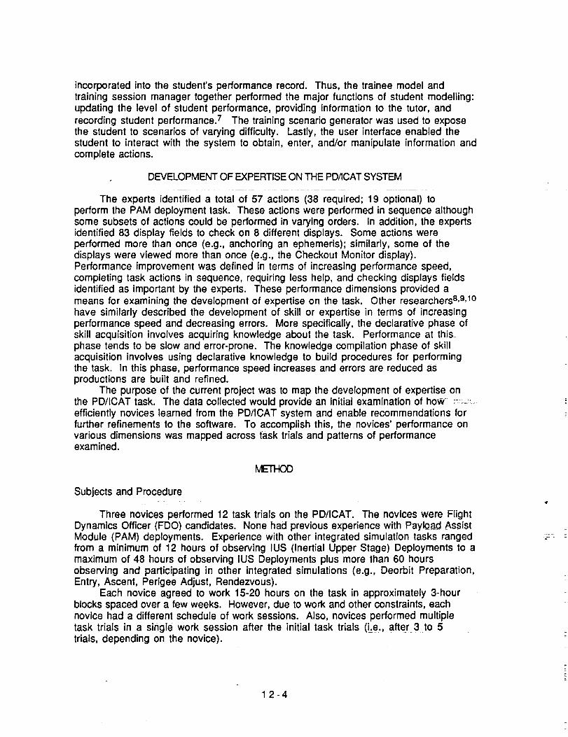
incorporated into the student's performance record. Thus, the trainee model andtraining session manager together performed the major functions of student modelling:updating the level of student performance, providing information to the tutor, andrecording student performance. 7 The training scenario generator was used to exposethe student to scenarios of varying difficulty. Lastly, the user interface enabled thestudent to interact with the system to obtain, enter, and/or manipulate information andcomplete actions.
DEVELOPMENT OF EXPERTISE ON THE PD/ICAT SYSTEM
The experts identified a total of 57 actions (38 required; 19 optional) toperform the PAM deployment task. These actions were performed in sequence althoughsome subsets of actions could be performed in varying orders. In addition, the expertsidentified 83 display fields to check on 8 different displays. Some actions wereperformed more than once (e.g., anchoring an ephemeris); similarly, some of thedisplays were viewed more than once (e.g., the Checkout Monitor display).Performance improvement was defined in terms of increasing performance speed,completing task actions in sequence, requiring less help, and checking displays fieldsidentified as important by the experts. These performance dimensions provided ameans for examining the development of expertise on the task. Other researchers 8,9,1°have similarly described the development of skill or expertise in terms of increasingperformance speed and decreasing errors. More specifically, the declarative phase ofskill acquisition involves acquiring knowledge about the task. Performance at thisphase tends to be slow and error-prone. The knowledge compilation phase of skillacquisition involves using declarative knowledge to build procedures for performingthe task. In this phase, performance speed increases and errors are reduced asproductions are built and refined.
The purpose of the current project was to map the development of expertise onthe PD/ICAT task. The data collected would provide an initial examination of howefficiently novices learned from the PD/ICAT system and enable recommendations forfurther refinements to the software. To accomplish this, the novices' performance onvarious dimensions was mapped across task trials and patterns of performanceexamined.
METHOD
Subjects and Procedure
Three novices performed 12 task trials on the PD/ICAT. The novices were FlightDynamics Officer (FDO) candidates. None had previous experience with Payload AssistModule (PAM) deployments. Experience with other integrated simulation tasks rangedfrom a minimum of 12 hours of observing IUS (Inertial Upper Stage) Deployments to amaximum of 48 hours of observing IUS Deployments plus more than 60 hoursobserving and participating in other integrated simulations (e.g., Deorbit Preparation,Entry, Ascent, Perigee Adjust, Rendezvous). _ _ _ _
Each novice agreed to work 15-20 hours on the task in approximately 3-hourblocks spaced over a few weeks. However, due to work and other constraints, eachnovice had a different schedule of work sessions. Also, novices performed multipletask trials in a single work session after the initial task trials (i.e., after 3 to 5trials, depending on the novice).
12-4

Noviceswereaskedto readthesectionon PAMdeploymentsin theSpin-StabilizedDeploymentsectionof the ProceduresManualpriorto comingto their first session. Atthe first sessionnoviceswereshownanexampleof the screendisplayandtold howtouse thekeyboardandthe mouseto enterand manipulatetask information.Theywereasked to "think out loud" as they performed the first task trial, that is, to describewhat they were doing. In addition, the novices were invited to give their commentsabout the task interface and to ask questions as they performed the task. Theirdescription of their actions, comments, and questions were tape recorded. Allcomments on the interface and questions about the task were noted by the researcher.However, only questions about the mechanics of the task were answered. Noinformation was provided about which actions to perform at various points in the task.The novices were also told that their comments about the interface would be discussed
with the task experts and the PD/ICAT programmers. Following each session, noviceswere shown a computer-generated feedback report describing their performance,their comments and questions were noted, and the next work session was scheduled.They were asked to "think out loud" again for Trials 3 and 9 (Trial 8 for one subjectwho was available for only 11 trials). On all other trials, the novices performed thetask without having their comments tape recorded. Their comments and questions werenoted by the researcher, usually at the end of the task trial.
The 12 task trials were completed in 5-6 work sessions. Following the last worksession, the novices were asked to complete two short, paper and pencil tests. First,novices were asked to sort a list of all task actions into the proper sequence as quicklyand accurately as possible. Second, novices were asked to identify information fields onscreen displays as quickly and accurately as possible. Printed copies of each screendisplay were provided on which novices circled or checkmarked information fields theythought they were supposed to check during the PAM deployment task. Two of thenovices completed these tests 7 days after and one novice 12 days after their last worksession. Finally, novices were debriefed and thanked for their participation.
Measures
Performance measures were collected by the computer during task performance.The performance measures collected for each trial were: trial time, number of actionscompleted, number of errors, number of help requests, and number of display fieldschecked. Trial time referred to the time required (in minutes) to complete a tasktrial. Number of actions completed referred to the number of actions (with or withouterrors) completed by the novice rather than by the Training Session Manager. (ThePD/ICAT system was structured such that when the novices made three consecutiveerrors while attempting to complete an action, the Training Session Manager used thedomain expert to complete the action.) Number of errors was the sum of three types oferrors: the number of actions performed in an incorrect sequence, typographicalerrors (i.e., inputs the computer was unable to interpret), and optional (butrecommended) actions which were not performed by the novice. Number of helprequests was the sum of two types of help requests: the number of times novicesrequested more information from a tutor message following an error and the number ofrequests for explanations of the current or last step of the task.
Finally, number of display fields checked was the sum of the checks made on 8unique screen displays, some viewed multiple times (see Table 1). The maximumscore was 83 display checks. Data was not available for one other display (DetailedManeuver Table 1) because the computer did not correctly record the number of
12-5

displayfieldschecked. Viewinganydisplaywas an optional (but recommended) action.(The PD/ICAT system was structured such that configuring and viewing each displayconstituted two separate actions. A display could be configured without being viewed.)The recommended sequence and frequency of viewing different displays was determinedby experts and incorporated into the PD/ICAT software. The Vector ComparisonDisplay, however, was the only display not viewed as often as recommended by theexperts. Rather than penalize the novices for failing to check displays fields on adisplay they failed to view, an average score was calculated. The score for the VectorComparison Display was calculated as the average number of display fields checkedeach time the display was viewed (e.g., the score was 5 if the nowce viewed the cl3_p_aytwice and checked 4 and 6 fields on the first and second viewings, respectively).
TABLE 1.- DESCRIPTION OF SCREEN DISPLAYS AND DISPLAY CHECKS.
# of Times # of DisplayDisplay Viewed Fields to Check
Vector Comparison*Trajectory DigitalsCheckout MonitorTrajectory Profile Status**Detailed Maneuver Table 2Weight Gain/Loss TableSupersighterFDO Deploy Comp
3 7,6,61 24 9,9,9,92 7,71 71 31 91 12
*An average score was used calculated from the 3 viewing opportunities.**Only the score for the 2nd viewing opportunity was used. Data was not correctlyrecorded by the computer for the 1st viewing opportun!ty.
Additional performance measures were collected using the paper and pencil testsadministered after the task trials. Three performance measures were collected on thesorting task. Sorting time referred to the time (in minutes) required to sort thesequence of actions. Unacceptable reversals referred to the number of actions sorted inincorrect sequences. Acceptable reversals referred to the number of actions sorted ina sequence regarded by the experts as an acceptable alternate sequence of actions. Twoperformance measures were collectecl_r0m the display checking task. Checking timereferred to the time (in minutes) required to check display fields on the 8 displayslisted in Table 1. Number of display checks recalled was the sum of the fields checkedon these 8 displays.
RESULTS
To examine how efficiently the novices learned the PD/ICAT task, their data wasplotted for each performance measure. As discussed below the data indicated rapidperformance improvements until Trial 5 and more gradual further improvements
12-6

through Trial 12. A logarithmic function was used to describe the data in eachmeasure.
As shown in Figure 1, the trial time required to perform the task decreasedrapidly until Trial 5. Further performance speed improvements were more gradual.In Trial 1 only one novice completed the task and required 195 minutes. The meantrial time was approximately 46 minutes by Trial 5 and decreased to approximately26 minutes by Trial 12. The data was described by a logarithmic function (Y =233.95 * X-.s3, R2= .87). Interestingly, the novices who were unable to completethe task in the initial task trials demonstrated a performance pattern similar to thatshown by Novice 1. Two novices failed to complete the task during the first 3-hoursession, and 1 novice failed to complete the task until the third session. However,these novices demonstrated trial times similar to Novice 1 by Trial 5. Finally, thedata indicates that the instruction to "think out loud" while performing the task slowsperformance speed. The time required to perform the task increased in Trial 3 forNovice 1, in Trial 8 for Novice 2, and in Trial 9 for Novices 1 and 3.
Q
3c
oE
m
I--
2OO
180
16O
140
120
100
8O
6O
4O
2O
0
Novice 1• Novice 2-- Novice 3
0 1 2 3 4 5 6 7 8 9 10 11 12 13
Task Trial
Figure 1.- Performance speed in Trials 1 through 12.
Number of actions completed also demonstrated rapid performance Improvementsuntil Trial 5 and then gradual further improvements. A logarithmic function (Y =
12-7

34.49 * X.22) accounted for 63% of the variance (see Figure 2). In Trial 1, Novice 1completed 43 actions out of the 57 possible actions. The remaining 14 actions werecompleted by the Training Session Manager, using the domain expert. Novices 2 and 3completed only 28 and 26 actions, respectively. An additional 5 actions werecompleted by the Training Session Manager. Thus, Novice 1 completed 75% of theactions he attempted and Novices 2 and 3 completed 85% and 84% of the actions theyattempted. However, one should note that Novices 2 and 3 completed or attempted tocomplete only 60% of the possible actions during Trial 1 while Novice 1 completed or
. attempted to complete all possible actions. The novices completed a mean of 52.33actions in Trial 5 and a mean of-5-3.67 actions in Trial 12. Further, the novicescompleted at least 96% of the actions they attempted in Tria! 5 and at least 98% inTrial i2._None of the novices attempted tO complete morb t_nan 5"5 actions. Thus,novices chose not to perform at least 2 of the optional actions In every trial.
6O
55
"Oo
• 50
E0
45
m¢,.o
m
o
o
E
Z
4O
35
3O
25
2O
Novice 1Novice 2
-- Novice 3
0 1 2 3 4 '5 6 7 8 9 10 1i 12 13
Task Trial
Figure 2.- Number of actions completed in Trials 1 through 12.
Number of errors demonstrated a similar pattern of performance. A logarithmicfunction (Y = 40.46 * X -1.°°) accounted for 69% of the variance (see Figure 3). InTrial 1, the novices made a mean of 24 errors. Novice 1, however, made .54errors/action attempted while Novices 2 and 3 made .58 and .87 errors/actionattempted, respectively. By Trial 5, the noyices made a mean o.f 4.33 errors and
V
12-8

further reducedtheir errors to a mean of 3.5 by Trial 12. Thus, by Trial 5 thenovices made a mean of only .08 errors/action attempted. By Trial 12, furtherperformance improvements resulted in a mean of only .06 errors/action attempted.
Similar to other performance measures, number of help requests demonstratedrapid reductions from Trial 1 to Trial 5, but there were few help requests followingTrial 5. A logarithmic function (Y = 46.44 * X -1.58) accounted for 91% of thevariance (see Figure 4). (Note: The data in Figure 4 reflect a transformation of [X +1] to enable a logarithmic function to be fit. Data reported in the text are in theiroriginal, untransformed units.) However, the novices showed much greatervariability in their help requests than in other performance measures, especially inTrials 1 and 2. In Trial 1, the number of help requests ranged from 7 to 32 requests.The number of help requests varied even more in Trial 2, ranging from 1 to 49requests. By Trial 3, however, the novices made similar numbers of requests with amean of 7.33 requests. In Trial 5, the novices made a mean of .67 help requests andonly one help request was made from Trial 8 through 12.
°,9LI,I
4O
35
30
25
qio 20
E
Z
15
10
5
Novice 1• Novice 2-- Novice 3
o0 1 2 3 4 5 6 7 8 9 10 11 12 13
Task Trial
Figure 3.- Number of errors made in Trials 1 through 12.
Finally, number of display fields checked demonstrated rapid performanceimprovements from Trial 1 to Trial 5 and more gradual improvements through Trial
12-9

12. A logarithmic function (Y = 25.94 * X .5°) accounted for 70% of the variance (seeFigure 5). In Trial 1, the novices checked a mean of 10.33 display fields. However,only Novice 1 had the opportunity to check all 83 display fields because the other twonovices did not complete the task in Trial 1. Thus, Novice 1 checked 13% of theappropriate display fields. Novice 2 checked 12% of the 34 display fields he viewed,and Novice 3 checked 59% of the 27 display fields he viewed. Although Novice 3checked a higher percentage of display fields than the other novices, it is not clear thathe understood which fields should be checked. He may have checked numerous fieldsbecause he was unsure which were important. The task software did not record checksof any display fields other than those identified as important by the experts. Thus,following Trial 1, the novices were instructed to check only those fields theyconsidered important in each display. In Trial 5, the novices checked a mean of 69.22fields which was 80% of the identified display fields. By Trial 12, the novices checkeda mean of 79.89 fields, checking 96% of the identified fields.
60
m
o
O"o
n,,
a.
-!-
O
,,Q
EZ
55
50
45
40
35
30
25
20
15
10
5
00
Novice 1Novice 2
-- Novice 3
1 2 3 4 5 6 7 8 9 10 11 12 13
Task Trial
Figure 4.- Number of help requests in Trials 1 through 12.
The results from the two paper and pencil tests were examined to determinewhether the novices knew the correct sequence of actions in the task and whether theyknew which display fields were important to check, as identified by the experts. The
12-10
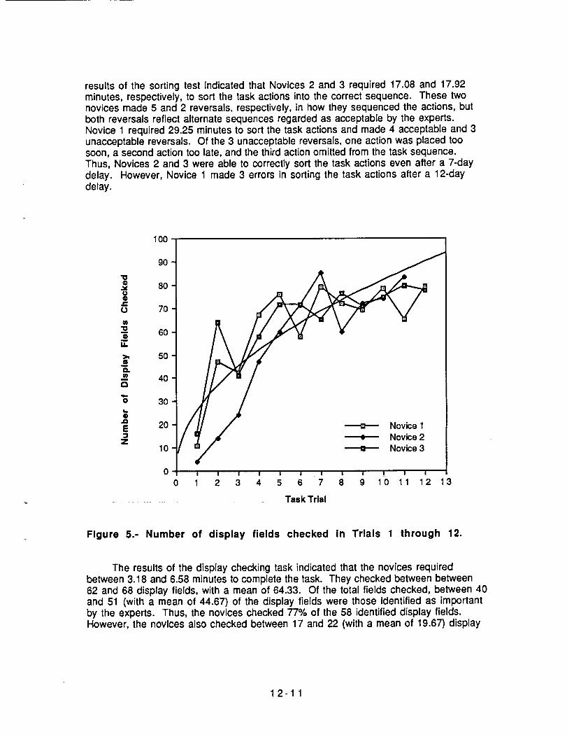
resultsof the sorting test indicated that Novices 2 and 3 required 17.08 and 17.92minutes, respectively, to sort the task actions into the correct sequence. These twonovices made 5 and 2 reversals, respectively, in how they sequenced the actions, butboth reversals reflect alternate sequences regarded as acceptable by the experts.Novice 1 required 29.25 minutes to sort the task actions and made 4 acceptable and 3unacceptable reversals. Of the 3 unacceptable reversals, one action was placed toosoon, a second action too late, and the third action omitted from the task sequence.Thus, Novices 2 and 3 were able to correctly sort the task actions even after a 7-daydelay. However, Novice 1 made 3 errors in sorting the task actions after a 12-daydelay.
1oo
90
,, 80ooJ=o 70
-o 6Oo
50
D=
4O0
o 30
.oE 20
Z10
Novice 1Novice 2Novice 3
00 1 2 3 4 5 6 7 8 9 10 11 12 13
Task Trial
Figure 5.- Number of display fields checked in Trials 1 through 12.
The results of the display checking task indicated that the novices requiredbetween 3.18 and 6.58 minutes to complete the task. They checked between between62 and 68 display fields, with a mean of 64.33. Of the total fields checked, between 40and 51 (with a mean of 44.67) of the display fields were those identified as importantby the experts. Thus, the novices checked 77% of the 58 identified display fields.However, the novices also checked between 17 and 22 (with a mean of 19.67) display
12-11

fields not identified as important. This indicated that 31% of the fields the noviceschecked were not identified as important by the experts.
DISCUSSION
The results indicated that performance improved most rapidly from Trial 1 toTrial 5 on the PD/ICAT task. Additional task trials showed smaller, more gradualimprovements. This suggests that the novices had developed effective procedures forperforming the task by Trial 5. Additional task trials enabled the novices to refinethese procedures, increasing performance Speed and decreasing errors. If the goal is totrain the novices to perform this specific task version as efficiently as possible,additional practice in Trials 6 through 12 may be warranted. However, the novicesperformed only the nominal PAM deployment task on the PD/ICAT. They also need tolearn how to deal with problems that can occur during a PAM deployment, e.g., an OMS(Orbital Maneuvering Subsystem) propellant leak. So, given the smallerimprovements following Trial 5, it may be reasonable after Trial 5 to expose thenovices to more problematic PAM deployment scenarios.
Prior to making this decision, though, criteria should be identified for eachperformance dimension. That is, one needs to identify acceptable levels of performancein terms of time (in minutes) required to complete a task trial, number of completedactions (both required and optional), number of errors made, number of helprequests, and number of display fields checked. These criteria, rather than a trialnumber, could then be used to determine when to expose a novice to a more difficulttask scenario.
The _esults of the two tests administered after task performance indicated thatthe novices were able to recall the appropriate sequence of task actions a week afterperforming the last task trial, although there may be some decrements in recall fordelays of more than a week. Similarly, the novices recalled 77% of the display fieldsto check after a week delay. However, decisions also need to be made here regarding 1)how many display fields should be recalled and 2) the potential benefits or costs ofchecking display fields not identified as important by the experts. In the nominal PAMdeployment task the novices performed, no costs were associated with checking fieldsother than those identified. One needs to determine under what conditions it is
acceptable and perhaps even desirable to check additional display fields. Experts mayneed to rank order the importance of checking different displays.
Finally, a few comments on the task interface are needed_rhese comments arebased on comments and problems reported to the researcher by the novices. First, thenovices experienced difficulty in beginning the ta.sk during Trial 1. All three noviceswere unsure what the first step should be. Consequently they received multiple errormessages and may have become frustrated. To alleviate this problem, it may beappropriate to provide novices with additional information prior to performing Trial1. This information could be in the form of task instructions, an example of the tasksequence performed by the computer as the novice observes, or perhaps step by stephelp in completing the task sequence in the first task trial.
Second, the novices reported that some displays should be accessible at any pointin the task. The PD/ICAT task as currently designed allows the novice to requestdisplays only at specific points in the task. The novices' report should be clarifiedwith experts and modifications made to the software to either provide novices withgreater access to displays or more explanation about why they should or should notneed to view a display at a specific point in time.
12-12

Third, all three noviceshad difficulty interpretingthe error messagesprovided.Furtherrefinementsof the PD/ICATtask should includeimprovementsin the tutoring(i.e., error messages)provided.
Finally,moreconsideration needs to be given to the data collected from novices'task performance. Observing the novices performing the task indicated that they oftenattempted to perform actions out of sequence, primarily in the initial task trials.However, while the PD/ICAT software currently records whether an action has beencompleted and number of errors associated with that action, no record is made of thespecific sequence in which the actions were attempted. Further refinements to thesoftware should enable the recording of sequencing information. Similarly, thecurrent PD/ICAT software records only checks of identified display fields. Thus, apossible task strategy for a novice would be to check every field in a display to ensurethat the machine recorded s/he had checked the important fields. A future enhancementof the software should include recording all display fields checked and perhapsproviding information to the novice on why the identified fields are important to check.
_U._ONS
Novices can efficiently learn to perform the PD/ICAT task which simulates anominal PAM deployment. Additional work is needed to more clearly identifyperformance criteria and expand the PD/ICAT software to include more problematicPAM deployment scenarios. Finally, refinements are needed to improve the tutoring(error messages) provided and to assist the novice in performing the first task trial.The generally positive results of this project provide an initial demonstration of theeffectiveness of the PD/ICAT software in teaching novices a nominal PAM deploymenttask and indicates the potential benefits of future refinements and expansions of thePD/ICAT software.
12-13

REFERENCES
1. Wenger, E. (1987). Artificial Intelligence and Tutoring Systems. Los Altos,CA: Morgan Kaufmann.
2. Loftin, R. B. (1987). A General Architecture for Intelligent TrainingSystems. Final Report, NASA/ASEE Summer Faculty Fellowship Program, JohnsonSpace Center, Contract No. 44-001-800.
3. Wang, L., Baffes, P., Loftin, R. B., &Hua, G. (1989). An intelligent trainingsystem for space shuttle flight controllers. Proceedings of the 1989 Conference onInnovative ADDlications of Artificial Intelligence.
4. VanLehn, K. (1988). Student modelling. In M. C. Poison & J. J. Richardson(Eds.), Foundations of Intelligent Tutoring Systems. Hillsdale, NJ: Erlbaum, 55-78.
5. Burton, R. R. & Brown, J. S. (1982). An investigation of computer coachingfor informal learning activities. In D. Sleeman & J. S. Brown (Eds.), Intelligent
Tutoring Systems. NY: Academic Press, 79-98.
6. Reiser, B. J., Anderson, J. R., & Farrell, R. G. (1985). Dynamic studentmodelling in an intelligent tutor for LISP programming. Proceedings of the 9thInternational Joint Conference on Artificial Intelligence (Vol. 1. DO. 8-14L
7. Biegel, J. E., Interrante, L. D., Sargeant, J. M., Bagshaw, C. E., Dixon, C. M.,Brooks, G. H., Sepulveda, J. A., & Lee, C. H. (1988). Input and instruction paradigmsfor an intelligent simulation training system. Proceedings of the 1st Florida ArtificialIntelligence Research Symposium (DD. 250-253).
8. Anderson, J. R. (1985). Cognitive Psvchol0gv and its Implications (2nd
_. NY: W. H. Freeman.
9. Chi, M. T. H., Glaser, R., & Rees, E. Expertise in problem solving. In R. J.Sternberg (Ed.), Advances Jn theJ:)sychologv of Human Intelligence (Vol. 1).Hillsdale, NJ: Erlbaum, 7-76.
10. Stevens, A., Collins, A., & Goldin, S. E. (1982). Misconceptions in students'understanding. In D. Sleeman & J. S. Brown (Eds.), Intelligent Tutoring Systems. NY:Academic Press, 13-24.
lr
v
12-14

J_J_._/_ REPORT DOCUMENTATION PAGE
National Aeronautics andSpace Ad m in istration
I
1. Report No. I
INASA CR 185601
4, Title and Subtitle
2. Government Accession NO. 3. Recipient's Catalog No.
5, Report Date
December 1989
6. Performing OrganizatiOn Code
8. Performing Organization Report No.
10. Work Unit NO.
12,
NASAJASEE Summer Faculty Fellowship Program--1989Volume 1
Author(s)
William B. Jones, Jr. and Stanley H. Goldstein, Editors
Performing Organization Name and Address
Texas A&M University
College Station, TX 77843
Sponsoring Agency Name and _ddress
National Aeronautics and Space Administration
Washin_on, D.C. 20546
11. Contract or Grant No.
NGT 44-001-800
3 Type of RepOrt and Period Covered
Contractor Report
14. _ponsormg Agency Code
t5. Supplementary Notes
16. Abstract
The 1989 Johnson Space Center (JSC) National Aeronautics and Space Administration (NASA)/American Society for
Engineering Education (ASEE) Summer Faculty Fellowship Program was conducted by Texas A&M University and JSC.The 10-week program was operated under the auspices of the ASEE. The program at JSC, as well as the programs at otherNASA Centers, was funded by the Office of University Affairs, NASA Headquarters, Washington, D.C. The objectives of
the program, which began nationally in 1964 and at JSC in 1965, are (1) to further the professional knowledge of qualkfied
engineering and science faculty members; (2) to stimulate an exchange of ideas between participants and NASA; (3) toenrich and refresh the research and teaching activities of participants' institutions; (4) to contribute to the research
objective of the NASA Centers
Each faculty fellow spent at least 10 weeks at JSC engaged in a research project commensurate with his/her interests andbackground and worked in collaboration with a NASA/JSC colleague. This document is a compilation of the final reports T
on the research projects performed by the faculty fellows during the summer o£ 1989. Volume 1 contains reports 1 through L13, and Volume 2 contains reports 14 through 26.
17. Key Words (Suggested by Author(s))
19.
18. Distribution Statement
!J'nclassi.fied - Unlimited
Security Classification (of this report)
Unclassified
20. Security Classsfication (of this page)
Unclassified
T
21. No. of pages /22 Price
338 _ NTIS
For sate by the National Technical Information Service, Spr,ngfietd, VA 22161-2171
;SC _-orm 1424 (Rev ._,ug _39) (Ethernet,Fan 88)
L'.s. c'.overnmeng: Printing 0EfLce:lg89-761-O!.4/00212
