nanoscale heat transport through solid-solid and … · nanoscale heat transport through...

Nanoscale Heat Transport Through Solid-solid and Solid-liquid Interfaces

Hari Harikrishna

Dissertation submitted to

Virginia Polytechnic Institute and State University

in partial fulfillment of the requirements for the degree of

Doctor of Philosophy

in

Engineering Mechanics

Scott T. Huxtable, Chair

William A. Ducker

Mark R. Paul

Mark A. Stremler

Raffaella De Vita

July 3, 2013

Blacksburg, Virginia

Keywords: Nanoscale heat transport, kapitza resistance, thermoreflectance,

solid-liquid interfaces, self-assmebled monolayers

Copyright 2013, Hari Harikrishna

Nanoscale Heat Transport Through Solid-solid and Solid-liquid Interfaces

Hari Harikrishna

Abstract

This dissertation presents an experimental investigation of heat transport through

solid-solid and solid-liquid interfaces. Heat transport is a process initiated by the presence

of a thermal gradient. All interfaces offer resistance to heat flow in the form of temperature

drop at the interface. In micro and nano scale devices, the contribution of this resistance

often becomes comparable to, or greater than, the intrinsic thermal resistance offered by the

device or structure itself. In this dissertation, I report the resistance offered by the interfaces

in terms of interface thermal conductance, G, which is the inverse of Kapitza resistance

and is quantified by the ratio of heat flux to the temperature drop. For studying thermal

transport across interfaces, I adapted a non-contact optical measurement technique called

Time-Domain Thermoreflectance (TDTR) that relies on the fact that the reflectivity of a

metal has a small, but measurable, dependence on temperature.

The first half of this dissertation is focused on investigating heat transport through

thin films and solid-solid interfaces. The samples in this study are thin lead zirconate-

titanate (PZT) piezoelectric films used in sensing applications and dielectric films such as

SiOC:H used in semiconductor industry. My results on the PZT films indicate that the

thermal conductivity of these films was proportional to the packing density of the elements

within the films. I have also measured thermal conductivity of dielectric films in different

elemental compositions. I also examined thermal conductivity of dielectric films for a variety

of different elemental compositions of Si, O, C, and H, and varying degrees of porosity. My

measurements showed that the composition and porosity of the films played an important

role in determining the thermal conductivity.

The second half of this dissertation is focused on investigating heat transport through

solid-liquid interfaces. In this regard, I functionalize uniformly coated gold surfaces with

a variety of self-assembled monolayers (SAMs). Heat flows from the gold surface to the

sulfur molecule, then through the hydrocarbon chain in the SAM, into the terminal group

of the SAM and finally into the liquid. My results showed that by changing the terminal

group in a SAM from hydrophobic to hydrophilic, G increased by a factor of three in water.

By changing the number of carbon atoms in the SAM, I also report that the chain length

does not present a significant thermal resistance. My results also revealed evidence of linear

relationship between work of adhesion and interface thermal conductance from experiments

with several SAMs on water. By examining a variety of SAM-liquid combination, I find that

this linear dependency does not hold as a unified hypothesis. From these experiments, I

speculate that heat transport in solid-liquid systems is controlled by a combination of work

of adhesion and vibrational coupling between the ω-group in the SAM and the liquid.

iii

Dedication

I dedicate this dissertation to my wife Neelima Krishnan and our kids Manu and Maya for

their constant encouragement, support and patience.

iv

Acknowledgments

First of all, I would like to express my deep sense of gratitude and profound thanks to Dr.

Scott T. Huxtable for allowing me to do my dissertation under his supervision. He is an

excellent philosopher and a great human being. He was very instrumental in me learning to

do things the right way. Our non-academic conversations have always inspired me to a great

extent. I am honored to have met you and your guidance is greatly appreciated.

I am also sincerely grateful to Dr. William A. Ducker for his professional expertise

in Chemical Engineering. His constant encouragement and inspiration were very helpful

in motivating me to go the extra mile to relearn chemistry 101. I am also thankful to

his students Dmitri Iarikov and Dean J. Mastropietro for teaching me proper chemistry lab

technique. I would also like to thank my committee members Dr. Mark R. Paul, Dr. Raffaella

De Vita and Dr. Mark A. Stremler for their guidance and feedback on this dissertation.

I thank our collaborators Ronnie Vargheese and Dr. Shashank Priya from Center

for Energy Harvesting Materials and Systems (CEHMS) for Lead zirconate titanate (PZT)

samples and also Dr. Sean W. King (and his group) from Intel R© Corporation for providing

v

the dielectric films.

I also thank Donald Leber for all the help he has offered me in our clean room facil-

ity. My friend Shree Narayanan was always ready to help when I had issues with sample

fabrication and characterization. I also appreciate the help and advice of my colleagues Dr.

Nitin C. Shukhla, Hao-Hsiang Liao and Chris Vernieri who guided me when I joined Prof.

Huxtable’s group.

During my time at Virginia Tech, I have taken several classes, met with many faculty

members in professional and friendly environments. I am grateful to have met them in my

life. All of them have brought positive changes in my life. So, thank you Dr. Mark R. Paul,

Dr. Scott L. Hendricks, Dr. Douglas P. Holmes, Dr. Zhaomin Yang and Dr. Alexander

Leonessa. Being involved in active badminton helped me relieve all the grad school stress.

Thanks to VT Badminton team and Rec Sports for their excellent support.

I thank my parents who have motivated me to do well in my life. A special word of

praise goes to my brother and my sister-in-law. One of our evening dinners has changed the

course of my life.

My wife, Neelima has been a constant source of inspiration. Bringing up a toddler boy

and a newborn girl while both of us attended graduate school was a huge challenge. Most

importantly, it has taught us how to stay focused to improve our productivity during the

daytime. For to be parents in graduate school, it is totally worth it.

vi

Contents

Abstract ii

Dedication iv

Acknowledgments v

Table of Contents vii

List of Figures xii

List of Tables xxi

1 Introduction 1

1.1 Heat transport basics . . . . . . . . . . . . . . . . . . . . . . . . . . . . . . . 1

1.2 Interface thermal conductance . . . . . . . . . . . . . . . . . . . . . . . . . . 3

1.3 Models for interface thermal conductance . . . . . . . . . . . . . . . . . . . . 4

vii

1.3.1 Acoustic mismatch model . . . . . . . . . . . . . . . . . . . . . . . . 5

1.3.2 Diffuse mismatch model . . . . . . . . . . . . . . . . . . . . . . . . . 5

1.3.3 Comparison of AMM and DMM . . . . . . . . . . . . . . . . . . . . . 6

1.4 Background on interface thermal conductance . . . . . . . . . . . . . . . . . 7

1.5 Organization of dissertation . . . . . . . . . . . . . . . . . . . . . . . . . . . 9

References . . . . . . . . . . . . . . . . . . . . . . . . . . . . . . . . . . . . . . . . 11

2 Experimental setup and mathematical modeling 13

2.1 Time-domain thermoreflectance (TDTR) . . . . . . . . . . . . . . . . . . . . 15

2.1.1 Experimental setup . . . . . . . . . . . . . . . . . . . . . . . . . . . . 17

2.1.2 Improvements to signal to noise ratio . . . . . . . . . . . . . . . . . . 20

2.1.3 Data acquisition . . . . . . . . . . . . . . . . . . . . . . . . . . . . . . 22

2.2 Mathematical modeling of TDTR . . . . . . . . . . . . . . . . . . . . . . . . 23

2.3 Sensitivity Analysis . . . . . . . . . . . . . . . . . . . . . . . . . . . . . . . . 25

2.4 Electrical conductivity for thin films . . . . . . . . . . . . . . . . . . . . . . . 28

References . . . . . . . . . . . . . . . . . . . . . . . . . . . . . . . . . . . . . . . . 30

3 Heat transport across solid-solid interfaces 33

viii

3.1 Thermal transport through thin piezoelectric films . . . . . . . . . . . . . . . 33

3.1.1 Background and objectives . . . . . . . . . . . . . . . . . . . . . . . . 34

3.1.2 Sample details . . . . . . . . . . . . . . . . . . . . . . . . . . . . . . . 36

3.1.3 TDTR analysis . . . . . . . . . . . . . . . . . . . . . . . . . . . . . . 38

3.1.4 Results and discussion . . . . . . . . . . . . . . . . . . . . . . . . . . 44

3.2 Thermal conductivity of low-k dielectric films . . . . . . . . . . . . . . . . . 51

3.2.1 Background and objectives . . . . . . . . . . . . . . . . . . . . . . . . 51

3.2.2 Sample details . . . . . . . . . . . . . . . . . . . . . . . . . . . . . . . 53

3.2.3 TDTR analysis . . . . . . . . . . . . . . . . . . . . . . . . . . . . . . 56

3.2.4 Results and discussions . . . . . . . . . . . . . . . . . . . . . . . . . . 59

References . . . . . . . . . . . . . . . . . . . . . . . . . . . . . . . . . . . . . . . . 66

4 The influence of interface bonding on thermal transport through solid-

liquid interfaces 71

4.1 Abstract . . . . . . . . . . . . . . . . . . . . . . . . . . . . . . . . . . . . . . 71

4.2 Introduction . . . . . . . . . . . . . . . . . . . . . . . . . . . . . . . . . . . . 72

4.3 Sample details . . . . . . . . . . . . . . . . . . . . . . . . . . . . . . . . . . . 75

4.4 Results and discussions . . . . . . . . . . . . . . . . . . . . . . . . . . . . . . 78

ix

4.5 Conclusions . . . . . . . . . . . . . . . . . . . . . . . . . . . . . . . . . . . . 84

References . . . . . . . . . . . . . . . . . . . . . . . . . . . . . . . . . . . . . . . . 86

5 Heat transport across solid-liquid interfaces 89

5.1 Background and objectives . . . . . . . . . . . . . . . . . . . . . . . . . . . . 90

5.2 Sample details . . . . . . . . . . . . . . . . . . . . . . . . . . . . . . . . . . . 93

5.2.1 Sensitivity analysis . . . . . . . . . . . . . . . . . . . . . . . . . . . . 97

5.2.2 Contact angle . . . . . . . . . . . . . . . . . . . . . . . . . . . . . . . 98

5.2.3 Infrared spectrum . . . . . . . . . . . . . . . . . . . . . . . . . . . . . 99

5.3 Mechanisms for the heat conduction . . . . . . . . . . . . . . . . . . . . . . . 101

5.4 Thermal conductance as a function of chain length . . . . . . . . . . . . . . 103

5.5 Thermal conductance as a function of terminal group . . . . . . . . . . . . . 106

5.5.1 Transport through gold-SAM-water interfaces . . . . . . . . . . . . . 107

5.5.2 Transport through gold-SAM-organic liquid interfaces . . . . . . . . . 113

5.6 Results and discussion . . . . . . . . . . . . . . . . . . . . . . . . . . . . . . 114

5.7 Conclusions . . . . . . . . . . . . . . . . . . . . . . . . . . . . . . . . . . . . 124

References . . . . . . . . . . . . . . . . . . . . . . . . . . . . . . . . . . . . . . . . 126

x

6 Conclusions and future work 130

6.1 Summary and conclusions . . . . . . . . . . . . . . . . . . . . . . . . . . . . 130

6.2 Future work . . . . . . . . . . . . . . . . . . . . . . . . . . . . . . . . . . . . 133

6.2.1 Solid-solid interfaces . . . . . . . . . . . . . . . . . . . . . . . . . . . 133

6.2.2 Solid-liquid interfaces . . . . . . . . . . . . . . . . . . . . . . . . . . . 135

A TDTR data collection 137

B self-assembled monolayer preparation 140

C Collection of experimental results 143

xi

List of Figures

1.1 Temperature profile across nanoscale dissimilar materials joined at the in-

terface between hot and cold plates. (a) Temperature drop at the interface.

(b) The interface is considered to be an imaginary layer of unknown thermal

properties with zero resistance across both interfaces. . . . . . . . . . . . . . 4

1.2 RAMM/RDMM vs acoustic impedance dissimilarity. Swartz and Pohl4 studied

AMM and DMM for various combinations of acoustic impedance dissimilarity. 6

1.3 Experimental measurements on interface thermal conductance on different

interfaces. Lyeo and Cahill15 summarized interface thermal conductance be-

tween various interfaces. . . . . . . . . . . . . . . . . . . . . . . . . . . . . . 9

2.1 Experimental setup of TDTR technique. The laser beam is split into pump

and probe beams using a beam splitter. The pump beam heats up the sample

and the probe beam monitors the thermal decay on the surface of the sample. 16

xii

2.2 Typical signals from TDTR experiments. (a) in-phase (Vin) and out-of-phase

(Vout) signals from the lock-in amplifier. (b) -Vin/Vout signal. Analyzing the

ratio of voltage signals minimizes non-idealities due to changes in pump-probe

overlap and defocusing of probe beam. . . . . . . . . . . . . . . . . . . . . . 20

2.3 Screen capture of data acquisition using LabVIEW software. The starting

point, step size, the dwell time, end point of the delay stage is controlled

through this graphical user interface. When the delay stage returns at the

end of an experiment, the software writes the position of delay stage, delay

time, in phase and out of phase voltages into a data file. . . . . . . . . . . . 22

2.4 Experimental TDTR data (solid diamond) and fit from the thermal model

(solid blue line) for a reference sample that consists of a thin layer of aluminum

evaporated on a sapphire substrate. . . . . . . . . . . . . . . . . . . . . . . . 25

2.5 Sensitivity analysis as a function of delay time with a modulation frequency

of f=10 MHz. . . . . . . . . . . . . . . . . . . . . . . . . . . . . . . . . . . . 27

2.6 Sensitivity analysis as a function of modulation frequency presented at a delay

time of t=0.2 ns . . . . . . . . . . . . . . . . . . . . . . . . . . . . . . . . . . 27

3.1 Schematic diagram (not to scale) of the PZT sample. Thin PZT film is grown

using sol-gel process on a Platinum surface. . . . . . . . . . . . . . . . . . . 36

3.2 Aluminum (∼30 nm) is deposited using electron beam evaporator. . . . . . . 38

xiii

3.3 Simulations from the mathematical model using either the oxide layer or the

silicon layer as the substrate. The blue open squares represent the simulation

where silicon was included in the model, and the red circles represent the case

where the silicon layer was removed from the model. Since the results from

the two different models are the same, we can ignore silicon in our models. . 39

3.4 The five unknowns parameters in studying the PZT sample. . . . . . . . . . 40

3.5 The five unknowns parameters in the problem is reduced to three by examining

a separate reference sample. . . . . . . . . . . . . . . . . . . . . . . . . . . . 41

3.6 Sensitivity analysis of PZT sample. . . . . . . . . . . . . . . . . . . . . . . . 42

3.7 Thermoreflectance data for sample PZT-100. The open red circles represents

the experimental data, while, the solid lines are the results from the models. 43

3.8 Thermoreflectance data on sample PZT-100 taken on three random spots on

the sample. . . . . . . . . . . . . . . . . . . . . . . . . . . . . . . . . . . . . 44

3.9 When the pump beam hits the aluminum, a strain wave is generated which

propagates through the metal film and reflects off the interface with the ad-

joining layer. This propagation is dependent on speed of sound in aluminum.

In this particular sample, the acoustic wave bounces within the aluminum a

few times before it decays. . . . . . . . . . . . . . . . . . . . . . . . . . . . 45

3.10 Experimental data (open circles) vs model data (solid line) for PZT samples. 47

xiv

3.11 Schematic diagram (not to scale) of the dielectric film grown on a silicon

substrate. . . . . . . . . . . . . . . . . . . . . . . . . . . . . . . . . . . . . . 54

3.12 (a) Aluminum deposited for thermoreflectance measurements using electron

beam evaporator in a cleanroom environment. (b) There are only two un-

knowns in the experiment. . . . . . . . . . . . . . . . . . . . . . . . . . . . . 56

3.13 Sensitivity analysis on dielectric samples. Here both k in Wm−1K−1 and G1

in MWm−2K−1 were changed individually by 5%. . . . . . . . . . . . . . . . 58

3.14 -Vin/Vout data from the mathematical model for k values of 0.5 W m−1 K−1

(open blue circles) and 0.6 W m−1 K−1 (open red diamonds) show a near

constant offset. . . . . . . . . . . . . . . . . . . . . . . . . . . . . . . . . . . 59

3.15 (a) Aluminum thickness measured from acoustic echoes from thermoreflectance

measurements. (b) Speed of sound in the dielectric film can be calculated from

the echo (around 500 ps). . . . . . . . . . . . . . . . . . . . . . . . . . . . . 61

4.1 Schematic diagram of the sample structures. The pump and probe laser beams

enter through the transparent fused silica substrate and are reflected from the

aluminum film. Aluminum is used as the thermoreflectance layer since it

exhibits a relatively large change in reflectivity with temperature at our laser

wavelength of 800 nm. Gold is a convenient choice for attaching monolayers

since gold-thiol interactions are well understood and allow for the formation

of SAMs with a variety of terminal groups (labeled ω). . . . . . . . . . . . . 76

xv

4.2 Comparison of experimental TDTR data with an analytical thermal model.

The plot displays the ratio of in-phase to out-of-phase voltage measured by

a lock-in amplifier at the photodiode (-Vin/Vout) as a function of the delay

time between the pump and probe beams. The solid circles and squares are

experimental data, and the solid lines represent the best fit to our model where

G is the only fitting parameter. The oscillations in the data for t ≤ 500 ps

are due to acoustic echoes in the metal layers. . . . . . . . . . . . . . . . . . 79

4.3 Measured interface thermal conductance at room temperature as a function

of the thermodynamic work of adhesion at the interface, WSL. The work

of adhesion is calculated from Equation 4.1 using the measured value of the

surface tension of water (γLV = 72 mJ m−2) and the advancing contact angle

of water on the SAM as shown in Table 4.1. The solid line is a least squares fit

to our data where G = 1.32 WSL + 13 (R2 = 0.987). The cluster of our data

at WSL 40 mJ m−2 and G 60 MWm−2K−1 represent the three alkane-thiols

of varying chain length (i.e. three homologues of n-undecanethiol with 11,

12, and 18 carbon atoms). The solid square symbols are measurements from

Ge et al. (Ref. 19) for various SAMs on Au and Al in water, and the open

squares are molecular dynamics simulations from Shenogina et al. (Ref. 20). 81

5.1 Schematic diagram (not to scale) of the sample. . . . . . . . . . . . . . . . . 94

xvi

5.2 Schematic diagram (cross-sectiton not to scale) of the flow cell used for the

thermoreflectance measurements. . . . . . . . . . . . . . . . . . . . . . . . . 95

5.3 Schematic diagrams for samples examined to determine G for solid-liquid in-

terfaes. (a). By studying a reference sample, we measure the thermal con-

ductivity of the fused silica substrate and the interface thermal conductance

between aluminum and the fused silica. (b) The only unknown in the SAM

sample is the interface thermal conductance between the SAM and the liquid 96

5.4 Sensitivity analysis of the thermal conductance, G, between a functionalized

gold surface and a liquid on a SAM sample. G has units of MWm−2K−1. . . 97

5.5 Schematic diagram (not to scale) of a droplet on the sample used for contact

angle measurements. γ is the interfacial free energy and θ is the contact angle. 98

5.6 The infrared spectrum of the ω-COOH monolayer. The peaks at 1700 cm−1

and 2800 cm−1 corresponds to C=O and C-H bonds, respectively. . . . . . . 100

5.7 TDTR measurements on samples prepared to study the effect of chain length

of SAMs. (a) Thermoreflectance measurements on C11, C12 and C18 are the

same. A best fit for G = 60 MWm−2K−1 was obtained from the mathematical

model. (b), (c) and (d) shows excellent matching between the experimental

data (open circles) and model (solid blue line). The amplitude of the Vin/Vout

signal in (b), (c) and (d) is different because of different metal thickness. . . 105

xvii

5.8 Thermoreflectance measurements on samples prepared to study the effects of

terminal group of SAMs. (a) G changes from 60− 190 MWm−2K−1 by chang-

ing the terminal group from hydrophobic ω-CH3 to hydrophilic ω-COOH. (b)

Interface thermal conductance for ω-pyrrol and ω-ester measured to be 140

MWm−2K−1. (c) There is no difference in thermoreflectance data between

ω-COOH and ω-OH coatings. (d) Thermal conductance did not change de-

spite changing the H to Br in the terminal group. The open circles represents

experimental data and solid black line represents data from the analytical

model. . . . . . . . . . . . . . . . . . . . . . . . . . . . . . . . . . . . . . . . 110

5.9 Interface thermal conductance as a function of work of adhesion, WSL. The

experimental data is denoted by red circles. The error bars correspond to

uncertainty values in G due to uncertainty in metal thicknesses and thermal

properties. The solid line is a least squares fit to our data (excluding the ω-

CH2Br) where G = 1.29 WSL + 14.39 (R2 = 0.989). The thermal conductance

for the ω-CH2Br monolayer does not fall on the straight line. This could be

due to weak van der Waals interactions between the SAM and water molecule

evident by examining the vibrational spectra of the SAM in water. . . . . . . 112

xviii

5.10 Comparison of interface thermal conductance as a function of work of adhe-

sion, WSL, for the ω-OH (open blue triangles) and the ω-COOH (open red

diamonds) SAMs against every liquid in the measurement. The crowded re-

sults in the low (35-60 mNm−1) WSL region is from the liquids (di-methyl

formamide, ethanol, benzene, hexadecane, chloroform, carbon tetrachloride

and hexane). The two liquids in the intermediate work of adhesion (90-100

mNm−1) are formamide and ethylene glycol. Water has the highest work of

adhesion WSL ∼ 135 mNm−1. . . . . . . . . . . . . . . . . . . . . . . . . . . 117

5.11 Comparison of interface thermal conductance as a function of work of adhesion

WSL for water and heavy water for various SAMs. (a) The open red markers

represent water and filled blue markers represent heavy water. . . . . . . . . 118

5.12 Interface thermal conductance of various SAMs on (a) di-methyl formamide

and (b) formamide as a function of work of adhesion. Vibrational spectra

match can reveal weak van der Waals interactions of Formamide with various

SAMs which results in low values of interface thermal conductance. Neither

work of adhesion nor vibrational overlap hypotheses explain the low thermal

conductance of di-methyl formamide. . . . . . . . . . . . . . . . . . . . . . . 120

5.13 Interface thermal conductance of various SAMs on (a) benzene and (b) carbon

tetrachloride. Larger G for benzene could not be explained whereas, low values

of G for SAMs-carbon tetrachloride can be attributed to the weak van der

Waals interactions. . . . . . . . . . . . . . . . . . . . . . . . . . . . . . . . . 121

xix

5.14 Chloroform forms only weak van der Waals interactions with the monolayers.

Hence, the high values of interface thermal conductance of various SAMs on

chloroform cannot be explained by any of the available hypotheses. . . . . . 122

5.15 Interface thermal conductance of various SAMs on (a) ethanol and ethylene

glycol (b) hexadecane and hexane. The better overlap in the vibrational

spectra in the larger molecules may explain the higher interface thermal con-

ductance in these SAM-liquid combinations. . . . . . . . . . . . . . . . . . . 123

5.16 Interface thermal conductance as a function of work of adhesion WSL for all

SAM-liquid combination from the Table 5.3. . . . . . . . . . . . . . . . . . . 125

xx

List of Tables

3.1 Pyrolysis and annealing conditions along with orientation and thickness of

PZT films. . . . . . . . . . . . . . . . . . . . . . . . . . . . . . . . . . . . . . 37

3.2 Thermal properties of thin PZT films measured by TDTR technique. . . . . 46

3.3 Inorganic low-k dielectric films . . . . . . . . . . . . . . . . . . . . . . . . . . 55

3.4 Thermal conductivity results for low-k dielectric films. . . . . . . . . . . . . . 60

4.1 Molecules and Water Contact Angles for the Preparation of Self-assembled

Monolayers. a). Angles are the measured advancing (Adv) and receding

(Rec) contact angles of water on the monolayer in air. The uncertainty values

listed for the contact angles span the range of values observed on repeated

measurements on multiple films. b). The uncertainty values for G represent

the range of values that could fit our experimental data given the propagation

of uncertainties in our experimental data and in the parameters that are input

to our thermal model (e.g. metal film thicknesses and conductivities). . . . . 77

xxi

5.1 Self-assembled Monolayer Molecules, their Water Contact Angles and interface

thermal conductance results. . . . . . . . . . . . . . . . . . . . . . . . . . . . 104

5.2 Thiol molecules, their water contact angles and thermal conductance between

gold-water interface. . . . . . . . . . . . . . . . . . . . . . . . . . . . . . . . 109

5.3 Interface thermal conductance, G, measured on a variety of SAM-Liquids

combination in units of MWm−2K−1 and the advancing (Adv) contact angle

for the liquid on the SAM. Work of adhesion, WSL=γ (1 + cosθ), for each

SAM-liquid combination is given in units of mN m−1. . . . . . . . . . . . . . 115

C.1 Thermal properties of PZT films. The results indicate that thermal conduc-

tivity have a dependence on crystal orientation of these films. . . . . . . . . 144

C.2 Thermal conductivity results for low-k dielectric films. Thermal conductivity

cannot be accurately predicted/explained solely from porosity, density, and

composition. . . . . . . . . . . . . . . . . . . . . . . . . . . . . . . . . . . . . 145

C.3 Self-assembled Monolayer Molecules, their Water Contact Angles and interface

thermal conductance results. The results show that the phonon transport is

not affected by the chain length of the monolayer. . . . . . . . . . . . . . . . 146

C.4 Molecules and water contact angles for the preparation of self-assembled mono-

layers. The results show that the terminal group have a significant impact on

heat conduction. . . . . . . . . . . . . . . . . . . . . . . . . . . . . . . . . . 147

xxii

C.5 Interface thermal conductance, G, measured on a variety of SAM-Liquids

combination in units of MWm−2K−1 and the advancing (Adv) contact angle

for the liquid on the SAM. Work of adhesion, WSL=γ (1 + cosθ), for each

SAM-liquid combination is given in units of mN m−1. . . . . . . . . . . . . . 148

xxiii

Chapter 1

Introduction

1.1 Heat transport basics

Heat transport in a medium originates from the presence of a thermal gradient. Macroscale

thermal transport depends on the bulk properties of the material such as thermal conduc-

tivity, heat capacity and density. Also, temperature which is an intensive property (is a

measure of the average kinetic energy of the atoms/molecules), in the macroscale is well

defined at every point. Hence, using continuum mechanics principles, Fourier’s law of heat

conduction can be derived as:

q′′

x = −k

(dT

dx

), (1.1)

where, q′′x is the heat flux along the direction x, k is the thermal conductivity of the

material along the direction x, and dTdX

is the temperature gradient in the direction x. Thermal

1

2

conductivity, k, is a property of the continuum, and it quantifies the ability of the medium to

conduct heat. This heat is conducted by carriers such as electrons and phonons (quantized

lattice vibrations). In metals, heat conduction, like electrical conduction, is dominated by

free electrons. In non-metals, heat transport is dominated by phonons. Thermal conductivity

for metals at any given temperature T is directly proportional to electrical conductivity as

observed by Wiedemann-Franz:

k

σ= L× T (1.2)

where, σ is the electrical conductivity, L is the Lorenz number (2.44×10−8) W Ω K−2.

Thermal conductivity for phonon related excitations is given as:

k =1

3C× v × ` (1.3)

where, C is the heat capacity, v is the mean velocity of phonons and ` is the mean free path

of the phonons. In nanoscale devices, the dimension of the material may become comparable

to the mean free path of the carriers. Thus, as the characteristic lengthscale of a structure

approaches the mean free path of the energy carriers, the relative importance of the boundary

or interface increases. Therefore, for nanostructured materials, the total thermal resistance

of the material may be dominated by the resistance at the interfaces rather than the intrinsic

thermal resistance of the material. In this dissertation, I report measurements of thermal

conductance across a variety of different solid-solid and solid-liquid interfaces.

3

1.2 Interface thermal conductance

An interface may be defined as a physical boundary between two different materials. The

concept of interface thermal conductance was first proposed by Kurti et al.1 while they

investigated the flow of helium below 1K . The first experimental results on interface thermal

resistance were reported by Kapitza2 while studying heat transfer between solid copper

and supercooled helium. The resistance offered by an interface to heat flow q′′

is directly

proportional to the drop in temperature ∆T across the interface. Kapitza resistance, R, is

defined as ∆T/q′′. Interface thermal conductance, G, is the inverse of R and is defined as

G =q

′′

∆T(1.4)

To better understand the concept of interface thermal conductance, consider an inter-

face between two dissimilar materials that are in intimate contact as shown in Figure 1.1(a).

The presence of a thermal gradient between the two materials generates a heat flux between

the hot and cold plates. All interfaces present a resistance to heat this heat flux, thus creating

a temperature drop at the interface. As mentioned previously, this temperature drop can be

quantified in terms of a Kapitza resistance or an interface thermal conductance. For typical

solid-solid or solid-liquid interfaces, G spans a range of 10 to 1000 MWm−2K−1. To put these

values in more familiar terms, one can consider an equivalent thermal resistance created by

a thin layer of oxide, where this resistance is equal to the thermal conductivity of the oxide

divided by its thickness. Assuming a typical thermal conductivity of k = 1 Wm−1K−1 for

the oxide, a G of 100 MWm−2K−1 presents an equivalent thermal resistance as a 10 nm

4

(a) (b)

Figure 1.1: Temperature profile across nanoscale dissimilar materials joined at the interface

between hot and cold plates. (a) Temperature drop at the interface. (b) The interface is

considered to be an imaginary layer of unknown thermal properties with zero resistance

across both interfaces.

thick layer of oxide. In a semiconductor application, a 10 nm thick oxide layer can degrade

the performance of the device quite drastically. On the other hand, jet engine turbines and

similar applications where thermal isolation is critical would benefit from interfaces with low

thermal conductance.

1.3 Models for interface thermal conductance

To explain the experimental behavior observed by Kapitza2, Khalatnikov3 proposed a mathe-

matical model based on the acoustic impedance mismatch between materials at an interface

called the Acoustic Mismatch Model (AMM). In the AMM model, it was assumed that

5

phonon transport is elastic, which worked accurately for lower temperature measurements.

In 1987, Swartz and Pohl4 developed a mathematical model taking into account for the

scattering of phonons called as Diffuse Mismatch Model (DMM).

1.3.1 Acoustic mismatch model

Acoustic impedance is defined as the product of mass density and speed of sound in the ma-

terial is analogous to the index of refraction in the field of optics. At an interface of dissimilar

materials, due to the mismatch in acoustic impedances, phonons behave in the same way as

an electromagnetic wave would scatter when it encounters a difference in refractive index.

Because the AMM model assumes no phonon scattering, this model underestimates thermal

conductance of interfaces between extreme large acoustic mismatch materials. However, it

also overestimates conductance of interfaces with materials of same acoustic impedance such

as silicon-grain boundary.

1.3.2 Diffuse mismatch model

In this model, it is assumed that the phonons incident upon the interface are elastically

scattered in random directions. The probability of scattering into one side of the interface

or the other is simply proportional to the densities of states for phonons in the different

materials. Due to elastic scattering at the interface the frequency of the phonon does not

alter during scattering at the interface. The model also assumes that an incident phonon will

6

never scatter into multiple lower frequency phonons or that multiple numbers of phonons

will never scatter into higher frequency phonons.

1.3.3 Comparison of AMM and DMM

Figure 1.2: RAMM/RDMM vs acoustic impedance dissimilarity. Swartz and Pohl4 studied

AMM and DMM for various combinations of acoustic impedance dissimilarity.

In summary, at low temperatures and at sufficiently defect-free interfaces, phonons

are not strongly scattered and therefore, the acoustic mismatch model is a realistic model.

At high temperature and at sufficiently imperfect interfaces, phonons will scatter at the

interface and therefore, the diffuse mismatch model leads to a more realistic description of the

experiments. Swartz and Pohl4 studied G using AMM and DMM for various combinations

of solid materials at low temperatures. Figure 1.2 shows the ratio of GAMM/GDMM vs the

acoustic mismatch of the dissimilar materials. The leftmost dotted line identifies a region

of solid-solid boundary with relatively little dissimilarity, such as aluminum on quartz, the

7

middle dotted line identifies a region of solid-solid boundary with large dissimilarity, such as

platinum on quartz. The rightmost dotted line marks the beginning of the region of extremely

large dissimilarity, as found in the Kapitza experiment(liquid helium-copper interface).

1.4 Background on interface thermal conductance

The first experimental investigation on interface thermal conductance (resistance) was re-

ported by Kapitza2 while studying heat transport across copper and supercooled helium.

Little5 modified the AMM model taking phonon scattering into consideration and found

that for a perfectly joined interface, the interface thermal conductance, G, is proportional to

the difference in the fourth power of the temperature on each side of the interface. Johnson

and Little investigated samples of copper, gold, tungsten, single-crystal lithium fluoride, and

single-crystal silicon in the temperature range from 1.25 to 2.10 K and found that Kapitza

resistances of these samples can be represented by a power law of temperature. Folinsbee6

measured Kapitza resistance between liquid or solid Helium and surfaces of Mg, Cu, W,

and Au in the temperature range 0.03 - 0.3 K and found excellent match with the AMM

model. Haug7 explained Kapitza conductance by modifying the AMM model taking into

account the phonon absorption in the solid caused by scattering on surface dislocations.

Huberman8 developed a mathematical model taking into account vibrational modes at the

interface between diamond and lead and found that the Kapitza conductance was ∼ 100

times higher than predicted by the Khalatnikov AMM model. Sergeev9 investigated metal-

8

insulator interface and found that strong electron phonon coupling at the interface. This

inelastic scattering of phonons was mathematically modeled and found excellent agreement

with Kapitza experiments.

In 1986, Paddock and Eesley10 introduced first thermal transport using picosecond

transient thermoreflectance by measuring thermal diffusion of single crystal nickel. Time-

domain thermoreflectance (TDTR) technique was later introduced by Cahill11 to study ther-

mal transport in dissimilar materials. Cahill also modified the Feldman’s solution for heat

tranfer in layered structures to measure cross plane thermal conductivity. Huxtable et al.12

used TDTR to image at micrometer scale the Cr-Ti interface. Costescu et al.13 used TDTR

to measure the thermal conductance across TiN/MgO and TiN/Al2O3 to be ∼ 650-700

MWm−2K−1. DMM predictions were found to be lower than this value.

Majumdar and Reddy proposed heat transport between metal/non-metal interface

can be facilitated only via two possible pathways: i) The electrons transfer their energy to

phonons in the metal and then phonons are carrying the heat across the interface and into

the non-metal. ii) The energy is transferred from electrons to phonons via a direct coupling

at the interface. This theory was found to be in good agreement with the experimental data

published by Costescu et al13.

A high interface thermal conductance of 4000 MWm−2K−1 was measured by Gundrum

et al.14 for Al/Cu interface. This was attributed to the lower contribution of phonons as

heat transport carriers across metal-metal interface. To study heat transport across a metal

and a non-metal interface, Lyeo and Cahill15 measured thermal conductance between Pb

9

and Bi ∼ 30 MWm−2K−1 and Bi and Hydrogen terminated silicon ∼ 8 MWm−2K−1. Figure

1.3 shows a collection of experimental measurements on interface thermal conductance.

Figure 1.3: Experimental measurements on interface thermal conductance on different in-

terfaces. Lyeo and Cahill15 summarized interface thermal conductance between various

interfaces.

1.5 Organization of dissertation

It can be observed from Figure 1.3 that thermal conductance varies from 8 MWm−2K−1

to 700 MWm−2K−1 depending on the carriers in the medium. The higher the G, lower the

10

resistance to heat flow and vice versa. It is critical to have a better understanding of thermal

conductance while designing devices involved in heat transport. In the following chapters, I

describe my measurements of interface thermal conductance across solid-solid and solid-liquid

interfaces. The experimental details are explained in depth in the second chapter along with

the details of the mathematical modeling and sensitivity analysis. The third chapter focuses

on heat transport across solid-solid interfaces. In the fourth chapter, I present the influence of

interface bonding on thermal transport through solid-liquid interfaces specifically for water.

In the fifth chapter, I explain different mechanisms that dictate thermal transport through

a wide variety of SAM-liquid combinations. Results and discussions are presented within.

Finally, I present conclusions on the current work along with future work to be completed

before dissertation in sixth chapter. Steps followed in measuring TDTR signals are explained

in detail in Appendix A. Self assembled monolayers (SAMs) are prepared by following steps

described in Appendix B. Appendix C lists all the results from the experiments from Chapters

3, 4 and 5.

References

1. Kurti, N., Rollin, B. V., and Simon, F. Physica 3(266) (1936).

2. Kapitza, P. L. Journal of Physics (USSR) 4(181) (1941).

3. Khalatnikov, I. M. Journal of Experimental and Theoretical Physics 22, 687 (1952).

4. Swartz, E. T. and Pohl, R. O. Reviews of Modern Physics 61(3), 605–668 (1989).

5. Little, W. A. Canadian Journal of Physics 37(334) (1959).

6. Folinsbee, J. T. and Anderson, A. C. Journal of Low Temperature Physics 17(409)

(1974).

7. Haug, H. and Weiss, K. Physics Letters A 45(170) (1972).

8. Huberman, M. L. and Overhauser, A. W. Physical Review B 50(5), 2865–2873 (1994).

9. Sergeev, A. V. Physical Review B 58(16), R10199–R10202 (1998).

10. Paddock, C. A. and Eesley, G. L. Journal of Applied Physics 60(1), 285–290 (1986).

11

12

11. Cahill, D. G., Goodson, K., and Majumdar, A. Journal of Heat Transfer-Transactions

of the Asme 124(2), 223–241 (2002).

12. Huxtable, S., Cahill, D. G., Fauconnier, V., White, J. O., and Zhao, J. C. Nature

Materials 3(5), 298–301 (2004).

13. Costescu, R. M., Wall, M. A., and Cahill, D. G. Physical Review B 67, 5 (2003).

14. Gundrum, B. C., Cahill, D. G., and Averback, R. S. Physical Review B 72(24), 245426

(2005).

15. Lyeo, H. K. and Cahill, D. G. Physical Review B 73(14), 144301 (2006).

Chapter 2

Experimental setup and mathematical

modeling

Thermal conductivity measurements on bulk materials have been extensively studied1,2.

Gustafsson et al.3,4 proposed transient hot strip method to study thermal properties of

insulating solids and fluids, specifically for water, to be ∼ 0.6 Wm−1K−1. Rosencwaig

and Gersho5 studied the photoacoustic effect on solids by exposing the sample to chopped

monochromatic light. Pessoa et al.6 measured thermal diffusivity of semiconductor and

amorphous materials using photoacoustics. Zammit et al.7 measured thermal conductivity

and optical absorption coefficients of silicon using photoacoustics. The measured value for

thermal conductivity of silicon was in good agreement with literature values. Later Zammit

et al.? extended this technique to measure heat capacity of liquid crystals. Heat capacity

and thermal conductivity of thin films using a pulse method was investigated by Filler et

13

14

al.8 on thin aluminum film. Kelemen9 proposed analytically a new technique to measure

thin film thermal conductivity by measuring thermal diffusivities. He also found that for

film thickness ≤ 500 nm the thermal conductivity depends on the film thickness.

Thermocouples were used to measure thermal conductivity and Young’s modulus for

thin films and coatings10. Picosecond acoustics were used to characterize thermal con-

ductivity of thin films11–13. Lin et. al.14 investigated different vibrational modes of gold

nanostructures using picosecond ultrasonics. Hostetler et al.15 measured thin film thickness

by observing ultrasonic waves generated by the femtosecond laser heating pulses.

The 3-ω method was developed by Cahill16,17 to measure thermal conductivity of bulk

materials. It was later extended by Lee and Cahill18 to measure thermal conductivity for

thin SiO2 and SiNx films. Their measurements were in excellent match with literature values

and found reduced thermal conductivity for decreasing film thickness.

Eesley et al.19 used picosecond laser pulses to generate acoustic pulses in thin metal

films using transient thermoreflectance (TTR) measurements on 129 nm nickel film. Paddock

et al.20 measured thermal diffusivity by using transient thermoreflectance in the single crys-

tal nickel film which was confirmed from the literature values. Clemens et al.21 later studied

the interfacial disorder on thermal diffusion between two metals. Capinski et al.22 modified

the experiments done by Eesley et al.19 and Paddock et al.20 and developed a picosecond

pump-probe technique to measure the thermal conductivity of GaAs/AlAs superlattices over

temperatures ranging 100 K to 375 K. Stoner and Maris23 used thermoreflectance to inves-

tigate Kapitza conductance for metal-dielectrics interface over temperatures ranging 50 K

15

to 300 K. They also measured thermal conductivities of the metal films which matched well

with the literature values. Cahill24 modified the pump probe technique proposed by Cap-

inski et al. and developed time-domain thermoreflectance (TDTR) using femtosecond laser

pulses to accurately measure the thin film thermal conductivity and the interface thermal

conductance between two dissimilar materials.

For my dissertation, I find time-domain thermoreflectance (TDTR) the best suited to

investigate thermal transport through solid-solid and solid-liquid interfaces. I explain this

experimental technique in depth in the following sections.

2.1 Time-domain thermoreflectance (TDTR)

For analyzing heat transport across interfaces, I adapted a non-contact optical measurement

technique called Time-Domain Thermoreflectance (TDTR) that relies on the fact that the re-

flectivity of a metal has a small, but measurable, dependence on temperature. A Ti:Sapphire

mode-locked laser is used to produce a series of sub-picosecond optical pulses with wavelength

800 nm at a repetition rate of 80 MHz. These pulses are split into two separate beams,

which are referred to as the ”pump” beam and the ”probe” beam. The pump beam heats

the sample, and the probe beam measures thermally induced change in reflectivity which

is proportional to the surface temperature. By changing the time delay between the pump

and probe beams with a mechanical delay stage, we can measure the thermal decay of a

sample with picosecond time resolution for delay times out to 3.4 ns. Thermal properties are

16

Figure 2.1: Experimental setup of TDTR technique. The laser beam is split into pump and

probe beams using a beam splitter. The pump beam heats up the sample and the probe

beam monitors the thermal decay on the surface of the sample.

17

extracted by curve fitting unknown parameters using an already established mathematical

model24.

2.1.1 Experimental setup

Figure 2.1 shows a schematic of our experimental setup. For our measurements, we use

an ultrafast laser (Mai Tai HP from Newport R©Corporation) which produces a series of

femtosecond optical pulses ∼ 100 fs in the near infrared region (typically 800 nm) at a

repetition rate of 80 MHz. The laser beam exiting the cavity (horizontal polarization) is

split into two separate beams, commonly referred to as the ”pump” and ”probe” beam

using a 50:50 non-polarizing beam splitter. The pump beam passes through an electro optic

modulator where it is modulated at 10 MHz (for best sensitivity of our measurements).

This modulated beam (vertical polarization) is focused on to the sample using a standard

microscope objective lens. The incident pump beam heats up the sample, as a fraction of

the energy in the pump beam is absorbed by a thin aluminum film on the surface of the

sample. The probe beam (horizontal polarization) is focussed with the objective lens on to

the same spot on the sample as the pump beam. The reflected probe beam is directed on to

a high-speed photodetector (silicon photodiode). A radio frequency (RF) lock-in amplifier

measures the photodiode signal at the pump modulation frequency. The lock-in amplifier

records the in-phase (Vin) and out-of-phase (Vout) voltages produced by the photodiode. By

delaying the arrival of the probe beam at the sample with respect to the pump beam, we can

examine how the sample cools on a picosecond time scale. Figure 2.2 shows such a temporal

18

decay of surface temperature with respect to delay time. This time delay is achieved by

using a corner cube retro-reflector mounted on a mechanical delay stage. The delay stage

has 600 mm of travel, which corresponds to ∼ 3 ns of delay between the pump and the probe

beam.

A CCD camera is used to capture a dark-field image of the sample surface. This image

of the sample surface is useful for focusing and aligning the pump and probe beams as well

as for ease in navigating to desired regions of the sample. Figure 2.2 (a) displays the in-

phase (Vin) and out-of-phase (Vout) voltages recorded by the lock-in amplifier. Figure 2.2

(b) shows the ratio of -Vin/Vout signal with respect to delay time. Many non-idealities in the

measurement, such as defocusing of the delayed probe beam, or changes in the pump-probe

overlap at the sample surface, affect both Vin and Vout in the same manner. Therefore, by

analyzing the ratio of (Vin/Vout) many of the non-idealities in the system can be minimized

or eliminated.

A thin film aluminum (∼ 40-50 nm), which has a large change in reflectivity with

respect to temperature (dR/dT ∼ 2 × 10−4 K−1 at a wavelength of 770 nm)24 is deposited

on the sample by electron beam evaporation (Physical Vapor Deposition) in the Micro &

Nano Fabrication Laboratory in Virginia Tech. The pump beam is focused on the sample

and is absorbed within the first 10-15 nm of the aluminum layer. The time required for

temperature to stabilize within the Aluminum layer is given by,

τ =d2Al

π2αAl

, (2.1)

19

where dAl and αAl are the thickness and thermal diffusivity of aluminum layer, respectively.

The surface temperature of the aluminum layer decays as heat diffuses from the metal layer,

across the aluminum-sample interface, through the sample, and into the underlying substrate.

This change in reflectivity (change in surface temperature) is monitored with the probe

beam which is directed to a photodetector. A lock-in amplifier records the in-phase (Vin)

and out-of-phase (Vout) voltages produced by the photodetector. The penetration depth of

the thermal wave created by the periodic heating in TDTR is controlled by the modulation

frequency, f. The penetration depth, d, of the thermal wave can be defined25 as the distance

from the surface at which the amplitude of the temperature oscillation is reduced by a factor

of 1/e.

A sound wave is generated when the aluminum film absorbs the energy from the pump

beam. This sound wave generated from the metal surface travels through the aluminum and

reflects off of the interface with the underlying layer. When this wave returns to the surface,

the change in strain affects the reflectivity which produces an increased in-phase data as

shown in Figure. 2.2(a). Since we know the speed of sound in aluminum (6420 m/s), the

film thickness can be calculated by using the round trip time required for the acoustic wave

travel.

20

−20 0 20−20

20

60

100

time (ps)

Sig

nal (

µ V

)

Vout

Vin

(a)

0.1 1 40

1

2

3

4

5

6

Delay time(ns)

−V

in/V

out

(b)

Figure 2.2: Typical signals from TDTR experiments. (a) in-phase (Vin) and out-of-phase

(Vout) signals from the lock-in amplifier. (b) -Vin/Vout signal. Analyzing the ratio of voltage

signals minimizes non-idealities due to changes in pump-probe overlap and defocusing of

probe beam.

2.1.2 Improvements to signal to noise ratio

Any number of minor modifications to the experimental apparatus can be beneficial for not

only obtaining accurate and repeatable data but also improves our signal to noise ratio for

a given application. Similarly, there are several pitfalls that one should be careful to avoid

when assembling a TDTR system and performing measurements. Several such details are

listed below.

• Since the laser beam diverges, we use a pair of Keplerian lens systems so that the pump

and probe beams have 1/e2 diameters of ∼ 25 µm at the surface of the sample.

21

• The pump beam is aligned ∼ 3 mm above the probe beam on the back of the objective.

This physical separation of the beams makes it easier to block the reflected pump beam

from reaching the photodetector and corrupting the signal.

• The photodetector senses the change in reflectivity from the sample. To amplify this

signal, an inductor is connected in series to the photodetector. The capacitance from

the photodetector together with the inductor create a series L-C circuit that amplifies

the signal. Here we use an inductor of 17.2 µH at a resonant frequency of 9.8 MHz.

• The magnitude of the signal is determined by the product of the pump and probe beam

energies. Thus the pump and probe beams do not need to be split in a 95/5 manner

as is typical for other pump-probe measurements.

• One potentially large source of error that requires careful attention is the phase of

the reference channel on the lock-in24. A convenient method for correctly setting

the phase is to examine the out-of-phase voltage, Vout(t), near t=0, since this voltage

should remain constant as the delay time crosses from negative to positive delay. Small

errors in the phase, ε, can be corrected after the raw data is acquired by multiplying

Vf (t) = Vin(t) + iVout(t) by a small phase correction factor of (1 - i ε). Errors in setting

the phase can be the dominant source of uncertainty for measurements ∼ 1 MHz or

less.

22

Figure 2.3: Screen capture of data acquisition using LabVIEW software. The starting point,

step size, the dwell time, end point of the delay stage is controlled through this graphical

user interface. When the delay stage returns at the end of an experiment, the software writes

the position of delay stage, delay time, in phase and out of phase voltages into a data file.

2.1.3 Data acquisition

A LabVIEW data acquisition system built specifically for TDTR handles all of the data

acquisition and communication between the computer, delay stage and the lock-in amplifier

as shown in Figure 2.3. A detailed data acquisition procedure is described in Appendix A.

23

2.2 Mathematical modeling of TDTR

TDTR is equivalent to a heat conduction problem where a semi-infinite solid is heated at the

surface by a periodic point source. This problem was explained and solved by Carslaw and

Jaeger26. With modifications, Feldman27 solved the thermal diffusion equation for a layered

geometry. The general model considers radial heat flow, however, since the penetration

depth of the thermal wave is generally much smaller than the 1/e2 radius of the pump and

probe beams, the heat flow is predominantly one dimensional24 and the measured thermal

conductivity is generally the conductivity in the direction normal to the surface.

The final solution to the heat equation can be derived as,

Re[∆RM(t)] =dR

dT

M∑m=−M

(∆T

(mτ

+ f)

+(

∆T(mτ− f

)))exp

(i2πmt

τ

)(2.2)

Im[∆RM(t)] = −i dRdT

M∑m=−M

(∆T

(mτ

+ f)−(

∆T(mτ− f

)))exp

(i2πmt

τ

)(2.3)

where R represents reflectivity, f is the pump modulation frequency in Hz, τ is the repetition

rate of the laser and i =√−1. The real and imaginary parts correspond to the in-phase

(Vin) and out-of-phase (Vout) signals measured by the lock-in amplifier. A fortran code was

first established (by Nitin C. Shukhla) to mimic the cooling behavior in thermal transport

of layered structures. Input to this fortran code is a parameter file. The first line of which

consists of laser properties such as laser frequency, modulation frequency, pump beam diam-

eter, probe beam diameters at the beginning and end of the delay stage respectively. This is

followed by thermal conductivity, k, volumetric heat capacity, C, and thickness of each layer.

For the substrate layer, the thickness is taken as one. Every interface between two dissimilar

24

materials is modeled as an additional layer of unknown thermal conductivity, volumetric

heat capacity of one Jcm−3K−1 and thickness of one nm. Interface thermal conductance is

calculated by dividing the unknown thermal conductivity by 1e−09 m (one nm). Interfacial

thermal conductance is usually reported in the units of MWm−2K−1.

Thermal properties of interest are extracted by adjusting the unknown parameters in

the thermal model until the model matches the experimental data. Typically, the inter-

face conductance between two layers and the thermal conductivity of a single layer can be

extracted simultaneously by using these two properties as fitting parameters in the model.

For metals, thin film thermal conductivity is often less than their bulk value. This can

be found using Wiedemann-Franz law from electrical conductivity (which in turn is found

by measuring 4 point probe film resistance). The volumetric heat capacity for all layers is

generally assumed to be the same as bulk values.

Figure 2.4 shows a comparison between experimental TDTR data on a reference sam-

ple that consists of a thin layer of aluminum evaporated on a sapphire substrate. The only

unknowns in this are the thermal conductivity of sapphire and the interface thermal conduc-

tance between aluminum and sapphire, both of which can be used as unknown parameters

while curve-fitting the model with experimental data. The parameters from the model cor-

respond to thermal conductivity of Sapphire of 30 Wm−1 K−1 and an interface thermal

conductance of 130 MWm−2 K−1 between aluminum and sapphire .

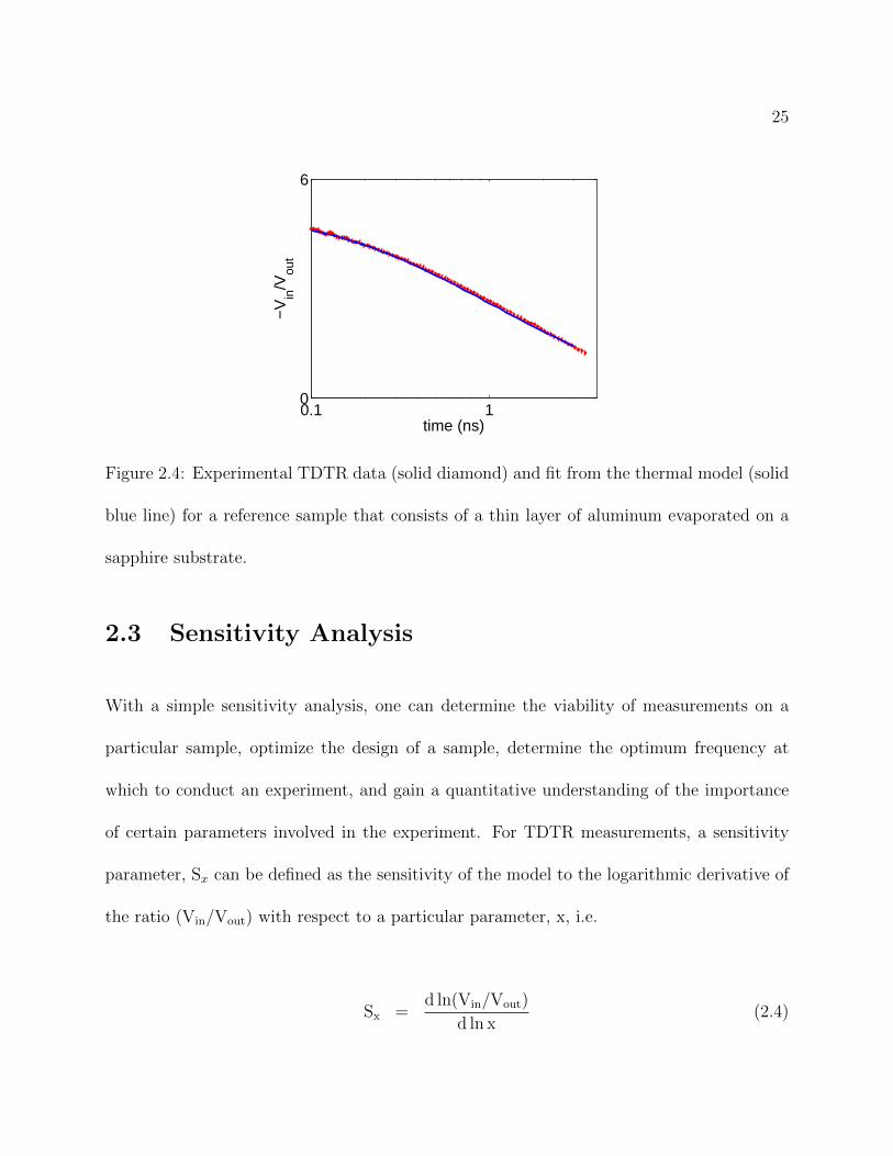
25

0.1 10

6

time (ns)

−V

in/V

out

Figure 2.4: Experimental TDTR data (solid diamond) and fit from the thermal model (solid

blue line) for a reference sample that consists of a thin layer of aluminum evaporated on a

sapphire substrate.

2.3 Sensitivity Analysis

With a simple sensitivity analysis, one can determine the viability of measurements on a

particular sample, optimize the design of a sample, determine the optimum frequency at

which to conduct an experiment, and gain a quantitative understanding of the importance

of certain parameters involved in the experiment. For TDTR measurements, a sensitivity

parameter, Sx can be defined as the sensitivity of the model to the logarithmic derivative of

the ratio (Vin/Vout) with respect to a particular parameter, x, i.e.

Sx =d ln(Vin/Vout)

d ln x(2.4)

26

Take, for example, the simple case of a film with kfilm = 1 Wm−1K−1 and Cfilm =

1Jcm−3K−1 deposited on a silicon substrate and coated with an aluminum film with thickness

of 100 nm, kAl = 180 Wm−1K−1, and CAl = 1.64 Jcm−3K−1. If the film could be grown

to thicknesses between 100 nm and 500 nm, a sensitivity analysis as shown in Figure 2.5 is

useful in understanding a few basic trends.

First, for the 100 nm film in Figure 2.5(a), we see that accurate determination of the

aluminum film thickness is critical and that the measurement is more sensitive to the con-

ductance at the film/substrate interface, G2, than the conductance at the aluminum/film

interface, G1. However, for a 500 nm thick film measured at the same frequency (Figure

2.5b), the penetration depth of the thermal wave is now confined to the film and the mea-

surement is not at all sensitive to G2 or the thermal conductivity of the substrate. For this

configuration, we also notice a typical feature in TDTR measurements in that the experi-

ment is sensitive to the thermal conductivity of the film, kfilm, at short delay times, while

the sensitivity to G1 increases at longer delay times. By fitting the model to the data at

short or long delay times one can improve the accuracy of determining either kfilm or G1.

Figures 2.6(a) and 2.6(b) show the sensitivities for the same 100 nm and 500 nm thick

films as a function of modulation frequencies between 150 kHz and 15 MHz with the delay

time fixed at 0.2 ns. Here the penetration depth of the thermal wave increases and the

influence of the substrate becomes important. For the thin film in Figure 2.6 (a), we see

that at low frequencies the measurement is sensitive primarily to the thermal conductivity

of the substrate and the thickness of the metal film. However, as the penetration depth of

27

0.1 1 4 −1.2

−0.6

0

0.6

Delay time (ns)

Sen

sitiv

ity

hAl

hfilm

G1

G2k

film

(a) hfilm=100 nm

0.1 1 4−1.2

−0.6

0

0.6

Delay time (ns)S

ensi

tivity

G2

G1

hfilm

hAl

kfilm

(b) hfilm=500 nm

Figure 2.5: Sensitivity analysis as a function of delay time with a modulation frequency of

f=10 MHz.

0.15 1 10 15−1.2

−0.6

0

0.6

Modulation frequency (MHz)

Sen

sitiv

ity

kfilm G2

G1

hfilm

hAl

(a) hfilm=100 nm

0.15 1 10 15−1.2

−0.6

0

0.6

Modulation frequency (MHz)

Sen

sitiv

ity

hfilm

hAl

G2

G1

kfilm

(b) hfilm=500 nm

Figure 2.6: Sensitivity analysis as a function of modulation frequency presented at a delay

time of t=0.2 ns

28

the thermal wave decreases at higher frequencies the importance of the substrate thermal

conductivity decreases and the influence of the film and the interfaces increases. For the

500 2m thick film in Figure 2.6 (b), several interesting trends are apparent. Most notable

is that the sensitivity to the thickness of the film crosses zero at 4 MHz, while there is

still significant sensitivity to the thermal conductivity of the film. Thus 4 MHz would be an

optimal frequency for measurements of the thermal conductivity of the film.

2.4 Electrical conductivity for thin films

As discussed previously in this chapter, one of the key inputs to our thermal model is the

thermal conductivity of the thin aluminum thermoreflectance layer. In measurements that

follow, the thermal conductivities of thin gold and platinum layers are also required. For the

thin metal films used in the TDTR measurements, the thermal conductivity is smaller than

for bulk samples, thus measurements on the actual films used in the experiments are neces-

sary. One simple, and reliable, method to determine thermal conductivity of metals is to use

the Wiedemann-Franz law in conjunction with measurements of the electrical conductivity.

The Wiedemann-Franz law can be written as,

k

σ= L× T, (2.5)

where, k is the thermal conductivity, σ is the electrical conductivity and L is Lorenz number

(2.44×10−8) W Ω K−2.

The Van der Pauw method is a four point probe technique for measuring the sheet

29

resistance of a flat material and this technique is widely used in the integrated circuit industry

for measuring electrical conductivity of thin films. The van der Pauw method is employed

because our samples are small and of arbitrary shape, and this method is effective even for

such structures. The four probes are placed arbitrarily along the periphery of the sample.

Current, I, is passed through two probes, and the difference in voltage, V, between the other

two probes is measured using a digital multimeter. Electrical conductivity can be calculated

by the following equation;

σ =ln(2)

πtF

(I

V

)(2.6)

where, t is the thickness of the thin film, and F is a geometric correction factor to account

for samples of various shapes and sizes as explained by Schroder28. The same measurement

is repeated three more times while changing the locations where current is passed and where

the voltage is measured. The electrical conductivity is then obtained by taking an average

of the four measurements. Automation of this process is achieved with the use of a Keithley

4200.

Thermal conductivities for thin aluminum (∼30 nm) and gold (∼30 nm) films were

found to be 180 Wm−1K−1 and 270 Wm−1K−1, respectively. Thermal conductivity of plat-

inum (∼150 nm) was found to be 71 Wm−1K−1.

References

1. Parrott, J., E. and Stuckes, A. Thermal Conductivity of Solids. Pion Limited, London,

(1975).

2. Suda, S., Kobayashi, N., Yoshida, K., Ishido, Y., and Ono, S. Journal of the Less-

Common Metals 74(1), 127–136 (1980).

3. Gustafsson, S. E. and Karawacki, E. Review of Scientific Instruments 54(6), 744–747

(1983).

4. Gustafsson, S. E., Karawacki, E., and Khan, M. N. Journal of Physics D-Applied Physics

12(9), 1411–1421 (1979).

5. Rosencwaig, A. and Gersho, A. Journal of Applied Physics 47(1), 64–69 (1976).

6. Pessoa, O., Cesar, C., Patel, N., Vargas, H., Ghizoni, C., and Miranda, L. Journal of

Applied Physics 59(4), 1316–1318 (1986).

7. Zammit, U., Marinelli, M., Scudieri, F., and Martellucci, S. Applied Physics Letters

50(13), 830–832 (1987).

30

31

8. Filler, R. L., Lindenfeld, P., and Deutscher, G. Review of Scientific Instruments 46(4),

439–442 (1975).

9. Kelemen, F. Thin Solid Films 36(1) (1976).

10. Krishnan, S., Babu, S. V., Bowen, R., Demejo, L. P., Osterhoudt, H., and Rimai, D. S.

Journal of Adhesion 42(1-2) (1993).

11. Grahn, H. T., Maris, H. J., and Tauc, J. Ieee Journal of Quantum Electronics 25(12),

2562–2569 (1989).

12. Vardeny, Z. Synthetic Metals 28(3) (1989).

13. Tas, G., Stoner, R. J., Maris, H. J., Rubloff, G. W., Oehrlein, G. S., and Halbout, J. M.

Applied Physics Letters 61(15) (1992).

14. Lin, H. N., Maris, H. J., Freund, L. B., Lee, K. Y., Luhn, H., and Kern, D. P. Journal

of Applied Physics 73(1) (1993).

15. Hostetler, J. L., Smith, A. N., and Norris, P. M. Microscale Thermophysical Engineering

1(3), 237–244 (1997).

16. Cahill, D. G., Fischer, H. E., Klitsner, T., Swartz, E. T., and Pohl, R. O. Journal of

Vacuum Science & Technology a-Vacuum Surfaces and Films 7(3) (1989).

17. Cahill, D. G. Review of Scientific Instruments 61(2), 802–808 (1990).

18. Lee, S. M. and Cahill, D. G. Journal of Applied Physics 81(6), 2590–2595 (1997).

32

19. Eesley, G. L., Clemens, B. M., and Paddock, C. A. Applied Physics Letters 50(12),

717–719 (1987).

20. Paddock, C. A. and Eesley, G. L. Journal of Applied Physics 60(1), 285–290 (1986).

21. Clemens, B. M., Eesley, G. L., and Paddock, C. A. Physical Review B 37(3), 1085–1096

(1988).

22. Capinski, W. S., Maris, H. J., Ruf, T., Cardona, M., Ploog, K., and Katzer, D. S.

Physical Review B 59(12), 8105–8113 (1999).

23. Stoner, R. J. and Maris, H. J. Physical Review B 48(22), 16373–16387 (1993).


25. Persson, A. I., Koh, Y. K., Cahill, D. G., Samuelson, L., and Linke, H. Nano Letters

9(12), 4484–4488 (2009).

26. Carslaw, H. S. and Jaeger, J. C. Conduction of Heat in Solids. Oxford University Press,

New York, (1959).

27. Feldman, A. High Temperatures-High Pressures 31(3), 293–298 (1999).

28. Schroder, D. K. Semiconductor Material and Device Characterization. Wiley & Sons,

New York, 2nd edition, (1998).

Chapter 3

Heat transport across solid-solid

interfaces

3.1 Thermal transport through thin piezoelectric films

There is a growing interest towards miniaturization of devices and structures to exploit the

unique and improved properties of materials at micro and nano lengthscales. With the re-

cent advancements in the fields of microfabrication, it is now possible to grow and analyze

materials with atomic layer precision. A better understanding of heat transport phenom-

ena is critical in designing and/or improving the performance of such nanoscale devices. In

this chapter, I use TDTR technique to examine the heat transport across Pb(ZrxTi1−x)O3

(PZT) thin films deposited using a sol-gel process on a substrate. The PZT materials ex-

33

34

hibit increased piezoelectric response and higher poling efficiency at x = 0.52. The thermal

conductivities of PZT films in different crystal orientations were found to be in the range of

1.5 - 1.75 Wm−1K−1. The interface thermal conductance between the PZT and substrate

was found to be in the range of 35 - 80 MWm−2 K−1.

3.1.1 Background and objectives

Smart structures use piezoelectric materials for various sensing and actuating applications

because of their unique coupling between electrical and mechanical forces. The first exper-

imental demonstration of a connection between macroscopic piezoelectric phenomena and

crystallographic structure was published in 1880 by Pierre and Jacques Curie1. Their ex-

periment consisted of a conclusive measurement of surface charges appearing on specially

prepared crystals (tourmaline, quartz, topaz, cane sugar and Rochelle salt) which were sub-

jected to mechanical stress. This effect is known as the piezoelectric effect. Materials such

as quartz, tourmaline, and rochelle salts exhibit natural piezoelectric properties. However,

their use is limited by many disadvantages including having low strength, being sensitive

to moisture and having limited operating temperature range.Commonly used piezoelectric

materials today include metal oxides since they are physically strong, chemically inert, and

relatively inexpensive to manufacture.

Most of the piezoelectric materials are crystalline solids. They can be single crystals,

either formed naturally or by synthetic processes, or they can be polycrystalline materials.

35

For a material to exhibit piezoelectric properties, its crystal structure must have no center

of symmetry. Crystals are commonly classified into seven crystal systems which are further

divided into 32 crystal classes (or point groups). Out of these 32 crystal classes, 21 are acen-

tric. All 21 acentric crystals except one exhibit the piezoelectric effect along the directional

axis. Out of the 20 piezoelectric classes, 10 have only one unique directional axis. Such

crystals are called as polar crystals and they show spontaneous polarization. The intensity

of polarization depends on the temperature. This is called the pyroelectric effect. These py-

roelectric crystals for which the magnitude and the direction of the spontaneous polarization

can be reversed by an external electric field are said to show ferroelectric behavior. Hence,

ferroelectric materials are a subset of piezoelectric materials2.

Lead zirconate-titanate (PZT) is one of the widely used ferroelectric materials. Zhuang

et al.3 studied dielectric, piezoelectric and elastic properties of PZT ceramic samples against

temperatures ranging from 4.2 to 300 K. Specific heat capacity of PZT films (x = 0.46, 0.48

and 0.50) were measured from 80 to 700 K by Yamazaki et al.4 Lang et al.5 measured heat

capacity of PZT films (x = 0.41 to 0.48) at temperatures ranging from 1.8 to 300 K. Kallaev

et al.6,7 measured thermal conductivity of ferroelectric ceramics to be in the range of 1.1 to

2.4 W m−1 K−1 at temperatures ranging from 300 K to 800 300 K. Thermal conductivity

was measured on hard PZT ceramics and soft PZT ceramics by Yarlagadda et al.8 to be in

the range of 0.01 W m−1 K−1 and 0.34 W m−1 K−1 at temperatures ranging 15 K to 300

K.

Here, I examine a variety of thin PZT films grown in different orientations (prepared by

36

a sol-gel method). Specifically, I use TDTR to measure thermal conductivity and interface

conductance across the layers. These samples were provided by our collaborators9 in Center

for Energy Harvesting Materials and Systems (CEHMS) at Virginia Tech.

3.1.2 Sample details

Fabrication and characterization of thin PZT films by sol-gel processing10–12 has been well

established for more than two decades. Norga13 studied the effect of numerous variables in-

volved in the sol-gel deposition process. Varghese et al.9 prepared the PZT thin films (∼ 70

nm) examined here by varying only the pyrolysis and annealing conditions (including ramp

up and down rates). A schematic diagram of the sample is shown in Figure 3.1. The PZT

Pt ~ 150 nm

Ti ~ 10 nm

Oxide ~ 300 nm

Si substrate

PZT ~ 70 nm

Figure 3.1: Schematic diagram (not to scale) of the PZT sample. Thin PZT film is grown

using sol-gel process on a Platinum surface.

films were deposited with a sol-gel process on a substrate which consists of 150 nm of plat-

37

Table 3.1: Pyrolysis and annealing conditions along with orientation and thickness of PZT

films.

Sample Pyrolysis AnnealingOrientation

[100] [110] [111]

Thickness

∼nm

PZT-A - - Amorphous 903

PZT-103

PZT-106

PZT-100

PZT-90

300C/3 min

300C/3 min

300C/3 min

250C/1.5 min

725C/30 min

775C/15 min

675C/45 min

625C/65 min

96.49% 3.51% 0%

92.86% 7.14% 0%

76.81% 23.19% 0%

72.41% 27.59% 0%

65.12

67.19

73.37

75.6

PZT-123

PZT-79

PZT-129

0/0

0/0

0/0

650C/45 min

675C/20 min

800C/45 min

5.88% 94.12% 0%

7.69% 92.31% 0%

0% 100% 0%

71.03

65.67

86.47

PZT-98

PZT-114

PZT-118

250C/1.5 min

250C/1.5 min

250C/1.5 min

675C/15 min

800C/60 min

750C/60 min

0% 8.77% 91.23%

0% 3.33% 96.67%

0% 3.92% 96.08%

93.84

82.06

72.94

PZT-125

PZT-104

0/0

300C/3 min

700C/40 min

775C/45 min

48.7% 1.3% 50%

39% 20.1% 40.9%

65.86

64.36

inum, 10 nm of titanium as an adhesion layer, 300 nm of SiO2 and a silicon substrate. Films

with different crystal oriented films are prepared by varying the pyrolysis and annealing con-

38

ditions as shown in Table. 3.1. Rotating orientation x-ray diffraction (XRD) measurements

are used to determine the crystal orientations of these samples. PZT film thicknesses were

measured by variable angle spectroscopic ellipsometry. The crystallographic orientation and

PZT film thickness of all the samples are also listed in Table 3.1.

3.1.3 TDTR analysis

For the TDTR measurements, a thin aluminum film (∼30 nm) was deposited on the PZT

layer in a cleanroom environment by electron beam evaporation (physical vapor deposition)

in the Micro & Nano Fabrication Laboratory at Virginia Tech. The heat pulses from the

Al ~ 30 nm

Pt ~ 150 nm

Ti ~ 10 nm

Oxide ~ 300 nm

Si substrate

PZT ~ 70 nm

Figure 3.2: Aluminum (∼30 nm) is deposited using electron beam evaporator.

39

pump laser do not penetrate beyond the thick (∼300 nm) oxide layer. Results from our

mathematical thermal model shows no difference whether the silicon substrate is included

in the model as observed in Figure. 3.3. Thus, we do not need to include the silicon in the

model, and we treat the oxide layer as the substrate.

0.1 1 40

0.5

1

1.5

2

2.5

3

time (ns)

−V

in/V

out

Figure 3.3: Simulations from the mathematical model using either the oxide layer or the

silicon layer as the substrate. The blue open squares represent the simulation where silicon

was included in the model, and the red circles represent the case where the silicon layer was

removed from the model. Since the results from the two different models are the same, we

can ignore silicon in our models.

Substrate model

When modeling the heat transport across the PZT sample shown in Figure 3.1, there are

many unknowns such as the interfacial thermal conductance between Al and PZT (G1), the

40

thermal conductivity of the PZT layer, kpzt, the thermal conductance between PZT and Pt

(G2), the thermal conductivity of the Pt layer, kpt, the thermal conductance between Pt and

Ti (G3) and so on. With this many unknowns, we are unable to find a best fit between the

model and the experimental data. To simplify this problem, TDTR measurements were first

made on a separate reference sample. The reference sample was made by depositing a thin

G1

G2

G3

G4

Oxide substrate

PZT - kPZT

Aluminum

Platinum

Titanium

Figure 3.4: The five unknowns parameters in studying the PZT sample.

film of Al (∼ 30nm) on the Pt/Ti/SiO2/Si substrate. A simpler mathematical model was used

to deduct thermal properties such as G3 and G4 by curve fitting to the experimental data as

shown in Figure 3.5. To find the thermal conductivity of Pt (kpt), electrical conductivity was

measured using van der Pauw’s four point method. Bulk values were assumed for thermal

conductivity and heat capacity of titanium and oxide layers. The thermal conductances

for the platinum- titanium interface and titanium-oxide interfaces were found to be 250

MWm−2K−1 100 MWm−2K−1 respectively.

41

G5

G3

G4

Oxide substrate

Aluminum

Platinum

Titanium

(a) Unknowns in the substrate model

0.1 10

4

time (ns)

−V

in/V

out

(b) G3 and G4 can be found by examining the

reference sample

Figure 3.5: The five unknowns parameters in the problem is reduced to three by examining

a separate reference sample.

Sensitivity analysis

Since there are three unknowns in the parameter fitting problem, we performed a sensitivity

analysis on our sample to determine how each of the unknowns affected the thermoreflectance

data. Here, the aluminum thickness was fixed at 30 nm, the thermal conductivity of the PZT

film was fixed at 1.5 Wm−1K−1 and the thickness of PZT film was fixed at 70 nm. In studying

the sensitivities, only one parameter was increased by 5% while keeping the others constant.

Figure 3.6 shows that our Vin/Vout data is more sensitive to the thermal conductivity of the

PZT films than the other unknowns, G1 and G2. Also, the sensitivity to kPZT is greatest at

short delay times and decreases at longer delay times. Sensitivity to G2 is almost constant

for all delay times. Also, as one would expect, the sensitivity to G2 increases for larger values

42

0.1 1 4−0.4

−0.2

0

0.2

0.4

0.6

Delay time (ns)

Sen

sitiv

ity

kPZT

G2

G1

hPZT

(a) G1 = 100 & G2 = 50

0.1 1 4−0.4

−0.2

0

0.2

0.4

0.6

Delay time (ns)

Sen

sitiv

ity

G1

kPZT

G2

hPZT

(b) G1 = 100 & G2 =100

0.1 1 4−0.4

−0.2

0

0.2

0.4

0.6

Delay time (ns)

Sen

sitiv

ity

kPZT

G1

G2

hPZT

(c) G1 = 50 & G2 = 100

0.1 1 4−0.4

−0.2

0

0.2

0.4

0.6

Delay time (ns)

Sen

sitiv

ity

G1h

PZT

G2

kPZT

(d) G1 = 50 & G2 = 50

Figure 3.6: Sensitivity analysis of PZT sample.

of G1 as shown in Figures 3.6 (a) and (d). Figure 3.6 also shows that the measurements are

sensitive to the thickness of the PZT film. However, accurate measurements of the PZT film

thickness are obtained by variable angle spectroscopic ellipsometry (VASE).

To better understand the sensitivity of the three unknowns, G1, kPZT and G2, on our

43

0.1 1 40

1

2

3

4

5

Delay time (ns)

−V

in/V

out

(a) PZT-100 thermoreflectance data vs model. G1 =

110, k = 1.60 & G2 = 60

0.1 1 40

1

2

3

4

5

Delay time (ns)

−V

in/V

out

(b) G1 = 120, k = 1.60 & G2 = 60

0.1 1 40

1

2

3

4

5

Delay time (ns)

−V

in/V

out

(c) G1 = 110, k = 1.75 & G2 = 60

0.1 1 40

1

2

3

4

5

Delay time (ns)

−V

in/V

out

(d) G1 = 110, k = 1.60 & G2 = 70

Figure 3.7: Thermoreflectance data for sample PZT-100. The open red circles represents the

experimental data, while, the solid lines are the results from the models.

model, Vin/Vout data on sample PZT-100 is plotted in Figure 3.7 represents the best fit

obtained through parameter fitting. The model in Figure 3.7(b) shows the result for ∼ 10%

increase in G1. The difference in the results from the model in (a) and (b) in obvious in

44

the figure, and also demonstrates the sensitivity in the experiments. Figure 3.7(c) shows ∼

10% increase in kPZT, and Figure 3.7(d) shows ∼ 20% increase in G2. It can be noted that

the three variables each affect the model in a different way. G1 changes radius of curvature

around delay times 0.5 ns, G2 offsets the amplitude of the signal by a constant value and

kPZT changes radius of curvature at longer delay time (3 ns). The fact that each variable

affects the model differently is an important point, and this allows us to find a best fit even

when we have multiple unknowns (e.g. we can fit k and G simultaneously).

3.1.4 Results and discussion

0.1 1 40

1

2

3

4

5

6

Delay time (ns)

−V

in/V

out

(a) Repeatability of Vin/Vout data on three spots of

the sample

0.1 10

1.2x 10

−3

time (ns)

Var

ianc

e

(b) Variance of Vin/Vout data on three spots of the

sample

Figure 3.8: Thermoreflectance data on sample PZT-100 taken on three random spots on the

sample.

Thermoreflectance data was collected using TDTR for all samples listed in Table 3.1.

45

Typical -Vin/Vout data from three random spots on sample PZT-100 are shown in Figure

3.8(a). The variance shown in Figure 3.8(b) between these three measurements is negligible

compared to the amplitude of the signal indicating that our measurements are repeatable

and the sample is uniform. Hence, the mean from our measurements on all spots is used for

our parameter fitting with the mathematical model.

All samples in Table 3.1 were coated with aluminum in batches on separate occasions.

Knowing the speed of sound in Aluminum (6420 m/s), we can calculate the aluminum

thickness by analyzing the acoustic echoes as shown in Figure 3.9. The aluminum thickness

goes in the model as an input parameter.

−20 0 20 400

1

2

3

4

5

6

Delay time (ps)

−V

in/V

out

Figure 3.9: When the pump beam hits the aluminum, a strain wave is generated which

propagates through the metal film and reflects off the interface with the adjoining layer.

This propagation is dependent on speed of sound in aluminum. In this particular sample,

the acoustic wave bounces within the aluminum a few times before it decays.

For all samples (except the amorphous sample) in Table 3.1, we have three unknowns

46

G1, kpzt and G2, and from the sensitivity analysis, we know that these three variables

Table 3.2: Thermal properties of thin PZT films measured by TDTR technique.

SampleOrientation

[100] [110] [111]

G1

(MWm−2K−1)

kPZT

(Wm−1K−1)

G2

(MWm−2K−1)

PZT-A Amorphous 100 0.53 -

PZT-103

PZT-106

PZT-100

PZT-90

96.49% 3.51% 0%

92.86% 7.14% 0%

76.81% 23.19% 0%

72.41% 27.59% 0%

110

110

110

110

1.65

1.65

1.60

1.60

60

60

60

50

PZT-123

PZT-79

PZT-129

5.88% 94.12% 0%

7.69% 92.31% 0%

0% 100% 0%

90

90

100

1.50

1.50

1.45

50

40

45

PZT-98

PZT-114

PZT-118

0% 8.77% 91.23%

0% 3.33% 96.67%

0% 3.92% 96.08%

110

100

100

1.70

1.70

1.70

60

50

50

PZT-125

PZT-104

48.7% 1.3% 50%

39% 20.1% 40.9%

110

120

1.65

1.65

65

60

influence our thermoreflectance result in three distinct ways. Hence, I am able to extract

the unknown variables by curve fitting the model against the experimental data.

47

0.1 1 4 0

1

2

3

4

5

6

Delay time (ns)

−V

in/V

out

PZT−106

PZT−103

(a) PZT-103 & PZT-106

0.1 1 4 0

1

2

3

4

5

6

Delay time (ns)

−V

in/V

out

PZT−100

PZT−90

(b) PZT-100 & PZT-90

0.1 1 4 0

1

2

3

4

5

6

Delay time (ns)

−V

in/V

out

PZT−79

PZT−129

PZT−123

(c) PZT-123, PZT-129 & PZT-79

0.1 1 4 0

1

2

3

4

5

6

Delay time (ns)

−V

in/V

out

PZT−98

PZT−118

PZT−114

(d) PZT-114, PZT-118 & PZT-98

0.1 1 4 0

1

2

3

4

5

6

Delay time (ns)

−V

in/V

out

PZT−125

PZT−104

(e) PZT-125 & PZT-104

0.1 1 40

1

2

Delay time (ns)

−V

in/V

out

(f) PZT-A

Figure 3.10: Experimental data (open circles) vs model data (solid line) for PZT samples.

48

I will discuss the results from these thermoreflectance measurements in the order in

which the samples are listed in Table 3.2. The thermal conductivity measurements carries

an error margin of ± 0.05 Wm−1K−1. The error margin in measuring the interface thermal

conductance is ± 10 MWm−2 K−1. The error margins represent the range of values that

could fit our experimental data given the propagation of errors in our experimental data

and in the parameters that are input to our thermal model (e.g. aluminum film thickness).

These measured values for thermal conductivities of PZT films are in the range of already

reported values in literature6–8.

In the amorphous sample (PZT-A), the PZT layer was measured to have ∼ 1 µm

thickness. The heat pulses from the laser will not pass beyond this thick PZT layer. In

this particular experiment, there are only two unknown parameters, G1 and kpzt. The

mathematical model was found to match the experimental data, as shown in Figure 3.10(f),

when the interface thermal conductance, G1, and the thermal conductivity kpzt were set to

100 MWm−2K−1 and 0.53 Wm−1K−1, respectively. This result from the amorphous sample

shows that irrespective of the crystalline orientation, the interface thermal conductance, G1,

between the aluminum and the PZT layers is roughly 100 MWm−2K−1 which is within the

expected range for a metal-oxide interface. Also, more than the G1, the thermal conductivity

of the PZT layer plays a dominant role in thermal transport.

Thermoreflectance measurements on samples PZT-106 and PZT-103 with almost pure

(≥ 90%) [100] crystal orientation yielded the thermal conductivity for these films to be 1.65

Wm−1K−1. Similarly, results from other pure crystal oriented films were measured to be 1.50

49

Wm−1K−1 for the [110] orientation and 1.7 Wm−1K−1 for the [111] orientation. The lower

values of kPZT for the [110] oriented films can be explained with the absence of pyrolysis

required during the sol-gel deposition. Pure oriented films in [100] and [111] have a specific

pyrolysis criteria for the formation of the film during the sol-gel process.

The trend exhibited by the thermal conductivity of PZT films, kPZT, resonates similar

to the trend shown by the packing density of face centered cubic system. [111] oriented fcc

crystal has the highest packing density given by 0.29/R2 and closely followed by packing

density of [100] oriented fcc crystal given by 0.25/R2. The lowest packing density in the fcc

crystal structure is for the [110] orientation given by 0.177/R2, where R is the radius of the

atom.

However, for samples PZT-100 and PZT-90, with ∼ 75% [100] crystal orientation,

thermal conductivity, kPZT, was measured to be 1.6 Wm−1K−1. This shows that the thermal

behavior of these films are similar to those of the pure oriented films. Similar predictions

could be made about samples PZT-125 and PZT-104. Both the samples have ∼ 50% of [100]

and [111] crystal orientation. The thermoreflectance measurements are repeated multiple

times on three random locations in the sample. More information about the sample crystal-

lographic orientation along with more intermediate samples is required to predict thermal

conductivity behavior of mixed oriented films.

From the sensitivity analysis we find that our measurements are most sensitive to the

thermal conductivity of PZT, kPZT, when compared to the interface thermal conductances,

G1 and G2. The interface thermal conductance, G2, is still relevant due to the thin PZT

50

films (∼ 70 nm). Sensitivity analysis also showed that sensitivity of G2 was a non-zero

constant. The value of G2 usually offsets the result produced by the mathematical model.

The lower values of the interface thermal conductance between the PZT and platinum layers

when compared with the interface thermal conductance between aluminum and PZT could

be explained by the thermal conductivities of the metal layers. The thermal conductivity of

platinum (71 Wm−1K−1) is about one-third of the value of aluminum (180 Wm−1K−1).

51

3.2 Thermal conductivity of low-k dielectric films

The speed of an electrical signal in an integrated circuit is determined by the switching time

of the individual transistors. The semiconductor industry thrives on the concept of Moore’s

Law14 which states that the number of transistors on integrated circuits doubles every 18-24

months. This improvement is achieved by shrinking the device dimensions which results

in increased density of transistors. As the density of transistors increased, the necessity

of a dielectric material better than silicon oxide (SiO2) became more evident to improve

switching time of these transistors. The films in this study, SiOC:H were prepared by Intel

Corporation using Plasma Enhanced Chemical Vapor Deposition (PECVD) by varying the

flow of 3-methyl silane and oxygen during the film growth. In this study, I measure the

thermal conductivity of a variety of thin SiOC:H (low-k dielectric) films using time-domain

thermoreflectance (TDTR) technique.

3.2.1 Background and objectives

Gordon E. Moore14 in 1965 proposed that the number of components in integrated circuits

doubles every year. He was not referring to a law of physics but rather a discipline for the

electronics industry to follow. In 1975, he revisited his initital proposal and stated that the

number of components in an integrated circuit will double every two years. The evolution

of processing speed, hard disk storage, memory capacity, and even the number of pixels in

a digital camera shows that the industry has dutifully followed this statement. This trend

52

has continued for the past four decades.

The dielectric constant, kd, is the ability of material to store charge. In the literature,

the symbol k is frequently used to denote the dielectric constant, but I will use kd since I

am using k for thermal conductivity. The dielectric material forms the insulating layer in a

metal oxide semiconductor field effect transistor (MOSFET) and separates the gate (poly-

crystalline silicon) and silicon substrate. Silicon dioxide (SiO2) with a dielectric constant of

3.9, has been the choice of gate oxide for many decades, as silicon oxide has excellent ther-

mal and mechanical stability. As transistors have decreased in size, the thickness of the gate

dielectric has steadily decreased in order to increase the gate capacitance and thereby drive

current, improving the device performance. As the thickness scales below 2 nm, leakage cur-

rents increase drastically, leading to high power consumption and reduced device reliability.

Replacing the silicon dioxide with a low-kd dielectric material of the same thickness reduces

capacitance, enabling faster switching speeds and lower heat dissipation.

Dielectric materials can be roughly classified as either inorganic with substantial amounts

of silicon (along with other elements) or organic with relatively little or no silicon. The pro-

posed low-kd insulator has to satisfy a variety of requirements including electrical stability

(low leakage current), thermal stability (withstand temperatures of larger than 400C), me-

chanical stability (large elastic modulus and hardness), low moisture adsorption, adhesion

stability (adheres well with interconnects/hardmasks/etchstops) to name a few.

Organic materials such as diamond-like carbon (DLC)15 and fluorinated diamond-

like carbon (FDLC)16 were the first low-kd dielectric materials prepared by PECVD. The

53

amorphous films are prepared at low temperatures below 250C to prevent formation of

graphite like films. Grill15,17 studied mechanical, optical, electrical and chemical properties

while Sanchez-Lopez et al.18 studied friction and wear properties of DLC films. Grill et al.19

found that fluorinated diamond-like carbon (FDLC) had better thermal stability compared to

DLC. However, FDLC films lacked adhesion stability due to the presence of high percentage

of fluorine. Stable DLC films with dielectric constants as low as 2.7 was achieved by annealing

in a non-oxidizing environment20.

In the meantime, inorganic dielectric materials were also developed from different pre-

cursors such as tetramethylsilane21 and Bis(trimethylsilyl)methane22. Subsequent research

demonstrated that inorganic films proved to a viable low-k dielectric material. These amor-

phous films are prepared by PECVD and contains C:H-Si-O in a mixture to be later called

SiOC:H. Grill and Patel23 showed that by proper choice of precursors and deposition condi-

tions dielectric constants as low as 2.1 can be achieved. Wu and Gleason24 used methlysilane,

dimethylsilane and trimethylsilane as precursors to form low-k SiOC:H films. They found

that the dielectric constant was independent of the precursor used and also found that these

films have high thermal stability and low moisture absorption.

3.2.2 Sample details

Typical methods for producing low-k dielectric films consist of introducing controlled lev-

els of nano-porosity during plasma enhanced chemical vapor deposition (PECVD) by in-

54

tentionally adding terminal organic groups during film deposition. These terminal groups

disrupt the SiO2 or network resulting in a material with increased free porosity25. Introduc-

ing nano-porosity also results in significantly lower values of important properties such as

Young’s modulus and fracture toughness25. King et al.26 studied the relationship between the

PECVD process parameters, nano-porosity and material properties of the resulting dielec-

tric film and found the threshold value for density and nano-porosity for moisture diffusion

through low-k materials. PECVD films composed of Si, C, O, and H (SiOC:H elementally

descriptive but not representing the stoichiometry) with kd ≥ 2.7 were reported in the litera-

ture21,27 and later implemented in IBM microprocessors at the 90 nm feature size (kd=3.0)28

as early as 2004.

Dielectric film ~ 500 nm

Si substrate

Figure 3.11: Schematic diagram (not to scale) of the dielectric film grown on a silicon

substrate.

The SiOC:H thin films used in this study were all deposited by plasma enhanced

chemical vapor deposition technique on a 300 mm diameter silicon wafer(100) as shown

in Figure 3.11. PECVD SiOC:H can be prepared from a variety of pure precursors or

precursor mixtures with or without an additional reactive gas. The precursors used for

55

deposition of these films were various combinations of silane, methylsilanes, alkoxysilanes,

nitrogen and ammonia. Table 3.3 shows the porosity, mass density (g cm−3) elemental

Table 3.3: Inorganic low-k dielectric films

Sample PorosityDensity

(g cm−3)

Composition

Si% O% C% H%

Thickness

(∼nm)

399 8% 1.29 16.36 26.10 15.05 42.49 490

405 24% 1.25 17.23 27.30 19.73 35.74 508

406 33% 1.08 15.57 25.40 22.14 36.88 505

424 32% 1.20 14.66 27.87 20.80 36.67 500

413 27% 1.20 16.05 28.03 19.71 36.21 500

420 33.5% 1.24 15.18 24.36 23.10 37.36 450

163 - 1.50 17.70 25.10 16.70 40.50 500

164 12% 1.30 14.60 12.70 26.30 46.30 490

162 34% 1.20 14.40 21.40 25.90 38.30 310

282 40% 1.00 13.30 24.60 24.10 38.10 360

288 - 2.25 28.60 58.40 1 5 435

composition and thickness of the film (nm) for each sample in this study. The porosity and

film thickness were measured using a Variable Angle Spectroscopic Ellipsometer(VASE).

Mass density was calculated from x-ray reflectivity (XRR) and Rutherford back scattering

56

(RBS) measurements agreed within 5%. Accurate elemental composition of these films is

measured by Rutherford back scattering (RBS) which relies on different recoil energy from

different elements.

3.2.3 TDTR analysis

Thermoreflectance measurements were made using TDTR on each sample in Table 3.3. A

thin layer of aluminum (∼ 40 nm) was deposited on the dielectric film by electron beam

evaporation (Physical Vapor Deposition) in the Micro & Nano fabrication laboratory in

Al ~ 40 nm


Si substrate

(a)

Al ~ 40 nm


Si substrate

G1

k

(b)

Figure 3.12: (a) Aluminum deposited for thermoreflectance measurements using electron

beam evaporator in a cleanroom environment. (b) There are only two unknowns in the

experiment.

Virginia Tech as shown in Figure 3.12(a). All of the dielectric films are roughly 400− 500

nm thick. Simulations using our mathematical model on these films shows that the heat

cannot penetrate into the silicon substrate. Hence, for all modeling purposes, we consider

57

this film as the substrate. There are only two unknowns in the system: interface thermal

conductance between the aluminum and the dielectric film, G1, and thermal conductivity of

the dielectric film, (k), as shown in Figure 3.12(b).

Sensitivity analysis

To understand the sensitivity two unknown parameters in the analytical model, each un-

known variable was changed by 5%. Thermal conductivity of amorphous hydrogenated

silicon carbide films (prepared by PECVD) was measured to be in the range of 0.1 − 1.8

W m−1 K−1 by Hondongwa et al.29. Similar low values for thermal conductivity of amor-

phous hydrogenated silicon carbide films were measured by Arlein et al.30. Bullen et al.31

measured similar values of thermal conductivities for amorphous carbon thin films using the

3-ω method. Thus, for the sensitivity analysis, I estimated thermal conductivity of the film

(k) to be 0.5 and 1.0 W m−1 K−1.

Figure 3.13(a) and (b) show that by changing the interface thermal conductance, G1,

from 100 to 200 MWm−2K−1, while the thermal conductivity of the film, k remained constant

at 0.5 Wm−1K−1 the TDTR technique is not sensitive to the interface between aluminum

and low thermal conductivity film. Similar conclusion can be drawn from Figure 3.13 (c)

and (d) where the thermal conductivity, k, was kept constant at 1.0 Wm−1K−1. In both

simulations, the sensitivity for G1 was near zero, while the sensitivity for k was nearly a non-

zero constant. This implies that for a low thermal conductivity film, the thermoreflectance

data (-Vin/Vout) from the analytical model shifts by nearly a constant value as shown in

58

0.1 1 4 −1

−0.5

0

0.5

1

Delay time(ns)

Sen

sitiv

ity

G1

k

(a) k = 0.5 & G = 100

0.1 1 4 −1

−0.5

0

0.5

1

Delay time(ns)

Sen

sitiv

ity

k

G1

(b) k = 0.5 & G = 200

0.1 1 4 −1

−0.5

0

0.5

1

Delay time(ns)

Sen

sitiv

ity

G1

k

(c) k = 1.0 & G = 100

0.1 1 4 −1

−0.5

0

0.5

1

Delay time(ns)

Sen

sitiv

ity

G1

k

(d) k = 1.0 & G = 200

Figure 3.13: Sensitivity analysis on dielectric samples. Here both k in Wm−1K−1 and G1 in

MWm−2K−1 were changed individually by 5%.

Figure 3.14. From this sensitivity study, we have reduced the number of unknowns from two

to only one unknown, the thermal conductivity, k, of the dielectric film.

59

0.1 1 40

0.25

0.5

0.75

1

Delay time (ns)

−V

in/V

out

kfilm

0.5 W m−1 K−1

kfilm

0.6 W m−1 K−1

Figure 3.14: -Vin/Vout data from the mathematical model for k values of 0.5 W m−1 K−1

(open blue circles) and 0.6 W m−1 K−1 (open red diamonds) show a near constant offset.

3.2.4 Results and discussions

The thermal conductivity of the low-kd dielectric films can be extracted by curve fitting with

the experimental thermoreflectance measurements. However, volumetric heat capacity of the

dielectric substrate material (defined as the product of specific heat capacity and density)

is one of the required inputs that go into the model. The dielectric material in the study is

a mixture of Si, C, O, and H where the elemental composition is (calculated by Rutherford

back scattering) listed in Table 3.3. In the early 19th century, Franz Neumann and Hermann

Kopp proposed that that the molecular heat capacity of a solid compound is the sum of the

60

Table 3.4: Thermal conductivity results for low-k dielectric films.


(gcm−3)

Composition

Si% O% C% H%

Cfilm

(J cm−3 K−1)

kfilm

(W m−1 K−1)

399 8% 1.29 16.36 26.10 15.05 42.49 1.30 0.21

405 24% 1.25 17.23 27.30 19.73 35.74 1.20 0.29

406 33% 1.08 15.57 25.40 22.14 36.88 1.06 0.23

424 32% 1.20 14.66 27.87 20.80 36.67 1.18 0.42

413 27% 1.20 16.05 28.03 19.71 36.21 1.16 0.24

420 33.5% 1.24 15.18 24.36 23.10 37.36 1.23 0.18

163 - 1.50 17.70 25.10 16.70 40.50 1.48 0.36

164 12% 1.30 14.60 12.70 26.30 46.30 1.41 0.40

162 34% 1.20 14.40 21.40 25.90 38.30 1.21 0.37

282 40% 1.00 13.30 24.60 24.10 38.10 1.01 0.56

288 - 2.25 28.60 58.40 1 5 1.76 1.33

atomic heat capacities of the elements in the solid32 given by,

C =N∑i=1

Ci × fi, (3.1)

where Ci and fi are the specific heat capacity and the mass fraction of the i-th component.

For alloys, heat capacity value calculated from Kopp-Neumann theory was in excel-

lent agreement with established literature values. However, the calculated heat capacities

61

for oxygen consisting solids (complex oxides) were quite different from the measured values.

This was attributed to the absence of the heat capacity of oxygen in solid form. Hurst et

al.33 proposed a modified Kopp Neumann theory where he measured the new elemental heat

capacities which approximated heat capacities close to their measured values. I used the

modified Kopp Neumann law to measure the volumetric heat capacities of the SiOC:H films

as listed in the Table 3.4. Sample 282 is a dense sample (0% porosity) of elemental compo-

sition close to a silicon dioxide (SiO2) film. The calculated heat capacity (1.76 Jcm−3K−1)

is within 6% of the literature value (1.66 Jcm−3K−1).

−20 0 20 40 50 −0.5

0

1

2

Delay time (ps)

−V

in/V

out

Aluminum Echo

(a)

0.1 1 4 0

0.75

1.5

Delay time (ns)

−V

in/V

out

Film echo

(b)

Figure 3.15: (a) Aluminum thickness measured from acoustic echoes from thermoreflectance

measurements. (b) Speed of sound in the dielectric film can be calculated from the echo

(around 500 ps).

Aluminum thickness required for the model can be calculated from the acoustic echoes

from the metal layer in the thermoreflectance measurements as shown in Figure 3.15(a). The

62

longitudinal speed of sound in polycrystalline aluminum is taken to be 6420 m/s. Another

interesting observance from the thermoreflectance measurement is that speed of sound in the

SiOC:H material can be calculated by using same principles since we already know the film

thickness from ellipsometry.

Thermoreflectance data was repeated multiple times on three random spots on the

sample. Table 3.4 lists thermal conductivity values for each film in the study. These values

are within 10% uncertainty owing to uncertainty in aluminum thickness and heat capacity

calculation.

I will discuss the results from these measurements in the order in which the samples

are listed in Table 3.4, with one exception. The last sample listed in the table (282) was

examined first as this sample is fully dense and close in composition to stoichiometric SiO2,

so one would expect that this sample would have k close to that of SiO2. Indeed, we find

k = 1.33 Wm−1K−1 for this sample which is nearly identical to that of SiO2, k=1.3 - 1.4

Wm−1K−1.

For the first sample (399), with 8% porosity we find that the thermal conductivity

is 0.21 Wm−1K−1. The second sample (405) is similar to 399 in composition, except 405

has slightly more Si (17.23% vs. 16.36%) and O (27.3% vs. 26.10%), considerably more

C (19.73% vs. 15.05%), and significantly less H (35.74% vs. 42.49%). Structurally, 405

is 24% porous compared to the 8% porosity of 399. Interestingly, despite the increase in

porosity, the thermal conductivity of 405 increases by over 35% from 0.21 Wm−1K−1 to

0.29 Wm−1K−1. This increase in thermal conductivity despite the increase in porosity can

63

be explained as follows. While the porosity was increased, the composition of the material

also changed. The most significant change was the reduction of low mass H, with a nearly

corresponding increase in C. Thus for 399 it seems likely that the low mass H effectively

acted as scattering sites in the film, and that the replacement of H with C was more than

enough to offset the increase in porosity.

Sample 406 falls between 399 and 405 in terms of composition. It has slightly less Si

and O, but considerably more C than the previous samples, and it also has nearly the same

H as 405. Here the increase in C is largely the result of the decrease in Si and O (heavier

atoms than C), and the porosity increases from 24% to 33%, so the overall density of this

sample decreases from 1.25 g cm−3 to 1.08 g cm−3. The result of these changes is that the

thermal conductivity of this sample falls back to 0.23 Wm−1K−1 which is between 399 and

405, so this result is consistent with the previous two samples. The increase in porosity and

decrease in density combine to reduce k nearly back to the that of the starting material in

399.

The next sample, 424, is the outlier of this group. The porosity (32%) is similar

to 406, and the composition changes somewhat as Si and C decrease, while O increases

significantly (25.4% to 27.87%) and H is essentially unchanged. The density increases back

to 1.2 g cm−3 and the thermal conductivity shows a dramatic increase from 0.23 to 0.42

Wm−1K−1, which turns out to be the largest thermal conductivity of the group in this

study. This result cannot be completely explained by the changes in composition, porosity,

or density. It seems likely that there must be more long-range order in this sample as

64

compared to the others. This more ordered structure could come from alignment of the

pores in the sample, or possibly from a slightly polycrystalline (or at least not completely

amorphous) structure of the material. Further measurements in the form of x-ray diffraction

(to determine crystallinity) or transmission electron microscopy (to determine structure) are

required in order to determine the mechanism(s) responsible for this comparatively large

thermal conductivity.

Sample 413 is most similar to samples 405 and 406, and the thermal conductivity of

413 is 0.24 Wm−1K−1 which is in line with 405 (0.29 W m−1K−1) and 406 (0.23 Wm−1K−1).

On the other hand, sample 420 is also similar to 406 in composition, but has a significantly

lower thermal conductivity of 0.18 Wm−1K−1. The porosity of these two samples is nearly

identical (33% vs. 33.5%), but the differences in composition give 420 a larger density of 1.24

g cm−3 compared to 1.08 for 406. These results also point to the need for further structural

characterization in order to understand the mechanism for the reduction in k.

Sample 163 is a fully dense material with composition most similar to the first sample

studied (399). The thermal conductivity of 163 is 0.36 Wm−1K−1 which is considerably larger

than k for 399 (0.21 Wm−1K−1). Here, given the similarity in composition, it seems likely

that the difference in k is due to the increased porosity in 399. Samples 162, 164, and 288 have

significant variations in density and composition, yet k for these three samples, are 0.40, 0.37,

and 0.56 Wm−1K−1, respectively. In terms of the composition and porosity, these relatively

large values for k are somewhat surprising. However, considering that all of these samples

have k below typical values for amorphous materials (k∼1 for many fully dense amorphous

65

materials), these results seem to indicate that the sample structure may be more sensitive

to the growth conditions than the actual composition. Since we see significant changes in

the thermal conductivity for similar compositions, it seems likely that the samples differ in

other, thermally important ways such as arrangement of pores, or long range order within

the material. While these results do not provide a conclusive route towards designing a new

class of low-kd materials, they do underscore the need for further structural characterization

of each new material, and they suggest that it may be possible to tune - to some degree -

the thermal properties of a material with a desired composition by carefully controlling the

growth conditions.

References

1. Curie, J. and Curie, P. Bulletin de la Societe minerologique de France 3, 90–93 (1880).

2. IEEE. IEEE Standard on Piezoelectricity. The Institute of Electrical Engineers,

Newyork, (1987).

3. Zhuang, Z., Haun, M., Jang, S.-J., and Cross, L. Ultrasonics, Ferroelectrics and Fre-

quency Control, IEEE Transactions on 36(4), 413 –416 july (1989).

4. Yamazaki, T., Onodera, A., Fujishita, H., Ishikawa, Y., and Tanaka, M. FERRO-

ELECTRICS 266, 139–151 (2002).

5. Lang, S. B., Zhu, W. M., and Ye, Z. G. Journal of Applied Physics 111(9), 5 (2012).

6. Kallaev, S. N., Gadjiev, G. G., Kamilov, I. K., Sadykov, S. A., Omarov, Z. M., and

Ferzilaev, R. M. Integrated Ferroelectrics 72, 23–26 (2005).

7. Kallaev, S. N., Gadzhiev, G. G., Kamilov, I. K., Ornarov, Z. M., Sadykov, S. A., and

Reznichenko, L. A. Physics of the Solid State 48(6) (2006).

66

67

8. Yarlagadda, S., Chan, M. H. W., Lee, H., Lesieutre, G. A., Jensen, D. W., and Messer,

R. S. Journal of Intelligent Material Systems and Structures 6(6), 757–764 (1995).

9. Varghese, R., Williams, M., Gupta, S., and Priya, S. JOURNAL OF APPLIED

PHYSICS 110(1) JUL 1 (2011).

10. Dey, S. K., Budd, K. D., and Payne, D. A. Ieee Transactions on Ultrasonics Ferroelectrics

and Frequency Control 35(1) (1988). Times Cited: 87.

11. Zhuang, Z. Q., Haun, M. J., Jang, S. J., and Cross, L. E. Advanced Ceramic Materials

3(5) (1988). Times Cited: 13.

12. Zhou, Q. F., Kuang, A. X., Zhou, T. S., and Wang, X. S. Ferroelectrics Letters Section

14(3-4) (1992). Times Cited: 7.

13. Orientation Selection in Sol-Gel Derived PZT Thin Films, volume 655, (2001).

14. Moore, G. E. Electronics 38, 114–117 (1965).

15. Grill, A. Diamond and Related Materials 8(2-5), 428–434 (1999). Grill, A 9th European

Conference on Diamond, Diamond-like Materials, Nitrides and Silicon Carbide (Diamond

1998) Sep 13-18, 1998 Iraklion, greece Renishaw plc, St Gobain, Elsevier Sci.

16. Endo, K., Shinoda, K., and Tatsumi, T. Journal of Applied Physics 86(5), 2739–2745

(1999).

17. Grill, A. Thin Solid Films 355, 189–193 (1999). Grill, A 26th International Conference

68

on Metallurgical Coating and Thin Films Apr 12-15, 1999 San diego, california Div Amer

Vacuum Soc, Vacuum Metallurgy & Thin Films.

18. Sanchez-Lopez, J. C., Donnet, C., Loubet, J. L., Belin, M., Grill, A., Patel, V., and

Jahnes, C. Diamond and Related Materials 10(3-7), 1063–1069 (2001). Sanchez-Lopez,

JC Donnet, C Loubet, JL Belin, M Grill, A Patel, V Jahnes, C 11th European Conference

on Diamond, Diamond-like Materials, Carbon Nanotubes, Nitrides and Silicon Carbide

(Diamond 2000) Sep 03-08, 2000 Oporto, portugal De Beers Ind Diamonds (UK) Ltd,

GFD Gesell Diamantprod mbH, Philips Res Labs, Elsevier Sci Si.

19. Grill, A., Patel, V., and Jahnes, C. Journal of the Electrochemical Society 145(5), 1649–

1653 (1998). ISI Document Delivery No.: ZJ387 Times Cited: 47 Cited Reference Count:

10 Grill, A Patel, V Jahnes, C Electrochemical soc inc Pennington.

20. Grill, A. Diamond and Related Materials 10(2), 234–239 (2001). Grill, A 3rd Specialist

Meeting on Amorphous Carbon (SMAC 2000) Aug 30-sep 01, 2000 Mondovi, italy.

21. Grill, A. and Patel, V. Journal of Applied Physics 85(6), 3314–3318 (1999).

22. Kim, Y. H., Lee, S. K., and Kim, H. J. Journal of Vacuum Science & Technology a-

Vacuum Surfaces and Films 18(4), 1216–1219 (2000). Part 1 46th National Symposium

of the American-Vacuum-Society Oct 25-29, 1999 Seattle, washington Amer Vacuum

Soc.

23. Grill, A. and Patel, V. Applied Physics Letters 79(6), 803–805 (2001). Grill, A Patel, V.

69

24. Wu, Q. G. and Gleason, K. K. Journal of Vacuum Science & Technology A 21(2),

388–393 (2003). Wu, QG Gleason, KK.

25. Maex, K., Baklanov, M. R., Shamiryan, D., Iacopi, F., Brongersma, S. H., and Yanovit-

skaya, Z. S. Journal of Applied Physics 93(11), 8793–8841 (2003). Maex, K Baklanov,

MR Shamiryan, D Iacopi, F Brongersma, SH Yanovitskaya, ZS.

26. King, S. W., Jacob, D., Vanleuven, D., Colvin, B., Kelly, J., French, M., Bielefeld, J.,

Dutta, D., Liu, M., and Gidley, D. ECS Journal of Solid State Science and Technology

1(6), N115–N122 (2012).

27. Nara, A. and Itoh, H. Japanese Journal of Applied Physics Part 1-Regular Papers Short

Notes & Review Papers 36(3B), 1477–1480 (1997). 1996 International Conference on

Solid State Devices and Materials (SSDM 96) Aug 26-29, 1996 Yokohama, japan Japan

Soc Appl Phys.

28. Grill, A., Edelstein, D., Restaino, D., Lane, M., Gates, S., Liniger, E., Shaw, T., Liu, X.-

H., Klaus, D., Patel, V., Cohen, S., Simonyi, E., Klymko, N., Lane, S., Ida, K., Vogt, S.,

Van Kleeck, T., Davis, C., Ono, M., Nogami, T., and Ivers, T. In Interconnect Technology

Conference, 2004. Proceedings of the IEEE 2004 International, 54–56, (2004).

29. Hondongwa, D., Olasov, L., Daly, B., King, S., and Bielefeld, J. Thin Solid Films

519(22), 7895 – 7898 (2011).

30. Arlein, J. L., Palaich, S. E. M., Daly, B. C., Subramonium, P., and Antonelli, G. A.

Journal of Applied Physics 104(3), 033508 (2008).

70

31. Bullen, A. J., O’Hara, K. E., Cahill, D. G., Monteiro, O., and von Keudell, A. Journal

of Applied Physics 88(11), 6317–6320 (2000).

32. Millard, E. B. Physical chemistry for colleges. Mc-Graw Hill, (1921).

33. Hurst, J. E. and Keith Harrison, B. Chemical Engineering Communications 112(1),

21–30 (1992).

Chapter 4

The influence of interface bonding on

thermal transport through solid-liquid

interfaces1

4.1 Abstract

We use time-domain thermoreflectance (TDTR) to show that interface thermal conductance,

G, is proportional to the thermodynamic work of adhesion between gold and water, WSL,

for a series of five alkane-thiol monolayers at the gold-water interface. WSL is a measure of

1Hari. Harikrishna, William. A. Ducker, and Scott. T. Huxtable, The influence of interface bonding on

thermal transport through solid-liquid interfaces, Applied Physics Letters, 102, 251606 (2013). Reprinted

with permission from Applied Physics Letters. Copyright 2013, American Institute of Physics.

71

72

the bond strength across the solid-liquid interface. Differences in bond strength, and thus

differences in WSL, are achieved by varying the terminal group (ω-group) of the alkane-thiol

monolayers on the gold. The interface thermal conductance values were in the range 60− 190

MWm−2K−1, and the solid-liquid contact angles span from 25 to 118.

4.2 Introduction

For sufficiently small materials and devices, thermal transport can be measurably affected

by interface conductance, or even the conductance of a single bond. This effect is growing

in technological importance as characteristic lengthscales of structures and devices continue

to get progressively smaller1–3. For example, interfacial thermal transport at a nanometer

scale is important in molecular electronics and conventional integrated circuits1,4,5, poly-

meric composites used in the air-vehicle industry6, layered structures for thermal barrier

coatings7, nanostructured thermoelectric materials8–10, and could play a role in the eventual

development of thermal rectifiers11,12. Interface thermal conductance is also important at

solid-liquid interfaces for cases including nanoparticle medical therapies13,14, evaporation15,

spray cooling16, and electrochemistry17,18. In this letter, we examine the fundamental mech-

anisms that control heat transfer at solid-liquid interfaces through measurements of the

interface thermal conductance as a function of the bonding between an organic film and

water.

A heat flux normal to an interface creates a temperature drop, ∆T, across the inter-

73

face. For a heat flux, JQ, across an interface, the interface thermal conductance, G, can be

quantified as G = -JQ/∆T. Using this definition, all of the thermal characteristics of the

interface are lumped into this single parameter in much the same way as the ”slip length”

lumps all momentum transport or the ”surface excess” lumps all excesses of material. Since

many different heat transfer mechanisms may contribute to G, it is often difficult to prop-

erly interpret experiments to determine which mechanisms dominate. Thus it is necessary in

experiments to control the interfacial properties so that only a limited number of variables

operate. Following in the footsteps of our predecessors19,20, we control the characteristics of

the solid-liquid interface through preparation of a series of self-assembled monolayers (SAMs)

on the solid. We use gold as the solid because of the facile preparation of well-ordered thiol

SAMs on gold21, and we maintain a constant monolayer structure, varying only the ω-group

(the terminal group of the thiol), with one exception. The structures of the molecules are

shown in Table 4.1. Our aim is to vary the strength of the bonding between the solid and

liquid and to examine the effect of bonding on G, with the hypothesis that stronger bond-

ing produces greater interface conductance. The simple-minded mechanism is that stronger

bonding of the solid to the liquid enables more efficient transfer of vibrational energy from

the solid to the liquid.

Our work follows the pioneering study by Ge et al.19 where they found that a sin-

gle monolayer of material at a solid-water interface caused a dramatic change in inter-

face conductance. They compared G for hydrophobic SAMs prepared from octadecyl-

trichlorosilane (OTS) to hydrophilic SAMs prepared from 2-methyoxy(polyethyleneoxy)-

74

proply-trichlorosilane (PEG-silane) at the interface between water and the native oxide on

aluminum. They measured G ∼ 60 MWm−2K−1 on the hydrophobic SAM, and G ∼180

MWm−2K−1 on the hydrophilic SAM. A similar trend was observed for SAMs at the inter-

face between water and gold. Here, G was only ∼ 50 MWm−2K−1 for a hydrophobic SAM

produced from adsorption of 1-octadecanethiol (C18), whereas G was ∼ 100 MWm−2K−1 for

a hydrophilic SAM produced from adsorption of 11-mercapto-1-undecanol (C11OH). Thus,

both comparisons showed greater interface conductance on a hydrophilic film than on a

hydrophobic film.

Shenogina et al.20 used molecular dynamics (MD) simulations to examine how the

ω-group of alkane-thiols affected G for the gold-water-system. They determined both the

interface conductance and the water contact angle, θ, from the simulations. Their results

showed that G was proportional to (1+cosθ) for θ between 60 and 115, and G was roughly

constant for 15 and 60. They explained the proportionality using the thermodynamic work

of adhesion, WSL, which is the minimum work required to separate the liquid from the solid

in vapor:

WSL = γSL + γLV − γSL ,

WSL = γSL (1 + cosθ)

(4.1)

where γSL, γSV, and γLV, are the interfacial tensions for the solid-liquid, solid-vapor,

and liquid-vapor interfaces, respectively.

Shenogina et al.′s result that G could be predicted with only knowledge of the work of

adhesion was remarkable in its simplicity. However, this prediction has yet to be rigorously

75

tested with experiments. The experimental work most closely related to these simulations,

the study by Ge et al.19, considered four interfaces and three were in reasonable agreement

with these predictions20. However, those measurements spanned two solids, different chem-

istry attaching the SAM to the solid, and different alkyl chain lengths. The purpose of the

current work is to provide more data but with variation of only the ω-group. In all cases we

have used gold-thiol chemistry so that differences in G between samples could be attributed

to the ω-group. The thiol molecules are shown in Table. 4.1, and are referred to by their

ω-group, e.g. ω-OH. The number of carbon atoms was kept at 11 for four of the five com-

pounds in Table. 4.1, but the ω-ester has a much shorter alkyl chain of only three carbon

atoms.

4.3 Sample details

Samples, shown schematically in Figure. 4.1, were prepared in the following manner. First, a

layer of aluminum was evaporated on a fused silica substrate. The aluminum layer is required

for our thermoreflectance measurements of G. Next, a layer of gold was evaporated on the

aluminum, and the film was immersed overnight in a 1 mM solution of the thiol in ethanol.

All thiols were purchased from Sigma-Aldrich. Each sample was rinsed in ethanol followed

by water. We found that the quality of the films was improved by immediate immersion

of the sample in the ethanol solution after removal from the vacuum chamber used for the

aluminum and gold evaporation. Advancing and receding contact angles were measured with

76

Pump beam

Probe beam

Fused Silica

Aluminum

Liquid

Gold

ω ω ω ω ω ω ω ω ω ω ω ω ω ω ω ω ω ω ω ω ω ω ω ω ω ω

SAM

Figure 4.1: Schematic diagram of the sample structures. The pump and probe laser beams

enter through the transparent fused silica substrate and are reflected from the aluminum film.

Aluminum is used as the thermoreflectance layer since it exhibits a relatively large change in

reflectivity with temperature at our laser wavelength of 800 nm. Gold is a convenient choice

for attaching monolayers since gold-thiol interactions are well understood and allow for the

formation of SAMs with a variety of terminal groups (labeled ω).

a contact angle goniometer (First Ten Angstroms) at room temperature, and are shown in

Table. 4.1. The data show a range of wettability spanning 25− 118, and the low degree of

hysteresis is consistent with homogeneous films.

77

Table 4.1: Molecules and Water Contact Angles for the Preparation of Self-assembled Mono-

layers. a). Angles are the measured advancing (Adv) and receding (Rec) contact angles of

water on the monolayer in air. The uncertainty values listed for the contact angles span the

range of values observed on repeated measurements on multiple films. b). The uncertainty

values for G represent the range of values that could fit our experimental data given the

propagation of uncertainties in our experimental data and in the parameters that are input

to our thermal model (e.g. metal film thicknesses and conductivities).

SAM

constituent

SAM MoleculeSAM

abbreviation

Contact anglea)Gb)

MWm−2K−1

1-undecanethiol ω-CH3

Adv: 118±2

Rec: 106±265 ± 5

Methyl 3-

Mercaptopropionate

ω-esterAdv: 76±2

Rec: 68±3140 ± 15

11-(1H-pyrrol-1-yl)

undecane-1-thiol

ω-pyrrolAdv: 78±3

Rec: 70±2140 ± 15

11-Mercapto-1-

undecanol

ω-OHAdv: 25±2

Rec: 20±2190 ± 30

11-Mercapto-

undecanoic acid

ω-COOHAdv: 27±3

Rec: 17±2190 ± 30

78

4.4 Results and discussions

We use time-domain thermoreflectance3,22 (TDTR) to measure the interface thermal con-

ductance, G, across the gold-water interfaces. TDTR is pump-probe optical technique that

is an excellent tool for sensitive interface thermal conductance measurements. A Ti:Sapphire

femtosecond laser emits pulses with a wavelength of 800 nm and 100 fs duration at a repeti-

tion rate of 80 MHz. The pulses are then split into pump and probe beams that are directed

to the surface of the sample, as shown schematically in Fig. 4.1. The pump beam is modu-

lated at a frequency of 10 MHz and this beam passes through the transparent fused silica

substrate and heats the aluminum surface of the sample. The reflectivity of aluminum23 ex-

hibits a relatively large change with respect to temperature near 800 nm, and this thermally

induced change in reflectivity is monitored with the time-delayed probe beam. The arrival

time of the probe beam at the surface of the sample is adjusted with the use of a mechanical

delay stage, and the reflected intensity of the probe beam is measured with a photodiode. A

lock-in amplifier records the in-phase and out-of-phase voltage produced by the photodiode.

Thus, we are able to monitor the thermal response of the surface of the aluminum film for

up to 3.5 ns after the pump beam heats the sample, as shown in Fig. 4.2. We use the ratio of

the in-phase and out-of-phase voltages, and we compare our experimentally measured ratio

with predictions from an analytical thermal model where G is the only fitting parameter24.

The details of the thermal model used to analyze the TDTR data are given by Cahill24,

but briefly, the model requires the thickness, heat capacity, and thermal conductivity of each

79

0.1 1 4 0

1

2

3

4

5

6

7

8

Delay time (ns)

−V

in/V

out

ω−COOHG ~ 190 MW m−2 K−1

ω−CH3

G ~ 60 MW m−2 K−1

Figure 4.2: Comparison of experimental TDTR data with an analytical thermal model. The

plot displays the ratio of in-phase to out-of-phase voltage measured by a lock-in amplifier

at the photodiode (-Vin/Vout) as a function of the delay time between the pump and probe

beams. The solid circles and squares are experimental data, and the solid lines represent the

best fit to our model where G is the only fitting parameter. The oscillations in the data for

t ≤ 500 ps are due to acoustic echoes in the metal layers.

layer. We take the bulk heat capacity for all of the layers in the system. Aluminum and gold

film thicknesses are measured with an atomic force microscope after wet chemical etching,

while the water and fused silica are treated as infinitely thick. The thermal conductivity of

the fused silica substrate is measured separately on a reference sample without a SAM or

water, while the thermal conductivity of water is taken from the literature. The thermal

80

conductivities of the gold and aluminum films are determined from electrical conductivity

measurements on the films in conjunction with the Wiedemann-Franz law. The interface

between the gold and water (including the SAM) is represented in the model as a 1 nm thick

layer where the ratio of the thermal conductivity to the thickness of the layer gives G. This

interface conductance is the only fitting parameter in the model and G is adjusted until the

least-squares error between the model and experiment is minimized. Our largest sources

of error in extracting G come from uncertainties in the thicknesses and conductivities of

the aluminum and gold films. All measurements are repeated on multiple samples prepared

separately, and each individual sample is measured at three different locations. Typical

variation between measurements on the same sample is less than 5%, and measurements

between samples prepared separately generally exhibit variations of less than 10%.

Our experimentally measured thermal conductance values for the gold-SAM-water

samples are shown as a function of the thermodynamic work of adhesion in Figure. 4.3.

Clearly G is a linear function of WSL for our data, and these measurements are consistent

with the predictions by Shenogina et al.,20 who first stated that G might correlate with the

thermodynamic work of adhesion at the interface (Eqn. 4.1). Our measurements on the

hydrophobic SAMs are also consistent with measurements done by Ge et al.19 However, we

note that we measure a much larger value of G for the same ω-OH SAM than reported by Ge

et al.19 The origin of this discrepancy is unclear, but our measurement of G for this ω-OH

SAM is consistent with our measurement on an ω-COOH SAM with nearly the same contact

angle as the ω-OH.

81

0 25 50 75 100 125 1500

30

60

90

120

150

180

210

240

Work of Adhesion (mJ/m2)

In

terf

ace

The

rmal

Con

duct

ance

(MW

/m2 K

)Present work (Experiments)Ge et al. (Experiements)Shenogina et al. (MD simulations)

Figure 4.3: Measured interface thermal conductance at room temperature as a function of the

thermodynamic work of adhesion at the interface, WSL. The work of adhesion is calculated

from Equation 4.1 using the measured value of the surface tension of water (γLV = 72 mJ

m−2) and the advancing contact angle of water on the SAM as shown in Table 4.1. The solid

line is a least squares fit to our data where G = 1.32 WSL + 13 (R2 = 0.987). The cluster

of our data at WSL 40 mJ m−2 and G 60 MWm−2K−1 represent the three alkane-thiols of

varying chain length (i.e. three homologues of n-undecanethiol with 11, 12, and 18 carbon

atoms). The solid square symbols are measurements from Ge et al. (Ref. 19) for various

SAMs on Au and Al in water, and the open squares are molecular dynamics simulations

from Shenogina et al. (Ref. 20).

82

We caution that the linear relationship between G and WSL observed here for gold-

water interfaces may not be universal for all solid-liquid systems. First, WSL is a measure

of the equilibrium work to separate the solid and liquid from contact to infinity, whereas we

expect that transmission of thermally induced vibrations would depend on the stiffness of

the interactions between the solid and liquid only near the equilibrium separation distance.

Second, this relationship has only been measured for a single planar gold-thiol-alkane-ω-

group-water system, and the nature of the interfacial bonding will vary considerably for

different solid-liquid systems. We can think of the interface as a set of conductances in

series, and perhaps alternate pathways in parallel. We would expect that the observed

relationship between G and WSL would only hold if the connection between the ω-group

and water were the limiting conductance. For the particular case studied here, this appears

likely. First, alkane thiols with small ω-groups have been previously shown to pack tightly on

gold21, thereby excluding solvent from the SAM. Otherwise solvent that penetrates the SAM

might provide an alternative conduction pathway. We note that greater G was observed

with some of the larger ω-groups, but there is not a uniform relationship. Second, other

parts of the monolayer could provide the limiting conductance. For our SAMs, we did

not vary the α-group (S-Au bond), so we do not know the importance of this bond, but the

relationship between G and the work of adhesion suggests that, in the molecules studied here,

the ω-group is not the limiting thermal resistance. Previous work suggests that conduction

through the alkyl chain is ballistic for straight chains and therefore does not limit interface

conductance25–28. (We also examine that conclusion below). Finally, water is a peculiar

83

liquid, and it would be wise to examine other substances before making a generalization.

As an alternative to using a thermodynamic parameter (WSL) to characterize the range

of SAMs used here, we also briefly comment on the bonding between the various ω-groups

and the liquid, which is the cause of the variation in WSL. The ω-CH3 forms only weak

van der Waals interactions with the water, whereas the ω-OH and ω-COOH groups form

strong and relatively stiff hydrogen bonds with water. Thus the high G SAMs have stiff and

strong bonds whereas the low G SAM has weak, lower stiffness bonding. The SAMs with

moderate values of G have some intermediate ability to bond with water. The ω-pyrrol is

aromatic, so it can also form quadrupolar bonds with water, and the ω-ester has hydrogen

bond acceptor sites that will have some limited access to hydrogen bond to water despite

the terminal methyl. A more detailed comparison between bond strength and G could be

obtained from MD simulations, such as those performed by Shenogina et al.20, where the

simulated G could be compared to the input bond forces.

We emphasize that we have observed only a correlation between work of adhesion

and G; this does not necessarily imply a mechanism because variation in G and in work

of adhesion may have the same root cause. We expect that G will depend on an overlap

of the density of the thermally stimulated vibrational states of the groups on either side

of and at the interface, and measurements of these vibrational states may reveal a more

fundamental correlation. It may simply be that the work of adhesion gives some measure of

the vibrational states.

Finally, we did test the effect of the alkyl chain length on the interface conductance

84

by measuring three homologues of n-undecanethiol with 11, 12, and 18 carbon atoms. The

values of G for these three samples fall within a narrow range of 60− 65 MWm−2K−1 with

the difference equal to our measurement uncertainty. Therefore the addition of seven methyl

units to the alkane portion of the molecule does not present a thermal resistance that is

measurable with our TDTR technique, and possibly the entire alkyl chain does not present

a measurable resistance. The contact angles of water on these SAMs were all in the range

of 117-119. Previously it has been predicted that gauche conformations in an alkane chain

should increase the scattering of phonons26. Earlier, infrared spectroscopic measurements29

of alkane-thiols with 12-16 carbon atoms showed there is an increasing ratio of gauche:trans

conformations with increasing number of methylene units, yet we are not able to resolve any

change in G by varying the chain length over the larger range of 11 to 18 carbon atoms.

Therefore our work does not provide support for sufficient gauche scattering of phonons to

make this mechanism the limiting conductance.

4.5 Conclusions

In summary, the results of interface thermal conductance measurements using time-domain

thermoreflectance show that the interface conductance is proportional to the work of ad-

hesion between the solid and liquid for the specific gold-thiol-alkane-ω-group-water system,

consistent with ideas presented by Ge et al.19 and by Shenogina et al.20. We also find that

the interface conductance is independent of the length of the alkyl chain in the range of

85

11-18 carbon units.

ACKNOWLEDGEMENTS: This work was supported in part by the Air Force Office of

Scientific Research under Grant No. FA9550-10-1-0518. The authors also appreciate support

from the Virginia Tech Institute for Critical Technology and Applied Science (ICTAS). We

thank Chris Progen and Don Leber for assistance with the SAMs and metal evaporation,

respectively.

References

1. Pop, E. Nano Research 3(3), 147–169 (2010).

2. Kim, W., Wang, R., and Majumdar, A. Nano Today 2(1), 40–47 (2007).

3. Cahill, D. G., Ford, W. K., Goodson, K. E., Mahan, G. D., Majumdar, A., Maris, H. J.,

Merlin, R., and Phillpot, S. R. Journal of Applied Physics 93(2), 793–818 (2003).

4. Nitzan, A. SCIENCE 317(5839), 759–760 (2007).

5. Segal, D. and Nitzan, A. Journal of Chemical Physics 117(8), 3915–3927 (2002).

6. Roy, A. K., Farmer, B. L., Varshney, V., Sihn, S., Lee, J., and Ganguli, S. Acs Applied

Materials & Interfaces 4(2), 545–563 (2012).

7. Zheng, X., Cahill, D. G., and Zhao, J. C. Advanced Engineering Materials 7(7), 622–626

(2005).

8. Kanatzidis, M. G. Chemistry of Materials 22(3), 648–659.

9. Minnich, A. J., Dresselhaus, M. S., Ren, Z. F., and Chen, G. Energy & Environmental

Science 2(5), 466–479 (2009).

86

87

10. Dresselhaus, M. S., Chen, G., Tang, M. Y., Yang, R. G., Lee, H., Wang, D. Z., Ren,

Z. F., Fleurial, J. P., and Gogna, P. Advanced Materials 19(8), 1043–1053 (2007).

11. Hu, M., Goicochea, J. V., Michel, B., and Poulikakos, D. Applied Physics Letters 95(15),

3 (2009).

12. Chang, C. W., Okawa, D., Majumdar, A., and Zettl, A. Science 314(5802), 1121–1124

(2006).

13. Huttmann, G. and Birngruber, R. Ieee Journal of Selected Topics in Quantum Electron-

ics 5(4), 954–962 (1999).

14. Zharov, V. P., Mercer, K. E., Galitovskaya, E. N., and Smeltzer, M. S. Biophysical

Journal 90(2), 619–627 (2006).

15. Ghasemi, H. and Ward, C. A. Journal of Physical Chemistry C 115(43), 21311–21319

(2011).

16. Horacek, B., Kiger, K. T., and Kim, J. International Journal of Heat and Mass Transfer

48(8), 1425–1438 (2005).

17. Arnolds, H. Progress in Surface Science 86(1-2), 1–40 (2011).

18. Yamakata, A. and Osawa, M. Journal of Physical Chemistry C 112(30), 11427–11432

(2008).

19. Ge, Z. B., Cahill, D. G., and Braun, P. V. Physical Review Letters 96(18), 4 (2006).

88

20. Shenogina, N., Godawat, R., Keblinski, P., and Garde, S. Physical Review Letters 102,

156101 (2009).

21. Bain, C., Troughton, E., Tao, Y., Evall, J., Whitesides, G., and Nuzzo, R. Journal of

the American Chemical Society 111(1), 321–335 (1989).

22. Huxtable, S. Time-Domain Thermoreflectance Measurements for Thermal Property

Characterization of Nanostructures, volume 2, chapter 13, 587–610. World Scientific

Publishing Co., Hackensack, NJ (2012).

23. Wang, Y., Park, J., Koh, Y. K., and Cahill, D. G. Journal of Applied Physics 108,

043507 (2010).


25. Duda, J. C., Saltonstall, C. B., Norris, P. M., and Hopkins, P. E. Journal of chemical

physics 134(9) MAR 7 (2011).

26. Sasikumar, K. and Keblinski, P. Journal of Applied Physics 109(11), 114307 (2011).

27. Wang, R. Y., Segalman, R. A., and Majumdar, A. Applied Physics Letters 89(17) (2006).

28. Wang, Z., Carter, J. A., Lagutchev, A., Koh, Y. K., Seong, N.-H., Cahill, D. G., and

Dlott, D. D. Science 317(5839), 787–790 (2007).

29. Bertilsson, L. and Liedberg, B. Langmuir 9(1), 141–149 (1993).

Chapter 5

Heat transport across solid-liquid

interfaces

Despite the importance of nanoscale solid-liquid interactions and heat transfer in many

biological, chemical, medical, and engineering applications, there are many unresolved fun-

damental issues that impede our ability to fully exploit and control solid-liquid forces and

thermal transport. For example, the slip length at a solid-liquid interface in fluid mechanics

is analogous to the thermal slip, or Kapitza length, in interfacial heat transfer. Both depend

on wetting, adhesion, the possible presence of vapor layer, etc., yet the relationship between

these two fundamental lengthscales remains unclear. In this work, I examine interface ther-

mal conductance and thermal transport across a comprehensive variety of functionalized

solid-liquid interfaces in order to gain a better understanding of the link between the forces

and mechanisms that control solid-fluid interactions and their role on heat transfer between

89

90

solids and liquids.

5.1 Background and objectives

Ever since Kapitza reported thermal resistance to heat flow across a copper-helium inter-

face1, there have been numerous theoretical and experimental studies to characterize the

phenomenon. Some of those studies are listed, and several other articles are discussed in

later sections in context with my work.

Low Kapitza resistance with a temperature dependence being inversely proportional to

T3 was reported by Amrit and Bossy2 at the liquid-solid interface 3He for the temperature

range between 50 mK and 250 mK as predicted by acoustic mismatch theory (AMM).

They investigated flow of mercury on glass and found slipping lengths exceeding 30 molecular

diameters are obtained for a contact angle of 140 (hydrophobic surface). Barrat and co

workers3,4 proposed that the hydrodynamic slip length was equivalent to Kapitza resistance

using non-equilibrium molecular dynamics. Neto et al.5 reported experimental investigations

of no slip boundary condition in newtonian fluids. Specifically, they reported the effects of

surface roughness, wettability and presence of gaseous layer on interfacial slip in detail.

The slip length in hydrophobic and hydrophilic surfaces was investigated by Cottin6. No-

slip boundary conditions are found for both glycerol and water on hydrophilic surfaces.

Significant slip is found on the hydrophobic surfaces, in the range of one hundred nanometers.

Luo and Lloyd7 used non-equilibrium molecular dynamics investigations to study ther-

91

mal conductance across gold-self assembled monolayer-gold junctions. They found a in-

creased thermal conductance, G, with temperature increase until 250 K and constant ther-

mal conductance in the range of 250 K to 400 K. They also calculated vibrational density

of states and proposed that thermal resistance was found mainly due to the limited popu-

lation on low frequency vibration modes in the SAM molecule. They also observed ballistic

energy transport in both the gold substrate and the SAM molecules and it was the gold-SAM

interfaces that dominated the thermal energy transport across the gold-SAM-gold junctions.

Luo and Lloyd8 also used Green-Kubo method using equilibrium molecular dynamics sim-

ulations on gold-SAM-gold junctions to measure in-plane thermal conductivity. Acharya et

al.9 used non-equilibrium molecular dynamics simulations and reported that increasing the

nanoscale roughness did not improve Kapitza conductance between self-assembled mono-

layers and water though improved solid-water contact area should have resulted in higher

Kapitza conductance.

Nanofluids, consisting of nanometer-sized solid particles dispersed in liquids, have re-

cently been demonstrated to have great potential for improving the heat transfer properties

of liquids. Wilson et al.10 measured thermal conductance, G, of suspensions of 3-10 nm

diameter gold, platinum, and gold-palladium nanoparticles in fluids. The measured val-

ues of thermal conductance for alkanethiol terminated Au nanoparticles in toluene was 20

MWm−2K−1, citrate stabilized platinum nanoparticles in water was 130 MWm−2K−1 and

gold-palladium nanoparticles in toluene was 5 MWm−2K−1. Ge et al.11 measured thermal

conductance of 100-300 MWm−2K−1 for gold-palladium nanoparticles (3-5 nm diameter) wa-

92

ter interfaces. Patel et al.12 used molecular dynamics simulations to show that the conduc-

tance of various liquid-liquid interfaces, for example, water-organic liquid, water-surfactant,

surfactant-organic liquid was in the range of 65-370 MWm−2K−1. O’Neal et al.13 studied

polyethylene glycol (PEG) coated gold nanoparticle (∼130 nm diameter) with peak optical

absorption in the near infrared region was used in laser ablation of tumor cells in mice.

Thermal conductivity of nanofluids was found to increase with particle concentration

by Choi et al.14. Low interfacial thermal conductance (12 MWm−2K−1) was observed during

heat transport in carbon nanotubes suspended in surfactant micelles in water by Huxtable

and co-workers15. Lower thermal conductance for carbon nanotubes in contact with poly-

mers in comparison to carbon nanotubes in contact with metal interface was reported by

Li et. al.16. Heat flow between carbon nanotubes and octane fluid17 was found to have a

low interfacial thermal conductance using classical molecular dynamics because of the weak

coupling between the rigid tube and the soft organic liquid. Interface thermal conductance

between protein and water interfaces18 was calculated using non-equilibrium molecular dy-

namics simulations in the range of 100-270 MW m−2 K−1. Alper and Hamad-Schifferli19 used

a transient absorption technique to examine the effects of various ligands on heat transfer

from Au nanorods. They found that well-packed hydrophobic layers kept water from the

interface giving G 150 MW m−2 K−1, while hydrophilic layers that were impregnated with

water had G approaching infinity. Schmidt et al.20 found that the concentration of hexade-

cyltrimethylammonium bromide (CTAB) on gold nanorods increased the conductance using

surface plasmon resonance experiments.

93

Hydrophobicity and hydrophilicity are often characterized macroscopically by the droplet

contact angle. However, a better understanding at the molecular level of such phenomenon

have, remained elusive. One of the main objectives of this study was to get a better un-

derstanding of heat transport across solid-liquid interfaces. Uniformly coated gold surfaces

functionalized with self assembled monolayers (SAMs) were prepared to investigate thermal

transport properties. Detailed sample preparation is outlined in the next section. Thermore-

flectance measurements were obtained using the TDTR experimental technique. By varying

the combination of SAM-Liquids, I investigate heat transport as a function of molecular chain

length and structure, terminal functional group, type of liquid and of interface bonding in

order to build on the recent predictions and experiments in the literature1.

5.2 Sample details

Gold is one of the most commonly used materials for surface functionalization studies. Gold-

thiol surface chemistry is well understood and allows for the formation of SAMs with a variety

of terminal groups21–24. Samples shown in Figure 5.1 were prepared in the order. For study-

ing heat transport across solid-liquid interfaces, we start with a low thermal conductivity,

and optically transparent fused silica substrate (0.5′′

in diameter), and we coat the substrate

with a thin (∼25 nm) layer of aluminum, followed by a thin (∼15 nm) layer of gold. Both

coatings are done in the Micro & Nano Fabrication Laboratory at Virginia Tech with electron

1A condensed version of my results from studying a variety of gold-SAM-water interfaces is presented in

Chapter 4. In this Chapter, I expand up on that work.

94

Pump beam

Probe beam

Fused Silica

Aluminum

Liquid

Gold

ω ω ω ω ω ω ω ω ω ω ω ω ω ω ω ω ω ω ω ω ω ω ω ω ω ω

SAM

Figure 5.1: Schematic diagram (not to scale) of the sample.

beam evaporation without breaking vacuum between the coatings. The aluminum layer is

required for our thermal measurements to act as a transducer since it exhibits a large change

in reflectivity with temperature at our laser wavelength of 800 nm. The metallic surfaces are

then treated within seconds of venting the evaporation chamber with a 1mM solution of the

thiol in ethanol to prevent oxide growth or other surface contamination. High chemisorption

between the sulfur (present in the thiol solution) and gold atoms results in a smooth coating

of a SAM on the gold surface.

Each sample was rinsed in water and blown dry before being mounted on a specially

designed flow cell as shown in Figure 5.2 for the thermoreflectance measurements. Two fluid

ports in the back of the flow cell allow us to flush the surface and change liquids in situ.

Time-domain thermoreflectance (TDTR) as explained in Chapter 2.1 is used to investigate

heat transfer across the interfaces. The pump and probe laser beams enter through the

95

optically transparent fused silica substrate and are focused on the aluminum surface. Heat

pulses from the pump beam are absorbed by the aluminum layer and heat flows through the

aluminum and gold layers across the surface coating and into the liquid (some heat also flows

back into the substrate). The time-delayed probe beam reflects off the aluminum layer and is

directed to the photodetector. The lock-in amplifier picks up the in-phase and out-of-phase

voltage from the photo detector.

Figure 5.2: Schematic diagram (cross-sectiton not to scale) of the flow cell used for the

thermoreflectance measurements.

The thermoreflectance experimental data is analyzed with a mathematical model for

heat flow on the sample. The inputs to the model are thermal conductivity, volumetric

heat capacity and thickness of each layer. Thermal conductivity of aluminum and gold are

measured to be 180 Wm−1K−1 and 270 Wm−1K−1, respectively, using the Wiedemann-Franz

law. The interface thermal conductance between aluminum and gold, G1, was found by Ge

96

G

Pump beam

Probe beam

Fused Silica

Aluminum ~ 25 nm

(a) kFS & GAl−FS

G2

Pump beam

Probe beam

Fused Silica

Aluminum ~ 25 nm

Liquid

Gold ~ 20 nm

ω ω

ω

ω ω ω ω ω ω ω ω ω ω ω ω ω ω ω ω ω ω ω ω ω ω ω ω

SAM

(b) GSAM−Liquid

Figure 5.3: Schematic diagrams for samples examined to determine G for solid-liquid inter-

faes. (a). By studying a reference sample, we measure the thermal conductivity of the fused

silica substrate and the interface thermal conductance between aluminum and the fused sil-

ica. (b) The only unknown in the SAM sample is the interface thermal conductance between

the SAM and the liquid

et al.25 to be 300 MWm−2K−1, which is similar to other metal-metal interfaces. For this

large of an interface thermal conductance, our measurements are not extremely sensitive to

the precise conductance value. The thermal conductivity for the fused silica substrate and

the interface thermal conductance between aluminum and the fused silica substrate were

measured to be 1.38 Wm−1K−1 and 100 MWm−2K−1, respectively, by examining a separate

aluminum-fused silica (reference) sample as shown in Figure 5.3(a). Heat capacities for

all layers were assumed to be the same as bulk values. The only unknown input parameter

remaining is the interface thermal conductance between the self-assembled monolayer (SAM)

and the liquid G2, as shown in Figure 5.3(b). Since G2 is the only unknown variable, from

97

here onwards it will be referred to as simply G in units of MWm−2K−1.

5.2.1 Sensitivity analysis

0.1 1 4 0

1

2

3

4

5

6

7

Delay time (ns)

−V

in/V

out

G = 50

G = 200

(a) Data from model for G = 50 (open circles) and

G = 200 (open diamond)

0.1 1 4 −0.15

−0.05

0

0.05

Delay time (ns)

Sen

sitiv

ity G = 200

G = 50

(b) Sensitivity of G with resect to delay time for G

= 50 (open circles) and G = 200 (open diamonds)

0.1 1 4−0.1

0

0.05

Delay time (ns)

Sen

sitiv

ity

Al 20nm

Al 45 nm

(c) G = 50 vs Al thickness in steps of 5 nm

0.1 1 4−0.1

0

0.05

Delay time (ns)

Sen

sitiv

ity

Al 45 nm

Al 20nm

(d) G = 200 vs Al thickness in steps of 5 nm

Figure 5.4: Sensitivity analysis of the thermal conductance, G, between a functionalized gold

surface and a liquid on a SAM sample. G has units of MWm−2K−1.

98

A sensitivity analysis as described in Chapter 2.3, was performed on our sample to find

out how each of the parameters affected the thermoreflectance data. Figure 5.4 (a) shows

the results from the model for G2 at 50 and 200 MWm−2K−1. The sensitivity of G2 at 50

and 200 MWm−2K−1 is plotted in Figure 5.4 (b). For higher values of interface thermal

conductance, sensitivity to the thermoreflectance measurements trends towards flattening

around zero value. Figure 5.4 (c) & (d) show that higher sensitivity for G2 can be attained

by using lower metal film thickness. In this sensitivity analysis, aluminum thickness was

fixed at 25 nm, and the gold thickness was fixed at 25 nm. It can also be noted that G = 50

MWm−2K−1 has the highest sensitivity at around 1 ns where as G = 200 MWm−2K−1 has

highest sensitivity at shorter delay times.

5.2.2 Contact angle

Air

Solid

Liquid

droplet

γSL γSA

γLA

θ

Figure 5.5: Schematic diagram (not to scale) of a droplet on the sample used for contact

angle measurements. γ is the interfacial free energy and θ is the contact angle.

99

The contact angle is the angle at which a liquid/air interface meets a solid surface.

The contact angle is a reflection of how strongly the liquid and solid molecules interact with

each other. The shape of a liquid/air interface is determined by the Young-Laplace equation,

which relates the adhesion energy, W , to the interfacial free energy, γ, and contact angle, θ

as derived below.

WSL = γSL + γLV − γSL ,

WSL = γSL (1 + cosθ)

(5.1)

For a hydrophobic surface, γSL is larger than γSA, thus allowing the droplet to curve

up like a ball whereas, for a hydrophilic surface, γSA is larger than γSL, hence allowing the

droplet to spread on the surface. Advancing and receding contact angles were measured with

a contact angle goniometer (First Ten Angstroms) at room temperature.

5.2.3 Infrared spectrum

Almost any compound consisting of organic or inorganic bonds absorbs electromagnetic

radiation in the infrared region of the spectrum. These bonds vibrate in the 2.5 µm to 25

µm region after absorbing the radiation. Radiation in this range corresponds to stretching

and bending vibrational frequencies of the bonds in the molecules. During the absorption

of the radiation, when the frequency matches with the resonant frequency of the molecule,

the energy absorbed by the molecule increases which results in an increased amplitude of

the vibrational bonds in the molecule. The spectrum is often plotted as a function of wave

number (inverse of wavelength).

100

800 1700280040000

0.05

0.1

Wave number (cm−1)

Abs

orba

nce

(arb

uni

ts)

C=OC−H

O−H

Figure 5.6: The infrared spectrum of the ω-COOH monolayer. The peaks at 1700 cm−1 and

2800 cm−1 corresponds to C=O and C-H bonds, respectively.

Our collaborators from Dr. William Ducker’s group in the Chemical Engineering

department at Virginia Tech studied the infrared spectrum of one of our monolayers in

air. Figure 5.6 shows the absorbance in the IR Spectrum for the ω-COOH monolayer. By

comparing this spectrum with the established spectrum in the literature26, the presence of

the ω-COOH SAM on the substrate is confirmed. This carboxylic acid has a peak at 1700

cm−1 which corresponds with the resonant frequency of the C=O bond. The other peak

around 2800 cm−1 corresponds to the stretching of the C-H bonds in the molecule.

Since the equipment necessary for these IR measurements only recently became avail-

able at Virginia Tech, we have not analyzed all of our SAMs. We also examined the infrared

101

spectra of films that had been stored in ethanol for periods of weeks, and found that the

hydrophilic SAMs dissolves in ethanol during storage.

This IR technique will be a powerful tool for future efforts in this same line of work

not only for characterizing the present of the SAM, but also for examining the degree of

vibrational matching between the SAM and the liquid. In general, thermal conduction

between dissimilar materials is enhanced when the two materials have similar vibrational

characteristics. By measuring the vibrational modes of the SAM and the liquid, it should

be possible to gain insight into the degree of vibrational matching or overlap between the

SAMs and the liquids. With these measurements, it would then be possible to examine the

hypothesis that the vibrational matching plays a significant role in heat transport across

these interfaces.

5.3 Mechanisms for the heat conduction

Thermal energy is transported by electrons and phonons. The heat deposited by the laser

is carried primarily by electrons in the aluminum and gold films. Phonons take over the

transport phenomenon from the gold surface into the liquid through the monolayer. A

uniform covering of the monolayer is readily demonstrated in the literature21,22,24 and this

uniform monolayer prevents the heat from going directly into the liquid.

In this study, I investigate thermal transport across gold-SAM-Liquid interfaces by

altering the combination of SAM-liquids. The thermal energy traveling from the gold layer

102

may encounter thermal resistance from the following:

1. Gold-Sulfur (α-group) bond at the metal surface

2. Hydrocarbon (alkane) chain in the monolayer molecule

3. Vibrational coupling of the hydrocarbon chain with the terminal group of the monolayer(ω-

group)

4. Vibrational coupling of the terminal group with the liquid

A simpler analogy would be to treat the interface thermal conductance as an electrical

problem where a few resistors are connected in series. For example, in a three resistor in

series combination, if two of them have low resistance and very high resistance for the third

resistor, the effect of the two low resistors is negligible. All the SAMs studied in this work

are sulfur based thiols. Hence, the effect of the coupling between the gold and the α group

could not be investigated. However, given the high chemisorption between gold and sulfur,

it seems unlikely that this resistor could be dominating the thermal transport. In the rest of

this chapter, I present detailed results on resistances offered by the length of the hydrocarbon

chain, the terminal group, and the coupling between the terminal group and the adjoining

liquid.

103

5.4 Thermal conductance as a function of chain length

The effects and importance of the transport of vibrational energy along the length of the

molecular chain, has been examined through molecular dynamics simulations by several

groups. Thus far the interface conductance has been found to be relatively insensitive to self-

assembled monolayer (SAM) chain length, for the rigid molecules that have been studied27,28.

Wang et al.29 studied thermal conductance of SAM’s (octanedithiol, nonanedithiol, and

decanedithiol) using the 3-ω technique on Au-SAM-GaAs samples and found no dependence

on the chain length.

Wang et al.30,31 developed an ultrafast flash thermal conductance measurement system

to examine heat transport through self-assembled monolayers of long-chain hydrocarbon

molecules attached to gold substrates. The gold substrates were flash heated to ∼ 800 C,

and the flow of heat into the chains was controlled by the interface conductance. These

measurements demonstrated that the heat burst traveled ballistically through the chain.

Duda et al.28 provided a nice summary of recent work and their own new calculations to

explain that the experimental observations of the lack of dependence of G on the SAM

length was likely due to the fact that the one-dimensional density of normal modes was

constant with regards to chain length and that most of these modes were above the maximum

phonon frequency of gold. In an interesting study, Sasikumar and Keblinski showed with

molecular dynamics simulations that while the length of the chain was not critical, the chain

conformation (i.e. whether it was linear or if it had kinks) was significant32. They found

104

that the kinks acted as strong and independent phonon scattering centers, indicating that

the ballistic heat transfer only occurred in straight chains.

Table 5.1: Self-assembled Monolayer Molecules, their Water Contact Angles and interface

thermal conductance results.

SAM

constituent

SAM Molecule Contact angleG

MWm−2K−1

HSC10H20-CH3 (C11) 1-undecanethiolAdv: 118±3

Rec: 106±365 ± 5

HSC11H22-CH3 (C12) 1-dodecanethiolAdv: 116±2

Rec: 110±260 ± 5

HSC17H34-CH3 (C18) 1-octadecanethiolAdv: 118±3

Rec: 108±265 ± 5

To study the effect of hydrocarbon chain length, three samples as tabulated in Table

5.1 were prepared by varying the number of carbon atoms in the thiol. The step by step

instructions involved in coating the gold surface with the self assembled monolayer is detailed

in Appendix B. The water contact angles for these SAMs spanned 115 to 120 which is in

line with previously reported literature values21,22.

Thermoreflectance data shown in Figure 5.7(a) indicates that the heat transport through

the chain does not depend on the chain length. These data represent an average of mea-

105

0.1 1 40

1

2

3

4

5

6

Delay time (ns)

−V

in/V

out

C11C12C18

G ~ 60 MW m−2K−1

(a)

0.1 1 40

1

2

3

4

5

6

7

Delay time (ns)

−V

in/V

out

(b) C11

0.1 1 40

1

2

3

4

5

6

7

Delay time (ns)

−V

in/V

out

(c) C12

0.1 1 40

1

2

3

4

5

6

7

Delay time (ns)

−V

in/V

out

(d) C18

Figure 5.7: TDTR measurements on samples prepared to study the effect of chain length of

SAMs. (a) Thermoreflectance measurements on C11, C12 and C18 are the same. A best fit

for G = 60 MWm−2K−1 was obtained from the mathematical model. (b), (c) and (d) shows

excellent matching between the experimental data (open circles) and model (solid blue line).

The amplitude of the Vin/Vout signal in (b), (c) and (d) is different because of different metal

thickness.

106

surements collected on three random spots on each sample. The interface conductance, G,

was extracted by curve fitting the mathematical model against the experimental data. The

values of G for these three samples fall within a narrow range of 60− 65 MWm−2K−1. The

amplitude of Vin/Vout signal in Figure 5.7(b), (c) and (d) are different because of different

metal thickness. Therefore, it can be concluded that effect of adding more alkane groups in

the thiol is not the major contributor in thermal resistance and that phonon transport in

the hydrocarbon chain is ballistic.

5.5 Thermal conductance as a function of terminal group

Explaining the mechanism of heat conduction, I reported earlier our lack of ability to study

the influence of the gold and α bond towards heat conduction in solid-liquid interfaces. In

the previous section, I report ballistic phonon transport through the hydrocarbon chain with

the help of Figure 5.7. Thus, there are only two resistances that can control heat transport

in gold-SAM-liquid interfaces. The hypotheses that dictate the heat flow are listed below:

1. Interface thermal conductance could be controlled by the work of adhesion, WSL

2. Heat conduction could be controlled by the vibrational overlap between the SAM

molecule and the liquid molecule at the interface

3. A combination of the above two hypotheses

107

Interface thermal conductance could be influenced by resistance internal to the SAM

if the vibrational coupling between the alkane chain and the ω-group of the SAM is poor.

Work of adhesion, WSL, which is the minimum amount of work required to separate the

liquid from the solid as shown in Equation 5.1 is a property of the surface. A droplet from

a completely wetting surface is difficult to be separated from the solid and thus this solid-

liquid interface has a large work of adhesion. However, a non-wetting surface has low work

of adhesion as a droplet on a hydrophobic surface can be separated easier than a completely

wetting surface. By studying the infrared absorption spectrum of the SAM in air and the

SAM in liquid, we can understand the change in the stiffness of a vibrating molecule that is

due to the stiffness of the additional bonding between the thiol and liquid. Evaluating such

a hypothesis requires extensive background in understanding principles involved in infrared

spectral measurements and analysis and is beyond the scope of this dissertation. However,

the basic principles are discussed in the relevant sections that follow.

5.5.1 Transport through gold-SAM-water interfaces

In the work done by Ge et al.25, they examined thermal transport across hydrophobic

and hydrophilic coatings at gold-water and aluminum-water interfaces. Hydrophobic coat-

ings were prepared by using octadecyltrichlorosilane (OTS) and 1-octadecanethiol (C18)

for aluminum and gold surfaces respectively. Hydrophilic SAMs were prepared by us-

ing 2-methyoxy(polyethyleneoxy)-proply-trichlorosilane (PEG-silane) on aluminum and 11-

mercapto-1-undecanol (C11OH) on the gold surface. They measured G of 50− 60 MWm−2K−1

108

for the hydrophobic coatings. However, for the hydrophilic coatings, a wider range of G val-

ues 100− 180 MWm−2K−1 was obtained from their experiments.

Following Ge et al.’s work, Shenogina et al.33 studied the effect of ω-group of alkane-

thiols on interface thermal conductance, G, for the goldwater system using molecular dy-

namics (MD) simulations. Their results showed that G was proportional to the work of

adhesion, WSL, which is the minimum work required to separate the liquid from the solid as

shown in Equation 5.1. To test this linear relationship hypothesis, we prepared six different

monolayers by varying the terminal group as shown in Table 5.2. While doing so, the alkane

chain length (number of carbon atoms) was kept constant except for the ester thiol. How-

ever, it was shown in the previous section that the phonon transport in the hydrocarbon

chain occurs ballistically and the resistance offered by the alkane chain is not the limiting

one.

Time-domain thermoreflectance measurements were used to measure the interface ther-

mal conductance, G on the gold-SAM-water interfaces from Table 5.2. Figure 5.8 (a) shows

that G increases by a factor of three when changing the surface coating from hydropho-

bic (ω-CH3) to hydrophilic (ω-COOH). Better conductance in hydrophilic surfaces can be

attributed to the stronger hydrogen bonding between the terminal groups (ω-COOH and

ω-OH) with the water (liquid) molecules. On the other hand, the hydrophobic ω-CH3 forms

only weak van der Waals interactions with the water molecule, thus leading to a smaller

conductance. Another way to interpret this phenomenon is from the perspective of work of

adhesion, WSL.

109

Table 5.2: Thiol molecules, their water contact angles and thermal conductance between

gold-water interface.

SAM

constituent

SAM MoleculeSAM

abbreviation

Contact angleG

MWm−2K−1


Adv: 118±2

Rec: 106±265 ± 5

Methyl 3-

Mercaptopropionate

ω-esterAdv: 76±2

Rec: 68±3140 ± 15

11-(1H-pyrrol-1-yl)

undecane-1-thiol

ω-pyrrolAdv: 78±3

Rec: 70±2140 ± 15

11-Mercapto-1-

undecanol

ω-OHAdv: 25±2

Rec: 20±2190 ± 30

11-Mercapto-

undecanoic acid

ω-COOHAdv: 27±3

Rec: 17±2190 ± 30

HSC10H20 – CH2Br 11-Bromo-

undecanethiol

ω-CH2BrAdv: 70±3

Rec: 61±270 ± 5

110

0.1 1 4 0

1

2

3

4

5

6

7

8

Delay time (ns)

−V

in/V

out


ω−CH3

G ~ 60 MW m−2 K−1

(a) ω-CH3 vs ω-COOH

0.1 1 4 0

1

2

3

4

5

6

7

8

Delay time (ns)

−V

in/V

out

ω−pyrrolG ~ 140 MW m−2 K−1

ω−esterG ~ 135 MW m−2 K−1

(b) ω-ester vs ω-pyrrol

0.1 1 4 0

1

2

3

4

5

6

7

8

Delay time (ns)

−V

in/V

out

ω−OHG ~ 200 MW m−2 K−1


(c) ω-COOH vs ω-OH

0.1 1 4 0

1

2

3

4

5

6

7

8

Delay time (ns)

−V

in/V

out

ω−CH2Br

G ~ 70 MW m−2 K−1

ω−CH3

G ~ 60 MW m−2 K−1

(d) ω-CH2Br vs ω-CH3

Figure 5.8: Thermoreflectance measurements on samples prepared to study the effects of

terminal group of SAMs. (a) G changes from 60− 190 MWm−2K−1 by changing the terminal

group from hydrophobic ω-CH3 to hydrophilic ω-COOH. (b) Interface thermal conductance

for ω-pyrrol and ω-ester measured to be 140 MWm−2K−1. (c) There is no difference in

thermoreflectance data between ω-COOH and ω-OH coatings. (d) Thermal conductance did

not change despite changing the H to Br in the terminal group. The open circles represents

experimental data and solid black line represents data from the analytical model.

111

The experimental results on hydrophobic and hydrophilic surfaces are consistent with

MD simulations provided by Shenogina et al.33. Surfaces with intermediate work of adhesion

(ω-pyrrol and ω-ester) gave intermediate values for G as shown in Table 5.2 and Figure 5.8

(b). Also, there was no noticeable difference in G values between the hydrophilic surfaces (ω-

COOH and ω-OH) as shown in Figure 5.8 (c). In the case of the hydroxyl SAM (ω-OH), we

measured the interface thermal conductance of 200 MWm−2K−1. This measurement though

different from literature25, is consistent with our measurement on the ω-COOH monolayer

that has a similar work of adhesion.

Figure 5.8 (d) gives the interesting result that by replacing an H with a Br (heavier)

atom in the methyl (ω-CH3) terminated SAM, the ω-CH2Br becomes more wetting (i.e. the

contact angle drops drastically ∼ 45), yet the interface thermal conductance remains the

same. The methyl (ω-CH3) terminated thiol can form only low van der Waals interactions

with the water molecule. Replacing the hydrogen atom with a bromine atom does improve

the bonding between the SAM and water molecule because C-Br interaction is much more

polar than C-H bond, yet they have totally different surface wetting characteristics (work of

adhesion).

Thus, it is evident that the work of adhesion, WSL, though critical in heat conduction

with a variety of SAM-water combination, does not paint the whole picture in thermal trans-

port across solid-liquid interfaces. The weak interaction forces between the SAM and water

molecule could be the dominant resistance in the case of ω-CH2Br terminated monolayers

though they have better adhesion characteristics compared to a ω-CH3 SAM as observed in

112

0 30 60 90 120 1500

60

120

180

240


G (

MW

/m2 K

)

ω−CH2Br

Figure 5.9: Interface thermal conductance as a function of work of adhesion, WSL. The

experimental data is denoted by red circles. The error bars correspond to uncertainty values

in G due to uncertainty in metal thicknesses and thermal properties. The solid line is a

least squares fit to our data (excluding the ω-CH2Br) where G = 1.29 WSL + 14.39 (R2 =

0.989). The thermal conductance for the ω-CH2Br monolayer does not fall on the straight

line. This could be due to weak van der Waals interactions between the SAM and water

molecule evident by examining the vibrational spectra of the SAM in water.

Figure 5.9. Poor overlap in vibrational spectra between the SAM and water molecule could

be the reason for the low G at this interface despite the large work of adhesion.

113

5.5.2 Transport through gold-SAM-organic liquid interfaces

With the experimental results from Figure 5.9, I propose that the work of adhesion alone

cannot be the dominant heat transport mechanism for all solid-liquid interfaces. Work of

adhesion, WSL, along with the vibrational overlap between the monolayer molecule and

the liquid molecule could explain the thermal transport in solid-SAM-liquid interfaces. For

example, interface thermal conductance, G, between the ω-CH2Br - water and ω-CH3 - water

interfaces can be explained by the weak vibrational overlap of the infrared spectra at their

resonant frequencies even though the SAMs have different adhesion characteristics.

In an attempt to understand the relative importance of work of adhesion and/or vi-

brational overlap, I extended my study to include a variety of liquids on several different

SAMs as shown in Table 5.3. These liquids were carefully chosen such that each liquid would

be miscible with the previous liquid. Thus when we used the flow cell and flushed a new

liquid into the cell, the new liquid would remove the previous liquid from the surface of the

SAM. The thermoreflectance measurements started with heavy water and were followed by

flushing deionized water, di-methyl formamide, formamide, ethanol, benzene, hexadecane,

chloroform, carbon tetrachloride, hexane, ethanol, ethylene glycol and finished with water.

Water and ethanol appear twice in this list as I repeated measurements on these liquids as

a check on the validity of my data.

One fused silica substrate (coated with the monolayer) was mounted in the flowcell

for the experiments and the liquids were flushed through the inlet and outlet ports in the

114

flowcell. The first measurements were carried out multiple times each on three random spots

on the sample with heavy water. Once we confirmed the repeatability of the experimental

data from the three spots, we used the third spot for all subsequent measurements. By

ensuring all the liquid measurements were on the same spot, the errors originating from any

variation in metal thicknesses can be minimized.

While using the analytical model to extract the value for G, we find that our mea-

surements are sensitive to the thermal effusivity of liquid in study. Thermal effusivity is

defined as the square root of the product of thermal conductivity and heat capacity. Water

has high thermal effusivity (2.52 × 106 W s0.5m−2K−1) where as some liquids have very low

effusivity. For example, hexane has thermal effusivity (0.183 × 106 W s0.5m−2K−1) an order

of magnitude lower than to water.

5.6 Results and discussion

Interface thermal conductance were extracted by using the mathematical model by curve fit-

ting the experimental thermoreflectance data as discussed previously in Chapter two. Table

5.3 shows the various SAM-liquid combination and their interface thermal conductance in

units of MWm−2K−1. Also listed in the Table 5.3 is the advancing contact angle made by

the liquid on the monolayer measured with a First Ten Angstroms goniometer along with

the work of adhesion on each interface. These films had less than 10 of hysteresis measured

by receding angle, indicating that the films are free of large scale defects or contamination.

115

Table 5.3: Interface thermal conductance, G, measured on a variety of SAM-Liquids com-

bination in units of MWm−2K−1 and the advancing (Adv) contact angle for the liquid on

the SAM. Work of adhesion, WSL=γ (1 + cosθ), for each SAM-liquid combination is given

in units of mN m−1.

SAM→

Liquid ↓ω-CH3 ω-pyrrol ω-OH ω-COOH ω-CH2Br

Heavy water

G: 70

Adv: 109

WSL: 49.1

G: 140

Adv: 70

WSL: 97.9

G: 200

Adv: 27

WSL: 137.6

G: 200

Adv: 27

WSL: 137.6

G: 70

Adv: 70

WSL: 97.6

Deionized water

G: 60

Adv:118

WSL: 40.9

G: 140

Adv: 75

WSL: 91.6

G: 200

Adv: 24

WSL: 139.3

G: 190

Adv: 23

WSL: 139.8

G: 70

Adv: 70

WSL: 97.7

Di-methyl

formamide

G: 50

Adv: 40

WSL: 65.5

G: 90

Adv: 45

WSL: 63.3

G: 120

Adv: 30

WSL: 65.5

G: 130

Adv: 30

WSL: 69.2

G: 50

Adv: 40

WSL: 65.5

Formamide

G: 45

Adv: 30

WSL: 108.6

G: 90

Adv: 30

WSL: 108.6

G: 120

Adv: 35

WSL: 105.8

G: 120

Adv: 27

WSL: 110

G: 40

Adv: 35

WSL: 105.8

Ethanol

G: 40

Adv: 15

WSL: 43.4

G: 60

Adv: 14

WSL: 43.5

G: 120

Adv: 18

WSL: 43.1

G: 130

Adv: 18

WSL: 43.1

G: 45

Adv: 20

WSL: 42.8

Continued on next page

116

Table 5.3 – continued from previous page

SAM→


Benzene

G: 45

Adv: 15

WSL: 56.7

G: 60

Adv: 16

WSL: 56.6

G: 160

Adv: 18

WSL: 56

G: 160

Adv: 13

WSL: 57

G: 45

Adv: 18

WSL: 56.3

Hexadecane

G: 45

Adv: 20

WSL: 53.3

G: 85

Adv: 18

WSL: 53.6

G: 150

Adv: 14

WSL: 54.1

G: 170

Adv: 18

WSL: 53.6

G: 50

Adv: 16

WSL: 53.9

Chloroform

G: 80

Adv: 18

WSL: 53.6

G: 90

Adv: 20

WSL: 53.3

G: 180

Adv: 14

WSL: 54.2

G: 180

Adv: 15

WSL: 54.1

G: 60

Adv: 15

WSL: 54.1

Carbon

tetrachloride

G: 30

Adv: 20

WSL: 54.7

G: 60

Adv: 18

WSL: 55

G: 120

Adv: 16

WSL: 55.3

G: 140

Adv: 14

WSL: 55.6

G: 40

Adv: 14

WSL: 55.3

Hexane

G: 50

Adv: 15

WSL: 36.2

G: 70

Adv: 16

WSL: 36.1

G: 120

Adv: 18

WSL: 35.9

G: 120

Adv: 20

WSL: 35.7

G: 40

Adv: 18

WSL: 35.9

Ethylene glycol

G: 40

Adv: 40

WSL: 84.2

G: 90

Adv: 24

WSL: 91.2

G: 160

Adv: 20

WSL: 92.5

G: 160

Adv: 16

WSL: 93.5

G: 50

Adv: 30

WSL: 89

117

Thermoreflectance results in Table 5.3 show an increasing trend in interface thermal

conductance in the order of ω-CH3, ω-pyrrol, ω-OH and ω-COOH for all the liquids in the

experiment. The hydroxyl terminated SAM (ω-OH) and the carboxylic acid terminated SAM

0 30 60 90 120 1500

60

120

180

240


G (

MW

/m2 −

K)

ω−OHω−COOH

Figure 5.10: Comparison of interface thermal conductance as a function of work of adhesion,

WSL, for the ω-OH (open blue triangles) and the ω-COOH (open red diamonds) SAMs against

every liquid in the measurement. The crowded results in the low (35-60 mNm−1) WSL region

is from the liquids (di-methyl formamide, ethanol, benzene, hexadecane, chloroform, carbon

tetrachloride and hexane). The two liquids in the intermediate work of adhesion (90-100

mNm−1) are formamide and ethylene glycol. Water has the highest work of adhesion WSL

∼ 135 mNm−1.

(ω-COOH) consistently have similar, but high values for interface thermal conductance as

shown in Figure 5.10. This heat conduction behavior may be due to the hydrogen bond

118

receptors (-OH) in both of the SAMs which is represented in terms of wettability (work of

adhesion) characteristics. The small differences in the interface thermal conductance and

work of adhesion (due to contact angle measurements) in Figure 5.10 is within the error

margin of the experiments.

While studying heat transport through solid-liquid interfaces with water as the liquid,

we already established that while G has a linear relationship with many SAM-water inter-

faces, the work of adhesion alone is not sufficient in determining the dominant mechanism

0 30 60 90 120 1500

60

120

180

240


G (

MW

/m2 −

K)

ω−CH3

ω−pyrrol

ω−OH

ω−COOH

ω−CH2Br

Figure 5.11: Comparison of interface thermal conductance as a function of work of adhesion

WSL for water and heavy water for various SAMs. (a) The open red markers represent water

and filled blue markers represent heavy water.

in heat conduction as shown in Figure 5.9. As a follow-up to the measurements on water,

119

I examined the same SAMs in contact with heavy water, D2O. The heavy water, formally

called deuterium oxide, contains an isotope of hydrogen called deuterium. The heavier atom

does not affect our thermal measurements as shown in Figure 5.11. This shows good bonding

between Deuterium from the liquid and the hydrophilic SAMs (ω-OH and ω-COOH) as was

evident in the case of water and hydrophilic films.

Interestingly, the vibrational overlap between the SAM and the liquids (H2O and

D2O) will certainly be different because of the different masses, yet we get similar thermal

conductance for water and heavy water. This behavior could arise from the fact that the

interface conductance offered by the strong vibrational overlap with water is already the

limiting case. A better overlap in vibrational spectra between the SAM and the heavy water

molecule does not contribute to any additional change in the overall thermal resistance. For

the other SAMs, the weaker interfacial interactions with water molecule does not get better

when these functionalized surfaces are paired with heavy water.

Following the water and heavy water measurements, I examined a variety of other

liquids on the same group of SAMs. It is important to remember that now that we are

examining liquids other than water, the contact angle of the liquid on the SAM does not tell

the entire story with regards to the work of adhesion since WSL = γ(1+cosθ). Each of these

other liquids has a different surface tension, thus the work of adhesion can be dramatically

different for two different liquids with the same contact angle on the same SAM.

In the cases of formamide and di-methyl formamide, the contact angles are low (θ ∼ 30-

40) and similar for all five SAMs shown in Table 5.3, but the surface tension for formamide

120

(γ=58.2 mN/m) is over 50% greater than for di-methyl formamide (γ=37.1 mN/m). Thus

the work of adhesion for formamide is also ∼ 50% greater than for di-methyl formamide

for the same liquids. Interestingly, despite the large difference in the work of adhesion, we

find nearly identical interface conductance values with these two liquids for all five SAMs

(see Figure 5.12(a) and (b)), indicating that the work of adhesion does not capture the

interactions that are responsible for controlling thermal transport at these interfaces. The

0 30 60 90 120 1500

60

120

180

240


G (

MW

/m2 −

K)

ω−CH3

ω−pyrrol

ω−OH

ω−COOH

ω−CH2Br

(a) Di-methyl formamide

0 30 60 90 120 1500

60

120

180

240


G (

MW

/m2 −

K)

ω−CH3

ω−pyrrol

ω−OH

ω−COOH

ω−CH2Br

(b) Formamide

Figure 5.12: Interface thermal conductance of various SAMs on (a) di-methyl formamide and

(b) formamide as a function of work of adhesion. Vibrational spectra match can reveal weak

van der Waals interactions of Formamide with various SAMs which results in low values of

interface thermal conductance. Neither work of adhesion nor vibrational overlap hypotheses

explain the low thermal conductance of di-methyl formamide.

lower thermal conductance behavior could be explained from the interactions between the

terminal group of the SAM and the liquid molecule. The di-methyl formamide has two

121

alkane chains in addition to [(CH2)2CH3NO] formamide, which is simply CH3NO. Both

these liquids form weak van der Waals interactions with the SAMs which could explain the

low and similar values of G. The longer liquid molecule should vibrate better at its resonant

frequencies compared to the shorter formamide. The dipole moment from the di-methyl

formamide should have resulted in a stronger overlap in the infrared spectra between the

SAM and liquid molecule. This similar trends of the interface thermal conductance could

not be explained by the work of adhesion or spectral overlap hypotheses. The infrared

spectra might offer additional information about the van der Waals forces which might be

canceling with the stronger dipole moments, thus, yielding almost constant interface thermal

conductance.

0 30 60 90 120 1500

60

120

180

240


G (

MW

/m2 −

K)

ω−CH3

ω−pyrrolω−OHω−COOHω−CH

2Br

(a) Benzene

0 30 60 90 120 1500

60

120

180

240


G (

MW

/m2 −

K)

ω−CH3


2Br

(b) Carbon tetrachloride

Figure 5.13: Interface thermal conductance of various SAMs on (a) benzene and (b) carbon

tetrachloride. Larger G for benzene could not be explained whereas, low values of G for

SAMs-carbon tetrachloride can be attributed to the weak van der Waals interactions.

122

Among the liquids in this study, benzene (C6H6) consistently had the largest, or nearly

the largest, G for each of the SAMs that we examined as shown in Figure 5.13 and Table 5.3.

Benzene can form only weak van der Waals with the SAMs and the high interface thermal

conductance cannot be explained by any of the hypotheses. Similarly, carbon tetrachloride

can form only weak interfacial bonding with the monolayer thus resulting in the low values

0 30 60 90 120 1500

60

120

180

240


G (

MW

/m2 −

K)

ω−CH3


2Br

Figure 5.14: Chloroform forms only weak van der Waals interactions with the monolayers.

Hence, the high values of interface thermal conductance of various SAMs on chloroform

cannot be explained by any of the available hypotheses.

for interface thermal conductance between the SAM and liquid. However, carbon chlorine

bond is stronger than the weak van der Waals bond and is a small molecule. The measured

values for interface thermal conductances in the gold-SAM-chloroform experiments were of

the same value (if not higher) in comparison to the gold-SAM-water as shown in Figure

5.14. Chloroform can only form van der Waals bonding with the monolayers. Studying the

123

vibrational overlap between the SAMs and chloroform may give more insights in to heat

conduction phenomenon.

However, in the case of ethanol and ethylene glycol, in theory the both liquids should

bond well with hydrophilic SAMs (ω-OH and ω-COOH), and thus, they should have high

0 30 60 90 120 1500

60

120

180

240


G (

MW

/m2 −

K)

ω−CH3


2Br

(a) Ethanol (open red markers); Ethylene glycol

(filled blue markers) Note that the open and filled

symbols are the same when the symbol is an x.

0 30 60 90 120 1500

60

120

180

240


G (

MW

/m2 −

K)

ω−CH3


2Br

(b) Hexadecane (open red markers); Hexane(filled

blue markers) Note that the open and filled symbols

are the same when the symbol is an x.

Figure 5.15: Interface thermal conductance of various SAMs on (a) ethanol and ethylene

glycol (b) hexadecane and hexane. The better overlap in the vibrational spectra in the

larger molecules may explain the higher interface thermal conductance in these SAM-liquid

combinations.

heat conduction. However, our results show that the interface thermal conductances for

the ethylene glycol combination was higher than the values for ethanol as shown in Figure

5.15(a). This difference in G can be explained by the influence of bonding between the

124

monolayer and the liquid by examining the infrared spectra of both liquids with the SAMs.

Ethylene glycol being a longer molecule can vibrate better with the SAM under a wide range

of frequencies which may be the mechanism responsible for the higher heat conduction.

Similar conclusions can be drawn from the hexane [CH3(CH2)4CH3] and hexadecane

[CH3(CH2)14CH3] experiment shown in Figure 5.15(b). The addition of a 10 extra alkane

chains (CH2) in the liquid should not improve the interface thermal conductance. Yet the

SAM-hexadecane combinations have higher values of G. This higher thermal conductance

behavior can possibly be explained with the vibrational coupling hypothesis. The longer

hexadecane molecule can absorb a larger range of frequencies and vibrate at lower frequencies

which match better with the SAMs and lead to better conductance compared to hexane.

5.7 Conclusions

In this chapter, I have measured the interfacial thermal conductance for a variety of SAM-

liquid combinations as shown in Figure 5.16 in an attempt to understand the importance

of work of adhesion and the effect of coupling of vibrational coupling between between the

terminal group in the monolayer and the liquid molecule in thermal transport through solid-

liquid interfaces. The work of adhesion hypothesis explains heat conduction among a small

subset of the solid-liquid measurements (e.g. when water is the liquid). The coupling of

vibrational modes between the monolayer and the liquid seem to be consistent with another

subset of results. However, the heat conduction could also be the result of a combination of

125

0 30 60 90 120 1500

60

120

180

240


G (

MW

/m2 −

K)

ω−CH

3

ω−pyrrol

ω−OH

ω−COOH

ω−CH2Br

Figure 5.16: Interface thermal conductance as a function of work of adhesion WSL for all

SAM-liquid combination from the Table 5.3.

these two hypotheses.

Thus, to gain a better understanding of the vibrational interactions between the SAM

and the liquid, and to possibly explain the remaining subset of our thermoreflectance mea-

surements, I propose another set of measurements: to study the infrared spectra between the

terminal group of the SAM and the liquid. By studying the absorption spectrum of a SAM

in air and the same SAM in contact with a liquid, we can gain a better understanding of

the vibrational interactions between the SAM and the liquid. Unfortunately, the equipment

required for these measurements only recently became available at Virginia Tech, thus these

measurements will not be included in this dissertation.

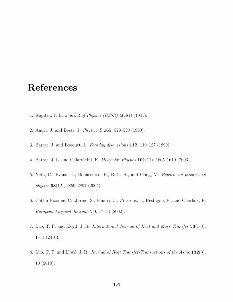
References

1. Kapitza, P. L. Journal of Physics (USSR) 4(181) (1941).

2. Amrit, J. and Bossy, J. Physica B 165, 529–530 (1990).

3. Barrat, J. and Bocquet, L. Faraday discussions 112, 119–127 (1999).

4. Barrat, J. L. and Chiaruttini, F. Molecular Physics 101(11), 1605–1610 (2003).

5. Neto, C., Evans, D., Bonaccurso, E., Butt, H., and Craig, V. Reports on progress in

physics 68(12), 2859–2897 (2005).

6. Cottin-Bizonne, C., Jurine, S., Baudry, J., Crassous, J., Restagno, F., and Charlaix, E.

European Physical Journal E 9, 47–53 (2002).

7. Luo, T. F. and Lloyd, J. R. International Journal of Heat and Mass Transfer 53(1-3),

1–11 (2010).

8. Luo, T. F. and Lloyd, J. R. Journal of Heat Transfer-Transactions of the Asme 132(3),

10 (2010).

126

127

9. Acharya, H., Mozdzierz, N. J., Keblinski, P., and Garde, S. Industrial & Engineering

Chemistry Research 51(4), 1767–1773 (2012).

10. Wilson, O. M., Hu, X. Y., Cahill, D. G., and Braun, P. V. Physical Review B 66(22),

224301 (2002).

11. Ge, Z. B., Cahill, D. G., and Braun, P. V. Journal of Physical Chemistry B 108(49),

18870–18875 (2004).

12. Patel, H. A., Garde, S., and Keblinski, P. Nano Letters 5(11), 2225–2231 (2005).

13. O’Neal, D. P., Hirsch, L. R., Halas, N. J., Payne, J. D., and West, J. L. Cancer Letters

209(2), 171–176 (2004).

14. Choi, S. U. S., Zhang, Z. G., Yu, W., Lockwood, F. E., and Grulke, E. A. Applied

Physics Letters 79(14), 2252–2254 (2001).

15. Huxtable, S. T., Cahill, D. G., Shenogin, S., Xue, L. P., Ozisik, R., Barone, P., Usrey,

M., Strano, M. S., Siddons, G., Shim, M., and Keblinski, P. Nature Materials 2(11),

731–734 (2003).

16. Li, Q. W., Liu, C. H., and Fan, S. S. Nano Letters 9(11), 3805–3809 (2009).

17. Shenogin, S., Xue, L. P., Ozisik, R., Keblinski, P., and Cahill, D. G. Journal of Applied

Physics 95(12), 8136–8144 (2004).

18. Lervik, A., Bresme, F., Kjelstrup, S., Bedeaux, D., and Rubi, J. M. Physical Chemistry

Chemical Physics 12(7), 1610–1617 (2010).

128

19. Alpert, J. and Hamad-Schifferli, K. Langmuir 26(6), 3786–3789 MAR 16 (2010).

20. Schmidt, A. J., Alper, J. D., Chiesa, M., Chen, G., Das, S. K., and Hamad-Schifferli, K.

Journal of Physical Chemistry C 112(35), 13320–13323 (2008).

21. Bain, C., Troughton, E., Tao, Y., Evall, J., Whitesides, G., and Nuzzo, R. Journal of

the American Chemical Society 111(1), 321–335 (1989).

22. Bain, C., Evall, J., and Whitesides, G. Journal of the American Chemical Society

111(18), 7155–7164 (1989).

23. Prime, K. L. and Whitesides, G. M. Science 252(5009), 1164–1167 (1991).

24. Bertilsson, L. and Liedberg, B. Langmuir 9(1), 141–149 (1993).

25. Ge, Z. B., Cahill, D. G., and Braun, P. V. Physical Review Letters 96(18), 4 (2006).

26. Pavia, D., Lampman, G., and Krisz, G. Introduction to Spectroscopy. The Wadsworth

group, (2001).

27. Nitzan, A. SCIENCE 317(5839), 759–760 (2007).

28. Duda, J. C., Saltonstall, C. B., Norris, P. M., and Hopkins, P. E. Journal of chemical

physics 134(9) MAR 7 (2011).

29. Wang, R. Y., Segalman, R. A., and Majumdar, A. Applied Physics Letters 89(17) (2006).

30. Wang, Z., Carter, J. A., Lagutchev, A., Koh, Y. K., Seong, N.-H., Cahill, D. G., and

Dlott, D. D. Science 317(5839), 787–790 (2007).

129

31. Wang, Z. H., Cahill, D. G., Carter, J. A., Koh, Y. K., Lagutchev, A., Seong, N. H., and

Dlott, D. D. Chemical Physics 350(1-3), 31–44 (2008).

32. Sasikumar, K. and Keblinski, P. Journal of Applied Physics 109(11), 114307 (2011).

33. Shenogina, N., Godawat, R., Keblinski, P., and Garde, S. Physical Review Letters 102,

156101 (2009).

Chapter 6

Conclusions and future work

6.1 Summary and conclusions

The success of many modern technologies is partially the result of continual miniaturization

of materials, structures, and devices. For example, electronic devices are made of layers with

thicknesses on the order of tens of nanometers and linewidths frequently are even smaller.

Many thermoelectric materials, optoelectronic devices, solar cells, thermal barrier coatings,

batteries, etc., involve nanostructured materials and/or a high density of interfaces. In all of

these cases, the thermal properties of the materials play a critical role in the performance of

the system. However, thermal transport at the micro and nanoscale can differ significantly

from heat transfer in bulk materials due to the high density of interfaces and boundaries in

nanostructured materials and systems.

130

131

Heat transport is a process initiated by the presence of a thermal gradient, and all

interfaces offer resistance to heat flow in the form of temperature drop at the interface. In

micro and nanoscale devices, the contribution of this resistance often becomes comparable

to, or greater than, the intrinsic thermal resistance offered by the device or structure itself.

However, experimental measurements of these interfaces are still lacking in the literature

due to the difficult nature of performing thermal measurements on materials at these small

scales.

This dissertation presents experimental investigations of heat transport through a vari-

ety of thin films, nanostructured materials, and through solid-solid and solid-liquid interfaces.

In addition to measurements of thermal conductivity, k, on thin films, I also measure inter-

face thermal conductance, G, which is the inverse of the Kapitza resistance and is quantified

by the ratio of heat flux to the temperature drop at an interface. All of these experiments

are performed with a non-contact optical measurement technique called time-domain ther-

moreflectance (TDTR), explained in Chapter two, that relies on the fact that the reflectivity

of a metal has a small, but measurable, dependence on temperature.

The first half of this dissertation focuses on investigating heat transport through thin

films and across solid-solid interfaces. The samples in this study are thin (∼ 80 nm thick)

lead zirconate-titanate (PZT) piezoelectric films used in sensing applications and dielectric

films such as SiOC:H used in the semiconductor industry. My results on the PZT films

indicate that the thermal conductivity of these films was proportional to the packing density

of the elements within the films, and the measurements also revealed a slight dependence

132

on the crystal orientation of the material. All of the samples had k between 1.5 and 1.7

Wm−1K−1 and interface conductances were ∼60 MWm−2K−1 for the Pt/PZT interfaces

and ∼100 MWm−2K−1 for the Al/PZT interfaces. I also examined thermal conductivity

of dielectric films for a variety of different elemental compositions of Si, O, C, and H, and

varying degrees of porosity. These films were grown via Plasma Enhanced Chemical Vapor

Deposition (PECVD), were ∼500 nm thick, and had k in the range of 0.18 to 0.56 Wm−1K−1.

My measurements showed that while the composition and porosity of the films played an

important role in determining the thermal conductivity, some additional factors such as long

range order and/or pore alignment also contribute.

The second half of this dissertation focuses on heat transport through solid-liquid

interfaces. In this regard, I functionalize uniformly coated gold surfaces with a variety of

self-assembled monolayers (SAMs) that are in contact with a liquid. The SAMs are used

to vary the surface interactions with the liquids. In the TDTR experiments, heat flows

from the gold surfaces to a sulfur molecule that forms the head (α-group) of the SAM, then

through the hydrocarbon chain of the SAM, into the tail (ω-group) of the SAM and finally

into the liquid. Experiments with several SAMs on water show that the interface thermal

conductance depends linearly on the work of adhesion between the SAMs and the water,

and that G can vary by a factor of ∼ 3 for hydrophobic (G∼65 MWm−2K−1) to (G∼190

MWm−2K−1) for hydrophilic SAMs. This result was predicted by theorists, but this work

provided the first conclusive experimental evidence of this linear dependence between G and

the work of adhesion. On similar experiments with SAMs of varying lengths, my results

133

confirmed that the hydrocarbon chain does not present a significant amount of thermal

resistance in comparison with the resistance elsewhere at the interface.

As a follow up to my experiments on water, I examined G for interfaces between SAMs

and a variety of other liquids in addition to water. These other liquids do not follow the same

linear dependence on the work of adhesion, and the interface thermal conductance for all

liquids is less than G for water as G spans a range of 30 to 190 MWm−2K−1 for the matrix of

SAM-liquid interfaces I examined. I also find that the SAM itself seems to play an important

role in the heat transport through the gold-SAM-liquid interface since certain SAMs greatly

impede heat transfer for all liquids. Since the work of adhesion was not adequate to explain

the observed interface conductance behavior, I speculate that heat transfer in these systems

is controlled by (a) vibrational coupling between the hydrocarbon chain in the SAM and the

ω-group, and (b) vibrational coupling between the ω-group and the liquid.

6.2 Future work

The following section include suggestions for future work to follow up on my studies

6.2.1 Solid-solid interfaces

The mixed oriented PZT films (for example PZT-125 and PZT-104) gave interesting results

in Table 3.2. The measured values for thermal conductivities were within the error margin

134

of the pure oriented films. More samples in the intermediate orientation have to be studied

to understand the trends of thermal conductivity in thin PZT devices. Also x-ray diffraction

measurements do not provide detailed information about the crystal orientation locations.

Examining these samples using a piezoresponse force microscopy (PFM) will reveal more

information about the ferroelectric domains. This will help us identify the crystal orientation

on the surface of the samples. Rutherford back scattering (RBS) studies will reveal elemental

compositions of the PZT material.

Intel R© Corporation has provided more samples based on SiON:H, SiCN:H, AlOC:H

and LiAlO3. The denser nitride based materials are ideal for low-k diffusion barriers and etch

stops in the semiconductor industry. The alumina based materials (AlOC:H) are suitable for

high-k based applications such as hard masks, while lithium based materials are ideal candi-

dates for potential electrolyte materials in batteries. Understanding the thermal properties

of these materials is essential to improve the device performance, and these new materials

should also produce useful scientific results for better understanding of heat transport in

complex materials.

Over the past decade considerable interest and attention has been given to materials

that exhibit multiple order parameters. Multiferroics are a class of materials which have

a coexistence of at least two ferroic orders (ferroelectric, ferromagnetic, or ferroelastic).

The interest in these materials is driven by the prospect of controlling charges by applied

magnetic fields and spins by applied voltages, and using these phenomena to construct new

forms of multifunctional devices. BiFeO3 is one such single phase multiferroic material

135

which has both high ferroelectric (TC=1083K) and antiferromagnetic Neel (TN=643K)

temperatures. Epitaxial BiFeO3 films were deposited on SrTiO3 substrates by pulsed laser

deposition (PLD) at 675C. It would be interesting to study the heat transport phenomenon

in such single phase multiferroic materials where the ferroelectric and magnetic ordering is

not concomitant using our TDTR experimental technique.

6.2.2 Solid-liquid interfaces

Heat transport across solid-liquid interfaces will be extended to identify the mechanisms that

control thermal transport across solid-liquid interfaces. Studying the absorption spectrum

using infrared spectroscopy will provide more insight into the energetic coupling between the

terminal group in the SAM and the adjoining liquid molecule. Also of great interest would

be to investigate the influence of external stimuli such as temperature and pressure. Certain

self-assembled monolayers change from hydrophobic to hydrophilic surface upon exposure

to ultra-violet light. In-situ measurements could provide more insight into the molecular

level understanding of thermal transport phenomena. The terminal group (ω-group) of

the SAM can also be changed from hydrophobic to hydrophilic group by using a cleaving

terminal chemical. These in-situ changes at the molecular level layer open up many potential

applications in drug delivery, self-cleaning, and micro-fluidics.

Nanobubbles of gas have been shown to be stable on surfaces within liquids under

certain conditions. Conduction through a gas will be much lower than through a liquid,

136

so the presence of adsorbed gas bubbles should have a dramatic effect on the interface

thermal conductance, G. The nanobubbles can be generated within a flowcell using an already

established procedure. Time-domain thermoreflectance can be used to measure G with and

without interfacial nanobubbles on the same sample.

Appendix A

TDTR data collection

The following procedure was followed in all of our TDTR experiments.

• Turn on the laser and let it warm up for ∼ 10-15 minutes. Confirm mode-locking in

the laser by connecting the photo-diode to an oscilloscope.

• The pump beam is separated by ∼ 3 mm from the top of the probe beam when viewed

at the back of the objective lens. This physical separation makes it easier to block the

reflected pump beam from reaching the photo diode.

• Check for parallelism of the pump and probe beams at the back of the objective lens.

• Mount the sample on the holder. Turn off the lights and block the pump and probe

beams. Turn on the circular light in the objective lens. With the help of the CCD

camera, focus on the sample. Focus cannot be achieved if there are irises in the camera

137

138

path.

• Open the probe beam. Use the polarizer to locate the probe beam on the monitor.

Center the probe beam on the scale (on the monitor) using the beam splitter (BS) on

the camera path. Block the probe beam again and open the pump beam. Use the

polarizer to locate the pump beam on the monitor. Center the pump beam on the

monitor using the polarizing beam splitter (PBS) on the pump path.

• Turn on the photodetector and position it to let the reflected probe beam fall on

the photodiode. Use an iris in front of the photodetector to block pump beam from

corrupting our signal.

• Open the Ensemble application (delay stage controlling software) on the data collection

computer and move the delay stage to positive time delay. There should be a signal

on the lock-in-amplifier.

• Upon blocking the probe beam (pump beam should be open in this step), the majority

of the signal should vanish. Whatever remains is from noise which can be eliminated

using a built-in offset in the lock-in-amplifier. Now the X and Y signals on the lock-

in-amplifier should be close to zero.

• Open the probe beam path and check the signal on the lock-in-amplifier. Maximize

the signal by overlapping the pump beam on the probe beam. This can be achieved

by using the x-y stage in the PBS mount.

139

• Open the LabVIEW program and adjust the out-of–phase voltage signal Vout(t) near

t = 0. This should be remain constant as the delay time crosses from negative to

positive delay.

• Collect the Vin/Vout signal for the aluminum-sapphire reference sample. Run the math-

ematical model to estimate the unknown parameters. Compare these parameters with

already established values. Repeat the process until the result matches the established

data.

• Aluminum deposited on sapphire substrate is our calibration sample. The thermal

conductivity of he sapphire substrate is measured to be ∼ 30 Wm−1K−1 and the

interface thermal conductance, G, between aluminum and sapphire is extracted to

be ∼ 130 MWm−2K−1.

Appendix B

self-assembled monolayer preparation

The following procedure was followed for preparation of self-assembled monolayers. Each

time, I have prepared 3 sets of every solution. Contact angle measurements were made

before and after thermoreflectance measurements. Many of the steps listed below involve

handling dangerous chemicals. Please follow appropriate safety procedures in handling such

materials.

• Clean up the vials using caustic (NaOH) solution. Measure ∼ 4.5 gms of NaOH and

add ∼ 40-50 mL of deionized (DI) water. Shake these vials rigorously until the salts

have dissolved completely. After waiting 10-15 minutes, shake these vials again. Empty

the caustic solution and rinse the vials with plenty of DI water. Repeat the rinsing

until you can see water run clear in the vials.

• We prepare 5 mM concentrated solution in 10 mL of 200 proof ethanol. Do the math-

140

141

ematical calculation to estimate how much chemical is needed to make the 5 mM

solution. If the chemical is solid, use a precise weighing scale and if the chemical is a

liquid, use an accurate micro-pipette.

• Measure 10 mL ethanol and pour it in the vials. Now drop the measured out chemical

in the vial. Swirl the vial to start the dissolving process. Sonicate for ∼ 2-3 min to

allow for better mixing of the chemical and ethanol. These solutions should be kept in

a dark and dry place for about 6-8 hours to allow complete mixing of the chemical in

ethanol.

• Sonicate the substrate (fused silica substrate) in alcohol for ∼ 15-20 minutes. Rinse in

another bath of alcohol for ∼ 10 minutes. Dry the substrates in the oven.

• Use e-beam evaporation to deposit thin films of aluminum and gold. Make sure alu-

minum is deposited first on the substrate. The samples are put in the thiol solution

immediately after venting the chamber. Always put a couple of extra substrates in

the evaporation chamber to account for dropped samples or accidents while removing

them from the substrate holder.

• Wait for the self-assembled monolayer formation on the gold surface for ∼ 12-18 hours.

• Take out the sample from the vial and rinse in ethanol. Hold the sample under a

running stream of DI water. Take extra caution not to drop the sample. Blow dry

with nitrogen gently to remove the water droplets. Measure contact angle using a

droplet. Repeat the contact angle measurements on three spots in a sample.

142

• Take another sample fresh from a vial. Rinse the sample in a running stream of DI

water. Mount the sample in our flow cell. Fill up two syringes (with Luer-lock) full of

DI water. Remove all of the bubbles by tapping on the cylinder of the syringes. Push

the air out using the plunger until DI water comes out. Use these syringes to fill up

the DI water in the flow cell.

• Follow procedure as mentioned in Appendix A to collect experimental thermoreflectance

data.

Appendix C

Collection of experimental results

This chapter lists all the results from experiments. The tables listed below are exact replica

from earlier chapters.

143

144

Table C.1: Thermal properties of PZT films. The results indicate that thermal conductivity

have a dependence on crystal orientation of these films.

SampleOrientation

[100] [110] [111]

G1

(MWm−2K−1)

kPZT

(Wm−1K−1)

G2

(MWm−2K−1)

PZT-A Amorphous 100 0.53 -

PZT-103

PZT-106

PZT-100

PZT-90

96.49% 3.51% 0%

92.86% 7.14% 0%

76.81% 23.19% 0%

72.41% 27.59% 0%

110

110

110

110

1.65

1.65

1.60

1.60

60

60

60

50

PZT-123

PZT-79

PZT-129

5.88% 94.12% 0%

7.69% 92.31% 0%

0% 100% 0%

90

90

100

1.50

1.50

1.45

50

40

45

PZT-98

PZT-114

PZT-118

0% 8.77% 91.23%

0% 3.33% 96.67%

0% 3.92% 96.08%

110

100

100

1.70

1.70

1.70

60

50

50

PZT-125

PZT-104

48.7% 1.3% 50%

39% 20.1% 40.9%

110

120

1.65

1.65

65

60

145

Table C.2: Thermal conductivity results for low-k dielectric films. Thermal conductivity

cannot be accurately predicted/explained solely from porosity, density, and composition.


(gcm−3)

Composition

Si% O% C% H%

Cfilm

(J cm−3 K−1)

kfilm

(W m−1 K−1)

399 8% 1.29 16.36 26.10 15.05 42.49 1.30 0.21

405 24% 1.25 17.23 27.30 19.73 35.74 1.20 0.29

406 33% 1.08 15.57 25.40 22.14 36.88 1.06 0.23

424 32% 1.20 14.66 27.87 20.80 36.67 1.18 0.42

413 27% 1.20 16.05 28.03 19.71 36.21 1.16 0.24

420 33.5% 1.24 15.18 24.36 23.10 37.36 1.23 0.18

163 - 1.50 17.70 25.10 16.70 40.50 1.48 0.36

164 12% 1.30 14.60 12.70 26.30 46.30 1.41 0.40

162 34% 1.20 14.40 21.40 25.90 38.30 1.21 0.37

282 40% 1.00 13.30 24.60 24.10 38.10 1.01 0.56

288 - 2.25 28.60 58.40 1 5 1.76 1.33

146

Table C.3: Self-assembled Monolayer Molecules, their Water Contact Angles and interface

thermal conductance results. The results show that the phonon transport is not affected by

the chain length of the monolayer.

SAM

constituent

SAM Molecule Contact angleG

MWm−2K−1

HSC10H20-CH3 (C11) 1-undecanethiolAdv: 118±3

Rec: 106±365 ± 5

HSC11H22-CH3 (C12) 1-dodecanethiolAdv: 116±2

Rec: 110±260 ± 5

HSC17H34-CH3 (C18) 1-octadecanethiolAdv: 118±3

Rec: 108±265 ± 5

147

Table C.4: Molecules and water contact angles for the preparation of self-assembled monolay-

ers. The results show that the terminal group have a significant impact on heat conduction.

SAM

constituent

SAM MoleculeSAM

abbreviation

Contact anglea)Gb)

MWm−2K−1


Adv: 118±2

Rec: 106±265 ± 5

Methyl 3-

Mercaptopropionate

ω-esterAdv: 76±2

Rec: 68±3140 ± 15

11-(1H-pyrrol-1-yl)

undecane-1-thiol

ω-pyrrolAdv: 78±3

Rec: 70±2140 ± 15

11-Mercapto-1-

undecanol

ω-OHAdv: 25±2

Rec: 20±2190 ± 30

11-Mercapto-

undecanoic acid

ω-COOHAdv: 27±3

Rec: 17±2190 ± 30

HSC10H20 – CH2Br 11-Bromo-

undecanethiol

ω-CH2BrAdv: 70±3

Rec: 61±270 ± 5

148

Table C.5: Interface thermal conductance, G, measured on a variety of SAM-Liquids com-

bination in units of MWm−2K−1 and the advancing (Adv) contact angle for the liquid on

the SAM. Work of adhesion, WSL=γ (1 + cosθ), for each SAM-liquid combination is given

in units of mN m−1.

SAM→


Heavy water

G: 70

Adv: 109

WSL: 49.1

G: 140

Adv: 70

WSL: 97.9

G: 200

Adv: 27

WSL: 137.6

G: 200

Adv: 27

WSL: 137.6

G: 70

Adv: 70

WSL: 97.6

Deionized water

G: 60

Adv:118

WSL: 40.9

G: 140

Adv: 75

WSL: 91.6

G: 200

Adv: 24

WSL: 139.3

G: 190

Adv: 23

WSL: 139.8

G: 70

Adv: 70

WSL: 97.7

Di-methyl

formamide

G: 50

Adv: 40

WSL: 65.5

G: 90

Adv: 45

WSL: 63.3

G: 120

Adv: 30

WSL: 65.5

G: 130

Adv: 30

WSL: 69.2

G: 50

Adv: 40

WSL: 65.5

Formamide

G: 45

Adv: 30

WSL: 108.6

G: 90

Adv: 30

WSL: 108.6

G: 120

Adv: 35

WSL: 105.8

G: 120

Adv: 27

WSL: 110

G: 40

Adv: 35

WSL: 105.8

Ethanol

G: 40

Adv: 15

WSL: 43.4

G: 60

Adv: 14

WSL: 43.5

G: 120

Adv: 18

WSL: 43.1

G: 130

Adv: 18

WSL: 43.1

G: 45

Adv: 20

WSL: 42.8

Continued on next page

149

Table C.5 – continued from previous page

SAM→


Benzene

G: 45

Adv: 15

WSL: 56.7

G: 60

Adv: 16

WSL: 56.6

G: 160

Adv: 18

WSL: 56

G: 160

Adv: 13

WSL: 57

G: 45

Adv: 18

WSL: 56.3

Hexadecane

G: 45

Adv: 20

WSL: 53.3

G: 85

Adv: 18

WSL: 53.6

G: 150

Adv: 14

WSL: 54.1

G: 170

Adv: 18

WSL: 53.6

G: 50

Adv: 16

WSL: 53.9

Chloroform

G: 80

Adv: 18

WSL: 53.6

G: 90

Adv: 20

WSL: 53.3

G: 180

Adv: 14

WSL: 54.2

G: 180

Adv: 15

WSL: 54.1

G: 60

Adv: 15

WSL: 54.1

Carbon

tetrachloride

G: 30

Adv: 20

WSL: 54.7

G: 60

Adv: 18

WSL: 55

G: 120

Adv: 16

WSL: 55.3

G: 140

Adv: 14

WSL: 55.6

G: 40

Adv: 14

WSL: 55.3

Hexane

G: 50

Adv: 15

WSL: 36.2

G: 70

Adv: 16

WSL: 36.1

G: 120

Adv: 18

WSL: 35.9

G: 120

Adv: 20

WSL: 35.7

G: 40

Adv: 18

WSL: 35.9

Ethylene glycol

G: 40

Adv: 40

WSL: 84.2

G: 90

Adv: 24

WSL: 91.2

G: 160

Adv: 20

WSL: 92.5

G: 160

Adv: 16

WSL: 93.5

G: 50

Adv: 30

WSL: 89

nanoscale heat transport through solid-solid and … · nanoscale heat transport through...

Documents