name: richard lawrence castelino date of degree: december ... · applicable. the cltd/scl/clf...
TRANSCRIPT
1
Name: Richard Lawrence Castelino Date of Degree: December, 1992
Institution: Oklahoma State University
Location: Stillwater, Oklahoma
Title of Study: IMPLEMENTATION OF THE REVISED TRANSFER FUNCTION METHOD AND EVALUATION OF THE CLTD/SCL/CLF METHOD
Pages in Study: 158 Candidate for the Degree of Master of Science Major Field: Mechanical Engineering Scope and Method: This thesis focuses mainly on the development of a load calculation
software program. Technical routines for building cooling load and heat extraction rate calculations were developed based on the revised Transfer Function Method (TFM). Heating load calculation routines were also developed. The program is user-interactive, menu-driven, and works under a graphical user interface. Cooling load results obtained by the CLTD/SCL/CLF (Cooling Load Temperature Difference/Solar Cooling Load/Cooling Load Factor) method, a simplified load calculation method, were compared to those obtained by the revised TFM. Tests were carried out for three representative zones and a number of cases involving externally shaded glass areas.
Findings and Conclusions: A number of implementation and methodological differences
in the two methods are pointed out and suitable corrections are suggested where applicable. The CLTD/SCL/CLF method was validated as a fairly accurate method for manual cooling load calculations. Differences in cooling loads by the two methods due to table round-off errors, interpolation for different latitudes, and calculations for dates other than the 21st using the CLTD/SCL/CLF method are small. However, significant differences in cooling loads are observed for externally shaded glass areas. It was found that the use of a north facing glass area to represent a completely shaded glass area (for the CLTD/SCL/CLF method) is not always accurate particularly for locations near the equator. It is suggested that shaded and unshaded SCLs be calculated separately for all facing directions and used for cooling load calculations. In addition, the CLTD/SCL/CLF method cannot account correctly for the past history of varying shaded/unshaded glass areas. This problem is an inherent limitation of the CLTD/SCL/CLF method.
ADVISOR'S APPROVAL__________________________________________________

2
IMPLEMENTATION OF THE REVISED TRANSFER
FUNCTION METHOD AND EVALUATION
OF THE CLTD/SCL/CLF METHOD
By
RICHARD LAWRENCE CASTELINO
Bachelor of Engineering
University of Bombay
Bombay, India
1987
Submitted to the Faculty of the Graduate College of the
Oklahoma State University in partial fulfillment of
the requirements for the Degree of
MASTER OF SCIENCE December, 1992

3
IMPLEMENTATION OF THE REVISED TRANSFER
FUNCTION METHOD AND EVALUATION
OF THE CLTD/SCL/CLF METHOD
Thesis Approved :
___________________________________________ Thesis Advisor
___________________________________________
___________________________________________
___________________________________________ Dean of the Graduate College
4
PREFACE
A professional software program, currently called HVAC, was developed in order
to calculate the cooling loads for a building based on the revised Transfer Function
Method. This program, written in the C-programming language, executes under
Microsoft WINDOWSTM as a user-interactive, menu driven program. In addition to
cooling load calculations, the program also performs calculations of the heat extraction
rates for desired zones, and the heating load for the building based upon steady state heat
transfer.
The results of the CLTD/SCL/CLF Method for three test zones and other test
cases of externally shaded glass areas were compared with those of the revised Transfer
Function Method. Differences in the implementation and calculation methodology of the
methods were pointed out and the results discussed.
I would first like to express my heart-felt gratitude to my parents, Lawrence and
Florine Castelino for their undying faith in me and their relentless efforts towards
ensuring a bright career for me. I attribute a major portion of my achievements to their
continued support and moral encouragement. Special thanks are also due to my sisters
Theresa and Claudette and my brother Placid whose prayers, friendship, and good wishes
have followed me and constantly reminded me of my goals in life. I love you all.
I wish to express sincere appreciation to my major advisor Dr. Jeffrey D. Spitler
for his continued guidance, patience, and inspiration during this demanding endeavor. I
am grateful to my other committee member Dr. Ronald D. Delahoussaye for his help
during the programming phase of the project, guiding me from obscurity to clarity, and
his keen insight in offering useful suggestions and tips. I also extend my gratitude to Dr.

5
Faye McQuiston for serving on my committee. This thesis work is largely a result of his
enormous contribution to the revised Transfer Function load calculation methodology.
Thanks are also due to Mr. Kyungho Song, my colleague on this project, a good friend,
and a software programmer par excellence, whom I respect for his understanding, co-
operation, and useful programming hints. Justice would not be done if I don't thank Dr.
Blayne Mayfield of the Computer Science Department whose terse and enlightened ways
of teaching have helped me understand better the more challenging aspects of the C (and
C++) language and perform more productively as a software developer.
This project has been funded by The Oklahoma Center for the Advancement of
Science & Technology (OCAST). Their generous financial support throughout my course
of study is greatly appreciated.

6
TABLE OF CONTENTS
Chapter Page
I. INTRODUCTION .......................................................................................... 1
Overview............................................................................................. 1 Literature Review ............................................................................... 4 Stephenson and Mitalas (1967) The Thermal Response Factor Method......................................................................... 4 Stephenson, and Mitalas (1971) Heat Conduction Transfer Function Calculations ............................................................ 5 Mitalas (1969, 1972) Validation of the Weighting Factor Method.................................................................................... 5 Rudoy and Duran (1975) The CLTD/CLF Method and the ASHRAE GRP 158 Load Calculation Manual................. 6 Machler and Iqbal (1985) Modification of the ASHRAE Clear Sky Irradiation Model ................................................... 7 Sowell and Chiles (1985), Sowell (1988a, b, & c) Classification of Zones based on Dynamic Response and Development of Weighting Factors ................................. 8 McQuiston and Harris (1988) Categorization of Roofs and Walls based on Thermal Response .................................. 10 McQuiston, Spitler, et al. (1992) Development of the Revised Cooling and Heating Load Calculation Manual .................................................................................... 11 Objectives ........................................................................................... 11
II. THE REVISED TRANSFER FUNCTION METHOD .................................. 13
Heat Transfer Flow Rates..................................................................... 13 Space Heat Gain .......................................................................... 13 Space Cooling Load .................................................................... 14 Space Heat Extraction Rate......................................................... 14 Cooling Coil Load....................................................................... 15 The revised Transfer Function Method ................................................ 15 Transfer Functions....................................................................... 16 Room Transfer Functions............................................................ 16 Calculation of heat gains..................................................................... 19 Solar Radiation............................................................................ 20 Time ............................................................................................ 20

7
Chapter Page
Solar Angles ................................................................................ 21 Solar Irradiation........................................................................... 24 Solar intensity and the ASHRAE Clear Sky Model.................... 25 External Shading ......................................................................... 27 Determination of the heat gains through Windows................................................................................. 31 Transient Heat Conduction through Walls and Roofs ................................................................................ 34 Heat Gains through ceilings, inter-zone partitions, and floors ............................................................... 38 Internal Heat Gains...................................................................... 39 Occupancy............................................................................ 39 Lighting................................................................................ 40 Miscellaneous Equipment.................................................... 41 Heat Gain through below grade surfaces..................................... 42 Heat gains due to Infiltration and Ventilation of Air....................................................................................... 42 Conversion of heat gains into cooling loads ............................... 44 Heat Extraction Rate and the Space Air Temperature ............................................................................ 45 Heat Extraction Rate......................................................... 46 The Space Air Transfer Function...................................... 47 Heat Extraction Rate and the Space Air Temperature Calculations .............................................. 48
III. THE CLTD/SCL/CLF METHOD .................................................................. 49
The CLTD/CLF Method and GRP 158 .............................................. 50 Walls and Roofs .......................................................................... 50 Fenestration ................................................................................. 52 Occupancy, Lighting, and Equipment ......................................... 53 Revisions to the CLTD/CLF Method ................................................. 54
IV. THE HVAC SOFTWARE PROGRAM......................................................... 57
Program Hierarchy.............................................................................. 57 Building....................................................................................... 59 Zones ........................................................................................... 59 Rooms ......................................................................................... 61 Heat Gain Elements..................................................................... 62 Calculations and Output ..................................................................... 67 Heating Load Calculations.................................................................. 70 V. ZONE DESCRIPTIONS................................................................................. 72

8
Chapter Page
Test Zone 1 - Retail Store ........................................................... 72 Test Zone 2 - Office Premises..................................................... 74 Test Zone 3 - Top Story Office .................................................. 77
VI. RESULTS AND DISCUSSION..................................................................... 79
Effect of inherent round-off error from tables .................................... 83 Effect of using CLTD/SCL/CLF tables for dates other than the 21st............................................................................ 85 Use of the CLTDTAB program while interpolating for different Latitudes........................................................................................... 88 Use of shaded and unshaded SCLs for solar heat gains through Fenestration ........................................................................ 91
VII. CONCLUSIONS AND RECOMMENDATIONS ......................................... 104
Conclusions......................................................................................... 104 Recommendations............................................................................... 106
REFERENCES............................................................................................................. 108
APPENDIXES ............................................................................................................. 111
APPENDIX A - SAMPLE COOLING LOAD CALCULATIONS FOR TEST ZONE 1................................................................. 112
APPENDIX B - COOLING LOAD RESULTS FOR TEST ZONE 2....... 136
APPENDIX C - COOLING LOAD RESULTS FOR TEST ZONE 3....... 140
APPENDIX D - COOLING LOAD COMPARISONS FOR EXTERNALLY SHADED GLASS AREAS.................. 143
APPENDIX E - COOLING LOAD COMPARISONS FOR TYPICALLY SHADED GLASS AREAS...................... 152

9
LIST OF TABLES
Table Page
I. Zone Parameters ................................................................................... 19
II. Solar Details for the 21st day of each month ....................................... 26
III. X and Y shading calculations for externally shaded glass areas .......... 30
IV. Coefficients of transmission and absorption for DSA glass................. 34
V. The normalized space air transfer function coefficients....................... 47
VI. The CLTDTAB Program options......................................................... 55
VII. Input details for the location dialog box at the building level.............. 60
VIII. Input details for the heat extraction dialog box at the zone level......... 61
IX. Input details for the Wall Parameters dialog box at the room level ..... 62
X. Input details for the roof or wall dialog box at the element level......... 63
XI. Input details for the glass areas dialog box at the roof or wall level .... 64
XII. Input details for the People Information dialog box at the element level.................................................................................................. 65
XIII. Input details for the Light Information dialog box at the element level.................................................................................................. 66
XIV. Input details for the Equipment Information dialog box at the element level.................................................................................................. 66
XV. Calculation of the individual heating loads by the HVAC program .... 70
XVI. Implementation differences between the HVAC and CLTDTAB programs .......................................................................................... 80
XVII. Cooling loads for the Retail Store Roof by the revised TF and the CLTD/SCL/CLF Methods ......................................................... 84
XVIII. Cooling loads for the Retail Store for the 6th of July .......................... 87
XIX. Cooling loads for 42°N latitude using interpolation for CLTDs.......... 89

10
Table Page
XX. Cooling loads for 6°N latitude using extrapolation for CLTDs ........... 90
XXI. Summary of comparison tests .............................................................. 103
XXII. Zone parameters for the Retail Store.................................................... 113
XXIII. Categorization of the Retail Store Wall ............................................... 114
XXIV. Categorization of the Retail Store Roof ............................................... 116
XXV. Conduction Transfer Functions for the Wall........................................ 117
XXVI. Sol-Air Temperatures and Conduction heat gains for South Wall....... 120
XXVII. The converging process from heat gains to cooling loads for the Lighting............................................................................................ 123
XXVIII. Comparison of the cooling loads by the revised TF and CLTD/SCL/CLF methods for the south window of the Retail Store ...................................................................................... 129
XXIX. Comparison of the cooling loads by the revised TF and CLTD/SCL/CLF methods for the Retail Store people .................... 130
XXX. Comparison of the cooling loads by the revised TF and CLTD/SCL/CLF methods for the Retail Store lighting................... 131
XXXI. Cooling loads for the Retail Store by the revised TFM and the CLTD/SCL/CLF Methods ......................................................... 134
XXXII. Comparison of the cooling loads by the revised TF and CLTD/SCL/CLF methods for Test Zone 2 ...................................... 137
XXXIII. Comparison of the cooling loads by the revised TF and CLTD/SCL/CLF methods for Test Zone 3 ...................................... 141
XXXIV. Cooling Loads by the revised TF method for the north window of office area (Test Zone 2).................................................................. 144
XXXV(a). Sample tables obtained by executing the SHADEC program for shadow lengths due to external shading (Horizontal Projections)... 145
XXXV(b). Sample tables obtained by executing the SHADEC program for shadow lengths due to external shading (Vertical Projections) ....... 146
XXXVI. Cooling Loads by the CLTD/SCL/CLF method for the north window of office area (Test Zone 2)................................................ 147

11
Table Page
XXXVII. Cooling Loads by the revised TF method for the east window of office area (Test Zone 2) ............................................................. 149
XXXVIII. Cooling Loads by the CLTD/SCL/CLF method for the east window of office area (Test Zone 2) ............................................................. 150
XXXIX. Maximum percent differences for the typically shaded glass areas ................................................................................................. 158

12
LIST OF FIGURES
Figure Page
2.1 The revised Transfer Function Method for calculating heat gains and cooling loads............................................................................................................. 17
2.2 Latitude (l), hour angle (h), and declination (δ) ............................................... 22
2.3 The solar altitude angle (β), solar azimuth angle (φ), surface azimuth (ψ), solar azimuth angle (γ), the angle of incidence (θ), and the tilt angle(α) for an arbitrarily tilted surface ..................................................................... 24
2.4 X-Y Shading for a Window with reveal........................................................... 29
2.5 Externally shaded glass area with reveal.......................................................... 30
4.1 Hierarchy of the HVAC software program ...................................................... 58
4.2 Flow chart of the HVAC program.................................................................... 68
5.1 Plan and Elevation views of the Retail Store ................................................... 73
5.2 Test Zone 2 - Office Premises.......................................................................... 75
5.3 View of Window at section A-A...................................................................... 75
5.4 Test Zone 3 - Top Story Office Premises......................................................... 76
6.1 Cooling loads by the revised TF and CLTD/SCL/CLF Methods for the Retail Store Roof ......................................................................................... 85
6.2 Cooling loads for the north window of test zone 2 by the revised TF and CLTD/SCL/CLF methods............................................................................ 93
6.3 Cooling loads for the east window of test zone 2 by the revised TF and CLTD/SCL/CLF methods............................................................................ 93
6.4 Transmitted cooling loads through the unshaded area of the east window of test zone 2................................................................................................ 94
6.5 An externally shaded south west facing window ............................................. 96
6.6 Cooling loads for the SW facing window at 0 °N by the revised TF and CLTD/SCL/CLF methods............................................................................ 97

13
Figure Page
6.7 Transmitted cooling loads through the shaded area of the SW facing window at 0 °N ............................................................................................ 97
6.8 Transmitted cooling loads through the unshaded area of the SW facing window at 0 °N ............................................................................................ 98
6.9 Cooling loads for the SW facing window at 24 °N by the revised TF and CLTD/SCL/CLF methods............................................................................ 100
6.10 Transmitted cooling loads through the shaded area of the SW facing window at 24 °N .......................................................................................... 101
6.11 Transmitted cooling loads through the unshaded area of the SW facing window at 24 °N .......................................................................................... 101
A.1 Total glass cooling loads for the south window of the Retail Store by the revised TF and the CLTD/SCL/CLF Methods ............................................ 132
A.2 Cooling loads for the people of the Retail Store by the revised TF and the CLTD/SCL/CLF Methods ............................................ 132
A.3 Cooling loads for the lighting of the Retail Store by the revised TF and the CLTD/SCL/CLF Methods ............................................ 133
A.4 Total cooling loads for the Retail Store by the revised TF and the CLTD/SCL/CLF Methods ........................................................................... 135
B.1 Total cooling loads for the office area of test zone 2 by the revised TF and the CLTD/SCL/CLF Methods............................................................... 138
B.2 Total cooling loads for the computer room of test zone 2 by the revised TF and the CLTD/SCL/CLF Methods......................................................... 138
B.3 Total cooling loads for test zone 2 by the revised TF and the CLTD/SCL/CLF Methods ........................................................................... 139
C.1 Total cooling loads for test zone 3 by the revised TF and the CLTD/SCL/CLF Methods ........................................................................... 142
D.1 Transmitted cooling loads for the shaded portion of the north window of office area (Test Zone 2) ......................................................................... 148
D.2 Transmitted cooling loads for the unshaded portion of the north window of office area (Test Zone 2) ......................................................................... 148
D.3 Transmitted cooling loads for the shaded portion of the east window of office area (Test Zone 2) ......................................................................... 151

14
Figure Page
E.1 Typically exterior shaded glass window .......................................................... 154
E.2 Cooling loads for North facing window (36°N) by the revised TF and CLTD/SCL/CLF Methods .................................................. 154
E.3 Cooling loads for NE facing window (36°N) by the revised TF and CLTD/SCL/CLF Methods .................................................. 155
E.4 Cooling loads for East facing window (36°N) by the revised TF and CLTD/SCL/CLF Methods............................................................... 155
E.5 Cooling loads for SE facing window (36°N) by the revised TF and CLTD/SCL/CLF Methods............................................................... 156
E.6 Cooling loads for South facing window (36°N) by the revised TF and CLTD/SCL/CLF Methods............................................................... 156
E.7 Cooling loads for SW facing window (36°N) by the revised TF and CLTD/SCL/CLF Methods............................................................... 157
E.8 Cooling loads for West facing window (36°N) by the revised TF and CLTD/SCL/CLF Methods............................................................... 157
E.9 Cooling loads for NW facing window (36°N) by the revised TF and CLTD/SCL/CLF Methods............................................................... 158

1
CHAPTER I
INTRODUCTION
Overview
Air-conditioning has been one of the more recent pursuits of man in his quest for a
more comfortable existence. The primary purpose of an air-conditioning system, whether
heating or cooling, is to maintain conditions that provide thermal comfort for the building
occupants and conditions that are required by the products and processes within the space.
Central heating systems were being developed in the Nineteenth Century while the
development of comfort cooling systems began in the early Twentieth Century. Since then,
progress in this direction has taken rapid strides with significant development in various
areas of science and technology.
Earlier load calculation methods paid little attention to the costs of operation of
air-conditioning systems often resulting in substantially oversized systems. However,
rising energy costs, complex building structures and construction materials, and concerns
for the environment and natural resources have necessitated continued refinement of load
calculation methods. Present day load calculation methods are directed more towards
accurately sized systems which result in economical system performance.
Load calculations of the earlier days were based on the elementary steady state
energy equation
q = U A ∆T (1.1)
where
q = cooling load (Btu/hr)

2
U = the heat transfer coefficient (Btu/hr-ft2-°F)
A = Area (ft2)
∆T = the difference between the outside
and inside temperatures (°F)
By the mid-1940s ASHRAE developed equivalent temperature differentials for
exterior surfaces facing different directions for the worst exposure to sunlight (with values
20 to 40 degrees above the actual temperature difference between the outside and inside)
and used them to calculate heat gains (Romine, 1992). However, these heat gains were
only instantaneous and considered the thermal storage only of these exterior surfaces in
delaying the heat passage through them. Subsequent storage of these and other heat gains
by the building's interior and its contents were not accounted for. Designers were aware of
this fact but were unable to represent it quantitatively. This resulted in over-estimated
cooling loads.
In 1967, ASHRAE introduced the Total Equivalent Temperature Difference/Time
Averaging (TETD/TA) Method (ASHRAE Handbook of Fundamentals, 1967). This
method, in addition to estimating the cooling loads due to convective heat gain from all
sources, attempted to evaluate the cooling loads due to radiative heat gains (heat gains
absorbed by the building's interior and later convected to the inside air) by a mathematical
time-averaging of these radiant heat gains. This procedure, however, was only an
approximation of the actual phenomenon of thermal lag. Besides, it required good
judgement on the part of the user to estimate the thermal characteristics of the building and
decide upon a suitable time-averaging period. In addition, the method required several
table look-ups, and the cooling load calculations were tedious and prone to errors
considering the kind of calculating tools available to practitioners at that time.
Efforts to explain the phenomenon of thermal lag more accurately and incorporate
it into load calculation methodology continued. In 1967, Mitalas and Stephenson
developed the thermal response factor method for cooling load calculations. By this time,

3
digital computers were available and traditional air-conditioning design methods were re-
examined in order to take advantage of the capabilities afforded by computers.
The Transfer Function Method, based on an extension of the response factor
methodology, successfully interpreted the phenomenon of thermal lag and delayed cooling
loads and first appeared in the ASHRAE Handbook (1972). The mid 70's saw the
development of the CLTD/CLF method for load calculation. This method, similar in some
respects to the TETD/TA method, but with more extensive data calculated using the TFM,
was developed as a manual method since computers were not generally available for
practicing HVAC engineers.
Advances in the computer industry since the early 80's have led to further changes
in load calculation methods. Since computers were now readily available to HVAC
designers and engineers, the Transfer Function Method became practical for use by HVAC
engineers and this encouraged further development of the method.
As the awareness for more economical air-conditioning systems has taken prime
importance, more attention is now focused on the thermal responses of the building
components with a view to obtain the most accurate air-conditioning load. The Transfer
Function Method is now regarded as the most accurate, yet practical cooling load
calculation method*. This Thesis, "Implementation of the Revised Transfer Function
Method and Evaluation of the CLTD/SCL/CLF Method", describes the implementation of
the revised Transfer Function Method including recent developments (Sowell - 1985 &
1988, McQuiston, et al. 1988). Results of a new manual method, the CLTD/SCL/CLF
Method, are compared to those of the revised TF Method.
Literature Review
* It is generally conceded that the most accurate method for calculation of building loads is the heat-balance method (BLAST User Reference - University of Illinois at Urbana Champaign, 1991). In fact, the heat-balance method was used to determine the room weighting factor coefficients that are used by the TFM. However, it has not been widely used for design load calculations, due to its presumed complexity.

4
This section surveys previous work carried out on the TFM and CLTD/SCL/CLF
Methods. The work carried out is listed in chronological order.
Stephenson and Mitalas (1967)
The Thermal Response Factor Method
Stephenson and Mitalas studied the effects of time-series and response factor
techniques in the calculation of transient heat conduction through building components. A
time-series is a series of numbers or quantities that represent the values of a particular
function at successive intervals of time. Response factors are a set of coefficients that
result from a time-series representation of a linear, invariable system (Mitalas and
Stephenson, 1967) to a unit time-series excitation function.
They developed response factors for walls (room-surface temperature response
factors) by modeling the wall response (heat flux) to triangular unit temperature excitation
pulses on the outer and inner surfaces of the walls.
Room heat balance equations were derived for the surfaces enclosing a room and
the room air. These heat balance equations described the dynamic thermal characteristics
of the room. These equations were used to calculate the room thermal response factors.
The surface temperature and room thermal response factors were employed to calculate the
surface temperatures and subsequently the room temperatures and heat extraction rates,
based on the corresponding room excitation components (heat gains). The necessity of a
computer to perform calculations was obvious, due to the size of each set of response
factors, and the number of sets of response factors.
Stephenson, and Mitalas (1971)

5
Heat Conduction Transfer Function Calculations
Stephenson and Mitalas further developed their response factor approach by
determining and applying the z-transform to problems in transient heat conduction. They
obtained the z-transfer functions for various surfaces (roofs and walls) made up of several
layers of different materials and subject to arbitrary variations of temperature. The transfer
functions replaced the theoretically infinite set of response factors into a finite set of
history coefficients which accounted for the past and current values of the variable(s) of
interest.
They explained two methods by which z-transfer functions could be calculated. The
first consisted of selecting appropriate input functions with known Laplace transforms and
z-transforms with an appropriate choice for the sampling interval. The second method
involved solving a set of simultaneous linear algebraic equations to obtain the coefficients
of a z-transfer function whose frequency response matched that of the s-transfer function at
selected frequencies. The resulting z-transfer functions obtained were similar to the
thermal response factors, but were more effective and economical in terms of computer
memory and run-time speed.
Mitalas (1969, 1972)
Validation of the Weighting Factor Method
The work carried out by Mitalas, Stephenson, and the ASHRAE Task Group on
Energy requirements (the thermal response factor and transfer function methods)
culminated in the development of the computer-oriented method which is now called the
"TRANSFER FUNCTION METHOD" and was incorporated in the 1972 ASHRAE
Handbook of Fundamentals. This method was so named because it utilizes the transfer
function concept to relate the cooling load to the heat gain, and the heat extraction rate to

6
the cooling load and the room temperatures. This method is described in detail in chapter
II.
An experimental validation check for the method, in particular the room weighting
factors that are employed to convert the heat gains into cooling loads was carried out
(Mitalas, 1969) and the loads predicted with weighting factors were found to be fairly
accurate when compared with the experimental values.
The major advantage of this new load calculation method is that in addition to
calculating the cooling loads it can determine the rate at which heat is extracted from the
space and also the space temperature when the capacity of the air-conditioning equipment
to be used is known. This unique feature helps the designer to check the variations in the
inside temperature for various load conditions and thereby select appropriate air-
conditioning machinery that will give optimum results working within the comfort zone.
Rudoy and Duran (1975) - The CLTD/CLF
Method and the ASHRAE GRP 158
Load Calculation Manual
The CLTD/CLF method for calculating cooling loads that is described in the
Cooling and Heating Load Calculation Manual (ASHRAE GRP 158) is based on research
carried out by Rudoy and Duran (1975).
ASHRAE sponsored research in order to compare the TETD/TA and Transfer
Function Methods (Rudoy and Duran-1975, ASHRAE H.O.F-1989). As part of their work,
Rudoy and Duran developed CLTD and CLF data based on the results of the TFM Method
applied to a group of representative applications. Their study involved close scrutiny of
each source (variable) that affected the cooling load. The effect of each of these variables
was then studied for its sensitivity on the final result. This resulted in the development of

7
CLTDs to be used for the one step calculations of cooling loads from conduction heat gain
through sunlit roofs and walls and conduction through exposed fenestration.
Cooling Load Factors (CLFs) were generated for similar one-step calculation of the
solar load through glass areas and the loads from internal sources. Both the CLTDs and
CLFs included the effect of the time delay caused by the effect of thermal storage.
This method was basically designed to be a manual method although it was
implemented on microcomputers shortly after they became available.
Machler and Iqbal (1985) - Modification of
the ASHRAE Clear Sky Irradiation Model
Machler and Iqbal (1985) highlighted the need to revise the ASHRAE Clear Sky
Model and develop new clear sky coefficients. They pointed out the following facts that
necessitated the revision of solar constants A, B, and C:
1) The accepted solar constant has been revised by the World Meteorological
Organization (1981) from 1322 W/m2 to 1367 W/m2.
2) The results of the ASHRAE algorithm do not match the more accurate simulations
carried out by Bird and Hulstrom (1981), especially for the winter months.
With the help of the Bird and Hulstrom model, new revised constants A, B, and C
were developed, by introducing turbidity in the revised ASHRAE Model. These new
values for the constants are used here for the calculation of the solar loads by the revised
Transfer Function Method.
8
Sowell and Chiles (1985) , Sowell (1988 a, b, & c)
Classification of Zones based on Dynamic
Response and Development of Weighting Factors
The CLTD/CLF data presented in ASHRAE GRP158 (1979) and the Handbooks of
1977, 1981, and 1985 were based on the TFM using the weighting factors developed by
Mitalas (1967). However, these weighting factors were based on a limited exploration of
the now known to be important criteria of zone geometry and construction. Furthermore, it
was found that for some zone geometries and constructions, the weighting factors gave
inaccurate results and the results of the CLTD/CLF calculations were questionable in other
situations.
Another source of erroneous results was the use of the CLFs that were calculated
for July 21, 40° N for all northern latitudes during summer months (May through
September). It was assumed that the SHGFmax (calculated for all directions, months, and
northern latitudes from 0°N to 60°N) successfully accounted for the variation in the solar
heat gain for other latitudes and dates. Such normalization of the solar heat gain resulted in
erroneous values of CLFs for latitude/month combinations other than July 21, 40°N,
particularly for locations whose sunrise and sunset times differed significantly from those
at July 21, 40°N (Spitler, et al. 1993).
ASHRAE sponsored a research project (RP-359) in order to update the CLTD/CLF
tables using more appropriate weighting factors accounting for a wider range of zones.
Work on this project resulted in three technical papers by Sowell and Chiles (1985, 1985a,
1985b). Their research confirmed the sensitivity of zone dynamic response to design
parameters that had hitherto not been addressed. It also showed that the variables affecting
this response had strong interactive effects, and in some situations, unexpected results were
obtained.
9
The main deficiency in their work was that the range of design parameters selected
for the parametric variation was limited. The parameters used included floor covering,
inside shading, ceilings, exterior wall construction, glass percent, and zone size.
Parameters not used and later found to be important included the wall height, zone
location, number of exterior walls, partition construction, and furniture. Besides, the DOE-
2.1 program that was used for the work was questioned as being "only an energy
calculation program" and that its potential to carry out accurate peak cooling load
calculations was not established* .
Project RP-472 was authorized by the ASHRAE Technical Committee 4.1 in order
to complete this "unfinished" work. The principal objectives of this project were to validate
the results of the calculation of the zone dynamic response to several heat gain components
and to classify all zones based on their dynamic thermal response characteristics
accounting for a well defined range of design parameters namely: floor plan, zone height,
number of exterior walls, glass percent, partition type, interior shading, zone location, slab
type, mid-floor construction, wall construction, roof construction, floor covering, ceiling
type and interior furnishings.
The findings of Sowell (1988) resulted in three papers that describe the calculation
of the cooling load dynamic response of 200,640 zones representing all 14 design
parameters. The DOE-2.1c program was modified in order to meet special assumptions for
peak load calculations, and the characterization of the zones was based on their dynamic
thermal response.
Zones that exhibited similar amplitude and delay were grouped together to form
"zone type groups" with a recommended set of weighting factors for each group. Basically
12 classes of zones were formed, representing single, perimeter, and interior zones located
on the top, bottom, or mid-floors of multi-story buildings or in single story buildings and
* It was shown later (Sowell, 1988b) to have sufficient accuracy.

10
the grouping process was carried out for solar, conduction, lighting, and
occupant/equipment heat gain components. Tables were generated so that the weighting
factors representative of any zone among the 200,640 possible types could be found with
ease.
McQuiston and Harris ( 1988 )
Categorization of Roofs and Walls
based on Thermal Response
The CLTD/CLF Method is generally employed as a manual method for the
calculation of cooling loads. Wall and roof CLTDs are obtained by selecting a similar wall
or roof type from the list (ASHRAE 1977, 1981, 1985, and 1989). If an exact match is not
found, complicated adjustments to the CLTDs are required before multiplication to the
product of the U-factor and the area. The wall and roof groups delineated in the ASHRAE
Handbooks do not cover the entire range of modern construction, and the results obtained
by the complicated adjustment to the CLTDs may not yield correct cooling loads. Hence,
McQuiston and Harris performed a study to devise a method to group roofs and walls with
similar transient heat transfer characteristics.
After investigating existing analytical and correlational methods for their efficiency
in predicting transient characteristics of multi-layered walls and roofs and grouping of
similar types, they developed a heuristic method wherein a wall or roof assembly was
placed into a particular group with transient heat transfer characteristics within a limited
range, based on a combination of four thermophysical and geometric parameters. This
resulted in an accurate representation of all common wall assemblies in 41 distinct wall
groups and all common roof assemblies in 42 roof groups. Each group, besides having a
number designation and the code letters defining the exact construction of each surface,
has a unique set of conduction heat transfer functions so as to produce conservative results.

11
These conduction transfer coefficients are used in the Transfer Function Method in order to
calculate the conduction heat gain for any representative wall or roof assembly that
matches with the particular group.
McQuiston, Spitler, et al. (1992)
Development of the Revised Cooling
and Heating Load Calculation Manual
The results of ASHRAE Research Projects 359 and 472 have necessitated the
development of a new load calculation manual incorporating the new data available on
zone response and wall/roof groups.
The scope of ASHRAE Research Project 626 was to write a new load calculation
manual incorporating the research results discussed above. As part of this project, the
CLTD/CLF method was substantially revised and software was developed in order to
access the weighting factor data developed by RP-472.
The new cooling and heating load calculation manual (McQuiston and Spitler,
1992) has been recently released by ASHRAE. Papers by Spitler, et al.(1993a, 1993b), and
Falconer, et al. (1993), which are currently under publication describe the load calculation
manual, the revised "CLTD/SCL/CLF" method, as it is now called, and the software
developed to access the weighting factor database. Thesis work by Lindsey (1991)
involved the development of the revised CLTD/SCL/CLF method both as a manual and
computer-oriented method.
Objectives
This project is part of research funded by the Oklahoma Center for the
Advancement of Science And Technology (OCAST) which includes the development of a
comprehensive and professional integrated load calculation and duct design program with

12
marketable graphical user interface (Microsoft WINDOWSTM). The goals of this project
are:
1) To develop the software for the technical calculations involved in the load
calculation program (cooling load with heat extraction) based on the revised
Transfer Function Method and the heating load.
2) To compare the results of the manual and computer-oriented versions of the
CLTD/SCL/CLF Method with the Transfer Function Method for different zone
configurations and design conditions.

13
CHAPTER II
THE REVISED TRANSFER FUNCTION METHOD
This chapter describes the methodology of the revised Transfer Function Method
for cooling load calculation and heat extraction rate calculations. References are made to
the new Load Calculation manual (1992), hereafter known as the LCM, for various tables
and other detailed descriptions. As background, brief explanations of the heat transfer rates
that affect air-conditioning design are given.
Heat Transfer Flow Rates
Building design load calculations are carried out to ascertain the peak load so as to
enable the selection of an appropriately sized HVAC system complete with the associated
ducting and water/refrigerant piping.
There are four related heat transfer rates, each of which varies with time:
1) Space heat gain
2) Space cooling or heating load
3) Space heat extraction rate, and
4) Cooling coil load
Space heat gain
The space heat gain (instantaneous rate of heat gain) is defined as the rate at which
heat enters into or is generated within a space at a given instant of time. Heat gains usually
occur in the following forms:

14
1) Solar radiation through fenestration.
2) Heat conduction through exterior surfaces like roofs and walls.
3) Heat conduction through interior surfaces like interior partitions, ceilings, and
floors with a temperature differential across them.
4) Heat generated within the space by occupants, lighting, and different types of
equipment and.
5) Energy transfer due to the ventilation and infiltration of outside air into the space.
Heat gain may be sensible and/or latent. Sensible heat gain is directly added to the
space by conduction, convection, and radiation. Latent heat gain is associated with the
addition of moisture to the conditioned space, including people, infiltration, and other
moisture generating processes.
Space Cooling Load
The space cooling load is defined as the rate at which heat must be removed from
the space in order to maintain a constant room air temperature. The total space cooling load
for a particular hour of the day is seldom the sum of the total instantaneous heat gains for
that hour because of the thermal storage effect.
Radiant heat gain is first absorbed by the surfaces enclosing the space - walls, floor,
and ceiling or roof and the surfaces within the space such as furniture. As soon as the
temperature of these objects exceeds that of the space air, some of their heat is transferred
to the surrounding air in the room by way of convection.
Space Heat Extraction Rate
The space heat extraction rate is defined as the rate at which heat is removed from
the conditioned space. When the room air temperature is maintained at a constant value

15
throughout the day, the space heat extraction rate equals the space cooling load. However,
the zone temperature does not remain constant throughout the day due to two factors:
1) Intentional variation of the space temperature such as night setback.
2) Proportional control of equipment used to maintain the space temperature resulting in an
offset that varies with varying cooling load.
A more realistic estimation of the energy removal of the cooling equipment can be
carried out by using a properly modeled control system. This involves including the
characteristics of the cooling equipment and its operating schedule for the time period.
Cooling Coil Load
The cooling coil load is defined as the rate at which energy is removed at a cooling
coil that serves one or more conditioned spaces. It is obtained by the adding the total sum
of the instantaneous cooling loads (considering constant room temperature) or the space
heat extraction rates (for varying room temperatures) and the external loads, if any.
External loads include the heat gain to the return air and the load imposed by outdoor
ventilation air.
The revised Transfer Function Method
The Transfer Function Method, so called because it employs the transfer function
concept to relate the cooling loads to heat gains, is considered to be the most accurate, yet
practical cooling load calculation method. It is based on two important concepts -
Conduction Transfer Functions (CTFs) and Room Transfer Functions (RTFs), commonly
referred to as weighting factors. Both conduction transfer functions and room transfer
functions are time series that relate a current variable to past values of itself and other
variables, at discrete time intervals, usually one hour periods for building load analysis.

16
Figure 2.1 shows how heat gains and cooling loads are obtained by the revised Transfer
Function Method for the different heat gain producing sources in a building.
Transfer Functions
A transfer function is a set of coefficients that relate an output function at some
specific time to the value of one or more driving (input excitation) functions at that time
and to previous values of both the input and output functions (G.P.Mitalas, 1972). Transfer
Functions are commonly derived from response factors (Mitalas and Stephenson, 1967),
which are infinite series that relate a current variable to past values of other variables, at
discrete time intervals. A transfer function converts the theoretically infinite set of
response factors into a finite number of significant terms for calculation purposes
(McQuiston and Spitler, 1992). These terms multiply both the past values of the variable
under consideration and the past and current values of other variables.
Room Transfer Functions
Room Transfer Functions are also referred to as Weighting Factors. While
converting the hourly heat gains to space cooling loads, these weighting factors are applied
to the previous and current values of heat gain, and previous values of the cooling load due
to that type of heat gain.
The equation for the cooling load in terms of the weighting factors is given as
Qθ = v0qθ +v1qθ - δ + v2qθ - 2δ - w1Qθ - δ - w2Qθ - 2δ (2.1)
where
δ = time interval, 1 hour (hrs)
θ = current hour
qθ = Heat gain for hour θ (Btu/hr)

17
Qθ = Cooling Load for hour θ (Btu/hr)
Calculate the hourly solarsolar intensities for each
exterior surface
Calculate the Transmitted Solar Heat Gain Factors for exterior glass areas
Calculate the AbsorbedSolar Heat Gain Factors for exterior glass areas
Calculate the hourly Sol -Air temperatures for each exterior surface
Calculate the cooling loads due to transmitted heat gains using the "SOLAR" RTF coefficients
Using the "CONDUCTION" RTF coefficients calculate the cooling loads due to(a) Absorbed Solar Heat Gains through glass areas(b) Conduction Heat Gains through glass areas(c) Conduction Heat Gains through exterior surfaces
Calculate Transmitted Solar Heat Gains for each hour
Calculate Absorbed Solar Heat Gain for each hour
Calculate Conduction Heat Gains through glass areas for each hour
Using Conduction Transfer Functions, calculate theConduction Heat Gains thru exterior surfaces and allinterior surfaces separating
zones with different temperatures
Calculate hourly Heat Gains due to Lighting
Calculate hourly Heat Gains due to Occupants
Calculate hourly Heat Gains due to Equipment
Using the "LIGHTING" RTF coefficients calculate hourly cooling loads due to lights from the lighting heat gains
Using the " OCCUPANT / EQUIPMENT "RTF coefficients calculate hourly coolingloads from the corresponding heat gains
Calculate cooling loads due to Infiltration
ΣΣΣΣ
Correct the cooling loads, ifrequired, for effects of temp.setback & control system
Characterize effects of the control system
Figure 2.1: The revised Transfer Function Method for calculating heat gains and cooling loads.

18
The terms v0, v1, v2, w1, and w2 are the coefficients of the room transfer function (based
on the z-transform) which is given by the relation:
K(z) = ( v0 + v1 z-1 + v2 z- 2 ) / ( 1 + w1 z-1 + w2 z- 2 ) (2.2)
There are three criteria governing the selection of the weighting factors:
1) the time interval δ
2) the type of the heat gain in the room and the location of its generation and
3) the thermal characteristics of the room
It was found that the weighting factors developed by Mitalas in 1967, and
subsequently used by Rudoy and Duran during the development of the CLTD/CLF method
do not apply to all buildings. The basic problem with these weighting factors as pointed
out by Sowell (1985,1988) is that these weighting factors do not reflect the effects of a
number of design parameters now known to be important. Further research in this direction
by Chiles and Sowell in 1985 (ASHRAE RP-339) and Sowell in 1988 (ASHRAE RP-472)
resulted in the development of the "v" and "w" weighting factors for 200,640 zone types.
These different zone types were based on fourteen parameters, different for each zone.
Table I lists the 14 zone parameters required in order to select the appropriate weighting
factors and the choices available for their selection. A custom database and software to
access the database were also developed.
Software developed as part of this project contains modified routines (Song, 1992)
which access the database in order to choose the appropriate sets of weighting factors that
closely match the actual zone depending upon the entered parameters.
Sowell, in his paper (1988a) describes the 14 parameters used to classify different
zones and subsequently develop the weighting factor database. Their importance and
strong interactive effects on the thermal response of zones are also discussed. A brief
subjective discussion of these factors is made in the new Load Calculation Manual
(McQuiston and Spitler, 1992). In general, different combinations of these parameters
result in the increase or decrease of the thermal response of zones.

19
TABLE I
ZONE PARAMETERS __________________________________________________________________
No. Parameter Meaning Choices __________________________________________________________________
1 ZG Zone Geometry 100 ft x 20 ft., 15 ft x 15 ft., 100 ft x 100 ft. 2 ZH Zone Height 8 ft., 10 ft., 20 ft. 3 NW # of Ext. Walls 1, 2, 3, 4, 0 4 ZL Zone Location Single-Story, Top Floor, Bottom Floor, Mid Floor 5 IS Interior Shade 100, 50, 0 percent 6 FN Furniture With, Without 7 EC Ext. Wall Constrn. 1, 2, 3, 4 (Table 2-3, LCM) 8 PT Partition Type 5/8 in. Gyp-Air-5/8 in. Gyp, 8 in. Concrete Block 9 MF Mid Flr. Type 8 in. Conc., 2.5 in. Conc., 1 in. Wood 10 ST Slab Type Mid Flr. Type, 4 in. Slab on 12 in. Soil 11 CT Ceiling Type 3/4 in. Acoustic Tile & Air Space, Without Ceiling 12 RT Roof Type 1, 2, 3, 4 (Table 2-4, LCM) 13 FC Floor Covering Carpet with Rubber Pad, Vinyl Tile 14 GL Glass Percent 10, 50, 90
_____________________________________________________________________
Calculation of heat gains
Before any calculations for the cooling loads and the heat extraction rates can be
carried out, it is necessary to determine the heat gains through the various components that
comprise the space under consideration.
The following sections describe the methodology of calculating the heat gains due
to
(a) solar radiation through fenestration
(b) transient heat conduction through exterior surfaces

20
(c) heat conduction through interior surfaces
(d) internal heat generating sources, and
(e) infiltration and ventilation of air.
Solar Radiation
Generally, cooling load calculations are carried out on an hourly basis. In order to
have a suitable representation of the solar radiation for a whole hour, calculations of the
solar radiation intensity are carried out at half past the hour. For example, for the 2:00 p.m.
- 3:00 p.m. hour, the solar radiation intensity is calculated for 2:30 p.m., which is an
adequate representation for the hour.
Time
The earth is divided into 360 degrees of a circular arc by the lines of longitude
running across its circumference and passing through the poles. Every 15 degrees of
longitude correspond to 1/24th of a day or 1 hour of time. The Universal Time or
Greenwich Civil Time (GCT) is the time along the zero longitude line that passes through
Greenwich, England. Local Civil Time (LCT) for a particular place depends upon its
longitude. Usually, a time zone covers roughly 15 degrees of longitude, even though the
zone may be irregular in shape. Standard Time is defined as the Local Civil Time for a
selected meridian near the center of the zone. In the continental United States, the four
standard time zones with their standard meridians are:
Eastern Standard Time : 75 degrees
Central Standard Time : 90 degrees
Mountain Standard Time : 105 degrees
Pacific Standard Time : 120 degrees

21
In most of the United States, clocks are set one hour ahead during the Spring leading to the
time known as Daylights Savings Time.
The Local Solar Time (LST) is calculated from the Local Civil Time by using a
quantity known as the equation of time. This is done as follows:
LST = LCT + equation of time (2.3)
The equation of time for the 21st day of each month is tabulated in Table II. The above
equation can be written in terms of the Standard Time as follows:
LST = Standard Time + 4 min./deg. * (Lst - Lloc) + eqn. of time (2.4)
where
Lst = The standard meridian for the local time zone (degrees) and
Lloc = The longitude of the location under consideration (degrees)
Solar Angles
The three fundamental quantities that are necessary to determine the solar radiation
incident on a specific location on the earth's surface are:
1) The location of the point on the earth's surface
2) The time of the day and
3) The day of the year
The above quantities can be used to determine the latitude, the hour angle, and the
sun's declination. Refer to figure 2.2. Consider a point P on the earth's surface which
represents a location in the northern hemisphere. The latitude l is the angular distance of
this point north(or south) of the equator. It is measured as the angle between the radius line
OP and the projection of this line on the equatorial plane (OP'), where O is the center of the
earth. The hour angle h is the angle between OP' the line joining the sun's and the earth's
centers on that plane. It is calculated as follows:

22
h = 0.25 deg./min. * (minutes of time from local solar noon) (2.5)
Fifteen degrees of the hour angle correspond to one hour of time. The hour angle is
maximum at sunrise or sunset and zero during local solar noon.
Figure 2.2: Latitude (l), hour angle (h), and declination (δ) (Reproduced from McQuiston and Parker-1988)
Solar noon can be described as the time when the sun is at its highest point in the sky. The
hour angles at sunrise and sunset on a given day are thus symmetric with respect to the
solar noon. The sign convention followed for the software is that hour angles are
considered negative for hours before solar noon and positive for the hours after solar noon.
The sun's declination (δ) is the angular distance of the sun's rays north (or south) of
the equator. It is represented as the angle between the line connecting the center of the
earth and the sun (OS) and the projection of that line on the equatorial plane (OP'). Table II
shows the declination of the sun for the 21st day of each month of the year. Although

23
declination differs slightly from year to year, for calculation purposes it is taken to be the
same.
The solar altitude angle (β), is the angular distance of the sun above the horizon
(see Fig 2.3). It is calculated by the following equation:
sin β = cos l cos h cosδ + sin l sinδ (2.6)
The solar azimuth angle (φ) is the angle measured in the horizontal plane between
the south and the projection of the sun's rays on that plane. It is calculated as follows:
cos φ = (sinβ sin l - sinδ) / (cosβ cosl) (2.7)
φ's are negative for negative hour angles (before solar noon), and positive for positive hour
angles (after solar noon).
The surface solar azimuth (γ), calculated for non-horizontal surfaces is the angle
between the projection of the sun's rays on a horizontal plane and the projection of the
normal to the surface in the horizontal plane. If ψ is the surface azimuth angle then we
have the following relation:
γ = � φ − ψ� (2.8)
where
ψ is taken to be negative for surfaces facing east of south and positive for surfaces
facing west of south.
The angle of incidence (θ) is the angle between the sun's rays and the normal to the
surface. The angle of tilt (α) is the angle between the normal to surface and the horizontal.
The angle of incidence can be calculated as:
cos θ = cos β cos γ sin α + sin β cos α (2.9)
Thus, for a vertical surface
cos θ = cos β cos γ (2.10) and for a horizontal surface
cos θ = sin β (2.11)

24
Normal to Horizontalsurface
Normal toVertical surface
N
S
E
W
V
H
γ
ψ
φ
β
Q
O
P
θ
α
Vertical Surface
Tilted Surface
Horizontal Surface
Figure 2.3: The solar altitude angle (β), solar azimuth angle (φ), surface azimuth (ψ), solar azimuth angle (γ), the angle of incidence (θ), and the tilt angle(α) for an arbitrarily tilted surface. (Adapted from ASHRAE Handbook of Fundamentals, 1989)
Solar Irradiation
The mean solar constant is the rate at which irradiation from the sun occurs on a
surface normal to its rays beyond the earth's atmosphere and at the mean earth-sun

25
distance. From recent studies, the value of the mean solar constant is found to be 433.4
Btu/hr-ft2 or 1367 W/m2.
The sun's radiation which enters the earth's atmosphere that contributes to the
cooling load is made up of the direct, diffuse, and reflected radiation components. Diffuse
radiation is that portion of the radiation scattered by the atmospheric constituents. The
remainder reaches the earth's surface as direct radiation. Besides, radiation may also be
reflected to a surface from other surfaces in its vicinity. The total irradiation on a surface
normal to the sun's rays is thus the sum of the normal direct irradiation, diffuse irradiation,
and the reflected irradiation.
Solar intensity and the ASHRAE
Clear Sky Model
The value of the mean solar constant mentioned earlier is for a surface outside the
earth's atmosphere and does not account for the absorption and scattering of the earth's
atmosphere, which can be significant even for clear days.
The direct normal intensity of the solar radiation at the earth's surface for a clear
day is given by the ASHRAE Clear Sky Model (ASHRAE, 1977): IDN = A exp (-B / sin β) (2.12)
where
A and B are the modified solar coefficients (Machler and Iqbal, 1985) given in
table II. The direct (beam) radiation ID, on the surface is determined as
ID = IDN cos θ (2.13)
where cosθ > 0
The beam radiation is zero if the incident angle is less than zero.

26
TABLE II
SOLAR DETAILS FOR THE 21st DAY OF EACH MONTH ___________________________________________________________ Month Eqn of Time Declination A B C (min) (degrees) Btu /hr-ft2. (Dimensionless) ___________________________________________________________
January -11.2 -20.00 381.2 0.141 0.103 February -13.9 -10.80 376.4 0.142 0.104 March -7.5 0.00 369.1 0.149 0.109 April 1.1 11.60 358.3 0.164 0.120 May 3.3 20.00 350.7 0.177 0.130 June -1.4 23.45 346.3 0.185 0.137 July -6.2 20.60 346.6 0.186 0.138 August -2.4 12.30 351.0 0.182 0.134 September 7.5 0.00 360.2 0.165 0.121 October 15.4 -10.50 369.7 0.152 0.111 November 13.8 -19.80 377.3 0.142 0.106 December 1.6 -23.45 381.8 0.141 0.103 ___________________________________________________________
NOTE: A, B, and C are modified coefficients (Machler and Iqbal,1985)
For vertical surfaces, the ratio between the diffuse radiation striking the surface and
the diffuse radiation incident on a horizontal surface, Y, is calculated as
Y = 0.55 + 0.437 cosθ + 0.313 cos2θ( 2.14 )
where cosθ > -0.2
else,
Y = 0.45 (2.15)
Equation 2.14 is based upon research carried out by Threlkeld (1963) on solar
radiation of surfaces for clear days, and is essentially a curve fit equation for the plot of Y
against cosθ.

27
The total diffuse intensity of radiation (Id) is the sum of the diffuse radiation from
the sky incident on the surface (Ids) and the diffuse radiation incident on the surface
reflected from the ground (Idg). Thus,
Id = Ids + Idg (2.16)
For vertical surfaces we have Ids = C Y IDN (2.17)
where C = The modified solar model coefficient (table II)
and
Idg= 0.5 * IDN ( C + sin β ) ρg (2.18)
where
ρg = The reflectance of the ground ( generally ρg = 0.2 )
For non-vertical surfaces
Ids = C IDN ( 1 + cos α ) / 2 and (2.19)
Idg = IDN ( C + sin β ) ρg ( 1 - cos α ) / 2 (2.20)
The total intensity of solar radiation is then given by
It = ID + Id (2.21)
External Shading
Since the heat transmitted through exposed fenestration contributes much to the
cooling load, the most effective way of reducing the solar load is to minimize the extent of
direct radiation by some means before it reaches the glass area. Effective shading
techniques can result in reductions of the solar radiation up to a maximum of about 80%.
Fenestration can be shaded by roof overhangs, vertical and horizontal architectural
projections, awnings, and other shading devices.
Several methods have been developed in order to calculate the solar heat gain
through glass areas with external shading by determining the shaded and unshaded areas of

28
the glass (ASHRAE 1975, Walton 1979, McCluney 1990). Walton and McCluney
developed shading calculation routines for complex geometries. However, the calculation
of the solar loads through shaded fenestration for this project is based on the "X-Y
shading" concept delineated by Threlkeld (1971) and McQuiston and Parker (1988). From
figure 2.4 we see that the dimensions x and y can be found as
x = b tan γ and
y = b tan δ (2.22)
where
tan δ = tan β / cos γ (2.23)
and
β = the sun's altitude angle
γ = the surface solar azimuth angle and
φ = the solar azimuth angle
ψ = the surface azimuth angle measured east or west from the south
The above equations are used on the assumption that the overhang is wide enough
so that the shadow extends completely across the window. The sign convention used for
the shading calculations is as follows:
If hour angle h is negative , then the solar azimuth angle φ is taken to be negative.
If hour angle h is positive , then the solar azimuth angle φ is taken to be positive.
This successfully takes care of the angle γ for surfaces facing east or west of south both in
the morning and afternoon hours.
If γ is greater than 90 degrees, the surface is entirely in the shade. By calculating
the x and y lengths for the fenestration, the shaded and unshaded areas are determined.
While the unshaded portion of the window receives both direct and diffuse radiation, the
shaded portion is assumed to receive only diffuse radiation.

29
Figure 2.4: X-Y Shading for a Window with reveal (Reproduced from McQuiston & Parker-1988)
The routines developed for shading calculation purposes for this project also
accommodate overhangs with projections on the exterior as well as window reveal. Refer
to figure 2.5. The figure depicts a glass window with external shading by means of an
awning of length 'a'. It is assumed that the awning extends over the entire width of the
window. The distance from the top of the window to the awning is 'b'. The awning has a
protrusion of length 'c'. Further, the window is within a reveal of length 'd'. Depending
upon the type of construction different cases of external shading exist. Based upon the
different values entered for a, b, c, and d the x and y lengths of the glass area for each hour
are calculated and the shaded and unshaded areas determined. Table III shows the
calculations involved for the different cases of shading.

30
a
bc
d
Figure 2.5: Externally shaded glass area with reveal
TABLE III
X AND Y SHADING CALCULATIONS FOR EXTERNALLY SHADED GLASS AREAS
_______________________________________________________________
CASE X Y _______________________________________________________________
1 ( b = 0, c = 0) = (d) * tan(γ) = [(a+d) * tan(β)] / cos(γ) 2 ( b > 0, c = 0) = (d) * tan(γ) = [((a+d) * tan(β)) / cos(γ)] - b 3 ( b = 0, c > 0) = (d) * tan(γ) = [((a+d) * tan(β)) / cos(γ)] + c
4 ( b > 0, c > 0) ( i ) b < c = (d) * tan(γ) = [((a+d) * tan(β)) / cos(γ)] + (c-b) ( ii ) b > c = (d) * tan(γ) = [((a+d) * tan(β)) / cos(γ)] - (b-c)
( iii ) b = c SAME AS CASE 1 _______________________________________________________________
NOTE: a = Overhang length, b = Window top to Overhang, c = Overhang protrusion, d = Reveal depth

31
Determination of heat gains
through Windows
The heat gain through fenestration is dependent upon a number of factors of which
the following are important:
1) The solar radiation intensity and the angle of incidence
2) The difference between the outdoor and indoor temperatures
3) The velocity and direction of air flow across the exterior and interior surfaces
4) The low temperature radiation exchange between the glass surfaces and the
surroundings.
5) The exterior or interior shading
Typically about 8% of the radiant energy from the solar radiation incident on an
unshaded window is reflected back outdoors. 5 to 50% of it is absorbed by the glass
depending upon its thickness and composition and the rest is transmitted directly inside to
contribute to the cooling load. The sum of the inward flowing absorbed heat gain and the
transmitted portions of the radiant energy represents the solar heat gain. In addition, there
is conduction through the glass due to the temperature difference across the window. Thus
the total heat gain across the window is as given below:
Total heat gain = Transmitted radiation + Inward flowing absorbed radiation +
Conduction heat gain i.e.
Total heat gain = Solar heat gain + Conduction heat gain
The calculation of solar heat gain is dependent upon the solar irradiation which is
discussed earlier in this chapter. The heat gains are expressed in terms of the solar heat
gain factors and shading coefficients. The solar heat gain factor is the hourly solar heat
gain through 1 ft2 of double strength sheet glass (DSA), the reference glass used by
ASHRAE, for a given orientation and time. The earlier version of the Transfer Function

32
Method had SGHFs which combined both the transmitted and absorbed solar heat gains.
However, refinements to the method have caused the two to be treated separately for
calculation purposes (Sowell, 1988). The transmitted solar heat gain that occurs through
one square foot of DSA glass is defined as the Transmitted Solar Heat Gain Factor
(TSHGF) and that absorbed by one square foot of the glass is called the Absorbed Solar
Heat Gain Factor (ASHGF).
Given that the direct and diffuse radiation intensities have been calculated earlier,
the procedure for calculating the Solar Heat Gain Factors is as follows:
The Transmitted Solar Heat Gain Factor (TSHGF) is calculated as
TSHGF = ID �j=0
5 tj [ cos θ ] j + Id * 2 �
j=0
5 tj / ( j + 2 ) (2.24)
where tj = Transmission Coefficients for the glass (Table IV)
τD = Transmittance of the DSA glass to direct (beam) radiation incident
upon the glass surface at an angle θ τd = Transmittance of the DSA glass to diffuse radiation incident upon the
glass surface
The Absorbed Solar Heat Gain Factor (ASHGF) is given by:
ASHGF = ID �j=0
5aj [ cos θ ] j + Id * 2 �
j=0
5 aj / ( j + 2 ) (2.25)
where aj = Absorption Coefficients for the glass (Table IV)
αD = Absorptance of the DSA glass to direct (beam) radiation incident upon
the glass surface at an angle θ. αd = Absorptance of the DSA glass to diffuse radiation

33
After the TSHGFs and ASHGFs have been calculated, the transmitted and absorbed solar
heat gains can be determined. The transmitted solar heat gain (TSHG) is given by
TSHG = TSHGF * SC * Area (2.26)
where
SC = Shading coefficient
The shading coefficient, as determined by the ASHRAE procedure for estimating
solar heat gains is the ratio between the solar heat gain through any given type of
fenestration system and the DSA glass. Thus the use of this shading coefficient here is an
approximation as the shading coefficients due to the individual transmitted and absorbed
components are not available.
The absorbed solar heat gain (ASHG) is given by: ASHG = ASHGF * SC * Ni * Area (2.27)
where Ni = The inward flowing fraction of the absorbed solar heat gain
The inward flowing fraction depends upon the inside and outside heat transfer
coefficients, hi and ho respectively and is approximated as:
Ni = hi / ( hi + ho ) (2.28)
The shading coefficients are calculated based upon natural convection conditions at
the inner surface of the fenestration, and the wind speed at the outer surface. The values of ho for wind speeds of 7.5mph and 5 mph are 4.0 Btu/hr-ft2-°F 3.0 Btu/hr-ft2-°F
respectively. For natural convection conditions on the inside, hi = 1.46 Btu/hr-ft2-°F which
gives a values of 0.267 (with wind speed = 7.5 mph) and 0.3274 (with wind speed = 5
mph) for Ni. Depending upon the prevalent indoor and outdoor conditions, the appropriate
value of the flowing fraction can be determined for calculation purposes.

34
TABLE IV
COEFFICIENTS OF TRANSMISSION AND ABSORPTION FOR DSA GLASS
________________________________________ j aj tj ________________________________________ 0 0.01154 -0.00885 1 0.77674 2.71235 2 -3.94657 -0.62062 3 8.57881 -7.07329 4 -8.38135 9.75995 5 3.01188 -3.89922 ________________________________________
Transient Heat Conduction through
Walls and Roofs
The Transfer Function Method uses conduction transfer functions to express the
heat gain through walls and roofs as a function of the previous values of the heat gain and
the previous values of the inside and outside temperatures. Since the TFM uses fixed
convection and radiation coefficients both on the inside and outside surfaces, the
conduction transfer functions are based upon the sol-air temperatures on the outside and
the room temperature, which is assumed to remain constant on the inside. The sol-air
temperature is defined as that temperature of the outdoor air, which, in the absence of all
radiation exchanges, gives the same rate of heat flux into the surface as would exist with
the actual combination of incident solar radiation, radiant energy exchange with the sky
and other outdoor surroundings, and convective heat exchange with the outdoor air. From
an energy balance on an exposed surface, the instantaneous rate of heat transfer, qo, from
the environment to the outside sunlit surface is given by:

35
qo = ho (to - two) + α I - εδR (2.29)
where
ho = coefficient of heat transfer at the outside surface (Btu/hr-ft2-°F)
to = temperature of the outdoor air (°F)
two = temperature of the outside surface (°F )
α = absorptivity of the outside surface to solar radiation
I = the combined incident solar radiation (direct, diffuse, and reflected) on
the outside surface (Btu/hr-ft2)
ε = the hemispherical emittance of the surface
δR = the difference between the long wave radiation incident on the surface
from the sky and surroundings, and the radiation emitted by a black
body at outdoor air temperature (Btu/hr-ft2)
In terms of the sol-air temperature te , the rate of heat transfer can be expressed as:
qo = ho (te - two) (2.30)
Thus,
te = to + α I/ho - εδR/ho (2.31)
For horizontal surfaces that receive long wave radiation only from the sky, δR is
about 20 Btu/hr-ft2 and if ε = 1 and ho = 3.0 Btu/hr-ft2-°F, the long wave correction term
is about -7.5 oF . Vertical surfaces receive long wave radiation from the ground and the
surrounding buildings as well as from the sky. Hence it is difficult to estimate an accurate
value for δR. During times of high solar radiation intensities, exterior surfaces are at higher
temperatures than the outside air and so the long wave radiation from these surfaces
compensates to some extent for the low emittance of the sky. Hence, for vertical surfaces
δR is taken to be zero.
For the HVAC software, in the case of inclined surfaces, a cosine fit is applied to
calculate δR depending upon the tilt of the surface from the horizontal. Thus
δR(inclined ) = 20.0 * cos(α) (2.32)

36
where
α = the tilt angle from the horizontal
The equation for calculating the heat gain through exterior walls and roofs,
considering the previous room temperatures to be constant is:
qe,θ = A
���
��� �
n=0
bn (te,θ - nδ) - �n=1
dn {(qe,θ - nδ) / A} - trc �n=0
cn (2.33)
where
qe,θ = the heat gain through the surface (Btu / hr.)
A = the indoor surface area (ft2)
q = time (hours)
δ = the time interval (hours)
n = the summation index (each summation has as many
terms as there are non-zero values of the coefficients)
te,θ-nδ = the sol - air temperature at time θ - nδ (°F)
trc = the constant indoor room temperature (°F)
bn cn dn = the Conduction Transfer Function Coefficients
Since the heat flux history terms on the right hand side are not known before hand,
the above equation needs to be solved iteratively for the 24 hour time period until
convergence is reached. Initially, all 24 heat flux terms are assumed to be zero.
Software has been developed in order to access the appropriate conduction transfer
function (CTF) coefficients from the database for the representative roof and wall
assemblies. This software is based on the routines originally written by Sowell (1988). The
conduction transfer function coefficients for walls and roofs are determined using the CTF
routines written. These CTF coefficients are selected from 41 wall and 42 roof types
grouped by McQuiston and Harris (1988) based on their thermal response characteristics.

37
The bn and cn coefficients obtained from the database are required to be "unnormalized" in
case the actual calculated value of the U-factor is different from that of the representative
roof/wall. This is done by multiplying by the ratio of the U-factor for the actual wall or
roof assembly to the U-factor of the matching representative wall or roof.
Following are the parameters that are specified to the wget routine that accesses the
CTF coefficients for a wall:
1) R-value Range: There are 17 different range values for the resistance depending upon
the construction of the wall. Table 2.5 in the LCM shows a list of construction materials
normally used for walls/roofs from which the resistances of the wall materials are
chosen. In case a wall material from this table is not found then an approximate
substitute from the table must be chosen. After the total R-value has been obtained, the
R-value range can be determined from table 2-6(a) of the LCM.
2) Primary Wall Material: This parameter represents the material with the most thermal
mass in the wall assembly and is chosen from the list in table 2-6(b) of the LCM.
3) Mass Location: There are three categories for the location of the thermal mass in the
wall with respect to the insulation viz. inside, outside, or integral. Table 2-6(c) of the
LCM shows the numerical values corresponding to the three choices.
4) Secondary Wall Material: This parameter represents the material with the most thermal
mass after the primary wall material. It is chosen from the 6 categories of materials in
table 2-6(d) of the LCM.
For a roof, the following parameters are to be specified to the rget routine in order
to access the CTF coefficients:
1) R-value Range: There are 6 different range values for the resistance depending upon the
construction of the roof. Table 2.5 of the LCM is used to choose the resistances for the
materials used for the roof. After the total R-value has been obtained, the R-value range
can be determined from table 2-7(a) of the LCM.

38
2) Roof Material: This represents the material that is the most thermally massive and is
chosen from table 2-7(b) of the LCM which lists 20 different material categories.
3) Mass Location: Again, there are three categories for the location of the thermal mass in
the roof with respect to the insulation viz. inside, outside, or integral. The choice is
made from table 2-6(c) of the LCM.
4) Suspended Ceiling: There may or may not be a suspended ceiling for the roof under
consideration. Depending upon this a value of either 1 (with) or 2 (without) is chosen.
The "HVAC" software program automatically calculates the R-value and chooses
the corresponding R-value range for roofs and walls once the construction materials have
been selected.
Calculation of the CTF coefficients is based on the exterior and interior heat
transfer coefficients, ho and hi respectively. Values of 3.0 Btu/hr-sq.ft-°F for ho and 1.46
Btu/hr-sq.ft-°F for hi are used for these calculations. These same values are employed for
the calculation of the sol-air temperatures.
Heat Gains through ceilings,
inter-zone partitions, and floors
If the conditioned space is adjacent to other areas where the temperatures, other
than being different, constantly change with time, the equation 2.32 is used to calculate the
heat gains by substituting the temperature of the adjacent space for the sol-air temperature*
. However, if the temperature of the adjacent space is constant throughout the day or the
variations in the adjacent air temperature are very small as compared to the difference
between the two temperatures, then the steady state heat transfer equation is used for the
calculation of the heat gains, namely:
* This can only be done if the temperature in the other zone is known before calculation. Otherwise, the heat balance method may be used.

39
qipθ = U A (tb - trc) (2.34)
where
U = Overall heat transfer coeff. of the inter-zone surface (Btu/hr-ft2-°F) tb = the air temperature of the adjacent space (°F)
trc = design air temperature of the space under consideration (°F)
The HVAC program performs cooling load calculations for inter-zone partitions
based on the assumption that the temperature in the adjacent zone is constant throughout
the zone and hence equation 2.34 is used.
Internal Heat Gains
The internal sources of heat gain in a building include occupancy, lighting, and
equipment. It is very important to closely examine the internal load diversity within a
building since the internal heat gain sources have particular schedules of operation
depending upon the type of activity in the building. This way an accurate estimation of the
internal heat gain can be made.
Occupancy
Heat gain from people is made up of two components, sensible heat gain and latent
heat gain. The amounts of these heat gains depend upon the level of activity of the
occupants and their metabolic rate. In general, the greater the level of activity, the greater
the relative amount of latent heat gain. Table 3 in chapter 26 of the ASHRAE Handbook of
Fundamentals gives rates of heat gains from occupants of conditioned spaces. This table is
often used for cooling load calculations. The sensible and latent heat gains from occupants
are calculated as
qs = N * Fu * q's (2.35)
and ql = N * Fu * q'l (2.36)

40
where
N = The maximum occupancy for the space
Fu = use factor, equals 1 for a room
q' = The heat gain per person (Table 3 - ASHRAE H.O.F, 1989)
The sensible and latent heat gain components are calculated separately for cooling
load purposes. Whereas the latent heat gain instantaneously becomes cooling load, there is
a delay in the conversion of the sensible heat gain into cooling load, depending upon
certain parameters of the conditioned space. For conversion of the heat gains due to
occupancy to the corresponding cooling loads, the sensible heat gain is assumed to be split
up as 30% convective - 70% radiant. If the split is other than this, the weighting factors are
normalized as follows (Load Calculation Manual, 1992):
v'0 = (r / r1) v0 + (1 - r / r1)
v'1 = (r / r1) v1 + (1 - r/r1) w1 and
v'2 = (r / r1) v2 + (1 - r / r1) w2
where
v0, v1, and v2 = the original weighting factors
v'0, v'1, and v'2 = the modified weighting factors
r1 = 0.7 (the radiative fraction based on which the original
weighting factors are calculated)
r = the actual radiative fraction ( 0 ≤ r ≤1)
The weighting factors w1 and w2 remain unchanged.
Lighting
The main heat producing sources in lighting are the light emitting elements (e.g
tungsten) or lamps, with additional heat being added by the other associated components in

41
the lighting fixtures that house these lamps. The instantaneous heat gain from electric
lighting is calculated as
q = 3.412 * W * Fu * Fs (2.37)
where
W = The total installed lighting wattage
Fu = Use Factor, the ratio of the wattage in use to the total installed wattage,
generally equals 1 for commercial applications
Fs = Special Allowance Factor or Ballast Factor in the case of fluorescent
and ventilated lighting fixtures .
The LCM gives a brief description of the special allowance factors for various
kinds of lighting. Normally, a value of 1.2 for this factor is used for general fluorescent
lighting. The conversion of the heat gains due to lighting to the corresponding cooling
loads is based on a convective-radiant split of 41 percent convective and 59 percent radiant
heat gain. If different, the weighting factors are normalized as explained earlier (in this
case r1 = 0.59).
Miscellaneous Equipment
Calculations of the heat gains from equipment includes estimation of the heat gains
from all types of appliances - steam, gas, and electrical. The enormous variety of such
appliances and their operating schedules make the heat gain estimations very subjective.
However, careful analysis of the available data, namely the schedule of operation and the
load factor for each piece of equipment results in reliable input information for the heat
gain calculations. The ASHRAE Handbook (1989) gives an exhaustive list of appliances
used in most conditioned areas with their recommended rates of heat gain, heat gain
factors, and operating efficiencies. Also given are the equations to be used to calculate the
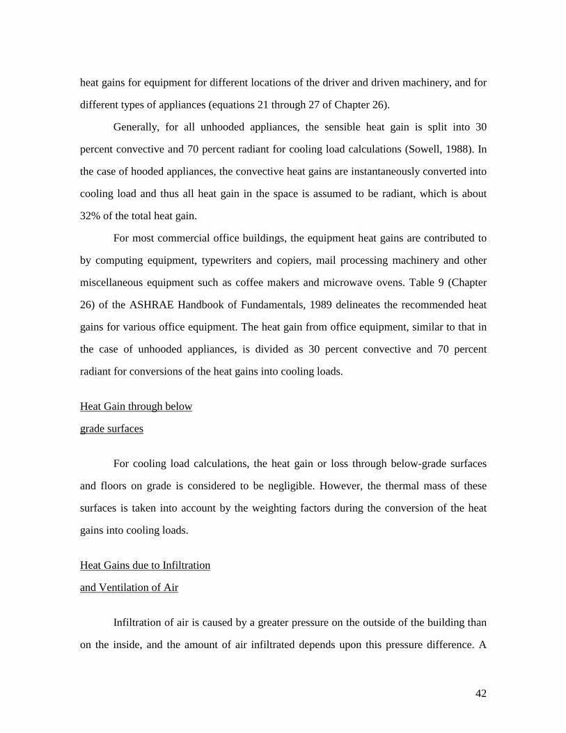
42
heat gains for equipment for different locations of the driver and driven machinery, and for
different types of appliances (equations 21 through 27 of Chapter 26).
Generally, for all unhooded appliances, the sensible heat gain is split into 30
percent convective and 70 percent radiant for cooling load calculations (Sowell, 1988). In
the case of hooded appliances, the convective heat gains are instantaneously converted into
cooling load and thus all heat gain in the space is assumed to be radiant, which is about
32% of the total heat gain.
For most commercial office buildings, the equipment heat gains are contributed to
by computing equipment, typewriters and copiers, mail processing machinery and other
miscellaneous equipment such as coffee makers and microwave ovens. Table 9 (Chapter
26) of the ASHRAE Handbook of Fundamentals, 1989 delineates the recommended heat
gains for various office equipment. The heat gain from office equipment, similar to that in
the case of unhooded appliances, is divided as 30 percent convective and 70 percent
radiant for conversions of the heat gains into cooling loads.
Heat Gain through below
grade surfaces
For cooling load calculations, the heat gain or loss through below-grade surfaces
and floors on grade is considered to be negligible. However, the thermal mass of these
surfaces is taken into account by the weighting factors during the conversion of the heat
gains into cooling loads.
Heat Gains due to Infiltration
and Ventilation of Air
Infiltration of air is caused by a greater pressure on the outside of the building than
on the inside, and the amount of air infiltrated depends upon this pressure difference. A

43
number of methods that calculate the rate of infiltration for building structures exist. The
most commonly used are the crack method and the air change method.
The crack method involves calculating the effective leakage area of cracks in
windows, doors, lighting fixtures, adjoining walls and roofs, and the building material and
using this in conjunction with the pressure difference due to various factors to calculate the
rate of infiltration.
Most experienced engineers and designers often estimate the infiltration rate by the
air change method wherein an assumption is made of the number of air changes per hour
(ACH) for the space under consideration based on the building structure and use. The rate
of infiltration is then given as
CFM = ACH * VOL/60 (2.38)
where
CFM = The rate of infiltration (ft3/min)
VOL = The volume of the space (ft3)
Sometimes outdoor air is supplied directly to the space for ventilation purposes. In
modern air-conditioning systems, however, the outdoor air is mixed with recirculated air
from the space and conditioned before being resupplied back to the space. While infiltrated
air is a load on the space, ventilated air introduced through the heating or cooling system is
a load on the heating or cooling coil.
In the summer, infiltrated air has to be cooled to the inside design temperature.
Assuming standard air conditions, this cooling load is calculated as
Qs = 1.10 * (Tout - Tin) * CFM (2.39)
where
Qs = The sensible cooling load due to infiltration (ft3/min)
Tout = Temperature of the outdoor air (°F)
Tin = Inside design temperature (°F)
CFM = The rate of infiltration (ft3/min.)

44
Infiltrated air also causes a latent load on the conditioned space since some of the
water vapor condenses during the cooling of the outdoor air. This latent load due to
infiltration is calculated as
Ql = 4840 * (Wout - Win) * CFM (2.40)
where
Ql = The latent cooling load due to infiltration (Btu/hr)
Wout = The specific humidity of outdoor air (lbmv/lbma)
Win = The specific humidity of inside air (lbmv/lbma)
Equations 2.39 and 2.40, with the terms inside the brackets interchanged, can be used with
reasonable accuracy to calculate the heating load due to infiltration of air.
Conversion of the heat gains into
cooling loads
After the heat gain qθ from the various components has been estimated, the
corresponding cooling load Qθ for the hour is calculated using equation 2.1:
Qθ = v0qθ + v1qθ - δ + v2qθ - 2δ - w1Qθ - δ - w2Qθ - 2δ
As discussed earlier, the weighting coefficients are chosen from the database using the
Weighting Factor routines. In order to convert the heat gains to corresponding cooling
loads, the procedure followed is the same for all components. Depending upon the type of
component, the WF routines return the appropriate weighting factors. There are basically
four types:
1) SOLAR - these are applied to the solar heat gains through fenestration
2) CONDUCTION - these are applied to the conduction heat gains from exterior surfaces
like walls and roofs, and interior partitions, as well as the absorbed heat gains through
fenestration systems.
3) LIGHTING - these are applied to the heat gains due to lighting and

45
4) OCCUPANT or EQUIPMENT - these are applied to the occupant and equipment heat
gains.
After the appropriate weighting factors have been selected, equation 2.1 is solved
iteratively for the 24 hour time period until convergence is reached. The initial values of
the cooling loads are taken to be zero. The cooling loads due to the infiltration of air are
calculated and added to the sum of the cooling loads for each zone for each hour to arrive
at the total cooling load for the building space.
Heat Extraction Rate and
the Space Air Temperature
The procedures for calculating the cooling load by the revised TFM described in
the preceding sections are based on a constant inside design temperature throughout the
day. However, the inside room temperature actually does not remain constant. It may vary
due to the following reasons:
1) Temperature setback which may be employed during the night time and weekends,
resulting in the space temperature to float during times when the space is unoccupied.
2) The cooling system cannot maintain exact control over the room temperature, and the
temperature may vary as the load varies throughout the day.
Heat extraction calculations along with the estimation of the space air temperatures
are possible with the TFM provided certain specifications of the cooling system and the
operating conditions are known. These include the maximum cooling capacity and the
cooling characteristics (heat extraction rate v/s the room air temperature) of the system.
The cooling loads calculated by the TFM are used as input data in order to determine the
heat extraction rate and the space air temperature. In addition, a space air transfer function
that relates the room air temperature to the heat extraction rate is used.
Heat Extraction Rate

46
The heat extraction characteristics of a cooling unit can be generally approximated
by the following linear equation:
ERθ = Wθ + (S * trθ) (2.41)
where
ERθ = The rate of heat removal from the space at time θ
trθ = The air temperature of the space at time θ
W, S = parameters that characterize the performance of the cooling equipment
The above equation is assumed to be applicable in the throttling range of the
control system. When the space air temperature lies outside the throttling range, the
parameter S is calculated as the slope of the line describing the extraction rate as a function
of the space air temperature. It is determined as follows:
S = (ERmax - ERmin)/ ∆ttr (2.42)
where
ERmax= the maximum extraction rate over the throttling range
ERmin = the minimum extraction rate over the throttling range
∆ttr = the throttling range of the control system
The intercept of this line, Wθ is calculated as
Wθ = ( ERmax + ERmin ) / 2 - ( S t*rθ) (2.43)
where
t*rθ = the thermostat set point temperature at time θ, equals the midpoint of
the throttling range
The Space Air Transfer Function

47
The space air transfer function relates the rate of heat extraction to the space air
temperature. It is represented as
�i=0
1 pi(ERθ-iδ - Qθ-iδ) = �
i=0
2 gi(trc - tθ-iδ) (2.44)
where
gi, pi = the coefficients of the space air transfer function
Q = the calculated cooling load for the room at time θ, based on an
assumed constant room temperature trc
Table V gives the normalized values of the g and p coefficients for light, medium, and
heavy constructions.
TABLE V
THE NORMALIZED SPACE AIR TRANSFER FUNCTION COEFFICIENTS
___________________________________________________________ Room Envelope g0* g1* g2* p0 p1
Construction Btu /hr-ft2°F (Dimensionless) ___________________________________________________________
Light +1.68 -1.73 +0.05 1.0 -0.82 Medium +1.81 -1.89 +0.08 1.0 -0.87 Heavy +1.85 -1.95 +0.10 1.0 -0.93 ___________________________________________________________ NOTE : For descriptions of light, medium, and heavy constructions, please refer Table 24 on page 26.27 of the ASHRAE Handbook of Fundamentals, 1989.
The values of the g coefficients are unnormalized using the following equations:
g0,θ = g*0 * A + p0 [ UA +1.1 ( Vθ + VIθ ) ] (2.45a)

48
g1,θ = g*1* A + p1[ UA +1.1 ( Vθ−δ VIθ−δ ] (2.45b)
g2,θ = g*2 * A (2.45c)
where
UA = the overall UA value for the zone (Btu/hr-ft2-°F)
V = the flow rate of ventilation air introduced directly into
the space (CFM)
VI = the flow rate of infiltration air (CFM)
Heat Extraction Rate and Space
Air Temperature Calculations
By simultaneous solving equations 2.41 and 2.44, the following equation for the
rate of heat extraction is obtained:
ERθ = ( Wθg0 + IθS ) / ( S + g0 ) (2.46)
where
Iθ = Error! (2.47)
In case the calculated value of ERθ from the above equation is greater than the maximum
extraction rate of the cooling unit ERmax, ERθ is set to be equal to ERmax. If the
calculated value of ERθ is less than ERmin, ERθ is set to be equal to ERmin. The space air
temperature trθ is then calculated as
trθ = ( Iθ - ERθ ) / g0,θ (2.48)
Since the prior values of ERθ and trθ are not known initially, the initial values of ERθ are
set at 0 Btu/hr for all 24 hours while those for trθ are set at 80°F. Equation 2.54 is solved
iteratively for the 24 hour time period until convergence for both the heat extraction and
space air temperatures is reached.

49
CHAPTER III
THE CLTD/SCL/CLF METHOD
The CLTD/SCL/CLF method, as it is now referred to, is basically a manual method
that was developed to be used instead of the rather "tedious" and "complex" calculations
involved in the TF method. This chapter briefly describes the methodology of the
CLTD/SCL/CLF method for cooling load calculations. The method is described in more
detail in the new cooling and heating load calculation manual (McQuiston and Spitler,
1992).
ASHRAE sponsored research to compare the TFM and TETD/TA methods (Rudoy
and Duran 1975, ASHRAE 1989). As part of their work on this project, Rudoy and Duran
generated Cooling Load Temperature Differential (CLTD) data for the direct one-step
calculation of the cooling load from the conduction heat gains through sunlit walls and
roofs and through fenestration. They also developed Cooling Load Factors (CLFs) for
similar one step calculations of solar loads through glass areas and for loads from internal
sources.
This method has undergone revision after significant research carried out by Sowell
(1985, 1988) and McQuiston and Harris (1988). A new method of categorizing of walls
and roofs based upon their thermal response characteristics has been developed. Zones
have been classified based on their thermal dynamic response using additional zone
parameters that were hitherto not considered important, and CTF coefficients and
weighting factors for these zone groups have been developed.

50
This huge database of CTF coefficients and weighting factors, recent research in
the areas of solar radiation, solar heat gains through fenestration and rapid advancements in
the personal computing field prompted ASHRAE to fund a research project RP-626. The
main objective of this project was to develop a new load calculation manual (McQuiston
and Spitler 1992), incorporating the latest modifications to the CLTD/CLF method.
Furthermore, both manual and computer-oriented versions were to be provided. The
following sections describe how the inaccuracies in the earlier versions of the CLTD/CLF
method have been eliminated.
The CLTD/CLF Method and GRP158
The CLTD/CLF method described in the ASHRAE GRP-158 is based on tabulated
CLTD/CLF factors developed by Rudoy and Duran (1975). These CLTD/CLF factors,
calculated using the TFM, are used for the calculation of the cooling loads for the various
components which are then normalized for environmental and zone conditions. This is
necessary because the TFM produces cooling loads for standard environmental conditions
and zone types.
Walls and Roofs
The TFM was used to calculate cooling loads for 36 types of roofs and 96 types of
walls. These cooling loads were based on the heat gain caused by outdoor air temperature
and solar radiation under standard conditions of 40°N, July 21st, a maximum outdoor
temperature of 95°F, daily temperature of 21°F, and an inside design temperature of 75°F
for a single standard zone of medium type construction. The CLTDs were obtained by
dividing the hourly cooling loads by the area of the roof or wall and its overall heat transfer
coefficient
CLTD = Q / (U * A) (3.1)

51
where
Q = The hourly cooling load (Btu/hr)
U = Overall heat transfer coefficient (Btu/hr-sq.ft.-°F)
A = Surface area (sq.ft.)
CLTDs for the 96 types of wall constructions and 36 types of roofs were calculated.
Walls were grouped into 7 different categories and CLTDs for 8 facing directions were
tabulated. Roofs were grouped into 13 categories with suspended ceilings and 13 without
and the CLTDs tabulated. In order to normalize these CLTDs for different latitudes,
months, indoor and outdoor design conditions, the following equation was applied:
CLTDcorr = (CLTD + LM) * K + (78-TR) + (TM - 85) (3.2)
where
LM = The latitude month correction factor, Table 32 Chap. 26 ASHRAE
H.O.F, 1989
K = Color adjustment factor applied after LM, equals 1 for dark colored
surfaces or light surfaces in an industrial area; equals 0.5 for
permanently light colored surfaces (rural areas)
TR = Inside design temperature, °F
TM = Mean temperature, °F = TO - DR / 2
TO = Outside design temperature, °F
DR = Mean daily range, °F
The original CLTD/CLF method however had a few drawbacks. First of all the
number of walls and roofs studied and grouped together based on their thermal
characteristics did not adequately represent all roof and wall constructions that are
commonly in use. Besides, in the case where a particular roof or wall assembly did not
match any representative surface in the group, complicated adjustments to the table CLTDs
were required. This sometimes lead to questionable results. Another problem was that

52
corrections to the CLTDs for varying latitudes and design months sometimes led to
significant inaccuracies in the cooling load values.
Fenestration
The cooling load through glass areas was divided into conductive and radiant
portions. Cooling load due to conduction was calculated based on equation 3.1. The
CLTDs for windows were tabulated in the same way as for roofs and walls with
corrections for values of the daily average temperature and indoor design temperatures
other than 85°F and 78°F respectively. Since the cooling load due to conduction through
windows is a very small portion of the overall load, no latitude-month corrections were
provided.
Calculation of the radiant cooling load involved the use of the shading coefficient
(SC) which represents the ratio of the solar heat gain of the glass area to that of a reference
glazing material (double strength, 1/8 in., sheet glass). Solar heat gains for each hour were
determined for different fenestration orientations using the ASHRAE Clear Sky model.
Then, using the weighting factor equation of the TFM, cooling loads were calculated for
light, medium, and heavy zones with and without interior shading. A Cooling Load Factor
(CLF) for each hour of the day was derived by dividing the hourly cooling load by the
product of the maximum solar heat gain for the day, the shading coefficient, and the glass
area
CLF = Q / (A * SC * SHGFmax ) (3.3)
where
Q = The cooling load for the reference glazing system (Btu/hr)
SHGFmax = Maximum solar heat gain factor, tabulated for all directions, months,
and 0°N latitude to 60°N latitude (Btu/hr)
A = The glass area (sq.ft.)

53
SC = The shading coefficient
CLFs were tabulated for July 21 at 40°N latitude, and were considered to represent
values for all the summer months at all northern latitudes. The tabulated CLFs, combined
with the SHGFmax were presumed to adequately account for the variation in the solar heat
gain for other latitudes and design months. Thus, cooling loads for a particular latitude and
design month were calculated by multiplying the corresponding SHGFmax by the CLF
calculated for July at 40°N latitude. This approximation caused erroneous results in the
cooling loads calculated because the tabulated CLFs were significantly in error for other
latitudes and design months, particularly for off-peak hours and for locations whose
sunrise and sunset hours differ significantly from those of July 21, 40°N.
Occupancy, Lighting, and Equipment
The cooling loads for people, lighting, and equipment were calculated using the
weighting factor equation of the TFM from unit heat gains and various operating schedules
(2 hrs, 4 hrs, 6 hrs etc.) The hourly cooling load was determined as
Q = qs * CLF + ql (3.4)
where
Q = the cooling load (Btu/hr)
qs = Sensible heat gain (Btu/hr)
ql = Latent heat gain (Btu/hr)
CLF = The cooling load factor, equals cooling load since heat gain is unity
The cooling load factors for people and equipment were obtained using a single
medium weight zone while those for lighting were determined using several zone types,
light fixture types, and ventilation schemes.
Revisions to the CLTD/CLF Method

54
Research by Sowell (1985, 1988) and McQuiston and Harris (1988) as part of
ASHRAE sponsored projects RP-359 and RP-472 has been described in the literature
review section of Chapter I. The revised methodology resulting from their work
successfully resolves many of the inaccuracies of the CLTD/CLF method and is described
here.
As part of ASHRAE research project 626, a new way of arriving at the solar heat
gains through fenestration has been introduced. This is done by using a new factor called
the Solar Cooling Load (SCL). Although tabulating the CLF as a function of month and
latitude would have solved the problem both SHGFmax and CLF would now be functions
of month and latitude creating an unnecessary step and other unnecessary tables. Instead,
the SCL takes into account both the solar heat gain and the zone response for any
latitude/month combination. The cooling load is calculated as
Q = A * SC * SCL (3.5)
Accordingly, the method is now called the CLTD/SCL/CLF method.
Another area of significant improvement is a more accurate analysis of zone
response using the weighting factors developed in ASHRAE-472. The weighting factors
developed as part of this project account for important zone parameters hitherto not used in
the earlier CLTD/CLF method.
New CLF data has been developed for the internal heat gain sources - people,
lighting, and equipment (both hooded and unhooded). The printed tables in the Load
Calculation Manual have been based on four representative zone types and the cooling
loads obtained compare appreciably with those obtained by the TFM (Spitler et al., 1993).
A software program called CLTDTAB, which is provided with the new load
calculation manual, produces custom SCL and CLF tables for any design month and
latitude, as well as for any zone type, without interpolation between latitudes as was
required earlier. Using the method as a computer oriented one, the results of the zone
response are closely comparable with those obtained with the TFM. By using the manual

55
or semi-manual options, some accuracy is sacrificed by limiting the size of the printed
tables available. Table VI explains how the CLTDTAB program generates the CLTD,SCL,
and CLF tables using the general and specific options.
TABLE VI
THE CLTDTAB PROGRAM OPTIONS _______________________________________________________________
GENERAL SPECIFIC _______________________________________________________________
1) Roofs - Roof CLTDs for 10 1) Roofs - Roof CLTDs for the most common roof types are desired roof type, month, latitude, tabulated for the desired month, and zone type are tabulated latitude, and zone parameters of the representative zone type
2) Walls - Wall CLTDs for 15 2) Walls - Wall CLTDs for the most common wall types are desired wall type, month, latitude, tabulated for the desired month, and zone type are tabulated latitude, and zone parameters of the representative zone type
3) Glass Areas - SCLs for four 3) Glass Areas - SCLs for the representative zone types - A,B,C, particular zone for the 8 directions and D (LCM, 1992) are tabulated and the horizontal are tabulated for for 8 different directions and the the desired month and latitude horizontal 4) No CLF tables are tabulated 4) CLFs for people (and unhooded equipment), lighting, and hooded equipment for the desired zone type are tabulated _______________________________________________________________
By using the "zone specific" option, the results obtained by the CLTD/SCL/CLF
method are nearly identical to those obtained by the revised TF method. Since the
"general" option uses representative zone, roof, and wall types, the results obtained are not
as accurate as those obtained by the revised TF method. The manual option of the
CLTD/SCL/CLF method using the printed tables induces more errors since interpolation is

56
required for other locations. Lindsey (1991) has tabulated the maximum percentage errors
between the computer program values and printed table values for different representative
roof and wall groups.
Spitler et al. (1993) describe the new load calculation manual and the revised
CLTD/SCL/CLF method in their recent papers. Description of the software developed to
access the CTF coefficients and weighting factors is made by Sowell (1992) while the
CLTDTAB program and the procedures involved in generating the CLTD, SCL and CLF
tables is described by Lindsey (1991), and a paper by Falconer et al. (1993).

57
CHAPTER IV
THE HVAC SOFTWARE PROGRAM
As part of this project, a software program has been developed in order to calculate
the cooling loads for a building based on the revised Transfer Function Method. This
program, written in the C-programming language, executes under Microsoft
WINDOWSTM as a user-interactive, menu driven program. In addition to cooling load
calculations, the program also performs calculations of the heat extraction rates for desired
zones, and the heating load for the building based upon steady state heat transfer. An
elaborate explanation of the graphical user interface and operation of the program appears
in the Users Reference Manual accompanying the software (Hodson, 1992). Different
aspects of the user-interface and the structure of the program are discussed by Song (1992).
This chapter attempts to give an overview of the program, including the technical
calculations.
Program Hierarchy
The program, which hereafter is called "HVAC", has a hierarchical data structure
and interface. The highest level item is a building for which the loads are to be calculated.
A building contains one or more zones which are each maintained at a uniform
temperature. Each of these zone contains one or more rooms which may have heat gains
due to walls, roofs, partition(s), people, lighting, equipment, and infiltration. Figure 4.1
shows the hierarchy that has been used for the program.

58
Building
Zone
Room
Zone
Room Room Room
Elements: Roof(s)Wall(s)Intz-Partition(s)LightingOccupancyEquipmentInfiltration
Elements: Roof(s)Wall(s)Intz-Partition(s)LightingOccupancyEquipmentInfiltration
Elements: Roof(s)Wall(s)Intz-Partition(s)LightingOccupancyEquipmentInfiltration
Elements: Roof(s)Wall(s)Intz-Partition(s)LightingOccupancyEquipmentInfiltration
Figure 4.1: Hierarchy of the HVAC software program
Each component shown in the figure is represented as a user-identifiable icon in the
program. The program allows the user to provide a distinct name to each component. The
following sections describe each component and its required input details.

59
Building
Besides a user given name, each building has a Location name. The calculations to
be performed (cooling load, heat extraction rate, and heating load) are set in the main
dialog box. The design day requirements and outdoor conditions for summer (cooling load
option) and winter (heating load option) are entered in the "Location" dialog box. Table
VII shows the input required for this dialog box.
The average air temperature is the daily average air temperature for the location
during the coldest winter months while the ground amplitude is the amplitude of variation
of the ground temperature from the daily average air temperature. These parameters are
required to calculate the heat losses through basements and floors. Values of the average
air temperature for various locations in the U.S. are available in Table 3.5 in Chapter 3 of
the Heating and Cooling Load Calculation Manual (1992), while Figure 4 in Chapter 25 of
the ASHRAE Handbook of Fundamentals (1989) shows the lines of constant amplitude of
the ground temperature.
Zones
Each building consists of one or more zones. A typical zone dialog box contains
input for the inside design conditions for summer and winter. The default inside conditions
for summer are 75°F dry bulb and 50% RH while those for winter are 70°F and 30% RH.
The design wet bulb temperature can be entered instead of the relative humidity.
Heat extraction rate calculations are carried out on a zone-by-zone basis. Table VIII
shows the input details for a typical heat extraction dialog box, which is brought up at the
zone level by the "File-Heat Extraction" menu.
Heat extraction rates are required to be re-calculated if any design information has
been modified after calculation has been done.

60
TABLE VII
INPUT DETAILS FOR THE "LOCATION" DIALOG BOX AT THE "BUILDING" LEVEL
________________________________________________________________ Name Units Comments ________________________________________________________________ City - } State - } Default settings are for Latitude Deg. & Min. } Stillwater, Oklahoma* Longitude Deg. & Min. } Time Zone } Atmospheric Pressure lbf/in2 } Default - 14.696 lbf/in2 (Used to } calculate the specific humidities) TIME - Local Solar Time - } OR } Default settings are Daylight Local Clock Time - } Savings Time ( Local Clock Time ) (Std. or Daylight } Savings Time) } SUMMER DESIGN } CONDITIONS } Month - } Default settings are based on the Day - } 2½% design conditions for the 21st Design Dry Bulb Temp. °F } of June for Stillwater, Oklahoma* Mean Coincident Wet } (ASHRAE H.O.F, 1989) Bulb Temp. °F } Daily Mean Range °F } WINTER DESIGN CONDITIONS } Design Dry Bulb Temp. °F } Wet Bulb Temperature °F } Default settings are based on the Relative Humidity - } 99% design conditions for Stillwater, Average Air Temperature °F } Oklahoma * (ASHRAE H.O.F, 1989) Ground Amplitude °F } ________________________________________________________________ * In case user wishes to change the default setting , the "save as default" button should be clicked after different data have been entered in the "Location" dialog box
TABLE VIII

61
INPUT DETAILS FOR THE "HEAT EXTRACTION" DIALOG BOX AT THE "ZONE" LEVEL
___________________________________________________________________
Name Units Comments ___________________________________________________________________ Ceiling Height ft. } Used to calculate the total volume of ACH - } the zone for the infiltration portion of } the heat extraction rate calculation ROOM ENVELOPE CONSTRUCTION Light, Medium, - } Used to select the normalized space or Heavy } air transfer (g and p) coefficients HEAT EXTRACTION Maximum value Btu/hr } Default: Zone Sensible Cooling Load + (a) 1000 Btu/hr if Peak Zone Sens. Cooling Load = 0 Btu/hr (b) 4000 Btu/hr if Peak Zone Sens. Cooling Load > 0 Btu/hr Minimum values Btu/hr } Default: 0 Btu/hr THERMOSTAT TEMP. Max. & Min. values °F } Defaults set at 2°F above and below the zone design temperature SCHEDULES Infiltration - A/C System - ___________________________________________________________________
Rooms
Each zone in a building has one or more rooms within it. The floor surface area
(ft2) and room ceiling height (ft.) are entered at the room dialog box. The weighting factors
for a particular room are determined by entering the 14 room parameters in the "Room
Parameters" dialog box. These 14 parameters are discussed in chapter II.
In addition, the heating load calculations require details about the level of the walls
of the room with respect to ground level in order to determine heating loads for above and

62
below grade walls. Table IX shows the 5 available choices for wall levels. Depending upon
the choice selected, the user is prompted to input either the floor U-Factor or the Perimeter
heat loss factor along with the slab perimeter adjoining the non air-conditioned areas and
accordingly, the heating load is calculated (using either the floor area or slab perimeter
with the corresponding U-Factor).
TABLE IX
INPUT DETAILS FOR THE "WALL PARAMETERS" DIALOG BOX AT THE "ROOM" LEVEL
________________________________________________________________
Name Units Comments ________________________________________________________________ WALL LEVEL ft. 1) Above Grade } Floor U - Factor required 2) On Grade } Slab Perimeter and Perimeter } U - Factor required 3) Less than 3' below grade } Heights above and below grade, Slab } Perimeter and Perimeter U - Factor reqd. 4) More than 3' below grade } Heights above and below grade and } Floor U - Factor required 5) Completely below grade } Floor U - Factor required ________________________________________________________________ NOTE : Refer to Table XV for heating load calculation for walls
Heat Gain Elements
The elements, some or all of which are present in rooms, are the sources of the heat
gains which result in cooling and heating loads. Basically, there are seven types of
elements that contribute to the heat gains: roofs or ceilings, walls, inter-zone partitions,
people, lighting, equipment, and infiltration.
Table X shows the input details required to specify roofs and walls. The roof or
wall type and U-Factor for the roof/wall can either be specified directly or be obtained by

63
setting the roof/wall type. Setting the roof/wall type means selecting the construction
materials that make up the roof or wall, its mass location, principal material, and the
secondary material (for walls) or the presence/absence of suspended ceiling (for roofs)
from the "Roof Type" or "Wall Type" dialog box. Once these are selected, the program
then automatically determines the appropriate roof/wall type from the database and the
corresponding CTF coefficients for the calculation of the heat gains. The data for different
construction materials are available in Table 11 of Chapter 26 of the ASHRAE Handbook
of Fundamentals, 1989.
TABLE X
INPUT DETAILS FOR THE "ROOF" OR "WALL" DIALOG BOX AT THE "ELEMENT" LEVEL
________________________________________________________________
Name Units Comments ________________________________________________________________ Facing Direction Deg. } Usually for walls - Measured clockwise from the North direction Tilt Deg. } Tilt from the horizontal. Roof/Wall Type - } Can either be input directly or details can Actual U-Factor Btu/hr-ft2 } be entered at the "Roof (Wall) Type" } dialog box Absorptance - } Solar Absorptance (Default : 0.9) Area ft2 } Can be entered directly or as a } combination of the length and breadth ________________________________________________________________
Roofs and walls may have glass areas in the form of skylights or doors and
windows. Details for these glass areas are entered in the "Glass Areas" dialog box. Table

64
XI shows the input requirements to calculate cooling loads through glass areas.
Information about the awning/overhang if present is used for shading calculations.
TABLE XI
INPUT DETAILS FOR THE "GLASS AREAS" DIALOG BOX AT THE "ROOF" or "WALL" LEVEL
________________________________________________________________
Name Units Comments ________________________________________________________________ Width of glass ft. Height of glass ft. Shading Coefficient - Glass U-Factor Btu/hr-ft2 AWNING/OVERHANG Overhang length (a) ft. } Glass to Overhang (b) ft. } Required to calculate the shaded and Overhang protrusion (c) ft. } unshaded glass areas for each hour Reveal depth (d) ft. } ________________________________________________________________
Inter-zone partitions are basically walls that separate zones maintained at different
temperatures, and calculation of the cooling load is based on steady state heat transfer.
Input information required to calculate the heat gain for a partition are the Area (ft2) and
U-Factor (Btu/hr-ft2) of the partition and the temperature of the adjacent zone (°F).
People, lighting, and equipment form the sources of internal heat gain. These heat
gains are made up of convective and radiant heat gain. The user specifies these fractions
the default values of which are 30% convective-70% radiant for people and equipment and
41% convective-59% radiant for lighting. These values can be changed depending upon
the heat gain. Accordingly, the program normalizes the weighting factors for the zone, as
explained in Chapter II. Tables XII, XIII, and XIV show the input requirements for the

65
people, lighting, and equipment elements. These are entered in the "People Information",
"Light Information", and "Equipment Information" dialog boxes.
Infiltration is entered as the number of air changes per hour (ACH). This indicates
the maximum design infiltration rate. The total infiltration rate is calculated as:
V = ACH * Room Volume (4.1)
where the room volume is determined from the room height and its floor area.
TABLE XII
INPUT DETAILS FOR THE "PEOPLE INFORMATION" DIALOG BOX AT THE "ELEMENT" LEVEL
________________________________________________________________ Name Units Comments ________________________________________________________________ Peak occupancy - Sensible heat gain/person Btu/hr } Default: 250 Btu/hr Latent heat gain/person Btu/hr } Default: 200 Btu/hr Radiant Fraction of heat gain - } Default: 0.70 Convective Fraction of heat gain - } Default: 0.30 SCHEDULE Schedule for people - ________________________________________________________________

66
TABLE XIII
INPUT DETAILS FOR THE "LIGHT INFORMATION" DIALOG BOX AT THE "ELEMENT" LEVEL
________________________________________________________________
Name Units Comments ________________________________________________________________ TOTAL INSTALLED LIGHTING Heat Gain/Area W/ft2 OR Total Heat Gain with Btu/hr } Lighting Multiplier is for multiple Lighting Multiplier } light elements with the same heat } gain data Radiant Fraction of heat gain - } Default: 0.59 Convective Fraction of heat gain - } Default: 0.41 SCHEDULE Schedule for lighting - ________________________________________________________________
TABLE XIV
INPUT DETAILS FOR THE "EQUIPMENT INFORMATION" DIALOG BOX AT THE "ELEMENT" LEVEL
________________________________________________________________
Name Units Comments ________________________________________________________________ Sensible heat gain Btu/hr Latent heat gain Btu/hr Equipment Multiplier } Equipment Multiplier is for multiple } Equipment elements with the same } heat gain data Radiant Fraction of heat gain - } Default: 0.70 Convective Fraction of heat gain - } Default: 0.30 SCHEDULE Schedule for Equipment - ________________________________________________________________

67
Internal sources of heat gains (people, lights, and equipment) and infiltration
require the use of a schedule in order to determine the hourly heat gains. A schedule is a
set of 24 hourly fractional multipliers used to determine the hourly heat gain of a particular
element. For people, lighting, and equipment, the schedule indicates the fraction of the
total peak heat gain for the particular hour. Default schedules are available and can be
modified or a completely new schedule may be generated and saved into the schedule
library.
Calculations and Output
Once all input data for the entire building have been entered, cooling and/or heating
load calculations can be carried out by using the "Calculate" menu option at the Building
level.
Before calculating the heat gains for any element, the program determines the
outside specific humidity, equation of time, declination, and the coefficients of the solar
model - A, B, and C for the date of calculation. It then determines the various solar angles
for each hour of the day (at half past the hour) required to estimate the solar radiation
loads. It then calculates the heat gains and cooling loads for each element one by one,
using the database for walls and roofs by selecting the appropriate wall/roof with its
conduction transfer coefficients and the weighting factors that correspond to the heat
transfer response of the zone. Figure 4.2 shows a schematic of the working of the software
program for cooling load calculations.
In case the user wishes to examine intermediate calculations, they can be written to
files by using the "File-Preferences" menu option. The intermediate files are named as
DATA.CLD and DATA.XTR for cooling load and heat extraction rates respectively
where DATA is the name of the data file. The program also has an "Auto Save" feature
which prevents the loss of data by saving all data before calculation is performed (when
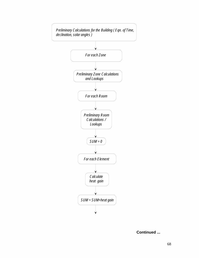
68
Preliminary Calculations for the Building ( Eqn. of Time, declination, solar angles )
For each Zone
Preliminary Zone Calculations and Lookups
For each Room
Preliminary Room Calculations / Lookups
SUM = 0
For each Element
Calculate heat gain
SUM = SUM+heat gain
Continued ...

69
ROOM LOADCALCULATIONS / SUMMATION
ZONE LOADCALCULATIONS / SUMMATION
andHeat Extraction Calculations ( if required )
BUILDING LOADCALCULATIONS / SUMMATION
Calculate Cooling Loadfor each element type
Figure 4.2: Flow chart of the HVAC program.
the "Calculate" menu item is invoked). The data is saved into the DATA.BAK file. This is
useful because the user does not have to change his original data file in case he was
performing only a test run.
Plots of the cooling loads can be examined on screen at all levels, from the
Building up to each Element and printed out if required. After the heating load has been
calculated, a dialog box containing the summary for the building pops up. Heating loads
for individual zones can be viewed within this dialog box using the "Zone" option.

70
The heat extraction calculations can be performed after the cooling load
calculations are done and the details for the heat extraction rates in the particular zone are
entered. Plots of the heat extraction and the space air temperature can be viewed on screen
at the "Zone" level.
The program also provides an option to print the results for the entire building. The
"Print" menu option is available at every level and hard copies of the results at any level
can be obtained. Thus, the user may print out an elaborate report of the building loads
beginning with each element or just a summary of the loads at the level he desires.
Heating Load Calculations
Heating load calculations are performed by the HVAC program using the steady
state heat transfer equation Q = U * A * ∆T. Table XV shows how the individual heating
loads are determined.
TABLE XV
CALCULATION OF INDIVIDUAL HEATING LOADS BY THE "HVAC" PROGRAM
___________________________________________________________________ Heating Load For Equation Comments ___________________________________________________________________ 1) Roofs, Walls*, Q = U*A* (Ti - To) Glass Areas, and Floors above exterior space 2) Floors on Grade Q = U'*P* (Ti - To) } U' is the perimeter heat loss } factor and P is the slab perimeter } measured in feet 3) Walls* and Floors below grade (a) Less than 3ft. below grade Q = U'*P* (Ti - To) (b) More than 3ft.

71
TABLE XV (Continued) ___________________________________________________________________ Heating Load For Equation Comments ___________________________________________________________________ below grade Q = U*A* (Ti - Tg) } Tg is the ground temperature } which is calculated from the } average air temp. and the ground } amplitude (c) Completely below grade Q = U*AT* (Ti - Tg) } AT is the total wall area 4) Infiltration Sensible Qs = 1.10*CFM (Ti - To) Latent Qs = 4840*CFM*(Wi - Wo) } Wi and Wo are the inside and } outside specific humidities ___________________________________________________________________ * Please refer to table IX for wall levels.

72
CHAPTER V
ZONE DESCRIPTIONS
In order to study the results of the revised Transfer Function Method and
compare them with those of the CLTD/SCL/CLF Method, three "fictitious" test zones
were selected. They are:
1) Retail Store: A single story rectangular zone with 2 exterior walls-one with
an exterior glass window, a roof and sources of internal load. The walls are
made of heavy construction material.
2) Office Premises: An office area with an adjoining computer room. These are
two mid-floor zones each at different temperatures. Exposed glass areas are
externally shaded by means of awnings.
3) Office in a High Rise Building: This is a top-floor office area with curtain
walls and a carpeted floor. Glass forms a major portion of the exterior
surfaces.
Following is a brief description of the zones and sample cooling load
calculations by the two methods.
Test Zone1 - Retail Store
This zone is a 70 ft. by 30 ft. corner zone, a retail store in a shopping mall
located in Stillwater, Oklahoma (Latitude 36'10", Longitude 97'05"). Figure 5.1 shows
the plan and elevation views of this test zone. It has two exterior walls, the East and
South Walls.

73
30 ft.
70 ft.
Retail Store
1 2 ft.7 f t.
N
Figure 5.1: Plan and Elevation views of the Retail Store

74
The 70 ft east wall has no exposed glass surfaces. However, the south wall has a 30 ft.
by 7 ft. high display window with no interior shading (shading coefficient of the glass
is 0.55 and its U-factor is 0.81 Btu/hr-sq.ft-°F). The north and west walls are interior
walls that adjoin other stores. The exterior walls are made of 4 in. face brick, 8 in.
concrete block, 0.75 in. polystyrene insulation with 1 in. furring strips (2 in. in width,
spaced 16 in. o.c.), and 0.5 in. dry wall. The roof of the zone is constructed from built
up roofing, rigid roof deck insulation, 2 in. concrete on a corrugated metal deck, and a
suspended ceiling. The interior walls are constructed from 0.5 in. dry wall and steel
studs. The floor of the zone is a 4 in. concrete slab on grade. The peak occupancy of
the store is about 15 people at times between 9 a.m. to 9 p.m. The fluorescent lights
are on from 8 a.m. to 10 p.m. There is no heat generating equipment in the zone and
the infiltration rate is taken to be 1.5 air changes per hour.
Test Zone 2 - Office Premises
This test zone is actually two zones - an office area and an adjoining computer
area which are maintained at 74 °F and 70 °F respectively. This office premise is on a
middle floor in a multi-story building in St. Louis, Missouri (Latitude 38'39",
Longitude 90'38"). Figure 5.2 depicts this test zone. The equipment room is not air-
conditioned. Exterior glass areas are shaded externally by means of awnings (Figure
5.3). The floors above and below these zones are air-conditioned. Assuming that the
temperature on the floors above and below remain constant throughout the day, the
ceiling and floor are treated as inter-zone partitions with steady state heat transfer
across them. The exterior walls of the office area are made of exterior finish, 8 in.
light weight concrete block and moderate insulation (R=4.5 °F-ft2-hr/Btu). The east
wall of the computer room is constructed of exterior finish, 4in. face brick, 8 in. light

75
wt. concrete block (filled) with an air space in between. The computer room adjoins
other office areas which are
Computer Room (70 °F)
Offices (74 °F)Equipment Room
Adjacent Office Areas
A
A
60'40'
35'
35'
2 0'
15'
N
Figure 5.2: Test Zone 2 - Office Premises
6 "6'
4 "
3'
6"
Figure 5.3: View of Window at section A-A
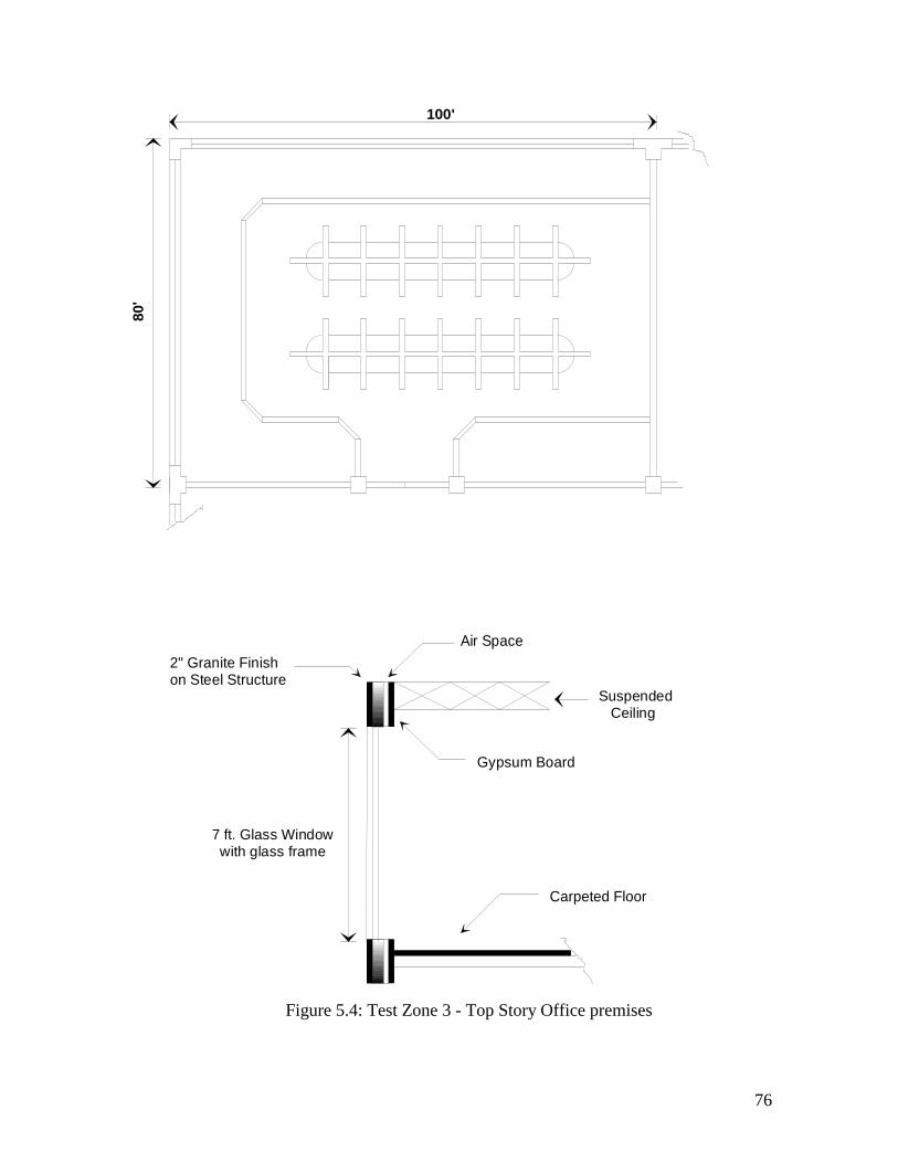
76
100'
7 ft. Glass Window with glass frame
2" Granite Finishon Steel Structure
Air Space
Gypsum Board
Suspended Ceiling
Carpeted Floor
80'
Figure 5.4: Test Zone 3 - Top Story Office premises

77
controlled at different temperatures and has electronic and computer machinery
operating throughout the day.
Schedules for people, lighting, and equipment for the office area are typical of
an 8 to 6 office area whereas those for the computer area extend to a greater part of the
day, since the equipment within it operates throughout the day. The internal heat
generating sources for the two areas are:
OFFICE COMPUTER ROOM
1) Occupancy 80 (8 a.m - 6 p.m.) 5 (8 a.m - 8 p.m.)
2) Lighting 1.9 W/ft2 (8 a.m - 6 p.m.) 1.5 W/ft2 (All 24 hrs)
3) Equipment 8000 Btu/hr sens. } 8 a.m to 25000 Btu/hr sens. }All 24
1600 Btu/hr latent } 6 p.m. 5500 Btu/hr latent }hours
Infiltration calculations are based on 2 ACH (7a.m - 7 p.m.) for the office area
and 1.5 ACH (All 24 hours) for the computer room.
Test Zone 3 - Top Story Office
This test zone is a huge office area situated on the top floor of a high rise
building in La Crosse, Wisconsin (Latitude 43'52", Longitude 91'15"). The office is
maintained at 75 °F. It has two exterior walls, one facing the north and the other facing
the west. The walls are of curtain type (light weight) with polished granite facing
bolted onto a steel structure on the outside and dry wall on the inside. Glass forms a
major portion of the exterior facade. No external shading exists for the glass areas.
The roof of this zone is made of 6" concrete with medium insulation and a vapor
barrier. The flooring of the zone is heavily carpeted. Figure 5.4 shows views of this
zone.

78
Schedules for people (occupancy - 300), lighting (2.5 W/ft2), and equipment
(70000 Btu/hr sensible and 6000 Btu/hr latent ) for the office area are on from 8 a.m.
to 6 p.m. and off at other times. The air-conditioning system is on from 7 a.m. to 7
p.m. and infiltration calculations are based on 2 air changes per hour.
Sample cooling load calculations for test zone 1 (The Retail Store) using both
methods are available in appendix A. Cooling load calculations for the other two test
zones by both methods are carried out along similar lines and compared. Comparison
tables and plots for these zones are available in the appendixes B and C. The results of
the different tests are discussed in chapter 6.

79
CHAPTER VI
RESULTS AND DISCUSSION
This chapter describes the results of the comparison tests carried out on the test
zones using the revised Transfer Function and CLTD/SCL/CLF methods. The
CLTD/SCL/CLF method is intended to give results very close to those of the revised TF
method. However, there are certain inherent limitations in the CLTD/SCL/CLF method.
These limitations are expected to cause some differences in the results obtained by the two
methods. The "manual" mode of the CLTD/SCL/CLF method has further limitations.
It was found that there are minor differences between the implementations of the
HVAC program and the CLTDTAB program. These are enumerated in Table XVI. In
order to have an accurate comparison between the two methods, the following changes
were implemented:
1) The CLTDTAB source code was modified to include the contribution of the Y factor.
2) A version of the HVAC (TFM) software that calculated the cooling loads at the hour
was prepared and used for the comparison tests.
3) All factors used in the load calculations were kept consistent for the two methods. The
following values were used:
ho = 3.0 Btu/hr-ft2-°F
ε = 0.9
δR = 20.0 Btu/hr-ft2

80
TABLE XVI
IMPLEMENTATION DIFFERENCES BETWEEN THE "HVAC" AND "CLTDTAB" PROGRAMS
_____________________________________________________________________ HVAC Program CLTDTAB Program Effect _____________________________________________________________________ 1) All Cooling Loads 1) All Cooling Loads are Due to the difference in the are calculated at calculated at the hour time of calculation, all solar half past the hour calculations are different 2) The Y - Factor is 2) The Y-Factor is not used. Differences in the solar included in the Instead, the following relation radiations for vertical calculations for solar is used: surfaces resulted in largely radiation through Ids = C*IDN* [1+cos(tilt)] / 2 differing values of sol-air vertical surfaces: Thus for vertical surfaces, temperatures by the two if cos θ > -0.2 [1+cos(tilt)] / 2 = 0.5 methods ( Max. difference Y = f ( cos θ ) This is an Isotropic model observed: 63.03 °F ; 155.31°F else of diffused radiation by the revised TF method & Y = 0.45 92.28 °F by the CLTD/SCL/CLF Ids = C*IDN*Y method ) This is an Anisotropic model of diffuse sky radiation 3) Absorbed solar heat 3) All absorbed solar heat Since the magnitude of the gains through glass gains through glass areas absorbed cooling loads is areas are converted are assumed to form small, the difference in these into cooling loads by instantaneous cooling load cooling loads ( ± 2 to 3 %) did using "conduction" not have any major effect on Weighting Factors the total cooling load 4) Values used for some 4) Corresponding values used Differences in the inward flowing constants were: were: fraction (Ni) and the sol-air
ho = 4.0 Btu/hr-ft2-°F ho = 3.0 Btu/hr-ft2-°F temperatures resulted in ε = 1.0 ε = 0.9 moderately different cooling load δR = 20.1 δR = 20.0 values (2 to 4 %) by the two methods _____________________________________________________________________

81
The methodological differences to be investigated include:
1) The use of the CLTDs, the SCLs and CLFs generated by the CLTDTAB program that
are tabulated with a small number of significant digits thereby inducing some round-off
error.
2) Use of the CLTD/SCL/CLF method for dates other than the 21st of the month which
requires interpolation. This may induce some error.
3) Use of the CLTDTAB program while interpolating for different latitudes.
4) Use of shaded and unshaded SCLs to calculate cooling loads through externally shaded
glass areas.
An exhaustive number of cooling load comparison tables and plots were obtained
for each of the test zones, some of which are reproduced here for discussion. Others are
found in the appendix.
In addition to the above comparison tests, the CLTD correction equation developed
by Rudoy and Duran (1975) was checked for its validity for varying outside and inside
temperatures and daily ranges. The equation is given as:
CLTDcorr = (CLTDtable + LM) * K + (78 - TR) + (TM- 85) (6.1)
where
LM = The latitude month correction factor
K = The color adjustment factor TR = Inside design temperature, °F
TM = Mean temperature, °F = TO - DR / 2
TO = Outside design temperature, °F
DR = Mean daily range, °F
The above correction equation can be approximated analytically to be a function of
the outside and inside temperatures and the mean daily range. Conduction heat transfer is
driven by the sol-air temperatures, and the inside temperature.
Thus,

82
qcond = f (Ti, To)
Assuming that the inside zone temperature remains constant, we can define To' such that
To' = To - Ti
Then,
qcond = f (To')
Furthermore, the following cosine fit can be applied to approximate the temperature profile
of ( To' ) for the day:
To' = ( Tmax' - DR/2) * [ A + B cos (2π ( h - hTmax ') / 24)]
where
Tmax' = the maximum value of To' for the day (°F)
DR = the mean daily range (°F)
A, B = constants for the curve fit
h = the hour under consideration
hTmax ' = the hour that corresponds to the maximum value of To'
Thus, as long as the profile of the temperature difference To' remains constant, the
temperature correction depends upon the term (Tmax' - DR/2), which is same as the
correction given by Rudoy and Duran.
Outside temperatures varying from 85°F to 105°F in steps of 5°F, inside design
temperatures from 50°F to 75°F in steps of 5°F, and mean daily ranges varying from 15°F
to 25°F in steps of 2°F were used to compare the results. Cooling load values obtained by
the revised TF and CLTD/SCL/CLF methods for varying values of the outside
temperature, inside temperature, and the mean daily range were nearly identical (maximum
error - 0.06 to 0.09 %). A change in the parameter (To, Ti, or DR) resulted only in a shift
of the cooling load profile by a proportional value, while the overall profile remained the
same.

83
Effect of inherent round-off error from tables
The CLTDTAB program generates custom tables containing the CLTDs for
commonly used roofs and walls, and SCL/CLF data for four representative zone types
using the "General" option. If the "Zone Specific" option is used then data pertaining to the
particular zone type is obtained. The CLTDs are in the form of integer numbers for each
hour while the SCLs and CLFs are tabulated with an accuracy of two decimal places. Due
to this round off, the potential difference in the values of the cooling loads for roofs and
walls using the table CLTDs and those obtained by using the revised TF method is ±0.5
times the UA value of the particular surface. For the SCLs and CLFs the difference is
±0.005 times the corresponding heat gain.
Keeping all other variables the same and using the "Zone Specific" option for the
CLTDTAB program, cooling loads were determined by using both the table as well as the
non-rounded values (obtained by debugging the CLTDTAB code) of the CLTDs. Using
the non-rounded values of the CLTDs is equivalent to using the revised TF method. It was
found that for almost every case for each hour, the difference in cooling load values was
within the maximum error specified above.
Table XVII shows these calculations for the retail store roof while Fig. 6.1 shows a
plot of the cooling loads obtained by the two methods. The minimal differences in the
cooling loads using the non-rounded CLTDs and the TF Method is attributed to very small
differences in the solar angles values and calculations thereafter.
Cooling loads by the two methods were then calculated based on the actual design
conditions and actual U-factors for the exterior surfaces (for the earlier test, the U-factor of
the representative wall/roof from the grouping tables was used). The calculated cooling
loads compared satisfactorily with cooling loads obtained by the revised TF method with
differences within the error range.

84
TABLE XVII
COOLING LOADS FOR THE RETAIL STORE ROOF BY THE REVISED TF AND THE CLTD/SCL/CLF METHODS
________________________________________________________________ Time TF CLTD Using non-rounded Values of CLTDs Method Method CLTD Load Difference CLTDNR. Load Difference ________________________________________________________________ 1 28288.37 32 28513.43 225.06 31.7447 28285.95 -2.420 2 25177.71 28 24949.25 -228.46 28.2538 25175.40 -2.311 3 22242.23 25 22276.12 33.89 24.9598 22240.30 -1.932 4 19480.59 22 19602.98 122.39 21.8606 19478.77 -1.818 5 16895.23 19 16929.85 34.62 18.9593 16893.58 -1.646 6 14523.10 16 14256.72 -266.39 16.2972 14521.53 -1.566 7 12838.88 14 12474.63 -364.25 14.4071 12837.37 -1.510 8 12512.91 14 12474.63 -38.28 14.0413 12511.43 -1.484 9 13775.12 15 13365.67 -409.45 15.4577 13773.50 -1.618 10 16527.30 19 16929.85 402.55 18.5462 16525.49 -1.807 11 20505.45 23 20494.03 -11.42 23.0106 20503.47 -1.977 12 25351.57 28 24949.25 -402.32 28.4490 25349.33 -2.239 13 30647.10 34 30295.52 -351.58 34.3916 30644.45 -2.647 14 35928.05 40 35641.79 -286.26 40.3182 35925.32 -2.732 15 40725.73 46 40988.06 262.33 45.7023 40722.79 -2.938 16 44609.82 50 44552.24 -57.59 50.0612 44606.77 -3.053 17 47212.65 53 47225.37 12.72 52.9822 47209.51 -3.141 18 48262.38 54 48116.41 -145.97 54.1601 48259.07 -3.310 19 47609.76 53 47225.37 -384.39 53.4278 47606.56 -3.202 20 45335.56 51 45443.28 107.72 50.8757 45332.52 -3.037 21 42067.44 47 41879.10 -188.34 47.2083 42064.71 -2.735 22 38527.55 43 38314.92 -212.63 43.2357 38524.94 -2.609 23 34996.87 39 34750.74 -246.13 39.2735 34994.44 -2.426 24 31569.19 35 31186.56 -382.63 35.4270 31567.04 -2.149 ________________________________________________________________ NOTE : 1) All loads are in Btu/hr 2) To = 95°F, Ti = 78°F, Mean daily range = 21°F 3) U-factor used = 0.424307 (U- factor of representative roof # 8) 4) Maximum Error Range = ± 0.5 *U*A = ± 0.5*0.424307*2100 = ± 445.52 Btu/hr

85
Similar tests were carried out for glass areas without external shading, lighting,
occupancy, and equipment to study the effects of using the table SCLs and CLFs as against
their actual values, with acceptable results (see Appendix A). However, since the
CLTDTAB program does not generate the CLFs for odd hour schedules (1hr, 3 hrs, 5 hrs
etc.), accurate comparisons for internal sources with odd hour schedules could not be
carried out. Interpolation of the CLFs does not yield correct results.
Thus it can be concluded that a reasonable degree of accuracy is maintained by
when reading off CLTD values from the tables.
Time (hrs)
0
5000
10000
15000
20000
25000
30000
35000
40000
45000
50000
TFM Method
CLTD
Figure 6.1: Cooling loads by the revised TF and CLTD/SCL/CLF Methods for the Retail Store Roof.
Effect of using CLTD/SCL/CLF tables
for dates other than the 21st

86
The CLTDTAB program generates data only for the 21st of any month of the year.
The "HVAC" software program however, is capable of calculating the cooling loads for
any day of the year. This is done by linear interpolation of the A, B, and C solar model
coefficients.
To examine the effect of using the CLTD/SCL/CLF data for days other than the
21st, cooling loads for the 6th of the month, which is about midway between the 21st days
of the preceding and next months, were calculated by the TF Method. These loads were
compared with the cooling loads obtained by using the CLTD/SCL/CLF data (which are
for the 21st of that month).
Of the three test zones, the retail store being driven by the roof, two walls and an
exposed glass area was used for the study since it has a greater percentage of exterior
surface areas. An important point to be noted is that the comparison was based on the
assumption that the outdoor design conditions are the same for both the 6th and the 21st of
the month, which actually may not be the case. Table XVIII shows the differences in the
cooling loads obtained.
It is seen that the increase in the difference of the cooling loads by using
CLTD/SCL/CLF data for the 6th is small compared to the magnitude of the load
(maximum difference = 0.7% for hour 13). With the outside design temperatures being the
same for the two days, the difference in the cooling loads is attributed to difference in the
beam and diffuse radiations incident on the exterior surfaces of the zone for the 6th and the
21st. This can be easily noticed as the differences are greater during the daytime and
smaller before sunrise and after sunset. Thus, the CLTD/SCL/CLF method may be used for
cooling load calculations with reasonable accuracy for days other than the 21st for similar
outside design conditions.

87
TABLE XVIII
COOLING LOADS FOR THE RETAIL STORE FOR THE 6th OF JULY
___________________________________________________________________ Time TF TF CLTD Difference Difference Increase in Method Method Method for the 6th for the 21st Difference (for the 6th) (for the 21st) ___________________________________________________________________ 1 28136.87 28105.63 27790.76 -346.11 -314.87 31.24 2 25750.16 25695.75 25326.26 -423.90 -369.49 54.41 3 23593.95 23543.25 23401.04 -192.91 -142.21 50.70 4 21713.26 21647.71 21564.14 -149.12 -83.57 65.55 5 20236.74 20217.27 20071.60 -165.14 -145.67 19.47 6 20008.52 20015.12 19929.40 -79.12 -85.72 -6.60 7 20623.65 20606.64 20357.24 -266.41 -249.40 17.01 8 22413.27 22389.05 22541.86 128.59 152.81 24.22 9 28756.11 28660.47 28699.22 -56.89 38.75 95.64 10 39080.20 38888.50 39081.97 1.77 193.47 191.70 11 45123.09 44851.28 45046.72 -76.37 195.44 271.81 12 50856.24 50505.85 50404.59 -451.65 -101.26 350.39 13 55342.14 54976.68 54872.24 -469.90 -104.44 365.46 14 58414.63 58103.42 57844.00 -570.63 -259.42 311.21 15 60080.10 59813.68 59687.66 -392.44 -126.02 266.42 16 60442.37 60299.60 60107.38 -334.99 -192.22 142.77 17 59738.30 59605.15 59251.59 -486.71 -353.56 133.15 18 57610.62 57516.27 57183.47 -427.15 -332.80 94.35 19 54382.28 54302.26 53724.24 -658.04 -578.02 80.02 20 51118.44 51041.20 50705.92 -412.52 -335.28 77.24 21 47950.48 47869.64 47379.07 -571.41 -490.57 80.84 22 42525.71 42469.85 41864.83 -660.88 -605.02 55.86 23 33507.79 33426.74 32910.45 -597.34 -516.29 81.05 24 30655.35 30597.85 30197.09 -458.26 -400.76 57.50 ___________________________________________________________________ NOTE : 1) To = 96 °F, Ti = 75 °F, DR = 24 °F 2) All loads are in Btu/hr

88
Use of the CLTDTAB program while interpolating for different Latitudes
The new load calculation manual (1992) contains CLTD and SCL data for northern
latitudes of 24, 36, and 48 degrees to be used for manual calculations. In order to calculate
the loads for locations at other latitudes, while using the printed tables, interpolation is
required. Alternatively, the CLTDTAB program can be used to generate a set of tables for
the particular latitude.
To compare the differences resulting from interpolation of the latitude, the table
values of the CLTDs for 36°N and 48°N were used to interpolate for values corresponding
to a latitude of 42°N. To keep all other values the same while performing the comparisons,
cooling loads determined by the TF Method were based on design conditions of 95°F
outside, 78°F inside and a mean daily range of 21°F. Cooling loads for the exterior east
wall of the Office from test zone 2 were calculated by both methods and compared. Table
XIX shows the interpolated values of the CLTDs vis-a-vis those obtained by using the
general option of the CLTDTAB for 42°N. The cooling loads obtained by the TF method
are tabulated for comparison. As can be seen the maximum percent difference in the
cooling loads obtained by interpolation is about 6.15 % at 8 hrs.
Similar comparison tests were carried out using the values of 24°N, 36°N, and
48°N to interpolate for intermediate latitudes and calculate the cooling loads by the
CLTD/SCL/CLF method. The maximum percent difference observed due to interpolation
ranged between 6 to 8 %.
Table XX shows the results of the comparison of the cooling loads for the east wall
of the office area of test zone 2 using extrapolated CLTDs for 6°N from the tabulated
values for 24°N and 36°N. This is an extreme test case and large differences in cooling
load values are observed. These are partly due to the fact that with the CLTD
TABLE XIX
COOLING LOADS FOR 42°N LATITUDE USING

89
INTERPOLATION FOR CLTDs _________________________________________________________________________________
Time TFM CLTD METHOD _________________________________________________________________________________
Cooling CLTD CLTD CLTD(42) Load_1 Difference CLTDs Load_2 Difference Load 36° N 48° N Interpol. ( Load_1 - for 42 deg ( Load_2 - TFM ) using TFM ) CLTDTAB _________________________________________________________________________________
1 941.03 17 17 17 950.30 9.27 16 894.4 -46.63 2 816.28 15 15 15 838.50 22.22 14 782.6 -33.68 3 702.20 12 13 12.5 698.75 -3.45 11 614.9 -87.30 4 598.04 11 11 11 614.90 16.86 10 559.0 -39.04 5 503.33 9 9 9 503.10 -0.23 8 447.2 -56.13 6 423.10 7 8 7.5 419.25 -3.85 7 391.3 -31.80 7 431.06 7 9 8 447.20 16.14 7 391.3 -39.76 8 655.75 11 14 12.5 698.75 43.00 12 670.8 15.05 9 1050.68 18 21 19.5 1090.05 39.37 20 1118.0 67.32 10 1488.41 26 28 27 1509.30 20.89 29 1621.1 132.69 11 1864.84 33 35 34 1900.60 35.76 35 1956.5 91.66 12 2117.21 37 39 38 2124.20 6.99 40 2236.0 118.79 13 2217.28 39 41 40 2236.00 18.72 41 2291.9 74.62 14 2187.05 39 40 39.5 2208.05 21.00 40 2236.0 48.95 15 2105.64 37 38 37.5 2096.25 -9.39 38 2124.2 18.56 16 2021.45 36 37 36.5 2040.35 18.90 36 2012.4 -9.05 17 1943.44 35 35 35 1956.50 13.06 35 1956.5 13.06 18 1864.20 33 34 33.5 1872.65 8.45 33 1844.7 -19.50 19 1772.99 32 32 32 1788.80 15.81 31 1732.9 -40.10 20 1659.20 30 30 30 1677.00 17.80 29 1621.1 -38.10 21 1520.39 27 27 27 1509.30 -11.10 26 1453.4 -66.99 22 1370.15 24 25 24.5 1369.55 -0.60 24 1341.6 -28.55 23 1220.29 22 22 22 1229.80 9.51 21 1173.9 -46.39 24 1076.37 19 20 19.5 1090.05 13.68 18 1006.2 -70.17 _________________________________________________________________________________
NOTE : To = 95 °F, Ti = 78 °F, DR = 21 °F U = 0.3 Btu/hr-ft2-°F, Area = 2100 ft2 Load_1 = U * Area * CLTD42(Interpolated) Load_2 = U * Area * CLTD42(CLTDTAB)

90
TABLE XX
COOLING LOADS FOR 6°N LATITUDE USING EXTRAPOLATION FOR CLTDs
________________________________________________________________________
Time TFM CLTD METHOD ________________________________________________________________________
Cooling CLTD CLTD CLTD(6) Load_1 Difference CLTDs Load_2 Difference Load 24° N 36° N Extrapol. ( Load_1 - for 6 deg ( Load_2 - TFM ) using TFM ) CLTDTAB _________________________________________________________________________________
1 857.70 15 17 12 670.80 -186.90 14 782.6 -75.10 2 743.06 13 15 10 559.00 -184.06 12 670.8 -72.26 3 637.53 11 12 9.5 531.05 -106.48 10 559.0 -78.53 4 540.61 9 11 6 335.40 -205.21 9 503.1 -37.51 5 452.00 8 9 6.5 363.35 -88.65 7 391.3 -60.70 6 372.01 6 7 4.5 251.55 -120.46 6 335.4 -36.61 7 304.51 6 7 4.5 251.55 -52.96 5 279.5 -25.01 8 330.66 10 11 8.5 475.15 144.49 6 335.4 4.75 9 590.88 17 18 15.5 866.45 275.57 11 614.9 24.02 10 1004.55 25 26 23.5 1313.65 309.10 20 1118.0 113.45 11 1419.71 33 33 33 1844.70 424.99 27 1509.3 89.60 12 1732.74 37 37 37 2068.30 335.56 33 1844.7 111.96 13 1894.62 39 39 39 2180.10 285.48 35 1956.5 61.88 14 1918.98 39 39 39 2180.10 261.12 35 1956.5 37.52 15 1882.74 37 37 37 2068.30 185.56 34 1900.6 17.86 16 1834.03 36 36 36 2012.40 178.37 33 1844.7 10.67 17 1781.93 34 35 32.5 1816.75 34.82 32 1788.8 6.87 18 1718.68 33 33 33 1844.70 126.02 31 1732.9 14.22 19 1631.52 31 32 29.5 1649.05 17.53 29 1621.1 -10.42 20 1514.89 28 30 25 1397.50 -117.39 27 1509.3 -5.59 21 1382.43 26 27 24.5 1369.55 -12.88 24 1341.6 -40.83 22 1245.87 23 24 21.5 1201.85 -44.02 22 1229.8 -16.07 23 1111.06 20 22 17 950.30 -160.76 19 1062.1 -48.96 24 980.94 18 19 16.5 922.35 -58.59 17 950.3 -30.64 _________________________________________________________________________________
NOTE : To = 95 °F, Ti = 78 °F, DR = 21 °F U = 0.3 Btu/hr-ft2-°F, Area = 2100 ft2 Load_1 = U * Area * CLTD6(Extrapolated)

91
Load_2 = U * Area * CLTD6(CLTDTAB)
values for both 24°N and 36°N being identical for some hours, extrapolation for 6°N yields
the same value. The maximum percent difference due to extrapolation in this case was
23.1% for hour 11.
Use of shaded and unshaded SCLs for solar heat gains through Fenestration
To calculate the cooling load due to the radiant heat gain through fenestration by
the CLTD/SCL/CLF method, a new factor called the Solar Cooling Load (SCL) is used.
This factor, described in chapter III takes into account both the solar heat gain and the zone
response for any latitude/month combination.
As pointed out earlier, the CLTDTAB program employs weighting factors to convert
the transmission heat gains only (SOLAR WFs). The heat gains due to absorption are not
converted to cooling load. Rather, they are assumed to directly represent instantaneous
cooling loads. This assumption is acceptable because for all cases the magnitudes of the
absorbed cooling loads are very small (2 to 3% of the total glass load). There are two other
important differences between the methodologies of the revised TF and CLTD/SCL/CLF
methods:
1) In the CLTD/SCL/CLF method, calculation of cooling loads through the shaded area of
glass areas is based on the SCLs determined for a north facing glass surface at that
location, which is assumed to represent a fully shaded glass surface, since it is almost
never reached by the direct rays of the sun.
2) The CLTD/SCL/CLF method employs shaded and unshaded SCLs to calculate the
cooling loads through the respective shaded and unshaded areas. The shaded SCLs
represent a glass area that is completely shaded throughout the day while the unshaded

92
SCLs represent a glass area that is completely unshaded throughout the day. In reality,
the shaded and unshaded glass areas may continuously vary during the day. Thus, the
CLTD/SCL/CLF method is incapable of correctly accounting for the past history of
varying shaded and unshaded glass areas.
In order to study the effect of the use of the north facing glass for shaded areas and
the shaded and unshaded SCLs, test zone 2 (the office premises) was used to compare
results obtained by the two methods. Besides this test zone, other cases of exterior shaded
windows were examined and the results for some important cases are described in the
following paragraphs.
The office of test zone 2 has three glass areas - two identical ones facing the north
and the other, similar to the first two, facing the east. Cooling loads for these glass areas
(only one of the north facing glass windows was considered) were calculated using the two
methods (all parameters including the date of calculation, latitude, and the zone parameters
were kept same for both methods) and compared. Figures 6.2 and 6.3 show the cooling
loads obtained by the two methods for the north and east glass areas.
From figure 6.2 (cooling load for north facing window for the office area) it can be
seen that there is an abrupt change in the cooling load profile for the CLTD/SCL/CLF
Method for some hours early morning and late evening. This is because with the sun rising
due north of east and setting due north of west, the window is actually subjected to beam
radiation (ID) from the sun during these hours, and remains partially unshaded. The SCLs
for the shaded area in the CLTD/SCL/CLF Method are based on a north facing glass area
and thus the effect of the beam radiation is included in the calculations of the transmitted
and absorbed cooling loads through the shaded areas too.

93
Time (hrs)
0
200
400
600
800
1000
1200
1400
1600
1800
2000
TFM
CLTD
Figure 6.2: Cooling loads for the north window of test zone 2 by the revised TF and CLTD/SCL/CLF methods
Time (hrs)
0
500
1000
1500
2000
2500
3000
3500
TFM
CLTD
Figure 6.3: Cooling loads for the east window of test zone 2 by the revised TF and CLTD/SCL/CLF methods
94
Time (hrs)
0
500
1000
1500
2000
2500
3000
TFM
CLTD
Figure 6.4: Transmitted cooling loads through the unshaded area of the east window of test zone 2
The revised TF Method however, performs calculations of the transmitted and
absorbed solar heat gains based on the shaded and unshaded portions and the facing
direction of the glass area. Since accurate heat gains are obtained this way, the cooling
loads determined by using the weighting factors are an accurate representation of the past
history of the heat gains for the day. Appendix D shows plots of the transmitted cooling
loads through the shaded and unshaded areas of the north and east glass areas.
Figure 6.3 is an example that shows the inability of the CLTD/SCL/CLF method to
accurately account for the varying shaded and unshaded glass area. This can explained
more clearly with respect to the tables XXXVII and XXXVIII from APPENDIX D and
figure 6.4. At hour 10, the east facing glass area is completely shaded after having been
partly shaded for the previous 5 hours. The cooling load for hour 10 predicted by the

95
CLTD/SCL/CLF method is based on a window that has been completely shaded for the
entire day. Therefore, the load predicted by the CLTD/SCL/CLF method is considerably
less than that predicted by the revised TF method, which correctly accounts for the beam
radiation transmitted through the window earlier in the day.
To further analyze the effect of exterior shading, the cooling load profiles by the
two methods were studied for externally shaded arbitrary facing glass areas at different
latitudes. Tests were carried out to check the severity of the use of the shaded SCLs (north
facing glass) for the shading calculations for glass areas at the equator. Generally, it is not
recommended that these SCLs be used for latitudes below 24 °N on account of beam
radiation being present for some hours at these latitudes for north facing glass (Load
Calculation Manual - 1979, 1992).
Figure 6.6 shows the cooling load profiles obtained by the two methods for a
southwest facing window. This exterior shading details for this window are shown in
figure 6.5. The window is 5' in width and 4' high (U-factor = 0.82, shading coefficient =
0.58, To = 95 °F, Ti = 75 °F, DR = 21 °F) and is located at 0 °N latitude (the equator).

96
N
SW
4.5'
1'5' Wide X 4' High Window
Figure 6.5: An externally shaded south west facing window

97
Time (hrs)
0
200
400
600
800
1000
1200
1400
TFM
CLTD
Figure 6.6: Cooling loads for the SW facing window at 0 °N by the revised TF and CLTD/SCL/CLF methods
Time (hrs)
0
200
400
600
800
1000
1200
TFM
CLTD
Figure 6.7: Transmitted cooling loads through the shaded area of the SW facing window at 0 °N

98
Time (hrs)
0
20
40
60
80
100
120
TFM
CLTD
Figure 6.8: Transmitted cooling loads through the unshaded area of the SW facing window at 0 °N
This configuration represents a somewhat extreme case of external shading. The awkward
behavior of the cooling load profile obtained by the CLTD/SCL/CLF method is due to
1) the contribution of the beam radiation to the SCLs calculated for the shaded glass area
(north orientation) and
2) The inability of the CLTD/SCL/CLF method to correctly account for the past history of
the varying areas of the shaded and unshaded portions of the glass areas in the cooling
load calculations.
As seen in figure 6.7, the transmitted cooling loads through the shaded portion of
the glass area by the two methods shows great variations with differences as much as
200% for some hours. This deviation of the cooling load profile from that obtained by the
TF method is a result of the beam radiation on a north facing glass area for these hours and

99
the corresponding heat gain being included in the SCL calculation for north (shaded)
facing glass.
Figure 6.8 shows the transmitted cooling loads by the two methods through the
unshaded areas. Since the south west facing window is shaded for most of the day except
for a few hours in the evening, the cooling load profiles show an increase towards the
evening. However, the cooling load calculations by the CLTD/SCL/CLF method are based
only on the respective shaded and unshaded areas at the hour of calculation and do not
account for the variation in these areas for the hours that preceded this hour. Thus, the
cooling load profile obtained does not accurately represent the actual load. On the other
hand, the TF method accounts for these changes during the conversion of the heat gains
into the corresponding cooling loads and thus the cooling load profile is more normalized.
This is why the cooling load profile by the CLTD/SCL/CLF method (figure 6.8) shows a
sudden rise in the cooling load from previous values of zero whereas that for the TF
method shows a more gradual increase from earlier positive values of the load.
Another test was carried out for a south west facing glass area ( 5 ft. wide by 4 ft. in
height) at 24 °N latitude. The temperatures selected were 95 °F on the outside and 75 °F on
the inside. The daily range was set at 21 °F. External shading details are the same as shown
in figure 6.5. A "heavy" zone was selected (no interior shade, no furniture, no suspended
ceiling, and vinyl tile for the floor) in order to obtain the most extreme possible effect. It
was found that with this configuration of the window, it remained completely shaded
throughout the day except at hour 18. The TF code was modified such that the glass area
remained totally unshaded at this hour. The CLTDTAB code was modified so as to
calculate the SCLs for shaded areas also. Using these separate values of the shaded and
unshaded SCLs cooling loads were determined for the window and compared with those
obtained by the revised TF method.
Figure 6.9 shows the cooling load profiles obtained by the two methods. On
observing the plots in figures 6.10 and 6.11, it can be concluded that while the TF method

100
successfully takes into consideration the past history of changing shaded and unshaded
areas of the window, the CLTD/SCL/CLF does not. Hence an abrupt change in the cooling
load profile is noticed.
Appendix E shows the cooling loads obtained by the two methods for a typical case
of external shading. The cooling load plots indicate the typical errors that may be
encountered with the use of the CLTD/SCL/CLF method for externally shaded glass areas.
Both the inability of the CLTD/SCL/CLF method to account for the past history of the
varying shaded/unshaded areas and the effect of the use of the North facing glass SCLs for
shaded glass areas are noticeable.
Time (hrs)
0
100
200
300
400
500
600
700
800
900
TFM
CLTD
Figure 6.9: Cooling loads for the SW facing window at 24 °N by the revised TF and CLTD/SCL/CLF methods

101
Time (hrs)
0
50
100
150
200
250
300
350
TFM
CLTD
Figure 6.10: Transmitted cooling loads through the shaded area of the SW facing window at 24 °N
Time (hrs)
0
100
200
300
400
500
600
700
TFM
CLTD
Figure 6.11: Transmitted cooling loads through the unshaded area of the SW facing window at 24 °N

102
From the tests carried out on the use of the SCLs for externally shaded glass areas, two
important conclusions can be drawn:
1) A north facing window does not always accurately represent a completely shaded glass
area throughout the day and significant inaccuracies in the cooling loads are obtained in
some cases, especially locations near the equator.
2) For the case of a glass window where shading caused by overhangs or awnings exists
and varies during the day, the application of the tabulated solar cooling loads (both the
shaded and unshaded) does not yield accurate cooling loads. This is because these SCLs
are calculated based on the assumption that the same condition prevails throughout the
day i.e the unshaded SCLs represent a glass area that is unshaded throughout the day
while the shaded SCLs represent a glass area that is fully shaded throughout the day.
Since the shaded and unshaded areas change their respective sizes, the cooling load is
not proportional to the total glass area, rather it is dependent on the past history of the
changing shaded and unshaded areas. The heat storage effect due to these varying areas
and their sizes needs to be taken into account during calculation of the cooling loads.
However, in the CLTD/SCL/CLF method, it is not possible to generate SCL tables for
varying areas because of the number of combinations that exist.
Todorovic and Curcija in their paper (1984) explained a possible way of
determining the cooling loads through glass areas accounting for the varying shaded and
unshaded areas. Their method, called the "Negative Cooling Load Method" first calculates
the cooling loads as if the glass area is completely unshaded. These loads are then
corrected to account for the effect of shading by using "negative storage factors". These
negative storage factors were tabulated for 8 directions for light, medium, and heavy zones
based on July 21, 40 °N latitude.
Table XXI summarizes the results of the various tests carried out to examine the
differences between the two methods.
TABLE XXI

103
SUMMARY OF COMPARISON TESTS
TEST RESULT 1) Using the rounded table values of the
CLTDs, SCLs, and CLFs for cooling load calculations
Differences in the loads obtained by using the table CLTDs for exterior roofs, walls, and the SCLs for glass areas without external shading were within the error range. Marginal differences in loads using the CLFs for internal sources (0.5 to 1%).
2) Using the table values of the CLTDs to calculate the cooling loads for dates other than the 21st
Cooling loads calculated by the two methods showed small differences for same outside design conditions (1%)
3) Using the CLTDTAB program while interpolating for different latitudes
Small differences in the cooling loads calculated by the two methods (6 to 8%).
4) (a) Using the SCLs for north facing glass as an approximation for shaded glass.
(b) Using the shaded and unshaded SCLs to calculate cooling loads through externally shaded glass areas
(a) Use of the north (shaded) SCLs for locations near the equator showed considerable differences in the cooling load values (Maximum difference observed = 120% for 0°N SW facing window). Moderate differences were found for latitudes farther north (12%)
(b) Large differences were observed in the transmitted cooling loads through glass areas that were unshaded for some part of the day (Maximum difference observed = 200% for 0°N SW facing window).
The CLTD/SCL/CLF cooling load profile showed its inherent inability to correctly account for the previous history of heat gains due to the varying shaded and unshaded areas. (Max. difference observed = 43% for east glass of test zone 2)

104
CHAPTER VII
CONCLUSIONS AND RECOMMENDATIONS
This chapter contains the conclusions that are drawn from the preceding chapters
and some recommendations for work that can be carried out on the subject in the future.
Conclusions
1) A comprehensive software program, currently called HVAC, has been developed. This
program calculates the cooling loads for a given building based on the revised Transfer
Function Method and is a user-friendly software working under a graphical user
interface (Microsoft WINDOWSTM). In addition to performing cooling load
calculations, the HVAC software program calculates the heat extraction rates for zones
of interest and heating loads for buildings.
2) The results of the comparison of the two methods, the revised TF and the
CLTD/SCL/CLF method, have brought forward many points:
a) The CLTDTAB program used to generate custom tables for the CLTD/SCL/CLF
method calculates the cooling loads at the hour rather than at half past the hour. The
HVAC program however, calculates the cooling loads at half the hour which is
considered to be an adequate representation of the hour. In order to have consistency
in the comparison, a version of HVAC which calculated the cooling loads at the
hour was prepared and cooling loads compared.
b) The results of the comparison of the two methods have validated the
CLTD/SCL/CLF method as a fairly accurate method for manual calculations of

105
cooling loads. Cooling loads obtained by the this method compared reasonably with
those obtained by the TF method for the various comparison tests that were carried
out (except for some cases where glass areas were externally shaded).
c) Differences in cooling loads through externally shaded glass areas were observed.
These were considerable for glass areas located near the equator. The SCLs
calculated for north facing glass and being used to determine cooling loads through
shaded areas did not give correct results for all cases and for glass areas near the
equator. This is due to the fact that for locations near the equator (latitudes less than
24 °N) north facing surfaces are exposed to sunlight, and hence beam radiation, for
some hours. It can thus be concluded that it is not quite appropriate to use the SCLs
of the north facing glass for shaded calculations near the equator. This has also been
recommended by the Load Calculation Manual (1992).
d) The cooling load profiles for the cooling loads due to transmitted heat gains for the
glass areas that receive direct sunlight for only some hours showed deviations on
account of the inherent inability of the CLTD/SCL/CLF method to correctly account
for the past history of heat gains due to varying shaded and unshaded glass areas.
This is because the SCLs are calculated on the basis that the same condition
prevailed throughout the day - i.e. the unshaded SCLs represent a glass area that is
unshaded throughout the day and the shaded SCLs represent a glass area that is
shaded throughout the day. Hence, while the cooling load profile of the revised TF
method showed a gradual change in the cooling load, that for the CLTD/SCL/CLF
method shows an abrupt shift for the hour(s) of change from shaded to unshaded.
e) Calculations of the cooling loads for heat gains due to internal sources using the
CLFs from the tables for even hour schedules (2hrs, 4 hrs, 6 hrs etc.) resulted in
closely matching values with those obtained by the TF method. However, no table
values are available for odd hour schedules (3 hrs, 5 hrs, 7 hrs etc.). Interpolation
for these values does not give correct values of the CLFs.

106
Recommendations
Following are some recommendations aimed at further improvement of the HVAC
software program and research in the area of cooling load calculation:
1) Like most software programs, the HVAC software has room for enhancement in a
number of areas with a view to make it more user-oriented:
(a) The HVAC program uses the X-Y shading concept to determine the shaded and
unshaded glass areas. Walton (1979) and McCluney (1990) have developed
shading algorithms for complex geometries. It is suggested that one of these
algorithms be employed for the HVAC program.
(b) The current version uses default values for various parameters like the
coefficients of heat transfer at the outside (ho) and inside surfaces (hi),
emissivity (ε), ground reflectance (ρg), and the long wave radiation difference
(δR). It is suggested that rather than restraining the program to use these default
values, the software can be modified so as to allow the user to enter values that
would suit his design specifications.
(c) While the program has a "Save as Default" feature, a library of locations with
their design conditions would make an excellent feature. This would save the
user from having to refer to the Handbook for design conditions and type them
in every time he performs load calculations for a different location.
2) The HVAC program has been tested for its correctness in determining cooling loads.
Comparison tests have been carried out with the CLTD/SCL/CLF method. It is
suggested that comprehensive tests with major energy (and load calculation)
programs like BLAST be carried out. This will prove beneficial in further validating
the software program, and in general the revised TF method.
3) The current CLTDTAB program calculates unshaded SCLs for 9 facing directions
(8 vertical + 1 horizontal). SCLs for the north facing glass are used for calculations

107
through shaded glass areas. There are two possible ways of representing the cooling
loads through glass areas:
(a) Calculate the SCLs for a shaded north facing glass area to be used for
approximating all shaded glass areas.
(b) Calculate both shaded and unshaded SCLs for the surface for each facing
direction separately and use them for calculations.
Either option can be used for cooling load calculations. However, it should be noted
that the current CLTDTAB program does not account for the Y - factor for vertical
surfaces. It is suggested that the SCL calculations be based on the anisotropic model
of diffuse sky radiation (inclusion of the Y - factor) and SCLs tabulated for all 9
directions.
4) There are several differences in implementation between the HVAC and CLTDTAB
programs. Following are a list of suggested modifications to the CLTDTAB
program:
(a) All calculations, including the solar radiation calculations be based on half past
the hour.
(b) Include the Y- factor in the calculations for solar radiation through vertical
surfaces.
(c) As mentioned above, shaded and unshaded SCLs be calculated separately for all
facing directions and used for cooling load calculations.

108
REFERENCES
ASHRAE. (1979, 1992). Cooling and Heating Load Calculation Manual. ASHRAE. (1967, 1972, 1985, 1989). ASHRAE Handbook of Fundamentals. Atlanta,
American Society of Heating, Refrigerating, and Air-Conditioning Engineers, Inc. Harris, S. M., & McQuiston, F. C. (1988). A study to categorize walls and roofs on the
basis of thermal response, ASHRAE Transactions, 94(2), 688 - 715. Hill, J. E., & Furlong, R. R., (1973). Ashrae Cooling Load Calculation, ASHRAE Journal,
15(1), 61 - 66. Lindsey, Kirk (1991). Revision of the CLTD/CLF Cooling Load Calculation Method,
M.S.Creative Component, Oklahoma State University. Machler, M. A., & Iqbal M. (1985). A modification of the ASHRAE clear sky irradiation
model, ASHRAE Transactions, 91(1A), 106 - 115. McCluney, R. (1986). Awning Shading Algorithm for Window Energy Studies, ASHRAE
Transactions, 92(1A), 430 - 438. McCluney, R. (1990). Awning Shading Algorithm Update, ASHRAE Transactions, 96(1),
34 - 38. McQuiston, F. C., & Parker, J. D. (1988). Heating, Ventilating, and Air-Conditioning
Analysis and Design, John Wiley & Sons, New York. Mitalas, G. P., & Stephenson, D. G. (1967). Cooling Load Calculations by Thermal
Response Factor Method, ASHRAE Transactions, 73(I), III.1.1 - 1.7. Mitalas, G. P., & Stephenson, D. G. (1967). Room Thermal Response Factors, ASHRAE
Transactions, 73(II), III.2.1 - 2.10. Mitalas, G. P. (1969). An experimental check on the weighting factor method of
calculating room cooling load, ASHRAE Transactions, 75(2), 222 - 232. Mitalas, G. P., & Stephenson, D. G. (1971). Calculation of heat conduction transfer
functions for multi - layer slabs, ASHRAE Transactions, 77(2), 117 - 126.

109
Mitalas, G. P. (1971). Transfer Function Method of calculating cooling loads, heat extraction and space temperature, ASHRAE Journal, 12, 54 - 56.
Romine, T. B. (Jr.) (1992). Cooling Load Calculation: Art or Science?, ASHRAE Journal,
34, 14 - 24.
Rudoy, W., & Duran, F. (1975). Development of an Improved Cooling Load Calculation
Method, ASHRAE Transactions, 81(2), 19 - 69. Spitler, J. D., McQuiston F.C., & Lindsey K. (1993). The CLTD/SCL/CLF Cooling Load
Calculation Method, ASHRAE Transactions. Spitler, J. D., McQuiston F.C., & Lindsey K. (1993). Development of a Revised Heating
and Cooling Load Calculation Manual, ASHRAE Transactions. Stephenson, D. G. (1968). Calculation of cooling load by digital computer, ASHRAE
Journal, 4, 41 - 43. Song, Kyungho (1992) . Development of the 'Building Load Calculation' Program,
M.S.Creative Component, Oklahoma State University. Sowell, E. F., & Chiles, D. C. (1984a). Characterization of zone dynamic response for CLF
/ CLTD tables, ASHRAE Transactions, 91(2A), 162 - 178. Sowell, E. F., & Chiles, D. C. (1984b). Zone descriptions and response characterizations
for CLF / CLTD calculations, ASHRAE Transactions, 91(2A), 179 - 200. Sowell, E. F., & Chiles, D. C. (1984c). A counter - intuitive effect of mass on zone cooling
load response, ASHRAE Transactions, 91(2A), 201 - 208. Sowell, E. F. (1988a). Load calculations for 200,640 zones, ASHRAE Transactions, 94(2),
716 - 736. Sowell, E. F. (1988b). Cross-check and modification of the DOE-2 program for calculation
of zone weighting factors, ASHRAE Transactions, 94(2), 737 - 753. Sowell, E. F. (1988c). Classification of 200, 640 parametric zones for cooling load
calculations, ASHRAE Transactions, 94(2), 754 - 777. Threlkeld, J. L. (1963). Solar Irradiation of Surfaces on Clear Days, ASHRAE
Transactions,69, 24 - 36. Threlkeld, J. L. & Jordan R. C. (1959). Direct Solar Radiation available on Clear Days,
ASHRAE Transactions, 64, 45 - 68.

110
Threlkeld, J. L. (1962). Thermal Environmental Engineering, Prentice Hall, New York 321.
Todorovic B. (1982). Cooling Loads from Solar Radiation through Partially Shaded
Windows, taking Heat Storage Effect into Account, ASHRAE Transactions, 88(2), 924 - 937.
Todorovic B. & Curcija D. (1984). Calculative Procedure for Estimating Cooling Loads
Influenced by Window Shadowing, Using Negative Cooling Load Method, ASHRAE Transactions, 90(2B), 662 - 677.
Walton, G. N. (1979). The Application of Homogeneous Coordinates to Shadowing
Calculations, ASHRAE Transactions, 86, 190 - 208.

111
APPENDICES

112
APPENDIX A
SAMPLE COOLING LOAD CALCULATIONS
FOR TEST ZONE 1

113
Sample Cooling Load Calculation for the Retail Store
using the revised TF Method
Determination of the Room Parameters
Table XXII shows the fourteen room parameters that define the Retail Store.
TABLE XXII
ZONE PARAMETERS FOR THE RETAIL STORE
__________________________________________________________________
No. Parameter Choice # Description (Closest match) __________________________________________________________________
1 Zone Geometry 1 100 ft x 20 ft. 2 Zone Height 2 10 ft. 3 # of Ext. Walls 2 2 4 Zone Location 1 Single-Story 5 Interior Shade 3 0 percent 6 Furniture 1 With 7 Ext. Wall Constrn. 4 Heavy wall with Moderate Insulation 8 Partition Type 1 5/8 in. Gyp-Air-5/8 in. Gyp 9 Mid Flr. Type 1 8 in. Conc. 10 Slab Type 2 4 in. Slab on 12 in. Soil 11 Ceiling Type 1 3/4 in. Acoustic Tile & Air Space 12 Roof Type 2 LW w/o suspended ceiling 13 Floor Covering 2 Vinyl Tile 14 Glass Percent 3 10
_____________________________________________________________________
Once the fourteen room parameters have been selected, the weighting factors for
the zone are determined using the Weighting Factor routines.

114
Determination of the Wall CTF Coefficients
The exterior wall of the store is categorized as shown in table XXIII.
The location of the thermal mass of the wall, the 8 in. heavy weight concrete block is
outside with respect to the insulation, hence the mass location is "mass out"
The corresponding resistance range No. 9 [table 2.6(a) of the LCM].
TABLE XXIII
CATEGORIZATION OF THE RETAIL STORE WALL
___________________________________________________________________
Code Letter Description R - Value (hr-sq.ft.-°F/Btu)
___________________________________________________________________ A0 Outside Surface Resistance 0.33 A2 4 in. Face Brick 0.43 B1 Airspace Resistance 0.91 C8 8 in. HeavyWeight Concrete Block 1.11 B2 1 in. Insulation 3.33 E1 3/4 in. Plaster or Gypsum 0.15 ( closest to dry wall ) E0 Inside Surface Resistance 0.69 ___________________________________________________________________ TOTAL RESISTANCE 6.95 ___________________________________________________________________
The primary and secondary wall materials are the 8 in. HW Concrete Block (C8) and the 4
in. face brick (A2).

115
When these parameters are passed to the wget routine, a wall type of 17 is returned with
the following CTF coefficients and a U- factor of 0.1439 Btu / hr-sq.ft.-F n bn dn 0 0.000000 1.000000 1 0.000005 -2.008750 2 0.000134 1.371200 3 0.000436 -0.378967 4 0.000300 0.039616 5 0.000051 -0.001647 6 0.000002 0.000023
These CTF coefficients need to be unnormalized based upon the ratio of the actual U-
factor of the wall and the U-factor that corresponds to the matching wall type. The actual
U-factor of the wall is calculated to be 0.15 Btu / hr-sq.ft.-F as compared to 0.04232 Btu /
hr-sq.ft.-F. Thus, the ratio is: Uactual / U wall type = 0.1439 / 0.04232 = 3.331
The unnormalized CTF coefficients are multiplied by this ratio and are tabulated as
follows: n bn dn 0 0.000000 1.000000 1 0.000017 -2.008750 2 0.000446 1.371200 3 0.001452 -0.378967 4 0.000999 0.039616 5 0.000170 -0.001647 6 0.000007 0.000023
and
�
cn = �
bn = 0.003091
Determination of the Roof CTF Coefficients

116
The roof of the store is categorized in a manner similar to the wall as shown in
table XXIV.
Mass Location: "mass in" as the 2 in. heavy weight concrete is on the inside with respect to
the insulation.
The corresponding resistance range is No. 2 [table 2.7(a) of the LCM].
The primary roof material is the 2 in. HW Concrete (C12).
The CTF coefficients before and after unnormalization are as shown in table XXV.
TABLE XXIV
CATEGORIZATION OF THE RETAIL STORE ROOF
____________________________________________________________________ Code Letter Description R - Value (hr-sq.ft.-°F/Btu) ____________________________________________________________________ A0 Outside Surface Resistance 0.33 E2 1/2 in. Slag 0.05 E3 3/8 in. Felt and Membrane 0.29 B2 1 in. Insulation 3.33 C12 2 in. HW Concrete 0.17 A3 Corrugated Metal Deck 0.00 E4 Ceiling Air Space 1.00 E5 Acoustic Tile 1.79 E0 Inside Surface Resistance 0.69 ____________________________________________________________________
TOTAL RESISTANCE 7.65 ____________________________________________________________________
Roof type selected : 8 (from rget routine)
U- factor : 0.4243 Btu / hr-sq.ft.-°F

117
Actual U - factor : 0.1226 Btu / hr-sq.ft.-°F
Ratio : 0.1226 / 0.4243 = 0.289
TABLE XXV
CONDUCTION TRANSFER COEFFICIENTS FOR THE WALL
_________________________________________________________
n Conduction CTF coefficients bn dn _________________________________________________________
Before After Unnormalization Unnormalization _________________________________________________________
0 0.000984 0.000284 1.000000 1 0.019384 0.005602 -1.102350 2 0.020827 0.006022 0.207496 3 0.002189 0.000633 -0.002865 4 0.000015 0.000004 0.000002 5 0.000000 0.000000 0.000000 6 0.000000 0.000000 0.000000 _________________________________________________________
and
�
cn = �
bn = 0.012545
Calculation of the heat gains

118
Solar radiation intensity. The following steps show the calculation of the solar
intensities and the sol-air temperatures for the South Wall of the store for the time period
09:00 hrs to 10:00 hrs for the 21st of June ( The calculations are based on 10:00 hrs )
Solar Time = 10:00 hrs
Hour Angle (h) = - 0.25 deg / min * (2 * 60)
= - 30.0 degrees
(SIGN CONVENTION: Hour angles are
negative for Local Solar Times before
noon)
Declination angle ( δ ) = +23.45* degrees (table 2-2)
Solar altitude angle ( β ) = sin - [( cos 36 cos 23.45 cos -30.0 ) +
( sin 36 sin 23.45 )]
= 61.24 degrees
Solar Azimuth angle ( φ ) = cos - [(sin β sin l - sin δ) / cos β cos l]
= 72.45 degrees
According to the sign convention, if the hour angle is negative, the angle φ is also taken as
negative, hence
φ = -72.45 degrees
Wall Facing angle = 180 degrees (facing South)
Wall Azimuth angle (ψ) = 0 degrees
According to the sign convention, if the surface faces east of south (Wall Facing angle <=
180) then ψ is negative. However, here ψ = 0 degrees
Wall Solar Azimuth angle (γ) = abs(φ - ψ)
= abs(-72.45 - 0)
* Note that all values calculated here may differ slightly from those tabulated using the HVAC program on account of round - off during calculations. For example, the value of declination calculated by the HVAC program is 0.4086 radians or 23.41 degrees.

119
= 72.45 degrees
Angle of incidence (θ) = cos - [ cos β cos γ ]
= 81.66 degrees Direct Normal Intensity (IDN) = A e ( - B / sin β )
where
A = 346.3 (Table II)
B = 0.185 (Table II)
C = 0.137 (Table II)
Hence IDN = 346.3 e ( - 0.185 / sin 61.24 )
= 280.42 Btu / hr-ft2
Direct Intensity (ID) = IDN cos θ
= 40.67 Btu / hr-ft2
Ratio (Y) = 0.55 + 0.437 cos θ + 0.313 cos2 θ
= 0.620
Diffuse Intensity (Id) = Ids + Idg
= C Y IDN + 0.5*IDN(C + sin β)* ρg
= 0.137 * 0.620 * 280.42 + 0.5 *
280.42 * ( 0.137 + 0.8766) * 0.2
= 52.24 Btu / hr-ft2
Total Solar Intensity (It) = ID + Id
= 92.91 Btu / hr-ft2
Sol-Air Temperature (te) = to + α It / ho - ε δR / ho
= 82.56 + 0.9 * 92.91 / 3.0 - 0.0 (Note: to is the outside hourly summer DBT calculated using the percent daily range - table
2.9 of the LCM)
= 110.43 °F

120
Calculation of the hourly heat gains due to conduction. Once the hourly sol-air
temperatures for the surface have been determined as shown in the earlier section, using
the bn, cn, and dn CTF coefficients, the hourly heat gains due to conduction are calculated
using equation 2.32: qe,θ = A
���
��� �
n=0
bn (te,θ - nδ) - �n=1
dn {(qe,θ - nδ) / A} - trc �n=0
cn
Thus, given that the design zone temperature is 75°F , the conduction heat gains for the
East facing wall are calculated. Note that the heat flux terms are initially assumed to be
zero. The above equation is used successively until convergence is reached for the 24 hour
periods. The results are as shown in table XXVI:
TABLE XXVI
SOL-AIR TEMPERATURES AND CONDUCTION HEAT GAINS FOR SOUTH WALL
______________________________________________________
Time Sol-Air Conduction Heat Gain (hr) Temp (°F) (Btu/hr) ______________________________________________________ 1 75.12 502.068 2 73.92 474.834 3 72.96 444.471 4 72.24 412.327 5 72.12 379.389 6 77.15 346.364 7 81.91 313.839 8 87.06 282.714 9 97.71 254.917 10 110.66 232.845
TABLE XXVI (continued)

121
______________________________________________________
Time Sol-Air Conduction Heat Gain (hr) Temp (°F) (Btu/hr) ______________________________________________________ 11 120.81 218.767 12 126.75 215.507 13 127.53 226.196 14 123.38 252.462 15 114.75 293.055 16 106.50 343.774 17 101.83 398.303 18 95.63 449.612 19 87.95 492.043 20 84.72 522.732 21 82.08 540.772 22 79.68 546.112 23 77.76 539.932 24 76.32 524.459 ______________________________________________________
Determination of the heat gains through Windows. The solar heat gain factors for
the window on the South wall for the time period 9:00 hrs to 10:00 hrs (10:00 hrs) are
calculated as follows:
Direct Intensity ( ID ) = 40.67 Btu / hr-ft2 (Calculated earlier)
Diffuse Intensity ( Id ) = 52.24 Btu / hr-ft2 (Calculated earlier)
TSHGF = ID �j=0
5 tj [ cos θ ] j + Id * 2 �
j=0
5 tj / ( j + 2 )
= 40.67 * 0.354113 + 52.24 * 0.799011
= 56.142 Btu / hr-ft2
( cos θ = cos ( 81.66 ) = 0.1451 )
TSHG = TSHGF * SC * A
= 56.142 * 0.55 * 210

122
= 6484.41 Btu / hr
ASHGF = ID �j=0
5aj [ cos θ ] j + Id * 2
�j=0
5 aj / ( j + 2 )
= 40.67 * 0.06384 + 52.24 * 0.05436
= 5.436 Btu / hr-ft2
ASHG = ASHGF * SC * Ni * A
= 5.436 * 0.55 * 0.327 * 210
= 205.314 Btu / hr
Conversion of the heat gains
into cooling loads
Once the hourly heat gains for all components of the zone have been calculated, the
corresponding hourly cooling loads due to the individual components have to be
calculated. For this purpose, we use equation 2.1 in conjunction with the appropriate
weighting factors. The following section shows the application of the weighting factors to
the lighting heat gains calculated for the retail store in order to convert the heat gains into
cooling loads:
5000 Btu/hr of fluorescent lighting is on from 8 a.m. until 10 p.m. Using the 14
room parameters for the retail store, the following WF coefficients were obtained from the
database:
v0 = 0.611160
v1 = -0.672670
v2 = 0.129870
w1 = -1.197180

123
w2 = 0.265540
Now, assuming the initial values of the cooling loads and the previous values of the
heat gains to be zero, equation 2.1 is used successively until convergence is reached for the
24 hour time period. The results of the convergence with the final cooling loads is as
depicted in table XXVII. Note that the cooling loads converge by around 5th or 6th day:
TABLE XXVII
THE CONVERGING PROCESS FROM HEAT GAINS TO COOLING LOADS FOR THE LIGHTING
___________________________________________________________________ Time COOLING LOAD (Btu/hr) (hr) 1st Iteration 2nd Iteration 3rd Iteration 4th Iteration 5th Iteration 6th Iteration ___________________________________________________________________ 1 0.00 1111.36 1206.50 1214.76 1215.48 1215.54 2 0.00 994.52 1080.45 1087.91 1088.56 1088.62 3 0.00 895.51 973.12 979.86 980.44 980.49 4 0.00 808.00 878.10 884.18 884.71 884.76 5 0.00 729.53 792.84 798.33 798.81 798.85 6 0.00 658.82 716.00 720.96 721.40 721.43 7 0.00 595.01 646.65 651.13 651.52 651.56 8 0.00 537.39 584.03 588.08 588.43 588.46 9 3055.80 3541.15 3583.28 3586.94 3587.25 3587.28 10 3350.79 3789.15 3827.20 3830.50 3830.79 3830.81 11 3541.86 3937.78 3972.14 3975.12 3975.38 3975.40 12 3692.28 4049.86 4080.89 4083.58 4083.82 4083.84 13 3821.62 4144.57 4172.60 4175.03 4175.24 4175.26 14 3936.51 4228.20 4253.51 4255.71 4255.90 4255.92 15 4039.72 4303.16 4326.03 4328.01 4328.19 4328.20 16 4132.78 4370.70 4391.36 4393.15 4393.30 4393.32 17 4216.77 4431.66 4450.31 4451.93 4452.07 4452.08 18 4292.61 4486.70 4503.54 4505.00 4505.13 4505.14 19 4361.11 4536.40 4551.61 4552.94 4553.05 4553.06 20 4422.97 4581.29 4595.03 4596.22 4596.33 4596.34 21 4478.84 4621.83 4634.24 4635.32 4635.41 4635.42 22 4529.31 4658.45 4669.66 4670.63 4670.72 4670.72 23 1519.08 1635.72 1645.85 1646.72 1646.80 1646.81

124
24 1265.25 1370.60 1379.74 1380.54 1380.60 1380.61 ___________________________________________________________________
Conversion of the other types
of heat gains into cooling loads
The transmitted solar heat gains (TSHGs) are converted into cooling loads by using
the SOLAR Weighting Factors, whereas the absorbed solar heat gains (ASHGs) are
converted into cooling loads using the CONDUCTION Weighting Factors. This is because
the absorbed solar heat gains are conducted through the glass area into the space, where it
is later convected and radiated in a manner similar to the heat conduction that takes place
through walls and roofs. Hence the response is similar.
The heat gains due to internal equipment or occupancy are converted into the
corresponding cooling loads using the OCCUPANT or EQUIPMENT Weighting Factors.
The Weighting Factors are the same for both types. This is because the heat gains from
both people and equipment are split into 70% radiant and 30% convective.
The heat gains from Lighting, as shown in the retail store problem earlier, uses the
LIGHTING Weighting Factors. The light heat gain is split into 59% radiant and 41%
convective.
The Total Cooling Load - Summation
of the hourly cooling loads
Once all the hourly cooling loads have been determined for each type of heat gain,
including the heat gain due to infiltration which forms an instantaneous cooling load, the
loads for each hour for each zone is added up to obtain the total hourly cooling load for the
building. Peak loads for each room, zone and the building can be determined and the air-
conditioning machinery designed/selected suitably. However, if the zone temperatures vary

125
significantly, the heat extraction rate, one of the added features of the Transfer Function
Method, can be carried out.
Cooling Load Calculation using the "CLTD/SCL/CLF" Method
The calculations of the cooling loads using the CLTD/SCL/CLF Method are based
on the tables generated by the CLTDTAB program. Option 2 (the specific option) was
used and the Retail Store details entered so as to obtain the CLTDs, SCLs and CLFs. These
values were then used to calculated the individual loads.
Cooling Load Due to Heat Gain
through Roofs and Walls
The calculations for the cooling loads for the roof of the retail store for the time
period 09:00 hrs to 10:00 hrs are as under:
Roof Area = 2100 ft2
Roof U-Factor = 0.1226 Btu / hr-ft2
CLTD from table = 19°F
Corrected CLTD = CLTD + ( 78 - Ti ) + ( Tm - 85 )
= 19 + ( 78 - 75 ) + ( 84 - 85 )
= 21°F
[ Tm = To - Daily Range/2
= 96 - 24/2 = 84°F ]
Cooling Load q = U * A * CLTD
= 0.1226 * 2100 * 21
= 5406.66 Btu / hr
Cooling Load Due To Heat Gain

126
Through Windows
The heat gain through glass areas is divided into the radiant and conductive
portions. The conduction cooling load is calculated as
qcond = U * A * CLTD
while that due to solar radiation is calculated as
qrad = A * SC * SCL
Thus,
qTotal = qcond + qrad
The cooling load through the south glass of the retail store for the time period 09:00 hrs to
10:00 hrs is calculated as follows:
Window Area = 210 ft2
Window U-Factor = 0.81 Btu / hr-ft2
Glass shading coeff. = 0.55
CLTD from table = 4°F
Corrected CLTD = 4 + ( 78 - 75 ) + ( 84 - 85 ) = 6°F
qconduction = 0.81 * 210 * 6
= 1020.6 Btu/hr
SCL from table = 35
qradiant = 210 * 0.55 * 35
= 4042.5 Btu/hr
Total Load, qTotal = 1020.6 + 4042.5
5063.1 Btu/hr
Cooling Loads due to
Internal Heat Gain

127
The cooling load calculations involving the internal heat gain sources utilize the
cooling load factor ( CLF ). The CLF is the fraction of the sensible heat gain that appears
as cooling load for the hour under consideration.
The internal cooling loads for the retail store for the time period 09:00 hrs to 10:00
hrs are calculated as follows:
Cooling Load Due to Lights = Sensible Gain * Fu * Fs * CLF
(Assuming Unvented Ceiling Plenum)
where
Fu = 1.0, Fs = 1.20
CLF = 0.77 from the CLF table
Now, in the HVAC program, the sensible heat gain entered is inclusive of the ballast factor
(Fs).
Hence,
qLights = 5000 * 1.0 * 0.77
= 3850.00 Btu/hr
Cooling Load from People = qSensible + qLatent
where
qSensible = Number of People * q's * Fd* CLF
= 15 * 250 * 1.0 * 0.69
= 2587.50 Btu/hr ( Delayed Load )
qLatent = Number of People * q'l * Fd
= 15*20*1.0 Btu/hr
= 3000 Btu/hr
Hence,
qTotal = 5587.50 Btu/hr

128
Cooling Loads due to
Infiltration
The calculation of the cooling load due to infiltration is the same as calculated by the TFM.
Infiltration Sensible Load = 1.1 * CFM * ∆T * Hour Fraction
= 1.1 * 630 * ( 77.4 - 75 ) * 1.0
= 1663.2 Btu/hr
Infiltration Latent Load = 4840 * CFM * ∆W * Hour Fraction
= 4840 * 630 * ( 0.013 - 0.0092 ) * 1.0
= 11586.96 Btu/hr
Total Infiltration Load = 1663.2 + 11586.96
= 13250.16 Btu/hr
Tables XXVIII, XXIX, and XXX show the cooling load comparisons for the south
glass window, people, lighting of the retail store respectively while figures A.1, A.2, and
A.3 depict the plots of the same. Table XXXI shows the total cooling loads for the retail
store calculated by both methods and the difference in these load values. Figure A.4
depicts the plot of these total cooling loads.
TABLE XXVIII

129
COMPARISON OF THE COOLING LOADS BY THE REVISED TF AND CLTD/SCL/CLF METHODS FOR THE SOUTH WINDOW
OF THE RETAIL STORE ___________________________________________________________________
Hour TF CLTD Difference Method Method ___________________________________________________________________ 1 1734.31 1665.30 -69.01 2 1444.89 1379.70 -65.19 3 1188.44 1209.60 21.16 4 966.62 924.00 -42.62 5 818.77 808.50 -10.27 6 1328.45 1386.00 57.55 7 1920.10 1848.00 -72.10 8 2613.75 2765.70 151.95 9 3533.16 3683.40 150.24 10 4972.23 5063.10 90.87 11 6492.20 6612.90 120.70 12 7623.09 7530.60 -92.49 13 8084.48 8040.90 -43.58 14 7880.94 7749.00 -131.94 15 7278.00 7110.60 -167.40 16 6774.52 6648.60 -125.92 17 6185.52 6016.50 -169.02 18 5369.15 5268.90 -100.25 19 4302.48 4120.20 -182.28 20 3708.73 3549.00 -159.73 21 3214.17 3093.30 -120.87 22 2761.42 2522.10 -239.32 23 2367.50 2236.50 -131.00 24 2033.10 1950.90 -82.20 ___________________________________________________________________
MAXIMUM PERCENT DIFFERENCE = 9.5% at 22 hrs

130
TABLE XXIX
COMPARISON OF THE COOLING LOADS BY THE REVISED TF AND CLTD/SCL/CLF METHODS FOR THE
RETAIL STORE PEOPLE ___________________________________________________________________
Hour TF CLTD Difference Method Method ___________________________________________________________________ 1 755.13 750.00 -5.13 2 679.89 675.00 -4.89 3 613.09 600.00 -13.09 4 553.11 562.50 9.39 5 499.06 487.50 -11.56 6 450.31 450.00 -0.31 7 406.32 412.50 6.18 8 366.64 375.00 8.36 9 330.83 337.50 6.67 10 5597.60 5587.50 -10.10 11 5791.79 5775.00 -16.79 12 5906.86 5925.00 18.14 13 5994.86 6000.00 5.14 14 6070.10 6075.00 4.90 15 6136.90 6150.00 13.10 16 6196.89 6187.50 -9.39 17 6250.94 6262.50 11.56 18 6299.69 6300.00 0.31 19 6343.67 6337.50 6.17 20 6383.36 6375.00 -8.36 21 6419.17 6412.50 -6.67 22 4152.40 4162.50 10.10 23 958.21 975.00 16.79 24 843.14 825.00 -18.14 ___________________________________________________________________
MAXIMUM PERCENT DIFFERENCE = 0.31% at 12 hrs

131
TABLE XXX
COMPARISON OF THE COOLING LOADS BY THE REVISED TF AND CLTD/SCL/CLF METHODS FOR THE
RETAIL STORE LIGHTING
___________________________________________________________________
Hour TF CLTD Difference Method Method ___________________________________________________________________ 1 1215.54 1200 -15.54 2 1088.62 1100 11.38 3 980.50 1000 19.50 4 884.76 900 15.24 5 798.85 800 1.15 6 721.43 700 -21.43 7 651.56 650 -1.56 8 588.46 600 11.54 9 3587.28 3600 12.72 10 3830.81 3850 19.19 11 3975.40 4000 24.60 12 4083.84 4100 16.16 13 4175.26 4200 24.74 14 4255.92 4250 -5.92 15 4328.20 4350 21.80 16 4393.32 4400 6.68 17 4452.08 4450 -2.08 18 4505.14 4500 -5.14 19 4553.06 4550 -3.06 20 4596.34 4600 3.66 21 4635.42 4650 14.58 22 4670.72 4650 -20.72 23 1646.81 1650 3.19 24 1380.61 1400 19.39 ___________________________________________________________________
MAXIMUM PERCENT DIFFERENCE = 0.59% at 13 hrs

132
Time (hrs)
0
1000
2000
3000
4000
5000
6000
7000
8000
9000
TFM
CLTD
Figure A.1: Total glass cooling loads for the south window of the Retail Store by the revised TF and the CLTD/SCL/CLF Methods
Time (hrs)
0
1000
2000
3000
4000
5000
6000
7000
TFM
CLTD
Figure A.2: Cooling loads for the people of the Retail Store by the revised TF and the CLTD/SCL/CLF Methods
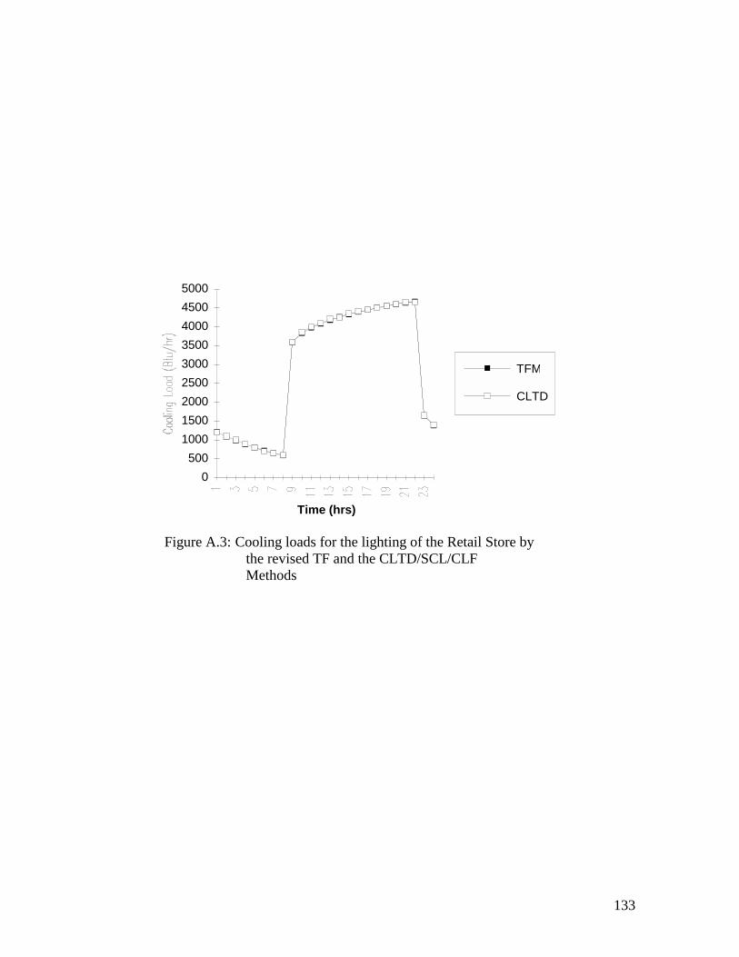
133
Time (hrs)
0500
100015002000250030003500400045005000
TFM
CLTD
Figure A.3: Cooling loads for the lighting of the Retail Store by the revised TF and the CLTD/SCL/CLF Methods

134
TABLE XXXI
COOLING LOADS FOR THE RETAIL STORE BY THE REVISED TF AND THE CLTD/SCL/CLF
METHODS ___________________________________________________________ Hour TOTAL COOLING LOAD (Btu/hr) ___________________________________________________________
By TF By CLTD Difference Method Method ___________________________________________________________ 1 28105.63 27790.76 -314.87 2 25695.75 25326.26 -369.49 3 23543.25 23401.04 -142.21 4 21647.71 21564.14 -83.57 5 20217.27 20071.60 -145.67 6 20015.12 19929.40 -85.72 7 20606.64 20357.24 -249.40 8 22389.05 22541.86 152.81 9 28660.47 28699.22 38.75 10 38888.50 39081.97 193.47 11 44851.28 45046.72 195.44 12 50505.85 50404.59 -101.26 13 54976.68 54872.24 -104.44 14 58103.42 57844.00 -259.42 15 59813.68 59687.66 -126.02 16 60299.60 60107.38 -192.22 17 59605.15 59251.59 -353.56 18 57516.27 57183.47 -332.80 19 54302.26 53724.24 -578.02 20 51041.20 50705.92 -335.28 21 47869.64 47379.07 -490.57 22 42469.85 41864.83 -605.02 23 33426.74 32910.45 -516.29 24 30597.85 30197.09 -400.76 ___________________________________________________________ NOTE : To = 96°F, Ti = 75°F, Mean daily range = 24°F

135
Time (hrs)
0
10000
20000
30000
40000
50000
60000
70000
TFM
CLTD
Figure A.4: Total cooling loads for the Retail Store by the revised TF and the CLTD/SCL/CLF Methods

136
APPENDIX B
COOLING LOAD RESULTS FOR TEST ZONE 2

137
TABLE XXXII
COMPARISON OF THE COOLING LOADS BY THE REVISED TF AND CLTD/SCL/CLF METHODS FOR
TEST ZONE 2 ________________________________________________________________________
Office Area Computer Room Total Load
Time TFM CLTD Difference TFM CLTD Difference
TFM CLTD Difference ________________________________________________________________________
1 11616.13 11233.95 -382.18 94126.6793222.93 -903.75 105742.8104456.9-1285.92 2 10797.18 10367.61 -429.57 93230.8892387.50 -843.38 104028.1102755.1-1272.95 3 10054.17 9538.97 -515.20 92501.4691716.65 -784.82 102555.6101255.6-1300.01 4 9383.03 9054.67 -328.36 91939.3491210.38 -728.95 101322.4100265.1-1057.32 5 8803.50 8638.28 -165.22 91709.7391033.29 -676.43 100513.2 99671.6 -841.66 6 10933.26 10846.51 -86.74 91977.5991349.97 -627.62 102910.9102196.5 -714.37 7 11737.98 11718.92 -19.06 92743.5392160.41 -583.12 104481.5103879.3 -602.18 8 43049.42 42482.61 -566.81 94178.4293629.19 -549.23 137227.8136111.8-1116.04 9 90687.96 89921.85 -766.11 98038.8997568.83 -470.06 188726.9187490.7-1236.17 10 95765.55 94561.29-1204.26 100608.50100087.60-520.82 196374.1194648.9-1725.16 11 100961.70100083.00-878.66 103519.60102910.60 -609.00 204481.3202993.6-1487.70 12 105536.80104823.10-713.68 106282.20105569.00 -713.16 211819.0210392.1-1426.90 13 108951.60108362.90-588.68 108388.80107556.60 -832.27 217340.4215919.5-1420.90 14 111290.30110949.70-340.60 109822.60108885.80 -936.81 221112.9219835.5-1277.40 15 112420.60112140.50-280.11 110406.40109392.00 -1014.36 222827.0221532.5-1294.50 16 112136.80111869.90-266.83 109973.70108910.80 -1062.89 222110.5220780.7-1329.80 17 110851.10110997.90146.80 108858.70107771.20-1087.52 219709.8218769.1-940.70 18 108809.70109470.20660.47 107067.80105973.20-1094.60 215877.5215443.4-434.10 19 60502.64 60515.26 12.62 104934.80103846.10-1088.75 165437.4164361.4-1076.08 20 17456.57 17496.70 40.13 102791.30101718.90-1072.36 120247.9119215.6-1032.27 21 15857.87 15784.58 -73.29 99228.1098108.47-1119.64 115086.0113893.1-1192.92

138
22 14577.85 14162.47 -415.39 97482.2896412.59-1069.69 112060.1110575.1-1485.07 23 13475.51 13296.13 -179.39 96085.8895070.90-1014.99 109561.4108367.0-1194.36 24 12500.30 12315.09 -185.22 95023.4594058.37 -965.09 107523.8106373.5-1150.29 ________________________________________________________________________
MAXIMUM PERCENT DIFFERENCE (For Total Load) = 0.89% at 10 hrs
Time (hrs)
0
20000
40000
60000
80000
100000
120000
TFM
CLTD
Figure B.1: Total cooling loads for the office area of test zone 2 by the revised TF and the CLTD/SCL/CLF Methods
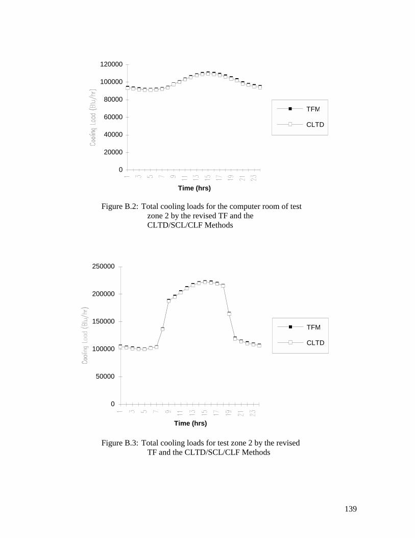
139
Time (hrs)
0
20000
40000
60000
80000
100000
120000
TFM
CLTD
Figure B.2: Total cooling loads for the computer room of test zone 2 by the revised TF and the CLTD/SCL/CLF Methods
Time (hrs)
0
50000
100000
150000
200000
250000
TFM
CLTD
Figure B.3: Total cooling loads for test zone 2 by the revised TF and the CLTD/SCL/CLF Methods

140
APPENDIX C
COOLING LOAD RESULTS FOR TEST ZONE 3

141
TABLE XXXIII
COMPARISON OF THE COOLING LOADS BY THE REVISED TF AND CLTD/SCL/CLF METHODS FOR
TEST ZONE 3 _________________________________________________________________________
Hour TF CLTD Difference Method Method _________________________________________________________________________ 1 23727.80 25064.10 1336.27 2 18187.19 20197.50 2010.30 3 13306.43 16302.10 2995.63 4 9020.04 10774.60 1754.56 5 8215.07 10153.90 1938.81 6 16304.08 18431.40 2127.30 7 18162.08 19995.40 1833.29 8 76105.56 78510.50 2404.96 9 316300.80 317950.00 1649.15 10 357195.20 357393.00 198.21 11 389149.30 387936.00 -1212.95 12 416000.80 413677.00 -2323.41 13 444173.00 440399.00 -3773.60 14 474906.30 469881.00 -5025.75 15 498809.70 493044.00 -5765.51 16 511363.50 505740.00 -5623.16 17 511820.10 505743.00 -6077.10 18 498220.30 493823.00 -4397.71 19 226218.00 221687.00 -4531.09 20 170058.70 169175.00 -883.77 21 62460.47 61864.00 -596.49 22 47748.47 46903.20 -845.23 23 37673.75 38874.10 1200.37 24 30021.13 31695.40 1674.30 _________________________________________________________________________
MAXIMUM PERCENT DIFFERENCE = 1.20% at 17 hrs

142
Time (hrs)
0
100000
200000
300000
400000
500000
600000
TFM
CLTD
Figure C.1: Total cooling loads for Test Zone 3 by the revised TF and the CLTD/SCL/CLF Methods

143
APPENDIX D
COOLING LOAD COMPARISONS FOR EXTERNALLY
SHADED GLASS AREAS
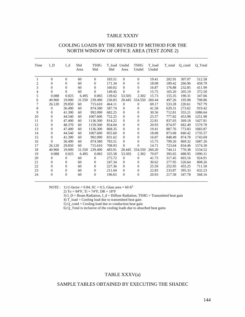
144
TABLE XXXIV
COOLING LOADS BY THE REVISED TF METHOD FOR THE NORTH WINDOW OF OFFICE AREA (TEST ZONE 2)
________________________________________________________________________ Time I_D I_d Shd TSHG T_load Unshd TSHG T_load T_total Q_cond Q_Total Area Shd Shd Area Unshd Unshd ________________________________________________________________________ 1 0 0 60 0 183.51 0 0 19.41 202.91 307.07 512.58 2 0 0 60 0 171.34 0 0 18.08 189.42 266.96 458.79 3 0 0 60 0 160.02 0 0 16.87 176.88 232.85 411.99 4 0 0 60 0 149.45 0 0 15.75 165.20 205.19 372.50 5 0.088 0.025 6.495 0.065 139.62 53.505 2.302 15.73 155.35 190.31 347.66 6 40.960 19.000 31.550 239.490 236.83 28.445 554.550 260.44 497.26 195.08 708.86 7 26.120 29.850 60 715.610 464.11 0 0 69.17 533.28 220.61 767.79 8 0 36.490 60 874.580 587.74 0 0 41.58 629.31 273.62 919.42 9 0 41.390 60 992.090 682.25 0 0 30.56 712.81 355.21 1086.64 10 0 44.540 60 1067.600 752.25 0 0 25.57 777.82 453.98 1251.98 11 0 47.400 60 1136.300 814.22 0 0 22.81 837.03 569.18 1427.81 12 0 48.370 60 1159.500 854.04 0 0 20.93 874.97 682.49 1579.78 13 0 47.400 60 1136.300 868.35 0 0 19.41 887.76 773.83 1683.87 14 0 44.540 60 1067.600 855.60 0 0 18.08 873.68 840.42 1735.57 15 0 41.390 60 992.090 831.62 0 0 16.87 848.49 874.78 1743.69 16 0 36.490 60 874.580 783.51 0 0 15.75 799.26 869.32 1687.26 17 26.120 29.850 60 715.610 708.93 0 0 14.71 723.64 834.46 1574.30 18 40.960 19.000 31.550 239.490 483.91 28.445 554.550 260.20 744.11 770.38 1534.52 19 0.088 0.025 6.495 0.065 325.58 53.505 2.302 70.07 395.65 688.95 1090.31 20 0 0 60 0 275.72 0 0 41.73 317.45 603.16 924.91 21 0 0 60 0 247.34 0 0 30.62 277.95 526.64 808.26 22 0 0 60 0 227.36 0 0 25.59 252.95 455.25 711.50 23 0 0 60 0 211.04 0 0 22.83 233.87 395.33 632.23 24 0 0 60 0 196.65 0 0 20.93 217.58 347.78 568.16 ________________________________________________________________________ NOTE : 1) U-factor = 0.84, SC = 0.5, Glass area = 60 ft2
2) To = 94°F, Ti = 74°F, DR = 18°F 3) I_D = Beam Radiation, I_d = Diffuse Radiation, TSHG = Transmitted heat gain 4) T_load = Cooling load due to transmitted heat gain 5) Q_cond = Cooling load due to conduction heat gain 6) Q_Total is inclusive of the cooling loads due to absorbed heat gains
TABLE XXXV(a)
SAMPLE TABLES OBTAINED BY EXECUTING THE SHADEC

145
PROGRAM FOR SHADOW LENGTHS DUE TO EXTERNAL SHADING (HORIZONTAL PROJECTIONS)
Shadow Lengths for Building Exterior Projections May 21st HORIZONTAL PROJECTION 38 Deg North Latitude Shadow Length Foot per Foot Projection, Sh/P Solar Time N NE E SE S SW W NW ---------------------------------------------------------------------------------------- 5 0.045 0.020 0.021 0.055 * * * * 6 0.781 0.246 0.224 0.444 * * * * 7 3.358 0.554 0.443 0.722 * * * * 8 * 1.034 0.714 0.985 29.407 * * * 9 * 1.978 1.105 1.291 5.260 * * * 10 * 5.055 1.813 1.718 3.680 * * * 11 * * 3.807 2.459 3.200 28.406 * * 12 * * * 4.353 3.078 4.353 * * 13 * * * 28.406 3.200 2.459 3.807 * 14 * * * * 3.680 1.718 1.813 5.055 15 * * * * 5.260 1.291 1.105 1.978 16 * * * * 29.407 0.985 0.714 1.034 17 3.358 * * * * 0.722 0.443 0.554 18 0.781 * * * * 0.444 0.224 0.246 19 0.045 * * * * 0.055 0.021 0.020 ----------------------------------------------------------------------------------------

146
TABLE XXXV(b)
SAMPLE TABLES OBTAINED BY EXECUTING THE SHADEC PROGRAM FOR SHADOW LENGTHS DUE TO EXTERNAL
SHADING (VERTICAL PROJECTIONS)
Shadow Lengths for Building Exterior Projections May 21st VERTICAL PROJECTION 38 Deg North Latitude Shadow Width Foot per Foot Projection, Sw/Pv Solar Time N NE E SE S SW W NW ---------------------------------------------------------------------------------------- 5 2.165 0.368 0.462 2.717 * * * * 6 3.487 0.554 0.287 1.804 * * * * 7 7.578 0.767 0.132 1.304 * * * * 8 * 1.050 0.024 0.953 41.203 * * * 9 * 1.532 0.210 0.653 4.761 * * * 10 * 2.943 0.493 0.340 2.030 * * * 11 * * 1.190 0.087 0.841 11.553 * * 12 * * * 1.000 0.000 1.000 * * 13 * * * 11.553 0.841 0.087 1.190 * 14 * * * * 2.030 0.340 0.493 2.943 15 * * * * 4.761 0.653 0.210 1.532 16 * * * * 41.203 0.953 0.024 1.050 17 7.578 * * * * 1.304 0.132 0.767 18 3.487 * * * * 1.804 0.287 0.554 19 2.165 * * * * 2.717 0.462 0.368 ----------------------------------------------------------------------------------------

147
TABLE XXXVI
COOLING LOADS BY THE CLTD/SCL/CLF METHOD FOR THE NORTH WINDOW OF OFFICE AREA (TEST ZONE 2)
________________________________________________________________________
Time Sh/P Sh Actual Sv/Pv Sv Unshd Shad SCL Q_unsh SCL Q_shd CLTD CLTD Q_cond Total Sh Area Area North Corr Load ________________________________________________________________________
1 0 0 0 0 0 0 60 7 0 7 210 1 5 252.0 462.0 2 0 0 0 0 0 0 60 7 0 7 210 0 4 201.6 411.6 3 0 0 0 0 0 0 60 7 0 7 210 -1 3 151.2 361.2 4 0 0 0 0 0 0 60 6 0 6 180 -2 2 100.8 280.8 5 0.05 0.16 0 2.17 1.08 53.52 6.48 6 160.56 6 19.44 -2 2 100.8 280.8 6 0.78 2.73 2.48 3.49 1.74 29.05 30.95 24 348.56 24 371.45 -2 2 100.8 820.8 7 3.36 11.75 11.50 7.58 3.79 0 60 24 0 24 720 -2 2 100.8 820.8 8 0 0 0 0 60 23 0 23 690 0 4 201.6 891.6 9 0 0 0 0 60 26 0 26 780 2 6 302.4 1082.4 10 0 0 0 0 60 28 0 28 840 4 8 403.2 1243.2 11 0 0 0 0 60 30 0 30 900 7 11 554.4 1454.4 12 0 0 0 0 60 31 0 31 930 9 13 655.2 1585.2 13 0 0 0 0 60 31 0 31 930 12 16 806.4 1736.4 14 0 0 0 0 60 31 0 31 930 13 17 856.8 1786.8 15 0 0 0 0 60 30 0 30 900 14 18 907.2 1807.2 16 0 0 0 0 60 28 0 28 840 14 18 907.2 1747.2 17 3.36 11.75 11.50 7.58 3.79 0 60 29 0 29 870 13 17 856.8 1726.8 18 0.78 2.73 2.48 3.49 1.74 29.05 30.95 33 479.26 33 510.74 12 16 806.4 1796.4 19 0.05 0.16 0 2.17 1.08 53.52 6.48 15 401.40 15 48.60 10 14 705.6 1155.6 20 0 0 0 0 0 0 60 12 0 12 360 8 12 604.8 964.8 21 0 0 0 0 0 0 60 10 0 10 300 6 10 504.0 804.0 22 0 0 0 0 0 0 60 9 0 9 270 4 8 403.2 673.2 23 0 0 0 0 0 0 60 9 0 9 270 3 7 352.8 622.8 24 0 0 0 0 0 0 60 8 0 8 240 2 6 302.4 542.4 ________________________________________________________________________
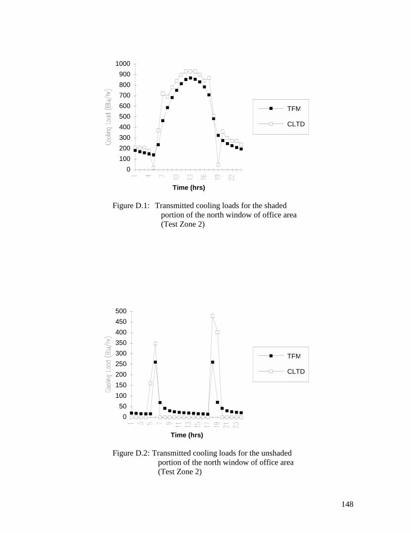
148
Time (hrs)
0100200300400500600700800900
1000
TFM
CLTD
Figure D.1: Transmitted cooling loads for the shaded portion of the north window of office area (Test Zone 2)
Time (hrs)
050
100150200250300350400450500
TFM
CLTD
Figure D.2: Transmitted cooling loads for the unshaded portion of the north window of office area (Test Zone 2)

149
TABLE XXXVII
COOLING LOADS BY THE REVISED TF METHOD FOR THE EAST WINDOW OF OFFICE AREA (TEST ZONE 2)
________________________________________________________________________ Time I_D I_d Shd TSHG T_load Unshd TSHG T_load T_total Q_cond Q_Total Area Shd Shd Area Unshd Unshd ________________________________________________________________________ 1 0 0 60 0 177.07 0 0 183.12 360.19 307.07 671.45 2 0 0 60 0 165.33 0 0 171.04 336.36 266.96 607.23 3 0 0 60 0 154.40 0 0 159.76 314.15 232.85 550.64 4 0 0 60 0 144.21 0 0 149.22 293.42 205.19 502.01 5 0.191 0.036 1.386 0.02 134.70 58.61 5.75 141.93 276.63 190.31 470.18 6 144.000 29.910 6.239 74.55 158.94 53.764032.101922.792081.74 195.08 2329.80 7 205.300 47.490 13.37 253.63 237.79 46.635072.102784.903022.68 220.61 3317.47 8 210.400 55.780 22.54 502.23 362.64 37.464240.602727.223089.87 273.62 3440.77 9 183.000 58.800 36.36 854.13 549.13 23.642375.902002.332551.46 355.21 2969.50 10 133.800 58.400 60 1399.80 842.03 0 0 851.79 1693.82 453.98 2182.70 11 70.400 55.860 60 1339.10 898.04 0 0 598.98 1497.01 569.18 2097.60 12 0 52.150 60 1250.20 900.29 0 0 488.81 1389.10 682.49 2100.67 13 0 47.400 60 1136.30 871.56 0 0 431.18 1302.74 773.83 2103.47 14 0 44.540 60 1067.60 850.69 0 0 393.61 1244.30 840.42 2110.23 15 0 39.870 60 955.78 808.05 0 0 364.37 1172.42 874.78 2070.76 16 0 33.500 60 803.03 740.07 0 0 339.16 1079.22 869.32 1969.49 17 0 25.310 60 606.62 643.50 0 0 316.36 959.86 834.46 1811.91 18 0 14.230 60 341.16 505.55 0 0 295.34 800.89 770.38 1584.36 19 0 0.016 60 0.37 319.77 0 0 275.80 595.57 688.95 1291.78 20 0 0 60 0 268.04 0 0 257.59 525.63 603.16 1135.04 21 0 0 60 0 239.38 0 0 240.59 479.97 526.64 1012.27 22 0 0 60 0 219.64 0 0 224.72 444.36 455.25 904.82 23 0 0 60 0 203.73 0 0 209.90 413.63 395.33 813.80 24 0 0 60 0 189.78 0 0 196.05 385.83 347.78 738.11 ________________________________________________________________________

150
TABLE XXXVIII
COOLING LOADS BY THE CLTD/SCL/CLF METHOD FOR THE EAST WINDOW OF OFFICE AREA (TEST ZONE 2)
________________________________________________________________________
Time Sh/P Sh Actual Sv/Pv Sv Unshd Shad SCL Q_unsh SCL Q_shd CLTD CLTD Q_cond Total Sh Area Area North Corr Load ________________________________________________________________________
1 0 0 0 0 0 0 60 17 0 7 210 1 5 252.0 462.0 2 0 0 0 0 0 0 60 16 0 7 210 0 4 201.6 411.6 3 0 0 0 0 0 0 60 15 0 7 210 -1 3 151.2 361.2 4 0 0 0 0 0 0 60 14 0 6 180 -2 2 100.8 280.8 5 0.02 0.07 0 0.46 0.2358.61 1.39 13 380.99 6 4.16 -2 2 100.8 486.0 6 0.22 0.78 0.53 0.29 0.1453.88 6.12 80 2155.0324 73.49 -2 2 100.82329.3 7 0.44 1.55 1.30 0.13 0.0746.6913.31126 2941.1424 159.78 -2 2 100.83201.7 8 0.71 2.50 2.25 0.02 0.0137.4722.54145 2716.2123 259.15 0 4 201.63177.0 9 1.11 3.87 3.62 0.21 0.1123.5836.43142 1673.8126 473.53 2 6 302.42449.7 10 1.81 6.35 6.10 0.49 0.25 0 60 123 0 28 840 4 8 403.21243.2 11 3.8113.3213.07 1.19 0.60 0 60 91 0 30 900 7 11 554.41454.4 12 0 0 0 0 0 0 60 65 0 31 930 9 13 655.21585.2 13 0 0 0 0 0 0 60 57 0 31 930 12 16 806.41736.4 14 0 0 0 0 0 0 60 53 0 31 930 13 17 856.81786.8 15 0 0 0 0 0 0 60 49 0 30 900 14 18 907.21807.2 16 0 0 0 0 0 0 60 45 0 28 840 14 18 907.21747.2 17 0 0 0 0 0 0 60 40 0 29 870 13 17 856.81726.8 18 0 0 0 0 0 0 60 34 0 33 990 12 16 806.41796.4 19 0 0 0 0 0 0 60 27 0 15 450 10 14 705.61155.6 20 0 0 0 0 0 0 60 24 0 12 360 8 12 604.8 964.8 21 0 0 0 0 0 0 60 22 0 10 300 6 10 504.0 804.0 22 0 0 0 0 0 0 60 21 0 9 270 4 8 403.2 673.2 23 0 0 0 0 0 0 60 19 0 9 270 3 7 352.8 622.8 24 0 0 0 0 0 0 60 18 0 8 240 2 6 302.4 542.4 ________________________________________________________________________

151
Time (hrs)
0100200300400500600700800900
1000
TFM
CLTD
Figure D.3: Transmitted cooling loads for the shaded portion of the east window of office area (Test Zone 2)

152
APPENDIX E
COOLING LOAD COMPARISONS FOR TYPICALLY
SHADED GLASS AREAS

153
Cooling Load Calculations by the revised TF and the CLTD/SCL/CLF
methods for typically shaded glass areas
Cooling loads were calculated for a typical case of external shading. Figure E.1
shows the exterior shading details for this glass area. The window is 4' in width and 6' high
(U-factor = 0.81, Shading coefficient = 0.55). The design conditions assumed were those
of Stillwater, Oklahoma (Latitude = 36 °N). Cooling loads for 8 facing directions of this
window were calculated by both methods and compared. Figures E.2 through E.9 show the
plots of the cooling loads for these 8 facing directions. These figures indicate the kind of
typical errors that may be encountered by using the CLTD/SCL/CLF method for externally
shaded glass areas. While the cooling load plots of the North East (fig. E.3) East (fig. E.4),
and South East (fig E.5) facing glass show the inability of the CLTD/SCL/CLF method to
account for the past history of the varying shaded/unshaded areas, that for South (fig. E.6),
South West (fig. E.7) and North West (fig. E.9) show the effect of the use of the North
facing glass SCLs to represent a completely shaded glass area. Table XXXIX shows the
maximum percent differences between the two methods for the 8 facing directions.

154
2'
1'
4' Wide by 6' High Window
Figure E.1: Typically exterior shaded glass window
Time (hrs)
0
500
1000
1500
2000
2500
TFM
CLTD
Figure E.2: Cooling loads for North facing window (36°N) by the revised TF and CLTD/SCL/CLF Methods

155
Time (hrs)
0
500
1000
1500
2000
2500
TFM
CLTD
Figure E.3: Cooling loads for NE facing window (36°N) by the revised TF and CLTD/SCL/CLF Methods
Time (hrs)
0
500
1000
1500
2000
2500
TFM
CLTD
Figure E.4: Cooling loads for East facing window (36°N) by the revised TF and CLTD/SCL/CLF Methods

156
Time (hrs)
0
500
1000
1500
2000
2500
TFM
CLTD
Figure E.5: Cooling loads for SE facing window (36°N) by the revised TF and CLTD/SCL/CLF Methods
Time (hrs)
0
500
1000
1500
2000
2500
TFM
CLTD
Figure E.6: Cooling loads for South facing window (36°N) by the revised TF and CLTD/SCL/CLF Methods
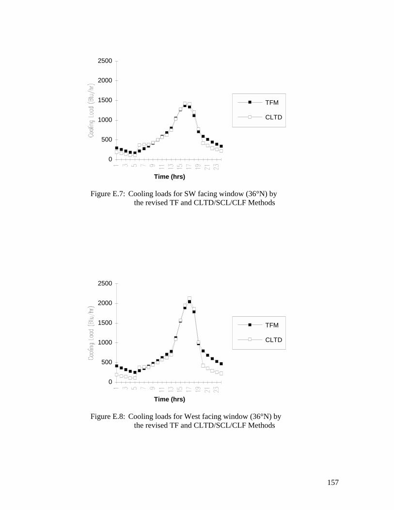
157
Time (hrs)
0
500
1000
1500
2000
2500
TFM
CLTD
Figure E.7: Cooling loads for SW facing window (36°N) by the revised TF and CLTD/SCL/CLF Methods
Time (hrs)
0
500
1000
1500
2000
2500
TFM
CLTD
Figure E.8: Cooling loads for West facing window (36°N) by the revised TF and CLTD/SCL/CLF Methods

158
Time (hrs)
0
500
1000
1500
2000
2500
TFM
CLTD
Figure E.9: Cooling loads for NW facing window (36°N) by the revised TF and CLTD/SCL/CLF Methods
TABLE XXXIX
MAXIMUM PERCENT DIFFERENCES FOR THE TYPICALLY SHADED GLASS AREA
____________________________________________________________ Facing Direction Maximum % Difference and Hour ____________________________________________________________
1) North 18.59 % at 0007 hrs. 2) North East 37.52 % at 0010 hrs. 3) East 43.99 % at 0011 hrs. 4) South East 27.59 % at 0012 hrs. 5) South 64.06 % at 0006 hrs. 6) South West 41.26 % at 0006 hrs. 7) West 54.16 % at 0001 hrs. 8) North West 43.51 % at 0001 hrs. ____________________________________________________________

159
VITA
Richard Lawrence Castelino
Candidate for the Degree of
Master of Science
Thesis: IMPLEMENTATION OF THE REVISED TRANSFER FUNCTION METHOD AND EVALUATION OF THE CLTD/SCL/CLF METHOD
Major Field: Mechanical Engineering
Biographical:
Personal Data: Born in Bombay, India on the 26th day of February, 1966, the son of Lawrence and Florine Castelino
Education: Graduated from Parle College, Bombay, India, in April 1983; received
Bachelor of Engineering Degree in Mechanical Engineering from University of Bombay in June, 1987; completed requirements for the Master of Science Degree at Oklahoma State University in December, 1992
Professional Experience: Research Assistant, Department of Mechanical and Aerospace Engineering,
Oklahoma State University, May 1991 to July, 1992 Teaching Assistant, Department of Mechanical and Aerospace Engineering,
Oklahoma State University, August 1990 to April, 1991 Project Engineer, Air-Conditioning and Refrigeration Business Group, M/s
Voltas Limited, Bombay, April 1988 to August, 1990 Graduate Engineer, M/s Constellation Dynamatics Private Limited, Bombay,
November, 1987 to March, 1988 Honors and Affiliations: Student Member - PHI KAPPA PHI National Honor Society Nominated to the NATIONAL DEAN'S LIST - 1992 Student Member - ASHRAE Student Member - Association for Computing Machinery (ACM)